XAFS ExperimentalMethods

Grant BunkerProfessor of Physics

BCPS Department/CSRRIIllinois Institute of Technology

AcknowledgementsEd Stern, Dale Sayers, Farrel Lytle, Steve Heald, Tim Elam, Bruce Bunker and other early members of the UW XAFS group

Firouzeh Tannazi (IIT/BCPS) (recent results on fluorescence in complex materials)

Suggested References:

Steve Heald’s article “designing an EXAFS experiment” in Koningsberger and Prins andearly work cited therein (e.g. Stern and Lu)

Rob Scarrow’s notes posted athttp://cars9.uchicago.edu/xafs/NSLS_2002/

Outline of talkSynchrotron Radiation Sources

Beamlines and optics

Experimental modes and samples

Detectors and Analyzers

Conclusion

Sources

Dipole Bend Magnets

Insertion Devices

Wigglers

Undulators

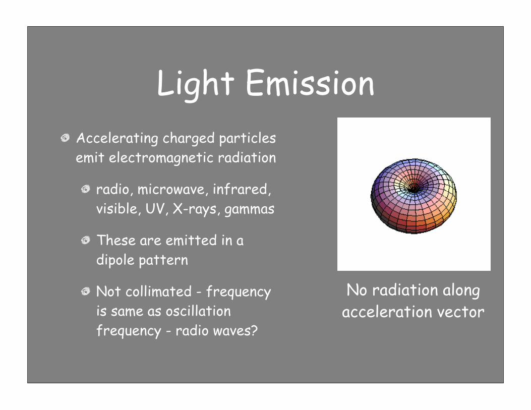
Accelerating charged particles emit electromagnetic radiation

radio, microwave, infrared, visible, UV, X-rays, gammas

These are emitted in a dipole pattern

Not collimated - frequency is same as oscillation frequency - radio waves?

Light Emission

No radiation alongacceleration vector

When particles move at speeds close to the speed of light

it’s still a dipole pattern in their instantaneous rest frame

but in lab frame, radiation pattern tilts sharply into the forward direction “headlight effect”

Frequency of emitted light measured in lab frame is dramatically higher -> x-rays

Relativity changes everything

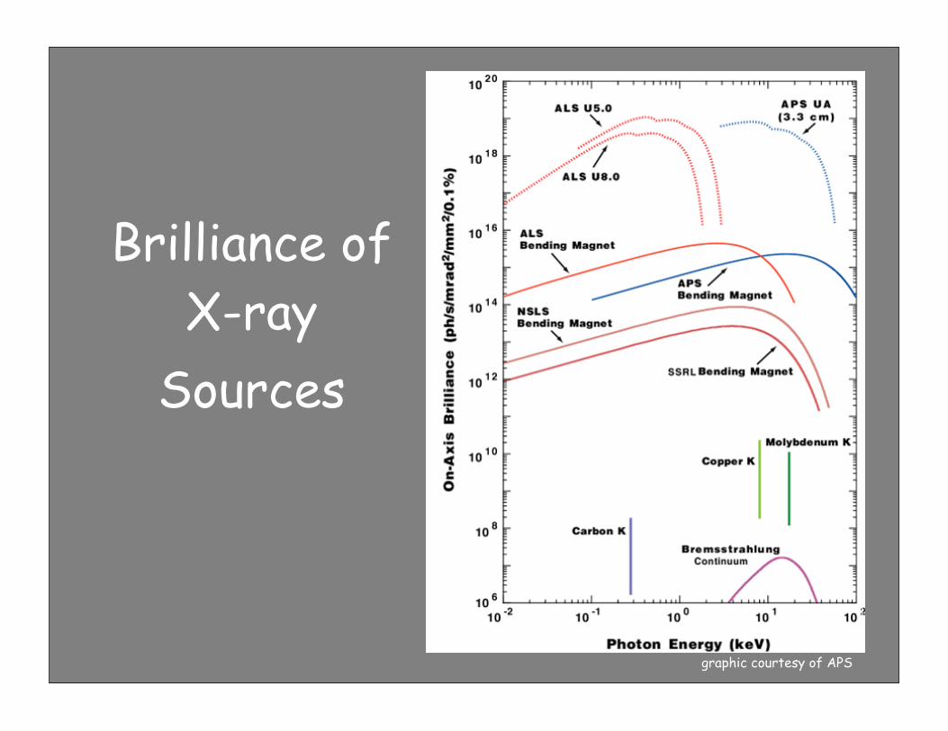
Brilliance of X-ray

Sources

graphic courtesy of APS

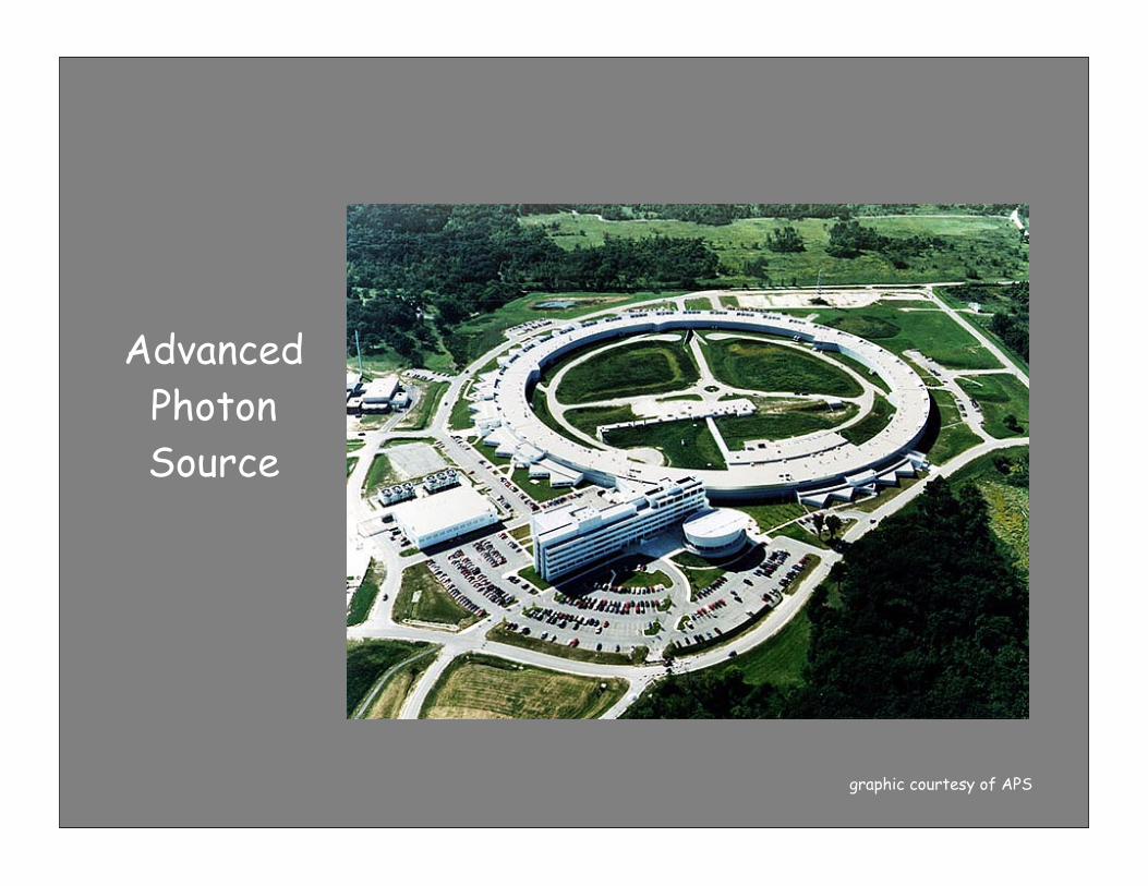
Advanced PhotonSource

graphic courtesy of APS

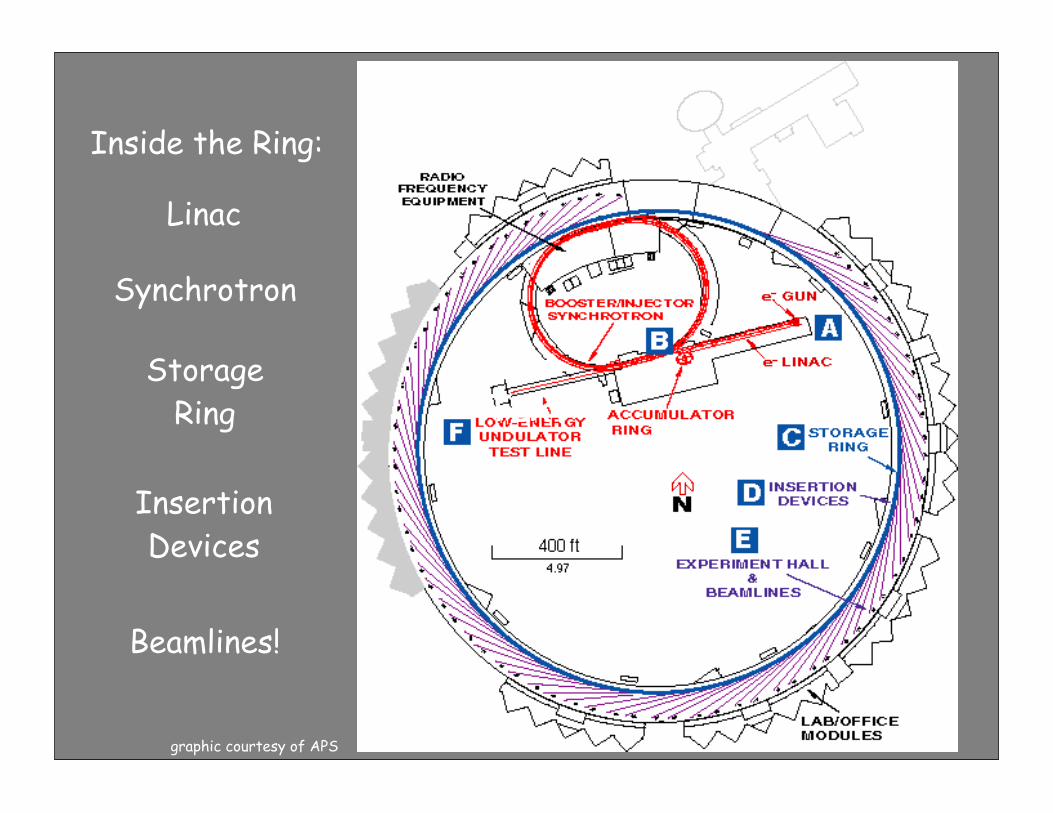
Storage Ring Text

Synchrotron

Text

Linac

Inside the Ring:

InsertionDevices

Beamlines!

graphic courtesy of APS

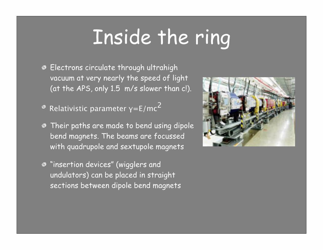
Electrons circulate through ultrahigh vacuum at very nearly the speed of light (at the APS, only 1.5 m/s slower than c!).

Relativistic parameter γ=E/mc2

Their paths are made to bend using dipole bend magnets. The beams are focussed with quadrupole and sextupole magnets

“insertion devices” (wigglers and undulators) can be placed in straight sections between dipole bend magnets

Inside the ring

Wherever the path of the electrons bends, their velocity vector changes

This acceleration causes them to produce electromagnetic radiation

In the lab rest frame, this produces a horizontal fan of x-rays that is highly collimated (to ΔΘ≈ 1/γ) in the vertical direction and extends to high energies

Energy is put back into electron beam by electrons “surfing” through radio frequency (RF) cavities

Synchrotron Radiation

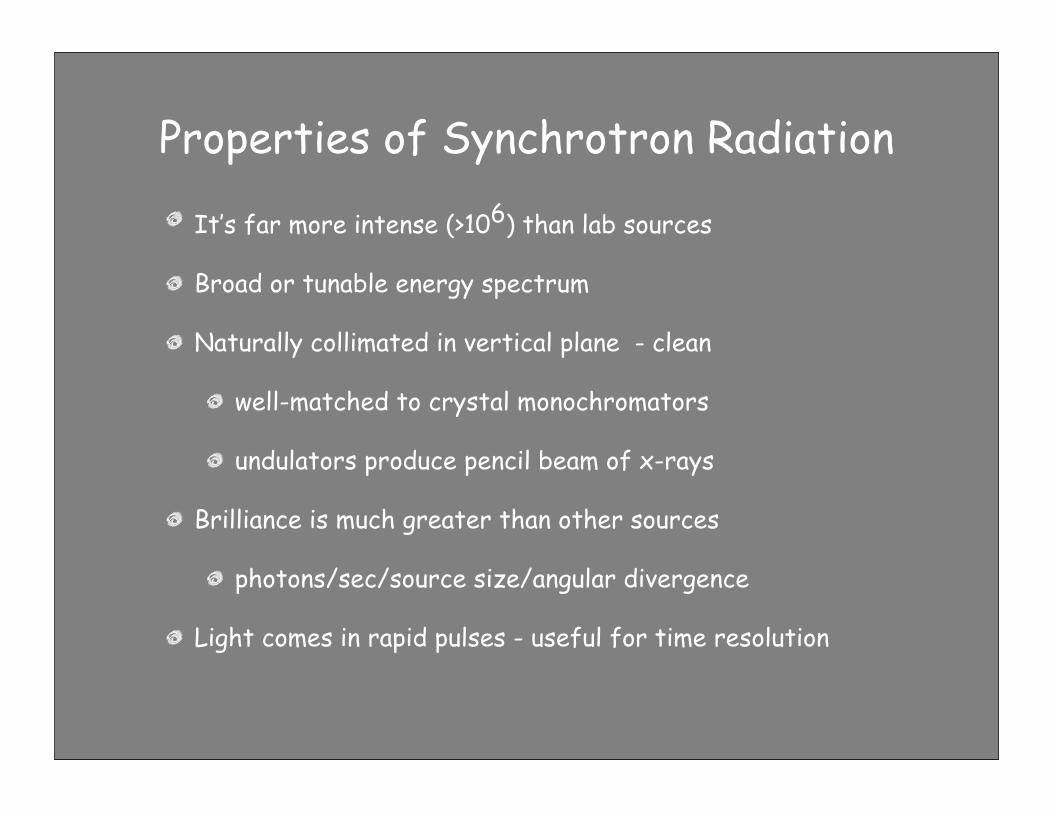
It’s far more intense (>106) than lab sources

Broad or tunable energy spectrum

Naturally collimated in vertical plane - clean

well-matched to crystal monochromators

undulators produce pencil beam of x-rays

Brilliance is much greater than other sources

photons/sec/source size/angular divergence

Light comes in rapid pulses - useful for time resolution

Properties of Synchrotron Radiation

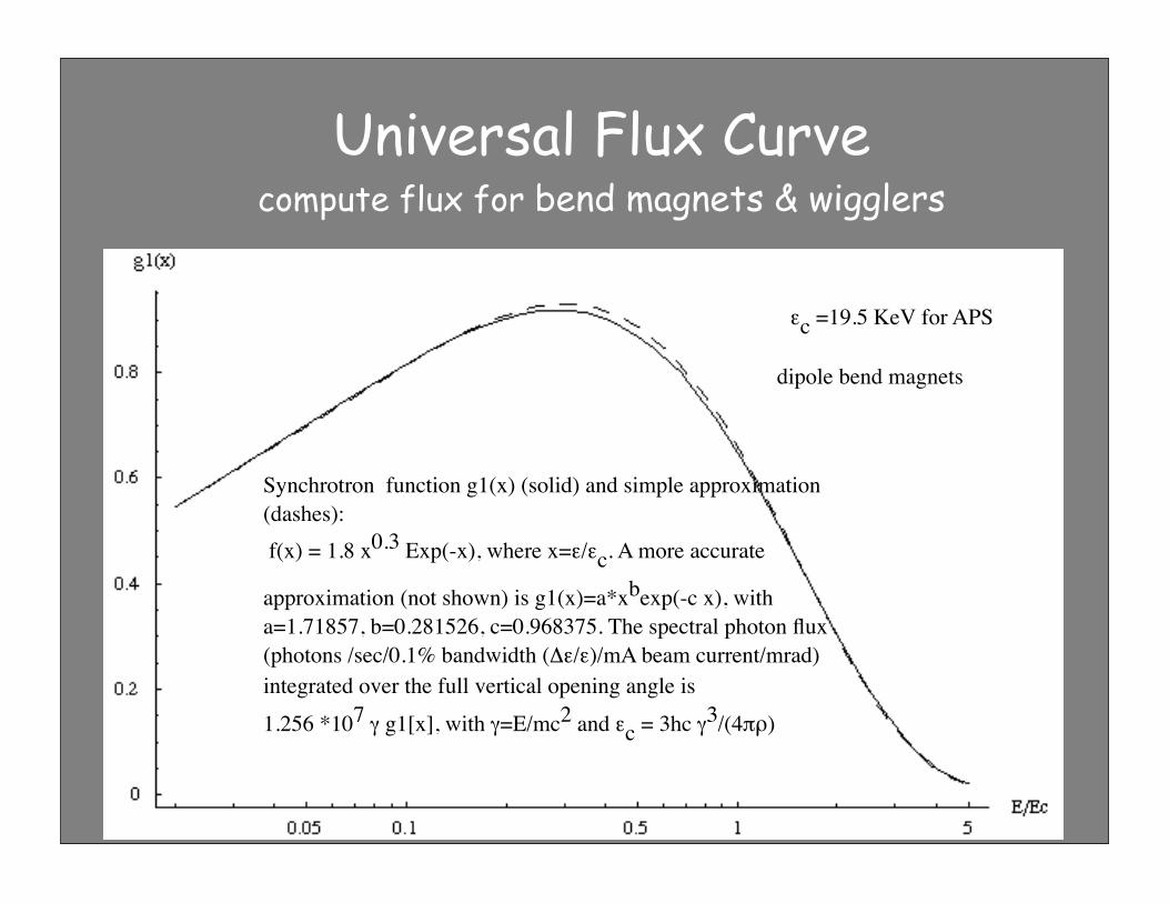
Universal Flux Curvecompute flux for bend magnets & wigglers

Synchrotron function g1(x) (solid) and simple approximation (dashes): f(x) = 1.8 x0.3 Exp(-x), where x=ε/εc. A more accurate

approximation (not shown) is g1(x)=a*xbexp(-c x), with a=1.71857, b=0.281526, c=0.968375. The spectral photon flux (photons /sec/0.1% bandwidth (Δε/ε)/mA beam current/mrad) integrated over the full vertical opening angle is

1.256 *107 γ g1[x], with γ=E/mc2 and εc = 3hc γ3/(4πρ)

TextText

εc =19.5 KeV for APS

dipole bend magnetsxt

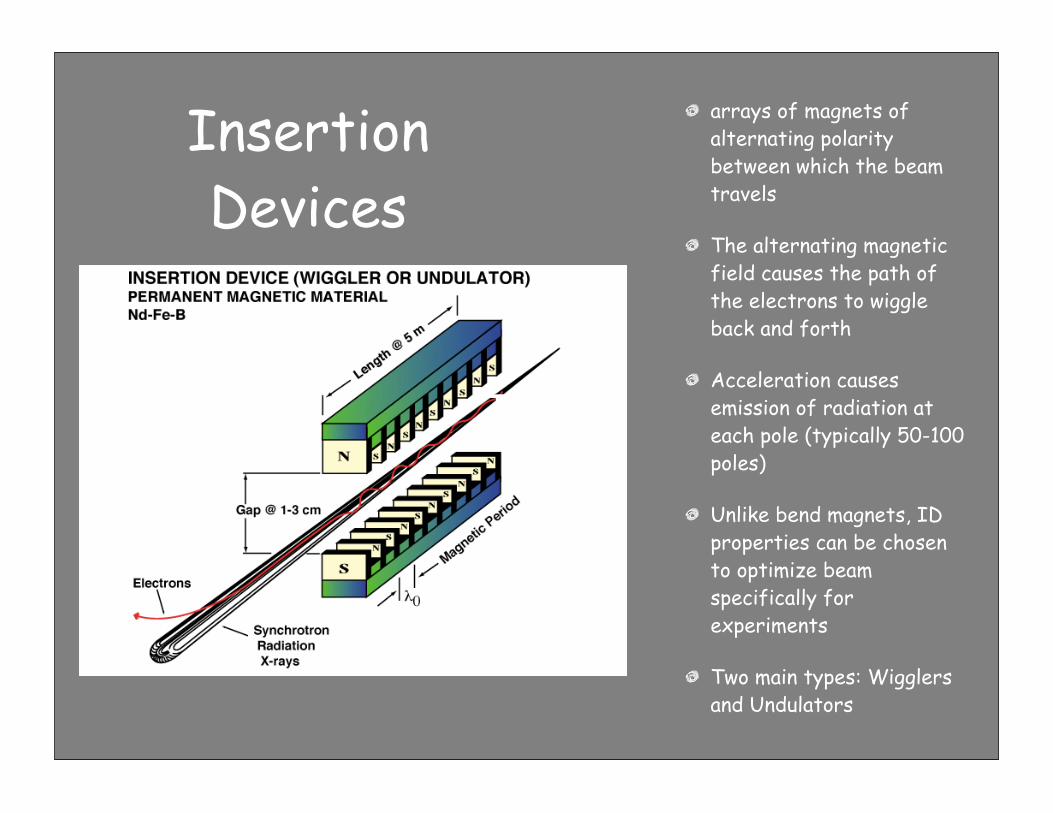
arrays of magnets of alternating polarity between which the beam travels

The alternating magnetic field causes the path of the electrons to wiggle back and forth

Acceleration causes emission of radiation at each pole (typically 50-100 poles)

Unlike bend magnets, ID properties can be chosen to optimize beam specifically for experiments

Two main types: Wigglers and Undulators

Text

Insertion Devices

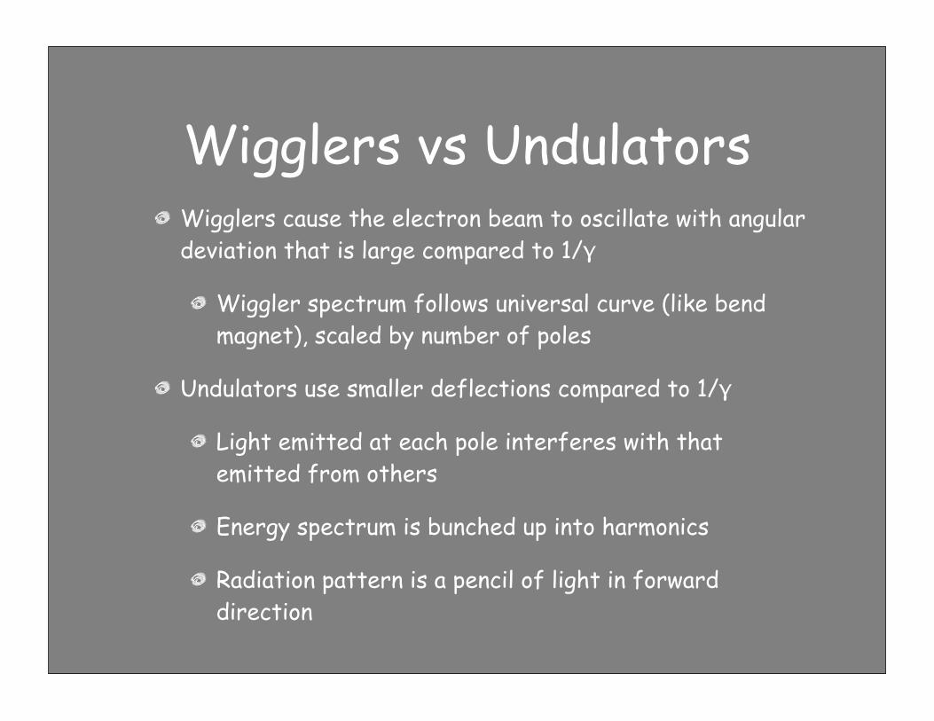
Wigglers cause the electron beam to oscillate with angular deviation that is large compared to 1/γ

Wiggler spectrum follows universal curve (like bend magnet), scaled by number of poles

Undulators use smaller deflections compared to 1/γ

Light emitted at each pole interferes with that emitted from others

Energy spectrum is bunched up into harmonics

Radiation pattern is a pencil of light in forward direction

Wigglers vs Undulators

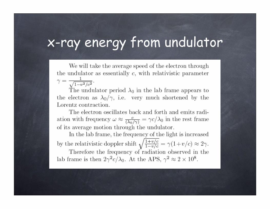
x-ray energy from undulator

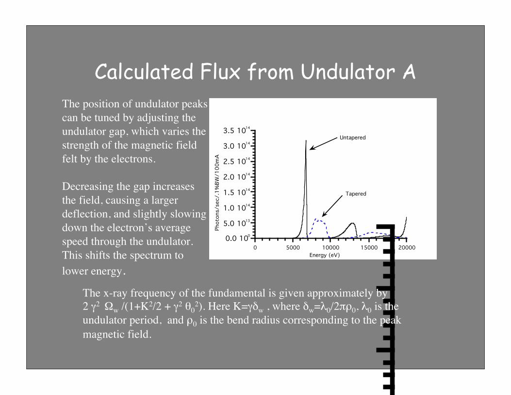
Calculated Flux from Undulator A

0.0 100

5.0 1013

1.0 1014

1.5 1014

2.0 1014

2.5 1014

3.0 1014

3.5 1014

0 5000 10000 15000 20000

Tapered

Untapered

Energy (eV)

Phot

ons/

sec/

.1%

BW/1

00m

A

The x-ray frequency of the fundamental is given approximately by 2 γ2 Ωw /(1+K2/2 + γ2 θ0

2). Here K=γδw , where δw=λ0/2πρ0, λ0 is the undulator period, and ρ0 is the bend radius corresponding to the peak magnetic field.

The position of undulator peakscan be tuned by adjusting theundulator gap, which varies thestrength of the magnetic fieldfelt by the electrons.

Decreasing the gap increasesthe field, causing a largerdeflection, and slightly slowingdown the electron’s averagespeed through the undulator.This shifts the spectrum tolower energy.

In the orbital plane, the radiation is nearly 100% linearly polarized

This can be used for polarized XAFS (x-ray linear dichroism) experiments on oriented specimens

Out of the orbital plane, bend magnet radiation has some degree of left/right circular polarization

Wiggler/undulator radiation is not circularly polarized (planar devices)

X-ray Polarization

Beamlines are complex instruments that prepare suitable x-ray beams for experiments, and protect the users against radiation exposure.

They combine x-ray optics, detector systems, computer interface electronics, sample handling/cooling, and computer hardware and software.

Beamlines

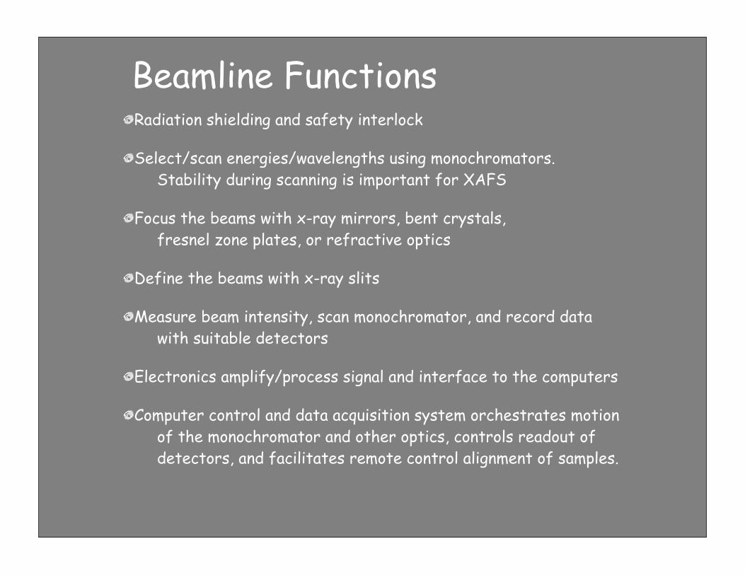
Beamline FunctionsRadiation shielding and safety interlock

Select/scan energies/wavelengths using monochromators.Stability during scanning is important for XAFS

Focus the beams with x-ray mirrors, bent crystals, fresnel zone plates, or refractive optics

Define the beams with x-ray slits

Measure beam intensity, scan monochromator, and record datawith suitable detectors

Electronics amplify/process signal and interface to the computers

Computer control and data acquisition system orchestrates motion of the monochromator and other optics, controls readout of detectors, and facilitates remote control alignment of samples.

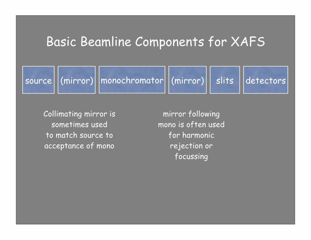
Basic Beamline Components for XAFS

(mirror)source monochromator detectorsslits(mirror)

Collimating mirror is sometimes used

to match source to acceptance of mono

mirror following mono is often used

for harmonic rejection or

focussing

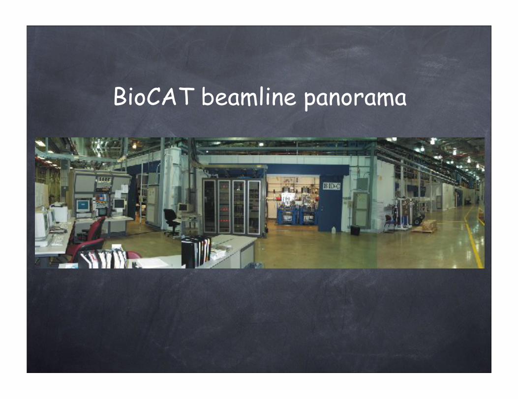
BioCAT beamline panorama

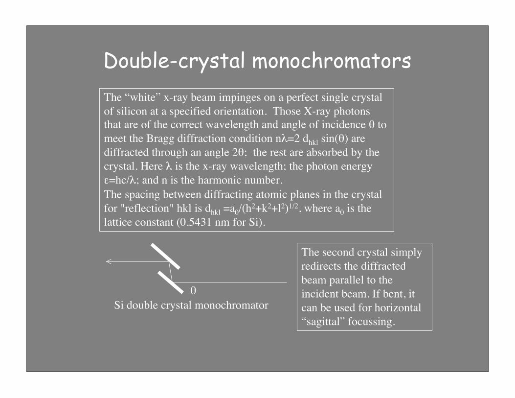
Double-crystal monochromatorsThe “white” x-ray beam impinges on a perfect single crystalof silicon at a specified orientation. Those X-ray photonsthat are of the correct wavelength and angle of incidence θ tomeet the Bragg diffraction condition nλ=2 dhkl sin(θ) arediffracted through an angle 2θ; the rest are absorbed by thecrystal. Here λ is the x-ray wavelength; the photon energyε=hc/λ; and n is the harmonic number.The spacing between diffracting atomic planes in the crystalfor "reflection" hkl is dhkl =a0/(h2+k2+l2)1/2, where a0 is thelattice constant (0.5431 nm for Si).

Si double crystal monochromatorθ

The second crystal simplyredirects the diffractedbeam parallel to theincident beam. If bent, itcan be used for horizontal“sagittal” focussing.

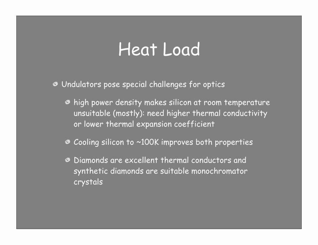
Undulators pose special challenges for optics

high power density makes silicon at room temperature unsuitable (mostly): need higher thermal conductivity or lower thermal expansion coefficient

Cooling silicon to ~100K improves both properties

Diamonds are excellent thermal conductors and synthetic diamonds are suitable monochromator crystals

Heat Load

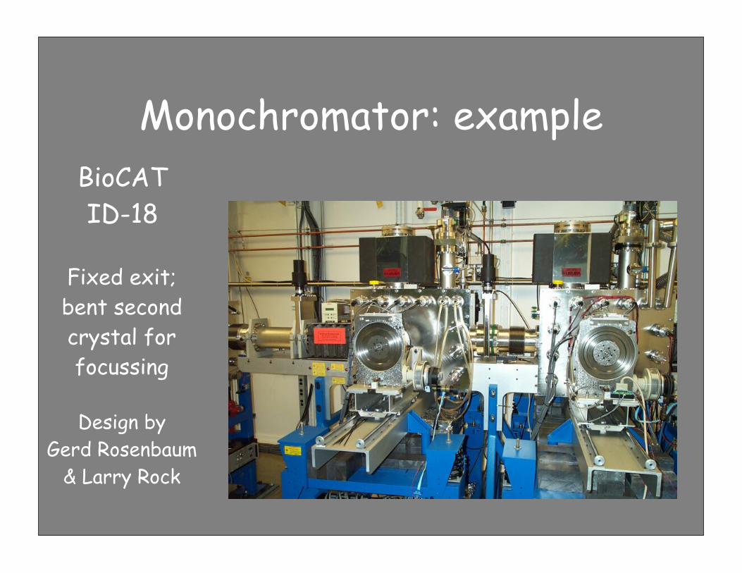
Monochromator: example

Design by Gerd Rosenbaum

& Larry Rock

BioCATID-18

Fixed exit; bent second crystal for focussing

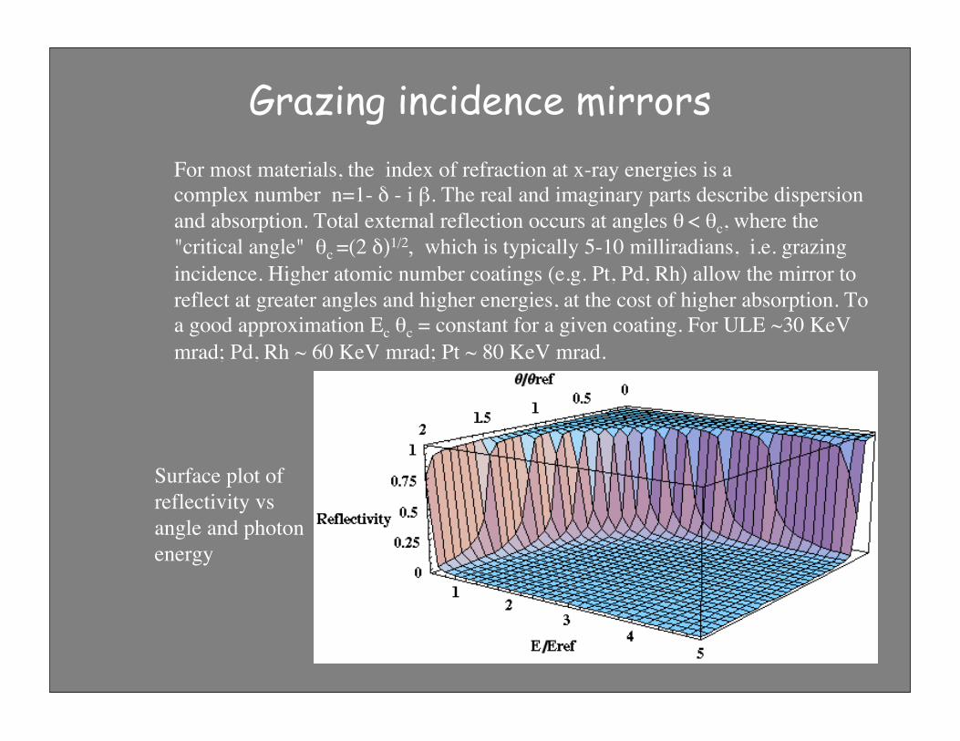
Grazing incidence mirrorsFor most materials, the index of refraction at x-ray energies is acomplex number n=1- δ - i β. The real and imaginary parts describe dispersionand absorption. Total external reflection occurs at angles θ < θc, where the"critical angle" θc =(2 δ)1/2, which is typically 5-10 milliradians, i.e. grazingincidence. Higher atomic number coatings (e.g. Pt, Pd, Rh) allow the mirror toreflect at greater angles and higher energies, at the cost of higher absorption. Toa good approximation Ec θc = constant for a given coating. For ULE ~30 KeVmrad; Pd, Rh ~ 60 KeV mrad; Pt ~ 80 KeV mrad.

Surface plot ofreflectivity vsangle and photonenergy

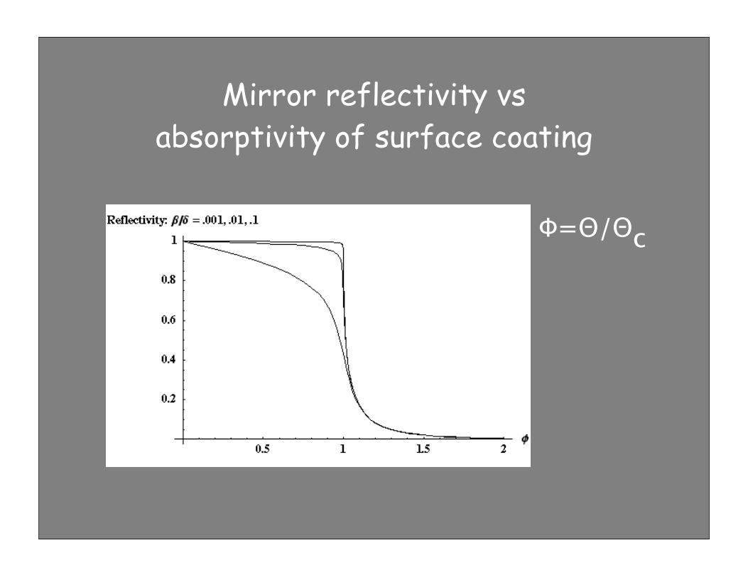
Mirror reflectivity vs absorptivity of surface coating

Φ=Θ/Θc

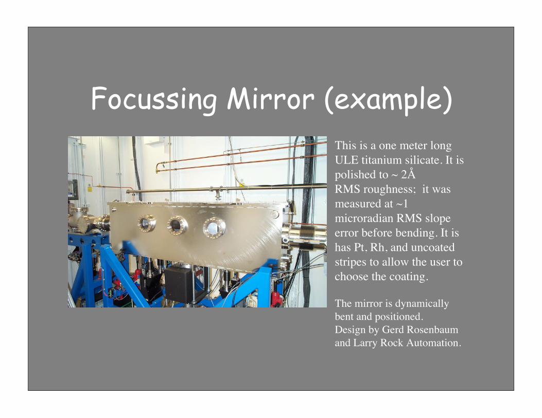
Focussing Mirror (example)This is a one meter longULE titanium silicate. It ispolished to ~ 2ÅRMS roughness; it wasmeasured at ~1microradian RMS slopeerror before bending. It ishas Pt, Rh, and uncoatedstripes to allow the user tochoose the coating.

The mirror is dynamicallybent and positioned.Design by Gerd Rosenbaumand Larry Rock Automation.

Monochromators transmit not only the desired fundamental energy, but also some harmonics of that energy. Allowed harmonics for Si(111) include 333, 444, 555, 777…

These can be reduced by slightly misaligning “detuning” the second crystal using a piezoelectric transducer (“piezo”). Detuning reduces the harmonic content much more than the fundamental.

If a mirror follows the monochromator, its angle can be adjusted so that it reflects the fundamental, but does not reflect the harmonics.

We have developed devices called “Beam Cleaners” can be made to select particular energies

Harmonics

Experimental ModesModes:

Transmission

Fluorescence

Electron yield

Designing the experiment requires an understanding of sample preparation methods, experimental modes, and data analysis

Comparison to theory requires stringent attention to systematic errors - experimental errors don’t cancel out with standard

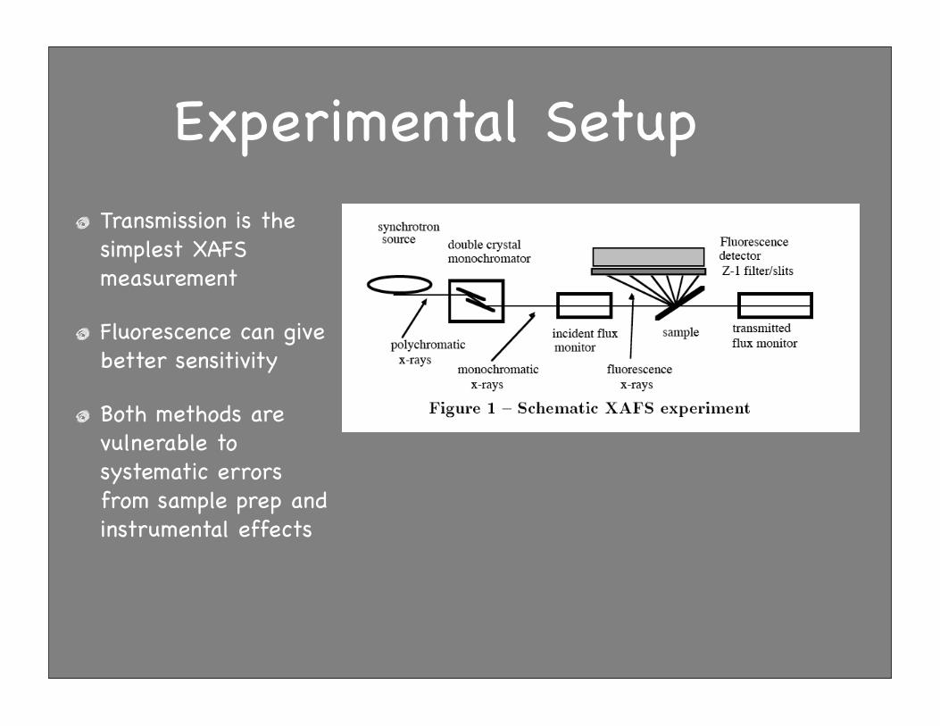
Transmission is the simplest XAFS measurement

Fluorescence can give better sensitivity

Both methods are vulnerable to systematic errors from sample prep and instrumental effects

Experimental Setup

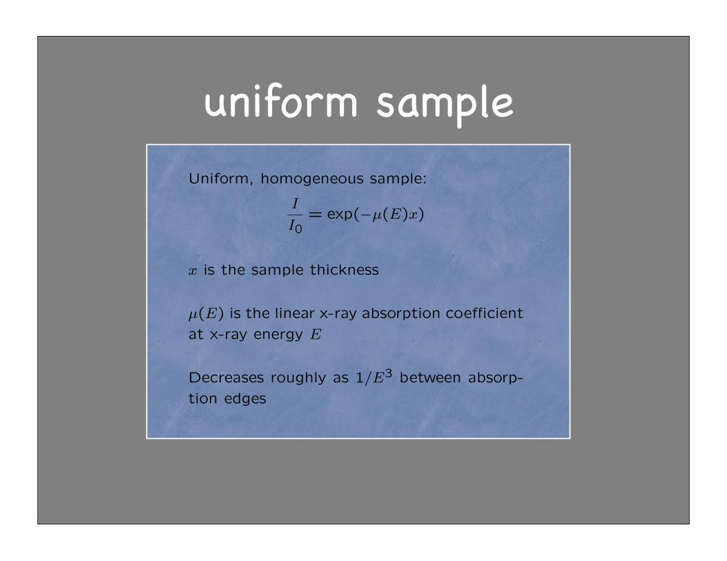
uniform sampleUniform, homogeneous sample:

I

I0= exp(!µ(E)x)

x is the sample thickness

µ(E) is the linear x-ray absorption coe!cientat x-ray energy E

Decreases roughly as 1/E3 between absorp-tion edges

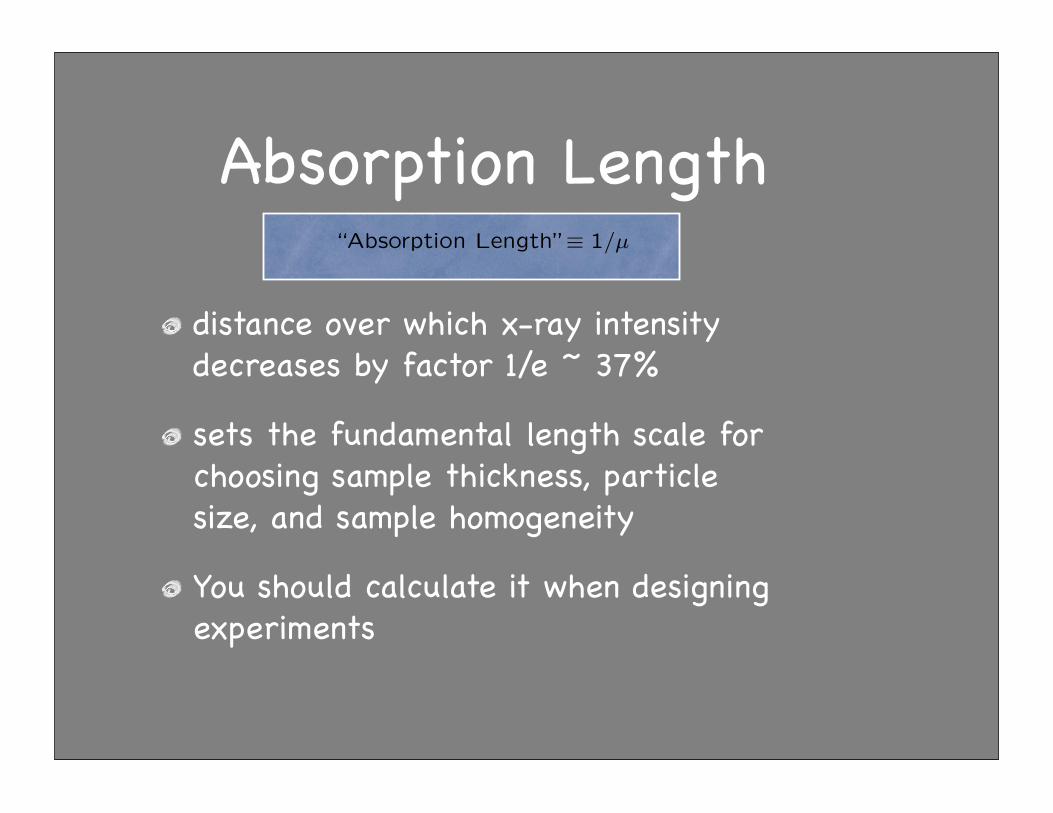
Absorption Length

distance over which x-ray intensity decreases by factor 1/e ~ 37%

sets the fundamental length scale for choosing sample thickness, particle size, and sample homogeneity

You should calculate it when designing experiments

“Absorption Length”! 1/µ

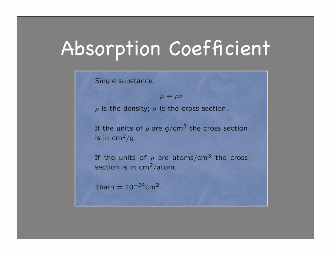
Absorption CoefficientSingle substance:

µ = !"

! is the density; " is the cross section.

If the units of ! are g/cm3 the cross sectionis in cm2/g.

If the units of ! are atoms/cm3 the crosssection is in cm2/atom.

1barn = 10!24cm2.

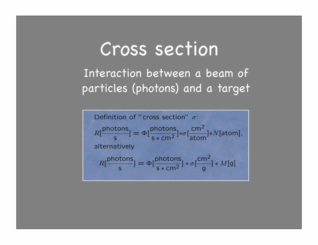
Cross section

Definition of ”cross section” !:

R[photons

s] = ![

photons

s ! cm2 ]!![cm2

atom]!N [atom],

alternatively

R[photons

s] = ![

photons

s ! cm2 ] ! ![cm2

g] ! M [g]

Interaction between a beam of particles (photons) and a target

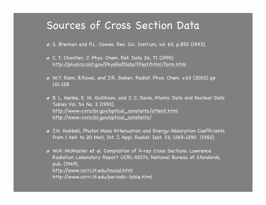
Sources of Cross Section DataS. Brennan and P.L. Cowan, Rev. Sci. Instrum, vol 63, p.850 (1992).

C. T. Chantler, J. Phys. Chem. Ref. Data 24, 71 (1995) http://physics.nist.gov/PhysRefData/FFast/html/form.html

W.T. Elam, B.Ravel, and J.R. Sieber, Radiat. Phys. Chem. v.63 (2002) pp 121-128.

B. L. Henke, E. M. Gullikson, and J. C. Davis, Atomic Data and Nuclear Data Tables Vol. 54 No. 2 (1993). http://www-cxro.lbl.gov/optical_constants/atten2.html http://www-cxro.lbl.gov/optical_constants/

J.H. Hubbell, Photon Mass Attenuation and Energy-Absorption Coefficients from 1 keV to 20 MeV, Int. J. Appl. Radiat. Isot. 33, 1269-1290 (1982)

W.H. McMaster et al. Compilation of X-ray Cross Sections. Lawrence Radiation Laboratory Report UCRL-50174, National Bureau of Standards, pub. (1969).http://www.csrri.iit.edu/mucal.htmlhttp://www.csrri.iit.edu/periodic-table.html

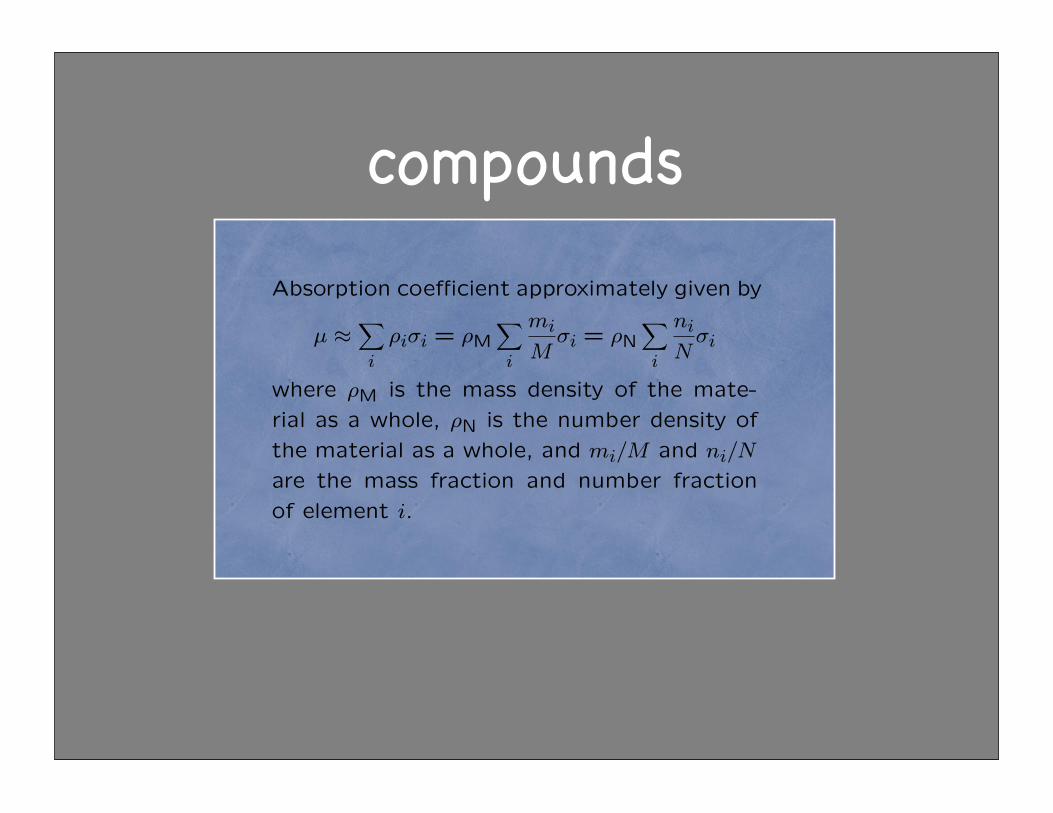
compoundsAbsorption coe!cient approximately given by

µ !!

i

!i"i = !M!

i

mi

M"i = !N

!

i

ni

N"i

where !M is the mass density of the mate-rial as a whole, !N is the number density ofthe material as a whole, and mi/M and ni/N

are the mass fraction and number fractionof element i.

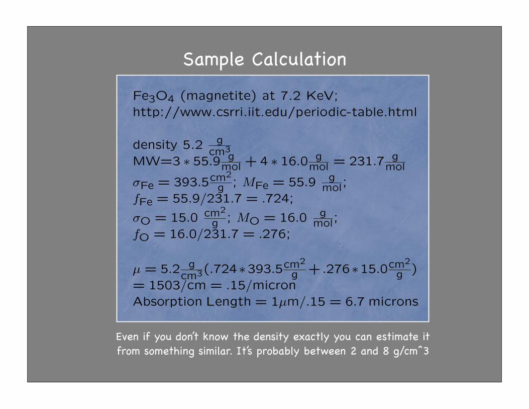
Fe3O4 (magnetite) at 7.2 KeV;http://www.csrri.iit.edu/periodic-table.html

density 5.2 gcm3

MW=3 ! 55.9 gmol + 4 ! 16.0 g

mol = 231.7 gmol

!Fe = 393.5cm2

g ; MFe = 55.9 gmol;

fFe = 55.9/231.7 = .724;

!O = 15.0 cm2

g ; MO = 16.0 gmol;

fO = 16.0/231.7 = .276;

µ = 5.2 gcm3(.724!393.5cm2

g + .276!15.0cm2

g )= 1503/cm = .15/micronAbsorption Length = 1µm/.15 = 6.7 microns

Sample Calculation

Even if you don’t know the density exactly you can estimate it from something similar. It’s probably between 2 and 8 g/cm^3

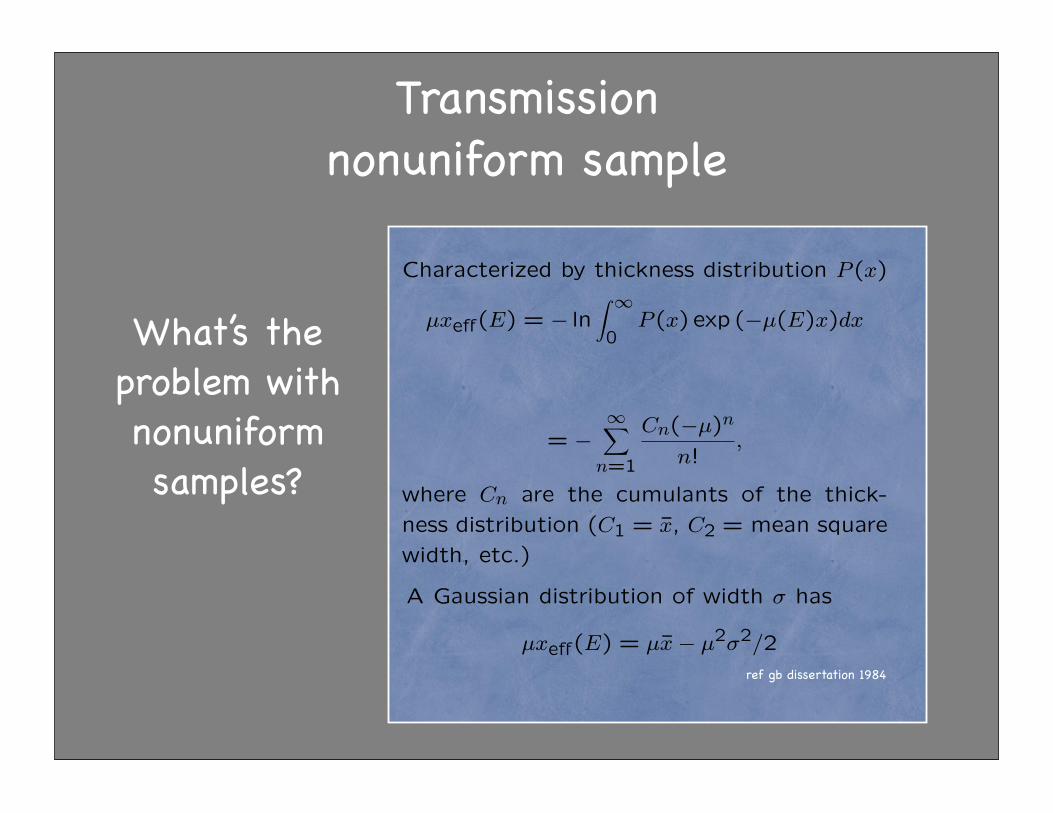
Transmissionnonuniform sample

Nonuniform Sample:

Characterized by thickness distribution P (x)

µxe!(E) = ! ln! "

0P (x) exp (!µ(E)x)dx

= !""

n=1

Cn(!µ)n

n!,

where Cn are the cumulants of the thick-ness distribution (C1 = x̄, C2 = mean squarewidth, etc.)

ref gb dissertation 1984

A Gaussian distribution of width ! has

µxe!(E) = µx̄! µ2!2/2

What’s theproblem withnonuniformsamples?

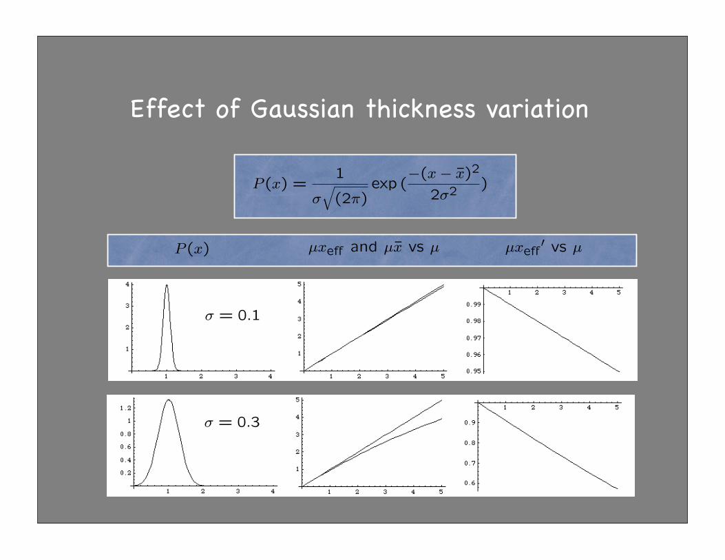
Effect of Gaussian thickness variation

P (x)

µxe! and µx̄ vs µ

µxe! vs µ

P (x)

µxe! and µx̄ vs µ

µxe! vs µ

P (x)

µxe! and µx̄ vs µ

µxe!! vs µ

P (x)

µxe! and µx̄ vs µ

µxe!! vs µ

! = 0.1

! = 0.3

P (x)

µxe! and µx̄ vs µ

µxe!! vs µ

! = 0.1

! = 0.3

P (x)

µxe! and µx̄ vs µ

µxe!! vs µ

! = 0.1

! = 0.3

P (x) =1

!!

(2")exp (

"(x " x̄)2

2!2 )

1 2 3 4

10

20

30

1 2 3 4 5

1

2

3

4

51 2 3 4 5

0.5

0.6

0.7

0.8

0.9

Effect of leakage/harmonics

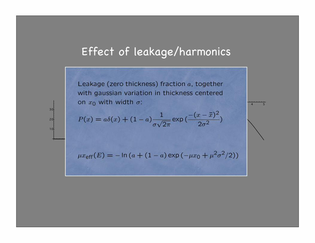
Leakage (zero thickness) fraction a, togetherwith gaussian variation in thickness centeredon x0 with width !:

P (x) = a"(x) + (1! a)1

!"

2#exp (

!(x! x̄)2

2!2 )

µxe!(E) = ! ln (a + (1! a) exp (!µx0 + µ2!2/2))

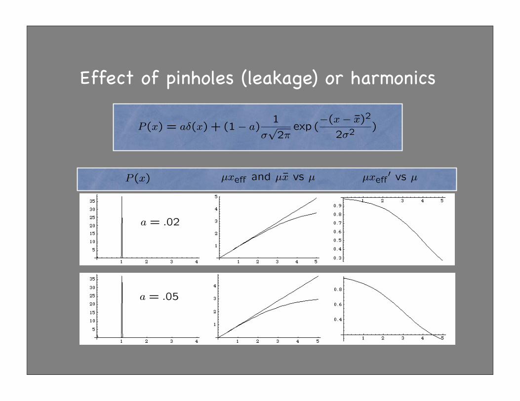
Effect of pinholes (leakage) or harmonics

P (x)

µxe! and µx̄ vs µ

µxe! vs µ

P (x)

µxe! and µx̄ vs µ

µxe! vs µ

P (x)

µxe! and µx̄ vs µ

µxe!! vs µ

a = .05

a = .02

a = .05

a = .02

Leakage (zero thickness) fraction a, togetherwith gaussian variation in thickness centeredon x0 with width !:

P (x) = a"(x) + (1! a)1

!"

2#exp (

!(x! x̄)2

2!2 )

µxe!(E) = ! ln (a + (1! a) exp (!µx0 + µ2!2/2))

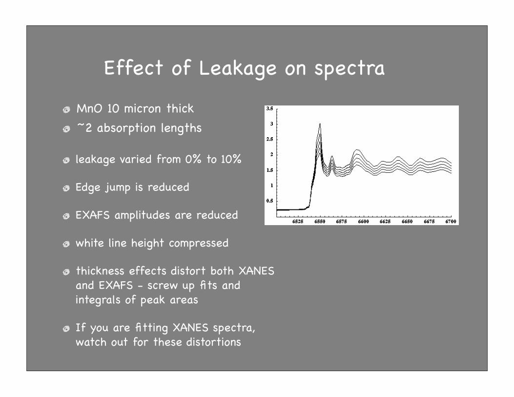
MnO 10 micron thick ~2 absorption lengths

leakage varied from 0% to 10%

Edge jump is reduced

EXAFS amplitudes are reduced

white line height compressed

thickness effects distort both XANES and EXAFS - screw up fits and integrals of peak areas

If you are fitting XANES spectra, watch out for these distortions

Effect of Leakage on spectra

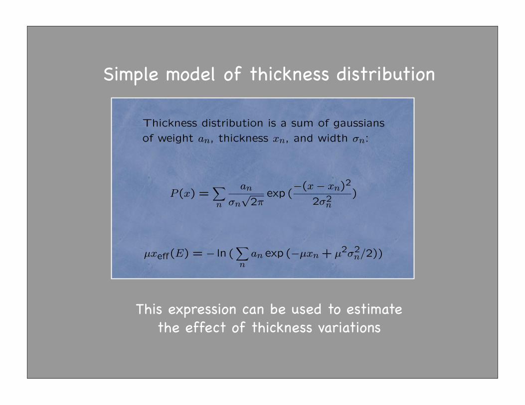
Thickness distribution is a sum of gaussiansof weight an, thickness xn, and width !n:

P (x) =!

n

an

!n!

2"exp (

"(x" xn)2

2!2n

)

µxe!(E) = " ln (!

nan exp ("µxn + µ2!2

n/2))

This expression can be used to estimatethe effect of thickness variations

Simple model of thickness distribution

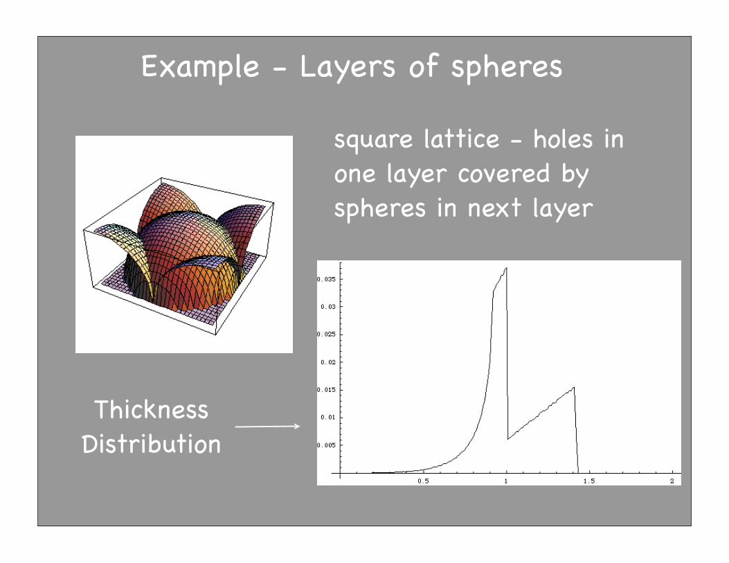
Example - Layers of spheres

square lattice - holes in one layer covered by spheres in next layer

ThicknessDistribution

Transmission mode -Summary

Samples in transmission should be made uniform on a scale determined by the absorption length of the material

Absorption length should be calculated when you’re designing experiments and preparing samples

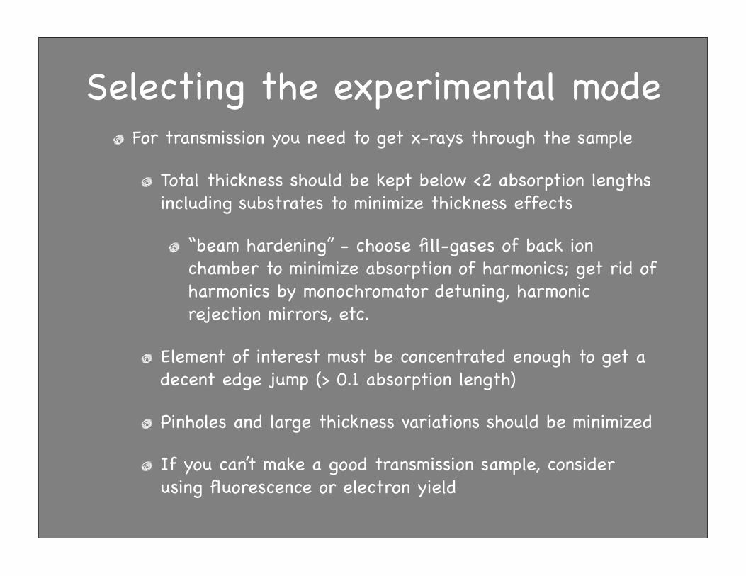
Selecting the experimental modeFor transmission you need to get x-rays through the sample

Total thickness should be kept below <2 absorption lengths including substrates to minimize thickness effects

“beam hardening” - choose fill-gases of back ion chamber to minimize absorption of harmonics; get rid of harmonics by monochromator detuning, harmonic rejection mirrors, etc.

Element of interest must be concentrated enough to get a decent edge jump (> 0.1 absorption length)

Pinholes and large thickness variations should be minimized

If you can’t make a good transmission sample, consider using fluorescence or electron yield

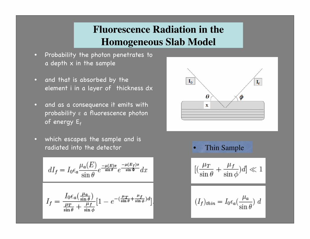
Fluorescence Radiation in the Homogeneous Slab Model

• Probability the photon penetrates to a depth x in the sample

• and that is absorbed by the element i in a layer of thickness dx

• and as a consequence it emits with probability ε a fluorescence photon of energy Ef

• which escapes the sample and is radiated into the detector • Thin Sample

Fluorescence samplesSimple in thin concentrated and thick dilute limits

Thick concentrated requires numerical corrections(e.g. Booth and Bridges, XAFS 12). Thickness effects can be corrected also if necessary by regularization (Babanov et al).

Sample Requirements

Particle size must be small compared to absorption lengths of particles (not just sample average). Can be troublesome for in situ studies

Homogeneous distribution

Flat sample surface preferred

Grazing incidence external reflection gives surface sensitivity

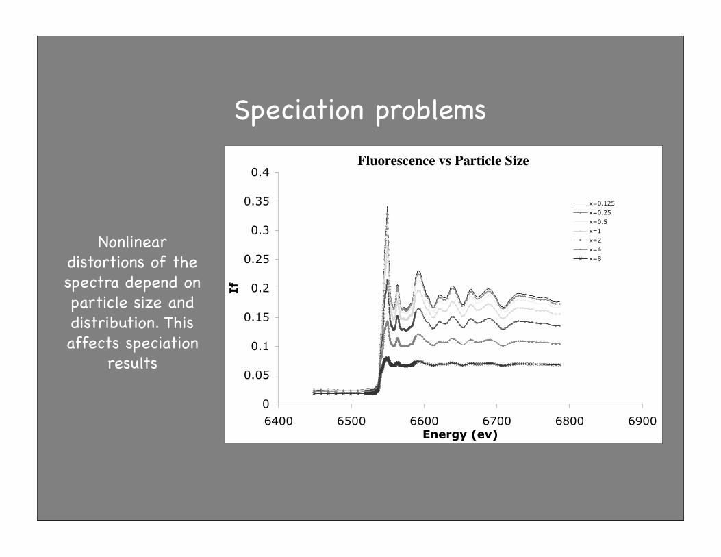
Speciation problems

47

On the other hand when d!", i.e. the “thick limit”, the exponential term

will vanish and for thick samples we will have:

(If )thick =I0!a(

µa

sin ! )µT

sin ! + µf

sin "

(5.6)

Fluorescence vs Particle Size

0

0.05

0.1

0.15

0.2

0.25

0.3

0.35

0.4

6400 6500 6600 6700 6800 6900

Energy (ev)

If

x=0.125

x=0.25

x=0.5

x=1

x=2

x=4

x=8

Figure 5.2. Fluorescence

But in general the measured fluorescence radiation depends nonlinearily on

µa. The nonlinearity problems arise when the sample consists of concentrated species

with particle sizes that are not small compared to one absorption length. In this

case the penetration depth into the particles has an energy dependence that derives

from the absorption coe!cient of the element of interest, making the interpretation of

the results much more complicated. Fig.5.2 [21] simulates how the measured XAFS

Nonlinear distortions of the spectra depend on particle size and distribution. This affects speciation

results

Dilute samples“dilute”: absorption of element of interest is much less than average absorption of sample

Even if the sample is dilute on average you may not be really in the dilute limit

Each individual particle must be small enough, otherwise you will get distorted spectra

Don’t just mix up your particles with a filler and think it’s dilute. First make particles small compared to one absorption length in the material of which the particles are composed.

Summary - FluorescenceParticle size effects are important in fluorescence as well as transmission

The homogeneous slab model is not always suitable but other models have been developed

If the particles are not sufficiently small, their shape, orientation, and distribution can affect the spectra in ways that can influence results

Particularly important for XANES and chemical speciation, but also important for EXAFS

Electron yield detectionsample is placed atop and electrically connected to the cathode of helium filled ion chamber

electrons ejected from surface of sample ionize helium - their number is proportional to absorption coefficient

The current is collected and it represents the signal, just in like an ionization chamber

Surface sensitivity of electron detection eliminates self-absorption problems but does not sample bulk material

Charging effects can be a problem

Sample InhomogeneitiesImportance of inhomogeneity also can depend on spatial structure in beam

bend magnets and wiggler beams usually fairly homogeneous

Undulator beams trickier because beam partially coherent

coherence effects can result in spatial microstructure in beam at micron scales

Beam Stability

Samples must not have spatial structure on the same length scales as x-ray beam. Change the sample, or change the beam.

Foils and films often make good transmission samples

stack multiple films if possible to minimize through holes

check for thickness effects (rotate sample)

Foils and films can make good thin concentrated or thick dilute samples in fluorescence

Consider grazing incidence fluorescence to reduce background and enhance surface sensitivity (see mirror equations later in this document)

SolutionsUsually solutions are naturally homogeneous

Can make good transmission samples if concentrated

Usually make good fluorescence samples (~1 millimolar and 100 ppm are routine), lower concentrations feasible

They can become inhomogeneous during experiment

phase separation

radiation damage can cause precipitation (e.g. protein solutions)

photolysis of water makes holes in intense beams

suspensions/pastes can be inhomogeneous

Particulate samplesFirst calculate the absorption length for the material

prepare particles that are considerably smaller than one absorption length of their material, at an energy above the edge

Many materials require micron scale particles for accurate results

Distribute the particles uniformly over the sample cross sectional area by dilution or coating

Making Fine Particles

During synthesis -> choose conditions to make small particles

Grinding and separating

sample must not change during grinding (e.g. heating)

For XAFS can’t use standard methods (e.g. heating in furnace and fluxing) from x-ray spectrometry, because chemical state matters

Have to prevent aggregation back into larger particles

Checking the samplecheck composition by spectroscopy or diffraction

visually check for homogeneity

caveat: x-ray vs optical absorption lengths

tests at beamline: move and rotate sample

digital microscope (Olympus Mic-D $800 US)

particle size analysis (Image/J free)

If you have nice instruments like a scanning electron microscope or light scattering particle size analyzer, don’t hesitate to use them

Preferred OrientationIf your sample is polycrystalline, it may orient in non-random way if applied to a substrate

since the x-ray beams are polarized this can introduce an unexpected sample orientation dependence

Test by changing sample orientation

Magic-angle spinning to eliminate effect

Control samplesIn fluorescence measurements always measure a blank sample without the element of interest under the same conditions as your real sample

Many materials have elements in them that you wouldn’t expect that can introduce spurious signals

Most aluminum alloys have transition metals

Watch out for impurities in adhesive films

Fluorescence from sample environment excited by scattered x-rays and higher energy fluorescence

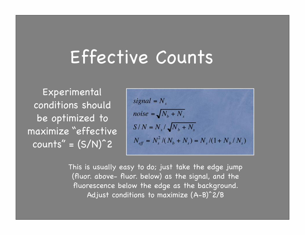
Effective Counts

signal = Ns

noise = Nb + Ns

S / N = Ns / Nb + Ns

Neff = Ns2 /(Nb + Ns ) = Ns /(1+ Nb / Ns )

Experimental conditions should be optimized to

maximize “effective counts” = (S/N)^2

This is usually easy to do; just take the edge jump (fluor. above- fluor. below) as the signal, and the fluorescence below the edge as the background.

Adjust conditions to maximize (A-B)^2/B

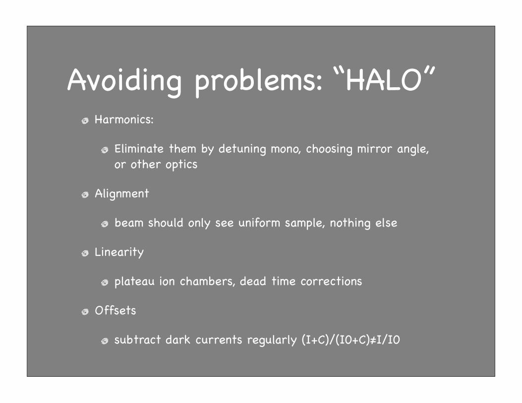
Avoiding problems: “HALO”Harmonics:

Eliminate them by detuning mono, choosing mirror angle, or other optics

Alignment

beam should only see uniform sample, nothing else

Linearity

plateau ion chambers, dead time corrections

Offsets

subtract dark currents regularly (I+C)/(I0+C)≠I/I0

Detector Linearity

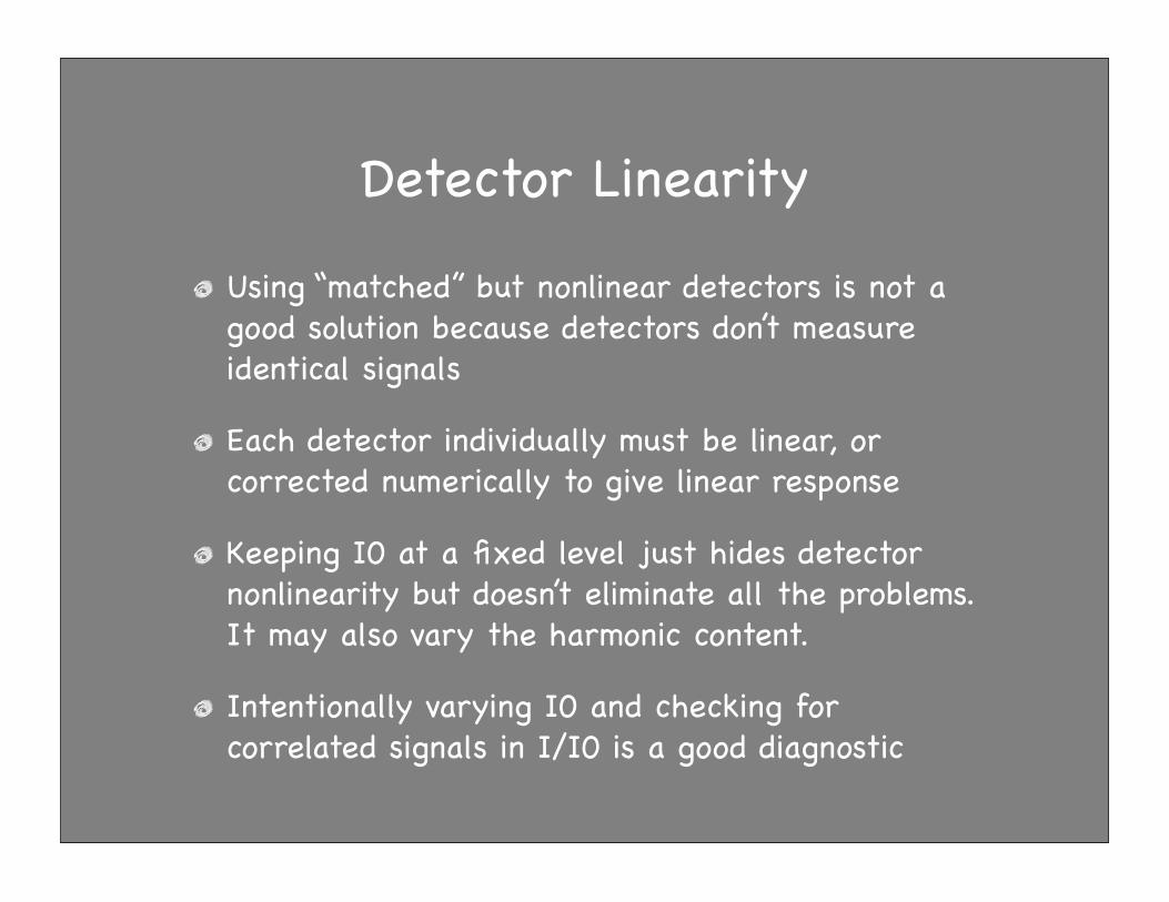
Using “matched” but nonlinear detectors is not a good solution because detectors don’t measure identical signals

Each detector individually must be linear, or corrected numerically to give linear response

Keeping I0 at a fixed level just hides detector nonlinearity but doesn’t eliminate all the problems. It may also vary the harmonic content.

Intentionally varying I0 and checking for correlated signals in I/I0 is a good diagnostic

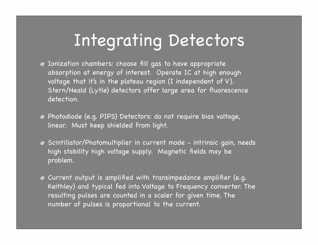
Integrating DetectorsIonization chambers: choose fill gas to have appropriate absorption at energy of interest. Operate IC at high enough voltage that it’s in the plateau region (I independent of V). Stern/Heald (Lytle) detectors offer large area for fluorescence detection.

Photodiode (e.g. PIPS) Detectors: do not require bias voltage, linear. Must keep shielded from light.

Scintillator/Photomultiplier in current mode - intrinsic gain, needs high stability high voltage supply. Magnetic fields may be problem.

Current output is amplified with transimpedance amplifier (e.g. Keithley) and typical fed into Voltage to Frequency converter. The resulting pulses are counted in a scaler for given time. The number of pulses is proportional to the current.

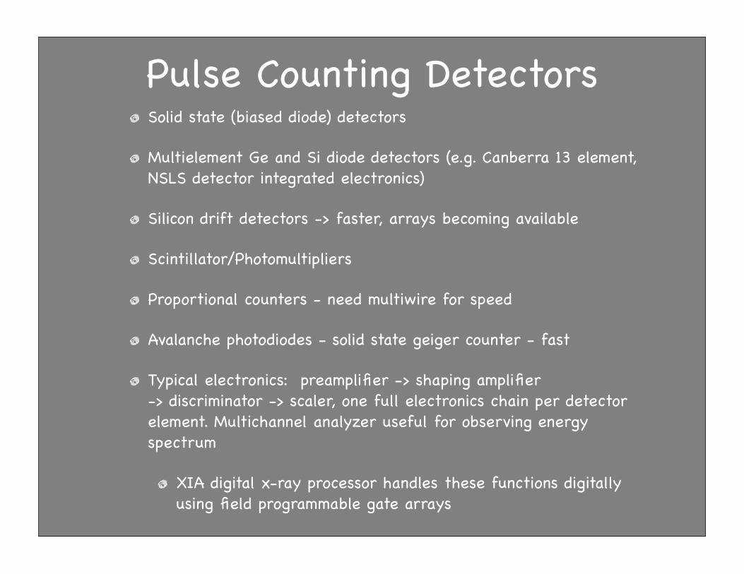
Pulse Counting DetectorsSolid state (biased diode) detectors

Multielement Ge and Si diode detectors (e.g. Canberra 13 element, NSLS detector integrated electronics)

Silicon drift detectors -> faster, arrays becoming available

Scintillator/Photomultipliers

Proportional counters - need multiwire for speed

Avalanche photodiodes - solid state geiger counter - fast

Typical electronics: preamplifier -> shaping amplifier -> discriminator -> scaler, one full electronics chain per detector element. Multichannel analyzer useful for observing energy spectrum

XIA digital x-ray processor handles these functions digitally using field programmable gate arrays

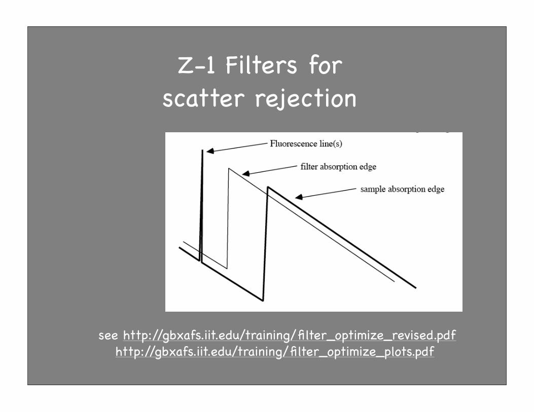
Z-1 Filters for scatter rejection

see http://gbxafs.iit.edu/training/filter_optimize_revised.pdfhttp://gbxafs.iit.edu/training/filter_optimize_plots.pdf

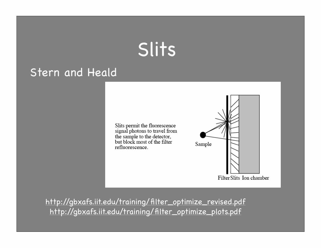
Slits

http://gbxafs.iit.edu/training/filter_optimize_revised.pdfhttp://gbxafs.iit.edu/training/filter_optimize_plots.pdf

Stern and Heald

Z-1 filters/slitsCan collect large solid angle with suitable detector (e.g. Stern/Heald ion chamber (Lytle detector)

Can be used a pre-filter for solid state detector arrays

Low pass filter only

Mostly useful for rejecting elastic scatter

Need good quality filters and effective slits

Inefficient for high background/signal ratios

No suitable filter for some elements

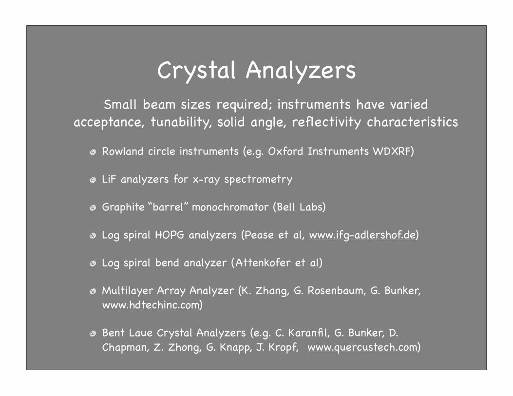
Crystal Analyzers

Rowland circle instruments (e.g. Oxford Instruments WDXRF)

LiF analyzers for x-ray spectrometry

Graphite “barrel” monochromator (Bell Labs)

Log spiral HOPG analyzers (Pease et al, www.ifg-adlershof.de)

Log spiral bend analyzer (Attenkofer et al)

Multilayer Array Analyzer (K. Zhang, G. Rosenbaum, G. Bunker, www.hdtechinc.com)

Bent Laue Crystal Analyzers (e.g. C. Karanfil, G. Bunker, D. Chapman, Z. Zhong, G. Knapp, J. Kropf, www.quercustech.com)

Small beam sizes required; instruments have variedacceptance, tunability, solid angle, reflectivity characteristics

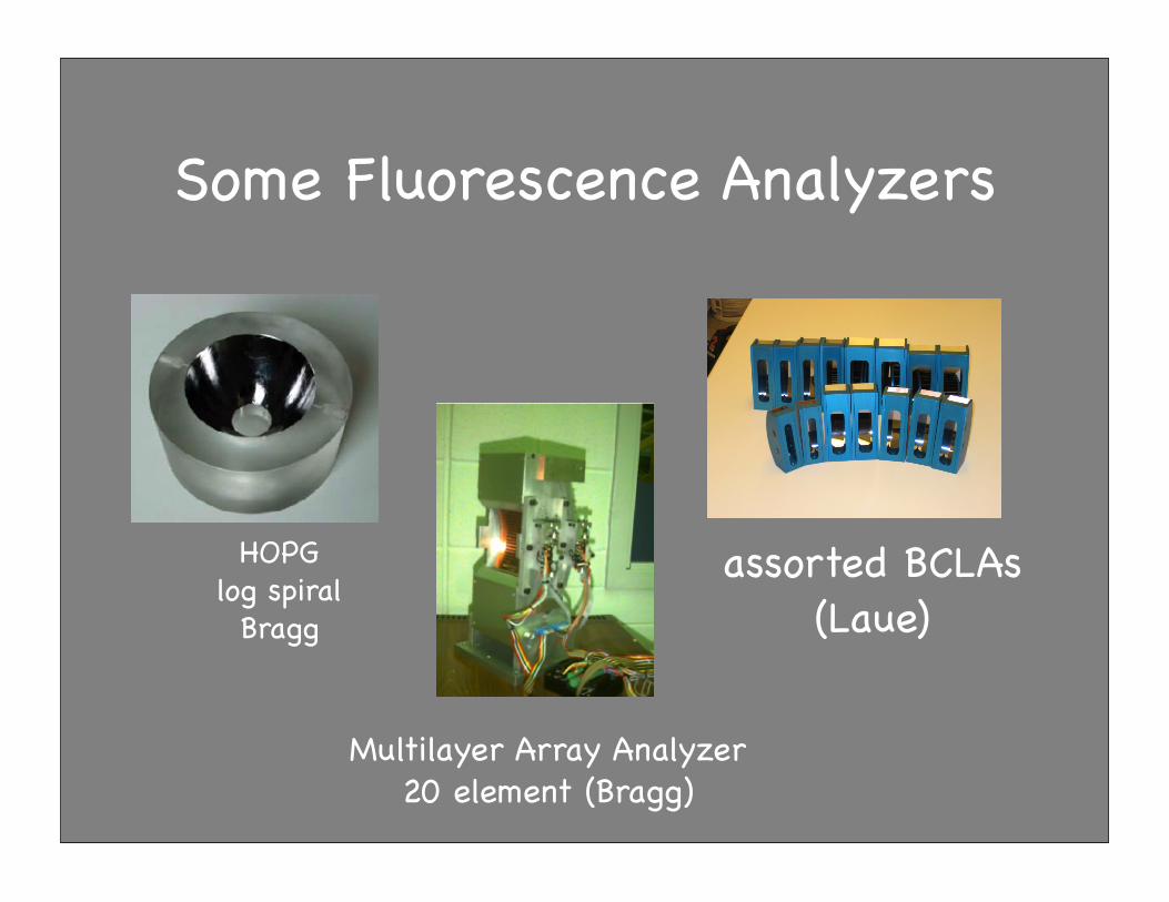
Some Fluorescence Analyzers

Multilayer Array Analyzer20 element (Bragg)

HOPGlog spiral

Bragg

assorted BCLAs(Laue)

ConclusionCalculate the absorption coefficients of your sample so you know what you are dealing with at the energies you care about. Think like an x-ray. Know what to expect.

Choose a beamline that can produce the kind of beam you need (flux, beam size, detectors available, etc). Choice of beamline/mode/sample/question_posed are interrelated decisions. Design the experiment iteratively with these in mind.

Make particles small compared to absorption length and make samples homogeneous

Check experimentally for thickness, particle size, and self absorption effects. Check a “blank” sample and a good reference sample.

Maximize your effective counts by choice of detector and experimental geometry. Quality of filters and slits matters. Do deadtime corrections.

“HALO” - check harmonics, alignment, linearity, offsets