Crop Simulation models; a research tool

Crop simulation models; a researCh tool

Agricultural College, Bapatla

Credit seminar on

By

Medida Sunil KumarBAD-14-06

1

ModelA model is a set of mathematical equations describing/mimic

behaviour of a system

Model simulates or imitates the behaviour of a real crop by

predicting the growth of its components

Modeling

Modeling is based on the assumption that any given process can

be expressed in a formal mathematical statement or set of

statements.

Simulation:

It is the process of building models and analyzing the system.

The art of building mathematical models and study their properties

in reference to those of the systems (de Wit, 1982)

Crop model:

Simple representation of a crop.

SYSTEM:

Limited part of reality that contains inter related

elements

Types of models (purpose for which it is designed )

Statistical & Empirical models

Mechanistic models

Deterministic models

Stochastic models

Static models

Dynamic models

Statistical & Empirical models

Direct descriptions of observed data, generally

expressed as regression equations

These models give no information on the mechanisms

that give rise to the response

Eg: Step down regressions, correlation, etc.

Mechanistic models

• These attempt to use fundamental mechanisms of plant

and soil processes to simulate specific outcomes

• These models are based on physical selection.

• Eg. photosynthesis based model.

Deterministic models

• These models estimate the exact value of the yield or

dependent variable.

• These models also have defined coefficients.

• Eg: NPK doses are applied and the definite yields are

given out.

Stochastic models

• The models are based on the probability of occurrence of

some event or external variable

• For each set of inputs different outputs are given along

with probabilities.

• These models define yield or state of dependent variable

at a given rate.

Static models

• Time is not included as a variables.

• Dependent and independent variables having values

remain constant over a given period of time.

Dynamic simulation models

• These models predict changes in crop status with time.

• Both dependent and independent variables are having

values which remain constant over a given period of time.

Chronology of crop simulation modeling

1960 Simple water-balance models

1965 Model photosynthetic rates of crop canopies (De Wit )

1970 Elementary Crop growth Simulator construction (De Wit )

1977 Introduction of micrometeorology in the models & quantification of canopy resistance (Goudriaan)

1978 Basic Crop growth Simulator (BACROS) [de Wit andGoudriaan]

1982 International Benchmark Sites Network for Agrotechnology Transfer) began the development of a model (University of Hawaii)Decision Support System for Agro- Technology Transfer (DSSAT)

1994 ORYZA1 (Kropff et al., 1994)

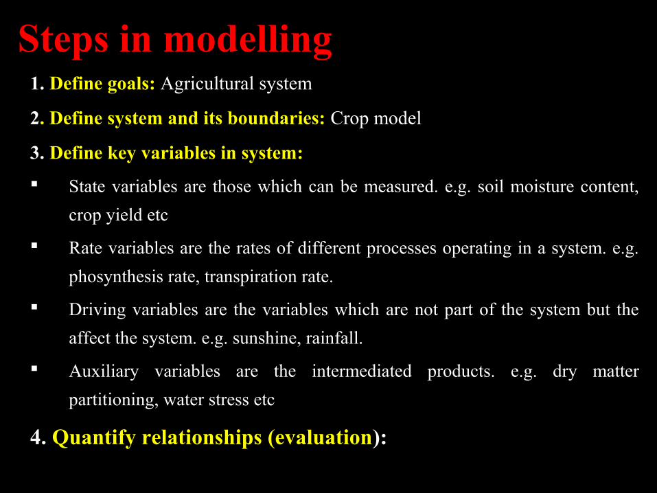
Steps in modelling 1. Define goals: Agricultural system

2. Define system and its boundaries: Crop model

3. Define key variables in system:

State variables are those which can be measured. e.g. soil moisture content,

crop yield etc

Rate variables are the rates of different processes operating in a system. e.g.

phosynthesis rate, transpiration rate.

Driving variables are the variables which are not part of the system but the

affect the system. e.g. sunshine, rainfall.

Auxiliary variables are the intermediated products. e.g. dry matter

partitioning, water stress etc

4. Quantify relationships (evaluation):

5. Calibration:

Model calibration is the initial testing of a model and tuning it to reflect a set of field data or process of estimating model parameters by comparing model predictions (out-put) for a given set of assumed conditions with observed data for the same conditions.

6. Validation:

Testing of a model with a data set representing "local" field data. This data set represents an independent source different from the data used to develop the relation

7. Sensitivity analysis:

Validated model is then tested for its sensitivity to different factors (e.g. temperature, rainfall, N dose). This is done to check whether the model is responding to changes in those factors or not.

Crop Simulation Models

Major & popular crop simulation models

DSSAT (Decision Support System for Agrotechnology Transfer)

AquaCrop

InfoCrop

APSIM (Agricultural Production System Simulator)

Overview of the components and sub-modular structure of DSSAT-CSM

J.W. Jones et al., 2003. Europ. J. Agronomy 18; 235-265

Components of AquaCrop, FAO model

http://www.fao.org/nr/water/infores_databases_aquacrop.html

INFOCROP

Sub-modular structure of APSIM model

Input files

Weather data

Soil data

Management data

Cultivar data

COEFF DEFINITIONSVAR# Identification code or number for a specific cultivarVAR-NAME Name of cultivarECO# Ecotype code or this cultivar, points to the Ecotype in the ECO file (currently not used).P1 Thermal time from seedling emergence to the end of the juvenile phase (expressed in degree days above a base temperature of 8ّ C(during which the plant is not responsive to changes in photoperiod.P2 Extent to which development (expressed as days) is delayed for each hour increase in photoperiod above the longest photoperiod at which development proceeds at a maximum rate (which is considered to be 12.5 hours).P5 Thermal time from silking to physiological maturity (expressed in degree days above a base temperature of 8Cّ).G2 Maximum possible number of kernels per plant.G3 Kernel filling rate during the linear grain filling stage and under optimum conditions (mg/day).PHINT Phylochron interval; the interval in thermal time (degree days)between successive leaf tip appearances.@VAR# VRNAME.......... ECO# P1 P2 P5 G2 G3 PHINTEG0011 S.C. 9 IB0001 400.0 0.200 620.0 650.0 11.4 40.00EG0004 SC 10 IB0001 400.0 0.300 865.0 720.0 11.5 38.90EG0013 S.C-103 IB0001 295.0 0.520 593.0 695.0 13.4 38.90EG0007 S.C-122 IB0001 270.0 0.500 580.0 650.0 13.6 38.90EG0008 S.C-124 IB0001 290.0 0.500 630.0 630.0 14.8 38.90EG0002 T.W.C.310 IB0001 430.0 0.200 868.0 700.0 10.0 40.00EG0014 T.W.C.323 IB0001 290.0 0.300 680.0 635.0 12.2 38.90

MAIZE

GENOTYPE COEFFICIENTS

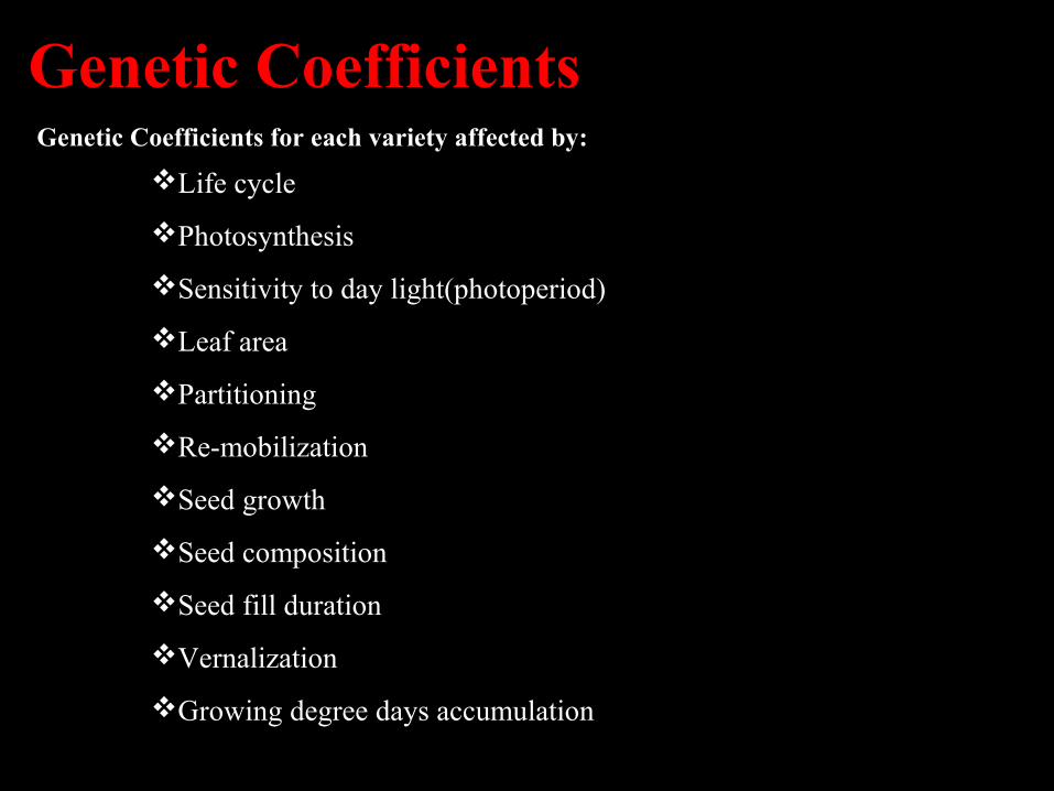
Genetic Coefficients

Life cycle

Photosynthesis

Sensitivity to day light(photoperiod)

Leaf area

Partitioning

Re-mobilization

Seed growth

Seed composition

Seed fill duration

Vernalization

Growing degree days accumulation

Genetic Coefficients for each variety affected by:

Who Uses simulation model Tools?

Agronomic Researchers and Extension Specialists

Policy Makers

Farmers and their Advisors

Private Sector

Educators

UsesOn Farm management

Crop system management: to evaluate optimum management

production for cultural practice.

Evaluate weather risk.

Investment decisions.

These are resource conserving tools

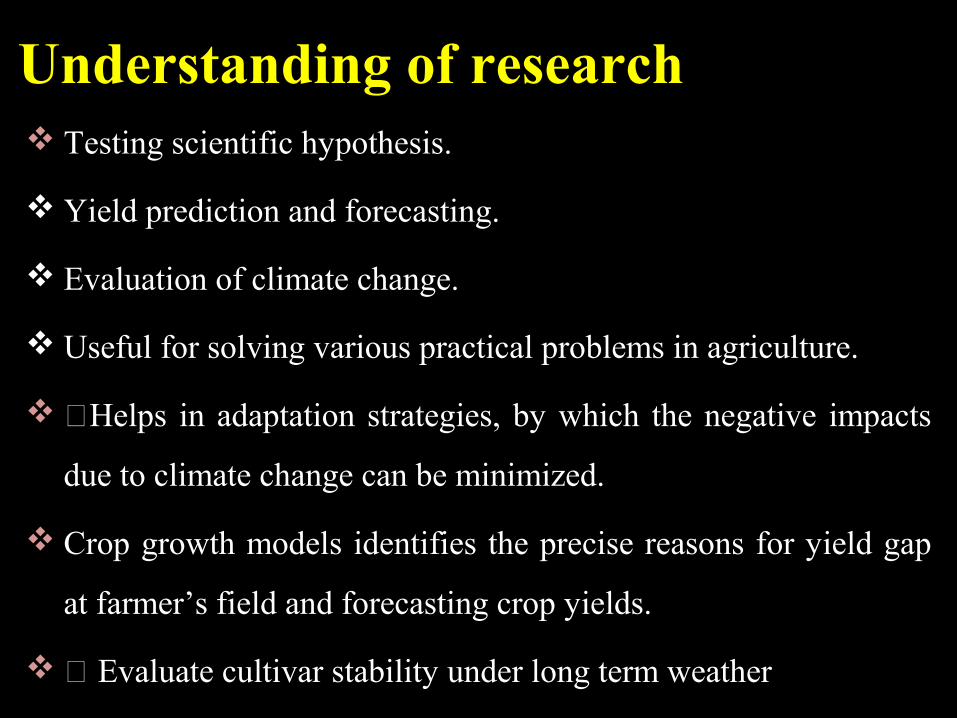
Understanding of research Testing scientific hypothesis.

Yield prediction and forecasting.

Evaluation of climate change.

Useful for solving various practical problems in agriculture.

�Helps in adaptation strategies, by which the negative impacts

due to climate change can be minimized.

Crop growth models identifies the precise reasons for yield gap

at farmer’s field and forecasting crop yields.

� Evaluate cultivar stability under long term weather

Experimental Data File

Cultivar data

Previous crop data

Crop Data during season

Output Depending on Option Setting and Simulation Application

Weather DataSoil Data

Crop Models

INPUTS

CERES rice

Y = grain yield as dry matter in g-2IH= harvest index (grain as a fraction of the aboveground biomass), nR= the value of the RUE in g MJ-2QdPARi= average daily total of incident PAR for a given month (i) in MJ m-2

Fi= fraction of PAR intercepted; Rn= number of days of radiation interception; Ri = fraction of the maximum RUE depending on crop performance, in g MJ-2

N= Number of months

Crop simulation models; a researCh

tool

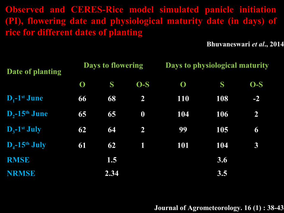
Observed and CERES-Rice model simulated panicle initiation (PI), flowering date and physiological maturity date (in days) of rice for different dates of planting

Journal of Agrometeorology. 16 (1) : 38-43

Bhuvaneswari et al., 2014

Date of plantingDays to flowering Days to physiological maturity

O S O-S O S O-S

D1-1st June 66 68 2 110 108 -2

D2-15th June 65 65 0 104 106 2

D3-1st July 62 64 2 99 105 6

D4-15th July 61 62 1 101 104 3

RMSE 1.5 3.6

NRMSE 2.34 3.5

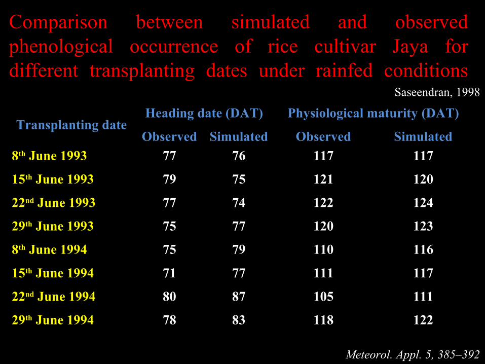
Comparison between simulated and observed phenological occurrence of rice cultivar Jaya for different transplanting dates under rainfed conditions

Meteorol. Appl. 5, 385–392

Saseendran, 1998

Transplanting dateHeading date (DAT) Physiological maturity (DAT)

Observed Simulated Observed Simulated

8th June 1993 77 76 117 117

15th June 1993 79 75 121 120

22nd June 1993 77 74 122 124

29th June 1993 75 77 120 123

8th June 1994 75 79 110 116

15th June 1994 71 77 111 117

22nd June 1994 80 87 105 111

29th June 1994 78 83 118 122

Comparison between Simulated and observed yield attributes and yield of rice cultivar Jaya under rainfed conditions fordifferent transplanting dates


Saseendran, 1998

Transplanting date

Grain yield (kg ha-1) Weight per grain Grain numberStraw weight at

harvest

Observed Simulated Observed Simulated Observed Simulated Observed Simulated

8th June 1993 5100 5089 0.030 0.030 16413 15135 4600 7758

15th June 1993 5300 5312 0.030 0.028 18735 16315 5100 7184

22nd June 1993 4300 4160 0.030 0.028 18565 17786 4500 6213

29th June 1993 3300 3267 0.030 0.029 16251 14679 4200 6743

8th June 1994 5200 5380 0.029 0.029 20520 19989 4900 5900

15th June 1994 5800 5855 0.030 0.030 21158 21892 5000 6900

22nd June 1994 6250 6600 0.029 0.030 20358 20099 5300 5400

29th June 1994 6500 6760 0.030 0.030 21899 21900 5800 5200

Average simulated crop and soil status at main development stages in rice cultivar of Jaya during 1993 & 1994 cropping seasons


Saseendran, 1998

Date Growth stagesBiomass (Kg ha-1)

LAI Leaf noET (mm)

Rain (mm)

Nitrogen stress

Water stress

8th June Transplanting 59 0.42 4 50 280 0.00 0.00

1st August End juvenile 3594 6.63 11 306 2094 0.00 0.03

8th August Panicle initiation 4892 7.72 12 348 2123 0.00 0.28

12th September Heading 9409 6.19 20 529 2571 0.00 0.49

21st September Begin grain fill 10725 4.26 20 620 2590 0.49 0.06

4th October End grain fill 12135 2.03 20 631 2735 0.47 0.00

7th October Maturity 12135 1.38 20 637 2740 0.00 0.00

7th October Harvest 12135 1.38 20 637 2740 0.00 0.00

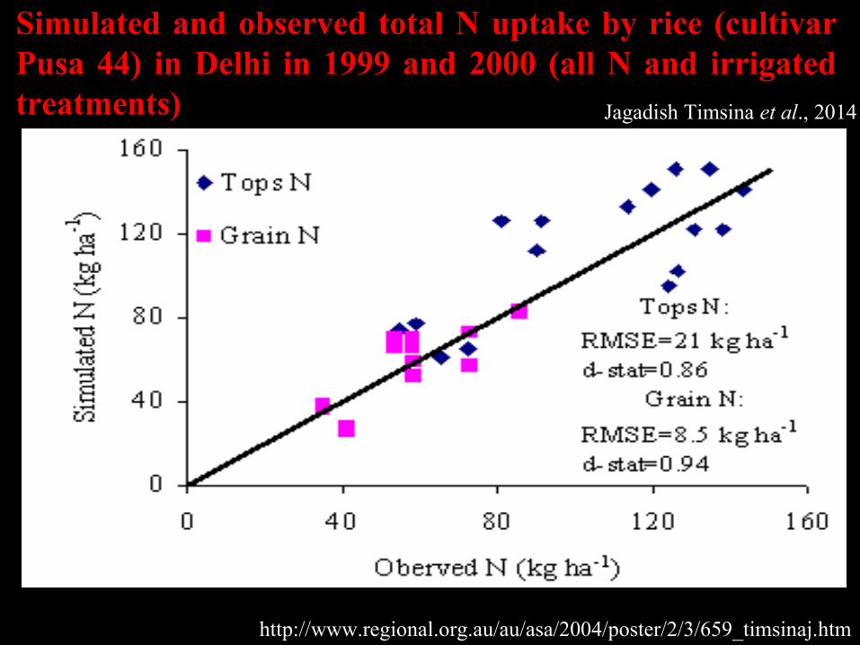
Simulated and observed total N uptake by rice (cultivar Pusa 44) in Delhi in 1999 and 2000 (all N and irrigated treatments) Jagadish Timsina et al., 2014

http://www.regional.org.au/au/asa/2004/poster/2/3/659_timsinaj.htm

Simulated seasonal cumulative mineralization of N in rice during 1999 in Delhi as influenced by N, FYM and water management

Pathak et al., 2004

http://www.clw.csiro.au/publications/technical2004/tr23-04.pdf

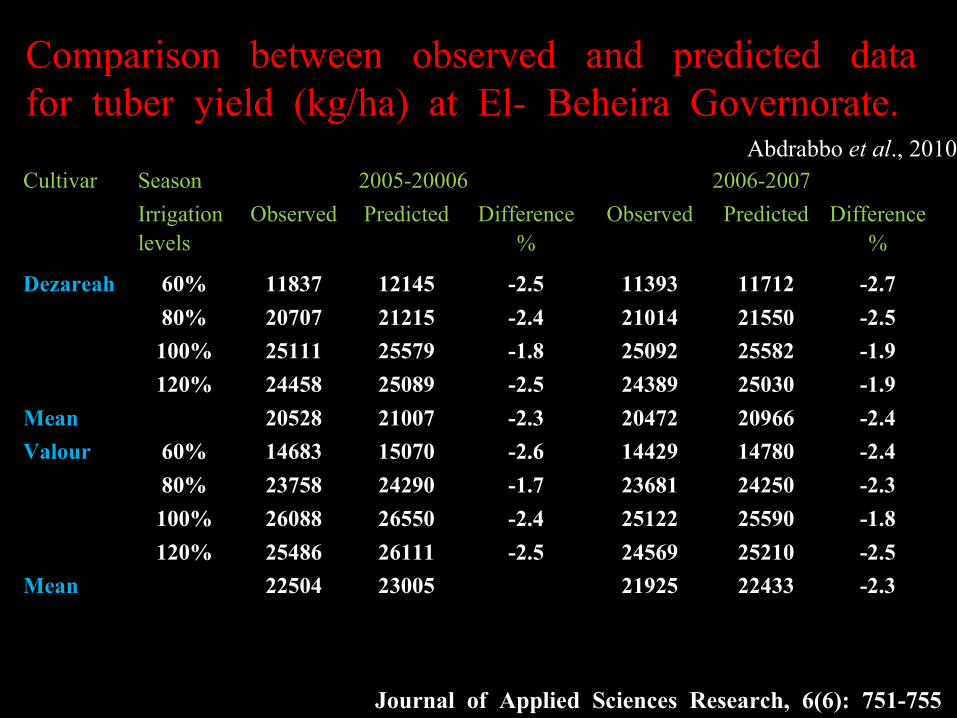
Comparison between observed and predicted data for tuber yield (kg/ha) at El- Beheira Governorate.

Cultivar Season 2005-20006 2006-2007

Irrigation levels

Observed Predicted Difference %

Observed Predicted Difference %

Dezareah 60% 11837 12145 -2.5 11393 11712 -2.7

80% 20707 21215 -2.4 21014 21550 -2.5

100% 25111 25579 -1.8 25092 25582 -1.9

120% 24458 25089 -2.5 24389 25030 -1.9

Mean 20528 21007 -2.3 20472 20966 -2.4

Valour 60% 14683 15070 -2.6 14429 14780 -2.4

80% 23758 24290 -1.7 23681 24250 -2.3

100% 26088 26550 -2.4 25122 25590 -1.8

120% 25486 26111 -2.5 24569 25210 -2.5

Mean 22504 23005 21925 22433 -2.3

Journal of Applied Sciences Research, 6(6): 751-755

Abdrabbo et al., 2010

Simulated and observed losses of N (kg ha-1) from rice in northwest India using CERES model

Pathak et al., 2004


Losses Observed a Simulated b

Denitrification 30 (10-40) 48Leaching 15 (10-18) 14Volatilization 25 (20-35) 4

a = Mean for saturated and AWD treatments with recommended N (120 kg ha-1)b = Mean for saturated and AWD treatments with recommended N (120 kg ha-1)

Impact of different rates of urea N on simulated rice yield, N losses and N use efficiency with saturated soil moisture regime in Delhi in 1999 using validated CERES 4.1 model.

Pathak et al., 2004


Climatic potential, on-station and on-farm yields of rice (Mg ha-1) and yield gaps in rice for three sites in India using validated CERES 4.1 model.

a = Average yield of the whole district with different water and nitrogen management

Pathak et al., 2004


Station namePotential

yield (A)

Actual yield Yield gap (%)

On station (B)

On farm a (C)

(A-B)A*100

(A-C) A*100

Ludhiana 10.8 7.8 5.6 28 48

Delhi 10.3 7.1 3.3 31 68

Modipuram 10.0 6.2 3.5 38 65

Effect of planting date on simulated potential yield of rice (Variety Pusa 44) in Delhi in 1999 using validated CERES 4.1 model Pathak et al., 2004


Observed and simulated yield of rice cultivar N2 with statistical analyses results. Agric Eng Int: CIGR Journal Open access at http://www.cigrjournal.org Vol. 15 (1), 19-26

Agric Eng Int: CIGR Journal Open access at http://www.cigrjournal.org Vol. 15 (1), 19-26

Akinbile, 2013

Crop parameter SI OB SI-OB R2 RMSE BIAS

Grain yield 2.63 2.41 0.22 0.99 0.16 0.06

Leaves & stem biomass

13.74 8.17 5.77 0.99 2.78 1.39

Total above ground biomass

16.47 10.58 5.89 0.99 2.68 1.34

Note: SI-Simulated Value (t/ha); OB-Observed value (t/ha); R2-Coefficient of determination; RMSE-Root mean square error;

Comparison between observed and simulated total grain yield against applied irrigation water


Akinbile, 2013

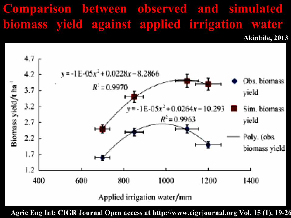
Comparison between observed and simulated biomass yield against applied irrigation water

Akinbile, 2013


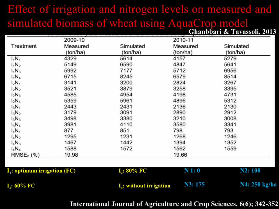
Effect of irrigation and nitrogen levels on measured and simulated biomass of wheat using AquaCrop model

Ghanbbari & Tavassoli, 2013

International Journal of Agriculture and Crop Sciences. 6(6); 342-352

I1: optimum irrigation (FC) I2: 80% FC

I3: 60% FC I4: without irrigation

N 1: 0 N2: 100

N3: 175 N4: 250 kg/ha

Main growth and development variables of CNT1 variety, obtained from observation, and simulation of ORYZA2000 and CERES-Rice. Thai Journal of Agricultural Science. 43(1): 17-29

Thai Journal of Agricultural Science. 43(1): 17-29

Wikarmpapraharn & Kositsakulchai, 2010

Variables Observed ORYZA CERES

Panicle initiation 53 48 45Anthesis 72 64 77Physiological Maturity 124 120 103

Yield at harvest maturity kg/ha 5275 5319 5202

LAI maximum 2.57 3.45 2.33

ORYZA2000 calibration against calibration data set from field experiment in 2007 under situation of potential production showing crop growth variables over the entire growing season. Thai Journal of Agricultural Science. 43(1): 17-29



ORYZA2000 calibrationStatistical indices

RMSE RMSEn D-index

Biomass of green leaves (kg/ha) 13.02 07.50 0.99

Biomass of panicle [Yield] (kg/ha) 08.16 00.85 0.99

Biomass of stem (kg/ha) 46.83 15.82 0.98

Total biomass (kg/ha) 69.36 08.68 0.99

Leaf area index (ha leaf/ha soil) 00.32 12.92 0.99



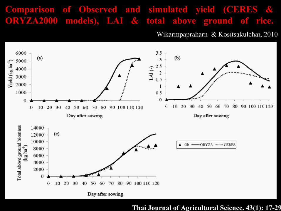
Comparison of Observed and simulated yield (CERES & ORYZA2000 models), LAI & total above ground of rice.

Comparison of observed and simulated stem biomass, total above ground biomass of rice using CERES and ORYZA.


Wikarmpapraharn and Kositsakulchai, 2010

Validation of dry tuber yield (t ha-1) and cultivars of potato cultivars Rosara and Karin using SUBSTOR model

Agriculturae Conspectus Scientificus; 73 (4), 227-234.

Sastana and Dufkova, 2008

Year

Rosara Karin

Water limited yield

Potential yield

Observed yield

Water limited yield

Potential yield

Observed yield

1994 06.1 19.4 06.5 05.6 18.5 07.61995 04.3 19.9 10.3 04.2 19.8 10.71996 08.4 22.0 11.4 08.3 22.0 10.81997 11.7 15.8 06.4 12.0 15.9 07.31998 09.5 26.6 05.5 09.7 26.7 09.21999 13.0 24.1 08.5 13.0 24.2 11.72000 07.1 21.6 08.4 06.94 21.7 09.52001 08.3 23.3 07.8 08.6 23.2 08.82002 17.3 23.6 11.7 17.6 24.0 12.0

Statistical summary comparing observed data with simulated values for DS rice–wheat cropping system using CropSyst simulation model

N= No. of observations; R2= Pearson’s correlation coefficient; RMSE= Root mean square error; MAE= Mean absolute error; MBEMBE= Mean biased error; ME= Modelling efficiency.

Singh et al., 2013

Current Science, 104 (10); 1324- 1331

Crop Parameter NObserved

meanPredicted

meanMAE

(Mg ha-1)R2

RMSE (Mg ha-1)

ME(%)

MBE(Mg ha-1)

Rice

Biomass (Mg ha-1)

24 7.20 6.55 0.65 0.97 0.70 53.0 0.65

Grain yield(Mg ha-1)

24 2.41 2.29 0.27 0.90 0.33 80.2 0.12

Wheat

Biomass (Mg ha-1)

24 7.82 7.11 0.71 0.95 0.80 76.2 0.70

Grain yield (Mg ha-1)

24 3.46 3.55 0.26 0.84 0.33 89.5 -0.10

Environment module

DSSAT Simulations of dry matter &Yields of Rice cultivar IR-20 (IR 20) for Tanjore District

Ramaraj et al., 2012

ISPRS Archives XXXVIII-8/W3 Workshop Proceedings: Impact of Climate Change on agriculture

Impact of elevated temperature on rice productivity (kg ha-1) under different dates of planting



Date of planting Current climateIncrease in temperature

1oC 2oC 3oC 4oC 5oC

D1-1st June 6687 -4 -15 -22 -37 -53

D2-15th June 5808 -4 -13 -23 -39 -53

D3-1st July 5200 -4 -12 -24 -40 -54

D4-15th July 4653 -4 -15 -25 -40 -56

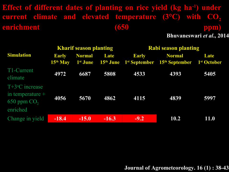
Effect of different dates of planting on rice yield (kg ha-1) under current climate and elevated temperature (3°C) with CO2 enrichment (650 ppm)



SimulationKharif season planting Rabi season planting

Early15th May

Normal 1st June

Late 15th June

Early1st September

Normal 15th September

Late 1st October

T1-Current climate

4972 6687 5808 4533 4393 5405

T+3oC increase in temperature + 650 ppm CO2

enriched

4056 5670 4862 4115 4839 5997

Change in yield -18.4 -15.0 -16.3 -9.2 10.2 11.0

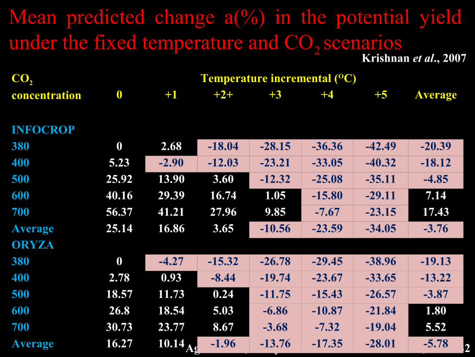
Mean predicted change a(%) in the potential yield under the fixed temperature and CO2 scenarios

Krishnan et al., 2007

Agriculture, Ecosystems and Environment 122; 233–242

CO2

concentration

Temperature incremental (OC)0 +1 +2+ +3 +4 +5 Average

INFOCROP380 0 2.68 -18.04 -28.15 -36.36 -42.49 -20.39400 5.23 -2.90 -12.03 -23.21 -33.05 -40.32 -18.12500 25.92 13.90 3.60 -12.32 -25.08 -35.11 -4.85600 40.16 29.39 16.74 1.05 -15.80 -29.11 7.14700 56.37 41.21 27.96 9.85 -7.67 -23.15 17.43Average 25.14 16.86 3.65 -10.56 -23.59 -34.05 -3.76ORYZA380 0 -4.27 -15.32 -26.78 -29.45 -38.96 -19.13400 2.78 0.93 -8.44 -19.74 -23.67 -33.65 -13.22500 18.57 11.73 0.24 -11.75 -15.43 -26.57 -3.87600 26.8 18.54 5.03 -6.86 -10.87 -21.84 1.80700 30.73 23.77 8.67 -3.68 -7.32 -19.04 5.52Average 16.27 10.14 -1.96 -13.76 -17.35 -28.01 -5.78

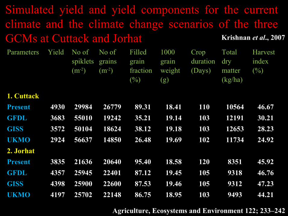
Simulated yield and yield components for the current climate and the climate change scenarios of the three GCMs at Cuttack and Jorhat Krishnan et al., 2007


Parameters Yield No of spiklets (m-2)

No of grains (m-2)

Filled grain fraction (%)

1000 grain weight (g)

Crop duration (Days)

Total dry matter (kg/ha)

Harvest index (%)

1. Cuttack

Present 4930 29984 26779 89.31 18.41 110 10564 46.67

GFDL 3683 55010 19242 35.21 19.14 103 12191 30.21

GISS 3572 50104 18624 38.12 19.18 103 12653 28.23

UKMO 2924 56637 14850 26.48 19.69 102 11734 24.92

2. Jorhat

Present 3835 21636 20640 95.40 18.58 120 8351 45.92

GFDL 4357 25945 22401 87.12 19.45 105 9318 46.76

GISS 4398 25900 22600 87.53 19.46 105 9312 47.23

UKMO 4197 25702 22148 86.75 18.95 103 9493 44.21

Estimated changes in rice yield predicted by the ORYZA1 model for each observation site in eastern India under the three GCM scenarios



SitesRice yields (t/ha)

GFDL GISS UKMO

Predicted change

(%)

Predicted yield (t/ha)

Predicted change

(%)


Predicted change

(%)


Bhubaneswar 4.46 -17.33 3.69 -20.36 3.55 -27.53 3.23

Chinsurah 5.18 -8.03 4.76 -8.72 4.73 -9.59 4.68Cuttack 4.93 -19.67 3.96 -20.32 3.93 -30.75 3.41Faizabad 4.72 -9.02 4.29 -11.27 4.19 -18.82 3.83Jabalpur 7.54 -11.05 6.71 -14.08 6.48 -21.05 5.95Jorhat 3.83 12.13 4.29 12.64 4.31 8.31 4.15

Kalyani 3.55 -7.75 3.27 -9.76 3.20 -16.51 2.96Pusa 3.82 -4.93 3.63 -6.31 3.58 -6.58 3.57Raipur 3.75 -2.79 3.65 -5.22 3.55 -10.09 3.37

Ranchi 4.50 -7.87 4.15 -10.35 4.03 -25.98 3.33

Average Change (%)

4.63 -7.63 4.24 -9.38 4.16 -15.86 3.85

Changes in yield (%) under the GCMs scenarios of the rice variety IR 36 under different sowing dates grown during the kharif season at Cuttack using InfoCrop model.



Changes in yield (%) under the GCMs scenarios of the rice variety IR 36 and IR 36 with improved temperature tolerance grown during the kharif season at Cuttack using InfoCrop model.



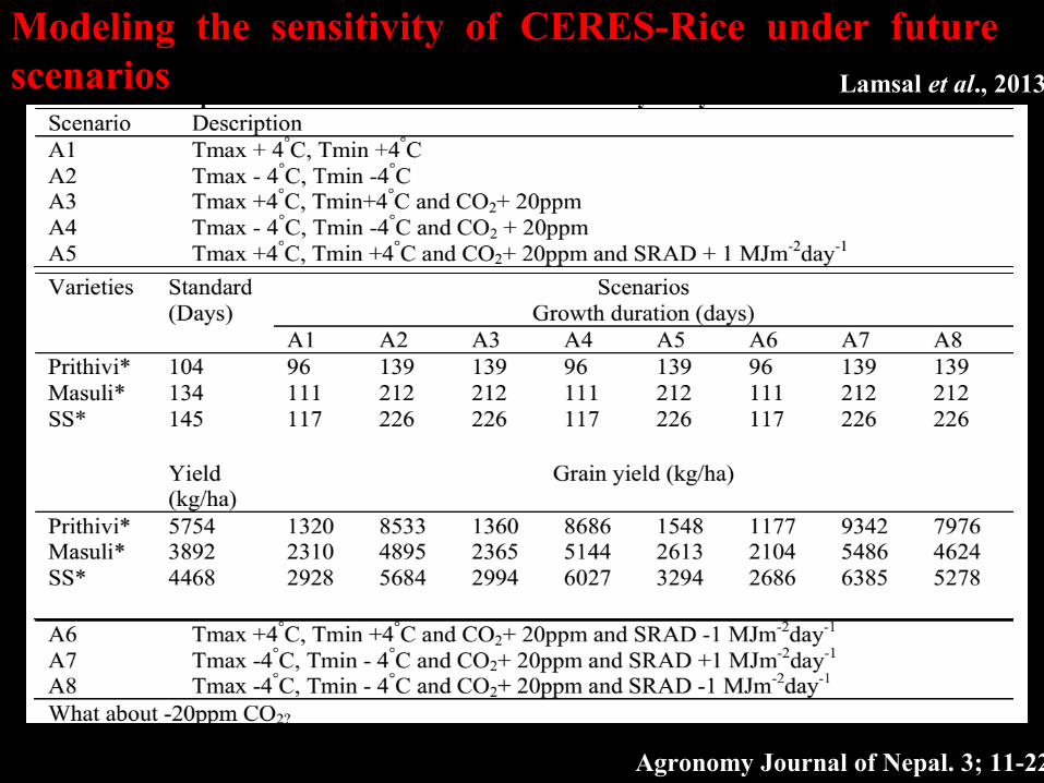
Modeling the sensitivity of CERES-Rice under future scenarios Lamsal et al., 2013

Agronomy Journal of Nepal. 3; 11-22

Predicted yield of BR3 variety of boro rice (kg ha-1) at 12 selected locations for the years 2008, 2030, 2050 and 2070 Jayanta Kumar Basak et al., 2010

Journal of Civil Engineering. 38 (2); 95-108

Effect of different sowing dates, irrigation levels on simulated potato yields under future climate scenario using SUBSTOR model of DSSAT under Egypt conditions Medany, M, 2006

http://www.agridema.org/opencms/export/sites/Agridema/Documentos/Egypt_Medany.pdf

Treatments Tuber fresh weight (kg/ha)

2005 2025 2050 2075 2100

Current Estimated

Difference %

Estimated Difference %



Irrigation 80 % 24730 23591 -4.7 24157 -2.4 24715 -1.2 24943 1.4

100% 25980 25033 -3.7 25863 -0.5 26137 1.5 26113 0.5

120 % 25397 24458 -3.7 25060 -1.3 25428 0.1 25487 0.4

Planting dates

Jan 1st 25703 27102 5.6 28223 9.9 29068 13.2 29531 15

Jan 15th 25750 23048 -10.5 23887 -7.2 24234 -5.9 24467 -4.9

Jan 30th 24653 22931 -7.1 22970 -6.9 22977 -6.9 22744 -7.8

Climate change scenarios

A1 25369 24402 -3.8 25147 -0.9 25547 0.6 25486 0.4

A2 25369 24423 -3.8 25147 -0.9 25697 1.2 25941 2.1

B1 25369 24308 -4.2 24782 -2.4 25171 -0.8 25416 0.1

B2 25369 24308 -4.2 25032 -1.4 25291 0.4 25480 0.4

Mean 25369 24360 -3.98 25027 -1.4 25426 0.16 25571 0.75

A1: Future world of very rapid economic growth with rapid introduction of new and more efficient technologies and reduction in regional differences in per capita income

A2: Very heterogeneous world, self-reliance and preservation of local identities, continuously increasing population. Economic development is primarily regionally orientation

B1: Convergent world with the same global population like A1 but introduction of clean and resource-efficient technologies. B2: Like A2 but world in which the emphasis is on local solutions to economic, social and environmental sustainability

63

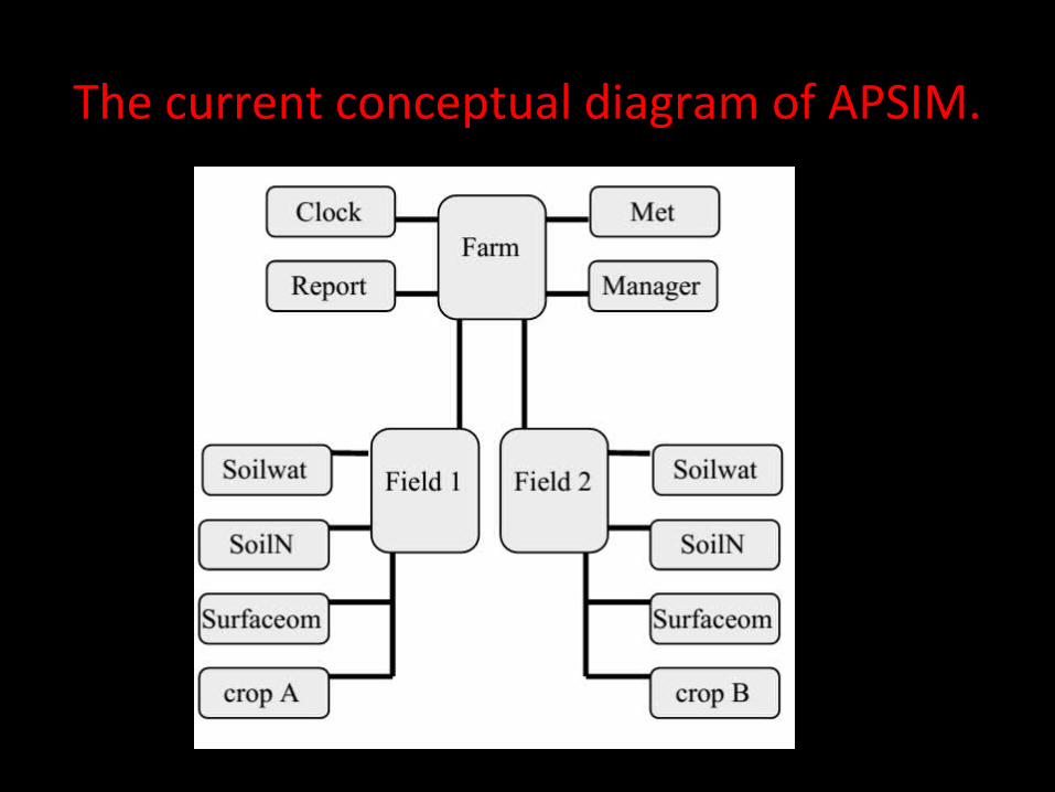
The current conceptual diagram of APSIM.

Simplified representation of the model with at the left side the modules (gathered as a function of their modality of call within the code), and at the right side the system with its three sub-systems (D: dominant crop; U:understorey crop divided into a shaded part: SU and a sunlit part: LU) and in the centre the number of calls of each module devoted to a particular part of the system.* corresponds to the modules modified for the adaptation to intercropping.

Interaction of intercropping system

Gliricidia/Dichanthium

Brisson et al., 2004

Agronomie, EDP Sciences. 24 (6-7); 409-421

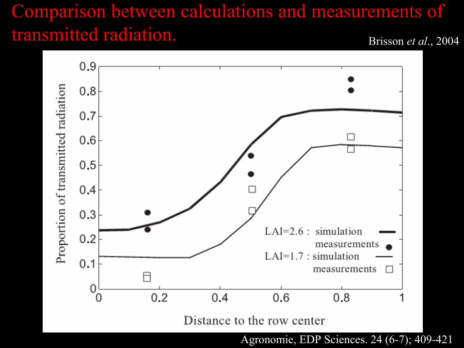
Comparison between calculations and measurements of transmitted radiation. Brisson et al., 2004


The two possible schemes of resistance networks used to estimate water requirement for intercrops (right side of the schemes) and the fluxes (left side of the schemes) the understory crop is near to the ground.

E= Evaporationm= maximumU=UnderstoryD=DominantES= soil evaporationraS and raA =eddy diffusion resistances:, racDand racU=bulk boundary layer resistances of bothCropsrS, rcD,and rcU=surface resistances:



The two possible schemes of resistance networks used to estimate water requirement for intercrops (right side of the schemes) and the fluxes (left side of the schemes) the understory crop is nearly as high as the dominant crop. Brisson et al., 2004


Illustration of the calculation of an equivalent plantingdensity for the understorey crop.



Simulation of root length production and a mean indicator of the constraint exerted by the soil on root distribution, in the case study of a Gliricidia-Dicanthium intercrop: monocrops above and intercrops below for both components Brisson et al., 2004


Simulation of root profile dynamics in the case study ofGliricidia-Dicanthium intercrop: monocrops above and intercropsbelow for both components.



Replacement series of relative yields of leek monoculture [ ], leek-celery intercrop[ ] and celery monoculture [ ] with three crop densities (40:20 [line], 20:10[dashed line] & 10:5 [dotted line] plants m2)



Seasonal changes in the modelled and measured values of total dry matter (TDM) for maize and beans using Model Brisson et al., 2004


Education

Crop Simulation models; a research tool