Embed Size (px)
Citation preview
Artificial IntelligenceSearch by Optimization
Andres Mendez-Vazquez
February 1, 2015
1 / 66
Outline
1 Introduction
2 Gradient DescentNotes about OptimizationNumerical Method: Gradient Descent
3 Hill ClimbingBasic TheoryAlgorithmEnforced Hill Climbing
4 Simulated AnnealingBasic IdeaThe Metropolis Acceptance CriterionAlgorithm
2 / 66
Introduction
Optimization SearchesSometimes referred to as iterative improvement or local search.
We will talk about four simple but e�ective techniques:1 Gradient Descent2 Hillclimbing3 Random Restart Hillclimbing4 Simulated Annealing
3 / 66
Introduction
Optimization SearchesSometimes referred to as iterative improvement or local search.
We will talk about four simple but e�ective techniques:1 Gradient Descent2 Hillclimbing3 Random Restart Hillclimbing4 Simulated Annealing
3 / 66
Why?
Local SearchAlgorithm that explores the search space of possible solutions in sequentialfashion, moving from a current state to a "nearby" one.
Why is this important?Set of configurations may be too large to be enumerated explicitly.Might there not be a poly-time algorithm for finding the maximum ofthe problem e�ciently.
I Thus local improvements can be a solution to the problem
4 / 66
Local Search Facts
What is interesting about Local SearchIt keeps track of single current stateIt move only to neighboring states
AdvantagesIt uses very little memoryIt can often find reasonable solutions in large or infinite (continuous)state spaces
5 / 66
Local Search Facts
What is interesting about Local SearchIt keeps track of single current stateIt move only to neighboring states
AdvantagesIt uses very little memoryIt can often find reasonable solutions in large or infinite (continuous)state spaces
5 / 66

What happen if you have the following
Something NotableWhat if you have a cost function with the following characteristics:
It is parametrically defined.It is smooth.
We can use the following techniqueGradient Descent
6 / 66
What happen if you have the following
Something NotableWhat if you have a cost function with the following characteristics:
It is parametrically defined.It is smooth.
We can use the following techniqueGradient Descent
6 / 66
Example
Consider the following hypothetical problem1 x =sales price of Intel’s newest chip (in $1000’s of dollars)2 f (x) =profit per chip when it costs $1000.00 dollars
Assume that Intel’s marketing research team has found that the profitper chip (as a function of x) is
f (x) = x2 ≠ x3
Assumewe must have x non-negative and no greater than one in percentage.
7 / 66

Thus
MaximizationObjective function is profit f (x) that needs to be maximized.
ThusSolution to the optimization problem will be the optimum chip sales price.
8 / 66

Thus
MaximizationObjective function is profit f (x) that needs to be maximized.
ThusSolution to the optimization problem will be the optimum chip sales price.
8 / 66
Outline
1 Introduction
2 Gradient DescentNotes about OptimizationNumerical Method: Gradient Descent
3 Hill ClimbingBasic TheoryAlgorithmEnforced Hill Climbing
4 Simulated AnnealingBasic IdeaThe Metropolis Acceptance CriterionAlgorithm
9 / 66
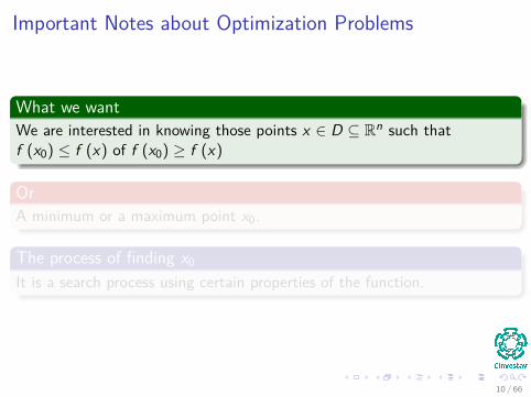
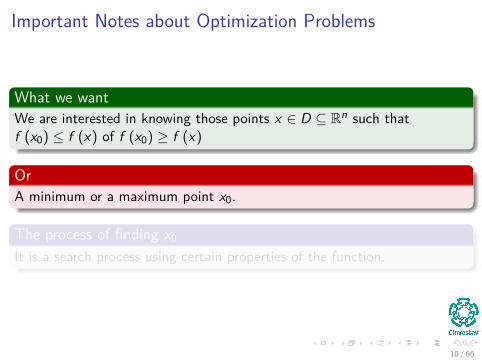
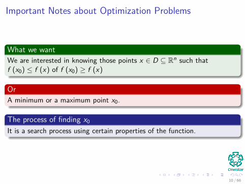
Important Notes about Optimization Problems
What we wantWe are interested in knowing those points x œ D ™ Rn such thatf (x0) Æ f (x) of f (x0) Ø f (x)
OrA minimum or a maximum point x0.
The process of finding x0It is a search process using certain properties of the function.
10 / 66
Important Notes about Optimization Problems
What we wantWe are interested in knowing those points x œ D ™ Rn such thatf (x0) Æ f (x) of f (x0) Ø f (x)
OrA minimum or a maximum point x0.
The process of finding x0It is a search process using certain properties of the function.
10 / 66
Important Notes about Optimization Problems
What we wantWe are interested in knowing those points x œ D ™ Rn such thatf (x0) Æ f (x) of f (x0) Ø f (x)
OrA minimum or a maximum point x0.
The process of finding x0It is a search process using certain properties of the function.
10 / 66
Thus
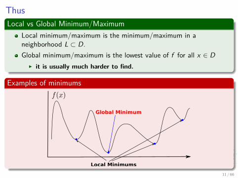
Local vs Global Minimum/MaximumLocal minimum/maximum is the minimum/maximum in aneighborhood L µ D.Global minimum/maximum is the lowest value of f for all x œ D
I it is usually much harder to find.
Examples of minimums
11 / 66
ThusLocal vs Global Minimum/Maximum
Local minimum/maximum is the minimum/maximum in aneighborhood L µ D.Global minimum/maximum is the lowest value of f for all x œ D
I it is usually much harder to find.
Examples of minimums
Local Minimums
Global Minimum
11 / 66
Furthermore
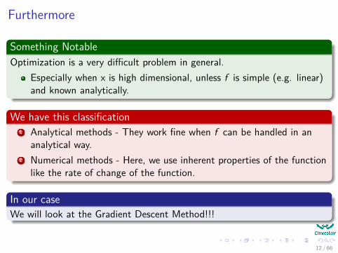
Something NotableOptimization is a very di�cult problem in general.
Especially when x is high dimensional, unless f is simple (e.g. linear)and known analytically.
We have this classification1 Analytical methods - They work fine when f can be handled in an
analytical way.2 Numerical methods - Here, we use inherent properties of the function
like the rate of change of the function.
In our caseWe will look at the Gradient Descent Method!!!
12 / 66
Furthermore
Something NotableOptimization is a very di�cult problem in general.
Especially when x is high dimensional, unless f is simple (e.g. linear)and known analytically.
We have this classification1 Analytical methods - They work fine when f can be handled in an
analytical way.2 Numerical methods - Here, we use inherent properties of the function
like the rate of change of the function.
In our caseWe will look at the Gradient Descent Method!!!
12 / 66
Analytical Method: Di�erentiating
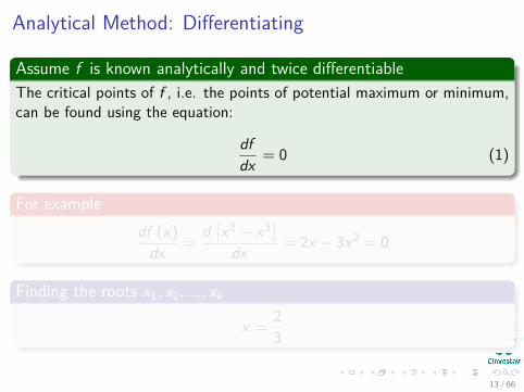
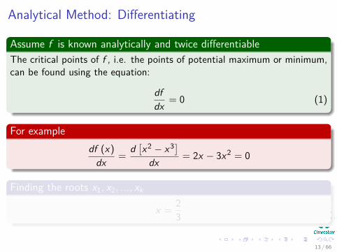
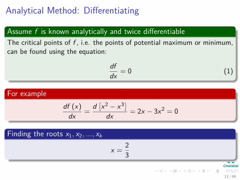
Assume f is known analytically and twice di�erentiableThe critical points of f , i.e. the points of potential maximum or minimum,can be found using the equation:
dfdx = 0 (1)
For exampledf (x)
dx = d#x2 ≠ x3$
dx = 2x ≠ 3x2 = 0
Finding the roots x1, x2, ..., x
k
x = 23
13 / 66
Analytical Method: Di�erentiating
Assume f is known analytically and twice di�erentiableThe critical points of f , i.e. the points of potential maximum or minimum,can be found using the equation:
dfdx = 0 (1)
For exampledf (x)
dx = d#x2 ≠ x3$
dx = 2x ≠ 3x2 = 0
Finding the roots x1, x2, ..., x
k
x = 23
13 / 66
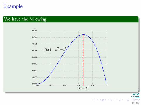
Example
We have the following
14 / 66
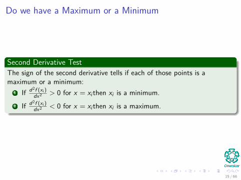
Do we have a Maximum or a Minimum
Second Derivative TestThe sign of the second derivative tells if each of those points is amaximum or a minimum:
1 If d
2f (x
i
)dx
2 > 0 for x = xi
then xi
is a minimum.2 If d
2f (x
i
)dx
2 < 0 for x = xi
then xi
is a maximum.
15 / 66
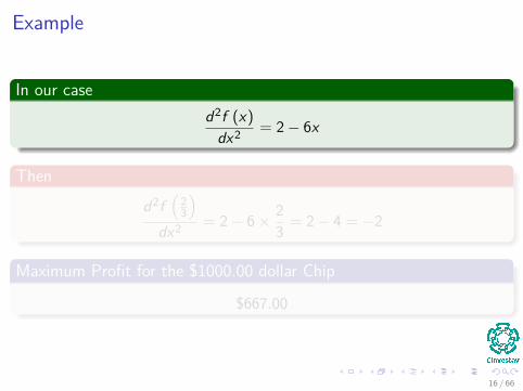
Example
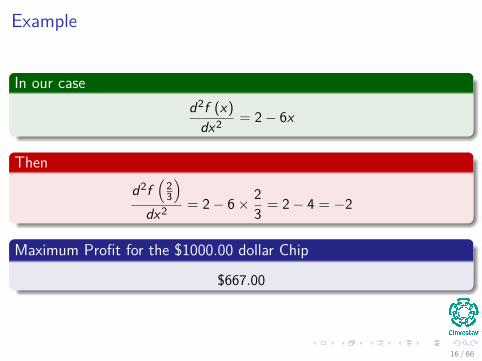
In our cased2f (x)
dx2 = 2 ≠ 6x
Thend2f
1232
dx2 = 2 ≠ 6 ◊ 23 = 2 ≠ 4 = ≠2
Maximum Profit for the $1000.00 dollar Chip
$667.00
16 / 66
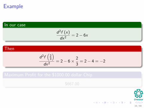
Example
In our cased2f (x)
dx2 = 2 ≠ 6x
Thend2f
1232
dx2 = 2 ≠ 6 ◊ 23 = 2 ≠ 4 = ≠2
Maximum Profit for the $1000.00 dollar Chip
$667.00
16 / 66
Example
In our cased2f (x)
dx2 = 2 ≠ 6x
Thend2f
1232
dx2 = 2 ≠ 6 ◊ 23 = 2 ≠ 4 = ≠2
Maximum Profit for the $1000.00 dollar Chip
$667.00
16 / 66
What if d2f (xi
)dx2 = 0?
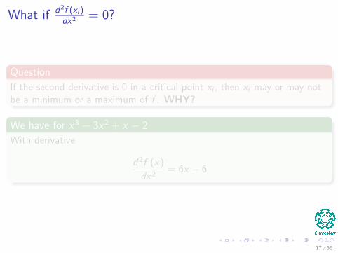
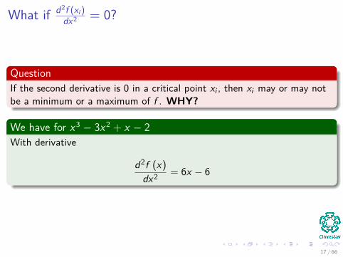
QuestionIf the second derivative is 0 in a critical point x
i
, then xi
may or may notbe a minimum or a maximum of f . WHY?
We have for x
3 ≠ 3x
2 + x ≠ 2With derivative
d2f (x)dx2 = 6x ≠ 6
17 / 66
What if d2f (xi
)dx2 = 0?
QuestionIf the second derivative is 0 in a critical point x
i
, then xi
may or may notbe a minimum or a maximum of f . WHY?
We have for x
3 ≠ 3x
2 + x ≠ 2With derivative
d2f (x)dx2 = 6x ≠ 6
17 / 66
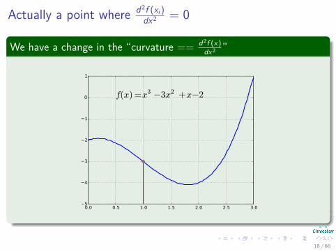
Actually a point where d2f (xi
)dx2 = 0
We have a change in the “curvature == d
2f (x)
dx
2 ”
18 / 66
Properties of Di�erentiating
GeneralizationTo move to higher dimensional functions, we will require to take partialderivatives!!!
SolvingA system of equations!!!
RemarkFor a bounded D the only possible points of maximum/minimum arecritical or boundary ones, so, in principle, we can find the global extremum.
19 / 66
Problems
A lot of themPotential problems include transcendent equations, not solvableanalytically.High cost of finding derivatives, especially in high dimensions (e.g. forneural networks)
ThusPartial Solution of the problems comes from a numerical technique calledthe gradient descent
20 / 66
Problems
A lot of themPotential problems include transcendent equations, not solvableanalytically.High cost of finding derivatives, especially in high dimensions (e.g. forneural networks)
ThusPartial Solution of the problems comes from a numerical technique calledthe gradient descent
20 / 66
Outline
1 Introduction
2 Gradient DescentNotes about OptimizationNumerical Method: Gradient Descent
3 Hill ClimbingBasic TheoryAlgorithmEnforced Hill Climbing
4 Simulated AnnealingBasic IdeaThe Metropolis Acceptance CriterionAlgorithm
21 / 66
Numerical Method: Gradient Descent
Imagine the followingf is a smooth objective function.Now you have a x0 state and you need to find the next one
Something NotableWe want to find x in the neighborhood D of x0 such that
f (x) < f (x0)
22 / 66
Numerical Method: Gradient Descent
Imagine the followingf is a smooth objective function.Now you have a x0 state and you need to find the next one
Something NotableWe want to find x in the neighborhood D of x0 such that
f (x) < f (x0)
22 / 66
Taylor’s Expansion
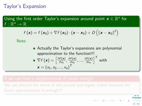
Using the first order Taylor’s expansion around point x œ Rn forf : Rn æ R
f (x) = f (x0) + Òf (x0) · (x ≠ x0) + O1Îx ≠ x0Î2
2
Note:Actually the Taylor’s expansions are polynomialapproximation to the function!!!Òf (x) =
ˈf (x)ˆx1
, ˆf (x)ˆx2
, ..., ˆf (x)ˆx
n
ÈT
withx = (x1, x2, ..., x
n
)T
If we can find a neighborhood D small enoughWe can discard the terms of the second and higher orders because thelinear approximation is enough!!!
23 / 66
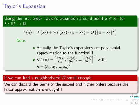
Taylor’s Expansion
Using the first order Taylor’s expansion around point x œ Rn forf : Rn æ R
f (x) = f (x0) + Òf (x0) · (x ≠ x0) + O1Îx ≠ x0Î2
2
Note:Actually the Taylor’s expansions are polynomialapproximation to the function!!!Òf (x) =
ˈf (x)ˆx1
, ˆf (x)ˆx2
, ..., ˆf (x)ˆx
n
ÈT
withx = (x1, x2, ..., x
n
)T
If we can find a neighborhood D small enoughWe can discard the terms of the second and higher orders because thelinear approximation is enough!!!
23 / 66
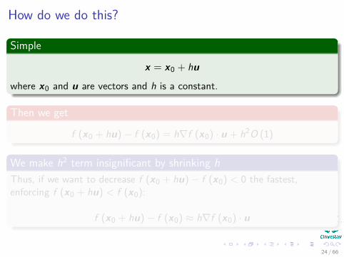
How do we do this?
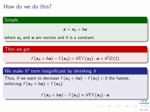
Simple
x = x0 + hu
where x0 and u are vectors and h is a constant.
Then we get
f (x0 + hu) ≠ f (x0) = hÒf (x0) · u + h2O (1)
We make h
2 term insignificant by shrinking h
Thus, if we want to decrease f (x0 + hu) ≠ f (x0) < 0 the fastest,enforcing f (x0 + hu) < f (x0):
f (x0 + hu) ≠ f (x0) ¥ hÒf (x0) · u
24 / 66
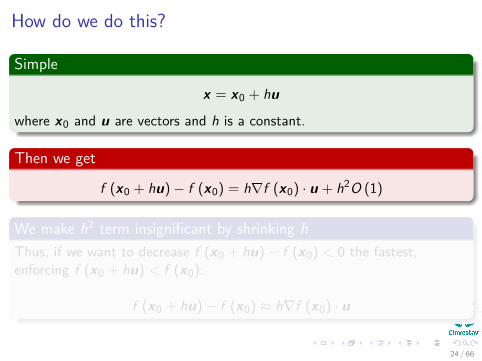
How do we do this?
Simple
x = x0 + hu
where x0 and u are vectors and h is a constant.
Then we get
f (x0 + hu) ≠ f (x0) = hÒf (x0) · u + h2O (1)
We make h
2 term insignificant by shrinking h
Thus, if we want to decrease f (x0 + hu) ≠ f (x0) < 0 the fastest,enforcing f (x0 + hu) < f (x0):
f (x0 + hu) ≠ f (x0) ¥ hÒf (x0) · u
24 / 66
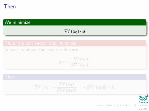
Then
We minimize
Òf (x0) · u
Thus, the unit vector that minimizeIn order to obtain the largest di�erence
u = ≠ Òf (x0)ÎÒf (x0)Î
Then
Òf (x0) · ≠ Òf (x0)ÎÒf (x0)Î = ≠ ÎÒf (x0)Î < 0
25 / 66
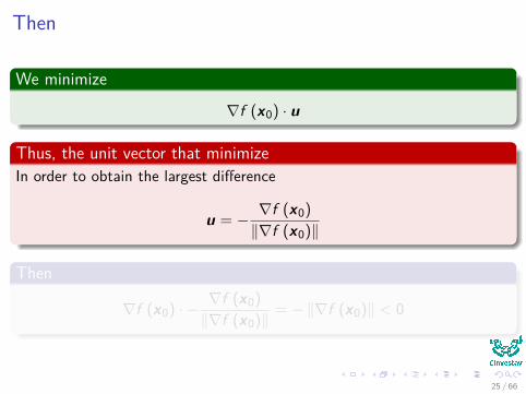
Then
We minimize
Òf (x0) · u
Thus, the unit vector that minimizeIn order to obtain the largest di�erence
u = ≠ Òf (x0)ÎÒf (x0)Î
Then
Òf (x0) · ≠ Òf (x0)ÎÒf (x0)Î = ≠ ÎÒf (x0)Î < 0
25 / 66
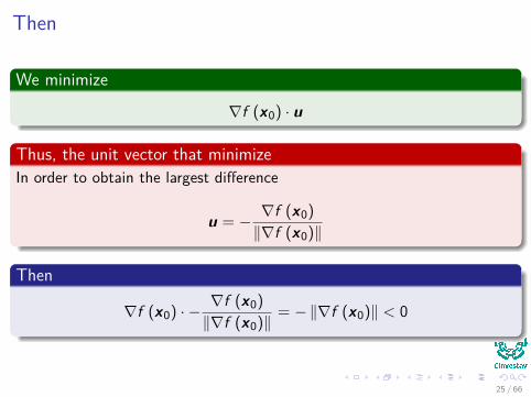
Then
We minimize
Òf (x0) · u
Thus, the unit vector that minimizeIn order to obtain the largest di�erence
u = ≠ Òf (x0)ÎÒf (x0)Î
Then
Òf (x0) · ≠ Òf (x0)ÎÒf (x0)Î = ≠ ÎÒf (x0)Î < 0
25 / 66
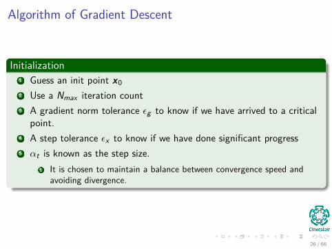
Algorithm of Gradient Descent
Initialization1 Guess an init point x02 Use a N
max
iteration count3 A gradient norm tolerance ‘
g
to know if we have arrived to a criticalpoint.
4 A step tolerance ‘x
to know if we have done significant progress5 –
t
is known as the step size.1 It is chosen to maintain a balance between convergence speed and
avoiding divergence.
26 / 66
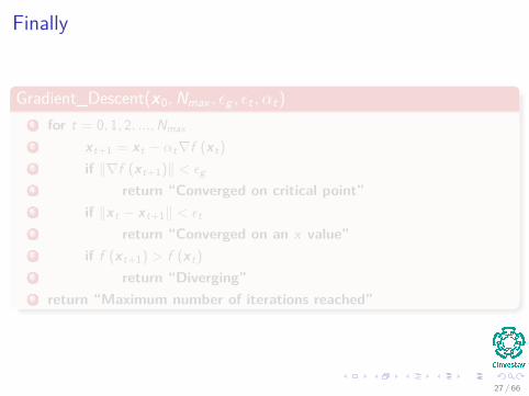
Finally
Gradient_Descent(x0, N
max
, ‘g
, ‘t
, –t
)1 for t = 0, 1, 2, ..., N
max
2x
t+1 = x
t
≠ –t
Òf (xt
)3 if ÎÒf (x
t+1)Î < ‘g
4 return “Converged on critical point”5 if Îx
t
≠ x
t+1Î < ‘t
6 return “Converged on an x value”7 if f (x
t+1) > f (xt
)8 return “Diverging”9 return “Maximum number of iterations reached”
27 / 66
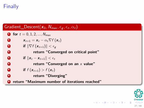
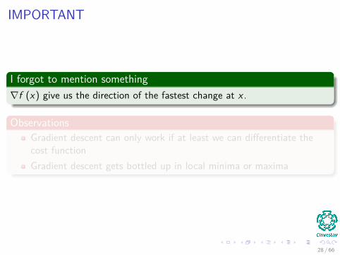
IMPORTANT
I forgot to mention somethingÒf (x) give us the direction of the fastest change at x .
ObservationsGradient descent can only work if at least we can di�erentiate thecost functionGradient descent gets bottled up in local minima or maxima
28 / 66
IMPORTANT
I forgot to mention somethingÒf (x) give us the direction of the fastest change at x .
ObservationsGradient descent can only work if at least we can di�erentiate thecost functionGradient descent gets bottled up in local minima or maxima
28 / 66
Outline
1 Introduction
2 Gradient DescentNotes about OptimizationNumerical Method: Gradient Descent
3 Hill ClimbingBasic TheoryAlgorithmEnforced Hill Climbing
4 Simulated AnnealingBasic IdeaThe Metropolis Acceptance CriterionAlgorithm
29 / 66
The Hill Climbing Heuristic (Greedy Local Search)
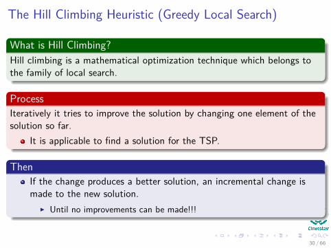
What is Hill Climbing?Hill climbing is a mathematical optimization technique which belongs tothe family of local search.
ProcessIteratively it tries to improve the solution by changing one element of thesolution so far.
It is applicable to find a solution for the TSP.
ThenIf the change produces a better solution, an incremental change ismade to the new solution.
I Until no improvements can be made!!!
30 / 66
The Hill Climbing Heuristic (Greedy Local Search)
What is Hill Climbing?Hill climbing is a mathematical optimization technique which belongs tothe family of local search.
ProcessIteratively it tries to improve the solution by changing one element of thesolution so far.
It is applicable to find a solution for the TSP.
ThenIf the change produces a better solution, an incremental change ismade to the new solution.
I Until no improvements can be made!!!
30 / 66
Example
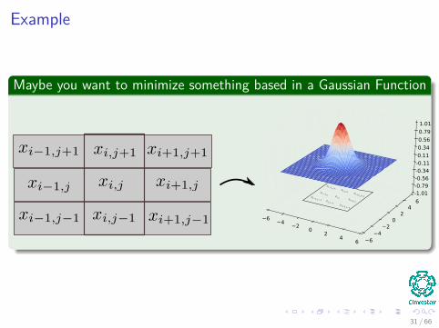
Maybe you want to minimize something based in a Gaussian Function
31 / 66
Outline
1 Introduction
2 Gradient DescentNotes about OptimizationNumerical Method: Gradient Descent
3 Hill ClimbingBasic TheoryAlgorithmEnforced Hill Climbing
4 Simulated AnnealingBasic IdeaThe Metropolis Acceptance CriterionAlgorithm
32 / 66
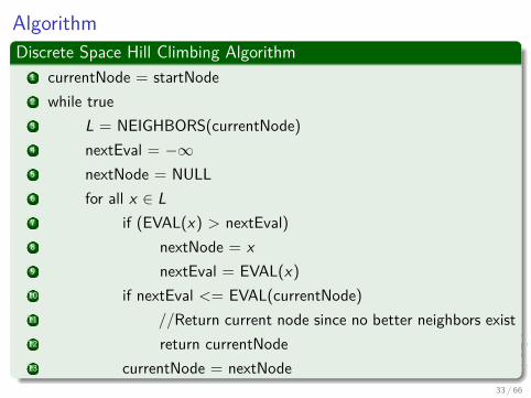
AlgorithmDiscrete Space Hill Climbing Algorithm
1 currentNode = startNode2 while true3 L = NEIGHBORS(currentNode)4 nextEval = ≠Œ5 nextNode = NULL6 for all x œ L7 if (EVAL(x) > nextEval)8 nextNode = x9 nextEval = EVAL(x)10 if nextEval <= EVAL(currentNode)11 //Return current node since no better neighbors exist12 return currentNode13 currentNode = nextNode
33 / 66
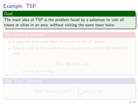
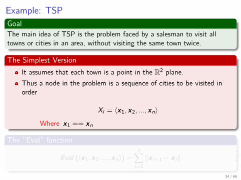
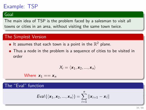
Example: TSPGoalThe main idea of TSP is the problem faced by a salesman to visit alltowns or cities in an area, without visiting the same town twice.
The Simplest VersionIt assumes that each town is a point in the R2 plane.Thus a node in the problem is a sequence of cities to be visited inorder
Xi
= Èx1, x2, ..., x
n
Í
Where x1 == x
n
The “Eval” function
Eval (Èx1, x2, ..., x
n
Í) =nÿ
i=1Îx
i+1 ≠ x
i
Î
34 / 66
Stu� to think about
Something NotableThe definition of the neighborhoods is not obvious or unique in general.
In our exampleA new neighbor will be created by swapping two cities
35 / 66
Stu� to think about
Something NotableThe definition of the neighborhoods is not obvious or unique in general.
In our exampleA new neighbor will be created by swapping two cities
35 / 66
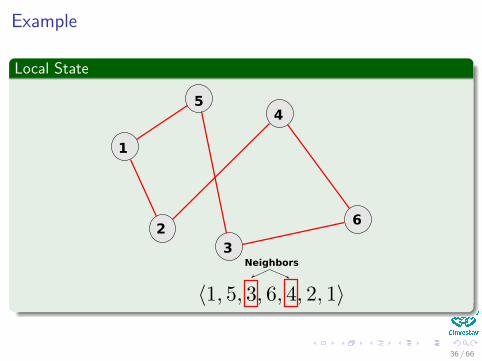
Example
Local State
1
54
623
Neighbors
36 / 66
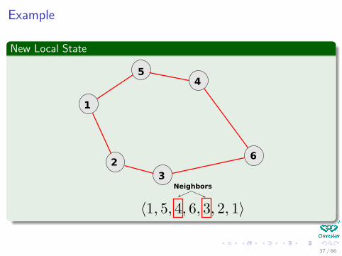
Example
New Local State
1
54
623
Neighbors
37 / 66
Actually
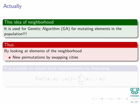
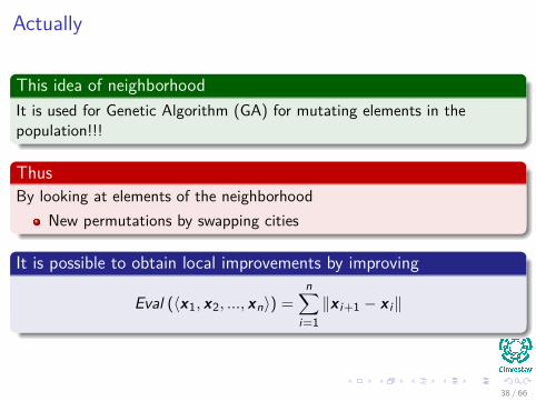
This idea of neighborhoodIt is used for Genetic Algorithm (GA) for mutating elements in thepopulation!!!
ThusBy looking at elements of the neighborhood
New permutations by swapping cities
It is possible to obtain local improvements by improving
Eval (Èx1, x2, ..., x
n
Í) =nÿ
i=1Îx
i+1 ≠ x
i
Î
38 / 66
Actually
This idea of neighborhoodIt is used for Genetic Algorithm (GA) for mutating elements in thepopulation!!!
ThusBy looking at elements of the neighborhood
New permutations by swapping cities
It is possible to obtain local improvements by improving
Eval (Èx1, x2, ..., x
n
Í) =nÿ
i=1Îx
i+1 ≠ x
i
Î
38 / 66
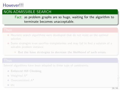
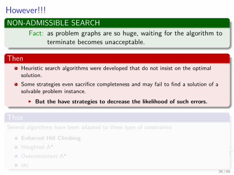
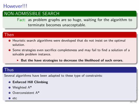
However!!!NON-ADMISSIBLE SEARCH
Fact: as problem graphs are so huge, waiting for the algorithm toterminate becomes unacceptable.
ThenHeuristic search algorithms were developed that do not insist on the optimalsolution.Some strategies even sacrifice completeness and may fail to find a solution of asolvable problem instance.
I But the have strategies to decrease the likelihood of such errors.
ThusSeveral algorithms have been adapted to these type of constraints:
Enforced Hill ClimbingWeighted A*Overconsistent A*etc
39 / 66
Outline
1 Introduction
2 Gradient DescentNotes about OptimizationNumerical Method: Gradient Descent
3 Hill ClimbingBasic TheoryAlgorithmEnforced Hill Climbing
4 Simulated AnnealingBasic IdeaThe Metropolis Acceptance CriterionAlgorithm
40 / 66
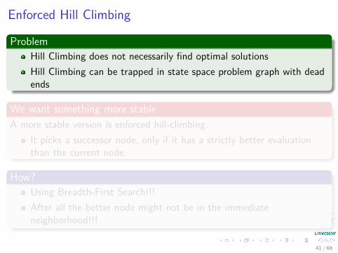
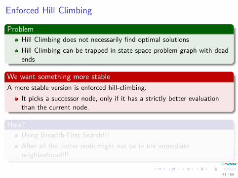
Enforced Hill Climbing
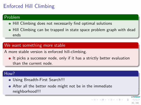
ProblemHill Climbing does not necessarily find optimal solutionsHill Climbing can be trapped in state space problem graph with deadends
We want something more stableA more stable version is enforced hill-climbing.
It picks a successor node, only if it has a strictly better evaluationthan the current node.
How?Using Breadth-First Search!!!After all the better node might not be in the immediateneighborhood!!!
41 / 66
Enforced Hill Climbing
ProblemHill Climbing does not necessarily find optimal solutionsHill Climbing can be trapped in state space problem graph with deadends
We want something more stableA more stable version is enforced hill-climbing.
It picks a successor node, only if it has a strictly better evaluationthan the current node.
How?Using Breadth-First Search!!!After all the better node might not be in the immediateneighborhood!!!
41 / 66
Algorithm
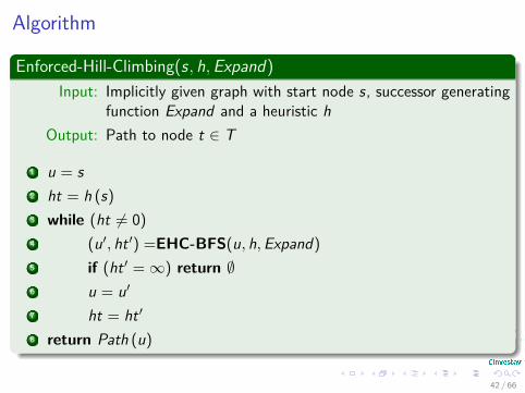
Enforced-Hill-Climbing(s, h, Expand)Input: Implicitly given graph with start node s, successor generating
function Expand and a heuristic hOutput: Path to node t œ T
1 u = s2 ht = h (s)3 while (ht ”= 0)4 (uÕ, ht Õ) =EHC-BFS(u, h, Expand)5 if (ht Õ = Œ) return ÿ6 u = uÕ
7 ht = ht Õ
8 return Path (u)
42 / 66
Algorithm
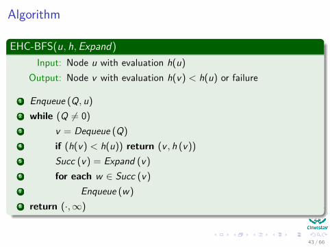
EHC-BFS(u, h, Expand)Input: Node u with evaluation h(u)
Output: Node v with evaluation h(v) < h(u) or failure
1 Enqueue (Q, u)2 while (Q ”= 0)3 v = Dequeue (Q)4 if (h(v) < h(u)) return (v , h (v))5 Succ (v) = Expand (v)6 for each w œ Succ (v)7 Enqueue (w)8 return (·, Œ)
43 / 66

The Problem with Dead-Ends
DefinitionGiven a planning task, a state S is called a dead end if and only if it isreachable and no sequence of actions achieves the goal from it.
We will look more about this in Classic Planning“The FF Planning System: Fast Plan Generation Through HeuristicSearch”
44 / 66
Then
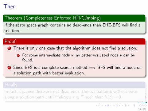
Theorem (Completeness Enforced Hill-Climbing)If the state space graph contains no dead-ends then EHC-BFS will find asolution.
Proof1 There is only one case that the algorithm does not find a solution.
1 For some intermediate node v , no better evaluated node v can befound.
2 Since BFS is a complete search method =∆ BFS will find a node ona solution path with better evaluation.
FinallyIn fact, because there are not dead-ends, the evaluation h will decreasealong a solution path until finding a t œ T such that h (t) = 0.
45 / 66
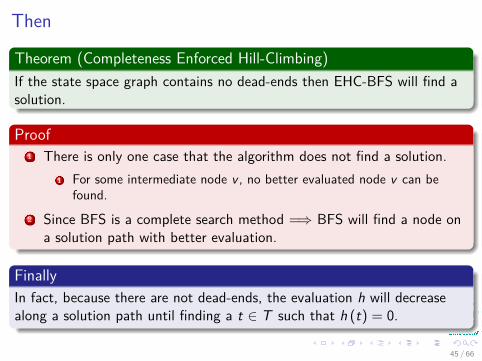
Then
Theorem (Completeness Enforced Hill-Climbing)If the state space graph contains no dead-ends then EHC-BFS will find asolution.
Proof1 There is only one case that the algorithm does not find a solution.
1 For some intermediate node v , no better evaluated node v can befound.
2 Since BFS is a complete search method =∆ BFS will find a node ona solution path with better evaluation.
FinallyIn fact, because there are not dead-ends, the evaluation h will decreasealong a solution path until finding a t œ T such that h (t) = 0.
45 / 66
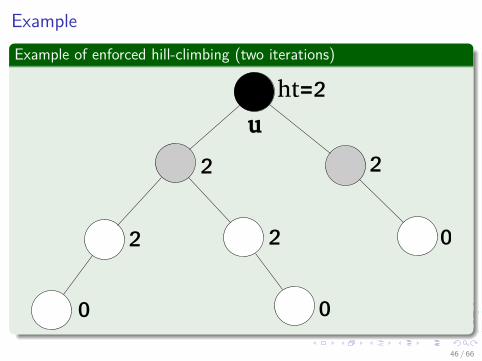
ExampleExample of enforced hill-climbing (two iterations)
u
ht=2
2
2 2 0
2
0 0
46 / 66
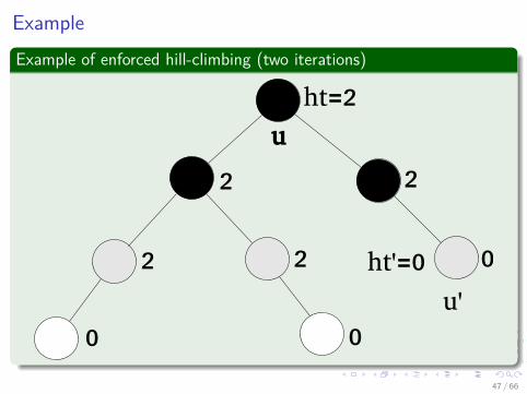
ExampleExample of enforced hill-climbing (two iterations)
u
ht=2
2
2 2 0
2
0 0
ht'=0u'
47 / 66
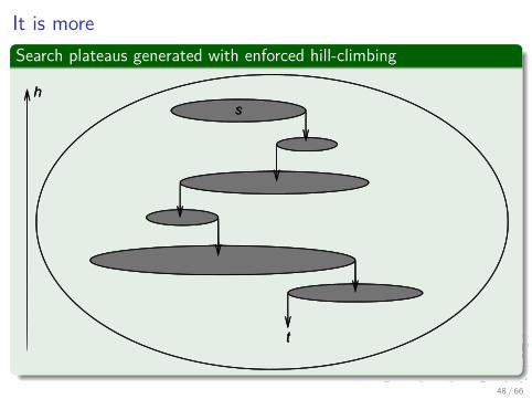
It is moreSearch plateaus generated with enforced hill-climbing
48 / 66
Even with this...
UnavoidableHill climbing is subject to getting stuck in a variety of local conditions.
Two SolutionsRandom restart hill climbingSimulated annealing
49 / 66
Even with this...
UnavoidableHill climbing is subject to getting stuck in a variety of local conditions.
Two SolutionsRandom restart hill climbingSimulated annealing
49 / 66
Random Restart Hill Climbing
Pretty obvious what this is...Generate a random start stateRun hill climbing and store answerIterate, keeping the current best answer as you go
I Stopping... when?
50 / 66
Outline
1 Introduction
2 Gradient DescentNotes about OptimizationNumerical Method: Gradient Descent
3 Hill ClimbingBasic TheoryAlgorithmEnforced Hill Climbing
4 Simulated AnnealingBasic IdeaThe Metropolis Acceptance CriterionAlgorithm
51 / 66
We can do better by using Simulated Annealing
Definition of termsAnnealing: Solid material is heated past its melting point and thencooled back into a solid state.Structural properties of the cooled solid depends on the rate ofcooling.
AuthorsMetropolis et al. (1953) simulated the change in energy of the systemas it cools, until it converges to a steady “frozen” state.Kirkpatrick et al. (1983) suggested using SA for optimization, appliedit to VLSI design and TSP
52 / 66
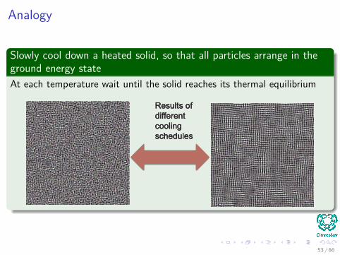
Analogy
Slowly cool down a heated solid, so that all particles arrange in theground energy stateAt each temperature wait until the solid reaches its thermal equilibrium
53 / 66
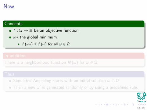
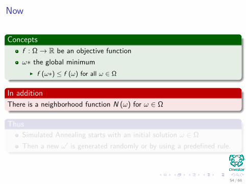
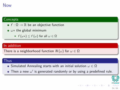
Now
Conceptsf : � æ R be an objective functionÊú the global minimum
I f (Êú) Æ f (Ê) for all Ê œ �
In additionThere is a neighborhood function N (Ê) for Ê œ �
ThusSimulated Annealing starts with an initial solution Ê œ �Then a new ÊÕ is generated randomly or by using a predefined rule.
54 / 66
Now
Conceptsf : � æ R be an objective functionÊú the global minimum
I f (Êú) Æ f (Ê) for all Ê œ �
In additionThere is a neighborhood function N (Ê) for Ê œ �
ThusSimulated Annealing starts with an initial solution Ê œ �Then a new ÊÕ is generated randomly or by using a predefined rule.
54 / 66
Now
Conceptsf : � æ R be an objective functionÊú the global minimum
I f (Êú) Æ f (Ê) for all Ê œ �
In additionThere is a neighborhood function N (Ê) for Ê œ �
ThusSimulated Annealing starts with an initial solution Ê œ �Then a new ÊÕ is generated randomly or by using a predefined rule.
54 / 66
Outline
1 Introduction
2 Gradient DescentNotes about OptimizationNumerical Method: Gradient Descent
3 Hill ClimbingBasic TheoryAlgorithmEnforced Hill Climbing
4 Simulated AnnealingBasic IdeaThe Metropolis Acceptance CriterionAlgorithm
55 / 66
The Metropolis Acceptance Criterion
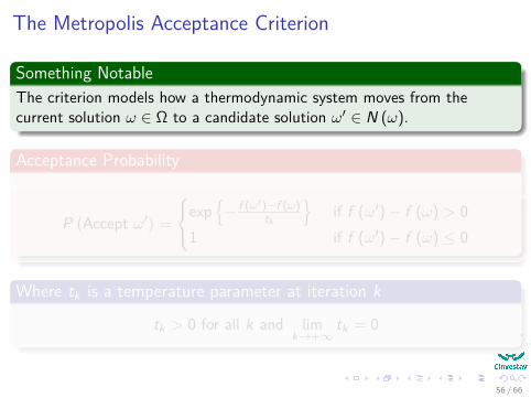
Something NotableThe criterion models how a thermodynamic system moves from thecurrent solution Ê œ � to a candidate solution ÊÕ œ N (Ê).
Acceptance Probability
P!Accept ÊÕ" =
Y]
[exp
Ó≠ f (ÊÕ)≠f (Ê)
t
k
Ôif f (ÊÕ) ≠ f (Ê) > 0
1 if f (ÊÕ) ≠ f (Ê) Æ 0
Where t
k
is a temperature parameter at iteration k
tk
> 0 for all k and limkæ+Œ
tk
= 0
56 / 66
The Metropolis Acceptance Criterion
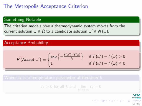
Something NotableThe criterion models how a thermodynamic system moves from thecurrent solution Ê œ � to a candidate solution ÊÕ œ N (Ê).
Acceptance Probability
P!Accept ÊÕ" =
Y]
[exp
Ó≠ f (ÊÕ)≠f (Ê)
t
k
Ôif f (ÊÕ) ≠ f (Ê) > 0
1 if f (ÊÕ) ≠ f (Ê) Æ 0
Where t
k
is a temperature parameter at iteration k
tk
> 0 for all k and limkæ+Œ
tk
= 0
56 / 66
The Metropolis Acceptance Criterion
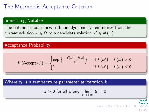
Something NotableThe criterion models how a thermodynamic system moves from thecurrent solution Ê œ � to a candidate solution ÊÕ œ N (Ê).
Acceptance Probability
P!Accept ÊÕ" =
Y]
[exp
Ó≠ f (ÊÕ)≠f (Ê)
t
k
Ôif f (ÊÕ) ≠ f (Ê) > 0
1 if f (ÊÕ) ≠ f (Ê) Æ 0
Where t
k
is a temperature parameter at iteration k
tk
> 0 for all k and limkæ+Œ
tk
= 0
56 / 66
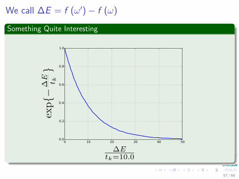
We call �E = f (ÊÕ) ≠ f (Ê)
Something Quite Interesting
57 / 66
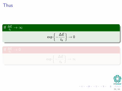
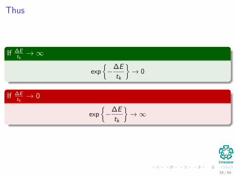
Thus
If �E
t
k
æ Œ
exp;
≠�Etk
<æ 0
If �E
t
k
æ 0
exp;
≠�Etk
<æ Œ
58 / 66
Thus
If �E
t
k
æ Œ
exp;
≠�Etk
<æ 0
If �E
t
k
æ 0
exp;
≠�Etk
<æ Œ
58 / 66
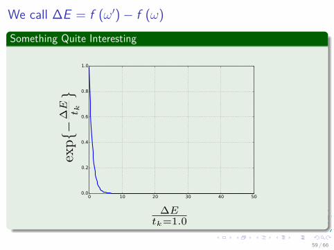
We call �E = f (ÊÕ) ≠ f (Ê)Something Quite Interesting
59 / 66
Meaning
The larger is the t
k
The more probable we accept larger jumps from f (Ê).
The smaller is t
k
We tend to accept only small jumps from f (Ê).
60 / 66
Meaning
The larger is the t
k
The more probable we accept larger jumps from f (Ê).
The smaller is t
k
We tend to accept only small jumps from f (Ê).
60 / 66
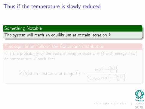
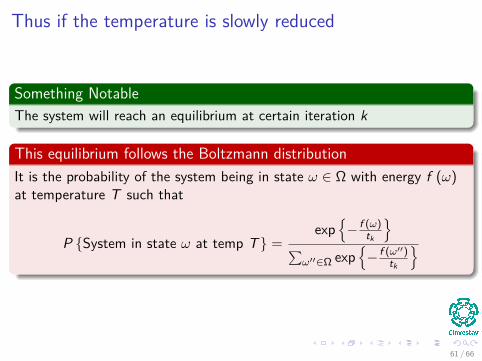
Thus if the temperature is slowly reduced
Something NotableThe system will reach an equilibrium at certain iteration k
This equilibrium follows the Boltzmann distributionIt is the probability of the system being in state Ê œ � with energy f (Ê)at temperature T such that
P {System in state Ê at temp T} =exp
Ó≠ f (Ê)
t
k
Ô
qÊÕÕœ� exp
Ó≠ f (ÊÕÕ)
t
k
Ô
61 / 66
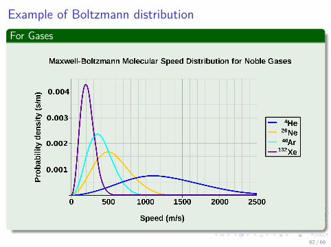
Example of Boltzmann distributionFor Gases
62 / 66
Outline
1 Introduction
2 Gradient DescentNotes about OptimizationNumerical Method: Gradient Descent
3 Hill ClimbingBasic TheoryAlgorithmEnforced Hill Climbing
4 Simulated AnnealingBasic IdeaThe Metropolis Acceptance CriterionAlgorithm
63 / 66
Parameters
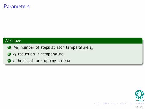
We have1 M
k
number of steps at each temperature tk
2 ‘t
reduction in temperature3 ‘ threshold for stopping criteria
64 / 66
Algorithm
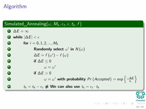
Simulated_Annealing(Ê, M
k
, ‘t
, ‘, t
k
, f )1 �E = Œ2 while |�E | < ‘
3 for i = 0, 1, 2, ..., Mk
4 Randomly select ÊÕ in N (Ê)5 �E = f (ÊÕ) ≠ f (Ê)6 if �E Æ 07 Ê = ÊÕ
8 if �E > 09 Ê = ÊÕ with probability Pr {Accepted} = exp
Ó≠�E
t
k
Ô
10 tk
= tk
≠ ‘t
# We can also use tk
= ‘t
· tk
65 / 66
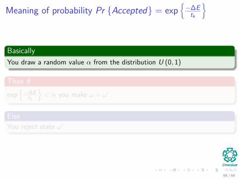
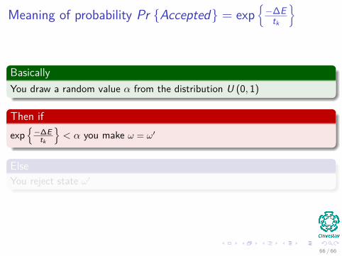
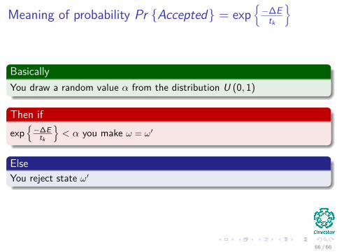
Meaning of probability Pr {Accepted} = exp;
≠�Etk
<
BasicallyYou draw a random value – from the distribution U (0, 1)
Then ifexp
Ó≠�E
t
k
Ô< – you make Ê = ÊÕ
ElseYou reject state ÊÕ
66 / 66
Meaning of probability Pr {Accepted} = exp;
≠�Etk
<
BasicallyYou draw a random value – from the distribution U (0, 1)
Then ifexp
Ó≠�E
t
k
Ô< – you make Ê = ÊÕ
ElseYou reject state ÊÕ
66 / 66
Meaning of probability Pr {Accepted} = exp;
≠�Etk
<
BasicallyYou draw a random value – from the distribution U (0, 1)
Then ifexp
Ó≠�E
t
k
Ô< – you make Ê = ÊÕ
ElseYou reject state ÊÕ
66 / 66