
A Hierarchical Algorithm for Fast Debye Summation withApplications to Small Angle Scattering
Nail A. Gumerov∗, Konstantin Berlin†, David Fushman‡, and Ramani Duraiswami§
University of Maryland, College Park
Oct 5, 2011Revised Mar 25, 2012
Abstract
Debye summation, which involves the summation of sinc functions of distances between all pairof atoms in three dimensional space, arises in computations performed in crystallography, small/wideangle X-ray scattering (SAXS/WAXS) and small angle neutron scattering (SANS). Direct evaluation ofDebye summation has quadratic complexity, which results in computational bottleneck when determin-ing crystal properties, or running structure refinement protocols that involve SAXS or SANS, even formoderately sized molecules. We present a fast approximation algorithm that efficiently computes thesummation to any prescribed accuracy ε in linear time. The algorithm is similar to the fast multipolemethod (FMM), and is based on a hierarchical spatial decomposition of the molecule coupled with lo-cal harmonic expansions and translation of these expansions. An even more efficient implementationis possible when the scattering profile is all that is required, as in small angle scattering reconstruction(SAS) of macromolecules. We examine the relationship of the proposed algorithm to existing approx-imate methods for profile computations, and show that these methods may result in inaccurate profilecomputations, unless an error bound derived in this paper is used. Our theoretical and computationalresults show orders of magnitude improvement in computation complexity over existing methods, whilemaintaining prescribed accuracy.
∗Institute for Advanced Computer Studies, University of Maryland, College Park, MD; and at Fantalgo, LLC, Elkridge, MD;email: [email protected]; web:http://www.umiacs.umd.edu/users/gumerov†Department of Chemistry and Biochemistry, Center for Biomolecular Structure and Organization, and Institute for Advanced
Computer Studies; all at the University of Maryland, College Park, MD; email:[email protected] web:https://sites.google.com/site/kberlin/‡Department of Chemistry and Biochemistry and Center for Biomolecular Structure and Organization, University of Maryland,
College Park, MD; email:[email protected]; web:http://www.chem.umd.edu/research/facultyprofiles/davidfushman§Department of Computer Science and Institute for Advanced Computer Studies, University of Maryland, College Park, MD;
and at Fantalgo, LLC; email: [email protected]; web:http://www.umiacs.umd.edu/users/ramani
1

1 Introduction
Solution small-angle scattering (SAS) of X-ray and neutrons senses the size and shape of a molecular object,and therefore is a powerful analytical tool capable of providing valuable structural information [16, 35].The ability to study molecules and their interactions under physiological conditions and with essentially nolimitation on the size of the system under investigation makes SAS an extremely promising complement tohigh-resolution techniques such as X-ray crystallography and solution NMR. With the rise of computationalpower, SAS studies have become increasingly popular, with the applications covering a broad range ofproblems, including structure refinement of biological macromolecules (proteins, nucleic acids) and theircomplexes [24, 23, 22, 40], elucidation of conformational ensembles and flexibility in solution [6, 11, 34, 5],validation of the macromolecular structures observed in crystals [11], and even the structure of bulk water[10] and X-ray and neutron diffraction patterns of various powder samples [45]. At the heart of all SASapplications to structural studies in chemistry and biology is the ability to predict the scattering data from agiven atomic-level structure. Performing this task accurately and efficiently is critical for successful use ofSAS in chemistry and structural biology. Skipping over the less computationally challenging preprocessinginvolved in SAS, the main problem for computing the scattering profile, I , of a molecular object can bewritten as the summation of the sinc kernel between all pairs of atoms in N -atom system,
I (q) =
N∑j=1
fj(q)ψj (q) , ψj (q) =
N∑l=1
fl (q) s(rj − rl), (1)
s(rj − rl) = sinc (qrjl) =sin(qrjl)
qrjl, rjl = |rj − rl| .
where ψj are partial sums, q is the scattering wavenumber (q = (4π/λ) sinϑ, with 2ϑ being the scatteringangle and λ the wavelength), rj is the coordinate of the jth atom, and fj are the atomic form factors.
The computational cost of directly evaluating Eq. (1) for each q is O(N2). For larger molecular systemsthe number of atoms considered may be extremely large (N > 105), especially when large crystals, or largemolecular complexes are considered. The quadratic computational cost becomes a prohibitive barrier foratomic level application of the Debye formula for such systems. This problem is further compounded, whenthe Debye sum has to be repeatedly calculated as part of a structural refinement protocol, e.g., [37, 18].
Due to the large computational cost of Eq. (1), numerous methods have been proposed for efficientlycomputing its approximation. Two approaches are most commonly used. In the first approach, the setdistances between the point-sets are assigned to a predetermined number of buckets, and the value of theDebye sum is approximated by summing over the buckets instead of the full set of distances [46, 25, 45].This approach is faster than direct evaluation if the number of q values is large relative to the number ofunique fj(q) values, or the fj(q) dependence of q can be factored out of the summation, which isthe case in small angle neutron scattering (SANS). In that case after the initial O(N2) computation of thebuckets, each additional summation for a new q value results only in a linear increase in computation time.While faster for certain problems than direct evaluation, the method is still limited by the O(N2) cost ofbucketization. Further, the error introduced by this approach has not been carefully ascertained.
The second widely used approach, is to expand the pre-orientationally-averaged scattering formula (fromwhich the Debye formulation is analytically derived) in terms of infinite series of spherical harmonics andthen analytically average the series using the orthogonality property of the basis functions [43, 36]. Thisseries is truncated at a conveniently small truncation number p, reducing the computational complexity toO(p2N) [44]. As will be shown below, unless the truncation pP is correctly chosen based on the problemsize D a computation that uses a preset constant cutoff can be divergent for the case of large qD, while atsmall qD the method may perform wasteful computation. As with the histogram (or bucketing) approach,the approximations introduced in the computation are not quantified a priori, and may be significant.
2

We present a method for computing the Debye sum which has a O(N logN) computational cost, whileproviding the user with the ability to bound the accuracy of the computation to an arbitrary precision ε. Ouralgorithm is related to the fast multipole method (FMM), first proposed by [19]. The FMM is a widely usedmethod for solving large scale particle problems arising in many diverse areas (molecular dynamics, astro-physics, acoustics, fluid mechanics, electromagnetics, scattered data interpolation, etc.) because of its abilityto achieve linear or O((N +M) logN) computation time for memory dense matrix vector products/sums,
ψ = Ψf ⇐⇒ ψj =
N∑l=1
Ψ(ρj , rl
)fl, j = 1, ...,M, (2)
to within a prescribed accuracy ε. Here rl andρj
are sets of N source and M evaluation pointsand Ψ (ρ, r) is the kernel function. It was first developed for the Coulomb kernel [19], which in 3D isΨ (ρ, r) = |ρ − r|−1, but has now been successively adapted for a multitude of other kernels, particularly,for the Green’s function of the Helmholtz equation (e.g. [29]). This is closely related to the present problem,since the function s (r) in Eq. (1) also satisfies the Helmholtz equation in three dimensions,
∇2s (r) + q2s (r) = 0, r ∈R3. (3)
However, in comparison to the Green’s function for the Helmholtz equation the Debye function is regular,and this results in a significantly simplified and accelerated algorithm.
We provide complexity estimates and tests of the developed algorithms. In addition, we show that ourmethod is significantly faster for even moderately large values of N than all previous methods described,while at the same time providing accurate results, and demonstrate when the methods presented by previousauthors may yield incorrect results.
2 SAS intensity computations
Before describing the new algorithm, we establish notation and show the relation between the two basicmethods for SAS intensity computations, first, based on the Debye sums, and, second, based on sphericalharmonic expansions.
The measured scattering intensity from a system of molecules in solution is proportional to the averagedscattering of a sample volume:
I (q) =⟨|A (q)|2
⟩Ω
=1
4π
∫Su
|A (q)|2 dS (u) , q = qu, (4)
where A (q) is the scattering amplitude from the particle in vacuo, 〈〉Ω denotes that the quantity is averagedover the unit sphere Su (all orientations), and u is a unit orientation vector. For atomic coordinates rj = rjsj ,|sj | = 1, and the corresponding atomic form factors fj(q), the scattering amplitude of a sample volume is
A (q) =N∑j=1
fj (q) exp (iq · rj) . (5)
3

2.1 Debye sums
The first method to compute I (q) is to just insert Eq. (5) into formula (4) and do the integration analytically
I (q) =1
4π
∫Su
N∑l=1
fl (q) exp (iq · rl)N∑j=1
fj (q) exp (−iq · rj) dS (s) (6)
=N∑l=1
N∑j=1
fl (q) fj (q)1
4π
∫Su
exp (iq · (rl − rj)) dS (s)
=N∑l=1
N∑j=1
fjfls(rj − rl) =
N∑j=1
fjψj ,
where ψj are provided by Eq. (1).
2.2 Spherical harmonic expansions
The second method exploits expansions over spherical harmonics (e.g. [44]). In this method for a given qwe introduce regular spherical basis functions
Rmn (r) = jn(qr)Y mn (s) = jn(qr)Y m
n (θ, ϕ) , r = rs. (7)
FunctionsRmn (r) here are given in spherical coordinates (r, θ, ϕ), r =r (sin θ cosϕ, sin θ sinϕ, cos θ), wherejn(qr) are spherical Bessel functions, while Y m
n (θ, ϕ) are the normalized spherical harmonics of degree nand order m,
Y mn (θ, ϕ) = (−1)m
√2n+ 1
4π
(n− |m|)!(n+ |m|)!
P |m|n (cos θ)eimϕ, (8)
n = 0, 1, 2, ...; m = −n, ..., n.
where P |m|n (µ) are the associated Legendre functions consistent with that in [1], or Rodrigues’ formulae
Pmn (µ) = (−1)m(1− µ2
)m/2 dm
dµmPn (µ) , n > 0, m > 0, (9)
Pn (µ) =1
2nn!
dn
dµn(µ2 − 1
)n, n > 0,
where Pn (µ) are the Legendre polynomials.Using the Gegenbauer series
exp (iq · rj) = 4π
∞∑n=0
n∑m=−n
inRmn (rj)Ymn (u), (10)
one can rewrite Eq. (5) in the form
A (q) =
∞∑n=0
n∑m=−n
Amn (q)Y mn (u), Amn (q) = 4πin
N∑j=1
fj (q)Rmn (rj). (11)
and determine the intensity after integration in Eq. (4)
I (q) =1
4π
∫Su
|A (q)|2 dS (u) =1
4π
∞∑n=0
n∑m=−n
|Amn (q)|2 . (12)
4

In practice the number of modes n can be truncated to p (n = 0, ..., p − 1), which provides summationof p2 terms in Eq. (12). Hence, to compute directly all needed Amn (q) using Eq. (11), one needs O(p2N)operations. Obviously, the second method should be faster than the direct Debye sum computation if p2 <N . Note that p is a growing function of q and should be selected according to the error bounds given in thispaper.
3 Algorithms for the Debye summation
3.1 Factored expansions of the 3D sinc kernel
3.1.1 Regular spherical basis functions
A regular solution of the Helmholtz equation, ψ (r), can be expanded into a series over spherical basisfunctions, Eq. (7),
ψ (r) =∞∑n=0
n∑m=−n
Cmn Rmn (r) , (13)
where Cmn are expansion coefficients.In [29] a formula is provided that allows the basis function Rmn (r + t) centered at r = −t to be ex-
pressed as an infinite series over the basis functions Rmn (r) centered at the origin. The Debye functioncan be related to the regular spherical basis function of order and degree zero, R0
0 as follows
s (r) =sin qr
qr= j0(qr) =
√4πR0
0 (r) . (14)
Using the mentioned formula, the Debye function centered at r = rs can be expressed over the regular basisfunctions as
s (r− rs) = 4π
∞∑n=0
n∑m=−n
R−mn (rs)Rmn (r) . (15)
3.1.2 Error bounds
In practical computations the infinite series or integrals should be replaced by finite series,
s (r− rs) = 4π
p−1∑n=0
n∑m=−n
R−mn (rs)Rmn (r) + εp, (16)
which create truncation errors εp, where p is the “truncation number.” Using the addition theorem forspherical harmonics and the fact that for the Legendre polynomials of arbitrary order |Pn (µ)| 6 1, |µ| 6 1,we can bound the |εp| as follows
|εp| =
∣∣∣∣∣4π∞∑n=p
n∑m=−n
R−mn (rs)Rmn (r)
∣∣∣∣∣ =
∣∣∣∣∣∞∑n=p
jn(qrs)jn(qr)4π
n∑m=−n
Y −mn (θs, ϕs)Ymn (θ, ϕ)
∣∣∣∣∣(17)
=
∣∣∣∣∣∞∑n=p
(2n+ 1) jn(qrs)jn(qr)Pn(cos θ′
)∣∣∣∣∣ 6∞∑n=p
(2n+ 1) |jn(qrs)| |jn(qr)| ,
5
where θ′ is the angle between vectors rs and r. Let the source rs and the evaluation point r be enclosed bya sphere of radius a centered at the origin, r 6 a, rs 6 a. Because
|jn(qr)| 6 (qr)n
[(2n+ 1)!!]6
(qa)n
[(2n+ 1)!!]
(see [1]) the error can be bounded as
|εp| 6∞∑n=p
(2n+ 1)(qa)2n
[(2n+ 1)!!]2<∞∑n=p
(qa)2n
(2n)!!(2n− 1)!!=∞∑n=p
(qa)2n
(2n)!(18)
=(qa)2p
(2p)!
∞∑n=0
(2p)!(qa)2n
(2n+ 2p)!<
(qa)2p
(2p)!
∞∑n=0
(qa)2n
(2n)!=
(qa)2p
(2p)!cosh (qa) 6
(qa)2p
(2p)!eqa.
Here we used the inequality
(2n)!(2p)!
(2n+ 2p)!=
1
C2n2n+2p
6 1, (19)
where C2n2n+2p are the binomial coefficients.
The above estimate shows that for given qa the series converges absolutely. Although the estimate (18)can be applied for any qa, for qa 1 a tighter bound can be established. The spherical Bessel functionsjn(qa) decay exponentially as functions of ηn = (qa)−1/3(n− qa+ 1/2). Hence, for ηn 1 the principalterm of the sum in the right hand side of Eq. (17) provides a good estimate of the entire sum, i.e.
|εp| . 2
(p+
1
2
)j2p(qa), ηp = (qa)−1/3(p− qa+
1
2) 1. (20)
In fact, the large ηn asymptotic behavior is achieved at moderate values of ηn & 2.The principal term of jp(qa) of asymptotic expansion for ηp 1 is [1]
jp(qa) =
(π
2qa
)1/2
Jp+1/2 (qa) ∼(π
2qa
)1/2
21/3
(p+
1
2
)−1/3
Ai(
21/3ηp
), (21)
where Jν and Ai are the Bessel function of order ν and the Airy function of the first kind. It is proven in[30] that
Ai (x) 6 Ai (0) exp
(−2
3x3/2
), Ai (0) =
1
32/3Γ (2/3)< 0.3351, x > 0, (22)
where Γ is the gamma-function. Combining Eqs (20)-(22), we obtain
|εp| .π
qa22/3Ai2 (0)
(p+
1
2
)1/3
exp
(−1
325/2η3/2
p
)(23)
<1
qa
[qa+ ηp(qa)1/3
]1/3exp
(−1
325/2η3/2
p
).
The asymptotic region we are interested in is p + 12 − qa qa, which provides ηp(qa)1/3 qa. If the
error is prescribed so that |εp| < ε, we obtain the following expression for p to achieve this error
p & phf (ε, qa) = qa+1
2
[3
2log
1
ε− log (qa)
]2/3
(qa)1/3. (24)
6

Figure 1 illustrates computations of the series truncation number p using the worst case (rs = r = a)according to Eq. (17) and the high qa approximation (24). It is not difficult to compute εp exactly forarbitrary p, since for rs = r = a and p = 0 the sum in the right hand side of Eq. (17) is equal to 1 [1], whilethe values for different p can be computed using the recursion εp+1 = εp − (2p + 1)j2
p(qa). In the samefigure, the dependence phf (ε, qa) provided by Eq. (24) is also plotted. Note that for the computed values ofε and range of qa shown in the figure, the maximum difference between the exact and approximate valuesof the truncation number p does not exceed 2. We also found that the equation for the truncation number,
p = [phf (ε, qa)] + 2, (25)
where [] denotes the integer part, provides a value for p not less that the exact truncation number in theconsidered range of parameters. This demonstrates an excellent agreement with the exact value even at lowfrequencies, so Eq. (25) can be used for fast and accurate estimation of the truncation number.
10 -1
10 0
10 1
10 2
10 3
10 0
10 1
10 2
10 3
qa
p
10 - 6
10 - 3
10 - 1 2
Figure 1: Minimum truncation number p(ε, qa) (solid lines) and its approximation, Eq. (24) (dashed lines)for prescribed values of error ε.
Note that dependence of type p ∼ qa+ f(ε)(qa)1/3 can be found in the FMM literature for the far fieldexpansions of the Green’s function for the Helmholtz equation (see e.g. [29, 30]). Comparison with thoseexpressions show that for the same error ε the truncation numbers for the Debye kernel are smaller. In fact,the present expression f(ε) is approximately equal to a similar expression g(ε1/2) used in those publications.
7

3.2 Algorithm 1: “Middleman” method
The “Middleman” method (e.g. see [29]) is the simplest, but for some cases the fastest O(N +M) methodto compute sums of type (2). The algorithm can be described in a few lines. Indeed, from Eqs (2) and (16)we have
ψl =N∑j=1
fjs (ρl − rj) =N∑j=1
fj
[4π
p−1∑n=0
n∑m=−n
R−mn (rj)Rmn (ρl) + εp
](26)
=
p−1∑n=0
n∑m=−n
Bmn R
mn (ρl) + ε(tot)p , Bm
n = 4πN∑j=1
fjR−mn (rj) , ε(tot)p =
N∑j=1
fjεp.
If the computational domain is bounded by a sphere of radius a, and the truncation number p is selectedso that an error ε(tot)p is tolerated, then O
(p2N
)operations are needed to compute Bm
n , n = 0, ..., p − 1,m = −n, ..., n and O
(p2M
)operations are needed to compute all ψl, l = 1, ...,M. The computation of
all required 2p2 basis functions Rmn (ρl) and R−mn (rj) is done via an O(p2) procedure (using recurrencesfor the spherical Bessel and associated Legendre functions) [29]. The total complexity of the algorithm is,therefore O(p2(N +M)).
This algorithm is faster than the brute force direct summation only if
p2(N +M) NM. (27)
This condition holds when p is controlled, which means that qa is not very large (see Eq. (24)). Moreprecisely, assuming M = N , and considering p ∼ qa = qD/2 (D = 2a) we can rewrite condition (27) as
qD (2N)1/2 . (28)
3.3 Algorithm 2: Hierarchical summation
For larger qD the value of p according to Eq. (24) becomes large leading to increased computational cost.We propose to use a different algorithm, which subdivides the domain hierarchically using local expansionsabout multiple expansion centers, and achieves lower complexity than the “Middleman” method. Translationoperators provide a mathematical foundation for merging expansions of smaller subdomains into a largerdomain, while maintaining the validity of the overall expansion. The advantage of the hierarchical methodis that only a low order representation of the subdomain is maintained. Optimal conditions on the numberof subdomains, or levels of hierarchical space subdivision are obtained to minimize the cost at a givenacceptable error, as is commonly done in the FMM.
3.3.1 Translations
In contrast to the FMM for singular kernels, here only local-to-local, or R|R - translations are used, thussignificantly simplifying the algorithm. These translations can be expressed by the action of a linear operatorthat enables change of the origin of the expansions. Consider two expansions of the same function (see Eq.(13)),
ψ (r) =
∞∑n=0
n∑m=−n
Cmn Rmn (r− r∗1) =
∞∑n=0
n∑m=−n
Cmn Rmn (r− r∗2) , (29)
where Cmn and Cmn are expansion coefficients for bases centered at r∗1 and r∗2 respectively. The basis func-tions centered at r = −t and r = 0 are related to each other via an infinite reexpansion matrix, (R|R)T (t),
8

whose entries, (R|R)m′m
n′n (t) are given in the appendix (e.g., see Eq. (52)). Knowing this operator one canrepresent a basis function centered at r = −t in terms of basis functions centered at the origin via
Rmn (r + t) =∞∑n′=0
n′∑m′=−n′
(R|R)m′m
n′n (t)Rm′
n′ (r) , n = 0, 1, ..., m = −n, ..., n, (30)
where t is the translation vector. Substituting this reexpansion into the first sum in Eq. (29) one finds thatthe coefficients Cmn in the new basis are related to the coefficients in the old basis Cmn as
Cmn =∞∑n′=0
n′∑m′=−n′
(R|R)mm′
nn′ (t)Cm′
n′ , t = r∗2 − r∗1, n = 0, 1, ..., m = −n, ..., n, (31)
since the expansion over the basis Rmn (r− r∗2) is unique. We will stack coefficients into a single vectorand use a more compact notation for translation operator as a matrix
C = (R|R) (t) C. (32)
In a practical numerical realization the series and matrix should be appropriately truncated and the truncationerror should be controlled to stay within the error bound.
3.3.2 Data Structures
The algorithm consists of two parts: an initial set-up stage where data structures and other precomputationsare performed, followed by a stage where the actual sum is obtained at each evaluation point. In a practicalimplementation where the sum may be computed for many values of the momentum transfer parameter q,the hierarchical data structures may only need be set up once, while the sum computations done many timesfor the same distribution of atoms.
All sources and evaluation points are enclosed into a cube with side d and diagonal D = d√
3, which istermed the “computational domain”. This cube is considered to be a box at level l = 0 in an octree structure[42]. Eight children cubes of level 1 are produced by division of each side of the initial cube by two. Theprocess of division continues down to level l = lmax, whose value is determined from cost optimizationconsiderations. At the end of the process we have an octree of depth lmax. All cubes at each level areindexed using Morton space-filling curve (spatial z−order) [42]. Such an indexing can be obtained using bitinterleaving [29]. This indexing also enables fast determination of children and parents of all boxes. Boxescontaining sources are called source boxes and boxes containing evaluation points are called receiver boxes.
To avoid wasteful computations, we make the algorithm adaptive, by skipping all empty boxes. Furtheradaptivity can be introduced as in the FMM [9, 29]; however, the space filling nature of atoms in macro-molecules (or crystals) implies that these considerations are likely to be unimportant in practice for profilecomputation.
In the present problem, since the computation involves all atom pairs, the “sources” rl and “receivers” ρjin Eq. (2) are the same point sets. At the stage of generation of data structure some precomputations of theentries of the translation operators can be performed, which can be stored and reused during the algorithm.We also determine truncation numbers for different levels, p0, ..., plmax ,consistent with the prescribed com-putation error and an optimal tree depth. Note that the truncation numbers depend on parameter qD which isreduced by half as the boxes become finer. At level l this should be taken as qDl,Dl = 2−lD0 = 2−lD. Theinitial data-structure phase is then followed by the sum evaluation, where initial expansion, and hierarchicalsummation for aggregation, and dissemination of the intermediate results is performed.
9
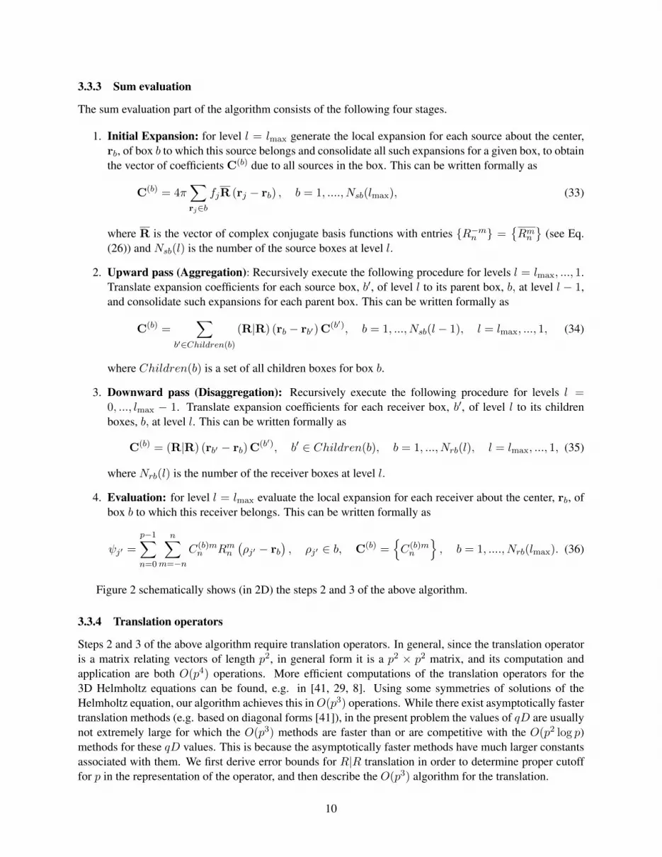
3.3.3 Sum evaluation
The sum evaluation part of the algorithm consists of the following four stages.
1. Initial Expansion: for level l = lmax generate the local expansion for each source about the center,rb, of box b to which this source belongs and consolidate all such expansions for a given box, to obtainthe vector of coefficients C(b) due to all sources in the box. This can be written formally as
C(b) = 4π∑rj∈b
fjR (rj − rb) , b = 1, ...., Nsb(lmax), (33)
where R is the vector of complex conjugate basis functions with entries R−mn =Rmn
(see Eq.(26)) and Nsb(l) is the number of the source boxes at level l.
2. Upward pass (Aggregation): Recursively execute the following procedure for levels l = lmax, ..., 1.Translate expansion coefficients for each source box, b′, of level l to its parent box, b, at level l − 1,and consolidate such expansions for each parent box. This can be written formally as
C(b) =∑
b′∈Children(b)
(R|R) (rb − rb′) C(b′), b = 1, ..., Nsb(l − 1), l = lmax, ..., 1, (34)
where Children(b) is a set of all children boxes for box b.
3. Downward pass (Disaggregation): Recursively execute the following procedure for levels l =0, ..., lmax − 1. Translate expansion coefficients for each receiver box, b′, of level l to its childrenboxes, b, at level l. This can be written formally as
C(b) = (R|R) (rb′ − rb) C(b′), b′ ∈ Children(b), b = 1, ..., Nrb(l), l = lmax, ..., 1, (35)
where Nrb(l) is the number of the receiver boxes at level l.
4. Evaluation: for level l = lmax evaluate the local expansion for each receiver about the center, rb, ofbox b to which this receiver belongs. This can be written formally as
ψj′ =
p−1∑n=0
n∑m=−n
C(b)mn Rmn
(ρj′ − rb
), ρj′ ∈ b, C(b) =
C(b)mn
, b = 1, ...., Nrb(lmax). (36)
Figure 2 schematically shows (in 2D) the steps 2 and 3 of the above algorithm.
3.3.4 Translation operators
Steps 2 and 3 of the above algorithm require translation operators. In general, since the translation operatoris a matrix relating vectors of length p2, in general form it is a p2 × p2 matrix, and its computation andapplication are both O(p4) operations. More efficient computations of the translation operators for the3D Helmholtz equations can be found, e.g. in [41, 29, 8]. Using some symmetries of solutions of theHelmholtz equation, our algorithm achieves this inO(p3) operations. While there exist asymptotically fastertranslation methods (e.g. based on diagonal forms [41]), in the present problem the values of qD are usuallynot extremely large for which the O(p3) methods are faster than or are competitive with the O(p2 log p)methods for these qD values. This is because the asymptotically faster methods have much larger constantsassociated with them. We first derive error bounds for R|R translation in order to determine proper cutofffor p in the representation of the operator, and then describe the O(p3) algorithm for the translation.
10

Figure 2: Schematic illustration of the Upward pass (aggregation, on the left) and the Downward pass(disaggregation, on the right) of the proposed fast hierarchical algorithm.
Error bounds Before deriving more rigorous estimates of the translation errors, let us turn attention toEq. (17). Assume that the source is located inside a domain of radius a centered at the origin, so that rs 6 a.The estimates of the truncation number obtained above for r 6 a, obviously, are not valid if the evaluationpoint is far from the expansion center. However, even in this case we can bound the error for p > qa asfollows
|εp| 6∞∑n=p
(2n+ 1) |jn(qrs)| |jn(qr)| 6∞∑n=p
(2n+ 1) jn(qa) |jn(qr)| . (37)
Since |jn(qr)| 6 1 for any values of n and qr, and for n > p > qa the functions jn(qa) decay exponentiallyas functions of ηn, we still can use the principal term for estimation of the entire sum. This provides
|εp| . 2
(p+
1
2
)jp(qa), ηp = (qa)−1/3(p− qa+
1
2) 1. (38)
This can be compared with Eq. (20). We can slightly modify the high qa error bound to obtain
|εp| .(π
qa
)1/2
25/6Ai (0)
(p+
1
2
)2/3
exp
(−1
323/2η3/2
p
)(39)
≈ 1
(qa)1/2
[qa+ ηp(qa)1/3
]2/3exp
(−1
323/2η3/2
p
).
11

From this we obtain, similarly to Eq. (24),
p & phf (ε, qa) = qa+1
2
(3 log
1
ε+
1
2log(qa)
)2/3
(qa)1/3. (40)
This coincides with the result obtained in [29] for the expansion of an arbitrary incident field.Accurate analysis of the effect of application of truncated translation matrix is provided in Appendix
A. This result shows that this error is consistent with (40), while just a small correction to the coefficientof log(qa) may be needed (see Eq. (61)). Such a correction slightly changes p as normally ε < (qa)−1
and 3 log ε−1 is the dominating term. The practical rule is to use Eqs (40) or (61) where p can be increasedby a small value, e.g., unity, from the computed value phf (ε, qa). Moreover, practical errors are usuallytwo orders of magnitude smaller than those provided by theoretical error bounds, since not all sources andevaluation points are located in the worst positions.
Summarizing, we can state that translations can be performed using truncated rectangular p2 × p′2
translation matrices, where p and p′ are truncation numbers assigned to levels of the octree to which andfrom which the translation occurs respectively.
RCR-decomposition To perform translation by direct matrix-vector multiplication from level to levelO(p4) operations are needed, assuming that the matrix is precomputed. As it is shown in [29] this method isnot fast enough to provide overall O(N logN) fast summation algorithm for 3D spatial distributions, as areencountered here, and at leastO(p3) translation methods are needed. Several methods of this complexity arediscussed and presented in [29], while we focus on the so-called RCR-decomposition (Rotation - Coaxialtranslation - Rotation), which first was introduced for the Laplace equation in [47], and further successfullyimplemented for the Laplace and Helmholtz equation in several FMM realizations (e.g. [29, 28]).
Formally, the RCR-decomposition of the translation matrix can be represented as
(R|R) (t) = Rot−1 (t/t) (R|R)(t)Rot(t/t), (41)
where operator Rot(t/t) provides rotation in the way that the unit vector t/t becomes the z-axis basis vectorof the new reference frame, operator (R|R)(t) provides coaxial translation by distance t along the z-axis,and Rot−1 (t/t) is inverse to Rot(t/t) (back rotation). Each of these operators has O
(p3)
complexity.For a rectangular p2 × p′2 matrix (R|R) (t) matrices Rot(t/t) and Rot−1 (t/t) are truncated to squarematrices p′2 × p′2 and p2 × p2, respectively, while matrix
(R|R
)(t) has size p2 × p′2. The saving comes
from the fact that all these matrices are block-sparse, as they act only on subspaces of expansion coefficientsCmn invariant to rotation (n) and invariant to coaxial translation (m), so the total number of non-zeroelements isO(p3) for each matrix. Entries of these matrices can be computed for costO(p3) using recursiveprocedures described in [26, 29]. Improved versions of these procedures are provided in Appendix B andC. Note that we found that the recursive process for rotation coefficients described in the above referencesis unstable for large p ( p & 80). We provide in the appendix an improved process, which we found to bestable even for very large p (tested up to several thousands).
3.3.5 Algorithm complexity and optimization
The algorithm for sum of non-singular functions described above has different complexity and optimizationthan the FMM which involves summation of singularities. The singularities in the FMM are avoided bybuilding neighborhood data structures, matrix decomposition to sparse (local) and dense (far) parts and abalance between the major costs of the local summation and translations. Translation costs are heavilydominated by the many multipole-to-local translations. These expensive parts of the FMM are all removed in
12

the present algorithm. Also the data structure for the present algorithm is much simpler, since the eliminationof multipole to local translation means that we do not need neighborhood lists.
In Step 1, the cost of generation of the initial plmax-truncated local-expansion for a single source in thedomain of size qDlmax is Bexpp
2lmax
, where Bexp is some constant. Similarly, the cost of evaluation of theexpansion, in Step 4, is the same for a single receiver point. The total cost of the expansion generation andevaluation for N sources and M receivers is Bexpp
2lmax
(N +M).Cost of a single translation from level l to l− 1 can be estimated as Btransp
3l using the O(p3) algorithms.
(Truncation numbers for levels l and l − 1 are of the same order – for large qD they differ by a factor oftwo). Here Btrans is some constant of order 1, which for simplicity is taken to be the same for all levels, andwhich is asymptotically correct for large qD. For estimations we can assume that all boxes in the octree areoccupied, as is expected in the macromolecular scattering. In this case at level l we have 8l boxes. We notethen that if all boxes are occupied then the cost of translations in the upward and downward passes of thealgorithm are the same, and so the total complexity of the algorithm can be estimated as
Ctot = Cexp + Ctrans, Cexp = Bexpp2lmax
(N +M) , Ctrans = 2Btrans
lmax∑l=1
8lp3l , (42)
where Cexp and Ctrans are total expansion and translation costs.The hierarchical algorithm is appropriate for large qD, where pl ∼ qDl/2. Since Dl = 2−lD we have
Ctrans ∼1
4Btrans
lmax∑l=1
8l2−3l (qD)3 =1
4Btranslmax (qD)3 , (43)
Cexp ∼1
4Bexp (N +M) 2−2lmax (qD)2 ,
Ctot =1
4(qD)2
[Bexp (N +M) 2−2lmax +BtranslmaxqD
].
It is seen then that for a given qD, N, and M, the function Ctrans (lmax) is growing, while the functionCexp (lmax) is decaying, so that there is an optimal value for their sum, Ctot. This minimum can be foundsimply from the condition that the derivative of Ctot with respect to lmax is zero. This provides the optimummaximum level, l(opt)max , and the cost of the optimized algorithm, C(opt)
tot (lmax):
l(opt)max =1
2log2
(2 log 2)Bexp (N +M)
BtransqD, (44)
C(opt)tot =
1
8(qD)3Btrans log2
(2e log 2)Bexp (N +M)
BtransqD.
So for fixed qD the optimal algorithm is scaled as O(log(N +M)), while for fixed N the scaling is approx-imately O((qD)3).
Now, if we consider a system of N = M atoms with typical interatomic distance da, which occupies acube with diagonal D and edge D/
√3 then D3 = 33/2Nd3
a and the above estimates for optimum settingsbecome
l(opt)max =1
2log2
(4 log 2)BexpN2/3
√3Btransqda
= O
(log
(N
(qda)3/2
)), (45)
C(opt)tot =
3√
3
8(qda)
3BtransN log2
(4e log 2)BexpN2/3
√3Btransqda
= O
((qda)
3N log
(N
(qda)3/2
)).
13

This shows that for fixed qda and increasingN the number of levels should increase asO(logN) and the al-gorithm scales as O(N logN). Another asymptotic behavior is also interesting – for fixed N and increasingqda the number of levels should decrease (!), while the total algorithm complexity is approximately scaledasO((qda)
3). The first fact is only due to the p3 translation scheme, where for large qD the amount of trans-lations (and so the levels) should be reduced in a scheme of minimal complexity. Formally, for qda & N2/3
the number of levels becomes less than 1, in which case one should use the “Middleman” scheme. In prac-tical applications of the small angle scattering qda usually does not exceed qda ∼ 102, which shows that thehigh qa switch to the “Middleman” algorithm may happen only for relatively small N . 103. On the otherhand, the “Middleman” scheme is not practical for large qD (see Eq. (28)), and such a switch may neverhappen in practice. For larger systems several levels (lmax > 1) are required.
We note that for small or moderate qD the truncation number does not depend strongly on qD, whichaffects the optimization estimates. If, for these values of qD we take the truncation number to be someconstant that is used for all levels, we can see from Eq. (42) that Cexp does not depend on lmax, while Ctrans
is a monotonically increasing function of lmax. This means that C(opt)tot is reached for lmax, which is as small
as possible, i.e. lmax = 0 and we revert to the “Middleman” scheme.
3.3.6 Combined algorithm
The above complexity consideration shows that a combined algorithm which includes a switch between the“Middleman” and the hierarchical algorithm can perform better for certain values of N and qda. Practicalvalues for such a switch depend on the algorithm implementation, hardware, etc. However, we can estimatethis region of parameters qualitatively, using Eq. (42), where we can put more accurate estimates for thetruncation number and study the parametric dependencies Ctot(qD,N ) numerically. We note then that if the“Middleman” scheme is used, then Eq. (24) should be used, which is different from Eq. (40) (which showsup for small and moderate qD). So, for the qualitative model we assume Bexp = Btrans = 1, M = N,
ε = 10−6, compute cost C(M)tot of the “Middleman” method as Cexp for lmax = 0 and p provided by Eq.
(24), while compute the cost of the hierarchical scheme as Ctot with pl determined by a = Dl−1/2 and Eq.(40) for optimal lmax (this always overestimates Ctrans), which we determine by finding the minimum of Ctotover a range of lmax (we will add const p = 1 to both Eq. (24) and (40) to have at least one term in theexpansion even for qa → 0). The switch for any particular values in the parametric space (qD,N) then isdetermined by the comparison of Ctot and C(M)
tot . We note that we also have a “brute force” algorithm ofcomplexity C(B)
tot = N2. In the comparison shown in Fig. 3 we also indicate the cases when this is faster.For qD . 10 the difference in performance between the Middleman and Hierarchical algorithms is
small. Fig. 3 also shows, as expected, that the brute force computations are more efficient than methodsbased on expansions for large qD and not very large N .
Fig. 4 shows that more accurate estimation of the truncation number substantially affects the scaling ofthe algorithm with respect to qD (and, in fact to N ). While asymptotically the scaling should be close toO((qD)3) , such scaling is realized only for very high qD & 103. For qD 103 the dependence of thecomplexity on this parameter is weaker.
4 Faster versions for SAS profile computation
The SAS intensity computations based on the Debye sums can be accelerated at least two times (in fact,even more) due to the following facts: 1) for these computations the source and receiver sets are the same;2) the final result are not the Debye sums, but sums (6). Let us consider modifications of the Middlemanmethod and the Hierarchical algorithm in this case.
14

qD
N
10 -1
10 0
10 1
10 2
10 3
10 3
10 4
10 5
10 6
10 7
Brute Force
Middleman
6
5
1
l m a x =
Hierarchical
2
3
4
Figure 3: Qualitative map in parameter space (qD,N ) of the region of best performance for the threedifferent algorithms to compute Debye sums. The numbers in the graph indicate the optimal maximum levelof the octree for the hierarchical algorithm.
4.1 Modified Middleman method for profile computation
Substituting ψj from Eq. (26) into Eq. (6) and neglecting the error term, we obtain
I (q) =N∑i=1
fi
p−1∑n=0
n∑m=−n
Bmn R
mn (ri) =
p−1∑n=0
n∑m=−n
Bmn
N∑i=1
fiRmn (ri) (46)
=1
4π
p−1∑n=0
n∑m=−n
Bmn B
mn =
1
4π
p−1∑n=0
n∑m=−n
|Bmn |
2 .
It is also not difficult to see by comparison of Eqs. (26) and (11) that
Amn (q) = 4πinN∑j=1
fj (q) jn (qrj)Y mn (sj) = 4πin
N∑j=1
fj (q)R−mn (rj) = inBmn . (47)
Obviously, due to these relations Eq. (12) turns into identity.Hence, the Middleman method is simply equivalent to the spherical harmonic expansion method,
with properly chosen truncation numbers. To compute the intensity there is no need to evaluate ψj , but
15

10 -1
10 0
10 1
10 2
10 3
10 0
10 2
10 4
10 6
10 8
10 10
10 12
qD
C t o t
10 4
N = 10 6
10 5
Figure 4: The cost Ctot of the algorithm for different N and varying qD. The dashed lines are computedusing Eq. (44) (M = N ) for N = 104, 105, and 106 , while the solid lines are computed using dependence(40) of the truncation number on qD.
simply sum up the norms of the expansion coefficients Bmn . The procedure of obtaining these coefficients is
twice as cheap as the computation of the Debye sumsψj since generation of the expansion has approximatelythe same cost as its evaluation. In practice the savings may be more substantial, since there is no need tostore and retrieve ψj from memory to provide a summation of N terms. This equivalency of the methodsalso establishes the error bound for the spherical expansion method, as p can be selected exactly as for theMiddleman method and the error bound (25) can be applied.
4.2 Hierarchical algorithm for profile computation
It should be noticed that the upward pass (34) ends up with expansion coefficients C for the entire domain,which are nothing but coefficients Bm
n in the Middleman method, since the expansion over the regularbasis functions is unique (we note that in all methods we can select the center of the entire domain as thecenter of the minimal sphere containing all atomic centers rj to reduce the radius of the domain). Hence,we can use Eq. (46) to compute the intensity. In this case we do not need the downward pass, as allBm
n are obtained in the upward pass results. Because the costs of the upward and downward passesare approximately the same, this reduces the computational time by factor 2. As mentioned above theactual savings can be larger, since in this case we do not need to store N quantities ψj and provide anadditional summation (which for large N may also introduce additional roundoff errors). Such savings can
16

be especially significant at large N (e.g. for N ∼ 106 − 107 we observed 3-4 times acceleration of thealgorithm).
5 Numerical examples
We implemented the algorithms described above and conducted performance tests in several settings, includ-ing random distributions, and profile computation of SAS for randomly generated proteins and for severalreal biomacromolecules. Since our algorithms were adapted from previous FMM implementations [32] theywere already parallelized for shared memory multicore architectures, and it is the setting we describe ourresults in. The parallelization efficiency was high (& 90%), so the reported computation times can be scaledto different configurations and clusters. In all test cases the source and evaluation points were the same, anddouble precision computations were used for all algorithms.
5.1 Random distribution tests
In the first test we distributed N = 103 − 107 source points uniformly and randomly inside a cube, andmeasured the wall clock time and errors for different qD = 0.1− 300 and prescribed accuracy ε = 10−12−10−3. The upper limit for qD is mainly related to the memory of the PC used, while for qD & 400 wealso observed an increase in the error due to lack of precision in the computation of the expansions andtranslation operators. These errors reduced to below the theoretical bounds if the algorithms are executedquadruple-precision. However this increases the time and memory needed, and qD must be selected withinthis limit for the present code.
For comparisons and error computations, we compute the exact solution for Neval ∼ 102 randomlyselected points from the total set and computed a relative L2 error for these points. The experimental errorperformance is always better than the prescribed tolerance, which is based on a worst case analysis, as isconfirmed by Fig. 5. The performance depends on the prescribed accuracy and we observed a 2 to 3 timesincrease of the computational time between the extreme cases of ε = 10−3 and 10−12. The cases presentedin the figure are the ones typically used in applications. We do not provide the errors for the “Middleman”method, for which the computation time is much larger. However, it is worth mentioning that the errors forthat method were usually a few orders of magnitude smaller than for the hierarchical algorithm. In bothcases we used a truncation number p = 2 + [phf ], where phf is provided by Eq. (24) for the former caseand Eq. (61) for the latter case.
Table 1 shows the wall clock time in seconds for some cases measured for a 4 core PC (Intel Core2 Extreme QX6700, 2.66GHz, 8GB RAM, all algorithms were parallelized via OpenMP). The prescribedaccuracy was ε = 10−3. For all these cases the hierarchical algorithm (H) outperforms the “Middleman”(M) and the brute force (B) methods. The two slowest methods have almost perfect time scaling of O(N)and O(N2), respectively, at large run times (the estimated times are shown in the parentheses). In thereported times we excluded the times for computing the data structure and for precomputations which aredone separately, and the cost of which is amortized over a set of computations. In any case, such timesnever exceeded the run time of the algorithm. The times for the hierarchical algorithm were computed forthe optimal octree depth, lmax, which was found experimentally. The relation lmax =
[l(opt)max
]− 1, restricted
by lmax < 7 with l(opt)max from Eq. (44) for Bexp = Btrans = 1 is in good agreement with the experimentallyobserved optimal lmax – in almost all cases the difference between them does not exceed 1 (a slight increaseis seen for large qD and a decrease for small qD). Fig. 6 displays computed data for an extended range.
It is seen from Table 1 and Figure 6 that for qD . 10 the performance of the Middleman algorithm iscomparable with that of the hierarchical algorithm, while the hierarchical algorithm becomes significantly
17
10 3
10 4
10 5
10 6
10 7
10 -14
10 -12
10 -10
10 -8
10 -6
N
L2
norm
re
lati
ve
err
or
qD = 100
10 - 6
e = 10 - 3
10 - 9
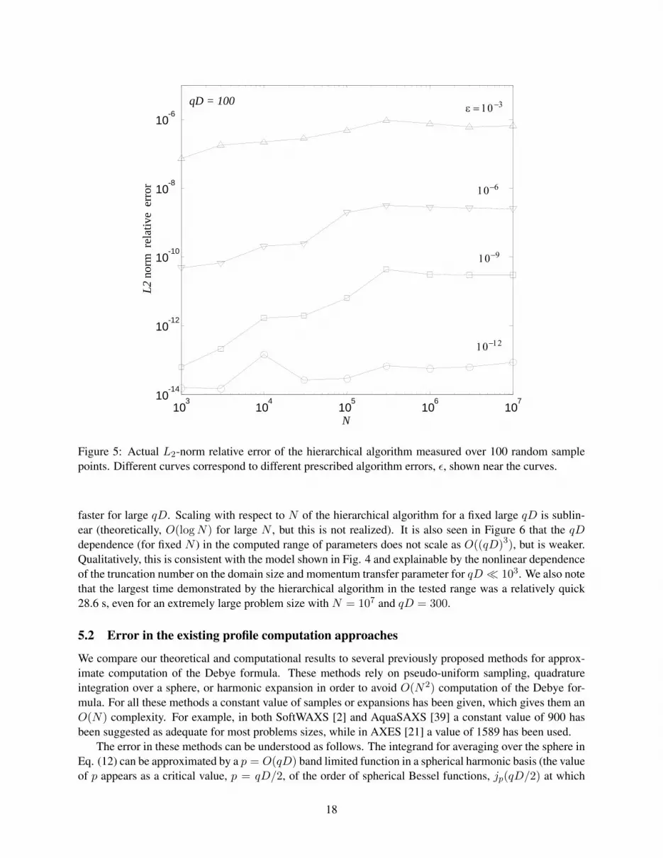
10 - 1 2
Figure 5: Actual L2-norm relative error of the hierarchical algorithm measured over 100 random samplepoints. Different curves correspond to different prescribed algorithm errors, ε, shown near the curves.
faster for large qD. Scaling with respect to N of the hierarchical algorithm for a fixed large qD is sublin-ear (theoretically, O(logN) for large N , but this is not realized). It is also seen in Figure 6 that the qDdependence (for fixed N ) in the computed range of parameters does not scale as O((qD)3), but is weaker.Qualitatively, this is consistent with the model shown in Fig. 4 and explainable by the nonlinear dependenceof the truncation number on the domain size and momentum transfer parameter for qD 103. We also notethat the largest time demonstrated by the hierarchical algorithm in the tested range was a relatively quick28.6 s, even for an extremely large problem size with N = 107 and qD = 300.
5.2 Error in the existing profile computation approaches
We compare our theoretical and computational results to several previously proposed methods for approx-imate computation of the Debye formula. These methods rely on pseudo-uniform sampling, quadratureintegration over a sphere, or harmonic expansion in order to avoid O(N2) computation of the Debye for-mula. For all these methods a constant value of samples or expansions has been given, which gives them anO(N) complexity. For example, in both SoftWAXS [2] and AquaSAXS [39] a constant value of 900 hasbeen suggested as adequate for most problems sizes, while in AXES [21] a value of 1589 has been used.
The error in these methods can be understood as follows. The integrand for averaging over the sphere inEq. (12) can be approximated by a p = O(qD) band limited function in a spherical harmonic basis (the valueof p appears as a critical value, p = qD/2, of the order of spherical Bessel functions, jp(qD/2) at which
18

qD = 0.3 qD = 3 qD = 30 qD = 300
N H M B H M B H M B H M B
104 <0.01 0.023 1.55 0.016 0.031 1.55 0.047 0.17 1.55 1.23 5.38 1.55105 0.062 0.11 158 0.11 0.19 158 0.17 0.92 158 2.52 53.3 158106 0.44 0.50 15800 0.56 1.17 15800 1.11 9.22 15800 7.05 533 15800
Table 1: Wall clock time (in seconds) for the hierarchical (H), “Middleman” (M), and brute force (B)algorithms. Numbers in italics are estimated rather than computed.
they change behavior from being oscillatory to exponentially decaying functions). This is a natural basis inthe space of square integrable functions on a unit sphere. We observe that it is insufficient to use p smallerthan qD/2 as this violates Nyquist sampling for an oscillatory function. Since the number of the sphericalharmonic basis functions of bandwidth less than p is p2, one can see that at least p2 = O(q2D2) samplingpoints are needed to provide an accurate integration for bandwidth p (this is actually a well known result,e.g. see [29] and references cited there). Hence, any accurate quadrature method applied for computation ofthe intensity for N atoms has complexity O(q2D2N).
phf + 2 p=15 p=50 p= phf + 2
PDB q=0.3 q=0.5 q=1.0 q=0.3 q=0.5 q=1.0 q=0.3 q=0.5 q=1.0 q=0.3 q=0.5 q=1.06LYZ 14 19 33 1.0e-9 2.0e-4 0.30 0 0 0 9.2e-9 1.9e-7 1.3e-72R8S 31 48 89 0.17 0.48 0.79 0 3.5e-9 0.12 7.5e-8 6.8e-8 2.7e-73R8N 44 70 132 0.53 0.81 0.94 7.7e-12 0.02 0.48 6.5e-8 2.3e-8 6.5e-81FFK 43 68 129 0.60 0.85 0.95 4.5e-13 0.02 0.50 6.0e-8 2.7e-8 3.7e-81AON 42 66 124 0.74 0.88 0.98 4.6e-14 0.01 0.59 5.0e-8 1.8e-8 7.4e-8
Table 2: The relative errors in the computation of the scattering profile using the “Harmonic” method onour example proteins (no water layer), for a single value of q in A−1 and prescribed tolerance ε = 10−3.phf + 2 is the order of the spherical harmonic expansion that should be used in the computation in orderto guarantee a relative error of less than ε. The values p = 15 and p = 50, are the default and maximumpossible order of spherical expansion in CRYSOL.
The most popular method for solving Eq. (6) is harmonic expansion, introduced in the program CRYSOL[44]. CRYSOL expands the integrand using spherical harmonics, and uses their orthogonality property toanalytically account for averaging over all possible orientations. The method assumes a constant cutoff forharmonic order (set to 15 by default, and capped at a maximum of 50), giving the method a complexity ofO(N). We demonstrate the potential magnitude of the errors in Table 2 for proteins of various sizes for theharmonic expansion approach suggested in [44], though the error could appear in any of the methods with afixed sampling in either the order of expansion, or the number of quadrature samples.
From Table 2 we see that for p = 15 the error becomes significantly larger than experimental errors inthe q ≤ 0.5A−1 region of the profile, even for relatively small molecules. Note that the errors are related tothe maximum distance between atoms, so a sparse pseudo-molecule, like the one used in DAMMIF [18] orin coarse amino-acid level representation, would have large errors even for small N . Increasing the valueof p to 50 moves the region of the error to higher values of q and larger proteins, but the error can still beseen. Using the proper value of p as derived in this paper ensures that a low error is achieved throughout.The reason for this error is that terms which are neglected may be non-ngeligible. In Figure 7 we plot therelative contributions to profile values of components for a given value of the spherical harmonic degreefor different values of q for a given molecule. It is seen that for q = 0.5A−1 p = 15 is inadequate, whilep = 50, while ensuring accurate computations, pays a penalty of over 50 % of wasteful computations, since
19

10 3
10 4
10 5
10 6
10 7
10 -1
10 0
10 1
10 2
N
Tim
e, s
10 -1
10 0
10 1
10 2
10 -1
10 0
10 1
10 2
qD
Tim
e, s
3
M
H
30
300
10 4
M M
M
H
B
H
M
H
10 6
M H
H
10 5
B 10 4
N =
qD =
Figure 6: The wall clock time for the hierarchical (H), “Middleman” (M), and brute force (B) algorithms atdifferent N and qD. The empty and filled markers correspond to the “M” and “H” algorithms at the samefixed parameter values shown near the curves.
a value of p = 40 would have sufficed. A value of p = 80 would have been sufficient for q = 1.0A−1, butnot for q = 2.0 where the right p is about 160. The scaling of p with qD is also seen here.
Therefore, all the previously described methods, if implemented accurately using the presented errorbounds, would have a fundamental theoretical complexity of at least O(q2D2N), which is higher than thetheoretical complexity of our proposed hierarchical method, and is identical to our proposed middlemanapproach.
5.3 Performance Results for Profile Computation
When we compute the SAXS or SANS scattering profile of a molecule, the relation between qD and Nis constrained by the atomic density of protein/RNA/DNA complexes in solution, and the range 0A−1 <q < 0.5A−1, for which the experimental data are usually collected. In the typical ab initio reconstructionof the scattering profile 50 uniformly spaced samples of q in that range are used. The number of atoms ina molecule can range from around 1000 for small molecules like ubiquitin, to 1, 000, 000+ for ribosomalsystems, with the atomic density of such systems being around d = 0.02A−3 (assuming a uniformly packedstructure inside a bounding sphere).
In order to show that the performance of the present hierarchical method is orders of magnitude fasterfor the SAS experimental domain, we first demonstrate the speed of the method on randomly generated
20

0 20 40 60 80 100 120 140 160
0.1
0.2
0.3
0.4
0.5
0.6
0.7
0.8
0.9
1
1.1
n
Rel
ativ
e C
on
trib
uti
on
to
I q
q=0.5
q=1.0
q=2.0
Figure 7: The relative contribution (scaled such that the maximum contribution is unity) to profile valuesby coefficients corresponding to different values of n (the degree of the expansion, n ≤ p, where p is thetruncation number). For this particular molecule, a value of p = 15 causes an error for all values of q, whilea value of p = 50 is adequate (but wasteful of computations) for the q = 0.5A−1 case, but inadequate forq = 1.0A−1 or q = 2.0A−1. A properly chosen truncation number can ensure accurate computations, whileensuring that no wasteful computations are performed.
proteins as well as several real structures from the PDB database, similar or identical to those which havebeen previously analyzed by SAS. To generate an N size random protein we randomly assign N atom in asphere of radius (3N/4dπ)1/3, while avoiding steric collisions. All proteins structures include the associatedhydrogen atoms, which are treated explicitly in the computation.
Below we compare the performance of our hierarchical algorithm at computing an ab initio SAS profilerelative to two popular approaches. The first method is a direct summation of Eq. (1) (what we previouslyreferred to as the brute force method) as provided by the function “calculate profile reciprocal” in the IMPv1.0 software package [33], we refer to this method as “IMP”. This method is exact, to within machineprecision. The second method is our implementation of the direct harmonic expansion method, similar tothe one used in the ATSAS software package, primarily in the popular CRYSOL [44] and DAMMIN/F [18]programs. However, to avoid the errors introduced by a fixed order of expansion, we vary the truncationnumber according to the value of qD by using Eq. (25). This is denoted as our “Middleman” method forSAS profiles.
Note that in the performance tests shown below we used IMP as is, without parallelizing the code. The
21

hierarchical and Middleman methods were parallelized. The benchmark cases were executed on a DualQuad-Core Intel Xeon X5560 CPU @ 2.80GHz 64bit Linux machine with 24GB ECC DDR3 SDRAM (8cores). The wall clock time was measured for generating a SAS profile made out of 50 uniformly spacedevaluations in the range 0.01A−1 ≤ q ≤ 0.5A−1, for randomly generated molecule with atomic density ofd = 0.02A−3. The results for the randomly generated data are presented in Fig. 8, while the results for realPDB structures are shown in Table 3.
10 3
10 4
10 5
10 6
10 -2
10 -1
10 0
10 1
10 2
10 3
Number of Atoms
Tim
e s
Linear
Brute
Middleman
Hierarchical
Figure 8: Timing results for computation of uniformly spaced 50 point SAS profile on uniformly dense,spherical, randomly generated proteins, with 0.01A−1 ≤ q ≤ 0.5A−1 and ε = 10−3. “Linear” linerepresents an ideal O(N ) linearly scaled algorithm.
From Fig. 8 we can see that our hierarchical method (“H”) is order of magnitude faster than the twoprevious approaches described here. In fact, the hierarchical method exhibits sub-linear performance forthe tested problem domains, while maintaining prescribed accuracy. Table 3 confirms similar performanceon actual molecular structures. Overall, the hierarchical method is about 10 to 60 times faster than theMiddleman method (“M”) on the benchmark problem domains, while the brute force IMP method (“B”) iscomputationally infeasible on all but the very small molecules. It is seen that the “H” algorithm for caseswith large enough N substantially outperforms the “M” algorithm (which in its turn outperforms the “B”algorithm).
Note that the timing results did not include the translation operators or setting of the data structure forthe hierarchical algorithm, since it is amortized over the set of computations or, in the case of translationoperators, can be precomputed and stored in a lookup table. Comparison to other existing software requires
22

None Layer SpherePDB N D H M B N D H M B N D H M B6LYZ 1959 53 0.1 0.5 1.8 6785 70 0.4 2.2 22 16207 69 0.8 5.0 1222R8S 11556 161 1.0 12.7 65 35923 179 2.0 46 620 329765 178 12 419 5.2(3)3R8N 93263 246 5.4 206 4.2(3) 214840 263 9.5 533 2.2(4) 1029628 262 40 2532 5.1(5)1FFK 94876 240 5.7 201 4.3(3) 256100 258 11 606 3.1(4) 880941 256 37 2143 3.7(5)1AON 118923 230 6.0 235 6.7(3) 255198 247 11 565 3.1(4) 845460 247 33 1875 3.4(5)
Table 3: Timing results (in seconds) for (H) Hierarchical, (M) Middleman, (B) Brute force IMP for varioussized molecules, where N is the number of atoms. “None” columns represent the molecule without anyadditional solvation layers. “Layer” includes additional atoms that form an 8A water layer around themolecule. “Sphere” includes additional atoms from an 8A water sphere around the molecule. Numbers initalics are estimated. Numbers written as a(b) indicate a number a× 10b.
additional analysis of the pre-processing and post-processing modules, and is therefore outside the scope ofthis paper.
6 Conclusion
We have developed and demonstrated a fast new algorithm for Debye summations based on hierarchicaldecomposition of the molecule, coupled with local harmonic expansion and translation. The developed hi-erarchical algorithm, in all computed cases, is faster and provides significantly better scaling than two ofthe popular methods tested, while at the same time providing accurate and theoretically provable resultsto within any prescribed accuracy. In addition, we have provided the theoretical framework for analyzingthe accuracy and computational cost of several of the previously proposed methods and demonstrated theircomputational dependence on N as well as, previously unpublished, dependence on qD. The dependenceon qD is critical for computing accurate results, as well as determining the computationally optimal sam-pling/cutoff value. As shown here, in the harmonic expansion approach (proposed in [44]) an incorrectcutoff introduces significant error in the computation.
Since this is only a prototype, we anticipate further improvements, such as further optimization for ourspecific problem type, GPU parallelization [31], and algorithmic improvement in local-to-local translations,could further significantly speedup the computation, and are the focus of our future research. The abovesoftware is being made part of a new high performance software package, ARMOR, which will also includeadditional NMR restraints [3, ?]. We hope that the computational improvement of our fast Debye summationmethod will lead to tighter integration of SAS into current structure refinement protocols.
7 Acknowledgement
This study has been partially supported by the New Research Frontiers Award of the Institute of the Ad-vanced Computer Studies of the University of Maryland and by Fantalgo, LLC.
A Appendix
A.1 Error bounds for translation
Assume that we perform translation from domain of radius a′ centered at r = 0 for which we have truncationnumber p′ to domain of radius a centered at r = t for which the truncation number is p. We will estimate the
23

translation matrix truncation error for a single sinc source. According to Eq. (16) the expansion coefficientsfor a single source are Cm
′n′ = 4πR−m
′
n′ (rs) , n′ = 0, ..., p′ − 1, m′ = −n′, ..., n′. So for translation of
this expansion we have
Cmn =
p′−1∑n′=0
n′∑m′=−n′
(R|R)mm′
nn′ (t)Cm′
n′ = 4π
p′−1∑n′=0
n′∑m′=−n′
(R|R)mm′
nn′ (t)R−m′
n′ (rs) , |rs| 6 a′. (48)
The error in the sinc function computed at point r and its approximation obtained via the truncated transla-tion of the truncated expansion then is
εpp′ = s (r− rs)−p−1∑n=0
n∑m=−n
Cmn Rmn (r− t) (49)
= s (r− rs)− 4π
p−1∑n=0
n∑m=−n
p′−1∑n′=0
n′∑m′=−n′
(R|R)mm′
nn′ (t)R−m′
n′ (rs)Rmn (r− t) .
Substituting here expansion (16) about center r = t, we obtain
εpp′ = 4π
p−1∑n=0
n∑m=−n
R−mn (rs − t)−p′−1∑n′=0
n′∑m′=−n′
(R|R)mm′
nn′ (t)R−m′
n′ (rs)
Rmn (r− t) + εp. (50)
Note now that by definition of the translation coefficients and symmetry (R|R)−m,−m′
nn′ (−t) = (R|R)m′m
n′n (t)(see [29]), we have
R−mn (rs − t) =∞∑n′=0
n′∑m′=−n′
(R|R)−mm′
nn′ (−t)Rm′
n′ (rs) =∞∑n′=0
n′∑m′=−n′
(R|R)m′m
n′n (t)R−m′
n′ (rs) . (51)
We also have the following integral representation of the translation coefficients [29]
(R|R)mm′
nn′ (t) = in−n′∫Su
eiqs·tY m′n′ (s)Y −mn (s) dS (s) . (52)
Substituting Eqs (51) and (52) into Eq. (50) and using the addition theorem for spherical harmonics, weobtain
εpp′ =1
4π
p−1∑n=0
∞∑n′=p′
(2n′ + 1)jn′(qrs)in−n′ (2n+ 1) jn(q |r− t|)
∫Su
eiqs·tPn′(s·rsrs
)Pn
(s· r− t
|r− t|
)dS (s)
+εp.
(53)
Since∣∣∣∣ 1
4π
∫Su
eiqs·tPn′(s·rsrs
)Pn
(s· r− t
|r− t|
)dS (s)
∣∣∣∣ 6 1
4π
∫Su
∣∣∣∣eiqs·tPn′(s·rsrs )Pn
(s· r− t
|r− t|
)∣∣∣∣ dS (s) 6 1,
(54)
the error can be bounded as
∣∣εpp′∣∣ 6 p−1∑n=0
(2n+ 1) |jn(q |r− t|)|∞∑
n′=p′
(2n′ + 1) |jn′(qrs)|+ |εp| . (55)
24

Since qrs 6 qa′, p′ > qa′ the second sum can be bounded by∣∣εp′∣∣ given by Eq. (38) (where primes should
be placed near a and p). The first sum can be bounded using |jn(q |r− t|)| 6 1, in which case the sum ofodd numbers from 0 to 2p− 1 is p2 and we obtain∣∣εpp′∣∣ 6 p2
∣∣εp′∣∣+ |εp| . (56)
Note that the last term here, |εp|, can be ignored, since for p given by Eq. (40) actual expansion error (23) isapproximately square of error (39). We also note that coefficient p2 of the first term can be improved due tothe following lemma.
Lemma 1 For x > 0 the following bound holds∑∞
n=0 (2n+ 1) |jn(x)| < C1 +C2x, where C1 and C2 aresome real positive numbers.
Proof. For n > x functions jn(x) decay exponentially and the series converges. So
∞∑n=0
(2n+ 1) |jn(x)| =[x]∑n=0
(2n+ 1) |jn(x)|+ ε (x) , ε (x) (57)
=∞∑
n=[x]
(2n+ 1) |jn(x)| < C (2x+ 1) jx(x),
where C is some constant of order 1. Since jx(x) is a monotonic decaying function of x, we have jx(x) <j0(0) = 1. The first sum can be bounded since the function in the right hand side is continuous and hassome maximum on the interval [0, 1], while for x > 1, 0 < n 6 [x] we have |jn(x)| < B/x, where B issome constant. Hence,
[x]∑n=0
(2n+ 1) |jn(x)| < B
x
[x]∑n=0
(2n+ 1) =B
x([x] + 1)2 < Bx+B1, x > 1. (58)
This completes the proof.
Remark 2 We computed this function numerically for 10−2 < x < 103 and found that C1 < 2, C2 < 1.
So, the error can be bounded as∣∣εpp′∣∣ 6 (C1 + C2p)∣∣εp′∣∣ ∼ p ∣∣εp′∣∣ . (59)
where C1 and C2 are some constants of order 1. For large qa we have p ∼ qa which is two times larger orsmaller than p′ ∼ qa′. Using Eq. (39) we have then
∣∣εpp′∣∣ . (qa′)5/6 exp
(−1
323/2η
3/2p′
), (60)
which provides a slightly larger truncation number for a region of size a (we replaced p′ with p and qa′ withqa).
p & phf (ε, qa) = qa+1
2
(3 log
1
ε+
5
2log(qa)
)2/3
(qa)1/3. (61)
25

A.2 The coaxial translation
Coaxial translation can be described as
Cmn =
p′−1∑n′=|m|
(R|R
)mnn′
(t)Cmn′ , m = 0,±1, ...,±(min(p, p′)− 1
), n = 0, 1, ..., p− 1. (62)
(in the general matrix(R|R
)mm′nn′
= 0 for m′ 6= m). Recursive computations of(R|R
)mnn′
(t) can be
performed only for non-negative |m| and for n > n′ (or n′ > n) due to symmetries(R|R
)mnn′
(t) =(R|R
)−mnn′
(t) = (−1)n+n′(R|R
)mn′n
(t). (63)
The recursive process starts with the initial values(R|R
)0
n0(t) = (−1)n
√2n+ 1jn(qt), n = 0, 1, ... (64)
Advancement in m can be performed using
b−m−1m+1
(R|R
)m+1
n,m+1= b−m−1
n
(R|R
)mn−1,m
− bmn+1
(R|R
)mn+1,m
, n = m+ 1,m+ 2, ... (65)
Advancement in n′ can be performed using
amn′(R|R
)mn,n′+1
= amn′−1
(R|R
)mn,n′−1
−amn(R|R
)mn+1,n′
+amn−1
(R|R
)mn−1,n′
, n′ = m,m+1, ...
(66)
In Eqs (65) and (66) the recursion coefficients are
amn =
√(n+1+m)(n+1−m)
(2n+1)(2n+3) , n > |m| ,0, n < |m| ,
, (67)
bmn =
sgn(m)
√(n−m−1)(n−m)(2n−1)(2n+1) , 0 6 m 6 n,
0, n < |m| .
where sgn(m) is defined as
sgn(m) =
1, m > 0,−1, m < 0.
(68)
A.3 Expressions for the rotation of coefficients
In general, an arbitrary rotation transform can be specified by three Euler angles of rotation. For rotation ofspherical harmonics it may be more convenient to use slightly modified Euler angles, and use angles α, β, γwhich are related to the spherical polar angles (θt, ϕt) of the unit vector t/t = (sin θt cosϕt, sin θt sinϕt, cos θt)as β = θt, α = ϕt (see Fig. 9). The original axis z in the rotated reference frame has spherical polar angles(β, γ), which is the definition of the third rotation angle. Since the rotation transform is a function of therotation matrix Q(α, β, γ) for which Q−1(α, β, γ) = Q(γ, β, α), we describe only the forward rotation,since the inverse rotation simply exchanges angles α and γ.
26

x
y
z
x
y
z
O
AAβ
α
x
y
z
x
y
z
O
AA
β
x
y
z
x
y
z
O
AA
x
y
z
xx
yy
zz
O
AAA
x
y
z
x
y
z
O
AA
x
y
z
xx
yy
zz
O
AAA
γ
tt
x
y
z
x
y
z
O
AAβ
α
x
y
z
x
y
z
O
AA
β
x
y
z
x
y
z
O
AA
x
y
z
xx
yy
zz
O
AAA
x
y
z
x
y
z
O
AA
x
y
z
xx
yy
zz
O
AAA
γ
tt
Figure 9: Rotation specified by angles α, β, and γ, where α and β are the spherical polar angles of thetranslation vector t in the original reference frame.
The rotation transform can be described by
Cmn = e−imγn∑
m′=−nHmm′n (β) eim
′αCm′
n , n = 0, 1, ..., p− 1, m′ = −n, ..., n, (69)
where Hmm′n (β) are the entries of a real dense matrix that can be computed recursively.
The basic recursion used for computation is derived in [29],
dm−1n Hm−1,m′
n − dmn Hm+1,m′n = dm
′−1n Hm,m′−1
n − dm′n Hm,m′+1n , (70)
dmn =1
2sgn(m) [(n−m)(n+m+ 1)]1/2 , m = −n, ..., n,
and sgn(m) is provided by Eq. (68). This recursion, however, should be applied carefully, due to potentialrecursion instabilities. For angles 0 < β < π/2 the maximum values of Hmm′
n (β) are reached on the maindiagonal m′ = m and subdiagonals m′ = m± 1. Figure 10 illustrates organization of the recursive processin this case (for the boundary points, m = n, recursion coefficients dmn = 0) . The values on the diagonalsand subdiagonals are computed via the axis flip transform, which corresponds to β = π/2:
Hmm′n (β) =
n∑ν=−n
Hmνn
(π2
)Hm′νn
(π2
)cos(νβ +
π
2
(m+m′
)). (71)
27
m
m’
n
- n
0
1
-1
2
n0 1
m
m’
n
0
1
2
β = π/2
0 < β < π/2
n1
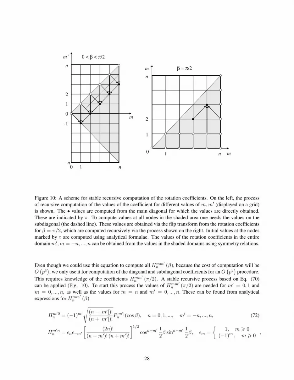
Figure 10: A scheme for stable recursive computation of the rotation coefficients. On the left, the processof recursive computation of the values of the coefficient for different values of m,m′ (displayed on a grid)is shown. The • values are computed from the main diagonal for which the values are directly obtained.These are indicated by . To compute values at all nodes in the shaded area one needs the values on thesubdiagonal (the dashed line). These values are obtained via the flip transform from the rotation coefficientsfor β = π/2, which are computed recursively via the process shown on the right. Initial values at the nodesmarked by are computed using analytical formulae. The values of the rotation coefficients in the entiredomainm′,m = −n, ..., n can be obtained from the values in the shaded domains using symmetry relations.
Even though we could use this equation to compute all Hmm′n (β), because the cost of computation will be
O(p4), we only use it for computation of the diagonal and subdiagonal coefficients for anO
(p3)
procedure.This requires knowledge of the coefficients Hmm′
n (π/2). A stable recursive process based on Eq. (70)can be applied (Fig. 10). To start this process the values of Hmm′
n (π/2) are needed for m′ = 0, 1 andm = 0, ..., n, as well as the values for m = n and m′ = 0, ..., n. These can be found from analyticalexpressions for Hmm′
n (β)
Hm′0n = (−1)m
′
√(n− |m′|)!(n+ |m′|)!
P |m′|
n (cosβ), n = 0, 1, ..., m′ = −n, ..., n, (72)
Hm′nn = εnε−m′
[(2n)!
(n−m′)! (n+m′)!
]1/2
cosn+m′ 1
2β sinn−m
′ 1
2β, εm =
1, m > 0
(−1)m , m > 0,
28

and the recurrence [29]
Hm′,m+1n−1 =
1
bmn
1
2
[b−m
′−1n (1− cosβ)Hm′+1,m
n − bm′−1n (1 + cosβ)Hm′−1,m
n
]− am′n−1 sinβHm′m
n
,
(73)
n = 2, 3, ..., m′ = −n+ 1, ..., n− 1, m = 0, ..., n− 2,
where amn and bmn are provided by Eq. (67). For small and moderate n this recursion can be used to obtainall rotation coefficients immediately, as it was done in [29], but for large n this is not stable. So we use Eqs(72) and (73) only for β = π/2 and Eq. (73) only for m = 0 to obtain Hm′1
n (π/2). Note than that thefollowing symmetries are used for faster computations
Hm′mn (β) = Hmm′
n (β) , Hm′mn (β) = H−m
′,−mn (β) , Hm′m
n (π − β) = (−1)n+m+m′ H−m′,m
n (β) .
(74)
The last equation provides an additional symmetry for β = π/2, while for other β it can be used to reduceall computations to the range 0 6 β 6 π/2. In fact, for the present algorithm only rotations with β = π/4and β = 3π/4 are needed. So the latter can be reduced to the former case, and only the constant coefficientsHm′mn (π/4) are needed. In principle, these coefficients can be precomputed and stored to reduce the run
time.
29
References
[1] Abramowitz, M.; Stegun, I.A.; National Bureau of Standards: Washington D.C,, 1965.
[2] Bardhan, J.; Park, S.; Makowski, L.; J Appl Crystallography, 2009, 42, 932-943.
[3] Berlin, K.; O’Leary, D.P.; Fushman, D.; J. Am. Chem., 2010, 132, 8961-8972.
[4] Berlin, K.; O’Leary, D.P.;Fushman, D.;Proteins: Struct., Funct., Bioinf., 2011, 79, 1097-0134.
[5] Bernado, P.; Mylonas,E.; Petoukhov, M.V.; Blackledge, M.; Svergun, D.I.; J Am Chem Soc 2007, 129,5656-5664.
[6] Bernado, P.; Modig, K.; Grela, P.; Svergun, D.I.; Tchorzewski, M.; Pons, M.; and Akke, M.; BiophysJ, 2010, 98, 2374-2382.
[7] Chen, S.H.; Ann Rev Phys Chem, 1986, 37, 351-399.
[8] Cheng,H.; Crutchfield,W.Y.;Gimbutas,Z.; Greengard, L.; Ethridge,F.; Huang,J.; Rokhlin, V.; Yarvin,N.; Zhao, J.; J Comput Phys, 2006, 216, 300-325.
[9] Cheng,H.; Greengard, L.; Rokhlin, V.; J Comput Phys, 1999, 155, 468-498.
[10] Clark,G.N.; Hura, G.L.; Teixeira, J.; Soper, A.K.; Head-Gordon, T.; Proc Natl Acad Sci USA, 2010,107, 14003-14007.
[11] Datta, A.B.; Hura, G.L.; Wolberger, C.; J Mol Biol 2009, 392, 1117-1124.
[12] Debye, P.; Ann Phys (Leipzig), 1915, 351, 809-823.
[13] Dongarra, J.J.; Sullivan, F. ; Computing in Science & Engineering, 2000, 2, 22-23.
[14] Engelman, D.M.; Moore, P.B.; Ann Rev Biophys Bioeng, 1975, 4, 219-241.
[15] Epton, M.A.; Dembart, B.; SIAM J Sci Comput, 1995, 16, 865-897.
[16] Feigin, L.A.; Svergun, D.I.; Plenum Press: New York, 1987.
[17] Forster, F.; Webb,B.; Krukenberg, K.A.; Tsuruta, H.; Agard, D.A.; Sali, A.; J Mol Biology, 2008, 382,1089-1106.
[18] Franke, D.; Svergun, D.I.; J Appl Cryst, 2009, 42, 342–346.
[19] Greengard, L.; Rokhlin, V.; J Comput Phys, 73, 1987, 325-348.
[20] Greengard, L.; Rokhlin, V.; Acta Numerica, 1997, 6, 229-269.
[21] Grishaev, A.; Guo, L.; Irving, T.; Bax, A.; J Am Chem Soc, 2010, 132, 15484-15486.
[22] Grishaev, A.; Wu, J.; Trewhella, J.; Bax, A.; J Am Chem Soc, 2005, 127, 16621-16628.
[23] Grishaev, A.; Ying,J.; Canny,M.D.; Pardi,A.; Bax, A.; J Biomol NMR, 2008, 42, 99-109.
[24] Grishaev,A.; Tugarinov, V.; Kay, L.E.; Trewhella, J.; Bax, A.; J Biomol NMR, 2008, 40, 95-106.
[25] Grover, R.F.; McKenzie, D.R.; Acta Cryst, 2001, A57, 739-740.
30

[26] Gumerov, N.A.; Duraiswami, R.; SIAM J Sci Comput, 2003, 25, 1344-1381.
[27] Gumerov, N.A.; Duraiswami, R.; J Comput Phys, 2006, 215, 363-383.
[28] Gumerov, N.A.; Duraiswami, R.; Univ. of Maryland Tech. Rep., UMIACS-TR-#2005-09, 2005.(http://www.cs.umd.edu/Library/TRs/CS-TR-4701/CS-TR-4701.pdf).
[29] Gumerov, N.A.; Duraiswami, R.; Elsevier: Oxford, UK, 2005.
[30] Gumerov, N.A.; Duraiswami, R.; J Comput Phys, 2007, 225, 206-236.
[31] Gumerov, N.A.; Duraiswami, R.; J Comput Phys, 2008, 227 8290-8313.
[32] Gumerov, N.A.; Duraiswami, R.; J Acoust Soc Am, 2009, 125, 191-205.
[33] IMP v1.0 software (available from http://salilab.org/imp/).
[34] Jehle,S.; Vollmar,B.S.; Bardiaux, B.; Dove,K.K.; Rajagopal,P.; Gonen,T.; Oschkinat, H.; Klevit, R.E.;Proc Natl Acad Sci USA, 2001, 108, 6409-6414.
[35] Koch, M.H.; Vachette, P.; Svergun D.I.; Q Rev Biophys, 2003, 36, 147-227.
[36] Lattman, E.E.; Proteins, 1989, 5, 149–155.
[37] Lipfert, J.; Doniach S.; Ann Rev Biophys Biomol Struct, 2007, 36, 307-327.
[38] Palosz, B.; Grzanka, E.; Gierlotka, S; Stelmakh, S.; Zeitschrift fur Kristallographie: 225, 12, 12thEuropean Powder Diffraction Conference, 2010, 588-598.
[39] Poitevin, F.; Orland, H.; Doniach, S.; Koehl, P.; Delarue, M; Nucleic Acids Res, 2011, 39, W184-189.
[40] Pons, C.; D’Abramo, M.; Svergun, D.I.; Orozco, M.; Bernado, P.; Fernandez-Recio, J.; J Mol Biol,2010, 403, 217-230.
[41] Rokhlin, V.; Appl Comput Harmonic Analysis, 1993, 1, 82-93.
[42] Samet, H.; Morgan Kaufmann: San Francisco, 2006.
[43] Stuhrmann, H.B.; Acta Cryst, 1970, A26, 297– 306.
[44] Svergun, D.; Barberato, C.; Koch, M.H.J.; J Appl Crystallography, 1995, 28, 768–773.
[45] Thomas, N.W.; Acta Cryst, 2010, A66, 64-77.
[46] Walther, D.; Cohen, F.; Doniach, S.; J Appl Crystallography, 2000, 33, 350-363.
[47] White, C.A.; Head-Gordon, M.; J Chem Phys, 1996, 105, 5061-5067.
[48] Yang, S.; Park, S.; Makowski, L.; Roux, B.; Biophys J, 2009, 96, 4449-4463.
31
Recommended


