
This content has been downloaded from IOPscience. Please scroll down to see the full text.
Download details:
IP Address: 128.180.11.192
This content was downloaded on 27/12/2013 at 19:14
Please note that terms and conditions apply.
Damage and noise sensitivity evaluation of autoregressive features extracted from structure
vibration
View the table of contents for this issue, or go to the journal homepage for more
2014 Smart Mater. Struct. 23 025007
(http://iopscience.iop.org/0964-1726/23/2/025007)
Home Search Collections Journals About Contact us My IOPscience
Smart Materials and Structures
Smart Mater. Struct. 23 (2014) 025007 (15pp) doi:10.1088/0964-1726/23/2/025007
Damage and noise sensitivity evaluation ofautoregressive features extracted fromstructure vibration
Ruigen Yao and Shamim N Pakzad
Department of Civil and Environmental Engineering, Lehigh University, Bethlehem, PA 18015, USA
E-mail: [email protected]
Received 25 June 2013, in final form 19 November 2013Published 23 December 2013
AbstractIn the past few decades many types of structural damage indices based on structural healthmonitoring signals have been proposed, requiring performance evaluation and comparisonstudies on these indices in a quantitative manner. One tool to help accomplish this objective isanalytical sensitivity analysis, which has been successfully used to evaluate the influences ofsystem operational parameters on observable characteristics in many fields of study. In thispaper, the sensitivity expressions of two damage features, namely the Mahalanobis distance ofautoregressive coefficients and the Cosh distance of autoregressive spectra, will be derivedwith respect to both structural damage and measurement noise level. The effectiveness of theproposed methods is illustrated in a numerical case study on a 10-DOF system, where theirresults are compared with those from direct simulation and theoretical calculation.
Keywords: sensitivity analysis, structural vibration monitoring, autoregressive modeling,autoregressive spectrum estimation, Yule–Walker method
(Some figures may appear in colour only in the online journal)
1. Introduction
Damage detection is a very crucial part in the regularassessment and maintenance routine for civil infrastructure.Traditionally this task is carried out by human inspection,and thereby is expensive, time-consuming and the accuracyrelies on individual expertise. Recently, the advancements insensing and computational technology have made it feasiblefor a sensor network to be installed on a civil structure, anddata collected from the sensors will then be processed toproduce information pertaining to the structural condition. Todate many research studies in the literature [1–4] devoted tothis topic can be found, forming a promising branch of studyoften referred to as data-driven structural health monitoring(SHM). Ideally, the new system will cost less than traditionalmethods because of the lowering prices of sensing systems,and produce more accurate and reliable decisions that are freeof human judgment bias or expertise. Moreover, SHM hasthe capability to reveal problems undetectable via ‘naked-eye’inspection such as internal fracture and delamination.
Vibration responses (e.g. acceleration, strain) areamong the most commonly measured signals for structuralmonitoring purposes. One category of widely employedvibration-based damage indices consists of modal prop-erties extracted using system identification/modal realiza-tion approaches [5–7]. Recently, many alternative damagefeatures [8–10] based on structural output are proposedto address the computational efficiency issues (especiallyfor time domain extraction algorithms) concerning modalproperties estimators [1]. Time series analysis [11] for singlechannel acceleration measurements is one of the notabletechniques attempted in a number of research articles [12–17],where algorithms such as scalar autoregressive (AR), autore-gressive/autoregressive with exogenous input (AR–ARX) andautoregressive with moving average (ARMA) modeling havebeen applied and functions of estimated model parametersused as damage features. These features are reported to beless complicated to compute and more sensitive to localdamage in their respective applications. References [13, 16]provide comparisons on the effect of local damage on the
10964-1726/14/025007+15$33.00 c© 2014 IOP Publishing Ltd Printed in the UK
Smart Mater. Struct. 23 (2014) 025007 R Yao and S N Pakzad
modal frequencies/shapes and autoregressive features, andit is observed in both case studies that the latter shows amore noticeable change than the former. Also, the AR–ARXmethod has demonstrated success in damage localizationin [13] and the ARMA method has been used to indicatedamage location and extent in [15]. The AR methods,however, are not sensitive to damage location [17]. It isnoted that univariate time series analysis methods are outputonly, and damage indices of this type are often functionsof structural signal autocovariance functions, which are inturn determined by the structural stiffness properties, thestructural geometry and excitation patterns. When the locationof damage does not correspond well with where the largestdamage-induced change in signal autocovariance functionsoccurs, damage localization based on time series analysisis likely to be very difficult. Still, these damage featureshave advantages such as being simple in concept, convenientfor statistical processing as they can be generated in largequantities, and suitable for decentralized structural monitoringapplications.
While it is important to propose and test newfeatures to improve the state-of-the-art of structural damagedetection, examination of the effect of structural change andenvironmental and operational factors on existing features inan analytically rigorous manner is also crucial for optimalfeature selection for different practices. Previously, researchhas been conducted on evaluating the adverse effect ofmeasurement noise on the accuracy of estimated modalparameters [18]. In this paper, the sensitivity of two damagefeatures based on AR modeling due to damage level andmeasurement noise is studied and an analysis methodology isproposed. The two methods are the Mahalanobis distance [19]of AR coefficients and the Cosh distance [20] of AR modelspectra between the baseline state and the current state. Thevalidity of this methodology is supported by simulation resultsfrom a 10-DOF bridge model.
The paper is organized as follows. Section 2 gives anexplanation of the theoretical relation between the structuralacceleration response and the family of AR modeling,together with an examination of the properties of the scalarYule–Walker AR coefficient estimators. Section 3 containsstepwise derivations regarding the analysis for the sensitivitywith respect to damage level and measurement noise forboth features. In section 4, sensitivity analysis is applied toa 10-DOF simulated model and the results are comparedwith those from direct simulation and theoretical calculation.Conclusions are then made on the efficiency of the algorithmsand the effectiveness of the features.
2. Autoregressive modeling for structural vibrationmeasurements
As noted in the introduction, sensor measurements do notreveal information concerning the structural state beingmonitored until they go through data-processing algorithms.Autoregressive (AR) modeling is one of the most effectivetime series analysis techniques and has found applications invibration monitoring of various types of structures [8, 13, 15]
that are instrumented with accelerometers. Here, differentaspects of AR modeling are investigated in two sections.Section 2.1 demonstrates the validity of AR modelingfor structural vibration signals and presents a proof ona multi-input–multi-output (MIMO) ARX model betweenthe excitation and acceleration response of a MDOFsystem. Since univariate AR estimators tend to behavedifferently from their multivariate counterparts becauseof the spatial correlation among structural responses,section 2.2 investigates the characteristics of single-input–single-output (SISO) AR coefficient estimators fromacceleration measurements to provide insight into thebehavior of the autoregressive features thus extracted.
2.1. Civil structural systems and AR/ARX model
An ARX model is a numerical tool that has been provedquite useful in describing causal systems subjected to aseries of external disturbances [21]. In an effort to derivean explicit ARX model for a N-degrees-of-freedom systembetween its excitation source and acceleration measurements,the system impulse response should be obtained, discretizedand transformed. To start, calculate the acceleration impulseresponse of the ith mode by twice differentiating Duhamel’sintegral of the displacement impulse response hi(t) [22]:
hi(t) =d2{∫ t
0 hi(t − τ)δ(τ ) dτ }
dt2
= hi(0)δ′(t)+ h′i(t − τ)δ(τ )|τ=t
+
∫ t
0
d2
dt2{hi(t − τ)}δ(τ ) dτ, (1)
where δ(τ ) here stands for the Dirac delta function. Theacceleration impulse response may be written as the sumof the second-order derivative of the displacement impulseresponse and an impulse term:
hi(t) =d2[hi(t)]
dt2+
1miδ(t)
=−ω2
Di
miωDie−ζiωnit sinωDit
+−2ζiωDiωni
miωDie−ζiωnit cosωDit
+ζ 2
i ω2ni
miωDie−ζiωnit sinωDit +
1miδ(t) (2)
where mi, ωni, ωDi and ζi are the modal mass, naturalfrequency, damped frequency and damping ratio of the ithmode, respectively. The discretized version of equation (2) is
ai[n] =−ω2
Di
miωDie−ζiωniTsn sinωDiTsn
+−2ζiωDiωni
miωDie−ζiωniTsn cosωDiTsn
+ζ 2
i ω2ni
miωDie−ζiωniTsn sinωDiTsn+
1miTs
δ(n) (3)
2
Smart Mater. Struct. 23 (2014) 025007 R Yao and S N Pakzad
where n is the time label in the discrete domain and Ts isthe sampling interval. Its corresponding z-transform can beobtained as
a(z) =
(−ω2
Di
miωDi+ζ 2
i ω2ni
miωDi
)
×e−ζiωniTsz−1 sinωDiTs
1− 2e−ζiωniTsz−1 cosωDiTs + e−2ζiωniTsz−2
+−2ζiωDiωni
miωDi
×1− e−ζiωniTsz−1 cosωDiTs
1− 2e−ζiωniTsz−1 cosωDiTs + e−2ζiωniTsz−2
+1
miTs. (4)
Defining the discretized modal input/output as qi[n] andpi[n], their relation can be expressed using an ARX model bytaking the inverse z-transform and rearranging equation (4):
qi[n] − 2e−ζiωniTs cosωDiTsqi[n− 1] + e−2ζiωniTs qi[n− 2]
=
(1
miTs−
2ζiωni
mi
)pi[n] + e−ζiωniTs
[−2 cosωDiTs
miTs
+ sinωDiTs
(−ωDi
mi+ζ 2
i ω2ni
miωDi
)
+ cosωDTs2ζiωni
mi
]pi[n− 1]
+e−2ζiωniTs
miTspi[n− 2]. (5)
For notational simplicity the coefficient expressions willbe omitted for now and equation (5) is denoted as
Ai(B)qi[n] = Ci(B)pi[n],
B: the backshift operator, i.e. Bp[n] = p[n− 1]. (6)
For the MDOF model discussed here, the matrix form ofrepresentation can be employed:
A(B)q[n] = C(B)p[n], (7)
where A(B) and C(B) are diagonal matrices consisting ofAi(B) and Ci(B) terms, respectively. q[n] is the modaldisplacement vector and p[n] is the modal input vector.Their relationship with the nodal input vector x[n] and nodaldisplacement vector y[n] are as follows:
y[n] = Φq[n], x[n] = ΦT−1p[n] (8)
where Φ here stands for the system eigenvector matrix.Therefore, the relation between the excitation and systemacceleration response can be expressed as a multivariate ARXmodel:
A′(B)y[n] = C′(B)x[n],
A′(B) = ΦA(B)Φ−1, C′(B) = ΦC(B)ΦT.(9)
Note that A′(0) = ΦA(0)Φ−1= ΦΦ−1
= I. For signalsgenerated from the multivariate ARX system under randomexcitation, each scalar signal can be viewed as a sum of
seemingly uncorrelated ARMA processes and modeled witha scalar ARMA process [23].
2.2. AR coefficient estimators for scalar acceleration signals
ARMA processes can be approximated with an AR processwith a large model order [24]. One main advantage of thelatter method is its computational efficiency. The definitionof a univariate AR model of order p is
x(t) =p∑
j=1
ϕjx(t − j)+ ox(t). (10)
In this equation, x(t) is the time series to be analyzed, ϕjterms are the AR model coefficients and ox(t) is the modelresidual. Because of its concise form, the AR model has beenwidely adopted for time series analysis for different purposes.One of the frequently used AR coefficient estimators is theYule–Walker estimator [24], which is obtained from solvingthe following equation:
ϕ1
ϕ2
ϕ3...
ϕp
=
R(0) R(1) R(2) · · · R(p− 1)
R(1) R(0) R(1) · · · R(p− 2)
R(2) R(1) R(0) · · · R(p− 3)...
......
. . ....
R(p− 1) R(p− 2) R(p− 3) · · · R(0)
−1
×
R(1)
R(2)
R(3)...
R(p)
= 0−1γ, (11)
where R(·) is the autocovariance function (ACF) of the timeseries and {ϕj} are the AR coefficients.
When an AR model (which is an all-pole system) isconstructed from the structural acceleration signal, spuriouspoles will be introduced because the model cannot properlyparameterize possible zeros in the underlying generatingfunction, leading to a large AR order for an accurate model:
1− βz−1≈
1− βz−1
1− βn+1z−(n+1)
=1
1+ βz−1 + · · · + βnz−n,
(|βz−1| < 1)
1− βz−1≈−βz−1(1− β−1z)
1− β−(n+1)zn+1
=−βn+1z−(n+1)
1+ βz−1 + · · · + βnz−n,
(|βz−1| > 1).
(12)
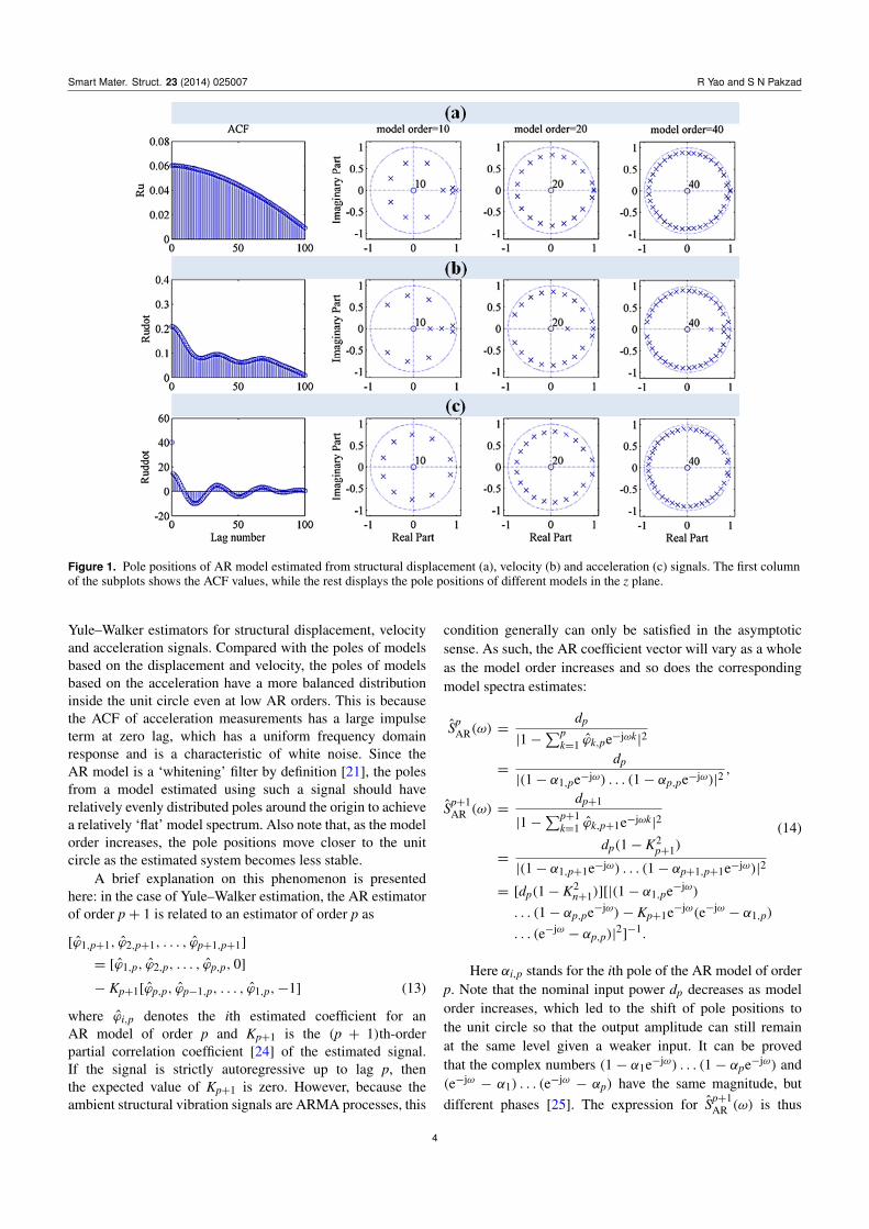
In either case the pole positions should be inside the unitcircle to ensure a stable system. Poles thus generated tendto be uniformly distributed around the unit circle. Figure 1shows the ACF and the pole location plots in the z plane of
3
Smart Mater. Struct. 23 (2014) 025007 R Yao and S N Pakzad
Figure 1. Pole positions of AR model estimated from structural displacement (a), velocity (b) and acceleration (c) signals. The first columnof the subplots shows the ACF values, while the rest displays the pole positions of different models in the z plane.
Yule–Walker estimators for structural displacement, velocityand acceleration signals. Compared with the poles of modelsbased on the displacement and velocity, the poles of modelsbased on the acceleration have a more balanced distributioninside the unit circle even at low AR orders. This is becausethe ACF of acceleration measurements has a large impulseterm at zero lag, which has a uniform frequency domainresponse and is a characteristic of white noise. Since theAR model is a ‘whitening’ filter by definition [21], the polesfrom a model estimated using such a signal should haverelatively evenly distributed poles around the origin to achievea relatively ‘flat’ model spectrum. Also note that, as the modelorder increases, the pole positions move closer to the unitcircle as the estimated system becomes less stable.
A brief explanation on this phenomenon is presentedhere: in the case of Yule–Walker estimation, the AR estimatorof order p+ 1 is related to an estimator of order p as
[ϕ1,p+1, ϕ2,p+1, . . . , ϕp+1,p+1]
= [ϕ1,p, ϕ2,p, . . . , ϕp,p, 0]
− Kp+1[ϕp,p, ϕp−1,p, . . . , ϕ1,p,−1] (13)
where ϕi,p denotes the ith estimated coefficient for anAR model of order p and Kp+1 is the (p + 1)th-orderpartial correlation coefficient [24] of the estimated signal.If the signal is strictly autoregressive up to lag p, thenthe expected value of Kp+1 is zero. However, because theambient structural vibration signals are ARMA processes, this
condition generally can only be satisfied in the asymptoticsense. As such, the AR coefficient vector will vary as a wholeas the model order increases and so does the correspondingmodel spectra estimates:
SpAR(ω) =
dp
|1−∑p
k=1 ϕk,pe−jωk|2
=dp
|(1− α1,pe−jω) . . . (1− αp,pe−jω)|2,
Sp+1AR (ω) =
dp+1
|1−∑p+1
k=1 ϕk,p+1e−jωk|2
=dp(1− K2
p+1)
|(1− α1,p+1e−jω) . . . (1− αp+1,p+1e−jω)|2
= [dp(1− K2n+1)][|(1− α1,pe−jω)
. . . (1− αp,pe−jω)− Kp+1e−jω(e−jω− α1,p)
. . . (e−jω− αp,p)|
2]−1.
(14)
Here αi,p stands for the ith pole of the AR model of orderp. Note that the nominal input power dp decreases as modelorder increases, which led to the shift of pole positions tothe unit circle so that the output amplitude can still remainat the same level given a weaker input. It can be provedthat the complex numbers (1 − α1e−jω) . . . (1 − αpe−jω) and(e−jω
− α1) . . . (e−jω− αp) have the same magnitude, but
different phases [25]. The expression for Sp+1AR (ω) is thus
4
Smart Mater. Struct. 23 (2014) 025007 R Yao and S N Pakzad
Figure 2. Illustration of the relation between structural damage/measurement noise and AR-based damage features.
further simplified as
Sp+1AR (ω)
=dp(1−K2
p+1)
|1−Kp+1e−j�(ω)|2|(1−α1e−jω)...(1−αpe−jω)|2
=(1−K2
p+1)SpAR(ω)
|1−Kp+1e−j�(ω)|2,
�(ω)
= 6(1−α1,pe−jω)...(1−αp,pe−jω)
e−jω(e−jω−α1,p)...(e−jω−αp,p)
= (p+ 1)ω + 26 (1− α1,pe−jω) . . . (1− αp,pe−jω).
(15)
When Kp+1 is significantly small, the pole positions of the ARspectrum will not change much as the model order increasesand the spectrum shape will converge.
3. Damage level and measurement noise sensitivityfor the AR damage features
Distance measures between characteristics of undamagedand damaged structure states are often adopted as damagefeatures. Damage features examined in this paper are theMahalanobis distance of AR coefficients and the Coshdistance of AR model spectra extracted from structuralacceleration measurements [14]. The Mahalanobis distance isa metric to evaluate the deviation within vectorial Gaussiansample groups [19]. Its definition is stated as below:
D2(ϕu, ϕb) = (ϕTu − ϕ
Tb )Σ
−1b (ϕu − ϕb) (16)
where ϕu is the feature vector (in this case, the ARcoefficients) from the unknown structural state and ϕb/Σbis the mean/covariance of feature vectors from the baselinestate. When the unknown vector ϕu is not generated from thebaseline distribution, it is expected that the distance value willincrease significantly.
From each vector of AR coefficients, a corresponding ARspectrum plot can be constructed:
S(p)AR(ω) =σ 2
e
|ϕ(ejω)|2=
σ 2e∣∣∑p
k=0 ϕke−jωk∣∣2 , (17)
where ϕ0 = 1. For feature extraction purposes the modelresidual variance σ 2
e is not calculated and set to unity, sinceits value is determined by excitation level. The Cosh spectraldistance based on AR spectrum estimates can be used as afrequency domain alternative to the Mahalanobis distance ofAR coefficients:
C(S, Sb) =1
2N
N∑j=1
[S(ωj)
Sb(ωj)+
Sb(ωj)
S(ωj)− 2
](18)
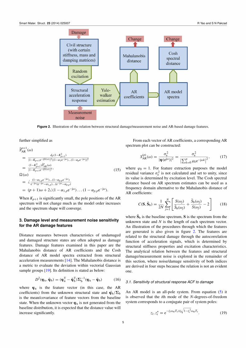
where Sb is the baseline spectrum, S is the spectrum from theunknown state and N is the length of each spectrum vector.An illustration of the procedures through which the featuresare generated is also given in figure 2. The features arerelated to the structural damage through the autocorrelationfunction of acceleration signals, which is determined bystructural stiffness properties and excitation characteristics.The analytical relation between the features and structuraldamage/measurement noise is explored in the remainder ofthis section, where noise/damage sensitivity of both indicesare derived in four steps because the relation is not an evidentone.
3.1. Sensitivity of structural response ACF to damage
An AR model is an all-pole system. From equation (5) itis observed that the ith mode of the N-degrees-of-freedomsystem corresponds to a conjugate pair of system poles:
zi, z∗i = e−ζiωniTs±j√
1−ζ 2i ωniTs . (19)
5
Smart Mater. Struct. 23 (2014) 025007 R Yao and S N Pakzad
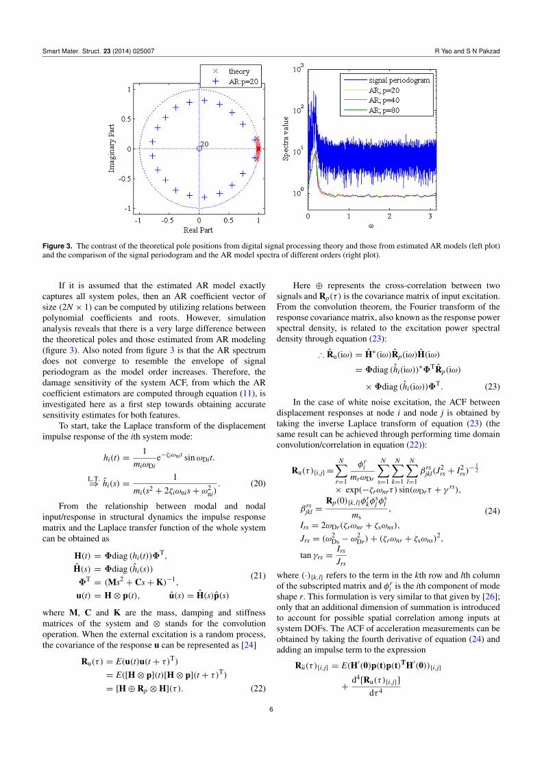
Figure 3. The contrast of the theoretical pole positions from digital signal processing theory and those from estimated AR models (left plot)and the comparison of the signal periodogram and the AR model spectra of different orders (right plot).
If it is assumed that the estimated AR model exactlycaptures all system poles, then an AR coefficient vector ofsize (2N × 1) can be computed by utilizing relations betweenpolynomial coefficients and roots. However, simulationanalysis reveals that there is a very large difference betweenthe theoretical poles and those estimated from AR modeling(figure 3). Also noted from figure 3 is that the AR spectrumdoes not converge to resemble the envelope of signalperiodogram as the model order increases. Therefore, thedamage sensitivity of the system ACF, from which the ARcoefficient estimators are computed through equation (11), isinvestigated here as a first step towards obtaining accuratesensitivity estimates for both features.
To start, take the Laplace transform of the displacementimpulse response of the ith system mode:
hi(t) =1
miωDie−ζiωnit sinωDit.
L.T.⇒ hi(s) =
1
mi(s2 + 2ζiωnis+ ω2ni). (20)
From the relationship between modal and nodalinput/response in structural dynamics the impulse responsematrix and the Laplace transfer function of the whole systemcan be obtained as
H(t) = Φdiag (hi(t))ΦT,
H(s) = Φdiag (hi(s))
ΦT= (Ms2
+ Cs+K)−1,
u(t) = H⊗ p(t), u(s) = H(s)p(s)
(21)
where M, C and K are the mass, damping and stiffnessmatrices of the system and ⊗ stands for the convolutionoperation. When the external excitation is a random process,the covariance of the response u can be represented as [24]
Ru(τ ) = E(u(t)u(t + τ)T)
= E([H⊗ p](t)[H⊗ p](t + τ)T)
= [H⊕ Rp ⊗H](τ ). (22)
Here ⊕ represents the cross-correlation between twosignals and Rp(τ ) is the covariance matrix of input excitation.From the convolution theorem, the Fourier transform of theresponse covariance matrix, also known as the response powerspectral density, is related to the excitation power spectraldensity through equation (23):
∴ Ru(iω) = H∗(iω)Rp(iω)H(iω)
= Φdiag (hi(iω))∗ΦTRp(iω)
× Φdiag (hi(iω))ΦT. (23)
In the case of white noise excitation, the ACF betweendisplacement responses at node i and node j is obtained bytaking the inverse Laplace transform of equation (23) (thesame result can be achieved through performing time domainconvolution/correlation in equation (22)):
Ru(τ ){i,j}=
N∑r=1
φri
mrωDr
N∑s=1
N∑k=1
N∑l=1
βrsjkl(J
2rs + I2
rs)−
12
× exp(−ζrωnrτ) sin(ωDrτ + γrs),
βrsjkl =
Rp(0){k,l}φrkφ
sj φ
sl
ms,
Irs = 2ωDr(ζrωnr + ζsωns),
Jrs = (ω2Ds − ω
2Dr)+ (ζrωnr + ζsωns)
2,
tan γrs =Irs
Jrs
(24)
where (·){k,l} refers to the term in the kth row and lth columnof the subscripted matrix and φr
i is the ith component of modeshape r. This formulation is very similar to that given by [26];only that an additional dimension of summation is introducedto account for possible spatial correlation among inputs atsystem DOFs. The ACF of acceleration measurements can beobtained by taking the fourth derivative of equation (24) andadding an impulse term to the expression
Ru(τ ){i,j} = E(H′(0)p(t)p(t)TH′(0)){i,j}
+d4[Ru(τ ){i,j}]
dτ 4
6
Smart Mater. Struct. 23 (2014) 025007 R Yao and S N Pakzad
= 88TRp88T{i,j}
+
N∑r=1
φri
mrωrd
N∑s=1
N∑k=1
N∑l=1
βrsjkl(J
2rs
+ I2rs)−
12ω4
nr exp(−ζrωrnτ)
×{[(1− 7ζ 2r )(1− ζ
2r )+ ζ
4r ] sin(ωDrτ
+ γrs)+ 4ζr(1− 2ζ 2r )(1− ζ
2r )
12
× cos(ωDrτ + γrs)}. (25)
Given the sensitivity of the modal properties to structuraldamage (derived in section 3.2), sensitivity of the accelerationACF to structural damage can be readily obtained:
dRu(τ ){i,j} =
N∑l=1
dRu(τ ){i,j}
dωnldωnl
+
N∑k=1
N∑l=1
dRu(τ ){i,j}
dφlk
dφlk. (26)
The complete time domain sensitivity formula is too long,but sensitivities for the spectral density can be obtained as
∴ 1Ru(iω) = 1{H∗(iω)Rp(iω)H(iω)}
= −H∗(iω)1KH∗(iω)Rp(iω)H(iω)
− H∗(iω)Rp(iω)H(iω)1KH(iω). (27)
Because the Yule–Walker method is a time domainestimation method, the spectral density sensitivity will not beused for evaluation of the sensitivities of damage features.Still, this result is worth mentioning here as it provides astraightforward representation of the change in response ACFas a function of the global stiffness variation.
3.2. Sensitivity of system eigenvalues and eigenvectors withrespect to changes in global stiffness matrix
To calculate the sensitivity of the ACF function to stiffnesschanges in the time domain, the sensitivity expressions forthe natural frequencies and mode shapes are needed. In thissection the first-order sensitivities of modal properties withrespect to a change in the global stiffness matrix are presented.
To begin with, the classical structural dynamics equationis examined:
My(t)+ Cy(t)+Ky(t) = x(t) (28)
where x(t) and y(t) represent the continuous excitation inputand displacement response, respectively. Natural vibrationfrequencies and mode shapes are obtained through eigenvalueanalysis of the M and K matrices:
(K− λiM)φi = 0, where λi = ω2i . (29)
Here the λi and φi terms are the system eigenvaluesand eigenvectors. Natural modal frequencies (angular) ωi arethe square roots of the corresponding eigenvalues. To getthe sensitivity of the modal properties to changes in the
stiffness matrix, first-order difference terms of both sides ofequation (29) are calculated:
1[(K− λiM)φi] = 1Kφi −1λiMφi
+ (K− λiM)1φi = 0,
(K− λiM)1φi = 1λiMφi −1Kφi.
(30)
Next all the eigenvectors are normalized with respect tothe mass matrix and the changes in eigenvectors are expressedas a weighted sum of the original normalized eigenvectors:
1φi =
N∑k=1
dikφk, where φTk Mφk = 1. (31)
Both sides of equation (31) are then premultipliedwith φT
r (r 6= i) and the mass/stiffness orthogonality betweendifferent modes is utilized to get the respective weight for eacheigenvector:
1λiφTr Mφi − φ
Tr 1Kφi = −φ
Tr 1Kφi,
N∑k=1
dikφTr (K− λiM)φk = dirφ
Tr (K− λiM)φr
= dir(φTr Kφr − λiφ
Tr Mφr)
= dir(λr − λi),
dir(λr − λi) = −φTr 1Kφi
⇒ dir = −φT
r 1Kφi
λr − λi.
(32)
When r = i, it can be proved that dir = 0. Therefore, thesensitivity of the ith eigenvector is orthogonal to itself and iscomputed as equation (33):
1(φTi Mφi) = 1⇒ 1φT
i Mφi = 0
⇒ drr = φTi M1φi/φ
Ti Mφi = 0,
∴ 1φi =
N∑r=1r 6=i
−φT
r 1Kφi
λr − λiφr.
(33)
The sensitivity of the natural frequencies is obtained bypremultiplying both sides of equation (31) with φT
i :
φTi (K− λiM)1φi = 1λiφ
Ti Mφi − φ
Ti 1Kφi
⇒ 1λi = φTi 1Kφi,
∵ λi = ω2i , ∴ 1ωi =
φTi 1Kφi
2ωi.
(34)
Sensitivity of the signal ACF to stiffness change canbe calculated by substituting equations (33) and (34) into(26). Thus to obtain the damage sensitivity of the features,only their sensitivity with respect to the acceleration ACF isneeded.
3.3. Sensitivity of the AR coefficients/spectra to ACF values
From equation (11), the sensitivity of the Yule–Walker ARestimators with respect to the changes in ACF can be derived
7
Smart Mater. Struct. 23 (2014) 025007 R Yao and S N Pakzad
as
d
ϕ1
ϕ2
ϕ3...
ϕp
/
dR(τ )
=
−Γ−2γ , τ = 0
Γ−1eτ − Γ−1 toeplitz (eτ+1)Γ−1γ 1 < τ < p,
Γ−1ep, τ = p
(35)
where eτ is a (p × 1) column vector with all elements equalto zero except for element τ , which equals 1. For the ARspectrum, the definition here states that it is
S(p)AR(ω) =1
|ϕ(ejω)|2=
1∣∣∑pk=0 ϕke−jωk
∣∣2 . (36)
In this definition, ϕ0 = 1. Its sensitivity to changes incoefficients can be computed as
dS(p)AR(ω)−1
dϕk= 2 Re
{e−jωk
(p∑
n=0
ϕnejωn
)},
dS(p)AR(ω)
dϕk= −2 Re
{e−jωk
(p∑
n=0
ϕnejωn
)}S(p)AR(ω)
2.
(37)
Thus by combining equations (35) and (37) the sensitivityof the spectrum to ACF changes is calculated.
3.4. Sensitivity of the AR coefficients/spectra to the increasein the noise level
To compute the influence of noise on damage featureestimation, consider the signal covariance sequence ofcontaminated signals. When white noise of standard deviationσ is added to the signal, its ACF sequence Rc will be
Rc(τ ) = R(τ )+ Rn(τ ) = R(τ )+ σ 2δ(τ ), (38)
where Rn(τ ) denotes the ACF of white noise. Therefore, thesensitivity of the estimated coefficients to the variance ofadditive Gaussian noise will be
d[ϕ1, ϕ2, . . . , ϕp]T
dσ 2 =d[(Γ+ σ 2I)−1γ ]
dσ 2 = −Γ−2γ . (39)
Sensitivity of the AR spectrum to the noise level canbe derived through combining equations (39) and (37) insection 3.3. It should be noted that the above formula only ac-counts for the extreme case (i.e. number of samples Ns =∞).For the finite sample scenario, the estimated noise correlationρn(τ ) is asymptotically normally distributed with variancen−1 at nonzero lags [11]. As such,
d[ϕ1, ϕ2, . . . , ϕp]T
dσ 2 = −Γ−1
×
1 ρn(1) ρn(2) · · · ρn(p− 1)
ρn(1) 1 ρn(1) · · · ρn(p− 2)
ρn(2) ρn(1) 1 · · · ρn(p− 3)...
......
. . ....
ρn(p− 1) ρn(p− 2) ρn(p− 3) · · · 1
Γ−1
×
R(1)
R(2)
R(3)...
R(p)
. (40)
The ACF of the original signal is also affected byestimation errors and exhibits an asymptotic Gaussiandistribution [11]. To avoid including unnecessary statisticalcomplexities and focus on the direct influence of structuraldamage/measurement noise level on damage features here itis assumed that the ACF estimators are exact (the asymptoticcase).
3.5. Sensitivity of the distance measures to changes in ARcoefficients/spectra
The theoretical feature values under the null hypothesis willbe needed for evaluation of relative sensitivity. The ARcoefficient estimators are asymptotically unbiased and followa multivariate Gaussian distribution with covariance matrixσ 2
eN Γ−1(σ 2
e = R(0) − γ TΓ−1γ ) [11]. Under this assumption,the Mahalanobis distance feature for the undamaged structuralstate has a chi-squared distribution with p degrees-of-freedom,and its statistical expectation is p. The expression for theexpected value of the Mahalanobis distance for the generalcase is presented in equation (41):
E(D2) = E(ϕTu − ϕ
Tb )Σ
−1b (ϕu − ϕb)
= E[(ϕTu − ϕ
Tu )Σ
−1b (ϕu − ϕu)]
+ [(ϕTu − ϕ
Tb )Σ
−1b (ϕu − ϕb)]
= trace [Σ−1b Σu] + [(ϕ
Tu − ϕ
Tb )Σ
−1b (ϕu − ϕb)].
(41)
The first- and second-order sensitivities of E(D2) tosignal covariance can then be computed. Note that, fornotational simplicity, θ is used to express the ACF value atan arbitrary lag:
dE(D2)
dθ
∣∣∣∣ϕu=ϕb,Σu=Σb
= trace[Σ−1
bdΣu
dθ
], (42)
d2E(D2)
dθ2
∣∣∣∣ϕu=ϕb,Σu=Σb
= trace[Σ−1
bd2Σu
dθ2
]
+ 2
[d(ϕT
u − ϕTb )
dθΣ−1
bd(ϕu − ϕb)
dθ
]. (43)
8
Smart Mater. Struct. 23 (2014) 025007 R Yao and S N Pakzad
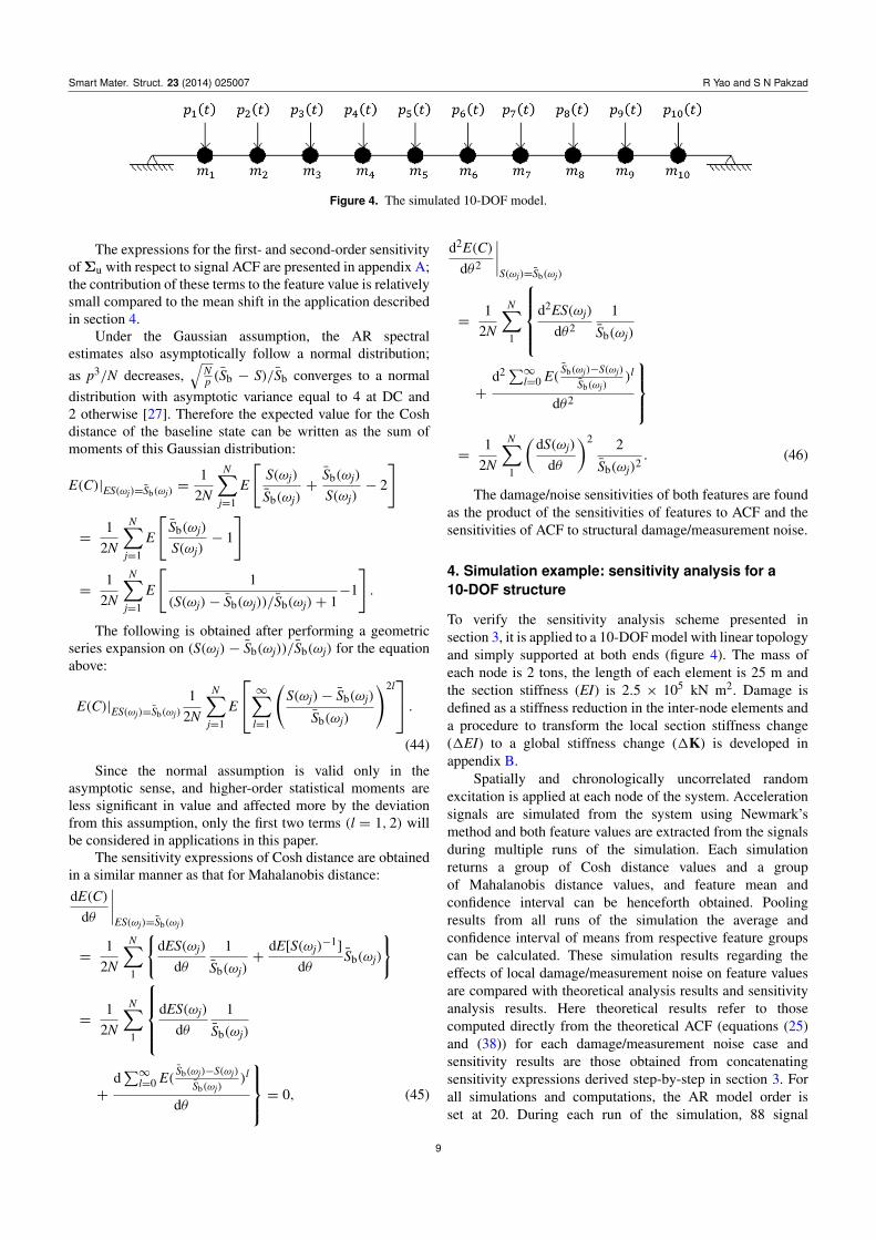
Figure 4. The simulated 10-DOF model.
The expressions for the first- and second-order sensitivityof Σu with respect to signal ACF are presented in appendix A;the contribution of these terms to the feature value is relativelysmall compared to the mean shift in the application describedin section 4.
Under the Gaussian assumption, the AR spectralestimates also asymptotically follow a normal distribution;
as p3/N decreases,√
Np (Sb − S)/Sb converges to a normal
distribution with asymptotic variance equal to 4 at DC and2 otherwise [27]. Therefore the expected value for the Coshdistance of the baseline state can be written as the sum ofmoments of this Gaussian distribution:
E(C)|ES(ωj)=Sb(ωj)=
12N
N∑j=1
E
[S(ωj)
Sb(ωj)+
Sb(ωj)
S(ωj)− 2
]
=1
2N
N∑j=1
E
[Sb(ωj)
S(ωj)− 1
]
=1
2N
N∑j=1
E
[1
(S(ωj)− Sb(ωj))/Sb(ωj)+ 1−1
].
The following is obtained after performing a geometricseries expansion on (S(ωj) − Sb(ωj))/Sb(ωj) for the equationabove:
E(C)|ES(ωj)=Sb(ωj)
12N
N∑j=1
E
∞∑l=1
(S(ωj)− Sb(ωj)
Sb(ωj)
)2l .
(44)
Since the normal assumption is valid only in theasymptotic sense, and higher-order statistical moments areless significant in value and affected more by the deviationfrom this assumption, only the first two terms (l = 1, 2) willbe considered in applications in this paper.
The sensitivity expressions of Cosh distance are obtainedin a similar manner as that for Mahalanobis distance:
dE(C)
dθ
∣∣∣∣ES(ωj)=Sb(ωj)
=1
2N
N∑1
{dES(ωj)
dθ1
Sb(ωj)+
dE[S(ωj)−1]
dθSb(ωj)
}
=1
2N
N∑1
dES(ωj)
dθ1
Sb(ωj)
+
d∑∞
l=0 E( Sb(ωj)−S(ωj)
Sb(ωj))l
dθ
= 0, (45)
d2E(C)
dθ2
∣∣∣∣S(ωj)=Sb(ωj)
=1
2N
N∑1
d2ES(ωj)
dθ2
1
Sb(ωj)
+
d2∑∞l=0 E( Sb(ωj)−S(ωj)
Sb(ωj))l
dθ2
=
12N
N∑1
(dS(ωj)
dθ
)2 2
Sb(ωj)2. (46)
The damage/noise sensitivities of both features are foundas the product of the sensitivities of features to ACF and thesensitivities of ACF to structural damage/measurement noise.
4. Simulation example: sensitivity analysis for a10-DOF structure
To verify the sensitivity analysis scheme presented insection 3, it is applied to a 10-DOF model with linear topologyand simply supported at both ends (figure 4). The mass ofeach node is 2 tons, the length of each element is 25 m andthe section stiffness (EI) is 2.5 × 10⁵ kN m2. Damage isdefined as a stiffness reduction in the inter-node elements anda procedure to transform the local section stiffness change(1EI) to a global stiffness change (1K) is developed inappendix B.
Spatially and chronologically uncorrelated randomexcitation is applied at each node of the system. Accelerationsignals are simulated from the system using Newmark’smethod and both feature values are extracted from the signalsduring multiple runs of the simulation. Each simulationreturns a group of Cosh distance values and a groupof Mahalanobis distance values, and feature mean andconfidence interval can be henceforth obtained. Poolingresults from all runs of the simulation the average andconfidence interval of means from respective feature groupscan be calculated. These simulation results regarding theeffects of local damage/measurement noise on feature valuesare compared with theoretical analysis results and sensitivityanalysis results. Here theoretical results refer to thosecomputed directly from the theoretical ACF (equations (25)and (38)) for each damage/measurement noise case andsensitivity results are those obtained from concatenatingsensitivity expressions derived step-by-step in section 3. Forall simulations and computations, the AR model order isset at 20. During each run of the simulation, 88 signal
9
Smart Mater. Struct. 23 (2014) 025007 R Yao and S N Pakzad
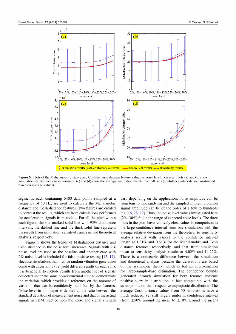
Figure 5. Plots of the Mahalanobis distance and Cosh distance damage feature values as noise level increases. Plots (a) and (b) showsimulation results from one experiment, (c) and (d) show the average simulation results from 50 runs (confidence intervals are constructedbased on average values).
segments, each containing 5400 data points sampled at afrequency of 50 Hz, are used to calculate the Mahalanobisdistance and Cosh distance features. Two figures are createdto contrast the results, which are from calculations performedfor acceleration signals from node 4. For all the plots withineach figure, the star-marked solid line with 95% confidenceintervals, the dashed line and the thick solid line representthe results from simulation, sensitivity analysis and theoreticalanalysis, respectively.
Figure 5 shows the trends of Mahalanobis distance andCosh distance as the noise level increases. Signals with 2%noise level are used as the baseline and another case with2% noise level is included for false positive testing [12, 17].Because simulations that involve random vibration generationcome with uncertainty (i.e. yield different results on each run),it is beneficial to include results from another set of signalscollected under the same noise/structural state to demonstratethe variation, which provides a reference on the amount ofvariation that can be confidently identified by the features.Noise level in this paper is defined as the ratio between thestandard deviation of measurement noise and that of the actualsignal. In SHM practice both the noise and signal strength
vary depending on the application; noise amplitude can befrom tens to thousands µg and the sampled ambient vibrationsignal amplitude can be of the order of a few to hundredsmg [18, 28, 29]. Thus, the noise level values investigated here(2%–30%) fall in the range of expected noise levels. The threelines in the plots have relatively close values in comparison tothe large confidence interval from one simulation, with theaverage relative deviation from the theoretical to sensitivityanalysis results with respect to the confidence intervallength at 1.31% and 0.68% for the Mahalanobis and Coshdistance features, respectively, and that from simulationmean to sensitivity analysis results at 4.02% and 14.22%.There is a noticeable difference between the simulationand theoretical analysis because the derivations are basedon the asymptotic theory, which is but an approximationfor large-sample-base estimation. The confidence boundsgenerated through simulation for both features indicatepositive skew in distribution, a fact compatible with theassumptions on their respective asymptotic distribution. Theaverage Cosh distance values from 50 simulations have amuch reduced, yet still largely uniform, confidence interval(from ±50% around the mean to ±10% around the mean)
10
Smart Mater. Struct. 23 (2014) 025007 R Yao and S N Pakzad
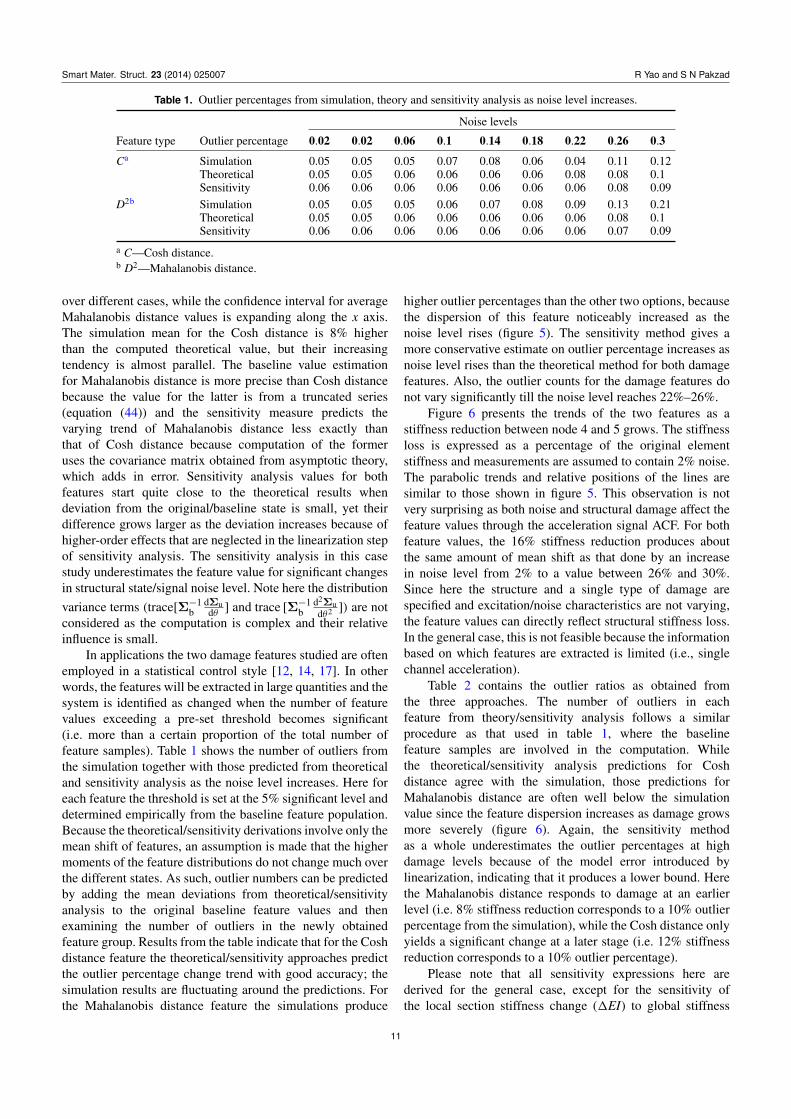
Table 1. Outlier percentages from simulation, theory and sensitivity analysis as noise level increases.
Feature type Outlier percentage
Noise levels
0.02 0.02 0.06 0.1 0.14 0.18 0.22 0.26 0.3
Ca Simulation 0.05 0.05 0.05 0.07 0.08 0.06 0.04 0.11 0.12Theoretical 0.05 0.05 0.06 0.06 0.06 0.06 0.08 0.08 0.1Sensitivity 0.06 0.06 0.06 0.06 0.06 0.06 0.06 0.08 0.09
D2b Simulation 0.05 0.05 0.05 0.06 0.07 0.08 0.09 0.13 0.21Theoretical 0.05 0.05 0.06 0.06 0.06 0.06 0.06 0.08 0.1Sensitivity 0.06 0.06 0.06 0.06 0.06 0.06 0.06 0.07 0.09
a C—Cosh distance.b D2—Mahalanobis distance.
over different cases, while the confidence interval for averageMahalanobis distance values is expanding along the x axis.The simulation mean for the Cosh distance is 8% higherthan the computed theoretical value, but their increasingtendency is almost parallel. The baseline value estimationfor Mahalanobis distance is more precise than Cosh distancebecause the value for the latter is from a truncated series(equation (44)) and the sensitivity measure predicts thevarying trend of Mahalanobis distance less exactly thanthat of Cosh distance because computation of the formeruses the covariance matrix obtained from asymptotic theory,which adds in error. Sensitivity analysis values for bothfeatures start quite close to the theoretical results whendeviation from the original/baseline state is small, yet theirdifference grows larger as the deviation increases because ofhigher-order effects that are neglected in the linearization stepof sensitivity analysis. The sensitivity analysis in this casestudy underestimates the feature value for significant changesin structural state/signal noise level. Note here the distribution
variance terms (trace[Σ−1b
dΣudθ ] and trace [Σ−1
bd2Σudθ2 ]) are not
considered as the computation is complex and their relativeinfluence is small.
In applications the two damage features studied are oftenemployed in a statistical control style [12, 14, 17]. In otherwords, the features will be extracted in large quantities and thesystem is identified as changed when the number of featurevalues exceeding a pre-set threshold becomes significant(i.e. more than a certain proportion of the total number offeature samples). Table 1 shows the number of outliers fromthe simulation together with those predicted from theoreticaland sensitivity analysis as the noise level increases. Here foreach feature the threshold is set at the 5% significant level anddetermined empirically from the baseline feature population.Because the theoretical/sensitivity derivations involve only themean shift of features, an assumption is made that the highermoments of the feature distributions do not change much overthe different states. As such, outlier numbers can be predictedby adding the mean deviations from theoretical/sensitivityanalysis to the original baseline feature values and thenexamining the number of outliers in the newly obtainedfeature group. Results from the table indicate that for the Coshdistance feature the theoretical/sensitivity approaches predictthe outlier percentage change trend with good accuracy; thesimulation results are fluctuating around the predictions. Forthe Mahalanobis distance feature the simulations produce
higher outlier percentages than the other two options, becausethe dispersion of this feature noticeably increased as thenoise level rises (figure 5). The sensitivity method gives amore conservative estimate on outlier percentage increases asnoise level rises than the theoretical method for both damagefeatures. Also, the outlier counts for the damage features donot vary significantly till the noise level reaches 22%–26%.
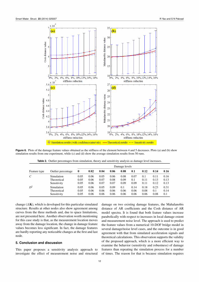
Figure 6 presents the trends of the two features as astiffness reduction between node 4 and 5 grows. The stiffnessloss is expressed as a percentage of the original elementstiffness and measurements are assumed to contain 2% noise.The parabolic trends and relative positions of the lines aresimilar to those shown in figure 5. This observation is notvery surprising as both noise and structural damage affect thefeature values through the acceleration signal ACF. For bothfeature values, the 16% stiffness reduction produces aboutthe same amount of mean shift as that done by an increasein noise level from 2% to a value between 26% and 30%.Since here the structure and a single type of damage arespecified and excitation/noise characteristics are not varying,the feature values can directly reflect structural stiffness loss.In the general case, this is not feasible because the informationbased on which features are extracted is limited (i.e., singlechannel acceleration).
Table 2 contains the outlier ratios as obtained fromthe three approaches. The number of outliers in eachfeature from theory/sensitivity analysis follows a similarprocedure as that used in table 1, where the baselinefeature samples are involved in the computation. Whilethe theoretical/sensitivity analysis predictions for Coshdistance agree with the simulation, those predictions forMahalanobis distance are often well below the simulationvalue since the feature dispersion increases as damage growsmore severely (figure 6). Again, the sensitivity methodas a whole underestimates the outlier percentages at highdamage levels because of the model error introduced bylinearization, indicating that it produces a lower bound. Herethe Mahalanobis distance responds to damage at an earlierlevel (i.e. 8% stiffness reduction corresponds to a 10% outlierpercentage from the simulation), while the Cosh distance onlyyields a significant change at a later stage (i.e. 12% stiffnessreduction corresponds to a 10% outlier percentage).
Please note that all sensitivity expressions here arederived for the general case, except for the sensitivity ofthe local section stiffness change (1EI) to global stiffness
11
Smart Mater. Struct. 23 (2014) 025007 R Yao and S N Pakzad
Figure 6. Plots of the damage feature values obtained as the stiffness of the element between 4 and 5 decreases. Plots (a) and (b) showsimulation results from one experiment, while (c) and (d) show the average simulation results from 50 runs.
Table 2. Outlier percentages from simulation, theory and sensitivity analysis as damage level increases.
Feature type Outlier percentage
Damage levels
0 0.02 0.04 0.06 0.08 0.1 0.12 0.14 0.16
C Simulation 0.05 0.06 0.05 0.06 0.08 0.07 0.1 0.11 0.16Theoretical 0.05 0.06 0.07 0.08 0.09 0.1 0.11 0.13 0.13Sensitivity 0.05 0.06 0.07 0.07 0.09 0.09 0.11 0.12 0.13
D2 Simulation 0.05 0.06 0.05 0.09 0.1 0.14 0.18 0.23 0.31Theoretical 0.05 0.06 0.06 0.06 0.06 0.06 0.08 0.1 0.14Sensitivity 0.05 0.06 0.06 0.06 0.06 0.06 0.06 0.08 0.1
change (1K), which is developed for this particular simulatedstructure. Results at other nodes also show agreement amongcurves from the three methods and, due to space limitations,are not presented here. Another observation worth mentioningfor this case study is that, as the measurement location movesaway from the damage location, the change in damage featurevalues becomes less significant. In fact, the damage featuresare hardly reporting any noticeable changes at the first and lastnode.
5. Conclusion and discussion
This paper proposes a sensitivity analysis approach toinvestigate the effect of measurement noise and structural
damage on two existing damage features, the Mahalanobisdistance of AR coefficients and the Cosh distance of ARmodel spectra. It is found that both feature values increaseparabolically with respect to increases in local damage extentand measurement noise level. The approach is used to predictthe feature values from a numerical 10-DOF bridge model inseveral damage/noise level cases, and the outcome is in goodagreement with that from simulated acceleration signals andtheoretical calculations. This observation supports the validityof the proposed approach, which is a more efficient way toexamine the behavior (sensitivity and robustness) of damagefeatures than repeating the simulation process for a numberof times. The reason for that is because simulation requires
12
Smart Mater. Struct. 23 (2014) 025007 R Yao and S N Pakzad
the generation of structural vibration signals and extraction offeature values for each noise/damage state, but the sensitivityvalues, once computed, can be applied to multiple states.
Since the approach introduced here involves using astructural FE model, modeling error can affect the procedurefrom two aspects: the baseline state signal estimation, whichaffects the noise and damage sensitivity estimation, andthe relation between the structural measurements and localdamage, which affects the damage sensitivity. For the first partof the problem, civil structures under ambient vibration aregenerally only well excited in a few low frequency modes. Ifthe FE model can be tuned such that its modes match thosemeasured from the real structure at the original state, then thestructural baseline state response ACFs can be estimated fromthe FE model with good accuracy. For the second part, there isno definite solution. However, ranges in which FE parametersvary can be assumed and damage sensitivity expressions forcertain parameter sets within the range can be computed toobtain the lower/upper bounds of damage feature sensitivity.
It is noted that the Mahalanobis distance and Coshdistance features respond not only to structural damage butalso to increase in the noise level. This fact implies that bothfeatures are not completely robust to variations unrelated tostructural change. This is partially due to the fact that thedamage identification algorithms use only the response from asingle channel, which is generated as a result of the interactionbetween several components (structure, environment andexcitation). However, as shown in the simulation exampleabove, it takes a significant increase in the noise level toproduce a feature value change that matches that from amoderate reduction of stiffness for both AR features. Thus,these damage indices are effective in monitoring a structurewith reasonably stable operating conditions.
The variation of environmental conditions (temperature,humidity, etc) often affects the damage features throughtheir influence on the structural material properties (andhence the stiffness properties). The traffic variation willchange the excitation amplitude, spatial pattern and frequencycontents. AR-based features will be robust to the excitationamplitude but are affected by the other two excitation factors.These non-structural influences are not examined in ananalytical manner unless the functional relationship betweenthe environmental conditions and structural stiffness is knownand the form of excitation variation is defined. The sensitivityterms can be derived by taking the derivative of signal ACFwith respect to these sources of influence. Further research isneeded to address these issues.
Acknowledgments
The research described in this paper is supported by theNational Science Foundation through Grant No. CMMI-0926898 by the Sensors and Sensing Systems Program and bya grant from the Commonwealth of Pennsylvania, Departmentof Community and Economic Development, through thePennsylvania Infrastructure Technology Alliance (PITA).
Appendix A. Calculation of the first- andsecond-order derivative of the covariance matrix ofAR coefficient vectors with respect to the ACF
The first-order derivative of the covariance matrix of theunknown state AR coefficients is first expressed as a functionof the derivatives of the AR residual variance σe and that ofthe inverse of the ACF Toeplitz matrix Γ:
d6u
dR(τ )=
dσe
dR(τ )Γ−1+ σe
dΓ−1
dR(τ ). (A.1)
According to their respective definitions, specificexpressions for dσe
dR(τ ) and dΓ−1
dR(τ ) are derived as follows:
dσe
dR(τ )=
1+ γ TΓ−1Γ−1γ , τ = 0
γ TΓ−1 toeplitz (eτ+1)Γ−1γ − 2eTτΓ−1γ ,
1 ≤ τ ≤ p− 1
−2eTτΓ−1γ , τ = p
(A.2)
dΓ−1
dR(τ )
=
{−Γ−1 toeplitz (eτ+1)Γ−1, 0 ≤ τ ≤ p− 1
0, τ = p.(A.3)
Likewise the second-order derivative of 6u can beobtained as a function of the first-/second-order derivatives ofσe and Γ−1:
d26u
dR(τ )2=
d2σe
dR(τ )2Γ−1+ 2
dσe
dR(τ )
dΓ−1
dR(τ )+ σe
d2Γ−1
dR(τ )2.
(A.4)
The second-order derivatives of σe and Γ−1 are computedby taking the derivatives of equations (A.2) and (A.3). Notethat application of these formulas requires substituting invalues of the first-order derivative of Γ−1:
d2σe
dR(τ )2=
2γ T dΓ−1
dR(0)Γ−1γ , τ = 0
2γ T dΓ−1
dR(τ )toeplitz (eτ+1)Γ−1γ
− 2γ T dΓ−1
dR(τ )eτ − 2eT
τ
dΓ−1
dR(τ )γ
− 2eTτΓ−1eτ , 1 ≤ τ ≤ p− 1
−2eTpΓ−1ep, τ = p
(A.5)
d20−1
dR(τ )2=
−dΓ−1
dR(τ )toeplitz (eτ+1)Γ−1
−Γ−1 toeplitz (eτ+1)dΓ−1
dR(τ ),
0 ≤ τ ≤ p− 1
0, τ = p.
(A.6)
13
Smart Mater. Struct. 23 (2014) 025007 R Yao and S N Pakzad
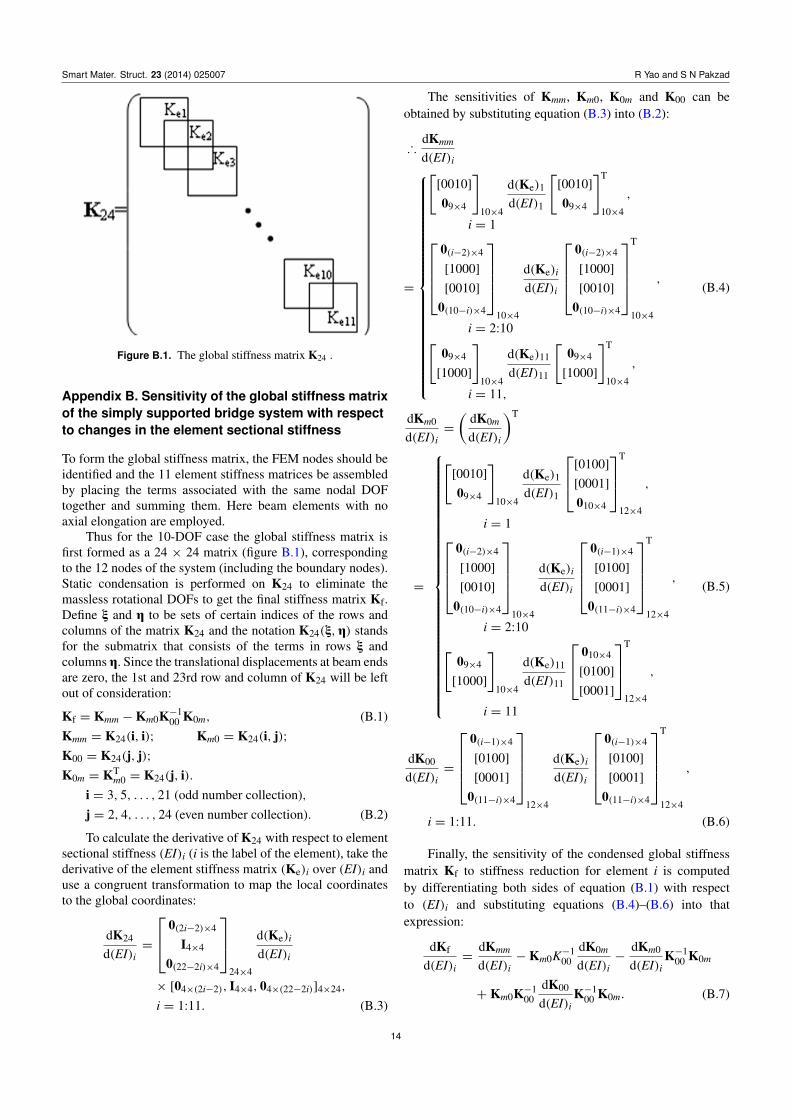
Figure B.1. The global stiffness matrix K24 .
Appendix B. Sensitivity of the global stiffness matrixof the simply supported bridge system with respectto changes in the element sectional stiffness
To form the global stiffness matrix, the FEM nodes should beidentified and the 11 element stiffness matrices be assembledby placing the terms associated with the same nodal DOFtogether and summing them. Here beam elements with noaxial elongation are employed.
Thus for the 10-DOF case the global stiffness matrix isfirst formed as a 24 × 24 matrix (figure B.1), correspondingto the 12 nodes of the system (including the boundary nodes).Static condensation is performed on K24 to eliminate themassless rotational DOFs to get the final stiffness matrix Kf.Define ξ and η to be sets of certain indices of the rows andcolumns of the matrix K24 and the notation K24(ξ,η) standsfor the submatrix that consists of the terms in rows ξ andcolumns η. Since the translational displacements at beam endsare zero, the 1st and 23rd row and column of K24 will be leftout of consideration:
Kf = Kmm −Km0K−100 K0m, (B.1)
Kmm = K24(i, i); Km0 = K24(i, j);
K00 = K24(j, j);
K0m = KTm0 = K24(j, i).
i = 3, 5, . . . , 21 (odd number collection),
j = 2, 4, . . . , 24 (even number collection). (B.2)
To calculate the derivative of K24 with respect to elementsectional stiffness (EI)i (i is the label of the element), take thederivative of the element stiffness matrix (Ke)i over (EI)i anduse a congruent transformation to map the local coordinatesto the global coordinates:
dK24
d(EI)i=
0(2i−2)×4
I4×4
0(22−2i)×4
24×4
d(Ke)i
d(EI)i
× [04×(2i−2), I4×4, 04×(22−2i)]4×24,
i = 1:11. (B.3)
The sensitivities of Kmm, Km0, K0m and K00 can beobtained by substituting equation (B.3) into (B.2):
∴dKmm
d(EI)i
=
[[0010]
09×4
]10×4
d(Ke)1
d(EI)1
[[0010]
09×4
]T
10×4
,
i = 10(i−2)×4
[1000]
[0010]
0(10−i)×4
10×4
d(Ke)i
d(EI)i
0(i−2)×4
[1000]
[0010]
0(10−i)×4
T
10×4
,
i = 2:10[09×4
[1000]
]10×4
d(Ke)11
d(EI)11
[09×4
[1000]
]T
10×4
,
i = 11,
(B.4)
dKm0
d(EI)i=
(dK0m
d(EI)i
)T
=
[[0010]
09×4
]10×4
d(Ke)1
d(EI)1
[0100]
[0001]
010×4
T
12×4
,
i = 10(i−2)×4
[1000]
[0010]
0(10−i)×4
10×4
d(Ke)i
d(EI)i
0(i−1)×4
[0100]
[0001]
0(11−i)×4
T
12×4
,
i = 2:10[09×4
[1000]
]10×4
d(Ke)11
d(EI)11
010×4
[0100]
[0001]
T
12×4
,
i = 11
(B.5)
dK00
d(EI)i=
0(i−1)×4
[0100]
[0001]
0(11−i)×4
12×4
d(Ke)i
d(EI)i
0(i−1)×4
[0100]
[0001]
0(11−i)×4
T
12×4
,
i = 1:11. (B.6)
Finally, the sensitivity of the condensed global stiffnessmatrix Kf to stiffness reduction for element i is computedby differentiating both sides of equation (B.1) with respectto (EI)i and substituting equations (B.4)–(B.6) into thatexpression:
dKf
d(EI)i=
dKmm
d(EI)i−Km0K−1
00dK0m
d(EI)i−
dKm0
d(EI)iK−1
00 K0m
+ Km0K−100
dK00
d(EI)iK−1
00 K0m. (B.7)
14
Smart Mater. Struct. 23 (2014) 025007 R Yao and S N Pakzad
References
[1] Doebling S W, Farrar C R and Prime M B 1998 A summaryreview of vibration-based damage identification methodsShock Vib. Dig. 30 91–105
[2] Ciang C C, Lee J R and Bang H J 2008 Structural healthmonitoring for a wind turbine system: a review of damagedetection methods Meas. Sci. Technol. 19 122001
[3] Peeters B, Maeck J and De Roeck G 2001 Vibration-baseddamage detection in civil engineering: excitation sourcesand temperature effects Smart Mater. Struct. 10 518
[4] Lynch J P, Sundararajan A, Law K H, Kiremidjian A S andCarryer E 2004 Embedding damage detection algorithms ina wireless sensing unit for operational power efficiencySmart Mater. Struct. 13 800
[5] Maia N M M, Silva J M M, Almas E A M and Sampaio R P C2003 Damage detection in structures: from mode shape tofrequency response function methods Mech. Syst. SignalProcess. 17 489–98
[6] Hearn G and Testa R B 1991 Modal analysis for damagedetection in structures J. Struct. Eng. 117 3042–63
[7] Salawu O S 1997 Detection of structural damage throughchanges in frequency: a review Eng. Struct. 19 718–23
[8] Worden K, Manson G and Fieller N R J 2000 Damagedetection using outlier analysis J. Sound Vib. 229 647–67
[9] Okafor A C and Dutta A 2000 Structural damage detection inbeams by wavelet transforms Smart Mater. Struct. 9 906
[10] Fang X, Luo H and Tang J 2005 Structural damage detectionusing neural network with learning rate improvementComput. Struct. 83 2150–61
[11] Brockwell P J and Davis R A 2009 Time Series: Theory andMethods (Berlin: Springer)
[12] Sohn H and Farrar C R 2001 Damage diagnosis using timeseries analysis of vibration signals Smart Mater. Struct.10 446
[13] Zhang Q W 2007 Statistical damage identification for bridgesusing ambient vibration data Comput. Struct. 85 476–85
[14] Yao R and Pakzad S N 2012 Autoregressive statistical patternrecognition algorithms for damage detection in civilstructures Mech. Syst. Signal Process. 31 355–68
[15] Nair K K, Kiremidjian A S and Law K H 2006 Timeseries-based damage detection and localization algorithm
with application to the ASCE benchmark structure J. SoundVib. 291 349–68
[16] Atamturktur S, Bornn L and Hemez F 2011 Vibrationcharacteristics of vaulted masonry monuments undergoingdifferential support settlement Eng. Struct. 33 2472–84
[17] Gul M and Necati Catbas F 2009 Statistical patternrecognition for structural health monitoring using timeseries modeling: theory and experimental verificationsMech. Syst. Signal Process. 23 2192–204
[18] Dorvash S and Pakzad S N 2012 Effects of measurement noiseon modal parameter identification Smart Mater. Struct.21 065008
[19] Mahalanobis P C 1936 On the generalized distance in statisticsProc. Natl Acad. Inst. Sci. India 2 49–55
[20] Gray A Jr and Markel J 1976 Distance measures for speechprocessing IEEE Trans. Acoust. Speech Signal Process.24 380–91
[21] Brockwell P J and Richard A D 2002 Introduction to TimeSeries and Forecasting (London: Taylor & Francis)
[22] Chopra A K 2006 Dynamics of Structures: Theory &Applications to Earthquake Engineering (Upper SaddleRiver, NJ: Prentice-Hall)
[23] Terasvirta T 1977 The invertibility of sums of discrete MA andARMA processes Scand. J. Stat. 4 165–70
[24] Porat B 1994 Digital Processing of Random Signals: Theoryand Methods (Englewood Cliffs, NJ: Prentice-Hall)
[25] Oppenheim A V, Schafer R W and Buck J R 2009Discrete-Time Signal Processing 3rd edn (Upper SaddleRiver: Prentice-Hall)
[26] James G H III, Carne T G and Lauffer J P 1993 The NaturalExcitation Technique (NExT) for Modal ParameterExtraction from Operating Wind Turbines No.SAND-92-1666 (Albuquerque, NM: Sandia National Labs)
[27] Berk K N 1974 Consistent autoregressive spectral estimatesAnn. Statist. 2 489–502
[28] Pakzad S N, Kim S, Fenves G L, Glaser S D, Culler D E andDemmel J W 2005 Multi-purpose wireless accelerometersfor civil infrastructure monitoring IWSHM 2005: 5th Int.Workshop on Structural Health Monitoring (Stanford, CA)
[29] Wang Y, Lynch J P and Law K H 2007 A wireless structuralhealth monitoring system with multithreaded sensingdevices: design and validation Struct. Infrastruct. Eng.3 103–20
15
Recommended


