Hindawi Publishing CorporationEURASIP Journal on Advances in Signal ProcessingVolume 2007, Article ID 94704, 12 pagesdoi:10.1155/2007/94704

Research ArticleHigh-Selectivity Filter Banks for Spectral Analysisof Music Signals

Filipe C. C. B. Diniz, Iuri Kothe, Sergio L. Netto, and Luiz W. P. Biscainho

LPS-PEE/COPPE and DEL/Poli, Universidade Federal do Rio de Janeiro (UFRJ), Caixa Postal 68504,21941-972 Rio de Janeiro, RJ, Brazil

Received 7 December 2005; Revised 10 August 2006; Accepted 10 September 2006

Recommended by Masataka Goto

This paper approaches, under a unified framework, several algorithms for the spectral analysis of musical signals. Such algorithmsinclude the fast Fourier transform (FFT), the fast filter bank (FFB), the constant-Q transform (CQT), and the bounded-Q trans-form (BQT), previously known from the associated literature. Two new methods are then introduced, namely, the constant-Qfast filter bank (CQFFB) and the bounded-Q fast filter bank (BQFFB), combining the positive characteristics of the previouslymentioned algorithms. The provided analyses indicate that the proposed BQFFB achieves an excellent compromise between thereduced computational effort of the FFT, the high selectivity of each output channel of the FFB, and the efficient distribution offrequency channels associated to the CQT and BQT methods. Examples are included to illustrate the performances of these meth-ods in the spectral analysis of music signals.

Copyright © 2007 Hindawi Publishing Corporation. All rights reserved.

1. INTRODUCTION

This paper aims at describing tools for the spectral analy-sis of music signals that are characterized by high-selectivityfilters, a channel frequency spacing that is more efficientfor this kind of signals, and acceptable computational com-plexity. The paper includes a brief overview of some relatedtechniques used in music spectral analysis. New tools whichachieve a good compromise between computational com-plexity and component discrimination are then introduced.

The standard spectral tool is the fast Fourier transform(FFT), which is the fast algorithm for the discrete Fouriertransform (DFT). The FFT is widely used in several applica-tions due to its simplicity [1]. Taking the FFT as a filter bank,it can be interpreted that such simplicity comes partly fromthe use of a low-order kernel filter, which results in poorlyselective channels. As an attempt to solve this problem, Limand Farhang-Boroujeny [2] took advantage of the FFT treestructure but with more complex kernel filters, resulting inthe so-called fast filter bank (FFB). The FFB complexity isslightly higher than the FFT’s, but with highly selective chan-nels in the frequency domain.

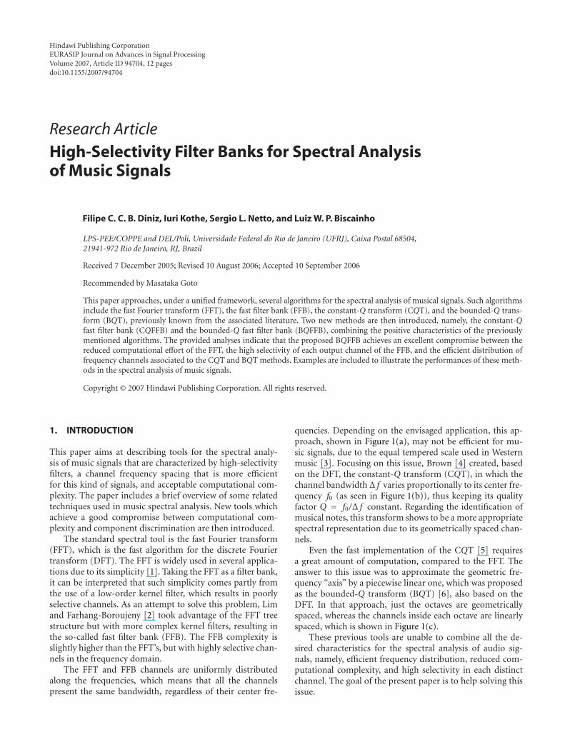
The FFT and FFB channels are uniformly distributedalong the frequencies, which means that all the channelspresent the same bandwidth, regardless of their center fre-

quencies. Depending on the envisaged application, this ap-proach, shown in Figure 1(a), may not be efficient for mu-sic signals, due to the equal tempered scale used in Westernmusic [3]. Focusing on this issue, Brown [4] created, basedon the DFT, the constant-Q transform (CQT), in which thechannel bandwidth Δ f varies proportionally to its center fre-quency f0 (as seen in Figure 1(b)), thus keeping its qualityfactor Q = f0/Δ f constant. Regarding the identification ofmusical notes, this transform shows to be a more appropriatespectral representation due to its geometrically spaced chan-nels.

Even the fast implementation of the CQT [5] requiresa great amount of computation, compared to the FFT. Theanswer to this issue was to approximate the geometric fre-quency “axis” by a piecewise linear one, which was proposedas the bounded-Q transform (BQT) [6], also based on theDFT. In that approach, just the octaves are geometricallyspaced, whereas the channels inside each octave are linearlyspaced, which is shown in Figure 1(c).

These previous tools are unable to combine all the de-sired characteristics for the spectral analysis of audio sig-nals, namely, efficient frequency distribution, reduced com-putational complexity, and high selectivity in each distinctchannel. The goal of the present paper is to help solving thisissue.

2 EURASIP Journal on Advances in Signal Processing

f 2 f 3 f 4 f 5 f 6 f 7 f 8 f 9 f Frequency

(a)

f 3 f 7 f Frequency

(b)

f 2 f 3 f 4 f 6 f 8 f 10 f 12 f Frequency

Linear Linear

(c)

Figure 1: Methods for spectral analysis of music signals: (a) linearfrequency spacing; (b) geometric frequency spacing; (c) piecewiselinear frequency spacing. The scales were arbitrarily selected.

For that purpose, the constant-Q fast filter bank(CQFFB) and the bounded-Q fast filter bank (BQFFB) toolsare thoroughly analyzed. The CQFFB [7, 8] is seen as a high-resolution version of the CQT, from which it inherits thehigh computational cost. After that, the BQFFB is introducedas the most efficient tool, combining the FFT-like reducedcomplexity, the BQT-like linear geometric frequency distri-bution, and the FFB-like high resolution. The original con-cept of the BQFFB was first given in [9]. The present paperincludes a complete description of this tool along with otherspectral analysis tools under a unified framework. A moreefficient implementation of the BQFFB, which avoids deci-mation filters, is newly introduced.

In the context of music information retrieval, the algo-rithms discussed in this work find application, for example,in automatic music transcription and musical feature extrac-tion.

The remains of this paper are organized as follows:Section 2 describes the linear frequency spacing methods,which are the FFT and its high-selectivity counterpart, theFFB. Section 3 presents the geometric frequency spacingmethods, which are the CQT and its high-selectivity equiv-alent, the CQFFB. Section 4 describes the piecewise lin-ear frequency methods, which are the BQT and its newlyimplemented high-selectivity form, the BQFFB. Section 5

(l, b)

Hl,b(z)

Hl,b (z)

Input signal(0, 0)

(1, 0)

(1, 1)

(2, 0)

(2, 1)

(2, 2)

(2, 3)

Channel 0

Channel 4

Channel 2

Channel 6

Channel 1

Channel 5

Channel 3

Channel 7

l = 1 l = 2 l = 3

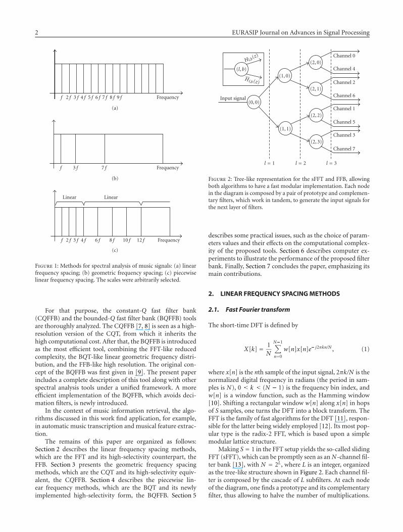
Figure 2: Tree-like representation for the sFFT and FFB, allowingboth algorithms to have a fast modular implementation. Each nodein the diagram is composed by a pair of prototype and complemen-tary filters, which work in tandem, to generate the input signals forthe next layer of filters.

describes some practical issues, such as the choice of param-eters values and their effects on the computational complex-ity of the proposed tools. Section 6 describes computer ex-periments to illustrate the performance of the proposed filterbank. Finally, Section 7 concludes the paper, emphasizing itsmain contributions.

2. LINEAR FREQUENCY SPACING METHODS

2.1. Fast Fourier transform

The short-time DFT is defined by

X[k] = 1N

N�1∑

n=0

w[n]x[n]e� j2πkn/N , (1)

where x[n] is the nth sample of the input signal, 2πk/N is thenormalized digital frequency in radians (the period in sam-ples is N), 0 � k � (N � 1) is the frequency bin index, andw[n] is a window function, such as the Hamming window[10]. Shifting a rectangular window w[n] along x[n] in hopsof S samples, one turns the DFT into a block transform. TheFFT is the family of fast algorithms for the DFT [11], respon-sible for the latter being widely employed [12]. Its most pop-ular type is the radix-2 FFT, which is based upon a simplemodular lattice structure.

Making S = 1 in the FFT setup yields the so-called slidingFFT (sFFT), which can be promptly seen as an N-channel fil-ter bank [13], with N = 2L, where L is an integer, organizedas the tree-like structure shown in Figure 2. Each channel fil-ter is composed by the cascade of L subfilters. At each nodeof the diagram, one finds a prototype and its complementaryfilter, thus allowing to halve the number of multiplications.

Filipe C. C. B. Diniz et al. 3

�40�20

0

�1 �0.8 �0.6 �0.4 �0.2 0 0.2 0.4 0.6 0.8 1

Gai

n(d

B)

Normalized frequency (�π rad/s)

�40�20

0

�1 �0.8 �0.6 �0.4 �0.2 0 0.2 0.4 0.6 0.8 1

Gai

n(d

B)

Normalized frequency (�π rad/s)

�40�20

0

�1 �0.8 �0.6 �0.4 �0.2 0 0.2 0.4 0.6 0.8 1

Gai

n(d

B)

Normalized frequency (�π rad/s)

�40�20

0

�1 �0.8 �0.6 �0.4 �0.2 0 0.2 0.4 0.6 0.8 1Gai

n(d

B)

Normalized frequency (�π rad/s)

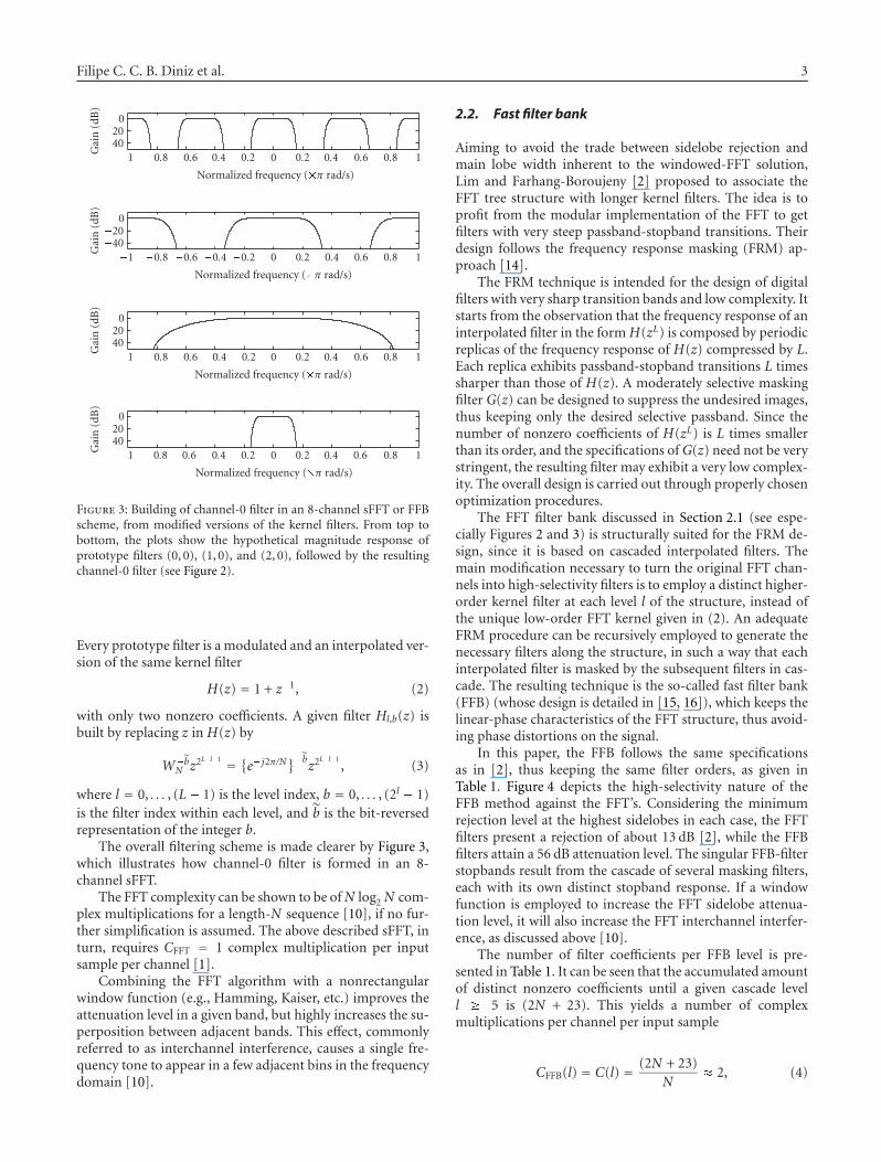
Figure 3: Building of channel-0 filter in an 8-channel sFFT or FFBscheme, from modified versions of the kernel filters. From top tobottom, the plots show the hypothetical magnitude response ofprototype filters (0, 0), (1, 0), and (2, 0), followed by the resultingchannel-0 filter (see Figure 2).

Every prototype filter is a modulated and an interpolated ver-sion of the same kernel filter

H(z) = 1 + z�1, (2)

with only two nonzero coefficients. A given filter Hl,b(z) isbuilt by replacing z in H(z) by

W�bN z2L�l�1 = {e� j2π/N}�bz2L�l�1

, (3)

where l = 0, . . . , (L� 1) is the level index, b = 0, . . . , (2l � 1)is the filter index within each level, and b is the bit-reversedrepresentation of the integer b.

The overall filtering scheme is made clearer by Figure 3,which illustrates how channel-0 filter is formed in an 8-channel sFFT.

The FFT complexity can be shown to be of N log2 N com-plex multiplications for a length-N sequence [10], if no fur-ther simplification is assumed. The above described sFFT, inturn, requires CFFT = 1 complex multiplication per inputsample per channel [1].

Combining the FFT algorithm with a nonrectangularwindow function (e.g., Hamming, Kaiser, etc.) improves theattenuation level in a given band, but highly increases the su-perposition between adjacent bands. This effect, commonlyreferred to as interchannel interference, causes a single fre-quency tone to appear in a few adjacent bins in the frequencydomain [10].

2.2. Fast filter bank

Aiming to avoid the trade between sidelobe rejection andmain lobe width inherent to the windowed-FFT solution,Lim and Farhang-Boroujeny [2] proposed to associate theFFT tree structure with longer kernel filters. The idea is toprofit from the modular implementation of the FFT to getfilters with very steep passband-stopband transitions. Theirdesign follows the frequency response masking (FRM) ap-proach [14].

The FRM technique is intended for the design of digitalfilters with very sharp transition bands and low complexity. Itstarts from the observation that the frequency response of aninterpolated filter in the form H(zL) is composed by periodicreplicas of the frequency response of H(z) compressed by L.Each replica exhibits passband-stopband transitions L timessharper than those of H(z). A moderately selective maskingfilter G(z) can be designed to suppress the undesired images,thus keeping only the desired selective passband. Since thenumber of nonzero coefficients of H(zL) is L times smallerthan its order, and the specifications of G(z) need not be verystringent, the resulting filter may exhibit a very low complex-ity. The overall design is carried out through properly chosenoptimization procedures.

The FFT filter bank discussed in Section 2.1 (see espe-cially Figures 2 and 3) is structurally suited for the FRM de-sign, since it is based on cascaded interpolated filters. Themain modification necessary to turn the original FFT chan-nels into high-selectivity filters is to employ a distinct higher-order kernel filter at each level l of the structure, instead ofthe unique low-order FFT kernel given in (2). An adequateFRM procedure can be recursively employed to generate thenecessary filters along the structure, in such a way that eachinterpolated filter is masked by the subsequent filters in cas-cade. The resulting technique is the so-called fast filter bank(FFB) (whose design is detailed in [15, 16]), which keeps thelinear-phase characteristics of the FFT structure, thus avoid-ing phase distortions on the signal.

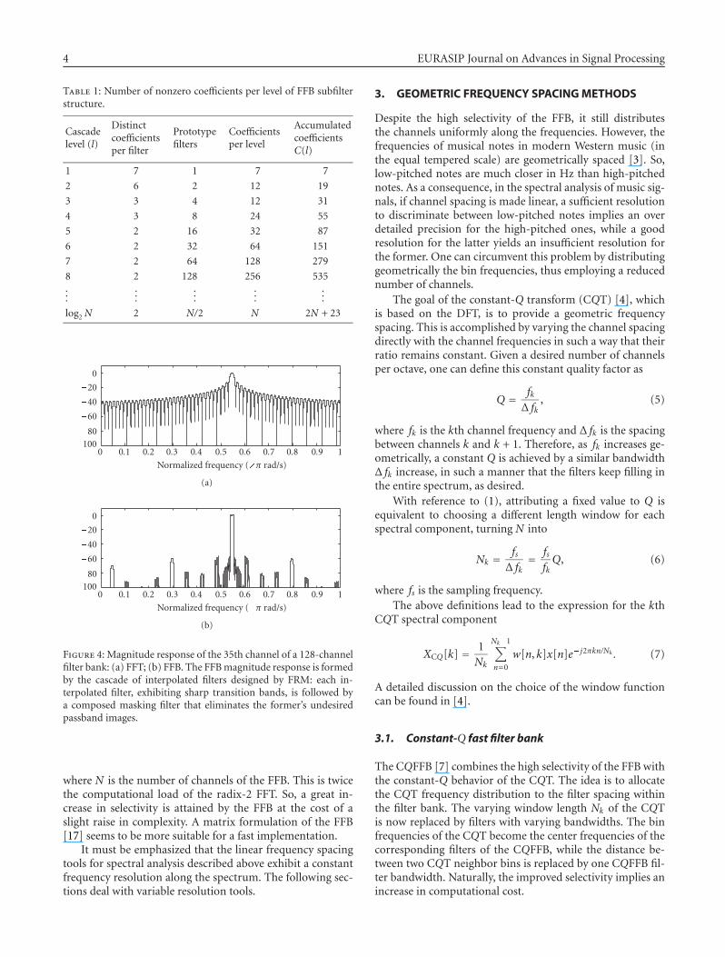
In this paper, the FFB follows the same specificationsas in [2], thus keeping the same filter orders, as given inTable 1. Figure 4 depicts the high-selectivity nature of theFFB method against the FFT’s. Considering the minimumrejection level at the highest sidelobes in each case, the FFTfilters present a rejection of about 13 dB [2], while the FFBfilters attain a 56 dB attenuation level. The singular FFB-filterstopbands result from the cascade of several masking filters,each with its own distinct stopband response. If a windowfunction is employed to increase the FFT sidelobe attenua-tion level, it will also increase the FFT interchannel interfer-ence, as discussed above [10].

The number of filter coefficients per FFB level is pre-sented in Table 1. It can be seen that the accumulated amountof distinct nonzero coefficients until a given cascade levell � 5 is (2N + 23). This yields a number of complexmultiplications per channel per input sample

CFFB(l) = C(l) = (2N + 23)N

� 2, (4)

4 EURASIP Journal on Advances in Signal Processing

Table 1: Number of nonzero coefficients per level of FFB subfilterstructure.

Cascadelevel (l)

Distinctcoefficientsper filter

Prototypefilters

Coefficientsper level

AccumulatedcoefficientsC(l)

1 7 1 7 7

2 6 2 12 19

3 3 4 12 31

4 3 8 24 55

5 2 16 32 87

6 2 32 64 151

7 2 64 128 279

8 2 128 256 535...

......

......

log2 N 2 N/2 N 2N + 23

�100�80

�60

�40

�20

0

0 0.1 0.2 0.3 0.4 0.5 0.6 0.7 0.8 0.9 1

Normalized frequency (�π rad/s)

(a)

�100�80

�60

�40

�20

0

0 0.1 0.2 0.3 0.4 0.5 0.6 0.7 0.8 0.9 1

Normalized frequency (�π rad/s)

(b)

Figure 4: Magnitude response of the 35th channel of a 128-channelfilter bank: (a) FFT; (b) FFB. The FFB magnitude response is formedby the cascade of interpolated filters designed by FRM: each in-terpolated filter, exhibiting sharp transition bands, is followed bya composed masking filter that eliminates the former’s undesiredpassband images.

where N is the number of channels of the FFB. This is twicethe computational load of the radix-2 FFT. So, a great in-crease in selectivity is attained by the FFB at the cost of aslight raise in complexity. A matrix formulation of the FFB[17] seems to be more suitable for a fast implementation.

It must be emphasized that the linear frequency spacingtools for spectral analysis described above exhibit a constantfrequency resolution along the spectrum. The following sec-tions deal with variable resolution tools.

3. GEOMETRIC FREQUENCY SPACING METHODS

Despite the high selectivity of the FFB, it still distributesthe channels uniformly along the frequencies. However, thefrequencies of musical notes in modern Western music (inthe equal tempered scale) are geometrically spaced [3]. So,low-pitched notes are much closer in Hz than high-pitchednotes. As a consequence, in the spectral analysis of music sig-nals, if channel spacing is made linear, a sufficient resolutionto discriminate between low-pitched notes implies an overdetailed precision for the high-pitched ones, while a goodresolution for the latter yields an insufficient resolution forthe former. One can circumvent this problem by distributinggeometrically the bin frequencies, thus employing a reducednumber of channels.

The goal of the constant-Q transform (CQT) [4], whichis based on the DFT, is to provide a geometric frequencyspacing. This is accomplished by varying the channel spacingdirectly with the channel frequencies in such a way that theirratio remains constant. Given a desired number of channelsper octave, one can define this constant quality factor as

Q = fkΔ fk

, (5)

where fk is the kth channel frequency and Δ fk is the spacingbetween channels k and k + 1. Therefore, as fk increases ge-ometrically, a constant Q is achieved by a similar bandwidthΔ fk increase, in such a manner that the filters keep filling inthe entire spectrum, as desired.

With reference to (1), attributing a fixed value to Q isequivalent to choosing a different length window for eachspectral component, turning N into

Nk = fsΔ fk

= fsfkQ, (6)

where fs is the sampling frequency.The above definitions lead to the expression for the kth

CQT spectral component

XCQ[k] = 1Nk

Nk�1∑

n=0

w[n, k]x[n]e� j2πkn/Nk . (7)

A detailed discussion on the choice of the window functioncan be found in [4].

3.1. Constant-Q fast filter bank

The CQFFB [7] combines the high selectivity of the FFB withthe constant-Q behavior of the CQT. The idea is to allocatethe CQT frequency distribution to the filter spacing withinthe filter bank. The varying window length Nk of the CQTis now replaced by filters with varying bandwidths. The binfrequencies of the CQT become the center frequencies of thecorresponding filters of the CQFFB, while the distance be-tween two CQT neighbor bins is replaced by one CQFFB fil-ter bandwidth. Naturally, the improved selectivity implies anincrease in computational cost.

Filipe C. C. B. Diniz et al. 5

In the following, two different implementations of theCQFFB are presented. The first one consists of the followingsteps.

(1) Knowing the necessary Q to achieve the desired levelof frequency detail, design an FFB with the minimuminteger L such that N = 2L � 2Q channels, and takethe filter corresponding to channel �Q�.

(2) For each channel k of the CQFFB,

(i) resample the input signal so that the new sam-pling frequency is

fs(k) = N

Qfminr

k�1, (8)

where

r = 2 + 1/Q2 + (1/Q)√

4 + 1/Q2

2(9)

is the center frequency ratio between contigu-ous channels and fmin is the center frequency ofchannel k = 1,

(ii) filter the resampled version of the input signal bythe FFB filter chosen in the first step.

Resampling the input signal to fs(k) moves the desiredfrequency range of the input signal into the passband of theselected FFB filter. The main disadvantage of this approach isspending a great amount of calculations to perform severalresamplings of the input signal. Moreover, it requires addi-tional antialiasing filterings. The complexity for a given chan-nel k, in terms of complex multiplications per input sample,amounts to

CCQFFB(k) = CR(k) +(CQ + 1

)γ(k), (10)

where CR(k) is the resampling cost, γ(k) is the resamplingfactor, both for channel k, and CQ is the cost of the FFB filterselected in the first step of the algorithm above.

An alternative implementation resamples the filters in-stead of the input signal [8]. Now the procedure is the fol-lowing.

(1) Knowing the necessary Q to achieve the desired levelof frequency detail, design an FFB with the minimuminteger L such that N = 2L � 2Q channels, and takethe filter corresponding to channel �Q�.

(2) For each channel k of the CQFFB,

(i) resample the impulse response of the filter cho-sen in the first step according to (8),

(ii) filter the input signal by the filter modified in theprevious step.

Resampling the impulse response of the selected FFB fil-ter to fs(k) moves the filter passband to the desired frequencyrange of the input signal. This renders the filtering morecomplex, since the filter bank loses an important feature ofthe original FFB filters: the large amount of null coefficients.On the other hand, the calculations for obtaining the filterscan be performed only once, offline. Now, the complexity for

a given channel k becomes

CCQFFB(k) = (CQ + 1)γ(k). (11)

Equations (11) and (12) show that the second CQFFB imple-mentation is less costly, since it does not include the parcelrelated to the resampling, performed only in the first imple-mentation. The overall complexity amounts to

CCQFFB, Total =q2∑

k=q1

(CQr

�k + 1), (12)

where q1 = �logr(2�D(N/2Q))�, q2 = �logr(N/2Q)�, and Dis the number of octaves.

This kind of tool can be useful, for example, in automaticmusic transcription, which requires the detection of whichmusical notes were played during the recording of a musicsignal. Conventional notes in Western equal tempered scaleare geometrically spaced; therefore, contiguous note patternsbecome equally spaced in a constant-Q representation [4](the ideal case would be a perfectly tuned fixed note instru-ment), which turns their detectability homogeneous alongthe spectrum. As a highly selective tool, the CQFFB makesan interesting choice for this application. The issue of har-monics is discussed in Section 5.3.

4. PIECEWISE LINEAR FREQUENCYSPACING METHODS

In order to reduce the high complexity inherent to the CQT,the bounded-Q transform (BQT) was proposed in [6]. In thisanalysis tool, only the octaves are geometrically separated,whereas within each octave, the frequency bins are equallyspaced, as seen in Figure 1(c). This channel distribution be-comes a good approximation for the geometric scale with aproper number of channels per octave, as will be illustratedin Section 6.

A constant-Q method designed for R channels per octavewould divide an octave starting at frequency f0 into band-widths given by

BWCQ(k) = f0[(

R

2)k�(

R

2)k�1]

, (13)

where k = 1, . . . ,R is the channel index. On the other hand,a bounded-Q method designed for N = 2L channels per oc-tave, with L is an integer, would result in bandwidths

BWBQ = f0N. (14)

Making BWBQ = BWCQ(1) and solving for N , one ob-tains the minimum number of bounded-Q channels peroctave that provides bandwidths equal to the narrowerconstant-Q bandwidth

Nmin = 2�log2(1/( R�2�1))�. (15)

6 EURASIP Journal on Advances in Signal Processing

π

2π 2π

π

2π 2π

π

2π 2π

π

2π 2π

2-channel FFB

2-channel FFB

4-channel FFB

Octave D

Octave D � 1

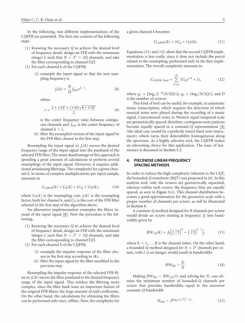
Figure 5: Procedure for building CQFFB filters in order to separateoctaves in the BQFFB.

4.1. Bounded-Q fast filter bank

The BQFFB combines the piecewise linear spacing of thebounded-Q scheme with the high selectivity of the FFB. Thiscan be achieved by using a CQFFB to separate the input sig-nal into octaves, and then applying an FFB within each oc-tave to obtain linearly spaced frequency bins. In this scheme,the CQFFB requires only ten output channels, correspond-ing to the 10-octave human auditory range, which does notdemand a heavy computational load. Each octave is then iso-lated from the others by using filters designed according tothe following procedure (see Figure 5).

(1) Obtain the filter for the highest octave, D, from thesecond filter of a 2-channel FFB.

(2) Obtain the filter for each remaining octave, d = (D �1), . . . , 1, as a cascade of the second filter of a 2(D�d+1)-channel FFB with the first filter of a 2(D�d)-channelFFB.

Using the filters already mentioned in Section 2.2 (i.e., withthe same orders as those described in [2]) for octave separa-tion, the total of nonzero coefficients required by the proce-dure above is given in Table 2.

The reasoning for this procedure is that the filter assignedto the highest octave, indexed by D, is the second filter of a

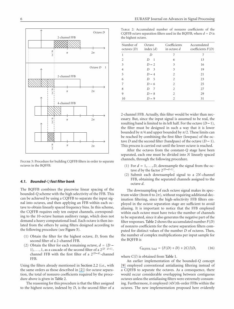
Table 2: Accumulated number of nonzero coefficients of theCQFFB octave separation filters used in the BQFFB, where d = D isthe highest octave.

Number ofoctaves (D)

Octaveindex (d)

Coefficientsin octave d

Accumulatedcoefficients F(D)

1 D 7 7

2 D � 1 6 13

3 D � 2 3 16

4 D � 3 3 19

5 D � 4 2 21

6 D � 5 2 23

7 D � 6 2 25

8 D � 7 2 27

9 D � 8 2 29

10 D � 9 2 31

2-channel FFB. Actually, this filter would be wider than nec-essary. But, since the input signal is assumed to be real, theresulting band is limited to its left half. For the octave (D�1),the filter must be designed in such a way that it is lowerbounded by π/4 and upper bounded by π/2. These limits canbe reached by combining the first filter (lowpass) of the oc-tave D and the second filter (bandpass) of the octave (D�1).This process is carried out until the lower octave is reached.

After the octaves from the constant-Q stage have beenseparated, each one must be divided into N linearly spacedchannels, through the following procedure.

(1) For d = 1, . . . ,D, downsample the signal from the oc-tave d by the factor 2(D�d+1).

(2) Submit each downsampled signal to a 2N-channelFFB, obtaining the separated channels assigned to theoctave d.

The downsampling of each octave signal makes its spec-trum wider (from 0 to 2π), without requiring additional dec-imation filtering, since the high-selectivity FFB filters em-ployed in the octave separation stage are sufficient to avoidaliasing. It is important to notice that the FFB employedwithin each octave must have twice the number of channelsto be separated, since it also generates the negative part of thefilter responses. Table 2 shows the accumulated number F(D)of nonzero coefficients for the octave separation filters com-puted for distinct values of the number D of octaves. Then,the number of complex multiplications per input sample forthe BQFFB is

CBQFFB, Total =(F(D) + D

)+ 2C(l)D, (16)

where C(l) is obtained from Table 1.An earlier implementation of the bounded-Q concept

[9] employed conventional antialiasing filtering instead ofa CQFFB to separate the octaves. As a consequence, therewould occur considerable overlapping between contiguousoctaves unless the antialiasing filters were extremely consum-ing. Furthermore, it employed (4N)th-order FFBs within theoctaves. The new implementation proposed here evidently

Filipe C. C. B. Diniz et al. 7

Table 3: Comparison between different spectral analysis tools. Theasterisk refers to the FFB-based high-selectivity tools, which tend tobe more complex than the FFT-based algorithms.

Analysistool

Frequencyspacing

Channelselectivity

Computationalcomplexity

FFT Linear Low Low

FFB Linear High Low (�)

CQT Geometric Low High

CQFFB Geometric High High (�)

BQT Piecewise linear Low Medium

BQFFB Piecewise linear High Medium (�)

supersedes that one with respect to frequency discrimina-tion, at a comparable computational burden.

Table 3 summarizes the main characteristics of all spec-tral analysis algorithms seen in this paper.

As a final remark, it must be added that, as opposed to theFFT and the FFB, neither the CQFFB nor the BQFFB is struc-turally invertible. The direct resynthesis of a signal analyzedthrough these methods requires a synthesis filter bank whichcan only approximate perfect reconstruction. This fact re-sults from the noninvertibility of their originating CQT [4].

5. PRACTICAL ISSUES

In the following, some design aspects concerning the prac-tical implementation and application of the proposed algo-rithms are addressed.

5.1. Choice of parameter values

The first problem to be taken into consideration is the fil-ter bank resolution. In musical applications, one can refer tothe geometric organization of the equal tempered scale usedin Western music [3]: each octave is divided into 12 musicalnotes following a geometric progression of ratio 12

2 � 1.06.

This ratio is known as a semitone. In order to detect a semi-tone variation, the resolution should be the square root ofthis value, that is, 24

2 � 1.03 (one quartertone).

If one wants to use constant-Q channels, as in the CQFFB[7], the corresponding quality factor is given by

Q= fk(Δ f )CQ

= fk(21/48 � 2�1/48

)fk� 1

0.0289� 34.6, (17)

where fk is the central frequency (in a geometric sense) and(Δ f )CQ is the bandwidth of any given channel k. To sim-plify the calculations, the resulting value for the Q-factor willbe 35.

The intended quartertone separation corresponds to R =24. Using (15), the bounded-Q solution should employ atleast Nmin = 64 channels per octave to make them all nar-rower than the constant-Q channels. For all practical pur-poses, N = 32 can be used, since only three of the twentyfour CQFFB channels are narrower than their BQFFB coun-terparts.

102

103

104

105

106

107

108

109

1010

0 500 1000 1500 2000 2500 3000 3500

Nu

mbe

rof

com

plex

mu

ltip

licat

ion

s

Number of channels

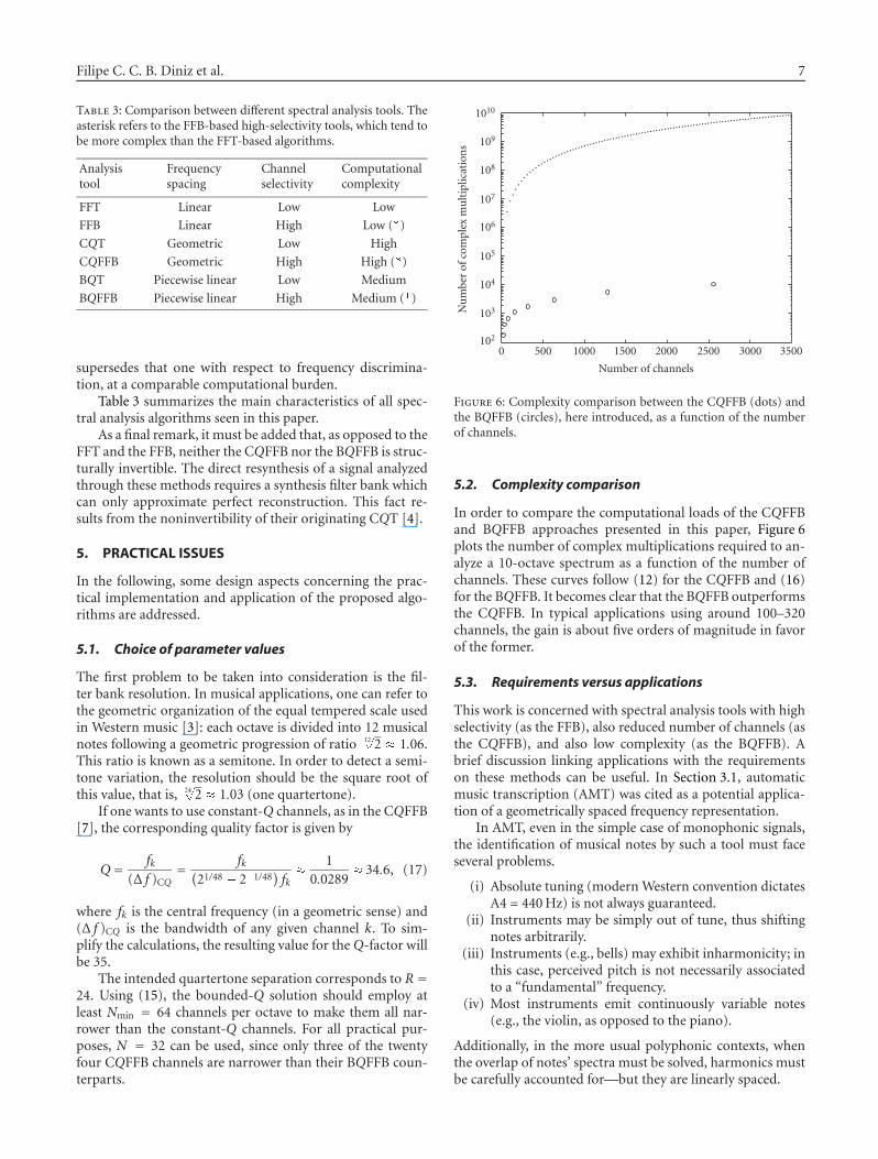
Figure 6: Complexity comparison between the CQFFB (dots) andthe BQFFB (circles), here introduced, as a function of the numberof channels.

5.2. Complexity comparison

In order to compare the computational loads of the CQFFBand BQFFB approaches presented in this paper, Figure 6plots the number of complex multiplications required to an-alyze a 10-octave spectrum as a function of the number ofchannels. These curves follow (12) for the CQFFB and (16)for the BQFFB. It becomes clear that the BQFFB outperformsthe CQFFB. In typical applications using around 100–320channels, the gain is about five orders of magnitude in favorof the former.

5.3. Requirements versus applications

This work is concerned with spectral analysis tools with highselectivity (as the FFB), also reduced number of channels (asthe CQFFB), and also low complexity (as the BQFFB). Abrief discussion linking applications with the requirementson these methods can be useful. In Section 3.1, automaticmusic transcription (AMT) was cited as a potential applica-tion of a geometrically spaced frequency representation.

In AMT, even in the simple case of monophonic signals,the identification of musical notes by such a tool must faceseveral problems.

(i) Absolute tuning (modern Western convention dictatesA4 = 440 Hz) is not always guaranteed.

(ii) Instruments may be simply out of tune, thus shiftingnotes arbitrarily.

(iii) Instruments (e.g., bells) may exhibit inharmonicity; inthis case, perceived pitch is not necessarily associatedto a “fundamental” frequency.

(iv) Most instruments emit continuously variable notes(e.g., the violin, as opposed to the piano).

Additionally, in the more usual polyphonic contexts, whenthe overlap of notes’ spectra must be solved, harmonics mustbe carefully accounted for—but they are linearly spaced.

8 EURASIP Journal on Advances in Signal Processing

All these considerations can be summarized in one sen-tence: there is no ideal frequency grid for the spectral analysisof music signals. In fact, depending on the target application,different solutions may be preferable. Under this perspective,the bounded-Q economy of 5 orders of magnitude in com-plexity over the constant-Q makes it a preferable analysis toolin general. The linear spacing of harmonics must not causemuch concern, if sufficient granularity is available, for ex-ample, it can be easily shown that with N linear channelsper octave, the system can separate the first 2N harmonicsof a given musical note. Of course, the fine granularity mustbe paralleled by sufficient separation capability, and this isthe importance of including the FFB filters in the proposedstructures.

In broad terms, the proposed methods can be seen asmusic-oriented time-frequency representations. They canprovide (magnitude, frequency) x time as parameters forgeneral music feature extraction systems, where higher-levellayers may process the information in a myriad of ways. Sincerelated applications often deal with great amounts of data,the reduced number of channels (and generated output sam-ples) is an important issue of the CQFFB and BQFFB tech-niques.

6. COMPUTER EXPERIMENTS

In this section, some computer simulations are carried outto assess the performance of the variable resolution high-selectivity methods using the linear frequency spacing meth-ods as a reference.

6.1. Two synthetic musical notes

First, consider a one-second test signal formed as the sum of8 pure tones of unit magnitude. The first two tones are at fre-quencies 263 Hz and 295 Hz, which correspond to notes C4and D4 slightly out of tune with respect to an equal temperedscale, to simulate a realistic situation. Their next three har-monics are also included. Since the main concern in this ex-periment is frequency detection, the component magnitudeswere made equal to simplify their visualization.

The frequency resolution value adopted in the CQFFBsimulation is Q = 35, as shown in (17), and will also serveas a reference in choosing the number of channels for theremaining methods. To keep the comparison fair, the chan-nel with the worst resolution in the linear spacing toolsshould satisfy the quarter tone constraint. This restrictionapplies to the lowest channel, which must contain the low-est test tone. To meet these conditions, both FFT and FFBdivide the spectrum in 4096 channels from 0 to 22050 Hz(assuming a sampling rate of 44100 Hz), each one 5.38 Hzwide.

The BQFFB, in turn, divides the spectrum (from its high-est limit) in seven octaves, plus the remaining lower fre-quency band (which includes the lowest test tone). Each ofthese eight subbands is linearly divided in 32 channels, thuskeeping in the lowest band the same spacing as the FFT andFFB tools.

0

0.2

0.4

0.6

0.8

1

300 400 500 600 700 800 900 1000 1100 1200

FFT

ampl

itu

de

Frequency (Hz)

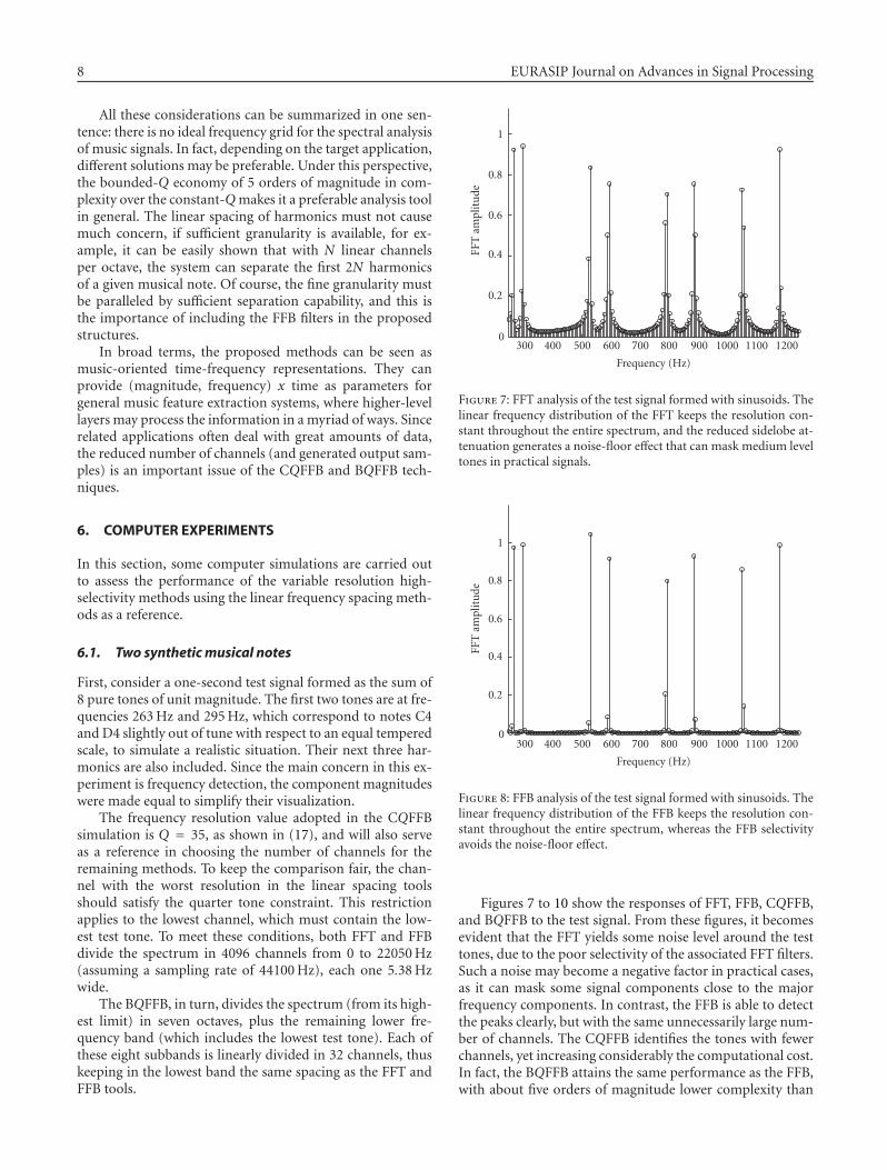
Figure 7: FFT analysis of the test signal formed with sinusoids. Thelinear frequency distribution of the FFT keeps the resolution con-stant throughout the entire spectrum, and the reduced sidelobe at-tenuation generates a noise-floor effect that can mask medium leveltones in practical signals.

0

0.2

0.4

0.6

0.8

1

300 400 500 600 700 800 900 1000 1100 1200

FFT

ampl

itu

de

Frequency (Hz)

Figure 8: FFB analysis of the test signal formed with sinusoids. Thelinear frequency distribution of the FFB keeps the resolution con-stant throughout the entire spectrum, whereas the FFB selectivityavoids the noise-floor effect.

Figures 7 to 10 show the responses of FFT, FFB, CQFFB,and BQFFB to the test signal. From these figures, it becomesevident that the FFT yields some noise level around the testtones, due to the poor selectivity of the associated FFT filters.Such a noise may become a negative factor in practical cases,as it can mask some signal components close to the majorfrequency components. In contrast, the FFB is able to detectthe peaks clearly, but with the same unnecessarily large num-ber of channels. The CQFFB identifies the tones with fewerchannels, yet increasing considerably the computational cost.In fact, the BQFFB attains the same performance as the FFB,with about five orders of magnitude lower complexity than

Filipe C. C. B. Diniz et al. 9

0

0.2

0.4

0.6

0.8

1

300 400 500 600 700 800 900 1000 1100 1200

CQ

FFB

ampl

itu

de

Frequency (Hz)

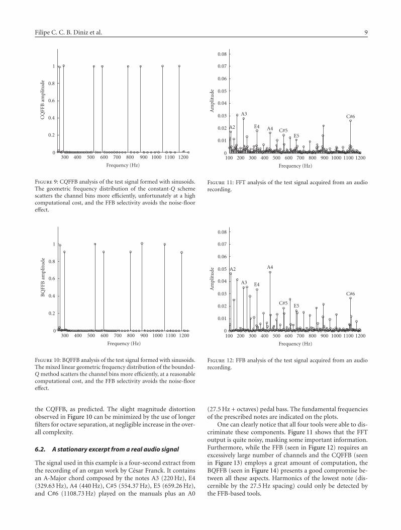
Figure 9: CQFFB analysis of the test signal formed with sinusoids.The geometric frequency distribution of the constant-Q schemescatters the channel bins more efficiently, unfortunately at a highcomputational cost, and the FFB selectivity avoids the noise-flooreffect.

0

0.2

0.4

0.6

0.8

1

300 400 500 600 700 800 900 1000 1100 1200

BQ

FFB

ampl

itu

de

Frequency (Hz)

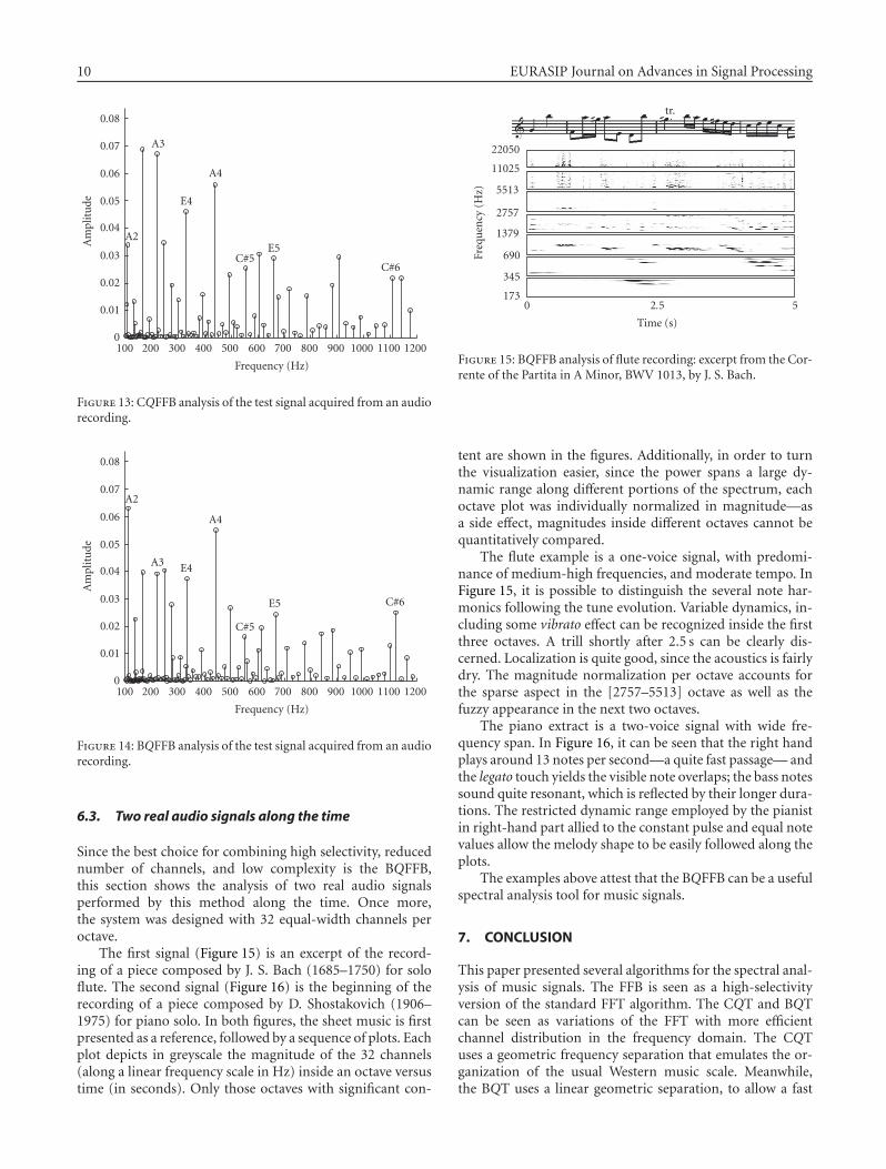
Figure 10: BQFFB analysis of the test signal formed with sinusoids.The mixed linear geometric frequency distribution of the bounded-Q method scatters the channel bins more efficiently, at a reasonablecomputational cost, and the FFB selectivity avoids the noise-flooreffect.

the CQFFB, as predicted. The slight magnitude distortionobserved in Figure 10 can be minimized by the use of longerfilters for octave separation, at negligible increase in the over-all complexity.

6.2. A stationary excerpt from a real audio signal

The signal used in this example is a four-second extract fromthe recording of an organ work by Cesar Franck. It containsan A-Major chord composed by the notes A3 (220 Hz), E4(329.63 Hz), A4 (440 Hz), C#5 (554.37 Hz), E5 (659.26 Hz),and C#6 (1108.73 Hz) played on the manuals plus an A0

0

0.01

0.02

0.03

0.04

0.05

0.06

0.07

0.08

100 200 300 400 500 600 700 800 900 1000 1100 1200

Am

plit

ude

Frequency (Hz)

A2

A3

E4 A4 C#5E5

C#6

Figure 11: FFT analysis of the test signal acquired from an audiorecording.

0

0.01

0.02

0.03

0.04

0.05

0.06

0.07

0.08

100 200 300 400 500 600 700 800 900 1000 1100 1200

Am

plit

ude

Frequency (Hz)

A2

A3 E4

A4

C#5 E5

C#6

Figure 12: FFB analysis of the test signal acquired from an audiorecording.

(27.5 Hz + octaves) pedal bass. The fundamental frequenciesof the prescribed notes are indicated on the plots.

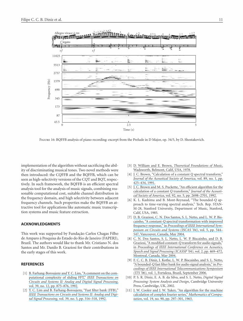
One can clearly notice that all four tools were able to dis-criminate these components. Figure 11 shows that the FFToutput is quite noisy, masking some important information.Furthermore, while the FFB (seen in Figure 12) requires anexcessively large number of channels and the CQFFB (seenin Figure 13) employs a great amount of computation, theBQFFB (seen in Figure 14) presents a good compromise be-tween all these aspects. Harmonics of the lowest note (dis-cernible by the 27.5 Hz spacing) could only be detected bythe FFB-based tools.

10 EURASIP Journal on Advances in Signal Processing

0

0.01

0.02

0.03

0.04

0.05

0.06

0.07

0.08

100 200 300 400 500 600 700 800 900 1000 1100 1200

Am

plit

ude

Frequency (Hz)

A2

A3

E4

A4

C#5E5

C#6

Figure 13: CQFFB analysis of the test signal acquired from an audiorecording.

0

0.01

0.02

0.03

0.04

0.05

0.06

0.07

0.08

100 200 300 400 500 600 700 800 900 1000 1100 1200

Am

plit

ude

Frequency (Hz)

A2

A3 E4

A4

C#5

E5 C#6

Figure 14: BQFFB analysis of the test signal acquired from an audiorecording.

6.3. Two real audio signals along the time

Since the best choice for combining high selectivity, reducednumber of channels, and low complexity is the BQFFB,this section shows the analysis of two real audio signalsperformed by this method along the time. Once more,the system was designed with 32 equal-width channels peroctave.

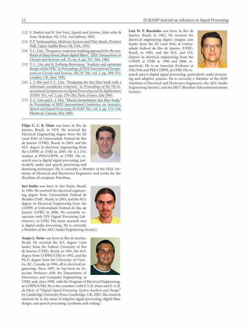
The first signal (Figure 15) is an excerpt of the record-ing of a piece composed by J. S. Bach (1685–1750) for soloflute. The second signal (Figure 16) is the beginning of therecording of a piece composed by D. Shostakovich (1906–1975) for piano solo. In both figures, the sheet music is firstpresented as a reference, followed by a sequence of plots. Eachplot depicts in greyscale the magnitude of the 32 channels(along a linear frequency scale in Hz) inside an octave versustime (in seconds). Only those octaves with significant con-

173

345

690

1379

2757

5513

11025

22050

0 2.5 5

Freq

uen

cy(H

z)

Time (s)

tr.

Figure 15: BQFFB analysis of flute recording: excerpt from the Cor-rente of the Partita in A Minor, BWV 1013, by J. S. Bach.

tent are shown in the figures. Additionally, in order to turnthe visualization easier, since the power spans a large dy-namic range along different portions of the spectrum, eachoctave plot was individually normalized in magnitude—asa side effect, magnitudes inside different octaves cannot bequantitatively compared.

The flute example is a one-voice signal, with predomi-nance of medium-high frequencies, and moderate tempo. InFigure 15, it is possible to distinguish the several note har-monics following the tune evolution. Variable dynamics, in-cluding some vibrato effect can be recognized inside the firstthree octaves. A trill shortly after 2.5 s can be clearly dis-cerned. Localization is quite good, since the acoustics is fairlydry. The magnitude normalization per octave accounts forthe sparse aspect in the [2757–5513] octave as well as thefuzzy appearance in the next two octaves.

The piano extract is a two-voice signal with wide fre-quency span. In Figure 16, it can be seen that the right handplays around 13 notes per second—a quite fast passage— andthe legato touch yields the visible note overlaps; the bass notessound quite resonant, which is reflected by their longer dura-tions. The restricted dynamic range employed by the pianistin right-hand part allied to the constant pulse and equal notevalues allow the melody shape to be easily followed along theplots.

The examples above attest that the BQFFB can be a usefulspectral analysis tool for music signals.

7. CONCLUSION

This paper presented several algorithms for the spectral anal-ysis of music signals. The FFB is seen as a high-selectivityversion of the standard FFT algorithm. The CQT and BQTcan be seen as variations of the FFT with more efficientchannel distribution in the frequency domain. The CQTuses a geometric frequency separation that emulates the or-ganization of the usual Western music scale. Meanwhile,the BQT uses a linear geometric separation, to allow a fast

Filipe C. C. B. Diniz et al. 11

43.5

87

173

345

690

1379

2757

5513

11025

0 2.5 5

Freq

uen

cy(H

z)

Time (s)

Allegro vivace 200 2 1 2 3 1 2 3 4 53 4 3 5 4 3 5 4 4 2 1 1 2 3

f legato

s f s f

Figure 16: BQFFB analysis of piano recording: excerpt from the Prelude in D Major, op. 34/5, by D. Shostakovich.

implementation of the algorithm without sacrificing the abil-ity of discriminating musical tones. Two novel methods werethen introduced: the CQFFB and the BQFFB, which can beseen as high-selectivity versions of the CQT and BQT, respec-tively. In such framework, the BQFFB is an efficient spectralanalysis tool for the analysis of music signals, combining rea-sonable computational cost, suitable channel distribution inthe frequency domain, and high selectivity between adjacentfrequency channels. Such properties make the BQFFB an at-tractive tool for applications like automatic music transcrip-tion systems and music feature extraction.

ACKNOWLEDGMENTS

This work was supported by Fundacao Carlos Chagas Filhode Amparo a Pesquisa do Estado do Rio de Janeiro (FAPERJ),Brazil. The authors would like to thank Mr. Cristiano N. dosSantos and Mr. Danilo B. Graziosi for their contributions inthe early stages of this work.

REFERENCES

[1] B. Farhang-Boroujeny and Y. C. Lim, “A comment on the com-putational complexity of sliding FFT,” IEEE Transactions onCircuits and Systems II: Analog and Digital Signal Processing,vol. 39, no. 12, pp. 875–876, 1992.

[2] Y. C. Lim and B. Farhang-Boroujeny, “Fast filter bank (FFB),”IEEE Transactions on Circuits and Systems II: Analog and Digi-tal Signal Processing, vol. 39, no. 5, pp. 316–318, 1992.

[3] D. William and E. Brown, Theoretical Foundations of Music,Wadsworth, Belmont, Calif, USA, 1978.

[4] J. C. Brown, “Calculation of a constant Q spectral transform,”Journal of the Acoustical Society of America, vol. 89, no. 1, pp.425–434, 1991.

[5] J. C. Brown and M. S. Puckette, “An efficient algorithm for thecalculation of a constant Q transform,” Journal of the Acousti-cal Society of America, vol. 92, no. 5, pp. 2698–2701, 1992.

[6] K. L. Kashima and B. Mont-Reynaud, “The bounded-Q ap-proach to time-varying spectral analysis,” Tech. Rep. STAN-M-28, Stanford University, Department of Music, Stanford,Calif, USA, 1985.

[7] D. B. Graziosi, C. N. Dos Santos, S. L. Netto, and L. W. P. Bis-cainho, “A constant-Q spectral transformation with improvedfrequency response,” in Proceedings of IEEE International Sym-posium on Circuits and Systems (ISCAS ’04), vol. 5, pp. 544–547, Vancouver, Canada, May 2004.

[8] C. N. Dos Santos, S. L. Netto, L. W. P. Biscainho, and D. B.Graziosi, “A modified constant-Q transform for audio signals,”in Proceedings of IEEE International Conference on Acoustics,Speech and Signal Processing (ICASSP ’04), vol. 2, pp. 469–472,Montreal, Canada, May 2004.

[9] F. C. C. B. Diniz, I. Kothe, L. W. P. Biscainho, and S. L. Netto,“A bounded-Q fast filter bank for audio signal analysis,” in Pro-ceedings of IEEE International Telecommunications Symposium(ITS ’06), vol. 1, Fortaleza, Brazil, September 2006.

[10] P. S. R. Diniz, E. A. B. da Silva, and S. L. Netto, Digital SignalProcessing: System Analysis and Design, Cambridge UniversityPress, Cambridge, UK, 2002.

[11] J. W. Cooley and J. W. Tukey, “An algorithm for the machinecalculation of complex fourier series,” Mathematics of Compu-tation, vol. 19, no. 90, pp. 297–301, 1965.

12 EURASIP Journal on Advances in Signal Processing

[12] S. Haykin and B. Van Veen, Signals and Systems, John wiley &Sons, Hoboken, NJ, USA, 2nd edition, 2002.

[13] P. P. Vaidyanathan, Multirate Systems and Filter Banks, PrenticeHall, Upper Saddle River, NJ, USA, 1992.

[14] Y. C. Lim, “Frequency-response masking approach for the syn-thesis of sharp linear phase digital filters,” IEEE Transactions onCircuits and Systems, vol. 33, no. 4, pp. 357–364, 1986.

[15] Y. C. Lim and B. Farhang-Boroujeny, “Analysis and optimumdesign of the FFB,” in Proceedings of IEEE International Sympo-sium on Circuits and Systems (ISCAS ’94), vol. 2, pp. 509–512,London, UK, June 1994.

[16] L. J. Wei and Y. C. Lim, “Designing the fast filter bank with aminimum complexity criterion,” in Proceedings of the 7th In-ternational Symposium on Signal Processing and Its Applications(ISSPA ’03), vol. 2, pp. 279–282, Paris, France, July 2003.

[17] Y. C. Lim and L. J. Wei, “Matrix formulation: fast filter bank,”in Proceedings of IEEE International Conference on Acoustics,Speech and Signal Processing (ICASSP ’04), vol. 5, pp. 133–136,Montreal, Canada, May 2004.

Filipe C. C. B. Diniz was born in Rio deJaneiro, Brazil, in 1979. He received theElectrical Engineering degree from the EE(now Poli) at Universidade Federal do Riode Janeiro (UFRJ), Brazil, in 2003, and theM.S. degree in electrical engineering fromthe COPPE at UFRJ in 2005. He is a D.S.student at PEE/COPPE, at UFRJ. His re-search area is digital signal processing, par-ticularly audio and speech processing anddenoising techniques. He is currently a Member of the IEEE (In-stitute of Electrical and Electronics Engineers) and works for theBrazilian oil company, Petrobras.

Iuri Kothe was born in Sao Paulo, Brazil,in 1980. He received the electrical engineer-ing degree from Universidade Federal deBrasılia (UnB), Brazil, in 2003, and the M.S.degree in Electrical Engineering from theCOPPE at Universidade Federal do Rio deJaneiro (UFRJ) in 2006. He currently co-operates with LPS (Signal Processing Lab-oratory), at UFRJ. His main research areais digital audio processing. He is currentlya Member of the AES (Audio Engineering Society).

Sergio L. Netto was born in Rio de Janeiro,Brazil. He received the B.S. degree (cumlaude) from the Federal University of Riode Janeiro (UFRJ), Brazil, in 1991, the M.S.degree from COPPE/UFRJ in 1992, and thePh.D. degree from the University of Victo-ria, BC, Canada, in 1996, all in electrical en-gineering. Since 1997, he has been an As-sociate Professor with the Department ofElectronics and Computer Engineering, atUFRJ, and, since 1998, with the Program of Electrical Engineering,at COPPE/UFRJ. He is the coauthor (with P. S. R. Diniz and E. A. B.da Silva) of “Digital Signal Processing: System Analysis and Design”by Cambridge University Press, Cambridge, UK, 2002. His researchinterests lie in the areas of adaptive signal processing, digital filterdesign, and speech processing (synthesis and coding).

Luiz W. P. Biscainho was born in Rio deJaneiro, Brazil, in 1962. He received theelectrical engineering degree (magna cumlaude) from the EE (now Poli) at Univer-sidade Federal do Rio de Janeiro (UFRJ),Brazil, in 1985, and the M.S. and D.S.degrees in electrical engineering from theCOPPE at UFRJ in 1990 and 2000, re-spectively. He is an Associate Professor atDEL/Poli and PEE/COPPE, at UFRJ. His re-search area is digital signal processing, particularly audio process-ing and adaptive systems. He is currently a Member of the IEEE(Institute of Electrical and Electronics Engineers), the AES (AudioEngineering Society), and the SBrT (Brazilian TelecommunicationsSociety).

Photograph © Turisme de Barcelona / J. Trullàs

Preliminary call for papers

The 2011 European Signal Processing Conference (EUSIPCO 2011) is thenineteenth in a series of conferences promoted by the European Association forSignal Processing (EURASIP, www.eurasip.org). This year edition will take placein Barcelona, capital city of Catalonia (Spain), and will be jointly organized by theCentre Tecnològic de Telecomunicacions de Catalunya (CTTC) and theUniversitat Politècnica de Catalunya (UPC).EUSIPCO 2011 will focus on key aspects of signal processing theory and

li ti li t d b l A t f b i i ill b b d lit

Organizing Committee

Honorary ChairMiguel A. Lagunas (CTTC)

General ChairAna I. Pérez Neira (UPC)

General Vice ChairCarles Antón Haro (CTTC)

Technical Program ChairXavier Mestre (CTTC)

Technical Program Co Chairsapplications as listed below. Acceptance of submissions will be based on quality,relevance and originality. Accepted papers will be published in the EUSIPCOproceedings and presented during the conference. Paper submissions, proposalsfor tutorials and proposals for special sessions are invited in, but not limited to,the following areas of interest.

Areas of Interest

• Audio and electro acoustics.• Design, implementation, and applications of signal processing systems.

l d l d d

Technical Program Co ChairsJavier Hernando (UPC)Montserrat Pardàs (UPC)

Plenary TalksFerran Marqués (UPC)Yonina Eldar (Technion)

Special SessionsIgnacio Santamaría (Unversidadde Cantabria)Mats Bengtsson (KTH)

FinancesMontserrat Nájar (UPC)• Multimedia signal processing and coding.

• Image and multidimensional signal processing.• Signal detection and estimation.• Sensor array and multi channel signal processing.• Sensor fusion in networked systems.• Signal processing for communications.• Medical imaging and image analysis.• Non stationary, non linear and non Gaussian signal processing.

Submissions

Montserrat Nájar (UPC)

TutorialsDaniel P. Palomar(Hong Kong UST)Beatrice Pesquet Popescu (ENST)

PublicityStephan Pfletschinger (CTTC)Mònica Navarro (CTTC)

PublicationsAntonio Pascual (UPC)Carles Fernández (CTTC)

I d i l Li i & E hibiSubmissions

Procedures to submit a paper and proposals for special sessions and tutorials willbe detailed at www.eusipco2011.org. Submitted papers must be camera ready, nomore than 5 pages long, and conforming to the standard specified on theEUSIPCO 2011 web site. First authors who are registered students can participatein the best student paper competition.

Important Deadlines:

P l f i l i 15 D 2010

Industrial Liaison & ExhibitsAngeliki Alexiou(University of Piraeus)Albert Sitjà (CTTC)

International LiaisonJu Liu (Shandong University China)Jinhong Yuan (UNSW Australia)Tamas Sziranyi (SZTAKI Hungary)Rich Stern (CMU USA)Ricardo L. de Queiroz (UNB Brazil)

Webpage: www.eusipco2011.org

Proposals for special sessions 15 Dec 2010Proposals for tutorials 18 Feb 2011Electronic submission of full papers 21 Feb 2011Notification of acceptance 23 May 2011Submission of camera ready papers 6 Jun 2011