Download pdf - Proper orthogonal decomposition of the dynamics in bolted joints

ARTICLE IN PRESS

Contents lists available at ScienceDirect

Journal of Sound and Vibration

Journal of Sound and Vibration 329 (2010) 1480–1498

0022-46

doi:10.1

� Cor

E-m

journal homepage: www.elsevier.com/locate/jsvi

Proper orthogonal decomposition of the dynamics in bolted joints

Abdur Rauf Khattak a,�, Seamus Garvey b, Atanas Popov b

a 1569, Street 39, I-10/2, Islamabad 44000, Pakistanb Department of Mechanical, Materials and Manufacturing Engineering, University of Nottingham, Nottingham, UK

a r t i c l e i n f o

Article history:

Received 21 April 2009

Received in revised form

11 September 2009

Accepted 13 November 2009

Handling Editor: L.G. Thamorthogonal decomposition is applied to joint dynamics in an attempt to arrive at a

Available online 6 December 2009

0X/$ - see front matter & 2009 Elsevier Ltd. A

016/j.jsv.2009.11.016

responding author. Tel.: +92 51 9257067.

ail address: [email protected] (A.R. Khattak

a b s t r a c t

Joints play an important role in the dissipation of vibration energy in built-up

structures. The highly nonlinear nature of joints with micro-slip is the main hurdle in

developing a reduced-order model which can simulate the dynamic behaviour of a joint

for a wide range of excitation conditions and geometries. In this paper, the proper

generic reduced-order model without a compromise on the physics of the system. Only

the linear part of the system of equations is reduced. The nonlinear part is determined

in the full space and then reduced before the numerical integration phase. The major

reduction in computational time is achieved by the increase in the size of the stable

time step and the reduced number of coordinates in the integration phase. The reduced-

order model, which is derived for an isolated and harmonically excited joint, is

successfully applied to separate joints with different geometries and excitation

conditions, e.g. harmonic and impulsive. The model is also capable of simulating the

dynamics of structures with joints. The results of the reduced-order model show good

agreement with a full model both in terms of the state of the system and its hysteretic

behaviour.

& 2009 Elsevier Ltd. All rights reserved.

1. Introduction

Joints, whether bolted or riveted, dissipate vibration energy through friction. Joints typically account for more than90 percent of the total dissipated energy in fabricated structures [1]. Friction damping is a highly nonlinear phenomenon,especially when friction forces are comparable to the restoring forces in joints. Several approaches have been adopted tosolve the nonlinear problem of friction damping. Metherell and Diller [2] have derived an analytical expression for the timehistory of the state of the joint with micro-slip and subjected to a single frequency harmonic excitation. According to thisapproach, the state of the joint is dependent on the past history of the micro-slip. Keeping track of this history is, however,cumbersome [3], especially when the forcing function contains harmonics of two or more frequencies [4]. The results of adetailed FE model have been utilised to determine the hysteretic behaviour of joints, [3,5,6], by utilising the so-calledJenkins element formulation. A very large FE model was developed at Sandia National Laboratory to reproduce themicro-slip behaviour of a joint using Coulomb friction [7]. The key parameters in these models, apart from the modelsgiven in [2] and [7], are obtained by curve fitting the response of a joint to known excitations [8,9]. It is, however, verydifficult to reproduce the response of the same joint with these models when the frequency and/or the amplitude of theexcitation is varied.

ll rights reserved.

).

www.elsevier.com/locate/jsvi

dx.doi.org/10.1016/j.jsv.2009.11.016

mailto:[email protected]

ARTICLE IN PRESS

A.R. Khattak et al. / Journal of Sound and Vibration 329 (2010) 1480–1498 1481

This study is aimed at developing a generalised joint model which should be capable of reproducing joint dynamics for awide range of amplitudes and frequencies of excitation with only a few degrees of freedom (dofs). The model is based onthe proper orthogonal decomposition (POD) of the time history of a representative joint. The POD is a method of extractingan optimal basis of spatially coherent structures, also known as proper orthogonal modes (POMs), from an ensemble oftime histories resulting from numerical simulations or experiments [10]. The motivation to apply the POD to jointdynamics comes from the fact that joints are almost always excited by external forces and/or imposed displacements at theends of the joint. This suggests the existence of some generic reduced order basis which should be capable of reproducingthe state of the joint for a wide variety of excitation conditions. The analyses are, however, subjected to certainassumptions which are usually made when treating joint dynamics. These include: (1) there is no gross or macro-slip in thejoint; (2) the excitation force and/or the imposed displacement act only at the free end of the joint; (3) clamping or normalforce is distributed uniformly along the length of the joint; (4) there is no elastic compliance between the contactingsurfaces; (5) the Coulomb formulation of friction force is used; and (6) the material behaves linearly.

It is also pertinent to mention that the model can easily be applied to structures with many shear lap joints. In that casethe amplitude of the excitation force at each joint can be determined from the linear finite element (FE) analysis of thestructure. This information will be utilised in properly scaling the POMs to reduce the nonlinear part of the structure.The linear part, of course, will require even lesser number generalised coordinates to fully simulate its behaviour. Thesegeneralised coordinates will depend on the frequency content of the excitation applied to the structure. The model will beapplied to several complex aerospace structures in future. In this paper, however, application of the model is restricted toharmonic and impulsive excitations.

2. System description

The system under investigation is a simple shear lap joint made of two similar plates clamped together with a numberof bolts causing a specified clamping pressure as shown in Fig. 1(a). The simplified representation of the joint for analysispurpose is shown in Fig. 1(b). It is reasonable to study the dynamics of joints based on the interaction of a deformable platepressed against a rigid surface, as suggested e.g. in [3,4]. This approach has been adopted here as it offers simplicity and canbe easily extended to the case of a joint having two deformable plates. It should be noted that the joint discussed here isfirst studied in isolation of the structure, so that a clearer understanding of the nonlinear dynamics of a bolted joint isgained. The structure of the joint is simulated by a simplified one dimensional FE model. The midpoint of the joint inFig. 1(a) is selected as a reference point and a zero imposed displacement is assigned to it as shown in Fig. 1(b). A uniformpressure P is applied to the plate normal to the axial direction. Harmonic excitation, Fexc is applied at the free end whilemembers of the friction force vector ff act along the length of the plate.

As shear joints are designed to withstand longitudinal forces by friction rather than by bearing loads in through-bolts,it is assumed throughout this work that the joint will not fail and will always have certain nodes that will not see anyrelative displacement. This length in which nodes do not experience micro-slip is usually termed the ‘grey’ length asopposed to the ‘active’ length in which the nodes experiences micro-slip. The active length is also the maximum lengthexperiencing micro-slip for a given excitation force. There can be both sticking and slipping regions in the active lengthwhile the grey length will have only sticking nodes and will remain unchanged for a given excitation condition.

2.1. Reference system

As a reference system, a plate of size 250�50�10 mm is analysed with 100 strut elements along its length. The valueof the friction coefficient is selected to be 0.7, while a uniform pressure of 8 MPa, equivalent to 100 kN of normal force,

ff

P

Fexc

Fexc

Fexc

(a)

(b)

Fig. 1. Geometry of the joint: (a) actual isolated joint; and (b) its simplified model.

ARTICLE IN PRESS

Fig. 2. Mesh sensitivity for displacement at the free end of the joint: (a) saturation of the displacement; and (b) comparison of a hysteresis curve with

that of pseudo-static analytical approach [4] using 100 elements (both curves are almost overlapped).

A.R. Khattak et al. / Journal of Sound and Vibration 329 (2010) 1480–14981482

is applied to the plate. A harmonic excitation force having amplitude of 63 kN at 1000 Hz is used which is 90 percent of thefriction limit, i.e. 90 percent of 0.7�100 kN. This amplitude value causes a slip in almost 90 percent of the joint lengthwhich contains enough number of nodes to determine reasonably smooth POMs.

The FE model consists of one dimensional strut elements having consistent stiffness and mass matrix formulation [11].The number of elements is selected on the basis of a mesh sensitivity study of the system and is found to be around 100elements along the entire joint length. The mesh sensitivity is a direct consequence of the nonlinearity of the system. In theabsence of nonlinear forces the same system dynamics can be modelled with fewer elements whose number is usuallybased on the frequency content of the excitation.

Fig. 2(a) shows the convergence of the value of displacement at the free end of the joint as a function of the number ofelements for harmonic loading at 1000 Hz with amplitude equal to 90 percent of the friction limit of the joint. The plot inthis figure shows a very small change, o1 percent compared with a model with a very large number of dofs, in the value ofdisplacement at this level of refinement (100 elements). A comparison of the hysteretic behaviour of the system at thislevel of mesh refinement with the results of the pseudo-static system analysed analytically in [4] in Fig. 2(b) shows a verygood agreement. The area enclosed by both curves, representing the energy dissipated per cycle, is equal to 2.0413 J.

3. Mathematical model

Dynamics of the joint model can be represented by the following system of equations:

KuþC _uþM €u ¼ fln � ff : (1)

Here K, C and M are the stiffness, viscous damping and mass matrices, respectively; u represents a vector of nodaldisplacements with a dot for derivatives with respect to time, fln is the vector of time dependant linear nodal excitationforces, while ff is the vector of nonlinear nodal friction forces. C is assumed to be proportional to the stiffness matrix K andcan be written as C¼ eK, where e¼ 10�5 is taken such as to accelerate convergence and to suppress contributions fromhigher resonances that are usually not of interest in mechanical systems.

The nonlinear Coulomb friction force vector, ff, which is governed by a sign function of the velocity, is represented bythe inverse tangent function to avoid a discontinuous friction force variation. It can be written, following [12], as

ff ¼ mfN2

ptan�1ðb _uÞ

� �: (2)

Here m is the coefficient of friction with the assumption that static and kinetic friction coefficients are equal, fN is thenormal force per node and b is a scalar that governs the slope of the curve representing the variation of friction force with_u, where _u is the vector of relative velocities between the rigid surface and the contacting nodes. A plot of normalisedinverse tangent function against _u, where _u is some nodal velocity, is shown in Fig. 3.

At lower excitation frequencies, resulting in lower nodal velocities for the same displacements, this factor should beincreased accordingly but this leads to increase in computational time. This is evident from Fig. 4 in which a comparison ofnodal displacements at the free end of the joint is given for two different values of the excitation frequency and twodifferent values of b. Fig. 4(a) shows that for a frequency of excitation equal to 5 Hz the change in displacement can be as

ARTICLE IN PRESS

Fig. 3. Variation of the friction force with velocity using the arctan function.

Fig. 4. Effect of the scaling constant b in Eq. (2), on the response of the joint: (a) fexc=5 Hz and (b) fexc=1000 Hz for b=107 (solid) and b=105 (dashed)

(both curves are overlapped (b)).


large as 9 percent when the value of b is increased from 105 to 107. Fig. 4(b) shows the corresponding change for excitationfrequency equal to 1000 Hz and is o1 percent. The computational time is also increased several times for this change inthe value of b.

4. POD of joint dynamics

The POD is closely related to the eigenvalue factorisation of a symmetric matrix [13] with the difference that the PODcan be applied to rectangular matrices as well. The time history of nodal displacements fuðtÞgp�n, where p is the number oftime steps and n is the number of nodes in the joint, is determined by numerical integration using (1) for the referencesystem. Using the POD, the matrix of nodal displacements is decomposed according to the following equation:

fuðtÞgp�n ¼Up�pRp�nVTn�n: (3)

Here ‘T’ in the exponent means transposition, U and V are orthogonal square matrices of size p and n, respectively. R is adiagonal but rectangular matrix having singular (proper) values s1;s2; . . . ;sn at its main diagonal. The columns of V are the

ARTICLE IN PRESS


POMs corresponding to the PVs s1;s2; . . . ;sn satisfying the orthogonality property vTi vj ¼ dij, where dij is the Kronecker

delta. It should be noted that the entries in the columns of V corresponding to the grey region are all zero. The matrix Vcontains the eigenvectors of the dot product fuðtÞgTp�nfuðtÞgp�n, corresponding to the eigenvalues l1; l2; . . . ; ln such thats2

i ¼ li while U is the matrix of eigenvectors for fuðtÞgp�nfuðtÞgTp�n. The factorisation in (3) can be obtained by a standard

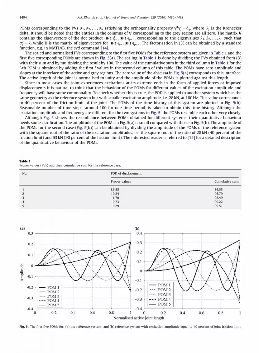
function, e.g. in MATLAB, the svd command [14].The scaled and normalised PVs corresponding to the first five POMs for the reference system are given in Table 1 and the

first five corresponding POMs are shown in Fig. 5(a). The scaling in Table 1 is done by dividing the PVs obtained from (3)with their sum and by multiplying the result by 100. The value of the cumulative sum in the third column in Table 1 for thei-th POM is obtained by adding the first i values in the second column of this table. The POMs have zero amplitude andslopes at the interface of the active and grey regions. The zero value of the abscissa in Fig. 5(a) corresponds to this interface.The active length of the joint is normalised to unity and the amplitude of the POMs is plotted against this length.

Since in most cases the joint experiences excitations at its extreme ends in the form of applied forces or imposeddisplacements it is natural to think that the behaviour of the POMs for different values of the excitation amplitude andfrequency will have some commonality. To check whether this is true, the POD is applied to another system which has thesame geometry as the reference system but with smaller excitation amplitude, i.e. 28 kN, at 100 Hz. This value correspondsto 40 percent of the friction limit of the joint. The POMs of the time history of this system are plotted in Fig. 5(b).Reasonable number of time steps, around 100 for one time period, is taken to obtain this time history. Although theexcitation amplitude and frequency are different for the two systems in Fig. 5, the POMs resemble each other very closely.

Although Fig. 5 shows the resemblance between POMs obtained for different systems, their quantitative behaviourneeds some clarification. The amplitude of the POMs in Fig. 5(a) is small compared with those in Fig. 5(b). The amplitude ofthe POMs for the second case (Fig. 5(b)) can be obtained by dividing the amplitude of the POMs of the reference systemwith the square root of the ratio of the excitation amplitudes, i.e. the square root of the ratio of 28 kN (40 percent of thefriction limit) and 63 kN (90 percent of the friction limit). The interested reader is referred to [15] for a detailed descriptionof the quantitative behaviour of the POMs.

Table 1Proper values (PVs) and their cumulative sum for the reference case.

No. POD of displacement

Proper values Cumulative sum

1 86.55 86.55

2 10.24 96.79

3 1.70 98.49

4 0.73 99.22

5 0.29 99.51

Fig. 5. The first five POMs for: (a) the reference system; and (b) reference system with excitation amplitude equal to 40 percent of joint friction limit.

ARTICLE IN PRESS


5. Reduction of the joint model

Assume for a moment that the grey and active lengths of the joint are known (this will be made clear in Section 6),the transformation matrix V is constructed such that the entries in its columns corresponding to the grey region are all zeroand the POMs are adjusted to the active region only. This transformation matrix is now applied to transform the systemequations, Eq. (1), using the first j columns of V. The first columns of V are selected as they correspond to the larger PVs.(The PVs are arranged in decreasing order).

Defining V1 ¼ fv1v2v3 . . . vjg, where vj are the first j columns of V and jrn, with u¼V1u0 in (1) and pre-multiplying thisequation by VT

1 results in the following reduced system of equations:

K0u0 þC0 _u 0 þM0 €u 0 ¼ fln0 � ff

0 ; (4)

where

K0 ¼VT1KV1; (5)

C0 ¼VT1CV1; (6)

M0 ¼VT1MV1; (7)

fln0 ¼VT

1fln (8)

and

ff0 ¼VT

1ff : (9)

These equations are straightforward except for (9) which is responsible for the nonlinear behaviour of the system.A reasonable value of j is normally selected based on the cumulative sum of the PVs. As a general rule, this value is taken tobe 99 percent of the total sum of PVs. In this analysis the first five POMs are selected to reduce the system of equationsalthough the cumulative sum of the corresponding PVs is slightly more than 99 percent, as can be seen from Table 1.Because the PVs can change slightly when varying the excitation conditions, the number of POMs is one higher than isstrictly indicated by the 99 percent criterion.

Eqs. (1) and (4) are usually solved using the state-space formulation. This method results in a system of first-orderequations that is double the size of the original system of second-order equations. The method assumes two new vectorssay y1 and y2 each of size n�1 such that y1=u and y2 ¼ _u i.e. y1 is the displacement vector and y2 is the velocity vector ofthe original system. This means that

_y1 ¼ _u ¼ y2 (10)

and

_y2 ¼ €u ¼ �M�1ðKuþC _u � flnþff Þ: (11)

These two equations result in the following first-order equation:

_y ¼Ayþb; (12)

with y¼ fy1 y2gT, where

A¼0n�n In�n

�M�1K �M�1C

� �(13)

and

b¼0n�n

M�1ðfln � ff Þ

( ): (14)

For the reduced system y1 ¼ u0, _y1 ¼ _u 0 ¼ y2 and matrix A and vector b are given by

A¼0k�k Ik�k

�M0�1K0 �M

0�1C0

� �(15)

and

b¼0k�k

Xðfln � ff Þ

( ); (16)

where X¼M0�1VT

1.For the reduced system, the velocity vector _u 0 has to be expanded at each time step to the full velocity vector using

_u ¼ V1 _u 0 in order to determine the nonlinear friction force vector according to (2). This expansion of reduced solution tothe full one for obtaining the full nonlinear force vector and then the compression of nonlinear force vector to the reduced

ARTICLE IN PRESS


one in (16) gives rise to additional computational cost at each time step. In spite of this drawback the method results incomputational savings, for the number of modes used in the analysis is much smaller when compared with the full size ofthe system.

6. Active length of the joint

It is mentioned before that the nodal displacements in the grey length only remain zero at all times. This suggests thatthe POD should be applied to the dynamics of the active region only, i.e. the POMs should be scaled according to thislength. It is, therefore, natural to determine the active length of a joint before embarking on the decomposition of thedynamics of the system.

A number of simulations have been performed to check if the active length can be determined beforehand at differentfrequencies including the internal resonance. The inertia forces of a dynamical system, which are dependent on thefrequency of excitation when keeping other factors unchanged, become predominant in the vicinity of a system resonance.This tends to increase the active length of a joint and means that if the applied force is scaled properly to include the inertiaeffects, the active length of the joint can be determined correctly. The dependence of the active length on the frequencycontent of the harmonic and impulse excitation forces is discussed in this section.

For the case of multi-harmonic excitation, the active length will be determined using the superposition principle, i.e.contributions from all the harmonics will be added at a point in time and the resulting maximum amplitude will be used todetermine the active length. This treatment is, however, not included in this paper.

6.1. Harmonic excitation

It is well known that the response of a linear SDOF system is amplified by the factor

Aa ¼1ffiffiffiffiffiffiffiffiffiffiffiffiffiffiffiffiffiffiffiffiffiffiffiffiffiffiffiffiffiffiffiffiffiffiffiffiffiffiffiffi

ð1� r2oÞ

2þð2rozÞ2

q ; (17)

where ro ¼o=on, o is the excitation frequency, on is the undamped resonance frequency and z is the damping ratio forthe mode having on as natural frequency. This is, however, not true for nonlinear systems especially bolted joints forwhich on is a function of both excitation frequency and amplitude. An iterative procedure is adopted to arrive at aplausible value for the scaling factor Aa. According to this procedure on is first determined on the basis of the amplitude ofexcitation at a given value of o. The value of the factor Aa is calculated from the initial value of on. This factor is thenapplied to scale the active length da. The increased active length reduces the natural frequency on which in turn increasesthe factor Aa. After a few iterations a converged value of the scaling factor can be achieved. The value of the damping ratio zis determined following the pseudo-static approach adopted in [4]. The term pseudo-static is used because the inertialeffects of the joint are ignored in this study although the excitation force is time dependant. According to this study theequivalent stiffness and damping of a joint, having an active length equal to da, can be written as

keq ¼2EAx

ffiffiffiffiffiffiffiffiffiffiffiffiffiffiffiffiffiffiffiffiffiffiffið9p2 � 16Þ

p3pda

(18)

and

ceq ¼8EAx

3pdao: (19)

These relations were derived analytically by modelling the joint with first-order differential equation and thus ignoring theinertia effects. The value of ceq is determined by equating the energy dissipated per cycle in the joint to that of a viscouslydamped system based on a commonly adopted linearisation approach. The value of keq is then determined from the first-order differential equation of the joint model. Eq. (18) shows that keq-N as the active length da-0, an obvious conclusionthat the stiffness of a strut with infinitesimal extendible length approaches infinity.

The loss factor Z and hence the damping ratio z can now be determined, following [16], as

z¼Z2¼

ceqo2keq

¼2ffiffiffiffiffiffiffiffiffiffiffiffiffiffiffiffiffiffiffiffiffiffiffi

ð9p2 � 16Þp ¼ 0:234: (20)

It is evident that the equivalent stiffness and damping are inversely proportional to the active length of the joint and theloss factor and the damping ratio are independent of the active length.

As an example the typical converging behaviour of the scaling factor Aa for Case I (Table 2) at 2000 Hz is shown in Fig. 6.In this example on=2�p�5000 rad/s, o=2�p�2000 rad/s, hence ro ¼ 0:4 and Aa=1.162. New value of the active lengthcomes out to be 0.25�1.162=0.2905 mm and hence the new on=2�p�4303 rad/s. After 15 iterations the convergedvalue of 1.3 is achieved.

Three cases are investigated to check the dependence of the active length on the excitation frequency. Parameter valuesfor these cases are given in Table 2. The first two cases are selected to determine the active length for different values of the

ARTICLE IN PRESS

Table 2System parameters used for the determination of active length of the joint in Fig. 1.

Parameter Case I Case II Case III

Joint length (mm) 500 250 500

Plate thickness (mm) 10 10 10

Plate width (mm) 50 50 50

Normal pressure (MPa) 50 50 50

Normal force (kN) 1.25�103 6.25�102 1.25�103

Friction coefficient 0.7 0.1 0.1

Excitation amplitude (kN) 437.5 31.25 37.5

First internal resonance (Hz) 5000 10 000 8333

Fig. 6. Convergence of scaling factor Aa.


friction coefficient keeping the amplitude of excitation equal to 50 percent of the friction limit. The third case is chosen todetermine the active length for a smaller value of the excitation amplitude, 30 percent of the friction limit. Results for thesecases are shown in Fig. 7. The plots in this figure show the variation of the active length with the frequency of excitation.The locations of the resonances of the systems are marked with arrows in these plots and the active length is taken as apercentage of the joint length. The first (solid) curve in these plots show the results of the full FE analysis of the problemwhile the second (dashed) curve show the active lengths determined by the above developed procedure using the POMs ofthe reference system.

Fig. 7 shows a good agreement between the actual active length obtained from the full FE analysis of the problem andthe scaled active length for values of the excitation frequencies outside, up to 50 percent, of the internal resonance of thesystem. The error in active length in Figs. 7(a), (b) and (c) is 3.2 percent, 1.8 percent and 5.9 percent, respectively, at about50 percent of the internal resonance. The relatively large error in Fig. 7(c) is a result of the smaller number of elements inthe active length of the joint. The increase in the error at frequencies more than 50 percent of the internal resonance is aresult of the assumptions made in the determination of the effective stiffness and damping. The values of keq and ceq aredetermined by linearisation of the hysteretic curve which is obtained by ignoring the inertia effects on the system. It is,however, very difficult to derive such simple relations for keq and ceq when the inertia of the system is included in theformulation of the problem.

It should, however, be noted that this discussion relates to the dependence of the active length of an isolated joint on itsinternal resonance. In real structures, the resonance of the whole structure is important and which is usually quite lowerthan the resonance of the joint. Hence the error in the value of the scaled active length, in general, will be smaller.

Fig. 8 shows the harmonic response histories at the free end, obtained from the full, reduced, pseudo-static and scaledpseudo-static analysis. In the scaled pseudo-static analysis, the amplitude is obtained by scaling the pseudo-static responsewith factor Aa. The system in Case I is selected for this analysis with the excitation frequency and amplitude equal to2000 Hz and 50 percent of the friction limit. This value of excitation frequency is large enough for the inertia forces to beincluded, while at the same time it is kept reasonably below the point where the amplification factor, Aa, does not givecorrect value of the active length. Only the steady-state part of the response is shown in this figure as the pseudo-staticapproach does not account for the transient behaviour at the beginning of the simulation. The time history from the

ARTICLE IN PRESS

30

35

40

1000

FE analysis

Scaled

Frequency (Hz)

Frequency (Hz) Frequency (Hz)

Act

ive

leng

th (

%)

50

55

60

65

1000

FE analysis

Scaled 40

60

80

500

FE analysis

Scaled

Act

ive

leng

th (

%)

Act

ive

leng

th (

%)

3500 6500 9500 3500 6000 8500 11000

3000 5000 7000

Fig. 7. The variation of active length (percent of total) with excitation frequency for different amplitudes of excitation for: Case I (a); Case II (b); and

Case III (c). The abscissa location marked with arrow shows the resonance of the system.

Fig. 8. Comparison of the displacement at the free end of the joint for the full, reduced, pseudo-static and scaled pseudo-static analysis (full and reduced

FE plots are overlapped).


pseudo-static analysis (dotted) and its scaled values (dashed-dotted) by applying Eq. (17) are also plotted in Fig. 8. Somerepresentative values of the results of these analyses are given in Table 3. The values in parentheses in Table 3 are theerrors compared with the full FE analysis. These values show that the reduced solution based on the scaled active lengthagrees well with the full solution. Finally the hysteresis curves corresponding to the time histories in Fig. 8 are plotted inFig. 9. These show the accuracy of the method developed in this paper. This figure also indicates the limitation of thepseudo-static approach at higher frequencies of excitation.

ARTICLE IN PRESS

Table 3Comparison of results of the dynamic and pseudo-static analyses based on scaling of the active length (Figs. 8 and 9).

Analysis type Max. displacement (m) Energy/cycle (J)

Dynamic FE analysis (full) 7.14�10�4 (0%) 681 (0%)

Dynamic FE analysis (reduced) 7.10�10�4 (0.6%) 680 (0.2%)

Pseudo-static [4] 5.47�10�4 (23.4%) 319 (53.2%)

Scaled pseudo-static 7.11�10�4 (0.4%) 415 (39.1%)

Fig. 9. Hysteresis curves corresponding to Fig. 8, full system (solid line), reduced (dashed), pseudo-static (dotted) and scaled pseudo-static (dashed-

dotted) (full and reduced solutions are overlapped).

50

60

70

80

90

100

1000

Frequency

Act

ive

leng

th (

% o

f to

tal)

Am

plitu

de

Time

dt

9

8

7

6

5

4

3

2

1

0

0 0.2 0.4 0.6 0.8 1 1.2 1.4 1.6

x 10-4

x 104

4500 8000 11500 15000

Fig. 10. (a) Variation of active length for impulsive excitation with the maximum frequency content of the excitation for load amplitudes equal to

70 percent (full), 60 percent (dashed) and 50 percent (dashed-dotted) of the joint friction limit; and (b) a representative impulsive excitation.


6.2. Impulsive excitation

The determination of the active length in the case of impulse excitation is even more complicated when compared tothe case of harmonic excitation. The complexity is due to the fact that the change in the amplitude of the excitation force isdiscontinuous and that the excitation is rich in frequencies when compared with the harmonic case.

The dynamic system of Case I is selected for this study and the active length of the joint for various loading amplitudesis plotted against maximum frequency, present in the impulsive excitation, in Fig. 10(a). The corresponding impulse isshown in Fig. 10(b). The maximum frequency present in the excitation can be found from dt in Fig. 10(b) using Nyquist

ARTICLE IN PRESS


rule. The three different curves in this figure correspond to three different amplitudes of the impulse. This figure showsthat the active length for one level of excitation can be scaled with the ratio of the amplitudes to obtain its value at anotherlevel of excitation. For example, the value of the active length for amplitude of the impulse equal to 50 percent of thefriction limit at 4500 Hz is 66 percent of the joint length. When this value of the active length is scaled for a load level equalto 70 percent of the friction limit, it comes out to be 70=50� 66¼ 92 which is quite close to the actual value at this level ofexcitation which is 99 percent of the joint length. The error in the scaled value of the active length is therefore 7 percent.The sensitivity of the response to the error in the value of the active length is discussed in the next section.

Although it is possible to relate the values of the active length for different amplitudes of the impulse having the samemaximum frequency for a given case, it is not very easy to reach at any general conclusion about the frequency dependenceof the active length for this kind of excitation.

6.3. Sensitivity of the response to the value of the active length

Sensitivity of the response to the active length of the joint is investigated by the application of a harmonic excitation tothe structure in Case I. The frequency of excitation is selected at 2000 Hz which is about 50 percent of the first internalresonance. The amplitude of excitation is selected as 50 percent of the friction limit. This amplitude suggests that the activelength, without taking into account the inertia effects, is 50 percent of the joint length, i.e. 250 mm. The first resonance ofthe structure in Case I having a length of 250 mm is 5000 Hz. The active length comes out to be 345 mm when the inertiaeffects are included according to (17). Results using this length for the reduced model are already reported in Table 3 andFig. 8.

To check the sensitivity of the response to change in the value of active length, two simulations are carried out. In thefirst one the active length obtained from the analysis of the full model is increased by 10 percent while in the second one itis reduced by 10 percent. Fig. 11(a) shows the response histories while Fig. 11(b) shows the hysteresis behaviour. Therepresentative values of the results of these analyses are given in Table 4 which is very encouraging as the maximum errorin response and/or energy dissipated per cycle is around 2 percent. This is due to the fact that the amplitude of the POMs issmall at the junction of the grey and active length. A small change in the value of the active length, therefore, does notaffect the solution appreciably.

Fig. 11. Sensitivity of the response to change in the value of active length: (a) displacement; and (b) force-deflection behaviour (curves are overlapping).

Table 4Sensitivity of the response on the change in the value of active length (Fig. 11).

Analysis type Max. displacement (m) Energy/cycle (J)

Dynamic FE analysis (full) 5.7�10�5 (0%) 681 (0.0%)

10% increase in active length 7.06�10�4 (1.1%) 672 (1.3%)

10% reduction in active length 7.3�10�4 (2.2%) 691 (1.5%)

ARTICLE IN PRESS


7. Application of the method to different systems

After having developed a procedure for the reduction of the size of the joint model and the determination of the activelength of the joint beforehand, different systems are analysed. These systems are essentially models of a joint subjected todifferent excitation conditions.

7.1. Harmonic excitation applied to an isolated joint

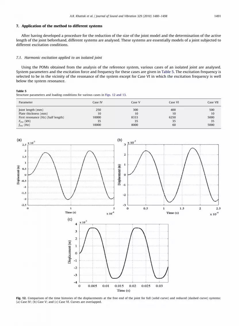
Using the POMs obtained from the analysis of the reference system, various cases of an isolated joint are analysed.System parameters and the excitation force and frequency for these cases are given in Table 5. The excitation frequency isselected to be in the vicinity of the resonance of the system except for Case VI in which the excitation frequency is wellbelow the system resonance.

Table 5Structure parameters and loading conditions for various cases in Figs. 12 and 13.

Parameter Case IV Case V Case VI Case VII

Joint length (mm) 250 300 400 500

Plate thickness (mm) 10 10 10 10

First resonance (Hz) (half length) 10000 8333 6250 5000

Fexc (kN) 35 35 35 35

fexc (Hz) 10000 8000 60 5000

Fig. 12. Comparison of the time histories of the displacements at the free end of the joint for full (solid curve) and reduced (dashed curve) systems:

(a) Case IV; (b) Case V; and (c) Case VI. Curves are overlapped.

ARTICLE IN PRESS


A comparison of the displacement time history for the full and reduced-order models for the three different cases isshown in Fig. 12. These displacements correspond to the node at the free end of the joint. Fig. 12(a) shows a comparisonbetween full and reduced systems for Case IV using five POMs. The solid and dashed curves correspond, respectively, to thefull and reduced model. These two curves overlie each other almost exactly. The same is true for Figs. 14(b) and (c)showing the comparison for Cases V and VI, respectively.

The percentage error in displacement of the reduced system for Case VII is shown in Fig. 13 and it is o2 percent. Theerror is plotted for one case only as in other cases the difference between full and reduced models is hardly noticeable.Fig. 12(a) and (b) do not show the stick slip behaviour very clearly. This is because the frequency of excitation is selected inthe vicinity of the system resonance. The stick-slip behaviour can be observed for the third case only which is obtained forexcitation with low frequency. A clearer picture of the stick-slip behaviour is shown in Fig. 14. This figure shows that nodesaway from the free end of the joint experience well-defined stick-slip behaviour. The four points selected for this figure areequally spaced along the length of the joint.

7.2. Impulsive excitation applied to an isolated joint

So far the various cases studied are concerned with harmonic excitations and they are relatively straightforward. Since asystem containing joints can be subjected to excitation conditions that are not necessarily a harmonic one, the procedureneeds to be investigated in case of more general excitation conditions. Impulsive excitation is one such case.

Fig. 13. The percent error (compared with full solution) for Case VII.

Fig. 14. Stick-slip behaviour of four equally spaced nodes along the length of the joint.

ARTICLE IN PRESS


In this section, an impulse input is used to excite the system. Parameters of the impulse input, i.e. the amplitude and thefrequency contents are selected so as to excite several internal resonances of the system. The geometry of the system inCase VII is selected for this purpose. A zoomed view of the impulse is shown in Fig. 15. The amplitude of the impulsiveinput is selected as 50 percent of the friction limit of the joint to make sure that at least 50 percent of the joint length isactive. Assume that the system length is 250 mm (50 percent of 500 mm). The extensional resonances for this length areodd-multiples of 5000, i.e. 5000, 15 000 and 25 000 Hz, etc. As can be seen from Fig. 15, the time for the force to reach to itspeak value is 2�10�5 s which can capture frequencies up to and including 25 000 Hz. According to the Nyquist rule thevalue of the time interval should be 1=2fexc in order to capture fexc. As the system has a softening behaviour, the first threeinternal resonances of this system will, however, be lower than the maximum frequency present in the excitation.

The first five POMs obtained from the time history of the transient response are shown in Fig. 16. These POMs areplotted against the length of the joint (grey plus active) and they show that for excitation amplitude of 50 percent of thefriction limit, the active length is almost 82 percent, suggesting that inertia effects are present. The cumulative sum for thefirst five PVs is slightly higher than 99 percent of the total. This suggests that five POMs should be used in the modelreduction of this system. The shape of the POMs in the active region looks quite similar to the ones obtained for harmonicexcitation, Fig. 5, except for the first one that contributes around 80.6 percent to the total sum of the PVs. The response atthe free end of the joint using the full system and reduced system is plotted in Fig. 17(a) with a zoomed view in Fig. 17(b).The various cases analysed are denoted (i) full system, (ii) reduced system using five POMs obtained from the impulse

Fig. 15. Zoomed view of the impulse.

Fig. 16. First five POMs for the step input case.

ARTICLE IN PRESS

Fig. 17. Response of joint to step excitation: (a) complete time history; and (b) zoomed view of (a). (i) Full system; (ii) reduced system using five POMs

obtained from impulsive excitation; (iii) same as (ii) but with 11 POMs and (iv) reduced system using five POMs obtained from harmonic excitation.

ff

PFexc

Fexc

500 mm200 mm

500 mm100 mm

Fexc

Fig. 18. Structure with a joint: (a) actual system; and (b) its simplified model.


response of the system, (iii) same as (ii) but with 11 POMs and (iv) using five POMs obtained from the response of thesystem to harmonic excitation. The error in any case is o1 percent. This suggests that the POMs obtained using theharmonic excitation can be used to reduce the dynamics of a joint subjected to impulse excitation. This is a very importantresult.

The case of excitations at frequencies between any two system resonances can also be handled with the same methodused for the impulsive excitations because it is again very difficult to determine the active length for excitations at morethan one frequency. A straightforward reason is the lack of validity of the superposition principal for the joint dynamics.

7.3. Harmonic excitation applied to a jointed structure

The jointed structure consists of two plates, each of size 700�50�10 mm. The joint is formed by clamping the twoplates with an overlapping length of 200 mm, see Fig. 18(a). A simplified model of the joint consists of a plate of size600�50�10 mm with only 100 mm experiencing friction force. This model is obtained by exploiting the anti-symmetry in

ARTICLE IN PRESS

Fig. 19. Time histories of displacement for full (solid) and reduced (dashed) solution: (a) at the free end of the linear region; and (b) at the junction of the

nonlinear and linear regions. The solid and dashed curves are almost overlapped.


the original structure and assuming the lower plate to be rigid. The simplified representation of the structure is shown inFig. 18(b).

The amplitude of the harmonic force is 50 percent of the friction limit and its frequency is 500 Hz. The clampingpressure is 50 MPa and the friction coefficient is 0.7. The active length of the joint subjected to this level of excitation,without considering the inertia effects, is 50 percent of the joint region (100 mm), i.e. it is 50 mm. This means that thelength of the structure experiencing displacement is 550 mm. The first resonance of a plate of this length is at around2273 Hz. This value is well above the excitation frequency of 500 Hz.

The active length is scaled by a factor Aa according to (4) to include the inertia effects of the portion of the structure thatexperiences motion. This value comes out to be 1.05, which means that the active length is 1.05�50 percent �53 percentof the 100 mm length.

The system response for the full and reduced-order models is shown in Fig. 19. Fig. 19(a) shows the displacement at thefree end of the linear region, while Fig. 19(b) shows the displacement at the junction of the nonlinear and the linearregions. The difference in displacements is hardly noticeable and is o1 percent of the response of the full system. The errorat the junction is slightly higher than 1 percent during the transient phase of the solution but is lower than 1 percentduring the steady state.

The steady-state energy dissipation in the joint region per cycle is the sum of energy dissipated at each node due tofriction. The values of the dissipated energies are 3.08 and 3.3 J for the full and reduced model, respectively. The error inenergy dissipation for the reduced model is, therefore, 8 percent of the value obtained for the full model. Although the errorin the dissipation of energy seems large, it seems to be acceptable due to the fact that joint model is solved using only fivePOMs that were determined from the dynamics of the reference system which is an entirely different system in terms ofthe excitation and geometry.

7.4. Impulsive excitation applied to a jointed structure

The method is now applied to the structure of Fig. 18(b) excited by an impulse. The impulse is shown in Fig. 20.The maximum amplitude of the impulse is 50 percent of the friction limit of the joint. The time for the impulse to reach itsmaximum value is selected to be 4�10�5 s. This value is small enough to excite at least the first three resonances of thestructure significantly. The third resonance of the structure at 50 percent load amplitude is 11 365 Hz which is the thirdodd-multiple of the first resonance at 2273 Hz. This suggests a value of 1=2� 11 365¼ 4:4� 10�5 s (applying the Nyquistrule) for the rise time of the impulse. A slightly smaller value, 4�10–5 s, is selected to be on the safe side.

The time histories of the full and reduced models are plotted in Fig. 21 and they are showing very good agreement.The maximum error in the nodal displacement between the full and reduced models at the free end of the structure andthe interface of the linear and nonlinear regions is 2.3 percent and 1.5 percent, respectively. It should be noted that thedecay envelope of the response does not follow the well-known linear decay behaviour. This is due to the magnitude offriction forces which are comparable to the elastic forces in the joint. This behaviour is also observed in [17]. The lineardecay behaviour is observed in systems which have smaller friction forces compared with the elastic forces, see forexample [11].

ARTICLE IN PRESS

Fig. 21. Time histories of displacement for full (solid) and reduced (dashed) solution for impulsive excitation: (a) at the free end of the linear region; and

(b) at the junction of the nonlinear and linear regions. The solid and dashed curves are almost overlapped.

Fig. 20. Time history of the impulsive force.


7.5. Evaluating the computational advantage of the model reduction

The main advantage in computational time is obtained from an increase in the size of the stable time step as only thelinear part of the model is reduced without reducing the number of nonlinear functions. The ratio of the length of the stabletime step size for the reduced and full model is inversely related to the ratio of their maximum eigenvalues, which is afactor of around 17 for joints studied in this paper.

It is known that the number of arithmetic operations required for the determination of the acceleration vector for abanded system of size n is of the order n or O(n), while for a system with full matrices of size n, it is O(n2) when the LUdecomposition is employed. The matrices obtained in the paper for the reduced models, having j generalised coordinates,are fully populated and hence require arithmetic operations of O(j2). In addition O(n) operations are required for thedetermination of the vector of nonlinear forces. The coefficient of n in the expression for total number of computations is,however, small compared with that for a banded system. This is explained in the next paragraph.

ARTICLE IN PRESS

Fig. 22. Variation of number of computations per time step to determine the rate vector.


While determining the second half of the rate vector, which is acceleration of the generalised coordinates, one needs atotal of 38n�24 operations per time step. Here, n is the number of generalised coordinates in the full system that is equalto 100. This means that a total of about 3800 computations are required. On the other hand, for the reduced system, oneneeds a total of 4nj�n� j computations for the expansion and compression phase and j2� j computations for thedetermination of the second half of the rate vector. The sum of these computations is around 1900. This shows a 50 percentreduction in computational time during the determination of the rate vector. This saving is, however, lost when thenumber of POMs is increased above nine. This can be seen from Fig. 22, where one has the number of computations pertime step as a function of the number of POMs. The number of coordinates in the full system is fixed to 100. The horizontalline shows the number of operations for the full system while the slant line shows the computations for the reducedsystem.

8. Conclusions

A model of the joint dynamics is developed which is parameter-free and physics-based and capable of modelling shearlap joints with reasonable accuracy. The method can be applied to different levels of loading and different joint parameters,e.g. different joint geometry, friction coefficients and clamping pressures. The inertia effects in the joint, which are usuallyignored, are automatically included in the formulation. The dynamics of both isolated joints and jointed structures can besimulated with accuracy for various excitation conditions.

An important feature of the method is the determination of the active length of a joint which is then used to properlyscale out the proper orthogonal modes. The active length can be determined easily for harmonic excitations in thesub-resonance range.

The method reduces the linear part of the system of equations. This results in a reduction in computational time interms of the increase in the size of the stable time step. This size is usually increased by a factor in excess of 10.The reduction in computational time is also obtained by the lower number of coordinates for the integration phase of thesolution.

Acknowledgements

I would also like to thank my department, National Centre for Physics, Pakistan for the financial support for the first twoyears of my research and the School of Mechanical, Materials, and Manufacturing Engineering, the University ofNottingham, for the financial support for the third year of my study.

References

[1] C.F. Beards, Damping in structural joints, Shock and Vibration Digest 24 (1992) 3–7.[2] A.F. Metherell, S.V. Diller, Instantaneos energy dissipation rate in a lap joint: uniform clamping pressure, Journal of Applied Mechanics (1968)

123–127.[3] D.D. Quinn, D. Segalman, Using series–series Iwan type models for understanding joint dynamics, Transactions of the ASME, Journal of Applied

Mechanics 72 (2005) 666–673.

ARTICLE IN PRESS


[4] G. Csaba, Modelling Microslip Friction Damping and its Influence on Turbine Blade Vibrations, Ph.D. Thesis, Linkoping University, 1998.[5] L. Gaul, J. Lenz, Nonlinear dynamics of structures assembled by bolted joints, Acta Mechanica 125 (1997) 169–181.[6] M. Oldfield, H. Ouyang, J.E. Mottershead, A. Kyprianou, Modelling and simulation of bolted joints under harmonic excitation, Materials Science Forum

440–441 (2003) 421–428.[7] D.W. Lobitz, D.L. Gregory, D.O. Smallwood, Comparison of finite element predictions to measurements from the Sandia microslip measurement.

Proceedings of the IMAC XIX, Orlando, 2001, pp. 1388–1394.[8] M.V. Sivaselvan, A.M. Reinhorn, Hysteretic models for deteriorating inelastic structures, Journal of Engineering Mechanics—ASCE 126 (2000) 633–640.[9] D. Segalman, Modelling joint friction in structural dynamics, Structural Control and Health Monitoring 13 (2006) 430–453.

[10] P. Holmes, J.L. Lumley, G. Berkooz, Turbulence, Coherent Structures, Dynamical Systems, and Symmetry, Cambridge University Press, Cambridge, 1996.[11] D.J. Inman, Engineering Vibration, Prentice-Hall, New Jersey, 2003.[12] R.I. Leine, D.H. Van Campen, A. De Kraker, L. Van Den Steen, Stick-slip vibrations induced by alternate friction models, Nonlinear Dynamics 16 (1998)

41–54.[13] G. Strang, Linear Algebra and its Applications, Thomas Learning Inc., 1988.[14] Matlab, Using Matlab Version 6, The Mathwork Inc, MA, 2000.[15] A.R. Khattak, Dynamic Characteristics of Bolted Joints, Ph.D. Thesis, University of Nottingham, Nottingham, 2006.[16] S.H. Crandall, The role of damping in vibration theory, Journal of Sound and Vibration 11 (1970) 3–18.[17] C.J. Hartwigsen, Y. Song, D.M. McFarland, L.A. Bergman, A.F. Vakakis, Experimental study of non-linear effects in a typical shear lap joint

configuration, Journal of Sound and Vibration 277 (2004) 327–351.