ETH Library
Spatio-Temporal Information andCommunication TechnologiesSupporting Sustainable PersonalMobility
Doctoral Thesis
Author(s):Bucher, Dominik
Publication date:2020
Permanent link:https://doi.org/10.3929/ethz-b-000457564
Rights / license:In Copyright - Non-Commercial Use Permitted
This page was generated automatically upon download from the ETH Zurich Research Collection.For more information, please consult the Terms of use.
Spatio-Temporal Informationand Communication TechnologiesSupporting Sustainable Personal MobilityDominik Christoph Bucher
ETH Zurich Dissertation No. 27129 2020
diss. eth no. 27129
S PAT I O - T E M P O R A L I N F O R M AT I O N A N DC O M M U N I C AT I O N T E C H N O L O G I E S
S U P P O RT I N G S U S TA I N A B L E P E R S O N A LM O B I L I T Y
A dissertation submitted toeth zurich
for the degree ofdoctor of sciences
presented bydominik christoph bucher
Master of Science in Electrical Engineering andInformation Technology (ETH Zurich)
born 22 October 1988
citizen of Muhlau, AG, Switzerland
supervised byProf. Dr. Martin Raubal, examiner
Prof. Dr. Harvey Miller, co-examinerProf. Dr. Krzysztof Janowicz, co-examiner
2020

Dominik Christoph Bucher: Spatio-Temporal Information and Communica-tion Technologies Supporting Sustainable Personal Mobility, © 2020
A B S T R A C T
Mobility and transport are responsible for approx. 30% of the totalGreenhouse Gas (GHG) emissions caused by humanity, primarily due tothe fact that 95% of the required energy is provided by non-renewablefossil fuels. Reducing this dependence on crude oil and optimizingmobility will not only increase its sustainability, but will also positivelyimpact the climate, our health and environment, and, if implementedcorrectly, ease the use of mobility and ensure equal access for every-one. This dissertation focuses on soft incentives enabled by ongoingadvances in Information and Communication Technologies (ICT). Nextto technological advances and policy changes, such incentives have thepotential to foster changes in mobility consumption and behavior. Thisis especially important in the short term, as other measures often takedecades to implement. The persuasive applications treated within thiswork are based on automatically and passively recorded mobility datathat not only give insights about the use of a transport system, but alsoallow giving feedback and interacting with individual people directly.
To extract information useful within a persuasive application, wefirst propose several methods to process mobility data to uncoverindividual mobility descriptors, preferences and progress along variousstages of behavior change. Based on this information, we presentroute computation algorithms that can supply people with feasibleand meaningful proposals of alternative behaviors (i.e., route options).The presented formalism and the related methods allow integratinga wide range of transport modes into high-level route planners. Theproactive computation of transport options (including less commonlyused transport modes such as carpooling) reduces the burden of findingmeans of travel and thus facilitates trying out and adopting moreenvironmentally sustainable mobility behaviors. Finally, we propose aset of (gamified) elements to be used within persuasive (smartphone)applications to effectively support people in making sustainable choices.The resulting framework is evaluated using the large-scale study GoEco!,and we find significant changes in mobility along systematic routes andfor groups of people that rely on the car as their predominant means oftransport.
iii
Z U S A M M E N FA S S U N G
Mobilitat und Transport sind fur ca. 30% der durch die Menschheitverursachten Treibhausgasemissionen verantwortlich, primar weil 95%der benotigten Energie durch nichterneuerbare fossile Energietrager zurVerfugung gestellt werden. Eine Reduktion der Abhangigkeit von Roholund eine Optimierung des Mobilitatsgebrauchs erhohen nicht nur dieNachhaltigkeit, sondern haben auch positive Auswirkungen auf dasKlima, unsere Gesundheit und Umwelt, und konnen die Nutzung vonMobilitat vereinfachen. Diese Dissertation fokussiert auf Anreizsysteme,die durch Fortschritte im Bereich der Informations- und Kommunika-tionstechnologie ermoglicht werden. Neben technischen Fortschrittensowie gesetzlichen Vorgaben (welche oft Jahrzehnte zur Umsetzungbrauchen) haben diese Anreizsysteme vor allem in naher Zukunft eingrosses Potential, das Verhalten und den Mobilitatsgebrauch positivzu beeinflussen. Die Anreizsysteme basieren auf automatisch und pas-siv aufgezeichneten Mobilitatsdaten, welche nicht nur aufzeigen, wieein Transportsystem benutzt wird, sondern auch erlauben, einzelnenNutzern Feedback zu geben und mit ihnen zu interagieren.
Um die notwendigen Informationen aus Mobilitatsdaten zu extrahie-ren, stellen wir zuerst verschiedene Methoden zur Erfassung von Indika-toren, individuellen Praferenzen, sowie Stufen von Verhaltensanderun-gen vor. Basierend darauf prasentieren wir eine Formalisierung vonTransportangeboten, welche mittels geeigneter Algorithmen zur Er-stellung von Routenplanen benutzt werden kann. Das pro-aktive Vor-schlagen von Routenalternativen und die Integration von weniger weitverbreiteten Transportmitteln (wie z.B. Carpooling) unterstutzt Verhal-tensanderungen, da dadurch der Planungsaufwand sinkt. Um die In-formationen und Routenalternativen effektiv einzusetzen, prasentierenwir ein Set an “Gamification”-Elementen, welche zur Unterstutzungvon nachhaltigem Verhalten benutzt werden konnen. Die Evaluationanhand des Forschungsprojekts GoEco! hat gezeigt, dass insbesondereauf regelmassig zuruckgelegten Strecken und bei Personen, die sichgrosstenteils auf das private Auto verlassen, signifikante Unterschiedeim Mobilitatsverhalten nach der Benutzung eines solchen Anreizsys-tems festgestellt werden konnen.
iv
P U B L I C AT I O N S
The following publications are included in parts or in an extendedversion in this dissertation:
• Paul Weiser, Dominik Bucher, Francesca Cellina, and Vanessa DeLuca (2015). ”A Taxonomy of Motivational Affordances for Mean-ingful Gamified and Persuasive Technologies.“ In: Proceedings ofthe EnviroInfo and ICT for Sustainability (ICT4S) 2015. Copenhagen:Atlantis Press.Conceptualization: PW, DB; Methodology: PW, DB; Formal Anal-ysis: PW, DB, FC, VL; Writing (Original Draft Preparation): PW,DB; Writing (Review and Editing): PW, DB, FC, VL;
• Dominik Bucher, Paul Weiser, Simon Scheider, and Martin Raubal(2015). ”Matching complementary spatio-temporal needs of peo-ple.“ In: Online proceedings of the 12th international symposium onlocation-based services.Conceptualization: DB; Methodology: DB, PW, SS; Formal Anal-ysis: DB; Writing—Original Draft Preparation: DB; Writing—Review and Editing: DB, PW, SS; Supervision: MR;
• Paul Weiser, Simon Scheider, Dominik Bucher, Peter Kiefer, andMartin Raubal (2016). ”Towards sustainable mobility behavior:Research challenges for location-aware information and commu-nication technology.“ In: GeoInformatica 20.2, pp. 213–239.Conceptualization: PW, SS; Methodology: PW, SS, DB, PK; FormalAnalysis: PW, SS, DB, PK; Writing—Original Draft Preparation:PW, SS, DB, PK; Writing—Review and Editing: PW, SS, DB, PK;Supervision: MR;
• Dominik Bucher, Francesca Cellina, Francesca Mangili, MartinRaubal, Roman Rudel, Andrea E Rizzoli, and Omar Elabed (2016).
”Exploiting Fitness Apps for Sustainable Mobility-Challenges De-ploying the GoEco! App.“ In: Proceedings of the 4th InternationalConference on ICT for Sustainability (ICT4S). Atlantis Press, pp. 89–98.Conceptualization: DB, FC; Methodology: DB, FC, FM, AR, OE;
v
vi
Formal Analysis: DB, FC, FM; Writing—Original Draft Prepara-tion: DB, FC, FM; Writing—Review and Editing: DB, FC; Supervi-sion: MR, RR;
• Francesca Cellina, Dominik Bucher, Roman Rudel, Martin Raubal,and Andrea E Rizzoli (2016). ”Promoting Sustainable MobilityStyles using Eco-Feedback and Gamification Elements: Intro-ducing the GoEco! Living Lab Experiment.“ In: 4th EuropeanConference on Behaviour and Energy Efficiency (BEHAVE 2016).Conceptualization: FC, RR, MR, AR; Methodology: FC, DB; For-mal Analysis: FC, DB; Writing—Original Draft Preparation: FC;Writing—Review and Editing: FC, DB, AR; Supervision: RR, MR;
• Francesca Cellina, Dominik Bucher, Martin Raubal, Roman Rudel,Vanessa De Luca, and Massimo Botta (2016). ”GoEco!-A set ofsmartphone apps supporting the transition towards sustainablemobility patterns.“ In: Change-IT Workshop at the 4th InternationalConference on ICT for Sustainability (ICT4S).Conceptualization: FC, DB; Methodology: FC, DB, VL, MB; For-mal Analysis: FC, DB; Writing—Original Draft Preparation: FC,DB; Writing—Review and Editing: FC, DB; Supervision: MR, RR;
• Dominik Bucher, David Jonietz, and Martin Raubal (2017). ”AHeuristic for Multi-modal Route Planning.“ In: Progress in Location-Based Services 2016, pp. 211–229.Conceptualization: DB; Methodology: DB, DJ; Formal Analy-sis: DB; Writing—Original Draft Preparation: DB, DJ; Writing—Review and Editing: DB, DJ; Supervision: MR;
• David Jonietz and Dominik Bucher (2017). ”Towards an An-alytical Framework for Enriching Movement Trajectories withSpatio-Temporal Context Data.“ In: Societal Geo-Innovation: ShortPapers, Posters and Poster Abstracts of the 20th AGILE Conference onGeographic Information Science. Wageningen University & Research9-12 May 2017, Wageningen, the Netherlands. Association of Geo-graphic Information Laboratories for Europe (AGILE), p. 133.Conceptualization: DJ, DB; Methodology: DJ, DB; Formal Analy-sis: DJ, DB; Writing—Original Draft Preparation: DJ, DB; Writing—Review and Editing: DJ, DB;
vii
• Dominik Bucher, Simon Scheider, and Martin Raubal (2017).
”A model and framework for matching complementary spatio-temporal needs.“ In: Proceedings of the 25th ACM SIGSPATIALInternational Conference on Advances in Geographic Information Sys-tems. ACM, p. 66.Conceptualization: DB; Methodology: DB, SS; Formal Analysis:DB; Writing—Original Draft Preparation: DB; Writing—Reviewand Editing: DB, SS; Supervision: MR;
• Haosheng Huang, Dominik Bucher, Julian Kissling, Robert Weibel,and Martin Raubal (2018). ”Multimodal Route Planning With Pub-lic Transport and Carpooling.“ In: IEEE Transactions on IntelligentTransportation Systems, pp. 1–13.Conceptualization: DB, HH; Methodology: JK, DB, HH; FormalAnalysis: JK, HH, DB; Writing—Original Draft Preparation: HH,DB; Writing—Review and Editing: HH, DB; Supervision: RW,MR;
• David Jonietz and Dominik Bucher (2018). ”Continuous trajectorypattern mining for mobility behaviour change detection.“ In:LBS 2018: 14th International Conference on Location Based Services.Springer, Cham, pp. 211–230.Conceptualization: DJ; Methodology: DJ, DB; Formal Analysis:DJ, DB; Writing—Original Draft Preparation: DJ, DB; Writing—Review and Editing: DJ, DB;
• David Jonietz, Dominik Bucher, Henry Martin, and Martin Raubal(2018). ”Identifying and Interpreting Clusters of Persons withSimilar Mobility Behaviour Change Processes.“ In: The AnnualInternational Conference on Geographic Information Science. Springer,Cham, pp. 291–307.Conceptualization: DJ, DB, HM; Methodology: DJ, DB, HM; For-mal Analysis: DJ, DB, HM; Writing—Original Draft Preparation:DJ, DB, HM; Writing—Review and Editing: DJ, DB, HM; Supervi-sion: MR;
• Dominik Bucher, Francesca Mangili, Claudio Bonesana, DavidJonietz, Francesca Cellina, and Martin Raubal (2018). ”DemoAbstract: Extracting eco-feedback information from automaticactivity tracking to promote energy-efficient individual mobilitybehavior.“ In: Computer Science-Research and Development 33.1-2,
viii
pp. 267–268.Conceptualization: DB, FM, DJ, FC; Methodology: DB, FM, DJ,FC; Formal Analysis: DB, FM, DJ, FC, CB; Writing—Original DraftPreparation: DB, DJ, FC; Writing—Review and Editing: DB, DJ,FC, FM, CB; Supervision: MR;
• Dominik Bucher, Francesca Mangili, Francesca Cellina, ClaudioBonesana, David Jonietz, and Martin Raubal (2019). ”From lo-cation tracking to personalized eco-feedback: A framework forgeographic information collection, processing and visualizationto promote sustainable mobility behaviors.“ In: Travel behaviourand society 14, pp. 43–56.Conceptualization: DB, FM, FC; Methodology: DB, FM, FC; For-mal Analysis: DB, FM, FC, CB; Writing—Original Draft Prepara-tion: DB, FM, FC; Writing—Review and Editing: DB, FM, FC, DJ;Supervision: DJ, MR;
• Francesca Cellina, Dominik Bucher, Jose Veiga Simao, RomanRudel, and Martin Raubal (2019). ”Beyond Limitations of CurrentBehaviour Change Apps for Sustainable Mobility: Insights from aUser-Centered Design and Evaluation Process.“ In: Sustainability11.8, p. 2281.Conceptualization: FC, DB, RR, MR; Methodology: FC, DB; For-mal Analysis: FC, DB, JVS; Writing—Original Draft Preparation:FC; Writing—Review and Editing: DB, JVS, MR, RR; Supervision:RR, MR;
• Francesca Cellina, Dominik Bucher, Francesca Mangili, Jose VeigaSimao, Roman Rudel, and Martin Raubal (2019). ”A Large Scale,App-Based Behaviour Change Experiment Persuading Sustain-able Mobility Patterns: Methods, Results and Lessons Learnt.“ In:Sustainability 11.9, p. 2674.Conceptualization: FC, RR, MR; Methodology: FC, DB, FM; For-mal Analysis: DB, FM, JVS, FC; Writing—Original Draft Prepara-tion: FC; Writing—Review and Editing: DB, FM, JVS; Supervision:RR, MR;
• D. Bucher, H. Martin, J. Hamper, A. Jaleh, H. Becker, P. Zhao, andM. Raubal (2020). ”Exploring Factors that Influence Individuals’Choice Between Internal Combustion Engine Cars and ElectricVehicles.“ In: AGILE: GIScience Series 1, p. 2.

ix
Conceptualization: DB, HM, HB; Methodology: DB, HM, AJ, HB,JH, PZ; Formal Analysis: DB, HM, AJ; Writing—Original DraftPreparation: DB, HM; Writing—Review and Editing: DB, HM;Supervision: MR;

A C K N O W L E D G M E N T S
I would like to thank all people involved in making this doctoral dis-sertation possible. First of all, this is Prof. Dr. Martin Raubal, forconstantly motivating and supporting me, discussing every possibleaspect of how to use tracked mobility data to support sustainable be-haviors, integrating me into his research group, bringing the results ofmy work throughout the time at ETH to people outside of our instituteand for allowing me to write this dissertation at the Chair of Geoin-formation Engineering (Institute of Cartography and Geoinformation)at ETH Zurich. I would also like to thank the co-examiners Prof. Dr.Harvey Miller and Prof. Dr. Krzysztof Janowicz for their supportthroughout the last years, and their willingness to read and discuss thisdissertation.
Of course, none of this would have been possible without the fruitfuland numerous collaborations with my colleagues from the MIE lab andthe Chair of Geoinformation Engineering. I remember countless insight-ful, educating, enlightening and also entertaining discussions with PaulWeiser, Simon Scheider, Christian Sailer, David Jonietz, Henry Martin,Pengxiang Zhao, Jannik Hamper of the MIE lab, Peter Kiefer, IoannisGiannopoulos, David Rudi, Fabian Gobel, Vasileios Anagnostopoulos,Tiffany Kwok, Luis Lutnyk, Kuno Kurzhals of the GeoGaze lab, FabioVeronesi, Stefano Grassi, Rene Buffat, Joram Schito of the energy lab,and, last but not least, Ruth Klay. Thank you all for the great time Icould spend with you at ETH Zurich!
A special thank you goes to all the collaborators outside our group,first and foremost the people from SUPSI: Francesca Cellina, RomanRudel, Francesca Mangili, Claudio Bonesana, Andrea Emilio Rizzoli,Jose Simao, Omar Elabed, Fabian Frei, Vanessa de Luca, MassimoBotta and Nikolett Kovacs. Especially throughout the first years of mydoctoral studies, you gave me a lot of insights into how interesting andfulfilling working within a larger research project can be! A particularlypleasant collaboration was with the Institute for Transport Planning andSystems (IVT) at ETH Zurich, in particular with Kay Axhausen, HenrikBecker, and Allister Loder. I would also like to thank the people fromthe University of Zurich with whom I had the chance to collaborate
xi

xii
over the years: Robert Weibel, Haosheng Huang, Ross Purves and Kai-Florian Richter. Finally, I would like to thank all the collaborators andcontributors outside of the mentioned institutions and all the studentsI had the pleasure to work with: Ye Hong, Simon Haumann, JulianKissling, Jorim Urner, Roswita Tschumperlin, Keyuan Yin, KatharinaHenggeler, Ray Pritchard, Andreas Fromelt, Esra Suel, Fernando Perez-Cruz, Jing Yang, Paolo Fogliaroni, Nikola Jankovic, Janis Munchrath,Christian Rupprecht, Rene Westerholt and many more.
Last but definitely not least, I am very grate- and thankful for allthe support I received from my family and friends throughout the lastyears! This includes in particular my parents Regula and Christoph, mysisters Monika and Bernadette (as well as Thomas and Leandra!), andmy girlfriend Angelina, but also my flatmates Jens, Andreas and Roman.Thank you all for continuously supporting me and accompanying meon my journey over the last few years!
C O N T E N T S
1 introduction 1
1.1 Motivation . . . . . . . . . . . . . . . . . . . . . . . . . . . 5
1.2 Problem Statement and Research Questions . . . . . . . . 6
1.3 Contribution and Scope . . . . . . . . . . . . . . . . . . . 8
1.4 Structure . . . . . . . . . . . . . . . . . . . . . . . . . . . . 9
2 ict supporting sustainable personal mobility 11
2.1 The Role of Individual Circumstances . . . . . . . . . . . 12
2.2 Sustainable Mobility . . . . . . . . . . . . . . . . . . . . . 17
2.2.1 Types of Sustainability . . . . . . . . . . . . . . . . 17
2.2.2 Reaching Sustainable Behavior . . . . . . . . . . . 20
2.2.3 The Role of Immediate Context . . . . . . . . . . . 22
2.2.4 Definition of Sustainable Mobility . . . . . . . . . 24
2.3 Integrated Mobility and Mobility as a Service . . . . . . 25
2.3.1 Multi-Modal Transport and Integrated Mobility . 26
2.3.2 Commoditization of Mobility . . . . . . . . . . . . 27
2.3.3 Definition of Mobility as a Service . . . . . . . . . 29
2.4 ICT in Support of Mobility . . . . . . . . . . . . . . . . . 32
2.4.1 ICT and GIS in the Mobility Sector . . . . . . . . 32
2.4.2 Automatic Tracking . . . . . . . . . . . . . . . . . 34
2.4.3 Route Planning . . . . . . . . . . . . . . . . . . . . 35
2.4.4 Mobility Feedback . . . . . . . . . . . . . . . . . . 36
2.4.5 Purchasing Mobility . . . . . . . . . . . . . . . . . 38
2.5 Information Processes Supporting Sustainable MAAS . . 38
3 background 41
3.1 Human Mobility Behavior . . . . . . . . . . . . . . . . . . 41
3.1.1 Human Behavior and Its Change . . . . . . . . . . 41
3.1.2 Transport Mode Choice . . . . . . . . . . . . . . . 50
3.1.3 Route Choice . . . . . . . . . . . . . . . . . . . . . 63
3.1.4 Relevance to this Dissertation . . . . . . . . . . . . 66
3.2 Movement and Mobility Analysis . . . . . . . . . . . . . . 66
3.2.1 Trajectory Analysis . . . . . . . . . . . . . . . . . . 67
3.2.2 Context and Circumstances . . . . . . . . . . . . . 71
3.2.3 Mobility and Transport Behavior Analysis . . . . 73
3.2.4 Relevance to this Dissertation . . . . . . . . . . . . 76
3.3 Planning Transport and Mobility . . . . . . . . . . . . . . 77
xiii
xiv contents
3.3.1 Planning Single-Mode Transport on Static Trans-port Networks . . . . . . . . . . . . . . . . . . . . 77
3.3.2 Dynamic Networks . . . . . . . . . . . . . . . . . . 79
3.3.3 Public Transport . . . . . . . . . . . . . . . . . . . 80
3.3.4 Carpooling and Ridesharing . . . . . . . . . . . . 81
3.3.5 Electric Mobility . . . . . . . . . . . . . . . . . . . 82
3.3.6 Autonomous Mobility and On-Demand Offers . . 83
3.3.7 Planning Multi-Modal Mobility Options . . . . . 84
3.3.8 Personalization . . . . . . . . . . . . . . . . . . . . 86
3.3.9 Relevance to this Dissertation . . . . . . . . . . . . 87
3.4 Mobility Feedback and its Influence on Choices . . . . . 88
3.4.1 Eco-Feedback . . . . . . . . . . . . . . . . . . . . . 88
3.4.2 Inducing Mobility Behavior Change . . . . . . . . 90
3.4.3 Gamification . . . . . . . . . . . . . . . . . . . . . . 92
3.4.4 Relevance to this Dissertation . . . . . . . . . . . . 94
4 analyzing mobility from trajectory data 95
4.1 Mobility Histories . . . . . . . . . . . . . . . . . . . . . . . 97
4.1.1 Movement and Mobility Tracking . . . . . . . . . 97
4.1.2 Data Segmentation . . . . . . . . . . . . . . . . . . 99
4.1.3 Augmenting Movement Data with Spatio-TemporalContext . . . . . . . . . . . . . . . . . . . . . . . . . 101
4.1.4 Extracting Basic Mobility Descriptors . . . . . . . 107
4.1.5 Transport Mode and Activity Purpose Inference . 110
4.2 Sustainability Metrics . . . . . . . . . . . . . . . . . . . . . 113
4.2.1 Environmental Impact . . . . . . . . . . . . . . . . 113
4.2.2 Monetary Cost . . . . . . . . . . . . . . . . . . . . 114
4.2.3 Financial and Social/Personal Capital Gains . . . 115
4.2.4 Combined Sustainability Indicators . . . . . . . . 116
4.3 Systematic Mobility and Mobility Preferences . . . . . . 118
4.3.1 Geometrical, Topological and Platial Aspects ofSystematic Mobility . . . . . . . . . . . . . . . . . 118
4.3.2 Transport Mode Choices . . . . . . . . . . . . . . . 121
4.4 Inferring User Behavior . . . . . . . . . . . . . . . . . . . 125
4.4.1 Mobility Choices over Time . . . . . . . . . . . . . 126
4.4.2 Behavior Change . . . . . . . . . . . . . . . . . . . 127
4.5 Data and Experiments . . . . . . . . . . . . . . . . . . . . 129
4.5.1 Mobility Histories . . . . . . . . . . . . . . . . . . 130
4.5.2 Sustainability Metrics . . . . . . . . . . . . . . . . 135
4.5.3 Systematic Mobility and Mobility Preferences . . 139
contents xv
4.5.4 User Behavior . . . . . . . . . . . . . . . . . . . . . 145
4.6 Chapter Summary . . . . . . . . . . . . . . . . . . . . . . 151
5 planning integrated and sustainable mobility 155
5.1 Formalizing Mobility Offers . . . . . . . . . . . . . . . . . 156
5.1.1 (Public) Transport Companies’ Offers . . . . . . . 160
5.1.2 Private Persons’ Offers and/or Available Trans-port Modes . . . . . . . . . . . . . . . . . . . . . . 161
5.1.3 Transfer Graphs . . . . . . . . . . . . . . . . . . . . 163
5.2 Matching Carpooling Transport Demands with Offers . 167
5.2.1 Modeling Carpooling as Time-Expanded Graphs 167
5.2.2 Merging Carpooling and Public Transport . . . . 169
5.2.3 Extracting Potential Matches . . . . . . . . . . . . 173
5.3 Evaluating Integrated Mobility Options . . . . . . . . . . 173
5.3.1 Context and Circumstances . . . . . . . . . . . . . 176
5.3.2 Previous Behavior and Preferences . . . . . . . . . 177
5.4 Determining Alternative Transport Options . . . . . . . . 179
5.4.1 Heuristic-based Planning Method . . . . . . . . . 180
5.4.2 Preference-based Planning Method . . . . . . . . 184
5.5 Data and Experiments . . . . . . . . . . . . . . . . . . . . 186
5.5.1 Matching Carpooling Demands with Offers . . . 187
5.5.2 Heuristically Generated Route Plans . . . . . . . . 190
5.5.3 Preference-based Route Plans . . . . . . . . . . . . 193
5.6 Chapter Summary . . . . . . . . . . . . . . . . . . . . . . 196
6 communicating mobility 199
6.1 Effective Communication of Mobility Behavior . . . . . . 199
6.1.1 General Design Principles . . . . . . . . . . . . . . 200
6.1.2 Mechanics . . . . . . . . . . . . . . . . . . . . . . . 204
6.2 Generating and Communicating Eco-Feedback . . . . . . 207
6.2.1 Mobility Reports . . . . . . . . . . . . . . . . . . . 208
6.2.2 Persuasive Apps . . . . . . . . . . . . . . . . . . . 210
6.3 Gamification . . . . . . . . . . . . . . . . . . . . . . . . . . 212
6.3.1 Elements . . . . . . . . . . . . . . . . . . . . . . . . 212
6.3.2 Computation and Assessment . . . . . . . . . . . 218
6.4 Data and Experiments . . . . . . . . . . . . . . . . . . . . 219
6.4.1 Project Setup . . . . . . . . . . . . . . . . . . . . . 219
6.4.2 Research Questions, Hypotheses and EvaluationMethods . . . . . . . . . . . . . . . . . . . . . . . . 223
6.4.3 Effects of GoEco! on Mobility Behavior . . . . . . 224
6.4.4 Evaluation of the Presented Mobility Alternatives 226
xvi contents
6.4.5 Survey and Interview Analyses . . . . . . . . . . . 228
6.5 Chapter Summary . . . . . . . . . . . . . . . . . . . . . . 236
7 discussion 237
7.1 Analyzing Mobility . . . . . . . . . . . . . . . . . . . . . . 237
7.2 Planning Mobility . . . . . . . . . . . . . . . . . . . . . . . 246
7.3 Communicating Mobility . . . . . . . . . . . . . . . . . . 251
7.4 A Systemic View . . . . . . . . . . . . . . . . . . . . . . . 256
8 conclusion 261
8.1 Summary . . . . . . . . . . . . . . . . . . . . . . . . . . . . 261
8.2 Contributions . . . . . . . . . . . . . . . . . . . . . . . . . 264
8.3 Towards Optimal Support of Sustainable Personal Mobility266
8.4 Future Work . . . . . . . . . . . . . . . . . . . . . . . . . . 267
a appendix 269
a.1 Computation of Urbanization Class . . . . . . . . . . . . 269
a.2 Ruleset for Route Computation Heuristic . . . . . . . . . 270
bibliography 275
notation 325
acronyms 329
funding acknowledgments 333
L I S T O F F I G U R E S
Figure 1.1 Overview of the Topics Covered in this Dissertation 10
Figure 2.1 Mobility Patterns of Personas . . . . . . . . . . . 14
Figure 2.2 People in Urbanization Classes . . . . . . . . . . 15
Figure 2.3 Transport Mode Choices for Different Classes . 16
Figure 2.4 Transtheoretical Model of Behavior Change . . . 21
Figure 2.5 Influence of Context on Transport Mode Choice 23
Figure 2.6 Multi-Modal Transport Mode Choices . . . . . . 27
Figure 2.7 Impacts of Mobility as a Service (MAAS) on Mo-bility Use . . . . . . . . . . . . . . . . . . . . . . . 29
Figure 2.8 Reported Location Tracking Accuracy . . . . . . 35
Figure 2.9 Information processes involved in supportingMAAS systems . . . . . . . . . . . . . . . . . . . . 39
Figure 3.1 Motivational Needs . . . . . . . . . . . . . . . . . 41
Figure 3.2 Stages of Behavior Change and Fogg’s Model . . 46
Figure 3.3 Variables Influencing Transport Mode Choice . . 51
Figure 3.4 Mobility Analysis for Persuasive Applications . 67
Figure 3.5 Different Settings for Route Planning . . . . . . 77
Figure 3.6 Core Concepts of Mobility Support Applications 88
Figure 4.1 Individual Mobility Analysis Processes . . . . . 96
Figure 4.2 Segmentation Layers of Individual Mobility . . 103
Figure 4.3 Map Matching . . . . . . . . . . . . . . . . . . . . 104
Figure 4.4 Trajectory Algebra . . . . . . . . . . . . . . . . . . 106
Figure 4.5 Tours and Subtours . . . . . . . . . . . . . . . . . 120
Figure 4.6 Temperature and Precipitation Context . . . . . 131
Figure 4.7 Point of Interest (POI) and Public Transport (PT)Stops Distributions . . . . . . . . . . . . . . . . . 132
Figure 4.8 Distance and Duration of Triplegs . . . . . . . . 133
Figure 4.9 Modal Splits . . . . . . . . . . . . . . . . . . . . . 134
Figure 4.10 Activity Splits . . . . . . . . . . . . . . . . . . . . 135
Figure 4.11 Transport Mode Prediction . . . . . . . . . . . . 136
Figure 4.12 Environmental Impacts . . . . . . . . . . . . . . . 137
Figure 4.13 Monetary Indicators . . . . . . . . . . . . . . . . 138
Figure 4.14 Sustainability Indicator . . . . . . . . . . . . . . . 139
Figure 4.15 Impact of Hour on Transport Mode Choice . . . 140
xvii
Figure 4.16 Share of Places in Staypoints . . . . . . . . . . . 141
Figure 4.17 Feature Importances for Internal CombustionEngine (ICE) car/Electric Vehicle (EV) Prediction 142
Figure 4.18 Autocorrelation Coefficients of Mobility Behavior 146
Figure 4.19 CH-Index for Different Cluster Numbers . . . . 147
Figure 4.20 Mobility Indicators in Different Clusters . . . . . 147
Figure 4.21 Anomalies in Behavior (User A) . . . . . . . . . 148
Figure 4.22 Anomalies in Behavior (User B) . . . . . . . . . . 149
Figure 4.23 L1/L2 Features for Behavior Change Clustering 150
Figure 4.24 Behavior Change Cluster Visualization . . . . . . 151
Figure 4.25 Explanations for Behavior Change Clustering . . 152
Figure 5.1 Processes involved in matching transport needs 156
Figure 5.2 Exemplary Transport Offer Specifications . . . . 160
Figure 5.3 Visualization of Transport Offer Specification . . 165
Figure 5.4 Exemplary Extracted Transfer Graph . . . . . . . 166
Figure 5.5 Linking of Carpooling (CP) and PT Networks . . 172
Figure 5.6 PageRank Density Map . . . . . . . . . . . . . . . 189
Figure 5.7 Carpooling Example: Bern to Olten . . . . . . . 190
Figure 5.8 Carpooling Example: Olten to Milano . . . . . . 190
Figure 5.9 Heuristic Planning (Persons A and B) . . . . . . 192
Figure 5.10 Heuristic Planning (Persons C and D) . . . . . . 193
Figure 5.11 Travel Feature Kernel Density Estimates . . . . . 194
Figure 5.12 Probabilistic Routing Surfaces . . . . . . . . . . . 195
Figure 5.13 Exemplary Computed Personalized Routes . . . 196
Figure 6.1 Processes Involved in Mobility Communication 200
Figure 6.2 Principles of Motivational Affordances . . . . . . 201
Figure 6.3 Paper-based Eco-Feedback Report . . . . . . . . 209
Figure 6.4 Suggestions for Alternatives . . . . . . . . . . . . 210
Figure 6.5 Feedback Screens used in GoEco! . . . . . . . . . 211
Figure 6.6 Goals and Challenges in GoEco! . . . . . . . . . . 214
Figure 6.7 Badges and Leaderboard in GoEco! . . . . . . . . 215
Figure 6.8 GoEco! Project Timeline . . . . . . . . . . . . . . . 219
Figure 6.9 GoEco! System Architecture . . . . . . . . . . . . 221
Figure 6.10 GoEco! Reports after Phase Two . . . . . . . . . . 222
xviii
List of Tables xix
Figure A.1 Location Classifications around Zurich . . . . . 270
L I S T O F TA B L E S
Table 2.1 CO2 emissions for various transport modes . . . 19
Table 2.2 GHG Emissions of Personas . . . . . . . . . . . . 20
Table 2.3 Current CO2 Offsetting Costs . . . . . . . . . . . 24
Table 2.4 Core Characteristics of MAAS . . . . . . . . . . . 31
Table 2.5 ICT Supporting Sustainable Mobility . . . . . . . 36
Table 4.1 Mobility Tracking Requirements . . . . . . . . . 98
Table 4.2 Characteristics of Classes of Transport Modes . 102
Table 4.3 Trajectory Algebra Operators . . . . . . . . . . . 105
Table 4.4 Context used for Triplegs and Staypoints . . . . 107
Table 4.5 Transport Mode Inference Features . . . . . . . . 111
Table 4.6 Transport Costs . . . . . . . . . . . . . . . . . . . 115
Table 4.7 Features of the ICE car/EV Choice Model . . . . 122
Table 4.8 Features to Detect Anomalous Behavior . . . . . 127
Table 4.9 Features to Detect Behavior Change . . . . . . . 129
Table 4.10 Logit Model (Triplegs) . . . . . . . . . . . . . . . 143
Table 4.11 Logit Model (Tours) . . . . . . . . . . . . . . . . . 144
Table 4.12 Accuracy and Explanatory Powers . . . . . . . . 145
Table 5.1 Pickup and Dropoff Types . . . . . . . . . . . . . 159
Table 5.2 (Public) Transport Mobility Offers . . . . . . . . 162
Table 5.3 Private Mobility Offers . . . . . . . . . . . . . . . 163
Table 5.4 Transfer Probability Features . . . . . . . . . . . 177
Table 5.5 Comparison Nearest Neighbor and CP Matching 188
Table 6.1 Comparisons Between Phases A and C . . . . . 225
Table 6.2 Comparisons Between Phases A and C (System-atic Routes) . . . . . . . . . . . . . . . . . . . . . . 226
Table 6.3 Comparisons Between Control and TreatmentGroups (Systematic Routes) . . . . . . . . . . . . 227
Table 6.4 Identification of Systematic Mobility and Poten-tial Alternatives . . . . . . . . . . . . . . . . . . . 228
Table 6.5 Attitude towards Environmental Questions . . . 229
Table 6.6 Evaluation of the GoEco! Application . . . . . . . 230

xx List of Tables
Table 6.7 Perception of GoEco! Elements . . . . . . . . . . 231
Table 6.8 Perception of GoEco! Elements (cont.) . . . . . . 233
Table A.1 Heuristic Rules for Routing . . . . . . . . . . . . 272
Table A.2 Heuristic Rules for Routing (cont.) . . . . . . . . 273
1I N T R O D U C T I O N
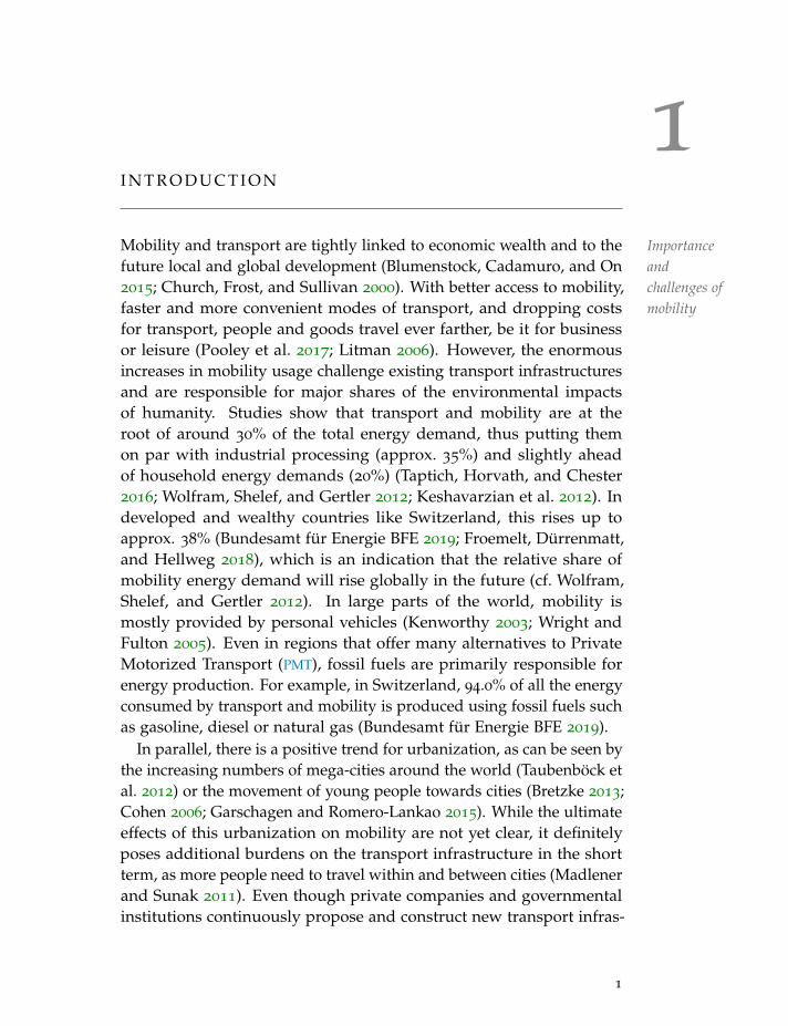
Mobility Importanceandchallenges ofmobility
and transport are tightly linked to economic wealth and to thefuture local and global development (Blumenstock, Cadamuro, and On2015; Church, Frost, and Sullivan 2000). With better access to mobility,faster and more convenient modes of transport, and dropping costsfor transport, people and goods travel ever farther, be it for businessor leisure (Pooley et al. 2017; Litman 2006). However, the enormousincreases in mobility usage challenge existing transport infrastructuresand are responsible for major shares of the environmental impactsof humanity. Studies show that transport and mobility are at theroot of around 30% of the total energy demand, thus putting themon par with industrial processing (approx. 35%) and slightly aheadof household energy demands (20%) (Taptich, Horvath, and Chester2016; Wolfram, Shelef, and Gertler 2012; Keshavarzian et al. 2012). Indeveloped and wealthy countries like Switzerland, this rises up toapprox. 38% (Bundesamt fur Energie BFE 2019; Froemelt, Durrenmatt,and Hellweg 2018), which is an indication that the relative share ofmobility energy demand will rise globally in the future (cf. Wolfram,Shelef, and Gertler 2012). In large parts of the world, mobility ismostly provided by personal vehicles (Kenworthy 2003; Wright andFulton 2005). Even in regions that offer many alternatives to PrivateMotorized Transport (PMT), fossil fuels are primarily responsible forenergy production. For example, in Switzerland, 94.0% of all the energyconsumed by transport and mobility is produced using fossil fuels suchas gasoline, diesel or natural gas (Bundesamt fur Energie BFE 2019).
In parallel, there is a positive trend for urbanization, as can be seen bythe increasing numbers of mega-cities around the world (Taubenbock etal. 2012) or the movement of young people towards cities (Bretzke 2013;Cohen 2006; Garschagen and Romero-Lankao 2015). While the ultimateeffects of this urbanization on mobility are not yet clear, it definitelyposes additional burdens on the transport infrastructure in the shortterm, as more people need to travel within and between cities (Madlenerand Sunak 2011). Even though private companies and governmentalinstitutions continuously propose and construct new transport infras-
1
2 introduction
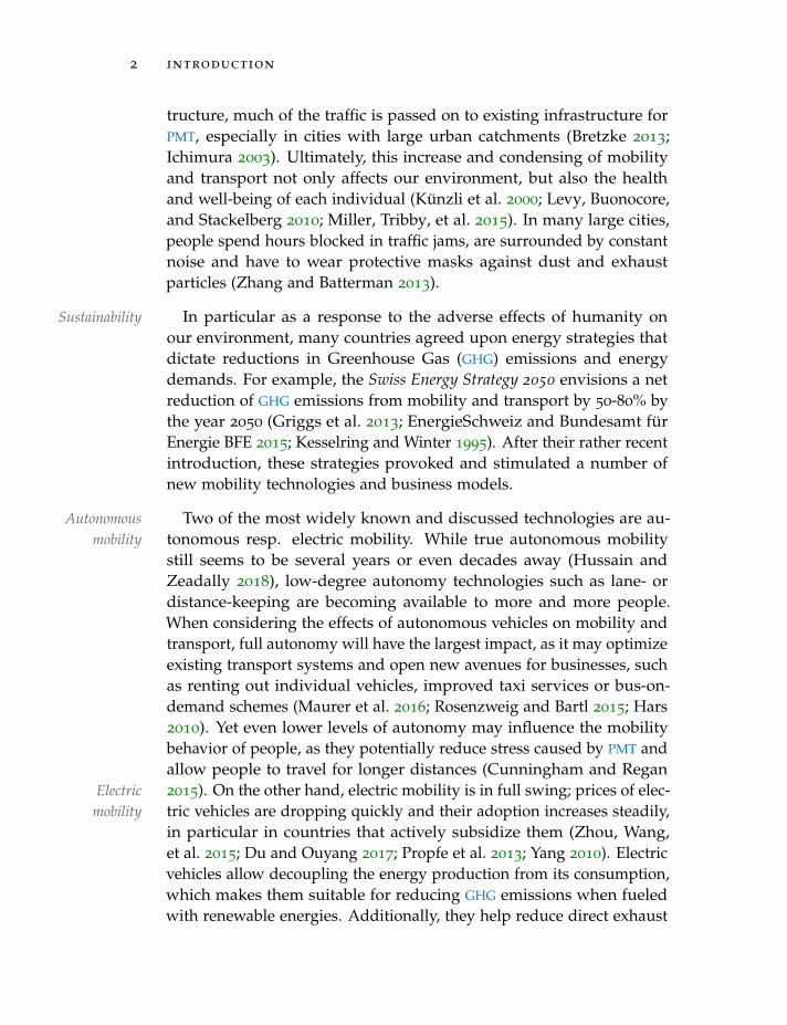
tructure, much of the traffic is passed on to existing infrastructure forPMT, especially in cities with large urban catchments (Bretzke 2013;Ichimura 2003). Ultimately, this increase and condensing of mobilityand transport not only affects our environment, but also the healthand well-being of each individual (Kunzli et al. 2000; Levy, Buonocore,and Stackelberg 2010; Miller, Tribby, et al. 2015). In many large cities,people spend hours blocked in traffic jams, are surrounded by constantnoise and have to wear protective masks against dust and exhaustparticles (Zhang and Batterman 2013).
InSustainability particular as a response to the adverse effects of humanity onour environment, many countries agreed upon energy strategies thatdictate reductions in Greenhouse Gas (GHG) emissions and energydemands. For example, the Swiss Energy Strategy 2050 envisions a netreduction of GHG emissions from mobility and transport by 50-80% bythe year 2050 (Griggs et al. 2013; EnergieSchweiz and Bundesamt furEnergie BFE 2015; Kesselring and Winter 1995). After their rather recentintroduction, these strategies provoked and stimulated a number ofnew mobility technologies and business models.
TwoAutonomousmobility
of the most widely known and discussed technologies are au-tonomous resp. electric mobility. While true autonomous mobilitystill seems to be several years or even decades away (Hussain andZeadally 2018), low-degree autonomy technologies such as lane- ordistance-keeping are becoming available to more and more people.When considering the effects of autonomous vehicles on mobility andtransport, full autonomy will have the largest impact, as it may optimizeexisting transport systems and open new avenues for businesses, suchas renting out individual vehicles, improved taxi services or bus-on-demand schemes (Maurer et al. 2016; Rosenzweig and Bartl 2015; Hars2010). Yet even lower levels of autonomy may influence the mobilitybehavior of people, as they potentially reduce stress caused by PMT andallow people to travel for longer distances (Cunningham and Regan2015).Electric
mobilityOn the other hand, electric mobility is in full swing; prices of elec-
tric vehicles are dropping quickly and their adoption increases steadily,in particular in countries that actively subsidize them (Zhou, Wang,et al. 2015; Du and Ouyang 2017; Propfe et al. 2013; Yang 2010). Electricvehicles allow decoupling the energy production from its consumption,which makes them suitable for reducing GHG emissions when fueledwith renewable energies. Additionally, they help reduce direct exhaust
introduction 3
from mobility, which especially plays a central role in bigger cities andalong frequently traveled roads (such as highways).
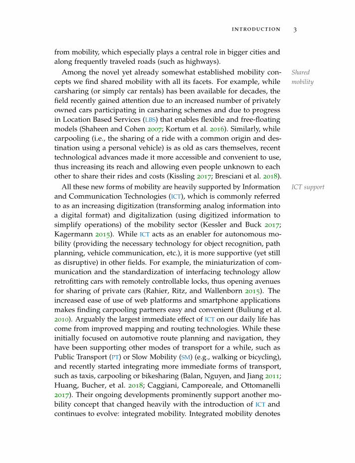
Among Sharedmobility
the novel yet already somewhat established mobility con-cepts we find shared mobility with all its facets. For example, whilecarsharing (or simply car rentals) has been available for decades, thefield recently gained attention due to an increased number of privatelyowned cars participating in carsharing schemes and due to progressin Location Based Services (LBS) that enables flexible and free-floatingmodels (Shaheen and Cohen 2007; Kortum et al. 2016). Similarly, whilecarpooling (i.e., the sharing of a ride with a common origin and des-tination using a personal vehicle) is as old as cars themselves, recenttechnological advances made it more accessible and convenient to use,thus increasing its reach and allowing even people unknown to eachother to share their rides and costs (Kissling 2017; Bresciani et al. 2018).
All ICT supportthese new forms of mobility are heavily supported by Informationand Communication Technologies (ICT), which is commonly referredto as an increasing digitization (transforming analog information intoa digital format) and digitalization (using digitized information tosimplify operations) of the mobility sector (Kessler and Buck 2017;Kagermann 2015). While ICT acts as an enabler for autonomous mo-bility (providing the necessary technology for object recognition, pathplanning, vehicle communication, etc.), it is more supportive (yet stillas disruptive) in other fields. For example, the miniaturization of com-munication and the standardization of interfacing technology allowretrofitting cars with remotely controllable locks, thus opening avenuesfor sharing of private cars (Rahier, Ritz, and Wallenborn 2015). Theincreased ease of use of web platforms and smartphone applicationsmakes finding carpooling partners easy and convenient (Buliung et al.2010). Arguably the largest immediate effect of ICT on our daily life hascome from improved mapping and routing technologies. While theseinitially focused on automotive route planning and navigation, theyhave been supporting other modes of transport for a while, such asPublic Transport (PT) or Slow Mobility (SM) (e.g., walking or bicycling),and recently started integrating more immediate forms of transport,such as taxis, carpooling or bikesharing (Balan, Nguyen, and Jiang 2011;Huang, Bucher, et al. 2018; Caggiani, Camporeale, and Ottomanelli2017). Their ongoing developments prominently support another mo-bility concept that changed heavily with the introduction of ICT andcontinues to evolve: integrated mobility. Integrated mobility denotes
4 introduction
multi-modal traveling, i.e., the use of multiple transport modes to reacha certain destination, that is actively supported by mobility and trans-port providers (i.e., they, or associated third-party service providers,implement access to transport modalities in an integrative manner;cf. Willing, Brandt, and Neumann 2017; Shaheen and Christensen 2014;Muller et al. 2004). To provide an integrative service, a train operatorcould, for example, work together with a local bikesharing providerthat solves the first/last mile problem from the train station to the finaldestination. Users of such a service would automatically receive offersand schedules from the integrated providers that conveniently get themfrom their origin to a chosen destination.
ItMobilitybehavior
is often claimed that to change mobility in the short term (andthus to reduce GHG emissions, traffic jams, etc.), people have to activelychange their behavior (Banister 2008; Prillwitz and Barr 2011; Jonietzand Bucher 2018). One possible behavioral change (among a generalreduction in travels or a switch to SM) is a transition to a more integrateduse of mobility, as it potentially increases the utilization of varioustransport modes. This higher utilization, and the fact that almost alltransport modes are more “eco-friendly” than PMT, will likely causea reduction of the environmental impacts of mobility and the relatedstress on transport systems.
BuildingMobility as aservice
heavily on technology supporting integrated mobility, thenew business model of Mobility as a Service (MAAS) aims at reducingthe burden on mobility consumers even further (Goodall and Dovey2017): It essentially offers automatic cost computation and billing forseveral (in a perfect scenario, all) modes of transport for travel, or evenreduces their cost to an upfront fixed one, reducing the variable costsof mobility to zero, and thus paving the way for an increased commodi-tization of mobility. This means that while previously people had toensure they had a properly maintained personal motorized vehicle orall the necessary PT passes, they now simply purchase mobility itself,irrespective of the actually used means of transport. This recent devel-opment resp. the term “as a service” originated from the ICT sector,where it became more and more cumbersome to keep soft- and hard-ware up to date, and maintainers started looking for ways to externalizethis infrastructure. In similar ways, MAAS also offers benefits to themaintainers, as they can highly standardize and optimize processes likemaintenance, purchase of new vehicles or ensuring their availability (cf.Nemtanu et al. 2016; Li and Voege 2017).
1.1 motivation 5
In Trackingparallel to these new or renewed forms of mobility, ICT wererecently developed that support automated and passive location track-ing (cf. Yuan, Raubal, and Liu 2012; Schussler and Axhausen 2009;Cellina, Forster, et al. 2013; Stenneth et al. 2011). These technologiesare currently primarily used for LBS such as local search or routingand navigation, but increasingly serve other mobility purposes as well,in particular in combination with spatio-temporal analyses (Huang,Gartner, et al. 2018). One basic example is data collection for statisticalpurposes, e.g., to replace survey-based mobility censuses. Other usecases of location tracking include improved transport infrastructureand city planning (Liu, Biderman, and Ratti 2009; Shoval 2008), person-alization of route planners (Cui, Luo, and Wang 2018), or the creationof (eco-)feedback that can be used to guide a person in his or her mo-bility choices, in particular with respect to ecological sustainability ofindividual mobility (Gabrielli et al. 2014; Froehlich, Dillahunt, et al.2009b; Jylha et al. 2013; Bie et al. 2012), thus playing an essential rolein the short-term reduction of GHG emissions. While theoretically notrequired for MAAS, tracking can be employed for billing and statisticalpurposes (e.g., to know how much individual mobility providers haveto be paid, or which routes are frequently used).
1.1 motivation
Giving Currentresearch
mobility (eco-)feedback to people to promote sustainable per-sonal mobility behaviors as well as the combination of MAAS offerswith location tracking are currently in the focus of research, and mostlyexist as part of pilot studies, proof-of-concept applications and recentlyfounded startups. Under the premise that more optimized mobilitychoices lead to reduced GHG emissions (and well aware of the Jevonsparadox that describes potential rebound effects; Jevons 1865), we mustdetermine how to best support people in these mobility choices. In par-ticular integrated mobility largely builds upon support by ICT, be thatthrough spatio-temporal analyses of automatically tracked data (withthe aim of improving the support, e.g., by providing better or more per-sonalized route planning) or through the integration of more transportmodes, eco-feedback, or personalization and context in applicationsand systems. While the ongoing research on route planners provides uswith quicker routes, for example by respecting the momentary traffic
6 introduction
situation, holistic support that takes into account the ecological impactsof travel, personal context or new forms of mobility is lacking.
WeResearch gap need to integrate sustainability goals next to personal goals andpreferences such as comfort, speed or price, to include novel forms ofmobility into route planning, and to provide feedback to the individualuser in order to properly support people in making sustainable mobilitychoices. Spatial and temporal information about movement and mobil-ity usage allows us to increasingly focus on individual people and theirmobility needs. Knowing about the impact of mobility usage allowsthem to reflect on their behavior, and to assess mobility options accord-ingly. Providing such (eco-)feedback within persuasive (smartphone)applications requires us to automatically process passively tracked mo-bility data, extract relevant information (in privacy-preserving ways)and use motivational elements to support people in meaningful ways.For the integration of novel forms of mobility (which do not all simplyprovide a means to get from an origin to a destination, but includedifferent peculiarities or constraints, such as spatial or temporal flexi-bility) and to enable collective outcomes, we need to adapt our currentroute planning systems to take into account a whole population, whereeach individual has its own goals and preferences. Especially conceptssuch as shared mobility rely on the communication between users, andnot just between users and transport agencies (or to put it in anotherway, “each user becomes a transport agency”). As shared mobility,and in particular MAAS, are important concepts for future mobility, itssupporting ICT must be built with these points in mind.
1.2 problem statement and research questions
Given the issues mobility and transport are currently facing, it is widelyargued that ICT must support sustainable and integrated mobility. Tothis end, sustainability criteria have to be combined with personal con-texts and preferences, as people are seldom willing to consider mobilityoptions if they are misaligned with their personal requirements. Asthis support should be as unobtrusive as possible, only giving peoplechoices and recommendations when asked for, the inclusion of personalcontext and preferences has to be automatic and passive. We can thussummarize the problem treated within this dissertation as follows:
In light of recent goals to reduce the ecological impacts of mobility and to
1.2 problem statement and research questions 7
optimize its use, a wealth of novel mobility options and concepts were devel-oped. To reach these goals, ICT must support these mobility options in anintegrated manner, taking sustainability criteria into account. It is yet unclearwhich processes are involved in this support, how they act together, and howtheir combination ultimately supports a transition towards a more ecologicaland convenient use of mobility.
This problem statement can be broken up into several research ques-tions, which will be refined and treated in later chapters:
1. What are the principal information processes and structures in-volved in supporting sustainable personal mobility and Mobilityas a Service (MAAS)?
2. What are the components and traits of automatically recordedmovement data that can be used to support mobility needs in anecologically sustainable way (e.g., by providing eco-feedback thatpeople can base their future decisions upon)?
3. How can we facilitate multi-modal route planning involving lesscommonly used modes of transport (such as carpooling or free-floating bicycles)? How can we assess the quality of the (potential)fulfillment of a transport need, taking into account personal pref-erences, contexts and potential sustainability goals?
4. How should transport options and choices be communicated tousers to support sustainable mobility behavior? Do people adjusttheir mobility behavior upon receiving (eco-)feedback based ontheir previous choices?
While the first question takes a very high-level view on the topic ofsustainable personal mobility and MAAS, building upon several researchprojects carried out during the work on this dissertation, questions twoto four consider individual processes in greater detail. Question twoconsiders location tracking and how it can be used to support personalmobility, especially in combination with question four, the commu-nication of the tracked mobility choices and the associated extractedbehavioral information. Question three considers the personalizationand collaborative nature of various mobility concepts, and how to findmeaningful mobility options, in particular when considering (currently)less frequently used modes of transport such as carpooling or free-floating bicycles, as well as potential future transport options such as
8 introduction
buses-on-demand. Finally, to effectively support sustainable personalmobility, these generated mobility choices must be communicated tousers alongside the individual feedback on mobility (question four).
1.3 contribution and scope
In essence, this dissertation aims at the development and assessmentof technology supporting sustainable personal mobility and MAAS.The core problem studied here is how to integrate automatically andpassively tracked movement and mobility data, and route planningwith the aim of providing people with sustainable and convenientmobility options.
The contributions of this dissertation can be summarized as follows:
1. Based on previous research and experience from several studies con-cerning the support of sustainable mobility through ICT, we propose amodel encompassing the information processes and structures involvedin this support. While this model is targeted at sustainable personalmobility, its individual components can be employed for a widerange of future mobility problems, such as giving meaningfulfeedback on mobility or creating personalized routing services forintegrated mobility.
2. We demonstrate how to process movement trajectories with the aim ofgenerating meaningful eco-feedback and personalized information forfurther use within route planning applications. Basing feedback andpersonalization on passively tracked location data (though notexclusively) provides an unobtrusive way of interaction with theuser, which is central when striving for a high adoption of atechnology.
3. We present novel high-level route planning methods that take intoaccount a variety of transport modes, personal context, and are ableto account for sustainability goals. In contrast to a large body ofresearch on route planning, which aims at finding novel resp.faster algorithms that work on large transport graphs, our focusis on integrated mobility and personalization.
4. Based on the research in the previous chapters, we provide a set ofcommunication strategies to nudge people towards more sustainable
1.4 structure 9
mobility behaviors. On the one hand, eco-feedback has the potentialto influence the mobility behavior of people; on the other hand,mobility options have to be communicated correctly for peopleto choose sustainable ones. Using the large-scale mobility studyGoEco!, we evaluate the proposed methods and strategies.
The presented technology, its evaluation, and the resulting societalimpacts provide a step towards a more energy-efficient use of mobility,thus reducing GHG emissions and helping to reach the sustainabilitygoals we set ourselves.
1.4 structure
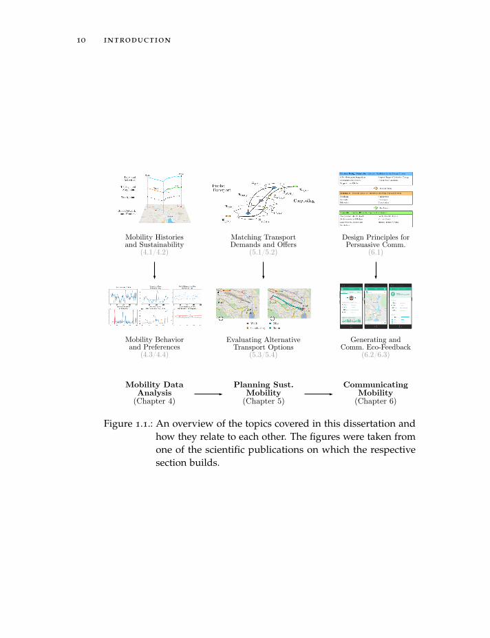
The dissertation is organized as follows: Chapter 2 introduces keyconcepts and provides definitions for the rest of the dissertation. Itends with a discussion of information processes involved in the supportof sustainable personal mobility and MAAS. Chapter 3 provides back-ground for all the processes and different emerging forms of mobilityintroduced in chapter 2. Chapters 4 to 6 each cover one part of therequired processes in supporting sustainable personal mobility. Asshown in Figure 1.1, this starts by dissecting tracked mobility, andbuilding models that capture individual mobility preferences and be-havior. Based on this information, we can generate a set of alternativetransport options and evaluate them with regards to their suitability fora single person. The last step involves communicating the unraveledaspects of a user’s mobility behavior with the intent of nudging theperson towards a more sustainable use of mobility. Finally, chapter 7
discusses all the parts in aggregation, and chapter 8 summarizes thefindings and contributions of this dissertation.
10 introduction
Mobility Historiesand Sustainability
(4.1/4.2)
Matching TransportDemands and Offers
(5.1/5.2)
Design Principles forPersuasive Comm.
(6.1)
Generating andComm. Eco-Feedback
(6.2/6.3)
Evaluating AlternativeTransport Options
(5.3/5.4)
Mobility Behaviorand Preferences
(4.3/4.4)
Mobility DataAnalysis(Chapter 4)
Planning Sust.Mobility(Chapter 5)
CommunicatingMobility(Chapter 6)
Figure 1.1.: An overview of the topics covered in this dissertation andhow they relate to each other. The figures were taken fromone of the scientific publications on which the respectivesection builds.
2I N F O R M AT I O N A N D C O M M U N I C AT I O NT E C H N O L O G I E S S U P P O RT I N G S U S TA I N A B L EP E R S O N A L M O B I L I T Y
Within this chapter, we first develop and elaborate on the core conceptsused throughout this thesis, namely sustainable mobility, integrated mobil-ity, and Mobility as a Service. In the second part, we identify how ICT
supports mobility, and in particular which processes and structures areinvolved in supporting sustainable personal mobility and sustainable Mobil-ity as a Service. To facilitate the explanations, to give concrete examplesand to evaluate our methods, we use data from four sources: the GoEco!project, the SBB Green Class study, the Swiss Mobility Census (SMC), aswell as the US National Household Travel Survey (NHTS).
The Data Sourcesidea behind the GoEco! project (cf. Bucher, Cellina, et al. 2016;Bucher, Mangili, Cellina, et al. 2019; Cellina, Bucher, Veiga Simao,et al. 2019; Cellina, Bucher, Mangili, et al. 2019) was to assess if andhow smartphone applications can influence the mobility behavior ofpeople. Inspired by applications to monitor and improve one’s ownfitness and health, GoEco! tracked peoples’ movement using the built-inGPS sensor of smartphones, and used motivational affordances such asgamification and eco-feedback to influence their mobility choices. Aspart of the experiment, around 200 people were interacting with theGoEco! app for three project phases: in the first and last (each lasting sixweeks), “baseline” mobility behavior was recorded, while during thetreatment phase in between (lasting three months), gamification wasemployed to nudge people towards more sustainable mobility behavior.
The SBB Green Class study (cf. Martin, Becker, et al. 2019) involvedapprox. 140 people who were given a general Public Transport (PT)pass (valid for unlimited travels throughout Switzerland), a privateElectric Vehicle (EV), as well as access to several mobility offers (car-and bikesharing, park and ride parking spaces, etc.) as part of a MAAS
offer. The idea of the Swiss Federal Railways (SBB) was to identify how
This chapter is based on Weiser, Scheider, et al. 2016; Bucher, Cellina, et al. 2016;Bucher, Weiser, et al. 2015; Bucher, Scheider, and Raubal 2017; Bucher, Mangili, Cellina,et al. 2019.
11
12 ict supporting sustainable personal mobility
people would use mobility if they were given commoditized accessfor an upfront fixed cost: Would they stop using trains and shift theirmobility consumption towards PMT resp. their newly available EV?Ultimately, the study aimed at answering the question if it would stillbe possible for SBB to position itself as a railway operator in the future,or if, due to the increasing digitalization and appearance of MAAS offers,it would have to shift its focus on becoming a mobility provider.
The SMC1 (cf. Biedermann et al. 2017) and NHTS2 (cf. McGuckin andFucci 2018) are censuses conducted by the governments of Switzerlandand the United States of America, respectively. They both involve arepresentative and statistically significant number of citizens that wereasked for their travel patterns during a single day. We primarily use thecensus data to put the developed methods into a bigger perspective.
2.1 the role of individual circumstances
To exemplify and facilitate the understanding of the impact of individ-ual circumstances on mobility choices, we introduce three personas.These personas correspond to real people from the GoEco! project, butare used in an exemplary way here, standing for respective groups ofthe population. This means that while their movement and mobilitywas recorded (using a tracking app on their smartphone) as shown inthe next sections, they represent hypothetical users in similar geograph-ical contexts, and their individual journeys and demographic attributesare not uncovered here. Where applicable and appropriate, we willrefer to the corresponding groups of the population by using data fromthe SMC and NHTS instead of the individual personas.
AliceMobilityPersonas
is a typical city dweller, living in a city with good public trans-port, comparably short distances, but restricted freedom for privatemotorized vehicles (i.e., many limited speed areas, one-way streets,traffic lights, etc.). Alice does not own a car nor does she participate inany particular (car-, bike-)sharing programs. She owns a public trans-port pass for the city, offering her fixed-cost access to trams and buses.Bob lives in a suburban area of the same city. In addition to owninga private car, he has a public transport pass allowing him fixed-costaccess to the city. Charlie lives in a rural area far from any major city,
1 The mobility census can be requested from www.bfs.admin.ch.2 The US National Household Travel Survey can be downloaded from nhts.ornl.gov.
2.1 the role of individual circumstances 13
and thus mostly relies on a car for travel. He does not have access toany other mobility tools except an irregularly running bus, for whichhe owns no pass, thus inducing a variable cost for him.
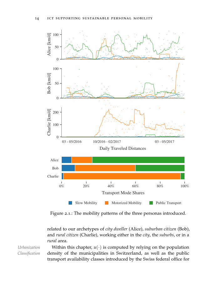
Figure 2.1 shows the daily distances each of these personas coverson top. On the bottom, the transport mode resp. modal split of thethree personas (in terms of distance covered) is displayed. As can beexpected, Alice mostly relies on public transport, Bob uses a mixturebetween public and private motorized transport, while Charlie almostsolely travels by car (note that he did not participate in the first projectphase). While we make no statements about the correlation of themodal split and weekly distances here, this figure is intended to showthat all of them cover significant distances each week, which is in linewith findings from studies analyzing the travel behavior in developedcountries (Metz 2012) as well as the SMC (Biedermann et al. 2017).
As GeneralMobilityContext
is already implied from these personas, individual context andcircumstances play a large role when planning and choosing mobilitynext to personal attitudes, values and goals (e.g., Ferdous et al. 2011;Atasoy, Glerum, and Bierlaire 2013; Kim and Ulfarsson 2008). Inparticular the general mobility patterns of a person (depicted in Figure 2.1on the bottom) are primarily defined by a few often-traveled routesthat usually involve the home and work locations (Do and Gatica-Perez2014; Schneider, Belik, et al. 2013). Their distances and connectionsto public transport, and the availability of transport passes or MAAS
offers drive the overall mobility consumption (Lachapelle and Frank2009; Yang et al. 2015). We thus introduce a measure of individualcircumstances by looking at a person’s mobility options in a holisticmanner to generalize from the three introduced personas. Based onthe locations of home and work, we use a location classification thatassigns each location on the map a value of either city, suburb or ruralto define a user’s general mobility context:
CGM = (u(fH), u(fW)) (2.1)
where fH and fW are features resp. properties of the home and worklocation, and u(·) is the function that maps any given location (specifiedby longitude and latitude) to an “urbanization class”. This classificationinto a set of locations L = {city, suburb, rural} is commonly found inthe literature (cf. Zhou, Xu, et al. 2004; Short Gianotti et al. 2016; Renski2008) and is also used in a similar form by various travel censuses.Using this formalism, we can build nine different user groups that are
14 ict supporting sustainable personal mobility
Figure 2.1.: The mobility patterns of the three personas introduced.
related to our archetypes of city dweller (Alice), suburban citizen (Bob),and rural citizen (Charlie), working either in the city, the suburbs, or in arural area.
WithinUrbanizationClassification
this chapter, u(·) is computed by relying on the populationdensity of the municipalities in Switzerland, as well as the publictransport availability classes introduced by the Swiss federal office for
2.1 the role of individual circumstances 15
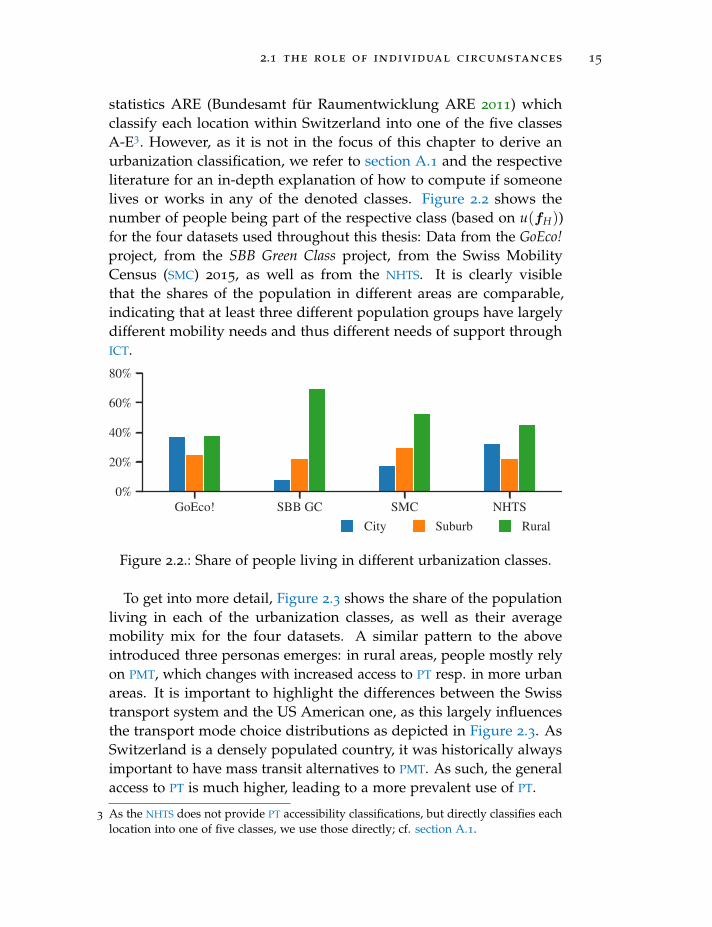
statistics ARE (Bundesamt fur Raumentwicklung ARE 2011) whichclassify each location within Switzerland into one of the five classesA-E3. However, as it is not in the focus of this chapter to derive anurbanization classification, we refer to section A.1 and the respectiveliterature for an in-depth explanation of how to compute if someonelives or works in any of the denoted classes. Figure 2.2 shows thenumber of people being part of the respective class (based on u(fH))for the four datasets used throughout this thesis: Data from the GoEco!project, from the SBB Green Class project, from the Swiss MobilityCensus (SMC) 2015, as well as from the NHTS. It is clearly visiblethat the shares of the population in different areas are comparable,indicating that at least three different population groups have largelydifferent mobility needs and thus different needs of support throughICT.
GoEco! SBB GC SMC NHTS0%
20%
40%
60%
80%
City Suburb Rural
Figure 2.2.: Share of people living in different urbanization classes.
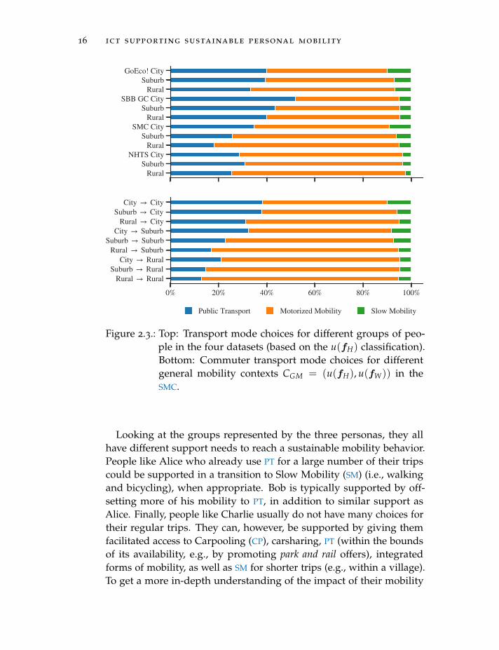
To get into more detail, Figure 2.3 shows the share of the populationliving in each of the urbanization classes, as well as their averagemobility mix for the four datasets. A similar pattern to the aboveintroduced three personas emerges: in rural areas, people mostly relyon PMT, which changes with increased access to PT resp. in more urbanareas. It is important to highlight the differences between the Swisstransport system and the US American one, as this largely influencesthe transport mode choice distributions as depicted in Figure 2.3. AsSwitzerland is a densely populated country, it was historically alwaysimportant to have mass transit alternatives to PMT. As such, the generalaccess to PT is much higher, leading to a more prevalent use of PT.
3 As the NHTS does not provide PT accessibility classifications, but directly classifies eachlocation into one of five classes, we use those directly; cf. section A.1.
16 ict supporting sustainable personal mobility
GoEco! CitySuburb
RuralSBB GC City
SuburbRural
SMC CitySuburb
RuralNHTS City
SuburbRural
0% 20% 40% 60% 80% 100%
City CitySuburb City
Rural CityCity Suburb
Suburb SuburbRural Suburb
City RuralSuburb Rural
Rural Rural
Public Transport Motorized Mobility Slow Mobility
Figure 2.3.: Top: Transport mode choices for different groups of peo-ple in the four datasets (based on the u(fH) classification).Bottom: Commuter transport mode choices for differentgeneral mobility contexts CGM = (u(fH), u(fW)) in theSMC.
Looking at the groups represented by the three personas, they allhave different support needs to reach a sustainable mobility behavior.People like Alice who already use PT for a large number of their tripscould be supported in a transition to Slow Mobility (SM) (i.e., walkingand bicycling), when appropriate. Bob is typically supported by off-setting more of his mobility to PT, in addition to similar support asAlice. Finally, people like Charlie usually do not have many choices fortheir regular trips. They can, however, be supported by giving themfacilitated access to Carpooling (CP), carsharing, PT (within the boundsof its availability, e.g., by promoting park and rail offers), integratedforms of mobility, as well as SM for shorter trips (e.g., within a village).To get a more in-depth understanding of the impact of their mobility
2.2 sustainable mobility 17
lifestyles, we have to define ecological sustainability within the contextof mobility.
2.2 sustainable mobility
While the term sustainability has been used for a long time (originallywithin the context of forestry, cf. Wiersum 1995), its modern use wascoined by a report from the World Commission on Environment andDevelopment (Keeble 1988) where it is described as “developmentthat meets the needs of the present without compromising the abilityof future generations to meet their own needs” (Keeble 1988, p.41).Since then, however, its meaning has evolved and the term is primarilyinterpreted along three dimensions: social, economic and environmen-tal (Kuhlman and Farrington 2010; Kates, Parris, and Leiserowitz 2005).
2.2.1 Types of Sustainability
Being socially sustainable can refer to the maintenance of law and order,meaning that societies do not deteriorate, but also to various societalcharacteristics such as income distribution, employment or access tomedical services (Kuhlman and Farrington 2010). Economic sustainabilityis a term commonly used within the context of companies and gov-ernments and describes the concept of healthy investments, i.e., thelong-term management and securing of a business’ value and monetaryresources. In a wider context, it also describes the relationships betweeneconomies and (sustainable) societal and environmental developments(Spangenberg 2005; Goerner, Lietaer, and Ulanowicz 2009). Within thecontext of this dissertation, we are mainly concerned with ecologicalsustainability, i.e., the continuous use of natural resources without im-pacting future generations’ possibilities to use them (Perrings 1991). Ina broader and currently more used context this also refers to boundingthe emission of GHG, with the aim of keeping the effects of humanity onthe global environment within certain bounds. Occasionally, cultural,technological and political dimensions are added to this list, whichrefer to the maintenance of cultural heritage, technological progressresp. a political climate that allows future generations to have the samechoices as we do today (Gibson 2001).
18 ict supporting sustainable personal mobility
The differentiation between social and economic sustainability isdisputed, as it can be argued that ultimately they measure the sameand “weighting” social and economic aspects twice as much as en-vironmental factors results in a bias towards “the well-being of thepresent generation, [while weighting] environmental [factors strongerwould] mean caring about the future” (Kuhlman and Farrington 2010,p.3439). Kuhlman and Farrington 2010 go even further, and equatesustainability defined based on these three pillars with the concept ofbeing “good”, arguing that this definition obscures its definition andmeaning. Instead, it is proposed to define sustainability in terms ofmaintaining well-being, which is easier to measure (e.g., by consideringaccess to food, shelter, education, etc.), over an indefinite amount oftime. While the discussion of what constitutes sustainability is im-portant and will continue to be led, we primarily focus on ecologicalsustainability within this thesis.
AStrong andWeak
Sustainability
second dimension contrasts strong and weak sustainability. Whileweak sustainability equates human (infrastructure, labor, knowledge,etc.) and natural capital (fossil fuels, biodiversity, etc.), the conceptof strong sustainability sees them as complementary and argues thatcertain parts of nature can never be made up for by human capital (e.g.,the ozone layer should never be compromised, as no gain in humancapital can compensate for the lack of its crucial service). A large shareof trips are made to increase human capital (e.g., for business meetings,to transport goods, or as part of a high quality of life), which makes adetailed contrasting juxtaposition between effects on human and naturalcapital necessary. In line with current trends (that favor the concept ofstrong sustainability, cf. Pelenc, Ballet, and Dedeurwaerdere 2015; Baruaand Khataniar 2016) and to keep this thesis focused on the supportof mobility choices using ICT, we primarily view the problem fromthe point of strong sustainability, arguing that the exhaustion of fossilfuels and the emission of GHG should be avoided in any case. However,to provide a more in-depth understanding of the trade-offs from thestandpoint of weak sustainability, we highlight the juxtaposition ofhuman and natural capital within this chapter and present ways toassess the sustainability of trips in chapter 4.
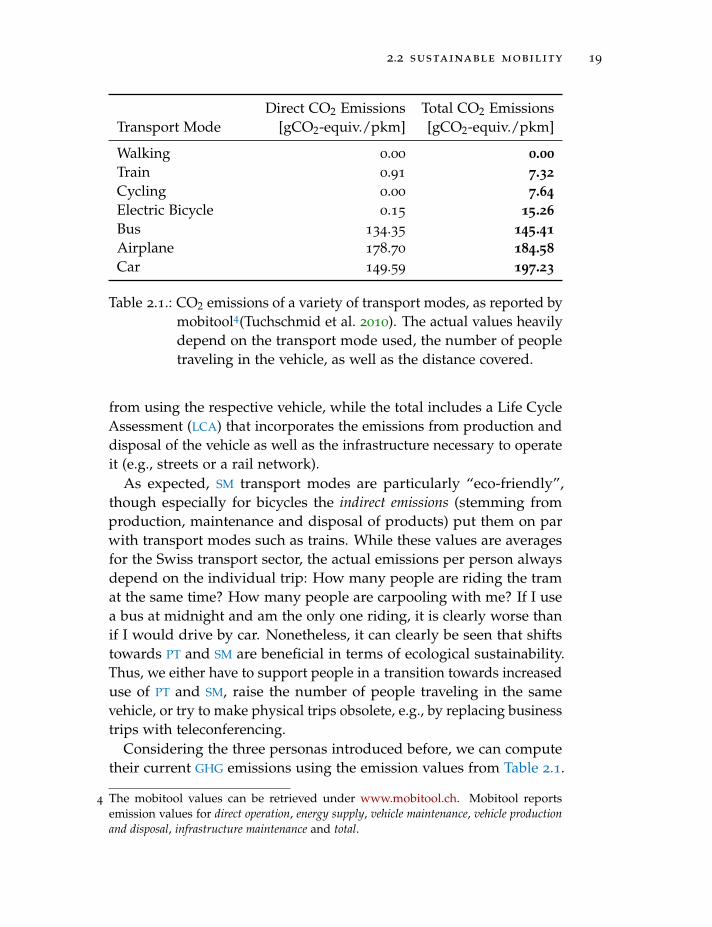
Before this background, it is necessary to consider the GHG emis-sions of various transport modes. Table 2.1 shows emission valuesfor various transport modes taken from the Switzerland-specific mo-bitool (Tuchschmid et al. 2010). The direct CO2 emissions result solely
2.2 sustainable mobility 19
Transport ModeDirect CO2 Emissions
[gCO2-equiv./pkm]Total CO2 Emissions[gCO2-equiv./pkm]
Walking 0.00 0.00Train 0.91 7.32Cycling 0.00 7.64Electric Bicycle 0.15 15.26Bus 134.35 145.41Airplane 178.70 184.58Car 149.59 197.23
Table 2.1.: CO2 emissions of a variety of transport modes, as reported bymobitool4(Tuchschmid et al. 2010). The actual values heavilydepend on the transport mode used, the number of peopletraveling in the vehicle, as well as the distance covered.
from using the respective vehicle, while the total includes a Life CycleAssessment (LCA) that incorporates the emissions from production anddisposal of the vehicle as well as the infrastructure necessary to operateit (e.g., streets or a rail network).
As expected, SM transport modes are particularly “eco-friendly”,though especially for bicycles the indirect emissions (stemming fromproduction, maintenance and disposal of products) put them on parwith transport modes such as trains. While these values are averagesfor the Swiss transport sector, the actual emissions per person alwaysdepend on the individual trip: How many people are riding the tramat the same time? How many people are carpooling with me? If I usea bus at midnight and am the only one riding, it is clearly worse thanif I would drive by car. Nonetheless, it can clearly be seen that shiftstowards PT and SM are beneficial in terms of ecological sustainability.Thus, we either have to support people in a transition towards increaseduse of PT and SM, raise the number of people traveling in the samevehicle, or try to make physical trips obsolete, e.g., by replacing businesstrips with teleconferencing.
Considering the three personas introduced before, we can computetheir current GHG emissions using the emission values from Table 2.1.
4 The mobitool values can be retrieved under www.mobitool.ch. Mobitool reportsemission values for direct operation, energy supply, vehicle maintenance, vehicle productionand disposal, infrastructure maintenance and total.
20 ict supporting sustainable personal mobility
Persona
Current GHG
emissions[kg/week]
Potential GHG
emissions[kg/week]
Average GHG
emissions (SMC)[kg/week]
Alice (City) 12.90 5.70 57.22
Bob (Suburban) 14.15 11.57 71.84
Charlie (Rural) 84.66 42.60 71.42
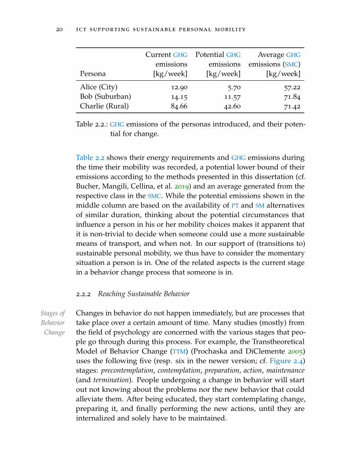
Table 2.2.: GHG emissions of the personas introduced, and their poten-tial for change.
Table 2.2 shows their energy requirements and GHG emissions duringthe time their mobility was recorded, a potential lower bound of theiremissions according to the methods presented in this dissertation (cf.Bucher, Mangili, Cellina, et al. 2019) and an average generated from therespective class in the SMC. While the potential emissions shown in themiddle column are based on the availability of PT and SM alternativesof similar duration, thinking about the potential circumstances thatinfluence a person in his or her mobility choices makes it apparent thatit is non-trivial to decide when someone could use a more sustainablemeans of transport, and when not. In our support of (transitions to)sustainable personal mobility, we thus have to consider the momentarysituation a person is in. One of the related aspects is the current stagein a behavior change process that someone is in.
2.2.2 Reaching Sustainable Behavior
ChangesStages ofBehaviorChange
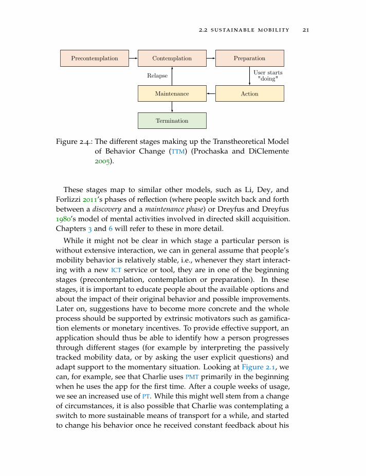
in behavior do not happen immediately, but are processes thattake place over a certain amount of time. Many studies (mostly) fromthe field of psychology are concerned with the various stages that peo-ple go through during this process. For example, the TranstheoreticalModel of Behavior Change (TTM) (Prochaska and DiClemente 2005)uses the following five (resp. six in the newer version; cf. Figure 2.4)stages: precontemplation, contemplation, preparation, action, maintenance(and termination). People undergoing a change in behavior will startout not knowing about the problems nor the new behavior that couldalleviate them. After being educated, they start contemplating change,preparing it, and finally performing the new actions, until they areinternalized and solely have to be maintained.
2.2 sustainable mobility 21
Precontemplation
Relapse User starts"doing"
Contemplation Preparation
Maintenance
Termination
Action
Figure 2.4.: The different stages making up the Transtheoretical Modelof Behavior Change (TTM) (Prochaska and DiClemente2005).
These stages map to similar other models, such as Li, Dey, andForlizzi 2011’s phases of reflection (where people switch back and forthbetween a discovery and a maintenance phase) or Dreyfus and Dreyfus1980’s model of mental activities involved in directed skill acquisition.Chapters 3 and 6 will refer to these in more detail.
While it might not be clear in which stage a particular person iswithout extensive interaction, we can in general assume that people’smobility behavior is relatively stable, i.e., whenever they start interact-ing with a new ICT service or tool, they are in one of the beginningstages (precontemplation, contemplation or preparation). In thesestages, it is important to educate people about the available options andabout the impact of their original behavior and possible improvements.Later on, suggestions have to become more concrete and the wholeprocess should be supported by extrinsic motivators such as gamifica-tion elements or monetary incentives. To provide effective support, anapplication should thus be able to identify how a person progressesthrough different stages (for example by interpreting the passivelytracked mobility data, or by asking the user explicit questions) andadapt support to the momentary situation. Looking at Figure 2.1, wecan, for example, see that Charlie uses PMT primarily in the beginningwhen he uses the app for the first time. After a couple weeks of usage,we see an increased use of PT. While this might well stem from a changeof circumstances, it is also possible that Charlie was contemplating aswitch to more sustainable means of transport for a while, and startedto change his behavior once he received constant feedback about his
22 ict supporting sustainable personal mobility
mobility. To make a distinction between voluntary behavior changesand effects that arise due to a change in circumstances, it is importantthat the context can be captured by an application in one way or another.These circumstances are often also the primary precondition to supportpeople in a meaningful way.
2.2.3 The Role of Immediate Context
Context has been defined in a number of domain-specific ways (Bazireand Brezillon 2005; Keßler, Raubal, and Janowicz 2007), and as alreadyhighlighted before, plays a central role when choosing mobility options,in a similar way as goals, expectations, attitudes, beliefs and valuesdo (e.g., Ferdous et al. 2011; Atasoy, Glerum, and Bierlaire 2013; Kimand Ulfarsson 2008). While the latter are related to the behavior in avery general way, and can usually be changed at varying speeds bytaking into account the models of behavior change introduced in theprevious section, context is more immediate and requires or enablessparks and facilitators (Fogg 2009) to help a person choose the mostoptimal transport option in a given situation. In the model by Fogg2009, a spark is a motivational trigger that increases the motivation of auser at the decision point, while a facilitator increases a person’s ability(this can also include the provision of new or different mobility optionsthat the user is unaware of). In the context of mobility, a spark couldbe given by a mobile app by offering an immediate reward for using asustainable transport mode once a person starts moving somewhere. Afacilitator could be the provision of a carpooling opportunity or if anapp points to a bikesharing station close by.
AsImmediateMobilityContext
already introduced above, there are various scopes of context wehave to consider. The general mobility context can be used to determinethe potential support for a user on a holistic level. The momentaryor immediate context, on the other hand, is primarily important forimmediate (i.e., real-time) support of a person. Considering thesepersonal and spatio-temporal circumstances, we adopt a formalizationof a user u’s immediate context when searching for transport options toperform a trip θ (from an origin O to a destination D) as:
Cu,θ = (fO,fD, Φ) (2.2)
where fO and fD describe properties (or features) of origin (the per-son’s momentary position) and destination, and Φ denotes the personal
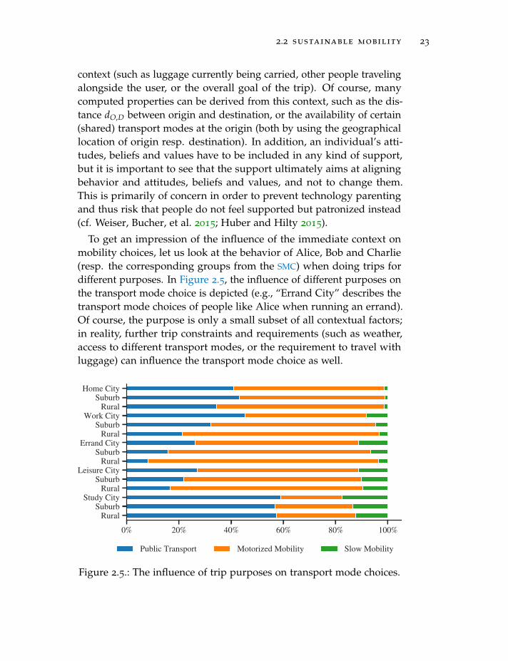
2.2 sustainable mobility 23
context (such as luggage currently being carried, other people travelingalongside the user, or the overall goal of the trip). Of course, manycomputed properties can be derived from this context, such as the dis-tance dO,D between origin and destination, or the availability of certain(shared) transport modes at the origin (both by using the geographicallocation of origin resp. destination). In addition, an individual’s atti-tudes, beliefs and values have to be included in any kind of support,but it is important to see that the support ultimately aims at aligningbehavior and attitudes, beliefs and values, and not to change them.This is primarily of concern in order to prevent technology parentingand thus risk that people do not feel supported but patronized instead(cf. Weiser, Bucher, et al. 2015; Huber and Hilty 2015).
To get an impression of the influence of the immediate context onmobility choices, let us look at the behavior of Alice, Bob and Charlie(resp. the corresponding groups from the SMC) when doing trips fordifferent purposes. In Figure 2.5, the influence of different purposes onthe transport mode choice is depicted (e.g., “Errand City” describes thetransport mode choices of people like Alice when running an errand).Of course, the purpose is only a small subset of all contextual factors;in reality, further trip constraints and requirements (such as weather,access to different transport modes, or the requirement to travel withluggage) can influence the transport mode choice as well.
0% 20% 40% 60% 80% 100%
Home CitySuburb
RuralWork City
SuburbRural
Errand CitySuburb
RuralLeisure City
SuburbRural
Study CitySuburb
Rural
Public Transport Motorized Mobility Slow Mobility
Figure 2.5.: The influence of trip purposes on transport mode choices.
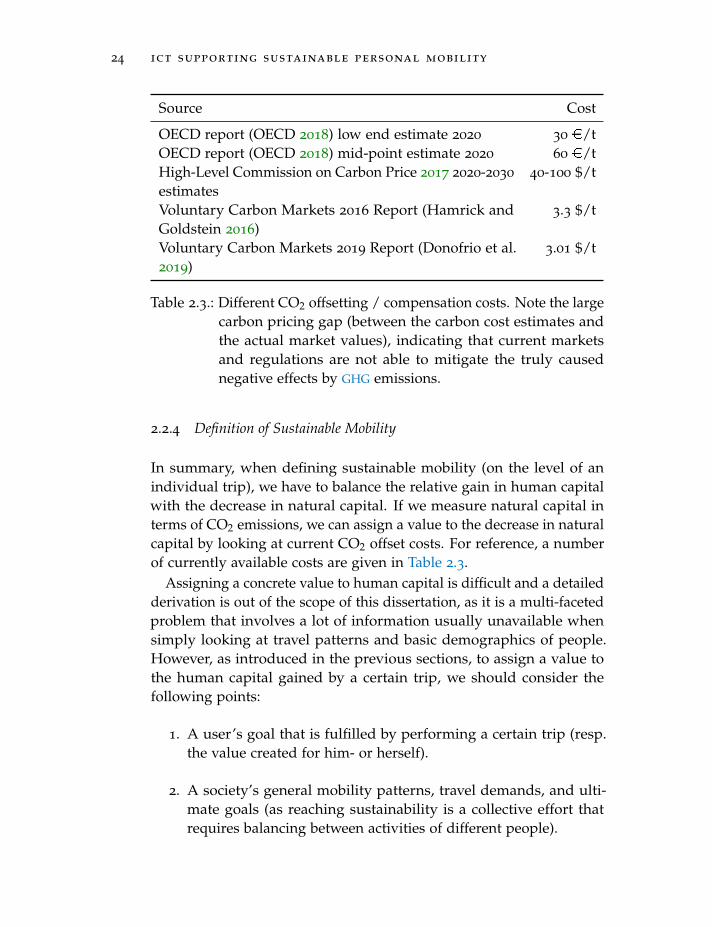
24 ict supporting sustainable personal mobility
Source Cost
OECD report (OECD 2018) low end estimate 2020 30 e/tOECD report (OECD 2018) mid-point estimate 2020 60 e/tHigh-Level Commission on Carbon Price 2017 2020-2030
estimates40-100 $/t
Voluntary Carbon Markets 2016 Report (Hamrick andGoldstein 2016)
3.3 $/t
Voluntary Carbon Markets 2019 Report (Donofrio et al.2019)
3.01 $/t
Table 2.3.: Different CO2 offsetting / compensation costs. Note the largecarbon pricing gap (between the carbon cost estimates andthe actual market values), indicating that current marketsand regulations are not able to mitigate the truly causednegative effects by GHG emissions.
2.2.4 Definition of Sustainable Mobility
In summary, when defining sustainable mobility (on the level of anindividual trip), we have to balance the relative gain in human capitalwith the decrease in natural capital. If we measure natural capital interms of CO2 emissions, we can assign a value to the decrease in naturalcapital by looking at current CO2 offset costs. For reference, a numberof currently available costs are given in Table 2.3.
Assigning a concrete value to human capital is difficult and a detailedderivation is out of the scope of this dissertation, as it is a multi-facetedproblem that involves a lot of information usually unavailable whensimply looking at travel patterns and basic demographics of people.However, as introduced in the previous sections, to assign a value tothe human capital gained by a certain trip, we should consider thefollowing points:
1. A user’s goal that is fulfilled by performing a certain trip (resp.the value created for him- or herself).
2. A society’s general mobility patterns, travel demands, and ulti-mate goals (as reaching sustainability is a collective effort thatrequires balancing between activities of different people).
2.3 integrated mobility and mobility as a service 25
3. A user’s momentary context, including travel requirements aswell as access to various transport modes, both physical as wellas from an economic point-of-view.
Formalizing this, we can capture the dependency of the humancapital gain Gh(θ) of a single trip θ on the various introduced factors asfollows:
Gh(θ) = f (Cu,θ , Gu, GS) (2.3)
where Gu and GS represent the goals of an individual resp. the societythe person is part of, and Cu,θ is defined as above. Adopting a weakinterpretation of sustainability, a trip θ can be considered “sustainable”,if the gain in human capital Gh(θ) is larger than the loss in naturalcapital Ln(θ):
Gh(θ) ≥ Ln(θ) (2.4)
It follows trivially that we either must reduce Ln, increase Gh, or donot engage in “unimportant” journeys. Even though it is not strictly nec-essary to achieve Ln(θ) = 0 under the definition of weak sustainability,there are two aspects that are worthy of pointing out:
• It is generally argued that humanity needs to drastically decreaseits reliance on fossil energy sources and reduce the thus causedGHG emissions. This argumentation implicitly corresponds to thefact that Ln(θ)� Gh(θ) for many trips.
• Ecological sustainability must be achieved by a society as a whole.While not directly visible in the above formula, GS incorporatesthe fact that some trips are of high importance to a society, yetit cannot be avoided that their Ln(θ) is very large (e.g., flights ofimportant decision makers or stakeholders).
In chapter 4, we will further elaborate on the topic by analyzing how(and how well) we can infer the sustainability of a given trip based onrecorded mobility data.
2.3 integrated mobility and mobility as a service
While people always had the freedom to shape their use of mobilityas they wanted (e.g., inter-modal, namely using different modes oftransport), integrated mobility denotes the concept of actively supportedinter-modal use of mobility. This active support is primarily coming from
26 ict supporting sustainable personal mobility
transport providers and third-party companies that facilitate the use ofdifferent modal combinations. Of course, this is closely related to MAAS,where a provider aims to bundle all possible mobility options, andprovide a seamless and integrated access to the individual transportmodes.
2.3.1 Multi-Modal Transport and Integrated Mobility
Multi-modality has always been important especially for public trans-port, where people usually combine multiple transport modes (at leastwalking plus a form of public transport, but often also multiple formsof PT, such as bus and train). More densely populated urban areas andnewly created mobility offers (which have their origin in the increaseddigitalization of the mobility sector and in the sustainability goals set bymany governments) further increased the use of multi-modal mobility.Many ICT companies additionally started offering mobility planningin an integrative manner: while for some third-party providers thismostly consists of combining multiple transport options within a sin-gle application, the transport providers themselves try to increase theusage of their transport modalities by offering people easy access tovarious first-/last-mile providers (e.g., the SBB integrate their train routeplanners with bikesharing offers in order to get people to/from thetrain stations).
Considering the three personas introduced above and the groupsthey stand for, multi-modal travel traditionally primarily concernsAlice (city-dweller) and Bob (living in a suburb), as Charlie (in a ruralarea) mostly drives by car (door-to-door). Looking at their use ofmulti-modal transport, we can see that Charlie does not often combinemultiple transport modes (except for car and walking), while Alice usesvarious forms of transport in combination to satisfy her travel needs.Figure 2.6 shows their use of various transport mode combinations.
The integration of various transport modes was supported early onby multi-modal route planners, either developed and supported bythe public transport providers themselves or by third-party travel andtransport companies. Recently, transport agencies have been focusingeven stronger on the integration of mobility: SBB, for example, launchedseveral offers in cooperation with other (complementary) providerswith the idea that people who have facilitated access to first-/last-miletransport modes would also be more likely to use their train network for
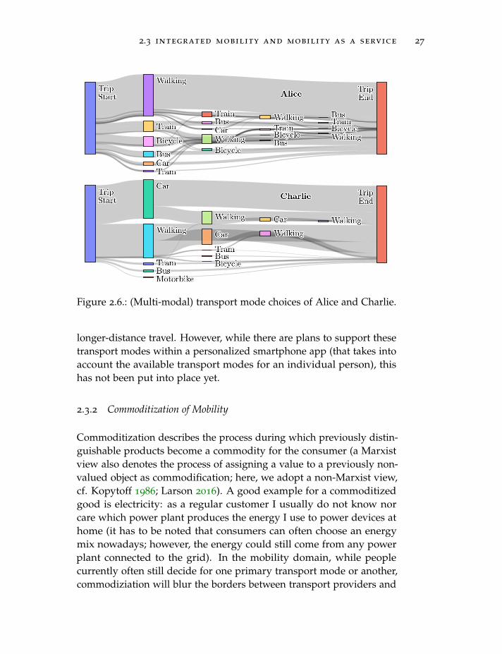
2.3 integrated mobility and mobility as a service 27
Figure 2.6.: (Multi-modal) transport mode choices of Alice and Charlie.
longer-distance travel. However, while there are plans to support thesetransport modes within a personalized smartphone app (that takes intoaccount the available transport modes for an individual person), thishas not been put into place yet.
2.3.2 Commoditization of Mobility
Commoditization describes the process during which previously distin-guishable products become a commodity for the consumer (a Marxistview also denotes the process of assigning a value to a previously non-valued object as commodification; here, we adopt a non-Marxist view,cf. Kopytoff 1986; Larson 2016). A good example for a commoditizedgood is electricity: as a regular customer I usually do not know norcare which power plant produces the energy I use to power devices athome (it has to be noted that consumers can often choose an energymix nowadays; however, the energy could still come from any powerplant connected to the grid). In the mobility domain, while peoplecurrently often still decide for one primary transport mode or another,commodiziation will blur the borders between transport providers and
28 ict supporting sustainable personal mobility
transport modes, letting people choose whichever option satisfies theirtransport needs best, irrespective of brand or price. Looking at howmost people have access to mobility nowadays, one could argue thatmobility already is a commoditized good, at least as far as it will everget (as there will always be significant differences, e.g., between a carand a train). However, we can see a novel view on mobility especiallywith younger people living in cities. Many of them do not own a carnor a driver’s license, and increasingly use a diverse mix of mobilityoptions to satisfy their travel needs (Metz 2012).
WhileMobility as aService
public transport providers have cooperated for a long time tooffer transport passes including various means of transport at a fixedcost, recently, alongside a new wave of novel mobility concepts, theyhave gone further, including not only public but also private means oftransport (Martin, Becker, et al. 2019). These are commonly referred toas MAAS offers, and encompass several competing models, e.g., payingan upfront fixed price, or involving automatic billing systems. MAAS
is a term coined by the “XX-as-a-Service” construct from softwarebusinesses (Xin and Levina 2008), where the main selling point is thatit is easier and more cost-effective to “outsource” certain functionalityto an external supplier (who is specialized in this service). In a similarway the idea of MAAS is that the consumer does not have to think aboutmobility (and in particular which mobility supplier to choose) anymore,but just consumes it like any other commodity.
Looking at the example of SBB, their primary MAAS offer is calledSBB Green Class, and includes a general public transport pass, an EV
(out of a selection of four different models), a parking space at the trainstation, as well as access to several car- and bikesharing platforms for afixed monthly cost (in the range of CHF 1070 to 2290, depending onthe electric vehicle and the general public transport pass). If we lookat Figure 2.7, we can see that the use of mobility changes after peoplestart using MAAS, mostly due to the newly available EV. The data inthis figure stems from the pilot study that was used to evaluate the SBBGreen Class offer before making it available to the general public5.
5 Note that the participants of the pilot received their EV at the start of the study(approximately in week 3 of 2017) which explains the sudden increase in EV usage.
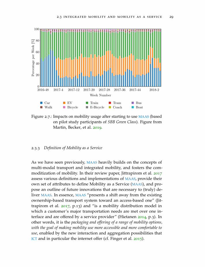
2.3 integrated mobility and mobility as a service 29
Percentagepe
rWeek[%
]100
80
60
40
20
02016-48
Car
Week Number
Walk Bicycle E-Bicycle Coach BoatEV Train Tram Bus
2017-4 2017-12 2017-20 2017-28 2017-36 2017-44 2018-2
Figure 2.7.: Impacts on mobility usage after starting to use MAAS (basedon pilot study participants of SBB Green Class). Figure fromMartin, Becker, et al. 2019.
2.3.3 Definition of Mobility as a Service
As we have seen previously, MAAS heavily builds on the concepts ofmulti-modal transport and integrated mobility, and fosters the com-moditization of mobility. In their review paper, Jittrapirom et al. 2017
assess various definitions and implementations of MAAS, provide theirown set of attributes to define Mobility as a Service (MAAS), and pro-pose an outline of future innovations that are necessary to (truly) de-liver MAAS. In essence, MAAS “presents a shift away from the existingownership-based transport system toward an access-based one” (Jit-trapirom et al. 2017, p.13) and “is a mobility distribution model inwhich a customer’s major transportation needs are met over one in-terface and are offered by a service provider” (Hietanen 2014, p.3). Inother words, it is the packaging and offering of a range of mobility options,with the goal of making mobility use more accessible and more comfortable touse, enabled by the new interaction and aggregation possibilities thatICT and in particular the internet offer (cf. Finger et al. 2015).
30 ict supporting sustainable personal mobility
BuildingCharacteris-tics of MAAS
on work by Hietanen 2014, Kamargianni, Li, et al. 2016,Kamargianni and Matyas 2017, Jittrapirom et al. 2017 further elabo-rate on the need of personalization, integration of subscription-basedconsumption, collection and processing of data to identify the besttransport solutions, mediation between providers and consumers, theimpact of Internet of Things (IOT), as well as the relation of MAAS to theconcept of a smart city. Their identified core characteristics of MAAS aregiven in Table 2.4. Note that we did not show the registration requirement(common for most internet-based services), the inclusion of other services(part of multiple actors) and the mobility currency (independent of MAAS),as we argue they are not central to a definition of MAAS. It is interestingto see that they additionally identified decision influence as a separatecharacteristic by reviewing various case studies, similar in spirit to thesupport of certain mobility behaviors as treated within this thesis. Suchinfluence systems have been part of several MAAS (pilot) offers, but anextensive treatment of supporting technology is not given. Similar toPangbourne et al. 2018, Jittrapirom et al. 2017 point out several aspectsof MAAS that have to be considered carefully, such as its relation tosustainable mobility (which, according to Holmberg et al. 2016, must beensured by proper tariffs, and according to other authors forms a coreelement of MAAS), its sociological implications (in particular with re-spect to low-density areas and low-income households), or operationalimpacts. Additionally, Pangbourne et al. 2018 provide a more in-depthtreatment of the issue of resilience (what happens if a large mobilityprovider goes out of business and there are no alternatives) and the“false promise of freedom” (it will be difficult to offer a trip from anyplace to another at an arbitrary time, given the physical limitations ofthe transport networks and infrastructure).
Breaking down the actors, we can classify them into three types ofstakeholders: a large number of transport providers (which can alsobe individuals participating in the gig economy, cf. Prassl 2018), ICT
providers (that offer the integrative parts of the system as well as ticket-ing and pricing), as well as users consuming the MAAS offers. While thetransport providers are responsible for providing the physical means oftransportation (including infrastructure, vehicles, potentially requiredhuman operators, maintenance, etc.), the ICT providers integrate trans-port options from multiple providers and handle access to their services,reservations, billing, etc. In the case of SBB in Switzerland, they (as oneof many transport providers) also try to position themselves as the ICT
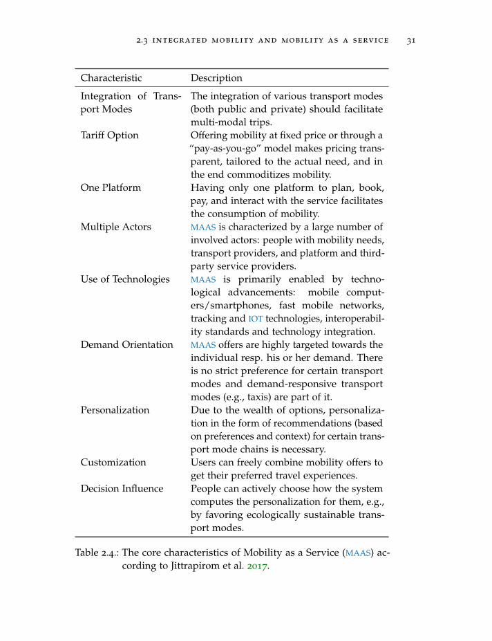
2.3 integrated mobility and mobility as a service 31
Characteristic Description
Integration of Trans-port Modes
The integration of various transport modes(both public and private) should facilitatemulti-modal trips.
Tariff Option Offering mobility at fixed price or through a“pay-as-you-go” model makes pricing trans-parent, tailored to the actual need, and inthe end commoditizes mobility.
One Platform Having only one platform to plan, book,pay, and interact with the service facilitatesthe consumption of mobility.
Multiple Actors MAAS is characterized by a large number ofinvolved actors: people with mobility needs,transport providers, and platform and third-party service providers.
Use of Technologies MAAS is primarily enabled by techno-logical advancements: mobile comput-ers/smartphones, fast mobile networks,tracking and IOT technologies, interoperabil-ity standards and technology integration.
Demand Orientation MAAS offers are highly targeted towards theindividual resp. his or her demand. Thereis no strict preference for certain transportmodes and demand-responsive transportmodes (e.g., taxis) are part of it.
Personalization Due to the wealth of options, personaliza-tion in the form of recommendations (basedon preferences and context) for certain trans-port mode chains is necessary.
Customization Users can freely combine mobility offers toget their preferred travel experiences.
Decision Influence People can actively choose how the systemcomputes the personalization for them, e.g.,by favoring ecologically sustainable trans-port modes.
Table 2.4.: The core characteristics of Mobility as a Service (MAAS) ac-cording to Jittrapirom et al. 2017.
32 ict supporting sustainable personal mobility
provider; an example of a traditional ICT provider positioning itselfas a transport provider could be Google resp. its holding companyAlphabet, who started developing their own cars (with the potentialaim of having autonomous taxis one day).
2.4 information and communication technologies in sup-port of mobility
As we have shown, the recent developments in the areas of transport,ICT, but also the need to become more (ecologically) sustainable en-able and entail changes in the way ICT supports our future mobilityconsumption. In the following we will provide an overview of thecurrent developments in the ICT sector that help in supporting MAAS
and sustainable mobility behavior.
2.4.1 ICT and GIS in the Mobility Sector
Information and Communication Technologies (ICT) support mobilityin a wide range of tasks: From direct interaction with mechanicalparts (e.g., motor or traction control in cars or electric battery chargemanagement), over systems orthogonal to but supportive of mobilityitself (e.g., entertainment systems in cars and airplanes), to advancedrouting and high-resolution mapping, autonomous driving, vehiclearea networks, logistics planning, booking and accounting, timetableoptimization and real-time adjustment systems, and many more, thereis barely a component within the general mobility domain that hasnot been touched by ICT. Yet, one can argue that the mobility andtransport sector is still far from being completely digitalized: mostvehicles are still operated by humans, choosing a route (resp. a meansof transport) and buying a ticket are still manually performed steps, theintegration of personal context data with publicly available transportdata is in its infancy, etc. Among various impacts of digitalization onurban transport and smart cities, Creutzig et al. 2019 point out severalkey innovation areas of ICT in relation to transport in the next decades:For one, the increasing amount of data and processing capabilities canhelp city planners to plan more efficient transport systems. Innovativebusiness models (enabled through ICT) such as bike- and carsharinghave the potential to greatly reduce the number of cars, thus also
2.4 ict in support of mobility 33
freeing up space previously needed for parking vehicles, and reducingcongestion, air pollution, and GHG emissions. Automated driving hasthe potential to substantially lower energy demands, and relies heavilyon ICT both for routing and navigation purposes as well as to interpretand utilize sensor readings (Goodchild 2018). Miller 2020 summarizesthe recent progress in analytics of individual and collective movement,and points at scientific and societal challenges related to achievingsustainable mobility: We are currently undergoing a “grand, real-worldexperiment with profound impacts on cities that will be difficult tounwind” (Miller 2020, p. 118). How ICT assist this experiment, fromplanning over monitoring to provision of support to the individual, willlargely impact its outcome. It is thus crucial to improve the collection,integration and analysis of mobility-related data and use tactial urbanismto quickly iterate on potential improvements to the mobility sector(Miller 2020; Silva 2016).
In Risks ofUsing ICT toOptimizeMobility
line with this, Creutzig et al. 2019 also mention that “severalsocial and environmental risks emerge from the massive and mostlyunregulated use of big data and artificial intelligence” (Creutzig et al.2019, p.2), and, arguably more important with respect to ecologicalsustainability, that “efficiency gains in mobility could be renderedmeaningless by induced demand for additional mobility [and shifts to]automotive travel” (Creutzig et al. 2019, p.2). Several studies highlightthat the impacts of a wide deployment of the mentioned technologiesand business models does not necessarily impact GHG emissions ina positive way (Pakusch et al. 2018; Walnum, Aall, and Løkke 2014).Examples of other emerging problems are the control of a populationusing a social scoring system, or the requirement for taxi drivers to worklonger shifts for costs that barely finance the ongoing costs of their cars(Creutzig et al. 2019). In essence, Creutzig et al. 2019 state that there arehigh risks of an unsustainable outcome of a digitalization of the mobilitysector, and that it thus is of paramount importance that decision-makersneed to properly leverage the new ICT technologies to reach urbansustainability goals. Among their recommendations we find a push forintegrative platforms that foster multi-modal and sustainable transport,and might result in a cooperative transport system as envisioned byMiller 2013.
Within GIS andMobility
this dissertation, we primarily look at how geospatial tech-nologies and Geographic Information Systems (GIS) (under the umbrellaterm of ICT) are able to support sustainable personal mobility and MAAS,
34 ict supporting sustainable personal mobility
with a particular focus on human mobility behavior. Miller and Shaw2015 describe a vision of GIS for transportation in the 21st century thatis in parts driven by a shift to data-abundant environments in recentyears (fostered by advancements in ICT and Location-Aware Technolo-gies (LAT)), but also simply by continuing developments over the lasttwenty years. Next to technical developments such as moving objectsdatabases, this includes a shift to individual-level data (in essence look-ing at individual activities instead of aggregate flows), more refinedheuristics or problem-adapted algorithms to solve prevalent problemsin transportation (such as vehicle routing or route planning), moreelaborate analysis and optimization methods, a focus on real-time ordynamic data, heterogeneous data (e.g., from social media, videos, in-dividual tracking devices, or IOT devices), and the adaption of open GIS
and data standards. We argue that in particular the focus on individu-als, combined with an ever-more accurate tracking of their activities,can help us in supporting them in their mobility choices.
2.4.2 Automatic Tracking
With the increased accuracy of location estimation technologies basedon Global Navigation Satellite Systems (GNSSs), Wi-Fi (based on WirelessLocal Area Network (WLAN) routers), cellphone towers, Bluetooth, etc.,and the wide availability and miniaturization of sensor technologyfound in smartphones, vehicles and tracking equipment, a wealthof spatio-temporal data on the location of vehicles and people hasbecome available. Often, these data are used within a user-centriccommercial setting, e.g., to offer LBS, to improve a product such asroadside assistance or route planning, but just as often the data isused for planning (e.g., location allocation or transport infrastructureplanning), for statistical purposes or for real-time updates on schedules(e.g., airplane arrivals/departures or public transport delays). Recent(prototypical) uses concerned automatic billing of transport usage,feedback on mobility behavior (as in the focus of this dissertation) orfacilitating the access to different mobility options. For example, Binuand Viswaraj 2016 describe and evaluate an Android-based system forimproved safety in carpooling, or Luo et al. 2019 discuss the dangers oftracking and routing technologies in relation to autonomous driving.
TheSmartphoneTracking
data used throughout this dissertation primarily stems from app-based smartphone tracking. The apps performing this tracking use the
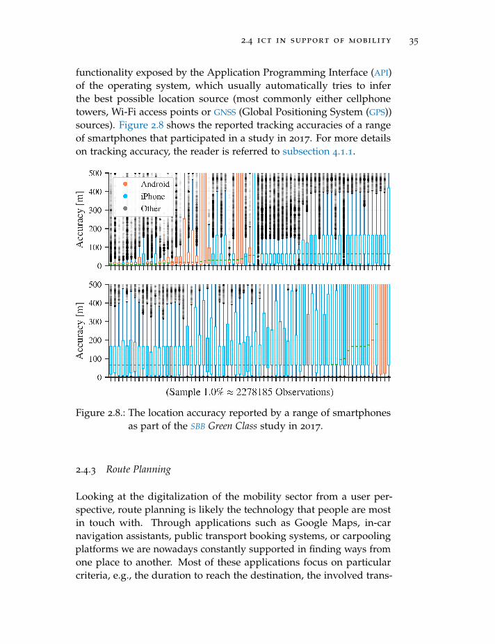
2.4 ict in support of mobility 35
functionality exposed by the Application Programming Interface (API)of the operating system, which usually automatically tries to inferthe best possible location source (most commonly either cellphonetowers, Wi-Fi access points or GNSS (Global Positioning System (GPS))sources). Figure 2.8 shows the reported tracking accuracies of a rangeof smartphones that participated in a study in 2017. For more detailson tracking accuracy, the reader is referred to subsection 4.1.1.
Figure 2.8.: The location accuracy reported by a range of smartphonesas part of the SBB Green Class study in 2017.
2.4.3 Route Planning
Looking at the digitalization of the mobility sector from a user per-spective, route planning is likely the technology that people are mostin touch with. Through applications such as Google Maps, in-carnavigation assistants, public transport booking systems, or carpoolingplatforms we are nowadays constantly supported in finding ways fromone place to another. Most of these applications focus on particularcriteria, e.g., the duration to reach the destination, the involved trans-
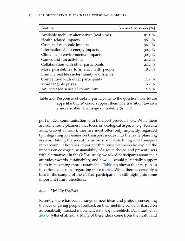
36 ict supporting sustainable personal mobility
Feature Share of Answers [%]
Available mobility alternatives (real-time) 51.5 %Health-related impacts 36.4 %Costs and economic impacts 36.4 %Information about energy impacts 30.3 %Climate and environmental impacts 30.3 %Games and fun activities 24.2 %Collaboration with other participants 24.2 %More possibilities to interact with peoplefrom my real life circles (family and friends)
18.2 %
Competition with other participants 12.1 %More tangible prizes 9.1 %An increased sense of community 3.0 %
Table 2.5.: Responses of GoEco! participants to the question how futureapps like GoEco! could support them in a transition towardsa more sustainable usage of mobility (n = 33).
port modes, communication with transport providers, etc. While thereare some route planners that focus on ecological aspects (e.g. Ferreira2014; Guo et al. 2015), they are most often only implicitly regardedby integrating low-emission transport modes into the route planningsystem. Taking the recent focus on sustainable living and transportinto account, it becomes important that route planners also explain theimpacts on ecological sustainability of a route choice, and present userswith alternatives. In the GoEco! study, we asked participants about theirattitudes towards sustainability, and how ICT would potentially supportthem in becoming more sustainable. Table 2.5 shows their responsesto various questions regarding these topics. While there is certainly abias in the sample of the GoEco! participants, it still highlights someimportant future directions.
2.4.4 Mobility Feedback
Recently, there has been a range of new ideas and projects concerningthe idea of giving people feedback on their mobility behavior (based onautomatically tracked movement data; e.g., Froehlich, Dillahunt, et al.2009b; Jylha et al. 2013). Many of these ideas come from the health and
2.4 ict in support of mobility 37
fitness domain, where a wealth of apps is available to support people intheir sports activities or eating behavior. They frequently use elementsfrom gamification (Weiser, Bucher, et al. 2015) to give people a playfulway of interacting with the respective topic.
Concerning the mobility domain, transferring these strategies to“gamify” the exposure to mobility is difficult, though, as mobility ishighly individual and driven not only by attitudes and beliefs, but alsoby the immediate context, the availability of certain transport modesand the financial circumstances. As such, it is, for example, problematicto have a contest on “who travels least” (which would be the equivalentof, e.g., a fitness cycling app that has a contest on “who cycles thefurthest”), as it would imply that noone was forced to use mobility forwork or personal reasons (e.g., to visit family members).
But even within this context, it was shown that (eco-)feedback onmobility has an influence on the transport and mobility behavior ofpeople (Cellina, Bucher, Mangili, et al. 2019). The respective appli-cations usually do not employ any competitive components nor anynumerical quantification of behavior (except the raw GHG emissions,which are often still displayed in a qualitative way to the users), butinstead use personal goals, challenges, or visualization strategies toprovide feedback and steer people towards a more sustainable behav-ior. Similarly, augmentations of existing transport apps (especially forpublic transport) show the CO2 emissions of different travel options ortry to quantify the ecological impact by offering monetary offsets fromwithin the app. Other forms of feedback are not necessarily related toecological reasons, but can be given to decrease costs, avoid congestedareas, or shift trips in time in order to avoid overcrowded means oftransport.
While feedback is not paramount for MAAS, it plays an important rolefor the sustainability of the mobility sector. It is argued that in the shortterm, GHG emission reductions in the mobility sector will have to comefrom modal and behavioral shifts, as new technologies take decades tobecome widely available—time that is not necessarily available if thetransport sector should be increasingly and urgently decarbonized. Toachieve these sustainability goals, more sustainable transport options(where available) should be shown to people, and they need to becomeaware of the scales of impact of one mode choice versus another.
38 ict supporting sustainable personal mobility
2.4.5 Purchasing Mobility
Last but not least, as MAAS is about the commoditization of mobility,billing should be transparent yet mostly hidden from a user. Future ICT
systems that support sustainable personal mobility and MAAS shouldthus integrate the negotiation and purchase of mobility, e.g., by auto-matic billing via the use of tracking data. The integrative aspect of MAAS
requires a wide range of mobility and transport providers to interact,not only in terms of multi-modal route planning, but also in terms ofcontext integration (e.g., when a traveler has certain requirements, theseneed to be fulfilled by the transport providers in an integrative way, forexample, by transporting luggage with other means of transport) andfinancial aspects. As such, an essential part of future ICT support in themobility domain will concern the standardized publishing of transportoffers and demands, and their automatic processing with respect tofinding the best possible transport options for any given person.
2.5 information processes supporting sustainable mobil-ity as a service
Figure 2.9 shows the ICT processes involved in supporting sustainablepersonal mobility and MAAS, as identified and outlined in this chapter.Starting from the user, we can analyze his or her mobility behavior, inorder to generate (and communicate) eco-feedback based on mobilitypatterns and usage, but also to infer the personal attitudes, goals, andcircumstances. In combination with additional spatio-temporal contextdata (such as POIs in the vicinity, or weather data), we can further refinethe analysis, and identify purposes for certain trips, assign transportmodes to raw GPS trajectories, or classify the users into different mobilityusage types.
On the other hand, it is important that users and transport providersspecify their mobility offers and demands/needs. Currently, this ismostly a one-way process, where various public transport and special-ized mobility providers publish their schedules and availabilities eitherusing a standardized format such as General Transit Feed Specifica-tion (GTFS)6, or within a confined web platform. Even if people are
6 The General Transit Feed Specification (GTFS) is a data exchange format that allowsPT providers to publish their transport schedules. More details can be found undergtfs.org.
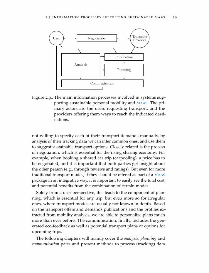
2.5 information processes supporting sustainable maas 39
User TransportProviderNegotiation
Communication
Analysis
Publication
Planning
Figure 2.9.: The main information processes involved in systems sup-porting sustainable personal mobility and MAAS. The pri-mary actors are the users requesting transport, and theproviders offering them ways to reach the indicated desti-nations.
not willing to specify each of their transport demands manually, byanalysis of their tracking data we can infer common ones, and use themto suggest sustainable transport options. Closely related is the processof negotiation, which is essential for the rising sharing economy. Forexample, when booking a shared car trip (carpooling), a price has tobe negotiated, and it is important that both parties get insight aboutthe other person (e.g., through reviews and ratings). But even for moretraditional transport modes, if they should be offered as part of a MAAS
package in an integrative way, it is important to easily see the total cost,and potential benefits from the combination of certain modes.
Solely from a user perspective, this leads to the component of plan-ning, which is essential for any trip, but even more so for irregularones, where transport modes are usually not known in depth. Basedon the transport offers and demands publications and the profiles ex-tracted from mobility analysis, we are able to personalize plans muchmore than ever before. The communication, finally, includes the gen-erated eco-feedback as well as potential transport plans or options forupcoming trips.
The following chapters will mainly cover the analysis, planning andcommunication parts and present methods to process (tracking) data

40 ict supporting sustainable personal mobility
to support people in increasing the sustainability of their mobilitybehavior.
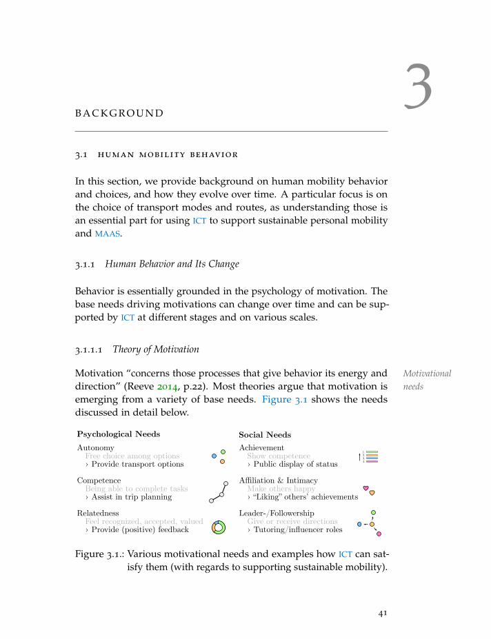
3B A C K G R O U N D
3.1 human mobility behavior
In this section, we provide background on human mobility behaviorand choices, and how they evolve over time. A particular focus is onthe choice of transport modes and routes, as understanding those isan essential part for using ICT to support sustainable personal mobilityand MAAS.
3.1.1 Human Behavior and Its Change
Behavior is essentially grounded in the psychology of motivation. Thebase needs driving motivations can change over time and can be sup-ported by ICT at different stages and on various scales.
3.1.1.1 Theory of Motivation
Motivation Motivationalneeds
“concerns those processes that give behavior its energy anddirection” (Reeve 2014, p.22). Most theories argue that motivation isemerging from a variety of base needs. Figure 3.1 shows the needsdiscussed in detail below.
Psychological Needs
AutonomyFree choice among options› Provide transport options
CompetenceBeing able to complete tasks› Assist in trip planning
RelatednessFeel recognized, accepted, valued› Provide (positive) feedback
AchievementShow competence› Public display of status
Affiliation & IntimacyMake others happy› “Liking” others’ achievements
Leader-/FollowershipGive or receive directions› Tutoring/influencer roles
1.2.3.4.
Social Needs
Figure 3.1.: Various motivational needs and examples how ICT can sat-isfy them (with regards to supporting sustainable mobility).
41
42 background
Psychological needs emerge without any exterior influence (Reeve 2014;Deci and Ryan 2004), and include the desire for autonomy, competenceand relatedness (Weiser, Bucher, et al. 2015).
• The desire for autonomy describes the need resp. desire to havechoices available, and the power to choose freely and indepen-dently of others (e.g., by providing a person with multiple trans-port options).
• Competence expresses our need to feel able to complete given tasks,and to improve the skills necessary for our actions (Reeve 2014;Csikszentmihalyi, Abuhamdeh, and Nakamura 2014; Werbachand Hunter 2012). This means that our tasks should neither betoo easy nor too difficult, in order not to bore or frustrate us.Keeping the difficulty of a task at a level corresponding to aperson’s skills can keep her in a state of “flow”, in which oneis completely absorbed in a task and does not feel how timepasses (Csikszentmihalyi, Abuhamdeh, and Nakamura 2014). ICT
often employ a so-called “on-boarding” phase, during which thedifficulty of a system is greatly reduced to match the (non-existent)skill of a user, e.g., by providing a tutorial phase. Graduallyincreasing the complexity of a system is an effective way to keepsomeone interested, and is, for example, heavily used in computergames.
• Relatedness describes the “need of engaging in relationships withothers” (Weiser, Bucher, et al. 2015, p.272). Relatedness can beinvoked simply by interacting with other persons, but to satisfythis need, one has to feel recognized, accepted and valued. It isinteresting that people not only personally relate to ICT, but alsointeract with them in a way that resembles their interaction withother humans (Fogg 2002). ICT thus can fulfill the role of providingthe needed recognition and acceptance, and can make humans feelvalued. In addition, it can greatly facilitate the interaction betweenhumans (also across large distances, cf. Miller 2013; Weiser,Scheider, et al. 2016; Jennings et al. 2014), thus making peoplefeel related who otherwise might have difficulties connectingwith other human beings. An example of ICT facilitating theseinteractions are the various social network platforms where people
3.1 human mobility behavior 43
can group and exchange themselves based on their interests, andnot solely on their physical location.
Social needs emerge from interactions with other people and arelearned over the course of our life. They encompass achievement,affiliation, intimacy and leadership and followership (Reeve 2014).
• Achievement denotes the desire to show competence, in particularin relation to a societal norm or direct competitors. Typical ele-ments from ICT that cater for our need for achievement are publicdisplays of status, e.g., in the form of a leaderboard in a computergame.
• Affiliation and intimacy relate to everything that lets us make otherpeople happy, resp. that other people do to make us happy andsatisfied. These desires are heavily used by online social networks,where one can “like” other people’s content, or “tag” friends inone’s own postings. While the first one shows an affiliation, thesecond signals a special friendship and thus can be interpreted asa form of intimacy between two persons.
• Leadership and followership are complementary concepts that ei-ther relate to “the desire to impact, control, and influence oth-ers” (Weiser, Bucher, et al. 2015, p.272) (cf. Winter 1973) or to theneed of direction given by someone in a leading position (Goffeeand Jones 2001). Interestingly, ICT can take an authoritarian roleover humans, for example when taking the role of an online tutorthat encourages people to study more (Fogg 2002). Leader- andfollowership are also closely related to power, which is often ex-ercised utilizing ICT, e.g., using leaderboards or score systems todepict particularly powerful individuals.
An Motivationalsources
often made additional distinction is between external and internal(resp. extrinsic and intrinsic) motivation (Sansone and Harackiewicz2000). While internal or intrinsic motivation is generated by one’s owngoals, expectations, beliefs and the self, external motivation stems fromenvironmental, social or cultural circumstances and influences (Reeve2014). The arguably best-known example of an extrinsic motivatoris money, but there exists a wealth of others. When ICT are used togenerate motivation (e.g., using gamification elements), they usuallytake the form of an external motivational source (Weiser, Bucher, et al.2015).
44 background
• Goals and expectations represent desired outcome states, events, orprocesses (Austin and Vancouver 1996). While goals direct andinfluence our behavior, expectations help us manage the choiceof actions (i.e., to evaluate efficacy and outcome). In order toexecute an action, both efficacy (the “ability to do something”)and outcome (the “likelihood that something succeeds”) have tobe high (Fogg 2009).
• A second form of internal motivators are attitudes, beliefs andvalues. They are all closely related, and build upon each other.Values are core ideals and preferences that lie at the base of ourpersonality and thus are difficult and slow to change. Beliefsare personal views on “what is true and what is false” (Weiser,Bucher, et al. 2015, p.273), mostly based on experiences. Theycan change once we experience new situations related to a belief.Attitudes, finally, are quickest to change and describe our likesand dislikes. They are usually formed on the basis of beliefs andvalues.
• The self describes the mental representation we have of ourselves.It is usually built through interaction with other people resp.the inspection of their reactions on our behavior (Markus 1983).Ultimately, people strive to an idealized perception of one’s self,behaving according to the conceptualization of one’s self alongthe way (“confirmation bias”, cf. Kahneman 2011).
HumansCognitivedissonance
usually try to keep their actions in line with their values,beliefs, and attitudes. This can either mean to adjust behavior so itfits with one’s values, or to adjust beliefs and attitudes to better reflectthe actions performed. If it is not possible to reach this alignment,people fall into a state of “cognitive dissonance” (Festinger 1962). Usingeducation, values, beliefs and attitudes can be influenced (Rokeach1973), in turn leading to such a “cognitive dissonance” which can resultin inducing behavior change.
3.1.1.2 Behavior and Its Change
WhetherRequirementsfor behavior
change
we decide to exhibit a certain behavior in a given situationprimarily depends on our motivation and ability, as well as the concreteprompt for us to execute an action (commonly refered to as trigger, cf.
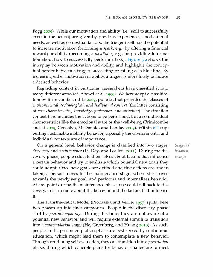
3.1 human mobility behavior 45
Fogg 2009). While our motivation and ability (i.e., skill to successfullyexecute the action) are given by previous experiences, motivationalneeds, as well as contextual factors, the trigger itself has the potentialto increase motivation (becoming a spark; e.g., by offering a financialreward) or ability (becoming a facilitator; e.g., by providing informa-tion about how to successfully perform a task). Figure 3.2 shows theinterplay between motivation and ability, and highlights the concep-tual border between a trigger succeeding or failing as a blue line. Byincreasing either motivation or ability, a trigger is more likely to inducea desired behavior.
Regarding context in particular, researchers have classified it intomany different areas (cf. Abowd et al. 1999). We here adopt a classifica-tion by Brimicombe and Li 2009, pp. 214, that provides the classes ofenvironmental, technological, and individual context (the latter consistingof user characteristics, knowledge, preferences and situation). The situationcontext here includes the actions to be performed, but also individualcharacteristics like the emotional state or the well-being (Brimicombeand Li 2009; Consolvo, McDonald, and Landay 2009). Within ICT sup-porting sustainable mobility behavior, especially the environmental andindividual contexts are of importance.
On Stages ofbehaviorchange
a general level, behavior change is classified into two stages:discovery and maintenance (Li, Dey, and Forlizzi 2011). During the dis-covery phase, people educate themselves about factors that influencea certain behavior and try to evaluate which potential new goals theycould adopt. Once new goals are defined and first actions are under-taken, a person moves to the maintenance stage, where she strivestowards the newly set goal, and performs and internalizes behavior.At any point during the maintenance phase, one could fall back to dis-covery, to learn more about the behavior and the factors that influenceit.
The Transtheoretical Model (Prochaska and Velicer 1997) splits thesetwo phases up into finer categories. People in the discovery phasestart by precontemplating. During this time, they are not aware of apotential new behavior, and will require external stimuli to transitioninto a contemplation stage (He, Greenberg, and Huang 2010). As such,people in the precontemplation phase are best served by continuouseducation, which might lead them to contemplate a new behavior.Through continuing self-evaluation, they can transition into a preparationphase, during which concrete plans for behavior change are formed.
46 background
Precontemplation Contemplation Preparation
Termination
Action
Mot
ivat
ion
Ability
Triggersucceeds
Facilitator
Spark
B=mat
Triggerfails
Mai
nten
ance
Pha
seD
isco
very
Pha
se
Relapse Start “doing”
Maintenance
Figure 3.2.: Behavior change models according to Prochaska and Velicer1997 and Li, Dey, and Forlizzi 2011. During the action(and maintenance) stages, behavior has to be triggered.Fogg 2009 states that the execution of a certain behavior Bdepends on the motivation m, ability a and trigger t itself(B = mat).
Once a person starts performing actions with a certain target behavior,she transitions into the maintenance phase according to Li, Dey, andForlizzi 2011. During the action phase, repeatedly carrying out the newbehavior leads someone from being a novice to an expert (cf. Dreyfusand Dreyfus 1980). Experienced users will transition to a maintenancephase, in which they still have to be kept motivated to exhibit the newbehavior, in order not to relapse back into the contemplation phase.Only when a behavior is truly “internalized” we can consider a newhabit to be formed, a process that can take a long time (Stawarz, Cox,and Blandford 2015). Figure 3.2 visualizes the explained concepts.
3.1.1.3 ICT Supporting Behavior Change
Information and Communication Technologies (ICT) are used to greateffect in supporting certain behaviors and the change of them. Well-known examples range from electronically assisted customer loyaltyprograms (where all spendings are tracked and rewarded with bonuspoints, miles, discounts, etc.), over websites and applications rewarding
3.1 human mobility behavior 47
people for their participation in discussion forums and for generatingcontent, to the infamous “likes” of many social media platforms thathave been shown to exhibit addictive characteristics and have recentlybeen under a lot of scrutiny due to their potentially dishearteningnature (Scissors, Burke, and Wengrovitz 2016; Blease 2015).
ICT Motivationalaffordances
usually support behavior change by offering motivational affor-dances. Originally invented by Gibson 1977, and based on the verbto afford, an affordance describes what a thing offers to an entity, i.e.,the “perceived and actual properties of a thing, primarily those func-tional properties that determine just how the thing could possibly beused” (Salomon 1997, p. 51). Norman 2013 discusses good design ofaffordances (but also signifiers, constraints, mappings and feedback) bytaking into account the psychopathology of everyday things and thepsychological traits influencing human actions. In his book, humancentered design as a philosophy is promoted: Instead of designingfrom a completely technical point of view, we should start “with a goodunderstanding of people and the needs that the design is intended tomeet” (Norman 2013, p. 9). To adopt this philosophy, understandingthe seven stages of action are central: defining goals, planning, spec-ifying, performing, perceiving, interpreting, and comparing. As canbe seen, these stages mostly fit into the preparation and action phasesintroduced in the previous section. Taking the example of a planninga mobility behavior change and thus defining a corresponding goal,we might plan to use a persuasive application to reach it. For this,the application does not only have to afford motivation (cf. Zhang2007), but it needs to be designed in a way that is understandable andeasily discoverable (Norman 2013). This example also highlights that ICT
supporting sustainable mobility has to go beyond offering motivationalaffordances, e.g., by offering educative measures or giving feedback.
Within the context of ICT, affordances are primarily studied in thesubfield of Human-Computer Interaction (HCI). Norman 1999 providesan interesting discussion of how the term affordance was originallyadopted within this field: an affordance was understood as a way tosignify that the interaction with a (virtual) object leads to some plannedoutcome. However, this is not adhering to the original definition, whereneither the signaling nor the planned outcome are of significance. Todistinguish between these different definitions, he introduces the termsreal affordances and perceived affordances (which loosely correspondto the later introduced term signifiers, namely indicators of possible
48 background
affordances, cf. Norman 2013). Raubal and Moratz 2008, based onRaubal 2001, extend the concept of affordances by dividing it intophysical, social-institutional, and mental affordances. Whereas the firstrequire physical requirements to be met (e.g., an object size must matcha person’s hand to grab it), social-institutional affordances revolvearound interactions between people and are thus often not bound to alocation (e.g., one can talk to another person via telephone), and mentalaffordances spring into existence when a person is in a situation andneeds to decide upon an action plan to reach his or her goals. Janowiczand Raubal 2007 use affordances to determine the similarity of objectsand use it within a case study involving an agent that has to reach acertain goal (e.g., changing a light bulb). To proceed towards the goal,the agent chooses entities that have similar affordance descriptors to aone that is chosen based on internal knowledge. A similar case can bemade when an agent has several transport modes available to reach aphysical location.
He, Greenberg, and Huang 2010 mention five different models thatcan be used to describe how we decide between different behaviors andthat thus should be respected when designing motivational affordances:the attitude model (favorable attitudes will lead to pro-environmentalbehavior), the rational-economic model (monetary costs determine ev-erything), the information model (if you know enough about a problem,you will act in the best possible way), the positive reinforcement model(actions have to be rewarded), and the elaboration likelihood model (weact according to logic and rationale, but are influenced by emotionalresponses to problems). Froehlich, Findlater, and Landay 2010 extendthis list with a model of responsible environmental behavior (whichincludes economic constraints and social pressure in addition to the in-tention to act), and norm-activation models (that are similar to attitudemodels, but root behavioral choices deeper in personal norms). Withinthis dissertation, we primarily rely on the information and positivereinforcement models, arguing that in the mobility sector, economicallydriven choices require policy changes (and are thus not tightly linkedto ICT; note that they can be actively promoted and motivated usingICT, however) and attitudes are difficult to change in short time frames(but will over time adjust themselves in accordance with the receivedinformation and rewards).
Analyzing current and past behavior and presenting it in an inter-pretable form can help users become aware of their own behavior, thus
3.1 human mobility behavior 49
forming a motivational affordance for introspection and the inductionof change. This effect can be strengthened by providing alternatives forpast and future behavior, as well as by offering comparisons to definednorms, goals, or other people (cf. Weiser, Scheider, et al. 2016). Thisform of support is rooted in the fact that people are often not awareof the impacts of their routine behavior, which is carried out subcon-sciously. By presenting viable alternatives, the difficult step of aligningmultiple goals of people can be alleviated—otherwise, a large effort isneeded to evaluate all the potential impacts on reaching different goalsand balancing them against each other. In similar ways, ICT is used tosimply educate people about different behaviors, and thus highlightpotentially “bad” behaviors, and/or how other people behave.
Other motivational affordances include social elements, such as col-laborative or competitive elements of an application. Cooperationdescribes all processes in which multiple individuals try to achievesomething by working together. They primarily target our need forrelatedness, but can also satisfy the needs for affiliation or leader- andfollowership; the latter when there are exclusive groups people canbelong to, and/or if there are special roles within a community thatmanage and lead it. For example, Gustafsson, Katzeff, and Bang 2010
evaluate a game targeting a reduction in domestic energy use thatbuilds upon cooperation within families and report that such persua-sive games show a lot of promise for demand management. Jung,Schneider, and Valacich 2010 look at how to enhance HCI interfacesfor collaborative applications and find that by building applicationsspecifically including motivational affordances, significant performancegains can be achieved. Competition, on the other hand, appeals to ourneeds of achievement and leadership (Weiser, Bucher, et al. 2015), andmainly works for people in comparable situations. Sepehr and Head2013 performed a study with college students and found that whilecompetition is highly motivating, it can also have a detrimental effecton the enjoyment of a task.
Finally, elements fostering challenge or rewarding certain behaviorscan both also be used as motivational affordances. Challenges primarilysatisfy our need for competence, as we get the chance to evaluate ourperformance. They work well for people who do not have a concretegoal or do not know how to reach one (Gustafsson, Katzeff, and Bang2010). Rewards relate to the needs of achievement and competence andare the prototypical example of extrinsic motivators (Reeve 2014; Weiser,
50 background
Bucher, et al. 2015). However, as Deci, Betley, et al. 1981 point out,while rewards can provide a strong motivational source, they are lesseffective for changing behavior in the long term. This is similar to mostextrinsic motivators, as they are not able to generate intrinsic motivation,and thus the behavior is only changed as long as the motivator exists.Munson and Consolvo 2012 find that rewards should have a surprisingaspect in order to be effective, and Frederick and Loewenstein 1999
point out that the rewards must be increasing over time to give peoplethe same amount of satisfaction.
FocusingLocation-Aware ICT
on geospatial and location-aware technologies, we primar-ily find applications that assist people in living a healthy lifestyle,employing game-like elements (Yoganathan and Kajanan 2013). Of-ten, these applications come in the form of fitness trackers that recordthe movement of people and let them evaluate their behavior over alonger period of time or in comparison with other people. Along thesame line, so-called exergames similarly stimulate (young) people toperform moderate to vigorous physical activity (Boulos and Yang 2013).The focus here is more on the game itself, and the healthy lifestyleis a (desired) by-product. An in-depth review of research combininglocation-aware ICT and mobility behavior will be given in section 3.4.
3.1.2 Transport Mode Choice
To know how to best support people in making sustainable mobilitychoices, it is important to understand why people choose a certainmobility behavior, especially since these choices are usually not onlydetermined by transport mode availability (resp. the built environ-ment), but also by a variety of socio-demographic, -economic and-psychological factors (Acker, Wee, and Witlox 2010). Figure 3.3 high-lights the different choices and influencing factors, as explained in thissection.
ABuiltenvironment
wealth of studies analyze the dependencies between the built en-vironment and travel behavior. Ewing and Cervero 2010 published ameta-analysis of over 200 studies in 2010, building upon qualitativework from numerous authors (Ewing and Cervero 2001; McMillan 2007;Pont et al. 2009; Stead and Marshall 2001). In essence, these studies in-tend to quantify the “potential to moderate travel demand by changingthe built environment” (Ewing and Cervero 2010, p. 267), includingdensity, diversity (of land uses), design (of street network), destination
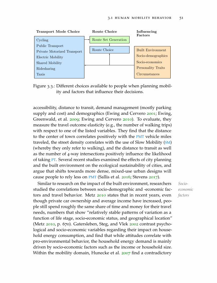
3.1 human mobility behavior 51
Route Set Generation
Route Choice
CyclingPublic TransportPrivate Motorized TransportElectric MobilityShared MobilityRidesharingTaxis
Built EnvironmentSocio-demographics
Socio-economics
Circumstances
Personality Traits
Transport Mode Choice Route Choice InfluencingFactors
Figure 3.3.: Different choices available to people when planning mobil-ity and factors that influence their decisions.
accessibility, distance to transit, demand management (mostly parkingsupply and cost) and demographics (Ewing and Cervero 2001; Ewing,Greenwald, et al. 2009; Ewing and Cervero 2010). To evaluate, theymeasure the travel outcome elasticity (e.g., the number of walking trips)with respect to one of the listed variables. They find that the distanceto the center of town correlates positively with the PMT vehicle milestraveled, the street density correlates with the use of Slow Mobility (SM)(whereby they only refer to walking), and the distance to transit as wellas the number of 4-way intersections positively influence the likelihoodof taking PT. Several recent studies examined the effects of city planningand the built environment on the ecological sustainability of cities, andargue that shifts towards more dense, mixed-use urban designs willcause people to rely less on PMT (Sallis et al. 2016; Stevens 2017).
Similar Socio-economicfactors
to research on the impact of the built environment, researchersstudied the correlations between socio-demographic and -economic fac-tors and travel behavior. Metz 2010 states that in recent years, eventhough private car ownership and average income have increased, peo-ple still spend roughly the same share of time and money for their travelneeds, numbers that show “relatively stable patterns of variation as afunction of life stage, socio-economic status, and geographical location”(Metz 2010, p. 670). Gatersleben, Steg, and Vlek 2002 contrast psycho-logical and socio-economic variables regarding their impact on house-hold energy consumption, and find that while attitudes correlate withpro-environmental behavior, the household energy demand is mainlydriven by socio-economic factors such as the income or household size.Within the mobility domain, Hunecke et al. 2007 find a contradictory
52 background
trend: psychological variables seem to influence both intent- as wellas impact-oriented behavior (however, the socio-economic variableshave to be controlled for). They explain these differences by their moreaccurate recording of mobility-related attitudes. Regarding the geo-graphical differences, Buehler 2011 analyzed the differences in PMT usebetween the USA and Germany. Even when controlling for factors ofthe built environment and the socio-economic background, people inthe USA travel at least 70% using PMT, whereas in Germany “only themost car-oriented groups of society display such high levels of car use”(Buehler 2011, p. 654), a difference that can potentially be explained byvarying transport policies and factors of the built environment such asthe availability of walkways or PT. Meng, Koh, and Wong 2016 builda multimodal logit model that highlights the dependencies betweensocio-demographic features and the choice for the first/last mile trans-port mode in Singapore. By interviewing 851 participants, they find arange of significant predictors, such as age, gender, household income,and a range of factors of the built environment.
WithinCircumstanceand
personality
the context of this dissertation, it is also important to considerthe effects of circumstantial factors and personal traits on transportchoices. Krygsman, Arentze, and Timmermans 2007 investigate cor-relations between performed activities and mode choices. They findthat people are more likely to include intermediate activities for simpletransport mode chains (such as solely taking PMT), and that complexmode chains in turn lead to simple activity chains. Similarly, they notethat the spatial and temporal constraints before heading to work aremuch tighter, leading to the result that discretionary activities are usu-ally scheduled after work, and only mandatory activities appear before.In a study involving Swedish commuters, Vredin Johansson, Heldt, andJohansson 2006 found that while time and cost play a significant role,personality traits such as the preference for flexibility or comfort areable to explain some of the transport mode choices. Similarly, they statethat personality traits determine our attitudes towards the environment,safety, comfort, convenience and flexibility (Vredin Johansson, Heldt,and Johansson 2006). Contrasting the results by Hunecke et al. 2007,Vredin Johansson, Heldt, and Johansson 2006 find no correlation be-tween the environmental stance of a person and the choice between caror bus; however, they note that in general a pro-environmental attitudelets a person prefer PT and SM. Collins and Chambers 2005 performeda similar study with students in Australia and conclude that due to the
3.1 human mobility behavior 53
relatively strong influence of personal beliefs on mode choice, policyshould “address situational and psychological factors in attempting toencourage a commuter transport mode shift toward more use of PT”(Collins and Chambers 2005, p. 658). Donald, Cooper, and Conchie2014 regard the problem utilizing theory of planned behavior (Ajzenet al. 1991), under which they find that the perceived behavioral control(the perception that the individual can perform the intended behavior)is the most impactful variable to predict a travel choice, in contrast tosubjective, moral and descriptive norms. Habits, on the other hand,may, if existent, “override” all mentioned factors. An important take-away is that “it may be necessary to break habits prior to implementingattitude-based campaigns” (Donald, Cooper, and Conchie 2014, p. 46),something that could be done by changing the built infrastructure, orforcing people to (re-)make a conscious decision for a transport modechoice in a previously habit-driven setting.
In the following, we will assess research results regarding choices ofvarious transport modes.
3.1.2.1 Cycling
With ConventionalBicycles
the recent focus on environmentally friendly transport modes,both electric as well as conventional bicycles came under investigation.Commutes are often subject of study, as they are regular and usually ofcomparatively short distances. Heinen, Maat, and Wee 2013 unveil cor-relations between work-related factors and the choice of an individualto commute by bicycle. They find that next to the personal attitude, theexpectations of coworkers, infrastructure (availability of storage andchanging facilities) and the availability of a bicycle drive the choice.Heinen, Maat, and Wee 2011 perform a similar study, finding that forshorter commutes, the opinion of others is an influencing factor, yetfor longer trips one’s attitudes have to be pro-cycling. Mostly, though,the direct benefits of cycling (time, comfort, flexibility) determine ifsomeone commutes by bicycle or not. As weather and seasons mightdetermine the choice to travel by bicycle, Bergstrom and Magnusson2003 preformed a study that evaluated the attitudes towards cyclingat low temperatures. While people who only cycle in summer wereprimarily influenced by environmental factors such as temperature,precipitation or road conditions, people who cycle the whole yearround are mostly driven by the desire to exercise and lead a healthy
54 background
lifestyle. The implications of their research include that health couldbe a proxy to achieve environmentally friendly behavior, but also thatby increasing roadElectric
Bicyclesmaintenance during winter the number of bicycle
trips could be increased. In similar spirit, Bucher, Buffat, et al. 2019
looked at which energy savings would be possible, given that peopleare willing to travel (by electric bicycle) at certain temperature andprecipitation levels. They find that roughly 10% of all emissions fromfossil fuel based commutes could be saved in Switzerland under theassumption that people would be willing to replace commutes of up toapprox. 15 minutes by bicycle. However, one has to be careful whenpromoting e-bicycle choices, as often the involved people are morelikely to transition from PT than from PMT, thus not necessarily largelychanging the environmental impacts (Cherry and Cervero 2007).
3.1.2.2 Public Transport
When it comes to Public Transport (PT), people’s choices are mostlydriven by its frequency, the access and egress times, as well as thenumber, location, and context of transfers (whereas waiting and walkingduring a transfer is particularly burdensome) (Anderson, Nielsen, andPrato 2017). In their work, Anderson, Nielsen, and Prato 2017 generatedpublic transport alternatives and found that while people are willingto wait a substantial amount of time during long trips, the transferpenalty similarly increases, indicating that travelers prefer to stay ona single mode of transport (e.g., to work during a train trip withouttransfer). Hensher and Rose 2007 built a nested logit model for bothwork-related as well as non-work trips and similarly found that thenumber of transfers, the fares (for PT) and costs (for PMT), followed byin-vehicle and waiting times correlate with the choice for a certain modeof (public) transport. Vrtic and Axhausen 2002 find that travel time andthe number of transfers are highly decisive, and that one (train) transferis equated with 19 minutes in-vehicle time. Another interesting findingconsists of the fact that car owners value the in-vehicle time higher thanpeople who do not own a car. Ye, Pendyala, and Gottardi 2007 observethat people tend to choose trip chains before they choose a mode, andthat users of PT prefer simpler trip chains. This in turn implies thatPT providers should not only improve service amenities along theirroutes, but also have to “cater to a multi-stop oriented complex activityagenda” (Ye, Pendyala, and Gottardi 2007, p. 111), which might call
3.1 human mobility behavior 55
for more flexible and individual access to PT (e.g., by using bus-on-demand systems or autonomous taxis). Looking at the choice process,Bovy and Hoogendoorn-Lanser 2005 additionally find that usuallypeople first choose a particular station to access PT (based, amongpreviously identified factors, on personal preferences), after which theyselect an access mode. Eluru, Chakour, and El-Geneidy 2012 examinehome-to-work/-school travel patterns, and conform the findings of thepreviously mentioned studies: They highlight that in comparison withtrips by train and metro, travel by bus is least favorable; that womenare less sensitive to travel time and that a reduction in bus travel timeswould greatly increase the likelihood that people travel by bus.
3.1.2.3 Private Motorized Transport
The use of Single Occupant Vehicles (SOVs) is examined from variouspoints of view. Klockner and Friedrichsmeier 2011 represent car choiceusing a two-level structural equation model: On the first level, tripattributes are considered; on the second, person-specific informationabout the individual, such as attitudes or personal norms. They findthat the person-specific attributes explain a large share of the variancein the data, stating that it is thus important to not only consider tripfeatures, but also individual characteristics. Their findings are sup-ported by Klockner and Blobaum 2010 who mention that situationalconstraints explain most of the variance in transport mode choice mod-els, but that habits and intentions can not be neglected. Regardingsituational constraints, Klockner and Friedrichsmeier 2011 observe thatcar access (which might itself be a “bad” predictor, as car ownershipusually requires a previously undergone decision process of similarform), trip duration, and the trip purpose are strong predictors forcar choice. The immediate context affects car usage in different ways:Weather and small disruptions of PT only marginally influence the trans-port mode choice, while major disruptions have significant impacts.Finally, they note that habits and perceived behavioral control showcorrelations with easily available trip information (such as the purposeor length of a trip) (Klockner and Friedrichsmeier 2011). Oppositeinteractions between intentions, norms and attitudes, and informationthat is difficult to obtain, were established. This means that for habitualbehavior, people tend to rely on simple rules, and that people withhigh levels of intention are willing to evaluate more complex decision
56 background
scenarios. For persuasive ICT, it might thus make sense to break downcomplexity in new situations, and/or increase the levels of intention,e.g., to travel in sustainable ways. Taking an intra-household pointof view, Scheiner and Holz-Rau 2012 analyze the gender differencesin households containing more drivers than cars. They find that the“economic power” within a household (i.e., who earns money) does notaffect car usage, however, there are indicators that the use of a car isdriven by the (gendered) social role someone takes in a household (e.g.,the person looking after children and being responsible for runningerrands might always use the car or vice versa).
3.1.2.4 Electric Mobility
ABuyingDecisions
large field of research is concerned with the question who buys anelectric car. Using a large-scale online survey in Norway, Klockner,Nayum, and Mehmetoglu 2013 find that EVs are commonly bought asa second car, a finding that contrasts the one by Haan, Mueller, andPeters 2006, which was, however, specifically targeted at the PluginHybrid Electric Vehicle (PHEV) Toyota Prius. In contrast to BatteryElectric Vehicles (BEVs), PHEVs can also be refueled during a journey at aregular gas station. In their study, Nayum, Klockner, and Mehmetoglu2016 clustered ICE car owners into five groups and contrasted them withEV owners, finding that there are large socio-psychological differencesbetween ICE car buyers and EV buyers. EV owners are generally moreenvironmentally friendly and show an increased perceived behavioralcontrol alongside attitudes and intentions to buy fuel-efficient cars.However, in summary across all groups, social and personal norms hadlittle influence (probably due to the comparably high costs involved inbuying a car that made the activation of personal norms inappropriate),and the buying decision mostly relied on a car’s performance andconvenience attributes. In a 2011 study involving residents of SanDiego county, USA, Axsen and Kurani 2013 found that a large shareof the population would consider a PHEV as their next car, as theyare worried about the limited range and recharging facilities as wellas the high price of EVs. Haan, Mueller, and Peters 2006 point outthe potential rebound effects from buying an electric car: these canmanifest as direct and indirect effects, and macro-level effects (taking awhole society into account; cf. Berkhout, Muskens, and W. Velthuijsen2000), both in terms of money as well as sustainability. Interestingly,
3.1 human mobility behavior 57
they do not find any rebound effects regarding vehicle size nor vehicleownership. It is pointed out that this might also be due to Prius buyersbeing “early adopters”, and thus one might not generalize across theentire population (Haan, Mueller, and Peters 2006). Similarly, theremight be a bias towards environmentally or financially overly awarepeople and/or people who do not consider cars as status symbols.
As RangeAnxiety
EVs exhibit some different properties than ICE cars (such as longerrecharging/refueling durations, shorter ranges, possibility to recuper-ate energy, etc.), researchers studied the differences between peopleusing ICE cars and people using EVs for travel. Klockner, Nayum, andMehmetoglu 2013 note that especially in households that own an EV
as their only car, the expected annual mileage is substantially lowerthan for households with multiple cars. This might be due to the factthat BEVs show limited ranges, or that people replacing an ICE car witha EV are actively trying to reduce their mileage. Range anxiety is apsychological phenomenon that occurs either during a drive when onerealizes that not enough energy is remaining to complete the trip, orduring the planning phase when one has to drive further than maxi-mally possible with a BEV (Noel et al. 2019). Several researchers arguedthat range anxiety “may be an over-stated concern” (Saxena et al. 2015,p. 275) as most of the regular trips can easily be covered by BEVs, evenafter battery degradation or for low-cost models with little range. Rauh,Franke, and Krems 2015 analyzed the differences in range anxiety be-tween experienced BEV users and people who never drove a BEV before,showing that experienced drivers exhibit much lower range anxiety,confirming the findings of Franke and Krems 2013. They conclude bystating that “teaching users relevant knowledge and skills [...] could beone fruitful approach to reduce the experience of range anxiety.” (Rauh,Franke, and Krems 2015, p.14). Similarly, when traveling by BEV, it wasfound that the initial State of Charge (SOC) has a large effect on rangeanxiety, and that unambiguous displays (e.g., showing the remainingrange at an accuracy of meters) are perceived as untrustworthy (Jung,Sirkin, et al. 2015).
3.1.2.5 Shared Mobility
Various Privatecarsharing
factors contribute to the likelihood for someone to carshare:Efthymiou, Antoniou, and Waddell 2013 find that younger and low-income people are more likely to share their car with others, alongside
58 background
people who are more environmentally aware. It is also noted thatcarsharing often replaces PT, similar to bikesharing replacing journeyspreviously performed on foot. Their findings coincide with researchby Kortum et al. 2016, who not only point out the generally increasingusage of carsharing, but also how residential density and the numberof people per household influence both the daily bookings (negatively)as well as their growth rate (positively). Becker, Ciari, and Axhausen2017 analyze the use of free-floating carsharing offers and find thatthey are primarily used for discretionary trips where no suitable PT
exists; a finding that contrasts with the use of station-based carsharing,which is frequently used in areas that have good accessibility to PT
and relatively high car ownership levels. In their case, free-floatingcarsharing was found to scale with the population density as wellas the number of carsharing members living in a region. Shaheen,Schwartz, and Wipyewski 2004 note that joining a carsharing programalso affects mobility use: In Europe, Vehicle Miles Traveled (VMT) dropbetween 30% and 70%, and from 10% to 60% of all people sell a vehicleafter joining a program. Other benefits of carsharing include the factthat it reduces the frequency of impulsive trips and makes peoplemore aware of the actual costs of a trip, which are often concealedfor PMT (Zheng, Scott, et al. 2009). Next to the psychological andsocio-economic resp. -demographic factors, features of the trip itselfalso determine the use of carsharing: Most important is usually thedistance as well as the availability of parking at the destination (Fleuryet al. 2017). In their study, Fleury et al. 2017 particularly focus oncorporate carsharing, which describes the concept of having a fleetof vehicles that members of a company can use at their discretion,without having individual vehicles assigned. They found that withinthis context, ease of use is crucial in determining the intentions ofemployees for using the service. Environmental views only marginallyinfluenced these intentions, related to job performance expectancy.Finally, communication plays a large role in the adoption of carsharing.Shaheen and Novick 2005 contrast the use of a brochure resp. a videoand test drive, and find that the intention to use carsharing was 33%for the first group, and 78% for the second one.
3.1 human mobility behavior 59
3.1.2.6 Carpooling and Ridesharing
Ridesharing Definitionanddevelopment
or carpooling is commonly defined as two or more peoplesharing a common itinerary and means of transport (Furuhata et al.2013) resp. “when two or more trips are executed simultaneously, in asingle vehicle” (Morency 2007, p. 240). While there is no consensus onthe differences between the different forms of ridesharing and carpool-ing, we here adopt the terminology introduced in the work by Agatzet al. 2012: Carpoolers unite to regularly travel to a certain locationtogether and often take turns driving (in these cases, there is also noneed for payment). Ridesharing, on the other hand, is more ad-hoc andbetween people who usually do not know each other beforehand (andthus often enabled of facilitated by ICT). Additionally, Agatz et al. 2012
make the distinction between dynamic and static ridesharing, wheredynamic refers to short-term/en-route planning of rideshares, andstatic to those problems that can be planned in advance (e.g., a holidaytrip). Technically, this definition includes both intra- as well as inter-household ridesharing (Buliung et al. 2010; Morency 2007; Vanoutriveet al. 2012; Teal 1987). We here put a slight focus on inter-householdridesharing, as it relies more on support from ICT than intra-householdcarpooling, which can be formed and planned based on verbal andinformal interaction (but nonetheless should be supported, e.g., bymotivational elements). Ridesharing is part of so-called CollaborativeConsumption (CC) which was recently enabled through ICT and is seenas a component of the sharing economy (Hamari, Sjoklint, and Ukkonen2015). Even though it is generally agreed upon that ridesharing hasnumerous potential benefits, such as reduced travel costs and emissions,or better utilization of vehicles and infrastructure (Furuhata et al. 2013;Amirkiaee and Evangelopoulos 2018), it still only makes up for a smallshare of mobility.
Several Characteris-tics
decades ago, Teal 1987 found that around 18 to 20% of theAmerican people used carpooling. Out of these, over 40% were mem-bers of household carpools, which consisted of 2 people in 95% of allcases. Among the inter-household carpools, 40% were sharing drivingresponsibilities (i.e., they take turns as drivers and contributors of avehicle), while 39% were only riding, and the rest was only driving.Typically, these carpools showed a high regularity, being active aroundfour out of five days per week (which means they are fixed commutingarrangements). This stands in contrast to intra-house carpools, which
60 background
are used much more infrequently (as they are less formal, and muchmore driven by convenience factors than economic ones). While theshare of carpoolers has stagnated or even reclined after the oil crisisin 1973 (Ferguson 1997; Pisarski 1997; Benklert 2004) and a shift to-wards intra-house carpooling took place (Morency 2007), it recentlystarted increasing again across several regions and contexts due torising concerns about the environment, increased urbanization andmore convenient access to carpooling through ICT.
ToPersonalfactors
find out what drives people’s choice regarding carpooling, Amirki-aee and Evangelopoulos 2018 conducted a survey with 481 undergrad-uate students from a large public university. They found that the“ridesharing participation intention” is largely driven by one’s attitudetowards ridesharing, which in turn mainly depends on trust, transporta-tion anxiety and potential time benefits. While trust mostly relates tothe “marketplace aspects” of ridesharing (i.e., one often has to carpoolwith a stranger), anxiety refers to the fact that ridesharing has a stress-migitating effect (Novaco and Collier 1994) and reduces unease dueto a variety of factors such as being on time, parking spaces or trafficcongestion. Time benefits mostly occur if the alternative would be totake public transport or a form of slow mobility (Amirkiaee and Evan-gelopoulos 2018). Economic benefits play a minor but significant role,while sustainability concerns and social aspects do not seem to influencechoices for or against ridesharing at all (Amirkiaee and Evangelopoulos2018). In contrast to their findings, Hamari, Sjoklint, and Ukkonen 2015
state that the attitude towards a certain CC behavior is significantlymotivated by the sustainability of the activity, as well as its enjoyment.Politis, Papaioannou, and Basbas 2012 examine the influence of variousbehavioral stages on transport mode choice and find that people inmore advanced stages are much more likely to carpool.
TheCorporate andgeographic
factors
accessibility to carpooling resp. ridesharing plays a major rolein its use. A context in which carpooling is often offered is within cor-porations (due to easy-to-use communication channels with potentialcarpoolers, a high regularity of behavior, as well as a guaranteed sharedorigin/destination) (DeHart-Davis and Guensler 2005; Vanoutrive et al.2012). Canning et al. 2010 find that economic aspects are the maindrivers for participating in corporate carpooling, followed by the un-availability of a personal car, and environmental and social aspects.Extending this work, Vanoutrive et al. 2012 study the effects of loca-tion, organization (sector) and promotion (i.e., marketing and man-
3.1 human mobility behavior 61
agement measures) on the choice behavior of commuters at severalworkplaces throughout Belgium. They find that psychological barriers,attitudes and perceptions correlate more with the choices to carpoolthan socio-demographics. Additionally, the location resp. accessibilityto a workplace influences the use of carpooling, as well as organiza-tional factors (work schedules or the sector the corporation is active in)and the amount of promotion carpooling receives from the corporatemanagement. This is in alignment with research by Teal 1987, whofound a correlation between the trip distance as well as the availabilityof public transport and the likelihood of participating in carpooling.Soft promotion measures (such as marketing or the creation of “pools”)were found to be less effective than discouraging measures (such asparking charges) (Vanoutrive et al. 2012; Canning et al. 2010). Compar-ing their work to previous research conducted by others (Buliung et al.2010; Canning et al. 2010; Ferguson 1997; Teal 1987), they also note thatgeneral patterns can be recognized. For example, households in lowerincome classes seem to carpool more (which might be linked to thefact that a lower income inversely correlates with vehicle ownership)and women with small children less often (due to their circumstances,where they often have to drop off/pick up the child at some place). Inalignment with previous research (Wang 2011), Vanoutrive et al. 2012
thus conclude that access to carpooling should be facilitated, but notactively promoted in areas with good public transport or bicyclinginfrastructure (as it is less efficient).
3.1.2.7 Taxis and Autonomous Mobility
Schmocker et al. 2008 Taxisperform a transport mode choice study involvingelderly people in London. They find that older people travel approx.5% of all their trips by taxi, a number that is significantly higher thanthe average of around 1.5% in London, and that it involves mostlyhomebound trips (e.g., when returning from a shopping center carryingbags). Among the available transport modes, taxis are as popular asdriving one’s own car or taking bus or tram, before taking the subwayor railway, or being a passenger in another person’s car (the latter isan indication that people do not like to be dependent on friends orfamily). This lack of generalizability in the study of Schmocker et al.2008 is partially confirmed by research by Stern 1993, who found thattaxis are an inferior alternative to paratransit services (smaller buses
62 background
that stop on demand). Roorda, Passmore, and Miller 2009 look atminor transport modes in the Toronto area. With regards to taxis, theyprimarily find that these usually originate from within the city centeror are frequently used to travel from/to the airport, and that peoplebelow 19 years are more likely to take public transit, most likely dueto a lack of drivers license and funds for more expensive transportmodes such as taxis. Another interesting takeaway is that people areapproximately six times as sensitive to parking than to travel costs. Jou,Hensher, and Hsu 2011 similarly look at the use of taxis to get fromTaipei (Taiwan) to the airport and find that both out-of-vehicle (to walkto the station, search for a vehicle, etc.) and in-vehicle travel time aswell as the overall time savings and the ease of use primarily drivethe transport mode choice. Participants of their survey indicated thatintra-variation of transport mode choices is uncommon, i.e., peoplealways take the transport mode they are used to. For all participants,financial aspects, such as parking fees, fuel cost or highway tolls playedan important role and students often asked friends or family to drivethem to the airport. An important takeway is also that the computedelasticity values for Mass Rapid Transit (MRT) systems indicate thatkeeping the out-of-vehicle time low is especially important for theadoption of public transport. Overall, and as Roorda, Passmore, andMiller 2009 note, transport mode choice models involving taxis sufferfrom a lack of data as this mode is infrequently used in comparison toothers.
EvenAutonomousmobility
though there are only few autonomous cars on the streets yet(and those are primarily being used within pilot experiments), severalresearchers looked at the intentions and attitudes of people towardsautonomous mobility. Becker and Axhausen 2017 performed a literaturereview on the acceptance and pricing of automated vehicles, and makethe distinction between private Autonomous Vehicles (AVs) and sharedAVs (which correspond to on-demand services on flexible routes). Theoutcomes of various studies indicate that a substantial share of thepopulation (18-50%) would either use the technology or at least thinkits development is important. Similarly, people would be willing topay an additional USD 3’000 to 7’253 for the addition of autonomouscapabilities to their cars. However, the complete dismissal of one’s owncar in favor of a shared autonomous taxi service is only accepted by afew—most people would rather replace their second car and keep theirprimary car for themselves. Autonomous vehicles were also found to
3.1 human mobility behavior 63
be more accepted with increasing age (which can be explained by thephysical limitations of older people) and among young people (who aregenerally open to new technology). Finally, Becker and Axhausen 2017
summarized that people who travel inter-modally are more inclinedto accept AVs, as are people from urban areas and those who oftentravel on highways and in congested traffic. Their findings are partiallyoverlapping with those by Jing et al. 2019, who do a similar literaturesurvey, and also perform a study with 906 persons in China. Theyparticularly highlight that a lack of knowledge about AV technologyand the difficulty of risk assessments are what keeps people from beinghighly in favor of AVs. Winter, Cats, et al. 2017 performed a stated-choice experiment to compare free-floating carsharing and AVs withPMT and PT. Their takeaway is that while early adopters would favorautonomous vehicles, there is an aversion among other groups of thepopulation. Malokin, Circella, and Mokhtarian 2015 examined theaspects of being able to do other activities while traveling by AV. Theyfind that this ability significantly increases the perceived utility andthus helps AVs gaining wide acceptance. However, they also point outthat this might happen as a replacement of PT and carpooling—whichgoes against many environmental goals.
3.1.3 Route Choice
Prato 2009 gives an extensive overview of route choice modeling thatincludes numerous transport modes within a transportation network.The author particularly highlights that route choice is fundamentallydifferent from destination or mode choice, as the number of potentialroutes is usually vast, and they are not “readily available” as they haveto be extracted from the transport network. Usually, the problem is di-vided into two parts: route set generation and choice (whereas a personchooses a particular route given some utility function on incompleteinformation). Starting with deterministic shortest-path algorithms (thatcreate the K best paths according to some utility function), Prato 2009
reviews labeling approaches (that have multiple optimization criteria,each assigned to a different label; e.g., shortest path, least congestedroads, etc.), link elimination approaches (that iteratively search for theshortest path after removing central links from a previously found one),and link penalty approaches (similar, but instead of removing links theyare heavily penalized). Among the reviewed stochastic approaches, we
64 background
find simulations (that draw link travel times or costs from a chosendistribution and use it to compute different paths) and doubly stochas-tic generation functions (that in addition have a stochastic componentthat models a traveler’s perception). Other approaches use behavioralrules or probabilities assigned to each possible route choice, potentiallycombined with a perception model that restricts the number of potentialchoices. Once a set of choices is available, a route choice model is usedto quantify the likelihood of choosing one route over another Prato 2009.For example, (multi-nominal) logit models express a probability foreach route within the choice set, based on a given utility function (thatdepends on the route and potentially on a person). Various correctionmethods exist that reduce the probability for very similar paths. Finally,Prato 2009 discusses a range of methods that cannot be expressed inclosed-form, and which thus have to be estimated using simulations.
ARoutepreferences
large share of the research on the actual routes people take toget to a certain destination involve cyclists—probably because safety,health and route properties matter more when cycling than when takingother transport modes. Menghini et al. 2010 look at route choices ofcyclists in Zurich based on GPS observations, allowing for much morefine-grained analyses compared to the traditional stated preferenceapproaches. In their study, they consider (generated) alternatives to thechosen route path, and evaluate them with respect to length, elevation,and road network peculiarities (traffic lights, roundabouts, bicycle lanes,traffic status, etc.). They find that the most characteristic path propertyis its length (for 36%, people chose the shortest route), followed byproperties such as the share of bicycle paths, the gradient of the route,or the number of traffic lights on the way. As most of their samplesstem from Zurich, which is a comparably hilly city, they mention that itwould be interesting to perform the same study in another city wherepeople could do detours around hills to see the actual relation betweenlength and route gradient. The study by Allemann and Raubal 2015
also features cyclists in Zurich; here, the authors search for route choicefactors distinguishing “regular” cyclists from people using an electricbicycle. The find that e-bikers tend to travel on roads shared withcars, that the distance is the most distinguishing factor, and that peopletraveling by e-bike feel they travel more safely and conveniently. Otherstudies include the one by Broach, Dill, and Gliebe 2012, who analyzea sample of 164 cyclists from Portland, Oregon. They also find thatcyclists are most sensitive to route length, gradient, and number of
3.1 human mobility behavior 65
traffic lights, but also to the number of turns along the route as well asthe traffic volume. Additionally, and going towards the analysis of theeffects of the built environment on cycling behavior, they mention thatoff-street bicycle paths as well as roads with traffic calming featuresare preferred by cyclists. For commuting trips, cyclists were mostlysensitive to route length and disregarded other route properties.
The The builtenvironment
last study already highlighted the importance of the built envi-ronment on route choices. Vedel, Jacobsen, and Skov-Petersen 2017 usea choice experiment among 3’891 cyclists in Copenhagen to put exactnumbers to the influences of different environmental features: cycletracks increase the willingness to cycle by 1.84 km, greenery by 0.8 km,the avoidance of crowded streets by 1 km, and the absence of stops by1.3 km. Among the most attractive streets for cyclists are designatedand segregated paths as well as shopping streets. Another importanttakeaway is that people who own a car yet still use the bicycle forcommutes primarily do so to get exercise, followed by simply liking tobicycle, being flexible, and being fast. Caulfield, Brick, and McCarthy2012 use a stated preference survey and get to similar results: cyclistsprefer segregated routes, independent of their cycling ability, followedby routes through residential streets and parks. Regarding the latter“bicycling experience”, Stinson and Bhat 2005 examined the effects ofdifferent experience levels on route preferences. Their classification intoexperienced, inexperienced, interested and uninterested cyclists (the latterbeing inexperienced as well) aligns well with the different motivationalstages. The most important takeaways are that experienced cyclists areprimarily interested in travel time and less in a possible separation fromautomobiles, which is vice versa for inexperienced cyclists. However, ingeneral all cyclists are interested in minimizing contact with motorizedtraffic. Pritchard, Bucher, and Frøyen 2019 performed a study involvinga structural intervention (a new contraflow bicycle lane) in Oslo, andmeasured the effects on cycling behavior. They observed behavioralchanges in terms of route choice: the streets running parallel to theintervention street witnessed a decrease in cyclists, who instead chosethe newly built road, even though it resulted in a slightly larger meanlength of all routes analyzed.

66 background
3.1.4 Relevance to this Dissertation
The given background on psychological needs, motivation, and thevarious transport mode and route choices models set the frame for theresearch presented in this dissertation. While we will primarily rely onthe presented background regarding motivation to guide the creationof motivational affordances and gamification elements in chapter 6, thetransport mode and route choice models (resp. the findings on relatedpredictor variables) are essential to generate appropriate feedback fromrecorded mobility data. The choices encoded in their parameters can,for example, be used to provide personalized route alternatives or toadapt supporting measures to the individual user (cf. chapter 4 andchapter 5). As such, an understanding of how they are built and howpeople generally choose different transport modes is relevant for thetopics discussed within this dissertation.
3.2 movement and mobility analysis
This section provides background on how individual mobility is an-alyzed, following the topics of chapter 4: mobility preferences andgoals, systematic mobility, and behavior. As the introductory part ofa special issue on Analysis of Movement Data, and based on Dodge2016, Dodge et al. 2016 provide a high-level summary of the state ofart in movement data analysis within the broader field of GeographicInformation Science. Essentially, there are two broad areas of research,namely the understanding of movement and the modeling of it. Thefield of understanding movement is further divided into quantifica-tion, context, and computational analysis, while modeling movement islinked to its simulation and prediction. Between these two larger fields,we can find validation (of analytics and models) and visualization(which helps in exploration, hypothesis formulation and communica-tion). The following literature review will loosely follow this structure,but be more adapted to the problems treated within this dissertation.Figure 3.4 shows the analyses used within the context of this disserta-tion to build applications that support people in sustainable mobility.The displayed analysis pipeline was found to be commonly requiredfor persuasive applications utilizing recorded location data and has
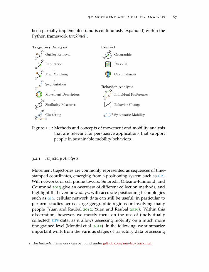
3.2 movement and mobility analysis 67
been partially implemented (and is continuously expanded) within thePython framework trackintel1.
Trajectory Analysis
Clustering
Similarity Measures
Movement Descriptors
Segmentation
?
Map Matching
Imputation
Outlier Removal
Context
Circumstances
Personal
Geographic
Behavior Analysis
Behavior Change
Systematic Mobility
Individual Preferences
Figure 3.4.: Methods and concepts of movement and mobility analysisthat are relevant for persuasive applications that supportpeople in sustainable mobility behaviors.
3.2.1 Trajectory Analysis
Movement trajectories are commonly represented as sequences of time-stamped coordinates, emerging from a positioning system such as GPS,Wifi networks or cell phone towers. Smoreda, Olteanu-Raimond, andCouronne 2013 give an overview of different collection methods, andhighlight that even nowadays, with accurate positioning technologiessuch as GPS, cellular network data can still be useful, in particular toperform studies across large geographic regions or involving manypeople (Yuan and Raubal 2012; Yuan and Raubal 2016). Within thisdissertation, however, we mostly focus on the use of (individuallycollected) GPS data, as it allows assessing mobility on a much morefine-grained level (Montini et al. 2015). In the following, we summarizeimportant work from the various stages of trajectory data processing
1 The trackintel framework can be found under github.com/mie-lab/trackintel.
68 background
and analysis as presented in the extensive overview paper of Zheng2015.
AfterUncertaintyand outliers
collecting movement data, it is usually required to removeoutliers, as the underlying data generation methods often exhibit quitelarge uncertainty margins. For example, GPS measurements in urbancanyons suffer from low accuracy, an effect that can be countered byusing more satellites, e.g., by combining position measurements frommultiple GNSS (Angrisano, Gaglione, and Gioia 2013). As smartphonesare able to use a wide range of positioning technologies and interpo-lations (cf. Brimicombe and Li 2009), their accuracies can also greatlyvary (Watzdorf and Michahelles 2010). Wang, Bah, and Hammad 2019
present an overview of the current state of the art in outlier detection.They classify the available options into distance-, clustering-, density-,ensemble-, and learning-based approaches. Within the mobility domain,many outlier detection algorithms focus on identifying anomalous tra-jectories or (traffic) flows. In order to detect anomalous individualGPS recordings, Chen, Cui, et al. 2016 propose a method based oncubic splines (adaptively modeling the trends of trajectories) to removeindividual position fixes and compare it to the more commonly appliedapproaches involving thresholds and Kalman filters (Gomez-Gil et al.2013; Chen, Zou, et al. 2015; Zheng 2015). They note that the advan-tages of their approach lie in the adaptability (to the trajectory), thepossibility to detect even small outliers, the robustness with regardsto sampling rate, the increased performance, and the fact that theirapproach is (almost) parameter free.
AlongMapmatching and
imputation
the same line as outlier detection are both imputation (ofmissing values or unknown properties, such as the transport modetaken) and map matching (the use of geographic context to improvelocation measurements). Barnett and Onnela 2020 argue that recordingGPS traces using people’s smartphones leads to a “tremendous missingdata problem” (Barnett and Onnela 2020, p.1). Their approach involvesresampling from previously recorded events whenever a certain intervaldoes not contain any data. As such, these approaches are mostlysuitable if the gaps in the data are short (but might be frequent). Zafaret al. 2017 present a solution to the imputation problem that works ona higher level than the actual position fixes. They essentially clusterlocations (and assign semantic labels to them), which allows imputingmissing locations at a later stage. Similarly, Martin, Bucher, Suel, etal. 2018 highlight another area of mobility data imputation: for some
3.2 movement and mobility analysis 69
trajectories and locations a person visits, the transport mode or purposeof the visit are known. Using this information, they propose a methodbased on graph convolutional neural networks to infer distributionsover all possible purposes for locations whose purpose is unknown.
A Segmentationrange of approaches exist to segment sequences of GPS positionfixes into parts of movement (covered by a certain mode of transport)and pauses in between. For example, Li, Zheng, et al. 2008 propose analgorithm that detects staypoints within a person’s movement. Theirmethod is based on spatial and temporal thresholds that define howlong a person has to stay within a certain radius before the locationis considered a staypoint. Hwang, Evans, and Hanke 2017 present asimilar approach, based on Density-Based Spatial Clustering of Applica-tions with Noise (DBSCAN), that additionally is able to handle temporalgaps in GPS data. They choose a temporal threshold of 3 min, referringto other work that proposes a range of 2-30 min for important placesin a person’s life (Ashbrook and Starner 2002; Ye, Zheng, et al. 2009).Similarly, the spatial threshold (i.e., the ε in DBSCAN) is chosen as 50
m, indicating the distance within which a person has to stay in orderfor the location to be considered a staypoint. Biljecki, Ledoux, andOosterom 2013 combine segmentation with identification of transportmode by using OpenStreetMap (OSM) data to extract potential transitionpoints, and iteratively merging segments that are likely covered by thesame mode of transport.
To Movementdescriptors
make movement data more readily interpretable and to answerconcrete questions, movement and mobility descriptors are commonlycomputed. For example, Laube and Purves 2011 compute speed, turn-ing angle and sinuosity of movement, and explore how different sam-pling frequencies influence the individual descriptors. They show thatcomputing these descriptors is indeed highly sensitive to the chosensampling frequency and that GPS measurement errors tend to mask theactual measurements at high frequencies. Hasan et al. 2013 go into moredetail, and propose descriptors such as rankings of different places, triplength distributions, staytime distributions, or visitation frequencies.Schneider, Belik, et al. 2013 analyze the sequential patterns appearingin a person’s mobility and find that we spend most of our trips to reachup to (the same) four locations. Gonzalez, Hidalgo, and Barabasi 2008
compute measures such as the radius of gyration, individual traveldistances, return probabilities, and visitation frequencies and find thatthey commonly follow some characteristic functions (often power laws).
70 background
DetectingTrajectorysimilarity
systematic patterns in mobility is usually done using var-ious forms of trajectory similarity measures. Toohey and Duckham2015 compare the most common trajectory similarity measures: longestcommon subsequence, Frechet distance, Dynamic Time Warping (DTW)and edit distance. They all essentially take two trajectories (orderedsequences of individual position fixes) and return a value in [0, ∞] thatdescribes their distance in terms of the chosen metric (whereas theinverse, in [0, 1], describes their similarity). Several researchers haveadapted these general similarity measures to specific problems. Forexample, Cruz, Macedo, and Guimaraes 2015 consider that in carpool-ing, pickup and dropoff points play an important role, and that onlyone of the participants has a car available. Additionally, intermediatetrajectory points are usually of lesser relevance, as long as the temporalconstraints can be fulfilled and the pickup and dropoff locations arealong the route. He, Hwang, and Li 2014 similarly consider carpooling,and additionally take into account that in order for two trajectoriesto be similar they have to co-occur at roughly the same time. Theseproblem-specific similarity measures often rely on general trajectorysimilarity measures, and combine them with other measures usingweighted models.
BasedTrajectoryclustering
on the similarity values between different trajectories, it ispossible to compute clusters, e.g., to determine frequently traveledtrips or groups of people who could rideshare together. Nanni andPedreschi 2006 adapt density-based clustering to explicitly consider thetemporal dimension given within movement trajectories. They arguethat for trajectory clustering, density-based approaches are particularlyuseful as clusters do not have to be of spherical nature (in parameterspace), they are very robust to noise, and they do not require an upfrontdecision about the number of clusters. Fu, Hu, and Tan 2005, on theother hand, use pairwise similarity between trajectories and spectraland hierarchical clustering to group vehicle trajectories from trafficvideos. The application of spectral clustering allows identifying anunspecified number of dominant paths, while the employed low-levelhierarchical clustering first allows to detect dominant paths, which latercan be refined into individual lanes of the road.
3.2 movement and mobility analysis 71
3.2.2 Context and Circumstances
Contextual Geographiccontext
data is frequently used to add additional information togeoreferenced data. Purves et al. 2014 identify three types of contextualdata: data that is collected alongside the movement (e.g., accelerometerdata or the temperature as measured by a smartphone that also collectsthe movement data), data that describes the space in which a movementoccurred (e.g., the precipitation or land use), and supplementary datathat describes the movement or data collection process itself (e.g., amotion function that describes the physical movement of a car). Withinthis dissertation, and in line with the work by Siła-Nowicka et al. 2016,we primarily focus on the second type, namely data that is readilyavailable in a wide range of geodata repositories and can be spatiallyand temporally linked to the movement. The reason for this choice isthat such data can easily be retrieved in a post-processing stage, there isa wealth of different context data available, and it only requires limitedexpert knowledge to integrate (in contrast to, for example, physicalmodels of vehicles).
In the context of Volunteered Geographic Information (VGI), Spin-santi and Ostermann 2013 use distances to other geographic entities,the population density and the predominant vegetation type within aregion as context, but mention the possible use of socio-demographicparameters, historical measurements or infrastructure conditions. Get-ting closer to the topic at hand, Buchin, Dodge, and Speckmann 2014
argue that since context drives mobility choices and patterns, it is ofparamount importance to include it within its analysis. Inspired by acase study involving hurricanes, they postulate that geographic contextcomes in the form of networks (e.g., trains are restricted to drive onthe railway network), land cover, obstacles (that hinder the passagethrough a certain geographic space), terrain (i.e., changes in elevation),ambient attributes (e.g., weather), time, and presence of other agents.Further, they note that context can be discrete or continuous, as well asdynamic or static. The presence of dynamic phenomena is noteworthyas an agent moving along a trajectory will “sample” the phenomena atdifferent points in time. Taking similarity analysis as an example, theypropose to combine contextual and spatial distance. In particular, theycompute a separate contextual distance based on the different contextareas the original trajectory passes through and combine it with thespatial distance by introducing a context weight. As an introductory
72 background
article to the special issue Geographies of Mobilities, Kwan and Schwanen2016 note similarly that we have to move beyond the “traditional notionof a static, area-based geographic context” (Kwan and Schwanen 2016,p. 251) as movement takes place in space and time, and is tightly linkedto continuously changing context. Kwan 2012 introduces the uncertaingeographic context problem, which similarly highlights the difficultiesin assigning context to movement. In this case, the uncertainty arisesfrom a lack of knowledge about the “influence area of” resp. “durationof exposition to” a certain contextual phenomenon, a problem that isclosely related to the Modifiable Areal Unit Problem (MAUP) (whichdescribes that aggregating measurements of geographic phenomenainto districts has far-reaching impacts on the resulting summary statis-tics). Siła-Nowicka et al. 2016 regard the analysis of human mobility,and focus on the relation between context and chosen transport modesas well as visited locations. In their work, context includes publictransport data (station locations) and POI data (augmented via manualinspection through Google Maps and OSM). Especially the geographicinformation about PT stations as well as the timetables for buses, trains,etc. can be used well for transport mode inference. Common to all theseintegrations of context and movement data is that they are manuallydefined by experts and restricted to the problem at hand. In chapter 4,we will treat this problem by introducing a formalism for specifyinghow context and mobility data should be combined.
NextPersonalcontext and
circum-stances
to geographic context, a variety of other, mostly temporal andpersonal information should be considered as circumstantial. Lovettet al. 2010 show that personal calendars in combination with socialnetwork data provide a valuable source of contextual information. Theyargue, however, that the calendar alone is unreliable (as meetings areoften shorter than planned, get canceled, etc.), and propose a data fusionmethod that is able to create missing calendar entries. Their data fusionpipeline uses spatio-temporal co-occurrence of office workers, searchestheir communication history for potential events, and schedules orupdates “missing events” accordingly. Do and Gatica-Perez 2012 usean ensemble model that is able to exploit multi-dimensional context inorder to solve next-place and stay duration prediction. In their case,context consists of the hour of day, day of week, an indicator separatingweekdays from weekends, visit frequencies, average stay duration, thenumber of Bluetooth devices in the vicinity as well as an indicator ifsomeone was using his or her phone. Adding these variables allowed
3.2 movement and mobility analysis 73
the researchers to improve both the next place as well as the durationprediction accuracy.
3.2.3 Mobility and Transport Behavior Analysis
The survey by Lin and Hsu 2014 groups numerous mobility analysismethods into four areas: location inference, transport mode identifica-tion, trajectory mining and activity recognition. While many of themare closely related to the above introduced trajectory analysis methods,we here consider their use to detect individual mobility preferences,systemic aspects of mobility, and how the use of mobility changes overtime.
Next Individualpreferences
to extracting general properties of (collective) mobility, move-ment trajectories are also being used to extract individual mobilitypreferences. Often, the aim is to improve smartphone route recom-mendation applications. Nack et al. 2015 propose a method to extractmobility habits that involves movement segmentation, transport modeidentification and trajectory clustering. Based on the resulting clus-ters (and the associated travel distributions), a heuristic for destinationprediction (based on visitation frequency, the weekday indicator andthe distribution of departure times) is presented. The authors alsointroduce an approach to identify habits based on counting how oftena certain trip was made within a certain time frame, which they arguecould be used to help people plan their daily schedules. With a sim-ilar intent, Logesh, Subramaniyaswamy, and Vijayakumar 2018 builda travel recommender system utilizing location data and a person’ssocial network profile. Based on individually generated POIs for eachuser, a recommender system proposes a route (taking into accountthe actions of similar users in similar situations), and a feedback looplets the system store a user’s decision for future use. Wu et al. 2018
propose a method that considers both individual preferences as well associal interactions within groups to improve location prediction. Thepresented two-stage approach first identifies groups of trajectories (afterclustering locations into places and extracting transition edges fromthem) and individual moving preferences (time-dependent transitionprobabilities between locations), after which they are integrated usinga linear regression model to yield transition probabilities that can beused for location prediction. Their results show that the predictionaccuracy improves, and that the social interaction influence makes up
74 background
for roughly 30% of the predicted probability. A similar split into in-dividual and collective preferences is given by Calabrese, Di Lorenzo,and Ratti 2010, who also rely on geographical context such as land useor POIs in vicinity. While they use a similar linear regression modelfor combination, they do not group people according to their mobilitybehavior, but instead formulate general properties of mobility based ontraveled distance, visited POIs and involved land use types.
Generally,Systematicmobility
many location data mining techniques aim at findingregularities (and correspondingly, irregularities) in mobility behaviorof people. Within this dissertation, we are primarily interested inmining trajectories from single persons, in order to find characteristicsand patterns within their individual behavior. This is in contrast toa large amount of work on general laws of mobility, such as the onesby Gonzalez, Hidalgo, and Barabasi 2008 describing travel distancedistributions or return probabilities or the ones by Alessandretti et al.2018 elaborating on the conserved quantity of visited places (whichis approx. 25). Pappalardo et al. 2015 process a large dataset fromcentral Italy and find that people either follow an explorer or a returnerpattern in their mobility. While returners exhibit a great amount ofregularity by only visiting a few preferred locations, explorers liketo visit previously unseen locations. To group people into the twoclasses, the k-radius of gyration is introduced, namely the radius ofgyration (the average weighted deviations of all visited locations byan individual from the center of mass for said individual) over the kmost frequented locations. However, while this computation of radiusof gyration gives valuable insights about an individual’s movement,it does not say anything about the regularity of individual trips. He,Li, et al. 2012 analyze individual users’ trajectory histories in order tofind routes that a user frequently covers at roughly the same time ofday. Their approach involves building a series of temporal grids, whichare used to group trips that were taken at roughly the same time. Theresulting shared trajectories are called support routes, and are matchedto each other via the use of a grid-based route table (that essentiallystores all the support routes’ trackpoints from different users in a grid).A query for a potential ridesharing trip then simply has to search formultiple routes appearing in both the origin and destination cell ofthe route table. While the ultimate goal in the work of Wang, Yuan,et al. 2015 is location prediction, they split a person’s mobility intoregularity and conformity: regularity is essentially computed based
3.2 movement and mobility analysis 75
on the visitation frequencies of various locations, and conformity is atime-dependent property that denotes if a location is frequently visitedby similar people. Their results again highlight that people’s mobilitybehavior is highly systematic, yet in those cases where they deviatefrom their usual patterns, considering the behavior of similar usersallows inferring what they do instead.
As Behaviorchangedetection
supporting eco-friendly behaviors play a central role within thisdissertation, we argue that the detection of different stages of behaviorand the transitions between them are of importance. To the best of ourknowledge, only a few studies have covered the topic of intra-personmobility variations. Schlich and Axhausen 2003 examined habitualtravel behavior based on a six-week travel diary and several differentmeasures to capture the similarity of travel behavior: the frequency ofsimilar activities within a certain period (based on Hanson and Huff1986), the frequency of matching trips on two different days (based onHuff and Hanson 2010), a two-level daily comparison of trips (wherefirst the order of trips is compared, and if there is a match, secondaryattributes such as the mode or trip purpose are considered; cf. Pas 1983),a time budget-based measure that compares activities performed withincertain intervals (based on Jones and Clarke 1988), and several others.Their results show a high variability among the different measures,especially when using the trip-based methods. Additionally, they showthat for the whole 6-week survey period there are no two days thatare completely dissimilar and they state that behavior is thus neither“totally repetitious nor totally variable” (Schlich and Axhausen 2003,p. 34). They conclude by saying that adapted measures that accountfor different groups of persons (with comparable temporal demands)could improve the measure of variability and facilitate recommend-ing travel options that have a lower environmental impact. Pendyala,Parashar, and Muthyalagari 2001 compute some of the same measureson a dataset from 81 individuals, collected over at least three weekdays.They find that weekdays play a large role when computing the variabil-ity (on weekdays, mobility behavior varies much less); similarly, longerobservation periods lead to a larger variability. Additionally, they statethat using GPS data leads to higher variabilities than using travel diaries(which are a more coarse representation of mobility behavior). Stopher,Moutou, and Liu 2013 analyze the effects of a travel behavior changeinitiative in Australia. They measure the variability between differentanalysis “waves” and find that people taking part in the initiative lower
76 background
their daily traveled kilometers by 5-6. Waerden, Timmermans, andBorgers 2003 use a survey to look at transport mode choice behaviorafter key events, such as home relocation, changing jobs, or buying acar. Among the recorded parameters within their study they looked athow a key event influenced the number of available alternatives as wellas their characteristics (e.g., travel costs, comfort or reliability), how itaffected the attitudes of people towards a transport mode, and how itaffected the choice behavior. They found that key events significantlyimpact the number of alternative options as well as the key character-istics of them. While the attitudes of people were not greatly affected,their behavior changed after moving to a new place, starting to work,and experiencing a change in the work situation. Lanzendorf 2003
theoretically introduces “mobility biographies” that aim at capturingan individual’s mobility behavior over his or her life time, modeled asa sequence of impactful events within the three domains life (includingsocial and cultural environments), accessibility (of relevant locations)and mobility (availability of various transport modes). Explicitly mod-eling effects of age, household composition, income, professional career,leisure activities, or transport system changes allows us to put theseevents into relation with the corresponding mobility choices.
3.2.4 Relevance to this Dissertation
The given background on movement and mobility analysis is used asa foundation for the research presented in chapter 4. In particular, webuild upon the research presented in this section when presenting themethods for the systematic combination of context and mobility data,the extraction of descriptors specifically tailored for eco-feedback, aswell as the automatic detection of behavior changes. As was highlightedin this section, while there is a wealth of research available on thesetopics, the focus is seldom on supporting individuals in sustainablemobility choices. Next to considering individual circumstances, con-text, preferences and attitudes this also entails a stronger focus on thequestion of what is sustainable, which information is supportive forreaching sustainable behaviors, and how behavior (and changes thereof)can be quantified and automatically analyzed.
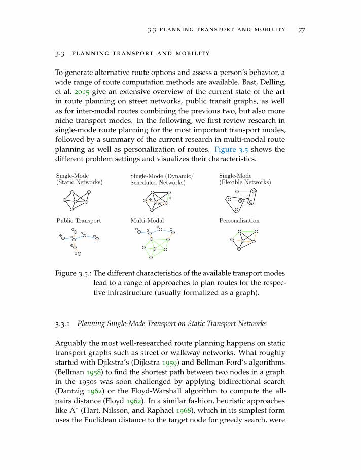
3.3 planning transport and mobility 77
3.3 planning transport and mobility
To generate alternative route options and assess a person’s behavior, awide range of route computation methods are available. Bast, Delling,et al. 2015 give an extensive overview of the current state of the artin route planning on street networks, public transit graphs, as wellas for inter-modal routes combining the previous two, but also moreniche transport modes. In the following, we first review research insingle-mode route planning for the most important transport modes,followed by a summary of the current research in multi-modal routeplanning as well as personalization of routes. Figure 3.5 shows thedifferent problem settings and visualizes their characteristics.
Single-Mode(Static Networks)
Single-Mode (Dynamic/Scheduled Networks)
Single-Mode(Flexible Networks)
Multi-ModalPublic Transport Personalization
Figure 3.5.: The different characteristics of the available transport modeslead to a range of approaches to plan routes for the respec-tive infrastructure (usually formalized as a graph).
3.3.1 Planning Single-Mode Transport on Static Transport Networks
Arguably the most well-researched route planning happens on statictransport graphs such as street or walkway networks. What roughlystarted with Djikstra’s (Dijkstra 1959) and Bellman-Ford’s algorithms(Bellman 1958) to find the shortest path between two nodes in a graphin the 1950s was soon challenged by applying bidirectional search(Dantzig 1962) or the Floyd-Warshall algorithm to compute the all-pairs distance (Floyd 1962). In a similar fashion, heuristic approacheslike A∗ (Hart, Nilsson, and Raphael 1968), which in its simplest formuses the Euclidean distance to the target node for greedy search, were
78 background
developed to handle large graphs. More modern approaches usuallyinvolve a lengthy preprocessing phase during which nodes are sortedaccording to their importance. For example, approaches involvinglandmarks choose a set of vertices to and from which the distancesto all vertices in the graph are computed (Goldberg and Harrelson2005). Using the triangle equality, it is then possible to compute lowerbounds for the distance from any vertex to the target, and iterativelychoose the vertex with the lowest bound for further continuation of thealgorithm. Similar, but not using individual vertices, is the approachof Arc Flags (Kohler, Mohring, and Schilling 2006). The idea hereis to separate a graph into multiple (roughly equal-sized) subgraphsand note for each subgraph if it lies on a shortest path to any vertexin each of the other subgraphs. A shortest path algorithm can thenquickly prune subgraphs that do not lie on the shortest path to thetarget subgraph. The algorithm has successfully been extended with ahierarchical component whereas the subgraphs themselves are groupedand pruned either as an aggregate or (if the subgraph lies on theshortest path to the target) individually one layer below (Mohring et al.2007). Using separators (essentially a set of vertices whose removalsplits the graph into multiple smaller subgraphs; for street networks,these could, for example, lie on roads between towns) and shortcutgraphs (that preserve the distance property between any two vertices inthe graph) (cf. Van Vliet 1978; Eppstein and Goodrich 2008), speedupsin route computation can be achieved as it can largely be performed onthe overlay graph, connecting individual separated subgraphs.
AmongHierarchicalmethods
the best-performing algorithms are those that make use ofhierarchic structures in transport networks given by arterial roads suchas highways (essentially adopting a “divide and conquer” strategy),similar to the way humans commonly plan routes (Car and Frank 1994).Highway hierarchies (Sanders and Schultes 2012) and highway noderouting (Schultes and Sanders 2007) are two approaches that use thefact that long-distance queries primarily result in routes passing a fewimportant nodes. Contraction hierarchies are a similar and widely-usedapproach (Geisberger et al. 2012) that inserts shortcut edges betweennodes and ranks them according to their importance. The bidirec-tional routing algorithm then always follows edges to “more important”nodes, which will result in the shortest path while only visiting a smallsubset of all nodes. Bounded-hop techniques such as labeling algo-rithms (Peleg 2000) or transit node routing (Bast, Funke, et al. 2007)
3.3 planning transport and mobility 79
precompute distances and store them as labels or special nodes withinthe graph for each node in order to have very low query times whichessentially consist of only a few table lookups. As most of the rout-ing methods exploit one or another transport network property, theircombination can yield further speedups. For example, the combina-tion of landmark- and hierarchy-based methods (Goldberg, Kaplan,and Werneck 2009) allows precomputing distances only for landmarkshigher up in the hierarchy, resulting in space savings. In practice, thechoice between one or another algorithm is usually driven by severalproperties: preprocessing time, disk storage space, and query time,which have to be traded off against each other. For a wide range ofrealistic scenarios, other properties come into focus, such as dynamism,time-dependence, or multiple objectives.
3.3.2 Dynamic Networks
Considering routing on street networks, dynamism plays an importantrole: traffic jams lead to lower average speeds, accidents can blockroutes, etc. A straightforward approach to using the above methods issimply to rerun the preprocessing on the updated graph. As this can beexhaustively costly, approaches were developed to selectively updatethe routing graph (Delling and Wagner 2007; Schultes and Sanders2007). It is also possible to have a resilient algorithm that still yieldscorrect routing results after updating weights, albeit with longer querytimes (Delling and Wagner 2007; Geisberger et al. 2012). Probablythe most successful approaches nowadays split preprocessing into ametric-independent phase, followed by a metric-dependent phase thatcan be run much quicker (Efentakis and Pfoser 2013; Dibbelt, Strasser,and Wagner 2014). Similarly, for many networks the dynamism is(approximately) known in advance (e.g., traffic jams tend to happenregularly at the same locations). Instead of using scalar edge weightsin the transport graph, they can be modeled as functions of time. Withslight adaptations, most of the presented approaches still work, albeitwith longer query times (Cooke and Halsey 1966; Delling and Nannicini2011; Batz et al. 2013), and often under the condition that the First InFirst Out (FIFO) property holds (departing later cannot lead to an earlierarrival). Closely related are range queries, whose purpose is to find thebest shortest path through a time-dependent network both in space as
80 background
well as in time (i.e., the departure and arrival times are not given, cf.Dehne, Omran, and Sack 2012).
3.3.3 Public Transport
A large difference between road and public transport networks is theschedule-based nature of the latter. Most PT systems around the worldfollow the same structure: a number of vehicles drive along given routes,stopping at predefined stations at specific points in time. To enableintegration into PT route planners, they usually publish their timetablesin the GTFS format, which follows the same structure (Google Inc. 2020;Barbeau 2013). The two main approaches to model PT networks aretime-expanded and time-dependent (Bast, Delling, et al. 2015). The formermodels all the possible departures from stops (at different times) asindividual vertices and uses directed edges to connect them, takinginto account time (e.g., departures at a certain stop can only be takenwhen coming from edges that arrive earlier) (Pallottino and Scutella1998; Schulz, Wagner, and Weihe 2001). Various approaches exist thatrefine this model, e.g., by introducing minimal transfer times at stops,or by using the periodicity of a timetable to save space by encodingmultiple departures into the same nodes. The time-dependent model issimilar in nature to the dynamic transport graphs for road networksdescribed previously. To save space, transfers are not unrolled, butinstead time-dependent functions encoding the possibility to transferfrom one vehicle to another at a given time are used (Stølting Brodaland Jacob 2004). Closely related are frequency-based models that storethe time-dependent transfers simply as the initial departure time plusthe frequency along the given trip (Bast and Storandt 2014).
A variety of algorithms try to solve either the earliest arrival problem(how to get to the destination as quickly as possible), the range problem(given a departure time range, what are the quickest options to get tothe destination), the latest departure problem (when does a trip haveto leave at the latest to still be at the destination before a given time),or a range of multicriteria problems (e.g., to minimize the number oftransfers) (cf. Bast, Delling, et al. 2015). While many algorithms arecomparable to their counterparts on road networks, some different ap-proaches like the Connection Scan Algorithm (Dibbelt, Pajor, Strasser,et al. 2013) or Round-based Public Transit Optimized Router (RAPTOR)(Delling, Pajor, and Werneck 2014) exist. They use the fact that by in-
3.3 planning transport and mobility 81
volving a temporal component the graphs become directed and acyclic,and can be stored in different structures such as departure-time-sortedarrays that can be scanned to get a PT route (Dibbelt, Pajor, Strasser,et al. 2013). The approach by (Delling, Pajor, and Werneck 2014) isessentially a dynamic program operating on arrays of trips and routes.Each of these arrays is scanned to retrieve reachable stops, which inturn lead to subsequent scans at the next iteration of the algorithm.
3.3.4 Carpooling and Ridesharing
Rideshare Fuzziness,flexibility,dynamism
and carpooling trips are generally longer than regular trips(Ferguson 1997), partially due to the required detours to pick up anddrop off passengers which make up around 17% of the trip distance(Rietveld et al. 1999). These detours make rideshare planning a non-trivial problem, especially considering the flexibility of the drivers andriders, the fuzziness of the itinerary descriptions, and the potentialto pick up and drop off multiple people (Huang, Bucher, et al. 2018).Of further importance for a rideshare planning system are the factsthat the involved entities are independent (thus both have to access thesame system to find each other), they usually have a financial incentive(i.e., a matching system should account for potential costs), there isa base “fear” of traveling with a stranger (which can be alleviatedby introducing a rating system), and that there are several ways howpeople can be matched (single driver, single rider, multiple drivers,multiple riders, and combinations thereof).
The focus of this dissertation on dynamic and inter-household rideshar-ing also means that the origins and destinations do normally not exactlycorrespond to each other, and suggests solutions globally optimizingdriver and rider assignments. However, this global perspective on theridesharing problem (which can be optimized for minimal system-widevehicle-miles, minimal system-wide travel times, or maximal numberof riders; cf. Agatz et al. 2012) is of little interest to the individualtraveler, for which reason we focus here more on the planning stepsfor an individual route request. Raubal, Winter, et al. 2007, based onthe theoretical model presented in previous work (Winter and Raubal2006), provide a solution based on short-range communication betweenindividual agents that uses concepts from time geography to bound thenumber of possibly shareable trips. Depending on the intended traveldistance, drivers usually only denote pickup and drop-off regions, as
82 background
they are able to move much quicker than the rider, and thus are flexiblein their pickup and dropoff locations. These fuzzy descriptions and theflexibility of drivers and riders lead to the fact that even though thereare many specialized web platforms that facilitate access to carpooling,there is usually much manual planning and negotiation involved. Toextend the use of carpooling into persuasive mobility support systems,it is important to develop planning systems that combine various trans-port modes (esp. public transport) with carpooling (Aissat and Varone2015; Bit-Monnot et al. 2013; Huang, Bucher, et al. 2018).
InLinking general, multi-modal routing is achieved by linking several trans-port networks using, for example, a nearest-neighbor approach (Bast,Delling, et al. 2015; Pajor 2009). In this case, every node of one transportnetwork is linked to the closest node of another (e.g., a train stationwould be linked to a footpath close by). Aissat and Varone 2015 proposea method (based on previous work by the same authors, cf. Varone andAissat 2015) that tries to replace sub-paths of a multi-modal plannerwith carpooling offers. Their method involves a way to determine thesuitability of a certain rideshare offer for the completion of a user’sitinerary, a substitution process to select the best driver, and a pruningof offers based on their arrival time. Bit-Monnot et al. 2013 present the 2synchronization points shortest paths problem and propose an efficient com-putation of itineraries, using a heuristical landmarks-based approach.Huang, Bucher, et al. 2018 extend the idea of nearest-neighbor-basedlinking with the concept of Drive Time Areas (DTAs). A DTA denotesthe area that someone can realistically reach within a certain amountof time. By linking transport networks based on drive time area, theflexibility and fuzziness of carpooling can be incorporated into theplanning problem. Referring again to the work by Agatz et al. 2012, theauthors state that there are still many open points regarding rideshareplanning: In particular, optimization (to handle a large number of po-tential rideshare participants), incentives to attract people to ridesharingsystems, and the inclusion of people’s preferences in order to give themmeaningful choices, are open problems.
3.3.5 Electric Mobility
Related to the different characteristics of EVs (e.g., shorter rangesinducing range anxiety, longer recharging times), many researchersstarted adapting route planning methods to account for the State of
3.3 planning transport and mobility 83
Charge (SOC). Within this context, the elevation profiles, road types, aswell as the braking behavior resp. energy recuperation functionalitygain in importance. Yao et al. 2013 use floating car data collected bycars in Beijing to determine the impact of road type on the energyconsumption of vehicles. Their findings correlate vehicle speed withroad type and energy consumption, and can be used as input for a routeplanning on a dynamic graph. However, as they do not include eleva-tion, their model is mostly applicable to flat areas. Graser, Asamer, andPonweiser 2015 explicitly study the impact of different Digital ElevationModels (DEMs) and interpolation methods on the energy consumptionestimation and find that high-resolution DEM can explain up to 30% ofthe used energy by changes in elevation. Baum et al. 2014 similarlyconsider elevation, but focus on finding routes that trade off speedin favor of energy conservation (i.e., they evaluate multiple differentspeeds on the same road segment). They propose heuristics to speedup computation times by several orders of magnitude. Another inter-esting problem is the consideration of recharging stations for extremelylong trips or for vehicles that are operated for many consecutive hours(e.g., taxis or delivery vehicles). Schneider, Stenger, and Goeke 2014
consider a special case of the Vehicle Routing Problem with Time Win-dows (VRPT), whereas delivery vehicles have a number of rechargingstations available to deliver goods to a number of clients (within giventime windows). They essentially solve a mixed-integer program thatoptimizes the traveled distance but respects the fact that the SOC nevercan get below zero, next to the usual boundary conditions (essentiallyto serve all customers within their time window).
3.3.6 Autonomous Mobility and On-Demand Offers
On-demand mobility is often regarded from a holistic optimizationpoint of view, commonly termed as Dial-A-Ride Problem (DARP) (Cordeauand Laporte 2007; Berbeglia, Cordeau, and Laporte 2010). The problemconsists of multiple vehicles that should serve a set of clients, expressingroute requests from a given origin to a destination, and will likely gainin importance with an increasing autonomy of vehicles. The problemitself is a generalization of a number of other problems such as thepickup and delivery vehicle routing problem, the traveling salesmanproblem or the VRPT introduced above (however, these are mostly con-cerned with non-human cargo). In general, these problems are solved
84 background
using dynamic, linear or mixed-integer programming with a numberof constraints (Cordeau 2006). Usually the optimization is only solvedon the subgraph of direct links between pickup and dropoff locations.Garaix et al. 2010 propose a more flexible approach involving a numberof alternatives that can be used within a multi-criteria optimization.This is especially important if not only travel time, but also cost shouldbe globally minimized. Closely related is the Demand Adaptive Systemor Mobility Allowance Shuttle Transport (MAST) problem (Malucelli,Nonato, and Pallottino 1999; Quadrifoglio, Hall, and Dessouky 2006),which arises from having fixed-route transport that is allowed to deviateslightly in order to pickup and dropoff people along the route (often,this is employed during phases of low demand to reduce the numberof vehicles and routes in operation). Quadrifoglio, Hall, and Dessouky2006 look at the problem by (theoretically) evaluating the impact ofdeviation corridor size on the throughput and transportation speed andproviding a formalism to compute upper and lower bounds. Zhao andDessouky 2008 perform a similar analysis and find that the optimallength of a MAST service corridor is roughly half of the distance thatthe shuttle could travel within one service cycle.
3.3.7 Planning Multi-Modal Mobility Options
Looking at the problem of getting from one location to another from anindividual traveler’s point of view, it becomes clear that the integrationwithin a larger transport network (and especially other transport modes)has to be considered. Generally, the combination of multiple transportmode graphs can be done by inserting transfer edges (Bast, Delling, etal. 2015), whereas the same model as introduced above can be used forthe different transport modes. In particular, the restricted networks (PT,bikesharing, ridesharing, etc.) are connected by unrestricted transportmodes (walking, driving by car, taxis, etc.). Often, the computed routesare selected due to some combined criterion: monetary cost, traveltime, number of transfers, walking duration, etc. (Bast, Delling, etal. 2015; Delling, Dibbelt, et al. 2013). Because simply applying oneof the above introduced algorithms can lead to high query times inmulti-criteria optimization settings, some of them have been explicitlyadapted to the problem. Delling, Dibbelt, et al. 2013 present multimodalmulticriteria RAPTOR that operates in rounds during which either aseparate algorithm for PT or an unconstrained transport mode is run,
3.3 planning transport and mobility 85
after which the criteria are recomputed for all reached vertices. Bast,Brodesser, and Storandt 2013 formulate a set of axioms that determinetrips that a user would unlikely take, which can be used at query timeto filter out unlikely routes.
Another approach to yield feasible routes was introduced by usinglabel constraints, whereas the labels denote different transport modesand enforce a certain order in the mode sequences (Barrett, Jacob, andMarathe 2000). Having their roots in regular language concepts, thelabel constraints can be combined with a range of routing algorithmsto retrieve shortest paths along combined networks. Many of thepreviously presented algorithms have been adopted to work with labelconstraints, e.g., contraction hierarchies (Dibbelt, Pajor, and Wagner2015) by only contracting vertices which belong to the subgraph of thesame transport mode. Querying then consists of both a query in thecontracted subgraphs, as well as running Djikstra’s algorithm on theuncontracted core graph.
Horn 2004 considers the combination of fixed-schedule and demand-responsive modes. He classifies transport modes into four classes: fixedroute modes (conventional PT), smart shuttles (on-demand buses thatare either zone- or point-based), roving buses (free-range service withpickup and dropoff restricted to PT stops), and taxis (door-to-door, maycarry multiple passengers). The journey planner, which is orchestratedby a request broker (that can book on-demand services), essentiallysearches the route solution space in a breadth-first way, whereas one-legged journeys are considered first, followed by two-legged journeys,and so on. The reasoning behind this is that in reality preferred routesoften involve the least number of legs, as waiting times or walkingduring mode transitions is badly perceived by travelers. As the resultingsolution space can potentially be huge, various speedup techniquesare proposed, such as not considering nodes with later arrival times,introducing time limits for waiting at intermediate nodes, etc. Horn2004 also mentions the importance to include user preferences and evenmore flexible on-demand services in the future.
Brands et al. 2014 build a multimodal router that additionally usesroute, stop and line choice models (logit) to consider how many andwhich people would choose a certain route over another. Using asimilar approach, Ambrosino and Sciomachen 2014 use a multi-criteriaobjective function and focus on “commuting points” that aggregatemany of the routes within the network through them. Their heuristic
86 background
approach yields a sequence of commuting points, but does not considermore niche transport modes (on-demand, sharing, etc.) and differentuser perceptions or preferences.
3.3.8 Personalization
WithSingle-modetransport
the increase of available data about individual’s mobility choicesand preferences, personalization gains in importance and new methodsand approaches become feasible. Personalization is possible withinindividual routes traveled by a single mode of transport, as for exampleshown in the work of Letchner 2006. The authors use historical GPS
traces to predict possible travel times (based on a speed extraction) anduser preferences (by introducing an inefficiency ratio that denotes howfar the chosen route deviates from the shortest one). The latter areincorporated into the routing algorithm by defining a utility functionthat prefers previously traversed road segments, arguing that peopleare likely to choose the same paths that they did before. Priedhorskyet al. 2012 rely on the concept of “bikeability”, which denotes for eachstreet segment and user how well it is suited for traversal by bicycle.They introduce various algorithms (clustering-based, collaborative fil-tering, machine learning) that predict the bikeability along a certainroad segment for a given user and find that even simple approacheslike taking the average of a user within a cluster leads to promisingresults. Funke and Storandt 2015 similarly provide single-mode routepersonalization, but pay more attention to the fact that commonly usedrouting algorithms on large graphs assume that the graphs are mostlystatic, thus they cannot easily account for personalization. Their ap-proach is based on the notion of k-path covers of graphs (essentiallysets of nodes where each path of length k in the graph will pass at leastone node in the set), on which various properties are computed thatcan be weighted during routing. The result is that the routing graphbecomes much smaller, which in combination with pruning methods(that remove parts of the graph that would always be dominated byothers) lead to speed-ups of around 20 to 100 over regular Djikstra. Daiet al. 2015 introduce (evolving over time) travel preference distributionsthat balance various features of trajectories against each other and arecomputed on historical data (e.g., distance vs. travel time, distancevs. fuel consumption, etc.). The routing algorithm then uses thesepreferences by looking for similar users that traveled from the chosen
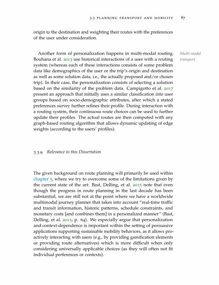
3.3 planning transport and mobility 87
origin to the destination and weighting their routes with the preferencesof the user under consideration.
Another Multi-modaltransport
form of personalization happens in multi-modal routing.Bouhana et al. 2013 use historical interactions of a user with a routingsystem (whereas each of these interactions consists of some problemdata like demographics of the user or the trip’s origin and destinationas well as some solution data, i.e., the actually proposed and/or chosentrip). In their case, the personalization consists of selecting a solutionbased on the similarity of the problem data. Campigotto et al. 2017
present an approach that initially uses a similar classification into usergroups based on socio-demographic attributes, after which a statedpreferences survey further refines their profile. During interaction witha routing system, their continuous route choices can be used to furtherupdate their profiles. The actual routes are then computed with anygraph-based routing algorithm that allows dynamic updating of edgeweights (according to the users’ profiles).
3.3.9 Relevance to this Dissertation
The given background on route planning will primarily be used withinchapter 5, where we try to overcome some of the limitations given bythe current state of the art: Bast, Delling, et al. 2015 note that eventhough the progress in route planning in the last decade has beensubstantial, we are still not at the point where we have a worldwidemultimodal journey planner that takes into account “real-time trafficand transit information, historic patterns, schedule constraints, andmonetary costs [and combines them] in a personalized manner” (Bast,Delling, et al. 2015, p. 64). We especially argue that personalizationand context-dependence is important within the setting of persuasiveapplications supporting sustainable mobility behaviors, as it allows pro-actively interacting with users (e.g., by providing gamification elementsor providing route alternatives) which is more difficult when onlyconsidering universally applicable choices (as they will often not fitindividual perferences or contexts).
88 background
3.4 mobility feedback and its influence on choices
Based on the previous sections, we provide a background on howtracking data was previously used to influence the mobility choices andbehaviors of people, and which data processing methods were appliedtherein. With regards to the topics covered within this dissertation, anemphasis will be put on persuasive and in particular gamified systems.Figure 3.6 highlights the central elements for which this section givesbackground information.
Eco-Feedback
GamificationPersuasiveApplications
Applications to SupportPeople in SustainableMobility Choices (asintroduced in thisDissertation)
Figure 3.6.: Central elements for supporting people in sustainable mo-bility choices using applications that build upon automati-cally and passively collected tracking data.
3.4.1 Eco-Feedback
Roughly starting with Fogg’s work on “computers as persuasive tech-nologies” (Fogg 1998), computers and more recently smartphones havebeen increasingly popular for habit formation, especially in the healthand wellness domain (West et al. 2012) and within the context ofhousehold energy saving (Fischer 2008). Froehlich, Findlater, andLanday 2010 focus on the questions of how HCI, and in particularcomputer-assisted eco-feedback should build on research from envi-ronmental psychology and which role it can take in making peoplebecome more ecologically sustainable. They provide a classificationof different (technology-assisted or -enabled) means to promote pro-environmental behavior: information, goal-setting, comparison (withother individuals or within groups), commitments, incentives/rewardsand “plain” feedback (which can be on a very fine-grained level or ofa summarizing nature). Froehlich, Findlater, and Landay 2010 further
3.4 mobility feedback and its influence on choices 89
provide an extensive review of the literature involving eco-feedback,and mention a lack of focus on HCI issues within the environmentalpsychology field, and vice versa a lack of psychological understandingof researchers in the HCI field. The resulting conclusion is that HCI andUbiComp (ubiquitous computing) researchers should study researchfrom environmental psychology for proven methods and inspiration.DiSalvo, Sengers, and Brynjarsdottir 2010 provide a similar review,focusing on identifying different research fields (within sustainable HCI)and emerging issues. Next to “plain” persuasive technology, they findresearchers mostly explore ambient awareness (non-intrusive forms offeedback), sustainable interaction design, formative user studies, andpervasive sensing. Further, they highlight interesting questions suchas whether we see the users as the problem or whether we intend tosolve their problems, or whether we want incremental improvementor fundamental changes in lifestyle, leading to their conclusion thatto advance the field of sustainable HCI it is important to foster debate,and tie it more strongly to other fields such as professional design orcomputer science.
Stawarz, Cox, and Blandford 2015 review 115 apps that give feed-back in the form of self-monitoring and reminders, but find that theirefficiency would improve if they relied on event-based cues more often(e.g., coupling a new habit to fixed events such as taking medicationright after breakfast), as self-tracking “plays an important role in thebehavior change process, [but] does not support habit formation [andturning] the new behavior into a daily routine” (Stawarz, Cox, andBlandford 2015, p. 2659). The authors argue that the list of includedfeatures indicates that these apps actually support motivation, and notthe change of behavior, which would be best supported by letting userscreate routines, send back-up notifications if these routines change, andprovide post-completion checks. Focusing more on ecological pointsof view, He, Greenberg, and Huang 2010 argue that most technologiesmotivating sustainable practices feature the same simple feedback onenergy use. Based on work from psychology, they propose conceptsand give recommendations that follow the stages of the transtheoreticalmodel to optimally use technology for people in different phases of be-havior change. Examples are to include both benefits and consequencesof a certain behavior in the feedback, referring to social norms, provideexamples for small actions, inform about discrepancies between atti-tudes and behavior, provide links to other people’s behavior, support
90 background
people in setting goals and plans to achieve them, provide positive re-inforcement immediately after performing an action, provide promptsfor habit-forming, foster self-reflection, and more.
Brynjarsdottir et al. 2012 take a more critical stance and argue that thedefinition of sustainability is often too narrow, for example, focusingonly on measures of behavior that can be sensed (and not the underlyingissues that cause said behavior). Often the focus is solely on individualsand their behaviors, and formulated from the point of view of an expert.A consequence is also the treatment of single points in time, and therelated inability to account for changes (in behavior and circumstances).Their conclusion is that it might be worthwhile to think about how wecan re-frame the issues and opportunities of sustainability, instead offocusing on how to provide “technical solutions to social problems”(Brynjarsdottir et al. 2012, p. 954). Li, Dey, and Forlizzi 2011 arguealong the same lines, but emphasize the needs of the individual (withregards to information retrieved from sensed data). Their alreadypreviously introduced two phases of discovery and maintenance split thequestions about status, history, goals, discrepancies, context and factorsthat users have in relation to their behavior.
3.4.2 Inducing Mobility Behavior Change
Several researchers looked at the impacts of persuasive technologies andin particular eco-feedback on mobility behavior. Early on, Froehlich, Dil-lahunt, et al. 2009b performed a study involving dedicated GPS sensorsin combination with smartphones to measure and analyze movementand mobility behavior, and to study the effects of eco-feedback relatedto mobility. As the number of people involved in the study was com-paratively low (13), the results presented in the paper mostly includequalitative statements given by users of the app during interviews. Ingeneral, the feedback was very positive, and especially the focus on a vi-sual representation that is not tightly linked to the exact CO2 emissionsor kilometers driven gave the users a way to playfully interact withthe problem at hand. Froehlich, Dillahunt, et al. 2009a report that eventhough the small study cannot make any statement about the behavioralchanges achieved, 7 out of the 13 participants continued to use the appafter the experiment was finished, indicating that people at least valuedthe feedback on mobility behavior and tried to use it to monitor and im-prove their mobility behavior. Gabrielli et al. 2014 summarize three user
3.4 mobility feedback and its influence on choices 91
studies and highlight future areas of research: due to the lack of holisticresearch that also considers the impact of persuasive interventions oncitizens’ lives over a long term and due to the focus on individualbehavior instead of collective mobility choices, it still remains largelyunclear if the proposed measures lead to long-term changes and if theyare better or worse, or simply complementary to, collective, societal, orpolicy measures. The presented three studies confirm that persuasivetechnologies can help users reach the maintenance stage in the TTM.The second presented study, MatkaHupi (Jylha et al. 2013), featured anapp including a journey planner, movement tracking, and various waysof eco-feedback. In particular the challenge functionality was liked byusers, followed by knowing the impacts on CO2 emissions of driving acar. Superhub (Carreras et al. 2012) was more focused on goal-settingand started out with 695 participants. As filling in the travel diariesevery day was a cumbersome task, eventually only data from 65 partici-pants could be used, however. Similarly, the rigor with which surveyswere answered dropped throughout the study, which makes drawingconclusions difficult. However, in general people liked the goal-settingfeatures and CO2 reporting. Bie et al. 2012 present tripzoom, a livinglab performed in several cities. They similarly use mobile sensors todetect mobility patterns, provide incentives, and additionally employsocial networks where people can share their individual performanceswithin the tripzoom community. The outcome of the project is unclear,however, several supplementary documents provide valuable insightsinto the creation and evaluation process. For example, Diana et al.2013 state the evaluation metrics, and mention that behavior can bemeasured by indicators such as the number of trips, the distance trav-eled, the travel time, travel cost, and CO2 emissions. Anagnostopoulou,Magoutas, et al. 2017 argue that personalization is an important trait ofpersuasive applications. They present the results of applying differentpersuasive strategies on people with different personality (based onthe Big Five: openness, conscientiousness, extraversion, agreeableness andneuroticism) and mobility traits (devoted drivers, image improvers, malcon-tented motorists, active aspirers, practical travelers, car contemplators, publictransport dependents, car-free choosers; cf. Anable and Wright 2013). Basedon the eight persuasive strategies2 and evaluated with 120 people by
2 Comparison, self-monitoring, suggestion, simulation (of potential impacts of a certainbehavior), cooperation, praise, personalization and competition.
92 background
means of survey, they find that all persuasion strategies work well forall mobility types with only minor differences.
Recently, Anagnostopoulou, Bothos, et al. 2016 and Klecha and Gi-anni 2018 reviewed the current state of the art in behavior changefor sustainable urban mobility. Anagnostopoulou, Bothos, et al. 2016
provide a summary of ten persuasive apps (some described above)and recommend to explore or incorporate the following mechanics infuture system design: personalization (increases the impact and accept-ability), localization (providing support at the appropriate location),timing (similar, but for time), and wearable devices (for unobtrusiveinteraction methods). Klecha and Gianni 2018 review 13 applications(some described above) and additionally analyze if the end-users wereinvolved in application development. This “citizen participation” canbe valuable as the resulting application is tailored to the needs of itsusers. In the reviewed applications, it was mostly performed via ques-tionnaires, interviews, focus groups and diaries. As it is in the bestinterest of citizens to travel sustainably, “an ideal solution would createconditions that empower and inform citizens, enabling them to createtheir own change through social innovation” (Klecha and Gianni 2018,p. 147).
3.4.3 Gamification
A popular strategy for persuasive applications is “the use of gamedesign elements in non-game contexts” (Deterding, Dixon, et al. 2011, p.10), commonly referred to as gamification of an application. Accordingto Deterding, Dixon, et al. 2011, gamification is closely related butdistinct from concepts such as serious games (where entertainment isnot the primary goal, but rather education or passing on information),pervasive games (where the real world plays a central role), alternatereality games (that mix events from the real and a fictitious world), andalso playful design (the adaptation of user interfaces based on learningsfrom games). Their definition makes strict assumptions about the natureof gamified systems: In contrast to playful approaches, gamificationfollows structured rules and contains competitive elements (which canalso include competing with “one’s self”); in contrast to serious games,gamification only uses certain elements to increase the motivation ofinteracting with a system in a desired way; gamification does notinvolve the use of gaming technology (e.g., engines or controllers),
3.4 mobility feedback and its influence on choices 93
but rather its design elements; gamification necessarily takes place ina non-game context. In Deterding 2011, the author makes a link tomotivational affordances: This essentially means that a system affordsinteractions that satisfy some psychological needs of the user—in thegame context this could be the need for achievement as given by aleaderboard.
Lister et al. 2014 reviewed gamification usage in 132 health and fit-ness apps found on the Apple App Store in 2014, and found that whilegamification principles were widespread, they mostly did not adhereto professional guidelines or industry standards (i.e., gamification wasonly sporadically applied and did not follow health behavior theory).Around 45% of the apps used some form of passive tracking of data,and most apps either used gamification to have the user interact withthe app more (57.6%), or perform completions of the desired behav-ior (75.8%). Going more towards sustainability, Shih and Jheng 2017
perform a literature review of persuasive strategies for energy-savingbehavior and a questionnaire that relates demographic features to per-suasiveness of different strategies. They find that over their wholesample, the reduction of complex behavior into simple tasks, rewardsand simulation (of potential behaviors) exhibit the largest persuasive-ness, while social comparison and normative influence (education orpeer pressure) are less useful in persuading people. However, thisdiffers across different ages and demographics. As a result of theirwork they present a list of game design elements that can be used toimplement each persuasive strategy. Kazhamiakin et al. 2015 link gami-fication and sustainable urban mobility, and present a framework thatallows implementing gamification on top of existing services. Their casestudy involved 40 participants in northern Italy and featured elementsinvolving sustainability, health, as well as rewards for using Park&Ridefacilities and resulted in a reduction of PMT after the gamified inter-vention. Similarly, Buningh, Martijnse-Hartikka, and Christiaens 2014
aimed at shifting people from using their PMT towards slow mobility,and found that their gamification mechanics (digital coach, team co-herence, peer pressure, competition and awards) lead to a reductionof approx. 20% during rush hour. Wells et al. 2014 use goal-settings,behavior tracking and challenges (involving points and levels) to fostersustainable mobility behavior within the SUPERHUB project.
94 background
3.4.4 Relevance to this Dissertation
The presented research on persuasive applications influencing mobil-ity behavior is mostly focused on qualitative and explorative research.Structured approaches how to build such applications and which mo-tivational elements are available are missing, as are larger-scale andlong-term studies. Additionally, there is little focus on comprehensiveanalyses of mobility behavior and the generation and presentation ofpotential (more sustainable) alternative behavior. Within chapter 6,we build upon the background presented in this chapter to overcomesome of these limitations and evaluate a persuasive application withina large-scale real-world study.
4A N A LY Z I N G M O B I L I T Y F R O M T R A J E C T O RY D ATA
Information about individual mobility behavior increases the rangeand effect of potential supporting measures that we can provide inan automated fashion, as they can be tailored to individual cases andadapted to the current behavior. Recent advances in ICT enable usto record the movements of vehicles and people using a variety ofdevices. Of particular importance are smartphones, as their ubiquityand increasingly powerful sensors allow tracking mobility of and in-teracting with almost any interested person. The data gathered can beused for a wide range of applications, from planning more efficienttransport infrastructure, over automated ticketing for public transportto support of individuals in their mobility choices. While previouswork thoroughly studied many aspects of processing mobility, we focuson the analysis with regards to providing better support for reachingsustainable mobility. Next to sustainability criteria, this includes theidentification of transport modes from GPS data of varying quality,combining context and mobility data, distinguishing systematic fromnon-systematic behavior, identifying mobility goals and preferences, aswell as grouping different behaviors and detecting changes thereof. Buthow do we best record, process and analyze movement data of peoplein order to support them in sustainable mobility choices?
We propose a framework for mobility data processing revolvingaround four primary goals: the use of these data to directly communicatethe effects of past mobility, to identify potential future mobility needs,to use past choices for improved planning of future mobility options, aswell as to provide motivational support for making sustainable mobilitychoices. Figure 4.1 shows the primary data structures and informationprocesses involved in our framework.
Starting from the user who carries a smartphone having a trackingapp installed, we first have to convert the sensor information to a move-ment trajectory. The following preprocessing steps convert the raw
This chapter and its contents, algorithms and figures are based on Bucher, Cellina,et al. 2016; Jonietz and Bucher 2017; Jonietz and Bucher 2018; Jonietz, Bucher, et al.2018; Bucher, Mangili, Cellina, et al. 2019; Bucher, Martin, Hamper, et al. 2020.
95
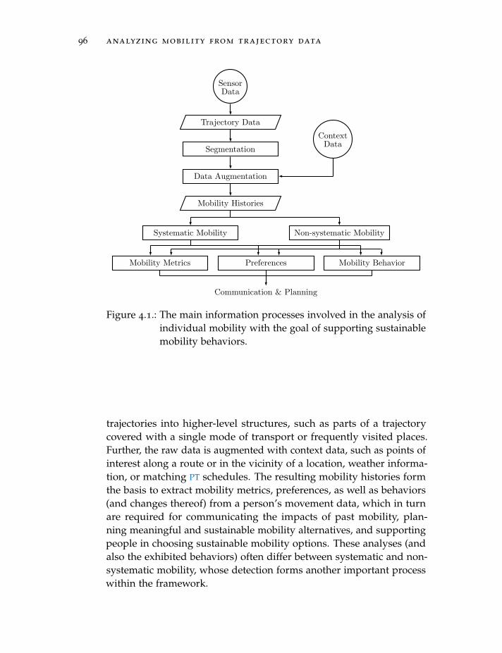
96 analyzing mobility from trajectory data
SensorData
ContextData
Data Augmentation
Segmentation
Mobility Histories
Trajectory Data
Systematic Mobility Non-systematic Mobility
Mobility Metrics Preferences Mobility Behavior
Communication & Planning
Figure 4.1.: The main information processes involved in the analysis ofindividual mobility with the goal of supporting sustainablemobility behaviors.
trajectories into higher-level structures, such as parts of a trajectorycovered with a single mode of transport or frequently visited places.Further, the raw data is augmented with context data, such as points ofinterest along a route or in the vicinity of a location, weather informa-tion, or matching PT schedules. The resulting mobility histories formthe basis to extract mobility metrics, preferences, as well as behaviors(and changes thereof) from a person’s movement data, which in turnare required for communicating the impacts of past mobility, plan-ning meaningful and sustainable mobility alternatives, and supportingpeople in choosing sustainable mobility options. These analyses (andalso the exhibited behaviors) often differ between systematic and non-systematic mobility, whose detection forms another important processwithin the framework.
4.1 mobility histories 97
4.1 mobility histories
Historical measurements of mobility (automatically and passively col-lected movement data) form the basis of the support framework pre-sented within this dissertation. Based on previous research and tech-nologies developed within several projects that are part of this disserta-tion, we here present the most important preprocessing steps to arriveat a consistent and useful representation of mobility.
4.1.1 Movement and Mobility Tracking
Tracking applications become increasingly powerful as the power con-sumption of passively running location estimation technologies drops.At the same time, more data can be sampled using a wide range ofsensors, e.g., the number of Bluetooth devices close by (to inform thelikelihood of being in a PT vehicle) or the momentary acceleration(whose patterns greatly vary depending on the mode of transport). Wedistinguish between movement data (the “raw” location recordings)and mobility data (where additional information, such as the mode oftransport or intermediate stops are identified). While more fine-graineddata gives us the possibility of having a more accurate picture of themobility behavior of a person, it is not necessarily required to knowsomeone’s location at all times, as much can be inferred by interpolationand augmentation with context data.
Table 4.1 Characteris-tics ofMobilityTracking
summarizes the most important characteristics of automat-ically tracked mobility data with respect to supporting sustainablepersonal mobility. Even though the exact route resp. movement tra-jectory is not necessarily of great interest (in contrast to the distancecovered or the start and end locations, which are needed to determinegoals of mobility and its systematic nature), it is usually easier to re-trieve than, for example, the transport requirements (which have tobe stated explicitly, or derived from similar situations). This is dueto the fact that passive location tracking is becoming more and morestandardized, and for the majority of smartphones it is relatively easyto release an app that collects movement trajectories. Usually, thesetrajectories consist of a sequence of individual, time-stamped trackpoints(also commonly denoted as location or position fixes, cf. Laube, Dennis,et al. 2007).
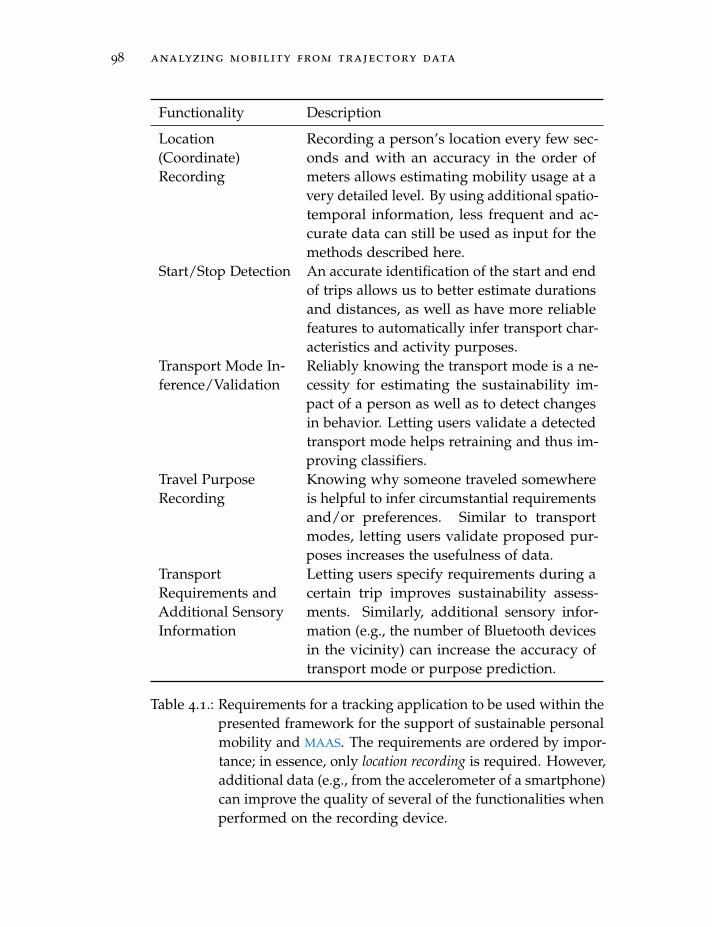
98 analyzing mobility from trajectory data
Functionality Description
Location(Coordinate)Recording
Recording a person’s location every few sec-onds and with an accuracy in the order ofmeters allows estimating mobility usage at avery detailed level. By using additional spatio-temporal information, less frequent and ac-curate data can still be used as input for themethods described here.
Start/Stop Detection An accurate identification of the start and endof trips allows us to better estimate durationsand distances, as well as have more reliablefeatures to automatically infer transport char-acteristics and activity purposes.
Transport Mode In-ference/Validation
Reliably knowing the transport mode is a ne-cessity for estimating the sustainability im-pact of a person as well as to detect changesin behavior. Letting users validate a detectedtransport mode helps retraining and thus im-proving classifiers.
Travel PurposeRecording
Knowing why someone traveled somewhereis helpful to infer circumstantial requirementsand/or preferences. Similar to transportmodes, letting users validate proposed pur-poses increases the usefulness of data.
TransportRequirements andAdditional SensoryInformation
Letting users specify requirements during acertain trip improves sustainability assess-ments. Similarly, additional sensory infor-mation (e.g., the number of Bluetooth devicesin the vicinity) can increase the accuracy oftransport mode or purpose prediction.
Table 4.1.: Requirements for a tracking application to be used within thepresented framework for the support of sustainable personalmobility and MAAS. The requirements are ordered by impor-tance; in essence, only location recording is required. However,additional data (e.g., from the accelerometer of a smartphone)can improve the quality of several of the functionalities whenperformed on the recording device.
4.1 mobility histories 99
Definition 4.1 (Trackpoint). A trackpoint p is a time-stamped coordinatepair (x, y) that denotes the location of an entity at a certain point intime t with an accuracy η: p = (t, x, y, η).
In our definition we omit the direct relation to the entity e (usuallya person whose movement is being recorded), but instead say thatp ∈ Pe if a trackpoint belongs to the set of points that correspond tothe movement of e. As the location tracking usually is not perfectlyaccurate, most tracking technologies specify an η as the radius (inmeters) of a circle around (x, y) in which the actual position of e fallswith a likelihood of pη = Pr(
√(x− x)2 + (y− y)2 ≤ η|x, y) = 95%
(where (x, y) is the true location of entity e at time t). We omit thealtitude z as it is not commonly required for the following methods;it needs to be noted that it can easily be added using a DEM, e.g., forenergy consumption models or to compute more meaningful bicycleroutes. Based on trackpoints, we can now define trajectories.
Definition 4.2 (Trajectory). A trajectory τ is a sequence of trackpointsthat are logically grouped due to some underlying characteristic andsorted by their timestamp: τ = (p1, . . . , pn).
Of course, ordering Pe (all trackpoints of an entity e) as a sequenceyields the complete movement trajectory of e (which we refer to astrack within this dissertation). However, it is often more interesting toconsider smaller segments of this complete movement as trajectories,such as the path taken from one POI to another. Note that we take apurely Lagrangian perspective on movement within this dissertation(i.e., movement is measured within an absolute reference system). Incontrast, a substantial share of previous research considered the Eulerianperspective, where movement is recorded using “check-ins”, e.g., at cellphone towers or Bluetooth beacons (cf. Laube, Dennis, et al. 2007).
4.1.2 Data Segmentation
As a first step of processing the raw trackpoints, they are segmentedinto various higher-level structures. When looking at mobility in asimplistic way, we can state that we consume mobility to get from onepoint of (personal) interest to another. At these points, we usuallyspend much more time than at any intermediate stops, such as whenwaiting to change the mode of transport or until a traffic light turnsgreen. We formalize this idea as staypoints, activities, triplegs and trips.
100 analyzing mobility from trajectory data
Definition 4.3 (Staypoint). A staypoint s is a coordinate pair (x, y) andan according arrival time ts and departure time te at which an entity earrives at resp. departs from the location: s = (ts, te, x, y).
Staypoints denote any location where a person spends a minimalamount of time, e.g., while waiting for a PT vehicle or taxi to arrive.Several researchers proposed methods to extract staypoints from rawtrackpoints. A frequently used method is given by Li, Zheng, et al.2008, who define a distance threshold θd and a duration thresholdθt, which are used by sequentially iterating through all trackpointsto find sequences of trackpoints during which neither θd nor θt werecrossed. Such a sequence of trackpoints pi ∈ Ps is then assigned toa staypoint s = (mini(pi.t), maxi(pi.t), ∑i pi.x/|Ps|, ∑i pi.y/|Ps|) (wherewe use the notation pi.x to denote the x coordinate of trackpoint pi),in essence assigning the mean coordinate of all associated trackpointsto staypoint s. Due to this averaging we also drop the reference to theaccuracy of a single trackpoint. From a higher-level perspective onmobility, and especially considering support for sustainable mobility,knowing when someone waited for a bus or train is not necessarily ofinterest, as it is not the ultimate goal of a trip. Instead, we introduceactivities—essentially staypoints with a purpose.
Definition 4.4 (Activity). An activity a, similar to a staypoint s, is acoordinate pair (x, y) and an according arrival time ts and departuretime te at which an entity e arrives at resp. departs from the location.In contrast to staypoints, activities denote the goals of trips, i.e., theyare associated with a certain purpose ω: a = (ts, te, x, y, ω).
As activities are a (in most cases strict) subset of staypoints (i.e., everyactivity is a staypoint, but not vice versa), they are commonly extractedby introducing additional, more restrictive duration thresholds and/orcontextual requirements such as being close to the home/work location.If not noted otherwise, we consider staypoints that were not clearlygenerated due to being forced to wait for something (e.g., a connectingtrain) and staypoints whose duration is longer than 35 minutes as activ-ities (where the 35 minute threshold was chosen based on experiencewith GPS recordings from various projects and following the argumen-tation that someone has to spend more than half an hour at a certainlocation for it to be considered a purposeful visit). The adopted defini-tion is in line with the common interpretation of activities as “events
4.1 mobility histories 101
that comprise a person’s existence [...] having a temporal duration andspatial extent” (Miller 2004, p. 648). As both staypoints and activitiestake place at different points in space and time, they must be connectedby some form of mobility consumption, namely triplegs and trips.
Definition 4.5 (Tripleg). A tripleg l is a segment (of a longer trip) be-tween two staypoints ss and se, covered with a single mode of transportm: l = (ss, se, m, Pl). Each tripleg has an associated geometry, denotedby the trajectory Pl .
Triplegs are extracted from the total sequence of trackpoints Pe \(∪sPs) (where all the trackpoints belonging to a staypoint are removed),by splitting the sequence into subsequences delimited by the staypointstart and end times. While we do not restrict the possible means oftransport here, a selection of interesting ones from the perspective ofa tracking app intending to support sustainable mobility is given inTable 4.2. Finally, similar to how we created triplegs from staypoints,we can create trips from activities.
Definition 4.6 (Trip). A trip θ is the connection between two consecutiveactivities as and ae, made up of a sequence of triplegs Lθ : θ = (as, ae, Lθ).
Based on triplegs, staypoints, and activities, the trips can be extractedas any consecutive sequence of triplegs that does not contain any inter-mediate activity. The resulting hierarchical segmentation is displayedin Figure 4.2. Note that the presented segmentation is in line withprevious definitions, e.g., by Axhausen 2007 (albeit triplegs are referredto as stages and staypoints are not considered in the cited work).
4.1.3 Augmenting Movement Data with Spatio-Temporal Context
A MapMatching
big advantage of geographical spatio-temporal data is that theyare embedded in the real world, for which an enormous wealth ofadditional data are available. Given tracking data in the previouslydefined format, we thus should add additional contextual data inorder to increase their usefulness. A commonly used data source forimproving the accuracy of the trajectories are the various transportnetworks, e.g., streets or railroad tracks. The so-called process of mapmatching “snaps” individual trackpoints to the transport network, andperforms a routing between all consecutive snapped trackpoints inorder to have a more accurate view of the route that an entity took
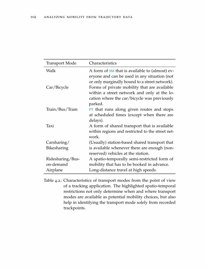
102 analyzing mobility from trajectory data
Transport Mode Characteristics
Walk A form of SM that is available to (almost) ev-eryone and can be used in any situation (notor only marginally bound to a street network).
Car/Bicycle Forms of private mobility that are availablewithin a street network and only at the lo-cation where the car/bicycle was previouslyparked.
Train/Bus/Tram PT that runs along given routes and stopsat scheduled times (except when there aredelays).
Taxi A form of shared transport that is availablewithin regions and restricted to the street net-work.
Carsharing/Bikesharing
(Usually) station-based shared transport thatis available whenever there are enough (non-reserved) vehicles at the station.
Ridesharing/Bus-on-demand
A spatio-temporally semi-restricted form ofmobility that has to be booked in advance.
Airplane Long-distance travel at high speeds.
Table 4.2.: Characteristics of transport modes from the point of viewof a tracking application. The highlighted spatio-temporalrestrictions not only determine when and where transportmodes are available as potential mobility choices, but alsohelp in identifying the transport mode solely from recordedtrackpoints.
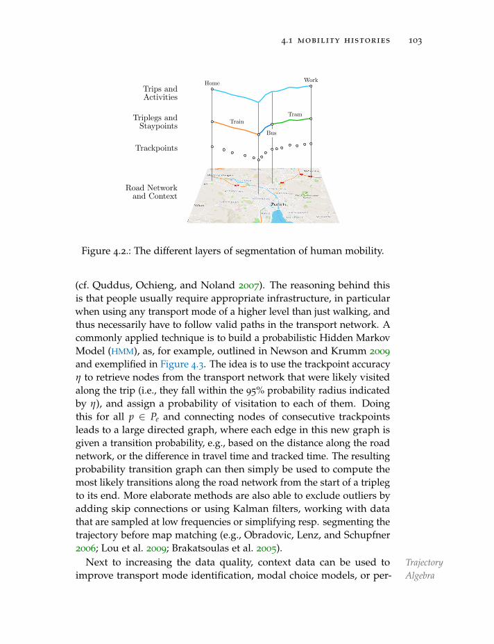
4.1 mobility histories 103
Trackpoints
Triplegs andStaypoints Train
Tram
Home WorkTrips andActivities
Road Networkand Context
Bus
Figure 4.2.: The different layers of segmentation of human mobility.
(cf. Quddus, Ochieng, and Noland 2007). The reasoning behind thisis that people usually require appropriate infrastructure, in particularwhen using any transport mode of a higher level than just walking, andthus necessarily have to follow valid paths in the transport network. Acommonly applied technique is to build a probabilistic Hidden MarkovModel (HMM), as, for example, outlined in Newson and Krumm 2009
and exemplified in Figure 4.3. The idea is to use the trackpoint accuracyη to retrieve nodes from the transport network that were likely visitedalong the trip (i.e., they fall within the 95% probability radius indicatedby η), and assign a probability of visitation to each of them. Doingthis for all p ∈ Pe and connecting nodes of consecutive trackpointsleads to a large directed graph, where each edge in this new graph isgiven a transition probability, e.g., based on the distance along the roadnetwork, or the difference in travel time and tracked time. The resultingprobability transition graph can then simply be used to compute themost likely transitions along the road network from the start of a triplegto its end. More elaborate methods are also able to exclude outliers byadding skip connections or using Kalman filters, working with datathat are sampled at low frequencies or simplifying resp. segmenting thetrajectory before map matching (e.g., Obradovic, Lenz, and Schupfner2006; Lou et al. 2009; Brakatsoulas et al. 2005).
Next TrajectoryAlgebra
to increasing the data quality, context data can be used toimprove transport mode identification, modal choice models, or per-
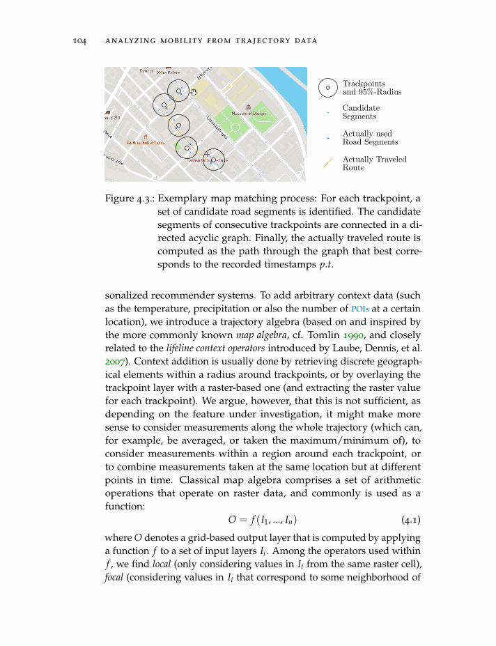
104 analyzing mobility from trajectory data
Trackpointsand 95%-Radius
CandidateSegments
Actually usedRoad Segments
Actually TraveledRoute
Figure 4.3.: Exemplary map matching process: For each trackpoint, aset of candidate road segments is identified. The candidatesegments of consecutive trackpoints are connected in a di-rected acyclic graph. Finally, the actually traveled route iscomputed as the path through the graph that best corre-sponds to the recorded timestamps p.t.
sonalized recommender systems. To add arbitrary context data (suchas the temperature, precipitation or also the number of POIs at a certainlocation), we introduce a trajectory algebra (based on and inspired bythe more commonly known map algebra, cf. Tomlin 1990, and closelyrelated to the lifeline context operators introduced by Laube, Dennis, et al.2007). Context addition is usually done by retrieving discrete geograph-ical elements within a radius around trackpoints, or by overlaying thetrackpoint layer with a raster-based one (and extracting the raster valuefor each trackpoint). We argue, however, that this is not sufficient, asdepending on the feature under investigation, it might make moresense to consider measurements along the whole trajectory (which can,for example, be averaged, or taken the maximum/minimum of), toconsider measurements within a region around each trackpoint, orto combine measurements taken at the same location but at differentpoints in time. Classical map algebra comprises a set of arithmeticoperations that operate on raster data, and commonly is used as afunction:
O = f (I1, ..., In) (4.1)
where O denotes a grid-based output layer that is computed by applyinga function f to a set of input layers Ii. Among the operators used withinf , we find local (only considering values in Ii from the same raster cell),focal (considering values in Ii that correspond to some neighborhood of
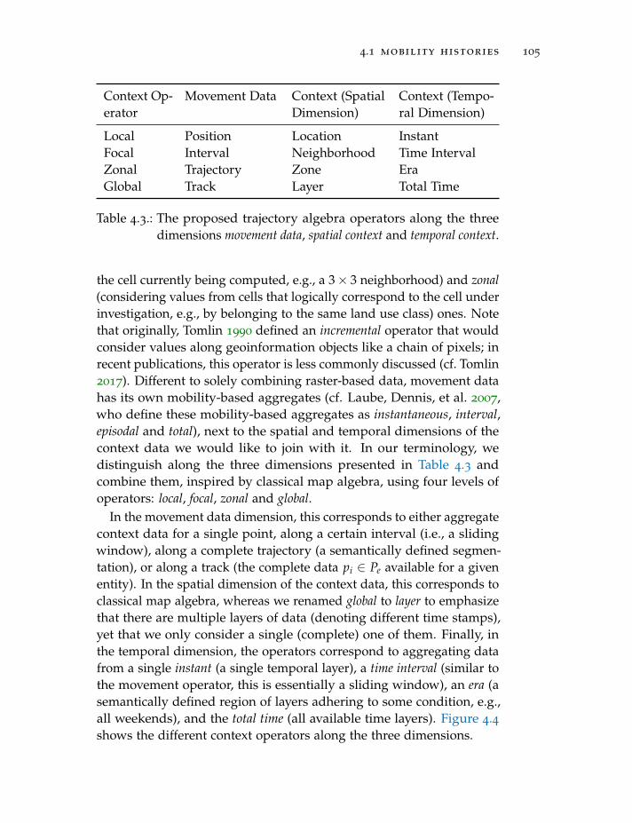
4.1 mobility histories 105
Context Op-erator
Movement Data Context (SpatialDimension)
Context (Tempo-ral Dimension)
Local Position Location InstantFocal Interval Neighborhood Time IntervalZonal Trajectory Zone EraGlobal Track Layer Total Time
Table 4.3.: The proposed trajectory algebra operators along the threedimensions movement data, spatial context and temporal context.
the cell currently being computed, e.g., a 3× 3 neighborhood) and zonal(considering values from cells that logically correspond to the cell underinvestigation, e.g., by belonging to the same land use class) ones. Notethat originally, Tomlin 1990 defined an incremental operator that wouldconsider values along geoinformation objects like a chain of pixels; inrecent publications, this operator is less commonly discussed (cf. Tomlin2017). Different to solely combining raster-based data, movement datahas its own mobility-based aggregates (cf. Laube, Dennis, et al. 2007,who define these mobility-based aggregates as instantaneous, interval,episodal and total), next to the spatial and temporal dimensions of thecontext data we would like to join with it. In our terminology, wedistinguish along the three dimensions presented in Table 4.3 andcombine them, inspired by classical map algebra, using four levels ofoperators: local, focal, zonal and global.
In the movement data dimension, this corresponds to either aggregatecontext data for a single point, along a certain interval (i.e., a slidingwindow), along a complete trajectory (a semantically defined segmen-tation), or along a track (the complete data pi ∈ Pe available for a givenentity). In the spatial dimension of the context data, this corresponds toclassical map algebra, whereas we renamed global to layer to emphasizethat there are multiple layers of data (denoting different time stamps),yet that we only consider a single (complete) one of them. Finally, inthe temporal dimension, the operators correspond to aggregating datafrom a single instant (a single temporal layer), a time interval (similar tothe movement operator, this is essentially a sliding window), an era (asemantically defined region of layers adhering to some condition, e.g.,all weekends), and the total time (all available time layers). Figure 4.4shows the different context operators along the three dimensions.
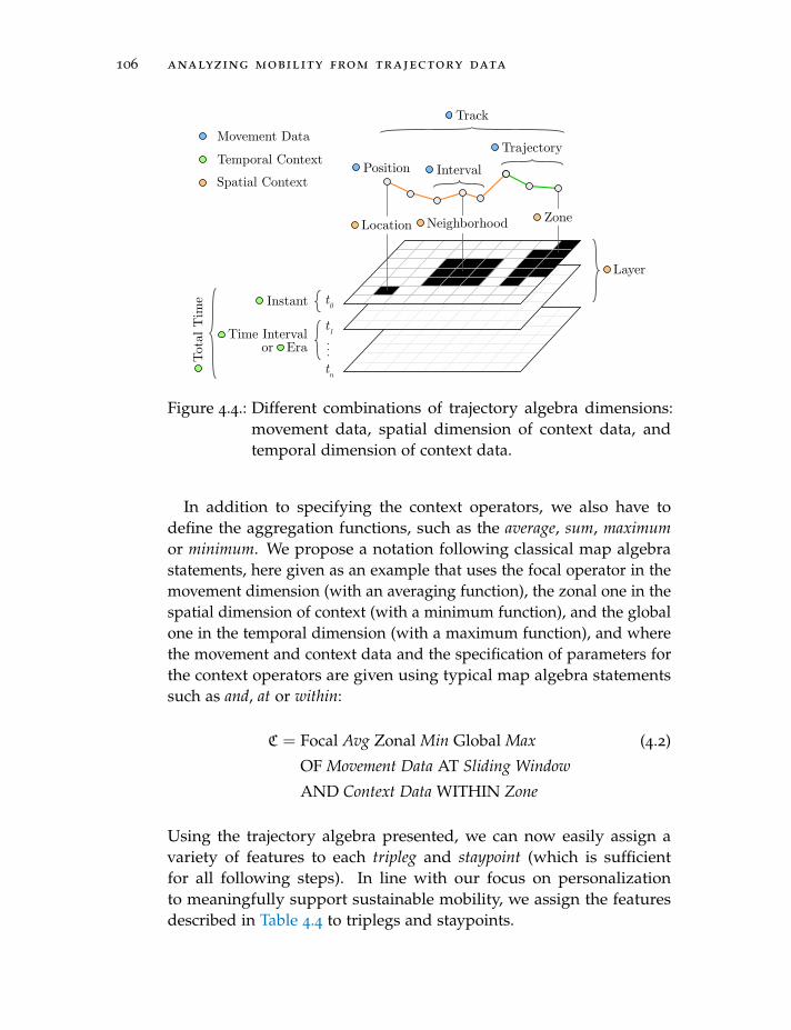
106 analyzing mobility from trajectory data
Time Intervalor Era
t0
t1
tn
Movement Data
Temporal Context
Spatial ContextPosition
Track
Location Neighborhood Zone
Layer
Instant
Tota
lTim
e
Interval
Trajectory
Figure 4.4.: Different combinations of trajectory algebra dimensions:movement data, spatial dimension of context data, andtemporal dimension of context data.
In addition to specifying the context operators, we also have todefine the aggregation functions, such as the average, sum, maximumor minimum. We propose a notation following classical map algebrastatements, here given as an example that uses the focal operator in themovement dimension (with an averaging function), the zonal one in thespatial dimension of context (with a minimum function), and the globalone in the temporal dimension (with a maximum function), and wherethe movement and context data and the specification of parameters forthe context operators are given using typical map algebra statementssuch as and, at or within:
C = Focal Avg Zonal Min Global Max (4.2)
OF Movement Data AT Sliding Window
AND Context Data WITHIN Zone
Using the trajectory algebra presented, we can now easily assign avariety of features to each tripleg and staypoint (which is sufficientfor all following steps). In line with our focus on personalizationto meaningfully support sustainable mobility, we assign the featuresdescribed in Table 4.4 to triplegs and staypoints.
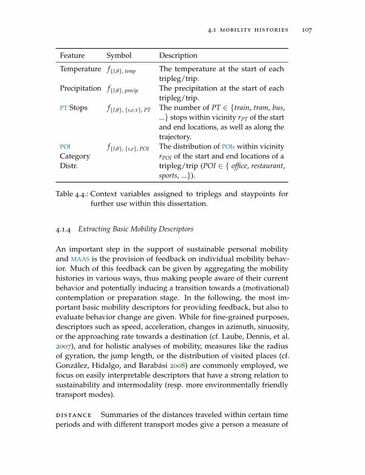
4.1 mobility histories 107
Feature Symbol Description
Temperature f{l,θ}, temp The temperature at the start of eachtripleg/trip.
Precipitation f{l,θ}, precip The precipitation at the start of eachtripleg/trip.
PT Stops f{l,θ}, {s,e,τ}, PT The number of PT ∈ {train, tram, bus,...} stops within vicinity rPT of the startand end locations, as well as along thetrajectory.
POI
CategoryDistr.
f{l,θ}, {s,e}, POI The distribution of POIs within vicinityrPOI of the start and end locations of atripleg/trip (POI ∈ { office, restaurant,sports, ...}).
Table 4.4.: Context variables assigned to triplegs and staypoints forfurther use within this dissertation.
4.1.4 Extracting Basic Mobility Descriptors
An important step in the support of sustainable personal mobilityand MAAS is the provision of feedback on individual mobility behav-ior. Much of this feedback can be given by aggregating the mobilityhistories in various ways, thus making people aware of their currentbehavior and potentially inducing a transition towards a (motivational)contemplation or preparation stage. In the following, the most im-portant basic mobility descriptors for providing feedback, but also toevaluate behavior change are given. While for fine-grained purposes,descriptors such as speed, acceleration, changes in azimuth, sinuosity,or the approaching rate towards a destination (cf. Laube, Dennis, et al.2007), and for holistic analyses of mobility, measures like the radiusof gyration, the jump length, or the distribution of visited places (cf.Gonzalez, Hidalgo, and Barabasi 2008) are commonly employed, wefocus on easily interpretable descriptors that have a strong relation tosustainability and intermodality (resp. more environmentally friendlytransport modes).
distance Summaries of the distances traveled within certain timeperiods and with different transport modes give a person a measure of
108 analyzing mobility from trajectory data
how personal mobility is in relation to familiar geographical extents,the mobility behavior of other people, and its change over time (e.g., inGoogle Maps, the totally traveled distance is compared to the distanceto the moon, or in an app by SBB, distances are given in comparison toextents of various administrative boundaries within Switzerland). Thedistance is computed as the sum of all distances between consecutivetrackpoints (which are optimally map matched):
d(Pe, ts, te, m) = ∑ di,i+1 (4.3)
di,i+1 = dist(pi, pi+1), ts ≤ pi.t ∧ pi.t < te∧l.m = m ∧ pi ∈ Pl
In Equation 4.3, the distances are broken down per mode. Consideringbehavior change towards more sustainable uses of mobility, knowingthe shares traveled with each mode (and the changes thereof) givespeople a sense of impact of different choices and lets them comparedifferent behaviors over time and among each other, and quantifypotential impacts of certain behaviors.
duration Potentially more influential than distance when regardingindividual mobility choices, feedback on the duration a person spendstraveling has a large impact on the mobility behavior, as it is a measurethat is used by many people to optimize their mobility choices (next tofinancial aspects; cf. Mokhtarian and Chen 2004).
∆(Pe, ts, te, m) = ∑ ∆i,i+1 (4.4)
∆i,i+1 = pi+i.t− pi.t, ts ≤ pi.t ∧ pi.t < te∧l.m = m ∧ pi ∈ Pl
Similar to the distance computations, the duration (given in Equa-tion 4.4) is usually computed per mode, in order to give people insightsabout the differences in temporal requirements of different modes.
modal split In its most simple form, the modal split helps classify-ing people in different mobility usage groups (cf. chapter 2) and givingthem an overview of their general mobility use tendencies. The modalsplit is usually either given in terms of distance, duration or numberof trips, which all emphasize different aspects of mobility: A distance-based split places faster transport modes more prominently, while a
4.1 mobility histories 109
duration-based split is rooted in the fact that people have given mobilitytime budgets that they use irrespectively of the actual transport mode(e.g., a person’s distance-based modal split often exhibits negligibleshares of SM, while a duration-based split displays more equal shares).A split based on the number of trips with a given transport mode looksat mobility from the perspective of a person’s choices, whereas eachindividual trip was preceded by a choice for a certain transport mode.
MS(Pe, ts, te, m) ={d, ∆, | · |}(Pe, ts, te, m)
∑m{d, ∆, | · |}(Pe, ts, te, m)(4.5)
Here, {d, ∆, | · |}(Pe, ts, te, m) denote the distance, duration or numberof trips with a given transport mode (as defined in Equation 4.3 andEquation 4.4).
trip aggregates The trip aggregates used within our work includethe total number of trips within a certain time period ntrips(ts, te) =
|θ|, ts ≤ θ.ts ∧ θ.te < te, the distribution of sequences of triplegs SM =
|θ|/|θ|, θ.Lθ .m = M (where M describes a sequence of mode choicesand θ.Lθ .m = M denotes that the tripleg sequence Lθ correspondsto the sequence M), and the number of staypoints per trip ns/θ =
|s|/|θ|, θ.ts ≤ s.ts ∧ s.te < θ.te. They allow a user to grasp his or hermobility behavior on a holistic level, give insights on the complexityof trips, and on potential room for optimization due to long waitingtimes.
activity aggregates To highlight which goals of mobility areresponsible for unsustainable behavior, we break down the modalsplit based on the purposes of the activities, as this gives a personan indication of where larger potentials for change are. First, it isinteresting for a person to know the number of times an activity of acertain purpose was performed na(ts, ts, ω) = |ai|, ts ≤ ai.ts ∧ ai.te <
te ∧ ai.ω = ω and the time spent performing the respective activities∆(ω) = ∑i(ai.te − ai.ts), ai.ω = ω. Targeting feedback enabling moresustainable mobility, people need to know the tripleg combinations(resp. the transport modes) used to reach activities of a certain purpose:Sω,M = |θ|/|θ|, θ.Lθ .m = M ∧ θ.ae.ω = θ.ae.ω = ω. To give morefine-grained feedback, the distances, durations and modal shares (asdefined previously) are similarly broken down by activity purposes.
110 analyzing mobility from trajectory data
4.1.5 Transport Mode and Activity Purpose Inference
Many tracking applications use the additional sensors available on asmartphone to estimate the transport mode someone is traveling with.While these additional data can greatly improve the transport moderecognition (e.g., Widhalm, Nitsche, and Brandie 2012; Shafique andHato 2015), for many datasets and -sources it is not available. Instead,we can use the spatial and temporal characteristics of the recordedtrackpoints, as well as the previously introduced contextual data to inferthe transport mode (e.g., by considering the speed of the traveling entity,patterns that correspond to public transport timetables, etc.). Further,many mobility recording applications allow their users to specify (resp.validate) the used transport modes and/or the purpose of a certainactivity. These validations of transport mode and purpose continuouslysupply a system with data that can be used to improve the models thatpredict which transport modes will likely be used to reach a certainlocation. We here propose a method that does not rely on very accurateGPS data nor additional sensor information (e.g., Bluetooth devices oraccelerometer values), but instead uses the continuously validated datain addition to contextual data to improve its transport mode prediction.The reason for this is that many commercial smartphone-based GPS
trackers prevent access to such fine-grained data, either because it isonly internally used or to save battery and mobile data.
AtFeatures usedfor
Classification
its core, our method consists of a naıve Bayes classifier that oper-ates on the features given in Table 4.5. These features are computedfor each tripleg that was identified using the segmentation techniquesintroduced in subsection 4.1.2. The first four features ( f s, f∑ d, fmax dand f ¯ ) do not require any additional context data and can simplybe computed from the trajectories themselves. The last three ( f∆,PT,fd,{s,e},PT and fns,PT) require computing PT alternatives resp. contextdata on the PT stops along the tripleg. In the experiments introducedlater, the PT modes considered consist of MPT = {train, tram, bus}, i.e.,it is required to compute PT alternatives for these three transport modesand count the number of stops of these three transport modes alongthe route.
Using these features, we can formalize the transport mode identi-fication problem as a prediction problem, taking the feature vector~f = [ f1, ..., fN ]
T = [ f s, ..., fns,PT]T (where N = 4+ 3 · |MPT|) as input and
the possible transport modes mj ∈ M = {walk, bicycle, car, bus, train, ...
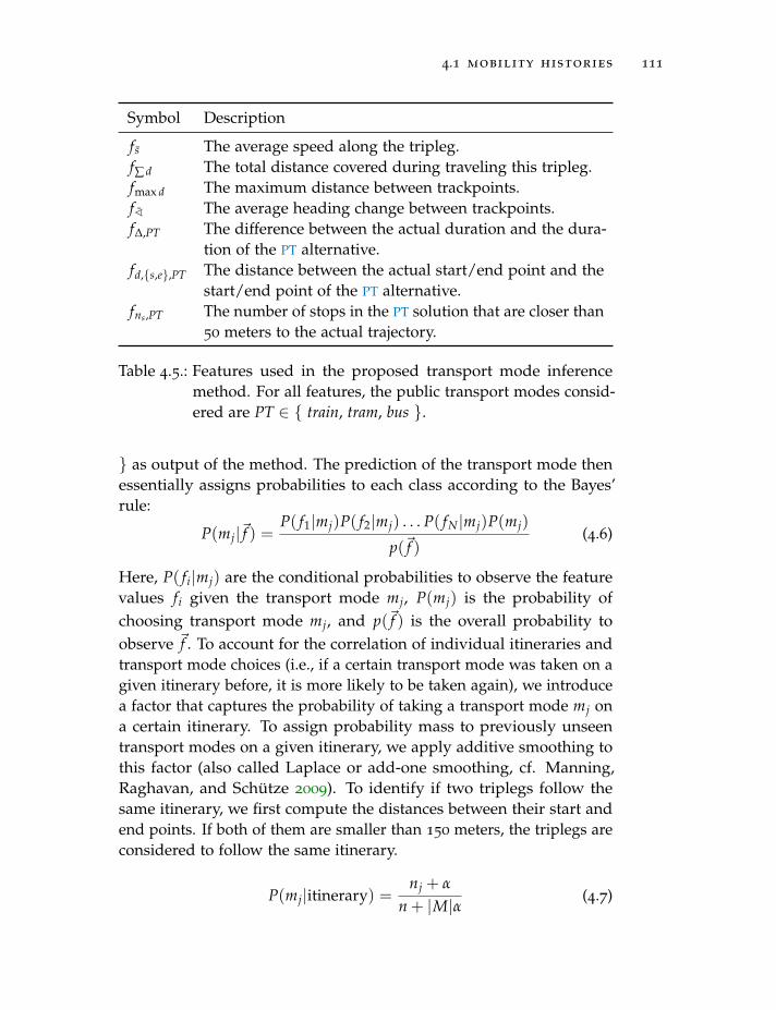
4.1 mobility histories 111
Symbol Description
f s The average speed along the tripleg.f∑ d The total distance covered during traveling this tripleg.fmax d The maximum distance between trackpoints.f ¯ The average heading change between trackpoints.f∆,PT The difference between the actual duration and the dura-
tion of the PT alternative.fd,{s,e},PT The distance between the actual start/end point and the
start/end point of the PT alternative.fns,PT The number of stops in the PT solution that are closer than
50 meters to the actual trajectory.
Table 4.5.: Features used in the proposed transport mode inferencemethod. For all features, the public transport modes consid-ered are PT ∈ { train, tram, bus }.
} as output of the method. The prediction of the transport mode thenessentially assigns probabilities to each class according to the Bayes’rule:
P(mj|~f ) =P( f1|mj)P( f2|mj) . . . P( fN |mj)P(mj)
p(~f )(4.6)
Here, P( fi|mj) are the conditional probabilities to observe the featurevalues fi given the transport mode mj, P(mj) is the probability ofchoosing transport mode mj, and p(~f ) is the overall probability toobserve ~f . To account for the correlation of individual itineraries andtransport mode choices (i.e., if a certain transport mode was taken on agiven itinerary before, it is more likely to be taken again), we introducea factor that captures the probability of taking a transport mode mj ona certain itinerary. To assign probability mass to previously unseentransport modes on a given itinerary, we apply additive smoothing tothis factor (also called Laplace or add-one smoothing, cf. Manning,Raghavan, and Schutze 2009). To identify if two triplegs follow thesame itinerary, we first compute the distances between their start andend points. If both of them are smaller than 150 meters, the triplegs areconsidered to follow the same itinerary.
P(mj|itinerary) =nj + α
n + |M|α (4.7)
112 analyzing mobility from trajectory data
Here, n denotes the number of triplegs corresponding to the itineraryunder consideration, nj the number of triplegs traveled with mode mj(following the same itinerary), α > 0 is a smoothing parameter, and |M|corresponds to the number of transport mode choices that our modelcan predict. The total probability is then computed as
P(mj|~f ) =1K
P(mj|~f )P(mj|itinerary), (4.8)
where K is a normalizing constant. Finally, it might not always bepossible to find a corresponding PT alternative (for the features ~fPT =
[ f∆,PT, ..., fns,PT]T). Thus, we model the conditional probability for these
features as:
P( ~fPT, PT = 0|mj) = P(PT = 0|mj) (4.9)
P( ~fPT, PT = 1|mj) = P(PT = 1|mj) · P( ~fPT|mj, PT = 1) (4.10)
= P(PT = 1|mj) · ∏fi∈ ~fPT
P( fi|mj, PT = 1)
Where PT = 0 means that the respective PT was not found, and PT = 1means it was found. This means that if there is no PT alternative found,we simply take the probability of not finding a PT alternative for atransport mode mj, and only otherwise consider the values of ~fPT.
Formulating the transport mode prediction as a naıve Bayes problem,incorporating new data is straightforward if we can model the distribu-tion of individual features as conjugate priors (i.e., adding a new sampledoes not change the shape of the distribution and its effects on thedistribution parameters are well known). Here, we assume Gaussianprobability distributions for all features, and choose a Gamma prior forthe parameters of all distributions, except P(PT = 1|mj), which uses aBeta prior. The resulting model is able to start (by computing the priors)from a small set of users/triplegs that formulate a base assumptionabout the dependence between features and outcome variables, whichis then continuously updated for each user individually. As the trans-port mode choices depend a lot on the individual, we train a model foreach user individually (that might start by using the priors computedfrom other users though).
4.2 sustainability metrics 113
4.2 sustainability metrics
Given the basic mobility descriptors, contextual features, as well asa transport mode, we can compute more advanced metrics such asthe involved costs, environmental impacts, relations to geographicalfeatures, or personal circumstances.
4.2.1 Environmental Impact
A commonly applied method to measure the environmental or eco-logical impact is the projection of all influences on the environmentonto GHG emissions, in particular CO2. Table 2.1 shows the emissionof CO2 caused by actively using a mode of transport. In addition tothese values, LCA gives an estimate of the totally emitted CO2 duringthe whole life cycle of a vehicle (including production and disposal ofthe vehicle, the processes involved in the energy supply chain, as wellas the emissions caused by infrastructure provision). In line with themethod given in subsection 2.2.4, we both present the ecological im-pact in terms of GHG emissions, and also the corresponding monetaryequivalent. The produced GHG equivalent can be expressed in terms ofaverage LCA values:
cGHG(θ) = ∑m∈Lθ .m
dm · (cproduction,m + cdisposal,m+ (4.11)
cenergy,m + cinfrastructure,m + cdirect,m)
Here, dm stands for the distance traveled by transport mode m (i.e., themobility descriptor d(Pe, ts, te, m), cf. Equation 4.3). The resulting valuecGHG(θ) describes the CO2 emissions stemming from a single trip θ. Tofacilitate comparisons with potential gains from performing the trip,we compute a monetary equivalent under the (arguably not perfectlyaccurate) assumption that money is a fair representation of value. Weuse CO2 offsetting costs ce/tCO2 as shown in Table 2.3 (note that we donot take the actual market values but the estimated true costs of GHG
emissions, i.e., the values in the range of $30-100/tCO2) to compute thismonetary equivalent. Assuming these costs include all the (potentially)occurring costs in the future, the conversion is simple:
cEco. Impact(θ) = cGHG(θ) · ce/tCO2 (4.12)
114 analyzing mobility from trajectory data
When considering an individual trip or an individual person on itsown, the resulting monetary costs (due to GHG emissions) are oftencomparatively low (especially when putting them into relation withthe monetary costs and gains due to salaries, personal and/or socialgains, etc.). This might be an indication that a) purely self-regulatedand market-driven approach at reaching sustainable mobility will havedifficulties reaching net-zero emissions and b) that to induce behaviorchange we should lean towards adopting the concept of strong sus-tainability, where human capital gains cannot make up for the loss ofnatural capital.
4.2.2 Monetary Cost
The monetary cost of individual trips mostly depends on contextualand personal factors, such as prices for gas, PT passes, or the value ofone’s own car. However, these values are often available for differentregions as averages over the whole population or certain demographicsub-populations. The monetary cost can thus be approximated similarlyby using a distance-based average cost per mode:
cMonetary(θ) = ∑m∈Lθ .m
dm · caverage,m (4.13)
caverage,m = cfixed,m/dtot,m + cvariable,m (4.14)
As these averages are computed over a large population, they includeboth fixed (cfixed,m) as well as variable costs (cvariable,m), which in realitycan influence mobility choices (e.g., Thøgersen 2009). For example, aperson having paid the (upfront) fixed cost of a personal car is morelikely to use it than someone who would first have to buy one, eventhough the averaged cost for them would essentially be the same. Con-sidering the example of Switzerland, Table 4.6 highlights some of thecosts associated with various transport modes. Note that these areapproximate average values; most transport providers do not calculatetheir prices based on the actual kilometers driven, but rather based onzones, occupancy, time of day, etc. As such, to get the most accuratecost estimation, the prices would have to be computed for each trip in-dividually. However, for many persuasive strategies an approximationusing the given values is sufficient.
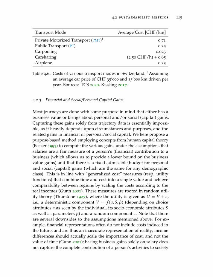
4.2 sustainability metrics 115
Transport Mode Average Cost [CHF/km]
Private Motorized Transport (PMT)†0.71
Public Transport (PT) 0.25
Carpooling 0.025
Carsharing (2.50 CHF/h) + 0.65
Airplane 0.23
Table 4.6.: Costs of various transport modes in Switzerland. †Assumingan average car price of CHF 35’000 and 15’000 km driven peryear. Sources: TCS 2020, Kissling 2017.
4.2.3 Financial and Social/Personal Capital Gains
Most journeys are done with some purpose in mind that either has abusiness value or brings about personal and/or social (capital) gains.Capturing these gains solely from trajectory data is essentially impossi-ble, as it heavily depends upon circumstances and purposes, and therelated gains in financial or personal/social capital. We here propose apurpose-based method employing concepts from human capital theory(Becker 1993) to compute the various gains under the assumptions thatsalaries are a fair measure of a person’s (financial) contribution to abusiness (which allows us to provide a lower bound on the businessvalue gains) and that there is a fixed admissible budget for personaland social (capital) gains (which are the same for any demographicclass). This is in line with “generalized cost” measures (resp. utilityfunctions) that combine time and cost into a single value and achievecomparability between regions by scaling the costs according to thereal incomes (Gunn 2001). These measures are rooted in random util-ity theory (Thurstone 1927), where the utility is given as U = V + ε,i.e., a deterministic component V = f (a, S, β) (depending on choiceattributes a as seen by the individual, its socio-economic attributes Sas well as parameters β) and a random component ε. Note that thereare several downsides to the assumptions mentioned above: For ex-ample, financial representations often do not include costs induced inthe future, and are thus an inaccurate representation of reality; incomedifferences should actually scale the importance of cost, and not thevalue of time (Gunn 2001); basing business gains solely on salary doesnot capture the complete contribution of a person’s activities to society
116 analyzing mobility from trajectory data
(the Covid-19 situation highlighted well that many low-wage workersare in reality essential for society); the split into (salary-based, thus notequally distributed) business gains and (equally distributed) rights forpersonal/social gains creates a bias towards the rich that is debatable.However, the presented approach is comparably easy to implementin practice, as in addition to tracking data only an approximate valueof a person’s salary is required (which is often readily available inmobility studies), and it yields reasonable approximations to rank trips(in particular intra-personally) according to their sustainability.
The financial gains of a work-related activity are given by the timespent performing the activity (incl. the trips required to get to/fromthe location) and the salary of the traveling person.
gFinancial(a) = ∆work(a) · gsalary (4.15)
Similarly, the personal gains can be computed for leisure-related activi-ties, and by considering the fixed admissible budget for personal gains(e.g., per week).
gPersonal(a) = ∆leisure(a) · gaverage (4.16)
gaverage = gfixed/∆tot, leisure (4.17)
Here, ∆tot, leisure denotes the total duration spent on leisure activitieswithin a certain time frame, and gfixed the fixed gains associated withthe same time frame (e.g., a weekly “budget” for leisure activities ofgfixed = CHF 500).
These quantifications of financial and social/personal gains allowus to reason if the use of a certain transport mode (or the travel itself)is justified for a given activity. The formulas might also give indi-cations about the tradeoffs made between travel speed and activitypurpose. For example, when having to travel somewhere for work,many people choose faster yet more expensive means of transport asthe corresponding financial gains are higher (or at least we are led tobelieve so).
4.2.4 Combined Sustainability Indicators
There are several ways in which we can determine whether a certainjourney should be considered “sustainable”. We here propose twomethods: 1) A more accurate one that takes into account both the
4.2 sustainability metrics 117
ecological as well as the monetary cost/gains as previously introduced.2) A heuristic approximation that relies on the fact that most peoplehave a certain time budget for overall travel (which remains relativelyconstant across different demographic groups as well as countries, cf.Metz 2008; Jang 2017) as well as for individual trips.
The first method is essentially captured in the following equation:
S(θ) = ωs · (gFinancial(aθ) + gPersonal(aθ)) (4.18)
− (cMonetary(θ) + cEco. Impact(θ))
Here, the sustainability value S(θ) (of a trip θ) is measured in financialterms resp. as overall (financial) gain (aθ denotes the activity enabled byperforming trip θ). If S(θ) is negative, the trip should have been avoided(resp. if choosing another transport mode reduces the ecological impactin such a way that the net S(θ) is positive again, the respective transportmode should be preferred). On the other hand, if S(θ) is positive and ifwe operate under the interpretation of weak sustainability (which canbe adopted for eco-feedback in order to adhere to the meaningfulnesscriterion), a trip can be regarded as sustainable. Using ωs we can makea trade-off between weak (ωs = 1) and strong sustainability (ωs = 0):In the case of strong sustainability, independently of potential gains,any trip that is not performed by SM (and thus not exhibiting anynegative environmental impacts) should be avoided. On the otherhand, under an interpretation of weak sustainability, many of the tripscan still be regarded as being sustainable, as their overall (positive)impacts outweigh the negative environmental influences. Note that werefrain from individually weighting the different costs (as is commonlydone based on stated preference data in order to have a more accuraterepresentation of the generalized cost from a person’s point of view;cf. Kumar, Basu, and Maitra 2004; Nour, Casello, and Hellinga 2010;Chintakayala and Maitra 2010), as we are not interested in a subjectiveassessment of cost, but look at the problem from the point of view ofsustainability.
The Rule-Based“Sustainabil-ity”Assessment
second approach was used in the GoEco! project (Bucher, Mangili,Cellina, et al. 2019) and involved three rules: A trip is regarded asnon-sustainable iff. 1) the user has access to an alternative transportmode, 2) whose usage for the given trip reduces its CO2 emissionsby at least 5%, and 3) which does not lead to an excessively longtrip duration. The last criterion is defined using the threshold dth =
(do + tmax)− tmax/(1+ dotmax), where tmax denotes the maximal increase
118 analyzing mobility from trajectory data
in duration (set as 1.2 hours under the assumption that this is anacceptable prolongation for longer trips; for shorter trips, the maximalprolongation is of course less) and do the duration of the original route.If the alternative mode of transport leads to a trip duration of morethan dth, it is rejected as a potential alternative.
As highlighted before, we here introduced concepts that are pri-marily of value within the weak sustainability interpretation. Takingthe position of strong sustainability, one must always argue that anytrip that leads to (non-negligible; e.g., a trip by bicycle can usually beconsidered negligible, even though CO2 was emitted as part of thebicycle production) CO2 output should be avoided. This also meansthat any person performing such trips should be nudged towards CO2
neutral travels, irrespective of the potential gains. We thus proposeto use the introduced sustainability indicators primarily to determinewhen a (more sustainable) alternative should have been chosen (whichin turn can of course be used to compute “optimal” mobility behavioror potentials for change), and not to exclude any trips from within apersuasive application.
4.3 systematic mobility and mobility preferences
Systematic mobility plays a central role for behavior change, as it iscommonly responsible of for a substantial share of the overall impactsof mobility, its regularity prevents people from actively thinking aboutchange, but once a change is implemented it can more easily lead tolong-lasting effects (Jager 2003). In this section, we first elaborate onhow to extract systematic patterns from mobility and how they canbe used for mobility feedback, after which we look at more concreteexamples of predictability of transport mode choices as well as groupsof people who travel in similar ways.
4.3.1 Geometrical, Topological and Platial Aspects of Systematic Mobility
Usually, people perform the same activities multiple times over a longertime period (e.g., going to work usually happens on a daily basis). Thisrecurrence is commonly used to cluster activities by specifying, forexample, that an activity has to be performed at a given location morethan three times in a month in order to be considered systematic. We
4.3 systematic mobility and mobility preferences 119
capture this concept by the notion of a place. Note that the definitionadopted here technically differs from common geographic interpreta-tions of “place” (cf. Miller 2007), which do not include clear (spatialor temporal) boundaries nor scales, but instead define a place as anarbitrary “space that is filled with meanings and objectives by humanexperiences” (Tuan 1977, p. 4). From a movement data perspective,however, those spaces often coincide with locations that are regularlyvisited, for which reason we adopt this definition.
Definition 4.7 (Place). A place Π is a geographical region (e.g., definedby a polygon) in which a given person regularly spends time. Formethods which rely on a single point for computations, the center ofmass of the area Π is used.
The identification of places is commonly performed using a cluster-ing approach like DBSCAN (Ester, Kriegel, and Xu 1996), hierarchicalclustering or disk-based clustering (cf. Xu and Wunsch 2005). In gen-eral, it is easier to identify places using a method that does not requirethe specification of the number of clusters beforehand, as this can varybetween persons. Commonly, home and work are regarded as “special”places, as they are changing infrequently and the transitions betweenthem make up for a large share of mobility needs. Based on places(which, in the most extreme cases have to be visited at least twice), wecan start identifying regular patterns of mobility.
Definition 4.8 (Tour). A tour Θ is a sequence of trips that start and endat the same place Π: Θ = (Π, LΘ). If Π = home, the tour is called ajourney.
Most tours are actually journeys, as most people start their dailyroutines in the morning by going to work or do errands, and returnhome later in the day. However, tours can be arbitrarily nested andoverlapping. For example, going to a restaurant during lunch breakcreates a sub-tour work→ restaurant→ work, embedded in the longerjourney starting and ending at home (cf. Figure 4.5). Tours are crucialfor meaningful suggestions of route alternatives, as they help keepingtransport mode use consistent (e.g., if someone leaves by car in themorning, the car should be returned in the evening; on the other hand,if someone does not leave by car, the car is not available later duringthe tour).
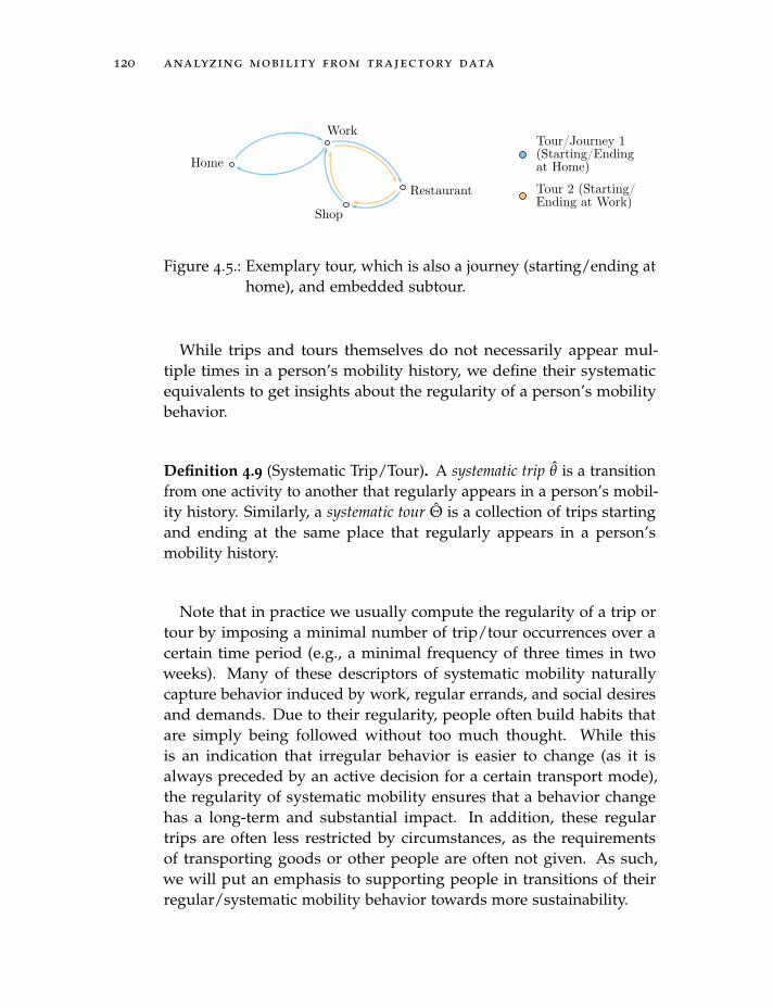
120 analyzing mobility from trajectory data
Home
Work
Restaurant
Shop
Tour/Journey 1(Starting/Endingat Home)
Tour 2 (Starting/Ending at Work)
Figure 4.5.: Exemplary tour, which is also a journey (starting/ending athome), and embedded subtour.
While trips and tours themselves do not necessarily appear mul-tiple times in a person’s mobility history, we define their systematicequivalents to get insights about the regularity of a person’s mobilitybehavior.
Definition 4.9 (Systematic Trip/Tour). A systematic trip θ is a transitionfrom one activity to another that regularly appears in a person’s mobil-ity history. Similarly, a systematic tour Θ is a collection of trips startingand ending at the same place that regularly appears in a person’smobility history.
Note that in practice we usually compute the regularity of a trip ortour by imposing a minimal number of trip/tour occurrences over acertain time period (e.g., a minimal frequency of three times in twoweeks). Many of these descriptors of systematic mobility naturallycapture behavior induced by work, regular errands, and social desiresand demands. Due to their regularity, people often build habits thatare simply being followed without too much thought. While thisis an indication that irregular behavior is easier to change (as it isalways preceded by an active decision for a certain transport mode),the regularity of systematic mobility ensures that a behavior changehas a long-term and substantial impact. In addition, these regulartrips are often less restricted by circumstances, as the requirementsof transporting goods or other people are often not given. As such,we will put an emphasis to supporting people in transitions of theirregular/systematic mobility behavior towards more sustainability.
4.3 systematic mobility and mobility preferences 121
4.3.2 Transport Mode Choices
Next to a spatio-temporal regularity, many people show high regulari-ties in their transport mode choices. Here, we will particularly highlighttwo areas of interest to persuasive technologies: 1) How people indi-vidually choose between different transport modes, exemplified by thechoice between car and e-car, an increasingly important question asEVs become more prevalent and show potential to greatly reduce theecological impact of mobility. 2) How people’s similarity in behaviorchange can be identified and used to group them according to theirbehavior, which in turn can be used to provide them different support,but also for political incentives or targeted marketing.
4.3.2.1 Factors Influencing the Choice between Internal Combustion EngineCars and Electric Vehicles
Transport mode choices can either be analyzed from a individual triplegperspective, or from the point of view of tours. The former providesmore insights regarding all individual transport mode choices, whilethe latter offers an arguably more realistic view from the perspectiveof the individual, who usually plans travel “as a whole”, also takinginto account how to return from a certain activity. We here present achoice model regarding the problem from both the tripleg as well as thetour perspective, and taking socio-demographic variables, tripleg/tourdescriptors, as well as spatio-temporal context into account. Table 4.7shows the features used within our choice model. As noted in thetable, the features for the tripleg and tour models slightly differ due totheir different underlying characteristics. For the purpose features, thepurposes of the next activity (for triplegs) resp. a majority vote of allinvolved activities’ purposes (for tours) are used. The spatio-temporalcontext is always computed using the starting point (in space and time)of the respective tripleg or tour.
Using these features as a base, we can apply a range of models topredict transport mode choices. As a straightforward (but more difficultto explain) model, we use a Random Forest (RF). RFs are non-linearclassifiers that consist of an ensemble of decision trees, and are fast totrain, robust to outliers, and in general yield high prediction accuracieseven without extensive hyperparameter tuning (Ho 1995). For betterexplainability (of the influence of different features), we also train a
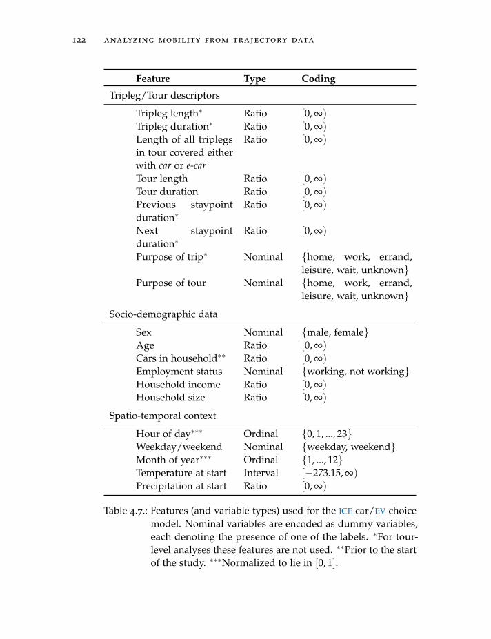
122 analyzing mobility from trajectory data
Feature Type Coding
Tripleg/Tour descriptors
Tripleg length∗ Ratio [0, ∞)
Tripleg duration∗ Ratio [0, ∞)
Length of all triplegsin tour covered eitherwith car or e-car
Ratio [0, ∞)
Tour length Ratio [0, ∞)
Tour duration Ratio [0, ∞)
Previous staypointduration∗
Ratio [0, ∞)
Next staypointduration∗
Ratio [0, ∞)
Purpose of trip∗ Nominal {home, work, errand,leisure, wait, unknown}
Purpose of tour Nominal {home, work, errand,leisure, wait, unknown}
Socio-demographic data
Sex Nominal {male, female}Age Ratio [0, ∞)
Cars in household∗∗ Ratio [0, ∞)
Employment status Nominal {working, not working}Household income Ratio [0, ∞)
Household size Ratio [0, ∞)
Spatio-temporal context
Hour of day∗∗∗ Ordinal {0, 1, ..., 23}Weekday/weekend Nominal {weekday, weekend}Month of year∗∗∗ Ordinal {1, ..., 12}Temperature at start Interval [−273.15, ∞)
Precipitation at start Ratio [0, ∞)
Table 4.7.: Features (and variable types) used for the ICE car/EV choicemodel. Nominal variables are encoded as dummy variables,each denoting the presence of one of the labels. ∗For tour-level analyses these features are not used. ∗∗Prior to the startof the study. ∗∗∗Normalized to lie in [0, 1].
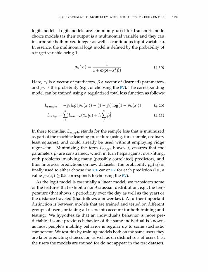
4.3 systematic mobility and mobility preferences 123
logit model. Logit models are commonly used for transport modechoice models (as their output is a multinomial variable and they canincorporate both mixed integer as well as continuous input variables).In essence, the multinomial logit model is defined by the probability ofa target variable being 1:
plr(xi) =1
1 + exp(−xTi β)
(4.19)
Here, xi is a vector of predictors, β a vector of (learned) parameters,and plr is the probability (e.g., of choosing the EV). The correspondingmodel can be trained using a regularized total loss function as follows:
Lsample = −yi log(plr(xi))− (1− yi) log(1− plr(xi)) (4.20)
Lridge =n
∑i
Lsample(xi, yi) + λm
∑j
β2j (4.21)
In these formulas, Lsample stands for the sample loss that is minimizedas part of the machine learning procedure (using, for example, ordinaryleast squares), and could already be used without employing ridgeregression. Minimizing the term Lridge, however, ensures that theparameters β j are constrained, which in turn helps against over-fitting,with problems involving many (possibly correlated) predictors, andthus improves predictions on new datasets. The probability plr(xi) isfinally used to either choose the ICE car or EV for each prediction (i.e., avalue plr(xi) ≥ 0.5 corresponds to choosing the EV).
As the logit model is essentially a linear model, we transform someof the features that exhibit a non-Gaussian distribution, e.g., the tem-perature (that shows a periodicity over the day as well as the year) orthe distance traveled (that follows a power law). A further importantdistinction is between models that are trained and tested on differentgroups of users, or taking all users into account for both training andtesting. We hypothesize that an individual’s behavior is more pre-dictable if some previous behavior of the same individual is known,as most people’s mobility behavior is regular up to some stochasticcomponent. We test this by training models both on the same users theyare later predicting choices for, as well as on distinct sets of users (i.e.,the users the models are trained for do not appear in the test dataset).
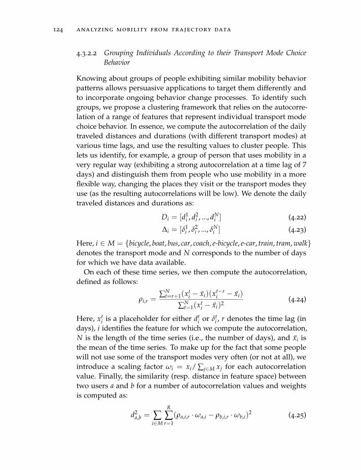
124 analyzing mobility from trajectory data
4.3.2.2 Grouping Individuals According to their Transport Mode ChoiceBehavior
Knowing about groups of people exhibiting similar mobility behaviorpatterns allows persuasive applications to target them differently andto incorporate ongoing behavior change processes. To identify suchgroups, we propose a clustering framework that relies on the autocorre-lation of a range of features that represent individual transport modechoice behavior. In essence, we compute the autocorrelation of the dailytraveled distances and durations (with different transport modes) atvarious time lags, and use the resulting values to cluster people. Thislets us identify, for example, a group of person that uses mobility in avery regular way (exhibiting a strong autocorrelation at a time lag of 7days) and distinguish them from people who use mobility in a moreflexible way, changing the places they visit or the transport modes theyuse (as the resulting autocorrelations will be low). We denote the dailytraveled distances and durations as:
Di = [d1i , d2
i , ..., dNi ] (4.22)
∆i = [δ1i , δ2
i , ..., δNi ] (4.23)
Here, i ∈ M = {bicycle, boat, bus, car, coach, e-bicycle, e-car, train, tram, walk}denotes the transport mode and N corresponds to the number of daysfor which we have data available.
On each of these time series, we then compute the autocorrelation,defined as follows:
ρi,r =∑N
t=r+1(xti − xi)(xt−r
i − xi)
∑Nt=1(xt
i − xi)2(4.24)
Here, xti is a placeholder for either dt
i or δti , r denotes the time lag (in
days), i identifies the feature for which we compute the autocorrelation,N is the length of the time series (i.e., the number of days), and xi isthe mean of the time series. To make up for the fact that some peoplewill not use some of the transport modes very often (or not at all), weintroduce a scaling factor ωi = xi/ ∑j∈M xj for each autocorrelationvalue. Finally, the similarity (resp. distance in feature space) betweentwo users a and b for a number of autocorrelation values and weightsis computed as:
d2a,b = ∑
i∈M
R
∑r=1
(ρa,i,r ·ωa,i − ρb,i,r ·ωb,i)2 (4.25)
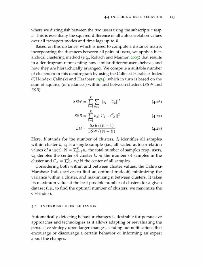
4.4 inferring user behavior 125
where we distinguish between the two users using the subscripts a resp.b. This is essentially the squared difference of all autocorrelation valuesover all transport modes and time lags up to R.
Based on this distance, which is used to compute a distance matrixincorporating the distances between all pairs of users, we apply a hier-archical clustering method (e.g., Rokach and Maimon 2005) that resultsin a dendrogram representing how similar different users behave, andhow they are hierarchically arranged. We compute a suitable numberof clusters from this dendrogram by using the Calinski-Harabasz Index(CH-index; Calinski and Harabasz 1974), which in turn is based on thesum of squares (of distances) within and between clusters (SSW andSSB):
SSW =K
∑k=1
∑i∈Ik
||xi − Ck||2 (4.26)
SSB =K
∑k=1
nk||Ck − CX||2 (4.27)
CH =SSB/(K− 1)
SSW/(N − K)(4.28)
Here, K stands for the number of clusters, Ik identifies all sampleswithin cluster k, xi is a single sample (i.e., all scaled autocorrelationvalues of a user), N = ∑K
k=1 nk the total number of samples resp. users,Ck denotes the center of cluster k, nk the number of samples in thecluster and CX = ∑N
i=1 xi/N the center of all samples.Considering both within and between cluster values, the Calinski-
Harabasz Index strives to find an optimal tradeoff, minimizing thevariance within a cluster, and maximizing it between clusters. It takesits maximum value at the best possible number of clusters for a givendataset (i.e., to find the optimal number of clusters, we maximize theCH-index).
4.4 inferring user behavior
Automatically detecting behavior changes is desirable for persuasiveapproaches and technologies as it allows adapting or reevaluating thepersuasive strategy upon larger changes, sending out notifications thatencourage or discourage a certain behavior or informing an expertabout the changes.
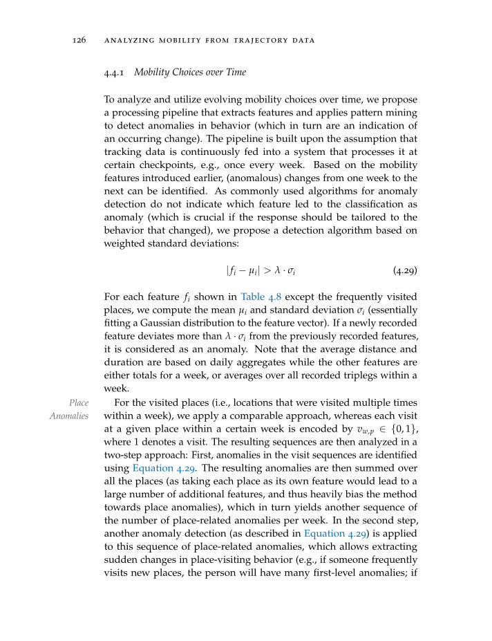
126 analyzing mobility from trajectory data
4.4.1 Mobility Choices over Time
To analyze and utilize evolving mobility choices over time, we proposea processing pipeline that extracts features and applies pattern miningto detect anomalies in behavior (which in turn are an indication ofan occurring change). The pipeline is built upon the assumption thattracking data is continuously fed into a system that processes it atcertain checkpoints, e.g., once every week. Based on the mobilityfeatures introduced earlier, (anomalous) changes from one week to thenext can be identified. As commonly used algorithms for anomalydetection do not indicate which feature led to the classification asanomaly (which is crucial if the response should be tailored to thebehavior that changed), we propose a detection algorithm based onweighted standard deviations:
| fi − µi| > λ · σi (4.29)
For each feature fi shown in Table 4.8 except the frequently visitedplaces, we compute the mean µi and standard deviation σi (essentiallyfitting a Gaussian distribution to the feature vector). If a newly recordedfeature deviates more than λ · σi from the previously recorded features,it is considered as an anomaly. Note that the average distance andduration are based on daily aggregates while the other features areeither totals for a week, or averages over all recorded triplegs within aweek.
ForPlaceAnomalies
the visited places (i.e., locations that were visited multiple timeswithin a week), we apply a comparable approach, whereas each visitat a given place within a certain week is encoded by vw,p ∈ {0, 1},where 1 denotes a visit. The resulting sequences are then analyzed in atwo-step approach: First, anomalies in the visit sequences are identifiedusing Equation 4.29. The resulting anomalies are then summed overall the places (as taking each place as its own feature would lead to alarge number of additional features, and thus heavily bias the methodtowards place anomalies), which in turn yields another sequence ofthe number of place-related anomalies per week. In the second step,another anomaly detection (as described in Equation 4.29) is appliedto this sequence of place-related anomalies, which allows extractingsudden changes in place-visiting behavior (e.g., if someone frequentlyvisits new places, the person will have many first-level anomalies; if
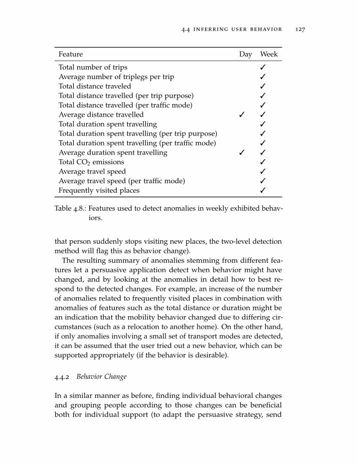
4.4 inferring user behavior 127
Feature Day Week
Total number of trips 3
Average number of triplegs per trip 3
Total distance traveled 3
Total distance travelled (per trip purpose) 3
Total distance travelled (per traffic mode) 3
Average distance travelled 3 3
Total duration spent travelling 3
Total duration spent travelling (per trip purpose) 3
Total duration spent travelling (per traffic mode) 3
Average duration spent travelling 3 3
Total CO2 emissions 3
Average travel speed 3
Average travel speed (per traffic mode) 3
Frequently visited places 3
Table 4.8.: Features used to detect anomalies in weekly exhibited behav-iors.
that person suddenly stops visiting new places, the two-level detectionmethod will flag this as behavior change).
The resulting summary of anomalies stemming from different fea-tures let a persuasive application detect when behavior might havechanged, and by looking at the anomalies in detail how to best re-spond to the detected changes. For example, an increase of the numberof anomalies related to frequently visited places in combination withanomalies of features such as the total distance or duration might bean indication that the mobility behavior changed due to differing cir-cumstances (such as a relocation to another home). On the other hand,if only anomalies involving a small set of transport modes are detected,it can be assumed that the user tried out a new behavior, which can besupported appropriately (if the behavior is desirable).
4.4.2 Behavior Change
In a similar manner as before, finding individual behavioral changesand grouping people according to those changes can be beneficialboth for individual support (to adapt the persuasive strategy, send
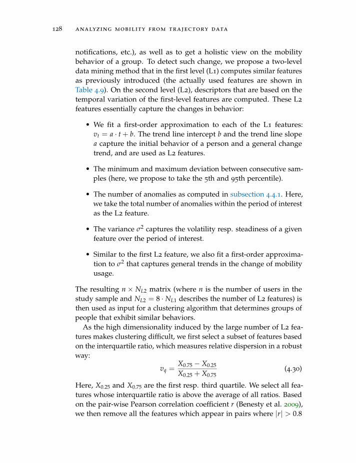
128 analyzing mobility from trajectory data
notifications, etc.), as well as to get a holistic view on the mobilitybehavior of a group. To detect such change, we propose a two-leveldata mining method that in the first level (L1) computes similar featuresas previously introduced (the actually used features are shown inTable 4.9). On the second level (L2), descriptors that are based on thetemporal variation of the first-level features are computed. These L2
features essentially capture the changes in behavior:
• We fit a first-order approximation to each of the L1 features:vt = a · t + b. The trend line intercept b and the trend line slopea capture the initial behavior of a person and a general changetrend, and are used as L2 features.
• The minimum and maximum deviation between consecutive sam-ples (here, we propose to take the 5th and 95th percentile).
• The number of anomalies as computed in subsection 4.4.1. Here,we take the total number of anomalies within the period of interestas the L2 feature.
• The variance σ2 captures the volatility resp. steadiness of a givenfeature over the period of interest.
• Similar to the first L2 feature, we also fit a first-order approxima-tion to σ2 that captures general trends in the change of mobilityusage.
The resulting n× NL2 matrix (where n is the number of users in thestudy sample and NL2 = 8 · NL1 describes the number of L2 features) isthen used as input for a clustering algorithm that determines groups ofpeople that exhibit similar behaviors.
As the high dimensionality induced by the large number of L2 fea-tures makes clustering difficult, we first select a subset of features basedon the interquartile ratio, which measures relative dispersion in a robustway:
vq =X0.75 − X0.25
X0.25 + X0.75(4.30)
Here, X0.25 and X0.75 are the first resp. third quartile. We select all fea-tures whose interquartile ratio is above the average of all ratios. Basedon the pair-wise Pearson correlation coefficient r (Benesty et al. 2009),we then remove all the features which appear in pairs where |r| > 0.8
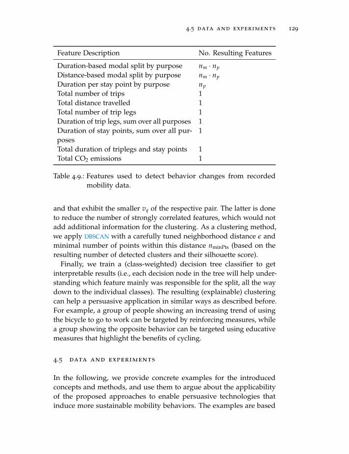
4.5 data and experiments 129
Feature Description No. Resulting Features
Duration-based modal split by purpose nm · np
Distance-based modal split by purpose nm · np
Duration per stay point by purpose np
Total number of trips 1Total distance travelled 1Total number of trip legs 1Duration of trip legs, sum over all purposes 1Duration of stay points, sum over all pur-poses
1
Total duration of triplegs and stay points 1Total CO2 emissions 1
Table 4.9.: Features used to detect behavior changes from recordedmobility data.
and that exhibit the smaller vq of the respective pair. The latter is doneto reduce the number of strongly correlated features, which would notadd additional information for the clustering. As a clustering method,we apply DBSCAN with a carefully tuned neighborhood distance ε andminimal number of points within this distance nminPts (based on theresulting number of detected clusters and their silhouette score).
Finally, we train a (class-weighted) decision tree classifier to getinterpretable results (i.e., each decision node in the tree will help under-standing which feature mainly was responsible for the split, all the waydown to the individual classes). The resulting (explainable) clusteringcan help a persuasive application in similar ways as described before.For example, a group of people showing an increasing trend of usingthe bicycle to go to work can be targeted by reinforcing measures, whilea group showing the opposite behavior can be targeted using educativemeasures that highlight the benefits of cycling.
4.5 data and experiments
In the following, we provide concrete examples for the introducedconcepts and methods, and use them to argue about the applicabilityof the proposed approaches to enable persuasive technologies thatinduce more sustainable mobility behaviors. The examples are based
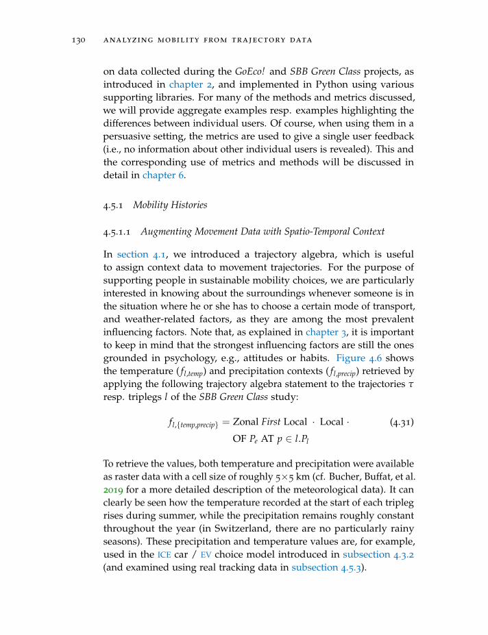
130 analyzing mobility from trajectory data
on data collected during the GoEco! and SBB Green Class projects, asintroduced in chapter 2, and implemented in Python using varioussupporting libraries. For many of the methods and metrics discussed,we will provide aggregate examples resp. examples highlighting thedifferences between individual users. Of course, when using them in apersuasive setting, the metrics are used to give a single user feedback(i.e., no information about other individual users is revealed). This andthe corresponding use of metrics and methods will be discussed indetail in chapter 6.
4.5.1 Mobility Histories
4.5.1.1 Augmenting Movement Data with Spatio-Temporal Context
In section 4.1, we introduced a trajectory algebra, which is usefulto assign context data to movement trajectories. For the purpose ofsupporting people in sustainable mobility choices, we are particularlyinterested in knowing about the surroundings whenever someone is inthe situation where he or she has to choose a certain mode of transport,and weather-related factors, as they are among the most prevalentinfluencing factors. Note that, as explained in chapter 3, it is importantto keep in mind that the strongest influencing factors are still the onesgrounded in psychology, e.g., attitudes or habits. Figure 4.6 showsthe temperature ( fl,temp) and precipitation contexts ( fl,precip) retrieved byapplying the following trajectory algebra statement to the trajectories τ
resp. triplegs l of the SBB Green Class study:
fl,{temp,precip} = Zonal First Local · Local · (4.31)
OF Pe AT p ∈ l.Pl
To retrieve the values, both temperature and precipitation were availableas raster data with a cell size of roughly 5×5 km (cf. Bucher, Buffat, et al.2019 for a more detailed description of the meteorological data). It canclearly be seen how the temperature recorded at the start of each triplegrises during summer, while the precipitation remains roughly constantthroughout the year (in Switzerland, there are no particularly rainyseasons). These precipitation and temperature values are, for example,used in the ICE car / EV choice model introduced in subsection 4.3.2(and examined using real tracking data in subsection 4.5.3).
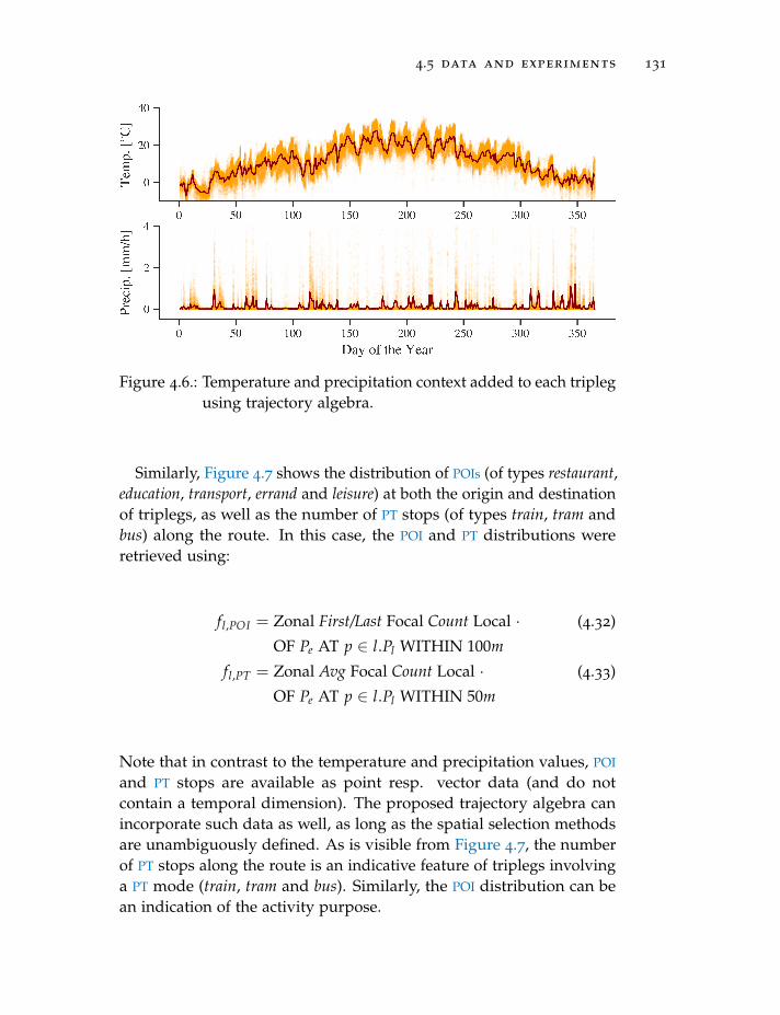
4.5 data and experiments 131
Figure 4.6.: Temperature and precipitation context added to each triplegusing trajectory algebra.
Similarly, Figure 4.7 shows the distribution of POIs (of types restaurant,education, transport, errand and leisure) at both the origin and destinationof triplegs, as well as the number of PT stops (of types train, tram andbus) along the route. In this case, the POI and PT distributions wereretrieved using:
fl,POI = Zonal First/Last Focal Count Local · (4.32)
OF Pe AT p ∈ l.Pl WITHIN 100m
fl,PT = Zonal Avg Focal Count Local · (4.33)
OF Pe AT p ∈ l.Pl WITHIN 50m
Note that in contrast to the temperature and precipitation values, POI
and PT stops are available as point resp. vector data (and do notcontain a temporal dimension). The proposed trajectory algebra canincorporate such data as well, as long as the spatial selection methodsare unambiguously defined. As is visible from Figure 4.7, the numberof PT stops along the route is an indicative feature of triplegs involvinga PT mode (train, tram and bus). Similarly, the POI distribution can bean indication of the activity purpose.
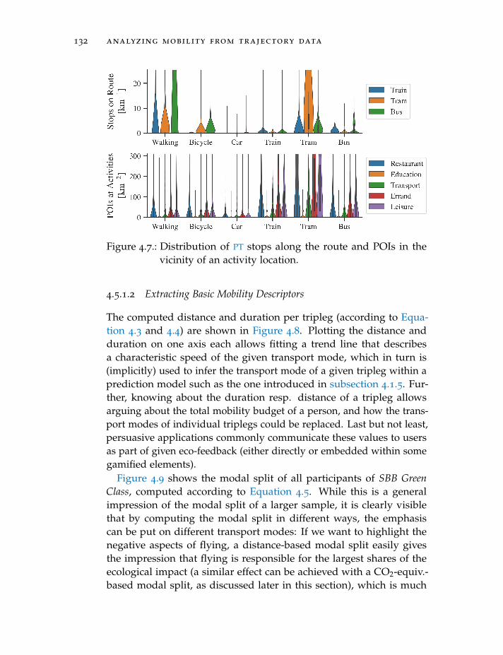
132 analyzing mobility from trajectory data
Figure 4.7.: Distribution of PT stops along the route and POIs in thevicinity of an activity location.
4.5.1.2 Extracting Basic Mobility Descriptors
The computed distance and duration per tripleg (according to Equa-tion 4.3 and 4.4) are shown in Figure 4.8. Plotting the distance andduration on one axis each allows fitting a trend line that describesa characteristic speed of the given transport mode, which in turn is(implicitly) used to infer the transport mode of a given tripleg within aprediction model such as the one introduced in subsection 4.1.5. Fur-ther, knowing about the duration resp. distance of a tripleg allowsarguing about the total mobility budget of a person, and how the trans-port modes of individual triplegs could be replaced. Last but not least,persuasive applications commonly communicate these values to usersas part of given eco-feedback (either directly or embedded within somegamified elements).
Figure 4.9 shows the modal split of all participants of SBB GreenClass, computed according to Equation 4.5. While this is a generalimpression of the modal split of a larger sample, it is clearly visiblethat by computing the modal split in different ways, the emphasiscan be put on different transport modes: If we want to highlight thenegative aspects of flying, a distance-based modal split easily givesthe impression that flying is responsible for the largest shares of theecological impact (a similar effect can be achieved with a CO2-equiv.-based modal split, as discussed later in this section), which is much
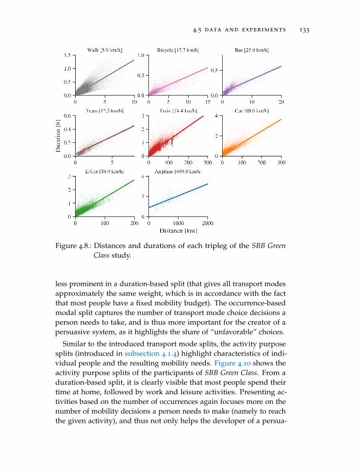
4.5 data and experiments 133
Figure 4.8.: Distances and durations of each tripleg of the SBB GreenClass study.
less prominent in a duration-based split (that gives all transport modesapproximately the same weight, which is in accordance with the factthat most people have a fixed mobility budget). The occurrence-basedmodal split captures the number of transport mode choice decisions aperson needs to take, and is thus more important for the creator of apersuasive system, as it highlights the share of “unfavorable” choices.
Similar to the introduced transport mode splits, the activity purposesplits (introduced in subsection 4.1.4) highlight characteristics of indi-vidual people and the resulting mobility needs. Figure 4.10 shows theactivity purpose splits of the participants of SBB Green Class. From aduration-based split, it is clearly visible that most people spend theirtime at home, followed by work and leisure activities. Presenting ac-tivities based on the number of occurrences again focuses more on thenumber of mobility decisions a person needs to make (namely to reachthe given activity), and thus not only helps the developer of a persua-
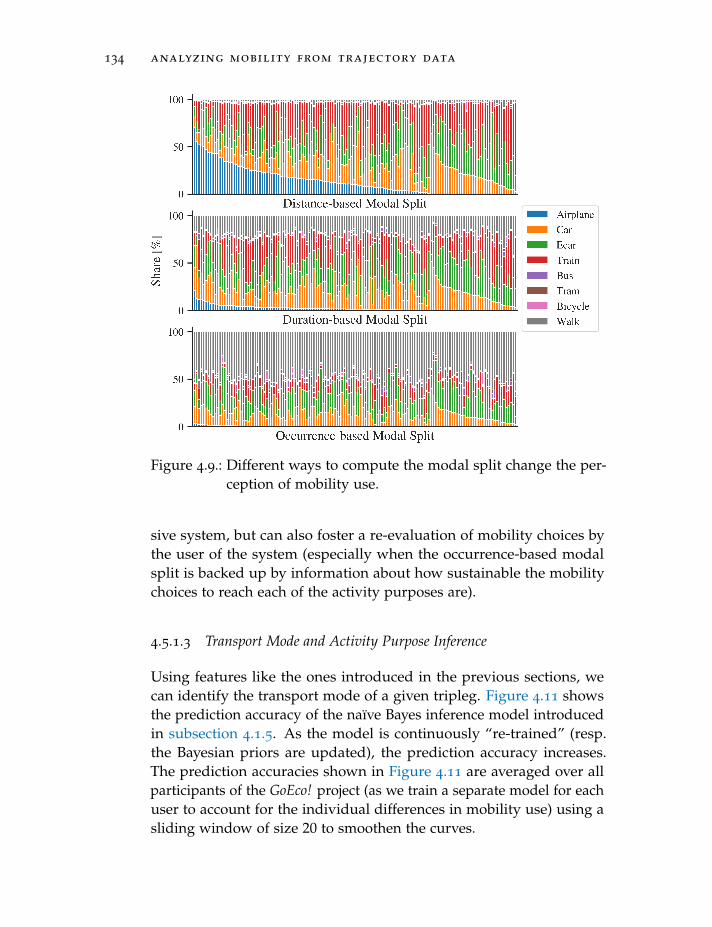
134 analyzing mobility from trajectory data
Figure 4.9.: Different ways to compute the modal split change the per-ception of mobility use.
sive system, but can also foster a re-evaluation of mobility choices bythe user of the system (especially when the occurrence-based modalsplit is backed up by information about how sustainable the mobilitychoices to reach each of the activity purposes are).
4.5.1.3 Transport Mode and Activity Purpose Inference
Using features like the ones introduced in the previous sections, wecan identify the transport mode of a given tripleg. Figure 4.11 showsthe prediction accuracy of the naıve Bayes inference model introducedin subsection 4.1.5. As the model is continuously “re-trained” (resp.the Bayesian priors are updated), the prediction accuracy increases.The prediction accuracies shown in Figure 4.11 are averaged over allparticipants of the GoEco! project (as we train a separate model for eachuser to account for the individual differences in mobility use) using asliding window of size 20 to smoothen the curves.
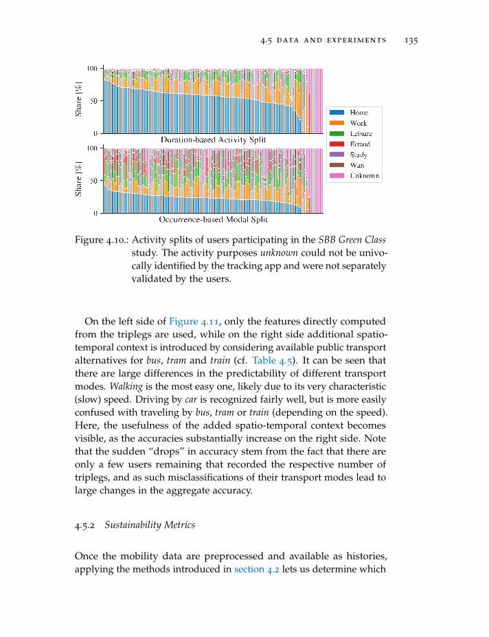
4.5 data and experiments 135
Figure 4.10.: Activity splits of users participating in the SBB Green Classstudy. The activity purposes unknown could not be univo-cally identified by the tracking app and were not separatelyvalidated by the users.
On the left side of Figure 4.11, only the features directly computedfrom the triplegs are used, while on the right side additional spatio-temporal context is introduced by considering available public transportalternatives for bus, tram and train (cf. Table 4.5). It can be seen thatthere are large differences in the predictability of different transportmodes. Walking is the most easy one, likely due to its very characteristic(slow) speed. Driving by car is recognized fairly well, but is more easilyconfused with traveling by bus, tram or train (depending on the speed).Here, the usefulness of the added spatio-temporal context becomesvisible, as the accuracies substantially increase on the right side. Notethat the sudden “drops” in accuracy stem from the fact that there areonly a few users remaining that recorded the respective number oftriplegs, and as such misclassifications of their transport modes lead tolarge changes in the aggregate accuracy.
4.5.2 Sustainability Metrics
Once the mobility data are preprocessed and available as histories,applying the methods introduced in section 4.2 lets us determine which
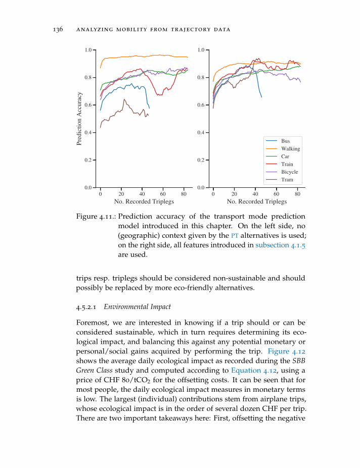
136 analyzing mobility from trajectory data
0 20 40 60 80No. Recorded Triplegs
0.0
0.2
0.4
0.6
0.8
1.0
Pred
ictio
n Ac
cura
cy
0 20 40 60 80No. Recorded Triplegs
0.0
0.2
0.4
0.6
0.8
1.0
BusWalkingCarTrainBicycleTram
Figure 4.11.: Prediction accuracy of the transport mode predictionmodel introduced in this chapter. On the left side, no(geographic) context given by the PT alternatives is used;on the right side, all features introduced in subsection 4.1.5are used.
trips resp. triplegs should be considered non-sustainable and shouldpossibly be replaced by more eco-friendly alternatives.
4.5.2.1 Environmental Impact
Foremost, we are interested in knowing if a trip should or can beconsidered sustainable, which in turn requires determining its eco-logical impact, and balancing this against any potential monetary orpersonal/social gains acquired by performing the trip. Figure 4.12
shows the average daily ecological impact as recorded during the SBBGreen Class study and computed according to Equation 4.12, using aprice of CHF 80/tCO2 for the offsetting costs. It can be seen that formost people, the daily ecological impact measures in monetary termsis low. The largest (individual) contributions stem from airplane trips,whose ecological impact is in the order of several dozen CHF per trip.There are two important takeaways here: First, offsetting the negative
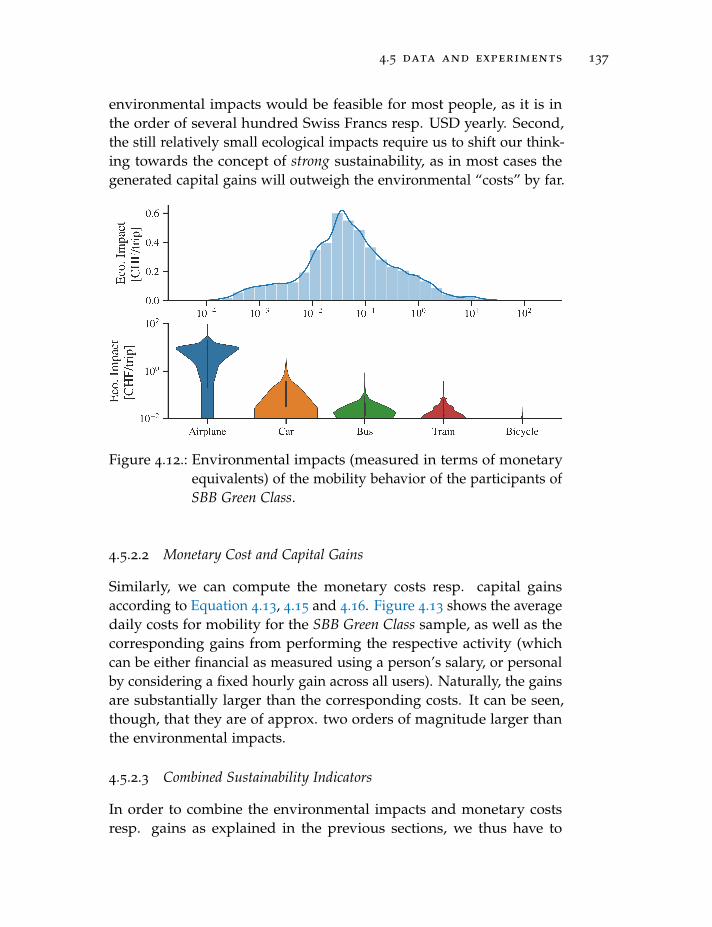
4.5 data and experiments 137
environmental impacts would be feasible for most people, as it is inthe order of several hundred Swiss Francs resp. USD yearly. Second,the still relatively small ecological impacts require us to shift our think-ing towards the concept of strong sustainability, as in most cases thegenerated capital gains will outweigh the environmental “costs” by far.
Figure 4.12.: Environmental impacts (measured in terms of monetaryequivalents) of the mobility behavior of the participants ofSBB Green Class.
4.5.2.2 Monetary Cost and Capital Gains
Similarly, we can compute the monetary costs resp. capital gainsaccording to Equation 4.13, 4.15 and 4.16. Figure 4.13 shows the averagedaily costs for mobility for the SBB Green Class sample, as well as thecorresponding gains from performing the respective activity (whichcan be either financial as measured using a person’s salary, or personalby considering a fixed hourly gain across all users). Naturally, the gainsare substantially larger than the corresponding costs. It can be seen,though, that they are of approx. two orders of magnitude larger thanthe environmental impacts.
4.5.2.3 Combined Sustainability Indicators
In order to combine the environmental impacts and monetary costsresp. gains as explained in the previous sections, we thus have to
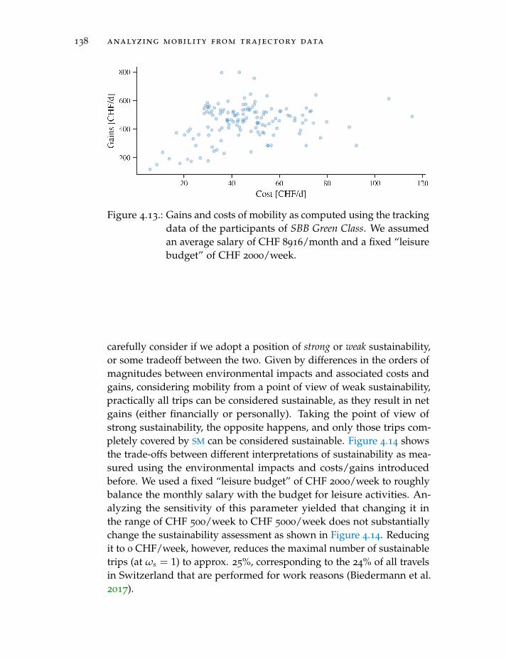
138 analyzing mobility from trajectory data
Figure 4.13.: Gains and costs of mobility as computed using the trackingdata of the participants of SBB Green Class. We assumedan average salary of CHF 8916/month and a fixed “leisurebudget” of CHF 2000/week.
carefully consider if we adopt a position of strong or weak sustainability,or some tradeoff between the two. Given by differences in the orders ofmagnitudes between environmental impacts and associated costs andgains, considering mobility from a point of view of weak sustainability,practically all trips can be considered sustainable, as they result in netgains (either financially or personally). Taking the point of view ofstrong sustainability, the opposite happens, and only those trips com-pletely covered by SM can be considered sustainable. Figure 4.14 showsthe trade-offs between different interpretations of sustainability as mea-sured using the environmental impacts and costs/gains introducedbefore. We used a fixed “leisure budget” of CHF 2000/week to roughlybalance the monthly salary with the budget for leisure activities. An-alyzing the sensitivity of this parameter yielded that changing it inthe range of CHF 500/week to CHF 5000/week does not substantiallychange the sustainability assessment as shown in Figure 4.14. Reducingit to 0 CHF/week, however, reduces the maximal number of sustainabletrips (at ωs = 1) to approx. 25%, corresponding to the 24% of all travelsin Switzerland that are performed for work reasons (Biedermann et al.2017).
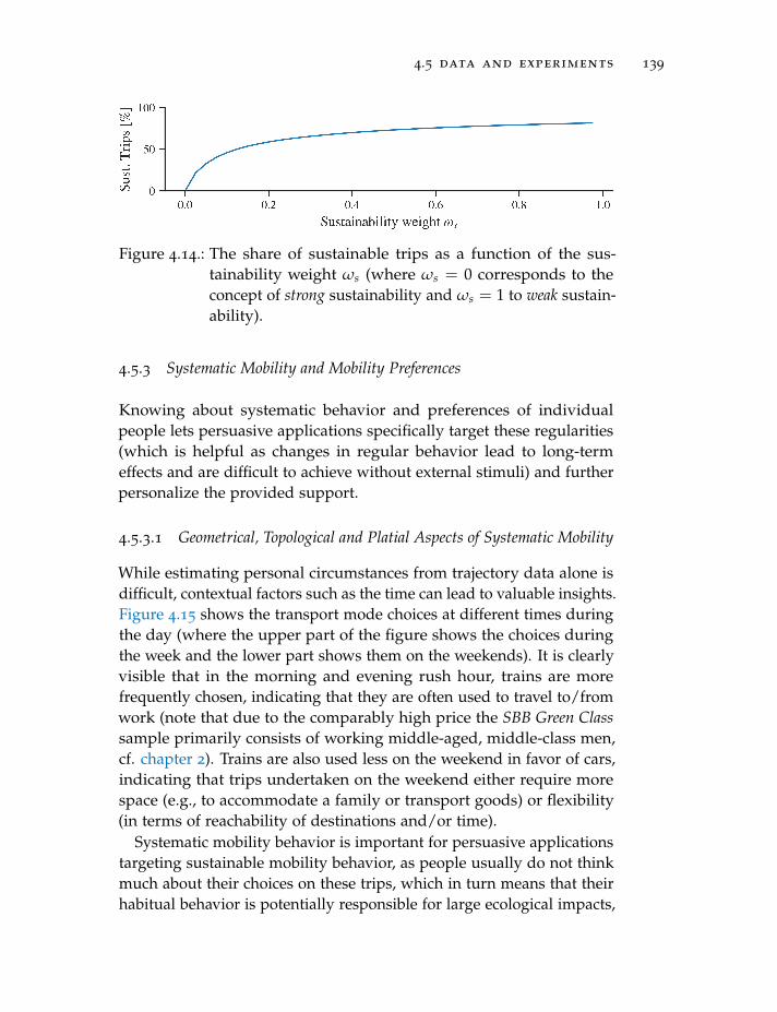
4.5 data and experiments 139
Figure 4.14.: The share of sustainable trips as a function of the sus-tainability weight ωs (where ωs = 0 corresponds to theconcept of strong sustainability and ωs = 1 to weak sustain-ability).
4.5.3 Systematic Mobility and Mobility Preferences
Knowing about systematic behavior and preferences of individualpeople lets persuasive applications specifically target these regularities(which is helpful as changes in regular behavior lead to long-termeffects and are difficult to achieve without external stimuli) and furtherpersonalize the provided support.
4.5.3.1 Geometrical, Topological and Platial Aspects of Systematic Mobility
While estimating personal circumstances from trajectory data alone isdifficult, contextual factors such as the time can lead to valuable insights.Figure 4.15 shows the transport mode choices at different times duringthe day (where the upper part of the figure shows the choices duringthe week and the lower part shows them on the weekends). It is clearlyvisible that in the morning and evening rush hour, trains are morefrequently chosen, indicating that they are often used to travel to/fromwork (note that due to the comparably high price the SBB Green Classsample primarily consists of working middle-aged, middle-class men,cf. chapter 2). Trains are also used less on the weekend in favor of cars,indicating that trips undertaken on the weekend either require morespace (e.g., to accommodate a family or transport goods) or flexibility(in terms of reachability of destinations and/or time).
Systematic mobility behavior is important for persuasive applicationstargeting sustainable mobility behavior, as people usually do not thinkmuch about their choices on these trips, which in turn means that theirhabitual behavior is potentially responsible for large ecological impacts,
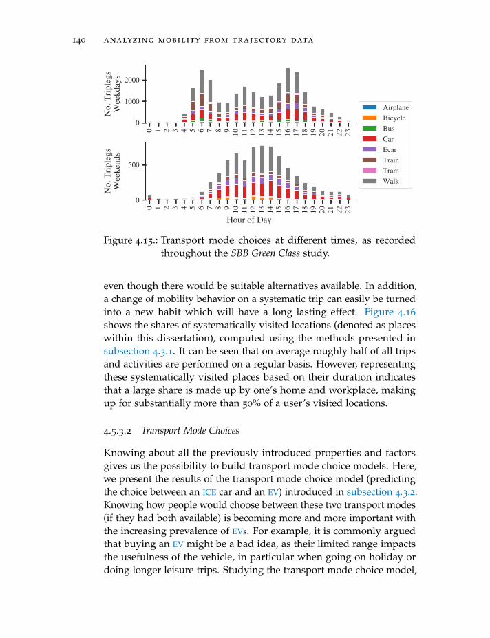
140 analyzing mobility from trajectory data
0 1 2 3 4 5 6 7 8 9 10 11 12 13 14 15 16 17 18 19 20 21 22 23
0
1000
2000
No. T
ripleg
sW
eekd
ays
0 1 2 3 4 5 6 7 8 9 10 11 12 13 14 15 16 17 18 19 20 21 22 23
Hour of Day
0
500
No. T
ripleg
sW
eeke
nds
AirplaneBicycleBusCarEcarTrainTramWalk
Figure 4.15.: Transport mode choices at different times, as recordedthroughout the SBB Green Class study.
even though there would be suitable alternatives available. In addition,a change of mobility behavior on a systematic trip can easily be turnedinto a new habit which will have a long lasting effect. Figure 4.16
shows the shares of systematically visited locations (denoted as placeswithin this dissertation), computed using the methods presented insubsection 4.3.1. It can be seen that on average roughly half of all tripsand activities are performed on a regular basis. However, representingthese systematically visited places based on their duration indicatesthat a large share is made up by one’s home and workplace, makingup for substantially more than 50% of a user’s visited locations.
4.5.3.2 Transport Mode Choices
Knowing about all the previously introduced properties and factorsgives us the possibility to build transport mode choice models. Here,we present the results of the transport mode choice model (predictingthe choice between an ICE car and an EV) introduced in subsection 4.3.2.Knowing how people would choose between these two transport modes(if they had both available) is becoming more and more important withthe increasing prevalence of EVs. For example, it is commonly arguedthat buying an EV might be a bad idea, as their limited range impactsthe usefulness of the vehicle, in particular when going on holiday ordoing longer leisure trips. Studying the transport mode choice model,
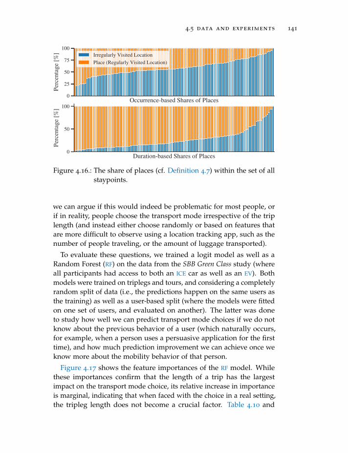
4.5 data and experiments 141
Occurrence-based Shares of Places0
25
50
75
100Pe
rcen
tage [
%] Irregularly Visited Location
Place (Regularly Visited Location)
Duration-based Shares of Places0
50
100
Perc
entag
e [%
]
Figure 4.16.: The share of places (cf. Definition 4.7) within the set of allstaypoints.
we can argue if this would indeed be problematic for most people, orif in reality, people choose the transport mode irrespective of the triplength (and instead either choose randomly or based on features thatare more difficult to observe using a location tracking app, such as thenumber of people traveling, or the amount of luggage transported).
To evaluate these questions, we trained a logit model as well as aRandom Forest (RF) on the data from the SBB Green Class study (whereall participants had access to both an ICE car as well as an EV). Bothmodels were trained on triplegs and tours, and considering a completelyrandom split of data (i.e., the predictions happen on the same users asthe training) as well as a user-based split (where the models were fittedon one set of users, and evaluated on another). The latter was doneto study how well we can predict transport mode choices if we do notknow about the previous behavior of a user (which naturally occurs,for example, when a person uses a persuasive application for the firsttime), and how much prediction improvement we can achieve once weknow more about the mobility behavior of that person.
Figure 4.17 shows the feature importances of the RF model. Whilethese importances confirm that the length of a trip has the largestimpact on the transport mode choice, its relative increase in importanceis marginal, indicating that when faced with the choice in a real setting,the tripleg length does not become a crucial factor. Table 4.10 and
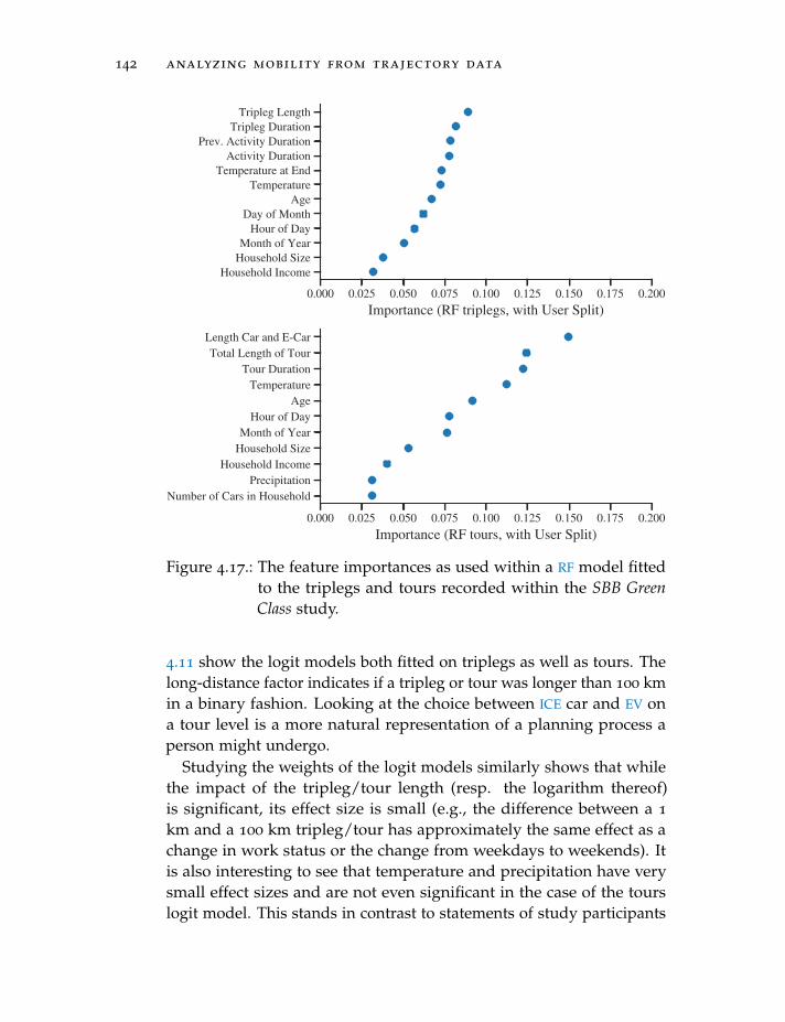
142 analyzing mobility from trajectory data
0.000 0.025 0.050 0.075 0.100 0.125 0.150 0.175 0.200Importance (RF triplegs, with User Split)
Tripleg LengthTripleg Duration
Prev. Activity DurationActivity Duration
Temperature at EndTemperature
AgeDay of Month
Hour of DayMonth of Year
Household SizeHousehold Income
0.000 0.025 0.050 0.075 0.100 0.125 0.150 0.175 0.200Importance (RF tours, with User Split)
Length Car and E-CarTotal Length of Tour
Tour DurationTemperature
AgeHour of Day
Month of YearHousehold Size
Household IncomePrecipitation
Number of Cars in Household
Figure 4.17.: The feature importances as used within a RF model fittedto the triplegs and tours recorded within the SBB GreenClass study.
4.11 show the logit models both fitted on triplegs as well as tours. Thelong-distance factor indicates if a tripleg or tour was longer than 100 kmin a binary fashion. Looking at the choice between ICE car and EV ona tour level is a more natural representation of a planning process aperson might undergo.
Studying the weights of the logit models similarly shows that whilethe impact of the tripleg/tour length (resp. the logarithm thereof)is significant, its effect size is small (e.g., the difference between a 1
km and a 100 km tripleg/tour has approximately the same effect as achange in work status or the change from weekdays to weekends). Itis also interesting to see that temperature and precipitation have verysmall effect sizes and are not even significant in the case of the tourslogit model. This stands in contrast to statements of study participants
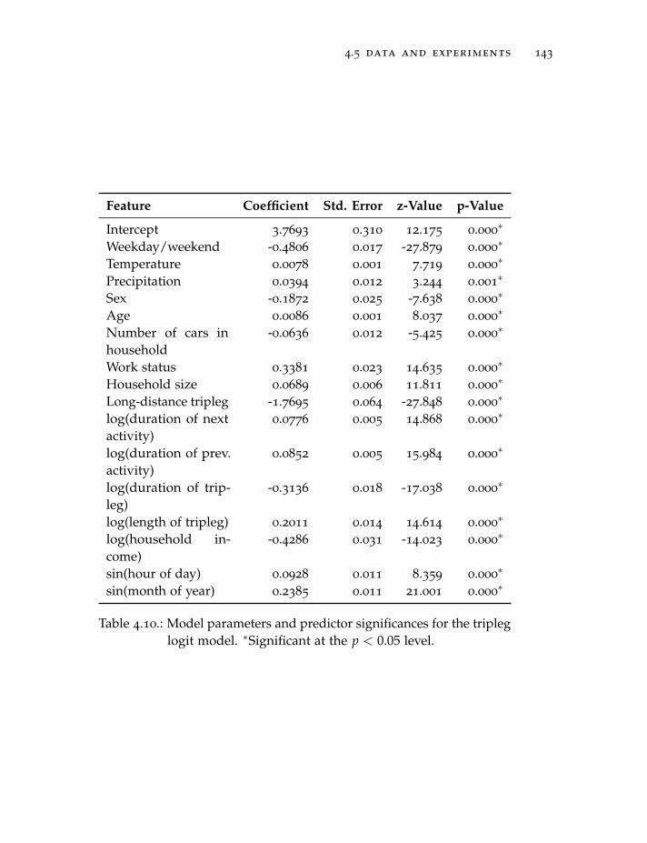
4.5 data and experiments 143
Feature Coefficient Std. Error z-Value p-Value
Intercept 3.7693 0.310 12.175 0.000∗
Weekday/weekend -0.4806 0.017 -27.879 0.000∗
Temperature 0.0078 0.001 7.719 0.000∗
Precipitation 0.0394 0.012 3.244 0.001∗
Sex -0.1872 0.025 -7.638 0.000∗
Age 0.0086 0.001 8.037 0.000∗
Number of cars inhousehold
-0.0636 0.012 -5.425 0.000∗
Work status 0.3381 0.023 14.635 0.000∗
Household size 0.0689 0.006 11.811 0.000∗
Long-distance tripleg -1.7695 0.064 -27.848 0.000∗
log(duration of nextactivity)
0.0776 0.005 14.868 0.000∗
log(duration of prev.activity)
0.0852 0.005 15.984 0.000∗
log(duration of trip-leg)
-0.3136 0.018 -17.038 0.000∗
log(length of tripleg) 0.2011 0.014 14.614 0.000∗
log(household in-come)
-0.4286 0.031 -14.023 0.000∗
sin(hour of day) 0.0928 0.011 8.359 0.000∗
sin(month of year) 0.2385 0.011 21.001 0.000∗
Table 4.10.: Model parameters and predictor significances for the tripleglogit model. ∗Significant at the p < 0.05 level.
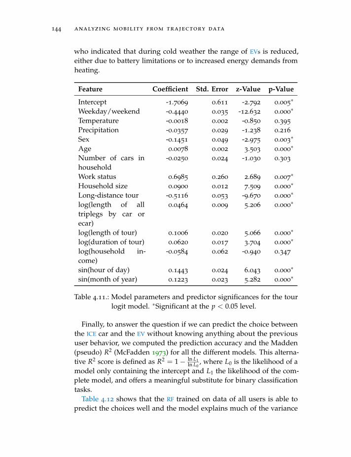
144 analyzing mobility from trajectory data
who indicated that during cold weather the range of EVs is reduced,either due to battery limitations or to increased energy demands fromheating.
Feature Coefficient Std. Error z-Value p-Value
Intercept -1.7069 0.611 -2.792 0.005∗
Weekday/weekend -0.4440 0.035 -12.632 0.000∗
Temperature -0.0018 0.002 -0.850 0.395
Precipitation -0.0357 0.029 -1.238 0.216
Sex -0.1451 0.049 -2.975 0.003∗
Age 0.0078 0.002 3.503 0.000∗
Number of cars inhousehold
-0.0250 0.024 -1.030 0.303
Work status 0.6985 0.260 2.689 0.007∗
Household size 0.0900 0.012 7.509 0.000∗
Long-distance tour -0.5116 0.053 -9.670 0.000∗
log(length of alltriplegs by car orecar)
0.0464 0.009 5.206 0.000∗
log(length of tour) 0.1006 0.020 5.066 0.000∗
log(duration of tour) 0.0620 0.017 3.704 0.000∗
log(household in-come)
-0.0584 0.062 -0.940 0.347
sin(hour of day) 0.1443 0.024 6.043 0.000∗
sin(month of year) 0.1223 0.023 5.282 0.000∗
Table 4.11.: Model parameters and predictor significances for the tourlogit model. ∗Significant at the p < 0.05 level.
Finally, to answer the question if we can predict the choice betweenthe ICE car and the EV without knowing anything about the previoususer behavior, we computed the prediction accuracy and the Madden(pseudo) R2 (McFadden 1973) for all the different models. This alterna-tive R2 score is defined as R2 = 1− ln L1
ln L0, where L0 is the likelihood of a
model only containing the intercept and L1 the likelihood of the com-plete model, and offers a meaningful substitute for binary classificationtasks.
Table 4.12 shows that the RF trained on data of all users is able topredict the choices well and the model explains much of the variance
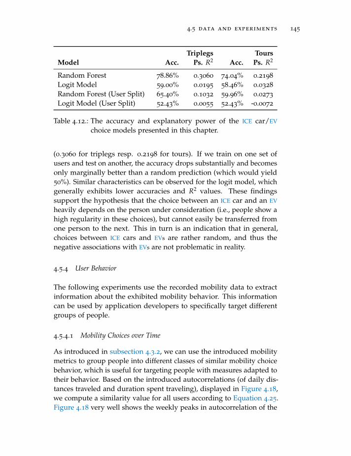
4.5 data and experiments 145
Triplegs ToursModel Acc. Ps. R2 Acc. Ps. R2
Random Forest 78.86% 0.3060 74.04% 0.2198
Logit Model 59.00% 0.0195 58.46% 0.0328
Random Forest (User Split) 65.40% 0.1032 59.96% 0.0273
Logit Model (User Split) 52.43% 0.0055 52.43% -0.0072
Table 4.12.: The accuracy and explanatory power of the ICE car/EV
choice models presented in this chapter.
(0.3060 for triplegs resp. 0.2198 for tours). If we train on one set ofusers and test on another, the accuracy drops substantially and becomesonly marginally better than a random prediction (which would yield50%). Similar characteristics can be observed for the logit model, whichgenerally exhibits lower accuracies and R2 values. These findingssupport the hypothesis that the choice between an ICE car and an EV
heavily depends on the person under consideration (i.e., people show ahigh regularity in these choices), but cannot easily be transferred fromone person to the next. This in turn is an indication that in general,choices between ICE cars and EVs are rather random, and thus thenegative associations with EVs are not problematic in reality.
4.5.4 User Behavior
The following experiments use the recorded mobility data to extractinformation about the exhibited mobility behavior. This informationcan be used by application developers to specifically target differentgroups of people.
4.5.4.1 Mobility Choices over Time
As introduced in subsection 4.3.2, we can use the introduced mobilitymetrics to group people into different classes of similar mobility choicebehavior, which is useful for targeting people with measures adapted totheir behavior. Based on the introduced autocorrelations (of daily dis-tances traveled and duration spent traveling), displayed in Figure 4.18,we compute a similarity value for all users according to Equation 4.25.Figure 4.18 very well shows the weekly peaks in autocorrelation of the
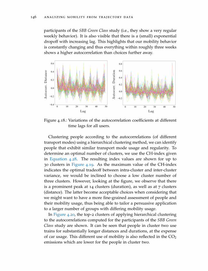
146 analyzing mobility from trajectory data
participants of the SBB Green Class study (i.e., they show a very regularweekly behavior). It is also visible that there is a (small) exponentialdropoff with increasing lag. This highlights that our mobility behavioris constantly changing and thus everything within roughly three weeksshows a higher autocorrelation than choices further away.
Autocorr.Distance
Autocorr.Duration
Lag Lag
Figure 4.18.: Variations of the autocorrelation coefficients at differenttime lags for all users.
Clustering people according to the autocorrelations (of differenttransport modes) using a hierarchical clustering method, we can identifypeople that exhibit similar transport mode usage and regularity. Todetermine an optimal number of clusters, we use the CH-index givenin Equation 4.28. The resulting index values are shown for up to30 clusters in Figure 4.19. As the maximum value of the CH-indexindicates the optimal tradeoff between intra-cluster and inter-clustervariance, we would be inclined to choose a low cluster number ofthree clusters. However, looking at the figure, we observe that thereis a prominent peak at 14 clusters (duration), as well as at 7 clusters(distance). The latter become acceptable choices when considering thatwe might want to have a more fine-grained assessment of people andtheir mobility usage, thus being able to tailor a persuasive applicationto a larger number of groups with differing mobility usage.
In Figure 4.20, the top-2 clusters of applying hierarchical clusteringto the autocorrelations computed for the participants of the SBB GreenClass study are shown. It can be seen that people in cluster two usetrains for substantially longer distances and durations, at the expenseof car usage. This different use of mobility is also reflected in the CO2
emissions which are lower for the people in cluster two.
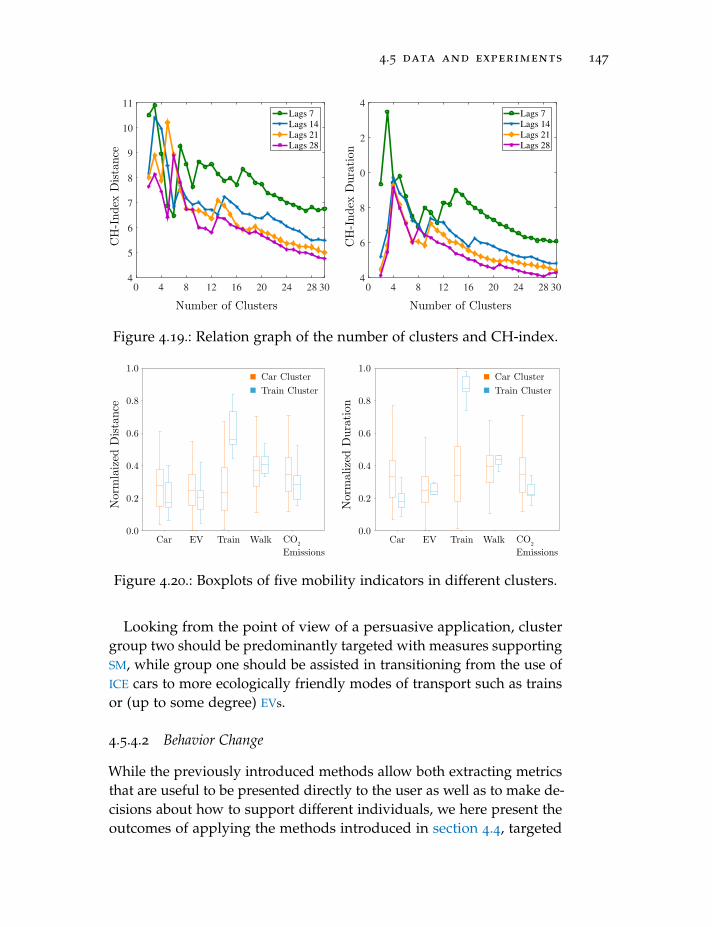
4.5 data and experiments 147
CH-IndexDuration
CH-IndexDistance
Number of Clusters Number of Clusters
Figure 4.19.: Relation graph of the number of clusters and CH-index.NormalizedDuration
NormlaizedDistance
0.0
0.2
0.4
0.6
0.8
1.0
0.0
0.2
0.4
0.6
0.8
1.0
Car EV Train Walk CO2
EmissionsCar EV Train Walk CO2
Emissions
Car ClusterTrain Cluster
Car ClusterTrain Cluster
Figure 4.20.: Boxplots of five mobility indicators in different clusters.
Looking from the point of view of a persuasive application, clustergroup two should be predominantly targeted with measures supportingSM, while group one should be assisted in transitioning from the use ofICE cars to more ecologically friendly modes of transport such as trainsor (up to some degree) EVs.
4.5.4.2 Behavior Change
While the previously introduced methods allow both extracting metricsthat are useful to be presented directly to the user as well as to make de-cisions about how to support different individuals, we here present theoutcomes of applying the methods introduced in section 4.4, targeted
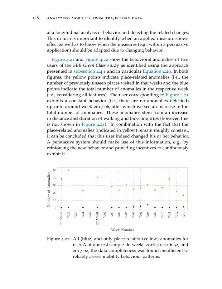
148 analyzing mobility from trajectory data
at a longitudinal analysis of behavior and detecting the related changes.This in turn is important to identify when an applied measure showseffect as well as to know when the measures (e.g., within a persuasiveapplication) should be adapted due to changing behavior.
Figure 4.21 and Figure 4.22 show the behavioral anomalies of twousers of the SBB Green Class study as identified using the approachpresented in subsection 4.4.1 and in particular Equation 4.29. In bothfigures, the yellow points indicate place-related anomalies (i.e., thenumber of previously unseen places visited in that week) and the bluepoints indicate the total number of anomalies in the respective week(i.e., considering all features). The user corresponding to Figure 4.21
exhibits a constant behavior (i.e., there are no anomalies detected)up until around week 2017-06, after which we see an increase in thetotal number of anomalies. These anomalies stem from an increasein distance and duration of walking and bicycling trips (however, thisis not shown in Figure 4.21). In combination with the fact that theplace-related anomalies (indicated in yellow) remain roughly constant,it can be concluded that this user indeed changed his or her behavior.A persuasive system should make use of this information, e.g., byreinforcing the new behavior and providing incentives to continuouslyexhibit it.
NumberofAnomalies
Week Number
0
2016-W48
W49
W50
W51
W52
2017-W01
W02
W03
W04
W05
W06
W07
W08
W09
W10
W11
W12
W13
10
20
30
40
50
Figure 4.21.: All (blue) and only place-related (yellow) anomalies foruser A of our test sample. In weeks 2016-50, 2016-52, and2017-02, the data completeness was found insufficient toreliably assess mobility behaviour patterns.
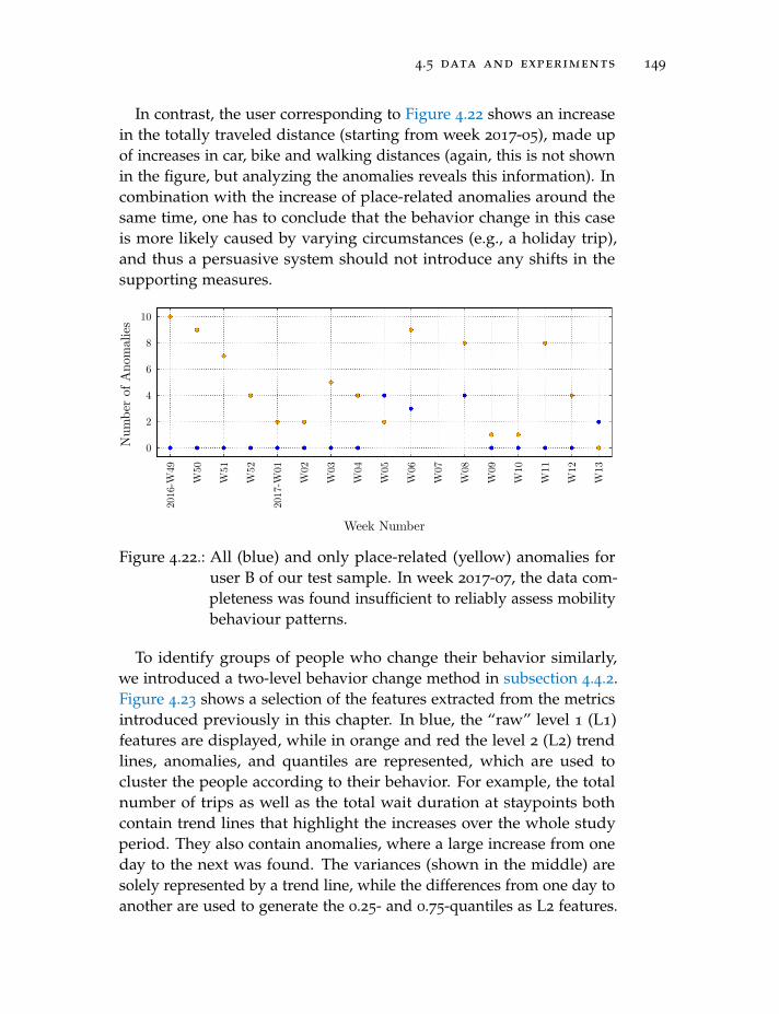
4.5 data and experiments 149
In contrast, the user corresponding to Figure 4.22 shows an increasein the totally traveled distance (starting from week 2017-05), made upof increases in car, bike and walking distances (again, this is not shownin the figure, but analyzing the anomalies reveals this information). Incombination with the increase of place-related anomalies around thesame time, one has to conclude that the behavior change in this caseis more likely caused by varying circumstances (e.g., a holiday trip),and thus a persuasive system should not introduce any shifts in thesupporting measures.
NumberofAnomalies
Week Number
0
2016-W49
W50
W51
W52
2017-W01
W02
W03
W04
W05
W06
W07
W08
W09
W10
W11
W12
W13
2
4
6
8
10
Figure 4.22.: All (blue) and only place-related (yellow) anomalies foruser B of our test sample. In week 2017-07, the data com-pleteness was found insufficient to reliably assess mobilitybehaviour patterns.
To identify groups of people who change their behavior similarly,we introduced a two-level behavior change method in subsection 4.4.2.Figure 4.23 shows a selection of the features extracted from the metricsintroduced previously in this chapter. In blue, the “raw” level 1 (L1)features are displayed, while in orange and red the level 2 (L2) trendlines, anomalies, and quantiles are represented, which are used tocluster the people according to their behavior. For example, the totalnumber of trips as well as the total wait duration at staypoints bothcontain trend lines that highlight the increases over the whole studyperiod. They also contain anomalies, where a large increase from oneday to the next was found. The variances (shown in the middle) aresolely represented by a trend line, while the differences from one day toanother are used to generate the 0.25- and 0.75-quantiles as L2 features.
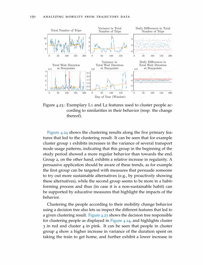
150 analyzing mobility from trajectory data
Total Number of Trips
Total Wait Durationat Staypoints
Variance inTotal Wait Duration
at Staypoints
Day of Year (Window)
Daily Differences inTotal Wait Duration
at Staypoints
Daily Differences in TotalNumber of Trips
Variance in TotalNumber of Trips
10
8
6
0 50 100 150 200 0 50 100 150 0 150 20050 100
0 50 100 150 200 0 50 100 150 0 150 20050 100
1
2 0
2
-2
0
2
-2
-4
3
4
41e3 1e6 1e3
3
2
1
0 0.0
2.01.51.00.5
2.5
Figure 4.23.: Exemplary L1 and L2 features used to cluster people ac-cording to similarities in their behavior (resp. the changethereof).
Figure 4.24 shows the clustering results along the five primary fea-tures that led to the clustering result. It can be seen that for examplecluster group 1 exhibits increases in the variance of several transportmode usage patterns, indicating that this group in the beginning of thestudy period showed a more regular behavior than towards the end.Group 2, on the other hand, exhibits a relative increase in regularity. Apersuasive application should be aware of these trends, as for examplethe first group can be targeted with measures that persuade someoneto try out more sustainable alternatives (e.g., by proactively showingthese alternatives), while the second group seems to be more in a habit-forming process and thus (in case it is a non-sustainable habit) canbe supported by educative measures that highlight the impacts of thebehavior.
Clustering the people according to their mobility change behaviorusing a decision tree also lets us inspect the different features that led toa given clustering result. Figure 4.25 shows the decision tree responsiblefor clustering people as displayed in Figure 4.24, and highlights cluster3 in red and cluster 4 in pink. It can be seen that people in clustergroup 4 show a higher increase in variance of the duration spent ontaking the train to get home, and further exhibit a lower increase in
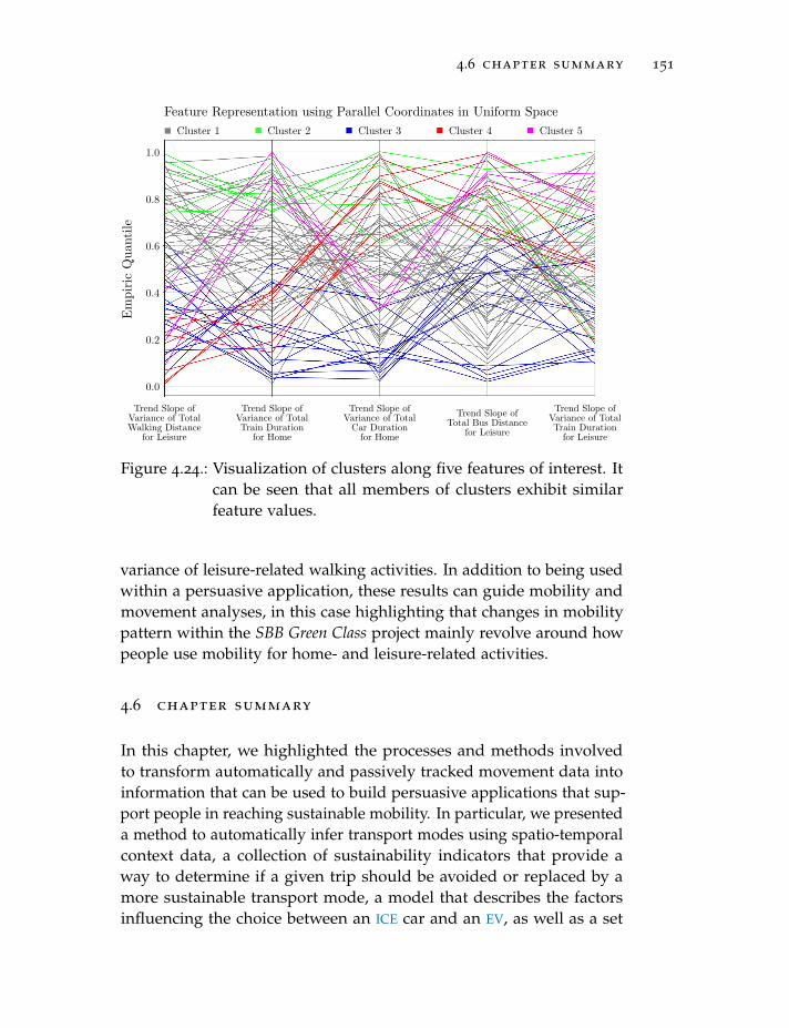
4.6 chapter summary 151
Feature Representation using Parallel Coordinates in Uniform SpaceEmpiricQuantile
1.0
0.8
0.6
0.4
0.2
0.0
Trend Slope ofVariance of TotalWalking Distance
for Leisure
Trend Slope ofVariance of TotalTrain Durationfor Home
Trend Slope ofVariance of TotalCar Durationfor Home
Trend Slope ofTotal Bus Distance
for Leisure
Trend Slope ofVariance of TotalTrain Durationfor Leisure
Cluster 1 Cluster 2 Cluster 3 Cluster 4 Cluster 5
Figure 4.24.: Visualization of clusters along five features of interest. Itcan be seen that all members of clusters exhibit similarfeature values.
variance of leisure-related walking activities. In addition to being usedwithin a persuasive application, these results can guide mobility andmovement analyses, in this case highlighting that changes in mobilitypattern within the SBB Green Class project mainly revolve around howpeople use mobility for home- and leisure-related activities.
4.6 chapter summary
In this chapter, we highlighted the processes and methods involvedto transform automatically and passively tracked movement data intoinformation that can be used to build persuasive applications that sup-port people in reaching sustainable mobility. In particular, we presenteda method to automatically infer transport modes using spatio-temporalcontext data, a collection of sustainability indicators that provide away to determine if a given trip should be avoided or replaced by amore sustainable transport mode, a model that describes the factorsinfluencing the choice between an ICE car and an EV, as well as a set
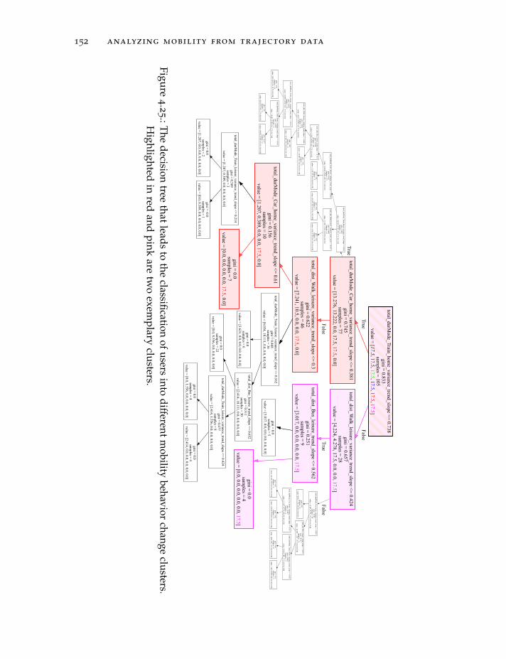
152 analyzing mobility from trajectory data
total_durMode_C
ar_home_variance_trend_slope
<=0.381
gini=0.745
samples=
77value
=[13.276,13.222,0.0,17.5,17.5,0.0]
True
total_dist_Walk_leisure_variance_trend_slope
<=0.424
gini=0.657
samples=
28value
=[4.224,4.278,17.5,0.0,0.0,17.5]
False
total_dist_Walk_leisure_variance_trend_slope
<=0.3
gini=0.622
samples=
46value
=[7.241,10.5,0.0,0.0,17.5,0.0]
total_durMode_Train_hom
e_variance_trend_slope<=
0.562gini=
0.492sam
ples=31
value=[6.034,2.722,0.0,17.5,0.0,0.0]
total_durMode_Train_leisure_variance_trend_slope
<=0.762
gini=0.361
samples=
23value
=[4.828,0.389,0.0,17.5,0.0,0.0]
total_dist_Walk_leisure_variance_trend_slope
<=0.371
gini=0.449
samples=
8value
=[1.207,2.333,0.0,0.0,0.0,0.0]
total_dist_Bus_leisure_trend_slope
<=0.714
gini=0.278
samples=
20value
=[3.017,0.389,0.0,17.5,0.0,0.0]
gini=-0.0
samples=
3value
=[1.81,0.0,0.0,0.0,0.0,0.0]
total_dist_Walk_leisure_variance_trend_slope
<=0.686
gini=0.202
samples=
18value
=[1.81,0.389,0.0,17.5,0.0,0.0]
gini=-0.0
samples=
2value
=[1.207,0.0,0.0,0.0,0.0,0.0]
total_durMode_Train_leisure_variance_trend_slope
<=0.352
gini=0.103
samples=
16value
=[0.603,0.389,0.0,17.5,0.0,0.0]
gini=-0.0
samples=
2value
=[1.207,0.0,0.0,0.0,0.0,0.0]
gini=-0.0
samples=
11value
=[0.0,0.0,0.0,13.75,0.0,0.0]
total_durMode_Train_hom
e_variance_trend_slope<=
0.343gini=
0.352sam
ples=5
value=[0.603,0.389,0.0,3.75,0.0,0.0]
gini=0.0
samples=
3value
=[0.0,0.0,0.0,3.75,0.0,0.0]
gini=0.477
samples=
2value
=[0.603,0.389,0.0,0.0,0.0,0.0]
gini=0.0
samples=
2value
=[1.207,0.0,0.0,0.0,0.0,0.0]
gini=-0.0
samples=
6value
=[0.0,2.333,0.0,0.0,0.0,0.0]
total_durMode_C
ar_home_variance_trend_slope
<=0.61
gini=0.156
samples=
10value
=[1.207,0.389,0.0,0.0,17.5,0.0]
gini=0.0
samples=
7value
=[0.0,0.0,0.0,0.0,17.5,0.0]
total_durMode_Train_leisure_variance_trend_slope
<=0.214
gini=0.369
samples=
3value
=[1.207,0.389,0.0,0.0,0.0,0.0]
gini=0.0
samples=
2value
=[1.207,0.0,0.0,0.0,0.0,0.0]
gini=-0.0
samples=
1value
=[0.0,0.389,0.0,0.0,0.0,0.0]
total_durMode_Train_leisure_variance_trend_slope
<=0.162
gini=0.468
samples=
36value
=[6.034,10.111,0.0,0.0,0.0,0.0]
gini=0.0
samples=
6value
=[3.621,0.0,0.0,0.0,0.0,0.0]
total_dist_Bus_leisure_trend_slope
<=0.652
gini=0.311
samples=
30value
=[2.414,10.111,0.0,0.0,0.0,0.0]
gini=0.0
samples=
22value
=[0.0,8.556,0.0,0.0,0.0,0.0]
total_durMode_Train_leisure_variance_trend_slope
<=0.424
gini=0.477
samples=
8value
=[2.414,1.556,0.0,0.0,0.0,0.0]
gini=0.0
samples=
4value
=[0.0,1.556,0.0,0.0,0.0,0.0]
gini=0.0
samples=
4value
=[2.414,0.0,0.0,0.0,0.0,0.0]
total_dist_Bus_leisure_trend_slope
<=0.562
gini=0.251
samples=
9value
=[3.017,0.0,0.0,0.0,0.0,17.5]
gini=0.0
samples=
5value
=[3.017,0.0,0.0,0.0,0.0,0.0]
gini=0.0
samples=
4value
=[0.0,0.0,0.0,0.0,0.0,17.5]
total_durMode_C
ar_home_variance_trend_slope
<=0.581
gini=0.383
samples=
19value
=[1.207,4.278,17.5,0.0,0.0,0.0]
gini=0.0
samples=
8value
=[0.0,3.111,0.0,0.0,0.0,0.0]
total_dist_Bus_leisure_trend_slope
<=0.471
gini=0.217
samples=
11value
=[1.207,1.167,17.5,0.0,0.0,0.0]
total_durMode_C
ar_home_variance_trend_slope
<=0.767
gini=0.477
samples=
4value
=[1.207,0.778,0.0,0.0,0.0,0.0]
total_durMode_Train_hom
e_variance_trend_slope<=
0.952gini=
0.043sam
ples=7
value=[0.0,0.389,17.5,0.0,0.0,0.0]
gini=0.0
samples=
2value
=[1.207,0.0,0.0,0.0,0.0,0.0]
gini=-0.0
samples=
2value
=[0.0,0.778,0.0,0.0,0.0,0.0]
gini=0.0
samples=
6value
=[0.0,0.0,17.5,0.0,0.0,0.0]
gini=0.0
samples=
1value
=[0.0,0.389,0.0,0.0,0.0,0.0]
FalseFalse
True
True
total_durMode_Train_hom
e_variance_trend_slope<=
0.738gini=
0.833sam
ples=105
value=[17.5,17.5,17.5,17.5,17.5,17.5]
Figure4.
25.:The
decisiontree
thatleadsto
theclassification
ofusersinto
differentmobility
behaviorchange
clusters.H
ighlightedin
redand
pinkare
two
exemplary
clusters.
4.6 chapter summary 153
of methods to automatically identify behavioral patterns and changesthereof. The information can be used mainly in three ways: 1) to guidean expert or an automated system in choosing which groups or individ-ual people to support with which measures, 2) to be directly presentedto users of persuasive applications or to form the basis for persuasivetechniques and personalization as outlined in chapter 5 and chapter 6,as well as 3) to facilitate and guide the analysis of tracking data withrespect to knowing if and how a certain persuasive intervention affectsthe mobility behavior and choices of people. The following chapterswill build upon the here retrieved information to compute and proposemeaningful alternatives as well as to communicate the informationto people in a way that supports them in a transition towards moresustainable mobility behavior.

5P L A N N I N G I N T E G R AT E D A N D S U S TA I N A B L EM O B I L I T Y
In the previous chapter, we have looked at how tracking data canbe used to identify individual mobility behavior, mobility needs anddemands, as well as changes thereof. The focus of this chapter lies onthe development of methods and approaches to use this informationto support people by giving them personalized and meaningful routealternative suggestions and by extending previous research on routeplanning. This will be done by incorporating personalization andproviding a generalized model of high-level route computations thatunify more niche and/or novel transport options (such as free-floatingsharing services, carpooling or buses-on-demand). Figure 5.1 givesa high-level overview of the processes involved in the planning ofintegrated and sustainable mobility options, as presented within thischapter. Starting from a specification of mobility offers (e.g., for PublicTransport (PT), Carpooling (CP) or free-floating micromobility services),we will present approaches to refine the specifications and extracttransfer graphs which describe when and where people can transferfrom one mode of transport to another. Following this, there are severalways we can use the graphs to compute high-level and/or completelyspecified route options that in turn can be utilized to improve persuasiveapplications that support people in achieving sustainable mobility.
We differentiate between two main approaches to compute routealternatives. On the one hand, we can create high-level transfer graphsthat are useful for personalized routing as the number of nodes inthe graphs is substantially lower than in a time-expanded (or time-dependent) graph covering a complete transport network (in particularcontaining all the individual streets, footpaths, and so on). This sec-ond approach, however, is useful to more quickly compute non- (ormarginally) personalized routes, as it allows relying on a wealth ofresearch speeding up graph computations on static graphs and does
This chapter and its contents, algorithms and figures are based on Bucher, Weiser, et al.2015; Bucher, Jonietz, and Raubal 2017; Bucher, Scheider, and Raubal 2017; Huang,Bucher, et al. 2018; Bucher, Mangili, Cellina, et al. 2019.
155
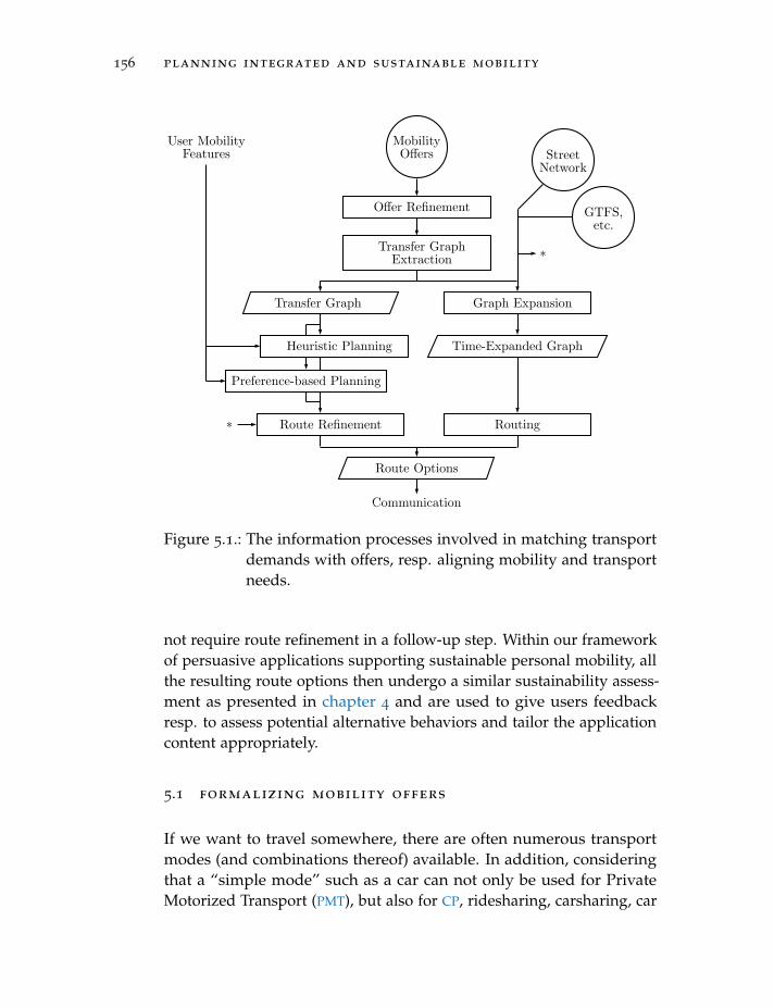
156 planning integrated and sustainable mobility
User MobilityFeatures
MobilityOffers Street
Network
GTFS,etc.
Transfer GraphExtraction
Graph ExpansionTransfer Graph
Route Refinement Routing
Offer Refinement
Communication
Time-Expanded Graph
Route Options
Heuristic Planning
Preference-based Planning
*
*
Figure 5.1.: The information processes involved in matching transportdemands with offers, resp. aligning mobility and transportneeds.
not require route refinement in a follow-up step. Within our frameworkof persuasive applications supporting sustainable personal mobility, allthe resulting route options then undergo a similar sustainability assess-ment as presented in chapter 4 and are used to give users feedbackresp. to assess potential alternative behaviors and tailor the applicationcontent appropriately.
5.1 formalizing mobility offers
If we want to travel somewhere, there are often numerous transportmodes (and combinations thereof) available. In addition, consideringthat a “simple mode” such as a car can not only be used for PrivateMotorized Transport (PMT), but also for CP, ridesharing, carsharing, car
5.1 formalizing mobility offers 157
rentals, taxi services, on-demand services, etc., it becomes obvious thatroute planning cannot only take into account the fastest way from onelocation to another on a static road network, but must be flexible interms of pickup and dropoff locations, routes, networks, schedules, etc.In this section, we provide a generalized formalization encompassinga wide range of transport modes (as used nowadays) that is flexibleenough to incorporate potentially appearing future means of transport,as long as they adhere to some basic assumptions and spatio-temporalconstraints. Specifying transport offers within this formalism enablesapplying a range of routing techniques as introduced later in the chapterwithout further modification or adaptation of the routing methods.
The most basic premise of our formalization is that people can changetransport modes at certain points or regions in space. For many trans-port modes, this is easy to grasp conceptually: we can only access atrain at a train station it stops at, our car can only be used at the pointwhere it is currently parked, a taxi operator only operates in a certain(though potentially large) region, micro-mobility vehicles can only bedropped off in a certain area, and so on. This is particularly importantfor planning routes, where this spatial flexibility has to be taken intoaccount: We cannot assume to always know the exact point in spacewhere someone changes a transport mode, as it is often possible withina larger region. We denote such points or regions as transfer locations.
Definition 5.1 (Transfer Location). A transfer location π ∈ Πm is thegeographic area within which one can change to resp. from a certaintransport mode m ∈ M.
Note that the set of transfer locations Πm in this definition is notrelated to the places Π from Definition 4.7. As already indicated,transfer locations can often be approximated as single points in space(consider, for example, a large train station: even though it comprisesa substantial area within which people can transfer to/from trains,it usually suffices to reduce it to one or a few access points for thepurpose of mobility planning). We denote the function telling us foreach transfer location π if it is a single Point or an Area as type(π):
type(π) : Π→ {A, P} (5.1)
Building on the formalization introduced in chapter 4, a tripleg ldefines a transition from one transfer location (where the person startedusing transport mode m) to the transfer location where the person
158 planning integrated and sustainable mobility
started using the transport mode of the following tripleg. As such,when generating mobility plans, we will refer to the same formalismof trajectories, triplegs, trips and tours, and features resp. contextassociated with them. Within the context of this chapter, we will focuson the following set of transport mode classes, which will be furtherexplained in later sections: M = {mwk, mpmt, mat, mfr, msr, mcp, mpt},corresponding to walking, private motorized transport, (autonomous) taxis,free floating rental systems, station-based rental and sharing, carpooling,and public transport. Note that walking is also explicitly considered atransport mode (that is available everywhere and at any time, and thuscan be used to connect arbitrary transport modes), in contrast to otherwork that uses walking solely for the purpose of introducing possibletransfers between other transport modes.
WhilePickup andDropoff Types
the specification of transport offers using pickup and dropofftransfer locations as given by Definition 5.1 would be sufficient for allfurther purposes, we here additionally introduce a schema to classifytransport modes according to their pickup and dropoff types with the aimof facilitating understanding of different transport characteristics withrespect to route planning. These pickup and dropoff types (specifiedin Table 5.1) usually do not vary within the transport mode (e.g., afree-floating scooter will always be picked up at a transfer locationwith type(π) = P and can be dropped off at one with type(π) = A),determine how different transport modes are connected with each other,and also how the offers available for the individual transport modehave to be specified. Naturally, anywhere corresponds to a transferlocation with type(π) = A that spans the whole region (in which theroute planner operates), within area corresponds to pickup resp. dropoffareas of type(π) = A and at discrete locations corresponds to transferlocations with type(π) = P. For example, walking would have both apickup as well as a dropoff type of A (anywhere), as it can be freelyused irrespective of the location, and PT is often of type PT → PT, as itonly can be accessed from transfer locations π where type(π) = P.
Given the set of pickup and dropoff locations for a certain transportmode m, we can now specify individual transport offers (i.e., actuallyavailable means of transport to get from a pickup to a dropoff transferlocation).
Definition 5.2 (Transport Offer). A transport offer for a transport mode mis described as a bipartite graph (P, D, ES), where the pickup locations
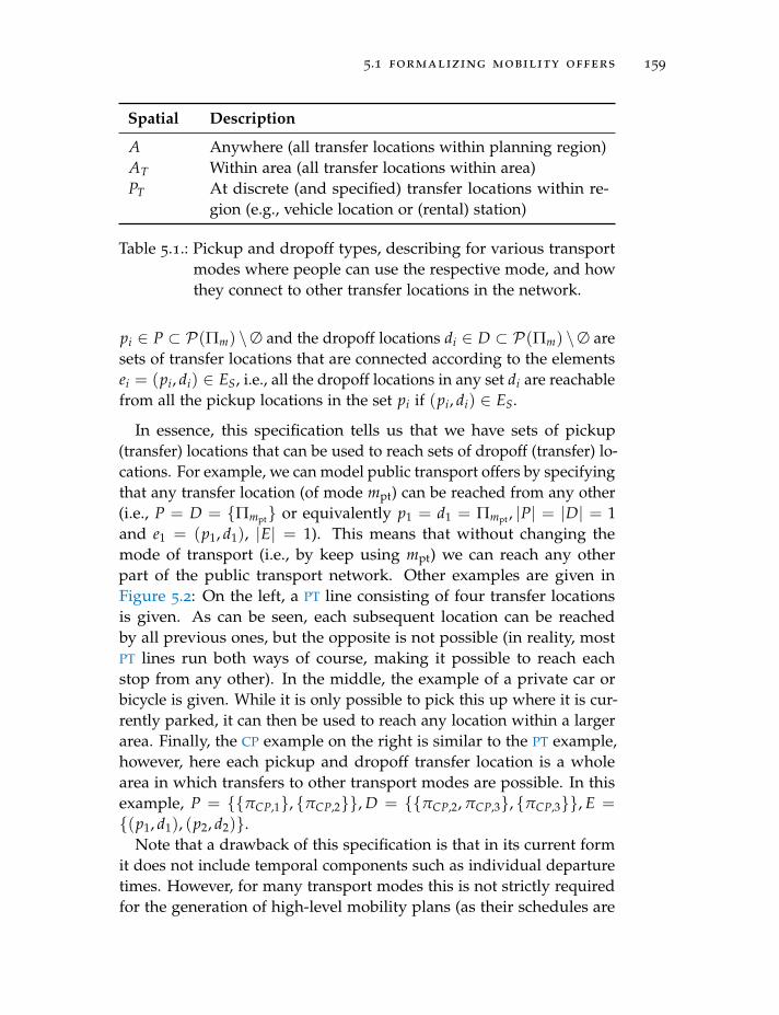
5.1 formalizing mobility offers 159
Spatial Description
A Anywhere (all transfer locations within planning region)AT Within area (all transfer locations within area)PT At discrete (and specified) transfer locations within re-
gion (e.g., vehicle location or (rental) station)
Table 5.1.: Pickup and dropoff types, describing for various transportmodes where people can use the respective mode, and howthey connect to other transfer locations in the network.
pi ∈ P ⊂ P(Πm) \∅ and the dropoff locations di ∈ D ⊂ P(Πm) \∅ aresets of transfer locations that are connected according to the elementsei = (pi, di) ∈ ES, i.e., all the dropoff locations in any set di are reachablefrom all the pickup locations in the set pi if (pi, di) ∈ ES.
In essence, this specification tells us that we have sets of pickup(transfer) locations that can be used to reach sets of dropoff (transfer) lo-cations. For example, we can model public transport offers by specifyingthat any transfer location (of mode mpt) can be reached from any other(i.e., P = D = {Πmpt} or equivalently p1 = d1 = Πmpt , |P| = |D| = 1and e1 = (p1, d1), |E| = 1). This means that without changing themode of transport (i.e., by keep using mpt) we can reach any otherpart of the public transport network. Other examples are given inFigure 5.2: On the left, a PT line consisting of four transfer locationsis given. As can be seen, each subsequent location can be reachedby all previous ones, but the opposite is not possible (in reality, mostPT lines run both ways of course, making it possible to reach eachstop from any other). In the middle, the example of a private car orbicycle is given. While it is only possible to pick this up where it is cur-rently parked, it can then be used to reach any location within a largerarea. Finally, the CP example on the right is similar to the PT example,however, here each pickup and dropoff transfer location is a wholearea in which transfers to other transport modes are possible. In thisexample, P = {{πCP,1}, {πCP,2}}, D = {{πCP,2, πCP,3}, {πCP,3}}, E =
{(p1, d1), (p2, d2)}.Note that a drawback of this specification is that in its current form
it does not include temporal components such as individual departuretimes. However, for many transport modes this is not strictly requiredfor the generation of high-level mobility plans (as their schedules are
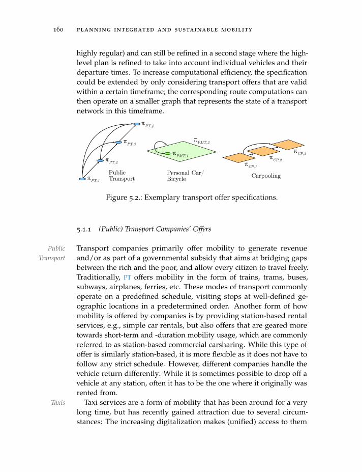
160 planning integrated and sustainable mobility
highly regular) and can still be refined in a second stage where the high-level plan is refined to take into account individual vehicles and theirdeparture times. To increase computational efficiency, the specificationcould be extended by only considering transport offers that are validwithin a certain timeframe; the corresponding route computations canthen operate on a smaller graph that represents the state of a transportnetwork in this timeframe.
PublicTransport
Personal Car/Bicycle Carpooling�PT,1
�PT,2
�PT,3
�PT,4
�PMT,1
�PMT,2
�CP,1�CP,2
�CP,3
Figure 5.2.: Exemplary transport offer specifications.
5.1.1 (Public) Transport Companies’ Offers
TransportPublicTransport
companies primarily offer mobility to generate revenueand/or as part of a governmental subsidy that aims at bridging gapsbetween the rich and the poor, and allow every citizen to travel freely.Traditionally, PT offers mobility in the form of trains, trams, buses,subways, airplanes, ferries, etc. These modes of transport commonlyoperate on a predefined schedule, visiting stops at well-defined ge-ographic locations in a predetermined order. Another form of howmobility is offered by companies is by providing station-based rentalservices, e.g., simple car rentals, but also offers that are geared moretowards short-term and -duration mobility usage, which are commonlyreferred to as station-based commercial carsharing. While this type ofoffer is similarly station-based, it is more flexible as it does not have tofollow any strict schedule. However, different companies handle thevehicle return differently: While it is sometimes possible to drop off avehicle at any station, often it has to be the one where it originally wasrented from.
TaxiTaxis services are a form of mobility that has been around for a verylong time, but has recently gained attraction due to several circum-stances: The increasing digitalization makes (unified) access to them
5.1 formalizing mobility offers 161
very easy and convenient, and manages to greatly reduce the price.In the same direction, it became much easier for people to offer taxiservices with their personal vehicles and/or as side jobs (cf. the gigeconomy; Prassl 2018). Finally, the promise of level 5 autonomous cars(Driving 2014) lets us imagine scenarios where taxi services are ubiqui-tous and can be offered at very low prices, as no human operators needto be involved anymore. In all these forms, taxis have in common thatthey operate in rather large geographical regions, and can pick up anddrop off people anywhere. In some cases, taxis are also not restrictedto single passengers, but can pick up and drop off multiple passengersat different locations and in the process optimize their occupancy rateand driving schedules. The largest restriction is that a taxi needs to beavailable in the vicinity of a passenger, which can be difficult duringhours of large demand.
Recently Free-FloatingVehicles
(and similarly enabled by the increasing digitalization),many companies have started to introduce free floating transport modeswhere transport vehicles can be picked up wherever they are currentlyparked, and must be returned within a larger geographic area (at anyfree parking spot). This is especially common for (short-term and -duration) carsharing, but even more recently also for a range of slowmobility transport modes such as (electric) bicycles, motor scooters andbattery-powered scooters (footboards with steering handles). Table 5.2summarizes the transport modes introduced as part of (public) trans-port companies’ offers, and shows the formalized pickup and dropofftypes.
5.1.2 Private Persons’ Offers and/or Available Transport Modes
Private Motorized Transport (PMT) PrivateTransport
and individual Slow Mobility (SM)offer flexible and convenient travel options for most people. While theSM transport mode walking is available for anyone at anytime (theo-retically to get anywhere, though practically limited by a maximumwalking distance), taking the bicycle, car, etc. requires these modes tobe present at the current location. As such, the transfer location wherethese modes can be taken are limited to single points in space, whereasthey can be dropped off (almost) anywhere.
It RidesharingandCarpooling
is common for people to share their individually traveled journeyswith other people, e.g., to share costs on longer trips or to decreasetraffic jams and/or be more sustainable (essentially by requiring less
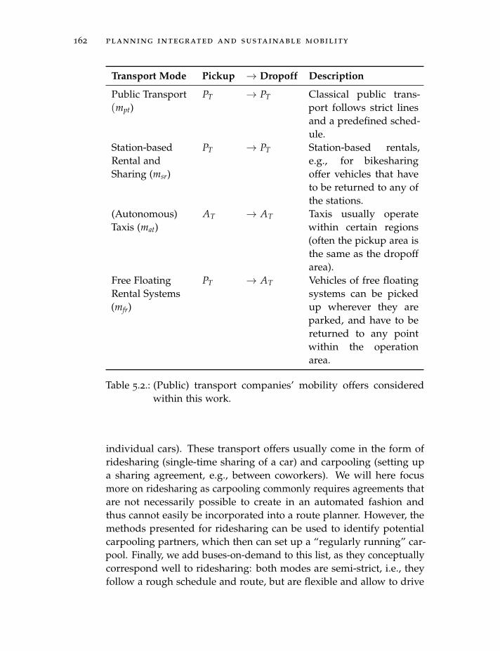
162 planning integrated and sustainable mobility
Transport Mode Pickup → Dropoff Description
Public Transport(mpt)
PT → PT Classical public trans-port follows strict linesand a predefined sched-ule.
Station-basedRental andSharing (msr)
PT → PT Station-based rentals,e.g., for bikesharingoffer vehicles that haveto be returned to any ofthe stations.
(Autonomous)Taxis (mat)
AT → AT Taxis usually operatewithin certain regions(often the pickup area isthe same as the dropoffarea).
Free FloatingRental Systems(mfr)
PT → AT Vehicles of free floatingsystems can be pickedup wherever they areparked, and have to bereturned to any pointwithin the operationarea.
Table 5.2.: (Public) transport companies’ mobility offers consideredwithin this work.
individual cars). These transport offers usually come in the form ofridesharing (single-time sharing of a car) and carpooling (setting upa sharing agreement, e.g., between coworkers). We will here focusmore on ridesharing as carpooling commonly requires agreements thatare not necessarily possible to create in an automated fashion andthus cannot easily be incorporated into a route planner. However, themethods presented for ridesharing can be used to identify potentialcarpooling partners, which then can set up a “regularly running” car-pool. Finally, we add buses-on-demand to this list, as they conceptuallycorrespond well to ridesharing: both modes are semi-strict, i.e., theyfollow a rough schedule and route, but are flexible and allow to drive
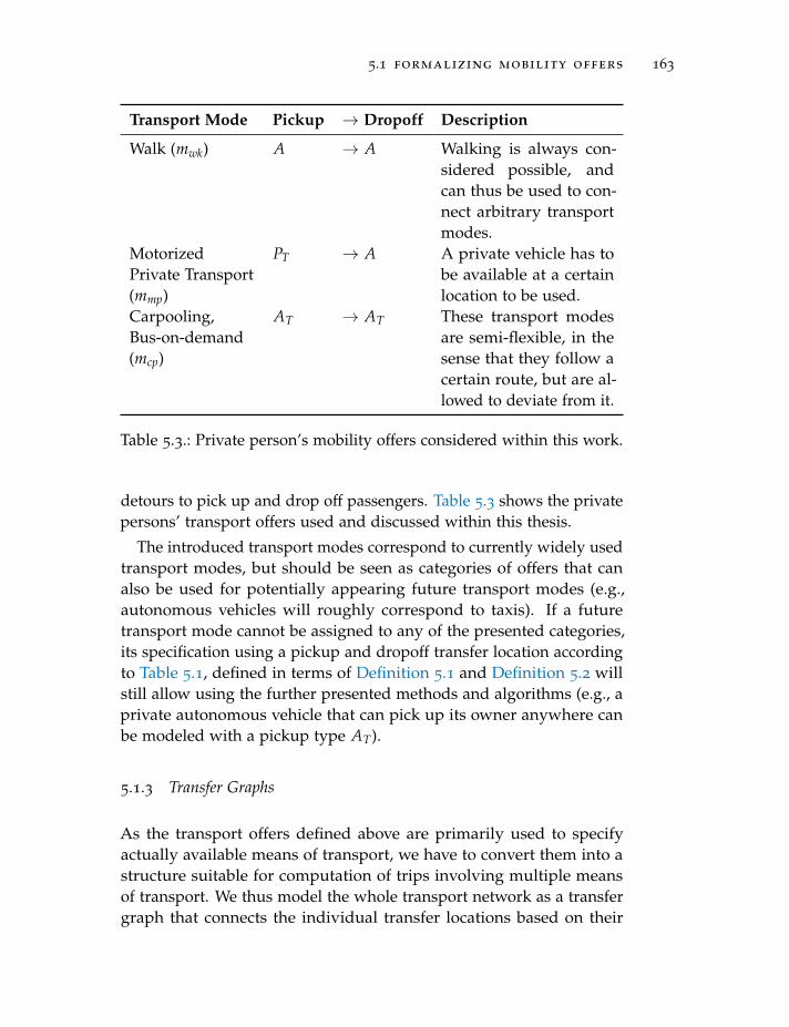
5.1 formalizing mobility offers 163
Transport Mode Pickup → Dropoff Description
Walk (mwk) A → A Walking is always con-sidered possible, andcan thus be used to con-nect arbitrary transportmodes.
MotorizedPrivate Transport(mmp)
PT → A A private vehicle has tobe available at a certainlocation to be used.
Carpooling,Bus-on-demand(mcp)
AT → AT These transport modesare semi-flexible, in thesense that they follow acertain route, but are al-lowed to deviate from it.
Table 5.3.: Private person’s mobility offers considered within this work.
detours to pick up and drop off passengers. Table 5.3 shows the privatepersons’ transport offers used and discussed within this thesis.
The introduced transport modes correspond to currently widely usedtransport modes, but should be seen as categories of offers that canalso be used for potentially appearing future transport modes (e.g.,autonomous vehicles will roughly correspond to taxis). If a futuretransport mode cannot be assigned to any of the presented categories,its specification using a pickup and dropoff transfer location accordingto Table 5.1, defined in terms of Definition 5.1 and Definition 5.2 willstill allow using the further presented methods and algorithms (e.g., aprivate autonomous vehicle that can pick up its owner anywhere canbe modeled with a pickup type AT).
5.1.3 Transfer Graphs
As the transport offers defined above are primarily used to specifyactually available means of transport, we have to convert them into astructure suitable for computation of trips involving multiple meansof transport. We thus model the whole transport network as a transfergraph that connects the individual transfer locations based on their
164 planning integrated and sustainable mobility
geographical extent as well as the specification given as transport offers(as defined before).
Definition 5.3 (Transfer Graph). A transfer graph G = (V , E), ∀e =
(π1, π2, Le) ∈ E : πi ∈ V describes how transfer locations πi are con-nected with various modes of transport. Le denotes the labels resp.properties of an edge e.
To build the transfer graph from the individual transfer locations andtransport offers, we start by adding all transfer locations as nodes of thegraph. For each of these vertices πi ∈ V , we then create an additionalvertex πi,m and add one edge e = (πi, πi,m, m(πi)) (where m(·) retrievesthe transport mode label from the underlying transfer location πi) tothis new vertex, acting as a placeholder for transferring to mode m atlocation πi. The vertices πi,m are then connected based on the transportspecification given in section 5.1 by inserting an edge e = (πi,m, πj, ·)for all pairs (πi, πj) that appear in pickup and dropoff combinationsin ES (i.e., πi ∈ pk, πj ∈ dk, ∀ek = (pk, dk) ∈ ES). After this step, wehave a graph consisting of a number of disconnected subgraphs (onefor each mode of transport resp. for each non-connected route withinthis transport mode).
In a second step, we connect these point locations to transfer areasto connect all subgraphs. In particular, for each (dropoff) transferpoint πi ∈ Π, type(πi) = P that is (geometrically) contained within a(pickup) area πj ∈ Π, type(πj) = A, we add a vertex πj,m and an edgee = (πi, πj,m, m(πj)), denoting the transfer to the respective transportmode. Based on the specifications of the reachability of transfer areas(given in Definition 5.2), the vertices πj,m are then connected to allother reachable transfer points, namely those that are contained withinreachable dropoff areas.
Finally, we add transfer points for any two transfer areas πi and πjthat intersect geometrically (where πi appears as a dropoff area andπj as a pickup area within the bipartite transport specification graph).In this case, for intersection areas having a diameter smaller than aconstant l, we add the geographic center (corresponding to the gravita-tional center) of the intersection polygon as a new vertex πi,j, a transportmode choice vertex πi,j,m, as well as an edge e = (πi,j, πi,j,m, m(πj)) thatdenotes the transfer to the transport mode available within area πj. Wechoose the geographic center as it corresponds to the mean positionof all points, i.e., the expected value of a transfer point (assuming an
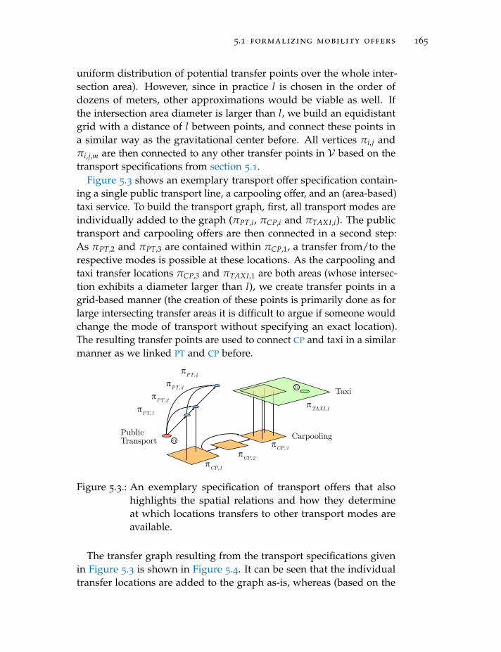
5.1 formalizing mobility offers 165
uniform distribution of potential transfer points over the whole inter-section area). However, since in practice l is chosen in the order ofdozens of meters, other approximations would be viable as well. Ifthe intersection area diameter is larger than l, we build an equidistantgrid with a distance of l between points, and connect these points ina similar way as the gravitational center before. All vertices πi,j andπi,j,m are then connected to any other transfer points in V based on thetransport specifications from section 5.1.
Figure 5.3 shows an exemplary transport offer specification contain-ing a single public transport line, a carpooling offer, and an (area-based)taxi service. To build the transport graph, first, all transport modes areindividually added to the graph (πPT,i, πCP,i and πTAXI,i). The publictransport and carpooling offers are then connected in a second step:As πPT,2 and πPT,3 are contained within πCP,1, a transfer from/to therespective modes is possible at these locations. As the carpooling andtaxi transfer locations πCP,3 and πTAXI,1 are both areas (whose intersec-tion exhibits a diameter larger than l), we create transfer points in agrid-based manner (the creation of these points is primarily done as forlarge intersecting transfer areas it is difficult to argue if someone wouldchange the mode of transport without specifying an exact location).The resulting transfer points are used to connect CP and taxi in a similarmanner as we linked PT and CP before.
PublicTransport Carpooling
Taxi�TAXI,1
�CP,1�CP,2
�CP,3
�PT,1
�PT,2
�PT,3
�PT,4
O
D
Figure 5.3.: An exemplary specification of transport offers that alsohighlights the spatial relations and how they determineat which locations transfers to other transport modes areavailable.
The transfer graph resulting from the transport specifications givenin Figure 5.3 is shown in Figure 5.4. It can be seen that the individualtransfer locations are added to the graph as-is, whereas (based on the
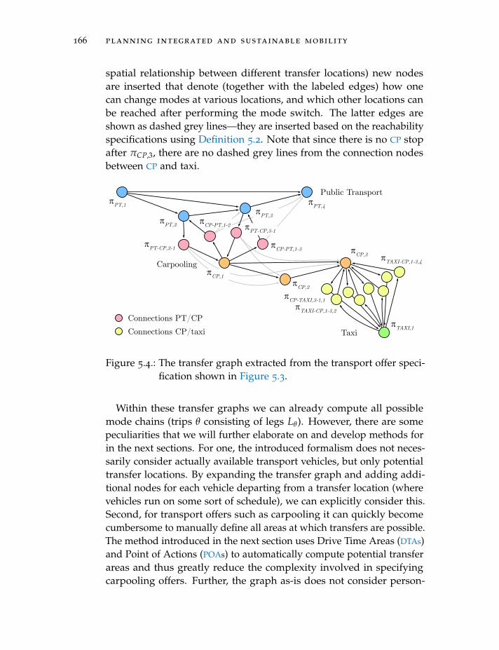
166 planning integrated and sustainable mobility
spatial relationship between different transfer locations) new nodesare inserted that denote (together with the labeled edges) how onecan change modes at various locations, and which other locations canbe reached after performing the mode switch. The latter edges areshown as dashed grey lines—they are inserted based on the reachabilityspecifications using Definition 5.2. Note that since there is no CP stopafter πCP,3, there are no dashed grey lines from the connection nodesbetween CP and taxi.
Public Transport
Carpooling
Connections PT/CPConnections CP/taxi Taxi
�PT,1
�TAXI,1
�CP-PT,1-2�PT,3
�PT,4
�CP,1�CP,2
�PT-CP,3-1
�CP,3
�PT,2
�PT-CP,2-1 �CP-PT,1-3
�CP-TAXI,3-1,1�TAXI-CP,1-3,2
�TAXI-CP,1-3,4
Figure 5.4.: The transfer graph extracted from the transport offer speci-fication shown in Figure 5.3.
Within these transfer graphs we can already compute all possiblemode chains (trips θ consisting of legs Lθ). However, there are somepeculiarities that we will further elaborate on and develop methods forin the next sections. For one, the introduced formalism does not neces-sarily consider actually available transport vehicles, but only potentialtransfer locations. By expanding the transfer graph and adding addi-tional nodes for each vehicle departing from a transfer location (wherevehicles run on some sort of schedule), we can explicitly consider this.Second, for transport offers such as carpooling it can quickly becomecumbersome to manually define all areas at which transfers are possible.The method introduced in the next section uses Drive Time Areas (DTAs)and Point of Actions (POAs) to automatically compute potential transferareas and thus greatly reduce the complexity involved in specifyingcarpooling offers. Further, the graph as-is does not consider person-
5.2 matching carpooling transport demands with offers 167
alization at all, and can quickly lead to computationally exhaustivesearches (e.g., when considering that by walking any transfer locationcould be reached at from point in the transfer graph), for which reasonwe add heuristic constraints and probabilistic models to compute whensomeone (likely) could transfer from one mode to another at a givenlocation in the following sections.
5.2 matching carpooling transport demands with offers
Carpooling or ridesharing may help towards a short-term solution ofmany problems caused by PMT such as GHG emissions or traffic jams, asthe cars are “already on the road”, and for many popular routes thereare enough drivers having roughly the same origin and destination toconsiderably reduce the number of individual rides along the route (cf.Correia and Viegas 2010; Deakin, Frick, and Shively 2010). However,it is difficult to bring these people together for a variety of reasons:people do not use the same matching platforms (websites), they wantto be flexible about possible detours and departure times, they mightbe afraid to share their car with someone else or to be matched with arisky driver, or they might have neither a financial incentive nor need(as mobility is cheap). Here, we do not concern ourselves with mostof these rather societal issues, and focus on the technical aspects offinding possible candidates to share a ride. The flexibility and fuzzinessinherent in carpooling makes it an interesting and non-trivial problem:Drivers can make small detours or delay their departure slightly, andusually this also means that when they specify an upcoming trip (to bematched with potential riders) it is only specified very crudely, usuallyby publishing a list of a few stops in major towns along the routetogether with a departure time and rough price indication.
5.2.1 Modeling Carpooling as Time-Expanded Graphs
For easy integration into popular route planners (such as Google Maps),many PT providers specify their planned schedules using a standardsuch as the GTFS. These standards follow the structure of public trans-port which is (historically and due to the involved infrastructural com-ponents) centered around routes that describe a set of trips followingthe same PT line, i.e., visiting the same stops. Even though there are
168 planning integrated and sustainable mobility
some differences (on which we will comment in the following sections),we here propose to model carpooling offers in a similar way, in orderto easily integrate them into existing route planning systems. Thisintegration will in particular allow us to link them to PT offers andanalyze the resulting benefits. Similar to the formalization presentedin chapter 4, we start with elementary connections (corresponding totriplegs):
Definition 5.4 (Elementary Connection). An elementary connection l isa connection between two PT stops ss and se that is served by a publictransport vehicle v, starting and arriving at ts and te: l = (v, ss, ts, se, te).
Connecting multiple elementary connections leads to trips (θ =
(l1, ..., ln)), which in turn are collected into routes as described above(e.g., “Bus Line 80”). Considering that multiple routes reuse the samestops, it is now possible to connect them in a way that lets us find routeoptions through a network involving multiple vehicles/transport modesand the respective transfers at certain stops. While the specificationusing GTFS differs in several ways from the generalized formalism pre-sented in section 5.1, its basic components of stops and trips can roughlybe considered the specialization of transfer locations and transport offersthat does not include area-based transfer locations.
Similar to the transformation of transport offers into a transfer graphintroduced in subsection 5.1.3, when transforming a specification oftransport offers using GTFS into a graph suitable for route computations,we have to model all the different possible mode choices and departuretimes in some way. With regards to modeling departure times, wecan use a time-dependent graph (where the edge weights are time-dependent, thus making it necessary to update the graph during theroute computations) or a time-expanded graph (where each possibledeparture from any stop is modeled as its own vertex, connected to thenext reachable stop). Within this section, we model the transport offersas a time-expanded graph, as it lets us use any “simple” routing algo-rithm (and the related speed-up techniques) such as Djikstra’s, and wedo not require the additional flexibility with regards to personalizationgiven by time-dependent or high-level graphs.
AModeling ofTransfers
similar choice has to be made when modeling transfers fromone mode to another. In subsection 5.1.3, we have chosen to add anadditional node describing the transfer between two different modes (asthis allows more easily assigning probabilities and enforcing constraints
5.2 matching carpooling transport demands with offers 169
on these choices). While this is a commonly chosen approach (cf. Bast,Delling, et al. 2015), the same effect can be achieved by adding alabeled edge that directly connects the trips of two different transportvehicles or modes. We embrace this approach here, and create a labeledtransition edge (carrying the label “transfer”) between two elementaryconnections where l1.te + tw < l2.ts, l1.se = l2.ss, stating that at everystop it is possible to transfer to connections departing later (l2.ts) thanthe arrival time of the incoming connection (l1.t2). We add additionalrestrictions on the creation of a transition edge: As it is often necessaryto plan a minimal amount of time for the transfer itself (e.g., 3 minutesfor a smaller train station), we enforce this minimum by introducinga waiting time tw that restricts the departures to be after l1.t2 + tw;Similarly, we add an upper bound for the waiting time (l1.te + tu ≥l2.ts, where tu is usually in the order of 60 minutes), which reducesthe number of created edges and thus the overall graph size. Thisis also in line with how transfers commonly happen: We wait forthe first connection that gets us towards our destination, and do notarbitrarily wait for later ones. The resulting graph contains edgesfor all elementary connections, and thus is called a time-expandedgraph (in contrast to a time-dependent graph) as all departures areexplicitly modeled and the graph does not have to be updated duringroute computations. Algorithm 5.1 shows the algorithm used to createtransfer edges between stops of elementary connections.
Summarizing, similar to regular PT schedules, we model carpoolingoffers utilizing a time-expanded graph, essentially using elementaryconnections to connect the individual stops specified by the driver.While for PT, the exact departure and arrival times are known, we haveto derive them for carpooling using a routing on the network. Note thatin the case of carpooling, a route nowadays commonly only consists ofa single trip, as the respective web platforms are primarily used to planone-time (and long-distance) drives.
5.2.2 Merging Carpooling and Public Transport
Starting from the CP model introduced in the previous section, which isin line with previous work and specifications such as GTFS, and sharesthe basic structure with the transfer graph specification introduced insection 5.1, we will now treat some of the peculiarities of CP (partiallygiven by the way CP offers are commonly specified nowadays) and argue
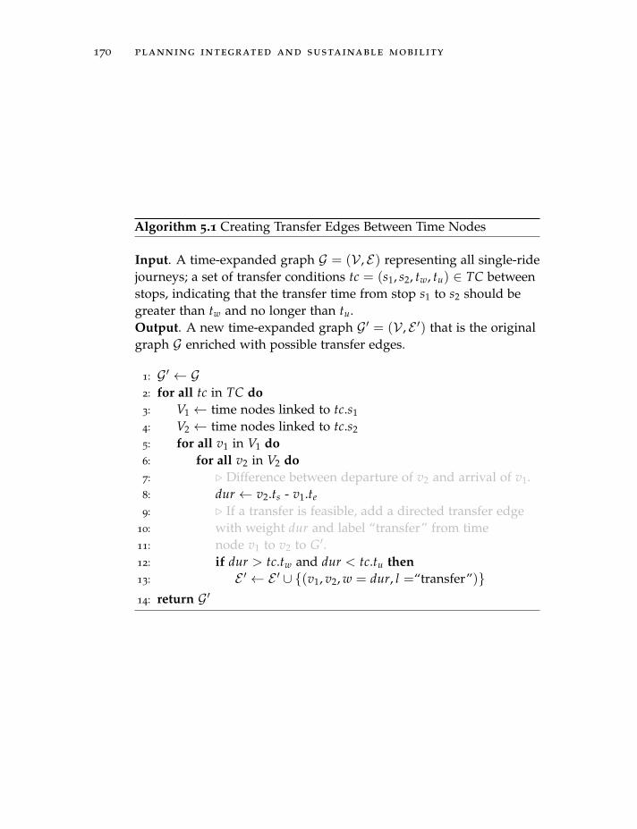
170 planning integrated and sustainable mobility
Algorithm 5.1 Creating Transfer Edges Between Time Nodes
Input. A time-expanded graph G = (V , E) representing all single-ridejourneys; a set of transfer conditions tc = (s1, s2, tw, tu) ∈ TC betweenstops, indicating that the transfer time from stop s1 to s2 should begreater than tw and no longer than tu.Output. A new time-expanded graph G ′ = (V , E ′) that is the originalgraph G enriched with possible transfer edges.
1: G ′ ← G2: for all tc in TC do3: V1 ← time nodes linked to tc.s1
4: V2 ← time nodes linked to tc.s2
5: for all v1 in V1 do6: for all v2 in V2 do7: . Difference between departure of v2 and arrival of v1.8: dur ← v2.ts - v1.te
9: . If a transfer is feasible, add a directed transfer edge10: with weight dur and label “transfer” from time11: node v1 to v2 to G′.12: if dur > tc.tw and dur < tc.tu then13: E ′ ← E ′ ∪ {(v1, v2, w = dur, l =“transfer”)}14: return G ′
5.2 matching carpooling transport demands with offers 171
how to best resolve the resulting issues. As the flexibility and fuzzinessof current approaches to match carpooling partners makes it a largelymanual process (of finding each other), we here propose an approachto automatically process the route specifications resulting in a transportoffer essentially corresponding to the one given in Definition 5.2. Theresulting specification of pickup and dropoff areas can be used to createa transfer graph as defined in section 5.1 or a time-expanded graph (bylinking the offers appropriately) as described here.
As we are particularly interested in the benefits of supplementingPT with CP offers (e.g., to reach badly connected regions), we willfocus on the integration resp. linking of CP and PT graphs. Given anumber of specified stops along a (potential) carpooling journey, twocommonly applied linking strategies are to simply allow transfers atthe closest PT stop to the given stop coordinate, or to allow transfersto any PT stop within the administrative boundary of the town ormunicipality. Both are not ideal, as they either do not respect theflexibility of the driver, or potentially require detours larger than thedriver is willing to make. We here use the concept of Drive TimeAreas (DTAs) to compute transfer areas for various points along the route(this concept is also commonly referred to as potential path space withinthe research field of time geography, cf. Hagerstrand 1970; Miller 1991).A DTA is a geographical space (around a point feature) that denotesthe area reachable by car within a certain amount of time. As manycarpooling offers only appear a single time, we compute DTAs around allPT stops (which is equivalent for our purposes) in order to reuse themwhen processing carpooling offers. Next to DTAs to handle the fuzzinessof origin, destination and stopover specification, we introduce Point ofActions (POAs) to handle the flexibility of a driver along the route. A POA
(also known under the term decision point, cf. Raubal and Winter 2002;Giannopoulos, Kiefer, and Raubal 2015) is any point along a route atwhich a driver has to take an action, such as leaving a highway, turningleft or right, or even continuing straight after a crossing. The POAs canbe retrieved by superimposing the route with the underlying transportnetwork, and are usually also given by many route planners for turn-by-turn instructions. Once all POA along a carpooling driver’s route areidentified, the (PT and carpooling) networks can be linked. This wouldbe possible with the method introduced in subsection 5.1.3 (whichwill create a general transfer graph). However, as we specifically treatthe connection of PT and CP, we introduce a more accurate approach
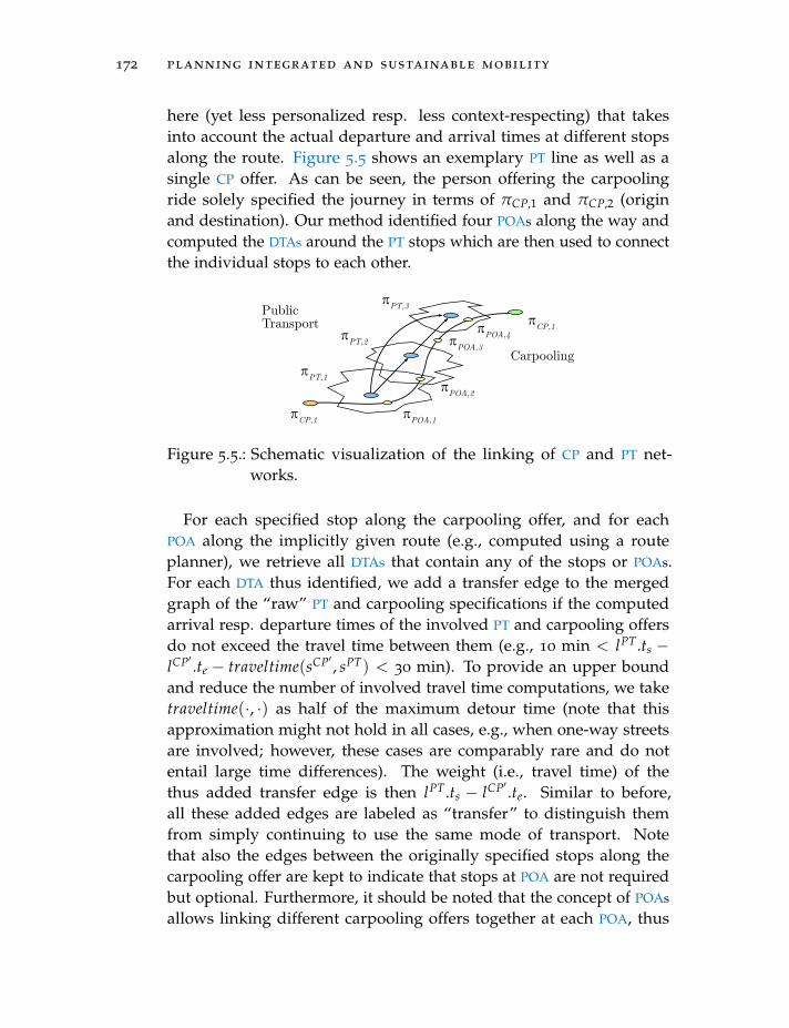
172 planning integrated and sustainable mobility
here (yet less personalized resp. less context-respecting) that takesinto account the actual departure and arrival times at different stopsalong the route. Figure 5.5 shows an exemplary PT line as well as asingle CP offer. As can be seen, the person offering the carpoolingride solely specified the journey in terms of πCP,1 and πCP,2 (originand destination). Our method identified four POAs along the way andcomputed the DTAs around the PT stops which are then used to connectthe individual stops to each other.
Carpooling
PublicTransport
�CP,1 �POA,1
�POA,2
�POA,3�POA,4
�CP,1
�PT,1
�PT,2
�PT,3
Figure 5.5.: Schematic visualization of the linking of CP and PT net-works.
For each specified stop along the carpooling offer, and for eachPOA along the implicitly given route (e.g., computed using a routeplanner), we retrieve all DTAs that contain any of the stops or POAs.For each DTA thus identified, we add a transfer edge to the mergedgraph of the “raw” PT and carpooling specifications if the computedarrival resp. departure times of the involved PT and carpooling offersdo not exceed the travel time between them (e.g., 10 min < lPT.ts −lCP′ .te − traveltime(sCP′ , sPT) < 30 min). To provide an upper boundand reduce the number of involved travel time computations, we taketraveltime(·, ·) as half of the maximum detour time (note that thisapproximation might not hold in all cases, e.g., when one-way streetsare involved; however, these cases are comparably rare and do notentail large time differences). The weight (i.e., travel time) of thethus added transfer edge is then lPT.ts − lCP′ .te. Similar to before,all these added edges are labeled as “transfer” to distinguish themfrom simply continuing to use the same mode of transport. Notethat also the edges between the originally specified stops along thecarpooling offer are kept to indicate that stops at POA are not requiredbut optional. Furthermore, it should be noted that the concept of POAs
allows linking different carpooling offers together at each POA, thus
5.3 evaluating integrated mobility options 173
enabling combinations of different carpooling offers, and that pickingup someone at a POA introduces delays for each of the following nodes.While the latter could be incorporated by recomputing the parts ofthe graph that might change due to such a detour, we here restrict theallowed detours (beyond the originally specified origin, destinationand stopovers) to a single one. This is in line with how carpooling isgenerally used, whereas not restricting detours would quickly add upto many smaller ones which in turn introduces a large inconveniencefor the driver. Algorithm 5.2 shows the complete algorithm used formerging and linking PT and carpooling graphs.
5.2.3 Extracting Potential Matches
The resulting time-expanded multi-modal graph can directly be usedwith any Dijkstra-like algorithm. Commonly, two types of queriesare required to find matches between carpooling drivers and riders(potentially involving PT). Routing with a given departure time rangedescribes the process of finding a multi-modal route from an origin to adestination where a person has a time window during which to depart.To answer such a query, we first identify all time nodes belonging tothe origin stop that fall within the given range. A routing algorithmthen finds the shortest path (in terms of total time) to any of the timenodes belonging to the destination stop. The resulting set of routes(i.e., for each of the departure time nodes, but it is also possible to“artificially” generate more routes by pruning nodes from a found pathand recomputing the route again) can then be ordered according tovarious criteria such as the total travel time, the involved costs, thenumber of transfers, etc. The other predominantly used form of routequeries is routing with a given arrival time range. In this case, the timenodes at the destination have to fall within the given range, and thesearch can either be performed backwards or forwards starting from alltime nodes of the origin stop.
5.3 evaluating integrated mobility options
Commonly, route options are computed based on the total travel timeor number of involved transfers (as transferring is often regarded asbeing more inconvenient than traveling a little bit longer). While this is
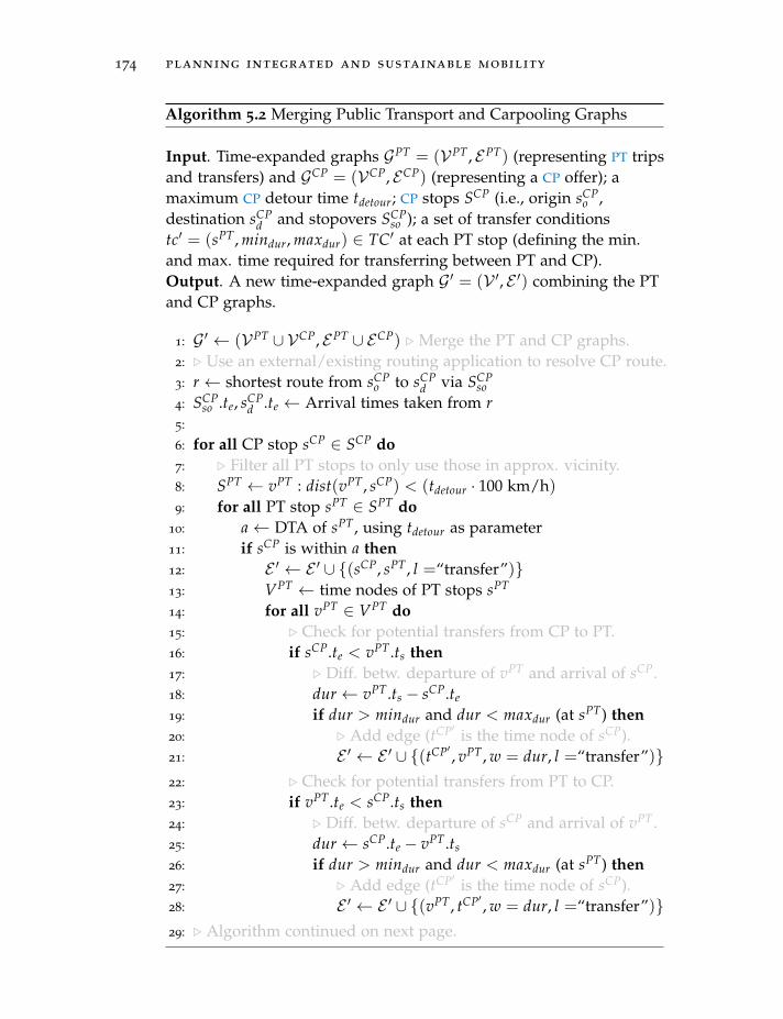
174 planning integrated and sustainable mobility
Algorithm 5.2 Merging Public Transport and Carpooling Graphs
Input. Time-expanded graphs GPT = (VPT, EPT) (representing PT tripsand transfers) and GCP = (VCP, ECP) (representing a CP offer); amaximum CP detour time tdetour; CP stops SCP (i.e., origin sCP
o ,destination sCP
d and stopovers SCPso ); a set of transfer conditions
tc′ = (sPT, mindur, maxdur) ∈ TC′ at each PT stop (defining the min.and max. time required for transferring between PT and CP).Output. A new time-expanded graph G ′ = (V ′, E ′) combining the PTand CP graphs.
1: G ′ ← (VPT ∪ VCP, EPT ∪ ECP) . Merge the PT and CP graphs.2: . Use an external/existing routing application to resolve CP route.3: r ← shortest route from sCP
o to sCPd via SCP
so4: SCP
so .te, sCPd .te ← Arrival times taken from r
5:
6: for all CP stop sCP ∈ SCP do7: . Filter all PT stops to only use those in approx. vicinity.8: SPT ← vPT : dist(vPT, sCP) < (tdetour · 100 km/h)9: for all PT stop sPT ∈ SPT do
10: a← DTA of sPT, using tdetour as parameter11: if sCP is within a then12: E ′ ← E ′ ∪ {(sCP, sPT, l =“transfer”)}13: VPT ← time nodes of PT stops sPT
14: for all vPT ∈ VPT do15: . Check for potential transfers from CP to PT.16: if sCP.te < vPT.ts then17: . Diff. betw. departure of vPT and arrival of sCP.18: dur ← vPT.ts − sCP.te
19: if dur > mindur and dur < maxdur (at sPT) then20: . Add edge (tCP′ is the time node of sCP).21: E ′ ← E ′ ∪ {(tCP′ , vPT, w = dur, l =“transfer”)}22: . Check for potential transfers from PT to CP.23: if vPT.te < sCP.ts then24: . Diff. betw. departure of sCP and arrival of vPT.25: dur ← sCP.te − vPT.ts
26: if dur > mindur and dur < maxdur (at sPT) then27: . Add edge (tCP′ is the time node of sCP).28: E ′ ← E ′ ∪ {(vPT, tCP′ , w = dur, l =“transfer”)}29: . Algorithm continued on next page.
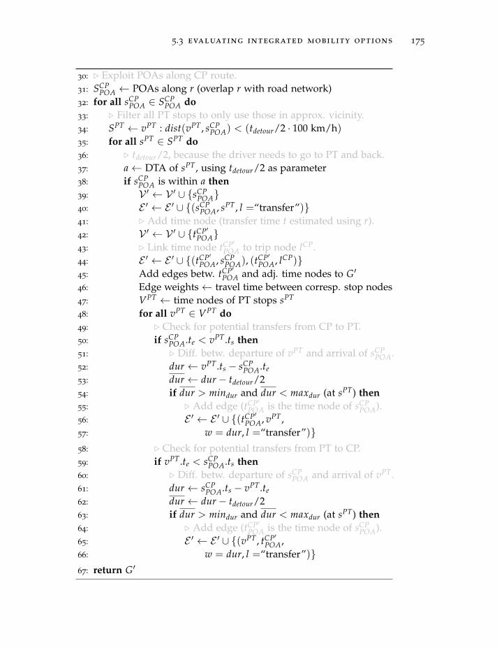
5.3 evaluating integrated mobility options 175
30: . Exploit POAs along CP route.31: SCP
POA ← POAs along r (overlap r with road network)32: for all sCP
POA ∈ SCPPOA do
33: . Filter all PT stops to only use those in approx. vicinity.34: SPT ← vPT : dist(vPT, sCP
POA) < (tdetour/2 · 100 km/h)35: for all sPT ∈ SPT do36: . tdetour/2, because the driver needs to go to PT and back.37: a← DTA of sPT, using tdetour/2 as parameter38: if sCP
POA is within a then39: V ′ ← V ′ ∪ {sCP
POA}40: E ′ ← E ′ ∪ {(sCP
POA, sPT, l =“transfer”)}41: . Add time node (transfer time t estimated using r).42: V ′ ← V ′ ∪ {tCP′
POA}43: . Link time node tCP′
POA to trip node lCP.44: E ′ ← E ′ ∪ {(tCP′
POA, sCPPOA), (t
CP′POA, lCP)}
45: Add edges betw. tCP′POA and adj. time nodes to G′
46: Edge weights← travel time between corresp. stop nodes47: VPT ← time nodes of PT stops sPT
48: for all vPT ∈ VPT do49: . Check for potential transfers from CP to PT.50: if sCP
POA.te < vPT.ts then51: . Diff. betw. departure of vPT and arrival of sCP
POA.52: dur ← vPT.ts − sCP
POA.te
53: dur ← dur− tdetour/254: if dur > mindur and dur < maxdur (at sPT) then55: . Add edge (tCP′
POA is the time node of sCPPOA).
56: E ′ ← E ′ ∪ {(tCP′POA, vPT,
57: w = dur, l =“transfer”)}58: . Check for potential transfers from PT to CP.59: if vPT.te < sCP
POA.ts then60: . Diff. betw. departure of sCP
POA and arrival of vPT.61: dur ← sCP
POA.ts − vPT.te
62: dur ← dur− tdetour/263: if dur > mindur and dur < maxdur (at sPT) then64: . Add edge (tCP′
POA is the time node of sCPPOA).
65: E ′ ← E ′ ∪ {(vPT, tCP′POA,
66: w = dur, l =“transfer”)}67: return G′
176 planning integrated and sustainable mobility
often desirable, many people show regular patterns in their mobilitychoices and strong preferences for one mode of transport or anotherthat are not only dependent on the travel time or distance to be covered,but depend on features as introduced in chapter 4, properties of thetransport network (e.g., someone who lives close to a well-connected PT
stop is likely to use PT to travel), or the availability of different modesfor certain triplegs (e.g., someone might show a strong preference totake the bicycle for the “first mile” to the train station, but only if it isnot raining). Using these influencing factors and thus personalizingroute computations can decrease the required manual interactions withICT before finding an appropriate route that conforms to one’s ownpreferences. Based on the same formalization as introduced in chapter 4
and further adapted to the problem of computing route options insection 5.1, we here introduce an approach to use the passively trackedmobility data to derive mobility choice preferences that can be used tocompute and/or evaluate route plans.
5.3.1 Context and Circumstances
To perform personalized routing on the graphs constructed in the pre-vious sections (in particular the transfer graph from subsection 5.1.3),two functions assigning probabilities to user choices are required. First,for any location πi that has multiple modes available (i.e., multipleconnected nodes πi,m), we need to determine the likelihood of a par-ticular mode of transport m being chosen. Second, each πi,m is usuallyconnected to several transfer locations πj (which can be reached byusing m), out of which we have to choose the most likely ones. Thefirst function primarily depends on contextual factors (such as the timeor destination of the planned trip), as well as features of the transferlocation πi. The second one additionally takes into account charac-teristics of the (potentially chosen) tripleg itself, such as its distance.Table 5.4 describes the features used within the prediction models inthis chapter: There are basic contextual features such as the hour ofday or the distances between various important locations for the tripand features related to the transfer graph itself, such as the Pagerank(Brin and Page 1998) (following the reasoning that someone might morelikely choose the train for a longer trip if a well-connected PT stop isclose by). While we can easily imagine other features to be added (e.g.,the position of the currently being evaluated tripleg within a larger trip;
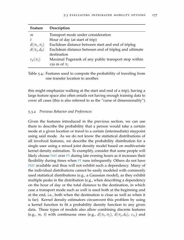
5.3 evaluating integrated mobility options 177
Feature Description
m Transport mode under considerationt Hour of day (at start of trip)d(πi, πj) Euclidean distance between start and end of triplegd(πj, dθ) Euclidean distance between end of tripleg and ultimate
destinationrp(πj) Maximal Pagerank of any public transport stop within
150 m of πj
Table 5.4.: Features used to compute the probability of traveling fromone transfer location to another.
this might emphasize walking at the start and end of a trip), having alarge feature space also often entails not having enough training data tocover all cases (this is also referred to as the “curse of dimensionality”).
5.3.2 Previous Behavior and Preferences
Given the features introduced in the previous section, we can usethem to describe the probability that a person would take a certainmode at a given location or travel to a certain (intermediate) staypointusing said mode. As we do not know the statistical distributions ofall involved features, we describe the probability distribution for asingle user using a mixed joint density model based on multivariatekernel density estimation. To exemplify, consider that some people willlikely choose PMT over PT during late evening hours as it increases theirflexibility during times when PT runs infrequently. Others do not havePMT available and thus will not exhibit such a dependency. Many ofthe individual distributions cannot be easily modeled with commonlyused statistical distributions (e.g., a Gaussian model), as they exhibitmultiple peaks in the distribution (e.g., when describing a dependencyon the hour of day or the total distance to the destination, in whichcase a transport mode such as walk is used both at the beginning andat the end, i.e., both when the destination is close as well as when itis far). Kernel density estimators circumvent this problem by usinga kernel function to fit a probability density function to any givendata. These types of models also allow combining discrete features(e.g., m, t) with continuous ones (e.g., d(πi, πj), d(πj, dθ), cπj ) and
178 planning integrated and sustainable mobility
result in a probability density function that can be used to computeprobabilities of all combinations of features. Thus, we model bothchoice functions (choosing a transport mode resp. choosing a certainintermediate staypoint) using a (parameterless) multivariate kerneldensity estimation (cf. Simonoff 2012):
fH(x) =1n
n
∑i=1
KH(x− xi) (5.2)
Here, KH(x) = |H |−1/2K(H−1/2x), K(·) is the kernel function, andH the bandwidth matrix (that has to be chosen, usually by minimizingthe mean integrated squared error). In Equation 5.2, xi are the featurevectors computed from all previously tracked triplegs of a single user.The kernel density estimator fH(x) then describes the probabilitydensity for any combination of features of any (potentially chosen)tripleg or mode within the transfer graph. Sampling these values givesus an indication about the likelihood of a certain combination appearingin the previously recorded mobility data of a user.
Regarding the first function pm(x−m) (determining the probability ofchoosing mode m at a given transfer location), we use the probabilitydensities given by Equation 5.2 to compute probabilities as follows(note that fH(x−m) describes a multivariate kernel density estimatornot including m as a feature):
pm(x−m) = Pr(m|x−m) =fH(x−m|m) fH(m)
fH(x−m)(5.3)
=fH(x−m|m) fH(m)
∑πi,mfH(x−m|m) fH(m)
x−m = (t, d(πj, dθ), rp(πj))
In essence, we use the Bayes’ rule to compute the probability of choosingmode m (given features x−m) at location πi by sampling the densityestimates at different points.
As the reachable locations after choosing a mode m for travel arepotentially unlimited (e.g., in the case of walking), we cannot computea true probability for traveling to a fixed location. To exemplify, con-sider taking the bus to get somewhere: If there is a single stop at thedestination, it is very likely that a traveler will get off at this stop (i.e.,pl(x) ≈ 1). However, if there were two bus stops right next to each
5.4 determining alternative transport options 179
other, the probability of leaving at one of them would be pl(x) ≈ 0.5each. Using this in a routing context (as introduced in more detailin subsection 5.4.2) would lead to lower probabilities for modes withwhich a large number of (intermediate) staypoints can be reached, forwhich reason we approximate the probability of choosing tripleg ldirectly using the probability density:
pl(x) ≈ fH(x) (5.4)
x = (m, t, d(πi, πj), d(πj, dθ), rp(πj))
This essentially corresponds to computing the probability of an in-finitesimally small region around the given combination of featuresx. As such, there are some caveats to this approach, foremost thatsufficient (and sufficiently distributed) data must be available in orderto prevent peaks in the distribution function (that in turn lead to largefeature spaces with pl(x) ≈ 0). In addition to normalizing the featuresthis ensures that they all exhibit comparable characteristics and thusthe sampled densities are in similar ranges. Further, choosing thisapproach prevents us from computing true probabilities (i.e., all thedifferent travel options do not necessarily sum up to one); instead wecompute a (proportional to the true probability) likelihood of travelingalong a given tripleg. Within a routing context, this approximation issufficient as it is proportional to the true probability and is applied forall transport modes equally.
Evaluating ProbabilitySurfaces
the probability functions will give us (discrete) probabilitysurfaces, where each transfer location is assigned a likelihood withwhich the user under consideration will pass by this location. We cannow sample these probability surfaces at potential transfer locationsin order to determine likely paths that someone could take through arouting graph. Embedding these probabilities within a transfer graphas introduced in section 5.1 and evaluating them on the fly allows usto compute personalized “most probable” route options for individualpeople.
5.4 determining alternative transport options
A route planning request is essentially a function that returns an or-dered sequence of triplegs Lθ , based on an origin o, a destination d, ata time t:
Lθ = r(o, d, t) (5.5)
180 planning integrated and sustainable mobility
In this section, we will introduce two methods to compute personalizedand context-dependent high-level mobility plans based on the transfergraphs and choice probabilities introduced before.
5.4.1 Heuristic-based Planning Method
First, we present a preprocessing heuristic that can be used to generatehigh-level mobility plans by specifying rules and constraints that haveto be followed in order for routes to be considered valid alternatives.While the thus generated routes could in theory also be computed bycombining various platforms or data sources and applying selectedrouting algorithms (cf. chapter 3), the resulting routing graphs quicklybecome very large and adapting them to incorporate various userconstraints and preferences leads to downstream graph changes thatare difficult to integrate on the fly during a routing request. Instead, werely upon the introduced transfer graph to build possible multi-modalroutes that respect various preconditions and only require updating asmaller graph during the request.
For the here presented heuristic, we add the set of user preferences P,a set of user constraints A and a description of context C to the aboveintroduced Equation 5.5 representing a route request. In addition,the generated routes each contain summary values Vi (e.g., denotingthe distance covered with each mode of transport, the overall energyconsumption or the financial cost of the trip), resulting in an updatedEquation 5.5:
{(Lθ,0, V0) , (Lθ,1, V1) , ...} = rheuristic(o, d, t, P, A, C) (5.6)
The core of the preprocessing heuristic revolves around a set of indi-vidual rules denoting preferences and constraints that adhere to thegeneral rule form of:
o[condition]→ m[condition]→ d[condition] : [outcomes] (5.7)
The rule denotes that the origin o and destination d have to fulfill somepreconditions for the mode m to be available, which in turn has toadhere to some conditions for the whole tripleg to be available andchosen for a given user. Exemplary conditions include the markingof a certain location with a given transport mode, the availability ofone’s own car at a location, or (in the case of a mode condition) the
5.4 determining alternative transport options 181
restriction of maximum length for walking triplegs. The outcomeseither involve the user, or the context (which gets updated to the nextpotential location if a certain tripleg is chosen for a user). An exemplaryrule could thus look like:
A[∅]→ (5.8)
WALK[(user[distWalked] + dist(A, B) < user[maxDist])
∧ (¬ context[rainyWeather])
∧ (context[currentTime] ∈ user[acceptableTimeIntvlWalk])]
→ B[∅] :
user[distWalked+ = dist(A, B)], context[time+ = time(A, B)]
This rule states that walking is possible at any location (i.e., the set oflocation requirements for both A and B is empty), but that the actionof walking itself is only possible if the total distance remains belowsome threshold, it is currently not raining, and the time at which thewalking action is performed is within some acceptable time intervals(e.g., someone might not want to walk during the night for safetyreasons). The outcome statement of the rule requires an update context,by adding the traveled distance to the distWalked counter as well as byupdating the time (i.e., in the next iteration of the route computation,the time has advanced by time(A, B) for all the subsequent paths).Note that in order to not rely on an underlying transport graph and tospeed up the computations, all distance computations use an Euclideanmeasure.
We use two functions to apply the heuristic to a transfer graph andthus compute high-level mobility plans: checkReachability considers allpossible origin and destination locations within a graph, in combinationwith all potentially available modes M, and checks whether the locationand mode conditions hold, i.e., if the transport mode could be usedat the given location to reach a potential destination. It returns tuples(Li, D, M) for each combination (starting at Li) that satisfies all precon-ditions. expand, on the other hand, does not respect any preconditionsbut instead is used to generate a new set of locations that can be reachedfrom a given location without any transfers (e.g., applying it on a PT
stop would yield all other PT stops that are connected by the same line).The function returns a tuple (O, Li, M, S) for every reachable location Lithat allows backtracking through the graph at the end of the algorithmto find the actual routes. The “running state” S contains additional
182 planning integrated and sustainable mobility
information about the route to reach Li which is necessary as a locationLi can usually be reached via multiple ways.
UsingRoute PlanComputation
the two introduced functions, we can compute the route plansas shown in Algorithm 5.3 (note that the algorithm is closely relatedto the way network time prisms are commonly computed, cf. Kui-jpers and Othman 2009; Jaegal and Miller 2016). Starting from the ori-gin/destination pair, we first see if there are direct ways to reach the des-tination from the origin, adding the resulting triples (o, d, m), m ∈ Mto the set of reachable locations S (that form the reachability graph asthey consist of connections between two transfer locations). The follow-ing steps are iteratively performed (e.g., until a maximum number oftransfers is reached or a minimal number of solutions has been found)from the direction of the origin (forward) as well as from the directionof the destination (backwards). This optimization is often performedin routing algorithms, as it reduces the solution space and in this casefavors solutions that pass through “hubs” of mobility, which includesmost trips longer than some very small distance. The iterative process-ing first expands the space of possible solutions. For each of the thusgenerated potentially reachable nodes, checkReachability determines if atransition using a given mode m is possible. In that case, the quadruple(Li, Lj, m) is added to the reachability graph. After a predefined numberof iterations (e.g., the specification of a maximum number of transfers),the function unfold retrieves all possible routes from the reachabilitygraph. In essence, unfold looks at all chains (O, Li, ..., D) by startingfrom the origin or destination and following edges in the reachabilitygraph.
The resulting solutions respect context as well as user preferencesand constraints. In contrast to performing a routing on a completetransportation network graph, the used transfer graph is much smallerand thus it becomes feasible to continuously update node and edgecharacteristics during the computation (essentially adopting a time-dependent graph, here applied to different mode choices).
Table A.1 shows a number of exemplary rules that can be used to com-pute meaningful and personalized route options by adapting variousparameters to preferences of users (and that are used in the experimentslater in this chapter). In this dissertation, we refrain from learning therules based on previously recorded data, and instead assume that anexpert defines a set of rules appropriate for different classes of people.After computing the route options, different ranking schemes can be
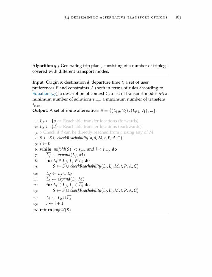
5.4 determining alternative transport options 183
Algorithm 5.3 Generating trip plans, consisting of a number of triplegscovered with different transport modes.
Input. Origin o; destination d; departure time t; a set of userpreferences P and constraints A (both in terms of rules according toEquation 5.7); a description of context C; a list of transport modes M; aminimum number of solutions smin; a maximum number of transferstmax.Output. A set of route alternatives S = {(Lθ,0, V0) , (Lθ,1, V1) , ...}.
1: L f ← {o} . Reachable transfer locations (forwards).2: Lb ← {d} . Reachable transfer locations (backwards).3: . Check if d can be directly reached from o using any of M.4: S← S ∪ checkReachability(o, d, M, t, P, A, C)5: i← 06: while |unfold(S)| < smin and i < tmax do7: L f ← expand(L f , M)
8: for Li ∈ L f , Lj ∈ Lb do9: S← S ∪ checkReachability(Li, Lj, M, t, P, A, C)
10: L f ← L f ∪ L f11: Lb ← expand(Lb, M)
12: for Li ∈ L f , Lj ∈ Lb do13: S← S ∪ checkReachability(Li, Lj, M, t, P, A, C)
14: Lb ← Lb ∪ Lb15: i← i + 116: return unfold(S)
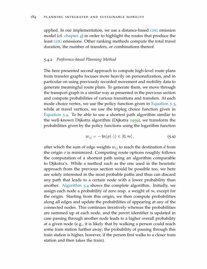
184 planning integrated and sustainable mobility
applied. In our implementation, we use a distance-based GHG emissionmodel (cf. chapter 4) in order to highlight the routes that produce theleast GHG emissions. Other ranking methods compute the total travelduration, the number of transfers, or combinations thereof.
5.4.2 Preference-based Planning Method
The here presented second approach to compute high-level route plansfrom transfer graphs focuses more heavily on personalization, and inparticular on using previously recorded movement and mobility data togenerate meaningful route plans. To generate them, we move throughthe transport graph in a similar way as presented in the previous sectionand compute probabilities of various transitions and transfers. At eachmode choice vertex, we use the policy function given in Equation 5.3,while at travel vertices, we use the tripleg choice function given inEquation 5.4. To be able to use a shortest path algorithm similar tothe well-known Dijkstra algorithm (Dijkstra 1959), we transform theprobabilities given by the policy functions using the logarithm function
wi,j = − ln(p(·)) ∈ [0, ∞] , (5.9)
after which the sum of edge weights wi,j to reach the destination d fromthe origin o is minimized. Computing route options roughly followsthe computation of a shortest path using an algorithm comparableto Djikstra’s. While a method such as the one used in the heuristicapproach from the previous section would be possible too, we hereare solely interested in the most probable paths and thus can discardany path that leads to a certain node with a lower probability thananother. Algorithm 5.4 shows the complete algorithm. Initially, weassign each node a probability of zero resp. a weight of ∞, except forthe origin. Starting from this origin, we then compute probabilitiesalong all edges and update the probabilities of appearing at any of theconnected nodes. This continues iteratively whereas the probabilitiesare summed up at each node, and the parent identifier is updated incase passing through another node leads to a higher overall probabilityat a given node (e.g., it is likely that by walking a person could reachsome train station further away; the probability of passing through thistrain station is higher, however, if the person first walks to a closer trainstation and then takes the train).
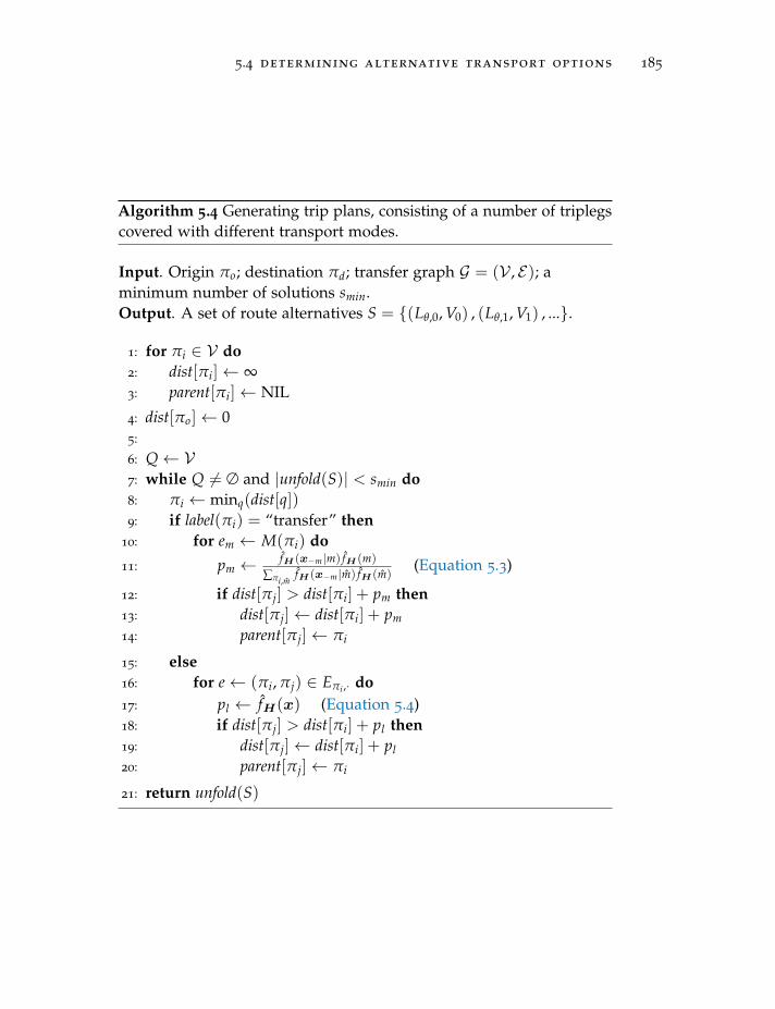
5.4 determining alternative transport options 185
Algorithm 5.4 Generating trip plans, consisting of a number of triplegscovered with different transport modes.
Input. Origin πo; destination πd; transfer graph G = (V , E); aminimum number of solutions smin.Output. A set of route alternatives S = {(Lθ,0, V0) , (Lθ,1, V1) , ...}.
1: for πi ∈ V do2: dist[πi]← ∞3: parent[πi]← NIL
4: dist[πo]← 05:
6: Q← V7: while Q 6= ∅ and |unfold(S)| < smin do8: πi ← minq(dist[q])9: if label(πi) = “transfer” then
10: for em ← M(πi) do11: pm ← fH (x−m|m) fH (m)
∑πi,mfH (x−m|m) fH (m)
(Equation 5.3)
12: if dist[πj] > dist[πi] + pm then13: dist[πj]← dist[πi] + pm
14: parent[πj]← πi
15: else16: for e← (πi, πj) ∈ Eπi ,· do17: pl ← fH(x) (Equation 5.4)18: if dist[πj] > dist[πi] + pl then19: dist[πj]← dist[πi] + pl20: parent[πj]← πi
21: return unfold(S)
186 planning integrated and sustainable mobility
Similar to Algorithm 5.3, in the end we backtrack through the reacha-bility graph (starting from the destination) to find the most probableroute (using the unfold(S) function). In order to generate multiple routeoptions, it is also possible to store all parents during the computationand backtrack along several routes. In a multi-modal setting this isparticularly easy as we can simply introduce a constraint that no two(mode) label sequences may be the same in the resulting route optionsset (e.g., we cannot have two routes consisting of mode sequences walk→ train→ walk). This results in a useful set of route options for some-one planning a journey (as they are all different), yet still allows us tosort according to the probability that someone chooses one route overanother.
5.5 data and experiments
In the following, we use various data sources to highlight the func-tionality and characteristics of the presented methods. The learnedpreferences rely on the tracked mobility data from the GoEco! and SBBGreen Class projects, the PT specifications in Switzerland (published bySBB on a yearly basis1), transport option availability data as published byseveral transport providers in Switzerland (and Zurich for local ones),carpooling data crawled from a large European carpooling platform,and the general street network given by OSM2. The transport availabilitydata from local providers includes carsharing3, free-floating bicycles(from the free-floating service by Smide), as well as station-based bike-sharing (offered by PubliBike). The carpooling method introduced insection 5.2 was implemented in Java, using the Neo4j graph database4.The heuristic and probabilistic methods from section 5.4 were imple-mented in Python as this allowed integrating a range of libraries toprocess the recorded mobility resp. the collected transport data moreeasily. The programs were run on commodity office computers andyielded results in the order of seconds.
1 The timetable can be downloaded from www.fahrplanfelder.ch.2 The OSM data used within this work is downloaded from download.geofabrik.de.3 The respective company Mobility publishes its available cars under www.mobility.ch.4 The database can be downloaded from neo4j.com.
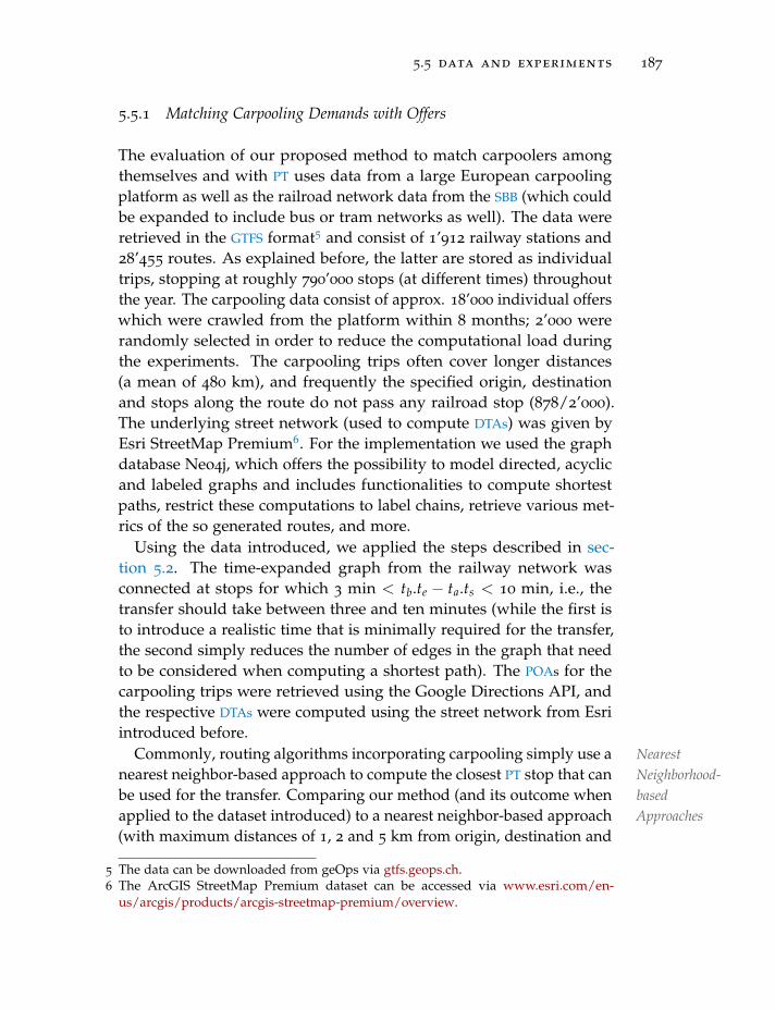
5.5 data and experiments 187
5.5.1 Matching Carpooling Demands with Offers
The evaluation of our proposed method to match carpoolers amongthemselves and with PT uses data from a large European carpoolingplatform as well as the railroad network data from the SBB (which couldbe expanded to include bus or tram networks as well). The data wereretrieved in the GTFS format5 and consist of 1’912 railway stations and28’455 routes. As explained before, the latter are stored as individualtrips, stopping at roughly 790’000 stops (at different times) throughoutthe year. The carpooling data consist of approx. 18’000 individual offerswhich were crawled from the platform within 8 months; 2’000 wererandomly selected in order to reduce the computational load duringthe experiments. The carpooling trips often cover longer distances(a mean of 480 km), and frequently the specified origin, destinationand stops along the route do not pass any railroad stop (878/2’000).The underlying street network (used to compute DTAs) was given byEsri StreetMap Premium6. For the implementation we used the graphdatabase Neo4j, which offers the possibility to model directed, acyclicand labeled graphs and includes functionalities to compute shortestpaths, restrict these computations to label chains, retrieve various met-rics of the so generated routes, and more.
Using the data introduced, we applied the steps described in sec-tion 5.2. The time-expanded graph from the railway network wasconnected at stops for which 3 min < tb.te − ta.ts < 10 min, i.e., thetransfer should take between three and ten minutes (while the first isto introduce a realistic time that is minimally required for the transfer,the second simply reduces the number of edges in the graph that needto be considered when computing a shortest path). The POAs for thecarpooling trips were retrieved using the Google Directions API, andthe respective DTAs were computed using the street network from Esriintroduced before.
Commonly NearestNeighborhood-basedApproaches
, routing algorithms incorporating carpooling simply use anearest neighbor-based approach to compute the closest PT stop that canbe used for the transfer. Comparing our method (and its outcome whenapplied to the dataset introduced) to a nearest neighbor-based approach(with maximum distances of 1, 2 and 5 km from origin, destination and
5 The data can be downloaded from geOps via gtfs.geops.ch.6 The ArcGIS StreetMap Premium dataset can be accessed via www.esri.com/en-
us/arcgis/products/arcgis-streetmap-premium/overview.
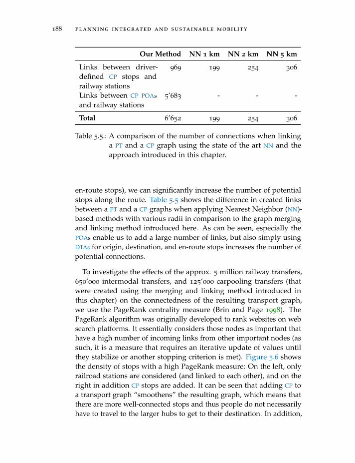
188 planning integrated and sustainable mobility
Our Method NN 1 km NN 2 km NN 5 km
Links between driver-defined CP stops andrailway stations
969 199 254 306
Links between CP POAs
and railway stations5’683 - - -
Total 6’652 199 254 306
Table 5.5.: A comparison of the number of connections when linkinga PT and a CP graph using the state of the art NN and theapproach introduced in this chapter.
en-route stops), we can significantly increase the number of potentialstops along the route. Table 5.5 shows the difference in created linksbetween a PT and a CP graphs when applying Nearest Neighbor (NN)-based methods with various radii in comparison to the graph mergingand linking method introduced here. As can be seen, especially thePOAs enable us to add a large number of links, but also simply usingDTAs for origin, destination, and en-route stops increases the number ofpotential connections.
To investigate the effects of the approx. 5 million railway transfers,650’000 intermodal transfers, and 125’000 carpooling transfers (thatwere created using the merging and linking method introduced inthis chapter) on the connectedness of the resulting transport graph,we use the PageRank centrality measure (Brin and Page 1998). ThePageRank algorithm was originally developed to rank websites on websearch platforms. It essentially considers those nodes as important thathave a high number of incoming links from other important nodes (assuch, it is a measure that requires an iterative update of values untilthey stabilize or another stopping criterion is met). Figure 5.6 showsthe density of stops with a high PageRank measure: On the left, onlyrailroad stations are considered (and linked to each other), and on theright in addition CP stops are added. It can be seen that adding CP toa transport graph “smoothens” the resulting graph, which means thatthere are more well-connected stops and thus people do not necessarilyhave to travel to the larger hubs to get to their destination. In addition,
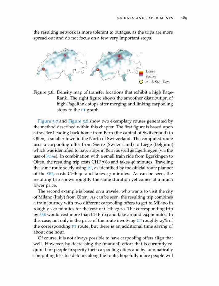
5.5 data and experiments 189
the resulting network is more tolerant to outages, as the trips are morespread out and do not focus on a few very important stops.
DenseSparse> 1.5 Std. Dev.
Figure 5.6.: Density map of transfer locations that exhibit a high Page-Rank. The right figure shows the smoother distribution ofhigh-PageRank stops after merging and linking carpoolingstops to the PT graph.
Figure 5.7 and Figure 5.8 show two exemplary routes generated bythe method described within this chapter. The first figure is based upona traveler heading back home from Bern (the capital of Switzerland) toOlten, a smaller town in the North of Switzerland. The computed routeuses a carpooling offer from Sierre (Switzerland) to Liege (Belgium)which was identified to have stops in Bern as well as Egerkingen (via theuse of POAs). In combination with a small train ride from Egerkingen toOlten, the resulting trip costs CHF 7.60 and takes 46 minutes. Travelingthe same route solely using PT, as identified by the official route plannerof the SBB, costs CHF 30 and takes 47 minutes. As can be seen, theresulting trip shows roughly the same duration yet comes at a muchlower price.
The second example is based on a traveler who wants to visit the cityof Milano (Italy) from Olten. As can be seen, the resulting trip combinesa train journey with two different carpooling offers to get to Milano inroughly 220 minutes for the cost of CHF 27.20. The corresponding tripby SBB would cost more than CHF 103 and take around 294 minutes. Inthis case, not only is the price of the route involving CP roughly 25% ofthe corresponding PT route, but there is an additional time saving ofabout one hour.
Of course, it is not always possible to have carpooling offers align thatwell. However, by decreasing the (manual) effort that is currently re-quired for people to specify their carpooling offers and by automaticallycomputing feasible detours along the route, hopefully more people will
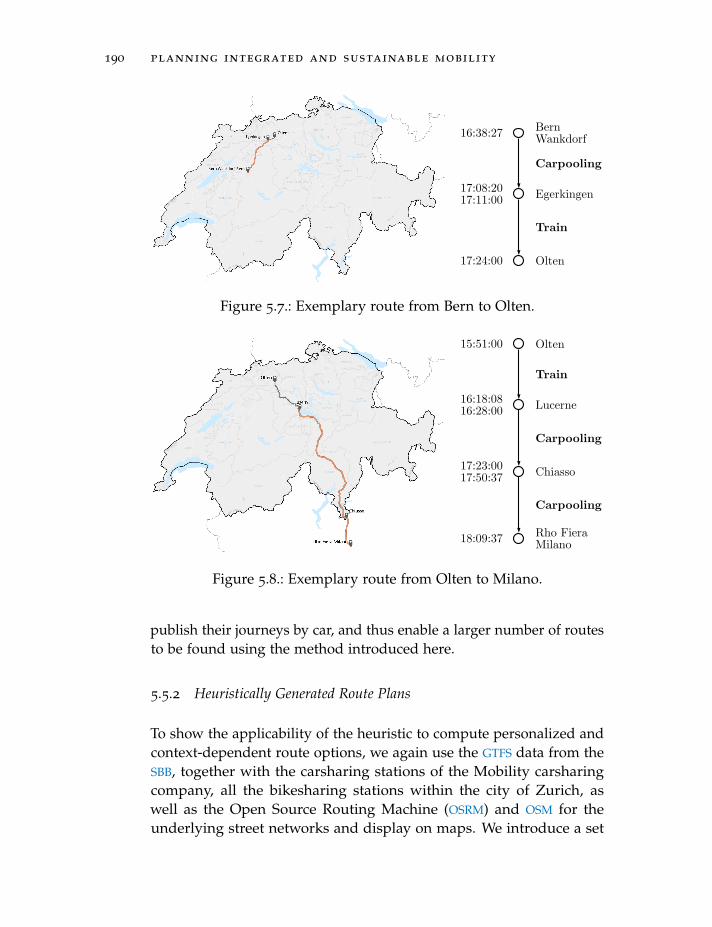
190 planning integrated and sustainable mobility
16:38:27 BernWankdorf
17:08:2017:11:00 Egerkingen
17:24:00 Olten
Carpooling
Train
Figure 5.7.: Exemplary route from Bern to Olten.
15:51:00 Olten
16:18:0816:28:00 Lucerne
17:23:0017:50:37 Chiasso
18:09:37 Rho FieraMilano
Train
Carpooling
Carpooling
Figure 5.8.: Exemplary route from Olten to Milano.
publish their journeys by car, and thus enable a larger number of routesto be found using the method introduced here.
5.5.2 Heuristically Generated Route Plans
To show the applicability of the heuristic to compute personalized andcontext-dependent route options, we again use the GTFS data from theSBB, together with the carsharing stations of the Mobility carsharingcompany, all the bikesharing stations within the city of Zurich, aswell as the Open Source Routing Machine (OSRM) and OSM for theunderlying street networks and display on maps. We introduce a set
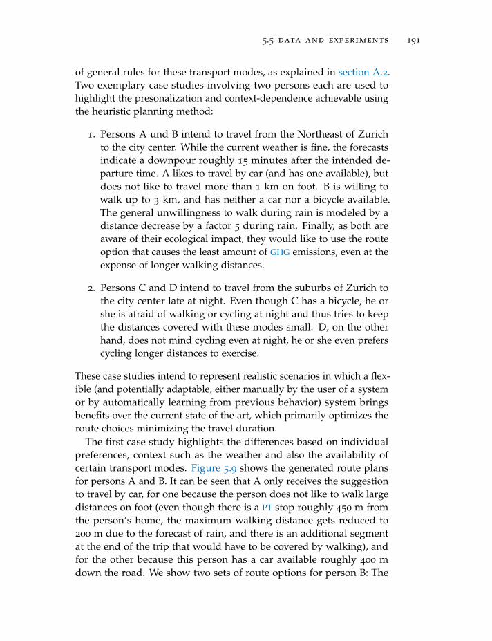
5.5 data and experiments 191
of general rules for these transport modes, as explained in section A.2.Two exemplary case studies involving two persons each are used tohighlight the presonalization and context-dependence achievable usingthe heuristic planning method:
1. Persons A und B intend to travel from the Northeast of Zurichto the city center. While the current weather is fine, the forecastsindicate a downpour roughly 15 minutes after the intended de-parture time. A likes to travel by car (and has one available), butdoes not like to travel more than 1 km on foot. B is willing towalk up to 3 km, and has neither a car nor a bicycle available.The general unwillingness to walk during rain is modeled by adistance decrease by a factor 5 during rain. Finally, as both areaware of their ecological impact, they would like to use the routeoption that causes the least amount of GHG emissions, even at theexpense of longer walking distances.
2. Persons C and D intend to travel from the suburbs of Zurich tothe city center late at night. Even though C has a bicycle, he orshe is afraid of walking or cycling at night and thus tries to keepthe distances covered with these modes small. D, on the otherhand, does not mind cycling even at night, he or she even preferscycling longer distances to exercise.
These case studies intend to represent realistic scenarios in which a flex-ible (and potentially adaptable, either manually by the user of a systemor by automatically learning from previous behavior) system bringsbenefits over the current state of the art, which primarily optimizes theroute choices minimizing the travel duration.
The first case study highlights the differences based on individualpreferences, context such as the weather and also the availability ofcertain transport modes. Figure 5.9 shows the generated route plansfor persons A and B. It can be seen that A only receives the suggestionto travel by car, for one because the person does not like to walk largedistances on foot (even though there is a PT stop roughly 450 m fromthe person’s home, the maximum walking distance gets reduced to200 m due to the forecast of rain, and there is an additional segmentat the end of the trip that would have to be covered by walking), andfor the other because this person has a car available roughly 400 mdown the road. We show two sets of route options for person B: The
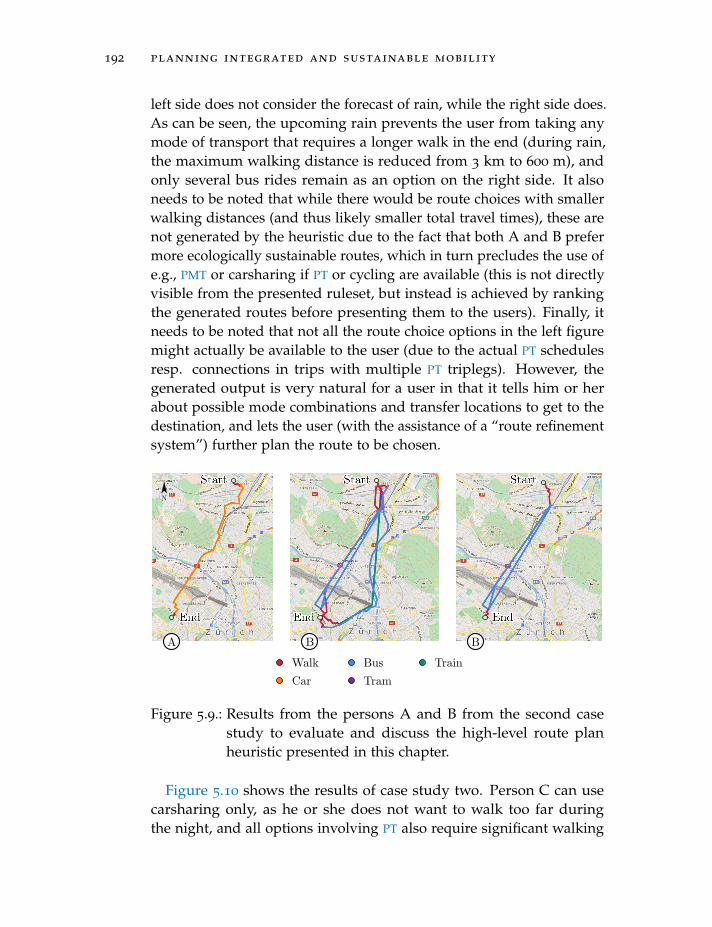
192 planning integrated and sustainable mobility
left side does not consider the forecast of rain, while the right side does.As can be seen, the upcoming rain prevents the user from taking anymode of transport that requires a longer walk in the end (during rain,the maximum walking distance is reduced from 3 km to 600 m), andonly several bus rides remain as an option on the right side. It alsoneeds to be noted that while there would be route choices with smallerwalking distances (and thus likely smaller total travel times), these arenot generated by the heuristic due to the fact that both A and B prefermore ecologically sustainable routes, which in turn precludes the use ofe.g., PMT or carsharing if PT or cycling are available (this is not directlyvisible from the presented ruleset, but instead is achieved by rankingthe generated routes before presenting them to the users). Finally, itneeds to be noted that not all the route choice options in the left figuremight actually be available to the user (due to the actual PT schedulesresp. connections in trips with multiple PT triplegs). However, thegenerated output is very natural for a user in that it tells him or herabout possible mode combinations and transfer locations to get to thedestination, and lets the user (with the assistance of a “route refinementsystem”) further plan the route to be chosen.
N
A B B
WalkCar
BusTram
Train
Figure 5.9.: Results from the persons A and B from the second casestudy to evaluate and discuss the high-level route planheuristic presented in this chapter.
Figure 5.10 shows the results of case study two. Person C can usecarsharing only, as he or she does not want to walk too far duringthe night, and all options involving PT also require significant walking
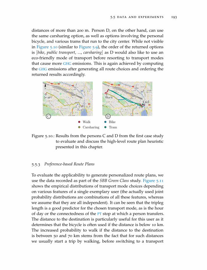
5.5 data and experiments 193
distances of more than 200 m. Person D, on the other hand, can usethe same carsharing option, as well as options involving the personalbicycle, and various trams that run to the city center. While not visiblein Figure 5.10 (similar to Figure 5.9), the order of the returned optionsis [bike, public transport, ..., carsharing] as D would also like to use aneco-friendly mode of transport before resorting to transport modesthat cause more GHG emissions. This is again achieved by computingthe GHG emissions after generating all route choices and ordering thereturned results accordingly.
C DWalkCarsharing
BikeTram
N
Figure 5.10.: Results from the persons C and D from the first case studyto evaluate and discuss the high-level route plan heuristicpresented in this chapter.
5.5.3 Preference-based Route Plans
To evaluate the applicability to generate personalized route plans, weuse the data recorded as part of the SBB Green Class study. Figure 5.11
shows the empirical distributions of transport mode choices dependingon various features of a single exemplary user (the actually used jointprobability distributions are combinations of all these features, whereaswe assume that they are all independent). It can be seen that the tripleglength is a good predictor for the chosen transport mode, as is the hourof day or the connectedness of the PT stop at which a person transfers.The distance to the destination is particularly useful for this user as itdetermines that the bicycle is often used if the distance is below 10 km.The increased probability to walk if the distance to the destinationis between 50 and 70 km stems from the fact that for such distanceswe usually start a trip by walking, before switching to a transport
194 planning integrated and sustainable mobility
mode such as car or train. The figure also highlights the importance ofnormalizing the features before using them in a routing context (i.e.,to lie in the range [0, 1]) as the sampled densities otherwise primarilydepend on the values the feature takes.
0.0001 0.0003Connectedness(Public Transport)
0
10000
20000
0 2 4Tripleg Length [km]
0
1
2
0 50 100Distance to Destination [km]
0.00
0.05
0.10
0 10 20Hour of Day
0.00
0.05
0.10
Prob
abili
tyD
ensit
yPr
obab
ility
Den
sity
TrainCarWalkTramBusBicycle
Figure 5.11.: Kernel density estimates of the probability distributionsof various features.
Figure 5.12 shows the “probability surfaces” as computed during therouting procedure. In this case, we simply look at the probabilities oftraveling to all transfer locations in the study region that are reachableby the chosen transport mode. As can be seen, when the person startswalking from the location denoted with Start, the probability is highestthat she or he will only travel to one of the transfer locations in vicinity.For all the other transport modes (that allow traveling further distancesmore easily), the probability of ending up close to the End location(resp. destination) is high. While the train can only stop at a fewselected stations and the evaluated carpooling offer only stops in thetwo transfer areas indicated by the grouped green dots, the free-floatingbicycle enables the user to travel anywhere. In contrast to walking,however, this user previously recorded data that shows that he or she iswilling to travel similar triplegs by bicycle, and as such the probabilityof ending up close to the destination (or directly at the destination) ishigher. It can also be seen that the probability of stopping before thedestination is higher than driving past it and walking back (i.e., there is
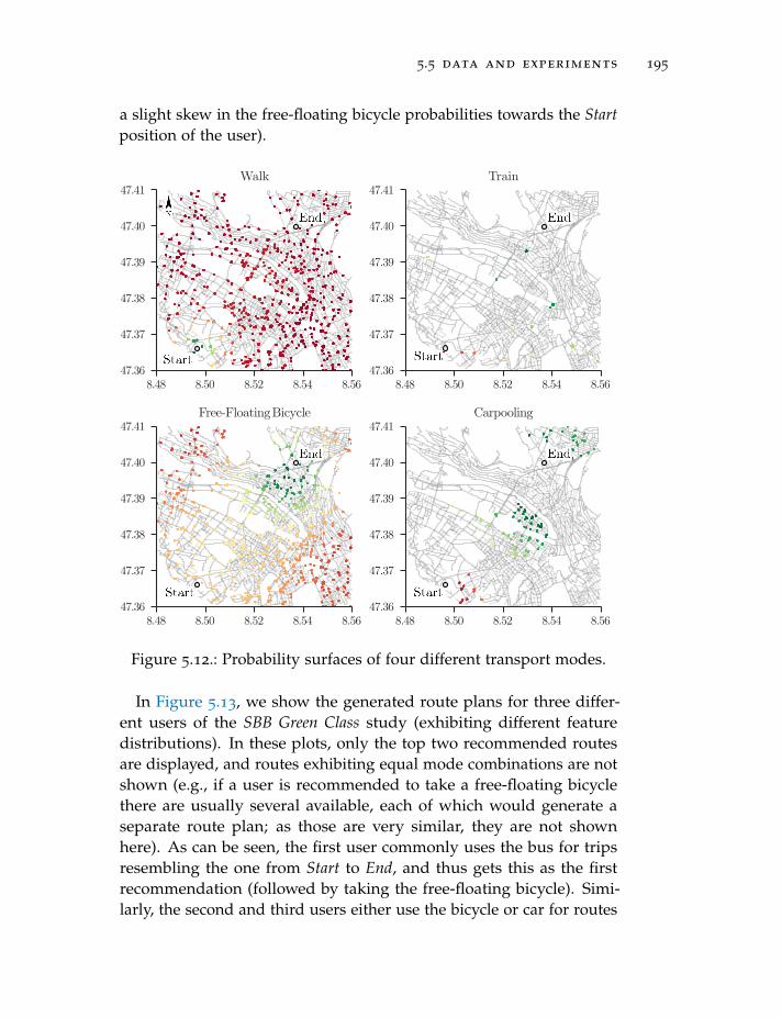
5.5 data and experiments 195
a slight skew in the free-floating bicycle probabilities towards the Startposition of the user).
8.48 8.50 8.52 8.54 8.5647.36
47.37
47.38
47.39
47.40
47.41Walk
8.48 8.50 8.52 8.54 8.5647.36
47.37
47.38
47.39
47.40
47.41Train
8.48 8.50 8.52 8.54 8.5647.36
47.37
47.38
47.39
47.40
47.41Free-FloatingBicycle
8.48 8.50 8.52 8.54 8.5647.36
47.37
47.38
47.39
47.40
47.41Carpooling
Figure 5.12.: Probability surfaces of four different transport modes.
In Figure 5.13, we show the generated route plans for three differ-ent users of the SBB Green Class study (exhibiting different featuredistributions). In these plots, only the top two recommended routesare displayed, and routes exhibiting equal mode combinations are notshown (e.g., if a user is recommended to take a free-floating bicyclethere are usually several available, each of which would generate aseparate route plan; as those are very similar, they are not shownhere). As can be seen, the first user commonly uses the bus for tripsresembling the one from Start to End, and thus gets this as the firstrecommendation (followed by taking the free-floating bicycle). Simi-larly, the second and third users either use the bicycle or car for routes
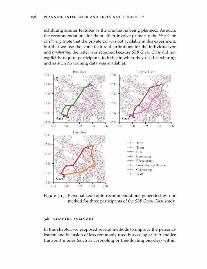
196 planning integrated and sustainable mobility
exhibiting similar features as the one that is being planned. As such,the recommendations for them either involve primarily the bicycle orcarsharing (note that the private car was not available in this experiment,but that we use the same feature distributions for the individual carand carsharing; the latter was required because SBB Green Class did notexplicitly require participants to indicate when they used carsharingand as such no training data was available).
8.48 8.50 8.52 8.54 8.5647.36
47.37
47.38
47.39
47.40
47.41
8.48 8.50 8.52 8.54 8.5647.36
47.37
47.38
47.39
47.40
47.41
8.48 8.50 8.52 8.54 8.5647.36
47.37
47.38
47.39
47.40
47.41
TrainTramBusCarsharingBikesharingFree-FloatingBicycleCarpoolingWalk
Bus User Bicycle User
Car User
Figure 5.13.: Personalized route recommendations generated by ourmethod for three participants of the SBB Green Class study.
5.6 chapter summary
In this chapter, we proposed several methods to improve the personal-ization and inclusion of less commonly used but ecologically friendliertransport modes (such as carpooling or free-floating bicycles) within
5.6 chapter summary 197
route planners. We argue that improving route planners is importantfor changing people’s mobility behavior towards a more sustainableone, as a) the assistance by technology increases the effectiveness offacilitators (i.e., the work required for a person to find an eco-friendlyroute alternative is smaller, and thus the people are more likely to tryout different alternatives), b) the resulting routes are often not onlymore ecologically friendly, but also lead to financial and/or temporalsavings (and thus form an additional motivator) and c) the resultingroutes can be used to gauge the potential for change for individual per-sons and thus facilitate proposing changes and improvements to peopleand embedding them within motivational affordances as discussed inthe next chapter. The three introduced methods focus on carpooling,heuristics that can be tuned to a wide range of personal preferencesand influencing context factors, and personalized route planning thatrelies on features as introduced in chapter 4 and the specification ofmobility offers in a generalized manner involving transfer points andareas, and the respective mode availabilities between them. The follow-ing chapter will build upon the here introduced planning methods tosupport people in their mobility choices using a range of persuasivemethods.

6C O M M U N I C AT I N G M O B I L I T Y
In the previous two chapters, we introduced ways to process passivelyrecorded tracking data with the aim of extracting information and gen-erating alternative route plans that could guide persuasive applicationsin the choice of strategy to help a user achieving more sustainablemobility. Here, we will present different approaches to utilize this infor-mation within the context of persuasive smartphone applications, andhighlight the results of their application within a large-scale user studyperformed in two geographically different contexts in Switzerland. SuchBehaviour Change Support Systems (BCSSs) are “information systemswith psychological and behavioral outcomes designed to form, alter orreinforce attitudes, behaviours or an act of complying without usingcoercion or deception” (Oinas-Kukkonen 2013, p. 1225). Figure 6.1shows a high-level overview of the processes involved in processingand communicating the data in a way that is meaningful for the indi-vidual user. Starting from the mobility information extracted directlyfrom the tracking data, and in combination with the alternative routeoptions generated as described in chapter 5, we can score a user’s pastbehavior, evaluate the available options, predict likely future mobilityneeds, and compute a set of persuasive elements based on these data.In this chapter and in line with the presented user study, many of theseelements revolve around gamification, which has been used previouslyto foster desirable behaviors successfully (cf. chapter 3).
6.1 effective communication of mobility behavior
A wealth of research treats the question of how to communicate behav-ior and incentives in ways that make them as effective as possible tosupport people in behavioral transitions (cf. chapter 3). Complementingthis research, we here present a taxonomy of motivational affordances
This chapter and its contents, algorithms and figures are based on Cellina, Bucher,Rudel, et al. 2016; Weiser, Scheider, et al. 2016; Weiser, Bucher, et al. 2015; Cellina,Bucher, Raubal, et al. 2016; Bucher, Cellina, et al. 2016; Bucher, Mangili, Cellina, et al.2019; Cellina, Bucher, Mangili, et al. 2019; Cellina, Bucher, Veiga Simao, et al. 2019.
199
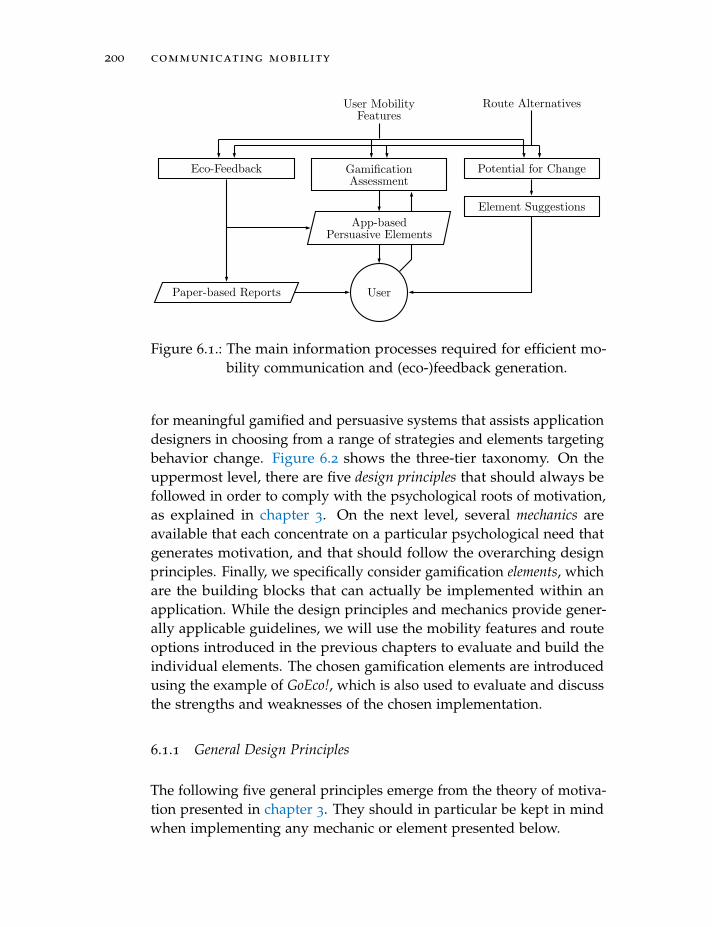
200 communicating mobility
User MobilityFeatures
Route Alternatives
User
GamificationAssessment
Element Suggestions
Potential for ChangeEco-Feedback
App-basedPersuasive Elements
Paper-based Reports
Figure 6.1.: The main information processes required for efficient mo-bility communication and (eco-)feedback generation.
for meaningful gamified and persuasive systems that assists applicationdesigners in choosing from a range of strategies and elements targetingbehavior change. Figure 6.2 shows the three-tier taxonomy. On theuppermost level, there are five design principles that should always befollowed in order to comply with the psychological roots of motivation,as explained in chapter 3. On the next level, several mechanics areavailable that each concentrate on a particular psychological need thatgenerates motivation, and that should follow the overarching designprinciples. Finally, we specifically consider gamification elements, whichare the building blocks that can actually be implemented within anapplication. While the design principles and mechanics provide gener-ally applicable guidelines, we will use the mobility features and routeoptions introduced in the previous chapters to evaluate and build theindividual elements. The chosen gamification elements are introducedusing the example of GoEco!, which is also used to evaluate and discussthe strengths and weaknesses of the chosen implementation.
6.1.1 General Design Principles
The following five general principles emerge from the theory of motiva-tion presented in chapter 3. They should in particular be kept in mindwhen implementing any mechanic or element presented below.
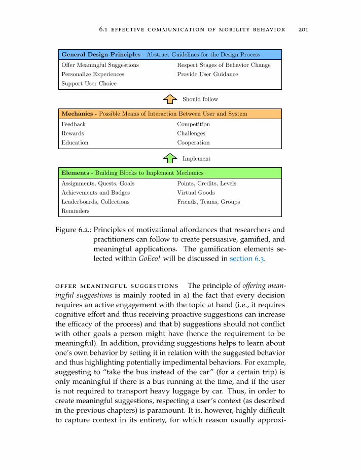
6.1 effective communication of mobility behavior 201
General Design Principles - Abstract Guidelines for the Design Process
Offer Meaningful SuggestionsPersonalize ExperiencesSupport User Choice
Respect Stages of Behavior ChangeProvide User Guidance
Should follow
Implement
Mechanics - Possible Means of Interaction Between User and System
FeedbackRewardsEducation Cooperation
CompetitionChallenges
Elements - Building Blocks to Implement Mechanics
Assignments, Quests, GoalsAchievements and BadgesLeaderboards, CollectionsReminders
Friends, Teams, Groups
Points, Credits, LevelsVirtual Goods
Figure 6.2.: Principles of motivational affordances that researchers andpractitioners can follow to create persuasive, gamified, andmeaningful applications. The gamification elements se-lected within GoEco! will be discussed in section 6.3.
offer meaningful suggestions The principle of offering mean-ingful suggestions is mainly rooted in a) the fact that every decisionrequires an active engagement with the topic at hand (i.e., it requirescognitive effort and thus receiving proactive suggestions can increasethe efficacy of the process) and that b) suggestions should not conflictwith other goals a person might have (hence the requirement to bemeaningful). In addition, providing suggestions helps to learn aboutone’s own behavior by setting it in relation with the suggested behaviorand thus highlighting potentially impedimental behaviors. For example,suggesting to “take the bus instead of the car” (for a certain trip) isonly meaningful if there is a bus running at the time, and if the useris not required to transport heavy luggage by car. Thus, in order tocreate meaningful suggestions, respecting a user’s context (as describedin the previous chapters) is paramount. It is, however, highly difficultto capture context in its entirety, for which reason usually approxi-
202 communicating mobility
mate tradeoffs are used (e.g., that an alternative would be viable for asystematically traveled route, if its duration does not exceed a certainthreshold).
support user choice Rooting in the psychological need for au-tonomy, the design principle of supporting user choices aims at lettingusers specify their own goals and the pace at which they work to-wards them. This stands in close relation to the previous principle ofmeaningful suggestions, essentially stating that people should be givenmore than “either-or” choices. Completely supporting user choice evenmeans considering the scenario that a user does not approve of any ofthe options proposed by the persuasive app, and let a user adapt thesystem to her liking. Giving users choices also prevents “technologyparenting”, whereas users are discouraged because they feel that anapplication has too much control over them, and thus stop using it.The gained autonomy gives room for empowerment strategies, wherea user can (virtually) practice a behavior or explore cause-and-effectrelationships and thus become more versed at various behaviors. Forexample, suggesting similar transport options in different situationslets a user experience their viability in various contexts and thus gain abetter understanding about the different options.
provide user guidance Providing user guidance usually takes theform of task reduction or tunneling, whereas the difficulty of a task iseither reduced or the experiences of a user are controlled. Providingguidance is important during the acquisition of new skills. Structuringinformation in an appropriate way can help people more easily graspdesired behaviors and the actions needed to achieve them. For exam-ple, presenting mobility data in an aggregated from and highlightingparticular traits that run contrary to the desired behavior helps a userunderstand quickly where improvement is needed. Giving concreteexamples of how to improve these traits, and guiding people by provid-ing achievable steps towards the target behavior reduces the complexityof a behavior change and nudges users in the “right direction”. Com-ponents that provide user guidance must be able to handle failures inexhibiting certain behaviors to prevent people from getting frustratedand relapsing to previous behavior. The latter gives a user of a systemthe freedom of choice, and thus again connects the process of achievingcompetence to the personal desire to do so (i.e., the need for autonomy).
6.1 effective communication of mobility behavior 203
provide personalized experience Personalizing experiences with-in a persuasive app usually takes two forms: On the one hand, lettingusers customize their experience within the app (e.g., by letting themmodify the user interface) gives them a sense of ownership and possibil-ity to express their self-identity. On the other hand, and more importantwithin the context of the here studied applications, tailoring the contentto the behavior of the user (or user group) satisfies our needs for relat-edness, affiliation and followership. In addition to being more useful ifthe elements within an app are personalized, the application designercan thus foster a stronger bond between the user and the motivationalartifact. It needs to be noted that personalization is often domain-dependent, though, and as such requires iterative design processes.As mobility is highly individual, personalization quickly becomes acentral aspect of any non-trivial application: By analyzing someone’srecorded trajectories, and giving feedback on how to improve behavior,the persuasive application already requires a deep understanding of aperson’s mobility (in contrast, consider a trivial app that only provideseducational elements, such as (randomly timed) notifications to go towork by bicycle).
design for every stage of behavior change As already dis-cussed previously, the path to acquiring a new behavior undergoesseveral stages. Optimally, applications automatically identify thesestages and implement elements that respect the current stage a personis in. For example, a person who is not aware of a certain behaviorthat is not in line with his or her overall goals (and thus is in a pre-contemplation stage), should be given information about the behavior,comparisons with alternatives, and information that allows reflectingon it. Later, alternative behaviors and the provision of small tasks(instead of suggesting the ultimate target behavior directly) increase theability of the user to get incrementally closer to the desired behavior.Highlighting the differences to other people and the desired outcomeprovides a strong motivational source, and thus can be selectively em-ployed to “overcome” difficult situations. And as noted before, duringstages where people take action in implementing certain behaviors,concrete suggestions, rearrangements of tasks, or even only informativefeedback can help the user to adjust his or her actions towards thedesired behavior.
204 communicating mobility
In the following, we will describe the individual mechanics, whichshould follow the introduced design principles to ensure a high persua-siveness.
6.1.2 Mechanics
Mechanics describe the ways in which a user and a (persuasive) systemcan interact. As such, it is not required that all of them are implementedwithin a single system, however, those which are, should be in line withthe general design principles introduced previously.
education Education intends to provide a user with knowledgeabout a potentially desirable behavior, but also about how to per-form tasks to reach it. It primarily targets the psychological needs forcompetence, but can also contain elements that satisfy the need forfollowership in case it is given via the role of instructors. Especiallyin early stages of behavior change, education plays a central role, as itcan highlight differences between an idealized self and the exhibitedbehavior and thus induce cognitive dissonances that form a strongmotivator. Similarly, it can point to normative behaviors (thus target-ing the needs for affiliation and relatedness), it can create awareness,and increase a user’s ability to perform certain tasks (essentially bygiving instructions). In later stages educative measures can keep atopic interesting by providing additional information. Education is bestused while respecting context: normative statements that lack context(such as “you must do x”, without any additional reasoning) have littleeffect on exhibited behaviors. Examples from the sustainable mobilitydomain include education about the environmental effects of differenttransport modes, statistics on mobility use within a certain region, orthe availability of different transport modes (that might previously beunknown to the user).
feedback Feedback is any information given back to a user thatlets her assess the currently (or recently) performed behavior. It iseither given instantly or after a short period of time (during which alarger amount of data can be accumulated into fewer representativeindicators), and is mostly visual, but can also be auditory, haptic, or ina variety of other forms (e.g., commonly, a notification on a smartphonecombines all three). Feedback is used in one form or another in most
6.1 effective communication of mobility behavior 205
computer applications, in particular in pervasive systems. Next toproviding motivation by showing discrepancies in exhibited and desiredbehavior, it can decrease the difficulty of tasks (e.g., when it containssuggestions about potential alternatives to the exhibited behavior) andthus “increase the ability” of a user. However, when feedback containsalternative behaviors, they must be meaningful and the user must begiven a choice, in order to prevent technology parenting. If feedback isgiven instantly after a behavior was exhibited, it forms a stronger linkthan when given in an “offline manner” (i.e., at a later point in time).Of particular importance within the context of mobility, the systemdesigner has to be careful that the feedback does not interfere with theactivity a user is currently performing. For example, notifying a userusing a visual cue while she is driving is distracting and leads to anincreased risk of accidents. Giving feedback in an accumulated format a later point has the advantage that it can be summarized well andthus more easily used to compare the current behavior to the past, andto other people in similar situations.
More IndirectFeedback
indirect forms of feedback do not necessarily require knowinganything about the user, but instead simply rephrase a situation or taskin such a way that a user is inclined to exhibit the desired behavior.For example, it was found that painting perpendicular and unevenlyspaced lines on the road lets people decrease their speed when passingthe respective road segment (Leonard 2008). Feedback can also be givenfor small and (potentially) unintentional behavior changes, which leadsto an adjustment of a person’s belief system and thus motivates largerand intentional future behavior. However, giving feedback that is notnecessarily in line with a person’s belief system can also have demo-tivating effects, as it results in inconsistencies in one’s representationof the world, and thus leads to a rejection of the imposed desirable be-havior. Such “boomerang feedback” has to be considered in most cases;for example, indicating the average behavior of a user group withinfeedback usually leads to a regression towards said average, even ifthe exhibited behavior was more sustainable. Finally, it is important tonote that the users of a persuasive application will not always utilizefeedback given to them to change or improve their behavior, as theywill often not have a complete and perfectly accurate representationof reality and will not strictly maximize sustainability. Giving correctfeedback at appropriate times will increase the perceived credibilityand persuasion capabilities, however.
206 communicating mobility
rewards Rewards are mechanics that solely generate motivation,and do not change the ability of a user to perform a certain task. Inaddition, the generated motivation is primarily external, and as suchhas a range of negative associations that require a system designer tocarefully evaluate if the benefits of employing rewards outweigh theirnegative connotations. While rewards fulfill the needs for achievementand competence in the best case, they might lead to a user performinga certain action solely for the reward in the long run, thus decreasingthe overall motivation (external and internal) to perform a desiredbehavior. Related to this, extrinsic motivators are unsuitable to inducelong-term behavior changes, as people will commonly only exhibitthe behavior as long as the reward is present, and stop as soon as theextrinsic motivator disappears. In addition, for a user to continuouslyperform a desired behavior, the reward size has to be increased overtime, and its frequency and predictability has to be changed in order tocontain a moment of surprise. Failing to do both will lead to decreasingmotivation and (as it is primarily an external motivator) falling back tothe original (potentially undesirable) behavior.
challenges Challenges are rooted in our need for competence.Their essence is to give a (somewhat difficult) goal that allows bench-marking one’s own behavior, skills, or performance. They are particu-larly useful when competition and cooperation is impossible, i.e., whenthe set of involved users and/or contexts is diverse. Additionally, theycan help people without goals or people who do not know how toachieve a (potentially too difficult) goal, by providing guidance and/orreframing the desired outcome in terms of the involved steps. For exam-ple, adding upfront or intermediate goals that are easy to reach (withina larger process to achieve some desired behavior) can increase thelikelihood that someone completes a task, as people feel like they arecompetent and making progress. Splitting up larger goals into smaller(more reachable) ones similarly relates to our need for competence, asthese smaller goals seem more reachable and thus satisfy our need tofeel competent more quickly. This strategy of “divide and conquer”can be found in many fields, and essentially describes how one largegoal can be overwhelming, preventing a person from starting to workon it at all. When choosing challenges and/or goals, it is important tochoose reasonable defaults, as people will usually not make the effort ofmanually adjusting them even when presented with multiple options.
6.2 generating and communicating eco-feedback 207
competition Rooted in the needs for achievement and leadership,competition is a mechanic that works well for people who are ap-proximately in the same situations and exhibit the same skills. Thesecomparisons with a rival party become demotivating, however, whenthe differences in skills are large or when one party faces highly dif-ferent circumstances. For example, giving a group of people awardsbased on how often they take the bicycle to work will demotivate peo-ple who need to transport baggage and thus cannot participate in thecompetition. Similarly, there are circumstances in which competitionmay be unwanted, e.g., within a family where one might follow anon-competitive ethic and want to foster cooperation and collaborationinstead. Finally, it needs to be noted that the framing of a comparison iscrucial, as it influences the outcomes greatly (as a very simple exampleconsider two rankings of participants where the one who uses thebicycle the most is on top in one, and the one who uses it the least ison top in the other; the resulting motivations will greatly differ).
cooperation Cooperation is the opposite of competition, buildingupon our needs for relatedness, affiliation and leader-/followership(when roles in a cooperative setting are distributed in a way that makesindividual people leaders for certain tasks). As cooperation alwaysinvolves a group of people that works together in an attempt to reacha goal, it naturally works in settings where people are social and themix of skills and knowledge within the group complements itself. Thismeans that everyone gets to “play a part” (and thus is able to show com-petence), and will feel related (due to the common goal) and affiliated(due to the inalienability in the team) to others. Having anonymousteams where people do not know each other is less motivational. Oftencooperation and competition are combined, whereas essentially groupsof cooperative teams are formed that compete against each other. In thecontext of persuasive applications supporting sustainable mobility co-operation could, for example, include functionality that rewards peoplefor carpooling together.
6.2 generating and communicating eco-feedback
Based on the general design principles and individual mechanics intro-duced above, there are several ways how to generate and communicateeco-feedback. Here (and in accordance with the chosen approaches
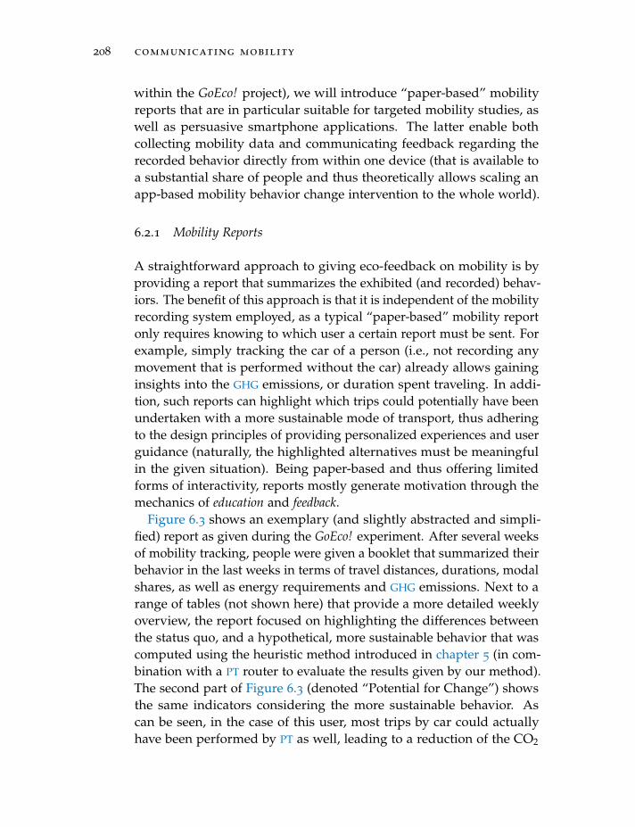
208 communicating mobility
within the GoEco! project), we will introduce “paper-based” mobilityreports that are in particular suitable for targeted mobility studies, aswell as persuasive smartphone applications. The latter enable bothcollecting mobility data and communicating feedback regarding therecorded behavior directly from within one device (that is available toa substantial share of people and thus theoretically allows scaling anapp-based mobility behavior change intervention to the whole world).
6.2.1 Mobility Reports
A straightforward approach to giving eco-feedback on mobility is byproviding a report that summarizes the exhibited (and recorded) behav-iors. The benefit of this approach is that it is independent of the mobilityrecording system employed, as a typical “paper-based” mobility reportonly requires knowing to which user a certain report must be sent. Forexample, simply tracking the car of a person (i.e., not recording anymovement that is performed without the car) already allows gaininginsights into the GHG emissions, or duration spent traveling. In addi-tion, such reports can highlight which trips could potentially have beenundertaken with a more sustainable mode of transport, thus adheringto the design principles of providing personalized experiences and userguidance (naturally, the highlighted alternatives must be meaningfulin the given situation). Being paper-based and thus offering limitedforms of interactivity, reports mostly generate motivation through themechanics of education and feedback.
Figure 6.3 shows an exemplary (and slightly abstracted and simpli-fied) report as given during the GoEco! experiment. After several weeksof mobility tracking, people were given a booklet that summarized theirbehavior in the last weeks in terms of travel distances, durations, modalshares, as well as energy requirements and GHG emissions. Next to arange of tables (not shown here) that provide a more detailed weeklyoverview, the report focused on highlighting the differences betweenthe status quo, and a hypothetical, more sustainable behavior that wascomputed using the heuristic method introduced in chapter 5 (in com-bination with a PT router to evaluate the results given by our method).The second part of Figure 6.3 (denoted “Potential for Change”) showsthe same indicators considering the more sustainable behavior. Ascan be seen, in the case of this user, most trips by car could actuallyhave been performed by PT as well, leading to a reduction of the CO2
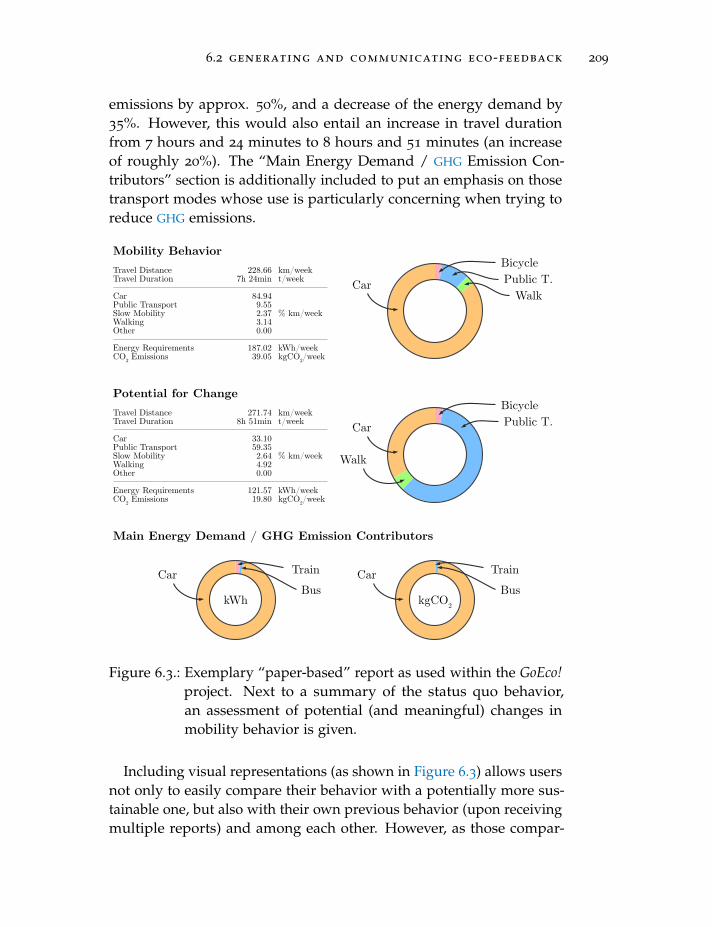
6.2 generating and communicating eco-feedback 209
emissions by approx. 50%, and a decrease of the energy demand by35%. However, this would also entail an increase in travel durationfrom 7 hours and 24 minutes to 8 hours and 51 minutes (an increaseof roughly 20%). The “Main Energy Demand / GHG Emission Con-tributors” section is additionally included to put an emphasis on thosetransport modes whose use is particularly concerning when trying toreduce GHG emissions.
Mobility BehaviorTravel DistanceTravel Duration
CarPublic TransportSlow MobilityWalkingOther
Energy RequirementsCO2 Emissions
228.667h 24min
84.949.552.373.140.00
187.0239.05
km/weekt/week
% km/week
kWh/weekkgCO2/week
Travel DistanceTravel Duration
CarPublic TransportSlow MobilityWalkingOther
Energy RequirementsCO2 Emissions
271.748h 51min
33.1059.352.644.920.00
121.5719.80
km/weekt/week
% km/week
kWh/weekkgCO2/week
Potential for Change
Main Energy Demand / GHG Emission Contributors
kWh kgCO2
Car Train
BusCar Train
Bus
Car Public T.Walk
Bicycle
Car Public T.
Walk
Bicycle
Figure 6.3.: Exemplary “paper-based” report as used within the GoEco!project. Next to a summary of the status quo behavior,an assessment of potential (and meaningful) changes inmobility behavior is given.
Including visual representations (as shown in Figure 6.3) allows usersnot only to easily compare their behavior with a potentially more sus-tainable one, but also with their own previous behavior (upon receivingmultiple reports) and among each other. However, as those compar-
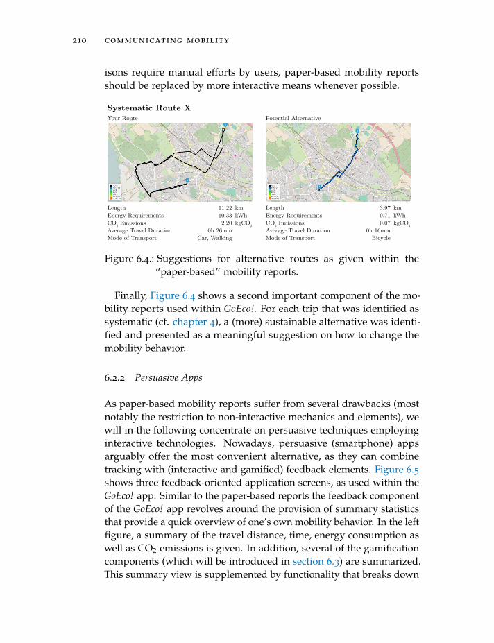
210 communicating mobility
isons require manual efforts by users, paper-based mobility reportsshould be replaced by more interactive means whenever possible.
Systematic Route XYour Route
LengthEnergy RequirementsCO2 EmissionsAverage Travel DurationMode of Transport
11.2210.332.20
0h 26minCar, Walking
kmkWhkgCO2
LengthEnergy RequirementsCO2 EmissionsAverage Travel DurationMode of Transport
3.970.710.07
0h 16minBicycle
kmkWhkgCO2
Potential Alternative
Figure 6.4.: Suggestions for alternative routes as given within the“paper-based” mobility reports.
Finally, Figure 6.4 shows a second important component of the mo-bility reports used within GoEco!. For each trip that was identified assystematic (cf. chapter 4), a (more) sustainable alternative was identi-fied and presented as a meaningful suggestion on how to change themobility behavior.
6.2.2 Persuasive Apps
As paper-based mobility reports suffer from several drawbacks (mostnotably the restriction to non-interactive mechanics and elements), wewill in the following concentrate on persuasive techniques employinginteractive technologies. Nowadays, persuasive (smartphone) appsarguably offer the most convenient alternative, as they can combinetracking with (interactive and gamified) feedback elements. Figure 6.5shows three feedback-oriented application screens, as used within theGoEco! app. Similar to the paper-based reports the feedback componentof the GoEco! app revolves around the provision of summary statisticsthat provide a quick overview of one’s own mobility behavior. In the leftfigure, a summary of the travel distance, time, energy consumption aswell as CO2 emissions is given. In addition, several of the gamificationcomponents (which will be introduced in section 6.3) are summarized.This summary view is supplemented by functionality that breaks down
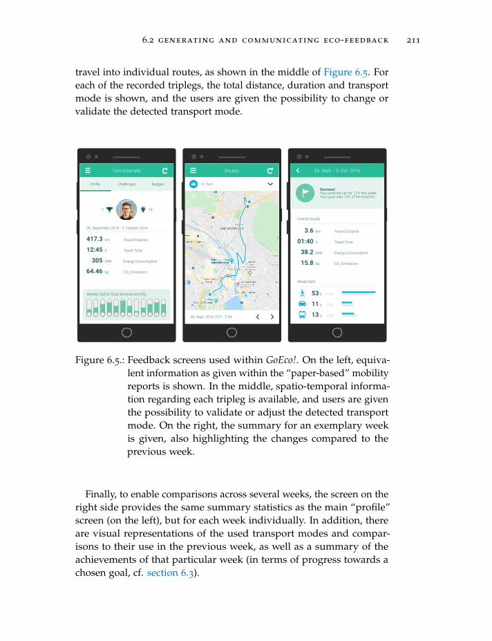
6.2 generating and communicating eco-feedback 211
travel into individual routes, as shown in the middle of Figure 6.5. Foreach of the recorded triplegs, the total distance, duration and transportmode is shown, and the users are given the possibility to change orvalidate the detected transport mode.
Tom Example
Weekly GoEco! Goal Achievement [%]
Profile Challenges
2 18
Badges
1 2 3 4 5 6 7 8 9 10 11 12
26. September 2016 - 3. October 2016
km Travel Distance417.3
h Travel Time12:45
kWh Energy Consumption305
kg CO2 Emissions64.46
Routes
28. Sept. 2016, 7:07 - 7:34
5.7 km
26. Sept. - 3. Oct. 2016
Success!You used the car for 11% this week.Your goal was 13% of the total km.
Overall results
km Travel Distance3.6
h Travel Time01:40
kWh Energy Consumption38.2
kg CO2 Emissions15.8
Modal Split
%53
%11
%
+10%
-15%
-23%13
Figure 6.5.: Feedback screens used within GoEco!. On the left, equiva-lent information as given within the “paper-based” mobilityreports is shown. In the middle, spatio-temporal informa-tion regarding each tripleg is available, and users are giventhe possibility to validate or adjust the detected transportmode. On the right, the summary for an exemplary weekis given, also highlighting the changes compared to theprevious week.
Finally, to enable comparisons across several weeks, the screen on theright side provides the same summary statistics as the main “profile”screen (on the left), but for each week individually. In addition, thereare visual representations of the used transport modes and compar-isons to their use in the previous week, as well as a summary of theachievements of that particular week (in terms of progress towards achosen goal, cf. section 6.3).
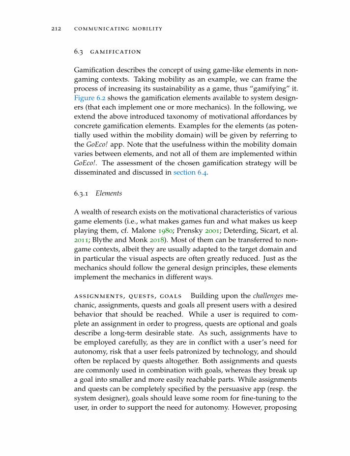
212 communicating mobility
6.3 gamification
Gamification describes the concept of using game-like elements in non-gaming contexts. Taking mobility as an example, we can frame theprocess of increasing its sustainability as a game, thus “gamifying” it.Figure 6.2 shows the gamification elements available to system design-ers (that each implement one or more mechanics). In the following, weextend the above introduced taxonomy of motivational affordances byconcrete gamification elements. Examples for the elements (as poten-tially used within the mobility domain) will be given by referring tothe GoEco! app. Note that the usefulness within the mobility domainvaries between elements, and not all of them are implemented withinGoEco!. The assessment of the chosen gamification strategy will bedisseminated and discussed in section 6.4.
6.3.1 Elements
A wealth of research exists on the motivational characteristics of variousgame elements (i.e., what makes games fun and what makes us keepplaying them, cf. Malone 1980; Prensky 2001; Deterding, Sicart, et al.2011; Blythe and Monk 2018). Most of them can be transferred to non-game contexts, albeit they are usually adapted to the target domain andin particular the visual aspects are often greatly reduced. Just as themechanics should follow the general design principles, these elementsimplement the mechanics in different ways.
assignments, quests, goals Building upon the challenges me-chanic, assignments, quests and goals all present users with a desiredbehavior that should be reached. While a user is required to com-plete an assignment in order to progress, quests are optional and goalsdescribe a long-term desirable state. As such, assignments have tobe employed carefully, as they are in conflict with a user’s need forautonomy, risk that a user feels patronized by technology, and shouldoften be replaced by quests altogether. Both assignments and questsare commonly used in combination with goals, whereas they break upa goal into smaller and more easily reachable parts. While assignmentsand quests can be completely specified by the persuasive app (resp. thesystem designer), goals should leave some room for fine-tuning to theuser, in order to support the need for autonomy. However, proposing
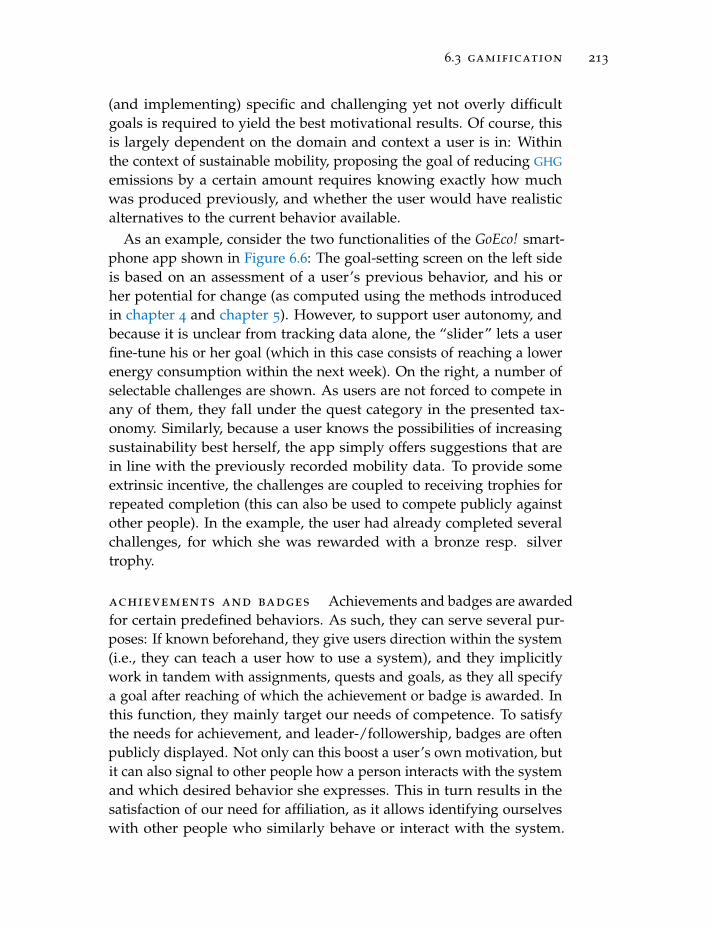
6.3 gamification 213
(and implementing) specific and challenging yet not overly difficultgoals is required to yield the best motivational results. Of course, thisis largely dependent on the domain and context a user is in: Withinthe context of sustainable mobility, proposing the goal of reducing GHG
emissions by a certain amount requires knowing exactly how muchwas produced previously, and whether the user would have realisticalternatives to the current behavior available.
As an example, consider the two functionalities of the GoEco! smart-phone app shown in Figure 6.6: The goal-setting screen on the left sideis based on an assessment of a user’s previous behavior, and his orher potential for change (as computed using the methods introducedin chapter 4 and chapter 5). However, to support user autonomy, andbecause it is unclear from tracking data alone, the “slider” lets a userfine-tune his or her goal (which in this case consists of reaching a lowerenergy consumption within the next week). On the right, a number ofselectable challenges are shown. As users are not forced to compete inany of them, they fall under the quest category in the presented tax-onomy. Similarly, because a user knows the possibilities of increasingsustainability best herself, the app simply offers suggestions that arein line with the previously recorded mobility data. To provide someextrinsic incentive, the challenges are coupled to receiving trophies forrepeated completion (this can also be used to compete publicly againstother people). In the example, the user had already completed severalchallenges, for which she was rewarded with a bronze resp. silvertrophy.
achievements and badges Achievements and badges are awardedfor certain predefined behaviors. As such, they can serve several pur-poses: If known beforehand, they give users direction within the system(i.e., they can teach a user how to use a system), and they implicitlywork in tandem with assignments, quests and goals, as they all specifya goal after reaching of which the achievement or badge is awarded. Inthis function, they mainly target our needs of competence. To satisfythe needs for achievement, and leader-/followership, badges are oftenpublicly displayed. Not only can this boost a user’s own motivation, butit can also signal to other people how a person interacts with the systemand which desired behavior she expresses. This in turn results in thesatisfaction of our need for affiliation, as it allows identifying ourselveswith other people who similarly behave or interact with the system.
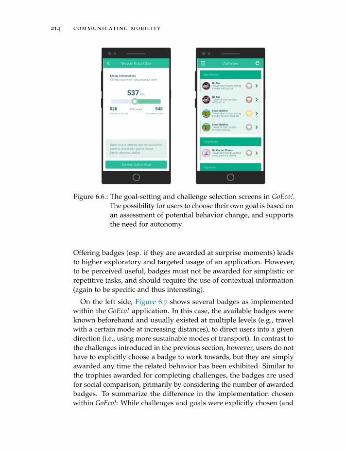
214 communicating mobility
Set this GoEco! Goal
Based on your reference data and your GoEco!potential, choose your goal for change.Set the value and... GoEco!
Energy ConsumptionsKilowatthours (kWh) consumed per week
kWh537
kWh/weekYour GoEco! potential Your reference data
526 548
Set your GoEco! Goal
Nights Out
Challenges
No CarTravel short routes duringthe day without car
Short Routes
No CarTravel all short routeswithout car
Slow MobilityTravel short routes duringthe day by slow mobility
Slow MobilityTravel all short routesby slow mobility
No Car, no PlanesTravel long routes withoutusing cars nor planes
Long Routes
Figure 6.6.: The goal-setting and challenge selection screens in GoEco!.The possibility for users to choose their own goal is based onan assessment of potential behavior change, and supportsthe need for autonomy.
Offering badges (esp. if they are awarded at surprise moments) leadsto higher exploratory and targeted usage of an application. However,to be perceived useful, badges must not be awarded for simplistic orrepetitive tasks, and should require the use of contextual information(again to be specific and thus interesting).
On the left side, Figure 6.7 shows several badges as implementedwithin the GoEco! application. In this case, the available badges wereknown beforehand and usually existed at multiple levels (e.g., travelwith a certain mode at increasing distances), to direct users into a givendirection (i.e., using more sustainable modes of transport). In contrast tothe challenges introduced in the previous section, however, users do nothave to explicitly choose a badge to work towards, but they are simplyawarded any time the related behavior has been exhibited. Similar tothe trophies awarded for completing challenges, the badges are usedfor social comparison, primarily by considering the number of awardedbadges. To summarize the difference in the implementation chosenwithin GoEco!: While challenges and goals were explicitly chosen (and
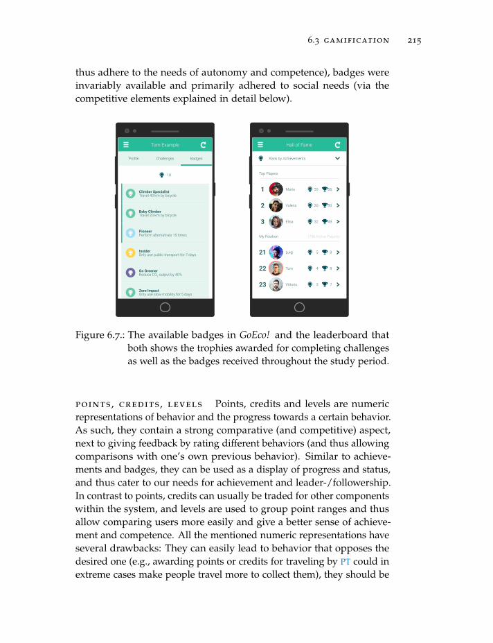
6.3 gamification 215
thus adhere to the needs of autonomy and competence), badges wereinvariably available and primarily adhered to social needs (via thecompetitive elements explained in detail below).
Tom Example
Profile Challenges
18
Badges
Climber SpecialistTravel 40 km by bicycle
Baby ClimberTravel 20 km by bicycle
PioneerPerform alternatives 15 times
InsiderOnly use public transport for 7 days
Go GreenerReduce CO2 output by 40%
Zero ImpactOnly use slow mobility for 5 days
Hall of Fame
5635Mario1
5030Valeria2
4932Elisa3
85Luigi21
84Tom22
73Vittorio23
Rank by Achievements
Top Players
My Position (756 Active Players)
Figure 6.7.: The available badges in GoEco! and the leaderboard thatboth shows the trophies awarded for completing challengesas well as the badges received throughout the study period.
points, credits, levels Points, credits and levels are numericrepresentations of behavior and the progress towards a certain behavior.As such, they contain a strong comparative (and competitive) aspect,next to giving feedback by rating different behaviors (and thus allowingcomparisons with one’s own previous behavior). Similar to achieve-ments and badges, they can be used as a display of progress and status,and thus cater to our needs for achievement and leader-/followership.In contrast to points, credits can usually be traded for other componentswithin the system, and levels are used to group point ranges and thusallow comparing users more easily and give a better sense of achieve-ment and competence. All the mentioned numeric representations haveseveral drawbacks: They can easily lead to behavior that opposes thedesired one (e.g., awarding points or credits for traveling by PT could inextreme cases make people travel more to collect them), they should be
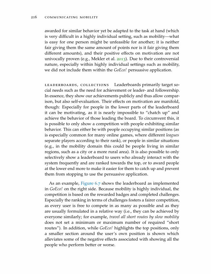
216 communicating mobility
awarded for similar behavior yet be adapted to the task at hand (whichis very difficult in a highly individual setting, such as mobility—whatis easy for one person might be unfeasible for another; it is neitherfair giving them the same amount of points nor is it fair giving themdifferent amounts), and their positive effects on motivation are notunivocally proven (e.g., Mekler et al. 2013). Due to their controversialnature, especially within highly individual settings such as mobility,we did not include them within the GoEco! persuasive application.
leaderboards, collections Leaderboards primarily target so-cial needs such as the need for achievement or leader- and followership.In essence, they show our achievements publicly and thus allow compar-ison, but also self-evaluation. Their effects on motivation are manifold,though: Especially for people in the lower parts of the leaderboardit can be motivating, as it is nearly impossible to “chatch up” andachieve the behavior of those leading the board. To circumvent this, itis possible to only show a competition with people exhibiting similarbehavior. This can either be with people occupying similar positions (asis especially common for many online games, where different leaguesseparate players according to their rank), or people in similar situations(e.g., in the mobility domain this could be people living in similarregions, such as a city or a more rural area). It is also possible to onlyselectively show a leaderboard to users who already interact with thesystem frequently and are ranked towards the top, or to award peopleat the lower end more to make it easier for them to catch up and preventthem from stopping to use the persuasive application.
As an example, Figure 6.7 shows the leaderboard as implementedin GoEco! on the right side. Because mobility is highly individual, thecompetition is based on the rewarded badges and completed challenges.Especially the ranking in terms of challenges fosters a fairer competition,as every user is free to compete in as many as possible and as theyare usually formulated in a relative way (i.e., they can be achieved byeveryone similarly; for example, travel all short routes by slow mobilitydoes not set a minimum or maximum number of required “shortroutes”). In addition, while GoEco! highlights the top positions, onlya smaller section around the user’s own position is shown whichalleviates some of the negative effects associated with showing all thepeople who perform better or worse.
6.3 gamification 217
reminders Reminders are used to prevent relapses into earlierstages of behavior change, can serve as feedback to a user, and en-courage habit formation (though their effectiveness to this purpose isdisputed). Their frequency and timeliness is important, but dependson the user and their content: For some people, reminders can quicklybecome a nuisance, while in other situations more frequent remindersare acceptable. For all reminders, it is better when they are generated byother human beings instead of in an automated fashion. Within GoEco!,reminders were provided for the weekly challenges (to choose one, butalso if the progress towards the challenge goal did not proceed as fastas necessary). These reminders were chosen before the backgroundof supporting users in their autonomy (i.e., they were reminded tochoose something themselves or about a choice they had previouslymade). Framing reminders in this way reduces the chance that they areperceived as a nuisance.
friends , teams , groups Offering social elements such as connect-ing with friends, or forming teams and groups adheres to our needsfor affiliation, relatedness and intimacy (and up to some degree toleader-/followership). Next to fostering cooperation, such functionali-ties offer possibilities to split up a user base into smaller groups (e.g.,a large mobility user study like GoEco! can be split up according tothe geographic region, or the personal situation of individual people),intra-group discussions on how to achieve certain goals, inter-groupcompetition, the possibility for more advanced users to help newcomersand/or weaker players, and also to equalize large differences in users(by teaming up stronger and weaker players). Similar to competitionbetween users, letting teams compare each other can act demotivatingfor weaker teams, though. Within GoEco!, friends, teams and groupswere not explored except for real-life meetings among participants (thisdid not have any effect on the information displayed within the appthough).
virtual goods Virtual goods are a special form of reward thathave a real economic value (i.e., can be bought and sold from withinthe gamified system). As such, they share most of the characteristicswith rewards such as achievements or points; in particular they adhereto our needs for achievement, competence, and leader-/followership.Similarly, they can also be used for social comparison, e.g., within a
218 communicating mobility
leaderboard—however, because of their economic value outside of thegamified system they go further and can be used as extrinsic motivator.Due to this and the fact that they can be bought as well, they areusually not required for intrinsically motivated people (who worktowards their goals of their own accord), and can even lead to adverseeffects (e.g., when people simply “buy their way up a leaderboard”).Finally, and very well visible in games that let you publicly displayyour purchased goods, the perceived effect you have on other players islargely influencing the decisions to buy virtual goods. Within GoEco!,there were no virtual goods due to their problems with the differentmotivation sources of people (i.e., the fact that they have detrimentaleffects on internally motivated people).
6.3.2 Computation and Assessment
For the introduced gamification elements to be unobtrusive and pro-active (i.e., they must be available to a user without any specific in-teraction), all computations must be made on the automatically andpassively tracked mobility data. As such, within GoEco!, we primarilyrelied on daily or weekly aggregates of mobility descriptors as intro-duced in chapter 4 and evaluated their change over time resp. theirrelation to descriptors exhibited under the assumption that a personwould always choose a sustainable alternative (when available and if thetrip was classified as unsustainable; cf. chapter 4 and 5). This periodicalre-evaluation of mobility behavior and gamification elements based onaggregates suffers from the drawback that users potentially have towait several hours after performing a trip before they get any feedbackor rewards from doing so. Developers of a persuasive resp. gamifiedapplication thus have to find a balance between immediate feedback(and thus a more “game-like” experience) and ease of computation andinterpretation of feedback (i.e., a daily aggregate is easily understoodand computed and can take a person’s complete exhibited behaviorinto account, while immediate feedback has to assess whether trips arecompleted already or if the app should withhold updating the gamifiedcomponents until a later time).
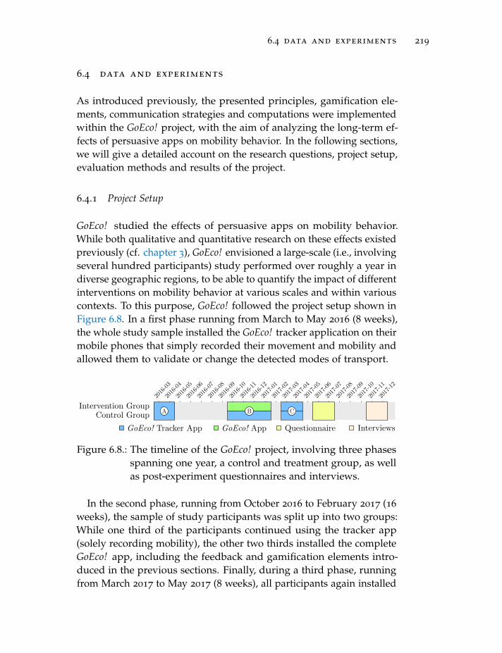
6.4 data and experiments 219
6.4 data and experiments
As introduced previously, the presented principles, gamification ele-ments, communication strategies and computations were implementedwithin the GoEco! project, with the aim of analyzing the long-term ef-fects of persuasive apps on mobility behavior. In the following sections,we will give a detailed account on the research questions, project setup,evaluation methods and results of the project.
6.4.1 Project Setup
GoEco! studied the effects of persuasive apps on mobility behavior.While both qualitative and quantitative research on these effects existedpreviously (cf. chapter 3), GoEco! envisioned a large-scale (i.e., involvingseveral hundred participants) study performed over roughly a year indiverse geographic regions, to be able to quantify the impact of differentinterventions on mobility behavior at various scales and within variouscontexts. To this purpose, GoEco! followed the project setup shown inFigure 6.8. In a first phase running from March to May 2016 (8 weeks),the whole study sample installed the GoEco! tracker application on theirmobile phones that simply recorded their movement and mobility andallowed them to validate or change the detected modes of transport.
Intervention GroupControl Group
GoEco! AppGoEco! Tracker App
2016-03
2016-04
2016-05
2016-06
2016-07
2016-08
2016-09
2016-10
2016-11
2016-12
2017-01
2017-02
2017-03
2017-04
2017-05
2017-06
2017-07
2017-08
2017-09
2017-10
2017-11
2017-12
A
Questionnaire Interviews
B C
Figure 6.8.: The timeline of the GoEco! project, involving three phasesspanning one year, a control and treatment group, as wellas post-experiment questionnaires and interviews.
In the second phase, running from October 2016 to February 2017 (16
weeks), the sample of study participants was split up into two groups:While one third of the participants continued using the tracker app(solely recording mobility), the other two thirds installed the completeGoEco! app, including the feedback and gamification elements intro-duced in the previous sections. Finally, during a third phase, runningfrom March 2017 to May 2017 (8 weeks), all participants again installed
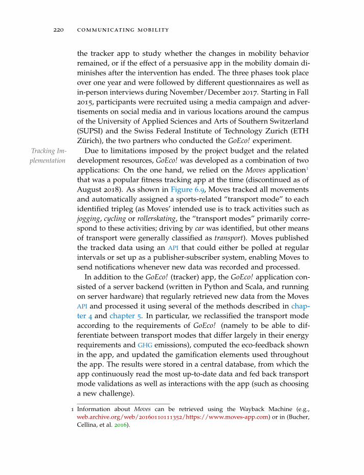
220 communicating mobility
the tracker app to study whether the changes in mobility behaviorremained, or if the effect of a persuasive app in the mobility domain di-minishes after the intervention has ended. The three phases took placeover one year and were followed by different questionnaires as well asin-person interviews during November/December 2017. Starting in Fall2015, participants were recruited using a media campaign and adver-tisements on social media and in various locations around the campusof the University of Applied Sciences and Arts of Southern Switzerland(SUPSI) and the Swiss Federal Institute of Technology Zurich (ETHZurich), the two partners who conducted the GoEco! experiment.
DueTracking Im-plementation
to limitations imposed by the project budget and the relateddevelopment resources, GoEco! was developed as a combination of twoapplications: On the one hand, we relied on the Moves application1
that was a popular fitness tracking app at the time (discontinued as ofAugust 2018). As shown in Figure 6.9, Moves tracked all movementsand automatically assigned a sports-related “transport mode” to eachidentified tripleg (as Moves’ intended use is to track activities such asjogging, cycling or rollerskating, the “transport modes” primarily corre-spond to these activities; driving by car was identified, but other meansof transport were generally classified as transport). Moves publishedthe tracked data using an API that could either be polled at regularintervals or set up as a publisher-subscriber system, enabling Moves tosend notifications whenever new data was recorded and processed.
In addition to the GoEco! (tracker) app, the GoEco! application con-sisted of a server backend (written in Python and Scala, and runningon server hardware) that regularly retrieved new data from the MovesAPI and processed it using several of the methods described in chap-ter 4 and chapter 5. In particular, we reclassified the transport modeaccording to the requirements of GoEco! (namely to be able to dif-ferentiate between transport modes that differ largely in their energyrequirements and GHG emissions), computed the eco-feedback shownin the app, and updated the gamification elements used throughoutthe app. The results were stored in a central database, from which theapp continuously read the most up-to-date data and fed back transportmode validations as well as interactions with the app (such as choosinga new challenge).
1 Information about Moves can be retrieved using the Wayback Machine (e.g.,web.archive.org/web/20160110111352/https://www.moves-app.com) or in (Bucher,Cellina, et al. 2016).
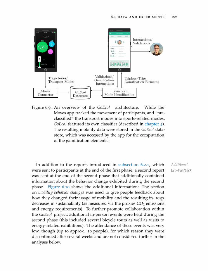
6.4 data and experiments 221
Tom Example
Weekly GoEco! Goal Achievement [%]
Profile Challenges
2 18
Badges
1 2 3 4 5 6 7 8 9 10 11 12
26. September 2016 - 3. October 2016
km Travel Distance417.3
h Travel Time12:45
kWh Energy Consumption305
kg CO2 Emissions64.46
MovesConnector
TransportMode Identification
GoEco!Datastore
Trajectories/Transport Modes
Triplegs/TripsGamification Elements
Interactions/Validations
Validations/GamificationInteractions
Figure 6.9.: An overview of the GoEco! architecture. While theMoves app tracked the movement of participants, and “pre-classified” the transport modes into sports-related modes,GoEco! featured its own classifier (described in chapter 4).The resulting mobility data were stored in the GoEco! data-store, which was accessed by the app for the computationof the gamification elements.
In AdditionalEco-Feedback
addition to the reports introduced in subsection 6.2.1, whichwere sent to participants at the end of the first phase, a second reportwas sent at the end of the second phase that additionally containedinformation about the behavior change exhibited during the secondphase. Figure 6.10 shows the additional information: The sectionon mobility behavior changes was used to give people feedback abouthow they changed their usage of mobility and the resulting in- resp.decreases in sustainability (as measured via the proxies CO2 emissionsand energy requirements). To further promote collaboration withinthe GoEco! project, additional in-person events were held during thesecond phase (this included several bicycle tours as well as visits toenergy-related exhibitions). The attendance of these events was verylow, though (up to approx. 10 people), for which reason they werediscontinued after several weeks and are not considered further in theanalyses below.
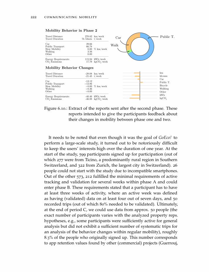
222 communicating mobility
Mobility Behavior in Phase 2
Mobility Behavior Changes
Car Public T.
Walk
Travel DistanceTravel Duration
CarPublic TransportSlow MobilityWalkingOther
Energy RequirementsCO2 Emissions
270.827h 53min
29.6666.780.003.560.00
115.9417.79
km/weekt/week
% km/week
kWh/weekkgCO2/week
kmhh:mmCarPublic T.BicycleWalkingOtherkWhkgCO2
Travel DistanceTravel Duration
CarPublic TransportSlow MobilityWalkingOther
Energy RequirementsCO2 Emissions
-28.08-21.45
-13.12+12.86+0.00+0.26+0.00
-40.46-46.88
km/weekt/week
% km/week
kWh/weekkgCO2/week
Figure 6.10.: Extract of the reports sent after the second phase. Thesereports intended to give the participants feedback abouttheir changes in mobility between phase one and two.
It needs to be noted that even though it was the goal of GoEco! toperform a large-scale study, it turned out to be notoriously difficultto keep the users’ interests high over the duration of one year. At thestart of the study, 599 participants signed up for participation (out ofwhich 277 were from Ticino, a predominantly rural region in SouthernSwitzerland, and 322 from Zurich, the largest city in Switzerland). 26
people could not start with the study due to incompatible smartphones.Out of the other 573, 212 fulfilled the minimal requirements of activetracking and validation for several weeks within phase A and couldenter phase B. These requirements stated that a participant has to haveat least three weeks of activity, where an active week was definedas having (validated) data on at least four out of seven days, and 50
recorded trips (out of which 80% needed to be validated). Ultimately,at the end of period C, we could use data from approx. 50 people (theexact number of participants varies with the analyzed property reps.hypotheses, e.g., some participants were sufficiently active for generalanalysis but did not exhibit a sufficient number of systematic trips foran analysis of the behavior changes within regular mobility), roughly8.3% of the people who originally signed up. This number correspondsto app retention values found by other (commercial) projects (Guerrouj,
6.4 data and experiments 223
Azad, and Rigby 2015; Sigg et al. 2019), and thus indicates that manypeople may not have perceived GoEco! primarily as a research project(in which case they would more likely have kept actively participatingwithin the study until the end), but rather as a regular app on themarket (that one removes once the novelty fades). While this reducesthe explanatory power of the analyses determining the effects of apersuasive app on mobility behavior, it gives additional insights aboutthe “real-life applicability” of a persuasive strategy centered aroundsmartphone apps.
6.4.2 Research Questions, Hypotheses and Evaluation Methods
The main research question of GoEco! follows the fourth questiongiven in chapter 1: Do people adjust their mobility behavior upon receiving(eco-)feedback based on their previous choices? To answer this question andas the main outcome of GoEco!, the three hypotheses stated below wereanalyzed:
Hypothesis 6.1. The average GHG emissions per kilometer are lowerafter the GoEco! intervention.
The main aim of a persuasive app such as GoEco! is to reduce theoverall ecological impact caused by its users’ mobility demands. Ourprimary proxy of the environmental impact are the GHG resp. CO2-equiv. emissions of individuals, for which reason Hypothesis 6.1 (andthe following ones) is formulated in terms of GHG emissions. UsingCO2-equiv. as a measure allows using emission factors computedwithin other research, and captures the entirety of GHGs that affect theenvironment. Of course, simply using a factor based on the distanceis only an approximation, however, computing the exact emissionsis usually not possible, as context such as the vehicle type, its exactvelocity, or the number of passengers is generally unknown. The secondhypothesis concerns the effects of the GoEco! app itself on the mobilitybehavior.
Hypothesis 6.2. The before/after difference in GHG emissions is largerfor people treated with the GoEco! app than for those who did not usethe app.
To ensure that the observed effects in Hypothesis 6.1 are not dueto external effects (such as seasonality, a general shift towards more
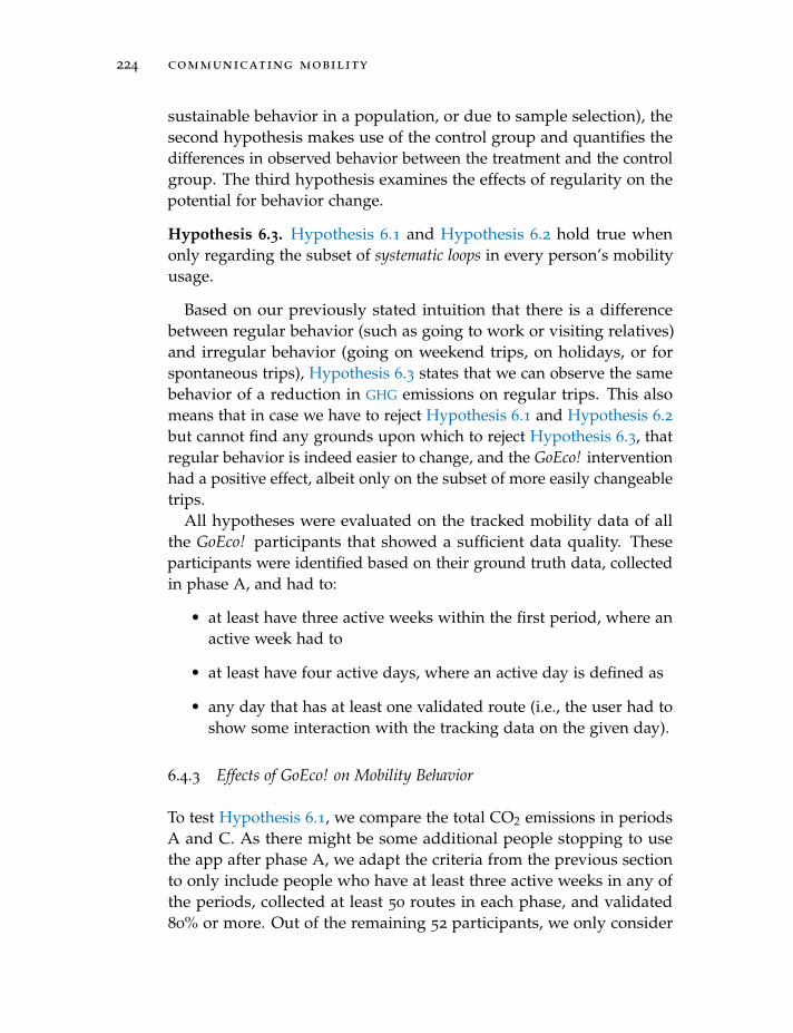
224 communicating mobility
sustainable behavior in a population, or due to sample selection), thesecond hypothesis makes use of the control group and quantifies thedifferences in observed behavior between the treatment and the controlgroup. The third hypothesis examines the effects of regularity on thepotential for behavior change.
Hypothesis 6.3. Hypothesis 6.1 and Hypothesis 6.2 hold true whenonly regarding the subset of systematic loops in every person’s mobilityusage.
Based on our previously stated intuition that there is a differencebetween regular behavior (such as going to work or visiting relatives)and irregular behavior (going on weekend trips, on holidays, or forspontaneous trips), Hypothesis 6.3 states that we can observe the samebehavior of a reduction in GHG emissions on regular trips. This alsomeans that in case we have to reject Hypothesis 6.1 and Hypothesis 6.2but cannot find any grounds upon which to reject Hypothesis 6.3, thatregular behavior is indeed easier to change, and the GoEco! interventionhad a positive effect, albeit only on the subset of more easily changeabletrips.
All hypotheses were evaluated on the tracked mobility data of allthe GoEco! participants that showed a sufficient data quality. Theseparticipants were identified based on their ground truth data, collectedin phase A, and had to:
• at least have three active weeks within the first period, where anactive week had to
• at least have four active days, where an active day is defined as
• any day that has at least one validated route (i.e., the user had toshow some interaction with the tracking data on the given day).
6.4.3 Effects of GoEco! on Mobility Behavior
To test Hypothesis 6.1, we compare the total CO2 emissions in periodsA and C. As there might be some additional people stopping to usethe app after phase A, we adapt the criteria from the previous sectionto only include people who have at least three active weeks in any ofthe periods, collected at least 50 routes in each phase, and validated80% or more. Out of the remaining 52 participants, we only consider
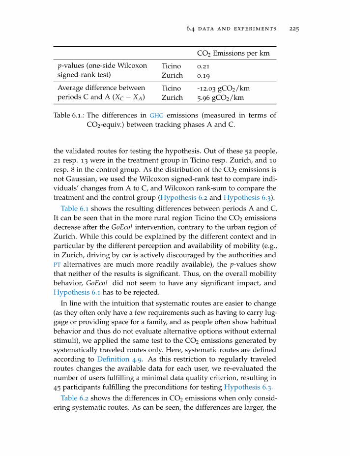
6.4 data and experiments 225
CO2 Emissions per km
p-values (one-side Wilcoxonsigned-rank test)
Ticino 0.21
Zurich 0.19
Average difference betweenperiods C and A (XC − XA)
Ticino -12.03 gCO2/kmZurich 5.96 gCO2/km
Table 6.1.: The differences in GHG emissions (measured in terms ofCO2-equiv.) between tracking phases A and C.
the validated routes for testing the hypothesis. Out of these 52 people,21 resp. 13 were in the treatment group in Ticino resp. Zurich, and 10
resp. 8 in the control group. As the distribution of the CO2 emissions isnot Gaussian, we used the Wilcoxon signed-rank test to compare indi-viduals’ changes from A to C, and Wilcoxon rank-sum to compare thetreatment and the control group (Hypothesis 6.2 and Hypothesis 6.3).
Table 6.1 shows the resulting differences between periods A and C.It can be seen that in the more rural region Ticino the CO2 emissionsdecrease after the GoEco! intervention, contrary to the urban region ofZurich. While this could be explained by the different context and inparticular by the different perception and availability of mobility (e.g.,in Zurich, driving by car is actively discouraged by the authorities andPT alternatives are much more readily available), the p-values showthat neither of the results is significant. Thus, on the overall mobilitybehavior, GoEco! did not seem to have any significant impact, andHypothesis 6.1 has to be rejected.
In line with the intuition that systematic routes are easier to change(as they often only have a few requirements such as having to carry lug-gage or providing space for a family, and as people often show habitualbehavior and thus do not evaluate alternative options without externalstimuli), we applied the same test to the CO2 emissions generated bysystematically traveled routes only. Here, systematic routes are definedaccording to Definition 4.9. As this restriction to regularly traveledroutes changes the available data for each user, we re-evaluated thenumber of users fulfilling a minimal data quality criterion, resulting in45 participants fulfilling the preconditions for testing Hypothesis 6.3.
Table 6.2 shows the differences in CO2 emissions when only consid-ering systematic routes. As can be seen, the differences are larger, the
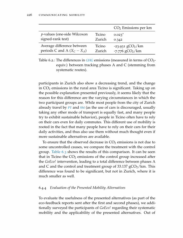
226 communicating mobility
CO2 Emissions per km
p-values (one-side Wilcoxonsigned-rank test)
Ticino 0.023∗
Zurich 0.342
Average difference betweenperiods C and A (XC − XA)
Ticino -23.931 gCO2/kmZurich -7.776 gCO2/km
Table 6.2.: The differences in GHG emissions (measured in terms of CO2-equiv.) between tracking phases A and C (stemming fromsystematic routes).
participants in Zurich also show a decreasing trend, and the changein CO2 emissions in the rural area Ticino is significant. Taking up onthe possible explanation presented previously, it seems likely that thereason for this difference are the varying circumstances in which thetwo participant groups are. While most people from the city of Zurichalready travel by PT and SM (as the use of cars is discouraged, usuallytaking any other mode of transport is equally fast, and many peopletry to exhibit sustainable behavior), people in Ticino often have to relyon their cars even for daily commutes. This different use of mobility isrooted in the fact that many people have to rely on their cars for theirdaily activities, and thus also use them without much thought even ifmore sustainable alternatives are available.
To ensure that the observed decrease in CO2 emissions is not due tosome uncontrolled causes, we compare the treatment with the controlgroup. Table 6.3 shows the results of this comparison. It can be seenthat in Ticino the CO2 emissions of the control group increased afterthe GoEco! intervention, leading to a total difference between phases Aand C and the control and treatment group of 33.137 gCO2/km. Thisdifference was found to be significant, but not in Zurich, where it ismuch smaller as well.
6.4.4 Evaluation of the Presented Mobility Alternatives
To evaluate the usefulness of the presented alternatives (as part of theeco-feedback reports sent after the first and second phases), we addi-tionally surveyed the participants of GoEco! regarding their systematicmobility and the applicability of the presented alternatives. Out of
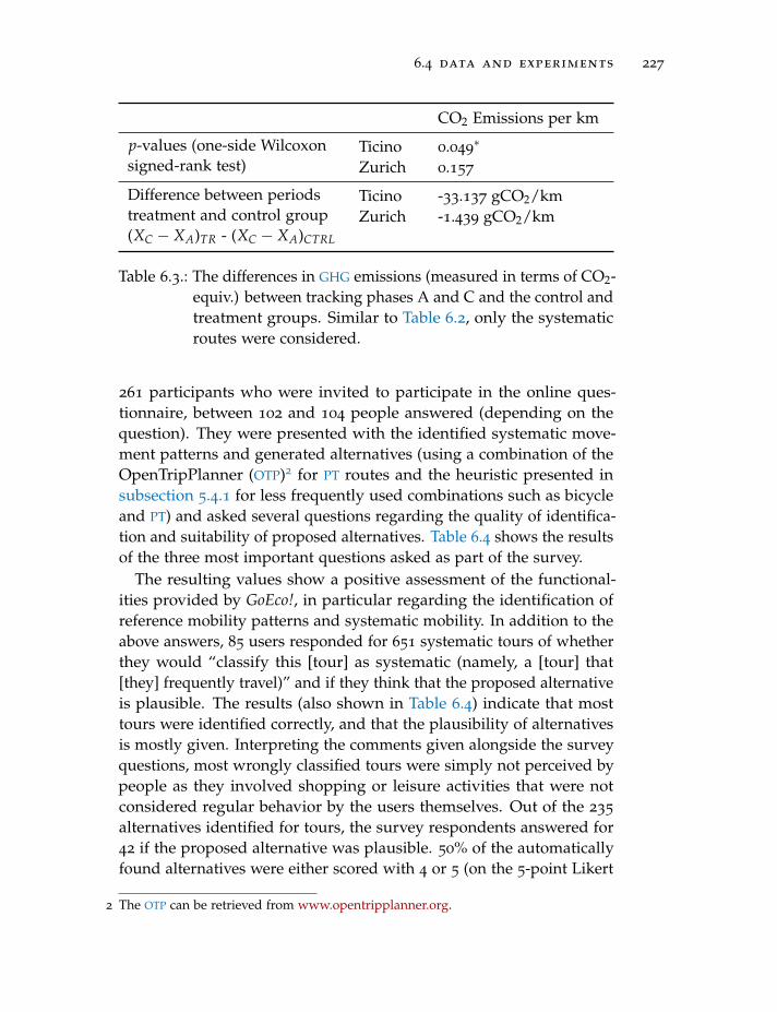
6.4 data and experiments 227
CO2 Emissions per km
p-values (one-side Wilcoxonsigned-rank test)
Ticino 0.049∗
Zurich 0.157
Difference between periodstreatment and control group(XC − XA)TR - (XC − XA)CTRL
Ticino -33.137 gCO2/kmZurich -1.439 gCO2/km
Table 6.3.: The differences in GHG emissions (measured in terms of CO2-equiv.) between tracking phases A and C and the control andtreatment groups. Similar to Table 6.2, only the systematicroutes were considered.
261 participants who were invited to participate in the online ques-tionnaire, between 102 and 104 people answered (depending on thequestion). They were presented with the identified systematic move-ment patterns and generated alternatives (using a combination of theOpenTripPlanner (OTP)2 for PT routes and the heuristic presented insubsection 5.4.1 for less frequently used combinations such as bicycleand PT) and asked several questions regarding the quality of identifica-tion and suitability of proposed alternatives. Table 6.4 shows the resultsof the three most important questions asked as part of the survey.
The resulting values show a positive assessment of the functional-ities provided by GoEco!, in particular regarding the identification ofreference mobility patterns and systematic mobility. In addition to theabove answers, 85 users responded for 651 systematic tours of whetherthey would “classify this [tour] as systematic (namely, a [tour] that[they] frequently travel)” and if they think that the proposed alternativeis plausible. The results (also shown in Table 6.4) indicate that mosttours were identified correctly, and that the plausibility of alternativesis mostly given. Interpreting the comments given alongside the surveyquestions, most wrongly classified tours were simply not perceived bypeople as they involved shopping or leisure activities that were notconsidered regular behavior by the users themselves. Out of the 235
alternatives identified for tours, the survey respondents answered for42 if the proposed alternative was plausible. 50% of the automaticallyfound alternatives were either scored with 4 or 5 (on the 5-point Likert
2 The OTP can be retrieved from www.opentripplanner.org.
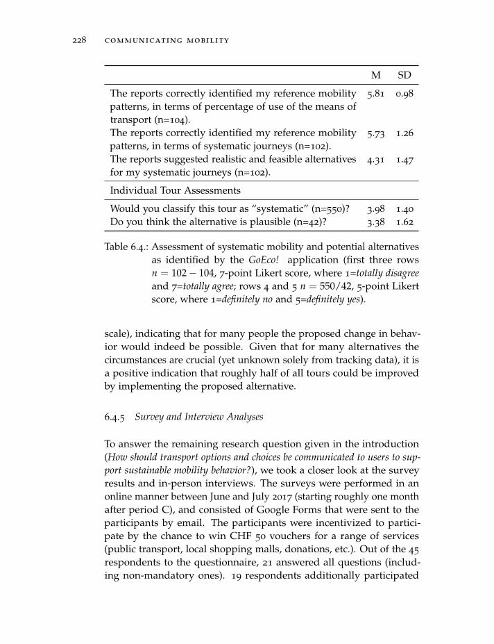
228 communicating mobility
M SD
The reports correctly identified my reference mobilitypatterns, in terms of percentage of use of the means oftransport (n=104).
5.81 0.98
The reports correctly identified my reference mobilitypatterns, in terms of systematic journeys (n=102).
5.73 1.26
The reports suggested realistic and feasible alternativesfor my systematic journeys (n=102).
4.31 1.47
Individual Tour Assessments
Would you classify this tour as “systematic” (n=550)? 3.98 1.40
Do you think the alternative is plausible (n=42)? 3.38 1.62
Table 6.4.: Assessment of systematic mobility and potential alternativesas identified by the GoEco! application (first three rowsn = 102− 104, 7-point Likert score, where 1=totally disagreeand 7=totally agree; rows 4 and 5 n = 550/42, 5-point Likertscore, where 1=definitely no and 5=definitely yes).
scale), indicating that for many people the proposed change in behav-ior would indeed be possible. Given that for many alternatives thecircumstances are crucial (yet unknown solely from tracking data), it isa positive indication that roughly half of all tours could be improvedby implementing the proposed alternative.
6.4.5 Survey and Interview Analyses
To answer the remaining research question given in the introduction(How should transport options and choices be communicated to users to sup-port sustainable mobility behavior?), we took a closer look at the surveyresults and in-person interviews. The surveys were performed in anonline manner between June and July 2017 (starting roughly one monthafter period C), and consisted of Google Forms that were sent to theparticipants by email. The participants were incentivized to partici-pate by the chance to win CHF 50 vouchers for a range of services(public transport, local shopping malls, donations, etc.). Out of the 45
respondents to the questionnaire, 21 answered all questions (includ-ing non-mandatory ones). 19 respondents additionally participated
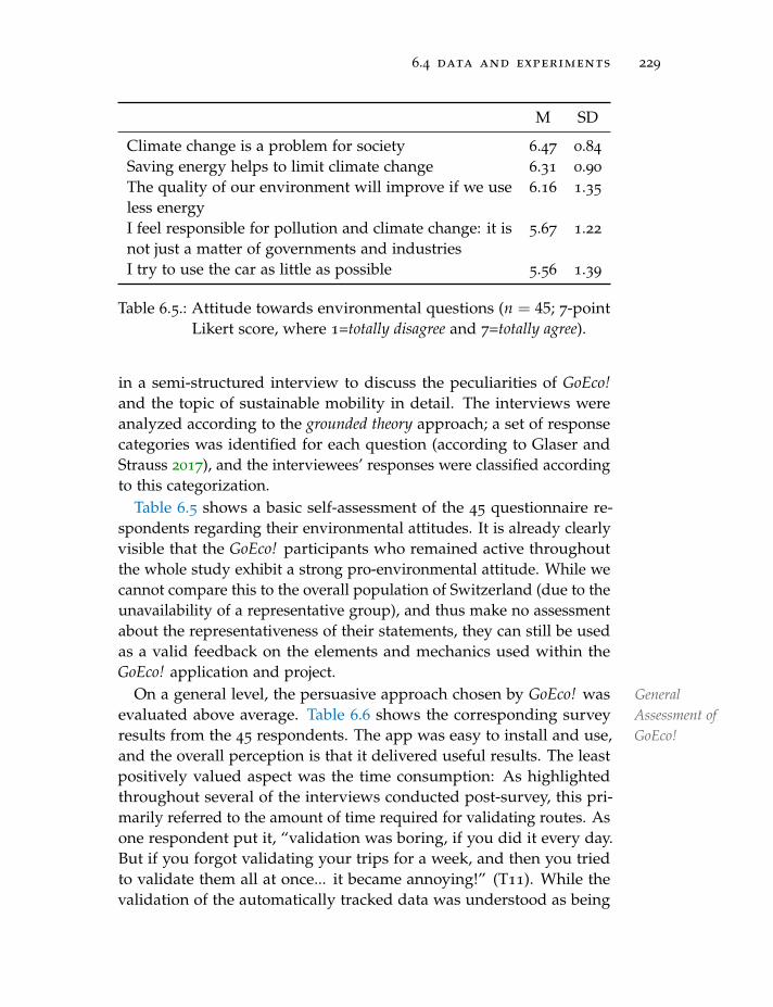
6.4 data and experiments 229
M SD
Climate change is a problem for society 6.47 0.84
Saving energy helps to limit climate change 6.31 0.90
The quality of our environment will improve if we useless energy
6.16 1.35
I feel responsible for pollution and climate change: it isnot just a matter of governments and industries
5.67 1.22
I try to use the car as little as possible 5.56 1.39
Table 6.5.: Attitude towards environmental questions (n = 45; 7-pointLikert score, where 1=totally disagree and 7=totally agree).
in a semi-structured interview to discuss the peculiarities of GoEco!and the topic of sustainable mobility in detail. The interviews wereanalyzed according to the grounded theory approach; a set of responsecategories was identified for each question (according to Glaser andStrauss 2017), and the interviewees’ responses were classified accordingto this categorization.
Table 6.5 shows a basic self-assessment of the 45 questionnaire re-spondents regarding their environmental attitudes. It is already clearlyvisible that the GoEco! participants who remained active throughoutthe whole study exhibit a strong pro-environmental attitude. While wecannot compare this to the overall population of Switzerland (due to theunavailability of a representative group), and thus make no assessmentabout the representativeness of their statements, they can still be usedas a valid feedback on the elements and mechanics used within theGoEco! application and project.
On GeneralAssessment ofGoEco!
a general level, the persuasive approach chosen by GoEco! wasevaluated above average. Table 6.6 shows the corresponding surveyresults from the 45 respondents. The app was easy to install and use,and the overall perception is that it delivered useful results. The leastpositively valued aspect was the time consumption: As highlightedthroughout several of the interviews conducted post-survey, this pri-marily referred to the amount of time required for validating routes. Asone respondent put it, “validation was boring, if you did it every day.But if you forgot validating your trips for a week, and then you triedto validate them all at once... it became annoying!” (T11). While thevalidation of the automatically tracked data was understood as being
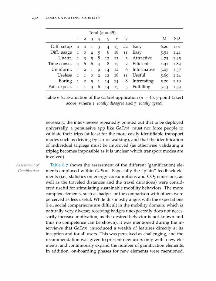
230 communicating mobility
Total (n = 45)1 2 3 4 5 6 7 M SD
Diff. setup 0 0 1 3 4 15 22 Easy 6.20 1.01
Diff. usage 1 0 4 5 6 18 11 Easy 5.51 1.41
Unattr. 1 3 5 8 12 13 3 Attractive 4.73 1.45
Time-consu. 4 6 6 4 8 15 2 Efficient 4.31 1.83
Uninform. 1 2 1 9 14 12 6 Informative 5.07 1.37
Useless 1 1 0 2 12 18 11 Useful 5.69 1.24
Boring 1 2 5 1 14 14 8 Interesting 5.20 1.50
Fail. expect. 1 1 3 6 14 15 5 Fulfilling 5.13 1.33
Table 6.6.: Evaluation of the GoEco! application (n = 45; 7-point Likertscore, where 1=totally disagree and 7=totally agree).
necessary, the interviewees repeatedly pointed out that to be deployeduniversally, a persuasive app like GoEco! must not force people tovalidate their trips (at least for the more easily identifiable transportmodes such as driving by car or walking), and that the identificationof individual triplegs must be improved (as otherwise validating atripleg becomes impossible as it is unclear which transport modes areinvolved).
Table 6.7Assessment ofGamification
shows the assessment of the different (gamification) ele-ments employed within GoEco!. Especially the “plain” feedback ele-ments (i.e., statistics on energy consumptions and CO2 emissions, aswell as the traveled distances and the travel durations) were consid-ered useful for stimulating sustainable mobility behaviors. The morecomplex elements, such as badges or the comparison with others wereperceived as less useful. While this mostly aligns with the expectations(i.e., social comparisons are difficult in the mobility domain, which isnaturally very diverse; receiving badges unexpectedly does not neces-sarily increase motivation, as the desired behavior is not known andthus no competence can be shown), it was mentioned during the in-terviews that GoEco! introduced a wealth of features directly at itsinception and for all users. This was perceived as challenging, and therecommendation was given to present new users only with a few ele-ments, and continuously expand the number of gamification elements.In addition, on-boarding phases for new elements were mentioned,
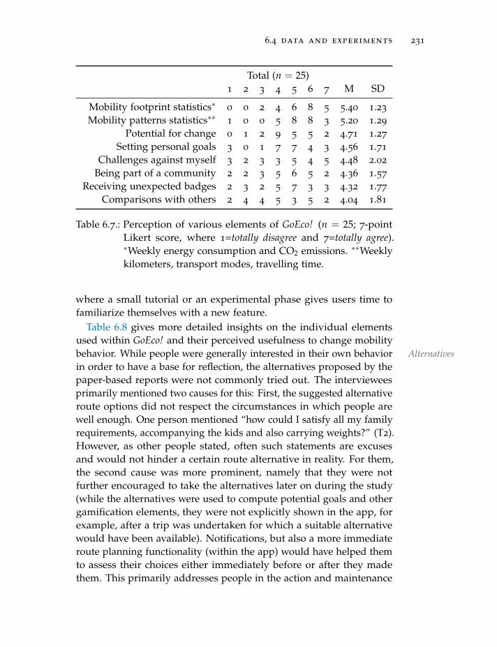
6.4 data and experiments 231
Total (n = 25)1 2 3 4 5 6 7 M SD
Mobility footprint statistics∗ 0 0 2 4 6 8 5 5.40 1.23
Mobility patterns statistics∗∗ 1 0 0 5 8 8 3 5.20 1.29
Potential for change 0 1 2 9 5 5 2 4.71 1.27
Setting personal goals 3 0 1 7 7 4 3 4.56 1.71
Challenges against myself 3 2 3 3 5 4 5 4.48 2.02
Being part of a community 2 2 3 5 6 5 2 4.36 1.57
Receiving unexpected badges 2 3 2 5 7 3 3 4.32 1.77
Comparisons with others 2 4 4 5 3 5 2 4.04 1.81
Table 6.7.: Perception of various elements of GoEco! (n = 25; 7-pointLikert score, where 1=totally disagree and 7=totally agree).∗Weekly energy consumption and CO2 emissions. ∗∗Weeklykilometers, transport modes, travelling time.
where a small tutorial or an experimental phase gives users time tofamiliarize themselves with a new feature.
Table 6.8 gives more detailed insights on the individual elementsused within GoEco! and their perceived usefulness to change mobilitybehavior. While Alternativespeople were generally interested in their own behaviorin order to have a base for reflection, the alternatives proposed by thepaper-based reports were not commonly tried out. The intervieweesprimarily mentioned two causes for this: First, the suggested alternativeroute options did not respect the circumstances in which people arewell enough. One person mentioned “how could I satisfy all my familyrequirements, accompanying the kids and also carrying weights?” (T2).However, as other people stated, often such statements are excusesand would not hinder a certain route alternative in reality. For them,the second cause was more prominent, namely that they were notfurther encouraged to take the alternatives later on during the study(while the alternatives were used to compute potential goals and othergamification elements, they were not explicitly shown in the app, forexample, after a trip was undertaken for which a suitable alternativewould have been available). Notifications, but also a more immediateroute planning functionality (within the app) would have helped themto assess their choices either immediately before or after they madethem. This primarily addresses people in the action and maintenance

232 communicating mobility
stages of the TTM, indicating that many of them either were motivatedto make their behavior more sustainable already before participating inGoEco!, or that GoEco! managed to successfully guide them through theprecontemplation and contemplation stages.
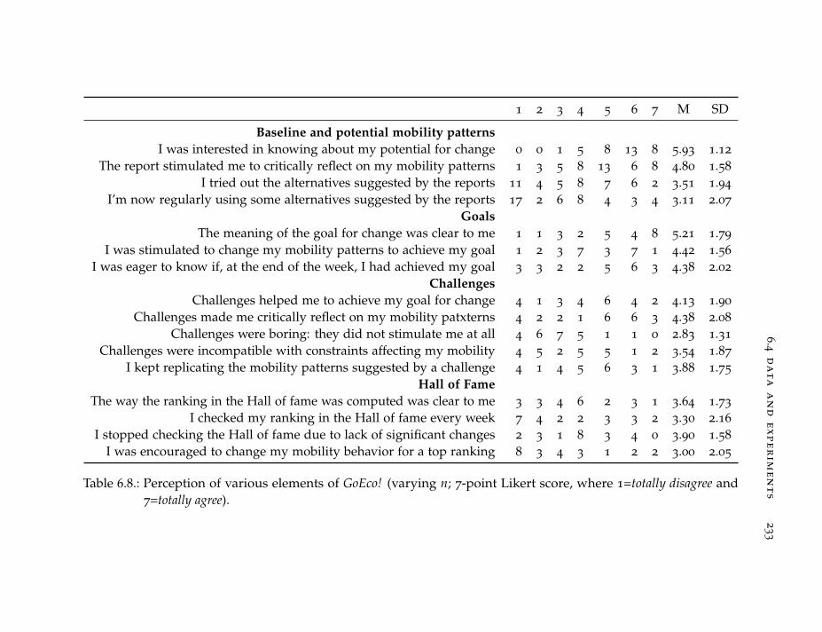
6.4
da
ta
an
de
xp
er
im
en
ts
23
3
1 2 3 4 5 6 7 M SD
Baseline and potential mobility patternsI was interested in knowing about my potential for change 0 0 1 5 8 13 8 5.93 1.12
The report stimulated me to critically reflect on my mobility patterns 1 3 5 8 13 6 8 4.80 1.58
I tried out the alternatives suggested by the reports 11 4 5 8 7 6 2 3.51 1.94
I’m now regularly using some alternatives suggested by the reports 17 2 6 8 4 3 4 3.11 2.07
GoalsThe meaning of the goal for change was clear to me 1 1 3 2 5 4 8 5.21 1.79
I was stimulated to change my mobility patterns to achieve my goal 1 2 3 7 3 7 1 4.42 1.56
I was eager to know if, at the end of the week, I had achieved my goal 3 3 2 2 5 6 3 4.38 2.02
ChallengesChallenges helped me to achieve my goal for change 4 1 3 4 6 4 2 4.13 1.90
Challenges made me critically reflect on my mobility patxterns 4 2 2 1 6 6 3 4.38 2.08
Challenges were boring: they did not stimulate me at all 4 6 7 5 1 1 0 2.83 1.31
Challenges were incompatible with constraints affecting my mobility 4 5 2 5 5 1 2 3.54 1.87
I kept replicating the mobility patterns suggested by a challenge 4 1 4 5 6 3 1 3.88 1.75
Hall of FameThe way the ranking in the Hall of fame was computed was clear to me 3 3 4 6 2 3 1 3.64 1.73
I checked my ranking in the Hall of fame every week 7 4 2 2 3 3 2 3.30 2.16
I stopped checking the Hall of fame due to lack of significant changes 2 3 1 8 3 4 0 3.90 1.58
I was encouraged to change my mobility behavior for a top ranking 8 3 4 3 1 2 2 3.00 2.05
Table 6.8.: Perception of various elements of GoEco! (varying n; 7-point Likert score, where 1=totally disagree and7=totally agree).
234 communicating mobility
WhileGoals goals were generally understood by the participants, their help-fulness in reaching a certain desirable behavior was disputed. Aroundone third of the survey respondents stated that goals stimulated themto change their mobility patterns, while for the others the effects wereless prominent. During the interviews, it became clear that goals were“quickly getting boring” (Z2) as they were not personalized enough (thesuggested goals were always chosen from a pool of relatively generictemplates, and primarily personalized in terms of the suggested desir-able behavior). Challenges were similarly assessed, and their usefulnesswas mainly seen in helping critically reflect previous behavior. A largeissue posed itself with the incompatibility of challenges with variousconstraints (a similar criticism as was mentioned with respect to thesuggested alternatives). As such, even though challenges were notperceived as boring, in the majority of cases they did not lead to alasting behavior change. The interview responses similarly indicatedthat the challenges were not personalized enough, i.e., sampling themfrom a pool of relatively generic challenges did not lead to enoughdiversity and thus reduced the interest in challenges in the long run.For example, one interviewee mentioned that she “could not increase[her] bicycle use anymore; [she] should [thus] not have been shownbicycle-related challenges”. Next to an increased personalization, it wasalso mentioned that an improved notification system (that for examplesends messages when a challenge is almost completed) could increasethe motivation generated by challenges. Along the same line, reframingchallenges in terms of the benefits (“do that, you save ten minutes”instead of “do that, it is a challenge”) would have made it clearer thatthe challenges actually lead to the desired behavior.
DuringNumericalRepresenta-
tions
the interviews, it was also highlighted that while the eco-feedback was generally perceived useful, its presentation as a collectionof numbers expressing CO2 emissions and energy usage in kWh wasdifficult to understand. A range of suggestions was given, such as to“back kWh up with gasoline liters” (T10), “relate tonnes of CO2 withother activities we are used to perform at home—for example, whatabout providing us with the amount of corresponding washing machinecycles?” (T1), “thanks to your use of the bicycle today, x liters of oil havenot been consumed” (T5), or “the CO2 emissions you saved are equal toy trees being planted” (T10). Additionally, feedback in terms of healthbenefits or monetary impact was mentioned as a useful addition—often, sustainable behavior correlates well with positive changes of
6.4 data and experiments 235
these measures, which can provide additional strong incentives to usemobility in a sustainable way. Summarizing the insights from theinterviews, it is difficult to grasp one’s environmental impact solelyfrom CO2 emission and energy usage numbers. While we explicitlychose this approach to give people autonomy in their interpretation ofthe tracked values, they mentioned that they optimally “would haveliked to receive some ’red/green light’ indications” (Z1), simply tomore quickly understand their behavior and not have to spend toomuch time manually assessing it.
When Badgesasked about badges, the interviewees generally respondedwith low interest. It was mentioned that they could be made moretangible by associating rewards such as planting trees somewhere inthe world with them: “I would like to get a badge notifying me I havecontributed to saving a certain amount of CO2 emissions and that asa reward a number of trees will be planted somewhere in the world”(T10). This would not only increase their perceived value, but alsoframe them in a collective (instead of individual) setting. Similarly, theinterviewees expressed a low interest in individual rewards (such asthe prizes awarded for the successful validation of routes), which mightbe explained by the fact that many GoEco! participants were alreadyintrinsically motivated, progressed beyond the precontemplation andcontemplation stages, and thus did not feel the need to be incentivizedby external motivators. As such, we cannot univocally state that re-wards do not work within persuasive applications: as previous researchreports, it is likely that especially for people in earlier stages of thebehavior change process and in less economically strong contexts eco-nomic rewards might help on-boarding them and providing incentivesuntil internal motivation is built.
As SocialComparisons
the final element assessed in the surveys, the social comparisonsgiven by the hall of fame were not perceived as particularly useful.The primary reason was the lack of dynamism, i.e., the leaderboardremained mostly constant throughout the study, and thus did not cap-ture interest by the participants. The suggested improvements vary:One interviewee responded that users should be ranked by “who savedmore petrol in absolute values over the week” (T5), which was contra-dicted by others as “if I am used to travel 4000 km by car every month,and I win a car-reducing challenge, are my efforts lower, higher or thesame as people travelling 400 km by car every month, and winning thesame trophy? If other people start from more favourable conditions
236 communicating mobility
than mine, but we are rewarded with the same trophy, we are rankedequally in the leaderboard. I perceive this as unfair and soon loseinterest in it” (T6). Summarizing, it can be stated that while the socialcomparison approach chosen by GoEco! tried to respect the differentcontexts by letting users choose from a set of challenges that were triedto be universally achievable, this was not well-enough communicatedand the participants were mostly confused by the hall of fame function-ality (which commonly operates on easily understandable numericalquantifications, such as points). Instead, and indicated by the intervie-wees, the social elements within a mobility behavior change applicationshould rather focus on community-building, e.g., by providing featuresthat allow interacting with other app users, sharing achievements on so-cial networks or with friends, collaborative (or competitive) challenges,more game-like challenges (“who travels furthest with an e-bike?” (Z7)),competitions among teams, or within corporate settings (similar to the“bike to work” challenge in Switzerland3).
6.5 chapter summary
In this chapter, we looked at the question of how to best communicateeco-feedback to people and how to best use persuasive smartphoneapps within the context of sustainable mobility. Based upon a taxonomyof motivational affordances for persuasive and gamified systems, webuilt the GoEco! app, which was employed within a large-scale studyspanning one year. Using the app led to a significant reduction inGHG emissions stemming from regularly traveled trips for people livingin more rural areas. However, likely due to the many (uncontrolled)influencing factors and potentially due to a lack of easily comprehen-sible goals when making mobility choices, no significant reductionswere found for people living in cities and/or for a persons’ mobilityconsidered as a whole. Several surveys and interviews pointed outstrengths and weaknesses of the GoEco! app, such as the well-workingtracking and transport mode identification or the sometimes discour-aging representation of all sustainability indicators as numbers, whichmade them difficult to understand and interpret.
3 Teams participating in www.biketowork.ch have to record the number of kilometerstraveled by bicycle to work. Prizes are drawn at the end of the competition for allteams who cycled to work on at least 50% of all days.
7D I S C U S S I O N
In this chapter, we will discuss the introduced methods and algorithmsin light of the research questions posed in chapter 1. Following thestructure of the previous chapters, we will first restate the overarchingresearch question and compare our methods and results to previouswork, followed by a discussion of their relevance and the potentialimpacts on the mobility behavior of people. The chapter concludeswith a systemic view (relating back to the first research question), acomparison to similar persuasive applications, and a discussion of thelimitations uncovered during this research.
7.1 analyzing mobility
RQ2: What are the components and traits of automatically recorded movementdata that can be used to support mobility needs in an ecologically sustainableway (e.g., by providing eco-feedback that people can base their future decisionsupon)?
In Comparisonto PreviousWork
chapter 4, we presented methods to process trajectory data withthe aim of creating applications that support people in sustainablepersonal mobility. In contrast to a substantial share of research onmobility analysis, we assume that detailed trajectories are collectedusing a GNSS, and do not consider call record data (utilizing cell phonetowers to locate people) or (paper-based) mobility surveys (cf. Smoreda,Olteanu-Raimond, and Couronne 2013). While it would be possible touse these less accurate resp. different data sources (e.g., using mobilitysurveys, researchers have the possibility to ask more detailed questionsabout each performed trip), we argue that the prevalence and ubiquityof smartphones (with built-in GNSS tracking and large batteries enablingcontinuous location recording) will foster a continuous shift towardshigh-accuracy data collection. Recording mobility at high levels ofdetail allows assessing individual differences and preferences betterand thus increasingly tailoring persuasive applications to individuals(whereas call record data and mobility surveys are commonly used to
237
238 discussion
study mobility behavior of a whole population or a larger study sample,e.g., Gonzalez, Hidalgo, and Barabasi 2008; Alessandretti et al. 2018;Pappalardo et al. 2015). Indeed, we know of several countries and citiesthat have been evaluating the suitability of smartphone tracking toeither replace or at least support the traditional phone- or paper-basedmobility census data collection. In addition, a range of small companiesstarted to sell products that enable automatic data collection at low costand effort (these applications can usually be used without any customintegration, whereas they simply record mobility, or within a largerapplication context using a Software Development Kit (SDK))1.
The presented data abstractions and methods to analyze mobilitydata contain two preprocessing steps that are of special interest for high-accuracy mobility data and of particular importance for the subsequentsteps. First, the segmentation procedures are usually not required forpaper-based surveys (and to a different extent for call record data), asthe collected data come in a segmented form already. Second, mapmatching is important for GPS traces that are already available at ahigh level of accuracy, as it allows to further increase the reliabilityof measurements (for lower-accuracy trajectories, one usually resortsto routing instead). For less accurate data sources, a reconstructionusing data from other people or the underlying transport graph canbe performed (e.g., Li, Gao, et al. 2019), but just as often the Euclideandistance (resp. jump length) is used, in particular if the researchaims at comparing relative differences between different trips (e.g.,Gonzalez, Hidalgo, and Barabasi 2008). Considering that we mostlyrely on higher-level abstractions (staypoints and triplegs) for the furtherprocessing of mobility data, one has to ask whether GNSS data comeat an unnecessarily high level of detail. This discussion tightly linksto privacy considerations, where we might only want to store the bareminimum of information required to provide meaningful feedback to aperson (cf. Giannotti and Pedreschi 2008). However, as we have seen,not only does accurate location data provide us with very fine-grainedmobility descriptors, it also lets us make better use of geographicalcontext, e.g., to infer the transport modes by considering PT stops alonga trajectory. In combination with the increased ease of use of locationtracking SDKs, the recent focus of large smartphone Operating System(OS) manufacturers on clearly highlighting the potential privacy risks
1 As examples, consider the MotionTag application (motion-tag.com) or the POSMOapplication (datamap.io).
7.1 analyzing mobility 239
of various tracking applications, and novel (exploratory) data sharingconcepts (e.g., data cooperatives, where people self-host their data andgive selective access to third-party applications or service providers),we are convinced that for many purposes high-detail location trackingwill be the standard in the future. To alleviate privacy issues, systemdevelopers should adhere to the fair information practices (Wachowiczet al. 2008): limiting the data collection to necessary information, keepdata only as long as required, specify the purpose of data collection,limit its use to a predefined purpose, safeguard it appropriately, informpeople about the stored data (upon request), and be accountable foradhering to these principles.
The TrajectoryAlgebra
introduced trajectory algebra to add contextual information totracking data can be seen as a combination resp. advancement of theconcepts of map algebra (Tomlin 1990; Tomlin 2017) and lifeline contextoperators (Laube, Dennis, et al. 2007). In contrast to classical mapalgebra that works on (temporally invariant) raster data, and the lifelinecontext operators that work by summarizing properties of the mobilitydata themselves, the combination of the two allows specifying the wayscontext data interact with mobility data in a standardized way (and thusensures transferability, quick exploratory iterations when designingnew context features, and potentially user-friendly implementationsdirectly within a GIS). As with every abstraction, there are certain casesthat cannot well be handled by it. For example, the trajectory algebraprimarily targets contextual data in a raster format (which is availableat every point in space, in contrast to vector data that is only availableat discrete locations), and while its usefulness for vector datasets is notdisputed (as also highlighted by the exampe given in Figure 4.7), thecorresponding specification would have to be expanded substantially,in particular when considering non-point vector data (such as othertrajectories, or areas resp. polygons) or operations such as retrieving thek nearest neighbors. One can imagine scenarios where context shouldbe retrieved from other mobility data, e.g., similarity measures couldbe used to automatically assign contextual data based on semanticallyor geometrically similar trajectories (cf. Janowicz, Raubal, and Kuhn2011), or context values could be integrated along the area a trajectorypasses through.
Extracting TransportModeIdentification
mobility features and augmenting trajectories with con-textual data enables the application of transport mode identification(and similarly, activity purpose imputation, cf. Martin, Bucher, Suel,
240 discussion
et al. 2018) models to further enhance the data. In the case of thetransport mode identification model presented in subsection 4.1.5 andevaluated in subsection 4.5.1, we can clearly see that the inclusion ofmobility-related context features leads to performance gains in themodel outputs (in particular regarding the PT modes). Comparing thisto similar models, the accuracy of roughly 85% is in line with other re-search that solely relies on mobility descriptors and contextual features(and not more fine-grained data as provided by accelerometers, Blue-tooth sensors, etc.). For example, Zheng, Liu, et al. 2008 compare fourinference models (Decision Tree, Bayesian Net, Support Vector Machineand Conditional Random Field) based on the GeoLife trajectories andfind that walking, driving by car, bus or bicycle can be distinguishedwith an accuracy of 74%. More recent work by Stenneth et al. 2011
reaches 93.5% based on features such as the average accuracy, speed,heading change, acceleration and geospatial context (distances to busand rail lines). Currently, researchers evaluate the suitability of neuralnetworks for transport mode inference, e.g., Dabiri and Heaslip 2018
use an approach based on convolutional neural networks (reaching anaccuracy of 84.4%) that has the benefit that features do not need to beengineered explicitly. Our method differs in that we use a PT router toassess whether a given PT alternative would have been available at thetime of travel, thus giving us the chance of integrating potential delaysand deviations from the regular schedule in PT. However, the increasedcomplexity of having to employ a PT router specifically for transportmode inference could also be seen as a drawback of our approach,as it not only necessitates a larger and more complex overall system,but also leads to longer inference times. In addition, our method wasdeveloped with a specific use case in mind (and evaluated within theGoEco! project, cf. Bucher, Cellina, et al. 2016): To infer transport modesfrom tracking data of unreliable quality (in our case, recorded usingthe third-party app Moves), to be able to differentiate between a largenumber of transport modes, and as input to a further validation step bythe users themselves (that in turn can be used to continuously retrainthe model). All the transport mode inference models (only relyingon location and context data) usually also benefit from a combinationwith models that additionally process the raw sensor data recordedby a smartphone. For example, Jahangiri and Rakha 2015 and Fanget al. 2017 both use machine learning approaches on sets of featuresincluding accelerometer and gyrocsope data, and reach accuracies of
7.1 analyzing mobility 241
approx. 95% in differentiating between standing still, walking, running,cycling and traveling in a vehicle. However, and as was the case forGoEco!, such data might not readily be available, as the complexity ofcollecting, storing and processing of this data is more complex andoften not provided by location tracking SDKs.
Summarizing MobilityHistories
mobility in terms of distances covered, durations spenttraveling, modal splits and activity aggregates is performed with theaim of supporting sustainable mobility behaviors resp. highlightingwhich choices and trips are responsible for the largest shares of negativeenvironmental impacts. In contrast to other mobility descriptors, as forexample introduced by Laube, Dennis, et al. 2007 (who mention speed,acceleration, azimuth, sinuosity, navigational displacement, approach-ing rate, and derivatives and standard deviations thereof) these valuesare all tightly linked to sustainability as defined in chapter 2 and 4 andare easily understandable also when given as feedback to non-experts.Other metrics such as the radius of gyration, jump length, or frequentlyvisited places (cf. Gonzalez, Hidalgo, and Barabasi 2008; Alessandrettiet al. 2018) are primarily valuable to study mobility patterns of a popu-lation, and are similarly valuable for experts who understand their exactmeaning and the laws they follow. However, as shown in section 4.5,there are still valuable insights for researchers and experts studyinga certain sample to be gained from the introduced mobility descrip-tors. Within the SBB Green Class project, the temporal development ofmodal splits was one of the main points of study, as it enabled gaininginsights on the usage of a MAAS offer over the duration of a year, andin particular highlighted that people behave more sustainable becauseof it. As such and in line with the survey responses given as part ofthe GoEco! dissemination activities (cf. chapter 6), we argue that toenable self-reflection on mobility behavior and to provide a basis forgamification elements, the extracted mobility histories are useful.
After Sustainabilitythe mobility descriptors have been extracted, and the respectivetransport modes are known, it is important to assess the sustainabilityof different trips (with regards to personal contexts and the relatedfinancial and personal gains) in order to give people meaningful feed-back. For example, many people do not have the possibility to workfrom home (though the recent Covid-19 crisis has shown that in manycases this is also an artificial restriction), and as such suggesting toavoid work-related trips is not meaningful for them as they couldnot realistically implement this behavior. The presented sustainability
242 discussion
metrics are based on GHG emission data from mobility and transport(Prillwitz and Barr 2011; Lane 2019; Boulouchos et al. 2017), as wellas on human capital theory (cf. Becker 1993), and try to balance thenecessity of performing a trip with its ecological impacts (given thelimited information available from tracking data). Due to the fact thatthe offsetting costs (of GHG emissions from mobility) only correspondto a small share of the overall mobility costs, and (usually) the overallcosts are only a small share of the financial and personal gains acquiredby performing the trip, we have to carefully consider if we want tosupport people from a point of view of weak or strong sustainability(where strong sustainability argues that no gain in human capital canmake up for a loss in natural capital, thus all GHG emissions should beavoided). In most previous work revolving around using persuasiveapplications to support sustainable mobility, this topic is not explicitlytreated, and instead a concept of strong sustainability is implicitly as-sumed, under which people are always recommended to avoid tripsresp. reduce GHG emissions. The work presented in this disserta-tion allows us to fine-tune support of sustainable behaviors better bychoosing from various strategies to compute route alternatives and todetermine when a given trip should be considered sustainable andwhen not. Holden 2012 provides an interesting discussion regardingthe topic, and formulates the requirements for sustainable mobility asfollows: Sustainable mobility 1) must not threaten long-term ecologicalsustainability, 2) it must ensure that basic mobility needs are satisfied(e.g., everyone must be able to get to work and to access vital services),and 3) inter- and intra-generational mobility equity must be promoted(i.e., everyone must have access to the same minimum level of mobility).Our dissemination of sustainability under various interpretations fitswell with the first and second points: While we have to ensure thatlong-term ecological sustainability is given, we still have to considerthat satisfying basic mobility needs is a requirement for everyone, andthus we should adopt our support of sustainable behaviors to primarilytarget those trips that are non-essential or for which meaningful andeasily accessible alternatives are available.
While adopting strong sustainability is a practicable approach (that iseasy to adopt and works under the assumption that people will balanceecological impacts with potential gains on their own), having moreinformation about which trip should potentially be avoided and whichis necessary allows an application to provide more selective feedback
7.1 analyzing mobility 243
and thus be more meaningful to its users. As the concluding surveysof the GoEco! study have shown, the participants thought it useful toknow about potential alternatives and were willing to implement themas well (cf. chapter 6).
It needs to be noted that the computations of the financial andsocial/personal capital gains as presented within this dissertation repre-sent a limited model. While basing the financial gains on the salary of aperson is a valid approximation under the assumption that a salary is anunbiased estimator of a person’s contribution towards an economy (i.e.,towards the generation of value), it is easily understandable that thethus generated value is not uniformly distributed across all times (andthus across all trips) and that the salary does not manage to captureall aspects of a person’s contribution to society (the current Covid-19
crisis highlights the importance of “essential workers” which often havelow salaries yet are indispensable within a society). As such, a muchmore fine-grained evaluation would be necessary—this, however, isdifficult to estimate from tracking data alone as the exact reasons fortravel are usually unknown (e.g., we do not know if someone has togo to work for an important meeting that generates substantial busi-ness or societal value or simply to do administrative work). Similarly,while the proposed measure for social/personal gains tries to incor-porate social equity (i.e., balance differences between rich and poor),it assumes that leisure-bound activities are necessarily “out-of-home”,which is clearly violated by many people being happy to spend theirleisure time in close vicinity of their homes and thus not consumingmobility as part of it (especially given the current Covid-19 situationwhere many people were even forced to stay at home). However, andwith the same reasoning, the proposed measure essentially gives everyindividual a “mobility budget” for leisure, and thus can be seen as afirst step into a fair assessment of the amount of GHG emissions thatshould be considered acceptable for leisure activities. Finally, bothmeasures are difficult to interpret in the case of multi-purpose or evenmulti-day activities (e.g., traveling somewhere by plane for a holiday).In the first case, we always associate the trip leading up to the activitywith the activity itself, which might distort the actual GHG emissionsapportioned to different activity purposes (e.g., if someone visits a gymclose to work before heading there, the potentially longer trip to thegym is associated with a leisure purpose, and the shorter trip from thegym to work is associated with the work purpose). In the second case,
244 discussion
a separate assessment for sub-trips should be made for a more accurateestimation, and in particular the airplane trips should not only considerthe first activity after reaching the destination, but all activities untilthe person flies back again.
SystematicEV Choice mobility forms a substantial part of our total mobility, andsupport of sustainable behaviors (resp. the provision of eco-friendlyalternative routes) for these parts of our mobility is generally regardedas positive and important as changes in those behaviors lead to long-term and impactful results (as the behavior is repeatedly and habituallyperformed). Inducing behavior change for these behaviors is difficultwithout external support, however (as we mostly rely on habits andusually do not re-evaluate systematically performed trips on a regularbasis; cf. Froehlich, Dillahunt, et al. 2009b; Cellina, Bucher, Veiga Simao,et al. 2019), for which reason it makes sense for a persuasive applicationto specifically treat systematic mobility. The presented identificationof commonly visited places and the associated tours was found to beworking well, as shown in Table 6.4. Of large interest for discussion isthe mode choice model presented in subsection 4.3.2 (that uses a uniquesample of persons who have access to both an ICE car as well as anEV). As presented in chapter 3, several studies highlighted the variousreasons people are still reluctant to completely adopt EVs. Amongthese are high prices, reduced ecological friendliness (due to the highefficiency of ICEs, the high energy costs of producing batteries, and thecharging of vehicles using coal and gas power) or the requirement fora (personal) charging station, but we also find that many people areworried that an EV might only cover a certain share of their mobilityneeds, and that they would require an ICE car to cover the rest (inparticular, long journeys). Assessing this question, we found that thechoices can indeed be better explained if we know how a person haschosen before (i.e., people tend to use the EV for a “typical” set of trips).However, if we do not know anything about a person before, predictingthe choices almost attributes to a random guess. This also implies thatwe cannot make a general statement about whether an EV would leadto the dreaded situations in which its range is not sufficient withoutknowing more about the mobility choices of a person beforehand. Thisfinding is in line with previous research as presented in chapter 3:While range anxiety is often brought up as a crucial argument whenbuying an EV (cf. Noel et al. 2019), in practice most of the trips are so
7.1 analyzing mobility 245
short that this does not play a role in the actual decision (Saxena et al.2015; Franke and Krems 2013; Rauh, Franke, and Krems 2015).
Finally BehaviorChange
, we showed several approaches to extract behavior changesresp. classify different behaviors based on tracking data. Several stud-ies looked at behavior (changes) from the perspective of visited placesresp. using proxies such as the radius of gyration or the jump length(Gonzalez, Hidalgo, and Barabasi 2008; Alessandretti et al. 2018). Whilethese measures allow us to assess the mobility behavior of a populationas a whole, they are less interesting from the perspective of a persuasiveapplication, as they can vary greatly from one week to another and arenot necessarily suitable to make statements about the sustainability ofa behavior (esp. in the case of looking at changes in visited places).However, searching for anomalies in these descriptors is a step towardsextracting information useful for persuasive applications, and is essen-tially the basis for the introduced methods. The method introducedin subsection 4.4.1 looks for such deviations from the norm in a num-ber of features and then provides the sum of found anomalies to thedeveloper of a persuasive application (note that these deviations canalso be detected in regular behavior as introduced in subsection 4.3.1,where they primarily stem from changes in transport modes). Theapproaches that group people either based on the autocorrelations oftheir traveled distances and the related durations, or on the trends ofvarious features, on the other hand, provide the application creatorwith a number of groups of people that should be supported differentlyby the application. As is often the case when detecting anomalies, theprocess of responding to the respective anomaly is thus not handledby the approaches presented in this dissertation. However, we canimagine cases in which this support could be automated as well: If abehavioral anomaly is detected in one week, and a user thus switchesfrom a group of ICE car users to a group of bicycle users, an applicationcould focus on bicycle-related challenges in the coming week, in orderto support resp. solidify this choice. On the other hand, a switch inthe opposite direction could be supplemented by educational measuressuch as highlighting the adverse effects of car trips on the environment.
Putting Relevance ofResults
the presented methods and results of chapter 4 into a biggerperspective, the interviews and surveys performed within the GoEco!project and various feedbacks received during the SBB Green Classproject demonstrated that the presented information is useful for people(both app users as well as system creators resp. the decision-makers
246 discussion
who were in charge of the SBB Green Class project), and generallythe raw position data were processed in meaningful and correct ways(cf. chapter 6). While the extracted information was used for theplanning algorithms and communication strategies in chapter 5 and 6,in particular the integration of the extracted behavior (changes) intopersuasive applications is yet an unsolved problem. The directionsgiven in this dissertation should be used as a basis for further researchon automatically adapting persuasive elements to the momentary statusof behavior change.
7.2 planning mobility
RQ3: How can we facilitate multi-modal route planning involving less com-monly used modes of transport (such as carpooling or free-floating bicycles)?How can we assess the quality of the (potential) fulfillment of a transport need,taking into account personal preferences, contexts and potential sustainabilitygoals?
InComparisonto Previous
Work
chapter 5, we provided a set of route planning methods that can beused to generate alternatives for previously exhibited behavior, and usethem as direct feedback to application users as well as to assess poten-tials for change. Our methods particularly focus on personalizationand context-dependence using heuristics (e.g., defined by an expert, theuser herself, or extracted from previously tracked mobility) and proba-bilities computed based on previous behavior, and less commonly usedmodes such as carpooling. We argue that personalization will becomesubstantially more important in the future, as it can further decrease thecognitive efforts required to plan routes (cf. Raubal and Panov 2009). Inaddition, personalization integrates well with persuasive applicationsthat intend to support people in sustainable choices whenever they arewithin the constraints exhibited by previous behavior.
The presented formalization of mobility offers (section 5.1) is an alter-native to commonly used specifications such as GTFS or the Open APIfor distributed journey planning (Comite Europeen de Normalisation2017). Naturally, these standards also include a wealth of informationnot necessary for our abstracted use cases (e.g., the names of stationsor railway operators), which would be required within a real-worlddeployment and to reach the vision of a Digital Earth (Guo et al. 1998).Such a complete digital representation of our planet would not only
7.2 planning mobility 247
simplify the accessibility and increase the usefulness of transport offersfor route planning, but could also be used to automatically extractknowledge, e.g., to determine the similarity between different trans-port modes or route plans (cf. Janowicz and Hitzler 2012). Currently,however, these standards usually solely encode a time-expanded graphin textual form. While we have shown in section 5.2 that it is possibleto transform carpooling offers into the same format in order to reuseexisting planning applications, the proposed high-level transport offerspecification provides a stronger abstraction that allows integrating awider range of transport modes more easily, and retains the flexibility(e.g., a bus-on-demand can drive small detours if requested by a passen-ger) and fuzzyness (e.g., for free-floating bicycles there are no specificreturn locations and they can be dropped off anywhere within an area)inherent in many of them. Specifying transport offers according to thisspecification presented in section 5.1 primarily enables us to create high-level route plans that require later refinement (taking into considerationactual departure times, potential delays, etc.). However, we argue thatthis follows a natural way of how people plan their trips as well (Carand Frank 1994)—first, we look at potential high-level tripleg chainsthat get us to our destination, evaluate if they conform with our per-sonal mobility preferences, and only then consider the actual transportschedules and involved partners. In addition, the introduced transportoffer specification is able to handle area-based transport modes such ascarpooling, taxis, free floating bicycles and cars or buses-on-demand bygenerating flexible transport graphs (meaning that people can transferbetween the same two transport modes at different locations).
The IntegratingPT and CP
method to combine carpooling offers with PT offers presented insection 5.2 advances the state of the art by merging the two transportgraphs while retaining their inherent flexibility (i.e., the fact that carpooldrivers can make detours and slightly advance or delay their departures)and fuzziness (i.e., the fact that carpooling route plans are usually onlyspecified in very coarse terms), resulting in a better connectivity ofboth the CP as well as the PT graphs. In contrast to previous workwhich focused mostly on replacing a single PT tripleg with a viableCP alternative (Varone and Aissat 2015; Aissat and Varone 2015; Bit-Monnot et al. 2013), the introduced approach automatically finds thebest possible CP alternative for any part of the journey. While therestriction on a maximum of one CP tripleg (from the perspective ofthe driver, i.e., the driver can only pick up a single passenger along the
248 discussion
whole trip; this is introduced to avoid re-computations of the departuretimes in the graph) is in line with how CP is commonly used, furtherresearch is still required to incorporate multiple (smaller) CP segments,especially with regards to more ad-hoc planning of shorter CP trips.Similarly, while the chosen graph-expansion (as opposed to havinga time-dependent graph) allows utilizing existing graph algorithmsand optimizations, it commonly leads to very large graphs. This couldbecome problematic when integrating numerous different transportmodes, and it should be further explored how to keep the graph sizewithin bounds, e.g., by continuously removing obsolete CP and PT offersand adding upcoming ones. Finally, it needs to be noted that mostbenefits from short-distance carpooling only start to appear when a lotof offers are available (as otherwise it simply will not be possible tofind anyone to carpool with). This will require integration of differentplatforms and substantially lower barriers to publish carpooling offers(e.g., applications could pro-actively suggest upcoming drives thatcould be shared with someone else).
InHeuristic andProbabilistic
Methods
line with existing research on time geography, it would be interest-ing to see how concepts from this research field could be used to boundthe number of nodes that need to be processed as part of a routing al-gorithm. For example, while accessibility is commonly used to quantifythe usefulness of a transportation system, a similar approach could beused to limit the reachable locations and thus reduce the required com-putations during a routing process (Miller and Wu 2000). This is notonly important when considering the DTAs (that correspond to potentialpath spaces), but also for the high-level routing methods presentedin subsection 5.4.1 and 5.4.2. While the focus of these methods is seton personalization (and to some degree, sustainability), the involvedcomputational constructs have many parallels to concepts from timegeography and navigation research (Miller 1991; Raubal, Winter, et al.2007). For example, future research should consider using the upperbounds given by network and space-time prisms to limit the numberof transfer locations that a person could realistically visit, and thuspotentially substantially decrease computation time.
Notwithstanding such a line of research, the proposed routing meth-ods are largely orthogonal to previous research. Exceptions are algo-rithms like RAPTOR (Delling, Pajor, and Werneck 2014) which similarlyfollow PT lines to retrieve all stops at which transfers are potentiallyavailable (in the case of RAPTOR, the primary reason is to use arrays
7.2 planning mobility 249
and their specific memory layout on a hard disk to speed up computa-tions). However, in contrast to these algorithms, the presented methodsallow incorporating a wide range of different transport modes andenable personalization by integrating mobility metrics retrieved fromtracking data. The resulting routes are of a high-level nature, and thusneed to be refined in a second step. It is an unsolved question how tofind a good balance in the tradeoff between yielding such high-levelroute plans and subsequent refinement steps (e.g., one could specifythe transfer graphs on an hourly basis, and thus lower the computa-tional complexity and false positives returned by the high-level routingalgorithm). In addition, the preferences and constraints introduced aspart of the heuristic method in subsection 5.4.1 are manually defined inchapter 5 (cf. appendix A). Retrieving them automatically (in a similarmanner to the preferences in subsection 5.4.2) would greatly enhancethe usefulness of the heuristic routing algorithm, as it could similarly“learn” from tracking data and mobility histories.
The preference-based planning method of subsection 5.4.2 uses fea-ture distributions modeled using parameter-free functions as describedin subsection 5.3.2. This allows integrating new features without know-ing about the exact distributions, and automatically using them aspreference values for the routing algorithm. In contrast to previousresearch, we thus have a very flexible way of generating personalizedroutes that is also not bound to a specific transport mode (a large shareof previous work concerns the personalization of car or bicycle trips,for example; cf. Stinson and Bhat 2005; Menghini et al. 2010; Vedel,Jacobsen, and Skov-Petersen 2017). However, the flexibility given bythe approach (e.g., when a person is walking somewhere, essentially allother transfer locations are reachable, albeit with a very low probability)can quickly lead to an exhaustive number of nodes to be visited. Whilechoosing bounds on the probabilities can mitigate these problems, itshould be further explored how to sort the nodes according to thelikelihood of being visited. For example, a spatial index may be usedto only process nodes that exceed a minimum visit likelihood (in thecase of a quad tree (Finkel and Bentley 1974), only the immediate resp.neighboring cells could be visited for walking transfers).
While Real-worldDeployment
all the introduced methods have been shown to work for thepresented case studies, some points deserve further attention beforea real-world deployment would be possible. First of all, we did notconsider in detail how we can ensure that the data used for route
250 discussion
planning is kept up to date. In more classical route planning appli-cations, this data only changes infrequently (e.g., the road networkonly expands slowly and train schedules are known many months inadvance). Many of the introduced transport modalities exhibit a highunpredictability: Ridesharing offers constantly change, free-floatingvehicles continuously need to update their pickup locations, etc. Due tothe focus on high-level plans (which in turn usually lead to routes withonly a few hops) we can greatly alleviate the efforts required to updatethe routing graphs, and only locally recompute potential transfers fromone mode to another. Nonetheless, the resulting graphs can quicklybecome highly connected, thus inducing a high computational loadthat leads to the second point that needs to be considered before areal-world deployment becomes possible: low system response times.The case study implementations exhibited response times in the orderof seconds and were not optimized in particular, however, the extentsthey spanned were comparably small. A real-world (and world-wide)deployment would likely lead to much larger query times, as mostof the vertices are more highly connected, leading to many more (po-tential) paths to a destination that need to be evaluated. A possibleoptimization (similar to how optimized street network routing works)is the utilization of hierarchies in the routing graph, where trips by cer-tain modes are restricted to smaller areas (e.g., for walking, where it isunlikely that someone walks for dozens of kilometers), in combinationwith summary nodes that essentially group a large number of nodes(e.g., in a certain geographic region) into a single one and thus can beevaluated a lot more quickly. Conceptually, these optimizations arecompatible with the introduced methods, but further evaluations arerequired to determine their potential efficiency gains and impacts onthe routing schemes.
TheRelevance ofResults
presented methods are particularly useful within the contextof supporting sustainable personal mobility, as they target intermodaluse of mobility (which is often a preferrable alternative to ICE carsand lets people reach locations that are otherwise only reachable bya personal vehicle). Additionally, the focus on less commonly usedmodes of transport (such as CP or free-floating bicycles) will enablerouting providers to include them into their planners, and thus make iteasier to find the corresponding route options. Regarding persuasiveapplications supporting sustainable mobility behaviors, especially thepersonalization and context-dependence is beneficial, as it allows us
7.3 communicating mobility 251
to provide custom-tailored feedback to each individual (e.g., routealternatives that match personal preferences) and allows assessing thepotential for change more realistically.
7.3 communicating mobility
RQ4: How should transport options and choices be communicated to usersto support sustainable mobility behavior? Do people adjust their mobilitybehavior upon receiving (eco-)feedback based on their previous choices?
In Comparisonto PreviousWork
chapter 6, we presented ways to communicate the previously identi-fied mobility histories and descriptors as well as the generated routealternatives to users of persuasive and gamified (smartphone) apps.Several other research studies presented prototypes for the mobilitydomain (inspired by other gamified systems, e.g., online communityplatforms or fitness applications) with different foci such as generallyfostering sustainable mobility, or promoting cycling or the use of PT (Bieet al. 2012; Froehlich, Dillahunt, et al. 2009b; Carreras et al. 2012). Ourwork is grounded in psychological research and thus revolves aroundsix core design principles, each adhering to several specific traits ofhuman motivation. Based on this, we make a distinction between threemain pillars: eco-feedback, which is of a more educational nature,gamification, which uses game elements to foster playful interactionswith the app, and an assessment of the potential for change, based onrouting alternatives retrieved by algorithms as presented in chapter 5.While (paper-based) eco-feedback is probably the easiest and most com-monly used method to foster mobility behavior changes, the systematictreatment of gamification elements (within the context of mobility), aswell as the foundation of them in a mobility assessment (as given by thepotential for change) are setting the work presented in this dissertationapart from previous studies.
The MotivationalAffordances
presented taxonomy of motivational affordances for persuasiveand gamified (smartphone) applications is based on the mentionedgeneral design principles and adds mechanics and concrete elements(how to implement mechanics within an application context) on top.While other research has studied the usefulness of gamified systems ina wide range of contexts, our taxonomy lets system designers chooseappropriate elements easily. For example, in the mobility domain,point-based competitive systems are mostly unsuitable as mobility is
252 discussion
highly individual and comparisons between different users are difficult.Remedy can be given by grouping people into classes with similarcircumstances, but this is usually difficult to unambiguously identifyfrom tracking data alone. In addition, point-based systems tend tofoster behavior that maximizes the number of points, and thus couldpotentially lead to people traveling actually more in order to receivemore points. However, and as the GoEco! experiment has shown,people like competitive settings within the context of apps that supportbehavior change. As such, studying how competitions can be madefair within a mobility setting, and how people can be grouped withothers exhibiting similar potentials and circumstances should be afocus of future research. Alternatively, gamification elements thatcombine competitive and cooperative mechanics should be examined ingreater detail (and in particular within the context of persuasive appssupporting them).
Further, among the feedback of GoEco! users it was often found thatthe timeliness of feedback is crucial. If route alternatives are giventoo far in advance or feedback with a too large delay, they lose theireffectiveness. Similar findings were reported by Fogg 2002, and pointinto a direction of future research that studies the impact of timely noti-fications on mobility choices (e.g., by detecting when someone leavesthe house, predicting where the person will likely go, and pro-activelysuggesting route options). Along the same line, deeper integrationwith LBS would be beneficial—among the mentioned functionalities byGoEco! participants were tools to analyze and plan mobility alternativesor to compute economic and health impacts, but we could also imaginea deeper integration with personal planners respecting spatio-temporalconstraints (Raubal, Miller, and Bridwell 2004). Finally, while the possi-bility for app users to set their own goals and choose challenges wasgenerally appreciated (as it adheres to the need for autonomy), themonotony of goals and challenges was criticized. Generating suchgamified elements based on previous behavior a user exhibited wouldincrease their attractiveness and thus ensure a long-term involvement ofpeople. For example, if the system often finds bicycle alternatives for acertain person, suggesting challenges that focus on using the bicycle orsetting a goal of a minimum number of kilometers traveled by bicyclewould make them more meaningful.
RegardingGamificationin GoEco!
the implementation of elements, the approaches chosenin GoEco! were generally liked by its users. In contrast to related
7.3 communicating mobility 253
research, we set a focus on supporting user choice resp. autonomy, andthus presenting most information as-is. While the idea was to fosteran understanding of what different values for energy usage or CO2
emissions mean (to enable people thinking about the respective unitsas they do about distance or weight measures), this proved to be notsufficiently tangible for many people to foster change. Instead, theapproaches chosen by other persuasive apps (cf. Jylha et al. 2013; Bieet al. 2012; Froehlich, Dillahunt, et al. 2009b) where GHG emissions andecological impacts are represented using visual elements (e.g., a treethat loses leaves or an iceberg that melts) were mentioned as preferable.This points at the fact that for many people, energy usage and GHG
emissions are intangible units, and we argue that future research shouldconsider how to make people get a better understanding of these units.For example, comparisons to household activities such as runninga washing machine, comparisons to commonly performed activities(such as taking a domestic flight), or comparisons to known measures(e.g., the average CO2 emissions per kilometer of an ICE car) should beincluded and tested for their effectiveness in educating people aboutthe impacts of different choices.
The presented one-year study GoEco!, involving initially approx. 600
people, was used to evaluate the proposed gamification concepts (andthe extraction of mobility metrics and generation of route alternativesthat they are based upon). It proved to be notoriously difficult to keepsuch a large sample motivated to interact with the app over the durationof one year (note that there were three tracking periods within thisone year). In line with general numbers on app usage (cf. Guerrouj,Azad, and Rigby 2015; Sigg et al. 2019), this is to be expected though (inparticular if the participants are not contractually bound to participatein the study until the end and do not receive any financial incentives fordoing so). The chosen “living lab” approach led to a wealth of insights,not only about the impacts of a persuasive app like GoEco!, but alsoabout the interest of various groups in the population to participate insuch a research experiment, how well the developed algorithms workin practice, and on the differences between research and setting up sucha project as a startup company.
Regarding Sample Biasthe interest in the population, we found that those peoplewho participated until the end were primarily people who alreadytravel in ecological ways and/or are interested in the topics of sustain-ability, energy use, and research in general. This highlights a potential
254 discussion
bias towards eco-friendly people that was partially confirmed for thepartition of the sample living in the more urban region of Zurich bycomparison to the SMC. In the rural area Ticino (where also significantchanges in mobility behavior after the GoEco! intervention were found),the average daily kilometers traveled and the average share of kilome-ters traveled by car correspond well to the SMC, indicating that thisshare of the study sample is more representative. As such, we concludethat in more rural areas a persuasive app like GoEco! shows largereffects than in a city like Zurich, where the self-selection bias is largerand people already travel in more sustainable ways. The responses ofpeople given to the questions about their pro-environmental attitudes(Table 6.5) further confirm potential biases in the study sample, andpoint out research directions resp. strategies to involve people who arenot already strongly intrinsically motivated. For example, providingmore extrinsic rewards and directly recruiting participants who areknown to travel often by car (e.g., via car ownership lists) could bestrategies to attract a more diverse user base. External incentives likefinancial payments can then still be reduced after an initial onboardingperiod to examine the longer-term effects resp. potentially generatedintrinsic motivation (that makes people keep using the app). Regardingsolely the analysis of potential outcomes, it is also possible to alleviatethe impacts of a biased sample by rebalancing it according to a knowndistribution, e.g., the demographics of a country (which are usuallyknown from the census) (Stephan 1942). This approach was, for exam-ple, used to compare the SBB Green Class data with data from the SwissMobility Census (SMC) (Martin, Becker, et al. 2019).
LookingMethodAssessment
at the evaluation of the various algorithms used withinGoEco!, the tables in subsection 6.4.5 highlight that the provided el-ements were generally seen as valid and useful. However, and asdiscussed before, even though this was the case, the timeliness of feed-back was often not given, and thus at the time of making a travelchoice, support or incentives were missing. This primarily points to thedirection of providing more real-time support, and thus also processingdata in real-time, in particular with respect to recognizing situationsin which a person will likely need to make a mobility choice andpro-actively nudging him or her into a sustainable direction. Such aprovision of real-time support would require predicting movementsand mobility choices of people, finding potential transport options,and communicating them in an unobtrusive (and potentially gamified)
7.3 communicating mobility 255
way to the user immediately. For example, in the case of determiningwhen CP would be a viable option to travel somewhere, this wouldinvolve matching a driver with a rider without any specific interactionswith them. For both the driver as well as the potential passenger, aprediction of the traveled path would have to be made, they would haveto be analyzed with regards to their similarity (i.e., the potential for thedriver to pick up the passenger and drop him or her off at the predicteddestination), and a negotiation process would have to be started (wherethey both see the CP option and potentially financial and ecologicalcosts and gains). As such a system would benefit from many peopleparticipating, Big Data (and mainly streaming) technologies should beconsidered to handle the real-time processing of large amounts of data(cf. Hitzler and Janowicz 2013; Tschumperlin, Bucher, and Schito 2018;Galic, Meskovic, and Osmanovic 2017).
GoEco! has also highlighted the differences between creating a persua-sive app as a research project or within a company. The original goal ofkeeping 800 participants over the duration of a year was not achieved,which was partially due to the aforementioned “usual” drop outs whenlaunching a new app (Sigg et al. 2019), but also due to technical issues,the requirements given by a research project (e.g., different study pe-riods, required validations to keep data quality high, or the controlgroup that did not get the full app but only a tracking version), and astrong focus on assessing if a persuasive app can have an impact on themobility behavior of people. The last point also prevented continuousadaption of the app or starting with a smaller set of functions andgradually adding more (which is commonly done when developinga commercial application). As such, in order to keep an experimentwith 800 people running over a whole year (where people are expectedto interact with a system on a daily basis) would likely require largefinancial incentives or the flexibility to deviate from the original planand exclude research activities.
Comparing GoEco! to other studies evaluating persuasive apps stillpoints out its uniqueness, though. Most studies in the domain ei-ther consider only a small sample or let the experiments run only fora few weeks (cf. Cellina, Bucher, Mangili, et al. 2019). In addition,many of these projects either evaluate the outcomes solely qualitatively(Froehlich, Dillahunt, et al. 2009b) or not in relation to sustainability(Jylha et al. 2013), or use other means to collect data and give feedbackto people (such as web-based surveys and feedbacks). In that respect,
256 discussion
the results of GoEco! are unique and show that persuasive applicationsthat make use of automatically and passively tracked mobility data canwork in settings where people naturally have room for improvement(with regards to sustainable mobility).
AsRelevance ofResults
the evaluation of the GoEco! project has shown, the deployment ofa persuasive application to influence mobility behavior can lead to GHG
emission savings in the order of 10-30% (cf. Table 6.1, 6.2, 6.3, as well asCellina, Bucher, Mangili, et al. 2019). While this cannot make mobilitycompletely sustainable in itself, the result is in agreement with the oftenused argument that reaching sustainability requires a large numberof smaller changes. This is because it is not possible to immediatelyswitch to completely sustainable technology, yet changes should happenfast in order to keep up with the sustainable development goals setby the United Nations (cf. UN Department of Economic and SocialAffairs 2020). Many of these changes involve gradual switches todifferent technologies, e.g., by subsidizing photovoltaic installationswhich could contribute to mobility provided by EVs if they are chargedat the workplace during the day (Buffat, Bucher, and Raubal 2018).Other changes are strongly related to behavior, such as switching toelectric bicycles for commuter mobility (Bucher, Buffat, et al. 2019). Thiswould likely also entail the provision of the respective infrastructure,i.e., “bicycle highways” leading from suburbs to the city center. Suchchanges could not only be supported by the respective subsidies, butalso by laws, and last but not least by persuasive apps as presentedwithin this dissertation.
7.4 a systemic view
RQ1: What are the principal information processes and structures involvedin supporting sustainable personal mobility and Mobility as a Service (MAAS)?
LookingComparisonto Previous
Work
at the proposed framework in its entirety, we can see par-allels to the systems used in other persuasive studies such as Ubi-Green (Froehlich, Dillahunt, et al. 2009b), tripzoom (Bie et al. 2012),or SUPERHUB (Carreras et al. 2012). Next to providing a frameworkencompassing the steps required to process tracking data to generateinformation useful for persuasive applications, in contrast to these, weput a stronger emphasis on the importance of founding the appliedmeasures in psychological theories, and (related to that) strive for per-
7.4 a systemic view 257
sonalized and meaningful elements within the applications. While theresults were generally approved by the study participants of GoEco!, thementioned aspects of supporting closer to “real-time” (i.e., at the actualpoint of time at which a mobility decision is made) and even in morepersonalized ways deserve further discussion. The first could benefitfrom a mobility prediction component that was not included in the pre-sented framework. Such a component could allow estimating when andwith which transport mode an upcoming trip will be performed, andthus notifying the person about potential alternatives shortly before. Awide range of research is concerned with such next place resp. trajectoryprediction (Bucher 2017), and the corresponding methods often rely onsimilar assessments of personal preferences and previous choices todetermine likely future choices. The second point of more closely align-ing motivational elements with previously exhibited behavior could beachieved by mapping the detected behaviors to the individual stagesof behavior change, and generating challenges and goals more closelyin alignment with the identified potentials for change. For example, ifwe detect that someone could often take the bicycle to reach his or heractivity locations, the corresponding challenges should be created, andin particular for those routes for which the bicycle was found to be aviable alternative.
Persuasive (Non-technological)Ways ofReachingSustainableMobility
applications are not the only way to make mobility moreenvironmentally sustainable. We can differentiate between four waysto change the mobility demands of people:
• Soft Incentives (as exemplified by the persuasive applicationsdiscussed within this dissertation). Targeting the choices that aremade before a certain trip is performed, soft measures aim atconvincing or nudging people into adopting certain behaviors.They are grounded in the theories of motivation presented in thisdissertation and mainly use knowledge about attitudes, previousbehaviors, context and circumstances to persuade people to adoptsustainable behaviors. Taking the example of GoEco!, we can seethat for systematic trips (e.g., commutes) reductions of approx.30% (cf. Table 6.3 and Cellina, Bucher, Mangili, et al. 2019) arepossible using such measures (corresponding to roughly 10% ofthe total environmental impact of mobility).
• Emerging Business Models. Ultimately caused by the increas-ing pressure to make mobility more sustainable, novel business
258 discussion
models such as micro-mobility, Mobility as a Service (MAAS) orvarious sharing schemes change the ways in which we use mobil-ity, and thus the demands for different transport modes. Takingthe example of the MAAS offer SBB Green Class, we can see thatsuch business models can lead to a reduction in GHG emissions.In this case, the offer including unlimited access to PT, varioussharing schemes and the provision of a compact-class EV led toan overall reduction of GHG emissions by approx. 30% (Martin,Becker, et al. 2019).
• Policy Measures. Laws and subsidies are steering mechanismsthat work well in practice but require agreement by citizens andthus a long time to be implemented. Often these “hard” incentivesare supported by educational measures and other soft incentivesto create acceptance within a population. In this context, mobilityis often embedded in a larger system of energy producers andconsumers, and thus laws and subsidies may be put in place thatsupport mobility in indirect ways. For example, a recent study byBuffat, Bucher, and Raubal 2018 found that a wide deployment ofphotovoltaic cells on people’s homes (e.g., fostered by subsidies)can lead to a reduction of GHG emissions in the order of 26% ofthe total commuter mobility GHG emissions (corresponding toapprox. 5% of the total mobility GHG emissions).
• The (Built) Environment. Finally, changes to the built environ-ment can shift mobility demands, for example, due to adjustmentsin availability of alternative transport modes, but also due to theperceived effects of a route on health, safety or comfort (Pritchard,Bucher, and Frøyen 2019). A promising example is the construc-tion of “bicycle highways” which facilitate access from suburbsto city centers. A study by Bucher, Buffat, et al. 2019 found thatroughly 44% of the commuter GHG emissions could be saved ifpeople would switch to electric bicycles for their commutes (corre-sponding to approx. 8% of the total GHG emissions by mobility).
The four discussed measures are of increasing difficulty (and thus timerequirements) for implementation. For example, while deploying anapplication like GoEco! can be done comparably quickly, changing thebuilt environment (and building new transport infrastructure) usuallytakes time in the order of decades. Naturally, all these measures run in

7.4 a systemic view 259
parallel to technical advances that continuously improve the efficiencyof our transport systems. However, it is often argued that especially inthe short term, soft incentives, new business models, and policies arerequired to keep the impact of mobility on our environment bounded.

8C O N C L U S I O N
In this chapter, we summarize our work, state our contributions andgive an outlook on potential future research avenues as identified aspart of the presented dissertation.
8.1 summary
This dissertation presents a framework for ICT supporting sustainablepersonal mobility via persuasive applications. Starting from automat-ically and passively recorded location data, we develop methods toextract mobility histories, related preferences and behaviors (resp. thechanges thereof). Building upon these structures, an assessment ofpotentially improved behaviors can be made, and suggestions on howto use a wide range of transport modes (intermodally) to decrease one’spersonal environmental impacts can be evaluated. Finally, we elaborateon the different forms of interaction between a (gamified) persuasiveapplication and its user with the aim of nudging the person into thedirection of more sustainable mobility choices. The effects and the ap-plicability of the methods presented are examined using two large-scalemobility studies: GoEco!, which in essence incorporates the methodsdeveloped within this dissertation, and SBB Green Class that studies theimpact of a MAAS offer on people’s mobility, with a particular focus onthe changed environmental impacts.
In ICT
SupportingSustainablePersonalMobility
chapter 2, we provide a general introduction to the topics ofsustainable mobility and how persuasive applications have to respectindividual contexts and circumstances in order to create meaningfulsupport of different mobility behaviors. We exemplify this by showingthat different groups of people commonly use mobility in differentways, depending on their access to both mobility itself but also to otherinfrastructure (e.g., for leisure activities or work). Even though it is im-possible to exactly determine the circumstances and influencing factorsfor all trips based on tracking data alone, using such spatio-temporalcontext can help an application (or its developer) to favor one persua-sive strategy over another. Looking at sustainability in particular, it
261
262 conclusion
additionally becomes crucial to define what should be considered as anacceptable environmental impact for a given activity. We distinguishbetween the two extremes of strong and weak sustainability, where ei-ther all trips producing GHG should be avoided, or only those whose(economic or social/personal) gains fall behind the “environmentalcost”. Along the same lines, we should differentiate between trips forwhich a reasonable alternative would be available, and those for whichthe chosen route was the only option. Considering this, integratedmobility and MAAS gain in importance, as they can let people usemobility in ways more closely tailored to their actual needs (e.g., con-stantly having commoditized access to both a car and the PT networklets people choose for each trip individually which option suits thembest). We conclude the chapter by giving a high-level perspective onthe information processes involved in supporting sustainable mobilityusing persuasive applications that sets the frame for answering thefirst research question. The later chapters fill in the presented buildingblocks in order to present a comprehensive framework for persuasiveapplications supporting sustainable mobility.
InBackground chapter 3, we start by providing an extensive review on the underly-ing psychological theories that drive human behavior. For a persuasiveapplication to meaningfully support a person in his or her choices, itis important to know in which state of behavior change the person is,and how we commonly progress in order to achieve a new behavior.For example, people who are unaware of the consequences of a certainbehavior are best supported by educative measures and comparing theirbehavior to other people in similar circumstances. During later stages,e.g., when trying out a new behavior, persuasive applications shoulddecrease the efforts required to continuously exhibit the behavior. Thiscan be done by pro-actively suggesting route alternatives or offeringsimple mechanisms to plan and evaluate various route options. Evenlater stages require motivational elements that keep a user engagedwith a certain behavior (such as gamification elements) until a (new)habit is formed. In this chapter, we also provide background on thethree main information processes involved in supporting sustainablebehaviors via persuasive applications: the processing and analysis ofmovement and mobility data, planning personalized (and thus mean-ingful) alternatives, and creating feedback out of the previous twoprocesses that helps people choosing sustainable mobility options. The
8.1 summary 263
subsequent chapters build upon this background and contribute tofilling the identified research gaps.
In MobilityAnalysis
chapter 4, we elaborate on the most crucial information whentrying to assess the sustainability of trips and create information thatis useful in supporting people in environmentally friendly behaviors.Next to basic mobility descriptors, this includes the inference of usedtransport modes, assessments of the environmental impacts in compari-son to the financial or social/personal gains, as well as the extractionof regularly exhibited patterns and mobility choice preferences. Thelatter are exemplified by a choice model quantifying the predictabilityof choices between ICE cars and EVs. This choice is becoming moreprevalent with the increasing availability of EVs and their droppingprices, but the continuing reluctance for their adoption due to rangeanxiety resp. fears that they cannot face one’s personal mobility needs.Our findings include that even though the choices of each individualexhibit predictability, this cannot be generalized to a population (givendemographic properties of the persons and descriptive features of eachtrip), and the choices appear random instead. This suggests that inthe overall perspective, practically all trips can be covered by an EV,and issues like the range anxiety do not play a role once an EV is avail-able. Finally, we propose several methods to extract groups of peopleexhibiting similar behaviors as well as changes in behavior, both ofwhich can be used by persuasive applications to tailor the employedsupportive mechanisms. These identified components and traits ofautomatically recorded movement data are of high importance whensupporting behavioral transitions towards sustainable mobility.
In MobilityPlanning
chapter 5, we provide a generalized abstraction to define point-and area-based transport offers, thus covering a large number of cur-rently available transport modes for their integration into high-levelroute planners. The benefits of such high-level planners is facilitatedpersonalization by simple adjustments of the planning graphs or restric-tions on the rules evaluated during computation. This is exemplified bytwo route computation methods: One uses heuristic rules (that can bechosen based on an expert’s assessment or by analyzing the past choicesof a person) to limit the available options and generated route plans,while the other computes routes based on probabilities computed fromprevious choices as recorded by a tracking application. Both can beused to directly compute meaningful route options for a given person(by corresponding to previously exhibited behavior), but also to com-
264 conclusion
pute sustainable alternatives (e.g., by providing more stringent ruleson the allowed GHG emissions or by using the preferences of people insimilar situations who exhibit generally lower GHG emissions due totheir mobility choices). To elaborate on the benefits of inter-modalityresp. integrated mobility, we introduce a method that allows combiningcarpooling offers with PT, thus improving both networks in terms ofconnectivity. The presented methods focus on personalization and theintegration of less commonly used transport modes in an inter-modalway, thus paving the way for more comprehensive and meaningfulestimations of potential route alternatives.
InCommunicat-ing Mobility
chapter 6 we present a taxonomy of motivational affordances forpersuasive and gamified technologies that was used to choose the ele-ments implemented within the GoEco! app. Due to the differences givenby the individual contexts and circumstances, persuasive applicationsfor supporting sustainable mobility cannot rely on motivational resp.gamified elements in the same way as applications in other fields do.For example, point-based systems usually assume “equal chances” foreveryone, and are thus difficult to employ in the mobility field withoutdiscouraging certain groups of people. The employed gamified motiva-tional elements as well as the more plain “eco-feedback” are evaluatedwithin the GoEco! project and are found to be helpful in supportingbehavior change. GoEco! highlighted that behavior change using suchan application is possible, albeit we only found significant changes inmore rural areas (where people naturally have to rely more on carsand show less “pro-environmental” attitudes). Among the importantfeatures were the provision of timely assistance, personalized and non-generic motivational elements, as well as eco-feedback giving users thechance to learn something about their own behavior. This chapter thusanswers how transport options and choices should be communicated tousers to support sustainable mobility behaviors, and that people indeedexhibit changes in their behavior after interacting with a persuasiveapplication.
8.2 contributions
Foremost, we presented a framework for supporting sustainable mobil-ity through persuasive ICT that encompasses all processes required togenerate meaningful eco-feedback (and related behavioral support inthe form of mobility alternatives and gamified elements) from passively
8.2 contributions 265
recorded mobility data. Within this framework, we highlighted threeareas and presented novel processing methods, approaches to generateroute plans, as well as ways to communicate the generated informationpersuasively to users:
• In the area of mobility analysis and processing, we presented a tra-jectory algebra to standardize the addition of context to mobilitydata and a related range of mobility descriptors useful for eco-feedback. Based on this context and descriptions of mobility, wepresented a Bayesian model to infer transport modes that utilizesspatio-temporal data and is able to continuously improve indi-vidual predictions for all users. To exemplify the importance ofmobility choices and to provide insights on the important choicebetween ICE cars and EVs, we presented a mode choice modeland discussed the impacts of applying the model to the datarecorded by the SBB Green Class study. Finally, we presentedseveral methods to detect mobility behavior change and discussedtheir integration in and importance for persuasive applications.
• In the area of planning integrated and sustainable mobility, we intro-duced a generalized description of mobility offers (that can beused for point- and area-based modes of transport), and threemethods to compute route alternatives. The first one emphasizedon carpooling as a potential way to increase the occupancy rateof cars and provided an integration with PT networks. The re-sults showed both an increased connectivity for the CP and the PT
networks, highlighting the potential benefits of a combination ofthe two. The other approaches focused on the utilization of per-sonal preferences and constraints to generate high-level mobilityplans. Such plans can be used to assess potential alternatives (andtheir sustainability), as feedback for people and (in combinationwith lower-level routes) to generate route plans involving a largenumber of (previously unavailable) transport modes.
• In the area of communicating mobility (eco-)feedback, we presented ataxonomy of motivational affordances for persuasive applicationsand the synopsis of recorded mobility data within eco-feedbackreports. The dissemination of the large-scale study GoEco! showedthe applicability of the persuasive approaches (and related meth-ods and algorithms) presented in this dissertation. We found
266 conclusion
that in particular in (rural) areas where people naturally relymore on their personal cars, applications like GoEco! can showsignificant effects in the mobility behavior of people. Among theprimary features of interest are real-time notifications (to supportsustainable behaviors immediately when the choice needs to bemade), the provision of alternative routes, as well as the inclusionof non-generic gamification elements to support motivation.
Embedded within the larger framework, the presented methods andapproaches provide a way to process mobility data with the aim ofsupporting sustainable mobility using persuasive applications and ICT.
8.3 towards optimal support of sustainable personal mo-bility
As can be seen from Figure 2.9, from a holistic perspective two largeparts on optimal support of sustainable personal mobility are missing.First, the provision of alternatives requires knowing about potentialtransport offers that could satisfy the needs of a person. While wegave concrete examples for cases in which these offers are known(e.g., carpooling where we crawled the offers from a large Europeancarpooling provider, or shared bicycle/car systems which were similarlycrawled), to make such alternative-finding globally available requiresmethods to specify and process transport offers in a well-defined andflexible way (that allows incorporating a wide range of transport modes).The generalized transport offer specification presented in chapter 5 isa first step into this direction, which could be combined by usingLinked Data technology (in contrast to a rigid format like GTFS), asthis would allow embedding transport modes within a larger contextand the automatic determination of similarities in offers (e.g., a personinterested in carpooling could indicate that she needs space for luggage,and we could use information about the individual cars on offer todetermine how well they would fit her need; cf. Hitzler and Janowicz2013; Janowicz and Raubal 2007). An example of such a specificationcan be found in Bucher, Scheider, and Raubal 2017; in this case, it isused not only to specify the offers themselves, but also to automaticallyalign peoples’ transport needs in terms of luggage requirements andavailable space in cars.
8.4 future work 267
Related to the automatic publication of transport offers is the inte-gration into routing systems (and potentially systems to determinesimilarities between offers) which optimally would be supported by apublisher-subscriber system that continuously ingests updates of exist-ing offers and newly available ones and passes them along to routingapplications. For example, a carpooling platform that would like to seeits offers integrated into a general purpose routing system like GoogleMaps could publish new offers using said system, upon which GoogleMaps would continuously integrate resp. update the transport offers.This in turn either requires the computation of high-level route plansas discussed in chapter 5 or continuous updates to the routing graphs(which must be sufficiently flexible to integrate personalization resp.mode selection). Additionally, and in particular with respect to person-alizing route options, such a holistic routing system should integratecontext data, e.g., from weather or as given by the traffic status.
The second larger part that was not discussed within this dissertationis the topic of negotiation. This is primarily related to shared transportmodes such as CP, taxis, or (private) rental cars and describes all theprocesses involved in determining the sufficiency of the vehicle’s prop-erties to fulfill the transport needs, the trustworthiness of the service(resp. driver and vehicle), and the related prices. In an optimal scenario,a person with a mobility need would get transparent access to theseproperties and could book transport from within one application andwithout the need to exchange clarifying messages or financial details.Current pilot MAAS offers aim into this direction, but focus mostly onpricing and payments and thus primarily on modes of transport wherethis is highly standardized (e.g., carpooling is usually not available as atransport option).
8.4 future work
Next to the major components explained in the previous section, thisdissertation highlighted several other directions for future research.First, in particular the automatic integration of extracted behavior(changes) into persuasive applications is a largely untreated field ofresearch. While we presented potential approaches to extract behavior,and while there exists work on mobility packages (that quantify the useof transport modes in characteristic ways, e.g., taking the car for longertrips and the bicycle for shorter ones), both the automated extraction as
268 conclusion
well as the utilization of this information within persuasive applicationsshould be further investigated. For example, it is an open questionif and how transitions from one stage of the TTM to the next can beextracted from tracking data, and how an application could make useof this. We have given some examples (such as focusing on educativemeasures if no behavior changes are detected and the exhibited behavioris not in line with the desired one), and gradually increase feedbackand motivational elements with increasing detection of behavioralanomalies.
Second, in this dissertation we introduced and discussed a potentialway to generate personalized high-level mobility options. As presentedhere, these options are decoupled from temporal considerations andthus require a low-level routing system to validate the proposed options.To further increase the real-world applicability of such a system, itshould incorporate more detailed information about transport offersand make use of the given restrictions to reduce the set of availableoptions and thus the required processing power. With regards tocarpooling, many societal and psychological factors stand in the way ofa ubiquitous adoption. While we do not argue how to best overcomethose, we think that by lowering the cognitive efforts required in findinga partner could greatly increase its usefulness. Especially short-distanceand ad-hoc ridesharing requires the prediction of mobility, the findingof people traveling similar routes, and the proactive suggestion of thesepotential carpooling trips to users.
Finally, GoEco! has shown the positive effects of a persuasive applica-tion built from components as introduced in this dissertation. However,and as the dissemination surveys and interviews have shown, a biggerfocus on real-time support, personalized motivational elements and theexploration of social elements for motivation remain largely unexplored.Follow-up studies to GoEco! could try to answer the questions if it ispossible to determine the exact point in time at which a route choice ismade, and if persuasive applications could support people in certaindecisions by providing timely information and sustainable mobilityoptions. Exploring persuasive applications within smaller communitiessuch as families, companies or housing blocks could open up newavenues as it would allow not only to let people compete in familiar(and often similar) settings, but also to share modes of transport andoptimize the performed trips and activities.
AA P P E N D I X
a.1 computation of urbanization class
In the following, we describe the procedure to classify locations intoone of three classes city, suburb and rural (as used within chapter 2). Weuse two datasets for this purpose:
• The division of a country into municipalities. For each of these,the number of citizens living in the municipality, the populationdensity as well as its extent must be known.
• A classification of public transport accessibility. For the experi-ments in this dissertation, we relied on the classification by theSwiss federal office for statistics ARE (Bundesamt fur Raumen-twicklung ARE 2011), which assigns every location a class A-E,depending on its distance to PT stops and the frequency of avail-able PT offers at the respective stops (within this classification, Adenotes best connected, and E worst).
To determine locations that should be considered as city, we onlyconsider the municipalities that either have a minimum number ofcitizens living within its boundaries, or that exceed a certain populationdensity threshold. In the case of Switzerland, we used a minimumof 40’000 citizens or a minimum density of 20 people per hectare toconsider a municipality “city-like”. The combination of these twocriteria is required due to the fact that municipalities in Switzerlandhave irregular extents (as such there are small municipalities borderingcity municipalities that still have very large population densities yet asmall number of citizens). The resulting municipality boundaries arethen intersected with all the locations classified into classes A or B (bythe ARE classification), resulting in a set of locations that lie within ahighly populated area and are well-accessible by PT. We classify theselocations as city.
Similarly, we determine suburban regions as having a minimum of15’000 citizens or a minimum density of 5 people per hectare, and
269
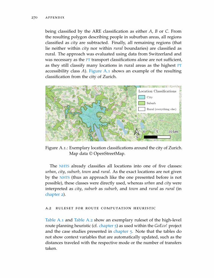
270 appendix
being classified by the ARE classification as either A, B or C. Fromthe resulting polygon describing people in suburban areas, all regionsclassified as city are subtracted. Finally, all remaining regions (thatlie neither within city nor within rural boundaries) are classified asrural. The approach was evaluated using data from Switzerland andwas necessary as the PT transport classifications alone are not sufficient,as they still classify many locations in rural areas as the highest PT
accessibility class A). Figure A.1 shows an example of the resultingclassification from the city of Zurich.
City
Suburb
Rural (everything else)
Location Classifications
Figure A.1.: Exemplary location classifications around the city of Zurich.Map data © OpenStreetMap.
The NHTS already classifies all locations into one of five classes:urban, city, suburb, town and rural. As the exact locations are not givenby the NHTS (thus an approach like the one presented before is notpossible), these classes were directly used, whereas urban and city wereinterpreted as city, suburb as suburb, and town and rural as rural (inchapter 2).
a.2 ruleset for route computation heuristic
Table A.1 and Table A.2 show an exemplary ruleset of the high-levelroute planning heuristic (cf. chapter 5) as used within the GoEco! projectand the case studies presented in chapter 5. Note that the tables donot show context variables that are automatically updated, such as thedistances traveled with the respective mode or the number of transferstaken.
A.2 ruleset for route computation heuristic 271
The ruleset also contains some factors that are in line with howpeople usually use different modes of transport and allow reducingthe solution space greatly. For example, it can be assumed that peoplewould not take the car to drive close to their destination, only to switchto a shared bicycle for the last few kilometers. To prevent these cases,we constrain the expand function in such a way that it only createstransfer locations for car journeys that are maximally half the totaldistance between origin and destination long. This does not preventthe heuristic from finding journeys such as walk→ car→ walk (wherethe car tripleg basically covers the whole distance), as these routes canstill be found in the checkReachability function.
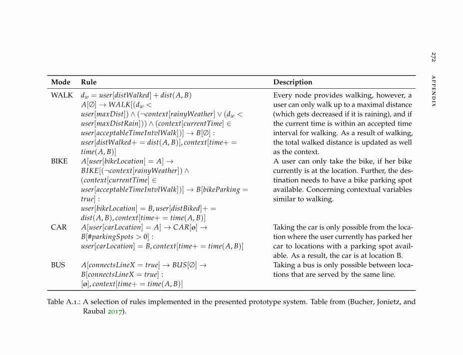
27
2a
pp
en
dix
Mode Rule Description
WALK dw = user[distWalked] + dist(A, B)A[∅]→WALK[(dw <
user[maxDist]) ∧ (¬context[rainyWeather] ∨ (dw <
user[maxDistRain])) ∧ (context[currentTime] ∈user[acceptableTimeIntvlWalk])]→ B[∅] :user[distWalked+ = dist(A, B)], context[time+ =
time(A, B)]
Every node provides walking, however, auser can only walk up to a maximal distance(which gets decreased if it is raining), and ifthe current time is within an accepted timeinterval for walking. As a result of walking,the total walked distance is updated as wellas the context.
BIKE A[user[bikeLocation] = A]→BIKE[(¬context[rainyWeather]) ∧(context[currentTime] ∈user[acceptableTimeIntvlWalk])]→ B[bikeParking =
true] :user[bikeLocation] = B, user[distBiked]+ =
dist(A, B), context[time+ = time(A, B)]
A user can only take the bike, if her bikecurrently is at the location. Further, the des-tination needs to have a bike parking spotavailable. Concerning contextual variablessimilar to walking.
CAR A[user[carLocation] = A]→ CAR[ø]→B[#parkingSpots > 0] :user[carLocation] = B, context[time+ = time(A, B)]
Taking the car is only possible from the loca-tion where the user currently has parked hercar to locations with a parking spot avail-able. As a result, the car is at location B.
BUS A[connectsLineX = true]→ BUS[∅]→B[connectsLineX = true] :[ø], context[time+ = time(A, B)]
Taking a bus is only possible between loca-tions that are served by the same line.
Table A.1.: A selection of rules implemented in the presented prototype system. Table from (Bucher, Jonietz, andRaubal 2017).
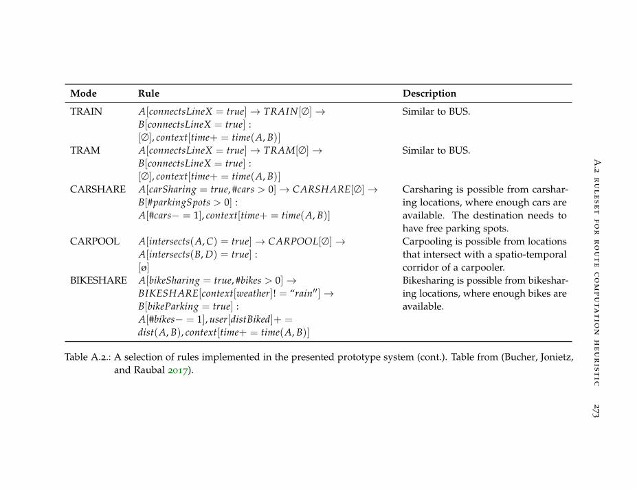
A.2
ru
le
se
tf
or
ro
ut
ec
om
pu
ta
tio
nh
eu
ris
tic
27
3
Mode Rule Description
TRAIN A[connectsLineX = true]→ TRAIN[∅]→B[connectsLineX = true] :[∅], context[time+ = time(A, B)]
Similar to BUS.
TRAM A[connectsLineX = true]→ TRAM[∅]→B[connectsLineX = true] :[∅], context[time+ = time(A, B)]
Similar to BUS.
CARSHARE A[carSharing = true, #cars > 0]→ CARSHARE[∅]→B[#parkingSpots > 0] :A[#cars− = 1], context[time+ = time(A, B)]
Carsharing is possible from carshar-ing locations, where enough cars areavailable. The destination needs tohave free parking spots.
CARPOOL A[intersects(A, C) = true]→ CARPOOL[∅]→A[intersects(B, D) = true] :[ø]
Carpooling is possible from locationsthat intersect with a spatio-temporalcorridor of a carpooler.
BIKESHARE A[bikeSharing = true, #bikes > 0]→BIKESHARE[context[weather]! = “rain′′]→B[bikeParking = true] :A[#bikes− = 1], user[distBiked]+ =
dist(A, B), context[time+ = time(A, B)]
Bikesharing is possible from bikeshar-ing locations, where enough bikes areavailable.
Table A.2.: A selection of rules implemented in the presented prototype system (cont.). Table from (Bucher, Jonietz,and Raubal 2017).

B I B L I O G R A P H Y
Abowd, Gregory D., Anind K. Dey, Peter J. Brown, Nigel Davies, MarkSmith, and Pete Steggles (1999). ”Towards a Better Understandingof Context and Context-Awareness.“ In: Handheld and UbiquitousComputing. Ed. by Hans-W. Gellersen. Lecture Notes in ComputerScience. Berlin, Heidelberg: Springer, pp. 304–307 (cit. on p. 45).
Acker, Veronique Van, Bert Van Wee, and Frank Witlox (Mar. 2010).
”When Transport Geography Meets Social Psychology: Toward aConceptual Model of Travel Behaviour.“ In: Transport Reviews 30.2,pp. 219–240 (cit. on p. 50).
Agatz, Niels, Alan Erera, Martin Savelsbergh, and Xing Wang (Dec.2012). ”Optimization for dynamic ride-sharing: A review.“ In: Euro-pean Journal of Operational Research 223.2, pp. 295–303 (cit. on pp. 59,81, 82).
Aissat, Kamel and Sacha Varone (2015). ”Carpooling as Complement toMulti-modal Transportation.“ In: Enterprise Information Systems. Ed.by Slimane Hammoudi, Leszek Maciaszek, Ernest Teniente, OlivierCamp, and Jose Cordeiro. Lecture Notes in Business InformationProcessing. Springer International Publishing, pp. 236–255 (cit. onpp. 82, 247).
Ajzen, Icek et al. (1991). ”The theory of planned behavior.“ In: Organiza-tional behavior and human decision processes 50.2, pp. 179–211 (cit. onp. 53).
Alessandretti, Laura, Piotr Sapiezynski, Vedran Sekara, Sune Lehmann,and Andrea Baronchelli (July 2018). ”Evidence for a conserved quan-tity in human mobility.“ In: Nature Human Behaviour 2.7, pp. 485–491
(cit. on pp. 74, 238, 241, 245).Allemann, Dominik and Martin Raubal (2015). ”Usage Differences
Between Bikes and E-Bikes.“ In: AGILE 2015: Geographic InformationScience as an Enabler of Smarter Cities and Communities. Ed. by FernandoBacao, Maribel Yasmina Santos, and Marco Painho. Lecture Notesin Geoinformation and Cartography. Cham: Springer InternationalPublishing, pp. 201–217 (cit. on p. 64).
Ambrosino, Daniela and Anna Sciomachen (Jan. 2014). ”An AlgorithmicFramework for Computing Shortest Routes in Urban Multimodal
275
276 bibliography
Networks with Different Criteria.“ In: Procedia - Social and BehavioralSciences 108, pp. 139–152 (cit. on p. 85).
Amirkiaee, S. Yasaman and Nicholas Evangelopoulos (May 2018). ”Whydo people rideshare? An experimental study.“ In: Transportation Re-search Part F: Traffic Psychology and Behaviour 55, pp. 9–24 (cit. onpp. 59, 60).
Anable, Jillian and Steve Wright (2013). Golden Questions and SocialMarketing Guidance Report. Tech. rep., p. 23 (cit. on p. 91).
Anagnostopoulou, Evangelia, Efthimios Bothos, Babis Magoutas, Jo-hann Schrammel, and Gregoris Mentzas (2016). ”Persuasive technolo-gies for sustainable urban mobility.“ In: arXiv preprint arXiv:1604.05957(cit. on p. 92).
Anagnostopoulou, Evangelia, Babis Magoutas, Efthimios Bothos, Jo-hann Schrammel, Rita Orji, and Gregoris Mentzas (2017). ”Exploringthe Links Between Persuasion, Personality and Mobility Types in Per-sonalized Mobility Applications.“ In: Persuasive Technology: Develop-ment and Implementation of Personalized Technologies to Change Attitudesand Behaviors. Ed. by Peter W. de Vries, Harri Oinas-Kukkonen, LisethSiemons, Nienke Beerlage-de Jong, and Lisette van Gemert-Pijnen.Lecture Notes in Computer Science. Cham: Springer InternationalPublishing, pp. 107–118 (cit. on p. 91).
Anderson, Marie Karen, Otto Anker Nielsen, and Carlo Giacomo Prato(Sept. 2017). ”Multimodal route choice models of public transportpassengers in the Greater Copenhagen Area.“ In: EURO Journal onTransportation and Logistics 6.3, pp. 221–245 (cit. on p. 54).
Angrisano, A., S. Gaglione, and C. Gioia (June 2013). ”Performanceassessment of GPS/GLONASS single point positioning in an urbanenvironment.“ In: Acta Geodaetica et Geophysica 48.2, pp. 149–161 (cit.on p. 68).
Ashbrook, D. and T. Starner (Oct. 2002). ”Learning significant loca-tions and predicting user movement with GPS.“ In: Proceedings. SixthInternational Symposium on Wearable Computers, pp. 101–108 (cit. onp. 69).
Atasoy, Bilge, Aurelie Glerum, and Michel Bierlaire (June 2013). ”Atti-tudes towards mode choice in Switzerland.“ In: disP - The PlanningReview 49.2, pp. 101–117 (cit. on pp. 13, 22).
Austin, James T. and Jeffrey B. Vancouver (1996). ”Goal constructs inpsychology: Structure, process, and content.“ In: Psychological Bulletin120.3, pp. 338–375 (cit. on p. 44).
bibliography 277
Axhausen, Kay Werner (Jan. 2007). ”Definition Of Movement and Ac-tivity For Transport Modelling.“ In: Handbook of Transport Modelling.Ed. by David A. Hensher and Kenneth J. Button. Vol. 1. EmeraldGroup Publishing Limited, pp. 329–343 (cit. on p. 101).
Axsen, Jonn and Kenneth S. Kurani (Oct. 2013). ”Hybrid, plug-in hybrid,or electric—What do car buyers want?“ In: Energy Policy 61, pp. 532–543 (cit. on p. 56).
Balan, Rajesh Krishna, Khoa Xuan Nguyen, and Lingxiao Jiang (2011).
”Real-time trip information service for a large taxi fleet.“ In: Proceed-ings of the 9th international conference on Mobile systems, applications, andservices - MobiSys ’11. Bethesda, Maryland, USA: ACM Press, p. 99
(cit. on p. 3).Banister, David (2008). ”The sustainable mobility paradigm.“ In: Trans-
port policy 15.2, pp. 73–80 (cit. on p. 4).Barbeau, Sean J (2013). ”The many uses of GTFS data – opening the
door to transit and multimodal applications.“ In: p. 24 (cit. on p. 80).Barnett, Ian and Jukka-Pekka Onnela (Apr. 2020). ”Inferring mobility
measures from GPS traces with missing data.“ In: Biostatistics 21.2,e98–e112 (cit. on p. 68).
Barrett, Chris, Riko Jacob, and Madhav Marathe (Jan. 2000). ”Formal-Language-Constrained Path Problems.“ In: SIAM Journal on Comput-ing 30.3, pp. 809–837 (cit. on p. 85).
Barua, Anamika and Bandana Khataniar (Apr. 2016). ”Strong or weaksustainability: A case study of emerging Asia.“ In: Asia-Pacific Devel-opment Journal 22.1, pp. 1–31 (cit. on p. 18).
Bast, Hannah, Mirko Brodesser, and Sabine Storandt (2013). ”ResultDiversity for Multi-Modal Route Planning.“ In: 13th Workshop onAlgorithmic Approaches for Transportation Modelling, Optimization, andSystems. Ed. by Daniele Frigioni and Sebastian Stiller. Vol. 33. Ope-nAccess Series in Informatics (OASIcs). Dagstuhl, Germany: SchlossDagstuhl–Leibniz-Zentrum fuer Informatik, pp. 123–136 (cit. onp. 85).
Bast, Hannah, Daniel Delling, Andrew Goldberg, Matthias Muller-Hannemann, Thomas Pajor, Peter Sanders, Dorothea Wagner, andRenato F. Werneck (Apr. 2015). ”Route Planning in TransportationNetworks.“ In: arXiv:1504.05140 [cs] (cit. on pp. 77, 80, 82, 84, 87, 169).
Bast, Hannah and Sabine Storandt (Nov. 2014). ”Frequency-based searchfor public transit.“ In: Proceedings of the 22nd ACM SIGSPATIAL In-ternational Conference on Advances in Geographic Information Systems.
278 bibliography
SIGSPATIAL ’14. Dallas, Texas: Association for Computing Machin-ery, pp. 13–22 (cit. on p. 80).
Bast, Holger, Stefan Funke, Peter Sanders, and Dominik Schultes (Apr.2007). ”Fast Routing in Road Networks with Transit Nodes.“ In:Science 316.5824, pp. 566–566 (cit. on p. 78).
Batz, G. Veit, Robert Geisberger, Peter Sanders, and Christian Vetter(Apr. 2013). Minimum time-dependent travel times with contraction hier-archies (cit. on p. 79).
Baum, Moritz, Julian Dibbelt, Lorenz Hubschle-Schneider, ThomasPajor, and Dorothea Wagner (2014). ”Speed-Consumption Tradeofffor Electric Vehicle Route Planning.“ In: 14th Workshop on AlgorithmicApproaches for Transportation Modelling, Optimization, and Systems. Ed.by Stefan Funke and Matus Mihalak. Vol. 42. OpenAccess Series inInformatics (OASIcs). Dagstuhl, Germany: Schloss Dagstuhl–Leibniz-Zentrum fuer Informatik, pp. 138–151 (cit. on p. 83).
Bazire, Mary and Patrick Brezillon (2005). ”Understanding Context Be-fore Using It.“ In: Modeling and Using Context. Ed. by David Hutchison,Takeo Kanade, Josef Kittler, Jon M. Kleinberg, Friedemann Mattern,John C. Mitchell, Moni Naor, Oscar Nierstrasz, C. Pandu Rangan,Bernhard Steffen, Madhu Sudan, Demetri Terzopoulos, Dough Ty-gar, Moshe Y. Vardi, Gerhard Weikum, Anind Dey, Boicho Kokinov,David Leake, and Roy Turner. Vol. 3554. Berlin, Heidelberg: SpringerBerlin Heidelberg, pp. 29–40 (cit. on p. 22).
Becker, Felix and Kay W. Axhausen (Nov. 2017). ”Literature reviewon surveys investigating the acceptance of automated vehicles.“ In:Transportation 44.6, pp. 1293–1306 (cit. on pp. 62, 63).
Becker, Gary S. (1993). Human capital: a theoretical and empirical analysis,with special reference to education. 3rd ed. Chicago: The University ofChicago Press (cit. on pp. 115, 242).
Becker, Henrik, Francesco Ciari, and Kay W. Axhausen (Aug. 2017).
”Modeling free-floating car-sharing use in Switzerland: A spatialregression and conditional logit approach.“ In: Transportation ResearchPart C: Emerging Technologies 81, pp. 286–299 (cit. on p. 58).
Becker, Henrik, Allister Loder, Basil Schmid, David Jonietz, DominikBucher, Martin Raubal, and Kay W. Axhausen (July 2018). ”Usagepatterns and impacts of a mobility flat rate traced with a SmartphoneApp.“ In: Proceedings of the 15th International Conference on TravelBehaviour Research, (IATBR2018) (cit. on p. 340).
bibliography 279
Bellman, Richard (1958). ”On a routing problem.“ In: Quarterly of AppliedMathematics 16.1, pp. 87–90 (cit. on p. 77).
Benesty, Jacob, Jingdong Chen, Yiteng Huang, and Israel Cohen (2009).
”Pearson Correlation Coefficient.“ In: Noise Reduction in Speech Pro-cessing. Vol. 2. Berlin, Heidelberg: Springer Berlin Heidelberg, pp. 1–4
(cit. on p. 128).Benklert, Yochai (2004). ”Sharing Nicely: On Shareable Goods and the
Emergence of Sharing as a Modality of Economic Production.“ In:The Yale Law Journal 114, pp. 273–358 (cit. on p. 60).
Berbeglia, Gerardo, Jean-Francois Cordeau, and Gilbert Laporte (Apr.2010). ”Dynamic pickup and delivery problems.“ In: European Journalof Operational Research 202.1, pp. 8–15 (cit. on p. 83).
Bergstrom, A and R Magnusson (Oct. 2003). ”Potential of transferringcar trips to bicycle during winter.“ In: Transportation Research Part A:Policy and Practice 37.8, pp. 649–666 (cit. on p. 53).
Berkhout, Peter H. G., Jos C. Muskens, and Jan W. Velthuijsen (June2000). ”Defining the rebound effect.“ In: Energy Policy 28.6, pp. 425–432 (cit. on p. 56).
Bie, Jing, Marcel Bijlsma, Gregor Broll, Hu Cao, Anders Hjalmarsson,Frances Hodgson, Paul Holleis, Ynze van Houten, K Jacob, JohanKoolwaaij, et al. (2012). ”Move better with tripzoom.“ In: InternationalJournal on Advances in Life Sciences 4.3, pp. 125–135 (cit. on pp. 5, 91,251, 253, 256).
Biedermann, Ferenc, David Altwegg, Christophe Siegenthaler, HanjaMaksim, Christian Perret, Antonin Danalet, Jean-Luc Muralti, ChristofSeewer, Matthias Kowald, and Aline Corpataux (May 2017). Verkehrsver-halten der Bevolkerung: Ergebnisse des Mikrozensus Mobilitat und Verkehr2015. Tech. rep. 840 -1500. Neuchatel und Bern: Bundesamt fur Statis-tik / Bundesamt fur Raumentwicklung (cit. on pp. 12, 13, 138).
Biljecki, Filip, Hugo Ledoux, and Peter van Oosterom (Feb. 2013).
”Transportation mode-based segmentation and classification of move-ment trajectories.“ In: International Journal of Geographical InformationScience 27.2, pp. 385–407 (cit. on p. 69).
Binu, P K and V S Viswaraj (Dec. 2016). ”Android based applicationfor efficient carpooling with user tracking facility.“ In: 2016 IEEEInternational Conference on Computational Intelligence and ComputingResearch (ICCIC), pp. 1–4 (cit. on p. 34).
Bit-Monnot, Arthur, Christian Artigues, Marie-Jose Huguet, and Marc-Olivier Killijian (Sept. 2013). ”Carpooling: the 2 Synchronization
280 bibliography
Points Shortest Paths Problem.“ In: 13th Workshop on AlgorithmicApproaches for Transportation Modelling, Optimization, and Systems (AT-MOS), p. 15 (cit. on pp. 82, 247).
Blease, C. R. (Mar. 2015). ”Too Many ’Friends,’ Too Few ’Likes’? Evolu-tionary Psychology and ’Facebook Depression’.“ In: Review of GeneralPsychology 19.1, pp. 1–13 (cit. on p. 47).
Blumenstock, Joshua, Gabriel Cadamuro, and Robert On (Nov. 2015).
”Predicting poverty and wealth from mobile phone metadata.“ In:Science 350.6264, pp. 1073–1076 (cit. on p. 1).
Blythe, Mark and Andrew Monk (July 2018). Funology 2: From Usabilityto Enjoyment. Springer (cit. on p. 212).
Bouhana, Amna, Afef Fekih, Mourad Abed, and Habib Chabchoub(June 2013). ”An integrated case-based reasoning approach for per-sonalized itinerary search in multimodal transportation systems.“In: Transportation Research Part C: Emerging Technologies 31, pp. 30–50
(cit. on p. 87).Boulos, Maged N. Kamel and Stephen P. Yang (Apr. 2013). ”Exergames
for health and fitness: the roles of GPS and geosocial apps.“ In:International Journal of Health Geographics 12.1, p. 18 (cit. on p. 50).
Boulouchos, Konstantinos, Stefan Hirschberg, Gloria Romera Guereca,Konstantinos Boulouchos, Francesca Cellina, Brian Cox, Gil Georges,Stefan Hirschberg, Merja Hoppe, David Jonietz, Ramachandran Kan-nan, Nikolett Kovacs, Lukas Kung, Tobias Michl, Martin Raubal,Roman Rudel, Warren Schenler, and Francesco Ciari (Mar. 2017).Towards an Energy Efficient and Climate Compatible Future Swiss Trans-portation System. Technical Report. Zurich, Switzerland: ETH Zurich(cit. on p. 242).
Bovy, Piet H. L. and Sascha Hoogendoorn-Lanser (July 2005). ”Mod-elling route choice behaviour in multi-modal transport networks.“ In:Transportation 32.4, pp. 341–368 (cit. on p. 55).
Brakatsoulas, Sotiris, Dieter Pfoser, Randall Salas, and Carola Wenk(2005). ”On Map-Matching Vehicle Tracking Data.“ In: Proceedings ofthe 31st VLDB Conference. Trondheim, Norway, p. 12 (cit. on p. 103).
Brands, Ties, Erik de Romph, Tim Veitch, and Jamie Cook (Jan. 2014).
”Modelling Public Transport Route Choice, with Multiple Access andEgress Modes.“ In: Transportation Research Procedia. Planning for thefuture of transport: challenges, methods, analysis and impacts - 41stEuropean Transport Conference Selected Proceedings 1.1, pp. 12–23
(cit. on p. 85).
bibliography 281
Bresciani, Chiara, Alberto Colorni, Francesca Costa, Alessandro Lue,and Luca Studer (July 2018). ”Carpooling: facts and new trends.“ In:2018 International Conference of Electrical and Electronic Technologies forAutomotive. Milan: IEEE, pp. 1–4 (cit. on p. 3).
Bretzke, Wolf-Rudiger (June 2013). ”Global urbanization: a major chal-lenge for logistics.“ In: Logistics Research 6.2, pp. 57–62 (cit. on pp. 1,2).
Brimicombe, Allan and Chao Li (Feb. 2009). Location-Based Services andGeo-Information Engineering. John Wiley & Sons (cit. on pp. 45, 68).
Brin, Sergey and Lawrence Page (Apr. 1998). ”The anatomy of a large-scale hypertextual Web search engine.“ In: Computer Networks andISDN Systems 30.1-7, pp. 107–117 (cit. on pp. 176, 188).
Broach, Joseph, Jennifer Dill, and John Gliebe (Dec. 2012). ”Wheredo cyclists ride? A route choice model developed with revealedpreference GPS data.“ In: Transportation Research Part A: Policy andPractice 46.10, pp. 1730–1740 (cit. on p. 64).
Brynjarsdottir, Hronn, Maria Hakansson, James Pierce, Eric Baumer,Carl DiSalvo, and Phoebe Sengers (2012). ”Sustainably unpersuaded:how persuasion narrows our vision of sustainability.“ In: Proceedingsof the 2012 ACM annual conference on Human Factors in ComputingSystems - CHI ’12. Austin, Texas, USA: ACM Press, p. 947 (cit. onp. 90).
Bucher, D., H. Martin, J. Hamper, A. Jaleh, H. Becker, P. Zhao, and M.Raubal (2020). ”Exploring Factors that Influence Individuals’ ChoiceBetween Internal Combustion Engine Cars and Electric Vehicles.“ In:AGILE: GIScience Series 1, p. 2 (cit. on pp. viii, 95).
Bucher, Dominik (2017). ”Vision Paper: Using Volunteered GeographicInformation to Improve Mobility Prediction.“ In: Proceedings of the 1stACM SIGSPATIAL Workshop on Prediction of Human Mobility. ACM,p. 2 (cit. on pp. 257, 340).
Bucher, Dominik, Rene Buffat, Andreas Froemelt, and Martin Raubal(2019). ”Energy and greenhouse gas emission reduction potentialsresulting from different commuter electric bicycle adoption scenariosin Switzerland.“ In: Renewable and Sustainable Energy Reviews 114,p. 109298 (cit. on pp. 54, 130, 256, 258, 339).
Bucher, Dominik, Francesca Cellina, Francesca Mangili, Martin Raubal,Roman Rudel, Andrea E Rizzoli, and Omar Elabed (2016). ”Exploit-ing Fitness Apps for Sustainable Mobility-Challenges Deploying theGoEco! App.“ In: Proceedings of the 4th International Conference on ICT
282 bibliography
for Sustainability (ICT4S). Atlantis Press, pp. 89–98 (cit. on pp. v, 11,95, 199, 220, 240).
Bucher, Dominik, David Jonietz, and Martin Raubal (2017). ”A Heuris-tic for Multi-modal Route Planning.“ In: Progress in Location-BasedServices 2016, pp. 211–229 (cit. on pp. vi, 155, 272, 273).
Bucher, Dominik, Francesca Mangili, Claudio Bonesana, David Jonietz,Francesca Cellina, and Martin Raubal (2018). ”Demo Abstract: Ex-tracting eco-feedback information from automatic activity tracking topromote energy-efficient individual mobility behavior.“ In: ComputerScience-Research and Development 33.1-2, pp. 267–268 (cit. on p. vii).
Bucher, Dominik, Francesca Mangili, Francesca Cellina, Claudio Bone-sana, David Jonietz, and Martin Raubal (2019). ”From location track-ing to personalized eco-feedback: A framework for geographic infor-mation collection, processing and visualization to promote sustain-able mobility behaviors.“ In: Travel behaviour and society 14, pp. 43–56
(cit. on pp. viii, 11, 20, 95, 117, 155, 199).Bucher, Dominik, Henry Martin, David Jonietz, Martin Raubal, and
Rene Westerholt (2021). ”Estimation of Moran’s I in the Contextof Uncertain Mobile Sensor Measurements.“ In: 11th InternationalConference on Geographic Information Science. Ed. by Krzysztof Janowiczand Judith A. Verstegen. Schloss Dagstuhl–Leibniz-Zentrum fuerInformatik (cit. on p. 339).
Bucher, Dominik, David Rudi, and Rene Buffat (2018). ”Captcha YourLocation Proof—A Novel Method for Passive Location Proofs inAdversarial Environments.“ In: LBS 2018: 14th International Conferenceon Location Based Services. Springer, Cham, pp. 269–291 (cit. on p. 340).
Bucher, Dominik, Simon Scheider, and Martin Raubal (2017). ”A modeland framework for matching complementary spatio-temporal needs.“In: Proceedings of the 25th ACM SIGSPATIAL International Conference onAdvances in Geographic Information Systems. ACM, p. 66 (cit. on pp. vii,11, 155, 266).
Bucher, Dominik, Paul Weiser, Simon Scheider, and Martin Raubal(2015). ”Matching complementary spatio-temporal needs of people.“In: Online proceedings of the 12th international symposium on location-based services (cit. on pp. v, 11, 155).
Buchin, Maike, Somayeh Dodge, and Bettina Speckmann (Dec. 2014).
”Similarity of trajectories taking into account geographic context.“ In:Journal of Spatial Information Science 9, pp. 101–124 (cit. on p. 71).
bibliography 283
Buehler, Ralph (July 2011). ”Determinants of transport mode choice:a comparison of Germany and the USA.“ In: Journal of TransportGeography 19.4, pp. 644–657 (cit. on p. 52).
Buffat, Rene, Dominik Bucher, and Martin Raubal (2018). ”Using lo-cally produced photovoltaic energy to charge electric vehicles.“ In:Computer Science-Research and Development 33.1-2, pp. 37–47 (cit. onpp. 256, 258, 338, 340).
Buliung, Ron N., Kalina Soltys, Randy Bui, Catherine Habel, and RyanLanyon (Nov. 2010). ”Catching a ride on the information super-highway: toward an understanding of internet-based carpool for-mation and use.“ In: Transportation 37.6, pp. 849–873 (cit. on pp. 3, 59,61).
Bundesamt fur Energie BFE (July 2019). Schweizerische Gesamtenergies-tatistik 2019 (cit. on p. 1).
Bundesamt fur Raumentwicklung ARE (Nov. 2011). OV-Guteklassen –Berechnungsmethodik ARE (cit. on pp. 15, 269).
Buningh, S, R Martijnse-Hartikka, and J Christiaens (2014). ”Mobi -modal shift through gamification.“ In: Proceedings of the TransportResearch Arena 2014. Paris, p. 8 (cit. on p. 93).
Caggiani, L., R. Camporeale, and M. Ottomanelli (June 2017). ”A realtime multi-objective cyclists route choice model for a bike-sharingmobile application.“ In: 2017 5th IEEE International Conference onModels and Technologies for Intelligent Transportation Systems (MT-ITS),pp. 645–650 (cit. on p. 3).
Calabrese, Francesco, Giusy Di Lorenzo, and Carlo Ratti (Sept. 2010).
”Human mobility prediction based on individual and collective geo-graphical preferences.“ In: 13th International IEEE Conference on Intelli-gent Transportation Systems. Funchal, Madeira Island, Portugal: IEEE,pp. 312–317 (cit. on p. 74).
Calinski, T. and J. Harabasz (Jan. 1974). ”A dendrite method for clusteranalysis.“ In: Communications in Statistics 3.1, pp. 1–27 (cit. on p. 125).
Campigotto, Paolo, Christian Rudloff, Maximilian Leodolter, and Diet-mar Bauer (Jan. 2017). ”Personalized and situation-aware multimodalroute recommendations: the FAVOUR algorithm.“ In: IEEE Trans-actions on Intelligent Transportation Systems 18.1, pp. 92–102 (cit. onp. 87).
Canning, P. E., S. J. Hughes, E. E. Hellawell, B. C. M. Gatersleben,and C. J. Fairhead (Dec. 2010). ”Reasons for participating in formalemployer-led carpool schemes as perceived by their users.“ In: Trans-
284 bibliography
portation Planning and Technology 33.8, pp. 733–745 (cit. on pp. 60,61).
Car, Adrijana and Andrew Frank (1994). ”General Principles of Hierar-chical Spatial Reasoning - The Case of Wayfinding.“ In: Proceedings ofthe Sixth International Symposium on Spatial Data Handling, SDH ’94.Edinburgh, Scotland, p. 12 (cit. on pp. 78, 247).
Carreras, Iacopo, Silvia Gabrielli, Daniele Miorandi, Andrei Tamilin,Fabio Cartolano, Michal Jakob, and Stefano Marzorati (2012). ”SU-PERHUB: a user-centric perspective on sustainable urban mobility.“In: Proceedings of the 6th ACM workshop on Next generation mobile com-puting for dynamic personalised travel planning - Sense Transport ’12. LowWood Bay, Lake District, UK: ACM Press, p. 9 (cit. on pp. 91, 251,256).
Caulfield, Brian, Elaine Brick, and Orla Therese McCarthy (July 2012).
”Determining bicycle infrastructure preferences – A case study ofDublin.“ In: Transportation Research Part D: Transport and Environment17.5, pp. 413–417 (cit. on p. 65).
Cellina, Francesca, Dominik Bucher, Francesca Mangili, Jose VeigaSimao, Roman Rudel, and Martin Raubal (2019). ”A Large Scale,App-Based Behaviour Change Experiment Persuading SustainableMobility Patterns: Methods, Results and Lessons Learnt.“ In: Sustain-ability 11.9, p. 2674 (cit. on pp. viii, 11, 37, 199, 255–257).
Cellina, Francesca, Dominik Bucher, Martin Raubal, Roman Rudel,Vanessa De Luca, and Massimo Botta (2016). ”GoEco!-A set of smart-phone apps supporting the transition towards sustainable mobilitypatterns.“ In: Change-IT Workshop at the 4th International Conference onICT for Sustainability (ICT4S) (cit. on pp. vi, 199).
Cellina, Francesca, Dominik Bucher, Roman Rudel, Martin Raubal, andAndrea E Rizzoli (2016). ”Promoting Sustainable Mobility Styles usingEco-Feedback and Gamification Elements: Introducing the GoEco!Living Lab Experiment.“ In: 4th European Conference on Behaviour andEnergy Efficiency (BEHAVE 2016) (cit. on pp. vi, 199).
Cellina, Francesca, Dominik Bucher, Jose Veiga Simao, Roman Rudel,and Martin Raubal (2019). ”Beyond Limitations of Current BehaviourChange Apps for Sustainable Mobility: Insights from a User-CenteredDesign and Evaluation Process.“ In: Sustainability 11.8, p. 2281 (cit. onpp. viii, 11, 199, 244).
Cellina, Francesca, Anna Forster, Davide Rivola, Luca Pampuri, RomanRudel, and Andrea Emilio Rizzoli (2013). ”Using Smartphones to
bibliography 285
Profile Mobility Patterns in a Living Lab for the Transition to E-mobility.“ In: Environmental Software Systems. Fostering InformationSharing. Ed. by Jirı Hrebıcek, Gerald Schimak, Miroslav Kubasek, andAndrea E. Rizzoli. IFIP Advances in Information and CommunicationTechnology. Springer Berlin Heidelberg, pp. 154–163 (cit. on p. 5).
Chen, Xiaojian, Tingting Cui, Jianhong Fu, Jianwei Peng, and Jie Shan(Dec. 2016). ”Trend-Residual Dual Modeling for Detection of Outliersin Low-Cost GPS Trajectories.“ In: Sensors 16.12, p. 2036 (cit. on p. 68).
Chen, Zhenghua, Han Zou, Hao Jiang, Qingchang Zhu, Yeng Chai Soh,and Lihua Xie (Jan. 2015). ”Fusion of WiFi, Smartphone Sensors andLandmarks Using the Kalman Filter for Indoor Localization.“ In:Sensors 15.1, pp. 715–732 (cit. on p. 68).
Cherry, Christopher and Robert Cervero (May 2007). ”Use character-istics and mode choice behavior of electric bike users in China.“ In:Transport Policy 14.3, pp. 247–257 (cit. on p. 54).
Chintakayala, Phani Kumar and Bhargab Maitra (Mar. 2010). ”ModelingGeneralized Cost of Travel and Its Application for Improvement ofTaxies in Kolkata.“ In: Journal of Urban Planning and Development 136.1,pp. 42–49 (cit. on p. 117).
Church, A, M Frost, and K Sullivan (July 2000). ”Transport and socialexclusion in London.“ In: Transport Policy 7.3, pp. 195–205 (cit. onp. 1).
Cohen, Barney (Jan. 2006). ”Urbanization in developing countries: Cur-rent trends, future projections, and key challenges for sustainability.“In: Technology in Society. Sustainable Cities 28.1, pp. 63–80 (cit. onp. 1).
Collins, Christy M. and Susan M. Chambers (Sept. 2005). ”Psychologicaland Situational Influences on Commuter-Transport-Mode Choice.“In: Environment and Behavior 37.5, pp. 640–661 (cit. on pp. 52, 53).
Comite Europeen de Normalisation (Nov. 2017). Public transport - OpenAPI for distributed journey planning. Tech. rep. TC 278 WI 00278420.Comite Europeen de Normalisation (cit. on p. 246).
Consolvo, Sunny, David W. McDonald, and James A. Landay (Apr.2009). ”Theory-driven design strategies for technologies that supportbehavior change in everyday life.“ In: Proceedings of the SIGCHI Con-ference on Human Factors in Computing Systems. CHI ’09. Boston, MA,USA: Association for Computing Machinery, pp. 405–414 (cit. onp. 45).
286 bibliography
Cooke, Kenneth L and Eric Halsey (June 1966). ”The shortest routethrough a network with time-dependent internodal transit times.“In: Journal of Mathematical Analysis and Applications 14.3, pp. 493–498
(cit. on p. 79).Cordeau, Jean-Francois (June 2006). ”A Branch-and-Cut Algorithm for
the Dial-a-Ride Problem.“ In: Operations Research 54.3, pp. 573–586
(cit. on p. 84).Cordeau, Jean-Francois and Gilbert Laporte (Sept. 2007). ”The dial-
a-ride problem: models and algorithms.“ In: Annals of OperationsResearch 153.1, pp. 29–46 (cit. on p. 83).
Correia, Goncalo and Jose Manuel Viegas (Aug. 2010). ”Applyinga structured simulation-based methodology to assess carpoolingtime–space potential.“ In: Transportation Planning and Technology 33.6,pp. 515–540 (cit. on p. 167).
Creutzig, Felix, Martina Franzen, Rolf Moeckel, Dirk Heinrichs, KaiNagel, Simon Nieland, and Helga Weisz (2019). ”Leveraging digital-ization for sustainability in urban transport.“ In: Global Sustainability2, e14 (cit. on pp. 32, 33).
Cruz, Michael O., Hendrik Macedo, and Adolfo Guimaraes (Nov. 2015).
”Grouping Similar Trajectories for Carpooling Purposes.“ In: 2015Brazilian Conference on Intelligent Systems (BRACIS), pp. 234–239 (cit.on p. 70).
Csikszentmihalyi, Mihaly, Sami Abuhamdeh, and Jeanne Nakamura(2014). ”Flow.“ In: Flow and the Foundations of Positive Psychology:The Collected Works of Mihaly Csikszentmihalyi. Ed. by Mihaly Csik-szentmihalyi. Dordrecht: Springer Netherlands, pp. 227–238 (cit. onp. 42).
Cui, Ge, Jun Luo, and Xin Wang (Mar. 2018). ”Personalized travelroute recommendation using collaborative filtering based on GPStrajectories.“ In: International Journal of Digital Earth 11.3, pp. 284–307
(cit. on p. 5).Cunningham, Mitchell and Michael A Regan (Oct. 2015). ”Autonomous
Vehicles: Human Factors Issues and Future Research.“ In: Proceedingsof the 2015 Australasian Road Safety Conference. Gold Coast, Australia,p. 12 (cit. on p. 2).
Dabiri, Sina and Kevin Heaslip (Jan. 2018). ”Inferring transportationmodes from GPS trajectories using a convolutional neural network.“In: Transportation Research Part C: Emerging Technologies 86, pp. 360–371
(cit. on p. 240).
bibliography 287
Dai, Jian, Bin Yang, Chenjuan Guo, and Zhiming Ding (Apr. 2015).
”Personalized route recommendation using big trajectory data.“ In:2015 IEEE 31st International Conference on Data Engineering, pp. 543–554 (cit. on p. 86).
Dantzig, George Bernard (1962). Linear programming and extensions.Vol. 48. Princeton: Princeton university press (cit. on p. 77).
Deakin, Elizabeth, Karen Trapenberg Frick, and Kevin M. Shively (Jan.2010). ”Markets for Dynamic Ridesharing?: Case of Berkeley, Cali-fornia.“ In: Transportation Research Record 2187.1, pp. 131–137 (cit. onp. 167).
Deci, Edward L., Gregory Betley, James Kahle, Linda Abrams, andJoseph Porac (Mar. 1981). ”When Trying to Win: Competition andIntrinsic Motivation.“ In: Personality and Social Psychology Bulletin 7.1,pp. 79–83 (cit. on p. 50).
Deci, Edward L. and Richard M. Ryan (2004). Handbook of Self-determinationResearch. University Rochester Press (cit. on p. 42).
DeHart-Davis, Leisha and Randall Guensler (2005). ”Employers as Me-diating Institutions for Public Policy: The Case of Commute OptionsPrograms.“ In: Policy Studies Journal 33.4, pp. 675–697 (cit. on p. 60).
Dehne, Frank, Masoud T. Omran, and Jorg-Rudiger Sack (Feb. 2012).
”Shortest Paths in Time-Dependent FIFO Networks.“ In: Algorithmica62.1, pp. 416–435 (cit. on p. 80).
Delling, Daniel, Julian Dibbelt, Thomas Pajor, Dorothea Wagner, andRenato F. Werneck (2013). ”Computing Multimodal Journeys in Prac-tice.“ In: Experimental Algorithms. Ed. by Vincenzo Bonifaci, CamilDemetrescu, and Alberto Marchetti-Spaccamela. Lecture Notes inComputer Science. Berlin, Heidelberg: Springer, pp. 260–271 (cit. onp. 84).
Delling, Daniel and Giacomo Nannicini (Apr. 2011). ”Core Routing onDynamic Time-Dependent Road Networks.“ In: INFORMS Journal onComputing 24.2, pp. 187–201 (cit. on p. 79).
Delling, Daniel, Thomas Pajor, and Renato F. Werneck (Oct. 2014).
”Round-Based Public Transit Routing.“ In: Transportation Science 49.3,pp. 591–604 (cit. on pp. 80, 81, 248).
Delling, Daniel and Dorothea Wagner (2007). ”Landmark-Based Rout-ing in Dynamic Graphs.“ In: Experimental Algorithms. Ed. by CamilDemetrescu. Lecture Notes in Computer Science. Berlin, Heidelberg:Springer, pp. 52–65 (cit. on p. 79).
288 bibliography
Deterding, Sebastian (May 2011). ”Situated motivational affordances ofgame elements: A conceptual model.“ In: Proceedings of the ACM CHIConference on Human Factors in Computing Systems 2011. Vancouver,BC, Canada, p. 5 (cit. on p. 93).
Deterding, Sebastian, Dan Dixon, Rilla Khaled, and Lennart Nacke(2011). ”From Game Design Elements to Gamefulness: Defining”Gamification”.“ In: Proceedings of the 15th International AcademicMindTrek Conference: Envisioning Future Media Environments. MindTrek’11. New York, NY, USA: ACM, pp. 9–15 (cit. on p. 92).
Deterding, Sebastian, Miguel Sicart, Lennart Nacke, Kenton O’Hara,and Dan Dixon (May 2011). ”Gamification: Using game-design el-ements in non-gaming contexts.“ In: CHI ’11 Extended Abstracts onHuman Factors in Computing Systems. CHI EA ’11. Vancouver, BC,Canada: Association for Computing Machinery, pp. 2425–2428 (cit.on p. 212).
Diana, Kusumastuti, Bie J, Veenstra S, Thomopoulos N, Klok E, vanHouten Y, van Berkum E, and S. Grant-Muller (2013). Evaluationapproach for operational success and effectiveness of incentives. ProjectReport. University of Canterbury (cit. on p. 91).
Dibbelt, Julian, Thomas Pajor, Ben Strasser, and Dorothea Wagner (2013).
”Intriguingly Simple and Fast Transit Routing.“ In: Experimental Al-gorithms. Ed. by Vincenzo Bonifaci, Camil Demetrescu, and AlbertoMarchetti-Spaccamela. Lecture Notes in Computer Science. Berlin,Heidelberg: Springer, pp. 43–54 (cit. on pp. 80, 81).
Dibbelt, Julian, Thomas Pajor, and Dorothea Wagner (Apr. 2015). User-Constrained Multimodal Route Planning (cit. on p. 85).
Dibbelt, Julian, Ben Strasser, and Dorothea Wagner (2014). ”Customiz-able Contraction Hierarchies.“ In: Experimental Algorithms. Ed. byJoachim Gudmundsson and Jyrki Katajainen. Lecture Notes in Com-puter Science. Cham: Springer International Publishing, pp. 271–282
(cit. on p. 79).Dijkstra, Edsger W. (1959). ”A Note on Two Problems in Connexion
with Graphs.“ In: Numerische mathematik 1.1, pp. 269–271 (cit. onpp. 77, 184).
DiSalvo, Carl, Phoebe Sengers, and Hronn Brynjarsdottir (2010). ”Map-ping the landscape of sustainable HCI.“ In: Proceedings of the 28thinternational conference on Human factors in computing systems - CHI ’10.Atlanta, Georgia, USA: ACM Press, p. 1975 (cit. on p. 89).
bibliography 289
Do, T. M. T. and D. Gatica-Perez (Mar. 2014). ”The Places of Our Lives:Visiting Patterns and Automatic Labeling from Longitudinal Smart-phone Data.“ In: IEEE Transactions on Mobile Computing 13.3, pp. 638–648 (cit. on p. 13).
Do, Trinh Minh Tri and Daniel Gatica-Perez (2012). ”Contextual con-ditional models for smartphone-based human mobility prediction.“In: Proceedings of the 2012 ACM Conference on Ubiquitous Computing- UbiComp ’12. Pittsburgh, Pennsylvania: ACM Press, p. 163 (cit. onp. 72).
Dodge, Somayeh (2016). ”From Observation to Prediction: The Trajec-tory of Movement Research in GIScience.“ In: Advancing geographicinformation science: the past and next twenty years, p. 15 (cit. on p. 66).
Dodge, Somayeh, Robert Weibel, Sean C. Ahearn, Maike Buchin, andJennifer A. Miller (May 2016). ”Analysis of movement data.“ In:International Journal of Geographical Information Science 30.5, pp. 825–834 (cit. on p. 66).
Donald, I. J., S. R. Cooper, and S. M. Conchie (Dec. 2014). ”An extendedtheory of planned behaviour model of the psychological factorsaffecting commuters’ transport mode use.“ In: Journal of EnvironmentalPsychology 40, pp. 39–48 (cit. on p. 53).
Donofrio, Stephen, Patrick Maguire, William Merry, and Steve Zwick(Dec. 2019). Financing Emissions Reductions for the Future: State of theVoluntary Carbon Markets 2019. Tech. rep. Forest Trends’ EcosystemMarketplace (cit. on p. 24).
Dreyfus, Stuart E and Hubert L Dreyfus (1980). A five-stage model of themental activities involved in directed skill acquisition. Tech. rep. CaliforniaUniv Berkeley Operations Research Center (cit. on pp. 21, 46).
Driving, Automated (2014). ”Levels of driving automation are definedin new SAE international standard J3016: 2014.“ In: SAE International:Warrendale, PA, USA (cit. on p. 161).
Du, Jiuyu and Danhua Ouyang (Feb. 2017). ”Progress of Chinese electricvehicles industrialization in 2015: A review.“ In: Applied Energy 188,pp. 529–546 (cit. on p. 2).
Efentakis, Alexandros and Dieter Pfoser (Nov. 2013). ”OptimizingLandmark-Based Routing and Preprocessing.“ In: Proceedings of theSixth ACM SIGSPATIAL International Workshop on Computational Trans-portation Science. IWCTS ’13. Orlando, FL, USA: Association for Com-puting Machinery, pp. 25–30 (cit. on p. 79).
290 bibliography
Efthymiou, Dimitrios, Constantinos Antoniou, and Paul Waddell (Sept.2013). ”Factors affecting the adoption of vehicle sharing systems byyoung drivers.“ In: Transport Policy 29, pp. 64–73 (cit. on p. 57).
Eluru, Naveen, Vincent Chakour, and Ahmed M. El-Geneidy (Nov.2012). ”Travel mode choice and transit route choice behavior in Mon-treal: insights from McGill University members commute patterns.“In: Public Transport 4.2, pp. 129–149 (cit. on p. 55).
EnergieSchweiz and Bundesamt fur Energie BFE (July 2015). FaktenblattNr. 5: Energiestrategie 2050 (cit. on p. 2).
Eppstein, David and Michael T. Goodrich (Nov. 2008). ”Studying (non-planar) road networks through an algorithmic lens.“ In: Proceedingsof the 16th ACM SIGSPATIAL international conference on Advances ingeographic information systems. GIS ’08. Irvine, California: Associationfor Computing Machinery, pp. 1–10 (cit. on p. 78).
Ester, Martin, Hans-Peter Kriegel, and Xiaowei Xu (1996). ”A Density-Based Algorithm for Discovering Clusters in Large Spatial Databaseswith Noise.“ In: Proceedings of the second international conference onknowledge discovery and data mining KDD-96. AAAI, p. 6 (cit. on p. 119).
Ewing, R, MJ Greenwald, M Zhang, J Walters, M Feldman, R Cervero,and J Thomas (2009). Measuring the impact of urban form and transitaccess on mixed use site trip generation rates—Portland pilot study. Tech.rep. US Environmental Protection Agency, Washington, DC (cit. onp. 51).
Ewing, Reid and Robert Cervero (Jan. 2001). ”Travel and the BuiltEnvironment: A Synthesis.“ In: Transportation Research Record 1780.1,pp. 87–114 (cit. on pp. 50, 51).
Ewing, Reid and Robert Cervero (June 2010). ”Travel and the BuiltEnvironment.“ In: Journal of the American Planning Association 76.3,pp. 265–294 (cit. on pp. 50, 51).
Fang, Shih-Hau, Yu-Xaing Fei, Zhezhuang Xu, and Yu Tsao (Sept. 2017).
”Learning Transportation Modes From Smartphone Sensors Based onDeep Neural Network.“ In: IEEE Sensors Journal 17.18, pp. 6111–6118
(cit. on p. 240).Ferdous, Nazneen, Ram M Pendyala, Chandra R Bhat, and Karthik C
Konduri (Jan. 2011). ”Modeling the influence of family, social context,and spatial proximity on non-motorized transport mode use.“ In:Transportation Research Record: Journal of the Transportation ResearchBoard 2230.1, p. 20 (cit. on pp. 13, 22).
bibliography 291
Ferguson, Erik (Nov. 1997). ”The rise and fall of the American carpool:1970–1990.“ In: Transportation 24.4, pp. 349–376 (cit. on pp. 60, 61, 81).
Ferreira, Joao (2014). ”Green Route Planner.“ In: Nonlinear Maps and theirApplications. Ed. by Clara Gracio, Daniele Fournier-Prunaret, TetsushiUeta, and Yoshifumi Nishio. Vol. 57. New York, NY: Springer NewYork, pp. 59–68 (cit. on p. 36).
Festinger, Leon (1962). A Theory of Cognitive Dissonance. Stanford Uni-versity Press (cit. on p. 44).
Finger, Matthias, Nadia Bert, David Kupfer, and European UniversityInstitute (2015). Mobility-as-a-Service: from the Helsinki experiment to aEuropean model? Luxembourg: Publications Office (cit. on p. 29).
Finkel, R. A. and J. L. Bentley (1974). ”Quad trees a data structure forretrieval on composite keys.“ In: Acta Informatica 4.1, pp. 1–9 (cit. onp. 249).
Fischer, Corinna (Feb. 2008). ”Feedback on household electricity con-sumption: a tool for saving energy?“ In: Energy Efficiency 1.1, pp. 79–104 (cit. on p. 88).
Fleury, Sylvain, Ariane Tom, Eric Jamet, and Elsa Colas-Maheux (Feb.2017). ”What drives corporate carsharing acceptance? A French casestudy.“ In: Transportation Research Part F: Traffic Psychology and Be-haviour 45, pp. 218–227 (cit. on p. 58).
Floyd, Robert W. (June 1962). Algorithm 97: Shortest path (cit. on p. 77).Fogg, B. J. (Dec. 2002). ”Persuasive technology: using computers to
change what we think and do.“ In: Ubiquity 2002.December, 5:2 (cit.on pp. 42, 43, 252).
Fogg, BJ (2009). ”A Behavior Model for Persuasive Design.“ In: Pro-ceedings of the 4th International Conference on Persuasive Technology.Persuasive ’09. New York, NY, USA: ACM, 40:1–40:7 (cit. on pp. 22,44–46).
Fogg, Bj (1998). ”Persuasive computers: perspectives and research di-rections.“ In: Proceedings of the SIGCHI conference on Human factors incomputing systems - CHI ’98. Los Angeles, California, United States:ACM Press, pp. 225–232 (cit. on p. 88).
Fogliaroni, Paolo, Dominik Bucher, Nikola Jankovic, and Ioannis Gi-annopoulos (2018). ”Intersections of Our World.“ In: 10th InternationalConference on Geographic Information Science. Vol. 114. Schloss Dagstuhl–Leibniz-Zentrum fuer Informatik, p. 3 (cit. on p. 340).
Franke, Thomas and Josef F. Krems (Feb. 2013). ”Interacting with limitedmobility resources: Psychological range levels in electric vehicle use.“
292 bibliography
In: Transportation Research Part A: Policy and Practice. Psychology ofSustainable Travel Behavior 48, pp. 109–122 (cit. on pp. 57, 245).
Frederick, Shane and George Loewenstein (1999). ”Hedonic adapta-tion.“ In: Well-being: The foundations of hedonic psychology. New York,NY, US: Russell Sage Foundation, pp. 302–329 (cit. on p. 50).
Froehlich, Jon, Tawanna Dillahunt, Predrag Klasnja, Jennifer Mankoff,Sunny Consolvo, Beverly Harrison, and James A Landay (2009a).
”UbiGreen: investigating a mobile tool for tracking and supportinggreen transportation habits.“ In: Proceedings of the sigchi conference onhuman factors in computing systems. ACM, pp. 1043–1052 (cit. on p. 90).
Froehlich, Jon, Tawanna Dillahunt, Predrag Klasnja, Jennifer Mankoff,Sunny Consolvo, Beverly Harrison, and James A. Landay (2009b).
”UbiGreen: investigating a mobile tool for tracking and supportinggreen transportation habits.“ In: Proceedings of the 27th internationalconference on Human factors in computing systems - CHI 09. Boston, MA,USA: ACM Press, p. 1043 (cit. on pp. 5, 36, 90, 244, 251, 253, 255, 256).
Froehlich, Jon, Leah Findlater, and James Landay (2010). ”The designof eco-feedback technology.“ In: Proceedings of the 28th internationalconference on Human factors in computing systems - CHI ’10. Atlanta,Georgia, USA: ACM Press, p. 1999 (cit. on pp. 48, 88).
Froemelt, Andreas, David J. Durrenmatt, and Stefanie Hellweg (Aug.2018). ”Using Data Mining To Assess Environmental Impacts ofHousehold Consumption Behaviors.“ In: Environmental Science &Technology 52.15, pp. 8467–8478 (cit. on p. 1).
Fu, Zhouyu, Weiming Hu, and Tieniu Tan (Sept. 2005). ”Similaritybased vehicle trajectory clustering and anomaly detection.“ In: IEEEInternational Conference on Image Processing 2005. Vol. 2, pp. II–602
(cit. on p. 70).Funke, Stefan and Sabine Storandt (2015). ”Personalized route planning
in road networks.“ In: Proceedings of the 23rd SIGSPATIAL InternationalConference on Advances in Geographic Information Systems - GIS ’15.Bellevue, Washington: ACM Press, pp. 1–10 (cit. on p. 86).
Furuhata, Masabumi, Maged Dessouky, Fernando Ordonez, Marc-Etienne Brunet, Xiaoqing Wang, and Sven Koenig (Nov. 2013). ”Rideshar-ing: The state-of-the-art and future directions.“ In: TransportationResearch Part B: Methodological 57, pp. 28–46 (cit. on p. 59).
Gabrielli, Silvia, Paula Forbes, Antti Jylha, Simon Wells, Miika Siren,Samuli Hemminki, Petteri Nurmi, Rosa Maimone, Judith Masthoff,and Giulio Jacucci (2014). ”Design challenges in motivating change

bibliography 293
for sustainable urban mobility.“ In: Computers in Human Behavior 41,pp. 416–423 (cit. on pp. 5, 90).
Galic, Zdravko, Emir Meskovic, and Dario Osmanovic (Apr. 2017).
”Distributed processing of big mobility data as spatio-temporal datastreams.“ In: GeoInformatica 21.2, pp. 263–291 (cit. on p. 255).
Garaix, Thierry, Christian Artigues, Dominique Feillet, and DidierJosselin (July 2010). ”Vehicle routing problems with alternative paths:An application to on-demand transportation.“ In: European Journal ofOperational Research 204.1, pp. 62–75 (cit. on p. 84).
Garschagen, Matthias and Patricia Romero-Lankao (Nov. 2015). ”Ex-ploring the relationships between urbanization trends and climatechange vulnerability.“ In: Climatic Change 133.1, pp. 37–52 (cit. onp. 1).
Gatersleben, Birgitta, Linda Steg, and Charles Vlek (May 2002). ”Mea-surement and Determinants of Environmentally Significant Con-sumer Behavior.“ In: Environment and Behavior 34.3, pp. 335–362 (cit.on p. 51).
Geisberger, Robert, Peter Sanders, Dominik Schultes, and ChristianVetter (Apr. 2012). ”Exact Routing in Large Road Networks UsingContraction Hierarchies.“ In: Transportation Science 46.3, pp. 388–404
(cit. on pp. 78, 79).Giannopoulos, Ioannis, Peter Kiefer, and Martin Raubal (2015). ”GazeNav:
Gaze-Based Pedestrian Navigation.“ In: Proceedings of the 17th Inter-national Conference on Human-Computer Interaction with Mobile Devicesand Services - MobileHCI ’15. Copenhagen, Denmark: ACM Press,pp. 337–346 (cit. on p. 171).
Giannotti, Fosca and Dino Pedreschi (Jan. 2008). Mobility, Data Miningand Privacy: Geographic Knowledge Discovery. Springer (cit. on p. 238).
Gibson, James J (1977). ”The Theory of Affordances.“ In: Perceiving,Acting, and Knowing. Ed. by Robert Shaw and John Bransford. Vol. 1.Hillsdale, New Jersey: Lawrence Erlbaum Associates (cit. on p. 47).
Gibson, Robert B (Sept. 2001). Specification of sustainability-based envi-ronmental assessment decision criteria and implications for determining”significance” in environmental assessment. Ottawa: Canadian Environ-mental Assessment Agency (cit. on p. 17).
Glaser, Barney G. and Anselm L. Strauss (July 2017). Discovery ofGrounded Theory: Strategies for Qualitative Research. Routledge (cit.on p. 229).
294 bibliography
Goerner, Sally J., Bernard Lietaer, and Robert E. Ulanowicz (Nov. 2009).
”Quantifying economic sustainability: Implications for free-enterprisetheory, policy and practice.“ In: Ecological Economics. The DPSIRframework for Biodiversity Assessment 69.1, pp. 76–81 (cit. on p. 17).
Goffee, Robert and Gareth Jones (Dec. 2001). ”Followership: It’s Per-sonal, Too.“ In: Harvard Business Review December 2001 (cit. on p. 43).
Goldberg, Andrew V. and Chris Harrelson (Jan. 2005). ”Computing theshortest path: A search meets graph theory.“ In: Proceedings of thesixteenth annual ACM-SIAM symposium on Discrete algorithms. SODA’05. Vancouver, British Columbia: Society for Industrial and AppliedMathematics, pp. 156–165 (cit. on p. 78).
Goldberg, Andrew V., Haim Kaplan, and Renato F. Werneck (2009).
”Reach for A*: Shortest Path Algorithms with Preprocessing.“ In:Shortest Paths: Ninth DIMACS Implementation Challenge. Providence:American Mathematical Society (cit. on p. 79).
Gomez-Gil, Jaime, Ruben Ruiz-Gonzalez, Sergio Alonso-Garcia, andFrancisco Javier Gomez-Gil (Nov. 2013). ”A Kalman Filter Implemen-tation for Precision Improvement in Low-Cost GPS Positioning ofTractors.“ In: Sensors 13.11, pp. 15307–15323 (cit. on p. 68).
Gonzalez, Marta C., Cesar A. Hidalgo, and Albert-Laszlo Barabasi(June 2008). ”Understanding individual human mobility patterns.“In: Nature 453.7196, pp. 779–782 (cit. on pp. 69, 74, 107, 238, 241, 245).
Goodall, Warwick and Tiffany Dovey (2017). ”The rise of mobility as aservice.“ In: Deloitte Review 20, p. 20 (cit. on p. 4).
Goodchild, Michael F. (May 2018). ”GIScience for a driverless age.“ In:International Journal of Geographical Information Science 32.5, pp. 849–855 (cit. on p. 33).
Google Inc. (2020). General Transit Feed Specification Reference. Specifica-tion Reference (cit. on p. 80).
Graser, Anita, Johannes Asamer, and Wolfgang Ponweiser (June 2015).
”The elevation factor: Digital elevation model quality and samplingimpacts on electric vehicle energy estimation errors.“ In: 2015 Interna-tional Conference on Models and Technologies for Intelligent TransportationSystems (MT-ITS), pp. 81–86 (cit. on p. 83).
Griggs, David, Mark Stafford-Smith, Owen Gaffney, Johan Rockstrom,Marcus C. Ohman, Priya Shyamsundar, Will Steffen, Gisbert Glaser,Norichika Kanie, and Ian Noble (Mar. 2013). ”Sustainable develop-ment goals for people and planet: Policy.“ In: Nature 495.7441, pp. 305–307 (cit. on p. 2).
bibliography 295
Guerrouj, Latifa, Shams Azad, and Peter C. Rigby (Mar. 2015). ”Theinfluence of App churn on App success and StackOverflow discus-sions.“ In: 2015 IEEE 22nd International Conference on Software Analysis,Evolution, and Reengineering (SANER), pp. 321–330 (cit. on pp. 222,253).
Gunn, Hugh (Apr. 2001). ”Spatial and temporal transferability of re-lationships between travel demand, trip cost and travel time.“ In:Transportation Research Part E: Logistics and Transportation Review. Ad-vances in the Valuation of Travel Time Savings 37.2, pp. 163–189
(cit. on p. 115).Guo, Chenjuan, Bin Yang, Ove Andersen, Christian S. Jensen, and Kris-
tian Torp (Apr. 2015). ”EcoSky: Reducing vehicular environmentalimpact through eco-routing.“ In: 2015 IEEE 31st International Confer-ence on Data Engineering, pp. 1412–1415 (cit. on p. 36).
Guo, H et al. (1998). ”The digital earth: understanding our planet in the21st century.“ In: Manual of Digital Earth, p. 843 (cit. on p. 246).
Gustafsson, Anton, Cecilia Katzeff, and Magnus Bang (Jan. 2010). ”Eval-uation of a pervasive game for domestic energy engagement amongteenagers.“ In: Computers in Entertainment (CIE) 7.4, 54:1–54:19 (cit. onp. 49).
Haan, Peter de, Michel G. Mueller, and Anja Peters (June 2006). ”Doesthe hybrid Toyota Prius lead to rebound effects? Analysis of sizeand number of cars previously owned by Swiss Prius buyers.“ In:Ecological Economics 58.3, pp. 592–605 (cit. on pp. 56, 57).
Hagerstrand, Torsten (1970). ”What about people in regional science?“In: Papers in regional science 24.1, pp. 7–24 (cit. on p. 171).
Hamari, Juho, Mimmi Sjoklint, and Antti Ukkonen (June 2015). ”Thesharing economy: Why people participate in collaborative consump-tion.“ In: Journal of the Association for Information Science and Technology67.9, pp. 2047–2059 (cit. on pp. 59, 60).
Hamrick, Kelley and Allie Goldstein (May 2016). Raising Ambition:State of the Voluntary Carbon Markets 2016. Tech. rep. Forest Trends’Ecosystem Marketplace (cit. on p. 24).
Hanson, Susan and James Huff (1986). ”Classification issues in theanalysis of complex travel behavior.“ In: Transportation 13.3, pp. 271–293 (cit. on p. 75).
Hars, Alexander (2010). ”Autonomous cars: The next revolution looms.“In: Thinking outside the box: Inventivio Innovation Briefs 10, p. 4 (cit. onp. 2).
296 bibliography
Hart, Peter E., Nils J. Nilsson, and Bertram Raphael (July 1968). ”AFormal Basis for the Heuristic Determination of Minimum CostPaths.“ In: IEEE Transactions on Systems Science and Cybernetics 4.2,pp. 100–107 (cit. on p. 77).
Hasan, Samiul, Christian M. Schneider, Satish V. Ukkusuri, and MartaC. Gonzalez (Apr. 2013). ”Spatiotemporal Patterns of Urban HumanMobility.“ In: Journal of Statistical Physics 151.1, pp. 304–318 (cit. onp. 69).
Haumann, Simon Tobias, Dominik Bucher, and David Jonietz (2017).
”Energy-based Routing and Cruising Range Estimation for ElectricBicycles.“ In: Societal Geo-Innovation: Short Papers, Posters and PosterAbstracts of the 20th AGILE Conference on Geographic Information Science.Wageningen University & Research 9-12 May 2017, Wageningen, theNetherlands. Association of Geographic Information Laboratories forEurope (AGILE), p. 145 (cit. on pp. 338, 341).
He, Helen Ai, Saul Greenberg, and Elaine M. Huang (Apr. 2010). ”Onesize does not fit all: applying the transtheoretical model to energyfeedback technology design.“ In: Proceedings of the SIGCHI Conferenceon Human Factors in Computing Systems. CHI ’10. Atlanta, Georgia,USA: Association for Computing Machinery, pp. 927–936 (cit. onpp. 45, 48, 89).
He, Wen, Kai Hwang, and Deyi Li (Oct. 2014). ”Intelligent CarpoolRouting for Urban Ridesharing by Mining GPS Trajectories.“ In: IEEETransactions on Intelligent Transportation Systems 15.5, pp. 2286–2296
(cit. on p. 70).He, Wen, Deyi Li, Tianlei Zhang, Lifeng An, Mu Guo, and Guisheng
Chen (2012). ”Mining regular routes from GPS data for ridesharingrecommendations.“ In: Proceedings of the ACM SIGKDD InternationalWorkshop on Urban Computing - UrbComp ’12. Beijing, China: ACMPress, p. 79 (cit. on p. 74).
Heinen, Eva, Kees Maat, and Bert van Wee (Jan. 2013). ”The effectof work-related factors on the bicycle commute mode choice in theNetherlands.“ In: Transportation 40.1, pp. 23–43 (cit. on p. 53).
Heinen, Eva, Kees Maat, and Bert van Wee (Mar. 2011). ”The role ofattitudes toward characteristics of bicycle commuting on the choiceto cycle to work over various distances.“ In: Transportation ResearchPart D: Transport and Environment 16.2, pp. 102–109 (cit. on p. 53).
Hensher, David A. and John M. Rose (June 2007). ”Development of com-muter and non-commuter mode choice models for the assessment of
bibliography 297
new public transport infrastructure projects: A case study.“ In: Trans-portation Research Part A: Policy and Practice. Bridging Research andPractice: A Synthesis of Best Practices in Travel Demand Modeling41.5, pp. 428–443 (cit. on p. 54).
Hietanen, Sampo (2014). ”’Mobility as a Service’ - the new transportmodel?“ In: Eurotransport 12.2, p. 3 (cit. on pp. 29, 30).
High-Level Commission on Carbon Price (May 2017). Report of theHigh-Level Commission on Carbon Prices. Tech. rep. International Bankfor Reconstruction, Development, and International DevelopmentAssociation / The World Bank (cit. on p. 24).
Hitzler, Pascal and Krzysztof Janowicz (2013). ”Linked Data, Big Data,and the 4th Paradigm.“ In: Semantic Web 4.3, pp. 233–235 (cit. onpp. 255, 266).
Ho, Tin Kam (Aug. 1995). ”Random decision forests.“ In: Proceedingsof 3rd International Conference on Document Analysis and Recognition.Vol. 1, 278–282 vol.1 (cit. on p. 121).
Holden, Mr Erling (Nov. 2012). Achieving Sustainable Mobility: Everydayand Leisure-time Travel in the EU. Ashgate Publishing, Ltd. (cit. onp. 242).
Holmberg, Per-Erik, Magda Collado, Steven Sarasini, and Mats Willian-der (2016). Mobility as a Service - MaaS : Describing the framework.Technical Report. Viktoria Swedish ICT AB, p. 54 (cit. on p. 30).
Horn, Mark E. T. (Feb. 2004). ”Procedures for planning multi-leg jour-neys with fixed-route and demand-responsive passenger transportservices.“ In: Transportation Research Part C: Emerging Technologies 12.1,pp. 33–55 (cit. on p. 85).
Huang, Haosheng, Dominik Bucher, Julian Kissling, Robert Weibel,and Martin Raubal (2018). ”Multimodal Route Planning With Pub-lic Transport and Carpooling.“ In: IEEE Transactions on IntelligentTransportation Systems, pp. 1–13 (cit. on pp. vii, 3, 81, 82, 155).
Huang, Haosheng, Georg Gartner, Jukka M. Krisp, Martin Raubal, andNico Van de Weghe (Aug. 2018). ”Location based services: ongoingevolution and research agenda.“ In: Journal of Location Based Services,pp. 1–31 (cit. on p. 5).
Huber, Martina Z. and Lorenz M. Hilty (2015). ”Gamification andSustainable Consumption: Overcoming the Limitations of PersuasiveTechnologies.“ In: ICT Innovations for Sustainability. Ed. by Lorenz M.Hilty and Bernard Aebischer. Vol. 310. Cham: Springer InternationalPublishing, pp. 367–385 (cit. on p. 23).
298 bibliography
Huff, James O. and Susan Hanson (Sept. 2010). ”Repetition and Vari-ability in Urban Travel.“ In: Geographical Analysis 18.2, pp. 97–114
(cit. on p. 75).Hunecke, Marcel, Sonja Haustein, Sylvie Grischkat, and Susanne Bohler
(Dec. 2007). ”Psychological, sociodemographic, and infrastructuralfactors as determinants of ecological impact caused by mobility be-havior.“ In: Journal of Environmental Psychology 27.4, pp. 277–292 (cit.on pp. 51, 52).
Hussain, R. and S. Zeadally (2018). ”Autonomous Cars: Research Re-sults, Issues and Future Challenges.“ In: IEEE Communications SurveysTutorials, pp. 1–1 (cit. on p. 2).
Hwang, Sungsoon, Christian Evans, and Timothy Hanke (2017). ”De-tecting Stop Episodes from GPS Trajectories with Gaps.“ In: SeeingCities Through Big Data: Research, Methods and Applications in UrbanInformatics. Ed. by Piyushimita (Vonu) Thakuriah, Nebiyou Tilahun,and Moira Zellner. Springer Geography. Cham: Springer InternationalPublishing, pp. 427–439 (cit. on p. 69).
Ichimura, Masakazu (Jan. 2003). ”Urbanization, Urban Environmentand Land Use: Challenges and Opportunities.“ In: Asia-Pacific Forumfor Environment and Development Expert Meeting. Vol. 23. Guilin, China,p. 14 (cit. on p. 2).
Jaegal, Young and Harvey Miller (2016). ”Similarity Measures for Net-work Time Prisms.“ In: International Conference on GIScience ShortPaper Proceedings 1.1 (cit. on p. 182).
Jager, Wander (2003). ”Breaking bad habits: a dynamical perspectiveon habit formation and change.“ In: Human Decision-Making andEnvironmental Perception–Understanding and Assisting Human Decision-Making in Real Life Settings. Libor Amicorum for Charles Vlek, Groningen:University of Groningen (cit. on p. 118).
Jahangiri, Arash and Hesham A. Rakha (Oct. 2015). ”Applying Ma-chine Learning Techniques to Transportation Mode Recognition Us-ing Mobile Phone Sensor Data.“ In: IEEE Transactions on IntelligentTransportation Systems 16.5, pp. 2406–2417 (cit. on p. 240).
Jang, Yoonjeung (2017). ”Acceptable travel time expenditure on Leisuretravel: Weekdays and weekend leisure travel.“ In: Proceedings of 2017International Conference of Asian-Pacific Planning Societies, p. 15 (cit. onp. 117).
Janowicz, Krzysztof and Pascal Hitzler (2012). ”The Digital Earth asknowledge engine.“ In: Semantic Web 3.3, pp. 213–221 (cit. on p. 247).
bibliography 299
Janowicz, Krzysztof and Martin Raubal (2007). ”Affordance-Based Simi-larity Measurement for Entity Types.“ In: Spatial Information Theory.Ed. by Stephan Winter, Matt Duckham, Lars Kulik, and Ben Kuipers.Vol. 4736. Berlin, Heidelberg: Springer Berlin Heidelberg, pp. 133–151
(cit. on pp. 48, 266).Janowicz, Krzysztof, Martin Raubal, and Werner Kuhn (May 2011).
”The semantics of similarity in geographic information retrieval.“ In:Journal of Spatial Information Science 2011.2, pp. 29–57 (cit. on p. 239).
Jennings, N. R., L. Moreau, D. Nicholson, S. Ramchurn, S. Roberts, T.Rodden, and A. Rogers (Nov. 2014). ”Human-agent collectives.“ In:Communications of the ACM 57.12, pp. 80–88 (cit. on p. 42).
Jevons, William Stanley (1865). The Coal Question; An Inquiry Concerningthe Progress of the Nation, and the Probable Exhaustion of Our Coal Mines.London & Cambridge: Macmillan & Co., p. 92 (cit. on p. 5).
Jing, Peng, Hao Huang, Bin Ran, Fengping Zhan, and Yuji Shi (Jan.2019). ”Exploring the Factors Affecting Mode Choice Intention ofAutonomous Vehicle Based on an Extended Theory of Planned Be-havior—A Case Study in China.“ In: Sustainability 11.4, p. 1155 (cit. onp. 63).
Jittrapirom, Peraphan, Valeria Caiati, Anna-Maria Feneri, Shima Ebrahi-migharehbaghi, Marıa J Alonso, and Jishnu Narayan (2017). ”Mo-bility as a Service: A Critical Review of Definitions, Assessments ofSchemes, and Key Challenges.“ In: Urban Planning 2.2, p. 14 (cit. onpp. 29–31).
Jones, Peter and Mike Clarke (1988). ”The significance and measurementof variability in travel behaviour.“ In: Transportation 15.1-2 (cit. onp. 75).
Jonietz, David and Dominik Bucher (2017). ”Towards an AnalyticalFramework for Enriching Movement Trajectories with Spatio-TemporalContext Data.“ In: Societal Geo-Innovation: Short Papers, Posters andPoster Abstracts of the 20th AGILE Conference on Geographic InformationScience. Wageningen University & Research 9-12 May 2017, Wageningen,the Netherlands. Association of Geographic Information Laboratoriesfor Europe (AGILE), p. 133 (cit. on pp. vi, 95).
Jonietz, David and Dominik Bucher (2018). ”Continuous trajectorypattern mining for mobility behaviour change detection.“ In: LBS2018: 14th International Conference on Location Based Services. Springer,Cham, pp. 211–230 (cit. on pp. vii, 4, 95).
300 bibliography
Jonietz, David, Dominik Bucher, Henry Martin, and Martin Raubal(2018). ”Identifying and Interpreting Clusters of Persons with SimilarMobility Behaviour Change Processes.“ In: The Annual InternationalConference on Geographic Information Science. Springer, Cham, pp. 291–307 (cit. on pp. vii, 95).
Jou, Rong-Chang, David A. Hensher, and Tzu-Lan Hsu (May 2011).
”Airport ground access mode choice behavior after the introductionof a new mode: A case study of Taoyuan International Airport inTaiwan.“ In: Transportation Research Part E: Logistics and TransportationReview. Selected papers from the 13th ATRS Conference, Abu Dhabi,2009 47.3, pp. 371–381 (cit. on p. 62).
Jung, J. H., Christoph Schneider, and Joseph Valacich (Feb. 2010). ”En-hancing the Motivational Affordance of Information Systems: TheEffects of Real-Time Performance Feedback and Goal Setting in GroupCollaboration Environments.“ In: Management Science 56.4, pp. 724–742 (cit. on p. 49).
Jung, Malte F., David Sirkin, Turgut M. Gur, and Martin Steinert (Apr.2015). ”Displayed Uncertainty Improves Driving Experience and Be-havior: The Case of Range Anxiety in an Electric Car.“ In: Proceedingsof the 33rd Annual ACM Conference on Human Factors in Computing Sys-tems. CHI ’15. Seoul, Republic of Korea: Association for ComputingMachinery, pp. 2201–2210 (cit. on p. 57).
Jylha, Antti, Petteri Nurmi, Miika Siren, Samuli Hemminki, and GiulioJacucci (2013). ”Matkahupi: a persuasive mobile application for sus-tainable mobility.“ In: Proceedings of the 2013 ACM conference on Perva-sive and ubiquitous computing adjunct publication. ACM, pp. 227–230
(cit. on pp. 5, 36, 91, 253, 255).Kagermann, Henning (2015). ”Change Through Digitization—Value
Creation in the Age of Industry 4.0.“ In: Management of PermanentChange. Ed. by Horst Albach, Heribert Meffert, Andreas Pinkwart,and Ralf Reichwald. Wiesbaden: Springer Fachmedien, pp. 23–45
(cit. on p. 3).Kahneman, Daniel (2011). Thinking, fast and slow. New York: Farrar,
Straus and Giroux - Macmillan Publishers (cit. on p. 44).Kamargianni, Maria, Weibo Li, Melinda Matyas, and Andreas Schafer
(2016). ”A Critical Review of New Mobility Services for Urban Trans-port.“ In: Transportation Research Procedia 14, pp. 3294–3303 (cit. onp. 30).
bibliography 301
Kamargianni, Maria and Melinda Matyas (Aug. 2017). ”The BusinessEcosystem of Mobility-as-a-Service.“ In: Proceedings of the 96th Trans-portation Research Board (TRB) Annual Meeting. Vol. 96. WashingtonDC, p. 14 (cit. on p. 30).
Kates, Robert W, Thomas M Parris, and Anthony A Leiserowitz (2005).
”What Is Sustainable Development? Goals, Indicators, Values, andPractice.“ In: Environment: science and policy for sustainable development47.3, pp. 8–21 (cit. on p. 17).
Kazhamiakin, Raman, Annapaola Marconi, Mirko Perillo, Marco Pis-tore, Giuseppe Valetto, Luca Piras, Francesco Avesani, and NicolaPerri (2015). ”Using gamification to incentivize sustainable urban mo-bility.“ In: 2015 IEEE First International Smart Cities Conference (ISC2).IEEE, pp. 1–6 (cit. on p. 93).
Keeble, Brian R. (Jan. 1988). ”The Brundtland report: ’Our commonfuture’.“ In: Medicine and War 4.1, pp. 17–25 (cit. on p. 17).
Kenworthy, Jeffrey (2003). ”Transport Energy Use and GreenhouseGases in Urban Passenger Transport Systems: A Study of 84 GlobalCities.“ In: Proceedings of the International Third Conference of the Re-gional Government Network for Sustainable Development. Notre DameUniversity, Fremantle, Western Australia, p. 28 (cit. on p. 1).
Keshavarzian, Maryam, Sara Kamali Anaraki, Mehrzad Zamani, and AliErfanifard (Sept. 2012). ”Projections of oil demand in road transporta-tion sector on the basis of vehicle ownership projections, worldwide:1972–2020.“ In: Economic Modelling 29.5, pp. 1979–1985 (cit. on p. 1).
Kesselring, P. and C. J. Winter (1995). ”World energy scenarios: a two-kilowatt society - plausible future or illusion.“ In: Energy days 94.Proceedings (cit. on p. 2).
Keßler, Carsten, Martin Raubal, and Krzysztof Janowicz (2007). ”TheEffect of Context on Semantic Similarity Measurement.“ In: On theMove to Meaningful Internet Systems 2007: OTM 2007 Workshops. Ed. byRobert Meersman, Zahir Tari, and Pilar Herrero. Vol. 4806. Berlin,Heidelberg: Springer Berlin Heidelberg, pp. 1274–1284 (cit. on p. 22).
Kessler, Tim and Christoph Buck (2017). ”How Digitization AffectsMobility and the Business Models of Automotive OEMs.“ In: PhantomEx Machina: Digital Disruption’s Role in Business Model Transformation.Ed. by Anshuman Khare, Brian Stewart, and Rod Schatz. Cham:Springer International Publishing, pp. 107–118 (cit. on p. 3).
Kim, Sungyop and Gudmundur F. Ulfarsson (Nov. 2008). ”Curbing au-tomobile use for sustainable transportation: analysis of mode choice
302 bibliography
on short home-based trips.“ In: Transportation 35.6, pp. 723–737 (cit.on pp. 13, 22).
Kissling, Julian (Apr. 2017). ”Modeling Carpooling for MultimodalRouting.“ MA thesis. Zurich: University of Zurich, ETH Zurich (cit.on pp. 3, 115).
Klecha, Lisa and Francesco Gianni (2018). ”Designing for SustainableUrban Mobility Behaviour: A Systematic Review of the Literature.“ In:Citizen, Territory and Technologies: Smart Learning Contexts and Practices.Ed. by Oscar Mealha, Monica Divitini, and Matthias Rehm. SmartInnovation, Systems and Technologies. Cham: Springer InternationalPublishing, pp. 137–149 (cit. on p. 92).
Klockner, Christian A. and Anke Blobaum (Dec. 2010). ”A comprehen-sive action determination model: Toward a broader understanding ofecological behaviour using the example of travel mode choice.“ In:Journal of Environmental Psychology 30.4, pp. 574–586 (cit. on p. 55).
Klockner, Christian A. and Thomas Friedrichsmeier (July 2011). ”Amulti-level approach to travel mode choice – How person character-istics and situation specific aspects determine car use in a studentsample.“ In: Transportation Research Part F: Traffic Psychology and Be-haviour 14.4, pp. 261–277 (cit. on p. 55).
Klockner, Christian Andreas, Alim Nayum, and Mehmet Mehmetoglu(June 2013). ”Positive and negative spillover effects from electric carpurchase to car use.“ In: Transportation Research Part D: Transport andEnvironment 21, pp. 32–38 (cit. on pp. 56, 57).
Kohler, Ekkehard, Rolf H. Mohring, and Heiko Schilling (2006). ”Fastpoint-to-point shortest path computations with arc-flags.“ In: In: 9thDimacs Implementation Challenge [29 (cit. on p. 78).
Kopytoff, Igor (1986). ”The cultural biography of things: commoditi-zation as process.“ In: The social life of things: Commodities in culturalperspective 68, pp. 70–73 (cit. on p. 27).
Kortum, Katherine, Robert Schonduwe, Benjamin Stolte, and BennoBock (2016). ”Free-Floating Carsharing: City-Specific Growth Ratesand Success Factors.“ In: Transportation Research Procedia 19, pp. 328–340 (cit. on pp. 3, 58).
Krygsman, Stephan, Theo Arentze, and Harry Timmermans (Dec. 2007).
”Capturing tour mode and activity choice interdependencies: A co-evolutionary logit modelling approach.“ In: Transportation ResearchPart A: Policy and Practice 41.10, pp. 913–933 (cit. on p. 52).
bibliography 303
Kuhlman, Tom and John Farrington (Nov. 2010). ”What is Sustainabil-ity?“ In: Sustainability 2.11, pp. 3436–3448 (cit. on pp. 17, 18).
Kuijpers, Bart and Walied Othman (Sept. 2009). ”Modeling uncertaintyof moving objects on road networks via space–time prisms.“ In:International Journal of Geographical Information Science 23.9, pp. 1095–1117 (cit. on p. 182).
Kumar, C.V., Debasis Basu, and Bhargab Maitra (June 2004). ”ModelingGeneralized Cost of Travel for Rural Bus Users: A Case Study.“ In:Journal of Public Transportation 7.2, pp. 59–72 (cit. on p. 117).
Kunzli, N, R Kaiser, S Medina, M Studnicka, O Chanel, P Filliger,M Herry, F Horak, V Puybonnieux-Texier, P Quenel, J Schneider,R Seethaler, J-C Vergnaud, and H Sommer (Sept. 2000). ”Public-health impact of outdoor and traffic-related air pollution: a Europeanassessment.“ In: The Lancet 356.9232, pp. 795–801 (cit. on p. 2).
Kwan, Mei-Po (Sept. 2012). ”The Uncertain Geographic Context Prob-lem.“ In: Annals of the Association of American Geographers 102.5,pp. 958–968 (cit. on p. 72).
Kwan, Mei-Po and Tim Schwanen (Jan. 2016). ”Geographies of Mobil-ity.“ In: Annals of the American Association of Geographers, pp. 1–14
(cit. on p. 72).Lachapelle, Ugo and Lawrence D Frank (Jan. 2009). ”Transit and Health:
Mode of Transport, Employer-Sponsored Public Transit Pass Pro-grams, and Physical Activity.“ In: Journal of Public Health Policy 30.1,S73–S94 (cit. on p. 13).
Lane, Bradley W. (Dec. 2019). ”Revisiting ’An unpopular essay ontransportation:’ The outcomes of old myths and the implicationsof new technologies for the sustainability of transport.“ In: Journalof Transport Geography. Celebrating 25 years of Journal of TransportGeography 81, p. 102535 (cit. on p. 242).
Lanzendorf, Martin (Aug. 2003). ”Mobility biographies. A new perspec-tive for understanding travel behaviour.“ In: Proceedings of the 10thInternational Conference on Travel Behaviour Research. Lucerne, p. 20
(cit. on p. 76).Larson, Katherine Anne (2016). ”From Luxury Product to Mass Com-
modity: Glass Production and Consumption in the Hellenistic World.“Doctoral Dissertation. Michigan, USA: University of Michigan (cit. onp. 27).
Laube, Patrick, Todd Dennis, Pip Forer, and Mike Walker (Sept. 2007).
”Movement beyond the snapshot – Dynamic analysis of geospatial
304 bibliography
lifelines.“ In: Computers, Environment and Urban Systems. GeospatialAnalysis and Modeling 31.5, pp. 481–501 (cit. on pp. 97, 99, 104, 105,107, 239, 241).
Laube, Patrick and Ross S. Purves (July 2011). ”How fast is a cow?Cross-Scale Analysis of Movement Data.“ In: Transactions in GIS 15.3,pp. 401–418 (cit. on p. 69).
Leonard, Thomas C. (Dec. 2008). ”Richard H. Thaler, Cass R. Sunstein,Nudge: Improving decisions about health, wealth, and happiness.“In: Constitutional Political Economy 19.4, pp. 356–360 (cit. on p. 205).
Letchner, Julia (2006). ”Trip Router with Individualized Preferences(TRIP): Incorporating Personalization into Route Planning.“ In: Eigh-teenth Conference on Innovative Applications of Artificial Intelligence.Boston, MA, USA, p. 6 (cit. on p. 86).
Levy, Jonathan I., Jonathan J. Buonocore, and Katherine von Stackel-berg (Oct. 2010). ”Evaluation of the public health impacts of trafficcongestion: a health risk assessment.“ In: Environmental Health 9.1,p. 65 (cit. on p. 2).
Li, Ian, Anind K. Dey, and Jodi Forlizzi (2011). ”Understanding My Data,Myself: Supporting Self-reflection with Ubicomp Technologies.“ In:Proceedings of the 13th International Conference on Ubiquitous Computing.UbiComp ’11. New York, NY, USA: ACM, pp. 405–414 (cit. on pp. 21,45, 46, 90).
Li, Mingxiao, Song Gao, Feng Lu, and Hengcai Zhang (Sept. 2019).
”Reconstruction of human movement trajectories from large-scalelow-frequency mobile phone data.“ In: Computers, Environment andUrban Systems 77, p. 101346 (cit. on p. 238).
Li, Quannan, Yu Zheng, Xing Xie, Yukun Chen, Wenyu Liu, and Wei-Ying Ma (2008). ”Mining User Similarity Based on Location History.“In: Proceedings of the 16th ACM SIGSPATIAL International Conferenceon Advances in Geographic Information Systems. GIS ’08. New York, NY,USA: ACM, 34:1–34:10 (cit. on pp. 69, 100).
Li, Yanying and Tom Voege (Mar. 2017). ”Mobility as a Service (MaaS):Challenges of Implementation and Policy Required.“ In: Journal ofTransportation Technologies 07, p. 95 (cit. on p. 4).
Lin, Miao and Wen-Jing Hsu (June 2014). ”Mining GPS data for mobilitypatterns: A survey.“ In: Pervasive and Mobile Computing 12, pp. 1–16
(cit. on p. 73).
bibliography 305
Lister, Cameron, Joshua H. West, Ben Cannon, Tyler Sax, and DavidBrodegard (2014). ”Just a Fad? Gamification in Health and FitnessApps.“ In: JMIR Serious Games 2.2, e9 (cit. on p. 93).
Litman, Todd (Sept. 2006). ”Changing Travel Demand: Implicationsfor Transport Planning.“ In: Institute of Transportation Engineers. ITEJournal; Washington 76.9, pp. 27–33 (cit. on p. 1).
Liu, Liang, Assaf Biderman, and Carlo Ratti (2009). ”Urban MobilityLandscape: Real-time Monitoring of Urban Mobility Patterns.“ In:Proceedings of the 11th international conference on computers in urbanplanning and urban management. Hong Kong, p. 17 (cit. on p. 5).
Logesh, R., V. Subramaniyaswamy, and V. Vijayakumar (2018). ”A per-sonalised travel recommender system utilising social network profileand accurate GPS data.“ In: Electronic Government, an InternationalJournal 14.1, p. 90 (cit. on p. 73).
Lou, Yin, Chengyang Zhang, Yu Zheng, Xing Xie, Wei Wang, andYan Huang (2009). ”Map-matching for low-sampling-rate GPS tra-jectories.“ In: Proceedings of the 17th ACM SIGSPATIAL InternationalConference on Advances in Geographic Information Systems - GIS ’09.Seattle, Washington: ACM Press, p. 352 (cit. on p. 103).
Lovett, Tom, Eamonn O’Neill, James Irwin, and David Pollington (Sept.2010). ”The calendar as a sensor: analysis and improvement usingdata fusion with social networks and location.“ In: Proceedings ofthe 12th ACM international conference on Ubiquitous computing. Copen-hagen Denmark: ACM, pp. 3–12 (cit. on p. 72).
Luo, Qian, Yurui Cao, Jiajia Liu, and Abderrahim Benslimane (Aug.2019). ”Localization and Navigation in Autonomous Driving: Threatsand Countermeasures.“ In: IEEE Wireless Communications 26.4, pp. 38–45 (cit. on p. 34).
Madlener, Reinhard and Yasin Sunak (Feb. 2011). ”Impacts of urbaniza-tion on urban structures and energy demand: What can we learn forurban energy planning and urbanization management?“ In: Sustain-able Cities and Society 1.1, pp. 45–53 (cit. on p. 1).
Malokin, Aliaksandr, Giovanni Circella, and Patricia L. Mokhtarian(2015). ”How Do Activities Conducted while Commuting InfluenceMode Choice? Testing Public Transportation Advantage and Au-tonomous Vehicle Scenarios.“ In: Proceedings of the 94th TransportationResearch Board Annual Meeting. Washington, D.C., USA (cit. on p. 63).
Malone, Thomas W. (Sept. 1980). ”What makes things fun to learn?heuristics for designing instructional computer games.“ In: Proceed-
306 bibliography
ings of the 3rd ACM SIGSMALL symposium and the first SIGPC sym-posium on Small systems. SIGSMALL ’80. Palo Alto, California, USA:Association for Computing Machinery, pp. 162–169 (cit. on p. 212).
Malucelli, Federico, Maddalena Nonato, and Stefano Pallottino (1999).
”Demand Adaptive Systems: Some Proposals on Flexible Transit.“ In:Operational Research in Industry. Ed. by Tito A. Ciriani, Stefano Gliozzi,Ellis L. Johnson, and Roberto Tadei. London: Palgrave Macmillan UK,pp. 157–182 (cit. on p. 84).
Manning, Christopher D, Prabhakar Raghavan, and Hinrich Schutze(2009). Introduction to Information Retrieval. Cambridge: CambridgeUniversity Press (cit. on p. 111).
Markus, Hazel (1983). ”Self-knowledge: An expanded view.“ In: Journalof Personality 51.3, pp. 543–565 (cit. on p. 44).
Martin, Henry, Henrik Becker, Dominik Bucher, David Jonietz, MartinRaubal, and Kay W. Axhausen (2019). ”Begleitstudie SBB Green Class- Abschlussbericht.“ Zurich (cit. on pp. 11, 28, 29, 254, 258, 339).
Martin, Henry, Dominik Bucher, Ye Hong, Rene Buffat, Christian Rup-precht, and Martin Raubal (2020). ”Graph-ResNets for short-termtraffic forecasts in almost unknown cities.“ In: Proceedings of MachineLearning Research 123, pp. 153–163 (cit. on p. 339).
Martin, Henry, Dominik Bucher, Esra Suel, Pengxiang Zhao, FernandoPerez-Cruz, and Martin Raubal (Dec. 2018). ”Graph ConvolutionalNeural Networks for Human Activity Purpose Imputation.“ In: NIPSSpatiotemporal Workshop at the 32nd Annual Conference on Neural Infor-mation Processing Systems (NIPS 2018) (cit. on pp. 68, 239, 339).
Martin, Henry, Ye Hong, Dominik Bucher, Rene Buffat, and ChristianRupprecht (Oct. 2019). Traffic4cast-Traffic Map Movie Forecasting – TeamMIE-Lab. Working Paper. Cornell University, p. 1910.13824 (cit. onp. 339).
Maurer, Markus, J. Christian Gerdes, Barbara Lenz, and HermannWinner (2016). Autonomous driving. New York, NY: Springer BerlinHeidelberg (cit. on p. 2).
McFadden, Daniel (1973). ”Conditional logit analysis of qualitativechoice behavior.“ In: Frontiers in Econometrics. New York: AcademicPress, pp. 105–142 (cit. on p. 144).
McGuckin, N. and A. Fucci (July 2018). Summary of Travel Trends: 2017National Household Travel Survey. Trends in travel behavior FHWA-PL-18-019. U.S. Department of Transportation, Federal Highway Admin-istration (cit. on p. 12).
bibliography 307
McMillan, Tracy E. (Jan. 2007). ”The relative influence of urban formon a child’s travel mode to school.“ In: Transportation Research Part A:Policy and Practice 41.1, pp. 69–79 (cit. on p. 50).
Mekler, Elisa D., Florian Bruhlmann, Klaus Opwis, and Alexandre N.Tuch (2013). ”Do points, levels and leaderboards harm intrinsic mo-tivation?: an empirical analysis of common gamification elements.“In: Proceedings of the First International Conference on Gameful Design,Research, and Applications - Gamification ’13. Toronto, Ontario, Canada:ACM Press, pp. 66–73 (cit. on p. 216).
Meng, M., P. Koh, and Y. Wong (June 2016). ”Influence of Socio-Demographyand Operating Streetscape on Last-Mile Mode Choice.“ In: Journal ofPublic Transportation 19.2 (cit. on p. 52).
Menghini, G., N. Carrasco, N. Schussler, and K. W. Axhausen (Nov.2010). ”Route choice of cyclists in Zurich.“ In: Transportation ResearchPart A: Policy and Practice 44.9, pp. 754–765 (cit. on pp. 64, 249).
Metz, David (May 2008). ”The Myth of Travel Time Saving.“ In: TransportReviews 28.3, pp. 321–336 (cit. on p. 117).
Metz, David (Sept. 2010). ”Saturation of Demand for Daily Travel.“ In:Transport Reviews 30.5, pp. 659–674 (cit. on p. 51).
Metz, David (May 2012). ”Demographic determinants of daily traveldemand.“ In: Transport Policy 21, pp. 20–25 (cit. on pp. 13, 28).
Miller, Harvey J. (Jan. 1991). ”Modelling accessibility using space-timeprism concepts within geographical information systems.“ In: Interna-tional journal of geographical information systems 5.3, pp. 287–301 (cit. onpp. 171, 248).
Miller, Harvey J. (Jan. 2004). ”Activities in Space and Time.“ In: Handbookof Transport Geography and Spatial Systems. Ed. by David A. Hensher,Kenneth J. Button, Kingsley E. Haynes, and Peter R. Stopher. Vol. 5.Emerald Group Publishing Limited, pp. 647–660 (cit. on p. 101).
Miller, Harvey J. (2007). ”Place-Based versus People-Based GeographicInformation Science.“ In: Geography Compass 1.3, pp. 503–535 (cit. onp. 119).
Miller, Harvey J. (July 2013). ”Beyond sharing: cultivating cooperativetransportation systems through geographic information science.“ In:Journal of Transport Geography 31, pp. 296–308 (cit. on pp. 33, 42).
Miller, Harvey J. (June 2020). ”Movement analytics for sustainablemobility.“ In: Journal of Spatial Information Science 2020.20, pp. 115–123
(cit. on p. 33).
308 bibliography
Miller, Harvey J. and Shih-Lung Shaw (2015). ”Geographic Informa-tion Systems for Transportation in the 21st Century.“ In: GeographyCompass 9.4, pp. 180–189 (cit. on p. 34).
Miller, Harvey J., Calvin P. Tribby, Barbara B. Brown, Ken R. Smith,Carol M. Werner, Jean Wolf, Laura Wilson, and Marcelo G. SimasOliveira (Nov. 2015). ”Public transit generates new physical activity:Evidence from individual GPS and accelerometer data before andafter light rail construction in a neighborhood of Salt Lake City, Utah,USA.“ In: Health & Place 36, pp. 8–17 (cit. on p. 2).
Miller, Harvey J. and Yi-Hwa Wu (2000). ”GIS Software for MeasuringSpace-Time Accessibility in Transportation Planning and Analysis.“In: GeoInformatica 4.2, pp. 141–159 (cit. on p. 248).
Mohring, Rolf H., Heiko Schilling, Birk Schutz, Dorothea Wagner, andThomas Willhalm (Feb. 2007). Partitioning graphs to speedup Dijkstra’salgorithm (cit. on p. 78).
Mokhtarian, Patricia L. and Cynthia Chen (Nov. 2004). ”TTB or not TTB,that is the question: a review and analysis of the empirical literatureon travel time (and money) budgets.“ In: Transportation Research PartA: Policy and Practice 38.9, pp. 643–675 (cit. on p. 108).
Montini, Lara, Sebastian Prost, Johann Schrammel, Nadine Rieser-Schussler, and Kay W. Axhausen (Jan. 2015). ”Comparison of TravelDiaries Generated from Smartphone Data and Dedicated GPS De-vices.“ In: Transportation Research Procedia. Transport Survey Methods:Embracing Behavioural and Technological Changes Selected contri-butions from the 10th International Conference on Transport SurveyMethods 16-21 November 2014, Leura, Australia 11, pp. 227–241 (cit.on p. 67).
Morency, Catherine (Mar. 2007). ”The ambivalence of ridesharing.“ In:Transportation 34.2, pp. 239–253 (cit. on pp. 59, 60).
Muller, Guido, Sebastian Buhrmann, Paul Riley, Hywel Wyn Rowlands,Tim Asperges, Veerle Beyst, Geert Claessens, Liesbeth Reekmans,Ilse Vleugels, Pedro Puig-Pey, Alicia Garcia de Miguel, and PaulHolloway (Oct. 2004). Towards Passenger Intermodality in the EU. Tech.rep. 2. Dortmund: European Commission, DG Energy and Transport(cit. on p. 4).
Munson, Sean A. and Sunny Consolvo (May 2012). ”Exploring goal-setting, rewards, self-monitoring, and sharing to motivate physicalactivity.“ In: 2012 6th International Conference on Pervasive Computing
bibliography 309
Technologies for Healthcare (PervasiveHealth) and Workshops, pp. 25–32
(cit. on p. 50).Nack, Lukas, Roman Roor, Michael Karg, Alexandra Kirsch, Olga Birth,
Sebastian Leibe, and Markus Strassberger (Sept. 2015). ”Acquisitionand Use of Mobility Habits for Personal Assistants.“ In: 2015 IEEE18th International Conference on Intelligent Transportation Systems. GranCanaria, Spain: IEEE, pp. 1500–1505 (cit. on p. 73).
Nanni, Mirco and Dino Pedreschi (Nov. 2006). ”Time-focused clusteringof trajectories of moving objects.“ In: Journal of Intelligent InformationSystems 27.3, pp. 267–289 (cit. on p. 70).
Nayum, Alim, Christian A. Klockner, and Mehmet Mehmetoglu (Jan.2016). ”Comparison of socio-psychological characteristics of conven-tional and battery electric car buyers.“ In: Travel Behaviour and Society3, pp. 8–20 (cit. on p. 56).
Nemtanu, Florin, Joern Schlingensiepen, Dorin Buretea, and ValentinIordache (June 2016). ”Mobility as a service in smart cities.“ In: Pro-ceedings of the 9th International Conference for Entrepreneurship, Inno-vation and Regional Development. Bucharest, Romania, p. 11 (cit. onp. 4).
Newson, Paul and John Krumm (2009). ”Hidden Markov map match-ing through noise and sparseness.“ In: Proceedings of the 17th ACMSIGSPATIAL International Conference on Advances in Geographic Informa-tion Systems - GIS ’09. Seattle, Washington: ACM Press, p. 336 (cit. onp. 103).
Noel, Lance, Gerardo Zarazua de Rubens, Benjamin K. Sovacool, andJohannes Kester (Feb. 2019). ”Fear and loathing of electric vehicles:The reactionary rhetoric of range anxiety.“ In: Energy Research & SocialScience 48, pp. 96–107 (cit. on pp. 57, 244).
Norman, Donald A (1999). ”Affordance, Conventions, and Design.“ In:Interactions 6.3, p. 5 (cit. on p. 47).
Norman, Donald A. (2013). The design of everyday things. Revised andexpanded edition. New York, New York: Basic Books (cit. on pp. 47,48).
Nour, Akram, Jeffrey M. Casello, and Bruce Hellinga (Jan. 2010). ”Anxiety-Based Formulation to Estimate Generalized Cost of Transit TravelTime.“ In: Transportation Research Record 2143.1, pp. 108–116 (cit. onp. 117).
Novaco, Raymond W. and Cheryl Collier (1994). Commuting Stress,Ridesharing, and Gender: Analyses from the 1993 State of the Commute
310 bibliography
Study in Southern California. Working Paper UCTC No. 208. Berkeley:University of California Transportation Center (cit. on p. 60).
Obradovic, Dragan, Henning Lenz, and Markus Schupfner (Nov. 2006).
”Fusion of Map and Sensor Data in a Modern Car Navigation Sys-tem.“ In: Journal of VLSI signal processing systems for signal, image andvideo technology 45.1, pp. 111–122 (cit. on p. 103).
OECD (Sept. 2018). Effective Carbon Rates 2018: Pricing Carbon EmissionsThrough Taxes and Emissions Trading. OECD (cit. on p. 24).
Oinas-Kukkonen, Harri (Aug. 2013). ”A foundation for the study ofbehavior change support systems.“ In: Personal and Ubiquitous Com-puting 17.6, pp. 1223–1235 (cit. on p. 199).
Pajor, Thomas (Mar. 2009). ”Multi-Modal Route Planning.“ DiplomaThesis. Karlsruhe: Universitat Karlsruhe (cit. on p. 82).
Pakusch, Christina, Gunnar Stevens, Alexander Boden, and Paul Bossauer(July 2018). ”Unintended Effects of Autonomous Driving: A Studyon Mobility Preferences in the Future.“ In: Sustainability 10.7, p. 2404
(cit. on p. 33).Pallottino, Stefano and Maria Grazia Scutella (1998). ”Shortest Path
Algorithms In Transportation Models: Classical and Innovative As-pects.“ In: Equilibrium and Advanced Transportation Modelling. Ed. byPatrice Marcotte and Sang Nguyen. Centre for Research on Trans-portation. Boston, MA: Springer US, pp. 245–281 (cit. on p. 80).
Pangbourne, Kate, Dominic Stead, Milos Mladenovic, and DimitrisMilakis (Mar. 2018). ”The Case of Mobility as a Service: A CriticalReflection on Challenges for Urban Transport and Mobility Gover-nance.“ In: Governance of the Smart Mobility Transition. Ed. by GregMarsden and Louise Reardon. Emerald Publishing Limited, pp. 33–48
(cit. on p. 30).Pappalardo, Luca, Filippo Simini, Salvatore Rinzivillo, Dino Pedreschi,
Fosca Giannotti, and Albert-Laszlo Barabasi (Nov. 2015). ”Returnersand explorers dichotomy in human mobility.“ In: Nature Communica-tions 6.1, p. 8166 (cit. on pp. 74, 238).
Pas, Eric I (Nov. 1983). ”A Flexible and Integrated Methodology forAnalytical Classification of Daily Travel-Activity Behavior.“ In: Trans-portation science 17.4, pp. 405–429 (cit. on p. 75).
Peleg, David (2000). ”Proximity-preserving labeling schemes.“ In: Jour-nal of Graph Theory 33.3, pp. 167–176 (cit. on p. 78).
bibliography 311
Pelenc, Jerome, Jerome Ballet, and Tom Dedeurwaerdere (2015). WeakSustainability versus Strong Sustainability. Tech. rep. United Nations,p. 4 (cit. on p. 18).
Pendyala, Ram M., A. Parashar, and G. R. Muthyalagari (2001). ”Mea-suring Day-to-Day Variability in Travel Behavior Using GPS Data.“In: Proceedings of the 79th annual meeting of the Transportation ResearchBoard (cit. on p. 75).
Perrings, Charles (Dec. 1991). ”Ecological sustainability and environ-mental control.“ In: Structural Change and Economic Dynamics 2.2,pp. 275–295 (cit. on p. 17).
Pisarski, A. E. (1997). ”Carpooling: Past trends and future prospects.“In: Transportation Quarterly 51.2 (cit. on p. 60).
Politis, Ioannis, Panagiotis Papaioannou, and Socrates Basbas (Aug.2012). ”Integrated Choice and Latent Variable Models for evaluatingFlexible Transport Mode choice.“ In: Research in Transportation Business& Management. Flexible Transport Services 3, pp. 24–38 (cit. on p. 60).
Pont, Karina, Jenny Ziviani, David Wadley, Sally Bennett, and RebeccaAbbott (Sept. 2009). ”Environmental correlates of children’s activetransportation: A systematic literature review.“ In: Health & Place 15.3,pp. 849–862 (cit. on p. 50).
Pooley, Colin G., Jean Turnbull, Mags Adams, Jean Turnbull, and MagsAdams (Mar. 2017). A Mobile Century? : Changes in Everyday Mobilityin Britain in the Twentieth Century. Routledge (cit. on p. 1).
Prassl, Jeremias (Apr. 2018). Humans as a Service: The Promise and Perilsof Work in the Gig Economy. Oxford University Press (cit. on pp. 30,161).
Prato, Carlo Giacomo (Jan. 2009). ”Route choice modeling: past, presentand future research directions.“ In: Journal of Choice Modelling 2.1,pp. 65–100 (cit. on pp. 63, 64).
Prensky, Marc (2001). ”Fun, play and games: What makes games engag-ing.“ In: Digital game-based learning 5.1, pp. 5–31 (cit. on p. 212).
Priedhorsky, Reid, David Pitchford, Shilad Sen, and Loren Terveen(2012). ”Recommending routes in the context of bicycling: algorithms,evaluation, and the value of personalization.“ In: Proceedings of theACM 2012 conference on Computer Supported Cooperative Work. Seattle,Washington, USA: ACM, p. 10 (cit. on p. 86).
Prillwitz, Jan and Stewart Barr (Nov. 2011). ”Moving towards sustain-ability? Mobility styles, attitudes and individual travel behaviour.“ In:
312 bibliography
Journal of Transport Geography. Special section on Alternative Travelfutures 19.6, pp. 1590–1600 (cit. on pp. 4, 242).
Pritchard, Ray and Dominik Bucher (2017). ”Targeted sensing technol-ogy for bicycle research-early results from a longitudinal study inOslo.“ In: International NTNU Sustainability Science Conference. NTNU,pp. 31–32 (cit. on p. 340).
Pritchard, Ray, Dominik Bucher, and Yngve Frøyen (May 2019). ”Doesnew bicycle infrastructure result in new or rerouted bicyclists? Alongitudinal GPS study in Oslo.“ In: Journal of Transport Geography 77,pp. 113–125 (cit. on pp. 65, 258, 339).
Prochaska, James O and Charles C DiClemente (2005). ”The transthe-oretical approach.“ In: Handbook of psychotherapy integration. Vol. 2,pp. 147–171 (cit. on pp. 20, 21).
Prochaska, James O. and Wayne F. Velicer (Sept. 1997). ”The Transthe-oretical Model of Health Behavior Change.“ In: American Journal ofHealth Promotion 12.1, pp. 38–48 (cit. on pp. 45, 46).
Propfe, Bernd, Danny Kreyenberg, Joerg Wind, and Stephan Schmid(May 2013). ”Market penetration analysis of electric vehicles in theGerman passenger car market towards 2030.“ In: International Journalof Hydrogen Energy 38.13, pp. 5201–5208 (cit. on p. 2).
Purves, Ross S., Patrick Laube, Maike Buchin, and Bettina Speckmann(Sept. 2014). ”Moving beyond the point: An agenda for research inmovement analysis with real data.“ In: Computers, Environment andUrban Systems 47, pp. 1–4 (cit. on p. 71).
Quadrifoglio, Luca, Randolph W. Hall, and Maged M. Dessouky (Aug.2006). ”Performance and Design of Mobility Allowance Shuttle Tran-sit Services: Bounds on the Maximum Longitudinal Velocity.“ In:Transportation Science 40.3, pp. 351–363 (cit. on p. 84).
Quddus, Mohammed A., Washington Y. Ochieng, and Robert B. Noland(Oct. 2007). ”Current map-matching algorithms for transport applica-tions: State-of-the art and future research directions.“ In: Transporta-tion Research Part C: Emerging Technologies 15.5, pp. 312–328 (cit. onp. 103).
Rahier, Michael, Thomas Ritz, and Ramona Wallenborn (2015). ”In-formation and Communication Technology for Integrated MobilityConcepts Such as E-Carsharing.“ In: E-Mobility in Europe: Trends andGood Practice. Ed. by Walter Leal Filho and Richard Kotter. GreenEnergy and Technology. Cham: Springer International Publishing,pp. 311–326 (cit. on p. 3).
bibliography 313
Raubal, Martin (Oct. 2001). ”Ontology and epistemology for agent-based wayfinding simulation.“ In: International Journal of GeographicalInformation Science 15.7, pp. 653–665 (cit. on p. 48).
Raubal, Martin, Dominik Bucher, and Henry Martin (2020). ”Geosmart-ness for personalized and sustainable future urban mobility.“ In:Urban Informatics. Springer (cit. on p. 339).
Raubal, Martin, Harvey J. Miller, and Scott Bridwell (2004). ”User-Centred Time Geography for Location-Based Services.“ In: GeografiskaAnnaler: Series B, Human Geography 86.4, pp. 245–265 (cit. on p. 252).
Raubal, Martin and Reinhard Moratz (2008). ”A Functional Model forAffordance-Based Agents.“ In: Towards Affordance-Based Robot Control.Ed. by Erich Rome, Joachim Hertzberg, and Georg Dorffner. LectureNotes in Computer Science. Berlin, Heidelberg: Springer, pp. 91–105
(cit. on p. 48).Raubal, Martin and Ilija Panov (2009). ”A Formal Model for Mobile
Map Adaptation.“ In: Location Based Services and TeleCartography II:From Sensor Fusion to Context Models. Ed. by Georg Gartner and KarlRehrl. Lecture Notes in Geoinformation and Cartography. Berlin,Heidelberg: Springer, pp. 11–34 (cit. on p. 246).
Raubal, Martin and Stephan Winter (2002). ”Enriching WayfindingInstructions with Local Landmarks.“ In: Geographic information science.Lecture Notes in Computer Science. Ed. by M.J. Egenhofer and D.M.Mark. Vol. 2478. Berlin: Springer, pp. 243–259 (cit. on p. 171).
Raubal, Martin, Stephan Winter, Sven Tessmann, and Christian Gais-bauer (Oct. 2007). ”Time geography for ad-hoc shared-ride trip plan-ning in mobile geosensor networks.“ In: ISPRS Journal of Photogram-metry and Remote Sensing. Theme Issue: Distributed Geoinformatics62.5, pp. 366–381 (cit. on pp. 81, 248).
Rauh, Nadine, Thomas Franke, and Josef F. Krems (Feb. 2015). ”Under-standing the Impact of Electric Vehicle Driving Experience on RangeAnxiety.“ In: Human Factors 57.1, pp. 177–187 (cit. on pp. 57, 245).
Reeve, Johnmarshall (Nov. 2014). Understanding Motivation and Emotion.John Wiley & Sons (cit. on pp. 41–43, 49).
Renski, Henry (Dec. 2008). ”New Firm Entry, Survival, and Growthin the United States: A Comparison of Urban, Suburban, and RuralAreas.“ In: Journal of the American Planning Association 75.1, pp. 60–77
(cit. on p. 13).Rietveld, Piet, Bert Zwart, Bert van Wee, and Toon van den Hoorn (Aug.
1999). ”On the relationship between travel time and travel distance
314 bibliography
of commuters.“ In: The Annals of Regional Science 33.3, pp. 269–287
(cit. on p. 81).Rokach, Lior and Oded Maimon (2005). ”Clustering Methods.“ In: Data
Mining and Knowledge Discovery Handbook. Ed. by Oded Maimon andLior Rokach. Boston, MA: Springer US, pp. 321–352 (cit. on p. 125).
Rokeach, Milton (1973). The nature of human values. The nature of humanvalues. New York, NY, US: Free Press (cit. on p. 44).
Roorda, Matthew J., Dylan Passmore, and Eric J. Miller (Dec. 2009).
”Including Minor Modes of Transport in a Tour-Based Mode ChoiceModel with Household Interactions.“ In: Journal of TransportationEngineering 135.12, pp. 935–945 (cit. on p. 62).
Rosenzweig, Juan and Michael Bartl (2015). ”A Review and Analy-sis of Literature on Autonomous Driving.“ In: E-Journal Making-ofInnovation, pp. 1–57 (cit. on p. 2).
Sallis, James F, Fiona Bull, Ricky Burdett, Lawrence D Frank, Pe-ter Griffiths, Billie Giles-Corti, and Mark Stevenson (Dec. 2016).
”Use of science to guide city planning policy and practice: how toachieve healthy and sustainable future cities.“ In: The Lancet 388.10062,pp. 2936–2947 (cit. on p. 51).
Salomon, Gavriel (1997). Distributed Cognitions: Psychological and Educa-tional Considerations. Cambridge University Press (cit. on p. 47).
Sanders, Peter and Dominik Schultes (Sept. 2012). ”Engineering high-way hierarchies.“ In: Proceedings of the 14th Annual European Sym-posium on Algorithms (ESA’06). Lecture Notes in Computer Science.Vol. 4168. Zurich, Switzerland: Springer, Berlin, pp. 804–816 (cit. onp. 78).
Sansone, Carol and Judith M. Harackiewicz (Sept. 2000). Intrinsic andExtrinsic Motivation: The Search for Optimal Motivation and Performance.Elsevier (cit. on p. 43).
Saxena, Samveg, Caroline Le Floch, Jason MacDonald, and Scott Moura(May 2015). ”Quantifying EV battery end-of-life through analysis oftravel needs with vehicle powertrain models.“ In: Journal of PowerSources 282, pp. 265–276 (cit. on pp. 57, 245).
Scheiner, Joachim and Christian Holz-Rau (Sept. 2012). ”Genderedtravel mode choice: a focus on car deficient households.“ In: Journalof Transport Geography. Special Section on Theoretical Perspectiveson Climate Change Mitigation in Transport 24, pp. 250–261 (cit. onp. 56).
bibliography 315
Schlich, Robert and Kay W Axhausen (2003). ”Habitual travel behaviour:Evidence from a six-week travel diary.“ In: Transportation 30.1, pp. 13–36 (cit. on p. 75).
Schmocker, Jan-Dirk, Mohammed A. Quddus, Robert B. Noland, andMichael G. H. Bell (July 2008). ”Mode choice of older and disabledpeople: a case study of shopping trips in London.“ In: Journal ofTransport Geography 16.4, pp. 257–267 (cit. on p. 61).
Schneider, Christian M., Vitaly Belik, Thomas Couronne, ZbigniewSmoreda, and Marta C. Gonzalez (July 2013). ”Unravelling dailyhuman mobility motifs.“ In: Journal of The Royal Society Interface 10.84,p. 20130246 (cit. on pp. 13, 69).
Schneider, Michael, Andreas Stenger, and Dominik Goeke (Mar. 2014).
”The Electric Vehicle-Routing Problem with Time Windows andRecharging Stations.“ In: Transportation Science 48.4, pp. 500–520 (cit.on p. 83).
Schultes, Dominik and Peter Sanders (2007). ”Dynamic Highway-NodeRouting.“ In: Experimental Algorithms. Ed. by Camil Demetrescu. Lec-ture Notes in Computer Science. Berlin, Heidelberg: Springer, pp. 66–79 (cit. on pp. 78, 79).
Schulz, Frank, Dorothea Wagner, and Karsten Weihe (Dec. 2001). ”Dijk-stra’s algorithm on-line: an empirical case study from public railroadtransport.“ In: Journal of Experimental Algorithmics (JEA) 5 (cit. onp. 80).
Schussler, Nadine and Kay W. Axhausen (2009). ”Processing GPS rawdata without additional information.“ In: Transportation ResearchRecord 2105, pp. 28–36 (cit. on p. 5).
Scissors, Lauren, Moira Burke, and Steven Wengrovitz (Feb. 2016).
”What’s in a Like? Attitudes and behaviors around receiving Likeson Facebook.“ In: Proceedings of the 19th ACM Conference on Computer-Supported Cooperative Work & Social Computing. CSCW ’16. San Fran-cisco, California, USA: Association for Computing Machinery, pp. 1501–1510 (cit. on p. 47).
Sepehr, Sepandar and Milena Head (Oct. 2013). ”Competition as anelement of gamification for learning: an exploratory longitudinalinvestigation.“ In: Proceedings of the First International Conference onGameful Design, Research, and Applications. Gamification ’13. Toronto,Ontario, Canada: Association for Computing Machinery, pp. 2–9
(cit. on p. 49).
316 bibliography
Shafique, Muhammad Awais and Eiji Hato (Jan. 2015). ”Use of accelera-tion data for transportation mode prediction.“ In: Transportation 42.1,pp. 163–188 (cit. on p. 110).
Shaheen, Susan A and Matthew Christensen (Feb. 2014). ”Is The FutureOf Urban Mobility Multi-Modal And Digitized Transportation Ac-cess?“ In: Cities on the Move. Mountain View, California: New CitiesFoundation, p. 5 (cit. on p. 4).
Shaheen, Susan A. and Adam P. Cohen (Jan. 2007). ”Growth in World-wide Carsharing: An International Comparison.“ In: TransportationResearch Record: Journal of the Transportation Research Board 1992.1,pp. 81–89 (cit. on p. 3).
Shaheen, Susan A. and Linda Novick (Jan. 2005). ”Framework forTesting Innovative Transportation Solutions: Case Study of CarLink,a Commuter Carsharing Program.“ In: Transportation Research Record1927.1, pp. 149–157 (cit. on p. 58).
Shaheen, Susan A., Andrew Schwartz, and Kamill Wipyewski (Jan.2004). ”Policy Considerations for Carsharing and Station Cars: Moni-toring Growth, Trends, and Overall Impacts.“ In: Transportation Re-search Record 1887.1, pp. 128–136 (cit. on p. 58).
Shih, Li-Hsing and Yi-Cin Jheng (July 2017). ”Selecting PersuasiveStrategies and Game Design Elements for Encouraging Energy SavingBehavior.“ In: Sustainability 9.7, p. 1281 (cit. on p. 93).
Short Gianotti, Anne G., Jackie M. Getson, Lucy R. Hutyra, and DavidB. Kittredge (June 2016). ”Defining urban, suburban, and rural: amethod to link perceptual definitions with geospatial measures ofurbanization in central and eastern Massachusetts.“ In: Urban Ecosys-tems 19.2, pp. 823–833 (cit. on p. 13).
Shoval, Noam (Feb. 2008). ”Tracking technologies and urban analysis.“In: Cities 25.1, pp. 21–28 (cit. on p. 5).
Sigg, Stephan, Eemil Lagerspetz, Ella Peltonen, Petteri Nurmi, and SasuTarkoma (Apr. 2019). ”Exploiting Usage to Predict Instantaneous AppPopularity: Trend Filters and Retention Rates.“ In: ACM Transactionson the Web 13.2, 13:1–13:25 (cit. on pp. 223, 253, 255).
Siła-Nowicka, Katarzyna, Jan Vandrol, Taylor Oshan, Jed A. Long,Urska Demsar, and A. Stewart Fotheringham (May 2016). ”Analysisof human mobility patterns from GPS trajectories and contextual in-formation.“ In: International Journal of Geographical Information Science30.5, pp. 881–906 (cit. on pp. 71, 72).
bibliography 317
Silva, Paulo (Nov. 2016). ”Tactical urbanism: Towards an evolutionarycities’ approach?“ In: Environment and Planning B: Planning and Design43.6, pp. 1040–1051 (cit. on p. 33).
Simonoff, Jeffrey S. (Dec. 2012). Smoothing Methods in Statistics. SpringerScience & Business Media (cit. on p. 178).
Smoreda, Zbigniew, Ana-Maria Olteanu-Raimond, and Thomas Couronne(Jan. 2013). ”Spatiotemporal Data from Mobile Phones for PersonalMobility Assessment.“ In: Transport Survey Methods. Ed. by JohannaZmud, Martin Lee-Gosselin, Marcela Munizaga, and Juan AntonioCarrasco. Emerald Group Publishing Limited, pp. 745–768 (cit. onpp. 67, 237).
Spangenberg, Joachim H. (2005). ”Economic sustainability of the econ-omy: concepts and indicators.“ In: International Journal of SustainableDevelopment 8.1/2, p. 47 (cit. on p. 17).
Spinsanti, Laura and Frank Ostermann (Sept. 2013). ”Automated ge-ographic context analysis for volunteered information.“ In: AppliedGeography 43, pp. 36–44 (cit. on p. 71).
Stawarz, Katarzyna, Anna L. Cox, and Ann Blandford (Apr. 2015).
”Beyond Self-Tracking and Reminders: Designing Smartphone AppsThat Support Habit Formation.“ In: Proceedings of the 33rd AnnualACM Conference on Human Factors in Computing Systems. CHI ’15.Seoul, Republic of Korea: Association for Computing Machinery,pp. 2653–2662 (cit. on pp. 46, 89).
Stead, Dominic and Stephen Marshall (Apr. 2001). ”The Relationshipsbetween Urban Form and Travel Patterns. An International Reviewand Evaluation.“ In: European Journal of Transport and InfrastructureResearch 1.2 (cit. on p. 50).
Stenneth, Leon, Ouri Wolfson, Philip S. Yu, and Bo Xu (2011). ”Trans-portation mode detection using mobile phones and GIS information.“In: Proceedings of the 19th ACM SIGSPATIAL International Conference onAdvances in Geographic Information Systems - GIS ’11. Chicago, Illinois:ACM Press, p. 54 (cit. on pp. 5, 240).
Stephan, Frederick F (1942). ”An iterative method of adjusting samplefrequency tables when expected marginal totals are known.“ In: TheAnnals of Mathematical Statistics 13.2, pp. 166–178 (cit. on p. 254).
Stern, Steven (July 1993). ”A disaggregate discrete choice model of trans-portation demand by elderly and disabled people in rural Virginia.“In: Transportation Research Part A: Policy and Practice 27.4, pp. 315–327
(cit. on p. 61).
318 bibliography
Stevens, Mark R. (Jan. 2017). ”Does Compact Development Make PeopleDrive Less?“ In: Journal of the American Planning Association 83.1, pp. 7–18 (cit. on p. 51).
Stinson, Monique and Chandra Bhat (Jan. 2005). ”A Comparison ofthe Route Preferences of Experienced and Inexperienced BicycleCommuters.“ In: Proceedings of the 84th Annual Transportation ResearchBoard. Washington DC (cit. on pp. 65, 249).
Stølting Brodal, Gerth and Riko Jacob (Feb. 2004). ”Time-dependentNetworks as Models to Achieve Fast Exact Time-table Queries.“ In:Electronic Notes in Theoretical Computer Science. Proceedings of ATMOSWorkshop 2003 92, pp. 3–15 (cit. on p. 80).
Stopher, Peter R., Claudine J. Moutou, and Wen Liu (June 2013). Sus-tainability of voluntary travel behaviour change initiatives: A 5-year study.Working Paper. Institute of Transport and Logistics Studies, TheUniversity of Sydney (cit. on p. 75).
Taptich, Michael N., Arpad Horvath, and Mikhail V. Chester (Apr. 2016).
”Worldwide Greenhouse Gas Reduction Potentials in Transportationby 2050: World GHG Reduction Potentials in Transport, 2050.“ In:Journal of Industrial Ecology 20.2, pp. 329–340 (cit. on p. 1).
Taubenbock, H., T. Esch, A. Felbier, M. Wiesner, A. Roth, and S. Dech(Feb. 2012). ”Monitoring urbanization in mega cities from space.“In: Remote Sensing of Environment. Remote Sensing of Urban Environ-ments 117, pp. 162–176 (cit. on p. 1).
TCS, Schweiz (Jan. 2020). Kilometerkosten 2020. Tech. rep. Emmen: TCSSchweiz, Mobilitatsberatung (cit. on p. 115).
Teal, Roger F. (May 1987). ”Carpooling: Who, how and why.“ In: Trans-portation Research Part A: General 21.3, pp. 203–214 (cit. on pp. 59,61).
Thøgersen, John (Nov. 2009). ”Promoting public transport as a subscrip-tion service: Effects of a free month travel card.“ In: Transport Policy16.6, pp. 335–343 (cit. on p. 114).
Thurstone, L. L. (1927). ”A law of comparative judgment.“ In: Psycho-logical Review 34.4, pp. 273–286 (cit. on p. 115).
Tomlin, C Dana (1990). Geographic information systems and cartographicmodelling. 910.011 T659g. New Jersey, US: Prentice-Hall (cit. on pp. 104,105, 239).
Tomlin, C. Dana (2017). ”Map Algebra.“ In: International Encyclopedia ofGeography. American Cancer Society, pp. 1–17 (cit. on pp. 105, 239).
bibliography 319
Toohey, Kevin and Matt Duckham (May 2015). ”Trajectory similaritymeasures.“ In: Sigspatial Special 7.1, pp. 43–50 (cit. on p. 70).
Tschumperlin, Roswita, Dominik Bucher, and Joram Schito (2018). ”Us-ing Stream Processing to Find Suitable Rides: An Exploration basedon New York City Taxi Data.“ In: Spatial Big Data and Machine Learningin GIScience Workshop at GIScience 2018. Schloss Dagstuhl–Leibniz-Zentrum fuer Informatik (cit. on pp. 255, 340).
Tuan, Yi-Fu (1977). Space and place: The perspective of experience. Universityof Minnesota Press (cit. on p. 119).
Tuchschmid, Matthias, Markus Halder, Christian Bauer, and Paul Scher-rer Institut (Feb. 2010). Hintergrund, Methodik & Emissionsfaktorenwww.mobitool.ch. Tech. rep., p. 51 (cit. on pp. 18, 19).
UN Department of Economic and Social Affairs (2020). United NationsSustainable Development Goals (cit. on p. 256).
Urner, Jorim, Dominik Bucher, Jing Yang, and David Jonietz (2018).
”Assessing the Influence of Spatio-Temporal Context for Next PlacePrediction using Different Machine Learning Approaches.“ In: ISPRSInternational Journal of Geo-Information 7.5, p. 166 (cit. on pp. 338, 340).
Van Vliet, Dirck (Feb. 1978). ”Improved shortest path algorithms fortransport networks.“ In: Transportation Research 12.1, pp. 7–20 (cit. onp. 78).
Vanoutrive, Thomas, Elien Van De Vijver, Laurent Van Malderen, BartJourquin, Isabelle Thomas, Ann Verhetsel, and Frank Witlox (May2012). ”What determines carpooling to workplaces in Belgium: loca-tion, organisation, or promotion?“ In: Journal of Transport Geography.Special Section on Rail Transit Systems and High Speed Rail 22,pp. 77–86 (cit. on pp. 59–61).
Varone, Sacha and Kamel Aissat (2015). ”Multi-modal Transportationwith Public Transport and Ride-sharing - Multi-modal Transporta-tion using a Path-based Method.“ In: Proceedings of the 17th Interna-tional Conference on Enterprise Information Systems. Barcelona, Spain:SCITEPRESS - Science, pp. 479–486 (cit. on pp. 82, 247).
Vedel, Suzanne Elizabeth, Jette Bredahl Jacobsen, and Hans Skov-Petersen (June 2017). ”Bicyclists’ preferences for route characteristicsand crowding in Copenhagen – A choice experiment study of com-muters.“ In: Transportation Research Part A: Policy and Practice 100,pp. 53–64 (cit. on pp. 65, 249).
Vredin Johansson, Maria, Tobias Heldt, and Per Johansson (July 2006).
”The effects of attitudes and personality traits on mode choice.“ In:
320 bibliography
Transportation Research Part A: Policy and Practice 40.6, pp. 507–525
(cit. on p. 52).Vrtic, M and KW Axhausen (2002). ”The impact of tilting trains in
Switzerland: a route choice model of regional- and long distancepublic transport trips.“ In: Presented at the 82nd Annual Meeting of theTransportation Research Board. Washington, D.C., USA, p. 25 (cit. onp. 54).
Wachowicz, M., A. Ligtenberg, C. Renso, and S. Gurses (2008). ”Char-acterising the Next Generation of Mobile Applications Through aPrivacy-Aware Geographic Knowledge Discovery Process.“ In: Mobil-ity, Data Mining and Privacy: Geographic Knowledge Discovery. Ed. byFosca Giannotti and Dino Pedreschi. Berlin, Heidelberg: Springer,pp. 39–72 (cit. on p. 239).
Waerden, Peter van der, Harry Timmermans, and Aloys Borgers (Aug.2003). ”The influence of key events and critical incidents on transportmode choice switching behaviour: a descriptive analysis.“ In: Pro-ceedings of the 10th International Conference on Travel Behaviour Research.Lucerne (cit. on p. 76).
Walnum, Hans, Carlo Aall, and Søren Løkke (Dec. 2014). ”Can ReboundEffects Explain Why Sustainable Mobility Has Not Been Achieved?“In: Sustainability 6.12, pp. 9510–9537 (cit. on p. 33).
Wang, Hongzhi, Mohamed Jaward Bah, and Mohamed Hammad (2019).
”Progress in Outlier Detection Techniques: A Survey.“ In: IEEE Access7, pp. 107964–108000 (cit. on p. 68).
Wang, Rui (Aug. 2011). ”Shaping carpool policies under rapid motoriza-tion: the case of Chinese cities.“ In: Transport Policy 18.4, pp. 631–635
(cit. on p. 61).Wang, Yingzi, Nicholas Jing Yuan, Defu Lian, Linli Xu, Xing Xie, Enhong
Chen, and Yong Rui (2015). ”Regularity and Conformity: LocationPrediction Using Heterogeneous Mobility Data.“ In: Proceedings ofthe 21th ACM SIGKDD International Conference on Knowledge Discoveryand Data Mining - KDD ’15. Sydney, NSW, Australia: ACM Press,pp. 1275–1284 (cit. on p. 74).
Watzdorf, Stephan von and Florian Michahelles (Nov. 2010). ”Accuracyof positioning data on smartphones.“ In: Proceedings of the 3rd Inter-national Workshop on Location and the Web. LocWeb ’10. Tokyo, Japan:Association for Computing Machinery, pp. 1–4 (cit. on p. 68).
Weiser, Paul, Dominik Bucher, Francesca Cellina, and Vanessa De Luca(2015). ”A Taxonomy of Motivational Affordances for Meaningful
bibliography 321
Gamified and Persuasive Technologies.“ In: Proceedings of the Envi-roInfo and ICT for Sustainability (ICT4S) 2015. Copenhagen: AtlantisPress (cit. on pp. v, 23, 37, 42–44, 49, 199, 338).
Weiser, Paul, Simon Scheider, Dominik Bucher, Peter Kiefer, and Mar-tin Raubal (2016). ”Towards sustainable mobility behavior: Researchchallenges for location-aware information and communication tech-nology.“ In: GeoInformatica 20.2, pp. 213–239 (cit. on pp. v, 11, 42, 49,199).
Wells, Simon, Henri Kotkanen, Michael Schlafli, Silvia Gabrielli, Ju-dith Masthoff, Antti Jyllha, and Paula Forbes (Oct. 2014). ”Towardsan applied gamification model for tracking, managing, & encourag-ing sustainable travel behaviours.“ In: EAI Endorsed Transactions onAmbient Systems 1.4, e2 (cit. on p. 93).
Werbach, Kevin and Dan Hunter (Oct. 2012). For the Win: How GameThinking Can Revolutionize Your Business. Wharton Digital Press (cit. onp. 42).
West, Joshua H., P. Cougar Hall, Carl L. Hanson, Michael D. Barnes,Christophe Giraud-Carrier, and James Barrett (2012). ”There’s anApp for That: Content Analysis of Paid Health and Fitness Apps.“In: Journal of Medical Internet Research 14.3, e72 (cit. on p. 88).
Widhalm, Peter, Philippe Nitsche, and Norbert Brandie (Nov. 2012).
”Transport mode detection with realistic Smartphone sensor data.“In: Proceedings of the 21st International Conference on Pattern Recognition(ICPR2012), pp. 573–576 (cit. on p. 110).
Wiersum, K. Freerk (May 1995). ”200 years of sustainability in forestry:Lessons from history.“ In: Environmental Management 19.3, pp. 321–329 (cit. on p. 17).
Willing, Christoph, Tobias Brandt, and Dirk Neumann (June 2017).
”Intermodal Mobility.“ In: Business & Information Systems Engineering59.3, pp. 173–179 (cit. on p. 4).
Winter, David G. (1973). The power motive. New York, NY, US: Free Press(cit. on p. 43).
Winter, Konstanze, Oded Cats, Karel Martens, and Bart van Arem(2017). ”A Stated-Choice Experiment on Mode Choice in an Eraof Free-Floating Carsharing and Shared Autonomous Vehicles.“ In:Presented at the 96th Transportation Research Board Annual Meeting (cit.on p. 63).
322 bibliography
Winter, Stephan and Martin Raubal (May 2006). ”Time Geography forAd-Hoc Shared-Ride Trip Planning.“ In: 7th International Conferenceon Mobile Data Management (MDM’06), pp. 6–6 (cit. on p. 81).
Wolfram, Catherine, Orie Shelef, and Paul Gertler (Feb. 2012). ”HowWill Energy Demand Develop in the Developing World?“ In: Journalof Economic Perspectives 26.1, pp. 119–138 (cit. on p. 1).
Wright, Lloyd and Lewis Fulton (Nov. 2005). ”Climate Change Mitiga-tion and Transport in Developing Nations.“ In: Transport Reviews 25.6,pp. 691–717 (cit. on p. 1).
Wu, Ruizhi, Guangchun Luo, Qinli Yang, and Junming Shao (2018).
”Learning Individual Moving Preference and Social Interaction forLocation Prediction.“ In: IEEE Access 6, pp. 10675–10687 (cit. on p. 73).
Xin, Mingdi and Natalia Levina (2008). ”Software-as-a Service Model:Elaborating Client-Side Adoption Factors.“ In: ICIS (cit. on p. 28).
Xu, Rui and D. Wunsch (May 2005). ”Survey of clustering algorithms.“In: IEEE Transactions on Neural Networks 16.3, pp. 645–678 (cit. onp. 119).
Yang, Chi-Jen (June 2010). ”Launching strategy for electric vehicles:Lessons from China and Taiwan.“ In: Technological Forecasting andSocial Change 77.5, pp. 831–834 (cit. on p. 2).
Yang, Lin, J. Aaron Hipp, Deepti Adlakha, Christine M. Marx, Rachel G.Tabak, and Ross C. Brownson (June 2015). ”Choice of commutingmode among employees: Do home neighborhood environment, work-site neighborhood environment, and worksite policy and supportsmatter?“ In: Journal of Transport & Health 2.2, pp. 212–218 (cit. onp. 13).
Yao, Enjian, Zhiqiang Yang, Yuanyuan Song, and Ting Zuo (2013).Comparison of Electric Vehicle’s Energy Consumption Factors for DifferentRoad Types. Research Article (cit. on p. 83).
Ye, Xin, Ram M. Pendyala, and Giovanni Gottardi (Jan. 2007). ”An explo-ration of the relationship between mode choice and complexity of tripchaining patterns.“ In: Transportation Research Part B: Methodological41.1, pp. 96–113 (cit. on p. 54).
Ye, Yang, Yu Zheng, Yukun Chen, Jianhua Feng, and Xing Xie (May2009). ”Mining Individual Life Pattern Based on Location History.“In: 2009 Tenth International Conference on Mobile Data Management:Systems, Services and Middleware, pp. 1–10 (cit. on p. 69).
bibliography 323
Yoganathan, Duwaraka and Sangaralingam Kajanan (2013). ”PersuasiveTechnology for Smartphone Fitness Apps.“ In: PACIS 2013 Proceedings,p. 185 (cit. on p. 50).
Yuan, Yihong and Martin Raubal (2012). ”Extracting Dynamic UrbanMobility Patterns from Mobile Phone Data.“ In: Geographic InformationScience. Ed. by Ningchuan Xiao, Mei-Po Kwan, Michael F. Goodchild,and Shashi Shekhar. Lecture Notes in Computer Science. Berlin,Heidelberg: Springer, pp. 354–367 (cit. on p. 67).
Yuan, Yihong and Martin Raubal (Aug. 2016). ”Analyzing the distribu-tion of human activity space from mobile phone usage: an individualand urban-oriented study.“ In: International Journal of GeographicalInformation Science 30.8, pp. 1594–1621 (cit. on p. 67).
Yuan, Yihong, Martin Raubal, and Yu Liu (Mar. 2012). ”Correlatingmobile phone usage and travel behavior – A case study of Harbin,China.“ In: Computers, Environment and Urban Systems. Special Issue:Geoinformatics 2010 36.2, pp. 118–130 (cit. on p. 5).
Zafar, Annam, Muhammad Kamran, Shafqat Ali Shad, and Wasif Nisar(July 2017). ”A Robust Missing Data-Recovering Technique for Mobil-ity Data Mining.“ In: Applied Artificial Intelligence 31.5-6, pp. 425–438
(cit. on p. 68).Zhang, Kai and Stuart Batterman (Apr. 2013). ”Air pollution and health
risks due to vehicle traffic.“ In: Science of The Total Environment 450-451,pp. 307–316 (cit. on p. 2).
Zhang, Ping (Jan. 2007). ”Toward a positive design theory: Principlesfor designing motivating information and communication technol-ogy.“ In: Designing Information and Organizations with a Positive Lens.Ed. by Michel Avital, Richard J. Boland, and David L. Cooperrider.Vol. 2. Advances in Appreciative Inquiry. Emerald Group PublishingLimited, pp. 45–74 (cit. on p. 47).
Zhao, Jiamin and Maged Dessouky (Feb. 2008). ”Service capacity de-sign problems for mobility allowance shuttle transit systems.“ In:Transportation Research Part B: Methodological 42.2, pp. 135–146 (cit. onp. 84).
Zheng, Jie, Michelle Scott, Michael Rodriguez, William Sierzchula, DavePlatz, Jessica Y. Guo, and Teresa M. Adams (Jan. 2009). ”Carsharing ina University Community: Assessing Potential Demand and DistinctMarket Characteristics.“ In: Transportation Research Record (cit. onp. 58).
324 bibliography
Zheng, Yu (May 2015). ”Trajectory Data Mining: An Overview.“ In:ACM Trans. Intell. Syst. Technol. 6.3, 29:1–29:41 (cit. on p. 68).
Zheng, Yu, Like Liu, Longhao Wang, and Xing Xie (2008). ”Learningtransportation mode from raw gps data for geographic applicationson the web.“ In: Proceeding of the 17th international conference on WorldWide Web - WWW ’08. Beijing, China: ACM Press, p. 247 (cit. onp. 240).
Zhou, De-min, Jian-chun Xu, John Radke, and Lan Mu (Dec. 2004). ”Aspatial cluster method supported by GIS for urban-suburban-ruralclassification.“ In: Chinese Geographical Science 14.4, pp. 337–342 (cit.on p. 13).
Zhou, Yan, Michael Wang, Han Hao, Larry Johnson, Hewu Wang, andHan Hao (June 2015). ”Plug-in electric vehicle market penetration andincentives: a global review.“ In: Mitigation and Adaptation Strategiesfor Global Change 20.5, pp. 777–795 (cit. on p. 2).
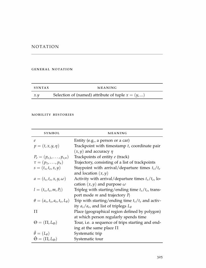
N O TAT I O N
general notation
syntax meaning
x.y Selection of (named) attribute of tuple x = (y, ...)
mobility histories
symbol meaning
e Entity (e.g., a person or a car)p = (t, x, y, η) Trackpoint with timestamp t, coordinate pair
(x, y) and accuracy η
Pe = (pe,1, . . . , pe,n) Trackpoints of entity e (track)τ = (p1, . . . , pn) Trajectory, consisting of a list of trackpointss = (ts, te, x, y) Staypoint with arrival/departure times ts/te
and location (x, y)a = (ts, te, x, y, ω) Activity with arrival/departure times ts/te, lo-
cation (x, y) and purpose ω
l = (ts, te, m, Pl) Tripleg with starting/ending time ts/te, trans-port mode m and trajectory Pl
θ = (as, ts, ae, te, Lθ) Trip with starting/ending time ts/te and activ-ity as/ae, and list of triplegs Lθ
Π Place (geographical region defined by polygon)at which person regularly spends time
Θ = (Π, LΘ) Tour, i.e. a sequence of trips starting and end-ing at the same place Π
θ = (Lθ) Systematic tripΘ = (Π, LΘ) Systematic tour
325
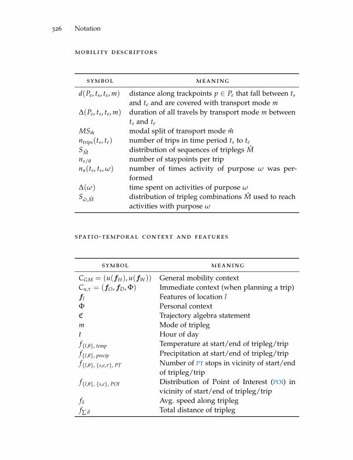
326 Notation
mobility descriptors
symbol meaning
d(Pe, ts, te, m) distance along trackpoints p ∈ Pe that fall between ts
and te and are covered with transport mode m∆(Pe, ts, te, m) duration of all travels by transport mode m between
ts and te
MSm modal split of transport mode mntrips(ts, te) number of trips in time period ts to te
SM distribution of sequences of triplegs Mns/θ number of staypoints per tripna(ts, ts, ω) number of times activity of purpose ω was per-
formed∆(ω) time spent on activities of purpose ω
Sω,M distribution of tripleg combinations M used to reachactivities with purpose ω
spatio-temporal context and features
symbol meaning
CGM = (u(fH), u(fW)) General mobility contextCu,τ = (fO,fD, Φ) Immediate context (when planning a trip)fl Features of location lΦ Personal contextC Trajectory algebra statementm Mode of triplegt Hour of dayf{l,θ}, temp Temperature at start/end of tripleg/tripf{l,θ}, precip Precipitation at start/end of tripleg/tripf{l,θ}, {s,e,τ}, PT Number of PT stops in vicinity of start/end
of tripleg/tripf{l,θ}, {s,e}, POI Distribution of Point of Interest (POI) in
vicinity of start/end of tripleg/tripf s Avg. speed along triplegf∑ d Total distance of tripleg
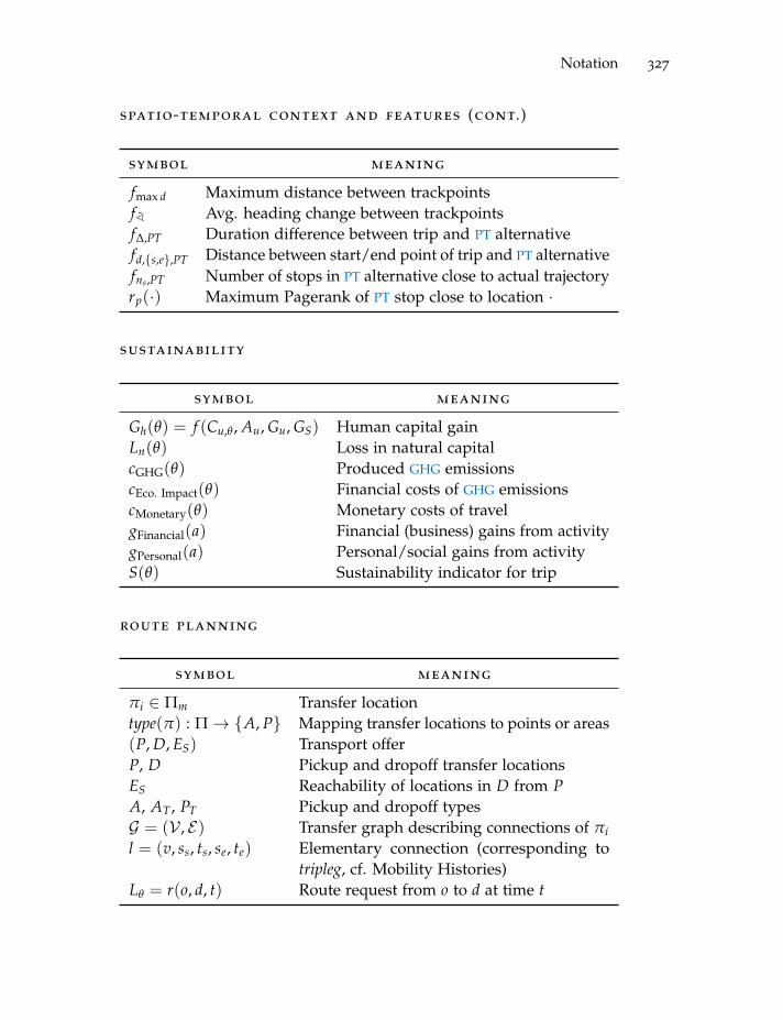
Notation 327
spatio-temporal context and features (cont.)
symbol meaning
fmax d Maximum distance between trackpointsf ¯ Avg. heading change between trackpointsf∆,PT Duration difference between trip and PT alternativefd,{s,e},PT Distance between start/end point of trip and PT alternativefns,PT Number of stops in PT alternative close to actual trajectoryrp(·) Maximum Pagerank of PT stop close to location ·
sustainability
symbol meaning
Gh(θ) = f (Cu,θ , Au, Gu, GS) Human capital gainLn(θ) Loss in natural capitalcGHG(θ) Produced GHG emissionscEco. Impact(θ) Financial costs of GHG emissionscMonetary(θ) Monetary costs of travelgFinancial(a) Financial (business) gains from activitygPersonal(a) Personal/social gains from activityS(θ) Sustainability indicator for trip
route planning
symbol meaning
πi ∈ Πm Transfer locationtype(π) : Π→ {A, P} Mapping transfer locations to points or areas(P, D, ES) Transport offerP, D Pickup and dropoff transfer locationsES Reachability of locations in D from PA, AT, PT Pickup and dropoff typesG = (V , E) Transfer graph describing connections of πil = (v, ss, ts, se, te) Elementary connection (corresponding to
tripleg, cf. Mobility Histories)Lθ = r(o, d, t) Route request from o to d at time t

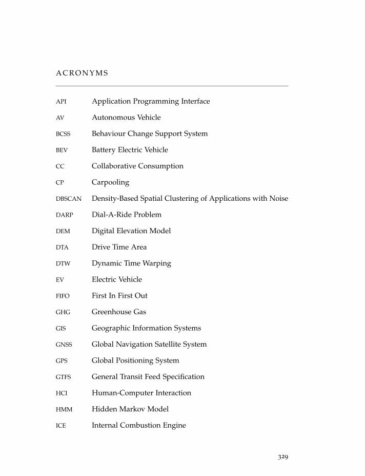
A C R O N Y M S
API Application Programming Interface
AV Autonomous Vehicle
BCSS Behaviour Change Support System
BEV Battery Electric Vehicle
CC Collaborative Consumption
CP Carpooling
DBSCAN Density-Based Spatial Clustering of Applications with Noise
DARP Dial-A-Ride Problem
DEM Digital Elevation Model
DTA Drive Time Area
DTW Dynamic Time Warping
EV Electric Vehicle
FIFO First In First Out
GHG Greenhouse Gas
GIS Geographic Information Systems
GNSS Global Navigation Satellite System
GPS Global Positioning System
GTFS General Transit Feed Specification
HCI Human-Computer Interaction
HMM Hidden Markov Model
ICE Internal Combustion Engine
329
330 Acronyms
ICT Information and Communication Technologies
IOT Internet of Things
LAT Location-Aware Technologies
LBS Location Based Service
LCA Life Cycle Assessment
MAAS Mobility as a Service
MAST Mobility Allowance Shuttle Transport
MAUP Modifiable Areal Unit Problem
MRT Mass Rapid Transit
NHTS US National Household Travel Survey
NN Nearest Neighbor
OS Operating System
OSM OpenStreetMap
OSRM Open Source Routing Machine
OTP OpenTripPlanner
PHEV Plugin Hybrid Electric Vehicle
PMT Private Motorized Transport
PT Public Transport
POA Point of Action
POI Point of Interest
RF Random Forest
SBB Swiss Federal Railways
SDK Software Development Kit
SM Slow Mobility
Acronyms 331
SMC Swiss Mobility Census
SOC State of Charge
SOV Single Occupant Vehicle
TTM Transtheoretical Model of Behavior Change
VGI Volunteered Geographic Information
VMT Vehicle Miles Traveled
VRPT Vehicle Routing Problem with Time Windows
WLAN Wireless Local Area Network

F U N D I N G A C K N O W L E D G M E N T S
GoEco! was funded by the Swiss National Science Foundation (SNF)within NRP 71 “Managing energy consumption” and is part of theSwiss Competence Center for Energy Research SCCER Mobility of theSwiss Innovation Agency Innosuisse.
SBB Green Class was funded by the Swiss Federal Railways SBB.
Parts of the research presented in this dissertation were additionallyfunded and supported by the Swiss Data Science Center (SDSC).
The SMC is provided by by the Swiss Federal Statistical Office.
The NHTS is provided by Federal Highway Administration of the U.S.Department of Transportation.
We would like to express our gratitude to all the funding organizationsand partners. Without you, this dissertation would not have beenpossible!
333

C U R R I C U L U M V I TA E
personal data
Name Dominik Christoph Bucher
Date of Birth October 22, 1988
Place of Birth Luzern (Switzerland)
Citizen of Muhlau (Switzerland)
Contact [email protected],[email protected]
Website http://dominikbucher.com
education
2015 – 2020 ETH Zurich, Chair of Geoinformation Engi-neeringDoctor of Sciences (Dr. sc. ETH Zurich)
2011 – 2013 ETH Zurich/The University of EdinburghMaster of Science in Electrical Engineering andInformation TechnologyFocus on Computer and Networks
2007 – 2010 ETH Zurich/The University of California,BerkeleyBachelor of Science in Electrical Engineering andInformation Technology
2001 – 2007 High School Oerlikon (KSOe)Matura (University Entrance Diploma)Focus on Applied Mathematics and Physics
335
336 Curriculum Vitae
professional experience
2016 – Now MIE LabCo-FounderMobility research lab within the Group ofGeoinformation Engineering at ETH Zurich.
2015 – Now BetaFarm GmbHCo-FounderCompany-builder hosting several projects.
2014 – Now earlyhire.chTech Lead / Co-OwnerLeading Swiss startup job platform.
2010 LevitronixInternship (Electrical Engineer)Specializes in bearingless electric motors.
2008 ETH ZurichUndergraduate Student InstructorIn Digital Circuits (Prof. G. Troster).
2007 – Now Community of Bassersdorf/KlotenOrganistPlaying the organ on weekends.
research projects
2019 – Now SCCER RideshareProject Proposal, Primary ResearcherGenerating automatic ridesharing suggestions.
2019 – Now SBB Mobility InitiativeAdvisor (within MIE lab)Analyzing a new MAAS offer by SBB.
2019 – Now SCCER Smart ChargingProject Proposal, Advisor (within MIE lab)Individual mobility needs and charging EVs.
Curriculum Vitae 337
2018 – Now COMMITProject Proposal, ResearcherContext-Aware Mobility Mining Tools(COMMIT) providing methods to processspatio-temporal data.
2017 – 2019 alpinaveraProject Proposal, Primary ResearcherOptimizing delivery schedules for farmers inmountain regions of Switzerland.
2017 – 2019 SBB Green Class I & IIProject Proposal, ResearcherAnalyzing a new MAAS offer by SBB.
2015 – Now SCCER MobilityAdvisor (within MIE Lab), ResearcherImproving individuals’ access to differentforms of mobility and transport.
2015 – 2018 GoEco!ResearcherStudying the potential of gamified apps toconvince people to travel more sustainably.
distinctions
2019 Runner-Up traffic4cast CompetitionNeurIPS 2019 Competition by IARAIPredicting traffic status using neural networks
2019 Best Poster Award Nominee6th Annual Conference SCCER MobilityAnalysis framework and results of the SBBGreen Class pilot studies
338 Curriculum Vitae
2019 Best Poster Award Nominee6th Annual Conference SCCER MobilityThe future of logistics: How will electric trucksshape the future energy demand and distribu-tion of Switzerland?
2018 Hack Zurich Challenge WinnerSiemens ChallengeTracking of people on railway platforms.
2018 Cover Story FeatureInternational Journal of Geo-InformationAssessing the Influence of Spatio-TemporalContext for Next Place Prediction using Dif-ferent Machine Learning Approaches (Urneret al. 2018).
2017 Best Paper Award NomineeD-A-CH+ Energieinformatik 2017Using Locally Produced Photovoltaic Energyto Charge Electric Vehicles (Buffat, Bucher, andRaubal 2018).
2017 Best Paper AwardAGILE 2017Energy-based Routing and Cruising RangeEstimation for Electric Bicycles (Haumann,Bucher, and Jonietz 2017).
2016 Hack Zurich Challenge WinnerSBB ChallengeUsing Bluetooth Beacons to provide indoorlocalization and app-based navigation.
2015 Best Paper Award NomineeICT for Sustainability (ICT4S), 2015A Taxonomy of Motivational Affordances forMeaningfulGamified and Persuasive Technolo-gies (Weiser, Bucher, et al. 2015).
2012 IET Present Around the World EuropeIET Europe – Paris, FranceSecond place at the European IET Presentaround the World finals in Paris (Local Brows-ing).
Curriculum Vitae 339
publications
Only publications that are not part of this dissertation (and thus men-tioned at the beginning of this dissertation) are listed here.
• Dominik Bucher, Henry Martin, David Jonietz, et al. (2021). ”Esti-mation of Moran’s I in the Context of Uncertain Mobile SensorMeasurements.“ In: 11th International Conference on GeographicInformation Science. Ed. by Krzysztof Janowicz and Judith A. Ver-stegen. Schloss Dagstuhl–Leibniz-Zentrum fuer Informatik.
• Martin Raubal, Dominik Bucher, and Henry Martin (2020). ”Geosmart-ness for personalized and sustainable future urban mobility.“ en.In: Urban Informatics. Accepted: 2020-04-20T08:49:11Z. Springer.
• Henry Martin, Dominik Bucher, Ye Hong, et al. (2020). ”Graph-ResNets for short-term traffic forecasts in almost unknown cities.“In: Proceedings of Machine Learning Research 123, pp. 153–163.
• Ray Pritchard, Dominik Bucher, and Yngve Frøyen (May 2019).
”Does new bicycle infrastructure result in new or rerouted bicy-clists? A longitudinal GPS study in Oslo.“ en. In: Journal ofTransport Geography 77, pp. 113–125.
• Henry Martin, Henrik Becker, et al. (2019). ”Begleitstudie SBBGreen Class - Abschlussbericht.“ de. Zurich.
• Henry Martin, Ye Hong, et al. (Oct. 2019). Traffic4cast-Traffic MapMovie Forecasting – Team MIE-Lab. en. Working Paper. Accepted:2020-01-09T06:18:52Z Publication Title: arXiv. Cornell University,p. 1910.13824.
• Dominik Bucher, Rene Buffat, et al. (2019). ”Energy and green-house gas emission reduction potentials resulting from differentcommuter electric bicycle adoption scenarios in Switzerland.“ In:Renewable and Sustainable Energy Reviews 114, p. 109298.
• Henry Martin, Dominik Bucher, Esra Suel, et al. (Dec. 2018).
”Graph Convolutional Neural Networks for Human Activity Pur-pose Imputation.“ en. In: NIPS Spatiotemporal Workshop at the 32nd
340 Curriculum Vitae
Annual Conference on Neural Information Processing Systems (NIPS2018). Accepted: 2019-08-13T09:18:58Z.
• Roswita Tschumperlin, Dominik Bucher, and Joram Schito (2018).
”Using Stream Processing to Find Suitable Rides: An Explorationbased on New York City Taxi Data.“ In: Spatial Big Data andMachine Learning in GIScience Workshop at GIScience 2018. SchlossDagstuhl–Leibniz-Zentrum fuer Informatik.
• Paolo Fogliaroni et al. (2018). ”Intersections of Our World.“In: 10th International Conference on Geographic Information Science.Vol. 114. Schloss Dagstuhl–Leibniz-Zentrum fuer Informatik, p. 3.
• Henrik Becker, Allister Loder, et al. (July 2018). ”Usage patternsand impacts of a mobility flat rate traced with a SmartphoneApp.“ en. In: Proceedings of the 15th International Conference onTravel Behaviour Research, (IATBR2018).
• Dominik Bucher, David Rudi, and Rene Buffat (2018). ”CaptchaYour Location Proof—A Novel Method for Passive Location Proofsin Adversarial Environments.“ In: LBS 2018: 14th InternationalConference on Location Based Services. Springer, Cham, pp. 269–291.
• Rene Buffat, Dominik Bucher, and Martin Raubal (2018). ”Usinglocally produced photovoltaic energy to charge electric vehicles.“In: Computer Science-Research and Development 33.1-2, pp. 37–47.
• Jorim Urner et al. (2018). ”Assessing the Influence of Spatio-Temporal Context for Next Place Prediction using Different Ma-chine Learning Approaches.“ In: ISPRS International Journal ofGeo-Information 7.5, p. 166.
• Dominik Bucher (2017). ”Vision Paper: Using Volunteered Geo-graphic Information to Improve Mobility Prediction.“ In: Proceed-ings of the 1st ACM SIGSPATIAL Workshop on Prediction of HumanMobility. ACM, p. 2.
• Ray Pritchard and Dominik Bucher (2017). ”Targeted sensing tech-nology for bicycle research-early results from a longitudinal studyin Oslo.“ In: International NTNU Sustainability Science Conference.NTNU, pp. 31–32.
Curriculum Vitae 341
• Simon Tobias Haumann, Dominik Bucher, and David Jonietz(2017). ”Energy-based Routing and Cruising Range Estimation forElectric Bicycles.“ In: Societal Geo-Innovation: Short Papers, Postersand Poster Abstracts of the 20th AGILE Conference on GeographicInformation Science. Wageningen University & Research 9-12 May2017, Wageningen, the Netherlands. Association of GeographicInformation Laboratories for Europe (AGILE), p. 145.
supervised theses
2020 Conserved Quantities in Transport Mode Choicesand Mobility Patterns of PeopleYe Hong, MSc thesis supervised by DominikBucher, Henry Martin and Prof. MartinRaubal.
2020 Traffic Map Forecasting using Graph Convolu-tional Neural NetworksKonstantin Arbogast, MSc thesis supervisedby Henry Martin, Dominik Bucher and Prof.Martin Raubal.
2020 Evaluation and Implementation of Trajectory Simi-larity Measures within the Context of a MobilityProcessing FrameworkSven Ruf, BSc thesis supervised by JannikHamper, Dominik Bucher and Prof. MartinRaubal.
2019 The Future of Logistics: How will Electric TrucksShape the Future Energy Demand and Distributionof Switzerland?Keyuan Yin, semester thesis supervised by Do-minik Bucher, Henry Martin, Dr. Rene Buffatand Prof. Martin Raubal.
2018 Real-Time Processing of Spatio-Temporal DataRoswita Tschumperlin, MSc thesis supervisedby Dominik Bucher and Prof. Martin Raubal.
342 Curriculum Vitae
2017 Renewable Power Production Potential in Car Park-ing AreasJanis Munchrath, semester thesis supervisedby Rene Buffat, Dominik Bucher and Prof.Martin Raubal.
2017 Assessing and Predicting Mobility Behavior usingNeural NetworksJorim Urner, MSc thesis supervised by Do-minik Bucher, Jing Yang, Dr. David Jonietz,Prof. Ross Purves and Prof. Martin Raubal.
2016 Carsharing and Carpooling in Multi-Modal Rout-ingJulian Kissling, MSc thesis supervised by Do-minik Bucher, Dr. Kai-Florian Richter, Dr.Haosheng Huang, Prof. Robert Weibel andProf. Martin Raubal.
2016 Optimizing the Operation Range of E-Bikes inRouting SystemsSimon Haumann, MSc thesis supervised byDominik Bucher and Prof. Martin Raubal.
2015 Das Traveling Salesman Problem und die Opti-mierung von AuslieferungszeitenKatharina Henggeler, BSc thesis supervised byDominik Bucher, Ioannis Giannopoulos andProf. Martin Raubal.
various
• Took part in the organization of the 14th Conference on LocationBased Services (LBS 18) and the Spatial Big Data and MachineLearning in GIScience workshop at GIScience 2018.
• Reviewed articles in Intelligent Transport Systems (IEEE), Journalof Location Based Services, Journal of Transport Geography, Sen-sors, Knowledge and Data Engineering, The Open TransportationJournal, and for various conferences and workshops.

Curriculum Vitae 343
• Taught classes within the following courses: GIS I, GIS II, GISIII, GIS and Geoinformatics Lab, Mobile GIS, Geodata Analysis,Geomatics Seminar, CAS Mobilitat der Zukunft.

colophon
This document was typeset in LATEX using the typographical look-and-feel classicthesis. Most of the graphics in this thesis are gener-ated using pgfplots and pgf/tikz. The bibliography is typeset usingbiblatex. Cover image by MagicH on Pixabay.
Recommended


