arX

iv:1

202.

6241

v1 [

astr

o-ph

.CO

] 2

8 Fe

b 20

12Mon. Not. R. Astron. Soc. 000, 000–000 (0000) Printed 29 February 2012 (MN LATEX style file v2.2)

The progenitors of present-day massive red galaxies up toz ≈ 0.7 - finding passive galaxies using SDSS-I/II andSDSS-III

Rita Tojeiro1∗, Will J. Percival1, David A. Wake2, Claudia Maraston1,

Ramin A. Skibba3, Idit Zehavi4, Ashley J. Ross1, Charlie Conroy6, Hong Guo4,

Marc Manera1, Karen L. Masters1,5, Janine Pforr7, Lado Samushia1,

Donald P. Schneider8,9, Daniel Thomas1, Dmitry Bizyaev10, Howard Brewington10,

Elena Malanushenko10, Viktor Malanushenko10, Daniel Oravetz10, Kaike Pan10,

Alaina Shelden10, Audrey Simmons10, Stephanie Snedden10

1Institute of Cosmology and Gravitation, Dennis Sciama Building, University of Portsmouth, Burnaby Road, Portsmouth, PO1 3FX, UK2Astronomy Department, Yale University, P.O. Box 208101, New Haven, CT 06520, USA3Steward Observatory, University of Arizona, 933 N. Cherry Ave., Tucson, AZ 85721, USA4Department of Astronomy and CERCA, Case Western Reserve University, 10900 Euclid Avenue, Cleveland, OH 44106, USA.5SEPnet, South East Physics Network (www.sepnet.ac.uk)6Harvard-Smithsonian Center for Astrophysics, Cambridge, MA, USA7NOAO, 950 N. Cherry Ave, Tucson, AZ 85719, USA8Department of Astronomy and Astrophysics, The Pennsylvania State University, University Park, PA 168029Institute for Gravitation and the Cosmos, The Pennsylvania State University, University Park, PA 1680210Apache Point Observatory, P.O. Box 59, Sunspot, NM 88349-0059, USA

29 February 2012

ABSTRACT

We present a comprehensive study of 250,000 galaxies targeted by the Baryon Oscil-lation Spectroscopic Survey (BOSS) up to z ≈ 0.7 with the specific goal of identifyingand characterising a population of galaxies that has followed passive evolution (nomergers) as closely as possible. We compute a likelihood that each BOSS galaxy is aprogenitor of the Luminous Red Galaxies (LRGs) sample, targeted by SDSS-I/II upz ≈ 0.5, by using the fossil record of LRGs and their inferred star-formation histories,metallicity histories and dust content. We determine merger rates, luminosity growthrates and the evolution of the large-scale clustering between the two surveys, and weinvestigate the effect of using different stellar population synthesis models in our con-clusions. We demonstrate that our sample is slowly evolving (of the order of 2± 1.5%Gyr−1 by merging) by computing the change in weighted luminosity-per-galaxy be-tween the two samples, and that this result is robust to our choice of stellar populationmodels. Our conclusions refer to the bright and massive end of the galaxy population,with Mi0.55 . −22, and M∗ & 1011.2M⊙, corresponding roughly to 95% and 40%of the LRGs and BOSS galaxy populations, respectively. Our analysis further showsthat any possible excess of flux in BOSS galaxies, when compared to LRGs, frompotentially unresolved targets at z ≈ 0.55 must be less than 1% in the r0.55−band(approximately equivalent to the g−band in the rest-frame of galaxies at z = 0.55).When weighting the BOSS galaxies based on the predicted properties of the LRGs,and restricting the analysis to the reddest BOSS galaxies, we find an evolution of thelarge-scale clustering that is consistent with dynamical passive evolution, assuming astandard cosmology. We conclude that our likelihoods give a weighted sample that isas clean and as close to passive evolution (in dynamical terms) as possible, and thatis optimal for cosmological studies.

Key words: galaxies: evolution - cosmology: observations - surveys

∗ E-mail: rita.tojeiro@port.ac.uk

c© 0000 RAS

2 Tojeiro et al.

1 INTRODUCTION

The Baryonic Oscillation Spectroscopic Survey (BOSS),part of the Sloan Digital Sky Survey III (SDSS-III), is anambitious galaxy redshift survey which will determine theexpansion rate of the Universe up to z ≈ 0.7 by measur-ing the baryonic acoustic oscillations (BAO) and redshift-space distortions (RSD) in the galaxy power spectrum(Eisenstein et al. 2011). At the end of the five-year observ-ing program, BOSS will have mapped 1.5 million massivegalaxies in 10,000 square degrees of sky, resulting in un-precedented volume and galaxy density. Forecasts indicatethat BOSS will yield measurements of the redshift-distancerelation dA(z) and of the Hubble parameter H(z) to 1% and1.8% at z = 0.35 and 1% and 1.7% at z = 0.55, respectively(at the 1-sigma confidence level, Eisenstein et al. 2011). Toachieve these ambitious goals systematic uncertainties in thedata, modelling and methodology must be kept to a mini-mum, and be understood as best as possible (see Ross et al.2011, Ross et al. in prep for a study on data systematics inBOSS).

A source of uncertainty in the modelling and measure-ment of the BAO is galaxy bias. Different populations ofgalaxies relate differently to the underlying matter densityfield, yielding different biases and often different scales thatmark the regime over which a linear, deterministic and scale-invariant bias model is applicable. To a certain extent onecan parametrise over this uncertainty, but nonetheless aninteresting question remains concerning how much gain ispossible if the bias modelling and evolution with redshiftwere well understood.

The best candidate for a population of galaxies witha well understood bias evolution is a population that hasbeen evolving passively (i.e., with no or very little merg-ing): the bias evolution is easily modelled using the Fry(1996) formalism (see also Tegmark & Peebles 1998). Mas-sive red galaxies are the prime candidates for such a popu-lation - they are composed mostly of old stellar populations(e.g. Maraston et al. 2009), and their growth via mergingsince a redshift of two has been constrained to be small(< 10%) even if strictly non-zero (e.g. Wake et al. 2008).Halo-modelling analyses of massive red galaxies have repeat-edly revealed a highly biased population (b ≈ 2) with a lowsatellite fraction (5 to 10%) - see e.g. Zehavi et al. (2005a);Wake et al. (2008); Zheng et al. (2009); White et al. (2011)- confirming their suitability for cosmological studies. De-parture from a pure passive evolution history has beenshown to have a dependence on luminosity and colour(Tojeiro & Percival 2010; Tojeiro et al. 2011), and thisopens up the possibility of weighting galaxies appropriately,so as to maximise the contribution of those that are morelikely to have been passively evolving, and minimise the con-tribution of those that are less likely to have done so. TheSDSS-I/II survey targeted LRGs using a mix of colour andluminosity selection cuts such as to follow the evolution ofa passively evolving population of stars. BOSS targeting,however, is much less restrictive in terms of luminosity andcolour (especially at z > 0.45 - see Section 2). It is thereforenot true that one population is automatically composed ofthe evolved products from the other.

One of the goals of this paper is to identify, in BOSS, themost likely progenitors of lower redshift SDSS-I/II LRGs,

and design a set of weights that allow a selection of thegalaxies that are linked by the same evolutionary history.

Our other major goal is to place quantitative con-straints on the formation and recent evolution of presentday luminous red galaxies, which in broad terms consti-tute a subset of what are typically called early-type galax-ies (ETGs). Efforts towards understanding ETGs and theirevolution can be split into two categories: those that fo-cus on their stellar content, and those that primarily aimto constrain their dynamical evolution, or merging history.Studies have been performed based on (see also referenceswithin): the mass or luminosity function of central galax-ies (Wake et al. 2006; Brown et al. 2007; Faber et al. 2007;Cool et al. 2008), and of their satellites (Tal et al. 2012);colour-magnitude diagram (Cool et al. 2006; Bernardi et al.2011); photometry SED fitting (Kaviraj et al. 2009;Maraston et al. 2009); absorption line fitting to individ-ual galaxies’ spectra (Trager et al. 2000; Thomas et al.2005, 2010; Carson & Nichol 2010) or to stacked spec-tra (Eisenstein et al. 2003; Graves et al. 2009; Zhu et al.2010); full spectral fitting (Jimenez et al. 2007); close-paircounts (Bell et al. 2006; Bundy et al. 2009) and clustering(Zehavi et al. 2005a; Sheth et al. 2006; Masjedi et al. 2006;Conroy et al. 2007; White et al. 2007; Brown et al. 2008;Masjedi et al. 2008; Wake et al. 2008; Tojeiro & Percival2010; De Propris et al. 2010). There is general agreementin the overall picture: ETGs constitute a uniform popu-lation of galaxies; are dominated by old and metal richstellar populations; their mean ages (either mass- or light-weighted) decrease with luminosity; and the most lumi-nous occupy the more dense environments. There is, how-ever, an increasing amount of evidence pointing towardssome amount of recent star formation in intermediate-massETGs (see e.g. Schawinski et al. 2007; Kaviraj et al. 2007;Salim & Rich 2010). This amount of star formation is not inconflict with the hierarchical model of structure formation,and Kaviraj et al. (2010), through evidence coming fromsmall morphological disruptions in early-type galaxies, ar-gue that it can be explained from the contributions fromminor-mergers.

On the clustering side, halo modelling is rapidly be-ing established as a successful tool to learn about galaxyformation (see e.g. Zehavi et al. 2005b; Zheng et al. 2007;Skibba & Sheth 2009; Skibba 2009; Ross & Brunner 2009;Zheng et al. 2009; Ross et al. 2010; Tinker & Wetzel 2010;Wake et al. 2011, and references within). It is a power-ful approach that connects galaxies with the dark matterhalos in which they reside, and which describes the dis-tribution of a population of galaxies in terms of centralsand satellites, as well as their relative ratio, as a func-tion of halo mass (which is well correlated with luminos-ity, see e.g. Swanson et al. 2008; Cresswell & Percival 2009;Ross et al. 2011). E.g., Zheng et al. (2007) use luminositydependent galaxy clustering at different epochs and the ex-pected growth of dark matter halos to infer a growth dueto star formation between z = 1 and the present day, afterroughly taking into account growth due to the merging ofcentrals and satellites. This type of description of galaxy as-sembly can then be directly compared to predictions fromsemi-analytical simulations (see Zehavi et al. 2012).

More specifically, the dynamical passive model can bedirectly tested by a halo model type of analyses. By per-

c© 0000 RAS, MNRAS 000, 000–000

The progenitors of LRGs to z≈0.7 3

forming HOD modelling at two different redshifts, one canevolve the best-fit halo model fitted at one redshift to an-other, assuming passive evolution. Comparison of the best-fit halo models provides insight about the dynamical evolu-tion of the sample, particularly in terms of satellite accre-tion and disruption. For most of the samples chosen, anal-yses show that a purely passive model would predict toomany satellites at low redshift, and therefore some galaxiesmust merge or be disrupted (see e.g. Conroy et al. 2007;White et al. 2007; Zheng et al. 2007; Brown et al. 2008;Wake et al. 2008; Seo et al. 2008). Measurements of mergerrates of massive galaxies vary significantly (see Table 4in Tojeiro & Percival 2010 for a summary), but luminositygrowth via merging seems confined to something between3-20% since z ≈ 1.

It seems increasingly likely that the assembly historyof massive galaxies is inexorably linked to the existence ofintra-cluster light (ICL) - a diffuse and scattered stellar com-ponent that can account for 10-50% of the stellar mass inclusters (see e.g. Feldmeier et al. 2004; Mihos et al. 2005;Purcell et al. 2007; Yang et al. 2009). A likely mechanismof its formation is the disruption of satellite galaxies whenhalos merge (see e.g. Conroy et al. 2007; Purcell et al. 2007;White et al. 2007; Yang et al. 2009 and discussions therein).A lack of conservation of light, or stellar mass, in galaxymergers has implications for the interpretation of the evo-lution of the luminosity function and inferred merger histo-ries. The fraction of light lost by a merging satellite to theintra-cluster medium remains largely unconstrained, withestimates at the large halo mass end from the studies citedabove varying between 15% and 80%. In the present workwe make no explicit allowances for the loss of Iight to theICM when two galaxies merge, but we will argue that ourresults are robust to this effect, within the limitations of themodels and data.

In the work presented here we approach the problemof galaxy assembly from a new direction, opposite in ethosto that of Zheng et al. (2007). We will use state of the artmodelling of the stellar evolution of a sample of galaxiesto directly quantify growth from star formation, and fromthat infer a galaxy-merger history. We compute a model forthe stellar evolution of SDSS-II LRGs by decomposing theirspectra into a series of star-formation and metallicity histo-ries, as well as dust content. This allows us to make predic-tions of their colour and magnitudes at any redshift. Thisinformation, when combined with the target selection infor-mation for BOSS galaxies, constrains the regions in colourand magnitude space in BOSS within which progenitors ofLRGs are more likely to reside. We then compute a setof weights that depend on the predicted evolution of eachgalaxy across the two surveys, and up-weight the objectsthat are more likely to be in both samples. The analysiswe present depends on underlying assumptions about stel-lar evolution, initial mass functions and dust modelling. Weperform the full analysis using two different sets of assump-tions, so as to give the reader an idea of the dependence ourfinal results on this type of uncertainty.

Isolating the likely progenitors of LRGs in BOSS is initself no test of the merging history of the sample. Followingon from our analyses in Tojeiro & Percival (2010, 2011), wetest the evolution in the number and luminosity density ofthe galaxies between LRGs and BOSS, as a way to mea-

sure the amount of merging or luminosity growth betweenthe two redshift surveys. We also use a luminosity-weightedtwo-point correlation function to further test the passive hy-pothesis - weighting the galaxies by luminosity produces aclustering statistic that, on large-scales, is less sensitive togalaxies within the sample merging.

This paper is organised as follows: in Section 2 we de-scribe our two data sets, including targeting; in Section 3we explain how we compute a stellar evolution model thatdescribes the stellar evolution of all galaxies and spans aredshift range between 0.23 and 0.7; in Section 4 we usethis stellar evolution model to compute a set of weights thatallows us to construct optimal samples of galaxies at dif-ferent redshifts and explore the evolution of LRGs in theBOSS volume; in Section 5 we compute merger-rates andaverage luminosity growth across the samples and, in Sec-tion 6, we compute the large-scale clustering of each of oursamples and compare to predictions from a purely passivemodel. Finally we discuss and summarise our conclusionsin Section 7. Where required we assume a flat Λ cold darkmatter (LCDM) cosmology with Ωm = 0.266, ΩΛ = 0.734and H0 = 71 kms−1Mpc−1.

2 DATA

The Sloan Digital Sky Survey (SDSS) has imaged overone quarter of the sky using a dedicated 2.5m telescope inApache Point, New Mexico (Gunn et al. 2006). For detailson the hardware, software and data-reduction see York et al.(2000) and Stoughton et al. (2002). In summary, the sur-vey was carried out on a mosaic CCD camera (Gunn et al.1998) and an auxiliary 0.5m telescope for photometric cali-bration. Photometry was taken in five bands: u, g, r, i and z(Fukugita et al. 1996), and magnitudes corrected for Galac-tic extinction using the dust maps of Schlegel et al. (1998).BOSS, a part of the SDSS-III survey (Eisenstein et al. 2011),has mapped an additional 5, 200 square degrees of southerngalactic sky, increasing the total imaging SDSS footprint tonearly 14, 500 square degrees, or just over one third of thecelestial sphere. All of the imaging was re-processed and re-leased as part of SDSS Data Release 8 (Aihara et al. 2011).

In SDSS-I/II, Luminous Red Galaxies (LRGs) were se-lected for spectroscopic follow-up according to the targetalgorithm described in Eisenstein et al. (2001), designed tofollow a passive stellar population in colour and apparentmagnitude space. In this paper we analyse the latest SDSSLRG spectroscopic sample (Data Release 7, Abazajian et al.2009), which includes around 180,000 objects with a spec-troscopic footprint of nearly 8000 sq. degrees and a redshiftrange 0.15 < z < 0.5. In SDSS-III, the BOSS target selec-tion extends the SDSS-I/II algorithm to target fainter andbluer galaxies in order to achieve a galaxy number densityof 3×10−4 h3 Mpc−3 and increase the redshift range out toz ≈ 0.7. The spectroscopic footprint of the BOSS data usedin this sample covers almost 3500 sq. degrees of sky, and cor-responds to the upcoming Data Release 9, which will markthe first spectroscopic data release of BOSS.

The targeting algorithms make use of five different def-initions of magnitudes as follows:

• SDSS uber-calibrated model magnitudes(Padmanabhan et al. 2008), computed using either an

c© 0000 RAS, MNRAS 000, 000–000

4 Tojeiro et al.

exponential or a DeVaucouleurs light profile fit to ther-band only, denoted here with the mod subscript;

• cmodel magnitudes, computed using the best-fit linearcombination of an exponential with a DeVaucouleurs lightprofile fit to each photometric band independently, and de-noted here with the subscript cmod;

• point-spread function (PSF) magnitudes, denoted witha psf subscript, and computed by fitting a PSF model to thegalaxy;

• petrosian magnitudes, computed from the petrosianflux (the flux measured within twice the Petrosian radius, inturn defined using the surface brightness of the galaxy, seePetrosian 1976; Strauss et al. 2002), and denoted here by asubscript p; and finally

• fibre magnitudes, computed within a 2 arcsec aperture,and denoted by a fib2 subscript.

In SDSS-I/II, redshift LRGs were selected using two dif-ferent algorithms. Cut-I predominantly but not exclusivelytargeted lower redshift galaxies (z . 0.43) using the follow-ing selection criteria:

rp < 13.1 + c‖ (1)

rp < 19.2 (2)

c⊥ < 0.2 (3)

µr,p < 24.2 mag arcsec2 (4)

rpsf − rmodel > 0.3, (5)

where the two colours, c‖ and c⊥ are defined as

c‖ = 0.7(g − r) + 1.2[(r − i)− 0.18] (6)

c⊥ = (r − i)− (g − r)/4− 0.18. (7)

Model magnitudes were used for the colour constraints,and petrosian magnitudes for the apparent magnitude andsurface brightness constraints. Cut II mostly but not exclu-sively targets LRGs at z & 0.4 following:

rp < 19.5 (8)

c⊥ > 0.45 − (g − r)/6 (9)

(g − r) > 1.3 + 0.35(r − i) (10)

µr,p < 24.2 mag arcsec2 (11)

rpsf − rmodel > 0.5. (12)

Two separate algorithms are necessary as the passivestellar population turns sharply in a g − r vs r − i colourplane, when the 4000A break moves through the filters.

In SDSS-III, galaxies at z . 0.43 are predominantlybut not exclusively targeted by the LOZ selection algorithm,akin to Cut I above, but extended to fainter magnitudes. ALOZ galaxy must pass the following:

rcmod < 13.6 + c‖/0.3, (13)

|c⊥| < 0.2, (14)

16 < rcmod < 19.6, (15)

where the two auxiliary colours c‖ and c⊥ are defined as forSDSS-I/II above.

Galaxies at z & 0.43 are predominantly but not exclu-sively targeted by the CMASS selection algorithm, which

extends the Cut II above by targeting both fainter and bluergalaxies. A CMASS galaxy must pass the following criteria:

17.5 < icmod < 19.9, (16)

rmod − imod < 0.2, (17)

d⊥ > 0.55, (18)

ifib2 < 21.5, (19)

icmod < 19.86 + 1.6(dperp − 0.8), (20)

where the auxiliary colour d⊥ is defined as

d⊥ = rmod − imod − (gmod − rmod)/8.0. (21)

CMASS objects must also pass the following star-galaxyseparation cuts:

ipsf − imod > 0.2 + 0.2(20.0 − imod), (22)

zpsf − zmod > 9.125 − 0.46zmod, (23)

unless they also pass the LOZ cuts.The CMASS selection algorithm was designed to loosely

follow a constant stellar mass limit and, unlike Cut-II inSDSS-II, it does not exclusively target red objects. There-fore, whereas both the LRG and CMASS samples are colour-selected, CMASS is a significantly more complete samplethan the LRGs, especially at the bright end. In this pa-per we will split our data into two distinct redshift slices,with our lower redshifts slice ranging between 0.23 < z <0.45 and our higher redshift slice between 0.45 < z <0.7. Our low redshift slice consists exclusively of SDSS-I/II LRGs (Cut-I and Cut-II) and contains approximately89,000 galaxies, and our high redshift slice consists exclu-sively of SDSS-III CMASS galaxies, with over 250,000 ob-jects. The low redshift cut-off is motivated by our previousanalysis of the LRGs that indicates the sample is signifi-cantly contaminated at lower redshifts (Tojeiro et al. 2011;Tojeiro & Percival 2011). We do not make use of LOZ galax-ies for the main analysis presented in this paper, mainly dueto the fact that the volume and number density sampled byLOZ currently lags behind that of the CMASS due to prob-lems in target selection at the beginning of the observingrun. We use LOZ galaxies only in Section 5.4, when investi-gating potentially unresolved targets in CMASS. The n(z)distribution of our two samples is shown in Fig. 1.

3 THE STELLAR EVOLUTION MODELLING

We use the 124 stellar evolution models computed inTojeiro et al. (2011) by stacking LRG spectra according totheir luminosity, redshift and colour, and subsequently anal-ysed them with VESPA (Tojeiro et al. 2007, 2009) to obtaindetailed star-formation histories as a function of lookbacktime. VESPA fits a linear combination of stellar populationsof different ages and metallicities, modulated by a dust ex-tinction, to the stacked optical spectra. Each star-formationhistory can then be translated into a detailed evolution ofany magnitude and colour with cosmic time. We have madeno changes to these publicly available models other thanincreasing the sampling in redshift, to provide better re-solved colour and magnitude evolution1. We consider the

1 The models from Tojeiro et al. (2011) are available athttp://www.icg.port.ac.uk/~tojeiror/lrg_evolution/

c© 0000 RAS, MNRAS 000, 000–000

The progenitors of LRGs to z≈0.7 5

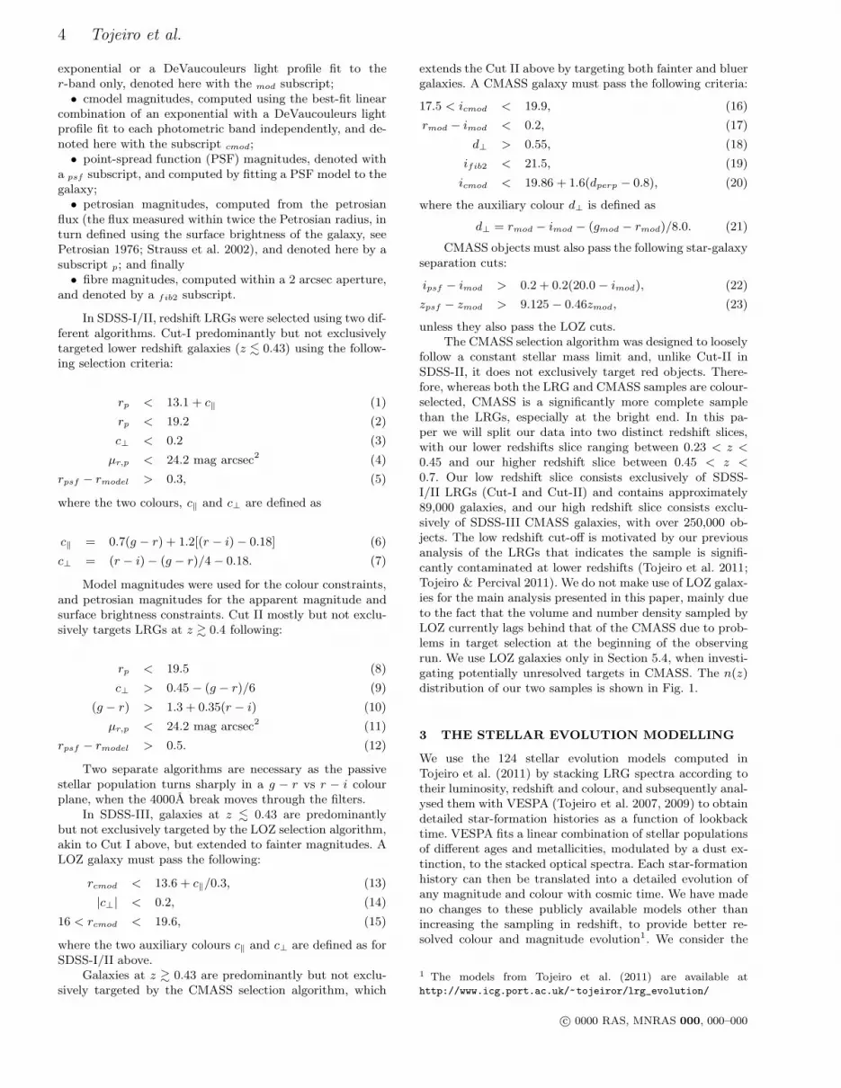
Figure 1. Number density as a function of redshift for the LRG(red) and the CMASS (black) samples. The dashed line at z =0.45 shows our chosen hard boundary between the two surveys -

we do not use any LRGs with z > 0.45 nor any CMASS galaxieswith z < 0.45

solutions obtained with two sets of stellar population mod-els: the Flexible Stellar Population Synthesis (FSPS) modelsof Conroy et al. (2009) and Conroy & Gunn (2010), and thestellar population models of Maraston & Stromback (2011)(M11) - we refer the reader to Section 4 of Tojeiro et al.(2011) for detailed information on the differences and sim-ilarities between the two sets of assumptions2. One of themain results in Tojeiro et al. (2011) is that, even thoughFSPS and M11 provide star-formation histories that havevery similar mass-weighted ages that decrease with luminos-ity, in the M11 case this is due to the presence of a popula-tion of stars of young to intermediate ages (1-3 Gyr), whilstin the FSPS case this is due to a slightly younger main burstof star formation, which extends to lower ages with decreas-ing luminosity. These differences in the star-formation histo-ries will have an impact on the results, and we will compareresults obtained using both models throughout the paper.In Section 3.1.1 we describe the star-formation histories re-covered with both sets of models in detail.

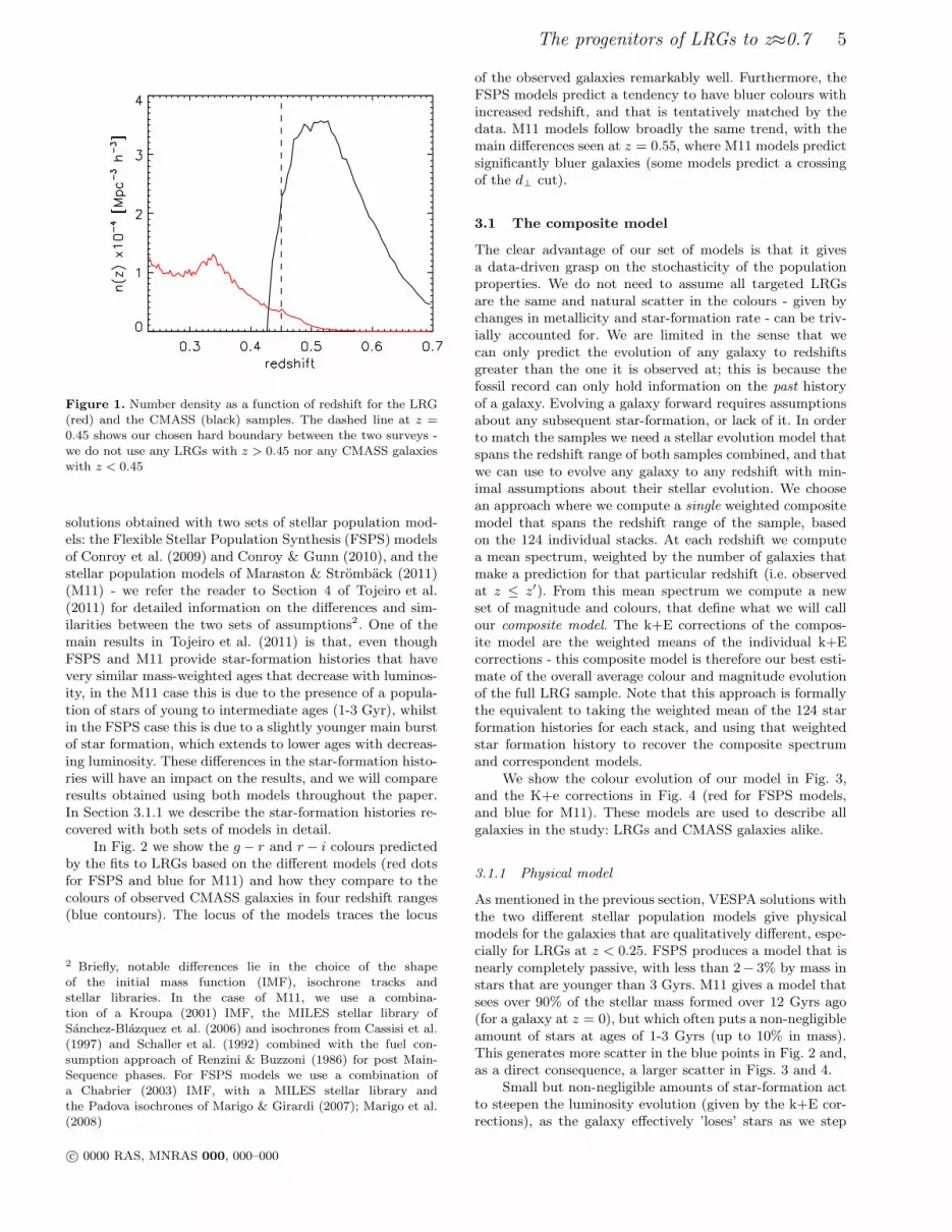
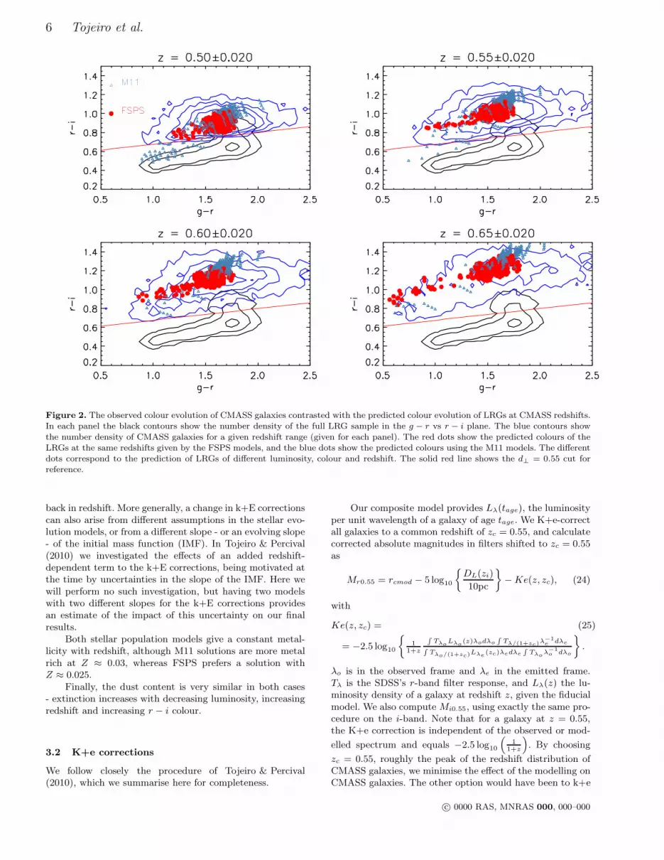
In Fig. 2 we show the g − r and r − i colours predictedby the fits to LRGs based on the different models (red dotsfor FSPS and blue for M11) and how they compare to thecolours of observed CMASS galaxies in four redshift ranges(blue contours). The locus of the models traces the locus

2 Briefly, notable differences lie in the choice of the shapeof the initial mass function (IMF), isochrone tracks andstellar libraries. In the case of M11, we use a combina-tion of a Kroupa (2001) IMF, the MILES stellar library ofSanchez-Blazquez et al. (2006) and isochrones from Cassisi et al.(1997) and Schaller et al. (1992) combined with the fuel con-sumption approach of Renzini & Buzzoni (1986) for post Main-Sequence phases. For FSPS models we use a combination ofa Chabrier (2003) IMF, with a MILES stellar library andthe Padova isochrones of Marigo & Girardi (2007); Marigo et al.(2008)

of the observed galaxies remarkably well. Furthermore, theFSPS models predict a tendency to have bluer colours withincreased redshift, and that is tentatively matched by thedata. M11 models follow broadly the same trend, with themain differences seen at z = 0.55, where M11 models predictsignificantly bluer galaxies (some models predict a crossingof the d⊥ cut).

3.1 The composite model

The clear advantage of our set of models is that it givesa data-driven grasp on the stochasticity of the populationproperties. We do not need to assume all targeted LRGsare the same and natural scatter in the colours - given bychanges in metallicity and star-formation rate - can be triv-ially accounted for. We are limited in the sense that wecan only predict the evolution of any galaxy to redshiftsgreater than the one it is observed at; this is because thefossil record can only hold information on the past historyof a galaxy. Evolving a galaxy forward requires assumptionsabout any subsequent star-formation, or lack of it. In orderto match the samples we need a stellar evolution model thatspans the redshift range of both samples combined, and thatwe can use to evolve any galaxy to any redshift with min-imal assumptions about their stellar evolution. We choosean approach where we compute a single weighted compositemodel that spans the redshift range of the sample, basedon the 124 individual stacks. At each redshift we computea mean spectrum, weighted by the number of galaxies thatmake a prediction for that particular redshift (i.e. observedat z ≤ z′). From this mean spectrum we compute a newset of magnitude and colours, that define what we will callour composite model. The k+E corrections of the compos-ite model are the weighted means of the individual k+Ecorrections - this composite model is therefore our best esti-mate of the overall average colour and magnitude evolutionof the full LRG sample. Note that this approach is formallythe equivalent to taking the weighted mean of the 124 starformation histories for each stack, and using that weightedstar formation history to recover the composite spectrumand correspondent models.

We show the colour evolution of our model in Fig. 3,and the K+e corrections in Fig. 4 (red for FSPS models,and blue for M11). These models are used to describe allgalaxies in the study: LRGs and CMASS galaxies alike.

3.1.1 Physical model

As mentioned in the previous section, VESPA solutions withthe two different stellar population models give physicalmodels for the galaxies that are qualitatively different, espe-cially for LRGs at z < 0.25. FSPS produces a model that isnearly completely passive, with less than 2− 3% by mass instars that are younger than 3 Gyrs. M11 gives a model thatsees over 90% of the stellar mass formed over 12 Gyrs ago(for a galaxy at z = 0), but which often puts a non-negligibleamount of stars at ages of 1-3 Gyrs (up to 10% in mass).This generates more scatter in the blue points in Fig. 2 and,as a direct consequence, a larger scatter in Figs. 3 and 4.

Small but non-negligible amounts of star-formation actto steepen the luminosity evolution (given by the k+E cor-rections), as the galaxy effectively ’loses’ stars as we step

c© 0000 RAS, MNRAS 000, 000–000

6 Tojeiro et al.

Figure 2. The observed colour evolution of CMASS galaxies contrasted with the predicted colour evolution of LRGs at CMASS redshifts.In each panel the black contours show the number density of the full LRG sample in the g − r vs r − i plane. The blue contours show

the number density of CMASS galaxies for a given redshift range (given for each panel). The red dots show the predicted colours of theLRGs at the same redshifts given by the FSPS models, and the blue dots show the predicted colours using the M11 models. The differentdots correspond to the prediction of LRGs of different luminosity, colour and redshift. The solid red line shows the d⊥ = 0.55 cut forreference.

back in redshift. More generally, a change in k+E correctionscan also arise from different assumptions in the stellar evo-lution models, or from a different slope - or an evolving slope- of the initial mass function (IMF). In Tojeiro & Percival(2010) we investigated the effects of an added redshift-dependent term to the k+E corrections, being motivated atthe time by uncertainties in the slope of the IMF. Here wewill perform no such investigation, but having two modelswith two different slopes for the k+E corrections providesan estimate of the impact of this uncertainty on our finalresults.

Both stellar population models give a constant metal-licity with redshift, although M11 solutions are more metalrich at Z ≈ 0.03, whereas FSPS prefers a solution withZ ≈ 0.025.

Finally, the dust content is very similar in both cases- extinction increases with decreasing luminosity, increasingredshift and increasing r − i colour.

3.2 K+e corrections

We follow closely the procedure of Tojeiro & Percival(2010), which we summarise here for completeness.

Our composite model provides Lλ(tage), the luminosityper unit wavelength of a galaxy of age tage. We K+e-correctall galaxies to a common redshift of zc = 0.55, and calculatecorrected absolute magnitudes in filters shifted to zc = 0.55as

Mr0.55 = rcmod − 5 log10

DL(zi)

10pc

−Ke(z, zc), (24)

with

Ke(z, zc) = (25)

= −2.5 log10

11+z

∫TλoLλo (z)λodλo

∫Tλ/(1+zc)

λ−1e dλe

∫Tλo/(1+zc)

Lλe (zc)λedλe∫Tλoλ−1

o dλo

.

λo is in the observed frame and λe in the emitted frame.Tλ is the SDSS’s r-band filter response, and Lλ(z) the lu-minosity density of a galaxy at redshift z, given the fiducialmodel. We also compute Mi0.55, using exactly the same pro-cedure on the i-band. Note that for a galaxy at z = 0.55,the K+e correction is independent of the observed or mod-

elled spectrum and equals −2.5 log10

(

11+z

)

. By choosing

zc = 0.55, roughly the peak of the redshift distribution ofCMASS galaxies, we minimise the effect of the modelling onCMASS galaxies. The other option would have been to k+e

c© 0000 RAS, MNRAS 000, 000–000

The progenitors of LRGs to z≈0.7 7

Figure 3. The composite stellar evolution model, computed ac-cording to the procedure in Section 3.1. In all panels the shadedcontours show the number density of LRGs (at z < 0.45 andon the bottom half of the last plot) and CMASS galaxies (atz > 0.45 and on the top half of the last plot). The red (blue)solid line shows our composite stellar model obtained using theFSPS (M11) VESPA star-formation histories. It is a weighted av-erage of the models shown in Fig. 2. The error bars show the 1σdispersion of the models shown in Fig. 2 in each redshift bin. Forreference, the yellow line shows the LRG purely passive model ofMaraston et al. (2009).

correct to median redshift of LRGs. However, as the compos-ite stellar evolution model is based on the spectra of LRGs,its predictions must be at least as robust for LRGs as forCMASS galaxies, if not more so. Therefore, our procedureis the more robust approach. We show the k+e correctionin the r− and i−bands in Fig. 4. For reference, in Fig. 5we show the expected observed-frame spectrum of a typi-cal galaxy in the sample at zc = 0.55, along side the threebroadband filters used in this paper.

Figure 4. K+e corrections in the r0.55-band (asterisks) and inthe i0.55-band (triangles).The red lines refer to the FSPS models,and the blue lines to the M11 models. The error bars show the 1σ

scatter around the mean from the 124 individual stacks. Thesecorrections allow us to compute the evolved absolute magnitudeof any galaxy at z = 0.55, in the two shifted filters (thereforefor galaxies at z = 0.55 this correction is fixed and independentof their spectra or modelling). The corrections in the r0.55 bandare steeper because it traces the 4000A break at these redshifts -see Fig. 5. The scatter in the M11 k+E corrections is larger, asthese models predict stochastic events of star-formation at youngto intermediate ages in some of the stacks.

Figure 5. The expected observed spectrum of a typical galaxyin the sample at z = 0.55 (black). The three broadband filtersused for target selection are overplotted: g−band in blue, r−bandin green and i−band in red. For reference, we show in grey theexpected observed spectrum of a galaxy at z = 0.3.

c© 0000 RAS, MNRAS 000, 000–000

8 Tojeiro et al.

3.3 Comparing CMASS and LR galaxies

We can use the K+e-corrected absolute magnitudes tobroadly characterise the two samples. Fig. 6 shows a simplecomparison of the magnitude distributions for both samplesand their evolution with redshift computed for both the r−and the i−band. Once again we show the results for theFSPS model in red and for the M11 model in blue. Here theonly model differences come through the K+e corrections,with the different slopes between models (shown in Fig. 4)naturally giving different k+E corrected absolute magni-tudes. M11 shows a steeper slope with respect to FSPS,with the crossing point at zc = 0.55. So for a galaxy atz < 0.55 M11 will predict a fainter k+E corrected absolutemagnitude at z = 0.55. Conversely, for a galaxy at z > 0.55,M11 will predict a brighter k+E corrected absolute magni-tude at z = 0.55. By construction, the absolute magnitudesfor galaxies sitting at z = 0.55 will match for both modelsdue to our choice of filters. The top panel of Fig. 6 showsthe effect of having different slopes for the k+E corrections -for LRGs this is about 0.3 magnitudes in the r0.55-band; forCMASS galaxies it is much smaller, at less than 0.1 mag-nitudes. These values are roughly halved for the i0.55-band.The bottom two panels of Fig. 6 show the evolution of thecorrected magnitudes with redshift (solid contours for FSPSand line contours for M11). As expected, we see a steeperevolution with redshift using the M11 contours.

Fig. 7 displays colour-magnitude relations. Here weshow only the results using FSPS models as the results aresimilar in both cases. The CMASS sample has a broaderrange in absolute magnitude and colour than the LRG sam-ple, as expected given the larger number density. The cleartrend seen between rest-frame colour andMr0.55 is explainedsimply by target selection. To help make this point we showthe expected evolution of the colour-magnitude relation ofan object at the faint end of the survey (cmodel = 19.9 atz = 0.45) and an observed colour of r − i = 0.8, betweenz = 0.25 and z = 0.7 - this is the red line in both plots. Anyobject to the faint side of the red lines would fail the mag-nitude cuts in the i−band of the CMASS algorithm. Thisgives an obvious artefact when plotting Mr0.55 vs colour,where upon the CMASS selection does not select faint bluegalaxies. The bright end slope is a consequence of volumeeffects, coupled with the slope of a typical galaxy spectra.

4 SAMPLE MATCHING

We now construct galaxy samples at high and low redshiftthat are coeval according to our composite stellar evolutionmodels. We continue to closely follow the methodology ofTojeiro & Percival (2010), which we summarise below. Wehave to take into account three redshift-dependent effects:

(i) the intrinsic evolution of the colour and brightness ofthe galaxies;

(ii) the varying errors on galaxy colour measurements;and

(iii) the varying survey selection function.

Our correction for (i) is given by our composite stel-lar evolution model. We include an evolving colour scatterterm to allow for (ii). Tojeiro & Percival (2010) used the

population scatter around the stellar evolution model withredshift. Tojeiro & Percival (2011) updated this term to bebased on the evolution of photometric errors as a function ofapparent magnitudes, which were modelled as a function ofredshift - see their Section 3. The motivation was two fold:firstly the photometric errors are driven principally by theapparent magnitude of an object, rather than its redshift;and secondly this is less dependent on choice of stellar evo-lution modelling. We adopt this approach here. For (iii) weconstruct a set of weights that assures a given populationof galaxies - in terms of colour and absolute magnitude - isgiven the same weight in the high and low redshift samples,as described in the next section.

4.1 Weighting scheme

We use the weighting scheme of Tojeiro & Percival (2010),which keeps the total weight of each galaxy population thesame in different redshift slices.

Suppose an LRG, gA, is faint and therefore can only beseen in a small fraction of the CMASS volume, fV , but canbe seen in the full LRG volume. Then our weighting schemewill give gA a weight that is equal to fV . Consider now afaint CMASS galaxy, that is observed in fV , and whose mag-nitude and colour evolution matches those predicted for gA.This galaxy will by definition also only be observed in a frac-tion fV of the CMASS volume. Our weighting scheme givesgB a weight on unity. Note this is the opposite approach tothe traditional Vmax weight, which would up-weight gB by1/fV and give gA a weight of unity.

Explicitly, for an LRG in a volume VLRG we calculate

wi =VLRG

V LRGmax,i

min

V LRGmax,i

VLRG,V CMASSmax,i

VCMASS

, (26)

and similarly for a CMASS galaxy, in a volume VCMASS :

wi =VCMASS

V CMASSmax,i

min

V LRGmax,i

VLRG,V CMASSmax,i

VCMASS

. (27)

Where the traditional Vmax estimator would up-weightgalaxies only visible in a fraction of the volume they wereobserved in, we instead give these galaxies a weight of unityand down-weight the corresponding galaxies with the sameproperties observed in the other volume.

The interpretation of the Vmatch weight is different thanthat of the traditional Vmax weighting. Whereas the lat-ter gives us the means to correct for incompleteness andyields true space densities, the former must be interpretedas a weighting scheme rather than a completeness correc-tion. I.e., Vmatch weighted number and luminosity densitiesare still potentially volume incomplete, but the populationsare weighted in such a way that they are equally representedat both redshifts. We can compare the distribution of totalweighted luminosity for the two slices, but we cannot inter-pret these functions as giving the true luminosity density.

The advantage of this weighting scheme is that we sam-ple different populations equally based on volume, and there-fore obtain a weighted population such that galaxies ob-served throughout a large volume are up-weighted. It alsoimplicitly checks that we are only using populations thatexist in both samples, without having to do such a test ex-plicitly (e.g. Wake et al. 2006).

c© 0000 RAS, MNRAS 000, 000–000

The progenitors of LRGs to z≈0.7 9

Figure 6. Comparing K+e corrected magnitudes in SDSS-I/II LRGs and BOSS CMASS galaxies. Top: the distribution of absolutemagnitudes for LRGs (dashed lines) and CMASS galaxies (solid lines). The different colours show the results from using different stellar

population models, with FSPS in red and M11 in blue. The two panels show the magnitude computed either in the rest-frame r− ori−band. Bottom: the absolute-magnitude with redshift on both samples. FSPS results are shown in the solid contours, and M11 in theline contours. The samples are split at z = 0.45; we do not use any LRGs with z > 0.45 nor any CMASS galaxies with z < 0.45. Theseplots show clearly the reach to fainter magnitudes of the CMASS sample. See main text for a discussion on the effect of the stellarpopulation models.

4.2 The progenitors of LRGs

A large value of Vmatch (Vmatch varies between 0 and 1) in-dicates that a galaxy belongs to a population that can beobserved across a large fraction of both surveys, and a smallvalue of Vmatch means a population of galaxies is only presentin a small fraction of the volume in at least one of the sur-veys. In other words, the larger this value for a CMASSgalaxy, the more likely this galaxy is a progenitor of a typi-cal LRG galaxy, and vice-versa.

Fig. 8 shows a mapping of the average value of thisweight onto the two CMASS targeting parameter spaces:a g − r vs r − i plot, and a d⊥ vs the cmodel magnitudein the i-band. We show the results using the FSPS modelsin the solid contours and the results using M11 in the linecontours, which are qualitatively similar. The colour-colourplot shows a clear trend for the average value of Vmatch toincrease to redder g − r colours, as expected if LRGs wereexclusively made of metal rich and old stars. Interestingly,we also see that some blue regions of the colour-colour plotdisplay an increase of the average value of the Vmatch weight.This relation is a result of the small but significant amountsof young to intermediate-aged stars detected in LRG spectra

at BOSS redshifts (corresponding roughly to stars aged be-tween 1 and 3 Gyr in SDSS-I/II galaxies). The orange linein the left-hand plot of Fig. 8 shows the g − i = 2.35 cutof Masters et al. (2011), which was motivated by the mor-phological analysis of a small subsample of CMASS galaxieswith Hubble Space Telescope (HST) imaging. They suggestselecting galaxies with g−i > 2.35 produces a cleaner sampleof early-type galaxies (90%) that are more traditionally as-sociated with typical LRGs. Additionally, we predict that atleast a fraction of the galaxies that sit in the blue end of thatcolour-colour plot are also LRG progenitors, temporarily vis-iting the blue cloud due to small amounts of star formation.Assuming they retain their morphology (it is hard to imag-ine a scenario where they would not), our analysis makesquantitative predictions on the fraction of star-forming el-lipticals that should be found on that part of the diagram,given the morphological mixing of the LRG sample (not cur-rently known, to our knowledge). This result can be turnedinto a test of SPS models, as different sets of models will pre-dict a different number density at those colours. We leavethis exploration for future work.

The right-hand side panel of Fig. 8 shows an uninter-rupted trend to lower Vmatch towards fainter magnitudes.

c© 0000 RAS, MNRAS 000, 000–000

10 Tojeiro et al.

Figure 7. Rest-frame, k+e corrected colour-magnitude relations for CMASS galaxies (filled contours) and LRGs (overploted blackcontours), as a function of Mi0.55 shown on the left panel, and as a function of Mr0.55 on the right hand side. CMASS galaxies showa broader range in their rest-frame Mr0.55 − Mi0.55, as well as fainter reach and median in both magnitudes. The right-hand side plotshows a clear trend of rest-frame colour with Mr0.55, with redder colour going with lower luminosity. This is trend is a result of targetselection, particularly the magnitude cut - we show the expected evolution of the colour-magnitude relation of an object at the faint endof the survey (cmodel= 19.9 at z = 0.45) and an observed colour of r − i = 0.8, between z = 0.25 and z = 0.7. Any object to the faintside of the red lines would fail the magnitude cuts of the CMASS algorithm.

Figure 8. Average Vmatch weight as a function of colours and i−band magnitude, shown for the two main targeting parameter spacediagrams in CMASS. A darker colour corresponds to a lower value of Vmatch , and the brighter colours to the regions in parameter spacethat have the largest likelihood of being progenitors of the LRG sample. The red solid lines show targeting cuts. The orange line on theplot on the left shows the morphology cut derived in Masters et al. (2011), and the dashed green line shows the blue cut of the cut-IIselection in Eisenstein et al. (2001).

Interestingly, the slope of the Vmatch contours are almostparallel to the sliding cut in d⊥ with i−band magnitude.This cut was designed to follow a line of constant stellarmass (Maraston et al. in prep) suggesting that the Vmatch

has a clear dependence on stellar mass, as it should.

A complementary way to examine the Vmatch weights isto isolate the CMASS galaxies with a small Vmatch weight.Fig. 9 shows the K+e-corrected absolute magnitude distri-bution of those CMASS galaxies with a Vmatch < 0.05, i.e.that are observed in less than 5% of the volumes of thesurveys. We clearly see these galaxies are well confined to

the faint end of the CMASS population. The difference be-tween the two models (given by the two yellow histograms),is dominated by the steeper luminosity evolution given byK+e corrections of the M11 models - CMASS galaxies aretypically brighter at LRG redshifts (when compared to aflatter luminosity evolution), and are seen through more ofits volume.

Fig. 10 presents the distribution of the absolute rest-frame r0.55 − i0.55 colour for the same populations as inFig. 9. Even though this distribution is biased towards thered end of the CMASS galaxies, it is by no means exclusively

c© 0000 RAS, MNRAS 000, 000–000

The progenitors of LRGs to z≈0.7 11

Figure 9. k+e corrected absolute magnitudes for CMASS galax-ies (black), LRGs (green) and the subset of CMASS galaxies thatis seen in less than 5% of the LRG volume according to our model(purple). These lie almost exclusively at the faint end, demon-strating how important the apparent magnitude cut is in thesample matching between the two surveys. Solid lines for resultsusing the FSPS models and dashed lines for results using M11.

so. The bias towards losing intrinsically redder galaxies is ex-plained by the fact that the CMASS sample is itself biasedtowards redder galaxies in Mr0.55 −Mi0.55 at the faint end(see Section 3.3 and Fig. 7) due to the i-band selection.

We show the fraction of CMASS galaxies that are ob-served in less than 5% of the LRG volume as a func-tion of redshift, absolute magnitude, g − r and rest-frameMr0.55 − Mi0.55 colours in Fig. 11. Once again these fig-ures demonstrate that magnitude is the dominant reasonwhy these galaxies are not well matched between samples,but rest-frame colour also plays a part - see the upturn inthe fraction of lost objects for bright Mr0.55 compared tothe fraction of lost objects for bright Mi0.55. These are thegalaxies with redder Mr0.55 −Mi0.55 rest-frame colours.

5 MEASURING POPULATION EVOLUTION

In order to compute merger and luminosity growth rates, wefirst define the samples of CMASS galaxies and LRGs to beinvestigated (Section 5.1). Having selected matched samples,we then study the evolution of a number of quantities. InSection 5.2 we consider luminosity functions and in Section5.3 the rates of change in number density, luminosity density,and typical luminosity per object.

5.1 Sample selection

In each survey we take the brightest objects until we reach agiven K+e corrected absolute magnitude, and we compute aVmatch - weighted comoving number density n and a Vmatch

- weighted luminosity density ℓ. We consider the followingoptions to define the limiting magnitude in each sample,Mmin,CMASS and Mmin,LRG:

• A flat cut in k+E corrected absolute magnitude across

Figure 10. Distribution of k+e corrected, absolute r0.55 - i0.55colours for CMASS galaxies (black), LRGs (green) and the subsetof CMASS galaxies (purple) that is seen in less than 5% of theLRG volume according to our model. Solid line for results usingthe FSPS models and dashed line for results using M11.

the two surveys: in this case Mmin,CMASS = Mmin,LRG. Ingeneral, nLRG 6= nCMASS and ℓLRG 6= ℓCMASS.

• A cut in K+e corrected absolute magnitude such thatboth samples have the same comoving number density. Inthis case nLRG = nCMASS by construction, but in generalMmin,CMASS 6= Mmin,LRG, and ℓLRG 6= ℓCMASS.

• A cut in K+e corrected absolute magnitude such thatboth samples have the same comoving luminosity density.In this case ℓLRG = ℓCMASS by construction, but in generalMmin,CMASS 6= Mmin,LRG, and nLRG 6= nCMASS . This canbe advantageous in clustering analyses that are luminosityweighted (see Section 6).

To avoid confusion we will refer to the number and lumi-nosity densities computed using a flat cut in absolute mag-nitude as n′ and ℓ′.

5.2 The luminosity function

With full knowledge of the completeness of the sample, wecan compute luminosity functions and study their evolution.The completeness, in terms of the sample one intended toselect, is primarily affected by the following well-understoodeffects:

(i) targeting completeness - not all objects that pass thetargeting cuts are targeted due to bright star masks, fibrecollisions or other tiling issues;

(ii) redshift failure - not all objects with a spectrum suc-cessfully yield a redshift;

(iii) star/galaxy separation - galaxies that fail the star-galaxy separation in spite of being genuine galaxy targets.

We use the targeting completeness and redshift fail-ure corrections as described in Percival et al. (2007) for theLRGs and in Ross et al. (in prep) for CMASS galaxies; bothsamples have very high spectroscopic completeness (> 97%).The fraction of galaxies lost to the star/galaxy separation

c© 0000 RAS, MNRAS 000, 000–000

12 Tojeiro et al.

Figure 11. The fraction of CMASS galaxies that is seen in lessthan 5% of the LRG volume as a function of redshift (first panel),absolute magnitude (second panel - solid line for Mr0.55 anddashed line for Mi0.55, observed g − r colour (third panel), andk+E correct rest-frame colour Mr0.55 − Mi0.55 (bottom panel).Red lines for results using the FSPS models and blue for M11.

can be estimated from commissioning data, where star-galaxy cuts are less restrictive or not included at all. Thisfraction is estimated to be 1% for CMASS galaxies (Pad-manabhan et al. in prep), 1% for cut-II LRGs and << 1%for cut-I LRGs (Eisenstein et al. 2001). This could result in asystematic underestimate of the number density of CMASSgalaxies compared to LRGs, which would at most be ≈ 1%.

Fig. 12 presents luminosity functions weighted byVmatch (right), and by the standard V/Vmax weights (left).We compute the luminosity function in Mi0.55 (top) andMr0.55 (bottom) absolute magnitudes. Recall that theVmatch scheme weighs each sample such that populations arematched in terms of volume. Compared to V/Vmax weightsthis downweights faint galaxies in both samples, such thatthe overall luminosity functions are matched. In case of zeromerger evolution or contamination (and in the case of per-fect modelling), our Vmatch weights fully account for changesin the stellar evolution and the two luminosity functions

should therefore match. Differences can be interpreted in anumber of ways:

(i) growth (i.e., merging);(ii) contamination: galaxies in CMASS that have identi-

cal colour and magnitudes to LRG progenitors but evolve tobe something else at low redshift;

(iii) resolution issues: close pairs of galaxies failing to beresolved in CMASS due to instrumental and atmosphericlimitations;

(iv) inadequacies in the modelling - in this case, mostlyin the slope of the k+E corrections.

It is clear that the luminosity functions of CMASSgalaxies and LRGs are better matched in Mi0.55 than inMr0.55. There is a larger uncertainty in the slope of thek+E corrections in the r−band, as that traces a region ofthe spectrum sensitive to small amounts of star formationat zc = 0.55. Small mismatches in the amount of star for-mation at those redshifts between our composite model andthe true star-formation rate of CMASS galaxies may not beenough to down-weight them using our method, but revealthemselves in a detailed comparison such as the one we at-tempt here. We therefore argue that the i−band luminosityis more reliable for the purposes of our analysis, as it is abetter tracer of overall luminosity, or stellar mass, of thegalaxy.

Differences in the shape of the luminosity function canhelp identify the reasons for the differences between the twosamples. We present a more quantitative analysis in the nextSection, where we construct three estimators to quantifydifferences in the amplitude and shape of the luminosityfunction, but first we look at the effect of using a differentk+E correction model.

Fig. 13 shows the same luminosity functions as Fig. 12,but using the absolute k+E corrected absolute magnitudesobtained using the M11 models. The differences are sub-stantial, especially for the LRGs. Note the differences arealready apparent in the uncorrected (dashed) curves, show-ing the reason lies with the computation of the absolutemagnitudes themselves, and not with the weighting scheme.These results are consistent with the steeper k+E correctionand the magnitude distributions shown in Figs. 6 and 9. Theeffect is primarily due to the k+E corrected absolute magni-tudes of the LRGs at zc = 0.55 - they are ≈ 0.3 magnitudesfainter than predicted with the flatter FSPS k+E correction.The differences are larger for the LRG magnitudes simplybecause of our choice of zc, which minimises the effect of themodelling for CMASS galaxies (see Section 3.2).

There is an overall improvement in the matching of allVmatch luminosity functions across the two surveys when us-ing only red CMASS galaxies (with g − i > 2.35) for bothmodels. This improvement is small, of only a few per cent,and is explained by the fact that the Vmatch weights arelower for the bluer galaxies, and so they are already beingdown-weighted when using the full sample.

Contrasting the two weighting schemes we see that thestandard V/Vmax weights up-weight galaxies at the faintend. Bright galaxies are visible in most of the survey andtherefore incur a small correction. This shifts the break ofthe luminosity function to fainter magnitudes when com-pared to the uncorrected curve, but the falling in numberdensity after that must not be trusted completely - V/Vmax

c© 0000 RAS, MNRAS 000, 000–000

The progenitors of LRGs to z≈0.7 13

Figure 12. Vmatch and Vmax weighted luminosity functions in the k+e corrected r0.55− and i0.55 bands (obtained using the FSPScomposite model), for the CMASS and LRG samples. The dashed lines show the un-weighted luminosity functions. The Vmax weights

work by mostly up-weighting the fainter galaxies, as can be seen in the two left panels. This typically breaks down for faint galaxies.The Vmatch weight, in turn, up- and down-weights galaxies according to their relative presence on the other survey - this can be seenin how effectively we down-weight faint galaxies in both surveys to get a luminosity function that is well matched - particularly in thei0.55−band. Poisson errors are negligible (∼ 1%) except for the brightest or faintest half magnitudes (1 − 10%). See text for furtherdiscussion.

weights get increasingly dominated by poisson error towardsfaint magnitudes (see Section 4.1). This is visibly the op-posite than what happens using the Vmatch weights in theopposite panels.

5.3 Rates of change

In order to understand the differences seen in Figs. 12 and 13we define three estimators to quantify changes as a functionof magnitude. For a pair of samples matched on luminositydensity, we define a merger rate as

rN =

(

1−nLRG

nCMASS

)

1

∆t, (28)

where ∆t is the time, in Gyr, between the mean redshiftof the two samples (defined such that ∆t > 0) . Similarly,for a pair of samples matched by number density we definea luminosity growth as

rℓ =

(

ℓLRG

ℓCMASS− 1

)

1

∆t. (29)

These two rates would be exactly a merger rate and aluminosity growth in the absence of complications such as

(i) resolution issues: close pairs of galaxies failing to beresolved within instrumental and atmospheric limitations;

(ii) contamination: galaxies in CMASS not following ourcomposite stellar evolution model and evolving into a differ-ent region of colour and magnitude space than that of theLRGs at low-redshift;

(iii) loss of light to the intra-cluster medium (ICM) whena merging event occurs; and

(iv) a systematic offset in the computation of the absolutemagnitudes as a result of the modelling.

We investigate (i) in Section 5.4. (ii) is an intrinsic lim-itation of any methodology without a full understanding ofthe evolution of all galaxy types. (iii) can potentially beinvestigated by using small-scale clustering and a halo oc-cupation distribution type of approach, in order to estimatethe fraction of satellite merging and a fraction of light lost tothe ICM. We do not perform such an analysis in the presentpaper, but we will show in Section 7 how, when taken to-gether, the results we show in this and in the next Section(large scale clustering) present a picture that points strongly

c© 0000 RAS, MNRAS 000, 000–000

14 Tojeiro et al.

Figure 13. Same as Fig. 12, but using the absolute magnitudes computed with M11 models.

towards a small amount of population growth. To deal with(iv), we also define a galaxy growth rate by using our sam-ples matched by a fixed k+E corrected absolute magnitude(see Section 5.1) as

rg =

(

1−n′LRG/ℓ

′LRG

n′CMASS/ℓ

′CMASS

)

1

∆t(30)

rg would match the merger rate even in the presenceof contaminants (assuming the luminosity function of thecontaminants was the same as the luminosity function ofthe CMASS galaxies). More generally, it can be interpretedas a rate of change of luminosity per single object acrossthe two surveys. Whereas rN and rℓ are dominated by therelative amplitude of the luminosity function between thetwo redshifts, rg tells us about differences in the shape.

5.3.1 Results

We compute rN and rℓ as a function of Mi0.55 (the mag-nitude of the faintest LRG in the sample, which was usedto compute the matched samples - see Section 5.1), whichare shown in Figs. 14 and 15. Our most inclusive samples(i.e., where Mi0.55 = −22) include ≈ 95% of the LRGs and≈ 40% of CMASS galaxies, and have large stellar masseswith M & 11.2M⊙ (Maraston et al. 2012, in prep).

rN is negative for all magnitudes, although it tendsto zero towards brighter magnitudes. This implies that, for

the same integrated luminosity density, there are more LRGgalaxies per comoving volume than there are CMASS galax-ies. I.e., CMASS galaxies appear to be brighter than LRGsin the i0.55 band. This is expected from our analysis of theluminosity functions of Figs. 12 and 13. We emphasise thatif this brightening was due simply to the stellar evolution,and in the absence of other complications, then our modeland Vmatch weights would account for it.

rℓ naturally tells a similar tale - for the same comov-ing number density, LRGs are hold less luminosity thanCMASS galaxies. Removing galaxies with observed colourg − i < 2.35 reduces this number by . 1% at the faintestmagnitudes, but a 5% discrepancy remains, even for the red-dest galaxies in the CMASS sample. As is obvious from theluminosity functions in Figs. 12 and 13, these rates are heav-ily dependent on the slope of the k+E corrections. Resultsusing the M11 models are identical in shape, but are lowerby a factor of two to three. I.e. - the uncertainty in themodelling of the k+E corrections can potentially overwhelmthese statistics. We return to this at the end of this section.One point of interest is how the Vmatch Mi0.55 CMASS lu-minosity function seems offset from that of the LRGs by analmost constant factor as a function of magnitude for bothFSPS and M11 - this is likely a result of a k+E correctionslope that is too steep.

To help understand the observed evolution, we exam-ine the rate of change in weighted luminosity per object, orrg as given by equation (30), which we show on the left-

c© 0000 RAS, MNRAS 000, 000–000

The progenitors of LRGs to z≈0.7 15

Figure 14. The merger rate, per Gyr, computed as per equation28 as a function of the magnitude of the faintest LRG in thesample. The black lines shows rN × 100 for the full sample, andthe red line for galaxies with g − i > 2.35. The results obtainedfrom using M11 models (dashed lines) show the same slope withmagnitude as the results using FSPS models (solid lines), but area factor of two to three lower. Poisson errors shown.

Figure 15. The luminosity growth, per Gyr, computed as perequation 29 as a function of the magnitude of the faintest LRGin the sample. The black lines shows rℓ × 100 for the full sample,and the red line for galaxies with g−i > 2.35. The results obtainedfrom using M11 models (dashed lines) show the same slope withmagnitude as the results using FSPS models (solid lines), but area factor of two to three lower. Poisson errors shown.

most panel of Fig. 16. Recall that, for this statistic, we se-lect galaxy samples based on a fixed k+E corrected absolutemagnitude. Using either SPS model, rg is between −1% (atthe bright end) and 2% (at the faint end). A steeper evo-lution seen with M11 is now clear, and it indicates thatthe typical luminosity per galaxy increases between the twosurveys, especially at the faint end. A similar trend is seenusing FSPS models, but it is less significant. Processes likemerging would act to change the shape of the luminosityfunction, according to the fraction and magnitude of the

merging galaxies. However, that is not what is observed inthe Mi0.55 luminosity function with either set of models. Inother words, the fact that we observe a small value of rg issupport for a slowly evolving weighted luminosity per galaxy

between the two surveys. Note that the sign is positive - i.e.n′

LRG/ℓ′LRGn′

CMASS/ℓ′

CMASS< 1, or in other words there is on aver-

age more luminosity per galaxy in the LRG sample. This isnow consistent with a small amount of luminosity growththrough merging.

For comparison, we also show rg computed using un-weighted number and luminosity densities, or using Vmax

-corrected densities. In the unweighted case, we see a muchsteeper trend in inferred merger rate with luminosity. Thistrend is dominated by incompleteness issues within the LRGsample, which becomes serious at around Mi0.55 = −23, ascan be seen in the dashed lines of Figs. 12 and 13. A V/Vmax

weight results in a lower inferred merger rate down to lowermagnitudes (Mi0.55 = −22.5), but shows a steep trend ofincreasing rg with decreasing luminosity beyond that. It isdifficult to assess whether this effect is due to V/Vmax beinginsufficient to fully correct for completeness or whether it isdue to a steeper merging rate at those luminosities (which inturn are down-weighted using the Vmatch approach). In anycase, this comparison demonstrates quite clearly that theway in which the Vmatch weights balance the two samples atlow luminosities results in a well matched sample in termsof comoving densities and average luminosity per galaxy.

To summarise: we have a complicated scenario: rN andrℓ only reflect a true merger rate or luminosity growth in theabsence of contamination or unresolved pairs, and a truecontamination/unresolved pairs fraction in the absence ofmerging. These two quantities are also sensitive to a changein the slope of k+E corrections as they rely on matchingsamples by luminosity and number density. They show asignificant excess of luminosity in CMASS, with respect towhat we should expect from LRGs. rg, measuring the changein the average luminosity per object, is less sensitive both tothe slope of the k+E correction and to contaminants (pro-vided they have a similar luminosity than the galaxies ofinterest). This quantity shows a modest evolution betweenthe two surveys (< 2%) for both stellar population synthesis(SPS) models.

We take this investigation further by seeing whetherunresolved pairs in CMASS could explain the excess of lu-minosity implied by rN and rℓ alone.

5.4 Unresolved pairs

We investigate this issue by looking at pairs of LRGswith another object (photometrically classified as a galaxy),within a ≈ 2” separation - the angular size subtended bysame the physical distance at z = 0.3 that corresponds to1.2” at z = 0.55. In other words, we find all LRGs with aclose companion such that they would be likely unresolveddue to seeing (taken to be typically 1.2”) at CMASS red-shifts. In order to increase our statistics, and to allow usto investigate this issue to fainter magnitudes, we performthis analysis in the LOZ sample. The LOZ targeting is verysimilar to that of the LRGs in terms of colour, but targetsfainter galaxies (see Section 2). We use the full photometricsample as this sample is very pure, with stellar contami-

c© 0000 RAS, MNRAS 000, 000–000

16 Tojeiro et al.

Figure 16. The change in average light per luminosity, per Gyr, computed as per equation 30 as a function of faintest galaxy in thesample. The three panels show the different weighting schemes used when computing number and luminosity densities: Vmatch on theleft, unweighted in the centre, and Vmax on the right. The black lines shows rg ×100 for the full sample, and the red line for galaxies withg − i > 2.35. When weighted by Vmatch , rg shows evidence for a slowly evolving population using both stellar population models (M11in dashed lines, FSPS in the solid lines). The trend in the middle panel is dominated by incompleteness issues in the LRG sample, whichare severe for Mi0.55 > −23 (see Figs. 12 and 13). V/Vmax weights (right) result in a low rg down to lower magnitudes than V/Vmax , butit rises a steeply with decreasing luminosity beyond that. This could be a result of an inadequate completeness correction, or increasedmerging rate at these luminosities. In any case, this comparison demonstrates clearly that the way in which the Vmatch weights balancethe two samples at low luminosities results in a well matched sample in terms of comoving densities and average luminosity per galaxy- as is our goal. Poisson errors are shown for one of the sets of models only for clarity - they are identical for the other set. See text forfurther discussion.

nation at less that 2% (Padmanabhan et al. in prep). Weapply the cuts described in Section 2 on DR8 photometry(Aihara et al. 2011), resulting in approximately 1 milliontargets. Of these, only ≈ 15,000 (30,000), or roughly 1.3%(2.4%) have a pair between 1.2” and 2” (2.4”). Approxi-mately half of these close neighbours are photometricallyclassified as galaxies and half are photometrically classifiedas stars. We also note that the foreground volume of a 2”arcsec disc at z = 0.3 is roughly one third of the foregroundvolume of a 1.2” arcsec disc at z = 0.55. So assuming aconstant number density of foreground objects, we shouldmultiply our estimate of the multiple fraction due to chancealignment by a factor of 3. We have no way to estimate howmany of the the close pairs are chance alignments and howmany are physically associated pairs. If we assume that allpairs are chance alignments we reach an estimate on thenumber of unresolved targets at CMASS redshifts of ≈ 2%.We show the distance profile of these pairs in Fig. 17.

We can use our estimate of unresolved multiples to cal-culate the additional flux brought into the CMASS samplefrom potentially unresolved neighbours. Fig. 18 shows theexcess in the r−band as a function of rmod from pairs clas-sified as galaxies (black dots, with the median in green).We over plot the unnormalised distributions of rmodel be-fore (blue) and after (red) adding the flux of the close pair.It is clear that the effect can be quite dramatic (approxi-mately 0.2 magnitudes) for objects fainter than rmod ≈ 18magnitudes. It is worth pointing out that in spite havingof smaller statistics, if we repeat the above analysis aroundLRG targets (as opposed to LOZ galaxies) we get perfectlyconsistent results.

Integrated over all galaxies with close neighbours, thetotal flux brought into the sample by neighbours photomet-rically classified as galaxies is roughly 7.5% of the r−bandflux of the LRGs. However, this is only happening to roughly

Figure 17. Number of LOZ galaxies with a photometric pairas a function of its distance. The blue line shows the distancesdistribution for photometric pairs classified as stars, and the redline shows the distances for photometric pairs classified as galax-ies. The black like is the sum of the two. The vertical dashedlines are representative of the seeing discs at z = 0.3(1.2”) and atz = 0.6(2”). The clear drop off in the number of pairs at distancessmaller than roughly 1” is due to the fact that we cannot resolvepairs closer than the seeing disc.

2% of the CMASS sample according to our more generousestimate, and is therefore too small to explain the observedexcess in luminosity in CMASS, compared to what is ex-pected from LRGs if we attribute this excess of luminosityto unresolved targets. Reversing the question, to explain theexcess in luminosity that we observe in the case of FSPSmodels at the faintest end (a 4% excess in luminosity inte-

c© 0000 RAS, MNRAS 000, 000–000

The progenitors of LRGs to z≈0.7 17

Figure 18. The excess magnitude in r−band introduced by po-tentially unresolved pairs from neighbours photometrically clas-

sified as galaxies, as a function of r−band magnitude (black dots,with the median in green). The histograms show the distributionof rmod before (blue) and after (red) adding the flux of the closeneighbour (histograms are not normalised to the y-axis, but sharea common normalisation).

grated over the sample; see Fig. 15), we require that over50% of the CMASS galaxies are in fact unresolved targetsdue to chance alignments (this number would have to in-crease by approximately a factor of two to explain the ex-cess in luminosity inferred using the M11 models). This is25 times larger than the fraction estimated by our analysesof close pairs in LOZ, suggesting that the slope of k+E cor-rections or contamination, rather than unresolved targets,is the mostly the source for the trends seen in Figs. 14 and15, and explains why we see only a small evolution in rg inFig. 16.

Masters et al. (2011) identified a significant number ofunresolved targets in CMASS by looking at HST COSMOSdata of a small sub-sample of CMASS galaxies. They esti-mate that ≈ 23 ± 4% of CMASS galaxies are in fact un-resolved pairs, of which approximately half are estimatedto be a result of chance alignment, and half physically con-nected pairs (i.e. satellites in the same dark matter halo).Note that we are not interested in any unresolved CMASSobjects that are also unresolved at low redshift, as any suchclose neighbours will have their flux accounted for in ourestimates of the LRGs luminosity, and therefore would notcontribute towards the discrepancy shown in Figs. 14 and15. Without information on the radial distribution of theunresolved CMASS targets analysed by Masters et al., a di-rect comparison is therefore not particularly insightful.

Our analysis shows clearly that unresolved targets can-not account for the excess in luminosity observed in CMASSgalaxies. This remains true even allowing for the fraction ofunresolved pairs measured by Masters et al. Once again weemphasise that the slope of k+E corrections, rather thanunresolved targets, is most likely the reason for the trends

seen in Figs. 14 and 15, and explains why we see only a smallevolution in rg in Fig. 16.

6 LARGE-SCALE CLUSTERING

The evolution of the large scale clustering has the potentialto help us interpret the results of the previous sections byconstraining the merging history of the sample. The evolu-tion of the large-scale linear bias has a well-defined evolu-tion, given by Fry (1996), for pure passive evolution (i.e., nomergers). This gives us the opportunity to check whetherour weighted samples are consistent with a small amount ofmerging and contamination, as suggested by Fig.16.

We will follow Tojeiro & Percival (2010) and weighgalaxies by their luminosity. The advantage is that anymerging happening amongst CMASS galaxies will not con-tribute towards a deviation from the Fry et al. model, pro-vided that no significant loss of light happens to the ICM.Note that even if this loss is significant, it is still preferen-tial to match samples by luminosity density and weight bygalaxy luminosity - see Section 7.

6.1 Measuring and modelling the correlation

function

The two-point correlation function, ξ(r) measures the excessprobability, dP (r) of finding a pair of galaxies at a givendistance r, compared to a purely random distribution:

dP (r) = n[1 + ξ(r)]dV (31)

In practice, we count pairs of galaxies in bins of r and µ,and use the Landy & Szalay (1993) estimator as

ξℓ(r) =

∑

µ DD(r, µ) − 2DR(r, µ) +RR(r, µ)∑

µ RR(r, µ)Pℓ (32)

where DD, DR and RR are normalised galaxy-galaxy,galaxy-random and random-random pair counts in bins ofr and µ respectively (µ is the cosine of the angle betweena galaxy pair and the line of sight). We use a random cat-alogue with the same angular mask as the data catalogue,and with an n(z) matched to that of the data. To avoid con-tributions from shot noise from the random pair counts, weuse random catalogues with 10 times the number density ofthe data.

Setting ℓ = 0 in equation (32) gives us the monopoleof the correlation function, as defined in Hamilton (1992)- this is the excess of finding a pair of galaxies at givendistance r averaged over pairs observed at all angles withrespect to the line of sight. The quadropole, or ℓ = 2 con-tains the next order of information, by effectively comparingthe power along and across lines of sight. ξ0 and ξ2 are bothaffected by redshift-space distortions and enhanced cluster-ing along the line-of-sight, which we model. Even though thepassive model of Fry (1996) constrains only the sphericallyaveraged power, or ξ0, we fit our data to models of ξ0 andξ2, as this improves our signal.

We model the isotropic, µ-averaged correlation function

c© 0000 RAS, MNRAS 000, 000–000

18 Tojeiro et al.

ξ(r) as in Samushia et al. (2012). A non-trivial survey geom-etry imprints a non-uniform distribution of pairs in µ on thedata. We correct for this effect as in Samushia et al. (2012).

6.2 Fitting the correlation function

To increase our resolution with redshift, we split each ofthe CMASS and LRG slices into two, giving a total of 4luminosity-matched slices centred at z =0.3, 0.4, 0.5 and0.6. For each of the slices we compute ξ0(r) and ξ2(r) accord-ing to Equation 32, and we use a simple 2-dimensional χ2

minimisation in order to find the best fitting scale-invariantamplitudes.

We estimate the errors and their covariance by usingmock simulations. We use mock catalogues constructed us-ing the Large Suite of Dark Matter Simulations (LasDamas,McBride et al. in prep) in order to construct 80 independentrealisations of ξ0 and ξ2 for the first two redshift slices (wesub-sample each mock in order to reproduce the n(z) in eachredshift slice). For the last two redshift slices, we use 600perturbation-theory halo mocks of Manera et al. (in prep),and follow the same procedure. To ensure a stable inversionof the covariance matrix, and to increase our signal-to-noisein each bin, we re-bin the correlation functions to 11 bins incomoving distance, logarithmically spaced between 30 and200 Mpc/h. This results in a total of 22 measurements to befitted by two parameters, totalling 20 degrees of freedom.

6.3 Large-scale bias evolution

The evolution of the amplitude of the monopole can be seenin the filled circles of Fig. 19, with error bars derived fromthe fits to all of the mocks, using the covariance matricesdescribed in the previous section.

To check whether our results are consistent with theFry (1996) evolution, we model the redshift evolution of theamplitude of the monopole, A0(z), as (Hamilton 1992):

A0(z) =

(

b2(z) +2

3f(z)b(z) +

1

5f2(z)

)

σ28(z) (33)

with σ8(z) = σ8(0)D(z)/D(0) and

b(z) = [b(z0)− 1]D(0)

D(z0)+ 1 (34)

f is the logarithmic derivative of the linear growth factorD(z) with expansion, f ≡ d logD(z)/d log a. For simplic-

ity we assume a LCDM cosmology and f(z) = Ωγ(z)m , with

γ(z) = 0.557 − 0.02z (Polarski & Gannouji 2008).We take z0 = 0.3 and use a simple χ2 minimisation to

fit the model of Equation 33 to our four data points. Weperform this analysis eight times:

(i) by weighting the galaxies by their luminosity andVmatch ;

(ii) by not weighting the galaxies;(iii) by weighting the galaxies by their luminosity and

Vmatch and applying a g − i > 2.35 cut; and(iv) by not weighting the galaxies and applying a g− i >

2.35 cut

with each of the two stellar population models. The χ2 val-ues of our fits can be seen in Fig. 19. For both the FSPS

and M11 results, the best-fit comes from when the data isweighted by Vmatch and by luminosity, and when we use onlygalaxies redder than g − i = 2.35. This result is a good in-dication that our weights are performing as expected, andthat there is less evolution towards the red end of the galaxypopulation, as expected. Weighting by Vmatch and luminositymakes a larger difference to the best-fitting χ2 than cuttingthe galaxies in colour - this is because the Vmatch weightseffectively down-weight blue galaxies most effectively. Theweights increase the overall amplitude of ξ0 simply becausewe are up-weighting the most luminous objects and these aremore biased (e.g. Zehavi et al. 2005b, 2011). FSPS modelsgive a formally better fit than M11 models, but note thatin the case of weighted red galaxies, both models give ac-ceptable fits to the passive model. This result is a welcomeconfirmation of our interpretation of Fig. 16. In summary,our weights and sample matching yield a sample of galaxiesthat is consistent with passive evolution. Moreover, this isrobust to the set of stellar population models used to createthe samples and compute the weights.

7 SUMMARY, DISCUSSION AND

CONCLUSIONS

In this paper we present a joint analysis of SDSS-I/II LRGsand BOSS CMASS galaxies, with the aim of identifying andcharacterising a coeval population of galaxies spanning aredshift range between 0.23 and 0.7. We are motivated fromthe desire to select a population of galaxies that is evolvingpassively in a dynamical sense (i.e. no mergers) as closelyas possible, as the large-scale bias evolution of such a pop-ulation can be understood analytically and yield significantgains in cosmological analysis of large-scale structure.

We focused on the progenitors of LRGs, as massive redgalaxies are prime candidates for such a population. As thetargeting selection in CMASS is significantly wider both incolour and magnitude (Section 2), we developed a set ofweights that optimally matches galaxies in terms of theirstellar evolution (Section 4.1). To do so, we relied on thefossil record of LRGs from which we extracted a stellar evo-lution model (Fig. 3). We then used this model to iden-tify the most likely progenitors of LRGs amongst CMASSgalaxies (Section 4.2). Finally we developed a number of es-timators to attempt to characterise and quantify populationevolution between the two surveys (Sections 5 and 6).

We find that CMASS galaxies are an extension of LRGsby being both intrinsically fainter and having a wider rangein observed and in rest-frame colour. Fig. 11 shows the frac-tion of CMASS galaxies that are not expected to evolveinto LRGs as a function of redshift, absolute magnitude,observed g − r colour and rest-frame Mr0.55 − Mi0.55 k+Ecorrected colour. We find a steep dependences in absolutemagnitude and rest-frame colours, confirming that CMASSgalaxies are broader in terms of intrinsic properties.

Our analysis of weighted number and luminosity den-sities using the rN and rℓ estimators (Figs. 15 and 14)points towards a scenario where the CMASS sample is typ-ically brighter expected from the LRG progenitors. To in-vestigate this issue further we considered the potential con-tamination from unresolved targets - i.e. CMASS targetsthat are targeted as a single object, but are in fact unre-

c© 0000 RAS, MNRAS 000, 000–000

The progenitors of LRGs to z≈0.7 19

Figure 19. The amplitude of the luminosity and Vmatch -weighted large-scale amplitude of ξ0 computed as a function of redshift (solidblack dots). The two lowest redshift points lie exclusively within the LRG sample, and the two highest redshift points exclusively in theCMASS sample. The open dots show the amplitude of the un-weighted large-scale power, fitted to the same scales. The red dots (openand filled) show the amplitude of ξ0 when selecting only CMASS galaxies with g− i > 2.35. The lines show the best fit passive model ofFry (1996) (Equation 33), obtained by assuming LCDM and fitting for b(z0) - the solid line is a fit to the filled (weighted) points, andthe dashed line is a fit to the open (not weighted) points. We give the minimum values of χ2 for each case. Left: FSPS models; right:M11 models.

solved pairs of stars of galaxies (Section 5.4). By examiningclose pairs of LOZ galaxies (such that they would be un-resolved at CMASS redshifts) we estimate that the extraluminosity from these pairs would be too small (< 1% inthe r0.55−band) to explain the excess in luminosity we seein CMASS, even in our most generous scenario. The mostlikely reason for the remaining differences is uncertainty inthe slope of the k+E corrections (which affect the absolutemagnitudes mostly of the LRGs), or contaminants - objectsin CMASS that share a region of colour-magnitude spacewith LRG progenitors but that evolve into something otherthan present-day massive red galaxies. Even though bothstellar population synthesis models used in this study givean identical trend of this luminosity excess with magnitude,we find it to be 2-3 times larger with the M11 models. Tohelp identify the reason for this luminosity excess, we lookat the rate of change in luminosity per object, rg, and at theevolution of the large-scale clustering.

The estimator rg was designed to be intrinsically lesssensitive to contaminants in CMASS (provided they have asimilar luminosity distribution to the galaxies of interest, inwhich case rg can be interpreted as a merger rate). It is alsoless sensitive the slope of the k+E corrections (mostly viathe sample selection, which is different to the sample selec-tion needed for rN and rℓ - see Section 5.1). We find that rgtests differences in shape of the luminosity function, whilstrN and rℓ are also sensitive to the relative amplitudes. Weonly small evolution in rg. Moreover, we find that this evo-lution (between −1% at the bright end and 2% at the faintend - see left-hand panel of Fig. 16) is much less sensitiveto the stellar population synthesis modelling. We comparedthe optimally Vmatch -weighted rg with the results obtainedusing a standard V/Vmax weight (Fig. 16). In that case wewould infer a merger rate of up to 13% at the faintest end,

showing that the weighting scheme we introduce is havingthe effect we intended: effectively matching the two sam-ples terms of comoving densities and average luminosity pergalaxy. This result is evidence for a small evolution in theproperties of the galaxies, once they are properly weighted.

We should comment on a possible systematic error in rgdue to the completeness estimation in each survey. In Sec-tion 5.2 we noted that the fraction of CMASS galaxies thatfail the star-galaxy separation (but which are nonethelessgenuine galaxies) is larger than the fraction of LRGs thatfail similar cuts at low redshift by at most 1%. This is asmall number, but comparable to the accuracy with whichwe aim to constrain the dynamical evolution of these galax-ies. We should therefore conservatively add 1% uncertaintyto the rates we show in Section 5.3.1. For our most inclu-sive sample (Mi0.55 < −22), rg is therefore constrained tobe 1.6± 1.5% with M11 models, and 0.4± 1.4% with FSPSmodels. Our most inclusive samples include ≈ 95% of theLRGs and ≈ 40% of CMASS galaxies, and have large stellarmasses with M & 11.2M⊙ (Maraston et al. 2012, in prep).

To place further constraints on the evolution of ourweighted samples, we investigate the evolution of the am-plitude of the large-scale clustering (Fig. 19). We find thatthe best fit to a dynamically passive evolution model (i.e.strictly no mergers, and assuming LCDM) happens whenwe weight the galaxies by Vmatch and luminosity, and we useonly red galaxies (g−i > 2.35). This is further evidence thatthe weights are working as they should, and we find formallygood fits to the passive model using both FSPS and M11 so-lutions, providing increased weight to our interpretation ofFigs. 15, 14 and 16.

c© 0000 RAS, MNRAS 000, 000–000

20 Tojeiro et al.

7.1 Comparison with previous work

Independent efforts to constrain the assembly and evolu-tion of massive galaxies range generally focus on the cosmicevolution of the luminosity function or on their clustering.Direct comparisons are difficult due to the different sam-ples used, which vary in terms of number density (or typicalminimum halo mass), magnitude or colour cuts, but this isnonetheless a useful exercise.

Cool et al. (2008) measured the evolution in the lumi-nosity function of LRGs up to z ≈ 0.9 by observing a smallsample of nearly 300 galaxies targeted using similar cuts toSDSS-II LRGs. They find that at the massive end, galaxiesmust not have grown by more than 50% between z = 0.9and z = 0.1, corresponding to less than 8% growth per Gyr.Wake et al. (2006) analysed SDSS-I/II and 2SLAQ LRGs,covering a redshift range between z = 0.17 and z = 0.6 andfound that no growth was necessary to explain the evolutionof the luminosity function, once a passive stellar evolutionmodel was applied. Brown et al. (2007) studied the lumi-nosity evolution of nearly 40,000 galaxies since z ≈ 1 in theBootes field. At the massive red end, they find that at least80% of the stellar mass of these galaxies had to be placeby z = 0.9, resulting in a mild growth of less than 3% perGyr to the present-day. Tojeiro & Percival (2010) measuredthe stellar growth of LRGs between 0.2 . z . 0.45 andfound it to vary between 2-6%, depending on the luminos-ity with brighter galaxies showing a smaller evolution. Forthe same luminosity range in this paper we find a smallermerger rate, in spite of the larger redshift range. This dis-crepancy is explained by a combination of different modelfor the stellar evolution of the galaxies and by an estima-tor that is less sensitive to overall offsets in magnitudes andpotential contaminants (see equation 30). Whereas studyingthe evolution of luminosity densities can certainly test de-parture from a purely or nearly passive dynamical evolution,it only formally tests a net influx of luminosity in or out ofthe samples between the two redshifts. Studies of the evolu-tion of the clustering of galaxies are therefore important incharacterising the mass assembly of these massive galaxies.

By fitting a halo model to a sample at high-redshift,evolving it passively to a lower redshift, and comparingit directly to a model fitted to data at that redshift al-lows for a direct comparison of predicted (from a passivemodel) and measured populations of centrals and satellitesfor samples matched in number density. Traditionally suchapproaches find too many satellites at low redshift, result-ing in too large a number density and an overestimation ofpower at all scales (see e.g. White et al. 2007; Brown et al.2008; Wake et al. 2008).

The usual interpretation is that a fraction of the satel-lites and/or centrals must have merged. Such approacheshave implied merger rates in the order of 2-8% per Gyr sincea redshift of 1, which is in apparent agreement with the re-sults presented here. An interesting disagreement, however,is the fact that such studies have found that the evolutionof the large-scale power departs significantly from the pas-sive model of Fry (1996); they find a nearly invariant large-scale amplitude as a function of redshift, which correspondsto effectively underestimating the bias at low redshift, withrespect to passive evolution. As mentioned previously themerging scenario - coming from HOD fits to smaller scales

- suggests that a fraction of galaxies in the sample at high-redshift must have merged, effectively reducing the large-scale power via two mechanisms. It primarily reduces thenumber of objects in high-mass halos, therefore decreasingthe overall bias of the sample. A likely secondary effect isthat merging within the sample must reduce the numberdensity at low redshift for the same population of galaxies -as the samples are matched in number density, resulting inan enrichment of less-biased galaxies at low redshift.

Our matching and weighting by luminosity bypasesboth of these problems. Firstly, when weighting galaxies bytheir luminosity, merging events between galaxies will notdecrease the relative contribution of the halos within whichthey reside to the overall bias of the sample. This is onlystrictly true in the case of no loss of light to the ICM, butwe argue here that weighting by luminosity will almost al-ways be better than any weighting scheme that depends onthe number of objects - in a merging of two objects the rel-ative contribution of a given halo will be reduced by 1/2if weighting by number. It follows that, provided that theoverall loss of light is less than 50% of the combined lightof the merging system, we have an estimation of the biasevolution that is less sensitive to merging of galaxies withinthe sample, and to which the Fry model is more applicable.Note that this is true even in the case of merging withinthe sample. Estimates on how much light may be lost to theintra-cluster medium varies. Based on a halo model analy-sis, White et al. (2007) estimated an upper bound on theloss of light to the ICM of 25 − 40% of the light of theaccreting satellite (not of the whole merging system), de-pending on halo mass; Skibba et al. (2007) argued that thisfraction should be between 5−15%. Using simulation-basedmodels Conroy et al. (2007) show how scenarios that allowdisrupted satellites to deposit up to 80% of their stars inthe ICM favour the observed evolution in the galaxy stel-lar mass function since z ∼ 1. Purcell et al. (2007) esti-mate that around 20% of the total light in massive halos(M > 1013M⊙) is in a diffuse component. Analyses as theones above show how understanding the mechanisms thatlead to the formation of the ICL is of clear importance tolearning how massive galaxies assemble. Nonetheless it re-mains clear that weighting by luminosity is in practice ad-vantageous if one wishes, as we do, to use a passive modelfor the evolution of the large-scale bias. The effectiveness ofour weighting scheme is nicely demonstrated with our clus-tering analysis, which shows how a passive model is a betterfit to the weighted data (see Fig. 19).

7.2 Final remarks and future work

We conclude that our sample is slowly evolving (to less that2% by merging, when samples are appropriately matchedand weighted), to the extent of what is testable by currentdata and models. We demonstrated the efficiency of a Vmatch

and luminosity weighting in constructing a sample that isas close to being dynamically passive as possible, whilst atthe same time not needing to cut the sample in colour orredshift; therefore optimising our signal. This aspect is par-ticularly important given broad nature of CMASS galaxieswith respect to LRGs.

In terms of future work, we will asses the cosmologicalgains of using our slowly evolving sample when measuring

c© 0000 RAS, MNRAS 000, 000–000

The progenitors of LRGs to z≈0.7 21

growth rates and redshifts-space distortions using the large-scale amplitude of the correlation function. We further in-tend to extend this analysis to the LOZ and main galaxysamples (Strauss et al. 2002), which will provide not onlybetter statistics for cosmology analysis, but will also allow astudy of evolutionary paths of other populations of galaxies.

8 ACKNOWLEDGMENTS

RT and WJP thank the European Research Council for sup-port. WJP also thanks the Science and Technology FacilitiesCouncil.

Funding for SDSS-III has been provided by the AlfredP. Sloan Foundation, the Participating Institutions, the Na-tional Science Foundation, and the U.S. Department of En-ergy. The SDSS-III web site is http://www.sdss3.org/.

SDSS-III is managed by the Astrophysical ResearchConsortium for the Participating Institutions of the SDSS-III Collaboration including the University of Arizona, theBrazilian Participation Group, Brookhaven National Lab-oratory, University of Cambridge, University of Florida,the French Participation Group, the German ParticipationGroup, the Instituto de Astrofisica de Canarias, the Michi-gan State/Notre Dame/JINA Participation Group, JohnsHopkins University, Lawrence Berkeley National Labora-tory, Max Planck Institute for Astrophysics, New Mex-ico State University, New York University, Ohio StateUniversity, Pennsylvania State University, University ofPortsmouth, Princeton University, the Spanish Participa-tion Group, University of Tokyo, University of Utah, Van-derbilt University, University of Virginia, University ofWashington, and Yale University.

REFERENCES

Abazajian K. N., et al., 2009, ApJ Supplement Series, 182,543

Aihara H., et al., 2011, ApJ Supplement Series, 193, 29Bell E. F., Phleps S., Somerville R. S., Wolf C., Borch A.,Meisenheimer K., 2006, ApJ, 652, 270

Bernardi M., Roche N., Shankar F., Sheth R. K., 2011,MNRAS, 412, L6

Brown M. J. I., Dey A., Jannuzi B. T., Brand K., BensonA. J., Brodwin M., Croton D. J., Eisenhardt P. R., 2007,ApJ, 654, 858

Brown M. J. I., Zheng Z., White M., Dey A., Jannuzi B. T.,Benson A. J., Brand K., Brodwin M., Croton D. J., 2008,ApJ, 682, 937

Bundy K., Fukugita M., Ellis R. S., Targett T. A., Belli S.,Kodama T., 2009, ApJ, 697, 1369

Carson D. P., Nichol R. C., 2010, MNRAS, pp 1163–+Cassisi S., Castellani M., Castellani V., 1997, A&AS, 317,108

Chabrier G., 2003, PASP, 115, 763Conroy C., Gunn J. E., 2010, ApJ, 712, 833Conroy C., Gunn J. E., White M., 2009, ApJ, 699, 486Conroy C., Ho S., White M., 2007, MNRAS, 379, 1491Conroy C., Wechsler R. H., Kravtsov A. V., 2007, ApJ,668, 826

Cool R. J., Eisenstein D. J., Johnston D., Scranton R.,Brinkmann J., Schneider D. P., Zehavi I., 2006, AJ, 131,736

Cool R. J., et al., 2008, ApJ, 682, 919Cresswell J. G., Percival W. J., 2009, MNRAS, 392, 682De Propris R., et al., 2010, AJ, 139, 794Eisenstein D. J., et al., 2001, AJ, 122, 2267Eisenstein D. J., et al., 2003, ApJ, 585, 694Eisenstein D. J., et al., 2011, AJ, 142, 72Faber S. M., et al., 2007, ApJ, 665, 265Feldmeier J. J., Mihos J. C., Morrison H. L., Harding P.,Kaib N., Dubinski J., 2004, ApJ, 609, 617

Fry J. N., 1996, ApJL, 461, L65+Fukugita M., Ichikawa T., Gunn J. E., Doi M., ShimasakuK., Schneider D. P., 1996, AJ, 111, 1748

Graves G. J., Faber S. M., Schiavon R. P., 2009, ApJ, 698,1590

Gunn J. E., et al., 1998, AJ, 116, 3040Gunn J. E., et al., 2006, AJ, 131, 2332Hamilton A. J. S., 1992, ApJL, 385, L5Jimenez R., Bernardi M., Haiman Z., Panter B., HeavensA. F., 2007, ApJ, 669, 947

Kaviraj S., et al., 2007, ApJ Supplement Series, 173, 619Kaviraj S., Peirani S., Khochfar S., Silk J., Kay S., 2009,MNRAS, 394, 1713

Kaviraj S., Tan K., Ellis R. S., Silk J., 2010, ArXiv e-printsKroupa P., 2001, MNRAS, 322, 231Landy S. D., Szalay A. S., 1993, ApJ, 412, 64Maraston C., Stromback G., 2011, MNRAS, 418, 2785Maraston C., Stromback G., Thomas D., Wake D. A.,Nichol R. C., 2009, MNRAS, 394, L107

Marigo P., Girardi L., 2007, A&AS, 469, 239Marigo P., Girardi L., Bressan A., Groenewegen M. A. T.,Silva L., Granato G. L., 2008, A&AS, 482, 883

Masjedi M., et al., 2006, ApJ, 644, 54Masjedi M., Hogg D. W., Blanton M. R., 2008, ApJ, 679,260

Masters K. L., et al., 2011, MNRAS, pp 1417–+Mihos J. C., Harding P., Feldmeier J., Morrison H., 2005,ApJL, 631, L41

Padmanabhan N., et al., 2008, ApJ, 674, 1217Percival W. J., et al., 2007, ApJ, 657, 51Petrosian V., 1976, ApJL, 209, L1Polarski D., Gannouji R., 2008, Physics Letters B, 660, 439Purcell C. W., Bullock J. S., Zentner A. R., 2007, ApJ,666, 20

Renzini A., Buzzoni A., 1986, in C. Chiosi & A. Renzini ed.,Spectral Evolution of Galaxies Vol. 122 of Astrophysicsand Space Science Library, Global properties of stellarpopulations and the spectral evolution of galaxies. pp 195–231

Ross A. J., Brunner R. J., 2009, MNRAS, 399, 878Ross A. J., et al., 2011, MNRAS, 417, 1350Ross A. J., Percival W. J., Brunner R. J., 2010, MNRAS,407, 420

Ross A. J., Tojeiro R., Percival W. J., 2011, MNRAS, 413,2078

Salim S., Rich R. M., 2010, ApJL, 714, L290Samushia L., Percival W. J., Raccanelli A., 2012, MNRAS,420, 2102

Sanchez-Blazquez P., Peletier R. F., Jimenez-Vicente J.,Cardiel N., Cenarro A. J., Falcon-Barroso J., Gorgas J.,

c© 0000 RAS, MNRAS 000, 000–000

22 Tojeiro et al.

Selam S., Vazdekis A., 2006, MNRAS, 371, 703Schaller G., Schaerer D., Meynet G., Maeder A., 1992,A&AS, 96, 269

Schawinski K., et al., 2007, ApJ Supplement Series, 173,512

Schlegel D. J., Finkbeiner D. P., Davis M., 1998, ApJ, 500,525

Seo H.-J., Eisenstein D. J., Zehavi I., 2008, ApJ, 681, 998Sheth R. K., Jimenez R., Panter B., Heavens A. F., 2006,ApJL, 650, L25

Skibba R. A., 2009, MNRAS, 392, 1467Skibba R. A., Sheth R. K., 2009, MNRAS, 392, 1080Skibba R. A., Sheth R. K., Martino M. C., 2007, MNRAS,382, 1940

Stoughton C., et al., 2002, AJ, 123, 485Strauss M. A., et al., 2002, AJ, 124, 1810Swanson M. E. C., Tegmark M., Blanton M., Zehavi I.,2008, MNRAS, 385, 1635

Tal T., Wake D. A., van Dokkum P. G., van den BoschF. C., Schneider D. P., Brinkmann J., Weaver B. A., 2012,ApJ, 746, 138

Tegmark M., Peebles P. J. E., 1998, ApJL, 500, L79Thomas D., Maraston C., Bender R., Mendes de OliveiraC., 2005, ApJ, 621, 673

Thomas D., Maraston C., Schawinski K., Sarzi M., Silk J.,2010, MNRAS, 404, 1775

Tinker J. L., Wetzel A. R., 2010, ApJ, 719, 88Tojeiro R., Heavens A. F., Jimenez R., Panter B., 2007,MNRAS, 381, 1252

Tojeiro R., Percival W. J., 2010, MNRAS, 405, 2534Tojeiro R., Percival W. J., 2011, MNRAS, pp 1224–+Tojeiro R., Percival W. J., Heavens A. F., Jimenez R., 2011,MNRAS, 413, 434

Tojeiro R., Wilkins S., Heavens A. F., Panter B., JimenezR., 2009, ApJ Supplement Series, 185, 1

Trager S. C., Faber S. M., Worthey G., Gonzalez J. J.,2000, AJ, 120, 165

Wake D. A., et al., 2006, MNRAS, 372, 537Wake D. A., et al., 2008, MNRAS, 387, 1045Wake D. A., et al., 2011, ApJ, 728, 46White M., et al., 2011, ApJ, 728, 126White M., Zheng Z., Brown M. J. I., Dey A., Jannuzi B. T.,2007, ApJL, 655, L69

Yang X., Mo H. J., van den Bosch F. C., 2009, ApJ, 693,830

York D. G., et al., 2000, AJ, 120, 1579Zehavi I., et al., 2005a, ApJ, 621, 22Zehavi I., et al., 2005b, ApJ, 630, 1Zehavi I., et al., 2011, ApJ, 736, 59Zehavi I., Patiri S., Zheng Z., 2012, ApJ, 746, 145Zheng Z., Coil A. L., Zehavi I., 2007, ApJ, 667, 760Zheng Z., Zehavi I., Eisenstein D. J., Weinberg D. H., JingY. P., 2009, ApJ, 707, 554

Zhu G., Blanton M. R., Moustakas J., 2010, ArXiv e-prints

c© 0000 RAS, MNRAS 000, 000–000