A Collaborative Filtering Approach for Protein-ProteinDocking Scoring FunctionsThomas Bourquard1,2,3, Julie Bernauer2, Jerome Aze1, Anne Poupon4,5,6*

1 Bioinformatics Group, INRIA AMIB, Laboratoire de Recherche en Informatique, Universite Paris-Sud, Orsay, France, 2 Bioinformatics Group, INRIA AMIB, Laboratoire

d’Informatique (LIX), Ecole Polytechnique, Palaiseau, France, 3 INRIA Nancy Grand Est, LORIA, Vandoeuvre-les-Nancy, France, 4 BIOS Group, INRA, UMR85, Unite

Physiologie de la Reproduction et des Comportements, Nouzilly, France, 5 CNRS, UMR6175, Nouzilly, France, 6 Universite Francois Rabelais, Tours, France

Abstract

A protein-protein docking procedure traditionally consists in two successive tasks: a search algorithm generates a largenumber of candidate conformations mimicking the complex existing in vivo between two proteins, and a scoring function isused to rank them in order to extract a native-like one. We have already shown that using Voronoi constructions and a wellchosen set of parameters, an accurate scoring function could be designed and optimized. However to be able to performlarge-scale in silico exploration of the interactome, a near-native solution has to be found in the ten best-ranked solutions.This cannot yet be guaranteed by any of the existing scoring functions. In this work, we introduce a new procedure forconformation ranking. We previously developed a set of scoring functions where learning was performed using a geneticalgorithm. These functions were used to assign a rank to each possible conformation. We now have a refined rank usingdifferent classifiers (decision trees, rules and support vector machines) in a collaborative filtering scheme. The scoringfunction newly obtained is evaluated using 10 fold cross-validation, and compared to the functions obtained using eithergenetic algorithms or collaborative filtering taken separately. This new approach was successfully applied to the CAPRIscoring ensembles. We show that for 10 targets out of 12, we are able to find a near-native conformation in the 10 bestranked solutions. Moreover, for 6 of them, the near-native conformation selected is of high accuracy. Finally, we show thatthis function dramatically enriches the 100 best-ranking conformations in near-native structures.

Citation: Bourquard T, Bernauer J, Aze J, Poupon A (2011) A Collaborative Filtering Approach for Protein-Protein Docking Scoring Functions. PLoS ONE 6(4):e18541. doi:10.1371/journal.pone.0018541

Editor: Iddo Friedberg, Miami University, United States of America

Received December 6, 2010; Accepted March 3, 2011; Published April 22, 2011

Copyright: � 2011 Bourquard et al. This is an open-access article distributed under the terms of the Creative Commons Attribution License, which permitsunrestricted use, distribution, and reproduction in any medium, provided the original author and source are credited.

Funding: The authors have no support or funding to report.

Competing Interests: The authors have declared that no competing interests exist.

* E-mail: Anne.Poupon@tours.inra.fr

Introduction

Most proteins fulfill their functions through the interaction with

other proteins [1]. The interactome appears increasingly complex

as the experimental means used for its exploration gain in

precision [2]. Although structural genomics specially addressing

the question of 3D structure determination of protein-protein

complexes have led to great progress, the low stability of most

complexes precludes high-resolution structure determination by

either crystallography or NMR. 3D structure of complexes are

thus poorly represented in the Protein Data Bank (PDB) [3]. The

fast and accurate prediction of the assembly from the structures of

the individual partners, called protein-protein docking, is therefore

of great value [4]. However, available docking procedures

technically suitable for large-scale exploration of the proteome

have shown their limits [5,6]. Indeed, amongst the easily available

methods for such exploration, a near-native solution is found in

the 10 best-ranked solutions (top 10) only for 34% of the studied

complexes. For biologists, exploring 10 different conformations for

experimental validation is already a huge effort. Making this

exploration knowing that the prediction will be confirmed only in

one case out of three is completely unacceptable. Consequently,

large-scale protein-protein docking will be useful for biologists only

if a near-native solution can be found in the top 10 in almost all

cases (ideally in the top 5 or even the top 3).

A docking procedure consists in two tasks, generally consecutive

and largely independent. The first one, called exploration, consists

in building a large number of candidates by sampling the different

possible orientations of one partner relatively to the other. The

second task consists in ranking the candidates using a scoring

function in order to extract near-native conformations. To be

accurate, scoring functions have to take into account both the

geometric complementarity and the physico-chemistry of amino

acids in interaction, since they both contribute to the stability of

the assembly [7,8].

Modeling multi-component assemblies often involves computa-

tionally expensive techniques, and exploring all the solutions is

often not feasible. Consequently, we previously introduced a

coarse-grained model for protein structure based on the Voronoi

tessellation. This model allowed the set up of a method for

discriminating between biological and crystallographic dimers [9],

and the design of an optimized scoring function for protein-protein

docking [10,11]. These results show that this representation retains

the main properties of proteins and proteins assemblies 3D

structures, making it a precious tool for building fast and accurate

scoring methods. We have also explored the possibility to use a

power diagram or Laguerre tessellation model, which gives a more

realistic representation of the structure. However we have shown

that this model does not give better results and increases

algorithmic complexity [12].

PLoS ONE | www.plosone.org 1 April 2011 | Volume 6 | Issue 4 | e18541

In this study, using the Voronoi representation of protein

structure, and an in-lab conformation generation algorithm, we

show different ways of optimizing the scoring method based on

probabilistic multi-classifiers adaptation and genetic algorithm.

Methods

Structure Representation and Conformation GenerationLike in our previous work [9–12], a coarse-grain model is used

to represent the protein structure. We define a single node for each

residue (the geometric center of side chain, including Ca), the

Delaunay triangulation (dual of the Voronoi diagram) of each

partner is then computed using CGAL [13] and the Voronoi

tessellation is built. The generation of candidate conformations is

performed as follows. For each node, a pseudo-normal vector is

built by summing the vectors linking this node to its neighbors. In

non-convex regions, this vector might point towards the interior of

the protein. In this case the opposite vector is taken. Depending on

the amino acid type, the length of this vector is made equal to the

radius of a sphere whose volume is equal to the average volume

occupied by this type of amino acid. This mean volume is taken

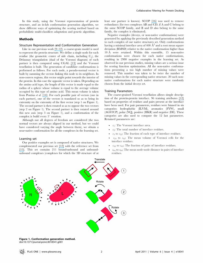
from Pontius et al. [14]. For each possible pair of vectors (one in

each partner), one of the vectors is translated so as to bring its

extremity on the extremity of the first vector (step 1 on Figure 1).

The second partner is then rotated so as to oppose the two vectors

(step 2 on Figure 1). The second partner is then rotated around

this new axis (step 3 on Figure 1), and a conformation of the

complex is build every 5u rotation.

Although not all degrees of freedom are considered (the two

normal vectors are always aligned in our method, but we could

have considered varying the angle between them), we obtain a

near-native conformation for all the complexes in the learning set.

Learning setOur positive examples set is composed of native structures. We

complemented our previous set [12] with the reference set from

[15]. This set contains 211 bound-unbound and unbound-

unbound complexes (complexes for which the 3D structure of at

least one partner is known). SCOP [16] was used to remove

redundancy (for two complexes AB and CD, if A and C belong to

the same SCOP family, and B and D also belong to the same

family, the complex is eliminated).

Negative examples (decoys, or non-native conformations) were

generated by applying the previously described generation method

to each complex of our native structures set. Only conformations

having a minimal interface area of 400 A2 and a root mean square

deviation (RMSD) relative to the native conformation higher than

10 A were retained. Within this ensemble, 15 non-native

conformations were chosen for each native conformations,

resulting in 2980 negative examples in the learning set. As

observed in our previous studies, missing values are a serious issue

for scoring function optimization. All the non-native conforma-

tions presenting a too high number of missing values were

removed. This number was taken to be twice the number of

missing values in the corresponding native structure. 20 such non-

native conformations for each native structure were randomly

chosen from the initial decoys set.

Training ParametersThe coarse-grained Voronoi tessellation allows simple descrip-

tion of the protein-protein interface. 96 training attributes [12]

based on properties of residues and pairs present at the interface

have been used. For pair parameters, residues were binned in six

categories: hydrophobic (ILVM), aromatics (FYW), small

(AGSTCP), polar (NQ), positive (HKR) and negative (DE). These

categories are also used to compute the 12 last parameters.

Retained parameters are:

N c1: The Voronoi interface area.

N c2: The total number of interface residues.

N c3 to c22: The fraction of each type of interface residues.

N c23 to c42: The mean volume of Voronoi cells for the

interface residues.

N c43 to c63: The fraction of pairs of interface residues.

N c64 to c84: The mean node-node distance in pairs of interface

residues.

Figure 1. Conformation generation method.doi:10.1371/journal.pone.0018541.g001

Collaborative Filtering for Protein Docking

PLoS ONE | www.plosone.org 2 April 2011 | Volume 6 | Issue 4 | e18541

N c85 to c90: The fraction of interface residues for each

category.

N c91 to c96: The mean volume of Voronoi cells for the

interface residues for each category.

All parameters were computed on the complete interface, defined

as all the residues having at least one neighbor belonging to the

second partner, including residues in contact with solvent molecules.

Genetic algorithmUsing previously defined training attributes, genetic algorithms

are used to find family of functions that optimize the ROC

(Receiver Operating Characteristics) criterion. We used a lzmscheme, with l~10 parents and m~80 children, and a maximum

of 500 generations. We used a classical cross-over and auto-

adaptative mutations. The ROC criterion is commonly used to

evaluate the performance of learning procedures by measuring the

area under the ROC curve (AUC). The ROC curve is obtained by

plotting the proportion of true positives against false positives.

The scoring functions used in this work have the form:

S(conf )~X

i

wi xi(conf ){cij j ð1Þ

where xi is the value of parameter i and wi and ci are the weights

and centering values respectively for parameter i. wi and ci are

optimized by the learning procedure. Learning was performed in a

10-fold cross-validation setting. Ten groups of models were

randomly chosen, each excluding 10% of the training set.

Learning was repeated n times for each training subset.

Consequently, each conformation is evaluated using n different

scoring functions, and for final ranking, the sum of the ranks

obtained by each function is used.

As described in the Results section, the number of functions nused in the computation of the final rank might have an impact on

the quality of the global ranking.

Collaborative filtering methodsSeveral previous studies have shown the strength of Collabo-

rative Filtering (CF) techniques in Information Retrieval problems

[17] to increase the accuracy of the prediction rate. In a common

CF recommender system, there is a list of m users, U1,U2, . . . ,Um

and a list of p items, I1,I2, . . . ,Ip and each user gives a mark to

each object. This mark can also be inferred from the user’s

behaviour. The final mark of each object is then defined by the

ensemble of marks received from each user.

In the present work, a classifier is a user, and conformations are

the items. Each classifier (user) assigns to each item (conformation)

a binary label (or mark): native’ (+) or non native (2).

12 classifiers have been trained on the learning set (see ‘‘Results

and Discussion’’), deriving from four different methods: decision

trees, rules, logistic regression and SVM (Support Vector

Machine). Most optimizations were done using Weka [18]. The

SVMlight [19] software was used for SVM computations.

In a first approach, we have used a default voting system: the

conformations are ranked according to the number of + marks

they have received. Since we have 12 classifiers, this determines 13

different categories: 12+, 11+, …, 0+.

Because 13 categories is far from enough to efficiently ranks a

very large number of conformations, we have also used a second

approach using an amplification average voting system. In this

system, the votes of each classifier are weighted by the precision.

Consequently, the + vote of each classifier is different from the +vote of a different classifier. This results in 212 categories. The

categories are ordered according to:

SCF~expS{

expSzð2Þ

Where Sz (respectively S{) is the sum of the precisions of the

classifiers that have voted + (respectively 2) for conformations of

this category. This score is assigned to each conformation of the

considered category.

Sz~Xn

i~1

11(votei~z)|pri S{~Xn

i~1

11(votei~{)|pri ð3Þ

Where votei represents the vote of the ith classifier and pri

represents its precision. In a unweighted approach, pri is set to 1

for all the classifiers.

Finally, the CF and GA methods have been coupled. For each

conformation evaluated with at least one positive vote (Szw0), the

score SCF{GA(C) of a given conformation C is the product of the

rank obtained by C in the GA, and SCF (C). For conformations

receiving only negative votes, the score SCF{GA(C) is set to be

maximal. The evaluated conformations are then re-ranked

according to this score (in decreasing order). It should be noted

that scores (and consequently ranks) obtained through this method

are not necessarily unique. To measure the number of possible

ranks for each method, taking into account the number of examples

to classify, we will use the granularity as defined in equation 4.

granularity(S)~number of ranks

number of examplesð4Þ

Where S is a set of evaluated conformations.

Evaluation of learning accuracyThe most commonly used criterion for evaluating the efficiency

of a learning procedure is the Area Under the ROC curve (ROC

AUC). The ROC curve is obtained by plotting the proportion of

true positives against the proportion of false positives. A perfect

learning should give an AUC of 1 (all the true positives are found

before any of the negatives), whereas a random function has an

AUC of 0.5 (each prediction has probabilities of 0.5 to be correct

or incorrect).

To measure the performances of the different scoring functions

we use precision, recall and accuracy using TP,FP,TN and FN as

in the confusion matrix (see Table 1). We will also use false

negative rate (FNR) and true negative rate (TNR).

Table 1. Confusion matrix.

solution

+ -

prediction + TP FP

- FN TN

TP: true positives, FP: false positives, FN: false negatives, TN: true negatives.doi:10.1371/journal.pone.0018541.t001

Collaborative Filtering for Protein Docking

PLoS ONE | www.plosone.org 3 April 2011 | Volume 6 | Issue 4 | e18541

These values can be computed as:

Precision~TP

TPzFPRecall~

TP

TPzFNAccuracy~

TPzTN

total

FNR~FN

TNzFNTNR~

TN

TNzFN

CAPRI ExperimentsTo evaluate the accuracy of our CF-GA scoring procedure, we

developed two protocols based on targets 22 to 40 of the CAPRI

(Critical Assessment of PRedicted Interaction) experiment. CAPRI

is a blind prediction experiment designed to test docking and

scoring procedures [20,21]. In the scoring experiment, a large set

of models submitted by the docking predictors is made available to

the community to test scoring functions independently of

conformation generation algorithms.

Four targets where eliminated for different reasons:

N

N

Nscoring method is not adapted to this problem yet.

For each target, the scoring ensemble was evaluated using GA,

CF and CF-GA methods.

For reasons exposed in ‘‘Results and Discussion’’, candidate

conformations where evaluated according to two different sets of

criteria.

In the fnat evaluation, we use only the fnat criterion, which is

the fraction of native contacts (the fraction of contacts between the

two partners in the evaluated conformation that do exist in the

native structure). Four quality classes can be defined:

N High (fnat $0.5),

N Medium (0.3# fnat ,0.5),

N Acceptable (0.1# fnat ,0.3),

N Incorrect (fnat,0.1)

CAPRI evaluation [21,23] also uses two other criteria: the

IRMSD (RMSD between prediction and native structure computed

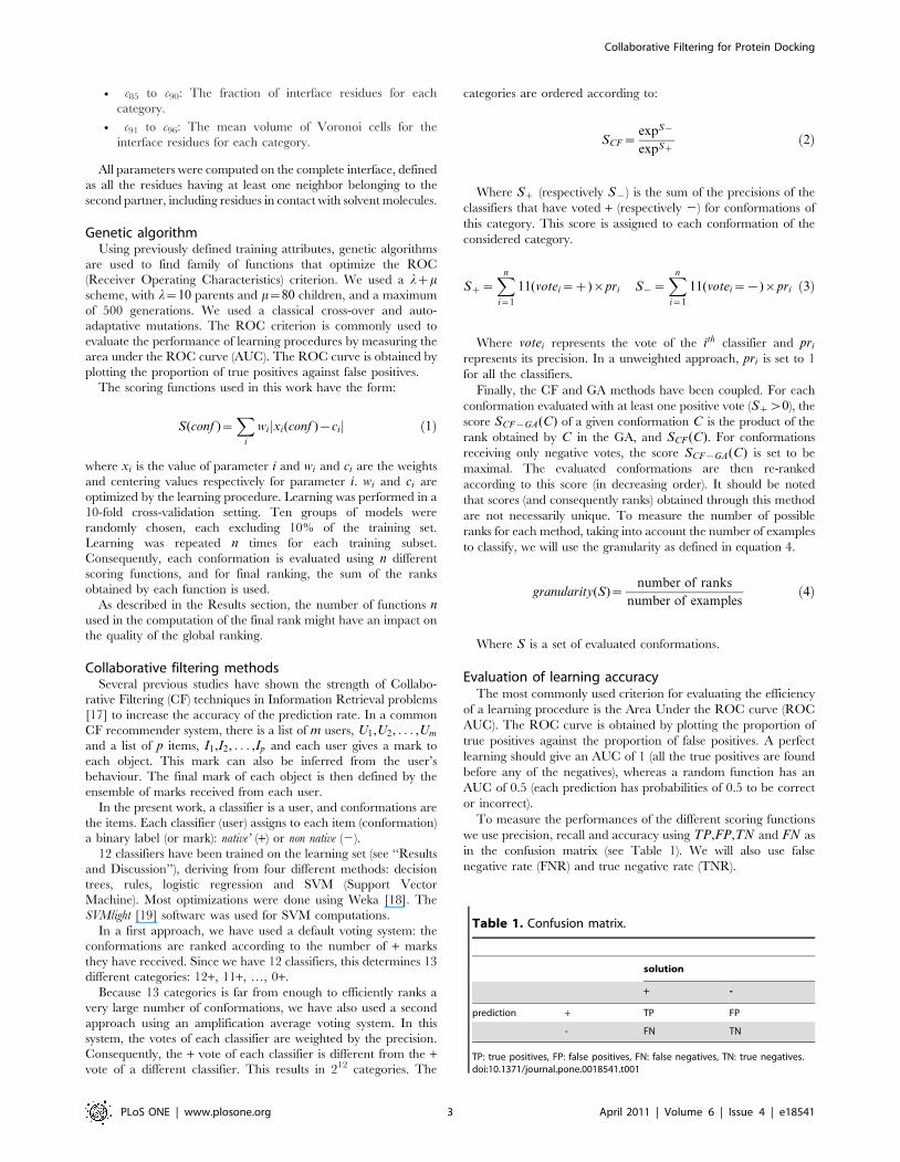
Figure 2. Genetic Algorithm performance as a function of the number of runs. For each number of runs n, the measure of the AUC hasbeen repeated 50 times using a 10-fold cross-validation protocol. Average, minimum and maximum values are plotted.doi:10.1371/journal.pone.0018541.g002

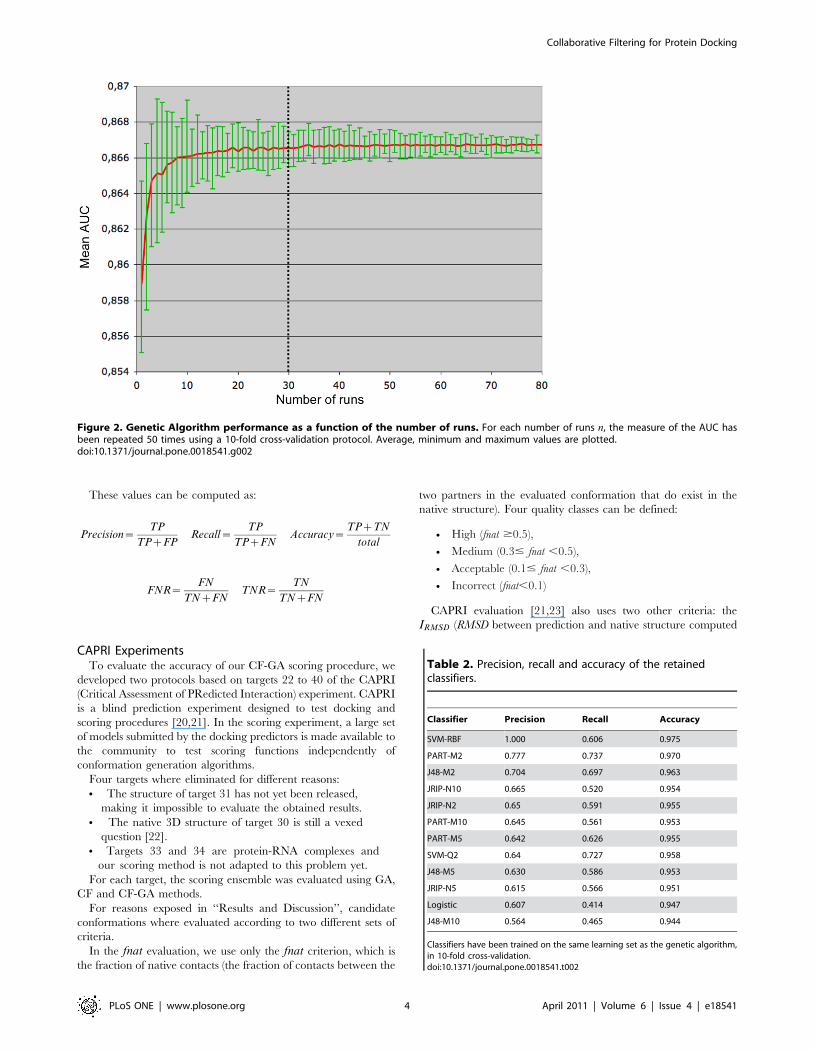
Table 2. Precision, recall and accuracy of the retainedclassifiers.

Classifier Precision Recall Accuracy

SVM-RBF 1.000 0.606 0.975

PART-M2 0.777 0.737 0.970

J48-M2 0.704 0.697 0.963

JRIP-N10 0.665 0.520 0.954

JRIP-N2 0.65 0.591 0.955

PART-M10 0.645 0.561 0.953

PART-M5 0.642 0.626 0.955

SVM-Q2 0.64 0.727 0.958

J48-M5 0.630 0.586 0.953

JRIP-N5 0.615 0.566 0.951

Logistic 0.607 0.414 0.947

J48-M10 0.564 0.465 0.944

Classifiers have been trained on the same learning set as the genetic algorithm,in 10-fold cross-validation.doi:10.1371/journal.pone.0018541.t002

Collaborative Filtering for Protein Docking

PLoS ONE | www.plosone.org 4 April 2011 | Volume 6 | Issue 4 | e18541

making it impossible to evaluate the obtained results.

The structure of target 31 has not yet been released,

The native 3D structure of target 30 is still a vexed

33 and 34 are protein-RNA complexes and

our

Targets

question [22].

only on interface atoms) and LRMSD (RMSD computed on all the

atoms of the smallest protein, the largest protein of prediction and

native structure being superimposed). Again four quality classes

are defined:

N High: (fnat $0.5) and (IRMSD #1 or LRMSD #1)

N Medium: [(0.3# fnat ,0.5) and (IRMSD #2.0 or LRMSD

#5.0)]or [(fnat .0.5 and IRMSD.1.0 or IRMSD.1.0)]

N Acceptable: [(0.1# fnat ,0.3) and (IRMSD #4.0 or LRMSD

#10.0)] or [fnat .0.3 and (LRMSD .5.0 or IRMSD .2.0)]

N Incorrect.

Results and Discussion

In our previous work, we have used different flavors of genetic

algorithm (GA) optimization to obtain scoring functions for

protein-protein docking. Since we have reached the limits of the

precision that can be obtained with GA alone, we combined the

GA-based scoring function with scoring functions built using four

other learning algorithms:

N Logistic regression (LR) [24];

N Support Vector Machines [25], using either radial-based

function (RBF), linear kernel (LK), polynomial kernel (PK)

or 2 and 4 quadratic kernels (QK2 and QK4);

N Decision trees, using the C4.5 learner [26] and, J48, its

implementation in Weka [18], using 2, 5 and 10 as

minimum numbers of examples required to build a leaf

(classifiers J48-M2, J48-M5 and J48-M10 respectively);

N Two-rules learners, using two different implementations

(JRIP [27] and PART [28]), using again 2, 5 and 10 as

minimum numbers of examples required to build a rule

(classifiers JRIP-M2, JRIP-M5, JRIP-M10, PART-M2,

PART-M5 and PART-M10).

Here we show how these 15 classifiers can be combined, in a

collaborative scheme and with the genetic algorithm procedure.

Predictions obtained with the genetic algorithmprocedure

The sensitivity (ability to discriminate true positives from false

positives, also called recall) of the genetic algorithm (GA) has been

evaluated using the ROC criterion. Since GA is a heuristic,

optimization must be repeated. The number of repetitions

necessary for obtaining a reliable result largely depends on the

specificity of the problem. To determine the number of repetitions

needed in our case, we have plotted the area under the ROC

curve (AUC) as a function of the number of runs. For each value of

the number of runs n, the experiment has been repeated 50 times

in 10-fold cross-validation. This allows to compute, for each n, the

mean value and the variance of the AUC. As can be seen on

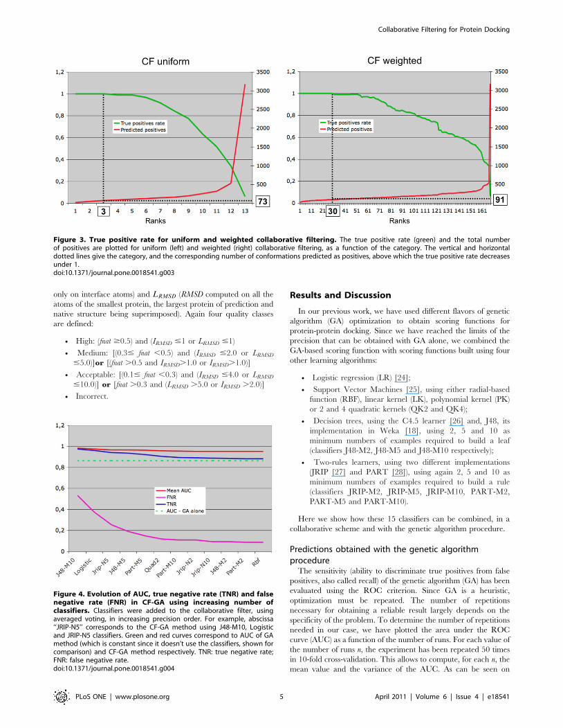
Figure 3. True positive rate for uniform and weighted collaborative filtering. The true positive rate (green) and the total numberof positives are plotted for uniform (left) and weighted (right) collaborative filtering, as a function of the category. The vertical and horizontaldotted lines give the category, and the corresponding number of conformations predicted as positives, above which the true positive rate decreasesunder 1.doi:10.1371/journal.pone.0018541.g003

Figure 4. Evolution of AUC, true negative rate (TNR) and falsenegative rate (FNR) in CF-GA using increasing number ofclassifiers. Classifiers were added to the collaborative filter, usingaveraged voting, in increasing precision order. For example, abscissa‘‘JRIP-N5’’ corresponds to the CF-GA method using J48-M10, Logisticand JRIP-N5 classifiers. Green and red curves correspond to AUC of GAmethod (which is constant since it doesn’t use the classifiers, shown forcomparison) and CF-GA method respectively. TNR: true negative rate;FNR: false negative rate.doi:10.1371/journal.pone.0018541.g004

Collaborative Filtering for Protein Docking

PLoS ONE | www.plosone.org 5 April 2011 | Volume 6 | Issue 4 | e18541

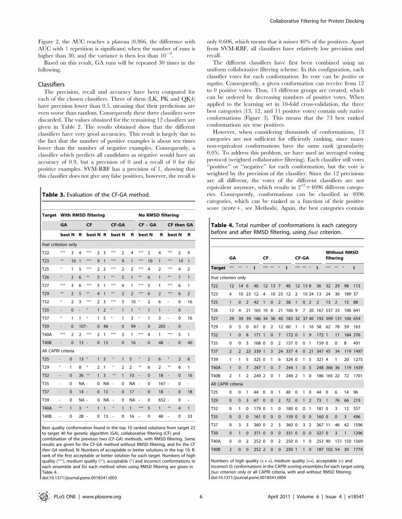
Figure 2, the AUC reaches a plateau (0.866, the difference with

AUC with 1 repetition is significant) when the number of runs is

higher than 30, and the variance is then less than 1029.

Based on this result, GA runs will be repeated 30 times in the

following.

ClassifiersThe precision, recall and accuracy have been computed for

each of the chosen classifiers. Three of them (LK, PK and QK4)

have precision lower than 0.5, meaning that their predictions are

even worse than random. Consequently these three classifiers were

discarded. The values obtained for the remaining 12 classifiers are

given in Table 2. The results obtained show that the different

classifiers have very good accuracies. This result is largely due to

the fact that the number of positive examples is about ten times

lower than the number of negative examples. Consequently, a

classifier which predicts all candidates as negative would have an

accuracy of 0.9, but a precision of 0 and a recall of 0 for the

positive examples. SVM-RBF has a precision of 1, showing that

this classifier does not give any false positives, however, the recall is

only 0.606, which means that it misses 40% of the positives. Apart

from SVM-RBF, all classifiers have relatively low precision and

recall.

The different classifiers have first been combined using an

uniform collaborative filtering scheme. In this configuration, each

classifier votes for each conformation. Its vote can be positive or

negative. Consequently, a given conformation can receive from 12

to 0 positive votes. Thus, 13 different groups are created, which

can be ordered by decreasing numbers of positive votes. When

applied to the learning set in 10-fold cross-validation, the three

best categories (13, 12, and 11 positive votes) contain only native

conformations (Figure 3). This means that the 73 best ranked

conformations are true positives.

However, when considering thousands of conformations, 13

categories are not sufficient for efficiently ranking, since many

non-equivalent conformations have the same rank (granularity

0.05). To address this problem, we have used an averaged voting

protocol (weighted collaborative filtering). Each classifier still votes

‘‘positive’’ or ‘‘negative’’ for each conformation, but the vote is

weighted by the precision of the classifier. Since the 12 precisions

are all different, the votes of the different classifiers are not

equivalent anymore, which results in 212 = 4096 different catego-

ries. Consequently, conformations can be classified in 4096

categories, which can be ranked as a function of their positive

score (scorez, see Methods). Again, the best categories contain

Table 3. Evaluation of the CF-GA method.

Target With RMSD filtering No RMSD filtering

GA CF CF-GA CF – GA CF then GA

best N R best N R best N R best N R best N R

fnat criterion only

T22 ??? 3 4 ??? 2 3 ??? 2 4 ??? 2 4 ??? 2 4

T23 ?? 10 1 ??? 9 1 ??? 9 1 ??? 10 1 ??? 10 1

T25 ? 1 5 ??? 2 2 ??? 2 2 ??? 4 2 ??? 4 2

T26 ? 2 6 ?? 5 1 ?? 5 1 ?? 6 1 ?? 7 1

T27 ??? 3 6 ??? 5 1 ??? 4 1 ??? 5 1 ??? 6 1

T29 ?? 2 5 ?? 4 1 ?? 2 2 ??? 6 2 ??? 6 2

T32 ? 2 3 ??? 2 3 ??? 3 10 ? 2 6 - 0 16

T35 - 0 - ? 1 2 ? 1 1 ? 1 1 - 0 -

T37 ? 1 1 ? 1 5 ? 1 3 ? 1 3 - 0 16

T39 - 0 107 - 0 48 - 0 99 - 0 205 - 0 -

T40A ??? 2 2 ??? 2 1 ??? 3 1 ??? 4 1 ??? 5 1

T40B - 0 13 - 0 13 - 0 16 - 0 48 - 0 40

All CAPRI criteria

T25 - 0 13 ? 1 5 ? 1 5 ? 2 6 ? 2 6

T29 ? 1 8 ? 2 1 ? 2 2 ?? 6 2 ?? 6 1

T32 - 0 36 ?? 1 3 ?? 1 10 - 0 18 - 0 16

T35 - 0 NA - 0 NA - 0 NA - 0 167 - 0 -

T37 - 0 14 - 0 13 - 0 17 - 0 18 - 0 18

T39 - 0 NA - 0 NA - 0 NA - 0 652 - 0 -

T40A ?? 1 3 ? 1 1 ? 1 1 ??? 5 1 ?? 4 1

T40B - 0 28 - 0 13 - 0 16 - 0 48 - 0 33

Best quality conformation found in the top 10 ranked solutions from target 22to target 40 for genetic algorithm (GA), collaborative filtering (CF) andcombination of the previous two (CF-GA) methods, with RMSD filtering. Sameresults are given for the CF-GA method without RMSD filtering, and for the CFthen GA method. N: Numbers of acceptable or better solutions in the top 10; R:rank of the first acceptable or better solution for each target. Numbers of highquality (???), medium quality (??), acceptable (?) and incorrect conformations ineach ensemble and for each method when using RMSD filtering are given inTable 4.doi:10.1371/journal.pone.0018541.t003

Table 4. Total number of conformations is each categorybefore and after RMSD filtering, using fnat criterion.

GA CF CF-GAWithout RMSDfiltering

Target ??? ?? ? I ??? ?? ? I ??? ?? ? I ??? ?? ? I

fnat criterion only

T22 12 14 6 40 12 13 7 40 12 13 8 36 32 29 98 113

T23 4 10 23 12 4 10 23 12 2 10 24 13 24 36 189 37

T25 1 0 2 42 1 0 2 38 1 0 2 2 13 2 13 88

T26 12 4 21 165 10 8 21 166 9 7 20 167 537 33 106 641

T27 29 39 39 186 34 36 40 183 32 37 40 192 399 131 106 654

T29 0 3 0 67 0 2 12 60 1 1 16 58 62 78 59 163

T32 1 0 8 171 1 0 7 172 0 1 9 172 1 11 184 376

T35 0 0 3 168 0 0 2 157 0 0 1 159 0 0 8 491

T37 2 2 23 339 1 3 24 337 4 0 21 347 45 34 119 1497

T39 1 1 5 325 0 1 6 324 0 1 5 321 4 1 20 1275

T40A 1 0 7 247 1 0 7 244 1 0 5 248 366 36 119 1439

T40B 2 1 2 249 2 0 1 249 2 1 0 186 165 22 72 1701

All CAPRI criteria

T25 0 0 1 44 0 0 1 40 0 1 0 44 0 6 14 96

T29 0 0 3 67 0 0 2 72 0 1 2 73 1 76 66 219

T32 0 1 0 179 0 1 0 180 0 0 1 181 0 3 12 557

T35 0 0 0 161 0 0 0 159 0 0 0 160 0 0 3 496

T37 0 3 3 360 0 2 3 360 0 3 2 367 11 46 42 1596

T39 0 1 0 371 0 0 0 331 0 0 0 327 0 3 1 1296

T40A 0 0 2 252 0 0 2 250 0 1 0 253 90 151 150 1569

T40B 2 0 0 252 2 0 0 250 1 1 0 187 102 54 30 1774

Numbers of high quality (? ? ?), medium quality (??), acceptable (?) andincorrect (I) conformations in the CAPRI scoring ensembles for each target usingfnat criterion only or all CAPRI criteria, with and without RMSD filtering.doi:10.1371/journal.pone.0018541.t004

Collaborative Filtering for Protein Docking

PLoS ONE | www.plosone.org 6 April 2011 | Volume 6 | Issue 4 | e18541

only true positives (see Figure 3). The results are even better than

those obtained with uniform CF, since the first non-native

conformation belongs to category 31, which means that the 91

best ranked conformations are natives.

However, when considering millions of conformations, 4096

categories are still not sufficient (granularity 0.15). For example,

when using the weighted-CF method on the learning set, the best

category (only positive votes) contains 24 conformations. Conse-

quently, this method cannot be used for ranking large data sets.

Combination of collaborative filtering and geneticalgorithm

Since CF efficiently eliminates non-native conformations, we

have used CF to weight the GA score (see Methods). This is what

we call the collaborative filtering - genetic algorithm (CF-GA)

method. The averaged voting configuration was used, and the CF-

GA score is obtained by multiplying the GA score by the ratio of

the exponential of positive and negative CF scores. Consequently,

the score of conformations classified as negatives by a majority of

classifiers have very low CF-GA scores. Figure 4 shows the

evolutions of AUC, true negative rate (TNR) and false negative

rate (FNR) as we add more classifiers in the CF (in increasing

precision order).

Another way of combining the two methods is to: first classify

the candidate conformations using the CF, retain only the

candidates of the best classes, then use the GA to rank them. To

evaluate this approach, we retained all the candidate conforma-

tions which rank was lower than N (N~(10,20,:::,100) have been

tested). These were then ranked using GA. The best results have

been obtained with N~100, but this method proved less efficient

than the CF-GA (see CF then GA in Table 3).

Using the 12 classifiers, the AUC is 0.98, but more importantly,

the FNR is only 0.09, meaning that more than 90% of the

conformations classified as natives are indeed natives. Unlike

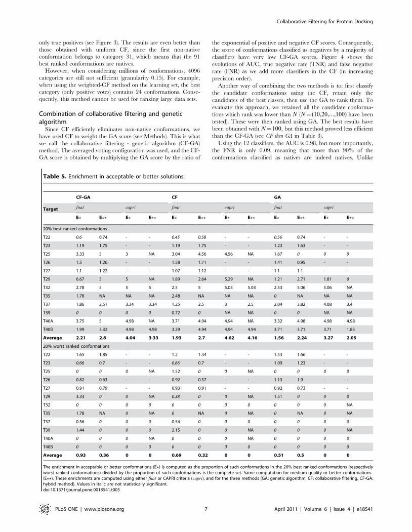
Table 5. Enrichment in acceptable or better solutions.

CF-GA CF GA

Target fnat capri fnat capri fnat capri

E? E?? E? E?? E? E?? E? E?? E? E?? E? E??

20% best ranked conformations

T22 0.6 0.74 - - 0.45 0.58 - - 0.56 0.74 - -

T23 1.19 1.75 - - 1.19 1.75 - - 1.23 1.63 - -

T25 3.33 5 3 NA 3.04 4.56 4.56 NA 1.67 0 0 0

T26 1.5 1.26 - - 1.58 1.71 - - 1.41 0.95 - -

T27 1.1 1.22 - - 1.07 1.12 - - 1.1 1.1 - -

T29 6.67 5 5 NA 1.89 2.64 5.29 NA 1.21 2.71 1.81 0

T32 2.78 5 5 5 2.5 5 5.03 5.03 2.53 5.06 5.06 NA

T35 1.78 NA NA NA 2.48 NA NA NA 0 NA NA NA

T37 1.86 2.51 3.34 3.34 1.25 2.5 3 2.5 2.04 3.82 4.08 3.4

T39 0 0 0 0 0.72 0 NA NA 0 0 NA NA

T40A 3.75 5 4.98 NA 3.71 4.94 4.94 NA 3.32 4.98 4.98 4.98

T40B 1.99 3.32 4.98 4.98 3.29 4.94 4.94 4.94 3.71 3.71 3.71 1.85

Average 2.21 2.8 4.04 3.33 1.93 2.7 4.62 4.16 1.56 2.24 3.27 2.05

20% worst ranked conformations

T22 1.65 1.85 - - 1.2 1.34 - - 1.53 1.66 - -

T23 0.66 0.7 - - 0.66 0.7 - - 1.09 1.23 - -

T25 0 0 0 NA 1.52 0 0 NA 0 0 0 0

T26 0.82 0.63 - - 0.92 0.57 - - 1.13 1.9 - -

T27 0.91 0.79 - - 0.93 0.91 - - 0.92 0.73 - -

T29 3.33 0 0 NA 0.38 0 0 NA 1.51 0 0 0

T32 0 0 0 0 0 0 0 0 0 0 0 NA

T35 1.78 NA 0 NA 0 NA 0 NA 0 NA 0 NA

T37 0.56 0 0 0 0.54 0 0 0 0 0 0 0

T39 1.44 0 0 0 2.15 0 0 NA 0 0 0 NA

T40A 0 0 0 NA 0 0 0 NA 0 0 0 0

T40B 0 0 0 0 0 0 0 0 0 0 0 0

Average 0.93 0.36 0 0 0.69 0.32 0 0 0.51 0.5 0 0

The enrichment in acceptable or better conformations (E?) is computed as the proportion of such conformations in the 20% best ranked conformations (respectivelyworst ranked conformations) divided by the proportion of such conformations is the complete set. Same computation for medium quality or better conformations(E??). These enrichments are computed using either fnat or CAPRI criteria (capri), and for the three methods (GA: genetic algorithm, CF: collaborative filtering, CF-GA:hybrid method). Values in italic are not statistically significant.doi:10.1371/journal.pone.0018541.t005

Collaborative Filtering for Protein Docking

PLoS ONE | www.plosone.org 7 April 2011 | Volume 6 | Issue 4 | e18541

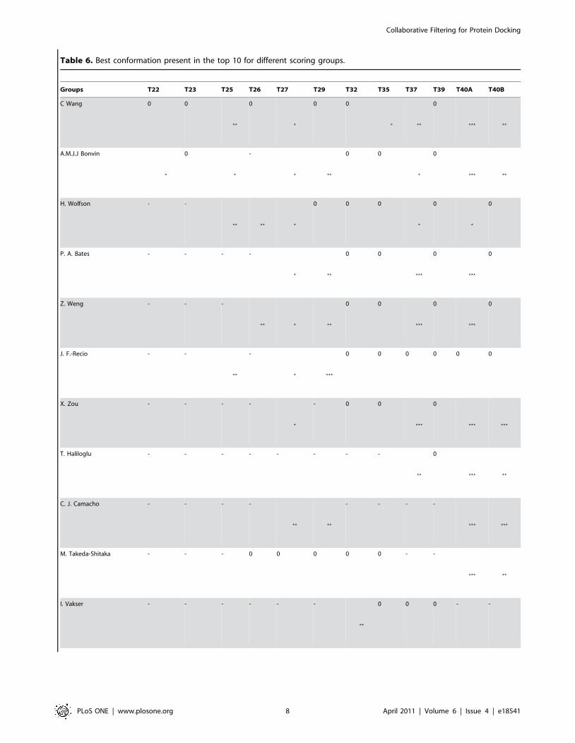
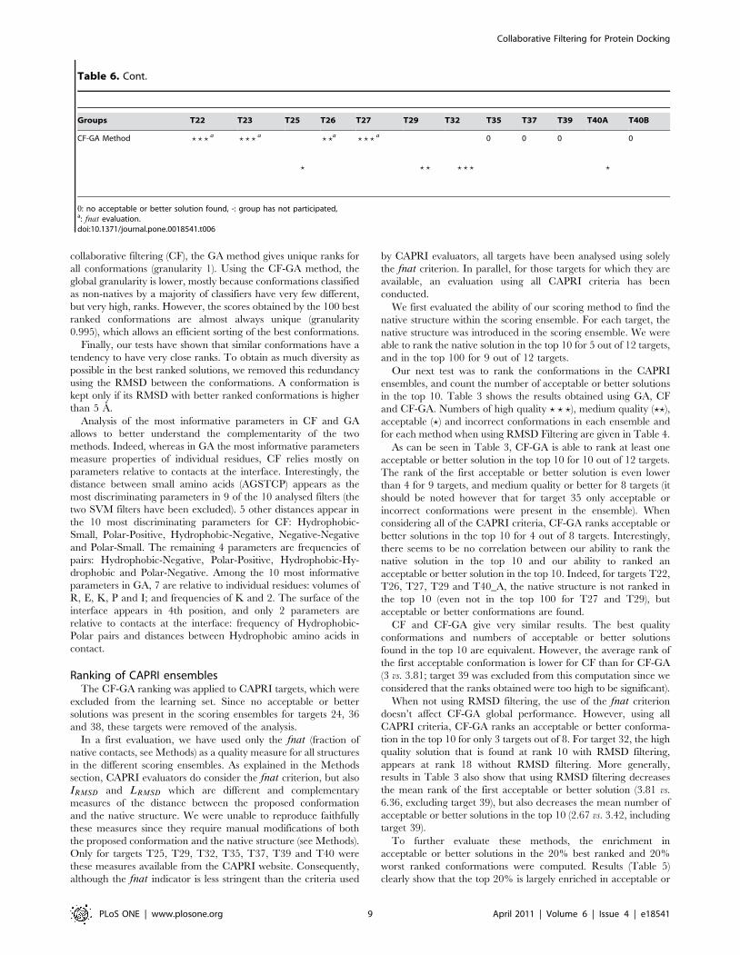
Table 6. Best conformation present in the top 10 for different scoring groups.

Groups T22 T23 T25 T26 T27 T29 T32 T35 T37 T39 T40A T40B

C Wang 0 0

??

0

?

0 0

? ??

0

??? ??

A.M.J.J Bonvin

?

0

?

-

? ??

0 0

?

0

??? ??

H. Wolfson - -

?? ?? ?

0 0 0

?

0

?

0

P. A. Bates - - - -

? ??

0 0

???

0

???

0

Z. Weng - - -

?? ? ??

0 0

???

0

???

0

J. F.-Recio - -

??

-

? ???

0 0 0 0 0 0

X. Zou - - - -

?

- 0 0

???

0

??? ???

T. Haliloglu - - - - - - - -

??

0

??? ??

C. J. Camacho - - - -

?? ??

- - - -

??? ???

M. Takeda-Shitaka - - - 0 0 0 0 0 - -

??? ??

I. Vakser - - - - - -

??

0 0 0 - -

Collaborative Filtering for Protein Docking

PLoS ONE | www.plosone.org 8 April 2011 | Volume 6 | Issue 4 | e18541

collaborative filtering (CF), the GA method gives unique ranks for

all conformations (granularity 1). Using the CF-GA method, the

global granularity is lower, mostly because conformations classified

as non-natives by a majority of classifiers have very few different,

but very high, ranks. However, the scores obtained by the 100 best

ranked conformations are almost always unique (granularity

0.995), which allows an efficient sorting of the best conformations.

Finally, our tests have shown that similar conformations have a

tendency to have very close ranks. To obtain as much diversity as

possible in the best ranked solutions, we removed this redundancy

using the RMSD between the conformations. A conformation is

kept only if its RMSD with better ranked conformations is higher

than 5 A.

Analysis of the most informative parameters in CF and GA

allows to better understand the complementarity of the two

methods. Indeed, whereas in GA the most informative parameters

measure properties of individual residues, CF relies mostly on

parameters relative to contacts at the interface. Interestingly, the

distance between small amino acids (AGSTCP) appears as the

most discriminating parameters in 9 of the 10 analysed filters (the

two SVM filters have been excluded). 5 other distances appear in

the 10 most discriminating parameters for CF: Hydrophobic-

Small, Polar-Positive, Hydrophobic-Negative, Negative-Negative

and Polar-Small. The remaining 4 parameters are frequencies of

pairs: Hydrophobic-Negative, Polar-Positive, Hydrophobic-Hy-

drophobic and Polar-Negative. Among the 10 most informative

parameters in GA, 7 are relative to individual residues: volumes of

R, E, K, P and I; and frequencies of K and 2. The surface of the

interface appears in 4th position, and only 2 parameters are

relative to contacts at the interface: frequency of Hydrophobic-

Polar pairs and distances between Hydrophobic amino acids in

contact.

Ranking of CAPRI ensemblesThe CF-GA ranking was applied to CAPRI targets, which were

excluded from the learning set. Since no acceptable or better

solutions was present in the scoring ensembles for targets 24, 36

and 38, these targets were removed of the analysis.

In a first evaluation, we have used only the fnat (fraction of

native contacts, see Methods) as a quality measure for all structures

in the different scoring ensembles. As explained in the Methods

section, CAPRI evaluators do consider the fnat criterion, but also

IRMSD and LRMSD which are different and complementary

measures of the distance between the proposed conformation

and the native structure. We were unable to reproduce faithfully

these measures since they require manual modifications of both

the proposed conformation and the native structure (see Methods).

Only for targets T25, T29, T32, T35, T37, T39 and T40 were

these measures available from the CAPRI website. Consequently,

although the fnat indicator is less stringent than the criteria used

by CAPRI evaluators, all targets have been analysed using solely

the fnat criterion. In parallel, for those targets for which they are

available, an evaluation using all CAPRI criteria has been

conducted.

We first evaluated the ability of our scoring method to find the

native structure within the scoring ensemble. For each target, the

native structure was introduced in the scoring ensemble. We were

able to rank the native solution in the top 10 for 5 out of 12 targets,

and in the top 100 for 9 out of 12 targets.

Our next test was to rank the conformations in the CAPRI

ensembles, and count the number of acceptable or better solutions

in the top 10. Table 3 shows the results obtained using GA, CF

and CF-GA. Numbers of high quality ? ? ?), medium quality (??),

acceptable (?) and incorrect conformations in each ensemble and

for each method when using RMSD Filtering are given in Table 4.

As can be seen in Table 3, CF-GA is able to rank at least one

acceptable or better solution in the top 10 for 10 out of 12 targets.

The rank of the first acceptable or better solution is even lower

than 4 for 9 targets, and medium quality or better for 8 targets (it

should be noted however that for target 35 only acceptable or

incorrect conformations were present in the ensemble). When

considering all of the CAPRI criteria, CF-GA ranks acceptable or

better solutions in the top 10 for 4 out of 8 targets. Interestingly,

there seems to be no correlation between our ability to rank the

native solution in the top 10 and our ability to ranked an

acceptable or better solution in the top 10. Indeed, for targets T22,

T26, T27, T29 and T40_A, the native structure is not ranked in

the top 10 (even not in the top 100 for T27 and T29), but

acceptable or better conformations are found.

CF and CF-GA give very similar results. The best quality

conformations and numbers of acceptable or better solutions

found in the top 10 are equivalent. However, the average rank of

the first acceptable conformation is lower for CF than for CF-GA

(3 vs. 3.81; target 39 was excluded from this computation since we

considered that the ranks obtained were too high to be significant).

When not using RMSD filtering, the use of the fnat criterion

doesn’t affect CF-GA global performance. However, using all

CAPRI criteria, CF-GA ranks an acceptable or better conforma-

tion in the top 10 for only 3 targets out of 8. For target 32, the high

quality solution that is found at rank 10 with RMSD filtering,

appears at rank 18 without RMSD filtering. More generally,

results in Table 3 also show that using RMSD filtering decreases

the mean rank of the first acceptable or better solution (3.81 vs.

6.36, excluding target 39), but also decreases the mean number of

acceptable or better solutions in the top 10 (2.67 vs. 3.42, including

target 39).

To further evaluate these methods, the enrichment in

acceptable or better solutions in the 20% best ranked and 20%

worst ranked conformations were computed. Results (Table 5)

clearly show that the top 20% is largely enriched in acceptable or

Groups T22 T23 T25 T26 T27 T29 T32 T35 T37 T39 T40A T40B

CF-GA Method ? ? ? a ? ? ? a

?

? ?a ? ? ? a

? ? ? ? ?

0 0 0

?

0

0: no acceptable or better solution found, -: group has not participated,a: fnat evaluation.doi:10.1371/journal.pone.0018541.t006

Table 6. Cont.

Collaborative Filtering for Protein Docking

PLoS ONE | www.plosone.org 9 April 2011 | Volume 6 | Issue 4 | e18541

better solutions, and even more in medium or better solutions

when considering the fnat criterion. The comparison between

these two categories is more difficult when using all of the CAPRI

criteria, since in most cases the computation cannot be made. It

can also be seen that CF-GA is better at enriching the top 20% in

acceptable or better solutions. It should also be noted that for the

three methods, using CAPRI criteria, no acceptable or better

solution is ranked in the worst 20%.

We have compared these results with the ones obtained by other

scoring groups on the 12 targets. As can be seen from Table 6, two

of the targets for which we do not find an acceptable or better

solution in the top 10 (T35 with all CAPRI criteria, and T39 with

either quality measures) were difficult targets, and only one group

obtained an acceptable solution for T35, none for T39. It should

also be noted that target 35 is not a biological complex, but the

assembly of two different modules belonging to the same protein

chain.

Target 37 was found by most scorers. Our failure for this target

is probably related to the fact that this complex is made of three

protein chains (A, C and D), and the docking was conducted using

only two of these chains. The resulting candidate interfaces, since

they represent only a portion of the native interface, are two small

to be favourably ranked by our method. Target 40 is also a trimer

(chains A, B and C), but this time with two distinct interfaces (CA:

target 40A, and CB: target 40B). The GA-CF method successfully

finds the CA interface, but fails to favourably rank a good

conformation for interface CB. The CA interface is significantly

larger than CB (1009.5 A2 vs. 731.3 A2). Here again, the size of this

second interface is two small for our method, especially since much

larger interfaces (corresponding to the CA interface) are found in

the proposed conformations.

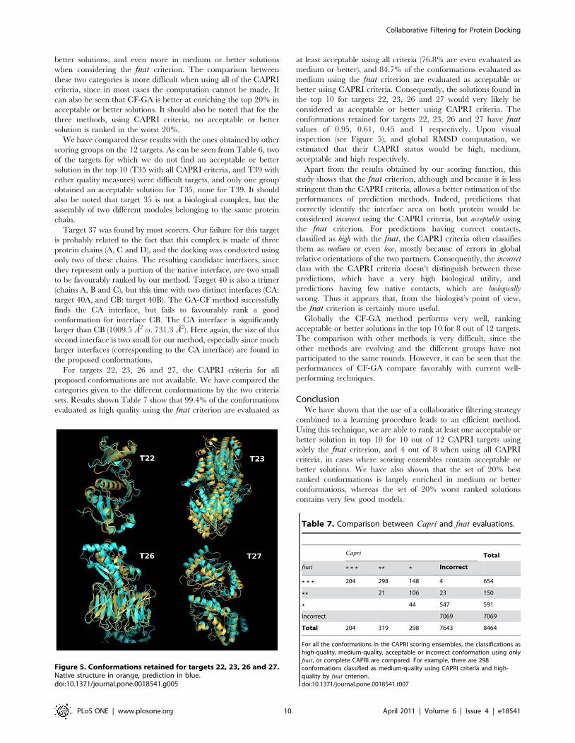
For targets 22, 23, 26 and 27, the CAPRI criteria for all

proposed conformations are not available. We have compared the

categories given to the different conformations by the two criteria

sets. Results shown Table 7 show that 99.4% of the conformations

evaluated as high quality using the fnat criterion are evaluated as

at least acceptable using all criteria (76.8% are even evaluated as

medium or better), and 84.7% of the conformations evaluated as

medium using the fnat criterion are evaluated as acceptable or

better using CAPRI criteria. Consequently, the solutions found in

the top 10 for targets 22, 23, 26 and 27 would very likely be

considered as acceptable or better using CAPRI criteria. The

conformations retained for targets 22, 23, 26 and 27 have fnatvalues of 0.95, 0.61, 0.45 and 1 respectively. Upon visual

inspection (see Figure 5), and global RMSD computation, we

estimated that their CAPRI status would be high, medium,

acceptable and high respectively.

Apart from the results obtained by our scoring function, this

study shows that the fnat criterion, although and because it is less

stringent than the CAPRI criteria, allows a better estimation of the

performances of prediction methods. Indeed, predictions that

correctly identify the interface area on both protein would be

considered incorrect using the CAPRI criteria, but acceptable using

the fnat criterion. For predictions having correct contacts,

classified as high with the fnat, the CAPRI criteria often classifies

them as medium or even low, mostly because of errors in global

relative orientations of the two partners. Consequently, the incorrect

class with the CAPRI criteria doesn’t distinguish between these

predictions, which have a very high biological utility, and

predictions having few native contacts, which are biologically

wrong. Thus it appears that, from the biologist’s point of view,

the fnat criterion is certainly more useful.

Globally the CF-GA method performs very well, ranking

acceptable or better solutions in the top 10 for 8 out of 12 targets.

The comparison with other methods is very difficult, since the

other methods are evolving and the different groups have not

participated to the same rounds. However, it can be seen that the

performances of CF-GA compare favorably with current well-

performing techniques.

ConclusionWe have shown that the use of a collaborative filtering strategy

combined to a learning procedure leads to an efficient method.

Using this technique, we are able to rank at least one acceptable or

better solution in top 10 for 10 out of 12 CAPRI targets using

solely the fnat criterion, and 4 out of 8 when using all CAPRI

criteria, in cases where scoring ensembles contain acceptable or

better solutions. We have also shown that the set of 20% best

ranked conformations is largely enriched in medium or better

conformations, whereas the set of 20% worst ranked solutions

contains very few good models.

Figure 5. Conformations retained for targets 22, 23, 26 and 27.Native structure in orange, prediction in blue.doi:10.1371/journal.pone.0018541.g005

Table 7. Comparison between Capri and fnat evaluations.

Capri Total

fnat ? ? ? ?? ? Incorrect

? ? ? 204 298 148 4 654

?? 21 106 23 150

? 44 547 591

Incorrect 7069 7069

Total 204 319 298 7643 8464

For all the conformations in the CAPRI scoring ensembles, the classifications ashigh-quality, medium-quality, acceptable or incorrect conformation using onlyfnat, or complete CAPRI are compared. For example, there are 298conformations classified as medium-quality using CAPRI criteria and high-quality by fnat criterion.doi:10.1371/journal.pone.0018541.t007

Collaborative Filtering for Protein Docking

PLoS ONE | www.plosone.org 10 April 2011 | Volume 6 | Issue 4 | e18541

The use of RMSD-filtering allows to increase the diversity of the

conformations present in the top 10, which decreases the mean

rank of the first acceptable or better conformation, but also

decreases the number of acceptable or better conformations in the

top 10. This is an advantage in an exploration perspective, since

the proposed conformations are very different from each other.

But this is also a disadvantage in an optimization or refinement

perspective, since, for example, a very favourably ranked medium

quality conformation can eliminate a high quality conformation

having a slightly higher rank.

Finally, we have seen that our method fails on trimers. In the

case of target 40 this is largely due to the fact that our method

searches the best interface, and is not trained to look for multiple

interfaces. Finding these interfaces would probably require

training the method specifically on complexes with more than

two chains.

Author Contributions

Conceived and designed the experiments: TB JB JA AP. Performed the

experiments: TB JB JA AP. Analyzed the data: TB JB JA AP. Contributed

reagents/materials/analysis tools: TB JB JA AP. Wrote the paper: TB JB

JA AP.

References

1. Wodak SJ, Janin J (2002) Structural basis of macromolecular recognition. Adv

Protein Chem 61: 9–73.2. Sanderson CM (2009) The cartographers toolbox: building bigger and better

human protein interaction networks. Brief Funct Genomic Proteomic 8: 1–11.

3. Berman H, Westbrook J, Feng Z, Gilliland G, Bhat T, et al. (2000) The ProteinData Bank. Nucleic Acids Research 28: 235–242.

4. Ritchie DW (2008) Recent progress and future directions in protein-proteindocking. Curr Protein Pept Sci 9: 1–15.

5. Mosca R, Pons C, Fernandez-Recio J, Aloy P (2009) Pushing structural

information into the yeast interactome by high-throughput protein dockingexperiments. PLoS Comput Biol 5: e1000490.

6. Kastritis PL, Bonvin AM (2010) Are scoring functions in protein-protein dockingready to predict interactomes? Clues from a novel binding affinity benchmark.

J Proteome Res 9: 2216–25.7. Halperin I, Ma B, Wolfson H, Nussinov R (2002) Principles of docking: An

overview of search algorithms and a guide to scoring functions. Proteins 47:

409–43.8. Andrusier N, Mashiach E, Nussinov R, Wolfson HJ (2008) Principles of exible

protein-protein docking. Proteins 73: 271–89.9. Bernauer J, Bahadur RP, Rodier F, Janin J, Poupon A (2008) DiMoVo: a

Voronoi tessellationbased method for discriminating crystallographic and

biological protein-protein interactions. Bioinformatics 24: 652–8.10. Bernauer J, Poupon A, Aze J, Janin J (2005) A docking analysis of the statistical

physics of protein-protein recognition. Phys Biol 2: S17–23.11. Bernauer J, Aze J, Janin J, Poupon A (2007) A new protein-protein docking scoring

function based on interface residue properties. Bioinformatics 23: 555–62.12. Bourquard T, Bernauer J, Aze J, Poupon A (2009) Comparing Voronoi and

Laguerre tessellations in the protein-protein docking context;. In: Sixth

International Symposium on Voronoi Diagrams (ISVD). pp 225–232.13. Boissonnat JD, Devillers O, Pion S, Teillaud M, Yvinec M (2002) Triangulations

in CGAL. Comput Geom Theory Appl 22: 5–19.14. Pontius J, Richelle J, Wodak S (1996) Deviations from standard atomic volumes

as a quality measure for protein crystal structures. J Mol Biol 264: 121–36.

15. Chen R, Mintseris J, Janin J, Weng Z (2003) A protein-protein docking

benchmark. Proteins 52: 88–91.

16. Murzin A, Brenner S, Hubbard T, Chothia C (1995) SCOP: a structural

classification of proteins database for the investigation of sequences and

structures. J Mol Biol 247: 536–40.

17. Su X, Khoshgoftaar TM (2009) A survey of collaborative filtering techniques.

Advances in Artificial Intelligence.

18. Hall M, Frank E, Holmes G, Pfahringer B, Reutemann P, et al. (2009) The weka

data mining software: An update. SIGKDD Explorations 11: 10–18.

19. Joachims T (1999) Making large-scale support vector machine learning practical.

CambridgeMA, , USA: MIT Press. pp 169–184.

20. Janin J, Henrick K, Moult J, Eyck L, Sternberg M, et al. (2003) CAPRI: a

Critical Assessment of PRedicted Interactions. Proteins 52: 2–9.

21. Lensink MF, Mendez R, Wodak SJ (2007) Docking and scoring protein

complexes: CAPRI 3rd Edition. Proteins 69: 704–18.

22. Tong Y, Chugha P, Hota PK, Alviani RS, Li M, et al. (2007) Binding of Rac1,

Rnd1, and RhoD to a novel Rho GTPase interaction motif destabilizes

dimerization of the plexin-B1 effector domain. J Biol Chem 282: 37215–24.

23. Mendez R, Leplae R, Lensink MF, Wodak SJ (2005) Assessment of CAPRI

predictions in rounds 3-5 shows progress in docking procedures. Proteins 60:

150–69.

24. le Cessie S, van Houwelingen JC (1992) Ridge estimators in logistic regression.

Applied Statistics 41: 191–201.

25. Scholkopf B, Burges CJ (1998) Advances in kernel methods - support vector

learning .

26. Quinlan JR (1993) C4.5: Programs for Machine Learning. Morgan Kaufmann.

27. Cohen WW (1995) Fast effective rule induction. In: In: Twelfth International

Conference on Machine Learning. pp 115–123.

28. Eibe Frank IHW (1998) Generating accurate rule sets without global

optimization. In: In: Fifteenth International Conference on Machine Learning.

pp 144–151.

Collaborative Filtering for Protein Docking

PLoS ONE | www.plosone.org 11 April 2011 | Volume 6 | Issue 4 | e18541