Customizing scoring functions for docking

Customizing scoring functions for docking

Tuan A. Pham Æ Ajay N. Jain

Received: 28 September 2007 / Accepted: 5 January 2008 / Published online: 14 February 2008

� Springer Science+Business Media B.V. 2008

Abstract Empirical scoring functions used in protein-

ligand docking calculations are typically trained on a dataset

of complexes with known affinities with the aim of gener-

alizing across different docking applications. We report a

novel method of scoring-function optimization that supports

the use of additional information to constrain scoring func-

tion parameters, which can be used to focus a scoring

function’s training towards a particular application, such as

screening enrichment. The approach combines multiple

instance learning, positive data in the form of ligands of

protein binding sites of known and unknown affinity and

binding geometry, and negative (decoy) data of ligands

thought not to bind particular protein binding sites or known

not to bind in particular geometries. Performance of the

method for the Surflex-Dock scoring function is shown in

cross-validation studies and in eight blind test cases. Tuned

functions optimized with a sufficient amount of data

exhibited either improved or undiminished screening per-

formance relative to the original function across all eight

complexes. Analysis of the changes to the scoring function

suggest that modifications can be learned that are related to

protein-specific features such as active-site mobility.

Introduction

The utility of molecular docking to drug discovery is

well established, and has been highlighted in a number of

recent reviews, benchmarking studies, and comparative

evaluations [1–3]. There are a multitude of approaches, but

they share the same underlying strategy: the marriage of a

search strategy to a scoring function with the goal of

identifying the optimal conformation and alignment (pose)

of a ligand bound to a site within a protein of known

structure. The earliest work in the area, pioneered by

Blaney and Kuntz, used a physics-based formulation of

scoring (essentially the non-bonded terms of a molecular

mechanics force-field) and a method for rigid-body place-

ment of small molecules [4]. Later approaches introduced

flexible search and empirically derived scoring functions

[5–10]. Surflex-Dock is a descendent of one of these earlier

dockers, called Hammerhead [11, 12].

Our most recent work regarding Surflex’s scoring

function focused on the idea of using negative training data

to provide a sensible basis for optimizing the repulsive

parameters of an empirical scoring function [13]. These

data took the form of computationally generated putative

decoy ligands, which were produced by docking a decoy

library to each of the protein structures from the complexes

used in the original parameter estimation [9]. By making

use of such data, it was possible to estimate the value of

repulsive terms such as protein-ligand interpenetration

instead of relying on an ad hoc value. The difficulty with

an approach relying only upon positive data (protein-ligand

complexes of known affinity) is that the inductive bias of

the most parsimonious estimation regime is to assume that

if an example of an interaction does not exist (e.g., a ligand

atom penetrating a protein atom) then nothing can be

concluded, which leads to a value of zero on the associated

term. This is in contrast with PMF-type approaches, where

the normalization procedures lead to an inductive bias

wherein the absence of an observation is indicative of low

probability, which results in a preference against unob-

served interactions [14, 15]. Our approach is related to one

T. A. Pham � A. N. Jain (&)

University of California, San Francisco, Box 0128,

San Francisco, CA 94143-0128, USA

e-mail: [email protected]

123

J Comput Aided Mol Des (2008) 22:269–286

DOI 10.1007/s10822-008-9174-y

reported by Smith et al. [16], who used ‘‘noise’’ molecules

in refining scoring functions for DOCK. However, the

genesis of the work reported here and that which preceded

it was our prior work that established the concept of mul-

tiple-instance learning in the area of 3D QSAR using both

active and inactive ligands [17, 18].

When docking methods are evaluated, there are three

criteria applied. First, docking accuracy measures the

probability that a ligand will be docked in a pose that

matches the experimental determination. Second, screen-

ing utility measures the ability of a docker to rank a list of

known ligands of a protein above a set of decoys. Third,

scoring accuracy measures the ability to rank a list of

active ligands in order of binding affinity. In most work

with scoring function development, the actual data for

parameter estimation relates to scoring accuracy [7, 9, 19,

20]. Parameters are sought to minimize the difference

between computed and experimental affinities for ligands

with known bound geometries. In our recent report, we

showed that it was possible to make use of negative data

which related to screening utility. The approach sought

parameters for a scoring function that would simulta-

neously minimize computed/experimental affinity differ-

ences and minimize the excursion of computed decoy

affinities beyond a fixed threshold [13].

In this paper, we generalize this concept so that infor-

mation from each of the three areas of docking application

may be used to influence the refinement of Surflex’s

scoring function. Data of the following form may be used

to refine the scoring function:

(1) Protein/ligand complexes of known affinity (as

before). The constraint is that the computed score

should be as close as possible to the experimental one

for the highest scoring pose that is close to the

experimentally determined one.(2) Ligands known not to bind a protein beyond some

threshold. The constraint is that the computed score

for any pose (expressed as pKd) should not exceed a

settable threshold.(3) Ligands known to bind a protein, but without a

precise determination of affinity. The constraint is

that the computed score for the best pose (expressed

as pKd) should exceed a settable threshold.(4) A set of ligands known to bind a protein along with a

set of ligands thought not to bind. The constraint is

that the separation of the best poses of actives and

decoys be maximized.(5) The correct pose of a ligand for a protein along with

incorrect poses of the same ligand. Here the constraint

is that the score for the best close-to-correct pose

must exceed all scores for clearly incorrect poses.

The first three types of data bear on scoring, the fourth

bears on screening utility, and the last bears on geometric

docking accuracy. The optimization procedure implements

a weighted objective function for parameter optimization

based on simultaneous consideration of all types of data. In

such an optimization problem, the issue of which pose of a

ligand to consider becomes important. As with our previ-

ous work [9, 17, 21], we explicitly address this problem by

making explicit choices of pose as the scoring function

evolves. For example, given a protein/ligand complex with

known affinity, it is appropriate to make use of the

experimental ligand pose as the initial pose in parame-

terizing the scoring function. However, while the exper-

imental pose may be a very good static approximation of

the true interaction between the ligand and protein, small

variations in the ligand position (within the accuracy of the

crystallographic experiment) may yield different scores.

Consider a computed pKd of 7.0 at the precise crystallo-

graphic pose of a ligand whose known pKd is 8.0. If a very

close pose yields a maximum for the function of 8.0, one

should use the 8.0 score, which entails no error for the

scoring function. This issue is discussed in detail in our

earliest work on scoring functions for docking [9], which

was based on earlier work in 3D QSAR [17]. The approach

has been formalized within the machine-learning commu-

nity as multiple-instance learning [18], and it has a

substantial impact on the performance of systems where

hidden variables (here the precise pose of a ligand) are

present.

In what follows, we demonstrate that this generalized

multiple-constraint optimization procedure is able to

improve the screening performance of Surflex-Dock in a

protein-target specific manner. Given that operational use

of docking programs typically involves a user with large

amounts of non-public data relating to the particular target

under study, we expect that the ability to specifically tune

docking parameters based on such data will lead to sub-

stantial practical benefits in all three areas of docking

performance.

The optimization procedure has been implemented as a

standalone Surflex program (Surflex-Dock-Optimize, ver-

sion 1.0). The scoring function parameter files can be used by

the released version of Surflex-Dock which has been updated

to allow for loading parameter files (version 2.11-lp). A

future release of the Surflex-Dock software will incorporate

the optimization feature directly. The software that imple-

ments the algorithms described here is available free of

charge to academic researchers for non-commercial use

(contact the corresponding author for details on obtaining the

software). Molecular data sets presented herein are also

available.

270 J Comput Aided Mol Des (2008) 22:269–286

123

Methods

The optimization procedure described herein is general

enough for use with any parameterized scoring function.

For the purposes of this paper, results are reported for the

scoring function used in Surflex-Dock. A relatively brief

review of this scoring function and its parameters will be

given as other work offers a more detailed account [3, 9].

This will be followed by a description of the data used for

training and testing optimized scoring functions. The last

section will describe the optimization procedure itself. All

training and testing data sets used in this study have been

taken from published docking benchmarks that are freely

available. They may be obtained by contacting the corre-

sponding author of this paper.

Scoring function

The scoring function employed by Surflex-Dock was

originally trained on 34 protein-ligand complexes repre-

senting a variety of functional classes whose dissociation

constants ranged from 10-3 to 10-14. This function was

optimized to predict the experimental binding affinities of

each complex, resulting in an effective means for modeling

the non-covalent interactions between small organic mol-

ecules and proteins. The function is continuous and piece-

wise differentiable with respect to pose. Listed in order of

import, the terms of the scoring function are hydrophobic

complementarity, polar complementarity, and entropy.

Parameters are listed in Table 1. The following four

equations define the scoring function:

steric score ¼ l1 exp� rþn1ð Þ2

n2 þ l21þ expn3 rþn4ð Þ

þ l3 max 0; r þ n5ð Þ2 ð1Þ

polar repulsion score ¼ l6 exp� rþn12ð Þ2

n13

� �

1

1þ expn3 � bij�við Þ bij�vjð Þ�n10ð Þ

" #ð3Þ

entropy score ¼ l7 � n rotð Þ þ l8 log molweightð Þð Þ ð4Þ

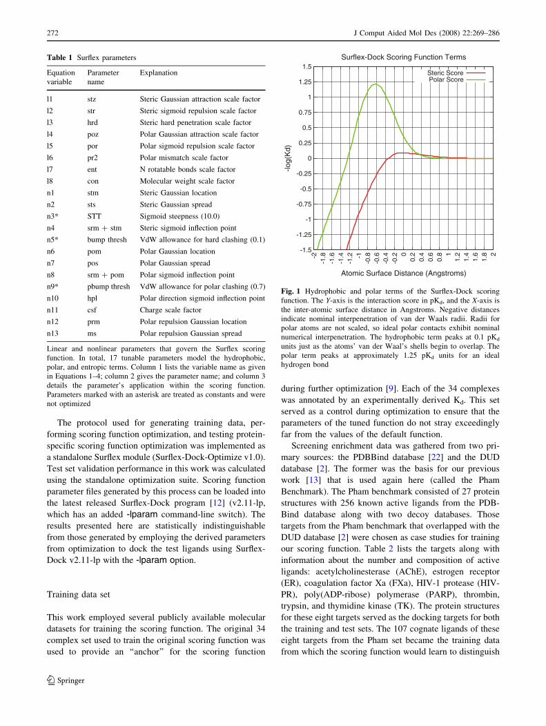
The hydrophobic and polar terms (Eqs. 1 and 2)

dominate the scoring function. These terms operate on the

pair-wise van der Waals surface distance r between atoms,

coupled with information such as element type, formal

charge, and atom status as a hydrogen bond donor or

acceptor. The distance dependence of the hydrophobic and

polar interactions are composed of a Gaussian, sigmoid,

and quadratic penetration term. The polar term is further

scaled by directionality and formal charge. The direction-

ality term between atoms I and J is computed based on

three vectors (normalized to unit length): the vector from

between I and J (bij in Eq. 2), the preferred direction of

interaction of I (vi), and the preferred direction of inter-

action of J (vj). If multiple directional preferences are

present (as for a carbonyl moiety), the preference that

yields the maximal polar interaction is used. Additional

details can be found in the original paper describing the

scoring function [9]. Figure 1 plots the relative hydropho-

bic and polar scores for an ideal contact. Due to the large

number of hydrophobic contacts typically seen between a

protein and a ligand, on average the hydrophobic term

tends to dictate scoring despite a smaller peak value per

ideal contact. An ideal hydrogen bond for the scoring

function exists, for example, when the center of the O in

C=O is 1.97 A away from the center of the H in an N-H

and the four atoms are co-linear. This results in a contri-

bution of 1.25 pKd units to the interaction score.

The polar repulsion term (Eq. 3) measures the penalty

for placing atoms of similar polarity in close proximity and

is scaled by direction. The remaining entropic term (Eq. 4)

captures the degrees of rotational and translational freedom

lost to the ligand upon binding. This ligand-centric penalty

scales linearly in the number of rotatable bonds and line-

arly with the log of its molecular weight.

As described in the Introduction, our previous work

refined the original scoring function, determining weights

for penalty terms that govern steric interpenetration and

noncomplementary polar contacts [13]. This new function

(Surflex-Dock v1.31 and all succeeding versions) was

shown to be an improvement over the original and is the

default scoring function used by the program. The set of

parameters that define the default function are the starting

point for further optimization in this work.

polar score ¼ l4 exp� rþn6ð Þ2

n7 þ l51þ expn3 rþn8ð Þ þ l3 max 0; r þ n9ð Þ2

� �1

1þ expn3 � bij�við Þ bij�vjð Þ�n10ð Þ

" #1þ n11cið Þ 1þ n11cj

� ��

ð2Þ

J Comput Aided Mol Des (2008) 22:269–286 271

123

The protocol used for generating training data, per-

forming scoring function optimization, and testing protein-

specific scoring function optimization was implemented as

a standalone Surflex module (Surflex-Dock-Optimize v1.0).

Test set validation performance in this work was calculated

using the standalone optimization suite. Scoring function

parameter files generated by this process can be loaded into

the latest released Surflex-Dock program [12] (v2.11-lp,

which has an added -lparam command-line switch). The

results presented here are statistically indistinguishable

from those generated by employing the derived parameters

from optimization to dock the test ligands using Surflex-

Dock v2.11-lp with the -lparam option.

Training data set

This work employed several publicly available molecular

datasets for training the scoring function. The original 34

complex set used to train the original scoring function was

used to provide an ‘‘anchor’’ for the scoring function

during further optimization [9]. Each of the 34 complexes

was annotated by an experimentally derived Kd. This set

served as a control during optimization to ensure that the

parameters of the tuned function do not stray exceedingly

far from the values of the default function.

Screening enrichment data was gathered from two pri-

mary sources: the PDBBind database [22] and the DUD

database [2]. The former was the basis for our previous

work [13] that is used again here (called the Pham

Benchmark). The Pham benchmark consisted of 27 protein

structures with 256 known active ligands from the PDB-

Bind database along with two decoy databases. Those

targets from the Pham benchmark that overlapped with the

DUD database [2] were chosen as case studies for training

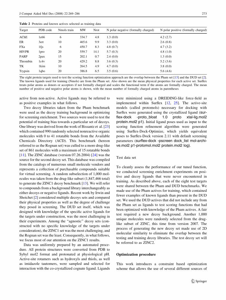
our scoring function. Table 2 lists the targets along with

information about the number and composition of active

ligands: acetylcholinesterase (AChE), estrogen receptor

(ER), coagulation factor Xa (FXa), HIV-1 protease (HIV-

PR), poly(ADP-ribose) polymerase (PARP), thrombin,

trypsin, and thymidine kinase (TK). The protein structures

for these eight targets served as the docking targets for both

the training and test sets. The 107 cognate ligands of these

eight targets from the Pham set became the training data

from which the scoring function would learn to distinguish

Table 1 Surflex parameters

Equation

variable

Parameter

name

Explanation

l1 stz Steric Gaussian attraction scale factor

l2 str Steric sigmoid repulsion scale factor

l3 hrd Steric hard penetration scale factor

l4 poz Polar Gaussian attraction scale factor

l5 por Polar sigmoid repulsion scale factor

l6 pr2 Polar mismatch scale factor

l7 ent N rotatable bonds scale factor

l8 con Molecular weight scale factor

n1 stm Steric Gaussian location

n2 sts Steric Gaussian spread

n3* STT Sigmoid steepness (10.0)

n4 srm + stm Steric sigmoid inflection point

n5* bump thresh VdW allowance for hard clashing (0.1)

n6 pom Polar Gaussian location

n7 pos Polar Gaussian spread

n8 srm + pom Polar sigmoid inflection point

n9* pbump thresh VdW allowance for polar clashing (0.7)

n10 hpl Polar direction sigmoid inflection point

n11 csf Charge scale factor

n12 prm Polar repulsion Gaussian location

n13 ms Polar repulsion Gaussian spread

Linear and nonlinear parameters that govern the Surflex scoring

function. In total, 17 tunable parameters model the hydrophobic,

polar, and entropic terms. Column 1 lists the variable name as given

in Equations 1–4; column 2 gives the parameter name; and column 3

details the parameter’s application within the scoring function.

Parameters marked with an asterisk are treated as constants and were

not optimized

-1.5

-1.25

-1

-0.75

-0.5

-0.25

0

0.25

0.5

0.75

1

1.25

1.5

-2-1

.8-1

.6-1

.4-1

.2 -1-0

.8-0

.6-0

.4-0

.2 0 0.2

0.4

0.6

0.8

1 1.2

1.4

1.6

1.8

2

)dK(gol-

Atomic Surface Distance (Angstroms)

Surflex-Dock Scoring Function Terms

Steric ScorePolar Score

Fig. 1 Hydrophobic and polar terms of the Surflex-Dock scoring

function. The Y-axis is the interaction score in pKd, and the X-axis is

the inter-atomic surface distance in Angstroms. Negative distances

indicate nominal interpenetration of van der Waals radii. Radii for

polar atoms are not scaled, so ideal polar contacts exhibit nominal

numerical interpenetration. The hydrophobic term peaks at 0.1 pKd

units just as the atoms’ van der Waal’s shells begin to overlap. The

polar term peaks at approximately 1.25 pKd units for an ideal

hydrogen bond


123

active from non-active. Active ligands may be referred to

as positive examples in what follows.

Two decoy libraries taken from the Pham benchmark

were used as the decoy training background in optimizing

for screening enrichment. Two sources were used to test the

potential of training bias towards a particular set of decoys.

One library was derived from the work of Bissantz et al. [23]

which contained 990 randomly selected nonreactive organic

molecules with 0 to 41 rotatable bonds from the Available

Chemicals Directory (ACD). This benchmark (hereon

referred to as the Rognan set) was culled to a more drug-like

set of 861 molecules with a maximum of 15 rotatable bonds

[11]. The ZINC database (version 07.26.2004) [24] was the

source for the second decoy set. This database was compiled

from the catalogs of numerous small molecule vendors and

represents a collection of purchasable compounds suitable

for virtual screening. A random subselection of 1,000 mol-

ecules was taken from the drug-like subset (1,847,466 total)

to generate the ZINC1 decoy benchmark [13]. We will refer

to compounds from a background library interchangeably as

either decoys or negative ligands. Recent work by Irwin and

Shoichet [2] considered multiple decoys sets and compared

their physical properties as well as the degree of challenge

they posed in screening. The DUD set itself, which was

designed with knowledge of the specific active ligands for

the targets under construction, was the most challenging in

their experiments. Among the ‘‘agnostic’’ decoy sets (con-

structed with no specific knowledge of the targets under

consideration), the ZINC1 set was the most challenging, and

the Rognan set was the least. Consequently, in what follows,

we focus most of our attention on the ZINC1 results.

Data was uniformly prepared by an automated proce-

dure. All protein structures were converted from PDB to

Sybyl mol2 format and protonated at physiological pH.

Active-site rotamers such as hydroxyls and thiols, as well

as imidazole tautomers, were sampled and selected for

interaction with the co-crystallized cognate ligand. Ligands

were minimized using a DREIDING-like force-field as

implemented within Surflex [12, 25]. The active-site

models (called protomols) necessary for docking with

Surflex were generated using the crystallized ligand (sur-

flex-dock -proto_bloat 1.0 proto xtal-lig.mol2

protein.mol2 p1). Initial ligand poses used as input to the

scoring function refinement algorithm were generated

using Surflex-Dock-Optimize, which yields equivalent

poses to Surflex-Dock version 2.11 with default screening

parameters (surflex-dock -pscreen dock_list mol-archi-

ve.mol2 p1-protomol.mol2 protein.mol2 log).

Test data set

To cleanly assess the performance of our tuned function,

we conducted screening enrichment experiments on posi-

tive and decoy ligands that were never encountered in

training. As described above, each of the eight test targets

were shared between the Pham and DUD benchmarks. We

made use of the Pham actives for training, which contained

fewer examples of known ligands than present in the DUD

set. We used the DUD actives that did not include any from

the Pham set as ligands to test scoring functions that had

been optimized with knowledge of the Pham actives. A fair

test required a new decoy background. Another 1,000

unique molecules were randomly selected from the drug-

like subset of ZINC, this time from version 2007. The

process of generating the new decoy set made use of 2D

molecular similarity to eliminate the overlap between the

testing and training decoy libraries. The test decoy set will

be referred to as ZINC2.

Optimization procedure

This work introduces a constraint based optimization

scheme that allows the use of several different sources of

Table 2 Proteins and known actives selected as training data

Target PDB code Nmols train MW Nrot N polar negative (formally charged) N polar positive (formally charged)

AChE 1e66 6 334.7 4.8 1.3 (0.0) 4.2 (2.7)

ER 3ert 10 465.6 9.9 3.3 (0.0) 2.6 (0.8)

FXa 1fjs 6 450.7 8.3 4.8 (0.7) 4.7 (3.2)

HIVPR 1pro 20 559.7 14.1 5.7 (0.3) 4.8 (1.0)

PARP 2pax 15 202.1 0.7 2.4 (0.0) 1.3 (0.0)

Thrombin 1c4v 20 429.2 8.8 3.6 (0.3) 5.2 (3.6)

TK 1kim 10 264.5 4.9 4.7 (0.0) 3.8 (0.0)

Trypsin 1qbo 20 386.8 6.5 3.5 (0.6) 5.6 (4.6)

The eight protein targets used to test the scoring function optimization approach are the overlap between the Pham set [13] and the DUD set [2].

The known ligands used for training (Nmols) are from the Pham set. Also shown are the mean physical properties for each active set. Surflex

treats polar atoms as donors or acceptors if not formally charged and scales the functional term if the atoms are formally charged. The mean

number of positive and negative polar atoms is shown, with the mean number of formally charged atoms in parentheses


123

data in customizing a scoring function. We will begin by

defining the available constraints and how they might be

utilized to create scoring functions optimized for a partic-

ular task. We will then cover the optimization protocol in

detail, along with the options that govern its use.

During any parameter optimization regime, the goal is to

extremize the value of an objective function as we explore

the parameter space. Our objective function is described by

user-defined constraints on training data. Constraints come

in three flavors: scoring, screening, and geometric. Together

these constraints combine to form the objective function.

Score constraints relate a particular protein and a single

ligand or set of ligands to a target score. The user can

specify whether the predicted score should be exactly/

above/below the target score. Moving in an undesired

direction from the target score incurs a squared penalty (see

Table 3). This is, in fact, the original training regime where

the scoring function was tuned to fit experimental binding

affinities [9]. In the current formulation, we would create

34 individual score constraints of equal weight, one for

each of the 34 protein-ligand complexes, indicating success

as an exact match to the experimental Kd. Using additional

such constraints, a user could potentially tune the perfor-

mance of a scoring function for more accurate rank-order

prediction of novel ligands. By focusing, for example, on

training data that was dominated by the lead series of

interest, better predictions of potency for new ligands in the

series could result.

Screening constraints allow a user to denote that one set

of positive ligands (e.g., a set of cognate ligands) should

score measurably higher than a set of negative ligands

(e.g., a set of decoys). Performance is assessed by ROC

AUC. A function that could flawlessly determine whether a

ligand is positive or negative would have an AUC of 1.0.

Conversely, a classifier which randomly assigned ligands a

positive or negative label would achieve an AUC of 0.5 in

the average case. The impact of a screening constraint on

the objective function is formulated as the square of its

ROC area’s deviation from 1.0 (see Table 3), scaled by 100

to ensure that its value shares the same effective range as

the other constraint types. Using such data, a user can tune

a scoring function to perform well in finding new leads for

a particular protein of interest in a screening experiment.

This particular scenario will be presented in detail in the

results that follow, owing to the existence of a large pub-

licly available database for testing.

Geometric constraints offer a method for addressing

what are termed ‘‘hard failures’’ in docking. Given an

incorrect prediction of a ligand’s pose, it may stem from

either a failure of the search method (the best pose was not

found, but it would have scored best, termed a soft failure).

Or, it may stem from a problem in the scoring function: the

best-scoring pose may actually score higher than the cor-

rect one (a hard failure). A geometric constraint enforces

the rule that no incorrect pose may score higher than the

best correct pose. Any deviation results in a squared pen-

alty (see Table 3). In focused medicinal chemistry efforts

that are guided in part by docking, the geometric predic-

tions can be very important. By providing a method to

learn from hard docking failures, a user can take advantage

of structures where docking predictions were wrong to

improve future performance.

Constraints can be organized further into weighted

groups. This feature allows one to arbitrate the influence of

certain constraints over the objective function. Consider the

following scenario: one has 34 protein-ligand complexes

whose scores the function should predict exactly (34 score

constraints). One also has a set of known actives and in-

actives for a given protein, necessitating the need for a

single screening constraint. It is important to explicitly be

able to control the relative importance of these two types of

constraints in modifying the scoring function. To ensure

that a single constraint is not overwhelmed by the presence

of numerous competing constraints, we can place the 34

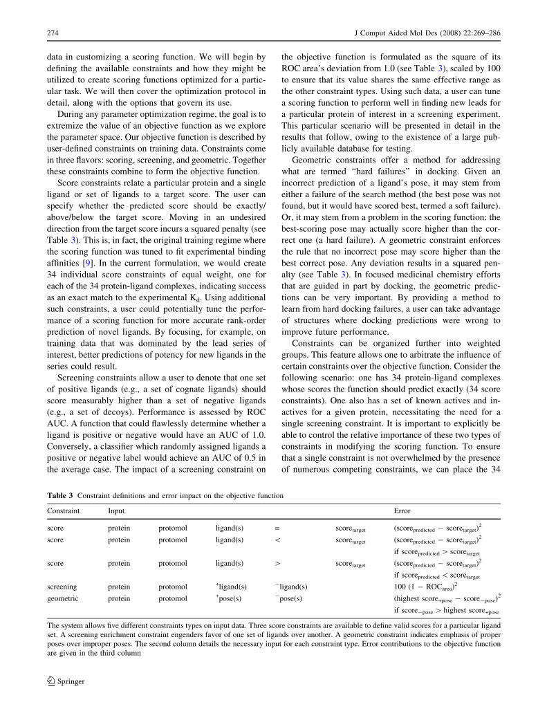
Table 3 Constraint definitions and error impact on the objective function

Constraint Input Error

score protein protomol ligand(s) = scoretarget (scorepredicted - scoretarget)2

score protein protomol ligand(s) \ scoretarget (scorepredicted - scoretarget)2

if scorepredicted [ scoretarget

score protein protomol ligand(s) [ scoretarget (scorepredicted - scoretarget)2

if scorepredicted \ scoretarget

screening protein protomol +ligand(s) -ligand(s) 100 (1 - ROCarea)2

geometric protein protomol +pose(s) -pose(s) (highest score+pose - score-pose)2

if score-pose [ highest score+pose

The system allows five different constraints types on input data. Three score constraints are available to define valid scores for a particular ligand

set. A screening enrichment constraint engenders favor of one set of ligands over another. A geometric constraint indicates emphasis of proper

poses over improper poses. The second column details the necessary input for each constraint type. Error contributions to the objective function

are given in the third column


123

score constraints in one group and the single screening

constraint in a second group. The optimization procedure is

implemented such that each constraint group has an equal

bearing on the objective function. In this example, the

objective function essentially will see first the 34 individual

scoring constraints and the single screening constraint as

having equal relative importance. Users may additionally

specify a weight be given to a group, providing more

control of influence of different data on the objective

function.

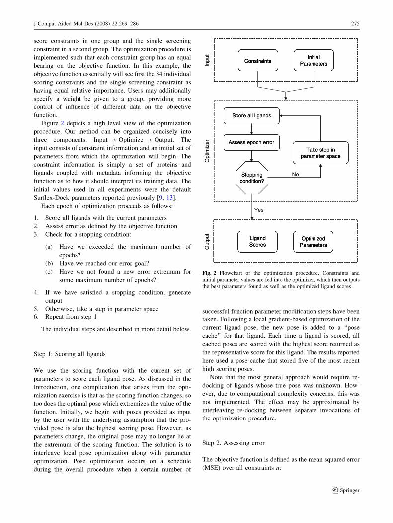
Figure 2 depicts a high level view of the optimization

procedure. Our method can be organized concisely into

three components: Input ? Optimize ? Output. The

input consists of constraint information and an initial set of

parameters from which the optimization will begin. The

constraint information is simply a set of proteins and

ligands coupled with metadata informing the objective

function as to how it should interpret its training data. The

initial values used in all experiments were the default

Surflex-Dock parameters reported previously [9, 13].

Each epoch of optimization proceeds as follows:

1. Score all ligands with the current parameters

2. Assess error as defined by the objective function

3. Check for a stopping condition:

(a) Have we exceeded the maximum number of

epochs?

(b) Have we reached our error goal?

(c) Have we not found a new error extremum for

some maximum number of epochs?

4. If we have satisfied a stopping condition, generate

output

5. Otherwise, take a step in parameter space

6. Repeat from step 1

The individual steps are described in more detail below.

Step 1: Scoring all ligands

We use the scoring function with the current set of

parameters to score each ligand pose. As discussed in the

Introduction, one complication that arises from the opti-

mization exercise is that as the scoring function changes, so

too does the optimal pose which extremizes the value of the

function. Initially, we begin with poses provided as input

by the user with the underlying assumption that the pro-

vided pose is also the highest scoring pose. However, as

parameters change, the original pose may no longer lie at

the extremum of the scoring function. The solution is to

interleave local pose optimization along with parameter

optimization. Pose optimization occurs on a schedule

during the overall procedure when a certain number of

successful function parameter modification steps have been

taken. Following a local gradient-based optimization of the

current ligand pose, the new pose is added to a ‘‘pose

cache’’ for that ligand. Each time a ligand is scored, all

cached poses are scored with the highest score returned as

the representative score for this ligand. The results reported

here used a pose cache that stored five of the most recent

high scoring poses.

Note that the most general approach would require re-

docking of ligands whose true pose was unknown. How-

ever, due to computational complexity concerns, this was

not implemented. The effect may be approximated by

interleaving re-docking between separate invocations of

the optimization procedure.

Step 2. Assessing error

The objective function is defined as the mean squared error

(MSE) over all constraints n:

ConstraintsInitial

ParametersConstraintsConstraintsInitial

ParametersInitial

Parameters

tupnI

Score all ligandsScore all ligands

Take step in parameter space

Take step in parameter space

Assess epoch errorAssess epoch errorrezimitp

O

Stopping condition?Stopping

condition?No

LigandScores

Optimized Parameters

LigandScoresLigandScores

Optimized ParametersOptimized

Parameters

tuptuO

Yes

Fig. 2 Flowchart of the optimization procedure. Constraints and

initial parameter values are fed into the optimizer, which then outputs

the best parameters found as well as the optimized ligand scores


123

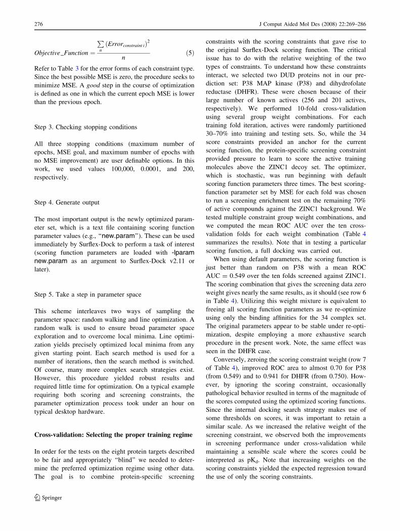
Objective Function ¼

Pn

Errorconstraint ið Þ2

nð5Þ

Refer to Table 3 for the error forms of each constraint type.

Since the best possible MSE is zero, the procedure seeks to

minimize MSE. A good step in the course of optimization

is defined as one in which the current epoch MSE is lower

than the previous epoch.

Step 3. Checking stopping conditions

All three stopping conditions (maximum number of

epochs, MSE goal, and maximum number of epochs with

no MSE improvement) are user definable options. In this

work, we used values 100,000, 0.0001, and 200,

respectively.

Step 4. Generate output

The most important output is the newly optimized param-

eter set, which is a text file containing scoring function

parameter values (e.g., ‘‘new.param’’). These can be used

immediately by Surflex-Dock to perform a task of interest

(scoring function parameters are loaded with -lparam

new.param as an argument to Surflex-Dock v2.11 or

later).

Step 5. Take a step in parameter space

This scheme interleaves two ways of sampling the

parameter space: random walking and line optimization. A

random walk is used to ensure broad parameter space

exploration and to overcome local minima. Line optimi-

zation yields precisely optimized local minima from any

given starting point. Each search method is used for a

number of iterations, then the search method is switched.

Of course, many more complex search strategies exist.

However, this procedure yielded robust results and

required little time for optimization. On a typical example

requiring both scoring and screening constraints, the

parameter optimization process took under an hour on

typical desktop hardware.

Cross-validation: Selecting the proper training regime

In order for the tests on the eight protein targets described

to be fair and appropriately ‘‘blind’’ we needed to deter-

mine the preferred optimization regime using other data.

The goal is to combine protein-specific screening

constraints with the scoring constraints that gave rise to

the original Surflex-Dock scoring function. The critical

issue has to do with the relative weighting of the two

types of constraints. To understand how these constraints

interact, we selected two DUD proteins not in our pre-

diction set: P38 MAP kinase (P38) and dihydrofolate

reductase (DHFR). These were chosen because of their

large number of known actives (256 and 201 actives,

respectively). We performed 10-fold cross-validation

using several group weight combinations. For each

training fold iteration, actives were randomly partitioned

30–70% into training and testing sets. So, while the 34

score constraints provided an anchor for the current

scoring function, the protein-specific screening constraint

provided pressure to learn to score the active training

molecules above the ZINC1 decoy set. The optimizer,

which is stochastic, was run beginning with default

scoring function parameters three times. The best scoring-

function parameter set by MSE for each fold was chosen

to run a screening enrichment test on the remaining 70%

of active compounds against the ZINC1 background. We

tested multiple constraint group weight combinations, and

we computed the mean ROC AUC over the ten cross-

validation folds for each weight combination (Table 4

summarizes the results). Note that in testing a particular

scoring function, a full docking was carried out.

When using default parameters, the scoring function is

just better than random on P38 with a mean ROC

AUC = 0.549 over the ten folds screened against ZINC1.

The scoring combination that gives the screening data zero

weight gives nearly the same results, as it should (see row 6

in Table 4). Utilizing this weight mixture is equivalent to

freeing all scoring function parameters as we re-optimize

using only the binding affinities for the 34 complex set.

The original parameters appear to be stable under re-opti-

mization, despite employing a more exhaustive search

procedure in the present work. Note, the same effect was

seen in the DHFR case.

Conversely, zeroing the scoring constraint weight (row 7

of Table 4), improved ROC area to almost 0.70 for P38

(from 0.549) and to 0.941 for DHFR (from 0.750). How-

ever, by ignoring the scoring constraint, occasionally

pathological behavior resulted in terms of the magnitude of

the scores computed using the optimized scoring functions.

Since the internal docking search strategy makes use of

some thresholds on scores, it was important to retain a

similar scale. As we increased the relative weight of the

screening constraint, we observed both the improvements

in screening performance under cross-validation while

maintaining a sensible scale where the scores could be

interpreted as pKd. Note that increasing weights on the

scoring constraints yielded the expected regression toward

the use of only the scoring constraints.


123

Given the evidence from the cross validation study on

P38 and DHFR, we chose to test the optimization scheme

on the blind data for the eight targets with two constraint

groups: a scoring constraint group defined by the scoring

constraints within the 34 complex set; and a screening

constraint group comprised of that complex’s training

actives and a set of decoys. The scoring and screening

constraint groups were assigned weights of 1 and 5,

respectively.

Results and discussion

The primary test of the scoring function optimization

method is in a screening enrichment assessment against

eight different protein targets (see Table 2). We have been

careful to avoid any contamination of the test by either the

active ligands used for scoring function tuning or by the

decoys used. The test data for each of the eight targets

includes novel active ligands and employs a different set of

decoy molecules (the ZINC2 set). We also uniformly

applied the procedure that was developed in our pre-

liminary work (which included cross-validation on two

other targets). The overall numerical results are presented

in Table 5, with plots of the relevant ROC curves presented

in Figs. 3 and 4. As has become standard practice, we have

characterized screening performance in terms of ROC

AUC, and we have also computed 95% confidence inter-

vals to bracket the performance of the tuned function in

each of the eight test cases. The results are broken into

three groups, based on the performance changes.

Improved performance: PARP and HIVPR

In the six cases where 10 or more active ligands were

available in the Pham set, we observed increased or

unchanged performance in all cases, with significant

improvements in two cases. These two cases (PARP and

HIVPR) will be discussed in detail here.

PARP

Poly-(ADP-ribose)-polymerase is involved in the response

to genomic damage that results in strand breaks. For spe-

cific proteins, PARP can add up to 200 residues of ADP-

ribose to form branched polymers, which act as binding

sites for repair proteins that play a central role in DNA

metabolism [26]. The majority of inhibitors used to tune

the scoring function for PARP were small and had rela-

tively weak binding, typically in the micromolar range

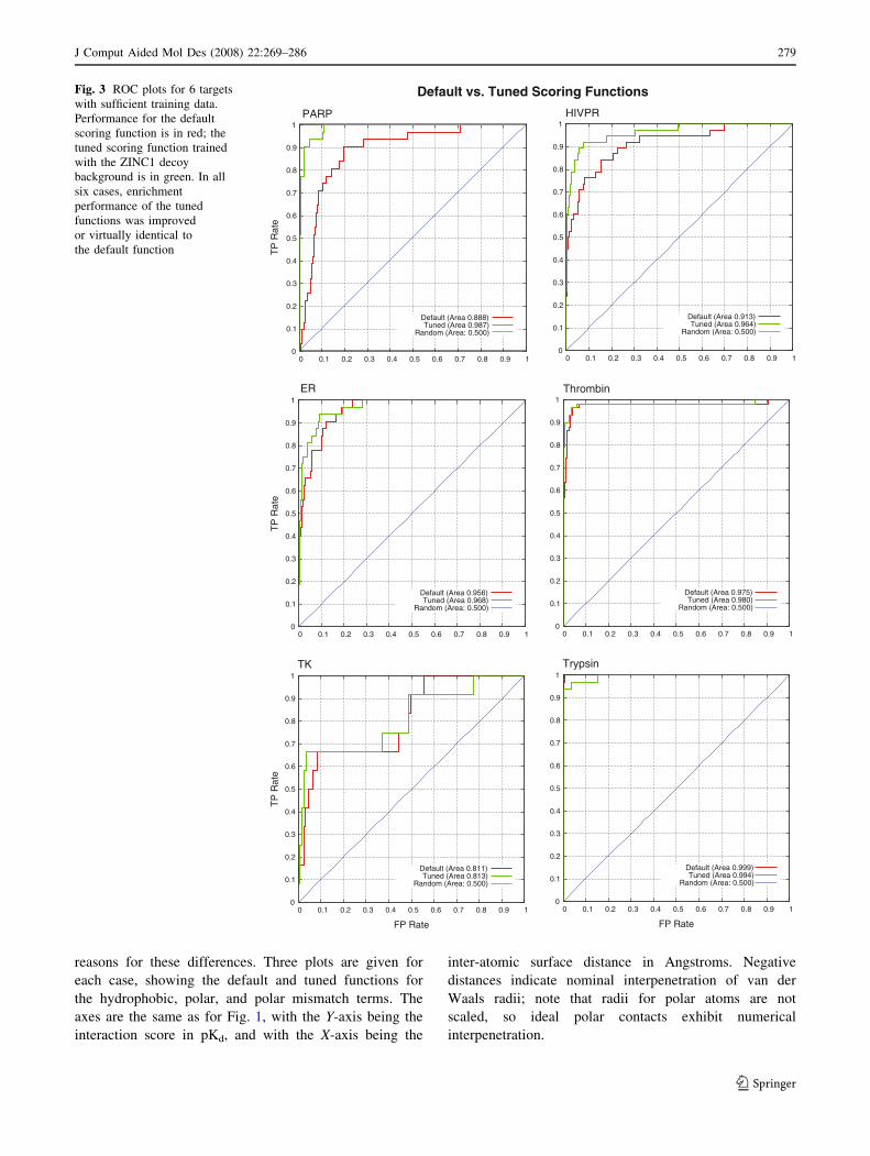
(see Fig. 5 for example structures). The first ROC plot of

Fig. 3 corresponds to the test of the PARP-focused tuned

scoring function on the blind test data. The improvement in

screening enrichment for the blind test molecules in this

case was pronounced, with an improvement in ROC AUC

of 0.10, corresponding to an increase in true-positive rate

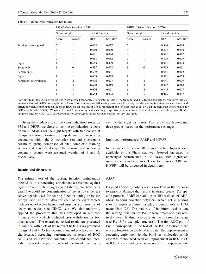
Table 4 Tenfold cross validation test results

P38 (Default function: 0.549) DHFR (Default function: 0.750)

Group weights Tuned function Group weights Tuned function

Score Screen ROC Std. Dev. Score Screen ROC Std. Dev.

Scoring overweighted 5 1 0.604 0.027 5 1 0.866 0.015

4 1 0.610 0.030 4 1 0.877 0.030

3 1 0.621 0.024 3 1 0.891 0.017

2 1 0.638 0.032 2 1 0.895 0.009

Equal 1 1 0.663 0.029 1 1 0.911 0.023

Score only 1 0 0.537 0.028 1 0 0.713 0.031

Screen only 0 1 0.699 0.031 0 1 0.941 0.012

Equal 1 1 0.663 0.029 1 1 0.911 0.023

Screening overweighted 1 2 0.676 0.027 1 2 0.941 0.009

1 3 0.670 0.019 1 3 0.942 0.010

1 4 0.676 0.021 1 4 0.945 0.007

1 5 0.683 0.024 1 5 0.945 0.007

For this study, the 256 actives of P38 were divided randomly 30/70 into 10 sets of 77 training and 179 testing molecules. Similarly, the 201

known actives of DHFR were split into 10 sets of 60 training and 141 testing molecules. For every set, the scoring function was then tuned with

different weight combinations; the mean ROC for all test sets of P38 is reported in the left side (pdb code: 1KV2); the right side shows results for

DHFR (pdb code: 3DFR). Weights of 1 and 5 for scoring and screening, respectively, were chosen for the blind test on eight targets. Bolded

numbers refer to ROC AUC corresponding to score/screen group weights chosen for use this study


123

from approximately 20–90% at a false positive rate of less

than 5%.

HIVPR

HIV-1 protease is an aspartic protease with a large, solvent-

accessible active site with several charged polar moieties

both interior and proximally exterior to the pocket. Crys-

tallographic studies have shown that interaction with the

interior catalytic triad Asp25-Thr26-Gly27 as well as sur-

face residues, Asp29 and Asp30, is important for enzyme

inhibition [27, 28]. The majority of inhibitors used in

training bind in the nanomolar range (example structures

are shown in Fig. 5). The second plot of Fig. 3 shows the

ROC curves for HIVPR. The tuned function shows a sub-

stantial increase in true positive rates at a false positive rate

of 5% relative to the default function from roughly 60% to

roughly 85%, corresponding to enhanced early enrichment.

Effects on test ligand scores

The ROC plots are sensitive to the relative separation of

active from decoy ligands. Increases in the scores for active

ligands, decreases for decoys, or a combination of both can

lead to improvements in recovery of active ligands and

increase in ROC AUC. The cumulative distributions of

positive and negative scores for the default and tuned

functions (Fig. 6) reveal the underlying impetus for

enrichment improvement.

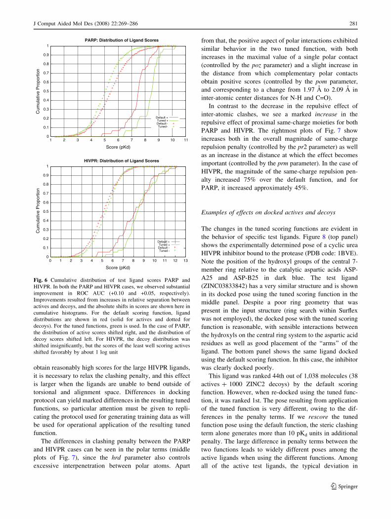
In the case of PARP, the increase in ROC AUC from

0.89 to 0.99 for the tuned function stemmed from a

decrease in the scores of the decoys relative to the untuned

function with a simultaneous increase in the scores of the

active ligands. The bulk of the actives, when docked with

the tuned scoring function, had scores approximately 1 log

unit higher than when docked using the default scoring

function (this corresponds to the rightward shift from the

solid red curve to the solid green curve in the top plot of

Fig. 6). Conversely, the inactives exhibited decreases of

roughly 0.5 log units. In the case of HIVPR, performance

increased from a ROC AUC of 0.913 to 0.964. However, in

this case, the distribution of decoy scores changed only

slightly and did so in the wrong direction. The improve-

ment in enrichment came from a significant upward shift of

the lowest scoring active ligands by about 1.0 log units.

With the default function, 40% of actives had pKd \ 7.5,

but only 20% of actives scored by the tuned functions had

pKd \ 7.5.

Effects on surflex-dock function terms

The underlying reasons for the performance increases

observed with PARP and HIVPR stemmed from different

sources. In the former case, we observed increased

ability to recognize actives and reject decoys. In the

latter case, both sets of scores increased, but with a

specific advantage to the actives. Inspection of the

individual terms of the scoring function before and after

the optimization procedure (Fig. 7) lends insight into the

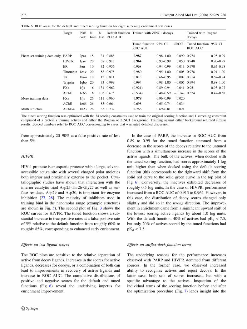
Table 5 ROC areas for the default and tuned scoring function for eight screening enrichment test cases

Target PDB

code

N

train

N

test

Default function

ROC AUC

Trained with ZINC1 decoys Trained with Rognan

decoys

Tuned function

ROC AUC

95% CI dROC Tuned function

ROC AUC

95% CI

Pham set training data only PARP 2pax 15 31 0.888 0.987 0.98–1.00 0.099 0.974 0.95–0.99

HIVPR 1pro 20 38 0.913 0.964 0.93–0.99 0.050 0.948 0.90–0.99

ER 3ert 10 32 0.956 0.968 0.94–0.99 0.013 0.970 0.95–0.98

Thrombin 1c4v 20 58 0.975 0.980 0.95–1.00 0.005 0.978 0.94–1.00

TK 1kim 10 12 0.811 0.813 0.66–0.95 0.002 0.814 0.67–0.94

Trypsin 1qbo 20 33 0.999 0.994 0.98–1.00 -0.005 0.994 0.98–1.00

FXa 1fjs 6 131 0.962 (0.921) 0.89–0.94 -0.041 0.951 0.93–0.97

AChE 1e66 6 103 0.675 (0.534) 0.48–0.59 -0.142 0.524 0.47–0.58

More training data FXa 1fjs 26 111 0.960 0.978 0.96–0.99 0.020

AChE 1e66 26 83 0.664 0.698 0.65–0.74 0.034

Multi structure AChE-a 1h23 26 83 0.732 0.753 0.69–0.81 0.021

The tuned scoring function was optimized with the 34 scoring constraints used to train the original scoring function and 1 screening constraint

comprised of a protein’s training actives and either the Rognan or ZINC1 background. Training against either background returned similar

results. Bolded numbers refer to ROC AUC corresponding to cases that warranted detailed discussion


123

reasons for these differences. Three plots are given for

each case, showing the default and tuned functions for

the hydrophobic, polar, and polar mismatch terms. The

axes are the same as for Fig. 1, with the Y-axis being the

interaction score in pKd, and with the X-axis being the

inter-atomic surface distance in Angstroms. Negative

distances indicate nominal interpenetration of van der

Waals radii; note that radii for polar atoms are not

scaled, so ideal polar contacts exhibit numerical

interpenetration.

0

0.1

0.2

0.3

0.4

0.5

0.6

0.7

0.8

0.9

1

0 0.1 0.2 0.3 0.4 0.5 0.6 0.7 0.8 0.9 1

etaR

PT

PARP

Default (Area 0.888)Tuned (Area 0.987)

Random (Area: 0.500)

0

0.1

0.2

0.3

0.4

0.5

0.6

0.7

0.8

0.9

1

0 0.1 0.2 0.3 0.4 0.5 0.6 0.7 0.8 0.9 1

HIVPR



0

0.1

0.2

0.3

0.4

0.5

0.6

0.7

0.8

0.9

1

0 0.1 0.2 0.3 0.4 0.5 0.6 0.7 0.8 0.9 1

etaR

PT

ER



0

0.1

0.2

0.3

0.4

0.5

0.6

0.7

0.8

0.9

1

0 0.1 0.2 0.3 0.4 0.5 0.6 0.7 0.8 0.9 1

Thrombin



0

0.1

0.2

0.3

0.4

0.5

0.6

0.7

0.8

0.9

1

0 0.1 0.2 0.3 0.4 0.5 0.6 0.7 0.8 0.9 1

etaR

PT

FP Rate

TK



0

0.1

0.2

0.3

0.4

0.5

0.6

0.7

0.8

0.9

1

0 0.1 0.2 0.3 0.4 0.5 0.6 0.7 0.8 0.9 1

FP Rate

Trypsin



Default vs. Tuned Scoring FunctionsFig. 3 ROC plots for 6 targets

with sufficient training data.

Performance for the default

scoring function is in red; the

tuned scoring function trained

with the ZINC1 decoy

background is in green. In all

six cases, enrichment

performance of the tuned

functions was improved

or virtually identical to

the default function


123

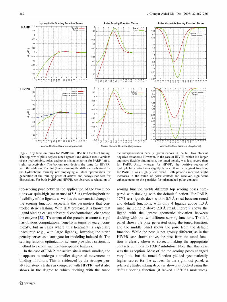
The hydrophobic terms show markedly different modi-

fications in response to tuning for PARP and HIVPR. In the

former case (top left plot), the penalty for atomic surface

interpenetration is decreased somewhat, and the area of

positive hydrophobic interaction (from the Gaussian in

Eq. 1) is both more narrow and has lower amplitude. In the

latter case, the softening of the overlap penalty is more

significant, and the area of positive interaction increases.

The tuned scoring function parameters are given in

Table 6. The decrease in sensitivity to inter-atomic clashes

is reflected in the value of the hrd parameter, which

changed from -0.95 (default function) to -0.16 (tuned

function). For HIVPR, we also considered the effect of

generating the training poses (and testing the resulting

tuned function) without the use of Surflex’s ligand pre-

minimization and post-docking all-atom optimization.

These procedures are part of the default screening protocol

of Surflex, since they help decrease dependence on input

ligand preparation and allow access to Cartesian move-

ments that can ameliorate clashes between the protein and

ligand [12]. This can be especially important for large

ligands. The blue curve in Fig. 7 shows that the tuned clash

penalty is even softer when the docking process is

restricted to a ligand’s internal coordinates. In order to

0

0.1

0.2

0.3

0.4

0.5

0.6

0.7

0.8

0.9

1

0 0.1 0.2 0.3 0.4 0.5 0.6 0.7 0.8 0.9 1

FP Rate

AChE


Tuned+20 (Area 0.698)Multi-structure (Area 0.753)

0

0.1

0.2

0.3

0.4

0.5

0.6

0.7

0.8

0.9

1

0 0.1 0.2 0.3 0.4 0.5 0.6 0.7 0.8 0.9 1

etaR

PT

FP Rate

Factor Xa


Tuned+20 (Area 0.978)

Default vs Tuned Scoring Functions With Additional Data

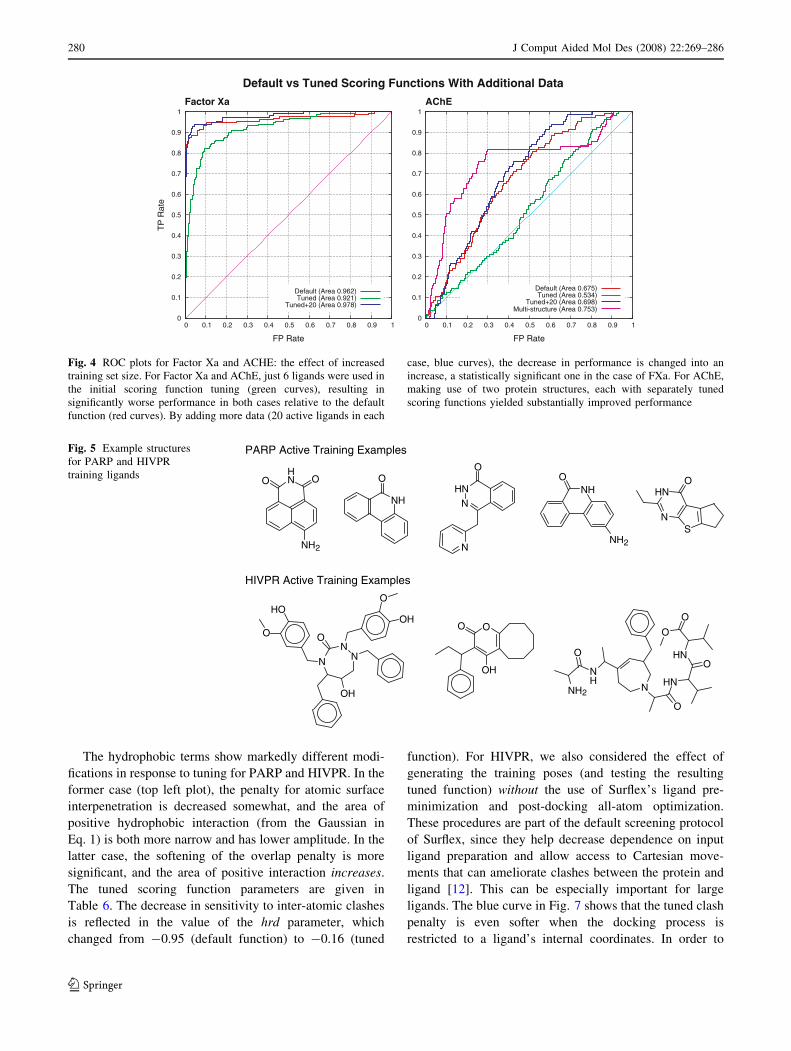
Fig. 4 ROC plots for Factor Xa and ACHE: the effect of increased

training set size. For Factor Xa and AChE, just 6 ligands were used in

the initial scoring function tuning (green curves), resulting in

significantly worse performance in both cases relative to the default

function (red curves). By adding more data (20 active ligands in each

case, blue curves), the decrease in performance is changed into an

increase, a statistically significant one in the case of FXa. For AChE,

making use of two protein structures, each with separately tuned

scoring functions yielded substantially improved performance

O

NH2

OHN O

NH

O

N

HN

N

ONH

NH2

O

SN

HN

ON

N

OH

N

O

HOOH

O

O O

OH

O

NH

N

O

HN

OHN

O

O

NH2

PARP Active Training Examples

HIVPR Active Training Examples

Fig. 5 Example structures

for PARP and HIVPR

training ligands


123

obtain reasonably high scores for the large HIVPR ligands,

it is necessary to relax the clashing penalty, and this effect

is larger when the ligands are unable to bend outside of

torsional and alignment space. Differences in docking

protocol can yield marked differences in the resulting tuned

functions, so particular attention must be given to repli-

cating the protocol used for generating training data as will

be used for operational application of the resulting tuned

function.

The differences in clashing penalty between the PARP

and HIVPR cases can be seen in the polar terms (middle

plots of Fig. 7), since the hrd parameter also controls

excessive interpenetration between polar atoms. Apart

from that, the positive aspect of polar interactions exhibited

similar behavior in the two tuned function, with both

increases in the maximal value of a single polar contact

(controlled by the poz parameter) and a slight increase in

the distance from which complementary polar contacts

obtain positive scores (controlled by the pom parameter,

and corresponding to a change from 1.97 A to 2.09 A in

inter-atomic center distances for N-H and C=O).

In contrast to the decrease in the repulsive effect of

inter-atomic clashes, we see a marked increase in the

repulsive effect of proximal same-charge moieties for both

PARP and HIVPR. The rightmost plots of Fig. 7 show

increases both in the overall magnitude of same-charge

repulsion penalty (controlled by the pr2 parameter) as well

as an increase in the distance at which the effect becomes

important (controlled by the prm parameter). In the case of

HIVPR, the magnitude of the same-charge repulsion pen-

alty increased 75% over the default function, and for

PARP, it increased approximately 45%.

Examples of effects on docked actives and decoys

The changes in the tuned scoring functions are evident in

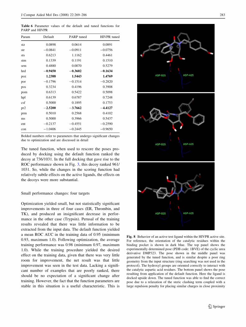
the behavior of specific test ligands. Figure 8 (top panel)

shows the experimentally determined pose of a cyclic urea

HIVPR inhibitor bound to the protease (PDB code: 1BVE).

Note the position of the hydroxyl groups of the central 7-

member ring relative to the catalytic aspartic acids ASP-

A25 and ASP-B25 in dark blue. The test ligand

(ZINC03833842) has a very similar structure and is shown

in its docked pose using the tuned scoring function in the

middle panel. Despite a poor ring geometry that was

present in the input structure (ring search within Surflex

was not employed), the docked pose with the tuned scoring

function is reasonable, with sensible interactions between

the hydroxyls on the central ring system to the aspartic acid

residues as well as good placement of the ‘‘arms’’ of the

ligand. The bottom panel shows the same ligand docked

using the default scoring function. In this case, the inhibitor

was clearly docked poorly.

This ligand was ranked 44th out of 1,038 molecules (38

actives + 1000 ZINC2 decoys) by the default scoring

function. However, when re-docked using the tuned func-

tion, it was ranked 1st. The pose resulting from application

of the tuned function is very different, owing to the dif-

ferences in the penalty terms. If we rescore the tuned

function pose using the default function, the steric clashing

term alone generates more than 10 pKd units in additional

penalty. The large difference in penalty terms between the

two functions leads to widely different poses among the

active ligands when using the different functions. Among

all of the active test ligands, the typical deviation in

0

0.1

0.2

0.3

0.4

0.5

0.6

0.7

0.8

0.9

1

1 2 3 4 5 6 7 8 9 10 11

noitroporP e vitalu

muC

Score (pKd)

PARP: Distribution of Ligand Scores

Default +Tuned +Default -Tuned -

0

0.1

0.2

0.3

0.4

0.5

0.6

0.7

0.8

0.9

1

0 1 2 3 4 5 6 7 8 9 10 11 12 13

noitroporP ev italu

muC

Score (pKd)

HIVPR: Distribution of Ligand Scores

Default +Tuned +Default - Tuned -

Fig. 6 Cumulative distribution of test ligand scores PARP and

HIVPR. In both the PARP and HIVPR cases, we observed substantial

improvement in ROC AUC (+0.10 and +0.05, respectively).

Improvements resulted from increases in relative separation between

actives and decoys, and the absolute shifts in scores are shown here in

cumulative histograms. For the default scoring function, ligand

distributions are shown in red (solid for actives and dotted for

decoys). For the tuned functions, green is used. In the case of PARP,

the distribution of active scores shifted right, and the distribution of

decoy scores shifted left. For HIVPR, the decoy distribution was

shifted insignificantly, but the scores of the least well scoring actives

shifted favorably by about 1 log unit


123

top-scoring pose between the application of the two func-

tions was quite high (mean rmsd of 5.5 A), reflecting both the

flexibility of the ligands as well as the substantial change in

the scoring function, especially the parameters that con-

trolled steric clashing. With HIV protease, it is known that

ligand binding causes substantial conformational changes to

the enzyme [28]. Treatment of the protein structure as rigid

has obvious computational benefits in terms of search com-

plexity, but in cases where this treatment is especially

inaccurate (e.g., with large ligands), lowering the steric

penalty serves as a surrogate for modeling induced fit. The

scoring function optimization scheme provides a systematic

method to exploit such protein-specific features.

In the case of PARP, the active site is much smaller, and

it appears to undergo a smaller degree of movement on

binding inhibitors. This is evidenced by the stronger pen-

alty for steric clashes as compared with HIVPR, and it also

shows in the degree to which docking with the tuned

scoring function yields different top scoring poses com-

pared with docking with the default function. For PARP,

17/31 test ligands dock within 0.5 A rmsd between tuned

and default functions, with only 4 ligands above 1.0 A

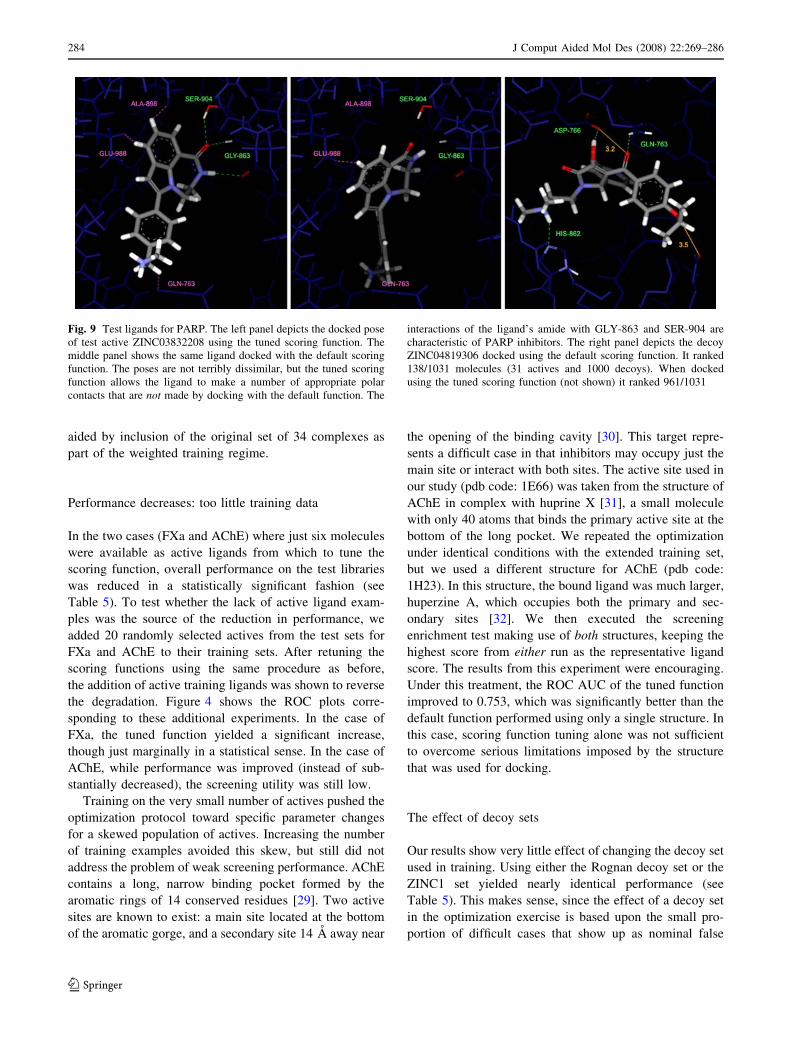
rmsd, including 2 above 2.0 A rmsd. Figure 9 shows the

ligand with the largest geometric deviation between

docking with the two different scoring functions. The left

panel shows the pose generated using the tuned function,

and the middle panel shows the pose from the default

function. While the pose is not grossly different, as in the

HIVPR case shown above, the pose from the tuned func-

tion is clearly closer to correct, making the appropriate

contacts common to PARP inhibitors. Note that this case

was the exception. Most of the top-scoring poses changed

very little, but the tuned function yielded systematically

higher scores for the actives. In the rightmost panel, a

relatively high-ranking decoy is shown as docked using the

default scoring function (it ranked 138/1031 molecules).

-1.5

-1.25

-1

-0.75

-0.5

-0.25

0

0.25

0.5

0.75

1

1.25

1.5

2- 8.1-6.1-4.1-2.1-1- 8. 0-6.0 -4. 0-2.0-0 2.0 4.0 6 .0 8.0 1 2 .1 4.1 6 .1 8.1 2

)dK(gol-

Hydrophobic Scoring Function Terms

DefaultTuned

-1.5

-1.25

-1

-0.75

-0.5

-0.25

0

0.25

0.5

0.75

1

1.25

1.5

2- 8.1-6.1-4.1-2 .1-1- 8. 0-6.0-4. 0-2. 0-0 2.0 4.0 6.0 8.0 1 2.1 4.1 6.1 8.1 2

Polar Scoring Function Terms

DefaultTuned

-3.75

-3.5

-3.25

-3

-2.75

-2.5

-2.25

-2

-1.75

-1.5

-1.25

-1

-0.75

-0.5

-0.25

0

2- 8.1-6.1-4.1-2.1-1- 8.0-6.0-4.0-2.0-0 2.0 4.0 6. 0 8.0 1 2.1 4.1 6. 1 8. 1 2

Polar Mismatch Scoring Function Terms

DefaultTuned

-1.5

-1.25

-1

-0.75

-0.5

-0.25

0

0.25

0.5

0.75

1

1.25

1.5

2- 8.1-6.1-4. 1-2.1-1- 8.0-6.0-4.0-2.0-0 2.0 4.0 6.0 8.0 1 2.1 4.1 6.1 8.1 2

)dK(gol-


DefaultTuned.pscreen.onTuned.pscreen.off

-1.5

-1.25

-1

-0.75

-0.5

-0.25

0

0.25

0.5

0.75

1

1.25

1.5

2- 8.1-6.1-4.1-2.1-1- 8.0-6.0-4.0-2.0-0 2 .0 4.0 6.0 8.0 1 2.1 4. 1 6 .1 8.1 2


DefaultTuned

-4.25

-4

-3.75

-3.5

-3.25

-3

-2.75

-2.5

-2.25

-2

-1.75

-1.5

-1.25

-1

-0.75

-0.5

-0.25

0

2- 8.1-6.1-4.1-2.1-1- 8.0-6.0-4. 0-2.0-0 2.0 4.0 6.0 8. 0 1 2. 1 4.1 6.18.1 2


DefaultTuned

PARP

HIVPR

Fig. 7 Key function terms for PARP and HIVPR: Effects of tuning.

The top row of plots depicts tuned (green) and default (red) versions

of the hydrophobic, polar, and polar mismatch terms for PARP (left to

right, respectively). The bottom row depicts the same for HIVPR,

with the addition of a plot (blue) showing the difference obtained for

the hydrophobic term by not employing all-atom optimization for

generation of the training poses of actives and decoys (see text for

discussion). For both PARP and HIVPR, we observed a relaxation of

the interpenetration penalty (green curves in the left two plots at

negative distances). However, in the case of HIVPR, which is a larger

and more flexible binding site, the tuned penalty was less severe than

for PARP. Also, whereas for HIVPR, the positive region of

hydrophobic contact was slightly broader than the original function,

for PARP it was slightly less broad. Both proteins received slight

increases in the value of polar contact and received significant

enhancements to the penalties for mismatched polar contacts


123

The tuned function, when used to rescore the poses pro-

duced by docking using the default function ranked the

decoy at 736/1031. In the full docking that gave rise to the

ROC performance shown in Fig. 3, this decoy ranked 961/

1031. So, while the changes in the scoring function had

relatively subtle effects on the active ligands, the effects on

the decoys were more substantial.

Small performance changes: four targets

Optimization yielded small, but not statistically significant

improvements in three of four cases (ER, Thrombin, and

TK), and produced an insignificant decrease in perfor-

mance in the other case (Trypsin). Perusal of the training

results revealed that there was little information to be

extracted from the input data. The default function yielded

a mean ROC AUC in the training data of 0.95 (minimum

0.93, maximum 1.0). Following optimization, the average

training performance was 0.98 (minimum 0.97, maximum

1.0). While the training procedure yielded the desired

effect on the training data, given that there was very little

room for improvement, the net result was that little

improvement was seen in the test data. Lacking a signifi-

cant number of examples that are poorly ranked, there

should be no expectation of a significant change after

training. However, the fact that the function parameters are

stable in this situation is a useful characteristic. This is

Table 6 Parameter values of the default and tuned functions for

PARP and HIVPR

Param Default PARP tuned HIVPR tuned

stz 0.0898 0.0614 0.0891

str -0.0841 -0.0911 -0.0756

sts 0.6213 1.1162 0.4461

stm 0.1339 0.1191 0.1510

srm 0.4880 0.0070 0.5279

hrd -0.9450 -0.3602 -0.1634

poz 1.2388 1.5443 1.4769

por -0.1796 -0.1514 -0.2820

pos 0.3234 0.4196 0.3908

pom 0.6313 0.5422 0.5098

hpl 0.6139 0.6787 0.7248

csf 0.5000 0.1895 0.1753

pr2 -2.5200 -3.7662 -4.4127

prm 0.5010 0.2568 0.4102

ms 0.5000 0.3966 0.5437

ent -0.2137 -0.4551 -0.2590

con -1.0406 -0.2445 -0.9650

Bolded numbers refer to parameters that undergo significant changes

due to optimization and are discussed in detail

Fig. 8 Behavior of an active test ligand within the HIVPR active site.

For reference, the orientation of the catalytic residues within the

binding pocket is shown in dark blue. The top panel shows the

experimentally determined pose (PDB code: 1BVE) of the cyclic urea

derivative DMP323. The pose shown in the middle panel was

generated by the tuned function, and is similar despite a poor ring

geometry from the input structure (ring searching was not used in the

protocol). The hydroxyl groups are oriented correctly to interact with

the catalytic aspartic acid residues. The bottom panel shows the pose

resulting from application of the default function. Here the ligand is

docked upside down. The tuned function was able to find the correct

pose due to a relaxation of the steric clashing term coupled with a

large repulsion penalty for placing similar charges in close proximity


123

aided by inclusion of the original set of 34 complexes as

part of the weighted training regime.

Performance decreases: too little training data

In the two cases (FXa and AChE) where just six molecules

were available as active ligands from which to tune the

scoring function, overall performance on the test libraries

was reduced in a statistically significant fashion (see

Table 5). To test whether the lack of active ligand exam-

ples was the source of the reduction in performance, we

added 20 randomly selected actives from the test sets for

FXa and AChE to their training sets. After retuning the

scoring functions using the same procedure as before,

the addition of active training ligands was shown to reverse

the degradation. Figure 4 shows the ROC plots corre-

sponding to these additional experiments. In the case of

FXa, the tuned function yielded a significant increase,

though just marginally in a statistical sense. In the case of

AChE, while performance was improved (instead of sub-

stantially decreased), the screening utility was still low.

Training on the very small number of actives pushed the

optimization protocol toward specific parameter changes

for a skewed population of actives. Increasing the number

of training examples avoided this skew, but still did not

address the problem of weak screening performance. AChE

contains a long, narrow binding pocket formed by the

aromatic rings of 14 conserved residues [29]. Two active

sites are known to exist: a main site located at the bottom

of the aromatic gorge, and a secondary site 14 A away near

the opening of the binding cavity [30]. This target repre-

sents a difficult case in that inhibitors may occupy just the

main site or interact with both sites. The active site used in

our study (pdb code: 1E66) was taken from the structure of

AChE in complex with huprine X [31], a small molecule

with only 40 atoms that binds the primary active site at the

bottom of the long pocket. We repeated the optimization

under identical conditions with the extended training set,

but we used a different structure for AChE (pdb code:

1H23). In this structure, the bound ligand was much larger,

huperzine A, which occupies both the primary and sec-

ondary sites [32]. We then executed the screening

enrichment test making use of both structures, keeping the

highest score from either run as the representative ligand

score. The results from this experiment were encouraging.

Under this treatment, the ROC AUC of the tuned function

improved to 0.753, which was significantly better than the

default function performed using only a single structure. In

this case, scoring function tuning alone was not sufficient

to overcome serious limitations imposed by the structure

that was used for docking.

The effect of decoy sets

Our results show very little effect of changing the decoy set

used in training. Using either the Rognan decoy set or the

ZINC1 set yielded nearly identical performance (see

Table 5). This makes sense, since the effect of a decoy set

in the optimization exercise is based upon the small pro-

portion of difficult cases that show up as nominal false

Fig. 9 Test ligands for PARP. The left panel depicts the docked pose

of test active ZINC03832208 using the tuned scoring function. The

middle panel shows the same ligand docked with the default scoring

function. The poses are not terribly dissimilar, but the tuned scoring

function allows the ligand to make a number of appropriate polar

contacts that are not made by docking with the default function. The

interactions of the ligand’s amide with GLY-863 and SER-904 are

characteristic of PARP inhibitors. The right panel depicts the decoy

ZINC04819306 docked using the default scoring function. It ranked

138/1031 molecules (31 actives and 1000 decoys). When docked

using the tuned scoring function (not shown) it ranked 961/1031


123

positives when using the default scoring function. As long

as a decoy set contains some reasonable candidates to be

such false positives, it will serve adequately. Note, how-

ever, that there are limits to this. A decoy set containing

only a large collection of different Fullerenes probably

would be of no utility in refining scoring functions for the

proteins under study. With respect to the effect of different

decoy sets on testing the performance of docking systems,

experience is somewhat mixed. While our results [13]

agree with those of Irwin and Shoichet [2] that the ZINC1

set (called the ‘‘Jain set’’ in [2]) is more challenging than

the Rognan set, the difference we observed was much

smaller in magnitude [12].

In this work, we have chosen to continue to use decoy

sets that have been constructed with no specific knowledge

of active ligand structures. We have done so for three

reasons. First, it provides a direct comparison to our pre-

vious studies, which employed the same (or similarly

constructed) decoy sets as well as overlapping protein

structures [11–13]. Second, while the statistical likelihood

of finding true ligands among a random collection of

screening compounds is known to be low (1/1,000–1/

10,000), it is not at all clear what the likelihood might be if

one selects a set of decoys that have similar size, charge,

and hydrophobicity characteristics, though it is almost

certainly higher. Third, even decoy sets that have been

shown to have relatively non-drug-like properties are suf-

ficient to distinguish the performance of many docking

protocols [3].

Accuracy of training poses

One might expect that having close to correct poses for

active ligands used in training would have a beneficial

impact on the tuned scoring functions. This is a difficult

effect to measure, in part because one typically employs a

single protein structure in screening, so we have used

single structures in our experiments. While all of the active

ligands in the Pham set (by construction) had known bound

poses, since protein conformations change, not all of those

poses would serve as appropriate starting points using a

single protein structure. Rather than using those directly,

we re-docked the active ligands using more aggressive

search parameters. In cases where a pose existed within

2 A rmsd of correct, and whose score was within 80% of

the highest score for any pose, we replaced the highest

scoring pose with this pose for purposes of training. This is

related to an approach reported by Smith et al. [16], where

the closest-docked-pose was used in scoring function

refinement and compared with making use of crystallo-

graphic poses. After this filtering method was applied, 76%

our training poses were within 2 A rmsd of correct, vs.

46% without filtering. We repeated the optimization

experiment summarized in Table 5. Virtually no difference

in test performance was detected across all eight com-

plexes. To a degree, this parallels what was found by

Warren et al. [1], where they observed little relationship

between docking accuracy and screening utility. However,

this is not an intuitive result and requires more

investigation.

Conclusions

The results reported here clearly demonstrate that the

parameters governing a scoring function for protein-ligand

interactions can be optimized to improve performance

for a particular task. Moreover, the multiple constraint

approach for constructing an objective function for opti-

mization of scoring functions introduces an extensible

framework for making use of many types of data. In this

work, we have optimized the Surflex-Dock scoring func-

tion to enhance screening enrichment for particular targets.

Significant screening improvement was possible when

training on as few as 15 known actives, with substantial

increases in early enrichment for HIV protease and PARP.

In all cases with 10 or more actives, screening performance

was improved or stayed the same. For those complexes

with less than 10 training ligands, use of the very small

data sets was problematic but was reversed by including

additional data.

As a practical matter, many practitioners of docking

spend a great deal of effort on very small numbers of tar-

gets. Frequently, such situations involve access to large

quantities of proprietary crystal structures as well as

structure-activity data. While refinement of scoring func-

tions for docking will continue toward addressing the

general case of application to any target, focused refine-

ment may prove to be of great utility to those whose

interests lie in studying a particular target as opposed to

caring about the generality of the methodology. By pro-

viding the tools for rapid optimization of scoring function

parameters to users, we hope that the subtle parameter

refinements seen here to yield large changes in perfor-

mance will be demonstrated on targets ‘‘in the wild.’’

As a theoretical matter, a rigorous treatment of the

multiple instance problem (which pose do we listen to?)

coupled with creative use of objective functions (can we

enforce a constraint that this ligand or pose is supposed to

score better than these others?) may prove to be of use

beyond scoring functions in docking or methods in 3D

QSAR. The place where such an approach has obvious

applicability, but has not yet been tried to our knowledge,

is in the development and refinement of empirical scoring

functions for use in protein folding.


123

Acknowledgements The authors gratefully acknowledge NIH for

partial funding of the work (grant GM070481). Dr. Jain has a financial

interest in BioPharmics LLC, a biotechnology company whose main

focus is in the development of methods for computational modeling in

drug discovery. Tripos Inc., has exclusive commercial distribution

rights for Surflex-Dock, licensed from BioPharmics LLC.

References

1. Warren GL, Andrews CW, Capelli AM, Clarke B, LaLonde J,

Lambert MH, Lindvall M, Nevins N, Semus SF, Senger S,

Tedesco G, Wall ID, Woolven JM, Peishoff CE, Head MS (2006)

A critical assessment of docking programs and scoring functions.

J Med Chem 49(20):5912–5931

2. Huang N, Shoichet BK, Irwin JJ (2006) Benchmarking sets for

molecular docking. J Med Chem 49(23):6789–6801

3. Jain AN (2006) Scoring functions for protein-ligand docking.

Curr Protein Pept Sci 7(5):407–420

4. Kuntz ID, Blaney JM, Oatley SJ, Langridge R, Ferrin TE (1982)

A geometric approach to macromolecule-ligand interactions. J

Mol Biol 161(2):269–288

5. Rarey M, Kramer B, Lengauer T, Klebe G (1996) A fast flexible

docking method using an incremental construction algorithm. J

Mol Biol 261(3):470–489

6. Goodsell DS, Morris GM, Olson AJ (1996) Automated docking

of flexible ligands: applications of AutoDock. J Mol Recognit

9(1):1–5

7. Bohm HJ (1994) The development of a simple empirical scoring

function to estimate the binding constant for a protein-ligand

complex of known three-dimensional structure. J Comput Aided

Mol Des 8(3):243–256

8. Welch W, Ruppert J, Jain AN (1996) Hammerhead: fast, fully

automated docking of flexible ligands to protein binding sites.

Chem Biol 3(6):449–462

9. Jain AN (1996) Scoring noncovalent protein-ligand interactions:

a continuous differentiable function tuned to compute binding

affinities. J Comput Aided Mol Des 10(5):427–440

10. Jones G, Willett P, Glen RC, Leach AR, Taylor R (1997)

Development and validation of a genetic algorithm for flexible

docking. J Mol Biol 267(3):727–748

11. Jain AN (2003) Surflex: fully automatic flexible molecular

docking using a molecular similarity-based search engine. J Med

Chem 46(4):499–511

12. Jain AN (2007) Surflex-Dock 2.1: robust performance from

ligand energetic modeling, ring flexibility, and knowledge-based

search. J Comput Aided Mol Des 21(5):281–306

13. Pham TA, Jain AN (2006) Parameter estimation for scoring

protein-ligand interactions using negative training data. J Med

Chem 49(20):5856–5868

14. Muegge I, Martin YC (1999) A general and fast scoring function

for protein-ligand interactions: a simplified potential approach. J

Med Chem 42(5):791–804

15. Gohlke H, Hendlich M, Klebe G (2000) Knowledge-based

scoring function to predict protein-ligand interactions. J Mol Biol

295(2):337–356

16. Smith R, Hubbard RE, Gschwend DA, Leach AR, Good AC

(2003) Analysis and optimization of structure-based virtual

screening protocols. (3). New methods and old problems in

scoring function design. J Mol Graph Model 22(1):41–53

17. Jain AN, Dietterich TG, Lathrop RH, Chapman D, Critchlow RE,

Bauer BE, Webster TA, Lozano-Perez T (1994) A shape-based

machine learning tool for drug design. J Comput Aided Mol Des

8(6):635–652

18. Dietterich TG, Lathrop RH, Lozano-Perez T (1997) Solving the

multiple instance problem with axis-parallel rectangles. Artif

Intell 89(1–2):31–71

19. Wang R, Liu L, Lai L, Tang Y (1998) SCORE: a new empirical

method for estimating the binding affinity of a protein-ligand

complex. J Mol Model 4:379–384

20. Wang R, Lai L, Wang S (2002) Further development and vali-

dation of empirical scoring functions for structure-based binding

affinity prediction. J Comput Aided Mol Des 16(1):11–26

21. Jain AN, Harris NL, Park JY (1995) Quantitative binding site

model generation: compass applied to multiple chemotypes tar-

geting the 5-HT1A receptor. J Med Chem 38(8):1295–1308

22. Wang R, Fang X, Lu Y, Yang CY, Wang S (2005) The PDBbind

database: methodologies and updates. J Med Chem 48(12):

4111–4119

23. Bissantz C, Folkers G, Rognan D (2000) Protein-based virtual

screening of chemical databases. 1. Evaluation of different

docking/scoring combinations. J Med Chem 43(25):4759–4767

24. Irwin JJ, Shoichet BK (2005) ZINC—a free database of com-

mercially available compounds for virtual screening. J Chem Inf

Model 45(1):177–182

25. Mayo SL, Olafson BD, Goddard WA (1990) DREIDING: a

generic force field for molecular simulations. J Phys Chem

94(26):8897–8909

26. Perkins E, Sun D, Nguyen A, Tulac S, Francesco M, Tavana H,

Nguyen H, Tugendreich S, Barthmaier P, Couto J, Yeh E, Thode

S, Jarnagin K, Jain AN, Morgans D, Melese T (2001) Novel

inhibitors of poly(ADP-ribose) polymerase/PARP1 and PARP2

identified using a cell-based screen in yeast. Cancer Res

61(10):4175–4183

27. Sham HL, Zhao C, Stewart KD, Betebenner DA, Lin S, Park CH,

Kong XP, Rosenbrook WJ, Herrin T, Madigan D, Vasavanonda S,

Lyons N, Molla A, Saldivar A, Marsh KC, McDonald E, Wideburg

NE, Denissen JF, Robins T, Kempf DJ, Plattner JJ, Norbeck DW

(1996) A novel, picomolar inhibitor of human immunodeficiency

virus type 1 protease. J Med Chem 39(2):392–397

28. Wlodawer A, Vondrasek J (1998) Inhibitors of HIV-1 protease: a

major success of structure-assisted drug design. Annu Rev Bio-

phys Biomol Struct 27:249–284

29. Axelsen PH, Harel M, Silman I, Sussman JL (1994) Structure and

dynamics of the active site gorge of acetylcholinesterase: syner-

gistic use of molecular dynamics simulation and X-ray

crystallography. Protein Sci 3(2):188–197

30. Silman I, Millard CB, Ordentlich A, Greenblatt HM, Harel M,

Barak D, Shafferman A, Sussman JL (1999) A preliminary

comparison of structural models for catalytic intermediates of

acetylcholinesterase. Chem Biol Interact 119–120:43–52

31. Dvir H, Wong DM, Harel M, Barril X, Orozco M, Luque FJ,

Munoz-Torrero D, Camps P, Rosenberry TL, Silman I, Sussman

JL (2002) 3D structure of Torpedo californica acetylcholines-

terase complexed with huprine X at 2.1 A resolution: kinetic and

molecular dynamic correlates. Biochemistry 41(9):2970–2981

32. Wong DM, Greenblatt HM, Dvir H, Carlier PR, Han YF, Pang

YP, Silman I, Sussman JL (2003) Acetylcholinesterase com-

plexed with bivalent ligands related to huperzine a: experimental

evidence for species-dependent protein-ligand complementarity.

J Am Chem Soc 125(2):363–373


123

Documents

Customizing scoring functions for docking