Stability and trim calculations for all kinds of models By Jo Ivens Communicate with the Author by email at this address:pj.ivens@virgin.net

   

 

     Tailless Pusher 

For nearly seventy years my trouble has been a desire to produce unusual models, quite possibly to be a “show off” at the field; also to find out things. Anyway, over that time-span, with the usual intervals, I have tried out all sorts of unconventional designs, such as tandem wing, canard, three-surface, tailless, Burnelli and Flying Flea. The main objective is to get the design near enough right to survive the first flight. For this, stability in pitch and yaw, and trim, must certainly be addressed, which requires some calculations.In 1986 an article by David Fraser (Ref. 1) provided the means to locate the center of gravity of all except the tailless. Then, the computer was beginning to be capable of taking his algebra and running fast and responsive design programs, which became my strong interest. Thus, for some twenty years, I have enjoyed designing all sorts of model configurations, based on Fraser,

with my additional programs – written in BASIC - which is still a capable method.

 Pitch stability.For adequate stability, the center of gravity (“CG”) must be suitably located. Every model flying publication that I consulted over the years told one to base it on the wing mean aerodynamic chord (“MAC”), which I will call the “popular” method; the honest authors tell you that is valid only for conventional models. Some recommend a static margin (“SM”) of their preferred fraction of the MAC. The SM is the distance that the CG is ahead of the neutral point (“NP”). The NP is the CG location corresponding to neutral stability, which requires some calculation compounded with judgment – not usually a simple matter.  The idea was that stability should be “normalized”, i.e. expressed as a dimensionless number, so that it is independent of model size, and dividing the restoring couple by a dimension typical of the model did this; which was taken to be the MAC. That was reasonable; however, there is no mathematical relation between pitch stability and an MAC, so that the popular method is not correct. For conventional models the popular method may locate the CG fairly well, by luck. For unconventional designs it is useless, and it was necessary to find a properly based method. Fraser showed that CG location ahead of the NP, for a chosen degree of pitch stability, is actually based on the distance (usually written “Ls”) between the aerodynamic centres (“AC”) of groups of flying surfaces, comprising wing(s) and tail(s); this I will call the “proper” method. That statement is derived from his math analysis based on elementary calculus, and it has been supported by my own trials. It follows that a short model is more sensitive to a given change of CG location, e.g. due to using fuel, than a long one; this is intuitively correct. The popular method for CG location cannot detect this.  Also, the popular expression “Vbar” or “tail volume”, which is the tail area times Ls divided by the wing area times MAC, can be seen to be irrelevant. This is because the tail exerts its effect about the CG, not about the wing AC, a fact seemingly ignored by all publications simply because the error involved is not all that great for a conventional design. However, that error can be very large for other layouts. Vbar should be ignored; it is not a proper measure of stability. 

A simple test is to locate the CG of a tandem wing design with wings of different MAC. One should get the same result whether the design is treated as conventional (wing-first) or tail-first. Similarly, try the Burnelli twin, which has a large lifting fuselage: what is the MAC? The popular method fails, and the proper method succeeds. That is true for all the other unconventional designs that I have been flying for years, so that there is plenty of evidence. By developing Fraser’s concept we arrive at the notion of a pitch stability coefficient, which I call “PC”. This enables one to choose how stable the model is to be, and to design all sorts of models of different layout and size with the same or any other chosen degree of stability. The eminent aerodynamicist Glauert proposed his normalized stability coefficient based upon Lsbefore 1930, but I have not found it in more modern textbooks. Fraser`s article explained clearly that pitch stability is independent of airfoil pitching moment, angles of incidence, steady-state downwash, and of weights and wing loading. However, all these become effective when calculating trim settings. I transposed his equations to make them suitable for a computer; at that time (1986-90) the available software was BASIC, venerable, but easy to use and actually quite sophisticated.At this point the concept of the “reference line” must be introduced. It is a lateral line on the plan, from which dimensions, such as the location of the AC of a surface, are to be measured for the purpose of calculating pitch stability. Its location is an open choice; I usually place it at the point where a main lifting surface meets the fuselage, e.g. at a wing root chord LE. 

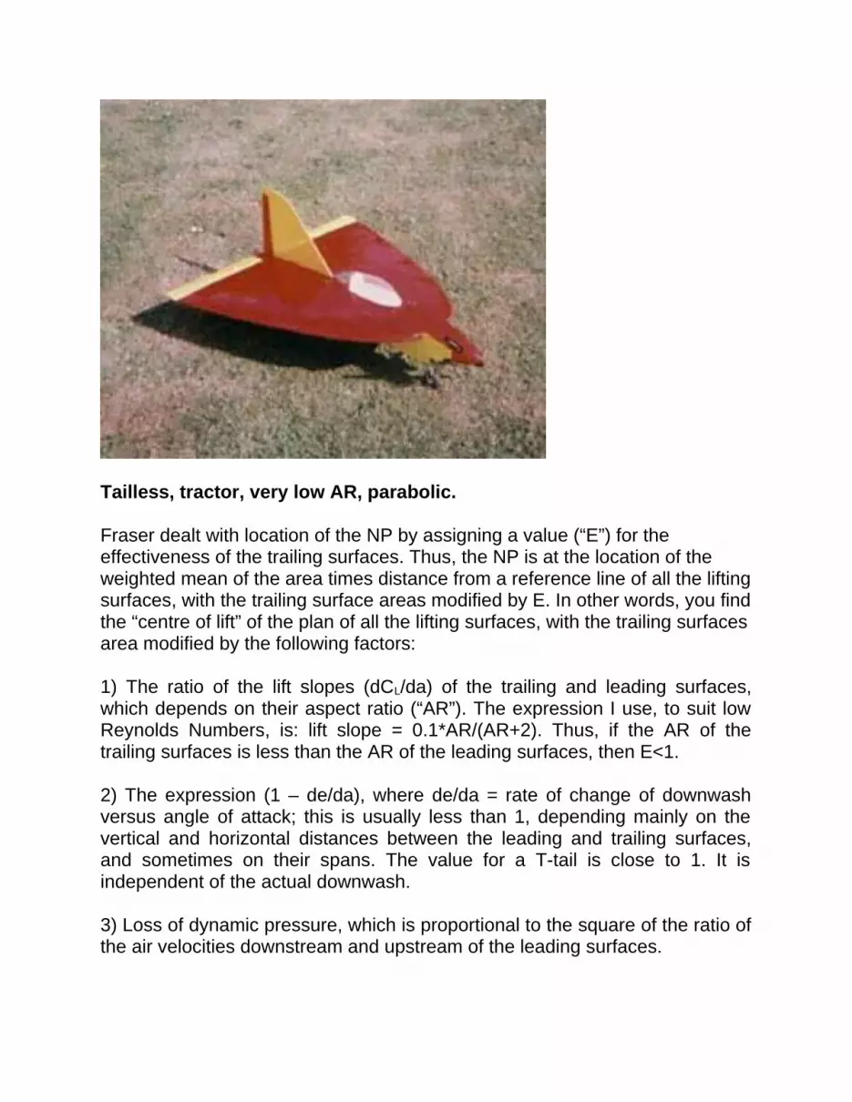
 Tailless, tractor, very low AR, parabolic. Fraser dealt with location of the NP by assigning a value (“E”) for the effectiveness of the trailing surfaces. Thus, the NP is at the location of the weighted mean of the area times distance from a reference line of all the lifting surfaces, with the trailing surface areas modified by E. In other words, you find the “centre of lift” of the plan of all the lifting surfaces, with the trailing surfaces area modified by the following factors: 1) The ratio of the lift slopes (dCL/da) of the trailing and leading surfaces, which depends on their aspect ratio (“AR”). The expression I use, to suit low Reynolds Numbers, is: lift slope = 0.1*AR/(AR+2). Thus, if the AR of the trailing surfaces is less than the AR of the leading surfaces, then E<1. 2) The expression (1 – de/da), where de/da = rate of change of downwash versus angle of attack; this is usually less than 1, depending mainly on the vertical and horizontal distances between the leading and trailing surfaces, and sometimes on their spans. The value for a T-tail is close to 1. It is independent of the actual downwash. 3) Loss of dynamic pressure, which is proportional to the square of the ratio of the air velocities downstream and upstream of the leading surfaces.

 

Since the value of E is obtained by successively multiplying these factors, it can be quite small. Also, evaluation of 2) & 3) above is quite difficult, needing reference to good books on aerodynamics, see Refs 2 & 3.  It is recommended, however, that 1) above should always be evaluated because it is important, and easy to do, and 2) above is well described in Ref. 3. I usually ignore 3) above due to lack of data.Sometimes I use one of these good books, sometimes another; this is because design is largely a matter of judgment. Pitch stability calculations

 

Since designing models requires numeracy, here are some of the equations I use. First, pitch stability, looking at figure 1:The X dimensions are measured from the AC of the leading surface(s). The AC of a surface is taken to be at the 1/4 chord of the corresponding MAC.X12 is the distance between the AC’s of leading and trailing surfaces, i.e., Ls. From the leading surface AC, XN is the distance to the NP, and X1 that to the CG. Fraser showed that PC = X1/X12 - 1/ (AW/E*AS+1); note: “*” is “x” (multiply) in computer characters.E is the effectiveness of the trailing surfaces; usually E<1; AW = area of leading surface(s), and AS = area of trailing surface(s).AW and AS can each consist of a group of surfaces, e.g., biplane, triplane or whatever. PC is dimensionless. By writing PC=0 the above equation yields:XN = X12/ (AW/E*AS+1), then,PC = (X1-XN)/X12 so that the stability coefficient is obtained for a given set of dimensions; alternatively,X1 = XN+PC*X12 so that the CG is located for a given stability coefficient.

 Figure 1 shows the format for a conventional model; not shown is a reference line, from which the drawing dimensions are reckoned. For example, it is preferable (essential?) to locate the CG from a real point like a wing root LE than from a theoretical point like the AC of a surface. For unconventional model layouts, the reference line may be placed anywhere convenient and the signs + or – in the above equations are suitably chosen. In the difficult case of the three-surface layout (like Piaggio ‘Avanti’), the leading surface is de-stabilizing and is ‘subtracted’. 

 Three Surface The aerodynamic center of lifting surfacesNext, we should address the task of locating the AC of a group of surfaces. A lifting surface may consist of a group of like surfaces vertically disposed (biplane, triplane, etc.), each comprising one or more multi-taper surfaces. There is no need for the tedious calculations to find a monoplane surface equivalent to those of a biplane or triplane, as suggested by some authors. I call each panel of a multi-taper surface an “element”. The AC of an element lies on the quarter-chord line (by convention), and it can be located very accurately by using simple equations; the drawing method so beloved by authors is a waste of time. 

 Elements bounded by straight lines are considered to be trapezoids, i.e. a quadrilateral with one pair of parallel sides, requiring only simple arithmetic derived by calculus. Conics - circular, elliptical and parabolic shapes - are also dealt with by schoolroom calculus, and I have developed simple expressions for locating the AC, relative to a reference line, of many of the possible plan forms. Complex surface shapes like those with a straight line LE and a curved TE, for example, are readily handled by employing a program based on what was called “Simpson’s Rule” in my schooldays. The AC of a multi-taper surface e.g., a wing comprising several different elements is found by calculating the weighted mean of area times distance of AC from the reference line of all the elements of a group. It is therefore simple, using a computer, to make changes in the dimensions of the model and get the new result very rapidly. At this point yet another design choice must be highlighted. If a body, e.g. fuselage or engine nacelle, obscures a lifting surface from above or below, should the over-laid area be counted as lifting? There is plainly a difference of opinion in current texts; my tedious study of several classic full-size aircraft revealed that the basis for items like wing area is confused - some do count the over-laid area, some do not, and they do not bother to tell the reader. My firm opinion is that the over-lay does not count, that is, lifting surfaces are those having an airfoil, and are clear of a fuselage or engine nacelle. I have found support for this view from practical results at the flying field. However, by all means make some allowance for body shape in special cases. 

 Tailless Tractor Delta Calculations to locate an AC Trapezoid: Now, let us look at figure 2: what we need to know is the value of M, the distance between the reference line and the AC, and the area A for an element. 

  

                                                                                                                                                        Let the taper ratio T/C = RM=MAC*CP+L/S*B, where CP=0.25, i.e., the quarter chord point.And, the area A=S*(C+T)/2Then, L=S/3*(1+2*R)/ (1+R), and, MAC=2*C/3*(1+R+R2)/ (1+R). Several trapezoids: Looking at figure 3, a string of two or more elements, like B-747 - (2); or SAAB ‘Viggin’ - (3).  

To locate the AC of the complete surface (‘ACW’) we calculate the weighted mean of all the values of M*A to obtain the distance MW of ACW from the reference line:-MW=(M1*A1+M2*A2+M3*A3)/(A1+A2+A3) Note that the usual published graphical method is limited to one element, whereas we can handle any number of elements by calculation. Remember, expressions like these have to be written one time only in the computer.It is worth noting that the MAC of the string of elements does not necessarily lie between a leading and trailing edge. Ellipse: Referring to figure 4, the “Spitfire” wing was composed of two quarter - ellipses having the same span S and different root chords C1 and C2.

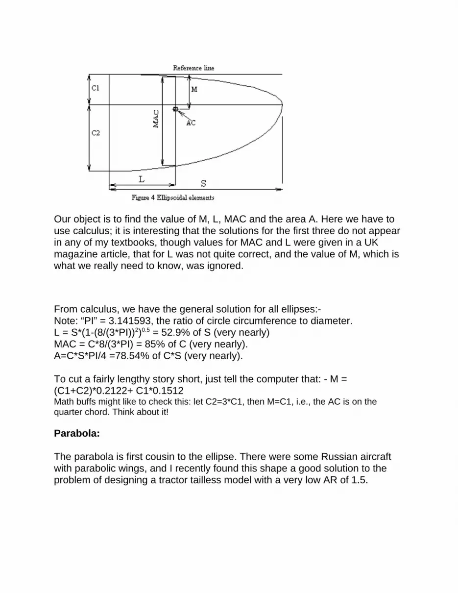
Our object is to find the value of M, L, MAC and the area A. Here we have to use calculus; it is interesting that the solutions for the first three do not appear in any of my textbooks, though values for MAC and L were given in a UK magazine article, that for L was not quite correct, and the value of M, which is what we really need to know, was ignored. 

From calculus, we have the general solution for all ellipses:-Note: “PI” = 3.141593, the ratio of circle circumference to diameter.L = S*(1-(8/(3*PI))2)0.5 = 52.9% of S (very nearly)MAC = C*8/(3*PI) = 85% of C (very nearly).A=C*S*PI/4 =78.54% of C*S (very nearly). To cut a fairly lengthy story short, just tell the computer that: - M = (C1+C2)*0.2122+ C1*0.1512Math buffs might like to check this: let C2=3*C1, then M=C1, i.e., the AC is on the quarter chord. Think about it! Parabola: The parabola is first cousin to the ellipse. There were some Russian aircraft with parabolic wings, and I recently found this shape a good solution to the problem of designing a tractor tailless model with a very low AR of 1.5.  

Calculus shows that the following convenient expressions apply, looking at figure 5:M=0.4*C, and, A=C*S*2/3.   Also, MAC=0.8*C, where C = root chord. Compound shapes: A surface having, for example, a straight line LE with an elliptical TE (e.g. Republic P-47) requires a math treatment where the chord is described by the sum of the y values of an expression for a straight line and for a curve, as shown in figure 6. 

For any element, MAC = (2/area) * integral (chord2) from 0 to ½ span, see Ref 4, p 27.This integral is messy, however, the problem is solved by writing ‘chord’ as a function of x then dividing the span into a number of narrow (‘dx’) chord wise strips. The chord is determined from the equations for the leading and trailing edges. For example, that for a straight line LE could take the form:c1 = C1- x/S * (C1 – T), or: c1 = C1 – x*tan(z).That for an elliptical TE might be: c2 = C2 * (1 – x2/S2)0.5.The area of each chordwise strip = (c1 + c2)*dx. 

Then, using (in BASIC, or equivalent) a “for-next” iteration, add up the values of (c1 + c2)2 and divide by the sum of the values of (c1 + c2), which gives the MAC. Then find the corresponding value of x, by substituting the corresponding value of either c1 or c2 into one of the two equations (for the leading or trailing edge). Then the AC can easily be located. A good value for ‘dx’ is 0.001*S, so that there will be 1000 iterations. Back in 1986-90, when this particular study was made, computers were so slow that there was time to queue at the coffee machine while running; 10 to 15 years later, the result comes up instantly. I have run this type of program for a range of compound shapes. No such solution for this particular problem has appeared in print, to my knowledge. Tailless: Neither Fraser nor anyone else, to my knowledge, has suggested a method of locating the CG of a tailless model other than by the ‘popular’ method, i.e. a static margin ahead of the AC of the whole wing. However, the elevons normally produce a down force at the wing TE to achieve positive pitch stability. My proposal is that if the elevons are treated as a conventional stabilizer, then calculation can be performed by the ‘proper’ method, as for tailed models. The lifting surface is what remains with the elevon removed. The ‘wing’ is treated as consisting of several trapezoids, as shown in figure 7, with, maybe, one or two full chord elements beside the elevon, and an element ahead of it having reduced chord; the ‘tail’ is the elevon trapezoid.

 

I have designed and built various such models, ranging from high AR backswept types like Northrop, through Deltas like Convair ‘Dagger’ to a low AR plane like the Handley-Page 115 of 1965. The lower the AR, the greater the error of the popular method, which results in the CG being so far forward as to make the landing flair difficult or impossible. The proper method, however, involves an unknown factor, that is, the value of E for an elevon. What I have done is to build and fly a number of such models, and from the observed results arrived at an empirical value of E=0.2 which is cautiously recommended. An expert author or two has ridiculed my idea, and they may be right; however, it seems that none can support the popular method by theory or practice. 

 Tailless Tractor V-tail design Ref. 5 featured an NACA report (#823 11/44) which showed that one should take care. It is usually considered that the surface areas are obtained by dividing the equivalent flat and upright surface area(s) by the cosine and sine of the vee angle to the horizontal, respectively. However, the report points out that these trig ratios should be squared because the rate of change of angle of attack is also changed by the same ratio. That is to say, V-tail surfaces should be larger than is commonly thought. 

The V-tail has always seemed to me to be a good choice, especially for slope-soarers, and my observations suggest that the NACA were probably right. Comparing otherwise similar models, with orthodox or V-tails, the latter appeared to need the NACA increased area in order to achieve similar pitch and yaw stability. It can be shown that, designed by the NACA method, the tail surface (‘wetted’) area is the same whether in Vee or conventional form.

 Yaw stability It can be said that there is positive yaw stability if the centre of lateral area (CLA) is trailing the CG. Just what constitutes lateral (side) area is open to discussion. Fin(s) and rudder(s) can be treated in the same way as horizontal lifting surfaces, and the calculations are similar. It is reasonable to add portions of the lateral area of bodies like fuselage, nacelles, and even airscrew(s); guidelines for this are difficult to find (but try Ref. 2). This is a nice test of designer judgment, interesting but not too critical. Then, having summed the yaw moments of the vertical surfaces (area times distance from CG to AC), in the same way as for “PC”, how should we normalize it so as to get a similar yaw stability coefficient “YC”? Personally, I divide by the span of the largest lifting surface, on the intuitive grounds that, if the main wingspan is large, then its yaw inertia is important. Others are free to disagree; a current author simply makes his fin and rudder “look right”, and I have no problem with that. However, experience suggests that it is useful to have a coefficient for yaw stability, so that one can make coherent changes to a design. This method has worked quite well for me, having found an empirical value of YC as a guideline for each kind of design. That is to say, I use values of YC as follows, for: Conventional = 0.05 - 0.07, Tailless = 0.04 - 0.08, Canard. = 0.07 - 0.1, and Glider = 0.03 - 0.04. It may also be useful to relate spinning to the value of YC, for, in my experience, if it is large then a spin, as an aerobatic manoeuvre, may be impossible. Trim: 

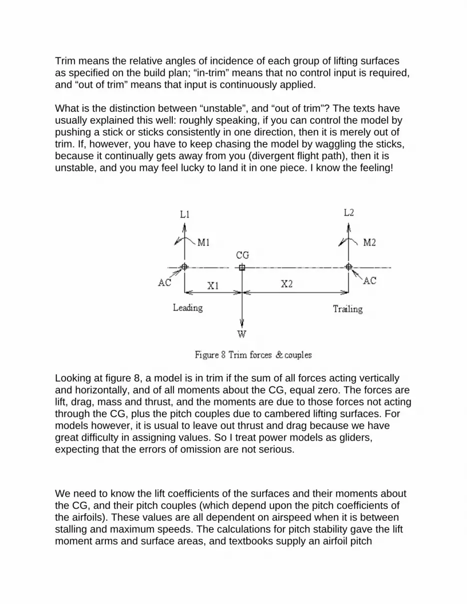
Trim means the relative angles of incidence of each group of lifting surfaces as specified on the build plan; “in-trim” means that no control input is required, and “out of trim” means that input is continuously applied. What is the distinction between “unstable”, and “out of trim”? The texts have usually explained this well: roughly speaking, if you can control the model by pushing a stick or sticks consistently in one direction, then it is merely out of trim. If, however, you have to keep chasing the model by waggling the sticks, because it continually gets away from you (divergent flight path), then it is unstable, and you may feel lucky to land it in one piece. I know the feeling!  

Looking at figure 8, a model is in trim if the sum of all forces acting vertically and horizontally, and of all moments about the CG, equal zero. The forces are lift, drag, mass and thrust, and the moments are due to those forces not acting through the CG, plus the pitch couples due to cambered lifting surfaces. For models however, it is usual to leave out thrust and drag because we have great difficulty in assigning values. So I treat power models as gliders, expecting that the errors of omission are not serious. 

We need to know the lift coefficients of the surfaces and their moments about the CG, and their pitch couples (which depend upon the pitch coefficients of the airfoils). These values are all dependent on airspeed when it is between stalling and maximum speeds. The calculations for pitch stability gave the lift moment arms and surface areas, and textbooks supply an airfoil pitch

coefficient - which is usually constant over the values of CL corresponding to the working speed range. The actual value of the pitching couple of a lifting surface is proportional to the MAC (or the mean chord), the area, and dynamic pressure Q, where Q=rho/2*v2; and rho=air density, v=airspeed. Angles of incidence are based on the difference between angle of attack ALPHA and the angle of zero lift, = ALPHA0 for the chosen airfoil. Returning to figure 8, the task is to evaluate L1 and L2, which in turn yields the CL and ALPHA of each group of surfaces (leading and trailing) so that equilibrium is obtained. The relative angle of incidence is often called the “decalage”, from the French word for ‘angular displacement’. This is calculated for several speeds from minimum to (a notional) maximum. Having chosen the trim speed, which corresponds to neutral elevator, the decalage of the lifting surfaces is now known. They are then arranged relative to the fuselage (if any) so that the flying attitude of the model is as you want it. Think “Whitley”, the WW2 RAF bomber! For different layouts such as three-surface, the diagram is altered to suit, same as for stability. In flight, pilot input to elevators or elevons obtains trim at all other airspeeds. In the case of the “Flying Flea”, control is uniquely done by rotating the leading wing, which changes the decalage; the range is surprisingly small, perhaps 5 degrees from Vmin to Vmax.Similarly, the ‘all-flying tail’, popular in modern gliders, controls by varying the decalage.   

 The “Flying Flea”, tandem wing.Pitch controlled by rotating the leading wing a few degrees. Trim calculations: Written for BASIC, we would have:L1+L2=W      where W = weight; forces resolved vertically.L1*X1+M1+M2=L2*X2     i.e., the sum of couples and moments about CG = zero. The general solution of these simultaneous equations is as follows:L1=(W*X2-M1-M2)/X12And, L2=W-L1So, for a group of lifting surfaces, lift L=CL*A*Q, and pitch couple M=CM*A*MAC*Q, where CM=airfoil pitch coefficient,and, CL=lift coefficient = LIFT SLOPE*ALPHA, where ALPHA = angle of attack (radians). To solve for the difficult three-surface case, one way to go is to combine two surfaces pragmatically, so that the simultaneous equation is valid, then alter the combination and try again. It can be done. In general, the angle of incidence =ALPHA-ALPHA0 where ALPHA0 = the zero lift angle of the airfoil. 

Trailing surfaces may be affected by downwash from leading surfaces; this is a matter of judgment in the context of trim, similarly to the effect of the rate of change of downwash in the stability calculations. Simple airfoil theory states that: downwash (degrees) = 18.24*CL/AR, at the TE of the surface.  But, if the trailing surface is distant from the wake centre by more than half the chord of the leading surface - as for a T-tail - the effect of downwash is greatly reduced. On the other hand, in the case of a very close up trailing surface - such as the “Flea” - experience has shown that the above equation serves as a reasonable guideline. There are other expressions for downwash to be found in texts, especially ref 2. Since we want to know the decalage (DEC) over the speed range, repetitive calculation is required, ideal for a PC, too laborious “by hand”. Also, since most textbooks are pre-PC, it is necessary to alter nearly all the symbols that have been used for decades in textbook equations. The PC may not recognize suffixes, subscripts, lower case or fancy Greek letters, so each of us has to invent our own. My practice is to use mnemonic strings, these may look lengthy but the PC memory is hardly taxed. Since we are dealing with force, length and time for trim calculations, we have to get the units right, which is up to each user - imperial or metric, for example.  I work in inches and ounces for designing, and convert to feet and pounds for dynamics. To find Vmin, and decalage DEC vs. airspeed V from Vmin to Vmax:-First, re-write dynamic pressure Q as a coefficient for V2: Q =  0.002378/(2*144)The sub-routine is (ignore my line numbers):- 1540 FWPM=Q*V^2*CMWF*AWF*MCWF/12    FWPM = Leading  surface pitch moment, CMWF = Leading surface pitch coefficient  (1/4 chord), AWF = Leading surface area,          MCWF = Leading surface mean chord or MAC. 1550 RWPM = Q*V^2*CMWR*AWR*MCWR/12   As 1540 but trailing surface pitch moment.1560 CLWF=(W/16*X2/12-FWPM-RWPM)/(Q*V^2*AWF*X12/12)   CLWF = Leading surface CL.1570 CLWR= (W/16-Q*V^2*AWF)/(Q*V^2*AWR)               CLWR = Trailing surface CL.

1580 AAWF=CLWF/SLWF         Leading surface angle of attack.  SLWF = lift slope, a, = ðCL/ða

1585 INCWF=AAWF+AA0WF         Angle of incidence.  AA0WF = zero lift angle.1590 AAWR=CLWR/SLWR             Trailing surface, angle of attack.1600 DW=18.24*CLWF/ARWF    Downwash, leading surface. The value 18.24 may be varied depending on the distance downstream and height h of the trailing surfaces. 1610 INCWR=AAWR+AA0WR+DW    Trailing surface, angle of incidence.1620 DEC=INCWF-INCWR           Decalage1630 RNWF=V/12*MCWF/.000156         Leading surface Reynolds number.1640 RETURN   Return to GOSUB command. To find Vmin, which corresponds to the condition CLWF  CLMWF (leading surface, CL, CLmax) we guess the lowest likely stalling speed for a start value for V; then to the sub-routine and back, then comparing CLWF to the value of CLMWF   0.05, say. The “gate” of 0.1 is notional, found by trial and error/experience; recommended as a starter. If CLWF fails to pass through the “gate” (yes, it is quite like penning sheep), then we change the value of V by adding or subtracting a small notional quantity, the “step”. Somewhere earlier in the program, then, will be a line like this:- 20 STEP=.05,     Increment of airspeed, ft/s.So, to find Vmin, we can write:-900 V=30   A guess at the value of Vmin

910 GOSUB 1540920 IF CLWF>(CLMWF+.05) THEN V=V+STEP:GOTO 910            V too low, ie., V<Vmin

930 IF CLWF<(CLMWF-.05) THEN V=V-STEP:GOTO 910              V too high, ie., V>Vmin

940 VMIN=V        Stalling speed (CLWF  CLMWF) Next, to construct a Table showing decalage vs airspeed, plus anything else available such as incidence, CL, downwash and RN, we can write:- 950 IF VMIN<30 THEN V=30 ELSE IF VMIN<40 THEN V=40:GOSUB 1540  The values 30 and 40 are given here from an actual example; this is trial and error time. Next, we obtain numbers for the Table:-960 V1=V:INCWF1=INCWF:INCWR1=INCWR:DEC1=DEC:CLWF1=CLWF:DW1=DW970 V=V+10:GOSUB 1540    And so on.

  The value 10 is a notional “step” in V; often a step of 5 is adequate. This iteration ceases at some preset high value of V, the data is then sorted into tabular form for printing; a typical result might look like this:  V ft/sec         40                50              60              70              80     AirspeedINCWF         +9.3        +2.7           +0.4            -0.9           -1.8     Leading surface incidence, deg.INCWR        +0.2         -2.7            -3.7            -4.3            -4.7    Trailing surface incidence, deg.Decalage     +9.0        +5.4            +4.2           +3.4           +2.9    Difference, deg.                                                                                                                    In order to draw the model plans, it is necessary to choose the airspeed for trim setting; some may choose a fairly low speed corresponding to take off or approach, others may prefer high cruise or maximum speed. I generally go for the former. At all other airspeeds, some pilot input to the elevator (or, strictly speaking, the pitch control) is required, though it may be so small that we do not notice it. It is entirely feasible to mix throttle and elevator in a programmable Tx to try for horizontal flight whatever the throttle opening; be warned, this a trial and error operation - adjustments should be quite small. Very gratifying when more-or-less right! Decalage is usually positive, that is, the leading surfaces are at greater incidence than the trailing surfaces. Some current authors state that decalage must be positive for pitch stability. This is not so, because in configurations like the “Flying Flea” the downwash effect evidently results in the model being trimmed with negative decalage, yet there is positive stability. That is my experience, based on two “Fleas”, which has told me not to believe everything I read. 

 Tandem wing, twin tractor Stall behaviour: Following a discussion of pitch stability, a note is required on the ultimate loss of pitch stability that is, when the model stalls. Fraser’s statements do not apply since we are not now looking at the effects of a micro-gust. At the stall, either the leading or the trailing surfaces reach CLMAX, with reduction in CL to follow, as ALPHA increases. It is clear that the design, which now includes the choice of airfoil sections, should ensure that the leading surface(s) stall first while the trailing surface(s) are still increasing CL as ALPHA increases. For unorthodox models like the tandem wing and canard, it is suggested that airfoil camber and thickness should be less in the leading surface(s) than in the trailing surface(s), so that the leading surface(s) should stall first.  

 Canard, Pusher In this connection, I have lately used airfoils as follows: Flea, leading & trailing = NACA 23012. Swept canard, leading = SD6060; trailing = NACA 2415, or MB253515. Tandems, leading = Gottingen 796; trailing = Gottingen 797. For the two latter types, the leading surface airfoil is thinner and less cambered than that of the trailing surface(s). Some of my earlier experimental swept canards and tandem wings employed thicker and more cambered airfoils up front, on the grounds that the leading surfaces are more heavily loaded than the trailing surfaces. They were stable, but stall behaviour was poor - the trailing surfaces lost lift first, very untidy. 

 Burnelli ‘lifting fuselage’ – the one built in Britain, which served thru WW2 My design procedure summarized

 1.      Sketch the plan and side elevations of the model using a CAD program,

like DesignCAD, reflecting the object(s) of the design, e.g. performance, maneuverability, load carrying, or just “unorthodox, how well will it fly?” This is where a design “vision” begins to become practical. 

2.      Calculate the CG location for a preferred value of PC; my particular choice of a minimum value is: PC = -0.08. I call this CG location the “aerodynamic CG”. 

3.       Calculate the CG location of the model when constructed, which I call the “structural CG”, using estimated values for the weight and cg location of every item, from motor(s) thru wings, tails, and fuselage, down to servos, battery, Rx and switch. Find the CG locations corresponding to fuel tank(s) empty and full. For this operation, almost any guess is better than nothing. With a little experience, it is surprising how well the location of the structural CG can be forecast.

 

4.      Run and re-run steps 1, 2 & 3, changing dimensions and shifting components until the structural and aerodynamic CG agree reasonably well. This should be at the worst case of fuel empty or full, and can include ballast. 

5.      Concurrently with positioning the CG to ensure reasonable pitch stability, obtain estimations of yaw stability, and, having chosen the airfoils, the decalage. It is not difficult to estimate stalling speed as well. These things are done by simple extensions to the pitch stability program.

 6.      Make working drawings using CAD, while quickly checking the effects of

dimensional or other changes using the calculation programs. 

To sum up, if you wish to design a conventional model then by all means use the simple magazine article ‘popular’ method for locating the CG; however, be aware that the method is incorrect and should never be used for an unconventional design; instead the ‘proper’ method is recommended both on the basis of sound mathematics and practical results.  

 Tandem Wing Book references:

 

1) ‘Equilibrium, stability & the load on your tail’ by David Fraser, pp101-119, Soartech #6, 1985

 

2) “The Design of the Aeroplane” by Darrol Stinton, pub. Granada, 1983

 

3) “Model Aircraft Aerodynamics”, by Martin Simons, pub. Argus, 1987

.

4) “Theory of wing sections”, by Abbott & von Doenhof, pub. Dover, NY, 1949.

 

5) Soartech #2, 1983