Adaptive Finite Elements For Reinforced Concrete Framed Structures

COMPUTATIONAL MECHANICSNew Trends and Applications

S. Idelsohn, E. Onate and E. Dvorkin (Eds.)c©CIMNE, Barcelona, Spain 1998

ADAPTIVE FINITE ELEMENTS FOR REINFORCEDCONCRETE FRAMED STRUCTURES

Alejandro Lago∗, Miguel Angel Bretones∗, Pierre Pegon†and Antonio Huerta∗

∗Departamento de Matematica Aplicada III, E.T.S de Ingenieros de CaminosUniversidad Politecnica de Cataluna

Campus Norte UPC, 08034 Barcelona, Spain

†Structural Mechanics Unit, Institute for Systems, Informatics and SafetyJRC of European Commission

I-21020 Ispra (VA), Italy

Key words: Adaptivity, Nonlinearity, Structural analysis, Reinforced concrete, Finiteelements

Abstract. This work focuses on the modelling of nonlinear response of reinforcedconcrete structures by means of the finite element method. A new technique whichemploys a variable mesh in order to reduce the computational cost of classical approachesis presented. For some piecewise linear constitutive models which are widely employedfor the modelling of reinforced concrete, some properties of the solution can be predicted.The knowledge of these properties can be used as a discretization criterion of thestructural elements. Therefore, the nonlinearity of the problem is easily handled with aniterative scheme that modifies adaptively the position of the nodes. The results obtainedon some framed structures show that with this scheme we obtain accurate solutions witha substancial reduction of the computational cost compared with the solutions obtainedwith fixed meshes, both for loading and unloading states.

1

A. Lago, M.A. Bretones, P.Pegon and A.Huerta

1 INTRODUCTION

A general analysis of structural behaviour beyond elastic state usually requiresthe use of numerical methods like the Finite Element Method (FEM), in which,obtaining reliable solutions depends on the use of dense meshes and, hence, on expensivecomputations1.

To overcome this drawback, it is possible to develop more sofisticated approachesbased on exploiting the aprioristic knowledge on the behaviour of the problem in order tomodify some of the characteristics of the discretization and reduce the number of degreesof freedom of the problem. In this context, some works have been presented. Leon etCorres, for example, modify the stiffness of the elements considering it variable alongthe beam axis2. More recently, Toi changes adaptively the position of the integrationpoints3,4.

A different approach is presented here. The characteristics of the mechanical modelsconsidered on every finite element and the position of the nodes of the mesh areiteratively adapted. Piecewise linear constitutive laws are considered to model thenonlinear sectional behaviour of reinforced concrete. Then, an strategy that willassociate to each of the different domains of the structure an specific kind of elementwith a suitable linear model may be a correct choice to reduce the number of unknownsof the problem and, therefore, to reduce the computational cost.

The main purpose of this work is to develop a technique with these possibilities, thatis, a technique which adapts in each load level the discretization, considering both theposition of the nodes and the mechanical model, in order to use the minimum numberof finite elements.

2 STATEMENT OF THE PROBLEM

The analysis focuses on two-dimensional framed structures consisting of beams. Ifbending is assumed to be the dominant effect, the problem can be defined by means ofthe Euler-Bernouilli theory, whose governing equations - equilibrium, compatibility andconstitutive law - can be expressed respectively as:

d2σ

dx2 = q (1)

ε =d2w

dx2 (2)

and

σ = σ(ε) , (3)

2


where w is the displacement of the beam axis, σ the bending moment, ε the curvatureon each section † and q the distributed load on the structure5.

The analysis of the behaviour of the structure is reduced to the knowledge of thebending moment σ and the curvature ε in each section. The influence of the material isdirectly introduced by the constitutive model assumed. Discussion on the constitutivemodel adopted is presented on the following subsection.

2.1 Constitutive model: piecewise linear σ − ε law

In nonlinear analysis, some simplified moment-curvature laws are adopted. Generally,these laws are defined by different loading and unloading linear branches6. We will referto these models as piecewise linear laws.

In this work, the elastic-plastic bilinear model, which is widely employed both instatic and dynamic analysis because of its simplicity, will be considered. In this model,unloading is assumed to take place along a linear branch parallel to the elastic one7. Analternative elastic-cracked-plastic model will also be introduced as a variation to considerthe difference between elastic and cracking states in reinforced concrete6. These twomodels are represented in Figures 1 and 2, respectively. In these figures, σc denotesthe cracking moment, σp the plastification moment and De, Dc, Dp are the bendingstiffness for the elastic, cracked and plastified section respectively.

Although only elastic-plastic and elastic-cracked-plastic laws are considered as aninitial framework, all the treatment of the problem could be applied to more complexmodels which have a larger number of linear branches.

Analytically, it can be considered that, in these piecewise linear models, the σ − εlaw is divided in different domains —e.g. elastic, cracked and plastic— depending onthe value of the bending moment. The values σc and σp define the boundaries of thesedomains. Each domain corresponds to one of the branches of the law which defines alinear relationship between moment (σ) and curvature (ε). This relationship can beexpressed as:

σ = D ε + σ0 (4)

where D is the bending stiffness related to each branch and σ0 the moment associatedwith the zero curvature state (stiff moment).

The parameters D and σ0 are constant on each of the domains. As an example, inelastic-cracked-plastic model, D and σ0 are:

D(σ) =

De if σ < σc

Dc if σc < σ < σp

Dp if σ > σp

(5)

† The non-standard notation is adopted to emphasize the idea that moment and curvature play the role of stressand strain in this generalized problem

3


σ0(σ) =

0 if σ < σc

0 if σc < σ < σp

σp0 if σ > σp

(6)

Dp

De

σσp

σσc

σ

ε

Dc

σσpDp

σ

ε

De

Figure 1. Elastic-plastic model Figure 2. Elastic-cracked-plastic model

2.2 Theorethical consequences of piecewise linear laws

Piecewise linear relationships σ − ε allow to infer a priori some properties of thesolutions which can be employed to improve the numerical treatment of the problem.

Property 1.- Given a bending moment distribution, each beam of the structure can bedivided in different domains, and, in each of these domains, the mechanical behaviouris linear and associated to one of the branches of the constitutive model.

An example of this division of domains for a given moment distribution is shownin Figure 3. The domains —elastic, cracked and plastic— are separated by the pointswhere the moment distribution has one of the values that define the different branchesof the constitutive law —that is, cracking moment σc or plastic moment σp. We willrefer to these boundary points as the characteristic points of the structure.

Justification of property 1

The general problem defined by equations (1)-(6) is typically nonlinear. Thedifferential equation that defines this problem, which is obtained by substituting theconstitutive equation (3) on the equilibrium equation (1), is expressed as

d2

dx2

(D

d2w

dx2 + σ0

)= q . (7)

4


This equation is nonlinear because both D and σ0 depend on the bending momentσ and, therefore, depend also on the displacement field w.

However, if the bending moment distribution is known and it is possible to know theposition of the characteristic points the structure can be split into the different domainsseparated by these points. Within each of these geometric domains —elastic, crackedor plastic— D and σ0 are constant and, then, equation (7) can be expressed as

Dd4w

dx4 = q , (8)

which is the equation that governs the linear elastic problem. Thus, behaviour ineach of the domains is linear and the global problem can be considered as linear non-homogeneous.

D p

σσc

σσp

ε

σ

D e D cD c

Bending Moment Law

Division of domains

Pla

stic

Cra

cke

d

Ela

stic

Cra

cke

d

Constitutive model

Figure 3. Domain division according to bending moment distribution

5


Property 2.- Because of the linear behaviour on each of the domains of the structure,the distribution of the solution on displacements can be inferred a priori. If only pointloads are considered, the solution on displacements is a cubic function within each ofthe domains of the structure.

Justification of property 2

From now on, only point loads on the structure will be considered (q = 0). With thishypothesis, due to linear behaviour within each of the domains in which the structurecan be divided, it is easily shown from equation (8) that the solution on displacementsmust be a cubic function within each of these domains. As well, equation (2) demandscontinuity on the first derivatives of displacement w (rotations continuity) in all thestructure. Thus, solution on displacements must be a cubic spline with C1 continuityand the discontinuities on the curvature (second derivative of w) can only be locatedon the boundaries of the domains, that is, on the characteristic points.

Concluding remark

Due to the use of a piecewise linear model, the problem can be reconsidered. Ifthe position of the characteristic points is known, that is, if it is possible to knownhow to place correctly the elastic, cracked and plastic parts in each beam of thestructure, the original nonlinear problem can be turned into a non-homogeneous linearone where the linear constitutive laws for each of the parts of the structure are different.Moreover, since only point loads are considered, the solution on displacements betweencharacteristic points is known to be a cubic function.

These properties can be directly employed to consider an improved finite elementtreatment of the problem which allows to drastically reduce the number of elementsneeded to discretize the structure.

3 NUMERICAL TREATMENT

To solve the nonlinear structural problem defined by equations (1)-(7), two differentapproaches are possible.

A classical nonlinear finite element computation seems the trivial approach. Thisrequires to consider at each Gauss point the complete piecewise linear model. Thus,dense meshes must be used to capture precisely the discontinuities between elastic,cracked and plastic areas and, hence, to obtain accurate solutions. As the computationalcost depends directly on the degrees of freedom of the problem, that is, on the densityof the mesh, computations are very expensive.

On the other hand, a more efficient approach is possible for piecewise linear in viewof properties 1 and 2. Property 1 suggests the following approach: determine first theposition of characteristic points and then, solve the non-homogeneous linear problem.All the effort is aimed at locating the characteristic points, possibly with an iterative

6


scheme. The problem becomes a nonlinear geometric problem, the mechanic part islinear. With such an algorithm, property 2 indicates that, once characteristic pointsare known, the exact solution can be captured if hermitic elements (Euler-Bernouillielements) are used between each pair of characteristic points. Or, from a morerealistic point of view, the error is governed by the accuracy in the location of thecharacteristic points. Nevertheless, in every beam only as many finite elements asdifferent mechanical domains are present for the load level are required. This impliesa substantial reduction in the degrees of freedom of the problem compared with theclassical approach.

Of course, with this new adaptative scheme, since geometry is the main unknown ofthe problem, it is necessary to employ an adaptive mesh. The position of the nodesmust be modified to make them coincide with the characteristic points, and the modelsconsidered in each element must be adapted to capture the different linear behaviour ofeach part of the beams of the structure.

The following algorithm is proposed. It is based on the cited ideas, namely:• An adaptive discretization composed by elements with linear elastic mechanical

models• Iterations on the geometry

The details of the implementation of this technique are presented in the followingsubsections.

3.1 Discretization of the problem

Each beam is discretized with a mesh consisting of two-noded hermitic elements,each with a different linear constitutive model. Each element is associated to one ofthe branches of the constitutive piecewise linear law and has a linear elastic behaviourdefined by the bending stiffness (De, Dc, Dp) of the branch to which it is associated, seeFigure 3.

The mesh is placed as follows. We consider a bending moment distribution. It definesa position of the characteristic points on each beam of the structure. We fit only onehermitic element with the appropiate constitutive model to each of the domains definedby these characteristic points. Thus, the nodes of the mesh are made to coincide with thecharacteristic points so that 1) discontinuities between the elastic, cracked and plasticparts are captured exactly, and 2) the minimum number of elements are employed toobtain the exact solution of the problem

An example of application of this discretization criterion for the elastic-cracked-plastic case is shown in Figure 4.

7


"Elastic" Element

"Plastic" Element

"Cracked" element

σc

σc

σp

σp

Figure 4. Structural element. Discretization criterion

3.2 Iterative scheme on geometry

As geometry is the main unknown of the problem, iterations are needed until nodesare placed correctly. This implies that both the position of the nodes and the mechanicalmodels associated to the elements are modified in each iteration.

The iteration scheme is basically defined as follows. Based on a previous momentdistribution, we may consider a initial position of the characteristic points and anassociated division of domains of the structure. Whether the geometry considered isthe correct one or not, a non-homogeneous linear problem has to be solved and a solutionin equilibrium with external forces can be obtained directly. This solution will definea new moment distribution. If the nodes have been correctly placed a priori, they willcoincide with the characteristic points defined by this moment solution. If they do not,the position of the nodes can be redefined according to this new moment distributionand iterate again. Then we will have to modify both the mesh and mechanical modelsand to solve a new non-homogeneous linear problem.

This way, we obtain an equilibrium solution in each iteration and with it, the meshand the mechanical models are adapted progressively to the final right position.

Of course, to define the complete evolution of the problem in a loading process, anincremental approach where solution in each step is calculated as an increment of thesolution on the previous step is required. The iterative scheme presented is developedmore precisely in each load step as it is shown in table 1.

A little remark has to be made about the way the solution is obtained. In eachiteration, we redefine the position of the nodes according to the solution on momentsobtained in the previous iteration. Once we have changed the discretization and, hence,

8


the mechanical model distribution, the solution for the ancient mesh is no longer inequilibrium. Thus, we can obtain a force residual and calculate linearly the correctionof the displacement field with this residual and the new discretization. It can beeasily proved that with this correction, we obtain the equilibrium solution for the newdiscretization. Then again, with the new moment solution obtained, if it is not enoughaccurate, we correct the geometry and we calculate the new correction.

Two other aspects must be considered when using this adaptive scheme. The firstone is the convergence control. The accurancy of the solutions cannot be controlledby verifying the residual of forces in a classical way since equilibrium is automaticallyobtained in each iteration. Instead, convergence must be proved on the geometry byverifying that the positions of the nodes coincide within a tolerance with that of thecharacteristic points defined by the bending moment solution law†. Moreover, as it isshown in some of the examples, the tolerance to demand on the characteristic pointscaptation is directly comparable to the minimum length of the elements necessary on afixed mesh to attain a equivalent accuracy on the displacement solution ††. The secondaspect to consider is the convergence order of scheme. With this iterative scheme aorder greater than linear is obtained since the calculation matrix is updated on eachiteration.

3.3 Extension to other behaviours

As it was mentioned, the treatment of the problem depends only on the fact thatpiecewise linear constitutive models are employed but does not on the number oflinear branches considered. Then, the new technique can be directly extended to anyother piecewise linear constitutive model, by introducing in the discretization as manydifferent types of elements as branches are in the law.

As an example, this work considers the possibility of unloading processes within thebilinear elastic-plastic model, where this unloading takes place along a branch parallelto the elastic one. To capture the parts of the structure which are in an unloading state,a new kind of element unloading with a linear behaviour defined by the elastic stiffnessDe is introduced.

† In this context, a equivalent forces criterion can be defined by verifying that the variation of the reactions onthe supports of the estructure between two iterations is null.

†† If we consider ∆xL

< tolerance, where ∆x is the maximum error on the position of the nodes and L de beamlength, then the minimum length of element in a fixed mesh (h) should be ∆x

9


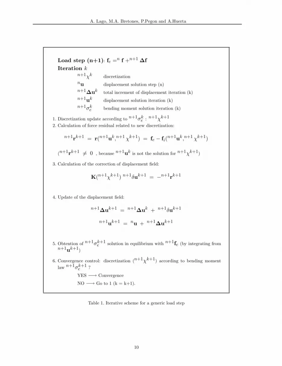
Load step (n+1): fe =n f +n+1 ∆fIteration k

n+1χk discretizationnu displacement solution step (n)n+1∆uk total increment of displacement iteration (k)n+1uk displacement solution iteration (k)n+1σk

e bending moment solution iteration (k)

1. Discretization update according to n+1σke : n+1χk+1

2. Calculation of force residual related to new discretization:

n+1rk+1 = r(n+1uk,n+1 χk+1) = fe − fi(n+1uk,n+1 χk+1)

(n+1rk+1 6= 0 , because n+1uk is not the solution for n+1χk+1)

3. Calculation of the correction of displacement field:

K(n+1χk+1) n+1δuk+1 = −n+1rk+1

4. Update of the displacement field:

n+1∆uk+1 = n+1∆uk + n+1δuk+1

n+1uk+1 = nu + n+1∆uk+1

5. Obtention of n+1σk+1e solution in equilibrium with n+1fe (by integrating from

n+1uk+1)

6. Convergence control: discretization (n+1χk+1) according to bending momentlaw n+1σk+1

e ?

YES −→ Convergence

NO −→ Go to 1 (k = k+1).

Table 1. Iterative scheme for a generic load step

10


5 EXAMPLES

5.1. Example FRAME I

In this example the portal frame shown in Figure 5 is studied. We adopt the elastic-plastic model. The characteristics of the model and the point load are shown in Figure5. We consider a constant step load of value of ∆fe = (1./16.) fp = 5.0 · 10−8 T wherefp is the plastification load for the structure.

An antisimetric load has been choosen in order to reduce all the study of the behaviourto one of the piles.

P

ε

σ

De = 3.0 · 10−3 T · m2 Dp = 1.0 · 10−4 T · m2

σp = 1.0 · 10−6 T · ml = 1 m

Figure 5. Example FRAME I.

Figures 6 and 7 show the behaviour of the solution obtained with the adaptativemesh compared with a reference solution obtained with a fixed mesh of 1000 elementper beam. Figure 6 shows the load-displacement law (displacement of the point of loadaplication has been taken as reference). Figure 7 shows the evolution of the plastificationpoints on the pile. The solution obtained with the adaptative mesh is practically equalto the reference solution (maximum relative error in displacement ' 1 · 10−4) althoughonly a total of 9 finite elements have been employed. As shown in Figure 7, this accuracyis possible because the adaptative mesh is able to perfectly capture the plastificationpoints.

11


DISPLACEMENT(m)

LOAD (T)

0.00 0.20 0.40 0.60 0.80 1.00 1.20 1.40 1.60

X1.E-3

0.00

1.00

2.00

3.00

4.00

5.00

6.00

7.00

8.00

9.00

X1.E-6

[] REFERENCE SOLUTIONX ADAPTIVE SOLUTION

Figure 6. Example FRAME I. Adaptive solution vs. Reference solution. Load- displacement law

LOAD (T)

LENGTH (m)

0.00 1.00 2.00 3.00 4.00 5.00 6.00 7.00 8.00 9.00

X1.E-6

0.00

0.20

0.40

0.60

0.80

1.00


Figure 7. Example FRAME I. Adaptive solution vs. Reference solution. Evolution ofthe plastic nodes on the right pilar

12


Figure 8 shows the discretization on three different load steps. On the left, thediscretization (grey = elastic elements, red = plastic elements). On the right, thebending moment law evolution (black = former step law, green = previous steps laws)

Displacement

Force

0.00 0.20 0.40 0.60 0.80 1.00 1.20 1.40 1.60

X1.E-3

0.00

1.00

2.00

3.00

4.00

5.00

6.00

7.00

8.00

9.00

X1.E-6

ABS

SCAL

0.

00

0.10

0.

20

0.30

0.

40

0.50

0.

60

0.70

0.

80

0.90

1.

00

-2.

00

-1.

60

-1.

20

-0.

80

-0.

40

0.

00

0.

40

0.

80

1.

20

1.

60

2.

00

X1.E

-6

P1PE

STAB

S

SCAL

0.

00

0.10

0.

20

0.30

0.

40

0.50

0.

60

0.70

0.

80

0.90

1.

00

-2.

00

-1.

60

-1.

20

-0.

80

-0.

40

0.

00

0.

40

0.

80

1.

20

1.

60

2.

00

X1.E

-6

P1PE

STP1

PEST

ABS

SCAL

0.

00

0.10

0.

20

0.30

0.

40

0.50

0.

60

0.70

0.

80

0.90

1.

00

-2.

00

-1.

60

-1.

20

-0.

80

-0.

40

0.

00

0.

40

0.

80

1.

20

1.

60

2.

00

X1.E

-6

P1PE

STP1

PEST

P1PE

ST

Figure 8. Example FRAME I. Adaptative discretization: (a) elastic zone (b) and (c)plastification

(a)

(b)

(c)

(a)

(b)(c)

13


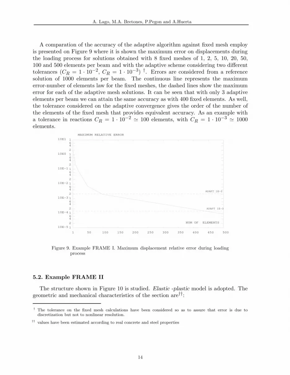
A comparation of the accuracy of the adaptive algorithm against fixed mesh employis presented on Figure 9 where it is shown the maximum error on displacements duringthe loading process for solutions obtained with 8 fixed meshes of 1, 2, 5, 10, 20, 50,100 and 500 elements per beam and with the adaptive scheme considering two differenttolerances (CR = 1 · 10−2, CR = 1 · 10−3) †. Errors are considered from a referencesolution of 1000 elements per beam. The continuous line represents the maximumerror-number of elements law for the fixed meshes, the dashed lines show the maximumerror for each of the adaptive mesh solutions. It can be seen that with only 3 adaptiveelements per beam we can attain the same accuracy as with 400 fixed elements. As well,the tolerance considered on the adaptive convergence gives the order of the number ofthe elements of the fixed mesh that provides equivalent accuracy. As an example witha tolerance in reactions CR = 1 · 10−2 ' 100 elements, with CR = 1 · 10−3 ' 1000elements.

NUM OF ELEMENTS

MAXIMUM RELATIVE ERROR

1 50 100 150 200 250 300 350 400 450 500

10E-5

10E-4

10E-3

10E-2

10E-1

10E0

10E1

1

1

1

1

1

1

1

2

2

2

2

2

2

4

4

4

4

4

4

6

6

6

6

6

6

ADAPT 1E-2

ADAPT 1E-3

Figure 9. Example FRAME I. Maximum displacement relative error during loadingprocess

5.2. Example FRAME II

The structure shown in Figure 10 is studied. Elastic -plastic model is adopted. Thegeometric and mechanical characteristics of the section are††:

† The tolerance on the fixed mesh calculations have been considered so as to assure that error is due todiscretization but not to nonlinear resolution.

†† values have been estimated according to real concrete and steel properties

14


Area A = 0.9 m2

Inerce I = 6.75 · 10−4 m4

Ee ' 3.0 · 10−6 T/m2

Ep = (1./30.)Ee ' 1.0 · 10−5 T/m2

σc = 6.4 T · m(De and Dp can be obtained by multiplying Ee and Ep by I)

Two different kinds of actions are considered: standard vertical loads (self weightand permanent loads) and magnified horizontal loads (the reason for this magnificationis to analyze the behaviour of the structure faced to an advanced plastification).

5,50 T

7,00 T

1,35 T 5,40 T 9,00 T 4,50 T

5,40 T 4,50 T9,00 T1,35 T

4 m

4 m

3,5 m 4 m 5 m

0,40 m

0,40 m

4 φ20

Figure 10. Example FRAME II. Structure definition

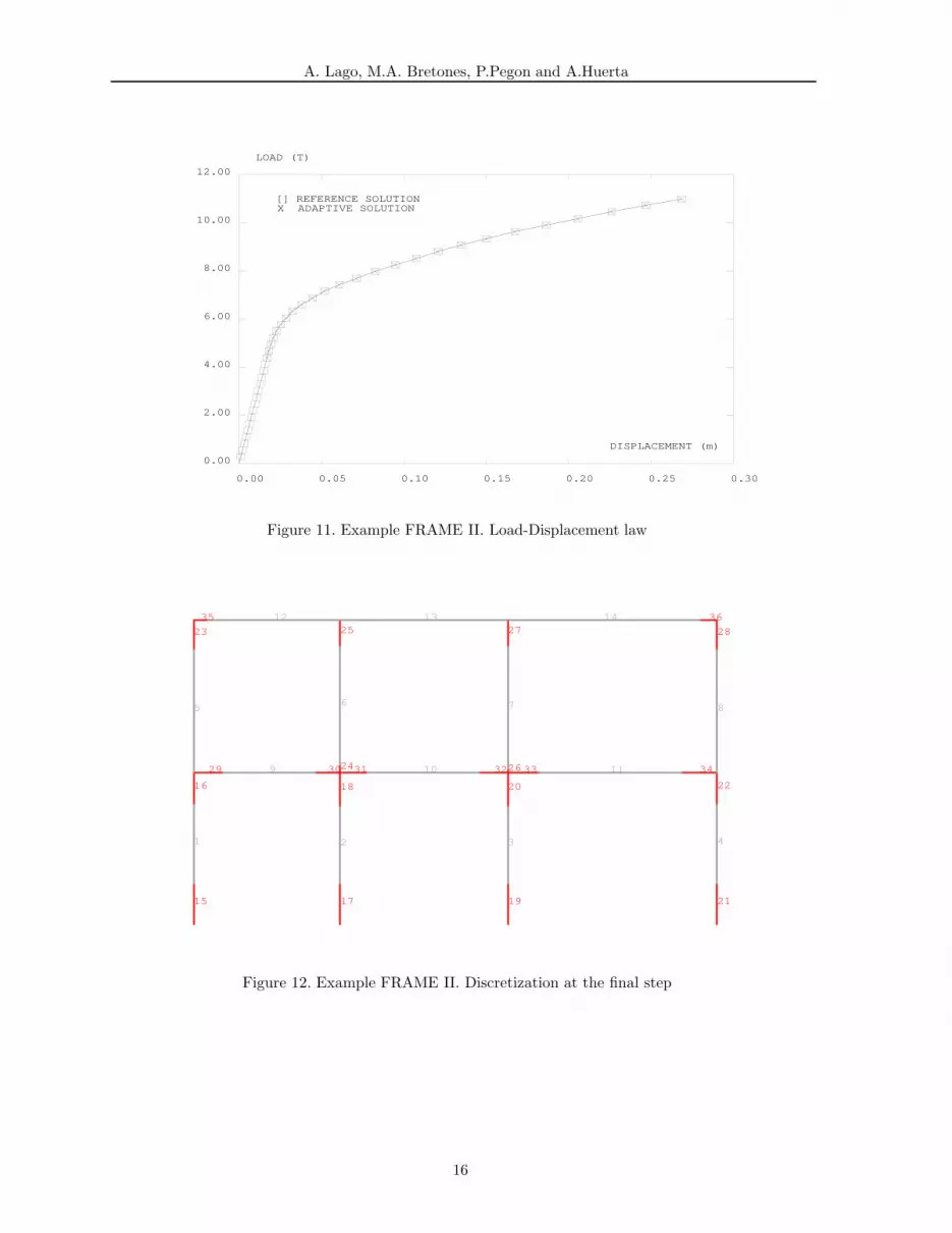
The results are shown on Figures 11 and 12. Figure 11 shows the load-displacementlaw on the up-left joint of the estructure. The adaptive solution is compared with areference solution obtained with a fixed mesh of 1000 elements per beam. Elastic stepson adaptive mesh are not shown. Once more, it can be seen that the adaptive meshcaptures correctly the solution.

Figure 12 shows the adaptive discretization on the last load step. This realistic andmore complex example evidences the real advantage of the new algorithm. With anincreasing number of beams, the reduction on the number of finite elements with theadaptive mesh is substantial. Only 36 elements have been necessary to attain the sameaccuracy as that of a 1400 element fixed mesh. This implies an outstanding reductionof the computational cost.

15


DISPLACEMENT (m)

LOAD (T)

0.00 0.05 0.10 0.15 0.20 0.25 0.30

0.00

2.00

4.00

6.00

8.00

10.00

12.00


Figure 11. Example FRAME II. Load-Displacement law

1 2 3 4

5 6 7 8

9 10 11

12 13 14

15

16

17

18

19

20

21

22

23

24

25

26

27 28

29 30 31 32 33 34

35 36

Figure 12. Example FRAME II. Discretization at the final step

16


5.3. Example FRAME III

This example consists of the same frame of the example FRAME I, but adoptingnow the elastic-cracked-plastic model. The characteristics of the model and the pointload applied are shown in Figure 13.

P

ε

σ

De = 3.0 · 10−3 T · m2 Dc = 1.2 · 10−3 T · m2 Dp = 1.0 · 10−4 T · m2

σc = 0.9 · 10−6 T · m σp = 1.0 · 10−6 T · ml = 1 m

Figure 13. Example FRAME III.

Figure 14 shows the load-displacement law obtained with the adaptive mesh.In that case, because of the employ of the elastic-cracked-plastic model, some

convergence problems have been detected depending on the mechanical valuesconsidered. Figure 15 shows the convergence analysis in the load step when crackinginitially appears. The analysis have been made with different De − Dc relationships.A loss of convergence can be detected as long as the difference between the stiffnessincreases (De is fixed and Dc decreases) and there is a critical difference whereconvergence is no longer possible. This is exclusively a constitutive model problemintroduced by the discontinuity of curvatures between elastic and cracked domains.This patological behaviour on convergence is still more evident in iteratives schemes offixed mesh where no solutions have been obtained for the mechanical values considered.

17


DISPLACEMENT (m)

LOAD (T)

0.00 1.00 2.00 3.00 4.00 5.00 6.00 7.00 8.00

X1.E-4

0.00

1.00

2.00

3.00

4.00

5.00

6.00

7.00

X1.E-6

Figure 14. Example FRAME III. Load-Displacement law for adaptive solution

ITERATION

REACTIONS CRITERIA

0 2 4 6 8 10 12 14 16

10E-6

10E-5

10E-4

10E-3

10E-2

10E-1

1

1

1

1

1

1

2

2

2

2

2

4

4

4

4

4

6

6

6

6

6

Dc=2.0E-3

Dc=1.5E-3

Dc=1.2E-3

Dc=1.0E-3

Dc=0.9E-3

TOLERANCE

Figure 15. Example FRAME III. Convergence analysis in the beginning of cracking.Convergence dependence on constitutive law

18


5.3. Example UNLOADING

We consider again the frame of the example FRAME I. We adopt the elastic-plasticbut with the posibility of unloading. We have applied to the structure a loading processsimilar to that of the previous example but including two cycles of unloading andreloading. In this case, non-uniform load steps are considered.

Figure 16 shows the comparison between the load-displacement law obtained withthe adaptive mesh and with a reference solution with fixed mesh (100 elements perbeam). The steps considered in the adaptive calculations have been joined with a linethat defines the load advance. In this example, all the plastic parts of the structurechange into unloading parts at once. That is why unloading takes always place along abranch parallel to the elastic one in load-displacement law.

DISPLACEMENT (m)

LOAD (T)

0.00 0.20 0.40 0.60 0.80 1.00 1.20 1.40 1.60

X1.E-3

0.00

1.00

2.00

3.00

4.00

5.00

6.00

7.00

8.00

9.00

X1.E-6


Figure 16. Example UNLOADING. Load-displacement law. Adaptive solution vs.Fixed mesh solution

6 CONCLUSIONS

We have developed an adaptive technique computationally effective to solve framedstructures of reinforced concrete with piecewise linear constitutive models. Thetechnique employs a minimum number of finite elements and iterates with an orderof convergence greater than linear. Therefore, it gives an outstanding reduction on thecomputational cost of solving the problem without losing accuracy.

This new scheme takes profit of some properties of the solution which can be inferreda priori when using piecewise linear models. It employs a variable discretization in

19


which we associate each element to each of the domains in which the structure canbe divided according to its mechanical behaviour. Both the possition of the nodesand the mechanical model associated to each element are redefined in each iteration inaccordance with the bending moment law.

The effectivity of the technique has been shown in different examples. Exampleswith loading and unloading processes show that accuracy can be drastically improvedcompared with fixed meshes with more than 100 times more elements. Importantreductions of CPU time are also achieved. Moreover, these advantages increase withthe complexity of the problem.

REFERENCES

[1] Crisfield, M.A. (1991), Non-linear Finite Element Analysis of Solids and Structures,John Wiley and Sons Ltd., England.

[2] Leon, J., Corres, H. “Efecto de la discretizacion en la representacion delcomportamiento no lineal de porticos de hormigon armado” , Aplicaciones del metodode los elementos finitos en ingenierıa Vol. 7 149 -158 (1986), Ediciones UPC,Barcelona

[3] Toi, Y. (1990) “Shifted integration technique in one-dimensional plastic collapseanalysis using linear and cubic finite elements”, International Journal for NumericalMethods in Engineering, Vol. 31, 1537-1552.

[4] Toi, Y. and Isobe, D. (1994) “Finite element analysis of quasi-static and dynamiccollapse behaviors of framed structures by the adaptively shifted integrationtechnique”, Computers & Structures Vol. 58, 947-955

[5] Timoshenko, S. and Young, D.H. (1962) Elements of strengh of materials, 4th ed.,D. Vaan Nostrand Company, Toronto.

[6] CEB-FIB, (1990) CEB-FIB Model code 1990 Comite Euro-International du Beton,Thomas Telford Ltd., England

[7] Saiidi, M., (1982) “Hysteresis model for reinforced concrete”, Journal of theStructural Division, ASCE ST5

20

Documents

Adaptive Finite Elements For Reinforced Concrete Framed Structures