An active filter design program (theory and application)

Rochester Institute of Technology Rochester Institute of Technology

RIT Scholar Works RIT Scholar Works

Theses

11-1-1982

An active filter design program (theory and application) An active filter design program (theory and application)

Louis Gabello

Follow this and additional works at: https://scholarworks.rit.edu/theses

Recommended Citation Recommended Citation Gabello, Louis, "An active filter design program (theory and application)" (1982). Thesis. Rochester Institute of Technology. Accessed from

This Thesis is brought to you for free and open access by RIT Scholar Works. It has been accepted for inclusion in Theses by an authorized administrator of RIT Scholar Works. For more information, please contact [email protected].

https://scholarworks.rit.edu/

https://scholarworks.rit.edu/theses

https://scholarworks.rit.edu/theses?utm_source=scholarworks.rit.edu%2Ftheses%2F5630&utm_medium=PDF&utm_campaign=PDFCoverPages

https://scholarworks.rit.edu/theses/5630?utm_source=scholarworks.rit.edu%2Ftheses%2F5630&utm_medium=PDF&utm_campaign=PDFCoverPages

mailto:[email protected]

Approved by:

AN ACTIVE FILTER DESIGN PROGP A \1 (theory and application)

by

Louis R. Gabello

A Thesis Submitted

in

Partial Fulfillment

of the

Requirements for the Degree of

MASTER OF SCIENCE

in

Electrical Engineering

Prof. Edward Salem --~~~~~~~------------(Thesis Advisor)

Prof. Fung Tseng ----------------------------

Name Illegible Prof. Harvey E. Rhody

--~--~----~~~----------(Department Head)

DEPARTMENT OF ELECTRICAL ENGINEERING

COLLEGE OF ENGINEERING

ROCHESTER INSTITUTE OF TECHNOLOGY

ROCHESTER, NEW YORK

NOVEMBER, 1982

I,

AN ACTIVE FILTER DESIGN PROGRAM (theory and application)

Louis R. Gabello , hereby grant permission to

Wallace Memorial Library, of R.I.T., to reproduce my thesis in whole

or part. Any reproduction will not be for commercial use or profit.

iv

ACKNOWLEDGEMENTS

I wish to thank all those who supported the development of this

thesis. My advisor, Dr. Edward Salem, showed much patience and wisdom

in guiding me through the entire thesis development. I also thank him

for providing my first exposure to this field. His enthusiasm and

knowledge provided the catalyst for my interest in filter design. I

thank Elizabeth Russo who typed the first manuscript of the thesis. My

deepest appreciation to Dorothy Haggerty who expertly typed the entire

final thesis text. Her relentless efforts and valuable comments were an

impetus for the completion of the thesis. To all of my family especial

ly my wife Marcy and our children, I dedicate this thesis. Their value

of education and loving support were the foundation of this effort.

Most importantly, I thank the one person who made this all possible, our

maker.

ABSTRACT

AN ACTIVE FILTER DESIGN PROGRAM

(theory and application)

Author: Louis R. Gabello

Advisor: Dr. Edward R. Salem

This thesis deals with the design of filters in the frequency do

main. The intention of the thesis is to present an overview of the con

cepts of filter design along with two significant developments: a com

prehensive filter design computer program and the theoretical develop

ment of an Nth order elliptic filter design procedure.

The overview is presented in a fashion which accents the filter

design process. The topics discussed include defining the attenuation

requirements, normalization, determining the poles and zeros,denor-

malization and implementation. For each of these topics the text ad

dresses the fundamental filter types (low pass through band stop) .

Within the topic of determining the poles and zeros, three classical

approximations are discussed: the Butterworth, Chebyshev and elliptic

function. The overview is concluded by illustrating selected methods of

implementing the basic filter types using infinite gain multiple feed

back (IGMF) active filters.

The second major portion of the thesis discusses the structure, use

and results of a computer program called FILTER. The program is very

extensive and encompasses all the design processes developed within the

thesis. The user of the program experiences an interactive session

where the design of the filter is guided from parameter entries through

the response evaluation and finally the determination of component

11

values for each stage of the active filter. Complete examples are

given.

Included within the program is an algorithm for determining the

transfer function of an Nth order elliptic function filter. The devel

opment of the theory and the resulting design procedure are presented in

the appendices. The elliptic theory and procedure represent an impor

tant result of the thesis effort. The significance of this development

stems from the fact that methods of elliptic filter design have pre

viously been too disseminated in the literature or inconclusive for an

Nth order design approach. Included in this development is a rapidly

converging method of determining the precise value of the elliptic sine

function. This function is an essential part of the elliptic design

process.

111

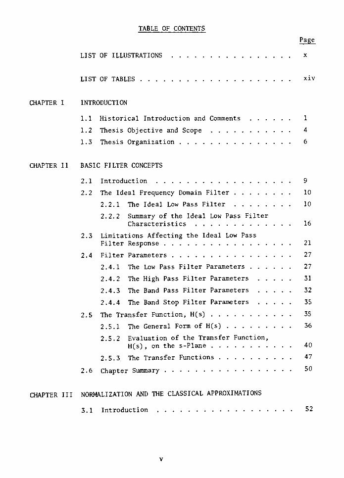
TABLE OF CONTENTS

Page

LIST OF ILLUSTRATIONS x

LIST OF TABLES xiv

CHAPTER I INTRODUCTION

1.1 Historical Introduction and Comments 1

1.2 Thesis Objective and Scope 4

1.3 Thesis Organization 6

CHAPTER II BASIC FILTER CONCEPTS

2.1 Introduction 9

2.2 The Ideal Frequency Domain Filter 10

2.2.1 The Ideal Low Pass Filter 10

2.2.2 Summary of the Ideal Low Pass Filter

Characteristics 16

2.3 Limitations Affecting the Ideal Low Pass

Filter Response 21

2.4 Filter Parameters 27

2.4.1 The Low Pass Filter Parameters 27

2.4.2 The High Pass Filter Parameters 31

2.4.3 The Band Pass Filter Parameters 32

2.4.4 The Band Stop Filter Parameters 35

2.5 The Transfer Function, H(s) 35

2.5.1 The General Form of H(s) 36

2.5.2 Evaluation of the Transfer Function,

H(s) , on the s-Plane 40

2.5.3. The Transfer Functions 47

2.6 Chapter Summary50

CHAPTER III NORMALIZATION AND THE CLASSICAL APPROXIMATIONS

3.1 Introduction 52

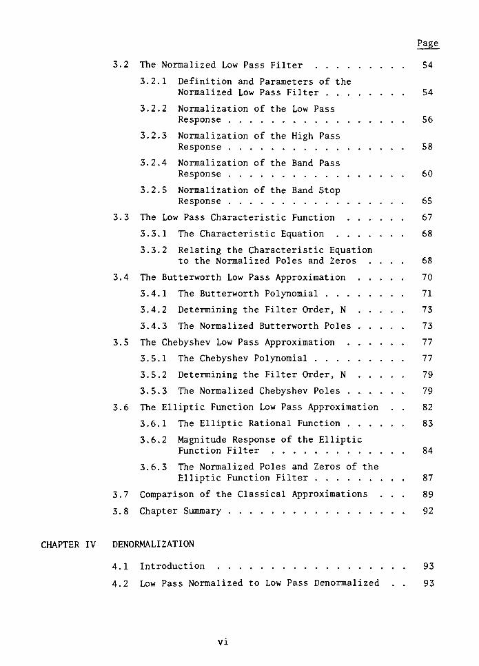
Page

3.2 The Normalized Low Pass Filter 54

3.2.1 Definition and Parameters of the

Normalized Low Pass Filter 54

3.2.2 Normalization of the Low Pass

Response 56

3.2.3 Normalization of the High Pass

Response 58

3.2.4 Normalization of the Band Pass

Response 60

3.2.5 Normalization of the Band StopResponse 65

3.3 The Low Pass Characteristic Function 67

3.3.1 The Characteristic Equation 68

3.3.2 Relating the Characteristic Equation

to the Normalized Poles and Zeros .... 68

3.4 The Butterworth Low Pass Approximation 70

3.4.1 The Butterworth Polynomial 71

3.4.2 Determining the Filter Order, N 73

3.4.3 The Normalized Butterworth Poles 73

3.5 The Chebyshev Low Pass Approximation 77

3.5.1 The Chebyshev Polynomial 77

3.5.2 Determining the Filter Order, N 79

3.5.3 The Normalized Chebyshev Poles 79

3.6 The Elliptic Function Low Pass Approximation . . 82

3.6.1 The Elliptic Rational Function 83

3.6.2 Magnitude Response of the Elliptic

Function Filter 84

3.6.3 The Normalized Poles and Zeros of the

Elliptic Function Filter 87

3.7 Comparison of the Classical Approximations ... 89

3.8 Chapter Summary 92

CHAPTER IV DENORMALIZATION

4.1 Introduction 93

4.2 Low Pass Normalized to Low Pass Denormalized . . 93

VI

Page

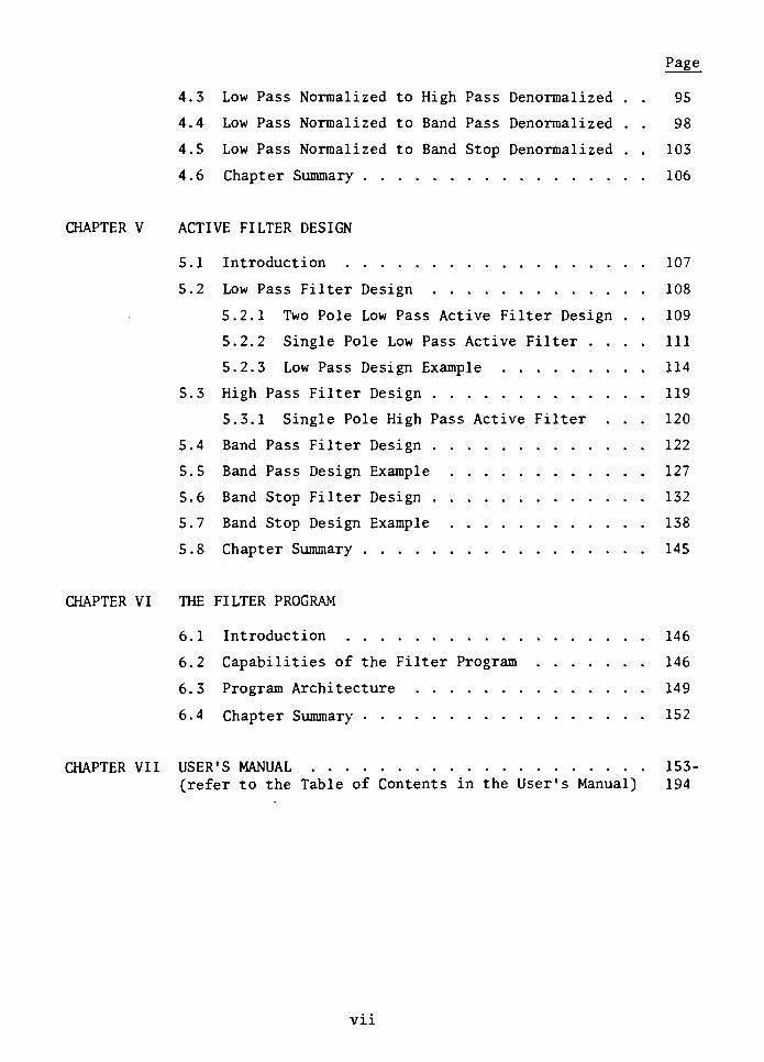
4.3 Low Pass Normalized to High Pass Denormalized . . 95

4.4 Low Pass Normalized to Band Pass Denormalized . . 98

4.5 Low Pass Normalized to Band Stop Denormalized . . 103


CHAPTER V ACTIVE FILTER DESIGN

5.1 Introduction 107

5.2 Low Pass Filter Design 108

5.2.1 Two Pole Low Pass Active Filter Design . . 109

5.2.2 Single Pole Low Pass Active Filter .... Ill

5.2.3 Low Pass Design Example 114

5.3 High Pass Filter Design 119

5.3.1 Single Pole High Pass Active Filter . . . 120

5.4 Band Pass Filter Design 122

5.5 Band Pass Design Example 127

5.6 Band Stop Filter Design 132

5.7 Band Stop Design Example 138


CHAPTER VI THE FILTER PROGRAM

6.1 Introduction 146

6.2 Capabilities of the Filter Program 146

6.3 Program Architecture 149


CHAPTER VII USER'S MANUAL 153-

(refer to the Table of Contents in the User's Manual) 194

vn

Page

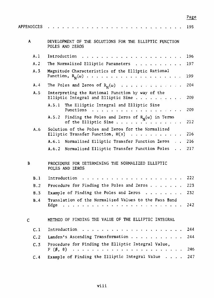
APPENDICES 195

A DEVELOPMENT OF THE SOLUTIONS FOR THE ELLIPTIC FUNCTION

POLES AND ZEROS

A.l Introduction 196

A. 2 The Normalized Elliptic Parameters 197

A. 3 Magnitude Characteristics of the Elliptic Rational

Function, Rjîo) 199

A. 4 The Poles and Zeros of RN(to) 204

A. 5 Interpreting the Rational Function by way of the

Elliptic Integral and Elliptic Sine 209

A. 5.1 The Elliptic Integral and Elliptic Sine

Functions 209

A. 5. 2 Finding the Poles and Zeros of K,(u) in Terms

of the Elliptic Sine 212

A. 6 Solution of the Poles and Zeros for the Normalized

Elliptic Transfer Function, H(s) 216

A. 6.1 Normalized Elliptic Transfer Function Zeros . . 216

A. 6. 2 Normalized Elliptic Transfer Function Poles . . 217

PROCEDURE FOR DETERMINING THE NORMALIZED ELLIPTIC

POLES AND ZEROS

B.l Introduction 222

B.2 Procedure for Finding the Poles and Zeros 223

B.3 Example of Finding the Poles and Zeros 232

B.4 Translation of the Normalized Values to the Pass Band

Edge 242

METHOD OF FINDING THE VALUE OF THE ELLIPTIC INTEGRAL

C.l Introduction 244

C.2 Landen's Ascending Transformation 244

C.3 Procedure for Finding the Elliptic Integral Value,

F (0, 9) 246

C.4 Example of Finding the Elliptic Integral Value .... 247

Vlll

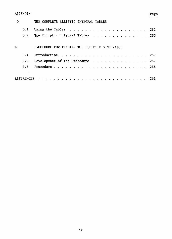
APPENDIX Page

D THE COMPLETE ELLIPTIC INTEGRAL TABLES

D.l Using the Tables 251

D.2 The Elliptic Integral Tables 253

E PROCEDURE FOR FINDING THE ELLIPTIC SINE VALUE

E.l Introduction 257

E.2 Development of the Procedure 257

E.3 Procedure 258

REFERENCES 261

IX

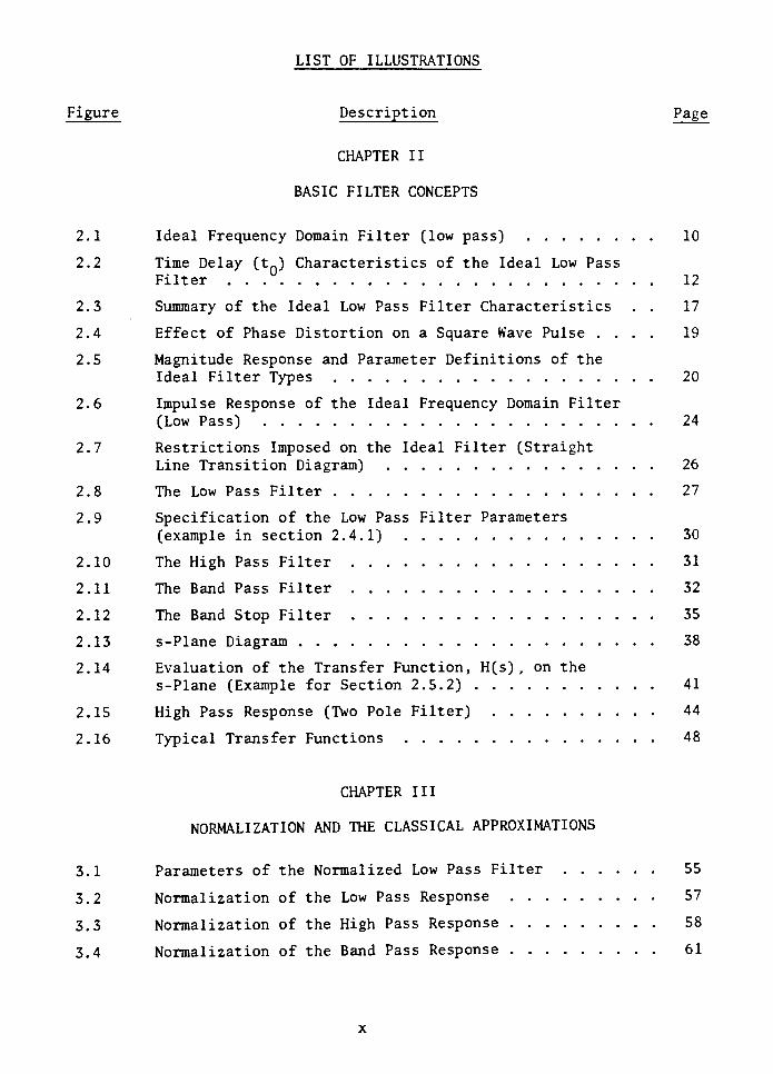
LIST OF ILLUSTRATIONS

Figure Description Page

CHAPTER II

BASIC FILTER CONCEPTS

2.1 Ideal Frequency Domain Filter (low pass) 10

2.2 Time Delay (t) Characteristics of the Ideal Low Pass

Filter . . 12

2.3 Summary of the Ideal Low Pass Filter Characteristics . . 17

2.4 Effect of Phase Distortion on a Square Wave Pulse .... 19

2.5 Magnitude Response and Parameter Definitions of the

Ideal Filter Types 20

2.6 Impulse Response of the Ideal Frequency Domain Filter

(Low Pass) 24

2.7 Restrictions Imposed on the Ideal Filter (Straight

Line Transition Diagram) 26

2.8 The Low Pass Filter 27

2.9 Specification of the Low Pass Filter Parameters

(example in section 2.4.1) 30

2.10 The High Pass Filter 31

2.11 The Band Pass Filter 32

2.12 The Band Stop Filter 35

2.13 s-Plane Diagram 38

2.14 Evaluation of the Transfer Function, H(s) ,on the

s-Plane (Example for Section 2.5.2) 41

2.15 High Pass Response (Two Pole Filter) 44

2.16 Typical Transfer Functions 48

CHAPTER III

NORMALIZATION AND THE CLASSICAL APPROXIMATIONS

3.1 Parameters of the Normalized Low Pass Filter 55

3.2 Normalization of the Low Pass Response 57

3.3 Normalization of the High Pass Response 58

3.4 Normalization of the Band Pass Response 61


3.5 Example of the Band Pass Normalization 64

3.6 Normalization of the Band Stop Response 66

3.7 Normalized Butterworth Magnitude Response 72

3.8 Butterworth Low Pass Example 74

3.9 Normalized Butterworth Poles for N = 2 76

3.10 Normalized Chebyshev Magnitude Response 78

3.11 Requirements for a Chebyshev Low Pass Filter (example) . 80

3.12 Normalized Chebyshev Poles for N = 3 82

3.13 Magnitude Response of the Normalized Low Pass Elliptic

Filter 85

3.14 Normalized Pole/Zero Pattern for the Elliptic Function

Filter 88

3.15 Comparison of the Normalized Butterworth, Chebyshev and

Elliptic Responses 91

CHAPTER IV

DENORMALIZATION

4.1 Transformation of the Low Pass Normalized to the Low

Pass Denormalized s-Plane 95

4.2 Transformation of the Low Pass Normalized to the High


4.3 Transformation of the Low Pass Normalized to the Band


4.4 Transformation of the Low Pass Normalized to the Band

Stop Denormalized s-Plane 105

CHAPTER V

ACTIVE FILTER DESIGN

5.1 Basic Filter Design Steps 108

5.2 Low Pass IGMF Active Filter (two-pole) 110

5.3 Low Pass Active Filter (single pole) 112

5.4 Low Pass Filter Design Summary 113

5.5 Low Pass Filter Requirements (example) 114

XI


5.6 Normalized Low Pass Filter (derived from figure 5.5) . . 115

5.7 Low Pass Butterworth IGMF Active Filter (N = 3,cutoff frequency = 20 Hz) 118

5.8 High Pass IGMF Active Filter (two-pole) . . [ 120

5.9 High Pass Active Filter (single pole) 121

5.10 High Pass Filter Design Summary 123

5.11 Band Pass IGMF Active Filter (two-pole) 125

5.12 Band Pass Filter Design Summary 126

5.13 Band Pass Filter Requirements (example) 127

5.14 Normalized Low Pass Filter 128

5.15 Butterworth Band Pass IGMF Active Filter

(f = 455 KHz, B = 10 KHz, N = 2) 132

5.16 Band Stop IGMF Active Filter (two-pole) 134

5.17 Butterworth Band Stop Filter Requirements (example) . . . 138

5.18 Normalized Low Pass Filter (derived from figure 5.17) . . 139

5.19 Butterworth IGMF Band Stop Filter (two-pole example) . . 143

5.20 Band Stop Filter Design Summary 144

CHAPTER VI

THE FILTER PROGRAM

6.1 Program Filter Architecture 150

CHAPTER VII

(refer to the List of Illustrations in the

User's Manual) 159

APPENDIX A

DEVELOPMENT OF THE SOLUTIONS FOR THE

ELLIPTIC FUNCTION POLES AND ZEROS

A.l Denormalized Elliptic Filter Response 197

A. 2 Normalized Elliptic Insertion Loss Parameters 199

XII


A. 3 Prescribed Characteristics of the Normalized Elliptic

Function, K,M 202

A. 4 Characteristics of the Normalized Elliptic Rational

Function 205

A. 5 Integrand Function of the Elliptic Integral 210

A. 6 Elliptic Integral Values (Real) as a Function of the

Amplitude, 0 211

A. 7 The Pass Band of the Elliptic Filter Transformed bythe Elliptic Integral (N = odd = 5) 213

A. 8 The Pass Band of the Elliptic Filter Transformed bythe Elliptic Integral (N = even = 6) 215

APPENDIX B

PROCEDURE FOR DETERMINING THE

NORMALIZED ELLIPTIC POLES AND ZEROS

B.l Normalized Low Pass Filter Parameters (parameter

basis for an elliptic filter design) 222

B.2 Elliptic Low Pass Filter Requirements 232

B.3 Normalized Low Pass Elliptic Filter (example) 233

B.4a Normalized Low Pass Elliptic Filter (N = 6) 241

B.4b Normalized Poles/Zeros for the Low Pass Elliptic

Filter (N = 6) 241

B.5 Normalization with respect to the Center Frequency vs.

the Cutoff Frequency 242

xm

LIST OF TABLES

Table No. Description Page

2.1 Parameter Definitions of the Magnitude Response

(Low Pass and High Pass) 29

2.2 Parameter Definitions of the Magnitude Response

(Band Pass and Band Stop) 34

B.l Elliptic Design Summary Work Sheet 229

B.2 Elliptic Design Summary Work Sheet (Example) 238

D.l Elliptic Integral Tables 254

D.2 Complete Elliptic Integral Table(85

< 6 < 90) ... 256

xiv

CHAPTER I

INTRODUCTION

1.1 Historical Introduction and Comments

The science of signal filtering has evolved from its infancy 66

years ago to a present day design technology. Inherent in this growth

has been the determination of network theorists to develop new filter

concepts and design procedures. A multitude of information sources and

computer programs have evolved to such purpose. For some engineers this

represents a variety of solutions while to others an informational di

lemma. Even with all this, there are still areas in filter design which

remain undeveloped. Let us briefly examine the historical background of

network and filter design synthesis and then examine the needs which

exist in this field today.

The concept of an electric filter was initially proposed in 1915 by

K. Wagner of Germany and G. Campbell of the United States. The concepts

were a result of their initial work, performed independently, which re

lated to loaded transmission lines and classical theories of vibrating

systems. The first practical method of filter design became available

when, in 1923, 0. Zobel proposed a synthesis method using multiple

reactances [l]. This method was used until the 1950's when W. Cauer and

S. Darlington published new network synthesis concepts related to the

use of rational functions (in particular the Chebyshev rational func

tion) [2]. Later, their concepts were recognized as the foundation for

modern day filter design. In the 1960's, network synthesis concepts

and procedures expanded and were proliferated by the classic texts

written by M. Van Valkenberg [3], L. Weinberg [4], A. Zverev [5] and

many others.

These network synthesis concepts, which resulted in filter design

techniques, became practical with the advent of the digital computer.

Prior to this, complex mathematics related to solving the insertion loss

characteristics of some filters were tedious and not exact. Such was

the case for solutions to the Chebyshev rational function as described

by Darlington and Cauer [2]. With the computer, these solutions were no

longer a barrier to filter design. As a result, tables and graphs became

available to the engineer for implementing these complex filter designs

[6], [7], Many filter forms and classes have since evolved from these

original ideas. Examples of these filters are the Butterworth, Bessel,

Chebyshev, image parameter, helical, crystal, etc.

Today, the electric filter manifests itself not only in electrical

and electronic fields but in most of the scientific community. For the

layman, the devices that have resulted from the remarkable developments

in network synthesis are literally packed into many consumer products as

special features (consider the controls on stereo players and recorders

as an example). Yet the development of filter concepts and their appli

cations do not end here.

New technologies are rapidly developing which combine the computa

tional power of the 16 bit and forthcoming 32 bit microprocessors with

filter synthesis concepts [8]. Image processing and voice analysis/

synthesis are some examples. These applications become increasingly

practical with advances in integrated circuits which implement complex

filter functions. (As an example, consider the FLT-U2 universal active

filter chip produced by Datel Intersil). Indeed, filter design principles

have set today's standard in technology. Their concepts and devices are

used as research tools by many fields in the scientific community. The

concepts of network synthesis are therefore essential as a basic tool

for the engineer. There remains however a realistic problem between

filter concepts and filter design.

Not all engineers are conversant with the different types, termi

nology and techniques of filter design. Certainly, the basic ideas

used, such as those derived from the theory of linear systems (Fourier,

Laplace transforms, etc.), have been presented to engineers. However ;

the everyday involvement of engineering responsibilities does not always

afford the opportunity to develop and make direct use of network syn

thesis and filter design concepts. This suggests that something addi

tional, perhaps a computer program, is needed to assist these engineers.

Although design aids such as tables and graphs are available in a variety

of texts, the design methodology often remains buried in complex analy

ses. Those who are involved "with filter design realize that such types

as the elliptic function filters are not practical without a computer due

to the complexity and precision of the mathematics involved. In light of

these problems, computer programs have been written to aid the filter de

sign process [9], [10]. Many of these programs are useful but very

limited. Most consider only a particular form or type of filter such as

the low pass Butterworth or Chebyshev approximations. There are other

filter types remaining such as the high pass, band pass and band stop

(reject). Still, other approximations exist for each of the above fil

ter types. Examples are the Bessel and elliptic function filters. A

person then realizes that there remains a need for a computer program

which combines the filter types and approximations used often by engi

neers. This program should assimilate all the facts, parameter variabili

ty, precision and design techniques into one source which could be drawn

upon as a practical tool. The days of research involved in evaluating

various filter types and their performance would then be minimized. Such

is the purpose of this thesis.

1.2 Thesis Objective and Scope

The objective of this thesis is to develop a computer program which

could be used by engineers as a practical design tool for electronic

active filter analysis and design in the frequency domain. The result of

this effort is a computer program called FILTER which assimilates into

one comprehensive algorithm the filter designs used often by engineers.

The program FILTER implements the low pass, high pass, band pass and band

stop magnitude responses using any of three classical approximations:

Butterworth, Chebyshev and elliptic (Cauer). The complex mathematics,

sorting of parameters and numerous iterations involved in these designs

are transparent to the user of the program. Instead, the user experiences

a simple interactive session which guides the design process from the

initial step of defining the parameters of the magnitude response to the

final step of component selection for an active filter circuit configura

tion.

To supplement this design program, this thesis text is provided.

The scope of the text is limited to the design concepts of filters in the

frequency domain. The thesis text begins with the basic definitions and

descriptions of filters; then it progresses through the theory of approxi-

4

mations and culminates with a design methodology for the basic filter

types. These design concepts are well established with the exception of

the elliptic function design procedure.

One of the major efforts in this thesis was the development of an

elliptic function design method. After analyzing the various sources of

literature, it was evident that the elliptic design procedures were quite

complex, incomplete and disseminated. Much remained between the theory

and a practical design procedure. Because the mathematics are complex,

involving elliptic integrals and elliptic trigonometric functions, a

computer program would be a necessity for implementing the elliptic fil

ter on a practical basis. Programs have been written for elliptic func

tion filters but again they are limited in scope, remain undocumented in

analysis and method or are just unavailable due to some propriety. A

clearly stated elliptic design procedure, even if complex, is presently

needed. This is especially true for active filter design. R. W. Daniels

has presented active filter concepts in his text[l0]. His text is a most

informative source on elliptic design since it includes both programs and

analyses pertaining to elliptic parameters. Yet a definitive procedure

with analytical support still remains somewhat nebulous for his solutions

to the elliptic integral and elliptic sine. These uncertainities have

been clarified and developed within this text.

An elliptic design method is presented in this thesis and is imple

mented by the FILTER program. The methods are based upon the elliptic

function theory presented by A. J. Grossman in his article "Synthesis of

Tchebycheff Parameter Symmetrical Filters" [ll] . Interestingly^ his

article describes the ideas presented by S. Darlington and then follows

through with the determination of the poles and zeros. This is one of

the most important steps in filter design. His discussion however was

limited to odd order functions and did not derive solutions to the

elliptic sine or integral. His interpretation, nonetheless, was clearly

presented. In this thesis, the concepts presented by Grossman are ex

panded to include the total design process of any order low pass through

band stop filters. The active filter implementation technique used is

based upon the concepts presented by R. W. Daniels[lO]. His concepts

were expanded here to include multiple iterations of reasonable component

values as a solution to implementing a larger range and optimization of

elliptic filters.

In summary, it is hoped that the program FILTER along with this

text, offer a practical design tool and reference for those filter types

most often used by engineers in small signal processing. In addition,

the development of the elliptic function design procedure will hopefully

promote its use.

The following is a discussion on the organization and purpose of

the chapters within the thesis text.

1.3 Thesis Organization

This text starts with the fundamental concepts of filters and

builds into a final design methodology. With this in mind, the contents

of the remaining text, 6 chapters in all, will now be discussed.

Chapter II provides an overview of the basic filter concepts which

are commonly drawn upon throughout the text. The terminology and graphi

cal representations of the four filter types are presented. These types

are the low pass, high pass, band pass and band stop. Initially these

6

types are discussed from an ideal point of view. Subsequently the

realistic forms and their terminology are presented. This leads to the

transfer function, H(s) , which conveniently describes the total filter

response (magnitude and phase) .

Chapter III introduces the concept of the normalized low pass fil

ter. The importance of the normalized low pass filter as the focal

point of the design process is established. In this normalization

process, methods are shown for converting each of the four filter types

into the normalized low pass form. The concept of the insertion loss

function is also presented. These concepts are then expanded to con

sider the Butterworth, Chebyshev and elliptic function approximations in

their normalized low pass form. Their magnitude and phase responses are

considered along with the pole/zero locations on the s-plane. Compari

sons are then made among these filter characteristics. As a result of

these discussions, the reader should develop an intuitive feeling for

the differences in the magnitude responses and their advantages or dis

advantages. In the design process, where the normalized low pass filter

is used, a person then realizes the choice among the three approximations

to meet his/her design specifications.

Chapter IV describes how the normalized low pass filter relates to

the other basic magnitude types such as high pass, band pass and band

stop filters. These relationships, described by two processes, normali

zation and transformation, are concisely and mathematically presented.

Having determined the poles and zeros, the process of denormalization is

presented as the step required to return from this normalized low pass

domain. The denormalized poles/zeros are the final pieces of information

needed to begin the hardware implementation. The theoretical development

of the design process is completed in this chapter. The steps of nor

malization, transformation, deriving the poles/zeros and denormalization

have all been developed and presented in chapters II-IV. What is needed

at this point is a section which pulls together all these concepts into

practical design methods.

Chapter V is a section on active filter design methodology. Here

the concepts of normalization through denormalization are applied for

each filter type (low pass through band stop) . These methods present the

total design process which starts by defining the desired filter response

parameters and culminates with an active filter circuit.

Chapter VI introduces the program FILTER. This program is a com

prehensive algorithm which implements all the concepts previously de

veloped. This chapter then describes how the program is structured to

handle the design variabilities and filter responses. A program map and

general flowchart aid this discussion.

Chapter VII is the user manual for the program FILTER. The specifi

cations, definitions of parameters and examples are given. The reader

should at least glance at this section and see the example program exe

cutions.

In the appendix, the development of the elliptic function design

method is presented with an example and theory of elliptic parameters.

This appendix is informative if a person desires an in-depth interpreta

tion of the elliptic parameters and how they relate to the design pro

cedure.

CHAPTER II

BASIC FILTER CONCEPTS

2.1 Introduction

This chapter provides an overview of the fundamental concepts which

are used to describe the characteristic responses of the basic filter

types. The basic filter types are the low pass, high pass, band pass

and band stop. This overview begins with a discussion of the magnitude

and phase characteristics of the ideal frequency domain filter. By

using the ideal form, the terms, definitions and analyses of the response

characteristics can be presented without great complexity. Following

this, a discussion is presented which explains how the magnitude shape

of the ideal frequency domain filter is altered due to practical limita

tions. This leads to the straight line transition diagram which repre

sents the non-ideal or realistic magnitude response of the filter.

These diagrams are presented for each of the four basic filter types

along with the symbols and definitions which are to be used commonly

throughout the text. The transfer function, H(s) , is then introduced as

a convenient mathematical representation of the realistic response of

the filter. The transfer function describes the magnitude response as

represented with the straight line transition diagram, as well as the

phase response. The general form of H(s) is presented. Then the par

ticular forms of the transfer functions and their representations on the

s-plane are presented for each of the four filter types.

By the end of this chapter, the reader should have an understanding

of the parameter definitions which describe the magnitude response of

the four filter types. In addition, the reader should be acquainted with

the representations of the filter types using the transfer function,

H(s).

2.2 The Ideal Frequency Domain Filter

In this section the four basic filter types (low pass, high pass,

band pass and band stop) are introduced in their ideal form. The pur

pose here is to review the magnitude shapes in the frequency domain and

introduce the terminology associated with these filters. Emphasis is

placed on examining the theory related to the low pass filter character

istics. The remaining filter types are simply presented without theo

retical involvement. This is because their ideal nature is similar to

the low pass and the same analytical thought process applies.

2.2.1 The Ideal Low Pass Filter

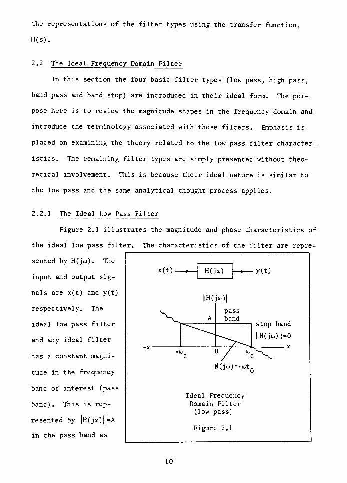
Figure 2.1 illustrates the magnitude and phase characteristics of

the ideal low pass filter. The characteristics of the filter are repre

sented by H(ju>) . The

input and output sig

nals are x(t) and y(t)

respectively. The

ideal low pass filter

and any ideal filter

has a constant magni

tude in the frequency

band of interest (pass

band) . This is rep

resented by |H(ju))|=A

in the pass band as

x(t) ^_ H(ju>) > y(t)

|H(jo))|

V A

pass

band

stop band

|H(juO|=0

-U) 0/0) ^-na /a \

0(jo))=-u)to

Ideal FrequencyDomain Filter

(low pass)

Figure 2.1

10

shown in figure 2.1. Outside of the pass band the magnitude is zero.

This region is defined as the stop band with |H(jo>)|=0 as shown in figure

2.1. The ideal filter also responds with a linear phase shift, 0(jo)),

throughout the pass band. Beyond the pass band the phase shift is of no

concern since, ideally, there is no output signal. Therefore, any phase

shift can exist. These ideal characteristics can be summarized for the

low pass filter as follows:

Magnitude =

|H(jo))| = A for -o> <oxo)

= 0 for (ul >o)a

Phase = 0(joi) =-o)tn for -o; <oxo>

J0 a a

=

any for |oi| >o)3.

where o) refers to the cutoff frequency. Let us examine the reason why

the phase shift, 0(joi), is -wt~ and then derive the function, H(joj), by

using the Fourier transform.

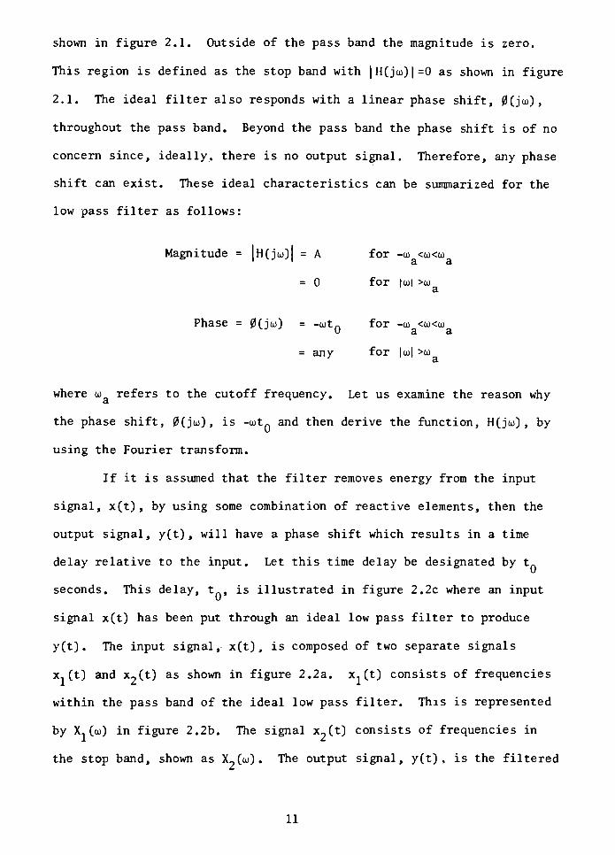
If it is assumed that the filter removes energy from the input

signal, x(t), by using some combination of reactive elements, then the

output signal, y(t) , will have a phase shift which results in a time

delay relative to the input. Let this time delay be designated by t_

seconds. This delay, t-, is illustrated in figure 2.2c where an input

signal x(t) has been put through an ideal low pass filter to produce

y(t) . The input signal, x(t) ,is composed of two separate signals

x. (t) and x2(t) as shown in figure 2.2a. x. (t) consists of frequencies

within the pass band of the ideal low pass filter. This is represented

by X1 (o>) in figure 2.2b. The signal x2(t) consists of frequencies in

the stop band, shown as X~(o)). The output signal, y(t) , is the filtered

11

Input Ideal Filter Output

x(t) H(jo>)

)

t A

Xô))

ft X2(o))i >

/

/ \

y(t)

A

t = 0

(a) (b)

Ax1(t-tQ)

(c)

Time Delay (t ) Characteristics

of the

Ideal Low Pass Filter

Figure 2.2

pass band signal component, x (t) , altered in magnitude to A and time de

layed by t seconds (figure 2.2c). The magnitude, A, is usually less

than the input magnitude unless the filter device is active. The fre

quency components in the stop band, X_(oj) as shown in figure 2.2b, have

been totally removed by the filter. The time delay, t, can be related

to the period, T, of any frequency component in x.(t) as follows:

-t,

Delay (cycles)

or in terms of phase,

0 - -

T tQ (radians)

The phase shift can then be described as a function of frequency since

12

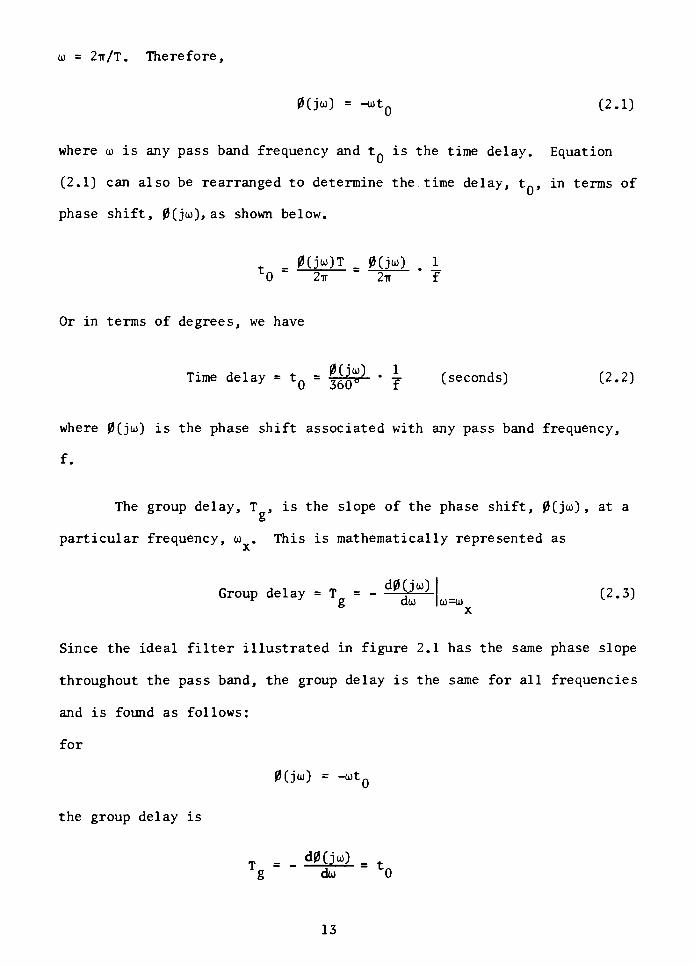
o) = 2tt/T. Therefore,

0(jo)) =

-o)tQ (2.1)

where o) is any pass band frequency and t is the time delay. Equation

(2.1) can also be rearranged to determine the. time delay, t, in terms of

phase shift, 0(jo)), as shown below.

_

0(ju>)T_ 0(jo))

. 1_^0 2tt 2tt f

Or in terms of degrees, we have

Time delay =

tQ=^j") . 1. (seconds) (2.2)

where 0(jo)) is the phase shift associated with any pass band frequency,

f.

The group delay, T ,is the slope of the phase shift, 0(ju), at a

particular frequency, o) . This is mathematically represented as

Group delay = T-

- ÎMg do)

(2.3)0)=O)

x

Since the ideal filter illustrated in figure 2.1 has the same phase slope

throughout the pass band, the group delay is the same for all frequencies

and is found as follows:

for

0(joi) = -tot

0

the group delay is

=d0(jo>) _

lg'

do) 0

13

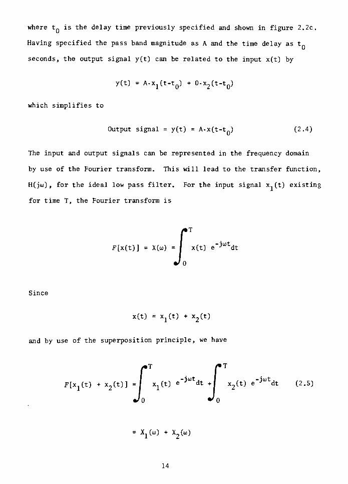
where tQ is the delay time previously specified and shown in figure 2.2c.

Having specified the pass band magnitude as A and the time delay as tn

seconds, the output signal y(t) can be related to the input x(t) by

y(t)= A.XjCt-tjj) + 0.x2(t-tQ)

which simplifies to

Output signal =y(t)

= A-x(t-tQ) (2.4)

The input and output signals can be represented in the frequency domain

by use of the Fourier transform. This will lead to the transfer function,

H(joj) , for the ideal low pass filter. For the input signal x1 (t) existing

for time T, the Fourier transform is

F[x(t)] = X(o>) = J x(t) e"jutdt

Since

x(t)=xx(t) + x2(t)

and by use of the superposition principle, we have

F[Xl(t) + x2(t)] =/ Xl(t) e^dt J x2(t) e"ja,tdt (2.5)

XjCu) + X2(oj)

14

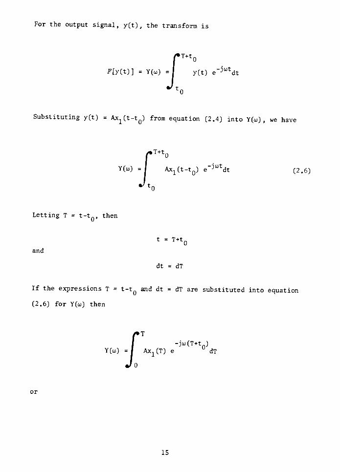
For the output signal, y(t) ,the transform is

{T+t0

y(t) e"jutdt

'0

Substituting y(t) =

Ax^t-t^ from equation (2.4) into Y(o)) , we have

,T+t0

Y(o)) =1 AXjCt-tjj) e-ja)tdt (2.6)

*0

Letting T =

t-tQ, then

t =

T+tQand

dt = dT

If the expressions T =

t-tQand dt = dT are substituted into equation

(2.6) for Y(oi) then

P= 1 Ax2

Jo

-jo)(T+t )

Y(o)) = I Ax. (T) eU

dT

or

15

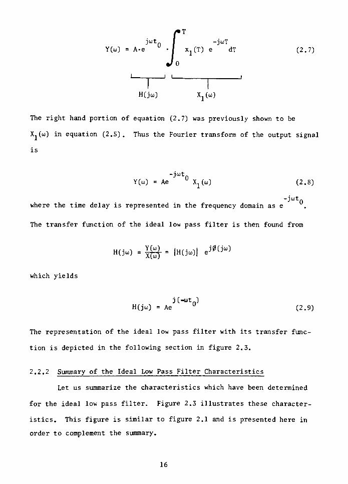
>T

jo)tQ | -jo)T

Y(o)) = A-e I x1(T) e dT (2.7)

H(jo)) Xôi)

The right hand portion of equation (2.7) was previously shown to be

Xj(o)) in equation (2.5). Thus the Fourier transform of the output signal

is

-jut

Y(o)) = Aeu

Xx(o)) (2.8)

-jut

where the time delay is represented in the frequency domain as e

The transfer function of the ideal low pass filter is then found from

= 1M = iHf,.,..,i ej0Cjw)

H(j) =

Y^f= lH^^l

which yields

J C-*t )

H(jo>) = Aeu

(2.9)

The representation of the ideal low pass filter with its transfer func

tion is depicted in the following section in figure 2.3.

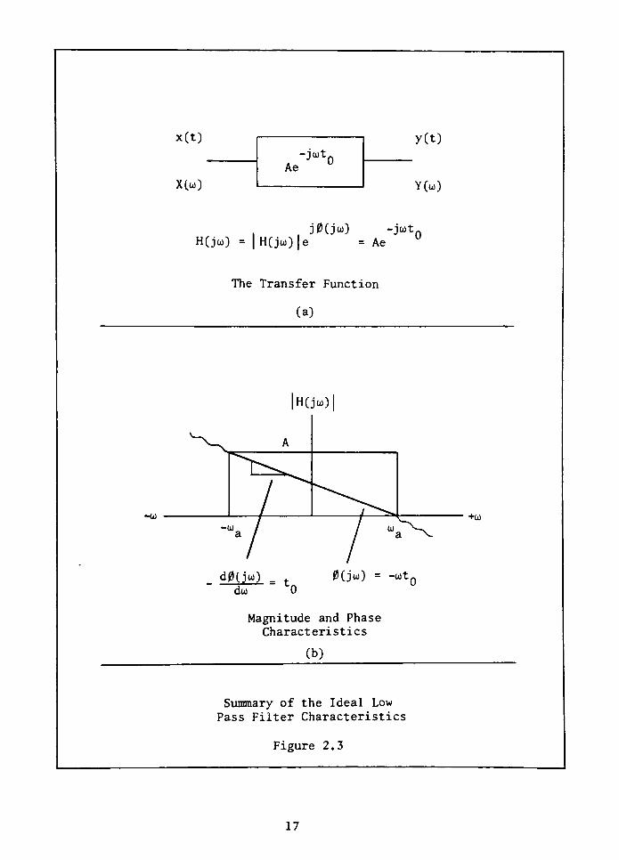
2.2.2 Summary of the Ideal Low Pass Filter Characteristics

Let us summarize the characteristics which have been determined

for the ideal low pass filter. Figure 2.3 illustrates these character

istics. This figure is similar to figure 2.1 and is presented here in

order to complement the summary.

16

x(t)

X(o))

-joit.

Ae

H(jo)) = |H(jo.)|ej0(jo>) -joit

= Ae

y(t)

Y(o))

0

The Transfer Function

(a)

-O)

H(jo))

d0(joQ _

do)"

0

0(jo>) =-o>t

0

Magnitude and Phase

Characteristics

(b)

+0)

Summary of the Ideal Low

Pass Filter Characteristics

Figure 2.3

17

The magnitude characteristics, as shown in figure 2.3b, were de

scribed as

|H(jo))| = A for -o) <oxo)3- 3.

= 0 for |a>|>o>.

where o> is the cutoff frequency. The linear phase shift was described

as

0(ju) =-o)t for -o) <o)<o>

VJ J0 a a

=

any for |o)|>oj.a

As a result of the linear phase shift, the phase delay was described as

0d= 0(o>a)

0)

X

0)

a

where 0(o) ) is the phase shift at the cutoff frequency and oi is any3. X

pass band frequency. The group delay was then described as

= _

d0(jo))

g

"

do)

= t_ for -o> <oxo)0 a a

The Fourier transform of the output signal was then found as

-jut

Y(o>) = Ae X(o>)

Having derived the ideal characteristics, now their interpretation will

be examined.

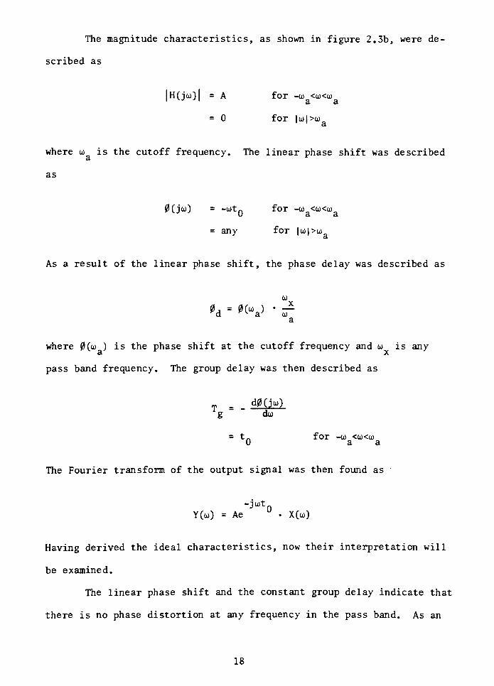
The linear phase shift and the constant group delay indicate that

there is no phase distortion at any frequency in the pass band. As an

18

example of how phase distortion affects a signal, consider the harmonics

which constitute a square wave pulse as depicted in figure 2.4a. The

ideal low pass filter would pass

the frequency components within

the pass band with equal time

delay, tn. If the frequency

constituents are passed with

unequal time delay, the output

signal would contain harmonic

distortion as depicted in fig

ure 2.4b. For the ideal fil

ter, harmonic distortion does

not occur. Also the gain con

stant, A, indicates that the

ideal filter responds equally

for all frequencies in the

v^t)

0

Square Wave Input Pulse

(a)

v0(t)

t

0 VT

Distorted Output Pulse

(b)

Effect of Phase Distortion on a

Square Wave Pulse

Figure 2.4

pass band. These characteristics are ideal and as such do not really

exist. These limitations are examined in detail in section 2.3. For

the moment however, let us accept these ideal characteristics and use

them to briefly describe the magnitude responses of the remaining filter

types.

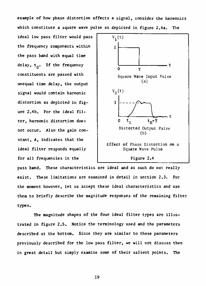
The magnitude shapes of the four ideal filter types are illus

trated in figure 2.5. Notice the terminology used and the parameters

described at the bottom. Since they are similar to those parameters

previously described for the low pass filter, we will not discuss them

in great detail but simply examine some of their salient points. The

19

low pass high pass

H(jo>)|

pass band

stop band

H(jo>)

stop

band

pass

band

band pass band stop

|H( ju)|

A

h- b hpass stop

band band

âl "a2 al

|H(.

A

j")|

h- b h

stop

band

pass

band

a2

H(jo))| magnitude of the filter response

A pass band magnitude

f cutoff frequency

f lower cutoff frequency

f upper cutoff frequency

B bandwidth = f _

- fn

a2 al

f center frequency /*al a2

Magnitude Response and Parameter

Definitions of the Ideal Filter Types

Figure 2.5

20

filters all have a pass band magnitude which is constant and arbitrarily

designated as A. Outside of the pass band the magnitude is zero. The

main difference among these ideal filters is where their pass bands and

stop bands occur on the frequency axis. The frequency band of interest

describes the type of filter to be used. For the low pass and high pass

filters, the pass band edge is described by one cutoff frequency, f, as

a.

shown in figure 2.5. For the band pass filter there are two cutoff fre

quencies, f and f , which describe the region of the pass band. For

the band stop filter, the region between the two cutoff frequencies, f ,n '

al

and fa2, describes the region of attenuation or stop band. The center

frequency, f , for both the band pass and band stop filters is usually

defined as the geometric mean of the two cutoff frequencies. That is

center frequency = fc

=

/fal fa2 (2.10)

We have thus far examined the magnitude and phase characteristics

of the ideal low pass filter. We then determined the transfer function

of the ideal filter which followed as a result of the time shifted output

signal i The remaining filter types were then simply presented in order

to illustrate their selective frequency bands of interest. Next we will

be concerned with the practical restraints which are imposed upon the

ideal response. As a result, the ideal magnitude response diagrams are

altered to represent the. realistic filter response.

2.3 Limitations Affecting the Ideal Low Pass Filter Response

The ideal frequency domain filter was discussed mainly to introduce

the magnitude characteristics and terminology of the four basic filter

types. Now the physical and temporal limitations which restrain the

21

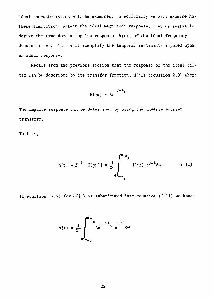
ideal characteristics will be examined. Specifically we will examine how

these limitations affect the ideal magnitude response. Let us initially

derive the time domain impulse response, h(t), of the ideal frequency

domain filter. This will exemplify the temporal restraints imposed upon

an ideal response.

Recall from the previous section that the response of the ideal fil

ter can be described by its transfer function, H(jo>) (equation 2.9) where

H(joj) = Ae

-io)tJ0

The impulse response can be determined by using the inverse Fourier

transform.

That is,

t(t)= F [H(jo))] =

^ ( H(jo)) eJ^do),-1

ru^.,,i _ X / u^..,J"*

a... (2.11)

If equation (2.9) for H(jo>) is substituted into equation (2.11) we have,

|*

-Jt0jot

f- I Ae e <

Ja

h(t) = ^_ | Aeue du

22

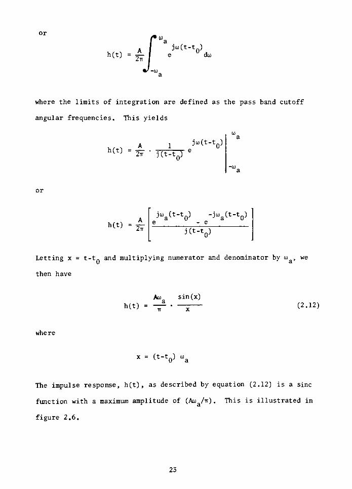
or

h(t) =

j"(t-t0)e do)

where the limits of integration are defined as the pass band cutoff

angular frequencies. This yields

h^=2T'J(tTy

e1

j"(t-t0)

or

h(t)2tt

jo,a(t-t ) -ja(t-t )i -_e

j(t-t )

Letting x = t-t_ and multiplying numerator and denominator by oi,we

0

then have

h(t) =

Als sin(x)a

(2.12)

where

x = (t-t0) a

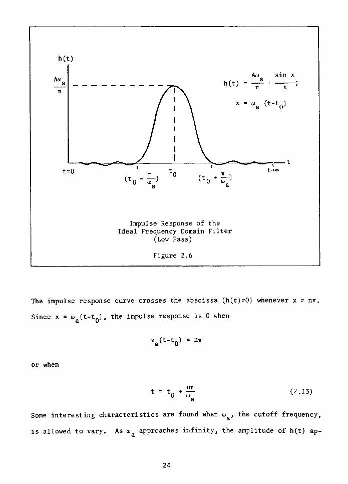
The impulse response, h(t), as described by equation (2.12) is a sine

function with a maximum amplitude of (Ao) /ir) . This is illustrated in

figure 2.6.

23

h(t)

Aoj

t=0

h(t) =

Ao) sin x

a

x =

o>a (t-tQ)

Impulse Response of the

Ideal Frequency Domain Filter

(Low Pass)

Figure 2.6

t-**=

The impulse response curve crosses the abscissa (h(t)=0) whenever x = mr.

Since x = to (t-t ) , the impulse response is 0 when

3 U

wa(t-t0)= nir

or when

mr

t =

tn +

0 o>

a

(2.13)

Some interesting characteristics are found when u> ,the cutoff frequency,

is allowed to vary. As oj approaches infinity, the amplitude of h(t) ap-

a.

24

proaches infinity as can be seen by equation (2.12). Also the impulse

response occurs only at t=tf) as seen in equation (2.13) for w equal toU 3

infinity. Therefore, as o> becomes extremely large, the impulse re-3.

sponse approaches a delta function. Now we are in a position to re

examine and summarize the restrictions which prevent us from obtaining

an ideal filter response. The effects of these limitations are shown

in figure 2.7 and are discussed below.

The impulse response extends from -=> to + in time. This infinite

time span cannot actually exist. The existence of h(t) for values of t

less than 0 requires the filter to respond with an output signal before

the impulse input to the filter takes place.

Aside from the impulse response, imperfect filter components pose

restrictions on an ideal filter response. Let us briefly discuss a few

of these based upon our intuitive reasoning.

The real filter cannot respond with infinite attenuation in the

stop band. This would be required in order to achieve |H(joj)| =0 in the

stop band. That is, all of the energy outside of the pass band would

have to be completely attenuated by the filter. This is not possible

since reactive elements contain some internal resistance. Some residual

noise always exists in the stop band area. Note the non-zero level in

the stop band region in figure 2.7.

The pass band magnitude cannot be constant. Some pass band varia

tion exists even if it is minute. A constant magnitude would require

the reactive elements in the filter to react with equal impedance for

all pass band frequencies.

The transition from the pass band to stop band cannot occur at one

25

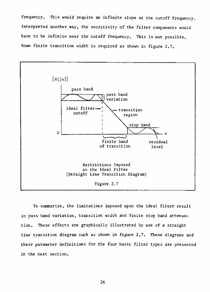
frequency. This would require an infinite slope at the cutoff frequency.

Interpreted another way, the sensitivity of the filter components would

have to be infinite near the cutoff frequency. This is not possible.

Some finite transition width is required as shown in figure 2.7.

H(jo))

z:

pass band

ZS3?

ideal filter

cutoff

pass band

ariation

y. transition

region

finite band

of transition

Restrictions Imposed

on the Ideal Filter

(Straight Line Transition Diagram)

residual

level

Figure 2.7

To summarize, the limitations imposed upon the ideal filter result

in pass band variation, transition width and finite stop band attenua

tion. These effects are graphically illustrated by use of a straight

line transition diagram such as shown in figure 2.7. These diagrams and

their parameter definitions for the four basic filter types are presented

in the next section.

26

2.4 Filter Parameters

Having examined the limitations which alter the ideal filter re

sponse, the straight line transition diagram was presented as a graphical

representation of the magnitude response of the realistic filter. In

this section the non-ideal magnitude shapes and parameters are presented

for each of the four filter types (low pass, high pass, band pass and

band stop). The mathematical representations of these responses will be

addressed in section 2.5.

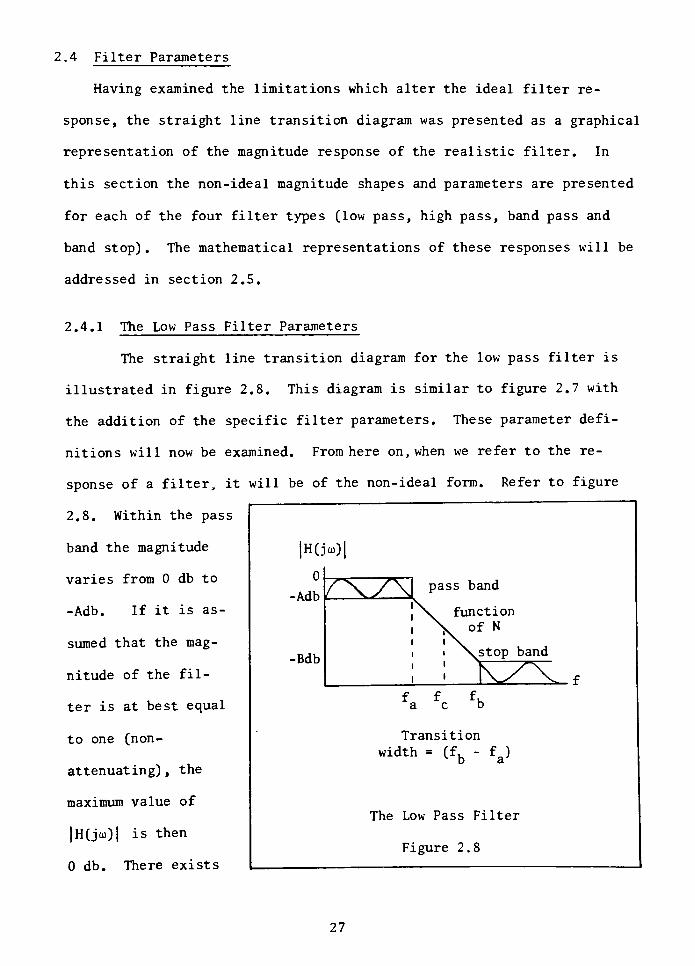
2.4.1 The Low Pass Filter Parameters

The straight line transition diagram for the low pass filter is

illustrated in figure 2.8. This diagram is similar to figure 2.7 with

the addition of the specific filter parameters. These parameter defi

nitions will now be examined. From here on, when we refer to the re

sponse of a filter, it will be of the non-ideal form. Refer to figure

2.8. Within the pass

band the magnitude

varies from 0 db to

|H(]

0

0))|

-AdbAA pass band

>< function-Adb. If it is as

X of N

sumed that the mag

-Bdb

i\i \stop band

nitude of the fili

i V/ v f

ter is at best equal a c b

to one (non-

wi

Transition

dth =

(ffe- ffl)

attenuating) , the

maximum value of

The Low Pass Filter

|H(ju))| is then

Figure 2.8

0 db. There exists

27

some pass band attenuation for which the magnitude is less than one and

the boundary of this variation is represented as -Adb. The pass band

variation can occur as a ripple, such as shown in figure 2.8 or as a

continually decreasing (monotonic) magnitude. The methods of achieving

these shapes will be discussed in Chapter III. The attenuation, -Adb,

is defined as the maximum pass band variation and is associated with the

pass band edge (cutoff) frequency designated as f . The stop band edge

frequency is represented as f, . Associated with f, is the minimum stop

band attenuation -Bdb. The transition width, TW, is defined as the dif

ference between the pass and stop band edge frequencies.

That is,

(2.14)TW fK

" fb a

The transition width and slope are directly related to the filter order,

N. As N increases, the transition width becomes narrower and results in

a faster attenuation rate. The method of determining the filter order -

N, is described in Chapter III. At this point it will simply be stated

that N is a function of f, ffc, -Adb and -Bdb. The frequency, f, is

defined as the center frequency of the transition region where

C =^7^b <2-15)

The center frequency did not hold any significance for the ideal filter

since the transition rate was infinite. We will find this term, f

useful in discussing the elliptic function filter in Chapter III.

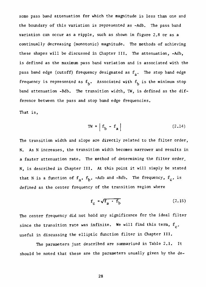
The parameters just described are summarized in Table 2.1. It

should be noted that these are the parameters usually given by the de-

28

signer when specifying the magnitude response of the low pass filter.

The same symbols and terms will also apply to the high pass filter dis

cussed in the following section.

(L

Parameter Definitions

of the

Magnitude Response

dw Pass and High Pass)

fa : pass band edge or cutoff

frequency

b : stop band edge frequency

-Adb: maximum pass band varia

tion occurring at f6

a

-Bdb: minimum stop band atten

uation at f.

fc : center frequency of the

transition region

a b

TW : transition width =

Table 2.1

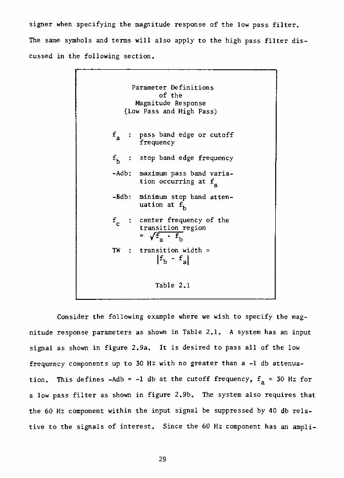
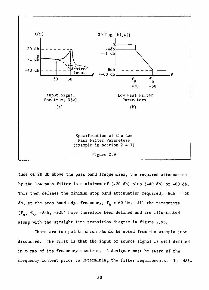
Consider the following example where we wish to specify the mag

nitude response parameters as shown in Table 2.1. A system has an input

signal as shown in figure 2.9a. It is desired to pass all of the low

frequency components up to 30 Hz with no greater than a -1 db attenua

tion. This defines -Adb= -1 db at the cutoff frequency, f = 30 Hz for

a low pass filter as shown in figure 2.9b. The system also requires that

the 60 Hz component within the input signal be suppressed by 40 db rela

tive to the signals of interest. Since the 60 Hz component has an ampli-

29

X(o))

20 db

-40 db^Jdesirec

input

30 60

Input Signal

Spectrum, X(oi)

(a)

20 Log

-Bdb

=-60 db

H(jo))|

Low Pass Filter

Parameters

(b)

Specification of the Low

Pass Filter Parameters

(example in section 2.4.1)

Figure 2.9

tude of 20 db above the pass band frequencies, the required attenuation

by the low pass filter is a minimum of (-20 db) plus (-40 db) or -60 db.

This then defines the minimum stop band attenuation required, -Bdb=-60

db, at the stop band edge frequency, f, = 60 Hz. All the parameters

(f,f,

, -Adb, -Bdb) have therefore been defined and are illustrated

along with the straight line transition diagram in figure 2.9b.

There are two points which should be noted from the example just

discussed. The first is that the input or source signal is well defined

in terms of its frequency spectrum. A designer must be aware of the

frequency content prior to determining the filter requirements. In addi-

30

tion, the source signal will appear to contain various noise levels de

pending upon the filter input characteristics. Noise versus input im

pedance is one example. The second point is that the stop band attenua

tion is determined by the system's need for a minimum signal to noise

ratio. (More accurately (S+N)/N).

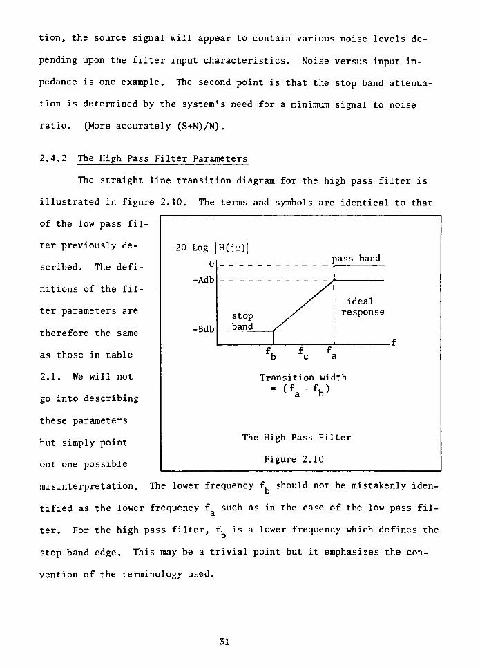
2.4.2 The High Pass Filter Parameters

The straight line transition diagram for the high pass filter is

illustrated in figure 2.10. The terms and symbols are identical to that

of the low pass fil

ter previously de 20 Log | H(jo))|

scribed. The defi 0pass band

-Adbj

nitions of the fil A

A I ideal

ter parameters are

stop / iresponse

-Bdbband

therefore the same

f

as those in table b c a

2.1. We will not Transition width

go into describing

= (f - fOa b

'

these parameters

but simply pointThe High Pass Filter

out one possibleFigure 2.10

misinterpretation. The lower frequency f, should not be mistakenly iden

tified as the lower frequency f such as in the case of the low pass fil-

ter. For the high pass filter, f, is a lower frequency which defines the

stop band edge. This may be a trivial point but it emphasizes the con

vention of the terminology used.

31

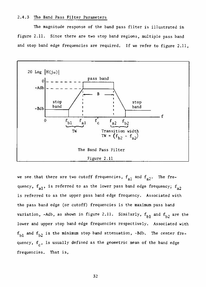
2.4.3 The Band Pass Filter Parameters

The magnitude response of the band pass filter is illustrated in

figure 2.11. Since there are two stop band regions, multiple pass band

and stop band edge frequencies are required. If we refer to figure 2.11,

20 Log

0

-Adb

-Bdb

H(jo))|

pass band

f

stop

band

B ?,

\ stop

band

0 f ff'

f fbl al c a2 132

widthTW

Th

Trans

TW =

e Band Pass F

Figure 2.11

ition

Cfb2

ilter

we see. that there are two cutoff frequencies, f . and f - The fre

quency, f .,is referred to as the lower pass band edge frequency; f _

is referred to as the upper pass band edge frequency. Associated with

the pass band edge (or cutoff) frequencies is the maximum pass band

variation, -Adb, as shown in figure 2.11. Similarly, f, and f,2 are the

lower and upper stop band edge frequencies respectively. Associated with

f,, and f, ,, is the minimum stop band attenuation, -Bdb. The center fre-

bl bz

quency, f ,is usually defined as the geometric mean of the band edge

frequencies. That is,

32

Center frequency = f = Jf . f

(2.16)'

/fbl*

fb2

The bandwidth, B, is defined as the range of frequencies in the pass

band. That is,

B =

(fa2- fal) (2.17)

Care should be taken when specifying or interpreting the bandwidth. A

person might assume that the bandwidth is associated with the -3 db pass

band edge frequencies. This is not necessarily the case. Rather, the

specification given should be properly associated with the design speci

fications f., f ~ and -Adb where -Adb is totally arbitrary. The sig

nificance of the -3 db pertains only to the Butterworth filter in the

event that -Adb is unspecified. Then it is normally assumed that

-Adb =-3 db and that the frequencies at -3 db define the bandwidth. A

transition width (TW) can also be described for the band pass filter as

fb2"

fa2| =|fbl"

fal| <2-18)TW =

This however is seldom used when specifying the band pass filter. We

will see the reason for this when the normalization process is examined.

The definitions and symbols just discussed are summarized in Table 2.2.

Note the similarity to that of table 2.1.

When specifying the parameters for the band pass filter, a number

of combinations of parameters are possible. For example, given the pass

and stop band edge frequencies, the center frequency and bandwidth can be

calculated using equations 2.16 and 2.17. Conversely, the pass band edge

frequencies can be derived from these equations when given the center

33

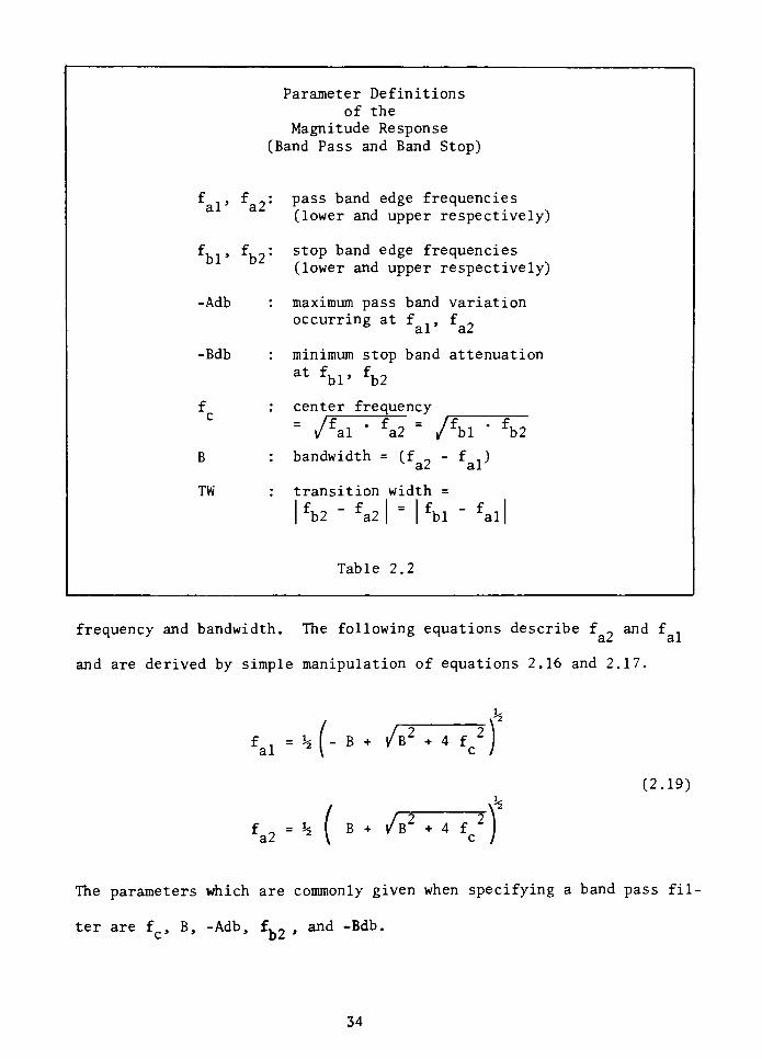
Parameter Definitions

of the

Magnitude Response

(Band Pass and Band Stop)

f,,f ?: pass band edge frequencies

(lower and upper respectively)

f,1 ,

f,_: stop band edge frequencies

(lower and upper respectively)

-Adb : maximum pass band variation

occurring at f, ,f _

al a2

-Bdb : minimum stop band attenuation

at fbl> fb2

f : center frequencyc

t/fal fa2=

/fbl'

fb2

B : bandwidth = (f _

- f Ja2 al

TW : transition width =

If - f I = I f - f Ib2 a2 rbl al |

Table 2.2

frequency and bandwidth. The following equations describe f _ and f1

and are derived by simple manipulation of equations 2.16 and 2.17.

fal= % (- B +

/b2 I 4 f/ )

fa2= % ( b +

a2 : 4f/)

(2.19)

The parameters which are commonly given when specifying a band pass fil

ter are f, B, -Adb, f, -

,and -Bdb.

34

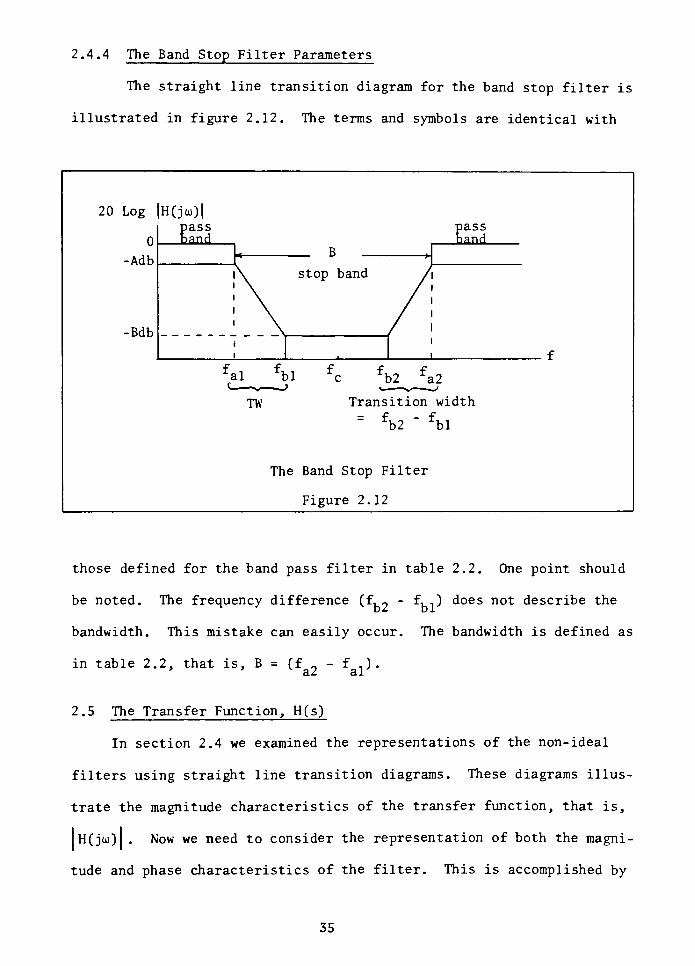
2.4.4 The Band Stop Filter Parameters

The straight line transition diagram for the band stop filter is

illustrated in figure 2.12. The terms and symbols are identical with

20 Log |H(joi)|

-Adb

-Bdb

pass

band

pass

hand

R>

\1 stop band

/ r

i

i

Lal Lbl b2 a2

TW Transition width

= fb2 bl

The Band Stop Filter

Figure 2.12

those defined for the band pass filter in table 2.2. One point should

be noted. The frequency difference (f, _- f, ..) does not describe the

bandwidth. This mistake can easily occur. The bandwidth is defined as

in table 2.2, that is, B = (fa2

fal>

2.5 The Transfer Function, H(s)

In section 2.4 we examined the representations of the non-ideal

filters using straight line transition diagrams. These diagrams illus

trate the magnitude characteristics of the transfer function, that is,

H(joi) . Now we need to consider the representation of both the magni

tude and phase characteristics of the filter. This is accomplished by

35

use of the Laplacian complex frequency, s = a + jo). The relationship be

tween the input and output of a filter is

H(s)=|g} (2.20)

where Y(s) and X(s) are found by use of the Laplace transform.

That is,

L[f(t)] = F(s) =| f(t) e"Stdt

where f(t) represents a time dependent function such as the filter in

put, x(t), or the output y(t). Notice that H(s) is shown as a rational

function. We will initially examine the general form of H(s). Subse-

quently; the particular transfer functions associated with each of the

filter types are discussed. This section will also develop the s-plane

diagrams which represent the transfer function, H(s) , in a graphical

manner.

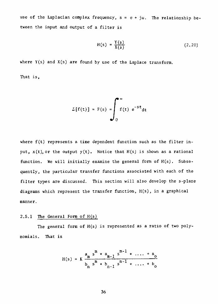
2.5.1 The General Form of H(s)

The general form of H(s) is represented as a ratio of two poly

nomials. That is

m m-1

a s +a . s +....+ an

"W " K"

S n-l

~

b s +b . s +....+b

n n-l o

36

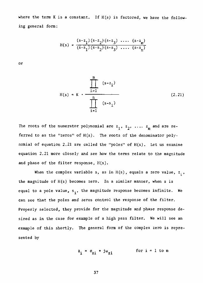
where the term K is a constant. If H(s) is factored, we have the follow

ing general form:

(s-z )(s-z )(s-z ) (s-zjH(s)

] - 3 m

(s-s1)(s-s2)(s-s3) (s~sn)

or

m

i=l

H(s) = K (2.21)

]I (S"Si}

i=l

The roots of the numerator polynomial are z,, z_, .... z and are re-

11 m

ferred to as the"zeros"

of H(s). The roots of the denominator poly

nomial of equation 2.21 are called the"poles"

of H(s). Let us examine

equation 2.21 more closely and see how the terms relate to the magnitude

and phase of the filter response, H(s).

When the complex variable s, as in H(s), equals a zero value, z. ,

the magnitude of H(s) becomes zero. In a similar manner, when s is

equal to a pole value, s., the magnitude response becomes infinite. We

can see that the poles and zeros control the response of the filter.

Properly selected, they provide for the magnitude and phase response de

sired as in the case for example of a high pass filter. We will see an

example of this shortly. The general form of the complex zero is repre

sented by

z. = o . + iu> . for i = 1 to m

1 ziJzi

37

and for the poles,

s. = o .+ jto .

1 pi pifor i = 1 to n

JO)

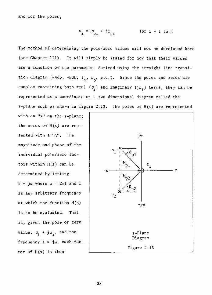
The method of determining the pole/zero values will not be developed here

(see Chapter III). It will simply be stated for now that their values

are a function of the parameters derived using the straight line transi

tion diagram (-Adb, -Bdb, f , f, , etc.). Since the poles and zeros area b

complex containing both real (a.) and imaginary (joi.) terms, they can be

represented as a coordinate on a two dimensional diagram called the

s-plane such as shown in figure 2.13. The poles of H(s) are represented

with an"x"

on the s-plane;

the zeros of H(s) are rep-

sented with a "o". The

magnitude and phase of the

individual pole/zero fac

tors within H(s) can be

determined by letting

s = joi where o) = 2irf and f

is any arbitrary frequency

at which the function H(s)

is to be evaluated. That

is, given the pole or zero

value, a. + jo)., and the'i

Jl

frequency s = jo), each fac

tor of H(s) is then

-JO)

s-Plane

Diagram

Figure 2.13

38

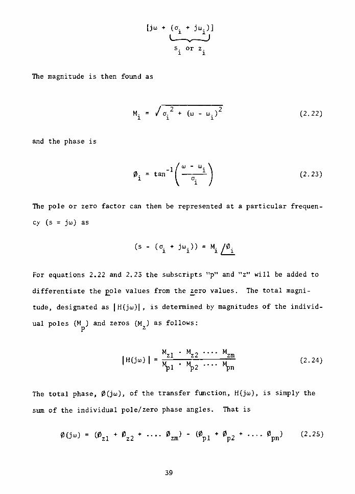
[ju +

(oi+ joii)]

The magnitude is then found as

M. - / 2 ' ^2

a. + (o) -

o).) (2.22)111

v J

and the phase is

/ 0) -

0). \

0i=

o.

X

(2-23)

The pole or zero factor can then be represented at a particular frequen

cy (s = joi) as

(s - (o. + jo).)) = M. /0.l l l/i

For equations 2.22 and 2.23 the subscripts"p"

and"z"

will be added to

differentiate the pole values from the z_ero values. The total magni

tude, designated as |H(jo))|, is determined by magnitudes of the individ

ual poles (M ) and zeros (M ) as follows:

p z

M . M, MrTTi1H(I=MZ1.MZ

....

C2.24)V

'

Mp2. M

pn

The total phase, 0(joi), of the transfer function, H(joi), is simply the

sum of the individual pole/zero phase angles. That is

0(j) -

(0zl+

*>z2+ *m> '

pl+

0p2+

V (2'25)

39

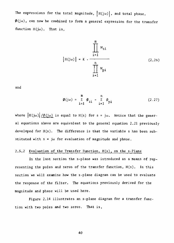
The expressions for the total magnitude, |h(jo>)|, and total phase,

0(joj), can now be combined to form a general expression for the transfer

function H(jo)). That is,

m

zi

i=l

|H(jo))| = K (2.26)

jP1

i=l

and

m n

0(jo)) =10-1 0 (2.27)i=l i=l

pl

where |H(jo))| /0(jo)) is equal to H(s) for s = jo). Notice that the gener

al equations above are equivalent to the general equation 2.21 previously

developed for H(s). The difference is that the variable s has been sub

stituted with s = jo) for evaluation of magnitude and phase.

2.5.2 Evaluation of the Transfer Function, H(s), on the s-Plane

In the last section the s-plane was introduced as a means of rep

resenting the poles and zeros of the transfer function, H(s). In this

section we will examine how the s-plane diagram can be used to evaluate

the response of the filter. The equations previously derived for the

magnitude and phase will be used here.

Figure 2.14 illustrates an s-plane diagram for a transfer func

tion with two poles and two zeros. That is,

40

JO)

-JO)

(a)

for s = jo) = 0

+ o

|H(o)| = 0

0(o) =180

-o

67.5'

-JO)

(b)

M . . M

0(jw)*90

s

(90%90-22.5-67.5)

Evaluation of the Transfer Function, H(s), on the s-Plane

(Example for Section 2.5.2)

Figure 2.14

41

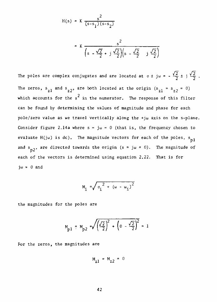
2

H(s) = K(s-s1)(s-s2)

2

= K

(s.q.^.q >q)

/2 i/T

The poles are complex conjugates and are located at c ju = - ~ j ^-- ,

The zeros, s . and s,

are both located at the origin (s,

= s = 0)zl z2

6 lzl z2

2which accounts for the s in the numerator. The response of this filter

can be found by determining the values of magnitude and phase for each

pole/zero value as we travel vertically along the +jo) axis on the s-plane.

Consider figure 2.14a where s = joi = 0 (that is, the frequency chosen to

evaluate H(jco) is dc). The magnitude vectors for each of the poles, s1

and s, are directed towards the origin (s = joi = 0). The magnitude of

each of the vectors is determined using equation 2.22. That is for

jo) = 0 and

Mi =/ai+ ^ "

î)

the magnitudes for the poles are

M .

= M .

pi p2 -mi* ( - if

For the zeros, the magnitudes are

M ,

= M = 0zl z2

42

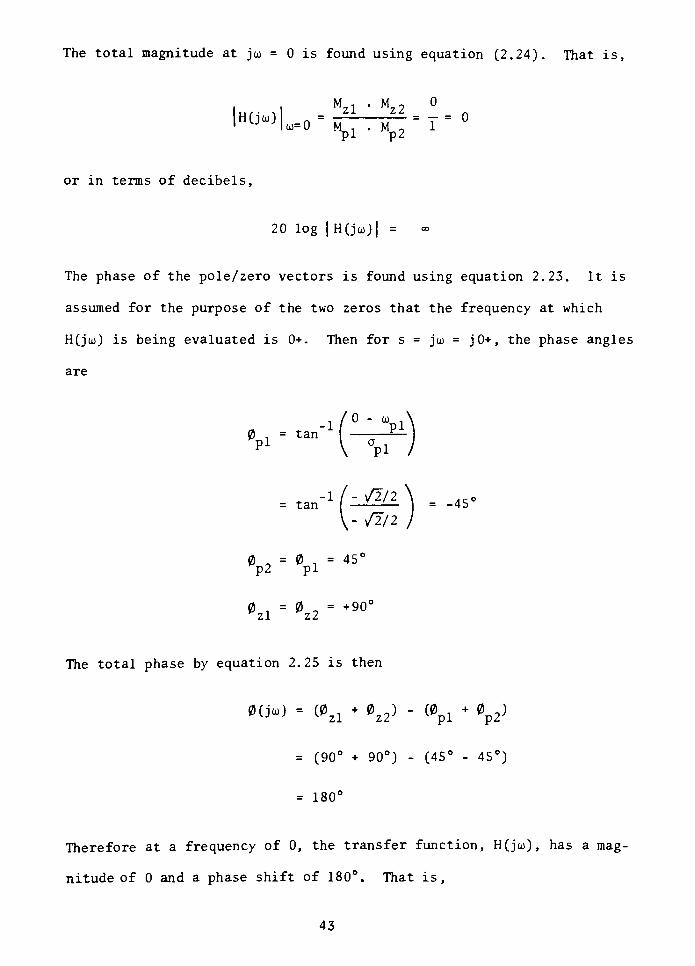
The total magnitude at jo) = 0 is found using equation (2.24). That is,

,,. ,1 Mzl Mz2 .

'H(jaiJlo,=0=Mn1 M?

= T=

P1 P2

or in terms of decibels,

20 log |H(joj)| =

The phase of the pole/zero vectors is found using equation 2.23. It is

assumed for the purpose of the two zeros that the frequency at which

H(jo)) is being evaluated is 0+. Then for s = jo) = j0+, the phase angles

are

0 =

tan"1(-_-!pl

V P1.

=

tan-l

zJlll \ .

- /2/2

*p2=

0pl=

45<

0zl-

0z2- +

90

The total phase by equation 2.25 is then

0(j") -

(0zl+ 0z2) -

(0pl+ 0p2)

=(90

+ 90) -

(45- 45)

=180

Therefore at a frequency of 0, the transfer function, H(jo>), has a mag

nitude of 0 and a phase shift of 180. That is,

43

H(jo)) = |H(jo>) | /0(jo)) = 0/180

This is illustrated in figure 2.15 at w = 0. As jo> becomes larger with

increasing frequency, we cross the cutoff frequency, oj . For the case ata.

hand, oj = 1 as shown in figure 2.15.3-

20 Log | H(jo))|

1

0

-3 db

A0 1 =

o)a

U)

0(jo))

180

90-~\

j\^n

u

0 1

High Pass Response

(Two Pole Filter)

Figure 2.15

Then, ats = jo> = jl, the magnitude and phase of H(joj) are found as

follows :

MPi

(^l)2

* ( /2.765

MP2 [4a-4 = 1.848

zl z2

44

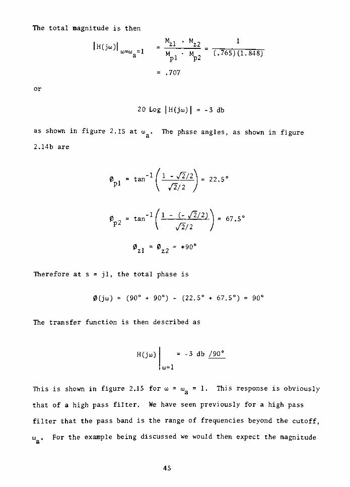
The total magnitude is then

M- . M

H(jo))|zl

*

l'z2

u=%=1 M M

~

(.765) (1.848)pi p2

=.707

or

20 Log |H(jo)) | =-3 db

as shown in figure 2.15 at u&. The phase angles, as shown in figure

2.14b are

fl -tan"1

f l^JUl), 22.5<

Pl

V /2/2 J

=tan-1^1

'

(~Â= 67.5<

P2 I Jill )

0zl.

0^-

+90<

Therefore at s = jl, the total phase is

0(joi) =(90

+ 90) -

(22.5

+ 67.5) =90'

The transfer function is then described as

H(jo))=-3 db

/90'

0)=1

This is shown in figure 2.15 for oj = oj = 1. This response is obviously3.

that of a high pass filter. We have seen previously for a high pass

filter that the pass band is the range of frequencies beyond the cutoff,

o) . For the example being discussed we would then expect the magnitude3-

45

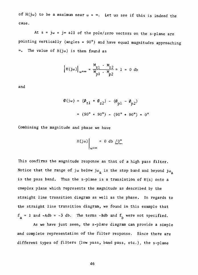
of H(jo>) to be a maximum near oi = . Let us see if this is indeed the

case.

At s = joj = j all of the pole/zero vectors on the s-plane are

pointing vertically (angles = 90) and have equal magnitudes approaching

. The value of H(joj) is then found as

M . M _

HCJU>L=

-srsr2-^ 1 = 0 db

o)= Mn

M _

pi p2

and

0(j) =

(0zl* 0z2J -

(0pl- 0p2)

=(90

+ 90) -

(90

+ 90) =0'

Combining the magnitude and phase we have

H(joj) = 0 db /0j0)=CD

This confirms the magnitude response as that of a high pass filter.

Notice that the range of joi below jo) is the stop band and beyond joi

is the pass band. Thus the s-plane is a translation of H(s) onto a

complex plane which represents the magnitude as described by the

straight line transition diagram as well as the phase. In regards to

the straight line transition diagram, we found in this example that

f = 1 and -Adb=-3 db. The terms -Bdb and f, were not specified.

a br

As we have just seen, the s-plane diagram can provide a simple

and complete representation of the filter response. Since there are

different types of filters (low pass, band pass, etc.), the s-plane

46

diagrams must vary accordingly. In fact, the s-plane provides a clear

pictorial representation of the unique characteristics of one filter

versus another given the same type of filter. These unique character

istics are discussed in Chapter III.

The following section illustrates the typical form of the trans

fer function, H(s), and the s-plane diagram associated with each filter

type. We will not go into any analysis of these forms as we just did

with the high pass example but simply discuss a few of the important

points.

2.5.3 The Transfer Functions

The previous sections examined the general form of the transfer

function, H(s), and a means of interpreting the filter response using

the s-plane diagram. In this section the typical forms of the transfer

functions are given for each filter type. The magnitude response curves

will not be presented here since the straight line transition diagrams

of section 2.4 serve this purpose.

The common forms of the second order transfer functions are il

lustrated for each filter type in figure 2.16. At first glance, there

are apparent differences in the transfer function equation, H(s), and in

the s-plane diagrams. This relates directly to the fact that they all

have different magnitude and phase responses. Let us briefly discuss

the salient points regarding the transfer function of each filter type.

Figure 2.16a illustrates the low pass filter characteristics.

The transfer function shown, H(s) is for a general two pole (N=2)Lii

filter as seen by the two factors (s-s.) and the two x's on the s-plane.

The number of poles can generally be any number greater than or equal to

47

H(s)LP (s-s1)(s-s2)

Low Pass

(a)

JO)

/

sl-,*

n1

01

s_ x

s

-JO)

H(s)

K's2

HP (s-Sl)(s-s2)

High Pass

(b)

sl~*

JO)

-^

52-K

-JO)

zrz2

Band Pass

H(s)K s

BP 2 2 2 2(s - Bss. + oj ) (s - Bss_ + o) )

Ks'

(s-sp(s-sp(s-sp(s-sp

Band Stop

H(s)

K'(s2

+ o)2)

BS ? -1 ? 2 -12(sJ

-

Bss^+ -

Bss2x

+ o)c)

K'(s-Zl)2 (s-z2)2

(s-sp(s-s2)(s-sp(s-s;)

Typical Transfer Functions

Figure 2.16

S3^-

J 1)

2r22^K

-joc

-JO)

JO)

s;_x v$)jwc=z1,z2

1^*

'2

3^x

!_x dPVZl'z2

-JO)

48

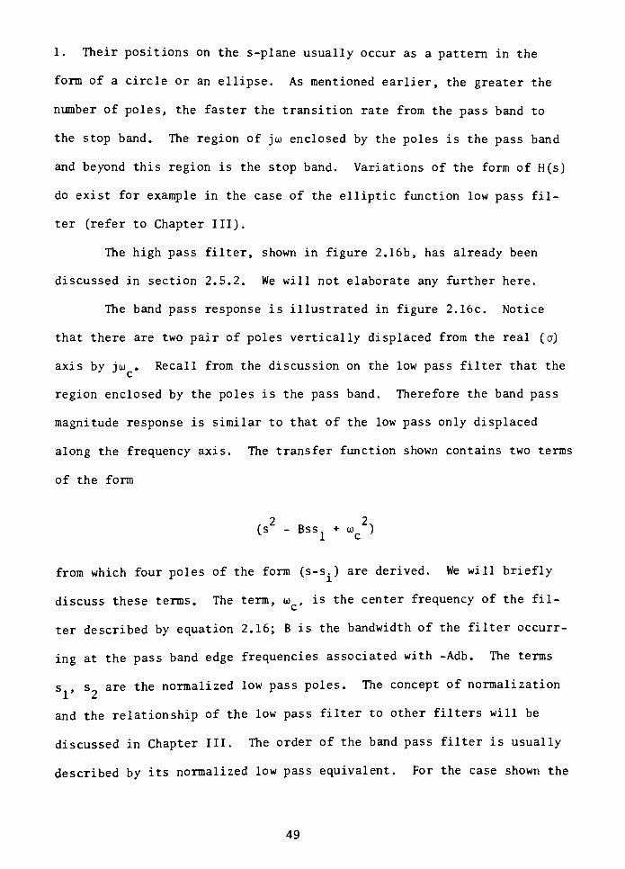
1. Their positions on the s-plane usually occur as a pattern in the

form of a circle or an ellipse. As mentioned earlier, the greater the

number of poles, the faster the transition rate from the pass band to

the stop band. The region of joi enclosed by the poles is the pass band

and beyond this region is the stop band. Variations of the form of H(s)

do exist for example in the case of the elliptic function low pass fil

ter (refer to Chapter III).

The high pass filter, shown in figure 2.16b, has already been

discussed in section 2.5.2. We will not elaborate any further here.

The band pass response is illustrated in figure 2.16c. Notice

that there are two pair of poles vertically displaced from the real (a)

axis by jo> . Recall from the discussion on the low pass filter that the

region enclosed by the poles is the pass band. Therefore the band pass

magnitude response is similar to that of the low pass only displaced

along the frequency axis. The transfer function shown contains two terms

of the form

/2 2,

(s -

Bss1+

o)c )

from which four poles of the form (s-s.) are derived. We will briefly

discuss these terms. The term, u> ,is the center frequency of the fil

ter described by equation 2.16; B is the bandwidth of the filter occurr

ing at the pass band edge frequencies associated with -Adb. The terms

s ,s are the normalized low pass poles. The concept of normalization

and the relationship of the low pass filter to other filters will be

discussed in Chapter III. The order of the band pass filter is usually

described by its normalized low pass equivalent. For the case shown the

49

low pass order is N=2. The translation to the band pass (denormaliza

tion) yields two quadratic terms such as those in the denominator of

H(s)R . Thus for a band pass filter, the number of poles equals 2N.

The band stop response is illustrated in figure 2.16d. Its

characteristics are similar to that of the band pass which accounts for

a band translation along the frequency axis. Notice however that in the

central region of the poles there exists two zeros, jz. and jz~ on the

+jo) axis. These zeros and their conjugates, -jz1and -jz9, are derived

2 22

from (s + o) ) in the numerator of H(s)R_. When the frequency variable,

jo), crosses through this region of the zeros, the magnitude of H(jo>)DC. isDO

decreasing and at the zeros, H(joi) = - . This then defines the stop

band region. The terms in the denominator of H(s)DC are defined the sameDO

as that of the band pass.

2.6 Summary

We started off Chapter II by discussing the ideal filter character

istics. In doing so the basic purpose of each filter, concerning the

magnitude response, was identified. Some terminology associated with the

ideal filters was introduced. Essentially the concepts of the ideal fil

ter served as a basis for the non-ideal responses.

In consideration of the realistic filter response, the ideal filter

was examined to show the areas which were limited in a real sense. This

led to the straight line transition diagram as a representation of the

magnitude response of the real filter. Then the transfer function was

introduced in its general form as a mathematical representation of not

only the magnitude response but phase as well. From this, the particular

characteristics of the transfer function were shown for each filter type.

50

In the discussion of the transfer functions for the band pass and

band stop filters, a relationship to the normalized low pass filter be

came evident. It turns out that all of the filter types do indeed have

a relationship to the normalized low pass filter. This relationship

provides for a very convenient manner with which the poles and zeros of

the various filter types are determined. This process of normalization

and the method of determining the poles/zeros is the topic of Chapter

III.

51

CHAPTER III

NORMALIZATION

AND THE

CLASSICAL APPROXIMATIONS

3.1 Introduction

In this chapter we examine the methods of determining the poles and

zeros of the transfer function, H(s). It was shown in chapter II that

the transfer function represented the complete response (magnitude and

phase) of the filter by way of the poles and zeros. It was also found

that when the transfer function is evaluated along the joi axis on the

s-plane, the magnitude response (phase also) could be determined. This

same magnitude response is described by the parameters associated with

the straight line transition diagram. Thus there exists a relationship

between these magnitude parameters and the pole/zero values on the

s-plane. The objective of this chapter is to analyze and demonstrate

the methods of finding the poles and zeros using the parameters from the

straight line transition diagram. Of importance also is describing the

unique magnitude response characteristics and the pole/zero patterns as

they relate to the classical approximations (Butterworth, Chebyshev and

elliptic) .

We approach the solution of deriving the poles and zeros by dis

cussing three main topics. These are 1) normalization, 2) the character

istic equation and 3) the classical approximations. The first topic,

normalization, deals with converting the straight line transition dia

grams of the four filter types into one simple low pass form, normalized

along the frequency axis. The resulting normalized low pass filter is

the basis of all filter design techniques. This form simplifies the task

52

of analyzing the variety of response requirements. Inherent in this

process of normalization is establishing a relationship between the four

filter types (low pass, high pass, band pass and band stop) and the nor

malized low pass form. The normalization equations are briefly pre

sented. Then examples are given to demonstrate the normalization

process for each filter type.

The second topic deals with the mathematical representation of the

normalized low pass filter. This representation is called the charac

teristic equation. Here we examine how the equation describes the nor

malized low pass filter and the manner in which it approximates the

ideal filter. An examination is also made of the various magnitude

shapes of the normalized low pass filter. The concept of insertion loss

is related to the characteristic equation. Then a discussion is pre

sented which relates the solution of the insertion loss function to the

normalized poles and zeros. As a result of these discussions we see the

relationship between the normalized low pass filter, the characteristic

equation and the pole/zero values of the transfer function, H(s).

The third topic, classical approximations, deals with three approxi

mations to the ideal normalized low pass filter. These classical func

tions are the Butterworth, Chebyshev and elliptic. Each has its unique

properties and objective in achieving one or more characteristics of the

ideal low pass response. For each of these we discuss the magnitude re

sponse as it relates to the approximating function. Then the methods of

evaluating the filter order, N, along with the poles and zeros are dis

cussed. Lastly a comparison is made among the three classical responses.

As a result of this chapter, the reader should develop an apprecia-

53

tion of how the filter design requirements, representented by the

straight line transition diagram, relate to the poles and zeros of the

transfer function, H(s) . In addition the reader should be acquainted

with the unique properties of each approximation to the ideal low pass

filter and how they suit the design needs.

3.2 The Normalized Low Pass Filter

In this section we establish the normalized low pass filter as a

basis for all filter designs. We begin by defining the normalized low

pass filter and its parameters. Then the normalization process is ex

amined for each of the four filter types (low pass through band stop) .

As a result we are left with one normalized form which can be used to

determine the poles and zeros. The use of the normalized low pass fil

ter eliminates the need for an abundance of design data in that only the

low pass design tables are needed.

3.2.1 Definition and Parameters of the Normalized Low Pass Filter

The straight line transition diagram for the normalized low pass

filter is illustrated in figure 3.1. The frequency axis (f ) is nor

malized such that the cutoff frequency is equal to 1. The normalized

pass band shown is the frequency range 0 < f < 1. (The term, fre

quency, is used although it is improper since the f axis is really

unitless.) The parameters of the magnitude response, as shown in figure

3.1, are defined in the same manner as we have previously done in chap

ter II with the addition of the subscript, n, on frequency values to in

dicate that they are normalized. These parameter definitions are summa

rized in figure 3.1. The shape of the magnitude response can varyde-

54

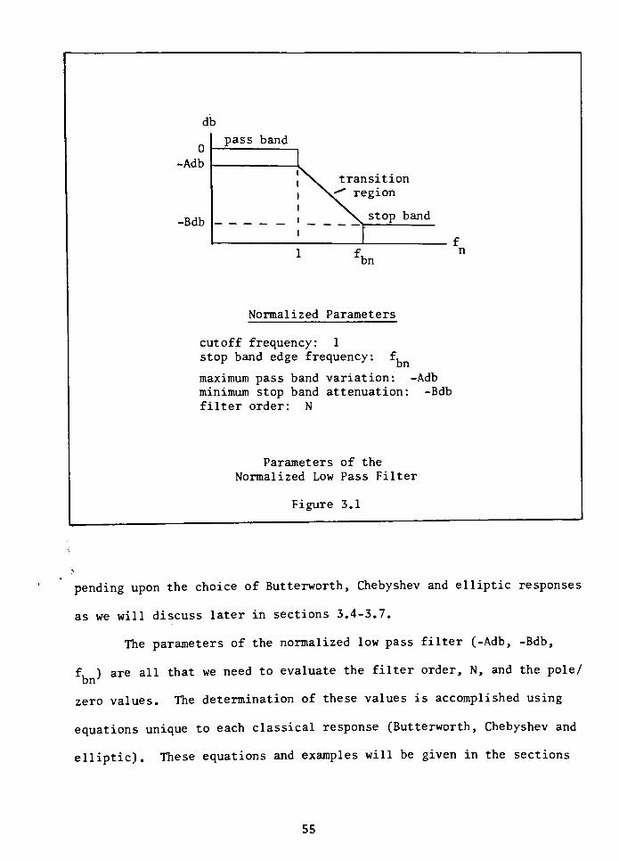
db

0

Adb

pass band

%^ transition

N^"

region

Rdbstop band

bn

Normalized Parameters

cutoff frequency: 1

stop band edge frequency: f,

maximum pass band variation: -Adb

minimum stop band attenuation: -Bdb

filter order: N

Parameters of the

Normalized Low Pass Filter

Figure 3.1

pending upon the choice of Butterworth, Chebyshev and elliptic responses

as we will discuss later in sections 3.4-3.7.

The parameters of the normalized low pass filter (-Adb, -Bdb,

f 1 are all that we need to evaluate the filter order, N, and the pole/bn'

zero values. The determination of these values is accomplished using

equations unique to each classical response (Butterworth, Chebyshev and

elliptic). These equations and examples will be given in the sections

55

to follow. For the remainder of this section we concern ourselves with

the methods of transforming the designer specified parameters of the

straight line transition diagrams into the normalized low pass filter.

3.2.2 Normalization of the Low Pass Response

Figure 3.2a illustrates the straight line transition diagram of

the non-normalized (denormalized) low pass filter. The objective is to

obtain the normalized form shown in figure 3.2b. Since the magnitude

response shape in figure 3.2a is already in the low pass form, the nor

malization process simply requires dividing the frequency values of

figure 3.2a by the cutoff frequency, f ,to obtain a normalized fre-

'3

quency axis, f .

That is,

f

f = ^ (3.1)xn f

a

where

f is any arbitrary frequency,

f is the cutoff frequency,3.

f is the normalized value of f .

xn x

Thus the normalized cutoff frequency, using equation 3.1, is f /f = 1d 3

and the normalized stop band edge frequency is ffe/fa= fbn-

Consider an example. Shown in figure 3.2a are the following

parameters: cutoff frequency (f ) = 20 Hz, stop band edge frequency

ff ) = 26 Hz. The normalized frequency values are found using equation

b

3.1 as follows:

56

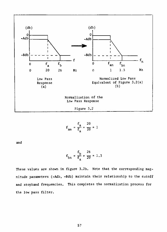
(db) (db)

0

-Adb

0

-Adb

-Bdb

k\ -Bdb

i \1 \

If f

0 fa fb

0 f fn

an bn

0 20 26 Hz 0 1 1.3 Hz

Low Pass

Response

(a)

Normalized Low Pass

Equivalent of Figure 3.2(a)

(b)

Normalization of the

Low Pass Response

Figu:re 3.2

and

fa 20

fan

= =

20= 1

a

fu 26

rbn f 201",a

a

These values are shown in figure 3.2b. Note that the corresponding mag

nitude parameters (-Adb, -Bdb) maintain their relationship to the cutoff

and stopband frequencies. This completes the normalization process for

the low pass filter.

57

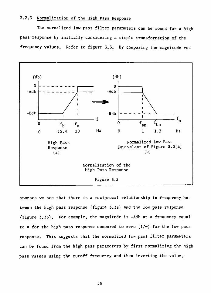
5.2.3 Normalization of the High Pass Response

The normalized low pass filter parameters can be found for a high

pass response by initially considering a simple transformation of the

frequency values. Refer to figure 3.3. By comparing the magnitude re-

(db) (db)

0

-Adb

-Bdb

0

-Adb

f

-Bdb

f

0

0

fb15.4

fa

20 Hz

D

0

f f.n

an bn

1 1.3 Hz

High Pass

Response

(a)

Normalized Low Pass


(b)


High Pass Response

Figure 3.3

sponses we see that there is a reciprocal relationship in frequency be

tween the high pass response (figure 3.3a) and the low pass response

(figure 3.3b). For example, the magnitude is -Adb at a frequency equal

to for the high pass response compared to zero (1/) for the low pass

response. This suggests that the normalized low pass filter parameters

can be found from the high pass parameters by first normalizing the high

pass values using the cutoff frequency and then inverting the value.

58

That is,

,-1

*-K(3.2)

where

f is any high pass frequency,

f is the high pass cutoff frequency,3-

f is the normalized low pass frequency value.

As an example, consider the frequency values shown in figure

3.3a, f = 20 Hz and f, = 15.4 Hz. The corresponding normalized low

pass values are shown in figure 3.3b and derived using equation 3.2 as

shown below.

fm"

[-T

20,-1

20= J

and

fbn "If,

15.4'

20= 1.3

Notice that the magnitude parameters, -Adb and -Bdb, remainthe same as

shown in figure 3.3b. It is interesting to compare this normalized low

pass filter response with the one previously found in section 3.2.2,

figure 3.2. The normalized parameters are the same and at this level

the high pass and low pass responses are equivalent. Analysis of the

pole/zero values using this normalized form will therefore apply to both

the high pass and low pass responses.

59

This completes the process of normalization as it pertains to the

high pass filter response. Now we will examine a slightly different in

terpretation of normalization as it applies to the band pass filter re

sponse .

3.2.4 Normalization of the Band Pass Response

The magnitude response of the band pass filter is similar in

shape to that of the low pass filter except that the passband has been

shifted to a higher center frequency. One might consider the normaliza

tion process of the band pass response to the normalized low pass filter

as a "band normalization". Instead of normalizing frequency values with

respect to the cutoff frequency as in the case of the low pass or high

pass, we simply normalize any arbitrary bandwidth with respect to the

bandwidth, B, defined by the passband edge frequencies.

That is,

fxn=

T(3'3)

where

B is the bandwidth at the cutoff frequencies equal to

a2al'

B is any arbitrary bandwidth,x

f is the resulting normalized value

xn

As an example, consider the normalized value of the bandwidth de

fined by the cutoff frequencies f&2 and fjas shown in figure 3.4a.

The width of the band at the cutoff frequencies is f _- f . Therefore

60

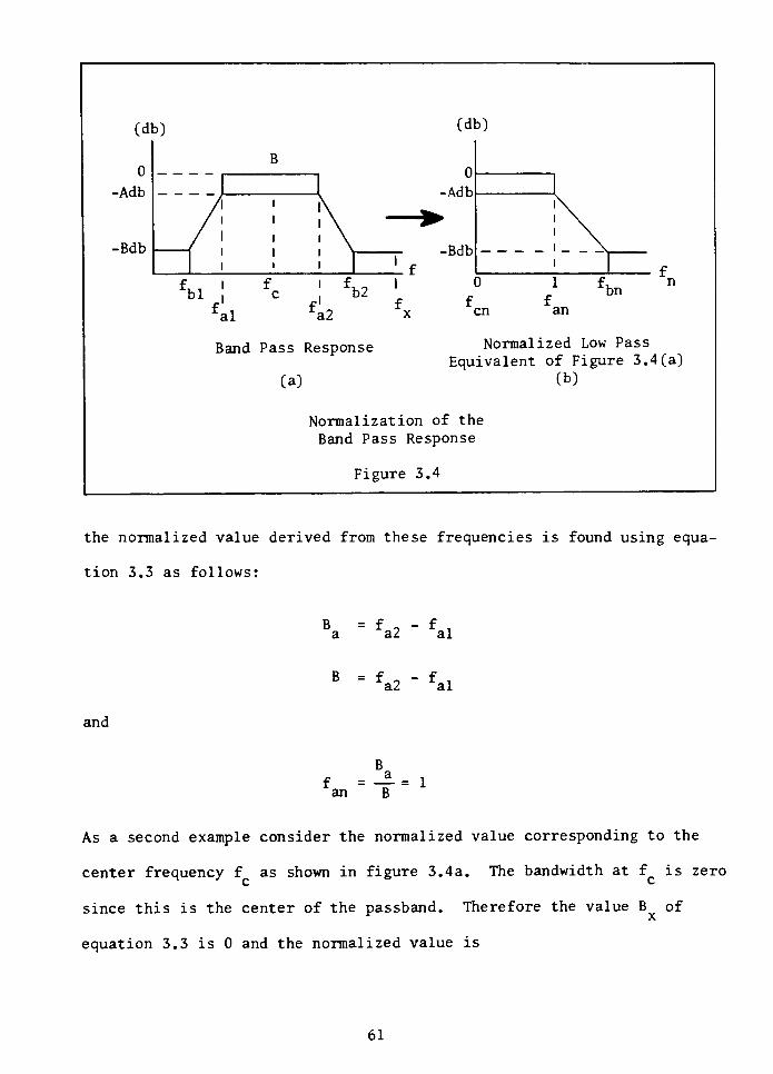
(db) (db)

oB

0

-Adb-Adb

-Bdb / !\-

-Bdb \1e c

fblfal

fc

f

fb2 *

a2 x

f

D

;nf

b"

an

Band Pass Response

(a)

Normal

Equivalent

Lzed Low Pass

of Figure 3.4(a)

(b)

Normalization

Band Pass Re

of the

;ponse

Figure 3 .4

the normalized value derived from these frequencies is found using equa

tion 3.3 as follows:

B =f,-f,a a2 al

B = f _- f .

a2 al

and

f = _. = ian B

As a second example consider the normalized value corresponding to the

center frequency f as shown in figure 3.4a. The bandwidth at f is zero

since this is the center of the passband. Therefore the value B of

equation 3.3 is 0 and the normalized value is

61

*-&-

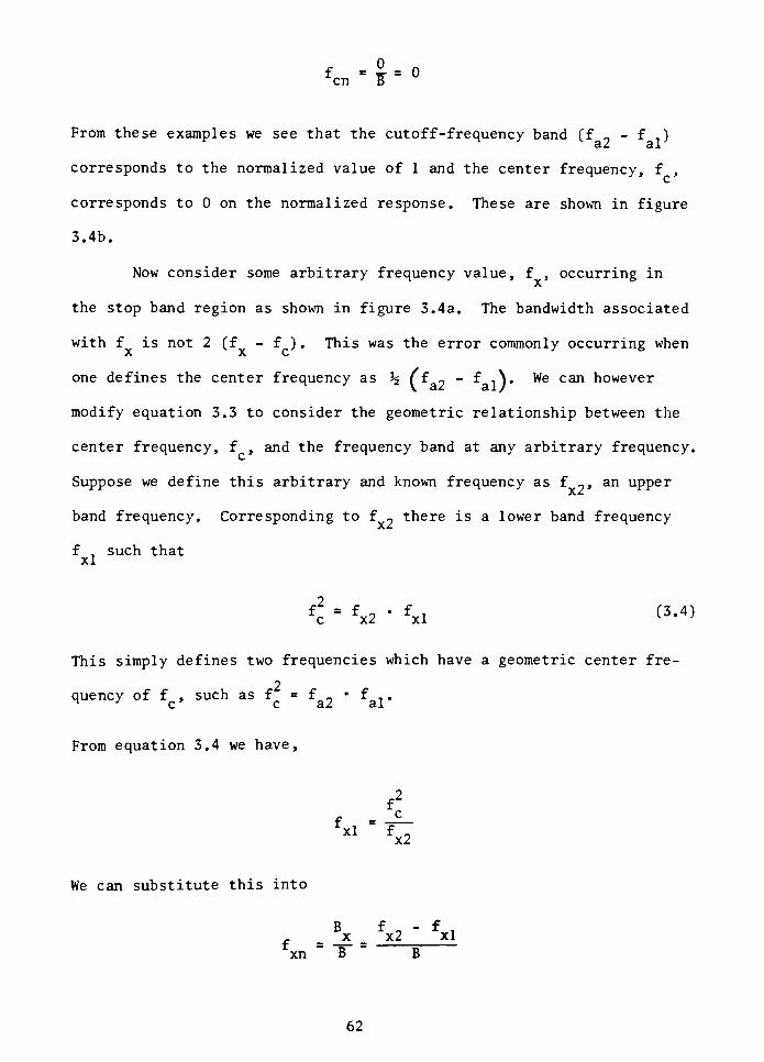
From these examples we see that the cutoff-frequency band (f _- f )

corresponds to the normalized value of 1 and the center frequency, f ,

corresponds to 0 on the normalized response. These are shown in figure

3.4b.

Now consider some arbitrary frequency value, f , occurring in

the stop band region as shown in figure 3.4a. The bandwidth associated

with f is not 2 (f - f ) . This was the error commonly occurring when

one defines the center frequency as \ (f 2~ f

-iVWe can however

modify equation 3.3 to consider the geometric relationship between the

center frequency, f ,and the frequency band at any arbitrary frequency.

Suppose we define this arbitrary and known frequency as f~,

an upper

band frequency. Corresponding to f . there is a lower band frequency

f,such that

xl

f2

= fo

fi (3.4)

c x2 xl* '

This simply defines two frequencies which have a geometric center fre-

2quency of f ,

such as f = f _ f , .

From equation 3.4 we have,

f2

fxl f _

x2

We can substitute this into

. \ fx2'

fxlxn

_

B B

62

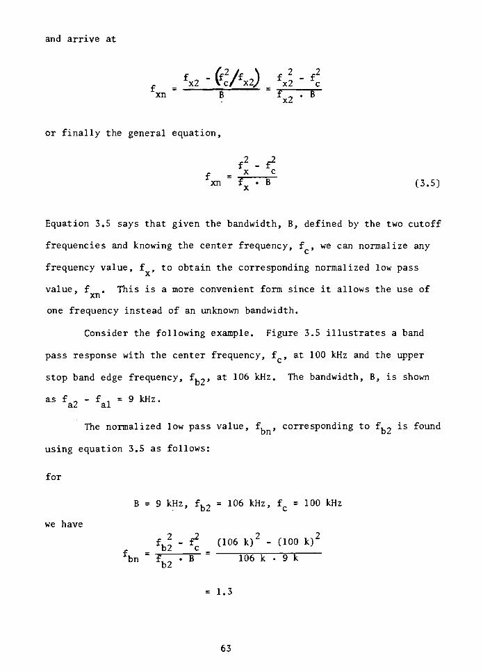
and arrive at

- (fcA2).

fx2'

l/fx2J.

fx2'

fcxn B f

"

. Bx2

or finally the general equation,

f2

x c

xn fx B (3.5)

Equation 3.5 says that given the bandwidth, B, defined by the two cutoff

frequencies and knowing the center frequency, f ,we can normalize any

frequency value, f ,to obtain the corresponding normalized low pass

value, f . This is a more convenient form since it allows the use of

xn

one frequency instead of an unknown bandwidth.

Consider the following example. Figure 3.5 illustrates a band

pass response with the center frequency, f ,at 100 kHz and the upper

stop band edge frequency, fh?, at 106 kHz. The bandwidth, B, is shown

as f _

- f .= 9 kHz.

a2 al

The normalized low pass value, f, , corresponding to f, - is found

using equation 3.5 as follows:

for

B = 9 kHz, fK, = 106 kHz, f = 100 kHz

we have

fb2

- f2. (106k)2

- (100k)'

bn f. _ B 106 k 9 kb2

= 1.3

63

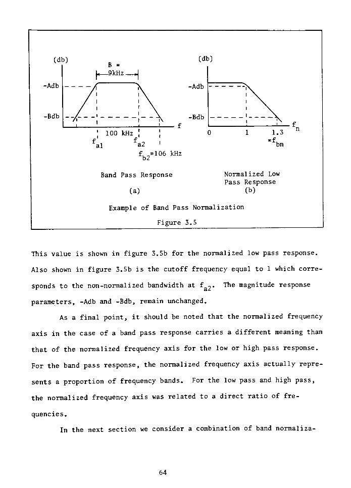
(db)

-Adb

-Bdb

(db)

-Adb

-Bdb

f. =106 kHzDZ

Band Pass Response

(a)

Example of Band Pass Normalization

Figure 3.5

Normalized Low

Pass Response

(b)

This value is shown in figure 3.5b for the normalized low pass response.

Also shown in figure 3.5b is the cutoff frequency equal to 1 which corre

sponds to the non -normalized bandwidth at f - The magnitude response

parameters, -Adb and -Bdb, remain unchanged.

As a final point, it should be noted that the normalized frequency

axis in the case of a band pass response carries a different meaning than

that of the normalized frequency axis for the low or high pass response.

For the band pass response, the normalized frequency axis actually repre

sents a proportion of frequency bands. For the low pass and high pass,

the normalized frequency axis was related to a direct ratio of fre

quencies.

In the next section we consider a combination of band normal iza-

64

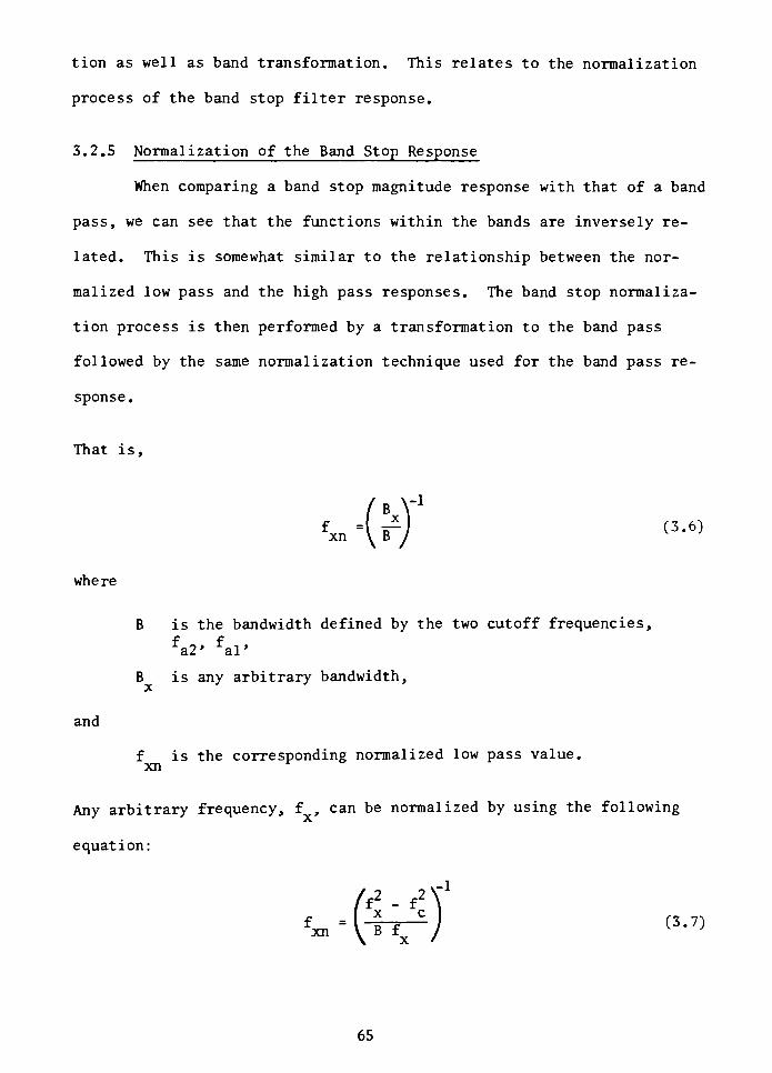
tion as well as band transformation. This relates to the normalization

process of the band stop filter response.

3.2.5 Normalization of the Band Stop Response

When comparing a band stop magnitude response with that of a band

pass, we can see that the functions within the bands are inversely re

lated. This is somewhat similar to the relationship between the nor

malized low pass and the high pass responses. The band stop normaliza

tion process is then performed by a transformation to the band pass

followed by the same normalization technique used for the band pass re

sponse.

That is,

fxn=(ir) ^

where

B is the bandwidth defined by the two cutoff frequencies,

fa2' al'

B is any arbitrary bandwidth,

and

f is the corresponding normalized low pass value.

xn

Any arbitrary frequency, f ,can be normalized by using the following

equation:

-1

(3.7)

65

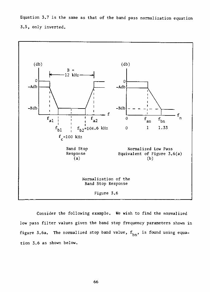
Equation 3.7 is the same as that of the band pass normalization equation

3.5, only inverted.

(db)

0

-Adb

-Bdb

I-B =

12kHz-

fb2=104.6 kHz

f =100 kHzc

Band StopResponse

(a)

(db)

0

-Adb

-Bdb

0

0

an bn

1 1.33

Normalized Low Pass


(b)


Band Stop Response

Figure 3.6

Consider the following example. We wish to find the normalized

low pass filter values given the band stop frequency parameters shown in

figure 3.6a. The normalized stop band value, f, ,is found using equa

tion 3.6 as shown below.

66

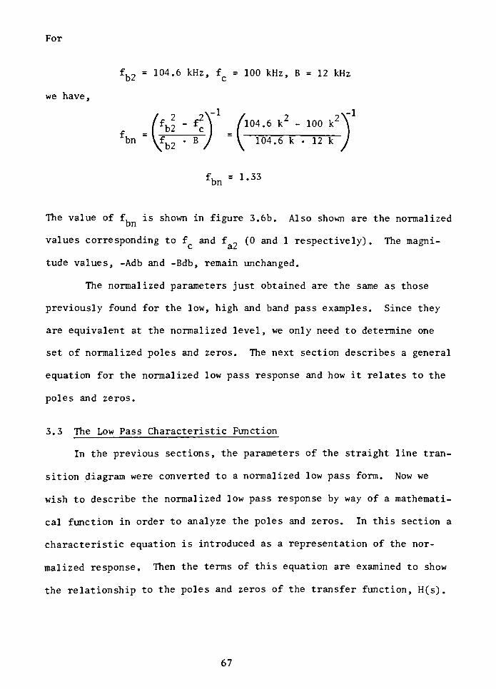
For

fbn i'33

The value of f, is shown in figure 3.6b. Also shown are the normalized

values corresponding to f and f _ (0 and 1 respectively). The magni

tude values, -Adb and -Bdb, remain unchanged.

The normalized parameters just obtained are the same as those

previously found for the low, high and band pass examples. Since they

are equivalent at the normalized level, we only need to determine one

set of normalized poles and zeros. The next section describes a general

equation for the normalized low pass response and how it relates to the

poles and zeros.

3.3 The Low Pass Characteristic Function

In the previous sections, the parameters of the straight line tran

sition diagram were converted to a normalized low pass form. Now we

wish to describe the normalized low pass response by way of a mathemati

cal function in order to analyze the poles and zeros. In this section a

characteristic equation is introduced as a representation of the nor

malized response. Then the terms of this equation are examined to show

the relationship to the poles and zeros of the transfer function, H(s) .

67

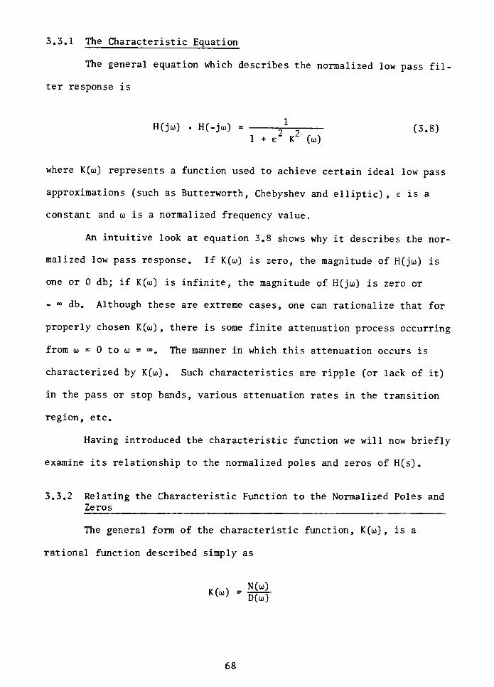
3.3.1 The Characteristic Equation

The general equation which describes the normalized low pass fil

ter response is

H(joj) . H(-joj) = -(3.8)

1 + e

KZ

(oj)

where K(o>) represents a function used to achieve certain ideal low pass

approximations (such as Butterworth, Chebyshev and elliptic) ,e is a

constant and u is a normalized frequency value.

An intuitive look at equation 3.8 shows why it describes the nor

malized low pass response. If K(o>) is zero, the magnitude of H(jo)) is

one or 0 db; if K(oj) is infinite, the magnitude of H(joj) is zero or

- db. Although these are extreme cases, one can rationalize that for

properly chosen K(o>), there is some finite attenuation process occurring

from oj = 0 to oj = . The manner in which this attenuation occurs is

characterized by K(oj). Such characteristics are ripple (or lack of it)

in the pass or stop bands, various attenuation rates in the transition

region, etc.

Having introduced the characteristic function we will now briefly

examine its relationship to the normalized poles and zeros of H(s).

3.3.2 Relating the Characteristic Function to the Normalized Poles and

Zeros

The general form of the characteristic function, K(oj), is a

rational function described simply as

K(a ~

DM

68

If this rational form of K(o>) is substituted into the characteristic

equation, 3.8, we have

H(joj) H(-joj) =

'

2N2

(o>)1 + e

?DZ

(oj)

This equation can be rearranged to show how the denominator of K(oj) re

lates to the zeros of H(joj).

That is,

H(-jo)) . H(jo)) =-,

^(f

D (oj) + e N (oj)

We can substitute s/j for oj to arrive at

2

H(s) H(-s) =

-^

D (s^_ (3.9)DZ

(s/j) + e

NZ

(s/j)

If the above equation for the transfer function is factored, we have

the following:

(s-z1)(s-z2) (s'zm)

H(S) =

(s-Sl)(s-s2) .... (s-sn) (3.10)

Equation 3. 10 is the general form of H(s) where z .... z, Sj

....

s^

are the normalized zero and pole values respectively. Notice that the

zeros (z) of H(s) are derived from the denominator (D(oj)) of the charac

teristic function, K(o>) . The pole values of H(s) are derived from

setting the denominator of H(s), as in equation 3.9, to zero.

69

That is,

D2

(s/j) +N2

(s/j) = 0

This simplifies to

i + t-MH = oD^

(s/j)

or

N2

(s/j) -i_D2

(s/j)

Therefore the values of the poles for the transfer function H(s) can be

determined by finding the values of s at which

K2

(w) = 4 (3-n)o>=

e

s/j

In the next three sections the characteristic function, K(oj) , is

related to three classical approximations: the Butterworth, Chebyshev

and elliptic. In these sections to follow, the objective is to deter

mine the normalized pole and zero values for the transfer function H(s).

3.4 The Butterworth Low Pass Approximation

In the previous section it was shown that the response of the nor

malized low pass filter is dependent upon a characteristic function,

K(o>). In this section K(o>) is described as it pertains to the classi

cal Butterworth approximation of the ideal normalized low pass filter.

70

We begin by defining the function K(oj) for the Butterworth response.

Subsequently a method is presented for determining the normalized

Butterworth s-plane poles.

3.4.1 The Butterworth Polynomial

The characteristic function, K(oj) , for the Butterworth approxi

mation is a polynomial described as

K(oj) =

(o>)N

(3.12)

where N is the order of the normalized low pass filter and oj is a nor

malized low pass frequency value. If K(oi) is substituted into equation

3.8, we have the characteristic equation for the normalized low pass

Butterworth response.

That is,

H(jo>) H(-jo)) = ^ =-

(3.13)

where, e is chosen as one. This equation can be rearranged to a more

convenient form for representing the magnitude response. Since H(joi)

and H(-joj) are even functions in magnitude and odd functions in phase,

we have

H(joj) H(-joj) =

|H(joj)|2

Equation 3.13 can therefore be modified to

20 Log H(jo>) =-10 Log (l +

oj) (3.14)

71

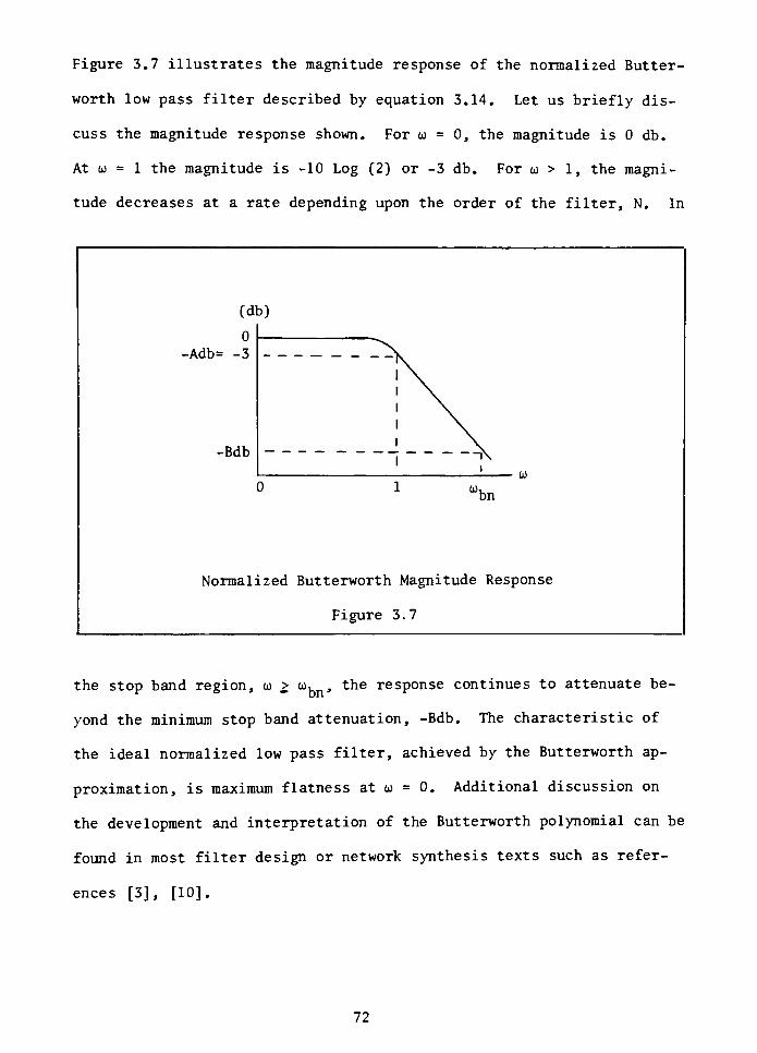
Figure 3.7 illustrates the magnitude response of the normalized Butter

worth low pass filter described by equation 3.14. Let us briefly dis

cuss the magnitude response shown. For oj = 0, the magnitude is 0 db.

At oj = 1 the magnitude is -10 Log (2) or -3 db. For o> > 1, the magni

tude decreases at a rate depending upon the order of the filter, N. In

(db)

0

-Adb=

-3 x

-Bdb

1"^

'0)

0 lo),bn

Normalized Butterworth Magnitude Response

Figure 3.7

the stop band region, oj > whn, the response continues to attenuate be

yond the minimum stop band attenuation, -Bdb. The characteristic of

the ideal normalized low pass filter, achieved by the Butterworth ap

proximation, is maximum flatness at oj = 0. Additional discussion on

the development and interpretation of the Butterworth polynomial can be

found in most filter design or network synthesis texts such as refer

ences [3], [10].

72

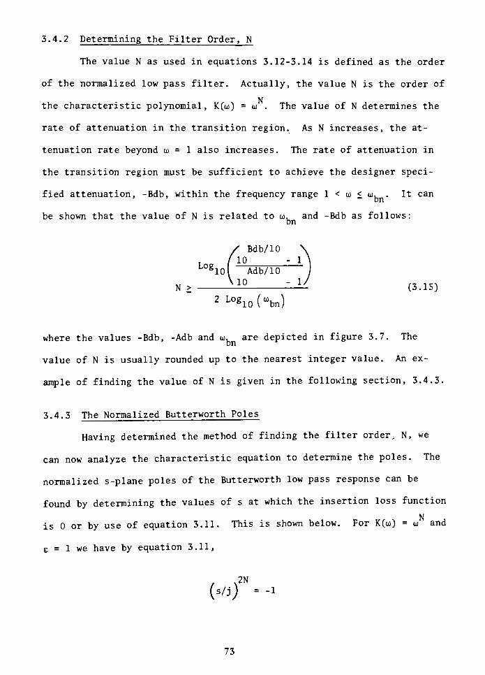
3.4.2 Determining the Filter Order, N

The value N as used in equations 3.12-3.14 is defined as the order

of the normalized low pass filter. Actually, the value N is the order of

Nthe characteristic polynomial, K(oj) = oj . The value of N determines the

rate of attenuation in the transition region. As N increases, the at

tenuation rate beyond oj = 1 also increases. The rate of attenuation in

the transition region must be sufficient to achieve the designer speci

fied attenuation, -Bdb, within the frequency range 1 < oj < oj, . It can

be shown that the value of N is related to oj, and -Bdb as follows:bn

Log

Bdb/ 10

10

10 1 Adb/10

\ 10

2 LOg10(%n)

N > (3.15)

where the values -Bdb, -Adb and oj, are depicted in figure 3.7. The

value of N is usually rounded up to the nearest integer value. An ex

ample of finding the value of N is given in the following section, 3.4.3.

3.4.3 The Normalized Butterworth Poles

Having determined the method of finding the filter order - N, we

can now analyze the characteristic equation to determine the poles. The

normalized s-plane poles of the Butterworth low pass response can be

found by determining the values of s at which the insertion loss function

N

is 0 or by use of equation 3.11. This is shown below. For K(oj) = oj and

e = 1 we have by equation 3.11,

2N

(s/j) =-1

73

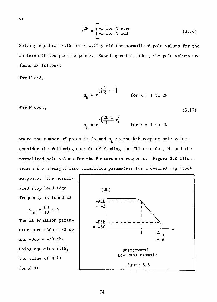
or

_ ) +1 for N even

1 for N odd(3.16)

Solving equation 3.16 for s will yield the normalized pole values for the

Butterworth low pass response. Based upon this idea, the pole values are

found as follows:

for N odd,

j(w ' ^

sk= e for k = 1 to 2N

for N even,(3.17)

s,= e

k

72k-l \

for k = 1 to 2N

where the number of poles is 2N and s, is the kth complex pole value.

Consider the following example of finding the filter order, N, and the

normalized pole values for the Butterworth response. Figure 3.8 illus

trates the straight line transition parameters for a desired magnitude

response. The normal

ized stop band edge

frequency is found as

0)

bn

60

10

The attenuation param

eters are -Adb= -3 db

and -Bdb= -30 db.

Using equation 3.15,

the value of N is

found as

(db)

Butterworth

Low Pass Example

Figure 3.8

74

30/10

.10- 1

3/10

V10"

V 3 002N > a-=

^=

r^rr= x -929

2 Log 6 1.556

Rounding up, N is chosen as 2. For N = 2 (even), the normalized pole

values are found using equation 3.17 as

s, =eJ

for k = 1 to 4

Using Euler's equation, s, can be expanded into real and imaginary terms

as follows:

sk=

k+

H= cos (k i)+ J sin (k

j)

Substituting for k = 1 to 4, the normalized low pass Butterworth poles

for N = 2 are as follows:

s. .

=.707 j .707

1,4

and

S2 3="-707 * j *77

The locations of the pole values reside on the unit circle at a rota

tional interval of ir/2 or45

as shown in figure 3.9.

75

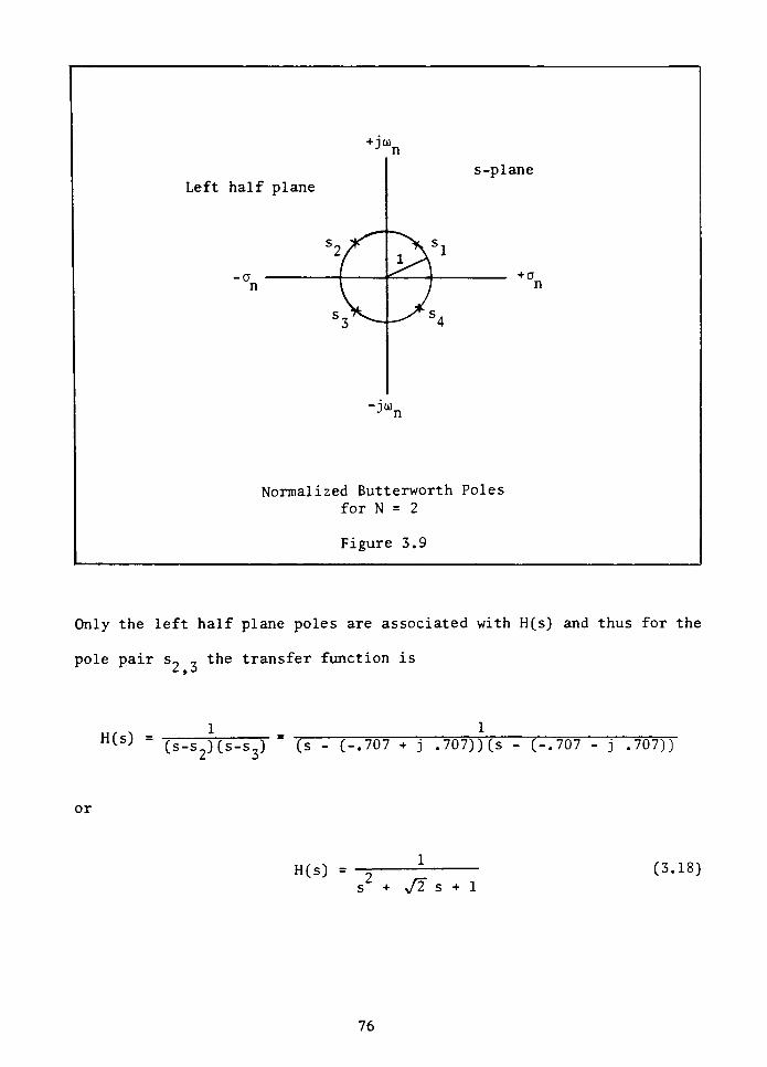
+ JOJJn

Left half plane

s-plane

A>rr 1

S^

| 4-fT

V /

K-A<

-j'

"n

Normalized Butterworth Poles

for N = 2

Figure 3.9

Only the left half plane poles are associated with H(s) and thus for the

pole pair s~ _ the transfer function is

H(s)(s-s2)(s-s3)

"

(s - (-.707 + j .707))(s - (-.707 - j .707))

or

H(s) =

s + JI s + 1

(3.18)

76

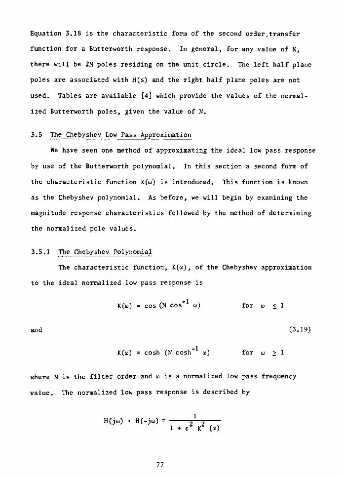
Equation 3.18 is the characteristic form of the second order. transfer

function for a Butterworth response. In general, for any value of N,

there will be 2N poles residing on the unit circle. The left half plane

poles are associated with H(s) and the right half plane poles are not

used. Tables are available [4] which provide the values of the normal

ized Butterworth poles, given the value of N.

3.5 The Chebyshev Low Pass Approximation

We have seen one method of approximating the ideal low pass response

by use of the Butterworth polynomial. In this section a second form of

the characteristic function K(oj) is introduced. This function is known

as the Chebyshev polynomial. As before, we will begin by examining the

magnitude response characteristics followed by the method of determining

the normalized pole values.

3.5.1 The Chebyshev Polynomial

The characteristic function, K(oj) , of the Chebyshev approximation

to the ideal normalized low pass response is

K(o>) = cos (N oj) for oj < 1

and (3.19)

K(oj) = cosh (N o>) for co > 1

where N is the filter order and u is a normalized low pass frequency

value. The normalized low pass response is described by

H(joj) H(-ju)-

5~~21 + e YT (oj)

77

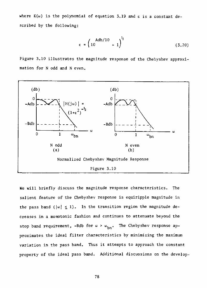
where K(oj) is the polynomial of equation 3.19 and e is a constant de

scribed by the following:

/ Adb/ 10

e = (lO -

l) (3.20)

Figure 3.10 illustrates the magnitude response of the Chebyshev approxi

mation for N odd and N even.

(db) (db)

0 " ">"\"

-Adb \^1_\ |H(jco) | =-Adb

!\ 2 -hi VCl+e )

*â

-Bdb

l N.i i

i \i i

3 1"bn 0 1 obn

0)

N odd N even

(a) (b)

Normalized Chebyshev Magnitude Response

Figure 3.10

We will briefly discuss the magnitude response characteristics. The

salient feature of the Chebyshev response is equiripple magnitude in

the pass band (|oj| < 1) . In the transition region the magnitude de

creases in a monotonic fashion and continues to attenuate beyond the

stop band requirement, -Bdb for to > oj, . The Chebyshev response ap

proximates the ideal filter characteristics by minimizing the maximum

variation in the pass band. Thus it attempts to approach the constant

property of the ideal pass band. Additional discussions on the develop-

78

ment of the Chebyshev approximation can be found in references [3] ,

[12].

3.5.2 Determining the Filter Order, N

The value of the filter order, N, is dependent upon the attenua

tion requirements (-Adb, -Bdb) specified for the transition region

(1 < oj < oj, ) . The value, N, describes the order of the polynomial as

well as the number of normalized low pass poles (2N) . The value of N

is found by the following:

' Bdb/10

10 - 1

N > -j- (3.21)

cosh (o), )bn'

where the values -Bdb and o), are depicted in figure 3.10 and c is de

scribed by equation 3.20. As previously mentioned, the value of N is

usually rounded up to the nearest integer value.

3.5.3 The Normalized Chebyshev Poles

The method of determining the normalized Chebyshev poles is

similar to the method used to find the Butterworth poles. We simply use

equation 3.11 letting K(oj) equal the Chebyshev polynomial (3.19) and

substitute o> = s/j. Then solving for s yields the complex s-plane pole

values. The development of the solutions of K(o>) will not be performed

here (see references [10], [12]). Rather the equations describing the

pole values are simply given as follows. The real (a ) and imaginary

(joi ) values of the Chebyshev normalized low pass poles are found from

79

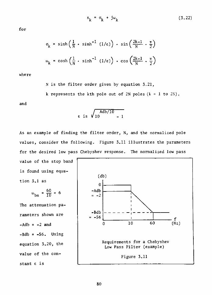
sk=

ak+

1\ (3.22)

for

where

and

ak=

sinh(^ (1/e))sin(-j^-

y)

0),= CO

ksh (I .

(1/e)). cos

(J^-. |)

N is the filter order given by equation 3.21,

k represents the kth pole out of 2N poles (k = 1 to 2N) ,

/ Adb/ 10

is V10 - 1

As an example of finding the filter order, N, and the normalized pole

values, consider the following. Figure 3.11 illustrates the parameters

for the desired low pass Chebyshev response. The normalized low pass

value of the stop band

is found using equa

tion 3.1 as

60

wbn=

10= 6

The attenuation pa

rameters shown are

-Adb= -2 and

-Bdb=-56. Using

equation 3.20, the

value of the con

stant e is

(db)

o

-Adb

= -2

-Bdb

= -56f

0 10 60 (Hz)

Requirements for a Chebyshev

Low Pass Filter (example)

Figure 3.11

80

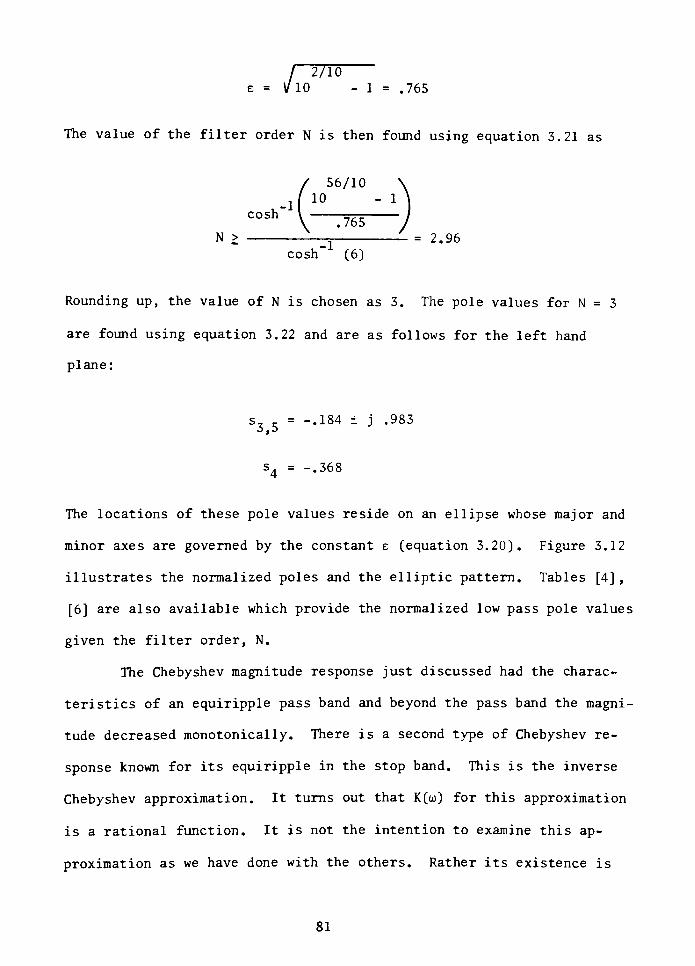
/ 2/10

= V10 - 1 ,765

The value of the filter order N is then found using equation 3.21 as

cosh

56/10

10 - 1

.765

N > = 2.96

(6)

Rounding up, the value of N is chosen as 3. The pole values for N = 3

are found using equation 3.22 and are as follows for the left hand

plane:

s3 5= -.184 j .983

s4=-.368

The locations of these pole values reside on an ellipse whose major and

minor axes are governed by the constant e (equation 3.20). Figure 3.12

illustrates the normalized poles and the elliptic pattern. Tables [4] ,

[6] are also available which provide the normalized low pass pole values

given the filter order, N.

The Chebyshev magnitude response just discussed had the charac

teristics of an equiripple pass band and beyond the pass band the magni

tude decreased monotonically. There is a second type of Chebyshev re

sponse known for its equiripple in the stop band. This is the inverse

Chebyshev approximation. It turns out that K(oj) for this approximation

is a rational function. It is not the intention to examine this ap

proximation as we have done with the others. Rather its existence is

81

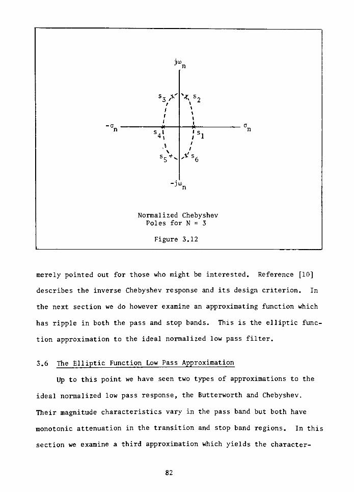
JUr

-a

s V3/* V s

/ V

\

i

s ' s,4. / 1

,1

/\

S5+- 'Vs6

-JO)

Normalized Chebyshev

Poles for N = 3

Figure 3.12

merely pointed out for those who might be interested. Reference [10]

describes the inverse Chebyshev response and its design criterion. In

the next section we do however examine an approximating function which

has ripple in both the pass and stop bands. This is the elliptic func

tion approximation to the ideal normalized low pass filter.

3.6 The Elliptic Function Low Pass Approximation

Lip to this point we have seen two types of approximations to the

ideal normalized low pass response, the Butterworth and Chebyshev.

Their magnitude characteristics vary in the pass band but both have

monotonic attenuation in the transition and stop band regions. In this

section we examine a third approximation which yields the character-

82

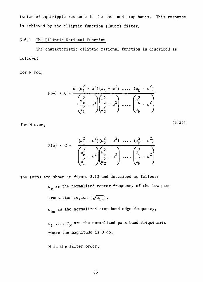
istics of equiripple response in the pass and stop bands. This response

is achieved by the elliptic function (Cauer) filter.

3.6.1 The Elliptic Rational Function

The characteristic elliptic rational function is described as

follows:

for N odd,

K(o>)

. 2 2, 2, ? 2Noj (ojx

- - 0) ) (oj2- 0) ) .... (ojn

- - 0) j

f ? V2 N (2 \OJ

c 20)

c 20)

c 2

2- 0)

20)

2- OJ

u1 J \*2 J ^N )

for N even,(3.23)

,7 2, ? 2. ? 2.

K(oj) =-- C(o)1

- - oj ) (o>2- 0) ) (o)N

- - 0) )

f ? \ /? \ /2 \0)

c 20)

c 20)

c 2

2' - 0)

2- 0)

2- 0)

^1 /V?2 > kWN /

The terms are shown in figure 3.13 and described as follows:

oj is the normalized center frequency of the low pass

c

transition region ( /id, J ,

is the normalized stop band edge frequency,OJ

bn

oj1 ....oj are the normalized pass band frequencies

where the magnitude is 0 db,

N is the filter order,

83

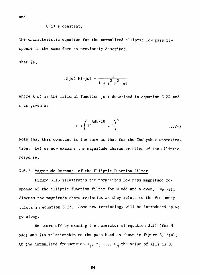
and

C is a constant.

The characteristic equation for the normalized elliptic low pass re

sponse is the same form as previously described.

That is,

H(jo)) H(-joj) =

j-^1 + e K (oj)

where K(oj) is the rational function just described in equation 3.23 and

e is given as

Adb/10\^

10 -

lj (3.24)

Note that this constant is the same as that for the Chebyshev approxima

tion. Let us now examine the magnitude characteristics of the elliptic

response.

3.6.2 Magnitude Response of the Elliptic Function Filter

Figure 3.13 illustrates the normalized low pass magnitude re

sponse of the elliptic function filter for N odd and N even. We will

discuss the magnitude characteristics as they relate to the frequency

values in equation 3.23. Some new terminology will be introduced as we

go along.

We start off by examing the numerator of equation 3.23 (for N

odd) and its relationship to the pass band as shown in figure 3.13(a).

At the normalized frequencies oj., oj2....

u>Nthe value of K(oj) is 0.

84

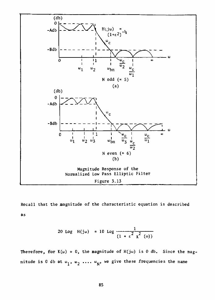
(db)

o

-Adb ^w^r_s-/\ H(jo,) =

,

l\(1^2)"*

\ ">

1 \ c

-Bdb

i i\A^\Aii i V V

0 ' 11 i Noc 1

oil o)2 u)bn uc

"1

N odd (= 5)

CO

(dt

0

-Adb

(a)

>)

-^<_ _ \c<_ _VL _\

1 Vc

-Bdb

i ii1 i V V

^^v

1_ O)

0' ' 1 1 vo> 1

lii | _ |

o)j o>2 o)3 o)bn o)3 c

oTJ

o>c

"1

N even (= 6)

(b)

Magnitude Response of the

Normalized Low Pass Elliptic Fi Iter

Figure 3.13

Recall that the magnitude of the characteristic equation is described

as

20 Log H(j(u) = 10 Log = ~

(1 + t K ())

Therefore, for K(oj) = 0, the magnitude of H(jo>) is 0 db. Since the mag

nitude is 0 db at u., u, .... t*K, we give these frequencies the name

85

ZEROS of ATTENUATION. Notice the difference in magnitude at oi = 0 be

tween N odd and N even in figure 3.13. The magnitude is 0 db at o> = 0

for N odd due to the singular term, oi, in the numerator of equation

3.23. Notice also that at o> = 1 the magnitude of the response is -Adb

-h2

which is derived from 20 Log (1 + e ) . From the form of the charac

teristic equation above we find that K(o>) must equal 1 at the pass band

frequencies where the magnitude is -Adb.

Now we focus our attention on the stop band region. By examining

the denominator of equation 3.23 we see that at the frequencies o> /o>.,

o)c/o>2 .... ojc/o>n, the value of K(o>) is . Then the magnitude of the re

sponse described by the characteristic function is zero or - db. The

frequencies oj^/oj, .... o> /oj., are shown in figure 3.13 at the minimumc i c N

points in the stop band region. We give these frequencies the term

FREQUENCIES of INFINITE LOSS.

At this point we observe that there is a relationship between the

pass band and stop band. Since the magnitude is 0 db at id., u. .... o>

in the pass band and - db at uc/u. .... uc/u} in the stop band, it

follows that the characteristic function K(oi) has the following recip

rocal property:

K<V' <3-25>

where is a constant given by

Bdb/10

L =' Âdb/lO" '

1 <3'26)

10 - 1>

86

This explains the salient features of the magnitude response shapes for

N odd and N even. Now we wish to address the problem of finding the

order of the filter, N, and the normalized pole/zero values.

3.6.3 The Normalized Poles and Zeros of the Elliptic Function Filter

The methods of determining the value N and subsequently the nor

malized poles and zeros is complex and involves an analysis of the char

acteristic rational function using elliptic integrals and elliptic

trigonometric functions. The reader is referred to the appendix for a

discussion of this analysis and an example. We can however gain some

insight to what the pole/zero values are by examining equation 3.23.

In section 3.3.2 it was pointed out that for a rational function

such as

D(oj)

the values at which D(oi) is zero correspond to the s-plane zeros of the

transfer function, H(s) , when oj = s/j. Therefore by equation 3.23 the

zeros of H(s) correspond to the complex values at which the denominator

of K(o>) is 0.

That is, for

s = j u>c /a^, j ">c/o>2.... j wc/ojn

we have the normalized s-plane zeros.

In regards to the pole values, we know from the examination of

the Chebyshev response that equiripple in the pass band corresponds to

an s-plane locus of poles in the shape of an ellipse. Combining these

87

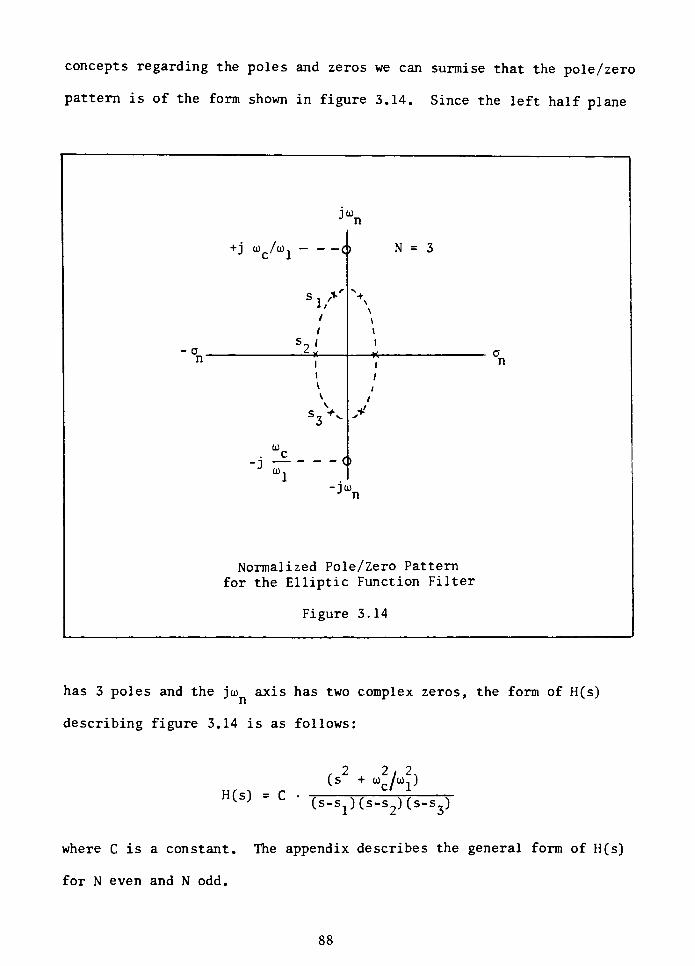
concepts regarding the poles and zeros we can surmise that the pole/zero

pattern is of the form shown in figure 3.14. Since the left half plane

a.

n

Vr

+j u /o). 4> N = 3

1/

I

V

V

\

S3^

. "cj

4>

-JO)

+'

n

an

Normalized Pole/Zero Pattern

for the Elliptic Function Filter

Figure 3.14

has 3 poles and the joi axis has two complex zeros, the form of H(s)

describing figure 3.14 is as follows:

H(s)

r2 2/2,(s + U^/Wj)

(s-s1)(s-s2)(s-s3)

where C is a constant. The appendix describes the general form of H(s)

for N even and N odd.

88

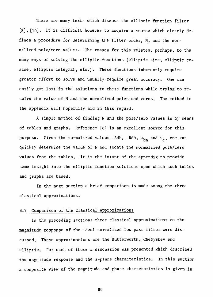
There are many texts which discuss the elliptic function filter

[5] , [10] It is difficult however to acquire a source which clearly de

fines a procedure for determining the filter order, N, and the nor

malized pole/zero values. The reason for this relates, perhaps, to the

many ways of solving the elliptic functions (elliptic sine, elliptic co

sine, elliptic integral, etc.). These functions inherently require

greater effort to solve and usually require great accuracy. One can

easily get lost in the solutions to these functions while trying to re

solve the value of N and the normalized poles and zeros. The method in

the appendix will hopefully aid in this regard.

A simple method of finding N and the pole/zero values is by means

of tables and graphs. Reference [6] is an excellent source for this

purpose. Given the normalized values -Adb, -Bdb, oi, and oi,one can

quickly determine the value of N and locate the normalized pole/zero

values from the tables. It is the intent of the appendix to provide

some insight into the elliptic function solutions upon which such tables

and graphs are based.

In the next section a brief comparison is made among the three

classical approximations.

3.7 Comparison of the Classical Approximations

In the preceding sections three classical approximations to the

magnitude response of the ideal normalized low pass filter were dis

cussed. These approximations are the Butterworth, Chebyshev and

elliptic. For each of these a discussion was presented which described

the magnitude response and the s-plane characteristics. In this section

a composite view of the magnitude and phase characteristics is given in

89

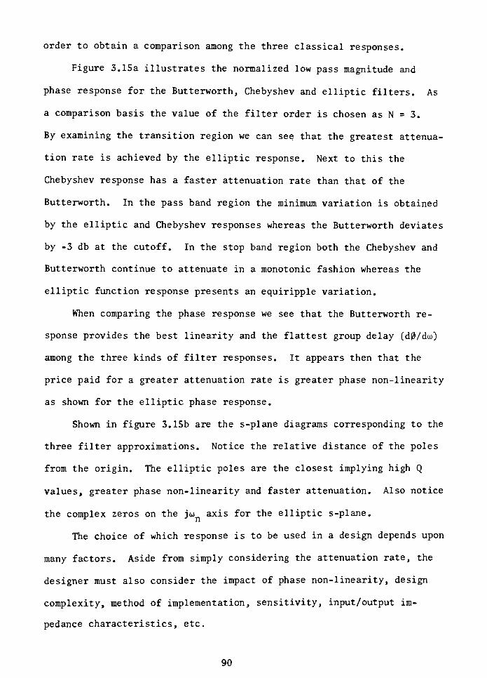
order to obtain a comparison among the three classical responses.

Figure 3.15a illustrates the normalized low pass magnitude and

phase response for the Butterworth, Chebyshev and elliptic filters. As

a comparison basis the value of the filter order is chosen as N = 3.

By examining the transition region we can see that the greatest attenua

tion rate is achieved by the elliptic response. Next to this the

Chebyshev response has a faster attenuation rate than that of the

Butterworth. In the pass band region the minimum variation is obtained

by the elliptic and Chebyshev responses whereas the Butterworth deviates

by -3 db at the cutoff. In the stop band region both the Chebyshev and

Butterworth continue to attenuate in a monotonic fashion whereas the

elliptic function response presents an equiripple variation.

When comparing the phase response we see that the Butterworth re

sponse provides the best linearity and the flattest group delay (d0/dos)

among the three kinds of filter responses. It appears then that the

price paid for a greater attenuation rate is greater phase non-linearity

as shown for the elliptic phase response.

Shown in figure 3.15b are the s-plane diagrams corresponding to the

three filter approximations. Notice the relative distance of the poles

from the origin. The elliptic poles are the closest implying high Q

values, greater phase non-linearity and faster attenuation. Also notice

the complex zeros on the joi axis for the elliptic s-plane.

The choice of which response is to be used in a design depends upon

many factors. Aside from simply considering the attenuation rate, the

designer must also consider the impact of phase non-linearity, design

complexity, method of implementation, sensitivity, input/output im

pedance characteristics, etc.

90

(db)

0

-3

H(jo>)

-Bdb

0(jo>)

]">t

/l

-1

Butterworth

ideal

low pass

o

n

Butterworth

Chebyshev

elliptic

elliptic

Butterworth

Chebyshev

(a)

^r Wr

-1

/ \

V /

V ,*

-i

0n

Chebyshev

(b)

-1

elliptic

..1

Comparison of the Normalized

Butterworth, Chebyshev and Elliptic Responses

Figure 3.15

91

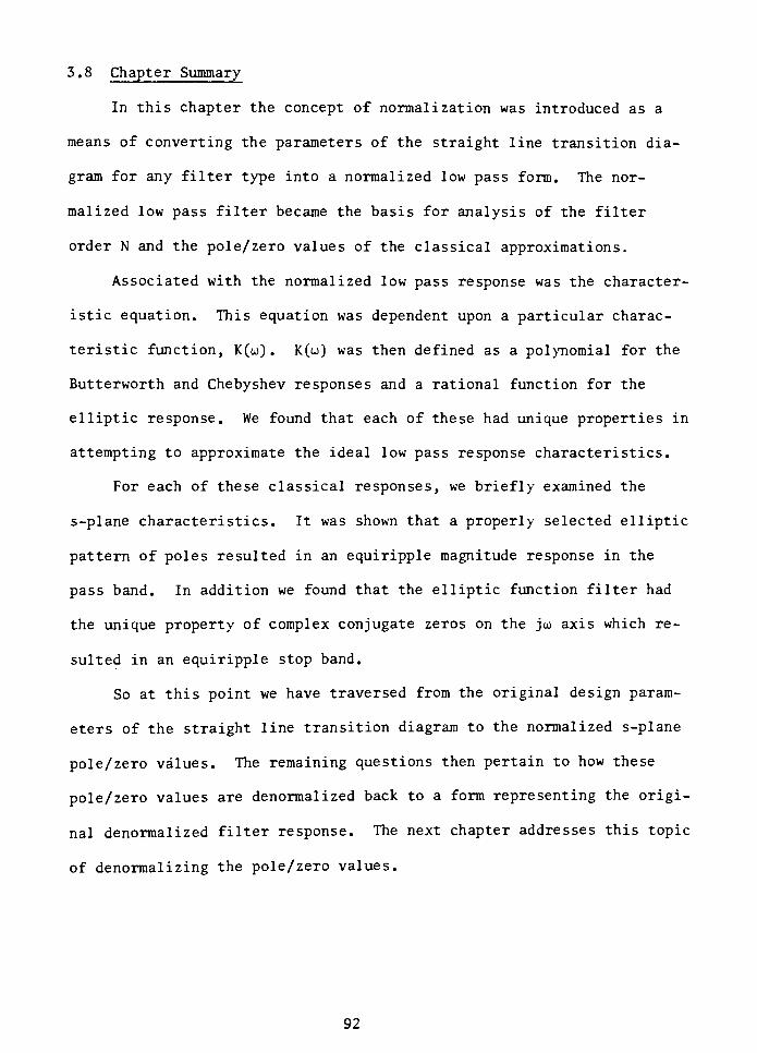
3.8 Chapter Summary

In this chapter the concept of normalization was introduced as a

means of converting the parameters of the straight line transition dia

gram for any filter type into a normalized low pass form. The nor

malized low pass filter became the basis for analysis of the filter

order N and the pole/zero values of the classical approximations.

Associated with the normalized low pass response was the character

istic equation. This equation was dependent upon a particular charac

teristic function, K(oj) . K(oj) was then defined as a polynomial for the

Butterworth and Chebyshev responses and a rational function for the

elliptic response. We found that each of these had unique properties in

attempting to approximate the ideal low pass response characteristics.

For each of these classical responses, we briefly examined the

s-plane characteristics. It was shown that a properly selected elliptic

pattern of poles resulted in an equiripple magnitude response in the

pass band. In addition we found that the elliptic function filter had

the unique property of complex conjugate zeros on the jo> axis which re

sulted in an equiripple stop band.

So at this point we have traversed from the original design param

eters of the straight line transition diagram to the normalized s-plane

pole/zero values. The remaining questions then pertain to how these

pole/zero values are denormalized back to a form representing the origi

nal denormalized filter response. The next chapter addresses this topic

of denormalizing the pole/zero values.

92

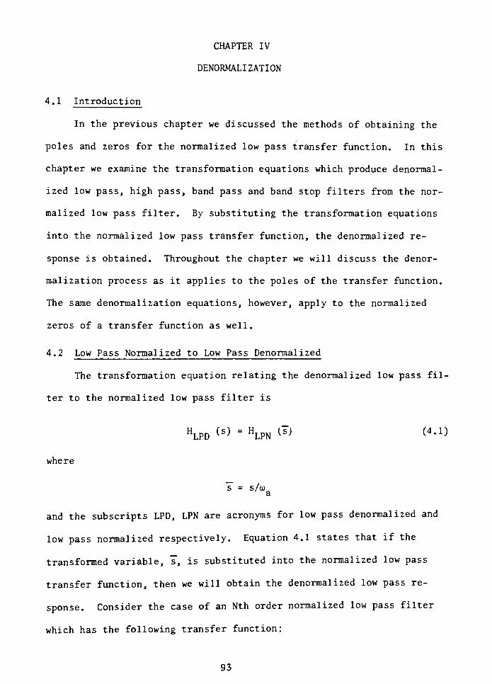
CHAPTER IV

DENORMALIZATION

4.1 Introduction

In the previous chapter we discussed the methods of obtaining the

poles and zeros for the normalized low pass transfer function. In this

chapter we examine the transformation equations which produce denormal

ized low pass, high pass, band pass and band stop filters from the nor

malized low pass filter. By substituting the transformation equations

into the normalized low pass transfer function, the denormalized re

sponse is obtained. Throughout the chapter we will discuss the denor

malization process as it applies to the poles of the transfer function.

The same denormalization equations, however, apply to the normalized

zeros of a transfer function as well.

4.2 Low Pass Normalized to Low Pass Denormalized

The transformation equation relating the denormalized low pass fil

ter to the normalized low pass filter is

HLPD ^=

HLPN & C4'1)

where

7 =

s/o)a

and the subscripts LPD, LPN are acronyms for low pass denormalized and

low pass normalized respectively. Equation 4.1 states that if the

transformed variable, s", is substituted into the normalized low pass

transfer function, then we will obtain the denormalized low pass re

sponse. Consider the case of an Nth order normalized low pass filter

which has the following transfer function:

93

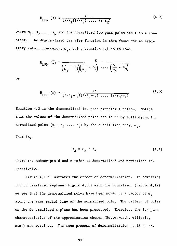
H (s) = (4-2)LPN

lSJ(s-Sl)(s-s2) .... (s-sN)

where s^, s2 ....s are the normalized low pass poles and K is a con

stant. The denormalized transfer function is then found for an arbi

trary cutoff frequency, oj using equation 4.1 as follows:9.

HIDM (s)LPN

' J/s

(=Z_,1Xs -*')-(%-*>')or

H (s) = *1 (4.3)LPD (s-sro)a)(s-s2.o)a) .... (s-sN-o)a)

Equation 4.3 is the denormalized low pass transfer function. Notice

that the values of the denormalized poles are found by multiplying the

normalized poles (s..,s .... s ) by the cutoff frequency, oj

.

That is,

s ,= o) s (4.4)dan y j

where the subscripts d and n refer to denormalized and normalized re

spectively.

Figure 4.1 illustrates the effect of denormalization. In comparing

the denormalized s-plane (Figure 4.1b) with the normalized (Figure 4.1a)

we see that the denormalized poles have been moved by a factor of oj

along the same radial line of the normalized pole. The pattern of poles

on the denormalized s-plane has been preserved. Therefore the low pass

characteristics of the approximation chosen (Butterworth, elliptic,

etc.) are retained. The same process of denormalization would be ap-

94

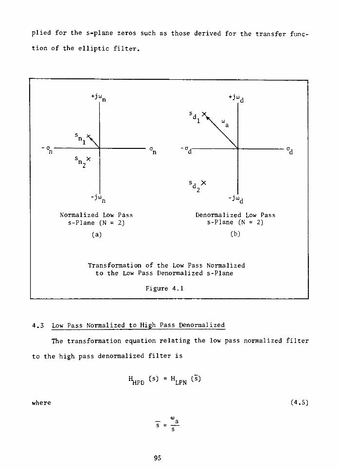
plied for the s-plane zeros such as those derived for the transfer func

tion of the elliptic filter.

a -

n

+J0)J T

V

-3n

Normalized Low Pass

s-Plane (N = 2)

n

(a)

sd X

+ JO0

-JO),

Denormalized Low Pass

s-Plane (N = 2)

(b)

Transformation of the Low Pass Normalized

to the Low Pass Denormalized s-Plane

Figure 4. 1

4.3 Low Pass Normalized to High Pass Denormalized

The transformation equation relating the low pass normalized filter

to the high pass denormalized filter is

"hPD (S) =

HLPN &

where (4.5)

O)

as =

s

95

The notation used here is similar to that of eq. 4.1. By substituting

s for s in the normalized low pass transfer function (eq. 4.2), the de-

normalized high pass transfer function can be found as shown below.

HLPN <s>

(r-- si)Gr-s2)(ir-

sn)

KsN

f0) - SS,)(0) -

SS) .... (0) - ss.,\.V a 1'^ a

2' V a N'

or

"hpd <> -

, ,x/ A t-vt<4-

rx-s-r)

Equation 4.6 is the denormalized high pass transfer function for the low

pass filter order, N. The denormalized poles shown in the denominator

are related to the normalized poles (s, s2

.... s ) as follows:

O)

sA= (4.7)

d sn

Equation 4.7 states that the denormalized high pass pole, sd, can be

found by inverting the normalized low pass pole, sn, (generally a com

plex value) and then multiplying by the arbitrary denormalized high pass

cutoff frequency, oj .Figure 4.2 illustrates the effect of the denor-

a

malization. The reciprocal relationship in s is denoted by the crossing

lines. Multiplying by oj results in a displacement along the radial

line of the inverted normalized pole as shown in figure 4.2b.

96

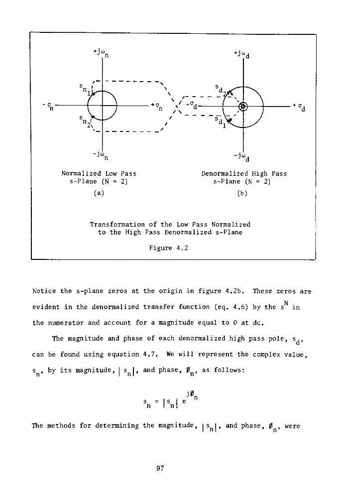
+ JOJ + J0)

a -

n

-jo)n

Normalized Low Pass

s-Plane (N = 2)

(a)

+ a ,

-jo)d

Denormalized High Pass

s-Plane (N = 2)

(b)


to the High Pass Denormalized s-Plane

Figure 4.2

Notice the s-plane zeros at the origin in figure 4.2b. These zeros are

Nevident in the denormalized transfer function (eq. 4.6) by the s in

the numerator and account for a magnitude equal to 0 at dc.

The magnitude and phase of each denormalized high pass pole, s, ,

can be found using equation 4.7. We will represent the complex value,

s , by its magnitude, Is I, and phase, 0 as follows:

JKs = s e

nIn"

The methods for determining the magnitude, is I, and phase, 0 ,were

97

presented in section 2.5.1. The denormalized high pass pole, s,, is

found from

j(-0n)0) OJ

a a _

sj= =

;'

d s sin n

Notice the inverse magnitude and negative phase relationship to the nor

malized values in the above equation for s,. In terms of the denormal

ized real (ad) and imaginary (jtoJ parts we have the following

sd=

ad+

jo)d (4.8)

where

d=

n0)

aIM2

jo)d=

+ JO)Jn

IM2

0)

a

4.4 Low Pass Normalized to Band Pass Denormalized

The transformation equation relating the band pass denormalized

filter to the low pass normalized filter is

HBPD (S) =

HLPN & <4-9)

where

2 2s +0)

cs =

Bs

B is the bandwidth,

98

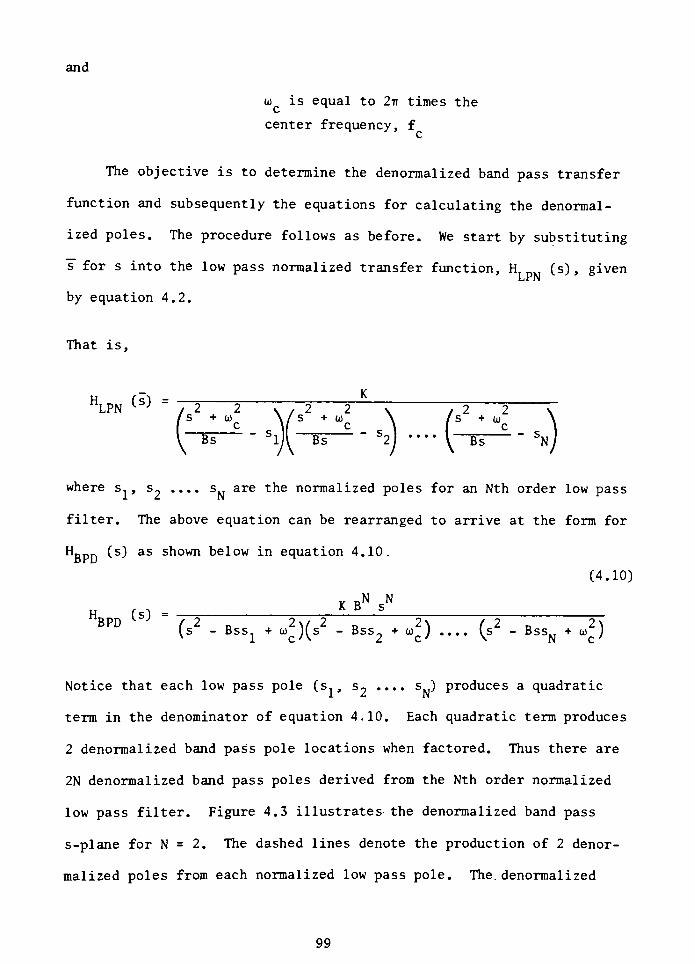
and

oj is equal to 2ir times the

center frequency, f

The objective is to determine the denormalized band pass transfer

function and subsequently the equations for calculating the denormal

ized poles. The procedure follows as before. We start by substituting

s for s into the low pass normalized transfer function, H (s) , given

Lr IN

by equation 4.2.

That is,

HIDM (s) =

LPN*- J

/ 2 2 \ / 2 2 \ / 2 2' " '

0)/s + 0) \/s +0) \ /s +

-"

SN

where s., s_ .... s are the normalized poles for an Nth order low pass

filter. The above equation can be rearranged to arrive at the form for

HBpn (s) as shown below in equation 4.10.

(4.10)

KBN

<;N

HBPD ^-

(s - Bss + oj )(s - Bss + oj ) .... (s - Bss + oj )

Notice that each low pass pole (s.., s2 .... s.,) produces a quadratic

term in the denominator of equation 4.10. Each quadratic term produces

2 denormalized band pass pole locations when factored. Thus there are

2N denormalized band pass poles derived from the Nth order normalized

low pass filter. Figure 4.3 illustrates the denormalized band pass

s-plane for N = 2. The dashed lines denote the production of 2 denor

malized poles from each normalized low pass pole. The. denormalized

99

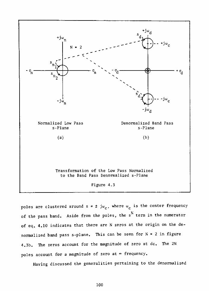
+J0)

+ JOJJ T

Ho -

n

N ..--

.^.

'

V.

0 a v-

o ,-

n v a -6*

-JO)

Normalized Low Pass

s-Plane

VG~

+J0)

+ o ,

-JO),

-jar

(a)

Denormalized Band Pass

s-Plane

(b)


to the Band Pass Denormalized s-Plane

Figure 4.3

poles are clustered around s = jo>c, whereojc

is the center frequency

N

of the pass band. Aside from the poles, the s term in the numerator

of eq. 4.10 indicates that there are N zeros at the origin on the de-

normalized band pass s-plane. This can be seen for N = 2 in figure

4.3b. The zeros account for the magnitude of zero at dc. The 2N

poles account for a magnitude of zero at frequency.

Having discussed the generalities pertaining to the denormalized

100

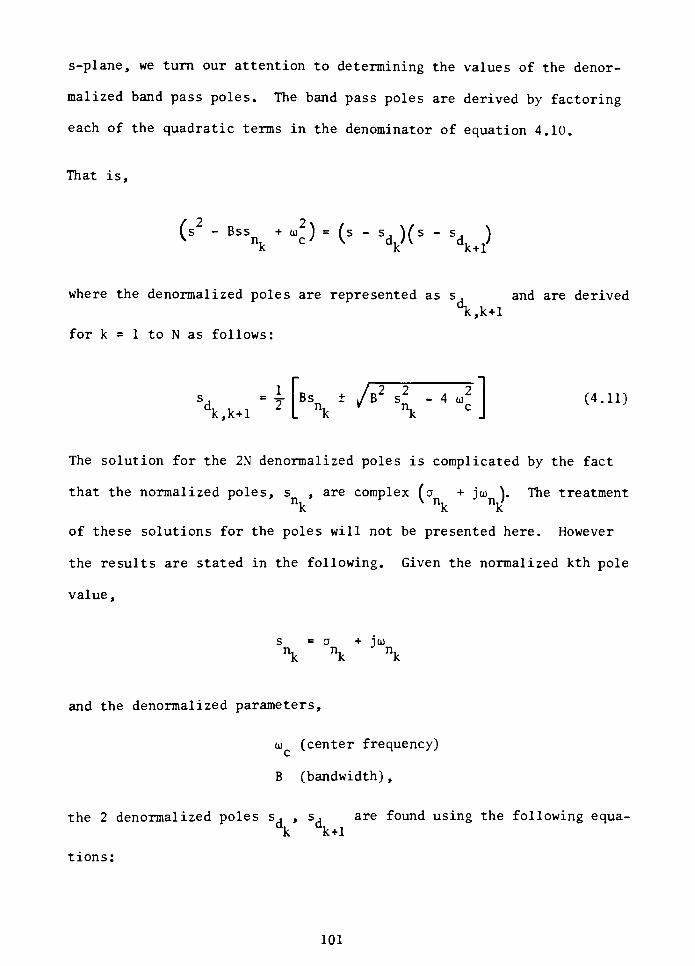
s-plane, we turn our attention to determining the values of the denor

malized band pass poles. The band pass poles are derived by factoring

each of the quadratic terms in the denominator of equation 4.10.

That is,

(s2- Bss +o)2)=(s - s)(s - s )k k k+1

where the denormalized poles are represented as s, and are derived

Tc.k+l

for k = 1 to N as follows:

^k+JBs^

/b2- 4

nkV\

(4.11)

The solution for the 2N denormalized poles is complicated by the fact

that the normalized poles, s ,are complex (a + joj \. The treatment

V K\ nk'

of these solutions for the poles will not be presented here. However

the results are stated in the following. Given the normalized kth pole

value,

S =0 + JO)

nk nk nk

and the denormalized parameters,

oj (center frequency)

B (bandwidth) ,

the 2 denormalized poles s, , sdare found using the following equa-

k k+1

tions:

101

\*

\*

J\(4.12)

(!k k

and

i,=

Cd,i

+

JX ,k+1 Tc+1 k+1

(4.13)

(I '

\ "I^R cos

7)+ J (I '

V"

2'R sin f)

where2 f2cf

tan

oj - (2 ID V

k = 1 to N

N = order of the normalized low pass filter

The above equations can be somewhat tedious to solve given any reason

able value of N but are necessary for determining the exact denormal

ized pole values. For most cases, approximations can be used in place

of the above equations. For the case where oj is much greater than

J ,0)

V \and B/2, equations 4.14 and 4.15 as shown below can be used to

determine the denormalized band pass pole values.

s ,

= (a ,+ jo>

, ^ = =- a + j ( oj + u )dk Uk V

2nk

v c 2nk

(4.14)

102

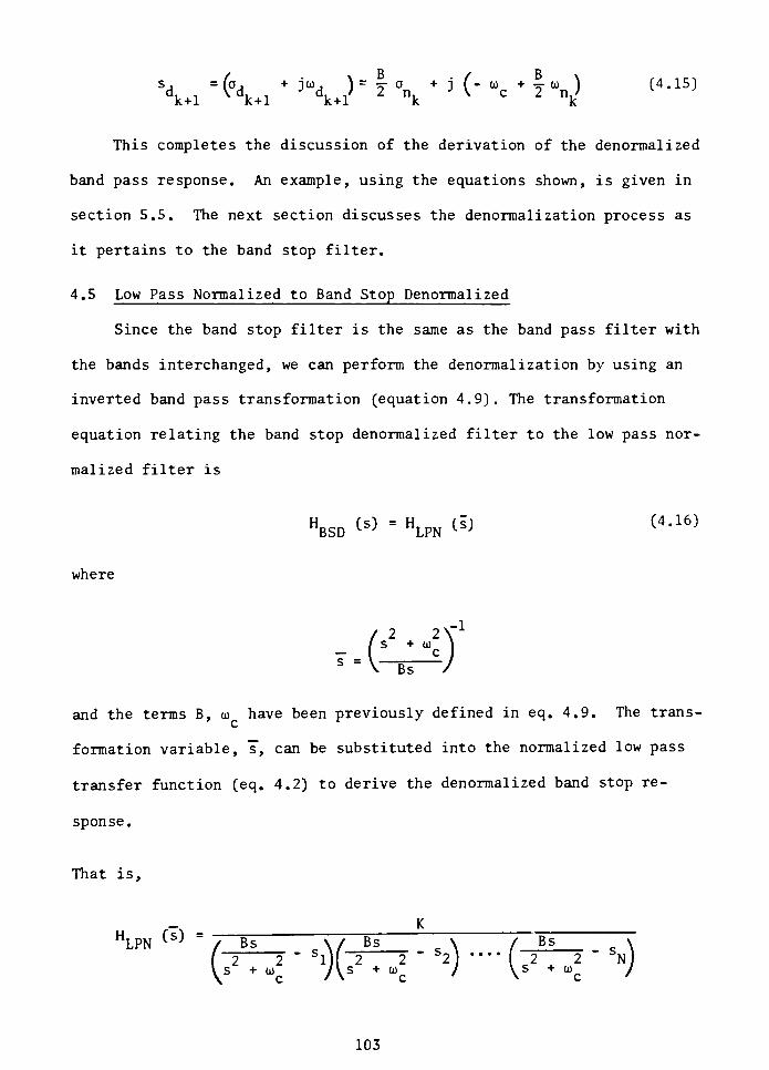
K+J dk+l <W2\

K C 2V

This completes the discussion of the derivation of the denormalized

band pass response. An example, using the equations shown, is given in

section 5.5. The next section discusses the denormalization process as

it pertains to the band stop filter.

4.5 Low Pass Normalized to Band Stop Denormalized

Since the band stop filter is the same as the band pass filter with

the bands interchanged, we can perform the denormalization by using an

inverted band pass transformation (equation 4.9). The transformation

equation relating the band stop denormalized filter to the low pass nor

malized filter is

H (s) = H fs) (4.16)BSD

L ;LPN

l J

where

Bs

and the terms B, oj have been previously defined in eq. 4.9. The trans

formation variable, s", can be substituted into the normalized low pass

transfer function (eq. 4.2) to derive the denormalized band stop re

sponse.

That is,

K

HLPN ^~

/ Bs \/ Bs \ / Bs

[2 2'

Slj[2 2"

S2] [2 2"

SNj

103

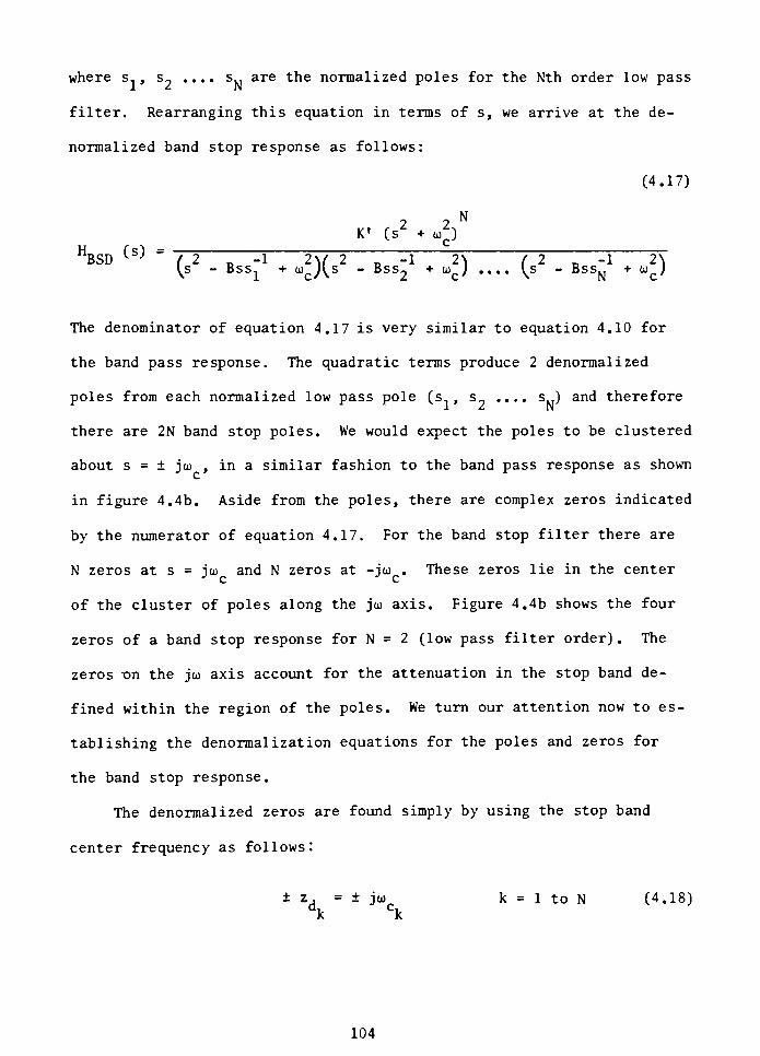
where s. , s_ .... sNare the normalized poles for the Nth order low pass

filter. Rearranging this equation in terms of s, we arrive at the de-

normalized band stop response as follows:

(4.17)

2 2N

V(s*

+ to )

HBSD ^=

( 2D

-1 2\/2D

-1 2\ ( 2 _ -1 2\^s - Bss. + oj J^s -

Bss2+ u>c) .... \s

-

BssN+ oj )

The denominator of equation 4.17 is very similar to equation 4.10 for

the band pass response. The quadratic terms produce 2 denormalized

poles from each normalized low pass pole (s..,s_ .... s ) and therefore

there are 2N band stop poles. We would expect the poles to be clustered

about s = joj,in a similar fashion to the band pass response as shown

in figure 4.4b. Aside from the poles, there are complex zeros indicated

by the numerator of equation 4.17. For the band stop filter there are

N zeros at s = joj and N zeros at -jo> . These zeros lie in the centerJc c

of the cluster of poles along the joj axis. Figure 4.4b shows the four

zeros of a band stop response for N = 2 (low pass filter order) . The

zeros on the jo) axis account for the attenuation in the stop band de

fined within the region of the poles. We turn our attention now to es

tablishing the denormalization equations for the poles and zeros for

the band stop response.

The denormalized zeros are found simply by using the stop band

center frequency as follows".

z .= jo) k = 1 to N (4.18)

ak ck

104

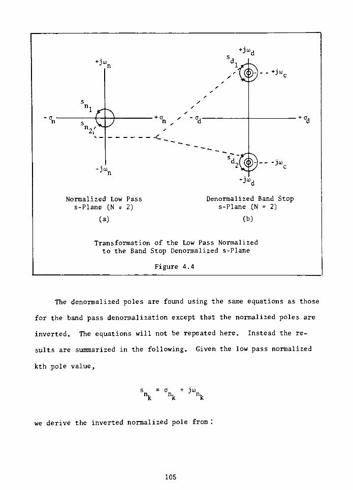
+ J0)

+J0)

a -

n

ni

r^0

<-}-- +JW,

+o^ ?

- o,-

n,

d

C

-JO)

n

+ a ,

Normalized Low Pass

s-Plane (N = 2)

(a)

p> joj.

Denormalized Band Stops-Plane (N = 2)

(b)


to the Band Stop Denormalized s-Plane

Figure 4.4

The denormalized poles are found using the same equations as those

for the band pass denormalization except that the normalized poles are

inverted. The equations will not be repeated here. Instead the re

sults are summarized in the following. Given the low pass normalized

kth pole value,

; = a + joj

nk nk nk

we derive the inverted normalized pole from

105

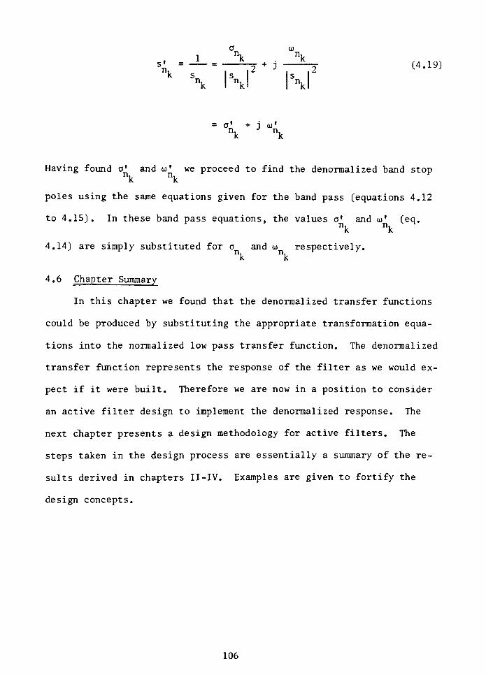
(J 0)

1 nk nk

k s~ si s

nk I nkl I nkl

= 0'

+ jin'

n,J

n,

Having found o'

andoj'

we proceed to find the denormalized band stop

poles using the same equations given for the band pass (equations 4.12

to 4.15). In these band pass equations, the valuesa'

ando>'

(eq.

nk \

4.14) are simply substituted for a and oj respectively.

k k

4.6 Chapter Summary

In this chapter we found that the denormalized transfer functions

could be produced by substituting the appropriate transformation equa

tions into the normalized low pass transfer function. The denormalized

transfer function represents the response of the filter as we would ex

pect if it were built. Therefore we are now in a position to consider

an active filter design to implement the denormalized response. The

next chapter presents a design methodology for active filters. The

steps taken in the design process are essentially a summary of the re

sults derived in chapters II-IV. Examples are given to fortify the

design concepts.

106

CHAPTER V


5.1 Introduction

In the previous chapter we derived the denormalized transfer func

tions. If we were to summarize the steps taken to arrive at the denor

malized transfer functions, as presented in the first four chapters, we

would have a list of the basic analytical steps needed to perform a fil

ter design. These steps are illustrated in figure 5.1. We started by

defining the magnitude response parameters of the desired filter using a

straight line transition diagram (step 1). Then the normalized low pass

filter was derived (step 2). Using the parameters of the normalized low

pass filter^ the filter order, N, and the normalized pole/zero values

were determined for a selected approximation (step 3). Then the nor

malized poles and zeros were transformed into the denormalized poles and

zeros which constitute the desired filter response (step 4). What re

mains is the final step of implementing the denormalized transfer func

tion (step 5) .

In this chapter we examine the techniques which implement the de-

normalized transfer functions using active filters. Among the various

classes of active filter designs, we will use the infinite-gain multiple-

feedback (IGMF) configuration. The term infinite-gain applies to the

ideal nature of the open loop gain, A, of an operational amplifier. The

term multiple feedback refers to the use of multiple feedback paths to

achieve a given transfer function. We will examine the design equations

used and the active filter networks needed to implement the denormalized

transfer functions.

107

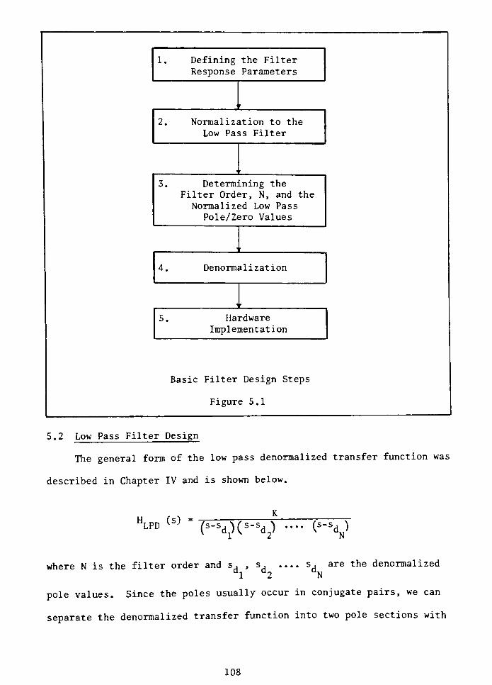
1. Defining the Filter

Response Parameters

'

2. Normalization to the

Low Pass Filter

"

3. Determining the

Filter Order, N, and the

Normalized Low Pass

Pole/Zero Values

"

4. Denormalization

V

5. Hardware

Implementation

Basic Filter Design Steps

Figure 5.1

5.2 Low Pass Filter Design

The general form of the low pass denormalized transfer function was

described in Chapter IV and is shown below.

HLPD (S) =

(s-sd)(s-sdp.... (s-s^)

where N is the filter order and s, , s, . . . . s, are the denormalized

1 2 N

pole values. Since the poles usually occur in conjugate pairs, we can

separate the denormalized transfer function into two pole sections with

108

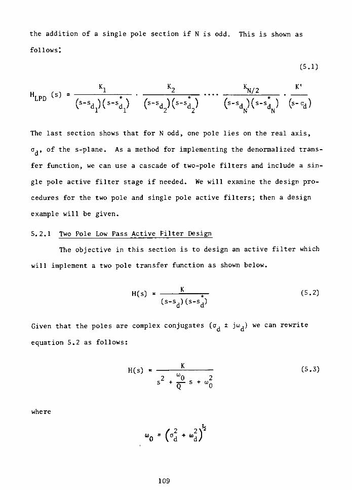
the addition of a single pole section if N is odd. This is shown as

follows!

(5.1)

Kl K2 h/2K'

HLPD <s> =

{*-%)(*'%) (S"SdJ(S"Sd) (s-sdJ(s"sd) (S"d)11 2 2 N N

The last section shows that for N odd, one pole lies on the real axis,

a,, of the s-plane. As a method for implementing the denormalized trans

fer function, we can use a cascade of two-pole filters and include a sin

gle pole active filter stage if needed. We will examine the design pro

cedures for the two pole and single pole active filters; then a design

example will be given.

5.2.1 Two Pole Low Pass Active Filter Design

The objective in this section is to design an active filter which

will implement a two pole transfer function as shown below.

H(S) = ^ ;- (5.2)

(s-sd)(s-sd)

Given that the poles are complex conjugates (a, joij we can rewrite

equation 5.2 as follows:

H(s) = - (5.3)

2 "0 2s +

CTS

W0

where

"o= (4 +

l)

109

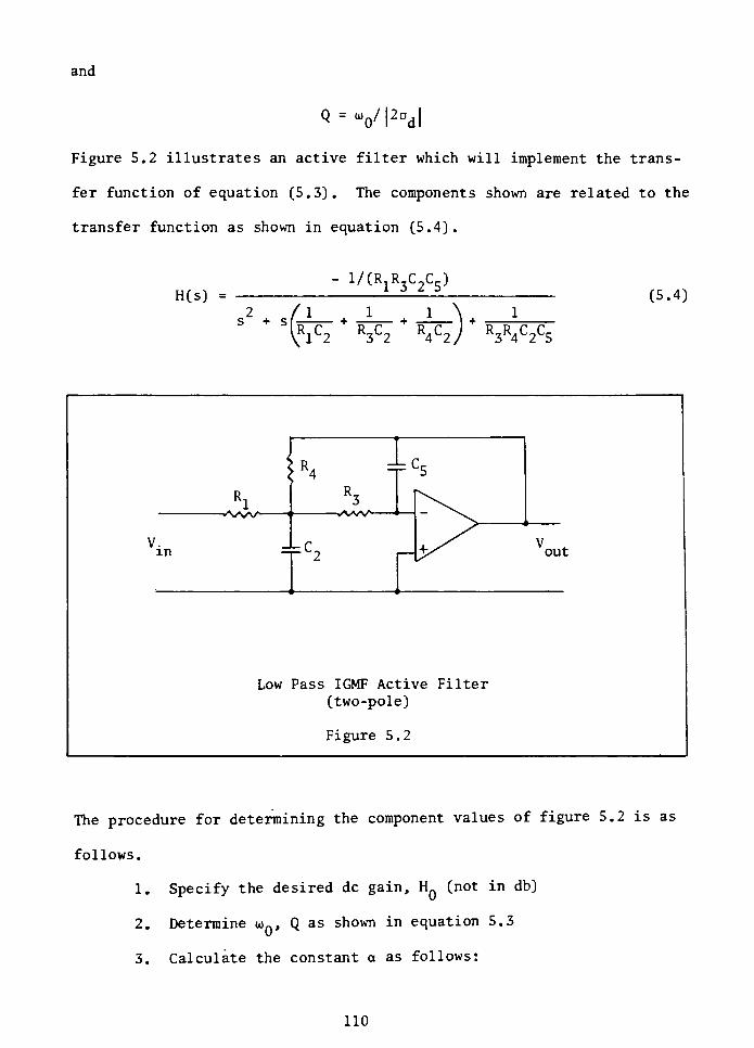
and

Q =

VI2odl

Figure 5.2 illustrates an active filter which will implement the trans

fer function of equation (5.3). The components shown are related to the

transfer function as shown in equation (5.4).

H(s) =

- 1/(R1R3C2C5)

(5.4)s2

+ si

R1C2 R3C2 R4C2. R3R4C2C5

V.in

Tn=c5

Ri 3-vWV>-

=tc. out

Low Pass IGMF Active Filter

(two-pole)

Figure 5 . 2

The procedure for determining the component values of figure 5.2 is as

follows.

1. Specify the desired dc gain, HQ(not in db)

2. Determine o)n, Q as shown in equation 5.3

3. Calculate the constant a as follows:

110

2

[1 +2V2

8

4. Select a reasonable value for C^(10~

is a good starting

value)

5. Find C2 from C2= a C5

6. Find R.. and R2 as follows:

N-l

Rl=

R2"

(u0 *

C5*

^~r%)

7. Determine R. from

R4=

H0*

Rl

If the first iteration of the above procedure does not yield reasonable

values, Cr is chosen differently and steps 5-7 are repeated. The design

er should consider other factors when choosing component values such as

input impedance, op-amp bias currents, component values at high fre

quencies, Johnson noise for low level applications, etc.

5.2.2 Single Pole Low Pass Active Filter

For the case where the filter order, N, is odd, the transfer func

tion will require a single pole section which has the following form

H(s) =

K'

(5.5)5 "

d

where the pole value, o, , is real. This was previously shown in equation

5.1. Figure 5.3 illustrates the single order filter configuration used

to implement the transfer function of equation 5.5. The component values

shown are related to the transfer function, equation 5.5, as follows:

111

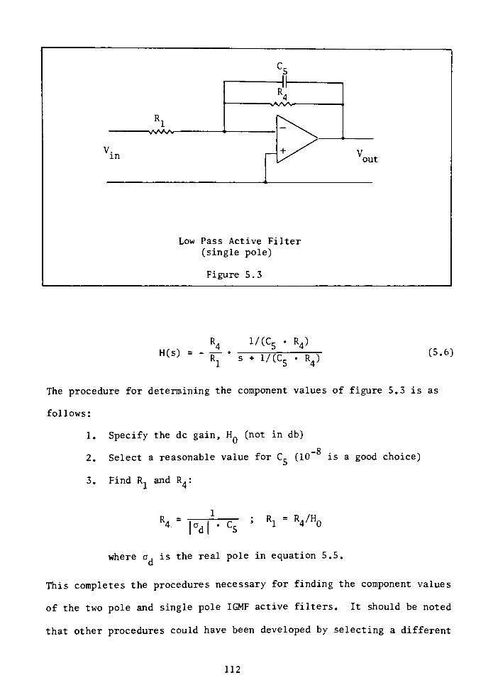
C5II

Rl

II

V.in

+Â Vout

Low Pass Active Filter

(single pole)

Figure 5.3

R< 1/(CC

H(s) = - 5-

R43

R:s +

1/(C5 R4)(5.6)

The procedure for determining the component values of figure 5.3 is as

follows:

1. Specify the dc gain, H (not in db)

-8

2. Select a reasonable value for C5(10~

is a good choice)

3. Find R. and R4:

R, =4~

i^dT^; Ri

=

R4/Ho

where o, is the real pole in equation 5.5.

This completes the procedures necessary for finding the component values

of the two pole and single pole IGMF active filters. It should be noted

that other procedures could have been developed by selecting a different

112

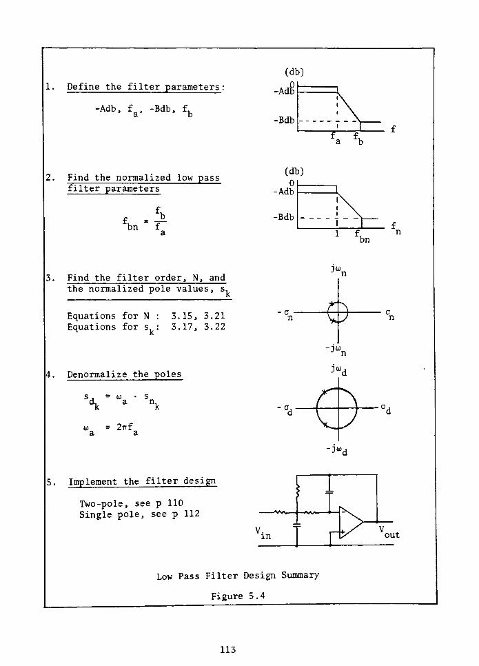
1. Define the filter parameters:

-Adb, f , -Bdb, f.a b

Find the normalized low pass

filter parameters

3.

fbn'

fa

Find the filter order, N, and

the normalized pole values, s.

Equations for N : 3.15, 3.21

Equations for s, : 3.17, 3.22

4. Denormalize the poles

k

s ,= 0) s

dk a n.

to = 2irfa a

5. Implement the filter design

Two-pole, see p 110

Single pole, see p 112

(db)

0

-Adb

-Bdb

, \v *

V.in

bn

J"

B

-jo)t

JU).

jud

J*

Low Pass Filter Design Summary

Figure 5.4

out

113

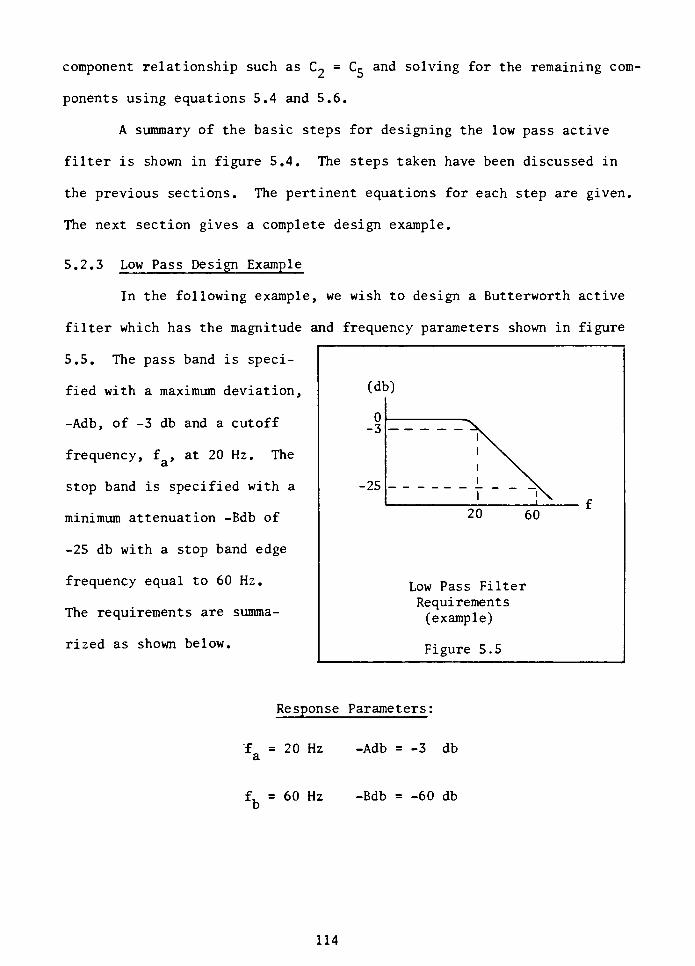
component relationship such as C2= Cr and solving for the remaining com

ponents using equations 5.4 and 5.6.

A summary of the basic steps for designing the low pass active

filter is shown in figure 5.4. The steps taken have been discussed in

the previous sections. The pertinent equations for each step are given.

The next section gives a complete design example.

5.2.3 Low Pass Design Example

In the following example, we wish to design a Butterworth active

filter which has the magnitude and frequency parameters shown in figure

5.5. The pass band is speci

fied with a maximum deviation,

-Adb, of -3 db and a cutoff

frequency, f ,at 20 Hz. The

3.

stop band is specified with a

minimum attenuation -Bdb of

-25 db with a stop band edge

frequency equal to 60 Hz.

The requirements are summa

rized as shown below.

(db)

Low Pass Filter

Requirements

(example)

Figure 5.5

Response Parameters:

f = 20 Hz -Adb=-3 db

a

fw = 60 Hz -Bdb=-60 db

b

114

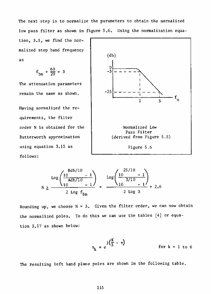
The next step is to normalize the parameters to obtain the normalized

low pass filter as shown in figure 5.6. Using the normalization equa

tion, 3.1, we find the nor

malized stop band frequency

as

f =

*= 3

bn 20

The attenuation parameters

remain the same as shown.

Having normalized the re

quirements, the filter

order N is obtained for the

Butterworth approximation

using equation 3.15 as

follows:

(db)

0

-3

\-25

! \.i

fn1 3

Normalized Low

Pass Filter

(derived from Figure 5.5)

Figure 5.6

Bdb/ 10

Log10

Adb/ 10

N >10

2 Log fbn

Log I

25/10

10 - ]

3/10

io -_i-

2 Log 3

= 2.6

Rounding up, we choose N = 3. Given the filter order, we can now obtain

the normalized poles. To do this we can use the tables [4] or equa

tion 3.17 as shown below:

sR= ej(f it)

for k = 1 to 6

The resulting left hand plane poles are shown in the following table.

115

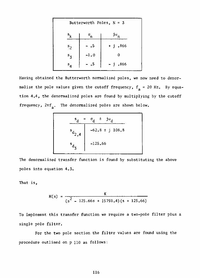
Butterworth Poles, N = 3

Skan

jojJn

S2-.5 + j .866

S3-1.0 0

S4-.5

- j .866

Having obtained the Butterworth normalized poles, we now need to denor-

malize the pole values given the cutoff frequency, f = 20 Hz. By equa-

a.

tion 4.4, the denormalized poles are found by multiplying by the cutoff

frequency, 2irf.

The denormalized poles are shown below.3.

sd=

ad ja)d

*2,4

-62.8 j 108.8

-125.66

The denormalized transfer function is found by substituting the above

poles into equation 4.3.

That is,

H(s) =

K

(s - 125.66s + 15791.4) (s + 125.66)

To implement this transfer function we require a two-pole filter plus a

single pole filter.

For the two pole section the filter values are found using the

procedure outlined on p 110 as follows:

116

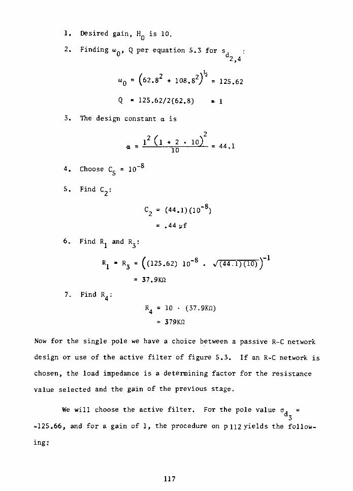
1. Desired gain, H is 10.

2. Finding oj, Q per equation 5.3 for s, :

d2,4

u0= (62. 82 + 108. = 125.62

Q =

125.62/2(62.8) = 1

3. The design constant a is

2l2 (l + 2 . 10) . . .

a=_^ _ i-= 44.1

4. ChooseC5

=10~8

5. Find C :

C2= (44.1) (10"8)

=.44 yf

6. Find R and R :

Rl=

R3= ((125-62) 10'8

. ^(44.1)

= 37.9Kft

7. Find R . :

4

R4= 10 (37.9KQ)

= 379Kn

Now for the single pole we have a choice between a passive R-C network

design or use of the active filter of figure 5.3. If an R-C network is

chosen, the load impedance is a determining factor for the resistance

value selected and the gain of the previous stage.

We will choose the active filter. For the pole value a, =

d3-125.66, and for a gain of 1, the procedure on p 112 yields the follow

ing:

117

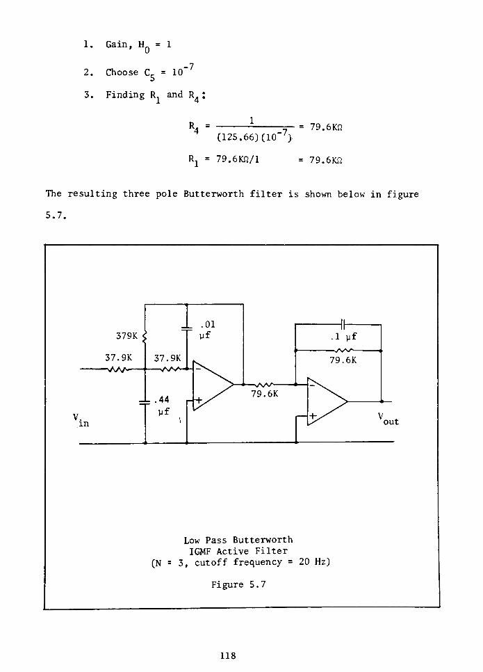
1. Gain, H = 1

2.

3.

-7

Choose Cr = 10

Finding R and R. :

R4=

(125.66) (10 ')

R2= 79.6KT2/1

79. em

79.6XSI

The resulting three pole Butterworth filter is shown below in figure

5.7.

379K <

37. 9K

V.in

37. 9K

.01

yf

*/w*

79. 6K

.1 yf

-VV>A-

79. 6K

Low Pass Butterworth

IGMF Active Filter

(N = 3, cutoff frequency= 20 Hz)

Figure 5.7

out

118

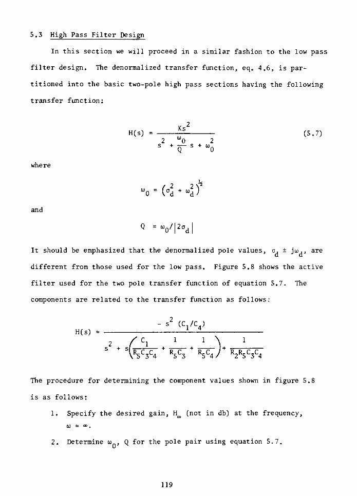
5.3 High Pass Filter Design

In this section we will proceed in a similar fashion to the low pass

filter design. The denormalized transfer function, eq. 4.6, is par

titioned into the basic two-pole high pass sections having the following

transfer function:

Ks2

H(s) = ^ (5.7)2 w0 2s + s + OJ

where

U0=

(d +wd)

and

Q=V|2od|

It should be emphasized that the denormalized pole values, o, joj,, are

different from those used for the low pass. Figure 5.8 shows the active

filter used for the two pole transfer function of equation 5.7. The

components are related to the transfer function as follows:

- {.CJC )

H(s) = 11

/Cl+_ + _i

\ 5 3 4 5 3 5

s + si r,+ tt-ft- + | +

5C4 / R2R5C3C4

The procedure for determining the component values shown in figure 5.8

is as follows:

1. Specify the desired gain, H^ (not in db) at the frequency,

oj = .

2. Determine o>, Q for the pole pair using equation 5.7.

119

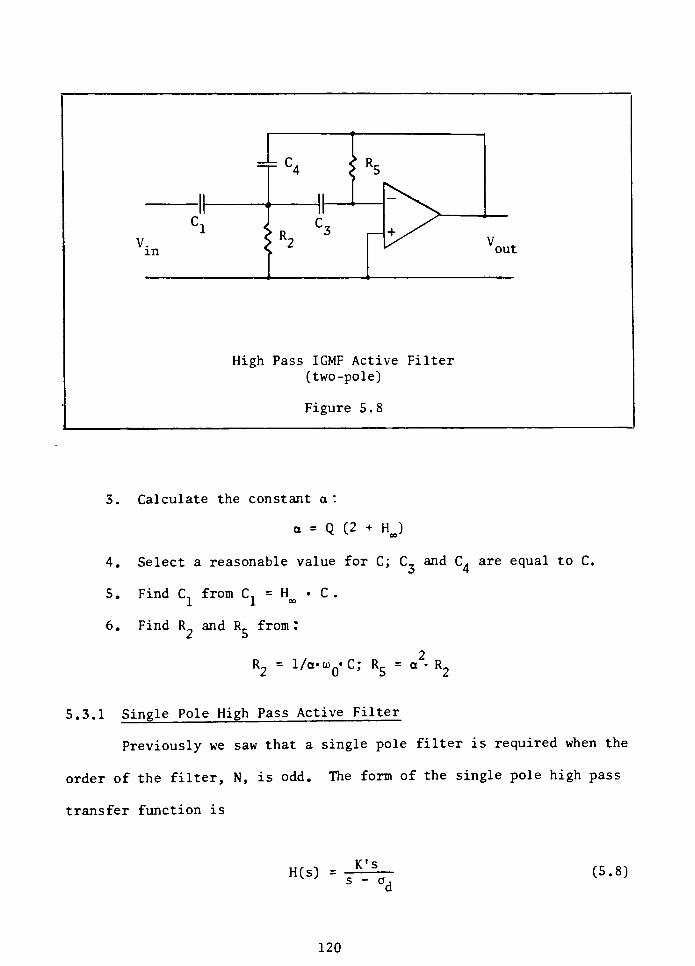
= C4 | R5

|| ||-N.

V.in

II

ClII

:r23 4-x^

Vout

High Pass IGMF Active Filter

(two-pole)

Figure 5.8

3. Calculate the constant a '.

a = Q (2 +HJ

4. Select a reasonable value for C; C, and C. are equal to C.

5. Find C, from C = H . C .

1 1

6. Find R and Rr from:

R2= l/a-oj^C; R$

= a

R2

5.3.1 Single Pole High Pass Active Filter

Previously we saw that a single pole filter is required when the

order of the filter, N, is odd. The form of the single pole high pass

transfer function is

H(s) =

K's

s- a-

(5.8)

120

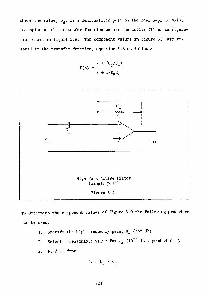
where the value, a,, is a denormalized pole on the real s-plane axis.

To implement this transfer function we use the active filter configura

tion shown in figure 5.9. The component values in figure 5.9 are re

lated to the transfer function, equation 5.8 as follows:

H(s) =

- s (Cj/ty

s +

1/R5C4

V.in

High Pass Active Filter

(single pole)

Figure 5.9

out

To determine the component values of figure 5.9 the following procedure

can be used:

1. Specify the high frequency gain, H^ (not db)

-8

2. Select a reasonable value for C4(10"

is a good choice)

3. Find C. from

C. = H C.1 CD 4

121

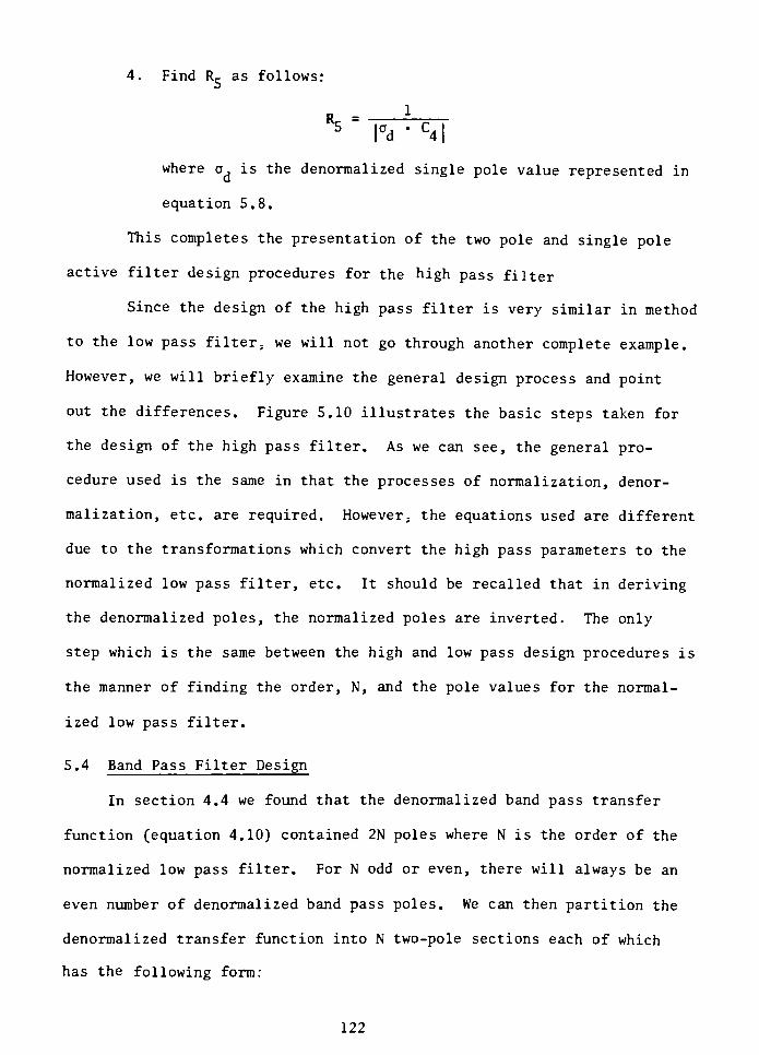
4. Find Rr as follows:

Rr =

5|d

*

C4|

where a, is the denormalized single pole value represented in

equation 5.8.

This completes the presentation of the two pole and single pole

active filter design procedures for the high pass filter

Since the design of the high pass filter is very similar in method

to the low pass filter- we will not go through another complete example.

However, we will briefly examine the general design process and point

out the differences. Figure 5.10 illustrates the basic steps taken for

the design of the high pass filter. As we can see, the general pro

cedure used is the same in that the processes of normalization, denor

malization, etc. are required. However- the equations used are different

due to the transformations which convert the high pass parameters to the

normalized low pass filter, etc. It should be recalled that in deriving

the denormalized poles, the normalized poles are inverted. The only

step which is the same between the high and low pass design procedures is

the manner of finding the order, N, and the pole values for the normal

ized low pass filter.

5.4 Band Pass Filter Design

In section 4.4 we found that the denormalized band pass transfer

function (equation 4.10) contained 2N poles where N is the order of the

normalized low pass filter. For N odd or even, there will always be an

even number of denormalized band pass poles. We can then partition the

denormalized transfer function into N two-pole sections each of which

has the following form:

122

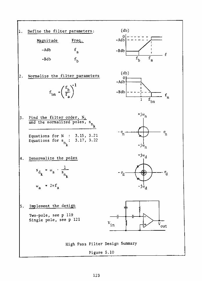
Define the filter parameters:

Magnitude Freq.

-Adb fa

-Bdb f,D

2. Normalize the filter parameters

1

J!A(^bn V f /a /

Find the filter order, N,

and the normalized poles, s

Equations for N

Equations for s

3.15, 3.21

3.17, 3.22


1s, = oj

-

d, as

k n.

oj= 27rf

a a

5. Implement the design

Two-pole, see p 119

Single pole, see p 121

(db)

0

-Adb

-Bdb

(db)Oh-

-Adb

-Bdb

-

o,

V.in

fb fa

1 fbn

+ J0)

e-jto

+ JU)

-JO)

F.

High Pass Filter Design Summary

Figure 5.10

a

n

out

123

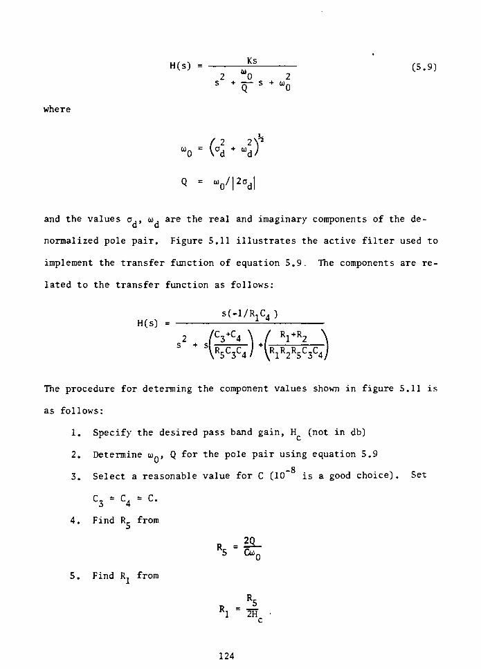
H^ =

J^ (3-9)2 0 2s + s +

0)Q

where

"0= (d +

ud)

Q -

VI2odl

'2

and the values o, , oj, are the real and imaginary components of the de-

normalized pole pair. Figure 5.11 illustrates the active filter used to

implement the transfer function of equation 5.9. The components are re

lated to the transfer function as follows:

s(-l/R1C4)

H(s) = ^

2C

s + s

C3*C4 \ / VR2

R5C3C4/ \R1R2R5C3C4

The procedure for determing the component values shown in figure 5.11 is

as follows:

1. Specify the desired pass band gain, H (not in db)

2. Determine o)n, Q for the pole pair using equation 5.9

-8

3. Select a reasonable value for C(10~

is a good choice). Set

C,= C. = C.

3 4

4. Find Rr from

5. Find R. from

R =^_

5 %

R -h.

*1 2Hc

124

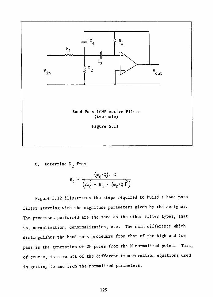
V.in

1

-VWu

out

Band Pass IGMF Active Filter

(two-pole)

Figure 5.11

6. Determine R2 from

R2=

(^/Q). C

(20)2-

Hc (o)0/Q f)

Figure 5.12 illustrates the steps required to build a band pass

filter starting with the magnitude parameters given by the designer.

The processes performed are the same as the other filter types, that

is, normalization, denormalization, etc.The main difference which

distinguishes the band pass procedure from that of the high and low

pass is the generation of 2N poles from the N normalized poles. This,

of course, is a result of the different transformation equations used

in getting to and from the normalized parameters.

125

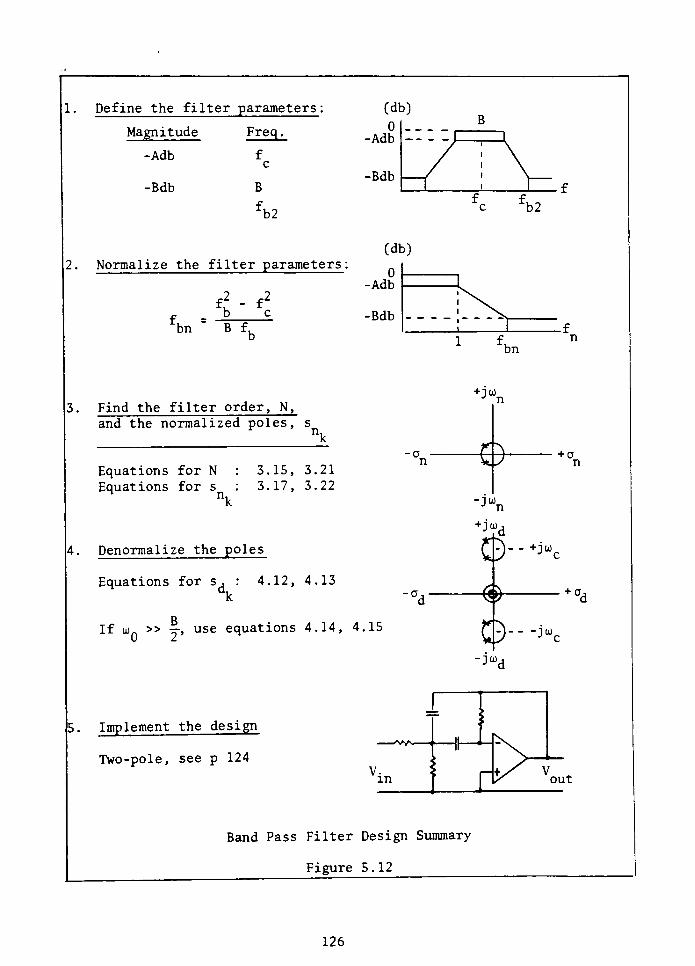
Define the filter parameters

Magnitude Freq.

-Adb f

(db)

-Bdb B

0

-Adb

-Bdb

b2

2. Normalize the filter parameters:

f2

-

f2

b c

(db)

bn"

B f.

0

-Adb

-Bdb

3. Find the filter order, N,



Equations for s , : 4.12, 4.13

Ifoin

>> =-, use equations 4.14, 4.15

Equations for N

Equations for s

n.

3.15, 3.21

3.17, 3.22

-o,

b2

bn

+J0)

> + 0

+jo)

+ 0,

D- -

-ju>,

-jur

5. Implement the design

Two-pole, see p 124

Vin H out

Band Pass Filter Design Summary

Figure 5.12

126

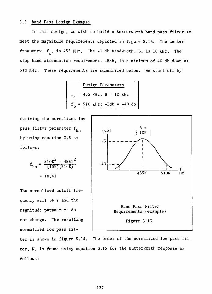
5.5 Band Pass Design Example

In this design, we wish to build a Butterworth band pass filter to

meet the magnitude requirements depicted in figure 5.13. The center

frequency, f ,is 455 KHz. The -3 db bandwidth, B, is 10 KHz. The

stop band attenuation requirement, -Bdb, is a minimum of 40 db down at

510 KHz. These requirements are summarized below. We start off by

Design Parameters

455 KHz; B = 10 KHz

f, = 510 KHz: -Bdb= -

b40 db

deriving the normalized low

pass filter parameter f,

by using equation 3.5 as

follows:

510K2

-

455K2

bn (10K)(510K)

= 10.41

The normalized cutoff fre

quency will be 1 and the

magnitude parameters do

not change. The resulting

normalized low pass fil-

455K 510K

Band Pass Filter

Requirements (example)

Figure 5.13

Hz

ter is shown in figure 5.14. The order of the normalized low pass fil

ter, N, is found using equation 3.15 for the Butterworth response as

follows:

127

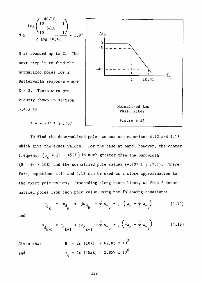
Log

N >

40/10

10 -_]

3/10

10 -_1

2 Log 10.41

= 1.97

N is rounded up to 2. The

next step is to find the

normalized poles for a

Butterworth response where

N = 2. These were pre

viously shown in section

3.4.3 as

s =-.707 j .707

(db)

10.41

Normalized Low

Pass Filter

Figure 5.14

To find the denormalized poles we can use equations 4.12 and 4.13

which give the exact values. For the case at hand, however, the center

frequency (o) = 2tt 455K ) is much greater than the bandwidth

(B = 2tt 10K) and the normalized pole values (-.707 j .707). There

fore, equations 4.14 and 4.15 can be used as a close approximation to

the exact pole values. Proceeding along these lines, we find 2 denor

malized poles from each pole value using the following equationst

jv =lv+ j K + lv) <4-14)S^

=

A+

dR ^ ^s.

.^. w fc

k

and

X A dv A 3% ik+1 k+1 k+1

to + j ( -oi +T o) ) (4.15)

2n, J\c2n, /

Given that

and

B = 2ir (10K) = 62.83 x10"

oj = 2tt (455K) = 2.859 x 10c

128

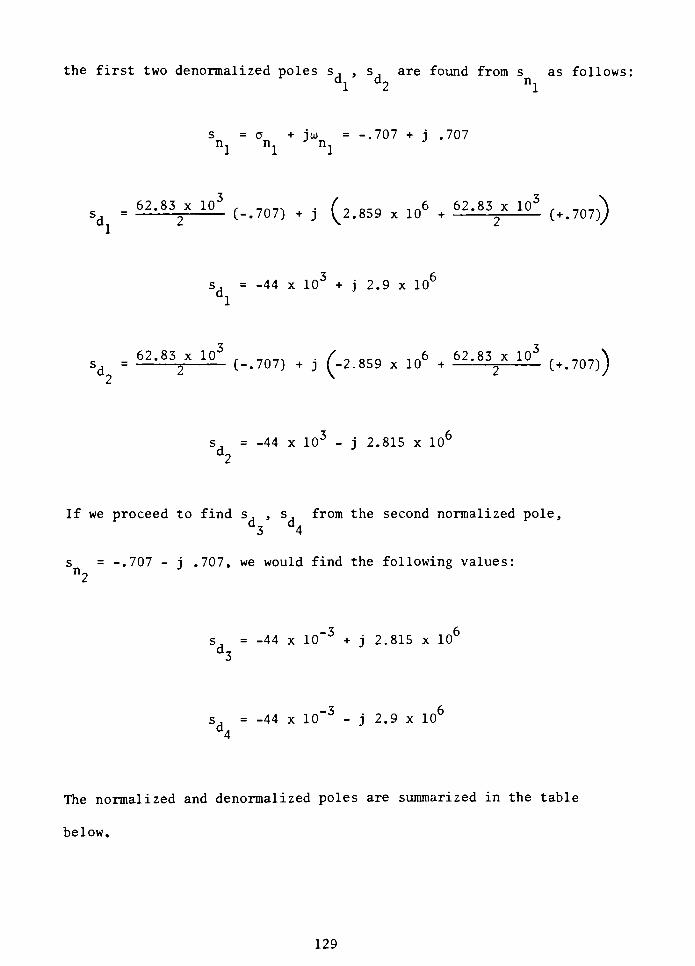
the first two denormalized poles s, , s, are found from s as follows:

dl d2 nl

s = a + joj =-.707 + j .707

nl nl nl

62.83 x

103

, _n_, . ( n crQin6 62.83 x

103

sd=

= (-.707) + j V 2.859 x 10 + =

s =-44 x

103

+ j 2.9 x

106

dl

62.83 x103

s

d22 (-.707) + j (-2.859 x

106

+62-852* 10

(+.707))

s =-44 x

103

- j 2.815 x106

If we proceed to find s. , s. from the second normalized pole,

d3 d4

s =-.707

- j .707, we would find the following values:

n2

Sj= -44 x

10"3

+ j 2.815 x

106

d3

sd= -44 x

10'3

- j 2.9 x106

4

The normalized and denormalized poles are summarized in the table

below.

129

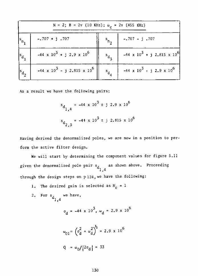
N = 2; B = 2tt (10 KHz); ojc= 2tr (455 KHz)

s -.707 + j .707 s

n2-.707

- j .707

\-44 x

103

+ j 2.9 x106

**3-44 x

103

+ j 2.815 x106

\-44 x

103

- j 2.815 x

106

%-44 x

103

- j 2.9 x

106

As a result we have the following pairs:

1,4

-44 x 10 j 2.9 x 10

s = -44 x103

j 2.815 x

106

2,3

Having derived the denormalized poles, we are now in a position to per

form the active filter design.

We will start by determining the component values for figure 5.11

given the denormalized pole pair s, as shown above. Proceeding1,4

through the design steps on p 124, we have the following:

1. The desired gain is selected as Hc= 1

2. For s, we have,dl,4

3 6

a = -44 x 10, oi,

= 2.9 x 10d a

/ 22\^ (

"oi" (ad +

wd)= 2-9 x 10

Q V|2ad|= 33

130

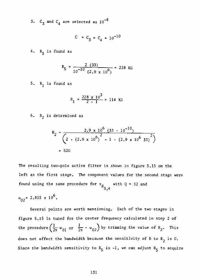
Q

3. C3 and C4 are selected as 10

c=c3

=

c4=io-10

4. R is found as

r -2 (33)

5~

,-10 JI J , 6= 228 K"

10"

(2.9 x 10")

5. R is found as

D228 x

103

,

Rj=

2 ;= 114 m

6. R2 is determined as

R =2.9 x

106

(33 . IP"10)

(2 (2.9 x 106) - 1 (2.9 x106

33) )= 52ft

The resulting two-pole active filter is shown in figure 5.15 on the

left as the first stage. The component values for the second stage were

found using the same procedure for s , with Q = 32 and

d3,4

o)Q2= 2.815 x 106.

Several points are worth mentioning. Each of the two stages in

figure 5.15 is tuned for the center frequency calculated in step 2 of

the procedure f= oj ory~ *

^02/ y trimming the value of R2. This

does not affect the bandwidth because the sensitivity of B to R is 0.

Since the bandwidth sensitivity to Rr is -1, we can adjust R_ to acquire

131

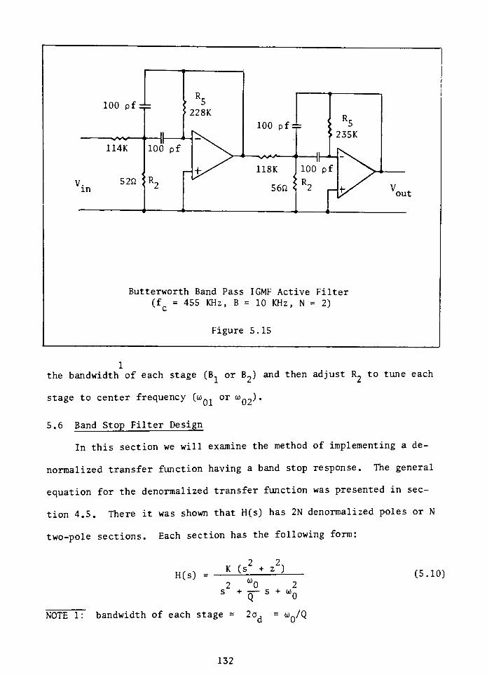
100 pf 4=

->/W ' ?

114K

V 52fiin

100 pf

100 pf :

-v/v23!

5

>35K

Butterworth Band Pass IGMF Active Filter

(f = 455 KHz, B = 10 KHz, N = 2)

Figure 5.15

out

the bandwidth of each stage (B or B2) and then adjust R2to tune each

stage to center frequency (oj or oj_)

.

5.6 Band Stop Filter Design

In this section we will examine the method of implementing a de-

normalized transfer function having a band stop response. The general

equation for the denormalized transfer function was presented in sec

tion 4.5. There it was shown that H(s) has 2N denormalized poles or N

two-pole sections. Each section has the following form:

H(s) =

2 2K (s + z )

2 "0

"

2s + s +

"0

(5.10)

NOTE 1: bandwidth of each stage =

2od=

ojq/Q

132

where

h

z is the center frequency of the filter response (2irf ),

"o= (d +

wd)

for the given pole pair and

* =

Vl2CTdl

In this section a two-pole IGMF active filter is presented which can im

plement the transfer function of equation 5.10.

The unique characteristic of the band stop response is that it con

tains complex zeros in the numerator. The previous designs did not have

complex transfer function zeros. To accommodate the zeros as well as

an IGMF design, we will use the active filter configuration as shown in

figure 5.16. This circuit concept was presented by T. Deliyannis [13]

and later expanded by J. J. Friend of Bell Laboratories [14]. The in

tention was to provide superior low sensitivity compared to other single

amplifier circuits as well as a minimal number of components. As an

added point, this circuit can be used for the elliptic transfer func

tions which contain s-plane zeros.

The procedure for determining the component values of figure 5.16

follows and it is rather lengthy. An example will be given after dis

cussing the procedure.

133

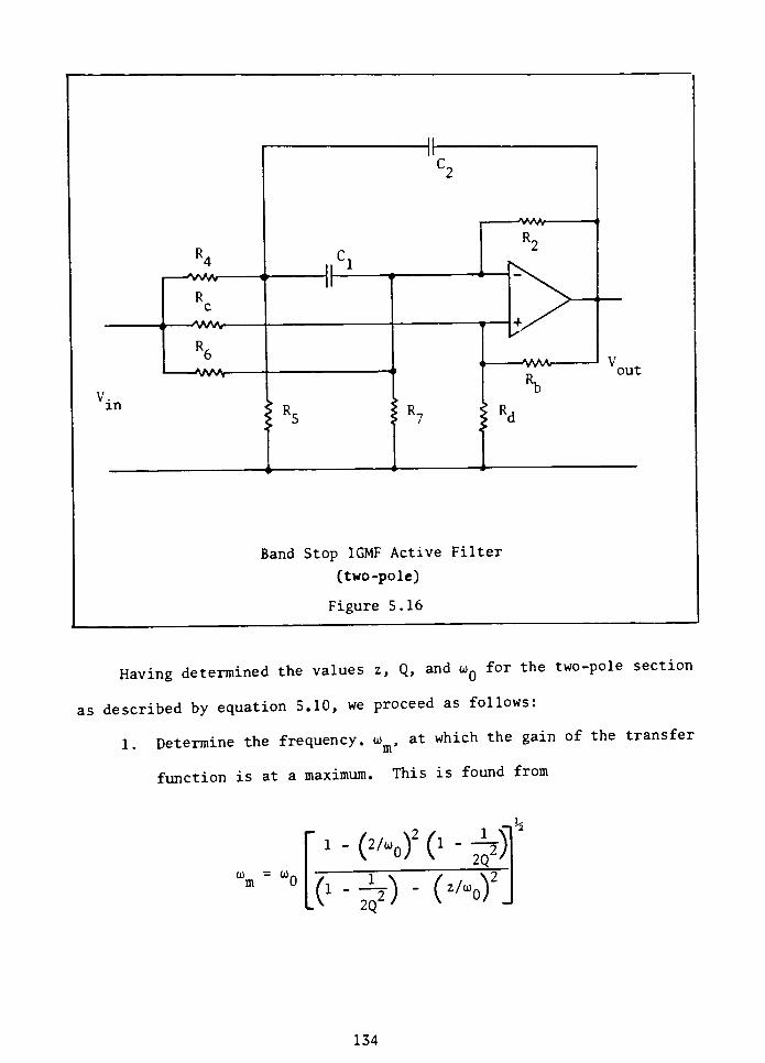
V.in

R4

R

i .<ÂA^

Cl

Hh

Band Stop IGMF Active Filter

(two -pole)

Figure 5.16

out

Having determined the values z, Q, ando)Q

for the two-pole section

as described by equation 5.10, we proceed as follows:

1. Determine the frequency. o)m, at which the gain of the transfer

function is at a maximum. This is found from

0) =

u>nm 0

1 -

(vo)2

o- 5

-MM

134

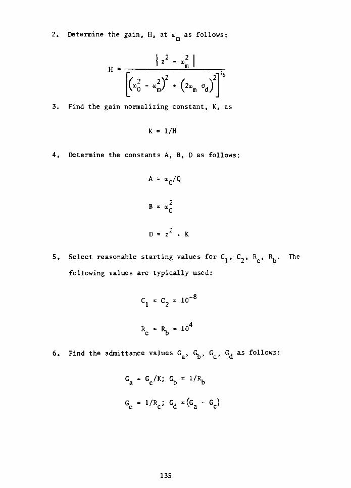
2. Determine the gain, H, at o) as follows:

H =

2 2z - O)

m

(u0 "

u)+ (2% d)

3. Find the gain normalizing constant, K, as

K = 1/H

4. Determine the constants A, B, D as follows:

A =

ojq/Q

B =oj.

D = z . K

5. Select reasonable starting values for C. , C~, R, R, . The

following values are typically used:

Cl"

C2' 10

-8

Rc"

*b" 10

6. Find the admittance values G, Gb, G Gd

as follows:

Ga" Gc/K; S

"

1/Rb

Gc= 1/RC; Gd =(Ga

- Gc)

135

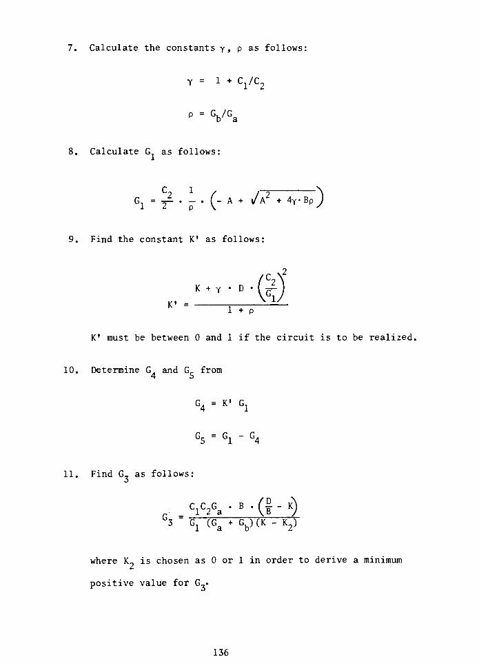
7. Calculate the constants y, p as follows:

Y= 1 +

C1/C2

P=

Gb/Ga

8. Calculate G as follows:

^= y~ - (- A +

A2+ 4Y-BP>)

9. Find the constantK'

as follows:

K + Y

(1 + p

K1must be between 0 and 1 if the circuit is to be realized.

10. Determine G4 and G,. from

G = V G.4 1

G5"

Gl'

G4

11. Find G, as follows:

C.C-G B

G =

1 2 a (*-<)J3

Gx (Ga+ Gb) (K - K2)

where K is chosen as 0 or 1 in order to derive a minimum

positive value for G_.

136

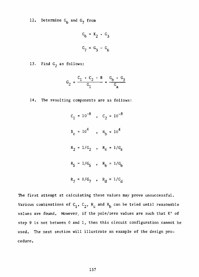
12. Determine G, and G-, fromo 7

G6=

K2*

G3

G7=

G3"

G6

13. Find G_ as follows:

C. C-, B G, G,n

1 2 b 3

G2=

g:+

14. The resulting components are as follows:

cx=

10"8

, c2=

10"8

4 4

Rc= 10

, Rb= 10

R2=

1/G2 , R4=

1/G4

R5=

1/G5 , R6=

1/G6

R?=

1/G? , Rd=

1/Gd

The first attempt at calculating these values may prove unsuccessful.

Various combinations of C. , C0, R and R, can be tried until reasonable1' 2'

c b

values are found. However, if the pole/zero values are such thatK'

of

step 9 is not between 0 and 1, then this circuit configuration cannot be

used. The next section will illustrate an example of the design pro

cedure.

137

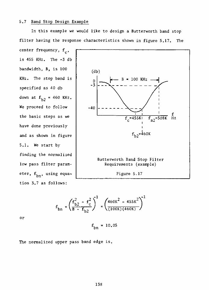
5.7 Band Stop Design Example

In this example we would like to design a Butterworth band stop

filter having the response characteristics shown in figure 5.17. The

center frequency ; f ,

is 455 KHz. The -3 db

bandwidth, B, is 100

KHz. The stop band is

specified as 40 db

down at f, _= 460 KHz.

D2

We proceed to follow

the basic steps as we

have done previously

and as shown in figure

5.1. We start by

finding the normalized

low pass filter param

eter, f,, using equa

tion 3.7 as follows:

(db)

f =455Kl

cf =508K Hza2

f. o=460Kt>2

Butterworth Band Stop Filter

Requirements (example)

Figure 5.17

bn

/f22 - f2\

/460K2- 455K2N\

=

\B fb2 /=

\(100K)(460K) /

or

f, = 10.05bn

The normalized upper pass band edge is,

138

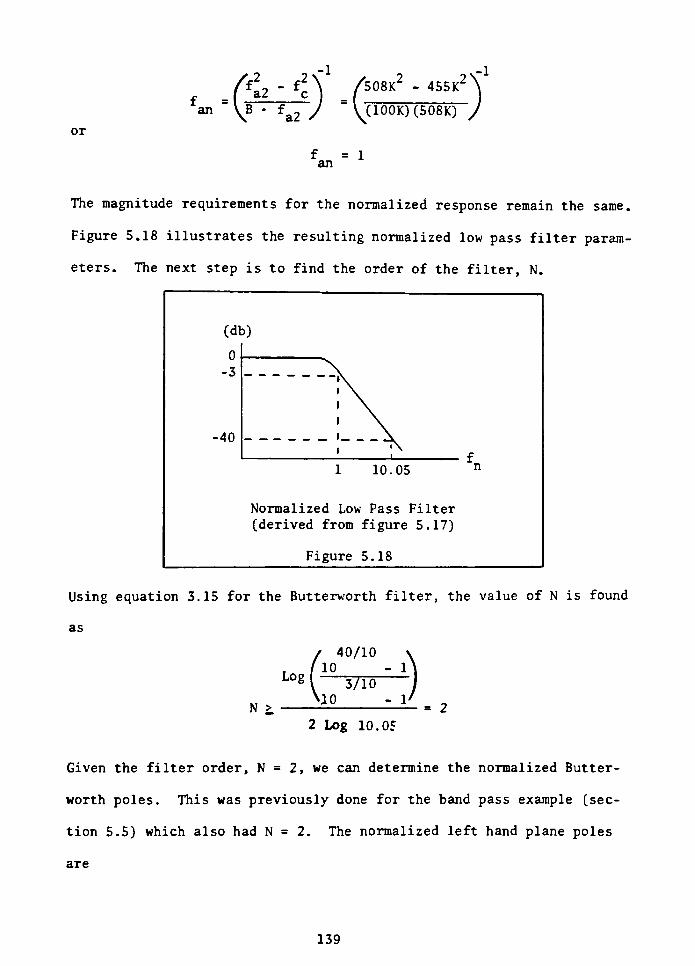
an

(<2'<\ (*\B *

fa2 /"

V1001

,-1

455K'

(100K)(508K)

or

fan=1

The magnitude requirements for the normalized response remain the same.

Figure 5.18 illustrates the resulting normalized low pass filter param

eters. The next step is to find the order of the filter, N.

(db)

0

-3

-40

'' f

1 10.05 n

Normalized Low Pass Filter

(derived from figure 5.17)

Figure 5.18

Using equation 3.15 for the Butterworth filter, the value of N is found

as

40/10

/ M

Log

N >

2 Log 10.0?

= 2

Given the filter order, N = 2, we can determine the normalized Butter

worth poles. This was previously done for the band pass example (sec

tion 5.5) which also had N = 2. The normalized left hand plane poles

are

139

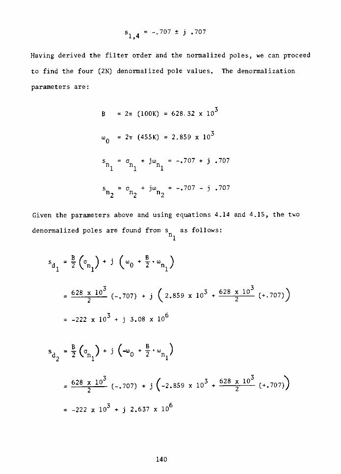
s,=-.707 j .707

1,4

Having derived the filter order and the normalized poles, we can proceed

to find the four (2N) denormalized pole values. The denormalization

parameters are:

B = 2ir (100K) = 628.32 x

103

oj = 2tt (455K) = 2.859 x103

s = a + joj =-.707 + j .707

ni ni nl

s = a + jo) =-.707

- j .707

n2 n2 n2

Given the parameters above and using equations 4.14 and 4.15, the two

denormalized poles are found from s as follows:

nl

\= K\) + 5 (a<> +

?-\)

=

628 *

1q3

(-.707) + j ( 2.859 x103

+628 * l^

( +.707))

= -222 x103

+ j 3.08 x106

sd2 =f (ani)+ j (^0 +T\)

-

628 *105

(-.707) + j (-2.859 x

103

+

628

\l0'

(+.707))

= -222 x103

+ j 2.637 x106

140

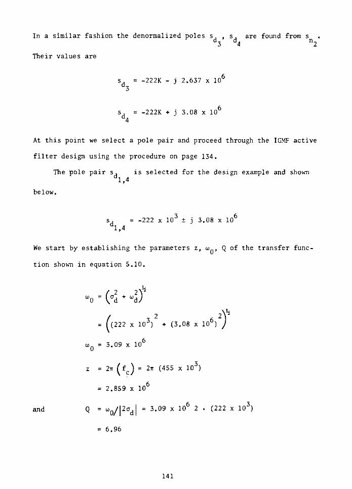
In a similar fashion the denormalized poles s. . s, are found from s

d3 d4 "2

Their values are

s =-222K

- j 2.637 x106

3

s, =-222K + j 3.08 x

106

d4

At this point we select a pole pair and proceed through the IGMF active

filter design using the procedure on page 134.

The pole pair s , is selected for the design example and shown

dl,4

below.

s, = -222 x

103

j 3.08 x

106

dl,4

We start by establishing the parameters z, o), Q of the transfer func

tion shown in equation 5.10.

h

uo= (ad +

ud)

/ 32

6

A'

= I (222 x lO0) + (3.08 x 10) j

and

oj = 3.09 x106

z = 2v li\ = 2tt (455 x 103)

= 2.859 x

106

Q =

w0/|2od|= 3.09 x

106

2 (222 x 103)

= 6.96

141

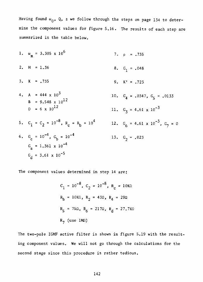
Having found o>Q, Q, z we follow through the steps on page 134 to deter

mine the component values for figure 5.16. The results of each step are

summarized in the table below.

1.o)m

= 3.305 x106

7. p=.735

2. H = 1.36 8. Gx=.048

3. K =.735 9. K'

=.723

4. A = 444 x103

10. G. =

.0347, Gc =.0133

124 b

B = 9.548 x 10

D = 6 x1012

11. G3= 4.61 x

10"3

5. C1=

C2= 10"8, Rc

=

Rb=

104

12. G6= 4.61 x 10"3, Gy

= 0

6. Gc= 10"4, Gb

=

10"4

13. G2=.023

G = 1.361 x

10"4

a

G, = 3.61 x10"5

d

The component values determined in step 14 are:

C. = 10'8, C_ = 10"8, R = 10JO21 '2

'c

Rb= lOKft, R2

= 43ft, R4 29^

R5= 75ft, R6

= 217ft, Rd= 27.7Kft

R? (use lMft)

The two-pole IGMF active filter is shown in figure 5.19 with the result

ing component values. We will not go through the calculations for the

second stage since this procedure is rather tedious.

142

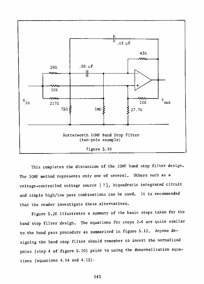
V.in

29ft

10K

217ft

.01 yf

,01 yf

43ft

-AWr\ 1.

-vwv-

75ft lMft

10K

27. 7K

Butterworth IGMF Band Stop Filter

(two-pole example)

Figure 5.19

out

This completes the discussion of the IGMF band stop filter design.

The IGMF method represents only one of several. Others such as a

voltage-controlled voltage source [7], biquadratic integrated circuit

and simple high/low pass combinations can be used. It is recommended

that the reader investigate these alternatives.

Figure 5.20 illustrates a summary of the basic steps taken for the

band stop filter design. The equations for steps 2-4 are quite similar

to the band pass procedure as summarized in figure 5.12. Anyone de

signing the band stop filtershould remember to invert the normalized

poles (step 4 of figure 5.20) prior to using the denormalization equa

tions (equations 4.14 and 4.15).

143

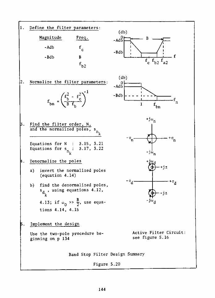
Define the filter parameters:

Magnitude

-Adb

-Bdb

H>2

Normalize the filter parameters:

1

(db)

Freq. 0-Adb

^_B *-

f \ /c-Bdb

1 \ /

B

f.

11

(

fc fb2 fa2

bni

-

gB f

,

3. Find the filter order, N,


n,

Equations for N : 3.15, 3.21

Equations for s : 3.17, 3.22

nk


a) invert the normalized poles

(equation 4.14)

b) find the denormalized poles,

s, , using equations 4.12,

k

4.13; if id. >>y, use equa

tions 4.14, 4.15

Implement the design

Use the two-pole procedure be

ginning on p 134

(db)

0-Adb

-Bdb _ i _

bn

+JU

-a

e-JO)

+ JO)

+ 0

5-+j:

- + a.

-jz

-JO)

Active Filter Circuit

see figure 5.16

Band Stop Filter Design Summary

Figure 5 . 20

144

5.8 Chapter Summary

In this chapter we examined the methods of implementing the denor

malized transfer functions using infinite-gain multiple feedback (IGMF)

active filters. We started by examining the basic steps of filter de

sign. These steps essentially outlined the discussions of the previous

chapters. The end objective was to derive the denormalized poles which

were used as the starting design parameters for the active filters. The

procedures were then presented for determining the component values of

the IGMF active filter circuits.

In comparing the four design procedures, the band stop filter ap

peared unique because the circuit provided transfer function zeros.

This circuit configuration is applicable to elliptic function filters

which also have transmission zeros.

We have at this point completed the analysis of parameters, trans

formations and design procedures required for the four basic filter

types (low pass through band stop). The next chapter deals with the de

velopment of a computer program called FILTER which performs the total

design process for each filter type and provides the IGMF component

values.

145

CHAPTER VI

THE FILTER PROGRAM

6.1 Introduction

In this chapter we will discuss a computer program which performs

the analysis and design of filters in the frequency domain. The name of

the program is FILTER.

The program was developed as part of this thesis with the primary

intention of acting as an aid to the filter design engineer. To accom

plish this objective, all of the analytical steps required for various

filter designs were assimilated into one comprehensive interactive al

gorithm. Of primary significance is the inclusion of a complete ellip

tic filter design ability. The program provides the engineer with the

ability to design and evaluate various filters without the burdens of

performing complex mathematics, referring to a variety of normalized

tables or being limited to a familiar and perhaps non-optimal design.

The discussions in the previous chapters have provided an overview

of the fundamental concepts upon which the FILTER program is based. The

program is actually much broader in scope and more complex in its ana

lytical abilities. The user interaction and guidance by the program are

extensive and therefore it is unnecessary to fully comprehend the in

tricacies in order to put it to full use. The following sections pro

vide a brief overview of the capabilities of the FILTER program and its

software architecture.

6.2 Capabilities of the FILTER Program

The FILTER program has the capability of designing low pass, high

pass, band pass and band stop filters using any of three classical ap-

146

proximations: Butterworth, Chebyshev and elliptic. Provisions have

been made to include the Bessel function approximation at a later date.

The following four items provide a summary of other major program capa

bilities.

1. The program can accept a wide variety of input parameter com

binations (magnitude and frequency) for specifying the desired

response. As an example, for a low pass filter, the user can

specify f , f, , -Adb and-Bdb*

arbitrarily, regardless of the

filter approximation used. This allows the designer to speci

fy the parameters according to the application requirements.

A Butterworth filter, for example, can be specified with a

cutoff frequency attenuation of -1 db instead of the typical

-3 db. The program determines if the parameters are appro

priate and returns a message to the user if they are not. A

simple example would be an entry error where the user reverses

the cutoff and stop band attenuation parameters. Many other

parameter checks are included. In addition, other secondary

parameters are derived from those given by the designer. An

example of this is the calculation of the cutoff frequency

given the filter order, N, and an arbitrary attenuation value

for a specific frequency.

2. Another capability of the program is to determine the normal

ized filter order, N, along with the normalized and denormal

ized poles/zeros. The maximum filter order is N = 100 for

the low and high pass and N = 50 for the band pass and band

*See section 2.4 for definitions.

147

stop. The capabilities above are the most significant features

of the program since they encompass the following analytical

processes:

a) normalization of the input parameters,

b) evaluation of N and the normalized poles/zeros for a de

sired classical approximation response,

c) denormalization

The special feature of item (b) above is that an elliptic func

tion algorithm has been developed to determine the Nth order

poles and zeros. The elliptic function design algorithm

follows the analytical methods described in the Appendix.

3. Aside from the analytical processes above, the program provides

the ability to evaluate the denormalized transfer function,

giving both magnitude and phase as a function of the frequency

range of interest. This enables the user to determine if the

selected approximation (Butterworth, Chebyshev, etc.) yields a

reasonable filter order as well as sufficient attenuation and

phase characteristics. If the result is unsatisfactory, the

user can alter some or all of the input parameters (magnitude,

frequency, filter type or selected approximation) and obtain a

new response.

4. Another capability of the program is to design an active filter

circuit using the calculated denormalized poles and zeros. The

component values can be determined for multiple stages of IGMF

active filter circuits. These values are displayed according

to stage number; their designations are referenced to the user's

148

manual. When determining the active filter circuit components,

multiple iterations are attempted at the design in order to ob

tain reasonable values. If these are not within the acceptable

range of values after a prescribed number of iterations, the

program stops the calculations and displays the last results.

Of special significance is the use of an IGMF single-stage

biquadratic active filter circuit. This circuit provides a

second order numerator and denominator transfer characteristic

and is employed as a canonical form for the elliptic and band

stop active filter circuit stages. A special algorithm was de

veloped specifically for the task of determining the component

values for this filter circuit. Aside from these IGMF active

filter circuit configurations, provisions have been made to

include the universal active filter integrated circuit (FLT-U2

or equivalent) as the active element at some later date.

The four main items discussed above have given an overview of the

major capabilities of the FILTER program. Following each of the

processes involved within the program, the resulting information is dis

played so the user can monitor and evaluate the progression of the de

sign. Throughout the session questions are asked of the user to deter

mine the course of action or acquire other important parameters. The

next section is a brief overview of the major algorithms which consti

tute the program and how they are organized.

6.3 Program Architecture

Figure 6.1 illustrates the software architecture of the FILTER pro

gram. Each block shown represents a considerable section of software

149

(

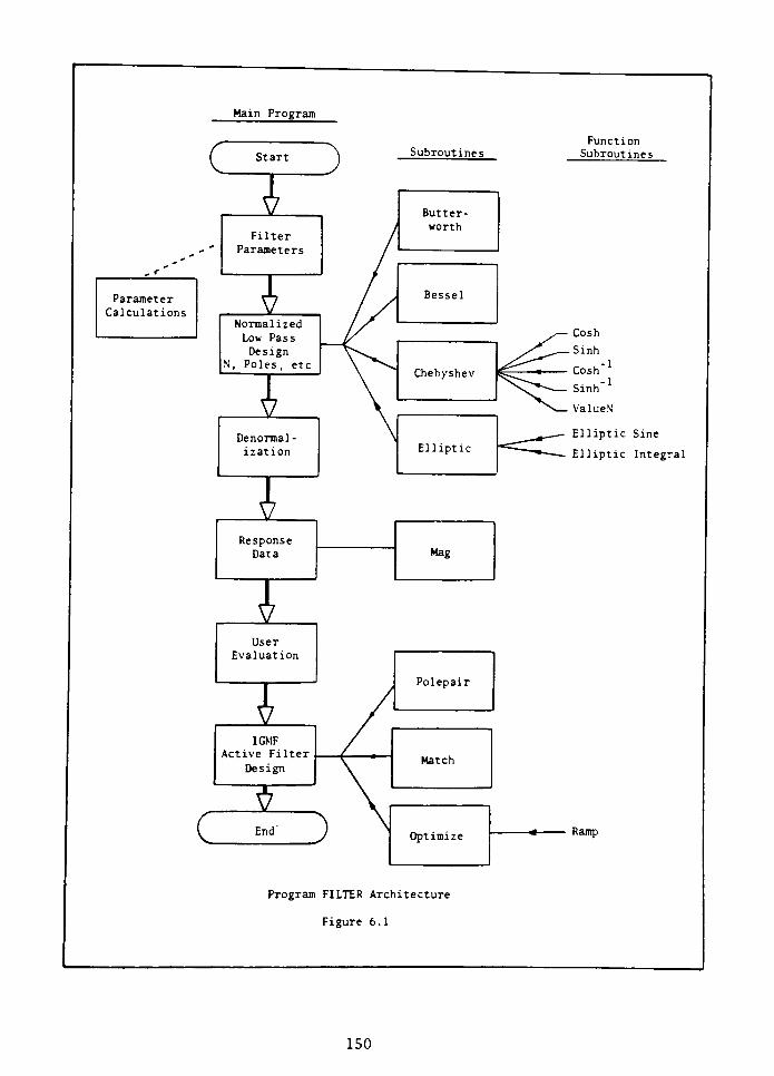
Main Program

Subroutines

Function

SubroutinesStart l

A j

, Cosh

s\_^. Sinh

tlButter

worth

Filter

Parameters

^r

BesselParameter

Calculations VNormalized

Low Pass

Design

N, Poles, etc.Chebyshev

V

^v^~~ Sinh

ValueN

^__Elliptic Sine

"~* Elliptic Integral

Denormal

ization Elliptic

hResponse

Data Mag

AUser

Evaluation

Polepair

4 //

IGMF

Active Filter

Design

/Match

\'

ft \

^ \Optimize

i EndV

tndj

Program FILTER Arch

Figure 6.1

itecture

150

algorithms. The program is organized in three tiers: the main program,

main subroutines and function subroutines.

The first tier, the main program, is denoted by the column of

blocks with heavy lines as shown in figure 6.1. The main program

follows the basic steps of filter design as discussed in Chapter V,

figure 5.1.

The second tier consists of subroutines which support the main

program by performing most of the analytical tasks. These routines are

particular to the kind of filter design requested. As an example, the

Butterworth subroutine, shown in figure 6.1 as one block, determines

the filter order, N, as well as the normalized poles. Included at this

second tier level is the elliptic function subroutine as shown.

Aside from the subroutines handling the classical approximations

(Butterworth, Chebyshev and elliptic) there are four others: Mag,

Polepair, Match and Optimize. The Mag subroutine finds the transfer

function magnitude, |H(jo))|,for a given frequency, oj. This routine

supports the main program block which directs the user evaluation. The

remaining three subroutines support the IGMF filter stage design.

Polepair performs the function of determining a pair of poles for the

second order stage transfer function. The routine, Match, scans the

denormalized zeros to select a pair to minimize stage overshoot. The

selection criterion is the nearest available zeros for the poles

closest to the joj axis. The routine, Optimize, determines the peak

frequency and magnitude for the stage transfer function. It then cal

culates a stage gain to minimize overshoot. All the routine parame

ters are passed to and from the main program using a Fortran COMMON

statement.

151

The third tier consists of subroutines designed to perform mathe

matical functions which are complex and therefore rather cumbersome to

include in the second tier subroutines. The third tier also includes

less complicated functions which were otherwise not available from the

computer library. Examples of these function subroutines are Cosh,

Inverse Cosh, Elliptic Sine, Elliptic Integral, Value N and Ramp. The

latter two routines determine the filter order, N, and the peak stage

amplitude respectively. Parameters are passed to the function sub

routines in most cases as a simple argument value such as x in sin(x).

This makes the task of analysis much easier at the second tier sub

routine level.

6.4 Chapter Summary

This chapter presented the salient features of the FILTER program

regarding its capabilities, user interaction and software structure.

This overview has not by any means given a description of all the user

alternatives or analytical capabilities within the program. The next

chapter, the user's manual, provides more detail on the use of the pro

gram along with examples of typical interactive sessions. The next

chapter is meant to be removed from the thesis as a guide when using

the program.

This chapter concludes the presentation of the thesis aside from

the Appendix. It is hoped that the discussions have built a sufficient

foundation for the reader to understand and appreciate the design of

filters and their contribution in the engineering field.

152

CHAPTER VII

USER'S MANUAL

The following chapter is a user's manual for the FILTER program.

Specifications of the program, input parameter formats and examples of

user sessions are given. The chapter is intended as an independent

section to be removed for use with the program.

153

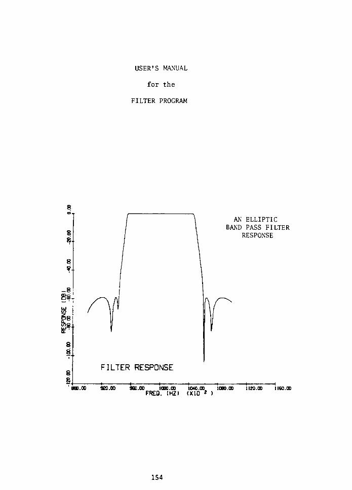
USER'S MANUAL

for the

FILTER PROGRAM

8

S-

8

-8

g8.

LU

to

8

8

8

8

AN ELLIPTIC

BAND PASS FILTER

RESPONSE

FILTER RESPONSE

880.00

-+-

SO .00 9BD.0O 1000.00

FREO. (HZ)

1040.00 1080.00

(XIO 2 )

1120.00 1160.00

154

User's Manual

Page i

No responsibility is assumed for inaccuracies or use of the infor

mation within this document or information acquired from the FILTER

program.

The information herein has been checked and is believed to be

accurate.

FIRST EDITION

(z\ COPYRIGHT 1981 BY LOUIS R. GABELLO

155

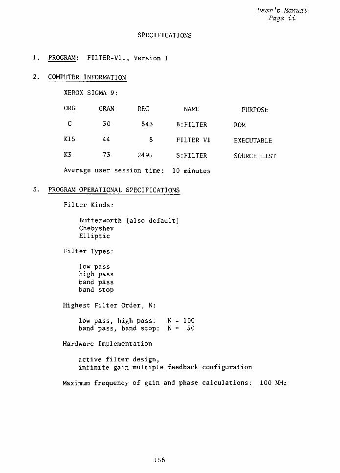
User's Manual

Page ii

SPECIFICATIONS

1. PROGRAM: FILTER-V1., Version 1

COMPUTER INFORMATION

XEROX SIGMA 9:

ORG GRAN REC NAME PURPOSE

C 30 543 B: FILTER ROM

K15 44 8 FILTER VI EXECUTABLE

K3 73 2495 S: FILTER SOURCE LIST

Average user session time: 10 minutes

PROGRAM OPERATIONAL SPECIFICATIONS

Filter Kinds:

Butterworth (also default)Chebyshev

Elliptic

Filter Types:

low pass

high pass

band pass

band stop

Highest Filter Order - N:

low pass, high pass: N = 100

band pass, band stop: N = 50

Hardware Implementation

active filter design,

infinite gain multiple feedback configuration

Maximum frequency of gain and phase calculations: 100 MHz

156

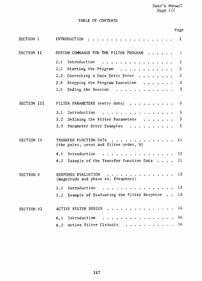
User's Manual

Page Hi

TABLE OF CONTENTS

Page

SECTION I INTRODUCTION 1

SECTION II SYSTEM COMMANDS FOR THE FILTER PROGRAM 2

2.1 Introduction 2

2.2 Starting the Program 2

2.3 Correcting a Data Entry Error 2

2.4 Stopping the Program Execution 3

2.5 Ending the Session 3

SECTION III FILTER PARAMETERS (entry data) 5

3.1 Introduction 5

3.2 Defining the Filter Parameters 5

3.3 Parameter Entry Examples 5

SECTION IV TRANSFER FUNCTION DATA 11

(the poles, zeros and filter order, N)

4.1 Introduction 11

4.2 Example of the Transfer Function Data .... 11

SECTION V RESPONSE EVALUATION 13

(magnitude and phase vs. frequency)

5.1 Introduction 13

5.2 Example of Evaluating the Filter Response . . 13

SECTION VI ACTIVE FILTER DESIGN 16

6.1 Introduction 16

6.2 Active Filter Circuits 16

157

User's Manual

Page iv

Page

SECTION VII USER INTERACTION (examples) 19

7.1 Introduction 19

7.2 A Chebyshev Band Pass Filter Design .... 19

(example one)

7.3 An Elliptic Low Pass Filter Design 24

(example two)

SECTION VIII A NOTE TO THE USER 29

(concerning evaluation and program limitations)

APPENDICES

A QUICK COMPARISON OF THE CLASSICAL FILTER

RESPONSES 32

B PROGRAM FLOW AND I/O SUMMARY 34

158

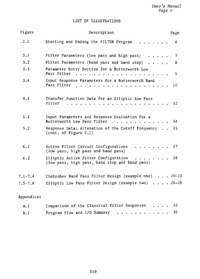
User's Manual

Page v

LIST OF ILLUSTRATIONS


2.1 Starting and Ending the FILTER Program 4

3.1 Filter Parameters (low pass and high pass) 7

3.2 Filter Parameters (band pass and band stop) 8

3.3 Parameter Entry Section for a Butterworth Low

Pass Filter 9

3.4 Input Response Parameters for a Butterworth Band

Pass Filter 10

4.1 Transfer Function Data for an Elliptic Low Pass

Filter 12

5.1 Input Parameters and Response Evaluation for a

Butterworth Low Pass Filter 14

5.2 Response Data; Alteration of the Cutoff Frequency . . 15

(cont. of Figure 5.1)

6.1 Active Filter Circuit Configurations 17

(low pass, high pass and band pass)

6.2 Elliptic Active Filter Configuration 18

(low pass, high pass, band stop and band pass)

7.1-7.4 Chebyshev Band Pass Filter Design (example one) . . . 20-23

7.5-7.8 Elliptic Low Pass Filter Design (example two) .... 25-28

Appendices

A.l Comparison of the Classical Filter Responses .... 33

B.l Program Flow and I/O Summary 35

159

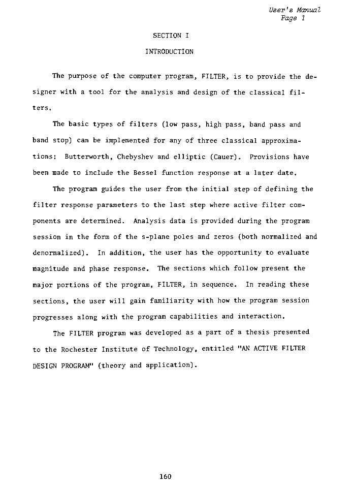
User's Manual

Page 1

SECTION I

INTRODUCTION

The purpose of the computer program, FILTER, is to provide the de

signer with a tool for the analysis and design of the classical fil

ters.

The basic types of filters (low pass, high pass, band pass and

band stop) can be implemented for any of three classical approxima

tions: Butterworth, Chebyshev and elliptic (Cauer). Provisions have

been made to include the Bessel function response at a later date.

The program guides the user from the initial step of defining the

filter response parameters to the last step where active filter com

ponents are determined. Analysis data is provided during the program

session in the form of the s-plane poles and zeros (both normalized and

denormalized). In addition, the user has the opportunity to evaluate

magnitude and phase response. The sections which follow present the

major portions of the program, FILTER, in sequence. In reading these

sections, the user will gain familiarity with how the program session

progresses along with the program capabilities and interaction.

The FILTER program was developed as a part of a thesis presented

to the Rochester Institute of Technology, entitled "AN ACTIVE FILTER

DESIGNPROGRAM"

(theory and application).

160

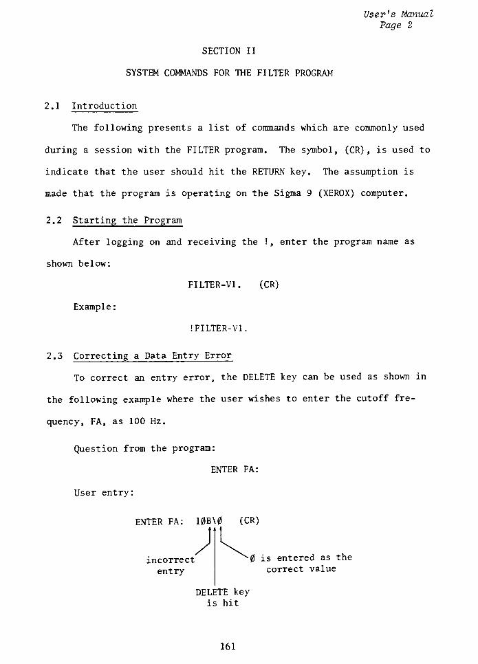
User's Manual

Page 2

SECTION II

SYSTEM COMMANDS FOR THE FILTER PROGRAM

2.1 Introduction

The following presents a list of commands which are commonly used

during a session with the FILTER program. The symbol, (CR) , is used to

indicate that the user should hit the RETURN key. The assumption is

made that the program is operating on the Sigma 9 (XEROX) computer.

2.2 Starting the Program

After logging on and receiving the !,enter the program name as

shown below:

FILTER-V1. (CR)

Example:

IFILTER-V1.

2.3 Correcting a Data Entry Error

To correct an entry error, the DELETE key can be used as shown in

the following example where the user wishes to enter the cutoff fre

quency, FA, as 100 Hz.

Question from the program:

ENTER FA:

User entry:

ENTER FA: 10B\0 (CR)

incorrect

entry

0 is entered as the

correct value

DELETE keyis hit

161

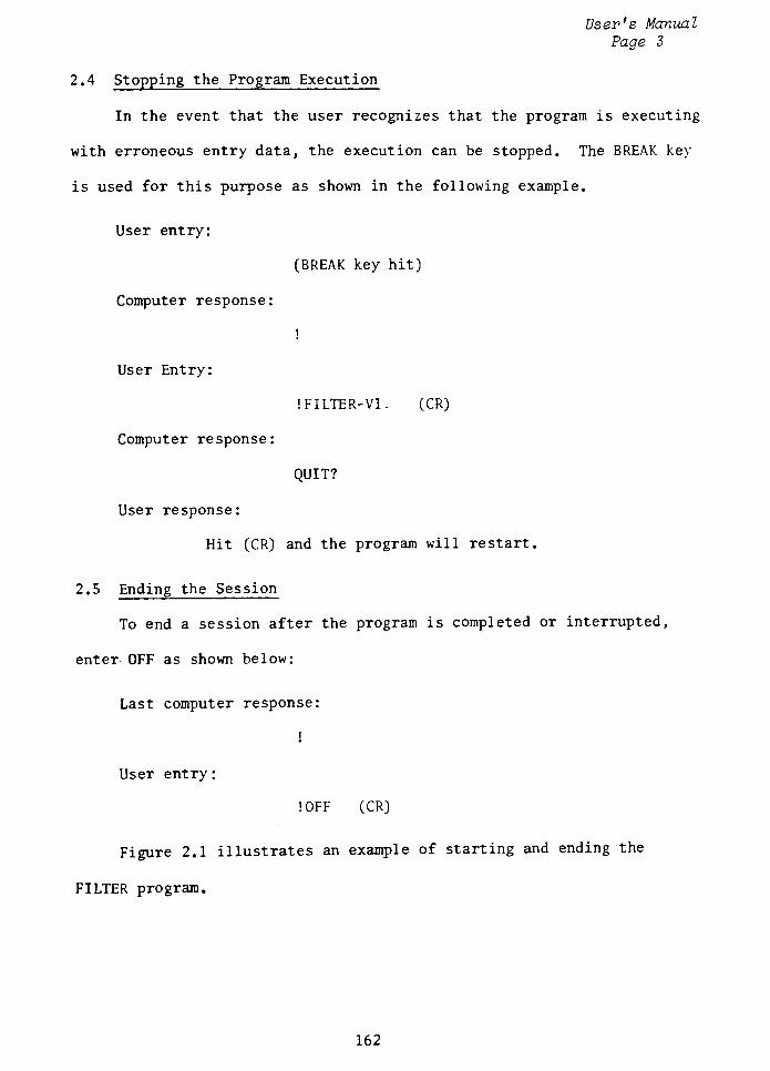
User's Manual

Page 3

2.4 Stopping the Program Execution

In the event that the user recognizes that the program is executing

with erroneous entry data, the execution can be stopped. The BREAK key

is used for this purpose as shown in the following example.

User entry:

(BREAK key hit)

Computer response:

i

User Entry:

1FILTER-V1. (CR)

Computer response:

QUIT?

User response:

Hit (CR) and the program will restart.

2.5 Ending the Session

To end a session after the program is completed or interrupted,

enter OFF as shown below:

Last computer response:

i

User entry:

!OFF (CR)

Figure 2.1 illustrates an example of starting and ending the

FILTER program.

162

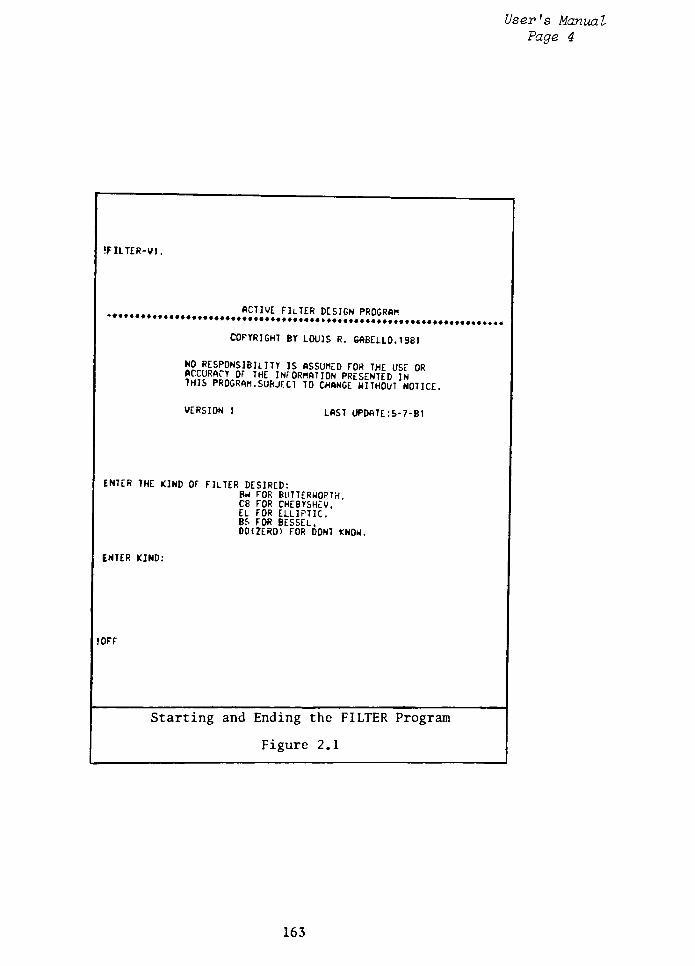
User's Manual

Page 4

IFILTER-V1.

..........

flCTIVE FILTER DESIGN PROGRAM

COPYRIGHT BY LOUIS R. 6ABELL0.1981

NO RESPONSIBILITY IS ASSUMED FOR THE USE ORACCURACY OF THE INFORMATION PRESENTED INTHIS PROGRAM. SUBJFCI TO CHANGE WITHOUT NOTICE.

VERSION 1 LAST UPDATE.-5-7-81

ENTER THE KIND OF FILTER DESIRED:Bu FOR BUTTERWOPTH.CB FOR CHEBYSHEV,EL FOR ELLIPTIC.BS FOR BESSEL.00 (ZERO) FOR DONT KNOW.

ENTER KIND:

!OFF

Starting and Ending the FILTER Program

Figure 2.1

163

User's Manual

Page 5

SECTION III

FILTER PARAMETERS

(entry data)

3.1 Introduction

After the user logs on, the FILTER program will request the design

parameters of the filter. These parameters include the selection of

classical responses (Butterworth, Chebyshev, elliptic), type of re

sponse (low pass, high pass, etc.) along with the attenuation and fre

quency parameters. The FILTER program accommodates many combinations

of input parameters (including defaults) . The user should try various

combinations to become familiar with the various possibilities. The

program however will guide the user in any event.

3.2 Defining the Filter Parameters

Prior to running the program, it is advisable to have a list of

the response parameters which you will use to define the desired fil

ter. Figures 3.1 and 3.2 illustrate the straight line transition dia

grams for the four filter types. The parameters used to define the

filter responses are shown. The symbols and their definitions are

those used by the FILTER program.

3.3 Parameter Entry Examples

Figure 3.3 illustrates the parameter entry section for a Butter

worth low pass filter. The desired filter has a cutoff frequency.

FA = 100 Hz with a maximum pass band deviation, -ADB=-3 db. The stop

band edge frequency, FB, is 860 Hz. The minimum stop band attenuation,

-BDB, is -40 db.

164

User's Manual

Page 6

Figure 3.4 illustrates an example of the input response parameters

for a Butterworth band pass filter. The desired filter has a center

frequency, FC = 455 KHz and a bandwidth, BD = 10 KHz. The maximum pass

band deviation -ADB, is -0.1 db. The stop band edge frequency, FB2, is

500 KHz with a minimum attenuation, -BDB=-40 db. All frequency en

tries are in hertz.

As part of the parameter entry section of the program, various in

ternal validation checks are made on the user data; when necessary the

program notifies the user and asks for a correction or verification on

the entered parameter(s) . An example of this is shown in Figure 3.4

where the user defines the bandwidth for the Butterworth filter as

10 KHz but the pass band edge attenuation, -ADB, is -1 db. The proper

bandwidth is defined for a Butterworth filter by the -3 db frequencies.

As shown, the program accepts the data, calculates the proper -3 db

bandwidth and notifies the user.

165

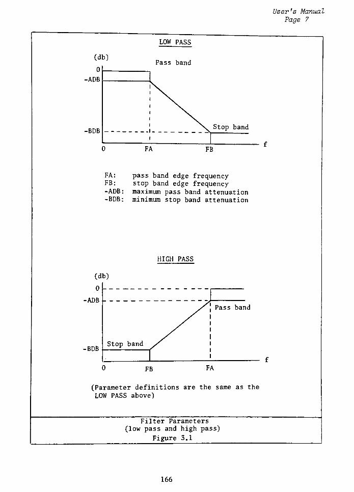
User's Manual

Page 7

LOW PASS

Pass band

-ADB

-BDBStop band

FA: pass band edge frequencyFB: stop band edge frequency-ADB: maximum pass band attenuation

-BDB: minimum stop band attenuation

HIGH PASS

-ADB

-BDB

(Parameter definitions are the same as the

LOW PASS above)

Filter Parameters

(low pass and high pass)

Figure 3.1

166

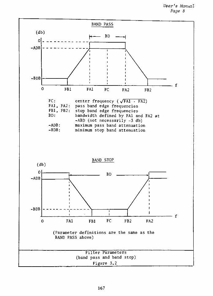
User's Manual

Page 8

BAND PASS

(db)

0

BD

-ADB

-BDB

FBI FA1

f

FC FA2 FB2

FC: center frequency ( y/Vkl FA2)

FA1, FA2: pass band edge frequencies

FBI, FB2: stop band edge frequencies

BD: bandwidth defined by FA1 and FA2 at

-ABD (not necessarily -3 db)-ADB: maximum pass band attenuation

-BDB: minimum stop band attenuation

BAND STOP

-ADB

-BDB

FA1 FBI FC FB2 FA2

(Parameter definitions are the same as the

BAND PASS above)

Filter Parameters

(band pass and band stop)

Figure 3.2

167

User's Manual

Page 9

ceca.

i

oorzo

oz

2 = -

o ccoca

uioacDa u;zzzzz a.a. a a <x<xcc co m co cc 2

cc cc acUIO, CklftU)w _

*

15 or cr

UI I-OI-

.Jl-t -*

a.

cr

=oui

ce

o

S ZuiZ UI3

UJ QUI3 SUICC3! Jjeru

ou> UI

_uo

O 00ZZO. ..Qu

CD -J>-UI- .. ..C_J QCUKZQZZUIUiUIZ ccfl-l-DIB-i-joaui

Irt n* i-tw (y) ûiuu or u^ cc

<Z ueca.<eu.u 0,oooce ce~ uiorujOOUI-UZZZ0-Z3U

>>T3 1 1

C cCO 0

</) c.in 0co +J

C- t/)

TJ a

C cCO CO

.C X!

0 -<_> ..

zzzzuiZiuZ=0=0oesoa

DCOC

ZZZZccccccccCD CD CD COmm a. o.

ecec>-i-

Q-0_mm

T3 c

G 0C3

c/i

w IT)

V) rt

cfl Cex

J=

2 M0 pH

. 1 -C

* _ 0 <- co

CO 0 1

> en UiZZ ^

m-*

r 3 *-

<C 0 OZ3z > _i UIUIO UI

0 > -j Zi-I ?

0 UI >-z>- CCor > m O0. > cc ceuiz O.

> 0 3z0 0.U

> cc a z mw> UIZCC cUI u> ZCSI 1

0 1 1 3 <J

or : gUI > _j

eii-

^ de_ J > >> mO>-

f* CO U<_>

u. Zui1 1 >-->

UI X - CDr ' 0 "US^H

llul

> ae -.-

O >- CO ra a. fiua

: 8moorz 0

coor5IACEO.

uior

ESU) i/>

Oi-i ce001

SZCEr-

cr> - zouu o3x -a

cem>-_iui>- cwuice^CO>mOÛl -JiÛ

OIju

CC0UUICOo

oisjjio

oaoucoe

ce

in - .

m m lo a.

m<E LOOeic>-

0. a. m

100

IliZZ0~<X <X

-iimc

o

a

mui

a

&

uio-

c8

Uu o

O 4->

H

c u.

oH 1/1

l-> l/>

O CO to

<L> 0.

>, O

U -J

K)

C XUJ ^j

IH

^ od) s

0) (U

E 4->

CO *->

U Z3

CO CQ

168

User's Manual

Page 10

> ui1 ^H

i z

1 a

u5 3h0 < aO ? i z? ui l <xuJO < cocaOu3 aitW i mac

Z 7 U> i i uiUi e i a.> ? I ^-o

ui i ace UJ 1o > O O 1 1 Q_ or i O 1

O 1to <JZ

o o i i aOOJIO i i UiUi

CC 1

to

cca tOZUi3 OU3

-o . i i CCZ m i

UI 1

t-iul 1

UO I

Z * i

UIUI

3<M I

Ou3 1

Ul< 1

ce i

U. 1

ei i

Ui ? =o ~- W l I i/l . o

^ UJ

cc

Ui UiOUi3 uOuiCC ^ ^ t I uj O uj

a aUI UI

ce or

i lOCCU.

vu.> UikO

UJOO

O..U-- I I JE Sizzzz i o i muluxi oi m

OOOO i o i

m i

-j i

CC 1

oO 1

UJ

I

a. cs<2 *

ZIO. "OUUICC CD >-

UJ O

OOOO I i oU. Ul 1 1 Xce co ce 03 i i i .

3a. SKKZQZ-

uaua i i a x at

aa

mz i

i CC io oz z

z ZUJUJUJ 2 uiuiuiui a i cc*-ma or id i

z z(9 O

Q uj u. u. 0C ul - <r u. u. o_ aDCOG 1 O I O CC

zzzz i i ji-ja

0- ? 1

Ouj 1

O 1

m mOC oooo; cr ccacccciori <r o _, cc a i ce i

Z

<UJ CC Uj t Dffifflffl I ul I 3ZOCD

0--Q"

I

OOuhuXO mmcwa. i ? *-ua ^ i

z ZZQ.Z3CZ mmoo i_i i oa m UJ * I

. .

3 *->-wO"C ccc i-ii-ii cczmi Z It i

tO 4H-U_JXC0

cc1-nr

a. 0. mm i u CCCC U 1 CO

33 rg fflUi 1Is-* 1

U ft

o cd a w O D<C u. CD 1

; -M +J

ce ceocea

0)

i 1

Ui LJOU 01 .HOr

z zozo4- ^ u.

ui uj (_n uj r CU1 c- <^ o-

^H O

cc >, uUX3 C

+J Ul

4) (/)

E co

CO 0.

CO T3D- G

rr

CD. cfl U

ODm aa 3

*a - Ul toCC

(Nl i CM

cc a

C J=

O 4-J

U fMU D. !h-ccu>- ui O

cc u CD 3uorz

w OulOS >h

CDvO to occ U-Offl 4-> 4->

m -

LO LO LO fl_

UJ cc uia

ou.ee a 3 4->

UJ *Z U 1 G- 3z

ccOOCCujS

uo o a

c cai i

a.

Ui

co

vuffiCk

>-orauito OU. 1

or z aceUI UJUJUlZ

zz

ccccccccoooo

z i oouccaa ooa.

uj oaoaaaUJUJUIQ. I -

z

U.U.UU.

o

ujO, 0- a. cO

to cc or o zUi

cc *>-

or uoa-o-

cc zzmza

- *

zcc ji aaaa

z a. orcccc <r~ z o*- uiaaormz o a

to 3 ce UI HUllDulO zUJ a. 1 UJ l/l z m m o. o z x ae

z i a Z UJCCCC0. cc o

CE

i go oa.o.3maa.

-u

zUJ CO o^

cc UI o o^ UJ or or

CC UlU.

-Ja-*

UIV1

O FN

uu. u. -X eO

UIAOUl-J O X

UI o_i ce t-

a. H- .. oo ui a^ z UJU. *j i^

3 or zUi See m o a

Sa. zo UJCC z

u X u cc>

3

l-O

UI

u. CBo

cc cc oor orz ceo oca

UJ ui >-UI UIM UIO UlO1 f-

*-* ?-U -U1 >-o

Z Zl2z

ZUI zm ze

UJ UJCD UIO Ui* UJ'

c* e*- r- ^>

169

User's Manual

Page 11

SECTION IV

TRANSFER FUNCTION DATA

(the poles, zeros and filter order, N)

4.1 Introduction

After entering the input parameters, the program evaluates the fil

ter order, N, and the transfer function poles (and zeros). Both the

normalized and denormalized values are provided to the user. Other in

formation such as elliptic integral parameters, bandwidth, oj and Q

(for the pole pair), etc. are provided as secondary parameters calcu

lated by the program.

4.2 Example of the Transfer Function Data

Figure 4.1 illustrates an example of acquiring the transfer func

tion poles and zeros for an elliptic low pass filter. The filter has a

-0.1 db attenuation at the cutoff frequency, FA = 100 Hz. The stop band

is defined by FB = 860 Hz with a minimum attenuation, -BDB= -40 db.

The resulting filter order, N, is three.

Figure 4.1 also illustrates the elliptic filter parameters derived

from tbe data entered by the user. These secondary parameters (small

Kl, Kl, V0, etc.) are significant only to those familiar with the for

mulation of the normalized poles and zeros.

170

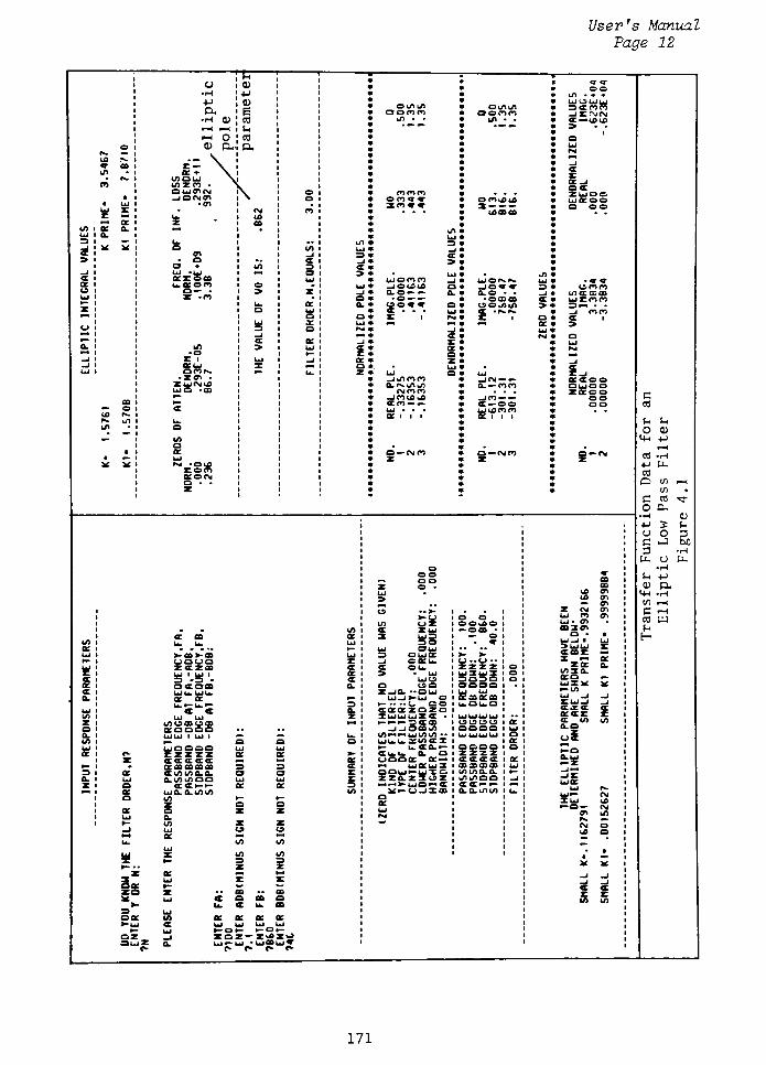
User's Manual

Page 12

tp 1

u . <DOS

H I+-1vO * ? ?

P 1 <D

: e

* UlOuJul* OkOkO m o i_fi lO * Dcnnoonn * oonn * _i zr\icsi

H d) un * urt . . CE ~iw0(j0

i ( i 1 . Sh*" "*"

-- >

^ O ! CO * a

r-

O 1 oj c..; p. * Ui

u> r- i \**

a i z- \ * CC* z* CC -1

occ* Z UiOo

Ul i or* \rs. i mouj ^

vco uizci . \

O UlCOCM \ O nnn ^ >

i Jfirgffl | X o OP,7C OfT-uOOJ uiccooUl 1

Z I

a an*T<? * z * a ooul

z u.

C\iU)

m > * tOCDOO

or i z 00m i or a. i

*o *UJ 1 o. Ui *3 u. tS) 3 *-J K * o IO Ui *

_j

CC COj 3 * CE

> o

a ? Olcc

3-J

i

<c> *

-J Ul 'UJ ^* O > UJ %/> mCC or zoa Ui uonn _j uo^n Ui * <T <Tor u crm o Ui >

-JOlCtA O* JO*7*7 3 * U-Plf*)o O . > z _J * Q.O 0- 0l O -j * to <r cocoUJ z <* o * -O -OCD0D cc * uiZP*><rt

zu. cc 0- ** o o r v a* oohOurt > 3

o Ui CC - * Ul* cc ->-*>

Z I rsi z t

_j menw a a * o * cc

ui -c Ui *? - m * ~ cc * >o 3 o rsi t*

_J >Ai *J CC * x * a

?CC cc -j z * Ui

a. Ul > Ul cc > ce * rvi> o ^- Z i* o *-j Z I Ui -i cc * z _J

i orui z o i Ui * * CCUJ 1 u. z ** ui a * uj

ji/inn * _jcy^

CL *s> l0 tO * Cl. - fi (T)rymrn * ...

V jC_i

* ceccoo* OuiOO

* zeecoc.

-inujj _jcnm- * oo

a i ^ CCfO^*- * C-OO * oo cflO 1 cc ui * ujijprici

U9 r- i

Ul 1 u.CC i t i cc . t

u ul/l

jo

o 0>

m

o I 1 1

I

1 ceUl z z

* 0*-(\** z

CO -H

ii Zlzam

P u.

cfl

Q Ulororvio . .

i t

z-

U)

C CO

O D.

4-> 3 Sh

O O 3c -J M

3 H

U. U U-

O 1 H

o O 1

O O 1

Z O i

CO i

CO i

J-l -l-l

Ui t

> t

to on i

U3 CO 1

CO I

<4H -H

Ul ^H

U -->- i i I Z rg CO i C <-t

>- O 1 O O l 1Ui CO Q0 i

CO UJu) uz i eotoo i t Ui * CO i

to i CC Z ui i OC0 i I a s co i

cc a ce i 3 uj3 i o i i o i HUJ

oru. U. ui i

^- i

3CT i * i I

Ui Oud 1 I

.

K

.

Ul *- a >-a Ui 1 3 oujcc i >- >- i i*

<jac->o z _j *=ceu. u "O - * i

Ul z ccza CC i CC ou. > ZZZZ i o i

E

S '-^ '.CC i > UJ lUlUl 1 O 1

CC CC l UiO 1 3030 > O I

or OCOGD O. ' o oo i oaoa >

CC UIU.UIU Z-JQ.-OU I Ui Ui i t

a. cc or^ i uj_i>-uj O I CBACCffi I I

U-l _J _J |

ZUi_i _j 1u_ ? u. 3 i

^. ....(_ coiu.au.ai i

Ul cc CC O. * cccccczazo i i i CCCC CC CC I

CCCCZ Z I

CC tA (A i

o.a i

Z i

OCC i

Ul Ul Ul Z XuiuiuiZCC - * UiUiUiui i -

z idoduo t-h-r-DCCD 1 OOOO I CC 1

o ceoooa .. _i_jocpvO i aaaa i ui >

a. UIUJ 1 Ul 1 u. * irtMMujtnin i UiUJuiui * a i

u> . O a o uju.u.xtoccz * i ce *

Ul uiaaaa w Ui u,cco.îaaoaiOi

-a !CwUJ 1

*-Z I

ae <*-zz z zz ce cc

>- 1 cc uu. ol aizzzzi i

z cccccc cccc *>* CC 1 oooce ce*-*i<caccccicei

^ or aaaa 3 3 CC i * UiCCUlZ CD3DCOCO i Ui i

3 or ccuiui a. a. a o Z t OQUHUlC I I/)LOQ.0l i 1JC !UJCC 1

UJ r-u iuj*-

rg i

ZUJ to i-0 fSjj ,

CO uO 1

fSk |

a. Ul o-mmoo Ui Ui z ZZO.ZZOZ i uluTOO I -J i

z a cc cc i i cc cc 3 l i-^ÛJO'-'CC * CCCC*^* i i

or uio. o, mm to * X. *- u> -J I CD 1 CkCLiOU) U. I

o

orUl

Ul

zoa.

o

zoz

O t ll

CC i ii

Ui I ll

r4 I ll

Ul z z rsi o i

U9 O 1-j UJ o o

u.or

Ul

to to

1

1

1* V 1

X 40

z

to

z

z or M **1 J 1

loUl

z

z

CD

z

CD

to to iX Ul cc a m aI" u c u. CD

3 Uloor in ce ce cc CCJ-UI cc ui Ui Ui -.^

ui*- <= *-?-

z_ 2 zo z~ ZtDX -

auiz 0. UJ w_^ UJ 3DuJVp- c* C" c- r-

171

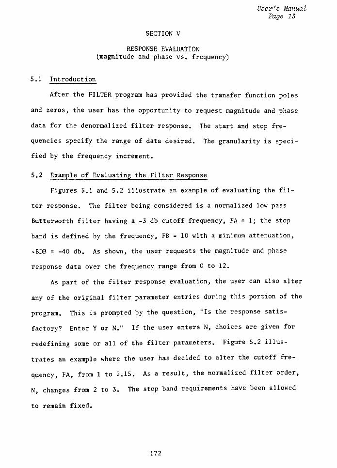
User's Manual

Page 13

SECTION V

RESPONSE EVALUATION

(magnitude and phase vs. frequency)

5.1 Introduction

After the FILTER program has provided the transfer function poles

and zeros, the user has the opportunity to request magnitude and phase

data for the denormalized filter response. The start and stop fre

quencies specify the range of data desired. The granularity is speci

fied by the frequency increment.

5.2 Example of Evaluating the Filter Response

Figures 5.1 and 5.2 illustrate an example of evaluating the fil

ter response. The filter being considered is a normalized low pass

Butterworth filter having a -3 db cutoff frequency, FA = 1 ; the stop

band is defined by the frequency, FB = 10 with a minimum attenuation,

-BUB=-40 db. As shown, the user requests the magnitude and phase

response data over the frequency range from 0 to 12.

As part of the filter response evaluation, the user can also alter

any of the original filter parameter entries during this portion of the

program. This is prompted by the question, "Is the response satis

factory? Enter Y orN." If the user enters N, choices are given for

redefining some or all of the filter parameters. Figure 5.2 illus

trates an example where the user has decided to alter the cutoff fre

quency, FA, from 1 to 2.15. As a result, the normalized filter order,

N, changes from 2 to 3. The stop band requirements have been allowed

to remain fixed.

172

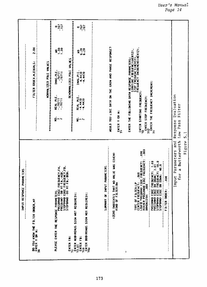
User 's Manual

Page 14

r^ *-^. p

oa * ooap. r^

^.p.

e i

a i> mat

OINifMUJ

LO |SJ

oj 1z

I u?u? o i- CC0. C -uiUl "Ui Z' |j0 Ul UllNw

m

UJ

3-i

CC>

1UJ

\ 3cr CB *-*-

Ul 1 Ui>-CCZ

_j i 1 CE

; >

Ul uiuiui

cc i

3 i

ul

ccuzir

Cw-u

O iz CE3CC

UJ I

1 uj a. aouu* Ui _j . Ul o o CuZZ

Z i

UJ

l

o0.

"-

oi Cl. r*. ^- 0.

* _nn

c, r ra

zO-CCUJu. 3

ceUl 1

a i

or i

O I

I

o . .

cc Ui o>-

tOOuJu)

aUJ

CT V V

Z I

z

cc

ZZZZO u. -J

*

O.* 3 Z_j o LO CC CL O UJ

ce ii

cccroz

1 cc> z <

cr <

o <

z* .

uji ui a .

uiCCOUi z

Ul Iul CC--CC ui

i i

U. 1Ul

Z

zo

tOtOu. QC

i- o zCE Za uj -

-5 <_> >-

Go

joaHa. Cwfn n a o o z u

r <r Z Ui Ui Z PI o o .CP*P. a

1 Ul

Z i I i

-j <r <r

cccco

~ CB 3 UJ

3 U, O 3o ui a

CO P4

3 <Dcr i i UJ

_j o ce ui !-H +->

Za1

5 *

2 CO i i

> -H-J u. - 0,or o uia UJ LI-

o .-\j ! O IN| gUJ C t- ZI m

z . Z

a cc

>- Ula a

a a uj uj

CU Ul

U) U)

C cfl-j Ui UJ uj.

3 <-

z z O 0-O Z Z Z ulPJui Q.Z uj-*-

UJ ujO

*> p- p- p- U) 3cu oDC J

T3 X

LT,

e -^ f-

CO >H 3

o

OO

o DC

u> 3 H

" o o f- !- U-zui

o >

0) 01

:> P(-!

o >->- i o oCD P

>-U I oto UZ 1 - o o co oa

m a Zui i o .

ucc a a z Ui3 i OUl u. u UJ OO I PI T CO cflce Ui O-J D.

PH

Ul >-a>-a ul 3 OuJC 1 >~ >-

UQUQ r -J OCT U. I CJ .-o -

UJ zee za cc CE OU. I zzzz O i +J o

3 <4Mzcc

Ul i y i

3 -3 -

QC

CC> uj I UIu3

UO I 30 OOO i

i

cc on oa 0. O oa i oaoa O.c uûu. ZZ L"Ou I UJ uj

C-0. cc or CO -j-uj i aaaau--w> 3 * (-i ao > uaua l-H

Ul cc cc 0- CECC arzczo >

ol UJ UJ z Zui UJ Ul Z CC 1 UJUIUJUI

z uioaoa *- ? o cc a ioouo ao oraaao _J _ioam i aaaa Ul i

a. uiui UJ u. */>* Ul/l\/l 1 ujujujuj a .

Ul a a o UJ u uamccz i a .

Ul ujaa a a UJ Ul ^- u. ct o_ aaoa o .

ce p- zzzz z or a >-

5ou a a i zzzz

Z ec a a <r a oa a ct <x ct ct a i

ara aa a 3 3 a uaul aaaa Ul i

3 or ccmmao. o o z aa ui? uj xa uimo.0. ^ i

a. a-mmoo Ul UJ zz clzioz mmooz ct <x ec or >-uio a i aeci-

8oeUl

-j

u.

I..

is

PP Ss */>

a

CCUJ

Ûjlffi t 0.O.U1U1 u I

z m a

X UJ cc a a a>- u> ec u cd

3 Ul

OK Ul z or or cc

-UJ CC ul Ul Ul Ul

.- UJ* .-> *-

OUIZ a. ui-

z -zoza- uiPlul UlC

P- r p- p- p- i

173

User's Manual

Page 15

~J <

CE <

> <

<C *

zcc <

o <

a. ldto

oco

cc

oo aOLD CkOtA

-JO OOa. o ooo oo

-JO ooCCijO 'lO

CC i I

OooouO .

i/ilOlOS . . .

tcoroco

ujcn

-J CO

a. to

O uTi

o en

ouo

o

ilO <T< LO

a. o r

tOuO uO

*x >m

UJLD lO

CC l i t

: r*-0

; ro ps. f\j co j3 cd o rsjo ro- "Of*iLi"i1/ia)u3>jjNf\ rN.p%.p.0~i _,*__

tt * '

CO- fO O CO fsiOr-Ojv oo ...

Zo - rsi en -v <x> m uD co o ro** CO^-^-fM(MfOfOmm^-*T^-

Ct I I t I I i I vj | | | i

-..--. r\jc\ioooooooooI 1 I I I t ( I I

UiUiUJUJUJUJUiUiUJOmjICH"- CO uo

<*

to O CO COUO<-i/l4rCDr%.(j}C(\ocCO>N.rs(OniT:r-<Tu3nOu39Zoov rsicni-ôuOfsjoosicn

*pN.rsi upmryrsi *~coto

-oooooooooocnoooooooooooooo*.ooUJOOOOOOOOOOCOOOotoo oooo ooooco <

U, CMnsifo^-tousrs.cococo

O*-fSi(T>^4l0t0rC0C0o-fNifO

ccor

cc

za.

cc

z

o

cc?

CE

zI -

zoo

to

Ou ZOO UJZ

oCCa.

oa.o

Qp-

v zoa<_>z oo. z. t -*uia

a iuiiô

o o-aO Zu

p- 03i-0a Z0-_l<- Ul

Z 3 ii

a Z uU

a o -m

_jujuiujzCC

Ul JIIIUm Oi-i-i- > ul

a z u. 03o UIUJUI Za UUOUi-

m I ZX 2 IX

Ul i-CTCT CT Z

a >- xzii-oa UUUUUIU

>- oo ccsucw

z i_> zUl a3 u. 3O ui o

o Ul

zz ii

?- aZE ma

ceo UIO

2

0) LO

X

P Oi

(h

^ rt

P O LL,

CO CQ <L>

3<u cr

U) CD

C Po u.

P.U) tp

0) <P

os op

3U

174

User's Manual

Page 16

SECTION VI


6.1 Introduction

The last major portion of the FILTER program provides for the hard

ware implementation of the denormalized transfer function (poles and

zeros) using active filters. The user enters the desired gain of the

filter in db. The program then identifies the circuit and component

values using the nomenclature in Figures 6.1 and 6.2.

6.2 Active Filter Circuits

Each of the active filter circuits shown in Figures 6.1 and 6.2

will implement one pole pair (second order transfer function). The de

sign of the overall active filter is then accomplished by cascading

stages of these second order active filters. The parameters identified

for each stage are the pole pair- co and Q. When N is odd and the fil

ter is a low or high pass, there will be one stage which implements a

single order function or one pole.

For the case where the filter is non-elliptic, the program pro

vides component values using the circuits in Figure 6.1. For the

elliptic filters and band stop filters, the program uses the circuit

configuration shown in Figure 6.2. This circuit provides for the com

plex numerator zeros in the denormalized transfer function. There are

other ways of implementing a transfer function with complex zeros

(such as the dual integrator or the voltage controlled voltage source

methods). However, this concept is unique in that it uses an infinite

gain multiple feedback (IGMF) design approach. This is consistent with

the IGMF design philosophy of the circuits in Figure 6.1.

175

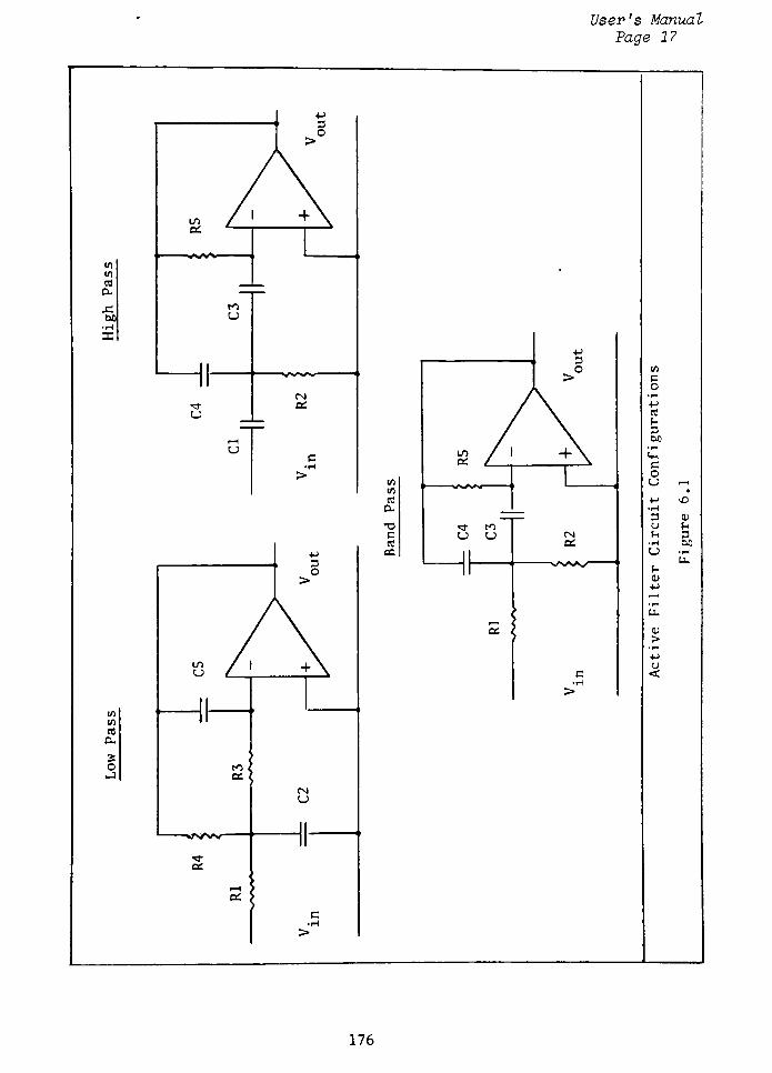
User's Manual

Page 17

Ul

Ul

cfl

O-

XOO

p

3O

>

LO

OS/ 1 +\

II

u

II

u

CM

OS

i i

u

>

cH

Ul

U)

cfl

D-

o-J

3O

LO

u

OS

u

*r

as

ui

Ul

CO

D-

V

c

CO

pa

p

3O

OS

CM

a:

cfl

p

300

LP

c

o

U i

3U

PTH

u

p

oi

cu

>H

P

o

<

CU

p

3DO

176

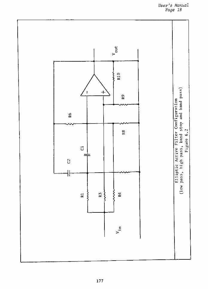
User's Manual

Page 18

3O

OS

cm

u

IF

NyNAJV

CO

OS

Kl

OS OS

u.

ui

CO

D.

CO T3

H CP CO

cfl XP

3 T3

00 CH Cfl

 Ul LL,

H CO

P aU

< X

oo

U H

H XP

c *<

H U)t < IT;

i 1 Cfl

LU G-

O

177

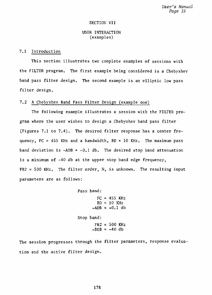
User's Manual

Page 19

SECTION VII

USER INTERACTION

(examples)

7.1 Introduction

This section illustrates two complete examples of sessions with

the FILTER program. The first example being considered is a Chebyshev

band pass filter design. The second example is an elliptic low pass

filter design.

7.2 A Chebyshev Band Pass Filter Design (example one)

The following example illustrates a session with the FILTER pro

gram where the user wishes to design a Chebyshev band pass filter

(Figures 7.1 to 7.4). The desired filter response has a center fre

quency, FC = 455 KHz and a bandwidth, BD = 10 KHz. The maximum pass

band deviation is -ADB=-0.1 db. The desired stop band attenuation

is a minimum of -40 db at the upper stop band edge frequency,

FB2 = 500 KHz. The filter order, N, is unknown. The resulting input

parameters are as follows:

Pass band:

FC = 455 KHz

BD = 10 KHz

-ADB= -0.1 db

Stop band:

FB2 = 500 KHz

-BDB=-40 db

The session progresses through the filter parameters, response evalua

tion and the active filter design.

178

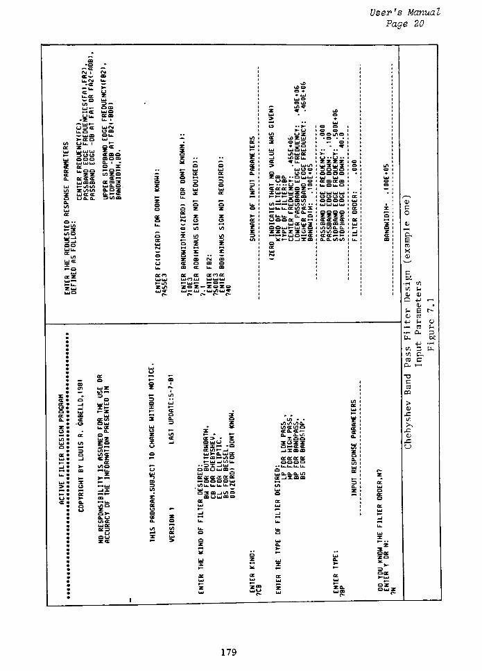
User's Manual

Page 20

-o.

arvi

cc au

-a>-

a o

UK z

-o Ul

3oa

-" UIO

PU. era

Z U 1

3a UJ <M

o oa

a

w uia

>-ao

PU I

auoa

zza a: a

uiaa

mmzmui

uj a apa- a.

zaaoaoa

a. i -

o x>-o>-

una

aaazUCLO.

0.OZ

oz

a

o

oo

UJU.

a

ozx

O i-i

a 3o

ce ui

o a

oo zaul Zrvi o

ui

< x a (Ni a

o a o a a

u a a u. a

an a a ana

uiul ujroul uiujui

.-m.-uii .-*

zm zoz zozo

uj -r ui'Ui- ujm uj <r

z>

o

UJ

O ^0

u*i c

a-Zui

OUI3? 30UJ O uj

U1UIZmauVu.

uj mUIO

OO *

- .-OUJUJ

-J >- UJ O

o oe

rzoz

juZC *

-oaa

joa m

. ujmm

.crlt ct I

u. a a.- a aso- a>-

uia ui 3Ji-UlO

oooo

zzzza CT CT CTaaaa

muia ammooaa>->-

aauiui

a

oa

lj

o i

aa <

a

ao

m3O

gm

UJ

U.K

a

a 2

a>- u>oa u.

UIOzo>-

a.omauia

0C3u

OP

.- Ul

3O Ul

J aa

*3

UJ

o -

Z m

a az -I

<_>

o

p

a

<J v

oa za o

Ul m

a

o

z

DC-> * ZOuO Ozx~ -a

CC Lrtr- _JUO-CwUiOCr ffi I uO OP~

1_J _J L/1 Lw

OZJU

UJ o

ccoccco: o: ccmOOOOuj

tOUUUUN

'Ui w

03 oa-jtooCDUUiXO

CC

O

a

Z

to -

wOc/lvO Cv-

tocctoo

CC O.CC p-

o a. toxao.

o

oazo

ozouz

p-

C-

ECO

X

Oj

C

00

H Ul

Ul POj CD

Q P

P E r^

a; co

p

co

IH CL

u.

CO cCL t-H

-a

Gcfl

CO

>

.c

Ul

X

XCD

J=

U

179

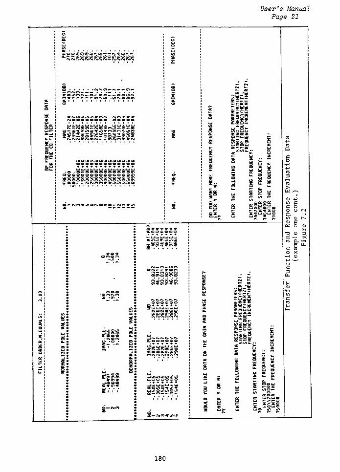
User's Manual

Page 21

oO.CCtnu i

lOOJiCOCOCOr^-ufi*- Pv.'TuCtPs.pN.

CL's-'^pOlJDlDlJDuDljDlOOl/1uOuOi_D'-0

rgcgCMOgCSifsjrjcgPa*-rgfsjc\jf\jcM

O <\|'s-0O Pw COwfOfsjCO .

ZCOlOPOCNj COCO- OOLfifMci^ CO f* J^ wO rs. CO CO cn

CE l l l l l l I I l l l i t i

i i i l i i i i t i i * *

UJ UJ UJ Ui UJ Ui Ui UJ Um t i i . i i i i i i , i

r. fsjcoco rsico jomui o coto to ^ a.LnoiLn<jnffir<NL/in

CEi/lCOÔ CO vD tfi KC*7OO03

Z^Hl COQOVrs- OCOtO COlO^

p^fsirsiacMcora corsjfoco-*a-<M

*jD <X> lO *J& tO LO UO (X> tO lO CO tO lO

OOOOOOOOOOOOO

o oo O OO OOOOO O O COOOOOOOOOOOOOOOOCO

uioooooooooooooocn

CCOO^lOOlOOlOOljOOlOOU^CO

u.oo (Sjcsirjm^rîOt/itocoLO

Lfi

O <N<n'LOtO's-COCOOCstCO<J-

lO

cc

IU.

ooUi

cc

i- ce

CC -uj

*UJ~X

: p-t

j >-ac z- Uuu

JZXZ

: uj ui:-

>-cc:o*uo

:uzz.CC'-JCH

U_D

J o>-

: zccz3 u.uj

=>iaio

j CC O UJ

t-*-CC

lOtOU.

oI

-I

o

or Su. O

p

zUl

3oUl

a

t- aor o ui

ec >- x*~ m *

moaoa

eeououUlOP-Oro

-f*Z V ZZ ^ UJ lDuJUJ-

eoo>p>p-p>

c -oi

a3a

aUJ

a

ao

a

a. >

a

0.91d ffl

va

JOIACD

CCCft

^-LJUI ' 'l.l'i/ ItJ

1 ' i ''j i > UJ <'

i UJ

rr CO CO -v

cm r u>ri

Of\t rco ro

ro cofvjorsj

03 c^ co a co co

Z uiui ui ui ui uj

* 0*. lO CNjO lo o

c\. rg (\i (SUM <\i

CE>

. UJ

UJbOOkO 1

_JtOOt> o

0- UJ. _

lPS.fu.pi^f%.fS.S.

a Ct o OOOOo

ST rsi ' '. T* uJ i - 1 1 1 1 - ' i j ui

r CC (M tO (MO tO O

i zaacc o*. co co

CC

z

P f* C\i f\i CM fSi <M *M

_J bO tO u*) tO tOus

0-O O OOOO

cca lOoc toUJtAO lAl/1 O lO

ce - co - * co *-

i i i i i i

Cv

az<c

ce ~~ *-

Ui>-CCZ

p-UljU

UJZXZ

IW-uJ

CC-_>>-CCccouu

CCujZ Z

Cw CC Lui"

U.3

Ui O >-

lOOUiO

zzcczO u, uJCUP- 3tOCCO-O

UiCCOui

cc <- cc

totou.

CE >

o-J

J

o

s

Ui oU CC UJ

zu.ccmm U.p- a.

CC OOUi

CE P-OZ*- too

ia eccocc

CC UJrS.UiO

UJ^^po

< z^zo

Z UJOUJO

Ul O Ul U*)

Cfl

O

CoH

P

CO

3-H

CO

>ll:

^7<u p

Ul cC o

o (J CM

p. .

U) CD r-

CD ca. o CD

P

-o CD 3

c i-H 00

cfl P- H

E U.

c cfl

o XH CD

p v '

o

c

3U-

PcdLP

U)

cCO

Pt-

180

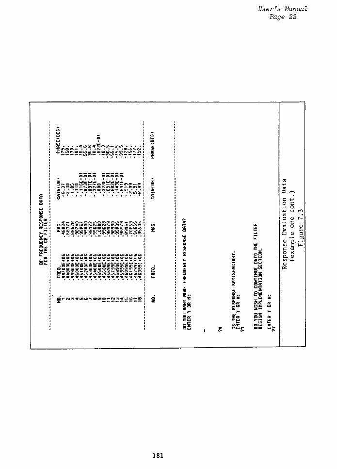
User's Manual

Page 22

. . . .fl-uja^fsiûo twouo*

j)(co- * * -oj cour<p--cu

r^L^FnOUjL/itDCOiJvCOL&u'lu'lCnrgJirsTl

r*-unco- OlOps-co-

CEp-

CC

OOOO ooooo.

I I I I t I I I I

a uuuu uiujuiuiuiars.ouiotjOcors-ps.ori^-tMfo- coco-oo

w(OfOO PvCnfMOfMCOaD^CO cococo

Z CD CO Cn O <T> CD CD 00 0"1

coro *.. rvjv/io

CE i t i I I i I I I I i i i i t

C9

^v-coor<uorgjuOoacnoLOcn ro i_n jtOOj's-CNi^tOOP^-rgOfNjPN.critT'. rûT-LOu". i*0

CEOf^'tO^^coocnLOotOcncococricncC'LOLjri

zaaaacocncDOôcncocooncccrioou*)vu?cocococococo cococococrtars.tjnco

oooooooooocncocncT'Cocococo

Ooooooooooocricocncricncnonon

UJP* CO 0~i O - -(NfOfl"tOuOljOPs.aCOO(NO

CBV^ûOuOLOiJAunu^LOLOLjûOu^tOtOtOtO

o fstorKTuOwsrs.acoo rs* ro*

uO to r-- ao

cca

ui

to

zaa.

-Z Oa Xj- >-

UJ 3Zza oo ai-ul p UJ

m

U1Z Oul Z

JE -

CO

co

>LU CD

CD

Ul

Co

PL <D

Ul '

<D

Cl

CD

P

3M

P, -H

E Lu

cfl

X

181

User's Manual

Page 23

FILTER DESIGN IMPLEMENTATION SECTION

ENTER THE TYPE OF DESIGN DESIRED:

A1INFINITE GAIN MULTIPLE FEEDBACK ( IGMF ) .

B1DUAL INTEGRATOR

ENTER A OR B:

?fi

IGMF DESIGN

INDICATE THE GAIN DESIRED IN THE PASSBAND

OR AT THE CENTER FREOUENCT.

ENTER DB (SIGN IS REQUIRED):

70

BP FILTER COMPONENT VALUES

(REFER TO FIGURE 6.1 IN THE USER MANUAL)

RESISTOR VALUES WITHIN THE RANGE OF

100 OHMS TO 1 MEGOHM COULD NOT BE SELECTED FOR THIS

STAGE. THE FOLLOWING REPRESENTS THE CLOSEST AVAILABLE

VALUES NEAREST THESE LIMITS FOR STAGE NO. 1:

STAGE Rl R2 R5 C3 C4

(KOHMS) (KOHMSI (KOHMS) (UF) <UF)

1 : 880. : .S00E-O1 : .176E04 : .378E-0* : .378E-04

STAGE Rl R2 RS C3 C4

(KOHMS) (KOHMS) (KOHMS) (UF) (UF)

2 MO. : .100 : 880. : .373E-04 : .373E-M

STAGE

3

Rl

(KOHMS)

880.

RESISTOR VALUES WITHIN THE RANGE OF

100 OHMS TO 1 MEGOHM COULD NOT BE SELECTED FOR THIS

STAGE. THE FOLLOWING REPRESENTS THE CLOSEST AVAILABLE

VALUES NEAREST THESE LIMITS FOR STAGE NO. 3:

R2 RS C3 C4

(KOHMS) (KOHMS) (UF). <UF>

.SOOE-01.176E*04 .368E-04

.368E-04

DO TOU WISH TO RERUN THE PROGRAM'

ENTER Y OR N:

7N

END OF PROGRAMSTOP*

I OFF

Active Filter Design Section

(example one completion)

Figure 7.4

182

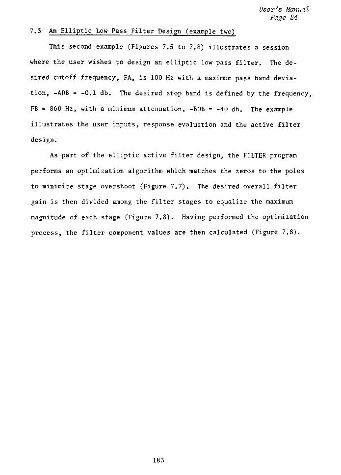
User's Manual

Page 24

7.3 An Elliptic Low Pass Filter Design (example two)

This second example (Figures 7.5 to 7.8) illustrates a session

where the user wishes to design an elliptic low pass filter. The de

sired cutoff frequency, FA, is 100 Hz with a maximum pass band devia

tion, -ADB=-0.1 db. The desired stop band is defined by the frequency,

FB = 860 Hz, with a minimum attenuation, -BDB =-40 db. The example

illustrates the user inputs, response evaluation and the active filter

design.

As part of the elliptic active filter design, the FILTER program

performs an optimization algorithm which matches the zeros to the poles

to minimize stage overshoot (Figure 7.7). The desired overall filter

gain is then divided among the filter stages to equalize the maximum

magnitude of each stage (Figure 7.8). Having performed the optimization

process, the filter component values are then calculated (Figure 7.8).

183

User 's Manual

Page 25

o o

oo

z a

UJ

a co>

m i

a i

Ul 1

i

Ul 1

Z I

a i

a i

a i

a i

u. u_O "1- i

>-a>-aUQUQzaza

m

aUl 1 Ul I

3 -3 -

oaoa

UJ

UJ

30 1 V

UJ Out I -"

3 uia >- >-

UIU UJU.a a

z -j oau i p --P

a a u < li.-z.-z. O 1

Ul I

m i

Z I

O I

a i

Ul 1

Ul 1

a i

u. u.a- a

a > UJ 1 UJZUJ Za UIO 1 3030 O 1

Ul UJ

moa o a

aoooo ..

a O OO 1 OOOO

Zja-'Ouj i uj ui

ui-j>-ui o aaaaUl Ul Ul I

3 ...-CJ OOluOuO

p-

z

aUJ

oao

UIOOOO

zzzzz

o aUl Ul

a a

az

aaazozo i

xuipuiza * i uiuiujuj

oaa i oooo a i

3 I

a i

Z I

a a a cc aor aaaa

ammo. Q_ammoo

3 3O OUl Ul

u

o

_j_joaui i aooo(OmmuiHUI,, 1 ujujuiui

uiuuama X i

u a o. oaoo

UJ I

O 1

a i

o i

a a a a >- auu a oizzzz

1 uiao.uiui a pooa a cc <x ct o: a i o

2ui a uiauiZ aaaa ul I

aUl

z o o z oaui uixo ' uimo-a 1

oa

z z z zzazzoz i mmoo _l 1P

3 mm>ô-c i ace 1

-j

Ul z z m ii-ujia i aauiui U. 1UJ LP O O 1 CD

u.a

Ul

m uia i

Ul I

p^ i

I

P-Ul z Ul Ul E

COX '

3 3z z

z a X

oaUl z z <D C

zo z co .. a w Ok ui a o a a iH

3u

Ul

a u aC P

oa ui a a a a 00 u>-UI a ui UJ Ul Ul

rl CDUl

z_QUIZ

-1 ZOZ ZUJX Ul 00O, ui ul uj CD uj "^ CD LO

1 p- P- P- P-

Q PCD

P P

CD CD

P E

CD

Pi i cfl 2H P OC

LL Cfl H

O- LP. Ul

UJ Ul pi

a _ cfl 3

ao

oai

0- P.

c01 UlZZ p*

CI 2 tz 3 m

oa o 03a i UIUIO UJ

o j SS1o Ul a

oa a ui aa a auix a 3 H

o O Ul 3 O mp

pz u. a uj Z mmuiao 0.0 X uiccmo

a o z m X aaa HUl UJ Z CT a . a amUl m zoz _j a: > z zoo

a

33 OUl

OuU OZZ -o.

2UZZ

O CTCT LUa o uiao am _i _ixaa

UJ _l a r uj.-o.uja:

a a mo aaaa_J

>- mo hijjiau OOOO^ a UP -3X _iui "U.UUU

u ZU>- -l

aapuiaUl o

auia aam

Ul z a aaaaaa z-izaa

> o UI3 oo O O uj

** **_iim

U1U.U.UUPJ m

a UJ Ul

p >- a z oza-jmo a

a aoo

zo

m

aUl

>

BCEB 0

oz

aUJ

aUl

i

u.

u

o

Ul

a>-

Ul

X

aUJ

Ul

a>

aUl*

z z-j z ZL

1Ul UJUI UJ wp!

184

User's Manual

Page 26

a-

OOto * ?

* uj O w uj

* OwOkO D*nnnOfOfO * Ooroco _jzr\*.r\i

ui * i/ i CE*tOuO> *m-w- >

onw

3n*T*r

o rototo

3tO CD CO

t*o

UJ *

ujomro _jwoNf"-

-lOLDLO O*Q.O- Ct * Q.O -

o * oaaoo<r"

a* oolOuo

CE Ui * CE -f^r*.

Z i rsj z

_JtOfOCO

Cvrs-iJOtO(NiCO CO

jnLfiLO

CECO

CC *

_JCO

CE *=> o

uj ui foro

cczccI

OCX

on-, ro

toct aco

ujzcon

_J co-n

CCCEOO

OUiOOZCCOO

OO

oCv.to

CEZa.

cc -Ui

-UJZWXN-

CC p-p-

UJ>-CCZt U UIUJ

ce -3>-a_CC o ooCCujZZO.CCUJ*-*

U.=>

UJ o>-

wouu

ZZO.ZO-LUQ.P- 13tocc ao

ujCOu

Cc p- CCtO U*jU

o

UJ

oUJ

a

ui

Ula a

a ui ui

ul o

zoz

_ 01

Z >M o->

Ul pi Ol

a jrcn

o -

UJ _l Ul

> UIUJ Zaazz aza a.

uizaaoUIK *

UlUl 1 -i

ZUI -J j

<r a<= aaaz ra m Ulo-o

zlj

Ul PJ

ZUI LOO PJoi m

ui

pi

P- Ul

1/1

a *

mo uj

U1ZP1

Ouj 01 INJONOI

a

a zoa

uapi

o

zcn

ZUNUl

ujo -a

ui

oa

o

CO ^

Q

P

c co oH O vD

(J o r~

c 23 p CD

u. P

CD 3p ^H OC

CD P H

Lp F LP

U) cfl

c X

CO o

p v '

t-

185

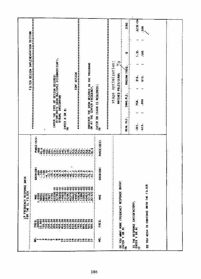
User's Manual

Page 27

Z '

o >

azo

U13uizaa oz

u CT

oaaoo

Ul Ul

aui>- z

a

za

IU.CT oZ3o a

auiam a

mo oUIUJ

aa au

z ma

CTuJO z

o

3COH

p

Cfl

N

H

EH

P

Po

CD a

bo

cfl u

\

o

2P>

\op CD

CD 60N CO

P

o U)

c

P

OLP

w3 CO

a to

CC O l

XoCt o*.

OOO* n diNCn fncLnLfifuCQco .

ousocsjcorov^v^L/iuOL/juiLjOuiLOtoac\jfgc\jrgcNjru^rgoijrj<>jCNifSi<N*rgcNiPv.

S

aoooouo *r cncn u-><n csiru^-cocococor*.

OOON

Zo >cNjavarsiuocorotocorghoacNip^>kO--

wm . . v c^rgfoono^ <r<rtOLnuOuDu?p^coct I ( I I i i t i t i i i i i i t i i i i

fufsjcvjcsjCMfSjfnrom*

oooooooooooooooi i i i i i i i i i i i i i i

i . 1 i . 1 1 . | jj i^ ujUi Ui UJ UiUi UJ UJ UJ Uiouûû^ tfaôrNjou^CTCNjij^vtocsjrîors*

uoinjr(ncMr)iriooc^(nN*7GCLnOD(nol\*Tccoaa to pop^toco

cMno'cocoo'

zoaaaro otocsi^-ooav^to- cnouolo*XCO*/fVU5H5CVJ fs.-(nfSj ^*>* f\j

3OUiujX

cc o ooooooooooooo^cricncrioicnoo

L1,ooou,ioi/ioLnoL/iOLnojioi*a.To*iTff.

un cî\iT)>n<f*ijijiij>iJ3(j;s.p.0Dffi(n

oUicc

o Ul

0_ z

toz

>- ooao z

u OP

z u UJ

a UIUI

O m3zzo

a zUl SUl

m

zOUI

z z z

z xx_,

z

ztr ma ma z

5 uio

a

zX

o

>- 1^

3 3Zoa IX OO a

Ul

m

oz U1Z OUI ZOUlZ Ul>- oo UJ

G60

H

Ul

CD

Q

P

CD

CD .

> p

H GP o

U o r-~

< .

o r^

T3 2

G p CD

Cfl PCD 3

C i M

O P H

H E LL.

P co

CO X

3 CD

i i * >

CO

>LU

CD

Ul

Cop.

U)

CD

Ct

186

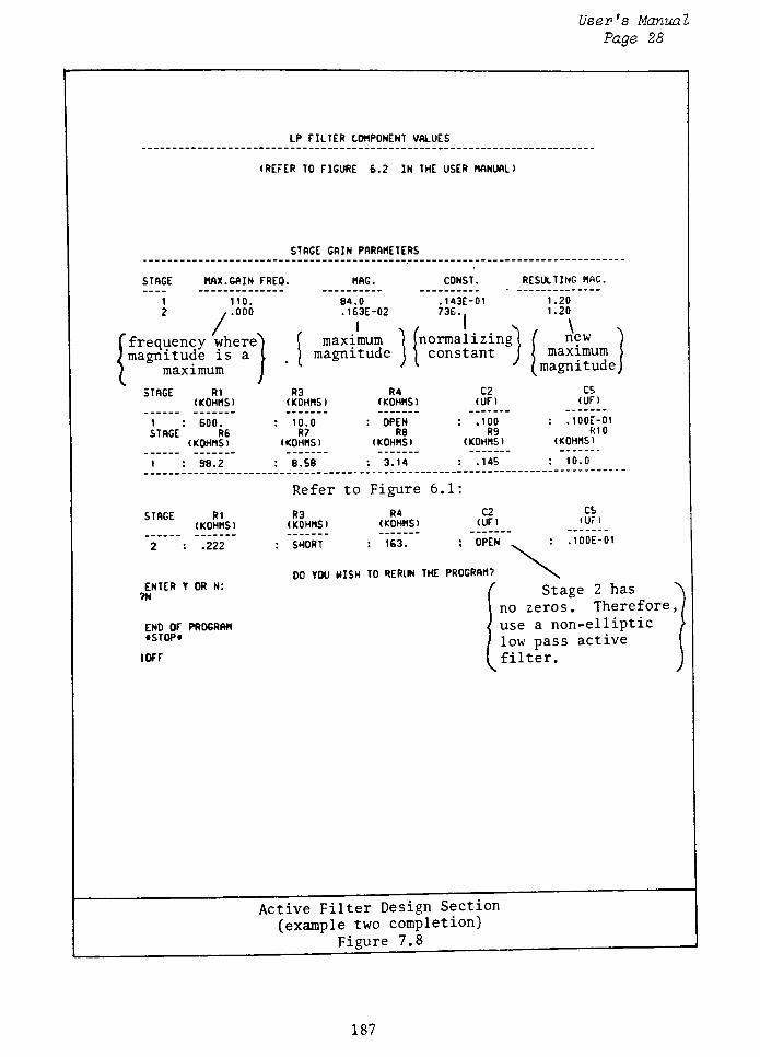
User's Manual

Page 28

LP FILTER COMPONENT VALUES

(REFER TO FIGURE 6.2 IN THE USER MANUAL)

STAGE GAIN PARAMETERS

STAGE

1

2

MAX. GAIN FREO. MAG.

/

110.

.000

J

{frequency where

magnitude is a

maximum

STAGE Rl

(KOHMS 1

1 : 600.

STAGE R6(KOHMS)

84.0

.163E-02

Imaximum

magnitude

const .

.143E-01

736.,

normalizingconstant

r 98.2

R3(KOHMS)

: 10.0

R7

(KOHMS)

: 8. 58

R4

(KOHMS)

: OPEN

R6

(KOHMS)

: 3.14

C2

(UF)

: .100

R9

(KOHMS)

: .145

RESULTING MAG.

1.20

1.20

f\new

, maximum'

magnitude,

cs

(UF)

: .100E-01

R10

(KOHMS)

10.0

Refer to Figure 6.1:

STAGE Rl

(KOHMS)

2 : .222

R3 R4 C2

(KOHMS) (KOHMS) (UF)

: SHORT : 163. ; OPEN%

C5

(UF )

: .100E-01

ENTER Y OR N:

m

DO YOU HISH TO RERUN THE PROGRAM?

Stage 2 ha

END OF PROGRAM

STOP*

I OFF

no zeros. Therefore,

use a non-elliptic

low pass active

filter.

Active Filter Design Section

(example two completion)

Figure 7.8

187

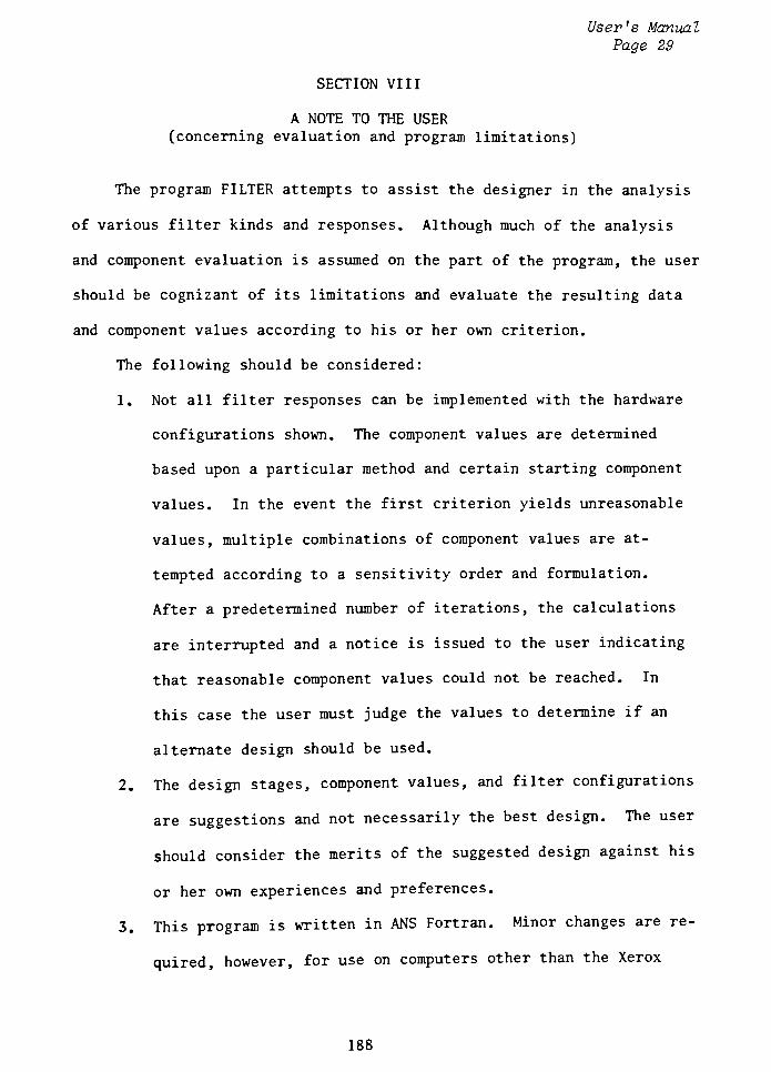
User's Manual

Page 29

SECTION VIII

A NOTE TO THE USER

(concerning evaluation and program limitations)

The program FILTER attempts to assist the designer in the analysis

of various filter kinds and responses. Although much of the analysis

and component evaluation is assumed on the part of the program, the user

should be cognizant of its limitations and evaluate the resulting data

and component values according to his or her own criterion.

The following should be considered:

1. Not all filter responses can be implemented with the hardware

configurations shown. The component values are determined

based upon a particular method and certain starting component

values. In the event the first criterion yields unreasonable

values, multiple combinations of component values are at

tempted according to a sensitivity order and formulation.

After a predetermined number of iterations, the calculations

are interrupted and a notice is issued to the user indicating

that reasonable component values could not be reached. In

this case the user must judge the values to determine if an

alternate design should be used.

2. The design stages, component values, and filter configurations

are suggestions and not necessarily the best design. The user

should consider the merits of the suggested design against his

or her own experiences and preferences.

3. This program is written in ANS Fortran. Minor changes are re

quired, however, for use on computers other than the Xerox

188

User's Manual

Page 30

Sigma 9. The program has been used on the Digital Equipment

Corporation VAX Computer without difficulty and with a few

minor alterations in syntax.

189

User's Manual

Page 31

APPENDIX

190

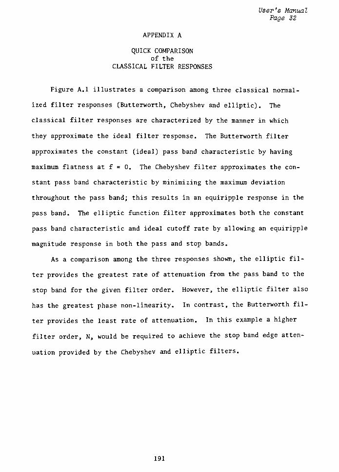
User's Manual

Page 32

APPENDIX A

QUICK COMPARISON

of the

CLASSICAL FILTER RESPONSES

Figure A.l illustrates a comparison among three classical normal

ized filter responses (Butterworth, Chebyshev and elliptic). The

classical filter responses are characterized by the manner in which

they approximate the ideal filter response. The Butterworth filter

approximates the constant (ideal) pass band characteristic by having

maximum flatness at f = 0. The Chebyshev filter approximates the con

stant pass band characteristic by minimizing the maximum deviation

throughout the pass band; this results in an equiripple response in the

pass band. The elliptic function filter approximates both the constant

pass band characteristic and ideal cutoff rate by allowing an equiripple

magnitude response in both the pass and stop bands.

As a comparison among the three responses shown, the elliptic fil

ter provides the greatest rate of attenuation from the pass band to the

stop band for the given filter order. However, the elliptic filter also

has the greatest phase non-linearity. In contrast, the Butterworth fil

ter provides the least rate of attenuation. In this example a higher

filter order, N, would be required to achieve the stop band edge atten

uation provided by the Chebyshev and elliptic filters.

191

User's Manual

Page 33

LPLp

vD

to

-a

cCO

oa

ui

ui

CO

1 LL,CO

<D Ul

T3 Uli-i CO

Cl

2O-]

to

n

c

I

o

O

Ol

>OJ oc H

U) "3 pX g ax> CO.HCD i i

X

u UJ

c

CN

I

oi-H

I

o

CN

oPi

I

o

I

o

LO

I

o

vO

I

0

o

o

o

o

o

o

CN

I

CD

3 Ul

*J C r->

H O JO

C P-T5CIO ul *'

cs a)

CD

U)

Co

Phui

4)

Oi

Ul

CD

U)

c

o

p.

U)

ill

Oi

p

CD

u.

CO ^H

o .

H <r

Ul

Ul CD

CO P. 1 3u M

H

CD LL

4=

P

LP

O

c

oU)

H

P

Cfl

p.

bO

u

192

User 's Manual

Page 34

APPENDIX B

PROGRAM FLOW AND I/O SUMMARY

Figure B.l illustrates a simplified flow chart for the FILTER pro

gram. The diagram shows the main sections of the program along with the

user inputs and computer outputs. The intention here is to acquaint the

user with the overall format and expectations of a user session.

193

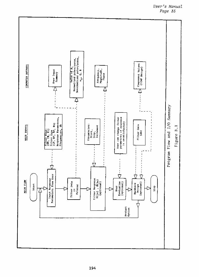
User's Manual

Page 35

o

3D. XC f-

ta

U h3

to

3

3 TJ

>

II

^~A

W

tft

u

a>

toas E "3

(0

P. -

T5-J U CCL_'

g- Ct <u

S^ - H -

as C

uu (-

& O 3

c zr

rtQS .- _J

U-w b.w =C LL.

/~\

-o

v_y

p

CO

3CO

T3

C

Cfl

2

O

ECO

P

DC

O

P

Cu

CO

CD

P

3Ojj

r-l LL

194

APPENDIX A

DEVELOPMENT OF THE SOLUTIONS FOR

THE ELLIPTIC FUNCTION POLES AND ZEROS

A. 1 Introduction

In this appendix we will examine the background and development of a

method for determining the poles and zeros for the Nth order normalized

elliptic low pass filter. This method was developed by expanding upon

the theory presented by A. J. Grossman [11] for the case of an odd order

filter. The following provides an overview of the sections in this ap

pendix.

In section A. 2 we will become familiar with the terminology and the

parameters of the elliptic filter magnitude response. These parameters

describe an insertion loss characteristic which has an equiripple pass

band and stop band magnitude response.

The next section (A. 3) describes the characteristics of a rational

function, R^w) , which will yield the prescribed insertion loss charac

teristics defined in section A. 2.

Section A. 4 then develops the relationship between the prescribed

form of the rational function and the required frequencies which yield

the equiripple response. This relationship turns out to be the elliptic

sine function.

The next section provides a more intuitive examination of the ellip

tic integral and elliptic sine functions as they apply towards describing

the elliptic rational function and its solutions.

The last section (A. 6) utilizes the concepts presented in sections

A. 2 to A. 6 to formulate the solution of the s-plane poles and zeros.

196

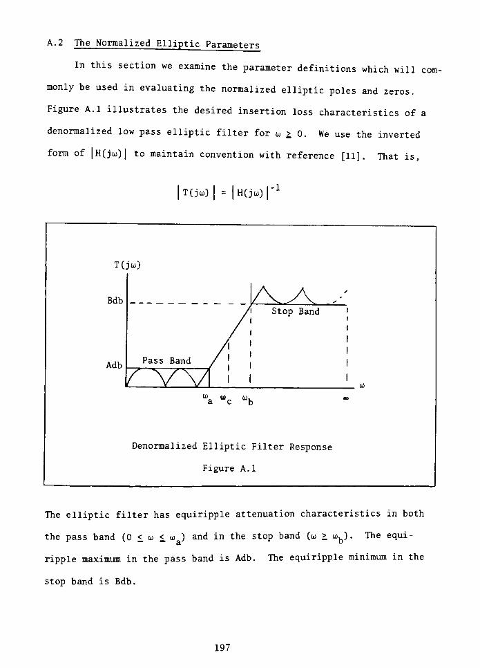
A. 2 The Normalized Elliptic Parameters

In this section we examine the parameter definitions which will com

monly be used in evaluating the normalized elliptic poles and zeros.

Figure A.l illustrates the desired insertion loss characteristics of a

denormalized low pass elliptic filter for ui >0. We use the inverted

form of |H(jco)| to maintain convention with reference [11]. That is,

T(jco) | = | HCjto)i-l

T(jui)

Bdb-

/Ky\ /Stop Band

AdbPass Band

AA i

>

/ VV i i

wa wc ub

Denormalized Elliptic Filter Response

Figure A.l

The elliptic filter has equiripple attenuation characteristics in both

the pass band (0 < oj < to ) and in the stop band (uj > tob) . The equi

ripple maximum in the pass band is Adb. The equiripple minimum in the

stop band is Bdb.

197

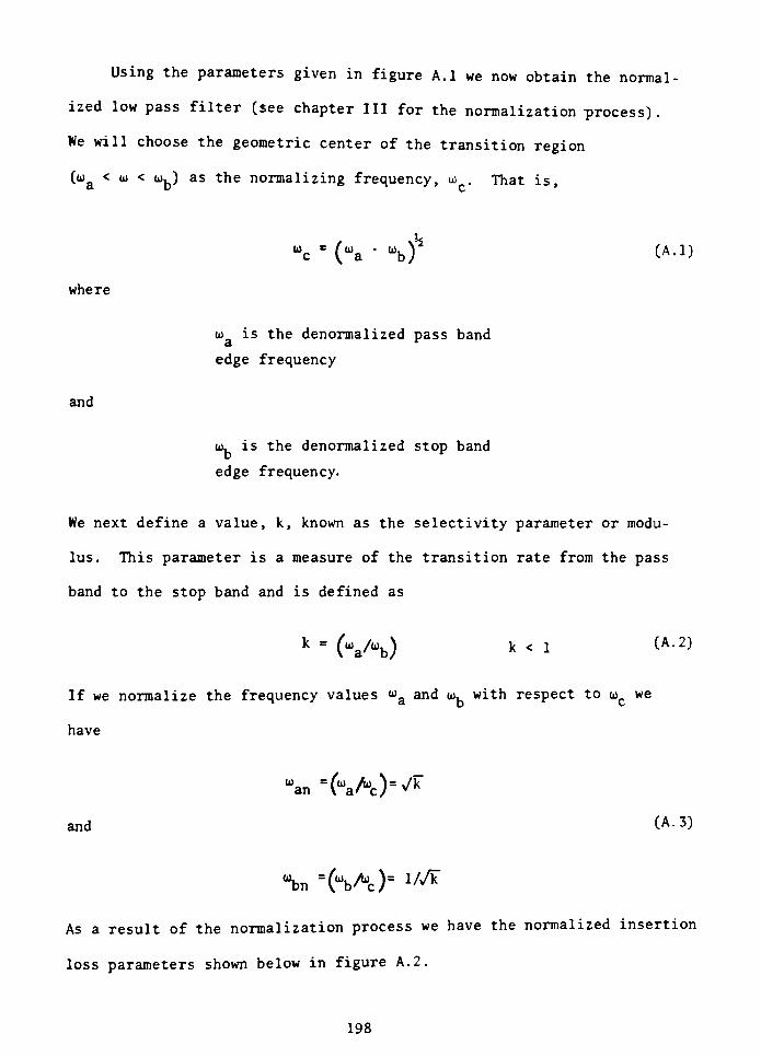
Using the parameters given in figure A.l we now obtain the normal

ized low pass filter (see chapter III for the normalization process).

We will choose the geometric center of the transition region

(oj&b) as the normalizing frequency, oj

. That is,

c*

("a "bf CA.l)

where

to is the denormalized pass band

edge frequency

and

a, is the denormalized stop band

edge frequency.

We next define a value, k, known as the selectivity parameter or modu

lus. This parameter is a measure of the transition rate from the pass

band to the stop band and is defined as

k =

(ua/ub) k K 1 CA'2)

If we normalize the frequency values wa and oj, with respect toojc

we

have

%! =KAc)=V^

and (A-3)

"bn"(Vc)" 1/yF

As a result of the normalization process we have the normalized insertion

loss parameters shown below in figure A. 2.

198

|T(joj)|

Bdb_

/VA y

Stop Band

AdbPass Band

A

A i

r vv i i <

o Jk 1 i/A

Normalized Elliptic Insertion

Loss Parameters

Figure A. 2

A. 3 Magnitude Characteristics of the Elliptic Rational Function, R>j(ijj)

Having normalized the insertion loss parameters, we now make some

observations regarding the equiripple characteristics in order to derive

a proper form of the elliptic approximation function, R^(uj) . (We assume

that the function, RN(to) , is unknown at the present.)

Recall from chapter III that the general transfer function, H(joj) ,

is characterized using an approximation function K(uj) as follows:

H(joj) H(-jto)1 + K2(oj)

= |H(jaO

where

e is a constant.

199

Since we defined | T(joj) I as

|T(joj)| = | HCjco)|_1

we can rewrite the characteristic equation as

where

and

T(joj) T(-jco) = 1 + R^(U) (A. 4)

e is a constant (which will be deter

mined shortly) ,

Rj.(aj) is the elliptic approximation

function substituted for K(uj)

the magnitude, |T(joj)|, has equiripple

characteristics as shown in figure A. 2

We would like to determine the function R*,(uO which results as a

consequence of the prescribed attenuation parameters as shown in figure

A. 2. In particular, we are interested in the values of R^to) at the

known frequencies of equal maxima and equal minima (/F and 1/^/k are two

such frequencies respectively) .

The pass band edge frequency, fk ,is an equimaximum point having a

prescribed attenuation, Adb. This is related to ^("0 by

Adb = 10 Log ( 1 +

R^ (7k))

The required value of R^ (/k~) is then found as

R2r rr,do Adb/1-l)

Rh(oj =A)

=

^

200

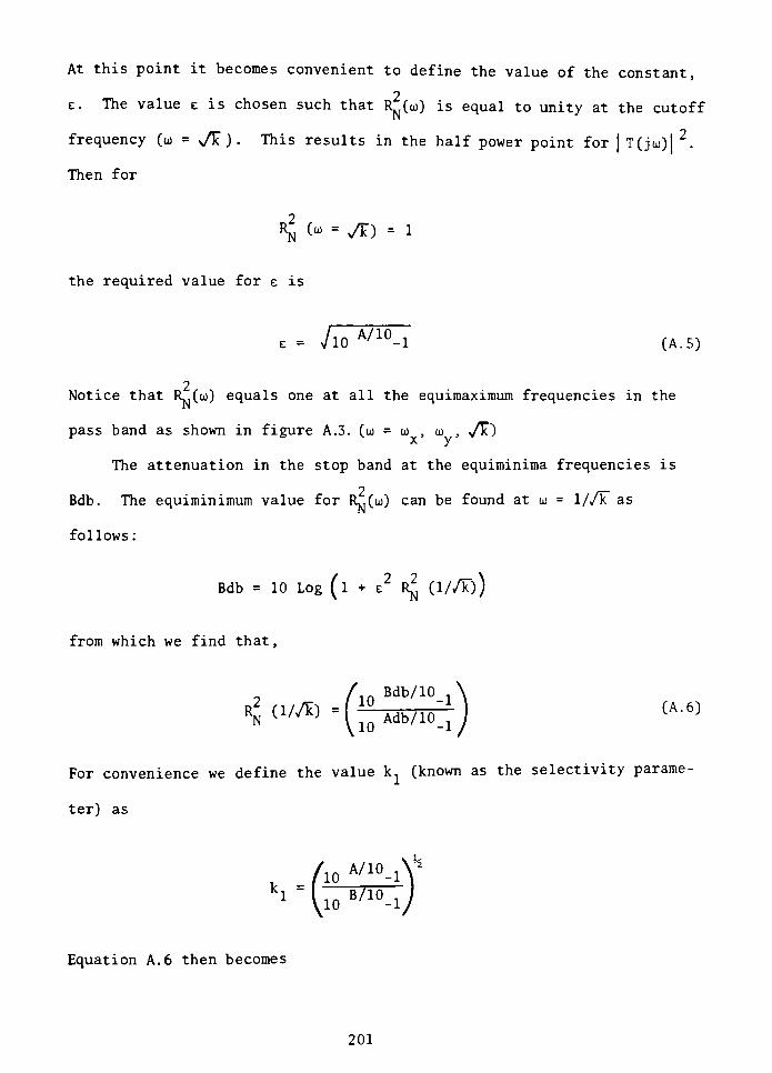
At this point it becomes convenient to define the value of the constant,

2e. The value e is chosen such that Ooj) is equal to unity at the cutoff

frequency (to =v/E ) . This results in the half power point for | T(joj)| 2.

Then for

rJ (oj =

yk) = 1

the required value for e is

AA1- 1 (A. 5)

2Notice that RTJ(uj) equals one at all the equimaximum frequencies in the

pass band as shown in figure A.3. (oj = to,

co, y/k")

x y

The attenuation in the stop band at the equiminima frequencies is

Bdb. The equiminimum value for Rôj) can be found at uj = as

follows:

Bdb = 10 Log (l +

R^ (1//F))

from which we find that,

/ Bdb/10

^/A)=(^wiotJ (a-6)

For convenience we define the value kj(known as the selectivity parame

ter) as

-(10 A/10-i

10 B/10-i

Equation A. 6 then becomes

201

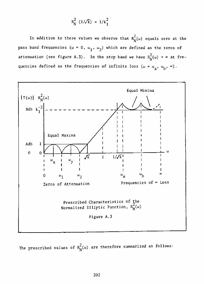
R^ (l//k)=

1/k2

In addition to these values we observe that Rôj) equals zero at the

pass band frequencies (oj = 0, to.., oj_) which are defined as the zeros of

2attenuation (see figure A. 3). In the stop band we have \t(oj) = at fre

quencies defined as the frequencies of infinite loss (to = oj , oj,, ) .

Equal Minima

Jl ^2

Zeros of Attenuation

a b

Frequencies of Loss

Prescribed Characteristics of the

Normalized Elliptic Function, R^to)

Figure A. 3

The prescribed values of R^(to) are therefore summarized as follows:

202

2RjÔ) =0 for to = 0, u u

= for oj = oj, oj,a' b'

=1 at the equimaxima fre

quencies : oj = to,

oj, /F

x y2

= 1/k.. at the equiminima fre

quencies

A rational function which satisfies these prescribed parameters shown in

figure A. 3 is as follows:

= ]_" (mi

-

u2)(4-

^2) (%-

^2)

^7 (ua "

u )(ub "

(l)2) (UN "

u2)

As a result of the equiripple characteristics in the pass band and stop

band, it can be shown (see A. J. Grossman, reference 11) that the nor

malized poles of R^fco) (oj, oj, .... toN) are the inverse values of the

zeros of R^fto) . That is, to= 1/oj_, to,

= 1/to. , etc. As a consequence,

the elliptic rational function has the following reciprocal property:

) =

C oW(A-7)

'lRÎ/oj)

Applying this reciprocal property to the normalized frequency values,

the elliptic rational function can be rewritten as follows:

for N odd, O-8)

1 to

(to2- to2)-

(to2- oj ) (ioN - oj )

v-0 =

Af

'

(i/.j. J)(v*22 -

2) K--2)

203

and for N even,

NA7 (i/,j .

-2Xi/-i-

-2) K-2)

where

to., to- ....o>N

are the normalized zeros

of attenuation,

and

1/oj., 1/oj2 .... 1/ojn are the normalized

frequencies of infinite loss.

This form of ^(oj) allows a clear interpretation of the frequencies

where R^foj) = 0 (zeros of R^fto) ) and where Rôj) = (poles of R^(to)) .

We have not however defined what these frequencies shall be in order to

achieve the prescribed equiripple magnitude characteristics in the pass

and stop bands. We shall see in the next section that these frequencies

are found using the elliptic sine function.

A. 4 The Poles and Zeros of Rôj)

In the previous section we determined the equimaxima and equiminima

values of the normalized rational function, Rn(oj) . These values were a

consequence of the prescribed insertion loss parameters and the desired

equiripple characteristics. We would now like to determine the fre

quency values of Rn(oj) which yield the equiripple response, that is, the

zeros of attenuation (zeros of ^(oj) ) and the frequencies of infinite

loss (poles of Rj^co)). The analysis will initially follow the approach

presented by A. J. Grossman [11] for the case of N odd. (N = 5 will

204

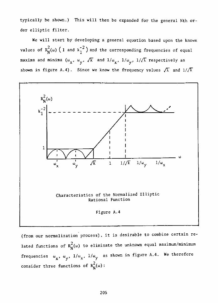
typically be shown.) This will then be expanded for the general Nth or

der elliptic filter.

We will start by developing a general equation based upon the known

2, s / . , , -2

values of Rm(oj) ( 1 and k ) and the corresponding frequencies of equal

maxima and minima (to,

to, /k and 1/oj

,1/oj

,l//k respectively as

x y x y

shown in figure A. 4). Since we know the frequency values /k and

h2

1

A)

. OJ

/A:Aa-;A/

/k 1 l//k 1/oj 1/tox y y x

Characteristics of the Normalized Elliptic

Rational Function

Figure A. 4

(from our normalization process) . it is desirable to combine certain re

lated functions of R^(to) to eliminate the unknown equal maximum/minimum

frequencies to ,to . l/u>v, l/u>v as shown in figure A. 4. We therefore

x y j^ /

2consider three functions of ^(A) :

205

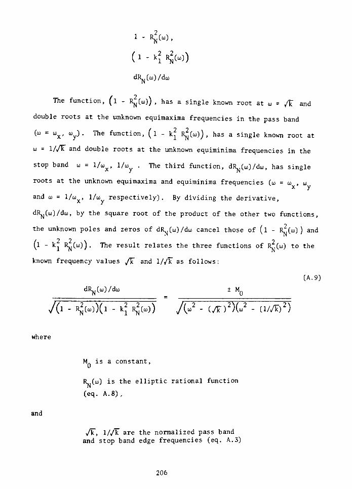
1 - ^C-0,

( i -

kl rJc))

dRN(oj)/doi

The function, (l -

Rôj)) , has a single known root at co = /k and

double roots at the unknown equimaxima frequencies in the pass band

1 -

k2 RjjCoO), has a single known root at

oj = 1//F and double roots at the unknown equiminima frequencies in the

stop band oj = l/o>x, 1/oj . The third function, dR^(co)/dto, has single

roots at the unknown equimaxima and equiminima frequencies (oj = to . co

x y

and to = 1/oj , 1/oj respectively). By dividing the derivative,x y

dRN(oj)/duj, by the square root of the product of the other two functions,

the unknown poles and zeros of dRJco) /dto cancel those of ( 1 - R^(oj) ) and

(l -

^ R^(co)). The result relates the three functions of RT(co) to the

known frequency values /k and l//k as follows:

(A. 9)

dRN(oj)/dcoMQ

/{l - R^(oj))(l -

k2

R^(oj))/(oj2

-

(/F)2)(oj2

- d//k)2)

where

M is a constant,

and

R^to) is the elliptic rational function

(eq. A. 8),

v/k", l/^k are the normalized pass band

and stop band edge frequencies (eq. A. 3)

206

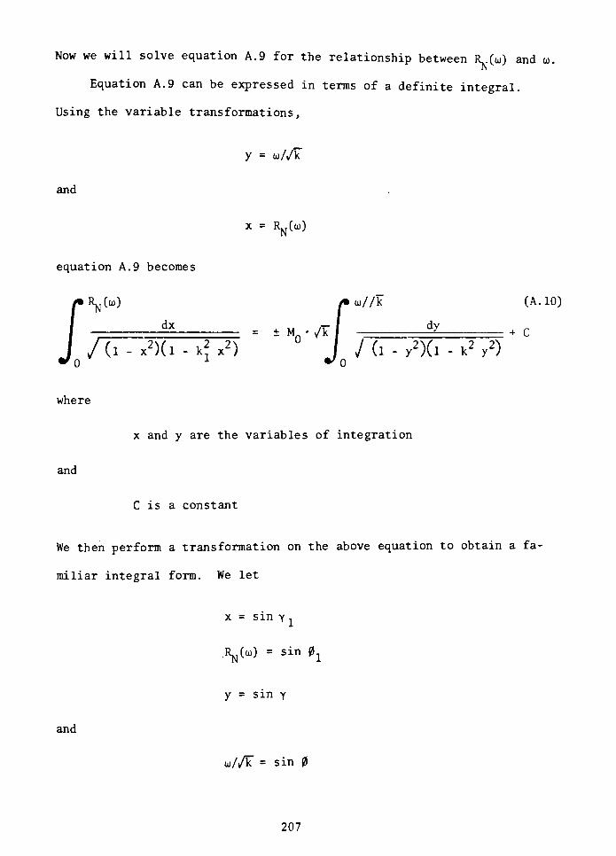
Now we will solve equation A. 9 for the relationship between R^(oj) and oj.

Equation A. 9 can be expressed in terms of a definite integral.

Using the variable transformations,

y= ojyVk

and

x = RjjCu)

equation A. 9 becomes

iyoj) /o>//k (A. 10)J^Cco)

JJ_L

J d -

y2)d-

k2

y2)

+ c

where

x and y are the variables of integration

and

C is a constant

We then perform a transformation on the above equation to obtain a fa

miliar integral form. We let

x = sin yj

R^(to) = sin 0j

y= sin y

and

u)//k = sin 0

207

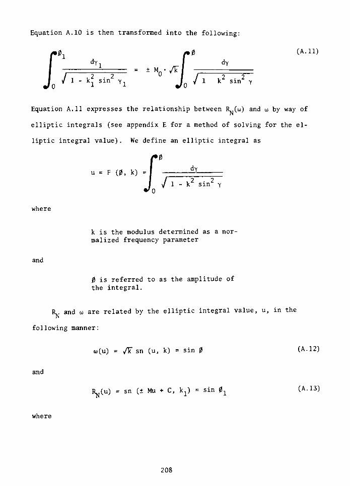
Equation A. 10 is then transformed into the following:

0 (A. 11)

dYl / dY

Mn /kI 2 2 I / 2 2/ 1 - k.. sin Y-, I / 1 k sin y

Equation A. 11 expresses the relationship between R^co) and to by way of

elliptic integrals (see appendix E for a method of solving for the el

liptic integral value) . We define an elliptic integral as

u- F (0,> -*?-

(0

I, k) =1

J z7'o

i,2 2k sm y

where

k is the modulus determined as a nor

malized frequency parameter

and

0 is referred to as the amplitude of

the integral.

R^ and to are related by the elliptic integral value, u, in the

following manner:

to(u)=

y/k sn (u, k) = sin 0 (A. 12)

and

Rû) = sn ( Mu + C, kx) = sin 0j(A. 13)

where

208

sn represents the elliptic sine trigonometric

function (see appendix E for a method of

evaluating the elliptic sine).

These two equations indicate that if we can provide the elliptic integral

values, u, for the given modulus values k and k., we can then solve for

the frequencies (eq. A. 12) which yield the equiripple characteristics.

In addition, the value of the rational function, R^to) can be found by

equation A. 13 for the corresponding values of u associated with co. (Ap

pendix B shows an example of how these values of u are derived and ap

plied.)

Equations A. 12 and A. 13 provide the primary tools by which we ana

lyze the elliptic response. They provide the basis for deriving the

poles and zeros of the normalized low pass elliptic transfer function,

H(s).

A. 5 Interpreting the Rational Function by way of the Elliptic Integral

and Elliptic Sine

In this section we would like to gain some insight into the concept

of the elliptic integral and elliptic sine functions. Then we will

examine how we determine the integral values, u = F (0, k) , which are

used in the solutions of the equiripple frequencies. As an end result,

we will have two sets of equations, in terms of the elliptic sine, which

describe the rational function and the proper normalized equimaxima/

equiminima frequencies .

A. 5.1 The Elliptic Integral and Elliptic Sine Functions

Suppose we are given the normalized modulus value, k (see equa

tion A. 2). Using k we can determine various elliptic integral values,

u, using the expression:

209

u = F (0, k) =

to

dY

i,2 - 2k sin y

(A. 14)

Figure A. 5 illustrates the integrand of u. We notice that this function,

( ,i,2 . 2 \

2

1 - k sin y ./ > varies in amplitude between 1 and G As

(,1-k sin yJ

(l- ,2)

3-

.u

2--

44 '

i

i i

r i

'M

" \\U w

il w

// v\

* T- Vv

>>-<-* ^-*.>u

II

II

ll

1 1

sin

A N\

80c

70c

60c

0 TT

232

I Y

2tt

Integrand Function of the Elliptic Integral

Figure A. 5

the modulus value k increases, the peak amplitude grows large (which ex

plains the difficulty in evaluating the integral value given k -

tt/2) . The elliptic integral equation (eq. A. 14) directs us to integrate

-h

the function (l - k sin y)over the range 0 to 0. (We will see in

appendix B how the required values of 0 are defined.) If we allow 0 to

vary, we find that the integral value, u, will vary as shown in figure

A. 6.

210

u = F (0, k)

u = 2K0

TT

"I1

sin k =0'

Elliptic Integral Values (Real) as a

Function of the Amplitude, 0

Figure A. 6

The value of the elliptic integral, u, at 0 = it/2 is, by convention,

designated as K, that is

u = F (tt/2, k) = K (A. 15)

Because of the periodicity of the integrand of u, we find that for every

A0 =

tt/2, the increment, of u is Au = K. That is,

u = F (0 = N \, k) = NK (A. 16)

The value, u = K, is therefore designated as the COMPLETE elliptic inte

gral value. We can also say that for any known elliptic integral value

211

u where

u = F (0, k) (0 < tt/2)

the following relationship holds:

r- , -/n is an\

u-= F (n tt + 0, k) = 2 n K + u WegeJ

Let us assume that we have determined a value of 0 which corre

sponds to a given integral value, u. The elliptic sine is simply the

sin (0). We represent this as follows:

sn (u, k) = sin (0) (A. 17)

For the complete elliptic integral value just discussed, we had u = K and

0 = tt/2 for the given modulus, k. The elliptic sine value for this case

is

sn (u, k) = sn (K, k)

= sin (tt/2) = 1

Other examples of finding the elliptic sine values are given in appendix

E.

A. 5. 2 Finding the Poles and Zeros of R,(oj) in Terms of the Elliptic

Sine

In section A. 4 we found that R^Coj) and to could be described using

elliptic sine functions governed by the modulus values k and k... In the

equation describing to (eq. A. 12), we find that when sn (u, k) = 1, the

value of to = /k (the pass band edge) . This occurs when u has the am

plitude, 0 = tt/2. The value of u at the pass band edge is therefore the

212

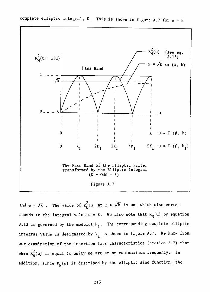
complete elliptic integral, K. This is shown in figure A. 7 for u = k

Rj(u) u(u)

^(u) (see eq.

A. 13)

: /k sn (u, k)

K u = F (0, k)

SKj u = F (0, kx)

The Pass Band of the Elliptic Filter

Transformed by the Elliptic Integral

(N = Odd = 5)

Figure A. 7

and to =</k . The value of R,(u) at to = /k is one which also corre

sponds to the integral value u = K. We also note that ^(u) by equation

A. 13 is governed by the modulus k.. The corresponding complete elliptic

integral value is designated by K as shown in figure A. 7. We know from

our examination of the insertion loss characteristics (section A. 3) that

when R^(oo) is equal to unity we are at an equimaximum frequency. In

addition, since ^(u) is described by the elliptic sine function, the

213

angle 0 must be some multiple of tt/2 forR^ to equal unity. Therefore,

the value of u corresponding to the equimaxima frequencies must be some

multiple of the complete integral, Ky As shown in figure A. 7 for the

case of N = 5, the complete elliptic integral, K is traversed 5 times

in the pass band. The zeros of attenuation occur at u = 0, 2K and 5K

We have therefore defined the integral values, u, as needed by equation

A. 12 to determine the zeros of R^to) . The zeros of RN(to) are found as

follows for N odd:

" = /k sn (u, k) (A. 18)

where

2K N - 1u = for = 0 to ^J.

and

N is the order of the normalized

low pass elliptic filter

We can perform a similar analysis for the case when N is even.

2Figure A. 8 illustrates to(u) and RN(u) for the case where N = 6. As

shown, we have three zeros of attenuation corresponding to the integral

values K,3K. and 5K. . The zeros of attenuation (zeros of R^to)) are

found as follows for N even:

to =v/k sn (u, k) (A. 19)

where

u = (2_L_l__v). K for = 1 to N/2u

N

and

214

N is the order of the normalized

low pass elliptic filter.

RjJ(u) oj(u)

0 i

to = /k sn (u, k)

K u=F(0,k)

16K1u=F(0,k1)

The Pass Band of the Elliptic Filter

Transformed by the Elliptic Integral

(N = Even = 6)

Figure A. 8

The value of the function Rû) in the pass band is found as follows for

N odd or event

fNK1 v "\Rû)

=sn^

-u.kj(A. 20)

215

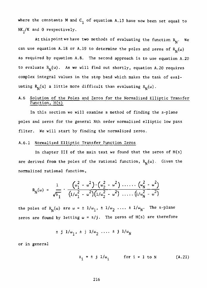
where the constants M and C of equation A. 13 have now been set equal to

NK../K and 0 respectively.

At this point we have two methods of evaluating the function R^ . We

can use equation A. 18 or A. 19 to determine the poles and zeros of R^foj)

as required by equation A. 8. The second approach is to use equation A. 20

to evaluate Rvr(u) . As we will find out shortly, equation A. 20 requires

complex integral values in the stop band which makes the task of eval

uating R>,(u) a little more difficult than evaluating Rn(oj) .

A. 6 Solution of the Poles and Zeros for the Normalized Elliptic Transfer

Function, H(s)

In this section we will examine a method of finding the s-plane

poles and zeros for the general Nth order normalized elliptic low pass

filter. We will start by finding the normalized zeros.

A. 6.1 Normalized Elliptic Transfer Function Zeros

In chapter III of the main text we found that the zeros of H(s)

are derived from the poles of the rational function, K,M . Given the

normalized rational function,

l_ ("l -

"2H"2-

"2) ("N -

"2)*M "

^

'

(i/.j -

2)(W2-

2) K -

2)

the poles of R^to) are to =

1/to^ l/to2 1/uyThe s-plane

zeros are found by letting to =

s/j . The zeros of H(s) are therefore

j l/to1, j l/to2 j 1/ojn

or in general

zi= j 1/to

ifor i = 1 to N (A. 21)

216

where to., to- ....ojn

have previously been defined by equation A. 19 as

the zeros of R>j(oj) or zeros of attenuation.

A. 6. 2 Normalized Elliptic Transfer Function Poles

Having solved for the normalized zeros of H(s) ,we now pursue the

normalized s-plane poles. This is the final step required in our effort

to define the elliptic transfer function, H(s) .

The determination of the complex s-plane poles for the elliptic

transfer function is based upon the understanding of the complex proper

ties of the elliptic trigonometric functions. We will not get too in

volved with the application of these functions for the solution of the

poles (see reference [11]). Rather, a simplified argument will be pre

sented. First we will discuss why complex integral values are required;

then the solution of the poles will be presented.

We start by considering the basic equation for the frequencies

defined as the zeros of attenuation. Recall from equation A. 19 that

to =}/k sn (u, k)

We would like to use this equation to transform the normalized frequency

axis. In doing so we first realize that the maximum value of sn (u, k)

is one. Therefore, in the stop band where to is greater than one, we re

quire a complex integral value which we will designate as jv.

That is,

to = /k sn (jv, k) for oj > /k (A. 22)

Next we attempt to define the complex integral value, v.

217

We set the insertion loss function equal to zero and solve for

That is,

1 + R^(oj) = 0

from which we find R^to) as

R^co) = j/e

Substituting equation A. 20 for R^fco) we have

sn l~j^-u,kj= j/e (A. 23)

We are interested in solving for an integral value which will yield the

imaginary value 1/e in equation A. 23. If we allow the following relation

ship,

NK,

-jf"u= jv (A. 24)

then equation A. 23 becomes

sn (jv, kj) = j/e (A. 25)

As shown in reference [11], one elliptic property is

sn (jv, kx) = j tn (v, kj)

where

tn is the elliptic tangent

and

218

Using this property, j/e can be related to the elliptic tangent as

follows :

j/e = jtn (v, k|)

or

V = F (0, k|) (A. 26)

where

0 =

tan"1

(1/e)

and

e - s/l0Adb/10-l

Equation A. 26 states that v is an elliptic integral value governed by

the modulusk'

and whose amplitude (upper limit of integration) is de

fined by 0; both 1/e andk'

are derived directly from the given normal

ized parameters, k.. and Adb. If we now relate v to u by equation A. 24,

we have the complex value,

u =

jv.J^=jv0 (A.27)

It can be shown [11] that this complex value is the imaginary part of the

integral value u + jv as required in equation A. 22. Equation A. 22 then

becomes

to = /k sn (u + jvQ, k) (A. 28)

where the values of u are found by equations A. 18 and A. 19; vQis found

by equation A.27.

219

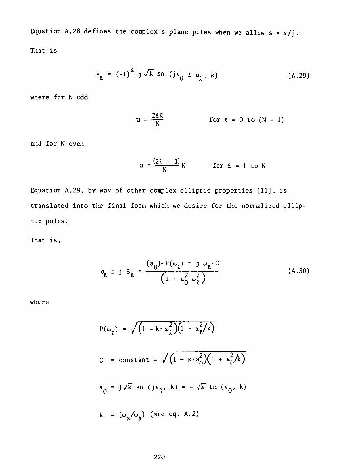
Equation A. 28 defines the complex s-plane poles when we allow s =

oj/j .

That is

s= i-A- j i/k sn

(jvQ u, k) (A. 29)

where for N odd

u = =* for = 0 to (N - 1)

and for N even

u =

(2N"

K for = 1 to N

Equation A. 29, by way of other complex elliptic properties [11], is

translated into the final form which we desire for the normalized ellip

tic poles.

That is,

.

ft

(aQ)-P(co) j VC

J 6=

7: r^\CA-30)

C1 +

Vii

where

P(to) = /(l -k-o)2)(l-

to2/k)

C = constant = /(l + k-aQ)(l +aQ/k)

aQ= j/k sn (jvQ, k) = - A tn (vQ, k)

k = (AaA)b) (see eq. A. 2)

220

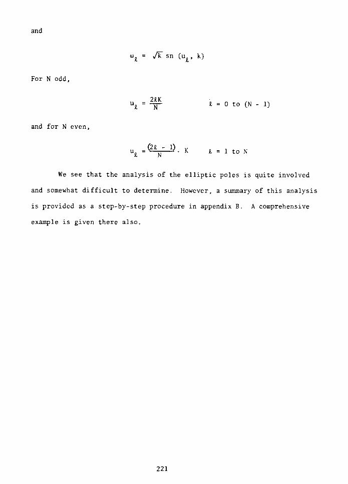
and

=v/k sn (u , k)

For N odd,

2K

u= = 0 to (N -

1)

and for N even,

N1 to N

We see that the analysis of the elliptic poles is quite involved

and somewhat difficult to determine. However, a summary of this analysis

is provided as a step-by-step procedure in appendix B. A comprehensive

example is given there also.

221

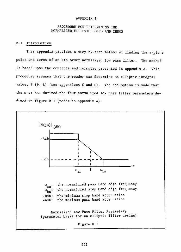
APPENDIX B

PROCEDURE FOR DETERMINING THE

NORMALIZED ELLIPTIC POLES AND ZEROS

B. 1 Introduction

This appendix provides a step-by-step method of finding the s-plane

poles and zeros of an Nth order normalized low pass filter. The method

is based upon the concepts and formulae presented in appendix A. This

procedure assumes that the reader can determine an elliptic integral

value, F (0, k) (see appendices C and D) . The assumption is made that

the user has derived the four normalized low pass filter parameters de

fined in figure B.l (refer to appendix A).

H(jto)(db)

-Adb

-Bdb

an

to, .

bn

-Bdb:

-Adb:

an bn

the normalized pass band edge frequency

the normalized stop band edge frequency

the minimum stop band attenuation

the maximum pass band attenuation

Normalized Low Pass Filter Parameters

(parameter basis for an elliptic filter design)

Figure B.l

222

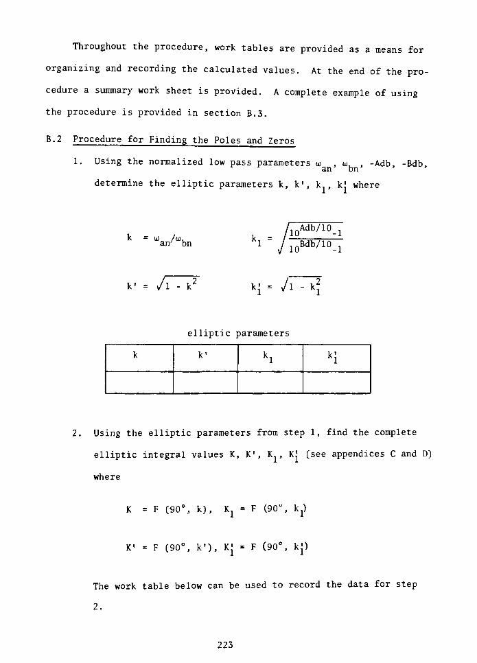
Throughout the procedure, work tables are provided as a means for

organizing and recording the calculated values. At the end of the pro

cedure a summary work sheet is provided. A complete example of using

the procedure is provided in section B.3.

B.2 Procedure for Finding the Poles and Zeros

1. Using the normalized low pass parameters to , to, , -Adb, -Bdb,an bn

determine the elliptic parameters k, k', k,

k'where

k = co /co,an'

bnk, =

10Adb/10-l

ioBdb/10-i

A Kl- />

elliptic parameters

kk'

klk '

Kl

2. Using the elliptic parameters from step 1, find the complete

elliptic integral values K, K', K., Kj (see appendices C and D)

where

K = F (90, k), Kx= F (90, kx)

K' = F (90, k'),K' = F (90, kj)

The work table below can be used to record the data for step

2.

223

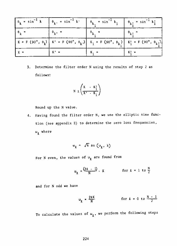
6. = sin kk

6, ,

=k'

k' 0, = sin k

Kll

ek, =k'

9k= 6k< =

9k=

kl Kl

K = F (90, ek)K'

= F (90, ek.) k. = F (90, ek) KJ= F (90, ek,)

K =K'

=

Kl=

Ki=

3. Determine the filter order N using the results of step 2 as

follows:

N >

K KJK'

K,

Round up the N value.

4. Having found the filter order N, we use the elliptic sine func

tion (see appendix E) to determine the zero loss frequencies,

to where

u= /k sn (u , k)

For N even, the values ofu

are found from

(2 - 1)u

~

NK for = 1 to

j

and for N odd we have

u. = ______

Nfor = 0 to

N - 1

To calculate the values of co ,we perform the following steps

224

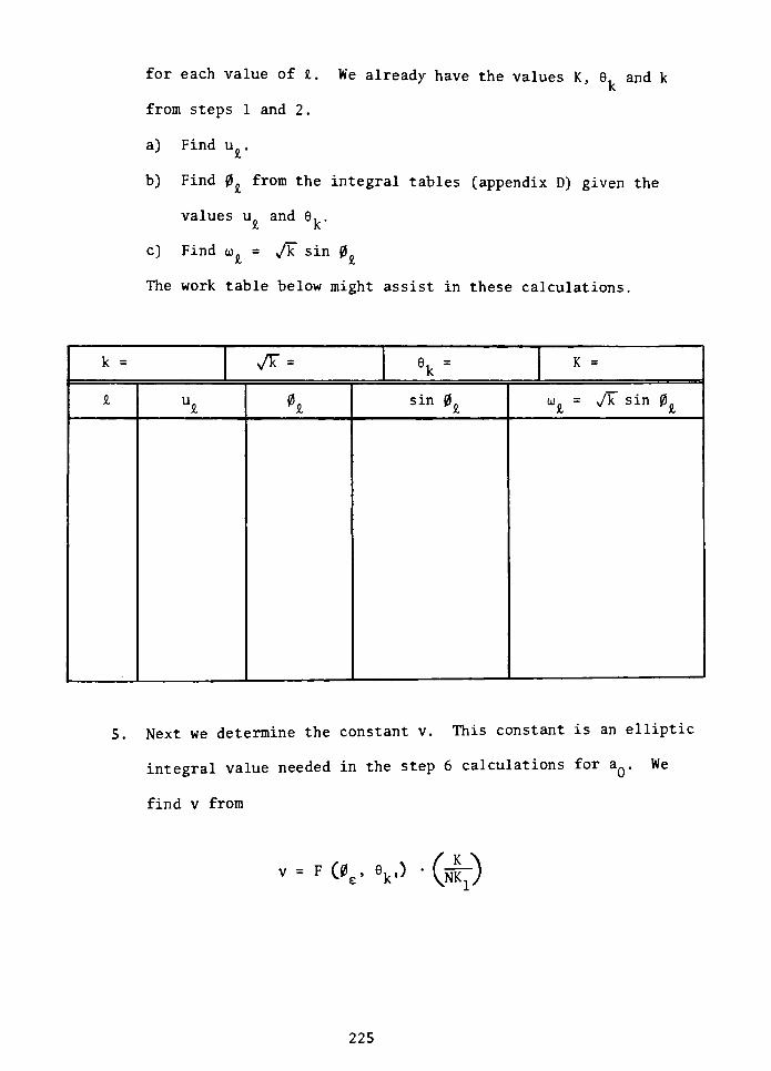
for each value of . We already have the values K, 6 and kjTV

from steps 1 and 2 .

a) Find u. .

b) Find 0 from the integral tables (appendix D) given the

values un and 6, .

k

c) Find to = /k sin 0

The work table below might assist in these calculations.

k = vT=

6k= K =

U K sin 0 oj= Jk sin 0

5. Next we determine the constant v. This constant is an elliptic

integral value needed in the step 6 calculations for aQ. We

find v from

F (*_ V>' (nk^)

225

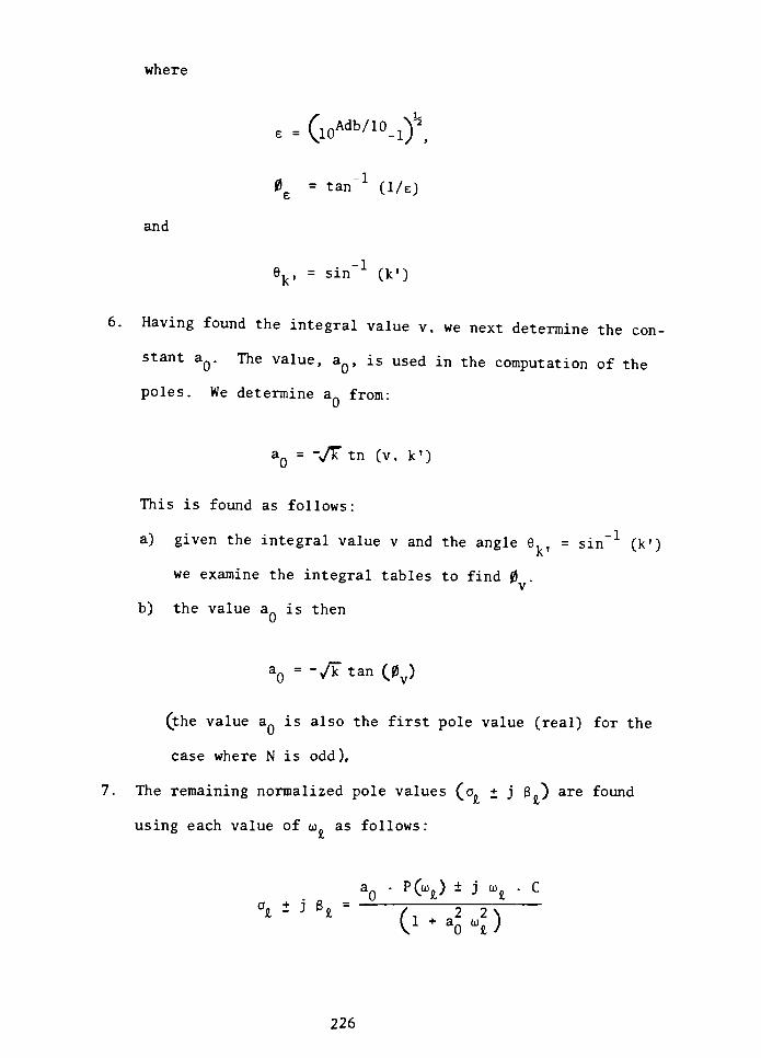
where

e =UO'(Âdb/lO^)^

0 = tan_1

(1/e)

and

ek, =sin"1

(k')

6. Having found the integral value v, we next determine the con

stant aQ. The value, aQ, is used in the computation of the

poles. We determine a from:

aQ= -v/T tn (v, k')

This is found as follows:

a) given the integral value v and the angle e,,

= (k')

we examine the integral tables to find 0v

b) the value a is then

aQ=-Jk tan (0y)

(the value a is also the first pole value (real) for the

case where N is odd),

7. The remaining normalized pole values (a. + j g.) are found

using each value of to. as follows:

a * J h= ^

0*-_-f)

226

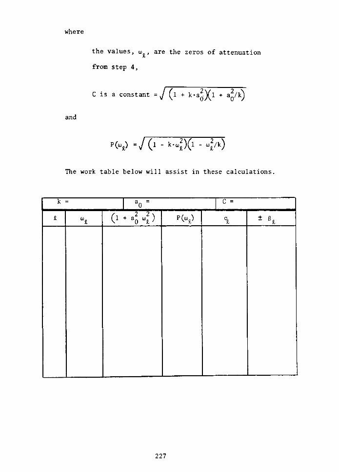
where

the values, oj, are the zeros of attenuation

from step 4,

C is a constant = J (l + ka2)(l +

a2/k)

and

p(U) -/(_ -k-oj2)(i

-o2/k)

The work table below will assist in these calculations,

k =

ao= C =

U 0 +

a0 U ) ?A) 1\

227

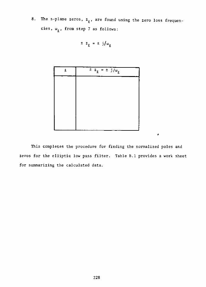
8. The s-plane zeros, z, are found using the zero loss frequen

cies, to, from step 7 as follows:

zo= j/V

h=

J/

This completes the procedure for finding the normalized poles and

zeros for the elliptic low pass filter. Table B.l provides a work sheet

for summarizing the calculated data.

228

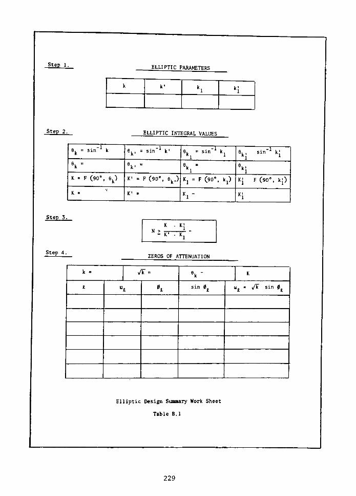
Step 1.ELLIPTIC PARAMETERS

h H

Step 2. ELLIPTIC INTEGRAL VALUES

6k=sin'1

k 6k, =sin-1

k'6. = k

1*

ek,sin"1

kj

6k=

V"

6k=

Kl \K = F (90, 8k)

K-= F (90, ek.) K. = F (90, kj)

K'F (90, k')

K- K'= Kl" K'

*1

Step 3.

Step 4.

N >K'

. K,

ZEROS OF ATTENUATION

k = ?k = \-K

tul h sin 0 _

* A sin 0

Elliptic Design Summary Work Sheet

Table B.l

229

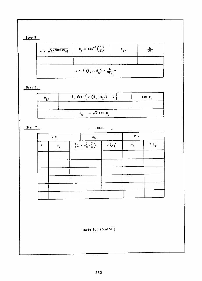
Step 5.

."--1

(.) VK

NK:e = /lOAdb/10-l

v-FC\..*e)=

Step 6.

V0yfor [fC0v. ek0 )

tan 0V

a0- tan 0y

Step 7. POLES

k =

aoc =

IL C1 +

a? w. ) P(l> B

Table B.l (Cont'd.)

230

Equations for step 7:

c - [0 ? *-_)0

?

_/*)]

*

p(^ [0 * ^2)(i -

.;A)]*

0vp^

1(1 +

-J-J

' * J B,

0 +

ao *)

Step 8.

z

ZEROS

*j7u,

Table B.l (Cont'd.)

231

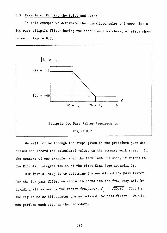
B.3 Example of Finding the Poles and Zeros

In this example we determine the normalized poles and zeros for a

low pass elliptic filter having the insertion loss characteristics shown

below in figure B.2.

H(jto)db

-Adb=-.1

-Bdb=-40

20 = f 26 Hz

Elliptic Low Pass Filter Requirements

Figure B.2

We will follow through the steps given in the procedure just dis

cussed and record the calculated values on the summary work sheet. In

the context of our example, when the term TABLE is used, it refers to

the Elliptic Integral Tables of the First Kind (see appendix D) .

Our initial step is to determine the normalized low pass filter.

For the low pass filter we choose to normalize the frequency axis by

dividing all values by the center frequency, f_ = J20. 26 = 22.8 Hz.

The figure below illustrates the normalized low pass filter. We will

now perform each step in the procedure.

232

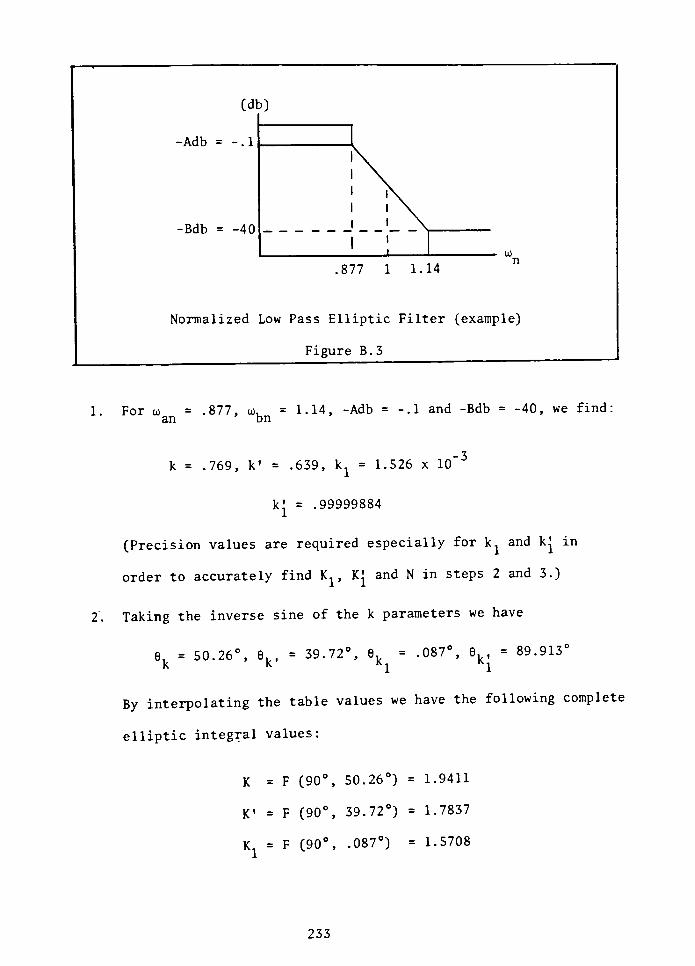
(db)

-Adb=-.1

-Bdb=-40

.877 1 1.14

Normalized Low Pass Elliptic Filter (example)

Figure B.3

1. For to =.877, ojv =1.14, -Adb

=-.1 and -Bdb

=-40, we find:

an bn

k =.769,

k'=.639, kj

= 1.526 x

kj=.99999884

(Precision values are required especially fork1

and k^ in

order to accurately find Kj, KJand N in steps 2 and 3.)

Taking the inverse sine of the k parameters we have

6k= 50.26, 6k,

= 39.72, 6k=.087, _k,

=

89.913

By interpolating the table values we have the following complete

elliptic integral values:

K = F (90, 50.26)= 1.9411

K' = F (90, 39.72)= 1.7837

K. = F (90, .087)

= 1.5708

233

and

K^= F (90, 89.913) = 7.8462

3. Using the integral values of step 2, the filter order N is cal

culated as 5.436.

N is then rounded up to the value 6.

4. Since N = 6 (even) we will have N/2 or 3 zeros of attenuation.

The integral values u for the zeros of attenuation are found

from

u =

(2Z ~

V . K for = 1 to N/2N

Therefore,

ux= K/6 = 1.9411/6 =

.324

u2= (3/6)- K =

.971

u = (5/6)- K = 1.6176

Given ek=

50.26

we find 6from

u= F (0, 50.26)

Using the tables we find the three values of 0 corresponding

to u . That is,

0 = 18.35, 02= 51.36, 03

=

78.04'

Then to. is found from

u.= ^k sin 0

234

We then have

to1=.276, oj2

=

.685, to,=.858

By inverting these values of ok we find the frequencies of in

finite loss corresponding to the infinite loss points in the

stop band. These values are also the zeros of H(s) . Thus

j z. = j 1/to. = j 3.623

j z2= j l/t_2

= j 1.46

j z,= j 1/oj_ = j 1.166

5. The respective values of e, 0 , 6,, and F (0, 6k,) are:

_

=(l0-1/10-l)2=.153

0^= tan"1(^)=

81.3

6 = 89.913,

and

F (81.3, 89.913)= 2.566

The value v is then found from:

v = F (81.3, 89.913)

= 2.566 (.206)

K

NKj

or

v =.5284

235

6. To find the constant a, we first find 0 given

v =.5284

= F (0v, ek.) = F (0y, 39.72).

By interpolating the table values we find

0v=29.73'

and

aQ= - yk tan 0y

>/.769 tan (29.73)

.5

7. The final step is to calculate the normalized pole values given

the values a, u>. and k from our work sheet. Since this is

rather lengthy; only one example will be shown. Given

u)j=

.276, aQ=-.5 and k =

.769

we have,

c . [(i . ..$(1?*iA

- i2s7

p()- [0 - ^Xi -

w/k)J=

-92

and

(l + a2to)= 1.019

236

Then

a0 PW J .o, j e, =

'i^ J pi

"

^r 2 VA

+

ao"J

=(-.5)(.92) j (.276)(1.257)

1.019

or

ol j Bx= (-.451 j .34)

This completes the example of finding the normalized poles and

zeros. The results are summarized on the work sheet (Table B.2) which

follows. In addition, the primary results (zeros of attenuation, fre

quencies of infinite loss and the pole/zero values) are illustrated in

figure B.4.

237

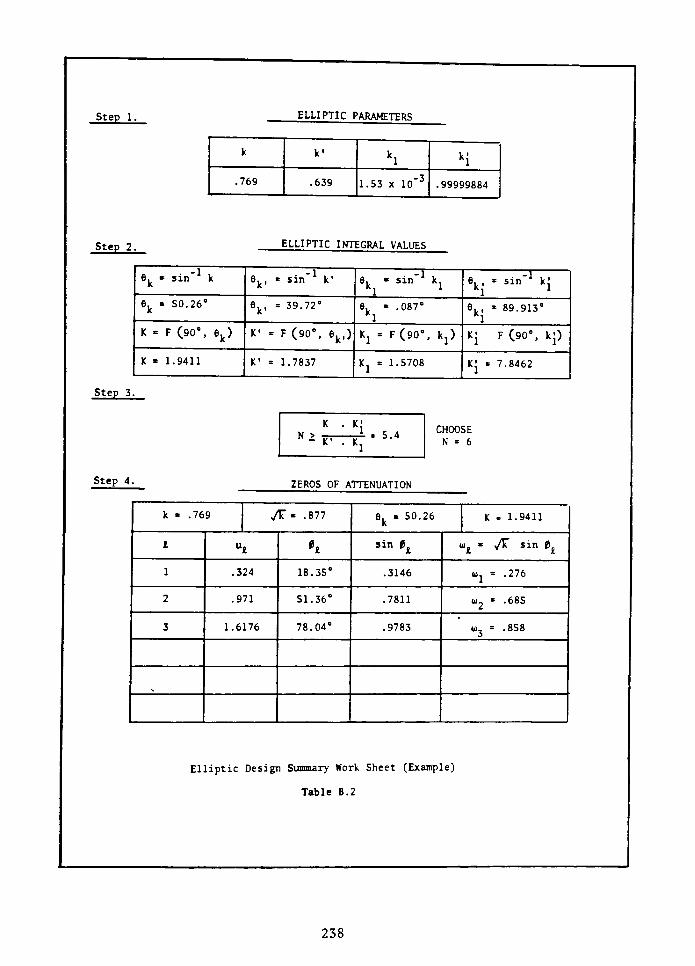
Step 1. ELLIPTIC PARAMETERS

k k'

klk'

1

.769 .639 1.53 xIO"3

.99999884

Step 2. ELLIPTIC INTEGRAL VALUES

8. k 8k, =sin"1

k'

\' "^ kl ek, =

sin"1

kj

ek50.26

8k, =39.72

6. -

*16.

,=89.913

1

K = F (90, ek)K'

F(90, ek.) K2= F(90, ka)

K'F (90, kj)

K = 1.9411 K'= 1.7837 K = 1.5708 K'

= 7.8462

Step 3.

Step 4.

N^K'.

kJ= 54

CHOOSE

N = 6

ZEROS OF ATTENUATION

k .769 JV '.ill 6. 50.26

kK = 1.9411

1ui \ sin 04 v>t

* y/F sin 0

1 .324

18.35

.3146

Uj=.276

2 .971

51.36

.7811

u2=.685

3 1.617678.04

.9783

u3=.858

Elliptic Design Summary Work Sheet (Example)

Table B.2

238

Step 5.

K flG) 6k'K

e - yio^/10-!

.153

81.3 89.913

.206

v"FOk"P-w;-

-528

Step 6.

V *y for (F <>v' ek-) ' v tan 0V

39.72 29.73

.57108

0- yTtmv -.5

Step 7.POLES

k -.769 a0-0.S C ' 1.257

I"l 0 *

*> *C-_> Cl i6l

1 .276 1.019 .92-.45 j .34

2 .685 1.1173 .5 -.22 j .771

3 .858 1.184.136

-.058 j .911

Table B.2 (Cont'd.)

239

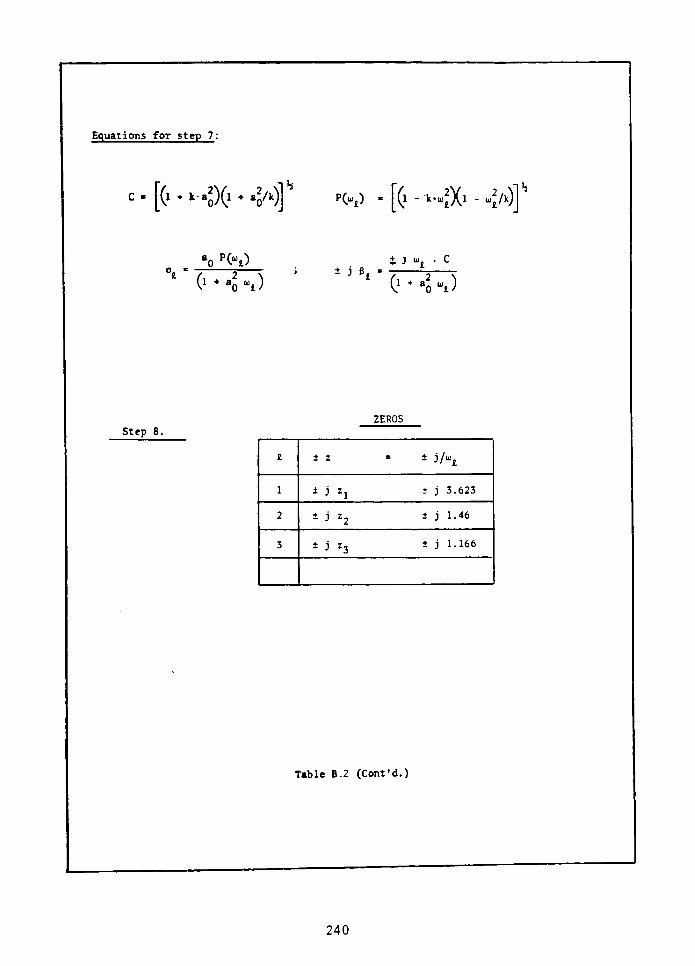
Equations for step 7:

[(} "-"oX1 * PK> - [( - v_f)(i -

.Ja)]

*o pC"t)

4"

0* 4 A' j e

=

i j "c

0 *

ao "l)

ZEROS

Step 8.

+ 23/

1 j Zjt j 3.623

2 * i l2+ j 1.46

3 1 J z3 j 1.166

Table B.2 (Cont'd.)

240

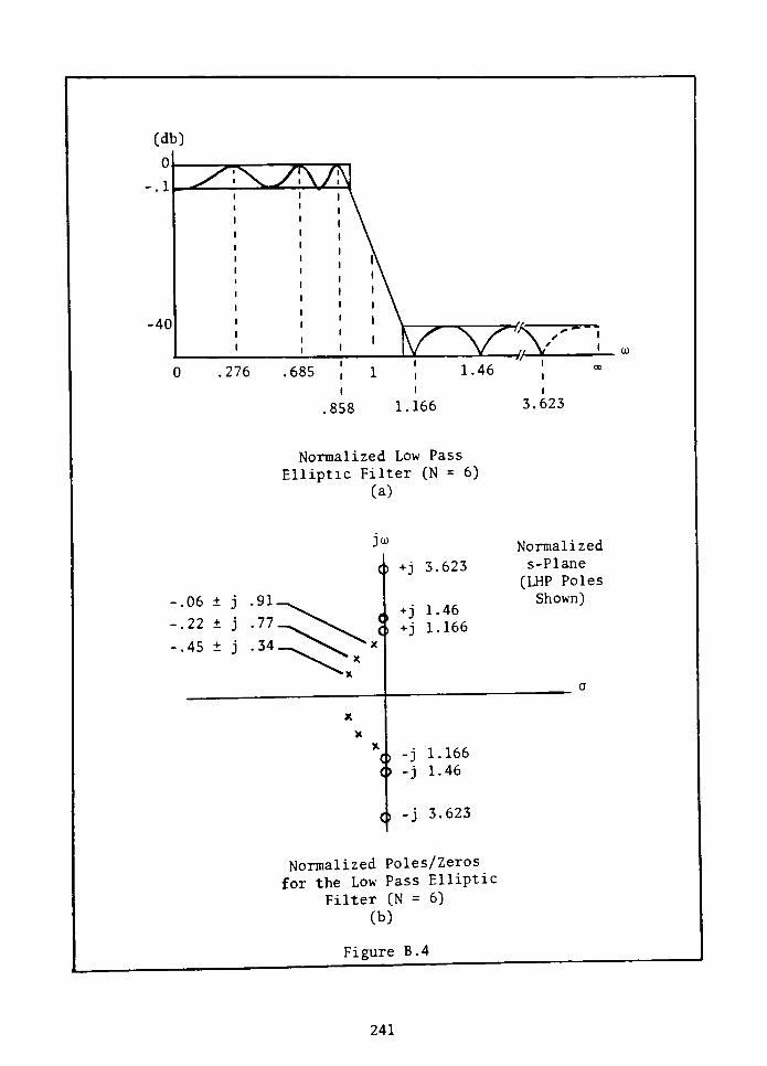
(db)

-.1

-40

^^\

55,276 ,685

1.46

.8581.166 3.623

Normalized Low Pass

Elliptic Filter (N = 6)

(a)

JOJ

h +j 3.623

<J+j 1-46

+j 1.166

c> -j1.166

O -j1.46

O -j3.623

Normalized

s-Plane

(LHP Poles

Shown)

Normalized Poles/Zeros

for the Low Pass Elliptic

Filter (N = 6)

(b)

Figure B.4

241

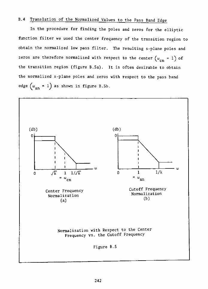
B.4 Translation of the Normalized Values to the Pass Band Edge

In the procedure for finding the poles and zeros for the elliptic

function filter we used the center frequency of the transition region to

obtain the normalized low pass filter. The resulting s-plane poles and

zeros are therefore normalized with respect to the center (oj =

1*) of

the transition region (figure B.5a). It is often desirable to obtain

the normalized s-plane poles and zeros with respect to the pass band

edge (oj =

1J as shown in figure B.5b.

(db)

0

en

Center Frequency

Normalization

(a)

(db)

0

=to.an

Cutoff Frequency

Normalization

(b)

Normalization with Respect to the Center

Frequency vs. the Cutoff Frequency

Figure B.5

242

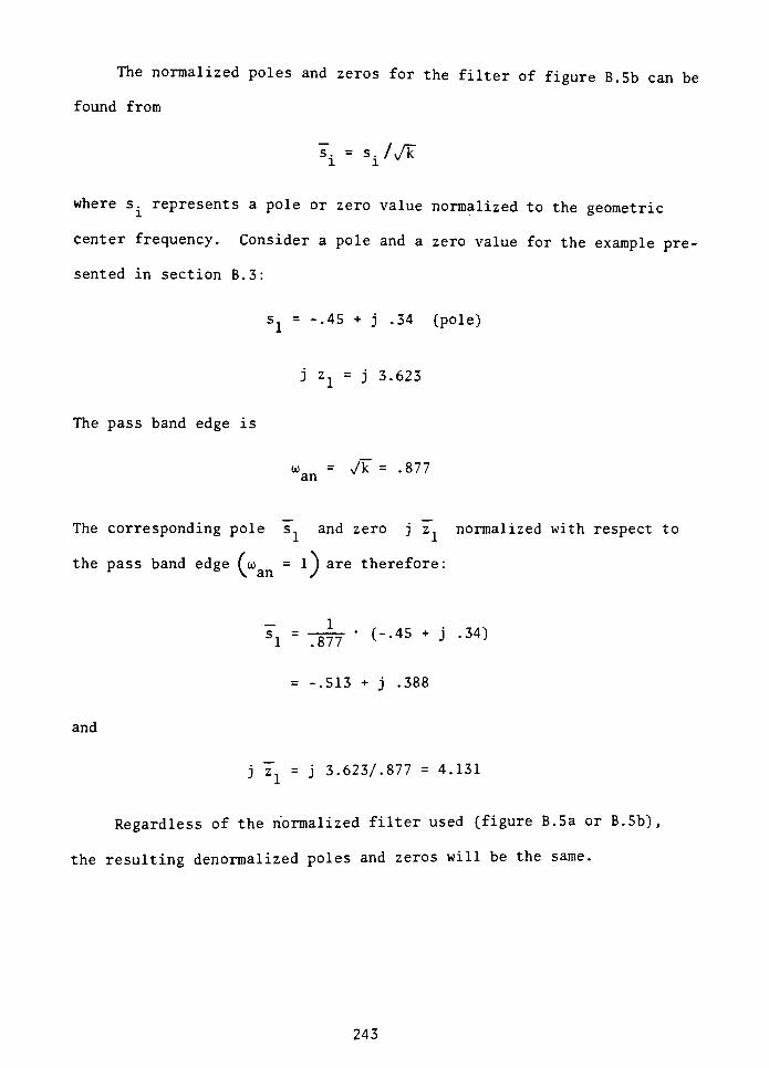
The normalized poles and zeros for the filter of figure B.5b can be

found from

s. = s. /Ak1 1

v

wheres^

represents a pole or zero value normalized to the geometric

center frequency. Consider a pole and a zero value for the example pre

sented in section B.3:

s =-.45 + j .34 (pole)

j zx= j 3.623

The pass band edge is

to = /k =.877

an

The corresponding pole s1 and zero j z normalized with respect to

the pass band edge (oj =

l) are therefore:

si=

T877*

C-45 + J -34)

=-.513 + j .388

and

j z = j 3. 623/. 877 = 4.131

Regardless of the normalized filter used (figure B.5a or B.5b),

the resulting denormalized poles and zeros will be the same.

243

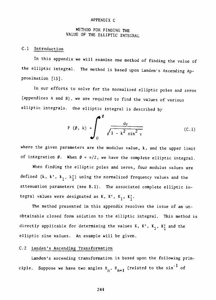
APPENDIX C

METHOD FOR FINDING THEVALUE OF THE ELLIPTIC INTEGRAL

C. 1 Introduction

In this appendix we will examine one method of finding the value of

the elliptic integral. The method is based upon Landen's Ascending Ap

proximation [15].

In our efforts to solve for the normalized elliptic poles and zeros

(appendices A and B) ,we are required to find the values of various

elliptic integrals. One elliptic integral is described by

F(0,k)=/ A ' (C-I / 1 - k sin y

VO

where the given parameters are the modulus value, k, and the upper limit

of integration 0. When 0 =

tt/2, we have the complete elliptic integral.

When finding the elliptic poles and zeros, four modulus values are

defined (k, k', k., kj) using the normalized frequency values and the

attenuation parameters (see B.l). The associated complete elliptic in

tegral values were designated as K,K'

,K

,

K'.

The method presented in this appendix resolves the issue of an un

obtainable closed form solution to the elliptic integral. This method is

directly applicable for determining the values K, K1, K,

K'and the

elliptic sine values. An example will be given.

C.2 Landen's Ascending Transformation

Landen's ascending transformation is based upon the following prin

ciple. Suppose we have two angles 6,

6 . (related to the of

244

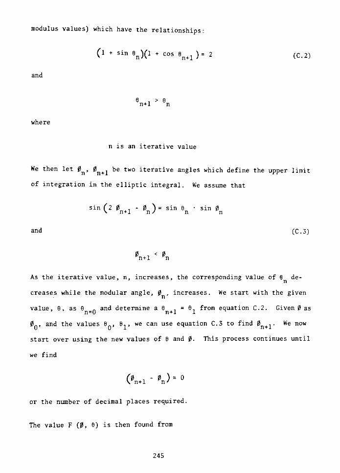
modulus values) which have the relationships:

(l + sin en)(l + cos en+1). 2 (C.2)

and

3 ,> e

n+l n

where

n is an iterative value

We then let 0^, 0^+1 be two iterative angles which define the upper limit

of integration in the elliptic integral. We assume that

sin (2 0 - 0 ") = sin 6 sin 0\ n+l tlJ n n

and (C.3)

0 < 0n+l n

As the iterative value, n, increases, the corresponding value of 6 de

creases while the modular angle, 0 ,increases. We start with the given

value, 6 , as 6 ~ and determine a 6 .

= 6. from equation C.2. Given 0 asn=0 n+l 1

0n, and the values 9n, 6., we can use equation C.3 to find 0 .. We now

start over using the new values of 6 and 0. This process continues until

we find

(0 ,

- 0 ) = 0V. n+l n'

or the number of decimal places required.

The value F (0, 6) is then found from

245

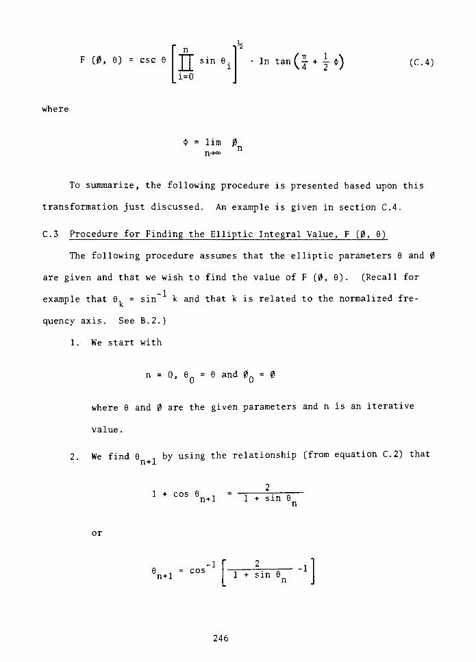
F (0, 6) = esc 6

11

ni=0

sin 6 .

iIn tan (,**) (C.4)

where

$ = lim 0n-+o

To summarize, the following procedure is presented based upon this

transformation just discussed. An example is given in section C.4.

C.3 Procedure for Finding the Elliptic Integral Value, F (0, 6)

The following procedure assumes that the elliptic parameters 6 and 0

are given and that we wish to find the value of F (0, 6). (Recall for

example that 8, = k and that k is related to the normalized fre

quency axis. See B.2.)

1. We start with

n = 0, 6Q= 6 and 0Q

= 0

where 9 and 0 are the given parameters and n is an iterative

value.

2. We find 6 , by using the relationship (from equation C.2) that

n+l

1 + cos 6n+l 1 + sin

or

n+l

cos'[

1 + sin

-1

246

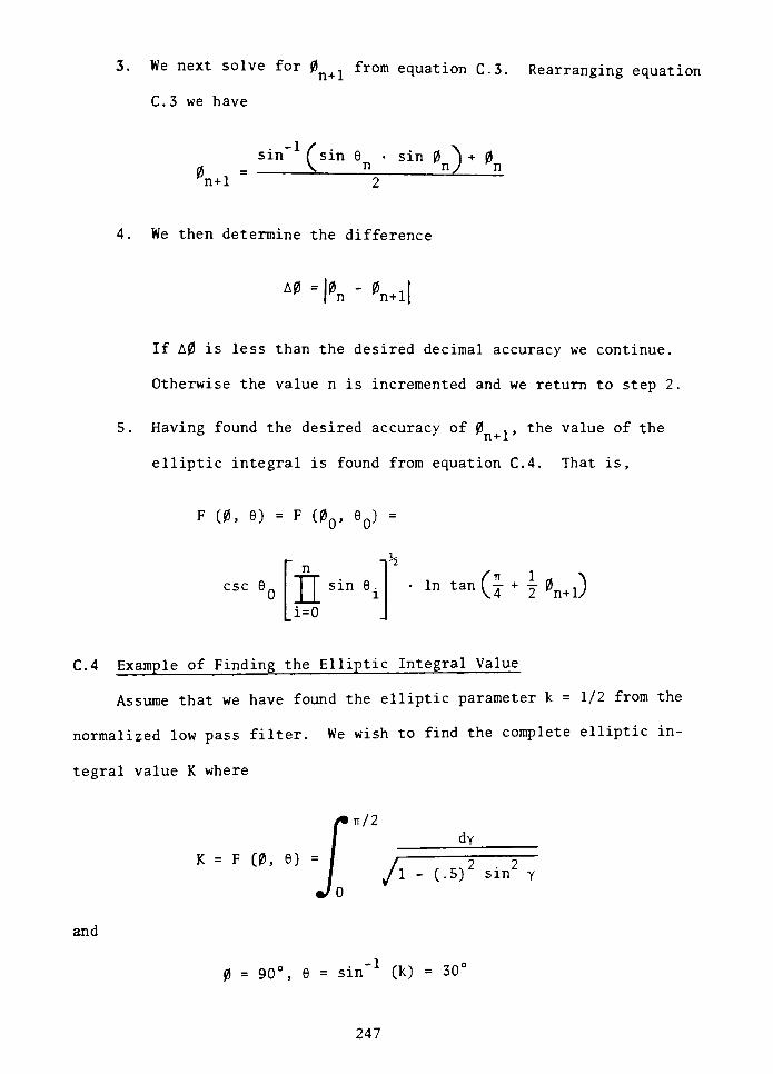
3. We next solve for 0^+1 from equation C.3. Rearranging equation

C.3 we have

n+l

(sin 6 sin 0^+0_ \ n ny *n

4. We then determine the difference

A0=|0n"0n+l|

If A0 is less than the desired decimal accuracy we continue.

Otherwise the value n is incremented and we return to step 2.

5. Having found the desired accuracy of 0 ,the value of the

elliptic integral is found from equation C.4. That is,

F (0, 6) = F (0Q5 eQ) =

esc 6,

11

ni=0

sin 6 , intan(j

+ i0n+1)

C.4 Example of Finding the Elliptic Integral Value

Assume that we have found the elliptic parameter k = 1/2 from the

normalized low pass filter. We wish to find the complete elliptic in

tegral value K where

tt/2

dY

K = F (0, 9)

/J -

(.5)2

y

and

-1

0 = 90, 6 = sin (k) = 30

247

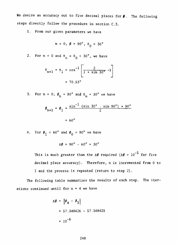
We desire an accuracy out to five decimal places for 0. The following

steps directly follow the procedure in section C.3.

1. From our given parameters we have

n = 0, 0 = 90, 6Q=30

2. For n = 0 and 6 = 8_= 30, we haven 0

n+l

= cos

70.53'

1 + sin30c -1

3. For n = 0, 0 =90

and 6 =30

we haven n

0n+l"

01_

(sin30

. sin 90) +90'

60'

4. For 0 =60

and 0 =90

we have

A0 =90

-

60

=30'

-5

This is much greater than the A0 required (A0 = 10 for five

decimal place accuracy) . Therefore, n is incremented from 0 to

1 and the process is repeated (return to step 2) .

The following table summarizes the results of each step. The iter

ations continued until for n = 4 we have

A* = |04"

03|

= 57.348426 - 57.348425

=

10"6

248

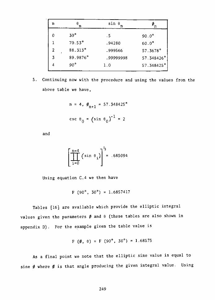
n en

sin 6n 0n

030

.5

90.0

170.53

.94280

60.0

288.313

.999566

57.3678

389.9876

.99999998

57.348426

490

1.057.348425

5. Continuing now with the procedure and using the values from the

above table we have,

n = 4, 0 .

=57.348425'

n+l

esc 6 = (sin = 2

and

n=4

ni=0

J[(3ine.) ,685094

Using equation C.4 we then have

F (90, 30) = 1.6857417

Tables [16] are available which provide the elliptic integral

values given the parameters 0 and 6 (these tables are also shown in

appendix D) . For the example given the table value is

F (0, 6) = F (90, 30) = 1.68575

As a final point we note that the elliptic sine value is equal to

sine 0 where 0 is that angle producing the given integral value. Using

249

the previous example, we are given

F (0, 30) = 1.68575 = K

We know that the required value for 0 is tt/2 to obtain the complete

elliptic integral (K) .

Then the elliptic sine value is

sn (u, 6) = sn (1.68575, 30)

= sin 0=1

Appendix E gives a fuller explanation of using the integral tables to

find the elliptic sine.

250

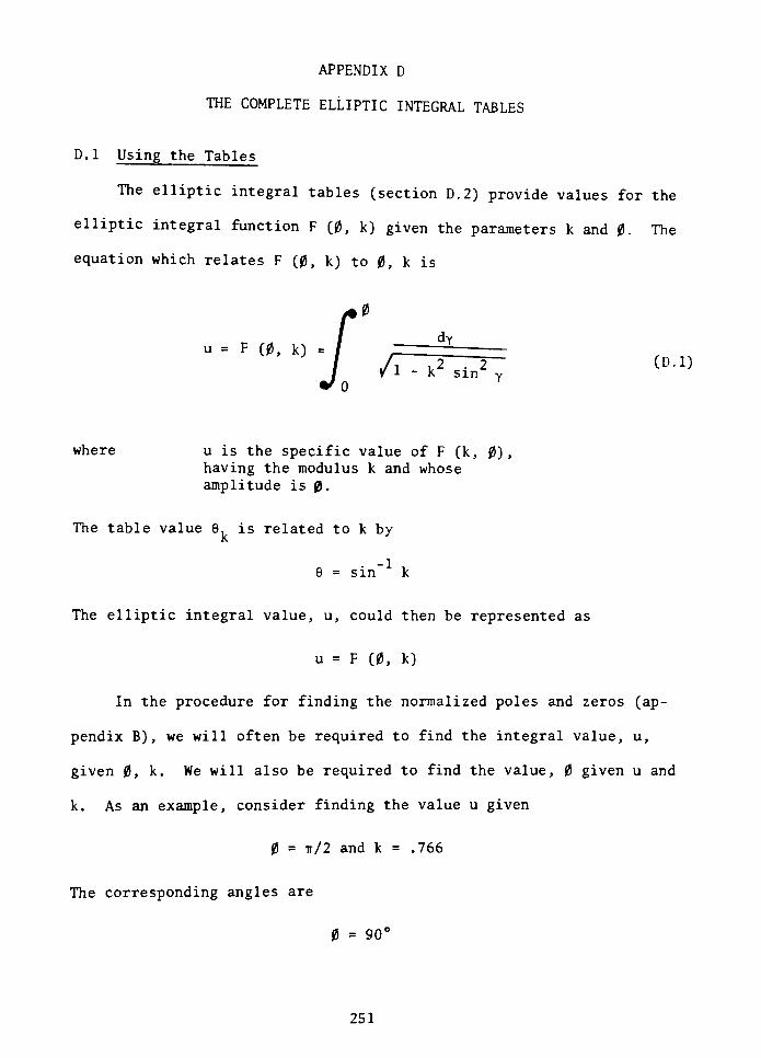
APPENDIX D

THE COMPLETE ELLIPTIC INTEGRAL TABLES

D.l Using the Tables

The elliptic integral tables (section D.2) provide values for the

elliptic integral function F (0, k) given the parameters k and 0. The

equation which relates F (0, k) to 0, k is

F (0, k) =

TO

0

/, v2 . 2 (D.l)V * - k sin Y

where u is the specific value of F (k, 0),

having the modulus k and whose

amplitude is 0.

The table value 6, is related to k by

9 = sin k

The elliptic integral value, u, could then be represented as

u = F (0, k)

In the procedure for finding the normalized poles and zeros (ap

pendix B) , we will often be required to find the integral value, u,

given 0, k. We will also be required to find the value, 0 given u and

k. As an example, consider finding the value u given

0 = it/2 and k =.766

The corresponding angles are

0 =90

251

and

8R=

.766=50

The elliptic integral value, u = F (90, 50) is found from the tables

at the intersection of the90

row for 0 and the50

column for 6. The

value is 1.9356. We then have

u = F (0, 9) = F (90, 50) = 1.9356

Whenever 0 =

tt/2, we refer to u as the complete elliptic integral of the

first kind.

As a second example, consider finding the value 0 given that

u =.4446 and k =

.766

To determine 0 we scan the 8 =50

column until we locate the value

0.4446. The corresponding value for 0 is 25. For the case where exact

values are not shown in the tables, interpolation is sufficient (for

8 < 90). For cases where 9 is greater than 85, a separate table is

provided to supplement the first.

The elliptic trigonometric functions have the argument 0 as derived

from F (0, 9) and are defined as follows:

elliptic sine = sin (0)

elliptic cosine = cos (0)

elliptic tangent = tan (0)

Since the value 0 is determined from a given integral value u and the

modulus k, the elliptic trigonometric functions are often represented as

follows:

252

elliptic sine = sn (u, k) = sin 0

elliptic cos = en (u, k) = cos 0

elliptic tan = tn (u, k) = tan 0

where we use the letter u to represent the elliptic integral value

F (0, k).

D.2 The Elliptic Integral Tables

The following tables (D.l and D.2) provide the values of the ellip

tic integral function F (0, k) . The values k (modulus) and 0 (ampli

tude) are the variables for which we desire the integral value. Note

that the table value 9 corresponds to

9 = (k)

With respect to other terminology, the following abbreviation is

often used

u = F (0, k)

or

u = F (0, 9)

The tables were taken from the C.R.C. Standard Mathematical Tables

[16]. For values of 9 > 85, a separate table is provided.

253

a <

z =

a

*I

X

_.

o

2

5c =

o >

J* II"

2 ?

y _

E*

I- ?> 3 r-

...ii

6 o d

^ i-

t*i;heS?lVl

o e 8

rt ae 2a * * 5

M M

doeo'6

a r- 3 3 rt is 5m 2 t- a <r. __

c 3 aK 06 45 ft m

do'6.6

i_-32e<c. odoodd

- * * <

ON -

co 6 n 2 ae

h i i t I

eddoo

r* ^ ?* a f-

_____

a o - r-

2 2 Z .2

*""

3 3 3 3 3

_I3_J5

36333

5 = 353xs-n2w m rt

3 O 3 8 8

8 5 a a ar- x ft fw * 2 5 A

8 8 0 0 8

rt x * rt _ 9 <a to r- rt <* ^ Ta a 8 n n^r-a c X n ix - rt t- o o x rt A *

10 .0 e e r- r- r- 1- x x x x

'ceo ddddd ddddd

a 3 ar* ^ ?* 3 r-

ddddd

SINNX 5

> * -p 3

03308 33800

x o t-

e* a r- aas rt 3rt rt

8 0 8 8 8

# 5- a rt 3

a a x x oe

x c is<-

z00008

- aesi * c1- a

1-

ddddd

I Ii(" t- CB

ifi rt "

a rt i

5 o r-

8 8 8 8 8

e 5 - 3 5

04-Nf_p N 3 r

SMViSN

: 3 3 3 3 83333

8 r-

rt o x â ?i -r

? ** ?* ;

ddddd

x - a.* 3 a r ox 5 rt >o

?* rt rt rt rt

O 8 8 3 O

:52g_

O 8 3 8 O

X 3 N ^* * Z 10 i

ddddd

* c c r- _

n r- X x a

SSlSSddddd

Sa*an- rt O r-

r* a rt toi~ r- I-

ddddd

I- M * t-r- x x x x

d d o o d

to a * a*t- v ri 5 n

a -r 3 n rt5n5no? -r *o r

8 3 3 3d

SX3C

n_X3fa r< x 3 rt s

et rt rt

ddddd o 8 e 3 o

rt r- a* aSr- JC-

ae 0 es *

*iea

do dssi.sddddd

a__

x et- a o rt

Sag n or- t *

ddddd

ss;;

O O O 8

_ ;i*kjn

O 3 3 3 O

O f- 5 rtrt e x â ?i

>*??***

doodd

n rt m r- 3^ 3 x c 3X rt tO

c* rt rt rt rt

8 3 3 O

^ a 10 ?*rt 3 a xr~ a - -t

rt rt ^ * ^

O 3 3 S^

O !_ Nt-S -V *

* 2 -5 3

NNJ-

3 x e*

iic.ci

ddddd

_ils3

00000 00000

tniMS Size

88303 0=300

. 3ri r *i m

3 3 3 3 3

O 3 - N 10

? 5 x *

X O rt &

X r. rt 3w a x r-

*^ a 5 r* ^ C X ?* *v*Ztai

3 3 3 3 3

illilm n

c?i*r p- r

3 3 3

*~ p tc rt m

SS f- aX 3 ^* to

1 3 5 5

x a o5n 5 r- to

M rt to r-g_-_3a "i *

M m ?i ^*

d o e 3 d 3 3 3 3 3

to *( 3

vreiaie

8 O 3 3 3

! 3 rta X X I- r-

; 3 3 3 3

t_ a rto l N

sdood

* to as

13 a ^ x rtn r n ; n

3 3 3 5 3

3 3 3 3 3

3 ?! =: U J^ 5 X

r* r e 5*rt rt ^ ^ *

3 3 3 3

SSa;

?S<nS S ie 5 e

3 3 3 3 8 3 3 3 i

to 1-- a rt

= C r~ r-

8 S 3

A :k= k fcf-itb

M M 74 N rt * rt rt rt .'

'ii

*

t."

3 r X rt

f ^ N_

l

X

3

~

,"_js

3 3 3 3zl

3 3 3

- i ; * :i

x a rt to

n n -: rt rt

5 V | 5 =1- x e m *

rt rt * ^

3 3 8 3 3

=x ^Sx a rt

^ * * tO .o

3Sito _. to

8 3 3 3 3

SIP

8 8 3

f;

3 S

3 8

5 = kzSr x

-

nf- 1- r~ x x

8 3 8 8 8

*

J

^?

l _ r x rtr- * n a 1-

3 8 3 3 3

Xr-x rt a

; ri s n

ddddd

d =v^- n?i n ri

ddddd

5 S = = Ii?, s = ? Si

a a a a 3a I-

.-

rt *

. r _?i t

rt rt ^- ? ?

m ^ r- 88 x = 0 rt! N S - !1? _:_.

ddddd

2^?!:S x e

-O tC tO

8 3 3 3

N

3

?2 rt

i 1 1 1 5ddddd

3 a a x^ 0 r- a1* r- r- r oe

ddddd

z

_

_

_

13 3 X rt

= I . "1 13 3 3 3 3

X rt x rt Xr* a r- *?i rt 0 t-

3 3 3 3

r a tn x*i n 0 -n

a 5 n- n :i n m

83 3 d d 8 3 = = 3

?i a r

1 = 53 =S t- a rt* ^ tc i.

3 3 3 3 3

0 a -N _:

a p- *

do::

rt

3

?* y.

iff3 3 3

tO

r^

a -

C r-

3 d

rt n- r- ar- t*. r. r- X

0 8 3 3 8

=

-"i *r x rt

= | S | sX

3

tl N M X

ri rt ts t*

3 3 8 C

rt X 5 i0

-"i ir:i*in

8 3 3

nmfi ri rt rt n

8 3 3 3 3

c-

a r

x c r r.

X 3 ?l rt

rt rt T ^

3 3 d 3 8

to * 5t- a rt a

>c r- a S^ v ^ to *

8 8 3 3 8 ddddd

rt *s a

dd 3

*J 0

a -

r*

O

Cl'Sf

8 3 3 3 3

_

A

>

Tl

1-*; r r rtn rj r-

i

_ _ '. x

3 3 3 3 3

T -1 1- > n?i r i

?i rt f-

3 3 3 3

*l l_2

3 3

: -f. n

M T

m n ?*

3 3 3 3 3 3 3 3

1 li^srt rt * r

3 3 3 3 8

ZNaSS- 3 0

ddddd

SZ8 8 8 3

rt

58

S *

- 3

_ 3 6

3a n.

3 3

ae 3 n ? r-

5i ti 8 Xnt: 1 jr- i- r~ r- r-

ddddd

2<

_

_

_

E_j

:_

**

r 2

3

Tl 1 - *

:i_l;T

3 3 3 8

X

3 3

-1 *?i m r

8 3 3

t * i r s

3 3 3 3 3

^ - r- rt ar* *5 M e r-

x e r* rt

rt rt*^ *

8 8 3 8 3

r a = rt

^ -^ O 3

3 3 3 3 8

O N <5 rt^ a $

SzSocddddd

?, 1 5 _ ;.illl

3 3 3 3d

W - 3 3 3

?! 5 5 5

8 8 3 3 8

-

t-t x rtr- t ;i. s n

8 d 5.::sd

N ?l N - 3

-f ? a f. ^3 ?< rt tfl r*

ddddd

= fi3 3

3 is 3i_- ? N

fi ?i S33 3 3

- 3 5 3>. ?i a

r- a=rt j

3 8 3 3 3

r- ? ?i a t-

8 X rt

rt rt ^ ** ^

X a u,?* a r-

5nx?2* tO

ddddd

r-_?

r* 3 x * ra

T*> a 0

ddddd

a n =

iillsd 0 3 d 3

8 X to rt

r~ r- r~ r- r~

ddddd

L

t^ x rt

= 1-1 'i3333d

n n_

- 3* n S 1.

C n n iC i

O 3 3 3

12^2 =

?I f 1 M W

3 8 J3 8 8

X rt X rt

a ^ - ar 5 rt ^

n ?) rt rt rt

ddddd

n n ?i n

a v - a

a x s -

n rt r ^ ^

ddddd

cisnxn

" * s _i

V * * "0

added

x n a * aa 5

*r to r- a_. tO tO t-S

d d 8 8 8

e.c-N

i.iliddddd

rt X * 0r * n S r-.

t~> r* r~ p- r*

8 3 8 8 8

2>

u-

r t t. n1- ^ ?i a 1-

= =_J.

8 3 3 3 3

t -1 O-1 T N ^

n rt i-i r- Is3 3

a t

3 3 311--- x 3 rt

rt rt ^ r

3 3 3 3 3

a e x rt x

5-t.n

w f ^

ddddd

si.!i38 3 38

..i.i

3993S

0 10 3 o art - x o

- r: .. 3 xi~. r~ r~ r~ i~.

ddddd

1 0

m hiii Z2b:^ St_ _ _

i6 0 O O 8

?i rt#* c1 ?i c-i n

_.r.exa5ft* CI -1 ?t rt

ti.rtVrt n rt S S5RS rt *

0 0 0 0 e

:i-c

V ^ * *

a.

ô

CN

I

\D

LO

r~j

&./ . &.o

LO O

<* vD

,Kl -

vl Di-H

o Xi

i-H Cd

wH

</> -^

a> rti-H o

rt 4->

H rt

e1 1 _

rt j=rn 4->

OO !t

4->

cI-H U

o as

H

4J U

a,

uj ou4h

C-

rt

Q

ID

i-H

X

E-

254

*

az

_i

hsr)

_

_

O

2

mil mil imii inii liin gggss i3_,_ ^=_iesse- -_:-:_;.. _ J _ _

"

_____*! *: ^**= 5 - 5 5 .j ;5i;;: 2 I

Illlf llPi -pi- 11 = 11 = **B, SggSg F = = ||g3:-

x,,,,sd dd- - 2 2 _ _: __;J ^ J

" "

!Z r T r "^ "i ^ -. *. >t * 3 o-^FifS 5USxa *_ ?. Z _;

"

.

____.__-, -, -lri ai n m fi n n rt rt -; rt

____ silss 3|s!I_ ill, I Mil?1SI-"

ss-sa ss_ =_

_= -_2

_______________ _____

*is i|-:s 3 = 5Sg si?._

;rt X S X ri _ _

I:;j =*

i = S-*55;,=

;

IE*. | __ = 5i _

= .- _-jf_p-2_3 a?.--?: 5r:_-2 2?l;t;_ -?,.^,

_____ _____ _____ _:l___ _____ !_5"_ issis I = _l ?| s N=_l

ss;j? =?,.-_! f Ji_

s _ s ; ; 5-?;= R_s_g ; s 1 2 _ 5 = a = - - -> _ -

fi-"--'j; _:'.._ iirtî^ 57ii _ 5 t:.;. 3 x2=1 _ -pr-g j =

_ ss

| _ _ 1 g~

:''.''. *>*-.-". TTr< "siif- Ssi.5 _ = _ _2 _ _

: 3 2

E?rrl c. S 5 I _ -.-__:; -j r,^ 5 2, S_;il 5 . 1 _

_- 5 - 5 p _ I

i'

_Sl?3-----

-j __

" -

_ ; _ J J' ! -. -"'T

***-

*.-; - ^ = i-I-; 1^ KZS = 3 _ _ _

_ _

_i_= i --!:;_l_l?_ ?'_.|3 =S--5 ?s_5S

s5;_rt; ==

___r5

_____ _____ _____ _____ !____ _____

= =S2 sk:5_ 5251 =

i- x 3 .-!"*

-!--Z__ _L! __ T, -. i_ ? -T. ^'~? 5 tOmo n- 3 -f 3 -: -i i -f _=

= f..___ __.E__

=g__Ef i'rtgy || = |1 as;||

_

_

~

- ".".!. -.-.-- -^ * * ? A a tfescs r~ r- r~ x x x x 5 a

Still =____ SS35I = ____ ss_.= = __ -.-.

r'i-l-i-t- r- r. r. r- > x x x xrt f. t 3X X x x x 5

a"

z_, r

_,

0

2<

y _.

-.

k

t" 7 1 3. s ?-

~

L;s.-.-*5

X rt x -.

_ | i F, _j !.|3l_r_ rt 3 a x

"

_r

^* ,r- X rt r- ;j x

-- X 3 'i<'

f-- r-. X X X

-

x -. rt n rt

_. 'r'*

!_:p"

x x x x r.

_. X -1 f-.I- r- i-. x X

S S i s

x 3 rt Xrt f r~ X

; i ; ;i ?> '^ - ^=j= 5S

r- -._

+*_ O trf -. il*!5;^?_a t r xr- i- r- r-.

-

rt

-p .: / n3 - x i- r-

x/

x r S

. _ 5 Si 3= F I = S

3 a x x a

IlIII5_!__

t-. m x -. ri

t- i- x rft ? X 31 1 n -i n rt MM --I--

<?;_,

2 r r, ,. 53 5 3 a 3

_

rt

__

T-_

~ *'

X X X X X

?l M -5r- _

v-

_ . _ _ _

3 3 3 3 3

?,-!__= 3 =. S S

& * X T a

_____

s a 5~

a fj = x

a X r- c_- f * ^ ^

-) ^ -1 O C

Z __ 3 5 _.

-îi;__ _ _

*

rt

3 rt h- O

-. i7_ 5x. _t X X

3 3 3 3 3

5i'

_ 5 53 3 3 3 3

X - X- 3 r t-

- - 3 S S

rt 3 x r_

iO ^ rt - 3

8 =-v

_. _. kl tO

1 $ ?, ?, i as rt rt rt rt III, Is 5 _ s ar~ r> rt -3

rt- .-

m

=_ t g

_

CI

-i - 1 i

X X X X X

rt -P ._ h- T.

^ ?, ^ ? Z_==!___.__Ii._l

rt .____ *

2 r S ?: <e

-rt .1* -.

-5 l _B

i. a rt ^

3 -r a j x

- ? 3 _. 2!

X - ,

S x

jrt - rt ; x r-

S 5 * I 3rt ? j _

5

3.

3 X * ?<

2 ^'l -I

~

Z7 x x x x

3 x w. rt

lll'li?i - r. t n

x ; __

rt _.

*-._.';

-. rt a r-

r~. a n ^

C 8 ;

5 rt__

a r--

rt rt rt rt rt

ti ri S rt rt

_ _ ; S 2A3;lz 5 rt ? 1

h3c x x x x

*i r ^ 5 s

|||f I 5 l_ _: E _2

O ?1 S -! g S a S s .

e n s - tiCI M w ?1 rt

_ ? ,. I -

X - !- M

t * -f ^ ^>

_

= 'rt5_! i*l .: 5 3

o X X z A1 _ ?, _

ia -r

--p a

l-

rt 3 X -.")

*.: = --iei>Z 3 ?

*l M

_|_22

-f -. r- __

-1 ?4 _l ?1 rt

x 3 rt x

n ; : _

r.rt ' X

~"* T T T

f- ri x rt x

_.___

?- X 3 i? T ? -ft

.....

3 rt o o Si;- j = S

" ri rt ^ to

5.11.O . P

_ oi rt * to

f- t- r .- i-

o o e p o

t-. x a 3# t- r- .- x

- 0 o_ O 0

x x x x ec_ f. x _ |x x x a

Ol

v_5

(N

I

LO

CM

- ^ co &,O

CTi O

v| Oi

vl

0)o 1 1

1 ,

O J_

T rt T>w r-

4->

i/; i-H cO 03 oi i (J <.)

_- H v '

rt 4->

h- rt

E

_H

_-1 O c_

rt _=

!h 4- fl)

M rt _H

<_>__

4- 01

C 1-

i i u

U Q-

4- Uc_

-i Btu o

t-i

4h

C

_

_-

rt

255

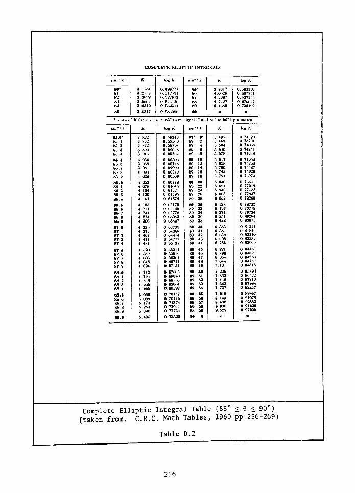
COMl'LKTK KIXIPTIC INTKGKALS

.111"1

-

A'

(*A iii-' t A l-K A

Bi"

81

82

K3

84

M

3.1534

3.2553

3.3699

3 5004

3 05)9

3 8317

0.498777

0.512591

0.527013

0.544120

0.502514

0.583396

ftS"

86

87

88

89

M

3.8317

4.0528

4.3387

4.74-7

5.4349

,

0.583396

0 B077.il

0.0373.V>

0.6761127

0 736192

_

X'nlu. _ o

A'

for biii-1 =85

Ui89"

l.y0.1"

uln89

to90

byuimiili-

bill-' 1A'

1-g A 1 iA'

log A

a_.r 3 832 0 58343Mt #'

5 435 0 73520

8., 1 3 852 0 5851 ,'J 89 2 5 469 U 73791

85.2 3 872 0 58794 89 4 5.504 0 74068

85 3 3 8U3 0 5902K 89 6 5 540 0 74351

85.4 3 UI4 0 59262 89 8 5.578 0 74648

84.* 3 936 0 59506 S 1* 5 617 0 74950

85.6 3 958 0.69748 89 12 5 658 0 75266

85 7 3 981 0 59999 89 14 ft 700 0 75587

85 8 4 MM 0 60249 89 16 ft 745 0 75929

85.9 4 028 0 60509 89 18 5 791 0 76275

_*. 4 U53 (1 60778 8* Z* 5 840 0 76641

86 1 4 078 0 61045 89 22 5 891 0 77019

8ti 2 4 104 0 61321 89 24 5 946 0 77422

86 3 4 130 0 61595 89 26 6.003 0 77837

86 4 4 157 0.61878 89 28 6 063 0 78269

84.- 4 185 0 62170 8* M 6 128 0 78732

86 6 4 214 0 62469 89 32 6 197 0 79218

86 7 4 244 0 62778 89 34 C.271 0 79734

86 8 4.274 0 6JUV1 89 36 C 351 0 80284

86 9 4 306 0 63407 89 38 6 438 0 80875

87.* t 119 0 63739 8* M 6 533 0 81511

87 1 4 372 0 64068 89 41 6 584 0 81849

87 2 4 407 0 64414 89 42 6 63'.i 0 82210

87 3 4 444 0 64777 89 43 6 696 0 82582

87.4 4 481 0 65137 89 44 6 756 0.82969

87.* 4 520 0 65514 _> U 6 821 0 833X5

87 6 4 562 0 0.V.II6 89 40 6 890 0 83822

87 7 4 003 0 66.(111 89 47 6 964 0 84286

87 8 4 648 0 66727 89 48 7 044 0 847K2

87.9 4 694 0 67154 89 49 7 131 0 85315

-8.* 4 743 0 67605 _ M 7 226 0 85891)

88 1 4 794 0 68070 89 51 7 332 0 _U-|_-

88 2 4 818 0 118556 89 52 7 449 0 87210

88 3 4 905 0 69064 89 53 7 583 0 87984

88 4 4 965 0.69592 89 54 7.737- 0 88857

88. i 030 0 70157 8t _4 7 919 0 89867

88 G 5 099 0 70749 80 56 8 143 0 91078

88 7 5 173 0.71374 89 57 8 430 0 92583

88 8 ft 253 0 72041 89 58 8 836 0 94626

88 9 5 340 0.72754 89 59 0.529 0 97905

St.* 5 435 0 73520 M _ 0

Complete Elliptic Integral Table(85

< 6 < 90)

(taken from: C.R.C. Math Tables, 1960 pp 256-269)

Table D.2

256

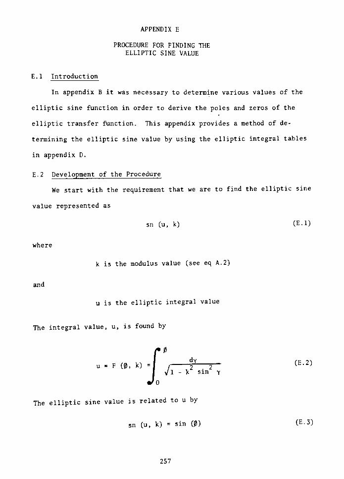
APPENDIX E

PROCEDURE FOR FINDING THE

ELLIPTIC SINE VALUE

E. 1 Introduction

In appendix B it was necessary to determine various values of the

elliptic sine function in order to derive the poles and zeros of the

elliptic transfer function. This appendix provides a method of de

termining the elliptic sine value by using the elliptic integral tables

in appendix D.

E. 2 Development of the Procedure

We start with the requirement that we are to find the elliptic sine

value represented as

sn (u, k) CE-1)

where

k is the modulus value (see eq A. 2)

and

u is the elliptic integral value

The integral value, u, is found by

0

ft/odv

u = F (0, k) =1j f

Y~

k sin y

(E.2)

The elliptic sine value is related to u by

sn (u, k) = sin (0) (E.3)

257

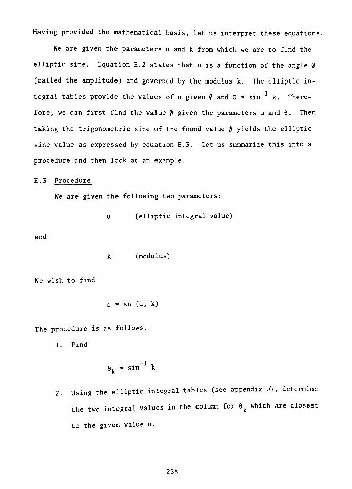
Having provided the mathematical basis, let us interpret these equations.

We are given the parameters u and k from which we are to find the

elliptic sine. Equation E.2 states that u is a function of the angle 0

(called the amplitude) and governed by the modulus k. The elliptic in

tegral tables provide the values of u given 0 and 6 = k. There

fore, we can first find the value 0 given the parameters u and 6. Then

taking the trigonometric sine of the found value 0 yields the elliptic

sine value as expressed by equation E.3. Let us summarize this into a

procedure and then look at an example.

E.3 Procedure

We are given the following two parameters:

u (elliptic integral value)

and

k (modulus)

We wish to find

p= sn (u, k)

The procedure is as follows:

1 .Find

-1 ,

6, = sin k

2. Using the elliptic integral tables (see appendix D) , determine

the two integral values in the column for 9kwhich are closest

to the given value u.

258

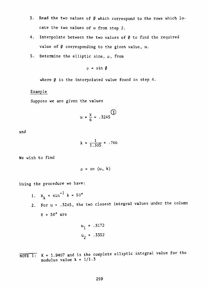
and

3. Read the two values of 0 which correspond to the rows which lo

cate the two values of u from step 2.

4. Interpolate between the two values of 0 to find the required

value of 0 corresponding to the given value, u.

5. Determine the elliptic sine, p, from

p= sin 0

where 0 is the interpolated value found in step 4.

Example

Suppose we are given the values

u = t =.3245

6

k-T305='766

We wish to find

p= sn (u, k)

Using the procedure we have:

1. ek= k =

50

2. For u =.3245,

the two closest integral values under the column

6 =

50

are

u. =.3172

u- =.3352

NOTE 1: K = 1.9407 and is the complete ellipticintegral value for the

modulus value k = 1/1-3

259

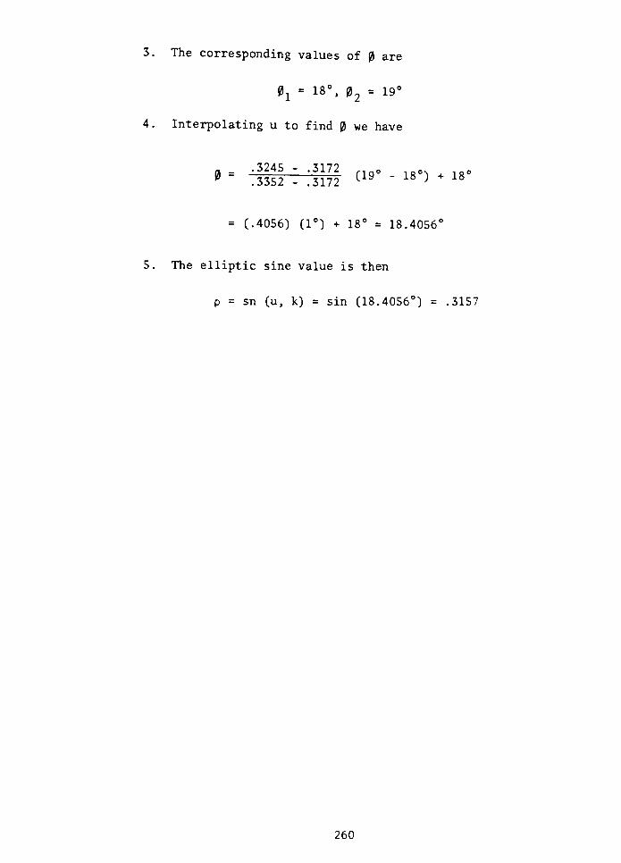
3. The corresponding values of 0 are

0. = 18, 02-

19

4. Interpolating u to find 0 we have

0 =

.3352:.3,72

(19" 18^ +

18

= (.4056) (1) +18

=18.4056

5. The elliptic sine value is then

p= sn (u, k) = sin (18.4056) =

.3157

260

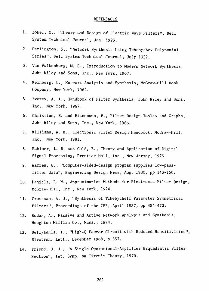
REFERENCES

1. Zobel, 0., "Theory and Design of Electric Wave Filters", Bell

System Technical Journal, Jan. 1923.

2. Darlington, S., "Network Synthesis Using Tchebyshev Polynomial

Series", Bell System Technical Journal, July 1952.

3. Van Valkenburg, M. E., Introduction to Modern Network Synthesis,

John Wiley and Sons, Inc., New York, 1967.

4. Weinberg, L. , Network Analysis and Synthesis, McGraw-Hill Book

Company, New York, 1962.

5. Zverev, A. I., Handbook of Filter Synthesis, John Wiley and Sons,

Inc. , New York, 1967.

6. Christian, E. and Eisenmann, E., Filter Design Tables and Graphs,

John Wiley and Sons, Inc., New York, 1966.

7. Williams, A. B., Electronic Filter Design Handbook, McGraw-Hill,

Inc. , New York, 1981.

8. Rabiner, L. R. and Gold, B., Theory and Application of Digital

Signal Processing, Prentice-Hall, Inc., New Jersey, 1975.

9. Warren, G., "Computer-aided-design program supplies low-pass-

filter data", Engineering Design News, Aug. 1980, pp 143-150.

10. Daniels, R. W. , Approximation Methods for Electronic Filter Design,

McGraw-Hill, Inc., New York, 1974.

11. Grossman, A. J., "Synthesis of Tchebycheff Parameter Symmetrical

Filters", Proceedings of the IRE, April 1957, pp 454-473.

12. Budak, A., Passive and Active Network Analysis and Synthesis,

Houghton Mifflin Co., Mass., 1974.

13. Deliyannis, T. , "High-Q Factor Circuit with Reduced Sensitivities",

Electron. Lett., December 1968, p 557.

14. Friend, J. J., "A Single Operational-Amplifier Biquadratic Filter

Section", Int. Symp. on Circuit Theory, 1970.

261

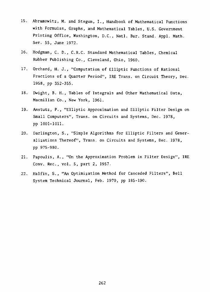
15. Abramowitz, M. and Stegun, I., Handbook of Mathematical Functions

with Formulas, Graphs, and Mathematical Tables, U.S. Government

Printing Office, Washington, D.C., Natl. Bur. Stand. Appl. Math.

Ser. 55, June 1972.

16. Hodgman, C. D., C.R.C. Standard Mathematical Tables, Chemical

Rubber Publishing Co., Cleveland, Ohio, 1960.

17. Orchard, H. J., "Computation of Elliptic Functions of Rational

Fractions of a Quarter Period", IRE Trans, on Circuit Theory, Dec.

1958, pp 352-355.

18. Dwight, B. H., Tables of Integrals and Other Mathematical Data,

Macmillan Co., New York, 1961.

19. Amstutz, P., "Elliptic Approximation and Elliptic Filter Design on

Small Computers", Trans, on Circuits and Systems, Dec. 1978,

pp 1001-1011.

20. Darlington, S., "Simple Algorithms for Elliptic Filters and Gener

alizations Thereof", Trans, on Circuits and Systems, Dec. 1978,

pp 975-980.

21. Papoulis, A., "On the Approximation Problem in Filter Design", IRE

Conv. Rec, vol. 5, part 2, 1957.

22. Halfin, S. , "An Optimization Method for Cascaded Filters", Bell

System Technical Journal, Feb. 1970, pp 185-190.

262

Documents

An active filter design program (theory and application)