Bayesian analysis of longitudinal data using growth curve models

http://jbd.sagepub.comDevelopment

International Journal of Behavioral

DOI: 10.1177/0165025407077764 2007; 31; 374 International Journal of Behavioral Development

Zhiyong Zhang, Fumiaki Hamagami, Lijuan Lijuan Wang, John R. Nesselroade and Kevin J. Grimm Bayesian analysis of longitudinal data using growth curve models

http://jbd.sagepub.com/cgi/content/abstract/31/4/374 The online version of this article can be found at:

Published by:

http://www.sagepublications.com

On behalf of:

International Society for the Study of Behavioral Development

can be found at:International Journal of Behavioral Development Additional services and information for

http://jbd.sagepub.com/cgi/alerts Email Alerts:

http://jbd.sagepub.com/subscriptions Subscriptions:

http://www.sagepub.com/journalsReprints.navReprints:

http://www.sagepub.com/journalsPermissions.navPermissions:

http://jbd.sagepub.com/cgi/content/abstract/31/4/374#BIBLSAGE Journals Online and HighWire Press platforms):

(this article cites 25 articles hosted on the Citations

© 2007 International Society for the Study of Behavioral Development. All rights reserved. Not for commercial use or unauthorized distribution. at UNIV OF VIRGINIA on July 12, 2007 http://jbd.sagepub.comDownloaded from

http://www.issbd.org

http://jbd.sagepub.com/cgi/alerts

http://jbd.sagepub.com/subscriptions

http://www.sagepub.com/journalsReprints.nav

http://www.sagepub.com/journalsPermissions.nav

http://jbd.sagepub.com/cgi/content/abstract/31/4/374#BIBL

http://jbd.sagepub.com

International Journal of Behavioral Development2007, 31 (4), 374–383

http://www.sagepublications.com

© 2007 The International Society for theStudy of Behavioural Development

DOI: 10.1177/0165025407077764

Introduction

To study phenomena in their time-related patterns ofconstancy and change is a primary reason for collecting longi-tudinal data. All longitudinal data share at least three features:(1) the same entities are observed repeatedly over time; (2) thesame measurements (including parallel tests) are used; and(3) the timing for each measurement is known (Baltes &Nesselroade, 1979; McArdle & Nesselroade, 2003). The needto analyze longitudinal data has stimulated the development oflongitudinal data analytic techniques and models that, in turn,have advanced the collection of longitudinal data. Growthcurve models (McArdle & Nesselroade, 2003; Meredith &Tisak, 1990) exemplify a widely used technique with a directmatch to the objectives of longitudinal research described byBaltes and Nesselroade (1979) – to analyze explicitly intrain-dividual change and interindividual differences in change.

In the past decades, growth curve models have evolved fromfitting a single curve for only one individual to fitting multi-level or mixed-effects models for multiple individuals and fromlinear to nonlinear models (Blozis, Conger, & Herring, 2007;McArdle, 2001; McArdle & Nesselroade, 2003; Meredith &Tisak, 1990; Tucker, 1958; Wishart, 1938). The use of thesemodels in social and behavioral research has grown rapidlysince Meredith and Tisak (1990) showed that growth curvemodels can be fitted as a restricted common factor model inthe structural equation modeling framework (see also,McArdle, 1988; McArdle & Epstein, 1987). For a morecomprehensive discussion of growth curve models, seeMcArdle and Nesselroade (2003).

For estimating growth curve models, the maximum likelihoodestimation (MLE) method is commonly used (Demidenko,

2004; Laird & Ware, 1982). MLE for growth curve models isembedded in commercial statistical packages, such as SASPROC MIXED and PROC NLMIXED and Splus LME andNLME. Recently, Bayesian methods have received more atten-tion as useful tools for estimating a variety of models includinggrowth curve models, in particular complex growth curvemodels which can be difficult or impossible to estimate in thecurrent MLE-based software (Lee & Chang, 2000; Lee & Liu,2000; McArdle & Wang, in press; Menzefricke, 1998; Pettitt,Tran, Haynes, & Hay, 2006; Seltzer, Wong, & Bryk, 1996).

Bayesian methods have become well established in thepsychological literature since their introduction to psychologyby Edwards, Lindman, and Savage (1963). Since then,Bayesian methods have been successfully applied to item-response models (Chang, 1996; Fox & Glas, 2001), factoranalytic models (Bartholomew, 1981; S. Lee, 1981), structuralequation models (Scheines, Hoijtink, & Boomsma, 1999),genetic models (Eaves & Erkanli, 2003), and multilevel models(Seltzer et al., 1996). Rupp, Dey, and Zumbo (2004) provideda valuable review of applications of Bayesian methods in socialand behavioral research and proposed that neither the appliednor the theoretical measurement communities can afford tomiss the opportunities opened up by Bayesian methods.

Even though Bayesian methods are powerful and can beused in a variety of analytic models, the strenuous program-ming and computational demands have discouraged manyresearchers from using them. Furthermore, the complexities ofthe models that usually need the application of Bayesianmethods make the methods seem remote for empiricalresearchers. In this study, we aim to draw researchers’attention to Bayesian methods and provide an easy way toimplement Bayesian analysis, especially for longitudinal data.

Bayesian analysis of longitudinal data using growth curve models

Zhiyong Zhang, Fumiaki Hamagami, Lijuan Wang, and John R. NesselroadeUniversity of Virginia, USA

Kevin J. GrimmUniversity of California, USA

Bayesian methods for analyzing longitudinal data in social and behavioral research are recommendedfor their ability to incorporate prior information in estimating simple and complex models. We firstsummarize the basics of Bayesian methods before presenting an empirical example in which we fit alatent basis growth curve model to achievement data from the National Longitudinal Survey ofYouth. This step-by-step example illustrates how to analyze data using both noninformative andinformative priors. The results show that in addition to being an alternative to the maximum likeli-hood estimation (MLE) method, Bayesian methods also have unique strengths, such as the system-atic incorporation of prior information from previous studies.These methods are more plausible waysto analyze small sample data compared with the MLE method.

Keywords: Bayesian analysis; growth curve models; informative priors; longitudinal data; poolingdata; WinBUGS

Correspondence should be sent to Dr Zhiyong Zhang, Departmentof Psychology, PO Box 400400, University of Virginia, Char-lottesville, VA 22903-4400, USA; e-mail: [email protected]



First, we provide a brief review of basic Bayesian terms andmethods, such as priors, posteriors, and the Markov chainMonte Carlo (MCMC) method. We then present the basicconcepts of the latent basis growth curve model used in theempirical data analysis. Finally, we present an empiricalexample, step-by-step, to show how to implement Bayesiananalysis practically using the softwareWinBUGS (Spiegelhalter,Thomas, Best, & Lunn, 2003) and BAUW (Zhang & Wang,2006). We show that Bayesian methods provide a directalternative to MLE and also demonstrate their uniquestrengths for analyzing longitudinal data.

Basic ideas of Bayesian methods

This section aims to introduce the basic ideas of Bayesianmethods (see also Walker, Gustafson, & Frimer, 2007) and isnaturally redundant with extant publications. For morecomplete descriptions of Bayesian analysis, we recommendBox and Tiao (1992), Carlin and Louis (2000), and Lee(2004). Researchers primarily interested in the application ofBayesian methods may choose to skip the mathematicalformulas and go directly to the verbal explanations.

Bayes’ theorem

Bayesian analysis is based on the tenet that the concept ofprobability can be applied to the degree to which a personbelieves a hypothesis or a proposition. The degree of belief inproposition H can be represented as Pr(H), which is also calledthe prior degree of belief in H. A simple version of Bayes’theorem (also known as Bayes’ rule) is,

Pr(H|E) , (1)

which indicates that the degree of belief in proposition H giventhe observed evidence E is equal to the joint probability of Hand E divided by the probability of E. Pr(H|E) is called theposterior degree of belief in H, in the sense of being theupdated belief after observing the evidence.

Usually, we have more than one hypothesis in our research.For example, if we have n different hypotheses, H1, H2, . . . ,Hn to explain a phenomenon, then Bayes’ theorem is stated as,

Pr(Hi|E) = , (2)

This declares that our posterior belief on Hi not only dependson the observed evidence E but also depends on our priorbeliefs regarding each hypothesis.

Bayes’ theorem is useful because it provides a way to calcu-late the probability of a hypothesis based on the evidence ordata. Given the evidence, the calculation of Pr(E|Hi) isstraightforward. However, when we observe some evidence, weare interested in the probability of the hypotheses conditionalon the evidence, Pr(Hi|E). Bayes’ theorem provides a way tocalculate this probability. But the calculation also depends onthe prior probabilities Pr(Hi). Thus, Bayes’ theorem providesa natural way to update our prior belief Pr(Hi) concerning thehypothesis to our posterior belief Pr(Hi|E) based on theevidence E.

So far, we have only discussed discrete probability appli-cations. For continuous probability problems, the hypothesesare represented by one or more continuous parameters from amodel denoted by θθ. The evidence, represented by the data, isdenoted by y. In this case, Bayes’ theorem is written as,

(3)

in which p(θθ) is the prior belief, prior probability distribution,or simply the prior of θθ; p(θθ|y) is the posterior belief, poste-rior probability distribution, or the posterior of θθ; and p(y|θθ)is the probability of the data which is also the likelihood L(θθ;y)in MLE.Because ∫θθ

p(θθ)p(θθ|y)dθθ is a normalizing constant, then

p(θθ|y) � p(θθ)p(y|θθ) = p(θθ)L(θθ;y), (4)

which states that a posterior is proportional to the prior timesthe likelihood.

Choice of priors

Bayes’ theorem shows how the prior belief is required forBayesian analysis. A prior is the available information about thehypothesis and unknown parameters before the data arecollected. The prior is classified as either an informative prioror a noninformative prior.

Noninformative priors. When no reliable prior informationconcerning the hypotheses or parameters exists, or an infer-ence based only on the data at hand is desired, noninformativepriors can be used. A noninformative prior does not favor anyhypothesis or value of a parameter. For example, in the discretecase, the prior

Pr(Hi) = 1/n, i = 1, . . . , n, (5)

is a noninformative prior because it assigns equal probabilityto each hypothesis Hi. For the continuous case, a similar prioris

π(θθ) = c, any c > 0. (6)

This prior is usually called an improper prior because its inte-gration is infinity.

Priors with only a little information about the unknownparameters are also called noninformative priors. For example,to estimate tomorrow’s temperature, we can specify a normaldistribution prior with mean 0 and variance 106. In this case,because of the large variance, the prior temperature infor-mation is very vague. In Bayesian analysis, the use of nonin-formative priors typically yields similar results to MLE.

Informative priors. Informative priors make Bayesian analysismore subjective because different priors can result in differentconclusions, a situation that has been criticized by frequentistsfor a long time. An informative prior may be constructedfrom previous studies. For example, if we want to predicttomorrow’s temperature, it is reasonable to use a normal distri-bution prior with the mean and variance equal to the mean andvariance of the temperature on the same day over the past20 years.

Clearly, the use of priors provides a way to pool and capi-talize on extant scientific findings. For example, before anyexperiment is carried out, we may know nothing about aparameter and thus specify a noninformative prior p(θθ). After

pp p

pp p

p p d( | )

( ) ( | )( )

( ) ( | )

( ) ( | )θθ θθ θθ θθ θθ

θθ θθy

yy

y

y= =

θθθθθ∫

Pr( | )Pr( )

Pr( | )Pr( )

E H H

E H H

i i

i ii

n

=∑

1

= ∩ =Pr( )Pr( )

Pr( | )Pr( )Pr( )

E HE

E H HE

INTERNATIONAL JOURNAL OF BEHAVIORAL DEVELOPMENT, 2007, 31 (4), 374–383 375



an experiment in which we obtain the data y1, we update ourknowledge about the parameter to p(θθ|y1). With an additionalexperiment, we obtain the data y2, and can use the posteriorp(θθ|y1) from the first experiment as the prior to update theknowledge about that parameter again.

Conjugate priors. Regardless of whether informative priors areused, one may try to use conjugate priors when they are appro-priate to simplify computation. A conjugate prior is a priorfrom the family of probability density functions from which thederived posterior density functions have similar function formsto the priors. For example, if we use a prior with a normaldistribution and derive a posterior also with a normal distri-bution based on the Bayes’ theorem, then this prior is a conju-gate prior (conjugate to the likelihood). The use of conjugatepriors can usually reduce the computation complexity of theposterior distribution largely. The exponential family of distri-butions, which includes the normal distribution, gamma distri-bution, beta distribution, and so on, is the most often usedfamily of distributions and has conjugate priors.

Statistical inference on posteriors1

Once the posterior distribution of the parameters is obtained,statistical inference can be performed. Because we know theposterior distribution of the unknown parameters, we can plottheir densities. However, such plots carry so much informationthat they become difficult to apprehend. Several statistics canbe used to summarize the information of the posterior and areanalogous to parameter estimates and standard errors fromMLE. In particular, we consider point estimations and credibleintervals.

Point estimation. Of the many point estimations, the mean isthe most widely used. Given the posterior, the mean is calcu-lated by

θθ– = ∫θθp(θθ|y)dθθ, (8)

which is the classical definition of the mean. Similarly, theassociated variance can be obtained with

Var(θθ) = ∫(θθ – θθ–)p(θθ|y)(θθ – θθ–)tdθθ. (9)

These are also called the posterior mean and posterior variance,respectively.

Credible interval. In Bayesian statistics, credible intervals areused for purposes similar to those of confidence intervals infrequentist statistics. Many times, a credible interval is directlycalled a confidence interval. Formally, a 100 � (1 – α)%credible interval (L, U) for θθ is obtained by

1 – α ≤ ∫U

Lp(θθ|y)dθθ, (10)

with L and U are lower and upper bounds, respectively.Because the parameter θθ is considered a random variable,

we can interpret the credible interval as “The probability thatθθ lies in the interval (L, U) given the observed data is at least100 � (1 – α)%.” In frequentist statistics, the confidenceinterval means that “If the experiment is repeated many timesand the confidence interval is calculated each time, then overall100 � (1 – α)% of them contain the true parameter θθ.”

Thus, the credible interval has a more intuitively appealinginterpretation.

Markov chain Monte Carlo methods

Statistical inference discussed in the previous section can bedone only when the integration in Equations 8–10 can be solvedimplicitly. However, this is usually impossible in practiceespecially when multiple unknown parameters are present. Inpractice, MCMC methods are generally used to circumventthe difficulty of multiple dimension integration. Many differentMCMC methods have been proposed, such as Metropolis–Hastings sampling, Gibbs sampling, and slicing sampling.Because Gibbs sampling is widely used, we focus on this method.

Gibbs sampling is an algorithm to generate a data point fromthe conditional distribution of each parameter, conditional onthe current values of the other parameters (Geman & Geman,1984). Let θθ = (θθ1, . . . , θθq) with q unknown parameters in themodel of interest. The conditional distribution π(θθi|θθi–1, . . . ,θθi–1, θθi+1, . . . θθq;y) for θθi can usually be obtained relatively easilyusing Bayes’ theorem. Then we can use the following schemeto sample the data points from the conditional distributions.

At the (i + 1)th iteration with current value θθ(i) = (θθ1(i), θθ2

(i),. . ., θθ q

(i)), update θθ(i+1) = (θθ1(i+1), θθ2

(i+1), . . . , θθq(i+1)) by means of

sequentially generating

θθ1(i+1) from π(θθ1|θθ2

(i), θθ3(i), . . . , θθq

(i);y),θθ2

(i+1) from π(θθ2|θθ1(i+1), θθ3

(i), . . . , θθq(i);y)

. . .θθq

(i+1) from π(θθq|θθ1(i+1), θθ2

(i+1), . . . , θθq–1(i+1);y).

Namely, the first parameter is updated based on values ofparameters from the previous iteration. The second parameteris updated based on the just-updated first parameter estimateand the not-yet-updated third to qth parameters. The thirdparameter is then updated based on the just-updated first andsecond parameter estimates and the not-yet-updated fourth toqth parameters. This process of updating parameters isperformed up to the qth parameter to finish one completeiteration. The iteration process above can be repeated I times.Geman and Geman (1984) showed that for sufficiently largeI, θθ(I ) can be viewed as a simulated observation from theposterior distribution π(θθ|y).

The simulated observations after I are then recorded forfurther analysis. For convenience, these observations aredenoted by θθ(m), m = 1, . . . , M. Sometimes, there are highlypositive autocorrelations between the successive observations.To reduce autocorrelation and the computing storage space,one could pick observations with fixed interval (or thin) aindexed 1, 1 + a, 1 + 2a, 1 + 3a, . . . to perform further analysis(Zuur, Garthwaite, & Fryer, 2002). The point estimation iscalculated by

θθ– =, θθ1+ma, (11)

with variance

Var(θθ) = (θθ1+ma – θθ–)(θθ1+ma – θθ–)t. (12)

To construct the credible interval, we use the percentiles ofthe generated sequences. For example, the lower bound of the100 � (1 – α)% credible interval is equal to the α/2 percentileof the sequence and the upper bound is equal to the 1 – α/2percentile.

11 0

1

N m

N

–

–

=∑

1

0

1

N m

N

=∑

–

376 ZHANG ET AL. / BAYESIAN ANALYSIS OF LONGITUDINAL DATA

1 Readers who are only interested in empirical studies may skip this sectionand proceed to the next section.



Two keys to using Gibbs sampling are to obtain theconditional posterior distributions and determine the conver-gence of the generated Markov chain (or determine I). Ifconjugate priors are used, conditional posteriors can usuallybe easily obtained. Furthermore, with the emergence of newsoftware such as WinBUGS, one does not need to specify theconditional posterior distributions explicitly. However, theconvergence diagnosis of the Markov chain is still underdevelopment although several ways have been suggested todetermine I. In practice, the “eyeball” method, monitoring theconvergence by visually inspecting the history plots of thegenerated sequences, is commonly used. Usually, if there is nochange point or trend in the plot, the convergence of the gener-ated sequence is accepted. To illustrate this, we plotted thehistory of generated sequences of three parameters in Figure1. At the beginning, the sequences either increased quickly(Figure 1a), or declined quickly (Figure 1b), or fluctuated alot (Figure 1c). However, after about 500 iterations, allsequences appear very flat and there is no noticeable trend orchange. Thus, the sequences converged after 500 iterations, inother words, I = 500. Furthermore, the sequences for allparameters converged at approximately the same time andconvergence should not be accepted until the sequences for allunknown parameters have converged. For example, although

the sequence in Figure 1b seemed to converge after 200iterations, we cannot say this sequence was converged becausethe other two sequences had not yet converged.

Latent basis growth curve model

Growth curve models have been widely used in the analysis ofgrowth processes in social and behavioral research (McArdle& Nesselroade, 2003; Meredith & Tisak, 1990). Figure 2shows a path diagram for the growth curve model used in thepresent analyses. The observed variables are drawn as squares,unobserved or latent variables are drawn as circles, and theconstant is represented by the triangle. The squares labeled y1through y4 are the observed data on occasions 1 through 4,respectively. L in the circle is the individual latent initial level,µL is the mean of the initial level across all the participants, andσL

2 is the variability around the initial level representinginterindividual differences in the latent initial level. S in thecircle corresponds to the slope, µS is the mean of the slopeacross all the participants, and σS

2 represents its variability, orindividual differences around the slope. The covariance, σLS,between level and slope is represented by the double-headedarrow between the latent variables. The circles labeled e1


0.0

0.5

1.0

Iteration

1 1000 2000 3000

1.5

0.00.250.5

0.75

Iteration

1 1000 2000 3000

1.0

0.00.050.1

0.15

Iteration

1 1000 2000 3000

0.2

Figure 1. History plots of three parameters.



through e4 are random errors, and their variance (σe2) is

assumed to be equal across time but it can vary across time. Land S are random-effects parameters that have different valuesfor each individual, whereas µL and µS are fixed-effectsparameters that are the same for all the participants.Mathematically, this model can be written as

yit = Li + αiSi+ eit

Li = µL + νLi i = 1, . . . , N; t = 1, . . . , T, (13)

Si = µS + νSi

with N denoting the sample size and T denoting the numberof occasions.

The model indicates that the observed variables y1–y4 aredetermined by the initial level (L), the slope (S), and error (e).Different growth curve shapes can be produced by adjustingthe weights of α1 through α4. For example, assigning them thevalues 1 through 4 would lead to a linear growth curve. α1 andα4 can be fixed and the values of α2 and α3 can be estimated.This particular model, in which the weights or basis co-efficients determine the shape of the growth curve, is knownas a latent basis growth model, and has the advantage that theform of the function is determined by the data rather thanspecified a priori.

The latent basis growth model is very flexible because it canform many kinds of growth trajectories by assigning differentvalues to αt. The different growth curves for two individualsare plotted in Figure 3. In the first plot, α = (0, .33, .66, 1)indicates a linear growth trajectory. In the second plot, α = (0,.8, .95, 1) indicates an exponential growth trajectory. In the

third plot, α = (1, .8, .25, 0) indicates a nonlinear declinecurve. Finally, α = (0, –1, 1, 0) indicates a fluctuating changetrajectory. Furthermore, only two of the basis coefficientsneed to be fixed for the identification and scaling purposes.Illustrative is fixing the first and second coefficients to be 0 and1 and estimating the other basis coefficients (McArdle &Nesselroade, 2003).

Empirical example

To illustrate how to practically implement Bayesian analysis,we present an empirical example.

Data

Data in this example are two subsets from the NationalLongitudinal Survey of Youth (NLSY).2 The first subsetincludes repeated measurements of N = 173 children. At thefirst measurement in 1986, the children were about 6–7 yearsof age. The same children were then repeatedly measured at2-year intervals for three additional measurement occasions(1988, 1990, and 1992). Missing data existed for some of thechildren. The second subset includes repeated measurementsof N = 34 children. At their first measurement in 1992, thechildren were also about 6–7 years of age. The same childrenwere also measured again at an approximate 2-year intervalfor another three times in years 1994, 1996, and 1998.Missing data also existed for several of the children. Thechildren from both data sets were tested using the PeabodyIndividual Achievement Test (PIAT) Reading Recognitionsubtest that measured word recognition and pronunciationability. The total score for this subtest ranged in value from 0to 84. In the present study, this score was rescaled by dividingby 10.


1

L S

µL µS

σLS

σL2 σS

2

e1

σe2

1

1 1 1 1

y1

e2

σe2

1

y2

e3

σe2

1

y3

e4

σe2

1

y4

α1

α2 α3α4

Figure 2. A growth curve model path diagram.

10

1 2

T

y

3 4

86

410

1 2

T

y

3 4

86

4

10

1 2

T

y

3 4

86

410

1 2

T

y

3 4

86

4

Figure 3. Manipulation of different growth curves with differentbasis coefficients.

2 For a complete description of NLSY, visit http://www.bls.gov/nls/



Research questions

For the first set of data, the empirical question was “Is theresystematic change in reading recognition and individual differ-ences in this change over time (8 years)?”. The technicalquestion to answer was “Is there difference between Bayesianestimation and MLE in parameter estimates?”. For the secondset of data, the technical question to answer was “How doesthe use of prior information affect the parameter estimates andstandard errors from a small sample?”.

Design of analyses

First, the first data set was analyzed using the Bayesian methodwith noninformative priors. Then the same data set wasanalyzed using MLE. The results from two methods werecompared. Second, the second data set was first analyzed usingthe Bayesian methods with noninformative priors as thebaseline. Then the informative priors were constructed fromthe results of the first data set and used in the analysis of thesecond data set. To further demonstrate the use of informativepriors in the small sample study, we selected part of the data(N = 20) from the second data set. Both full informative priorsand half informative priors as defined in the next section wereused to analyze the selected data.

In all Bayesian analysis, conjugate priors were used. For themeans of initial level and slope, the normal distribution priorwas used. For the variance of measurement error, the inversegamma distribution prior was used and for the covariancematrix of the random effects parameters, the inverse Wishartdistribution prior was used. Finally, normal distribution priorswere used for the basis coefficients.

Implementation of the analyses

All Bayesian analyses were implemented using WinBUGS andBAUW. WinBUGS is widely used free software for Bayesiananalysis and is very flexible for both simple and complex models.Although WinBUGS can be used as menu-driven software, it isstill not easy to use for at least two reasons. First, programminga model in WinBUGS requires understanding the details of theprobability form for that model, which is usually missing in mosttextbooks especially for empirical researchers. Second, the dataformat of WinBUGS is similar to that of R or Splus, whichmakes the data conversion frustrating.

In order to advance the application of Bayesian analysis andmake the implementation of the analysis easier, the softwarecalled BAUW (Zhang & Wang, 2006) was used. BAUW canbe used to generate WinBUGS programs for many kinds ofmodels, such as growth curve models, latent difference scoremodels (McArdle & Hamagami, 2001), and IRT models(Embretson & Reise, 2000). BAUW is the menu-drivensoftware and only needs a few inputs to generate fullWinBUGS programs, including data conversion. For theanalysis of the first data set by using the latent basis model, weneed to input the sample size (173), the number of occasions(4), the missing data indicator (dot “.” in the data file for thisexample), and the data file. WinBUGS program generatedfrom BAUW is given in Appendix A. The program can thenbe run in WinBUGS by clicking menus.3

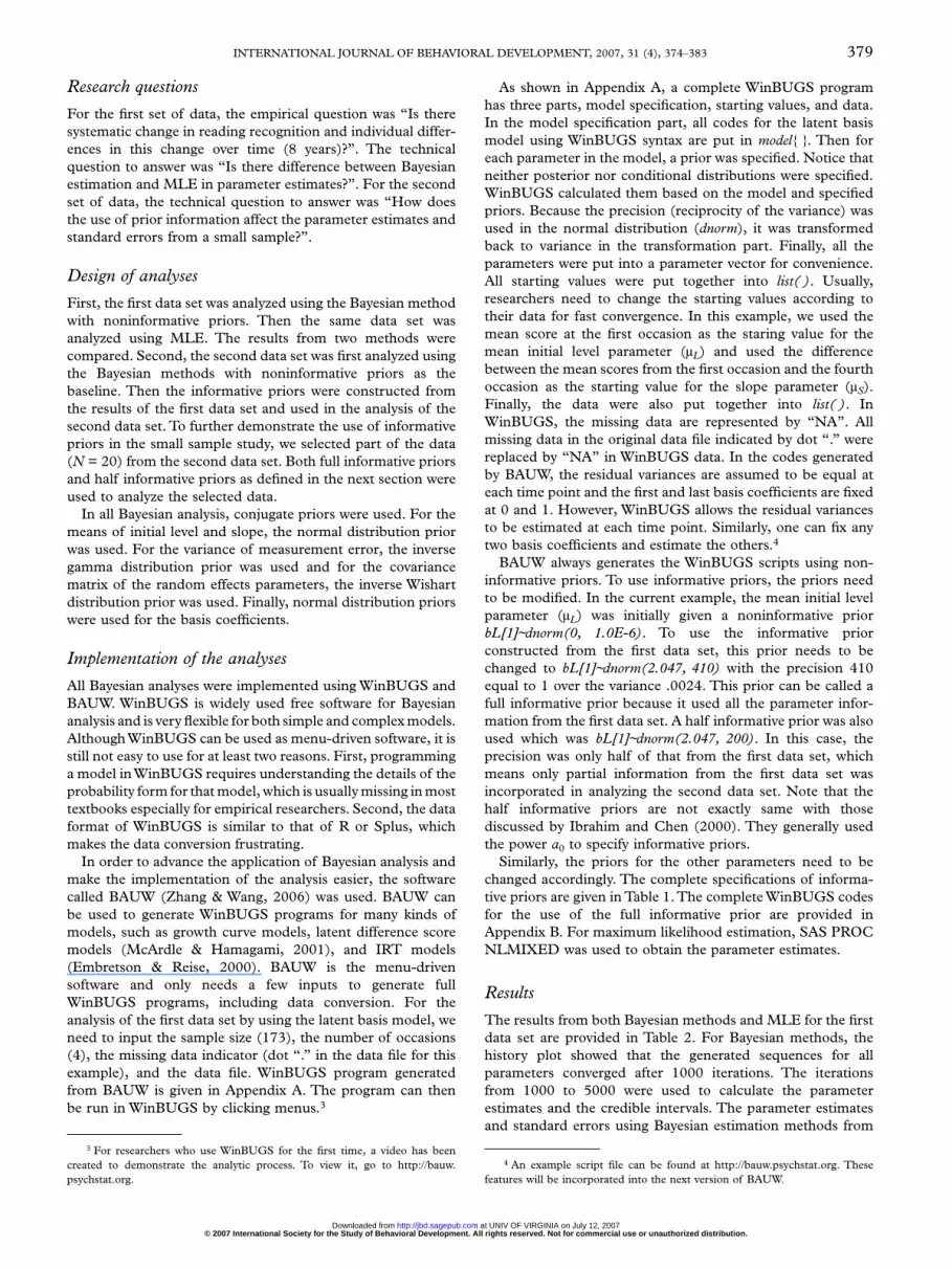
As shown in Appendix A, a complete WinBUGS programhas three parts, model specification, starting values, and data.In the model specification part, all codes for the latent basismodel using WinBUGS syntax are put in model{ }. Then foreach parameter in the model, a prior was specified. Notice thatneither posterior nor conditional distributions were specified.WinBUGS calculated them based on the model and specifiedpriors. Because the precision (reciprocity of the variance) wasused in the normal distribution (dnorm), it was transformedback to variance in the transformation part. Finally, all theparameters were put into a parameter vector for convenience.All starting values were put together into list( ). Usually,researchers need to change the starting values according totheir data for fast convergence. In this example, we used themean score at the first occasion as the staring value for themean initial level parameter (µL) and used the differencebetween the mean scores from the first occasion and the fourthoccasion as the starting value for the slope parameter (µS).Finally, the data were also put together into list( ). InWinBUGS, the missing data are represented by “NA”. Allmissing data in the original data file indicated by dot “.” werereplaced by “NA” in WinBUGS data. In the codes generatedby BAUW, the residual variances are assumed to be equal ateach time point and the first and last basis coefficients are fixedat 0 and 1. However, WinBUGS allows the residual variancesto be estimated at each time point. Similarly, one can fix anytwo basis coefficients and estimate the others.4

BAUW always generates the WinBUGS scripts using non-informative priors. To use informative priors, the priors needto be modified. In the current example, the mean initial levelparameter (µL) was initially given a noninformative priorbL[1]~dnorm(0, 1.0E-6). To use the informative priorconstructed from the first data set, this prior needs to bechanged to bL[1]~dnorm(2.047, 410) with the precision 410equal to 1 over the variance .0024. This prior can be called afull informative prior because it used all the parameter infor-mation from the first data set. A half informative prior was alsoused which was bL[1]~dnorm(2.047, 200). In this case, theprecision was only half of that from the first data set, whichmeans only partial information from the first data set wasincorporated in analyzing the second data set. Note that thehalf informative priors are not exactly same with thosediscussed by Ibrahim and Chen (2000). They generally usedthe power a0 to specify informative priors.

Similarly, the priors for the other parameters need to bechanged accordingly. The complete specifications of informa-tive priors are given in Table 1.The complete WinBUGS codesfor the use of the full informative prior are provided inAppendix B. For maximum likelihood estimation, SAS PROCNLMIXED was used to obtain the parameter estimates.

Results

The results from both Bayesian methods and MLE for the firstdata set are provided in Table 2. For Bayesian methods, thehistory plot showed that the generated sequences for allparameters converged after 1000 iterations. The iterationsfrom 1000 to 5000 were used to calculate the parameterestimates and the credible intervals. The parameter estimatesand standard errors using Bayesian estimation methods from


3 For researchers who use WinBUGS for the first time, a video has beencreated to demonstrate the analytic process. To view it, go to http://bauw.psychstat.org.

4 An example script file can be found at http://bauw.psychstat.org. Thesefeatures will be incorporated into the next version of BAUW.



https://www.researchgate.net/publication/226244061_Item_Response_Theory_for_Psychologists?el=1_x_8&enrichId=rgreq-f1437981-fb57-4533-b668-03e0b49d8f3d&enrichSource=Y292ZXJQYWdlOzIzMDc1NzE2NTtBUzoxNTAwMDE4NTAyNjE1MDlAMTQxMjc3NDYzNjQ4Mw==

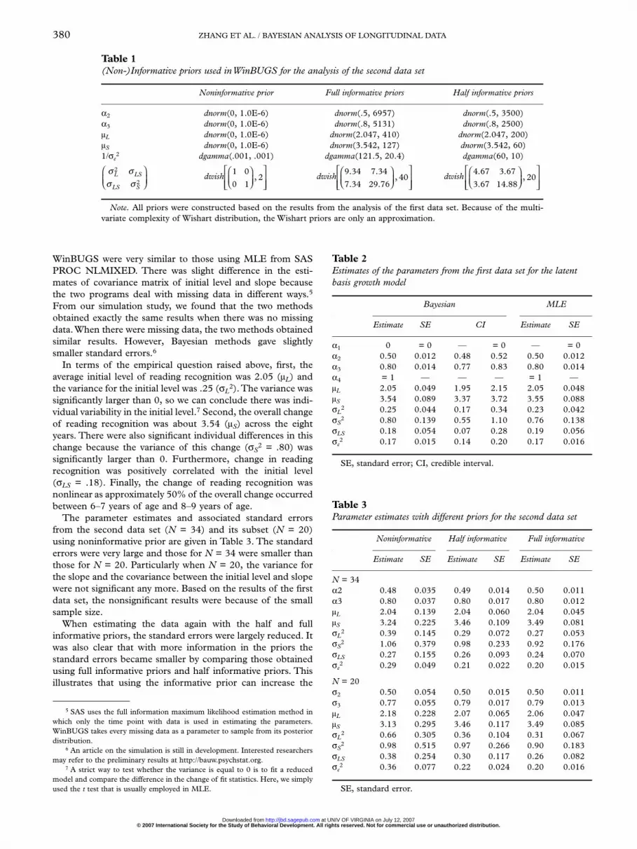
WinBUGS were very similar to those using MLE from SASPROC NLMIXED. There was slight difference in the esti-mates of covariance matrix of initial level and slope becausethe two programs deal with missing data in different ways.5

From our simulation study, we found that the two methodsobtained exactly the same results when there was no missingdata.When there were missing data, the two methods obtainedsimilar results. However, Bayesian methods gave slightlysmaller standard errors.6

In terms of the empirical question raised above, first, theaverage initial level of reading recognition was 2.05 (µL) andthe variance for the initial level was .25 (σL

2).The variance wassignificantly larger than 0, so we can conclude there was indi-vidual variability in the initial level.7 Second, the overall changeof reading recognition was about 3.54 (µS) across the eightyears. There were also significant individual differences in thischange because the variance of this change (σS

2 = .80) wassignificantly larger than 0. Furthermore, change in readingrecognition was positively correlated with the initial level(σLS = .18). Finally, the change of reading recognition wasnonlinear as approximately 50% of the overall change occurredbetween 6–7 years of age and 8–9 years of age.

The parameter estimates and associated standard errorsfrom the second data set (N = 34) and its subset (N = 20)using noninformative prior are given in Table 3. The standarderrors were very large and those for N = 34 were smaller thanthose for N = 20. Particularly when N = 20, the variance forthe slope and the covariance between the initial level and slopewere not significant any more. Based on the results of the firstdata set, the nonsignificant results were because of the smallsample size.

When estimating the data again with the half and fullinformative priors, the standard errors were largely reduced. Itwas also clear that with more information in the priors thestandard errors became smaller by comparing those obtainedusing full informative priors and half informative priors. Thisillustrates that using the informative prior can increase the


Table 1(Non-)Informative priors used in WinBUGS for the analysis of the second data set

Noninformative prior Full informative priors Half informative priors

α2 dnorm(0, 1.0E-6) dnorm(.5, 6957) dnorm(.5, 3500)α3 dnorm(0, 1.0E-6) dnorm(.8, 5131) dnorm(.8, 2500)µL dnorm(0, 1.0E-6) dnorm(2.047, 410) dnorm(2.047, 200)µS dnorm(0, 1.0E-6) dnorm(3.542, 127) dnorm(3.542, 60)1/σe

2 dgamma(.001, .001) dgamma(121.5, 20.4) dgamma(60, 10)

dwish dwish dwish

Note. All priors were constructed based on the results from the analysis of the first data set. Because of the multi-variate complexity of Wishart distribution, the Wishart priors are only an approximation.

4 67 3 67

3 67 14 8820

. .

. .,

⎛⎝⎜

⎞⎠⎟

⎡

⎣⎢⎢

⎤

⎦⎥⎥

9 34 7 34

7 34 29 7640

. .

. .,

⎛⎝⎜

⎞⎠⎟

⎡

⎣⎢⎢

⎤

⎦⎥⎥

1 0

0 12

⎛⎝⎜

⎞⎠⎟

⎡

⎣⎢⎢

⎤

⎦⎥⎥

,σ σσ σ

L LS

LS S

2

2

⎛

⎝⎜⎞

⎠⎟

5 SAS uses the full information maximum likelihood estimation method inwhich only the time point with data is used in estimating the parameters.WinBUGS takes every missing data as a parameter to sample from its posteriordistribution.

6 An article on the simulation is still in development. Interested researchersmay refer to the preliminary results at http://bauw.psychstat.org.

7 A strict way to test whether the variance is equal to 0 is to fit a reducedmodel and compare the difference in the change of fit statistics. Here, we simplyused the t test that is usually employed in MLE.

Table 2Estimates of the parameters from the first data set for the latentbasis growth model

Bayesian MLE

Estimate SE CI Estimate SE

α1 0 = 0 — = 0 — = 0α2 0.50 0.012 0.48 0.52 0.50 0.012α3 0.80 0.014 0.77 0.83 0.80 0.014α4 = 1 — — — = 1 —µL 2.05 0.049 1.95 2.15 2.05 0.048µS 3.54 0.089 3.37 3.72 3.55 0.088σL

2 0.25 0.044 0.17 0.34 0.23 0.042σS

2 0.80 0.139 0.55 1.10 0.76 0.138σLS 0.18 0.054 0.07 0.28 0.19 0.056σe

2 0.17 0.015 0.14 0.20 0.17 0.016

SE, standard error; CI, credible interval.

Table 3Parameter estimates with different priors for the second data set

Noninformative Half informative Full informative

Estimate SE Estimate SE Estimate SE

N = 34α2 0.48 0.035 0.49 0.014 0.50 0.011α3 0.80 0.037 0.80 0.017 0.80 0.012µL 2.04 0.139 2.04 0.060 2.04 0.045µS 3.24 0.225 3.46 0.109 3.49 0.081σL

2 0.39 0.145 0.29 0.072 0.27 0.053σS

2 1.06 0.379 0.98 0.233 0.92 0.176σLS 0.27 0.155 0.26 0.093 0.24 0.070σe

2 0.29 0.049 0.21 0.022 0.20 0.015

N = 20σ2 0.50 0.054 0.50 0.015 0.50 0.011σ3 0.77 0.055 0.79 0.017 0.79 0.013µL 2.18 0.228 2.07 0.065 2.06 0.047µS 3.13 0.295 3.46 0.117 3.49 0.085σL

2 0.66 0.305 0.36 0.104 0.31 0.067σS

2 0.98 0.515 0.97 0.266 0.90 0.183σLS 0.38 0.254 0.30 0.117 0.26 0.082σe

2 0.36 0.077 0.22 0.024 0.20 0.016

SE, standard error.



statistical efficiency and power. The informative priors can beviewed as additional or extra data. Sometimes, researchers may“pool” data sets, which is analogous to the use of informativepriors. Using informative priors is like to pooling one set ofdata with another.

After using the informative priors, the results from the firstand second data sets were very consistent and the conclusionsreached were the same for the two data sets. This is reasonablebecause the two data sets measured participants with the sameage from two different cohorts (1979/1980 cohort and1985/1986 cohort).

Discussion

The power of Bayesian methods in estimating complex modelsfor complex data analysis is indisputable. Besides the capabil-ity for implementing estimation procedures, which generallycannot be done in MLE, the ease, flexibility, and computationtime were also very acceptable (Arminger & Muthen, 1998;Dunson, 2003; McArdle & Wang, in press). Other merits ofBayesian methods have also been demonstrated throughout thepresent article. First, Bayesian methods interpret traditionalstatistics in a more intuitive way. For example, the meaning ofthe credible interval and p-value matches the common senseinterpretation of these concepts. Second, Bayesian methodsprovide a clear way to incorporate prior information that bothincreases the statistical power of analysis and formulizes theaccumulation of scientific findings. In the current study, evenwhen the sample size was only 20, we still obtained reasonableresults through using informative priors. Because Bayesianinference is not based on the asymptotic nature of the estima-tors as MLE is (Casella & Berger, 2001), it can be argued tobe a more plausible way to analyze small sample data sets(Rindskopf, 2006).

We believe that it is timely for empirical researchers to giveserious consideration to trying out Bayesian methods for theirinitial data analysis. To facilitate such efforts, the primary goalof this article has been to provide the basics of Bayesianmethods in the context of a popular modeling technique(latent growth curve models) and to render the application ofBayesian methods practical by using currently availablesoftware. To meet the special needs of longitudinal dataanalysts, we demonstrated the step-by-step application ofBayesian methods on a latent basis growth model using anempirical data set. The results showed that Bayesian methodscan obtain similar parameter estimates to those from MLEwhen using noninformative priors. More importantly, they hadunique strengths, such as the intuitive interpretation of theresults and the efficient incorporation of prior information toempirical data analysis.

Although Bayesian methods can be used as the directalternative to MLE for parameter estimation when usingnoninformative priors, we would like to emphasize the appli-cation of informative priors. Progress in scientific researchrests on accumulated knowledge. The Bayesian methods andBayes’ theorem provide a natural “chain” for incorporatingprevious findings with current findings through the use ofinformative priors, which generally cannot be done formally intraditional statistics. Thus, informative priors should be usedif reliable prior information is available. Furthermore, priorinformation is usually available for social and behavioralresearch. One type of prior information arises from theory.The

theory underlying an experiment can be used to build ourmodel.This theory actually acts as prior information. A secondtype of prior has been widely used in quantitative models. Forexample, in factor analytic models and IRT models, factorscores are usually assumed to come from a normal distributionwith means of 0 and 1. This kind of specification is equivalentto specifying the prior distribution in Bayesian framework. Thethird type of prior information arises from previous researchoutcomes. In the present study, we used the results frommodeling growth of reading recognition of 6–7-year-oldchildren from a 1979/1980 cohort to construct informativepriors for the study of 6–7-year-old children from a 1985/1986cohort.

Bayesian methods using informative priors can also beviewed as the alternative to meta-analysis (Wolf, 1986) andmega-analysis (McArdle & Horn, 2004). A meta-analysiscombines the results of several closely related studies and amega-analysis combines the raw data of several related studiesdirectly. Because raw data from different studies are usually notavailable, the use of the research results from public sources isa more frequent occurrence than is the use of raw data.Bayesian methods using informative priors actually provide afeasible way to combine data of a current study with the resultsfrom related previous related studies, which is more practicalthan meta-analysis and mega-analysis. Our present analysesalso demonstrate that we can use only partially available infor-mation in Bayesian analysis. If the prior information is not veryreliable, a less informative prior can be constructed from allthe available information.

Bayesian methods have been criticized for the choice ofpriors. For example, in the present analyses, when we analyzedthe same subset of participants with noninformative priors, fullinformative priors, and half informative priors, the results weredifferent. Discrepancies may become greater when differentresearchers use different prior information because of theiraccessibility to currently available information. Thus, whenpriors are used, these priors should be reported explicitly.Furthermore, when conclusions are drawn, the use of priorsshould be kept in mind.

To simplify the demonstration, we employed a univariategrowth curve model. However, the Bayesian methods usedhere can be expanded to include multiple growth models toevaluate how intraindividual differences in intraindividualchange covary across more than one set of variables(Hamagami, Zhang, & McArdle, submitted). Furthermore,Bayesian methods can be used to estimate more complexnonlinear models, such as univariate and bivariate nonlinearchange points models (McArdle & Wang, in press). BesidesDIC produced by WinBUGS (Spiegelhalter, Best, Carlin, &Linde, 2002), the other statistics can be constructed based onthe log-likelihood statistics given by WinBUGS to comparemodels.

Programming and computational demands have limited theapplication of Bayesian methods in the past. However, theavailability of WinBUGS and BAUW and other software nowrenders the programming process a series of mouse-clicking.Also, current computational power makes computing time nolonger a significant concern. For example, in this study, it tooka laptop with Celeron CPU = 1.7 GHZ and RAM = 512 lessthan 30 seconds to finish the computations. More importantly,complexities of models make the programming and computa-tional demands for Bayesian methods even less than those forthe traditional MLE methods (McArdle & Wang, in press).




References

Arminger, G., & Muthen, B.O. (1998). A Bayesian approach to nonlinear latentvariable models using the Gibbs sampler and the Metropolis–Hastings algo-rithm. Psychometrika, 63, 271–300.

Baltes, P.B., & Nesselroade, J.R. (1979). History and rationale of longitudinalresearch. In J.R. Nesselroade & P.B. Baltes (Eds.), Longitudinal research in thestudy of behavior and development (pp. 1–39). New York: Academic Press.

Bartholomew, D.J. (1981). Posterior analysis of the factor model. British Journalof Mathematical and Statistical Psychology, 34, 93–99.

Blozis, S.A., Conger, K.J., & Harring, J. (2007). Nonlinear latent curve modelsfor multivariate longitudinal data. International Journal of Behavioral Develop-ment, 31, 340–346.

Box, G.E.P., & Tiao, G.C. (1992). Bayesian inference in statistical analysis. NewYork: Wiley.

Carlin, B.P., & Louis, T.A. (2000). Bayes and empirical Bayes methods for dataanalysis (2nd ed.). Boca Raton, FL: Chapman and Hall/CRC.

Casella, G., & Berger, R.L. (2001). Statistical inference (2nd ed.). Pacific Grove,CA: Duxbury Press.

Chang, H.-H. (1996). The asymptotic posterior normality of the latent trait forpolytomous IRT models. Psychometrika, 61, 445–463.

Demidenko, E. (2004). Mixed models:Theory and applications. New York: Wiley.Dunson, D. (2003). Dynamic latent trait models for multidimensional longitu-

dinal data. Journal of the American Statistical Association, 98(463), 555–563.Eaves, L., & Erkanli, A. (2003). Markov Chain Monte Carlo approaches to

analysis of genetic and environmental components of human developmentalchange and G X E interaction. Behavior Genetics, 33, 279–299.

Edwards,W., Lindman, H., & Savage, L.J. (1963). Bayesian statistical inferencefor psychological research. Psychological Review, 70, 193–242.

Embretson, S.E., & Reise, S.P. (2000). Item response theory for psychologists.Mahwah, NJ: Erlbaum.

Fox, J.-P., & Glas, C.A.W. (2001). Bayesian estimation of a multilevel IRT modelusing Gibbs sampling. Psychometrika, 66, 271–288.

Geman, S., & Geman, D. (1984). Stochastic relaxation, Gibbs distributions, andthe Bayesian restoration of images. IEEE Transactions on Pattern Analysis andMachine Intelligence, 6, 721–741.

Hamagami, F., Zhang, Z., & McArdle, J.J. (submitted). Comparison of param-eter estimations of the latent difference score model using structure equationmodel and Bayesian method.

Ibrahim, J.G., & Chen, M.-H. (2000). Power prior distributions for regressionmodels. Statistical Science, 15, 46–60.

Laird, N.M., & Ware, J.H. (1982). Random-effects models for longitudinal data.Biometrics, 38, 963–974.

Lee, J.C., & Chang, C.H. (2000) Bayesian analysis of a growth curve model witha general autoregressive covariance structure. Scandinavian Journal of Statis-tics, 27, 703–713.

Lee, J.C., & Liu, K.-C. (2000) Bayesian analysis of a general growth curve modelwith predictions using power transformations and AR(1) autoregressivedependence. Journal of Applied Statistics, 27, 321–336.

Lee, P.M. (2004). Bayesian statistics: An introduction (3rd ed.). London: Arnold.Lee, S. (1981). A Bayesian approach to confirmatory factor analysis. Psycho-

metrika, 46, 153–160.McArdle, J.J. (1988). Dynamic but structural equation modeling of repeated

measures data. In J.R. Nesselroade & R.B. Cattell (Eds.), The handbook ofmultivariate experimental psychology, 2 (pp. 561–614). New York: PlenumPress.

McArdle, J.J. (2001). A latent difference score approach to longitudinal dynamicstructural analyses. In R. Cudeck, S. du Toit, & D. Sorbom (Eds.), Structuralequation modeling: Present and future (pp. 342–380). Lincolnwood, IL: Scien-tific Software International.

McArdle, J.J., & Epstein, D. (1987). Latent growth curves within developmentalstructural equation models. Child Development, 58, 110–133.

McArdle, J.J., & Hamagami, F. (2001). Latent difference score structural modelsfor linear dynamic analyses with incomplete longitudinal data. In L. Collins& A. Sayer (Eds.), New methods for the analysis of change (pp. 139–175). Wash-ington, DC: American Psychological Association.

McArdle, J.J., & Horn, J.L. (2004). A mega analysis of the WAIS:Adult intelligenceacross the life-span. Mahwah, NJ: Erlbaum.

McArdle, J.J., & Nesselroade, J.R. (2003). Growth curve analysis in contempor-ary psychological research. In J. Schinka & W. Velicer (Eds.), Comprehensivehandbook of psychology: Research methods in psychology (Vol. 2, p. 447–480).New York: Wiley.

McArdle, J.J., & Wang, L. (in press). Modeling age-based turning points in longi-tudinal life-span growth curves of cognition. In P. Cohen (Ed.), Turning pointsresearch. Mahwah, NJ: Erlbaum.

Menzefricke, U. (1998) Bayesian prediction in growth-curve models with corre-lated errors. Test, 8(1), 75–93.

Meredith, W., & Tisak, J. (1990). Latent curve analysis. Psychometrika, 55,107–122.

Pettitt, A.N., Tran, T.T., Haynes, M.A., & Hay, J.L. (2006). A Bayesian hier-archical model for categorical longitudinal data from a social survey of immi-grants. Journal of Royal Statistical Society, A, 169, 97–114.

Rindskopf, D. (2006, June). Some neglected relationships between cognitive psychol-ogy and statistics: How people try to think using advanced statistical methodswithout realizing it. Paper presented at the 71st Annual Meeting of the Psycho-metric Society, Montreal, Canada.

Rupp, A.A., Dey, D.K., & Zumbo, B.D. (2004). To Bayes or not to Bayes, fromwhether to when: Applications of Bayesian methodology to modeling. Struc-tural Equation Modeling: A Multidisciplinary Journal, 11, 424–451.

Scheines, R., Hoijtink, H., & Boomsma, A. (1999). Bayesian estimation andtesting of structural equation models. Psychometrika, 64, 37–52.

Seltzer, M.H., Wong, W.H.M., & Bryk, A.S. (1996). Bayesian analysis in appli-cations of hierarchical models: Issues and methods. Journal of EducationalStatistics, 21, 131–167.

Spiegelhalter, D.J., Best, N.G., Carlin, B.P., & Linde, A. v. d. (2002). Bayesianmeasures of model complexity and fit. Journal of the Royal Statistical Society:Series B (Statistical Methodology), 64, 583–639.

Spiegelhalter, D.J., Thomas, A., Best, N., & Lunn, D. (2003).WinBUGS manualversion 1.4. (MRC Biostatistics Unit, Institute of Public Health, RobinsonWay, Cambridge CB2 2SR, UK) http://www.mrc-bsu.cam.ac.uk/bugs

Tucker, I.R. (1958). Determination of parameters of a functional relation byfactor analysis. Psychometrika, 23, 19–23.

Walker, L.J., Gustafson, P., & Frimer, J.A. (2007). The application of Bayesiananalysis to issues in developmental research. International Journal ofBehavioral Development, 31.

Wishart, J. (1938). Growth rate determinations in nutrition studies with thebacon pig, and their analyses. Biometrika, 30, 16–28.

Wolf, F.M. (1986). Meta-analysis: Quantitative methods for research synthesis.Beverly Hills, CA: SAGE.

Zhang, Z., & Wang, L. (2006). BAUW: Bayesian analysis using WinBUGS,Version1.0. [Computer software and manual]. Available: http://bauw.psychstat.org

Zuur, G., Garthwaite, P.H., & Fryer, R.J. (2002). Practical use of MCMCmethods: Lessons from a case study. Biometrical Journal, 44, 433–455.

Appendix A

WinBUGS program for the latent basis modelgenerated from BAUW

#model specification model{

for (i in 1:N){LS[i,1:2]~dmnorm(Mu[i,1:2], Inv_cov[1:2,1:2]) Mu[i,1]<-bL[1]Mu[i,2]<-bS[1]for (t in 1:T){

y[i,t]~dnorm(MuY[i,t], Inv_sig_e)MuY[i,t]<-LS[i,1]+LS[i,2]*A[t]

}}

#Prior distribution, can be changed to use informative priorfor (i in 1:1){

bL[i]~dnorm(0,1.0E-6)bS[i]~dnorm(0,1.0E-6)

}A[1]<-0for (t in 2:T-1){

A[t]~dnorm(0,1.0E-6)}A[T]<-1Inv_cov[1:2,1:2]~dwish(R[1:2,1:2], 2)R[1,1]<-1R[2,2]<-1R[2,1]<-R[1,2]





R[1,2]<-0Inv_sig_e~dgamma(.001,.001)#Transform the parametersCov[1:2,1:2]<-inverse(Inv_cov[1:2,1:2])Sig_L<-Cov[1,1]Sig_S<-Cov[2,2]rho<-Cov[1,2]/sqrt(Cov[1,1]*Cov[2,2])Sig_e<-1/Inv_sig_e#all parameter are put into Para Para[1]<-Sig_LPara[2]<-Sig_SPara[3]<-Cov[1,2]Para[4]<-rhoPara[5]<-Sig_ePara[6]<-bL[1]Para[7]<-bS[1]Para[8]<-A[2]Para[9]<-A[3]

} #end of model part

#Starting values#You can change the starting values by yourself here.list(Inv_cov= structure(.Data = c(1,0,0,1),.Dim=c(2,2)), Inv_sig_e=1,

A=c(NA,0.333333,0.666667,NA), bL=c(2),bS=c(3))

#Data

list(N=173,T=4,y = structure(.Data = c(2.6,4.9,5.5,7.2,......1.8,3.9,NA,NA), .Dim = c(173,4)))

Appendix B

WinBUGS program with informative priors

model{for (i in 1:N){

LS[i,1:2]~dmnorm(Mu[i,1:2], Inv_cov[1:2,1:2])

Mu[i,1]<-bL[1]Mu[i,2]<-bS[1]for (t in 1:T){

y[i,t]~dnorm(MuY[i,t], Inv_sig_e)MuY[i,t]<-LS[i,1]+LS[i,2]*A[t]

}}

#Prior distribution, can be changed to use informative priorfor (i in 1:1){

bL[i]~dnorm(2.047, 410)bS[i]~dnorm(3.542, 127)

}A[1]<-0A[2]~dnorm(.5, 6957)A[3]~dnorm(.8, 5131)A[T]<-1

Inv_cov[1:2,1:2]~dwish(R[1:2,1:2], 40)R[1,1]<-9.344603R[2,2]<-29.765950R[2,1]<-R[1,2]R[1,2]<-7.343389

Inv_sig_e~dgamma(121.5, 20.4)#Transform the parametersCov[1:2,1:2]<-inverse(Inv_cov[1:2,1:2])Sig_L<-Cov[1,1]Sig_S<-Cov[2,2]rho<-Cov[1,2]/sqrt(Cov[1,1]*Cov[2,2])Sig_e<-1/Inv_sig_e#all parameter are put into Para Para[1]<-Sig_LPara[2]<-Sig_SPara[3]<-Cov[1,2]Para[4]<-rhoPara[5]<-Sig_ePara[6]<-bL[1]Para[7]<-bS[1]Para[8]<-A[2]Para[9]<-A[3]

} #end of model part



Documents

Bayesian analysis of longitudinal data using growth curve models