Longitudinal data analysis

Longitudinal data analysis

Applications of random coefficient modeling

to leadership research

Robert E. Ployharta,*, Brian C. Holtza, Paul D. Blieseb

aDepartment of Psychology, George Mason University, Fairfax, VA 22030, USAbWalter Reed Army Institute of Research, USA

Accepted 9 May 2002

Abstract

Understanding how leaders develop, adapt, and perform over time is central to many theories of

leadership. However, for a variety of conceptual and methodological reasons, such longitudinal

research remains uncommon in the leadership domain. The purpose of this paper is to introduce the

leadership scholar to conceptual issues involved in longitudinal design and analysis, and then

demonstrate the application of random coefficient modeling (RCM) as a framework capable of

modeling longitudinal leadership data. The RCM framework is an extension of the traditional

regression model, so many readers will already have the fundamental knowledge required to use RCM.

However, RCM has the additional capability of analyzing the kinds of data commonly found in

longitudinal studies, including correlated observations, missing data, and heterogeneity over time.

Further, the RCM allows for testing predictors of change over time. Thus, we introduce conceptual

issues related to longitudinal research, discuss RCM within the context of regression, and conclude

with an application of the RCM approach. We use a common substantive example throughout the

paper to facilitate our discussion of the RCM.

D 2002 Elsevier Science Inc. All rights reserved.

1. Introduction

It is probably not an overstatement to claim that the cumulative knowledge gained from

applied psychological research gives us little insight into how people develop, behave,

1048-9843/02/$ – see front matter D 2002 Elsevier Science Inc. All rights reserved.

PII: S1048 -9843 (02 )00122 -4

* Corresponding author.

E-mail address: [email protected] (R.E. Ployhart).

The Leadership Quarterly 13 (2002) 455–486

perform, and grow over time. Indeed, the vast majority of the organizational literature is

focused on cross-sectional designs. And while such research is certainly valuable, we are

often interested in the prediction of behavior at more than one point of time. That is, our

interest is often in the prediction, understanding, and consequences of behavior over time

(e.g., George & Jones, 2000; Goodman, Lawrence, Ancona, & Tushman, 2001).

Research focused on understanding leadership behavior nicely illustrates the disconnection

between our theoretical interests and the way we test theory. Indeed, Yukl (2002) notes that

some of the most interesting questions in the leadership field are neglected because we fail to

examine behavior over time. Some examples of leadership theory that are fundamentally

interested in leader behavior over time include (a) identifying leadership potential (Atwater,

Dionne, Avolio, Camobreco, & Lau, 1999; Marshall-Mies et al., 2000); (b) trying to

determine the consequences of leadership behaviors (Porter & Bigley, 2001); and (c) creating

development programs to enhance leadership skills (Fulmer & Vicere, 1996). All such

questions are in some part longitudinal in nature; leadership is expected to have an important

and long-term impact on individual, group, and organizational performance (Day & Lord,

1988; Hogan, Curphy, & Hogan, 1994).

And yet while leadership theory clearly incorporates time as a dimension, it is difficult to

find leadership research that is truly of a longitudinal nature. Yukl (2002) notes that most

leadership research works labeled as longitudinal often consist of surveys administered a few

months apart. Gerstner and Day (1997) point out that, with notable exceptions (e.g.,

Wakabayashi, Graen, Graen, & Graen, 1988), few longitudinal studies have been conducted

over long time spans. Unfortunately, failing to consider how leadership unfolds over time

results in incomplete tests of leadership theories. Consequently, it is vital to select

longitudinal methods that are appropriate for testing leadership theories, rather than simply

using the most convenient methods—methods that tend to be cross-sectional (Rogosa, 1995;

Yukl, 2002).

Perceived difficulties in collecting and analyzing longitudinal data are probably among the

most important factors prohibiting longitudinal leadership research. For example, subject

mortality has been a problem in studying leader behavior over time (e.g., Liden, Wayne, &

Stilwell, 1993) and interpreting longitudinal results (e.g., Duchon, Green, & Taber, 1986).

Another important issue associated with longitudinal research is that measures obtained at

one time period may influence answers at subsequent time periods (e.g., Atwater et al., 1999;

Liden et al., 1993). Given so many practical difficulties, it is not surprising that leadership

research has tended to be cross-sectional.

The purpose of this article is to make longitudinal research methods more accessible to

leadership researchers by introducing random coefficient models (RCM).1 RCMs can

accommodate many of the common problems with longitudinal research (subject mortality,

1 We denote the term random coefficient models to refer to the class of models that use empirical Bayes

methods to simultaneously estimate intraindividual change and interindividual differences (Goldstein, 1989; Hand

& Crowder, 1996). Such models are occasionally referred to as hierarchical linear models (HLMs); we reserve the

use of this term for the software program of the same name (Bryk, Raudenbush, & Congdon, 1996). Thus, our

discussion of RCM is more general than the HLM program.

R.E. Ployhart et al. / The Leadership Quarterly 13 (2002) 455–486456

correlated observations), and are based on regression models familiar to most researchers.

Our purpose is to provide a relatively nontechnical introduction into the practice of analyzing

longitudinal research data. We believe that longitudinal methods have been neglected in

leadership research because researchers are not familiar with the techniques, the techniques

are described in highly technical terms, or researchers perceive problems (e.g., missing data)

that will prohibit the use of longitudinal designs. Our goal is to break down these barriers by

making the material more accessible. For those who would like more detail concerning the

statistical theory underlying these methods, we provide many relevant citations.

Our article complements the many recent papers written on the analysis of change, yet

addresses issues not directly covered in any of these other works. First, we focus on the

modeling of longitudinal data using RCM. Hofmann (1997) and Hofmann, Griffin, and Gavin

(2000) have discussed how RCMs may be used to analyze multilevel data, but their reviews

do not discuss the many issues unique to the analysis of longitudinal data. Similarly, Chan’s

(1998, 2002) discussions have focused primarily on latent growth modeling (LGM). LGM is

similar to RCM except that it is based on structural equation modeling.

Second, recent articles have provided rich descriptions of conceptual issues related to time

(e.g., George & Jones, 2000; Mitchell & James, 2001), but have not provided the detail

necessary to translate these ideas into practice (e.g., specifically how to analyze the data).

Finally, no research has linked the conceptual and methodological issues together within

longitudinal RCMs in a manner applicable to applied researchers. In this article, we develop

the RCMmodel starting from a basic regression framework. Given that many readers are likely

to be familiar with regression, we believe that an understanding of longitudinal analyses within

the RCM will be broadly accessible. Thus, the purpose of our article is to tie conceptual and

methodological longitudinal research issues together within the context of RCM.

2. A longitudinal leadership example

To facilitate our introduction of RCM and present it in substantive terms, we shall use the

same leadership example throughout the paper.2 Suppose our interest is in understanding how

project team leaders adapt to their new leadership responsibilities over the first year of the

team’s life cycle. The project teams consist of individuals with distributed expertise; they are

combined to solve a particular problem and are disbanded as soon as the problem is solved. The

task is interdependent, such that no single team member can complete the team task without

input from other team members. Such teams are becoming increasingly common in practice

(Kozlowski, Gully, Nason, & Smith, 1999). The challenge for the leader is to keep the diverse

team members working together towards the attainment of the common team objective.

Research suggests that the transition into this type of leadership responsibility is a difficult

one—requiring the new team leaders to be resourceful and adaptive. Indeed, much of the

leader and team development happens quickly over the first year. We apply the theory of

2 Please note that these data and example were constructed to illustrate the various issues involved in

longitudinal RCM.

R.E. Ployhart et al. / The Leadership Quarterly 13 (2002) 455–486 457

leadership and team effectiveness proposed by Kozlowski, Gully, McHugh, Salas, and

Cannon-Bowers (1996) to understand this process.

This theory argues that leadership is a dynamic process that requires the leader to adapt to

two role responsibilities: (1) a developmental role requiring the leader to intervene and

develop the team into a cohesive unit, and (2) a task contingency role requiring the leader to

adapt his or her behavior to changes in the task demand cycle (ranging from low intensity to

high intensity). A notable feature of this theory is that it links leader behavior to team

performance in a dynamic system. Specifically, the team is conceptualized as progressing

through four distinct stages (early formation, late formation, maintenance, and recovery), and

the leader’s behavior is expected to change depending on the stage of team development and

task intensity.

Thus, a contingency perspective on leadership is used, and our focus is on leader

adaptability to these new responsibilities. Because the theory is a dynamic theory of leader

adaptation over time, time must be a central feature of the design to allow any adequate test of

this theory. Therefore, for each quarter over their first year as project team leaders, the leaders

(n= 102) are evaluated on a variety of performance measures completed by team members

and supervisory personnel. The performance measures are combined into a single overall

composite that ranges from 0 (poor performance) to 200 (excellent performance). Because so

much of the leadership role involves developing team members and creating team cohesion

(Kozlowski et al., 1996), we hypothesize that leader personality—particularly emotional

stability and agreeableness—will facilitate team–follower interactions and thus explain

differences in leadership adaptability over the first year. Leader personality scores are

obtained from selection measures administered prior to employment. In the following

sections, we use this example to illustrate the conceptual and methodological issues in

longitudinal modeling.

3. Conceptual issues in longitudinal research

In this section, we discuss several conceptual issues and questions that must be considered

before analyzing the longitudinal data. A complete description of such issues has been clearly

detailed by Burchinal and Appelbaum (1991), George and Jones (2000), Mitchell and James

(2001), Nesselroade and Baltes (1979), and Wohlwill (1973). The issues raised in this section

must be considered before the appropriate type of RCM can be identified.

3.1. How many time periods?

A pretest–posttest design is not a longitudinal design and is poorly suited to the study of

change over time (Rogosa, 1988, 1995). The reason such designs are limited is because with

only two measurement periods, the most complex form of change can only be a straight line

(e.g., Rogosa, 1995). However, because many constructs appear to change in curvilinear (or

nonlinear) functions (e.g., Gersick, 1989; Hofmann, Jacobs, & Baratta, 1993; Mitchell &

James, 2001), multiple times of measurement are required to adequately model the change


process. An adequate assessment of change will thus require three or more time periods.

Extending the number of measurement occasions not only allows a more detailed description

of change, but also increases the reliability of the measurement process (e.g., Willett, 1989).

It is important to recognize that the number of measurement periods is also affected by the

shape, trend, or change of the hypothesized behavior over time. For example, the Kozlowski

et al. (1996) theory of adaptive leadership suggests that the leader’s developmental behavior

is driven by the stage of team development. With four stages of team development proposed

by the theory, four times of data collection are minimally necessary (although more would be

better).

3.2. Timing of data collection

An often neglected issue in longitudinal studies refers to the timing of data collection.

Should data be collected once a week, once a month, or once a year? Should the longitudinal

study be over several months or several years? In organizational research, the timing of such

measures may not be under the researcher’s control; rather, it may be based on the

organization’s existing human resources procedures or other constraints. However, it is critical

that careful thought be given to this issue because the data collection must be consistent with

the nature of the change process under investigation (Collins, 1991; Mitchell & James, 2001).

For example, there is little to be learned about leader adaptability by repeatedly measuring

leader behavior when the project team remains in the same stage of team development.

Rather, the measurement periods must be sufficiently spaced to accommodate each stage of

team development. Thus, it is important to first hypothesize about the nature of the change

process before designing the longitudinal study (Ancona, Okhuysen, & Perlow, 2001).

Likewise, when archival data must be used, one must consider whether the data were

collected in such a way as to inform questions of change.

A related question concerns whether there are equal amounts of time between measure-

ment periods (Ancona et al., 2001). We are not talking here about missing data (that comes

later), but instances where the researcher must administer measures at different time intervals.

For example, suppose one project team moves through two of the four stages of team

development within 1 month (i.e., formation of team coherence), but then remains in the third

stage (maintenance of coherence) for 6 months and then the final stage (recovery of

coherence) for 2 months. In contrast, a different project team has more intragroup conflict

and remains in the first stage for 6 months, passes through the second and third stages in 1

month, and then remains in the final stage for 3 months. Such differences in team

development have important theoretical implications (Kozlowski et al., 1996) and will dictate

when measurement should take place. In this example, these measurements will not be

equally spaced; fortunately, unequal time spacing poses no problems for RCM analyses.

3.3. Individual change versus group change

At what level of analysis is the nature of the change hypothesized to occur? Is it the interest

in the leader’s adaptability over time (individual change), or the leader’s effectiveness on


team members over time (team change)? Will one model individual leader adaptability

(different curves estimated for each individual leader), or average leader adaptability (one

curve for all leaders) (Burchinal & Appelbaum, 1991)? Answering these questions may seem

straightforward, but in practice it is not. Consider the leadership adaptability study: If one

computed the mean at each time period and ran a repeated-measures ANOVA on the

performance ratings, would this be testing individual leader adaptability, or the average

leaders’ adaptability? The answer is that a repeated-measures ANOVA would be analyzing

average leader adaptability because only a single trend would represent time for all

individuals. It would not be directly testing questions about how a particular individual

changed over time. To do so would require methods we will discuss later.

3.4. Within- versus between-person change

Even if the interest is on change at the individual level, there are choices as to whether

change is expected to occur within persons or between people. In longitudinal research, these

are known as intraindividual change and interindividual change, respectively. The distinction

is simple: In examining intraindividual change, we focus on whether there is within-person

variability in performance over time. In contrast, interindividual change focuses on the

between-person differences in how people change over time.

Thus, one needs to consider two fundamental questions when proposing to conduct

longitudinal research: (a) What does the within-person change process look like (intra-

individual change)? (b) Are there interindividual differences in how people change?

Oftentimes, one is interested in both kinds of change, such as whether there is within-person

change over time for the whole sample, and whether the type or function of within-person

change is different for different types of people. This is certainly true in our leadership

example: Intraindividual change tells us the nature of leader adaptability to project team

requirements, and interindividual differences in change tell us whether the nature of leader

adaptability is a function of leader emotional stability and agreeableness.

It is worth noting that correlations have often been used to study change (e.g., Barrett,

Caldwell, & Alexander, 1989), but such methods cannot easily capture the nature of within-

and between-person change (see Rogosa, 1980, 1988, 1995; Rogosa & Willett, 1985). The

reason is because the correlation can only assess rank order changes across time; it does not

specify the form of within- and between-person change.

For example, consider the leadership adaptability project. In Fig. 1, there is perfect rank

order stability of leaders across time, but the high between-time correlations would fail to

capture the nature of interindividual differences in intraindividual change (i.e., leaders

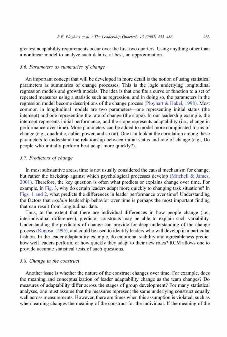
improve over time, but at different rates). Similarly, correlations based on the data in Fig.

2 would be low and, although indicative of between-person changes, they would again not

identify the nature of interindividual differences in the intraindividual adaptability that is

occurring. Alternatively, a method capable of analyzing intra- and interindividual differences

could be used to understand whether those individuals who show decreasing performance in

Fig. 2 are also those with lower agreeableness, for example. We shall see that the RCM

methodology is capable of analyzing such questions.


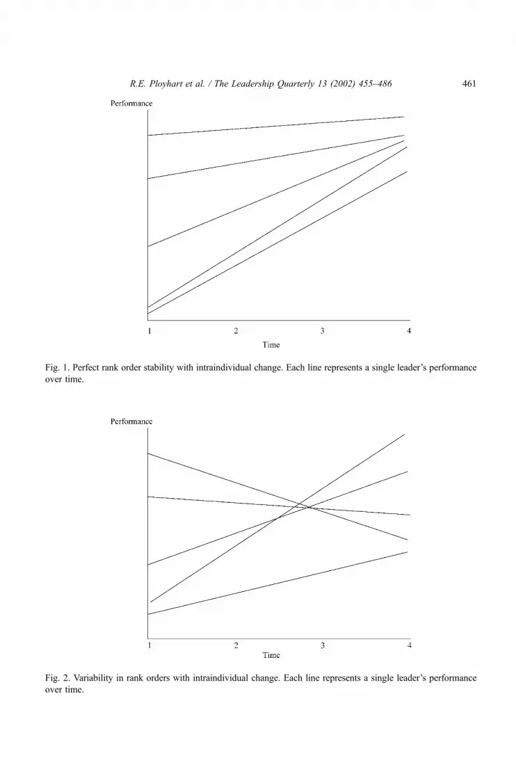
Fig. 1. Perfect rank order stability with intraindividual change. Each line represents a single leader’s performance

over time.

Fig. 2. Variability in rank orders with intraindividual change. Each line represents a single leader’s performance

over time.


3.5. Linear versus nonlinear change

Linear change occurs when a straight line, with either a positive or negative slope,

describes the function of change. Both Figs. 1 and 2 represent linear change. Nonlinear

change occurs when the change has at least one curve in the slope. For example, a learning

curve represents a nonlinear process. While most researchers will model a linear process

because it is relatively robust (Dawes, 1979; Dawes & Corrigan, 1974), many leadership

phenomena, such as development and adaptability, are likely to be nonlinear (e.g., Kozlowski

et al., 1996; Yukl, 2002). For example, in their meta-analytic review, Gerstner and Day (1997)

suggested it is unlikely that leader–member exchange relationships change in a linear

fashion. Rather, they suggest that change patterns will differ according the nature of the

dyadic relationship, or according to the perspective of the leader or member.

Such is the case in our leadership adaptability example. Fig. 3 shows the data for five

subjects over the four measurement periods. Nonlinear change is certainly present for

Subjects 1, 2, 3, and 5; for each of these subjects, a negatively accelerated or ‘‘learning

curve’’ type of change function seems to be present. In contrast, Subject 4 follows a linear

process. Such nonlinear data are consistent with the dynamic Kozlowski et al. (1996) theory

proposing that the leader’s behavior is contingent on changing task and team characteristics.

First, the groups and teams literature suggests that there is a discontinuous breaking point

between when the team forms and the team’s project deadline (Gersick, 1989).

Second, the Kozlowski et al. (1996) theory argues that teams go through four distinct

stages, and leader behavior must adapt to each stage. In such instances, leader behavior that

never changes would probably not be adaptive or successful. In Fig. 3, we see that the

Fig. 3. Sample data of five leader’s performance ratings assessed over four quarters.


greatest adaptability requirements occur over the first two quarters. Using anything other than

a nonlinear model to analyze such data is, at best, an approximation.

3.6. Parameters as summaries of change

An important concept that will be developed in more detail is the notion of using statistical

parameters as summaries of change processes. This is the logic underlying longitudinal

regression models and growth models. The idea is that one fits a curve or function to a set of

repeated measures using a statistic such as regression, and in doing so, the parameters in the

regression model become descriptions of the change process (Ployhart & Hakel, 1998). Most

common in longitudinal models are two parameters—one representing initial status (the

intercept) and one representing the rate of change (the slope). In our leadership example, the

intercept represents initial performance, and the slope represents adaptability (i.e., change in

performance over time). More parameters can be added to model more complicated forms of

change (e.g., quadratic, cubic, power, and so on). One can look at the correlation among these

parameters to understand the relationship between initial status and rate of change (e.g., Do

people who initially perform best adapt more quickly?).

3.7. Predictors of change

In most substantive areas, time is not usually considered the causal mechanism for change,

but rather the backdrop against which psychological processes develop (Mitchell & James,

2001). Therefore, the key question is often what predicts or explains change over time. For

example, in Fig. 3, why do certain leaders adapt more quickly to changing task situations? In

Figs. 1 and 2, what predicts the differences in leader performance over time? Understanding

the factors that explain leadership behavior over time is perhaps the most important finding

that can result from longitudinal data.

Thus, to the extent that there are individual differences in how people change (i.e.,

interindividual differences), predictor constructs may be able to explain such variability.

Understanding the predictors of change can provide for deep understanding of the change

process (Rogosa, 1995), and could be used to identify leaders who will develop in a particular

fashion. In the leader adaptability example, do emotional stability and agreeableness predict

how well leaders perform, or how quickly they adapt to their new roles? RCM allows one to

provide accurate statistical tests of such questions.

3.8. Change in the construct

Another issue is whether the nature of the construct changes over time. For example, does

the meaning and conceptualization of leader adaptability change as the team changes? Do

measures of adaptability differ across the stages of group development? For many statistical

analyses, one must assume that the measures represent the same underlying construct equally

well across measurements. However, there are times when this assumption is violated, such as

when learning changes the meaning of the construct for the individual. If the meaning of the


construct does change over time, the assessment of change becomes considerably more

complex and one cannot directly apply the methods described in this paper. Instead, LGM

would be the preferred approach.

In sum, these conceptual issues must be considered before conducting and analyzing a

longitudinal study. Section 4 now introduces the concept of longitudinal analysis using RCM.

4. Growth modeling and random effects regression

Previously, we discussed the difference between interindividual change and intraindividual

change. Here we build on these concepts and extend the study of intraindividual change into

what is known as growth curve modeling. A growth curve approach to analyzing longitudinal

data has become the dominant approach in many fields of psychology (e.g., developmental,

educational), biology, pharmacology, and agriculture. The study of growth curves was

originated independently by Rao (1958) and Tucker (1958), and has been popularized in

recent years by HLM (Bryk & Raudenbush, 1987) and LGM (McArdle & Epstein, 1987;

Meredith & Tisak, 1990).

The essence of a growth model is to observe each person’s repeated scores across time.

Thus, the focus is on within-person change over time (i.e., intraindividual change). If

everyone changes the same way, the average growth curve would adequately summarize

each person’s change. However, more often than not, there are sizeable individual differences

in how people change, such that some people increase over time while others decrease or stay

the same. Figs. 1 and 2 give examples of such processes. Further, people may not follow the

same growth trajectory; some may follow a linear path, while others may follow nonlinear

forms of growth or change, as is shown in Fig. 3.

A model of individual change (Rogosa, 1995) is required to address such questions,

requiring a correspondingly appropriate analytic strategy. Thus, full understanding of

individual change over time requires an examination of both interindividual differences

(i.e., between-person differences) and intraindividual change (i.e., within-person change). In

our leadership adaptability example, we are interested in both the type of performance

adaptability shown in the leader’s behavior over time (intraindividual change), and what

explains differences in leader adaptability (i.e., emotional stability and agreeableness).

The easiest way to understand growth modeling is through random effects regression,

which should be familiar to readers with a regression background. Let us first consider the

nature of the growth model, starting first with the familiar cross-sectional regression model.

The generic regression model takes the following form:

Yi ¼ b0 þ b1ðXiÞ þ ei ð1Þ

where i = 1,. . .,n subjects and Xi = trend over time.

This familiar model assumes that errors are independent and normally distributed, with a

mean of zero and a constant variance. In the usual cross-sectional analysis, the data are

structured such that each row represents a single subject’s scores. The top half of Table 1

shows the usual data layout in the context of our adaptability example (Fig. 3 shows these


numbers graphically). There is no way to analyze anything other than average change across

leaders in this data, as would be common practice in a repeated-measures ANOVA using

trend analysis methods. Thus, Eq. (1) summarizes only average (mean) change over time.

However, if we restructure these data so that we can regress the four repeated dependent

variables onto time for each subject, we would be able to analyze the data using a growth

model. In this manner, we can use the regression coefficients to summarize the nature of

change (adaptability) within and between individuals. Therefore, in growth models, the data

matrix is restructured such that each row represents a subject’s score at a particular time. A

sample data matrix for this structure is shown in the lower half of Table 1. Notice that there

are two differences from before: There are now as many rows as there are time periods for

each subject (i.e., Number of rows =Number of time periods�Number of subjects), and a

new variable ‘‘Time’’ has been added to the data.

Also of note is that the longitudinal dataset contains a within-person component

(performance) and a between-person component (emotional stability and agreeableness).

The data are now structured so that one can begin to analyze interindividual differences in

intraindividual performance, i.e., analyze a growth model. Substantively, one can now regress

leader performance ratings onto time to understand the nature of leader adaptability.

One can do this very simply with regression by regressing the vector of performance onto

time for each subject individually. Such a model would look like Eq. (1), with the addition of

subscripts for subjects and time:

Yti ¼ b0i þ b1iðXtiÞ þ eti ð2Þ

where i = 1,. . .,n subjects; Xti = coding of time; and t = 1,. . .,T time periods.

Notice that this model has an intercept and slope for each subject because we run the

regression analysis separately for each subject. Conceptually (and in matrix notation), the

regression analysis for the first subject would look like this:

Y ¼ X B þ E

80

107

116

122

2666666664

3777777775¼

1 0

1 1

1 2

1 3

2666666664

3777777775

b0

b1

24

35þ

e1

e2

e3

e4

2666666664

3777777775

In this representation, Y is a vector of repeated leader performance measures; X is a matrix

representing time via two vectors: The first column of ones is used to represent the intercept,

and the second column of zero to three represents the metric for time (0 = Time 1; 1 = Time 2;

2 = Time 3; 3 = Time 4). The B vector represents regression parameters that are referred to as


growth parameters because they summarize the nature of change. b0 is the intercept and

represents the point at which the regression line crosses the Y-axis. In our adaptability

example, the intercept represents the point at which Time = 0 and substantively refers to the

leader’s initial performance in the first stage of team development. More generally, the

intercept is referred to as ‘‘initial status’’, and it is for this reason that it is often convenient to

code the first time period as zero. However, if there was a compelling reason, one could

change the intercept to represent final performance if time was coded 3, 2, 1, 0. The b1regression parameter represents the slope or rate of change over time.

Table 1

Cross-sectional and longitudinal data

Cross-sectional dataseta

Subject Perf1 Perf2 Perf3 Perf4

Emotional

stability Agreeableness

1 80 107 116 122 4 6

2 63 100 110 117 6 7

3 74 89 95 100 9 3

4 81 85 87 90 2 4

5 68 76 80 83 3 2

Growth curve dataset

Between

Within Emotional

Subject Performance stability Agreeableness Time

1 80 4 6 0

1 107 4 6 1

1 116 4 6 2

1 122 4 6 3

2 63 6 7 0

2 100 6 7 1

2 110 6 7 2

2 117 6 7 3

3 74 9 3 0

3 89 9 3 1

3 95 9 3 2

3 100 9 3 3

4 81 2 4 0

4 85 2 4 1

4 87 2 4 2

4 90 2 4 3

5 68 3 2 0

5 76 3 2 1

5 80 3 2 2

5 83 3 2 3a Performance ranges from 0 to 200; emotional stability and agreeableness range from 1 to 10.


In our example, this would represent the rate of performance improvement the leader has

shown over time (i.e., how effectively the leader adapted to different responsibilities).

Because this can differ for each subject, slopes (rate of change) may differ in magnitude

and direction (i.e., positive or negative). Positive (negative) slopes represent leaders who

effectively (ineffectively) adapt; large (small) slopes represent leaders who adapt quickly

(slowly). Thus, by running separate regression equations for each subject, the simple

regression model can produce an intercept (initial status) and slope (rate of change or

adaptability) parameter for each subject. Finally, the E vector represents a vector of time- and

person-specific errors. As in all regression models, one can examine the errors to ensure that

time has been adequately conceptualized and that the regression model is appropriate.

If one were to run such an individual regression analysis, save the intercept and slope

parameters to a new file, and then take the mean and variance of each slope parameter, one

could estimate the average change across subjects (mean intercept and slope), and the amount

of interindividual differences between subjects in how they change (variance in intercept and

slope). That is, the mean of b0 and b1 would, respectively, estimate the average leader’s initial

status (initial performance) and rate of change (adaptability), and the variance in b0 and b1would, respectively, estimate how much leaders differed in their initial status and rate of

change (see Bliese & Ployhart, 2002). For example, if the slope shows considerable

variability and the intercept does not, it would suggest that most leaders perform the same

initially but differ in how quickly and how well they adapt to their new responsibilities.

It is important to recognize that the two regression (growth) parameters summarize the

nature of change for that specific person. In the analyses, each individual’s intercept and slope

are free to randomly vary. That is, the growth parameters are not constant across individuals

(as they would be in fixed regression) but instead represent growth curves from individuals

randomly drawn from a population. Each parameter, therefore, has a mean and variance.

Further, notice that the matrix representing time is the same for each person; only the growth

parameters differ across people. Thus, the growth parameters may be thought of as how much

a given subject follows a particular form of growth or change. In a later section, we discuss

how time may be structured to test specific hypotheses about the nature or type of change.

Although running separate regression equations for each individual is a powerful tool for

summarizing change, it is limited in that it cannot easily accommodate missing data,

heterogeneous data, and correlated errors—the very conditions likely to be found in

longitudinal research. It is also rather cumbersome to use when a study contains numerous

individuals. The RCM is capable of addressing these limitations.

5. The basic RCM in longitudinal research

A random effects regression model is the basis of a RCM. In fact, Eq. (2) equivalently

describes a simple RCM model that is analyzing change over time. As such, the classic

regression model is one subtype of RCM. Based on the random effect regression model,

RCM generalizes into a number of different models that allow one to analyze different forms

of intraindividual change (e.g., Bryk & Raudenbush, 1987, 1992; Goldstein, 1989; Hand &


Crowder, 1996). However, RCM further generalizes to include a second set of individual

difference measures and parameters that predict the intraindividual parameters. These

individual difference coefficients are fixed, between-person effects (e.g., using personality

to predict leadership adaptability). Thus, one first specifies the intraindividual model, and

then attempts to identify predictors of the change parameters.

One important difference in RCM is that it estimates both the regression parameters and

the variability among those parameters simultaneously. In some notation (particularly HLM),

this is done by estimating two models: a Level 1 model containing the growth parameters,

and a Level 2 model that allows individual differences (variance) around those parameters.

Level 1 : Yti ¼ b0i þ b1iðXtiÞ þ eti

Level 2 : b0i ¼ p00 þ r0i

b1i ¼ p10 þ r1i ð3Þ

where i = 1,. . .,n subjects; X = time; and t = 1,. . .,T time periods.

Rearranging the terms in the two-level RCM, as is common in some software packages

(e.g., SAS), would provide the following:

Yti ¼ ½p00 þ p10ðXtiÞ� þ ½r0i þ r1iðXtiÞ þ eti� ¼ ½fixed effects� þ ½random effects�:

What this RCM model says is that the intercept (b0i) is composed of both a fixed effect

(p00; average initial status for all individuals) and a random residual effect (r0i; individual

differences in initial status). Similarly, the slope (b1i) is composed of both a fixed effect (p10;

average rate of change for all individuals) and a random residual effect (r1i; individual

differences in rate of change). Thus, the RCM model allows for the testing of both

intraindividual change (the fixed effects) and interindividual differences in intraindividual

change (the random effects).

RCM most often uses restricted maximum likelihood (REML) estimation. REML is based

on maximum likelihood estimation; it is based on a theory of the properties of normal

distributions in large samples and simultaneously estimates multiple parameters using an

iterative procedure. REML allows RCMs to simultaneously estimate parameter estimates and

variances for within- and between-person parameters, and provides appropriate statistical

tests even under the conditions described below (Bryk & Raudenbush, 1987, 1992).

In the following sections, we discuss several issues that have made it difficult to adequately

test and understand change in the past, and show how RCM can address these limitations. To

facilitate our discussion of these topics, we continue our use of the leadership adaptability

example.


6. Parameterizing growth

When one fits a trend or curve to longitudinal data, one is said to be modeling the data (i.e.,

using a statistical model to summarize the nature of the change). If we want to understand how

individuals adapt to their new responsibilities as project team leaders, we need to statistically

model the data in accordance with the dynamic theory of leadership (Kozlowski et al., 1996).

In RCM, the parameters summarize the nature of this adaptability, and thus models that use

different parameters will summarize change differently. The choice of parameters is not

arbitrary, even though it is often treated as such in most of the published literature.

As we discussed earlier, there is a distinction between linear and nonlinear data, and there

is thus a distinction between linear and nonlinear models. Unfortunately, these distinctions are

often confused in the literature and in statistics books, but there is a precise distinction

between these models that reflects how they use their parameters. In a nonlinear model, the

parameters summarizing change are either in an exponent, or contain an exponent (Burchinal

& Appelbaum, 1991). A nonlinear model can precisely model a nonlinear process. In

contrast, the parameters in linear models do not contain an exponent, or are part of an

exponent. A linear model cannot describe a nonlinear process. However, a linear model can

approximate a nonlinear process by adding more parameters (e.g., quadratic, cubic, etc.).

Such models are called curvilinear: They are linear models that use multiple parameters to

approximate nonlinear change. However, only a nonlinear model can precisely model a

nonlinear process of change.

Let us start with the familiar curvilinear polynomial model. Following our leader

adaptability example (see Fig. 3), we expect that there is a strong form of nonlinear growth

that approximates a learning curve. Thus, we may model change as follows:

Yti ¼ b0i þ b1iðTimetiÞ þ b2iðTime2tiÞ þ eti ð4Þwhere i = 1,. . .,n subjects and t = 1,. . .,T time periods.

In Eq. (4), we have only squared the independent variable ‘‘Time’’ to accommodate the

nonlinear performance change shown in the figure. Substantively, b0 represents initial levels of

performance (i.e., performance at the first quarter), b1 represents the rate of linear change (i.e.,

the direction and magnitude of leader adaptability), and b2 represents an ‘‘acceleration’’

parameter. That is, b2 indicates, beyond a steady increasing or decreasing level of adaptation

(b1), if there are people who adapt extremely quickly (or slowly). The b2 parameter thus allows

for the curvature in the data shown by Subjects 1, 2, 3, and 5, who rapidly adapt and then begin

to approach a level of asymptote. The model for the first subject would look like this:

80

107

116

122

2666666664

3777777775¼

1 0 0

1 1 1

1 2 4

1 3 9

2666666664

3777777775

b0

b1

b2

266664

377775þ

e1

e2

e3

e4

2666666664

3777777775


One could continue to add growth parameters to approximate even more nonlinear forms

of growth by raising the ‘‘Time’’ matrix to a higher power (up to the cubic power in the

case of four time periods). Additionally, one could allow random variability in the growth

parameters (the bs) by adding a Level 2 model (i.e., b0i =p00 + r0i; b1i =p10 + r1i; b2i =

p20 + r2i). Again, because the independent variable is being raised to a higher power, it is

important to emphasize that this is a curvilinear model. While this curvilinear parameterization

is simple to use, the cost comes in terms of multicollinearity. Because the independent

variables are simply the same variables raised to a higher power, multicollinearity is high and it

becomes difficult to estimate and test the amount of variance attributable to a particular growth

parameter because the covariances among the independent variables are so high. That is, it

would be difficult to separate the variance in rate of change (slope) from the variance in

acceleration. Further, the RCM model will often not be able to provide a unique estimate for

each regression parameter under instances of extreme multicollinearity.

A solution to this problem comes from the use of orthogonal polynomials to model

change. Orthogonal polynomials are vectors of numbers that are uncorrelated to each other.

When used to model time, they decompose a trend or curve into different sources of unique

variance: linear variance, quadratic variance, cubic variance, and so on. Because of this

property, they are often the preferred approach to analyzing change (Burchinal & Appelbaum,

1991; Rovine & von Eye, 1991; Stoolmiller, 1995). All that differs in a orthogonal

polynomial model is the way time is structured. Using the example from the adaptability

data where we model a quadratic function:

80

107

116

122

2666666664

3777777775¼

1 �3 þ1

1 �1 �1

1 þ1 �1

1 þ3 þ1

2666666664

3777777775

b0

b1

b2

266664

377775þ

e1

e2

e3

e4

2666666664

3777777775

Notice that there is no longer a zero value for time, so the intercept will now represent the

time period midway between the second and third observations. That is, the intercept

parameter b0 will now represent leader performance halfway through the first year of the

project team. While this is somewhat of an inconvenience in interpreting the intercept

parameter, the benefit is that the correlation between the linear parameter and the quadratic

parameter is zero, and thus one can uniquely estimate and test the variance in each parameter.

Curvilinear models analyzed using orthogonal polynomials will almost always allow a unique

estimate for each parameter.

Polynomial models and orthogonal polynomial models are similar, but they are not the

same from a substantive perspective. Clearly, interpretation of the intercept will differ, as will

the precise meaning of the other growth parameters. The reason occurs solely due to the

different use of numbers to assign a metric to time. Also important to remember is that


polynomial and orthogonal polynomial models are both curvilinear; they are not nonlinear

models. At best, they can approximate and summarize a nonlinear growth function, but they

cannot precisely define it (e.g., Cudek, 1996). A nonlinear RCM model useful for analyzing

data, such as that shown in Fig. 3, may take the form of the following power curve (Eq. (5)):

Yti ¼ ðb0iÞðTimeb1iti Þ þ eti ð5Þ

where i = 1,. . .,n subjects and t = 1,. . .,T time periods.

Although only two growth parameters are analyzed (intercept and slope), the use of

exponents ensures that they can precisely define the nature of the nonlinear growth curve.

Notice that in this model, the intercept (b0) still refers to initial status, but the b1 parameter

now simultaneously represents the direction, magnitude, and acceleration of leader change

(adaptability). That is, the slope parameter can define the trends shown in Fig. 3 as a single

number representing adaptable performance. Further, both growth parameters may vary for

each person, as denoted by the subscript i.

Whether a set of repeated measures will be analyzed with linear, curvilinear, or nonlinear

models is less of a statistical question than a substantive one. In cognitive psychology, much

debate centers around the meaning of a particular parameter, and many different learning

functions have been fit to correctly model a learning (or forgetting) curve. In the cognitive

literature, the process is truly nonlinear and the interest is in modeling this process exactly. In

other areas of psychology, particularly those in the organizational sciences, the interest may

simply be on summarizing a process and, in such cases, a curvilinear model may be sufficient.

One might wonder why we do not use nonlinear models more frequently in the

organizational literature. There are several reasons. First, the linear model is a robust model,

and a linear trend will explain most of the variance in even a nonlinear process (Dawes,

1979). Second, few variables modeled in the social sciences have the reliability necessary to

identify a nonlinear process (it is probably for this reason that most nonlinear models are

confined to biopsychology and cognitive psychology, which study reaction times). Third, the

measures themselves may not be sensitive to change processes, and the use of new dynamic

measurement systems may be required (e.g., Vallacher, Nowak, Markus, & Strauss, 1998).

Fourth, a sufficient number of time periods must be measured for nonlinear functions to

appear. Fifth, nonlinear models are foreign to many researchers and are complex: Many

require starting values and specification of derivatives before the model can run. Finally, it is

difficult to determine the correct nonlinear function. That is, for each major family of curves

(e.g., power), there are actually a number of specific curves (e.g., power, modified power, root

fit power, etc.) to choose from. The family of curves is often very similar, yet differs in the

exact use of parameters—precisely what one uses to understand change.

This issue of RCM parameterization really boils down to whether there is a theoretical

reason to expect a particular curve or trend (‘‘confirmatory’’), or if they are to be estimated

from the data (‘‘exploratory’’) (Burchinal & Appelbaum, 1991; Nesselroade & Baltes, 1979).

For example, if past research strongly suggests that leader adaptability will follow a particular

nonlinear function, one is reasonably certain that the measures are highly reliable, and there

are a sufficient number of time points, then nonlinear RCMs should be used. Applications of


curvilinear models to such nonlinear questions may help describe the growth function, but

they will not help explain it. Unfortunately, there are few theories that are so precisely

specified in the organizational sciences that one can identify the correct type of nonlinear

model. Therefore, in practice, curvilinear RCMs are likely to be most commonly used, as

would be true in our leadership adaptability example.

Thus, it is important to recognize that using growth models to understand change is highly

dependent on the way the model is parameterized. There are a variety of ways to model

longitudinal data, and oftentimes these models can produce a close-to-equivalent fit, making

it hard to distinguish which is the most appropriate. The choice as to how to model the data is

best viewed as a balance of theoretical and statistical considerations.

6.1. Patterns in the error structure

Traditional regression assumes that the errors are uncorrelated, have a mean of zero, and a

constant variance. Longitudinal research almost guarantees that such assumptions will be

violated. For example, if leader adaptability occurs in response to project team characteristics

and task intensity, then the results of early leader behavior would influence later leader

behavior (Kozlowski et al., 1996). The substantive consequences of violating the error

assumptions can be serious, such as biased significance tests and incorrect estimates of model

fit. Fortunately, RCM models can accommodate such violations by relaxing requirements on

the error structure. In most research works, we pay little attention to the error terms, but in

longitudinal research, the error terms can become very informative because they help

diagnose different types of change processes.

Specifically, the RCM error structure may actually be represented as a matrix of error

variances and covariances. In our four-measurement adaptability example, the traditional

regression assumptions would look as follows:

E ¼

s2 0 0 0

0 s2 0 0

0 0 s2 0

0 0 0 s2

2666666664

3777777775

Notice that the errors are uncorrelated and have a constant variance, s2. Such a structure is

necessary for the significance tests in regression to be accurate. However, there are two major

violations to these assumptions that RCM is capable of addressing.

First, heterogeneity often occurs when the spread of scores at each measurement period

increases with time—creating a fan shape to the data. This happens, for example, when

differences between people become greater over time, as is shown in Fig. 3. As task and role

responsibilities become more demanding, leaders differ in how well they can adapt to such

demands. Alternatively, homogeneity over time can be common when people become more


similar over time (or due to attrition). The attraction–selection–attrition (ASA) model

(Schneider, 1987) would predict that units become more similar over time because those

with different personalities, values, and so on, leave the organization. Thus, if the leader

develops a particular degree of cohesion, those whose values do not fit with the team are more

likely to leave (Kozlowski et al., 1996).

Second, longitudinal research often results in nonindependence among observations. Such

nonindependence usually shows up in the form of correlated errors, such that errors at one

time period are related to another. The difficulty with correlated errors primarily affects

significance tests: Because errors are correlated, standard errors for parameter estimates tend

to be smaller than they should be, and thus, significance tests are inflated (i.e., increased Type

I error and thus more liberal significance tests).

Finally, heterogeneity and correlated errors may both be present. An example of such an

effect is shown below. Notice that the error variances on the diagonal are no longer the same,

and the covariances are also free to vary:

E ¼

s211 s12 s13 s14

s21 s222 s23 s24

s31 s32 s233 s34

s41 s42 s43 s244

2666666664

3777777775

There are a variety of different correlated error structures, including autoregressive,

toeplitz, and autoregressive with moving average models. DeShon, Ployhart, and Sacco

(1998) discuss many of these models in some detail. RCMs allow the researcher to identify

and test the appropriateness of these and many other error structures. It is worth emphasizing,

however, that nonindependence does not influence effect size estimation. Thus, as long as

there is a reasonable degree of nonindependence, the parameter estimates themselves are not

affected. And if one was only interested in effects sizes, the issue of nonindependence would

not matter. However, if significance tests are of interest, then one must correctly model the

error structure, and different error structures can change the significance values for

parameters. It is, therefore, critical to correctly model the error structure.

6.2. Missing data and attrition

The issue of missing data in longitudinal research is frequently encountered. In fact, many

applied researchers would consider subject attrition to be the major impediment to longit-

udinal research. Historically, attrition would often render the longitudinal study useless

because there would be so few participants at the final time period. Further, the consequence

of attrition may result in biased parameter estimates. For example, Sturman (2001) found that

parameter estimates of longitudinal performance trends may be biased if people leave the

organization in nonrandom ways.


However, in recent years, a variety of improvements have been made in estimation, and

most of the newer longitudinal methods (particularly RCM) can easily accommodate missing

data, at least as long as they are not too severe and occur in a somewhat random fashion. As

long as REML is the estimation method and the data are missing completely at random

(MCAR; e.g., when subjects miss some measures because of reasons unrelated to the variables

under the study), one may use RCM and be confident that the parameter estimates will be

accurate (Pinheiro & Bates, 2000). Even weaker forms of this assumption, such as when the

data are missing at random (MAR), will provide reasonably close parameter estimates (Little

& Schenker, 1995; Muthen, Kaplan, & Hollis, 1987; Pinheiro & Bates, 2000).

However, if the missing data are not random, such as when members leave teams they do

not fit with, or when poor performers do not complete questionnaires, then the missing data

are not random and can lead to biased parameter estimation. Sturman (2001) gives an

illustration of such concerns, and DeShon et al. (1998) discuss different issues with missing

data in longitudinal research and how to handle them. Fortunately, the programming of RCM

is not complicated by missing data: Simply run the model as usual, being careful to closely

examine the results for anything that looks unusual (e.g., negative variances).

6.3. Unequal spacing of measurements

RCM can accommodate designs where individuals are measured at different times. Such

designs may occur for theoretical (e.g., Ancona et al., 2001; Mitchell & James, 2001) or

practical reasons. As we discussed earlier, we may wish to assess leader behavior during each

stage of team formation specified in the Kozlowski et al. (1996) theory. However, teams are

not likely to go through each stage at the same time or remain in each stage for the same

duration. As long as we correctly code our measures to reflect these differences in time, the

RCM model can analyze these data without difficulty.

6.4. Assessments of model fit

One attractive feature of RCM is that one may obtain overall model fit statistics (e.g.,

Akaike’s Information Criterion, or AIC; log likelihood ratio tests), thereby allowing a series of

nested model comparisons. AIC is a fit index that rewards model fit and parsimony (Sakamoto,

Ishiguro, & Kitagawa, 1986), and smaller numbers indicate a better fit (zero is perfect). The

log likelihood ratio is a general method for comparing nested models fit by maximum

likelihood (Lehman, 1986). The difference between two models is summarized in terms of (a)

the change in the number of parameters, and (b) the change in the log likelihood ratio. With

these two parameters, one can conduct a log likelihood test of statistical significance because

the � 2 log likelihood ratio closely approximates a Chi-square distribution.

For example, one could first test differences between models with a random intercept and

slope, a fixed slope (meaning all people show identical forms of adaptability or performance

change), and a fixed intercept and slope. Further, one may propose different error structures

and see the corresponding differences and reductions in AIC and the log likelihood ratios.

The error structure that provides the smallest values would provide the best representation of


the data. RCM can also provide significance tests for individual parameters, such as the

growth parameters.3

6.5. Predicting change

So far, we have focused our discussion on modeling and summarizing the change process

through the use of growth parameters. While informative, the real understanding obtained in

longitudinal designs comes from identifying predictors of the change process, i.e., why do

people change in different ways? Why do some people adapt more quickly to their leadership

roles than others? This is easily accomplished in RCM. We have already described the RCM

model for estimating intraindividual change; recall the Level 1 model from Eq. (3):

Yti ¼ b0i þ b1iðXtiÞ þ eti:

Remember that the b0 and b1 parameters summarize growth for a given person; in the Level

2 model, the mean of these parameters represents average growth, and the variance in these

parameters represents variability in growth. In our leadership example, the intercept refers to

performance in the first quarter of the team’s existence, while the slope represents the amount

and direction of change (adaptability) shown by the leader. Because the growth parameters

summarize the nature of change, they may be used as the dependent variables to be predicted

by individual difference measures. Therefore, if we expect that emotional stability and

agreeableness explain individual differences in leader change (adaptability), and we think that

leadership change (adaptability) has both a linear and a curvilinear growth function (see Fig.

3), we can test this question as follows (Eq. (6)):

Level 1 model : Yti ¼ b0i þ b1iðTimetiÞ þ b2iðTime2tiÞ þ eti

Level 2 model : b0i ¼ p00 þ p01ðEmotional StabilityiÞ þ p02ðAgreeablenessiÞ þ r0i

b1i ¼ p10 þ p11ðEmotional StabilityiÞ þ p12ðAgreeablenessiÞ þ r1i

b2i ¼ p20 þ p21ðEmotional StabilityiÞ þ p22ðAgreeablenessiÞ þ r2i:

ð6Þ

Because there are three growth parameters required to model leader adaptability, there are

three corresponding Level 2 model equations required to predict this change. Thus, the Level

3 It is important to note that when using REML estimation to compare fit across different random effects

models, the fixed effects must remain the same. That is, the REML-based estimators of model fit can only inform

questions about the random effects portion of the model. If one wants to compare the fixed effects, maximum

likelihood estimation must be used. A comprehensive discussion of this issue is found in Diggle, Liang, and Zeger

(1994), Longford (1993), Pinheiro and Bates (2000) (see Bliese & Ployhart, 2002 for a less technical description

with growth models).


1 model designates the form of intraindividual differences in change (adaptability), and the

Level 2 model designates the forms of interindividual differences in change.

Let us interpret these growth parameters in more substantive terms. The growth parameter

b0 represents initial leader performance, and the equation ‘‘p00 +p01(Emotional Stabilityi) +

p02(Agreeablenessi)’’ examines the extent to which emotional stability and agreeableness

explain individual differences in initial performance. The growth parameters b1 and b2,

respectively, represent the rate and acceleration in performance change (adaptability), and

their corresponding Level 2 equations examine the extent to which emotional stability and

agreeableness explain individual differences in rate and acceleration. Thus, we can predict

how much variance in adaptability may be attributable to individual differences in person-

ality. Answering these questions brings out the full power of the RCM and longitudinal

research.

7. An application of RCM to leadership research

Bliese and Ployhart (2002) have proposed a sequence of steps to be conducted when

using RCM to analyze growth data. Briefly, they have delineated a procedure for analyzing

RCM growth data, the correct significance tests to be used at each stage in the procedure,

and how to interpret each of the parameter estimates. Further, they have provided many

examples using the free statistical software, R. In this section, we follow the steps

suggested by Bliese and Ployhart to analyze the leadership adaptability data collected over

the first year of the project team’s life. However, we use the SAS software Proc Mixed

procedure (see Littell, Milliken, Stroup, & Wolfinger, 1996), thereby demonstrating the

simplicity of another common RCM software application capable of analyzing longitudinal

growth data.

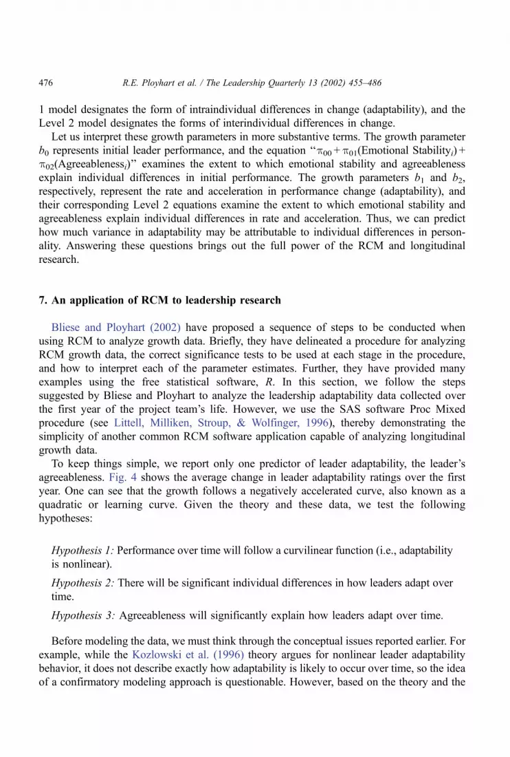
To keep things simple, we report only one predictor of leader adaptability, the leader’s

agreeableness. Fig. 4 shows the average change in leader adaptability ratings over the first

year. One can see that the growth follows a negatively accelerated curve, also known as a

quadratic or learning curve. Given the theory and these data, we test the following

hypotheses:

Hypothesis 1: Performance over time will follow a curvilinear function (i.e., adaptability

is nonlinear).

Hypothesis 2: There will be significant individual differences in how leaders adapt over

time.

Hypothesis 3: Agreeableness will significantly explain how leaders adapt over time.

Before modeling the data, we must think through the conceptual issues reported earlier. For

example, while the Kozlowski et al. (1996) theory argues for nonlinear leader adaptability

behavior, it does not describe exactly how adaptability is likely to occur over time, so the idea

of a confirmatory modeling approach is questionable. However, based on the theory and the


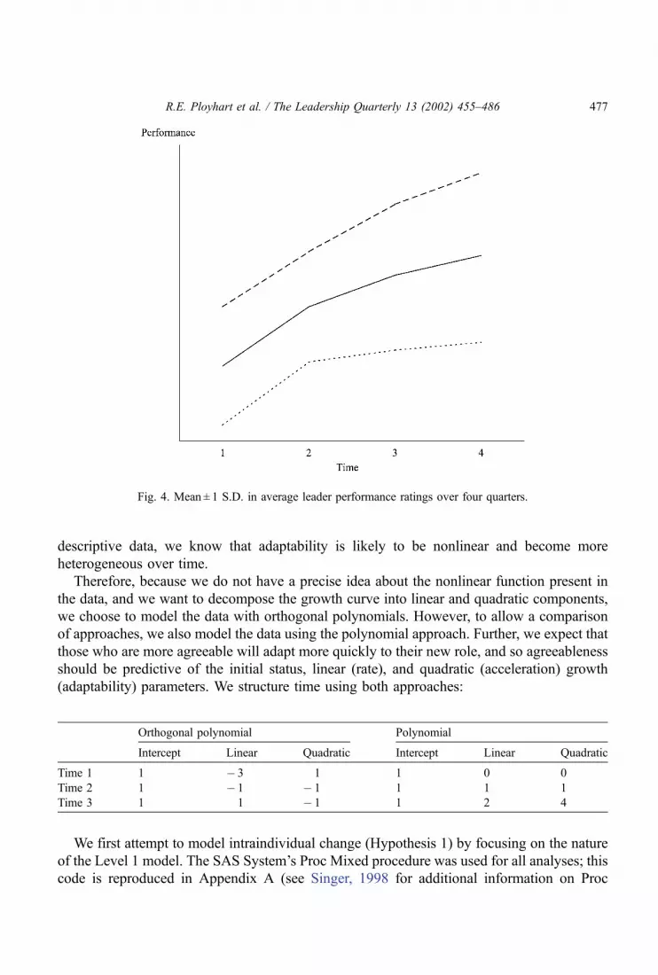
descriptive data, we know that adaptability is likely to be nonlinear and become more

heterogeneous over time.

Therefore, because we do not have a precise idea about the nonlinear function present in

the data, and we want to decompose the growth curve into linear and quadratic components,

we choose to model the data with orthogonal polynomials. However, to allow a comparison

of approaches, we also model the data using the polynomial approach. Further, we expect that

those who are more agreeable will adapt more quickly to their new role, and so agreeableness

should be predictive of the initial status, linear (rate), and quadratic (acceleration) growth

(adaptability) parameters. We structure time using both approaches:

We first attempt to model intraindividual change (Hypothesis 1) by focusing on the nature

of the Level 1 model. The SAS System’s Proc Mixed procedure was used for all analyses; this

code is reproduced in Appendix A (see Singer, 1998 for additional information on Proc

Fig. 4. Mean ± 1 S.D. in average leader performance ratings over four quarters.

Orthogonal polynomial Polynomial

Intercept Linear Quadratic Intercept Linear Quadratic

Time 1 1 � 3 1 1 0 0

Time 2 1 � 1 � 1 1 1 1

Time 3 1 1 � 1 1 2 4


Mixed and interpreting the output). Specifically, we first test a model with only a linear

growth parameter (b1), and then add a quadratic growth parameter (b2). We test the addition

of these parameters sequentially, and find that the significance values for both parameters is

less than P< .05. Therefore, we conclude that the following quadratic model best approx-

imates the data:

Change in Performance ¼ 95:22þ 4:50ðLinearÞ � 2:45ðQuadraticÞ: ð7Þ

Because we are using orthogonal polynomials, the zero point for time is halfway through

the first year. Substantively, we interpret these growth parameters such that the midyear

average performance score is 95.22. Leaders adapt moderately well to their new roles over

time, as the average performance increase corresponds to 4.50 points per quarter. However,

some participants adapt rapidly early in the process and then start to ‘‘taper off’’ over time;

the negative quadratic term reflects how much this linear trend begins to level off. The

polynomial approach reaches a similar conclusion, finding that a quadratic trend is present in

the data:

Change in Performance ¼ 79:27þ 16:35ðTimeÞ � 2:46ðTime2Þ: ð8Þ

Notice that the estimates of the growth parameters differ between Eqs. (7) and (8); the

difference only reflects the coding of time. Because Eq. (8) codes the first quarter as zero, the

intercept in this model represents initial performance scores in the first quarter and is,

therefore, lower than that presented in Eq. (7) (which is performance at midyear). In Eq. (8),

we find an average increase in performance of 16.35 points, higher than that in Eq. (7)

because it starts with the first time period and, hence, is more affected by the large

improvement from Time 1 to Time 2. The quadratic parameter is nearly identical in both

models, indicating the same degree of acceleration in adaptability. Because Time 1 = 0 in the

polynomial model, we can examine the correlation between initial performance and

adaptability over time. Interestingly, the correlation between the intercept and the linear

parameter is � .55, while the correlation between initial status and acceleration is .44. It

would appear that those who initially demonstrate higher performance when the project team

is formed will be the same leaders who quickly adapt to their new roles and responsibilities.

Leaders who initially perform poorly in their role will not be able to catch those who perform

better. It would, therefore, be desirable to be able to predict or identify leaders who will

initially perform better.

While Eqs. (7) and (8) differ in terms of their specific parameter estimates, they will

produce identical predicted average performance equations that reflect Fig. 4. The difference

in estimates comes only from the way in which time is structured (i.e., orthogonal polynomial

versus polynomial), and in how the growth parameters are interpreted (e.g., midyear, first

quarter). Thus, the form of intraindividual adaptability follows a quadratic, negatively

accelerated curve, supporting Hypothesis 1. Most of the adaptation occurs in the first two

quarters on the job.


The next step in the model fitting sequence is to examine the extent to which there is

variance in the growth parameters, or interindividual differences in adaptability (Hypothesis

2). Following Bliese and Ployhart (2002), we proceed one growth parameter at a time and

allow variance in the growth parameter. That is, we start by testing whether there is

significant variance in the intercept (b0), followed by significant variance in the slope (b1),

and finally significant variance in acceleration (b2). In each new model, we compare

differences in AIC values (smaller values indicate better fit) and compute likelihood ratio

tests.

In contrast to previous recommendations (e.g., Bryk & Raudenbush, 1992), we do not

interpret the significance tests of the particular variance estimates because recent research

suggests that these estimates are very inaccurate (see Bliese & Ployhart, 2002). Rather, we

compare differences in AIC and likelihood ratio tests (however, see footnote 3). These

analyses suggest that there is explainable variability only in the intercept and slope

parameters, in both the orthogonal polynomial (sb02 = 146.97; sb1

2 = 7.65) and polynomial

(sb02 = 81.98; sb1

2 = 23.25) approaches. There was no meaningful variance in the quadratic

parameter, indicating that leaders tended to show the same degree of acceleration in

adaptability. Substantively, these findings suggest that leaders differ in terms of their initial

levels of adaptability and the rate by which they become more adaptable. Such findings

generally support Hypothesis 2 and the propositions in the Kozlowski et al. (1996) theory

regarding the dynamic nature of leadership.

The final step in assessing the intraindividual growth model is to examine the nature of the

error structure. So far, we have proceeded by using an uncorrelated error structure with

constant error variances. We suspect that the heterogeneity of adaptability scores increases

over time (see Fig. 4), and that the errors are likely to be correlated. If severe enough, this

heterogeneity and correlation among the errors could influence our significance tests. Thus,

we examine three additional error structures (others are possible; we offer these for illustrative

purposes)—an autoregressive structure [AR(1)] that requires constant error variances but

allows errors to correlate (note that a single parameter estimates the pattern of correlations

among the errors, which decline exponentially across time); an error structure with

uncorrelated but heterogeneous errors [UN(1)]; and an autoregressive structure with hetero-

geneous errors (ARH).

We run all three models and again compare differences in AIC values (smaller values are

better) and likelihood ratio tests (which can be tested via the change in likelihoods). As seen

below, the autoregressive with heterogeneous error structure provides the best fit to the data

(we do not report the polynomial results because they are nearly the same):

Error parameters AIC � 2 Log likelihood ratio

Baseline 1 3387.8 3381.8

AR(1) 2 3387.8 3379.8

UN(1) 4 3388.4 3376.4

ARH 5 3380.8 3368.8


Thus, the nature of intraindividual change in performance follows a negatively accelerated

‘‘learning curve.’’ Leaders adapt the most during the first half year on the job, and there are

individual differences in their initial levels of adaptability and how quickly they adapt.

Now that we know the basic structure of adaptability, the next step involves building the

Level 2 model and examining predictors of adaptable performance. Substantively, we are

asking why there are individual differences in initial status and rate of adaptability

(Hypothesis 3). Here we focus only on predicting the intercept (b0) and slope (b1) parameters

because the previous analyses found no individual differences in the acceleration (b2)

parameter. The overall RCM model with orthogonal polynomials is shown below (the

polynomial model is the same by replacing Linear and Quadratic variables with Time and

Time2) (Eq. (9)):

Level 1 model : Change in Performance ¼ b0i þ b1iðLinearÞ þ b2iðQuadraticÞ

Level 2 model : b0i ¼ p00 þ p01ðAgreeablenessiÞ þ r0i

b1i ¼ p10 þ p11ðAgreeablenessiÞ þ r1i: ð9Þ

When we run this model using orthogonal polynomials, we find that agreeableness

significantly predicts initial status (effect size = 8.66, P< .05) and the rate of adaptability

(effect size = 2.08, P< .05). This suggests that those who are more agreeable are more likely

to be adaptive midyear and increase their adaptivity over the year. However, when using

polynomials, we find that agreeableness only significantly predicts the rate of adaptability

(effect size = 4.37, P < .05). In this model, those who are more agreeable are likely to be more

adaptive.

The reason for the difference between the two models again comes from the coding of

time; because the polynomial model codes time such that the intercept represents the first

quarter, there is no relationship to agreeableness. Apparently, agreeableness only relates to

adaptability sometime after the first quarter. This highlights an important point that is

neglected in nearly all of the growth modeling literature—that the choice of parameterizing

growth is not arbitrary and must be carefully considered. Here, we would conclude that

agreeableness contributes to adaptability, but not to initial levels of performance. These

results provide partial support for Hypothesis 3.

8. Conclusions

Many questions in leadership research fundamentally reduce to questions of understanding

the nature, determinants, and consequences of leader behavior over time. However, much past

research has not made such longitudinal questions an explicit focus of the design or analysis,

and more longitudinal studies are needed to better understand leadership processes that unfold

overtime (Bauer & Green, 1996; Gerstner & Day, 1997; Yukl, 2002). We have attempted to


provide a relatively nontechnical demonstration of how RCM can be used to study leadership

processes over time.

We hope that such a tutorial will show that questions of change can be more informative if

studied with methods that explicitly analyze change, in particular analyzing predictors of

change using growth models in a RCM framework. The methods described in this paper are

based on regression and are likely to be familiar to most applied researchers. Those who

would like more detailed technical information on RCM are referred to many sources (e.g.,

Bliese, 2002; Bliese & Ployhart, 2002; Bryk & Raudenbush, 1987, 1992; Goldstein, 1989;

Hand & Crowder, 1996).

While the purpose of this article has been on RCM, it is important to recognize that other

methods can analyze longitudinal data and have certain strengths and weaknesses relative to

RCM. Of these approaches, the most similar is LGM. LGM is an extremely flexible and

powerful technique for the study of change, and we encourage readers to examine the several

excellent introductions into LGM (e.g., Chan, 1998; Duncan, Duncan, Strycker, Li, & Alpert,

1999; Willett & Sayer, 1994).

We would like to conclude by reiterating a few critical issues with RCM. First, we have

emphasized repeatedly how the choice of parameterizing the growth curves is not arbitrary, as

this choice may very well affect the significance tests and substantive interpretations. In this

paper, we have only raised the issue to increase awareness, but have not solved it. Other than

relying on strong theory whenever possible, the only empirical insight into the problem is to

examine the fit of the model to the data. The problem occurs when equivalent empirical fit is

observed for different kinds of models. Thus, our cautious recommendation is to analyze

longitudinal data using a variety of theoretically defensible parameterizations, including both

orthogonal polynomials and polynomials, and nonlinear models, whenever reasonable. If the

substantive results are consistent across models, one may present the results that are the most

parsimonious, allow the clearest interpretation, and most directly test the underlying theory.

Alternatively, if the empirical results between models diverge for reasons due to the

parameterization of time, one should probably report these discrepant results, and then argue

for adopting the model that best represents the underlying theory and purpose for the study

(this may or may not be the most supported model). In our previous example on adaptability,

if one was interested in adaptability at the first quarter, the polynomial approach should be

reported. Readers may go to several excellent sources describing theoretical issues relating to

the parameterization of time (e.g., George & Jones, 2000; Mitchell & James, 2001; see

Goodman et al., 2001).

Second, and relatedly, the choice of parameterizing the growth curves fundamentally

impacts the nature of the predictors of change. As we saw in the adaptability example,

changing the nature of the growth model can impact the significance of the interindividual

difference predictors. Indeed, one might rightfully argue that a nonlinear model would have

been the appropriate model for analyzing the adaptability data. To the extent that the growth

model is misspecified, the interindividual difference predictors are not linked to the variables

of interest. That is, the growth model dictates the nature of the dependent variables, so

changing the parameterization of growth may dramatically change the nature of the

dependent variable and thus relations to predictors of change.


This is not an issue to be taken lightly. Therefore, we strongly urge researchers to consider

the theoretical and empirical adequacy of their growth model before trying to identify

predictors of change. When appropriate, nonlinear RCMs should be modeled (most software

packages can readily handle nonlinear models as well as categorical dependent variables).

Further, researchers should identify the assumptions underlying a particular model (note that

other models may produce different results), and possibly acknowledge that modeling a

nonlinear process with a curvilinear model may only be approximating the question of

interest.

Third, when interpreting the results of growth models, it is important to recognize that the

model can only be used to describe growth given the time period of study. For example, if

we modeled the adaptability data over 5 years instead of 1 year, a different pattern of

change may occur. Further, the relationships between the interindividual differences

predictors and the growth parameters could change. Thus, researchers should be careful

when interpreting their models such that their conclusions remain within the time periods

under investigation.

Finally, we have not discussed the issues of statistical power in RCM growth models. The

reasons are because such information has only recently become available for RCMs, and

because there are many issues to consider when calculating power (e.g., number of repeated

observations, spacing of observations, sample size, effect size, function of change, etc.). We

refer readers to Muthen and Curran (1997) and Raudenbush and Liu (2001) for more detailed

information on power and growth models.

In conclusion, we hope that future researchers who desire to study leadership longitudin-

ally will adopt methods capable of answering such questions. RCM offers one such useful

approach, and its use is likely to result in a greater understanding of the nature and

consequences of leadership in organizations.

Acknowledgments

We thank Paul Hanges for his many helpful comments on previous drafts of this paper, and

two anonymous reviewers for their suggestions. Their input greatly improved the quality of

this manuscript.

Appendix A. SAS Proc Mixed code for analyzing longitudinal data

Words in capitals are SAS commands and options, words in small letters are variables.

A.1. Level 1 model to test form of growth

PROC MIXED NOCLPRINT UPDATE COVTEST; CLASS id time; MODEL adapt=

linear quad/SOLUTION DDFM=BW HTYPE= 1 CORRB; RUN;


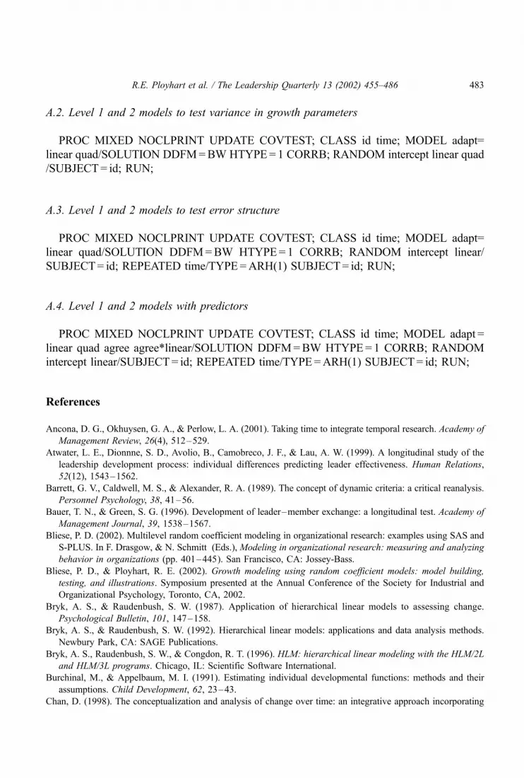
A.2. Level 1 and 2 models to test variance in growth parameters


linear quad/SOLUTION DDFM=BW HTYPE= 1 CORRB; RANDOM intercept linear quad

/SUBJECT= id; RUN;

A.3. Level 1 and 2 models to test error structure


linear quad/SOLUTION DDFM=BW HTYPE= 1 CORRB; RANDOM intercept linear/

SUBJECT= id; REPEATED time/TYPE=ARH(1) SUBJECT= id; RUN;

A.4. Level 1 and 2 models with predictors

PROC MIXED NOCLPRINT UPDATE COVTEST; CLASS id time; MODEL adapt =

linear quad agree agree*linear/SOLUTION DDFM=BW HTYPE= 1 CORRB; RANDOM

intercept linear/SUBJECT= id; REPEATED time/TYPE=ARH(1) SUBJECT= id; RUN;

References

Ancona, D. G., Okhuysen, G. A., & Perlow, L. A. (2001). Taking time to integrate temporal research. Academy of

Management Review, 26(4), 512–529.

Atwater, L. E., Dionnne, S. D., Avolio, B., Camobreco, J. F., & Lau, A. W. (1999). A longitudinal study of the

leadership development process: individual differences predicting leader effectiveness. Human Relations,

52(12), 1543–1562.

Barrett, G. V., Caldwell, M. S., & Alexander, R. A. (1989). The concept of dynamic criteria: a critical reanalysis.

Personnel Psychology, 38, 41–56.

Bauer, T. N., & Green, S. G. (1996). Development of leader–member exchange: a longitudinal test. Academy of

Management Journal, 39, 1538–1567.

Bliese, P. D. (2002). Multilevel random coefficient modeling in organizational research: examples using SAS and

S-PLUS. In F. Drasgow, & N. Schmitt (Eds.), Modeling in organizational research: measuring and analyzing

behavior in organizations (pp. 401–445). San Francisco, CA: Jossey-Bass.

Bliese, P. D., & Ployhart, R. E. (2002). Growth modeling using random coefficient models: model building,

testing, and illustrations. Symposium presented at the Annual Conference of the Society for Industrial and

Organizational Psychology, Toronto, CA, 2002.

Bryk, A. S., & Raudenbush, S. W. (1987). Application of hierarchical linear models to assessing change.

Psychological Bulletin, 101, 147–158.

Bryk, A. S., & Raudenbush, S. W. (1992). Hierarchical linear models: applications and data analysis methods.

Newbury Park, CA: SAGE Publications.

Bryk, A. S., Raudenbush, S. W., & Congdon, R. T. (1996). HLM: hierarchical linear modeling with the HLM/2L

and HLM/3L programs. Chicago, IL: Scientific Software International.

Burchinal, M., & Appelbaum, M. I. (1991). Estimating individual developmental functions: methods and their

assumptions. Child Development, 62, 23–43.

Chan, D. (1998). The conceptualization and analysis of change over time: an integrative approach incorporating


longitudinal means and covariance structures analysis (LMACS) and multiple indicator latent growth modeling

(MLGM). Organizational Research Methods, 1, 421–483.

Chan, D. (2002). Latent growth modeling. In F. Drasgow, & N. Schmitt (Eds.), Modeling in organizational

research: measuring and analyzing behavior in organizations(pp. 302–349). San Francisco, CA: Jossey-Bass.

Collins, L. M. (1991). Measurement in longitudinal research. In L. M. Collins, & J. L. Horn (Eds.), Best methods

for the analysis of change: recent advances, unanswered questions, future directions (pp. 137–148).

Washington, DC: American Psychological Association.

Cudek, R. (1996). Mixed-effects models in the study of individual differences with repeated measures data.

Multivariate Behavioral Research, 31, 371–403.

Dawes, R. M. (1979). The robust beauty of improper linear models in decision making. American Psychologist,

34, 571–582.

Dawes, R. M., & Corrigan, B. (1974). Linear models in decision making. Psychological Bulletin, 81, 95–106.

Day, D. V., & Lord, R. G. (1988). Executive leadership and organizational performance: suggestions for a new

theory and methodology. Journal of Management, 14, 453–464.

DeShon, R. P., Ployhart, R. E., & Sacco, J. M. (1998). The estimation of reliability in longitudinal models.

International Journal of Behavior and Development, 22, 493–515.

Diggle, P. J., Liang, K. Y., & Zeger, S. L. (1994). Analysis of longitudinal data. Oxford, England: Oxford

University Press.

Duchon, D., Green, S. G., & Taber, T. D. (1986). Vertical dyad linkage: a longitudinal assessment of antecedents,

measures, and consequences. Journal of Applied Psychology, 71(1), 56–60.

Duncan, T. E., Duncan, S. C., Strycker, L. A., Li, F., & Alpert, A. (1999). An introduction to latent variable

growth curve modeling. Mahwah, NJ: Lawrence Erlbaum Associates.

Fulmer, R. M., & Vicere, A. (1996). Strategic leadership development: crafting competitiveness. Oxford: Cap-

stone.

George, J. M., & Jones, G. R. (2000). The role of time in theory and theory building. Journal of Management, 26,

657–684.

Gersick, C. J. (1989). Marking time: predictable transitions in task groups. Academy of Management Journal, 32,

274–309.

Gerstner, C. R., & Day, D. V. (1997). Meta-analytic review of leader–member exchange theory: correlates and

construct issues. Journal of Applied Psychology, 82(6), 827–844.

Goldstein, H. (1989). Models for multilevel response variables with an application to growth curves. In R. D.

Bock (Ed.), Multilevel analysis of educational data (pp. 107–125). New York: Academic Press.

Goodman, P. S., Lawrence, B. S., Ancona, D. G., & Tushman, M. L. (2001). Introduction: special topic forum on

time and organizational research. Academy of Management Review, 26(4), 507–511.

Hand, D., & Crowder, M. (1996). Practical longitudinal data analysis. London: Chapman & Hall.

Hofmann, D. A. (1997). An overview of the logic and rationale of hierarchical linear models. Journal of Manage-

ment, 23, 723–744.

Hofmann, D. A., Griffin, M. A., & Gavin, M. B. (2000). The application of hierarchical linear modeling to

organizational research. In K. J. Klein, & S. W. J. Kozlowski (Eds.), Multilevel theory, research, and methods

in organizations: foundations, extensions, and new directions (pp. 467–511). San Francisco, CA: Jossey-Bass.

Hofmann, D. A., Jacobs, R., & Baratta, J. E. (1993). Dynamic criteria and the measurement of change. Journal of

Applied Psychology, 78, 194–204.

Hogan, R., Curphy, G. J., & Hogan, J. (1994). What we know about leadership effectiveness and personality.

American Psychologist, 49, 493–504.

Kozlowski, S. W. J., Gully, S. M., McHugh, P. P., Salas, E., & Cannon-Bowers, J. A. (1996). A dynamic theory of

leadership and team effectiveness: developmental and task contingent leader roles. Research in Personnel and

Human Resource Management, 14, 253–305.

Kozlowski, S. W. J., Gully, S. M., Nason, E. R., & Smith, E. M. (1999). Developing adaptive teams: a theory of

compilation and performance across levels and time. In D. R. Ilgen , & E. D. Pulakos (Eds.), The changing

nature of performance (pp. 240–292). San Francisco, CA: Jossey-Bass.


Lehmann, E. L. (1986). Testing statistical hypotheses. New York: Wiley.

Liden, R. C., Wayne, S. J., & Stilwell, D. (1993). A longitudinal study on the early development of leader–

member exchanges. Journal of Applied Psychology, 78(4), 662–674.

Littell, R. C., Milliken, G. A., Stroup, W. W., & Wolfinger, R. D. (1996). SAS system for mixed models. Cary, NC:

SAS Institute.

Little, R. J. A., & Schlenker, N. (1995). Missing data. In G. Arminger, C. C. Clogg, & M. E. Sobel (Eds.),

Handbook of statistical modeling for the social and behavioral sciences (pp. 39–75). New York: Plenum.

Longford, N. T. (1993). Random coefficient modeling. New York: Oxford University Press.

Marshall-Mies, J. C., Fleishman, E. A., Martin, J. A., Zaccaro, S. J., Baughman, W. A., & McGee, M. L. (2000).

Development and evaluation of cognitive and metacognitive measures for predicting leadership potential.

Leadership Quarterly, 11, 135–153.

McArdle, J. J., & Epstein, D. (1987). Latent growth curves within developmental structural equation models.

Child Development, 58, 110–133.

Meredith, W., & Tisak, J. (1990). Latent curve analysis. Psychometrika, 55, 107–122.

Mitchell, T. R., & James, L. R. (2001). Building better theory: time and the specification of when things happen.

Academy of Management Review, 26, 530–547.

Muthen, B. O., & Curran, P. J. (1997). General longitudinal modeling of individual differences in exper-

imental designs: a latent variable framework for analysis and power estimation. Psychological Methods,

2, 371–402.

Muthen, B. O., Kaplan, D., & Hollis, M. (1987). On structural equation modeling with data that are not missing

completely at random. Psychometrika, 52, 431–462.

Nesselroade, J. R., & Baltes, P. B. (1979). Longitudinal research in the study of behavior and development. New

York: Academic Press.

Pinheiro, J. C., & Bates, D. M. (2000). Mixed-effects models in S and S-PLUS. New York: Springer-Verlag.

Ployhart, R. E., & Hakel, M. D. (1998). The substantive nature of performance variability: predicting interindi-

vidual differences in intraindividual performance. Personnel Psychology, 51, 859–901.

Porter, L. W., & Bigley, G. A. (2001). Motivation and transformational leadership: some organizational context

issues. In M. Erez, & U. Kleinbeck (Eds.), Work motivation in the context of a globalizing economy (pp. 279–

291). Mahwah, NJ: Lawrence Erlbaum Associates.

Rao, C. R. (1958). Some statistical methods for comparison of growth curves. Biometrics, 14, 1–17.

Raudenbush, S. W., & Liu, X. F. (2001). Effects of study duration frequency of observations and sample size on

power in studies of group differences in polynomial change. Psychological Methods, 6, 387–401.

Rogosa, D. R. (1980). A critique of cross-lagged correlations. Psychological Bulletin, 88, 245–258.

Rogosa, D. R. (1988). Myths about longitudinal research. In K. W. Schaie, R. T. Campbell, W. Meredith, & S. C.

Rawlings (Eds.), Methodological issues in aging research (pp. 171–209). New York: Springer.

Rogosa, D. R. (1995). Myths and methods: ‘‘myths about longitudinal research’’ plus supplemental questions. In

J. M. Gottman (Ed.), The analysis of change (pp. 3–66). Mahwah, NJ: Lawrence Erlbaum Associates.

Rogosa, D. R., & Willett, J. B. (1985). Understanding correlates of change by modeling individual differences in

growth. Psychometrika, 50, 203–208.

Rovine, M. J., & von Eye, A. (1991). Applied computational statistics in longitudinal research. Cambridge, MA:

Academic Press.

Sakamoto, Y., Ishiguro, M., & Kitagawa, G. (1986). Akaike information criterion statistics. Dordrecht, Holland:

Reidel.

Schneider, B. (1987). The people make the place. Personnel Psychology, 40, 437–453.

Singer, J. D. (1998). Using SAS Proc mixed to fit multilevel models, hierarchical models, and individual growth

models. Journal of Educational and Behavioral Statistics, 24, 323–355.

Stoolmiller, M. (1995). Using latent growth curve models to study developmental processes. In J. M. Gottman

(Ed.), The analysis of change (pp. 103–138). Mahwah, NJ: Lawrence Erlbaum Associates.

Sturman, M. C. (2001). The implications of linking the dynamic performance and turnover literatures. Journal of

Applied Psychology, 86, 684–696.


Tucker, L. R. (1958). Determination of parameters of a functional relation by factor analysis. Psychometrika, 23,

19–23.

Vallacher, R. R., Nowak, A., Markus, J., & Strauss, J. (1998). Dynamics in the coordination of mind and action.

In M. Kofta , G. Weary (Eds.), Personal control in action: cognitive and motivational mechanisms (pp. 27–

59). New York: Plenum.

Wakabayashi, M., Graen, G., Graen, M., & Graen, M. (1988). Japanese management progress: mobility into

middle management. Journal of Applied Psychology, 73, 217–227.

Willett, J. B. (1989). Some results on reliability for the longitudinal measurement of change: implications for the

design of studies of individual growth. Educational and Psychological Measurement, 49, 587–602.

Willett, J. B., & Sayer, A. G. (1994). Using covariance structure analysis to detect correlates and predictors of

individual change over time. Psychological Bulletin, 116, 363–381.

Wohlwill, J. F. (1973). The study of behavioral development. New York: Academic Press.

Yukl, G. (2002). Leadership in organizations. (5th ed.).Upper Saddle River, NJ: Prentice-Hall.


Documents

Longitudinal data analysis