Boundary-Domain IntegralEquation Systems for the StokesSystem with Variable Viscosity

and Diffusion Equation inInhomogeneous Media

Carlos Fresneda-Portillo

Supervised by Prof. Sergey E. Mikhailov

Department of Mathematics, Brunel University London

A thesis submitted for the degree of

Doctor of Philosophy

November 2016

2

Esta tesis esta dedicada a mi madre, Marıa Elena Portillo Valdes, por su

constante apoyo y carino incondicional.

This thesis is solely dedicated to my mother, Marıa Elena Portillo Valdes,

due to her constant love and support.

Acknowledgements

First of all, I would like to thank my supervisor, Sergey Mikhailov, for giving

me the opportunity to have an interview to explain and show my mathemat-

ical background; for being enormously patient; and for bringing up so many

opportunities to publish and present my work.

Secondly, I would like ackowledge the funding received from the Department

of Mathematical Sciences from Brunel University of London for my PhD and

conferences as well as for providing me with the great opportunity to teach in

Higher Education. In particular, I would like to thank very much to Steven

Noble and Susan Browne for being very welcoming and supportive throughout

all my teaching activities and for listening to all my teaching ideas.

As well, I would like to mention the support received from my dear PhD col-

leagues, especially, Chris Knapp, Hammed Hasseli and Layal Hakim.

In addition, I would like to show my gratitude to my secondary school teachers,

in particular, to Claudio Bravo, Marıa Luisa Sanchez for giving me plenty of

enthusiasm in Mathematics; and to Angel Martinez Martinez, the counsellor

of my secondary school, who offered infinite support through all the difficult

moments.

Furthermore, I would like to thank my university professor, Prof. Sanz Serna

for all his support given for the PhD applications.

To conclude, I would like to enormously acknowledge the support received from

my Ornitorringos and my Terrelisticos, as from any other of my closed friends.

With a particular mention to Laura de la Fuente, Ignacio Portillo, Daniel de Una,

Amaia Lesta, Julia Mosquera, Hector Izquierdo, Coral Pizarro, Beatriz Esgueva,

Natalia Abejon, Marisol Herranz, Lorena Herranz and Raquel Gonzalez.

Last but not least, I highly appreciate the support received from my sister,

Edurne, my brother, Enrique, my uncle and my father.

iii

Abstract

The importance of the Stokes system stems from the fact that the Stokes sys-

tem is the stationary linearised form of the Navier Stokes system [Te01, Chap-

ter 1]. This linearisation is allowed when neglecting the inertial terms at a

low Reinolds numbers Re << 1. The Stokes system essentially models the be-

haviour of a non-turbulent viscous fluid. The mixed interior boundary value

problem related to the compressible Stokes system is reduced to two different

BDIES which are equivalent to the original boundary value problem. These

boundary-domain integral equation systems (BDIES) can be expressed in terms

of surface and volume parametrix-based potential type operators whose prop-

erties are also analysed in appropriate Sobolev spaces. The invertibility and

Fredholm properties related to the matrix operators that define the BDIES are

also presented.

Furthermore, we also consider the mixed compressible Stokes system with vari-

able viscosity in unbounded domains. An analysis of the similarities and dif-

ferences with regards to the bounded domain case is presented. Furthermore,

we outline the mapping properties of the surface and volume parametrix-based

potentials in weighted Sobolev spaces. Equivalence and invertibility results still

hold under certain decay conditions on the variable coefficient

The last part of the thesis refers to the mixed boundary value problem for the sta-

tionary heat transfer partial differential equation with variable coefficient. This

BVP is reduced to a system of direct segregated parametrix-based Boundary-

Domain Integral Equations (BDIEs). We use a parametrix different from the

one employed by Chkadua, Mikhailov and Natroshvili in the paper [CMN09].

Mapping properties of the potential type integral operators appearing in these

equations are presented in appropriate Sobolev spaces. We prove the equivalence

between the original BVP and the corresponding BDIE system. The invertibil-

ity and Fredholm properties of the boundary-domain integral operators are also

analysed in both bounded and unbounded domains.

v

Biography

I was born in Burgos, Spain. I studied in the Secondary School, Juan Martın “El Empeci-

nado”. Throughout my life, I have always had very clear I wanted to teach.

Since I was 14 years old I was very passionate about Mathematics. I studied a 5 years

integrated Master of Mathematics degree at the University of Valladolid, which in several

ocassions, demotivated me due to the level of difficulty of the exams. In addition, during

the forth year, I studied at the University of Versailles-Saint Quentin, where I wrote my

Master thesis in “Maxwell Equations with applications to microwave modelling”.

After I graduated, I came to the UK and worked as a waiter, cover teacher, private

tutor, form tutor and teaching assistant. One year afterwards, I was awarded a studentship

to study the PhD in “Boundary Domain Integral Equations for Stokes System” under the

supervision of Prof. Sergey Mikhailov and Dr. Michael Warby. My research interests are

Integral Equations, Operator Theory, Quantum Mechanics, Partial Differential Equations

and Numerical Analysis of PDEs and Integral Equations, Curriculum in Mathematics and

Enabling Learning in Mathematics.

My interests are not only centered in Mathematics, but also I like playing piano, painting

with oils, travelling, politics and nature.

During my PhD, I took part in 9 conferences in which I presented my work. Furthermore,

I have two publications.

vi

PUBLICATIONS

• S.E. Mikhailov and C.F.Portillo, BDIE System to the Mixed BVP for the Stokes Equa-

tions with Variable Viscosity. In: Integral Methods in Science and Engineering: The-

oretical and Computational Advances. C. Constanda and A. Kirsh, eds., Springer

(Birkhuser): Boston, ISBN 978-3-319-16727-5, 2015, DOI: 10.1007/978-3-319-16727-

5 33.

• S.E. Mikhailov and C.F.Portillo, A New Family of Boundary-Domain Integral Equa-

tions for a Mixed Elliptic BVP with Variable Coefficient. Proceedings of the 10th UK

Conference on Boundary Integral Methods, 13-14 July 2015 (Edited by P. Harris),

ISBN 978-1-910172-05-6, 2015, 76-84.

TALKS

• A New Family of Boundary-Domain Integral Equation Systems for a Mixed Elliptic

Boundary Value Problem with Variable Coefficient in Unbounded Domains 14th In-

ternational Conference on Integral Methods in Science and Engineering (IMSE 2016),

University of Padua, July 2016.

• Boundary Domain Integral Equations for the Mixed Compressible Stokes System with

Variable Viscosity in Bounded Domains, MAFELAP 2016, The Mathematics of Finite

Elements and its Applications, Brunel University London, June 2016.

• A New Family of Boundary Domain Integral Equations for a Mixed Elliptic BVP with

Variable Coefficient on a Bounded and Unbounded Domains BAMC, British Collo-

quium of Applied Mathematics, University of Oxford, April 2016.

• A New Family of Boundary-Domain Integral Equation Systems for a Mixed Ellip-

tic Boundary Value Problem with Variable Coefficient, Exterior Problems, 10th UK

vii

Conference in Boundary Integral Methods UKBIM10, University of Brighton, July

2015.

• A New Family of Boundary-Domain Integral Equation Systems for a Mixed Ellip-

tic Boundary Value Problem with Variable Coefficient in Bounded Domains, Brunel

Student Symposium, Brunel University London, April 2015.

• A New Family of Boundary-Domain Integral Equation Systems for a Mixed Elliptic

Boundary Value Problem with Variable Coefficient, Joint British Mathematical Col-

loquium - British Applied Mathematics Colloquium, University of Cambridge, April

2015.

• Boundary Domain Integral Equations for the Mixed Interior Boundary Value Prob-

lem for the Stokes System with Variable Coefficient, London Mathematical Society,

London, December 2014.

• Boundary Domain Integral Equations for the Mixed Boundary value Problem for the

Stokes System with Variable Coefficient, 13th International Conference on Integral

Methods for Science and Engineering IMSE, Karlsruhe (Germany), July 2014.

• Green Identities for the Stokes System with Variable Coefficient. Brunel Student

Symposium, Brunel University London, March 2014.

viii

Contents

1 Introduction 4

1.1 Arrangement of the thesis . . . . . . . . . . . . . . . . . . . . . . . . . . . . 6

1.2 Literature Review . . . . . . . . . . . . . . . . . . . . . . . . . . . . . . . . 7

2 BDIES for the compressible Stokes system in bounded domains 11

2.1 Introduction . . . . . . . . . . . . . . . . . . . . . . . . . . . . . . . . . . . . 11

2.2 Preliminaries . . . . . . . . . . . . . . . . . . . . . . . . . . . . . . . . . . . 12

2.3 Parametrix and Remainder . . . . . . . . . . . . . . . . . . . . . . . . . . . 16

2.4 Hydrodynamic parametrix-based potentials . . . . . . . . . . . . . . . . . . 17

2.4.1 Volume and surface potentials . . . . . . . . . . . . . . . . . . . . . . 17

2.4.2 Mapping properties . . . . . . . . . . . . . . . . . . . . . . . . . . . 18

2.5 The Third Green Identities . . . . . . . . . . . . . . . . . . . . . . . . . . . 26

2.6 BDIES M11 . . . . . . . . . . . . . . . . . . . . . . . . . . . . . . . . . . . . 33

2.7 BDIES M22 . . . . . . . . . . . . . . . . . . . . . . . . . . . . . . . . . . . . 40

3 BDIES for the compressible Stokes system in exterior domains 53

3.1 Introduction . . . . . . . . . . . . . . . . . . . . . . . . . . . . . . . . . . . . 53

3.2 Preliminaries . . . . . . . . . . . . . . . . . . . . . . . . . . . . . . . . . . . 53

3.3 Parametrix and Remainder . . . . . . . . . . . . . . . . . . . . . . . . . . . 57

3.4 Hydrodynamic potentials . . . . . . . . . . . . . . . . . . . . . . . . . . . . 58

3.4.1 Mapping properties . . . . . . . . . . . . . . . . . . . . . . . . . . . 58

3.5 The Third Green Identities . . . . . . . . . . . . . . . . . . . . . . . . . . . 62

1

3.6 BDIES . . . . . . . . . . . . . . . . . . . . . . . . . . . . . . . . . . . . . . . 65

3.6.1 BDIES - M11 . . . . . . . . . . . . . . . . . . . . . . . . . . . . . . . 65

3.6.2 BDIES - M22 . . . . . . . . . . . . . . . . . . . . . . . . . . . . . . . 67

3.7 Equivalence and Invertibility theorems . . . . . . . . . . . . . . . . . . . . . 68

3.7.1 Equivalence theorem . . . . . . . . . . . . . . . . . . . . . . . . . . . 68

3.7.2 Invertibility results for the system (M11) . . . . . . . . . . . . . . . 69

3.7.3 Invertibility results for the system (M22) . . . . . . . . . . . . . . . 76

4 A new family of BDIES for a scalar mixed elliptic interior BVP 85

4.1 Introduction . . . . . . . . . . . . . . . . . . . . . . . . . . . . . . . . . . . . 85

4.2 Preliminaries and the BVP . . . . . . . . . . . . . . . . . . . . . . . . . . . 86

4.3 Parametrices and remainders . . . . . . . . . . . . . . . . . . . . . . . . . . 88

4.4 Volume and surface potentials . . . . . . . . . . . . . . . . . . . . . . . . . . 88

4.5 Third Green identities and integral relations . . . . . . . . . . . . . . . . . . 92

4.6 BDIE system for the mixed problem . . . . . . . . . . . . . . . . . . . . . . 94

5 A new family of BDIES for a scalar mixed elliptic exterior BVP 99

5.1 Introduction . . . . . . . . . . . . . . . . . . . . . . . . . . . . . . . . . . . . 99

5.2 Preliminaries . . . . . . . . . . . . . . . . . . . . . . . . . . . . . . . . . . . 99

5.3 Boundary Value Problem . . . . . . . . . . . . . . . . . . . . . . . . . . . . 101

5.4 Parametrices and remainders . . . . . . . . . . . . . . . . . . . . . . . . . . 102

5.5 Surface and volume potentials . . . . . . . . . . . . . . . . . . . . . . . . . . 103

5.6 Third Green identities and integral relations . . . . . . . . . . . . . . . . . . 106

5.7 BDIES . . . . . . . . . . . . . . . . . . . . . . . . . . . . . . . . . . . . . . . 108

5.8 Representation Theorems and Invertibility . . . . . . . . . . . . . . . . . . . 111

5.9 Fredholm properties and Invertibility . . . . . . . . . . . . . . . . . . . . . . 114

2

6 Conclusions and Further Work 117

6.1 Conclusions . . . . . . . . . . . . . . . . . . . . . . . . . . . . . . . . . . . . 117

6.2 Further Work . . . . . . . . . . . . . . . . . . . . . . . . . . . . . . . . . . . 118

Bibliography 119

3

Chapter 1

Introduction

The Stokes system of partial differential equations is derived from the linearised steady-state

Navier Stokes system. This line highlights the importance of the Stokes system as the main

step to understand the popular Navier Stokes system whose study is highly encouraged and

rewarded by the Clay Institute which offers a million dollars for the sophisticated proofs of

existence, uniqueness and regularity of the solutions.

Needless to say, that if such amount of money is involved is because of the numerous

applications in Science and Engineering such as Oceanography, Climatology or Magnetoflu-

idynamics.

The Stokes system models the motion of a laminar viscous fluid, that is, a fluid whose

motion does not depend on the time. A graphical picture of this scenario, would be a calm

river.

The case of variable viscosity, as in general for any variable coefficient, refers to non

homogeneous media, in this case, the viscosity of the fluid depends on the point within the

fluid. A possible scenario to illustrate this situation could be a river of lava. The higher

the temperature of the lava, the lower the viscosity. Therefore the fluid will tend to move

slower as the viscosity increases.

The Stokes system also models how the fluid behaves when it encountes an obstacle.

Returning to the river of lava example, it could happen that the lava comes accross with

a house or a rock. Thanks to the Stokes system with variable viscosity we could predict

4

the possible directions the lava could take around the around the building and maybe

predict how much time we have to save the building before it is consumed by the heat.

Mathematically, this is the most general approach for the Stokes system, when the domain

is not simply connected and it can be easily derived from the results of this thesis.

5

1.1 Arrangement of the thesis

Chapter 1 Literature review

In this chapter, we will go through some of the most influential authors on the study of the

incompressible and compressible Stokes system for the constant viscosity case, boundary

integral equations and boundary-domain integral equations. Results on the fundamental

solution, theory of hydrodynamic potentials, Green identities, existence and uniqueness of

Dirichlet, Neumann-traction and mixed boundary value problems are presented.

Chapter 2 BDIES for the compressible Stokes system in bounded domains

In this chapter, we introduce an appropriate parametrix for the compressible Stokes system

in order to deduce two equivalent boundary domain integral equation systems (BDIES) to

the mixed compressible Stokes problem. We study in detail the relationships of the new

parametrix-based volume and surface potentials to obtain mapping properties. Theorems

of equivalence, Fredholm and invertibility properties are proved at the end of the chapter.

Chapter 3 BDIES for the compressible Stokes system in exterior domains

In this chapter, we follow the same route as in Chapter two to obtain boundary domain

integral equation systems, however, this time in unbounded domains. We prove mapping

properties in weighted Sobolev spaces under certain decay conditions on the variable coef-

ficient. Theorems of equivalency, Fredholm properties and invertibility are proved at the

end of the chapter.

Chapter 4 A new family of BDIES for a scalar mixed elliptic interior BVP

In this chapter, we consider a scalar partial differential equation A(x, ∂x; a(x))u = f ,

where a(x) is the variable coefficient. For this scalar equation, a parametrix of the form

P y(x, y; a(y)) for the operator A(x, ∂x; a(x)) has already been studied in [CMN09]. Here,

we introduce parametrices of the form P x(x, y; a(x)) for the same operator A(x, ∂x; a(x)).

This parametrix leads to a new family of boundary domain integral equations. A system

6

of BDIES is derived. Results on equivalence of the BDIES and the mixed BVP are shown

on Sobolev spaces. Mapping properties of the surface and volume potentials based on this

new parametrix are proven.

Chapter 5 A new family of BDIES for a scalar mixed elliptic exterior BVP

Following the introduction of the previous chapter, we tackle the same mixed boundary

value problem in a unbounded domain. We derive an analogous system of BDIEs, prove

equivalence and invertibility. We analyse the obstacles to overcome for unbounded domains

to prove similar results as in chapter 4 for bounded domains.

Chapter 6 Conclusions and further work

In this chapter, we present a summary of the conclusions drwan from the results as well as

open problems to be studied in the future.

1.2 Literature Review

Although the first construction of hydrodynamical potentials is owed to Lichtenstein and

Odqvist, see [Li27] and [Od30]. However, the first author gathering an exhaustive descrip-

tion of the potential theory applied to the Stokes system is given in [La69]. The importance

of the hydrodynamic potential theory stems from the fact that it only differs from the

harmonic potential theory in the kernels of the potentials. Therefore, as the potential the-

ory has been extensively studied during the XIX and XX century, similar results can be

obtained for the case of the Stokes system.

The derivation of the fundamental solution using the Fourier transform and the Helmholtz

decomposition is given in [La69, p.50-p.51]. This has a double great advantage. On one

hand, an explicit fundamental solution allows to use fast and robust numerical methods in

order to approximate the solution such as the boundary element method (BEM) [Ste07,

Chapter 10]. On the other hand, the Helmholtz decomposition, see e.g. [Bo04, Appendix

7

2.5], allows to understand in depth the properties of the solutions of the Navier Stokes

equations (cf. [So01]).

An integral representation formulae for the velocity and pressure, for an incompressible

fluid with constant viscosity is also presented in [La69]. The third Green identites are

then used to derive integral equations for the Dirichlet problem and Neumann-traction

problem for the Stokes system. The main results are shown in [La69, Section 3.3], where

there is a further investigation of the solvability and uniqueness of the solution for both

aforementioned problems. Nevertheless, there is not much detail about the spaces where

this unique solvability is discussed. Thus, in the following sections a functional approach

is used to study the existence in the classical spaces of continuous functions and in some

weaker classes of Sobolev spaces.

In broad words, Ladyzhenskaya develops an extensive study of the Stokes system mainly

using a functional approach rather than from the point of view of boundary integral equa-

tions or the Fredholm alternative. To understand in depth both approaches, it is essential

to study first the mapping properties of the surface and volume (newtonian) hydrodynamic

potentials.

M. Costabel presents in [Co88] the elementary results of continuity and positivity of the

boundary potentials and newtonian potentials in the general case of a second order elliptic

operator. Furthermore, he shows some elementary results of uniqueness using the variational

approach in Sobolev and Lebesgue spaces over Lipschitz domains, via Lax-Milgram Lemma.

W. Wenland and G. Hsiao, in [HsWe08] gather most of the boundary integral operators

mapping properties for various partial differential equations, in particular for the incom-

pressible Stokes system. A table with the compatibility conditions for the interior and

exterior incompressible Stokes, with Dirichlet and Neumann boundary conditions can be

found in [HsWe08, Table 2.3.3]. Variational formulations for the Stokes system are also

deduced for the Dirichlet and Neumann, interior and exterior boundary value problems.

In addition, in this book, results on Fredholm theorems and Fredholm properties of the

8

potentials are presented.

Furthermore, I would like to highlight Theorem 2.3.2. from [HsWe08]. This theorem,

with versions in [KoPo04] and [ReSt03], characterises the eigenspaces of the direct value of

the single layer potential and hypersingular operator for the constant coefficient case.

Existence, non uniqueness and uniqueness for the compressible Stokes with constant rate

of expansion, this means the divergence of the velocity field remains constant, are discussed

in [Ko07] using classical spaces of continuous functions.

The great advantage of applying the BEM in the homogeneous constant coefficient case

is the fact that we can reduce a boundary value problem for a partial differential equation

(PDE) defined in a three dimensional domain to a integral equation over the boundary of

the domain. Computationally, the complexity considerably decreases since we reduce the

dimensionality of the problem. Consequently, some algorithms involving boundary elements

are able to approximate the solution of such boundary value problems - homogeneous with

constant coefficient - much more rapidly than, for example, with the finite element method

(FEM).

Following the same approach as in [McL00, Chapters 6 & 7], it is possible to input

the fundamental solution and the right hand side of the PDE with constant coefficient,

into the second Green identity to obtain a integral representation formula, third Green

identity, for the solution, its trace and its conormal derivative (or traction in the case of the

Stokes system). The solution of the boundary value problem will satisfy these third Green

identities in the domain. Then, some extensions to the boundary data are introduced in

order to completely segregate the trace and conormal derivative from the solution function,

[McL00, Theorem 7.9]. Using this approach, one can derive integral equations for the

Dirichlet and Neumann problem, or systems for the case of the mixed problem.

The subsequent essential steps are: proving the equivalence between the original bound-

ary value problem and the boundary integral equation system (BIES) and showing the

invertibility of the operators that define the boundary integral equation (BIE).

9

Furthermore, since we work with Sobolev spaces in bounded domains, we can apply the

Rellich compactness theorem to prove compact properties of integral operators related with

embeddings of Sobolev spaces. The importance of the compactness property stems from

the fact that it can be very useful at the time of applying Fredholm alternative theorems,

(cf., [McL00]) to prove uniqueness of a BIE.

In general, it is essential to have an explicit fundamental solution in order to use BEM

for numerical approximations. Examples of numerical approximation of boundary domain

integral equations BDIEs) can be found in [GMR13, MiMo11, Mi06].

For elliptic equations and systems, even though the fundamental solution may exist, see

[Ru06, Theorem 8.4 and Theorem 8.5], it is not always known explicitly. This is the most

common scenario when the PDE has variable coefficients.

Although fundamental solutions might not be available for the variable coefficient case;

if the corresponding PDE with constant coefficient has a fundamental solution explicitly

known, it might be possible to construct a parametrix or Levi function (cf. [CMN09, Mi02,

MiPo15-I]). This parametrix plays the role of an approximation to the fundamental solution.

It can substituted into the second Green identity to obtain integral representation formulas

and from there, deduce an integral equation. However, in contrast with the constant coeffi-

cient case, the integral equations derived will be not only defined on the boundary but also

within the domain leading to BDIEs.

Boundary value problems (BVPs) with variable coefficients normally arise in the context

of non-homogenenous media such as a material with heterogeneous electrical conductivity

or a fluid with different temperatures.

BDIEs and parametrices are well studied nowadays for scalar equations for elliptic

boundary value problems, e.g., [CMN09, MiPo15-II, CMN13] and references therein. Nev-

ertheless, little is known about other types of BVPs. For instance: the Stokes system is

elliptic in the sense of Douglis - Nirenberg but not in the sense of Petrovski and therefore the

analysis of the Stokes system with variable coefficient remains open, see [KoPo04, HsWe08].

10

Chapter 2

BDIES for the compressible Stokessystem in bounded domains

2.1 Introduction

Boundary integral equations and the hydrodynamic potential theory for the Stokes system

with constant viscosity have been extensively studied by numerous authors, e.g., [La69,

LiMa73, HsWe08, ReSt03, Ste07, KoWe06, WeZh91].

Although the compressible Stokes System with variable viscosity has been extensively

studied, it has not yet been reduced to BDIES following a similar approach as in [CMN09].

In contrast to [CMN09], the BVP approached in this chapter consists of a system of four

equations with four unknowns: the three component velocity field and the scalar pressure

field.

In the case of constant viscosity, fundamental solutions for both, velocity and pressure,

are available. Notwithstanding, these fundamental solutions are not available in the variable

coefficient case for which a parametrix (Levi function), (see e.g., [CMN09, Mi02, MiPo15-I,

MiPo15-II]) is needed in order to derive the (BDIES).

However, a parametrix for a certain PDE is not unique and neither is it in the case of

a PDE system. Therefore, the choice of an appropriate parametrix is not a trivial decision

at all. In [MiPo15-I], we develop BDIES for the mixed imcompressible Stokes problem

defined over a bounded domain. Equivalence between the BVP-BDIES is shown, however,

invertibility results are not proved.

11

In this chapter, we derive two BDIES equivalent to the original mixed compressible

Stokes system defined on a bounded domain. Furthermore, mapping properties of the hy-

drodynamic surface and volume potentials are shown. The main results are the equivalence

theorems and the invertibility theorems of the operators defined by the BDIES.

2.2 Preliminaries

Let Ω = Ω+ be a bounded and simply connected domain and let Ω− := R3 r Ω+

. We will

assume that the boundary S := ∂Ω is simply connected, closed and infinitely differentiable,

S ∈ C∞. Furthermore, S := SN ∪ SD where both SN and SD are non-empty, connected

disjoint manifolds of S. The border of these two submanifolds is also infinitely differentiable,

∂SN = ∂SD ∈ C∞.

Let v be the velocity vector field; p the pressure scalar field and µ ∈ C∞(Ω) be the

variable kinematic viscosity of the fluid such that µ(x) > c > 0.

The Stokes operator is defined as

Aj(p,v)(x) : =∂

∂xiσji(p,v)(x) (2.1)

=∂

∂xi

(µ(x)

(∂vj∂xi

+∂vi∂xj− 2

3δji divv

))− ∂p

∂xj, j, i ∈ 1, 2, 3,

where δji is Kronecker symbol. Here and henceforth we assume the Einstein summation

in repeated indices from 1 to 3. We also denote the Stokes operator as A = Aj3j=1.

Ocassionally, we may use the following notation for derivative operators: ∂j = ∂xj :=∂

∂xj

with j = 1, 2, 3; ∇ := (∂1, ∂2, ∂3).

For a compressible fluid divv = g, which gives the following stress tensor operator and

the Stokes operator, respectively, to

σji(p,v)(x) = −δji p(x) + µ(x)

(∂vi(x)

∂xj+∂vj(x)

∂xi− 2

3δji g

),

Aj(p,v)(x) =∂

∂xi

(µ(x)

(∂vj∂xi

+∂vi∂xj− 2

3δji g

))− ∂p

∂xj, j, i ∈ 1, 2, 3.

12

In what followsHs(Ω), Hs(S) are the Bessel potential spaces, where s ∈ R is an arbitrary

real number (see, e.g., [LiMa73], [McL00]). We recall that Hs coincide with the Sobolev–

Slobodetski spaces W s2 for any non-negative s. Let Hs

K := g ∈ H1(R3) : supp(g) ⊆ K

where K is a compact subset of R3. In what follows we use the bold notation: Hs(Ω) =

[Hs(Ω)]3 for 3-dimensional vector spaces. We denote by Hs(Ω) the subspace of Hs(R3),

Hs(Ω) := g : g ∈Hs(R3), supp g ⊂ Ω; similarly, H

s(S1) = g ∈Hs(S), supp g ⊂ S1

is the Sobolev space of functions having support in S1 ⊂ S.

We will also make use of the following space, (cf. e.g. [Co88] [CMN09])

H1,0(Ω;A) := (p,v) ∈ L2(Ω)×H1(Ω) : A(p,v) ∈ L2(Ω),

endowed with the norm

‖(p,v)‖H1,0(Ω;L) :=(‖p‖2L2(Ω) + ‖v‖2

H1(Ω)+ ‖A(p,v)‖2L2(Ω)

)1/2.

The operator A acting on (p,v) is well defined in the weak sense provided µ(x) ∈ L∞(Ω)

as

〈A(p,v),u〉Ω := −E((p,v),u), ∀u ∈ H1(Ω),

where the form E :[L2(Ω)×H1(Ω)

]× H

1(Ω) −→ R is defined as

E ((p,v),u) :=

∫ΩE ((p,v),u) (x) dx, (2.2)

and the function E ((p,v),u) is defined as

E ((p,v),u) (x) : =1

2µ(x)

(∂ui(x)

∂xj+∂uj(x)

∂xi

)(∂vi(x)

∂xj+∂vj(x)

∂xi

)− 2

3µ(x)divdivv(x) divu(x)− p(x)divu(x). (2.3)

For sufficiently smooth functions (p,v) ∈ Hs−1(Ω±) × Hs(Ω±) with s > 3/2, we can

define the classical traction operators on the boundary S as

T±i (p,v)(x) := γ±σij(p,v)(x)nj(x), (2.4)

13

where nj(x) denote components of the unit outward normal vector n(x) to the boundary

S of the domain Ω and γ±( · ) denote the trace operators from inside and outside Ω.

Traction operators (2.4) can be continuously extended to the canonical traction oper-

ators T± : H1,0(Ω±,A) → H−1/2(S) defined in the weak form similar to [Co88, Mi11,

CMN09] as

〈T±(p,v),w〉S := ±∫

Ω±

[A(p,v)γ−1w + E

((p,v),γ−1w

)]dx,

∀ (p,v) ∈H1,0(Ω±,A), ∀w ∈H1/2(S).

Here the operator γ−1 : H1/2(S)→H1(R3) denotes a continuous right inverse of the trace

operator γ : H1(R3)→H1/2(S).

Furthermore, if (p,v) ∈ H1,0(Ω,A) and u ∈ H1(Ω), the following first Green identity

holds, cf. [Co88, Mi11, CMN09, MiPo15-I],

〈T+(p,v),γ+u〉S =

∫Ω

[A(p,v)u+ E ((p,v),u) (x)]dx. (2.5)

Applying the identity (2.5) to the pairs (p,v), (q,u) ∈ H1,0(Ω,A) with exchanged

roles and subtracting the one from the other, we arrive at the second Green identity, cf.

[McL00, Mi11], ∫Ω

[Aj(p,v)uj −Aj(q,u)vj + q divv − p divu] dx =

〈T+(p,v),γ+u〉S − 〈T+(q,u),γ+v〉S . (2.6)

Now we are ready to define the mixed BVP for which we aim to derive equivalent BDIES

and investigate the existence and uniqueness of their solutions.

For f ∈ L2(Ω), g ∈ L2(Ω), ϕ0 ∈ H1/2(SD) and ψ0 ∈ H−1/2(SN ), find (p,v) ∈

H1,0(Ω,A) such that:

A(p,v)(x) = f(x), x ∈ Ω, (2.7a)

div(v)(x) = g(x), x ∈ Ω, (2.7b)

rSDγ+v(x) = ϕ0(x), x ∈ SD, (2.7c)

rSNT+(p,v)(x) = ψ0(x), x ∈ SN . (2.7d)

14

Applying the first Green identity it is easy to prove the following uniqueness result.

Theorem 2.1. Mixed BVP (2.7) has at most one solution in the space H1,0(Ω,A).

Proof. Let us suppose that there are two possible solutions: (p1,v1) and (p2,v2) belonging

to the space (p,v) ∈ H1,0(Ω,A), that satisfy the BVP (2.7). Then, the pair (p,v) :=

(p2,v2) − (p1,v1) also belongs to the space (p,v) ∈ H1,0(Ω,A) and satisfies the following

homogeneous mixed BVP

A(p,v)(x) = 0, x ∈ Ω, (2.8a)

div(v)(x) = 0, x ∈ Ω, (2.8b)

rSDγ+v(x) = 0, x ∈ SD, (2.8c)

rSNT+(p,v)(x) = 0, x ∈ SN . (2.8d)

The first Green identity (2.5) holds for any u ∈H1(Ω) and for any pair (p,v) ∈H1,0(Ω,A).

Hence, we can choose u ∈H10,div(Ω;SD) ⊂H1(Ω), where the spaceH1

0,div(Ω;SD) is defined

as

H10,div(Ω;SD) := u ∈H1(Ω) : γ+

SDu = 0, divu = 0 in Ω.

Due to (2.8a), (p,v) ∈ H1,0(Ω,A). Consequently, the first Green identity can be applied

to u ∈H10,div(Ω;SD) and (p,v) ∈H1,0(Ω,A),∫

Ω

1

2µ(x)

(∂ui(x)

∂xj+∂uj(x)

∂xi

)(∂vi(x)

∂xj+∂vj(x)

∂xi

)dx = 0. (2.9)

In particular, one could choose u := v since v ∈ H10,div(Ω;SD). Then, the first Green

identity now reads: ∫Ω

1

2µ(x)

(∂vi(x)

∂xj+∂vj(x)

∂xi

)2

dx = 0.

As µ(x) > 0, the only possibility is that v(x) = a + b × x, i.e., v is a rigid movement,

[McL00, Lemma 10.5]. Nevertheless, taking into account the Dirichlet condition (2.8c), we

deduce that v ≡ 0. Hence, v1 = v2.

Considering now v ≡ 0 and keeping in mind the Neumann-traction condition (2.8d), it

is easy to conclude that p1 = p2.

15

2.3 Parametrix and Remainder

When µ(x) = 1, the operator A becomes the constant-coefficient Stokes operator A, for

which we know an explicit fundamental solution defined by the pair of fields (qk, uk), where

ukj represent components of the incompressible velocity fundamental solution and qk rep-

resent the components of the pressure fundamental solution (see e.g. [La69], [KoWe06],

[HsWe08]).

qk(x,y) =(xk − yk)

4π|x− y|3,

ukj (x,y) = − 1

8π

δkj

|x− y|+

(xj − yj)(xk − yk)|x− y|3

, j, k ∈ 1, 2, 3.

Therefore, (qk, uk) satisfy

Aj(qk, uk)(x) =

3∑i=1

∂2ukj∂x2

i

− ∂qk

∂xj= δkj δ(x− y).

Let us denote σij(p,v) := σij(p,v)|µ=1. Then, in the particular case µ = 1, the stress

tensor σij(qk, uk)(x− y) reads as

σij(qk, uk)(x− y) =

3

4π

(xi − yi)(xj − yj)(xk − yk)|x− y|5

,

and the boundary traction becomes

Ti(x; qk, uk)(x,y) : = σij(qk, uk)(x− y)nj(x)

=3

4π

(xi − yi)(xj − yj)(xk − yk)|x− y|5

nj(x).

Let us define a pair of functions (qk,uk)k=1,2,3 as

qk(x,y) =µ(x)

µ(y)qk(x,y) =

µ(x)

µ(y)

xk − yk4π|x− y|3

, j, k ∈ 1, 2, 3. (2.10)

ukj (x,y) =1

µ(y)ukj (x,y) = − 1

8πµ(y)

δkj

|x− y|+

(xj − yj)(xk − yk)|x− y|3

, (2.11)

Then,

σij(x; qk,uk)(x,y) =µ(x)

µ(y)σij(q

k, uk)(x− y),

Ti(x; qk,uk)(x,y) := σij(x; qk,uk)(x,y)nj(x) =µ(x)

µ(y)Ti(x; qk, uk)(x,y).

16

Substituting (2.11)-(2.10) in the Stokes system with variable coefficient (2.1) gives

Aj(x; qk,uk)(x,y) = δkj δ(x− y) +Rkj(x,y), (2.12)

where

Rkj(x,y) =1

µ(y)

∂µ(x)

∂xiσij(q

k, uk)(x− y) = O(|x− y|)−2)

is a weakly singular remainder. This implies that (qk,uk) is a parametrix of the operator

A.

2.4 Hydrodynamic parametrix-based potentials

2.4.1 Volume and surface potentials

Let us define the parametrix-based Newton-type and remainder vector potentials

Ukρ(y) = Ukjρj(y) :=

∫Ωukj (x,y)ρj(x)dx,

Rkρ(y) = Rkjρj(y) :=

∫ΩRkj(x,y)ρj(x)dx, y ∈ R3,

for the velocity, and the scalar Newton-type pressure and remainder potentials

Qρ(y) = Qjρj(y) :=

∫Ωqj(x,y)ρj(x)dx, (2.13)

Qρ(y) = Qjρ(y) :=

∫Ωqj(x,y)ρ(x)dx, (2.14)

R•ρ(y) = R•jρj(y) := 2 v.p.

∫Ω

∂qj(x,y)

∂xi

∂µ(x)

∂xiρj(x)dx− 4

3ρj∂µ

∂yj, y ∈ R3, (2.15)

for the pressure. The integral in (2.15) is understood as a 3D strongly singular integral in

the Cauchy sense.

For the velocity, let us also define the parametrix-based single layer potential, double

layer potential and their respective direct values on the boundary, as follows:

Vkρ(y) = Vkjρj(y) := −∫Sukj (x,y)ρj(x) dS(x), y /∈ S,

Wkρ(y) = Wkjρj(y) := −∫STj(x; qk,uk)(x,y)ρj(x) dS(x), y /∈ S,

Vkρ(y) = Vkjρj(y) := −∫Sukj (x,y)ρj(x) dS(x), y ∈ S,

Wkρ(y) =Wkjρj(y) := −∫STj(x; qk,uk)(x,y)ρj(x) dS(x), y ∈ S.

17

For pressure in the variable coefficient Stokes system, we will need the following single-

layer and double layer potentials:

Pρ(y) = Pjρj(y) := −∫Sqj(x,y)ρj(x)dS(x),

Πρ(y) = Πjρj(y) := −2

∫S

∂qj(x,y)

∂n(x)µ(x)ρj(x)dS(x), y /∈ S.

Let us also denote

W ′kρ(y) =W ′kjρj(y) := −∫STj(y; qk,uk)(x,y)ρj(x) dS(x), y ∈ S,

L±k ρ(y) := T±k (Πρ,Wρ)(y), y ∈ S,

where T±k are the traction operators for the compressible fluid.

2.4.2 Mapping properties

The parametrix-based integral operators, depending on the variable coefficient µ(y), can be

expressed in terms of the corresponding integral operators for the constant coefficient case,

µ = 1,

Ukρ(y) =1

µ(y)Ukρ(y), (2.16)

Rkρ(y) =−1

µ(y)

[ ∂

∂yjUki(ρj∂iµ)(y) +

∂

∂yiUkj(ρj∂iµ)(y)− Qk(ρj∂jµ)(y)

], (2.17)

Qjρ(y) =1

µ(y)Qj(µρ)(y), (2.18)

R•jρj(y) = −2∂

∂yiQj(ρj∂iµ)(y)− 2ρj(y)

∂µ

∂yj(y), (2.19)

Vkρ(y) =1

µ(y)Vkρ(y), Wkρ(y) =

1

µ(y)Wk(µρ)(y), (2.20)

Vkρ(y) =1

µ(y)Vkρ(y), Wkρ(y) =

1

µ(y)Wk(µρ)(y), (2.21)

Pjρj(y) = Pjρj(y), Πjρj(y) = Πj(µρj)(y), (2.22)

W ′kρ = W ′kρ−(∂iµ

µVkρ+

∂kµ

µViρ−

2

3δki∂jµ

µVjρ

)ni, (2.23)

Lk(τ ) := Lk(µτ ). (2.24)

Note that the velocity potentials defined above are not incompressible for the variable co-

efficient µ(y). The following assertions of this section are well-known for the constant

18

coefficient case, see e.g. [KoWe06, HsWe08]. Then, by relations (2.16)-(2.23) we obtain

their counterparts for the variable-coefficient case.

Theorem 2.2. The following operators are continuous:

Uik : Hs(Ω)→Hs+2(Ω), s ∈ R, (2.25)

Uik : Hs(Ω)→Hs+2(Ω), s > −1/2, (2.26)

Rik : Hs(Ω)→Hs+1(Ω), s ∈ R, (2.27)

Rik : Hs(Ω)→Hs+1(Ω), s > −1/2, (2.28)

Qk : Hs(Ω)→ Hs+1(Ω), s ∈ R, (2.29)

Qk : Hs(Ω)→ Hs+1(Ω), s > −1/2, (2.30)

R•k : Hs(Ω)→ Hs(Ω), s ∈ R. (2.31)

R•k : Hs(Ω)→ Hs(Ω), s > −1/2. (2.32)

Proof. Since the surface S is infinitely differentiable, the operators U and Q are respectively

pseudodifferential operators of order −2 and −1, see [HsWe08, Lemma 5.6.6. and Section

9.1.3]. Then, the continuity of the operators U and Q from the ‘tilde spaces’ immediately

follows by virtue of the mapping properties of the pseudodifferential operators (see, e.g.

[Es81, McPr86]). Alternatively, these mapping properties are well studied for the constant

coefficient case, i.e. operators U and Q, see [HsWe08, Lemma 5.6.6]. Consequently, the

respective mapping properties for the remainder operators (2.27) and (2.31) immediately

follow by considering the relation (2.17).

For the remaining part of the proof, we shall assume that s ∈ (−1/2, 1/2). In this case,

Hs(Ω) = Hs(Ω). Hence, the continuity of the operator (2.26) immediately follows from the

continuity of (2.25).

Let us consider now that s ∈(1/2, 3

2

). Then, let g = (g1, g2, g3), g ∈ Hs(Ω). It is

well known that ∂jgi ∈ Hs−1(Ω) and that γ+g ∈ Hs−1/2(S) due to the continuity of the

∂j operator and the trace theorem. Consequently, it is possible to use the representation

19

obtained by integrating by parts, (see [CMN09, Theorem 3.8])

∂jUikgk = Uik(∂jgk) + Vik(γ+gknj), i, j, k ∈ 1, 2, 3 (2.33)

where nj denotes the components of the normal vector to the surface S directed outwards

the domain.

Keeping in mind the mapping properties Vik and Uik, provided by Theorems 2.2 and

2.5, we can deduce that ∂jUikgk ∈ Hs+1(Ω) is continuous for j ∈ 1, 2, 3. Consequently,

the continuity of the operator (2.26) immediately follows from relations (2.16) and (2.20),

for s ∈ (1/2, 3/2).

Furthermore, one can prove by induction on k ∈ N, using the representation provided by

the identity (2.33) and the fact that the operator (2.26) is continuous for s ∈ (−1/2, 1/2),

that the operator (2.26) is also continuous for s ∈ (k− 1/2, k+ 1/2). The continuity of the

operator (2.26) for the cases s = k + 1/2 is proven by applying the theory of interpolation

of Bessel potential spaces (see, e.g. [Tr78, Chapter 4]).

The continuity of the operator (2.30) can be proven following a similar argument.

Consequently, the respective mapping properties for the remainder operators (2.28) and

(2.32) immediately follow from the continuity of the operators (2.30), (2.26) and the relation

(2.17).

The following corollary reflects the mapping property of the vector operator Q which

transforms a scalar function into a vector as opposed as the scalar operator Q, which

transforms a vector function into a scalar function, whose mapping properties are already

well known, see e.g. [HsWe08, Lemma 5.6.6.] for the constant coefficient case and presented

in the previous theorem for the variable coefficient case.

Corollary 2.3. The following operators are continuous

Qk : Hs(Ω)→Hs+1(Ω), s ∈ R, (2.34)

Qk : Hs(Ω)→Hs+1(Ω), s > −1/2. (2.35)

20

Proof. Let us consider φ ∈ Hs(Ω). We denote by

E∆(x, y) =−1

4π|x− y|,

the fundamental solution of the three-dimensional Laplace equation. Note the following

property

qk =∂E∆

∂xk= −∂E∆

∂yk. (2.36)

The newtonian volume potential for the Laplace equation is defined as

P∆φ(y) =

∫ΩE∆(x, y)φ(x) dx, (2.37)

and solves the Poisson equation ∆ω = φ in Ω. It is well known that P∆ has the following

mapping properties, see [CMN09, Theorem 3.8]:

P∆ : Hs(Ω) −→ Hs+2(Ω), s ∈ R, (2.38)

P∆ : Hs(Ω) −→ Hs+2(Ω), s >−1

2. (2.39)

Let us take into account the relation (2.36) to deduce,

Qkφ =

∫Ωqk(x, y)φ(x) dx =

∫Ω

∂E∆

∂xk(x, y)φ(x) dx

= − ∂

∂yk

∫ΩE∆(x, y)φ(x) dx = −∂P∆φ

∂yk.

By virtue of the mapping properties (2.38) and (2.39), P∆φ ∈ Hs+2(Ω) and hence

−∂(P∆φ)

∂yk∈ Hs+1(Ω),

from where it follows the result.

Theorem 2.4. The following operators, with s > 1/2,

Rik : Hs(Ω)→Hs(Ω), R•k : Hs(Ω)→Hs−1(Ω),

γ+Rik : Hs(Ω)→Hs−1/2(S), T±ik (R•,R) : H1,0(Ω;A)→H−1/2(S)

are compact.

21

Proof. The proof of the compactness for the operators Rik, γ+Rik and R•k immediately

follows from Theorem 2.2 and the trace theorem along with the Rellich compact embedding

theorem. To prove the compactness of the operator T±ik (R•,R) we consider a function

g ∈H1(Ω). Then, (R•g,Rg) ∈ H1(Ω)×H2(Ω) and hence, (R•g,Rg) ∈H1,0(Ω;A).

The operator T± is the composite of a differential operator, of order 1 with respect to

the first variable and of order 2 with respect to the second variable, and the trace opera-

tor γ± which reduces the regularity by 1/2 according to the Trace Theorem. Therefore,

T±ik (R•g,Rg) ∈H1/2(S). Then, the compactness follows from the Rellich compact embed-

ding H1/2(S) ⊂H−1/2(S).

The theorems in the remainder of this section are well known for the constant coeffi-

cient case, see e.g. [KoWe06, HsWe08]. Then by relations (2.16)-(2.23) we obtain their

counterparts for the variable-coefficient case.

Theorem 2.5. Let s ∈ R. Let S1 and S2 be two non empty manifolds on S with smooth

boundary ∂S1 and ∂S2, respectively. Then, the following operators are continuous:

Vik : Hs(S)→Hs+ 32 (Ω), Wik : Hs(S)→Hs+1/2(Ω),

Vik : Hs(S)→Hs+1(S), Wik : Hs(S)→Hs+1(S),

rS2Vik : Hs(S1)→Hs+1(S2), rS2Wik : H

s(S1)→Hs+1(S2),

L±ik : Hs(S)→Hs−1(S), W ′ik : Hs(S)→Hs+1(S).

Proof. The theorem follows from the relations (2.16)-(2.23) and the continuity of the coun-

terpart operators for the constant coefficient case, see e.g. [KoWe06, HsWe08].

Theorem 2.6. Let s ∈ R, let S1 and S2 be two non-empty manifolds with smooth bound-

aries, ∂S1 and ∂S2, respectively. Then, the following operators are compact:

rS2Vik : Hs(S1) −→Hs(S2),

rS2Wik : Hs(S1) −→Hs(S2),

rS2W ′ik : Hs(S1) −→Hs(S2).

22

Proof. The proof follows by applying the Rellich compactness embedding to the mapping

properties of the operators V ,W and W ′ given by Theorem 2.5.

Theorem 2.7. The following operators are continuous

(P,V ) : H−1/2(S) −→H1,0(Ω;A), (2.40)

(Π,W ) : H1/2(S) −→H1,0(Ω;A), (2.41)

(Q,U) : L2(Ω) −→H1,0(Ω;A), (2.42)

(R•,R) : H1(Ω) −→H1,0(Ω;A), (2.43)

(4µ

3I,Q) : L2(Ω) −→H1,0(Ω;A). (2.44)

Proof. To prove that an arbitrary pair (p,v) ∈ H1,0(Ω;A), we need to see that (p,v) ∈

L2(Ω)×H1(Ω) and A(p,v) ∈ L2(Ω).

By expanding the operator Aj(y; p,v)

Aj(y; p,v) = Aj(y; p, µv)− ∂

∂yi

[vj∂µ

∂yi+ vi

∂µ

∂yj− 2

3δji vl

∂µ

∂yl

], (2.45)

we can see that if v ∈H1(Ω), then the second them in (2.45) belongs to L2(Ω). Therefore,

we only need to check that Aj(y; p, µv) ∈ L2(Ω).

We will use this argument in what follows. First, let us prove the corresponding mapping

property for the pair the pair (2.40). Let Ψ ∈H−1/2(S). Then, (PΨ,VΨ) ∈ L2(Ω)×H1(Ω)

by virtue of Theorems 2.5 and 2.11. Now, Aj(PΨ, µVΨ) = Aj(PΨ, VΨ) by applying

relations (2.20) and (2.22). As (P, V ) is the single layer potential for the Stokes operator

with constant viscosity µ = 1, we obtain Aj(PΨ, VΨ) = 0, what completes the proof for

the pair (2.40).

Let us now prove it for the operator (2.41). Let Φ ∈ H1/2(S). By virtue of Theorems

2.5 and 2.11, (ΠΦ,WΦ) ∈ L2(Ω) ×H1(Ω). Moreover, by applying relations (2.20) and

(2.22) we deduce Aj(ΠΦ, µWΦ) = Aj(Π(µΦ), W (µΦ)) = 0, since (Π, W ) is the double

layer potential for the Stokes operator with constant viscosity µ = 1, which completes the

proof for the operator (2.41).

23

For the operator (2.42), we follow again a similar argumet. Let f ∈ L2(Ω), taking into

account the mapping properties of the volume potentials, see Theorem 2.2 and relation

(2.16), we deduce that Aj(Qf , µUf) = Aj(Qf , Uf) = f since (Q, U), what completes the

proof for the operator (2.42).

In the case of the operator (2.43), the situation is easier due to the extra regularity.

Let v ∈ H1(Ω), then (R•v,Rv) ∈ H1(Ω) × H2(Ω) by virtue of Theorem 2.2. Hence,

A(R•v,Rv) ∈ L2(Ω).

Let us prove the corresponding property for the operator (2.44). Let g ∈ L2(Ω), then by

virtue of Corollary 2.3, the pair (4µ

3g,Qg) ∈ L2(Ω) ×H1(Ω). Now, applying the relation

(2.18), we obtain

Aj(4

3gµ, Q(µg)) =

∂

∂yi

(∂Qj(µg)

∂yi+∂Qi(µg)

∂yj− 2

3δji divQ(µg)

)− 4

3

∂(µg)

∂yj

=∂

∂yi

(2∂Qi(µg)

∂yj− 2

3δji (µg)

)− 4

3

∂(µg)

∂yj

= 2∂

∂yj

(∂Qi(µg)

∂yi

)− 2

∂(µg)

∂yj= 0, (2.46)

since, see [Bo04, Appendix A1],

∂Qi(µg)

∂yi= µg,

which completes the proof of the theorem.

Theorem 2.8. If τ ∈H1/2(S), ρ ∈H−1/2(S), then the following jump relations hold:

γ±Vkρ = Vkρ, γ±Wkτ = ∓1

2τk +Wkτ

T±k (Pρ,V ρ) = ±1/2ρk +W ′kρ.

Proof. The proof of the theorem directly follows from relations (2.20) and (2.23) and the

analogous jump properties for the counterparts of the operators for the constant coefficient

case of µ = 1, see [HsWe08, Lemma 5.6.5].

24

Theorem 2.9. Let τ ∈H1/2(S). Then, the following jump relation holds:

(L±k − Lk)τ =

γ±(µ

[∂i

(1

µ

)Wk(µτ ) + ∂k

(1

µ

)Wi(µτ )− 2

3δki ∂j

(1

µ

)Wj(µτ )

])ni. (2.47)

where

Lk(τ ) := Lk(µτ ).

Proof. The pair of operators (Π,W ) defines a continuous mapping by virtue of Theorem

2.7. In addition, the co-normal derivative is a continuous operator since it is the composition

of a differential operator σik and the trace operator, which is continuous by virtue of the

Trace Theorem. Consequently, it is only necessary to prove the theorem for functions of

C∞(S), since this set is dense in H1/2(S). Therefore, let τi ∈ C∞(S),

L±ikτi := T±k (Πiτi,Wikτi) = γ±σik(Πiτi,Wikτi)ni

= γ±σik(Πi(µτi),1

µWik(µτi))ni

= γ±σik(Πi(µτi), Wik(µτi))ni

+ γ±(µ

[∂i

(1

µ

)Wk(µτ ) + ∂k

(1

µ

)Wi(µτ )− 2

3δki ∂j

(1

µ

)Wj(µτ )

])ni

= L±ik(µτk)

+ γ±(µ

[∂i

(1

µ

)Wk(µτ ) + ∂k

(1

µ

)Wi(µτ )− 2

3δki ∂j

(1

µ

)Wj(µτ )

])ni.

Now, by virtue of the Lyapunov-Tauber theorem, L+ik(µτk) = L−ik(µτk). Hence we can

define:

Lkτ := L+k (µτ ) = L−k (µτ ).

From which it follows (2.47).

25

Corollary 2.10. Let S1 be a non empty submanifold of S with smooth boundary. Then,

the operators

rS1L : H1/2

(S1) −→H−1/2(S),

rS1(L± − L) : H1/2

(S1) −→H1/2(S),

are continuous and the operators

rS1(L± − L) : H1/2

(S1) −→H−1/2(S),

are compact.

Proof. The continuity of the operators rS1L and rS1(L± − L) and follows from Theorems

2.9 and 2.5. The compactness of rS1(L±− L) directly follows from the compact embedding

H1/2(S1) ⊂H−1/2(S1).

Theorem 2.11. The following pressure surface potential operators are continuous:

Pk : Hs− 32 (S)→ Hs−1(Ω), s ∈ R, (2.48)

Πk : Hs−1/2(S)→ Hs−1(Ω), s ∈ R. (2.49)

Proof. The proof follows from relations (2.22) and the analogous result [HsWe08, Lemma

5.6.6] for the potentials P and Π.

2.5 The Third Green Identities

Let B(y, ε) ⊂ Ω be a ball with a small enough radius ε and centre y ∈ Ω. In this new

domain, the integrands of the operators R and R• belong to L2(Ω rB(y, ε)). In addition,

the parametrix (qk,uk) ∈ H1,0(Ω r B(y, ε);A) since we have removed the singularity.

Therefore, we can apply the second Green identity (2.6) in the domain Ω \ B(y, ε) to any

(p,v) ∈H1,0(Ω;A) and to the parametrix (qk,uk), keeping in mind the relation (2.12) and

applying the standard limiting procedures, i.e., ε→ 0, see, e.g. [Mr70], we obtain

v + Rv − V T+(p,v) +Wγ+v = UA(p,v) + Q(div(v)), in Ω. (2.50)

26

Theorem 2.12. An integral representation formula for the pressure p is given by

p+R•v − PT (p,v) + Πγ+v = QA(p,v) +4µ

3divv, in Ω. (2.51)

Proof. Multiplying equation (2.1) by the fundamental pressure vector qj , and integrating

the result over the domain Ω we obtain∫Ωqj

[∂

∂xi

(µ

(∂vj∂xi

+∂vi∂xj− 2

3δji divv

))]dx−

∫Ω

∂p

∂xjqjdx =

∫ΩAj(p,v)qj dx. (2.52)

Applying the first Green identity to the first term⟨qj ,

∂

∂xi

(µ

(∂vj∂xi

+∂vi∂xj− 2

3δji divv

))⟩Ω

=

−⟨∂qj∂xi

, µ

(∂vj∂xi

+∂vi∂xj− 2

3δji divv

)⟩Ω

+

⟨qj , µ

(∂vj∂xi

+∂vi∂xj− 2

3δji divv

)nj

⟩S

, (2.53)

and also in the second term⟨qj ,

∂p

∂xj

⟩Ω

= −⟨∂qj∂xj

, p

⟩Ω

+

⟨qj ,

∂p

∂xjnj

⟩S

. (2.54)

The duality brackets < , >· in (2.53) and in the remaining part of the proof, emphasise the

fact that the kernel of the integral in the second term in (2.53) is strongly singular and

hence the integral should be understood in the distribution sense. This integral exists since

µ ∈ C∞(Ω) and the remaining part of the integrand belongs to L2(Ω). Consequently, the

convergence of this integral is guaranteed by the density of D(Ω) in Sobolev spaces.

Substituting (2.53) and (2.54) into (2.52) and rearranging terms we get⟨qj ,

∂

∂xi

(µ

(∂vj∂xi

+∂vi∂xj− 2

3δji divv

))⟩Ω

−⟨qj ,

∂p

∂xj

⟩Ω

=

−⟨∂qj∂xi

, µ

(∂vj∂xi

+∂vi∂xj− 2

3δji divv

)⟩Ω

+

⟨µ , qj

(∂vj∂xi

+∂vi∂xj− 2

3δji divv

)nj

⟩S

+

⟨∂qj∂xj

, p

⟩Ω

−⟨qj ,

∂p

∂xjnj

⟩S

= 〈qj , Aj(p,v)〉Ω . (2.55)

27

Grouping together the integral terms over S from (2.55) we obtain⟨qj , µ

(∂vj∂xi

+∂vi∂xj− 2

3δji divv

)nj

⟩S

−⟨qj ,

∂p

∂xjnj

⟩S

= 〈qj , Tj(p,v)〉S . (2.56)

In addition, from [Bo04, Appendix 3], taking into account that the integration is in the

distribution sense ⟨∂qj∂xj

, p

⟩Ω

= 〈δ, p〉 = p. (2.57)

Let us now simplify the first term in the right hand side of (2.55)⟨∂qj∂xi

, µ

(∂vj∂xi

+∂vi∂xj− 2

3δji divv

)⟩=⟨

∂qj∂xi

, µ

(∂vj∂xi

+∂vi∂xj

)⟩Ω

−⟨∂qj∂xj

,2µ

3divv

⟩Ω

. (2.58)

The first term in (2.58) can be simplified using the symmetry∂qj∂xi

=∂qi

∂xjand the second

term can also be simplified in a similar manner as in (2.57). Hence,⟨∂qj∂xi

, µ

(∂vj∂xi

+∂vi∂xj− 2

3δji divv

)⟩Ω

= 2

⟨∂qj∂xi

, µ∂vi∂xj

⟩Ω

− 2µ

3divv (2.59)

Applying the product rule and the first Green identity to the first term in (2.59), we obtain⟨∂qj∂xi

, µ∂vj∂xi

⟩Ω

=

⟨dx ,

∂

∂xi

(µ∂qj∂xi

vj

)⟩Ω

−⟨∂

∂xi

(µ∂qj∂xi

), vj

⟩Ω

=

⟨∂qj∂xi

, µvjni

⟩S

−⟨∂qj∂xi

, vj∂µ

∂xi

⟩Ω

−⟨∂2qj∂x2

i

, vjµ

⟩Ω

. (2.60)

The last term in (2.60) can be simplified further by taking into consideration the harmonic

properties of qk.⟨∂2qj∂x2

i

, µvj

⟩Ω

=

⟨∂δ

∂xj, µvj

⟩Ω

= −∂(µvj)

∂xj= −vj

∂µ

∂xj− µdivv. (2.61)

Let us now substitute backwards by plugging (2.61) into (2.60)⟨∂qj∂xi

, µ∂vj∂xi

⟩Ω

=

⟨∂qj∂xi

, µvjni

⟩S

−⟨∂qj∂xi

, vj∂µ

∂xi

⟩Ω

−⟨∂2qj∂x2

i

, vjµ

⟩Ω

=

⟨∂qj∂xi

, µvjni

⟩S

−⟨∂qj∂xi

, vj∂µ

∂xi

⟩+ vj

∂µ

∂xj+ µdivv. (2.62)

28

Now, plug (2.62) into (2.59),⟨∂qj∂xi

, µ

(∂vj∂xi

+∂vi∂xj− 2

3δji divv

)⟩Ω

=

2

⟨∂qj∂xi

, µvjni

⟩S

− 2

⟨∂qj∂xi

, vj∂µ

∂xi

⟩Ω

+ 2vj∂µ

∂xj+ 2µdivv − 2µ

3divv. (2.63)

Now, substitute (2.63) into (2.55), (2.57) into (2.56), and (2.56) into (2.55). As a result, we

obtain ⟨qj ,

∂

∂xi

(µ

(∂vj∂xi

+∂vi∂xj− 2

3δji divv

))⟩Ω

−⟨∂p

∂xj, qj

⟩Ω

=

−⟨∂qj∂xi

, µ

(∂vj∂xi

+∂vi∂xj− 2

3δji divv

)⟩Ω

+

⟨qj , µ

(∂vj∂xi

+∂vi∂xj− 2

3δji divv

)nj

⟩S

+

⟨∂qj∂xj

, p

⟩Ω

−⟨qj ,

∂p

∂xjnj

⟩S

= −2

⟨∂qj∂xi

, µvjni

⟩S

+ 2

⟨∂qj∂xi

, vj∂µ

∂xi

⟩Ω

− 2vj∂µ

∂xj− 4µ

3divv

+ p+ 〈qj , Tj(p,v)〉S = 〈qj , Aj(p,v) 〉Ω .

Finally, rearranging terms and writing this expression in terms of the potential operators,

we obtain the result (2.51).

If the couple (p,v) ∈ H1,0(Ω;A) is a solution of the Stokes PDEs (2.7a)-(2.7b) with

variable coefficient, then (2.50) and (2.51) give

p+R•v − PT (p,v) + Πγ+v = Qf +4µ

3g in Ω, (2.64)

v + Rv − V T+(p,v) +Wγ+v = Uf + Qg in Ω. (2.65)

We will also need the trace and traction of the third Green identities for (p,v) ∈H1,0(Ω;A)

on S. We highlight that the traction operator is well defined applied to the third Green

identities (2.64)-(2.65) by virtue of Theorem 2.7.

1/2γ+v + γ+Rv − VT+(p,v) + Wγ+v = γ+Uf + γ+Qg, (2.66)

1/2T+(p,v) + T+(R•,R)v −W ′T+(p,v) + L+γ+v = T+(g,f) (2.67)

29

where

T+(g,f) := T+(Qf +4µ

3g, Uf + Qg). (2.68)

One can prove the following three assertions that are instrumental for proving the equiv-

alence of the BDIES and the mixed PDE.

Theorem 2.13. Let v ∈ H1(Ω), p ∈ L2(Ω), g ∈ L2(Ω), f ∈ L2(Ω), Ψ ∈ H−1/2(S) and

Φ ∈H1/2(S) satisfy the equations

p+R•v − PΨ + ΠΦ = Qf +4µ

3g in Ω, (2.69)

v + Rv − VΨ +WΦ = Uf + Qg in Ω. (2.70)

Then (p,v) ∈ H1,0(Ω,A) and solve the equations A(p,v) = f and div(v) = g. Moreover,

the following relations hold true:

P(Ψ− T+(p,v))−Π(Φ− γ+v) = 0 in Ω, (2.71)

V (Ψ− T+(p,v))−W (Φ− γ+v) = 0 in Ω. (2.72)

Proof. Firstly, the fact that (p,v) ∈H1,0(Ω,A) is a direct consequence of the Theorem 2.7.

Secondly, let us prove that (p,v) solve the PDE and div(v) = g. Multiply equation

(2.70) by µ and apply relations (2.16)-(2.18) along with relation (2.20) to obtain

v = Uf + Q(µg)− µRv + VΨ− W (µΦ). (2.73)

Apply the divergence operator to both sides of (2.73), taking into account relation (2.17)

and the fact that the potentials U , V , and W are divergence free. Hence, we obtain

div(µv) = div(Uf + Q(µg)− µRv + VΨ− W (µΦ)

)=

= divQ(µg)− div(µRv). (2.74)

To work out div(µRv) we apply the relation of (2.17) and take into account the diver-

gence free of the operators involved and the harmonic properties of the pressure newtonian

potential as follows.

30

div(µRv) =∂(µRkv)

∂yk=

− ∂

∂yk

(∂

∂yjUki(vj∂iµ) +

∂

∂yiUkj(vj∂iµ)− Qk(vj∂jµ)

)=

∂

∂ykQk(vj∂jµ) = −v∇µ. (2.75)

From (2.74) and (2.75), it immediately follows

div(µv) = divQ(µg)− div(µRv) = µg + v∇µ⇒ div(v) = g.

Further, to prove that (p,v) is a solution of the PDE we use equations (2.64) and (2.65)

which we can now use as we have proved that (p,v) ∈ H1,0(Ω;A). Then, substract these

from equations (2.69) and (2.70) respectively to obtain

ΠΦ∗ − PΨ∗ = Q(A(p,v)− f), (2.76)

WΦ∗ − VΨ∗ = U(A(p,v)− f). (2.77)

where Ψ∗ := T+(p,v)−Ψ, and Φ∗ = γ+v −Φ.

After multiplying (2.77) by the variable viscosity coefficient and apply the potential

relation (2.22) along with (2.16) and (2.20), to equations (2.76) and (2.77), we arrive at

Π(µΦ∗)− PΨ∗ = Q(A(p,v)− f),

W (µΦ∗)− VΨ∗ = U(A(p,v)− f).

Applying the Stokes operator with µ = 1, to these two previous equations, taking into

account that the right hand side are the newtonian potentials for the velocity and pressure,

A(Π(µΦ∗)− P (Ψ∗), W (µΦ∗)− VΨ∗) = A(Q(A(p,v)− f), U(A(p,v)− f));

⇒ 0 = A(p,v)− f ⇒ A(p,v) = f .

Hence, the pair (p,v) solves the PDE.

Finally, the relations (2.72) and (2.71) follow from the substitution of

A(p,v)− f = 0

31

in (2.76) and (2.77).

Lemma 2.14. Let S = S1 ∪ S2, where S1 and S2 are open non-empty non-intersecting

simply connected submanifolds of S with infinitely smooth boundaries. Let Ψ∗ ∈ H−1/2

(S1),

Φ∗ ∈ H1/2

(S2). If

P(Ψ∗)−Π(Φ∗) = 0, VΨ∗(x)−WΦ∗(x) = 0, in Ω, (2.78)

then Ψ∗ = 0, and Φ∗ = 0, on S.

Proof. Multiplying the second equation in (2.78) by µ and applying the relations (2.20), we

obtain

VΨ∗(x)− W (µΦ∗(x)) = 0. (2.79)

Defining the functions Ψ = Ψ∗ and Φ = µΦ∗, we can write the previous equation (2.79) in

terms of these new functions:

V Ψ(x)− W Φ(x) = 0 in Ω. (2.80)

By keeping in mind the jump relations given in Theorem 2.8, we take the trace of the first

equation in (2.80) restricted to S1 and the traction of both equations in (2.80) restricted to

S2. Consequently, arrive at the following system of equations:rS1VΨ(x)− rS1WΦ(x) = 0, on S1,

rS2W ′Ψ(x)− rS2LΦ(x) = 0, on S2,

which can be written using matrix notation as follows:

MX = 0,

where

M =

[rS1V −rS1WrS2W ′ −rS2L

], X =

[Ψ

Φ

]. (2.81)

Hence, it will suffice to prove that M is positive definite. This system has been studied

previously in [KoWe06, Theorem 3.10] which concludes that the only possible solution is

X = 0. From where it follows the result.

32

2.6 BDIES M11

We aim to obtain two different BDIES for mixed BVP (2.7). This is a well known procedure,

see [CMN09], [MiPo15-I] and [Mi02] and further references therein.

To this end, let the functions Φ0 ∈H1/2(S) and Ψ0 ∈H−1/2(S) be some continuations

of the boundary functions ϕ0 ∈ H1/2(SD) and ψ0 ∈ H−1/2(SN ) from (2.7c) and (2.7d).

Let us now represent

γ+v = Φ0 +ϕ, T+(p,v) = Ψ0 +ψ on S, (2.82)

where ϕ ∈ H1/2

(SN ) and ψ ∈ H−1/2

(SD) are unknown boundary functions.

Let us now take equations (2.64) and (2.65) in the domain Ω and restrictions of equa-

tions (2.66) and (2.67) to the boundary parts SD and SN , respectively. Substituting there

representations (2.82) and considering further the unknown boundary functions ϕ and ψ

as formally independent of (segregated from) the unknown domain functions p and v, we

obtain the following system (M11) consisting of four boundary-domain integral equations

for four unknowns, (p,v) ∈H1,0(Ω,A), ϕ ∈ H1/2

(SN ) and ψ ∈ H−1/2

(SD):

p+R•v − Pψ + Πϕ = F0, in Ω, (2.83a)

v + Rv − V ψ +Wϕ = F , in Ω, (2.83b)

rSDγ+Rv − rSD

Vψ + rSDWϕ = rSD

γ+F −ϕ0, on SD, (2.83c)

rSNT+(R•,R)v − rSN

W ′ψ + rSNL+ϕ = rSN

T+(F0,F )−ψ0, on SN , (2.83d)

where

F0 = Qf +4

3gµ+ PΨ0 −ΠΦ0, F = Uf + Qg + VΨ0 −WΦ0. (2.84)

By virtue of Lemma 2.13, (F0,F ) ∈H1,0(Ω,A) and hence T (F0,F ) is well defined.

We denote the right hand side of BDIE system (2.83) as

F11∗ := [F0,F11] = [F0,F , rSD

γ+F −ϕ0, rSNT+(F0,F )−ψ0]>, (2.85)

33

which implies F ∈H1,0(Ω,A)×H1/2(SD)×H−1/2(SN ).

Note that BDIE system (2.83) can be split into the BDIE system (M11), of 3 vector

equations (2.83b), (2.83c), (2.83d) for 3 vector unknowns, v, ψ and ϕ, and the scalar

equation (2.83a) that can be used, after solving the system, to obtain the pressure, p. The

system (M11) given by equations (2.83a)-(2.83d) can be written using matrix notation as

M11∗ X = F11

∗ , (2.86)

where X represents the vector containing the unknowns of the system

X = (p,v,ψ,ϕ)> ∈ L2(Ω)×H1(Ω)× H−1/2

(SD)× H1/2

(SN )

The matrix operator M11∗ is defined by

M11∗ =

I R• −P Π0 I + R −V W0 rSD

γ+R −rSDV rSD

W0 rSN

T+(R•,R) −rSNW ′ rSN

L

.We note that the mapping properties of the operators involved in the matrix imply the

continuity of the operator

M11∗ : L2(Ω)×H1(Ω)× H

−1/2(SD)× H

1/2(SN )

−→ L2(Ω)×H1(Ω)×H1/2(SD)×H−1/2(SN ).

Remark 2.15. The term F11∗ = 0 if and only if (f , g,Φ0,Ψ0) = 0.

Proof. It is evident that (f , g,Φ0,Ψ0) = 0 implies F11∗ = 0. Hence, we shall only focus on

proving F11∗ = 0 ⇒ (f , g,Φ0,Ψ0) = 0. Taking into account how the terms F and F0 are

defined, see (2.84), considering that F0 = 0 and F = 0, we can deduce by applying Lemma

2.13 to equations (2.84) that f = 0, g = 0 and that

PΨ0 −ΠΦ0 = 0,

VΨ0 −WΦ0 = 0.

34

In addition, as F0 = 0 and F = 0 , we get that

rSDγ+F − rSD

Φ0 = 0, ⇒ rSDΦ0 = 0,

rSNT+(F0,F )− rSN

Ψ0 = 0 ⇒ rSNΨ0 = 0.

Consequently, Ψ0 ∈ H−1/2(SN ) and Φ0 ∈ H1/2(SD) . Therefore, the hypotheses of Lemma

2.14 are satisfied, we thus obtain that Ψ0 = 0 and Φ0 = 0 on S.

Theorem 2.16 (Equivalence Theorem). Let f ∈ L2(Ω), g ∈ L2(Ω) and let Φ0 ∈H−1/2(S)

and Ψ0 ∈ H−1/2(S) be some fixed extensions of ϕ0 ∈ H1/2(SD) and ψ0 ∈ H−1/2(SN )

respectively.

(i) If some (p,v) ∈H1,0(Ω;A) solve the mixed BVP (2.7), then

(p,v,ψ,ϕ) ∈H1,0(Ω;A)× H−1/2

(SD)× H1/2

(SN ),

where

ϕ = γ+v −Φ0, ψ = T+(p,v)−Ψ0 on S, (2.87)

solve BDIE system (2.83).

(ii) If (p,v,ψ,ϕ) ∈H1,0(Ω;A)× H−1/2

(SD)× H1/2

(SN ) solve the BDIE system (2.83)

then (p,v) solve mixed BVP (2.7) and ψ,ϕ satisfy (2.87).

(iii) The BDIE system (2.83) is uniquely solvable in H1,0(Ω;A)×H−1/2

(SD)×H1/2

(SN ).

Proof. (i) Let (p,v) ∈ H1,0(Ω;A) be a solution of the BVP. Let us define the functions

ϕ and ψ by (2.87). By the BVP boundary conditions, γ+v = ϕ0 = Φ0 on SD and

T+(p,v) = ψ0 = Ψ0 on SN . This implies that (ψ,ϕ) ∈ H−1/2

(SD) × H1/2

(SN ). Taking

into account the third Green identities (2.64)-(2.67), we immediately obtain that (p,v,ϕ,ψ)

solve system (2.83).

ii) Conversely, let (p,v,ψ,ϕ) ∈H1,0(Ω;A)×H−1/2

(SD)×H1/2

(SN ) solve BDIE system

(2.83). If we take the trace of (2.83b) restricted to SD, use the jump relations for the trace of

35

V andW , see Theorem 2.8, and subtract it from (2.83c), we arrive at rSDγ+v−1

2rSD

ϕ = ϕ0

on SD. As ϕ vanishes on SD, therefore the Dirichlet condition of the BVP is satisfied.

Repeating the same procedure but now taking the traction of (2.83a) and (2.83b),

restricted to SN , using the jump relations for the traction of (Π,W ) and subtracting it

from (2.83d), we arrive at rSNT (p,v)− 1

2rSN

ψ = ψ0 on SN . Since ψ vanishes on SN , the

Neumann condition of the BVP is satisfied.

Since ϕ0 = Φ0, on SD; and ψ0 = Ψ0, on SN ; the conditions (2.87) are satisfied,

respectively, on SD and SN . Hence, Ψ∗ ∈ H−1/2

(SD), Φ∗ ∈ H1/2

(SN ).

Due to relations (2.83a) and (2.83b) the hypotheses of Lemma 2.13 are satisfied with

Ψ = ψ+Ψ0 and Φ = ϕ+Φ0 . As a result, we obtain that (p,v) is a solution of A(p,v) = f

satisfying

V (Ψ∗)−W (Φ∗) = 0, P(Ψ∗)−Π(Φ∗) = 0 in Ω, (2.88)

where

Ψ∗ = ψ + Ψ0 − T+(p,v), Φ∗ = ϕ+ Φ0 − γ+v.

Since Ψ∗ ∈ H−1/2

(SD), Φ∗ ∈ H1/2

(SN ), and (2.88) hold true, then by applying Lemma

2.14 for S1 = SD, and S2 = SN , we obtain Ψ∗ = Φ∗ = 0, on S. This implies conditions

(2.87).

Finally, item (iii), the unique solvability of the BDIES (2.83) follows from from the

unique solvability of the BVP, see Theorem 2.1, and items (i) and (ii).

Theorem 2.17. The operator

M11∗ : L2(Ω)×H1(Ω)× H

−1/2(SD)× H

1/2(SN )

−→ L2(Ω)×H1(Ω)×H1/2(SD)×H−1/2(SN ) (2.89)

is continuously invertible.

36

Proof. The operator M11∗ is continuous due the mapping properties of the operators in-

volved, see Theorems 2.2, 2.5 and 2.11.

Let us now prove the invertibility. For this purpose, we define the following operator:

M11 =

I R• −P Π0 I −V W0 0 −rSD

V rSDW

0 0 −rSNW ′ rSN

L

,and consider the new system

M11X = F11 (2.90)

where X = [p, v, φ, ψ]> and F = [F111 , F11

2 , F113 , F11

4 ]>. In this case, X ∈ L2(Ω)×H1(Ω)×

H−1/2

(SD)× H1/2

(SN ) and F11 ∈ L2(Ω)×H1(Ω)×H1/2(SD)×H−1/2(SN ).

Consider now, the last two equations of the system (2.90),

−rSDVψ + rSD

Wφ = F113 , (2.91)

−rSNW ′ψ + rSN

Lφ = F114 . (2.92)

Multiplying equation (2.91) by µ and apply the relations (2.20) and (2.24) to obtain

−rSDVψ + rSD

W(µφ) = µF113 , (2.93)

−rSNW ′ψ + rSN

L(µφ) = F114 . (2.94)

This system is uniquely solvable, as the matrix operator of the left hand side is the operator

M from Lemma 2.14 which we already know that is invertible, cf. [KoWe06, Theorem

3.10]. Therefore, φ and ψ are uniquely determined by (2.91) and (2.92). Consequently, v is

uniquely determined from the second equation of the system (2.90) and thus also is p from

the first equation. This argument proves the invertibility of the operator M11 and hence

M11 has Fredholm index 0.

Furthermore, the operator M11∗ − M11 is a compact perturbation of the operator M11

∗

due to the compact mapping properties given by theorems 2.4, 2.6 and 2.10. As a conse-

quence the operator M11∗ has also Fredholm index 0.

37

By virtue of the Equivalence Theorem 2.16 and Remark 2.15, the homogeneous system

(M11) has only the trivial solution, hence M11∗ is invertible.

Theorem 2.18. The operator

M11∗ : H1,0(Ω;A)× H

−1/2(SD)× H

1/2(SN ) (2.95)

−→H1,0(Ω;A)×H1/2(SD)×H−1/2(SN ) (2.96)

is continuously invertible.

Proof. Let us consider the solution X = (M11∗ )−1F11

∗ of the system (2.86). Here, F11∗ ∈

L2(Ω) ×H1(Ω) ×H1/2(SD) ×H−1/2(SN ) is an arbitrary right hand side and (M11∗ )−1 is

the inverse of the operator (2.89) which exists by virtue of Theorem 2.17.

Applying Lemma 2.13 to the first two equations of the system (M11), we get that

X ∈ H1,0(Ω;A)× H−1/2

(SD)× H1/2

(SN ) if F11∗ ∈ H1,0(Ω;A)×H1/2(SD)×H1/2(SN ).

Consequently, the operator (M11∗ )−1 is also the continuous inverse of the operator (2.95).

Corollary 2.19. Let f ∈ L2(Ω), g ∈ L2(Ω), φ0 ∈ H1/2(SD) and ψ0 ∈ H−1/2(SN )

respectively. Then, the BVP (2.7) is uniquely solvable in H1,0(Ω;A) and the operator

AM : H1,0(Ω;A) −→ L2(Ω)× L2(Ω)×H1/2(SD)×H−1/2(SN )

is continuously invertible.

Proof. The BDIES (M11) is uniquely solvable and equivalent to the BVP (2.7) by virtue of

Theorem 2.16. In addition, as the operator that defines the system (M11) is continuously

invertible, see Theorem 2.18,

A−1M (f , g, rSD

Φ0, rSNΨ0) = [c1 , c2]>

where c1 and c2 are the first two coordinates of the vector (M11∗ )−1F11

∗ :

c1 = π1((M11∗ )−1F11

∗ ) c2 = π2((M11∗ )−1F11

∗ ),

38

where the vector F11∗ is given by (2.85). Here, π1 and π2 denote the canonical projections

into the first component and second component respectively. The term F11∗ can be seen

as a continuous function of (f , g,Ψ0,Φ0) due to the mapping properties of the operators

involved. The projections are continuous and therefore A−1M is a composition of continuous

operators, from where the result follows.

The last three vector equations of the system (M11) are segregated from p. Hence, we

can define the new system given by equations (2.83b), (2.83c), (2.83d) which can be written

using matrix notation as

M11Y = F11, (2.97)

where Y represents the vector containing the unknowns of the system

Y = (v,ψ,ϕ)> ∈H1(Ω)× H−1/2

(SD)× H1/2

(SN )

The matrix operator M11 is defined by

M11 =

I + R −V WrSD

γ+R −rSDV rSD

WrSN

T+(R•,R) −rSNW ′ rSN

L

Corollary 2.20. The operator

M11 : H1(Ω)× H−1/2

(SD)× H1/2

(SN ) −→H1(Ω)×H1/2(SD)×H−1/2(SN )

is continuous and continuously invertible.

Proof. The operator is continuous due to the mapping properties of the operators involved.

Let us assume that M11 is not invertible. Then, the system (2.97) has at least two

different solutions (v1,ψ1,φ1) and (v2,ψ2,φ2). Then, using equation (2.83a), we can obtain

the corresponding pressure for each of the two solutions. Hence, we have two solutions for the

system (M11) (p1,v1,ψ1,φ1) and (p2,v2,ψ2,φ2). However, the BDIES (2.83) is uniquely

solvable by virtue of Theorem 2.16. Therefore, both solutions must be the same.

Since the equations (2.83b)-(2.83d) coincide with the equations of the BDIES (2.83),

the solution of the latter one given by X =M11∗ F11∗ , where X = [p,v,φ,ψ]> provides the

39

solution Y = [v,φ,ψ]> of the system M11Y = F11 for any arbitrary right hand side F11

what implies the invertibility of the operator M11.

2.7 BDIES M22

Let, as before, Φ0 ∈ H1/2(S) and Ψ0 ∈ H−1/2(S) be some continuations of the bound-

ary functions ϕ0 ∈ H1/2(SD) and ψ0 ∈ H−1/2(SN ) from (2.7c) and (2.7d). Let us now

represent

γ+v = Φ0 +ϕ, T+(p,v) = Ψ0 +ψ, on S, (2.98)

where ϕ ∈ H1/2

(SN ) and ψ ∈ H−1/2

(SD) are unknown boundary functions.

Let us now take equations (2.64) and (2.65) in the domain Ω and restrictions of equa-

tions (2.66) and (2.67) to the boundary parts SN and SD respectively. Substituting there

representations (2.98) and considering further the unknown boundary functions ϕ and ψ

as formally independent of (segregated from) the unknown domain functions p and v, we

obtain the following system of BDIEs

p+R•v − Pψ + Πϕ = F0, in Ω, (2.99a)

v + Rv − V ψ +Wϕ = F , in Ω, (2.99b)

1

2ψ + rSD

T+(R•,R)v − rSDW ′ψ + rSD

L+ϕ = FD, on SD, (2.99c)

1

2ϕ+ rSN

γ+Rv − rSNVψ + rSN

Wϕ = FN on SN , (2.99d)

whose unknowns are (p,v) ∈ H1,0(Ω,A), ϕ ∈ H1/2

(SN ) and ψ ∈ H−1/2

(SD), and where

the terms in the right hand side F0 and F are given by (2.84). On the other hand the terms

FD and FN are defined as:

FD := rSDT+(F0,F )− rSD

Ψ0, FN := rSNγ+F − rSN

Φ0. (2.100)

Note that the BDIE system (2.99a)-(2.99d) can be split into the BDIE system (M22),

of 3 vector equations, (2.99b)-(2.99d), for 3 vector unknowns, v, ψ and ϕ, and the separate

equation (2.99a) that can be used, after solving the system, to obtain the pressure, p.

40

However, since the couple (p,v) shares the space H1,0(Ω,A), equations (2.99b), (2.99c)

and (2.99d) are not completely separate from equation (2.99a).

The system (2.99a)-(2.99d) can be written using matrix notation as follows

M22∗ X = F22

∗ , (2.101)

where the matrix operator M22∗ is defined by

M22∗ =

I R• −P Π0 I + R −V W

0 rSDT+(R•,R) rSD

(1

2I −W ′

)rSD

L+

0 rSNγ+R −rSN

V rSN

(1

2I + W

)

, (2.102)

the vector X = (p,v,ψ,ϕ)> ∈ L2(Ω) ×H1(Ω) × H−1/2

(SD) × H1/2

(SN ) represents the

unknowns of the system, and the vector

F22∗ := [F0,F22] = [F0,F , rSN

γ+F − rSNΦ0, rSD

T+(F0,F )− rSDΨ0]>

is the right hand side and F22∗ ∈ L2(Ω)×H1(Ω)×H−1/2(SD)×H1/2(SN ).

Due to the mapping properties involved in (2.102), the operator

M22∗ : L2(Ω)×H1(Ω)×H

−1/2(SD)×H

1/2(SN ) −→ L2(Ω)×H1(Ω+)×H−1/2(SD)×H1/2(SN )

is bounded.

Remark 2.21. The term F22∗ := [F0,F , rSD

T+(F0,F ) − rSDΨ0, rSN

γ+F − rSNΦ0]> = 0

if and only if (f , g,Φ0,Ψ0) = 0.

Proof. It is evident that (f , g,Φ0,Ψ0) = 0 implies F22∗ = 0. Hence, we shall only focus on

proving F22∗ = 0 ⇒ (f , g,Φ0,Ψ0) = 0. Taking into account how the terms F and F0 are

defined, see (2.84), considering that F0 = 0 and F = 0, we can deduce by applying Lemma

2.13 that f = 0, g = 0 and that

PΨ0 −ΠΦ0 = 0,

VΨ0 −WΦ0 = 0.

41

In addition, since F0 = 0 and F = 0, we have

rSDT+(F0,F )− rSD

Ψ0 = 0 ⇒ rSDΨ0 = 0,

rSNγ+F − rSN

Φ0 = 0, ⇒ rSNΦ0 = 0.

Consequently, Ψ0 ∈ H−1/2(SN ) and Φ0 ∈ H1/2(SD) . Therefore, the hypotheses of Lemma

2.14 are satisfied and by applying it, we thus obtain that Ψ0 = 0 and Φ0 = 0 on S.

Theorem 2.22 (Equivalence Theorem). Let f ∈ L2(Ω), g ∈ L2(Ω), Φ0 ∈ H−1/2(S)

and Ψ0 ∈ H−1/2(S) be some fixed extensions of ϕ0 ∈ H1/2(SD) and ψ0 ∈ H−1/2(SN ),

respectively.

(i) If some (p,v) ∈ L2(Ω) × H1(Ω) solve the mixed BVP (2.7), then (p,v,ψ,ϕ) ∈

H1(Ω)× L2(Ω)× H−1/2

(SD)× H1/2

(SN ), where

ϕ = γ+v −Φ0, ψ = T+(p,v)−Ψ0, on S, (2.103)

solve the BDIE system (2.99a)-(2.99d).

(ii) If (p,v,ψ,ϕ) ∈ L2(Ω) ×H1(Ω) × H−1/2

(SD) × H1/2

(SN ) solve the BDIE system

(2.99a)-(2.99d), then (p,v) solve the mixed BVP (2.7) and the functions ψ,ϕ satisfy

(2.103).

(iii) The BDIES (2.99a)-(2.99d) is uniquely solvable in L2(Ω) ×H1(Ω) × H−1/2

(SD) ×

H1/2

(SN ).

Proof. i) Let (p,v) ∈ L2(Ω)×H1(Ω) be a solution of the BVP. Let us define the functions

ϕ and ψ by (2.87). By the BVP boundary conditions, γ+v = ϕ0 = Φ0 on SD and

T+(p,v) = ψ0 = Ψ0 on SN . This implies that (ψ,ϕ) ∈ H−1/2

(SD) × H1/2

(SN ). Taking

into account the Green identities (2.65)-(2.67), we immediately obtain that (p,v,ϕ,ψ)

solves the system (2.102).

42

ii) Conversely, let (p,v,ψ,ϕ) ∈ L2(Ω) ×H1(Ω) × H−1/2

(SD) × H1/2

(SN ) solve the

BDIE system (2.99a)-(2.99d). Then, the equations (2.84) applied to the BDIEs (2.99a)-

(2.99b) allow us to apply Lemma 2.13 with Ψ = ψ + Ψ0 and Φ = ϕ+ Φ0, to deduce that

the pair (p,v) ∈H1,0(Ω;A) and solves the system (2.7a)-(2.7b).

As (p,v) ∈ H1,0(Ω;A), the (canonical) traction operator is well defined and we can

work out the traction of (2.99a) and (2.99b) restricted to SD and subtract it from (2.99b)

to get

rSDT (p,v)− rSD

Ψ0 = ψ, on SD. (2.104)

Take the trace of (2.99b) restricted to SN and subtract it from (2.99d) to get

rSNγ+v − rSN

Φ0 = ϕ, on SN . (2.105)

Consequently, equations (2.104) and (2.105) imply that conditions (2.103) are satisfied

on SN and SD respectively.

Furthermore, from Lemma 2.13 we also obtain that the following identities are satisfied

P(Ψ∗)−Π(Φ∗) = 0, V (Ψ∗)−W (Φ∗) = 0, in Ω, (2.106)

where

Ψ∗ := ψ + Ψ0 − T+(p,v), Φ∗ := ϕ+ Φ0 − γ+v, on S. (2.107)

In addition, Ψ∗ ∈ H−1/2

(SD) and Φ∗ ∈ H1/2

(SN ) due to (2.104) and (2.105). Now, we

can apply Lemma 2.14 with S1 = SD and S2 = SN , to obtain Ψ∗ = Φ∗ = 0 on S. Subsitute

Ψ∗ = Φ∗ = 0 on (2.107) to deduce that relations (2.103) are satisfied in the whole boundary

S. Considering that supp(φ) ⊂ SD, supp(ψ) ⊂ SN , rSDΦ0 = φ0 and rSN

Ψ0 = ψ0; it is easy

to deduce that the pair (p,v) also satisfy the boundary conditions.

iii) Items (i) and (ii) state that the BDIES (M22) is equivalent to the BVP (2.7a)-(2.7d).

Since this BVP has only one solution, then the uniqueness of the solution of the BDIES

(M22) follows.

43

Lemma 2.23. Let S = S1∪ S2, where S1 and S2 are two non-intersecting simply connected

nonempty submanifolds of S with infinitely smooth boundaries. For any vector

F = (F0,F ,Ψ,Φ)> ∈H1,0(Ω;A)×H−1/2(S1)×H1/2(S2)

there exists another vector

(g∗,f∗,Ψ∗,Φ∗)> = CS1,S2F ∈ L2(Ω)×L2(Ω)×H−1/2(S)×H1/2(S)

which is uniquely determined by F and such that

Qf∗ +4

3µg∗ + PΨ∗ −ΠΦ∗ = F0, in Ω, (2.108a)

Uf∗ + Qg∗ + VΨ∗ −WΦ∗ = F , in Ω, (2.108b)

rS1Ψ∗ = Ψ, on S1, (2.108c)

rS2Φ∗ = Φ, on S2. (2.108d)

Furthermore, the operator

CS1,S2 : H1,0(Ω;A)×H−1/2(S1)×H1/2(S2)

−→ L2(Ω)×L2(Ω)×H−1/2(S)×H1/2(S)

is continuous.

Proof. Let Ψ0 be some fixed extension of Ψ from S1 to the whole boundary S. Likewise,

let Φ0 be some fixed extension of Φ from S2 onto S. Assume that such extensions exist and

preserve the functions spaces, i.e., Ψ0 ∈H−1/2(S), Φ0 ∈H1/2(S) and moreover, satisfy

‖ Ψ0 ‖H−1/2(S)≤ C0 ‖ Ψ ‖H−1/2(S1), ‖ Φ0 ‖H1/2(S)≤ C0 ‖ Φ ‖H1/2(S2)

for some C0 positive constant, independent of Ψ and Φ, (cf. [Tr78, Subsection 4.2]). Con-

sequently, arbitrary extensions of the functions Ψ and Φ can be represented as

Ψ∗ = Ψ0 + ψ, ψ ∈ H−1/2

(S2), (2.109)

Φ∗ = Φ0 + ϕ, ϕ ∈ H1/2

(S1). (2.110)

44

The functions Ψ∗ and Φ∗, in the form (2.109) and (2.110), satisfy the conditions (2.108c)

and (2.108d). Consequently, it is only necessary to show that the functions g∗,f∗, ψ and ϕ

can be chosen in a particular way such that equations (2.108a)-(2.108b) are satisfied.

Applying the potential relations (2.16)-(2.22) to equations (2.108a)-(2.108b), we obtain

Qf∗ +4

3µg∗ + P

(Ψ0 + ψ

)− Π (µΦ0 + µϕ) = F0, (2.111)

Uf∗ + Q(µg∗) + V(Ψ0 + ψ

)− W (µΦ0 + µϕ) = µF . (2.112)

Apply the Stokes operator with constant viscosity µ = 1, A, to equations (2.111) and

(2.112). Then, apply the divergence operator to equation (2.112). As a result, we obtain

f∗ = A(F0, µF ) (2.113)

µg∗ = div(µF )⇒ g∗ =div(µF )

µ(2.114)

which shows that the function f∗ is uniquely determined by F0 and µF and belongs to

L2(Ω) since (F0, µF ) ∈ H1,0(Ω;A). In addition, (2.114) shows that g∗ is also uniquely

determined by F and belongs to L2(Ω) due to the fact that µF ∈H1(Ω).

Let us substitute now (2.113) and (2.114) into equations (2.111)-(2.112) and move each

term which is not depending on either ψ or φ to the right hand side

Pψ − Π(µϕ) = F0 −4

3div(µF )− Q

(A(F0, µF )

)− P(Ψ0) + Π(µΦ0), (2.115)

in Ω,

V ψ − W (µϕ) = µF − U(A(F0, µF )

)− Q(µF )− V (Ψ0) + W (µΦ0), (2.116)

in Ω.

Let us denote with J = (J0,J) the right hand side of (2.115)-(2.116)

J0 :=

(F0 −

4

3div(µF )− Q

(A(F0, µF )

)− P(Ψ0) + Π(µΦ0)

),

J :=(µF − U

(A(F0, µF )

)− Qdiv(µF )− V (Ψ0) + W (µΦ0)

).

It is easy to check that J satisfies the incompressible homogeneous Stokes system with

µ = 1: A(J0,J) = 0 and divJ = 0.

45

If the functions ψ and ϕ satisfy (2.115)-(2.116). Then, they will also satisfy the following

system:

rS2γ+(V ψ − W (µϕ)

)= rS2

(γ+J

), (2.117)

rS1

[T

+(P(ψ)− Π(µϕ), V ψ − W (µϕ)

)]= rS1

(T

+(J0,J)

). (2.118)

The system (2.117)-(2.118) can be written using matrix notation as follows[rS2V rS2γ

+W

rS1W′

rS1L

] [ψµϕ

]=

[rS2 (γ+J)

rS1

(T

+(J0,J)

) ] . (2.119)

The matrix operator given by the lefthand side of the equations (2.117)-(2.118) is an iso-

morphism between the spaces H−1/2

(S2) × H1/2

(S1) onto H1/2(S2) × H−1/2(S1) (see,

[KoWe06, Theorem 3.10]). Therefore, the simultaneous equations (2.117) and (2.118) are

uniquely solvable with respect to ϕ and ψ. We denote the solution of (2.117)-(2.118) by

ψ0

and ϕ0.

Substitute now ψ0

and ϕ0 into (2.111)-(2.112)

Pψ0− Π(µϕ0) = F0 −

4

3µdiv(µF )− Q

(A(F0, µF )

)− P(Ψ0) + Π(µΦ0), (2.120)

in Ω,

V ψ0− W (µϕ0) = µF − U

(A(F0, µF )

)− Qdiv(µF )− V (Ψ0) + W (µΦ0), (2.121)

in Ω.

Let us rewrite equations (2.120) and (2.121) in terms of the parametrix-based potential

operators by applying (2.16)-(2.22)

P(Ψ0 + ψ0)−Π(Φ0 + ϕ0) +Q

(A(F0, µF )

)+

4

3µdiv(µF ) = F0, in Ω,

V (Ψ0 + ψ0)−W (Φ0 + ϕ0) + U

(A(F0, µF )

)+ Qdiv(µF ) = F , in Ω.

Hence, Ψ∗ = Ψ0+ψ0

and Φ∗ = Φ0+ϕ0 are uniquely determined by virtue of the uniqueness

of solution of the mixed problem for the Stokes system with µ = 1. Additionally, g∗ and f∗

are uniquely determined by conditions (2.113) and (2.114).

46

The continuity and linearity of the operator CS1,S2 is owed to the linearity and continuity

of the operators involved.

Corollary 2.24. For any

F = ((F0,F ),F2,F3)> ∈H1,0(Ω;A)×H−1/2(S1)×H1/2(S2),

there exists a unique four-tuple

(g∗,f∗,Ψ∗,Φ∗)> = CS1,S2F ∈ L2(Ω)×L2(Ω)×H−1/2(S)×H1/2(S),

such that

Qf∗ +4

3µg∗ + PΨ∗ −ΠΦ∗ = F0, inΩ, (2.122)

Qg∗ + Uf∗ + VΨ∗ −WΦ∗ = F , inΩ, (2.123)

rS1(T+(F0,F1)−Ψ∗) = F2, on S1 (2.124)

rS2(γ+F1 −Φ∗) = F3, on S2. (2.125)

Furthermore, the operator

CS1,S2 : H1,0(Ω;A)×H−1/2(S1)×H1/2(S2) −→ L2(Ω)×L2(Ω)×H−1/2(S)×H1/2(S)

is continuous.

Proof. Take Ψ := rS1T+(F0,F1) − F2. Let us check, Ψ ∈ H−1/2(S1). Firstly, F2 ∈

H−1/2(S1). Secondly, (F0,F1) ∈ H1,0(Ω;A), then T+(F0,F1) ∈ H−1/2(S) and hence

rS1T+(F0,F1) ∈H−1/2(S1). Therefore Ψ ∈H−1/2(S1).

In a similar fashion we take Φ := rS2γ+F1−F3. It is easy to see by applying the trace

theorem that rS2γ+F1 ∈ H1/2(S2) and therefore Φ ∈ H1/2(S2). The Corollary follows

from applying Lemma 2.23 with Ψ := rS1T+(F0,F1)−F2 and Φ := rS2γ

+F1 −F3.

Theorem 2.25. The operator

M22∗ : H1,0(Ω;A)× H

−1/2(SD)× H

1/2(SN ) −→H1,0(Ω;A)×H−1/2(SD)×H1/2(SN )

(2.126)

is continuous and continuously invertible.

47

Proof. Let us consider an arbitrary right hand side to the system (2.101),

F22∗ ∈H1,0(Ω;A)×H−1/2(SD)×H1/2(SN )

. By virtue of the Corollary 2.24, the right hand side F22∗ can be written in the form

(2.122)-(2.125) with S1 = SD and S2 = SN . In addition, (g∗,f∗,Ψ∗,Φ∗)> = CSD,SN

F22

where the operator CSD,SNis bounded and has the following mapping property

CSD,SN: H1,0(Ω;A)×H−1/2(SD)×H1/2(SN )

−→ L2(Ω)×L2(Ω)×H−1/2(S)×H1/2(S).

By virtue of Corollary 2.19 and the equivalence theorem of the system (M22), Theorem

2.22, there exists a solution of the equationM22∗ X = F22

∗ . This solution can be represented

as

X = [p,v,ψ,φ]> = (M22∗ )−1F22

∗ ,

where the operator

(M22∗ )−1 : H1,0(Ω;A)×H−1/2(SD)×H1/2(SN )

−→H1,0(Ω;A)× H−1/2

(SD)× H1/2

(SN ).

is given by

(p,v) = A−1M [g∗,f∗, rSD

Ψ∗, rSNΦ∗]>, ψ = T+(p,v)−Ψ∗, φ = γ+v −Φ∗,

where the A−1M . Consequently, the operator (M22

∗ )−1 is a right inverse of the operator

(2.126). In addition, (M22∗ )−1 is also the double sided inverse due to the injectivity of

(2.126) given by the Theorem 2.22.

Particularly, when µ = 1, the operator A becomes A and R = R• ≡ 0. Consequently,

the boundary-domain integral equations system (2.102) can be reduced to a boundary in-

tegral equation system (BIES) consisting of 2 vector equations

rSD

(1

2ψ − W ′ψ + Lϕ

)= rSD

T+(F0,F )− rSDΨ0 on SD, (2.127)

rSN

(1

2ϕ− Vψ + Wϕ

)= rSN

γ+F − rSNΦ0 on SN . (2.128)

48

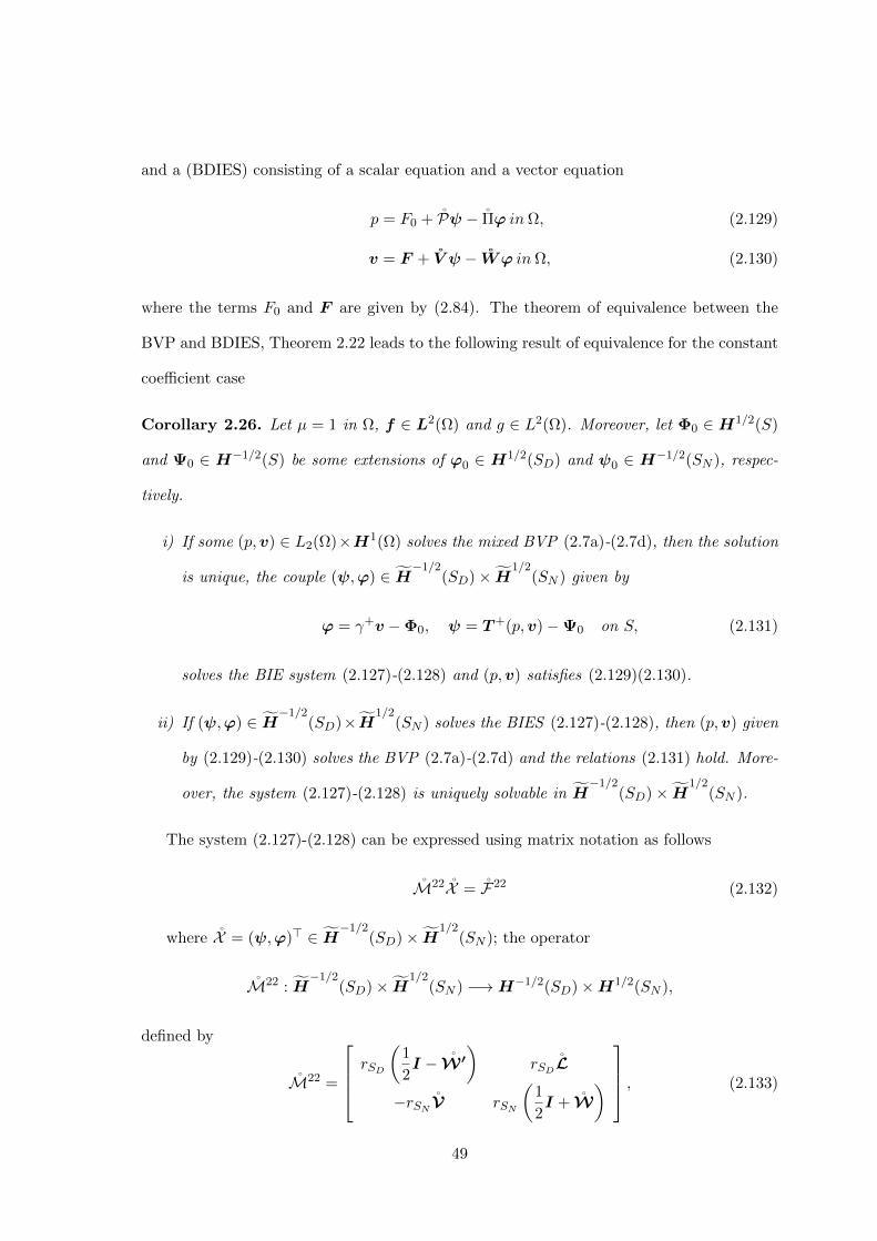
and a (BDIES) consisting of a scalar equation and a vector equation

p = F0 + Pψ − Πϕ inΩ, (2.129)

v = F + V ψ − Wϕ inΩ, (2.130)

where the terms F0 and F are given by (2.84). The theorem of equivalence between the

BVP and BDIES, Theorem 2.22 leads to the following result of equivalence for the constant

coefficient case

Corollary 2.26. Let µ = 1 in Ω, f ∈ L2(Ω) and g ∈ L2(Ω). Moreover, let Φ0 ∈H1/2(S)

and Ψ0 ∈ H−1/2(S) be some extensions of ϕ0 ∈ H1/2(SD) and ψ0 ∈ H−1/2(SN ), respec-

tively.

i) If some (p,v) ∈ L2(Ω)×H1(Ω) solves the mixed BVP (2.7a)-(2.7d), then the solution

is unique, the couple (ψ,ϕ) ∈ H−1/2

(SD)× H1/2

(SN ) given by

ϕ = γ+v −Φ0, ψ = T+(p,v)−Ψ0 on S, (2.131)

solves the BIE system (2.127)-(2.128) and (p,v) satisfies (2.129)(2.130).

ii) If (ψ,ϕ) ∈ H−1/2

(SD)×H1/2

(SN ) solves the BIES (2.127)-(2.128), then (p,v) given

by (2.129)-(2.130) solves the BVP (2.7a)-(2.7d) and the relations (2.131) hold. More-

over, the system (2.127)-(2.128) is uniquely solvable in H−1/2

(SD)× H1/2

(SN ).

The system (2.127)-(2.128) can be expressed using matrix notation as follows

M22X = F22 (2.132)

where X = (ψ,ϕ)> ∈ H−1/2

(SD)× H1/2

(SN ); the operator

M22 : H−1/2

(SD)× H1/2

(SN ) −→H−1/2(SD)×H1/2(SN ),

defined by

M22 =

rSD

(1

2I − W ′

)rSD

L

−rSNV rSN

(1

2I + W

) , (2.133)

49

and the right hand side F22 ∈H−1/2(SD)×H1/2(SN ) is given by

F22 =

[rSD

(T+F −Ψ0

)rSN

(γ+F −Φ0)

]. (2.134)

The operator M22 is evidently continuous. Moreover, in virtue of Corollary 2.26, the

operator M22 is also injective.

Theorem 2.27. The operator

M22 : H−1/2

(SD)× H1/2

(SN ) −→H−1/2(SD)×H1/2(SN )

is invertible.

Proof. A solution of the system (2.132) with an arbitrary right hand side

F22 = [F22

2 , F22

3 ]> ∈H−1/2(SD)×H1/2(SN ) (2.135)

is given by the pair (ψ,ϕ) which satisfies the following extended system:

M22X = F22, (2.136)

where X = (p,v,ψ,ϕ)>, F22 = (0,0, F222 , F

223 )> and

M22 =

I 0 −P Π

0 I −V W

0 0 rSD

(1

2I − W ′

)rSD

L

0 0 −rSNV rSN

(1

2I + W

)

(2.137)

In virtue of Theorem 2.25 with µ = 1, the operator M22 has a bounded inverse.

Theorem 2.28. The operator

M22∗ : L2(Ω)×H1(Ω)×H

−1/2(SD)×H

1/2(SN ) −→ L2(Ω)×H1(Ω)×H−1/2(SD)×H1/2(SN ),

is continuously invertible.

50

Proof. Let us consider the following operator

M22 =

I 0 −P Π0 I −V W

0 0 rSD

(1

2I − W ′

)rSD

L

0 0 −rSNV rSN

(1

2I + W

)

(2.138)

The operator M22 is a compact perturbation of the operator M22∗ due to the compact

properties given by Theorem 2.6, Theorem 2.4 and Corollary 2.10. Using the relations

(2.23) and (2.20), we can express the operator M22 in the form

M22 = diag

(1,

1

µI, I,

1

µI

)M22diag(1, µI, I, µI) (2.139)

where diag(a, bI, cI, dI) represents a 10 by 10 diagonal matrix

diag(a, bI, cI, dI) =

a 0 0 00 b 0 00 0 c 00 0 0 d

. (2.140)

The operator M22 defined by (2.137) can be understood as a triangular block matrix

with the three following diagonal operators

I : L2(Ω+) −→ L2(Ω+),

I : H1(Ω+) −→H1(Ω+),

M22 : H−1/2

(SD)× H1/2

(SN ) −→H−1/2(SD)×H1/2(SN ).

In virtue of Theorem 2.27, the operator M22 is invertible. Consequently, M22 is an

invertible operator as well. As µ is strictly positive, the diagonal matrices are invertible

and the operator M22 is also invertible. Thus, the operator M22∗ is a zero index Fredholm

operator.

The invertibility of the operator simply follows from the injectivity of the operatorM22∗

derived from Theorem 2.22 (iii).

The last three vector equations of the system (M22) are segregated from p. Therefore,

we can define the new system given by equations (2.99b)-(2.99d) which can be written using

51

matrix notation as

M22Y = F22, (2.141)

where Y represents the vector containing the unknowns of the system

Y = (v,ψ,φ) ∈H1(Ω)× H−1/2

(SD)× H1/2

(SN ),

and the matrix operator M22 is given by

M22 :=

I + R −V W

rSDT+(R•,R) rSD

(1

2I −W ′

)rSD

L+

rSNγ+R −rSN

V rSN

(1

2I + W

) .

Theorem 2.29. The operator M22

M22 : H1(Ω)× H−1/2

(SD)× H1/2

(SN ) −→H1(Ω)×H−1/2(SD)×H1/2(SN ),

is continuous and continuously invertible.

Proof. The operator is continuous due to the mapping properties of the operators involved.

Let us assume that M22 is not invertible. Then, the system (2.141) has at least two

different solutions (v1,ψ1,φ1) and (v2,ψ2,φ2). Then, using equation (2.99a), we can obtain

the corresponding pressure for each of the two solutions. Hence, we have two solutions for

the system (M22) (p1,v1,ψ1,φ1) and (p2,v2,ψ2,φ2). However, the BDIES (2.99a)-(2.99d)

is uniquely solvable by virtue of Theorem 2.22. Therefore, both solutions must be the same

what implies the invertibility of the operator M22.

Since the equations (2.99b)-(2.99d) coincide with the equations of the BDIES (2.101),

the solution of the latter one given by X =M22∗ F22∗ , where X = [p,v,φ,ψ]> provides the

solution Y = [v,φ,ψ]> of the system M22Y = F22 for any arbitrary right hand side F22

what implies the invertibility of the operator M22.

52

Chapter 3

BDIES for the compressible Stokessystem in exterior domains

3.1 Introduction

In this chapter, we derived two BDIES equivalent to the original mixed compressible Stokes

system defined on a exterior domain. Furthermore, mapping properties of the hydrodynamic

surface and volume potentials are shown in weighted Sobolev spaces. The main results are

the equivalence theorems and the invertibility theorems of the operators defined by the

BDIES.

3.2 Preliminaries

Let Ω := Ω+ be a unbounded (exterior) simply connected domain and let Ω− := R3 r Ω+

be the complementary (bounded) subset of Ω. The boundary S := ∂Ω is simply connected,

closed and infinitely differentiable, S ∈ C∞. Furthermore, S := SN ∪ SD where both SN

and SD are non-empty, connected disjoint manifolds of S. In addition, the border of these

two submanifolds is also infinitely differentiable, ∂SN = ∂SD ∈ C∞.

To ensure uniquely solvability of the BVPs in exterior domains, we will use weighted

Sobolev spaces with weight

ω(x) = (1 + |x|2)1/2,

(see e.g., [CMN13, Ha71, Ne03, Gr87, Gr78, LiMa73, NePl73]. Let

L2(ω−1; Ω) = g : ω−1g ∈ L2(Ω),

53

be the weighted Lebesgue space and H1(Ω) the following weighted Sobolev (Beppo-Levi)

space constructed using the L2(ω−1; Ω) space

H1(Ω) := g ∈ L2(ω−1; Ω) : ∇g ∈ L2(Ω)

endowed with the corresponding norm

‖ g ‖2H1(Ω):=‖ ω−1g ‖2L2(Ω) + ‖ ∇g ‖2L2(Ω) .

The analogous vector counterpart of H1(Ω) reads

H1(Ω) := g ∈ L2(ω−1; Ω) : ∂jgi ∈ L2(Ω), i, j ∈ 1, 2, 3.

Taking into account that D(Ω) is dense in H1(Ω) it is easy to prove that D(Ω) is dense

in H1(Ω). For further details, cf. [CMN13, p.3] and more references therein.

If Ω is unbounded, then the seminorm

|g|H1(Ω) :=‖ ∇g ‖L2(Ω),

is equivalent to the norm ‖ g ‖H1(Ω) in H1(Ω) [LiMa73, Chapter XI, Part B, §1]. On the

contrary, if Ω− is bounded, then H1(Ω−) = H1(Ω−). If Ω′ is a bounded subdomain of an

unbounded domain Ω and g ∈H1(Ω), then g ∈H1(Ω′).

Let us introduce H1(Ω) as the completion of D(Ω) in H1(R3); let H

−1(Ω) := [H1(Ω)]∗

and H−1(Ω) := [H1(Ω)]∗ be the corresponding dual spaces. Evidently, the space L2(ω; Ω) ⊂

H−1(Ω).

For any generalised function g in H−1

(Ω), we have the following representation property

(see ansatz (2.5.129) in [Ne03]), gj = ∂igij + g0j , gij ∈ L2(R3) and are zero outside the

domain Ω, whereas g0j ∈ L2(ω; Ω). Consequently, D(Ω) is dense in H

−1(Ω) and D(R3) is

dense in H−1(R3).

Condition 3.1. The remainder includes first order derivatives of the variable coefficient

µ. For this reason, we will assume that µ ∈ C1(R3) ∩ L∞(R3) as well as ω∇µ ∈ L∞(R3).

In addition, we will assume that there exist constants C1 and C2 such that

0 < C1 < µ(x) < C2. (3.1)

54

The operator A acting on v ∈ H1(Ω) and p ∈ L2(Ω) is well defined in the weak sense

as long as the variable coefficient µ(x) is bounded, i.e. µ ∈ L∞(Ω), as

〈A(p,v),u〉Ω = −E((p,v),u), ∀u ∈ D(Ω), (3.2)

where E ((p,v),u) (x) and E ((p,v),u) are defined as in (2.2) and (2.3) respectively.

E ((p,v),u) (x) : =1

2µ(x)

(∂ui(x)

∂xj+∂uj(x)

∂xi

)(∂vi(x)

∂xj+∂vj(x)

∂xi

)− 2

3µ(x)div v(x) divu(x)− p(x)divu(x).

The bilinear functional

E ((p,v),u) :(L2(Ω)×H1(Ω)

)× H

1(Ω) −→ R

is bounded. Thus, by density of D(Ω) in H1(Ω), the operator

A : L2(Ω)×H1(Ω) −→H−1(Ω)

is also bounded and gives the weak form of the operator (2.1).

We will also make use of the following space, (cf. e.g., [Co88] [CMN09]),

H1,0(Ω;A) := (p,v) ∈ L2(Ω)×H1(Ω) : A(p,v) ∈ L2(ω; Ω),

endowed with the norm, ‖ · ‖H1,0(Ω;L), where

‖(p,v)‖H1,0(Ω;A) :=(‖p‖2L2(Ω) + ‖v‖2H1(Ω)

+ ‖ωA(p,v)‖2L2(Ω)

)1/2.

For sufficiently smooth functions v and p in Ω±, we can write the classical traction operators

on the boundary S as (2.4), in which nj(x) denote the components of the unit normal vector

n(x) to the boundary S directed outwards the exterior domain Ω. Moreover, γ± denote the

trace operators from inside and outside Ω which according to the trace theorem satisfy the

mapping property γ± : H1(Ω) −→H1/2(S), [CMN13, p.4].

55

Traction operators (2.4) can be continuously extended to the canonical traction oper-

ators T± : H1,0(Ω±,A) → H−1/2(S) defined in the weak form similar to [Co88, Mi11,

CMN13] as

〈T+(p,v),w〉S :=

∫Ω±

[A(p,v)γ+

−1w + E((p,v),γ+

−1w)]dx

∀ (p,v) ∈H1,0(Ω±,A), ∀w ∈H1/2(S),

where the operator γ+−1 : H1/2(S)→H1(Ω) denotes a continuous right inverse of the trace

operator γ+ : H1(Ω)→H1/2(S).

Furthermore, if (p,v) ∈H1,0(Ω,A) and u ∈H1(Ω), the first Green identity (2.5) holds.

Applying the identity (2.5) to the pairs (p,v), (q,u) ∈H1,0(Ω,A) with exchanged roles

and subtracting the one from the other, we arrive at the second Green identity, cf. [McL00,

Mi11], ∫S

(Tj(p,v)uj − Tj(q,u)vj) dS(x) =∫Ω

[Aj(p,v)uj −Aj(q,u)vj + q div v − p divu

]dx. (3.3)

Mixed problem For f ∈ L2(ω,Ω), ϕ0 ∈H1/2(SD), g ∈ L2(ω,Ω) and ψ0 ∈H−1/2(SN ),

find (p,v) ∈H1,0(Ω,A) such that:

A(p,v) = f , in Ω, (3.4a)

div(v)(x) = g, in Ω, (3.4b)

γ+v = ϕ0, on SD, (3.4c)

T+(p,v) = ψ0, on SN . (3.4d)

Theorem 3.2. The mixed BVP (3.4) has at most one solution in the space H1,0(Ω;A).

Proof. Let us suppose that there are two possible solutions: (p1,v1) and (p2,v2) belonging

to the space H1,0(Ω;A), that satisfy the BVP (3.4). Then, the pair (p,v) := (p2,v2) −

56

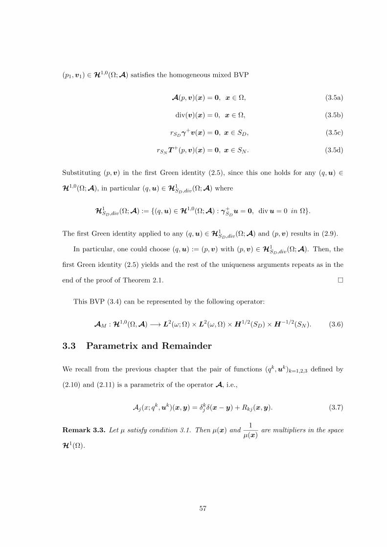
(p1,v1) ∈H1,0(Ω;A) satisfies the homogeneous mixed BVP

A(p,v)(x) = 0, x ∈ Ω, (3.5a)

div(v)(x) = 0, x ∈ Ω, (3.5b)

rSDγ+v(x) = 0, x ∈ SD, (3.5c)

rSNT+(p,v)(x) = 0, x ∈ SN . (3.5d)

Substituting (p,v) in the first Green identity (2.5), since this one holds for any (q,u) ∈

H1,0(Ω;A), in particular (q,u) ∈H1SD,div

(Ω;A) where

H1SD,div

(Ω;A) := (q,u) ∈H1,0(Ω;A) : γ+SDu = 0, divu = 0 in Ω.

The first Green identity applied to any (q,u) ∈H1SD,div

(Ω;A) and (p,v) results in (2.9).

In particular, one could choose (q,u) := (p,v) with (p,v) ∈ H1SD,div

(Ω;A). Then, the

first Green identity (2.5) yields and the rest of the uniqueness arguments repeats as in the

end of the proof of Theorem 2.1.

This BVP (3.4) can be represented by the following operator:

AM : H1,0(Ω,A) −→ L2(ω; Ω)×L2(ω,Ω)×H1/2(SD)×H−1/2(SN ). (3.6)

3.3 Parametrix and Remainder

We recall from the previous chapter that the pair of functions (qk,uk)k=1,2,3 defined by

(2.10) and (2.11) is a parametrix of the operator A, i.e.,

Aj(x; qk,uk)(x,y) = δkj δ(x− y) +Rkj(x,y). (3.7)

Remark 3.3. Let µ satisfy condition 3.1. Then µ(x) and1

µ(x)are multipliers in the space

H1(Ω).

57

3.4 Hydrodynamic potentials

As the parametrix that we are considering is the same as in the previous chapter the

hydrodynamic potentials defined in Section 2.4 remain the same. In addition, we will

introduce the operators U,Q,R and R• whose definitions coincide, respectively, with the

definition of the operators U ,Q,R and R• with the sole difference that Ω = R3.

Condition 3.4. Apart from the condition 3.1, we will sometimes also assume the following:

µ ∈ C2(R3); ω2∂j∂iµ ∈ L∞(R3). (3.8)

3.4.1 Mapping properties

The following assertions have been recently studied by [KLMW] for the constant coefficient

case. Then by relations (2.16)-(2.24) we obtain their counterparts for the variable-coefficient

case. Let us highlight that the operators U ,Q, Q,R, R• are defined in the same way as

U ,Q,Q,R and R• with the particularity that Ω = R3.

Theorem 3.5. The following vector operators are continuous under condition 3.1,

U : H−1(R3) −→H1(R3), (3.9)

U : H−1

(Ω) −→H1(Ω), (3.10)

Q : L2(R3) −→H1(R3), (3.11)

Q : L2(Ω) −→H1(Ω), (3.12)

Q : H−1(R3) −→ L2(R3), (3.13)

Q : H−1

(Ω) −→ L2(Ω), (3.14)

R : L2(ω−1;R3) −→H1(R3), (3.15)

R : L2(ω−1; Ω) −→H1(Ω), (3.16)

R• : L2(ω−1;R3) −→ L2(R3), (3.17)

R• : L2(ω−1; Ω) −→ L2(Ω). (3.18)

58

Proof. Let us consider relations (2.16) and (2.18). Then, the continuity of the operators U ,

U , Q and Q then follows from the continuity of the operators U , U , Q and Q proved in

[KLMW, Lemma 3.1].

Let us prove now the continuity of the operator (3.15). Taking into consideration (2.17),

we need only need to prove the continuity of the terms ∂jUki(gj∂iµ) and Qk(gj∂jµ).

First, let us note that by condition 3.1, µ and1

µare bounded and act as multipliers in

the space H1(Ω). In addition, condition 3.1 states that ω∂iµ ∈ L∞(R3). Consequently, for

any function gj ∈ L2(ω−1;R3), we have that gj∂iµ ∈ L2(R3), see [CMN13, Theorem 4.1].

Let us prove continuity of the term ∂jUki(gj∂iµ) in (2.17). For this purpose, we consider

a function gj in D(R3). Then

∂jUki(gj∂iµ) = −Uki∂j(gj∂iµ). (3.19)

Considering the density of D(R3) in H−1(R3), we can extend the relation (3.19) from D(R3)

to H−1(R3). Hence, we only need to prove that ∂j(gj∂iµ) ∈ H−1(Ω). To do this, we will

use again the density of D(R3) in H−1(R3). Let ρn ∈ D(R3) converging to gj∂iµ ∈ L2(R3).

Then, ∂j(ρn) will converge to ∂j(gj∂iµ) in H−1(R3) ⊂ H−1(R3). Then, the continuity of

the operator ∂jUki(gj∂iµ) follows from the continuity of the operator (3.9).

The continuity of the operators ∂iUkj(gj∂iµ) and Qk(gj∂jµ) can be proved in a similar

way. Consequently, the operator (3.15) is continuous.

Continuity of the operator (3.15) implies the continuity of the operator (3.16).

Let us prove now the continuity of the operator (3.17). Taking into account (2.19), the

continuity of the operator (3.17) will follow from the continuity of the operator ∂jQ(∂iµgj).

Applying a similar density argument as for the previous proof, we can deduce ∂jQ(∂iµgj) =

−Q∂j(∂iµgj). Since, ∂j(∂iµgj) ∈ H−1(R3), the continuity of ∂jQ(∂iµgj) directly follows

now from the continuity of the operator (3.14).

Continuity of the operator (3.18) is implied by the continuity of the operator (3.17).

The mapping property of the operator (3.11)-(3.12) differs from the vector operators Q and

Q and need to be proven.

59

Let us consider φ ∈ D(R3) ⊂ L2(R3). Note the following property

qk =∂E∆

∂xk. (3.20)

where

E∆(x, y) =−1

4π|x− y|,

is the fundamental solution of the Laplace equation. The newtonian volume potential is

defined as

P∆φ(y) =

∫R3

E∆(x, y)φ(x) dx, (3.21)

and solves the Poisson equation ∆ω = φ in R3. It is well known that the Laplace operator

∆ : H1(R3) −→ H−1(R3) has a continuous inverse, ∆−1 : H−1(R3) −→ H1(R3). The inverse

operator, ∆−1 can be seen as a continuous extension of the operator P∆ due to the density

of D(R3) within H−1(R3). Take into account (3.20), we can deduce

Qkφ =

∫R3

qk(x, y)φ(x) dx =

∫R3

∂E∆

∂xk(x, y)φ(x) dx = −

∫R3

E∆(x, y)∂φ(x)

∂xkdx.

Hence, Qkφ = −P∆(∂kφ).

Let φ ∈ L2(R3), then for any function g ∈ D(Ω), we have that

〈φ , ∂kg〉R3 = −〈∂kφ , g〉R3 (3.22)

Hence, as the first term in (3.22) is the scalar product in L2(R3) which is well de-

fined since the integrand belongs to L2(R3) by virtue of the Cauchy-Schwartz inequality.

Therefore, also is the second term. By density, we can extend (3.22) from g ∈ D(R3) to

g ∈ H1(R3) by density, and hence to H1(R3).

Now, the second term could thus be interpreted as ∂kφ ∈ H−1(R3) ⊂ H1(R3) since

D(R3) is dense in H1(R3), see [Bn10, Corollary 10.4.11].

As a result, Qkφ = −P∆(∂kφ) ∈ H1(R3). Consequently, by (2.18), the mapping property

(3.11) follows and thus also does (3.12).

60

Theorem 3.6. The following operators are continuous under condition 3.1

V : H−1/2(S) −→H1(Ω), (3.23)

P : H−1/2(S) −→ L2(Ω), (3.24)

W : H1/2(S) −→H1(Ω), (3.25)

Π : H1/2(S) −→ L2(Ω). (3.26)

Proof. Let us consider relations (2.20) and (2.22). The continuity of the operators V , P,

W and Π then follows from the continuity of the operators V , W , P and Π which has

already being proved in [KLMW, Lemma 3.3].

Corollary 3.7. The following operators are continuous under conditions 3.1 and condition

3.4,

(P,V ) : H−1/2(S) −→H1,0(Ω;A), (3.27)

(Π,W ) : H1/2(S) −→H1,0(Ω;A), (3.28)

(Q,U) : L2(ω; Ω) −→H1,0(R3;A), (3.29)

(R•,R) : H1(Ω) −→H1,0(Ω;A), (3.30)(4

3µI,Q

): L2(Ω) −→H1,0(Ω;A). (3.31)

Proof. Let us consider first the single layer potentials (Pg,V g) ∈ H1(Ω) × L2(Ω) for

g ∈H−1/2(S). Let us apply the operator A taking into consideration (2.20) and (2.22)

A (Pg,V g) = A(Pg, 1

µV g

)= Aj

(Pg, Vkg

)+ ∂k

(µ

[∂j(1/µ)Vkg + ∂k(1/µ)Vjg −

2

3δkj ∂i(1/µ)Vig

]).

Now, the term Aj(Pg, Vkg

)vanishes and the second term belongs to L2(ω; Ω) since

V g ∈ H1(Ω). The same argument works for the double layer potential (W ,Π) g with

g ∈ H1/2(S). In addition it works for the Newtonian potentials (U ,Q) with the sole

difference that Aj(Qg, Ukg

)= gj and g ∈ L2(ω; Ω).

61

For the remainder operators g ∈ H1(Ω) and hence (R•g,Rg) ∈ H1(Ω) × H2(Ω).

Consequently, A (R•g,Rg) ∈H1(Ω) ⊂ L2(ω; Ω).

For the operator (4

3gµ, Q(µg)), we proceed on a similar manner as before

A(

4

3gµ,Qg

)= A

(4

3gµ,

1

µQ(µg)

)= Aj

(4

3gµ,

1

µQ(µg)

)+ ∂k

(∂j(1/µ)Qk(µg) + ∂k(1/µ)Qj(µg)− 4

3δjk∂i(1/µ)Qk(µg)

).

Since Qj(µg) ∈ H1(Ω) by virtue of Theorem 3.5, the whole second term belongs to

L2(ω; Ω). Hence, we only need to prove that Aj(4

3gµ, Q(µg)) ∈ L2(ω; Ω). We have that

(2.46) holds. Hence, (4

3gµ, Q(µg)) ∈H1,0(Ω;A), as in the proof of the analogous property

(2.44) for bounded domains.

3.5 The Third Green Identities

Third Green identities for (p,v) ∈ H1,0(Ω;A) and to the parametrix (qk,uk) can be ob-

tained following a similar approach as in the previous chapter, see Theorem 2.12 and iden-

tities (2.50).

v + Rv − V T+(p,v) +Wγ+v = UA(p,v) + Qdiv(v) in Ω, (3.32)

p+R•v − PT (p,v) + Πγ+v = QA(p,v) +4µ

3div(v) in Ω. (3.33)

If the couple (p,v) ∈ H1,0(Ω;A) is a solution of the Stokes PDE (3.4a) with variable

coefficient, then (3.32) and (3.33) give

v + Rv − V T+(p,v) +Wγ+v = Uf + Qg, (3.34)

p+R•v − PT (p,v) + Πγ+v = Qf +4µ

3g in Ω. (3.35)

Let us recall that the traction operator is well defined due to the mapping properties pro-

vided by the Theorem 3.7. Consequently we can obtain the trace and traction of the third

Green identities for (p,v) ∈H1,0(Ω;A) on S.

1/2γ+v + γ+Rv − VT+(p,v) + Wγ+v = γ+Uf + γ+Qg, (3.36)

62

1/2T+(p,v) + T+(R•,R)v −W ′T+(p,v) + L+γ+v = T+(f , g), (3.37)

where

T+(f , g) := T+(Qf +4µ

3g,Uf + Qg) (3.38)

One can prove the following two assertions that are instrumental for proof of equivalence

of the BDIES and the BVPs.

Lemma 3.8. Let conditions 3.1 and 3.4 hold. Let v ∈ H1(Ω), p ∈ L2(Ω), g ∈ L2(Ω),

f ∈ L2(ω; Ω), Ψ ∈H−1/2(S) and Φ ∈H1/2(S) satisfy the equations

p+R•v − PΨ + ΠΦ = Qf +4µ

3g, in Ω (3.39)

v + Rv − VΨ +WΦ = Uf + Qg, in Ω. (3.40)

Then (p,v) ∈ H1,0(Ω,A) and solve the equations A(p,v) = f and div v = g. Moreover,

the following relations hold true:

P(Ψ− T+(p,v))−Π(Φ− γ+v) = 0, in Ω, (3.41)

V (Ψ− T+(p,v))−W (Φ− γ+v) = 0, in Ω. (3.42)

Proof. By virtue of Corollary 3.7, it is easy to deduce that (p,v) ∈ H1,0(Ω,A). The

remaining part of the proof follows word by word from Theorem 2.13.

Lemma 3.9. Let S = S1 ∪ S2, where S1 and S2 are open non-empty non-intersecting

simply connected submanifolds of S with infinitely smooth boundaries. Let Ψ∗ ∈ H−1/2

(S1),

Φ∗ ∈ H1/2

(S2). If

P(Ψ∗)−Π(Φ∗) = 0, VΨ∗(x)−WΦ∗(x) = 0, in Ω, (3.43)

then Ψ∗ = 0, and Φ∗ = 0, on S.

Proof. Multiply the second equation in (3.43) by µ and apply relations (2.20)

VΨ∗ − W (µΦ∗) = 0 on Ω. (3.44)

63

Then apply the trace operator in both sides taking into account the jump relations given

by Theorem 2.8,

VΨ∗(x) +1

2(µΦ∗)− W(µΦ∗) = 0 in S. (3.45)

Apply the potential relations (2.22) to the first equation in (3.43) to obtain

PΨ∗ − Π(µΦ∗) = 0 (3.46)

Now apply the traction operator at both sides of equations (3.45)-(3.46) taking as pressure

equation (3.46) and as velocity (3.45), keeping in mind the jump relations given by Theorem

2.8 to obtain

1

2Ψ∗ + W ′Ψ∗ − L(µΦ∗) = 0 onS. (3.47)

To ease the notation, let Φ := (µΦ∗) and Ψ := Ψ∗. We consider now the system with

equations (3.45) and (3.47) which can be written using matrix notation as follows:

CΩ+X = 0, (3.48)

where,

CΩ+ =

1

2I − W V

−L 1

2I + W ′

, X =

[Φ

Ψ

]. (3.49)

Here, the matrix operator CΩ+ denotes the so-called Calderon projector. We can relate the

Calderon projector of the exterior domain with the corresponding projector for the bounded

domain by the relation CΩ+ = I − CΩ− , see [HsWe08, Formula 2.3.28]. Therefore, we only

need to focus on showing that the system [I − CΩ− ]X = 0 is uniquely solvable.

The system [I − CΩ− ]X = 0 reads:

−VΨ− 1

2Φ + WΦ = 0, in S, (3.50)

1

2Ψ− W ′Ψ + LΦ = 0, in S. (3.51)

Take the restriction to SD of (3.50) and the restriction of (3.51) to SN , we obtain

M =

[−rS1V +rS1W−rS2W ′ +rS2L

], X =

[Ψ

Φ

]. (3.52)

The system (3.52) can be written using matrix notation as

64

−MX = 0.

The operator M was already studied in Lemma 2.14, and is positive definite, from where

it follows the unique solvability of (3.48).

3.6 BDIES

We aim to obtain two different segregated BDIES for the mixed BVP (3.4). This is a

well known procedure as shown in [CMN09], [MiPo15-I] and [Mi02] and further references

therein.

To this end, let the functions Φ0 ∈ H1/2(S) and Ψ0 ∈ H−1/2(S) be respective contin-

uations of the boundary functions ϕ0 ∈ H1/2(SD) and ψ0 ∈ H−1/2(SN ) from (3.4c) and

(3.4d).

where ϕ ∈ H1/2

(SN ) and ψ ∈ H−1/2

(SD) are unknown boundary functions.

3.6.1 BDIES - M11

Let us now take equations (3.34) and (3.35) in the domain Ω and restrictions of equations

(3.36) and (3.37) to the boundary parts SD and SN , respectively. Substituting there rep-

resentations (2.82) and considering further the unknown boundary functions ϕ and ψ as

formally independent of (segregated from) the unknown domain functions p and v, we ob-

tain the following system of four boundary-domain integral equations for four unknowns,

(p,v) ∈H1,0(Ω,A), ϕ ∈ H1/2

(SN ) and ψ ∈ H−1/2

(SD),:

p+R•v − Pψ + Πϕ = F0 in Ω, (3.53a)

v + Rv − V ψ +Wϕ = F in Ω, (3.53b)

rSDγ+Rv − rSD

Vψ + rSDWϕ = rSD

γ+F −ϕ0 on SD, (3.53c)

rSNT+(R•,R)v − rSN

W ′ψ + rSNL+ϕ = rSN

T+(F0,F )−ψ0 on SN , (3.53d)

where

F0 = Qf − 2

3µg + PΨ0 −ΠΦ0, F = Uf + Qg + VΨ0 −WΦ0. (3.54)

65

Applying Lemma 3.8 to (3.54), keeping in mind the equations (3.53a) and (3.53b), and

taking into account the mapping properties delivered by Theorem 3.5, Theorem 3.6 and

Theorem 3.7, we obtain that (F0,F ) ∈H1,0(Ω,A).

We denote the right hand side of BDIE system (3.53) as

F11∗ := [F0,F11] = [F0,F , rSD

γ+F −ϕ0, rSNT+(F , F )−ψ0]>, (3.55)

which implies F11∗ ∈H1,0(Ω,A)×H1/2(SD)×H−1/2(SN ).

Note that BDIE system (3.53) can be split into the BDIE system (M11), of 3 vector

equations (3.53b), (3.53c), (3.53d) for 3 vector unknowns, v, ψ and ϕ, and the separate

equation (3.53a) that can be used, after solving the system, to obtain the pressure, p.

However since the couple (p,v) shares the space H1,0(Ω,A), equations (3.53b), (3.53c),

(3.53d) are not completely separate from equation (3.53a).

The system (M11) given by equations (3.53b), (3.53c), (3.53d) can be written using

matrix notation as

M11∗ X = F11

∗ , (3.56)

where X represents the vector containing the unknowns of the system

X = (p,v,ψ,ϕ)> ∈ L2(Ω)×H1(Ω)× H−1/2

(SD)× H1/2

(SN )

The matrix operator M11 is defined by

M11∗ =

I R• −P Π0 I + R −V W0 rSD

γ+R −rSDV rSD

W0 rSN

T+(R•,R) −rSNW ′ rSN

L

.We note that the mapping properties of the operators involved in the matrix imply the

continuity of the operator

M11∗ : L2(Ω)×H1(Ω)× H

−1/2(SD)× H

1/2(SN )

−→ L2(Ω)×H1(Ω)×H−1/2(SD)×H1/2(SN ).

Remark 3.10. The term F11∗ = 0 if and only if (f , g,Φ0,Ψ0) = 0.

66

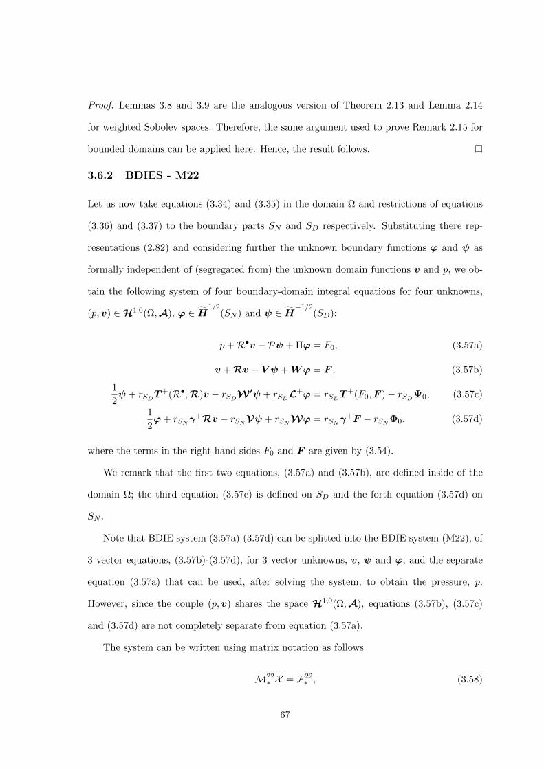
Proof. Lemmas 3.8 and 3.9 are the analogous version of Theorem 2.13 and Lemma 2.14

for weighted Sobolev spaces. Therefore, the same argument used to prove Remark 2.15 for

bounded domains can be applied here. Hence, the result follows.

3.6.2 BDIES - M22

Let us now take equations (3.34) and (3.35) in the domain Ω and restrictions of equations

(3.36) and (3.37) to the boundary parts SN and SD respectively. Substituting there rep-

resentations (2.82) and considering further the unknown boundary functions ϕ and ψ as

formally independent of (segregated from) the unknown domain functions v and p, we ob-

tain the following system of four boundary-domain integral equations for four unknowns,

(p,v) ∈H1,0(Ω,A), ϕ ∈ H1/2

(SN ) and ψ ∈ H−1/2

(SD):

p+R•v − Pψ + Πϕ = F0, (3.57a)

v + Rv − V ψ +Wϕ = F , (3.57b)

1

2ψ + rSD

T+(R•,R)v − rSDW ′ψ + rSD

L+ϕ = rSDT+(F0,F )− rSD

Ψ0, (3.57c)

1

2ϕ+ rSN

γ+Rv − rSNVψ + rSN

Wϕ = rSNγ+F − rSN

Φ0. (3.57d)

where the terms in the right hand sides F0 and F are given by (3.54).

We remark that the first two equations, (3.57a) and (3.57b), are defined inside of the

domain Ω; the third equation (3.57c) is defined on SD and the forth equation (3.57d) on

SN .

Note that BDIE system (3.57a)-(3.57d) can be splitted into the BDIE system (M22), of

3 vector equations, (3.57b)-(3.57d), for 3 vector unknowns, v, ψ and ϕ, and the separate

equation (3.57a) that can be used, after solving the system, to obtain the pressure, p.

However, since the couple (p,v) shares the space H1,0(Ω,A), equations (3.57b), (3.57c)

and (3.57d) are not completely separate from equation (3.57a).

The system can be written using matrix notation as follows

M22∗ X = F22

∗ , (3.58)

67

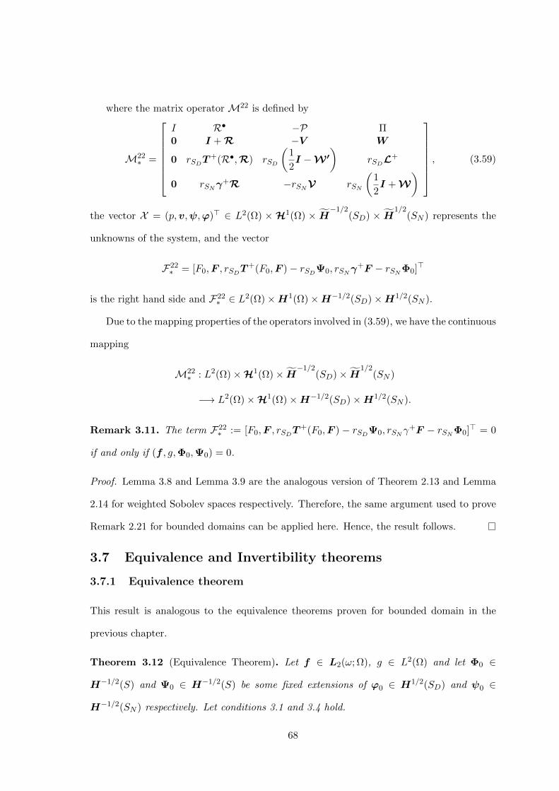
where the matrix operator M22 is defined by

M22∗ =

I R• −P Π0 I + R −V W

0 rSDT+(R•,R) rSD

(1

2I −W ′

)rSD

L+

0 rSNγ+R −rSN

V rSN

(1

2I + W

)

, (3.59)

the vector X = (p,v,ψ,ϕ)> ∈ L2(Ω) ×H1(Ω) × H−1/2

(SD) × H1/2

(SN ) represents the

unknowns of the system, and the vector

F22∗ = [F0,F , rSD

T+(F0,F )− rSDΨ0, rSN

γ+F − rSNΦ0]>

is the right hand side and F22∗ ∈ L2(Ω)×H1(Ω)×H−1/2(SD)×H1/2(SN ).

Due to the mapping properties of the operators involved in (3.59), we have the continuous

mapping

M22∗ : L2(Ω)×H1(Ω)× H

−1/2(SD)× H

1/2(SN )

−→ L2(Ω)×H1(Ω)×H−1/2(SD)×H1/2(SN ).

Remark 3.11. The term F22∗ := [F0,F , rSD

T+(F0,F ) − rSDΨ0, rSN

γ+F − rSNΦ0]> = 0

if and only if (f , g,Φ0,Ψ0) = 0.

Proof. Lemma 3.8 and Lemma 3.9 are the analogous version of Theorem 2.13 and Lemma

2.14 for weighted Sobolev spaces respectively. Therefore, the same argument used to prove

Remark 2.21 for bounded domains can be applied here. Hence, the result follows.

3.7 Equivalence and Invertibility theorems

3.7.1 Equivalence theorem

This result is analogous to the equivalence theorems proven for bounded domain in the

previous chapter.

Theorem 3.12 (Equivalence Theorem). Let f ∈ L2(ω; Ω), g ∈ L2(Ω) and let Φ0 ∈

H−1/2(S) and Ψ0 ∈ H−1/2(S) be some fixed extensions of ϕ0 ∈ H1/2(SD) and ψ0 ∈

H−1/2(SN ) respectively. Let conditions 3.1 and 3.4 hold.

68

(i) If some (p,v) ∈H1,0(Ω;A) solves the mixed BVP (3.4), then

(p,v,ψ,ϕ) ∈H1,0(Ω;A)× H−1/2

(SD)× H1/2

(SN ),

where

ϕ = γ+v −Φ0, ψ = T+(p,v)−Ψ0 on S, (3.60)

solve the BDIES (M11) and (M22).

(ii) If (p,v,ψ,ϕ) ∈H1,0(Ω;A)×H−1/2

(SD)×H1/2

(SN ) solves one of the BDIES, (M11)

or (M22), then it solves all the BDIES. Furthermore, the pair (p,v) solves the mixed

BVP (3.4) and the functions ψ,ϕ satisfy (3.60).

(iii) The BDIES: (M11) and (M22) have at most one solution in the space H1,0(Ω;A)×

H−1/2

(SD)× H1/2

(SN ).

Proof. The proof of item (i) follows from the derivation of the BDIES (M11) and (M22)

in a similar way as in Theorems 2.16 and 2.22 for the corresponding results for bounded

domains.

Item (ii) in bounded domains is proven by applying Theorems 2.13 and 2.14. As we

have proven an analogous result for unbounded domains, see Lemmas 3.8 and 3.9 which

also holds for bounded domains. Therefore, a similar argument as in Theorems 2.16 and

2.22 for the corresponding results for bounded domains can be applied here from where the

result follows.

Finally, item (iii) follows from the fact that the BVP (3.4) has at most one solution.

As the BVP is equivalent to the BDIES (M11) and (M22) then, these latter ones can have

only up to one solution.

3.7.2 Invertibility results for the system (M11)

To prove the more general results of invertibility using wider spaces: H1(Ω) × L2(ω; Ω)

instead of H1,0(Ω;A), in bounded domains required compactness of the operator R and

R• which is obtained in virtue of the compact embedding properties of Sobolev spaces, see

69

[Br84]. However, the compact embeddings provided by the Rellich compactness theorem

do not hold for exterior (unbounded) domains. To overcome this issue, it is possible to

split the operators R and R• in the sum of two operators, one operator whose norm can

be made arbitrarily small whilst the other possesses the compact property, as in [CMN13,

Lemma 7.4].

To make the decomposition of the remainder operators we will require the following

condition.

Condition 3.13. In the following theorems, we will require the following condition:

lim|x|→∞

ω(x)∇µ(x) = 0. (3.61)

The proof of the following Lemma follows a similar argument as in [CMN13, Lemma

7.4] for the corresponding scalar case.

Lemma 3.14. Let conditions 3.1 and 3.13 hold. Then, for any ε > 0 the operator R can

be represented as R = Rs + Rc, where ‖ Rs ‖H1(Ω)< ε, while Rc : H1(Ω) −→ H1(Ω) is

compact.

Proof. Let B(0, ε) be a ball with centre in 0 ∈ R3 and radius ε > 0 big enough such that

S ⊆ B(0, ε). Consider a cut-ff function χ such that 0 ≤ χ(y) ≤ 1 in R3 with the particular

property that χ(y) = 1, if y ∈ B(0, ε), and χ(y) = 0, if y ∈ R3 r B(0, 2ε). Let us now

introduce the two following operators:

Rcg := R(χg), Rsg := R((1− χ)g), for g ∈H1(Ω). (3.62)

Taking into account the relations (2.16) and (2.17), we can obtain the following inequality

‖Rsg‖H1(Ω) = ‖R((1− χ)g)‖H1(Ω)

= ‖−2

µ∂jUkihij −

2

µ∂iUkjhij −

1

µQkhjj‖H1(Ω)

= ‖ 2

µUki[∂jhij ] +

2

µUkj [∂ihij ]−

1

µQkhjj‖H1(Ω)

≤ ‖ 4

C1Ukj [∂ihij ]−

1

µQkhjj‖H1(Ω)

≤ k1‖U‖H−1(Ω)→H1(Ω)+ k2‖Q‖L2(ω;Ω)→H1(Ω)

70

where hij := (1− χ)gj∂iµ.

Let us find estimates for k1 and k2. On one hand,

k1 := 4‖∂ihij‖H−1(Ω)= 4‖∂i[(1− χ)gj∂iµ]‖H−1(Ω)

≤ 4‖[(1− χ)gj∂iµ]‖L2(Ω)

≤ 12 ‖gj‖L2(ω−1;Ω)‖ω∂iµ‖L∞(R3rB(0,ε)) ≤ 12‖gj‖H1(Ω)‖ω∂iµ‖L∞(R3rB(0,ε)).

On the other hand,

k2 := ‖hjj‖L2(Ω) = ‖[(1− χ)gj∂jµ]‖L2(Ω)

≤ ‖gj‖L2(ω−1;Ω)‖ω∂jµ‖L∞(R3rB(0,ε)) ≤ ‖gj‖H1(Ω)‖ω∂iµ‖L∞(R3rB(0,ε)).

Using the estimates for k1 and k2, we obtain the following estimate for the norm of Rsg

‖Rsg‖H1(Ω) ≤ k1‖U‖H−1(Ω)→H1(Ω)+ k2‖Q‖L2(ω;Ω)→H1(Ω)

≤ 12‖gj‖H1(Ω)‖ω∂iµ‖L∞(R3rB(0,ε))‖U‖H−1(Ω)→H1(Ω)

+ ‖gj‖H1(Ω)‖ω∂iµ‖L∞(R3rB(0,ε))‖Q‖L2(ω;Ω)→H1(Ω). (3.63)

Taking the limit as ε → +∞ in (3.63), the term ‖ω∂iµ‖L∞(R3rB(0,ε)) → 0 by virtue of

condition 3.13. Therefore, as ε→ +∞, ‖Rsg‖H1(Ω) → 0, what completes the proof for the

operator Rsg.

To prove now that Rcg is compact, we still consider the same cut-off function χ. By

the definition of χ, we know that χ(y) > 0 if y is in the closure of B(0, 2ε). Consequently,

the operator

Rc : H1(Ω) −→H1(Ω),

satisfies the following relation Rcg = RΩ2ε(χg|Ω2ε) where Ω2ε := Ω ∩B(0, 2ε) and

(RΩ2ε)kρ(y) :=

∫Ω2ε

Rkj(x,y)ρj(x)dx, y ∈ R3.

Note that Ω2ε is a bounded domain and hence, the operator Rc : L2(Ω2ε) −→ H1(Ω) is

continuous by virtue of Theorem 3.5. Furthermore, the restriction operator |Ω2ε is con-

tinuous and has the following mapping property |Ω2ε : H1(Ω) −→ H1(Ω2ε). Now, as the

71

domain Ω2ε is bounded we can apply the Rellich compact embedding theorem to show that

the embedding H1(Ω2ε) ⊂ L2(Ω2ε) is compact from where it follows that the operator

Rc : H1(Ω) −→H1(Ω) is compact.

Reasoning very similarly we can obtain the equivalent result for the remainder operator

resulting from the pressure terms.

Lemma 3.15. Let conditions 3.1 and 3.13 hold. Then, for any ε > 0 the operator R• can

be represented as R• = R•s + R•c , where ‖ R•s ‖H1(Ω)< ε, while R•c : H1(Ω) −→ L2(Ω) is

compact.

Proof. Let B(0, ε) be a ball with centre in 0 ∈ R3 and radius ε > 0 big enough such that

S ⊆ B(0, ε). Consider a cut-ff function χ such that 0 ≤ χ(y) ≤ 1 in R3 with the particular

property that χ(y) = 1, if y ∈ B(0, ε), and χ(y) = 0, if y ∈ R3 r B(0, 2ε). Let us now

introduce the two following operators:

R•cg := R•(χg), R•sg := R•((1− χ)g), for g ∈H1(Ω). (3.64)

Taking into account the relations (2.19), we can obtain the following inequality

‖R•sg‖H1(Ω) = k3‖Q‖L2(ω;Ω)→H1(Ω) + k4. (3.65)

On one hand

k3 := ‖2∂ihij‖H−1(Ω)≤ 6‖gj‖H1(Ω)‖ω∂iµ‖L∞(R3rB(0,ε)).

where hij := (1− χ)gj∂iµ. On the other hand

k4 :=4

3‖hjj‖H1(Ω) ≤ ‖gj‖H1(Ω)‖ω∂iµ‖L∞(R3rB(0,ε)).

Substituting k3 and k4 into (3.65), and taking the limit ε → +∞ the result follows for

the operator R•s. For the operator R•c we follow a word by word argument to deduce that

the operator R•c |Ω2ε : H1(Ω) −→ H1(Ω2ε) is continuous, see Theorem 3.5, and therefore

by virtue of the Rellich compactness theorem, the operator R•c |Ω2ε : H1(Ω) −→ L2(Ω2ε) is

compact.

72

Corollary 3.16. Let conditions 3.1 and 3.61 hold. Then, the operator

I + R : H1(Ω) −→H1(Ω),

is Fredholm with zero index.

Proof. Applying the Lemma 3.14, we have R = Rs+Rc so ‖Rs ‖H1(Ω)< 1 hence I+Rs is

invertible. On the other hand Rc is compact and hence I +Rs is invertible and a compact

perturbation of the operator I + R, from where follows the result.

To simplify the notation we will consider the following notation:

X11 := H1(Ω)× H−1/2

(SD)× H1/2

(SN ), X11∗ := L2(Ω)× X11,

Y11 := H1(Ω)×H1/2(SD)×H−1/2(SN ), Y11∗ := L2(Ω)× Y11,

Y22 := H1(Ω)×H−1/2(SD)×H1/2(SN ), Y22∗ = L2(Ω)× Y22.

Theorem 3.17. Let conditions 3.1, 3.4 and 3.13 hold. Then, the operator

M11∗ : X∗ −→ Y11

∗ (3.66)

is invertible.

Proof. Let M11∗ : X∗ → Y11

∗ be the operator defined by the following matrix:

M11∗ :=

I R• −P Π0 I −V W0 0 −rSD

V rSDW

0 0 −rSNW ′ rSN

L

Note that the operator M11

∗ is a block diagonal upper triangular matrix operator. The first

two blocks are given by the identity operators I and I whereas the third block is given by

the corresponding terms of the third and forth rows and columns.

Taking into account [KoWe06, Theorem 3.10] applied to the last two rows of the matrix

operator M11∗ along with the mapping properties appearing in Theorems 3.6 and 3.7, we

can conclude that the operator M11∗ is continuously invertible operator and hence Fredholm

with index(M11∗ ) = 0.

73

The operator M11∗ − M11

∗ has the form:

M11∗ − M11

∗ =

0 0 0 00 R 0 00 rSD

γ+R 0 0

0 rSNT+(R•,R) rSN

(W ′ − W ′) rSN(L+ − L)

.By virtue of Lemma 3.14, we can obtain the following decomposition for the operator

M11∗ − M11

∗

M11∗ − M11

∗ =M11∗s +M11

∗c ,

where

M11s :=

0 R•s 0 00 Rs 0 00 rSD

γ+Rs 0 00 rSN

T+(R•s,Rs) 0 0

and

M11∗c :=

0 0 0 00 Rc 0 00 rSD

γ+Rc 0 0

0 rSNT+(R•c ,Rc) rSN

(W ′ − W ′) rSN(L+ − L)

.Using the Lemma 3.14, we know that ‖ Rs ‖ and ‖ R•s ‖ can be made aribitrarly small,

and hence small enough to satisfy the inequality ‖ M11∗s ‖X∗→Y11

∗< 1/ ‖ (M11

∗ )−1 ‖X∗→Y11∗

.

Consequently, the operator M11∗ +M11

∗s : X∗ → Y11∗ is continuously invertible.

Furthermore, the operatorM11c is compact since Rc is compact due to Lemma 3.14 and

the mapping properties of the operatorsW ′ and L+−L given by Theorem 2.6 and Corollary

2.10.

Therefore, the operator M11∗ : X∗ → Y11

∗ is Fredholm with zero index. Moreover, this

operator is also injective in virtue of Theorem 3.12 from where follows its invertibility.

Theorem 3.18. Let conditions 3.1, 3.4 and 3.13 hold. Then the operator

M11∗ : H1,0(Ω;A)× H

−1/2(SD)× H

1/2(SN )

−→H1,0(Ω;A)×H1/2(SD)×H−1/2(SN ) (3.67)

is continuous and continuously invertible.

74

Proof. Let us consider the solution X = (M11∗ )−1F11

∗ of the system (3.56). Here, F11∗ ∈

H1,0(Ω;A) ×H1/2(SD) ×H−1/2(SN ) is an arbitrary right hand side and (M11∗ )−1 is the

inverse of the operator (3.66) which exists by virtue of Theorem 3.17.

Applying Lemma 3.8 to the first two equations of the system (M11), we get that

X ∈ H1,0(Ω;A) × H−1/2

(SD) × H1/2

(SN ) if F11∗ ∈ H1,0(Ω;A) ×H1/2(SD) ×H1/2(SN ).

Consequently, the operator (M11∗ )−1 is also the continuous inverse of the operator (3.67).

The following corollary is the analogous of the corollary 2.19 for bounded domains.

Corollary 3.19. Let f ∈H1,0(Ω;A), g ∈ L2(ω; Ω), φ0 ∈H1/2(SD) and ψ0 ∈H−1/2(SN ).

In addition, let conditions 3.1, 3.4 and 3.13 hold. Then, the BVP (3.4) is uniquely solvable

in H1,0(Ω;A). Furthermore, the operator

AM : H1,0(Ω,A) −→ L2(ω; Ω)×L2(ω,Ω)×H1/2(SD)×H−1/2(SN ), (3.68)

is continuously invertible.

Proof. Let Φ0 ∈ H1/2(S) and Ψ0 ∈ H−1/2(S) be some extensions of ϕ0 ∈ H1/2(SD) and

ψ0 ∈H−1/2(SN ), respectively.

The BDIES (M11) is uniquely solvable and equivalent to the BVP (3.4) by virtue of

Theorem 3.12. In addition, as the operator that defines the system (M11) is continuously

invertible, see Theorem 3.18. The remaining part of the proof is similar is as in Corollary

2.19.

When µ = 1, the operator A becomes A, R = R• ≡ 0 and the boundary-domain

integral equations system (3.57a)-(3.57d) becomes a BIES with 6 equations and 6 unknowns,

namely,

rSD

(1

2ψ − W ′ψ + Lϕ

)= rSD

T+(F0,F )− rSDΨ0, on SD, (3.69)

rSN

(1

2ϕ− Vψ + Wϕ

)= rSN

γ+F − rSNΦ0, on SN . (3.70)

75

and a BDIES with 4 equations and 4 unknowns, namely,

p = F0 + Pψ − Πϕ, inΩ, (3.71)

v = F + V ψ − Wϕ, inΩ. (3.72)

where the terms F0 and F are given by (3.54).

By considering µ = 1 in Theorem 3.17 and Corollary 3.19, we obtain the following

corollary

Corollary 3.20. Let µ = 1 in Ω, f ∈ L2(Ω) and g ∈ L2(ω; Ω). Moreover, let Φ0 ∈

H1/2(S) and Ψ0 ∈H−1/2(S) be some extensions of ϕ0 ∈H1/2(SD) and ψ0 ∈H−1/2(SN ),

respectively. Furthermore, let conditions 3.1, 3.4 and 3.13 hold.

i) If some (p,v) ∈ L2(ω; Ω) × H1(Ω) solves the mixed BVP (3.4a)-(3.4d), then the

solution is unique, the couple (ψ,ϕ) ∈ H−1/2

(SD)× H1/2

(SN ) given by (3.60) solves

the BIE system (3.69)-(3.70) and (p,v) satisfies (3.71)-(3.72).

ii) If

(ψ,ϕ) ∈ H−1/2

(SD)× H1/2

(SN )

solves the BIES (3.69)-(3.70), then (p,v) ∈ H1,0(Ω;A) given by (3.71)-(3.72) solves

the BVP (3.4a)-(3.4d) and the relations (3.60) hold. Moreover, the BDIE solution is

unique H−1/2

(SD)× H1/2

(SN ).

3.7.3 Invertibility results for the system (M22)

In this section we present some lemmas which deal with integral representation formulae for

the corresponding right hand sides of the BDIES given. These theorems are analogous of

those for bounded domains presented in the previous chapter, see Lemma 2.23 and Corollary

2.24.

Lemma 3.21. Let S = S1∪S2, where S1 and S2 are two non-intersecting simply connected

nonempty submanifolds of S with infinitely smooth boundaries. For any vector

76

F = (F0,F ,Ψ,Φ)> ∈H1,0(Ω;A)×H−1/2(S1)×H1/2(S2)

there exists another vector

(g∗,f∗,Ψ∗,Φ∗)> = CS1,S2F ∈ L2(ω; Ω)×L2(ω; Ω)×H−1/2(S)×H1/2(S)

which is uniquely determined by F and such that

Qf∗ +4

3µg∗ + PΨ∗ −ΠΦ∗ = F0, in Ω, (3.73a)

Uf∗ + Qg∗ + VΨ∗ −WΦ∗ = F , in Ω, (3.73b)

rS1Ψ∗ = Ψ, on S1, (3.73c)

rS2Φ∗ = Φ, on S2. (3.73d)

Furthermore, the operator

CS1,S2 : H1,0(Ω;A)×H−1/2(S1)×H1/2(S2)

−→ L2(Ω)×L2(Ω)×H−1/2(S)×H1/2(S)

is continuous.

Proof. Let Ψ0, Φ0 be some fixed extensions of Ψ and Φ from S1 to the whole boundary

S and from S2 onto S respectively. Let us choose this extensions in such a way that they

preserve the functions spaces, i.e., Ψ0 ∈ H−1/2(S), Φ0 ∈ H1/2(S) (cf. [Tr78, Subsection

4.2]). Consequently, arbitrary extensions of the functions Ψ and Φ can be represented as

Ψ∗ = Ψ0 + ψ, ψ ∈ H−1/2

(S2), (3.74)

Φ∗ = Φ0 + ϕ, ϕ ∈ H1/2

(S1). (3.75)

The functions Ψ∗ and Φ∗, in the form (3.74) and (3.75), satisfy the conditions (3.73c)

and (3.73d). Consequently, it is only necessary to show that the functions g∗,f∗, ψ and ϕ

can be chosen in a particular way such that equations (3.73a)-(3.73b) are satisfied.

77

Applying the potential relations (2.16)-(2.22) to equations (3.73a)-(3.73b), we obtain

Qf∗ +4

3µg + P

(Ψ0 + ψ

)− Π (µΦ0 + µϕ) = F0, (3.76)

Uf∗ + Q(µg∗) + V(Ψ0 + ψ

)− W (µΦ0 + µϕ) = µF . (3.77)

Apply the Stokes operator with constant viscosity µ = 1, A, to equations (3.76) and (3.77).

Then, apply the divergence operator to equation (3.77). As a result, we obtain

f∗ = A(F0, µF ) (3.78)

µg∗ = div(µF )⇒ g∗ =div(µF )

µ(3.79)

which shows that the function f∗ is uniquely determined by F0 ∈ L2(ω; Ω) and ,µF and

belongs to L2(ω; Ω) since (F0, µF ) ∈H1,0(Ω;A) by virtue of the mapping properties given

by Theorem 2.7. In addition, (3.79) shows that g∗ is also uniquely determined by F and

belongs to L2(ω; Ω) due to the fact that µF ∈H1(Ω).

Let us substitute now (3.78) and (3.79) into equations (3.76)-(3.77) and move each term

which is not depending on either ψ or φ to the right hand side

Pψ − Π(µϕ) = F0 −4

3div(µF )− Q

(A(F0, µF )

)− P(Ψ0) + Π(µΦ0), (3.80)

in Ω,

V ψ − W (µϕ) = µF − U(A(F0, µF )

)− Q(µF )− V (Ψ0) + W (µΦ0), (3.81)

in Ω.

Let us denote with J = (J0,J) the right hand side of (3.80)-(3.81)

J0 :=

(F0 −

4

3div(µF )− Q

(A(F0, µF )

)− P(Ψ0) + Π(µΦ0)

),

J :=(µF − U

(A(F0, µF )

)− Qdiv(µF )− V (Ψ0) + W (µΦ0)

).

If the functions that we are looking for satisfy ψ and ϕ satisfy (3.80)-(3.81). Then, they

will satisfy as well the following system

rS2γ+(V ψ − W (µϕ)

)= rS2

(γ+J

), (3.82)

rS1

[T

+(P(ψ)− Π(µϕ), V ψ − W (µϕ)

)]= rS1

(T

+(J0,J)

). (3.83)

78

The system (3.82)-(3.83) can be written using matrix notation as follows[rS2V rS2γ

+WrS1W ′ rS1L

] [ψµϕ

]=

[rS2 (γ+J)

rS1

(T

+(J0,J)

) ] . (3.84)

The matrix operator given by the lefthand side of the equations (3.82)-(3.83) is an isomor-

phism between the spaces H−1/2

(S2)×H1/2

(S1) ontoH1/2(S2)×H−1/2(S1) (see, [KoWe06,

Theorem 3.10]). Note that this system depends only in the boundary and hence the same

argument works for both bounded and unbounded domains.

Therefore, the simultaneous equations (3.82) and (3.83) are uniquely solvable with re-

spect to ϕ and ψ. We denote the solution of (3.82)-(3.83) by ψ0

and ϕ0.

Substitute now ψ0

and ϕ0 into (3.76)-(3.77)

Pψ0− Π(µϕ0) = F0 −

4

3µdiv(µF )− Q

(A(F0, µF )

)− P(Ψ0) + Π(µΦ0), (3.85)

in Ω,

V ψ0− W (µϕ0) = µF − U

(A(F0, µF )

)− Qdiv(µF )− V (Ψ0) + W (µΦ0), (3.86)

in Ω.

Let us rewrite equations (3.85) and (3.86) in terms of the parametrix-based potential oper-

ators by applying (2.16)-(2.22)

P(Ψ0 + ψ0)−Π(Φ0 + ϕ0) +Q

(A(F0, µF )

)+

4

3µdiv(µF ) = F0, in Ω,

V (Ψ0 + ψ0)−W (Φ0 + ϕ0) + U

(A(F0, µF )

)+ Q div(µF ) = F , in Ω.

Hence, Ψ∗ = Ψ0 + ψ and Φ∗ = Φ0 + ϕ are uniquely determined by virtue of the uniqueness

of solution of the mixed problem for the Stokes system with µ = 1. Additionally, g∗ and f∗

are uniquely determined by conditions(3.78) and (3.79).

Therefore, we have found a vector (g∗,f∗,Ψ∗,Φ∗) which is uniquely determined by

(F0,F ,Ψ,Φ) and such that it satisfies (3.73a)-(3.73d). The uniqueness follows from the

system (3.84). Making this system homogeneous by considering F = Ψ = Φ = 0 and

79

F0 = 0 then f∗ = 0 which leads to:

P(Ψ∗)−Π(Φ∗) = 0,

V (Ψ∗)−W (Φ∗) = 0.

with Ψ∗ ∈ H−1/2

(S2) and Φ∗ ∈ H1/2

(S1). Hence, we conclude that Ψ∗ = 0 and Φ∗ = 0 in

virtue of Lemma 2.14.

The continuity and linearity of the operator CS1,S2 is owed to the linearity and continuity

of the operators involved.

Corollary 3.22. For any

F = ((F0,F1),F2,F3)> ∈H1,0(Ω;A)×H−1/2(S1)×H1/2(S2),

there exists a unique four-tuple

(g∗,f∗,Ψ∗,Φ∗)> = CS1,S2F ∈ L2(ω; Ω)×L2(ω; Ω)×H−1/2(S)×H1/2(S),

such that

Qf∗ +4

3µg∗ + PΨ∗ −ΠΦ∗ = F0, inΩ, (3.87)

Uf∗ + Qg∗ + VΨ∗ −WΦ∗ = F1, inΩ, (3.88)

rS1(T+(F0,F1)−Ψ∗) = F2, on S1 (3.89)

rS2(γ+F1 −Φ∗) = F3, on S2. (3.90)

Furthermore, the operator

CS1,S2 : H1,0(Ω;A)×H−1/2(S1)×H1/2(S2) −→ L2(ω; Ω)×L2(ω; Ω)×H−1/2(S)×H1/2(S)

is continuous.

Proof. Take Ψ := rS1T+(F0,F1) − F2. Let us check, Ψ ∈ H−1/2(S1). Firstly, F2 ∈

H−1/2(S1). Secondly, (F0,F1) ∈ H1,0(Ω;A), then T+(F0,F1) ∈ H−1/2(S) and hence

rS1T+(F0,F1) ∈H−1/2(S1). Therefore Ψ ∈H−1/2(S1).

80

In a similar fashion, let Φ := rS2γ+F1 − F3. It is easy to see by applying the trace

theorem that rS2γ+F1 ∈ H1/2(S2) and therefore Φ ∈ H1/2(S2). The Corollary follows

from applying Lemma 3.21 with Ψ := rS1T+(F0,F1)−F2 and Φ := rS2γ

+F1 −F3.

Theorem 3.23. Let conditions 3.1, 3.4 and 3.13 hold. Then, the operator

M22∗ : H1,0(Ω;A)× H

−1/2(SD)× H

1/2(SN ) −→H1,0(Ω;A)×H−1/2(SD)×H1/2(SN ),

(3.91)

is continuously invertible.

Proof. Let us consider an arbitrary right hand side to the system (3.58)

F22 ∈H1,0(Ω;A)×H−1/2(SD)×H1/2(SN ).

By virtue of the Corollary 3.22, the right hand side F22 can be written in the form (3.87)-

(3.90) with S1 = SD and S2 = SN . In addition, (g∗,f∗,Ψ∗,Φ∗)> = CSD,SN

F22 where the

operator CSD,SNis bounded and has the following mapping property

CSD,SN: H1,0(Ω;A)×H−1/2(SD)×H1/2(SN )

−→ L2(ω; Ω)×L2(ω; Ω)×H−1/2(S)×H1/2(S).

By virtue of Corollary 2.19 and the equivalence theorem of the system (M22), Theorem

3.12, there exists a solution of the equationM22∗ X = F22

∗ . This solution can be represented

as X = (M22∗ )−1F22

∗ where the operator

(M22∗ )−1 : H1,0(Ω;A)×H−1/2(SD)×H1/2(SN )

−→H1,0(Ω;A)× H−1/2

(SD)× H1/2

(SN ),

which is given by

(p,v) = A−1M [g∗,f∗, rSD

Ψ∗, rSNΦ∗]>, ψ = T+(p,v)−Ψ∗, φ = γ+v −Φ∗,

where the A−1M is continuous, see Corollary 3.19. Consequently, the operator (M22

∗ )−1 is a

right inverse of the operator (3.91). In addition, (M22∗ )−1 is also the double sided inverse

due to the injectivity of (3.91) given by the Theorem 3.12.

81

The system (3.69)-(3.70) can be expressed using matrix notation as follows

M22X = F22 (3.92)

where X = (ψ,ϕ)> ∈ H−1/2

(SD)× H1/2

(SN ); the operator

M22 : H−1/2

(SD)× H1/2

(SN ) −→H−1/2(SD)×H1/2(SN ),

is defined by

M22 =

rSD

(1

2I − W ′

)rSD

L

−rSNV rSN

(1

2I + W

) , (3.93)

and the right hand side F22 ∈H−1/2(SD)×H1/2(SN ) is given by

F22 =

[rSD

(T+(F0,F )−Ψ0

)rSN

(γ+F −Φ0)

]. (3.94)

The operator M22 is evidently continuous. Moreover, in virtue of Corollary 3.20(ii), the

operator M22 is also injective.

Theorem 3.24. Let conditions 3.1, 3.4 and 3.13 hold. Then, the operator

M22 : H−1/2

(SD)× H1/2

(SN ) −→H−1/2(SD)×H1/2(SN )

is continuously invertible.

Proof. A solution of the system (3.92) with an arbitrary right hand side

F22 = [F22

2 , F22

3 ]> ∈H−1/2(SD)×H1/2(SN ) (3.95)

is given by the pair (ψ,ϕ) which satisfies the following extended system

M22X = F22 (3.96)

where X = (p,v,ψ,ϕ)>, F22 = (0,0, F222 , F

223 )> and

M22 =

I 0 −P Π

0 I −V W

0 0 rSD

(1

2I − W ′

)rSD

L

0 0 −rSNV rSN

(1

2I + W

)

(3.97)

82

In virtue of Theorem 3.23 with µ = 1, the operator M22 has a bounded right inverse which

is also the left inverse of M22 since the latter one is injective.

Theorem 3.25. Let conditions 3.1, 3.4 and 3.13 hold. Then, the operator

M22∗ : X∗ −→ Y22

∗ (3.98)

is invertible.

Proof. Let M22∗ = M22 given by (2.138). As in the proof of Theorem 2.28 we obtain that

the operator M22∗ is invertible.

By virtue of Lemma 3.14, we have

M22 − M22∗ =M22

∗s +M22∗c ,

where

M22s :=

0 R•s 0 00 Rs 0 00 rSD

γ+Rs 0 00 rSN

T+(R•s,Rs) 0 0

.Using the Lemma 3.14, we know that ‖ Rs ‖ and ‖ R•S ‖ can be made aribitrarly small,

and hence small enough to satisfy the inequality ‖ M22∗s ‖X∗→Y22

∗< 1/ ‖ (M22

∗ )−1 ‖X∗→Y22∗

.

Consequently, the operator M22∗ +M22

∗s : X∗ → Y22∗ is continuously invertible.

Furthermore, the operatorM22c is compact since Rc is compact due to Lemma 3.14 and

the mapping properties of the operatorsW ′ and L+−L given by Theorem 2.6 and Corollary

2.10.

Therefore, the operator M22∗ : X∗ → Y22

∗ is Fredholm with zero index. Moreover, this

operator is also injective in virtue of Theorem 3.12 and the Remark 3.11, from where follows

its invertibility.

Let us consider the BDIES (M11) and (M22). Since the unknown p only appears in the

first equation, then we can focus on solving the simplified system containing the remaining

83

vector equations with unknowns X = (v,ψ,φ) ∈ X. Then the operators that define the

simplified systems (M11) and (M22) are given by

M11 =

I + R −V WrSD

γ+R −rSDV rSD

WrSN

T+(R•,R) −rSNW ′ rSN

L

,

M22 =

I + R −V W

rSDT+(R•,R) rSD

(1

2I −W ′

)rSD

L+

rSNγ+R −rSN

V rSN

(1

2I + W

) .

The corresponding right hand sides are given by

F11 := [F , rSDγ+F −ϕ0, rSN

T+(F , F )−ψ0]> ∈ Y11,

F22 := [F , rSDT+(F0,F )− rSD

Ψ0, rSNγ+F − rSN

Φ0]> ∈ Y22.

Consequently, we can write the systems (M11) and (M22) as

M11X = F11, M22X = F22.

Since the pressure unknown only appears on the first equation of the BDIES (M11) and

(M22), the invertibility of the operatorsM11 andM22 is implied by the invertibility of the

operators M11∗ and M22

∗ .

Corollary 3.26. The operators

M11 : X −→ Y11, M22 : X −→ Y22,

are continuous and continuously invertible.

84

Chapter 4

A new family of BDIES for a scalarmixed elliptic interior BVP

4.1 Introduction

Boundary-Domain Integral Equations for the scalar equation with variable coefficient have

been obtained using parametrix. This chapter concentrates on the idea that there is not

only one appropriate parametrix for a PDE (or system) that works.

For this scalar equation, a family of weakly singular parametrix of the form P x(x, y; a(x))

for the particular operator:

A(x, ∂x; a(x))u :=∂

∂x

(a(x)

∂u

∂x

),

has been studied in [CMN09, CMN10, CMN13].

The new family of parametrices of the form P y(x, y; a(y)) has not been studied yet

and we analyse this scenario for a mixed elliptic boundary value problem in both bounded

and unbounded domains. Mapping properties of the corresponding P y-based potentials are

proved in bounded domains and appropriate Sobolev spaces.

The main difference from considering a parametrix depending on the same variable

or different from the PDE operator stems from the fact that the relations between the

parametrix based potentials with their counterparts for constant coefficients become more

difficult to deal with. Notwithstanding, the same mapping properties in Sobolev-Bessel

potential spaces still hold. Therefore, it is still possible to prove equivalence and invertibility

85

for a BDIES derived from the original BVP. These results are published in [MiPo15-II].

4.2 Preliminaries and the BVP

The domains. Let Ω = Ω+ be a bounded simply connected domain, Ω− := R3 r Ω+

the complementary (unbounded) subset of Ω. The boundary S := ∂Ω is simply connected,

closed and infinitely differentiable, S ∈ C∞. Furthermore, S := SN ∪SD where both SN and

SD are non-empty, connected disjoint manifolds of S. The border of these two submanifolds

is also infinitely differentiable, ∂SN = ∂SD ∈ C∞.

PDE. Let us introduce the following partial differential equation whith variable smooth

positive coefficient a(x) ∈ C∞(Ω):

Au(x) := A(x)[u(x)] :=

3∑i=1

∂

∂xi

(a(x)

∂u(x)

∂xi

)= f(x), x ∈ Ω, (4.1)

where u(x) is an unknown function and f is a given function on Ω. It is easy to see that if

a ≡ 1 then, the operator A becomes ∆, the Laplace operator.

Function spaces. We will make use of the space, see e.g. [Co88, CMN09],

H1,0(Ω;A) := u ∈ H1(Ω) : Au ∈ L2(Ω)

which is a Hilbert space with the norm defined by

‖ u ‖2H1,0(Ω;A):=‖ u ‖2H1(Ω) + ‖ Au ‖2L2(Ω).

Traces and conormal derivatives. For a scalar function w ∈ Hs(Ω±), s > 1/2, the

trace operator γ±( · ) := γ±S ( · ), acting on w is well defined and γ±w ∈ Hs−1/2(S) (see,

e.g., [McL00, Mi11]). For u ∈ Hs(Ω), s > 3/2, we can define on S the conormal derivative

operator, T±, in the classical (trace) sense:

T±[u(x)] := T±x u =

3∑i=1

a(x)ni(x)

(∂u

∂xi

)±= a(x)

(∂u(x)

∂n(x)

)±,

86

where n(x) is the exterior unit normal vector directed outwards the interior domain domain

Ω at a point x ∈ S. Note the subscript x refers to the variable of differentiation in the

conormal derivative.

Moreover, for any function u ∈ H1,0(Ω;A), the canonical conormal derivative T±u ∈

H−1/2(Ω) is well defined, cf. [Co88, McL00, Mi11],

〈T±u,w〉S := ±∫

Ω±[(γ−1ω)Au+ E(u, γ−1w)]dx, for all w ∈ H1/2(S), (4.2)

where γ−1 : H1/2(S) −→ H1K(R3) is a continuous right inverse to the trace operator whereas

the function E is defined as

E(u, v)(x) :=

n∑i=1

a(x)∂u(x)

∂xi

∂v(x)

∂xi,

and 〈 · , · 〉S represents the L2−based dual form on S.

Boundary value problem We aim to derive boundary-domain integral equation systems

for the following mixed boundary value problem. Given f ∈ L2(Ω), φ0 ∈ H1/2(SD) and

ψ0 ∈ H−1/2(SN ), we seek a function u ∈ H1(Ω) such that

Au = f, in Ω; (4.3a)

rSDγ+u = φ0, on SD; (4.3b)

rSNT+u = ψ0, on SN ; (4.3c)

where equation (4.3a) is understood in the weak sense, the Dirichlet condition (4.3b) is un-

derstood in the trace sense and the Neumann condition (4.3c) is understood in the functional

sense (4.2).

By Lemma 3.4 of [Co88] (cf. also Theorem 3.9 in [Mi11]), the first Green identity holds

for any u ∈ H1,0(Ω;A) and v ∈ H1(Ω),

〈T±u, γ+v〉S := ±∫

Ω[vAu+ E(u, v)]dx. (4.4)

The following assertion is well known and can be proved, e.g., using the Lax-Milgram lemma

as in [Ste07, Chapter 4].

87

Theorem 4.1. The BVP (4.3) has one and only one solution.

4.3 Parametrices and remainders

For a given operator A, the parametrix is not unique. For example, the parametrix

P y(x, y) =1

a(y)P∆(x− y), x, y ∈ R3,

was employed in [Mi02, CMN09], for the operator A defined in (4.1). The remainder

corresponding to the parametrix P y is

Ry(x, y) =3∑i=1

1

a(y)

∂a(x)

∂xi

∂

∂xiP∆(x− y) , x, y ∈ R3. (4.5)

In this chapter, for the same operator A defined in (4.1), we will use another parametrix,

P (x, y) := P x(x, y) =1

a(x)P∆(x− y), x, y ∈ R3, (4.6)

which leads to the corresponding remainder

R(x, y) = Rx(x, y) = −3∑i=1

∂

∂xi

(1

a(x)

∂a(x)

∂xiP∆(x, y)

)

= −3∑i=1

∂

∂xi

(∂(ln a(x))

∂xiP∆(x, y)

), x, y ∈ R3.

Note that the both remainders Rx and Ry are weakly singular, i.e.,

Rx(x, y), Ry(x, y) ∈ O(|x− y|−2).

This is due to the smoothness of the variable coefficient a.

4.4 Volume and surface potentials

The volume parametrix-based Newton-type potential and the remainder potential are re-

spectively defined, for y ∈ R3, as

Pρ(y) :=

∫ΩP (x, y)ρ(x) dx, Rρ(y) :=

∫ΩR(x, y)ρ(x) dx.

88

The parametrix-based single layer and double layer surface potentials are defined for

y ∈ R3 : y /∈ S, as

V ρ(y) := −∫SP (x, y)ρ(x) dS(x), Wρ(y) := −

∫ST+x P (x, y)ρ(x) dS(x).

We also define the following pseudo-differential operators associated with direct values

of the single and double layer potentials and with their conormal derivatives, for y ∈ S,

Vρ(y) := −∫SP (x, y)ρ(x) dS(x), Wρ(y) := −

∫STxP (x, y)ρ(x) dS(x),

W ′ρ(y) := −∫STyP (x, y)ρ(x) dS(x), L±ρ(y) := T±y Wρ(y).

The operators P,R, V,W,V,W,W ′ and L can be expressed in terms the volume and

surface potentials and operators associated with the Laplace operator, as follows

Pρ = P∆

(ρa

), (4.7)

Rρ = −∇ · [P∆(ρ)∇ ln a] , (4.8)

V ρ = V∆

(ρa

), (4.9)

Vρ = V∆

(ρa

), (4.10)

Wρ = W∆ρ− V∆

(ρ∂(ln a)

∂n

), (4.11)

Wρ =W∆ρ− V∆

(ρ∂(ln a)

∂n

), (4.12)

W ′ρ = aW ′∆(ρa

), (4.13)

L±ρ = Lρ− aT±∆V∆

(ρ∂(ln a)

∂n

), (4.14)

Lρ := aL∆ρ. (4.15)

The symbols with the subscript ∆ denote the analogous surface potentials for the con-

stant coefficient case, a ≡ 1. Furthermore, by the Liapunov-Tauber theorem, L+∆ρ = L−∆ρ =

L∆ρ.

Using relations (4.7)-(4.15) it is now rather simple to obtain, similar to [CMN09], the

mapping properties, jump relations and invertibility results for the parametrix-based sur-

face and volume potentials, provided in theorems/corollary 4.2-4.8, from the well-known

properties of their constant-coefficient counterparts (associated with the Laplace equation).

89

Theorem 4.2. Let s ∈ R. Then, the following operators are continuous:

P : Hs(Ω) −→ Hs+2(Ω), s ∈ R, (4.16)

P : Hs(Ω) −→ Hs+2(Ω), s > −1

2, (4.17)

R : Hs(Ω) −→ Hs+1(Ω), s ∈ R, (4.18)

R : Hs(Ω) −→ Hs+1(Ω), s > −1

2. (4.19)

Corollary 4.3. Let s > 1/2, let S1 be a non-empty submanifold of S with smooth boundary.

Then, the following operators are compact:

R : Hs(Ω) −→ Hs(Ω),

rS1γ+R : Hs(Ω) −→ Hs−1/2(S1),

rS1T+R : Hs(Ω) −→ Hs−3/2(S1).

Theorem 4.4. Let s ∈ R. Then, the following operators are continuous:

V : Hs(S) −→ Hs+3/2(Ω), W : Hs(S) −→ Hs+1/2(Ω).

Theorem 4.5. Let s ∈ R. Then, the following operators are continuous:

V : Hs(S) −→ Hs+1(S), W : Hs(S) −→ Hs+1(S),

W ′ : Hs(S) −→ Hs+1(S), L± : Hs(S) −→ Hs−1(S).

Theorem 4.6. Let ρ ∈ H−1/2(S), τ ∈ H1/2(S). Then the following operators jump rela-

tions hold:

γ±V ρ = Vρ, γ±Wτ = ∓1

2τ +Wτ, T±V ρ = ±1

2ρ+W ′ρ.

Theorem 4.7. Let s ∈ R, let S1 and S2 be two non-empty manifolds with smooth bound-

aries, ∂S1 and ∂S2, respectively. Then, the following operators

rS2V : Hs(S1) −→ Hs(S2),

rS2W : Hs(S1) −→ Hs(S2),

rS2W ′ : Hs(S1) −→ Hs(S2).

90

are compact.

Theorem 4.8. Let S1 be a non-empty simply connected submanifold of S with infinitely

smooth boundary curve, and 0 < s < 1. Then, the operators

rS1V : Hs−1(S1) −→ Hs(S1), V : Hs−1(S) −→ Hs(S),

are invertible.

Proof. Relation (4.9) gives Vg = V∆g∗, where g = g∗/a. The invertibility of V then follows

from the invertibility of V∆, see references [CoSt87, Theorem 2.4] and [CMN10, Theorem

3.5].

Theorem 4.9. Let S1 be a non-empty simply connected submanifold of S with infinitely

smooth boundary curve, and 0 < s < 1. Then, the operator

rS1L : Hs(S1) −→ Hs−1(S1),

is invertible whilst the operators

rS1(L± − L) : Hs(S1) −→ Hs−1(S1),

are compact.

Proof. Relation (4.14) gives

Lρ = L±ρ+ aT+∆V∆

(ρ∂(ln a)

∂n

)= L±ρ+ aT−∆V∆

(ρ∂(ln a)

∂n

).

Take into account Lρ := aL∆ρ and the invertibility of the operator L∆, see references

[CoSt87, Theorem 2.4] and [CMN10, Theorem 3.6]; we deduce the invertibility of the oper-

ator L. To prove the compactness properties, we consider the identity:

L±ρ− Lρ = a

(∓1

2I −W ′∆

)(ρ∂(ln a)

∂n

).

Since ρ ∈ Hs(S1), due to the mapping properties of the operatorW ′, L±−ρLρ ∈ Hs. Then,

immediately follows from the compact embedding Hs(S) ⊂ Hs−1(S), that the operators

rS1(L± − L) : Hs(S1) −→ Hs−1(S1),

are compact.

91

4.5 Third Green identities and integral relations

In this section we provide the results similar to the ones in [CMN09] but for our, different,

parametrix (4.6).

Let u, v ∈ H1,0(Ω;A). Subtracting from the first Green identity (4.4) its counterpart

with the swapped u and v, we arrive at the second Green identity, see e.g. [McL00],∫Ω

[uAv − vAu] dx =

∫S

[uT+v − v T+u

]dS(x). (4.20)

Taking now v(x) := P (x, y), we obtain from (4.20) by the standard limiting procedures (cf.

[Mr70]) the third Green identity for any function u ∈ H1,0(Ω;A):

u+Ru− V T+u+Wγ+u = PAu, in Ω. (4.21)

If u ∈ H1,0(Ω;A) is a solution of the partial differential equation (4.3a), then, from

(4.21) we obtain:

u+Ru− V T+u+Wγ+u = Pf, inΩ; (4.22)

1

2γ+u+ γ+Ru− VT+u+Wγ+u = γ+Pf, on S; (4.23)

1

2T+u+ T+Ru−W ′T+u+ L+γ+u = T+Pf, on S. (4.24)

For some distributions f , Ψ and Φ, we consider a more general, indirect integral relation

associated with the third Green identity (4.22):

u+Ru− VΨ +WΦ = Pf, in Ω. (4.25)

Lemma 4.10. Let u ∈ H1(Ω), f ∈ L2(Ω), Ψ ∈ H−1/2(S) and Φ ∈ H1/2(S) satisfying the

relation (4.25). Then u belongs to H1,0(Ω,A); solves the equation Au = f in Ω, and the

following identity is satisfied,

V (Ψ− T+u)−W (Φ− γ+v) = 0 in Ω. (4.26)

92

Proof. First, let us prove that u ∈ H1,0(Ω;A). Since u ∈ H1(Ω) it suffices to prove that

Au ∈ L2(Ω). Therefore, take equation (4.25) and apply the relations (4.7), (4.9) and (4.11)

to obtain

u =Pf −Ru+ VΨ−WΦ

=P∆

(f

a

)−Ru+ V∆

(Ψ

a

)−W∆Φ + V∆

(∂(ln a)

∂nΦ

). (4.27)

We note that Ru ∈ H2(Ω) due to the mapping properties (4.19). Moreover, V∆ and W∆

in (4.27) are harmonic potentials, while P∆ is the Newtonian potential for the Laplacian,

i.e., ∆P∆

(f

a

)=f

a. Consequently, ∆u =

f

a− ∆Ru ∈ L2(Ω). Hence, Au ∈ L2(Ω) and

u ∈ H1,0(Ω;A).

Since u ∈ H1,0(Ω;A), the third Green identity (4.22) is valid for the function u, and we

proceed subtracting (4.22) from (4.25) to obtain

W (γ+u− Φ)− V (T+u−Ψ) = P(Au− f). (4.28)

Let us apply relations (4.7), (4.9) and (4.11) to (4.28), and then, apply the Laplace operator

to both sides. Hence, we obtain

Au− f = 0, (4.29)

i.e., u solves (4.3a). Finally, substituting (4.29) into (4.28), we prove (4.26).

Lemma 4.11. Let Ψ∗ ∈ H−1/2(S). If

VΨ∗(y) = 0, y ∈ Ω (4.30)

then Ψ∗(y) = 0.

Proof. Taking the trace of (4.30)gives:

VΨ∗(y) = V4(

Ψ∗

a

)(y) = 0, y ∈ Ω,

from where the result follows due to the invertibility of the operator V4 (cf. Theorem

4.8).

93

4.6 BDIE system for the mixed problem

We aim to obtain a segregated boundary-domain integral equation system for mixed BVP

(4.3). To this end, let the functions Φ0 ∈ H1/2(S) and Ψ0 ∈ H−1/2(S) be respective

continuations of the boundary functions φ0 ∈ H1/2(SD) and ψ0 ∈ H−1/2(SN ) to the whole

S. Let us now represent

γ+u = Φ0 + φ, T+u = Ψ0 + ψ, on S, (4.31)

where φ ∈ H1/2(SN ) and ψ ∈ H−1/2(SD) are unknown boundary functions.

To obtain one of the possible boundary-domain integral equation systems we employ

identity (4.22) in the domain Ω, and identity (4.23) on S, substituting there γ+u = Φ0 + φ

and T+u = Ψ0 + ψ and further considering the unknown functions φ and ψ as formally

independent (segregated) of u in Ω. Consequently, we obtain the following system (M12)

of two equations for three unknown functions,

u+Ru− V ψ +Wφ = F0 in Ω, (4.32a)

1

2φ+ γ+Ru− Vψ +Wφ = γ+F0 − Φ0 on S, (4.32b)

where

F0 = Pf + VΨ0 −WΦ0. (4.33)

We remark that F0 belongs to the space H1(Ω) in virtue of the mapping properties of

the surface and volume potentials, see Theorems 4.2 and 4.4.

The system (M12), given by (4.32a)-(4.32b) can be written in matrix notation as

M12X = F12, (4.34)

where X represents the vector containing the unknowns of the system,

X = (u, ψ, φ)> ∈ H1(Ω)× H−1/2(SD)× H1/2(SN ), (4.35)

the right hand side vector is

F12 := [F0, γ+F0 −Ψ0]> ∈ H1(Ω)×H1/2(S),

94

and the matrix operator M12 is defined by:

M12 =

[I +R −V W

γ+R −V 1

2I +W

]. (4.36)

We note that the mapping properties of the operators involved in the matrix imply the

continuity of the operator

M12 : H1(Ω)× H−1/2(SD)× H1/2(SN ) −→ H1(Ω)×H1/2(S).

Theorem 4.12. Let f ∈ L2(Ω). Let Φ0 ∈ H1/2(S) and Ψ0 ∈ H−1/2(S) be some fixed

extensions of φ0 ∈ H1/2(SD) and ψ0 ∈ H−1/2(SN ) respectively.

i) If some u ∈ H1(Ω) solves the BVP (4.3), then the triple (u, ψ, φ)> ∈ H1(Ω) ×

H−1/2(SD)× H1/2(SN ), where

φ = γ+u− Φ0, ψ = T+u−Ψ0, on S, (4.37)

solves the BDIE system (M12).

ii) If a triple (u, ψ, φ)> ∈ H1(Ω)× H−1/2(SD)× H1/2(SN ) solves the BDIE system then

u solves the BVP and the functions ψ, φ satisfy (4.37).

iii) The system (M12) is uniquely solvable.

Proof. First, let us prove item i). Let u ∈ H1(Ω) be a solution of the boundary value

problem (4.3) and let φ, ψ be defined by (4.37). Then, due to (4.3b) and (4.3c), we have

(ψ, φ) ∈ H−1/2(SD)× H1/2(SN ).

Then, it immediately follows from the third Green identities (4.22) and (4.23) that the

triple (u, φ, ψ) solves BDIE system (M12).

Let us prove now item ii). Let the triple (u, ψ, φ)> ∈ H1(Ω)× H−1/2(SD)× H1/2(SN )

solve the BDIE system (M12). Taking the trace of the equation (4.32a) and substract it

from the equation (4.32b), we obtain

φ = γ+u− Φ0, on S. (4.38)

95

This means that the first condition in (4.37) is satisfied. Now, restricting equation (4.38)

to SD, we observe that φ vanishes as supp(φ) ⊂ SN . Hence, φ0 = Φ0 = γ+u on SD and

consequently, the Dirichlet condition of the BVP (4.3b) is satisfied.

We proceed using the Lemma 4.10 in the first equation of the system (M12), (4.32a),

with Ψ = ψ + Ψ0 and Φ = φ+ Φ0 which implies that u is a solution of the equation (4.3a)

and also the following equality:

V (Ψ0 + ψ − T+u)−W (Φ0 + φ− γ+u) = 0 in Ω. (4.39)

In virtue of (4.38), the second term of the previous equation vanishes. Hence,

V (Ψ0 + ψ − T+u) = 0, in Ω. (4.40)

Now, in virtue of Lemma 4.11 we obtain

Ψ0 + ψ − T+u = 0, on S. (4.41)

Since ψ vanishes on SN , we can conclude that Ψ0 = ψ0 on SN . Consequently, equation

(4.41) implies that u satisfies the Neumann condition (4.3c).

Item iii) immediately follows from the uniqueness of the solution of the mixed boundary

value problem 4.1.

Lemma 4.13. (F0, γ+F0 − Φ0) = 0 if and only if (f,Φ0,Ψ0) = 0.

Proof. It is trivial that if (f,Φ0,Ψ0) = 0 then (F0, γ+F0 − Φ0) = 0. Conversely, supposing

that (F0, γ+F0 − Φ0) = 0, then taking into account equation (4.33) and applying Lemma

4.10 with F0 = 0 as u, we deduce that f = 0 and VΨ0 −WΦ0 = 0 in Ω. Now, the second

equality, γ+F0 − Φ0 = 0, implies that Φ0 = 0 on S and applying Lemma 4.11 gives Ψ0 = 0

on S.

Theorem 4.14. The operator

M12 : H1(Ω)× H−1/2(SD)× H1/2(SN ) −→ H1(Ω)×H1/2(S),

is invertible.

96

Proof. Let M120 be the matrix operator defined by

M120 :=

[I −V W

0 −V 1

2I

]. (4.42)

The operatorM120 is also bounded due to the mapping properties of the operators involved.

Furthermore, the operator

M12 −M120 : H1(Ω)× H−1/2(SD)× H1/2(SN ) −→ H1(Ω)×H1/2(S)

is compact due to the compact mapping properties of the operatorsR andW, (cf. Theorems

4.3 and 4.7).

Let us prove that the operator M120 is invertible. For this purpose, we consider the

following system with arbitrary right hand side F = [F1, F2]> ∈ H1(Ω) ×H1/2(S) and let

X = (u, ψ, φ)> ∈ H1(Ω)× H−1/2(SD)× H1/2(SN ) be the vector of unknowns

M120 X = F . (4.43)

Writing (4.43) component-wise,

u− V ψ +Wφ = F1, in Ω, (4.44a)

1/2φ− Vψ = F2, on S. (4.44b)

Equation (4.44b) restricted to SD gives:

−rSDVψ = rSD

F2. (4.45)

Due to the invertibility of the operator V (cf. Lemma 4.8), equation (4.45) is uniquely

solvable on SD. Equation (4.45) means that (Vψ + F2) ∈ H1/2(SN ). Thus, the unique

solvability of (4.45) implies that φ is also uniquely determined by the equation

φ = (2Vψ + 2F2) ∈ H1/2(SN ). (4.46)

Consequently, u also is uniquely determined by the first equation (4.44a) of the system.

Furthermore, since V ψ, Wφ ∈ H1(Ω), we have u ∈ H1(Ω).

97

Thus, the operator M120 is invertible and the operator M12 is a zero index Fredholm

operator due to the compactness of the operatorM12−M120 . Hence the Fredholm property

and the injectivity of the operator M12, provided by item iii) of Theorem 4.13, imply the

invertibility of operator M12.

98

Chapter 5

A new family of BDIES for a scalarmixed elliptic exterior BVP

5.1 Introduction

Unlike for the case of bounded domains, the Rellich compactness embeding theorem is not

available for Sobolev spaces defined over unbounded domains. Nevertheless, we present a

lemma to reduce the remainder operator to two operators: one invertible and one compact.

Therefore, we can still benefit from the Fredholm Alternative theory to prove uniqueness

of the solution.

5.2 Preliminaries

Let Ω = Ω+ be a unbounded exterior connected domain, Ω− := R3rΩ+

the complementary

(bounded) subset of Ω. The boundary S := ∂Ω is simply connected, closed and infinitely

differentiable, S ∈ C∞. Furthermore, S := SN ∪SD where both SN and SD are non-empty,

connected disjoint manifolds of S. The border of these two submanifolds is also infinitely

differentiable: ∂SN = ∂SD ∈ C∞.

We consider the following PDE:

Au := A(x)[u(x)] :=

3∑i=1

∂

∂xi

(a(x)

∂u(x)

∂xi

)= f(x), x ∈ Ω, (5.1)

where u(x) is the unknown function, a(x) ∈ C∞, a(x) > 0, is the variable coefficient and f

is a given function on Ω. It is easy to see that if a ≡ 1 then, the operator A becomes the

Laplace operator ∆.

99

We will also make use of some the Sobolev weighted spaces the weight ω(x) = (1+|x|2)1/2

as introduced in Chapter 4. We recall here those that are particularly relevant for this

chapter.

The operator A acting on u ∈ H1(Ω) is well defined in the weak sense as long as the

variable coefficient a(x) is bounded, i.e. a ∈ L∞(Ω), as

〈Au, v〉 = −〈a∇u,∇v〉 = −E(u, v) ∀v ∈ D(Ω), (5.2)

where

E(u, v) :=

∫ΩE(u, v)(x)dx, E(u, v)(x) := a(x)∇u(x)∇v(x). (5.3)

Note that the functional E(u, v) : H1(Ω) × H1(Ω) −→ R is continuous, thus by the

density of D(Ω) in H1(Ω), also is the operator A : H1(Ω) −→ H−1(Ω) in (5.2) which gives

the distributional form of the operator A given in (5.1).

From now on, we will assume a(x) ∈ L∞(Ω) and that there exist two positive constants,

C1 and C2, such that:

0 < C1 < a(x) < C2. (5.4)

For a scalar function w ∈ H1(Ω) in virtue of the trace theorem it follows that γ±w ∈

H1/2(S) where the trace operator on S from Ω± are denoted by γ±. Consequently, if

w ∈ H1(Ω), then w ∈ H1(Ω) and it follows that γ±w ∈ H1/2(S), (see, e.g., [McL00, Mi11]).

For u ∈ Hs(Ω); s > 3/2, we can define by T± the conormal derivative operator acting

on S understood in the classical sense:

T±[u(x)] :=

3∑i=1

a(x)ni(x)γ±(∂u

∂xi

)= a(x)γ±

(∂u(x)

∂n(x)

), (5.5)

where n(x) is the exterior unit normal vector to the domain Ω at a point x ∈ S.

However, for u ∈ H1(Ω) (as well as for u ∈ H1(Ω)), the classical co-normal derivative

operator may not exist on the trace sense. We can overcome this difficulty by introducing

the following function space for the operator A, (cf. [CMN13, Gr78])

H1,0(Ω;A) := g ∈ H1(Ω) : Ag ∈ L2(ω; Ω) (5.6)

100

endowed with the norm

‖ g ‖2H1,0(Ω;A):=‖ g ‖2H1(Ω) + ‖ ωAg ‖2L2(Ω) .

Now, if a distribution u ∈ H1,0(Ω;A) we can define the conormal derivative T+u ∈

H−1/2(S) using the Green’s formula, cf. [McL00, CMN13],

〈T+u,w〉S := ±∫

Ω±[(γ+−1ω)Au+ E(u, γ+

−1w)] dx, for all w ∈ H1/2(S), (5.7)

where γ+−1 : H1/2(S) → H1(Ω) is a continuous right inverse to the trace operator γ+ :

H1(Ω) −→ H1/2(S). whereas the brackets 〈u, v〉S represent the duality brackets of the

spaces H1/2(S) and H−1/2(S) which coincide with the scalar product in L2(S) when u, v ∈

L2(S).

The operator T+ : H1,0(Ω;A) −→ H−1/2(S) is bounded and gives a continuous extension

on H1,0(Ω;A) of the classical co-normal derivative operator (5.5). We remark that when

a ≡ 1, the operator T+ becomes T+∆ = δn := n · ∇, which is the continuous extension on

H1,0(Ω; ∆) of the classical normal derivative operator.

In a similar manner as in the proof [McL00, Lemma 4.3] or [Co88, Lemma 3.2], the first

Green identity holds for a distribution u ∈ H1,0(Ω;A)

〈T+u, γ+v〉S =

∫Ω

[vAu+ E(u, v)]dx, ∀v ∈ H1(Ω). (5.8)

Applying the identity (5.8) to u, v ∈ H1,0(Ω;A) and then exhanging roles and sub-

tracting the one from the other, we arrive to the following second Green identity, see e.g.

[McL00]

∫Ω

[vAu− uAv] dx =

∫S

[γ+v T+u− γ+uT+v

]dS(x). (5.9)

5.3 Boundary Value Problem

We aim to derive a BDIES equivalent to the following BVP defined in an exterior domain for

further investigation of existence and uniqueness of solution. In the following, S := SN ∪SD

where both SN and SD are non-empty, connected disjoint manifolds of S.

101

Mixed problem Let S := SN ∪ SD, where both SN and SD are non-empty, connected

disjoint manifolds of S. Find v ∈ H1,0(Ω;A) such that:

Au = f, in Ω; (5.10)

rSDγ+u = φ0, on SD; (5.11)

rSNT+u = ψ0, on SN ; (5.12)

where equation (5.10) is understood in the distributional sense and f ∈ L2(ω,Ω), the second

equation (5.11) is understood in the trace sense and φ0 ∈ H1/2(SD) and the third equation

(5.12) is understood in the functional sense and ψ0 ∈ H−1/2(SN ). The boundary of Ω,

S = SD ∪ SN .

Each of these systems can be represented by the three following operators:

AM : H1,0(Ω;A) −→ L2(ω,Ω)×H1/2(SD)×H−1/2(SN );

The following result is well known and it has been proven using variational settings and

the Lax Milgram lemma, see [CMN13, Appendix A] and also [Ha71, Nt65, Gr87, Gr78] and

more references therein.

Theorem 5.1. If a(x) ∈ L∞(Ω+) and a(x) > 0, the mixed, Dirichlet and Neumann prob-

lems are uniquely solvable in H1,0(Ω+;A) and the corresponding inverse operators are con-

tinuous

A−1M : L2(ω,Ω)×H1/2(SD)×H−1/2(SN ) −→ H1,0(Ω;A);

5.4 Parametrices and remainders

In this chapter we will use the same parametrix and remainder as in the previous chapter

P y(x, y) =1

a(y)P∆(x− y), x, y ∈ R3,

102

whose corresponding remainder is

Ry(x, y) =3∑i=1

1

a(y)

∂a(x)

∂xi

∂

∂xiP∆(x− y) , x, y ∈ R3. (5.13)

Condition 5.2. To obtain BDIES, we will assume the following condition further on unless

stated otherwise:

a ∈ C1(R3) and ω∇a ∈ L∞(R3). (5.14)

Remark 5.3. If a satisfies (5.4) and (5.14), then ‖ ga ‖H1(Ω)≤ k1 ‖ g ‖H1(Ω), ‖ g/a ‖H1(Ω)≤

k2 ‖ g ‖H1(Ω) where the constants k1 and k2 do not depend on g ∈ H1(Ω), i.e., the functions

a and 1/a are multipliers in the space H1(Ω). Furthermore, as long as a ∈ C1(S), then∂a

∂n

is also a multiplier.

5.5 Surface and volume potentials

Since we are using the same parametrix as in the previous chapter, all the notations, relations

and mapping properties remain valid. We shall only focus on those mapping properties

which are different, especially the mapping properties in weighted Sobolev spaces.

One of the main differences with respect the bounded domain case is that the integrands

of the operators V , W , P and R and their corresponding direct values and conormal deriva-

tives do not always belong to L1. In these cases, the integrals should be understood as the

corresponding duality forms (or their their limits of these forms for the infinitely smooth

functions, existing due to the density in corresponding Sobolev spaces).

The stationary diffusion equation with variable coefficient preserves a strong relation

with the Laplace equation which can be exploited to obtain mapping properties of the

surface and volume potentials and its jump relations. Mapping properties for slightly dif-

ferent parametrix based potential type operators in weighted Sobolev spaces are analysed

in [CMN13].

Condition 5.4. In addition to conditions (5.4) and (5.14), we will also sometimes assume

the following condition:

ω2∆a ∈ L∞(Ω). (5.15)

103

Remark 5.5. Note as well that due to the boundedness of the function a and the continuity

of the function ln a, the components of ∇(ln a) and ∆(ln a) will be bounded as well.

Theorem 5.6. The following operators are continuous under condition (5.14):

V :H−1/2(S) −→ H1(Ω), W :H1/2(S) −→ H1(Ω).

Proof. Let us consider a function g ∈ H−1/2(S), theng

aalso belongs to H−1/2(S) in virtue

of Remark 5.3. Then, relation (4.9) along with the mapping property V∆ : H−1/2(S) −→

H1(Ω; ∆), it is clear that V g = V∆

(ga

)∈ H1(Ω; ∆) what implies V g ∈ H1(Ω).

Let us consider a function g ∈ H1/2(S), then∂(ln a)

∂ng also belongs toH1/2(S) in virtue of

Remark 5.3. In addition, by virtue of the Rellich embedding theorem H−1/2(S) ⊂ H1/2(S).

Then, relation (4.11) along with the mapping properties V∆ : H−1/2(S) −→ H1(Ω; ∆) and

W∆ : H1/2(S) −→ H1(Ω; ∆) it is clear that Wg ∈ H1(Ω; ∆) what implies Wg ∈ H1(Ω).

Corollary 5.7. The following operators are continuous under condition (5.14) and (5.15),

V : H−1/2(S) −→ H1,0(Ω;A), (5.16)

W : H1/2(S) −→ H1,0(Ω;A). (5.17)

Proof.

Ag = ∇a∇g + a∆g. (5.18)

From Theorem 5.6, we have that V g ∈ H1(Ω) for some g ∈ H1/2(S). Hence, it suffices to

prove that V g ∈ L2(ω; Ω).

Taking into account relation (4.9) and applying (5.18) to we get

AV∆

(ga

)=

3∑i=1

∂a

∂yi

∂V∆

∂yi

(ga

)+ a∆V∆

(ga

)=

3∑i=1

∂a

∂yi

∂V∆

∂yi

(ga

). (5.19)

By virtue of the mapping property for the operator V provided by Theorem 5.6, the last

term belongs to L2(ω; Ω) since (5.4) is satisfied. This, completes the proof for the operator

V .

The proof for the operator W follows from a similar argument.

104

Theorem 5.8. The following operators are continuous under condition (5.14),

P : H−1(R3) −→ H1(R3), (5.20)

R : L2(ω−1;R3) −→ H1(R3), (5.21)

P : H−1(Ω) −→ H1(R3). (5.22)

Proof. Let g ∈ H−1(R3). Then, by virtue of the relation (4.7) Pg = P∆(g/a). Since

Condition 5.14 holds, (g/a) ∈ H−1(R3) and thefore the continuity of the operator P follows

from the continuity of P∆ : H−1(R3) −→ H1(R3), which at the same time implies the

continuity of the operator (5.22), see [CMN13, Theorem 4.1] and more references therein.

Let us prove now the continuity of the operator R. Due to the second condition in

(5.14), ∇a ∈ L2(R3) is a multiplier in the space L2(ω−1;R3). Let g ∈ L2(ω−1;R3), then the

relation (4.8) applies and gives

Rg(y) = −∇ ·P∆(g · ∇(ln a))(y) = −3∑i=1

∂

∂yiP∆

(g · ∂(ln a)

∂xi

)(y)

= −3∑i=1

P∆

[∂

∂xi

(g · ∂(ln a)

∂xi

)](y) := −P∆g

∗. (5.23)

In this case, g∗ ∈ H−1(R3) as a result of a similar argument as in Theorem 3.5 to prove the

property (3.11). Here ∆ ln a and ∇ ln a are multipliers under conditions (5.14) and (5.4)

respectively in the space H−1(R3) as well as in H1(R3).

As the operator

P∆ : H−1(R3) −→ H1(R3)

is continuous, the operator R : L2(ω−1;R3) −→ H1(R3) is also continuous.

Theorem 5.9. The following operators are continuous under condition (5.14) and (5.15),

P : L2(ω; Ω) −→ H1,0(R3;A), (5.24)

R : H1(Ω) −→ H1,0(Ω;A). (5.25)

105

Proof. To prove the continuity of the operator (5.24), we consider a function g ∈ L2(ω; Ω)

and its extension by zero to R3 which we denote by g. Clearly, g ∈ L2(ω;R3) ⊂ H−1(R3)

and then P∆g = P∆g ∈ H1(R3). Bearing in mind that

A(y)[Pg(y)] = g(y) +

3∑i=1

∂a(y)

∂yi

∂P∆

∂yi

(ga

)(y),

under conditions (5.14) and (5.15), we conclude that A(y)[Pg(y)] ∈ L2(ω,Ω) and there-

fore Pg ∈ H1,0(Ω,A).

Finally, let us prove the continuity of the operator (5.25). The continuity of the operator

R : H1(Ω) −→ H1(Ω) follows from the continuous embedding H1(Ω) ⊂ L2(ω−1; Ω) and the

continuity of the operator (5.21). Hence, we only need to prove thatA(y)[Rg(y)] ∈ L2(ω; Ω).

For g ∈ H1(Ω) we have

A(y)[Rg(y)] =∂a(y)

∂yi

∂Rg∂yi

+ a(y)∆Rg(y).

As Rg ∈ H1(Ω), we only need to prove that ∆Rg(y) ∈ L2(ω; Ω). Using the relation (4.8)

∆Rg(y) = ∆ [−∇ · P∆(g∇(ln a))] = −∇ ·∆P∆(g∇(ln a)) = −∇ · (g∇(ln a)),

since g ∈ H1(Ω), then g ∈ L2(ω,Ω). ∇(ln a) is a multiplier in the space H1(Ω) by virtue

of the second condition in (5.14), then (g∇ ln a) ∈ H1(Ω). Consequently, −∇ · (g∇ ln a) ∈

H1(Ω). The rest of the proof follows from condition (5.15) and Theorem 5.8 which imply

the continuity of the operator AR : H1(Ω) −→ L2(ω; Ω) and hence the continuity of the

operator (5.25).

5.6 Third Green identities and integral relations

Let Bε(y) be the ball centered at y ∈ Ω with radius ε sufficiently small. Then, R(·, y) ∈

L2(ω; Ω r Bε(y)) and thus P (·, y) ∈ H1,0(Ω r Bε(y)). Applying the second Green (5.9)

identity with v(y) = P (y, ·) and any distribution u ∈ H1,0(Ω;A) in ΩrBε(y) with v = P (y, ·)

and using standard limiting procedures ε→ 0 (cf. [Mr70]) we obtain the third Green identity

(integral representation formula) for the function u ∈ H1,0(Ω;A):

u+Ru− V T+u+Wγ+u = PAu, in Ω. (5.26)

106

If u ∈ H1,0(Ω;A) is a solution of the PDE (5.10), then, from (5.26), we obtain

u+Ru− V T+(u) +Wγ+u = Pf, in Ω. (5.27)

Taking the trace and the conormal derivative of (5.27), we obtain integral representation

formulae for the trace and traction of u respectively:

1

2γ+u+ γ+Ru− VT+u+Wγ+u = γ+Pf, on S, (5.28)

1

2T+u+ T+Ru−W ′T+u+ L+γ+u = T+Pf, on S. (5.29)

For some distributions f,Ψ and Ψ, we consider a more indirect integral relation associ-

ated with the third Green identity (5.27)

u+Ru− VΨ +WΦ = Pf, in Ω. (5.30)

Lemma 5.10. Let u ∈ H1(Ω), f ∈ L2(ω; Ω), Ψ ∈ H−1/2(S) and Φ ∈ H1/2(S), satisfying

the relation (5.30). Let conditions (5.14) and (5.15) hold. Then u ∈ H1,0(Ω,A), solves the

equation Au = f in Ω and the following identity is satisfied

V (Ψ− T+u)−W (Φ− γ+v) = 0, in Ω. (5.31)

Proof. To prove that u ∈ H1,0(Ω;A), taking into account that by hypothesis u ∈ H1(Ω), so

there is only left to prove that Au ∈ L2(ω; Ω). Firstly we write the operator A as follows:

A(x)[u(x)] = ∆(au)(x)−3∑i=1

∂

∂xi

(u

(∂a(x)

∂xi

)).

It is easy to see that the second term belongs to L2(ω; Ω). Keeping in mind Remark

5.3 and the fact that u ∈ H1(Ω), then we can conclude that the term u∇a ∈ H1(Ω) since

due to the second condition in (5.14) ∇a is a multiplier in the space H1(Ω) and therefore

∇(u∇a) ∈ L2(ω; Ω).

Now, we only need to prove that ∆(au) ∈ L2(ω; Ω). To prove this we look at the relation

(5.30) and we put u as the subject of the formula. Then, we use the potential relations

(4.7), (4.9) and (4.11)

u = Pf −Ru+VΨ−WΦ = P∆

(f

a

)−Ru+V∆

(Ψ

a

)−W∆Φ +V∆

(∂(ln(a))

∂nΦ

)(5.32)

107

In virtue of the Theorem 5.9, Ru ∈ L2(ω; Ω). Moreover, the terms in previous expression

depending on V∆ or W∆ are harmonic functions and P∆ is the newtonian potential for the

Laplacian, i.e. ∆P∆

(f

a

)=

f

a. Consequently, applying the Laplacian operator in both

sides of (5.32), we obtain:

∆u =f

a−∆Ru. (5.33)

Thus, ∆u ∈ L2(ω; Ω) from where it immediately follows that ∆(au) ∈ L2(ω; Ω). Hence

u ∈ H1,0(Ω;A). The rest of the proof is equivalent to Lemma 4.10.

The proof of the following statement is the counterpart of Lemma 4.11 for exterior

domains. The proof follows from the invertibility of the operator V∆, see [McL00, Corollary

8.13].

Lemma 5.11. Let Ψ∗ ∈ H−1/2(S). If

VΨ∗(y) = 0, y ∈ Ω, (5.34)

then Ψ∗(y) = 0.

Proof. Take the trace of (5.34) and relation (4.9), to obtain

VΨ∗(y) = V∆

(Ψ∗

a

)(y) = 0, y ∈ S. (5.35)

Then, applying [McL00, Corollary 8.13], we obtain that the equation (5.35) is uniquely

solvable. Hence, Ψ∗(y) = 0.

5.7 BDIES

Let the functions Φ0 ∈ H1/2(S) and Ψ0 ∈ H−1/2(S) be continuous fixed extensions to S

of the functions φ0 ∈ H1/2(SD) and ψ0 ∈ H1/2(SN ). Moreover, let φ ∈ H1/2(SN ) and

ψ ∈ H−1/2(SD) be arbitrary functions formally segregated from u, cf. [CMN09, CMN13,

MiPo15-II].

108

We will derive a system of BDIEs for the BVP (5.10)-(5.12) substituting the following

functions:

γ+u = Φ0 + φ, T+u = Ψ0 + ψ, on S; (5.36)

in the third Green identities (5.27)-(5.29).

In what follows, we will denote by X the vector of unknown functions

X = (u, ψ, φ)> ∈ H := H1,0(Ω;A)× H−1/2(SD)× H1/2(SN ) ⊂ X

where

X := H1(Ω)× H−1/2(SD)× H1/2(SN ). (5.37)

M12 We substitute the functions (5.36) in (5.27) and (5.28) to obtain the following BDIES

(M12)

u+Ru− V ψ +Wφ = F0, in Ω, (5.38a)

1

2φ+ γ+Ru− Vψ +Wφ = γ+F0 − Φ0, on S. (5.38b)

We denote by M12 the matrix operator that defines the system (M12):

M12 =

[I +R −V +W

γ+R −V 1

2I +W

], (5.39)

and by F12 the right hand side of the system

F12 = [F0, γ+F0 − Φ0 ]>.

The systems (M12) can be expressed in terms of matrix notation as

M12X = F12 (5.40)

If the conditions (5.14) and (5.15) hold, then due to the mapping properties of the potentials,

F12 ∈ F12 ⊂ Y12, while operators M12 : H → F12 and M12 : X → Y12 are continuous.

Here, we denote

F12 := H1,0(Ω,A)×H1/2(S), Y12 := H1(Ω)×H1/2(S).

109

Theorem 5.12. [Equivalence BDIES - BVP] Let f ∈ L2(ω; Ω), let Φ0 ∈ H−1/2(S) and

let Ψ0 ∈ H−1/2(S) be some fixed extensions of φ0 ∈ H1/2(SD) and ψ0 ∈ H−1/2(SN ),

respectively. Let conditions (5.14) and (5.15) hold.

i) If some u ∈ H1,0(Ω;A) solves the BVP (5.10)-(5.12), then the triplet (u, ψ, φ)> ∈

H1,0(Ω;A)× H−1/2(SD)× H1/2(SN ) where

φ = γ+u− Φ0, ψ = T+u−Ψ0, on S,

solves the BDIES (M12).

ii) If a triple (u, ψ, φ)> ∈ H1,0(Ω;A)× H−1/2(SD)× H1/2(SN ) solves the BDIES (M12),

then this solution is unique. Furthermore, u solves the BVP (5.10)-(5.12) and the

functions ψ, φ satisfy

φ = γ+u− Φ0, ψ = T+u−Ψ0, on S. (5.41)

Proof. The proof of item i) automatically follows from the derivation of the BDIES (M12).

Let us prove now item ii). Let the triple (u, ψ, φ)> ∈ H1(Ω)× H−1/2(SD)× H1/2(SN )

solve the BDIE system. Taking the trace of the equation (5.38a) and substract it from the

equation (5.38b), we obtain

φ = γ+u− Φ0, on S. (5.42)

This means that the first condition in (5.41) is satisfied. Now, restricting equation (5.42)

to SD, we observe that φ vanishes as supp(φ) ⊂ SN . Hence, φ0 = Φ0 = γ+u on SD and

consequently, the Dirichlet condition of the BVP (5.11) is satisfied.

We proceed using the Lemma 5.10 in equation (5.38a), with Ψ = ψ+Ψ0 and Φ = φ+Φ0

which implies that u is a solution of the equation (5.10) and also the following equality:

V (Ψ0 + ψ − T+u)−W (Φ0 + φ− γ+u) = 0 in Ω. (5.43)

In virtue of (5.42), the second term of the previous equation vanishes. Hence,

V (Ψ0 + ψ − T+u) = 0, in Ω. (5.44)

110

Now, in virtue of Lemma 5.11 we obtain

Ψ0 + ψ − T+u = 0, on S. (5.45)

Since ψ vanishes on SN , we can conclude Ψ0 = ψ0 on SN . Consequently, equation (5.45)

implies that u satisfies the Neumann condition (5.12).

5.8 Representation Theorems and Invertibility

In this section, we aim to prove the invertibility of the operatorM12 : H→ F12 by showing

first that the arbitrary right hand side F12 from the respective spaces can be represented in

terms of the parametrix-based potentials and using then the equivalence theorems.

The following result is the counterpart of [CMN13, Lemma 7.1]. The analogous result

for bounded domains can be found in [CMN09, Lemma 3.5].

Lemma 5.13. For any function F∗ ∈ H1,0(Ω;A), there exists a unique couple (f∗,Ψ∗) =

CF∗ ∈ L2(ω; Ω)×H−1/2(S) such that

F∗(y) = Pf∗(y) + VΨ∗(y), y ∈ Ω, (5.46)

where C : H1,0(Ω;A)→ L2(ω; Ω)×H−1/2(S) is a linear continuous operator.

Proof. Let us assume that such functions f∗ and Ψ∗, satisfying (5.46), exist. Then, we aim

to find expressions of these functions in terms of F∗. Applying the potential relations (4.9),

(4.7) to the equation (5.46), we obtain

F∗(y) = P∆

(f∗a

)(y) + V∆

(Ψ∗a

)(y), y ∈ Ω. (5.47)

Applying the Laplace operator at both sides of the equation (5.47), we get

f∗ = a∆F∗. (5.48)

On the other hand, we can rewrite equation (5.47) as

V∆

(Ψ∗a

)(y) = Q(y), y ∈ Ω, (5.49)

111

where

Q(y) := F∗(y)− P∆ (∆F∗) . (5.50)

Now, we take the trace of (5.49)

V∆

(Ψ∗a

)(y) = γ+Q(y), y ∈ S. (5.51)

It is well known that the direct value operator of the single layer potential for the Laplace

equation V∆ : H−1/2(S) −→ H1/2(S) is invertible (cf. e.g. [McL00, Corollary 8.13]). Hence,

we obtain the following expresion for Ψ∗:

Ψ∗(y) = aV−1∆ γ+Q(y), y ∈ S. (5.52)

Relations (5.48) and (5.52) imply the uniqueness of the couple (f∗,Ψ∗).

Now, we just simply need to prove that the pair (f∗,Ψ∗) given by (5.52) and (5.48) sat-

isfies (5.46). For this purpose, let us note that the single layer potential operator, V∆(Ψ∗/a)

with Ψ∗ given by (5.52), as well as Q(y) given by (5.50) are both harmonic functions. Since

Q(y) and V∆(Ψ∗/a) are two harmonic functions that coincide on the boundary due to (5.51),

then they must be identical in the whole Ω due to the uniqueness of solution to the Dirichlet

problem for the Laplace equation, see [CMN13, Theorem 3.1]. As a consequence, (5.49) is

true which implies (5.46). Thus, relations (5.48), (5.50) and (5.52) give

(f∗,Ψ∗) = CF∗ := (a∆F∗, aV−1∆ γ+[F∗ − P∆(a∆F∗)]). (5.53)

Since all the operators involved in the definition (5.53) of the operator C are continuous and

linear, the operator C is also continuous and linear.

Corollary 5.14. Let

(F0,F1) ∈ H1,0(Ω;A)×H1/2(∂Ω).

Then there exists a unique triplet (f∗,Ψ∗,Φ∗) such that (f∗,Ψ∗,Φ∗) = C∗(F0,F1)>, where

C∗ : H1,0(Ω,A)×H1/2(S)→ L2(ω; Ω)×H−1/2(S)×H1/2(S) is a linear an bounded operator

112

and (F0,F1) are given by

F0 = Pf∗ + VΨ∗ −WΦ∗ in Ω (5.54)

F1 = γ+F0 − Φ∗ on ∂Ω (5.55)

Proof. Taking Φ∗ = γ+F0 − F1 and applying the previous lemma to F∗ = F0 + WΦ∗ we

prove existence of the representation (5.54) and (5.55). The uniqueness follows from the

homogenenous case when F0 = F1 = 0. Then, (5.55) implies Φ∗ = 0 and consequently, by

(5.54) and Lemma 5.13, we get Ψ∗ = 0 and f∗ = 0.

We are ready to prove one of the main results for the invertibility of the matrix operator

of the BDIES (M12).

Theorem 5.15. If conditions (5.14) and (5.15) hold, then the following operator is con-

tinuous and continuously invertible:

M12 : H→ F12 (5.56)

Proof. In order to prove the invertibility of the operator M12 : H −→ F12, we apply the

Corollary 5.14 to any right-hand side F12 ∈ F12 of the equation M12U = F12. Thus, F12

can be uniquely represented as (f∗,Ψ∗,Φ∗)> = C∗F12 as in (5.54)-(5.55) where C∗ : F12 −→

L2(ω; Ω)×H−1/2(S)×H1/2(S) is continuous.

In virtue of the equivalence theorem for the system (M12), Theorem 5.12, and the

invertibility theorem for the boundary value problem with mixed boundary conditions,

Theorem 5.1, the matrix equationM12U = F12 has a solution U = (M12)−1F12 where the

operator (M12)−1, is given by expressions

u = A−1M [f∗, rSD

Φ∗, rSNΨ∗], ψ = T+u−Ψ∗, φ = γ+u− Φ∗, (5.57)

where (f∗,Ψ∗,Φ∗)> = C∗F12. Consequently, the operator (M12)−1 is a continuous right

inverse to the operator (5.56). Moreover, the operator (M12)−1 results to be a double sided

inverse in virtue of the injectivity implied by Theorem 5.12.

113

5.9 Fredholm properties and Invertibility

In this section, similar to [CMN13, Section 7.2], we are going to benefit from the compactness

properties of the operator R to prove invertibility of the operatorM12 : X→ Y12. For this

we will have to split the operator R into two parts , one which can be made arbitrarily

small and the other part will be contact. Then, we shall simply make use of the Fredholm

alternative to prove the invertibility of these operators. However, we can only split the

operator R if the PDE satisfies the additional condition

lim|x|→∞

ω(x)∇a(x) = 0. (5.58)

Lemma 5.16. Let conditions (5.14) and (5.58) hold. Then, for any ε > 0 the operator R

can be represented as R = Rs +Rc, where ‖ Rs ‖H1(Ω)< ε, while Rc : H1(Ω) → H1(Ω) is

compact.

Proof. Let B(0, r) be the ball centered at 0 with radius r big enough such that S ⊂ Br.

Furthermore, let χ ∈ D(R3) be a cut-off function such that χ = 1 in S ⊂ Br, χ = 0 in

R3 rB2r and 0 ≤ χ(x) ≤ 1 in R3. Let us define by Rcg := R(χg), Rsg := R((1− χ)g).

We will prove first that the norm of Rs can be made infinitely small. Let g ∈ H1(Ω),

then

‖ Rsg ‖H1(Ω)=‖3∑i=1

P∆

[∂

∂xi

(3∑i=1

∂(ln a)

∂xi(1− χ)g

)]‖H1(Ω)≤ k ‖ P∆ ‖H−1(Ω)

,

with k :=3∑i=1

‖ ∂

∂xi

(3∑i=1

∂(ln a)

∂xi(1− χ)g

)‖H−1(Ω)

≤

3∑i=1

‖ ∂(ln a)

∂xi(1− χ)g ‖L2(Ω)≤ 3 ‖ g ‖L2(ω−1;Ω)‖ ω∇a ‖L∞(R3rBr) ≤

3 ‖ g ‖H1(Ω)‖ ω∇a ‖L∞(R3rBr) .

Consequently, we have the following estimate:

‖ Rsg ‖H1(Ω) = 3 ‖ g ‖H1(Ω)‖ ω∇a ‖L∞(R3rBr)‖ P∆ ‖H−1(Ω).

114

Using the previous estimate is easy to see that when ε → +∞ the norm ‖ Rsg ‖H1(Ω)

tends to 0. Hence, the norm of the operator Rs can be made arbitrarily small.

To prove the compactness of the operator Rcg := R(χg), we recall that supp(χ) ⊂

B(0, 2r). Then, one can express Rcg := RΩr([χg|Ωr ]) where the operator R is defined now

over Ωr := Ω∩B2r which is a bounded domain. As the restriction operator |Ωr : H1(Ω) −→

H1(Ωr) is continuous, in virtue of Theorem 5.8, the operator Rcg : L2(Ωr) −→ H1(Ωr) is

also continuous. Due to the boundedness of Ωr, we have H1(Ωr) = H1(Ωr) and thus the

compactness of Rcg follows from the Rellich Theorem applied to the embedding L2(Ωr) ⊂

H1(Ωr).

Corollary 5.17. Let conditions (5.14) and (5.58) hold. Then, the operator I+R : H1(Ω)→

H1(Ω) is Fredholm with zero index.

Proof. Using the previous Lemma, we have R = Rs + Rc so ‖ Rs ‖< 1 hence I + Rs is

invertible. On the other hand Rc is compact and hence I +Rs a compact perturbation of

the operator I +R, from where it follows the result.

Theorem 5.18. If conditions (5.14), (5.15) and (5.58) hold, then the operator

M12 : X→ Y12, (5.59)

is continuously invertible.

Proof. Let

M120 =

[I −V W

0 −V 1

2I

].

Let U = (u, ψ, φ) ∈ X be a solution of the equation M120 U = F , where F = (F1,F2) ∈

H1(Ω)×H1/2(S). Then, U will also solve the following extended system

u+Wφ− V ψ = F1 in Ω,

1

2φ− Vψ = F2 on S, (5.60)

−rSDVψ = rSD

F2 on SD.

115

Furthermore, every solution of the system (5.60) will solve the equation M120 U = F .

The system (5.60) can be written also in matrix form as M120 U = F where F denotes

the right hand side and M120 is defined as

M120 :=

I W −V0

1

2I −V

0 0 −rSDV

.We note that the three diagonal operators:

I : H1(Ω) −→ H1(Ω),

1

2I : H1/2(S) −→ H1/2(S),

−rSDV : H−1/2(SD) −→ H1/2(SD)

are invertible, cf. Theorem 4.8. Hence, the operator M120 which defines the system (5.60)

is invertible.

Now, let ψ ∈ H−1/2(SD) such that the third equation in the system (5.60) is satisfied.

Then, solving φ from the second equation of the system, we get φ = 2(Vψ+F2) ∈ H1/2(SN )

from where the invertibility of the operator M120 follows.

Now, we decompose M12 −M120 = M12

s +M12c and we prove that M12

0 +M12s is a

compact perturbation ofM12. Consequently,M12 is Fredholm with index zero. In addition,

as the operator M12 is one to one, we conclude that it is also continuously invertible.

116

Chapter 6

Conclusions and Further Work

6.1 Conclusions

A parametrix for the Stokes system with variable viscosity has been obtained in Chapters 2

and 3. This parametrix has allowed us to establish relationships between the hydrodinamic

potentials for the constant coefficient case, µ = 1 and the variable viscosity case. As a

result, multiple mapping properties regarding the compactness and boundedness of the

hydrodynamical surface and volume operators in appropriate Sobolev spaces have been

proved.

Furthermore, we have obtained integral representation formulae for the solution of the

mixed BVP for the Stokes system, in the interior case and in the exterior case. These

formulae have allowed us to construct BDIES equivalent to the original mixed BVP with

variable coefficient.

The existence and uniqueness of solution of the BDIES have been proved as well as

mapping properties of the matrix operators that defined these systems, such us boundedness

and invertibility on the usual Sobolev spaces for the interior domain case and also on

weighted Sobolev spaces for the case of exterior domains.

Moreover, the second part of the thesis, Chapters 4 and 5, has concentrated on the idea

that there is more than one appropriate parametrix for a PDE (or system) that works.

In particular, the family of parametrices of the form P x(x, y; a(x)), different to the family

P y(x, y; a(y)) already analysided in [CMN09]. This new family of parametrices has not yet

117

been studied and we have analysed this scenario for a mixed elliptic BVP in both bounded

and unbounded domains. Mapping properties of the corresponding P x-based potentials are

proved in both bounded and unbounded domains in Sobolev and weighted Sobolev spaces,

respectively.

Using this new family of parametrices, we have been able to deduce a BDIES. Further-

more, we have proven that this BDIES is equivalent to the original BVP in both interior and

exterior domains. As a result, the uniqueness is automatically proved once the uniqueness

of the BVP has been proved.

Moreover, continuouity and invertibility of the matrix operator that defines the BDIES

has been proved by applying the compactness properties and the Fredholm alternative

theory.

6.2 Further Work

• One of the main ideas for further work is studying the systems analogous (M12) and

(M21) of [CMN09] for the compressible Stokes system in both bounded and unbounded

domains. These two systems will have the feature that they are not uniquely solvable

due to the degenerate case of the operators V and L, see [ReSt03].

• Derive the corresponding BDIES for the compressible Stokes system for the Dirichlet

and Neumann problems in both bounded and unbounded domains.

• Reproduce the analogous results as in the two previous items for the 2D case.

• Generalise the previous results for Lipschitz domains.

• Develop and implement a numerical scheme to solve the BDIES.

118

Bibliography

[AGG97] Amrouche, C., Girault, V., and Giroire, J.: Dirichlet and Neumann exterior

problems for the n-dimensional Laplace operator. An approach in weighted

Sobolev spaces, J. Math. Pures Appl. 76 (1997), 55-81.

[BMMW] Brown, R., Mitrea, I., Mitrea, M. and Wright, M.: Mixed boundary value prob-

lems for the Stokes system. Transactions of the American Mathematical Society

362 3 (2010), 12111230.

[Bo04] Bossavit, A.: Electromagnetisme, en Vue de la Modelisation, Springer, Berlin

(2003).

[Bn10] Bony, J.M.: Course d’Analyse, Theorie des Distributions et Analyse de Fourier,

Les Editions de l’Ecole Polytechnique, Palaiseau (2010).

[Br84] Brezis, H.: Analisis Funcional, Alianza Editorial, Madrid (1984).

[DaLi90] Dautray, R. and Lions, J.: Mathematical Analysis and Numerical Methods for

Science and Technology, Integral Equations and Numerical Methods, Vol. 4,

Springer, Berlin (1990).

[CMN09] Chkadua, O., Mikhailov, S.E. and Natroshvili, D.: Analysis of direct boundary-

domain integral equations for a mixed BVP with variable coefficient, I: Equiva-

lence and invertibility. J. Integral Equations Appl. 21 (2009), 499-543.

119

[CMN10] Chkadua, O., Mikhailov, S.E. and Natroshvili, D.: Analysis of direct boundary-

domain integral equations for a mixed BVP with variable coefficient, II: Solution

regularity and asymptotics. J. Integral Equations Appl. 22 (2010), 19-37.

[CMN13] Chkadua, O., Mikhailov, S.E. and Natroshvili, D.: Analysis of direct segregated

boundary-domain integral equations for variable-coefficient mixed BVPs in ex-

terior domains, Analysis and Applications 11 (2013), 1-33.

[Co88] Costabel, M.: Boundary integral operators on Lipschitz domains: Elementary

results, SIAM J. Math. Anal. 19 (1988), 613-626.

[CoSt87] Costabel, M. and Stephan, E.P.: An improved boundary element Galerkin

method for three dimensional crack problems, J. Integral Equations Operator

Theory 10 (1987), 467-507.

[Es81] Eskin G.: Boundary value problems for elliptic pseudodifferential equations,

American Mathematical Society 52 (1981), 539-560.

[FKV88] Fabes, E.B., Kenig, C.E. and Verchota, G.C.: The Dirichlet problem for the

Stokes system on Lipschitz domains, Duke Mathematical 57 (1988), 769-793.

[GST05] Galindo Soto, F., Sanz Gil, J. and Tristan Vega, L.A.: Guıa Practica de Calculo

Infinitesimal en Varias Variables. Thomson, Madrid (2005).

[GiSe91] Girault, V. and Sequeira, A.: A well posed problem for the exterior Stokes

equations in two and three dimensions. Arch. Rational Mech. Anal. 114 (1991),

313-333.

[Gr87] Giroire, J.: Etude de quelques problemes aux limites exterieurs et rsolution par

quations intgrales, These de Doctorat d’Etat, Universite Pierre-et-Marie-Curie

- Paris VI, (1987).

120

[Gr78] Giroire, J. and Nedelec, J.: Numerical solution of an exterior Neumann problem

using a double layer potential, Math. Comp. 32 (1978), 973-990.

[GMR13] Grzhibovskis, R., Mikhailov, S.E. and Rjasanow, S.: Numerics of boundary-

domain integral and integro-differential equations for BVP with variable coeffi-

cient in 3D, Computational Mechanics 51 (2013), 495-503.

[Ha71] Hanouzet B.: Espaces de Sobolev avec poids. Application au Probleme de Dirich-

let dans un demi espace, Rendiconti del Seminario Matematico della Universita

di Padova, 46 (1971), 227-272.

[HsWe08] Hsiao, G.C. and Wendland, W.L.: Boundary Integral Equations. Springer, Berlin

(2008).

[HSW00] Hsiao, G.C., Schnack, E. and Wendland, W.L.: Hybrid coupled finite-boundary

element methods for elliptic systems of second order, Computer Methods in Ap-

plied Mechanics and Engineering 190 (2000), 431-485.

[InMo93] Ingber, M.S. and Mondy, L.A.: Direct second kind boundary integral formulation

for Stokes flow problems. Computational Mechanics 11 (1993), 11-27.

[Ko07] Kohr, M.: Boundary value problems for the Stokes system in bounded domains

in Rn. J. Comput. Appl. Math. 201 (2007), 128-145.

[KoPo04] Kohr, M. and Pop, I.: Viscous Imcompressible Flow. WIT Press, Southampton

(2004).

[KoWe06] Kohr, M. and Wendland, W.L.: Variational boundary integral equations for the

Stokes system. Applicable Anal. 85 (2006), 1343-1372.

[KLMW] Kohr M., Lanza de Cristoforis, M., Mikhailov, S.E. and Wendland, W.L., Integral

potential method for transmission problem with Lipschitz interface in R3 for

121

the Stokes and Darcy-Forchheimer-Brinkman PDE systems, ArXiv: 1510.04981,

2015, 1-31.

[La69] Ladyzhenskaya, O.A.: The Mathematical Theory of Viscous Incompressible

Flow. Gordon & Breach, New York (1969).

[Li27] Lichtenstein, L.: Uber einige Existenzprobleme der Hydrodynamik Mathema-

tische Zeitschrift 26 (1927), 196-323.

[LiMa73] Lions, J.L. and Magenes, E.: Non-Homogeneous Boundary Value Problems and

Applications. Springer, Berlin (1973).

[Ma83] Maulen, J.: Losungen der Poissongleichung und harmonishe Vektorfelder in un-

bershrankten Gebieten, Math. Meth. Appl. Sci. 5 (1983), 227-272.

[McL00] McLean, W.: Strongly Elliptic Systems and Boundary Integral Equations. Cam-

bridge University Press (2000).

[McPr86] Michlin, S.G. and Prossdorf, S.: Singular Integral Operators, Springer Berlin

(1986).

[Mi11] Mikhailov, S.E.: Traces, extensions and co-normal derivatives for elliptic systems

on Lipschitz domains. J. Math. Anal. Appl. 378 (2011), 324-342.

[Mi06] Mikhailov, S.E.: Analysis of united boundary-domain integro-differential and

integral equations for a mixed BVP with variable coefficient, Math. Methods

Appl. Sci. 29 (2006), 715-739.

[Mi02] Mikhailov, S.E.: Localized boundary-domain integral formulations for prob-

lems with variable coefficients, Engineering Analysis with Boundary Elements

26 (2002), 681-690.

[MiMo11] Mikhailov, S.E. and Mohamed, N.A.: Iterative solution of boundary-domain

integral equation for BVP with variable coefficient, Proceedings of the 8th UK

122

Conference on Boundary Integral Methods, ed. D. Lesnic, Leeds University Press,

(2011), 127-134.

[MiPo15-I] Mikhailov, S.E. and Portillo, C.F.: BDIE system to the mixed BVP for the

Stokes equations with variable viscosity, Integral Methods in Science and Engi-

neering: Theoretical and Computational Advances. C. Constanda and A. Kirsh,

eds., Springer, Boston (2015), 401-412.

[MiPo15-II] Mikhailov, S.E. and Portillo, C.F.: A New Family of Boundary-Domain Inte-

gral Equations for a Mixed Elliptic BVP with Variable Coefficient, in Proceedings

of the 10th UK Conference on Boundary Integral Methods, Brighton University

Press, (2015), 76-84.

[Mr70] Miranda, C.: Partial Differential Equations of Elliptic Type. 2nd edn., Springer,

(1970).

[MtWr12] Mitrea, M. and Wright, M.: Boundary value problems for the Stokes system in

arbitrary Lipschitz domains. Societe Mathematique de France, (2012).

[NePl73] Nedelec, J. and Planchard, J.: Une methode variationnelle d’elements finis pour

la resolution numerique d’un probleme exterieur dans R3, ESAIM: Mathematical

Modelling and Numerical Analysis 7 (1973), 105-129.

[Ne03] Nedelec, J.: Acoustic and Electromagnetic Equations, Applied Mathematical

Sciences, Springer-Verlag, Berlin (2001).

[Nt65] Neto, J.B.: Inhomogeneous boundary value problems in a half space, Annals of

Sc. Sup. Pisa 19 (1965), 331-365.

[Od30] Odqvist, F.K.: Uber die randwertaufgaben der hydrodynamik zaher

flussigkeiten, Math. Z. 32 (1930), 329-375.

123

[ReSt03] Reidinger, B. and Steinbach, O.: A symmetric boundary element method for

the Stokes problem in multiple connected domains. Math. Meth. Appl. Sci. 26

(2003), 77-93.

[RoRe93] Le Roux, C. and Reddy, B.D.: The steady Navier-Stokes equations with mixed

boundary conditions: application to free boundary flows. Nonlinear Analysis,

Theory, Methods & Applications 20 (1993), 1043-1068.

[Ru06] Rudin, W.: Functional Analysis. McGraw-Hill, New York (2006).

[So01] Sohr, H.: The Navier-Stokes Equations, An Elementary Functional Approach.

Birkhauser (2010).

[StTa02] Starita, G. and Tartaglione, A.: On the traction problem for the Stokes system.

Mathematical Models and Methods in Applied Scienes 12 (2002), 813-834.

[Ste07] Steinbach, O.: Numerical Approximation Methods for Elliptic Boundary Value

Problems. Springer Berlin (2007).

[Te01] Temam, R.: Navier-Stokes Equations, AMS, (2001).

[Tr78] Triebel, H.: Interpolation Theory, Function Spaces, Differential Operators,

North-Holland, Amsterdam, (1978).

[To84] Tozeren, H.:Boundary Integral Equation Method for Some Stokes Problems. In-

ternational Journal for Numerical Methods in Fluids 4 (1984), 159-170.

[WeZh91] Wenland, W.L. and Zhu, J.: The boundary element method for three dimen-

sional Stokes flow exterior to an open surface. Mathematical and Computer Mod-

elling 6 (1991), 19-42.

124