PHY 808 Dissertation

PART 1

Integral Equations

PART 2

Geophysical Problem

By Group N;

GIWA KUNLE WASIU (BIOPHYSICS)

AGBOEBA THANKGOD (GEOPHYSICS)

PALMER THEOPHILUS EZE (GEOPHYSICS)

UBOGWU FELIX (THEORETICAL PHYSICS)

Course Lecturer: Professor John, Idiodi

July, 2013

PART 1:

STATEMENT OF THE PROBLEM: This problem is to discuss integral equations and their

application to physical problems, outlining the various techniques for solving them as

treated in [1] and [2].

INTEGRAL EQUATIONS

INTRODUCTION

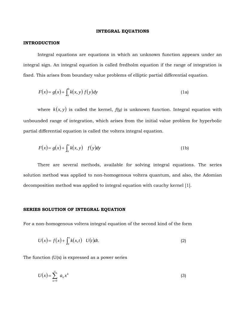
Integral equations are equations in which an unknown function appears under an

integral sign. An integral equation is called fredholm equation if the range of integration is

fixed. This arises from boundary value problems of elliptic partial differential equation.

b

adyyfyxkxgxF , (1a)

where yxk , is called the kernel, f(y) is unknown function. Integral equation with

unbounded range of integration, which arises from the initial value problem for hyperbolic

partial differential equation is called the voltera integral equation.

x

adyyfyxkxgxF , (1b)

There are several methods, available for solving integral equations. The series

solution method was applied to non-homogenous voltera quantum, and also, the Adomian

decomposition method was applied to integral equation with cauchy kernel [1].

SERIES SOLUTION OF INTEGRAL EQUATION

For a non-homogenous voltera integral equation of the second kind of the form

x

adttUtxkxfxU ., (2)

The function (U(x) is expressed as a power series

k

k

u

xaxU

0

(3)

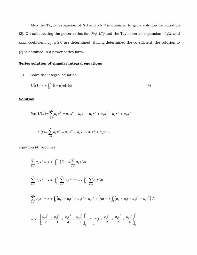
Also the Taylor expansion of f(x) and k(x,t) is obtained to get a solution for equation

(2). On substituting the power series for U(x), U(t) and the Taylor series expansion of f(x) and

k(x,t) coefficient 0, kak are determined. Having determined the co-efficient, the solution to

(2) is obtained in a power series form.

Series solution of singular integral equations

1.1 Solve the integral equation

dttuutxtUx

0 (4)

Solution

Put 5

5

4

4

3

3

2

2

1

1

0

0

0

xaxaxaxaxaxaxaxUk

k

k

3

3

2

2

1

1

0

0

0

xaxaxaxaxatUk

k

k

equation (4) becomes

0

00 k

k

k

x

k

k

k dtxaxExxa

0

00

1

00 k

k

k

x

k

k

k

x

k

k

k dttaxdttaxxa

xx

k

k

k dttatataaxdttatatataxxa0

3

3

2

2100

4

3

3

2

2

10

0

xx

tatatatax

tatatatax

0

4

3

3

2

2

10

0

5

3

4

2

3

1

2

0

4325432

4325432

4

3

3

2

2

10

5

3

4

2

3

1

2

0 tatatatax

tatatatax

5334223112

0

0

4534232x

aax

aax

aaxa

ax

201262

5

3

4

2

3

1

2

05

5

4

4

3

3

2

2

1

1

0

0

xaxaxaxaxxaxaxaxaxaxa

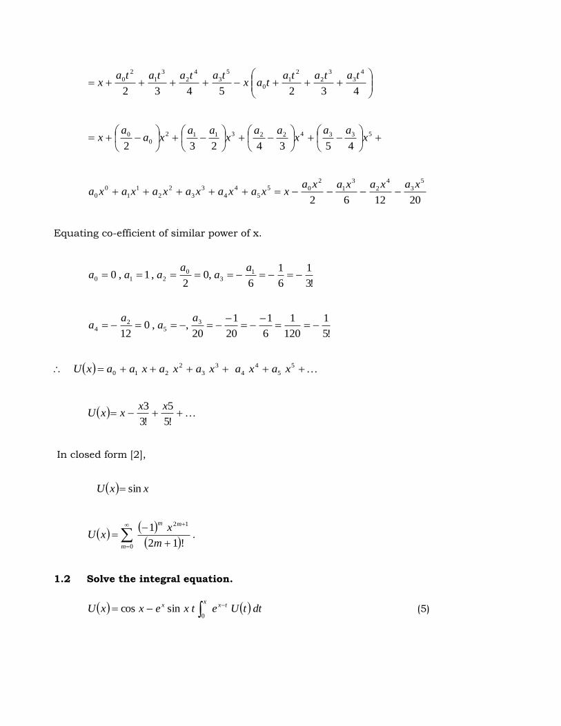
Equating co-efficient of similar power of x.

!3

1

6

1

6,0

2,1,0 1

3

0

210 a

aa

aaa

!5

1

120

1

6

1

20

1

20,,0

12

3

52

4

a

aa

a

5

5

4

4

3

3

2

210 xaxaxaxaxaaxU

!5

5

!3

3 xxxxU

In closed form [2],

xxU sin

0

12

!12

1

m

mm

m

xxU .

1.2 Solve the integral equation.

dttUetxexxU txx

x

0

sincos (5)

4

4

3

3

2

210

0

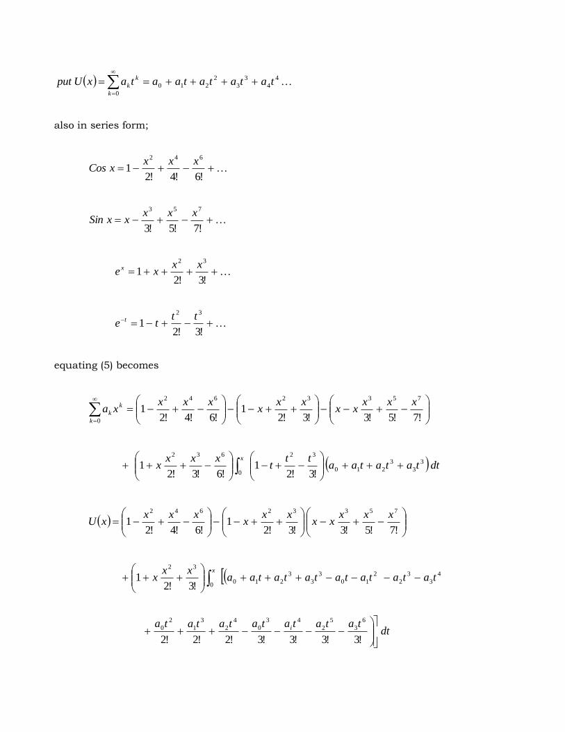
tatatataataxUputk

k

k

also in series form;

!6!4!2

1642 xxx

xCos

!7!5!3

753 xxxxxSin

!3!2

132 xx

xe x

!3!21

32 ttte t

equating (5) becomes

!7!5!3!3!21

!6!4!21

75332642

0

xxxxx

xxx

xxxxa

k

k

k

dttatataatt

txxx

xx

3

3

3

210

32

0

632

!3!21

!6!3!21

!7!5!3!3!21

!6!4!21

75332642 xxxxx

xxx

xxxxU

dttatatatatatata

tatatatatatataaxx

x

i

x

!3!3!3!3!2!2!2

!3!21

6

3

5

2

43

0

4

2

3

1

2

0

4

3

3

2

2

10

3

3

3

2100

32

!7!5!3!3!21

!6!4!21

75332642 xxxxx

xxx

xxxxU

dttaa

aa

ta

aataaaxx

xx

30133

20

120100

32

!3!2

!2!3!21

!7!5!3!3!21

!6!4!21

75332642 xxxxx

xxx

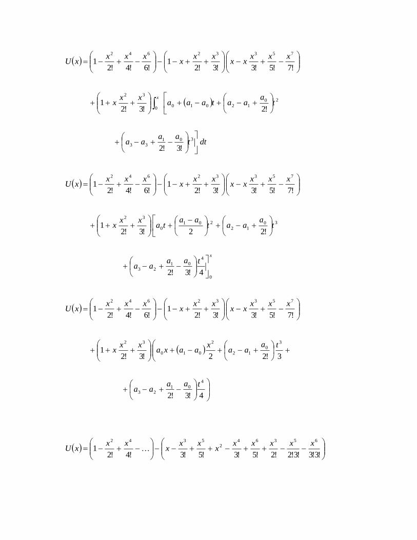
xxxxU

x

taaaa

ta

aataa

taxx

x

0

4

0123

30

12

201

0

32

4!3!2

!22!3!21

!7!5!3!3!21

!6!4!21

75332642 xxxxx

xxx

xxxxU

4!3!2

3!22!3!21

4

0123

3

0

12

2

010

32

taaaa

taaa

xaaxa

xxx

!3!3!3!2!2!5!3!5!3!4!21

653642

5342 xxxxxx

xxx

xxxU

4!3!23!22

4

0123

3

0

12

2

010

taaaa

taaa

xaaxa

643!222

6

0

4

01

4

0

12

3

0

3

01

2

0

uataa

taaa

xaxaaxa

4012300

2

201

0

342

224261246

2

23!4!21

aaaaaaa

xaa

xax

xxxx

xU

40123

3011201

0

24

1

2426124

3

1

6

21

2

1

211

xaaaa

xaaa

xaa

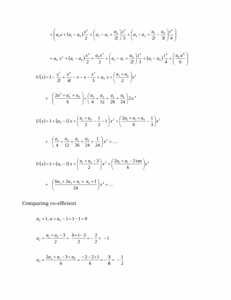
xaxU

40133

311201

0

24

126

6

tan22

2

311

xaaaa

xaa

xaa

xaxU

Comparing co-efficient

0111,1 00 aaa

12

2

2

310

2

301

2

aa

a

2

1

6

3

6

122

6

32 012

3

aaaa

8

1

24

11023

24

126 0123

4

aaaa

a

821

432

4

4

3

3

2

210

xxxxU

tatataxaaxU

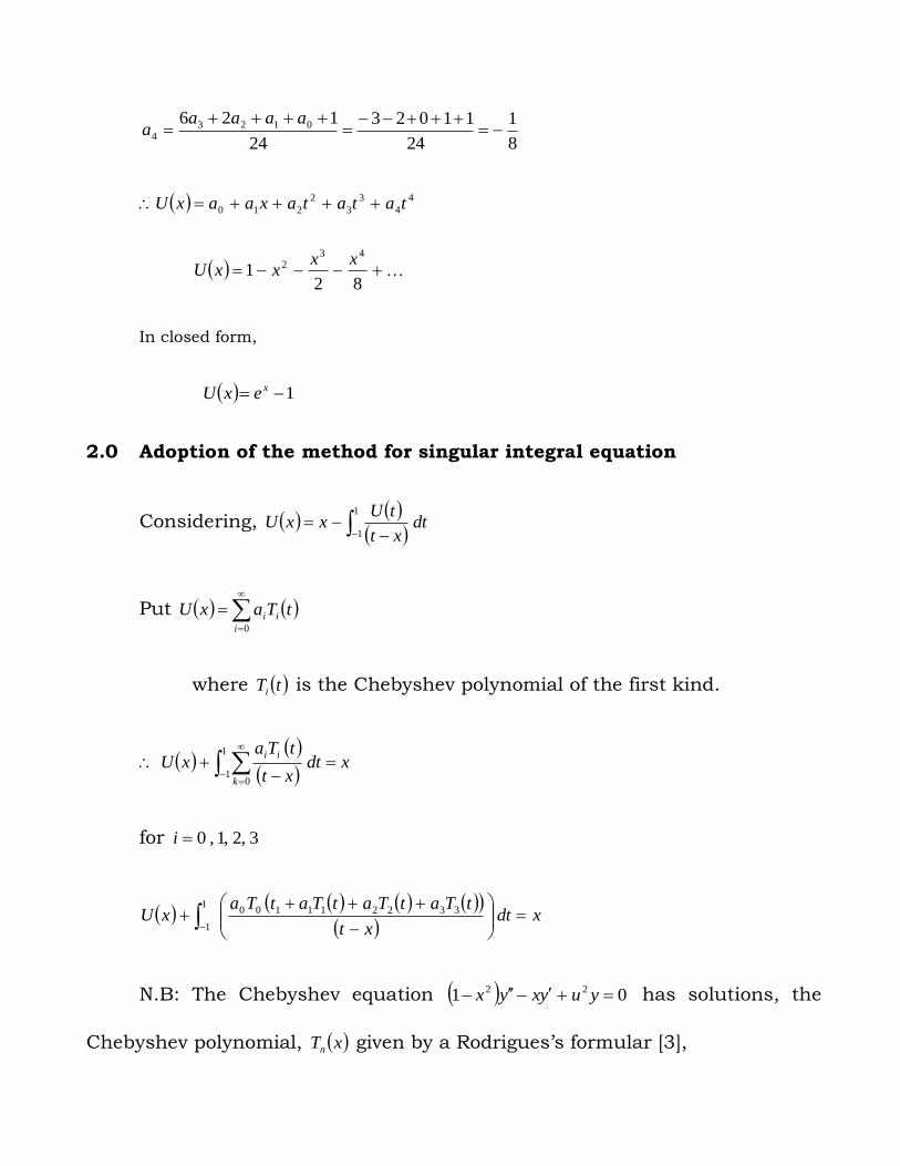
In closed form,

1 xexU

2.0 Adoption of the method for singular integral equation

Considering,

1

1dt

xt

tUxxU

Put

0i

ii tTaxU

where tTi is the Chebyshev polynomial of the first kind.

1

10

xdtxt

tTaxU

k

ii

for 3,2,1,0i

xdtxt

tTatTatTatTaxU

3322111001

1

N.B: The Chebyshev equation 01 22 yuyxyx has solutions, the

Chebyshev polynomial, xTn given by a Rodrigues’s formular [3],

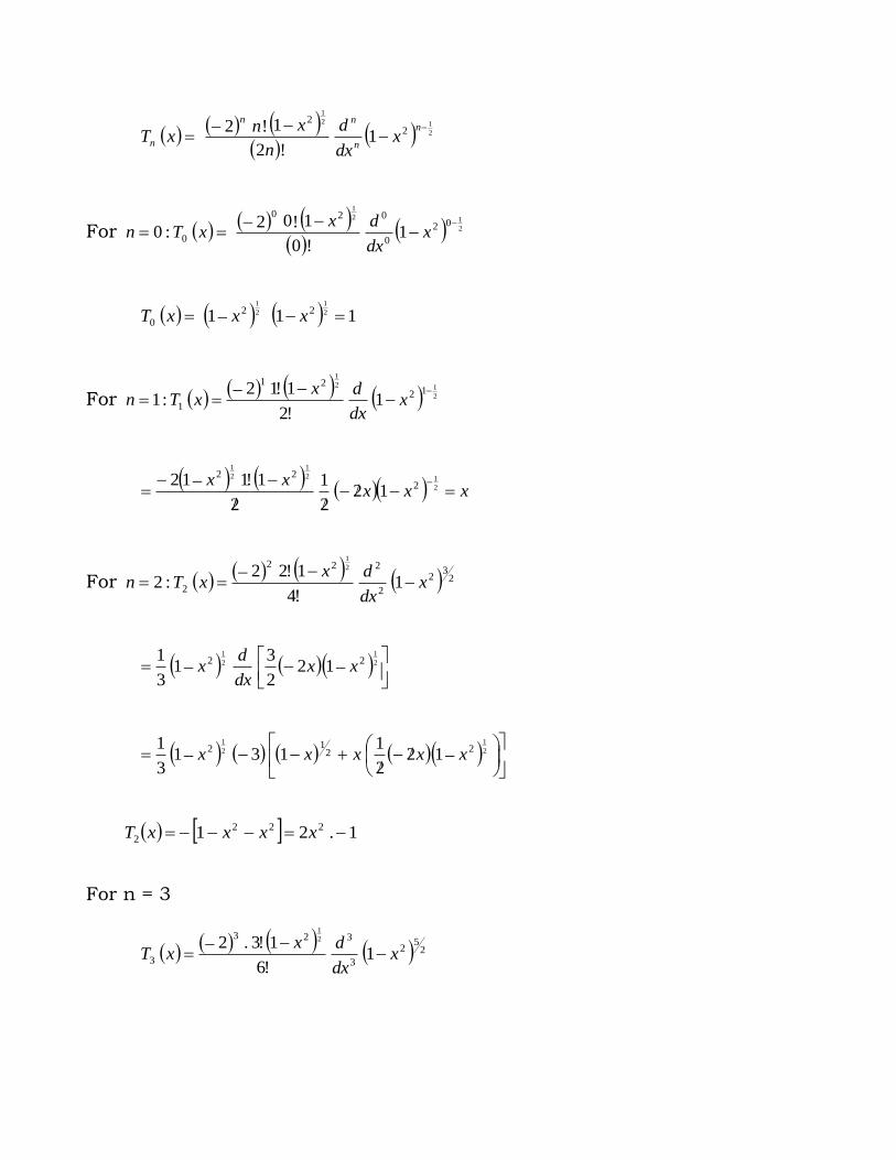
2

12

1

22

1!2

1!2

n

n

nn

n xdx

d

n

xnxT

For

2

12

1

02

0

020

0 1!0

1!02:0

x

dx

dxxTn

111 2

1

2

122

0 xxxT

For 2

12

1

1221

1 1!2

1!12:1

x

dx

dxxTn

xxxxx

2

12

1

2

1

222

122

1

2

1!112

For 23

2

2

222

2 1!4

1!22:2

2

1

xdx

dxxTn

2

1

2

122 12

2

31

3

1xx

dx

dx

2

1

2

122

12 122

1131

3

1xxxxx

1.21 222

2 xxxxT

For n = 3

25

2

3

323

3 1!6

1!3.2 2

1

xdx

dxxT

2

32

2

22 12

2

51

15

12

1

xxdx

dx

2

1

2

122

322 12

2

3.11

3

1xxxx

dx

dx

2

1

2

1

2

1222

1222 12

2

1..123212.

2

31

3

1xxxxxxx

2

1

2

1

2

12322

122 11211 xxxxxxx

322

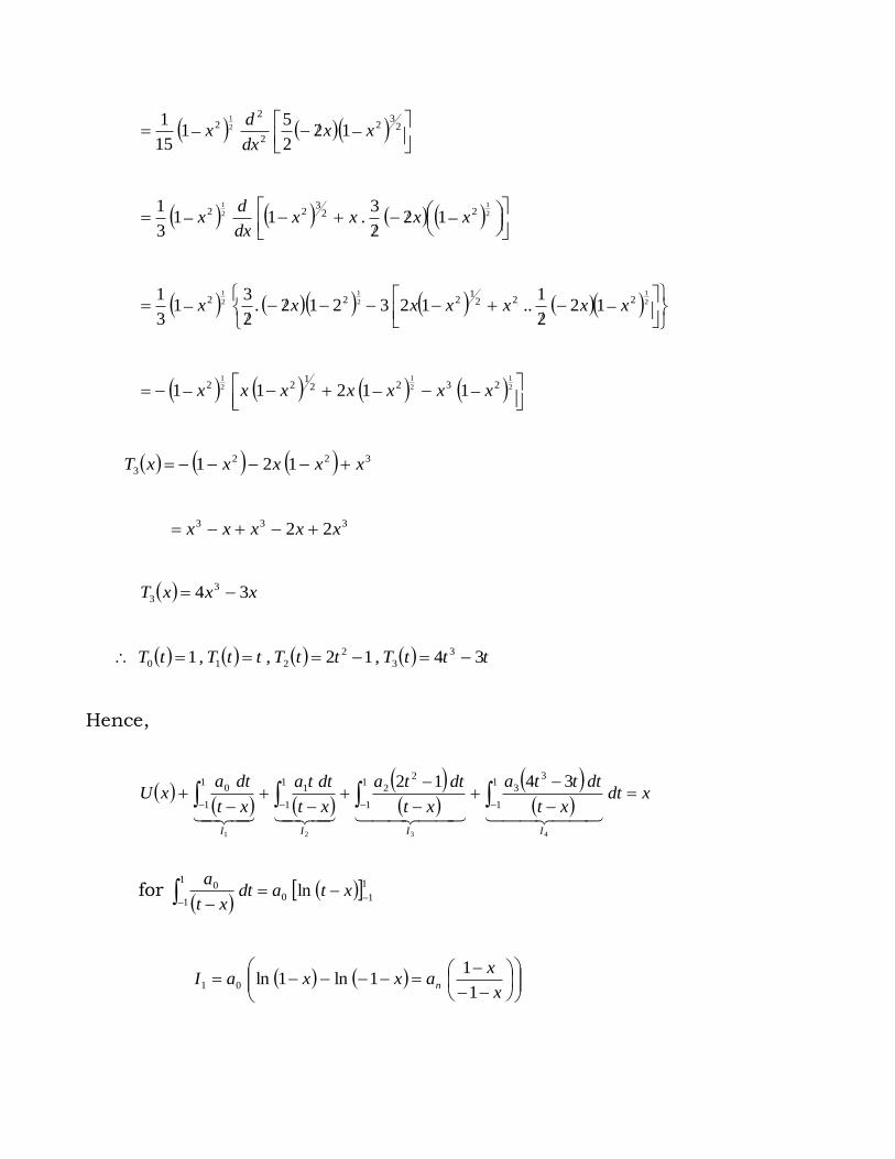
3 121 xxxxxT

333 22 xxxxx

xxxT 34 3

3

tttTttTttTtT 34,12,,1 3

3

2

210

Hence,

xdtxt

dttta

xt

dtta

xt

dtta

xt

dtaxU

IIII

4321

1

1

3

31

1

2

21

1

11

1

0 3412

for

11

1

10

0 ln

xtadtxt

a

x

xaxxaI n

1

11ln1ln01

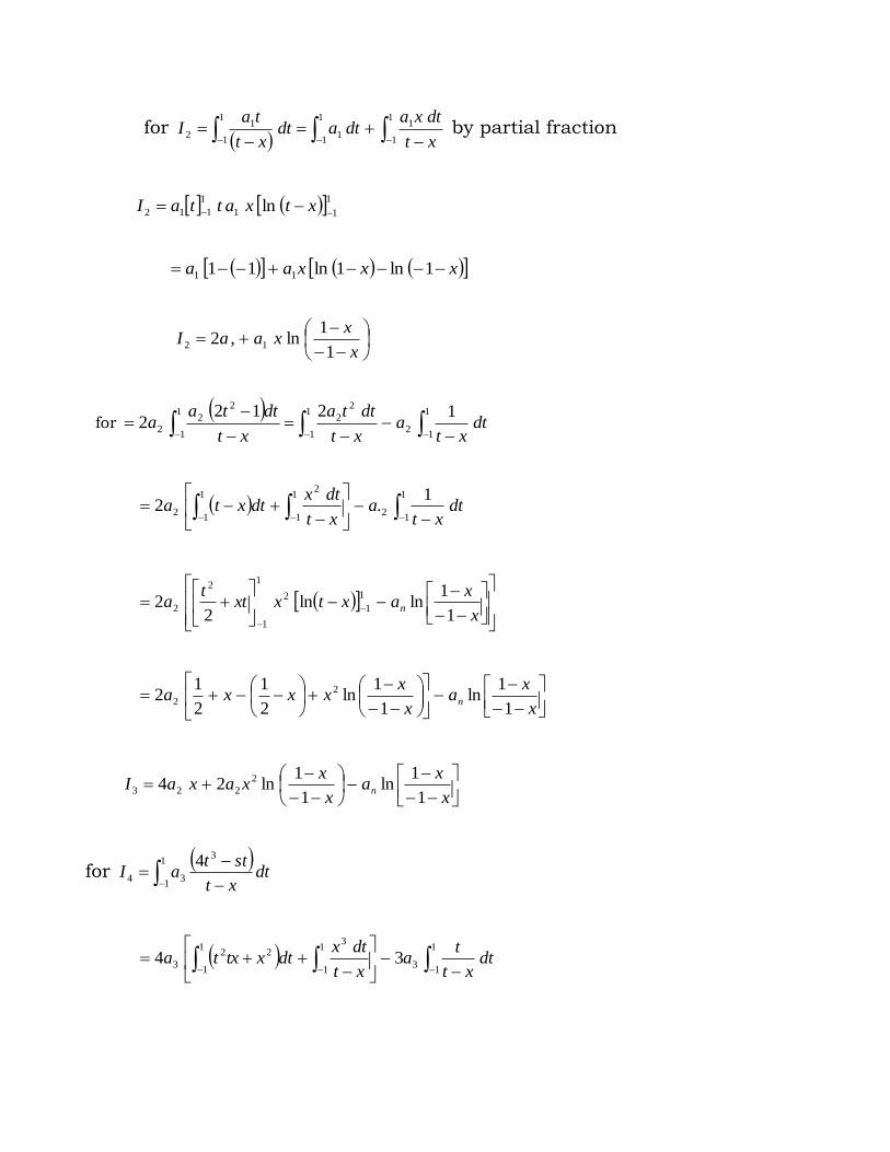
for

1

1

11

1

1

11

12

xt

dtxadtadt

xt

taI by partial fraction

111

1

112 ln xtxattaI

xxxaa 1ln1ln11 11

x

xxaaI

1

1ln,2 12

for

dtxt

axt

dtta

xt

dttaa

1

12

1

1

2

21

1

2

22

12122

dtxt

axt

dtxdtxta

1

12

1

1

21

12

1.2

x

xaxtxxt

ta n

1

1lnln

22

1

1

2

1

1

2

2

x

xa

x

xxxxa n

1

1ln

1

1ln

2

1

2

12 2

2

x

xa

x

xxaxaI n

1

1ln

1

1ln24 2

223

for

dtxt

sttaI

31

134

4

dtxt

ta

xt

dtxdtxtxta

1

13

1

1

31

1

22

3 34

x

xxha

x

xxtx

tta

1

123

1

1ln

334 3

3

1

1

223

3

x

xxaa

x

xaxx

xx

xa

1

1ln36

1

1ln4

23

1

23

14 333

322

3

x

xxaa

x

xaxxaI

1

1ln36

1

1ln42

3

24 333

32

34

x

xxaa

x

xaxxa

aI

1

1ln36

1

1ln48

3

8333

32

33

4

x

xxaxa

x

xxaa

x

xaxU

1

1ln24

1

1ln2

1

1ln 2

22110

xx

xxaa

x

xaxxa

a

x

xa

1

1ln36

1

1ln48

3

8

1

1ln 233

32

33

2

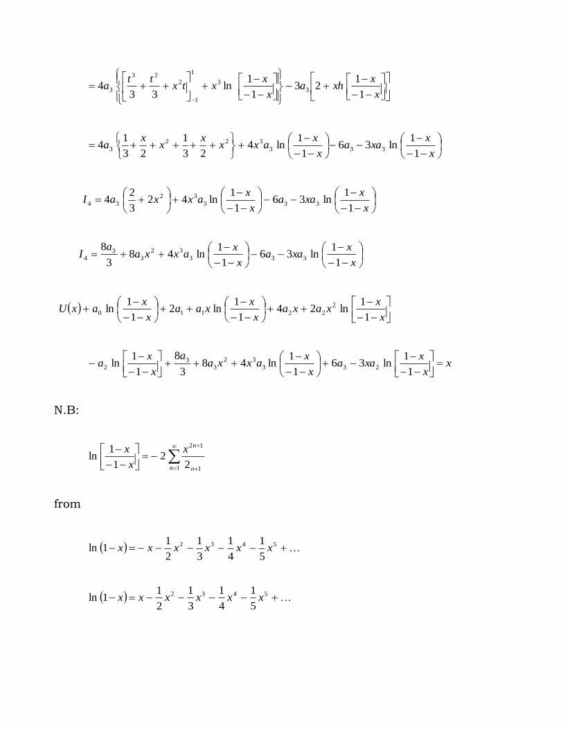
N.B:

1 1

12

22

1

1ln

n n

nx

x

x

from

5432

5

1

4

1

3

1

2

11ln xxxxxx

5432

5

1

4

1

3

1

2

11ln xxxxxx

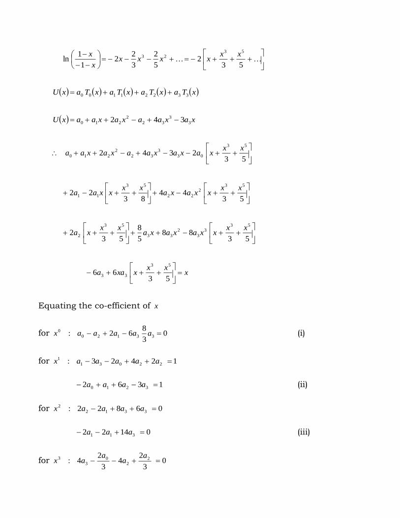
532

5

2

3

22

1

1ln

5323 xx

xxxxx

x

xTaxTaxTaxTaxU 33221100

xaxaaxaxaaxU 3

3

32

2

210 342

532342

53

03

3

32

2

210

xxxaxaxaaxaxaa

5344

8322

532

22

53

11

xxxxaxa

xxxxaa

5388

5

8

532

533

3

2

33

53

2

xxxxaxaxa

xxxa

xxx

xxaa

5366

53

33

Equating the co-efficient of x

for 03

862: 33120

0 aaaaax (i)

for 12423: 22031

1 aaaaax

1362 3210 aaaa (ii)

for 06822: 3312

2 aaaax

01422 311 aaa (iii)

for 03

24

3

24: 2

2

0

3

3 a

aa

ax

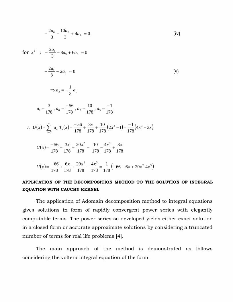
043

10

3

23

20 aaa

(iv)

for 0683

2: 33

14 aaa

x

023

23

1 aa

(v)

133

1aa

178

1,

178

10,

178

56,

178

33201

aaaa

xxxx

xTaxU nn

n

34178

112

178

10

178

3

178

56 32

0

178

3

178

4

178

10

178

20

178

3

178

56 32 xxxxxU

3232

4.20666178

1

178

4

178

20

178

6

178

66xxx

xxxxU

APPLICATION OF THE DECOMPOSITION METHOD TO THE SOLUTION OF INTEGRAL

EQUATION WITH CAUCHY KERNEL

The application of Adomain decomposition method to integral equations

gives solutions in form of rapidly convergent power series with elegantly

computable terms. The power series so developed yields either exact solution

in a closed form or accurate approximate solutions by considering a truncated

number of terms for real life problems [4].

The main approach of the method is demonstrated as follows

considering the voltera integral equation of the form.

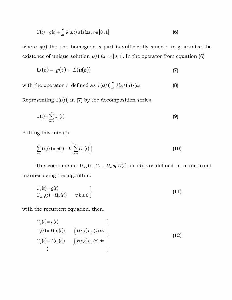
1,0,,0

tdssutsktgtUt

(6)

where tg the non homogenous part is sufficiently smooth to guarantee the

existence of unique solution 1,0tfortu . In the operator from equation (6)

tuLtgtU (7)

with the operator L defined as dssutsktuLt

,0 (8)

Representing tuL in (7) by the decomposition series

0n

n tUtU (9)

Putting this into (7)

00 n

n

n

n tULtgtU (10)

The components tUofUUUU n210 ,, in (9) are defined in a recurrent

manner using the algorithm.

01

0

ktuLtU

tgtU

K

(11)

with the recurrent equation, then.

t

t

dssutsktuLtU

dssutsktuLtU

tgtU

0112

0001

0

)(,

)(, (12)

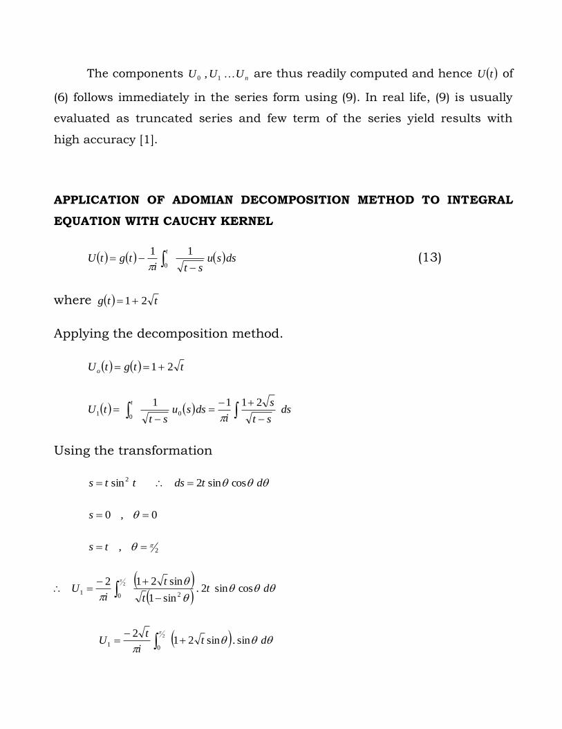
The components nUUU 10 , are thus readily computed and hence tU of

(6) follows immediately in the series form using (9). In real life, (9) is usually

evaluated as truncated series and few term of the series yield results with

high accuracy [1].

APPLICATION OF ADOMIAN DECOMPOSITION METHOD TO INTEGRAL

EQUATION WITH CAUCHY KERNEL

dssusti

tgtUt

11

0 (13)

where ttg 21

Applying the decomposition method.

ttgtUo 21

dsst

s

idssu

sttU

t

21110

01

Using the transformation

dtdstts cossin2sin 2

0,0 s

2, ts

dtt

t

iU cossin2.

sin1

sin21220

1

2

dti

tU sin.sin21

2 2

01

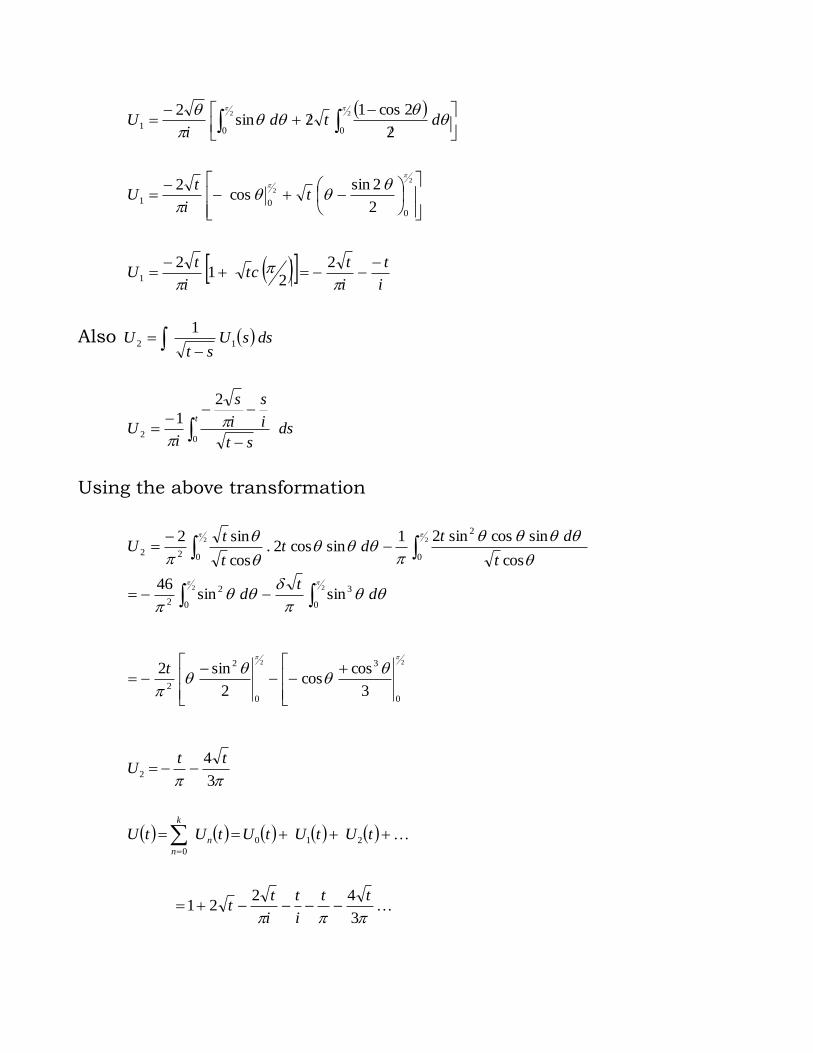
dtdi

U22

001

2

2cos12sin

2

2

2

001

2

2sincos

2

t

i

tU

i

t

i

tct

i

tU

2

21

21

Also dssUst

U 12

1

dsst

i

s

i

s

iU

t

0

2

2

1

Using the above transformation

22

0

2

022cos

sincossin21sincos2.

cos

sin2

t

dtdt

t

tU

22

0

3

0

2

2sinsin

46

d

td

22

0

3

0

2

2 3

coscos

2

sin2

t

3

42

ttU

tUtUtUtUtU n

k

n

210

0

3

4221

tt

i

t

i

tt

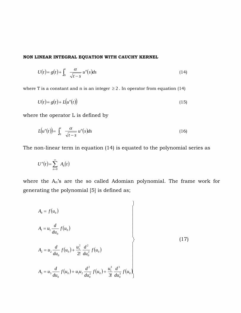
NON LINEAR INTEGRAL EQUATION WITH CAUCHY KERNEL

dssust

tgtU nt

0

(14)

where T is a constant and n is an integer 2 . In operator from equation (14)

tuLtgtU n (15)

where the operator L is defined by

dssust

tuL nt

n

0

(16)

The non-linear term in equation (14) is equated to the polynomial series as

tAtU n

n

n

0

where the An’s are the so called Adomian polynomial. The frame work for

generating the polynomial [5] is defined as;

03

0

33

102

0

2

210

0

33

02

0

22

10

0

22

0

0

11

00

!3

!2

ufdu

duuf

du

duuuf

du

duA

ufdu

duuf

du

duA

ufdu

duA

ufA

(17)

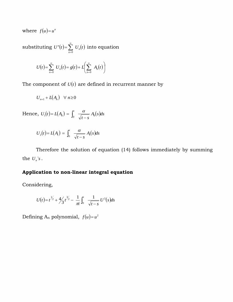
where nuuf

substituting tUtU n

n

n

0

into equation

tALtgtUtU n

n

n

n 00

The component of tU are defined in recurrent manner by

01 nALU nn

Hence, dssAst

ALtUt

00

01

dssAst

ALtUt

10

12

Therefore the solution of equation (14) follows immediately by summing

the sUn` .

Application to non-linear integral equation

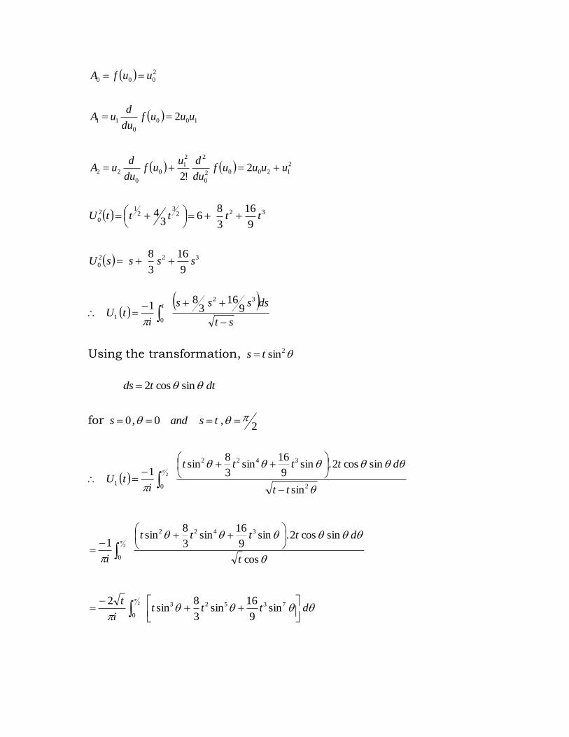
Considering,

dssUsti

tttUt

2

0

23

21 11

34

Defining An polynomial, 2uuf

2

12002

0

22

10

0

22

100

0

11

2

000

2!2

2

uuuufdu

duuf

du

duA

uuufdu

duA

uufA

3223

21

2

09

16

3

86

34 tttttU

322

09

16

3

8ssssU

st

dssss

itU

t

32

01

916

38

1

Using the transformation, 2sints

dttds sincos2

for 2

,0,0 tsands

2

3422

01

sin

sincos2.sin9

16sin

3

8sin

1 2

tt

dtttt

itU

cos

sincos2.sin9

16sin

3

8sin

1

3422

0

2

t

dtttt

i

dttti

t

73523

0sin

9

16sin

3

8sin

2 2

2 22

0 0

735

0

23 sin9

16sin

3

8sin

2

dttttti

ttU

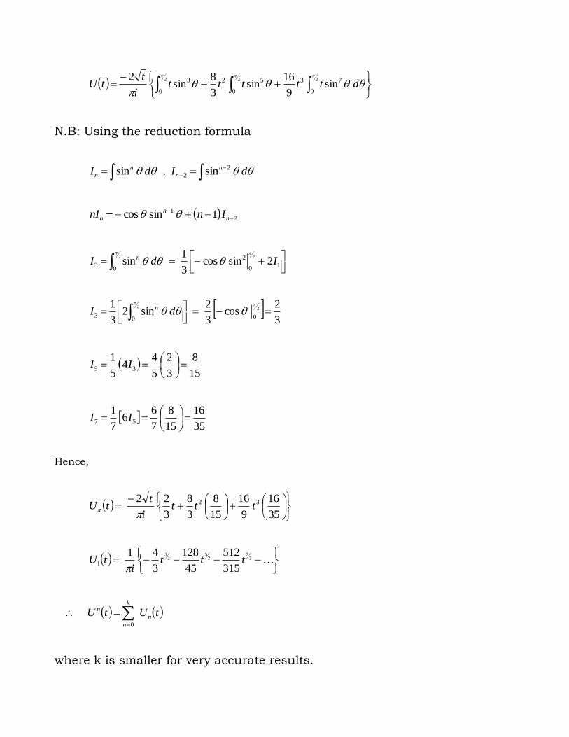
N.B: Using the reduction formula

dIdI n

n

n

n

2

2 sin,sin

2

1 1sincos

n

n

n InnI

1

0

2

03 2sincos

3

1sin

22

IdI n

3

2cos

3

2sin2

3

122

003

dI n

15

8

3

2

5

44

5

135

II

35

16

15

8

7

66

7

157

II

Hence,

35

16

9

16

15

8

3

8

3

22 32 ttti

ttU

27

25

23

315

512

45

128

3

411 ttt

itU

tUtU n

k

n

n

0

where k is smaller for very accurate results.

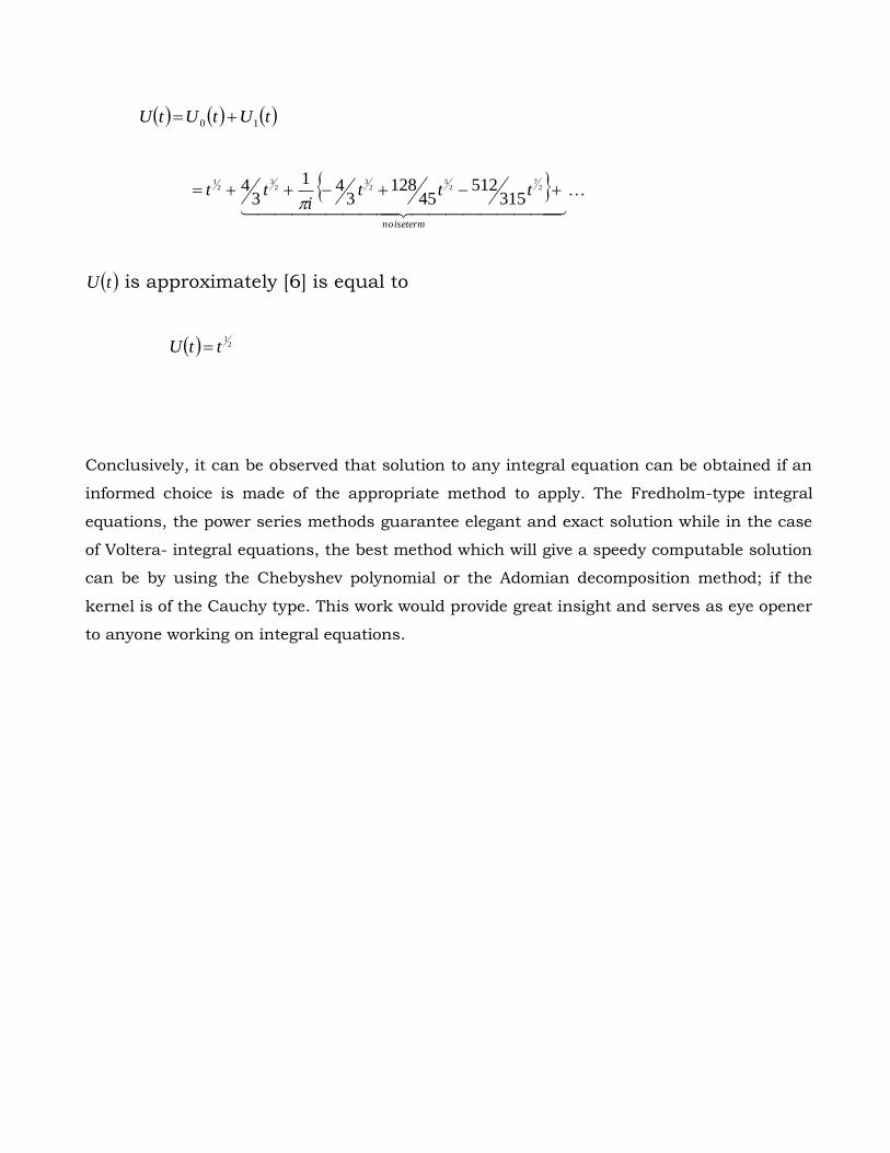
tUtUtU 10

termnoise

ttti

tt 27

25

23

23

21

315512

45128

341

34

tU is approximately [6] is equal to

21

ttU

Conclusively, it can be observed that solution to any integral equation can be obtained if an

informed choice is made of the appropriate method to apply. The Fredholm-type integral

equations, the power series methods guarantee elegant and exact solution while in the case

of Voltera- integral equations, the best method which will give a speedy computable solution

can be by using the Chebyshev polynomial or the Adomian decomposition method; if the

kernel is of the Cauchy type. This work would provide great insight and serves as eye opener

to anyone working on integral equations.

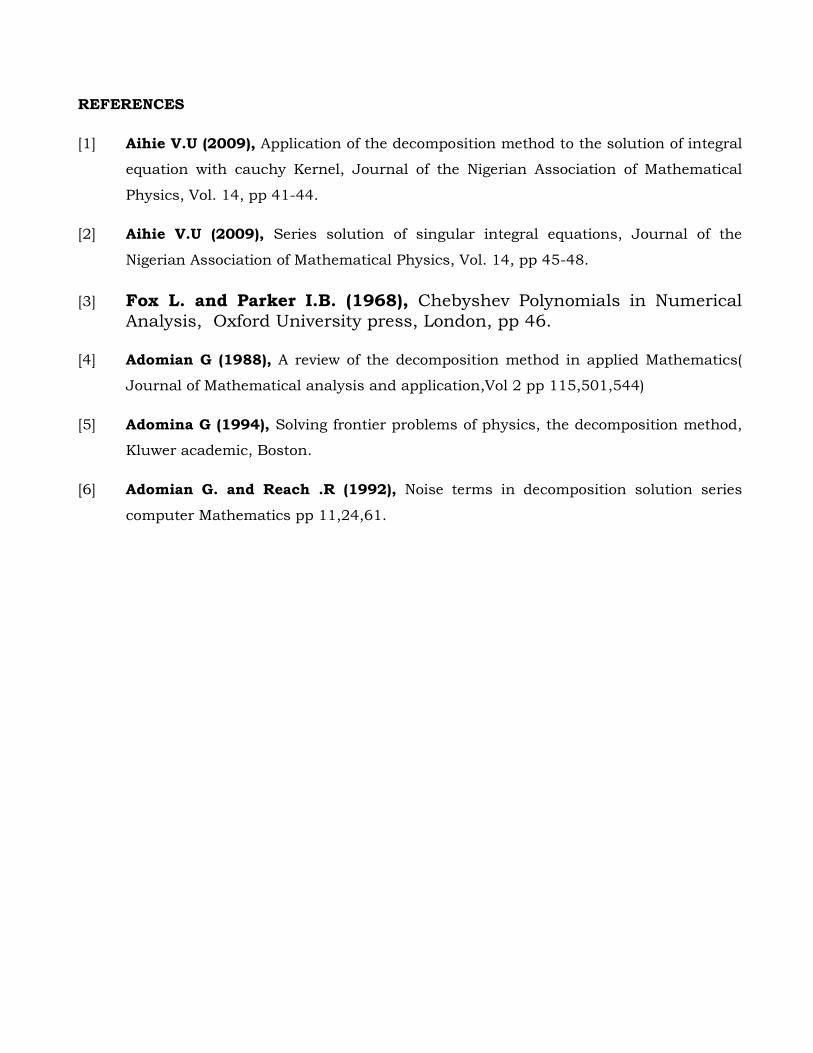
REFERENCES

[1] Aihie V.U (2009), Application of the decomposition method to the solution of integral

equation with cauchy Kernel, Journal of the Nigerian Association of Mathematical

Physics, Vol. 14, pp 41-44.

[2] Aihie V.U (2009), Series solution of singular integral equations, Journal of the

Nigerian Association of Mathematical Physics, Vol. 14, pp 45-48.

[3] Fox L. and Parker I.B. (1968), Chebyshev Polynomials in Numerical

Analysis, Oxford University press, London, pp 46. [4] Adomian G (1988), A review of the decomposition method in applied Mathematics(

Journal of Mathematical analysis and application,Vol 2 pp 115,501,544)

[5] Adomina G (1994), Solving frontier problems of physics, the decomposition method,

Kluwer academic, Boston.

[6] Adomian G. and Reach .R (1992), Noise terms in decomposition solution series

computer Mathematics pp 11,24,61.

PART2: GEOPHYSICAL PROBLEM

STATEMENT OF PROBLEM:

To deduce the application and correlation of Bessel functions to the potential

and resistivity obtained by vertical electrical sounding of n-layered earth. To

show that the derived potentials and resistivity using mathematical analysis

correlates with the experimental results obtained by the Egbai (2002), Asokia

et al (2001) as well as Asokia et al (2002).

1.0 INTRODUCTION

This is a dissertation to derive the potential, resistivity transform and

apparent resistivity of a stratified earth as used in the published papers of

Egbai (2002), Asokia et al (2001) and Asokhia et al (2002). To start with, it is

necessary to explain resistivity.

Electrical resistivity also called specific electrical resistance is the repulsion of

a current within a circuit. It explains the relationship between voltage

(amount of electrical pressure) and ampere (amount of electrical current). The

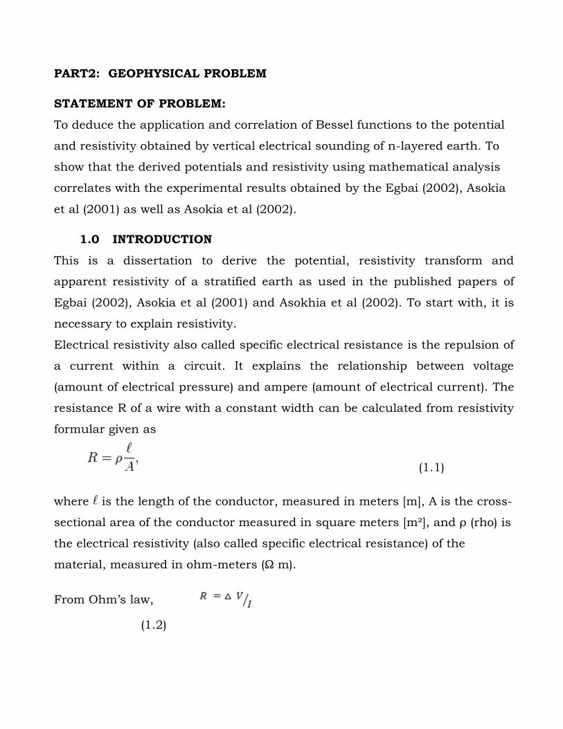
resistance R of a wire with a constant width can be calculated from resistivity

formular given as

(1.1)

where is the length of the conductor, measured in meters [m], A is the cross-

sectional area of the conductor measured in square meters [m²], and ρ (rho) is

the electrical resistivity (also called specific electrical resistance) of the

material, measured in ohm-meters (Ω m).

From Ohm’s law,

(1.2)

Where

= Potential difference across sample (V )

= Electric current through the sample (A)

Equating equations (1.1) and (1.2), we obtain

· (1.3)

From (1.3) above, we obtain

(1.4)

Where;

E = Electric field (V/m)

j = Current density (A/m2)

σ = conductivity (S)

2.0 THE POINT SOURCE ON A STRATIFIED EARTH.

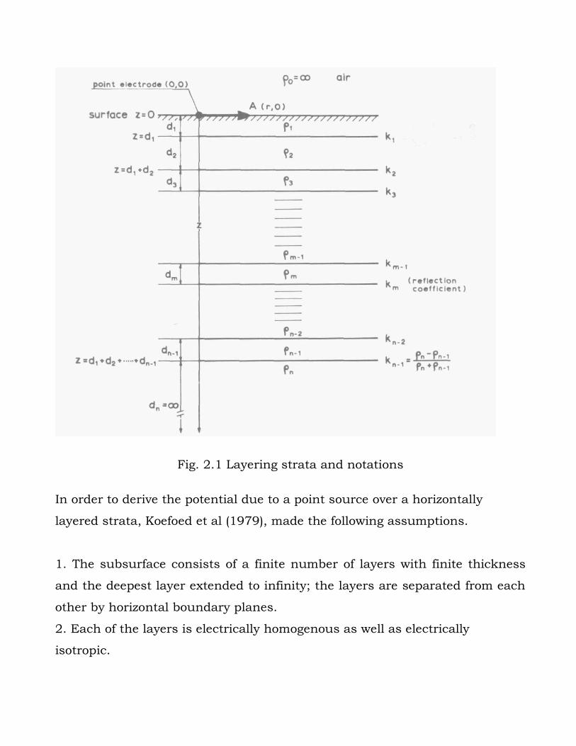
Fig. 2.1 Layering strata and notations

In order to derive the potential due to a point source over a horizontally

layered strata, Koefoed et al (1979), made the following assumptions.

1. The subsurface consists of a finite number of layers with finite thickness

and the deepest layer extended to infinity; the layers are separated from each

other by horizontal boundary planes.

2. Each of the layers is electrically homogenous as well as electrically

isotropic.

3. The field is generated by a current source that is located at the surface of

the earth.

4. The current emitted by the source is direct current.

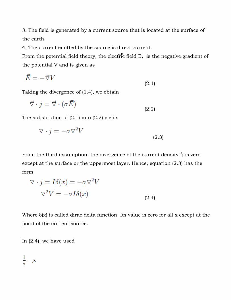
From the potential field theory, the electric field E, is the negative gradient of

the potential V and is given as

(2.1)

Taking the divergence of (1.4), we obtain

(2.2)

The substitution of (2.1) into (2.2) yields

(2.3)

From the third assumption, the divergence of the current density j is zero

except at the surface or the uppermost layer. Hence, equation (2.3) has the

form

(2.4)

Where δ(x) is called dirac delta function. Its value is zero for all x except at the

point of the current source.

In (2.4), we have used

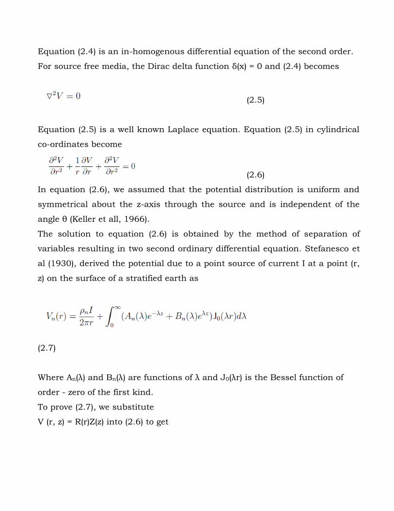
Equation (2.4) is an in-homogenous differential equation of the second order.

For source free media, the Dirac delta function δ(x) = 0 and (2.4) becomes

(2.5)

Equation (2.5) is a well known Laplace equation. Equation (2.5) in cylindrical

co-ordinates become

(2.6)

In equation (2.6), we assumed that the potential distribution is uniform and

symmetrical about the z-axis through the source and is independent of the

angle θ (Keller et all, 1966).

The solution to equation (2.6) is obtained by the method of separation of

variables resulting in two second ordinary differential equation. Stefanesco et

al (1930), derived the potential due to a point source of current I at a point (r,

z) on the surface of a stratified earth as

(2.7)

Where An(λ) and Bn(λ) are functions of λ and J0(λr) is the Bessel function of

order - zero of the first kind.

To prove (2.7), we substitute

V (r, z) = R(r)Z(z) into (2.6) to get

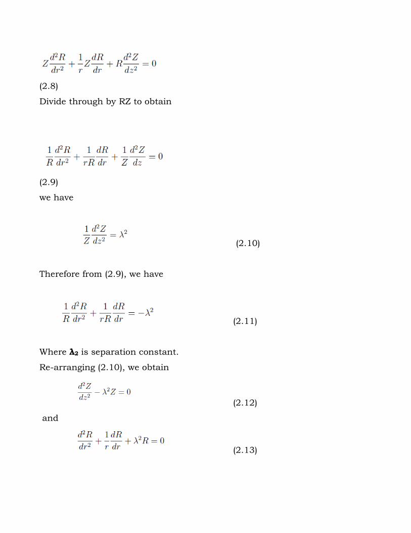
(2.8)

Divide through by RZ to obtain

(2.9)

we have

(2.10)

Therefore from (2.9), we have

(2.11)

Where λ2 is separation constant.

Re-arranging (2.10), we obtain

(2.12)

and

(2.13)

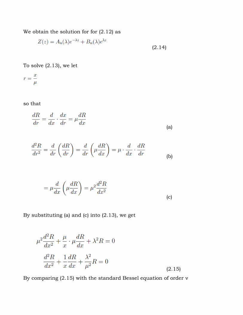
We obtain the solution for for (2.12) as

(2.14)

To solve (2.13), we let

so that

(a)

(b)

(c)

By substituting (a) and (c) into (2.13), we get

(2.15)

By comparing (2.15) with the standard Bessel equation of order ν

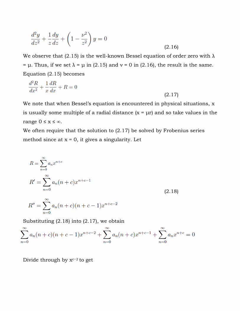
(2.16)

We observe that (2.15) is the well-known Bessel equation of order zero with λ

= μ. Thus, if we set λ = μ in (2.15) and ν = 0 in (2.16), the result is the same.

Equation (2.15) becomes

(2.17)

We note that when Bessel’s equation is encountered in physical situations, x

is usually some multiple of a radial distance (x = μr) and so take values in the

range 0 ≤ x ≤ ∞.

We often require that the solution to (2.17) be solved by Frobenius series

method since at x = 0, it gives a singularity. Let

(2.18)

Substituting (2.18) into (2.17), we obtain

Divide through by xc−2 to get

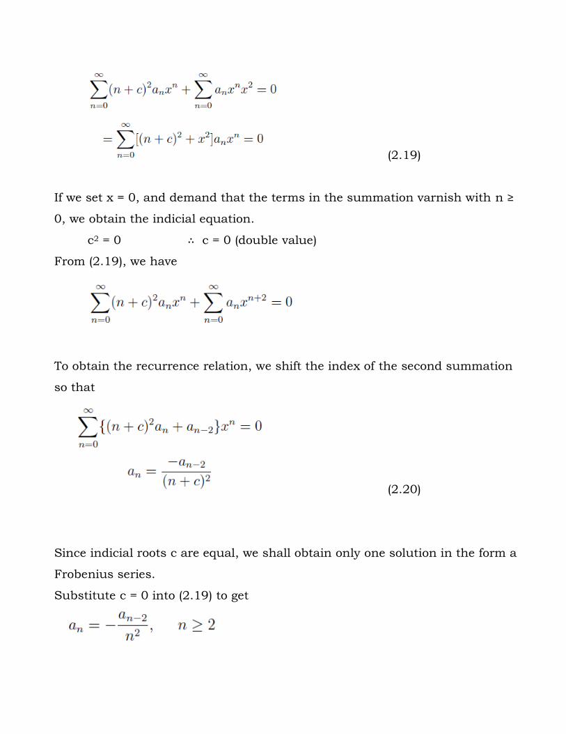
(2.19)

If we set x = 0, and demand that the terms in the summation varnish with n ≥

0, we obtain the indicial equation.

c2 = 0 ∴ c = 0 (double value)

From (2.19), we have

To obtain the recurrence relation, we shift the index of the second summation

so that

(2.20)

Since indicial roots c are equal, we shall obtain only one solution in the form a

Frobenius series.

Substitute c = 0 into (2.19) to get

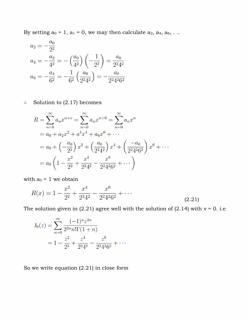
By setting a0 = 1, a1 = 0, we may then calculate a2, a4, a6, . ..

∴ Solution to (2.17) becomes

with a0 = 1 we obtain

(2.21)

The solution given in (2.21) agree well with the solution of (2.14) with ν = 0. i.e

So we write equation (2.21) in close form

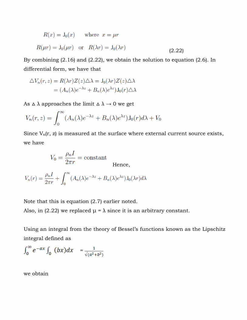
(2.22)

By combining (2.16) and (2.22), we obtain the solution to equation (2.6). In

differential form, we have that

As △ λ approaches the limit △ λ → 0 we get

Since Vn(r, z) is measured at the surface where external current source exists,

we have

Hence,

Note that this is equation (2.7) earlier noted.

Also, in (2.22) we replaced μ = λ since it is an arbitrary constant.

Using an integral from the theory of Bessel’s functions known as the Lipschitz

integral defined as

=

we obtain

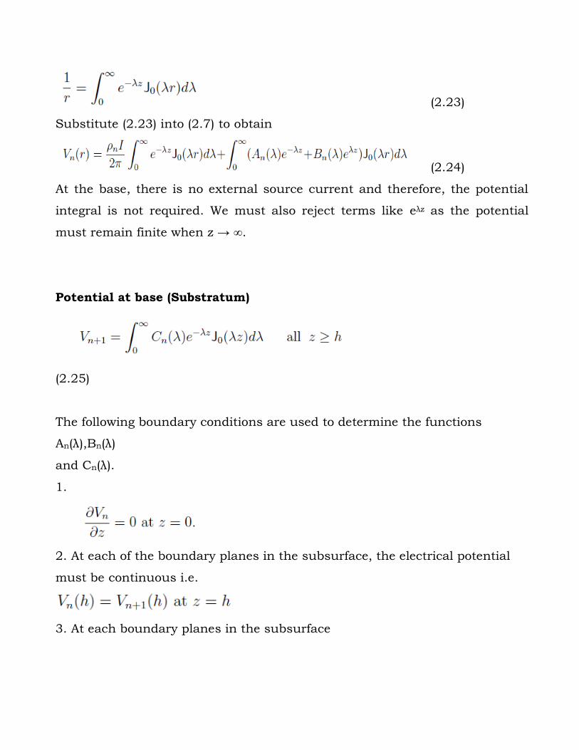
(2.23)

Substitute (2.23) into (2.7) to obtain

(2.24)

At the base, there is no external source current and therefore, the potential

integral is not required. We must also reject terms like eλz as the potential

must remain finite when z → ∞.

Potential at base (Substratum)

(2.25)

The following boundary conditions are used to determine the functions

An(λ),Bn(λ)

and Cn(λ).

1.

2. At each of the boundary planes in the subsurface, the electrical potential

must be continuous i.e.

3. At each boundary planes in the subsurface

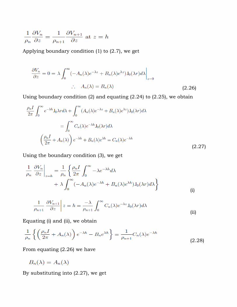
Applying boundary condition (1) to (2.7), we get

(2.26)

Using boundary condition (2) and equating (2.24) to (2.25), we obtain

(2.27)

Using the boundary condition (3), we get

(i)

(ii)

Equating (i) and (ii), we obtain

(2.28)

From equating (2.26) we have

By substituting into (2.27), we get

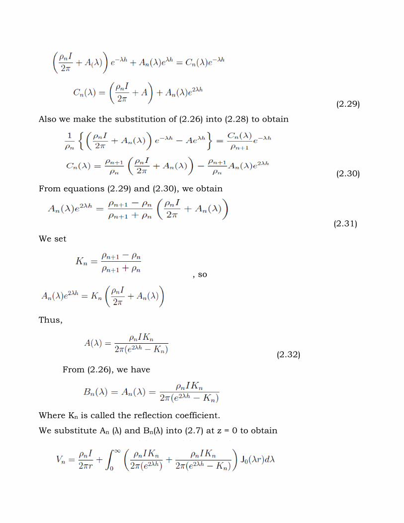
(2.29)

Also we make the substitution of (2.26) into (2.28) to obtain

(2.30)

From equations (2.29) and (2.30), we obtain

(2.31)

We set

, so

Thus,

(2.32)

From (2.26), we have

Where Kn is called the reflection coefficient.

We substitute An (λ) and Bn(λ) into (2.7) at z = 0 to obtain

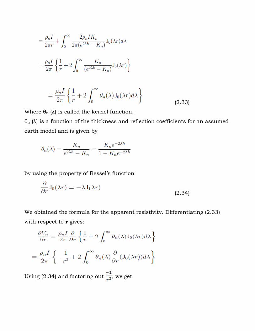
(2.33)

Where θn (λ) is called the kernel function.

θn (λ) is a function of the thickness and reflection coefficients for an assumed

earth model and is given by

by using the property of Bessel’s function

(2.34)

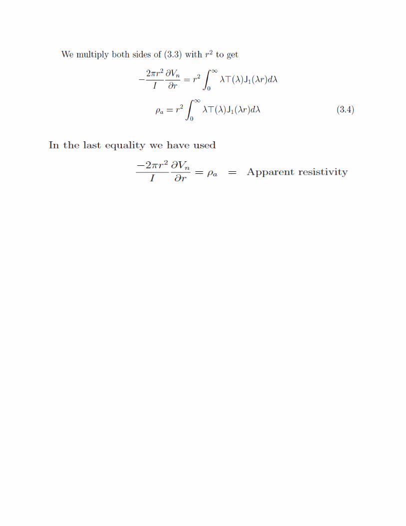
We obtained the formula for the apparent resistivity. Differentiating (2.33)

with respect to r gives:

Using (2.34) and factoring out , we get

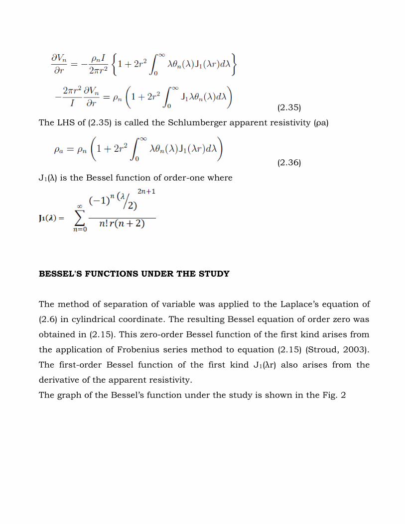
(2.35)

The LHS of (2.35) is called the Schlumberger apparent resistivity (ρa)

(2.36)

J1(λ) is the Bessel function of order-one where

BESSEL'S FUNCTIONS UNDER THE STUDY

The method of separation of variable was applied to the Laplace’s equation of

(2.6) in cylindrical coordinate. The resulting Bessel equation of order zero was

obtained in (2.15). This zero-order Bessel function of the first kind arises from

the application of Frobenius series method to equation (2.15) (Stroud, 2003).

The first-order Bessel function of the first kind J1(λr) also arises from the

derivative of the apparent resistivity.

The graph of the Bessel’s function under the study is shown in the Fig. 2

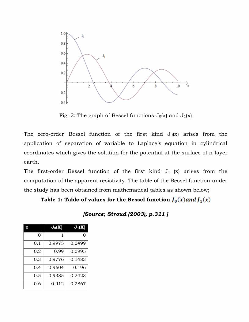
Fig. 2: The graph of Bessel functions J0(x) and J1(x)

The zero-order Bessel function of the first kind J0(x) arises from the

application of separation of variable to Laplace’s equation in cylindrical

coordinates which gives the solution for the potential at the surface of n-layer

earth.

The first-order Bessel function of the first kind J1 (x) arises from the

computation of the apparent resistivity. The table of the Bessel function under

the study has been obtained from mathematical tables as shown below;

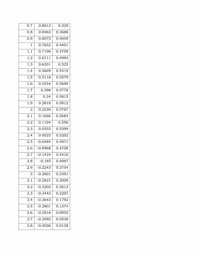
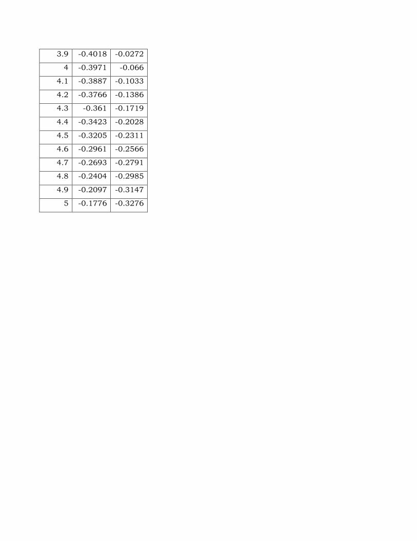
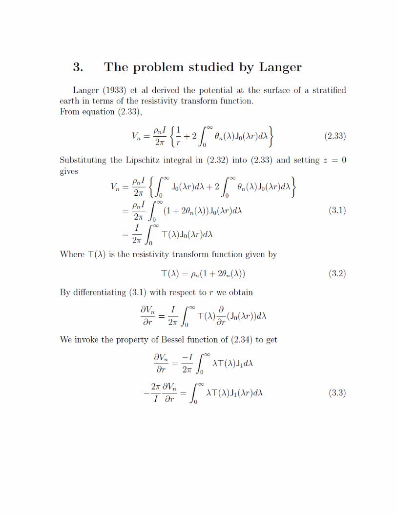
Table 1: Table of values for the Bessel function

[Source; Stroud (2003), p.311 ]

z J0(X) J1(X)

0 1 0

0.1 0.9975 0.0499

0.2 0.99 0.0995

0.3 0.9776 0.1483

0.4 0.9604 0.196

0.5 0.9385 0.2423

0.6 0.912 0.2867

0.7 0.8812 0.329

0.8 0.8463 0.3688

0.9 0.8075 0.4059

1 0.7652 0.4401

1.1 0.7196 0.4709

1.2 0.6711 0.4983

1.3 0.6201 0.522

1.4 0.5669 0.5419

1.5 0.5118 0.5579

1.6 0.4554 0.5699

1.7 0.398 0.5778

1.8 0.34 0.5815

1.9 0.2818 0.5812

2 0.2239 0.5767

2.1 0.1666 0.5683

2.2 0.1104 0.556

2.3 0.0555 0.5399

2.4 0.0025 0.5202

2.5 -0.0484 0.4971

2.6 -0.0968 0.4708

2.7 -0.1424 0.4416

2.8 -0.185 0.4097

2.9 -0.2243 0.3754

3 -0.2601 0.3391

3.1 -0.2921 0.3009

3.2 -0.3202 0.2613

3.3 -0.3443 0.2207

3.4 -0.3643 0.1792

3.5 -0.3801 0.1374

3.6 -0.3918 0.0955

3.7 -0.3992 0.0538

3.8 -0.4026 0.0128

3.9 -0.4018 -0.0272

4 -0.3971 -0.066

4.1 -0.3887 -0.1033

4.2 -0.3766 -0.1386

4.3 -0.361 -0.1719

4.4 -0.3423 -0.2028

4.5 -0.3205 -0.2311

4.6 -0.2961 -0.2566

4.7 -0.2693 -0.2791

4.8 -0.2404 -0.2985

4.9 -0.2097 -0.3147

5 -0.1776 -0.3276

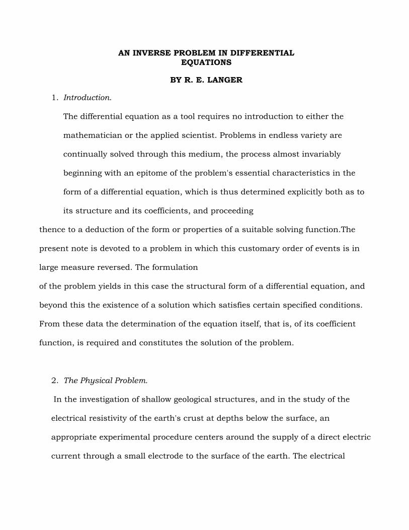
AN INVERSE PROBLEM IN DIFFERENTIAL EQUATIONS

BY R. E. LANGER

1. Introduction.

The differential equation as a tool requires no introduction to either the

mathematician or the applied scientist. Problems in endless variety are

continually solved through this medium, the process almost invariably

beginning with an epitome of the problem's essential characteristics in the

form of a differential equation, which is thus determined explicitly both as to

its structure and its coefficients, and proceeding

thence to a deduction of the form or properties of a suitable solving function.The

present note is devoted to a problem in which this customary order of events is in

large measure reversed. The formulation

of the problem yields in this case the structural form of a differential equation, and

beyond this the existence of a solution which satisfies certain specified conditions.

From these data the determination of the equation itself, that is, of its coefficient

function, is required and constitutes the solution of the problem.

2. The Physical Problem.

In the investigation of shallow geological structures, and in the study of the

electrical resistivity of the earth's crust at depths below the surface, an

appropriate experimental procedure centers around the supply of a direct electric

current through a small electrode to the surface of the earth. The electrical

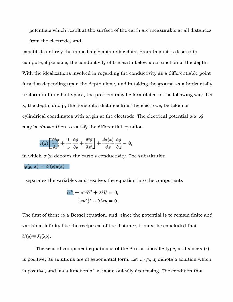
potentials which result at the surface of the earth are measurable at all distances

from the electrode, and

constitute entirely the immediately obtainable data. From them it is desired to

compute, if possible, the conductivity of the earth below as a function of the depth.

With the idealizations involved in regarding the conductivity as a differentiable point

function depending upon the depth alone, and in taking the ground as a horizontally

uniform in-finite half-space, the problem may be formulated in the following way. Let

x, the depth, and ρ, the horizontal distance from the electrode, be taken as

cylindrical coordinates with origin at the electrode. The electrical potential ø(ρ, x)

may be shown then to satisfy the differential equation

in which (x) denotes the earth's conductivity. The substitution

separates the variables and resolves the equation into the components

The first of these is a Bessel equation, and, since the potential is to remain finite and

vanish at infinity like the reciprocal of the distance, it must be concluded that

The second component equation is of the Sturm-Liouville type, and since (x)

is positive, its solutions are of exponential form. Let 1{x, λ) denote a solution which

is positive, and, as a function of x, monotonically decreasing. The condition that

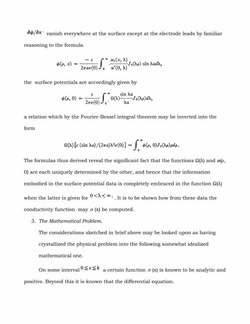
vanish everywhere at the surface except at the electrode leads by familiar

reasoning to the formula

the surface potentials are accordingly given by

a relation which by the Fourier-Bessel integral theorem may be inverted into the

form

The formulas thus derived reveal the significant fact that the functions Ω(λ) and ø(ρ,

0) are each uniquely determined by the other, and hence that the information

embodied in the surface potential data is completely embraced in the function Ω(λ)

when the latter is given for . It is to be shown how from these data the

conductivity function may (x) be computed.

3. The Mathematical Problem.

The considerations sketched in brief above may be looked upon as having

crystallized the physical problem into the following somewhat idealized

mathematical one.

On some interval a certain function (x) is known to be analytic and

positive. Beyond this it is known that the differential equation.

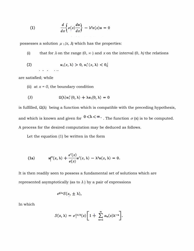
possesses a solution 1{x, λ) which has the properties:

(i) that for λ on the range (0, ∞ ) and x on the interval (0, h) the relations

are satisfied; while

(ii) at x = 0, the boundary condition

is fulfilled, Ω(λ) being a function which is compatible with the preceding hypothesis,

and which is known and given for . The function (x) is to be computed.

A process for the desired computation may be deduced as follows.

Let the equation (1) be written in the form

It is then readily seen to possess a fundamental set of solutions which are

represented asymptotically (as to λ ) by a pair of expressions

In which

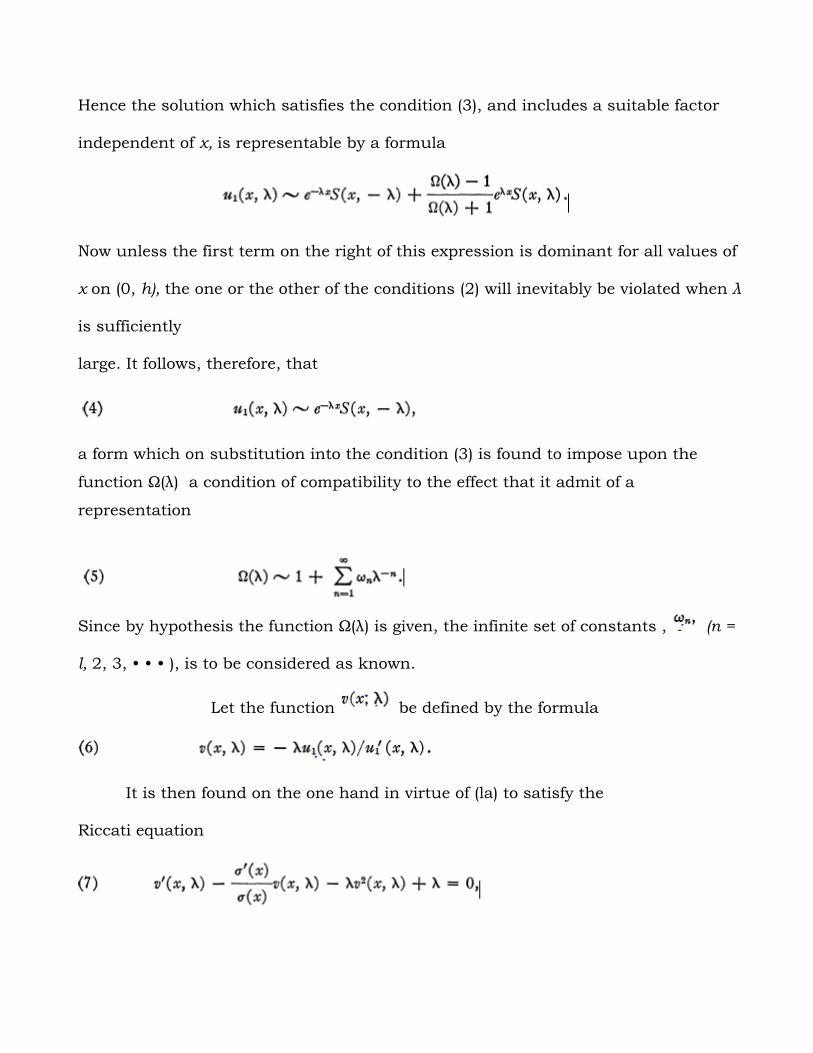
Hence the solution which satisfies the condition (3), and includes a suitable factor

independent of x, is representable by a formula

Now unless the first term on the right of this expression is dominant for all values of

x on (0, h), the one or the other of the conditions (2) will inevitably be violated when λ

is sufficiently

large. It follows, therefore, that

a form which on substitution into the condition (3) is found to impose upon the

function Ω(λ) a condition of compatibility to the effect that it admit of a

representation

Since by hypothesis the function Ω(λ) is given, the infinite set of constants , (n =

l, 2, 3, • • • ), is to be considered as known.

Let the function be defined by the formula

It is then found on the one hand in virtue of (la) to satisfy the

Riccati equation

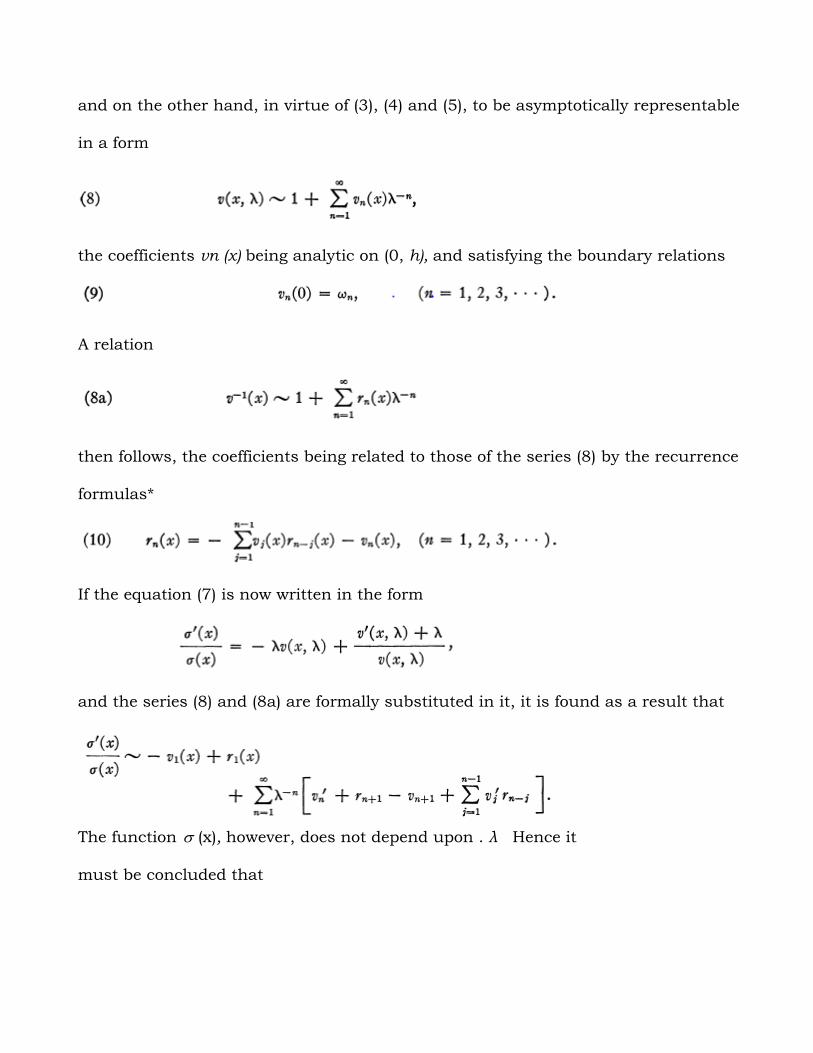
and on the other hand, in virtue of (3), (4) and (5), to be asymptotically representable

in a form

the coefficients vn (x) being analytic on (0, h), and satisfying the boundary relations

A relation

then follows, the coefficients being related to those of the series (8) by the recurrence

formulas*

If the equation (7) is now written in the form

and the series (8) and (8a) are formally substituted in it, it is found as a result that

The function (x), however, does not depend upon . λ Hence it

must be concluded that

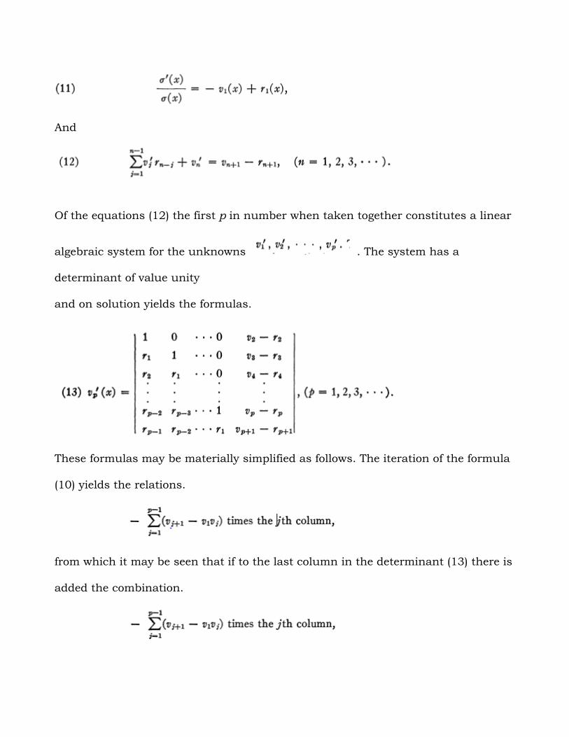
And

Of the equations (12) the first p in number when taken together constitutes a linear

algebraic system for the unknowns . The system has a

determinant of value unity

and on solution yields the formulas.

These formulas may be materially simplified as follows. The iteration of the formula

(10) yields the relations.

from which it may be seen that if to the last column in the determinant (13) there is

added the combination.

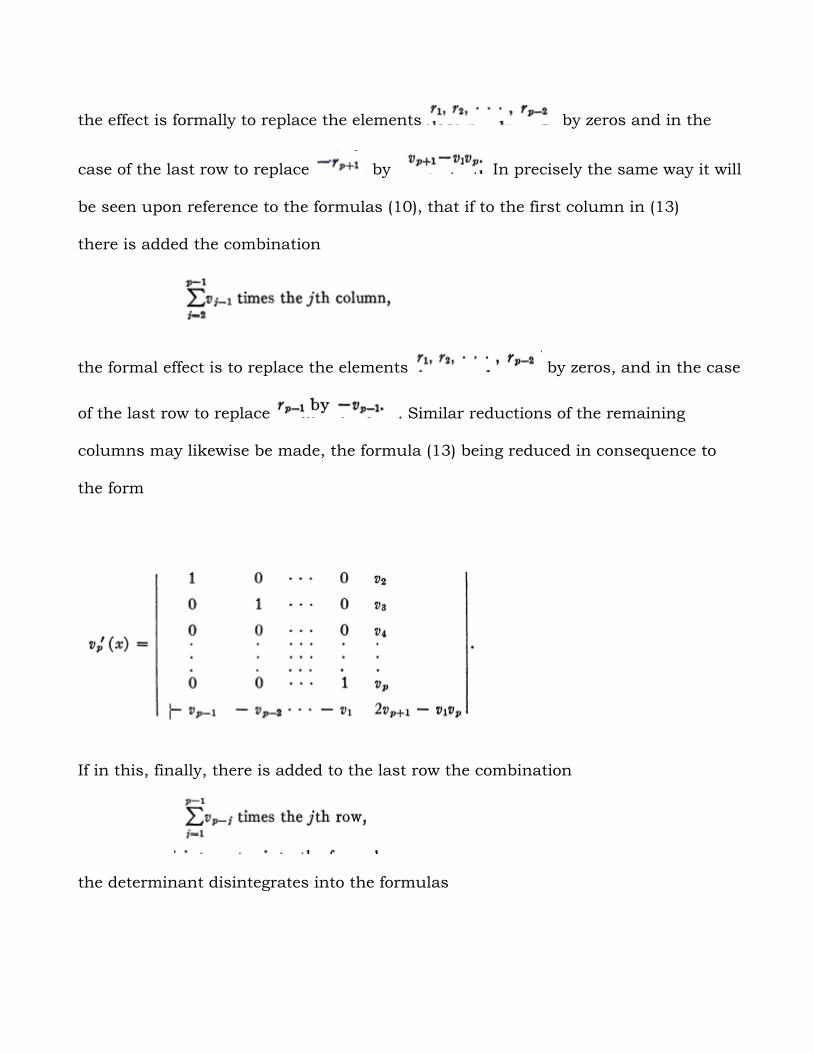
the effect is formally to replace the elements by zeros and in the

case of the last row to replace by In precisely the same way it will

be seen upon reference to the formulas (10), that if to the first column in (13)

there is added the combination

the formal effect is to replace the elements by zeros, and in the case

of the last row to replace . Similar reductions of the remaining

columns may likewise be made, the formula (13) being reduced in consequence to

the form

If in this, finally, there is added to the last row the combination

the determinant disintegrates into the formulas

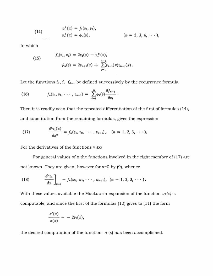
In which

Let the functions f1, f2, f3...., be defined successively by the recurrence formula

Then it is readily seen that the repeated differentiation of the first of formulas (14),

and substitution from the remaining formulas, gives the expression

For the derivatives of the functions v1(x)

For general values of x the functions involved in the right member of (17) are

not known. They are given, however for x=0 by (9), whence

With these values available the MacLaurin expansion of the function v1{x) is

computable, and since the first of the formulas (10) gives to (11) the form

the desired computation of the function (x) has been accomplished.

CONCLUSION

By series of mathematical methods and analysis we have been able to

achieve the potential at the surface of the two layered earth at the distanced r

from the current source (I).

Also the kernel function which is a function of the thickness and

reflection coefficient was obtained for the assumed earth model.

The Bessel zero- order function of the first kind and first order of

the first kind arose from the calculation for an n- layered earth with

apparent resistivity and arbitrary thickness considered.

In conclusion we obtained the tables for the Bessel function under focus

and then plotted an elegant figure to show the proper behavior of the function

for the n-layer earth surface. The derived potential and resistivity correlates

with studies carried out by Asokhia et al (2001). Finally, the resistivity

transformation function T(x) obtained, properly agrees with the works of

Langer et al (1993) as also stated by Gosh D.P (1971).

REFERENCES

Asokhia M.B and Ujuanbi O. (2001), J. Nig. Ass. Math. Phys. Vol. 5, 79-88.

Asokhia M. B, S.O. Azi and O. Ujuanbi O. (2002), J. Nig. Ass. Math. Phys.

Vol. 4, 269-280.

Egbai J.C. (2002), J. Nig. Ass. Math. Phys. Vol 6, 207-222

Ghosh. D. P. (1971), The application of Linear Filter Theory to the Direct

Interpolation of Geo-electrical Resistivity Sounding measurement, Geophysical

Prospecting (Netherlands) V. 19, no 2, 192-217

Stroud K.A (2003), Advanced Engineering Maths, 4th Ed., palgrave

macmillian, New York, 305-311

Keller G. V. and Friscknecht F. C. (1966), Electrical Methods in

Geophysical Prospecting, Pergamon Press, 90-196 and 299-353

Koefoed O. and Dirks F.J. (1979), Determination of resistivity sounding

filters by the Wiener-Hopf least squares method, Geophysical Prospecting

Vol.27, 245-250.

Stefanesco S., Schlumberger C. and Schlumberger M. (1930), Sur la

distribution electrique potentielle autour d’une prise de terre ponctuelle dans

un terrain a couches horizontals, homogenes et isotopes. J. de physique et le

padium, series 7, Vol. 1, 132-140.