The Schwarzschild–Milne Integral Equation - Springer

Appendix AThe Schwarzschild–Milne Integral Equation

The exact solution of (2.15)–(2.17) is obtained as follows. We define, as before, thelocal average intensity

J (τ) = 1

2

∫ 1

−1I (τ,μ)dμ, (A.1)

and the formal solution of (2.15) is

I ={∫ ∞

τe−(t−τ)/μJ (t) dt

μ, μ > 0,∫ τ

0 e−(t−τ)/μJ (t) dt(−μ)

, μ < 0,(A.2)

providing J does not grow exponentially as τ → ∞ (specifically, J = o(eτ )). Sub-stituting this expression back into (A.1), we find, after some algebra, that J satisfiesthe Schwarzschild–Milne integral equation

J (τ) = 1

2

∫ ∞

0E1

(|t − τ |)J (t) dt, (A.3)

and the flux conservation law (2.17) can be written in the form

Φ = 2π

[∫ ∞

τ

J (t)E2(t − τ) dt −∫ τ

0J (t)E2(τ − t) dt

]. (A.4)

The exponential integrals E1 and E2 are defined by

E2(y) = y

∫ ∞

y

e−s

s2ds, E1(y) =

∫ ∞

y

e−s

sds; (A.5)

(A.4) acts as a normaliser for the linear equation (A.3).Equation (A.3) is amenable to treatment by the Wiener–Hopf technique. It de-

fines J for τ > 0, and we extend the definition of J so that

J = 0, τ < 0, (A.6)

A. Fowler, Mathematical Geoscience, Interdisciplinary Applied Mathematics 36,DOI 10.1007/978-0-85729-721-1, © Springer-Verlag London Limited 2011

793

http://dx.doi.org/10.1007/978-0-85729-721-1

794 A The Schwarzschild–Milne Integral Equation

and we define a function h(τ), h = 0 for τ > 0, so that

J (τ) = 1

2

∫ ∞

−∞E1

(|t − τ |)J (t) dt + h(τ), (A.7)

for all values of τ . Write K(t) = 12E1(|t |), so that, if we take Fourier transforms of

(A.7), we get

J+ = KJ+ + h−, (A.8)

where J+(z) is the transform of J and the + indicates that J+(z) is analytic in anupper half plane (since J = 0 for τ < 0). Since J = o(eτ ) as τ → ∞, this is at leastIm z > 1. Similarly h− is analytic in a lower half-plane.

The solution of (A.8) is now effected through the splitting of (1− K) into factorsanalytic in upper and lower half planes, and this can be done by solution of anappropriate Hilbert problem. The transform K is defined as

K(z) =∫ ∞

−∞K(s)eisz ds, (A.9)

and we find that

K = 1

2izln

(1 + iz

1 − iz

)= 1

ztan−1 z. (A.10)

We will now strengthen our assumption on J so that J does not grow exponentiallyas τ → ∞, i.e., J = o(eατ ) for any α > 0; then J+ is analytic in Im z > 0. Our aimnow is to find a function G analytic in Im z <

> 0 such that G+/G− = 1 − K on R,

and this is done by solving the Hilbert problem lnG+ − lnG− = ln(1 − K). To dothis we wish to have 1 − K �= 0, in order that ln(1 − K) be Hölder continuous. Onthe other hand we want ln{1−K(t)} → 0 as t ∈ R → ±∞. These concerns motivatethe modification of 1 − K(t) by a factor (t2 + 1)/t2, since 1 − K = O(t2) as t → 0(and is non-zero for t �= 0), so that we seek a function G such that

G+(t)

G−(t)=

(t2 + 1

t2

)[1 − 1

2itln

(1 + it

1 − it

)], (A.11)

for t ∈ R. Clearly G is only determined up to a multiplicative analytic function,and to be specific we will suppose G± → 1 as z → ∞. We take the branches ofln(1 ± it) to be such that ln 1 = 0. The solution of (A.11) is

G(z) = exp

[1

2πi

∫ ∞

−∞ln

{(t2 + 1

t2

)(1 − 1

ttan−1 t

)}dt

t − z

], (A.12)

and with this definition of G(z) (and thus G+(t) and G−(t)), Eq. (A.8) for J+ canbe written in the form, for t ∈ R,

z2

z + iG+J+ = (z − i)h−G−. (A.13)

A The Schwarzschild–Milne Integral Equation 795

Fig. A.1 Inversion contourfor (A.16)

Clearly the left hand side defines the limit on Im z = 0+ of a function analyticin the upper half plane Im z > 0, while the right hand side is the limit on Im z = 0−of a function analytic in Im z < 0 (since (A.7) implies that h grows no faster thanJ (−τ)). We infer that each function can be analytically continued into its oppositehalf plane, thus defining an entire function E(z), so that

J+(z) = (z + i)E(z)

z2G+(z). (A.14)

The definition of J+ as a Fourier transform requires J+ → 0 as z → ∞, whilealso G+ → 1 as z → ∞. It follows that J+ ∼ E/z, which requires that E = ic isconstant, i.e.,

J+ = ic(z + i)

z2G+(z), (A.15)

and the constant c is determined by the normalising condition (A.4). (The factor i

is inserted for later convenience.)Some information on the structure of J+ can be gleaned from (A.11). Evidently

G+ can be extended to Im z < 0, and G− to Im z > 0 by the reciprocal relationship

G+(z)

G−(z)=

(z2 + 1

z2

)[1 − 1

2izln

(1 + iz

1 − iz

)]. (A.16)

Care needs to be used in interpreting (A.16). If Im z < 0, then (A.16) provides ananalytic continuation for G+ there, which shows that the continuation of G+ toIm z < 0 (very definitely not equal to G−) has a logarithmic branch point at z = −i.Similarly G−, extended to Im z > 0, has a logarithmic branch point at z = +i.Therefore J+, extended via (A.15) to Im z < 0, has a double pole at z = 0 (asG+(0) = 1√

3�= 0) and a branch cut which we may take from −i to −i∞.

The inverse transform of (A.15) is

J (τ) = 1

2π

∫ ∞

−∞J+(z)e−izτ dz, (A.17)

796 A The Schwarzschild–Milne Integral Equation

where the contour is indented above the origin. If τ < 0, we complete the contour inthe upper half plane, whence we have J = 0 (as we assumed). If τ > 0, we completethe contour as shown in Fig. A.1. The result of this is that

J (τ) = −i

[Res

{J+e−izτ

}∣∣z=0 + 1

2π

∫ ∞

0e−τ(1+x)

[J++ − J−+

]dx

], (A.18)

where J++ (x) = J+[−i + xe−iπ/2], J−+ (x) = J+[−i + xe3iπ/2]. Calculation of theresidue yields the result

Res |z=0 = ic√

3(1 + τ − j), (A.19)

where

j = 1

π

∫ ∞

0

[1

(1 − t−1 tan−1 t)− 1 − 3

t2

]dt

1 + t2. (A.20)

We use (A.16) to substitute for G+ in (A.15), and then we find

J±+ (x) = −c

(2 + x)G−[−i(1 + x)]l±(x), (A.21)

where

l±(x) = 1 − 1

2(2 + x)

[ln

(2 + x

x

)± iπ

]. (A.22)

It follows that

J++ − J−+ = iπc

g−(x)[{

2 + x − 12 ln

( 2+xx

)}2 + π2

4

] , (A.23)

where g−(x) = G−(−i − ix), and from (A.12), we find

g−(x) = exp

[− (1 + x)

2π

∫ ∞

−∞ln

[(t2 + 1

t2

)(1 − 1

ttan−1 t

)]dt

{t2 + (1 + x)2}].

(A.24)Finally, therefore, J = cJ0(τ ), where

J0(τ ) = √3(1+τ −j)+ π

2e−τ

∫ ∞

0

e−xτ dx

g−(x)[{

2 + x − 12 ln

( 2+xx

)}2 + π2

4

] . (A.25)

Evidently J ≈ c√

3(1− j + τ)+o(e−τ ) as τ → ∞, which confirms the assumptionof non-exponential growth.

It only remains to compute c (which is evidently real, hence the choice of con-stant ic in (A.15)), and there seems no obvious short cut other than laborious sub-stitution of the expression (A.25) for J into (A.4), which can be written in the form

c = Φ

2π∫ ∞

0 J0(t)H(τ − t) dt, (A.26)

A.1 Exercises 797

where

H(θ) ={

E2(−θ), θ < 0,

−E2(θ), θ > 0.(A.27)

A.1 Exercises

A.1 What is wrong with the following argument? To determine c in (A.26), write(A.4) in the form (since J = 0 for τ < 0)

Φ = 2π

∫ ∞

−∞J (t)H(τ − t) dt,

where

H(θ) ={

E2(−θ), θ < 0,

−E2(θ), θ > 0.

A Fourier transform yields, via the convolution theorem,

Φ

2πiz= J+(z)H (z),

where

H (z) = −2i

∫ ∞

0E2(θ) sin zθ dθ.

Show that

−∫ ∞

0E2(θ)eizθ dθ = ln(1 − iz) + iz

z2,

so that

Φ

2πiz= 2iJ+

[2iz − ln

( 1+iz1−iz

)]z2

.

Since also

J+ = ic(z + i)

z2G+(z),

this implies

G+(z) = A(z + i)[1 − 1

2izln

( 1+iz1−iz

)]z2

,

where A = 8πcΦ

; but this is not analytic in Im z > 0.

Appendix BTurbulent Flow

Shear flows become turbulent if the Reynolds number Re is sufficiently large. Usu-ally, this means Re ∼ 103. For flow in a cylindrical pipe, the Reynolds number isconventionally chosen to be

Re = Ud

ν, (B.1)

where U is the mean velocity, d is the pipe diameter, and ν is the kinematic viscosity.With this definition, the onset of turbulence occurs at Re = 2,300, although thedetails of the transition process are complicated (Fowler and Howell 2003), andoccur over a range of Reynolds number.

Most obviously, one might suppose that turbulence arises because of an insta-bility of the uniform (laminar) flow, and for half a century this motivated the studyof the famous Orr–Sommerfeld equation (one version of which is studied in Ap-pendix C), which describes normal modes of the linearised Navier–Stokes equationsdescribing perturbations about a steady uniform flow. Commonly such studies aredone in two dimensions, for example for plane Poiseuille flow, when the Reynoldsnumber is defined in terms of the maximum (centre-line) speed of the laminar flowand the half-width. This leads to a definition which is 3

4 of that which would ariseusing the mean velocity and width. For plane Poiseuille flow, it is found that thesteady flow is linearly unstable if Re > 5,772; on the other hand, turbulence sets inat Re ≈ 1,000 (Orszag and Patera 1983). For pipe flow, the flow is linearly stableat all Reynolds numbers, although the decay rate of disturbances tends to zero asRe → ∞.

It appears that the transition to turbulence is only vaguely related to the stabil-ity of the uniform state. The story is most simply told in the plane Poiseuille case.The instability at Re = Rec = 5,772 is subcritical, and an (unstable) branch of finiteamplitude stationary solutions bifurcates for Re < Rec, and exists down to aboutRe = 2,900 before bending back on to a higher amplitude stable branch. Crucially,the (two-dimensional) stability or instability occurs on a long viscous time scale.However, these stationary solutions are subject to a three-dimensional instabilitywhich occurs on the fast convective time scale, and it is this which appears to causethe transition. Its occurrence at Re ≈ 1,000 is associated with the fact that while the


799

http://dx.doi.org/10.1007/978-0-85729-721-1

800 B Turbulent Flow

two-dimensional equilibria no longer exist there, two-dimensional disturbances willstill decay on the slow viscous time scale, thus allowing the rapid three-dimensionalgrowth. Essentially the same story occurs in pipe flow, although there it seems thatRec = ∞. Numerical experiments have also found unstable travelling wave struc-tures, now in the form of arrays of longitudinal vortices, and transition is associatedwith their existence (Eckhardt et al. 2007).

Since in fact, turbulence is an irregular, chaotic motion, it seems most likelythat its occurrence is associated with the occurrence of a homoclinic bifurcation(Sparrow 1982), which not only produces the strange turbulent motion, but also thevarious travelling wave structures that can be found.

B.1 The Reynolds Equation

The actual calculation of turbulent flows is usually done following Reynolds’s(1895) formulation of averaged equations. We write the Navier–Stokes equationsfor an incompressible flow in the form

∂ui

∂xi

= 0,

ρ∂ui

∂t+ ρ

∂

∂xj

(uiuj ) = − ∂p

∂xi

+ μ∇2ui,

(B.2)

where suffixes i represent the components, and the summation convention is used(i.e., summation over repeated suffixes is implied). If we denote time averages byan overbar, and fluctuations by a prime, thus

ui = ui + u′i , (B.3)

then averaging of (B.2) yields

∂ui

∂xi

= 0,

ρ∂

∂xj

(ui uj ) + ∂

∂xj

(ρu′iu

′j ) = − ∂p

∂xi

+ μ∇2ui .

(B.4)

The second of these can be written in the form

(u.∇)u = −∇p + ∇.{τ + τT

}, (B.5)

where

τij = 2μ ˙εij , ˙εij = 1

2

(∂ui

∂xj

+ ∂uj

∂xi

)(B.6)

is the ordinary molecular mean stress, and

τTij = −ρu′

iu′j (B.7)

B.2 Eddy Viscosity 801

is called the Reynolds stress. The essential problem in describing fully turbulentflows is to close the averaged model by prescribing the Reynolds stress.

B.2 Eddy Viscosity

The simplest way to close the Reynolds equation is to suppose that

τTij = 2μT

˙εij , (B.8)

by analogy to (B.6). The coefficient μT is called the eddy viscosity. This itself canbe prescribed in various ways, but the simplest is to take it as constant. For example,in a channel flow we might take

μT = ρεT ud, (B.9)

where d is the depth and u the mean velocity. More generally, one allows μT to varywith distance from bounding walls, as described below.

Measurements in turbulent wall-bounded flows lead to the definition of a frictionfactor f through the wall stress

τw = fρu2. (B.10)

Here, u is the mean velocity, and the friction factor f = 18λ in Schlichting’s (1979)

notation. For an open channel flow, (B.9) is consistent with (B.10) if εT = 13f .

Typical values for f are small, for example Blasius’s law in smooth-walled pipeflows has

f ≈ 0.04

Re1/4(B.11)

for Reynolds numbers in the range 104–105, and thus f ∼ 0.004 and εT ∼ 0.001.Roughness of the wall gives correspondingly larger values of f and εT . Notice thatε−1T is the Reynolds number based on the eddy viscosity, and is relatively large,

reflecting the well-known fact that the turbulent eddies disturbing the mean floware of relatively small amplitude. A more realistic form for the eddy viscosity usesPrandtl’s mixing length theory, which is motivated by observations that the meanvelocity profile is approximately logarithmic. The following discussion is based onthat of Schlichting (1979).

The friction velocity is defined as

u∗ =√

τw

ρ(B.12)

(note that u∗ � u since generally f � 1), thus

f =(

u∗u

)2

. (B.13)


For a one-dimensional shear flow, with coordinate z normal to the wall (at z = 0),Prandtl’s mixing length hypothesis is

τ = ρl2∣∣∣∣∂u

∂z

∣∣∣∣∂u

∂z, (B.14)

where τ is the shear stress, l is the mixing length, and u the velocity; Prandtl furthersuggests

l = κz, (B.15)

with κ a constant. If we suppose τ = τw = constant, then

u∗ = κz∂u

∂z, (B.16)

thus

u

u∗= C + 1

κln

(u∗zν

), (B.17)

which is the famous universal logarithmic velocity profile. See also Question 5.11and the discussion on turbulent flow and eddy viscosity in the notes in Sect. 5.9 forChap. 5.

B.3 Pipe Flow

We now consider the case of flow in a pipe of radius a, and suppose that (B.17)applies, where z is radial distance inwards from the wall. If um is the maximumvelocity at z = a, then (B.17) implies

um − u = u∗κ

ln

(a

z

), (B.18)

and the mean velocity u = 2a2

∫ a

0 (a − z)udz satisfies

um − u = 3u∗2κ

. (B.19)

In addition, comparison of (B.17) and (B.18) implies

um = u∗κ

ln

(au∗ν

)+ u∗C. (B.20)

Using (B.19) and (B.13), and defining the Reynolds number

Re = ud

ν, (B.21)

B.4 Extension to Rivers 803

where the pipe diameter d = 2a, we find

1√f

= 1

κln

[Re

√f

] + C − 3

2κ− 1

κln 2. (B.22)

Extensive measurements indicate that this formula is very successful in predictingf (Re) assuming κ = 0.4, C = 5.5. The principal assumption involved is that of aneddy viscosity

νT = κ2z2∣∣∣∣∂u

∂z

∣∣∣∣. (B.23)

B.4 Extension to Rivers

The above results are easily extended to a river of depth d . Suppose now that

τ = τw

(1 − z

d

)= ρκ2z2u′2, (B.24)

where u′ = ∂u/∂z. Integrating, we find, with u = um at z = d ,

um − u = u∗κ

∫ 1

z/d

(1 − ξ)1/2 dξ

ξ= 2

u∗κ

[ln cot

1

2α − cosα

], (B.25)

where α = sin−1√

zd

. With the mean flow u = 1d

∫ d

0 udz, we find

um − u = 2u∗3κ

, (B.26)

while comparison of (B.25) as z → 0 with (B.17) yields

um

u∗= C − 2

κ+ 1

κln

(4u∗d

ν

), (B.27)

and elimination of um between (B.26) and (B.27) gives, with Re = ud/ν,

1√f

= 1

κln

[Re

√f

] + C − 8

3κ+ 1

κln 2, (B.28)

essentially the same result as (B.22).

B.5 Manning’s Law

It is of interest to compare the laboratory born flow law (B.28) with a flow law suchas that of Manning. Manning’s law is

u = R2/3S1/2

n, (B.29)


where R is the hydraulic radius and S is the downstream slope. For a wide river, wetake R = d and τw = ρgdS. We thus have

uR = νRe, f u2 = gRS, (B.30)

from which we find

u =(

gSνRe

f

)1/3

, R =(

ν2Re2f

gS

)1/3

, (B.31)

and Manning’s law (B.29) can be written in the form

f =[gS1/10n9/5

ν1/5

]Re−1/5, (B.32)

broadly comparable to (B.28). (As mentioned above, the often used Blasius relation(B.11) approximating (B.28) has f ∝ Re−1/4.)

B.6 Entry Length

It is well-known that the development of laminar pipe Poiseuille flow from a plugentry flow occurs over an extended distance (the entry length) which scales as dRe.The entry length scale is determined by the diffusion of vorticity through laminarboundary layers into the core potential flow. If we scale up this process to rivers, withd = 1 m, Re = 106, it would suggest entry lengths of 1000 km! In reality, however,such boundary layers would be turbulent, and a better notion of entry length wouldbe d/εT , perhaps 100 m; and in fact sinuous channels and bed roughness will ensurethat river flow will always be fully turbulent.

However, the entry length concept provides a framework within which one canpose Kennedy’s (1963) potential flow model for dune formation (see Chap. 5), evenif in practice it is not realistic. Further, if one adopts a constant eddy viscosity modelof turbulent flow, then the small value of εT is consistent with an inviscid outersolution away from the boundary, even if the assumption of a shear free velocity isnot. On the other hand, it is conceivable that in laboratory experiments, the outerinviscid flow might indeed be a plug flow if the entry conditions are smooth.

B.7 Sediment Deposition

Suppose now that a suspended sediment concentration c(z) is maintained in a turbu-lent flow by the action of an eddy viscosity. The units of c are taken to be mass perunit volume of the stream. In equilibrium, we have a balance between the upwardturbulent flux and the downward velocity, which we take as vs :

−νT

∂c

∂z= vsc. (B.33)

B.7 Sediment Deposition 805

We suppose Reynolds’ analogy that the eddy momentum diffusivity is equal to theeddy sediment diffusivity, and between (B.23) and (B.24), we have

νT = κu∗z(

1 − z

d

)1/2

. (B.34)

Solving this gives

c = cs

(z

d

)Z

exp

[−Z

∫ 1

z/d

dξ

ξ

[1

(1 − ξ)1/2− 1

]], (B.35)

where Z is the Rouse number,

Z = vs

κu∗. (B.36)

Unfortunately, this gives c = 0 at z = 0 and thus zero deposition there! This is dueto the artificial singularity in u as z → 0, and an artificial escape from this quandaryis to evaluate c at a small distance above the bed. As a simple alternative we supposeνT is constant, given by (B.9) for example. Then

c = c0 exp

[−vsz

νT

], (B.37)

and the mean concentration is

c = c0

R

(1 − e−R

), (B.38)

where

R = vsd

νT

. (B.39)

If we use (B.9) and (B.13), then

R = vs

εT u= κ

√f

εT

Z. (B.40)

The sediment deposition rate is, from (B.33) and cf. (5.10),

ρsvD = c0vs = cvsD, (B.41)

where (B.38) implies

D(R) = R

1 − e−R. (B.42)

Other expressions involving νT (z) give similar expressions which increase with R

(or Z) (Einstein 1950).

Appendix CAsymptotic Solution of the Orr–SommerfeldEquation

In this appendix we provide an asymptotic solution of the Orr–Sommerfeld equa-tion describing rapid shear flow over a slightly wavy boundary. The description isbased on the asymptotic theory described by Drazin and Reid (1981), which itselfdescribes a body of research stemming from original investigations by Heisenbergand Tollmien. The theory is, however, rather difficult to follow, and is gone throughin detail here for that reason.

The Orr–Sommerfeld equation is

ik[U

(Ψ ′′ − k2Ψ

) − U ′′Ψ] = 1

R

[Ψ iv − 2k2Ψ ′′ + k4Ψ

], (C.1)

and describes the z-dependent amplitude of a horizontal Fourier mode (of zero wavespeed) of wave number k. U(z) is the basic horizontal velocity profile. The boundaryconditions we impose are those corresponding to no slip at the perturbed boundaryand free slip at the top surface:

Ψ = 0, Ψ ′ = 1 at z = 0,

Ψ = 0, Ψ ′′ = 0 at z = 1.(C.2)

We seek asymptotic solutions for R � 1. Accordingly, there is an outer solution

Ψ ∼ Λ

[Ψ0 + 1

RΨ1 + · · ·

], (C.3)

where Λ is a scaling parameter to be chosen so that Ψ0 = O(1). The equation forΨ0 is the inviscid (Rayleigh) equation

U(Ψ ′′

0 − k2Ψ0) − U ′′Ψ0 = 0, (C.4)

and we might expect to satisfy the boundary conditions on the free surface z = 1. Infact, we see that specification of Ψ0 = 0 on z = 1 automatically implies that Ψ ′′

0 = 0there. The outer solution is written in terms of two independent Frobenius series of


807

http://dx.doi.org/10.1007/978-0-85729-721-1

808 C Asymptotic Solution of the Orr–Sommerfeld Equation

(C.4), expanded about z = 0. Assuming U(0) = 0, U ′(0) = U ′0 �= 0, we have these

two solutions given by

ψ1 = zP1(z),

ψ2 = P2(z) + U ′′0

U ′0ψ1 ln z,

(C.5)

where

P1 = 1 + U ′′0

2U ′0z + 1

6

(U ′′′

0

U ′0

+ k2)

z2 + · · · ,

P2 = 1 +(

U ′′′0

2U ′0

− U ′′20

U ′20

+ 1

2k2

)z2 + · · · ,

(C.6)

and the functions P1 and P2 are easily found numerically (Drazin and Reid 1981,pp. 137–138).

We denote

P1(1) = P11, P2(1) = P21; (C.7)

then the outer solution at leading order is

Ψ ∼ Λ[P21ψ1 − P11ψ2 + O

(R−1)]. (C.8)

Evidently, this does not satisfy the boundary conditions at z = 0, and we antic-ipate a boundary layer of thickness ε � 1 (to be chosen), in which the neglectedterms become important. We define

z = εζ, (C.9)

and expand (C.8) in terms of ζ . The result is that

Ψ ∼ Λ

[−P11 + εζ

{P21 − P11

U ′′0

U ′0

ln(εζ )

}+ · · ·

], (C.10)

and Van Dyke’s (1975) matching principle indicates that we may need two terms ofthe inner expansion to match to this.

In the boundary layer, it is appropriate to choose

ε = 1

(ikRU ′0)

1/3, (C.11)

with the phase of ε (ph ε) defined as −π/6 (we suppose U ′0 > 0 and k > 0). In this

case R−1 ∼ ε3, and the second term in the outer solution is of relative order ε3. Wethen write

Ψ ∼ Λ[χ0 + εχ1 + · · · ], (C.12)

C Asymptotic Solution of the Orr–Sommerfeld Equation 809

Fig. C.1 Contours for theAiry integral (C.15)

and the equations for χ0 and χ1 are

LD2χ0 = 0,

LD2χ1 = ζ 2U ′′0

2U ′0

χ ′′0 − U ′′

0

U ′0χ0,

(C.13)

where the operators L and D are defined by

D = d

dζ, L = D2 − ζ. (C.14)

Reid (1972), see also Drazin and Reid (1981, pp. 465 ff.) shows how to solve theseequations in terms of a class of generalised Airy functions.

We begin by defining the functions

A(L)p (ζ ) = 1

2πi

∫L

t−peζ t− 13 t3

dt, (C.15)

where L is one of the contours shown in Fig. C.1, and p is an integer. We denote thefunction defined via the contour Lk as A

(k)p . (Drazin and Reid’s notation is different;

they write A(k)p (ζ ) as Ak(ζ,p).) These functions are analytic, and satisfy the third

order differential equation

(LD + p − 1)Ap = 0. (C.16)

The functions A(1)p ,A

(2)p ,A

(3)p are independent, and by contraction of L1 ∪ L2 ∪ L3,

we see that

A(1)p + A(2)

p + A(3)p = A(0)

p = −Bp(ζ ), (C.17)


Fig. C.2 The Stokes sectorsTi (bounded by the Stokeslines) and the anti-Stokessectors Si (bounded by theanti-Stokes lines) for (C.15).The signs in the sectorsindicate the sign of arg 2

3 z3/2

as z → ∞

where Bp is a polynomial in ζ for integral p, in particular Bp = 0 for p ≤ 0, and

B1(ζ ) = 1, B2(ζ ) = ζ, B3(ζ ) = 1

2ζ 2. (C.18)

The functions Ap satisfy the equations

LD2Ap+1 = −(p − 1)Ap,

DAp = Ap−1, (C.19)

ζAp = pAp+1 + Ap−2,

the last of these following from the first two together with (C.16). In particular,LA0 = 0 and A

(k)0 are the Airy functions; for example, A

(1)0 (ζ ) = Ai (ζ ). We also

have the rotation formulae

A(2)p (ζ ) = e−2(p−1)πi/3A(1)

p

(ζe2πi/3),

A(3)p (ζ ) = e2(p−1)πi/3A(1)

p

(ζe−2πi/3). (C.20)

It is clear from (C.19) that the solution for χ0 in (C.13) is of the form

χ0 = χ00 + χ01ζ + α0A(1)2 (ζ ) + β0A

(3)2 (ζ ). (C.21)

(Although A(2)2 is another possible solution, it is not independent because of (C.17),

and because B2(ζ ) = ζ .)Drazin and Reid (1981) give the asymptotic behaviour as ζ → ∞ of the functions

A(k)p , based on the method of steepest descents and the rotation formulae (C.20). The

Stokes sectors Ti are delimited by Stokes lines at arg ζ = 0, 2π/3, 4π/3, and withinthese, the anti-Stokes lines are arg ζ = π/3, π , 5π/3 (see Fig. C.2). Note that weseek the behaviour of A

(k)2 as ζ → ∞ along arg ζ = π/6 (since ζ = (ikRU ′

0)1/3z),


which lies in the sector S1: − π3 < arg ζ < π

3 , in which the functions A+ and A−defined by Drazin and Reid (p. 463, Eq. (A12)) respectively grow and decay expo-nentially. From their Eq. (A14), we then see that A

(1)p → 0 as ζ → ∞eiπ/6, while

A(3)p grows exponentially. Therefore β0 = 0 in (C.21).Next we turn to the solution for χ1. From (C.13), we have, using D2A2 = A0,

LD2χ1 = U ′′0

U ′0

[1

2α0ζ

2A(1)0 − χ00 − χ01ζ − αA

(1)2

]. (C.22)

The solution to this equation is (using (C.18))

χ1 = χ10 + χ11ζ + α1A(1)2 (ζ ) + U ′′

0

U ′0

[α0

{−1

2A

(1)0 + 1

10A

(1)−3 + A

(1)3

}

+ 1

2χ01ζ

2 − χ00φ

], (C.23)

where we use LD2B3 = −B2 and again suppress A(3)2 (ζ ), and φ is a particular

solution to

LD2φ = B1. (C.24)

For matching purposes, φ must not grow exponentially at ∞eπi/6.The use of the relation LD2Bp+1 = −(p − 1)Bp does not help here, because if

p = 1, then LD2B2 = 0. To find a solution, we now define the further generalisedAiry functions

A(k)pq (ζ ) = 1

2πi

∫Lk

t−p(ln t)qeζ t− 13 t3

dt, (C.25)

where arg t ∈ (0,2π). (Drazin and Reid write A(k)pq (ζ ) as Ak(ζ,p, q).) We also de-

fine the loop integrals

B(k)pq (ζ ) = 1

2πi

∫ (0+)

∞e2(k−1)iπ/3t−p(ln t)qeζ t− 1

3 t3dt, (C.26)

where the loop contours in (C.26) are defined by Erdélyi et al. (1953, p. 13), andused by Olver (1974) and Reid (1972). The notation

∫ (0+)

adenotes an integral over

a contour which is a loop beginning and ending at the point a, and which enclosesthe origin (and encircles it counterclockwise). For the integrands with branch pointsas in (C.26), these are thus the keyhole contours Lk as indicated in Fig. C.3.

It is straightforward to derive analogues of (C.19) (which apply to any of thecontours Lk or Lk), and these are (for Apq or Bpq )

DApq = Ap−1,q ,

(LD + p − 1)Apq = qAp,q−1, (C.27)

LD2Ap+1,q = −(p − 1)Apq + qAp,q−1,


Fig. C.3 Two of the threeloop contours for (C.26), L1

and L2

and in particular we see that

LD2A21 = A1, (C.28)

since it is clear that Ap0 = Ap for any p. Incidentally, note that when q = 0, theintegrands of (C.26) do not have a branch point, and therefore the loop contours Lk

are all equivalent to L0, so that B(k)p0 = Bp , and in particular

LD2B(k)21 = B1 (C.29)

for each contour Lk . Consulting (C.24), we see that any of B(k)21 is a particular so-

lution for φ in (C.23), but we require one which does not grow exponentially. It isclear, since LD2A

(k)2 = 0, that the difference between the various B

(k)21 for different

k will be a sum of multiples of A(k)2 , and this is explicitly provided by the connection

formulae of Drazin and Reid (p. 475, Eq. (A43)):

B(2)21 − B

(3)21 = 2πiA

(1)2 ,

B(1)21 − B

(2)21 = 2πiA

(3)2 .

(C.30)

The object now is to find an appropriate solution of (C.29) which does not growexponentially as ζ → ∞eπi/6, and for this we need to know the asymptotic be-haviour of one of the B

(k)21 . At this point we diverge from the discussion by Drazin

and Reid (pages 178, 474). We consider explicitly the contour integral over L2:

B(2)p1

= 1

2πi

∫ (0+)

∞e2πi/3t−p ln t eζ t− 1

3 t3dt. (C.31)

In choosing the contour, we anticipate that we will require Re(ζ t) < 0, and to bespecific, we define arg t ∈ (− 4π

3 , 2π3 ) in (C.31). We have, successively,

B(2)p1 = − ∂

∂p

[1

2πi

∫ (0+)

∞e2πi/3t−peζ t− 1

3 t3dt

](C.32)


and thus (put t3 = 3u)

B(2)p1 = − ∂

∂p

[1

2πi

∫ (0+)

∞e2πi/3

∞∑n=0

(− 13

)n

n! t3n−peζ t dt

]; (C.33)

the method of proof of Watson’s lemma then implies

B(2)p1 ∼ − ∂

∂p

[ ∞∑n=0

(− 13

)n

n!1

2πi

∫ (0+)

∞e2πi/3t3n−peζ t dt

], (C.34)

provided Re(ζ t) < 0.Equation (6), page 14, of Erdélyi et al. (1953) gives

1

2πi

∫ (0+)

∞eiδ

t−3e−tX dt = (Xe−iπ )s−1

�(s)(C.35)

for any value of s, where, if arg t ∈ (δ,2π + δ), then −( 12π + δ) < argX < 1

2π − δ.In the present case, arg ζ = π

6 , so that if we define δ = − 4π3 , (and note that

∞e−4πi/3 = ∞e2πi/3), X = ζeiπ , then argX = 7π6 and lies between −π

2 − δ = 5π6

and π2 − δ = 11π

6 . We thus have, for arg ζ = π6 ,

1

2πi

∫ (0+)

∞e2πi/3t−setζ dt = ζ s−1

�(s), (C.36)

and hence (C.34) gives, with s = p − 3n,

B(2)p1 (ζ ) ∼ − ∂

∂p

[ ∞∑n=0

(− 13

)n

n!ζp−3n−1

�(p − 3n)

]. (C.37)

Carrying out the differentiation,

B(2)p1 (ζ ) ∼

∞∑n=0

(− 13

)n

n!{−ζp−3n−1 ln ζ

�(p − 3n)+ ζp−3n−1 �′(p − 3n)

�2(p − 3n)

}. (C.38)

Finally we put p = 2. Noting that �′/�2 is finite and 1/�(r) = 0 for non-positiveintegers r , we have

B(2)21 (ζ ) ∼ −ζ ln ζ + ψ(2)ζ + O

(ζ−2), (C.39)

for ζ → ∞ with −π6 < arg ζ < 5π

6 , and in particular when arg ζ = π6 ; ψ = �′/� is

the digamma function.We may now finally define a particular solution for φ in (C.24) to be (cf. (C.29))

φ = B(2)21 (ζ ). (C.40)


Before we complete the solution by matching to the outer solution, we compare(C.40) with results of Drazin and Reid (page 178). They choose (Eq. (27.49)) φDR =B

(3)21 , and match in the sector −π < arg ζ < 1

3π , where their Eq. (27.50) implies

φDR ∼ −ζ [ln ζ − 2πi] + ψ(2)ζ. (C.41)

The connection formula (C.30)1 implies that φDR and φ have the same asymptoticbehaviour, since A

(1)2 is exponentially small for −π

3 < arg ζ < π3 (Drazin and Reid,

Eq. (A36), page 473). The only distinction between (C.39) and (C.41) is thus in thephase of ln ζ . (Note that the error term in Eq. (27.50) of Drazin and Reid shouldread O(ξ−2).)

In fact, neither Drazin and Reid (nor Reid 1972) are specific about the phaseeither of t or of ζ in the definition of the loop integrals B

(k)pq , although earlier (page

468) they suppose − 43π < arg ζ < 2

3π . If we define the modified loop integral

B(2)21 (ζ ) = 1

2πi

∫ (0+)

[∞e2πi/3,∞e8πi/3]t−2 ln t eζ t− 1

3 t3dt, (C.42)

just as in (C.31), but with arg t ∈ ( 2π3 , 8π

3 ), then we see immediately that (since

B(k)20 (ζ ) = B2(ζ ) = ζ )

B(2)21 (ζ ) = B

(2)21 (ζ ) + 2πiζ, (C.43)

which allows consistency between (C.39) and (C.41) if φDR = B(2)21 or, equivalently,

B(3)21 . We thus consider the discrepancy between the two accounts to be due to the

choice by Reid (1972) of a different phase of ζ in applying Erdélyi et al.’s formula.

C.1 Matching

To summarize thus far, we have an outer solution (C.8):

Ψ ∼ Λ[P21Ψ1(z) − P11ψ2(z) + O

(ε3)], (C.44)

where, as z = εζ → 0,

Ψ ∼ Λ

[−P11 + εζ

{P21 − P11

U ′′0

U ′0

ln ε

}− εP11

U ′′0

U ′0ζ ln ζ + · · ·

]. (C.45)

The inner solution is, from (C.12), (C.21) with β0 = 0, (C.23) and (C.40),

Ψ ∼ Λ

[{χ00 + χ01ζ + α0A

(1)2 (ζ )

}

+ ε

{χ10 + χ11ζ + α1A

(1)2 (ζ ) + U ′′

0

U ′0

[α0

{−1

2A

(1)0 + 1

10A

(1)−3 + A

(1)3

}

+ 1

2χ01ζ

2 − χ00B(2)21 (ζ )

]}+ · · ·

], (C.46)

C.1 Matching 815

which must satisfy the boundary conditions (from (C.2)) Ψ = 0, dΨ/dζ = ε onζ = 0. To accommodate these, we choose

Λ = εΛ1 + ε2Λ2 + · · · , (C.47)

and thus specify (using the fact that DAp = Ap−1, DBpq = Bp−1,q )

χ00 + α0A(1)2 (0) = 0,

χ01 + α0A(1)1 (0) = 1/Λ1,

χ10 + α1A(1)2 (0) + U ′′

0

U ′0

[α0

{−1

2A

(1)0 (0) + 1

10A

(1)−3(0) + A

(1)3 (0)

}

− χ00B(2)21 (0)

]= 0,

χ11 + α1A(1)1 (0) + U ′′

0

U ′0

[α0

{−1

2A

(1)−1(0) + 1

10A

(1)−4(0) + A

(1)2 (0)

}

− χ00B(2)11 (0)

]= −Λ2/Λ

21.

(C.48)

It remains to choose α0, α1,Λ1,Λ2, and these must follow from matching (C.45)and (C.46). For large ζ , (C.46) is

Ψ ∼ Λ

[χ00 + χ01ζ + ε

{χ10 + χ11ζ

+ U ′′0

U ′0

[1

2χ01ζ

2 − χ00{−ζ ln ζ + ψ(2)ζ

}]}+ · · ·

]. (C.49)

Matching thus requires (we telescope the terms in ln ε)

χ00 = −P11,

χ01 = 0,

χ10 = 0,

χ11 = P21 − P11U′′0

U ′0

ln ε − χ00ψ(2)U ′′

0

U ′0.

(C.50)

The eight equations in (C.48) and (C.50) determine the unknowns α0, α1, Λ1, Λ2,

χ00, χ01, χ10 and χ11. In particular, we want to calculate d2Ψ

dz2 |z=0. At leading order,

this is (with ε = (ikRU ′0)

−1/3)

d2Ψ

dz2

∣∣∣∣z=0

∼ (ikRU ′0)

1/3Λ1α0A(1)0 (0), (C.51)


so it suffices to determine Λ1 and α0. We have χ00 = −P11 which is known bysolving the Rayleigh equation, and χ01 = 0. Therefore

α0 = P11

A(1)2 (0)

, Λ1 = A(1)2 (0)

P11A(1)1 (0)

. (C.52)

Notice that calculation of other coefficients requires the knowledge of B(2)21 (0) and

B(2)11 (0). In view of our circumspection concerning B

(2)pq , we would need to be suspi-

cious of the definitions given by Drazin and Reid (Eq. (A39), page 474). The valuesof A

(1)p (0) are given by Drazin and Reid (page 468, Eq. (A11)), in particular,

A(1)1 (0) = −1

3, A

(1)2 (0) = 1

34/3�( 4

3

) . (C.53)

Note that α0Λ1 = 1/A(1)1 (0) = −3, and A

(1)0 (0) = Ai(0) = 1

32/3�( 23 )

≈ 0.355, thus

d2Ψ

dz2

∣∣∣∣0∼ −3(ikRU ′

0)1/3Ai(0) ≈ −1.06(ikRU ′

0)1/3. (C.54)

Note that this result (see comment after (C.11)) applies for k > 0 (and U ′0 > 0). For

k < 0, we use the fact that Ψ is the Fourier transform of a real function, and hence

Ψ (z,−k) = Ψ (z, k). (C.55)

Appendix DMelting, Dissolution, and Phase Changes

The study of phase change and chemical reactions involves from the outset the mag-ical art of thermodynamics. I have yet to meet an applied mathematician who claimsto understand thermodynamics, and the interface of the subject with fluid dynamicsraises serious fundamental issues. These we skirt, providing instead a cookbook ofrecipes. The initial material can be found in Batchelor (1967), while its extension tophase change and reaction involves (geo)chemical thermodynamics, as expoundedby Kern and Weisbrod (1967) and Nordstrom and Munoz (1994), for example.

D.1 Thermodynamics of Pure substances

The state of a pure material is described by two independent quantities, such astemperature and pressure. Any other property of the material is then in principle afunction of these two. Among such properties we have the volume, V ; the internalenergy, E; and a number of thermodynamic variables: the entropy S, the enthalpyH , the Helmholtz free energy F , and the Gibbs free energy G.

We distinguish between intensive and extensive variables. Intensive variables arethose which describe properties of the material; they are local. Pressure and tem-perature are examples of intensive variables. Extensive variables are those whichdepend on the amount of material; volume is one such variable. Typically, exten-sive variables are simply intensive variables multiplied by the amount of substance,measured in moles.1 If n moles of a substance have extensive variables V , H , S, E,F and G (all capitals), then the corresponding intensive variables are the specificvolume v = V/n, and the specific enthalpy, entropy, internal energy, Gibbs free en-

1A mole of a substance is a fixed number (Avogadro’s number, ≈ 6×1023) of molecules (or atoms,as appropriate) of it. The weight of one mole in grams is called the (gram) molecular weight. Themolecular weight of compound substances is easily found. For example, carbon (C) has a molecularweight of 12, while oxygen (O2) has a molecular weight of 32; thus the molecular weight of CO2is 44, and we can write MCO2 = 44 × 10−3 kg mole−1.


817

http://dx.doi.org/10.1007/978-0-85729-721-1

818 D Melting, Dissolution, and Phase Changes

ergy and Helmholtz free energy are defined similarly (and may be denoted as lowercase variables). In addition, the material density ρ is equal to 1/v.

Definitions of H , F and G are

H = E + pV,

F = E − T S, (D.1)

G = H − T S.

Two further relations are then necessary to determine E and S. An equation ofconservation of energy (discussed in Sect. D.2) determines E, and the entropy S isdetermined via the differential relation

T dS = dE + p dV. (D.2)

It will be convenient sometimes to work with the intensive forms of the variables,thus division of (D.2) yields

T ds = de + p dv. (D.3)

From this latter relation we have the expressions(

∂e

∂v

)s

= −p,

(∂e

∂s

)v

= T , (D.4)

and if we now form the mixed second derivative ∂2e∂s∂v

in two ways, we derive therelation (

∂p

∂s

)v

= −(

∂T

∂v

)s

, (D.5)

which is one of the four Maxwell relations. The others are derived in a similar wayby considering mixed partial derivatives of h, f and g, yielding

(∂v

∂s

)p

=(

∂T

∂p

)s

,

(∂v

∂T

)p

= −(

∂s

∂p

)T

, (D.6)

(∂p

∂T

)v

=(

∂s

∂v

)T

.

Four partial derivatives are associated with specifically named quantities, whichcan be measured. These are the coefficient of thermal expansion

β = 1

v

(∂v

∂T

)p

, (D.7)

D.2 The Energy Equation 819

the coefficient of isothermal compressibility

ξ = −1

v

(∂v

∂p

)T

, (D.8)

the specific heat at constant pressure,

cp = T

(∂s

∂T

)p

, (D.9)

and the specific heat at constant volume,

cv = T

(∂s

∂T

)v

. (D.10)

With these definitions, we can write

T ds = de + p dv = cp dT − βvT dp, (D.11)

which is useful in writing the energy equation, as we will now see.

D.2 The Energy Equation

The basic equations of conservation of mass, momentum and energy for a fluid withdensity ρ, velocity u and internal energy e are

∂ρ

∂t+ ∇.(ρu) = 0,

∂ρui

∂t+ ∇.(ρuiu) = ∇.σ i + ρfi,

∂

∂t

[1

2ρu2 + ρe + ρχ

]+ ∇.

[{1

2ρu2 + ρe + ρχ

}u]

= ∇.(σ iui) − ∇.q,

(D.12)

where σ i = σij ej , q is the heat flux, and the conservative body force f is defined by

f = −∇χ, (D.13)

where χ is the potential. Algebraic manipulation of the energy equation using theother two leads to the energy equation in the form

ρde

dt= σij εij − ∇.q, (D.14)

where

εij = 1

2

(∂ui

∂xj

+ ∂uj

∂xi

)(D.15)


is the strain rate. We can write

σij εij = −p∇.u + τij εij , (D.16)

where τij is the deviatoric stress tensor, and using the conservation of mass equation(D.12)1, we find

ρ

[de

dt+ p

dv

dt

]= τij εij − ∇.q ≡ R. (D.17)

The right hand side R of this equation consists of the viscous dissipation and theheat transport. Using (D.11), this leads to

ρTds

dt= R. (D.18)

Using the relation in (D.11), the energy equation can also be written in the form

ρcp

dT

dt− βT

dp

dt= R, (D.19)

and using the definition of (specific) enthalpy, it takes the form

ρdh

dt− dp

dt= R. (D.20)

These different forms are variously of use depending on the material properties.In particular, for a perfect gas one can show (see Question D.12) that

dh = cp dT , de = cv dT . (D.21)

The second of these also applies to an incompressible fluid.

D.3 Phase Change: Clapeyron Equation

The use of the free energies G (Gibbs free energy) and F (Helmholtz free energy)is that they describe thermodynamic equilibrium conditions. Specifically, they takeminimum (and thus stationary) values at equilibrium. The difference between themresides in the external conditions. At constant temperature and pressure, the Gibbsfree energy is a minimum, while at constant temperature and volume, the Helmholtzfree energy is a minimum. Of course, we are never really interested in systemswhich are at equilibrium. Implicitly, thermodynamics is useful because we typicallyassume that in systems away from equilibrium (pretty much everything), there isa rapid relaxation of some parts of the system towards equilibrium. For example,it is common to assume that in melting or freezing, the solid–liquid interface is atthe melting point. This is often a good assumption, but not always. One needs to beaware that in practice, we assume thermodynamic relations in a quasi-equilibrium

D.4 Phase Change in Multi-component Materials 821

manner. If there is a gradient in the Gibbs free energy, then transport will occur totry to minimise the free energy. A gradient in temperature causes heat transport; agradient in pressure causes fluid flow. A gradient in chemical potential (discussed inSect. D.4) causes Fickian diffusion.

A simple use of the Gibbs free energy is in determining the Clapeyron relation,which relates melting temperature (or any phase change temperature) to pressure.The Gibbs free energy is G = H − T S, and using (D.2), we find (for intensivevariables)

dg = v dp − s dT . (D.22)

Suppose now that we have a phase boundary between, say, solid and liquid (of thesame material), denoted by subscripts s and l. At the phase boundary, equilibriumdictates that gs = gl , where these are the free energies in the solid and liquid phase.Inequality would cause transport, as we have said. Suppose the melting temperatureis TM , and the system moves to a different temperature and pressure. At the newequilibrium, the perturbations to the free energies must be equal, thus �gs = �gl ,and thus

vs�p − ss�T = vl�p − sl�T , (D.23)

whence�TM

�p= �v

�s, (D.24)

where

�v = vl − vs (D.25)

is the change of specific volume on melting, and

�s = sl − ss (D.26)

is the change of specific entropy on melting. We define the latent heat to be

L = TM�s, (D.27)

so that (D.24) takes the form of the Clapeyron equation,

L�TM

TM

=(

1

ρl

− 1

ρs

)�p. (D.28)

This relation, or its differential equivalent, describes the form of the phase transitioncurves which, for ice-water-water vapour, have been drawn in Fig. 2.7.

D.4 Phase Change in Multi-component Materials

Now we consider materials, such as alloys or aqueous solutions, which contain morethan one substance. In a sense, we have already introduced this by considering two


different phases of a pure material. If we suppose that we have ni moles of substancei (these are thus extensive variables), then each substance has its own Gibbs freeenergy, and these contribute additively to the total free energy. The free energy ofeach phase is called its chemical potential, and the chemical potential μi of phase i

is defined more precisely by asserting that the total Gibbs free energy satisfies

dG = V dp − S dT +∑

i

μi dni, (D.29)

thus

μi = ∂G

∂ni

, (D.30)

where the derivative is evidently at constant temperature and pressure. The chemicalpotential is thus an intensive variable. Suppose we have a solid in equilibrium witha liquid. Since the differential increments in (D.29) are all independent, we canimagine a change of solid i to liquid i, such that dnL

i = −dnSi . The consequent

change in Gibbs free energy is (μLi − μS

i ) dnLi , and in equilibrium this must be

zero. Thus we must have

μLi = μS

i (D.31)

at equilibrium, in each component. Just as heat flows down a temperature gradient,so substance is transported down a chemical potential gradient.

For a perfect gas, the specific Gibbs free energy g(T ,p) satisfies

∂g

∂p

∣∣∣∣T

= v = RT

p(D.32)

(since G = ng and pV = nRT , for n moles of the gas), and thus

g = g0 + RT lnp. (D.33)

In a mixture of gases, the partial pressure of each component gas is that pressureit would have if the other gases were removed. Dalton’s law says that the partialpressures are additive, so that their sum is the total pressure of the gas mixture. Ifwe suppose in a mixture that the analogue of (D.33) holds for partial energies andpressures, i.e.,

gi = g0i + RT lnpi, (D.34)

then since piV = niRT and gi is the chemical potential of gas i, we can write

μi = μ0i + RT ln ci, (D.35)

where ci is the molar fraction of phase i (= ni∑i ni

). This relation more generallycharacterises an ideal mixture, whether it be of gases, liquids or solids.

Now let us consider an interface (we will think of it as a solid-liquid interface)between the melt and solid of a two component mixture containing substances A

D.4 Phase Change in Multi-component Materials 823

Fig. D.1 The double tangentconstruction for cS and cL.The curves are the graphs ofthe functions gS and gL

defined by (D.38), in whichwe define (the units arearbitrary)μ0

A(L) = μ0B(L) = RT ,

μ0A(S) = 1, μ0

B(S) = 4. Thefigure shows the constructionat RT = 2.5. c denotes theconcentration as molefraction of A

Fig. D.2 Typical phaseequilibrium for an idealsolution. The same formulaeare used as in constructingFig. D.1, with the rangecorresponding to 1 ≤ RT ≤ 4

and B . We will suppose the mixture is ideal. At the interface, the chemical potentialsof each component must be equal, thus

μLA = μS

A, μLB = μS

B, (D.36)

and these will determine the interfacial concentrations as functions of temperature.To be specific, let c denote the molar fraction of component A, so that 1 − c is themolar fraction of B . Then the bulk Gibbs free energies (one in each phase) are

g = μAc + μB(1 − c), (D.37)

and for an ideal solution, we have

g = μ0B(1 − c) + μ0

Ac + RT[c ln c + (1 − c) ln(1 − c)

]. (D.38)

The two functions gS and gL are thus convex upwards functions, and the criterionfor equilibrium as in (D.36) is obtained by drawing a common tangent to gS and gL,as indicated in Fig. D.1, and done in Question D.3; this gives the solid and liquidconcentrations in equilibrium for a particular temperature; as the temperature varies,we obtain the typical phase diagram shown in Fig. D.2.

Although our discussion is motivated by gases, the concept of an ideal solutionapplies equally to liquids and solids. Indeed, Fig. 9.4 shows a phase diagram essen-tially the same as that in Fig. D.2, for the solid solution of albite and anorthite. As


Fig. D.3 A typical phasediagram for a mixture(pyroxene–plagioclase) witha eutectic point. Suchdiagrams are common foraqueous solutions

for liquids and gases, ideal solutions occur when there is no penalty for introducingmolecules of different substance. In the case of solids, this means replacing atomsin the crystal lattice.

For non-ideal solutions, the logarithmic terms such as ln c in the free energyare replaced by corresponding quantities lna, where a is a function of c called theactivity. One typical effect is to make the free energy curves gS and gL have multipleminima, and this allows for more than one pair of liquidus and solidus values at agiven temperature. A typical such consequent phase diagram is shown in Fig. D.3,which is actually that for pyroxene and plagioclase shown in Fig. 9.12. Here thereare two liquidus curves, which meet at the eutectic point. The solidus curves inthis diagram are vertical, thus on freezing, one forms either pure pyroxene or pureplagioclase, depending on which side of the eutectic the liquid composition lies.Below the eutectic point only solid can exist in equilibrium.

D.5 Melting and Freezing

In discussing phase change, we have mostly referred to melting and freezing. Interms of pure materials, there is no distinction to be made between this, boiling andcondensation (of liquid and gas), and sublimation and condensation (of solid andgas). A point we will now make is that there is similarly no distinction between thedifferent corresponding situations which refer to multi-component phase change.The melting and freezing of an alloy is familiar in industrial contexts (in formingsolid castings) as well as the environment. The simplest example is the case of aniceberg, consisting of fresh water ice in equilibrium with a slightly salty ocean. Ice-bergs are of course not formed by freezing the ocean (but sea ice is), but the principlewill serve. Freezing of salty sea water occurs on a diagram similar to Fig. D.3; for asufficiently dilute solution, freezing forms more or less pure water ice, with the saltbeing rejected into the water. We routinely refer to this as freezing.

D.6 Precipitation and Dissolution

Suppose, however, that we take a salty solution at high temperature. Better, thinkof sugar dissolved in water (or tea) at high temperatures. The solubility is greater at

D.7 Evaporation and Boiling 825

higher temperatures, and if we cool the tea (a lot), eventually the sugar will comeout of solution; it precipitates, while at high temperature it dissolves. We do not nor-mally think of this as melting and freezing, but the process is exactly the same. Theonly difference to the iceberg is that we are on the other side of the eutectic. Now,when we take our saline solution at high salt concentration and high temperature,and lower the temperature, we reach a liquidus on the other side of the eutectic tothat of the iceberg; solid salt is frozen (but we say it is precipitated), and the rem-nant water becomes purer. Or, if we pour salt into water when we cook, it dissolvesas we heat the water; we aid the dissolution by stirring, which increases the avail-able surface area for dissolution. We do not think that the salt is melting; but it is.There is no distinction between the processes of melting and freezing of alloys andprecipitation and dissolution of solutes.

D.7 Evaporation and Boiling

Surely, however, evaporation and boiling are not the same at all? Evaporation occurscontinually at temperatures below the boiling point: we sweat; boiling occurs at afixed temperature. For water, boiling occurs at 100°C at sea level. But evaporationoccurs from oceans at their much lower temperatures. Certainly, on the top of MountEverest, boiling temperature is reduced, but this is because the pressure is lower, andoccurs through the Clapeyron effect.

So then, what is evaporation? The saturation vapour pressure of water vapour,psv , is a function of temperature, given by the solution of (2.56), and it increasesto a pressure of one bar (sea level atmospheric pressure) at a temperature of 100°C,where boiling occurs spontaneously.

It is all, in fact, the same story. The ocean, let us say, is pure water (ignore salt).The atmosphere is a two component mixture (let us say) of water vapour and air;it is an alloy. If we take a hot atmosphere and reduce its temperature, condensa-tion occurs at a temperature which depends on atmospheric composition. The molarfraction of water vapour in the atmosphere is just pv/pa , the vapour pressure di-vided by the atmospheric pressure. On what would be the liquidus (but now mustbe the vaporus2), the vapour pressure has its saturation value, the molar fraction ofwater vapour is psv/pa = csv , and the saturation temperature Ts is a function of csv .What has boiling to do with this? Not much! Evaporation is boiling. What we nor-mally call boiling refers to the position of the vaporus when csv = 1, i.e. psv = pa .For given atmospheric pressure, we cannot raise the liquid temperature beyond thevaporus temperature at vapour concentration of one. If we change atmospheric pres-sure, then this temperature will change. Yes, because of Clapeyron, but also becausepressure dictates concentration. Gases are different because the amount of gas de-pends on pressure. For liquids and solids, this is mostly not the case.

2Solidus is a perfectly good Latin word, but liquidus is not; vaporus is invented here.


D.8 Chemical Reactions

Surely chemical reactions are different? So it would appear. If we pour vinegar(acetic acid) into a kettle furred up with limescale (calcium carbonate), the limescalewill dissolve, or react, forming carbon dioxide in the process. In a coal fire, the car-bon in the coal reacts with oxygen, forming carbon dioxide. There is no equilibriumsurface or phase diagram here, surely?

But in fact the difference is only one of degree. When a salt M dissolves in waterto the point of saturation, the equilibrium that results is a consequence of a simplereversible reaction

MSkD

�kP

ML, (D.39)

where kD is the rate of dissolution and kP is the rate of precipitation. The fact thatthere is an equilibrium is a consequence of the reversibility. The only effective dif-ference between this and a chemical reaction is that the examples cited above arealmost irreversible. If we burn coal in a sealed environment, the carbon reacts withthe oxygen to form a mixed atmosphere of O2 with CO2, just as when we evap-orate water vapour in air. If the reaction is reversible, then an equilibrium will beobtained. In practice (in this example) the backward reaction rate is negligible, andso the equilibrium which obtains occurs when the coal is (almost) entirely used up.Chemical reaction is thus the process describing the evolution towards thermody-namic equilibrium.

D.9 Surface Energy

Interfaces between two materials, be they both fluids, fluid and solid, or any othersuch combination, carry a surface energy per unit area, denoted γ . The existence ofa surface energy causes a pressure jump across the interface, and the requirement offorce balance (Newton’s third law) on the massless interface means that the interfaceappears to carry a tension, the surface tension. To see how the surface energy inducesthis pressure jump, we consider equilibrium of a system containing an interface. Forexample, we may think of a box containing fluid with a gas bubble in it. To changethe surface area of the interface, we may alter the external pressure, and thus theequilibrium is that associated with constant volume and temperature, for which therelevant minimum is obtained by the Helmholtz free energy F . The basic recipe foran increment of F for each phase follows from (D.1) and (D.2), and is

dF = −p dV − S dT ; (D.40)

when the surface area of a phase interface has a surface energy per unit area γ , thena change in surface area dA causes an additional contribution γ dA, which mustalso be included. Suppose the two sides of the interface are denoted by subscripts −and +, and have corresponding pressures p− and p+. For an isothermal change at

D.10 Pre-melting 827

constant total volume, dV− = −dV+, and thus the increment of the total Helmholtzfree energy of the system is

dF = −p− dV− − p+ dV+ + γ dA = −(p− − p+) dV− + γ dA = 0, (D.41)

and thus

p− − p+ = γ∂A

∂V−. (D.42)

This determines the pressure jump at the interface. It is a result of differential geom-etry that ∂A

∂V− = 2κ , where κ is the mean curvature of the surface (the average of thetwo principal curvatures); for example the mean curvature κ of a spherical surfacemeasured from the side on which the centre of the sphere lies is just 1/R, where R

is the sphere radius.

D.9.1 The Gibbs–Thomson Effect

The curvature of an interface also has an effect on the melting temperature, and thisis known as the Gibbs–Thomson effect. For this we may go back to the Clapeyrontype argument and specific Gibbs free energy of each phase (i.e., their chemicalpotentials). Denoting these as before as gs and gl , but now allowing solid and liquidpressures to change independently, we have

vs�ps − ss�T = vl�pl − sl�T , (D.43)

and with L = TM�s being the latent heat, we have the generalised Clapeyron rela-tion

L�TM

TM

=(

1

ρl

− 1

ρs

)�pl − (ps − pl)

ρs

, (D.44)

in which the first term on the right is the Clapeyron effect of changing pressure, andthe second is the Gibbs–Thomson effect, which describes change of melting tem-perature with surface curvature, since ps − pl = 2γ κ , with the curvature measuredfrom the solid side of the interface.

D.10 Pre-melting

It is commonly the case that a solid will maintain a thin liquid film of its melt at aninterface with, for example, a quartz grain, even at temperatures below the freezingpoint. This phenomenon is known as ‘pre-melting’ (Dash et al. 2006; Wettlaufer andWorster 2006), and is associated with an excess free energy manifested by very thinfilms due to a variety of intermolecular forces, for example Van der Waals forces.The scale on which these forces act is measured in molecular diameters, and so the


film thicknesses over which these free energy effects are important are of the orderof nanometres. Just as for surface energy, pre-melting causes an excess pressure,called the disjoining pressure, to occur in the film, and it causes a displacement ofthe freezing temperature. A particular geophysical problem in which this disjoiningpressure is important is in the phenomenon of frost heave (Rempel et al. 2004),wherein freezing soil is uplifted, causing the heave which can be very damaging toroads and structures. The force generated in frost heave can be very large, of theorder of bars, and this force is due to the disjoining pressure in the thin water filmswhich separate the ice from the soil grains.3

To understand the dynamic effects, we consider a thin film of thickness h sepa-rating an ice surface from a foreign solid surface. In the absence of the film, the ice-solid interface has a surface energy which we denote by γsi , while the interpositionof a liquid film creates two new surfaces, of interfacial energies γsw (solid-water)and γiw (ice-water). In addition, the liquid film has a Gibbs free energy per unit areaof the form

G = ρlμlh + Φ(h), (D.45)

where μl is the chemical potential energy of the bulk liquid, and Φ is the free energyassociated with intermolecular forces. In particular, we suppose

Φ(0) = γsi, Φ(∞) = γsw + γiw; (D.46)

the liquid film is energetically preferred if �γ < 0, where

�γ = γsw + γiw − γsi, (D.47)

and it is in this case that a positive disjoining pressure occurs. We write

Φ = γsi + �γφ(h), (D.48)

where φ increases monotonically from zero at h = 0 to one at h = ∞. For example,Van der Waals forces lead to a form for φ of

φ =[

1 − σ 2

h2

]+, (D.49)

where the constant σ is of the order of a molecular diameter. Clearly, if �γ < 0,then Φ is a monotonically decreasing function of h, while the bulk free energy is anincreasing function, and thus a minimum of G in (D.45) will be obtained when h isfinite, if |�γ | is sufficiently large. This causes the wetting film.

3This is perhaps an inverted way of looking at it. Heaving requires the maintenance of the filmbetween ice and soil grains; as long as the film is maintained, heave will occur. The presence of alarge overburden pressure will eventually suppress heave, but the necessary pressures are large.

D.11 Liesegang Rings 829

D.10.1 Disjoining Pressure

We consider the Helmholtz free energy of a film of thickness h. Following a smallperturbation to the film thickness,

dF = −pw dVw − pi dVi − S dT + AdΦ, (D.50)

where A is surface area. We have dVw = Adh; for an isothermal change at constantvolume dVw = −dVi = Adh, and therefore

pi − pw = −Φ ′(h) = −�γφ′(h); (D.51)

this is the disjoining pressure. For (D.49), this leads to

pi − pw = − A6πh3

, (D.52)

where A is the Hamaker constant

A = 12πσ 2�γ. (D.53)

D.10.2 Freezing Point Depression

Finally we consider the effect of a thin film on the freezing point. This simply fol-lows from (D.44), which we write in the form

L�T

TM

= (vw − vi)�pw − vi�(pi − pw), (D.54)

and thus, from (D.51), (ignoring liquid pressure variations)

L(T − TM)

TM

≈ �γ φ′(h)

ρi

. (D.55)

For �γ < 0, this represents the freezing point depression due to pre-melting only;the Clapeyron and Gibbs–Thomson effects can be added to the right hand side.Because φ′ ∝ 1

h3 , these thin films can be maintained to temperatures quite a waybelow the normal freezing point.

D.11 Liesegang Rings

As discussed in Chap. 9, Liesegang rings can form when crystals are precipitatedin a dilute solution. Liesegang himself put some silver nitrate on a gel containingpotassium dichromate, and the resulting silver dichromate crystals precipitate in


bands. In this section, we describe a model due to Keller and Rubinow (1981) whichaims to explain the phenomenon, based on the earlier ideas of Ostwald.

Keller and Rubinow consider the reaction scheme

A + Bk+�k−

Cp→ D, (D.56)

in which A would represent the silver nitrate seed crystal, B would be the dilutedichromate solution, C is the reaction product silver dichromate, and D is the solidprecipitate. In one dimension, a suitable set of equations is

at = DAaxx − r,

bt = DBbxx − r,

ct = DCcxx + r − p,

dt = p,

(D.57)

where r is the reaction rate and p is the precipitation rate, given respectively by

r = k+ab − k−c, (D.58)

and

p ={

q(c − cs) if c ≥ cn (> cs) or d > 0,

0 if c < cn and d = 0,(D.59)

where cs is the saturation concentration of C and cn is the required supersaturationfor nucleation. Let us suppose that DB = DC , and the reaction is very fast, so thatr ≈ 0. Then

c ≈ Kab, (D.60)

where

K = k+k−

. (D.61)

Suitable initial conditions are

a = 0, b = b0, c = d = 0 at t = 0, (D.62)

and suitable boundary conditions are

a = a0, bx = cx = 0 at x = 0. (D.63)

Adding the equations for b and c, and defining B = b + c, we obtain

Bt = DBBxx − p, (D.64)


and in addition (D.60) implies

c = AB, (D.65)

where

A = Ka

1 + Ka. (D.66)

Keller and Rubinow assume that the reaction term r can be neglected in the equationfor a, essentially on the basis that if b0 � a0 (the dichromate is very dilute), thenvery little A is removed in forming the product. In this case A simply diffuses awayfrom the seed crystal, providing an expression for a as

a = a0 erfc

(x

2√

DAt

). (D.67)

It is convenient to scale the equations, and we therefore choose the scales

d, c,B ∼ b0, p ∼ qb0, t ∼ 1

q, x ∼

√DB

q; (D.68)

then the dimensionless model is

Bt = Bxx − p,

dt = p,(D.69)

where

p ={

AB − As if AB ≥ An (> As) or d > 0,

0 if AB < An and d = 0,(D.70)

where we define

cs = b0As, cn = b0An. (D.71)

The function A is given by

A = κ erfc θ

1 + κ erfc θ, θ = βx

2√

t, (D.72)

in which

κ = Ka0, β =√

DB

DA

. (D.73)

Note that A is a monotonically O(1) decreasing function of θ , which tends to zeroat infinity. The initial and boundary conditions are

B = 1, p = 0 at t = 0;Bx = 0 at x = 0,

B → 1 as x → ∞.

(D.74)


It should be noted that since the time scale is that of precipitation (and thus quitefast in the laboratory), we can expect the length and time scales to be small, so thatlarge space and time solutions of this model are of interest.

D.11.1 Central Precipitation

The maximum value of A = κ1+κ

is at θ = 0, and thus precipitation will begin atx = 0 providing κ

1+κ> An; we presume this to be the case. Keller and Rubinow

give an ingenious (but heuristic) approximate solution for their model, which wenow emulate. Initially, there is a central precipitating region 0 < x < R(t), wherep > 0, and p = 0 outside this. First, they suppose that A is slowly varying in space,and that R is slowly varying in time, so that a quasi-static solution is appropriate.Since B is continuous at R, then AB = An there, and this solution is

AB = As + (An − As) cosh(√

Ax)

cosh(√

AR). (D.75)

For x > R, a stationary solution is not possible, but for slowly varying R,

B = 1 +(

An

A− 1

)erfc

{x − R

2√

t

}. (D.76)

Equating the derivatives Bx at R±, we find that R is determined by the relation

√A − An√

A= (An − As)

√πt tanh

(√AR

), (D.77)

in which A(θ) is given by (D.72), with

θ = βR

2√

t. (D.78)

To solve this, we define

u = √AR, (D.79)

and then (D.77) can be written in the form

u tanhu = 2θ

β√

π

{A(θ) − An

An − As

}. (D.80)

The right hand side is a unimodal (one-humped) function of θ , while u tanhu isan increasing function of u. Therefore u(θ) is a positive function in the range0 < θ < θn, where A(θn) = An. Consulting (D.77), we see that initially A = An andthereafter increases with t . Therefore, initially θ = θn and decreases with increas-ing t . Since A is increasing as is R, u must increase, but it cannot do so indefinitely,


because of the maximum value of u(θ). In consequence, there is a finite time t∗when R reaches a maximum R∗, and the solution cannot be continued beyond thistime.

Keller and Rubinow go on to suggest that a sequence of precipitation bands willsubsequently form, and they analyse these based on the same approximating solu-tions. The question arises, whether there is any rational basis for supposing that theirapproximation method is valid.

The two principal assumptions in the solution method are that A is slowly varyingin space for x < R, and that R is slowly varying in time. The first of these requiresθ defined by (D.78) to be small, and since A ranges from

A0 = κ

1 + κ(D.81)

to An at x = R, this requires

δ = κ

1 + κ− An � 1. (D.82)

The assumption that R is slowly varying, i.e., that the time derivative in (D.69)1can be ignored, requires t � x2 ∼ R2, and thus, from (D.78), θ � β . Assumingβ ∼ O(1), as seems likely, this condition is included by (D.82).

We write

θ = δΘ, (D.83)

and then (D.80) can be approximated by

u2 ≈ 2δ2Θ(1 − a′Θ)

β√

π(An − As), (D.84)

where

a′ = 2κ√π(1 + κ)2

. (D.85)

From (D.78) and (D.79), we then find

R ≈ δκ√

πt

A0{βA0 + (An − As)πκt} , (D.86)

and R reaches its maximum

R∗ = δ

2A0

{κ

βA0(An − As)

}1/2

(D.87)

at time

t∗ = βA0

πκ(An − As). (D.88)

These results provide a basis for a direct asymptotic approach, based, for example,on the limit δ � 1, with the other parameters being taken as O(1).


D.12 Exercises

D.1 The density ρ, velocity u and internal energy e of a fluid are given by theconservation laws

∂ρ

∂t+ ∇.(ρu) = 0,

∂ρui

∂t+ ∇.(ρuiu) = ∇.σ i + ρfi,

∂

∂t

[1

2ρu2 + ρe + ρχ

]+ ∇.

[{1

2ρu2 + ρe + ρχ

}u]

= ∇.(σ iui) − ∇.q,

where σ i = σij ej , q is the heat flux, and the conservative body force f is definedby

f = −∇χ,

where χ is the potential.Show that the momentum equation can be written in the form

ρ

[∂ui

∂t+ u.∇ui

]= ∂σij

∂xj

+ ρfi,

and that the energy equation can be reduced to

ρde

dt= σij εij − ∇.q.

D.2 The perfect gas law may be written in the form

v = RT

Mp,

where R is the gas constant, and M is the molecular weight. Show that β = 1T

,and deduce that for a perfect gas,

dh = cp dT ,

where h is specific enthalpy.Use the relation

de = T ds − p dv

and the definition of the specific heat at constant volume,

cv = T

(∂s

∂T

)v

,

D.12 Exercises 835

to show that

de = cv dT − p dv + T

(∂p

∂T

)v

dv

[hint: use the Maxwell relations]. Hence show that, for a perfect gas,

de = cv dT .

D.3 The functions gS(c) and gL(c) are defined by

g = Ac + B(1 − c),

for coefficients AS and BS , and AL and BL, respectively, and these are definedby

A = a + RT ln c,

B = b + RT ln(1 − c),

with similar subscripting S,L of the coefficients a and b.Show that the conditions AL = AS and BL = BS are solved by values cL,

cS which satisfy

g′S(cS) = g′

L(cL) = g(cS) − g(cL)

cS − cL

.

Appendix EAveraged Equations in Two Phase Flow

E.1 Discontinuities and Jump Conditions

Suppose we have a conservation law of the form

∂φ

∂t+ ∇.F = 0, (E.1)

which is derived from the integral conservation law

d

dt

∫V

φ dV = −∫

∂V

F.ndS. (E.2)

From first principles we can derive the jump condition across surfaces where φ andF are discontinuous:

[φ]+− = Vn[Fn]+−, (E.3)

where + and − refer to the values either side of the surface of discontinuity, and n isthe unit normal at this surface (pointing either way); Vn is the speed of the surface inthe direction of the normal, and Fn = F.n. In the common case of a fluid in motion,where the conservation law takes the form

∂φ

∂t+ ∇.(φu) = ∇.J, (E.4)

the corresponding jump condition is

[φ(un − Vn) − Jn

]+− = 0. (E.5)

The basic equations of conservation of mass, momentum and energy for a fluidwith density ρ, velocity u and internal energy e were given in (D.12), and are re-peated here:

∂ρ

∂t+ ∇.(ρu) = 0,


837

http://dx.doi.org/10.1007/978-0-85729-721-1

838 E Averaged Equations in Two Phase Flow

∂ρui

∂t+ ∇.(ρuiu) = ∇.σ i + ρfi, (E.6)

∂

∂t

[1

2ρu2 + ρe + ρχ

]+ ∇.

[{1

2ρu2 + ρe + ρχ

}u]

= ∇.(σ iui) − ∇.q;

in the last equation, χ is the potential energy. The corresponding jump conditionsare

[ρ(un − Vn)

]+− = 0,

[ρui(un − Vn) − σin

]+− = 0, (E.7)

[{1

2ρu2 + ρe + ρχ

}(un − Vn)

]+

−= [σ .u.n − qn]+−.

Note that these jump conditions are implied automatically by the integral forms ofthe conservation laws, assuming there is no production at the surface (e. g., of energyby a surface reaction). Therefore the integral forms can be applied directly to findthe total mass, momentum and energy conservation laws for a two phase flow inwhich the density and energy in particular may be discontinuous.

Let us define the interfacial source term

Γ = Γ− = −[ρ(un − Vn)

]−, (E.8)

where we define the unit normal n− here to be pointing from the − phase towardsthe + phase. If we suppose that there is no slip across an interface, [u.t]+− = 0, wheret is any tangent vector at the interface, then the momentum jump condition (E.7)2implies

[σnt ]+− = 0, [σnn]+− = −Γ [un]+−, (E.9)

and the energy jump condition becomes

Γ

[1

2u2 + e

]+

−+ [σnnun − qn]+− = 0, (E.10)

since we take the potential energy χ to be continuous.

E.2 Averaging Methods

Next, we consider the derivation of averaged equations for two-phase flows. This isa subject which has been the subject of a number of different investigations, see forexample Ishii (1975) and Drew and Passman (1999), and also the thorough overviewby Drew and Wood (1985). Averaging proceeds as in the derivation of averagedequations for turbulent flows (see Sect. B.1), but the choice of average is not clear

E.2 Averaging Methods 839

cut. A local space average seems the most obvious choice, but only for homogeneousflows. A local time average is a better choice, but in fact preference is usually givento the ensemble average over a number of realisations of the flow. For stationaryflows, this is likely to be equivalent to a local time average.

Further complication arises since often one is concerned with axial flows in apipe (for example in a volcanic vent), where a cross-sectional average is appropriateeither as well as, or instead of a local time average. There seem to be few exampleswhere two-phase models in two or three dimensions are proposed.

There are various different ways to derive averaged equations. We follow Drewand Wood (see also Fowler 1997) in using an indicator function Xk which is equal toone in phase k (k = 1,2) and zero otherwise. We denote averages by overbars, andthe averaged equations are obtained by multiplying the point forms of the governingequations by Xk and then averaging. This procedure introduces derivatives of thepiecewise continuous Xk , and these must be interpreted using generalised functions.To see how this works, consider a general conservation law of the form

∂

∂t(ρψ) + ∇.(ρψu) = −∇.J + ρf, (E.11)

where ψ is the conserved quantity (per unit mass), u is the fluid velocity, J is theflux, and f is a volumetric source. Multiplying by Xk and averaging yields the exactequation

∂

∂t(Xkρψ) + ∇.[Xkρψu]

= −∇.[XkJ] + Xkρf

+ ρψ

{∂Xk

∂t+ ui .∇Xk

}+ {

ρψ(u − ui ) + J}.∇Xk, (E.12)

where ui is the velocity of the interface between the phases, and we assume that∇f = ∇f , ∂f/∂t = ∂f /∂t , which will be the case for sufficiently well-behavedf . Derivatives of Xk are interpreted as generalised functions. Thus, for example,j.∇Xk is defined, for any smooth test function φ which vanishes at infinity, throughthe identity

∫V

φj.∇Xk dV = −∫

V

Xk∇.(φj) dV = −∫

Vk

∇.(φj) dV = −∫

Sk

φjn dS, (E.13)

where jn is the normal component of j at the interface, pointing away from phase k.This suggests that j.∇Xk can be identified with the specific surface average of −j.n,which is consistent with the fact that ∇Xk is essentially a delta function centred onthe interface.


To interpret the interfacial advective derivative of Xk , we have, for test functionsφ(x, t) which vanish both at x → ∞ and t → ±∞,

∫ ∫φ

[∂Xk

∂t+ ui .∇Xk

]dV dt

= −∫ ∫

Xk

[∂φ

∂t+ ui .∇φ

]dV dt

= −∫ ∞

−∞

∫Vk(t)

[∂φ

∂t+ ui .∇φ

]dV dt

= −∫ ∞

−∞d

dt

∫Vk(t)

φ dV dt = −[∫

Vk(t)

φ dV

]∞

−∞= 0. (E.14)

The averaged form of (E.12) is now derived in terms of the averaged volumefraction αk , density ρk , velocity uk , species ψk , flux Jk , and source fk , defined as

αk = Xk, αkρk = Xkρ, αkρkuk = Xkρu,

αkρkψk = Xkρψ, αkJk = XkJ, αkρkfk = Xkρf ,(E.15)

and the conservation law (E.12) then takes the form

∂

∂t(αkρkψk) + ∇.

{αkρkψk

(uk + Uψ

k

)}

= −∇.(αkJk) + αkρkfk + {ρψ(u − ui ) + J

}.∇Xk, (E.16)

where the profile velocity Uψk is defined by

αkρkψkUψk = Xkρψu − αkρkψkuk. (E.17)

In one-dimensional flows, Uψk = (D

ψk − 1)uk , and D

ψk is called a profile coefficient.

Apart from this, the last term in (E.16), representing interfacial transfer of ψ , mustbe constituted.

E.3 Mass and Momentum Equations

Conservation of mass is determined from (E.11) by putting

ψ = 1, J = 0, f = 0. (E.18)

The corresponding equations for each phase are, from (E.16), with ψk = 1, Jk = 0and U1

k = 0,

∂

∂t(αkρk) + ∇.[αkρkuk] = Γk, (E.19)

E.3 Mass and Momentum Equations 841

where

Γk = ρ(u − ui ).∇Xk, (E.20)

and Γ represents a mass source due to phase change (without which u = ui at theinterface).

Next, consider momentum conservation. With appropriate interpretation of ten-sor notation, we put

ψ = u, J = −T ≡ pI − τ , f = g, (E.21)

where p is the pressure, τ is the deviatoric stress tensor, and g is gravity. In addition,we write

Xkρuu = αkρkukuk − αkT′k; (E.22)

the second term can be interpreted as (minus) the Reynolds stress (cf. (B.7)). Themomentum equation can thus be written as

∂

∂t(αkρkuk) + ∇.[αkρkukuk] = ∇.

[αk(Tk + T′

k)] + αkρkg + Mk + um

kiΓk, (E.23)

where

αkTk = Xk(−pI + τ ), Mk = (pI − τ ).∇Xk,

umki = ρu(u − ui ).∇Xk

ρ(u − ui ).∇Xk

.(E.24)

We define the average pressure and deviatoric stress in phase k to be

pk = Xkp

αk

, τ k = Xkτ

αk

. (E.25)

It is conventional to separate the local interfacial stresses from those due to largescale variations in αk by writing the interfacial momentum source as

Mk = pki∇αk + M′k, (E.26)

where

M′k = (p − pki)∇Xk − τ .∇Xk, (E.27)

pki is the average interfacial pressure in phase k, and we use the fact that ∇Xk =∇αk . Thus the momentum equation can be written as

∂

∂t(αkρkuk) + ∇.(αkρkukuk) = −αk∇pk + (pk − pki)∇αk + ∇.[αkτ k]

+ ∇.[αkT′k] + αkρkg + M′

k + umkiΓk. (E.28)


Often we may ignore the Reynolds stresses as well as the macroscopic viscousstresses, and if we ignore surface energy effects, we may take pk = pki . The termM′

k is the interfacial force, and is generally much larger than the other stress terms.In this case, the momentum equation becomes

∂

∂t(αkρkuk) + ∇.(αkρkukuk) = −αk∇pk + αkρkg + M′

k + umkiΓk. (E.29)

The interfacial force M′k includes the important interfacial drag, as well as other

forces, in particular the virtual mass force. Interfacial drag is due to friction at theinterface, while virtual mass terms are associated with relative acceleration. Thereare various other forces which are sometimes included, also (see Drew and Wood1985). The momentum source from phase change um

kiΓk is often ignored. In condi-tions of slow flow, constitution of the interfacial drag as a term proportional to thevelocity difference between the phases leads to Darcy’s law.

E.4 Energy Equation

The point form of the energy equation is given in (E.6) or (D.12); we use the formof (D.14), specifically

∂

∂t(ρe) + ∇.(ρeu) = −∇.q + T:∇u. (E.30)

To derive the averaged version, we put ψ = e, J = q, ρf = T :∇u in (E.12). Byanalogy with (E.22), we define the turbulent heat transport q′

k via

Xkρeu = αkρkekuk + αkq′k; (E.31)

we then obtain (cf. (E.16)) the averaged energy equation

∂

∂t(αkρkek) + ∇.{αkρkekuk} = −∇.

{αk(qk + q′

k)} + αkDk + ekiΓk + Ek, (E.32)

where

Dk = XkT:∇uαk

, eki = ρe(u − ui ).∇Xk

ρ(u − ui ).∇Xk

, Ek = q.∇Xk, (E.33)

and are respectively the average viscous dissipation, the interfacial internal energytransfer, and the interfacial heat transfer. The first two of these are generally negligi-ble, while the third is usually large, at least if the two phases have different averagetemperatures. It is because of this that typically temperature does not vary locally,so that it suffices to consider total energy conservation. To see why this should be,we need to consider the averaged jump conditions between the phases.

E.5 Jump Conditions 843

E.5 Jump Conditions

The jump conditions for the point forms of the conservation laws in (E.7) have theircounterpart in the averaged equations. For the general conservation law (E.11), thecorresponding jump condition at an interface is

[−{ρψ(u − ui ) + J

}.n

]+− = mψ, (E.34)

where n = n− points from − to +, and mψ represents a surface production term,which is normally zero. From (E.13), we can identify

⟨ − {ρψ(u − ui ) + J

}.nk

⟩∣∣∂Vk

= {ρψ(u − ui ) + J

}.∇Xk, (E.35)

where nk points out of phase k, and the angle brackets denote a specific surfaceaverage (i.e., a surface integral over the interface divided by the volume); thus (withno surface source term) the jump conditions for the averaged equations take theform

∑k

{ρψ(u − ui ) + J

}.∇Xk = 0, (E.36)

bearing in mind that n1 = −n2.Mass and momentum jump conditions are quite straightforward. Consulting

(E.18) and (E.20), we have∑

k

Γk = 0; (E.37)

consulting (E.21) and (E.24), we have

∑k

(Mk + um

kiΓk

) = 0. (E.38)

Energy is slightly more opaque, since we have to go back to the conservation formof the equation in (E.6) to derive the appropriate jump condition. This takes the form

∑k

{1

2

(ue

ki

)2Γk + ekiΓk + Ek + Wk

}= 0, (E.39)

where the extra terms not defined in (E.33) are given by

(ue

ki

)2 = ρu2(u − ui ).∇Xk

ρ(u − ui ).∇Xk

, Wk = −T.u.∇Xk, (E.40)

representing the interfacial kinetic energy transport and the interfacial work.


E.5.1 Practical Approximations

Generally speaking, the interfacial momentum flux umkiΓk can be neglected, so that

(E.38) reduces to the force balance∑

k

Mk ≈ 0. (E.41)

The interfacial kinetic energy and interfacial work terms in (E.40) are generallysmall, and additionally we suppose eki ≈ ek , so that (E.39) becomes the Stefan con-dition ∑

k

(ekΓk + Ek) = 0. (E.42)

We can normally also neglect the dissipation term in (E.32). If we suppose thatthe interfacial transport terms Ek , typically proportional to the difference in tem-perature between the phases, are large, then the conclusion is that the temperaturesmust be equal, and a single equation for the temperature then follows from addingthe energy equations for the two phases. Adopting the jump condition (E.42), thisleads to

∂

∂t

{∑k

αkρkek

}+ ∇.

{∑k

αkρkekuk

}= −∇.

{∑k

αk(qk + q′k)

}. (E.43)

Generally, we are only concerned with energy conservation when there is phasechange, i.e., Γk �= 0. In this case, the assumption of local thermodynamic equi-librium prescribes the local temperature as the freezing or boiling temperature asappropriate. Thus the energy equation does not in fact determine the temperature,but serves to determine the mass source due to phase change, Γk . To see how thishappens, we need to relate the internal energies ek to temperature T .

E.5.2 Thermodynamics

Quite generally, (D.3), (D.9) and (D.10) imply that the enthalpy and internal energysatisfy

∂h

∂T

∣∣∣∣p

= cp,∂e

∂T

∣∣∣∣v

= cv, (E.44)

and one usually takes

h = cpT , e = cvT . (E.45)

Commonly one rewrites the energy equation in terms of the enthalpy, since in phasechange problems the latent heat is defined (at a fixed pressure and temperature) by

L = TM�s = �e + p�v = �h. (E.46)

E.6 Nye’s Energy Equation in a Subglacial Channel 845

Using (E.19) and (E.37), we can write the energy equation in the form

∑k

[{Γk + αkρk

d

dtk

}(hk − pk

ρk

)]= ∇.[K∇T ], (E.47)

where K is the phase-averaged thermal conductivity, including both molecular andturbulent conductivities,

K =∑

k

αkKk, (E.48)

andd

dtk= ∂

∂t+ uk.∇. (E.49)

For example, consider a vapour–liquid flow, with hg −hl = L. Denoting specificheats as cpk , we can write (E.47) in the form

ΓgL +∑

k

[αkρkcpk

dTM

dtk−

{∂

∂t(αkpk) + ∇.(αkpkuk)

}]= ∇.[K∇TM ], (E.50)

and this determines the mass source term Γg (which is positive for boiling, andnegative for condensation).

E.6 Nye’s Energy Equation in a Subglacial Channel

A particular variant of the procedures outlined above is Nye’s derivation of theenergy equation governing water flow in a sub-glacial channel. In particular, thevariables and thus also the equations are cross-sectionally averaged. Nye (1976)provided his Eq. (11.4) with the minimum of fuss. Let us now try and derive thisequation using the principles enunciated above. The equation is

ρwcw

[S

∂θw

∂t+ Q

∂θw

∂x

]= Q

(ρwg sinα − ∂p

∂x

)− m

[L + cw(θw − θi)

], (E.51)

in which θw is the water temperature, S is the channel cross-sectional area, Q = Su

is the volume flux, p is the channel pressure, and θi is the surrounding ice tempera-ture, taken as constant. See Chap. 11 for further details.

To derive this in detail, we need to derive also the appropriate forms of the con-servation of mass and momentum equations in the channel. To begin with, we notethe general relation

d

dt

∫V (t)

LdV =∫

V (t)

∂L

∂tdV +

∫∂V

LVn dS, (E.52)

where Vn is the normal velocity of the moving boundary ∂V of the time dependentvolume V . This applies whether or not the volume V is a material volume. If it is,


then Vn = un, the fluid normal velocity. For a subglacial channel, this is not the case.We can then relate the rate of change of the integral of L over V (t) to that over thematerial volume which is instantaneously coincident with V :

d

dt

∫V (t)

LdV = d

dt

∫Vm(t)

LdV −∫

∂V

L(un − Vn)dS, (E.53)

where Vm is the corresponding material volume.The equation of conservation of mass follows from putting L = ρ (= ρw). The

mass∫Vm

ρ dV is conserved, and mass conservation takes the form

∂

∂t

∫V (t)

ρ dV +∫

∂V‖ρun dS = −

∫∂V⊥

ρ(un − Vn)dS, (E.54)

where we take the volume V to be the cross section of the channel times a small(fixed) increment δx in the downstream direction, ∂V‖ denotes the end faces of thevolume (on which Vn = 0), and ∂V⊥ denotes the ice-water interface. Dividing byδx and letting δx → 0, we obtain conservation of mass in the form

∂

∂t(ρS) + ∂

∂x(ρSu) = m, (E.55)

where u is the average velocity and ρ is the average density over the cross section,and

m =∫

∂S−Γ ds = −

∫∂S−

[ρ(un − Vn)

]− ds; (E.56)

∂S− is the perimeter of the cross section S, taken on the inside.This same procedure allows us to form averaged momentum and energy equa-

tions. The basic momentum equation in integral form is

d

dt

∫Vm(t)

ρui dV =∫

∂V

σ i .ndS +∫

V

ρfi dV, (E.57)

and performing the same reduction as above leads to

∂

∂t

∫V

ρui dV +∫

∂V‖ρuiun dS

= −∫

∂V⊥ρui(un − Vn)dS −

∫∂V

pni dS +∫

∂V

τ i .ndS +∫

V

ρfi dV, (E.58)

where we write σ = −pδ + τ , δ being the unit tensor and τ being the deviatoricstress tensor. We now use the divergence theorem on the pressure term to write thisas

∂

∂t

∫V

ρui dV +∫

∂V‖ρuiun dS

= −∫

∂V⊥ρui(un − Vn)dS −

∫V

∂

∂xi

(p + ρχ)dV +∫

∂V

τ i .ndS, (E.59)

E.6 Nye’s Energy Equation in a Subglacial Channel 847

in which we suppose that ρ is constant; χ is the gravitational potential energy. Tak-ing i = 1 (the x direction) and averaging, we obtain the momentum equation in theform

∂

∂t(ρSu) + ∂

∂x

(ρSu2) = −S

∂

∂x(p + ρχ) − τwl, (E.60)

where l is the wetted perimeter, τw is the wall stress. Importantly, no slip at thewall implies u1 = 0 on ∂V⊥ (if we assume downstream ice velocity is negligible).We have neglected deviatoric longitudinal stress on the ends of ∂V . Note that it isimportant to convert the surface integral in pressure in (E.58) to the volume integralin (E.59) before deriving (E.60) (otherwise we would be tempted to put the S coef-ficient of the pressure term inside the derivative). Specifically, (E.59) takes the form

∂

∂t(ρuS δx) + · · · = − ∂

∂x(p + ρχ)S δx + · · · = −S δ(p + ρχ) + · · · , (E.61)

and on dividing by δx, we obtain (E.60). (This is analogous to the absorption of theterm pk∇αk into the interfacial term in (E.26).)

Note also that taking i = 3 (the z direction) gives us the hydrostatic condition (ifwe neglect deviatoric normal stress)

∂

∂z(p + ρχ) = 0. (E.62)

The energy equation is derived in a similar way. We take the integral form of thethird equation in (E.6), and apply the same procedure as above. This leads us to

∂

∂t

∫V

ρ

[e + 1

2u2 + χ

]dV +

∫∂V‖

ρ

[e + 1

2u2 + χ

]un dS

= −∫

∂V⊥ρ

[e + 1

2u2 + χ

](un − Vn)dS +

∫∂V

(σijuinj − qn) dS. (E.63)

We split the stress tensor up as before and conflate the pressure and potential energyterm. Averaging the consequent result, putting u1 = 0 on ∂V⊥, assuming ρt = 0,and neglecting deviatoric longitudinal stress, then leads (after a good deal of manip-ulation) to the averaged energy equation

ρS

[∂

∂t

(e + 1

2u2

)+ u

∂

∂x

(e + 1

2u2

)]= −

∫∂S

qn ds − Su∂

∂x(p + ρχ) − 1

2mu2.

(E.64)This is essentially Nye’s equation (E.51), if we neglect the kinetic energy termsproportional to 1

2u2, and put e = cwθw and χ = g(z cosα − x sinα). The details ofthe algebraic manipulation form the substance of Question E.1.

To complete the derivation of (E.51), we need to constitute the heat flux term∫∂S

qn ds. In Nye’s equation, this is given by∫

∂S

qn ds = m[L + cw(θw − θi)

]. (E.65)


To derive this, we go back to the jump conditions (E.9) and (E.10). First we notethat the right hand side of (E.65) is the jump in enthalpy −[h]+− = hw − hi , wherethe enthalpy is h = e + p

ρ. Next we assume that the ice is at the melting point, so

that θi is constant and there is no heat flux from the ice to the interface. Thereforethe heat flux in (E.65) is −∫

∂S[qn]+− ds, and thus (E.65) will follow from the result

that

Γ [h]+− = [q]+−, (E.66)

where Γ is given by (E.8). The jump in enthalpy is related to the jump in internalenergy by the relation

[h]+− = [e]+− − p�v, (E.67)

where v = 1/ρ is the specific volume, and we define the change of volume �v onmelting as

�v = −[v]+− = 1

ρw

− 1

ρi

. (E.68)

From (E.8), we derive

Γ �v = [un]+−, (E.69)

and thus from (E.9), we have

σ+nn = −p − Γ (u+

n − u−n ) = −p − Γ 2�v. (E.70)

Hence we obtain

[σnnun]+− = −pΓ �v − Γ 2�vu+n , (E.71)

and thus (E.10) implies, using (E.67),

Γ [h]+− = [qn]+− + Γ 2�vu+n , (E.72)

where we take [ 12u2]+− = 0 assuming no slip at the interface; (E.66) and then also

(E.65) follow on neglecting the term Γ 2�vu+n , which is comparable to the kinetic

energy of the ice.

E.7 Exercises

E.1 Consider the energy equation in the form of (E.63):

∂

∂t

∫V

ρ

[e + 1

2u2 + χ

]dV +

∫∂V‖

ρ

[e + 1

2u2 + χ

]un dS

= −∫

∂V⊥ρ

[e + 1

2u2 + χ

](un − Vn)dS +

∫∂V

(σij uinj − qn) dS,

E.7 Exercises 849

where the volume V is a short cylindrical segment of length δx, with theice/water interface being denoted as ∂V⊥ with normal in the (e2, e3) plane,and the ends being denoted as ∂V‖, with normal in the e1 direction. By usingthe relationship that

d

dt

∫V (t)

LdV =∫

V (t)

∂L

∂tdV +

∫∂V

LVn dS,

where Vn is the normal velocity of ∂V , show that the energy equation can bewritten in the form

∂

∂t

∫V

ρ

[e + 1

2u2

]dV +

∫∂V‖

ρ

[e + 1

2u2

]un dS +

∫V

ρtχ dV

= −∫

∂V⊥ρ(un − Vn)

(e + 1

2u2

)dS −

∫∂V⊥

qn dS

−∫

∂V⊥(p + ρχ)un dS −

∫∂V‖

(p + ρχ)un dS,

where we take ∂V‖ to be fixed in space, write σij = −pδij + τij , and assumethat deviatoric longitudinal stress and longitudinal heat flux are negligible, andthat u1 = 0 on ∂V⊥. What does the term

∫V

ρtχ dV represent physically?Assuming now that ρ is constant, show that the averaged energy equation

can be written as

∂

∂t

[ρSe + 1

2ρSu2

]+ ∂

∂x

[ρSeu + 1

2ρSu3

]

= me − ∂

∂x

[(p + ρχ)Su

] −∫

∂S

(p + ρχ)un ds −∫

∂S

qn ds,

where S is the cross-sectional area, and

m = −∫

∂S

ρ[un − Vn]ds.

Using this last equation, show that

m

ρ= −

∫∂S

un ds + St ,

and by assuming that p + ρχ is constant (why?) on ∂S, show that

−∫

∂S

(p + ρχ)un ds = (p + ρχ)(Su)x,

where you should assume conservation of mass in the form

(ρS)t + (ρSu)x = m.


Using conservation of mass again, deduce from the above that the energyequation can finally be written in the form

ρS

[∂

∂t

(e+ 1

2u2

)+u

∂

∂x

(e+ 1

2u2

)]= −

∫∂S

qn ds−Su∂

∂x(p+ρχ)− 1

2mu2.

References

Aagaard P, Helgeson H (1983) Activity/composition relations among silicates and aqueous solu-tions: II. Chemical and thermodynamic consequences of ideal mixing of atoms on homologicalsites in montmorillonites, illites, and mixed-layer clays. Clays Clay Miner 31:207–217

Abbott MR, Lighthill MJ (1956) A theory of the propagation of bores in channels and rivers. MathProc Camb Philos Soc 52:344–362

Abramowitz M, Stegun I (1964) Handbook of mathematical functions. Dover, New YorkAgustin L et al (EPICA community) (2004) Eight glacial cycles from an Antarctic ice core. Nature

429:623–628Aharonov E, Whitehead JA, Kelemen PB, Spiegelman M (1995) Channeling instability of up-

welling melt in the mantle. J Geophys Res 100:20433–20450Ahern JL, Turcotte DL (1979) Magma migration beneath an ocean ridge. Earth Planet Sci Lett

45:115–122Ahnert F (1996) Introduction to geomorphology. Arnold, LondonAlbarède F (2003) Geochemistry: an introduction. Cambridge University Press, CambridgeAllen JRL (1971) Transverse erosional marks of mud and rock: their physical basis and geological

significance. Sediment Geol 5:167–385Allen JRL (1985) Principles of physical sedimentology. Chapman and Hall, LondonAlley RB (1989) Water-pressure coupling of sliding and bed deformation: I. Water system.

J Glaciol 35:108–118Alley RB (2002) The two-mile time machine: ice cores, abrupt climate change, and our future.

Princeton University Press, PrincetonAlley RB, Mayewski PA, Sowers T, Stuiver M, Taylor KC, Clark PU (1997) Holocene climatic

instability: a prominent, widespread event 8200 years ago. Geology 25:483–486Alley RB, Anandakrishnan S, Jung P (2001) Stochastic resonance in the North Atlantic. Pale-

oceanography 16(2):190–198Altuhafi FN, Baudet BA, Sammonds P (2009) On the time-dependent behaviour of glacial sedi-

ments. Quat Sci Rev 28:693–707Alvarez LW, Alvarez W, Asaro F, Michel HV (1980) Extraterrestrial cause for the Cretaceous-

Tertiary extinction. Science 208:1095–1108Anderson DL (2007) New theory of the Earth. Cambridge University Press, CambridgeAndrews DG (2000) An introduction to atmospheric physics. Cambridge University Press, Cam-

bridgeAngevine CL, Turcotte DL (1983) Porosity reduction by pressure solution: a theoretical model for

quartz arenites. Geol Soc Amer Bull 94:1129–1134Aris R (1956) On the dispersion of a solute in a fluid flowing through a tube. Proc R Soc A 235:67–

78Aris R (1975) Mathematical theory of diffusion and reaction in permeable catalysts. Two volumes.

Oxford University Press, Oxford


851

http://dx.doi.org/10.1007/978-0-85729-721-1

852 References

Arrhenius S (1896) On the influence of carbonic acid in the air upon the temperature of the ground.Philos Mag 41:237–275

Athy LF (1930) Density, porosity, and compaction of sedimentary rocks. Am Assoc Pet Geol Bull14:1–22

Avrami M (1939) Kinetics of phase change. I. General theory. J Chem Phys 7:1103–1112Avrami M (1940) Kinetics of phase change. II. Transformation–time relations for random distri-

bution of nuclei. J Chem Phys 8:212–224Audet DM, Fowler AC (1992) A mathematical model for compaction in sedimentary basins. Geo-

phys J Int 110:577–590Bader FG (1978) Analysis of double-substrate limited growth. Biotechnol Bioeng 20:183–202Bagnold RA (1936) The movement of desert sand. Proc R Soc Lond A 157:594–620Bagnold RA (1941) The physics of blown sand and desert dunes. Methuen, LondonBaker VR (2001) Water and the martian landscape. Nature 412:228–236Baker VR, Milton DJ (1974) Erosion by catastrophic floods on Mars and Earth. Icarus 23:27–41Baldwin P (1985) Zeros of generalized Airy functions. Mathematika 32:104–117Balmforth NJ, Mandre S (2004) Dynamics of roll waves. J Fluid Mech 514:1–33Balmforth NJ, Provenzale A, Whitehead JA (2001) The language of pattern and form. In: Balm-

forth NJ, Provenzale A (eds) Geomorphological fluid mechanics. Springer, Berlin, pp 3–33Barcilon V, MacAyeal DR (1993) Steady flow of a viscous ice stream across a no-slip/free-slip

transition at the bed. J Glaciol 39(131):167–185Barnard JA, Bradley JN (1985) Flame and combustion, 2nd edn. Chapman and Hall, LondonBarry RG, Chorley RJ (1998) Atmosphere, weather and climate, 7th edn. Routledge, LondonBatchelor GK (1967) An introduction to fluid dynamics. Cambridge University Press, CambridgeBaú D, Gambolati G, Teatini P (2000) Residual land subsidence near abandoned gas fields raises

concern over Northern Adriatic coastland. Eos 81(22):245–249Bear J (1972) Dynamics of fluids in porous media. Elsevier, Amsterdam (Dover reprint, 1988)Bear J, Bachmat Y (1990) Introduction to modelling of transport phenomena in porous media.

Kluwer, DordrechtBear J, Verruijt A (1987) Modelling groundwater flow and pollution. Reidel, DordrechtBebernes J, Eberly D (1989) Mathematical problems from combustion theory. Springer, New YorkBeeftink HH, van der Heijden RTJM, Heijnen JJ (1990) Maintenance requirements: energy supply

from simultaneous endogenous respiration and substrate consumption. FEMS Microbiol Lett73:203–209

Bender CM, Orszag SA (1978) Advanced mathematical methods for scientists and engineers.McGraw-Hill, New York

Benjamin TB (1959) Shearing flow over a wavy boundary. J Fluid Mech 6:161–205Benjamin TB, Bona JL, Mahony JJ (1972) Model equations for long waves in nonlinear dispersive

systems. Philos Trans R Soc Lond A 272:47–78Benn DA, Evans DJA (1998) Glaciers and glaciation. Edward Arnold, LondonBennett MR, Glasser NF (2010) Glacial geology: ice sheets and landforms, 2nd edn. Wiley, Lon-

donBensoussan A, Lions JL, Papanicolaou G (1978) Asymptotic analysis for periodic structures.

North-Holland, AmsterdamBentley CR (1987) Antarctic ice streams: a review. J Geophys Res 92:8843–8858Bercovici D (1993) A simple model of plate generation from mantle flow. Geophys J Int 114:635–

650Bercovici D (2003) The generation of plate tectonics from mantle convection. Earth Planet Sci Lett

205:107–121Bercovici D (ed) (2009a) Mantle dynamics. Treatise on geophysics, vol 7. Elsevier, AmsterdamBercovici D (2009b) Mantle dynamics past, present and future: an introduction and overview. In:

Bercovici D (ed) Mantle dynamics. Treatise on geophysics, vol 7. Elsevier, Amsterdam, pp1–30

Bercovici D, Michaut C (2010) Two-phase dynamics of volcanic eruptions: compaction, compres-sion and the conditions for choking. Geophys J Int 182:843–864

References 853

Bergles AE, Collier JG, Delhaye JM, Hewitt GF, Mayinger F (1981) Two-phase flow and heattransfer in the power and process industries. Hemisphere, McGraw-Hill, New York

Berner RA, Lasaga AC, Garrels RM (1983) The carbonate–silicate geochemical cycle and its effecton atmospheric carbon dioxide over the past 100 million years. Am J Sci 283:641–683

Bigg G (2003) The oceans and climate, 2nd edn. Cambridge University Press, CambridgeBirchwood RA, Turcotte DL (1994) A unified approach to geopressuring, low-permeability zone

formation, and secondary porosity generation in sedimentary basins. J Geophys Res 99:20051–20058

Bittner D, Schmeling H (1995) Numerical modelling of melting processes and induced diapirismin the lower crust. Geophys J Int 123:59–70

Björnsson H (1974) Explanation of jökulhlaups from Grímsvötn, Vatnajökull, Iceland. Jökull 24:1–26

Björnsson H (1988) Hydrology of ice caps in volcanic regions. Societas Scientarium Islandica,University of Iceland, Reykjavik

Björnsson H (1992) Jökulhlaups in Iceland: prediction, characteristics and simulation. Ann Glaciol16:95–106

Blatter H (1995) Velocity and stress fields in grounded glaciers: a simple algorithm for includingdeviatoric stress gradients. J Glaciol 41:333–344

Blumberg PN, Curl RL (1974) Experimental and theoretical studies of dissolution roughness.J Fluid Mech 65:735–751

Bolchover P, Lister JR (1999) The effect of solidification on fluid-driven fracture, with applicationto bladed dykes. Proc R Soc Lond A 455:2389–2409

Bolshakov VA (2003) Modern climatic data for the Pleistocene: implications for a new concept ofthe orbital theory of paleoclimate. Russ J Earth Sci 5:125–143

Bond G et al (1992) Evidence for massive discharges of icebergs into the North Atlantic oceanduring the last glacial period. Nature 360:245–249

Bond GC, Showers W, Cheseby M, Lotti R, Almasi P, de Menocal P, Priore P, Cullen H, HajdasI, Bonani G (1997) A pervasive millennial-scale cycle in North Atlantic Holocene and glacialclimates. Science 278:1257–1266

Bond GC, Showers W, Elliott M, Evans M, Lotti R, Hajdas I, Bonani G, Johnson S (1999) TheNorth Atlantic’s 1–2 kyr climate rhythm: relation to Heinrich events, Dansgaard/Oeschger cy-cles and Little Ice Age. In: Clark PU, Webb RS, Keigwin LD (eds) Mechanisms of globalclimate change. Geophys monogr, vol 112. AGU, Washington, pp 35–58

Boulton GS, Hindmarsh RCA (1987) Sediment deformation beneath glaciers: rheology and geo-logical consequences. J Geophys Res 92:9059–9082

Bowden FP, Yoffe YD (1985) Initiation of growth of explosion in liquids and solids. CambridgeUniversity Press, Cambridge

Bowen NL (1956) The evolution of the igneous rocks. Dover, New YorkBrandeis G, Jaupart C (1986) On the interaction between convection and crystallisation in cooling

magma chambers. Earth Planet Sci Lett 77:345–361Brandeis G, Jaupart C, Allègre CJ (1984) Nucleation, crystal growth and the thermal regime of

cooling magmas. J Geophys Res 89:10161–10177Brandt A, Fernando HJS (eds) (1995) Double-diffusive convection. AGU, WashingtonBrenner H (1980) A general theory of Taylor dispersion phenomena. Phys Chem Hydrodyn 1:91–

123Bretz JH (1923) The channeled scablands of the Columbia Plateau. J Geol 31:617–649Bretz JH (1969) The Lake Missoula floods and the Channeled Scabland. J Geol 77:505–543Broecker WS (1991) The great ocean conveyor. Oceanography 4:79–89Broecker WS, Bond G, Klas M (1990) A salt oscillator in the glacial Atlantic? I: the concept.

Paleoceanography 5:469–477Brown GM (1956) The layered ultrabasic rocks of Rhum, Inner Hebrides. Philos Trans R Soc A

240:1–53Bryce J (1833) On the evidences of diluvial action in the north of Ireland. J Geol Soc Dublin

1:34–44

854 References

Buckmaster JD, Ludford GSS (1982) Theory of laminar flames. Cambridge University Press, Cam-bridge

Budyko MI (1969) The effect of solar radiation variations on the climate of the Earth. Tellus21:611–619

Bueler E, Brown J (2009) Shallow shelf approximation as a “sliding law” in a thermomechanicallycoupled ice sheet model. J Geophys Res 114:F03008. doi:10.1029/2008JF001179

Burgers JM (1948) A mathematical model illustrating the theory of turbulence. Adv Appl Mech1:171–199

Busse FH (1985) Transition to turbulence in Rayleigh–Bénard convection. In: Swinney HL, GollubJP (eds) Hydrodynamic instabilities and the transition to turbulence, 2nd edn. Topics in appliedphysics, vol 45. Springer, Berlin

Butterworth D, Hewitt GF (1977) Two-phase flow and heat transfer. Oxford University Press,Oxford

Cadbury D (2000) The dinosaur hunters. Fourth estate, LondonCalov R, Ganopolski A, Petoukhov V, Claussen M, Greve R (2002) Large-scale instabilities of

the Laurentide ice sheet simulated in a fully coupled climate-system model. Geophys Res Lett29(24):69. doi:10.1029/2002GL016078

Carrier GF, Krook M, Pearson CE (1966) Functions of a complex variable. McGraw-Hill, NewYork

Cathles LM (1975) The viscosity of the Earth’s mantle. Princeton University Press, PrincetonChandler MA, Sohl LE (2000) Climate forcings and the initiation of low-latitude ice sheets during

the Neoproterozoic Varanger glacial interval. J Geophys Res D 105(10):20737–20756Chandrasekhar S (1960) Radiative transfer. Dover, New YorkChandrasekhar S (1981) Hydrodynamic and hydromagnetic stability. Dover, New YorkChanson H (2005) Physical modelling of the flow field in an undular tidal bore. J Hydraul Res

43:234–244Chanson H (2009) Current knowledge in hydraulic jumps and related phenomena A survey of

experimental results. Eur J Mech B, Fluids 28:191–210Chapman MG, Gudmundsson MT, Russell AJ, Hare TM (2003) Possible Juventae Chasma sub-ice

volcanic eruptions and Maja Valles ice outburst floods, Mars: implications of Mars GlobalSurveyor crater densities, geomorphology, and topography. J Geophys Res 108(E10):5113.doi:10.1029/2002JE002009

Chapman S (1930) A theory of upper atmospheric ozone. Mem R Meteorol Soc 3:103–125Charru F, Hinch EJ (2006) Ripple formation on a particle bed sheared by a viscous liquid. Part 1.

Steady flow. J Fluid Mech 550:111–121Chorley RJ (ed) (1969) Introduction to physical hydrology. Methuen, LondonChow VT (1959) Open-channel hydraulics. McGraw-Hill, New YorkChristensen UR (1984a) Heat transport by variable viscosity convection and implications for the

Earth’s thermal evolution. Phys Earth Planet Inter 35:264–282Christensen UR (1984b) Convection with pressure- and temperature-dependent non-Newtonian

rheology. Geophys J R Astron Soc 77:343–384Christensen UR (1985) Heat transport by variable viscosity convection. II: pressure influence, non-

Newtonian rheology and decaying heat sources. Phys Earth Planet Inter 37:183–205Christensen U, Harder H (1991) Three-dimensional convection with variable viscosity. Geophys J

Int 104:213–226Christensen UR, Yuen DA (1984) The interaction of a subducting lithospheric slab with a chemical

or phase-boundary. J Geophys Res 89:4389–4402Christensen UR, Yuen DA (1985) Layered convection induced by phase transitions. J Geophys Res

90:10291–10300Chugunov VA, Wilchinsky AV (1996) Modelling of a marine glacier and ice-sheet–ice-shelf tran-

sition zone based on asymptotic analysis. Ann Glaciol 23:59–67Clague JJ, Mathews WH (1973) The magnitude of jökulhlaups. J Glaciol 12:501–504Clark PU, Walder JS (1994) Subglacial drainage, eskers, and deforming beds beneath the Lauren-

tide and Eurasian ice sheets. Geol Soc Amer Bull 106:304–314

http://dx.doi.org/10.1029/2008JF001179

http://dx.doi.org/10.1029/2002GL016078

http://dx.doi.org/10.1029/2002JE002009

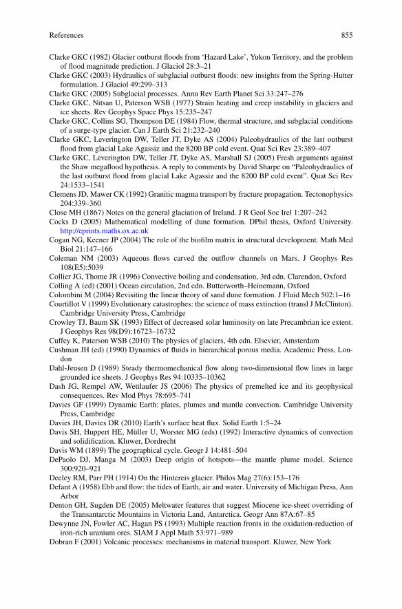
References 855

Clarke GKC (1982) Glacier outburst floods from ‘Hazard Lake’, Yukon Territory, and the problemof flood magnitude prediction. J Glaciol 28:3–21

Clarke GKC (2003) Hydraulics of subglacial outburst floods: new insights from the Spring-Hutterformulation. J Glaciol 49:299–313

Clarke GKC (2005) Subglacial processes. Annu Rev Earth Planet Sci 33:247–276Clarke GKC, Nitsan U, Paterson WSB (1977) Strain heating and creep instability in glaciers and

ice sheets. Rev Geophys Space Phys 15:235–247Clarke GKC, Collins SG, Thompson DE (1984) Flow, thermal structure, and subglacial conditions

of a surge-type glacier. Can J Earth Sci 21:232–240Clarke GKC, Leverington DW, Teller JT, Dyke AS (2004) Paleohydraulics of the last outburst

flood from glacial Lake Agassiz and the 8200 BP cold event. Quat Sci Rev 23:389–407Clarke GKC, Leverington DW, Teller JT, Dyke AS, Marshall SJ (2005) Fresh arguments against

the Shaw megaflood hypothesis. A reply to comments by David Sharpe on “Paleohydraulics ofthe last outburst flood from glacial Lake Agassiz and the 8200 BP cold event”. Quat Sci Rev24:1533–1541

Clemens JD, Mawer CK (1992) Granitic magma transport by fracture propagation. Tectonophysics204:339–360

Close MH (1867) Notes on the general glaciation of Ireland. J R Geol Soc Irel 1:207–242Cocks D (2005) Mathematical modelling of dune formation. DPhil thesis, Oxford University.

http://eprints.maths.ox.ac.ukCogan NG, Keener JP (2004) The role of the biofilm matrix in structural development. Math Med

Biol 21:147–166Coleman NM (2003) Aqueous flows carved the outflow channels on Mars. J Geophys Res

108(E5):5039Collier JG, Thome JR (1996) Convective boiling and condensation, 3rd edn. Clarendon, OxfordColling A (ed) (2001) Ocean circulation, 2nd edn. Butterworth–Heinemann, OxfordColombini M (2004) Revisiting the linear theory of sand dune formation. J Fluid Mech 502:1–16Courtillot V (1999) Evolutionary catastrophes: the science of mass extinction (transl J McClinton).

Cambridge University Press, CambridgeCrowley TJ, Baum SK (1993) Effect of decreased solar luminosity on late Precambrian ice extent.

J Geophys Res 98(D9):16723–16732Cuffey K, Paterson WSB (2010) The physics of glaciers, 4th edn. Elsevier, AmsterdamCushman JH (ed) (1990) Dynamics of fluids in hierarchical porous media. Academic Press, Lon-

donDahl-Jensen D (1989) Steady thermomechanical flow along two-dimensional flow lines in large

grounded ice sheets. J Geophys Res 94:10335–10362Dash JG, Rempel AW, Wettlaufer JS (2006) The physics of premelted ice and its geophysical

consequences. Rev Mod Phys 78:695–741Davies GF (1999) Dynamic Earth: plates, plumes and mantle convection. Cambridge University

Press, CambridgeDavies JH, Davies DR (2010) Earth’s surface heat flux. Solid Earth 1:5–24Davis SH, Huppert HE, Müller U, Worster MG (eds) (1992) Interactive dynamics of convection

and solidification. Kluwer, DordrechtDavis WM (1899) The geographical cycle. Geogr J 14:481–504DePaolo DJ, Manga M (2003) Deep origin of hotspots—the mantle plume model. Science

300:920–921Deeley RM, Parr PH (1914) On the Hintereis glacier. Philos Mag 27(6):153–176Defant A (1958) Ebb and flow: the tides of Earth, air and water. University of Michigan Press, Ann

ArborDenton GH, Sugden DE (2005) Meltwater features that suggest Miocene ice-sheet overriding of

the Transantarctic Mountains in Victoria Land, Antarctica. Geogr Ann 87A:67–85Dewynne JN, Fowler AC, Hagan PS (1993) Multiple reaction fronts in the oxidation-reduction of

iron-rich uranium ores. SIAM J Appl Math 53:971–989Dobran F (2001) Volcanic processes: mechanisms in material transport. Kluwer, New York

http://eprints.maths.ox.ac.uk

856 References

Dockery J, Klapper I (2001) Finger formation in biofilm layers. SIAM J Appl Math 62:853–869Dold JW (1985) Analysis of the early stage of thermal runaway. Q J Mech Appl Math 38:361–387Dowty E (1980) Crystal growth and nucleation theory and the numerical simulation of igneous

crystallisation. In: Hargraves RB (ed) Physics of magmatic processes. Princeton UniversityPress, Princeton, pp 419–485

Drazin PG, Johnson RS (1989) Solitons: an introduction. Cambridge University Press, CambridgeDrazin PG, Reid WH (1981) Hydrodynamic stability. Cambridge University Press, CambridgeDressler RF (1949) Mathematical solution of the problem of roll waves in inclined open channels.

Commun Pure Appl Math 2:149–194Drew DA, Passman SL (1999) Theory of multicomponent fluids. Springer, New YorkDrew DA, Wood RT (1985) Overview and taxonomy of models and methods for workshop on

two-phase flow fundamentals. National Bureau of Standards, GaithersburgDrozdowski E (1986) An international drumlin biography. Boreas 15:310Dullien FAL (1979) Porous media: fluid transport and pore structure. Academic Press, New YorkDurán O, Herrmann HJ (2006) Vegetation against dune mobility. Phys Rev Lett 97:188001Durand G, Gagliardini O, Zwinger T, Le Meur E, Hindmarsh RCA (2009) Full Stokes modeling

of marine ice sheets: influence of the grid size. Ann Glaciol 50(52):109–114Eberl D, Hower J (1976) Kinetics of illite formation. Geol Soc Amer Bull 87:1326–1330Eberl HJ, Parker DF, Van Loosdrecht MCM (2001) A new deterministic spatio-temporal continuum

model for biofilm development. Comput Math Methods Med 3:161–175Eckhardt B, Schneider TM, Hof B, Westerweel J (2007) Turbulent transition in pipe flow. Annu

Rev Fluid Mech 39:447–68Edelstein-Keshet L (2005) Mathematical models in biology. SIAM, PhiladelphiaEhrhard P, Riley DS, Steen PH (eds) (2001) Interactive dynamics of convection and solidification.

Kluwer, DordrechtEinstein HA (1950) The bedload function for bedload transportation in open channel flows. Tech

Bull No 1026, USDA, Soil Conservation Service, pp 1–71Embleton C, King CAM (1968) Glacial and periglacial geomorphology. Edward Arnold, LondonEmeleus CH (1987) The Rhum layered complex, Inner Hebrides, Scotland. In: Parsons I (ed)

Origins of igneous layering. NATO ASI series C, vol 196. Reidel, Dordrecht, pp 263–286Emerson SR, Hedges JI (2008) Chemical oceanography and the marine carbon cycle. Cambridge

University Press, CambridgeEngelhardt H, Humphrey N, Kamb B, Fahnestock M (1990) Physical conditions at the base of a

fast moving Antarctic ice stream. Science 248:57–59Engelund F (1970) Instability of erodible beds. J Fluid Mech 42:225–244Engelund F, Fredsøe J (1982) Sediment ripples and dunes. Annu Rev Fluid Mech 14:13–37England AH (1971) Complex variable methods in elasticity. Wiley-Interscience, LondonErdélyi A, Magnus W, Oberhettinger F, Tricomi FG (1953) Higher transcendental functions, vol 1.

McGraw-Hill, New YorkErlingsson U (2006) Lake Vostok behaves like a ‘captured lake’ and may be near to creating an

Antarctic jökulhlaup. Geogr Ann 88A:1–7Evatt G, Fowler AC, Clark CD, Hulton N (2006) Subglacial floods beneath ice sheets. Philos Trans

R Soc 364:1769–1794Finsterwalder S (1907) Die Theorie der Gletscherschwankungen. Z Gletschkd 2:81–103Fisher RA (1937) The wave of advance of advantageous genes. Ann Eugen 7:353–369Flemings MC (1974) Solidification processing. McGraw-Hill, New YorkFlint RF (1930) The origin of the Irish “eskers”. Geogr Rev 20:615–630Foulger GR, Natland JH (2003) Is “hotspot” volcanism a consequence of plate tectonics? Science

300:921–922Fowkes ND, Mahony JJ (1994) An introduction to mathematical modelling. Wiley, ChichesterFowler AC (1979) Glacier dynamics. DPhil thesis, University of OxfordFowler AC (1983) On the thermal state of the earth’s mantle. J Geophys 53:42–51Fowler AC (1985a) Fast thermoviscous convection. Stud Appl Math 72:189–219Fowler AC (1985b) A mathematical model of magma transport in the asthenosphere. Geophys

Astrophys Fluid Dyn 33:63–96

References 857

Fowler AC (1986) A sliding law for glaciers of constant viscosity in the presence of subglacialcavitation. Proc R Soc Lond A 407:147–170

Fowler AC (1987a) A theory of glacier surges. J Geophys Res 92:9111–9120Fowler AC (1987b) Sliding with cavity formation. J Glaciol 33:255–267Fowler AC (1989) A mathematical analysis of glacier surges. SIAM J Appl Math 49:246–262Fowler AC (1990) A compaction model for melt transport in the Earth’s asthenosphere. Part II:

applications. In: Ryan MP (ed) Magma transport and storage. Wiley, Chichester, pp 15–32Fowler AC (1992a) Modelling ice sheet dynamics. Geophys Astrophys Fluid Dyn 63:29–65Fowler AC (1992b) Convection and chaos. In: Yuen DA (ed) Chaotic processes in the geological

sciences. Springer, New York, pp 43–69Fowler AC (1993a) Towards a description of convection with temperature and pressure dependent

viscosity. Stud Appl Math 88:113–139Fowler AC (1993b) Boundary layer theory and subduction. J Geophys Res 98:21997–22005Fowler AC (1997) Mathematical models in the applied sciences. Cambridge University Press,

CambridgeFowler AC (2000) An instability mechanism for drumlin formation. In: Maltman A, Hambrey MJ,

Hubbard B (eds) Deformation of glacial materials. Spec pub geol soc, vol 176. GeologicalSociety, London, pp 307–319

Fowler AC (2003) On the rheology of till. Ann Glaciol 37:55–59Fowler AC (2009) Dynamics of subglacial floods. Proc R Soc A 465:1809–1828. doi:10.1098/rspa.

2008.0488Fowler AC (2010) The formation of subglacial streams and mega-scale glacial lineations. Proc R

Soc Lond A 466:3181–3201. doi:10.1098/rspa.2010.0009Fowler AC, Howell PD (2003) Intermittency in the transition to turbulence. SIAM J Appl Math

63:1184–1207Fowler AC, Johnson C (1995) Hydraulic runaway: a mechanism for thermally regulated surges of

ice sheets. J Glaciol 41:554–561Fowler AC, Johnson C (1996) Ice sheet surging and ice stream formation. Ann Glaciol 23:68–73Fowler AC, Larson DA (1978) On the flow of polythermal glaciers. I. Model and preliminary

analysis. Proc R Soc Lond A 363:217–242Fowler AC, Larson DA (1980a) The uniqueness of steady state flows of glaciers and ice sheets.

Geophys J R Astron Soc 63:333–345Fowler AC, Larson DA (1980b) On the flow of polythermal glaciers II. Surface wave analysis. Proc

R Soc Lond A 370:155–171Fowler AC, McGuinness MJ (1982) A description of the Lorenz attractor at high Prandtl number.

Physica D 5:149–182Fowler AC, O’Brien SBG (1996) A mechanism for episodic subduction on Venus. J Geophys Res

101:4755–4763Fowler AC, O’Brien SBG (2003) Lithospheric failure on Venus. Proc R Soc Lond A 459:2663–

2704Fowler AC, Schiavi E (1998) A theory of ice sheet surges. J Glaciol 44:104–118Fowler AC, Scott DR (1996) Hydraulic crack propagation in a porous medium. Geophys J Int

127:595–604Fowler AC, Yang X-S (1998) Fast and slow compaction in sedimentary basins. SIAM J Appl Math

59:365–385Fowler AC, Yang X-S (1999) Pressure solution and viscous compaction in sedimentary basins.

J Geophys Res 104:12989–12997Fowler AC, Yang X-S (2003) Dissolution/precipitation mechanisms for diagenesis in sedimentary

basins. J Geophys Res 108(B10):2509. doi:10.1029/2002JB002269Fowler AC, Kopteva N, Oakley C (2007) The formation of river channels. SIAM J Appl Math

67:1016–1040Fowler AC, Toja R, Vázquez C (2009) Temperature dependent shear flow and the absence of

thermal runaway in valley glaciers. Proc R Soc Lond A 466:363–382Fowler AC, McGuinness MJ, Ellis AS (2011) On an evolution equation for sand dunes. SIAM J

Appl Math, submitted

http://dx.doi.org/10.1098/rspa.2008.0488



http://dx.doi.org/10.1029/2002JB002269

858 References

Francis P, Oppenheimer C (2004) Volcanoes, 2nd edn. Oxford University Press, OxfordFrançois B, Lacombe F, Herrmann HJ (2002) Finite width of shear zones. Phys Rev E 65:031311Frappé-Sénéclauze T-P, Clarke GKC (2007) Slow surge of Trapridge Glacier, Yukon Territory,

Canada. J Geophys Res 112:F03S32. doi:10.1029/2006JF000607Fredsøe J (1974) On the development of dunes in erodible channels. J Fluid Mech 64:1–16Freed RL, Peacor DR (1989) Geopressured shale and sealing effect of smectite to illite transition.

Am Assoc Pet Geol Bull 73:1223–1232Freeze RA, Cherry JA (1979) Groundwater. Prentice-Hall, LondonFrench RH (1994) Open-channel hydraulics. McGraw-Hill, New YorkFreund LB (1990) Dynamic fracture mechanics. Cambridge University Press, CambridgeFricker HA, Scambos T, Bindschadler R, Padman L (2007) An active subglacial water system in

West Antarctica mapped from space. Science 315:1544–1548Fudge TJ, Humphrey NF, Harper JT, Pfeffer WT (2008) Diurnal fluctuations in borehole water

levels: configuration of the drainage system beneath Bench Glacier, Alaska, USA. J Glaciol54:297–306

Gakhov FD (1990) Boundary value problems. Dover, New YorkGanopolski A, Rahmstorf S (2001) Rapid changes of glacial climate simulated in a coupled climate

model. Nature 409:153–158Ganopolski A, Rahmstorf S (2002) Abrupt glacial climate changes due to stochastic resonance.

Phys Rev Lett 88(3):038501. doi:10.1103/PhysRevLett.88.038501García M, Parker G (1991) Entrainment of bed sediment into suspension. J Hydraul Eng 117:414–

435Ghil M, Childress S (1987) Topics in geophysical fluid dynamics. Springer, BerlinGill AE (1982) Atmosphere-ocean dynamics. Academic Press, San DiegoGlassman I (1987) Combustion, 2nd edn. Academic Press, OrlandoGoodwin ID (1988) The nature and origin of a jökulhlaup near Casey Station, Antarctica. J Glaciol

34:95–101Goudie A (1993) The nature of the environment, 3rd edn. Blackwell, OxfordGradshteyn IS, Ryzhik IM (1980) Table of integrals, series and products, Corrected and enlarged

edition. Academic Press, New YorkGray P, Scott SK (1990) Chemical oscillators and instabilities: non-linear chemical kinetics.

Clarendon, OxfordGrigoryan SS, Krass MS, Shumskiy PA (1976) Mathematical model of a three-dimensional non-

isothermal glacier. J Glaciol 17:401–417Grindrod P (1991) Patterns and waves. Oxford University Press, OxfordGrout FF (1945) Scale models of structures related to batholiths. Am J Sci 243-A:260–284. (Daly

volume)Gudmundsson GH (2003) Transmission of basal variability to a glacier surface. J Geophys Res

108(B5):2253. doi:10.1029/2002JB002107Gudmundsson MT, Sigmundsson F, Björnsson H (1997) Ice-volcano interaction of the 1996 Gjálp

subglacial eruption, Vatnajökull, Iceland. Nature 389:954–957Gudmundsson MT, Sigmundsson F, Björnsson H, Högnadóttir T (2004) The 1996 eruption at

Gjálp, Vatnajökull ice cap, Iceland: efficiency of heat transfer, ice deformation and subglacialwater pressure. Bull Volcanol 66:46–65

Haberman R (1998) Mathematical models. Society for Industrial and Applied Mathematics,Philadelphia

Hack JT (1957) Studies of longitudinal profiles in Virginia and Maryland. USGS Prof Paper, 294-B

Hagan PS, Polizzotti RS, Luckman G (1986) Internal oxidation of binary alloys. SIAM J ApplMath 45:956–971

Hall J (1815) On the revolutions of the Earth’s surface. Trans R Soc Edinb 7:169–184Hargraves RB (ed) (1980) Physics of magmatic processes. Princeton University Press, PrincetonHarland WB (1964) Critical evidence for a great infra-Cambrian glaciation. Geol Rundsch 54:45–

61

http://dx.doi.org/10.1029/2006JF000607

http://dx.doi.org/10.1103/PhysRevLett.88.038501

http://dx.doi.org/10.1029/2002JB002107

References 859

Harland WB (2007) Origins and assessment of snowball Earth hypotheses. Geol Mag 144:633–642

Heinrich H (1988) Origin and consequences of cyclic ice rafting in the Northeast Atlantic Oceanduring the past 130000 years. Quat Res 29:142–152

Hershenov J (1976) Solutions of the differential equation u′′′ +λ2zu′ + (α −1)λ2u = 0. Stud ApplMath 55:301–314

Hess PC (1989) Origins of igneous rocks. Harvard University Press, CambridgeHewitt GF, Hall-Taylor NS (1970) Annular two-phase flow. Pergamon, OxfordHewitt IJ, Fowler AC (2008) Seasonal waves on glaciers. Hydrol Process 22:3919–3930Hewitt IJ, Fowler AC (2009) Melt channelization in ascending mantle. J Geophys Res 114:B06210.

doi:10.1029/2008JB006185Hinch EJ (1991) Perturbation methods. Cambridge University Press, CambridgeHindmarsh RCA (1993) Qualitative dynamics of marine ice sheets. In: Peltier WR (ed) Ice in the

climate system. Springer, Berlin, pp 67–99Hindmarsh RCA (1998) The stability of a viscous till sheet coupled with ice flow, considered at

wavelengths less than the ice thickness. J Glaciol 44:285–292Hindmarsh RCA (2009) Consistent generation of ice-streams via thermo-viscous instabilities mod-

ulated by membrane stresses. Geophys Res Lett 36:L06502Hindmarsh RCA, Le Meur E (2001) Dynamical processes involved in the retreat of marine ice

sheets. J Glaciol 47:271–282Hodge SM (1974) Variations in the sliding of a temperate glacier. J Glaciol 13:349–369Hofmann AW, Hart SR (2007) Another nail in which coffin? Science 315:39–40Hoffman N (2000) White Mars: a new model for Mars’ surface and atmosphere based on CO2.

Icarus 146:326–342Hoffman PF, Kaufman AJ, Halverson GP, Schrag DP (1998) A Neoproterozoic snowball Earth.

Science 281:1342–1346Holland DM, Jacobs SS, Jenkins A (2003) Modelling the ocean circulation beneath the Ross Ice

Shelf. Antarct Sci 15:13–23Holland DM, Thomas RH, de Young B, Ribergaard MH (2008) Acceleration of Jakobshavn Isbrae

triggered by warm subsurface ocean waters. Nat Geosci 1:659–664Holmes A (1978) Principles of physical geology, 3rd edn, revised by Doris Holmes. Wiley, New

YorkHolmes MH (1995) Introduction to perturbation theory. Springer, New YorkHolmes MH (2009) Introduction to the foundations of applied mathematics. Springer, DordrechtHolton JR (2004) An introduction to dynamic meteorology, 4th edn. Elsevier, BurlingtonHooke RLeB (2005) Principles of glacier mechanics, 2nd edn. Cambridge University Press, Cam-

bridgeHooke RLeB, Laumann T, Kohler J (1990) Subglacial water pressures and the shape of subglacial

conduits. J Glaciol 36:67–71Hooke RLeB, Hanson B, Iverson NR, Jansson P, Fischer UH (1997) Rheology of till beneath

Storglaciären, Sweden. J Glaciol 43(143):172–179Hoppensteadt F (1975) Mathematical theories of populations: demographics, genetics and epi-

demics. Society for Industrial and Applied Mathematics, PhiladelphiaHort M, Spohn T (1991) Numerical simulation of the crystallization of multicomponents in thin

dikes or sills. 2. Effects of heterocatalytic nucleation and composition. J Geophys Res 96:485–499

Horton RE (1945) Erosional development of streams and their drainage basins; hydrophysicalapproach to quantitative morphology. Bull Geol Soc Am 56:275–370

Houghton JT (2002) The physics of atmospheres, 3rd edn. Cambridge University Press, Cam-bridge

Houghton JT, Meira Filho LG, Callander BA, Harris N, Kattenberg A, Maskell K (eds) (1996)Climate change 1995: the science of climate change. Cambridge University Press, Cambridge

Howard AD (1978) Origin of the stepped topography on the Martian poles. Icarus 34:581–599Howard AD (1994) A detachment-limited model of drainage basin evolution. Water Resour Res

30:2261–2285

http://dx.doi.org/10.1029/2008JB006185

860 References

Howard LN (1966) Convection at high Rayleigh number. In: Görtler H (ed) Proc 11th int congappl mech. Springer, Berlin, pp 1109–1115

Howard LN, Kopell N (1977) Slowly varying waves and shock structures in reaction-diffusionequations. Stud Appl Math 56:95–145

Howell PD (1996) Models for thin viscous sheets. Eur J Appl Math 7:321–343Howison SD (2005) Practical applied mathematics: modelling, analysis, approximation. Cam-

bridge University Press, CambridgeHubbard BP, Sharp MJ, Willis IC, Nielsen MK, Smart CC (1995) Borehole water-level varia-

tions and the structure of the subglacial hydrological system of Haut Glacier d’Arolla, Valais,Switzerland. J Glaciol 41:572–583

Hughes TJ (1973) Is the West Antarctic ice sheet disintegrating? J Geophys Res 78:7884–7910Hunt JCR, Leibovich S, Richards KJ (1988) Turbulent shear flows over low hills. Q J R Meteorol

Soc 114:1435–1470Hunt JM (1990) Generation and migration of petroleum from abnormally pressured fluid compart-

ments. Am Assoc Pet Geol Bull 74:1–12Huppert HE (1986) The intrusion of fluid mechanics into geology. J Fluid Mech 173:557–594Huppert HE (1990) The fluid mechanics of solidification. J Fluid Mech 212:209–240Huppert HE (2000) Geological fluid mechanics. In: Batchelor GK, Moffatt HK, Worster MG (eds)

Perspectives in fluid dynamics. Cambridge University Press, Cambridge, pp 447–506Huppert HE, Sparks RSJ (1980) The fluid dynamics of a basaltic magma chamber replenished by

influx of hot, dense, ultrabasic magma. Contrib Mineral Petrol 75:279–289Huppert HE, Sparks RSJ (1988) The fluid dynamics of crustal melting by injection of basaltic sills.

Trans R Soc Edinb 79:237–243Hutter K (1983) Theoretical glaciology. Reidel, DordrechtHutter K, Olunloyo VOS (1980) On the distribution of stress and velocity in an ice strip, which is

partly sliding over and partly adhering to its bed, by using a Newtonian viscous approximation.Proc R Soc Lond A 373:385–403

Hutter K, Yakowitz S, Szidarovsky F (1986) A numerical study of plane ice sheet flow. J Glaciol32:139–160

Hüttmann A, Wilson RD, Thornton SF, Lerner DN (2003) Natural attenuation of ammonium ata former coal carbonisation plant (Mansfield, UK): conceptual model for biodegradation pro-cesses. In: Consoil 2003, Gent, Conference Proceedings CD, pp 1542–1547

Hyde WT, Crowley TJ, Baum SK, Peltier WR (2000) Neoproterozoic ‘snowball Earth’ simulationswith a coupled climate/ice sheet model. Nature 405:425–429

Iken A (1981) The effect of subglacial water pressure on the sliding velocity of a glacier in anidealized numerical model. J Glaciol 27:407–422

Imbrie J, Imbrie KP (1979) Ice ages; solving the mystery. Harvard University Press, CambridgeInnes R (1732) Miscellaneous letters on several subjects in philosophy and astronomy, I, p 4. S Birt,

LondonIrvine TN (1987) Layering and related structures in the Duke Island and Skaergaard intrusions:

similarities, differences, and origins. In: Parsons I (ed) Origins of igneous layering. NATO ASIseries C, vol 196. Reidel, Dordrecht, pp 185–245

Ishii M (1975) Thermo-fluid dynamic theory of two-phase flow. Eyrolles, ParisIvanov AB, Muhleman DO (2000) The role of sublimation for the formation of the Northern ice

cap: results from the Mars Orbiter Laser Altimeter. Icarus 144:436–448Iverson NR, Baker RW, Hooyer TS (1997) A ring-shear device for the study of till deformation:

tests on tills with contrasting clay contents. Quat Sci Rev 16(9):1057–1066Izumi N, Parker G (1995) Inception of channelization and drainage basin formation: upstream-

driven theory. J Fluid Mech 283:341–363Izumi N, Parker G (2000) Linear stability analysis of channel inception: downstream-driven theory.

J Fluid Mech 419:239–262Jackson PS, Hunt JCR (1975) Turbulent wind flow over a low hill. Q J R Meteorol Soc 101:929–

955Jarvis GT, McKenzie D (1982) Mantle convection as a boundary layer phenomenon. Geophys J R

Astron Soc 68:389–427

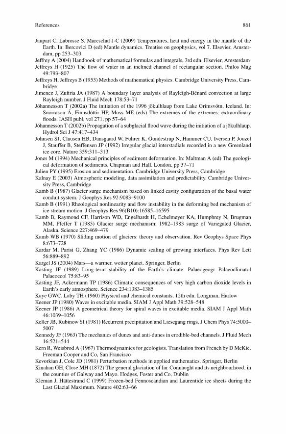
References 861

Jaupart C, Labrosse S, Mareschal J-C (2009) Temperatures, heat and energy in the mantle of theEarth. In: Bercovici D (ed) Mantle dynamics. Treatise on geophysics, vol 7. Elsevier, Amster-dam, pp 253–303

Jeffrey A (2004) Handbook of mathematical formulas and integrals, 3rd edn. Elsevier, AmsterdamJeffreys H (1925) The flow of water in an inclined channel of rectangular section. Philos Mag

49:793–807Jeffreys H, Jeffreys B (1953) Methods of mathematical physics. Cambridge University Press, Cam-

bridgeJimenez J, Zufiria JA (1987) A boundary layer analysis of Rayleigh-Bénard convection at large

Rayleigh number. J Fluid Mech 178:53–71Jóhannesson T (2002a) The initiation of the 1996 jökulhlaup from Lake Grímsvötn, Iceland. In:

Snorrason Á, Finnsdóttir HP, Moss ME (eds) The extremes of the extremes: extraordinaryfloods. IASH publ, vol 271, pp 57–64

Jóhannesson T (2002b) Propagation of a subglacial flood wave during the initiation of a jökulhlaup.Hydrol Sci J 47:417–434

Johnsen SJ, Clausen HB, Dansgaard W, Fuhrer K, Gundestrup N, Hammer CU, Iversen P, JouzelJ, Stauffer B, Steffensen JP (1992) Irregular glacial interstadials recorded in a new Greenlandice core. Nature 359:311–313

Jones M (1994) Mechanical principles of sediment deformation. In: Maltman A (ed) The geologi-cal deformation of sediments. Chapman and Hall, London, pp 37–71

Julien PY (1995) Erosion and sedimentation. Cambridge University Press, CambridgeKalnay E (2003) Atmospheric modeling, data assimilation and predictability. Cambridge Univer-

sity Press, CambridgeKamb B (1987) Glacier surge mechanism based on linked cavity configuration of the basal water

conduit system. J Geophys Res 92:9083–9100Kamb B (1991) Rheological nonlinearity and flow instability in the deforming bed mechanism of

ice stream motion. J Geophys Res 96(B10):16585–16595Kamb B, Raymond CF, Harrison WD, Engelhardt H, Echelmeyer KA, Humphrey N, Brugman

MM, Pfeffer T (1985) Glacier surge mechanism: 1982–1983 surge of Variegated Glacier,Alaska. Science 227:469–479

Kamb WB (1970) Sliding motion of glaciers: theory and observation. Rev Geophys Space Phys8:673–728

Kardar M, Parisi G, Zhang YC (1986) Dynamic scaling of growing interfaces. Phys Rev Lett56:889–892

Kargel JS (2004) Mars—a warmer, wetter planet. Springer, BerlinKasting JF (1989) Long-term stability of the Earth’s climate. Palaeogeogr Palaeoclimatol

Palaeoecol 75:83–95Kasting JF, Ackermann TP (1986) Climatic consequences of very high carbon dioxide levels in

Earth’s early atmosphere. Science 234:1383–1385Kaye GWC, Laby TH (1960) Physical and chemical constants, 12th edn. Longman, HarlowKeener JP (1980) Waves in excitable media. SIAM J Appl Math 39:528–548Keener JP (1986) A geometrical theory for spiral waves in excitable media. SIAM J Appl Math

46:1039–1056Keller JB, Rubinow SI (1981) Recurrent precipitation and Liesegang rings. J Chem Phys 74:5000–

5007Kennedy JF (1963) The mechanics of dunes and anti-dunes in erodible-bed channels. J Fluid Mech

16:521–544Kern R, Weisbrod A (1967) Thermodynamics for geologists. Translation from French by D McKie.

Freeman Cooper and Co, San FranciscoKevorkian J, Cole JD (1981) Perturbation methods in applied mathematics. Springer, BerlinKinahan GH, Close MH (1872) The general glaciation of Iar-Connaught and its neighbourhood, in

the counties of Galway and Mayo. Hodges, Foster and Co, DublinKleman J, Hättestrand C (1999) Frozen-bed Fennoscandian and Laurentide ice sheets during the

Last Glacial Maximum. Nature 402:63–66

862 References

Knighton D (1998) Fluvial forms and processes: a new perspective. Arnold, LondonKnittle E, Jeanloz R (1991) Earth’s core–mantle boundary: results of experiments at high pressures

and temperatures. Science 251:1438–1443Koestler A (1964) The sleepwalkers. Penguin Books, LondonKöhler P, Fischer H (2006) Simulating low frequency changes in atmospheric CO2 during the last

740000 years. Clim Past 2:57–78Köhler P, Fischer H, Munhoven G, Zeebe RE (2005) Quantitative interpretation of atmospheric

carbon records over the last glacial termination. Glob Biogeochem Cycles 19:GB4020.doi:10.1029/2004GB002345

Kopell N, Howard LN (1973) Plane wave solutions to reaction-diffusion equations. Stud ApplMath 42:291–328

Korteweg DJ, de Vries G (1895) On the change of form of long waves advancing in a rectangularcanal, and on a new type of long stationary waves. Philos Mag Ser 5 39:422–443

Kramer S, Marder M (1992) Evolution of river networks. Phys Rev Lett 68:205–208Krauskopf KB, Bird DK (1995) Introduction to geochemistry. McGraw-Hill, New YorkKroy K, Sauermann G, Herrmann HJ (2002a) Minimal model for sand dunes. Phys Rev Lett

88:054301Kroy K, Sauermann G, Herrmann HJ (2002b) Minimal model for aeolian sand dunes. Phys Rev E

66:031302Kurz W, Fisher DJ (1998) Fundamentals of solidification, 4th edn. Trans Tech, ZurichLakin WD, Ng BS, Reid WH (1978) Approximations to the eigenvalue relation for the Orr-

Sommerfeld problem. Philos Trans R Soc 289:347–371Lamb, Sir Horace (1945) Hydrodynamics, 6th edn. Dover reprint of the 1932 sixth edition. Dover,

New YorkLambe TW, Whitman RV (1979) Soil mechanics, SI version. Wiley, New YorkLang C, Leuenberger M, Schwander J, Johnsen S (1999) 16°C rapid temperature variation in cen-

tral Greenland 70000 years ago. Science 286:934–937Lasaga AC, Berner RA, Garrels RM (1985) An improved geochemical model of atmospheric CO2

fluctuations over the past 100 million years. In: Sundquist ET, Broecker WS (eds) The carboncycle and atmospheric CO2: natural variations Archaen to present. AGU, Washington, pp 397–411

Le Grand HE (1988) Drifting continents and shifting theories. Cambridge University Press, Cam-bridge

Leuenberger MC, Lang C, Schwander J (1999) Delta 15N measurements as a calibration tool forthe paleothermometer and gas–ice age differences: a case study for the 8200 BP event on GRIPice. J Geophys Res 104(D18):22163–22170

Li M, Richmond O (1997) Intrinsic instability and non-uniformity of plastic deformation. Int JPlast 13:765–784

Lighthill MJ, Whitham GB (1955a) On kinematic waves. I. Flood movement in long rivers. ProcR Soc Lond A 229:281–316

Lighthill MJ, Whitham GB (1955b) On kinematic waves. II. A theory of traffic flow on long,crowded roads. Proc R Soc Lond A 229:317–345

Lin CC, Segel LA (1974) Mathematics applied to deterministic problems in the natural sciences.MacMillan, New York

Liñán A, Williams FA (1993) Fundamental aspects of combustion. Oxford University Press, Ox-ford

Liou KN (2002) An introduction to atmospheric radiation, 2nd edn. Academic Press, San DiegoLister JR, Kerr RC (1991) Fluid-mechanical models of crack propagation and their application to

magma transport in dykes. J Geophys Res 96:10049–10077Lliboutry LA (1956) La mécanique des glaciers en particulier au voisinage de leur front. Ann

Geophys 12:245–276Lliboutry LA (1958a) La dynamique de la Mer de Glace et la vague de 1891–95 d’après les mésures

de Joseph Vallot. In: Physics of the movement of ice (Chamonix symposium). IAHS publ,vol 47. IAHS Press, Wallingford, pp 125–138. Available to download at http://www.iahs.info/redbooks/047.htm

http://dx.doi.org/10.1029/2004GB002345

http://www.iahs.info/redbooks/047.htm

http://www.iahs.info/redbooks/047.htm

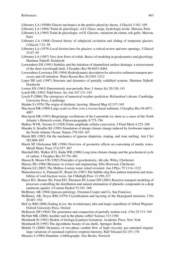
References 863

Lliboutry LA (1958b) Glacier mechanics in the perfect plasticity theory. J Glaciol 3:162–169Lliboutry LA (1964) Traité de glaciologie, vol I. Glace, neige, hydrologie nivale. Masson, ParisLliboutry LA (1965) Traité de glaciologie, vol II. Glaciers, variations du climat, sols gelés. Masson,

ParisLliboutry LA (1968) General theory of subglacial cavitation and sliding of temperate glaciers.

J Glaciol 7:21–58Lliboutry LA (1979) Local friction laws for glaciers: a critical review and new openings. J Glaciol

23:67–95Lliboutry LA (1987) Very slow flows of solids. Basics of modeling in geodynamics and glaciology.

Martinus Nijhoff, DordrechtLoewenherz DS (1991) Stability and the initiation of channelized surface drainage: a reassessment

of the short wavelength limit. J Geophys Res 96:8453–8464Loewenherz-Lawrence DS (1994) Hydrodynamic description for advective sediment transport pro-

cesses and rill initiation. Water Resour Res 30:3203–3212Loper DE (ed) (1987) Structure and dynamics of partially solidified systems. Martinus Nijhoff,

DordrechtLorenz EN (1963) Deterministic non-periodic flow. J Atmos Sci 20:130–141Lynch DK (1982) Tidal bores. Sci Am 247:131–143Lynch P (2006) The emergence of numerical weather prediction: Richardson’s dream. Cambridge

University Press, CambridgeMaaløe S (1978) The origin of rhythmic layering. Mineral Mag 42:337–345MacAyeal DR (1989) Large-scale ice flow over a viscous basal sediment. J Geophys Res 94:4071–

4087MacAyeal DR (1993) Binge/purge oscillations of the Laurentide ice sheet as a cause of the North

Atlantic’s Heinrich events. Paleoceanography 8:775–784Malkus WVR, Veronis G (1958) Finite amplitude cellular convection. J Fluid Mech 4:225–260Manabe S, Stouffer RJ (1995) Simulation of abrupt climate change induced by freshwater input to

the North Atlantic Ocean. Nature 378:165–167Marsh BD (1982) On the mechanics of igneous diapirism, stoping, and zone melting. Am J Sci

282:808–855Marsh SP, Glicksman ME (1996) Overview of geometric effects on coarsening of mushy zones.

Metall Mater Trans 27A:557–567Marshall HG, Walker JCG, Kuhn WR (1988) Long term climate change and the geochemical cycle

of carbon. J Geophys Res 93:791–801Mason B, Moore CB (1982) Principles of geochemistry, 4th edn. Wiley, ChichesterMassey BS (1986) Measures in science and engineering. Ellis Horwood, ChichesterMatson LE (2007) The Malkus–Lorenz water wheel revisited. Am J Phys 75:1114–1122Matuszkiewicz A, Flamand JC, Bouré JA (1987) The bubble-slug flow pattern transition and insta-

bilities of void-fraction waves. Int J Multiph Flow 13:199–217Mayer KU, Benner SG, Frind EO, Thornton SF, Lerner DN (2001) Reactive transport modeling of

processes controlling the distribution and natural attenuation of phenolic compounds in a deepsandstone aquifer. J Contam Hydrol 53:341–368

McBirney AR (1984) Igneous petrology. Freeman Cooper and Co, San FranciscoMcBirney AR, Noyes RM (1979) Crystallisation and layering of the Skaergaard intrusion. J Pet

20:487–554McCoy RM (2006) Ending in ice: the revolutionary idea and tragic expedition of Alfred Wegener.

Oxford University Press, OxfordMcKenzie DP (1984) The generation and compaction of partially molten rock. J Pet 25:713–765McNutt MK (2006) Another nail in the plume coffin? Science 313:1394Meinhardt H (1982) Models of biological pattern formation. Academic Press, New YorkMeinhardt H (1995) The algorithmic beauty of sea shells. Springer, BerlinMelnik O (2000) Dynamics of two-phase conduit flow of high-viscosity gas-saturated magma:

large variations of sustained explosive eruption intensity. Bull Volcanol 62:153–170Menzies J (1984) Drumlins: a bibliography. Geo Books, Norwich

864 References

Meyer-Peter E, Müller R (1948) Formulas for bed-load transport. In: Proc int assoc hydraul res,3rd annual conference, Stockholm, pp 39–64

Miller RN (2007) Numerical modelling of ocean circulation. Cambridge University Press, Cam-bridge

Millero FJ (1995) Thermodynamics of the carbon dioxide system in the oceans. Geochim Cos-mochim Acta 59:661–677

Monod J (1949) The growth of bacterial cultures. Annu Rev Microbiol 3:371–394Moore DR, Weiss NO (1973) Two-dimensional Rayleigh-Bénard convection. J Fluid Mech

58:289–312Moore PL, Iverson NR (2002) Slow episodic shear of granular materials regulated by dilatant

strengthening. Geology 30:843–846Moresi L-N, Solomatov VS (1995) Numerical investigation of 2D convection with extremely large

viscosity variations. Phys Fluids 7:2154–2162Moresi L-N, Solomatov VS (1998) Mantle convection with a brittle lithosphere: thoughts on the

global tectonic styles of the Earth and Venus. Geophys J Int 133:669–682Morgan JP, Blackman DK, Sinton JM (eds) (1992) Mantle flow and melt generation at mid-ocean

ridges. Geophysical monograph, vol 71. AGU, WashingtonMorgan WJ (1971) Convection plumes in the lower mantle. Nature 230:42–43Morland LW (1976a) Glacier sliding down an inclined wavy bed. J Glaciol 17:447–462Morland LW (1976b) Glacier sliding down an inclined wavy bed with friction. J Glaciol 17:463–

477Morland LW (1984) Thermo-mechanical balances of ice sheet flow. Geophys Astrophys Fluid Dyn

29:237–266Morland LW, Johnson IR (1980) Steady motion of ice sheets. J Glaciol 25:229–246Morland LW, Shoemaker EM (1982) Ice shelf balances. Cold Reg Sci Technol 5:235–251Morris S (1982) The effects of strongly temperature-dependent viscosity on slow flow past a hot

sphere. J Fluid Mech 124:1–26Morris S, Canright D (1984) A boundary layer analysis of Bénard convection in a fluid of strongly

temperature-dependent viscosity. Phys Earth Planet Inter 29:320–329Munhoven G, François LM (1996) Glacial–interglacial variability of atmospheric CO2 due to

changing continental silicate rock weathering: a model study. J Geophys Res 101:21423–21437Murray JD (2002) Mathematical biology, 2 volumes. Springer, BerlinMuskhelishvili NI (1953) Singular integral equations (Translation edited by JRM Radok). Noord-

hoff, GroningenNataf H-C, Richter FM (1982) Convection experiments in fluids with highly temperature-

dependent viscosity and the thermal evolution of the planets. Phys Earth Planet Inter 29:320–329

Nayfeh AH (1973) Perturbation methods. Wiley-Interscience, New YorkNeedham DJ, Merkin JH (1984) On roll waves down an open inclined channel. Proc R Soc Lond

A 394:259–278Newell AC (1985) Solitons in mathematics and physics. Society for Industrial and Applied Math-

ematics, PhiladelphiaNewell AC, Whitehead JA (1969) Finite bandwidth, finite amplitude convection. J Fluid Mech

38:279–303Ng FSL (1998) Mathematical modelling of subglacial drainage and erosion. DPhil thesis, Oxford

UniversityNg F, Björnsson H (2003) On the Clague-Mathews relation for jökulhlaups. J Glaciol 49:161–172Ng FSL, Zuber MT (2003) Albedo feedback in the patterning mechanisms of Martian polar caps.

In: 3rd international conference on Mars polar science and exploration, abstract #8061, Lunarand Planetary Science Institute, Houston (CD-ROM)

Ng FSL, Zuber MT (2006) Patterning instability on the Mars polar ice caps. J Geophys Res111:E02005. doi:10.1029/2005JE002533

Nicolas A (1986) A melt extraction model based on structural studies in mantle peridotites. J Pet27:999–1022

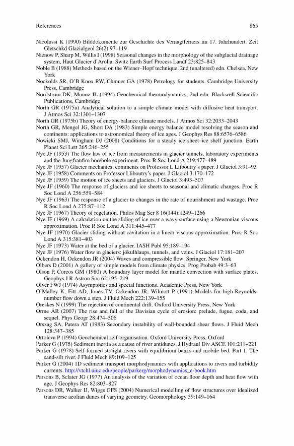
http://dx.doi.org/10.1029/2005JE002533

References 865

Nicolussi K (1990) Bilddokumente zur Geschichte des Vernagtferners im 17. Jahrhundert. ZeitGletschkd Glazialgeol 26(2):97–119

Nienow P, Sharp M, Willis I (1998) Seasonal changes in the morphology of the subglacial drainagesystem, Haut Glacier d’Arolla. Switz Earth Surf Process Landf 23:825–843

Noble B (1988) Methods based on the Wiener–Hopf technique, 2nd (unaltered) edn. Chelsea, NewYork

Nockolds SR, O’B Knox RW, Chinner GA (1978) Petrology for students. Cambridge UniversityPress, Cambridge

Nordstrom DK, Munoz JL (1994) Geochemical thermodynamics, 2nd edn. Blackwell ScientificPublications, Cambridge

North GR (1975a) Analytical solution to a simple climate model with diffusive heat transport.J Atmos Sci 32:1301–1307

North GR (1975b) Theory of energy-balance climate models. J Atmos Sci 32:2033–2043North GR, Mengel JG, Short DA (1983) Simple energy balance model resolving the season and

continents: applications to astronomical theory of ice ages. J Geophys Res 88:6576–6586Nowicki SMJ, Wingham DJ (2008) Conditions for a steady ice sheet–ice shelf junction. Earth

Planet Sci Lett 265:246–255Nye JF (1953) The flow law of ice from measurements in glacier tunnels, laboratory experiments

and the Jungfraufirn borehole experiment. Proc R Soc Lond A 219:477–489Nye JF (1957) Glacier mechanics; comments on Professor L Lliboutry’s paper. J Glaciol 3:91–93Nye JF (1958) Comments on Professor Lliboutry’s paper. J Glaciol 3:170–172Nye JF (1959) The motion of ice sheets and glaciers. J Glaciol 3:493–507Nye JF (1960) The response of glaciers and ice sheets to seasonal and climatic changes. Proc R

Soc Lond A 256:559–584Nye JF (1963) The response of a glacier to changes in the rate of nourishment and wastage. Proc

R Soc Lond A 275:87–112Nye JF (1967) Theory of regelation. Philos Mag Ser 8 16(144):1249–1266Nye JF (1969) A calculation on the sliding of ice over a wavy surface using a Newtonian viscous

approximation. Proc R Soc Lond A 311:445–477Nye JF (1970) Glacier sliding without cavitation in a linear viscous approximation. Proc R Soc

Lond A 315:381–403Nye JF (1973) Water at the bed of a glacier. IASH Publ 95:189–194Nye JF (1976) Water flow in glaciers: jökulhlaups, tunnels, and veins. J Glaciol 17:181–207Ockendon H, Ockendon JR (2004) Waves and compressible flow. Springer, New YorkOlbers D (2001) A gallery of simple models from climate physics. Prog Probab 49:3–63Olson P, Corcos GM (1980) A boundary layer model for mantle convection with surface plates.

Geophys J R Astron Soc 62:195–219Olver FWJ (1974) Asymptotics and special functions. Academic Press, New YorkO’Malley K, Fitt AD, Jones TV, Ockendon JR, Wilmott P (1991) Models for high-Reynolds-

number flow down a step. J Fluid Mech 222:139–155Oreskes N (1999) The rejection of continental drift. Oxford University Press, New YorkOrme AR (2007) The rise and fall of the Davisian cycle of erosion: prelude, fugue, coda, and

sequel. Phys Geogr 28:474–506Orszag SA, Patera AT (1983) Secondary instability of wall-bounded shear flows. J Fluid Mech

128:347–385Ortoleva P (1994) Geochemical self-organisation. Oxford University Press, OxfordParker G (1975) Sediment inertia as a cause of river antidunes. J Hydraul Div ASCE 101:211–221Parker G (1978) Self-formed straight rivers with equilibrium banks and mobile bed. Part 1. The

sand-silt river. J Fluid Mech 89:109–125Parker G (2004) 1D sediment transport morphodynamics with applications to rivers and turbidity

currents. http://vtchl.uiuc.edu/people/parkerg/morphodynamics_e-book.htmParsons B, Sclater JG (1977) An analysis of the variation of ocean floor depth and heat flow with

age. J Geophys Res 82:803–827Parsons DR, Walker IJ, Wiggs GFS (2004) Numerical modelling of flow structures over idealized

transverse aeolian dunes of varying geometry. Geomorphology 59:149–164

http://vtchl.uiuc.edu/people/parkerg/morphodynamics_e-book.htm

866 References

Parsons I (ed) (1987) Origins of igneous layering. NATO ASI series C, vol 196. Reidel, DordrechtParteli EJR, Durán O, Herrmann HJ (2007) Minimal size of a barchan dune. Phys Rev E 75:011301Parteli EJR, Durán O, Tsoar H, Schwämmle V, Herrmann HJ (2009) Dune formation under bi-

modal winds. Proc Natl Acad Sci 106:22085–22089Paterson WSB (1994) The physics of glaciers, 3rd edn. Pergamon, OxfordPattyn F, de Smedt B, Souchez R (2004) Influence of subglacial Vostok lake on the regional ice

dynamics of the Antarctic ice sheet: a model study. J Glaciol 50:583–589Payne AJ, Dongelmans PW (1997) Self-organization in the thermomechanical flow of ice sheets.

J Geophys Res 102:12219–12233Pearson JRA (1958) On convection cells induced by surface tension. J Fluid Mech 4:489–500Pedlosky J (1987) Geophysical fluid dynamics, 2nd edn. Springer, BerlinPelletier JD (2004) How do spiral troughs form on Mars? Geology 32(4):365–367Pelletier JD (2008) Quantitative modeling of Earth surface processes. Cambridge University Press,

CambridgePeregrine DH (1966) Calculations of the development of an undular bore. J Fluid Mech 25:321–

330Petford N, Lister JR, Kerr RC (1994) The ascent of felsic magmas in dykes. Lithos 32:161–168Petit JR, Jouzel J, Raynaud D, Barkov NI, Barnola J-M, Basile I, Bender M, Chappellaz J, Davis

M, Delaygue G, Delmotte M, Kotlyakov VM, Legrand M, Lipenkov VY, Lorius C, Pépin L,Ritz C, Saltzman E, Stievenard M (1999) Climate and atmospheric history of the past 420000years from the Vostok ice core, Antarctica. Nature 399:429–436

Picioreanu C, van Loosdrecht MCM, Heijnen JJ (1998) Mathematical modeling of biofilmstructure with a hybrid differential-discrete cellular automaton approach. Biotechnol Bioeng58:101–116

Pierrehumbert RT (2004) High atmospheric carbon dioxide necessary for the termination of globalglaciation. Nature 429:646–648

Pillow AF (1952) The free convection cell in two dimensions. Dept of Supply, Aeronautical Re-search Laboratories, Report A.79 [Dept of Mathematics, University of Queensland, St Lucia,Queensland 4067, Australia]

Pitcher WS (1997) The nature and origin of granite, 2nd edn. Chapman and Hall, LondonPolubarinova-Kochina PYa (1962) Theory of ground water movement. Princeton University Press,

PrincetonPrice M (1985) Introducing groundwater. George Allen and Unwin, LondonProsperetti A, Satrape JV (1990) Stability of two-phase flow models. In: Joseph DD, Schaeffer DG

(eds) Two-phase flow models and waves. Springer, New York, pp 98–117Pugh DT (1987) Tides, surges and mean sea-level. Wiley, ChichesterPye K, Tsoar H (1990) Aeolian sand and sand dunes. Unwin Hyman, LondonQuareni F, Yuen DA, Sewell G, Christensen UR (1985) High Rayleigh number convection with

strongly variable viscosity: a comparison between mean field and two-dimensional solutions.J Geophys Res 90:12633–12644

Rahmstorf S (1995) Bifurcations of the Atlantic thermohaline circulation in response to changesin the hydrological cycle. Nature 378:145–149

Rahmstorf S (2002) Ocean circulation and climate during the past 120000 years. Nature 419:207–214

Rathbun AP, Marone C, Alley RB, Anandakrishnan S (2008) Laboratory study of the frictionalrheology of sheared till. J Geophys Res 113:F02020. doi:10.1029/2007JF000815

Rayleigh, Lord (1908) Note on tidal bores. Proc R Soc Lond A 81:448–449Rayleigh, Lord (1916) On convective currents in a horizontal layer of fluid when the higher tem-

perature is on the under side. Philos Mag 32:529–546Reese CC, Solomatov VS (2002) Mean field heat transfer scaling for non-Newtonian stagnant lid

convection. J Non-Newton Fluid Mech 107:39–49Reese CC, Solomatov VS, Moresi L-N (1999) Non-Newtonian stagnant lid convection and mag-

matic resurfacing on Venus. Icarus 139:67–80Reid WH (1972) Composite approximations to the solutions of the Orr-Sommerfeld equation. Stud

Appl Math 51:341–368

http://dx.doi.org/10.1029/2007JF000815

References 867

Rempel AW, Wettlaufer JS, Worster MG (2004) Premelting dynamics in a continuum model offrost heave. J Fluid Mech 498:227–244

Reynolds AJ (1965) Waves on the erodible bed of an open channel. J Fluid Mech 22:113–133Reynolds O (1895) On the dynamical theory of incompressible viscous fluids and the determination

of the criterion. Philos Trans R Soc Lond A 186:123–164Ribe NM (2009) Analytical approaches to mantle dynamics. In: Bercovici D (ed) Mantle dynamics.

Treatise on geophysics, vol 7. Elsevier, Amsterdam, pp 167–226Richards K (1982) Rivers: form and process in alluvial channels. Methuen, LondonRichards KJ (1980) The formation of ripples and dunes on an erodible bed. J Fluid Mech 99:597–

618Richardson CN, Lister JR, McKenzie D (1996) Melt conduits in a viscous porous matrix. J Geo-

phys Res 101:20423–20432Rittmann BE, McCarty PL (1980) Model of steady-state-biofilm kinetics. Biotechnol Bioeng

22:2343–2357Roberts GO (1977) Fast viscous convection. Geophys Astrophys Fluid Dyn 8:197–233Roberts GO (1979) Fast viscous Bénard convection. Geophys Astrophys Fluid Dyn 12:235–272Roberts MJ (2005) Jökulhlaups: a reassessment of floodwater flow through glaciers. Rev Geophys

43:RG1002Robin G de Q (1955) Ice movement and temperature distribution in glaciers and ice sheets.

J Glaciol 2:523–532Robinson JR (1967) Finite amplitude convection cells. J Fluid Mech 30:577–600Rodríguez-Iturbe I, Rinaldo A (1997) Fractal river basins. Cambridge University Press, CambridgeRöthlisberger H (1972) Water pressure in intra- and subglacial channels. J Glaciol 11:177–203Rowbotham F (1970) The Severn bore, 2nd edn. David and Charles, Newton AbbotRubinstein J, Mauri R (1986) Dispersion and convection in periodic porous media. SIAM J Appl

Math 46:1018–1023Ruddiman WF (2001) Earth’s climate: past and future. Freeman, New YorkRyan MP (ed) (1990) Magma transport and storage. Wiley, ChichesterSaffman PG (1959) A theory of dispersion in a porous medium. J Fluid Mech 6:321–349Sahimi M (1995) Flow and transport in porous media and fractured rock. VCH, WeinheimSamarskii AA, Galaktionov VA, Kurdyumov SP, Mikhailov AP (1995) Blow-up in quasilinear

parabolic equations. de Gruyter expositions in mathematics, vol 19. de Gruyter, BerlinSanchez-Palencia E (1983) Homogenization method for the study of composite media. Springer,

BerlinSass BM, Rosenberg PE, Kittrick JA (1987) The stability of illite/smectite during diagenesis: an

experimental study. Geochim Cosmochim Acta 51:2103–2115Sauermann G, Kroy K, Herrmann HJ (2001) Continuum saltation model for sand dunes. Phys Rev

E 64:031305Sayag R, Tziperman E (2008) Spontaneous generation of pure ice streams via flow insta-

bility: role of longitudinal shear stresses and subglacial till. J Geophys Res 113:B05411.doi:10.1029/2007JB005228

Schlichting H (1979) Boundary layer theory. McGraw-Hill, New YorkSchmidt MW, Vautravers MJ, Spero HJ (2006) Rapid subtropical North Atlantic salinity oscilla-

tions across Dansgaard–Oeschger cycles. Nature 443:561–564Schoof C (2005) The effect of cavitation on glacier sliding. Proc R Soc Lond A 461:609–627Schoof C (2007a) Pressure-dependent viscosity and interfacial instability in coupled ice-sediment

flow. J Fluid Mech 570:227–252Schoof C (2007b) Marine ice-sheet dynamics. Part 1. The case of rapid sliding. J Fluid Mech

573:27–55Schoof C (2007c) Ice sheet grounding line dynamics: steady states, stability and hysteresis. J Geo-

phys Res 112:F03S28. doi:10.1029/2006JF000664Schoof C, Hindmarsh RCA (2010) Thin-film flows with wall slip: an asymptotic analysis of higher

order glacier flow models. Q J Mech Appl Math 63:73–114Schubert G, Turcotte DL, Olson P (2001) Mantle convection in the Earth and planets. Cambridge

University Press, Cambridge

http://dx.doi.org/10.1029/2007JB005228

http://dx.doi.org/10.1029/2006JF000664

868 References

Schulte P et al (2010) The Chicxulub asteroid impact and mass extinction at the Cretaceous-Paleogene boundary. Science 327:1214–1218

Schwämmle V, Herrmann H (2004) Modelling transverse dunes. Earth Surf Process Landf 29:769–784

Scott DR, Stevenson DJ (1984) Magma solitons. Geophys Res Lett 11:1161–1164Scott DR, Stevenson DJ, Whitehead JA (1986) Observations of solitary waves in a viscously de-

formable pipe. Nature 319:759–761Segel LA (1969) Distant side-walls cause slow amplitude modulation of cellular convection.

J Fluid Mech 38:203–224Selby MJ (1993) Hillslope materials and processes, 2nd edn. Oxford University Press, OxfordSellers WD (1969) A climate model based on the energy balance of the Earth-atmosphere system.

J Appl Meteorol 8:392–400Sellmeijer JB, Koenders MA (1991) A mathematical model for piping. Appl Math Model 15:646–

651Severinghaus JP, Brook EJ (1999) Abrupt climate change at the end of the last glacial period

inferred from trapped air in polar ice. Science 286:930–934Shapiro MA, Keyser DA (1990) Fronts, jet streams and the tropopause. In: Newton CW,

Holopainen EO (eds) Extratropical cyclones. The Erik Palmén memorial volume. Amer MetSoc, Boston, pp 167–191

Sharpe D (2005) Comments on: “Paleohydraulics of the last outburst flood from glacial Lake Agas-siz and the 8200 BP cold event” by Clarke et al. [Quat Sci Rev 23:389–407 (2004)]. Quat SciRevs 24:1529–1532

Shaw J (1983) Drumlin formation related to inverted meltwater erosional marks. J Glaciol 29:461–479

Shaw J, Kvill D, Rains B (1989) Drumlins and catastrophic subglacial floods. Sediment Geol62:177–202

Shields A (1936) Anwendung der Ähnlichkeits mechanik und der Turbulenzforschung auf dieGeschiebebewegung. Mitteilung der Preussischen Versuchanstalt für Wasserbau und Schiffbau,Heft 26, Berlin

Shreve RL (1985) Esker characteristics in terms of glacier physics, Katahdin esker system, Maine.Geol Soc Amer Bull 96:639–646

Siegert MJ (2005) Lakes beneath the ice sheet: the occurrence, analysis, and future exploration ofLake Vostok and other Antarctic subglacial lakes. Annu Rev Earth Planet Sci 33:215–245

Siegert MJ, Dowdeswell JA, Gorman MR, McIntyre NF (1996) An inventory of Antarctic sub-glacial lakes. Antarct Sci 8:281–286

Siegert MJ, Ellis-Evans JC, Tranter M, Mayer C, Petit J-R, Salamatin A, Priscu JC (2001) Physical,chemical and biological processes in Lake Vostok and other Antarctic subglacial lakes. Nature414:603–608

Sigurdsson H (ed) (2000) Encyclopedia of volcanoes. Academic Press, San DiegoSih GC (ed) (1973) Methods of analysis and solutions of crack problems. Noordhoff, LeydenSinclair, Sir John (ed) (1791–1799) The statistical account of Scotland: drawn up from the com-

munications of the ministers of the different parishes, 21 vols. William Creech, EdinburghSmith JD (1970) Stability of a sand bed subjected to a shear flow of low Froude number. J Geophys

Res 75:5928–5940Smith JD, McLean SR (1977) Spatially averaged flow over a wavy surface. J Geophys Res

83:1735–1745Smith JE (1971) The dynamics of shale compaction and evolution in pore-fluid pressures. Math

Geol 3:239–263Smith TR (2010) A theory for the emergence of channelized drainage. J Geophys Res 115:F02023.

doi:10.1029/2008JF001114Smith TR, Bretherton FP (1972) Stability and the conservation of mass in drainage basin evolution.

Water Resour Res 8:1506–1529Smith TR, Birnir B, Merchant GE (1997a) Towards an elementary theory of drainage basin evolu-

tion: I. The theoretical basis. Comput Geosci 23:811–822

http://dx.doi.org/10.1029/2008JF001114

References 869

Smith TR, Birnir B, Merchant GE (1997b) Towards an elementary theory of drainage basin evolu-tion: II. A computational evaluation. Comput Geosci 23:823–849

Sneddon IN, Lowengrub M (1969) Crack problems in the classical theory of elasticity. Wiley, NewYork

Solomatov VS (1996) Stagnant lid convection on Venus. J Geophys Res 101:4737–4753Solomon S (1999) Stratospheric ozone depletion: a review of concepts and history. Rev Geophys

37:275–316Sparks RSJ, Huppert HE, Koyaguchi T, Hallworth MA (1993) Origin of modal and rhythmic ig-

neous layering by sedimentation in a convecting magma chamber. Nature 361:246–249Sparks RSJ, Bursik MI, Carey SN, Gilbert JS, Glaze LS, Sigurdsson H, Woods AW (1997) Volcanic

plumes. Wiley, ChichesterSparrow C (1982) The Lorenz equations: bifurcations, chaos, and strange attractors. Springer, New

YorkSparrow EM, Cess RD (1978) Radiation heat transfer. Hemisphere, BelmontSpence DA, Turcotte DL (1985) Magma driven propagation of cracks. J Geophys Res 90:575–580Spence DA, Sharp PW, Turcotte DL (1987) Buoyancy-driven crack propagation: a mechanism for

magma migration. J Fluid Mech 174:135–153Spiegelman M, Kelemen PB, Aharonov E (2001) Causes and consequences of flow organization

during melt transport: the reaction infiltration instability in compactible media. J Geophys Res106:2061–2078

Spohn T, Hort M, Fischer H (1988) Numerical simulation of the crystallization of multicomponentmelts in thin dikes or sills. 1. The liquidus phase. J Geophys Res 93:4880–4894

Spring U, Hutter K (1981) Numerical studies of jökulhlaups. Cold Reg Sci Technol 4:227–244Spring U, Hutter K (1982) Conduit flow of a fluid through its solid phase and its application to

intraglacial channel flow. Int J Eng Sci 20:327–363Starostin AB, Barmin AA, Melnik OE (2005) A transient model for explosive and phreatomag-

matic eruptions. J Volcanol Geotherm Res 143:133–151Stern ME (1960) The ‘salt fountain’ and thermohaline convection. Tellus 12:172–175Stevenson DJ (1989) Spontaneous small-scale melt segregation in partial melts undergoing defor-

mation. Geophys Res Lett 16:1067–1070Stocker TF, Johnsen SJ (2003) A minimum thermodynamic model for the bipolar seesaw. Pale-

oceanography 18:1087. doi:10.1029/2003PA000920Stocker TF, Wright DG (1991) Rapid transitions of the ocean’s deep circulation induced by changes

in surface water fluxes. Nature 351:729–732Stoker JJ (1957) Water waves: the mathematical theory with applications. Interscience, New YorkStommel H (1961) Thermohaline convection with two stable régimes of flow. Tellus 13:224–230Strahler AN (1952) Hypsometric (area altitude) analysis of erosional topography. Geol Soc Amer

Bull 63:1117–1142Strutt JW (Lord Rayleigh) (1871) On the light from the sky, its polarization and colour. Phil Mag

41:107–120Su MD, Xu X, Zhu JL, Hon YC (2001) Numerical simulation of tidal bore in Hangzhou Gulf and

Qiantangjiang. Int J Numer Methods Fluids 36:205–247Sugden D, Denton G (2004) Cenozoic landscape evolution of the Convoy Range to Mackay Glacier

area, Transantarctic Mountains: onshore to offshore synthesis. Geol Soc Am Bull 116:840–857Sugden DE, John BS (1976) Glaciers and landscape: a geomorphological approach. Edward

Arnold, LondonSumer BM, Bakioglu M (1984) On the formation of ripples on an erodible bed. J Fluid Mech

144:177–190Sykes RI (1980) An asymptotic theory of incompressible turbulent boundary-layer flow over a

small hump. J Fluid Mech 101:647–670Tackley P (1998) Self-consistent generation of tectonic plates in three-dimensional mantle convec-

tion. Earth Planet Sci Lett 157:9–22Tackley P (2000a) Self-consistent generation of tectonic plates in time-dependent, three-

dimensional mantle convection simulations. 1. Pseudoplastic yielding. Geochem GeophysGeosyst 1(8):1021. doi:10.1029/2000GC000036

http://dx.doi.org/10.1029/2003PA000920

http://dx.doi.org/10.1029/2000GC000036

870 References

Tackley P (2000b) Self-consistent generation of tectonic plates in time-dependent, three-dimensional mantle convection simulations. 2. Strain weakening and asthenosphere. GeochemGeophys Geosyst 1(8):1026. doi:10.1029/2000GC000043

Tackley PJ (2009) Mantle geochemical dynamics. In: Bercovici D (ed) Mantle dynamics. Treatiseon geophysics, vol 7. Elsevier, Amsterdam, pp 437–505

Takahashi T, Sutherland SC, Sweeney C, Poisson A, Metzl N, Tilbrook B, Bates N, WanninkhofR, Feely RA, Sabine C, Olafsson J, Nojiri Y (2002) Global sea–air CO2 flux based on climato-logical surface ocean pCO2, and seasonal biological and temperature effects. Deep-Sea Res II49:1601–1622

Tayler AB (1986) Mathematical models in applied mechanics. Clarendon, OxfordTaylor GI (1953) Dispersion of soluble matter in a solvent flowing slowly through a tube. Proc R

Soc Lond A 219:186–203Taylor KC, Lamorey GW, Doyle GA, Alley RB, Grootes PM, Mayewski PA, White JWC, Barlow

LK (1993) The ‘flickering switch’ of late Pleistocene climate change. Nature 361:432–436Taylor KC, Mayewski PA, Alley RB, Brook EJ, Gow AJ, Grootes PM, Meese DA, Saltzman ES,

Severinghaus JP, Twickler MS, White JWC, Whitlow S, Zielinski GA (1997) The Holocene–Younger Dryas transition recorded at Summit, Greenland. Science 278:825–827

Teichman J, Mahadevan L (2003) The viscous catenary. J Fluid Mech 478:71–80Thomas GE, Stamnes K (1999) Radiative transfer in the atmosphere and ocean. Cambridge Uni-

versity Press, CambridgeThomas RH (1979) The dynamics of marine ice sheets. J Glaciol 24:167–177Toggweiler JR, Russell JL, Carson SR (2006) Mid-latitude westerlies, atmospheric CO2, and cli-

mate change during the ice ages. Paleoceanography 21:PA2005. doi:10.1029/2005PA001154Tricker RAR (1965) Bores, breakers, waves and wakes. Elsevier, New YorkTucker GE, Slingerland RL (1994) Erosional dynamics, flexural isostasy, and long-lived escarp-

ments: a numerical modeling study. J Geophys Res 99:12229–12243Tulaczyk SM, Kamb B, Engelhardt HF (2000) Basal mechanics of Ice Stream B, West Antarctica.

I. Till mechanics. J Geophys Res 105(B1):463–481Turcotte DL (1992) Fractals and chaos in geology and geophysics. Cambridge University Press,

CambridgeTurcotte DL, Ahern JL (1978) A porous flow model for magma migration in the asthenosphere.

J Geophys Res 83:767–772Turcotte DL, Oxburgh ER (1967) Finite amplitude convection cells and continental drift. J Fluid

Mech 28:29–42Turner JS (1973) Buoyancy effects in fluids. Cambridge University Press, CambridgeTurner JS (1974) Double-diffusive phenomena. Annu Rev Fluid Mech 6:37–54Vallis G (2006) Atmospheric and oceanic fluid dynamics. Cambridge University Press, CambridgeVan der Veen CJ (1999) Fundamentals of glacier dynamics. Balkema, RotterdamVan Dyke MD (1975) Perturbation methods in fluid mechanics. Parabolic Press, StanfordVan Rijn LC (1984) Sediment transport. Part II. Suspended load transport. J Hydraul Eng

110:1613–1641Vosper SB, Mobbs SD, Gardiner BA (2002) Measurements of the near-surface flow over a hill. Q

J Meteorol Soc 128:2257–2280Waddington ED (1986) Wave ogives. J Glaciol 32:325–334Wager LR, Brown GM (1968) Layered igneous rocks. Oliver and Boyd, EdinburghWaitt RB Jr (1984) Periodic jökulhlaups from Pleistocene Glacial Lake Missoula—new evidence

from varved sediment in Northern Idaho and Washington. Quat Res 22:46–58Walder JS (1982) Stability of sheet flow of water beneath temperate glaciers and implications for

glacier surging. J Glaciol 28:273–293Walder JS (1986) Hydraulics of subglacial cavities. J Glaciol 32:439–446Walder JS, Costa JE (1996) Outburst floods from glacier-dammed lakes: the effect of mode of lake

drainage on flood magnitude. Earth Surf Proc Landf 21:701–723Walder JS, Fowler A (1994) Channelised subglacial drainage over a deformable bed. J Glaciol

40:3–15

http://dx.doi.org/10.1029/2000GC000043

http://dx.doi.org/10.1029/2005PA001154

References 871

Walder J, Hallet B (1979) Geometry of former subglacial water channels and cavIties. J Glaciol23:335–346

Walker JCG, Hays PB, Kasting JF (1981) A negative feedback mechanism for the long-term stabi-lization of Earth’s surface temperature. J Geophys Res 86(C10):9776–9782

Walker G (2003) Snowball Earth: the story of the great global catastrophe that spawned life as weknow it. Bloomsbury, London

Wallis GB (1969) One-dimensional two-phase flow. McGraw-Hill, New YorkWang Y, Merino E (1993) Oscillatory magma crystallisation by feedback between the concentra-

tions of the reactant species and mineral growth rates. J Pet 34:369–382Wanner O, Eberl H, Morgenroth E, Noguera DR, Picioreanu C, Rittmann BE, van Loosdrecht

MCM (2006) Mathematical modeling of biofilms. Report of the IWA Biofilm Modeling TaskGroup, Scientific and Technical Report No 18, IWA Publishing, London

Ward RC, Robinson M (2000) Principles of hydrology, 4th edn. McGraw-Hill, New YorkWarren WP, Ashley GM (1994) Origins of the ice-contact stratified ridges (eskers) of Ireland.

J Sediment Res A 64:433–449Watson GN (1944) A treatise on the theory of Bessel functions, 2nd edn. Cambridge University

Press, CambridgeWealthall GP, Thornton SF, Lerner DN (2001) Natural attenuation of MTBE in a dual porosity

aquifer. In: 6th international conference on in situ and on site bioremediation, San Diego, pp 59–66

Weertman J (1957a) On the sliding of glaciers. J Glaciol 3:33–38Weertman J (1957b) Deformation of floating ice shelves. J Glaciol 3:39–42Weertman J (1958) Travelling waves on glaciers. In: IUGG symposium, Chamonix. Int assoc hy-

drol sci publ, vol 47, pp 162–168Weertman J (1971) Velocity at which liquid-filled cracks move in the Earth’s crust or in glaciers.

J Geophys Res 76:8544–8553Weertman J (1972) General theory of water flow at the base of a glacier or ice sheet. Rev Geophys

Space Phys 10:287–333Weertman J (1974) Stability of the junction of an ice sheet and an ice shelf. J Glaciol 13:3–11Weertman J (1979) The unsolved general glacier sliding problem. J Glaciol 23:97–115Wegener A (1966) The origin of continents and oceans, 4th edn, transl J Biram. Dover, New YorkWeinberg RF, Podladchikov YY (1994) Diapiric ascent of magmas through power-law crust and

mantle. J Geophys Res 99:9543–9559Weng WS, Hunt JCR, Carruthers DJ, Warren A, Wiggs GFS, Livingstone I, Castro I (1991) Air

flow and sand transport over sand-dunes. Acta Mech, Suppl 2:1–22Wesseling P (1969) Laminar convection cells at high Rayleigh number. J Fluid Mech 36:625–637Wettlaufer JS, Worster MG (2006) Premelting dynamics. Annu Rev Fluid Mech 38:427–452Whalley PB (1987) Boiling, condensation, and gas-liquid flow. Clarendon, OxfordWhitham GB (1974) Linear and nonlinear waves. Wiley, New YorkWilchinsky AV (2007) The effect of bottom boundary conditions in the ice-sheet to ice-shelf tran-

sition zone problem. J Glaciol 53:363–367Wilchinsky AV (2009) Linear stability analysis of an ice sheet interacting with the ocean. J Glaciol

55:13–20Wilchinsky AV, Chugunov VA (2000) Ice-stream–ice-shelf transition: theoretical analysis of two-

dimensional flow. Ann Glaciol 30:153–162Wilchinsky AV, Chugunov VA (2001) Modelling ice flow in various glacier zones. J Appl Math

Mech 65:479–493. In Russian: Prikl Mat Mekh 65:495–510Willett SD, Brandon MT (2002) On steady states in mountain belts. Geology 30:175–178Willgoose G (2005) Mathematical modeling of whole landscape evolution. Annu Rev Earth Sci

33:443–459Willgoose G, Bras RL, Rodríguez-Iturbe I (1991) A coupled channel network growth and hillslope

evolution model: I. Theory. Water Resour Res 27:1671–1684Williams FA (1985) Combustion theory, 2nd edn. Benjamin/Cummings, Menlo ParkWinchester S (2001) The map that changed the world. Viking, Penguin Books, London

872 References

Wingham DJ, Siegert MJ, Shepherd A, Muir AS (2006) Rapid discharge connects Antarctic sub-glacial lakes. Nature 440:1033–1037

Winstanley H (2001) The formation of river networks. MSc dissertation, Oxford UniversityWolanski E, Williams D, Spagnol S, Chanson H (2004) Undular tidal bore dynamics in the Daly

Estuary, Northern Australia. Estuar Coast Shelf Sci 60:629–636Worster MG (1997) Convection in mushy layers. Annu Rev Fluid Mech 29:91–122Worster MG (2000) Solidification of fluids. In: Batchelor GK, Moffatt HK, Worster MG (eds)

Perspectives in fluid dynamics. Cambridge University Press, Cambridge, pp 393–446Worster MG, Huppert HE, Sparks RSJ (1990) Convection and crystallization in magma cooled

from above. Earth Planet Sci Lett 101:78–89Yang X-S (2000) Nonlinear viscoelastic compaction in sedimentary basins. Nonlinear Process

Geophys 7:1–7Yang X-S (2008) Mathematical modelling for earth scientists. Dunedin Academic Press, Edin-

burghYu J, Kevorkian J (1992) Nonlinear evolution of small disturbances into roll waves in an inclined

open channel. J Fluid Mech 243:575–594Yuen DA, Schubert G (1979) The role of shear heating in the dynamics of large ice masses.

J Glaciol 24:195–212Yuen DA, Maruyama S, Karato S-I, Windley BF (eds) (2007) Superplumes: beyond plate tectonics.

Springer, DordrechtZammett RJ, Fowler AC (2010) The morphology of the Martian ice caps: a mathematical model

of ice-dust kinetics. SIAM J Appl Math 70:2409–2433Zeebe RE, Wolf-Gladrow D (2001) CO2 in seawater: equilibrium, kinetics, isotopes. Elsevier,

Amsterdam

Index

AAbrasion, 335Absorption, 67Acid–base buffering, 115Acmite, 548Activation energy, 10, 467, 496, 583Activation volume, 496Activation waves, 682Activator–inhibitor system, 44, 704Activity, 824Adiabatic temperature, 76Adsorption, 422Agassiz, Louis, 465, 726Albedo, 65, 706Albite, 546Allivalite, 594Alloy solidification, 603Amazon, 248Ammonium, 428Ammonium chloride, 604Amphibole, 548Amphidromic points, 201Anatexis, 557, 580Andesite, 544, 555Anorthite, 546Anorthosite, 593Antarctic Bottom Water (ABW), 192Antarctic Ice Sheet, 618

initial growth, 109Antarctica, 331, 618Anti-cyclone, 180Anti-dunes, 267, 271Arborescent, 663Arctic Ocean, 618Arrhenius expression, 10, 583Arterial drainage, 663Asia, 331

Asthenosphere, 467, 557Atmospheric circulation, 139Augite, 548, 592Averaging, 411, 417

for turbulent flow, 800for two-phase flow, 837

Avogadro’s number, 817

BBacteria, 423Badlands, 774Bar, 267Baroclinic instability, 65, 140, 176Barometric number, 471Basalt, 466, 540

alkali, 553olivine, 544quartz, 553tholeiitic, 544

Basalt tetrahedron, 553Batholith, 557Beam theory, 758

viscous, 783Bedload, 273, 707Bedload transport, 335Belousov–Zhabotinskii reaction, 604Bending moment, 763Benjamin–Bona–Mahony (BBM) equation,

260, 610Bergschrund, 718Bessel function, 304, 382Bicarbonate buffering, 115, 135Bifurcation, 1, 53, 475

homoclinic, 800Hopf, 8, 524supercritical, 475

Binge-purge model, 120


873

http://dx.doi.org/10.1007/978-0-85729-721-1

874 Index

Biofilm growth, 451Biomass, 423Bioremediation, 421, 451Biotite, 545, 552Black body, 65Blow up, 35, 53, 360, 361, 374, 384, 714Boiling, 825Bond number, 33Boulder clay, 622Boulders, 331Boundary layer, 6, 397

in magma transport, 569stress, 515thermal, 489

Boundary layer theory, 490for variable viscosity convection, 498for viscous ice beams, 766

Boussinesq approximation, 472, 557Boussinesq equations, 490Boussinesq number, 471Bretz, Harlen, 783Brittle failure, 517Brunt–Väisälä frequency, 166, 182BTEX, 432Buckley–Leverett equation, 406, 407Burgers’ equation, 24, 53, 403Byerlee’s law, 518

CCalcite, 539Calcium carbonate, 110, 135Canals, 666Cantor set, 334Capillary suction, 399Carbon

cycle, 109, 121in oceans, 114, 133

Carbon dioxide, 86, 110, 121frost, 704

Carbonate alkalinity, 122Carboniferous, 618Cauchy integral, 312Cavitation, 659, 698Cellular models, 374Cementation, 387, 436, 445, 539Chalk, 387Channel formation, 358, 372Channelled Scablands, 774, 783Chaos, 486Chapman layer, 78Characteristics, 18, 227, 238

method of, 674Chasma Borealis, 704Chemical potential, 822

Chemical reactions, 826Chézy’s law, 225, 226, 702Chute and pool, 271Clapeyron relation, 542, 557, 820, 821

in mantle, 530Clausius–Clapeyron equation, 82, 129Clay, 331, 387Climate dynamics, 65Co-range, 203Co-tidal lines, 203Coarsening, 330

of Röthlisberger channels, 665Cobbles, 331Coefficient

of isothermal compressibility, 819of thermal expansion, 818

Cohesion, 450Columbia Glacier, 625Combustion, 53Community matrix, 8Compaction, 387, 436, 444, 452

viscoelastic, 452viscous, 448

Compaction layer, 569Complex variables, 572, 601, 656, 658, 722Compression index, 442Concave, 342Condensation rate, 143Conservation law, 2, 837Consolidation, 441

coefficient of, 444Constitutive laws, 2Contact angle, 399Contaminant plume, 422Contaminant transport, 415Continental crust, 530, 555Continental drift, 465, 525Continental flood basalts (CFB), 555Convection, 79

at high Rayleigh number, 488, 526countercurrent, 598hexagonal cells, 475in magma chambers, 591layered, 530Marangoni, 524oscillatory, 521Rayleigh–Bénard, 524sub-continental, 529variable viscosity, 526with temperature and pressure dependent

viscosity, 526with temperature dependent viscosity, 495

Convex, 342

Index 875

Convex function, 37Cordilleran Ice Sheet, 774Coriolis force, 197Coriolis parameter, 157Coronae, 523Cotectic, 549Crag-and-tail, 726Craggaunowen, 240Cretaceous–Tertiary boundary, 599Crystallisation, 579, 604

oscillatory, 604Crystals

equiaxed, 581growth kinetics, 583

Curvature, 32Cyclones, 180

Dδ(x), 29D′′ layer, 531Dansgaard–Oeschger events, 100, 120, 193,

776, 783Darcy’s law, 225, 388, 443, 558Davisian cycle, 332, 371Day after tomorrow, 171Deccan Traps, 541, 600Deforming till, 661Degenerate diffusion, 341, 360, 394, 403Delamination layer, 501Delta function, 29, 228Deposition, 275Depressions, 180Desorption, 423Diagenesis, 436, 441, 452Diapirs, 601Diffusion creep, 560Diffusion flame, 451Diffusion-driven instability, 48Dinosaurs, 599Diopside, 548Discontinuous crystallisation series, 551Disjoining pressure, 828, 829Dislocation creep, 560Dislocations, 486Dispersion coefficient, 416

lateral, 417longitudinal, 417

Dissipation number, 472Dissolution, 436, 817, 824Dissolved inorganic carbon (DIC), 115Distinguished limit, 358Dittus–Boelter correlation, 744DNAPL, 422Doodson number, 197

Double-diffusive convection, 589, 604Drainage, 725Drumlins, 686, 725

etymology, 725instability theory of, 687

Dual porosity, 388models, 409

Ductile failure, 518Dunes, 267, 270

aeolian, 322barchan, 270eddy viscosity model, 285fluvial, 322Herrmann model, 320linear, 270mixing-length model, 292Orr–Sommerfeld–Exner model, 289potential flow model, 275seif, 270separation bubble, 270St. Venant model, 279star, 270suspended sediment model, 282transverse, 270, 686

Dupuit approximation, 395Dust-albedo feedback, 705Dynamic fracture, 576

EEady model, 176, 219Eddy viscosity, 141, 211, 296, 318, 801Effective pressure, 441, 450, 618, 688Eigenvalue problem, 368,200 year cooling event, 102, 774, 783Ekman layer, 160, 215Ekman number, 159, 183Elastohydrodynamics, 575Electron acceptor, 423Electron donor, 423Energy balance models, 83, 119

with CO2, 112zonally averaged, 84

Energy equation, 469, 819Enstatite, 548, 551Enthalpy, 817Entrainment, 335Entropy, 817Entry length, 804EPICA, 93Ergun equation, 390Erosion, 275, 332

detachment-limited, 367headward, 370transport-limited, 368

876 Index

Erosional cycle, 332Error function integral, 190Eskers, 686, 699, 727

beaded, 700Euler–Mascheroni constant, 304Eutectic, 547Evaporation, 825Excitable media, 45Exner equation, 334Exothermic reaction, 10Exponential integrals, 793Extinctions, 599

FFayalite, 551Feldspar, 332, 550

potassium, 437Fennoscandian ice sheet, 618Fermentation, 423Ferrosilite, 549Firn line, 674Fisher’s equation, 26, 54Fitzhugh–Nagumo equations, 55, 62, 704Flood basalts, 531, 600Flood hydrograph, 226Floods, 232

from ice sheets, 773, 783Antarctica, 774

on Mars, 778Forbes bands, 619Forced pendulum, 14, 56Forsterite, 551Four Ashes, 425, 451Fractals, 333Fracture mechanics, 571, 601Freezing, 824Freezing point depression, 829Friction factor, 224, 801Friction velocity, 801Frobenius series, 807Frontogenesis, 179Frost heave, 685, 828Froude number, 151, 225, 231, 265, 280, 286,

307, 338, 743

GGabbro, 592Gas constant, 10, 467, 496Generalised Airy functions, 809Generalised function, 29Geochemistry, 529, 544Geometric linearity, 355, 364Geophysical fluid dynamics, 139, 211Geopotential, 141, 212

Geostrophic circulation, 141, 158Geostrophic wind, 159Geyser, 598GFD summer program, 532Giant’s Causeway, 590Gibbs free energy, 566, 817, 821, 828Gibbs–Thomson effect, 827Ginzburg–Landau equation, 476, 488, 524Gjálp eruption, 759Glacier

drainage, 655, 725stream-cavity duality, 727

sliding, 655, 722subtemperate, 723Weertman’s law, 722

sliding with cavitation, 659surges, 619

Glaciers, 617early paintings, 719tidewater, 625waves on, 618

Glen’s law, 627, 630, 662, 706Global thermohaline circulation, 192, 212Global warming, 86Golden syrup, 468Gondwanaland, 93, 331Grain size, 389, 392Granite, 466, 540, 544, 556Granodiorite, 544Gravel, 331, 387Greenhouse effect, 66, 119, 706

runaway, 89Greenland, 618Green’s function, 299Grey atmosphere, 70, 143Grímsvötn, 626, 741

1972 jökulhlaup, 756breaking the seal, 751

GRIP ice core, 100, 120Grounding line, 625, 647, 650, 720Groundwater flow, 387, 393Gulf of Mexico, 445Gulf Stream, 182, 188

HHack’s law, 333Hadley circulation, 140Hawaii, 466, 600Hedenbergite, 548Heinrich events, 98, 120, 685, 719Helmholtz free energy, 817, 826, 829Henry’s law, 115Herculaneum, 598

Index 877

Hilbert problem, 311, 574, 659, 794Hilbert transform, 299, 696Hillslope, 331, 371

evolution, 363, 366Himalayas, 331Hintereisferner, 719Hodge diagram, 679Hölder continuous, 312, 794Holmes, Arthur, 465, 525Homoclinic bifurcation, 800Homogenisation, 390, 412, 417, 450Hopf bifurcation, 8Hornblende, 545, 552Horton–Strahler system, 333Hotspots, 600Howard, Lou, 521

bubble convection model, 532Hudson Bay, 685Hudson Strait mega-surges, 685, 719Huppert, Herbert, 603Huronian, 618Hurricanes, 180Hvorslev yield surface, 518Hydraulic

conductivity, 390jump, 265radius, 225, 747runaway, 683

Hydrocarbon, 421, 432Hydrological cycle, 223Hydrostatic pressure, 75, 151Hyperbolic equation, 440, 674Hyperbolic system, 237Hypersthene, 548Hysteresis, 10, 399, 442

as a cause of ice ages, 94

IIce

ablation, 617accumulation, 617ages, 92, 120caps, 617cauldrons, 758sheet, 617, 719

Antarctic, 618Fennoscandian, 618Greenland, 618grounding line, 625Laurentide, 618model, 33non-isothermal model, 637shallow ice approximation, 631

shelves, 625, 647, 719

streams, 624, 668, 682, 719simple model, 672

Ice-albedo feedback, 93Iceland, 466, 600Ideal mixture, 822Ill-posedness, 212, 260, 307, 346Illite, 436Incompatible trace elements, 530, 556India, 331Indicator function, 839Instability, 8, 235, 305

for dune formation, 317for river channels, 339, 372in convection, 473of grounding line, 653of ice shelves, 625of ice/till flow, 697of subglacial drainage, 664Turing, 48

Interfacial force, 842Interfacial growth, 584Internal energy, 817Internal heating number, 472International Glaciological Society, 718Iron, 432Island uplift, 341Isle of Rum, 594

JJackson–Hunt theory, 318Jadeite, 548Jakobshavn Isbrae, 624, 719Jeffreys, Harold, 465Jensen’s inequality, 37, 383John Scott Russell, 54Jökulhlaups, 101, 120, 626, 779

1996 eruption, 741, 756, 779Nye model, 742, 779Nye’s energy equation, 845on Mars, 784rôle of lake temperature, 780sub-Laurentide, 776wide channels, 779

Jump condition, 20, 837, 843

KK-feldspar, 545Kalsilite, 553Karst, 332Katabatic wind, 591, 599, 707Kinematic condition, 628Kirchhoff’s law, 67Koch snowflake, 333

878 Index

Korteweg–de Vries equation, 54, 260Kozeny–Carman law, 392KPZ equation, 43Kronecker delta, 36, 417Kuroshio, 183

LLabrador sea, 685Lake Agassiz, 103, 774Lake Missoula, 774Lake Rogen, 686Lake Vostok, 774Lakes

sub-Antarctic, 783Lambert Glacier, 624Lamé coefficients, 572Landau equation, 475, 476Landscape, 331Laplace integrals, 350Laplace’s equation, 394Lapse rate, 81Larsen B Ice Shelf, 625Latent heat, 821Latitude, 148Lattice models, 374Laurentide ice sheet, 618Layered igneous intrusions, 591, 604Legendre polynomial, 86, 194Lewis number, 615Liesegang rings, 604, 829Limestone, 387, 436, 539Limit cycle, 9

in ice ages, 114Linked cavities, 664Linked cavity drainage system, 621Lion’s Bay, B.C., 239Lithosphere, 467Little ice age, 617LNAPL, 422, 432Local radiative equilibrium, 71Local thermodynamic equilibrium, 67Loch Ness, 464Logarithmic velocity profile, 802London basin, 436Long wave approximation, 231Longitude, 148Lubrication theory, 31, 150, 628

MMagma ascent, 542Magma chambers, 539, 579

batholith, 540, 580dykes, 580laccolith, 540, 580

layered, 591lopolith, 540sills, 580

Magma ocean, 555Magma transport, 539, 600

compaction model, 727Magmafracture, 571, 601Magmatic cycle, 540Magmons, 601Magnetite, 592Malkus water wheel, 532Manganese, 432Manning flow law, 225, 226, 662, 743, 803

channel roughness, 782Mantle convection, 463, 524Mantle plume, 463Marble, 387Marine ice sheet instability, 653Mars, 704, 784

dunes on, 270north polar ice cap, 704

Mathematical modelling, 1, 52Mauna Loa, 86Maxwell fluid, 517Meander, 267Mega-scale glacial lineations (MSGL), 686Melt transport, 557Melting, 553, 817, 824

incongruent, 551Membrane stress approximation, 670, 720Mesosphere, 76Meta-liquidus, 594Meyer-Peter Müller law, 336, 340Mica, 548Microbial growth, 423Mid-ocean ridge basalt (MORB), 530, 543,

555Milankovitch theory, 96Mixed layer, 182Mixing ratio, 81, 145Mixing-length theory, 293, 801Mobility, 406Moho, 555Mohr–Coulomb law, 693Mole, 76, 817Molecular weight, 76

of air, 83of carbon dioxide, 111, 173of water vapour, 83

Monoclinal flood wave, 25, 232for glaciers, 736

Monod kinetics, 423MORB, 530, 543, 555

Index 879

MSGL, 686MTBE, 432Multiple scales, 475Multivaluedness, 660, 680, 683, 712Mushy zone, 567, 581, 585, 603

in D′′ layer, 531

NNAPL, 422Navier–Stokes equations, 469Neoproterozoic, 108, 618Nepheline, 546, 552Nisqually Glacier, 619Nitrate, 428Non-dimensionalisation, 3, 150, 231, 336, 400,

424, 470for magmafracture, 577for Mars polar troughs, 708ice sheet temperature, 635of Nye model, 744

Nonlinear diffusion, 29, 53, 374, 394, 442, 445for ice sheet profile, 644

Nonlinear Schrödinger (NLS) equation, 58Nonlinear stability, 475Nonlinear wave equation, 407Normal consolidation line, 442North Atlantic Deep Water (NADW), 192North Atlantic salt oscillator, 104, 193Nucleation, 580, 604

oscillatory, 594Nullclines, 7Nusselt number, 493Nye, John, 718

OOccam’s razor, 464Ocean acidity, 116Ocean island basalt (OIB), 530, 543, 555Oceanic circulation, 139OIB, 530, 543, 555Olivine, 530, 545, 551, 592Olivine tholeiite, 553Optical depth, 71Optically dense limit, 73Ordovician, 618Organic carbon, 428Orr–Sommerfeld equation, 285, 374, 799, 807Orthoclase, 547Oscillations, 7Overconsolidation, 442Overland flow, 223Ozone layer, 77, 119

PPangaea, 464Paris basin, 436Partial melting, 542Particle Reynolds number, 274, 336, 389Particle settling velocity, 338Pattern formation, 47, 55Péclet number, 4, 80, 152, 416, 429, 602Perfect gas law, 76, 141Peridotite, 544, 555Peritectic, 553Permeability, 389, 408Perovskite, 530Perturbation theory, 52Petitcodiac, 248pH, 118Phase change, 817, 820

alloys, 821aqueous solutions, 821in mantle, 529

Phase diagram, 544of water, 82pyroxene-plagioclase, 824ternary, 548

Phase plane analysis, 7for jökulhlaups, 749

Phenol, 425Phreatic surface, 388, 394Piezometric surface, 388Pigeonite, 592Piping, 450Plagioclase, 545, 592

flotation problem, 593Planck function, 68Planetary boundary layer, 159, 295Planforms, 475, 479Plastic lid, 519Plate tectonics, 463Pleistocene, 618Plemelj formulae, 574Pliny the Younger, 598Plume hypothesis, 600Poincaré map, 334Poiseuille flow, 388Pompeii, 598Porosity, 387Porous medium, 388, 540

equation, 394Potassium dichromate, 829Potential temperature, 152Prandtl, Ludwig, 293Prandtl number, 472, 615Prandtl–Batchelor theorem, 171, 491Pre-melting, 827

880 Index

Precipitation, 436, 824, 829Pressure seals, 452Pressure solution, 445, 452Pyroclastic flow, 598Pyroxene, 545

QQuartz, 437, 545Quartz diorite, 544Quasi-geostrophic potential vorticity equation,

164, 168, 212, 218

RRadiation, 65

emission, 67infra-red, 69intensity, 66short-wave, 68

Radiativeenergy balance, 706heat flux, 73, 143heat transfer, 66, 119heat transfer equation, 68

Radioactive heating, 469Rainsplash, 331Rapid flow, 225Rayleigh equation, 807Rayleigh number, 467, 471, 589, 615

compositional, 590, 615critical value, 475

Rayleigh–Bénard convection, 469, 524Reaction–diffusion equations, 41, 54, 685, 704Redox reactions, 423Regelation, 603, 655Regolith, 332Relative permeability, 400

tensor, 414Relative saturation, 398Relaxation oscillations, 8Reservoir zone, 682Resonance, 14Respiration, 423Response diagram, 15Resurfacing, 468Retardation factor, 422Rexco, 428, 451Reynolds equation, 800Reynolds number, 224, 388, 799

turbulent, 286Reynolds stress, 224, 295, 390, 801Rheology

of till, 622, 661, 724viscoelastic, 517viscoplastic, 519

Rhodinia, 93Rhum intrusion, 594Rhyolite, 540Ribbed moraine, 686Richards equation, 399Richardson, Lewis Fry, 212Rills, 354Ripples, 270River networks, 333Rivers, 223

braided, 268patterns in, 267

Rivulets, 354Rock

acid, 540, 544basic, 540, 544felsic, 544igneous, 387, 539mafic, 466, 544metamorphic, 387, 539sedimentary, 387, 539silicate, 539

Rogen moraine, 686Roll waves, 237, 238, 256Ronne–Filchner ice shelf, 633Roscoe yield surface, 518Ross ice shelf, 633Rossby number, 151, 157Röthlisberger channels, 620, 661

open channel flow, 782Rouse number, 805Rum intrusion, 594, 605Rumford, Count, 524

SSalt fingers, 590, 604Sand, 387Sandstone, 387, 436, 539Saprolite, 332Saturation vapour pressure, 82, 706, 825Scale height, 76Scaling, 5

for glaciers, 717for ice cauldron collapse, 760for Liesegang rings, 831

Scattering, 67, 74, 124Mie, 75Rayleigh, 75, 119

Schuster–Schwarzschild approximation, 72Schwarzschild–Milne integral equation, 793Seasonal waves, 619, 678Second stress invariant, 627Secular terms, 478

Index 881

Sediment deposition, 804Sediment transport, 273, 317, 335Sedimentary basins, 436, 444Seiches, 200Seine, 248Seligman, Gerald, 718Separation, 308, 322Severn bore, 248Shadowing function, 664Shale, 387, 436, 539Shallow ice approximation, 626, 628

for glaciers, 626for ice sheets, 631for ice shelves, 647for ice streams, 668

Shallow water theory, 628Shaw, John, 726Shear force, 763Shear layer, 302

for ice sheet, 641Sheetwash, 331Shields stress, 273, 336Shock, 20, 228, 588, 677Shock structure, 25, 232, 255, 402

for glacier surface waves, 735Short wave approximation, 231Side-branching, 371Sierpinski gasket, 333Silica, 539Silt, 331, 387Silver dichromate, 604, 829Silver nitrate, 829Similarity solution, 29, 404

delamination layer, 507for ice beam, 769

Sine-Gordon equation, 58Singular perturbation, 55, 144, 168, 189, 247,

255, 340, 354, 363, 370, 408, 491,752, 766, 771, 784

Siple Coast, 624, 671, 682, 684Skaergaard intrusion, 591, 604Skeiðarárjökull, 742Skin stress, 515Slab stress, 510Sliding law, 618, 655Sliding velocity, 630, 634Smectite, 436Smith–Bretherton theory, 372Snow avalanche, 599Snow melting, 401Snowball Earth, 108, 121, 618Soil, 387Solid angle, 66Solid solution, 546, 551

Solitary waves, 45Solitons, 28, 54Solubility, 115Solubility limit, 439Solvability condition, 485Solvus, 547Sparks, Steve, 603Specific heat, 819Specific surface area, 437Spherical polar coordinates, 148Spherical trigonometry, 195Spinel, 530St. Alban’s, 432, 451St. Venant equations, 230, 334Stagnant lid, 502Stefan condition, 568Stefan number, 155, 587, 602Stefan problem, 585Stefan–Boltzmann constant, 66Stefan’s law, 145Stokes equations, 650Stokes lines, 351, 810Stokes settling velocity, 275Stommel box model, 104, 120Strained coordinates, method of, 209, 675, 718Stratopause, 76Stratosphere, 75Stream power, 701Stress corrosion, 576Stress intensity factor, 575Strombolian burp, 598Strong seal, 754Strouhal number, 198Sturm–Liouville form, 732Sub-characteristics, 6, 247Sub-temperate sliding, 634Subcritical crack propagation, 576Subcritical flow, 265Subduction, 468, 517, 519, 528

partial melting, 542Subglacial floods, 101Subglacial hydrology, 618Sublimation, 706Sulphate, 432Summation convention, 627Supercritical flow, 265Superplumes, 531, 599Supersaturation, 830Surface energy, 826, 828Surface roughness layer, 296Surface tension, 32, 826Surface waves, 618

882 Index

Surges, 619, 673, 680, 719Suspended load, 273

TTaylor dispersion, 416, 451Tectonic uplift, 332Temperate

ice, 646sliding, 635

Temperature inversion, 81Tension, 763Thermal boundary layer, 492, 499

for ice sheets, 639Thermal expansion coefficient, 469Thermal plume, 489Thermal runaway, 35

for ice sheets, 645, 719Thermal wind, 165Thermodynamic equilibrium, 566Thermodynamics, 817

intensive and extensive variables, 817Thermosphere, 76Tidal bores, 248, 257Tidal equations, 194Tides, 193, 198, 212Tidewater glaciers, 625Till, 621, 693Time scale, 339Tortuosity, 410Trace elements, 556Trade winds, 65Tranquil flow, 225Trapridge Glacier, 621Triple point, 154, 706Tropopause, 76Troposphere, 75, 139Trough formation, 713Tsien Tang, 248Tsunamis, 193, 205Tunnel valleys, 701Turbidity currents, 593, 599Turbulence, 53, 80, 106, 141, 213, 223, 273,

292, 318, 390, 799transition to, 799weak, 524

Turing instability, 48Two-phase flow, 57, 212, 406, 445, 558, 597,

605annular, 597bubbly, 597churn, 598slug, 597Taylor bubbles, 597

UUndercooling, 583Undular bores, 257Unsaturated zone, 388, 398

VVadose zone, 388Van der Pol oscillator, 52, 56Van der Waals force, 827Vaporus, 825Variational principle, 36Variegated Glacier, 620, 680Vatnajökull, 626, 741Vector potential, 479Venus, 468, 541

coronae, 523resurfacing, 521surface features, 521tectonics on, 521

Vernagtferner, 719Vesuvius, 598Villarrica volcano, 598Viscosity

of basalt, 540, 596of Earth’s mantle, 467of ice, 617of polycrystalline rocks, 496of rhyolite, 540, 596temperature-dependent, 468

Viscous dissipation, 820Viscous droplet, 31, 617Void fraction, 597Void ratio, 442Volatile exsolution, 110, 597Volcanic eruptions, 596

effusive, 596Hawaiian, 541, 596Plinian, 541, 596, 598Strombolian, 541, 596, 597Vulcanian, 596

Volcanismback-arc, 463

Volcanoes, 605Von Kármán, 293Von Mises transformation, 492, 640

WWaiting time, 33Water table, 388Wave ogives, 619Wavelength selection, 246Waves, 18, 235

gravity, 160

Index 883

Waves (cont.)Kelvin, 160kinematic, 619nonlinear, 19, 237on glaciers, 673, 718Poincaré, 160Rossby, 65, 175seasonal, 619, 678sound, 160spiral, 55, 61, 704travelling, 26, 41, 239, 588

Weak seal, 754Weak solubility limit, 436, 452Weathering, 110, 331, 387Weertman film, 634Weertman’s law, 659Wegener, Alfred, 464, 525Well-posedness, 290West Antarctic Ice Sheet, 625Westerly wind, 140

Western boundary current, 188Wet adiabat, 81, 128Wetting phase, 399Whillans ice stream, 624Whitham, Gerry, 718Wind driven circulation, 140, 182WKB approximation, 347, 373

turning point analysis, 348Wollastonite, 110Worster, Grae, 604

YYield stress, 517, 593

for till, 693Younger Dryas, 102Yucatán peninsula, 599

ZZonal flow, 65, 140, 173

Documents

The Schwarzschild–Milne Integral Equation - Springer