THE CONSIGNMENT STOCK OF INVENTORIES IN PRESENCE

OF OBSOLESCENCE

Marco CATENA a, Andrea GRASSI b, Alessandro PERSONA a,∗ a Dipartimento di Tecnica di Gestione dei Sistemi Industriali, Università di Padova,

Stradella S. Nicola 3, 36100 Vicenza, Italy b Dipartimento di Scienze e Metodi dell’Ingegneria, Università degli Studi di Modena e Reggio Emilia,

Via Fogliani 1, 42100 Reggio Emilia, Italy

Abstract

The Consignment Stock (CS) inventory policy is becoming an important strategy that companies

adopt to face new manufacturing and supply chain management challenges. The CS policy implies

great collaboration between the buyer and his supplier, pushing them toward a complete exchange

of information and a consistent sharing in management risks. In such a context, the effects of the

product obsolescence have to be carefully evaluated since they fall onto both actors, causing an

increase in total supply chain costs. This paper proposes an analytical model able to take into

account the effects of obsolescence in a supply chain managed with a CS policy. The deterministic

single-vendor single-buyer CS model is herein used as a base to develop the proposed model. A

comparison with a non-obsolescence optimal solution available in literature is presented. Moreover,

the stochastic behavior of the product lifetime estimation is also taken into consideration. Results

demonstrate that effects of obsolescence can consistently influence the global optimum condition.

Keywords: Consignment stock, Inventory management, Obsolescence, Supply Chain.

∗ Corresponding author: Prof. Alessandro Persona Dipartimento di Tecnica di Gestione dei Sistemi Industriali, Università di Padova, Stradella S. Nicola 3, 36100 Vicenza, Italy. Tel +39 0444 998745 - Fax +39 0444 998888 E-mail: persona@gest.unipd.it (A. Persona)

THE CONSIGNMENT STOCK OF INVENTORIES IN PRESENCE

OF OBSOLESCENCE Abstract

The Consignment Stock (CS) inventory policy is becoming an important strategy that companies

adopt to face new manufacturing and supply chain management challenges. The CS policy implies

great collaboration between the buyer and his supplier, pushing them toward a complete exchange

of information and a consistent sharing in management risks. In such a context, the effects of the

product obsolescence have to be carefully evaluated since they fall onto both actors, causing an

increase in total supply chain costs. This paper proposes an analytical model able to take into

account the effects of obsolescence in a supply chain managed with a CS policy. The deterministic

single-vendor single-buyer CS model is herein used as a base to develop the proposed model. A

comparison with a non-obsolescence optimal solution available in literature is presented. Moreover,

the stochastic behavior of the product lifetime estimation is also taken into consideration. Results

demonstrate that effects of obsolescence can consistently influence the global optimum condition.

Keywords: Consignment stock, Inventory management, Obsolescence, Supply Chain. 1. Introduction

The inventory management and control is a problem widely discussed in international literature.

While the first studies were oriented to an independent optimisation of inventory levels for the

supplier and the retailer and to a discount approach to maximize the vendor profit, recent

approaches analyse the interactions between the two actors. In fact, it is acknowledged that the

Economic Order Quantity (EOQ) model gives an optimal solution for the buyer, but it is always

unacceptable to the vendor. The Economic Production Quantity (EPQ) of the vendor usually differs

greatly from the EOQ, triggering off negotiations on the price per item and on the size of the batch

1

supplied. Monahan (1984) developed an optimal quantity discount pricing schedule for the vendor

to obtain larger orders from customers, and consequently fewer manufacturing set-ups per year and

fewer transportation discounts, allowing the buyer to have money in use earlier in the year. Lee and

Rosenblatt (1986) improved Monahan’s method imposing an economic constraint on the maximum

discount and relaxing the order-for-order policy for the supplier. Lal and Staelin (1984) proposed a

pricing discount schedule for multiple buyer groups. Kim and Hwang (1988) developed a model for

an optimal discount schedule assuming a single incremental discount system.

Models, whose objectives were to increase supplier profit through a discount policy, were proposed

by Goyal (1987a, 1987b), Drezner and Wesolowsky (1989). Weng (1995) studied supplier and

buyer coordination, analyzing the effects of quantity discount on channel coordination in case of

price sensitive demand and order quantities function of transaction costs. Corbett and De Groote

(2000) dropped symmetric information assumption and derived the supplier’s optimal quantity

discount scheme where the buyer holds private information about his costs structure.

To overcome the local minimization of costs both for the vendor and the buyer, and to move toward

the global minimization of the costs for the two parties, it is necessary to view the system as an

integrated whole and to exchange information about production, demand and shipments data. That

is possible, if collaborative arrangement can be enforced by some contractual agreement between

the buyer and the supplier (Lee and Rosenblatt, 1986). Goyal (1977) suggested a Joint Economic

Lot Size (JELS) model where the objective was to minimize the total relevant costs for both the

vendor and the buyer. Banerjee (1986), generalizing Goyal model, examined the economic benefits

of a joint optimal ordering policy in which the vendor manufactured each buyer shipment as a

separate batch. Goyal (1988) relaxed the Banerjee assumption for the vendor to produce the

purchaser’s orders on a lot-for-lot basis and demonstrated that producing in multiple lots of

purchasers’ orders was a better solution. A wide review of models which provided a coordinate

mechanism between buyer and vendor up to 1989 was proposed by Goyal and Gupta (1989). Hill

(1997) showed that sending shipments with sizes increased by a general fixed factor was a better

2

solution than the previous ones. Hill (1999), combining an equal shipment size policy and Goyal’s

(1995) policy , where the shipments were made as soon as the buyer was about to run out of stock,

determined the form of the globally-optimal batching and shipping policy for a single-vendor

single-buyer context, assuming a deterministic environment. This policy gave lower total costs than

the previous ones. Hoque and Goyal (2000) developed an optimal policy assuming that a lot was

transferred to the buyer in a finite number of equal and unequal batch sizes, increased by a fixed

factor, imposing a transport equipment finite capacity constraint.

Recently, a new inventory policy, defined as Consignment Stock (CS) policy (Braglia and

Zavanella 2003, Valentini and Zavanella 2003) or Supplier-Owned Inventory (SOI) strategy (Yap

1999, Piplani and Viswanathan 2003) was studied. The CS is based on the cooperation between the

buyer and the vendor and it has been more and more followed as industrial practice. With a CS

policy, the vendor removes his inventory and maintains this stock at the buyer’s premises. The

buyer can draw on the material when need arises and only pays for the quantity drawn, while the

vendor maintains the inventory management and replenishment responsibility. Valentini and

Zanella (2003) described the new policy and the main fundamentals, underlining potential benefits

and pitfalls, and showed that a CS policy allows for both vendor and buyer to reduce total joint

costs and stock-out risks while assuring a higher service level in case of fluctuating demand, when

compared to the Hill model. Piplani and Viswanathan (2003), assuming a one-buyer multi-vendor

approach, proposed a numerical study that confirmed the lower total joint costs of a CS policy in

comparison with a continuous review inventory policy. This reduction increased with the increase

in share of total demand from the buyer that employed a CS policy. Finally Braglia and Zavanella

(2003), starting from the Hill model (1999), proposed a model to evaluate the performance of the

policy and of the situations where it could be adopted successfully, showing that a CS policy was a

useful approach to inventory management in case of delivery lead times or market demand which

were variable over time.

3

An essential assumption in the entire previous model is the infinite lifetime of the products. In fact,

buyer and vendor determine production, inventory and shipments which minimize the average total

cost per unit time neglecting the obsolescence costs. This obsolescence is caused by the strong

competition in the markets, the products differentiation, the reduction in the products life cycle and

the rapid technical innovations. These trends imply that the function fulfilled by a component is no

longer required, or that there is a suitable item which performs similar functions (Brown et al.,

1964). The obsolescence causes a partial or a total loss of value of the inventory on hand, forcing

buyer and vendor to deviate from the optimal lot sizing, inventory level and shipment quantity

calculated by means of the previous models. Many works study the optimal lot size in order to

minimize holding costs in presence of obsolescence (Joglekart and Lee 1993, Karuna 1994, Dohi

and Osaki 1995, Song and Zipkin 1996, Van Delft and Vial 1996), but ignore the total cost of

integrated supply chains. The obsolescence presents difficulties in inventory management, and these

problems are amplified in a CS policy since a basic assumption of this strategy is the freedom on

the vendor part to manage the buyer inventory stock between the minimum level s and the

maximum S, shifting the greater part of the obsolescence risk to the buyer.

This paper proposes a model able to manage the effects of the product obsolescence on an

integrated single-vendor and single-buyer system working with a Consignment Stock inventory

policy. Such a model is an extension of the Braglia and Zavanella’s (2003) approach to the case of

limited product lifetime, allowing the analyst to determine the globally-optimal batching and

shipping quantity.

In the next section a Consignment Stock policy will be described, then an analytical model for

managing the Consignment Stock in presence of obsolescence will be introduced. Later, the

optimization approach for the buyer stock value S and the comparison with Braglia and Zavanella’s

model will be presented. Finally the stochastic item life period case is analyzed.

4

2. Consignment stock policy

The Consignment Stock policy is a recent managing inventory policy that is coming in use as

industrial practice. A CS agreement between a vendor and a buyer implies a great collaboration and

integration between the two parties. In fact, the supplier places the products stock in the buyer’s

warehouse without charge, and all items belong to the supplier until the buyer draws on them

according to its production planning. This policy allows the vendor to eliminate its inventory by

moving it to the buyer’s premises, but the supplier should assure the buyer an available stock level

between a minimum s and a maximum S values, located on the buyer’s premises. The continuous

exchange of inventory data level between the two parties, implicit in a CS agreement, allows the

buyer to achieve a higher service level through the elimination of the demand perturbation

perceived by the vendor and caused by the buyer’s order policy.

Literature highlights several benefits for the buyer:

• A suppression of the inventory holding costs, because the buyer only pays when drawing on

the raw material;

• A higher service level compared to a traditional policy because the vendor guarantees a

minimum stock level s in the buyer’s warehouse;

• A reduction in administrative costs because the purchase order processing is lower than that

of a traditional policy;

• An application of just-in-time procurement without high replenishment costs.

The CS strategy allows the vendor to organize the production in a more cost saving manner

(Valentini and Zavanella 2003). The benefits for the vendor are:

• Access to the final demand without the filter of the buyer’s order policy;

• A reduction in the warehouse dimensions;

• A reduction in production costs for the increased batch production size and a reduction in

set-up numbers per period;

• A reduction in shipping costs compared to a just-in-time procurement.

5

The CS strategy allows the vendor to produce a batch of material of a higher size than the Economic

Joint Order (Corbett 2001) and to ship this to the buyer in a unique shipment, in the event of a high

vendor production rate compared to buyer’s demand, or in multiple shipments in other cases. The

size of the vendor’s production quantity is related to a key decision in a CS agreement, that is the

determination of the maximum level S and the minimum s of the inventory. Previous researches

(Valentini and Zavanella, 2003; Braglia and Zavanella, 2003) showed that the vendor and the buyer

had two contrasting objectives in this choice. The supplier wants to keep the s level as low as

possible to reduce holding costs, while maintaining the S level as high as possible to increase

production flexibility and reduce shipping costs. The production quantity for the vendor is lower or

equal to sS − . On the contrary, the buyer wants to keep the s level as high as possible for assuring

a high service level and the S level close to s for limiting the space occupied by the products.

3. Consignment stock model with obsolescence

3.1 Analytical model

The model proposed in this paper is an extension of Braglia and Zavanella’s (BZ) approach in order

to take into account the effects of obsolescence. The authors presented a model able to determine

the optimal shipment quantity, and consequently the maximum inventory level S on the buyer’s

premises for a CS policy, adapting Hill’s (1999) model. The model proposed here , as the BZ one,

assumes a single-vendor single-buyer system, where the vendor produces in batches and incurs in

set-up costs, and the buyer consumes with a fixed rate. Each batch is dispatched to the buyer in a

number of shipments, some of which occur while production is still taking place. The lead time of

each shipment is equal to zero and the basic model assumes that shipment batches are sent as soon

as the vendor’s inventory achieves the shipment quantity. The buyer is subject to a fixed order

emission cost and the vendor to a fixed transport cost, both independent from the quantity shipped.

6

Both parties incur in time-proportional material holding costs, at different rates. The s inventory

level has been set equal to zero.

As in previous researches (Goyal 1988, Hill 1999, Braglia and Zavanella 2003), the demand and the

vendor’s production rates are considered both constant and continuous. Moreover, the vendor’s

production rate is assumed higher than the demand rate ( )DP > . The item holding costs per time

unit is greater for the buyer than for the vendor, since the item value increases as it descends along

the supply chain as a consequence of transport cost and vendor profit.

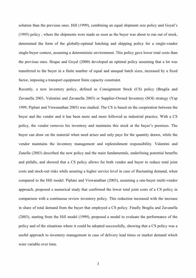
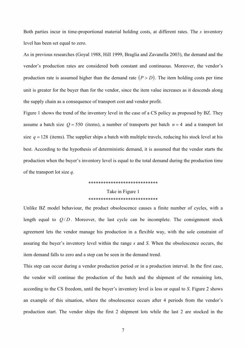
Figure 1 shows the trend of the inventory level in the case of a CS policy as proposed by BZ. They

assume a batch size 550=Q (items), a number of transports per batch 4=n and a transport lot

size 128=q (items). The supplier ships a batch with multiple travels, reducing his stock level at his

best. According to the hypothesis of deterministic demand, it is assumed that the vendor starts the

production when the buyer’s inventory level is equal to the total demand during the production time

of the transport lot size q.

****************************

Take in Figure 1

****************************

Unlike BZ model behaviour, the product obsolescence causes a finite number of cycles, with a

length equal to DQ / . Moreover, the last cycle can be incomplete. The consignment stock

agreement lets the vendor manage his production in a flexible way, with the sole constraint of

assuring the buyer’s inventory level within the range s and S. When the obsolescence occurs, the

item demand falls to zero and a step can be seen in the demand trend.

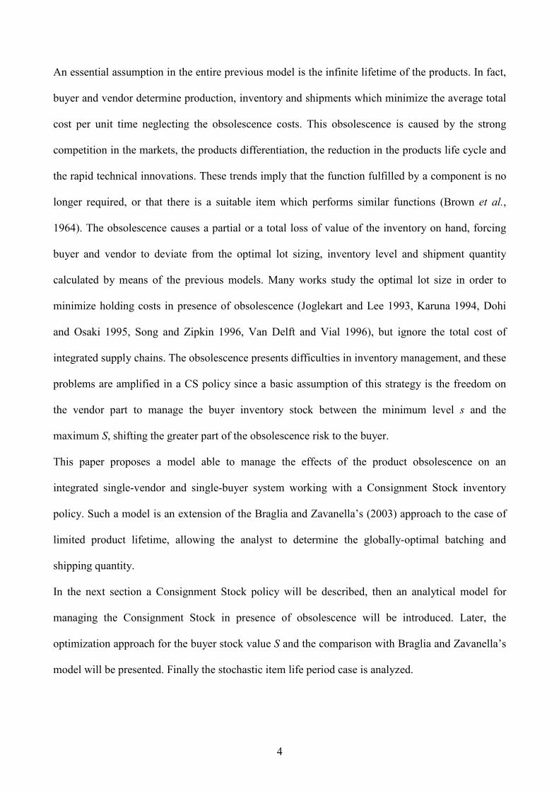
This step can occur during a vendor production period or in a production interval. In the first case,

the vendor will continue the production of the batch and the shipment of the remaining lots,

according to the CS freedom, until the buyer’s inventory level is less or equal to S. Figure 2 shows

an example of this situation, where the obsolescence occurs after 4 periods from the vendor’s

production start. The vendor ships the first 2 shipment lots while the last 2 are stocked in the

7

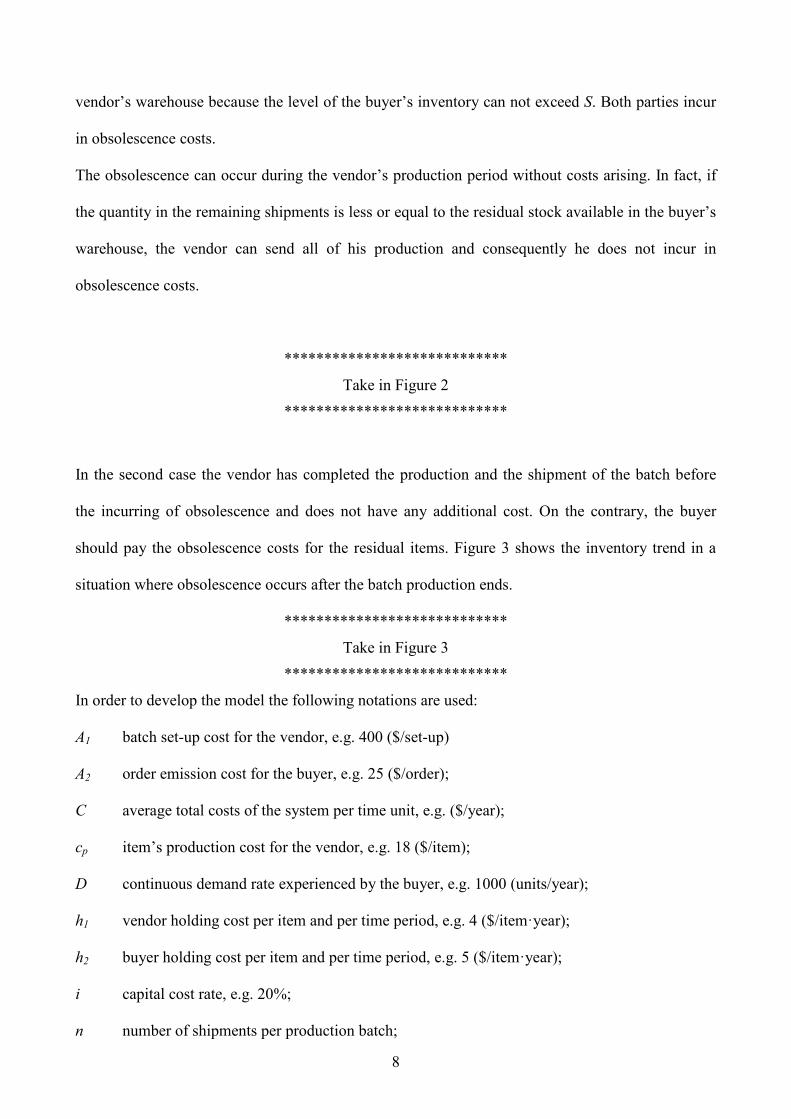
vendor’s warehouse because the level of the buyer’s inventory can not exceed S. Both parties incur

in obsolescence costs.

The obsolescence can occur during the vendor’s production period without costs arising. In fact, if

the quantity in the remaining shipments is less or equal to the residual stock available in the buyer’s

warehouse, the vendor can send all of his production and consequently he does not incur in

obsolescence costs.

****************************

Take in Figure 2

****************************

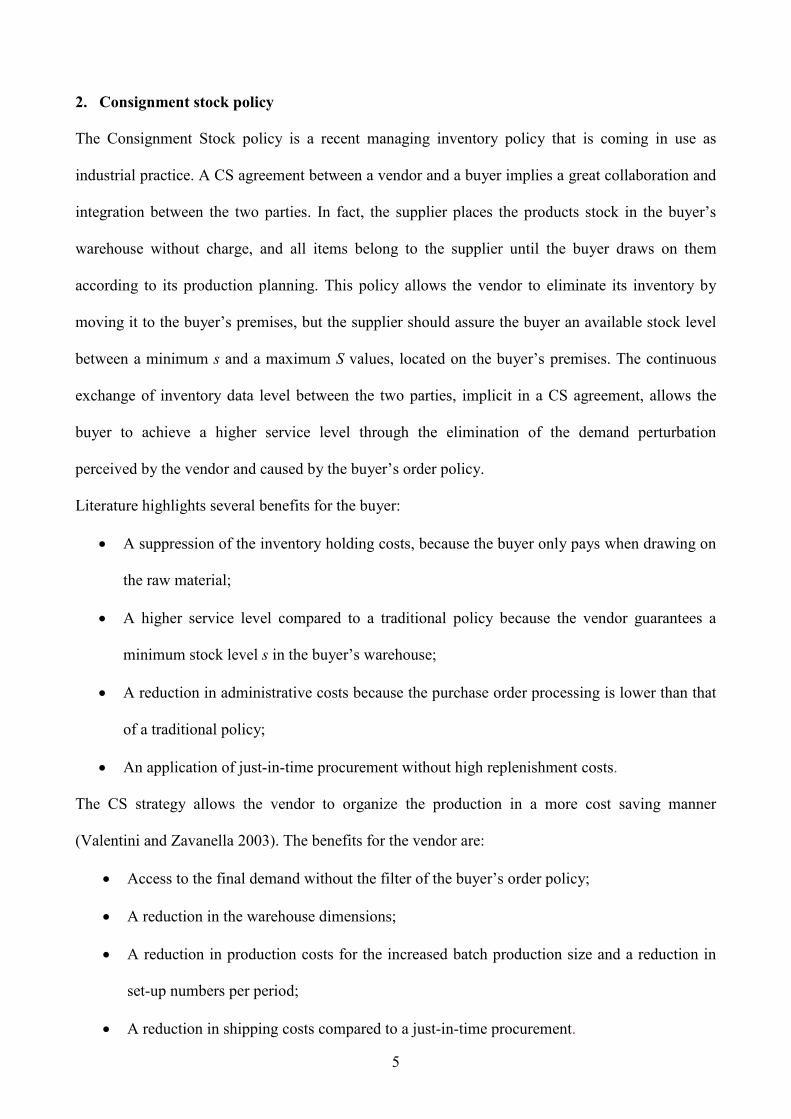
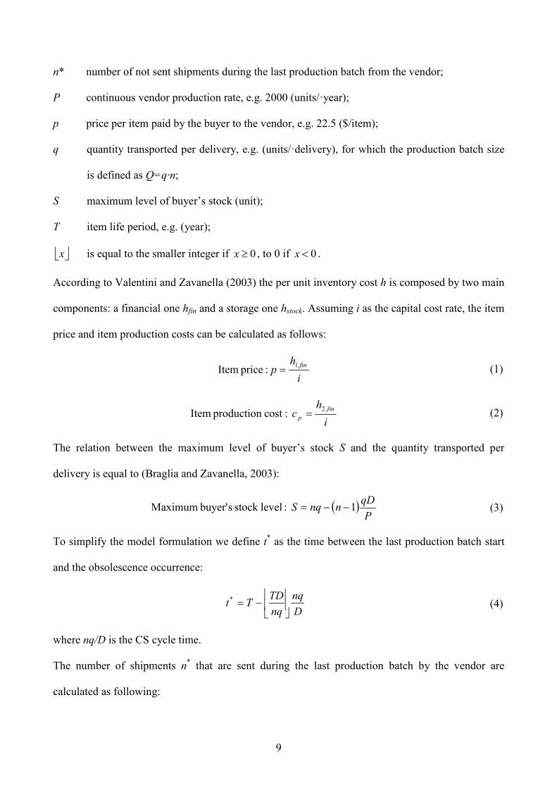
In the second case the vendor has completed the production and the shipment of the batch before

the incurring of obsolescence and does not have any additional cost. On the contrary, the buyer

should pay the obsolescence costs for the residual items. Figure 3 shows the inventory trend in a

situation where obsolescence occurs after the batch production ends.

****************************

Take in Figure 3

****************************

In order to develop the model the following notations are used:

A1 batch set-up cost for the vendor, e.g. 400 ($/set-up)

A2 order emission cost for the buyer, e.g. 25 ($/order);

C average total costs of the system per time unit, e.g. ($/year);

cp item’s production cost for the vendor, e.g. 18 ($/item);

D continuous demand rate experienced by the buyer, e.g. 1000 (units/year);

h1 vendor holding cost per item and per time period, e.g. 4 ($/item·year);

h2 buyer holding cost per item and per time period, e.g. 5 ($/item·year);

i capital cost rate, e.g. 20%;

n number of shipments per production batch;

8

n* number of not sent shipments during the last production batch from the vendor;

P continuous vendor production rate, e.g. 2000 (units/·year);

p price per item paid by the buyer to the vendor, e.g. 22.5 ($/item);

q quantity transported per delivery, e.g. (units/·delivery), for which the production batch size

is defined as Q=q·n;

S maximum level of buyer’s stock (unit);

T item life period, e.g. (year);

x is equal to the smaller integer if 0≥x , to 0 if 0<x .

According to Valentini and Zavanella (2003) the per unit inventory cost h is composed by two main

components: a financial one hfin and a storage one hstock. Assuming i as the capital cost rate, the item

price and item production costs can be calculated as follows:

The relation between the maximum level of buyer’s stock S and the quantity transported per

delivery is equal to (Braglia and Zavanella, 2003):

To simplify the model formulation we define t* as the time between the last production batch start

and the obsolescence occurrence:

where nq/D is the CS cycle time.

The number of shipments n* that are sent during the last production batch by the vendor are

calculated as following:

ih

p ,fin1 :price Item = (1)

ih

c ,finp

2 :cost production Item = (2)

( )P

qDnnqS 1 :levelstock sbuyer' Maximum −−= (3)

Dnq

nqTDT t*

−= (4)

9

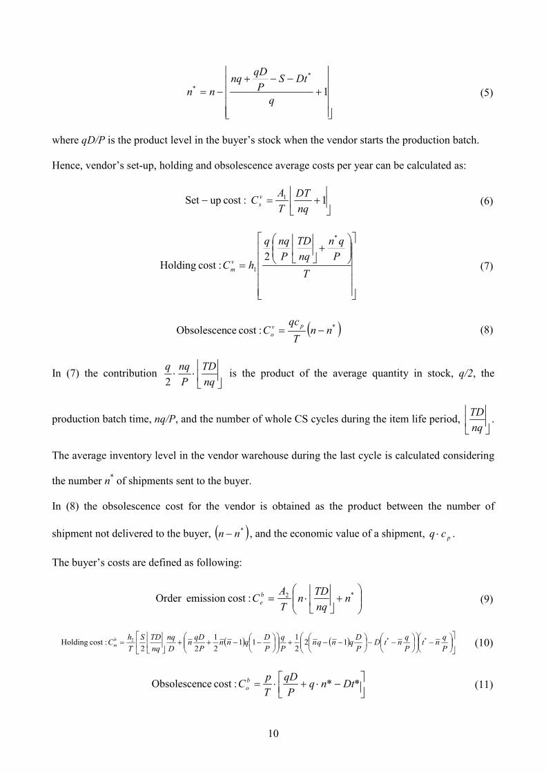
where qD/P is the product level in the buyer’s stock when the vendor starts the production batch.

Hence, vendor’s set-up, holding and obsolescence average costs per year can be calculated as:

In (7) the contribution

⋅⋅

nqTD

Pnqq

2 is the product of the average quantity in stock, q/2, the

production batch time, nq/P, and the number of whole CS cycles during the item life period,

nqTD .

The average inventory level in the vendor warehouse during the last cycle is calculated considering

the number n* of shipments sent to the buyer.

In (8) the obsolescence cost for the vendor is obtained as the product between the number of

shipment not delivered to the buyer, ( )*nn − , and the economic value of a shipment, pcq ⋅ .

The buyer’s costs are defined as following:

+−−+

−= 1q

DtSP

qDnqn n

*

* (5)

+=− 1 :cost upSet 1

nqDT

TA C v

s (6)

+

=T

Pqn

nqTD

Pnqq

hC

*

vm

2 :cost Holding 1 (7)

( )*pvo nn

Tqc

C −= :cost ceObsolescen (8)

+

⋅= *b

e nnqTDn

TAC 2 :costemission Order (9)

( ) ( )

−

−−

−−+

−−++

=

Pqnt

PqntD

PDqnqn

Pq

PDqnn

PqDn

Dnq

nqTDS

ThC **b

m 122111

21

22 :cost Holding 2 (10)

−⋅+⋅= Dt*n*q

PqD

TpC b

o :cost ceObsolescen (11)

10

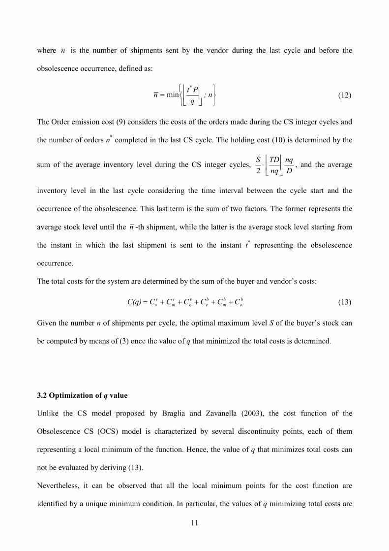
where n is the number of shipments sent by the vendor during the last cycle and before the

obsolescence occurrence, defined as:

The Order emission cost (9) considers the costs of the orders made during the CS integer cycles and

the number of orders n* completed in the last CS cycle. The holding cost (10) is determined by the

sum of the average inventory level during the CS integer cycles, Dnq

nqTDS

⋅

2, and the average

inventory level in the last cycle considering the time interval between the cycle start and the

occurrence of the obsolescence. This last term is the sum of two factors. The former represents the

average stock level until the n -th shipment, while the latter is the average stock level starting from

the instant in which the last shipment is sent to the instant t* representing the obsolescence

occurrence.

The total costs for the system are determined by the sum of the buyer and vendor’s costs:

Given the number n of shipments per cycle, the optimal maximum level S of the buyer’s stock can

be computed by means of (3) once the value of q that minimized the total costs is determined.

3.2 Optimization of q value

Unlike the CS model proposed by Braglia and Zavanella (2003), the cost function of the

Obsolescence CS (OCS) model is characterized by several discontinuity points, each of them

representing a local minimum of the function. Hence, the value of q that minimizes total costs can

not be evaluated by deriving (13).

Nevertheless, it can be observed that all the local minimum points for the cost function are

identified by a unique minimum condition. In particular, the values of q minimizing total costs are

= n;

qPtn

*

min (12)

bo

bm

be

vo

vm

vs CCCCCC C(q) +++++= (13)

11

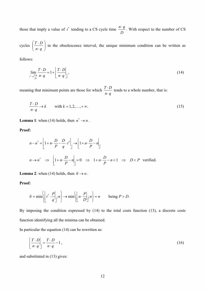
those that imply a value of *t tending to a CS cycle time D

qn ⋅ . With respect to the number of CS

cycles

⋅⋅qnDT in the obsolescence interval, the unique minimum condition can be written as

follows:

,1lim*

⋅⋅

+=⋅⋅

⋅→ qn

DTqnDT

Dqnt

(14)

meaning that minimum points are those for which qnDT⋅⋅ tends to a whole number, that is:

.,,2,1with ∞+=→⋅⋅

2kkqnDT (15)

Lemma 1: when (14) holds, then nn →* .

Proof:

−⋅+→

⋅−⋅+=− n

PDnt

qD

PDnnn 11 **

PDnPDnn

PDnnn <⇒<−⋅+⇒=

−⋅+⇒→ 1101* verified.

Lemma 2: when (14) holds, then nn → .

Proof:

. being;min;min * DPnnDPnn

qPtn >=

⋅→

⋅=

By imposing the condition expressed by (14) to the total costs function (13), a discrete costs

function identifying all the minima can be obtained.

In particular the equation (14) can be rewritten as:

,1−⋅⋅

=

⋅⋅

qnDT

qnDT (16)

and substituted in (13) gives:

12

( ) ( ) ( )

,1

121

21 2

21

21min

PDqp

T

Dqn

PDqnqn

qnDT

Th

Pqn

qnDT

ThAnA

qnDT

TqC

⋅⋅⋅+

+

⋅⋅

⋅⋅−−⋅⋅⋅

⋅⋅

⋅+⋅⋅

⋅

⋅⋅

⋅+⋅+⋅

⋅⋅

⋅=

(17)

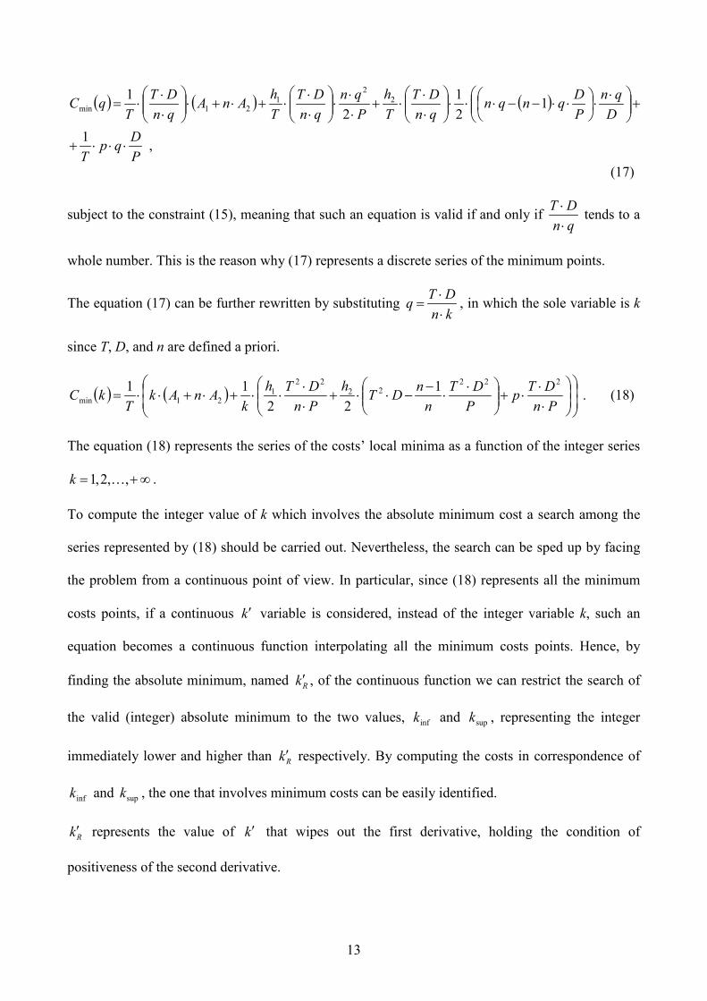
subject to the constraint (15), meaning that such an equation is valid if and only if qnDT⋅⋅ tends to a

whole number. This is the reason why (17) represents a discrete series of the minimum points.

The equation (17) can be further rewritten by substituting knDTq⋅⋅

= , in which the sole variable is k

since T, D, and n are defined a priori.

( ) ( ) .122

11 22222

221

21min

⋅⋅

⋅+

⋅⋅

−−⋅⋅+

⋅⋅

⋅⋅+⋅+⋅⋅=PnDTp

PDT

nnDTh

PnDTh

kAnAk

TkC (18)

The equation (18) represents the series of the costs’ local minima as a function of the integer series

∞+= ,,2,1 2k .

To compute the integer value of k which involves the absolute minimum cost a search among the

series represented by (18) should be carried out. Nevertheless, the search can be sped up by facing

the problem from a continuous point of view. In particular, since (18) represents all the minimum

costs points, if a continuous k ′ variable is considered, instead of the integer variable k, such an

equation becomes a continuous function interpolating all the minimum costs points. Hence, by

finding the absolute minimum, named Rk ′ , of the continuous function we can restrict the search of

the valid (integer) absolute minimum to the two values, infk and supk , representing the integer

immediately lower and higher than Rk ′ respectively. By computing the costs in correspondence of

infk and supk , the one that involves minimum costs can be easily identified.

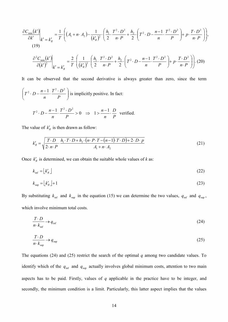
Rk ′ represents the value of k ′ that wipes out the first derivative, holding the condition of

positiveness of the second derivative.

13

( ) ( )( )

,122

11 22222

221

221min

⋅⋅

⋅+

⋅⋅

−−⋅⋅+

⋅⋅

⋅⋅′

−⋅+⋅=′=′′∂

′∂PnDTp

PDT

nnDTh

PnDTh

kAnA

TkkkkC

RR

(19)

( )( ) ( )

.122

12 22222

221

32min

2

⋅⋅

⋅+

⋅⋅

−−⋅⋅+

⋅⋅

⋅⋅′

⋅=′=′′∂

′∂PnDTp

PDT

nnDTh

PnDTh

kTkkkkC

RR

(20)

It can be observed that the second derivative is always greater than zero, since the term

⋅⋅

−−⋅

PDT

nnDT

222 1 is implicitly positive. In fact:

PD

nn

PDT

nnDT ⋅

−>⇒>

⋅⋅

−−⋅

1101 222 verified.

The value of Rk ′ is then drawn as follow:

( )( )21

21 212 AnA

pDDTnTPnhDThPn

DTkR ⋅+⋅⋅+⋅⋅−−⋅⋅⋅+⋅⋅

⋅⋅⋅⋅

=′ (21)

Once Rk ′ is determined, we can obtain the suitable whole values of k as:

Rkk ′=inf (22)

1sup +′= Rkk (23)

By substituting infk and supk in the equation (15) we can determine the two values, infq and supq ,

which involve minimum total costs.

infinf

qknDT

→⋅⋅ (24)

supsup

qknDT

→⋅⋅ (25)

The equations (24) and (25) restrict the search of the optimal q among two candidate values. To

identify which of the infq and supq actually involves global minimum costs, attention to two main

aspects has to be paid. Firstly, values of q applicable in the practice have to be integer, and

secondly, the minimum condition is a limit. Particularly, this latter aspect implies that the values

14

infq and supq which involve minimum costs are not exactly equal to the ratios infknDT

⋅⋅ and

supknDT

⋅⋅

respectively, but are an infinitesimal higher to those ratios. Concluding, the real applicable q which

involves global minimum costs is either the first integer greater than infq or the first integer greater

than supq that involves the minimum value of the equation (13).

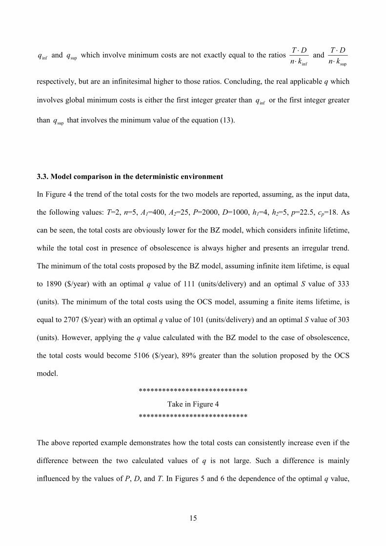
3.3. Model comparison in the deterministic environment

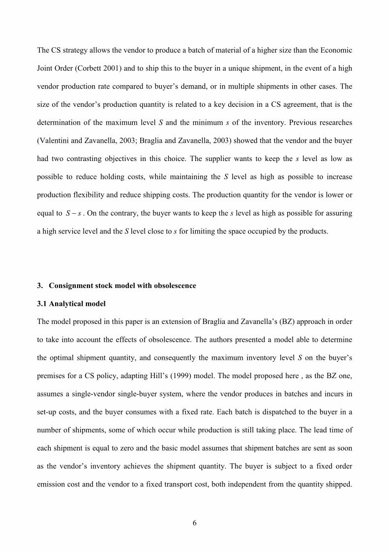
In Figure 4 the trend of the total costs for the two models are reported, assuming, as the input data,

the following values: T=2, n=5, A1=400, A2=25, P=2000, D=1000, h1=4, h2=5, p=22.5, cp=18. As

can be seen, the total costs are obviously lower for the BZ model, which considers infinite lifetime,

while the total cost in presence of obsolescence is always higher and presents an irregular trend.

The minimum of the total costs proposed by the BZ model, assuming infinite item lifetime, is equal

to 1890 ($/year) with an optimal q value of 111 (units/delivery) and an optimal S value of 333

(units). The minimum of the total costs using the OCS model, assuming a finite items lifetime, is

equal to 2707 ($/year) with an optimal q value of 101 (units/delivery) and an optimal S value of 303

(units). However, applying the q value calculated with the BZ model to the case of obsolescence,

the total costs would become 5106 ($/year), 89% greater than the solution proposed by the OCS

model.

****************************

Take in Figure 4

****************************

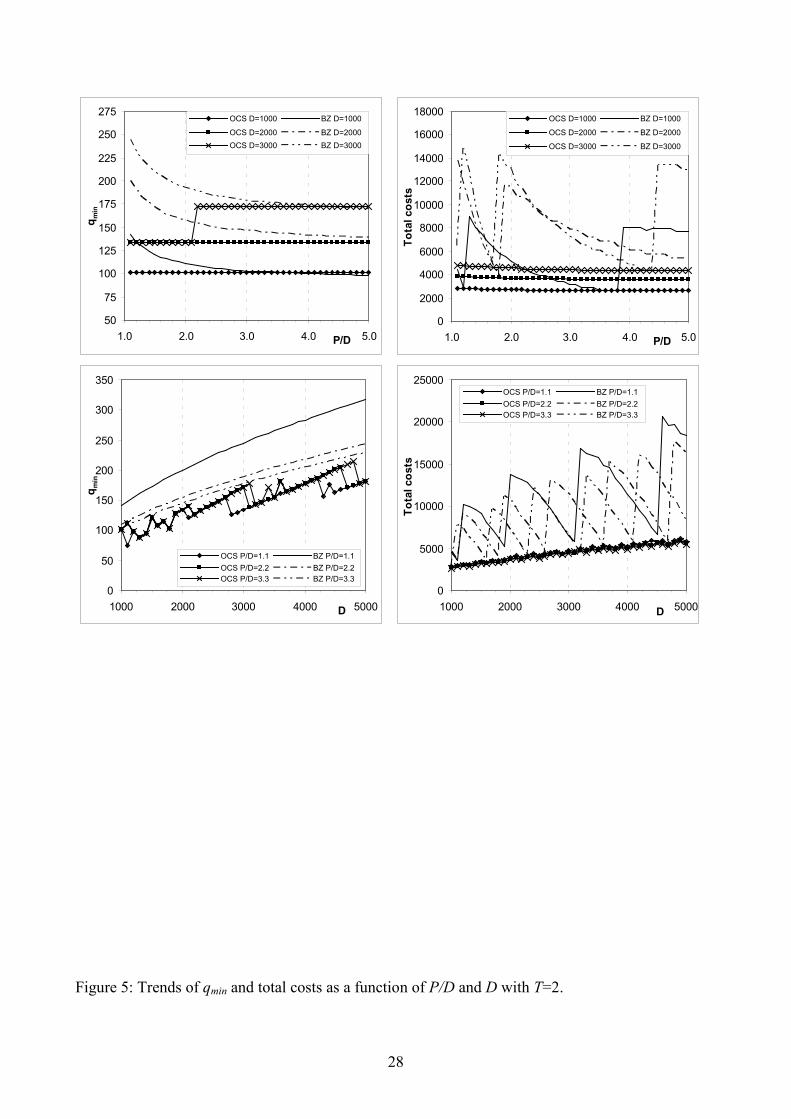
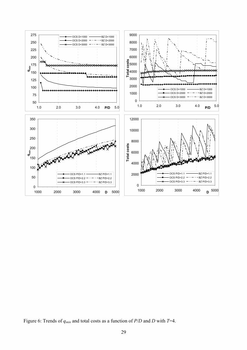
The above reported example demonstrates how the total costs can consistently increase even if the

difference between the two calculated values of q is not large. Such a difference is mainly

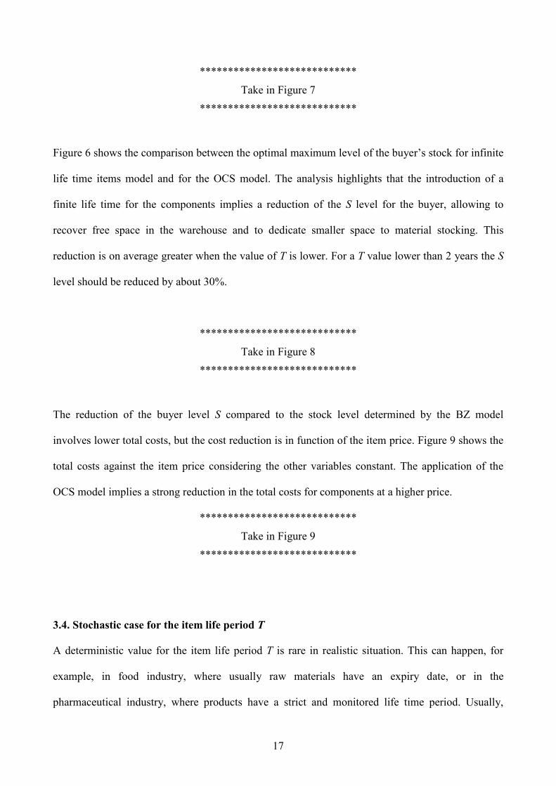
influenced by the values of P, D, and T. In Figures 5 and 6 the dependence of the optimal q value,

15

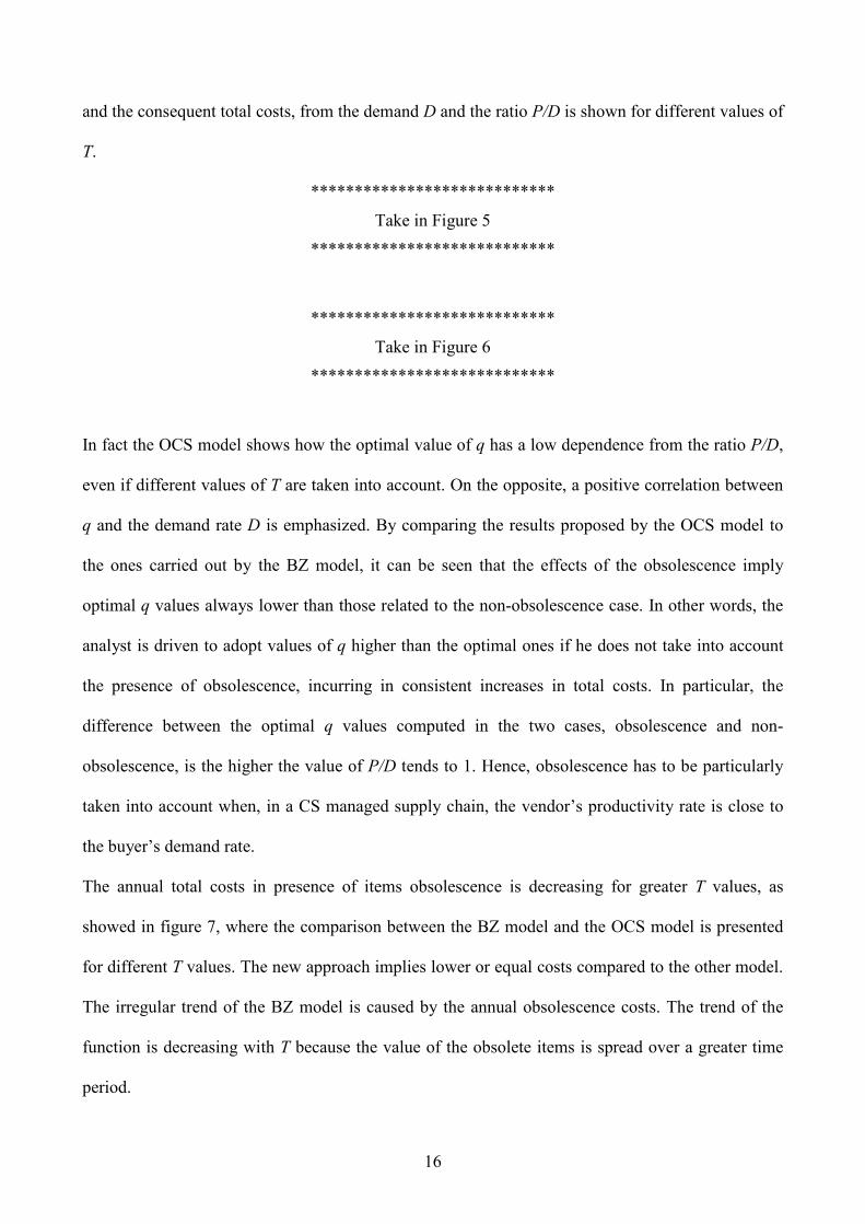
and the consequent total costs, from the demand D and the ratio P/D is shown for different values of

T.

****************************

Take in Figure 5

****************************

****************************

Take in Figure 6

****************************

In fact the OCS model shows how the optimal value of q has a low dependence from the ratio P/D,

even if different values of T are taken into account. On the opposite, a positive correlation between

q and the demand rate D is emphasized. By comparing the results proposed by the OCS model to

the ones carried out by the BZ model, it can be seen that the effects of the obsolescence imply

optimal q values always lower than those related to the non-obsolescence case. In other words, the

analyst is driven to adopt values of q higher than the optimal ones if he does not take into account

the presence of obsolescence, incurring in consistent increases in total costs. In particular, the

difference between the optimal q values computed in the two cases, obsolescence and non-

obsolescence, is the higher the value of P/D tends to 1. Hence, obsolescence has to be particularly

taken into account when, in a CS managed supply chain, the vendor’s productivity rate is close to

the buyer’s demand rate.

The annual total costs in presence of items obsolescence is decreasing for greater T values, as

showed in figure 7, where the comparison between the BZ model and the OCS model is presented

for different T values. The new approach implies lower or equal costs compared to the other model.

The irregular trend of the BZ model is caused by the annual obsolescence costs. The trend of the

function is decreasing with T because the value of the obsolete items is spread over a greater time

period.

16

****************************

Take in Figure 7

****************************

Figure 6 shows the comparison between the optimal maximum level of the buyer’s stock for infinite

life time items model and for the OCS model. The analysis highlights that the introduction of a

finite life time for the components implies a reduction of the S level for the buyer, allowing to

recover free space in the warehouse and to dedicate smaller space to material stocking. This

reduction is on average greater when the value of T is lower. For a T value lower than 2 years the S

level should be reduced by about 30%.

****************************

Take in Figure 8

****************************

The reduction of the buyer level S compared to the stock level determined by the BZ model

involves lower total costs, but the cost reduction is in function of the item price. Figure 9 shows the

total costs against the item price considering the other variables constant. The application of the

OCS model implies a strong reduction in the total costs for components at a higher price.

****************************

Take in Figure 9

****************************

3.4. Stochastic case for the item life period T

A deterministic value for the item life period T is rare in realistic situation. This can happen, for

example, in food industry, where usually raw materials have an expiry date, or in the

pharmaceutical industry, where products have a strict and monitored life time period. Usually,

17

buyers and vendors do not know the life time of the items, because this value is generally

determined by the market demand for the final products sold by the buyer and for which these items

are assembled or used, or by any eventual redesign of the components carried out by one of the two

actors.

The variability of T causes some difficulties in the estimation of the optimal quantity q transported

per delivery and consequently the maximum level for the buyer stock S. To analyze the impact of

this uncertainty a simulation study has been performed. The T parameter has been assumed

normally distributed with mean μT and standard deviation σT. The standard deviation σT is in

function of the uncertainty about the life time period and a low value of the indicator has been

hypothesized as being equal to T/100, while a high value equal to T/2. For a single couple of value

of μT and σT, 1000 different values of T have been generated and the mean total costs value for

different values of the quantity transported per delivery q were calculated.

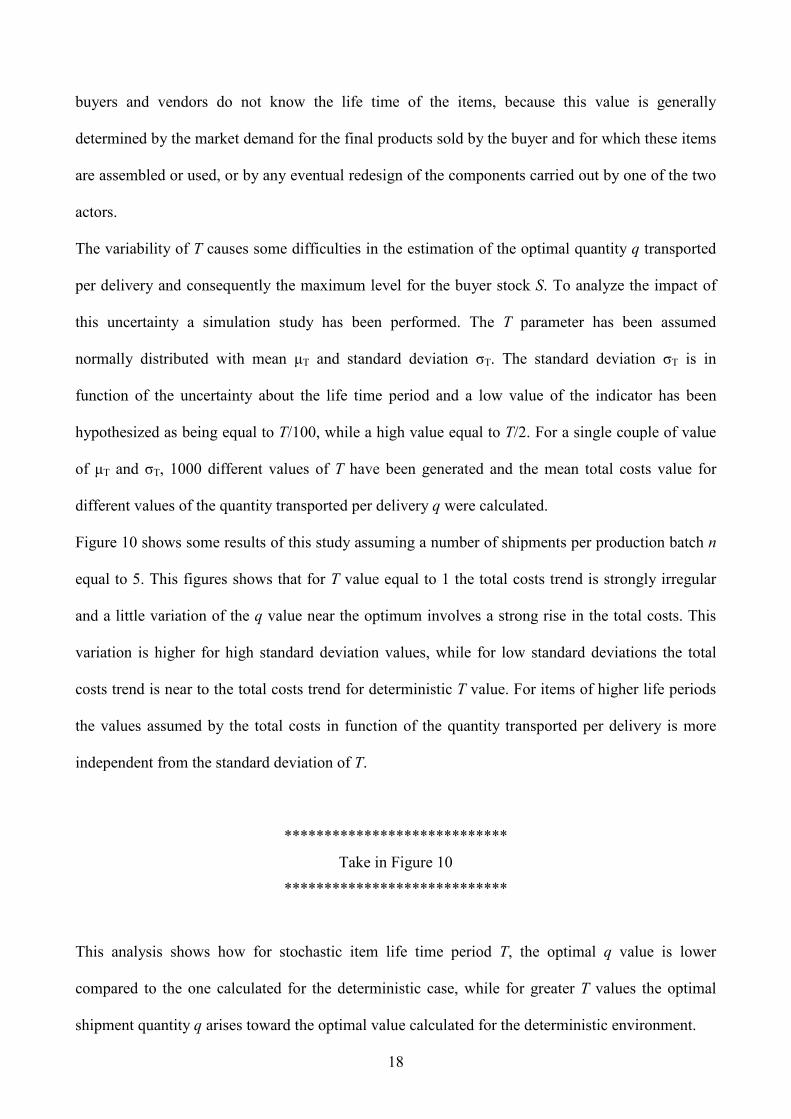
Figure 10 shows some results of this study assuming a number of shipments per production batch n

equal to 5. This figures shows that for T value equal to 1 the total costs trend is strongly irregular

and a little variation of the q value near the optimum involves a strong rise in the total costs. This

variation is higher for high standard deviation values, while for low standard deviations the total

costs trend is near to the total costs trend for deterministic T value. For items of higher life periods

the values assumed by the total costs in function of the quantity transported per delivery is more

independent from the standard deviation of T.

****************************

Take in Figure 10

****************************

This analysis shows how for stochastic item life time period T, the optimal q value is lower

compared to the one calculated for the deterministic case, while for greater T values the optimal

shipment quantity q arises toward the optimal value calculated for the deterministic environment.

18

Moreover, the simulation highlights how very critical is, for a low value of the item life period, the

determination of the optimal quantity q transported per delivery, and consequently the maximum

buyer stock level S, since a wrong estimation implies substantial higher costs for both vendor and

buyer. For higher values of T, the q and S estimation is less critical, because the total costs trend is

smoother and less irregular.

****************************

Take in Table 1

****************************

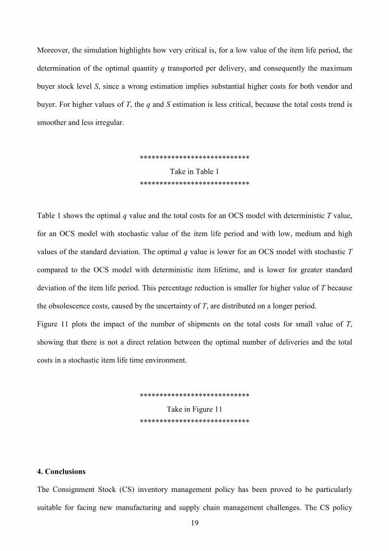
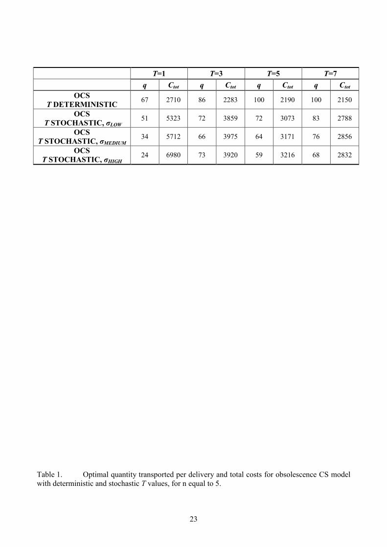
Table 1 shows the optimal q value and the total costs for an OCS model with deterministic T value,

for an OCS model with stochastic value of the item life period and with low, medium and high

values of the standard deviation. The optimal q value is lower for an OCS model with stochastic T

compared to the OCS model with deterministic item lifetime, and is lower for greater standard

deviation of the item life period. This percentage reduction is smaller for higher value of T because

the obsolescence costs, caused by the uncertainty of T, are distributed on a longer period.

Figure 11 plots the impact of the number of shipments on the total costs for small value of T,

showing that there is not a direct relation between the optimal number of deliveries and the total

costs in a stochastic item life time environment.

****************************

Take in Figure 11

****************************

4. Conclusions

The Consignment Stock (CS) inventory management policy has been proved to be particularly

suitable for facing new manufacturing and supply chain management challenges. The CS policy

19

implies a complete exchange of information between the buyer and his supplier, and a consistent

sharing in management risks. In such a context, the consideration of the product obsolescence

effects on the total costs of the supply chain is of great interest.

This work proposes an analytical model, based on the Braglia and Zavanella’s approach, which

concerns the deterministic single-vendor single-buyer productive situation, allowing the analyst to

identify the optimal inventory level and shipment policy for optimizing total costs when products

are characterized by a finite lifetime. Results show that the presence of obsolescence reduces the

optimal inventory level, particularly in case of a short period of life. The ratio between the vendor’s

production rate and the buyer’s demand rate is another important parameter to take into account. In

particular, the effects of obsolescence on the correct estimation of the optimal shipment dimension

are higher when the production rate is close to the demand rate. Moreover, simulations have been

carried out to assess the impact of the stochastic estimation of the item lifetime period. Results

show how the optimal shipment dimension for the stochastic life time case is always smaller than

that concerning the deterministic case. The higher the uncertainty in product life time estimation the

lower is the dimension of the shipment, with respect to the deterministic case. Moreover, results

emphasize that there is no relation between the number of deliveries and the total costs.

In conclusion, this work provides to the analyst a robust methodology and some important insights

in how to manage the effects of obsolescence in such a way as to reduce total costs in a supply

chain managed with a CS policy.

Future works

Further work might evaluate the multi-buyer or multi-vendor environments, the case of

obsolescence and stochastic demand, and the evaluation of the inventory level for buyer and vendor

in case of transfer of ownership, from vendor to buyer, after a fixed period from the delivery of the

products.

20

References

BANERJEE, A., 1986, A joint economic lot size model for purchaser and vendor. Decision Sciences, 17, 292-311.

BRAGLIA, M., and ZAVANELLA, L., 2003, Modelling an industrial strategy for inventory management in supply chains: the ‘Consignment Stock’ case. International Journal of Production Research, 41, 3793-3808.

BROWN, G.W., LU, J.Y., and WOLFSON, R.J., 1964, Dynamic modelling of inventories subject to obsolescence. Management Science, 11, 51-63.

CORBETT, C.J., 2001, Stochastic inventory systems in a supply chain with asymmetric information: cycle stocks, safety stocks, and consignment stock. Operations Research, 49, 487-500.

CORBETT, C. J., and DE GROOTE, X., 2000, A supplier’s optimal quantity discount policy under asymmetric information. Management Science, 46, 444-450.

DOHI, T., and OSAKI, S., 1995, Optimal inventory policies under product obsolescent circumstance. Computers & Mathematics with Applications, 29, 23-30.

DREZNER, Z., and WESOLOWSKY, G.O., 1989, Multi-buyer discount pricing. European Journal of Operational Research, 40, 38-42.

GOYAL, S.K., 1977, Determination of optimum quantity for a two-stage production system. Operational Research Quarterly, 28, 865-870.

GOYAL, S.K., 1987a, Determination of a supplier’s economic ordering policy. Journal of Operational Research Society, 38, 853-857.

GOYAL, S.K., 1987b, Comment on: A generalized quantity discount pricing model to increase supplier’s profits. Management Science, 33, 1635-1636.

GOYAL, S. K., 1988, A joint economic lot size model for purchaser and vendor: A comment. Decision Science, 19, 236-241.

GOYAL, S.K., and GUPTA, P., 1989, Integrated inventory models: The buyer-vendor coordination. European Journal of Operational Research, 41, 261-269.

GOYAL, S.K., 1995, A one-vendor multi-buyer integrated inventory model: A comment. European Journal of Operational Research, 82, 209-210.

HILL, R.M., 1997, The single-vendor single-buyer integrated production-inventory model with a generalised policy. European Journal of Operational Research, 97, 493-499.

HILL, R.M., 1999, The optimal production and shipment policy for the single-vendor single-buyer integrated production-inventory problem. International Journal of Production Research, 37, 2463-2475.

HOQUE, M.A., and GOYAL, S.K., 2000, An optimal policy for a single-vendor single-buyer integrated production-inventory system with capacity constraint of the transport equipment. International Journal of Production Economics, 65, 305-315.

JOGLEKART, P., and LEE, P., 1993, Exact formulation of inventory costs and optimal lot size in face of sudden obsolescence. Operations Research Letters, 14, 283-290.

KARUNA, J., 1994, Lot sizing for a product subject to obsolescence or perishability. European Journal of Operational Research, 75, 287-295.

KIM, K.H., and HWANG, H., 1988, An incremental discount pricing schedule with multiple customer and single price break. European Journal of Operational Research, 35, 71-79.

LAL, R., and STAELIN, R., 1984, An approach for developing an optimal discount pricing policy. Management Science, 30, 1524-1539.

21

LU, L., 1995, A one-vendor multi-buyer integrated inventory model. European Journal of Operational Research, 81, 312-323.

LEE, H. L., and ROSENBLATT, M. J., 1986, A generalized quantity discount pricing model to increase supplier’s profits. Management Science, 32, 1117-1185.

MONAHAN, J.P., 1984, A quantity discount pricing model to increase vendor profits. Management science, 30, 720-726.

PIPLANI, R., and VISWANATHAN, S., 2003, A model for evaluating supplier-owned inventory strategy. International Journal of Production Economics, 81-82, 213-224.

SONG, J.S., and ZIPKIN, P.H., 1996, Managing inventory with the prospect of obsolescence. Operations Research, 44, 215.

VALENTINI, G., and ZAVANELLA, L., 2003, The consignment stock of inventories: industrial case and performance analysis. International Journal of Production Economics, 81-82, 213-224.

VAN DELFT, C., and VIAL, J.P., 1996, Discounted costs, obsolescence and planned stockouts with the EOQ formula. International Journal of Production Economics, 44, 255-265.

WENG, Z.K., 1995, Channel coordination and quantity discounts. Management Science, 41, 1509-1522.

YAP, R., 1999, Holding the Aces in Manufacturing Logistics. Proceedings of Manufacturing Logistics for the 21st Century, Singapore, http://www.ych.com/c-conference.htm.

22

T=1 T=3 T=5 T=7 q Ctot q Ctot q Ctot q Ctot

OCS T DETERMINISTIC 67 2710 86 2283 100 2190 100 2150

OCS T STOCHASTIC, σLOW 51 5323 72 3859 72 3073 83 2788

OCS T STOCHASTIC, σMEDIUM 34 5712 66 3975 64 3171 76 2856

OCS T STOCHASTIC, σHIGH 24 6980 73 3920 59 3216 68 2832

Table 1. Optimal quantity transported per delivery and total costs for obsolescence CS model with deterministic and stochastic T values, for n equal to 5.

23

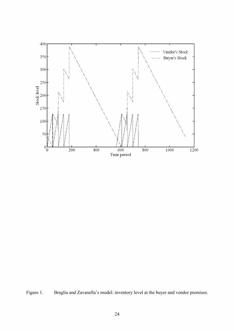
Figure 1. Braglia and Zavanella’s model: inventory level at the buyer and vendor premises.

24

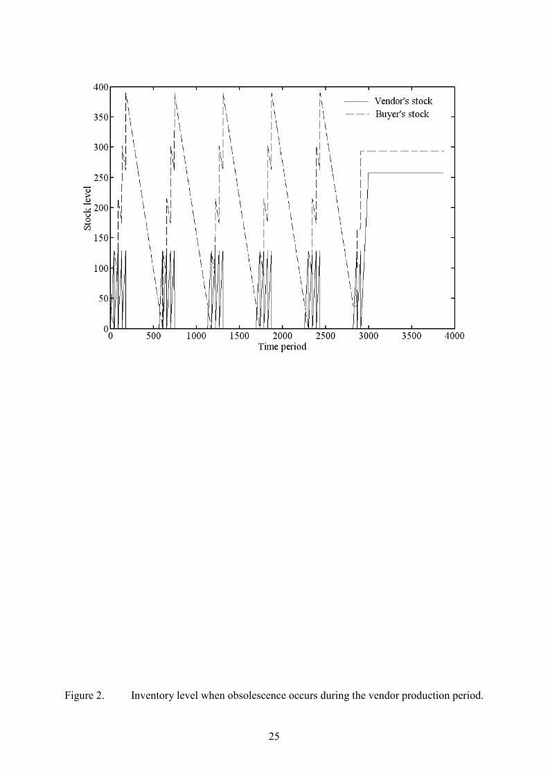
Figure 2. Inventory level when obsolescence occurs during the vendor production period.

25

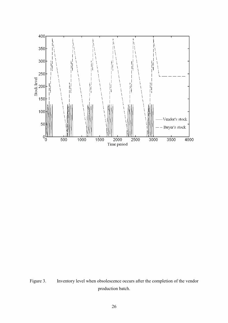
Figure 3. Inventory level when obsolescence occurs after the completion of the vendor

production batch.

26

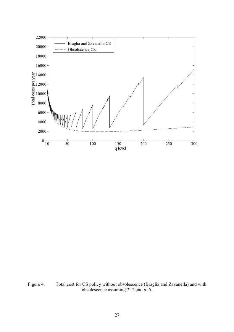
Figure 4. Total cost for CS policy without obsolescence (Braglia and Zavanella) and with obsolescence assuming T=2 and n=5.

27

50

75

100

125

150

175

200

225

250

275

1.0 2.0 3.0 4.0 5.0P/D

q min

OCS D=1000 BZ D=1000

OCS D=2000 BZ D=2000OCS D=3000 BZ D=3000

0

2000

4000

6000

8000

10000

12000

14000

16000

18000

1.0 2.0 3.0 4.0 5.0P/D

Tota

l cos

ts

OCS D=1000 BZ D=1000

OCS D=2000 BZ D=2000

OCS D=3000 BZ D=3000

0

50

100

150

200

250

300

350

1000 2000 3000 4000 5000D

q min

OCS P/D=1.1 BZ P/D=1.1OCS P/D=2.2 BZ P/D=2.2OCS P/D=3.3 BZ P/D=3.3

0

5000

10000

15000

20000

25000

1000 2000 3000 4000 5000D

Tota

l cos

tsOCS P/D=1.1 BZ P/D=1.1OCS P/D=2.2 BZ P/D=2.2OCS P/D=3.3 BZ P/D=3.3

Figure 5: Trends of qmin and total costs as a function of P/D and D with T=2.

28

50

75

100

125

150

175

200

225

250

275

1.0 2.0 3.0 4.0 5.0P/D

q min

OCS D=1000 BZ D=1000OCS D=2000 BZ D=2000OCS D=3000 BZ D=3000

0

1000

2000

3000

4000

5000

6000

7000

8000

9000

1.0 2.0 3.0 4.0 5.0P/D

Tota

l cos

ts

OCS D=1000 BZ D=1000OCS D=2000 BZ D=2000OCS D=3000 BZ D=3000

0

50

100

150

200

250

300

350

1000 2000 3000 4000 5000D

q min

OCS P/D=1.1 BZ P/D=1.1OCS P/D=2.2 BZ P/D=2.2OCS P/D=3.3 BZ P/D=3.3

0

2000

4000

6000

8000

10000

12000

1000 2000 3000 4000 5000D

Tota

l cos

ts

OCS P/D=1.1 BZ P/D=1.1OCS P/D=2.2 BZ P/D=2.2OCS P/D=3.3 BZ P/D=3.3

Figure 6: Trends of qmin and total costs as a function of P/D and D with T=4.

29

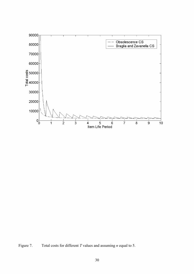
Figure 7. Total costs for different T values and assuming n equal to 5.

30

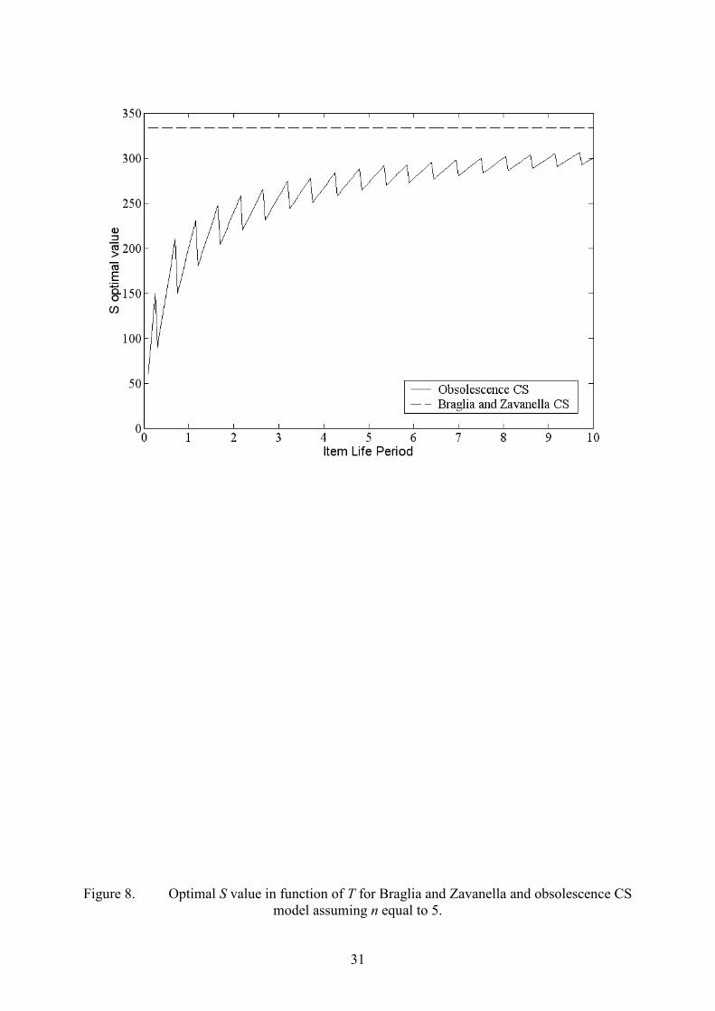
Figure 8. Optimal S value in function of T for Braglia and Zavanella and obsolescence CS model assuming n equal to 5.

31

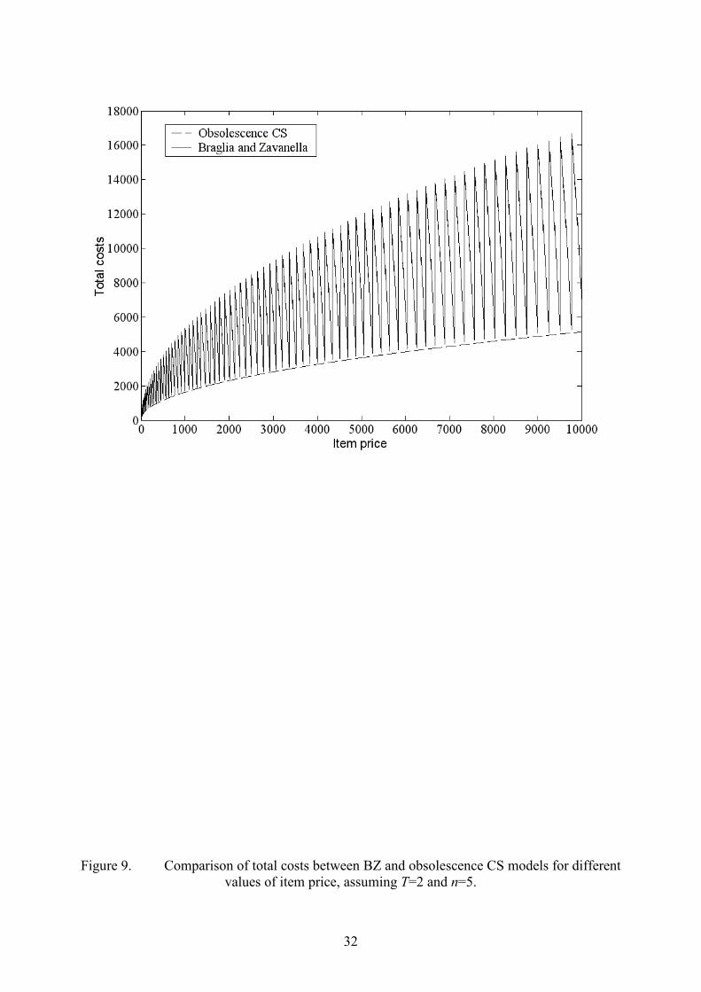
Figure 9. Comparison of total costs between BZ and obsolescence CS models for different values of item price, assuming T=2 and n=5.

32

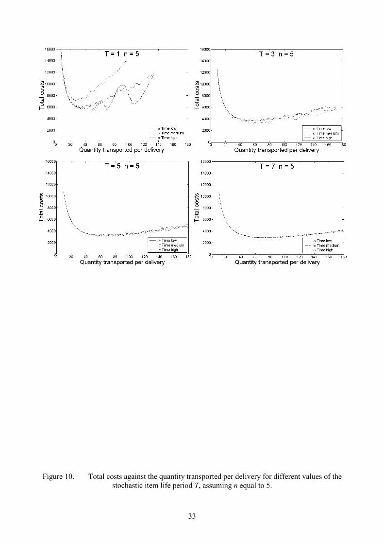
Figure 10. Total costs against the quantity transported per delivery for different values of the stochastic item life period T, assuming n equal to 5.

33

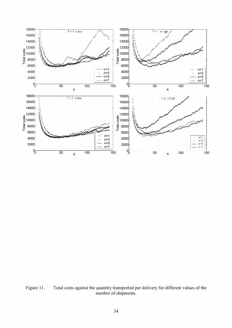
Figure 11. Total costs against the quantity transported per delivery for different values of the number of shipments.

34