Remote Sens. 2012, 4, 830-848; doi:10.3390/rs4040830

Remote Sensing ISSN 2072-4292

www.mdpi.com/journal/remotesensing Article

LiDAR Sampling Density for Forest Resource Inventories in Ontario, Canada

Paul Treitz 1,*, Kevin Lim 2, Murray Woods 3, Doug Pitt 4, Dave Nesbitt 3 and Dave Etheridge 5

1 Department of Geography, Queen’s University, Kingston, ON K7L 3N6, Canada 2 Lim Geomatics Inc., P.O. Box 45089, 680 Eagleson Road, Ottawa, ON K2M 2G0, Canada;

E-Mail: kevin@limgeomatics.com 3 Southern Science & Information Section, Ontario Ministry of Natural Resources, 3301 Trout Lake

Road, North Bay, ON P1A 4L7, Canada; E-Mail: murray.woods@ontario.ca (M.W.); dave.nesbitt@ontario.ca (D.N.)

4 Canadian Wood Fibre Centre, Canadian Forest Service, 1219 Queen St. E., Sault Ste. Marie, ON P6A 2E5, Canada; E-Mail: Doug.Pitt@NRCan-RNCan.gc.ca

5 Northeast Science & Information Section, Ontario Ministry of Natural Resources, P.O. Bag 3020, South Porcupine, ON P0N 1H0, Canada; E-Mail: dave.etheridge@ontario.ca

* Author to whom correspondence should be addressed; E-Mail: paul.treitz@queensu.ca; Tel.: +1-613-533-2903; Fax: +1-613-533-6122.

Received: 22 February 2012; in revised form: 16 March 2012 / Accepted: 16 March 2012 / Published: 27 March 2012

Abstract: Over the past two decades there has been an abundance of research demonstrating the utility of airborne light detection and ranging (LiDAR) for predicting forest biophysical/inventory variables at the plot and stand levels. However, to date there has been little effort to develop a set of protocols for data acquisition and processing that would move governments or the forest industry towards cost-effective implementation of this technology for strategic and tactical (i.e., operational) forest resource inventories. The goal of this paper is to initiate this process by examining the significance of LiDAR data acquisition (i.e., point density) for modeling forest inventory variables for the range of species and stand conditions representing much of Ontario, Canada. Field data for approximately 200 plots, sampling a broad range of forest types and conditions across Ontario, were collected for three study sites. Airborne LiDAR data, characterized by a mean density of 3.2 pulses m−2 were systematically decimated to produce additional datasets with densities of approximately 1.6 and 0.5 pulses m−2. Stepwise regression models, incorporating LiDAR height and density metrics, were developed for each of the three LiDAR datasets across a range of forest types

OPEN ACCESS

Remote Sens. 2012, 4

831

to estimate the following forest inventory variables: (1) average height (R2(adj) = 0.75–0.95); (2) top height (R2(adj) = 0.74–0.98); (3) quadratic mean diameter (R2(adj) = 0.55–0.85); (4) basal area (R2(adj) = 0.22–0.93); (5) gross total volume (R2(adj) = 0.42–0.94); (6) gross merchantable volume (R2(adj) = 0.35–0.93); (7) total aboveground biomass (R2(adj) = 0.23–0.93); and (8) stem density (R2(adj) = 0.17–0.86). Aside from a few cases (i.e., average height and density for some stand types), no decimation effect was observed with respect to the precision of the prediction of the majority of forest variables, which suggests that a mean density of 0.5 pulses m−2 is sufficient for plot and stand level modeling under these diverse forest conditions across Ontario.

Keywords: light detection and ranging; LiDAR; airborne laser scanning; ALS; laser pulse density; forest resource inventory; remote sensing; forestry

1. Introduction

There has been a rapid growth in the application of airborne light detection and ranging (LiDAR) data for forestry, especially with respect to the potential production of enhanced forest resource inventories (eFRI) and much improved land base feature delineation. Numerous studies have demonstrated that forest inventory variables can be measured and modeled accurately (and precisely) from LiDAR height and density metrics [1–3]. These include critical parameters, such as species identification [4], mean diameter at breast height (DBH) [5,6], stand and canopy structural complexity [7,8], forest succession [8], fractional cover [9], leaf area index (LAI) [9,10], crown closure [11], timber volume [6,12,13] and biomass [14–17]. Estimation of many forest inventory variables using LiDAR data is now moving beyond the research realm and into the operational forum [18–22].

However, standards for the acquisition, processing and application of LiDAR data for forestry and natural resources inventory and management are not well defined, nor are they likely to be standardized across all inventory variables or forest types. For example, data acquisition standards that determine the optimal acquisition of LiDAR data for forestry (in terms of forest variable estimation and cost efficiency) have not been universally defined, nor is there documentation of expert knowledge defining suitable acquisition criteria (i.e., survey design) for estimating forest variables. These standards are required for the forest industry to gain the best possible return from the technology across a range of forest conditions and for specific operational requirements, as well as to maintain consistency across surveys within regions. This deficiency must be addressed to provide the forest sector, both in industry and government, with a distinct competitive advantage in achieving truly sustainable forest management that encompasses economic, ecological, and social values.

The overall goal of our research has been to examine acquisition standards for collecting, processing and analyzing LiDAR data to derive forest inventory attributes that lead to the production of an eFRI for Ontario forests. A number of researchers have examined the impacts of different sensor and survey parameters on estimating forest inventory variables [23–33]. It has been shown that the plot-level vertical distribution of LiDAR pulse returns remains relatively consistent with flying altitude, albeit with some subtle differences [27,28]. Næsset [32] also examined the effects of different

Remote Sens. 2012, 4

832

sensors, flying altitudes and pulse repetition frequencies on LiDAR-derived metrics for estimating mean tree height and timber volume for Norway Spruce (Picea abies (L.) Karst) and Scots Pine (Pinus sylvestris L.). Results revealed minor differences in precision for the various acquisition parameters and systematic differences between acquisitions of up to 2.5% for mean tree height and 10.7% for timber volume. However, it is not clear as to what impact pulse repetition frequency has on these estimates, since this variable could not be isolated between acquisitions, due to integrated effects of different sensors and flying heights.

Further, it has been demonstrated that pulse power has significant impacts on canopy attribute characterization, a variable that will vary with sensor pulse repetition frequency and flying altitude [26]. The minimum distance between first and last returns also appears to increase with increasing flying altitude, potentially altering the statistical distribution of LiDAR returns within a forest canopy [31]. However, Lim et al. [34] examined the statistical nature of 23 LiDAR-derived height and density metrics for two LiDAR sampling densities (data acquired on separate acquisitions at different altitudes). Only a very small number of metrics corresponding to the tails of the distribution of the laser canopy heights differed between the two surveys, indicating that plot-level data characterized by higher laser sampling densities do not necessarily result in richer data for biophysical variable estimation. Similarly, Bater et al. [33] also observed that most LiDAR first return vegetation height metrics did not differ between flight lines of identical sensor and survey parameters, but with differing point densities in areas of overlap. The authors concluded that when sensor setting and data acquisition parameters are held constant, and time dependent forest dynamics have not changed, LiDAR data are suitable for forest monitoring.

The above studies provide substantial insight into the effects of sensor characteristics and survey designs on LiDAR data point distributions, metrics and variable estimation. However, it is difficult to isolate single sensor or data acquisition parameters when trying to examine their effects, due to their integrated nature and co-dependency. In addition, these studies also exhibit different experimental designs across contrasting forest environments, which make comparison difficult [32,33].

Specifically, a key question that has yet to be isolated and fully addressed, and that the forest industry continues to ask as it considers operationalizing the use of LiDAR in forest resource inventories, is: What is the optimal point density for predicting forest inventory variables? It is still not clear how LiDAR data collected at different point densities impacts the estimation of a full range of forest biophysical variables for forest ecosystems across Ontario. Point density is a function of flight and sensor parameters which continue to evolve with the development of new sensor technologies. These developments will continue to impact data acquisition costs. This research focuses specifically on sampling density in order to determine the impacts of LiDAR point density on the prediction of forest inventory variables, independent of sensor or flight parameters. It is assumed that lower LiDAR point densities will translate into reduced data acquisition costs, always a consideration when conducting forest resource inventories. To investigate this question, we examined the impact of three point densities (3.2, 1.6, and 0.5 pulses m−2) derived from the same LiDAR data acquisition on the prediction of several forest inventory variables for forest types common across Ontario. In this manner, we were able to isolate the effect of sampling density on the estimation of forest biophysical variables for a range of forest ecosystems.

Remote Sens. 2012, 4

833

2. Methodology

2.1. Study Areas

The three study areas were chosen to exemplify the majority of Ontario’s commercial forest landbase. These included the Swan Lake Research Forest (SLRF), Petawawa Research Forest (PRF) and Romeo Malette Forest (RMF) (Figure 1).

Figure 1. Locations of the three study sites in Ontario, Canada.

2.1.1. Swan Lake Research Forest

The SLRF is a 2000 ha forest located 250 km north of Toronto within the Algonquin Provincial Park (45°28′N, 78°45′W) (Figure 1). Elevation at the site ranges from 412 to 587 m above sea level (a.s.l.). The site lies on the Precambrian Shield and is characterized by rolling hills and high rocky ridges that are separated by valleys, scoured by glaciation. Outwash flats, ablation moraines, and drumlinoid

Remote Sens. 2012, 4

834

deposits provide soil deposits ranging from coarse to medium texture [21]. The Algonquin Dome, due to its elevation, has a climate that is generally more cool and wet than its surrounding areas [35]. Based on climate normals from the climate station at Huntsville, Ontario, the SLRF has a mean annual temperature of 5.5 °C (January mean (−10.2 °C); July mean (19.4 °C)). The average annual precipitation is 1,032 mm with 746 mm falling as rain whereas the average annual snowfall is 286 cm [36]. The SLRF is situated within the Great Lakes–St. Lawrence Forest region and comprises mature stands of shade– and mid–tolerant hardwoods (sugar maple [Acer saccharum Marsh.], American beech [Fagus grandifolia Ehrh.], soft maple [Acer rubrum L.], yellow birch [Betula alleghaniensis Britt.], ironwood [Ostrya virginiana (Mill.) K. Koch]), conifers (eastern hemlock [Tsuga canadensis (L.) Carrière], eastern white pine [Pinus strobus L.], white spruce [Picea glauca (Moench) Voss], red spruce [Picea rubens Sarg.], eastern larch [Larix laricina (Du ROI) K. Koch], eastern white cedar [Thuja occidentalis L.], balsam fir [Abies balsamea (L.) Mill.]), and minor proportions of mid–tolerant and intolerant hardwoods (i.e., white birch [Betula papyrifera Marsh.], black cherry [Prunus serotina Ehrh.], white ash [Fraxinus americana L.], black ash [Fraxinus nigra Marsh.], and trembling aspen [Populus tremuloides Michx.]).

2.1.2. Petawawa Research Forest

The PRF is located approximately 200 km west of Ottawa and 180 km east of North Bay, just east of Chalk River, Ontario (Figure 1). Climate normals for PRF include a mean annual temperature of 4.3 °C (January mean (−13.0 °C); July mean (19.2 °C)). The average annual precipitation is 853 mm with 651 mm falling as rain. Average annual snowfall is 204 cm [36]. PRF lies on the southern edge of the Precambrian Shield with its topography strongly influenced by glaciation and post-glacial outwashing. The terrain is dominated by: (i) extensive sand plains of mostly deltaic origin; (2) imposing hills, shallow, sandy soils, and bedrock outcrops; and (3) gently rolling hills with moderately deep, loamy sand containing numerous boulders [21]. Elevations in the area range from 140 to 280 m a.s.l. The research forest encompasses 10,000 ha of mixed mature natural and plantation forest that is representative of the Great Lakes–St. Lawrence Forest and is characterized by eastern white pine, red pine (Pinus resinosa Ait.), trembling aspen, and white birch. Red oak (Quercus rubra L.) dominates poor, dry soils in the area. Boreal forest species from the north and shade-tolerant hardwoods from the south exist on suitable sites.

2.1.3. Romeo Malette Forest

The RMF is located in the northeast portion of Ontario’s Boreal Forest near Timmins, Ontario (Figure 1). It has a relatively cool climate with a mean annual temperature of 1.3 °C (January mean (−17.5 °C); July mean (17.4 °C)). The average annual precipitation is 831 mm with 558 mm falling as rain. Average annual snowfall is 313 cm [36]. It is an active forest management unit with approximately 532,000 productive forest hectares. The forest is characterized by extensive coniferous stands on poorly drained lowlands and gently rising uplands. The northern portion of the study area (approximately 40% of the forest area) is located on clay sites, best described as relatively flat to gently rolling, interspersed with depressions and eskers [37]. The elevation in the north has a narrow range (i.e., from 305 to 320 m), resulting in a high water table and poor drainage across extensive clay

Remote Sens. 2012, 4

835

deposits [37]. In the southern area (i.e., approximately 60% of the study area), the forest consists of glacial deposits of boulder sand till overlying bedrock with elevation ranging from 305 to 381 m a.s.l. Topography is typically rolling with the soils exhibiting good drainage [37]. The dominant species are black spruce [Picea mariana (Mill) B.S.P.], white birch, trembling aspen, jack pine [Pinus banksiana Lamb.], eastern white cedar, white spruce, eastern larch, and balsam fir. Species occurring less frequently include black ash, yellow birch, soft maple and red and white pine.

2.2. LiDAR Data

Airborne LiDAR data were collected in August 2007 for each of the study areas on a strip basis using an Optech ALTM 3100 mounted in a Cessna Grand Caravan aircraft. The base mission was flown at 1,000 m altitude with a 20° field of view (½ angle), scan rate of 54 Hz, and a maximum pulse repetition frequency of 100,000 Hz. This configuration resulted in a cross-track spacing of 0.499 m, an along track spacing of 0.572 m, an average pulse density of 3.2 pulses m−2, and a swath width of approximately 475 m. The LiDAR data were classified as ground or non-ground returns by the vendor using the TerraScan software and proprietary algorithms.

2.3. Ground Reference Data

The forest types sampled were: (i) tolerant hardwoods (i.e., sugar maple, beech, yellow birch) (Tol-Hwd); (ii) Great Lakes–St. Lawrence pine communities (i.e., white pine, red pine, jack pine) (GrtLks-Pine); (iii) Boreal black spruce (Boreal-SB); (iv) Boreal jack pine (Boreal-PJ); (v) Boreal intolerant hardwoods (i.e., white birch, trembling aspen) (Boreal-IH); and (vi) Boreal mixed woods (Boreal-MW). Ground reference data were collected for the three study areas during the periods of November–December 2007 and May–October 2008. A circular, fixed area plot of 400 m2 (11.28 m radius) was used for sampling all forest types except the tolerant hardwood group, where a 1,000 m2 (17.84 m radius) plot size was used to better represent the uneven-aged size class structures present. The centre of each circular plot was geo-referenced with a Trimble Pro XT™ kinematic GPS unit connected to a Hurricane™ antenna, mounted on a tripod. A minimum of 300 GPS points were collected for each post position and later post-processed against a base station to achieve sub-meter accuracy.

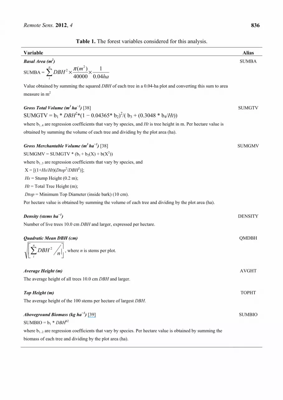
Each plot had all trees larger than or equal to 10.0 cm measured for DBH with a diameter tape. Each tree was assessed for species, status (i.e., live or dead), crown class (i.e., dominant, co-dominant, etc.) and visual quality. A Vertex™ hypsometer was used to measure tree height for each tree in the plot. Heights of deciduous species were measured during leaf-off conditions to obtain the most accurate height measurements possible. The forest variables included in the analysis are presented in Table 1.

A total of 32 plots were established in the SLRF and assigned to the Tol-Hwd forest type. Similarly, 35 plots were established in the PRF and assigned to the GrtLks-Pine forest type while 136 plots were established in the RMF, with each plot assigned to one of four forest types (i.e., Boreal-IH, Boreal-MW, Boreal-PJ and Boreal-SB). A summary of the field data for each study site and based on forest type are presented in Table 2.

Remote Sens. 2012, 4

836

Table 1. The forest variables considered for this analysis.

Variable Alias Basal Area (m2)

SUMBA = ∑ ××n

i hamDBH

04.01

40000)( 2

2 π

Value obtained by summing the squared DBH of each tree in a 0.04-ha plot and converting this sum to area

measure in m2

SUMBA

Gross Total Volume (m3 ha−1) [38]

SUMGTV = b1 * DBH2*(1 − 0.04365* b2)2/( b3 + (0.3048 * b4/Ht)) where b1..4 are regression coefficients that vary by species, and Ht is tree height in m. Per hectare value is

obtained by summing the volume of each tree and dividing by the plot area (ha).

SUMGTV

Gross Merchantable Volume (m3 ha−1) [38]

SUMGMV = SUMGTV * (b1 + b2(X) + b(X2))

where b1..3 are regression coefficients that vary by species, and

X = [(1+Hs/Ht)(Dtop2/DBH2)];

Hs = Stump Height (0.2 m);

Ht = Total Tree Height (m);

Dtop = Minimum Top Diameter (inside bark) (10 cm).

Per hectare value is obtained by summing the volume of each tree and dividing by the plot area (ha).

SUMGMV

Density (stems ha−1)

Number of live trees 10.0 cm DBH and larger, expressed per hectare.

DENSITY

Quadratic Mean DBH (cm)

⎥⎦

⎤⎢⎣

⎡∑ nDBHn

i

2 , where n is stems per plot.

QMDBH

Average Height (m)

The average height of all trees 10.0 cm DBH and larger.

AVGHT

Top Height (m)

The average height of the 100 stems per hectare of largest DBH.

TOPHT

Aboveground Biomass (kg ha−1) [39]

SUMBIO = b1 * DBHb2

where b1..2 are regression coefficients that vary by species. Per hectare value is obtained by summing the

biomass of each tree and dividing by the plot area (ha).

SUMBIO

Remote Sens. 2012, 4

837

Table 2. Field data statistics for each study site and forest type.

Variable

Tolerant

Hardwoods

(n = 32)

Great Lakes

Pine (n = 35)

Boreal Black

Spruce (n = 34)

Boreal Jack

Pine (n = 35)

Boreal Intolerant

Hardwoods

(n = 33)

Boreal

Mixed woods

(n = 34)

Mean Std. Dev. Mean Std. Dev. Mean Std. Dev. Mean Std. Dev. Mean Std. Dev. Mean Std. Dev.

AVGHT

(m) 18.9 1.5 22.9 5.3 12.9 2.2 16.1 2.1 16.7 2.0 15.6 2.0

TOPHT

(m) 24.9 1.7 28.5 5.4 16.7 2.5 20.2 3.1 22.6 3.6 22.3 3.8

QMDBH

(cm) 28.5 3.7 31.8 10.4 14.2 2.0 17.0 2.8 18.2 3.7 19.4 2.7

SUMBA

(m2·ha−1) 25.9 3.8 37.1 13.8 25.8 10.5 21.2 9.6 31.4 10.8 32.7 10.5

SUMGTV

(m3·ha−1) 232.8 40.2 434.5 209.3 162.7 79.4 248.8 94.1 266.5 119.9 265.1 117.0

SUMGMV

(m3·ha−1) 201.9 37.2 404.0 206.7 109.0 62.6 105.4 88.7 216.2 116.7 223.1 108.1

BIOMASS

(kg·ha−1) 203,514 34,132 147,058 56,780 100,833 42,733 127,458 45,404 128,732 55,040 138,493 45,676

DENSITY

(stems·ha−1) 421.0 107.8 607.6 393.8 1643.0 691.0 1414.5 470.5 1198.5 307.8 1102.2 334.2

2.4. Data Processing

All LiDAR returns were normalized against a triangulated irregular network (TIN) that was developed using the LiDAR returns that were classified as ground. The process involved subtracting from the original z-value of a return the z-value on the TIN matching its x-y coordinates. No height threshold (e.g., 2 m; [40]) was used to filter the LiDAR data. Preliminary tests indicated that application of a height threshold did not improve model performance.

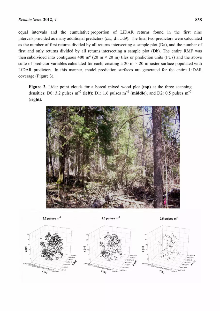
LiDAR data were decimated according to the methodology described by Raber et al. [41]. A decimation level 0 (D0) represented the original dataset characterized by a point density of approximately 3.2 pulses m−2. The decimation level 1 (D1) LiDAR dataset was derived by taking alternating pulses along each scan line with each scan line retained, thereby increasing the cross track spacing by a factor of two. For the decimation level 2 (D2) LiDAR dataset, every fourth point along each scan line was retained, thereby increasing the cross track spacing by a factor of 4, and every other scan line was retained, resulting in an increase in the along-track spacing by a factor of 2. The systematic decimation resulted in the D1 and D2 LiDAR datasets possessing point densities of approximately 1.6 and 0.5 pulses m−2, respectively (Figure 2).

Predictor variables were derived statistics from the normalized LiDAR data. In each case, “all” returns were used, and height thresholds were not used to filter point data. Potential predictors included basic statistics of mean height (mean), standard deviation (std_dev), and absolute deviation around the mean height (abs_dev), as well as deciles of LiDAR canopy height (i.e., p10…p90) and the maximum (max) LiDAR height. For each plot, the range of LiDAR height measurements was divided into 10

Remote Sens. 2012, 4

838

equal intervals and the cumulative proportion of LiDAR returns found in the first nine intervals provided as many additional predictors (i.e., d1…d9). The final two predictors were calculated as the number of first returns divided by all returns intersecting a sample plot (Da), and the number of first and only returns divided by all returns intersecting a sample plot (Db). The entire RMF was then subdivided into contiguous 400 m2 (20 m × 20 m) tiles or prediction units (PUs) and the above suite of predictor variables calculated for each, creating a 20 m × 20 m raster surface populated with LiDAR predictors. In this manner, model prediction surfaces are generated for the entire LiDAR coverage (Figure 3).

Figure 2. Lidar point clouds for a boreal mixed wood plot (top) at the three scanning densities: D0: 3.2 pulses m−2 (left); D1: 1.6 pulses m−2 (middle); and D2: 0.5 pulses m−2 (right).

Remote Sens. 2012, 4

839

Figure 3. Sample model predicted surface generated from LiDAR height and density metrics (i.e., Gross Merchantable Volume (GMV)) for the Romeo Malette Forest (RMF).

2.5. Statistical Analyses

Multiple stepwise regressions with a significance level of 0.05 were used for constructing models for predicting forest inventory variables. A diagnosis of each model was performed to determine if parametric statistical assumptions were satisfied. The Shapiro-Wilk Test was used to determine if

Remote Sens. 2012, 4

840

residuals were normally distributed and the Brown-Forsythe Test was used to check for the presence of heteroscedasticity (i.e., unequal error variance). As LiDAR predictors have been reported to be highly correlated, the variance inflation factors (VIFs) for the predictors used in each model were examined. Candidate models where predictors exhibited VIFs greater than 10 were discarded, as these would suggest the presence of multi-collinearity in the predictor data [42].

Effect of Decimation Treatments

For each forest variable, predictions from the models constructed for the different decimation levels were compared to respective observed values to create a multivariate response vector of absolute prediction errors for each plot:

ei(j) = [e0i(j), e1i(j), e2i(j)] (1)

where, e0i(j) is the absolute error associated with the undecimated prediction for plot j within each forest/type i (Tol-Hwd, GrtLks-Pine, Boreal-PJ, Boreal-SB, Boreal-IH and Boreal-MW):

)()()( 0ˆ0 jijiji yye −= , (2)

and e1i(j) and e2i(j) denote similar errors for the decimated predictions, 1.6 and 0.5 pulses m−2, respectively.

Prediction errors were then subjected to repeated measures analyses of variance (RMANOVA), treating the different forests/types as fixed effects, and making comparisons of the different decimation levels (within-subject effects) with multivariate tests (Wilks’ lambda). RMANOVA is used when all members of a sample are measured repeatedly under a number of different conditions. Within the context of this study, it was a particular forest variable for a plot that was repeatedly predicted using LiDAR data of three varying point densities. Given repeated measurements, the use of a standard ANOVA is not appropriate [43]. We contrasted the different decimation levels to test for increases in prediction error that were proportional and disproportional to the decimation levels applied (i.e., linear and quadratic contrasts, respectively, associated with increasing decimation). With this approach, the following null hypothesis was tested for each forest variable:

H0: Decimation of the LiDAR point cloud from 3.2 to 1.6 and 0.5 pulses m−2 does not reduce prediction precision; versus

Ha1: Decimation of the LiDAR point cloud reduces prediction precision proportional to decimation level; or

Ha2: Decimation of the LiDAR point cloud reduces prediction precision disproportional to decimation level.

In cases where a decimation × forest/type interaction was indicated, similar analyses by forest/type were used to reveal the source of interaction.

3. Results and Discussion

For illustration purposes, the models developed for each variable for Boreal-SB and Boreal-IH plot data are presented in Tables 3 and 4. For black spruce, the models typically exhibit very high coefficients of determination (i.e., R2 and R2(adj)) with RMSEs, expressed as a percentage of the

Remote Sens. 2012, 4

841

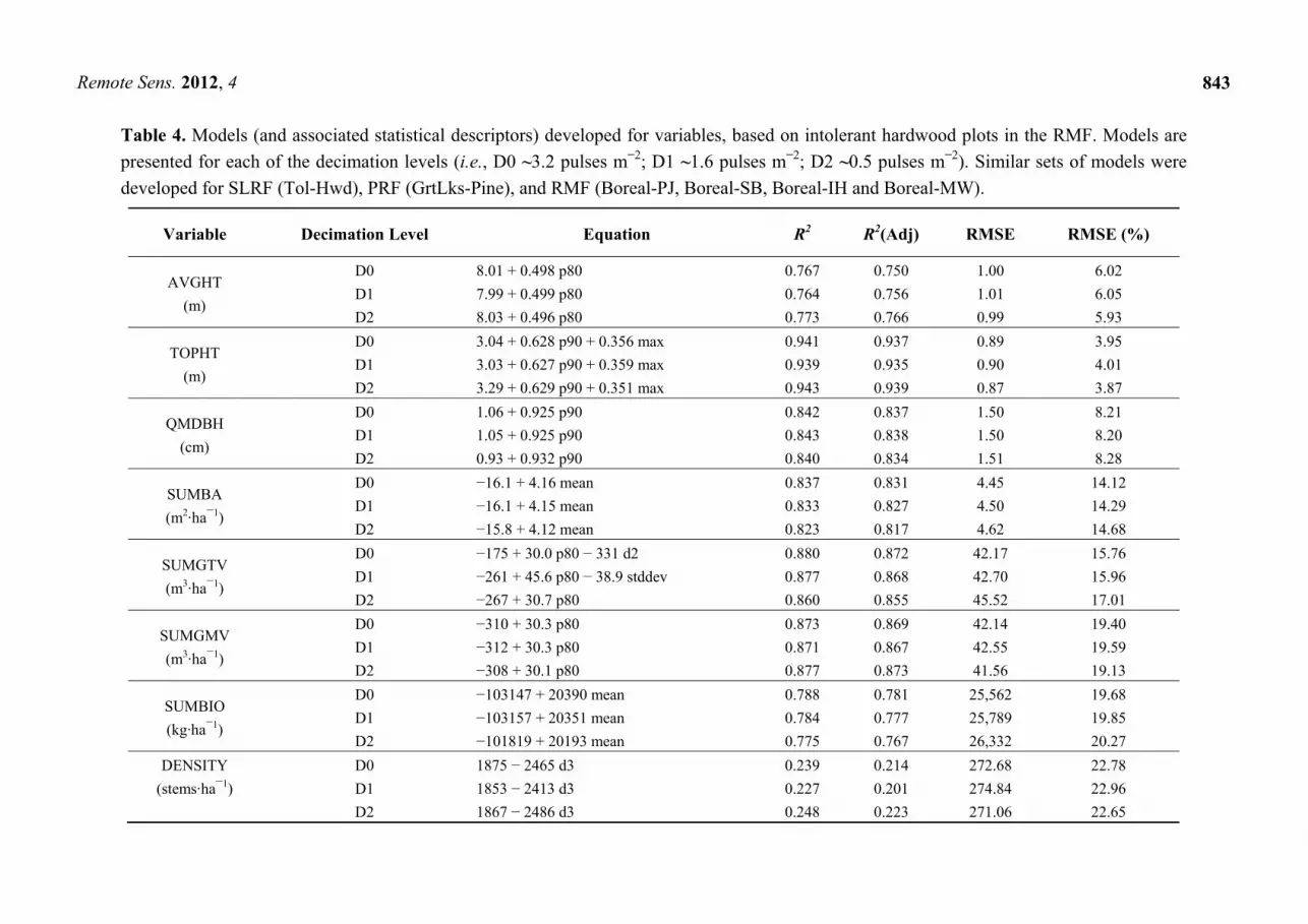
predicted means, ranging from approximately 4–19%, typically with only one or two input variables (Table 3). Models developed for variables based on intolerant hardwood plots in the RMF also exhibited high adjusted coefficients of determination (i.e., R2(adj) = 0.201–0.939) with RMSEs ranging from 4 to 23%. Variable-by-stand type results indicate that height-related models (i.e., AVGHT; TOPHT; QMDBH) tended to perform well (i.e., RMSEs < 10%) and volume/biomass-related models (i.e., SUMBA; SUMGTV, SUMGMV, SUMBIO) performed moderately well (RMSEs typically 10–20%). Density models tended to exhibit the highest RMSEs (Table 5).

For all forest variables tested, overall model prediction precision varied strongly with forest/type (p ≤ 0.02; Table 6). Boreal-SB variables tended to be predicted with the greatest precision (lowest mean absolute errors) and GrtLks-Pine variables with the least precision. The Boreal-SB stands were quite similar in that the majority were upland sites with mature black spruce of natural origin, whereas the GrtLks-Pine communities were more diverse in terms of species, management, and origin. The range of conditions sampled included unmanaged white pine, shelterwood white and red pine, thinned and unmanaged red pine plantations, as well as some natural jack pine stands. In future work, this group will be subdivided further to better consider the volume/height relationships for these species and management conditions.

With the exception of 2 of the 8 forest variables tested, we generally found little evidence to reject the null hypothesis that decimation of the LiDAR point cloud has no affect on model precision (p > 0.10; Table 6). In overall analyses, mean prediction errors tended to increase with decimation for the variables DENSITY and AVGHT (p ≤ 0.02), but there was evidence to suggest that this situation was not consistent across all forest/types studied (p ≤ 0.10). More specifically, DENSITY prediction errors for Boreal-PJ increased from 226 stems ha−1 at 3.2 pulses m−2, to 299 and 324 stems ha−1 through decimation to 1.6 and 0.5 pulses m−2 respectively (decimation linear, p < 0.01).

To a lesser extent, prediction errors for GrtLks-Pine increased from 171 stems ha−1 at 3.2 pulses m−2, to 211 and 192 stems ha−1 through decimation to 1.6 and 0.5 pulses m−2 respectively (decimation quadratic, p = 0.09). Thinning treatments had been applied to these forests/types potentially giving rise to increased error as a function of insufficient sample size to account for a suitable range of density conditions.

Similarly, AVGHT prediction errors for Boreal-MW and GrtLks-Pine tended to increase sharply (30 to 40%) with the highest level of decimation (i.e., 0.5 pulses m−2) (decimation quadratic, p ≤ 0.10). However, these examples appear rare in the context of the overall data set and one may argue that with a significance level of 10%, we might expect to observe trends that suggest rejection of H0 up to 10% of the time simply through random chance alone. Thus, we feel that it is reasonable to conclude that decimation of the LiDAR point cloud from 3.2 to 1.6 and 0.5 pulses m−2 did not reduce the prediction precision of the forest variables tested.

The ability to significantly reduce LiDAR pulse density for forest inventory modeling without affecting prediction accuracy or precision provides significant financial savings in data acquisition and processing. Although not tested in this study, it is anticipated that accurate and precise digital elevation models (DEMs) of a finer scale than possible in the past can also be derived from low density LiDAR data, even in leaf-on conditions.

Remote Sens. 2012, 4

842

Table 3. Models (and associated statistical descriptors) developed for variables, based on black spruce plots in the RMF. Models are presented for each of the decimation levels (i.e., D0 ~3.2 pulses m−2; D1 ~1.6 pulses m−2; D2 ~0.5 pulses m−2). Similar sets of models were developed for SLRF (Tol-Hwd), PRF (GrtLks-Pine), and RMF (Boreal-PJ, Boreal-SB, Boreal-IH and Boreal-MW).

Variable Decimation Level

Equation R2 R2 (Adj)

RMSE RMSE (%)

AVGHT D0 2.41 + 0.948 p90 + 2.80 d1 − 0.0821 Da 0.951 0.946 0.49 3.81 (m) D1 1.73 + 0.836 p90 + 2.99 d2 0.941 0.938 0.53 4.16 D2 2.34 + 0.802 p90 + 2.26 d3 0.936 0.932 0.56 4.34 TOPHT D0 2.32 + 0.547 max + 0.436 p90 0.923 0.918 0.69 4.10 (m) D1 2.10 + 0.578 max + 0.429 p90 0.927 0.922 0.66 3.98 D2 3.79 + 0.577 max + 0.326 p90 0.903 0.897 0.77 4.58 QMDBH D0 8.03 + 1.18 p90 − 0.327 Da − 0.138 p40 0.838 0.822 0.82 5.80 (cm) D1 8.58 + 1.07 p90 − 0.308 Da 0.783 0.769 0.95 6.72 D2 2.44 + 1.12 p90 − 0.234 Da + 5.33 d6 0.863 0.850 0.76 5.34 SUMBA (m2·ha−1)

D0 58.9 - 20.2 d5 + 1.58 p50 − 0.379 Db 0.918 0.909 3.01 11.68 D1 −0.91 + 2.23 p50 + 0.622 Da 0.910 0.904 3.15 12.22 D2 48.6 + 1.26 p60 + 1.27 p40 − 0.478 Db 0.935 0.929 2.66 10.33

SUMGTV (m3·ha−1)

D0 −702 + 32.1 mean − 210 d6 + 873 d9 − 110 p20 0.949 0.942 17.96 11.04 D1 −66.3 + 42.2 mean − 5.59 p30 0.927 0.922 21.52 13.23 D2 268 + 23.5 mean − 3.30 Db + 4.95 p40 0.942 0.936 19.14 11.77

SUMGMV (m3·ha−1)

D0 −114 + 5.63 p40 + 17.4 p90 0.916 0.910 18.19 16.69 D1 −182 + 20.1 p80 + 7.02 p40 + 113 d4 0.915 0.907 18.25 16.74 D2 −195 + 41.5 mean + 164 d3 − 282 p10 0.939 0.933 15.46 14.18

SUMBIO D0 −321894 + 15682 mean − 114298 d6 + 427669 d9 0.925 0.918 11 673 11.58 (kg·ha−1) D1 −17265 + 21243 mean 0.905 0.902 13 199 13.09 D2 157912 + 11931 mean − 1752 Db + 3131 p40 0.932 0.925 11 143 11.05 DENSITY (stems·ha−1)

D0 −112 − 4076 d3 + 3254 p10 − 159 p30 − 180 p80 − 56.4 Db + 106 p40 + 9705 d9 0.888 0.857 231.84 14.11 D1 5380 − 4678 d4 + 5580 p10 − 134 p30 − 95.9 p90 0.794 0.766 313.83 19.10 D2 11212 − 2363 d4 − 204 p90 − 80.4 Db + 70.5 p40 0.861 0.842 257.74 15.69

Remote Sens. 2012, 4

843

Table 4. Models (and associated statistical descriptors) developed for variables, based on intolerant hardwood plots in the RMF. Models are presented for each of the decimation levels (i.e., D0 ~3.2 pulses m−2; D1 ~1.6 pulses m−2; D2 ~0.5 pulses m−2). Similar sets of models were developed for SLRF (Tol-Hwd), PRF (GrtLks-Pine), and RMF (Boreal-PJ, Boreal-SB, Boreal-IH and Boreal-MW).

Variable Decimation Level Equation R2 R2(Adj) RMSE RMSE (%)

AVGHT (m)

D0 8.01 + 0.498 p80 0.767 0.750 1.00 6.02 D1 7.99 + 0.499 p80 0.764 0.756 1.01 6.05 D2 8.03 + 0.496 p80 0.773 0.766 0.99 5.93

TOPHT (m)

D0 3.04 + 0.628 p90 + 0.356 max 0.941 0.937 0.89 3.95 D1 3.03 + 0.627 p90 + 0.359 max 0.939 0.935 0.90 4.01 D2 3.29 + 0.629 p90 + 0.351 max 0.943 0.939 0.87 3.87

QMDBH (cm)

D0 1.06 + 0.925 p90 0.842 0.837 1.50 8.21 D1 1.05 + 0.925 p90 0.843 0.838 1.50 8.20 D2 0.93 + 0.932 p90 0.840 0.834 1.51 8.28

SUMBA (m2·ha−1)

D0 −16.1 + 4.16 mean 0.837 0.831 4.45 14.12 D1 −16.1 + 4.15 mean 0.833 0.827 4.50 14.29 D2 −15.8 + 4.12 mean 0.823 0.817 4.62 14.68

SUMGTV (m3·ha−1)

D0 −175 + 30.0 p80 − 331 d2 0.880 0.872 42.17 15.76 D1 −261 + 45.6 p80 − 38.9 stddev 0.877 0.868 42.70 15.96 D2 −267 + 30.7 p80 0.860 0.855 45.52 17.01

SUMGMV (m3·ha−1)

D0 −310 + 30.3 p80 0.873 0.869 42.14 19.40 D1 −312 + 30.3 p80 0.871 0.867 42.55 19.59 D2 −308 + 30.1 p80 0.877 0.873 41.56 19.13

SUMBIO (kg·ha−1)

D0 −103147 + 20390 mean 0.788 0.781 25,562 19.68 D1 −103157 + 20351 mean 0.784 0.777 25,789 19.85 D2 −101819 + 20193 mean 0.775 0.767 26,332 20.27

DENSITY D0 1875 − 2465 d3 0.239 0.214 272.68 22.78 (stems·ha−1) D1 1853 − 2413 d3 0.227 0.201 274.84 22.96

D2 1867 − 2486 d3 0.248 0.223 271.06 22.65

Remote Sens. 2012, 4

844

Table 5. Root Mean Square Errors (RMSEs) for model developed for variables, based on forest inventory plots in the Romeo Malette Forest, Swan Lake Research Forest and Petawawa Research Forest. RMSEs are presented for each of the decimation levels (i.e., D0 ~3.2 pulses m−2; D1 ~1.6 pulses m−2; D2 ~0.5 pulses m−2). Percent RMSEs are presented in brackets.

Variable Romeo Malette Forest Swan Lake Research

Forest Petawawa Research

Forest

Jack Pine Black Spruce Intolerant Hardwoods Mixed Woods Tolerant Hardwoods Great Lakes Pine

D0 D1 D2 D0 D1 D2 D0 D1 D2 D0 D1 D2 D0 D1 D2 D0 D1 D2

AVGHT (m)

0.79 (4.9)

0.81 (5.0)

0.83 (5.2)

0.49 (3.8)

0.53 (4.2)

0.56 (4.3)

1.00 (6.0)

1.01 (6.1)

1.00 (5.9)

0.73 (4.6)

0.84 (5.3)

0.93 (6.0)

0.62 (3.4)

0.62 (3.4)

0.59 (3.2)

1.5 (6.6)

1.5 (6.7)

2.0 (9.2)

TOPHT (m)

0.42 (2.1)

0.50 (2.5)

0.56 (2.8)

0.69 (4.1)

0.66 (4.0)

0.77 (4.6)

0.89 (4.0)

0.90 (4.0)

0.87 (3.9)

0.55 (2.5)

0.63 (2.8)

0.61 (2.8)

0.83 (3.5)

0.84 (3.5)

0.86 (3.5)

1.2 (4.4)

1.3 (4.6)

1.3 (4.7)

QMDBH (cm)

1.5 (8.7)

1.4 (8.4)

1.6 (9.3)

0.82 (5.8)

0.95 (6.7)

0.76 (5.3)

1.50 (8.2)

1.50 (8.2)

1.51 (8.3)

1.61 (8.3)

1.63 (8.4)

1.65 (8.5)

2.3 (8.4)

2.0 (7.2)

2.0 (7.1)

5.4 (17.5)

5.4 (17.5)

4.3 (14.0)

SUMBA (m2·ha−1)

4.3 (13.7)

4.5 (14.4)

4.2 (13.5)

3.0 (11.7)

3.2 (12.2)

2.7 (10.3)

4.5 (14.1)

4.5 (14.3)

4.6 (14.7)

5.4 (16.6)

5.4 (16.4)

5.5 (16.8)

3.2 (12.6)

3.1 (12.5)

3.2 (12.8)

5.2 (14.6)

5.2 (14.4)

5.4 (14.9)

SUMGTV (m3·ha−1)

31.1 (12.5)

31.8 (12.8)

31.7 (12.7)

18.0 (11.0)

21.5 (13.2)

19.1 (11.8)

42.2 (15.8)

42.7 (16.0)

45.5 (17.0)

48.1 (18.2)

47.1 (17.8)

48.2 (18.2)

29.2 (12.9)

26.3 (11.7)

28.9 (12.8)

57.1 (13.7)

55.7 (13.3)

59.9 (14.4)

SUMGMV (m3·ha−1)

33.6 (17.2)

31.1 (15.9)

26.1 (13.4)

18.2 (16.7)

18.3 (16.7)

15.5 (14.2)

42.1 (19.4)

42.6 (19.6)

41.6 (19.1)

42.7 (19.1)

41.4 (18.6)

42.9 (19.2)

28.9 (14.8)

28.9 (14.8)

27.0 (13.8)

57.5 (14.8)

57.1 (14.7)

56.1 (14.5)

SUMBIO (kg·ha−1)

17,479 (13.7)

17,972 (14.1)

17,842 (14.0)

11,673 (11.6)

13,199 (13.1)

11,143 (11.1)

25,789 (19.7)

25,562 (19.9)

26,332 (20.3)

20,000 (14.4)

19,469 (14.1)

22,510 (16.3)

26,884 (13.6)

28,532 (14.5)

28,966 (14.7)

33,135 (23.3)

32,250 (22.7)

29,989 (21.1)

Density (stems·ha−1)

278.2 (19.7)

372.7 (26.4)

394.3 (27.9)

231.8 (14.1)

313.8 (19.1)

257.7 (15.7)

272.7 (22.8)

274.8 (23.0)

271.1 (22.7)

312.6 (28.4)

313.7 (28.5)

312.7 (28.4)

51.9 (12.7)

42.1 (10.3)

43.7 (10.7)

226.7 (37.8)

265.1 (44.2)

247.8 (41.3)

Remote Sens. 2012, 4

845

Table 6. Summary of mean absolute errors for the decimation levels tested and p-values from RMANOVA (Wilks’ lambda) testing for decimation and forest/type effects and their interaction. (Note: values in bold suggest a loss of precision with increasing decimation for some forest/types).

AVGHT

m

TOPHT

m

QMDBH

cm

SUMBA

m2·ha−1

SUMGTV

m3·ha−1

SUMGMV

m3·ha−1

SUMBIO

kg·ha−1

DENSITY

stems·ha−1

Overall mean absolute error:

3.2 pulses·m−2 0.65 0.59 1.69 3.4 29.1 29.4 17,285 176 1.6 pulses·m−2 0.68 0.59 1.69 3.3 29.1 28.5 17,631 206 0.5 pulses·m−2 0.76 0.61 1.52 3.4 30.5 27.3 17,688 201

Source of variation: Decimation 0.02 0.30 0.09 0.94 0.46 0.23 0.62 <0.01 linear <0.01 0.14 0.05 0.86 0.25 0.10 0.56 <0.01 quadratic 0.17 0.57 0.08 0.82 0.29 0.64 0.80 0.07 Decimation × Forest/Type 0.10 0.98 <0.01 0.96 0.72 0.87 0.32 <0.01 Forest/Type <0.01 <0.01 <0.01 0.02 <0.01 <0.01 <0.01 <0.01

4. Conclusions

The results from this research demonstrate that a point density of 0.5 pulses·m−2 is sufficient for the estimation of forest inventory variables at the plot and stand levels for the different forest types considered in this study. In cases where a decimation effect was observed for a forest variable, the effect may be attributed to differences in model form, specifically as it relates to number of predictors used. This study provides further evidence that low-density LiDAR-based predictions offer significant potential for integration into tactical forest resource inventories for a range of forest ecosystems across Ontario. LiDAR data can provide a number of important surfaces (i.e., bare earth digital elevation model; forest inventory predictor surfaces) that are critical to tactical forest management and planning. Further research into the generation of additional surfaces related to terrain should provide more precise characterization of moisture and nutrient regimes for modeling of forest ecosites.

Acknowledgements

The authors gratefully acknowledge financial support from the Ontario Centre of Excellence for Earth and Environmental Technologies and the Forest Research Partnership (i.e., Tembec Inc., Ontario Ministry of Natural Resources, Canadian Wood Fibre Centre). Treitz also acknowledges research support from the Natural Sciences and Engineering Research Council and the Premier’s Research Excellence Award. Thanks to the following individuals for contributions to field data collection and logistics: Kelly Von Bargen, Paul Courville, Beth Denaburg, Michelle Desaulniers, Karin van Ewijk, Stephanie Gagliardi, Anne Hagerman, Anthony Iserhoff, Katalijn MacAfee, Jem Morrison, Stefanie Phelan, Meg Southee, Stan Vasiliauskas. The authors would like to thank two anonymous reviewers for their thoughtful reviews and constructive comments.

Remote Sens. 2012, 4

846

References

1. Hyyppa, J.; Hyyppa, H.; Leckie, D.; Gougeon, F.; Yu, X.; Maltamo, M. Review of methods of small-footprint airbone laser scanning for extracting forest inventory data in boreal forests. Int. J. Remote Sens. 2008, 29, 1339-1366.

2. Wulder, M.A.; Bater, C.W.; Coops, N.C.; Hilker, T.; White, J.C. The role of LiDAR in sustainable forest management. Forest. Chron. 2008, 84, 807-826.

3. van Leeuwen, M.; Nieuwenhuis, M. Retrieval of forest structural parameters using LiDAR remote sensing. Eur. J. For. Res. 2010, 129, 749-770.

4. Suratno, A.; Seielstad, C.; Queen, L. Tree species identification in mixed coniferous forest using airborne laser scanning. ISPRS J. Photogramm. 2009, 64, 683-693.

5. Lefsky, M.; Hudak, A.T.; Cohen, W.B.; Acker, S.A. Geographic variability in LiDAR predictions of forest stand structure in the Pacific Northwest. Remote Sens. Environ. 2005, 95, 532-548.

6. Næsset, E.; Bollandsås, O.M.; Gobakken, T. Comparing regression methods in estimation of biophysical properties of forest stands from two different inventories using laser scanner data. Remote Sens. Environ. 2005, 94, 541-553.

7. Kane, V.R.; McGaughey, R.J.; Bakker, J.D.; Gersonde, R.F.; Lutz, J.A.; Franklin, J.F. Comparisons between field- and LiDAR-based measures of stand structural complexity. Can. J. For. Res. 2010, 40, 761-773.

8. Van Ewijk, K.Y.; Treitz, P.M.; Scott, N.A. Characterizing forest succession in Central Ontario using LiDAR-derived indices. Photogramm. Eng. Remote Sensing 2011, 77, 261-269.

9. Morsdorf, F.; Koetz, B.; Meier, E.; Itten, K.I.; Allgöwer, B. Estimation of LAI and fractional cover from small footprint airborne laser scanning data based on gap fraction. Remote Sens. Environ. 2006, 104, 50-61.

10. Zhao, K.; Popescu, S. LiDAR-based mapping of leaf area index and its use for validating BLOBCARBON satellite LAI products in a temperate forest of the Southern USA. Remote Sens. Environ. 2009, 113, 1628-1645.

11. Jensen, J.L.R.; Humes, K.S.; Conner, T.; Williams, C.J.; DeGroot, J. Estimation of biophysical characteristics for highly variable mixed-conifer stands using small-footprint Lidar. Can. J. For. Res. 2006, 36, 1129-1138.

12. Maltamo, M.; Eerikäinen, K.; Packalén, P.; Hyyppä, J. Estimation of stem volume using laser scanning-based canopy height metrics. Forestry 2006, 79, 217-229.

13. Yu, X.; Hyyppä, J.; Kaartinen, H.; Maltamo, M.; Hyyppä, H. Obtaining plotwise mean height and volume growth in boreal forests using multi-temporal laser surveys and various change detection techniques. Int. J. Remote Sens. 2008, 29, 1367-1386.

14. Popescu, S.D.; Wynne, R.H.; Nelson, R.F. Measuring individual tree crown diameter with lidar and assessing its influence on estimating forest volume and biomass. Can. J. Remote Sens. 2003, 29, 564-577.

15. Lim, K.; Treitz, P. Estimation of aboveground forest biomass from airborne discrete return Laser scanner data using canopy-based quantile estimators. Scand. J. Forest Res. 2004, 19, 558-570.

16. Woods, M.; Lim, K.; Treitz, P. Predicting forest stand variables from lidar data in the Great Lakes—St. Lawrence Forest of Ontario. Forest. Chron. 2008, 84, 827-839.

Remote Sens. 2012, 4

847

17. Næsset, E.; Gobakken, T. Estimation of above- and below-ground biomass across regions of the boreal forest zone using airborne laser. Remote Sens. Environ. 2008, 112, 3079-3090.

18. Næsset, E. Practical large-scale forest stand inventory using small-footprint airborne scanning laser. Scand. J. For. Res. 2004, 19, 164-179.

19. Evans, D.L.; Roberts, S.D.; Parker, R.C. LiDAR—A new tool for forest measurements? Forest. Chron. 2006, 82, 211-218.

20. Stephens, P.R.; Watt, P.J.; Loubser, D.; Haywood, A.; Kimberly. M.O. Estimation of Carbon Stocks in New Zealand Planted Forest Using Airborne Scanning LiDAR. In Proceedings of ISPRS Workshop on Laser Scanning 2007, Espoo, Finland, 12–14 September 2007; In IAPRS; 2007; Volume XXXVI, Part 3/W52.

21. Woods, M.; Pitt, D.; Penner, M.; Lim, K.; Nesbitt, D.; Etheridge, D.; Treitz, P. Operational implementation of a LiDAR inventory in Boreal Ontario. Forest. Chron. 2011, 87, 512-528.

22. Stone, C.; Penman, T.; Turner, R. Determining an optimal model for processing lidar data at the plot level: Results for a Pinus radiata plantation in New South Wales, Australia. New Zealand J. For. Sci. 2011, 41, 191-205.

23. Næsset, E. Effects of different flying altitudes on biophysical stand properties estimated from canopy height and density measured with a small-footprint airborne scanning laser. Remote Sens. Environ. 2004, 91, 243-255.

24. Næsset, E. Assessing sensor effect and effect of leaf-off and leaf-on canopy conditions on biophysical stand properties derived from small footprint airborne laser data. Remote Sens. Environ. 2005, 98, 356-370.

25. Andersen, H.E.; Reutebuch, S.E.; McGaughey, R.J. A rigorous assessment of tree height measurements obtained using airborne lidar and conventional field methods. Can. J. For. Res. 2006, 32, 355-366.

26. Chasmer, L.; Hopkinson, C.; Smith, B.; Treitz, P. Examining the influence of changing laser pulse repetition frequencies on conifer forest canopy returns. Photogramm. Eng. Remote Sensing 2006, 72, 1359-1367.

27. Goodwin, N.R.; Coops, N.C.; Culvenor, D.S. Assessment of forest structure with airborne lidar and the effects of platform altitude. Remote Sens. Environ. 2006, 103, 140-152.

28. Hopkinson, C. The influence of flying altitude and beam divergence on canopy penetration and laser pulse return distribution characteristics. Can. J. Remote Sens. 2007, 33, 312-324.

29. Magnusson, M.; Fransson, J.E.S.; Holmgren, J. Effects on estimation accuracy of forest variables using different pulse density of laser data. Forest Sci. 2007, 53, 619-626.

30. Gobakken, T.; Næsset, E. Assessing effects of laser point density, ground sampling intensity, and field sample plot size on biophysical stand properties derived from airborne laser scanner data. Can. J. For. Res. 2008. 38, 1095-1109.

31. Morsdorf, F.; Frey, O.; Meier, E.; Itten, K.I.; Allgöwer, B. Assessment of the influence of flying altitude and scan angle on biophysical vegetation products derived from airborne laser scanning. Int. J. Remote Sens. 2008, 29, 1387-1406.

32. Næsset, E. Effects of different sensors, flying altitudes, and pulse repetition frequencies on forest canopy metrics and biophysical stand properties derived from small-footprint airborne laser data. Remote Sens. Environ. 2009, 113, 148-159.

Remote Sens. 2012, 4

848

33. Bater, C.W.; Wulder, M.A.; Coops, N.C.; Nelson, R.F.; Hilker, T.; Næsset, E. Stability of sample-based scanning-lidar-derived vegetation metrics for forest monitoring. IEEE Trans. Geosci. Remote Sens. 2011, 49, 2385-2392.

34. Lim, K.; Hopkinson, C.; Treitz, P. Examining the effects of sampling point densities on laser canopy height and density metric. Forest. Chron. 2008, 84, 876-885.

35. Cole, W.G.; Mallory, E. Swan Lake Forest Research Reserve 20-year Management Plan, 2005–2025; Ontario Ministry of Natural Resources: Sault Ste. Marie, ON, Canada, 2005.

36. Environment Canada. National Climate Data and Information Archive; 2012. Available online: http://climate.weatheroffice.gc.ca/climate_normals/index_e.html (accessed on 1 March 2012).

37. Bazeley, D.G.; Morandin, L.; MacIsaac, S. Contingency Forest Management Plan for the Romeo Malette Forest Timmins District, Northeast Region Tembec Industries Inc. for the 2-year period from April 1, 2007 to March 31, 2009; 2009. Available online: http://hdl.handle.net/1873/13655 (accessed on 1 March 2012).

38. Honer, T.G.; Ker, M.F.; Alemdag, I.S. Metric Timber Tables for the Commercial Tree Species of Central and Eastern Canada; Information Report M–X–140; Maritimes Forest Research Centre, Canadian Forestry Service: Fredericton, NB, Canada, 1983; p. 139.

39. Ter-Mikaelian, M.T.; Korzukhin, M.D. Biomass equations for sixty-five North American tree species. For. Ecol. Manage. 1997, 97, 1-24.

40. Næsset, E. Predicting forest stand characteristics with airborne scanning laser using a practical two-stage procedure and field data. Remote Sens. Environ. 2002, 80, 88-99.

41. Raber, G.T.; Jensen, J.R.; Hodgson, M.E.; Tullis, J.A.; Davis, B.A.; Berglund, J. Impact of LiDAR nominal post-spacing on DEM accuracy and flood zone delineation. Photogramm. Eng. Remote Sensing 2007, 73, 793-804.

42. Neter, J.; Kutner, M.H.; Nachtsheim, C.J.; Wasserman, W. Applied Linear Statistical Models, 4th ed.; WCB/McGraw-Hill: Boston, MA, USA, 1996.

43. Popescu, S.C.; Zhao, K. A Voxel-based LiDAR method for estimating crown base height for deciduous and pine trees. Remote Sens. Environ. 2008, 112, 767-781.

© 2012 by the authors; licensee MDPI, Basel, Switzerland. This article is an open access article distributed under the terms and conditions of the Creative Commons Attribution license (http://creativecommons.org/licenses/by/3.0/).