1

Dual-branch residual network for lung nodule segmentation

Haichao Cao1, Hong Liu1*, Enmin Song1, Chih-Cheng Hung2, Guangzhi Ma1, Xiangyang Xu1,

Renchao Jin1 and Jianguo Lu1.

1Huazhong University of Science and Technology, School of Computer Science & Technology,

Wuhan, 430074, China

2Kennesaw State University, the Laboratory for Machine Vision and Security Research, 1000

Chastain Rd., Kennesaw, USA, GA 30144

*E-mails: hl.cbib@gmail.com

Abstract

An accurate segmentation of lung nodules in computed tomography (CT) images

is critical to lung cancer analysis and diagnosis. However, due to the variety of lung

nodules and the similarity of visual characteristics between nodules and their

surroundings, a robust segmentation of nodules becomes a challenging problem. In

this study, we propose the Dual-branch Residual Network (DB-ResNet) which is a

data-driven model. Our approach integrates two new schemes to improve the

generalization capability of the model: 1) the proposed model can simultaneously

capture multi-view and multi-scale features of different nodules in CT images; 2) we

combine the features of the intensity and the convolution neural networks (CNN). We

propose a pooling method, called the central intensity-pooling layer (CIP), to extract

the intensity features of the center voxel of the block, and then use the CNN to obtain

the convolutional features of the center voxel of the block. In addition, we designed a

weighted sampling strategy based on the boundary of nodules for the selection of

those voxels using the weighting score, to increase the accuracy of the model. The

proposed method has been extensively evaluated on the LIDC dataset containing 986

nodules. Experimental results show that the DB-ResNet achieves superior

segmentation performance with an average dice score of 82.74% on the dataset.

Moreover, we compared our results with those of four radiologists on the same dataset.

The comparison showed that our average dice score was 0.49% higher than that of

human experts. This proves that our proposed method is as good as the experienced

radiologist.

Keywords: Lung nodule segmentation; Residual neural networks; Deep learning;

Computer-aided diagnosis

2

1. Introduction

Lung cancer is a relatively common and deadly cancer with a five-year survival

rate of only 18% [1]. The use of computed tomography (CT) images for treatment,

monitoring, and analysis is an important strategy for early lung cancer diagnosis and

survival time improvement [2]. With this technique, the accurate segmentation of lung

nodules is important because it can directly affect the subsequent analysis results [3].

Due to the fact that the number of CT images is increasing, the development of a

robust automatic segmentation model has important clinical significance for avoiding

tedious manual treatment and reducing the diagnostic difference among doctors [4].

Due to the heterogeneity of lung nodules on CT images (as shown in Fig. 1), it

has been difficult to obtain an accurate segmentation performance [5–7]. Specifically,

the similarity of visual characteristics between nodules and their surroundings causes

the difficulty for the segmentation. In particular, the juxtapleural nodules (Fig. 1(b)),

because its intensity is very similar to the lung wall, makes it difficult to segment such

nodules using conventional methods. A similar situation is the ground-glass opacity

(GGO, Fig. 1(e)) nodules, which, due to their low contrast to the surrounding

background, result in simple threshold- and morphological-based methods that cannot

handle such nodules. In addition, for calcific nodules (Fig. 1(d)), because of the high

contrast with surrounding pixels, a simple threshold segmentation method (for

example, OTSU algorithm) can segment such nodules well, but such methods cannot

be applied to both the juxtapleural nodules and the GGO nodules. It is a challenge to

adapt to these three types of nodules at the same time. Finally, for the cavitary nodules

with a black hole (Fig. 1(c), since the intensity difference of each part is large, it is

also a challenge to accurately segment such nodules. It should be pointed out that

there are some nodules with small diameters in the lungs as shown in Fig. 1(f). These

nodules are very similar to the intensity of the surrounding noise, which makes these

nodules more difficult to be distinguished.

(a) (b) (c) (d) (e) (f)

(a) isolated nodule (b) juxtapleural nodule (c) cavitary nodule (d) calcific nodule (e) GGO nodule (f) small nodule

Fig. 1. Example image of a heterogeneous lung nodule in CT image. Note that (e) GGO in

sub-figure (d) represents a ground-glass opacity nodule, and sub-figure (f) is a small nodule

having a diameter of less than 4.4 mm.

The intensity-based method using morphological operations [8,9] and region

3

growing [5,10] were used for lung nodule segmentation. In addition,

energy-optimized methods such as graph cut [11] and level set [7] have also been used.

However, both approaches are not robust for segmenting juxtapleural nodules and

small nodules with a diameter of less than 6 mm. For example, in a morphology-based

method, the size of the morphological template is difficult to be adaptive for the

nodules of various diameters [5]. Some effective measures are semi-automatic

interaction methods that require user intervention [12] and shape-constrained methods

based on specific rules [7,13]. However, this method may fail for irregular nodules

due to the violation of shape assumption. The limitations of segmentation directly

using raw gray values indicate that a robust method for segmentation of lung nodules

is urgently needed.

In recent years, in the field of medical image segmentation, convolutional neural

networks (CNN) have achieved good performance [14–16]. However, for various

types of lung nodules as shown in Fig. 1, the applicability of CNN-based methods is

not fully explored yet.

In order to adapt to the heterogeneity of lung nodules, we followed the voxel

classification scheme and proposed a Dual-Branch Residual Network (DB-ResNet),

which is suitable for various types of lung nodule segmentation. In general, our

technical contributions in this work have the following four aspects.

(1) For small nodules and juxtapleural nodules, the proposed DB-ResNet model

can achieve attractive segmentation performance (Fig. 1).

(2) A Dual-branch CNN architecture based on ResNet is proposed in which the

extracted multi-view and multi-scale features are used to classify each voxel (Section

3.1.2). In this architecture, multi-view branches are used to model the upper, middle,

and lower slices while the multi-scale branches are used to model the three different

scales of the middle slice (Fig. 2).

(3) We proposed a central intensity-pooling layer that preserves the intensity

features centered on the target voxel rather than the intensity information at the

boundary. We incorporate the traditional intensity features into the CNN architecture

to achieve a performance improvement in the nodule segmentation model (Section

3.1.3).

(4) The weighted sampling strategy [17] was improved to handle the unbalanced

training labels to achieve efficient model training. In this improved sampling strategy,

the small nodules can be adequately sampled based on the number of voxels located at

the boundary of the nodules (Section 3.2).

4

2. Related Work

In recent years, many methods for segmentation of lung nodules have been

proposed, such as morphological based methods, region growing based methods,

energy based optimization methods, and machine learning based methods. Below we

will further describe these four types of methods.

In the morphology method, in order to remove the nodule-attached vessels,

morphological operations were applied and lung nodules were then isolated according

to the selection of connected regions [18,19]. Further, in order to better separate the

lung wall from the juxtapleural nodules, a morphological operation combining the

shape hypothesis was introduced, replacing the fixed size morphological template

[20,21]. In addition, a 2-D rolling ball filter [9] has also been proposed to process

juxtapleural nodules. In general, the segmentation of nodules is very challenging by

using morphological operations [8].

In the region growing method, we first need to specify the seed point for the

region growing, and then iterate until the termination condition is met. Such methods

are only well adapted to isolate calcified nodules, but are not able to segment the

nodule similar to the juxtapleural nodules. In order to alleviate this problem,

Dehmeshki et al. proposed a new region growing method based on intensity

information, distance, fuzzy connectivity and peripheral contrast [10]. Although

Dehmeshki et al. introduced a variety of rules, they still do not adapt well to

irregularly shaped nodules because they have almost no rules to follow. There are

similar problems, as well as the segmentation method of lung nodules based on

convexity model and morphological operation proposed by Kubota et al. [5].

In the energy optimization method, people usually convert the segmentation task

into an energy minimization task to process. For example, in [22–25], the author uses

a level set function to characterize the image, and when the segmented contour

matches the nodule boundary, the energy function reaches a minimum. A similar

approach is the lung nodules segmentation method based on shape prior hypotheses

and level sets, proposed by Farag et al. [7]. In addition, the graph cut method that

converts the lung nodule segmentation task into the maximum flow problem is also

used [11,26,27]. However, these methods are not well adapted to the GGO nodules

and the juxtapleural nodules.

In the machine learning method, in order to segment the target, related features

need to be designed and extracted for subsequent voxel classification [28–31]. For

example, Lu et al. designed a set of features with translational and rotational

invariance that played a positive role in classification [32]. Wu et al. proposed a

5

method for segmentation of lung nodules based on conditional random fields, which

extracted the texture and shape features of nodules [33]. Hu et al. segmented the lungs

and then performed vascular feature extraction based on the Hessian matrix to obtain

the mask of the lung blood vessels. The blood vessels are then removed from the lung

mask and the artificial neural networks are used for the classification [34].

CNN is conceptually similar to previous machine learning-based methods, which

is also the solution of transforming the segmentation task into the voxel classification

problem. For example, Ciresan et al. used CNN to classify voxels in microscopic

images to segment neuronal cell membranes [35]. Similarly, Zhang et al. apply depth

CNN to classify voxels in MR images to obtain the mask of infant brain tissue [16]. In

addition, the CNN models using multiple views [36], multiple branches [37], or a

combination of both [38] have also been proposed for segmentation of lung nodules.

Wang et al. proposed a semi-automatic central focused convolutional neural network

[17] for voxels classification, however, the model is not ideal for small nodules. On

the other hand, full convolutional neural network (FCN) [39] is another approach of

image segmentation. For example, the 2D UNet network architecture proposed by

Ronneberger et al. [40] and the 3D UNet network architecture proposed by Çiçek et al.

[41] are a kind of segmentation method that can better adapt to medical images.

3. Our Proposed Method

We will describe our proposed method in detail below. The method is divided into

three components: 1) the model architecture, 2) the sampling strategy, and 3) the

post-processing approach.

3.1. The Model Architecture

The proposed DB-ResNet model utilizes three longitudinal views (three

contiguous slices) and three transversal scales to segment the lung nodules. Given a

voxel in a slice of the CT images, we extract multiple views from the slices centered

in the current voxel and multiple different size of patches as multiple scales. In this

study, we limit the multiple views and scales to three views and scales. Three views

are taken from the previous, current and next slices. The multiple views and scales

will be used as input, and then output the probability that this voxel belongs to the

nodule. Fig. 2 shows the proposed architecture of DB-ResNet. Table 1 shows the

corresponding network parameters.

6

ResBlock1 ResBlock2

AP

APC

oncate

Co

ncate

Co

ncate

ResBlock1 ResBlock2

Central Intensity Pooling

ConvBlock

ConvBlock

1.0

0.8

0.4

0.2

0.0

Probability Map

multi-scale branch

multi-view branch

3x35x35

Rescaled to

3x35x35

Central Pooling 1 Central Pooling 2

1 2 3 4

1x1,m 3x3,m 1x1,nBN, PReLU BN, PReLU PReLU+

ResBlock

3x3,k 3x3,kBN, PReLU BN, PReLU

ConvBlock

(a)

(b)

(c)

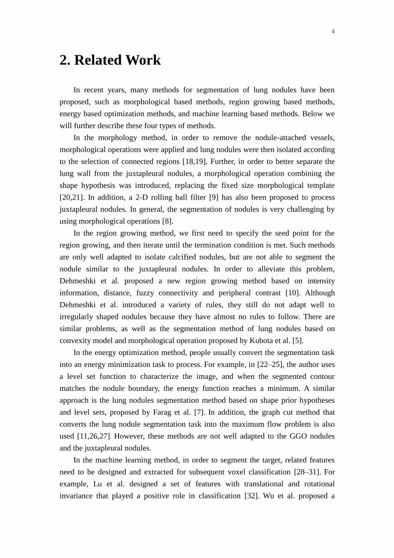
Fig. 2. (a) Illustration of the proposed DB-ResNet architecture where AP and Concate represent

the Average Pooling operation and Concatenate operation, respectively. The symbol

indicates where the Central Intensity-Pooling can be placed, (b) the diagram of the convolution

block (ConvBlock), and (c) the diagram of the residual block (ResBlock). The parameters k, m

and n indicate the number of channels.

Table 1. Network parameters of the DB-ResNet. Building blocks are shown in brackets with the

numbers of blocks stacked. Downsampling is performed using Central Pooling before the first

layer of ResBlock1_x and ResBlock2_x.

Layer name Output size 32-Layer 83-Layer 134-Layer

ConvBlock_x 35×35 3 3, 36 2 3 3, 36 2 3 3, 36 2

ResBlock1_x 17×17

1 1, 128

3 3, 128 4

1 1, 512

1 1, 128

3 3, 128 4

1 1, 512

1 1, 128

3 3, 128 8

1 1, 512

ResBlock2_x 8×8

1 1, 256

3 3, 256 6

1 1, 1024

1 1, 256

3 3, 256 23

1 1, 1024

1 1, 256

3 3, 256 36

1 1, 1024

1×1 Average Pooling，Concatenate，2-d fc，softmax

Params 0.68×107 2.3×107 3.7×107

7

3.1.1. Network structure

The network contains two deep branches that share the same structure, but the

inputs used for training are different. Each branch of the proposed network

architecture contains 32 convolutional layers, two central pooling layers [17], one

central intensity-pooling (CIP) layer (see Section 3.1.3 for a detailed description) and

one shared fully-connected layer. The 32 convolution layers in the CNN are divided

into three categories: the first is a ConvBlock consisting of two convolutional layers,

the second is a ResBlock cluster consisting of four residual blocks [42], and the last is

a ResBlock cluster consisting of six residual blocks. In order to speed up the training

process, each convolutional layer is batch-normalized to normalize the corresponding

output [43]. After each convolution layer, a parametric rectified linear unit (PReLU) is

used as a nonlinear activation function [44].

We use the average pooling (Fig. 2, AP) for the output of the last convolutional

layer of each branch. The output of the average pooling is then concatenated with the

output of the CIP layer to fuse the depth features produced by the convolution layer

and the intensity features generated by the CIP layer. At the end of the model layers,

the features generated by the two CNN branches are combined with the concatenation,

and the concatenated results are then connected to a fully-connected layer to capture

the correlation of the features generated by the two CNN branches.

The goal of network training is to maximize the probability of the correct class

for each voxel. We achieve this by minimizing the cross-entropy loss of each training

sample. For a given input patch belonging to {0, 1}, assuming that ny is a true label,

then the loss function is defined as shown in Equation (1):

1

1[ ( ) (1 ) (1- )]

N

n n n n

n

L y log y y log yN

（1）

Where ny represents the prediction probability of the DB-ResNet, and N is the

number of samples.

In the experiment, we used the Stochastic Gradient Descent (SGD)）algorithm [45]

as a model update method. The SGD optimizer has several parameter settings: the

initial learning rate is 0.001, and then the learning rate is decreased by ten percent in

every five epochs. In addition, the momentum setting is 0.9. However, due to the

limitation of GPU memory, only a batch size of 32 samples are used. In order to avoid

overfitting during the training process, we adopted the early stopping training strategy

[46].

8

3.1.2. Dual-Branch Architecture

The proposed dual-branch residual network (DB-ResNet) architecture aims to

capture both multi-view features in multiple slices and multi-scale features in the

current slice.

The input size of the multi-view branch is a 3 × 35 × 35 3D data patch.

Specifically, for a voxel, we extend the current, previous, and subsequent slices

centered on this voxel to extract training patches (see Fig. 2, Multi-view Branch). This

three-slice patch extracted are treated as three channel images and fed to the

multi-view CNN branch.

Simultaneously, we have introduced a multi-scale branch trying to focus on

learning features from the current slice because of their high resolution in all CT scans.

The purpose of designing multi-scale branches is to model the relationship among

three-scale patches through the feature extraction layer. Firstly, three image patches

with a size of 65×65, 50×50 and 35×35, respectively, were extracted on the target

voxels from three slices. They are then rescaled to the same size of 35×35 using a

third-order spline interpolation and forming three-channel patches as input to a

multi-scale CNN branch (see Fig. 2, multi-scale branch).

In addition, in order to further improve the segmentation performance, we also

integrate the residual learning structure into the network. Moreover, we use the

bottleneck structure where the head and end are 1x1 convolutions (to reduce and

restore dimensions) and the middle is a 3x3 convolution, replacing the original

residual learning structure, which can reduce network parameters and increase

network depth [42].

3.1.3. The Central Intensity-Pooling

The conventional segmentation method usually utilizes the intensity information

of the target. For the segmentation of nodules, we can also use the same information.

In particular, for isolated nodules and calcified nodules, the intensity information is

useful due to a large contrast between the nodules and the surrounding background.

Therefore, we designed a pooling layer that calculates either the center position of the

feature map or its surrounding intensity information.

Fig. 3 shows the central intensity-pooling process for three different pooling

kernel sizes. Among them, the yellow mark corresponds to a pooling process with a

pooing kernel size of 1x1, and the result is the intensity value of the pixel in the center

of the input image. The blue mark corresponds to the pooling process with a pooling

kernel size of 3x3, and the result is the average intensity value of the surrounding 3x3

9

region centered on the center pixel of the input image. The corresponding pooling

process for the red mark is similar to the blue mark. In practice, we designed two

different sizes of the pooling kernel. One is a smaller local pooling kernel that can

obtain local intensity information at the center of the image; the other is a larger

global pooling kernel that can obtain richer contextual information. Since we predict

the category of the center voxel of the patch, the proposed central intensity-pooling

helps to extract the intensity features at the center of the patch.

K->3x3

K->1x1

K->5x5

Input image

9x9

Output image

1x1

K : kernal size Mean intensity value

Fig. 3. A central intensity-pooling process: this shows the processing of three different pooling

kernel sizes, corresponding to the red, blue, and yellow, and the sizes are 5x5, 3x3, and 1x1,

respectively.

This central intensity-pooling consists of two parameters: 1) the size of the

different pooling kernel and 2) the number of pooling kernels for each type. As

mentioned earlier, in this study, we have introduced two different sizes of the pooling

kernel, and the number of pooling kernel for each type has only one. These two types

correspond to the local pooling kernel and the global pooling kernel. In our

experiment, the size of the local pooling kernel is 1x1, and the size of the global

pooling kernel is 3x3.

3.2. The weighted sampling strategy

Since our approach focuses on automatically learning advanced semantic features

from images, a large number of voxel patches are needed as training samples to

improve the accuracy of the model. However, in a CT slice, the ratio of nodule to

non-nodular voxel is generally 1:370 ( 2 2:r S r , where r=15 is the maximum

radius of the nodule and S=5122 is the area of each slice), which is a highly data

imbalance problem. If a traditional random sampling is used, this will lead to a trained

model that is biased towards the non-nodal classes. Therefore, in order to avoid this

10

problem, we use a weighted sampling strategy [17]. However, our experimental

results have found that this weighted sampling strategy has poor sampling results for

small nodules with a diameter of less than 6 mm.

To elaborate further on the above issue, we assume that the nodules in each slice

are circular, and the nodule diameter of the kth slice is R. Then, the total number of

nodule voxels and nodule voxels at the boundary in the kth slice can be approximated

as 2 / 4R and R , respectively. According to the original weighted sampling

method, only 40% of the total number of nodal voxels is sampled. If R is less than 10,

the number of sampling points of the nodule class will be smaller than the number of

the voxels sampled at the boundary. In our experiment, we found that if a nodule is

less than 6mm in diameter, it will have almost half of the voxels at their boundary are

not sampled.

In order to solve the problem of insufficient number of samples for small nodules,

we set the number of nodule samples to twice the number of voxels at the nodule

boundary. Simultaneously, we also ensure that the number of non-nodule samples is

the same as the number of nodule samples. It should be noted that for small nodules

that are less than 6 mm in diameter, the total number of nodule voxels might be less

than twice the number of boundary voxels. In this case, we will take all the voxels of

such small nodules to improve the generalization capability of the model for such

small nodules. Experimental results have shown that this improved sampling strategy

increases the average dice score from 78.89% to 80.30%. The detailed results are

given in Table 3 of Section 4.4.

3.3. Post-processing

Since the method proposed in this paper is a semi-automatic segmentation model,

it is necessary to give the volume of interest (VOI) where the nodule is located before

segmentation. However, since the nodules are usually distributed over multiple CT

slices, it is tedious to manually specify the region of interest (ROI) in which the

nodules are located, layer-by-layer. To facilitate the doctor's operation, we performed

the following post-processing operation, that is, it is only necessary to manually

designate a bounding box called a starting slice on one CT slice.

Then repeat applying the same bounding box to the previous and next slices until

the following experimental conditions are satisfied: The nodule intersection area of

the current slice and the previous slice is less than 30% of the nodule area in the

previous slice.

To remove the noisy voxels, we made a simple connected region selection as

follows: 1) When noise appears in the starting slice, we select the isolated region

11

closest to the center of the bounding box, and 2) when noise occurs in other slices, we

choose the connected region where the overlap O=V(Gt∩Seg)/V(Gt∪Seg) (will be

explained in detail in Section 4.2) of the current slice and the previous slice nodule

mask is the largest.

4. Data and Experiments

We give the information of the dataset and experiments in detail in this section.

The evaluation criteria and the ablation study of the proposed method are described

below.

4.1. Data

We used public datasets from the Lung Image Database Consortium and Image

Database Resource Initiative (LIDC) in our experiments and for comparison [47–49].

In this study, we studied 986 nodule samples annotated by four radiologists. Due to

the differences in labeling between the four radiologists, the 50% consistency

criterion [5] was used to generate the ground-truth boundary.

We randomly partitioned 986 nodules into three subsets for training, validation,

and testing with the number of nodules contained in each subset was 387, 55, and 544,

respectively. As shown in Table 2, the clinical characteristics of the three subsets have

a similar statistical distribution.

Table 2. The data distribution of the LIDC dataset training, validation and testing sets. Among

them, the values are displayed in the format of mean ± standard deviation.

Characteristics Training set

（n=387)

Validation Set

(n=55)

Test set

(n=544)

Diameter(mm) 8.34±4.73 8.17±4.61 7.90±4.14

Sphericity 3.80±0.58 3.84±0.62 3.85±0.58

Margin 4.07±0.73 4.06±0.81 4.11±0.78

Spiculation 1.61±0.78 1.54±0.69 1.57±0.74

Texture 4.56±0.83 4.45±0.98 4.57±0.80

Calcification 5.65±0.80 5.68±0.77 5.67±0.80

Internal structure 1.01±0.16 1.03±0.20 1.01±0.08

Lobulation 1.74±0.72 1.75±0.74 1.69±0.71

Subtlety 4.00±0.78 3.89±0.74 3.95±0.75

Malignancy 2.95±0.91 2.87±0.77 2.91±0.91

Note: The range of all characteristic values except diameter, internal structure and calcification is

1-5, wherein the internal structure and calcification range from 1 to 4, 1 to 6, respectively. Margin

indicates the clarity of the nodule edge. Lobulation and spiculation indicate the number of these

shapes. Texture is a statistic of the distribution properties of the local gray information of nodules.

12

Internal structural represents the internal composition of the nodule. Malignancy, calcification,

and Sphericity indicate the possibility that the nodule is such a feature. Subtlety describes the

contrast of the nodule region and its surrounding region. There were no significant statistical

differences in the characteristics of the three subsets.

4.2. Evaluation criteria

To evaluate the segmentation results of the DB-ResNet model, we used the

average surface distance (ASD) and dice similarity coefficient (DSC) as the primary

evaluation criteria. DSC is a metric that is widely used to measure the overlap

between two segmentation results [15,37]. Moreover, in order to ensure the robustness

of the evaluation, we also use the true prediction value (PPV) and sensitivity (SEN) as

auxiliary evaluation parameters. The entire definition is shown in formulae (2)-(5).

2 ( )

( ) ( )

V Gt SegDSC

V Gt V Seg

I （2）

1( ( , ) ( , ))

2i Gt j Seg i Seg j GtASD mean min d i j mean min d i j （3）

( )

( )

V Gt SegSEN

V Gt

I （4）

( )

( )

V Gt SegPPV

V Auto

I （5）

Among them, "Gt" represents the result of expert labeling; "Seg" represents the

segmentation result of DB-ResNet model. V represents the volume size calculated in

voxel units and d (i, j) represents the Euclidean distance between the voxel i and voxel

j measured in millimeters.

4.3. The Detail of Implementation

In the experiment, we used a weighted sampling strategy (Section 3.2) to sample

0.47 million voxel patches extracted from the LIDC training set. To avoid overfitting,

we used a training strategy for early stopping: if there is no more improvement in

performance, it will stop in an extra training with 10 epochs. It has been found

through experiments that the DB-ResNet model generally stops around the 16th epoch,

so we set the upper limit of the training epoch to 20. Our experiment is based on the

Keras deep learning framework and the coding language is Python 3.6. Our

experiment was carried out on a server equipped with an Intel Xeon processor and

125GB memory. In the model training, acceleration is performed on the NVIDIA

13

GTX-1080Ti GPU (11GB video memory), and the DB-ResNet model takes about 31

hours to converge.

4.4. Ablation Study

To verify the effectiveness of each component in the DB-ResNet architecture, we

designed an ablation experiment based on the CF-CNN network architecture [17]. The

relevant experimental results are shown in Table 3.

Table 3. Ablation study on LIDC testing dataset. Note that Scale represents the 50*50 size of the

multi-scale branch; BWS represents a weighted sampling strategy based on the boundary points;

DB represents dual-branch architecture; ResNet represents the residual network, see Table 1;

CIP_N denotes adding a central intensity-pooling layer from the first to the Nth position; Post

indicates the proposed post-processing operation.

Method DSC ASD SEN PPV

CF-CNN 78.55 12.49 0.27 0.35 86.01 15.22 75.79 14.73

CF-CNN + Scale 78.89 11.67 0.26 0.29 86.21 14.66 75.95 14.41

CF-CNN + Scale + BWS 80.30 11.34 0.26 0.45 85.40 13.27 78.69 14.49

DB-ResNet32 82.37 10.98 0.22 0.34 88.36 13.09 79.58 13.30

DB-ResNet83 81.33 11.69 0.24 0.39 86.94 14.42 79.33 14.08

DB-ResNet134 79.56 11.28 0.25 0.36 87.92 13.24 75.35 14.66

DB-ResNet32 + CIP_1 82.54 10.20 0.19 0.21 89.06 11.79 79.17 13.31

DB-ResNet32 + CIP_2 82.69 10.46 0.21 0.30 88.69 12.18 79.62 13.29

DB-ResNet32 + CIP_3 81.67 10.46 0.21 0.25 88.93 12.32 77.94 13.68

DB-ResNet32 + CIP_4 80.52 11.45 0.23 0.37 88.89 12.89 76.14 14.97

DB-ResNet32+ CIP_1 + Post 82.74 10.19 0.19 0.21 89.35 11.79 79.64 13.34

（1）Effect of Boundary-based Weighted Sampling (BWS)

In Table 3, CF-CNN + Scale indicates that we added a 50x50 scale to the 2-D

branch of CF-CNN and then combined it with two scales of 65x65 and 35x35 to form

our multi-scale branch. The DSC obtained by CF-CNN + Scale is 78.89%, which is

slightly higher than that of CF-CNN. Then, based on CF-CNN + Scale, a weighted

sampling strategy based on the boundary points is applied, and the DSC obtained is

80.30%. Compared to CF-CNN + Scale, its performance has improved by nearly

1.5%, which verifies the effectiveness of the boundary-based weighted sampling

strategy.

（2）Effect of Residual Network

In Table 3, based on CF-CNN + Scale + BWS, DB-ResNet32 replaces two

convolution blocks with two residual blocks. At this time, the DSC is 82.37%, which

is an increased performance of two percent compared to the previous 80.30%. This

14

proves the effectiveness of the residual block. Then, based on the ideas of ResNet101

and ResNet152 [42], we improve the network performance by increasing the depth of

the network, but according to the results of the sixth and seventh rows in Table 3, it

does not achieve what we expected. This may be due to the excessive complexity of

the network, which leads to overfitting of the model.

（3）Effect of Central Intensity-Pooling

Based on DB-ResNet32, we integrated the proposed central intensity-pooling

layer into DB-ResNet32. In order to verify the effectiveness of the central intensity

-pooling layer, we performed four experiments, corresponding to rows 8-11 in Table 3.

By comparing these four rows, we can see that DB-ResNet32 + CIP_1 is the best with

an ASD of 0.19, which is an improvement of three percent over DB-ResNet32. For

the other three performance indicators, both the DSC and the SEN are increased

except the PPV is decreased by 0.41%. For the reason why the performance of

DB-ResNet32 + CIP_3 and DB-ResNet32 + CIP_4 decline more obviously, our

opinion is that the features used for classification, the proportion of traditional

intensity features is increasing, even exceeding the deep convolutional features. This

is unreasonable because the deep convolution feature in our network is crucial.

Specifically, for DB-ResNet32 + CIP_3, the ratio of intensity features to convolution

features is 584:1024, and the ratio for DB-ResNet32 + CIP_4 is 1608:1024.

（4）Effect of Post-processing

Finally, we verified the effectiveness of the proposed post-processing method. By

comparing the ninth row and the last row in Table 3, it can be seen that although the

performance is not significantly improved, the four performance measures are

improved.

5. Results and Discussion

We give the overall performance of our method, the robustness of the proposed

segmentation model, and the experimental comparison with other methods below.

5.1. Overall performance

To better observe the performance of the proposed method in the testing set, we

plot the histogram between the DSC value and the number of nodules, based on all

samples in the testing set, as shown in Fig. 4. By observing Fig. 4, we can easily

conclude that most of the nodules have a DSC value higher than 0.8.

15

To see if the segmentation results of our proposed method are comparable to

those hand-labeled by human experts, we performed a consistency comparison

between DB-ResNet and four radiologists, as shown in Table 4. Our results show that

the stability of DB-ResNet is slightly weaker than that of four different radiologists.

However, the DSC between DB-ResNet and each radiologist is 83.15% on average,

which is higher than the average of 82.66% among inter-radiologists.

Fig. 4. DSC distributions of the LIDC testing set

Table 4. Mean DSCs (%) of consistency comparison between DB-ResNet and each radiologist,

where R1 to R4 represent four radiologists.

R1 R2 R3 R4 Average

R1 – 82.61 82.47 82.49

82.66 0.48 R2 82.61 – 83.72 82.36

R3 82.47 83.72 – 82.32

R4 82.49 82.36 82.32 –

DB-ResNet 82.32 84.02 82.94 83.30 83.15 0.62

5.2. Robustness of Segmentation

In order to prove the robustness of the proposed method, we base the nine

characteristics corresponding to each nodule as the benchmark, and divide the testing

set into different groups according to the characteristic scores of the nodule. Table 5

lists the DSC average values of different nodule groups. As can be seen from Table 5,

DB-ResNet can handle all types of nodules with similar performance, which reflects

16

the segmentation robustness of our method.

Further, we have collated the evaluation results of challenging small nodules and

attached nodules. The relevant results are shown in Table 6. According to the

experimental results in Table 6, it can be seen that the potential robust segmentation of

the DB-ResNet is independent of the type of nodules and the size of nodules.

Table 5. The DSC average values on different nodule groups.

Characteristics Characteristic scores

1 2 3 4 5 6

Malignancy 78.16

[44]

81.57

[143]

83.24

[206]

84.57

[135]

83.96

[16] –

Sphericity – 78.00

[13]

81.89

[96]

82.62

[393]

87.30

[42] –

Margin – 75.61

[33]

82.50

[60]

82.66

[281]

84.35

[170] –

Spiculation 82.99

[300]

82.05

[192]

83.83

[24]

83.74

[26]

84.63

[2] –

Texture 65.18

[7]

79.67

[22]

80.53

[8]

81.69

[117]

83.59

[390] –

Calcification – – 78.85

[23]

82.10

[39]

85.68

[30]

82.80

[452]

Internal structure 82.82

[541]

67.89

[3] – – – –

Lobulation 82.72

[235]

82.44

[249]

84.14

[39]

83.87

[21] – –

Subtlety 65.53

[1]

77.94

[28]

80.30

[88]

82.26

[308]

87.06

[119] –

Table 6. In the LIDC testing sets，DSCs and ASDs for nodules attached，non-attached, less than

6mm and more than 6mm in diameter.

LIDC testing set LIDC testing set

Attached Non-attached Diameter<6mm Diameter>=6mm

(n=131) (n=413) (n=241) (n=303)

DSC (%) 81.79 83.04 79.97 84.94

ASD (mm) 0.25 0.17 0.16 0.21

5.3. Experimental Comparison

To illustrate the efficiency of the proposed method, we compared the results with

other methods. Two different comparisons are provided: 1) a comparison with various

different types of segmentation methods recently proposed and 2) a comparison on the

same network architecture with the basic components of the network are different.

17

Table 7 shows the quantification results for the different types of segmentation

methods. The results are in the format of "mean ± standard deviation." In order to

ensure the fairness of the comparison, the methods compared with DB-ResNet in

Table 7, the conditions of the experiments are consistent with DB-ResNet including

boundary-based sampling strategy, central intensity-pooling layer and post-processing

methods. According to the experimental results shown in Table 7, the proposed

method is superior to the existing segmentation methods.

Table 7. Mean ± standard deviation of the results for various segmentation methods. The best

performance is indicated in bold font.

Network Architecture DSC (%) ASD (mm) SEN (%) PPV (%)

FCN-UNet [40] 77.84 21.74 1.79 7.52 77.98 24.52 82.52 21.55

CF-CNN [17] 78.55 12.49 0.27 0.35 86.01 15.22 75.79 14.73

MC-CNN [50] 77.51 11.40 0.29 0.31 88.83 12.34 71.42 14.78

MV-CNN [51] 75.89 12.99 0.31 0.39 87.16 12.91 70.81 17.57

MV-DCNN [38] 77.85 12.94 0.33 0.36 86.96 15.73 77.33 13.26

MCROI-CNN [52] 77.01 12.93 0.30 0.35 85.45 15.97 73.52 14.62

Cascaded-CNN [37] 79.83 10.91 0.26 0.34 86.86 13.35 76.14 13.46

DB-ResNet 82.74 10.19 0.19 0.21 89.35 11.79 79.64 13.34

Table 8 shows the quantification results of several segmentation methods of the

same architecture but with different components. The results are also shown in the

format of “mean ± standard deviation”. In order to achieve a fair comparison, in Table

8, except for the basic components, the other testing conditions are the same. By

comparing the experimental results in rows 2 to 8 in Table 8, we can conclude that the

DB-ResNet performs the best.

Table 8. Mean ± standard deviation of quantitative results of segmentation methods using different

basic network architectures. The best performance is indicated in the bold font.

Network Architecture DSC (%) ASD (mm) SEN (%) PPV (%)

DB-VGG [53] 80.30 11.34 0.26 0.45 85.40 13.27 78.69 14.49

DB-GoogLeNet [54] 80.61 10.38 0.23 0.29 86.51 12.76 78.03 13.78

DB-Inception-V3 [55] 81.90 10.61 0.22 0.34 87.74 13.57 79.51 13.53

DB-Inception-V4 [56] 80.68 12.40 0.26 0.45 84.67 15.44 80.07 14.55

DB-DenseNet [57] 80.52 11.13 0.24 0.32 86.44 13.95 77.98 13.83

DB-ResDenseNet [58] 79.08 12.27 0.26 0.31 87.58 14.87 75.27 14.55

DB-ResNet 82.74 10.19 0.19 0.21 89.35 11.79 79.64 13.34

To allow a visual comparison of different approaches, the segmentation results

are given in Fig. 5. We demonstrated six representative nodules for visual comparison

from the LIDC testing set. Notations L1 to L6 shown in Fig. 5 correspond to calcific

nodule, juxtapleural nodule, ground-glass opacity nodule, cavitary nodule, isolated

nodule, and small nodule less than 6 mm in diameter, respectively. With the visual

18

comparison, it can be seen that the overall performance of the FCN-UNet and

MV-CNN methods is slightly inferior to other methods, especially for cavitary

nodules and GGO nodules. For isolated nodules, MC-CNN and MCROI-CNN

methods performed slightly worse. MCROI-CNN and Cascaded-CNN methods are

slightly less effective for juxtapleural nodules. For central calcified nodules, the

segmentation results of the MV-DCNN method are incomplete. For small nodules and

cavitary nodules, CF-CNN and Cascaded-CNN methods are less adaptable. In

contrast, DB-ResNet is still robust when it segments these nodules. This comparison

illustrate its significant feature learning capability.

Ground truth

CF-CNN

MC-CNN

MV-CNN

MV-DCNN

MCROI-CNN

Cascaded-CNN

MB-ResNet

L5L2 L4L1 L3 L6

FCN-UNet

Fig. 5. A visual comparison of the segmentation results. From top to bottom: the ground truth of

nodule, segmentation result of CF-CNN, MC-CNN, MV-CNN, MV-DCNN, MCROI-CNN,

Cascaded-CNN, and DB-ResNet. Notations L1 to L6 are nodules of different types from the LIDC

testing set.

Fig. 6 further shows multiple segmented slices of juxtapleural nodules and small

nodules from the LIDC testing set with the application of the DB-ResNet. This

comparison indicates that the segmentation results of the DB-ResNet have a large

overlap with the ground truth contours.

19

J1 J2 J3 J4 J5

J21 J22 J23

J6 J7 J8 J9 J10

J11 J12 J13 J14 J15

J16 J17 J18 J19 J20

S1 S2 S3

S4 S5 S6

S7

Fig.6. Segmentation results of DB-ResNet on juxtapleural nodule (J1-L23) and small nodule with

a diameter of 4.8 mm (S1-S7) from the LIDC testing set. The yellow and red contours represent

the segmentation results of DB-ResNet and the ground truth, respectively. The yellow volume data

and the red volume data correspond to the 3-D renderings of the DB-ResNet and the ground truth,

respectively. The number in the upper left corner of each image represents the slice number where

the nodule is located.

6. Conclusion

In this study, we proposed a DB-ResNet model for lung nodule segmentation. The

model extracts features through dual-branch networks. By comparing with the

existing lung nodule segmentation methods, our method showed encouraging

accuracy in the lung nodule segmentation task, and the average dice score of 82.74%

for the LIDC dataset. Especially, the DB-ResNet model can successfully segment

challenging cases such as juxtapleural nodules and small nodules.

In future work, we plan to develop a lung nodule detection algorithm based on the

DSSD (deconvolutional single shot detector) network architecture, and then combine

it with our method to implement a fully automated segmentation system of the lung

nodule.

Acknowledgements

This work is supported by the National Key R&D Program of China (Grant No.

20

2017YFC0112804) and the National Natural Science Foundation of China (Grant No.

81671768). The authors acknowledge the National Cancer Institute and the

Foundation for the National Institutes of Health and their critical role in the creation

of the publicly available LIDC-IDRI Database for this study.

References

[1] S.R. L., M.K. D., J. Ahmedin, Cancer statistics, 2017, CA. Cancer J. Clin. 67 (2017) 7–30.

doi:10.3322/caac.21387.

[2] H.J.W.L. Aerts, E.R. Velazquez, R.T.H. Leijenaar, C. Parmar, P. Grossmann, S. Carvalho, J.

Bussink, R. Monshouwer, B. Haibe-Kains, D. Rietveld, F. Hoebers, M.M. Rietbergen, C.R.

Leemans, A. Dekker, J. Quackenbush, R.J. Gillies, P. Lambin, Decoding tumour phenotype by

noninvasive imaging using a quantitative radiomics approach, Nat. Commun. 5 (2014) 4006.

doi:10.1038/ncomms5006.

[3] H. MacMahon, J.H.M. Austin, G. Gamsu, C.J. Herold, J.R. Jett, D.P. Naidich, E.F. Patz, S.J.

Swensen, Guidelines for Management of Small Pulmonary Nodules Detected on CT Scans: A

Statement from the Fleischner Society, Radiology. 237 (2005) 395–400.

doi:10.1148/radiol.2372041887.

[4] A.P. Reeves, A.B. Chan, D.F. Yankelevitz, C.I. Henschke, B. Kressler, W.J. Kostis, On

measuring the change in size of pulmonary nodules, IEEE Trans. Med. Imaging. 25 (2006)

435–450. doi:10.1109/TMI.2006.871548.

[5] T. Kubota, A.K. Jerebko, M. Dewan, M. Salganicoff, A. Krishnan, Segmentation of pulmonary

nodules of various densities with morphological approaches and convexity models, Med. Image

Anal. 15 (2011) 133–154. doi:https://doi.org/10.1016/j.media.2010.08.005.

[6] B.C. Lassen, C. Jacobs, J.-M. Kuhnigk, B. van Ginneken, E.M. van Rikxoort, Robust

semi-automatic segmentation of pulmonary subsolid nodules in chest computed tomography

scans, Phys. Med. Biol. 60 (2015) 1307–1323. doi:10.1088/0031-9155/60/3/1307.

[7] A.A. Farag, H.E.A.E. Munim, J.H. Graham, A.A. Farag, A Novel Approach for Lung Nodules

Segmentation in Chest CT Using Level Sets, IEEE Trans. Image Process. 22 (2013) 5202–5213.

doi:10.1109/TIP.2013.2282899.

[8] S. Diciotti, S. Lombardo, M. Falchini, G. Picozzi, M. Mascalchi, Automated Segmentation

Refinement of Small Lung Nodules in CT Scans by Local Shape Analysis, IEEE Trans.

Biomed. Eng. 58 (2011) 3418–3428. doi:10.1109/TBME.2011.2167621.

[9] T. Messay, R.C. Hardie, S.K. Rogers, A new computationally efficient CAD system for

pulmonary nodule detection in CT imagery, Med. Image Anal. 14 (2010) 390–406.

doi:https://doi.org/10.1016/j.media.2010.02.004.

[10] J. Dehmeshki, H. Amin, M. Valdivieso, X. Ye, Segmentation of Pulmonary Nodules in

Thoracic CT Scans: A Region Growing Approach, IEEE Trans. Med. Imaging. 27 (2008)

467–480. doi:10.1109/TMI.2007.907555.

[11] X. Ye, G. Beddoe, G.G. Slabaugh, Automatic Graph Cut Segmentation of Lesions in CT Using

Mean Shift Superpixels., Int. J. Biomed. Imaging. 2010 (2010) 983963:1-983963:14.

doi:10.1155/2010/983963.

21

[12] T. Messay, R.C. Hardie, T.R. Tuinstra, Segmentation of pulmonary nodules in computed

tomography using a regression neural network approach and its application to the Lung Image

Database Consortium and Image Database Resource Initiative dataset, Med. Image Anal. 22

(2015) 48–62. doi:https://doi.org/10.1016/j.media.2015.02.002.

[13] M. Keshani, Z. Azimifar, F. Tajeripour, R. Boostani, Lung nodule segmentation and

recognition using SVM classifier and active contour modeling: A complete intelligent system,

Comput. Biol. Med. 43 (2013) 287–300.

doi:https://doi.org/10.1016/j.compbiomed.2012.12.004.

[14] P. Moeskops, M.A. Viergever, A.M. Mendrik, L.S. de Vries, M.J.N.L. Benders, I. Išgum,

Automatic Segmentation of MR Brain Images With a Convolutional Neural Network, IEEE

Trans. Med. Imaging. 35 (2016) 1252–1261. doi:10.1109/TMI.2016.2548501.

[15] S. Valverde, A. Oliver, E. Roura, S. González-Villà, D. Pareto, J.C. Vilanova, L.

Ramió-Torrentà, À. Rovira, X. Lladó, Automated tissue segmentation of MR brain images in

the presence of white matter lesions, Med. Image Anal. 35 (2017) 446–457.

doi:https://doi.org/10.1016/j.media.2016.08.014.

[16] W. Zhang, R. Li, H. Deng, L. Wang, W. Lin, S. Ji, D. Shen, Deep convolutional neural

networks for multi-modality isointense infant brain image segmentation., Neuroimage. 108

(2015) 214–224. doi:10.1016/j.neuroimage.2014.12.061.

[17] S. Wang, M. Zhou, Z. Liu, Z. Liu, D. Gu, Y. Zang, D. Dong, O. Gevaert, J. Tian, Central

focused convolutional neural networks: Developing a data-driven model for lung nodule

segmentation, Med. Image Anal. 40 (2017) 172–183. doi:10.1016/j.media.2017.06.014.

[18] W.J. Kostis, A.P. Reeves, D.F. Yankelevitz, C.I. Henschke, Three-dimensional segmentation

and growth-rate estimation of small pulmonary nodules in helical CT images, IEEE Trans. Med.

Imaging. 22 (2003) 1259–1274. doi:10.1109/TMI.2003.817785.

[19] L. Gonçalves, J. Novo, A. Campilho, Hessian based approaches for 3D lung nodule

segmentation, Expert Syst. Appl. 61 (2016) 1–15.

doi:https://doi.org/10.1016/j.eswa.2016.05.024.

[20] D. Sargent, S.Y. Park, Semi-automatic 3D lung nodule segmentation in CT using dynamic

programming, in: Proc.SPIE, 2017. https://doi.org/10.1117/12.2254575.

[21] J.M. Kuhnigk, V. Dicken, L. Bornemann, A. Bakai, D. Wormanns, S. Krass, H.O. Peitgen,

Morphological segmentation and partial volume analysis for volumetry of solid pulmonary

lesions in thoracic CT scans, IEEE Trans. Med. Imaging. 25 (2006) 417–434.

doi:10.1109/TMI.2006.871547.

[22] T.F. Chan, L.A. Vese, Active contours without edges, IEEE Trans. Image Process. 10 (2001)

266–277. doi:10.1109/83.902291.

[23] E.E. Nithila, S.S. Kumar, Segmentation of lung nodule in CT data using active contour model

and Fuzzy C-mean clustering, Alexandria Eng. J. 55 (2016) 2583–2588.

doi:https://doi.org/10.1016/j.aej.2016.06.002.

[24] J. Wang, H. Guo, Automatic Approach for Lung Segmentation with Juxta-Pleural Nodules

from Thoracic CT Based on Contour Tracing and Correction., Comp. Math. Methods Med.

2016 (2016) 2962047:1-2962047:13. doi:10.1155/2016/2962047.

[25] P.P.R. Filho, A.C. da Silva Barros, J.S. Almeida, J.P.C. Rodrigues, V.H.C. de Albuquerque, A

new effective and powerful medical image segmentation algorithm based on optimum path

snakes, Appl. Soft Comput. 76 (2019) 649–670. doi:https://doi.org/10.1016/j.asoc.2018.10.057.

22

[26] Y. Boykov, V. Kolmogorov, An experimental comparison of min-cut/max- flow algorithms for

energy minimization in vision, IEEE Trans. Pattern Anal. Mach. Intell. 26 (2004) 1124–1137.

doi:10.1109/TPAMI.2004.60.

[27] S. Mukherjee, X. Huang, R.R. Bhagalia, Lung nodule segmentation using deep learned prior

based graph cut, in: 2017 IEEE 14th Int. Symp. Biomed. Imaging (ISBI 2017), 2017: pp.

1205–1208. doi:10.1109/ISBI.2017.7950733.

[28] L. Lu, A. Barbu, M. Wolf, J. Liang, M. Salganicoff, D. Comaniciu, Accurate polyp

segmentation for 3D CT colongraphy using multi-staged probabilistic binary learning and

compositional model, in: 2008 IEEE Conf. Comput. Vis. Pattern Recognit., 2008: pp. 1–8.

doi:10.1109/CVPR.2008.4587423.

[29] L. Lu, J. Bi, M. Wolf, M. Salganicoff, Effective 3D object detection and regression using

probabilistic segmentation features in CT images, in: CVPR 2011, 2011: pp. 1049–1056.

doi:10.1109/CVPR.2011.5995359.

[30] S. Mukhopadhyay, A Segmentation Framework of Pulmonary Nodules in Lung CT Images, J.

Digit. Imaging. 29 (2016) 86–103. doi:10.1007/s10278-015-9801-9.

[31] S. Shen, A.A.T. Bui, J. Cong, W. Hsu, An automated lung segmentation approach using

bidirectional chain codes to improve nodule detection accuracy, Comput. Biol. Med. 57 (2015)

139–149. doi:https://doi.org/10.1016/j.compbiomed.2014.12.008.

[32] L. Lu, P. Devarakota, S. Vikal, D. Wu, Y. Zheng, M. Wolf, Computer Aided Diagnosis Using

Multilevel Image Features on Large-Scale Evaluation BT - Medical Computer Vision. Large

Data in Medical Imaging, in: B. Menze, G. Langs, A. Montillo, M. Kelm, H. Müller, Z. Tu

(Eds.), Springer International Publishing, Cham, 2014: pp. 161–174.

[33] D. Wu, L. Lu, J. Bi, Y. Shinagawa, K. Boyer, A. Krishnan, M. Salganicoff, Stratified learning

of local anatomical context for lung nodules in CT images, in: 2010 IEEE Comput. Soc. Conf.

Comput. Vis. Pattern Recognit., 2010: pp. 2791–2798. doi:10.1109/CVPR.2010.5540008.

[34] Y. Hu, P.G. Menon, A neural network approach to lung nodule segmentation, in: Proc.SPIE,

2016. https://doi.org/10.1117/12.2217291.

[35] D.C. Ciresan, A. Giusti, L.M. Gambardella, J. Schmidhuber, Deep Neural Networks Segment

Neuronal Membranes in Electron Microscopy Images. BT - Advances in Neural Information

Processing Systems 25: 26th Annual Conference on Neural Information Processing Systems

2012. Proceedings of a meeting held December 3-6, 20, (2012) 2852–2860.

http://papers.nips.cc/paper/4741-deep-neural-networks-segment-neuronal-membranes-in-electr

on-microscopy-images.

[36] A. Prasoon, K. Petersen, C. Igel, F. Lauze, E. Dam, M. Nielsen, Deep Feature Learning for

Knee Cartilage Segmentation Using a Triplanar Convolutional Neural Network BT - Medical

Image Computing and Computer-Assisted Intervention – MICCAI 2013, in: K. Mori, I.

Sakuma, Y. Sato, C. Barillot, N. Navab (Eds.), Springer Berlin Heidelberg, Berlin, Heidelberg,

2013: pp. 246–253.

[37] M. Havaei, A. Davy, D. Warde-Farley, A. Biard, A.C. Courville, Y. Bengio, C. Pal, P.-M.

Jodoin, H. Larochelle, Brain tumor segmentation with Deep Neural Networks., Med. Image

Anal. 35 (2017) 18–31. doi:10.1016/j.media.2016.05.004.

[38] S. Wang, M. Zhou, O. Gevaert, Z. Tang, D. Dong, Z. Liu, J. Tian, A multi-view deep

convolutional neural networks for lung nodule segmentation, in: 2017 39th Annu. Int. Conf.

IEEE Eng. Med. Biol. Soc., 2017: pp. 1752–1755. doi:10.1109/EMBC.2017.8037182.

23

[39] J. Long, E. Shelhamer, T. Darrell, Fully convolutional networks for semantic segmentation, in:

2015 IEEE Conf. Comput. Vis. Pattern Recognit., 2015: pp. 3431–3440.

doi:10.1109/CVPR.2015.7298965.

[40] O. Ronneberger, P. Fischer, T. Brox, U-Net: Convolutional Networks for Biomedical Image

Segmentation BT - Medical Image Computing and Computer-Assisted Intervention –

MICCAI 2015, in: N. Navab, J. Hornegger, W.M. Wells, A.F. Frangi (Eds.), Springer

International Publishing, Cham, 2015: pp. 234–241.

[41] Ö. Çiçek, A. Abdulkadir, S.S. Lienkamp, T. Brox, O. Ronneberger, 3D U-Net: Learning Dense

Volumetric Segmentation from Sparse Annotation BT - Medical Image Computing and

Computer-Assisted Intervention – MICCAI 2016, in: S. Ourselin, L. Joskowicz, M.R. Sabuncu,

G. Unal, W. Wells (Eds.), Springer International Publishing, Cham, 2016: pp. 424–432.

[42] K. He, X. Zhang, S. Ren, J. Sun, Deep Residual Learning for Image Recognition, in: 2016

IEEE Conf. Comput. Vis. Pattern Recognit., 2016: pp. 770–778. doi:10.1109/CVPR.2016.90.

[43] S. Ioffe, C. Szegedy, Batch Normalization: Accelerating Deep Network Training by Reducing

Internal Covariate Shift. BT - Proceedings of the 32nd International Conference on Machine

Learning, ICML 2015, Lille, France, 6-11 July 2015, (2015) 448–456.

http://jmlr.org/proceedings/papers/v37/ioffe15.html.

[44] K. He, X. Zhang, S. Ren, J. Sun, Delving Deep into Rectifiers: Surpassing Human-Level

Performance on ImageNet Classification, in: 2015 IEEE Int. Conf. Comput. Vis., 2015: pp.

1026–1034. doi:10.1109/ICCV.2015.123.

[45] L. Wang, Y. Yang, R. Min, S. Chakradhar, Accelerating deep neural network training with

inconsistent stochastic gradient descent, Neural Networks. 93 (2017) 219–229.

doi:https://doi.org/10.1016/j.neunet.2017.06.003.

[46] R. Caruana, S. Lawrence, C.L. Giles, Overfitting in Neural Nets: Backpropagation, Conjugate

Gradient, and Early Stopping. BT - Advances in Neural Information Processing Systems 13,

Papers from Neural Information Processing Systems (NIPS) 2000, Denver, CO, USA, (2000)

402–408.

http://papers.nips.cc/paper/1895-overfitting-in-neural-nets-backpropagation-conjugate-gradient

-and-early-stopping.

[47] S.G. Armato, G. McLennan, L. Bidaut, M.F. McNitt-Gray, C.R. Meyer, A.P. Reeves, B. Zhao,

D.R. Aberle, C.I. Henschke, E.A. Hoffman, E.A. Kazerooni, H. MacMahon, E.J.R. Van Beeke,

D. Yankelevitz, A.M. Biancardi, P.H. Bland, M.S. Brown, R.M. Engelmann, G.E. Laderach, D.

Max, R.C. Pais, D.P.Y. Qing, R.Y. Roberts, A.R. Smith, A. Starkey, P. Batrah, P. Caligiuri, A.

Farooqi, G.W. Gladish, C.M. Jude, R.F. Munden, I. Petkovska, L.E. Quint, L.H. Schwartz, B.

Sundaram, L.E. Dodd, C. Fenimore, D. Gur, N. Petrick, J. Freymann, J. Kirby, B. Hughes, A.

Vande Casteele, S. Gupte, M. Sallamm, M.D. Heath, M.H. Kuhn, E. Dharaiya, R. Burns, D.S.

Fryd, M. Salganicoff, V. Anand, U. Shreter, S. Vastagh, B.Y. Croft, The Lung Image Database

Consortium (LIDC) and Image Database Resource Initiative (IDRI): a completed reference

database of lung nodules on CT scans, Med. Phys. 38 (2011) 915–931. doi:10.1118/1.3528204.

[48] A.A.A. Setio, F. Ciompi, G. Litjens, P. Gerke, C. Jacobs, S.J. van Riel, M.M.W. Wille, M.

Naqibullah, C.I. Sánchez, B. van Ginneken, Pulmonary Nodule Detection in CT Images: False

Positive Reduction Using Multi-View Convolutional Networks, IEEE Trans. Med. Imaging. 35

(2016) 1160–1169. doi:10.1109/TMI.2016.2536809.

[49] A.A.A. Setio, A. Traverso, T. de Bel, M.S.N. Berens, C. van den Bogaard, P. Cerello, H. Chen,

24

Q. Dou, M.E. Fantacci, B. Geurts, R. van der Gugten, P.A. Heng, B. Jansen, M.M.J. de Kaste,

V. Kotov, J.Y.-H. Lin, J.T.M.C. Manders, A. Sóñora-Mengana, J.C. García-Naranjo, E.

Papavasileiou, M. Prokop, M. Saletta, C.M. Schaefer-Prokop, E.T. Scholten, L. Scholten, M.M.

Snoeren, E.L. Torres, J. Vandemeulebroucke, N. Walasek, G.C.A. Zuidhof, B. van Ginneken,

C. Jacobs, Validation, comparison, and combination of algorithms for automatic detection of

pulmonary nodules in computed tomography images: The LUNA16 challenge, Med. Image

Anal. 42 (2017) 1–13. doi:10.1016/j.media.2017.06.015.

[50] W. Shen, M. Zhou, F. Yang, D. Yu, D. Dong, C. Yang, Y. Zang, J. Tian, Multi-crop

Convolutional Neural Networks for lung nodule malignancy suspiciousness classification,

Pattern Recognit. 61 (2017) 663–673. doi:https://doi.org/10.1016/j.patcog.2016.05.029.

[51] G. Kang, K. Liu, B. Hou, N. Zhang, 3D multi-view convolutional neural networks for lung

nodule classification, PLoS One. 12 (2017) e0188290. doi:10.1371/journal.pone.0188290.

[52] W. Sun, B. Zheng, W. Qian, Automatic feature learning using multichannel ROI based on deep

structured algorithms for computerized lung cancer diagnosis, Comput. Biol. Med. 89 (2017)

530–539. doi:10.1016/j.compbiomed.2017.04.006.

[53] K. Simonyan, A. Zisserman, Very Deep Convolutional Networks for Large-Scale Image

Recognition., CoRR. abs/1409.1 (2014). http://arxiv.org/abs/1409.1556.

[54] C. Szegedy, W. Liu, Y. Jia, P. Sermanet, S. Reed, D. Anguelov, D. Erhan, V. Vanhoucke, A.

Rabinovich, Going deeper with convolutions, in: 2015 IEEE Conf. Comput. Vis. Pattern

Recognit., 2015: pp. 1–9. doi:10.1109/CVPR.2015.7298594.

[55] C. Szegedy, V. Vanhoucke, S. Ioffe, J. Shlens, Z. Wojna, Rethinking the Inception Architecture

for Computer Vision, in: 2016 IEEE Conf. Comput. Vis. Pattern Recognit., 2016: pp.

2818–2826. doi:10.1109/CVPR.2016.308.

[56] C. Szegedy, S. Ioffe, V. Vanhoucke, A.A. Alemi, Inception-v4, Inception-ResNet and the

Impact of Residual Connections on Learning. BT - Proceedings of the Thirty-First AAAI

Conference on Artificial Intelligence, February 4-9, 2017, San Francisco, California, USA.,

(2017) 4278–4284. http://aaai.org/ocs/index.php/AAAI/AAAI17/paper/view/14806.

[57] G. Huang, Z. Liu, L. v. d. Maaten, K.Q. Weinberger, Densely Connected Convolutional

Networks, in: 2017 IEEE Conf. Comput. Vis. Pattern Recognit., 2017: pp. 2261–2269.

doi:10.1109/CVPR.2017.243.

[58] Y. Zhang, Y. Tian, Y. Kong, B. Zhong, Y. Fu, Residual Dense Network for Image

Super-Resolution., CoRR. abs/1802.0 (2018). http://arxiv.org/abs/1802.08797.