Business and Social Sciences Review (BSSR)

Vol . 1, No . 4, (October - 2011)

www.bssreview.org ISSN: 2047-6485

4

Copyright © 2011 – Society of Business and Social Sciences

EXPORT GROWTH AND VOLATILITY OF EXCHANGE RATE:

A PANEL DATA ANALYSIS

Madiha Zafar

Ex-student of M. Phil. Economics Economics Department, University of the Punjab, Lahore, Pakistan.

Khalil Ahmad

Assistant Professor Economics Department, University Of The Punjab, Lahore, Pakistan

email: hafizkhalil62@yahoo.com

ABSTRACT The impact of exchange rate volatility on exports has long been debated in

economic literature: some supporting the negative relation whereas others

supporting a positive relation. In this backdrop, this study applies a fixed

effects model selected on the basis of hausman (1978) specification test to

ascertain the impact of exchange rate volatility on exports growth of 16 latin

american countries over the period 1980 to 2008. The study finds a negative

significant effect of exchange rate volatility on export growth. This finding is

consistent with the findings of many earlier studies. The issue can be further

explored using intra-regional trade or disaggregated approach i.e.

Considering comparative advantage products.

Keywords: Exports Growth; Exchange Rate Volatility; Hausman Specification Test; Fixed Effects Model; Latin American Countries.

INTRODUCTION

Exports being an engine of the growth of an economy play a vital role towards the attainment of sustainable path of development. The sustained momentum of exports is indicative of the surplus productive capacity of an economy. Traders are always motivated by the incentives and facilities provided by the authorities so trade policies can also be considered as an important contributing factor in this regard. Although a host of factors (exchange rate, FDI, real income and its growth rate, openness, money supply etc) can influence exports growth, however, the volatility of exchange rate exerts a special influence on the exports level of an economy. The exchange rate of an economy not only shows the strength of the domestic currency but also the position of that particular economy in the world. The debate of the volatile nature of exchange rate is not new and has always been the center of attraction for researches to open up new avenues. In the global economy, a country’s survival in the international trade also depends on the structure of its exchange rate. The movements in exchange rate can be associated with unanticipated fluctuations in the level of trade of the specified economy. After the break down of Bretton Woods fixed

Business and Social Sciences Review (BSSR)

Vol . 1, No . 4, (October - 2011)

www.bssreview.org ISSN: 2047-6485

5

Copyright © 2011 – Society of Business and Social Sciences

exchange rate system in the early 1970s, the topic got more attention due to the flexible nature of exchange rate. It was argued that moving from fixed to flexible exchange rates would make exchange rates more stable in the long run, but it is evident that the volatility of exchange rates has increased rather than decreasing. The importance of the exchange rate risk also augments due to the opening up of world market and the reduction in trade barriers. Exchange rate fluctuations are not as bad as are considered because profit generating activities can be associated with it. However, when exchange rate becomes more volatile, the final impact on trade depends on the degree of risk aversion. The volatility of exchange rate is a measure of the day- to-day movement of the exchange rate with respect to the importing and exporting country and the high volatility in exchange rates makes the financial environment for international transactions riskier. A representative exporter / importer generally makes the contract to sell / buy in one period and the money is received / paid in the other period which is dependent on the realization of the exchange rate in the second period. This exposes the traders to exchange rate risk. Therefore, the advocates of fixed or managed exchange rate system have long argued the debate regarding the negative nexus between exchange rate volatility and trade. This argument has also been reflected in the establishment of the European Monetary Union, as one of the stated purposes of EMU is to reduce exchange rate uncertainty in order to promote intra-EU trade and investment (European Commission, 1990). However, the opponents have maintained an argument on the availability of good instruments to hedge against the exchange rate volatility. The uncertainty of exchange rate also hinges on its nature as it could be real or nominal. The nominal exchange rate is basically the indication of the position of the domestic currency versus foreign. It is generally believed that higher the exchange rate, the higher will be the exports. However, ultimate impact depends on the structure of exchange rate i.e. overvalued, undervalued. The changes in the real exchange rate (inflation-adjusted) result in the rising or lowering of the prices of goods of the specific economy in local currency terms around the world. An appreciating currency raises the price of domestic goods on the international market, while a depreciating currency lowers these prices. The volatility is basically the unpredictable movements in the exchange rate so the ultimate impact can be positive or negative owing to the theoretical background. In the early theoretical literature, a number of studies (e.g., Clark, 1973; Baron, 1976b; Hooper and Kohlhagen, 1978; Broll, 1994; Wolf, 1995) support the view that an increase in exchange rate volatility retards the level of international trade. On the other hand, De Grauwe (1988) stressed that the dominance of income effects over substitution effects can lead to a positive relationship between trade and exchange-rate volatility. Theoretical models of hysteresis in international trade suggest that, when significant sunk costs are involved in international transactions, exchange-rate uncertainty can affect trade behavior, including that of risk-neutral firms.

Business and Social Sciences Review (BSSR)

Vol . 1, No . 4, (October - 2011)

www.bssreview.org ISSN: 2047-6485

6

Copyright © 2011 – Society of Business and Social Sciences

Most of the earlier studies have employed only time series or cross sectional data and the results regarding the empirical investigation are mixed. For example, Hooper and Kohlhagen (1978), Gotur (1985), Bailey et al (1986), Bailey and Tavlas (1988) used time-series data to examine the impact of exchange rate volatility on exports of industrialized countries and found no evidence of any negative effect. On the other hand, Cushman (1988); Akhtar and Hilton (1984); Kenen and Rodrick (1986); De Grauwe (1988); Koray and Lastrapes (1989); Pozo, S. (1992); Chowdhury (1993) and Arize (1995) found an evidence of significant negative effect. However, another strand of literature that came across an evidence of positive effects of the volatile nature of exchange rate includes Asseery and Peel (1991), Franke (1991), Sercu and Vanhulle (1992), Mckenzie and Brooks (1997) and Baum et al. (2004). Similarly, using pooled time-series cross-sectional data, Wei (1999), Rose (2000), Baak (2004), Chit et al., (2010) found negative effect of exchange rate volatility on trade. In the context of Latin American countries, Sauer and Bohara (2001) and Billen et al. (2005) compared the effects of exchange rate volatility between different continents and found a more negative effect for Latin America than for Asia. However, the empirical methodologies are different as Billen et al. (2005) employed a gravity model. Yet it is difficult to compare and generalize the results of different studies because the data, sample periods, countries, volatility measures, regression equations, and estimation techniques differ widely. This paper aims to answer the ongoing debate regarding the volatile nature of exchange rate for sixteen Latin American countries on the annual basis from 1980-2008. A panel data set of 448 observations has been used to ascertain the impact of the exchange rate volatility on the exports of Latin American economies. The volatility has been captured by the standard deviation method owing to the nature of data. The Hausman specification test has been applied to verify whether a Fixed or Random Effects Model is valid. The test suggests that in this instance, fixed effect model is the better choice. The empirical evidence indicates that volatility has significant negative effects on exports of Latin American economies. Historical Trends of Export and Exchange Rate in Latin American Economies

The extensive borrowing of Latin American countries most notably Brazil, Argentina and Mexico during 1960s and 1970s for the sake of infrastructure programs ultimately became the reason of 1980s crisis. Typically, a financial crisis arises as an economy enters a recession that follows a period of industrious economic activity fueled by credit and capital inflows. On account of the debt crisis of 1980s (August 1982), when Mexico declared that she would no longer be able to service its debt, the region plunged into the years of economic depression and hyper-inflation which eroded the purchasing power of masses. The substantial amount of capital outflow to US led to depreciation of the exchange rate and rising real rate of interest. Annual economic growth in the region which was averaged around 5.3 and 5.6 percent during 1960s and 1970s respectively plummeted to 1.7 percent during 1980s.1 The Latin American crisis was a result of bad macroeconomic policies and

1 See Corbo, V. (2007)

Business and Social Sciences Review (BSSR)

Vol . 1, No . 4, (October - 2011)

www.bssreview.org ISSN: 2047-6485

7

Copyright © 2011 – Society of Business and Social Sciences

foreign borrowing by governments. In the wake of crisis, most nations switched from import substitution industrialization models (i.e., inwards development) towards export oriented industrialization strategy (i.e., outwards development) which helped to achieve the real export growth of 4.9 percent during 1980-89.2 In order to overcome the twin crises of 1980, i.e., the heavy external debt burden and stagnant economic growth, Latin American countries started to pursue the model of openness and deregulation by undertaking impressive reform programs starting from the late 1980s.3 The model of openness and deregulation have acquired the notable features like liberalization of trade regimes and reduction in the tariffs, privatization of the state enterprises, liberalization of foreign investment laws, simplification of tax system, high and stable real exchange rate to increase international competitiveness for export promotion. The model of openness and deregulation proved to be successful and promoted economic growth in the region as indicated by the growth rate of 3 percent during 1990s. Another important achievement has been the reduction in the rate of inflation to a single digit level. In the 90s, LA exports grew on average at 8% per year, which was higher than the 6.9% world export expansion. Therefore, several Latin American countries such as Mexico, El Salvador, and Paraguay managed to expand their exports substantially and showed export growth rate higher than 11 percent.4 The decade of 1990s has been characterized by the two important features in the perspective of trade regimes. First, most LA countries have implemented a unilateral trade liberalization process, i.e., each Latin American country has decided to reduce its tariff and non-tariff barriers independently of what the rest of the world has done. The second feature is related to the surprising proliferation of (bilateral) free trade agreements (FTA) during the 1990s. In addition, the decade has seen the creation of important sub-regional preferential trading areas like NAFTA5 and MERCOSUR.6 The 1990s could, therefore, be called the decade of Free Trade Agreements (FTA) in Latin America which registered a significant increase of intra-Latin American export growth (Fischer and Meller (2001)). However, the repercussion of fast liberalization had some limitations also as the inflows of foreign capital which peaked in 1993, fell in 1995 as a consequence of the Mexican crisis and grew again until the eruption of the Asian crisis in 1997-1998. This crisis also engulfed the financial markets of some Latin American countries, most notably, Brazil, Argentina, Chile, and Mexico came under pressure, however, their immediate policy response helped to ease the pressures significantly. Therefore, the substantial improvement in policies and

2 See World Bank (1990), ‘World Development Report,’ Vol. 13.

3 See Shixue, J. (2001).

4 See Fischer and Meller (2001).

5On January 1, 1994, the North American Free Trade Agreement between the United States, Canada,

and Mexico (NAFTA) entered into force. 6 MERCOSUR implies Southern Common Market (in English). It is a Regional Trade Agreement (RTA)

between Argentina, Brazil, Paraguay and Uruguay founded in 1991.

Business and Social Sciences Review (BSSR)

Vol . 1, No . 4, (October - 2011)

www.bssreview.org ISSN: 2047-6485

8

Copyright © 2011 – Society of Business and Social Sciences

economic fundamentals over the past decade helped Latin America to weather the Asian crisis.7 Latin America showed resilience after a difficult year of 1999 (i.e., Brazilian crisis8) and GDP growth picked up to 4.1 percent in 2000. The region showed recovery on the back of stronger domestic demand, a turnaround in investment after a sharp contraction in the previous year, a rise in exports supported by the earlier exchange rate depreciations in most countries and the general improvement in the regional as well as the global economy. The increase in commodity prices especially oil and metal played an important role in the recovery by giving support in domestic demand and in easing external financing conditions.9 Latin America as a whole experienced in 2001–02 its worst downturn in two decades, as the region experienced a growth rate of 0.6 percent in 2001. The economic performance further worsened as real GDP contracted by 0.1 percent during 2002. The decline was due to economic crisis in Argentina10 and its spillover effects on Uruguay and Paraguay, as well as the ongoing political crisis in Venezuela. However, economic activity stabilized in the second half of 2002, supported by a turnaround in net exports, as the substantial real exchange rate depreciations earlier in the year boosted exports and curtailed imports.11 The region’s growth, at least from 2003 until the first half of 2007, was based on an

extremely favorable external situation resulting from the sustained expansion of the world economy and abundant liquidity in international capital markets. Another stimulus was furnished by the rapid industrialization process under way in the developing countries of Asia, particularly China and India, which has changed the structure of world demand. Latin America and the Caribbean’s export volumes soared at the same time as the terms of trade

improved, which led to the region’s accumulation of large trade surpluses.12 Economic activity in Latin America and the Caribbean grew by a robust 5.7 percent in 2007, slightly stronger than in 2006 (i.e., 5.5 percent). The year 2007 also proved to be a turning point for goods imports as, contrary to the pattern observed in the two preceding years, imports began to outpace exports in terms of growth. This trend lasted throughout the latter part of the year and into 2008 and contributed to the decline of the goods balance surplus. This fairly sharp and widespread decline has been fuelled by the rising prices of raw materials and by the appreciation of the exchange rate in several countries, which has pushed up import growth (ECLAC 2008).

7 World Economic Outlook (May, 1998).

8 The Brazilian Real was devalued in February, 1999.

9 World Economic Outlook ( May, 2000).

10The collapse of the convertibility regime in Argentina during 2001-2002 which involved abandonment

of the currency board, devaluation of the peso, a crises in the banking system and default on the

external public debt. 11

World Economic Outlook (April, 2003). 12

ECLAC (2008).

Business and Social Sciences Review (BSSR)

Vol . 1, No . 4, (October - 2011)

www.bssreview.org ISSN: 2047-6485

9

Copyright © 2011 – Society of Business and Social Sciences

However, the economies of Latin America as a whole grew by 4.2% in 2008 as activity contracted in the fourth quarter of 2008 due to the economic slump in advanced economies, especially the United States, the region’s largest trading partner. Therefore,

depressing the external demand and lowering revenues from exports, tourism and remittances.

REVIEW OF LITERATURE

Theoretical Perspective

This section discusses the existing literature on the relation between exchange rate volatility and international trade, starting first with an overview of the theoretical models and then a survey of empirical work. In the early theoretical literature, a number of models support the view that an increase in exchange rate volatility retards the level of international trade. These models [for example see, Clark (1973); Baron (1976b); Hooper and Kohlhagen (1978); Broll (1994); and Wolf (1995)] consider firms exposed to exchange risk. A typical argument in this literature is that higher exchange risk lowers the risk-adjusted expected revenue from exports, and therefore reduces the incentives to trade. However, these results are derived from partial equilibrium models. Also, most of this literature assumes that the exchange rate is the sole source of risk for the decision-maker, and either ignores the availability of hedges (forward contracts, or non-linear hedges like options and portfolios of options) or takes the prices of the hedge instruments as given. Taking into account the firm’s option to (linearly) hedge its contractual exposure, other

partial-equilibrium models such as Ethier (1973) and Baron (1976a) show that exchange rate volatility may not have any impact on trade volume if firms can hedge using forward contracts. Viaene and de Vries (1992) extend this analysis by incorporating a mature forward market into their analysis. In this case, exchange rate volatility has conflicting effects on importers and exporters (who are on opposite sides of the forward contract) and they find that the net effect of exchange rate volatility on trade is ambiguous. De Grauwe (1988) stressed that the dominance of income effects over substitution effects can lead to a positive relationship between trade and exchange-rate volatility. This is because, if exporters are sufficiently risk averse, an increase in exchange-rate volatility raises the expected marginal utility of export revenue and therefore induces them to increase exports. De Grauwe (1988) suggested that the effects of exchange-rate uncertainty on exports should depend on the degree of risk aversion. A very risk-averse exporter who worries about the decline in revenue may export more when risks are higher. On the other hand, a less risk-averse individual may not be concerned with the worst possible outcome and, considering the return on export less attractive, may decide to export less when risks are higher. Similarly, Dellas and Zilberfarb (1993) use an asset portfolio model, where the asset is a nominal un-hedged trade contract subject to exposure of changes in the exchange rate, to show that increased exchange-rate volatility can increase or decrease trade, depending on

Business and Social Sciences Review (BSSR)

Vol . 1, No . 4, (October - 2011)

www.bssreview.org ISSN: 2047-6485

10

Copyright © 2011 – Society of Business and Social Sciences

the nature of the risk aversion parameter assumed. A convex (concave) function induces increased (reduced) exports as volatility increases. De Grauwe (1988) and, Dellas and Zilberfarb (1993) indicate that two effects are at work in determining the outcome of the effect of volatility on trade. An increase in risk makes the consumer less inclined to expose his or her resources to the possibility of a loss. This implies a negative impact (a substitution effect). On the other hand, higher riskiness makes it necessary to commit more resources to savings (to export more) to protect oneself against very low consumption of the imported goods in the next period. Which effect dominates depends on the degree of risk aversion. While these models allow the firm to hedge or at least diversify its exchange risk, they still ignore the firm’s option to adjust its production in response to the exchange rate. Models

that focus on the firm’s flexibility tend to conclude that a higher exchange risk actually

stimulates trade. The reason is that, when firms are allowed to optimally respond to exchange rate changes, the revenue per unit of an exportable good (De Grauwe, 1992; Sercu, 1992) or the entire cash flow from exporting (Franke, 1991; Sercu and Van Hulle, 1992) becomes convex functions of the exchange rate. From this it follows that the expected unit revenue or the expected cash flow increases when the volatility of the exchange rate increases. These models, however, still take the demand functions or the cash flow function as given, and therefore, ignore how the demand or cash flow function is affected by changes in the economy that are the cause of an increase in exchange risk. Moreover, these models treat the exchange rate as exogenous, and therefore independent of the actions of the average firm. The positive effects of the volatile nature of the exchange rate on foreign trade have also been put forward by Bailey and Tavlas (1988) and Tavlas and Swamy (1997). These authors argue that, if traders gain knowledge through trade, enabling them to anticipate changes in exchange rates better than the average participant in the foreign exchange market, they can profit from this knowledge. That profit may offset the risk represented by movements in the exchange rate. The income earned by using such knowledge in the foreign-exchange market may offset the risk represented by movements in the exchange rate. Theoretical models of hysteresis in international trade have shown that increased uncertainty from high volatility in exchange-rates can also influence foreign trade. Hysteresis refers to effects that continue steadily after the conditions that brought them about have been removed. Although these theoretical models show that trade flows are characterized by hysteresis, they also suggest that hysteresis in trade flows can be explained by the combination of sunk costs (that are non-recoverable by a foreign firm upon exit) and exchange-rate uncertainty. A foreign firm's ability to enter or exit is linked to the levels of exchange rate. Their work suggests that, when significant sunk costs are involved in international transactions, exchange-rate uncertainty can affect trade behavior, including that of risk-neutral firms. However, it is difficult to identify which way trade will be affected. For example, Froot and Klemperer (1989, p. 643) show that exchange-rate

Business and Social Sciences Review (BSSR)

Vol . 1, No . 4, (October - 2011)

www.bssreview.org ISSN: 2047-6485

11

Copyright © 2011 – Society of Business and Social Sciences

uncertainty can affect the price and quantity of trade, either positively or negatively, when market share matters under an oligopolistic market structure, regardless of risk choices. Dixit (1989) also shows that, in the presence of sunk costs, the hysteresis band or the zone of inaction widens as exchange rate becomes more volatile implying that the industry becomes less responsive to exchange rate movements. In such a case, uncertainty brings about a wait-and-see attitude among agents. In sum, the impact of exchange-rate volatility on foreign trade is an empirical issue because theory alone cannot determine the sign of the relation between foreign trade and exchange-rate volatility. Empirical Evidence

Before embarking on a journey of any empirical investigation, an extensive review of the previous studies is required to have a deep insight of the varied techniques and the associated results. Most of the earlier studies have employed only time series or cross sectional data and the results regarding the empirical investigation are mixed. For example, Hooper and Kohlhagen (1978), Gotur (1985), Bailey, Tavlas and Ulan (1986), Bailey and Tavlas (1988), and Holly (1995) used time-series data to examine the impact of exchange rate volatility on exports of industrialized countries and found no evidence of any negative effect. On the other hand, Cushman (1988); Akhtar and Hilton (1984); Kenen and Rodrick (1986); Thursby and Thursby (1987); De Grauwe (1988); Peree and Steinherr (1989); Koray and Lastrapes (1989); Pozo, S. (1992); Chowdhury (1993) and Arize (1995) found an evidence of significant negative effect. Cross-sectional studies, such as Brada and Mendez (1988) and Frankel and Wei (1993) also found a negative impact of exchange risk on trade volume, but the effect was, in most cases, relatively small. However, another strand of literature that came across an evidence of positive effects of the volatile nature of exchange rate includes Asseery and Peel (1991), Franke (1991), Sercu and Vanhulle (1992), Mckenzie and Brooks (1997) and Baum et al. (2004).

The impact of exchange rate volatility on the export growth of developing countries13 is also in conformity with the results of other authors investigating industrial countries. For instance, Bahmani-Oskooee (1991); Arize et al. (2000, 2003; 2008); Doganlar (2002) investigated the relationship between exports and exchange rate volatility in emerging and developing economies. They found the statistically significant negative effect of exchange rate volatility on the exports by using time series data. However, these studies focused on the impact of real effective exchange rate volatility on total exports of a country, not on bilateral trade. The exchange rate variability was captured by employing the moving average standard deviation method. On the other hand, Arize et al. (2008), focused on the conditional measure of volatility as Engle (1983, p. 287) notes the conditional variance is “of more relevance to economic agents planning their behavior”; therefore, exchange-rate uncertainty was proxied by the Engle (1983) model (now well known as the autoregressive conditional heteroskedasticity (ARCH)).

13

See Bahmani-Oskooee (1991), Hassan and Tufte (1998), Arize et al., (2000, 2003, 2008), Doganlar

(2002), Mustafa and Nishat (2004), Aurangzeb, Stengos and Mohammad (2005), Onafowora and Owoye

(2008), Aliyu, S. U. R. (2010).

Business and Social Sciences Review (BSSR)

Vol . 1, No . 4, (October - 2011)

www.bssreview.org ISSN: 2047-6485

12

Copyright © 2011 – Society of Business and Social Sciences

Another important contribution in this area of research has been made by employing gravity model.14 The gravity equation has been extensively used in empirical work and has been highly successful in explaining trade flows. In its basic form, the gravity model explains that bilateral trade flows between countries depends positively on the product of their GDPs and negatively on their geographical distance from each other. Countries with larger economies tend to trade more in absolute terms, while distance can be viewed as a proxy for transportation costs which acts as a hindrance to trade. In addition, population is often included as an explanatory variable as an additional measure of country size. In many applications a host of dummy variables are added to account for shared characteristics which would increase the probability of trade between two countries, such as common borders, common language and common currency, being a colonizer and a colony to each other, membership in European Union, members of GATT/WTO and a membership in a free trade association. In addition, the researchers also add the exchange rate uncertainty to ascertain its impact on trade flows.

Rose (2000), Clark et al., (2004), Baak (2004), Billen et al., (2005), Tenreyro (2007) and Chit et al., (2010) used panel data by employing a gravity model. Wei (1999) estimated a panel of 63 countries over the years 1975, 1980, 1985 and 1990; a total of over 1000 country pairs were examined. Using switching regressions, for country pairs with large potential trade, exchange-rate volatility had a negative and significant effect on bilateral trade among the countries considered.

Dell’Ariccia (1999) carried out the empirical investigation for the Western European countries due to the homogeneity in terms of technology and factor endowment. Exchange rate volatility (ERV) has been measured by: the standard deviation of the first difference of the logarithmic exchange rate; the sum of the squares of the forward errors, and the percentage difference between the maximum and the minimum of the nominal spot rate. By employing the methods of pooled OLS, Two-stage GLS, fixed and random effects, and covering the sample period of 20 years from 1975 to 1994 for 15 EU countries plus Switzerland, an evidence of a small but significant negative effect of bilateral volatility on trade was found. Rose (2000) obtained results similar to Dell’Ariccia (1999) by employing a gravity model. He used a panel data set of 186 countries for the five years: 1970, 1975, 1980, 1985, and 1990. The impact of volatility on trade was more pronounced in the case of simple OLS as he found that reducing volatility by one standard deviation would increase bilateral trade by about 13 per cent as compared to the four per cent in the case of random effects.

Clark et al (2004) employed varied ERV measures and examined not only aggregate trade but also covered homogenous and differentiated products. Their analysis differs due to the

14

See Frankel and Wei (1993), Wei (1999), Dell’Ariccia (1999), Rose (2000), Baak, S. J. (2004), Clark, P., et

al. (2004), Billen, D. et al. (2005) and Tenreyro (2007) etc.

Business and Social Sciences Review (BSSR)

Vol . 1, No . 4, (October - 2011)

www.bssreview.org ISSN: 2047-6485

13

Copyright © 2011 – Society of Business and Social Sciences

inclusion of fund members as compared to the study of only G7 countries earlier (IMF, 1984). The study used a panel data set which covers 178 Fund member countries every fifth year from 1975 to 2000. For aggregate data, simple OLS (country fixed effects and time effects, time varying country effects) has been used. While Seemingly Unrelated Regressions (SUR) technique has been used for the analysis of disaggregated trade. By employing both time and country fixed effects, they found statistically significant negative impact on the level of trade while positive in the case of time-varying fixed effects. Thus they concluded that the evidence of the depressing effect of exchange rate volatility depends on the particular methodology being employed in the estimation.

To check the validity of the hypothesis that the impact of exchange rate volatility is time-dependent, Baak (2004) estimated the impact of exchange rate volatility on the trade of Asia-Pacific region. The paper used annual data from 1980 to 2002 by employing a gravity model in which the dependent variable was the product of the exports of two trading countries, and a generalized gravity model (unilateral exports model) in which the dependent variable was the exports from one country to another. The whole sample period was split into three sub-periods i.e. (1980-1988, 1989-1996, 1997-2002) and estimation was performed for the data of the sub-periods along with the data for the whole period to check the validity of the above mentioned hypothesis. The impact of exchange rate volatility turned out to be negative and significant for the period from 1980 to 2002, regardless of incorporating fixed effects or random effects. However, the magnitude of the coefficient declined when fixed effects or random effects were incorporated in the regression. The results also indicated that the negative impact of ERV had been weakened since 1989 when Asia Pacific Economic Cooperation (APEC) had launched and surged again from 1997 when the Asian financial crisis broke out.

Billen et al (2005) used annual data from 1980 to 2004 for trade between ten East and Southeast Asian countries and their major trading partners and trade between seventeen Latin American countries and the same major trading partners as opposed to Baak (2004) who used data for Asia Pacific countries. The estimated coefficient values for real GDP, border, distance, and bilateral free trade were highly significant. The results revealed that exchange rate volatility had a negative impact on exports, in Asia as well as in Latin America. However, the impact was found to be stronger in Latin America.

However, the findings of Tenreyro (2007) and Hondroyiannis et al. (2008) are quite different from the previous empirical studies regarding panel data as they found no evidence of negative ERV. Tenreyro (2007) dealt with the problems generated by heteroskedsasticity and zero trade observations by estimating the trade-volatility relation in levels, instead of logarithms, as is usually done. The analysis covered 87 countries (developed and developing) by using annual data from 1970 to 1997 for all pairs of countries. However, the paper made a contribution to the international policy debate by showing that ERV does not harm export flows.

Business and Social Sciences Review (BSSR)

Vol . 1, No . 4, (October - 2011)

www.bssreview.org ISSN: 2047-6485

14

Copyright © 2011 – Society of Business and Social Sciences

Hondroyiannis et al (2008) extended the model of Bailey et al. (1986) by using the more advanced estimation techniques. The study used quarterly data from 1977:1-2003:4 by covering G7 countries plus Ireland, Netherlands, Norway, Spain and Switzerland. Three measures of volatility i.e. absolute values of the quarterly percentage change in the exporting nation’s REER, log of the eight-quarter moving standard deviation of REER and GARCH have been used as opposed to the absolute value of the percentage change in the nominal trade-weighted exchange rate (NEER) in the case of Bailey et al. (1986). The paper found no evidence of negative ERV regardless of the measure of volatility by employing Common fixed coefficients, Fixed effects, Random effects, GMM and Random coefficients. The model also incorporated an important variable of real export earnings of oil-exporting countries and found its impact significant and positive.

Chit et al. (2010) employed varied ERV measures i.e. the standard deviation of the first difference of the log RER, the moving average standard deviation (MASD) of the quarterly log of bilateral RER, and the conditional volatilities of the exchange rates using a GARCH model. The paper used quarterly data from 1982:Q1 to 2006:Q4 and estimated the impact of bilateral ERV on exports among the five East Asian countries– China, Indonesia, Malaysia, the Philippines, and Thailand as well as on export flows to 13 other industrialized countries (Australia, Austria, Belgium, Canada, Denmark, France, Germany, Italy, Japan Netherlands, Spain, UK & US). The model also investigated the impact of home country’s

GDP, importing country’s GDP, and a set of gravity variables – the distance between the two countries (Dist), sharing of a common border (CB), and membership of the ASEAN Free Trade Area (AFTA) on the export flows. They found statistically significant negative impact on bilateral exports by employing Pedroni’s (1999) panel co-integration tests, GMM, fixed-effect and random-effects. The coefficients of home country’s GDP as well as the importing

country’s GDP were found to have a positive effect on the bilateral exports.

A more recent notable contribution in the literature has been made by Hall et al (2010) as they carried out an empirical investigation to find an evidence of significant effects of volatility between emerging market economies (EMEs) and developing countries. The study used quarterly data from 1980:1-2006:4 for the emerging market economies and 1980:1-2005:4 for the developing countries by using two measures of volatility i.e. log of the eight-quarter moving standard deviation of real effective exchange rate and GARCH. The paper found no evidence of negative exchange rate volatility in the case of emerging market economies as compared to the evidence of significant negative effects in the case of developing countries by employing generalized method of moments (GMM) and time-varying-coefficient (TVC). The difference in the findings of emerging and developing countries has been supported by an argument of open capital markets of EMEs.

The findings of varied researchers are teemed with a lot of diversified results owing to the specified techniques, time period and the sample of countries being considered. The debate of the volatile nature of exchange rate has always been a center of attraction due to the diversity of the nature of topic i.e., the type of exchange rate (whether real or nominal, effective or bilateral), frequency of the data and the most important of all is the measure to

Business and Social Sciences Review (BSSR)

Vol . 1, No . 4, (October - 2011)

www.bssreview.org ISSN: 2047-6485

15

Copyright © 2011 – Society of Business and Social Sciences

capture the volatile nature of exchange rate. So, there is always an open room to make more contribution as well as developments in the debatable topic due to its associated multiplicity.15

METHODOLOGY AND DESCRIPTION OF DATA

Various export models have been used in the literature with similar varying results. However, the findings depend on many factors, such as the sample period, frequency, nature of the data, the group of countries under consideration and most important is the statistical measure to capture volatility. The empirical model in this study is specified as follows: X= f (Y, O, RER, V) (1) Where export volume (X) of the country is a function of home country’s GDP (Y), trade

openness (O), real exchange rate (RER), and real exchange rate variability (V). Taking logs of the variables, assuming log-linearity, equation (1) can be written as:

ln Xit = α + β1 ln Yit + β2 ln Oit + β3 ln RERit + β4 Vit + eit (2) where ln represents natural log of the variables and eit is a stochastic error term. Definition of variables and Data

A panel data set of 16 Latin American countries for the period 1980-2008 has been used. The data has been collected from World Development Indicators (WDI, 2008) and IMF’s

International Financial Statistics CD-ROM. The description of the underlying variables is given below. Exports

Learner and Stern (1970) suggest that the quantity or volume of exports is more appropriate to use than value of exports as the measure of total exports demand. The choice of volume of exports (export quantity index) as opposed to the real exports depends on the availability of data as export price indices16 are required to deflate nominal exports into real terms. However, such export price indices that are based on international transactions are more readily available for the industrialized countries, and in cases where the deflators are available for developing countries, their coverage of commodities are not uniform and their frequency is such that it does not allow for meaningful econometric analysis. Unit value indices are most commonly used as surrogates for export price indices.

15

Appendix A provides an overview of how a number of papers have answered the query regarding the volatile

nature of the exchange rate as well as a summary of the results obtained by each of these studies. 16

Export price index is an index calculated for the prices of one or specified group of commodities

entering into international trade using ideally free on board export prices. It reflects an average of the

proportionate changes in the prices of a specified set of items.

Business and Social Sciences Review (BSSR)

Vol . 1, No . 4, (October - 2011)

www.bssreview.org ISSN: 2047-6485

16

Copyright © 2011 – Society of Business and Social Sciences

However, Goldstein and Khan (1985) note that the problem with unit value indices17 is that they change with the commodity composition of trade even when the ‘true’ prices of traded

products remain unchanged. The illustration of the export volume of Latin American countries is given in Appendix D. Real Gross Domestic Product

GDP at purchaser's prices is the sum of gross value added by all resident producers in the economy plus any product taxes and minus any subsidies not included in the value of the products. It is calculated without making deductions for depreciation of fabricated assets or for depletion and degradation of natural resources. Data are in constant 2000 U.S. dollars. (WDI, 2008) Gross domestic product shows the productive level of an economy as it takes into account the value of all goods and services produced within the geographical boundaries of the country. So, exports being the domestically produced good also depend on the income level of the country thus having a positive relationship. The choice of real GDP rather than nominal GDP hinges on the fact that the ability of society to provide economic satisfaction to its members ultimately depends on the quantities of goods and services produced, therefore providing a better measure of economic well being.

Trade Openness

Theoretically, an increase in openness is assumed to be arising from a decline in tariff rates, leading to a fall in the domestic prices of importable. This will lead to high demand of foreign currency (to take advantage of cheap imports), and less demand for domestic currency. Hence this is expected to lessen exchange rate volatility, increase competitiveness and promote exports. As a result, the openness variable is expected to carry a positive sign. (Aliyu, S. U. R. (2010) Trade openness can be calculated with a lot of formulae depending on the underlying requirement. Openness is basically indicative of the total trade share of the specified economy to its GDP level. The higher the share, the higher will be the pronounced participation of that country in the trade flows. Therefore, the most basic measure of trade intensity, the so-called ‘‘trade openness’’ is the ratio of exports plus imports to GDP.

Exchange Rate

The Nominal exchange rate is defined as amount of local currency per unit of foreign currency. Whereas the real exchange rate is the relative price of the goods of two countries. 18

17

A unit value index measures the change in the value of items regardless of whether the items are

homogenous and, therefore, can be affected by changes in the mix of items as well as changes in their

prices. 18

Several studies have used Real Effective Exchange Rate to determine the impact of exchange rate on exports.

However, the choice of real exchange rate hinges on the fact that US is the major trading partner of most of the Latin

American economies.

Business and Social Sciences Review (BSSR)

Vol . 1, No . 4, (October - 2011)

www.bssreview.org ISSN: 2047-6485

17

Copyright © 2011 – Society of Business and Social Sciences

The choice of real rather than nominal exchange rate caters the decision regarding the inclusion of the price effects of both economies. In addition, a fall in the relative domestic price due to exchange rate depreciation (an increase in the level of directly quoted exchange rate) may lead to an increase in exports so real exchange rate is expected to have a positive impact on export growth. The real exchange rate is calculated by multiplying the nominal exchange rate of the specified economy by the ratio of consumer price index of US and consumer price index of the local economy. The US dollar is chosen as a numeraire because it is widely transacted in international markets. When real exchange rate (RER) is calculated as number of local or home currency units (LCU) per foreign currency units, then an appreciation is recorded as a fall in index.

RER = Nominal Exchange Rate (LCU per $) X (CPI) US / (CPI) Domestic

Exchange Rate Volatility

The detailed analysis of the theoretical underpinnings and empirical evidence indicates that the possible effects of exchange rate volatility on exports are mixed. The adverse effects of the exchange rate volatility are due to the high cost associated with higher risk for risk-averse traders. Another possible reason is that the exchange-rate risk for developing countries is generally not hedged because forward markets are not accessible to all traders. Another school of thought19 that argues about the positive effects is of the view that traders may anticipate future exchange rate movements better than the average foreign exchange market participant and that the profits from this knowledge could offset the risk of exchange rate variability. Therefore, the impact of exchange rate volatility on exports cannot be determined as a priori. A suitable measure of exchange rate volatility is required to capture the unanticipated movements in the exchange rate. Various20 statistical measures of the variability have been suggested in the literature. The present study applies the standard deviation of exchange rates as the measure of exchange rate volatility.21 According to Sercu and Uppal (2000), the standard deviation is one of the major measures of exchange rate volatility. Specifically, the annual real exchange rate volatility vt is defined as the annual standard deviation of the return of the monthly exchange rate. The volatility of the real exchange rate is computed as:

19

Bailey and Tavlas (1988). 20

Moving-sample standard deviation (Chowdhury, A.R. (1993); Arize, A.C. et al. (2000) GARCH (Pozo, S.

(1992); Clark, P. et al. (2004); Onafowora and Owoye (2008);Hondroyiannis et al. (2008) ;Chit et al.

(2010).

However, Baillie and Bolerslev (1989) indicate that only in the case of higher frequency data (daily and

weekly) are ARCH and GARCH effects significant. Baum et al (2002) also mention that a GARCH model

fitted to the monthly data may find very weak persistence of shocks. 21

See Akhtar and Hilton (1984), Cote (1994), Baum et al. (2002), Baak, S. J. (2004), Billen et al (2005), Xu

Junqian (2007).

Business and Social Sciences Review (BSSR)

Vol . 1, No . 4, (October - 2011)

www.bssreview.org ISSN: 2047-6485

18

Copyright © 2011 – Society of Business and Social Sciences

vit = [ å=

12

111

1

k

( ΔLRERkit - i tLRERD )2 ]1/2

where vit is variability in exchange rate of country i in year t; ΔLRERkit is the return of the

real exchange rate of country i in month k of year t and i t

LRERD is the annual average of

the percentage change in exchange rate of country i in year t. The graphical representation of the exchange rate volatility is given in Appendix E.

ESTIMATION METHODS

Since measuring the export volume of a set of countries on the specified variables entails the elements of both time series and cross sectional effects, a panel data model can effectively capture the fluctuations caused by structural and institutional characteristics of different countries being analyzed. The panel data approach has many advantages over cross sectional or time series data set. Firstly, panel data provides us a larger number of degrees of freedom that leads to efficiency gain of the estimates. It also reduces the collinearity among the explanatory variables by increasing the number of data points and thus improves the efficiency of the econometric estimates. Secondly, panel data can help control for individual heterogeneity as it takes into account a greater degree of the heterogeneity in characteristics of countries over time. The pooled Ordinary Least Square (OLS) model refers to the Common Intercept Model where for all cross sectional units only one intercept is used. (e.g. in equation 2)

ln Xit = α + β1 ln Yit + β2 ln Oit + β3 ln RERit + β4 Vit + eit (2) Equation (2) is the specific form of this type of model where α stands for common

intercept. The slope coefficients in the model are assumed to be homogeneous across all countries and through all time periods. However, the institutional and structural characteristics may vary from one country to other and imposing a single relationship on all units is likely to suppress this information. These characteristics can include the export promotion strategies, degree of product differentiation and political regimes. A compromise approach is to allow uniform shifts across the cross sectional units while assuming all slope coefficients as common. The econometric literature suggests the following approaches for the uniform shifts i.e., Fixed Effects Model and Random Effects Model. The two approaches in the panel data are discussed below in detail. Fixed Effects Model

The Fixed Effects Model (FEM) assumes that shifts across the countries are deterministic. The intercept term is allowed to vary across countries while random variations are

Business and Social Sciences Review (BSSR)

Vol . 1, No . 4, (October - 2011)

www.bssreview.org ISSN: 2047-6485

19

Copyright © 2011 – Society of Business and Social Sciences

assumed to be independent across countries. Equation (2) is modified accordingly and given as, ln Xit = α + αi + β1 ln Yit + β2 ln Oit + β3 ln RERit + β4 Vit + eit (3) where αi indicates the country specific effects.22 The estimation strategy applied is called the Least Squares Dummy Variable (LSDV). The FEM suffers from certain shortcomings as it deprives the model of a larger number of degrees of freedom. Another point is that the simple error structure assumed in FEM may be inappropriate. There may be heteroscedastic errors across individual units or autocorrelated errors within countries across time or there may be spatial correlations between countries both within a particular year and across time. All of these outcomes are possible and the simple FEM approach adopted ignores these issues. It is possible to correct the variance-covariance matrix for heteroscedasticity using the White (1980) method. It is also not difficult to allow for an autoregressive [AR (1)] error process in the estimation procedure.

Random Effects Model

In the Random Effects Model (REM) the country specific effects are taken as random as compared to FEM where these were assumed to be deterministic. This is based on the assumption that random variation in various cross sectional units come from overlapping not from the same sample. The random variations are composed of common and cross sectional components. The formulation of the model is given below, ln Xit = α + β1 ln Yit + β2 ln Oit + β3 ln RERit + β4 Vit + ui + eit (4) where ui is a group specific random elements. The description for variables is similar to Fixed Effects Model. In this model all the components of the error term are assumed to be random and not fixed. In particular:

E(ui ) = E(eit) = 0;

E(ui Xit) = E(eit Xit) = 0;

Var(ui ) = s2u ; Var(eit ) = s2e This model is sometimes referred as variance or an error components model. The type of model specified above is called a one-way error components model. The disturbance term is composed of a cross-sectional component (ui) and a combined time series and cross-sectional component (eit). The random variations across cross sections are present but not

22

These intercepts can be represented by a set of binary variables. These variables absorb the influence

of all omitted variables that differ from one country to another but these are constant over time.

Business and Social Sciences Review (BSSR)

Vol . 1, No . 4, (October - 2011)

www.bssreview.org ISSN: 2047-6485

20

Copyright © 2011 – Society of Business and Social Sciences

across time in this model. The estimation strategy applied here is called the Generalized Least Squares (GLS) procedure. Hausman Specification Test

The Hausman specification test serves to verify whether a Fixed or Random Effects Model is valid. The major difference between the two models is that the FEM formulation is viewed as one where investigators make inferences conditional on the fixed effects in the sample, whereas the REM formulation is viewed as one where investigators make unconditional inferences with respect to the population for all effects. The random effects formulation treats the random effects as independent of the explanatory variables i.e., E (ui Xit) = 0. And the violation of this assumption may lead to inconsistency and bias in the parameters estimated. The main advantage of the Fixed Effects model is its relative ease of estimation and that it does not require independence of the fixed effects from the other explanatory variables. The main disadvantage is that it requires estimation of N separate intercept coefficients. This causes problems because much of the variation that exists in the data is used up in estimating these different intercept terms. The main advantage of the Random Effects Model is that it uses up fewer degrees of freedom in estimation. The main disadvantage of the model is the assumption that random effects are assumed to be independent of the included explanatory variables. It is possible that there may be unobservable characteristics not included in the regression but that are correlated with characteristics that would violate the random effects assumption. In determining which model is the more appropriate to use, a statistical test can be implemented. The Hausman Specification test compares the Random Effects estimator to the Fixed Effects estimator. If the null hypothesis is rejected, this favors the Fixed Effects estimator’s treatment of the omitted effects (i.e., it favors the FEM but only relative to the REM). The use of the test in this case is to discriminate between a model where the omitted heterogeneity is treated as fixed and correlated with the explanatory variables, and a model where the omitted heterogeneity is treated as random and independent of the explanatory variables. If the omitted effects are uncorrelated with the explanatory variables, the Random Effects estimator is consistent and efficient. However, the Fixed Effects estimator is consistent but not efficient. If the effects are correlated with the explanatory variables, the Fixed Effects estimator is consistent and efficient but the Random Effects estimator is inconsistent. On the assumption of just one explanatory variable in the regression model, the Hausman test is expressed as:

H = cb-b

b-b 2

1~

)v a r ()v a r (

][

R EF E

F ER E2

(5)

Business and Social Sciences Review (BSSR)

Vol . 1, No . 4, (October - 2011)

www.bssreview.org ISSN: 2047-6485

21

Copyright © 2011 – Society of Business and Social Sciences

If the test statistic exceeds the relevant critical value, the Random Effects model is rejected in favor of the Fixed Effects Model.

EMPIRICAL ANALYSIS

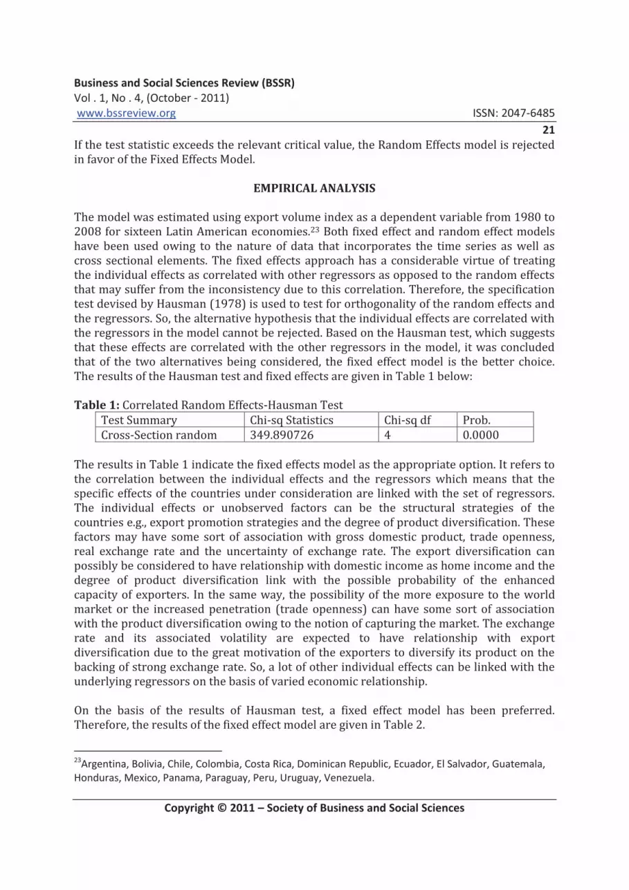
The model was estimated using export volume index as a dependent variable from 1980 to 2008 for sixteen Latin American economies.23 Both fixed effect and random effect models have been used owing to the nature of data that incorporates the time series as well as cross sectional elements. The fixed effects approach has a considerable virtue of treating the individual effects as correlated with other regressors as opposed to the random effects that may suffer from the inconsistency due to this correlation. Therefore, the specification test devised by Hausman (1978) is used to test for orthogonality of the random effects and the regressors. So, the alternative hypothesis that the individual effects are correlated with the regressors in the model cannot be rejected. Based on the Hausman test, which suggests that these effects are correlated with the other regressors in the model, it was concluded that of the two alternatives being considered, the fixed effect model is the better choice. The results of the Hausman test and fixed effects are given in Table 1 below: Table 1: Correlated Random Effects-Hausman Test

Test Summary Chi-sq Statistics Chi-sq df Prob.

Cross-Section random 349.890726 4 0.0000

The results in Table 1 indicate the fixed effects model as the appropriate option. It refers to the correlation between the individual effects and the regressors which means that the specific effects of the countries under consideration are linked with the set of regressors. The individual effects or unobserved factors can be the structural strategies of the countries e.g., export promotion strategies and the degree of product diversification. These factors may have some sort of association with gross domestic product, trade openness, real exchange rate and the uncertainty of exchange rate. The export diversification can possibly be considered to have relationship with domestic income as home income and the degree of product diversification link with the possible probability of the enhanced capacity of exporters. In the same way, the possibility of the more exposure to the world market or the increased penetration (trade openness) can have some sort of association with the product diversification owing to the notion of capturing the market. The exchange rate and its associated volatility are expected to have relationship with export diversification due to the great motivation of the exporters to diversify its product on the backing of strong exchange rate. So, a lot of other individual effects can be linked with the underlying regressors on the basis of varied economic relationship.

On the basis of the results of Hausman test, a fixed effect model has been preferred. Therefore, the results of the fixed effect model are given in Table 2.

23

Argentina, Bolivia, Chile, Colombia, Costa Rica, Dominican Republic, Ecuador, El Salvador, Guatemala,

Honduras, Mexico, Panama, Paraguay, Peru, Uruguay, Venezuela.

Business and Social Sciences Review (BSSR)

Vol . 1, No . 4, (October - 2011)

www.bssreview.org ISSN: 2047-6485

22

Copyright © 2011 – Society of Business and Social Sciences

The regression coefficients estimated from the sample period (1980-2008) have expected signs and are statistically significant. The home country income i.e., real gross domestic product has a positive and significant effect on the exports of all countries. The growth of home income, an indicative of the better living standard of the people, gives thrust to the exporters to expand the productive activities thus the level of exports. The results are consistent with the study by Chit et al (2010) who found exporting country’s income

elasticity as positive and significant. Table 2: The Fixed Effect Model

Variable Sample period 1980-2008

t-statistic

Constant (β0) -12.0910* -3.7507

Real GDP (β1) 0.6922* 5.3996

Openness (β2) 0.3875* 4.9472

Real ER (β3) 0.1056* 2.4709

Volatility (β4) -0.2340* -2.8628

AR(1) 0.9335* 49.6737

Durbin-h test -1.59

No. of obs. 448

R2 0.9652

Note: * denotes the significance level at 1%

Trade penness has always been accompanied by the building of resilience mechanism that augments the ability of an economy to withstand unexpected shocks. The openness of economies towards international trade is also considered as an effective strategy for accelerating economic growth. The aforementioned statement has been supported by the results as the estimated coefficients (i.e. elasticities) of openness exert a positive impact on the exports of Latin American countries. This finding is quite comparable to the results of Aliyu, S. U. R. (2010) who found that exports are positively related to the index of openness. The openness of region and the increase in exports is also evident from the trade regimes of 1990s when most of the countries reduced their tariff and non-tariff barriers. The real exchange rate elasticities also exert a positive impact on the volume of exports. It indicates that a higher exchange rate implies a lower relative price so conducive for the growth of exports. However, the volatility of exchange rate has a negative impact on the export growth. The deleterious effects can be attributed to the fact that the hedging opportunities are seldom available for exporters in developing countries. Another reason hinges on the fact that the real exchange rates of many Latin American countries remain very volatile owing to highly unstable domestic inflation rates. In many cases, nominal exchange rates have been volatile as well. Between 1982 and 1990, Argentina, Brazil, and Mexico experienced sharp devaluations and extremely high inflation.24 Some of these

24

See Frenkel and Rapetti (2010).

Business and Social Sciences Review (BSSR)

Vol . 1, No . 4, (October - 2011)

www.bssreview.org ISSN: 2047-6485

23

Copyright © 2011 – Society of Business and Social Sciences

inflationary experiences involved devaluation/inflation spirals, where currency devaluation increases inflation, which further overvalues the real exchange rate, leading to another devaluation, etc. The estimation results using the volatility measure suggest that an increase in exchange rate volatility by one standard deviation (5.9 percent) around its mean would lead to a reduction in exports of Latin American economies by about 1.4 percent.25 The negative impact of exchange rate volatility may perhaps be linked with the currency crises of the region, most notably of Mexican and Brazilian crises in 1995 and 1999 respectively as well as the collapse of the convertibility regime in Argentina during 2001-2002.

CONCLUSION

Using panel data set for sixteen Latin American economies during the 1980-2008, this study provides evidence in support of the view that the trade effects of real exchange rate volatility are detrimental in Latin American countries. The fixed effect model has been used to investigate the impact of exchange rate volatility. The empirical results derived in this paper are consistent with findings of studies on both developed and less developed countries suggesting that exchange-rate volatility has a significant negative impact on the export flows. The volatility of the exchange rate may reflect the changes in the policy regimes or the underlying shocks to the economy so this does not necessarily imply that the authorities can attenuate the deleterious effects by just stabilizing the exchange rate only. Therefore, the possible negative impact of the exchange rate on trade flows can be taken care of by maneuvering the unprecedented fluctuations in the exchange rate. This can possibly be done by adopting inflation targeting regimes as have been practiced by various Latin American countries.26 However, the integration of the domestic economy into the international trade also exposes an economy to the harsh situations as happened during Asian crises of 1999 and US economic slowdown of 2007. Therefore, the ultimate and the final weapon can be the strong domestic policies to withstand the unexpected shocks. The trade effects of exchange rate volatility can be further explored by considering intra-regional trade. The disaggregated trade or the products which provide a comparative advantage to the economy (i.e., specialized tradable goods) may be investigated to gain a further insight of the relevant query.

REFERENCES

[1]. Akhtar, M. A. and A. S. Hilton (1984), “Effects of exchange rate uncertainty on

German and US trade,” Federal Reserve Bank of New York Quarterly Review, 9, 7-16.

25

This impact is computed as the estimated coefficient in the regression equation multiplied by one

standard deviation of the volatility measure, multiplied by 100 to convert to percent. 26

Brazil, Chile, Colombia, Mexico and Peru.

Business and Social Sciences Review (BSSR)

Vol . 1, No . 4, (October - 2011)

www.bssreview.org ISSN: 2047-6485

24

Copyright © 2011 – Society of Business and Social Sciences

[2]. Aliyu, S. U. R. (2010), “Exchange Rate Volatility and Export Trade in Nigeria: An

Empirical Investigation,” Applied Financial Economics, 20, 13, 1071-1084. [3]. Arize, A.C. (1995): The effects of exchange rate volatility on US exports: an empirical

investigation, Southern Economic Journal 62, 34-43. [4]. Arize, A. C., Osang, T., & Slottje, D.J. (2000), “Exchange-rate Volatility and Foreign

Trade: Evidence from Thirteen LDCs,” Journal of Business and Economic Statistics, 18, 1, 10-17.

[5]. Arize, A.C., Malindretos, J. & Kasibhatla, K.M. (2003), “Does Exchange Rate Volatility

Depress Export Flows: The Case of LDCs,” International Advances in Economic

Research, 9, 1, 7-19. [6]. Arize, A.C., Osang, T., & Slottje, D.J. (2008), “Exchange-rate volatility in Latin

America and its impact on foreign trade,” International Review of Economics and

Finance, 17,1,33-44. [7]. Asseery, A. and Peel, D. A. (1991), “The Effects of Exchange Rate Volatility on

Exports,”Economics Letters, 37, 173-77 [8]. Aurangzeb, A., Stengos, T. and Mohammad, A.U. (2005), “Short-Run and Long-Run

Effects of Exchange Rate Volatility on the Volume of Exports: A Case Study for Pakistan,”International Journal of Business and Economics, 4, 3, 209-222.

[9]. Baak, S. J. (2004), “Exchange Rate Volatility and Trade among the Asia Pacific

Countries,” Econometric Society Far Eastern Meeting

[10]. Bahmani-Oskooee, M. (1991), “Exchange Rate Uncertainty and Trade Flows of Developing Countries,” The Journal of Developing Areas, 25, 4, 497-508.

[11]. Baillie, R.T., Bollerslev, T., 1989. The message in daily exchange rates: a conditional variance tale. Journal of Business and Economic Statistics 7, 297–305.

[12]. Bailey, M. J., Tavlas, G. S., and Ulan, M. (1986), “Exchange-Rate Variability and Trade Performance: Evidence for the Big Seven Industrial Countries,”Weltwirtschaftliches

Archiv, 122, 466-477. [13]. Bailey, M. J. and G. S. Tavlas (1988), “Trading and Investment under Floating Rates:

The US Experience,” Cato Journal, 8, 2, 421-49. [14]. Baron, David P. (1976a), “Flexible Exchange Rates, Forward Markets and the Level

of Trade,” American Economic Review, 66, 253-66. [15]. Baron, David P. (1976b), “Fluctuating Exchange Rates and the Pricing of Exports,”

Economic Inquiry, 14 , 425-38. [16]. Baum, C. F., M. Caglayan, and N. Ozkan (2004), “Nonlinear Effects of Exchange Rate

Volatility on the Volume of Bilateral Exports,”Journal of Applied Econometrics Vol. 19, 1-23.

[17]. Baum, S. Mullins, P. Stimson, R. and O’Connor, K. (2002) “Communities of the post- industrial city”, Urban Affairs Review, 37, 2, pp. 322-357.

[18]. Billen, D., Garcia, M. M. and Khasanova, N. (2005), “Is the Effect of Exchange Rate Volatility on Trade More Pronounced in Latin America than in Asia?” Institute for

World Economics Kiel, Germany, Working Paper, 434 [19]. Brada, J. C., and Mendez, J. A. (1988), “Exchange-rate risk, Exchange Rate Regime

and the Volume of International Trade,” Kyklos, 41, 263−280.

Business and Social Sciences Review (BSSR)

Vol . 1, No . 4, (October - 2011)

www.bssreview.org ISSN: 2047-6485

25

Copyright © 2011 – Society of Business and Social Sciences

[20]. Broll, U. (1994), “Foreign Production and Forward Markets,” Australian Economic

Papers, 62, 1-6. [21]. Chit, M. M., Rizov, M, and Willenbockel, D. (2010), “Exchange Rate Volatility and

Exports: New Empirical Evidence from the Emerging East Asian Economies,” The

World Economy, 33: 239–263 doi: 10.1111/j.1467-9701.2009.01230.x [22]. Chowdhury, A. (1993), “Does exchange rate volatility depress trade flows? Evidence

from error-correction models,” The Review of Economics and Statistics, 75, 4, 700-706

[23]. Clark, Peter B. (1973), “Uncertainty, Exchange Risk, and the Level of International

Trade,”Western Economic Journal, 11 (September): 302-13. [24]. Clark, P., Tamirisa, N., and Wei, S.J., (2004), “Exchange Rate Volatility and Trade

Flows-Some New Evidence,” International Monetary Fund

[25]. Corbo, V. (2007), “Latin America in a globalized world: challenges ahead,” Central

Bank of Chile

[26]. Côté, A. (1994), “Exchange-rate volatility and Trade,” Working Paper 94-5, Bank of

Canada [27]. Cushman, D. O. (1988), “U.S. Bilateral Trade Flows and Exchange Risk during the

Floating Period,” Journal of International Economics, 25, 317−330 [28]. De Grauwe, P. (1988), “Exchange Rate Variability and the Slowdown in Growth of

International Trade,” IMF Staff Papers, 35, 1, 63−84. [29]. De Grauwe, Paul (1992), “The Benefits of a Common Currency,”The Economics of

Monetary Integration, edited by Paul De Grauwe. New York: Oxford University Press.

[30]. Dellas, H. and Zilberfarb, B-Z. (1993), “Real Exchange Rate Volatility and

International Trade: A re-examination of the theory,” Southern Economic Journal, 59, 641-647.

[31]. Dell’Ariccia, G. (1999), “Exchange Rate Fluctuations and Trade Flows: Evidence form European Union,”IMF Staff Papers, 46, 3, 315-334.

[32]. Dixit, A. (1989), “Entry and Exit Decisions Under Uncertainty,”Journal of Political

Economy, 97, 620−638. [33]. Doganlar, M., (2002), “Estimating the impact of exchange rate volatility on exports

evidence from Asian countries,” Applied Economics Letters 9,13, 859–863. [34]. ECLAC (Economic Commission for Latin America and the Caribbean), 2008,

Economic survey of Latin America and the Caribbean 2007-2008: Macroeconomic policy and volatility. Santiago: United Nations, Economic Commission for Latin America and the Caribbean.

[35]. Engle, R. F., (1983), “Estimates of the Variance of U.S. Inflation Based upon the ARCH

Model,”Journal of Money, Credit and Banking, 15, 286-301. [36]. Ethier, W. (1973), “International Trade and the Forward Exchange Market,”

American Economic Review, 63, 3, 494-503. [37]. European Commission (1990), ‘One Market, One Money: An Evaluation of the

Potential Benefits and Costs of Forming an Economic and Monetary Union’,

European Economy, 44.

Business and Social Sciences Review (BSSR)

Vol . 1, No . 4, (October - 2011)

www.bssreview.org ISSN: 2047-6485

26

Copyright © 2011 – Society of Business and Social Sciences

[38]. Fischer, R., and Meller, P. (2001), “Latin American Trade Regimes Reforms and

Perceptions,” in. R. Fischer (editor), Latin America and the Global Economy: Export

Trade and the Threat of Protectionism. Macmillan, London [39]. Franke, G. (1991), “Exchange Rate Volatility and International Trading Strategy,”

Journal of International Money and Finance, 10, 292-307 [40]. Frankel, J. and Wei, S. (1993), “Trade Blocs and Currency Blocs,” NBER Working

Paper No. 4335. [41]. Frenkel Roberto and Martin Rapetti (April, 2010), “A Concise History of Exchange

Rate Regimes in Latin America,” Center for Economic and Policy Research

[42]. Froot, Kenneth A. and Paul D. Klemperer. (1989), “Exchange Rate Pass-through When Market Share Matters,” American Economic Review, 637-54.

[43]. Goldstein, M. and Khan, M. (1985), “ Income and price effects in foreign trade,” in

Handbook of International Trade, 2 (Eds) R. W. Jones and P. B. Kenen, North Holland, Amsterdam.

[44]. Gotur, P. (1985), “Effects of exchange rate volatility on trade,” IMF Staff Papers, 32, 3,475–512.

[45]. Hall, S., Hondroyiannis, G., Swamy, P. A. V. B., Talvas G. and Ulan, M. (2010), “Exchange-rate volatility and export performance: Do emerging market economies resemble industrial countries or other developing countries?” Economic Modelling (2010),doi:10.1016/j.econmod. 2010.01.014

[46]. Hassan, M. K. and Tufte, D. R. (1998), “Exchange rate volatility and aggregate export

growth in Bangladesh,”Applied Economics, 30, 2,189-201 [47]. Hausman, J.A., (1978), “Specification tests in econometrics”, Econometrica 46, 1251-

1272. [48]. Holly, S. (1995), “Exchange rate uncertainty and export performance: supply and

demand effects,”Scottish Journal of Political Economy 42, 381-391. [49]. Hondroyiannis, G., Swamy, P. A. V. B., Tavlas, G.S., and Ulan, M., (2008), “Some

Further Evidence on Exchange-Rate Volatility and Exports,”Review of World

Economics (Weltwietschaftliches Archiv) 144, 1, 151–180. [50]. Hooper, P. and S. Kohlhagen (1978), “The effect of exchange rate uncertainty on the

prices and volume of international trade,” Journal of International Economics 8, 483-511.

[51]. IMF (various issues), World Economic Outlook. [52]. Kenen, P. B. and D. Rodrik (1986), “Measuring and analysing the effects of short-

term volatility in real exchange rates,”The Review of Economics and Statistics, 68,2, 311–5.

[53]. Koray, F. and W. D. Lastrapes.( 1989), “Real exchange rate volatility and the United

States (U.S.) bilateral trade: A VAR approach,”The Review of Economics and Statistics, 71,702–12.

[54]. Learner, E. and Stern, R. (1970), “Quantitative International Economics,” Allyn and

Bacon, Boston. [55]. McKenzie, M. and Brooks, R. (1997), “ The Impact of Exchange Rate Volatility on

German-U.S. Trade Flows,” Journal of International Financial Markets, Institutions

and Money,7, 73-87.

Business and Social Sciences Review (BSSR)

Vol . 1, No . 4, (October - 2011)

www.bssreview.org ISSN: 2047-6485

27

Copyright © 2011 – Society of Business and Social Sciences

[56]. Mustafa, K. and Nishat, M. (2004), “Volatility of Exchange Rate and Export Growth in Pakistan: The Structure and Interdependence in Regional Markets,” The Pakistan

Development Review, 43, 4, 813-828. [57]. Onafowora, O. A. and Owoye, O. (2008), “Exchange rate volatility and Export Growth

in Nigeria,” Applied Economics, 2008, 40, 1547–1556. [58]. Pedroni, P., (1999) Critical values for cointegration tests in heterogenous panels

with multiple regressors, Oxford Bulletin of Economics and Statistics, Special Issue, 653-670.

[59]. Peree, E. and A. Steinherr, (1989), “Exchange Rate Uncertainty and Foreign Trade,”

European Economic Review, 33, 1241-1264. [60]. Pozo, S. (1992), “Conditional Exchange-Rate Volatility and the Volume of

International Trade: Evidence from the Early 1900s,” The Review of Economics and

Statistics, 74, 2, 325-329. [61]. Qian, Y and P. Varangis (1994), “Does Exchange Rate Volatility Hinder Export

Growth? Additional Evidence,” Empirical Economics, 19, 371-396. [62]. Rose, A. (2000), “One Money, One Market: The Effect of Common Currencies on

Trade,” Economic Policy 30, 7-33. [63]. Sauer, C. and Bohara, A. K. (2001), “Exchange Rate Volatility and Exports: Regional

Differences between Developing and Industrialized Countries,” Review of

International Economics, 9(1), 133-152. [64]. Sercu, P. (1992), “Exchange Rates, Volatility and the Option to Trade,” Journal of

International Money and Finance, 11, 579-93. [65]. Sercu, P. and R. Uppal, 2000, “Exchange Rate Volatility, Trade and Capital Flows

under Alternative. Exchange Rate Regimes,” Cambridge University Press [66]. Sercu, P. and Vanhulle, C. (1992), “Exchange Rate Volatility, International Trade and

the Value of Exporting Firms,” Journal of Banking and Finance, 16, 155-82. [67]. Shixue, J. (2001), “Evolution of the Latin American Development Models in the 20th

Century: Lessons and Implications for Other Developing Countries,” Asian Journal of

Latin American Studies,14, 1: 173-197. [68]. Tavlas, G. S., and Swamy, P. A. V. B. (1997), “Macroeconomic Policies and World

Financial Integration,” In M. U. Fratianni, D. Salvatore, & H. Von Itazen (Eds.),

Macroeconomic Policy in Open Economics (248−280). Westport, Connecticut, USA:

Greenwood Press. [69]. Tenreyro, S. (2007), “On the Trade Impact of Nominal Exchange Rate Volatility,”

Journal of Development Economics, 82, 485-508. [70]. Thursby, M.C. and J.G. Thursby (1987), “Bilateral trade flows, the Linder hypothesis

and exchange risk,” Review of Economics and Statistics, 69, 488-495. [71]. United Nations, Economic Commission for Latin America and the Caribbean. (2007-

08) Economic Survey of Latin America and the Caribbean [72]. http://www.eclac.org/cgibin/getProd.asp?xml=/publicaciones/xml/3/33873/P33

873.xml&xsl=/de/tpl-i/p9f.xsl&base=/tpl-i/top-bottom.xslt [73]. Viaene, J. M. and de Vries, C. G. (1992), “International Trade and Exchange Rate

Volatility,” European Economic Review, 36, 1311-21.

Business and Social Sciences Review (BSSR)

Vol . 1, No . 4, (October - 2011)

www.bssreview.org ISSN: 2047-6485

28

Copyright © 2011 – Society of Business and Social Sciences

[74]. Wei, S.J., (1999), “Currency hedging and goods trade,” European Economic Review 43, 1371-1394.

[75]. White, H., (1980), “A Heteroscedasticity-Consistent Covariance Matrix Estimator and a Direct Test for Heteroscedasticity,” Econometrica, 48, 817-838.

[76]. Wolf, A. (1995), “Import and Hedging Uncertainty in International Trade,” Journal of Futures Markets, 15, 101-110.

[77]. World Bank (1990), World Development Report, Vol. 13 [78]. Xu Junqian., (2007), “UK Textile Imports: The Relative Performance of China and the

Role of Exchange Rate Volatility,” Labour and management in development, 8.

Appendix B

Summary Statistics of Main Variables

Variable Mean Standard Deviation Minimum Maximum

Export Volume 4.2494 0.5965 1.8466 5.8878

Real GDP 24.0059 1.3235 22.1214 27.2758

Openness -0.7064 0.6284 -2.4167 0.8616

Real Exchange Rate 3.4331 2.9358 -0.6111 10.1262

Real Exchange Rate Volatility 0.0289 0.0592 0.0017 0.7458

Business and Social Sciences Review (BSSR)

Vol . 1, No . 4, (October - 2011)

www.bssreview.org ISSN: 2047-6485

29

Copyright © 2011 – Society of Business and Social Sciences

Appendix C

Hausman Specification Test

Correlated Random Effects - Hausman Test

Pool: Untitled

Test cross-section random effects

Test Summary Chi-Sq. Statistic Chi-Sq. d.f. Prob.

Cross-section random 359.429944 4 0.0000

Cross-section random effects test comparisons:

Variable Fixed Random Var (Diff.) Prob.

Ln Y 1.052366 0.531512 0.002340 0.0000

Ln O 0.877247 1.172469 0.001855 0.0000

Ln RER 0.197967 0.052324 0.001573 0.0002

V 0.168033 0.130435 0.000421 0.0669

Cross-section random effects test equation:

Dependent Variable: LEQI_?

Method: Panel Least Squares

Date: 10/03/10 Time: 01:02

Sample: 1980 2008

Included observations: 29

Cross-sections included: 16

Total pool (balanced) observations: 464

Variable Coefficien

t Std. Error t-Statistic Prob.

C -21.07832 1.321512 -15.95015 0.0000

Ln Y 1.052366 0.055203 19.06356 0.0000

Ln O 0.877247 0.056758 15.45584 0.0000

Ln RER 0.197967 0.042256 4.684948 0.0000

V 0.168033 0.196117 0.856799 0.3920

Effects Specification

R-squared 0.855510 Mean dependent var 4.249438

Adjusted R-squared 0.849326 S.D. dependent var 0.596548

S.E. of regression 0.231560 Akaike info criterion -

0.045807

Sum squared resid 23.80732 Schwarz criterion 0.132636

Log likelihood 30.62734 Hannan-Quinn criter. 0.024434

F-statistic 138.3614 Durbin-Watson stat 0.302009

Prob(F-statistic) 0.000000

Business and Social Sciences Review (BSSR)

Vol . 1, No . 4, (October - 2011)

www.bssreview.org ISSN: 2047-6485

30

Copyright © 2011 – Society of Business and Social Sciences

Appendix D Fixed Effects Model

Dependent Variable: LEQI

Method: Pooled Least Squares

Sample (adjusted): 1981 2008

Included observations: 28 after adjustments

Cross-sections included: 16

Total pool (balanced) observations: 448

Convergence achieved after 19 iterations

Variable Coefficient Std. Error t-Statistic Prob.

C -12.09097 3.223630 -3.750730 0.0002

Ln Y 0.692184 0.128193 5.399552 0.0000

Ln O 0.387466 0.078321 4.947179 0.0000

Ln RER 0.105608 0.042740 2.470955 0.0139

V -0.234017 0.081743 -2.862827 0.0044

AR(1) 0.933513 0.018793 49.67365 0.0000

Fixed Effects (Cross)

_BOL—C 1.372900

_COLOMB—C -1.117107

_DR—C -0.324711

_ECU—C -0.009886

_ES—C 0.458520

_GUAT—C 0.776816

_HOND—C 0.891758

_PARAG—C 0.978980

_PERU—C 0.128621

_ARG—C -0.820995

_CHILE—C -0.888385

_COSTAR—C -0.013879

_MEXICO—C -1.668919

_PANAMA—C 0.552170

_URUG—C 0.627721

_VENEZ—C -0.943604

Effects Specification

Cross-section fixed (dummy variables)

R-squared 0.965189 Mean dependent var 4.272843

Adjusted R-squared 0.963559 S.D. dependent var 0.582284

S.E. of regression 0.111156 Akaike info criterion -1.510030

Sum squared resid 5.275830 Schwarz criterion -1.317618

Log likelihood 359.2468 Hannan-Quinn criter. -1.434179

F-statistic 591.9658 Durbin-Watson stat 2.137903

Prob(F-statistic) 0.000000

Business and Social Sciences Review (BSSR)

Vol . 1, No . 4, (October - 2011)

www.bssreview.org ISSN: 2047-6485

31

Copyright © 2011 – Society of Business and Social Sciences

APPENDIX E

APPENDIX F

Exports of Latin American Countries

0

1

2

3

4

5

6

1980 1982 1984 1986 1988 1990 1992 1994 1996 1998 2000 2002 2004 2006 2008

Years

Exp

ort

Vo

lum

e (

Leq

ui)

Exchange Rate Volatility In Latin America

0

0.02

0.04

0.06

0.08

0.1

0.12

1980 1982 1984 1986 1988 1990 1992 1994 1996 1998 2000 2002 2004 2006 2008

Years

Business and Social Sciences Review (BSSR)

Vol . 1, No . 4, (October - 2011)

www.bssreview.org ISSN: 2047-6485

32

Copyright © 2011 – Society of Business and Social Sciences

Appendix D

Fixed Effects Model

Dependent Variable: LEQI

Method: Pooled Least Squares

Sample (adjusted): 1981 2008

Included observations: 28 after adjustments

Cross-sections included: 16

Total pool (balanced) observations: 448

Convergence achieved after 19 iterations

Variable Coefficient Std. Error t-Statistic Prob.

C -12.09097 3.223630 -3.750730 0.0002

Ln Y 0.692184 0.128193 5.399552 0.0000

Ln O 0.387466 0.078321 4.947179 0.0000

Ln RER 0.105608 0.042740 2.470955 0.0139

V -0.234017 0.081743 -2.862827 0.0044

AR(1) 0.933513 0.018793 49.67365 0.0000

Fixed Effects (Cross)

_BOL—C 1.372900

_COLOMB—C -1.117107

_DR—C -0.324711

_ECU—C -0.009886

_ES—C 0.458520

_GUAT—C 0.776816

_HOND—C 0.891758

_PARAG—C 0.978980

_PERU—C 0.128621

_ARG—C -0.820995

_CHILE—C -0.888385

_COSTAR—C -0.013879

_MEXICO—C -1.668919

_PANAMA—C 0.552170

_URUG—C 0.627721

_VENEZ—C -0.943604

Effects Specification

Cross-section fixed (dummy variables)

R-squared 0.965189 Mean dependent var 4.272843

Adjusted R-squared 0.963559 S.D. dependent var 0.582284

S.E. of regression 0.111156 Akaike info criterion -1.510030

Sum squared resid 5.275830 Schwarz criterion -1.317618

Log likelihood 359.2468 Hannan-Quinn criter. -1.434179

F-statistic 591.9658 Durbin-Watson stat 2.137903

Prob(F-statistic) 0.000000

Business and Social Sciences Review (BSSR)

Vol . 1, No . 4, (October - 2011)

www.bssreview.org ISSN: 2047-6485

33

Copyright © 2011 – Society of Business and Social Sciences

Appendix G

Graphical Representation of the Volatility of Real Exchange Rate (Sixteen Latin American Countries)

Argentina

0 0

0.05 0.05

0.1 0.1

0.15 0.15

0.2 0.2

0.25 0.25

0.3 0.3

0.35 0.35

0.4 0.4

0.45

1980 1984 1988 1992 1996 2000 2004 2008 Years

Bolivia

0 0

0.1 0.1

0.2 0.2

0.3 0.3

0.4 0.4

0.5 0.5

0.6 0.6

0.7 0.7

0.8

1980 1984 1988 1992 1996 2000 2004 2008 Years

Chile

0 0

0.0

1 0.0

0.0

2 0.0

0.0

3 0.0

0.0

4 0.0

0.0

5 0.0

0.0

6 0.0

0.0

7 0.0

0.0

8 0.0

0.0

9

198

0 198

4 198

8 199

2 199 200

0 200

4 200

8 Years

Colombia

0 0

0.01 0.01

0.02 0.02

0.03 0.03

0.04 0.04

0.05 0.05

0.06

1980 1984 1988 1992 1996 2000 2004 2008 Years

Costa Rica

0 0

0.02 0.02

0.04 0.04

0.06 0.06

0.08 0.08

0.1 0.1

0.12 0.12

0.14 0.14

0.16 0.16

0.18 0.18

0.2

1980 1984 1988 1992 1996 2000 2004 2008 Years

Dominican Republic

0 0

0.05 0.05

0.1 0.1

0.15 0.15

0.2 0.2

0.25 0.25

0.3 0.3

0.35

1980 1984 1988 1992 1996 2000 2004 2008 Years

Business and Social Sciences Review (BSSR)

Vol . 1, No . 4, (October - 2011)

www.bssreview.org ISSN: 2047-6485

34

Copyright © 2011 – Society of Business and Social Sciences

Ecuador

0 0

0.02 0.02

0.04 0.04

0.06 0.06

0.08 0.08

0.1 0.1

0.12 0.12

0.14

1980 1984 1988 1992 1996 2000 2004 2008

Years

El Salvador

0

0.05

0.1

0.15

0.2

0.25

1980 1984 1988 1992 1996 2000 2004 2008 Years

Guatemala

0 0

0.05 0.05

0.1 0.1

0.15 0.15

0.2 0.2

0.25 0.25

0.3

1980 1984 1988 1992 1996 2000 2004 2008

Years

Honduras

0 0

0.02 0.02

0.04 0.04

0.06 0.06

0.08 0.08

0.1 0.1

0.12 0.12

0.14 0.14

0.16

1980 1984 1988 1992 1996 2000 2004 2008

Years

Mexico

0 0

0.02 0.02

0.04 0.04

0.06 0.06

0.08 0.08

0.1 0.1

0.12 0.12

0.14 0.14

0.16 0.16

0.18 0.18

0.2

1980 1984 1988 1992 1996 2000 2004 2008

Years

Panama

0 0

0.002 0.00202

0.004 0.00404

0.006 0.00606

0.008 0.008

0.01 0.01

0.012 0.01212

0.014

1980 1984 1988 1992 1996 2000 2004 2008

Years

Paraguay

0 0

0.02 0.02

0.04 0.04

0.06 0.06

0.08 0.08

0.1 0.1

0.12 0.12

0.14 0.14

0.16 0.16

0.18 0.18

0.2

1980 1984 1988 1992 1996 2000 2004 2008

Years

Peru

0 0

0.05 0.05

0.1 0.1

0.15 0.15

0.2 0.2

0.25 0.25

0.3 0.3

0.35 0.35

0.4

1980 1984 1988 1992 1996 2000 2004 2008 Years

Business and Social Sciences Review (BSSR)

Vol . 1, No . 4, (October - 2011)

www.bssreview.org ISSN: 2047-6485

35

Copyright © 2011 – Society of Business and Social Sciences

Uruguay

0 0

0.02 0.02

0.04 0.04

0.06 0.06

0.08 0.08

0.1 0.1

0.12 0.12

0.14 0.14

0.16 0.16

0.18

1980 1984 1988 1992 1996 2000 2004 2008 Years

Venezuela

0

0.05

0.1

0.15

0.2

0.25

1980 1984 1988 1992 1996 2000 2004 2008 Years

Business and Social Sciences Review (BSSR)

Vol . 1, No . 4, (October - 2011)

www.bssreview.org ISSN: 2047-6485

36

Copyright © 2011 – Society of Business and Social Sciences

AN ANALYSIS OF THE FACTOR RESPONSIBLE FOR UNEMPLOYMENT

AMONG YOUNG GRADUATES IN PAKISTAN

Dr. Shahid A. Zia

Imperial College of Business Studies, Lahore (Pakistan)

Shahinshah Babar Khan

PhD Scholar, Department of Education International Islamic University, Islamabad (Pakistan)

Saddaf Ayub Raja

PhD Scholar, Department of Education International Islamic University, Islamabad (Pakistan)

Asghar Ali

Lecturer, Training and Staff Development Institute, Punjab Group of Colleges, Lahore (Pakistan)

ABSTRACT In Pakistan, unemployment among educated youth is a challenge for

government and society. Every year, universities are producing thousands of

graduates in different disciplines. Young graduates and their parents assume

that after completing higher education, will found attractive jobs, while in fact,

there is an adverse situation in the market. Society demands skilled individuals

who should be able to work in the global age, while majority of the university

graduates have degrees but no skill for the actual work place. While young

graduates argue that they learn what they were taught. The present study tries

to explore the factors which are responsible for unemployment among the

educated youth. It was found that use of technology, communication skills,

English language skills are the need of the hour, while young graduates are not

equipped with these skills. Moreover, lack of confidence, trend towards public

sector jobs, lacks of skills needed for business are some other factors

responsible for unemployment among educated youth.

INTRODUCTION It is admitted fact that educated mass are more beneficial for the economic growth of any nation. In any society, schools, colleges and universities prepare work force and top management for different fields of life. Even few years of schooling effects an individual’s every sphere of life. One extra year of schooling increases an individual’s earning up to 10

% (UNESCO, 2010). Education is considered a lifelong process that brings positive changes in the personality of an individual. Rena (2006) states: What a student obtains from the school and college is only a small part of the education that

needs for the economic and social life of human being. Thus, both in the case of man who is