Embed Size (px)
Citation preview

Extrapolation-based implicit-explicit generallinear methods
A. Cardone,∗ Z. Jackiewicz,† A. Sandu,‡ and H. Zhang§
January 13, 2014
Abstract For many systems of differential equations modeling problemsin science and engineering, there are natural splittings of the right handside into two parts, one non-stiff or mildly stiff, and the other one stiff.For such systems implicit-explicit (IMEX) integration combines an explicitscheme for the non-stiff part with an implicit scheme for the stiff part. In arecent series of papers two of the authors (Sandu and Zhang) have developedIMEX GLMs, a family of implicit-explicit schemes based on general linearmethods. It has been shown that, due to their high stage order, IMEXGLMs require no additional coupling order conditions, and are not marredby order reduction. This work develops a new extrapolation-based approachto construct practical IMEX GLM pairs of high order. We look for methodswith large absolute stability region, assuming that the implicit part of themethod is A- or L-stable. We provide examples of IMEX GLMs with optimalstability properties. Their application to a two dimensional test problemconfirms the theoretical findings.
Key words. IMEX methods, general linear methods, error analysis,order conditions, stability analysis
∗Dipartimento di Matematica, Universita degli studi di Salerno, Fisciano (Sa), 84084Italy, e-mail: [email protected]. The work of this author was supported by travel fel-lowship from the Department of Mathematics, University of Salerno.†Department of Mathematics, Arizona State University, Tempe, Arizona 85287, e-mail:
[email protected], and AGH University of Science and Technology, Krakow, Poland.‡Department of Computer Science, Virginia Polytechnic Institute & State University,
Blacksburg, Virginia 24061, e-mail: [email protected].§Department of Computer Science, Virginia Polytechnic Institute & State University,
Blacksburg, Virginia 24061, e-mail: [email protected].
1
arX
iv:1
304.
2276
v1 [
cs.N
A]
8 A
pr 2
013

1 Introduction
Many practical problems in science and engineering are modeled by large sys-tems of ordinary differential equations (ODEs) which arise from discretizationin space of partial differential equations (PDEs) by finite difference methods,finite elements or finite volume methods, or pseudospectral methods. Forsuch systems there are often natural splittings of the right hand sides of thedifferential systems into two parts, one of which is non-stiff or mildly stiff,and suitable for explicit time integration, and the other part is stiff, andsuitable for implicit time integration. Such systems can be written in theform
y′(t) = f(y(t)
)+ g(y(t)
), t ∈ [t0, T ],
y(t0) = y0,(1.1)
where f(y) represents the non-stiff processes, for example advection, andg(y) represents stiff processes, for example diffusion or chemical reaction, insemi-discretization of advection-diffusion-reaction equations [18].
Implicit-explicit (IMEX) integration approach discretizes the non-stiffpart f(y) is with an explicit method, and the stiff part g(y) with an implicit,stable method. This strategy seeks to ensure the numerical stability of thesolution of (1.1) while reducing the amount of implicitness, and therefore theoverall computational effort. IMEX multistep methods were introduced byCrouzeix [13] and Varah [25] and further analyzed in [2, 14]. IMEX Runge-Kutta methods have been investigated in [1, 10, 20, 22, 23, 30].
In a recent series of papers the last two authors and their collaboratorshave proposed the new IMEX GLM family of implicit-explicit schemes basedon general linear methods. A general formalism for partitioned GLMs andtheir order conditions was developed by Zhang and Sandu [28]. The par-titioned method formalism was then used to construct IMEX GLMs. Thestarting and ending procedures, linear stability, and stiff convergence prop-erties of the new family have been analyzed. Zhang and Sandu examinedpractical methods of second order in [27] and of third order in [28]. A classof IMEX two step Runge-Kutta (TSRK) methods was proposed by Zharovskiand Sandu [29].
The results in [27, 28, 29] prove that the general linear framework iswell suited for the construction of multi-methods. Specifically, owing to thehigh stage orders, no coupling conditions are needed to ensure the order ofaccuracy of the partitioned GLM [28]. In addition, it has been shown that
2

IMEX GLMs are particularly attractive for solving stiff problems, whereother multistage methods may suffer from order reduction [28].
This paper extends our previous work [27, 28, 29] and develops a newextrapolation-based approach for the construction of practical IMEX GLMschemes of high order and high stage order.
The organization of this paper is as follows. General linear methods andthe implicit-explicit variants are reviewed in Section 2. The new extrapolation-based IMEX GLMs are derived in Section 3, and their order conditions arepresented. The stability analysis is performed in Section 4 and specific meth-ods are constructed in Section 5. Numerical experiments are presented inSection 6, and Section 7 gives some concluding remarks and plans for futurework.
2 Implicit-explicit general linear methods
In this section we briefly review GLMs and the IMEX GLM family.The GLMs for ODEs were introduced by Burrage and Butcher [4] and
further investigated in [3, 5, 7, 11, 12, 15, 16, 17]. We also refer the reader tothe review article [8] and the recent monograph [19] and references therein.
A diagonally implicit GLM for (1.1) is defined byY
[n+1]i = h
i∑j=1
aij
(f(Y
[n+1]j
)+ g(Y
[n+1]j
))+
r∑j=1
uijy[n]j , i = 1, 2, . . . , s
y[n+1]i = h
s∑j=1
bij
(f(Y
[n+1]j
)+ g(Y
[n+1]j
))+
r∑j=1
vijy[n]j , i = 1, 2, . . . , r,
(2.1)n = 0, 1, . . . , N−1. Here, N is a positive integer, h = (T−t0)/N , tn = t0+nh,
n = 0, 1, . . . , N , Y[n+1]i are approximations of stage order q to y(tn + cih),
i.e.,Y
[n+1]i = y(tn + cih) +O(hq+1), i = 1, 2, . . . , s, (2.2)
y[n]i are approximations of order p to the linear combinations of the derivatives
of the solution y at the point tn, i.e.,
y[n]i =
p∑k=0
qikhky(k)(tn) +O(hp+1), i = 1, 2, . . . , r, (2.3)
3

and y is the solution to (1.1). These methods can be characterized by theabscissa vector c = [c1, . . . , cs]
T , the coefficient matrices A = [aij] ∈ Rs×s,U = [aij] ∈ Rs×r, B = [aij] ∈ Rr×s, V = [aij] ∈ Rr×r, the vectorsq0, . . . ,qs ∈ Rr defined by qi = [qj,i]1≤j≤r, and four integers: the order p, thestage order q, the number of external approximations r, and the number ofstages or internal approximations s.
The method (2.1) can be written in a compact formY [n+1] = h(A⊗ I)
(f(Y [n+1]
)+ g(Y [n+1]
))+ (U⊗ I)y[n],
y[n+1] = h(B⊗ I)(f(Y [n+1]
)+ g(Y [n+1]
))+ (V ⊗ I)y[n],
(2.4)
n = 0, 1, . . . , N − 1, and the relation (2.3) takes the form
y[n] =
p∑k=0
qkhky(k)(tn) +O(hp+1). (2.5)
Applying (2.1) to the basic test equation y′(t) = λy(t), t ≥ 0, λ ∈ C,leads to the recurrence equation
y[n+1] = S(z)y[n], n = 0, 1, . . . ,
z = hλ, with the stability matrix given by
S(z) = V + zB(I− zA)−1U. (2.6)
We also define the stability polynomial η(w, z) by
η(w, z) = det(wI− S(z)
). (2.7)
The region of absolute stability of the method (2.1) is the subset of thecomplex plane
A =z ∈ C : all roots wi(z) of η(w, z) are in the unit circle
. (2.8)
The traditional concepts of A(α)-stability, A-stability, and L-stability applydirectly to GLMs via (2.8).
In this paper we will examine only methods of high stage order, i.e.,methods where q = p − 1 or q = p. It has been shown in [9, 6, 19] that the
4

GLM (2.1) has order p and stage order q = p or q = p− 1 if and only if
ck − kAck−1 − k!Uqk = 0 , k = 0, 1, . . . , q , and (2.9)k∑`=0
k!
`!qk−` − kBck−1 − k!Vqk = 0 , k = 0, 1, . . . , p . (2.10)
An IMEX-GLM [29, Definition 4] has the form Y [n+1] = h(Aexp ⊗ I) f(Y [n+1]
)+ h(Aimp ⊗ I) g
(Y [n+1]
)+ (U⊗ I)y[n],
y[n+1] = h(Bexp ⊗ I) f(Y [n+1]
)+ h(Bimp ⊗ I) g
(Y [n+1]
)+ (V ⊗ I)y[n],
(2.11)where Aexp, Bexp correspond to the explicit part and Aimp, Bimp to theimplicit part. The methods share the same abscissa cexp = cimp, whichmakes (2.11) internally consistent [29, Definition 2]. The methods also sharethe same coefficient matrices Uexp = Uimp = U and Vexp = Vimp = V.The coefficients qexp
k , qimpk in (2.5) can be different, which means that the
implicit and explicit components use different initialization and terminationprocedures. An IMEX-GLM (2.11) is a special case of a partitioned GLM [29,Definition 1]; while in (2.11) the right hand side is split in two components,stiff and nonstiff, a partitioned GLM allows for splitting in an arbitrarynumber of components.
It has been shown in [29, Theorem 2] that an internally consistent parti-tioned GLM (and, in particular, the IMEX GLM (2.11)) has order p and stageorder q ∈ p−1, p if and only if each component method (Aexp,Bexp,U,V)and
(Aimp,Bimp,U,V
)has order p and stage order q. We note that no
additional “coupling” conditions are needed for the IMEX GLM (i.e., no or-der conditions that contain coefficients of both the implicit and the explicitschemes).
3 Extrapolation-based IMEX GLMs
3.1 Method formulation
In this section we derive the new extrapolation-based IMEX GLMs. Considerthe following extrapolation formula depending on stage values Y
[n]k and Y
[n+1]k
5

at two consecutive steps
f[n+1]j =
s∑k=1
αjkf(Y
[n]k
)+
j−1∑k=1
βjkf(Y
[n+1]k
), j = 1, 2, . . . , s. (3.1)
Substituting f[n+1]j in (3.1) for f
(Y
[n+1]j
)in (2.1) leads to the proposed class
of extrapolation-based IMEX GLMs. The simple example of IMEX methodconsisting of the explicit Euler method combined with the A-stable implicitθ-method corresponding to θ ≥ 1/2 is presented in [18].
Substituting (3.1) into (2.1) leads to
Y[n+1]i = h
i∑j=1
s∑k=1
aijαjkf(Y
[n]k
)+ h
i∑j=1
j−1∑k=1
aijβjkf(Y
[n+1]k
)+ h
i∑j=1
aijg(Y
[n+1]j
)+
r∑j=1
uijy[n]j , i = 1, 2, . . . , s,
y[n+1]i = h
s∑j=1
s∑k=1
bijαjkf(Y
[n]k
)+ h
s∑j=1
j−1∑k=1
bijβjkf(Y
[n+1]k
)+ h
i∑j=1
bijg(Y
[n+1]j
)+
r∑j=1
vijy[n]j , i = 1, 2, . . . , r,
n = 0, 1, . . . , N − 1. Changing the order of summation in the double sumsabove and then interchanging the indices j and k we obtain
Y[n+1]i = h
s∑j=1
i∑k=1
aikαkjf(Y
[n]j
)+ h
i−1∑j=1
i∑k=j+1
aikβkjf(Y
[n+1]j
)+ h
i∑j=1
aijg(Y
[n+1]j
)+
r∑j=1
uijy[n]j , i = 1, 2, . . . , s,
y[n+1]i = h
s∑j=1
s∑k=1
bikαkjf(Y
[n]j
)+ h
s−1∑j=1
s∑k=j+1
bikβkjf(Y
[n+1]j
)+ h
s∑j=1
bijg(Y
[n+1]j
)+
r∑j=1
vijy[n]j , i = 1, 2, . . . , r.
6

These relations lead to IMEX GLMs of the form
Y[n+1]i = h
s∑j=1
aijf(Y
[n]j
)+ h
i−1∑j=1
a∗ijf(Y
[n+1]j
)+ h
i∑j=1
aijg(Y
[n+1]j
)+
r∑j=1
uijy[n]j , i = 1, 2, . . . , s,
y[n+1]i = h
s∑j=1
bijf(Y
[n]j
)+ h
s−1∑j=1
b∗ijf(Y
[n+1]j
)+ h
s∑j=1
bijg(Y
[n+1]j
)+
r∑j=1
vijy[n]j , i = 1, 2, . . . , r,
(3.2)
n = 0, 1, . . . , N − 1, where the coefficients aij, a∗ij, bij, and b∗ij are defined by
aij =i∑
k=1
aikαkj, a∗ij =i∑
k=j+1
aikβkj, bij =s∑
k=1
bikαkj, b∗ij =s∑
k=j+1
bikβkj.
In matrix notation
A = [aij] ∈ Rs×s, A∗ = [a∗ij] ∈ Rs×s, B = [bij] ∈ Rr×s, B∗ = [b∗ij] ∈ Rr×s.
withA = Aα, A∗ = Aβ, B = Bα, B∗ = Bβ,
where α = [αij] ∈ Rs×s, β = [βij] ∈ Rs×s. Observe that the matrix A∗ isstrictly lower triangular and that the last column of the matrix B∗ is zero.
In matrix notation the extrapolation-based IMEX-GLM is defined by:
Y [n+1] = h(A⊗ I)f(Y [n]
)+ h(A∗ ⊗ I)f
(Y [n+1]
)+h(A⊗ I)g
(Y [n+1]
)+ (U⊗ I)y[n], (3.3)
y[n+1] = h(B⊗ I)f(Y [n]
)+ h(B∗ ⊗ I)f
(Y [n+1]
)+h(B⊗ I)f
(Y [n+1]
)+ (V ⊗ I)y[n],
n = 0, 1, . . . , N − 1.
7

The explicit part of (3.3), obtained for g(y) = 0, can be represented as asingle GLM extended over two steps from tn−1 to tn and tn to tn+1, as follows
Y [n]
Y [n+1]
Y [n+1]
y[n+1]
=
0 0 I 0
A A∗ 0 U
A A∗ 0 U
B B∗ 0 V
f(Y [n]
)f(Y [n+1]
)Y [n]
y[n]
. (3.4)
The abscissa vector is cexp = [(c− e)T , cT ]T .Similarly, the implicit part of the IMEX scheme (3.2) corresponding to
f(y) = 0 assumes the formY [n]
Y [n+1]
Y [n+1]
y[n+1]
=
0 0 I 0
0 A 0 U
0 A 0 U
0 B 0 V
g(Y [n]
)g(Y [n+1]
)Y [n]
y[n]
. (3.5)
This method has the order and stage order of the underlying GLM (2.1),since it is the same method. The abscissa vector is cimp = [(c − e)T , cT ]T ,and therefore the method (3.3) is internally consistent.
3.2 Construction of the interpolant
We define the local discretization errors η(tn + cjh) of the extrapolationformula (3.1) by the relation
f(y(tn + cjh)
)=
s∑k=1
αjkf(y(tn−1 + ckh)
)+
+
j−1∑k=1
βjkf(y(tn + ckh)
)+ η(tn + cjh),
(3.6)
j = 1, 2, . . . , s. Letting ϕ(t) = f(y(t)) the relation (3.6) can be written inthe form
η(tn + cjh) = ϕ(tn + cjh)−s∑
k=1
αjkϕ(tn + (ck − 1)h
)−
j−1∑k=1
βjkϕ(tn + ckh),
8

j = 1, 2, . . . , s. Expanding ϕ(tn + cjh), ϕ(tn + (ck − 1)h), and ϕ(tn + ckh)into Taylor series around tn we obtain
η(tn + cjh) =
p∑l=0
(cljl!−
s∑k=1
αjk(ck − 1)l
l!−
j−1∑k=1
βjkclkl!
)hlϕ(l)(tn) +O(hp+1).
Assuming that the extrapolation procedure given by (3.1) has order p, i.e.,η(tn + cjh) = O(hp), leads to the following system of equations for the inter-polation coefficients:
s∑k=1
αjk(ck−1)` = c`j−j−1∑k=1
βjkc`k, ` = 0, 1, . . . , p−1, j = 1, 2, . . . , s. (3.7)
In matrix notation we have
α (c− e)` + β c` = c` , ` = 0, 1, . . . , p− 1 . (3.8)
3.3 Stage and order conditions
Lemma 3.1 Assume that the underlying GLM (2.4) has order p and stageorder q = p or q = p− 1, and that the interpolation formula (3.1) has orderp (3.8). Then the explicit method (3.4) has order p and stage order q.
Proof:The method (3.4) has the coefficients
Aexp =
[0 0
A A∗
], Bexp =
[A A∗
B B∗
], cexp =
[c− e
c
].
where e = [1, . . . , 1]T ∈ Rs,
Uexp =
[I 0
0 U
], Vexp =
[0 U
0 V
],
and the vectors
qexp0 =
[e
q0
]; qexp
i =
[(c−e)ii!
qi
], i = 1, . . . , p .
9

We verify directly that the extrapolation-based explicit method (3.4) hasstage order q, i.e., it satisfies equations (2.9)
(cexp)k − kAexp (cexp)k−1 − k!Uexp qexpk
=
[0
ck − kA(α (c− e)k−1 + β ck−1
)− k!Uqk
]
=
[0
ck − kAck−1 − k!Uqk
]from (3.8)
=
[0
0
], k = 0, 1, . . . , q from (2.9) .
From (2.10) we verify that the method (3.4) has order p
k∑`=0
k!
`!qexpk−` − kB
exp (cexp)k−1 − k!Vexp qexpk
=k∑`=0
k!
`!
(c− e)k−`
(k − `)!qk−`
− k [A (α (c− e)k−1 + β ck−1
)B(α (c− e)k−1 + β ck−1
)]− k!
[Uqk
Vqk
]
=
k∑`=0
k!
`!
(c− e)k−`
(k − `)!− kAck−1 − k!Uqk
k∑`=0
k!
`!qk−` − kBck−1 − k!Vqk
from (3.8)
=
[0
0
], k = 0, 1, . . . , p from (2.9), (2.10), and (3.9) .
For the first component we have used the fact that
c` =((c− e) + e
)`=
k∑`=0
`!
k! (`− k)!(c− e)k−` . (3.9)
2
To analyze the order and stage order of IMEX GLMs (3.2) we will imposesome conditions on the local discretization errors of the internal and external
10

stages of the underlying GLM (2.1) and on the accuracy of the extrapolationprocedure (3.1).
We have the following result.
Theorem 3.1 Assume that the underlying GLM (2.1) has order p and stageorder q = p or q = p−1, and that the extrapolation procedure (3.1) has orderp. Then the IMEX GLM (3.2) has order p and stage order q = p or q = p−1.
Proof:The method (3.3) is an IMEX GLM of the form (2.11) [28, Definition
1]. The explicit (3.4) and implicit (3.5) components have the same order pand stage order q, and they share the same abscissa vector and the samecoefficients
cexp = cimp , Uimp = Uexp , Vimp = Vexp .
The result follows directly from [28, Theorem 2].
2
3.4 Prothero-Robinson convergence of IMEX GLMs
The extrapolation IMEX-GLM schemes (3.2) do not suffer from order re-duction phenomenon when applied to stiff systems of differential equations.Following [5, 28, 29] we consider the Prothero-Robinson (PR) [24] test prob-lem of the form
y′(t) = µ(y(t)− φ(t)
)+ φ′(t), t ≥ 0,
y(0) = φ(0),(3.10)
where µ ∈ C has a large and negative real part and φ(t) is a slowly varyingfunction. The solution to (3.10) is y(t) = φ(t). The IMEX scheme (3.2) issaid to be PR-convergent if the application of (3.2) to the equation (3.10)leads to the numerical solution y[n] whose global error satisfies∥∥∥∥∥y[n] −
p∑k=0
qkhky(k)(tn)
∥∥∥∥∥ = O(hp) as h→ 0 and hµ→ −∞.
We have the following result.
11

Theorem 3.2 Assume that the implicit GLM (2.1) has order p and stageorder q = p− 1 or q = p, and that the extrapolation formula (3.1) has orderp. Then the IMEX scheme (3.2) is PR-convergent with order min(p, q) ash → 0, hµ → −∞, and hµ ∈ SI . Here, SI is the stability region of theimplicit GLM (3.5).
Proof: The result follows directly from [28, Theorem 3] on PR-convergenceof IMEX-GLMs.
2
4 Stability analysis of IMEX GLMs
To analyze stability properties of IMEX GLMs (3.2) we use the test equation
y′(t) = λ0y(t) + λ1y(t), t ≥ 0, (4.1)
where λ0 and λ1 are complex parameters. Applying (3.3) to (4.1) and lettingzi = hλi, i = 0, 1, we obtain
(I− (z0A
∗ + z1A))Y [n+1] = z0AY
[n] + Uy[n],
−(z0B∗ + z1B)Y [n+1] + y[n+1] = z0BY
[n] + Vy[n],
n = 0, 1, . . . , N − 1. This is equivalent to the matrix recurrence relation[Y [n+1]
y[n+1]
]= M(z0, z1)
[Y [n]
y[n]
], (4.2)
where the stability matrix M(z0, z1) is defined by
M(z0, z1) =
[m11(z0, z1) m12(z0, z1)
m21(z0, z1) m22(z0, z1)
]
withm11(z0, z1) = z0
(I− (z0A
∗ + z1A))−1
A,
m12(z0, z1) =(I− (z0A
∗ + z1A))−1
U,
12

m21(z0, z1) = z0
(B + (z0B
∗ + z1B)(I− (z0A
∗ + z1A))−1
A),
m22(z0, z1) = V + (z0B∗ + z1B)
(I− (z0A
∗ + z1A))−1
U.
We define also the stability function of the IMEX GLM (3.2) as a character-istic polynomial of the stability matrix M(z0, z1), i.e.,
p(w, z0, z1) = det(wI−M(z0, z1)
).
For z0 = 0 the stability matrix M(0, z1) and polynomial p(w, 0, z1) = wsη(w, z1)are those of the underlying GLM (2.1). For z1 = 0 we obtain M(z0, 0), andit can be verified that this corresponds to the stability matrix of the explicitmethod (3.4).
We say that the IMEX GLM (3.2) is stable for given z0, z1 ∈ C if all theroots wi(z0, z1), i = 1, 2, . . . , s + r, of the stability function p(w, z0, z1) areinside of the unit circle. As observed in [18] in the context of IMEX θ-methodsof order one, a large region of absolute stability for the explicit method (3.4)and good stability properties (for example A- or L-stability) for the implicitmethod are not sufficient to guarantee desirable stability properties of theoverall IMEX GLM (3.2). We have to investigate the stability properties ofthe combined as IMEX GLM [29, 28].
In this paper we will be mainly interested in IMEX schemes which areA(α)- or A-stable with respect to the implicit part z1 ∈ C. To investigatesuch methods we consider, similarly as in [18, 28], the sets
Sα =
z0 ∈ C : the IMEX GLM is stable for any
z1 ∈ C : R(z1) < 0 and∣∣Im(z1)
∣∣ ≤ tan(α)∣∣R(z1)
∣∣.
(4.3)For fixed values of y ∈ R we define also the sets
Sα,y =
z0 ∈ C : the IMEX GLM is stable for fixed
z1 = −|y|/ tan(α) + iy
. (4.4)
It follows from the maximum principle that
Sα =⋂y∈R
Sα,y. (4.5)
Observe also that the region Sα,0 is independent of α, and corresponds to theregion of absolute stability of the explicit method (3.4). This region will be
13

denoted by SE. We haveSα ⊂ SE, (4.6)
and we will look for IMEX GLMs for which the stability region Sα containsa large part of the stability region SE of the explicit method (3.4), for someα ∈ (0, π/2], preferably for α = π/2.
The boundary ∂Sα,y of the region Sα,y can be determined by the boundarylocus method which computes the locus of the curve
∂Sα,y =z0 ∈ C : p
(eiθ, z0,−|y|/ tan(α) + iy
)= 0, θ ∈ [0, 2kπ]
,
where k is a positive integer.
−3.5 −3 −2.5 −2 −1.5 −1 −0.5 0 0.50
0.5
1
1.5
2
2.5
Re(z0)
Im(z
0)
y0=m x
0
max(x0)
Figure 4.1: Points on the intersection of the ray y0 = mx0 and ∂Sπ/2,yfor y = −1.5,−1.0, . . . , 1.5 (circles) and on the intersection of y0 = mx0and ∂Sπ/2 (square). This figure corresponds to IMEX GLM scheme withp = q = r = s = 2 for m = −1, λ = 0.3, and β21 = 4.3
We have also developed an algorithm to determine the boundary ∂Sα ofthe stability region Sα. For fixed direction m corresponding to the ray
y0 = mx0,
and for fixed z1 = −|y|/ tan(α) + iy (or any z1 ∈ C) we can compute thepoint z0 = x0 + iy0 of intersection of the boundary ∂Sα,y of Sα,y with the rayy0 = mx0 taking into account that such a point satisfies the condition
maxi=1,2,...,s+r
∣∣∣wi(z0,−|y|/ tan(α) + iy)∣∣∣ = 1.
14

This can be done by the bisection method which terminates when the con-dition ∣∣∣ max
i=1,2,...,s+r
∣∣∣wi(z0,−|y|/ tan(α) + iy)∣∣∣− 1
∣∣∣ ≤ tol, (4.7)
with accuracy tolerance tol is satisfied. We apply this method to the interval[x0, 0] with x0 large enough so that the condition (4.7) is not satisfied for thefirst iteration of bisection method. This process leads to the definition of thefunction
x0 = f(m,α, y),
where x0 corresponds to the points z0 = x0+iy0 ∈ ∂Sα,y. Then the boundary∂Sα of the region Sα can be determined by minimizing the negative valueof this function for m ∈ R and plotting the resulting points z0 = x0 + iy0.This algorithm is illustrated in Fig. 4.1, where we have plotted points onthe intersection of the ray y0 = mx0 and ∂Sπ/2,y for y = −1.5,−1.0, . . . , 1.5(circles) and on the intersection of y0 = mx0 and ∂Sπ/2 (square). This figurecorresponds to IMEX GLM scheme with p = q = r = s = 2 for m = −1,λ = 0.3, and β21 = 4.3. This minimization can be accomplished using thesubroutine fminsearch.m in Matlab applied to f(m,α, y) for fixed values ofm ∈ R and α ∈ [0, π/2] starting with appropriately chosen initial guesses fory. This process will be next applied to specific IMEX GLMs.
5 Construction of IMEX GLMs with desir-
able stability properties
In this section we describe the construction of IMEX GLMs (3.2) up to theorder p = 4 with large regions of absolute stability S with respect to theexplicit part assuming that the implicit part is A- or L-stable.
We will always start with implicit DIMSIM with p = q = r = s and theabscissa vector c given in advance. After computing the coefficient matri-ces A and V so that the resulting method has Runge-Kutta stability withthe underlying Runge-Kutta formula which is A- or L-stable, the coefficientmatrix B is computed from the relation
B = B0 −AB1 −VB2 + VA. (5.1)
15

Here, B0, B1, and B2 are s× s matrices with the (i, j) elements given by∫ 1+ci
0
φj(x)dx
φj(cj),
φj(1 + ci)
φj(cj),
∫ ci
0
φj(x)dx
φj(cj), φi(x) =
s∏j=1,j 6=i
(x− cj),
i = 1, 2, . . . , s, compare Th. 5.1 in [6] or Th. 3.2.1 in [19].
5.1 IMEX GLMs with p = q = r = s = 1
Consider the implicit θ-method defined by Y [n+1] = hθ(f(Y [n+1]) + g(Y [n+1])
)+ y[n],
y[n+1] = h(f(Y [n+1]) + g(Y [n+1])
)+ y[n],
(5.2)
n = 0, 1, . . . , N − 1. This method is A-stable for θ ∈ [1/2, 1] and L-stable forθ ∈ (1/2, 1]. Consider also the extrapolation procedure
f(Y [n+1]) = f(Y [n]), (5.3)
n = 1, 2, . . . , N − 1. Substituting (5.3) into (5.2) we obtain IMEX θ-methodof the form Y [n+1] = hθ
(f(Y [n]) + g(Y [n+1])
)+ y[n],
y[n+1] = h(f(Y [n]) + g(Y [n+1])
)+ y[n],
(5.4)
n = 1, 2, . . . , N − 1. We would like to point out that this variant of IMEXscheme is different from IMEX θ-method considered in [18]. Observe thatthe method (5.4) requires a starting procedure to compute Y [1] ≈ y(t0 + θh)and y[1] ≈ y(t1).
The method (5.2) can be represented by the abscissa c = θ, the parti-tioned matrix [
A U
B V
]=
[θ 1
1 1
],
and q0 = 1, q1 = 0, and the explicit formula corresponding to g(y) = 0 in
16

(5.4) is GLM with c = [θ − 1, θ]T ,
[A U
B V
]=
0 0 1 0
θ 0 0 1
θ 0 0 1
1 0 0 1
, (5.5)
and q0 = [1, 1]T , q1 = [θ − 1, 0]T .
−4 −3.5 −3 −2.5 −2 −1.5 −1 −0.5 00
0.2
0.4
0.6
0.8
1
Re(z0)
Im(z
0)
θ=1
θ=1/2θ=2/3
θ=3/4
θ=4/5
Figure 5.1: Stability regions SE = SE(θ) of explicit methods for θ = 1/2,2/3, 3/4, 4/5, and 1
−4.5 −4 −3.5 −3 −2.5 −2 −1.5 −1 −0.5 0 0.50
0.5
1
1.5
Re(z0)
Im(z
0)
Figure 5.2: Stability regions Sπ/2,y(θ), y = −1.0,−0.9, . . . , 1.0 (thin lines),Sπ/2(θ) (shaded region), and SE(θ) (thick line) for θ = 3/4
It can be verified that the stability matrix of IMEX scheme (5.4) takesthe form
M(z0, z1) =1
1− θz1
[θz0 1
z0 1 + (1− θ)z1
].
17

−4.5 −4 −3.5 −3 −2.5 −2 −1.5 −1 −0.5 0 0.50
0.5
1
1.5
Re(z0)
Im(z
0)
Figure 5.3: Stability regions Sπ/2,y(θ), y = −1.0,−0.9, . . . , 1.0 (thin lines),Sπ/2(θ) (shaded region), and SE(θ) (thick line) for θ = 2/3
To investigate stability properties of (5.4) it is more convenient to work withthe polynomial obtained by multiplying the characteristic function p(w, z0, z1)of M(z0, z1) by a factor (1−θz1)2. The resulting quadratic polynomial, whichwill be denoted by the same symbol p(w, z0, z1), takes the form
p(w, z0, z1) = (1−θz1)2w2−(1−θz1)(1+θz0+(1−θ)z1
)w−(1−θ)z0(1−θz1).
The stability polynomial of the explicit methods (5.5) obtained by lettingg(y) = 0 in (5.4) corresponds to z1 = 0 and is given by
p(w, z0, 0) = w2 − (1 + θz0)w − (1− θ)z0.
The stability regions SE = SE(θ) corresponding to this polynomial are plot-ted in Fig 5.1 for θ = 1/2, 2/3, 3/4, 4/5 and 1. Observe that the stabilityregion of the method (5.5) corresponding to θ = 1 is the unit disk
SE = SE(1) =z0 ∈ C : |z0 + 1| < 1
.
We will investigate next the regions Sπ/2 = Sπ/2(θ) defined by (4.3). Weanalyze first the case θ = 1. It follows from Schur criterion applied to thepolynomial p(w, z0, iy) that z0 ∈ Sπ/2(1) if and only if
y2 − 2x0 − x20 − y20 > 0
for any y ∈ R. This is equivalent to
(x0 + 1)2 + y20 < 1 or |z0 + 1| < 1
18

and it follows that in this case Sπ/2(1) = SE(1). For θ ∈ (1/2, 1) Sπ/2(θ)is no longer equal to SE(θ), but Sπ/2(θ) contains some part of SE(θ). Thisis illustrated in Fig. 5.2 for θ = 3/4 and in Fig. 5.3 for θ = 2/3. In thesefigures we have plotted the regions Sπ/2,y = Sπ/2,y(θ) defined by (4.4) fory = −1.0,−0.9, . . . , 1.0 (thin lines), the regions Sπ/2 = Sπ/2(θ) defined by(4.3) (shaded regions), and the regions SE = SE(θ) corresponding to explicitmethods (5.5) for θ = 3/4 and θ = 2/3. We can see that for these values ofθ the sets Sπ/2(θ) contain quite large parts of SE(θ). These figures illustratealso the relation (4.5) and the inclusion (4.6). For θ = 1/2 it follows fromSchur criterion that z0 ∈ Sπ/2(1/2) if and only if
x20 + y20 < 4 and x0y2 − 4yy0 − x0(x0 + 2)2 − y20(4 + x0) > 0
for any y ∈ R. This implies that
x0 > 0 and (2 + x0)2(x20 + y20) < 0
and it follows that Sπ/2(1/2) is empty.
5.2 IMEX GLMs with p = q = r = s = 2
Consider the implicit DIMSIM with c = [0, 1]T , the coefficient matrices givenby
[A U
B V
]=
λ 0 1 02
1+2λλ 0 1
8λ3+12λ2−2λ+54(2λ+1)
1−4λ24
12
+ λ 12− λ
8λ3+20λ2−2λ+34(2λ+1)
−8λ3−12λ2+10λ−14(2λ+1)
12
+ λ 12− λ
,
and the vectors q0, q1, and q2 equal to
q0 =
[1
1
], q1 =
[−λ
−2λ2+λ−12λ+1
], q2 =
[0
1−2λ2
].
It was demonstrated in [19] that this method has order p = 2 and stageorder q = 2. Moreover, this method is A-stable if λ ≥ 1/4 and L-stable forλ = (2±
√2)/2.
19

The coefficients αjk of the extrapolation formula (3.1) of order p = 2computed from the system (3.7) corresponding to p = s = 2 take the form
α =
[α11 α12
α21 α22
]=
[0 1
−1 2− β21
],
and the matrices A, A∗, B, and B∗ appearing in the representation of IMEXGLM (3.2), and the corresponding explicit scheme (3.3) or (3.4), are givenby
A =
[0 λ
−λ 2+(2−β21)λ+2(2−β21)λ21+2λ
], A∗ =
[0 0
β21λ 0
],
B =
[4λ2−1
47−β21+2(1−β21)λ+4(1+β21)λ2−8(1−β21)λ3
4(1+2λ)
1−10λ+12λ2+8λ3
4(1+2λ)1+β21+2(9−5β21)λ−4(1−3β21)λ2−8(1−β21)λ3
4(1+2λ)
],
B∗ =
[β21(1−4λ2)
40
−β21(1−10λ+12λ2+8λ3)4(1+2λ)
0
].
0 1 2 3 4 5 6 7 80
2
4
6
8
β21
are
as
area of SE
area of Sα
Figure 5.4: Areas of stability regions SE = SE(β21) and Sα = Sα(β21) forα = π/2 and β21 ∈ [0, 8]
To investigate the stability properties of the resulting IMEX scheme wewill work with the stability polynomial p(w, z0, z1) obtained by multiplyingstability function of the method by a factor (1 − λz1)
2. It can be verifiedthat this polynomial takes the form
p(w, z0, z1) = w((1− λz1)2w3 − p3(z0, z1)w2 + p2(z0, z1)w − p1(z0, z1)
),
20

−4 −3.5 −3 −2.5 −2 −1.5 −1 −0.5 0 0.50
0.5
1
1.5
2
Re(z0)
Im(z
0)
Figure 5.5: Stability regions Sπ/2,y, y = −2.0,−1.8, . . . , 2.0 (thin lines), Sπ/2(shaded region), and SE (thick line) for λ = (2−
√2)/2 and β21 ≈ 4.64
1
1
1 1
2
2
2 2
2
3
3
33
3
3
3
4
4
4
4
4
5
5
5
5
β21
λ
3 3.5 4 4.5 5 5.5 60.25
0.26
0.27
0.28
0.29
0.3
0.31
0.32
0.33
0.34
0.35
Figure 5.6: Contour plots of the area of stability region Sπ/2 of IMEX GLMsfor p = q = r = s = 2
with the coefficients p1(z0, z1), p2(z0, z1), and p3(z0, z1) which depend also onλ and β21. These coefficients are given by
p1(z0, z1) =4− β21 − 2(4− β21)λ+ 4β21λ
2 − 8β21λ3
4(1 + 2λ)z0 +
1− 4λ+ 2λ2
2z20 ,
21
−4 −3.5 −3 −2.5 −2 −1.5 −1 −0.5 0 0.50
0.5
1
1.5
2
Re(z0)
Im(z
0)
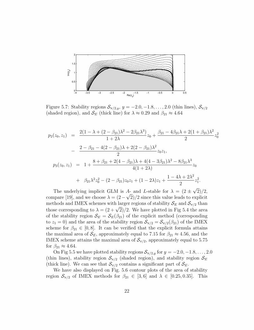
Figure 5.7: Stability regions Sπ/2,y, y = −2.0,−1.8, . . . , 2.0 (thin lines), Sπ/2(shaded region), and SE (thick line) for λ ≈ 0.29 and β21 ≈ 4.64
p2(z0, z1) =2(1− λ+ (2− β21)λ2 − 2β21λ
3)
1 + 2λz0 +
β21 − 4β21λ+ 2(1 + β21)λ2
2z20
− 2− β21 − 4(2− β21)λ+ 2(2− β21)λ2
2z0z1,
p3(z0, z1) = 1 +8 + β21 + 2(4− β21)λ+ 4(4− 3β21)λ
2 − 8β21λ3
4(1 + 2λ)z0
+ β21λ2z20 − (2− β21)z0z1 + (1− 2λ)z1 +
1− 4λ+ 2λ2
2z21 .
The underlying implicit GLM is A- and L-stable for λ = (2 ±√
2)/2,compare [19], and we choose λ = (2−
√2)/2 since this value leads to explicit
methods and IMEX schemes with larger regions of stability SE and Sπ/2 than
those corresponding to λ = (2 +√
2)/2. We have plotted in Fig 5.4 the areaof the stability region SE = SE(β21) of the explicit method (correspondingto z1 = 0) and the area of the stability region Sπ/2 = Sπ/2(β21) of the IMEXscheme for β21 ∈ [0, 8]. It can be verified that the explicit formula attainsthe maximal area of SE, approximately equal to 7.15 for β21 ≈ 4.56, and theIMEX scheme attains the maximal area of Sπ/2, approximately equal to 5.75for β21 ≈ 4.64.
On Fig 5.5 we have plotted stability regions Sπ/2,y for y = −2.0,−1.8, . . . , 2.0(thin lines), stability region Sπ/2 (shaded region), and stability region SE(thick line). We can see that Sπ/2 contains a significant part of SE.
We have also displayed on Fig. 5.6 contour plots of the area of stabilityregion Sπ/2 of IMEX methods for β21 ∈ [3, 6] and λ ∈ [0.25, 0.35]. This
22

area attains its maximum value approximately equal to 5.83 for β21 ≈ 4.59and λ ≈ 0.29. This point is marked by the symbol ‘×’ on Fig. 5.6. OnFig 5.7 we have plotted stability regions Sπ/2,y for y = −2.0,−1.8, . . . , 2.0(thin lines), stability region Sπ/2 (shaded region), and stability region SE(thick line) corresponding to these values of β21 and λ. We can see againthat Sπ/2 contains a significant part of SE.
5.3 IMEX GLMs with p = q = r = s = 3
Let λ ≈ 0.43586652 be a root of the cubic polynomial
ϕ(λ) = λ3 − 3λ2 +3
2λ− 1
6,
and consider the implicit DIMSIM with c = [0, 1/2, 1]T , the coefficient matrixA given by
A =
0.43586652 0 0
0.25051488 0.43586652 0
−1.2115943 1.0012746 0.43586652
,the rank one coefficient matrix V = evT , where e = [1, 1, 1]T and
v =[
0.55209096 0.73485666 −0.28694762]T,
and the vectors q0, q1, q2, and q3 equal to q0 = e,
q1 =[−0.43586652 −0.18638140 0.77445315
]T,
q2 =[
0 −0.092933261 −0.43650382]T,
q3 =[
0 −0.033649982 −0.17642592]T.
Computing the coefficient matrix B from the relation (5.1) leads to themethod of order p = 3 and stage order q = 3. It was demonstrated in[19] that the resulting method is A- and L-stable.
23

The coefficients αjk of the extrapolation formula (3.1) of order p = 3computed from the system (3.7) corresponding to p = s = 3 take the form
α =
α11 α12 α13
α21 α22 α23
α31 α32 α33
=
0 0 1
1 −3 3− β213− β32 3β32 − 8 6− β31 − 3β32
.To investigate the stability properties of the resulting IMEX scheme we
will work with the stability polynomial p(w, z0, z1) obtained by multiplyingstability function of the method by a factor (1−λz1)3, where λ is the diagonalelement of the matrix A. It can be verified that this polynomial takes theform
p(w, z0, z1) = (1− λz1)3w6 − p5(z0, z1)w5 + p4(z0, z1)w4 − p3(z0, z1)w3
+ p2(z0, z1)w2 − p1(z0, z1)w + p0(z0, z1),
with the coefficients p0(z0, z1), p1(z0, z1), p2(z0, z1), p3(z0, z1), p4(z0, z1), andp5(z0, z1) which are polynomials of degree less than or equal to 3 with respectto z0 and z1. These coefficients depend also on β21, β31, and β32.
−2.5 −2 −1.5 −1 −0.5 0 0.50
0.5
1
1.5
2
Re(z0)
Im(z
0)
Figure 5.8: Stability regions Sπ/2,y, y = −2.0,−1.8, . . . , 2.0 (thin lines), Sπ/2(shaded region), and SE (thick line) for β21 ≈ 1.13, β31 ≈ 1.45, and β32 ≈−0.158
We have performed a computer search in the parameter space β21, β31,and β32 looking first for methods for which the stability region SE of theexplicit method is maximal. This corresponds to the parameter values β21 ≈1.13, β31 ≈ 1.45, β32 ≈ −0.158, for which the area of SE is approximately
24

−2.5 −2 −1.5 −1 −0.5 0 0.50
0.5
1
1.5
2
Re(z0)
Im(z
0)
Figure 5.9: Stability regions Sπ/4,y, y = −2.0,−1.8, . . . , 2.0 (thin lines), Sπ/4(shaded region), and SE (thick line) for β21 ≈ 1.13, β31 ≈ 1.45, and β32 ≈−0.158
−2.5 −2 −1.5 −1 −0.5 0 0.50
0.5
1
1.5
2
Re(z0)
Im(z
0)
Figure 5.10: Stability regions Sπ/2,y, y = −2.0,−1.8, . . . , 2.0 (thin lines),Sπ/2 (shaded region), and SE (thick line) for β21 ≈ 1.39, β31 ≈ −0.146, andβ32 ≈ 1.24
equal to 3.54. The stability region SE of the resulting method is plottedon Fig. 5.8 by a thick line. We have also plotted stability regions Sπ/2,yfor y = −2.0,−1.8, . . . , 2.0 (thin lines) and the stability region Sπ/2 (shadedregion) of the corresponding IMEX scheme. We can see that this region Sπ/2is substantially smaller than the region SE, the area of Sπ/2 is approximatelyequal to 0.39. However, we can obtain larger regions Sα for values of αsmaller than π/2, i.e., if we relax the requirement that the implicit part ofIMEX scheme is A-stable and require instead A(α)-stability for α < π/2.This is illustrated on Fig. 5.9, where we have plotted again the stabilityregion SE of the explicit method (thick line), stability regions of Sα,y fory = −2.0,−1.8, . . . , 2.0 (thin lines), and stability region Sα (shaded region)
25

−2.5 −2 −1.5 −1 −0.5 0 0.50
0.5
1
1.5
2
Re(z0)
Im(z
0)
Figure 5.11: Stability regions Sπ/4,y, y = −2.0,−1.8, . . . , 2.0 (thin lines),Sπ/4 (shaded region), and SE (thick line) for β21 ≈ 1.25, β31 ≈ 1.62, andβ32 ≈ 0.0555
for α = π/4. The area of this region is approximately equal to 1.91.We have also performed a computer search looking for methods for which
stability regions Sα are maximal for some fixed values of α. For α = π/2this corresponds to the parameter values β21 ≈ 1.39, β31 ≈ −0.146, andβ32 ≈ 1.24 for which the area of Sπ/2 is approximately equal to 0.50. Forα = π/4 this corresponds to the parameter values β21 ≈ 1.25, β31 ≈ 1.62, andβ32 ≈ 0.00555 for which the area of Sπ/4 is approximately equal to 2.80. Wehave plotted on Fig. 5.10 and Fig. 5.11 the stability regions SE of the resultingexplicit methods (thick lines), the regions Sα,y for y = −2.0,−1.8, . . . , 2.0(thin lines) and stability regions Sα of IMEX schemes (shaded regions) forα = π/2 and α = π/4.
5.4 IMEX GLMs with p = q = r = s = 4
Let λ ≈ 0.57281606 be a root of the polynomial
ϕ(λ) = λ4 − 4λ3 + 3λ2 − 2
3λ+
1
24,
26

and consider the implicit DIMSIM with c = [0, 1/3, 2/3, 1]T , the coefficientmatrix A given by
A =
0.57281606 0 0 0
0.15022075 0.57281606 0 0
0.59515808 −0.26632807 0.57281606 0
1.7717286 −1.64234444 0.39147320 0.57281606
,the rank one coefficient matrix V = evT , where e = [1, 1, 1, 1]T and
v =[
15.615037 −46.967269 41.290082 −8.9378502]T,
and the vectors q0, q1, q2, q3, and q4 equal to q0 = e,
q1 =[−0.57281606 −0.38970348 −0.23497940 −0.093673420
]T,
q2 =[
0 −0.13538313 −0.070879128 0.21364995]T,
q3 =[
0 −0.025650275 −0.063113738 −0.11549405]T,
q4 =[
0 −0.0030214983 −0.018412760 −0.062996758]T.
Computing the coefficient matrix B from the relation (5.1) leads to themethod of order p = 4 and stage order q = 4. It was demonstrated in[26] that the resulting method is A- and L-stable.
The coefficients αjk of the extrapolation formula (3.1) of order p = 4computed from the system (3.7) corresponding to p = s = 4 take the form
α =
0 0 0 1
−1 4 −6 4− β21β32 − 4 15− 4β32 2(3β32 − 10) 10− β31 − 4β32
α41 α42 α43 α44
,with
α41 = β42 + 4β43 − 10, α42 = 36− 4β42 − 15β43,
α43 = 6β42 + 20β43 − 45, α44 = 20− β41 − 4β42 − 10β43.
27

−1.8 −1.6 −1.4 −1.2 −1 −0.8 −0.6 −0.4 −0.2 00
0.5
1
1.5
Re(z0)
Im(z
0)
Figure 5.12: Stability regions Sπ/4,y, y = −2.0,−1.8, . . . , 2.0 (thin lines),Sπ/4 (shaded region), and SE (thick line) for β21 ≈ 0.0645, β31 ≈ −0.351,and β32 ≈ 0.272, β41 ≈ −2.82, β42 ≈ 3.47, β43 ≈ −1.05
−0.8 −0.7 −0.6 −0.5 −0.4 −0.3 −0.2 −0.1 00
0.2
0.4
0.6
0.8
1
Re(z0)
Im(z
0)
π/12 π/6 π/4 π/3 5π/12 π/20
Figure 5.13: Stability regions Sα for α = 0, π/12, π/6, π/4, π/3, 5π/12,and π/2 for β21 ≈ 0.0645, β31 ≈ −0.351, and β32 ≈ 0.272, β41 ≈ −2.82,β42 ≈ 3.47, β43 ≈ −1.05
To investigate the stability properties of the resulting IMEX scheme wewill work with the stability polynomial p(w, z0, z1) obtained by multiplyingstability function of the method by a factor (1−λz1)4, where λ is the diagonalelement of the matrix A. It can be verified that this polynomial takes theform
p(w, z0, z1) = (1− λz1)4w8 − p7(z0, z1)w7 + p6(z0, z1)w6 − p5(z0, z1)w5
+ p4(z0, z1)w4 − p3(z0, z1)w3 + p2(z0, z1)w
2 − p1(z0, z1)w + p0(z0, z1),
with coefficients p0(z0, z1), p1(z0, z1), p2(z0, z1), p3(z0, z1), p4(z0, z1), p5(z0, z1),p6(z0, z1), and p7(z0, z1) which are polynomials of degree less than or equal
28

−0.8 −0.7 −0.6 −0.5 −0.4 −0.3 −0.2 −0.1 00
0.2
0.4
0.6
0.8
1
Re(z0)
Im(z
0)
Figure 5.14: Stability regions Sπ/2,y, y = −2.0,−1.8, . . . , 2.0 (thin lines),Sπ/2 (shaded region), and SE (thick line) for β21 ≈ −0.00516, β31 ≈ −0.939,β32 ≈ 1.18, β41 ≈ −1.71, β42 ≈ 2.07, and β43 ≈ 0.32
−0.8 −0.7 −0.6 −0.5 −0.4 −0.3 −0.2 −0.1 00
0.2
0.4
0.6
0.8
1
Re(z0)
Im(z
0)
Figure 5.15: Stability regions Sπ/4,y, y = −2.0,−1.8, . . . , 2.0 (thin lines),Sπ/4 (shaded region), and SE (thick line) for β21 ≈ 0.0964, β31 ≈ −0.278,β32 ≈ 0.464, β41 ≈ −1.63, β42 ≈ 2.73, and β43 ≈ −0.678
to 4 with respect to z0 and z1. These coefficients depend also on β21, β31,β32, β41, β42, and β43.
We have performed a computer search in the parameter space β21, β31,β32, β41, β42, and β43 looking first for methods for which the stability regionSE of the explicit method is maximal. This corresponds to the parametervalues β21 ≈ 0.0625, β31 ≈ −0.355, β32 ≈ 0.272, β41 ≈ −2.84, β42 ≈ 3.49,β43 ≈ −1.06, for which the area of SE is approximately equal to 2.82. Thestability region SE of the resulting method is plotted on Fig. 5.12 by a thickline. We have also plotted stability regions Sπ/4,y for y = −2.0,−1.8, . . . , 2.0(thin lines) and the stability region Sπ/4 (shaded region) of the corresponding
29

IMEX scheme. The area of Sπ/4 is approximately equal to 0.32. We havealso plotted on Fig. 5.13 stability regions Sα for α = 0, π/12, π/6, π/4,π/3, 5π/12, and π/2 corresponding to the same values of βij. We can see inparticular that the region Sπ/2 is quite small, its area is approximately equalto 0.0069.
As in Section 5.3 we have also performed a computer search lookingdirectly for methods for which stability regions Sα are maximal for somefixed values of α. For α = π/2 this corresponds to the parameter valuesβ21 ≈ −0.00516, β31 ≈ −0.939, β32 ≈ 1.18, β41 ≈ −1.71, β42 ≈ 2.07, andβ43 ≈ 0.32, for which the area of Sπ/2 is approximately equal to 0.16. For α =π/4 this corresponds to the parameter values β21 ≈ 0.0964, β31 ≈ −0.278,β32 ≈ 0.464, β41 ≈ −1.63, β42 ≈ 2.73, and β43 ≈ −0.678, for which thearea of Sπ/4 is approximately equal to 0.65. We have plotted on Fig. 5.14and Fig. 5.15 the stability regions SE of the resulting explicit methods (thicklines), the regions Sα,y for y = −2.0,−1.8, . . . , 2.0 (thin lines) and stabilityregions Sα of IMEX schemes (shaded regions) for α = π/2 and α = π/4.
6 Numerical experiments
The extrapolation-based IMEX GLMs constructed in Section 5 have beenimplemented in Matlab. The required starting values y[0] and Y [0] were com-puted by finite difference approximations from solutions obtained with theMatlab routine ode15s.
The test problem is the two dimensional shallow-water equations system[21], which approximates a thin layer of fluid inside a shallow basin:
∂
∂th+
∂
∂x(uh) +
∂
∂y(vh) = 0
∂
∂t(uh) +
∂
∂x
(u2h+
1
2gh2)
+∂
∂y(uvh) = 0 (6.1)
∂
∂t(vh) +
∂
∂x(uvh) +
∂
∂y
(v2h+
1
2gh2)
= 0 .
Here h(t, x, y) is the fluid layer thickness, u(t, x, y) and v(t, x, y) are the com-ponents of the velocity field, and g denotes the gravitational acceleration.The spatial domain is Ω = [−3, 3]2 (spatial units), and the integration win-dow is t0 = 0 ≤ t ≤ tf = 10 (time units). We use reflective boundary
30

conditions and the initial conditions at t0 = 0
u(t0, x, y) = v(t0, x, y) = 0 , h(t0, x, y) = 1 + e−‖(x,y)−(c1,c2)‖22 , (6.2)
with the Gaussian height profile c1 = 1/3 and c2 = 2/3.A second order Lax-Wendroff finite difference scheme is used for space
discretization, resulting in a semi-discrete ODE system of the form
d
dtU(t) = F (U) = FU
(U)· U(t)︸ ︷︷ ︸
g(U)
+(F (U)− FU
(U)· U(t)
)︸ ︷︷ ︸f(U)
, (6.3)
where U(t) is a combined column vector of the discretized state variables
(h, uh, vh), and FU = ∂F/∂U be the Jacobian of right hand side. We considera splitting of equation (6.3) into the linear part g(U), considered stiff, andthe nonlinear part f(U), considered non-stiff. The linear stiff part is treatedimplicitly, and the non-stiff part is treated explicitly.
We compare the numerical results for the solution at the final time with areference solution computed by the Matlab function ode15s with very tighttolerances atol = rtol = 10−14. The errors are measured in L2 norms. Theerror diagram against the time step size is presented in Fig. 6.1. The observedorders for all the methods tested match the theoretical predictions.
7 Concluding remarks
General linear methods offer an excellent framework for the construction ofimplicit-explicit schemes. In this paper we develop a new extrapolation-basedapproach for the construction of practical IMEX GLM schemes of high orderand high stage order. The accuracy, linear stability, and Prothero-Robinsonconvergence are analyzed. These schemes are particularly attractive for solv-ing stiff problems, where other multistage methods may suffer from orderreduction.
The extrapolation-based mechanism offers a systematic approach for con-structing IMEX GLM schemes. The construction starts with the selection ofan implicit component method with suitable stability and order properties.The explicit component is then obtained though an optimization procedurethat maximized the combined stability region of the pair. We apply thismethodology to construct IMEX pairs of orders one to four.
31

10−2
10−1
10−6
10−5
10−4
10−3
10−2
10−1
100
Time step h
Errorin
L2norm
p= 2,IMEX GLMO(h2)p= 3,IMEX GLMO(h3)p= 4,IMEX GLMO(h4)
Figure 6.1: Error vs. time step size for several extrapolation-based IMEX-GLMs applied to the shallow water equations test problem.
Future work is planned to extend the extrapolation idea to constructother types of partitioned GLMs, including parallel time integrators, andasynchronous pairs of methods that do not share the same abscissae.
Acknowledgements. The results reported in this paper were obtainedduring the visit of the first author to the Arizona State University in January–March of 2013. This author wish to express her gratitude to the Schoolof Mathematical and Statistical Sciences for hospitality during this visit.The work of Sandu and Zhang has been supported in part by the awardsNSF OCI-8670904397, NSF CCF-0916493, NSF DMS-0915047, NSF CMMI-1130667, NSF CCF-1218454, AFOSR FA9550-12-1-0293-DEF, AFOSR 12-2640-06, and by the Computational Science Laboratory at Virginia Tech.
References
[1] Ascher, U.M., Ruuth, S.J., Spiteri, R.J.: Implicit-explicit Runge-Kuttamethods for time-dependent partial differential equations. Appl. Numer.
32

Math 25, 151–167 (1997)
[2] Ascher, U.M., Ruuth, S.J., Wetton, B.T.R.: Implicit-explicit methodsfor time-dependent partial differential equations. SIAM J. Numer. Anal.32(3), 797–823 (1995)
[3] Burrage, K.: Parallel and sequential methods for ordinary differentialequations. Clarendon Press, New York, NY, USA (1995)
[4] Burrage, K., Butcher, J.: Non-linear stability of a general class of dif-ferential equation methods. BIT Numerical Mathematics 20, 185–203(1980)
[5] Butcher, J.C.: The numerical analysis of ordinary differential equations:Runge-Kutta and general linear methods. Wiley-Interscience, New York,NY, USA (1987)
[6] Butcher, J.C.: Diagonally-implicit multi-stage integration methods.Appl. Numer. Math. 11(5), 347–363 (1993)
[7] Butcher, J.C.: Numerical methods for ordinary differential equations.John Wiley & Sons Ltd., Chichester (2003)
[8] Butcher, J.C.: General linear methods. Acta Numer. 15, 157–256 (2006)
[9] Butcher, J.C., Jackiewicz, Z.: Diagonally implicit general linear methodsfor ordinary differential equations. BIT 33(3), 452–472 (1993)
[10] Calvo, M.P., de Frutos, J., Novo, J.: Linearly implicit Runge-Kuttamethods for advection-reaction-diffusion equations. Appl. Numer. Math.37(4), 535–549 (2001)
[11] Cardone, A., Jackiewicz, Z.: Explicit Nordsieck methods with quadraticstability. Numerical Algorithms 60, 1–25 (2012)
[12] Cardone, A., Jackiewicz, Z., Mittelmann, H.: Optimization-based searchfor Nordsieck methods of high order with quadratic stability. Math.Model. Anal. 17(3), 293–308 (2012)
[13] Crouzeix, M.: Une methode multipas implicite-explicite pourl’approximation des equations d’evolution paraboliques. Numer. Math.35(3), 257–276 (1980)
33
[14] Frank, J., Hundsdorfer, W., Verwer, J.G.: On the stability of implicit-explicit linear multistep methods. Appl. Numer. Math. 25(2-3), 193–205(1997). Special issue on time integration (Amsterdam, 1996)
[15] Hairer, E., Lubich, C., Wanner, G.: Geometric numerical integration: structure-preserving algorithms for ordinary differential equations.Springer-Verlag, New York (2002)
[16] Hairer, E., Nørsett, S.P., Wanner, G.: Solving ordinary differential equa-tions. I, Springer Series in Computational Mathematics, vol. 8, secondedn. Springer-Verlag, Berlin (1993). Nonstiff problems
[17] Hairer, E., Wanner, G.: Solving ordinary differential equations. II,Springer Series in Computational Mathematics, vol. 14. Springer-Verlag,Berlin (2010). Stiff and differential-algebraic problems, Second revisededition, paperback
[18] Hundsdorfer, W., Verwer, J.: Numerical solution of time-dependentadvection-diffusion-reaction equations, Springer Series in Computa-tional Mathematics, vol. 33. Springer-Verlag, Berlin (2003)
[19] Jackiewicz, Z.: General linear methods for ordinary differential equa-tions. John Wiley & Sons Inc., Hoboken, NJ (2009)
[20] Kennedy, C.A., Carpenter, M.H.: Additive Runge-Kutta schemes forconvection-diffusion-reaction equations. Appl. Numer. Math. 44(1-2),139–181 (2003)
[21] Liska, R., Wendroff, B.: Composite schemes for conservation laws. SIAMJournal on Numerical Analysis 35(6), pp. 2250–2271 (1998)
[22] Pareschi, L., Russo, G.: Implicit-explicit Runge-Kutta schemes for stiffsystems of differential equations. In: Recent trends in numerical anal-ysis, Adv. Theory Comput. Math., vol. 3, pp. 269–288. Nova Sci. Publ.,Huntington, NY (2001)
[23] Pareschi, L., Russo, G.: Implicit-Explicit Runge-Kutta schemes andapplications to hyperbolic systems with relaxation. J. Sci. Comput.25(1-2), 129–155 (2005)
34

[24] Prothero, A., Robinson, A.: On the stability and accuracy of one-step methods for solving stiff systems of ordinary differential equations.Math. Comput 28(125), 145–162 (1974)
[25] Varah, J.M.: Stability restrictions on second order, three level finitedifference schemes for parabolic equations. SIAM J. Numer. Anal. 17(2),300–309 (1980)
[26] Wright, W.M.: The construction of order 4 DIMSIMs for ordinary dif-ferential equations. Numer. Algorithms 26(2), 123–130 (2001)
[27] Zhang, H., Sandu, A.: A second-order diagonally-implicit-explicit multi-stage integration method. Procedia CS 9, 1039–1046 (2012)
[28] Zhang, H., Sandu, A.: Partitioned and implicit-explicit general linearmethods for ordinary differential equations. http://arxiv.org/abs/
1302.2689 (2013)
[29] Zharovski, E., Sandu, A.: A class of implicit-explicit two-step Runge-Kutta methods. Tech. Rep. TR-12-08, Computer Science, VirginiaTech., http://eprints.cs.vt.edu/archive/00001183 (2012)
[30] Zhong, X.: Additive semi-implicit Runge-Kutta methods for computinghigh-speed nonequilibrium reactive flows. J. Comput. Phys. 128(1),19–31 (1996)
35