Delft University of Technology Comparison of Implicit and Explicit

Delft University of Technology

Comparison of Implicit and Explicit Vegetation Representations in SWAN HindcastingWave Dissipation by Coastal Wetlands in Chesapeake Bay

Baron-Hyppolite, C.G.; Lashley, Chris; Garzon, Juan; Miesse, Tyler; Bricker, Jeremy

DOI10.3390/geosciences9010008Publication date2018Document VersionFinal published versionPublished inGeosciences (Switzerland)

Citation (APA)Baron-Hyppolite, C. G., Lashley, C., Garzon, J., Miesse, T., & Bricker, J. (2018). Comparison of Implicit andExplicit Vegetation Representations in SWAN Hindcasting Wave Dissipation by Coastal Wetlands inChesapeake Bay. Geosciences (Switzerland), 9(1), [8]. https://doi.org/10.3390/geosciences9010008

Important noteTo cite this publication, please use the final published version (if applicable).Please check the document version above.

CopyrightOther than for strictly personal use, it is not permitted to download, forward or distribute the text or part of it, without the consentof the author(s) and/or copyright holder(s), unless the work is under an open content license such as Creative Commons.

Takedown policyPlease contact us and provide details if you believe this document breaches copyrights.We will remove access to the work immediately and investigate your claim.

This work is downloaded from Delft University of Technology.For technical reasons the number of authors shown on this cover page is limited to a maximum of 10.

https://doi.org/10.3390/geosciences9010008

https://doi.org/10.3390/geosciences9010008

geosciences

Article

Comparison of Implicit and Explicit VegetationRepresentations in SWAN Hindcasting WaveDissipation by Coastal Wetlands in Chesapeake Bay

Christophe Baron-Hyppolite 1, Christopher H. Lashley 1,*, Juan Garzon 2, Tyler Miesse 2,Celso Ferreira 2 and Jeremy D. Bricker 1

1 Department of Hydraulic Engineering, Faculty of Civil Engineering and Geosciences, Delft University ofTechnology, PO Box 5048, 2600 GA Delft, The Netherlands; [email protected] (C.B.-H.);[email protected] (J.D.B.)

2 Sid and Reva Dewberry Department of Civil, Environmental and Infrastructure Engineering, George MasonUniversity, 4400 University Drive, MS-6C1, Fairfax, VA 22030, USA; [email protected] (J.G.);[email protected] (T.M.); [email protected] (C.F.)

* Correspondence: [email protected]

Received: 28 November 2018; Accepted: 21 December 2018; Published: 24 December 2018 ��

Abstract: Assessing the accuracy of nearshore numerical models—such as SWAN—is importantto ensure their effectiveness in representing physical processes and predicting flood hazards.In particular, for application to coastal wetlands, it is important that the model accurately representswave attenuation by vegetation. In SWAN, vegetation might be implemented either implicitly,using an enhanced bottom friction; or explicitly represented as drag on an immersed body.While previous studies suggest that the implicit representation underestimates dissipation, field datahas only recently been used to assess fully submerged vegetation. Therefore, the present studyinvestigates the performance of both the implicit and explicit representations of vegetation in SWANin simulating wave attenuation over a natural emergent marsh. The wave and flow modules withinDelft3D are used to create an open-ocean model to simulate offshore wave conditions. The domain isthen decomposed to simulate nearshore processes and provide the boundary conditions necessary torun a standalone SWAN model. Here, the implicit and explicit representations of vegetation are finallyassessed. Results show that treating vegetation simply as enhanced bottom roughness (implicitly)under-represents the complexity of wave-vegetation interaction and, consequently, underestimateswave energy dissipation (error > 30%). The explicit vegetation representation, however, shows goodagreement with field data (error < 20%).

Keywords: storm surge; hurricane; SWAN; vegetation; wave dissipation; bottom roughness;drag coefficient; hard versus soft countermeasures

1. Introduction

1.1. Background

Coastal zones have experienced massive population growth for decades, leading to large denselypopulated urban centers that have dramatically changed coastal environments around the world.These regions are often exposed to potentially destructive hurricanes or coastal storms that can lead tolarge economic and societal losses if not properly forecasted or mitigated. To properly represent andquantify coastal flood hazards, complex numerical modeling is carried out for nearshore, and offshorewave climates. Accurately modeling wave climates means incorporating a variety of complex processes,such as wind-wave generation, energy transfer between frequencies; and dissipation by wave breaking,

Geosciences 2019, 9, 8; doi:10.3390/geosciences9010008 www.mdpi.com/journal/geosciences

http://www.mdpi.com/journal/geosciences

http://www.mdpi.com

http://dx.doi.org/10.3390/geosciences9010008

http://www.mdpi.com/journal/geosciences

http://www.mdpi.com/2076-3263/9/1/8?type=check_update&version=2

Geosciences 2019, 9, 8 2 of 22

bottom friction and vegetation. Among these complex processes, wave dissipation and the resultingstorm surge reduction by vegetation has garnered interest for its potential as a cost-effective softcountermeasure in flood mitigation and protection [1,2].

Camfield [3] and Kobayashi et al. [4] both formulated analytical solutions to describe thedissipation waves experience as they propagate over vegetation. Both solutions derived the dragimposed by vegetation using the Manning roughness coefficient (n) [5], which was traditionallyused to describe bottom roughness of flows over open channels and flood plains. This implicitapproach expressed the drag related to vegetation as an enhanced bottom friction, ignoring theinfluence of vegetation height, density and diameter on the magnitude of the drag forces. Studieslike [6–9] continued to use this formulation in both numerical and physical modeling studies; however,these studies have also identified the need to describe the force applied by vegetation as both a bottomfriction and drag force. This conclusion is reinforced by [10–12], which revealed the complexity of thewave dissipation process. They identified how vegetation height, density, and diameter can spatiallyvary dissipation rates horizontally and vertically across vegetation fields [13]. Further emphasis wasplaced on the impact of flexible vegetation on wave dissipation, showing that flexible vegetation canlead to a reduction of wave dissipation and change in velocity profile [14,15]. These findings werefurther elaborated on in [16] which identified an effective length at which relative motion between theblade and water is significant. This suggests that to implement flexible vegetation the effective lengthcan be used in numerical models as opposed to just the length. Cavallaro et al. [17] also showed thatthe drag coefficient is influenced by the ratio between plant length and water depth.

These findings have led to several assessments of the vegetation representations in the widely-usednearshore numerical models, such as SWAN [2,18–20] and XBeach [21]. Smith et al. [19] indicatedthe potential limitations of using n to represent wave dissipation by vegetation and supportedits conclusions with laboratory data. Nowacki et al. [20] conducted an assessment similar toSmith et al. [19] on fully submerged sea grass, indicating the potential shortcomings of relatingvegetation characteristics to friction length and bottom friction by relation. Such assessments—wherethe formulations and input parameters of the numerical model are evaluated—may identify areas ofimprovement and, accordingly, improve how we manage coastal hazards.

Using field data collected during Hurricane Joaquin (2015), this paper focuses on theimplementation of vegetation in the SWAN numerical model [22] providing a comparison betweenthe: (i) implicit approach, where vegetation is represented as an enhanced bottom friction throughthe use of n, and (ii) the explicit approach, where vegetation is represented as drag on an immersedbody, while simultaneously providing additional information on wave dissipation during extremeweather events. It is important to mention that the SWAN model cannot directly simulate diffraction,which may be important over wetlands. Other models such as the aforementioned XBeach modeland 2DH Boussinesq models described in [23–25], which resolve individual waves, can capture thisphysics directly. However, SWAN is one of the most commonly used nearshore models for replicationof storm waves (forced by hurricane winds) over vegetation fields at large spatial scales because it isphase-averaged and therefore able to simulate large domains over long time periods.

1.2. SWAN Model Description

SWAN is a widely-used spectral (phase-averaged) numerical model which predicts the evolutionof wave energy in space and time. It assumes that a random sea state is composed of an infinitenumber of linear waves whose height are a function of wave frequency and the direction of wavepropagation. For an individual wave train, the rate of change of wave energy (action) flux is balancedby the wave energy transfer among different wave components in different directions and differentfrequencies as well as energy input and dissipation. The basic conservation equation follows [22]:

∂A∂t

+∂cx A

∂x+

∂cy A∂y

+∂cθ A

∂θ+

∂cσ A∂σ

=Stot

σ, (1)


Stot = Sin + Snl4 + Snl3 + Sds,w + Sds,b + Sds,br, (2)

where A is the wave action density, σ is the relative frequency; cx, cy, cθ and cσ are the propagationspeeds in x, y, directional and frequency space; and (Stot) represents source (input) and sink (dissipation)terms. Source terms represent wind input (Sin), quadruplet (Snl4) and triad (Snl3) wave–waveinteractions; while sink terms represent dissipation by white-capping (Sds,w), bottom friction (Sds,b) anddepth-limited wave breaking (Sds,br).

With the implicit approach, vegetation may be represented in Sds,b by means of the Madsenformula [26]. This requires the conversion of the Manning roughness coefficient into a friction length(KN), as shown below from Equation (3) to Equation (6):

KN = Hexp

[−(

1 +kH

16

n√

g

)], (3)

14√

fw+ log

14√

fw= −0.08 + log

abKN

, (4)

Cb = fwg√2

Urms, (5)

Sds,b = −Cbσ2

g2sinh2(kd)E(σ, θ), (6)

where Sds,b is the energy dissipation due to bottom friction, Cb is the drag coefficient, σ is the frequency,k is the wave number, E(σ, θ) is the total energy in both the frequency and directional space, H is thesignificant wave height, n is the Manning roughness coefficient, fw is the non-dimensional frictionfactor, ab is the representative near-bottom excursion amplitude, and the bottom orbital motion.This suggests that in SWAN, vegetation represented implicitly is treated as an enhanced bottomfriction value, made to represent the increase resistance that occurs when the waves interact withthe saltmarsh.

The adjustment of the Madsen bottom friction formulation is done through the selection of theappropriate n values. The magnitude of the n is dependent on characteristics, such as: material,surface irregularities, flood plain cross section, obstructions in the flood plain, and vegetation [27].The influence these characteristics have on the overall n is determined by survey and laboratory testsand can be influenced by personal judgment [27]. Once these values are determined, it is advised tocompare roughness results to areas with similar characteristics. This uncertainty was addressed by theUnited States National Land Cover Data base (NLCD) [28], which gives coastal regions n values foruse by engineers in the United States.

There are still key interactions that the n may not properly represent, such as resistance due todrag forces on the water column. Drag caused by water flowing through marshland can vary verticallyor horizontally and have a higher impact on the water column than the manning bottom roughnesscoefficient [11]. Both studies of Dalrymple et al. [13] and Méndez et al. [10] focus on representingvegetation as a field of stiff cylinders, allowing them to assign vegetation characteristics to the cylinders.The drag force between the vegetation and the wave field acts on the surface area of the cylinders.The explicit vegetation representation stems from the study of [13] on wave diffraction due to areasof energy dissipation, which expresses energy losses as work carried out by the vegetation on theincoming wave and is shown in Equation (7). This method assumes stiff vegetation, ignoring theinfluence of sway on the wave dissipation. In SWAN, the Dalrymple formula is modified by [29]for irregular waves, giving the mean rate of energy dissipation per unit horizontal area due to wavedamping by vegetation shown in Equation (7). Where (ρ) references to the density of ocean water,(CD) is the drag coefficient of the vegetation, (bv) is the stem diameter, (Nv) is the number of plants,


(g) is the gravitational acceleration, (k) is the wave number, (σ) is the frequency, (αh) is the vegetationheight, (h) is the water depth and (Hrms) is root mean square wave height.

εv =1

2√

πρCDbvNv

gk2σ

3 sinh3kαh + 3sinhkαhcosh kh

H3rms (7)

Neumeier and Amos [11] show that vegetation characteristics used in Equation (7) not only varyhorizontally across a marsh but also vertically, causing the dissipation profiles to vary vertically aswell as horizontally. This highlights the complexity of the dissipation process, as described in [13];a complexity that is not addressed when using the implicit manning roughness implementation.

1.3. Site Description

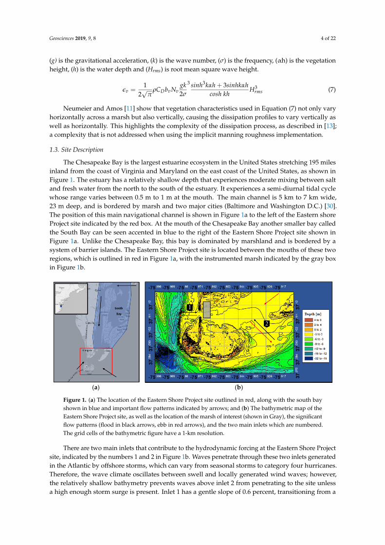
The Chesapeake Bay is the largest estuarine ecosystem in the United States stretching 195 milesinland from the coast of Virginia and Maryland on the east coast of the United States, as shown inFigure 1. The estuary has a relatively shallow depth that experiences moderate mixing between saltand fresh water from the north to the south of the estuary. It experiences a semi-diurnal tidal cyclewhose range varies between 0.5 m to 1 m at the mouth. The main channel is 5 km to 7 km wide,23 m deep, and is bordered by marsh and two major cities (Baltimore and Washington D.C.) [30].The position of this main navigational channel is shown in Figure 1a to the left of the Eastern shoreProject site indicated by the red box. At the mouth of the Chesapeake Bay another smaller bay calledthe South Bay can be seen accented in blue to the right of the Eastern Shore Project site shown inFigure 1a. Unlike the Chesapeake Bay, this bay is dominated by marshland and is bordered by asystem of barrier islands. The Eastern Shore Project site is located between the mouths of these tworegions, which is outlined in red in Figure 1a, with the instrumented marsh indicated by the gray boxin Figure 1b.

Geosciences 2018, 8, x FOR PEER REVIEW 5 of 22

(a) (b)

Figure 1. (a) The location of the Eastern Shore Project site outlined in red, along with the south bay

shown in blue and important flow patterns indicated by arrows; and (b) The bathymetric map of the

Eastern Shore Project site, as well as the location of the marsh of interest (shown in Gray), the

significant flow patterns (flood in black arrows, ebb in red arrows), and the two main inlets which are

numbered. The grid cells of the bathymetric figure have a 1‐km resolution.

Similar to the mouth of the Chesapeake Bay, the Eastern Shore Project site experiences a semi‐

diurnal tide cycle with a tidal range varying between 0.5 m to 1 m. With the most landward portion

of the site lying 1 m above mean sea level, the site is only partially inundated during high spring tide

and is completely dry during low spring tide. During the transition from flood to ebb, the dominant

flow to the research site enters from the mouth of the South Bay indicated by the red arrows in Figure

1. The flow continues around Raccoon Island and exits through inlet 1, into the main channel of the

Chesapeake Bay.

The project site is covered by Spartina Alterniflora, a saltmarsh plant found commonly along the

eastern coast of the United States. The wider area also consists of deciduous coastal forest, coastal

shrubland and coastal grassland. These various vegetation types each contribute to the mitigation of

flood hazards impacting the surrounding community.

1.4. Data Description

The field data is recorded using 4 Trublue 255‐70530 pressure gauges set along the marsh from

the leading edge to the rear. These pressure gauges provide temperature (Celsius) and pressure (PSI)

readings, taken at intervals of a 0.25 seconds from 24 September to 2 October of 2015. The gauges

have an accuracy of ±0.5% FS TEB with a resolution of 0.01% FS or better (FS meaning full scale or

difference between the highest and lowest measurement, and TEB means total error band which

includes errors due to non‐linearity, hysteresis, non‐repeatability and thermal effects). The pressure

time series is converted to a water level time series where the significant wave heights (Hs) and

periods can be extracted through spectral analysis. These results are then used to validate the model.

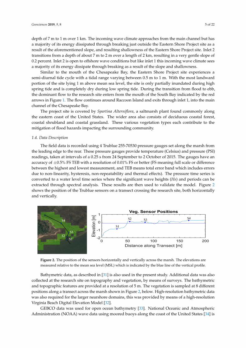
Figure 2 shows the position of the Trublue sensors on a transect crossing the research site, both

horizontally and vertically.

Bathymetric data, as described in [31] is also used in the present study. Additional data was also

collected at the research site on topography and vegetation, by means of surveys. The bathymetric

and topographic features are provided at a resolution of 5 m. The vegetation is sampled at 8 different

positions along a transect across the marsh shown in Figure 2, below. High‐resolution bathymetric

data was also required for the larger nearshore domains, this was provided by means of a high‐

resolution Virginia Beach Digital Elevation Model [32].

GEBCO data was used for open ocean bathymetry [33]. National Oceanic and Atmospheric

Administration (NOAA) wave data using moored buoys along the coast of the United States [34] is

Figure 1. (a) The location of the Eastern Shore Project site outlined in red, along with the south bayshown in blue and important flow patterns indicated by arrows; and (b) The bathymetric map of theEastern Shore Project site, as well as the location of the marsh of interest (shown in Gray), the significantflow patterns (flood in black arrows, ebb in red arrows), and the two main inlets which are numbered.The grid cells of the bathymetric figure have a 1-km resolution.

There are two main inlets that contribute to the hydrodynamic forcing at the Eastern Shore Projectsite, indicated by the numbers 1 and 2 in Figure 1b. Waves penetrate through these two inlets generatedin the Atlantic by offshore storms, which can vary from seasonal storms to category four hurricanes.Therefore, the wave climate oscillates between swell and locally generated wind waves; however,the relatively shallow bathymetry prevents waves above inlet 2 from penetrating to the site unlessa high enough storm surge is present. Inlet 1 has a gentle slope of 0.6 percent, transitioning from a


depth of 7 m to 1 m over 1 km. The incoming wave climate approaches from the main channel but hasa majority of its energy dissipated through breaking just outside the Eastern Shore Project site as aresult of the aforementioned slope, and resulting shallowness of the Eastern Shore Project site. Inlet 2transitions from a depth of about 7 m to 2 m over a length of 2 km, resulting in a very gentle slope of0.2 percent. Inlet 2 is open to offshore wave conditions but like inlet 1 this incoming wave climate seesa majority of its energy dissipate through breaking as a result of the slope and shallowness.

Similar to the mouth of the Chesapeake Bay, the Eastern Shore Project site experiences asemi-diurnal tide cycle with a tidal range varying between 0.5 m to 1 m. With the most landwardportion of the site lying 1 m above mean sea level, the site is only partially inundated during highspring tide and is completely dry during low spring tide. During the transition from flood to ebb,the dominant flow to the research site enters from the mouth of the South Bay indicated by the redarrows in Figure 1. The flow continues around Raccoon Island and exits through inlet 1, into the mainchannel of the Chesapeake Bay.

The project site is covered by Spartina Alterniflora, a saltmarsh plant found commonly alongthe eastern coast of the United States. The wider area also consists of deciduous coastal forest,coastal shrubland and coastal grassland. These various vegetation types each contribute to themitigation of flood hazards impacting the surrounding community.

1.4. Data Description

The field data is recorded using 4 Trublue 255-70530 pressure gauges set along the marsh fromthe leading edge to the rear. These pressure gauges provide temperature (Celsius) and pressure (PSI)readings, taken at intervals of a 0.25 s from 24 September to 2 October of 2015. The gauges have anaccuracy of ±0.5% FS TEB with a resolution of 0.01% FS or better (FS meaning full scale or differencebetween the highest and lowest measurement, and TEB means total error band which includes errorsdue to non-linearity, hysteresis, non-repeatability and thermal effects). The pressure time series isconverted to a water level time series where the significant wave heights (Hs) and periods can beextracted through spectral analysis. These results are then used to validate the model. Figure 2shows the position of the Trublue sensors on a transect crossing the research site, both horizontallyand vertically.


used to validate the regional model results. Regional model tide data was provided by the TPXO7.2

tidal model [35]. Landcover data used in the SWAN standalone model to identify vegetation cover

at the research site which was provided [28].

Figure 2. The position of the sensors horizontally and vertically across the marsh. The elevations are

measured relative to the mean sea level (MSL) which is indicated by the blue line of the vertical

profile.

1.4.1. General Wave Climate

Figure 3 shows the wave climate recorded by the four Trublue pressure sensors on the marsh.

Figure 3a show a decrease in wave energy across all frequencies from sensors 1 to 4, with most of the

energy focused between 2 Hz to 5 Hz. This indicates a locally generated wind wave climate entering

the marsh at sensor 1. Figure 3b indicates a transition of the Tp range from 2 s–10 s to 2 s–16 s,

suggesting a transition of wave energy from high to low frequencies. Figure 3c shows a range of Hs

from 0.02 m to 0.42 m, with the peak wave height occurring on 27 September. During the time of

interest, the wave heights are reduced by about 80% from sensor 1 to sensor 4. Figure 3d shows the

water levels recorded at the marsh about the NAVD88 vertical datum as well as the tide cycle during

this time. The storm surge is the difference between the water level and the astronomical tide. Like

the Hs the peak water level occurs during 27 September where it reaches 1.15 m resulting in a storm

surge of about 0.4 m. From Figure 3b–3d there are gaps in the wave data caused by cutoffs applied

at points where the water levels are too low for the pressure sensors to reliably record accurate data.

The cutoff applied for sensors 1 to 3 are 0.3 m above the vertical datum; for sensor 4 the cut off is

applied at 0.5 m above the vertical datum.

Figure 2. The position of the sensors horizontally and vertically across the marsh. The elevations aremeasured relative to the mean sea level (MSL) which is indicated by the blue line of the vertical profile.

Bathymetric data, as described in [31] is also used in the present study. Additional data was alsocollected at the research site on topography and vegetation, by means of surveys. The bathymetricand topographic features are provided at a resolution of 5 m. The vegetation is sampled at 8 differentpositions along a transect across the marsh shown in Figure 2, below. High-resolution bathymetric datawas also required for the larger nearshore domains, this was provided by means of a high-resolutionVirginia Beach Digital Elevation Model [32].

GEBCO data was used for open ocean bathymetry [33]. National Oceanic and AtmosphericAdministration (NOAA) wave data using moored buoys along the coast of the United States [34] is


used to validate the regional model results. Regional model tide data was provided by the TPXO7.2tidal model [35]. Landcover data used in the SWAN standalone model to identify vegetation cover atthe research site which was provided [28].

1.4.1. General Wave Climate

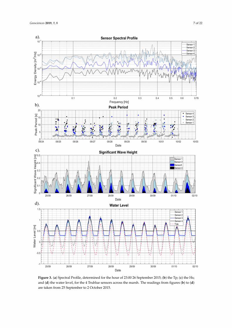
Figure 3 shows the wave climate recorded by the four Trublue pressure sensors on the marsh.Figure 3a show a decrease in wave energy across all frequencies from sensors 1 to 4, with most ofthe energy focused between 2 Hz to 5 Hz. This indicates a locally generated wind wave climateentering the marsh at sensor 1. Figure 3b indicates a transition of the Tp range from 2 s–10 s to 2 s–16 s,suggesting a transition of wave energy from high to low frequencies. Figure 3c shows a range of Hsfrom 0.02 m to 0.42 m, with the peak wave height occurring on 27 September. During the time ofinterest, the wave heights are reduced by about 80% from sensor 1 to sensor 4. Figure 3d shows thewater levels recorded at the marsh about the NAVD88 vertical datum as well as the tide cycle duringthis time. The storm surge is the difference between the water level and the astronomical tide. Like theHs the peak water level occurs during 27 September where it reaches 1.15 m resulting in a storm surgeof about 0.4 m. From Figure 3b–d there are gaps in the wave data caused by cutoffs applied at pointswhere the water levels are too low for the pressure sensors to reliably record accurate data. The cutoffapplied for sensors 1 to 3 are 0.3 m above the vertical datum; for sensor 4 the cut off is applied at 0.5 mabove the vertical datum.

Geosciences 2019, 9, 8 7 of 22Geosciences 2018, 8, x FOR PEER REVIEW 7 of 22

Figure 3. (a) Spectral Profile, determined for the hour of 23:00 26 September 2015; (b) the Tp; (c) the

Hs; and (d) the water level, for the 4 Trublue sensors across the marsh. The readings from figures (b)

to (d) are taken from 25 September to 2 October 2015.

Figure 3. (a) Spectral Profile, determined for the hour of 23:00 26 September 2015; (b) the Tp; (c) the Hs;and (d) the water level, for the 4 Trublue sensors across the marsh. The readings from figures (b) to (d)are taken from 25 September to 2 October 2015.


1.4.2. Wind

Wind and sea level air pressure are provided by the ECMWF (European Center for Medium rangeWeather Forecast) atmospheric operational model. The data provided by the ECMWF encompasses thewhole of the Gulf of Mexico as well as part of the Atlantic Ocean just off the east coast of the UnitedStates. The grid has a 0.141 degree or 15.5 km north–south and a 12.5 km east–west resolution witha time step of 6 h between each wind velocity and pressure reading [36]. The local accuracy of thiswind model was verified by Garzon et al. [37]. The ECMWF winds were compared with local weatherstations, the highest correlation occurred at the mouth of Chesapeake Bay where it reached over 95%correlation to station data [37].

2. Modeling Approach

In order to run the SWAN standalone model (SSAM) for the study area, boundary conditionsneeded to be determined. This was done through the creation of a Delft 3D Flow + Wave modelthat recreates the necessary offshore and nearshore wave conditions. This Methodology section istherefore broken down into three parts, each describing the models mentioned above. These partsinclude: (i) the largest (2120 km by 2483 km) Open Ocean model (OOM), whose purpose is to recreateoffshore wave climate and storm surge due to meteorological forcing; (ii) the Nearshore ProcessesModel (NPM), which refines portions of the OOM to recreate the nearshore processes necessary toproduce boundary conditions; and (iii) the SWAN Standalone model (SSAM), which uses the boundaryconditions produced by the NPM to assess the vegetation representations.

2.1. Open Ocean Model (OOM)

The OOM model was created in Delft3D Flow + Wave modules using the meteorological data,GEBCO bathymetry and TPXO7.2 tide data [35]. The Delft 3D Flow and Wave modules were two-waycoupled, meaning that the Wave module passed information on radiation stresses to the Flow module,and the Flow module passed information on water depth and flow speed to the wave module [38].The time step for this computation is set to 10 min with the coupling interval set to 60 min. Riemannboundary conditions are selected for this model in order to minimize reflection.

The final setup of the OOM model consists of two computational grids shown in Figure 4,a 0.075-degree (8.25 km) resolution outer domain and a 0.015-degree (1.6km) resolution inner domain(which was decomposed from the larger grid), three 0.141-degree equidistant meteorological grids,and 0.008 degree (0.9 km) bathymetric grid. The time step is set at 12 s and the simulations cover15 days, starting on 20 September 2015 and ending on 5 October 2015. The bottom friction for the wavemodule uses the JONSWAP formulation with a roughness coefficient of 0.06 to indicate a wave climatebetween swell and wind sea states [39,40]. The wind drag values were adjusted to 0.001 and 0.002as a result of calibration which indicated that lower wind drags resulted in more accurate modeledpeak periods. The formulation for wave dissipation by whitecapping (deep-water wave breaking) waschanged from the Komen et al. [41] formulation to the Van der Westhuysen et al. [42] formulation forthe same reason, as suggested in [42].



Figure 4. Placement of the three model domains with the open ocean model and its inner and outer

domain in the top left, the Nearshore Processes Model with the finer domains outlined by rectangles

on the right and the SWAN model on the bottom left. The SWAN model also depicts the points at

which the boundaries were implemented as well as the transect on which the pressure gauge and

vegetation surveys were conducted.

2.2. Nearshore Processes Model (NPM)

After the completion of the OOM, its inner domain was broken down into three increasingly

smaller domains. Each domain is reduced by a factor of 5—relative to the preceding domain size—

until a near 5‐meter resolution is achieved, to match that of the SSAM. The NPM is forced by the

OOM, therefore, all physical processes are the same. However, parameters such as the manning

roughness for the flow module and the breaker parameter, which controls the ratio of breaking waves

to local water depth, were adjusted to calibrate the model because it had been too dissipative,

resulting in larger errors for the water levels. The bottom roughness for the flow module, specified

here using Manning n, is therefore set to 0.015. The SWAN breaker parameter was set to 0.5 due to

the shallow and relatively flat characteristics of the research site, as discussed in [43] and [44]. These

regions required finer bathymetry which was provided by the data discussed in Sections 2.1.

2.3. SWAN Standalone Model (SSAM)

From the NPM, boundary conditions for the SSAM are extracted as spectral data (.sp2) for 20

observation points. These points provided the wave characteristics necessary to run the SSAM. The

NPM was also used to create water level, current velocity and wind velocity fields that were applied

to the SSAM.

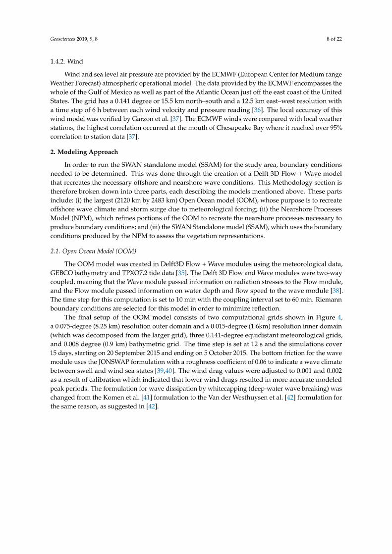
Figure 4. Placement of the three model domains with the open ocean model and its inner and outerdomain in the top left, the Nearshore Processes Model with the finer domains outlined by rectangles onthe right and the SWAN model on the bottom left. The SWAN model also depicts the points at whichthe boundaries were implemented as well as the transect on which the pressure gauge and vegetationsurveys were conducted.

2.2. Nearshore Processes Model (NPM)

After the completion of the OOM, its inner domain was broken down into three increasinglysmaller domains. Each domain is reduced by a factor of 5—relative to the preceding domain size—untila near 5-m resolution is achieved, to match that of the SSAM. The NPM is forced by the OOM, therefore,all physical processes are the same. However, parameters such as the manning roughness for theflow module and the breaker parameter, which controls the ratio of breaking waves to local waterdepth, were adjusted to calibrate the model because it had been too dissipative, resulting in largererrors for the water levels. The bottom roughness for the flow module, specified here using Manning n,is therefore set to 0.015. The SWAN breaker parameter was set to 0.5 due to the shallow and relativelyflat characteristics of the research site, as discussed in [43,44]. These regions required finer bathymetrywhich was provided by the data discussed in Section 2.1.

2.3. SWAN Standalone Model (SSAM)

From the NPM, boundary conditions for the SSAM are extracted as spectral data (.sp2) for20 observation points. These points provided the wave characteristics necessary to run the SSAM.The NPM was also used to create water level, current velocity and wind velocity fields that wereapplied to the SSAM.


The land cover file used for the explicit vegetation implementation in SWAN takes advantage ofthe “NPLANTS” command to create vegetation cover of varying density. The landcover file indicatesthat the vegetated regions have a uniform density equivalent to 100% of the density provided by theSWAN command file. The vegetation height, density and diameter are all specified to match thoseobserved in the field [31]. These values were averaged and applied as constant values across the marsh(density: 344 stems/m2, vegetation height: 0.71 m and diameter: 5.2 mm).

The selection of the drag coefficient for the explicit representation is based on three formulations;the first of which was proposed by Méndez et al. [10], demonstrated in Equation (8), which wasdetermined through laboratory experiments using flexible plastic strips to represent the vegetation.

CD =2200Re

2.2+ 0.08 (8)

where Re is the Reynolds number, determined as a function of velocity, stem diameter, viscosity anddensity. The second formulation is that of Jadhav and Chen [45],which was determined from fieldobservations taken during a tropical cyclone shown in Equation (9).

CD =2600Re

+ 0.36 (9)

The final formulation was determined using the drag relation discussed by Smith et al. [19],who used synthetic Spartina Alterniflora in a laboratory experiment to produce Equation (10).

CD =744Re

1.27+ 0.76 (10)

Unlike Equation (8), both Equations (9) and (10) were developed with field data of SpartinaAlterniflora plants. Since the vegetation species is constant throughout the marsh, the diameter doesnot change significantly; however, the velocity—used to determine Re—is strongly dependent on thewave climate. Therefore, to determine which current velocity best represents the 20 September to6 October wave climate largest, smallest, and average current velocities that occur at the Eastern Shoreresearch site are used to determine the Re. The current velocity during the period of interest variesfrom 0.1 m/s to 0.7 m/s giving a range of Re values from 430 to 5000.

For the implicit vegetation representation, a second land cover file uses Equation (3) to determineKN values for the different portions of the marsh. These are implemented in SWAN using the Madsenbottom friction formulation (Equations (3)–(6)), effectively implementing the Manning “n” as anadjusted friction length.

Both files require the identification of vegetation types in the region. The vegetation was identifiedusing the Virginia Gap land cover data [28]. This dataset classifies many land cover types into theirown classification and presents them on a map that encompasses the entire United States. This datashowed that the research site was completely covered by saltmarsh, which has an n value of 0.035 [46].

3. Results

The OOM results are validated using observed data provided by the National Oceanic andAtmospheric Association [34]. These buoys and tide stations provide the Hs, Tp, wave direction andwater level between 20 September and 6 October, 2015. The NPM, as well as the SSAM, are bothvalidated using the Trublue pressure sensor data shown in Figure 3.

3.1. Open Ocean Model

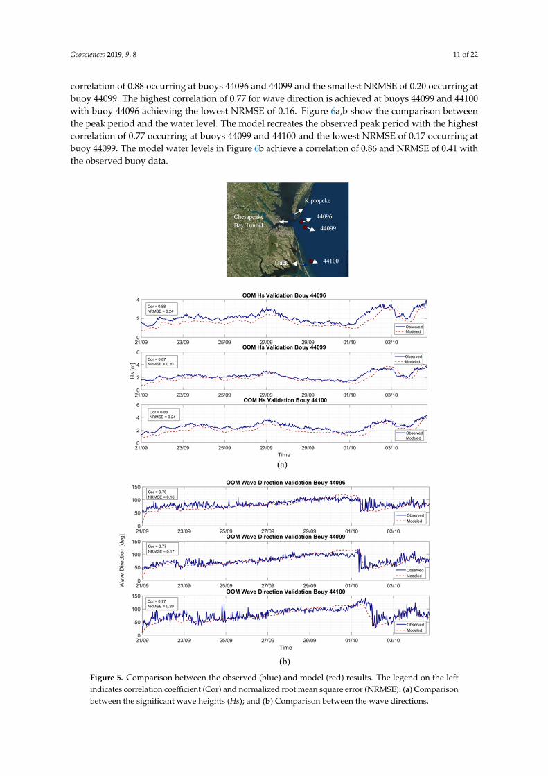
The NOAA buoy and tide station data used to validate the OOM is shown in Figures 5 and 6 alongwith their corresponding correlation coefficient and normalized root mean squared error. Figure 5a,bshow the comparison of the Hs and Wave direction. The model recreates the Hs with the largest


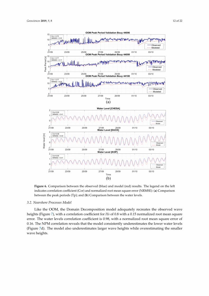
correlation of 0.88 occurring at buoys 44096 and 44099 and the smallest NRMSE of 0.20 occurring atbuoy 44099. The highest correlation of 0.77 for wave direction is achieved at buoys 44099 and 44100with buoy 44096 achieving the lowest NRMSE of 0.16. Figure 6a,b show the comparison betweenthe peak period and the water level. The model recreates the observed peak period with the highestcorrelation of 0.77 occurring at buoys 44099 and 44100 and the lowest NRMSE of 0.17 occurring atbuoy 44099. The model water levels in Figure 6b achieve a correlation of 0.86 and NRMSE of 0.41 withthe observed buoy data.


occurring at buoy 44099. The highest correlation of 0.77 for wave direction is achieved at buoys 44099

and 44100 with buoy 44096 achieving the lowest NRMSE of 0.16. Figure 6a and Figure 6b show the

comparison between the peak period and the water level. The model recreates the observed peak

period with the highest correlation of 0.77 occurring at buoys 44099 and 44100 and the lowest NRMSE

of 0.17 occurring at buoy 44099. The model water levels in Figure 6b achieve a correlation of 0.86 and

NRMSE of 0.41 with the observed buoy data.

Figure 5. Comparison between the observed (blue) and model (red) results. The legend on the left

indicates correlation coefficient (Cor) and normalized root mean square error (NRMSE): (a)

Comparison between the significant wave heights (Hs); and (b) Comparison between the wave

directions.

Figure 5. Comparison between the observed (blue) and model (red) results. The legend on the leftindicates correlation coefficient (Cor) and normalized root mean square error (NRMSE): (a) Comparisonbetween the significant wave heights (Hs); and (b) Comparison between the wave directions.


Figure 6. Comparison between the observed (blue) and model (red) results. The legend on the left

indicates correlation coefficient (Cor) and normalized root mean square error (NRMSE): (a)

Comparison between the peak periods (Tp); and (b) Comparison between the water levels.

3.2. Nearshore Processes Model

Like the OOM, the Domain Decomposition model adequately recreates the observed wave

heights (Figure 7), with a correlation coefficient for Hs of 0.8 with a 0.15 normalized root mean square

error. The water levels correlation coefficient is 0.98, with a normalized root mean square error of

0.16. The NPM correlation reveals that the model consistently underestimates the lower water levels

(Figure 7d). The model also underestimates larger wave heights while overestimating the smaller

wave heights.

Figure 6. Comparison between the observed (blue) and model (red) results. The legend on the leftindicates correlation coefficient (Cor) and normalized root mean square error (NRMSE): (a) Comparisonbetween the peak periods (Tp); and (b) Comparison between the water levels.

3.2. Nearshore Processes Model

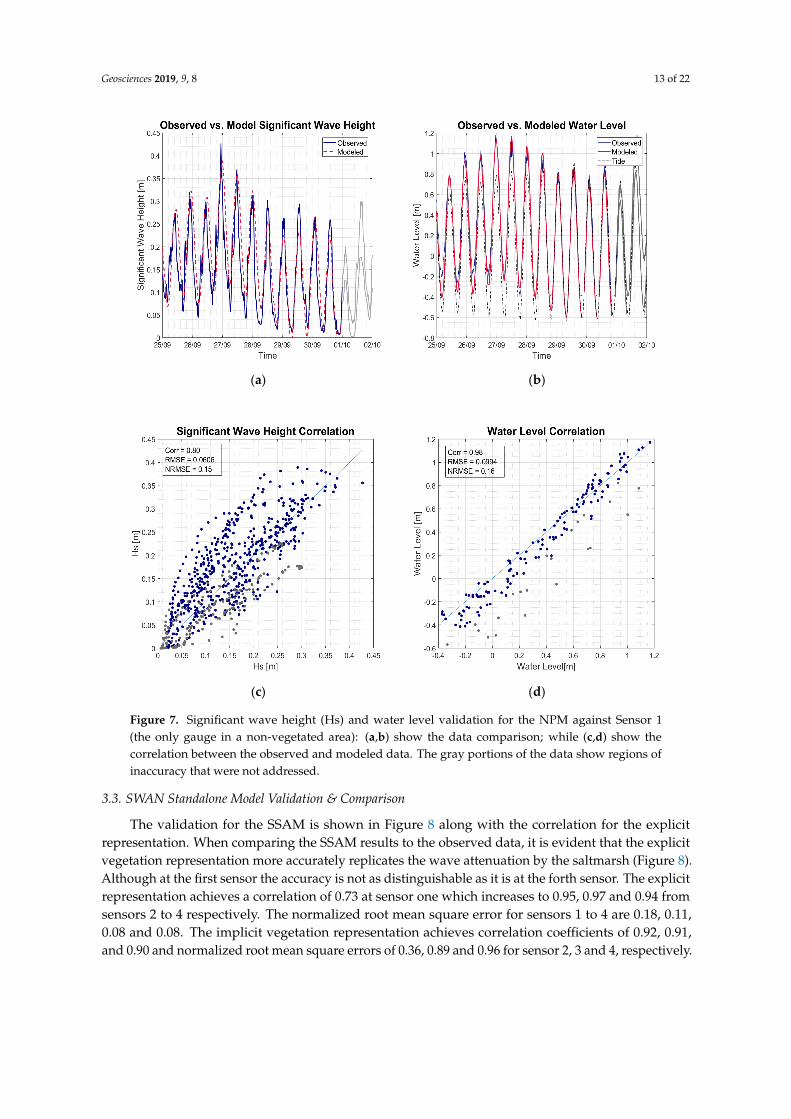
Like the OOM, the Domain Decomposition model adequately recreates the observed waveheights (Figure 7), with a correlation coefficient for Hs of 0.8 with a 0.15 normalized root mean squareerror. The water levels correlation coefficient is 0.98, with a normalized root mean square error of0.16. The NPM correlation reveals that the model consistently underestimates the lower water levels(Figure 7d). The model also underestimates larger wave heights while overestimating the smallerwave heights.


(a) (b)

(c) (d)

Figure 7. Significant wave height (Hs) and water level validation for the NPM against Sensor 1

(the only gauge in a non‐vegetated area): (a) and (b) show the data comparison; while (c) and (d)

show the correlation between the observed and modeled data. The gray portions of the data show

regions of inaccuracy that were not addressed.

3.3. SWAN Standalone Model Validation & Comparison

The validation for the SSAM is shown in Figure 8 along with the correlation for the explicit

representation. When comparing the SSAM results to the observed data, it is evident that the explicit

vegetation representation more accurately replicates the wave attenuation by the saltmarsh (Figure

8). Although at the first sensor the accuracy is not as distinguishable as it is at the forth sensor. The

explicit representation achieves a correlation of 0.73 at sensor one which increases to 0.95, 0.97 and

0.94 from sensors 2 to 4 respectively. The normalized root mean square error for sensors 1 to 4 are

0.18, 0.11, 0.08 and 0.08. The implicit vegetation representation achieves correlation coefficients of

0.92, 0.91, and 0.90 and normalized root mean square errors of 0.36, 0.89 and 0.96 for sensor 2, 3 and

4, respectively.

Figure 7. Significant wave height (Hs) and water level validation for the NPM against Sensor 1(the only gauge in a non-vegetated area): (a,b) show the data comparison; while (c,d) show thecorrelation between the observed and modeled data. The gray portions of the data show regions ofinaccuracy that were not addressed.

3.3. SWAN Standalone Model Validation & Comparison

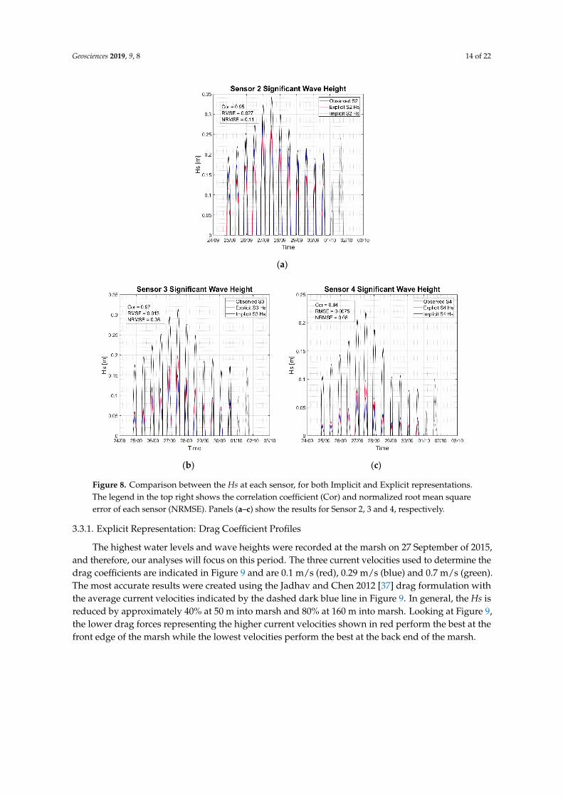
The validation for the SSAM is shown in Figure 8 along with the correlation for the explicitrepresentation. When comparing the SSAM results to the observed data, it is evident that the explicitvegetation representation more accurately replicates the wave attenuation by the saltmarsh (Figure 8).Although at the first sensor the accuracy is not as distinguishable as it is at the forth sensor. The explicitrepresentation achieves a correlation of 0.73 at sensor one which increases to 0.95, 0.97 and 0.94 fromsensors 2 to 4 respectively. The normalized root mean square error for sensors 1 to 4 are 0.18, 0.11,0.08 and 0.08. The implicit vegetation representation achieves correlation coefficients of 0.92, 0.91,and 0.90 and normalized root mean square errors of 0.36, 0.89 and 0.96 for sensor 2, 3 and 4, respectively.


(a)

(b) (c)

Figure 8. Comparison between the Hs at each sensor, for both Implicit and Explicit representations.

The legend in the top right shows the correlation coefficient (Cor) and normalized root mean square

error of each sensor (NRMSE). Panels (a), (b) and (c) show the results for Sensor 2, 3 and 4,

respectively.

3.3.1. Explicit Representation: Drag Coefficient Profiles

The highest water levels and wave heights were recorded at the marsh on 27 September of 2015,

and therefore, our analyses will focus on this period. The three current velocities used to determine

the drag coefficients are indicated in Figure 9 and are 0.1 m/s (red), 0.29 m/s (blue) and 0.7 m/s (green).

The most accurate results were created using the Jadhav and Chen 2012 [37] drag formulation with

the average current velocities indicated by the dashed dark blue line in Figure 9. In general, the Hs is

reduced by approximately 40% at 50 meters into marsh and 80% at 160 meters into marsh. Looking

at Figure 9, the lower drag forces representing the higher current velocities shown in red perform the

best at the front edge of the marsh while the lowest velocities perform the best at the back end of the

marsh.

Figure 8. Comparison between the Hs at each sensor, for both Implicit and Explicit representations.The legend in the top right shows the correlation coefficient (Cor) and normalized root mean squareerror of each sensor (NRMSE). Panels (a–c) show the results for Sensor 2, 3 and 4, respectively.

3.3.1. Explicit Representation: Drag Coefficient Profiles

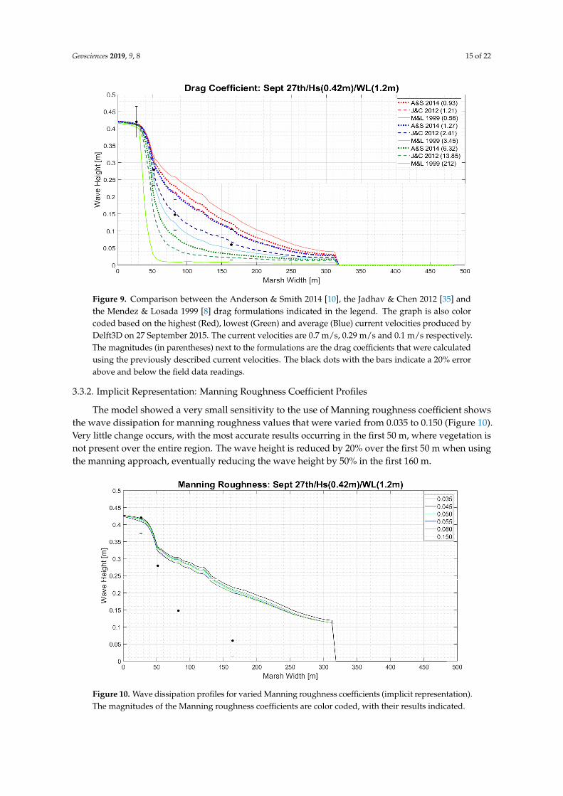
The highest water levels and wave heights were recorded at the marsh on 27 September of 2015,and therefore, our analyses will focus on this period. The three current velocities used to determine thedrag coefficients are indicated in Figure 9 and are 0.1 m/s (red), 0.29 m/s (blue) and 0.7 m/s (green).The most accurate results were created using the Jadhav and Chen 2012 [37] drag formulation withthe average current velocities indicated by the dashed dark blue line in Figure 9. In general, the Hs isreduced by approximately 40% at 50 m into marsh and 80% at 160 m into marsh. Looking at Figure 9,the lower drag forces representing the higher current velocities shown in red perform the best at thefront edge of the marsh while the lowest velocities perform the best at the back end of the marsh.


Figure 9. Comparison between the Anderson & Smith 2014 [10], the Jadhav & Chen 2012 [35] and the

Mendez & Losada 1999 [8] drag formulations indicated in the legend. The graph is also color coded

based on the highest (Red), lowest (Green) and average (Blue) current velocities produced by Delft3D

on 27 September 27, 2015. The current velocities are 0.7m/s, 0.29m/s and 0.1 m/s respectively. The

magnitudes (in parentheses) next to the formulations are the drag coefficients that were calculated

using the previously described current velocities. The black dots with the bars indicate a 20% error

above and below the field data readings.

3.3.2. Implicit Representation: Manning Roughness Coefficient Profiles

The model showed a very small sensitivity to the use of Manning roughness coefficient shows

the wave dissipation for manning roughness values that were varied from 0.035 to 0.150 (Figure 10).

Very little change occurs, with the most accurate results occurring in the first 50 meters, where

vegetation is not present over the entire region. The wave height is reduced by 20% over the first 50

meters when using the manning approach, eventually reducing the wave height by 50% in the first

160 meters.

Figure 10. Wave dissipation profiles for varied Manning roughness coefficients (implicit

representation). The magnitudes of the Manning roughness coefficients are color coded, with their

results indicated.

Figure 9. Comparison between the Anderson & Smith 2014 [10], the Jadhav & Chen 2012 [35] andthe Mendez & Losada 1999 [8] drag formulations indicated in the legend. The graph is also colorcoded based on the highest (Red), lowest (Green) and average (Blue) current velocities produced byDelft3D on 27 September 2015. The current velocities are 0.7 m/s, 0.29 m/s and 0.1 m/s respectively.The magnitudes (in parentheses) next to the formulations are the drag coefficients that were calculatedusing the previously described current velocities. The black dots with the bars indicate a 20% errorabove and below the field data readings.


The model showed a very small sensitivity to the use of Manning roughness coefficient showsthe wave dissipation for manning roughness values that were varied from 0.035 to 0.150 (Figure 10).Very little change occurs, with the most accurate results occurring in the first 50 m, where vegetation isnot present over the entire region. The wave height is reduced by 20% over the first 50 m when usingthe manning approach, eventually reducing the wave height by 50% in the first 160 m.


Figure 9. Comparison between the Anderson & Smith 2014 [10], the Jadhav & Chen 2012 [35] and the

Mendez & Losada 1999 [8] drag formulations indicated in the legend. The graph is also color coded

based on the highest (Red), lowest (Green) and average (Blue) current velocities produced by Delft3D

on 27 September 27, 2015. The current velocities are 0.7m/s, 0.29m/s and 0.1 m/s respectively. The

magnitudes (in parentheses) next to the formulations are the drag coefficients that were calculated

using the previously described current velocities. The black dots with the bars indicate a 20% error

above and below the field data readings.


The model showed a very small sensitivity to the use of Manning roughness coefficient shows

the wave dissipation for manning roughness values that were varied from 0.035 to 0.150 (Figure 10).

Very little change occurs, with the most accurate results occurring in the first 50 meters, where

vegetation is not present over the entire region. The wave height is reduced by 20% over the first 50

meters when using the manning approach, eventually reducing the wave height by 50% in the first

160 meters.

Figure 10. Wave dissipation profiles for varied Manning roughness coefficients (implicit

representation). The magnitudes of the Manning roughness coefficients are color coded, with their

results indicated.

Figure 10. Wave dissipation profiles for varied Manning roughness coefficients (implicit representation).The magnitudes of the Manning roughness coefficients are color coded, with their results indicated.


3.3.3. Wave Energy Dissipation Processes

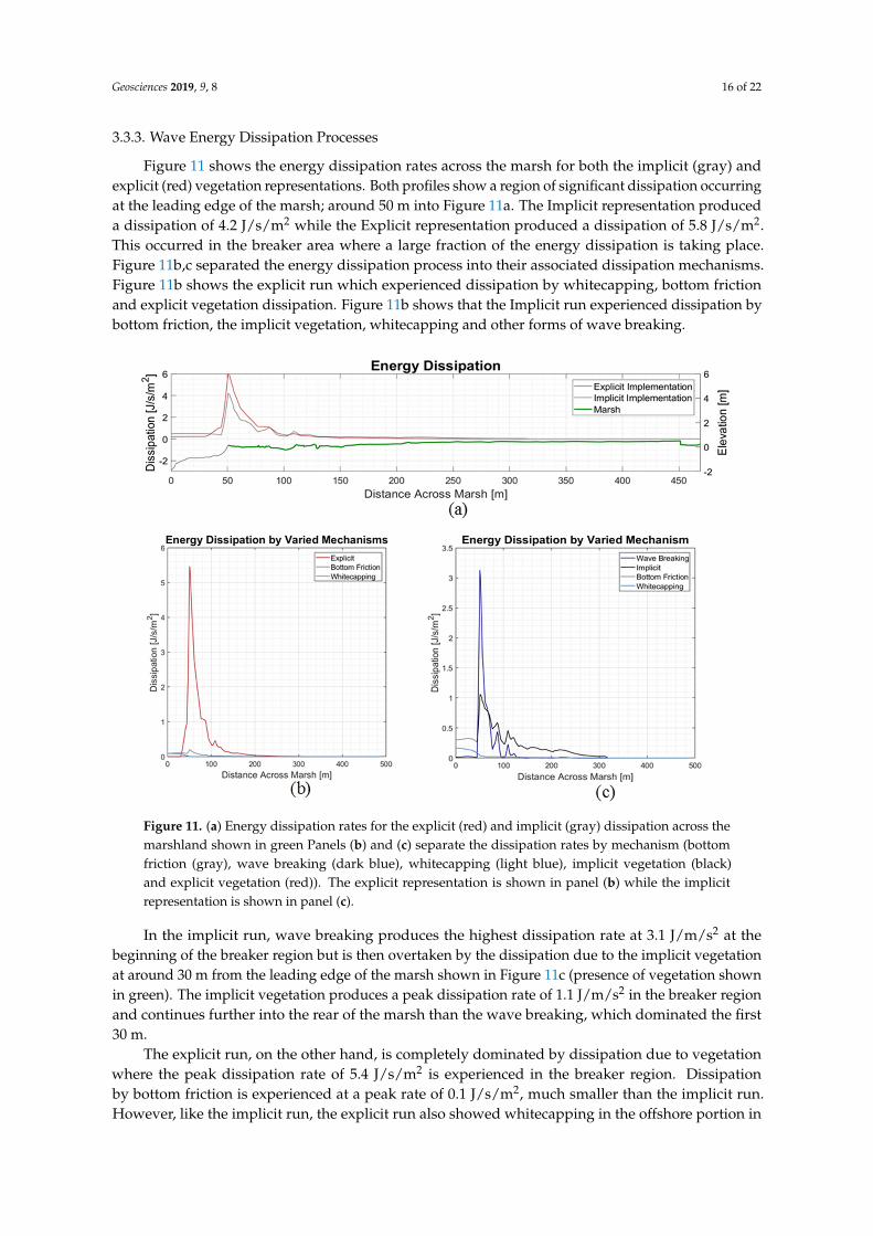
Figure 11 shows the energy dissipation rates across the marsh for both the implicit (gray) andexplicit (red) vegetation representations. Both profiles show a region of significant dissipation occurringat the leading edge of the marsh; around 50 m into Figure 11a. The Implicit representation produceda dissipation of 4.2 J/s/m2 while the Explicit representation produced a dissipation of 5.8 J/s/m2.This occurred in the breaker area where a large fraction of the energy dissipation is taking place.Figure 11b,c separated the energy dissipation process into their associated dissipation mechanisms.Figure 11b shows the explicit run which experienced dissipation by whitecapping, bottom frictionand explicit vegetation dissipation. Figure 11b shows that the Implicit run experienced dissipation bybottom friction, the implicit vegetation, whitecapping and other forms of wave breaking.


3.3.3. Wave Energy Dissipation Processes

Figure 11 shows the energy dissipation rates across the marsh for both the implicit (gray) and

explicit (red) vegetation representations. Both profiles show a region of significant dissipation

occurring at the leading edge of the marsh; around 50 meters into Figure 11a. The Implicit

representation produced a dissipation of 4.2 J/s/m2 while the Explicit representation produced a

dissipation of 5.8 J/s/m2. This occurred in the breaker area where a large fraction of the energy

dissipation is taking place. Figure 11b and Figure 11c separated the energy dissipation process into

their associated dissipation mechanisms. Figure 11b shows the explicit run which experienced

dissipation by whitecapping, bottom friction and explicit vegetation dissipation. Figure 11b shows

that the Implicit run experienced dissipation by bottom friction, the implicit vegetation,

whitecapping and other forms of wave breaking.

In the implicit run, wave breaking produces the highest dissipation rate at 3.1 J/m/s2 at the

beginning of the breaker region but is then overtaken by the dissipation due to the implicit vegetation

at around 30 m from the leading edge of the marsh shown in Figure 11c (presence of vegetation

shown in green). The implicit vegetation produces a peak dissipation rate of 1.1 J/m/s2 in the breaker

region and continues further into the rear of the marsh than the wave breaking, which dominated the

first 30 m.

The explicit run, on the other hand, is completely dominated by dissipation due to vegetation

where the peak dissipation rate of 5.4 J/s/m2 is experienced in the breaker region. Dissipation by

bottom friction is experienced at a peak rate of 0.1 J/s/m2, much smaller than the implicit run.

However, like the implicit run, the explicit run also showed whitecapping in the offshore portion in

front of the marsh, which is completely overtaken by other dissipation mechanisms shoreward of the

marsh edge.

Figure 11. (a) Energy dissipation rates for the explicit (red) and implicit (gray) dissipation across the

marshland shown in green Panels (b) and (c) separate the dissipation rates by mechanism (bottom

friction (gray), wave breaking (dark blue), whitecapping (light blue), implicit vegetation (black) and

Figure 11. (a) Energy dissipation rates for the explicit (red) and implicit (gray) dissipation across themarshland shown in green Panels (b) and (c) separate the dissipation rates by mechanism (bottomfriction (gray), wave breaking (dark blue), whitecapping (light blue), implicit vegetation (black)and explicit vegetation (red)). The explicit representation is shown in panel (b) while the implicitrepresentation is shown in panel (c).

In the implicit run, wave breaking produces the highest dissipation rate at 3.1 J/m/s2 at thebeginning of the breaker region but is then overtaken by the dissipation due to the implicit vegetationat around 30 m from the leading edge of the marsh shown in Figure 11c (presence of vegetation shownin green). The implicit vegetation produces a peak dissipation rate of 1.1 J/m/s2 in the breaker regionand continues further into the rear of the marsh than the wave breaking, which dominated the first30 m.

The explicit run, on the other hand, is completely dominated by dissipation due to vegetationwhere the peak dissipation rate of 5.4 J/s/m2 is experienced in the breaker region. Dissipationby bottom friction is experienced at a peak rate of 0.1 J/s/m2, much smaller than the implicit run.However, like the implicit run, the explicit run also showed whitecapping in the offshore portion in


front of the marsh, which is completely overtaken by other dissipation mechanisms shoreward of themarsh edge.

The main difference between the two runs is the role that wave breaking plays in the implicit runwhen compared to the explicit run. By excluding the influence of the various vegetation properties onwave attenuation (implicit representation), waves are able to retain their energy further shorewardresulting in intense wave breaking over the first 50 m of marsh (Figure 11b). On the other hand—withthe explicit representation—the waves experience significant attenuation by vegetation; such that thebreaking criteria (ratio of breaking wave height to water depth) is not violated and, thus preventsintense wave breaking (Figure 11a) [2].

4. Discussion

This section will discuss the validation of the OOM and NPM models as well as the comparisonbetween the implicit and explicit representations. Section 4.1 briefly describes the observed trends ofthe three models and how they manifested themselves from the OOM model to the SSAM. Section 4.2focuses on the difference in wave dissipation rate and dissipation mechanism between the twoimplementations. The results are also compared to existing research to identify how this papercompares the current work.

4.1. Model Calibration and Validation

The OOM model was able to recreate the observed wave climate with reasonable accuracy butshowed a tendency to underestimate the significant wave heights, peak periods and water levels.To alleviate this issue whitecapping, computational grid resolution, bathymetric grid resolution andwind drag were adjusted through sensitivity analysis, producing the results shown in Figures 5 and 6.

The adjustment of the whitecapping from the default formulation of Komen et al. [41] to that ofVan der Westhuysen et al. [42] was done because the findings in [42] indicated an underestimationof peak periods in mixed wind and swell sea states when using the Komen et al. [41] formulation.This indicates that the wave climate is a mixed sea state whose energy distribution is impacted by thepresence of whitecapping in the model which demands a reasonable amount of attention.

The refining of the bathymetric and computational grids to 0.015 degrees improved the results,indicating that key bathymetric features were not captured when a coarser grid resolution of 0.075was used. There were also 1- to 2-m differences in depth which can impact the extent to which bottomfriction and wave breaking affect the development of the incoming wave climate.

The wind drag also proved to have major impact on the peak periods, with lower wind dragcoefficient values such as the 0.01 and 0.02 producing larger peak periods. The wind drag influencehow much energy is transferred across the wind sea interface as well as the celerity of the incomingwave climate. The wind drag and whitecapping are also interconnected within SWAN, magnifying theinfluence the wind drag has on the peak period.

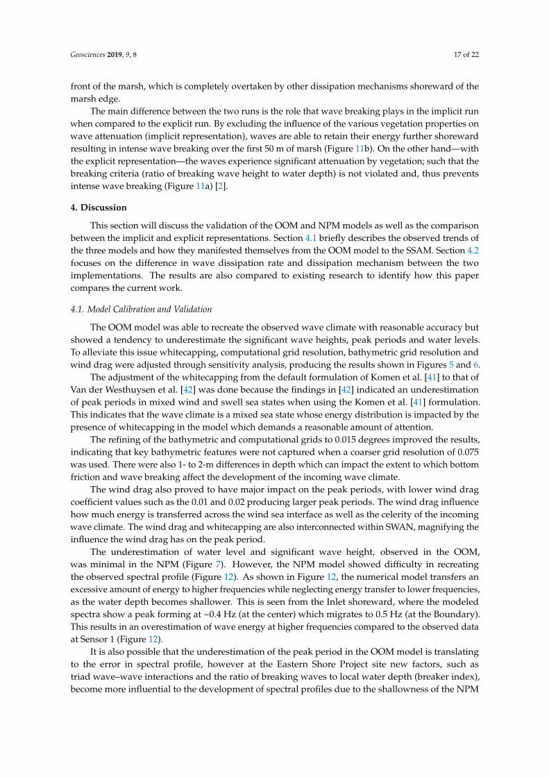
The underestimation of water level and significant wave height, observed in the OOM,was minimal in the NPM (Figure 7). However, the NPM model showed difficulty in recreatingthe observed spectral profile (Figure 12). As shown in Figure 12, the numerical model transfers anexcessive amount of energy to higher frequencies while neglecting energy transfer to lower frequencies,as the water depth becomes shallower. This is seen from the Inlet shoreward, where the modeledspectra show a peak forming at ~0.4 Hz (at the center) which migrates to 0.5 Hz (at the Boundary).This results in an overestimation of wave energy at higher frequencies compared to the observed dataat Sensor 1 (Figure 12).

It is also possible that the underestimation of the peak period in the OOM model is translatingto the error in spectral profile, however at the Eastern Shore Project site new factors, such astriad wave–wave interactions and the ratio of breaking waves to local water depth (breaker index),become more influential to the development of spectral profiles due to the shallowness of the NPM


when compared to the OOM. Therefore, it is necessary to further study the development of the spectralprofile in this region.


compared to the OOM. Therefore, it is necessary to further study the development of the spectral

profile in this region.

These factors are a fraction of a large group of variables that can influence the final wave

characteristics of the OOM and NPM. The number of variables calibrated in these models are a

testament to the complexity of the wave generation and propagation process. Due to the complexity

of these processes, numerical models will rarely be able to perfectly recreate observed wave climates.

Regardless, the OOM and NPM models have demonstrated that these tools can be used to model

bulk parameters such as significant wave height and water levels to a NRMSE below 20%, which is

beneficial to further assessment of the Chesapeake Bay coastal region.

Figure 12. Variation in wave spectral density (determined for the hour of 23:00 26 September, 2015)

across the research site leading up to the Sensor 1.

4.2. Explicit Versus Implicit Vegetation Representations

The SSAM was able to appropriately recreate the observed wave climate across the marsh using

the explicit vegetation implementation (Figure 9) but significantly less so when the implicit

representation was used (Figure 10). Along with general performance, the two vegetation

representations produced different wave dissipation mechanisms which can be very important when

considering the morphological stability of the marsh. The minor errors in the explicit representation

may be attributed to the constant drag coefficient and vegetation characteristics, which are not

representative of real‐world conditions where these variables vary horizontally and vertically across

Figure 12. Variation in wave spectral density (determined for the hour of 23:00 26 September 2015)across the research site leading up to the Sensor 1.

These factors are a fraction of a large group of variables that can influence the final wavecharacteristics of the OOM and NPM. The number of variables calibrated in these models are atestament to the complexity of the wave generation and propagation process. Due to the complexityof these processes, numerical models will rarely be able to perfectly recreate observed wave climates.Regardless, the OOM and NPM models have demonstrated that these tools can be used to modelbulk parameters such as significant wave height and water levels to a NRMSE below 20%, which isbeneficial to further assessment of the Chesapeake Bay coastal region.

4.2. Explicit Versus Implicit Vegetation Representations

The SSAM was able to appropriately recreate the observed wave climate across the marsh using theexplicit vegetation implementation (Figure 9) but significantly less so when the implicit representationwas used (Figure 10). Along with general performance, the two vegetation representations produceddifferent wave dissipation mechanisms which can be very important when considering themorphological stability of the marsh. The minor errors in the explicit representation may be


attributed to the constant drag coefficient and vegetation characteristics, which are not representativeof real-world conditions where these variables vary horizontally and vertically across the marsh.The significant overestimation of significant wave height in the implicit representation, on the otherhand, suggests that treating vegetation dissipation as merely enhanced bottom friction ignores themore complex processes occurring throughout the water column, as discussed in [11]. A more detaileddiscussion of the two implementations are presented below.

For the explicit representation, SWAN performed the best when using the Jadhav and Chen [45]drag coefficient formulation and the average current velocity of 0.29 m/s (Figure 9). This findingdiffers from that of Vuik et al. [2], who found that the Méndez et al. [10] formulation resulted in abetter agreement with their observed field data. In the present study, [10] is the second-best fittingdrag coefficient for the observed field data. Both the forcing and vegetation details differ betweenthis study and [2]. The vegetation present in [2] is submerged, similar to the vegetation present inthe laboratory experiment where [10] was derived. Jadhav and Chen [45] shared similar forcing andvegetation characteristics to the Eastern Shore Project site, it therefore may be more appropriate torecreate the observed filed data, as shown in Figure 9.

Additionally, the drag coefficient was held constant throughout the marsh which, though relativelyaccurate, is not representative of real-world conditions. As presented in Section 2.3, the drag coefficientis a function of the Reynolds number which itself is a function of current velocity. Current velocity isnot naturally constant and can be influenced by vegetation density, vegetation height and water depthas describe in [11]. Neumeier and Amos [11] observed that vegetation characteristic vary based onwave forcing, from the front to the back of the marsh; which was observed in the vegetation data of theEastern Shore Project site, shown in [31]. These characteristics influence the vertical and horizontal rateof change in the current velocity, the development of boundary layers, and creation of free streamingregions [11], all of which can impact the dissipation rate.

For the implicit representation, the Manning “n” values of 0.055, 0.080 and 0.150 performed thesame. This is likely caused by the limit placed on the friction factor formulation applied in SWAN,as discussed in [20]; overcoming this limitation would require an adjustment of the source code inorder to change the friction factor formulation to that of [47]. However, it is important to note that theformulation used in [20] was implemented for fully submerged sea grass which behaves differently tothe emergent vegetation observed at the Eastern Shore Project site. An n value of 0.055 was ultimatelychosen as the appropriate value for the implicit representation because it represents marsh vegetation,whereas the other two represent coastal shrubs (n = 0.080) and coastal forest (n = 0.150).

When comparing the explicit Jadhav and Chen [45] drag formulation (Figure 9) and the implicitManning, n = 0.055 (Figure 10), the explicit representation outperforms. Both implementations hadhigh correlation coefficients across the marsh but differed greatly in NRMSE. While the explicitrepresentation maintains a NRMSE below 0.15 (or 15%) from sensors 2 to 4, the implicit representationproduced NRMSE that exceeded 0.30 from sensor 2 to 4. These results showed that the implicitrepresentation, using the SWAN default friction factor formulation, cannot adequately recreate thewave dissipation produced by emergent marsh vegetation. The magnitude of the bottom frictionapplied through the implicit representation is not large enough to appropriately mimic the verticallyand horizontally varied drag forces across the marsh.

Figure 11 showed that the representations not only differed in the magnitude of wave dissipationbut also in the dissipation mechanisms they produced. While the explicit representation showed that amajority of the wave energy is being dissipated by the vegetation throughout the marsh, the implicitrepresentation is initially dominated by wave breaking at the leading edge of the marsh. The vegetationdoes become the dominant from of dissipation once the flatter parts of the marsh are reached, but theamount of dissipation that the vegetation is responsible for in the implicit representation is a smallfraction of that in the explicit representation.

These characteristics can be observed in [2,20] who also separated the breaker mechanisms presenton marsh lands. The dissipation mechanisms in the implicit representation more closely resembles


a mud flat than a salt marsh, which can also be seen in [2] who conducted a similar break downfor an unvegetated region. These dissipation mechanisms can become important when assessingthe morphological changes of a salt marsh and should be considered when conducting this typeof modeling.

5. Conclusions

The results showed an under performance by the implicit representation of vegetation whencompared to the explicit representation, when using the default Manning-based friction factorformulation currently implemented in SWAN, corroborating the findings of Smith et al. [19] and [20].The inability for the implicit representation to produce a friction factor large enough to fully recreatethe magnitude of dissipation produced by densely vegetated marsh limits its applicability in modelingthese regions. Furthermore, the implementations produced different types of dissipation mechanismswhich may influence the modeling accuracy of morphological models in coastal regions. The workdone in this paper is a first step in a wide range of analysis that can be carried out. Further assessment isneeded on the friction factor implementation, in order to determine whether the improved performanceby the implicit representation observed in [20] holds true for emergent vegetation. This would shedlight on where the limits of this implementation lie, and provide guidance to coastal engineers whoapply numerical modeling to investigate vegetated intertidal areas.

Author Contributions: Conceptualization, J.D.B., C.F., and C.L.; investigation, C.B.-H. and C.L.; resources,T.M. and J.G..; writing—original draft preparation, C.B.H., C.L., C.F., and J.D.B.; writing—review and editing,C.B.-H., C.L., C.F., and J.D.B.; supervision, J.D.B., C.F., and C.L.

Acknowledgments: We are grateful to Madeline Keefer and the Fulbright Netherlands-America Foundation forinitiating research on this topic. We also thank Stefan Aarninkhof and Marcel Zijlema for their expert advice.

Conflicts of Interest: The authors declare no conflict of interest. The funders had no role in the design of thestudy; in the collection, analyses, or interpretation of data; in the writing of the manuscript, or in the decision topublish the results.

References

1. Zhang, K.; Liu, H.; Li, Y.; Xu, H.; Shen, J.; Rhome, J.; Smith, T.J., III. The role of mangroves in attenuatingstorm surges. Estuar. Coast. Shelf Sci. 2012, 102, 11–23. [CrossRef]

2. Vuik, V.; Jonkman, S.N.; Borsje, B.W.; Suzuki, T. Nature-based flood protection: The efficiency of vegetatedforeshores for reducing wave loads on coastal dikes. Coast. Eng. 2016, 116, 42–56. [CrossRef]

3. Camfield, F.E. Wind-Wave Propagation Over Flooded, Vegetated Land; Coastal Engineering Research Center:Fort Belvoir, VA, USA, 1977.

4. Kobayashi, N.; Raichle, A.W.; Asano, T. Wave attenuation by vegetation. J. Waterw. Port Coast. Ocean Eng.1993, 119, 30–48. [CrossRef]

5. Manning, R.; Griffith, J.P.; Pigot, T.; Vernon-Harcourt, L.F. On the Flow of Water in Open Channels and Pipes;Institution of Civil Engineers: Dublin, Ireland, 1890.

6. Wu, F.-C.; Shen, H.W.; Chou, Y.-J. Variation of roughness coefficients for unsubmerged and submergedvegetation. J. Hydraul. Eng. 1999, 125, 934–942. [CrossRef]

7. Smith, J.M. Modeling Nearshore Waves for Hurricane Katrina; Engineer Research And Development Center:Vicksburg, MS, USA, 2007.

8. Wamsley, T.V.; Cialone, M.A.; Smith, J.M.; Atkinson, J.H.; Rosati, J.D. The potential of wetlands in reducingstorm surge. Ocean Eng. 2010, 37, 59–68. [CrossRef]

9. Augustin, L.N.; Irish, J.L.; Lynett, P. Laboratory and numerical studies of wave damping by emergent andnear-emergent wetland vegetation. Coast. Eng. 2009, 56, 332–340. [CrossRef]

10. Méndez, F.J.; Losada, I.J.; Losada, M.A. Hydrodynamics induced by wind waves in a vegetation field.J. Geophys. Res. Oceans 1999, 104, 18383–18396. [CrossRef]

11. Neumeier, U.; Amos, C.L. The influence of vegetation on turbulence and flow velocities in Europeansalt-marshes. Sedimentology 2006, 53, 259–277. [CrossRef]

http://dx.doi.org/10.1016/j.ecss.2012.02.021

http://dx.doi.org/10.1016/j.coastaleng.2016.06.001

http://dx.doi.org/10.1061/(ASCE)0733-950X(1993)119:1(30)

http://dx.doi.org/10.1061/(ASCE)0733-9429(1999)125:9(934)

http://dx.doi.org/10.1016/j.oceaneng.2009.07.018


http://dx.doi.org/10.1029/1999JC900119

http://dx.doi.org/10.1111/j.1365-3091.2006.00772.x


12. Anderson, M.E.; Smith, J.M. Wave attenuation by flexible, idealized salt marsh vegetation. Coast. Eng. 2014,83, 82–92. [CrossRef]

13. Dalrymple, R.A.; Kirby, J.T.; Hwang, P.A. Wave diffraction due to areas of energy dissipation. J. Waterw. PortCoast. Ocean Eng. 1984, 110, 67–79. [CrossRef]

14. Houser, C.; Trimble, S.; Morales, B. Influence of blade flexibility on the drag coefficient of aquatic vegetation.Estuaries Coasts 2015, 38, 569–577. [CrossRef]

15. Cavallaro, L.; Viviano, A.; Paratore, G.; Foti, E. Experiments on surface waves interacting with flexibleaquatic vegetation. Ocean Sci. J. 2018, 53, 461–474. [CrossRef]

16. Luhar, M.; Nepf, H. Wave-induced dynamics of flexible blades. J. Fluids Struct. 2016, 61, 20–41. [CrossRef]17. Cavallaro, L.; Re, C.L.; Paratore, G.; Viviano, A.; Foti, E. Response of posidonia oceanica to wave motion in

shallow-waters-preliminary experimental results. Coast. Eng. Proc. 2011, 1, 49. [CrossRef]18. Suzuki, T.; Zijlema, M.; Burger, B.; Meijer, M.C.; Narayan, S. Wave dissipation by vegetation with layer

schematization in swan. Coast. Eng. 2012, 59, 64–71. [CrossRef]19. Smith, J.M.; Bryant, M.A.; Wamsley, T.V. Wetland buffers: Numerical modeling of wave dissipation by

vegetation. Earth Surf. Process. Landf. 2016, 41, 847–854. [CrossRef]20. Nowacki, D.J.; Beudin, A.; Ganju, N.K. Spectral wave dissipation by submerged aquatic vegetation in a

back-barrier estuary. Limnol. Oceanogr. 2017, 62, 736–753. [CrossRef]21. Van Rooijen, A.; Van Thiel de Vries, J.; McCall, R.; Van Dongeren, A.; Roelvink, J.; Reniers, A. Modeling of

wave attenuation by vegetation with xbeach. In Proceedings of the E-proceedings of the 36th IAHR WorldCongress, The Hague, The Netherlands, 28 June–3 July 2015.

22. Booij, N.; Ris, R.C.; Holthuijsen, L.H. A third-generation wave model for coastal regions—1. Modeldescription and validation. J. Geophys. Res. Oceans 1999, 104, 7649–7666. [CrossRef]

23. Kennedy, A.B.; Chen, Q.; Kirby, J.T.; Dalrymple, R.A. Boussinesq modeling of wave transformation, breaking,and runup. I: 1D. J. Waterw. Port Coast. Ocean Eng. 2000, 126, 39–47. [CrossRef]

24. Theophanis, V.K.; Nigel, P.T. Breaking waves in the surf and swash zone. J. Coast. Res. 2003, 19, 514–528.25. Viviano, A.; Musumeci, R.E.; Foti, E. A nonlinear rotational, quasi-2dh, numerical model for spilling wave

propagation. Appl. Math. Model. 2015, 39, 1099–1118. [CrossRef]26. Madsen, O.S.; Poon, Y.-K.; Graber, H.C. Spectral wave attenuation by bottom friction: Theory. In Proceedings

of the 21st International Conference on Coastal Engineering, Malaga, Spain, 20–25 June 1988; AmericanSociety of Civil Engineers: New York, NY, USA, 1988; pp. 492–504.

27. Arcement, G.J.; Schneider, V.R. Guide for Selecting Manning’s Roughness Coefficients for Natural Channels andFlood Plains; US Government Printing Office: Washington, DC, USA, 1989.

28. U.S. Geological Survey. Geological Survey Gap/Landfire National Terrestrial Ecosystems; U.S. Geological Survey:Reston, VA, USA, 2016.

29. Mendez, F.J.; Losada, I.J. An empirical model to estimate the propagation of random breaking andnonbreaking waves over vegetation fields. Coast. Eng. 2004, 51, 103–118. [CrossRef]

30. Xiong, Y.; Berger, C.R. Chesapeake bay tidal characteristics. J. Water Resour. Prot. 2010, 2, 619. [CrossRef]31. Paquier, A.-E.; Haddad, J.; Lawler, S.; Ferreira, C.M. Quantification of the attenuation of storm surge

components by a coastal wetland of the US Mid Atlantic. Estuaries Coasts 2017, 40, 930–946. [CrossRef]32. DOC; NOAA; NESDIS; NCEI. Virginia Beach Coastal Digital Elevation Model; National Oceanic and

Atmospheric Administration: Silver Spring, MD, USA, 2007.33. IOC; IHO; BODC. Cemenary Edition of the GEBCO Digital Atlas; published on CD-ROM on behalf of the

Intergovernmental Oceanographic Commission and the International Hydrographic Organization as part ofthe General Bathymetric Chart of the Oceans: Liverpool, UK, 2003.

34. NOAA; NWS; NDBC; UD. National Data Buoy Center; National Centers for Environmental Information:Asheville, NC, USA, 1971.

35. Egbert, G.D.; Erofeeva, S.Y. Efficient inverse modeling of barotropic ocean tides. J. Atmos. Ocean. Technol.2002, 19, 183–204. [CrossRef]

36. ECMRWF. Ecmwf’s operational model analysis, starting in 2011; Research Data Archive at the National Centerfor Atmospheric Research, Computational and Information Systems Laboratory: Boulder, CO, USA, 2011.

37. Garzon, J.L.; Ferreira, C.M.; Padilla-Hernandez, R. Evaluation of weather forecast systems for storm surgemodeling in the chesapeake bay. Ocean Dyn. 2018, 68, 91–107. [CrossRef]



http://dx.doi.org/10.1007/s12237-014-9840-3

http://dx.doi.org/10.1007/s12601-018-0037-8

http://dx.doi.org/10.1016/j.jfluidstructs.2015.11.007

http://dx.doi.org/10.9753/icce.v32.waves.49


http://dx.doi.org/10.1002/esp.3904

http://dx.doi.org/10.1002/lno.10456

http://dx.doi.org/10.1029/98JC02622


http://dx.doi.org/10.1016/j.apm.2014.07.030


http://dx.doi.org/10.4236/jwarp.2010.27071

http://dx.doi.org/10.1007/s12237-016-0190-1

http://dx.doi.org/10.1175/1520-0426(2002)019<0183:EIMOBO>2.0.CO;2

http://dx.doi.org/10.1007/s10236-017-1120-x


38. Manual, D.D.-F. Delft3D-3D/2D modelling suite for integral water solutions-hydro-morphodynamic s.Deltares Delft. Version 2014, 3, 34158.

39. Hasselmann, K.; Barnett, T.; Bouws, E.; Carlson, H.; Cartwright, D.; Enke, K.; Ewing, J.; Gienapp, H.;Hasselmann, D.; Kruseman, P. Measurements of Wind-Wave Growth and Swell Decay during the Joint NorthSea Wave Project (JONSWAP); Ergänzungsheft 8-12; Deutches Hydrographisches Institut: Hamburg,Germany, 1973.

40. Bouws, E.; Komen, G. On the balance between growth and dissipation in an extreme depth-limited wind-seain the southern north sea. J. Phys. Oceanogr. 1983, 13, 1653–1658. [CrossRef]

41. Komen, G.J.; Cavaleri, L.; Donelan, M.; Hasselmann, K.; Hasselmann, S.; Janssen, P. Dynamics and Modellingof Ocean Waves; Komen, G.J., Cavaleri, L., Donelan, M., Hasselmann, K., Hasselmann, S., Janssen, P.A.E.M.,Eds.; Cambridge University Press: Cambridge, UK, August 1996; p. 554, ISBN 0521577810.

42. Van der Westhuysen, A.J.; Zijlema, M.; Battjes, J.A. Nonlinear saturation-based whitecapping dissipation inswan for deep and shallow water. Coast. Eng. 2007, 54, 151–170. [CrossRef]

43. Massel, S. On the largest wave height in water of constant depth. Ocean Eng. 1996, 23, 553–573. [CrossRef]44. Nelson, R.C. Depth limited design wave heights in very flat regions. Coast. Eng. 1994, 23, 43–59. [CrossRef]45. Jadhav, R.S.; Chen, Q. Field investigation of wave dissipation over salt marsh vegetation during tropical

cyclone. Coast. Eng. Proc. 2012, 1, 41. [CrossRef]46. Bunya, S.; Dietrich, J.C.; Westerink, J.; Ebersole, B.; Smith, J.; Atkinson, J.; Jensen, R.; Resio, D.; Luettich, R.;

Dawson, C. A high-resolution coupled riverine flow, tide, wind, wind wave, and storm surge model forsouthern louisiana and mississippi. Part I: Model development and validation. Mon. Weather Rev. 2010, 138,345–377. [CrossRef]

47. Swart, D.H. Offshore Sediment Transport and Equilibrium Beach Profiles; Delft Hydraulics Laboratory: Delft,The Netherlands, 1974.

© 2018 by the authors. Licensee MDPI, Basel, Switzerland. This article is an open accessarticle distributed under the terms and conditions of the Creative Commons Attribution(CC BY) license (http://creativecommons.org/licenses/by/4.0/).

http://dx.doi.org/10.1175/1520-0485(1983)013<1653:OTBBGA>2.0.CO;2


http://dx.doi.org/10.1016/0029-8018(95)00049-6

http://dx.doi.org/10.1016/0378-3839(94)90014-0

http://dx.doi.org/10.9753/icce.v33.waves.41

http://dx.doi.org/10.1175/2009MWR2906.1

http://creativecommons.org/

http://creativecommons.org/licenses/by/4.0/.

Documents

Delft University of Technology Comparison of Implicit and Explicit