1

Farm Household Incomes and US Government ProgramPayments

Joe Dewbre and Ashok Mishra*

A paper prepared for presentation at the Annual Meeting of the AAEA,Long Beach, California, July 28-31, 2002

Abstract: This paper assesses the impacts of government program payments made to US farmers underselected programs. Using a model of farm household resource allocation and data from the USDA-ERSARMS survey, the analysis considers the effects of the various kinds of program payments on the timeallocation of farm operators and spouses and on farm household income.

2

I. Introduction

The U.S. government makes direct payments to farmers under several different farm programs.

Antecedents to these programs date to earlier times when incomes of farm households were low compared

to those of other US households; income disparities that have now largely disappeared (Mishra et al. 2002).

Citing data revealing the economic situation of today’s farm households comparable to (or better than)

non-farm households, Gardner questions the equity of farm income support policy. Here, we question the

efficiency of farm income support policy, asking what fraction of total farm program payments can be

counted as net income gain for farm households. The impact of farm program payments on incomes of

farm households depends critically on the criteria farmers must meet to be eligible for payments, the way

the program is implemented and the economic characteristics of the farm households and of the farm

covered by the program.

This paper features analysis of payments made to farmers under three programs: transition payments

(AMTA) loan deficiency payments (LDP) and a category that combines disaster and market loss assistance

payments, which we label D_PAYMENTS. Analytical effort focuses on quantifying the effects of such

payments, first on the time allocation of farm operators and their spouses and then on income transfer

efficiency - the proportion of the total transfer from budgetary funds that can be counted as income gain.

The gain in farm household income per dollar of taxpayer money spent will be less than a dollar regardless

of the government program under which payments are made. There are inescapable administrative costs

and there are deadweight losses when citizens are taxed to obtain the funds (Alston and Hurd). In this

paper though we focus on two additional kinds of transfer efficiency losses: 1) those that arise when farm

resources are reallocated in response to changes in relative prices induced by program payments and 2)

leakages of benefits to people who own farmland but do not farm.

3

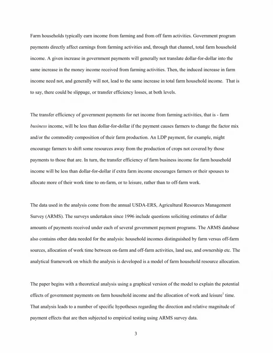
Farm households typically earn income from farming and from off farm activities. Government program

payments directly affect earnings from farming activities and, through that channel, total farm household

income. A given increase in government payments will generally not translate dollar-for-dollar into the

same increase in the money income received from farming activities. Then, the induced increase in farm

income need not, and generally will not, lead to the same increase in total farm household income. That is

to say, there could be slippage, or transfer efficiency losses, at both levels.

The transfer efficiency of government payments for net income from farming activities, that is - farm

business income, will be less than dollar-for-dollar if the payment causes farmers to change the factor mix

and/or the commodity composition of their farm production. An LDP payment, for example, might

encourage farmers to shift some resources away from the production of crops not covered by those

payments to those that are. In turn, the transfer efficiency of farm business income for farm household

income will be less than dollar-for-dollar if extra farm income encourages farmers or their spouses to

allocate more of their work time to on-farm, or to leisure, rather than to off-farm work.

The data used in the analysis come from the annual USDA-ERS, Agricultural Resources Management

Survey (ARMS). The surveys undertaken since 1996 include questions soliciting estimates of dollar

amounts of payments received under each of several government payment programs. The ARMS database

also contains other data needed for the analysis: household incomes distinguished by farm versus off-farm

sources, allocation of work time between on-farm and off-farm activities, land use, and ownership etc. The

analytical framework on which the analysis is developed is a model of farm household resource allocation.

The paper begins with a theoretical analysis using a graphical version of the model to explain the potential

effects of government payments on farm household income and the allocation of work and leisure1 time.

That analysis leads to a number of specific hypotheses regarding the direction and relative magnitude of

payment effects that are then subjected to empirical testing using ARMS survey data.

4

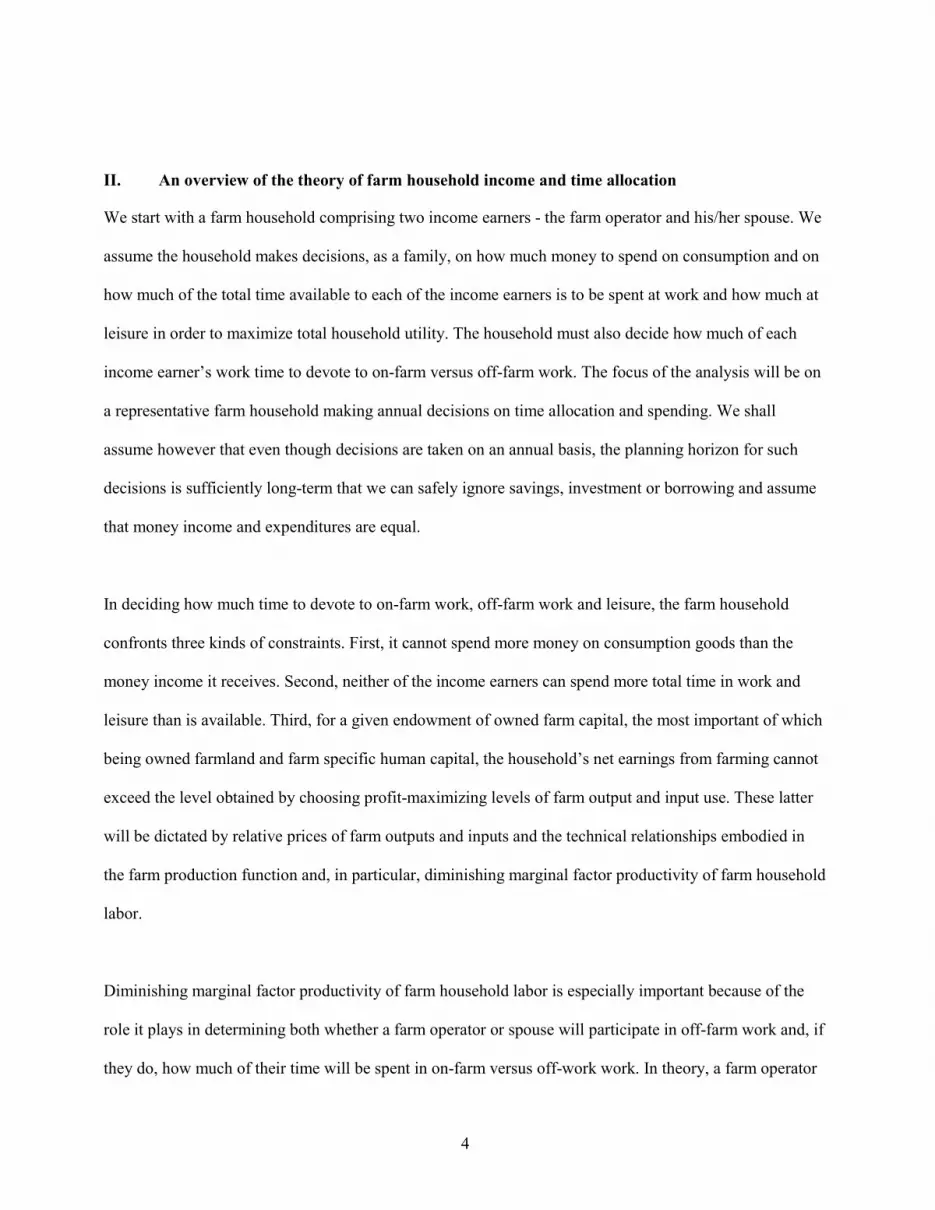
II. An overview of the theory of farm household income and time allocation

We start with a farm household comprising two income earners - the farm operator and his/her spouse. We

assume the household makes decisions, as a family, on how much money to spend on consumption and on

how much of the total time available to each of the income earners is to be spent at work and how much at

leisure in order to maximize total household utility. The household must also decide how much of each

income earner’s work time to devote to on-farm versus off-farm work. The focus of the analysis will be on

a representative farm household making annual decisions on time allocation and spending. We shall

assume however that even though decisions are taken on an annual basis, the planning horizon for such

decisions is sufficiently long-term that we can safely ignore savings, investment or borrowing and assume

that money income and expenditures are equal.

In deciding how much time to devote to on-farm work, off-farm work and leisure, the farm household

confronts three kinds of constraints. First, it cannot spend more money on consumption goods than the

money income it receives. Second, neither of the income earners can spend more total time in work and

leisure than is available. Third, for a given endowment of owned farm capital, the most important of which

being owned farmland and farm specific human capital, the household’s net earnings from farming cannot

exceed the level obtained by choosing profit-maximizing levels of farm output and input use. These latter

will be dictated by relative prices of farm outputs and inputs and the technical relationships embodied in

the farm production function and, in particular, diminishing marginal factor productivity of farm household

labor.

Diminishing marginal factor productivity of farm household labor is especially important because of the

role it plays in determining both whether a farm operator or spouse will participate in off-farm work and, if

they do, how much of their time will be spent in on-farm versus off-work work. In theory, a farm operator

5

or spouse will allocate additional hours to farm work only so long as the marginal value product of those

hours, i.e. the implicit wage for on-farm work, is greater than the wage they could earn in off-farm work.

We assume that the off-farm wage earned by a farm operator or spouse is independent of the amount of

time they spend in off-farm work. Likewise, we shall assume that farmers confront perfectly competitive

output and input markets such that neither the price they receive for their output nor the prices they pay for

purchased inputs vary with quantities produced or purchased respectively. Finally, we shall ignore how

differences in the certainty equivalence of expected on-farm versus off-farm earnings might complicate the

picture. Mishra and Goodwin and Mishra and Holthausen analyze implications of variability in farm and

off-farm earnings for labor supply decisions of farm households.

The basic ideas underlying the analysis are illustrated in figure 1, a graphical depiction of the farm

household model that draws heavily on presentations in articles by Schmitt, by Sumner and by Lee. It

represents the optimal allocation of time, the level of income and utility for a representative farm

household. When read from left to right the horizontal axis in figure 1 measures the amount of time spent

working: zero hours on the extreme left to a maximum of T hours on the extreme right. Correspondingly,

when read right to left that axis measures time spent at leisure, such that at the extreme left all time is spent

in leisure and none at work and at the extreme right all time is spent at work and none at leisure.

6

U’’U’

Y’f

Farm

inco

me

Yt

Ynf

On-farm work Off-farm work Leisure time

Tf T’f TwO T

Yo

W

MVPf

Off- farm

in come

Tot al farm

h ousehol d income

Ymax

Yf

A

C

B

D

Non- w

age inc ome

Figure 1. Time allocation and farm household income

The vertical axes measure total income and expenditure, traced out by the income possibility curve

originating at the origin, point O, passing through the points A, B and D and terminating at Ymax, the

maximum income attainable when all available time is allocated to work, none to leisure. Three categories

of income are distinguished. The first is non-wage income and is denoted as Yo in the figure. It is that

income a farm household would receive even when zero hours are devoted to work. This category includes

such things as retirement income, dividends, interest, rents and, of especial importance here - farm profits2.

The latter is important here because farm profits constitute one channel through which farm program

payments may affect total farm household income and time allocation. We are concerned in this analysis

both with total business profits of the farm firm as well as that part left over after the farm household pays

rents on fixed assets owned by other people, a critical consideration given the importance of rented land for

many farm operations.

7

The second category of farm household income represented in the figure is that income the farm household

earns from work time devoted to farming activities. It is denoted Yf and is traced out by the curve that starts

at A and passes through the points marked B and C. Notice that the slope of this curve declines as more

hours are allocated to farm work reflecting the assumption of diminishing marginal productivity of farm

labor.

Changes in farm program payments may also, depending on the degree to which the payment is coupled to

production, lead to changes in the marginal value product of farm household labor, i.e. in the location and

slope of the farm income curve. The third category of farm household income shown is off-farm earnings

denoted Ynf in the figure. Earnings from off-farm work are determined by the off-farm wage rate

represented by the (constant) slope of the income possibility curve over the segment D to Ymax.

The indifference curves labeled U’ and U’’ show equal-utility combinations of income (which is the same

as total consumption under the above assumptions) and leisure. The household maximizes utility by

choosing that combination of work time and leisure yielding the highest attainable utility given the

constraints. In the absence of off-farm work opportunities the farm household would maximize utility by

choosing to allocate T’f hours to on-farm work and T-T’f hours to leisure at the tangency point C of the

indifference curve labeled U’ with the income possibility curve. However, the existence of off-farm work

opportunities at wage rate W means the household can obtain the higher utility associated with the

indifference curve U’’, by choosing tangency point D and working only Tf hours on-farm, Tw hours off the

farm and spending T-Tw hours in leisure activities. This is because at all points to the right of point B on

the income possibility curve the off-farm wage rate – W, is higher than the marginal value product of farm

household labor – MVPf.

Notice that under these conditions the assumption of utility maximization – equating the marginal utility of

income and leisure with the off-farm wage rate, is enough to ensure that the farm household will allocate

8

less time to on-farm work in the presence of off-farm earning opportunities. Compare T’f versus Tf in the

figure. On the other hand, the total number of hours worked, the sum of on-farm and off-farm hours, Tw in

the figure would logically be greater than the total number of hours worked in the absence of off-farm

earnings opportunities - T’f. Encouragingly, estimates of on-farm, off-farm and total work hours of farm

operators and spouses obtained from the ARMS survey data confirm both these insights: farm households

who allocate some of their work time to off-farm employment work fewer hours on-farm and more hours

in total. (See Mishra et al. (2002) and Table 1 below.)

Changes in the off-farm wage rate, in the marginal value product of farm household labor or in the level of

non-wage income could all potentially change the location and slopes of the income possibility curve. Any

such change will lead to re-allocations of a farm household’s total time endowment between work and

leisure and, depending on the nature of the change, a reallocation of work time between on-farm and off-

farm activities. Our concern is with shifts in the curve and changes in its slope caused by changes in

different kinds of government program payments.

Decoupled government payments, time allocation and farm household income

We can use the model depicted in figure 1 to anticipate some of the findings in this respect. First though

we need to acknowledge that the equilibrium depicted there in which the household optimally allocates

some of its time to off-farm work requires that particular combination of household preferences and on-

farm and off-farm earning opportunities. Many farm households have preferences for work and leisure or

they confront off-farm work opportunities that lead to an equilibrium in which none of their available work

time is allocated to off-farm work. The effect of government payments on time allocation may be slightly

different depending on which of these two categories a farm household is in.

9

U

Farm

inco

me

Yt

On-farm work Off-farm work Leisure time

Tf TwO T

Yo

Off-farm

i ncome

Tot al househ old inco m

e

Ymax

F

U’

Y’max

T’w

Y’t

Y’o

Increase indecoupled payment

Non-w

a ge income

Figure 2. Effect of decoupled payment on time allocation and farm household income

Consider first the potential impact of a small increase in a farm program payment that is completely

decoupled from farm production decisions - AMTA payments are generally considered to fit such a

description. Such a payment would have an effect as shown in figure 2 similar to that of an increase in non-

wage income, i.e. it would merely shift the income possibility curve upwards giving a tangency with an

indifference curve at a higher level of total farm household income and utility. Assuming that farm

households regard leisure as a normal good, such an increase in income would lead to an increase in the

amount of time demanded for leisure activities and a reduction in total time spent working. If, in the initial

situation some of the available work time was allocated to off farm work, the response would be to reduce

the number of hours worked off the farm, with possibly no implications for the amount of time worked on

10

the farm. (Except of course if the change were large enough to induce the farm household to stop working

off the farm altogether in which case we might expect a reduction in on-farm working hours as well.)

Alternatively, if in the initial situation the farm household allocated none of its available work time to off-

farm work the response would be to reduce hours of work on the farm. Thus we see that whether the farm

household allocates some or none of its available work time to off-farm work a decoupled payment would

be expected to reduce time spent working and increase time spent in non-work activities.

What is the expected transfer efficiency of a completely decoupled payment, i.e. what percentage of the

transfer ends up as net gain in total farm household income? The short answer is – less than 100 percent.

There are two main reasons. First, some of the money received by the farm business in the form of

decoupled payments may be paid out in the form of rents on assets owned by other people, land

undoubtedly the most important example. Second, if measured in terms of the induced change in money

income the transfer efficiency even for that part of the decoupled payment kept by the farm household

would be less than 100 percent. Only if leisure time were valued by the household at the same money wage

as work time and transfer efficiency measured in terms of the induced change in full income would transfer

efficiency even for that part of the payment kept by the farm household be 100 percent. (Full income is the

sum of money income and an estimate of the money value of leisure time. Usually the wage rate is used to

estimate the per hour value of leisure time (Deaton and Muellbauer)).

Coupled government payments, time allocation and farm household income

Consider now the impact of a change in a government payment coupled to production; a deficiency

payment that leads to a higher effective price paid for farm output for example. This case is illustrated in

figure 3. This would cause an increase in the marginal value product of all productive factors including

farm household labor and would be revealed in both a leftward rotation and an upward shift of the farm

income segment of the income possibility curve. The leftward rotation comes from the revaluation of time

11

devoted to farm work, the upward shift from the induced increase in farm profits. Recall that an optimizing

farm household will allocate time to farm work so long as the marginal value product of time spent in on-

farm work activities is greater than the wage rate.

U

Farm

inco

me

Yt

On-farm work Off-farm work Leisure time

TfTwO T

Yo

Off-farm

income

Total h ousehold incom

e

Ymax

F

U’

Y’max

T’w

Y’t

T’f

F’Increase in MVP of farmwork.time

Increase in farm profit Non -w

age in come

Figure 3. Effect of coupled payment on time allocation and farm household income

Thus, if in the initial situation the farm household allocates some of its time to off-farm work, an increase

in the marginal value product of farm household labor leads unambiguously to an increase in hours

devoted to farming activities and a decrease in hours devoted to off-farm work. However, we can not say

based on theoretical considerations alone whether such a change would lead to an increase, a decrease or

no change in the total number of hours worked. Neither can we say for sure that if in the initial situation

12

the farm household allocates none of its time to off-farm work, an increase in a coupled payment would

lead to an increase in time devoted to on-farm work. The ambiguity results from the fact that for farm

households in this category the coupled payment simultaneously increases both the price of their leisure

and their full income.

The transfer efficiency of a coupled payment would, as for a decoupled payment, also be expected to be

less than 100 percent. This occurs for the same reasons cited in discussing the transfer efficiency of a

decoupled payment and more. In reckoning the transfer efficiency of a coupled payment we must

acknowledge an additional source of transfer efficiency loss – the opportunity costs of resources the farm

household diverts from other productive activities to production of the supported commodity. These

include the reallocations of work time traced out above as well as the reallocations of land and possibly

other assets owned by the farm household. All other things the same, we might expect the income transfer

efficiency of a decoupled payment to be greater than that of a coupled payment. Indeed, economic theory

guarantees such an outcome for an individual farm household. It need not hold for a sample of farm

households where, for example, those benefiting most from decoupled payments, own a smaller share of

the land they farm than those farm households benefiting most from coupled payments.

III. Data

The mathematical version of the model depicted in figures 1-3 comprises equations corresponding to the

demands for leisure and for consumption as well as the factor demand equations for farm household labor,

land and other inputs that could be derived from the farm production function. Ideally, data would be

available to directly estimate the behavioral parameters of those equations as in Singh, Squire and Strauss

or Gronau. Unfortunately, the data collected in past ARMS surveys is not sufficiently comprehensive to

allow such analysis at this time.3 Instead, following a suggestion by Gardner (p. 91), we use the data that

are available to study selected hypotheses directly using simple regression analysis.

13

The ARMS survey is conducted annually by the Economic Research Service and the National Agricultural

Statistics Service. ARMS uses a multi-phase sampling design and allows each sampled farm to represent a

number of farms that are similar in the population, the number of which being the survey expansion factor

(see Kott; Dubman for more technical detail). The expansion factor, in turn, is defined as the inverse of the

probability of the surveyed farm being selected. The survey collects data to measure the financial condition

(farm income, expenses, assets, and debts) and operating characteristics of farm businesses, the cost of

producing agricultural commodities, hours worked on and off the farm (by both farm operator and the

spouse) and money incomes by source for farm operator households.

The target population is operators associated with farm businesses representing agricultural production

across the United States. A farm is defined as an establishment that sold or normally would have sold at

least $1,000 of agricultural products during the year. Farms can be organized as sole proprietorships,

partnerships, family corporations, non-family corporations, or cooperatives. Data are collected from one

operator per farm, the senior farm operator. A senior farm operator is the operator who makes most of the

day-to-day management decisions.

For the purpose of this study we combined observations from surveys taken in 1998, 1999 and 2000 and

then dropped out observations in the following categories of operator households deemed not especially

relevant to our analytical objectives:

1. Those organized as non-family corporations or cooperatives.

2. Those in the typology of farm households covered by ARMS (see Hoppe) that are classified as

retirement and residential/lifestyle farm households.

3. Those farm households who did not receive either AMTA or LDP or MLA payments.

14

Finally, we split the sample in two: one sub-sample contains those households (6751 of them) reporting

some off-farm wages and salaries, the other those households (5989 of them) who reported no off-farm

wages and salaries. Table 1 presents definitions and means of variables used in the regression analysis.

Both sub-samples contained information on the number of hours worked, both on-farm and off-farm and

separately for the farm operator and the spouse. We calculated leisure hours as the residual of total hours

available to either operator or spouse (24x7x50=8400 hours) less the reported number of hours of work

time. 4

Table 1 – Variable names, definitions and sample averagesVariable: Definition: Sample average for farm households with:

Some off-farm work No off-farm workFARMSIZE Value of agricultural production

produced by the farm ($)398,600 606,400

AMTA Total Agricultural Market TransitionAct payments received by the farm ($)

8,861 7,617

LDP Total loan deficiency paymentsreceived by the farm ($)

7,319 6,782

D_PAYMENT1 Total agricultural disaster paymentsreceived by the farm ($)

5,691 5,453

OTHERINC2 Other income ($) 6,982 18,735FARMHR_O Hours worked on the farm by the

operator in a year2,824 2,850

FARMHR_S Hours worked on the farm by thespouse in a year

489 749

OFFHR_O Hours worked off the farm by theoperator in a year

560 56

OFFHR_S Hours worked off the farm by thespouse in a year

1,408 53

WORKHR_O Total number of hours worked by theoperator (yearly)

3,384 2,906

WORKHR_S Total number of hours worked by thespouse (yearly)

1,897 802

LEISURE_O Leisure hours of the operator in a year 5,016 5,493LEISURE_S Leisure hours of the spouse in a year 6,502 7,597TOTHHI Total household income ($) 62,756 46,532

Sample size 6,752 5,989

15

Source: Agricultural Resource Management Survey (ARMS) 1998, 1999, and 2000.1 Includes payments in the form of market loss assistance and other federal and state agricultural program payments.2 Includes income from interest and dividends, off-farm sources such as net rental income from non-farm properties,

private pension, annuities, disability, social security, military retirement, and other public retirement andpublic assistance programs.

IV. Estimated results

We undertook two kinds of regression analysis corresponding to the relationships depicted, respectively,

on the horizontal and vertical axes of figures 1-3. In the first of these we investigated selected hypotheses

about the effects of government payments on time allocated to work versus leisure of farm operators and

spouses. In the second we estimated the effects of government payments on the total income of farm

households.

Table 2 below shows selected hypotheses implied by the theoretical analysis using the farm household

model. Potential effects are distinguished according to whether the payment is coupled to or decoupled

from production and then according to whether the recipients do or do not have off-farm work. In the table

the plus signs denote relationships that theory suggests are positive and the minus signs theoretical

relationships that are negative. A zero indicates no effect and a question mark signals ambiguity.

Table 2 – Hypothesized effects of payments on time allocation and farm household income.Direction of effect on time devoted to:

leisure where individual has: on-farm work1 Transfer efficiencyPayment type: some off-farm work no off-farm workDecoupled + + 0/-? +<100%Coupled -/+? -/+? + +<100%1 Refers only to those households allocating some of their time to off-farm work.

The three regression equations we used to investigate these hypotheses were:

(1) � �OTHERINC D_PAYMENT, LDP, AMTA, , , FARMSIZEfLEISURE ji �

(2) � �OTHERINC D_PAYMENT, LDP, AMTA, , 1, FARMSIZEfONFARM i �

16

(3) � �OTHERINC D_PAYMENT, LDP, AMTA, , FARMSIZEfTOTHHI j �

i =1,2 for operator and spouse respectively, j =1,2 for households having some and no off-farm work

respectively. Note that because of the constraint on total hours, the effects of a change in leisure for on-

farm work hours for farm households having no off-farm work is implied by the results for equation (1).

That means equation (2) needs to be estimated only for the sample of farm households having some off

farm work.

Time allocation and government payments

Table 3 presents the ordinary least squares estimates of regression coefficients for Equations (1) and (2).

The adjusted R2 of 0.21 and 0.25 for farm operators and spouses, with and without off-farm income,

respectively, indicates that the explanatory variables used in the least squares explained 21 percent and 25

percent of the variation in leisure hours. These levels of explained variation are fairly typical when

analyses are based on cross-sectional data.

Table 3 – Ordinary least squares estimates of leisure hours and on-farm hours equationsLeisure hours On-farm work hours

Some off-farm work: No off-farm work:Operator Spouse Operator Spouse Operator Spouse

INTERCEPT 5001.87c 6481.15c 5529.32c 7572.09c 27448.84c 442.24c

FARMSIZE -0.3611b -0.4376c -0.3280c -0.3953b 1.3202c 0.6363c

AMTA 0.0011c 0.0008a 0.0005 b 0.0009b -0.0004 -0.0006LDP -0.0036c -0.0006 -0.0004 0.0000 0.0010b 0.0002D_PAYMENT 0.0001 -0.0014c -0.0025c -0.0010a 0.0018c 0.0013a

OTHERINC 0.0014c 0.0019c 0.0019 c 0.0009c -0.0025c -0.0007

R2(Adjusted) 0.26 0.26 0.22 0.21 0.20 0.20a, b, c Denotes two-tailed statistical significance at 0.10, 0.05, and 0.01 levels, respectively.

FARMSIZE is the value of agricultural products produced by the farm, an indicator of farm size. We

included this variable to control for farm size under the assumption that regardless of the level or type of

government payment received the total number of hours worked by a farm operator and spouse would be

greater, the greater is the size of their farm operation. The working assumption for regression analysis is

17

that AMTA payments are decoupled and LDP payments are coupled giving expected signs for their

respective regression coefficients as in Table 2. We presume that disaster payments help keep some

farmers and spouses who might otherwise allocate more time to off-farm work or possibly quit farming

altogether to remain in business. Moreover, since this variable also contains information on market loss

assistance we might hypothesize an effect similar to commodity program payments that result in higher-

than-otherwise returns from farming also contributing to a decrease in the hours of leisure and an increase

in on-farm work hours. This leads us to suspect both the sign and magnitude of the estimated regression

coefficient on this variable to be similar to that of the coupled deficiency payment in all three equations.

The category ‘other income’ combines income received by the farm household in the form of stocks and

dividends, interest, social security payments and so on, i.e. that income the household receives whether it

devotes any time to work activities or not. Because we assume leisure is a normal good we expect that an

increase in the amount of such income would unambiguously increase leisure and decrease work time.

The estimated signs of the regression coefficients on government payment variables are, with few

exceptions, consistent with expectations derived from the farm household model (Table 2). The estimated

coefficients for AMTA payments in all the equations in which leisure time is the dependent variable are

positive and generally similar in magnitude to the estimated coefficients attached to the ‘other income’

variable in those equations. The associated coefficients in the equations for on-farm work time (estimated

only on the samples of farm operators and spouses who allocate some work time to off-farm work) are

negative, but not statistically significantly different from zero. Taken together these findings support the

notion that AMTA payments are decoupled, with effects on the demand for leisure of both farm operators

and spouses similar to that implied by the theory of labor supply of an increase in pure income.

The estimated coefficients on LDP payments and the D_PAYMENTS are, with two exceptions, negative in

all those equations in which leisure is the dependent variable. In those two instances where the estimated

18

coefficients are positive (loan deficiency payments for the sample of spouses with no time allocated to off-

farm work, and disaster payments for the sample of farm operators with some time allocated to off-farm

work) the estimate is not significantly different from zero. Relatedly, the estimated coefficients on LDP

payments and D_PAYMENTS in those equations where on-farm work time is the dependent variable are

all positive. Taken together these results are consistent with the notion that these two categories of

payments are coupled to production.

The coefficient on FARMSIZE is negative and statistically significant in all cases where leisure is the

dependent variable, positive and significant when on-farm hours is the dependent variable. This result,

implying farm operators and spouses take less leisure as the farm size increases, is consistent with findings

reported in Sumner (1982); Mishra and Goodwin; Mishra and Holthausen; and Lass and Gempesaw5.

Estimated transfer efficiency of government payments

In interpreting the results it may be helpful to recall the distinction made in the first part of the paper

between two potential sources of transfer efficiency loss. First, there are the opportunity costs of diverting

farm resources: whether from off-farm to on-farm uses (including leisure) or from unsupported to

supported commodities on the farm. Consider, as a concrete example, the effects of a deficiency payment

for wheat. Let us suppose that farm households responded by increasing the quantity of wheat they

produce. This might mean that some portion of a farm household’s available work time formerly spent

working off the farm might now be spent seeding, weeding and reaping wheat. It might also mean that

some pastureland gets ploughed and planted to wheat. The consequent reduction in off-farm income and in

livestock enterprise returns would have to be subtracted from the extra wheat earnings to arrive at the net

gain in farm household income. The empirical results above showing the impact of various kinds of

payments on time allocation of farm operators and spouses lend credence to the idea that these kinds of

adjustments are part of the real world.

19

Second, there are the losses in transfer efficiency that come from the fact that a part of the economic

benefit of a government payment goes to people who do not farm. In collecting the data for the ARMS

survey, respondents are asked how much money the farm operation received in government payments.

Some of this money will be paid out in the form of higher rents to landlords. And some may be paid out in

the form of higher-than-otherwise interest expenses or, equivalently, a lower-than-otherwise return on

equity capital. Such higher interest expenses/lower returns on equity would result if the price of land

reflected the expected value of future payments prior to its purchase or refinancing6 by the current owner.

(See Barnard et al., 1997 and 2001.)

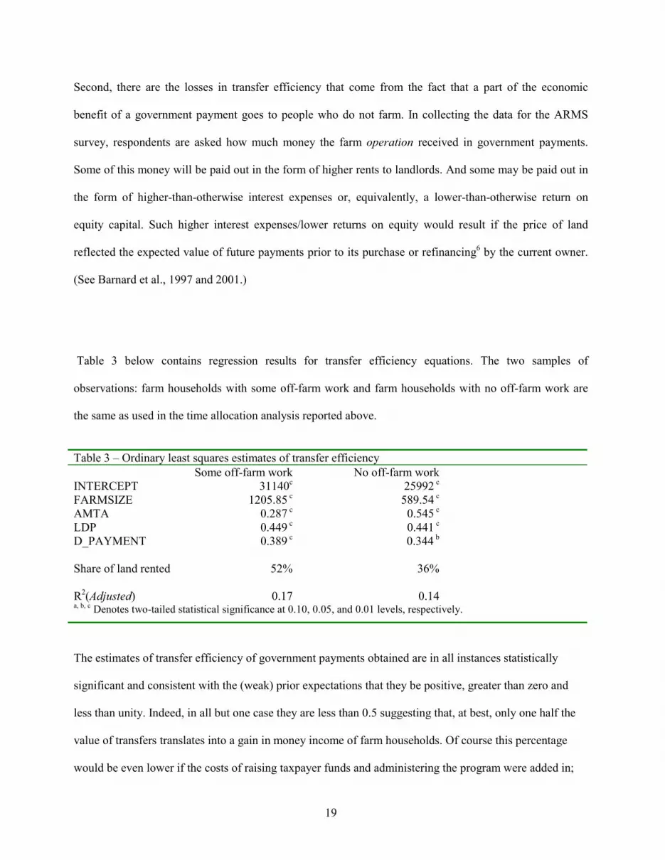
Table 3 below contains regression results for transfer efficiency equations. The two samples of

observations: farm households with some off-farm work and farm households with no off-farm work are

the same as used in the time allocation analysis reported above.

Table 3 – Ordinary least squares estimates of transfer efficiencySome off-farm work No off-farm work

INTERCEPT 31140c 25992 c

FARMSIZE 1205.85 c 589.54 c

AMTA 0.287 c 0.545 c

LDP 0.449 c 0.441 c

D_PAYMENT 0.389 c 0.344 b

Share of land rented 52% 36%

R2(Adjusted) 0.17 0.14a, b, c Denotes two-tailed statistical significance at 0.10, 0.05, and 0.01 levels, respectively.

The estimates of transfer efficiency of government payments obtained are in all instances statistically

significant and consistent with the (weak) prior expectations that they be positive, greater than zero and

less than unity. Indeed, in all but one case they are less than 0.5 suggesting that, at best, only one half the

value of transfers translates into a gain in money income of farm households. Of course this percentage

would be even lower if the costs of raising taxpayer funds and administering the program were added in;

20

lower still for programs that stimulate production leading to lower market prices for the supported

commodities.

Surprisingly, the lowest estimated transfer efficiency is attached to AMTA payments (0.29 for the sample

of farm households reporting some off-farm work), that category of payments which might be regarded as

most efficient. On the other hand, the highest estimated transfer efficiency (0.55 for the sample of farm

households reporting no off-farm work) is also attached to that category of payments.

Why is the estimated transfer efficiency of AMTA payments so low and why is it so different between the

sample of farm households who have some off-farm work versus those with none? The answers to both

parts of the question may be related to the importance of rented land in the farm factor mix. That

percentage (52%) is relatively high for the sample of farm households who have some off-farm work and,

though lower (36%) is significant for that sample of farm households reporting no off-farm work. Recall in

this connection that some recipients of AMTA payments might also be paying relatively higher financing

costs if they bought their land at prices inflated by the expected value of those payments.

This leads us to a further speculation about the relatively higher estimated transfer efficiencies for the

coupled LDP and D_PAYMENTS (for farm households reporting off-farm work). This result would be

consistent with a higher proportion of owned land among those farm households benefiting from coupled

as opposed to decoupled payments.

V. Implications

The reported analysis reveals that, insofar as their effects on household time allocation are concerned,

AMTA payments exhibit characteristics consistent with those of decoupled payments. It also reveals that,

insofar as their effects on household time allocation are concerned, loan deficiency payments and payments

in the category that combines market loss assistance and disaster payments, exhibit characteristics

21

consistent with their being coupled payments. If valid, these are significant findings with implications for

international discussions about the way that support measures are classified for trade negotiations.

A government payment that delivers one dollar of income benefits to farm households for each one-dollar

outlay of taxpayer funds necessarily has no effect on production or trade (Dewbre, Anton and Thompson,

Schmitz and Vercammen). But the reverse need not hold. That is, a completely decoupled payment can be

less than 100% efficient. Administrative costs, the dead-weight costs of taxation and the cost of payments

made to unintended beneficiaries assure this will be so even for the most decoupled of farm program

payments.

In this analysis we obtained estimates of transfer efficiency for AMTA payments (a category for which

results from the analysis of time allocation suggest are completely decoupled) that are well less than dollar-

for-dollar. Indeed, results for the sample of observations of farm households with some off-farm work

show AMTA payments as even less efficient than either of the categories of coupled payments. Such

findings may simply reflect land ownership patterns. That is to say, AMTA payments may be inefficient

not because they lead to economic distortions and resource misallocation but simply because they go

mainly to landowners who do not (any longer) farm. LDP payments may be more efficient despite the

associated distortions to resource use and production because a higher share of their benefits is going to

people who are actively farming. To the extent this is so it would imply that policies that best achieve their

domestic income objectives might not be those which best serve international policy objectives.

REFERENCES

Alston, J.M., and B.H. Hurd “Some neglected social costs of government spending in farm programs”American Journal of Agricultural Economics 75(4) (1993):149-156.

22

Barnard, C.H., G. Whittaker, D. Wesenberger and M. Ahearn “Evidence of capitalization of directgovernment payments into U.S. cropland values.” American Journal of AgriculturalEconomics 79(5) (1997): 1642-1650.

Barnard, C.H., R. Nehring, J. Ryan, R. Collender and B. Quinby “Higher cropland value from farmprogram payments: who gains?” Agricultural Outlook: November 2001,pp. 26-30, Washington,USDA-ERS.

Deaton, A. and J. Muellbauer Economics and Consumer Behaviour Cambridge University Press, 1993.

Dewbre, J.H., J. Anton and W. Thompson “The transfer efficiency and trade effects of direct payments.”American Journal of Agricultural Economics 83(5) (2001).

Dubman, R.W. “Variance Estimation with USDA’s Farm Costs and Returns Surveys and AgriculturalResource Management Study Survey” AGES 00-01(2000) Economic Research Service, U.S.Department on Agriculture, Washington D.C.

Gardner, B.L. “Changing economic perspectives on the farm problem” Journal of Economic Literature,Vol. XXX (March 1992), pp. 62-101.

Gronau, R. “Leisure, home production and work: the theory of the allocation of time revisited” Journal ofPolitical Economy, Vol. 85 (1997) Pp. 1099-1124.

Hoppe, R.A. “Structural and Financial Characteristics of U.S. Farms, 1996”, 21st Annual Family FarmReport to the Congress, AIB # 735 (2000) Economic Research Service, U. S. Department ofAgriculture, Washington D.C. 2000.

Kott, P. “Using the Deleted-A-Group Jackknife Variance Estimator in New Surveys” Unpublished Report(December 1997) National Agricultural Statistics, U.S. Department of Agriculture, Washington D.C.

Lass, D. J. and C.M. Gempesaw “The Supply of Off-farm Labor: A Random Coefficient Approach”American Journal of Agricultural Economics, 74(1992): 400-411.

Lee, J. “Allocating farm resources between farm and non-farm uses” American Journal of AgriculturalEconomics, 47(1965): 83-92.

Mishra, A., H. El-Osta, M. Morehart, J. Johnson, and J. Hopkins “Income, wealth, and well-being of farmhouseholds” (forthcoming) Agricultural Economics Report (June 2002) Economic Research Service,U.S. Department of Agriculture, Washington D.C.

Mishra, Ashok K. and B. K. Goodwin "Farm Income Variability and the Supply of Off-farm Labor"American Journal of Agricultural Economics, 79 (August 1997): 880-887.

Mishra, Ashok K. and D. M. Holthausen “Effect of Farm Income and Off-Farm Wage Variability on Off-Farm Labor Supply” (forthcoming) Agricultural and Resource Economics Review 31(2) October2002.

Schmitz, A. and J. Vercammen “Efficiency of Farm Programs and their Trade-Distorting Effect” inG.C. Rauser, GATT Negotiations and the Political Economy of Policy Reform, (1995): 35-36.

Schmitt, G.H. “What do agricultural income and productivity measurements really mean” AgriculturalEconomics, Vol. 2 (1988) Pp. 139-157.

23

Singh, I., L. Squire and J. Strauss (ed.) Agricultural Household Models Baltimore: Johns HopkinsUniversity Press for the World Bank, 1986.

Sumner, D. A. “The Off-Farm Labor Supply of Farmers” American Journal of Agricultural Economics,64(1982): 499-509.

1 The term ‘leisure’ is used throughout the paper to refer to that time not spent working on the farm or in ajob off the farm. We recognize that some of that time would be spent in activities, e.g. cleaning the house,mowing the lawn, changing diapers and so on, that many of us would not consider remotely connected to‘leisure’.

2 Profits are taken here to mean residual non-labour earnings the farm household receives.

3 The 2001 survey included some additional questions soliciting information on wage rates paid farmoperators and spouses for their off-farm work that may permit a more ambitious program of econometricanalysis in the near future.

4 In a few cases survey respondents reported an unrealistically large number of hours of off-farm work. Toavoid these observations having undue influence on the results we introduced a maximum of 4000 hoursimposing the restriction that neither the farm operator nor the spouse could possibly work more than twofull-time jobs off the farm.

5 Both Sumner and Lass and Gempesaw used total acres as an indicator of farm size.

6 Strictly speaking, refinancing the land would have implications for transfer efficiency only if the moneyobtained was used to finance consumption, not investment. Presumably, higher expenses on a loan takenout to finance investment would be offset in the income/expense accounting by a flow of returns equal, atthe least, to the interest costs on the loan.