Embed Size (px)
Citation preview

University of Groningen
Global trade in services, jobs, and incomesBohn, Timon
DOI:10.33612/diss.104863895
IMPORTANT NOTE: You are advised to consult the publisher's version (publisher's PDF) if you wish to cite fromit. Please check the document version below.
Document VersionPublisher's PDF, also known as Version of record
Publication date:2019
Link to publication in University of Groningen/UMCG research database
Citation for published version (APA):Bohn, T. (2019). Global trade in services, jobs, and incomes. University of Groningen, SOM researchschool. https://doi.org/10.33612/diss.104863895
CopyrightOther than for strictly personal use, it is not permitted to download or to forward/distribute the text or part of it without the consent of theauthor(s) and/or copyright holder(s), unless the work is under an open content license (like Creative Commons).
The publication may also be distributed here under the terms of Article 25fa of the Dutch Copyright Act, indicated by the “Taverne” license.More information can be found on the University of Groningen website: https://www.rug.nl/library/open-access/self-archiving-pure/taverne-amendment.
Take-down policyIf you believe that this document breaches copyright please contact us providing details, and we will remove access to the work immediatelyand investigate your claim.
Downloaded from the University of Groningen/UMCG research database (Pure): http://www.rug.nl/research/portal. For technical reasons thenumber of authors shown on this cover page is limited to 10 maximum.
Download date: 31-07-2022

Global Trade in Services, Jobs, and Incomes
TimonBohn

Publisher: University of Groningen Groningen, The Netherlands Printed by:
Ipskamp Drukkers B.V.
ISBN:
978-94-034-2158-2
eISBN: 978-94-034-2157-5 Copyright © 2019 Timon Bohn All rights reserved. No part of this publication may be reproduced, stored in a retrieval system of any nature, or transmitted in any form or by any means, electronic, mechanical, now known or hereafter invented, including photocopying or recording, without prior written permission of the publisher.

Global Trade in Services, Jobs, and Incomes
PhDthesis
to obtain the degree of PhD at the University of Groningen on the authority of the
Rector Magnificus Prof. C. Wijmenga and in accordance with
the decision by the College of Deans.
This thesis will be defended in public on
Thursday 19 December 2019 at 12:45 hours
by
TimonIsmaelBohn
born on 30 June 1986
in Stanford, United States

SupervisorsProf. S. Brakman Prof. H.W.A. Dietzenbacher
AssessmentCommitteeProf. B. Los
Prof. J.G.M. Marrewijk
Prof. H. Vandenbussche

i
Acknowledgments
It might have seemed inevitable that I would write a dissertation. After all, I always valued my
education and my dad and both of my grandfathers, Dr. Alfred Bittel and Dr. Lothar Bohn, have
doctoral degrees. Yet, I was quite unsure whether this was also my path - until I arrived in
Groningen in 2012 as part of a double master’s degree program. I quickly grew excited about
the research topics emphasized here involving global value chains and input-output analysis.
They complemented well my prior interest and internships in the areas of trade and MNEs. So,
when the opportunity for a PhD presented itself, I knew this is what I wanted to do.
As I soon found out, turning a passion for the field into a dissertation is a completely
different matter. Achieving this goal would not have been possible without the full support of
my supervisors Erik Dietzenbacher and Steven Brakman. I greatly value Steven’s expertise in
international trade, and I admire his perceptive and measured way of thinking in all situations -
all the way to navigating the tricky process of publishing a paper. Erik always got the most out
of me, urging me to aim for high-quality papers that were worthy to submit to top journals and
of interest to a broad audience. Erik made sure everyone was on the same page and that my
PhD was progressing smoothly. I am extremely grateful to Erik and Steven for their excellent
supervision and guidance. I thank you both for always displaying confidence in me.
I would like to thank members of my PhD reading committee - Bart Los, Charles van
Marrewijk and Hylke Vandenbussche - for taking the time to carefully review my dissertation.
Furthermore, I am grateful to Nadim Ahmad, Nanno Mulder, Marcel Vaillant and Dayna
Zaclicever for our close collaboration on the GVC indicators guide over several years. I much
appreciate them allowing me to use our manuscript as a chapter in my dissertation.
I also wish to recognize the roles of Bart Los, Marcel Timmer and Nanno Mulder in laying
the groundwork for my PhD. I still remember Bart’s warm welcome to Göttingen-Groningen
double-degree students like myself back in 2012 and how he (among others) piqued my interest
in the field. I also thank Bart for his detailed feedback on my papers during SOM PhD
conferences. Marcel not only supervised my master’s thesis but encouraged me to consider a
PhD and arranged my internship at the United Nations in Chile. This internship turned out to
be very fruitful as I met Nanno, my internship supervisor with whom I ended up co-authoring
two papers. Nanno showed me how research is like outside of the university and its links to
policymaking. Marcel and Nanno were instrumental in reassuring me that pursuing a PhD was
an excellent idea and helped to prepare that transition.

ii
I thank all my colleagues on the 5th floor for their great support. Everyone in the GEM
department was welcoming and happy to assist me with any requests I had. Administrative
issues were taken care of thanks to the fantastic GEM secretaries. A big thanks goes to Ellen,
Rina and the PhD coordinators at the SOM Graduate School for assistance in general PhD
matters, such as keeping us updated about PhD-relevant events. Teaching was also a part of my
PhD. It was a great pleasure working with Tristan in my first two years, from whom I learned
a lot about teaching, as we taught a brand-new bachelor course together.
I had officemates for about half of my PhD, during which I much appreciated the company
of Fabian and Nikos. But I felt closely connected to my colleagues even in long periods when
I had an office to myself. A major factor contributing to an enjoyable work environment were
the many friendships that developed with fellow PhD students. In my first year I met Joeri,
Xianjia, Ferdinand and Stefan; soon thereafter Aobo, Bingqian, Daan, Fred, Johannes, Kailan,
Maite, Nikos, Duc, Romina and other great people. There is not enough space to write about
each of you individually, but all of you played a part in creating a fun and memorable PhD
experience. Whether at lunch and coffee breaks during work, or at countless get-togethers
afterwards – for sports, games, movies, dinners, birthdays and weekends away... it was so great
to be around such wonderful, supportive and fun people. I am also grateful to current and former
members of HOST and Vineyard - especially my former housemate Esther - for their
friendships and the many activities that enriched my time here. I also valued the support of my
good friend Micha in Germany who was always there to talk to about anything.
Finally, the love and support of my family – my mom, my dad, my five siblings and my
grandparents – is truly immeasurable. My dad gave me excellent advice in every kind of
situation and, as a professor himself, could relate well to the bumpy road towards a PhD degree.
My relatives in Germany – Marianne and Lothar, Marga and Alfred, Annja and Joachim - gave
me the comforts of a home away from home when I could not be in California (including every
Christmas). I am deeply indebted to my incredible grandma Marianne. She has been a source
of unconditional support and encouragement in all aspects of my life, not only during my PhD
but ever since I moved from California to Germany 13 years ago. My grandfathers Dr. Alfred
Bittel and Dr. Lothar Bohn sadly both passed away while I was writing this dissertation. They
inspired me and reinforced the importance of education with their own doctoral degrees from
many decades ago. Opa Alfred und Opa Lothar - Ich widme Euch diese Doktorarbeit.
Timon
Groningen, November 2019

iii
Contents
1 Introduction 1
1.1 Background and objective .......................................................................................... 1
1.2 Indicators on global value chains ............................................................................... 3
1.3 Global trade in services .............................................................................................. 4
1.4 Global trade in jobs .................................................................................................... 5
1.5 Global trade in incomes .............................................................................................. 7
2 Indicators on global value chains: A guide for empirical work 9
2.1 Introduction .............................................................................................................. 10
2.2 Indicators based on international trade statistics ...................................................... 12
2.2.1 Trade data ..................................................................................................... 12
2.2.2 Trade data-based GVC indicators................................................................. 14
2.2.3 Limitations of trade data ............................................................................... 19
2.3 Indicators based on input-output tables .................................................................... 20
2.3.1 Trade in value added ..................................................................................... 20
2.3.2 Input-output analysis .................................................................................... 21
2.3.3 TiVA database .............................................................................................. 24
2.3.4 Input-output table based GVC indicators ..................................................... 25
2.3.5 Limitations of IOT based statistics ............................................................... 44
2.4 Some final considerations......................................................................................... 46
Appendix Chapter 2 .......................................................................................................... 48
3 The role of services in globalisation 55
3.1 Introduction .............................................................................................................. 56
3.2 Literature .................................................................................................................. 58
3.2.1 The growing importance of services ............................................................ 58
3.2.2 Two questions ............................................................................................... 60
3.3 Analytical framework and data sources ................................................................... 62
3.4 Empirical results ....................................................................................................... 68
3.4.1 Identifying the relative importance of services over time ............................ 68
3.4.2 Did services travel further than manufactured goods? ................................. 72
3.5 Conclusion and discussion ....................................................................................... 75
Appendix Chapter 3 .......................................................................................................... 77

iv
4 Who’s afraid of Virginia WU? The labor composition and labor gains of trade 91
4.1 Introduction .............................................................................................................. 92
4.2 Literature .................................................................................................................. 95
4.2.1 The labor footprint ........................................................................................ 95
4.2.2 Factor content of trade .................................................................................. 96
4.2.3 Our approach ................................................................................................ 97
4.3 Methodology............................................................................................................. 98
4.4 Data sources............................................................................................................ 100
4.5 Results: US case study............................................................................................ 102
4.5.1 US labor footprint ....................................................................................... 102
4.5.2 Counterfactual exercises ............................................................................. 106
4.6 Extensions............................................................................................................... 109
4.6.1 Sectoral substitutability and worker endowments ...................................... 109
4.6.2 Sensitivity analysis ..................................................................................... 111
4.6.3 Comparative perspective of the other countries in WIOD ......................... 113
4.7 Conclusions and Evaluation ................................................................................... 117
Appendix Chapter 4 ........................................................................................................ 120
5 From trade in value added to trade in income 129
5.1 Introduction ............................................................................................................ 130
5.2 Statistical challenges: three questions .................................................................... 134
5.3 Methodology........................................................................................................... 137
5.3.1 Background principles ................................................................................ 138
5.3.2 Road map .................................................................................................... 139
5.3.3 Step 1: estimation of the diagonal elements of the matrix ......................... 141
5.3.4 Step 2: estimation of the off-diagonal elements of the matrix ................... 143
5.4 Data sources............................................................................................................ 145
5.5 Results .................................................................................................................... 150
5.5.1 Diagonal elements of the matrix ................................................................. 150
5.5.2 Off-diagonal elements of the matrix ........................................................... 153
5.5.3 Analysis: exports of GNI ............................................................................ 158
5.5.4 Analysis: trade balance of income .............................................................. 165
5.6 Conclusion .............................................................................................................. 170
Appendix Chapter 5 ........................................................................................................ 175
6 Summary and conclusions 195
References 205
Dutch summary – Nederlandse samenvatting 217

1
Chapter 1
Introduction
1.1 Background and objective The globalization of the world economy has accelerated cross-border movements of goods,
services, labor, and capital. This has profound implications for the analysis of international
trade and in determining the importance of trade for an economy’s well-being.
The most significant development over the past 25 years has been the emergence of
international production networks, also known as global value chains (GVCs), which
increasingly dominate world trade (Baldwin, 2016; Gereffi and Fernandez-Stark, 2016).
Although globalization has been with us for hundreds of years, Baldwin argues that GVCs
represent a recent structural change in the type of trade flows. Trade used to involve the
exchange of goods and services between countries that were mostly, if not entirely, produced
by the domestic factors of production of the exporting economy and consumed by final users
of the importing economy. Nowadays, international production networks have sliced up the
production of goods and services into tasks that are dispersed across different countries. Design,
assembly, marketing, distribution, and support activities are typically performed in a country
that has a comparative advantage for one or more of these tasks. These export-oriented and
specialized activities may themselves involve foreign-owned capital or cross-border workers.
They are also often coordinated by multinational enterprises (MNEs).
The global fragmentation of production was made possible with rapidly decreasing
transportation and communication costs and has led to a rapid rise in intermediate products (i.e.,
parts and components) crossing international borders (Baldwin 2006, 2016). Importantly,
fragmentation has implications for what trade implies for an economy. This thesis contributes
to the literature on GVCs by investigating the characteristics and potential benefits of trade in
the context of global production fragmentation. There is also a large literature on the industry-
and firm-level perspective of GVCs, for example of industry case-studies and ‘upgrading’
strategies (Gereffi, 1999; Gereffi and Fernandez-Stark, 2016). I restrict myself in this thesis to
macro, country-level aspects.
2 Chapter 1
Trade is traditionally measured in terms of gross exports. Bilateral gross export figures
depict the gross flows of goods and services between countries and will continue to be the most
important statistic for a country’s customs officials. Nonetheless, these statistics have
significant analytical limitations that are magnified by the restructuring of the world economy.
First, gross exports reflect the industry of the exported product, which may differ from the
upstream industries involved in its production. Services account for only a small share of
countries’ gross exports despite their critical importance as inputs and enablers of international
production networks and the ‘servicification’ trend of manufacturing (Low, 2013). Second,
gross export statistics do not differentiate between value added that was created domestically
by the exporting country and value added that was created by other countries (i.e., foreign value-
added). Hence, the domestic value-added embodied in a traded product, which contributes to a
country’s gross domestic product (GDP), may be less than the full export value. Third, gross
exports are generally insufficient to identify a country’s position in international production
networks, i.e., in terms of differentiating between upstream vs. downstream activities and
determining where a country is creating value. This makes it more challenging to evaluate the
true economic benefits of a country’s participation in GVCs and international trade.
These developments raise important questions. First, to what extent can conventional trade
data still be used in the context of international production networks? What are alternative
measures? Second, given the growing interconnectedness of the world economy through GVCs
and multinational firms, what are the implications of trade nowadays for a country in terms of
generating domestic value-added, contributing to national income, and enabling higher
consumption possibilities? Taking into consideration the analytical limitations of gross export
statistics, I apply existing and newly developed approaches to assess the importance and
benefits of trade from different perspectives. I juxtapose three types of trade in particular: trade
in gross exports, trade in value added (or the jobs embodied therein), and lastly, trade in income,
to address the topics and questions that are introduced in this chapter. A point of focus is also
to account for the role of foreign production factors in a country’s domestic value-added
production and their contributions to sustaining a country’s overall consumption bundle.
It should be noted that these different perspectives are complementary. All my calculations
use gross exports data to start with, so high-quality data on gross exports remain important. The
noted limitations of gross exports are not an appeal to abolish gross trade statistics. Instead, the
interpretation of pure gross exports differs. This means that policymakers and the media are
susceptible to misinterpreting them. For example, gross exports are popularly applied to trade
balances. The nature of the bilateral US trade deficit with China still receives much international

Introduction 3
attention. However, bilateral trade balances are overstated given that the contributions of
foreign/intermediate suppliers to the traded products captured in these statistics do not come to
light. Trade balances can also be analyzed in the context of value added or, in the more novel
approach I employ in Chapter 5, in terms of the gross national income (GNI) induced in each
country by foreign consumption of final products (i.e., final demands) in counterpart countries.
A comparison of conventional trade balances with value-added and income perspectives would
more completely and adequately depict the true nature of interdependencies between countries.
1.2 Indicators on global value chains In Chapter 2, I review the main approaches and techniques used in the GVC literature. I
critically evaluate and discuss an array of indicators for gross measures of trade and indicators
derived from input-output frameworks. In my view, the existing literature has lacked a user-
friendly guide on the different approaches that are available to measure trade and to characterize
a country’s position in international production networks. This is an indication that the field is
‘young’, and no convergence has been reached yet. In addition, as the field is still relatively
new, many users struggle to fully understand what indicators are available, how they have been
constructed, and how they should be used. The analytical potential of indicators relevant to
GVCs is enticing not just to researchers, but also to policymakers and international
organizations. Thus, it is essential to make them accessible also to non-specialists and to provide
guidance to users on which indicators can be useful in empirical work. There is a need for a
more comprehensive overview of the tools available, including the trade in value added
approach, along the lines of recent surveys of the field by Los (2017) and Johnson (2018).
Chapter 2 has two main objectives. First, I introduce the current challenges of assessing
countries’ participation in international trade and production networks. I highlight the key
issues that are involved, explain why GVC-based indicators are necessary, and lay the
groundwork for my own empirical work in subsequent chapters of this thesis. The widespread
use of relatively new databases, notably the World Input-Output Database (WIOD) and the
OECD Trade in Value Added (TiVA) database, have given rise to a growing and active research
field related to topics involving GVCs. This thesis contributes to this literature by developing
new applications using the WIOD based on existing and newly developed GVC-based
indicators. Second, the chapter is designed to be a guide for new users to the methodological
approaches in the field. I summarize the current state of knowledge on measuring trade in
international production networks by reviewing in a systematic and comparative manner many

4 Chapter 1
different indicators. I describe what these various measures indicate. This discussion goes
beyond just the indicators that are employed later in the thesis.
The more popular GVC indicators use input-output frameworks and international input-
output tables to measure the foreign value-added contained in a country’s gross exports (= the
degree of ‘vertical-specialization’) and/or the domestic value-added contributing to the
consumption bundle of foreign countries (= ‘value-added exports’). The indicators capture,
among other aspects, the import content of exports and identify the industries that generate
value added in trade. These indicators show that the ratio of domestic value-added to gross
exports varies widely across countries, but is generally declining after 1990 (i.e., the foreign
value-added content of a country’s gross exports is rising) (Johnson, 2014). Also, it is revealed
that manufacturing exports have a higher degree of vertical specialization than services exports.
1.3 Global trade in services The first application of the GVC indicators focusses on the characteristics of trade in services.
It is well-established in the GVC literature that services make up a larger share of value-added
exports than gross exports. Services thus feature more prominently in international trade than
would be perceived based on gross trade statistics (Johnson and Noguera, 2012; Heuser and
Mattoo, 2017; Miroudot and Cadestin, 2017). This is because gross exports do not indicate the
extent that services inputs are embodied in manufacturing exports or in the exports of other
sectors. Services are critically important as value creators and enablers of international
production networks (Low, 2013). Manufacturing firms increasingly look to services to add
value to their products and to raise their productivity (leading to a bundling of services with
goods).
However, services have remained an understudied aspect of international trade. Visibility
of the importance of services is not sufficiently transmitted to the general public. This lack of
awareness of the role of services is partly due to the focus on gross exports and a lack of suitable
data until now. The indicators introduced in Chapter 2 and based on world input-output tables
are well-suited to investigate the role of services. Indicators of value-added induced by foreign
final demand measure the contributions of all trade-related activities to a country’s GDP. The
indicators not only capture direct services exports, but also indirect services, i.e., domestic
services inputs such as energy, transport, software, and financing that are embodied in other
traded products. Industry-level decompositions of these indicators separate out the trade-related

Introduction 5
value-added contributions of services (or of specific services industries) from the respective
contributions of other sectors and industries.
In Chapter 3, I employ value-added export indicators and (for purposes of comparison)
gross export-based indicators to investigate the role of services in globalization for the period
2000-2014. First, from an empirical perspective, it has not been studied to what extent services
activities are becoming more important for trade relative to manufacturing activities in the
European Union (EU-15 member states), North America, and East Asia. Hence, I ask: has trade
of value-added in services (i.e., the value added created by domestic service industries and
embodied in foreign consumption of final products) grown more than trade of value-added in
manufacturing in these three regions? A confirmation of a growing role for services would
emphasize the importance of the liberalization of services trade (efforts which may be boosted
by a better availability of statistics). This could involve looking at policies to reduce the
regulatory burdens of trade in services and strengthening regulatory cooperation between
countries. Services face higher and more complex types of trade barriers relative to goods
(Miroudot et al., 2013). Thus, beyond autonomous trade measures, new policy and
(multilateral) trade negotiation methods may be necessary to unlock the full potential of
services, e.g., in terms of increasing manufacturing competitiveness. This requires having the
correct facts first about services.
Second, to my knowledge no previous work has analyzed whether trade in services is more
likely to be intraregional (i.e., traded between countries in the same region) or interregional
(i.e., traded between countries in different regions) when measured from the standpoint of the
distance between the country of value creation and country of final consumption. It is a stylized
fact that it is often concluded that trade in goods is still intraregional (Baldwin and Lopez-
Gonzalez, 2015). But this may not necessarily also be the case for services. Hence, I ask: does
trade of value-added in services travel further than trade of value-added in manufacturing?
1.4 Global trade in jobs Chapter 4 applies a GVC framework by considering the jobs – both foreign and domestic – that
are embodied in a country’s consumption of final goods and services.
In the US, import competition from China and the election of President Trump drew much
attention to the potential adverse impacts of trade. The current political climate reflects concerns
about the ballooning US trade deficit, the growing influence of China, particularly since China’s
accession to the WTO in 2001, and the belief that trade is driving certain workers out of

6 Chapter 1
employment. These developments are closely related to the international fragmentation of
production, which has increased outsourcing and offshoring opportunities. This has probably
propelled a reallocation of jobs across countries, e.g., manufacturing jobs going from the US to
China. In consequence, the US has been renegotiating major trade agreements, such as the
Transatlantic Trade and Investment Partnership (TTIP), the North American Free Trade
Agreement (NAFTA), and the free trade pact with South Korea.
Recent research tends to emphasize the ‘lost’ manufacturing jobs due to import competition
– especially jobs going from the US to China (Acemoglu et al., 2016; Autor et al., 2013; Pierce
and Schott, 2016). The possible benefits of trade with China, including access to lower-priced
or more efficient foreign workers and suppliers, are also well-documented. Increased
international specialization is commonly viewed as leading to overall welfare gains. However,
what has not been studied intensely is the ‘labor footprint’ along supply chains.
In Chapter 4, I use the labor footprint to gain new insights into the implications of trade for
employment and for a country’s consumption bundle. The labor footprint relates to the broader
footprint concept popular in the analysis of other issues, including carbon emissions, water use,
biodiversity, and inequality. Although the idea of using the labor footprint has recently started
appearing in the literature to address social inequality issues (Gomez-Paredes et al., 2015), to
my knowledge it has yet to be used for the analysis of jobs at the country-level. I define a
country’s global labor footprint as the global amount of labor that is embodied in the final
products that this country consumes. I ask: how much does the US rely on ‘imported’ foreign
labor (of different skill-types and sectors) relative to its own domestic workers to sustain its
consumption patterns and standards? Then I employ the labor footprint concept to assess the
ability of a country to be self-sufficient in a counterfactual autarky situation (given certain
assumptions). Would the US need to sacrifice some of its consumption of final goods and
services if there were no involvement of foreign workers, i.e., in a situation of autarky? I focus
on the US and the period 1995-2008, but the counterfactual exercises provide results for 39
other, mostly developed, countries. I also determine a country’s so-called labor gains of trade.
Labor gains of trade are identified as a situation where the labor footprint in autarky exceeds
the number of employed workers of this country. This would then imply a reduced consumption
under autarky.

Introduction 7
1.5 Global trade in incomes While developed countries are concerned about losing manufacturing jobs, emerging and
developing countries also have reasons to question the true benefits of certain outsourcing and
investment arrangements. GVCs have helped many countries to integrate into the world
economy and increase the amount of goods and services they trade. At the same time, MNEs
and their foreign affiliates play a leading role in GVCs. They account for more than half of all
international trade (Cadestin et al., 2019). This suggests that countries may not be able to
translate all their domestic value-added from trade-related activities into national income. For
example, MNE affiliates may send (i.e., repatriate) their capital profits to the country where the
firm’s headquarters or investors are located. Emerging and developing countries receiving
much foreign investment may be most susceptible to repatriation.
The role of foreign suppliers of capital and labor could have the opposite implication for
developed countries. Many of the largest MNEs are headquartered in developed economies and
make large direct investments abroad. This may enable their home countries to capture more of
the economic benefits linked to final demand abroad (including but not limited to income
related to trade) than what is suggested by value-added exports. Suppose a US MNE operating
in Mexico earns a profit on the goods and services it exports to Germany. Then value added is
generated in Mexico and, quite possibly, some of the value added turns into income for US
owners of capital. These income linkages could mitigate some concerns about the drawbacks
of international integration in countries like the US, and impact trade and investment policies.
The distinction between domestic value-added (GDP) and gross national income (GNI) is
consequential in the context of the value-added indicators discussed and employed in earlier
chapters. That is, the degrees to which a country’s domestic value-added (GDP) and national
income (GNI) depend on foreign final demand (also bilaterally) are likely to differ.
In Chapter 5, I propose a way of estimating the national income implications of foreign
consumption by exploring cross-border income flows and the investment nexus. This income
channel has already been identified in the GVC literature as a relevant issue (Ahmad and
Ribarsky, 2014), but to my knowledge its importance has not yet been investigated empirically
in a global analysis. This aspect has been neglected in the GVC literature due to data limitations.
Another motivation for the analysis involves the depiction of bilateral dependencies between
countries. This from-whom-to-whom perspective is relevant because it can help policymakers
identify investment linkages and to forecast possible repercussions of economic shocks abroad.
It should be noted that my analysis is broad and considers where all value added in a country,

8 Chapter 1
not only value added related to trade or MNE activities, ends up. Hence, I also account for the
German cross-border worker employed in Luxembourg who is engaged in a non-tradable sector
and generates value added in Luxembourg but income (via her/his wage) in Germany.
I begin by developing a general framework to show how much value added created in a
country translates into income gains for this country’s residents as opposed to income gains for
foreign suppliers of capital and labor. Data on these bilateral relationships do not currently exist.
My contribution is to deconstruct the GDP of 42 countries plus ‘the rest of the world’ into
bilateral transfers of primary incomes by making novel use of the Balance of Payments, national
accounts, and data on cross-border investment positions. The resulting GDP-GNI matrix
indicates what share of GDP is part of the same country’s national income and what shares end
up as part of the national income of counterpart countries. The GDP-GNI matrix is used in
conjunction with trade in value added data derived from world input-output tables to produce a
new matrix of trade in income. This new matrix shows the exports of income for each country.
I use the new data to investigate who gains income from foreign consumption of final
products. I compare the results to trade in value added measures. I then do similar comparisons
for trade balances. Where do transfers of income (according to the GDP-GNI matrix) end up?
And what shares of GNI do different countries export (according to the matrix of trade in
income)? To what extent does the large US trade deficit - both overall and its bilateral deficits
with countries like China and Mexico - differ in terms of value-added and income?
In Chapter 6, I summarize the main findings (and caveats) of my research, discuss policy
implications and links between the chapters, and suggest future research directions.

9
This chapter is based on Ahmad et al. (2017). I added endnotes at the end of this chapter to correct typos in the OECD Working Paper version (reproduced here) and to provide additional clarification or context.
Chapter 2
Indicators on global value chains: A
guide for empirical work
ABSTRACT
Traditionally, the main source of data used to measure countries’ participation in international production networks or global value chains (GVCs) has been conventional international trade statistics. However, international fragmentation of production has weakened the analytic interpretability of these data as intermediate goods but also services cross borders many times on the way to their final destination. This is often referred to as the double (or multiple)-counting problem of international trade statistics. This, in turn, has led to the development of a new branch of trade statistics, referred to as Trade in Value-Added (TiVA) providing new insights on GVCs, and corresponding databases, notably the OECD-WTO TiVA database, which provide a measure of international interdependencies through the construction of global input-output tables that show how producers in one country provide goods and/or services to producers and consumers in others. But with the field still relatively new, many users are struggling to fully understand how these new indicators should be used and indeed how they have been constructed. This document is designed to address those difficulties, providing, where appropriate guidance on “dos” and “don’ts”. It also reviews many other typical GVC indicators derived outside of input-output frameworks; recognising that gross measures of trade, and indicators derived from them, remain important and relevant for policy making.

10 Chapter 2
2.1 Introduction The increasing fragmentation of production processes into activities scattered across different
countries has challenged economists and statisticians to find ways to measure the extent of these
developments and their potential implications. This phenomenon is intrinsically related to a
surge in international trade in intermediate products, which dominate world trade flows,
characterised in large part, and indeed further complicated, by the increasing role played by
multinational enterprises (MNEs) (whether through intra-affiliate transactions or indeed
through the control of supply chains). Increasingly, countries and firms specialise in particular
stages of production according to their comparative and competitive advantages, and are linked
in vertical supply chains through trade in intermediate products. This trend has been facilitated
by technological progress, which has reduced transportation and communication costs, together
with significant declines in trade barriers.
Traditionally, the main source of data used to measure countries’ participation in
international production networks or global value chains (GVCs) has been conventional
international trade statistics, which, in the case of goods, offer the advantage of timely
availability for a large number of countries, with a high level of disaggregation (in terms of
products and trading partners), and with a high degree of international comparability.
As shown below, these data can be used to generate a suite of indicators that reveal the
diversity of a country’s direct export and import partners, as well as the products in which it
trades. However, international fragmentation of production has weakened the analytic
interpretability of these data and, in particular, analyses that attempt to show the benefits of
trade to an economy (be that in terms of value added or jobs), as well as the true nature of
interconnectedness across economies. This is often referred to as the double (or multiple)-
counting problem of international trade statistics.
Perhaps the classic example of the impact of the phenomenon concerns processing trade,
where firms, typically at the end of value chains, import parts for final assembly. Conventional
gross trade data would indicate that the country has a comparative advantage in the production
of the final good, despite the fact that it may have added relatively little value to the actual good
through low-skilled part tasks. Thus, the comparative advantage should more accurately be
described in this case as low-skilled assembly labour, rather than high-tech goods production.

Indicators on global value chains 11
Some countries maintain a special set of customs statistics related to processing trade1 that
can provide insights (and account for) any related ‘double-counting’. However, for most
countries these data are not available. Moreover, often processing trade statistics only reflect
the tip of the iceberg, as they only consider trade associated with a special type of sub-
contracting or outsourcing arrangement, and do not cover all other activities (the majority)
related to the geographic fragmentation of production.2 Indeed very little of the goods exported
today, with the possible exception of mineral and agricultural products (and even here imported
know-how services play a role), are produced exclusively within any one country.
To tackle head-on the double-counting problem that affects conventional trade data, whilst
also better revealing the true nature of international and interindustry interdependencies,
statisticians have recently begun to develop indicators using global supply and use tables
(SUTs) and input-output tables (IOTs), which link national SUTs or IOTs and bilateral trade
data (e.g., OECD-WTO, 20133). Perhaps the best known initiative in this area is the Trade in
Value Added (TiVA) database, which reflects a concerted effort by the Organisation for
Economic Co-operation and Development (OECD) and the World Trade Organisation (WTO)
to mainstream the development of (and improvements to) the necessary data within official
national statistical information systems.4 Indeed, at the 2015 United Nations Statistics
Commission meeting the official statistics community endorsed the recommendations of the
Friends of the Chair Group on International Trade and Economic Globalisation, including, in
particular, the following:
Mainstreaming the development of recurrent global supply and use tables and input-
output tables and building on work undertaken by OECD, in order to expand the
coverage of the OECD-WTO database on trade in value added.
Rising to this challenge the international statistics community has stepped-up co-operation,
with the OECD in particular coordinating the development of a network of international
agencies (and countries), each playing their role as developers of regional IOTs (for the regions
where they have expertise and formal networks of national statisticians) that can be brought
1 This refers to the trade of export processing zones (EPZs), which offer firms special customs arrangements (like tariff exemptions or reductions) on condition that imported intermediates are re-exported after assembly activities are completed. Examples of these data sets are the US Offshore Assembly Programme (OAP) and the European Union Processing Trade statistics, used in several empirical studies on international fragmentation of production (e.g., Feenstra et al., 2000; Swenson, 2005; Egger and Egger, 2005; Baldone et al., 2007). 2 Processing trade statistics capture the cases where intermediate products are imported to be processed internally and then re-exported, as well as those where intermediates are exported to be processed abroad and then re-imported. 3 www.oecd.org/sti/ind/49894138.pdf. 4 Annex A provides an overview of other initiatives in this area.

12 Chapter 2
together and integrated within a global IOT. The United Nations’ Economic Commission for
Latin America and the Caribbean (UN-ECLAC) is actively working with the OECD to explore
the feasibility of mainstreaming the activity within the Latin American region, which partly
reflects the catalyst for this paper.
In that sense, this document is designed to accelerate that process and maximise its
feasibility by describing, in a comprehensive and integrated manner, a set of core indicators
that are typically used to trace and analyse production fragmentation across countries;
highlighting in addition their limitations (in particular, with regards to the changes introduced
in the latest version of international accounting standards, the 2008 System of National
Accounts). In this sense it is important to note that the document does not set out to be
exhaustive in its coverage. Many other indicators exist, including many that have recently been
developed as a result of new innovations in TiVA type analysis. But these are not typically in
widespread use and, with respect to the newer indicators, they remain, to some extent, works-
in-progress.
The note is also motivated by growing calls from users for a better understanding of the
‘dos and don’ts’ of the suite of indicators generated by these new statistical tools, which can be
fostered by describing their structure, applications and limitations.
The following section sets the scene by describing indicators based on traditional
international trade data. Section 2.3 introduces the input-output framework, used to create trade
in value added estimates. Finally, Section 2.4 concludes.
2.2 Indicators based on international trade statistics 2.2.1 Trade data
Merchandise trade data are arguably one of the richest sources of data available in the economic
statistics information system. They provide product-level information (with the Harmonised
System (HS) coding covering around 5 000 goods), with almost complete country coverage and
the identification of partner relationships. As such, despite some comparability issues relating
to the trade regime used in the country (special versus general trade), recorded country of import
and recorded country of export, asymmetries,5 and treatment of confidential data, merchandise
trade data provide one of the most important sources of information to derive GVC indictors.
5 Although the OECD has developed a balanced merchandise trade dataset, see www.oecd.org/officialdocuments/publicdisplaydocumentpdf/?cote=STD/CSSP/WPTGS%282016)18 &docLanguage=En.

Indicators on global value chains 13
Trade in services data, collected according to the Extended Balance of Payments System
(EBOPS), are also an important source of information. However, the quality of these data is
significantly inferior to that on merchandise trade. For example, the level of product detail
available rarely extends beyond dozens for most countries, and very few countries provide
bilateral data.6
In addition, many countries have recently begun to develop new datasets that link the firms
identified in customs records with the same firm recorded in statistical business registers (Trade
by Enterprise Characteristics (TEC) database), to develop new insights on firms engaged in
international trade.7
Because of the comparability issues regarding trade in services and the relative novelty and
limited country coverage of TEC data, the more abundant and detailed merchandise trade data
have typically formed the key focus of most traditional and conventional indicators on GVCs.
In large part, this reflects the ability of merchandise trade data to differentiate between products
on the basis of their likely end-use (for example, whether the goods are intermediate,
consumption or capital in nature).
GVCs are seen as synonymous with international fragmentation of production. The ability
to identify trade in intermediate products, as distinct from trade in final goods, can provide
important insights into how countries integrate into GVCs, and indeed where they position
themselves in those chains.
Notwithstanding the data on intermediate goods available in national SUTs and IOTs8
(described in more detail below), the most commonly used definition of intermediate goods in
merchandise trade is based on the United Nations’ Broad Economic Categories (BEC)
classification,9 which provides a simple tool to link trade data to the three basic System of
National Accounts’ (SNA) classes: intermediate goods, capital goods and consumption goods.10
6 The OECD and WTO have developed a balanced view of trade in services with missing estimates generated using a gravity model, https://one.oecd.org/document/STD/CSSP/WPTGS%282017)4/en/pdf. 7 https://one.oecd.org/document/STD/CSSP/WPTGS%282017)5/en/. 8 For example, Hummels et al. (2001) use national IOTs to show that vertical specialisation (i.e., the use of imported inputs in producing goods that are exported) has increased over time, and explained 30% of the growth in exports of 14 OECD and emerging market countries between 1970 and 1990. 9 The original BEC classification, issued in 1971, was defined in terms of the Standard International Trade Classification (SITC) revision 1. Since then, it has been updated three times: 1) in 1976 in terms of the SITC revision 2; 2) in 1986 in terms of the SITC revision 3; and 3) in 2002, based on the more detailed goods description provided by the 2002 edition of the Harmonized Commodity Description and Coding System (United Nations, 2003). This fourth version, set up with reference to the third revision of the SITC, can be found at http://unstats.un.org/unsd/cr/registry/regdnld.asp?Lg=1. The fifth revision was endorsed by the UN Statistical Commission at its 47th session in 2016. 10 The SNA intermediate goods class corresponds to the BEC code numbers 111 (food and beverages mainly for industry, primary), 121 (food and beverages mainly for industry, processed), 21 (industrial supplies not elsewhere specified, primary), 22 (industrial supplies not elsewhere specified, processed), 31 (primary fuels and

14 Chapter 2
Several studies investigate international production fragmentation using the BEC
classification as a starting point (for references see Sturgeon and Memedovic, 2010). However,
the BEC classification is far from perfect and has been criticised for its subjective allocation of
products, which is based on expert judgment concerning descriptive characteristics, particularly
with regards to the fact that some goods may be used both as intermediates and final products
(for example flour, which is classified as intermediate but can also be a consumption good if
bought by households), and which may not align with the equivalent allocations used in national
SUTs. In addition, up until the 4th Revision, the BEC classification was not available for trade
in services. This has been addressed in the latest (5th) revision but the high level of aggregation
in services trade data (as well as its novelty and limited availability in many countries) has
restricted its application.
This has led many to refine the BEC classification in their own analyses. Sturgeon and
Memedovic (2010), for example, use industry-specific manufactured intermediate goods (MIG)
classifications in order to isolate 'true' (differentiated, customised, product-specific)
intermediates from generic intermediates. The OECD, as part of its work in producing TiVA,
has also developed a refinement to the BEC system that introduces categories of mixed use
(Bilateral Trade Database by Industry and End-Use Category, BTDIxE).11
2.2.2 Trade data-based GVC indicators The most commonly used GVC indicators based on international trade statistics are presented
below. They are shown in a way that is not contingent on any actual definition used to define
intermediate trade (i.e., BEC or alternatives).
Share of intermediate goods in exports and imports
The most basic version of this indicator measures the share of a country’s exports of
intermediate goods in its total goods’ exports, which provides broad insights into the relative
position of a country within GVCs (i.e., more or less upstream in the production of intermediate
goods compared to final demand goods):
XISH� = EXGRI�EXGR� (2.1)
lubricants), 322 (processed fuels and lubricants), 42 (parts and accessories of capital goods, excluding transport equipment), and 53 (parts and accessories of transport equipment). 11 www.oecd.org/trade/bilateraltradeingoodsbyindustryandend-usecategory.htm.

Indicators on global value chains 15
where EXGRI� = ∑ EXGR��q��∈��� are country c’s exports of intermediate goods; EXGR� =∑ EXGR��q�� are country c’s total goods exports; q=1, 2,…, Q is the product index; and � ∈int is the subset of products corresponding to intermediate goods.
A variation of this indicator quantifies the share of imports of intermediate goods in total
goods imports, which is particularly useful for countries participating in the downstream stages
of supply chains (i.e., the assembly of finished goods from imported components):
MISH� = IMGRI�IMGR� (2.2)
where IMGRI� = ∑ IMGR��q��∈��� country c’s imports of intermediate goods; and IMGR� =∑ IMGR��q�� are country c’s total goods imports.
This indicator can also be used to provide insights into the integration of countries in
bilateral and regional production networks, by calculating equivalent shares on a bilateral or
regional basis.
Share of intermediate goods in total trade
This indicator shows the share of intermediates in total goods trade, including both exports and
imports:
TISH� = EXGRI� + IMGRI�EXGR� + IMGR� (2.3)
It can also be computed considering bilateral or regional trade flows.
Although TISH provides a complementary view of a country’s participation in GVCs to
the two separate indicators described above, this is not a comprehensive view. For example, a
country with high levels of imports and exports relative to its gross domestic product (GDP)
may have a similar TISH ratio to a country with a low ratio of trade to GDP.
Relative importance of trade in intermediates
Dullien (2010) proposes a variant of the previous indicator, which attempts to address some of
the inadequacies mentioned above. The indicator, referred to here as the “relative importance
of trade in intermediates” (RITI), is defined as the ratio of intermediate goods trade to a
country’s GDP:

16 Chapter 2
RITI� = EXGRI� + IMGRI�GDP� (2.4)
By relating intermediates trade to GDP, instead of to total trade, this indicator provides insights
into the relative importance of a country’s participation in international production networks to
the economy. However, both the share of intermediates in total trade (TISH) and the RITI index
have the shortcoming that a country that imports a large volume of intermediate goods and re-
exports those goods as intermediates without adding much domestic value could exhibit high
values of both indicators. Additionally, like TISH, the RITI index cannot provide information
on a country’s position in value chains. Finally, although the indicator provides a better measure
of the relative importance of trade to the economy, comparisons across countries should be
conducted with care as larger economies will typically have lower ratios, in part reflecting the
larger relative importance of domestic consumption, but also the relative potential of internal
domestic supply chains to provide intermediates.
Ratio of intermediate imports to exports
This indicator, also called coverage ratio, relates a country’s imports of intermediates to its
intermediate exports, and can be used as a broad measure of a country’s position in GVCs:
CRI� = IMGRI�EXGRI� (2.5)
Countries located at the beginning of the production chain (upstream) tend to import fewer
intermediates and export more, resulting in a relatively low value of CRI. In contrast, countries
that specialise in assembly and are located at the other end of the supply chain (downstream)
tend to import more intermediate goods and export relatively less, resulting in a comparatively
high value of CRI. However, some care is needed in interpretation as the indicator is not able
to address scale (i.e., differences in economic size), nor is it necessarily able to provide for
robust and meaningful international comparisons. For example, a country that imports most
intermediates for producing final goods destined for domestic markets, and that has relatively
limited intermediate exports will have a significantly higher ratio than an equivalent country
with higher intermediate imports and exports.

Indicators on global value chains 17
Grubel-Lloyd index
Intra-industry trade indices in intermediates serve as a proxy of a country’s insertion in GVCs,
as well as to identify bilateral production linkages between countries and regions. A high level
of intra-industry trade in intermediates (i.e., two-way exchange of intermediate goods within
the same industry) is interpreted as indicating greater production links between participating
countries, which would reflect international fragmentation.12
The most widely used intra-industry trade measure is the Grubel-Lloyd (GL) index. This
index relates the net exports of a group of products q (usually defined within a standard
industrial classification) with total trade (i.e., the sum of exports and imports) of the same
products. At the bilateral level, the GL index in intermediates can be computed as:
GL�, = 1 − ∑ #EXGR�, �q� − IMGR�, �q�#�∈���∑ $EXGR�, �q� + IMGR�, �q�%�∈��� (2.6)
where EXGR�, �q� are country c’s exports of intermediate products q to country p; and IMGR�, �q� are country c’s imports of intermediate products q from country p.
GL can be calculated for a country’s world-wide trade as:
GL� = & '(∑ $EXGR�, �q� + IMGR�, �q%�∈��� �∑ $EXGR��q� + IMGR��q�%�∈��� ) (1 − ∑ #EXGR�, �q� − IMGR�, �q�#�∈���∑ $EXGR�, �q� + IMGR�, �q�%�∈��� )* (2.7)
13
where EXGR��q� = ∑ EXGR�, �q� are country c’s total exports of intermediate products q;
and IMGR��q� = ∑ IMGR�, �q� are country c’s total imports of intermediate products q.
The index takes values between zero and one: values close to zero indicate a low level of
intra-industry trade, whereas values approaching one indicate a high level of intra-industry
trade.14
One shortcoming of the GL index is that it is highly sensitive to the level of aggregation of
the trade data used (De Backer and Yamano, 2012). Another drawback of this indicator is its
static nature, in the sense that it refers to the pattern of trade in one year. When the structure of
12 It should be noted that, when intra-industry trade indices are computed including both intermediate and final goods, a high index value could not only indicate international fragmentation of production but also horizontal and vertical product differentiation for final goods (De Backer and Yamano, 2012). 13 The index can also be calculated for a selected group of trade partners, as the weighted average of bilateral indexes. 14 In the absence of intra-industry trade the index would be equal to zero (indicating pure inter-industry trade), while in the absence of inter-industry trade it would be equal to one (indicating pure intra-industry trade).

18 Chapter 2
changes in trade patterns is important, marginal or “quasi-dynamic” intra-industry trade
measures should be used (Brülhart, 2002).15
Revealed comparative advantages and product sophistication
The Revealed Comparative Advantage (RCA) index measures the intensity with which a
country exports a product (or group of products). When applied to trade in intermediates, it can
be computed as:
RCA��q� = EXGR��q� ∑ EXGR��q��∈���⁄∑ EXGR��q�� ∑ ∑ EXGR��q��∈����⁄ = EXGR��q� ∑ EXGR��q��⁄∑ EXGR��q��∈��� ∑ ∑ EXGR��q��∈����⁄ (2.8)
where EXGR��q� are country c’s exports of intermediate product(s) q.
First proposed by Balassa (1965), this index measures whether a product’s share in a
country’s export basket is larger or smaller than the product’s share in world trade (or,
alternatively, whether a country’s share in a product’s world market is larger or smaller than
the country’s share in total world trade). Thus, a value larger (smaller) than one indicates that
the country has a revealed comparative advantage (disadvantage) in the product(s).
Based on the RCA index, Hausmann et al. (2007) define a measure of product
sophistication:
PRODY�q� = 1∑ RCA��q�� & RCA��q�� GDPPC� (2.9)
where GDPPCc is the GDP per capita of country c.
PRODY can be used to rank traded goods in terms of their implied productivity. Thus, the
sophistication of a country’s productive structure can be estimated as the weighted average
PRODY of the products the country exports (where the weights are the shares of the products
in the country’s export basket).
The use of PRODY has been criticised due to the endogeneity of its definition (i.e., “rich
countries export rich country products”). Hidalgo (2009) addresses this issue by proposing an
alternative measure (referred to as PRODY/ ), based on network analysis concepts:
15 “Quasi-dynamic” measures of intra-industry trade consider trade flows in two different time periods, for example, by comparing two GL indices. This approach would be appropriate for a comparative static analysis, but it does not allow conclusions on the structure of the change in trade flows. See Brülhart (2002) for alternative “quasi-dynamic” and marginal intra-industry trade measures.

Indicators on global value chains 19
PRODY/ �q� ≈ 1k� & RCA/��q�� k� (2.10)
where RCA/��q� = 1 if RCA��q� ≥ RCA∗ (with RCA* a threshold RCA level); k� =∑ RCA/��q�� represents the diversification of country c (given by the number of connections
that the country has in the RCA network; i.e., the number of products with RCA); and k� =∑ RCA/��q�� is the ubiquity of product q in the network (given by the number of countries that
export the product with RCA).
This alternative indicator is the basis of the so-called method of reflections, which allows
estimating the complexity of countries’ productive structures and the sophistication of products
(Hidalgo, 2009; Hidalgo and Hausmann, 2009). The main downside of both measures is that
they are derived using gross measures of trade. So, for example, a country engaged in assembly
activities at the end of a high-tech value chain will appear to have a relative comparative
advantage in the manufacture of high-tech goods, whereas the truth would more accurately
reflect a comparative advantage in cheap labour.
2.2.3 Limitations of trade data
Indicators based on gross trade data have been widely used to evaluate the integration of
countries into international production networks. This is facilitated by the fact that trade data
are easily available and comparable across countries. However, and regardless of the definition
of intermediate goods considered, conventional trade statistics have one key shortcoming that
limits their suitability for the analysis of geographical production fragmentation. This chiefly
reflects their inability to show the value added contributed by countries (firms) within each
stage of the production process. Indeed, trade data on their own cannot reveal from which
industries the value was added (i.e., products were exported) nor from which industries the
products were imported. The inability of gross trade data to provide these perspectives is
perhaps best characterised by the low shares of services trade in conventional statistics, relative
to their contribution to overall economic activity, which reflects in large part the fact that the
contribution of upstream services to goods exports is not accounted for in gross trade data.
A comprehensive and more accurate measurement of international production
fragmentation, that tackles these shortcomings, requires combining trade data with data on the
input-output structure of trading nations. This is the approach underlying the GVC indicators
presented below.

20 Chapter 2
2.3 Indicators based on input-output tables
2.3.1 Trade in value added
The emergence of GVCs as a dominant feature of world production poses challenges for
empirical analysis of international trade. Since conventional trade statistics are affected by
double-counting problems, their use may give a misleading perspective of the contribution of
trade to economic growth and income (OECD-WTO, 2013).
Gross export data would only reflect actual benefits to the exporting economy’s GDP16, if
the entire production process took place within that single country, which reflects an archaic
view of production given the rise of international fragmentation. To the extent that exported
goods usually require foreign inputs (either directly or indirectly17), the gross value of exports
differs from the domestic value added contained in those exports. In fact, as shown below, gross
export flows can be decomposed into domestic value-added components and imported
components (foreign value added). While exports’ contribution to economic well-being (in
terms of income or employment) depends positively on their domestic value-added content, an
increase in gross export flows may not necessarily imply a significant benefit to the exporting
economy.
Additionally, the increasing complexity of international production networks is making it
more difficult to identify the origin of goods. On the one hand, the value added incorporated in
a final product may come from several countries, apart from the country of origin ascribed by
customs records (Escaith, 2014b). For example, domestic value added exported by a country A
to a country B may be indirectly exported to third countries by being embodied in country B’s
exports. Since customs records only reflect goods’ last country of origin, value added could
even end up being exported to a country with which no direct bilateral trade exists. Likewise,
domestic value added may return to the exporting economy embodied in imported products. In
addition, because they only have a product dimension, conventional gross trade statistics cannot
on their own reveal the industries (and so production process used) of the economy where value
added originates.
For the above reasons, there is an increasing recognition that analyses based on gross trade
data can result in inaccurate assessments of the impact of international trade, which could lead
16 The OECD is also leading international efforts to look through the pure trade and production, or GDP perspective, by developing accounting frameworks that also capture international flows related to value-added generated by foreign direct investment (a Gross National Income (GNI) perspective) (see Ahmad, 2015). 17 Imported intermediates are used directly in the production of exported goods, and/or exported goods require intermediate inputs from domestic suppliers who, in turn, require foreign intermediates to produce those inputs.

Indicators on global value chains 21
to misguided political decisions. In contrast, the measurement of trade in value-added terms
provides a better estimation of the contribution of trade to economic growth and job creation,
as it aims to identify the domestic value (contribution) that each country adds to goods and
services exports. In addition, bilateral trade imbalances measured in value-added terms may be
very different from those implied by gross trade data (although total trade balances are the
same18), since the latter exaggerate deficits with final goods producers (surpluses of exporters
of final products).
In order to assess the actual contribution of each participating country and industry, the
gross value of exports should be decomposed into value-added contributions from domestic and
foreign industries. This can be done using international (intercountry or multiregional) IOTs,
which combine national accounts and bilateral trade statistics linking production processes
within and across countries. By capturing both direct and indirect linkages and exchanges
between countries and industries, international IOTs are able to account for fragmentation of
production, avoiding the double-counting problems that affect conventional trade data. Another
key advantage of IOTs is that they classify products according to their use (as an input into
another industry’s production or as final demand).
2.3.2 Input-output analysis In input-output analysis, the relationship between supply and demand of an economy c with K
industries can be expressed in the following way19:
4� = 5�67 + 8� (2.11)
where yc is a K×1 vector of the output of country c by source industry; 5�6 is a K×K matrix of
domestic intermediate demand for the products of country c (with z�6�i, j� being the value of
domestic products from industry i used as intermediates by industry j); is a K×1 vector of
ones; and fc is a K×1 final demand vector for the products of country c by source industry
(which includes both domestic final demand and gross exports).
Thus,
18 Measuring trade in value-added terms does not change the overall trade balance of a country; it redistributes the surpluses and deficits across partner countries. 19 An input-output model is constructed from observed data (expressed in monetary terms) for a particular economic area (usually a country) and a particular time period (usually a year). As it is customary in this literature, we use upper-case bold letters for matrices and lower-case bold letters for vectors. For simplicity, the time index is omitted here.

22 Chapter 2
<y��1�⋮y��K�@ = A z�6�1,1� … z�6�1, K�⋮ ⋱ ⋮z�6�K, 1� ⋯ z�6�K, K�E <1⋮1@ + <f��1�⋮f��K�@ (2.12)
Each industry’s intermediate demand of domestically produced products can be expressed in
terms of technical coefficients, so that equation (2.11) translates into:
4� = G�64� + 8� (2.13)
where G�6 is the K×K matrix of direct domestic input coefficients (or technical coefficients) of
country c. Each coefficient a�6�i, j� indicates the value of products from domestic industry i used
by industry j as intermediate inputs to produce one (monetary) unit of output (i.e., a�6�i, j� =z�6�i, j�/y��j�).
Equation (2.13) represents the fundamental input-output identity introduced by Leontief
(1936). The model can be rewritten as:
�J − G�6�4� = 8� (2.14)
where I is a K×K identity matrix.
Therefore:
4� = �J − G�6�KL8� = M�8� (2.15)
where �J − G�6�KL or Bc is the multiplier matrix, known as the Leontief inverse (or total
requirements matrix). This matrix indicates how much output from each domestic industry is
directly and indirectly required in country c to produce a given vector of final demand. For
example, to satisfy one unit of final demand (i.e., to produce one unit of output) industry j
requires a�6�i, j� units from domestic industry i; in turn, to produce those a�6�i, j� units industry
i will require inputs from other domestic industries, generating in turn additional input
requirements of those industries. Thus, the Leontief inverse captures all direct and indirect
flows of domestic intermediate products involved in the production of one unit of each
industry’s output.
It is also possible to construct a G�N matrix of direct imported input coefficients of country
c. Each coefficient a�N�i, j� shows the foreign inputs from industry i required by domestic
industry j to produce one unit of output (i.e., a�N�i, j� = z�N�i, j�/y��j�, where z�N�i, j� is the value

Indicators on global value chains 23
of imported products from industry i used as intermediates by industry j). As shown in
subsection 2.3.4, matrices G�6 (from which Bc is obtained) and G�N are the key components of
most GVC indicators based on IOT information, which can be computed using national (i.e.,
single country) tables. Other indicators require the use of an international IOT.20
Following Johnson and Noguera (2012), in an international input-output framework with
N countries equation (2.13) can be expressed as:
4 = G4 + 8 (2.16)
with:
4 = <4L⋮4O@ , G = AGL,L … GL,O⋮ ⋱ ⋮GO,L ⋯ GO,OE , and 8 =⎣⎢⎢⎢⎢⎡& 8L,T ⋮& 8O, ⎦⎥⎥
⎥⎥⎤ (2.17)
where each yc is a K×1 vector of the output of country c by source industry (with y��i� being
the value of output in industry i of country c); each Ac,p is a K×K technical coefficient matrix
with elements a�, �i, j� = z�, �i, j� y �j�⁄ (where z�, �i, j� is the value of products from industry
i in source country c used as intermediates by industry j in destination country p); and each fc,p
is a K×1 vector of final demand in country p of products from country c by source industry.21
Again,
4 = �J − G�KL8 = M8 (2.18)
where I is a (K×N)×(K×N) identity matrix.
Matrix A (referred to here as global technical coefficient matrix) summarises the entire
structure of within-country, cross-country, and cross-industry intermediate products linkages.
Consequently, the global Leontief inverse B (or global total requirements matrix) indicates how
much output from each country and industry is required to produce a given vector of world final
demand f.
20 Matrices G�6 and G�N can also be obtained from an international IOT. 21 Thus, for each industry i in country c gross output is given by: y��i� = ∑ ∑ z�, �i, j� + ∑ f�, �i� X .

24 Chapter 2
2.3.3 TiVA database Although input-output analysis has a very long tradition, initiated by Wassily Leontief in 1936,
its use has seen a resurgence in recent years. International (inter-country, world, global,
multiregional or multi-country) IOTs provide a powerful tool for studying the interdependent
structure that increasingly characterises production processes worldwide. They are an extension
of the basic IOT framework in which the use of both intermediate and final imported products
is broken down by origin country, showing in which foreign industry they were produced.
The construction of international IOTs requires harmonising and consolidating national
IOTs (or SUTs) and bilateral trade data across countries, which usually needs significant
transformation of data originally validated in national statistical systems. In recent years in
particular, there have been a number of initiatives to develop such tables (see Annex A). The
OECD Inter-Country Input-Output (ICIO) database that underpins the OECD-WTO TiVA
database, is one of the best known of these initiatives, and the only one aiming to develop an
internationally recognised ‘official’ international IOT within a coordinated network of national
and international statistics agencies; a position reinforced at the 2015 meeting of the UN
Statistical Commission.22
TiVA provides a publicly available dataset that includes a number of indicators of trade in
value-added terms, as well as the underlying inter-country IOTs.23 It currently covers 63
economies (all 34 OECD countries and 29 non-member countries, including Brazil, China,
India, Indonesia, Russia, and South Africa), with a breakdown into 34 industries and availability
for the years 1995 to 2011. The latest release of the database was in March 2017, which included
estimates up to 2014 produced using nowcasting techniques. The initiative plans to continue
releasing more detailed data in terms of country coverage and industry disaggregation, as
momentum develops, and has seen extensions into a number of other policy relevant areas
including on jobs and the environment24, with additional extensions expanding industry
granularity to provide insights on the role of SMEs and MNEs in GVCs25. Indicators currently
included in the TiVA database, amongst many others include a decomposition of gross exports
and the services content of gross exports by domestic and foreign origin, and the domestic value
22 http://unstats.un.org/unsd/statcom/doc15/2015-12-TradeStats-E.pdf. 23 TiVA indicators can be accessed online at: http://www.oecd.org/industry/ind/measuringtradeinvalue-addedanoecd-wtojointinitiative.htm. The underlying inter-country IOTs are available for downloading at: http://www.oecd.org/sti/ind/input-outputtablesedition2015accesstodata.htm. 24 http://oe.cd/io-emp and http://oe.cd/io-co2. 25 www.oecd.org/std/its/enterprises-in-global-value-chains.htm and www.oecd.org/trade/OECD-WBGg20- gvc-report-2015.pdf.

Indicators on global value chains 25
added embodied in foreign final demand. In addition, the dataset includes information on
bilateral trade balances based on flows of value added embodied in domestic final demand
(which take into account the domestic or foreign origin of value added), and the intermediate
imports embodied in exports.
The data was derived from the OECD’s database of national IOTs and SUTs, which were
integrated and harmonised into a global system using additional statistical sources, such as the
Bilateral Trade in Goods by Industry and End-use (BTDIxE), International Trade in Services
(TIS) and the Structural Analysis (STAN) industry databases. The main advantage, compared
to other initiatives, is the statistical network within which this database was constructed,
capitalising on the OECD’s networks of official statistics agencies and its official Committees
and Working Parties, omitting countries and industries that lacked sufficiently reliable data.
This position is being further strengthened through the development of partnerships and closer
collaboration with other regional initiatives (including Eurostat’s FIGARO26 and APEC-TIVA)
and with UN regional agencies (including ECLAC). However, in recognition that some
assumptions are required, meaning that Trade in Value Added is only estimated and not
measured per se, the OECD refers to the indicators as estimates. Note however that the same
limitations and assumptions in this instance also apply to other initiatives.
2.3.4 Input-output table based GVC indicators
The shortcomings of international trade statistics, in light of the increasing role played by
international production networks in the world economy, have led to a greater use of input-
output data to examine geographical production fragmentation and value added in trade. As a
result, a number of indicators based on IOTs have been developed. This section presents a
review of the main indicators, some of which may be computed from national IOTs (i.e., they
do not require the use of an international IOT).
Ratio of imported inputs to domestic inputs
This indicator compares the values of imported and domestic intermediates used in production
by country c. It can be computed on the basis of both national and international IOTs as:
RMD� = 7G�N4�7G�64� (2.19)
26 Full International and Global Accounts for Research in Input-Output Analysis.

26 Chapter 2
where is a 1×K vector of ones; G�N is a K×K matrix of direct imported input coefficients of
country c; G�6 is a K×K matrix of direct domestic input coefficients of country c; and yc is a
K×1 vector of the output of country c by source industry.27 The indicator could also be
computed at the sectoral level, as the ratio of imported inputs to domestic inputs used by each
industry (see the equation in the Annex).
A value of RMD above (below) one indicates that imported (domestic) intermediates have
a larger share in the country/industry’s total inputs. Additionally, an increase (decrease) in the
indicator over time would point to growing (decreasing) importance of international sourcing;
however, care is needed in interpretation as movements over time may reflect differences in
relative price variations, amongst other things. Moreover, the indicator only provides a limited
perspective on countries’ integration in GVCs, since it does not differentiate between imported
inputs ultimately used to produce goods and services for domestic consumption and exports.
Vertical specialisation
Vertical specialisation is defined as the use of foreign intermediates in producing exported
products. According to Hummels et al. (2001), vertical specialisation occurs when: a) a good is
produced in two or more sequential stages, b) two or more countries add value during the
production of the good, and c) at least one country uses imported inputs in its stage of the
production process, and some of the resulting output is exported. Therefore, while all imported
intermediates are consistent with (a) and (b), only those that become embodied in exported
goods are consistent with the third condition.
Four vertical specialisation indicators are presented below.
27 From an international IOT, G�N can be obtained as: G�N = ∑ G ,� Y� .

Indicators on global value chains 27
Direct import content of exports
The most basic indicator of vertical specialisation, referred to here as VSD, was initially
suggested by Hummels et al. (2001):
VSD� = 7G�N[�7[� (2.20)
where G�N is the K×K direct import coefficient matrix of country c; ec is a K×1 vector of
gross exports of country c by source industry; and is a 1×K vector of ones.
This indicator can be computed using both national and international IOTs. It provides an
estimate of the direct import content of exports28, and so is limited in the sense that it cannot
reveal the importance of indirect imports (i.e., those used by upstream domestic suppliers to
any given exporting industry). Amongst other things, this also means that the value of the
indicator, at least for the total economy, will vary, potentially significantly, depending on the
degree of aggregation (i.e., the value of K). Indeed, the greater the degree of disaggregation the
lower the value of VSD.i
VSD can also be computed considering bilateral exports in the following way:
VSD�, = 7G�N[�, 7[�, (2.21)
where ec,p is a K×1 vector of gross exports from country c to country (or group of countries) p
by source industry. Thus, imported inputs directly embodied in a country’s exports can be
decomposed by destination country or region. In addition, an international IOT provides the
means to decompose VSD on the basis of the import’s country of origin.
Total (direct and indirect) import content of exports
The production of exports requires the direct use of both domestic and foreign intermediates.
In turn, inputs sourced from domestic suppliers may require the use of imported intermediates,
as well as inputs produced by other domestic industries which, in turn, use foreign intermediates
in their production process, and so on. As discussed above, ignoring these indirect import
requirements leads to an underestimation of the foreign content of exports and, therefore, the
importance of imports for production.
28 In addition, imported inputs do not necessarily embody only foreign inputs (i.e., they may also embody inputs supplied by the importing country through an upstream exporting activity).

28 Chapter 2
Following this logic, a second indicator of vertical specialisation – referred to as VS
(Hummels et al., 2001) – incorporates both direct and indirect imported inputs embodied in a
country’s exports:
VS� = 7G�N�J − G�6�KL[�7[\ = 7G�NM�[�7[� (2.22)
where G�N and G�6 correspond, respectively, to the K×K direct import and domestic input
coefficient matrices of country c; I is a K×K identity matrix; Bc is the K×K Leontief inverse
of country c; ec is the K×1 vector of gross exports of country c by source industry; and denotes
a 1×K vector of ones.
Additionally, VS can be computed on a bilateral basis as:
VS�, = 7G�N�J − G�6�KL[�, 7[�, = 7G�NM�[�, 7[�, (2.23)
where ec,p is a K×1 vector of gross exports from country c to country (or group of countries) p
by source industry.
Also, from VS and VSD the indirect foreign content of exports (as a share of total gross
exports) can be computed as:
VSI� = 7G�N$J − G�6%KL[� − 7G�N[�7[� = 7G�N ]$J − G�6%KL − J^ [�7[� = 7G�N�M� − J�[�7[� (2.24)
A proxy of the domestic value added embodied in exports could be computed as the difference
between gross exports and total (direct and indirect) foreign inputs contained in those exports:
DVAX/ � = 7[� − 7G�N�J − G�6�KL[� = 7_J − G�N�J − G�6�KL`[� = 7�J − G�NM\�[� (2.25)
It should be noticed that VS provides only a first order approximation to the foreign value-
added content of exports. It is not able to account for any domestic value added that may be
embodied in imported inputs, reflecting, for example two-way trade in intermediates (i.e., when
a country’s exported products are used as inputs by other countries to produce goods that are
shipped back home). That being said, the evidence suggests that for many countries, at least at
the total economy level, estimates of VS (as well as VSI and DVAX/ ) computed using national
IOTs are very close to the equivalent estimates one would derive using an international IOT.

Indicators on global value chains 29
However, the relationship begins to breakdown when estimates are derived by partner and
industry.
In addition, international IOTs can provide more detailed insights on the position of
countries in international production chains, which cannot be done with a national IOT alone.
A relatively higher value of VS for intermediates indicates a stronger integration in the upstream
production of parts and components (for the production of other goods), while a higher value
of VS for final goods reflects a greater importance of downstream assembly activities.
Exports embodied in other countries’ exports
A third vertical specialisation indicator, called VS2, portrays an alternative perspective of a
country’s participation in GVCs by capturing the exports embodied in other countries’ exports.
While VSD and VS look at vertical specialisation from the viewpoint of an exporting country
demanding intermediates from abroad, VS2 measures vertical specialisation from the viewpoint
of an exporting country supplying intermediate inputs abroad (Yi, 2003):29
VS2� = ∑ 7 G�, $J − G , %KL[ Y� 7[� = ∑ 7G�, M , [ Y� 7[� (2.26)
where G�, is a K×K matrix of input coefficients of country p for the products imported from
country c (with each coefficient a�, �i, j� showing the inputs from industry i in country c
required in country p by industry j to produce one unit of output); G , is the K×K matrix of
direct domestic technical coefficients of country p; I is a K×K identity matrix; Bp,p is the K×K
Leontief inverse matrix of country p (given by the block matrix drawn from the global Leontief
inverse); [ is a K×1 vector of the exports of country p by source industry; [� is a K×1 vector
of the exports of country c by source industry; and is a 1×K vector of ones.
Thus, VS2 indicates how much of a country’s exports are used as intermediate inputs in
the production of other countries’ exports. Naturally, countries that participate heavily in the
first stages of the production chain (such as the extraction of natural resources), and those
specialised in the production of intermediates (e.g., parts and components), will tend to have
higher ratios.
29 As pointed out in UNCTAD (2013), “although the degree to which exports are used by other countries for further export generation may appear less relevant for policymakers as it does not change the domestic value-added contribution of trade, the participation rate is a useful indicator for the extent to which a country’s exports are integrated in international production networks and it is thus helpful in exploring the trade-investment nexus”.

30 Chapter 2
Together, VS2 and VS give a more complete picture of countries’ involvement in GVCs,
both upstream (i.e., as a producer of intermediates to be included in other countries’ exports)
and downstream (i.e., as a demander of imported intermediates to include in one’s own exports)
(Hummels et al., 2001). Of note here is that VS measures, as defined above, are based on
national IOTs and, so, do not adjust for any domestic value added that may be included in
imports.
As in the case of the other two indicators of vertical specialisation presented above, VS2
can be computed considering bilateral or regional exports (by not summing over partner
countries p or by summing over a subset of these countries, respectively).30ii
Vertical specialization-based trade
Amador and Cabral (2009) propose a relative measure of vertical specialisation-based trade
(i.e., the use of imported inputs in producing goods that are exported) that combines information
from IOTs and international trade data. International trade data is used in the identification and
quantification of vertical specialisation activities, while input-output information is used to
identify which products are intermediate goods employed in the production of other products.31
An international product specialisation index, based on Balassa (1965), is computed for
both exports and imports in order to identify the relevant vertical specialisation activities. In
terms of the notation previously used, the index for exports can be expressed as:
Bcdefg,h∗ = EXGR�,�EXGR�μcdefh = EXGR�,�EXGR�1N ∑ EXGR�,�EXGR�O�kL (2.27)
30 Also, the import content of exports could be computed in levels (i.e., the value of imported inputs embodied in exports), instead of being expressed as a share of gross exports like in equations (2.18) to (2.22) and (2.24). In addition, it could be disaggregated by exporting industry (either considering bilateral or total country’s exports). 31 Amador and Cabral (2009) use information from the 1997 IOT of the United States to identify the intermediate products used in the production of each good, assuming that the main characteristics of the production chain do not change over time and from one country to another. Although the authors recognise that this can be a strong assumption, they argue that “the inputs used in the production of each good probably depend more on technology than on cross-country differences”, while “the fact that US produces most existing goods ensures abroad production coverage”.

Indicators on global value chains 31
where EXGRc,i are country c’s exports of products from industry i; EXGR� are country c’s total
exports; and μcdefh = LO ∑ cdefg,hcdefgO�kL is the unweighted average export share of industry i across
N countries.32
Similarly, the index for imports can be written as:
BlNefg,m∗ = IMGR�,XIMGR�μlNefm = IMGR�,XIMGR�1N ∑ IMGR�,XIMGR�O�kL (2.28)
where IMGRc,j are country c’s imports of products from industry j; IMGR� are country c’s total
imports; and μlNefm = LO ∑ lNefg,mlNefgO�kL is the unweighted average import share of industry j across
countries.33
The basic intuition behind this vertical specialisation measure is that if a country shows
simultaneously a high export share of a good and a high import share of a related intermediate
product, relative to the world averages, then international vertical linkages are likely to play a
role. The definition of high export and import shares depends on the distribution of Bcdef∗ and BlNef∗ , respectively. In every period t, if Bcdefg,h∗ > Bcdefh∗ofp and BlNefg,m∗ > BlNefm∗ofp , then product
j is identified as associated with vertical specialisation activities in country c; where j is an
intermediate good used in the production of i, and Bcdefh∗ofp and BlNefm∗ofp are the threshold
percentiles of the cross-country distribution of Bcdefg,h∗ and BlNefg,m∗ , respectively.34
Once identified, vertical specialisation activities are quantified. In each country and for
each product j, the value of intermediate imports that surpasses the value implied by the
threshold percentile is considered as trade due to vertical specialisation activities in period t.
This “excess” of intermediate imports is estimated by first determining, for each country in each
period, the level of imports that would make BlNefg,m∗ = BlNefm∗ofp , which is given by the following
expression:
32 Alternatively, the index can be computed using average shares weighted by each country’s participation in world
exports: μcdefhq = ∑ cdefg,hcdefgO�kL cdefg∑ cdefgrgst .
33 Also in this case, weighted average shares could be considered. 34 Since the detection of relevant vertical specialisation activities using this procedure depends heavily on the percentile that defines the threshold, and in order to abstract from intra-industry trade or country characteristics that would justify trade flows somewhat higher than the world average, Amador and Cabral (2009) consider five different high-order threshold percentiles (75, 80, 85, 90, and 95). The use of different threshold percentiles provides an interval for the dimension of estimated vertical specialisation activities.

32 Chapter 2
IMGR�,Xofp =BlNefm∗ofpN u∑ IMGR ,XIMGR O Y� v $∑ IMGR�,wxwYX %
1 − BlNefm∗ofpN u1 + ∑ IMGR ,XIMGR O Y� v (2.29)
35iii
Then, in each period t the relative measure of vertical specialisation activities for each
country/product pair is computed as:
VSM�,Xofp = IMGR�,X − IMGR�,Xofp (2.30)
Given its additive properties, in each period, VSM�,Xofp can be summed to provide a breakdown
of vertical specialisation-related trade by country or by product over time. Also, the results can
be grouped by geographical area or in accordance with any upper-level product classification.
To facilitate comparisons between countries or products and over time, the measure is
computed as a percentage of total imports for each country/geographical area or for each
product:
VSM�ofp = ∑ VSM�,XofpX∑ IMGR�,XX (2.31)
or VSMXofp = ∑ VSM�,Xofp�∑ IMGR�,X� (2.32)
The relative nature of this measure is given by the fact that the yearly identification and
quantification of vertical specialisation activities is based on the relative dimension of trade
flows, which are compared with an international threshold that changes over time. As the
35 From equation (2.26): BlNefm∗ofp = yz{|g,m}|~yz{|gtru∑ yz{|�,myz{|�r��g v�tr�yz{|g,m}|~yz{|g � . Thus:
BlNefm∗ofp '1N (& IMGR ,XIMGR O Y� ) + 1N (IMGR�,XofpIMGR� )* = IMGR�,XofpIMGR�
BlNefm∗ofp �LO u∑ lNef�,mlNef�O Y� v� $IMGR�,Xofp + ∑ IMGR�,wxwYX % = IMGR�,Xofp �1 − LO BlNefm∗ofp �
BlNefm∗ofp �LO u∑ lNef�,mlNef�O Y� v� $∑ IMGR�,wxwYX % = IMGR�,Xofp '1 − �yz{|m∗}|~O (1 + u∑ lNef�,mlNef�O Y� v)*, from which IMGR�,Xofp
is obtained.

Indicators on global value chains 33
authors point out, the measure should be taken as conservative because, in dynamic terms, it
only captures the cases where the increase of vertical specialisation activities is strong enough
to translate into a growth of intermediate imports above that implied by the international
threshold. This would result in an underestimation of vertical specialisation activities in
situations where the international threshold is increasing.
The main advantage of this indicator, over related measures of vertical specialisation like
Hummels et al. (2001), is the ability to generate estimates over a longer time period (Baldwin
and Lopez-Gonzalez, 2015). VS requires an IOT for every year, whereas VSM only requires a
general view of a production function (based on insights from IOTs at a given point in time),
which is assumed to be stable and generalisable to all countries. However, evidence from
national IOTs points to significant differences in production functions for a given industry
across countries, enlarged in recent years by fragmentation of production; thus, some care is
necessarily needed in making comparisons across countries and time. As before, care is also
needed in interpreting measures over time on account of differential price changes across
products.
Trade in value added indicatorsiv
In many respects, measures that capture the value added embodied in a country’s exports mirror
those that capture exports’ import content. So, for example, using only a national IOT, and
leaving aside taxes and subsidies, the complement of (i.e., 1 minus) the share of imports in a
country’s exports equals the domestic value-added (in basic prices) share. However, as noted
above, in a global context the issue is more complex as, in reality, imports often include
domestic value added that was exported and then re-imported.
Indeed, it is at least in part to capture these flows (in addition to better understanding the
nature of interconnectedness) that global IOTs have been developed. Koopman et al. (2014)
elaborate these arguments further and point out that the measures of vertical specialisation
developed by Hummels et al. (2001), using only national IOTs, are implicitly based on the
assumption that the value of imports originates wholly from foreign sources, which does not
hold in the presence of two-way trade in intermediate goods. They highlight this by
decomposing the value of gross export flows into distinct components that differentiate between
domestic value added and import content, further broken down into different items such as
intermediate exports passing to third countries, intermediates and finished exports that are
consumed as final demand in the importing country, and domestic value added that returns to

34 Chapter 2
the host embodied in imports. These breakdowns, or variants of them, form the basis of many
of today’s key measures of trade in value added, described in more detail below.
One issue worth re-emphasising, although it is of general relevance to many of the
indicators presented above, concerns the impact of aggregation within an input-output
framework (whether that framework is national or multiregional). The underlying assumption
in indicators that use IOTs is that the firms allocated to a given industry each have the same
import content relative to their output and the same export propensity relative to their output.
However, where information at the firm level is available, it points to exporting firms having
different import intensities and export propensities (in particular, it points to exporting firms
typically having higher imports per unit of output than non-exporting firms). This means for
example that, all other things being equal, measures of the import content of exports based on
IOTs will generally be downward biased, and estimates of the domestic value content of exports
will be upward biased. Work is however on-going to improve the quality of national SUTs,
through the construction of what have become referred to as Extended SUTs, encouraging splits
of industries into grouping that better capture heterogeneity in import-output and export-output
ratios (through a focus on characteristics of firms that are more homogeneous with regards to
GVC measurement).36
Domestic value-added content of exports
As intimated above, the domestic value-added embodied in a country’s exports can be divided
into three components: direct value-added, indirect value-added and re-imported value-added.
Direct value-added reflects the direct contribution made by the industry producing the exported
product, indirect value-added reflects the indirect contribution of domestic suppliers made
through upstream transactions, and re-imported value-added reflects the domestic value-added
that returned home embodied in intermediate imports used by the industry in question (see also
Ahmad, 2015). While direct and indirect domestic value-added can be computed using national
IOTs, the calculation of re-imported domestic value-added requires a multiregional IOT.
Total (direct and indirect) domestic value-added contained in country c’s gross exports is
given by:
DVAX� = 7����J − G\6�KL[� (2.33)
36 www.oecd.org/sti/ind/tiva/eSUTs_TOR.pdf.

Indicators on global value chains 35
where ��� is a K×K diagonal matrix of value-added coefficients of country c by source
industry37; G�6 is the K×K matrix of direct domestic input coefficients of country c; I is a K×K
identity matrix; ec is a K×1 vector of gross exports of country c by source industry; and is a
1×K vector of ones.
The direct domestic value-added content of gross exports is computed as:
DVAXD� = 7���[� (2.34) v
Thus, the indirect domestic value-added embodied in a country’s gross exports (originating
from domestic intermediates) is given by:
DVAXI� = DVAX� − DVAXD� = 7���_�J − G�6�KL − J`[� (2.35)
The domestic value-added content of gross exports can be decomposed into a sum of value-
added exported to different destination countries (which could also be grouped in regions), by
replacing vector e in equations (2.33) to (2.35) with a K×N matrix of gross exports from each
industry of origin to each destination country. It could also be disaggregated by exporting
industry (by not multiplying by ɩ).vi
Additionally, the domestic value-added content of gross exports can be decomposed into
that contained in direct exports that serve foreign intermediate demand and direct exports that
satisfy foreign final demand38:
DVAX�lO� = 7����J − G�6�KL[�lO� (2.36)
DVAX�� = 7����J − G�6�KL[�� (2.37)
37 ��� = �v�,L 0 ⋯ 00 v�,� ⋯ 0⋮ ⋮ ⋱ ⋮0 0 ⋯ v�,��, where the ith element of the diagonal is the value-added share (i.e., the ratio of value-
added to gross production) of industry i from country c. Each v�,� can be computed as v�,� = 1 − ∑ a��j, i�� = 1 −∑ $a�6�j, i� + a�N�j, i�%X (from national IOTs), or as v�,� = 1 − ∑ ∑ a ,��j, i��� (from an international IOT, where a ,��j, i� is the value of inputs from industry j in source country p used by industry i in destination country c to produce one unit of output). 38 The decomposition of gross exports by type of demand served requires the use of multiregional input-output data.
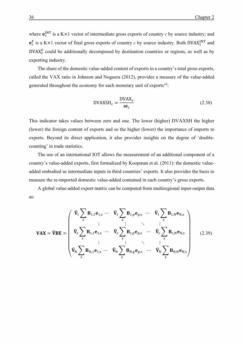
36 Chapter 2
where [�lO� is a K×1 vector of intermediate gross exports of country c by source industry; and [�� is a K×1 vector of final gross exports of country c by source industry. Both DVAX�lO� and DVAX�� could be additionally decomposed by destination countries or regions, as well as by
exporting industry.
The share of the domestic value-added content of exports in a country’s total gross exports,
called the VAX ratio in Johnson and Noguera (2012), provides a measure of the value-added
generated throughout the economy for each monetary unit of exportsvii:
DVAXSH� = DVAX�7[� (2.38)
This indicator takes values between zero and one. The lower (higher) DVAXSH the higher
(lower) the foreign content of exports and so the higher (lower) the importance of imports to
exports. Beyond its direct application, it also provides insights on the degree of ‘double-
counting’ in trade statistics.
The use of an international IOT allows the measurement of an additional component of a
country’s value-added exports, first formalized by Koopman et al. (2011): the domestic value-
added embodied as intermediate inputs in third countries’ exports. It also provides the basis to
measure the re-imported domestic value-added contained in each country’s gross exports.
A global value-added export matrix can be computed from multiregional input-output data
as:
�G� = ��M� =⎝⎜⎜⎜⎜⎜⎛
��L & ML,L[L,�� ⋯ ��L & ML, [ ,�� ⋯ ��L & ML,O[O,��⋮ ⋮ ⋱ ⋮��� & M�,L[L,�� ⋯ ��� & M�, [ ,�� ⋯ ��� & M�,O[O,��⋮ ⋮ ⋱ ⋮��O & MO,L[L,�� ⋯ ��O & MO, [ ,�� ⋯ ��O & MO,O[O,�� ⎠⎟⎟⎟⎟⎟⎞
(2.39)

Indicators on global value chains 37
where �� is a (K×N)×(K×N) diagonal value-added coefficient matrix39; B is the
(K×N)×(K×N) global Leontief inverse matrix (where each block M�, is a K×K matrix that
gives the amount of sectoral gross output in producing country c required per unit of output by
each industry in destination country p); and E is a (K×N)×N matrix of gross exports (where
each [ ,� is a K×1 vector of gross exports of country p to country s by source industry).viii
The diagonal terms of matrix VAX measure the domestic value-added embodied in each
country’s gross exports (i.e., ��� ∑ M�,�[�,�� is a K×1 vector of domestic value-added contained
in country c’s exports by source industry). Each country’s indirect value-added exports (i.e.,
the domestic value-added embodied as intermediate inputs in third countries’ gross exports) are
given by the sum of off-diagonal elements along each row of matrix VAX40:
DVAX2� = 7��� & & M�, [ ,�� Y� (2.40)
41ix
Finally, the re-imported domestic value-added content of gross exports can be computed for
each country c as the difference between total value-added exports and its direct and indirect
components42:
DVAXR� = 7��� & M�,�[�,�� − DVAXD� − DVAXI� (2.41) x
As noted above, these estimates are likely, in practice, to be upward biased.
39 �� = ⎝
⎛��L 0 ⋯ 00 ��� ⋯ 0⋮ ⋮ ⋱ ⋮0 0 ⋯ ��O⎠⎞, where each ��� is a K×K diagonal matrix of direct value-added coefficients of country
c by source industry. The ith element of the diagonal of each ��� matrix is v�,� = 1 − ∑ ∑ a ,��j, i��� , where a ,��j, i� is the value of inputs from industry j in source country p required by industry i in destination country c for one unit of output. Alternatively, �� = diag_�J − G��7`, where G� is the transpose of the (K×N)×(K×N) global technical coefficient matrix, I is a (K×N)×(K×N) identity matrix, and ɩ is a (K×N)×1 vector of ones. Thus, the first set of K elements of the diagonal of �� contains the value-added coefficients for country c=1, followed by the K value-added coefficients for country c=2, and so on. 40 The name given here to this indicator (DVAX2) was adopted following the criterion used for naming the measures of vertical specialisation presented before (i.e., VS and VS2). 41 The so-called reflected domestic value-added (i.e., the domestic value-added embodied in a country’s intermediate exports used by the direct importer to produce goods shipped back to source) can be separated from indirect value-added exports in equation (2.38) (as 7��� ∑ M�, [ ,� ). 42 DVAX is equivalent to OECD-WTO’s EXGR_DVA indicator, and DVAXSH is equivalent to OECD-WTO’s EXGR_DVASH indicator. The OECD-WTO database also provides separate measures for the direct, indirect and re-imported components of the domestic value-added content of exports (called EXGR_DDC, EXGR_IDC and EXGR_RIM, respectively).

38 Chapter 2
Foreign value-added content of exports
The foreign value-added content of exports, conceptually similar to Hummels et al. (2001) VS1
indicator, can be computed for each country c from a multiregional IOT as the sum of off-
diagonal elements along each column of matrix VAX:
FVAX� = & 7�� & M ,�[�,�� Y� = & 7�� M ,�[� Y� (2.42)
where �� is the K×K diagonal matrix of value-added coefficients of country p; Bp,c is the K×K
block matrix drawn from the global Leontief inverse that gives the amount of gross output in
producing country p required for one unit of country c’s output (by origin and destination
industries); [c,s is a K×1 vector of gross exports of country c to country s by source industry;
ec is a K×1 vector of country c’s total gross exports by source industry; and 7 is a 1×K vector
of ones.
This indicator can also be computed by breaking up exports by industry of origin,
destination country, and/or type of demand served (final or intermediate), as in the case of
DVAX. In addition, it can be decomposed by country of origin (i.e., FVAXp,c representing the
value-added from country p embodied in country c’s exports), and indeed by source industry
within each origin country.
The FVAX ratio for country c is given by43:
FVAXSH� = FVAX�7[� = 1 − DVAXSH� (2.43)
xi
Equation (2.43) shows that the sum of domestic and foreign value-added contents of exports
must account for all gross exports (i.e., value-added from all sources must sum to official trade
flows), both at aggregate and sector level (where taxes and subsidies on production and taxes
(and subsidies) on products incurred on intermediate consumption by industries in country c
are included in measures of domestic value added).
GVC participation index
43 FVAX is equivalent to OECD-WTO’s EXGR_FVA indicator, and FVAXSH is equivalent to OECD-WTO’s EXGR_FVASH indicator.

Indicators on global value chains 39
Koopman et al. (2011) propose an indicator, referred to as the GVC participation index, which
aims to capture the nature of a country’s involvement in vertically fragmented production
processes. The index of country c is given by:
GVC_participation� = DVAX2�7[� + FVAX�7[� (2.44)
where DVAX2� is the value-added of country c embodied as intermediate inputs in other
countries’ gross exports (or indirect value-added exports); FVAX� is the foreign value-added
embodied in country c’s gross exports; ec is a K×1 vector of country c’s total gross exports by
source industry; and 7 is a 1×K vector of ones.
Often the index is used to compare countries’ participation in GVCs relative to other
countries and over time. Indeed, a common interpretation is that the higher the foreign value-
added embodied in gross exports and the higher the domestic value-added contained in third
countries’ gross exports, the higher the country’s participation in international production
chains. This is however a mistake, as the indicator only provides a measure of the relative
importance in a country’s exports of upstream (backward linkages) and downstream (forward
linkages) positions in international production networks (where the downstream component
provides a narrow measure of upstream participation). For example, a country with exports
amounting to a marginal share of GDP may have a participation index of one, while a country
with a low participation index could have a very high share of exports to GDP –indeed it should
be noted that, typically, the larger the economy the lower the index–. Thus, the indicator should
instead be used to describe the nature of a country’s participation in GVCs. For countries lying
upstream in the value-chain (i.e., those who participate by providing inputs to other countries),
the indirect value-added share in gross exports will generally be higher than the share of foreign
value-added. In contrast, for countries lying downstream in the value-chain (i.e., those who use
a large portion of imported intermediates to produce final goods for exports), the share of
foreign value-added will be higher than that of indirect value-added exports.
Note, too, that the downstream component of the index strictly attempts to capture value
added embodied in parts that are shipped through to a third country, to provide a narrow
definition of GVC participation. As such, by design, it does not capture any domestic value
added exported in intermediate inputs that are used by the importing country to produce goods
for domestic final consumption. In other words, the indicator is likely to produce a lower
estimate of GVC participation (as defined) for countries whose exports of intermediates are

40 Chapter 2
disproportionately directed to larger economies, where the capacity to further process the
intermediates for selling on in their larger consumer market, is also larger, compared to smaller
economies.
In addition, it should be noted that the measure is designed to capture the flows of value
added as they pass through GVCs. In this sense, which is also a consideration for many other
GVC indicators (including VS), it is important to note that the measure will be affected by the
extent to which the parent firm, controlling a value chain with goods and services passing
through affiliates, chooses to record flows related to management and control services, and in
particular flows related to the use of intellectual property. In practice, especially because of the
opportunities provided by fiscal optimisation, these can be recorded in official statistics as either
primary income flows (and, so, not recorded as trade) or trade in services. In the latter case,
participation indices will generally provide lower measures of participation, all other things
being equal, for the countries where parent firms are located.
Value-added induced by final demand
The indicators that decompose gross export flows on the basis of the origin and destination of
value-added presented above are not the only prism through which trade in value-added can be
measured. A complementary approach is to look at where the value-added is consumed as final
consumption at the end of the value chain.
Measures of trade in value-added based on this approach can be computed using
multiregional input-output data, from which the global value-added production matrix is
obtained as44:
�G¦ = ��M¦ =⎝⎜⎜⎜⎜⎜⎛
��L & ML,�8�,L� ⋯ ��L & ML,�8�, � ⋯ ��L & ML,�8�,O�⋮ ⋮ ⋱ ⋮��� & M�,�8�,L� ⋯ ��� & M�,�8�, � ⋯ ��� & M�,�8�,O�⋮ ⋮ ⋱ ⋮��O & MO,�8�,L ⋯� ��O & MO,�8�, � ⋯ ��O & MO,�8�,O� ⎠⎟⎟⎟⎟⎟⎞
(2.45)
where �� is the (K×N)×(K×N) diagonal value-added coefficient matrix; B is the
(K×N)×(K×N) global Leontief inverse matrix (where each block M�,� is a K×K matrix that
44 Based on Koopman et al. (2014).

Indicators on global value chains 41
gives total requirements from country c for one unit of country p’s gross output, by origin and
destination industries); and F is a (K×N)×N matrix of final demand (where each 8�, is a K×1
vector of final products produced in country s and consumed in country p).
Thus, elements in the diagonal columns of the (K×N)×N matrix resulting from equation
(2.45) (i.e., ��� ∑ M�,�8�,�� ) give each country’s production of value-added absorbed at home
(including the domestic value-added that returns home after being processed abroad: ��� ∑ M�,�8�,��Y� ). Exports of value-added that are finally consumed as final demand are given
by the elements in the off-diagonal columns of matrix VAF.
From the final demand perspective, total domestic value-added induced in country c by
foreign final demand (or total value-added exports) can therefore be computed as:
DVAF� = 7��� & & M�,�8�, � Y� (2.46)
where 7 is a 1×K vector of ones.xii
Following Koopman et al. (2014), DVAF can be decomposed according to where and
how value-added exports are absorbed:
DVAF� = 7��� & M�,�8�, Y� + 7��� & M�, 8 , Y� + 7��� & & M�, 8 ,��Y�, Y� (2.47)
The first term in equation (2.47) is the domestic value-added content of country c’s (direct)
final exports; the second term denotes the domestic value-added embodied in country c’s
intermediate exports used by the direct importing country to produce final products that are
consumed domestically; and the third term is the domestic value-added in country c’s
intermediate exports used by the direct importing country to produce final products for third
countries.
Thus, the demand-side approach provides a measure of the value-added of one country
directly and indirectly contained in other countries’ final demand. By reflecting the domestic
value embodied in each country’s exports of intermediates that are further processed and sold
to final consumers in other countries, DVAF shows how industries in one country are connected
to consumers in other countries, even where no direct trade relationship exists (Ahmad, 2015).
Value-added exports can also be expressed as a share of gross exports:

42 Chapter 2
DVAFSH� = DVAF�7[� (2.48)
where ec is a K×1 vector of country c’s gross exports by source industry.
In addition, it is possible to calculate the foreign value-added induced by each country’s
domestic final demand (i.e., the value-added used by one country to satisfy its final demand but
created in other countries). For each country c, total foreign value-added embodied in domestic
final demand (or total value-added imports) can be computed as:
FVAF� = 7 & & �� M ,�8�,�� Y� (2.49)
Similarly to DVAF, FVAF can be decomposed according to where and how value-added
imports originate:
FVAF� = 7 & �� M ,�8�,� Y� + 7 & �� M , 8 ,� Y� + 7 & & �� M ,�8�,��Y�, Y� (2.50)
Therefore, total value-added imports of country c include the foreign value-added embodied in
country c’s intermediate imports used to produce final products that are consumed domestically
(first term of equation (2.50)); the foreign value-added that comes directly from a partner
country to satisfy country c’s final demand (second term of equation (2.50)); and the foreign
value-added in country c’s final imports that has been indirectly transferred through other
partner countries (last term of equation (2.50)). Thus, this indicator shows how industries
abroad are connected to consumers at home, even where no direct trade relationship exists.
The difference between DVAF and FVAF gives the country’s trade balance in value-added
terms:
TBVAF� = DVAF� − FVAF� (2.51)
The domestic value-added induced by foreign final demand (or value-added exports) can be
decomposed into the value-added generated by final demand in different countries (which could
also be grouped into regions). It can also be disaggregated by exporting industry. Similarly,
foreign value-added induced in each country by domestic final demand (or value-added
imports) can be decomposed by origin country and/or source industry, showing where this

Indicators on global value chains 43
value-added originates. Thus, countries’ trade positions in value-added terms can be calculated
at the bilateral level.45
Length of GVCsxiii
The length of GVCs is defined by the number of production stages involved. It is related to the
“average propagation length”, an indicator whose origins lie in traditional input-output analysis
(Dietzenbacher and Romero, 2007). Based on the index of the number of production stages
proposed by Fally (2012a, 2012b) for a single country IOT, in an international IOT framework
an index providing an indication of the length of GVCs can be computed as:
§ = 7�J − G�KL = 7M (2.52)
where n is a 1×(N×K) vector with the indexes for all countries and industries; 7 is a 1×�N×K)
vector of ones; and M = �J − G�KL is the global Leontief inverse.
An index value of one indicates that there is only a single production stage in the final
industry, and increasing values reflect additional inputs from the same industry or other
industries. It can also be computed distinguishing between domestic and imported inputs,
illustrating the relative importance of domestic and foreign stages of the value chain.
Some care is however needed in using the index. For a start, it is important to note that the
index is not in and of itself, in practice, a measure of length. More accurately, the index is a
measure of the average number of stages (plants) involved in the production chain, weighted
by the value added at each stage, and this in turn presupposes that the production chain follows
a sequential (snakes) rather than concurrent (spiders) process (Baldwin and Venables, 2013).
In addition, the index in theory requires establishment (or plant) level data, which is not
typically available in a conventional IOT (which instead provides data on the basis of industries,
i.e., aggregations of plants). This means that the results can be, in turn, sensitive to the level of
industry aggregation used in IOTs, and indeed the nature of the statistical unit (e.g., many
European economies create their tables using information on enterprises and not
establishments), and indeed whether transactions within firms are consolidated or not –
typically the smaller the statistical unit, and the lower the degree of consolidation, the higher
the estimate of the stages of production. Nevertheless, despite these caveats, the indicator
provides useful, albeit broad, insights on the length and evolution of the value chains.
45 OECD-WTO’s demand-side indicators include the domestic value-added embodied in foreign final demand (FFD_DVA), the foreign value-added embodied in domestic final demand (DFD_FVA), as well as the bilateral trade balance in value-added terms (BALVAFD).

44 Chapter 2
Distance to final demandxiv
Distance to final demand reflects countries’ location in the value chain (upstream or
downstream). Fally (2012a, 2012b) and Antràs et al. (2012) propose a measure of
“upstreamness”, based on the number of stages between the production of a good and final
demand. Thus, starting from one industry in a given country, the index measures how many
stages of production are left before the goods or services produced by this industry reach final
demand.
In an international IOT framework, a measure of the distance to final demand can be
computed as:
¨ = 7�J − ©�KL (2.53)
where d is a 1×(N×K) vector with the indexes for all countries and industries; 7 is a 1×�N×K)
vector of ones; I is a (K×N)×(K×N) identity matrix; G is a (K×N)×(K×N) global matrix of
output coefficients (or allocation coefficients); and �J − ©�KL is the so-called Ghosh inverse.46
Note that the measure corresponds to the more traditionally known Ghosh-inverse forward-
linkage measure.
A larger value of dc(i) implies that industry i in country c is more specialised in the
production of inputs at the beginning of the value chain, relative to other industries with lower
indexes. The same caveats presented above for length of GVCs are also relevant here.
2.3.5 Limitations of IOT based statistics The use of multiregional IOTs has become a common approach for empirically evaluating
countries’ participation in GVCs. However, it is important to note that this data source poses
some limitations. The construction of these tables is a data-intensive process and presents
numerous challenges, creating a trade-off between country and time coverage and degree of
reliability, because for certain countries the quality of the data is poor. In particular, the precise
identification of the links between exports of one country and the purchasing industries or final
demand consumers in the importing country is subject to numerous problems, due to data
restrictions and inconsistencies across countries (Ahmad, 2015).
46 Each coefficient of matrix G is given by g�, �i, j� = z�, �i, j� y��i�⁄ , where z�, �i, j� is the value of products from industry i in source country c used as intermediates by industry j in destination country p, and y��i� is the value of industry i’s output in country c. Thus, these allocation coefficients represent the distribution of industry i’s output across domestic and foreign industries.
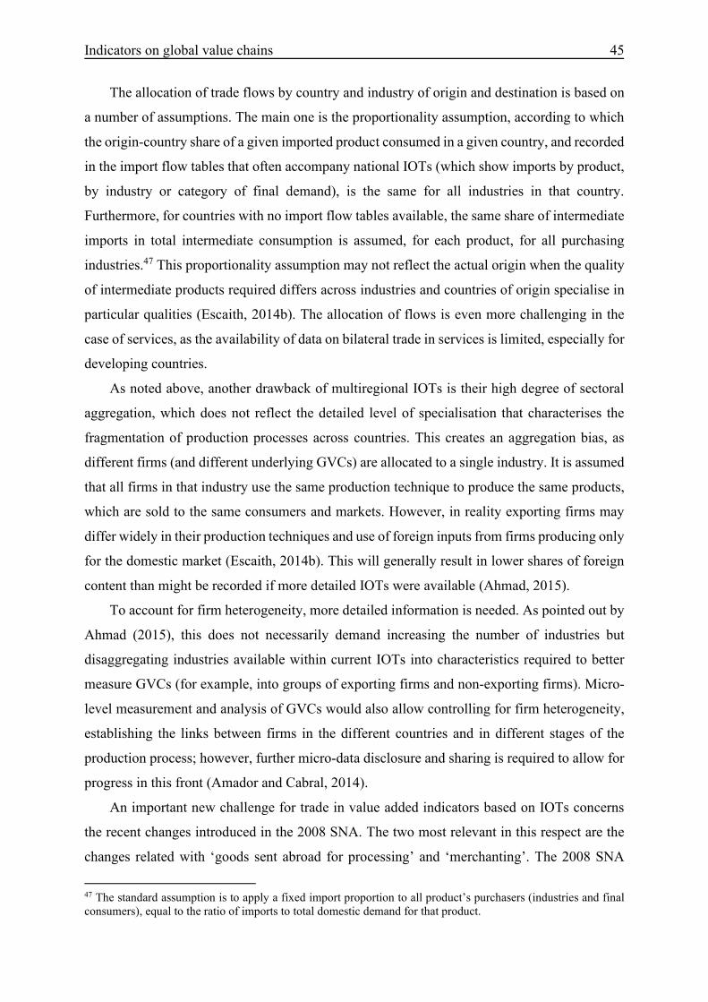
Indicators on global value chains 45
The allocation of trade flows by country and industry of origin and destination is based on
a number of assumptions. The main one is the proportionality assumption, according to which
the origin-country share of a given imported product consumed in a given country, and recorded
in the import flow tables that often accompany national IOTs (which show imports by product,
by industry or category of final demand), is the same for all industries in that country.
Furthermore, for countries with no import flow tables available, the same share of intermediate
imports in total intermediate consumption is assumed, for each product, for all purchasing
industries.47 This proportionality assumption may not reflect the actual origin when the quality
of intermediate products required differs across industries and countries of origin specialise in
particular qualities (Escaith, 2014b). The allocation of flows is even more challenging in the
case of services, as the availability of data on bilateral trade in services is limited, especially for
developing countries.
As noted above, another drawback of multiregional IOTs is their high degree of sectoral
aggregation, which does not reflect the detailed level of specialisation that characterises the
fragmentation of production processes across countries. This creates an aggregation bias, as
different firms (and different underlying GVCs) are allocated to a single industry. It is assumed
that all firms in that industry use the same production technique to produce the same products,
which are sold to the same consumers and markets. However, in reality exporting firms may
differ widely in their production techniques and use of foreign inputs from firms producing only
for the domestic market (Escaith, 2014b). This will generally result in lower shares of foreign
content than might be recorded if more detailed IOTs were available (Ahmad, 2015).
To account for firm heterogeneity, more detailed information is needed. As pointed out by
Ahmad (2015), this does not necessarily demand increasing the number of industries but
disaggregating industries available within current IOTs into characteristics required to better
measure GVCs (for example, into groups of exporting firms and non-exporting firms). Micro-
level measurement and analysis of GVCs would also allow controlling for firm heterogeneity,
establishing the links between firms in the different countries and in different stages of the
production process; however, further micro-data disclosure and sharing is required to allow for
progress in this front (Amador and Cabral, 2014).
An important new challenge for trade in value added indicators based on IOTs concerns
the recent changes introduced in the 2008 SNA. The two most relevant in this respect are the
changes related with ‘goods sent abroad for processing’ and ‘merchanting’. The 2008 SNA
47 The standard assumption is to apply a fixed import proportion to all product’s purchasers (industries and final consumers), equal to the ratio of imports to total domestic demand for that product.
46 Chapter 2
recommends that imports and exports should be recorded on a strict change of ownership basis.
That is, flows of goods between the country owning the goods and the country providing the
processing services should not be recorded as imports and exports of goods. Instead, the fee
paid to the processing unit should be recorded as an import of processing services by the country
owning the goods and an export of processing services by the country providing it. The
consequence of this for trade-in-value-added based indicators may be profound. For example,
following the implementation of the 2008 SNA recommendations, countries with large
processing activities, and therefore with a high import content of exports in current trade in
value added estimates, will see significant falls in these ratios (as any intermediate import used
in the processing activity whose ownership remains with the principal firm supplying the
processor will no longer be recorded as intermediate consumption on official SUTs and IOTs).
Other indicators, for example the backward component of the GVC participation index, will be
similarly affected. For mechanting, complications will be introduced whenever purchases and
subsequent sales by a merchanter cross over two periods, as in the first period an imputation
for imports as a negative export will necessarily be made in the country where the merchanter
is resident. To overcome these challenges, the OECD is working with partners to investigate
the scope to re-impute flows for goods for processing, such that intermediate consumption of
imports continues to be recorded (in other words, assuming that ownership has changed).
2.4 Some final considerations The increasing fragmentation of production processes across countries has challenged
economists and statisticians to find new ways to measure the extent of this phenomenon and its
potential implications. The purpose of this paper is to present a review of the main indicators
on GVCs currently in widespread use, and to serve as a guide for empirical work.
The indicators commonly used to analyse countries’ participation in international
production networks, based on either international trade data or IOTs, each have their strengths
and weaknesses. Measures based on international trade data have the advantage of high
coverage (in terms of countries and time periods) and low complexity of the required data, as
well as an acceptable degree of comparability across countries. In addition, the detailed product-
level information on trade in intermediate goods –relative to that of IOTs – allows for a more
precise characterisation of countries’ specialisation patterns. However, a shortcoming of trade
data is that there is no link to production, and so to the industry of origin or indeed the industry
actually using any intermediate in its production process. Additionally, the growing complexity

Indicators on global value chains 47
of international production networks makes it increasingly difficult for conventional trade
measures to capture the full linkages among countries (since customs records often only reflect
a product’s last country of origin, although efforts are being made to improve this through the
compilation of additional data such as country of consignment). Another important drawback
of trade data is that they are affected by double-counting issues, as the value of intermediate
products is counted each time they (or the good in which they are subsequently embedded)
cross a national border, which can artificially inflate the importance of trade. Also, available
trade data only insufficiently account for trade in services, since they do not reflect the value
originating in service-related activities that is embodied in traded goods.
Indicators based on input-output statistics improve upon measures based on conventional
trade data in terms of the accuracy of the resulting quantification and characterisation of GVCs.
By capturing both direct and indirect linkages and exchanges between countries and industries,
multiregional IOTs allow for the measurement of the foreign content of exports and the value
truly generated by each country (and industry). This avoids the double-counting problems
inherent in trade statistics, fully tracking the original sources of the value-added embodied in
gross trade flows. However, the accuracy of the measurement of production fragmentation is
constrained by the high degree of sectoral aggregation in IOTs, which creates an aggregation
bias and generally, at least following the 1993 SNA, results in lower shares of foreign content
than might be recorded if more detailed tables were available. Accuracy is also affected by the
proportionality assumption, on which the allocation of trade flows by country of origin and
destination is based. Additionally, the limited availability of comparable input-output data
(especially for developing countries) hampers the country and time coverage of indicators based
on input-output statistics.
Notwithstanding that indicators based on multiregional IOTs represent a substantial
methodological advance, considerable work still needs to be done in order to adequately map
and measure countries’ participation in GVCs. The existing databases allow macro-sectoral
level analyses, but more detailed information is required to account for firm heterogeneity (for
example, by splitting industries into groups of exporting firms and non-exporting firms). The
use of firm-level data, a line of research that has emerged recently, can also improve the quality
of the information provided by IOTs; however, further micro-data disclosure and sharing is
required to allow for progress in this front. Also, the coverage of developing countries in
international IOTs should be extended using official data, in order to adequately reflect the
actual specificities of these countries (Escaith, 2014b).

48 Chapter 2
Appendix Chapter 2
OECD Inter-country Input-Output (ICIO) database
The OECD ICIO underpins the OECD-WTO TiVA database. The latest version of the ICIO
contains data for 63 economies and 34 industries (on an ISIC Rev 3 basis) following the 1993
SNA, and cover the years 1995-2011, with additional tables based on now-casting techniques
available for the 2012-2014 period. Future releases in 2018 and beyond will be on a 2008 SNA
basis, as countries increasingly implement the latest accounting standards. The efforts in this
regard are expected to be bolstered as regional partners engaged in similar initiatives, such as
Eurostat’s FIGARO initiative, APEC-TiVA, ECLAC, TiVA and NAFTA-TiVA, gather
momentum.
A. Other initiatives to create inter-country input-output tables
An early example of efforts to look at inter-country relationships is the Global Trade Analysis
Project (GTAP), coordinated by the Center for Global Trade Analysis of Purdue University.
Set up in the 1990s, primarily for economic modelling purposes, the GTAP database is a “cross-
section of consistent data on consumption, production, and trade” for a particular reference
year.48 Although the sources of the database are national IOTs, GTAP is not an international
IOT (as this concept is understood). One drawback of this database is that it does not provide
separate data for trade in intermediate and final products, thus making it necessary to transform
trade flows in order to construct inter-country IOTs from GTAP data (Tsigas et al., 2012). Also,
since it is benchmarked only on trade statistics, sector level supply and demand data for
individual countries may show large discrepancies with corresponding national accounts
statistics. Another shortcoming of the GTAP database is that there is no consistency imposed
between its different versions, which makes it difficult to perform comparisons over time.
The first true inter-country IOT is the Asian International Input-Output Table (AIIOT),
produced by the Institute of Developing Economies-Japan External Trade Organization (IDE-
JETRO) in collaboration with the national statistical offices and research institutes of the
participating countries. AIIOT comprises 9 Asian economies (China, Indonesia, Japan,
Malaysia, Philippines, Republic of Korea, Singapore, Taiwan, and Thailand) plus the Unites
States, with five-year interval tables for the period 1985-2005. More recently, international IOT
48 The last version available (version 9), released in May 2015, has three reference years (2004, 2007 and 2011), 140 regions (countries) and 57 sectors. For a description of this and previous versions see www.gtap.agecon.purdue.edu/databases/default.asp.
Indicators on global value chains 49
databases with a more ‘global’ scope have become available, including the Trade in Value-
Added (TiVA) database and the two described next: the World Input-Output Database
(WIOD), and Eora.49
a) World Input-Output Database
The WIOD is a publicly available multiregional input-output database developed by a
consortium of European institutions to “analyze the effects of globalization on trade patterns,
environmental pressures and socio-economic development” (Timmer, 2012).50 The most recent
version, released in 2016, covers 43 countries which account for more than 85% of world GDP
(the 28 members of the European Union, Norway, Switzerland, and 13 major non-European
economies), and estimates for the non-covered part of the world (presented as “Rest of the
world”), with a timeframe spanning 15 years (from 2000 to 2014).51 This is an update to the
2013 release of the database, which covered 40 countries with a slightly earlier timeframe (from
1995 to 2011).52
The first step in the construction of the database was building a time series of national
SUTs. National SUTs (or IOTs) published by the National Statistical Institutes were taken as a
starting point to construct harmonised and standardised SUTs with 56 industries that together
cover the entire economy.53 These harmonized SUTs were then benchmarked to National
Accounts and used to estimate national tables for non-benchmark years (using the so-called
SUT-RAS method, developed for this specific purpose). The second step consisted in linking
national SUTs across countries through detailed bilateral international trade statistics, to
49 Other multiregional input-output databases are the GTAP-MRIO (based on the GTAP database) and EXIOPOL (see Tukker and Dietzenbacher, 2013; Andrew and Peters, 2013; and Tukker et al., 2013). Unlike WIOD, Eora and TiVA, these two databases are not publicly available and have a greater emphasis on environmental issues. 50 The WIOD project, funded by the European Commission, included the following institutions: University of Groningen, and CPB Netherlands Bureau for Economic Policy Analysis (The Netherlands); Institute for Prospective Technological Studies (Spain); The Vienna Institute for International Economic Studies, and Österreichisches Institut für Wirtschaftsforschung (Austria); Zentrum für Europäische Wirtschaftsforschung, and Hochschule Konstanz (Germany); The Conference Board Europe (Belgium); Institute of Communication and Computer Systems (Greece); Central Recherche SA, and the Organisation for Economic Cooperation and Development (OECD) (France). The full database is available free of charge at www.wiod.org, and a detailed description of its construction can be found in Dietzenbacher et al. (2013). 51 The non-European countries covered are Australia, Brazil, Canada, China, India, Indonesia, Japan, Mexico, Republic of Korea, Russia, Taiwan, Turkey, and the United States. Estimations for “Rest of the World” are based on bilateral trade data and totals for industry output and final use categories from the UN National Accounts, assuming the average input structure of key emerging countries (Brazil, Russia, India, China, Indonesia, and Mexico). 52 See Timmer et al. (2016) for more information on the updated WIOD and how it compares to the initial release. 53 Products classification is based on the international Classification of Products by Activity (CPA), while industries classification is based on revision 4 of the International Standard Industrial Classification of all economic activities (ISIC Rev. 4) (or ISIC Rev. 3 in the 2013 release of the WIOD). The tables adhere to the 2008 version of the SNA (in the 2013 release of the WIOD, the 1993 version of the SNA is used).

50 Chapter 2
construct international SUTs in which the use of products is broken down according to origin
country.54 Finally, international SUTs were transformed into symmetric World Input-Output
Tables (WIOTs) of the format 56 industries by 56 industries.
The WIOD database consists of time series of: 1) national tables (national IOTs at current
prices and national SUTs at current and previous year prices), and 2) world tables (international
SUTs at current and previous year prices, WIOTs at current and previous year prices, and
interregional IOTs for 6 regions (Euro-zone, Non-Euro European Union, NAFTA, China, East
Asia, and BRIIAT55)). Additionally, the database provides detailed socio-economic and
environmental satellite accounts (capital stock, investment, wages and employment by skill
type, energy use, emissions, land use, materials use and water use). The tables trace the flows
of consumption, production and incomes within and across countries, and break down products
according to their origin. Thus, WIOD can be used for both inter-temporal and cross-country
comparisons.
b) Eora database
Eora is a publicly available multiregional input-output database that focuses on environment
issues and has as primary aim the comprehensiveness of coverage, both in terms of countries
and industries.56 It covers 187 countries with a time frame spanning from 1990 to 2011, and
includes 25-500 industries (depending on the country).
The database draws upon information from a variety of primary data sources: national
IOTs, SUTs and national accounts data from countries’ statistical offices; macroeconomic
aggregates from the United Nations National Accounts Main Aggregates Database; and trade
data from the United Nations Commodity Trade Statistics Database (COMTRADE) and the
United Nations Service Trade Statistics Database. In order to create a continuous time series of
balanced and consistent multiregional IOTs, combining the often conflicting data sources and
dealing with missing data, interpolation and estimation techniques are used. Since the tables are
balanced to match principally data from large economies, there are important deviations from
54 Use tables were first split into domestic products and foreign products (based on a distinction by end-use categories derived from a refinement of BEC codes); in a second stage, the use of foreign products was split according to country of origin. 55 BRIIAT comprises Brazil, Russia, India, Indonesia, Australia, and Turkey. 56 The Eora project was developed by the University of Sydney and funded by the Australian Research Council. The full database can be downloaded for free at http://worldmrio.com, and a description of its construction can be found in Lenzen et al. (2013). The UNCTAD TiVA dataset, which provides statistics related to trade in value-added, was constructed using the Eora multiregional IOTs.

Indicators on global value chains 51
observed trade flows and GDP (Cattaneo et al., 2013).57 Therefore, the database should be used
with caution, especially if a high reliability and precision of the results on smallest countries
(for which input-output data availability is often very limited) is important.58
A guiding principle of Eora is close adherence to the raw data, in the sense that changes to
the structure of the original raw data are avoided as much as possible, for the sake of
transparency. Thus, the database includes original SUTs, industry-by-industry or product-by-
product IOTs, depending on the country, with data expressed in current national currencies.
These different national tables are linked into one yearly compound multiregional IOT
(constructed in current US dollars), where original national sectoral disaggregations are
maintained. However, Eora also provides a time series of harmonised multiregional IOTs, based
on a 25-industry classification. The monetary tables are complemented by satellite accounts
covering 35 environmental and resource use indicators.
The main advantage of Eora over WIOD is its broader country coverage, which makes
possible a more comprehensive analysis of developing countries’ participation in GVCs.
However, the inclusion of data-poor countries reduces the level of statistical rigor, raising
concerns about the accuracy of such analysis.
c) EXIOPOL database
EXIOPOL is a detailed, transparent, harmonised, global Multi-Regional Environmentally
Extended Input-Output Table that covers 43 countries with 129 industry sectors and products.
It also, by design, includes data on 30 emitted substances and 80 resources by industry. The
latest version covers data for 2007.
57 The database provides information on the reliability of the raw data by means of standard deviation estimates, which reflect the extent to which each data point was interpolated or estimated, during the process of assembling the global multiregional IOTs, from constituent primary data sources. However, in many cases the standard deviations of raw data are based on assumptions, since very little information on the uncertainty of macroeconomic and input-output data is available. 58 For 74 of the 187 countries covered in the database, specific IOTs or SUTs were obtained from various statistical agencies. For a small number of countries (including Australia, the United Kingdom and some Central Asian economies) tailor-made input-output data sets were used. In other cases, national IOTs were estimated from actual macroeconomic aggregates using a “template” 25-sector IOT, which is considered to describe a typical economic structure.
52 Chapter 2
Endnotes These endnotes correct typos in the OECD Working Paper version (post-
publication) and provide additional clarification or context. i (p. 27) The statement is not true in all situations (Hummels et al., 2001). For example, suppose a sector produces two goods: one that relies heavily on imported intermediates and is heavily exported; the second good uses no imported inputs and is not exported. At the sectoral level, VSD is underestimated (hence a disaggregation increases VSD). Aggregation matters and can lead to either an underestimation or overestimation of VSD. ii (p. 30) The footnote should refer to equations (2.20), (2.22), and (2.26). iii (p. 32) The footnote should refer to equation (2.28), not to (2.26). iv (p. 33) The OECD-WTO TiVA initiative considers Trade in Value Added to include indicators that measure value-added embodied in gross trade and indicators that measure value-added embodied in (foreign) final demand. The OECD does not make a distinction in terminology between those two sets of indicators. However, in the Groningen tradition, only the latter set of indicators refers to trade in value-added (along the lines of Johnson and Noguera, 2012) while the former would be considered indicators based on vertical specialization (along the lines of Hummels et al., 2001). We use the broad OECD meaning of trade in value added, which includes all the above indicators, to be consistent with the terminology still used by the organization that published this document. Thus the sections “Domestic value-added content of exports” and “Foreign value-added content of exports” (based on VAX notation) refer to indicators related to value-added embodied in gross trade (i.e., using the vertical specialization approach); and the section “Value-added induced by final demand” (based on VAF notation) refers to indicators related to value-added embodied in final demand (i.e., using the value-added exports approach). Note that our references to VAX do not relate to the VAX-ratio measure by Johnson and Noguera (2012). For further information and a list of OECD indicators, many of which are similarly defined as ours, see: OECD (2019). v (p. 35) Equation (2.34) contains a typo: instead of VAXD� it should be DVAXD�. vi (p. 35) The sentence in parenthesis is incorrect. The correct way of disaggregating the domestic value-added content of gross exports is by post-multiplying by a K×K diagonal matrix �ª�, indicating all exports for each separate industry, i.e., 7���_�J − G�6�KL − J`�ª�. vii (p. 36) Equation (2.38) is misattributed as Johnson and Noguera’s (2012) proposed VAX ratio. This is incorrect because the VAX ratio indicates the exports of value-added induced by foreign final demand (i.e., value-added exports) for each monetary unit of exports, not DVAX� (which we had defined as domestic value-added embodied in gross exports). viii (p. 37) This sentence contains a typo relating to the definition of the Leontief inverse. The Leontief inverse refers to the (extra) amount of sectoral gross output in producing country c required per (extra) unit of final demand (not “per unit of output”).

Indicators on global value chains 53
ix (p. 37) The footnote should refer to equation (2.40), not to (2.38). x (p. 37) In equation (2.41), DVAXD� − DVAXI� can be simplified as DVAX�. xi (p. 38) Equation (2.43) is only true if DVAX� = 7���M�,�[\. The previous paragraphs correctly explain how to measure the domestic value-added in gross exports using multi-regional or global IOTs (based on block matrices derived from the global Leontief inverse). This is what was intended to be reflected in equation (2.43). However, equation (2.33) had defined DVAX� based on a national IOT, which could cause confusion in its interpretation. The definition of DVAX� in equation (2.33) would be incorrect if used in the context of equation (2.43). xii (p. 41) Note that Johnson and Noguera’s (2012) VAX-ratio indicator is obtained by dividing DVAF� by gross exports of country c. xiii (p. 43) Equation (2.52) on length of GVCs is based on an indicator in De Backer and Miroudot (2014) and Los (2017). This indicator is inspired by Fally’s indicator on GVC length (based on a national IOT), which we adapted to an ICIO table. We emphasize that this is only an indicator of the length of the value chain, not an actual measure of GVC length (which requires plant-level information). Los (2017) observes that there are two key differences between the type of indicator we present in equation (2.52) and the measure of average propagation lengths (APL) proposed by Dietzenbacher and Romero (2007). First, the sale of a product to final users is a transaction in the production process. An index value of one thus implies that all goods and services produced are directly purchased by final consumers (i.e., no intermediate inputs are used to produce a final good or service). Second, the indicator aggregates all upstream industries i when measuring the average number of transactions required before final users are the owners of a product delivered by industry j. Hence, Los (2017) argues that the indicator is appropriately characterized as showing the importance of specialized activities in GVCs. This is based on a weighted average of the production length involved in the industries that provide inputs to the production process. If equation (2.52) is element-wise post-multiplied by a (K×N)×(K×N) matrix of zeroes in the diagonal blocks and ones elsewhere, the average number of international transactions (giving the physical degree of international fragmentation of production processes) is computed. xiv (p. 44) Equation (2.53) is better characterized as showing the position of countries in the value chain and gives the average number of production stages for industry output to be absorbed in final demand. This is also based on an indicator in De Backer and Miroudot (2014) and Los (2017). The measure corresponds to the row sum of the Ghosh Inverse matrix. The row sum gives the strength of total forward linkages in the production process (Johnson, 2018). Note that there is a mistake in the equation in De Backer and Miroudot (2014), which is also reflected in equation (2.53). The Gosh inverse should be post-multiplied (instead of pre-multiplied) by a vector of ones. Thus, the correct equation for distance to final demand (see e.g., Los, 2017) is ¨ = �J − ©�KL7, where 7 is a column-vector of ones and ¨ is also a column-vector.

54 Chapter 2

55
This chapter is based on Bohn et al. (2018).
Chapter 3
The role of services in globalisation
ABSTRACT
This paper explores the role of services in international trade and global value chains, and adds to our knowledge on recent trends in globalisation. We employ indicators for trade in value‐added (VA) and for gross exports, and address the following two questions: (i) has trade of VA in services (i.e., the VA created by domestic service industries and embodied in foreign consumption of final products) grown more than trade of VA in manufacturing; and (ii) does trade of VA in services travel further than trade of VA in manufacturing. Based on the World Input‐Output Database (WIOD), we find, in general, that for the period 2000–14, the share of services in exports of VA grew over time, whilst the share of manufacturing remained constant (or grew relatively less). Second, throughout the entire period, services had a larger share in interregional exports of VA than in intraregional exports of VA, whilst the opposite was true for manufacturing. Services were thus more global than manufacturing.

56 Chapter 3
3.1 Introduction
Empirical trade research is focused on manufactured goods despite the rapid growth of services
trade (Feenstra, 2016). To a large extent, this is caused by data restrictions on services trade.
Services are not only directly traded but also indirectly embodied in manufacturing exports
(Drake-Brockman and Stephenson, 2012). The indirect contributions of (domestic) services
inputs in exported manufactured goods are not captured by traditional statistics such as balance
of payments statistics.59 Gross exports thereby—potentially—understate the significance of
services, and also the extent of globalisation (Johnson, 2014).
This paper focuses on the role of services and addresses the following two questions to
highlight the growing importance of services trade. First, it is often stated that the growing
usage of information and communication technologies has expanded the scope of services and
enhanced their tradability (Baldwin, 2016). Is this trend reflected in a rising importance of trade
in services relative to trade in manufactured goods over time? Second, assuming relatively low
transport barriers related to services, trade in services (when compared to manufacturing) could
be more important in interregional trade than in intraregional trade. The ICT revolution reduces
trade barriers and facilitates fragmentation of the production process (Baldwin, 2016). Do
services, which we define in a broad sense to include both embedded services and direct
services exports, therefore travel further than manufactured goods? These questions follow
Low’s (2013) call for more analytical research on the characteristics of services in global value
chains. They also serve the goal of Baldwin and Lopez-Gonzalez (2015) to stimulate more
empirical and theoretical work on how the internationalisation of production has altered the
nature and impact of globalisation.
The analysis is primarily based on trade in value-added. The trade in value-added
perspective employs a different method than does a standard trade analysis based on gross trade.
This approach involves using input–output analysis to measure the value-added produced in
one country that ends up in the consumption bundle of another country. In the case of services
trade, this captures the direct value-added of domestic services industries that is embodied in a
product traded by industries in trade. We use two indicators to capture the significance of
services both from an upstream and a downstream viewpoint.
59 Trade in services data is collected according to the Extended Balance of Payments System (EBOPS) in the International Monetary Fund’s Balance of Payments Statistics, but the quality is lower than for goods trade; in addition, few countries provide bilateral data or much product level detail (Ahmad et al., 2017).

The role of services in globalisation 57
Previous research shows that three-quarters of all services embodied in value-added trade
are embedded services rather than directly traded (Heuser and Mattoo, 2017). To provide a
complementary analysis that considers only directly traded products, we compare the value-
added data to a more conventional approach that draws upon gross exports. Gross exports
provide only the value of all products directly exported by services industries and
manufacturing industries (even if there are industries from other sectors that contribute to their
respective total export values). The distinction between embedded services and directly traded
services is important when the relative distances of services and manufactured goods in trade
are analysed in Section 3.4.2. The main source for the analyses is the World Input-Output
Database (Dietzenbacher et al., 2013), containing time-series data on trade linkages for 43
countries and 56 industries.
In general, we find that trade in value-added created in services increased more than trade
in value-added created in manufacturing during the period 2000–14. This holds especially for
the European Union and North America. Second, trade of value-added in services is traded over
longer distances than trade of value-added in manufacturing. That is, services had a larger share
in the interregional exports of value-added than in the intraregional exports of value-added and
the opposite held for manufacturing. In Europe, it was especially the value-added created in
financial intermediation services and business services (IT and consulting) that was more
important in interregional trade in value-added. The findings hold not only for trade in value-
added indicators (which account for the large indirect value-added created by services
industries) but also when indicators are used that capture the direct exports of services industries
themselves (gross export figures). These findings add to our knowledge of globalisation: trade
is increasing worldwide, and interregional globalisation in the sense of rising trade between
countries from different regions is related to the role of services being more truly global than
the role of manufacturing.
The paper is structured as follows. Section 3.2 explains why services may be growing in
importance in trade. It is explained how a value chain-based approach provides a better
statistical depiction of the services embodiment of trade. Section 3.3 describes the approach to
measure services trade and presents the methodology and data sources. Indicators are
introduced to measure a country’s dependence on trade as a share of its GDP and final demand.
Section 3.4 applies the indicators to answer the research questions. Section 3.5 concludes and
discusses some implications.
58 Chapter 3
3.2 Literature 3.2.1 The growing importance of services
Recent growth in world trade is closely intertwined with the emergence of global production
networks.60 Specialisation no longer refers to sectors within countries but to specialisation in
different activities within production networks. This implies that international trade is
characterised by trade in intermediate products (Jones and Kierzkowski, 2001). The
international fragmentation of production has been helped by the ICT revolution that came on
top of the sharp decline in trade barriers since the late 1980s. Baldwin (2006, 2016) refers to
this phenomenon as the “second unbundling” and argues that it represents the transition to a
new era of globalisation.61 These developments can be illustrated from the perspective of global
value chains (GVCs). A GVC encompasses all productive (value-adding) activities across
countries involved in bringing a product to the final consumer. This includes initial conception
(e.g., R&D), production, assembly, marketing and distribution, final delivery and support
(Gereffi and Fernandez-Stark, 2016). While the final product in a GVC is completed in one
country only and then sent to the consumer, the product contains intermediate inputs and value-
added contributions sourced from one or more countries.
The “second unbundling” is not just a technological revolution in manufacturing but also a
revolution in services as the use of services is pivotal in the spatial unbundling of tasks. The
rise of information and communication technologies (ICT) reduced the coordination costs of
complex production processes, enabling the global fragmentation of production. Embodied
services were also traded in antiquity (see O’Rourke and Williamson, 2002; who debate how
long ago globalisation began), but sophisticated ICT services, transport and financial services
have in recent decades helped to facilitate highly fragmented production processes that source
inputs (parts and components) from all over the world. For these reasons, services have been
referred to as the “glue” linking fragments within production chains together (Drake-Brockman
and Stephenson, 2012; Low, 2013). So, services can be expected to play an increasingly
essential role in trade.
This also has policy consequences. The National Board of Trade (2012) of Sweden, for
instance, indicates how GVCs have implications for trade policy and management of trade
60 Equivalent terms commonly used to refer to the importance of international production networks include the unbundling or fragmentation of production, supply chain trade, trade in tasks and vertical specialisation. 61 Globalisation’s “first unbundling” began in the 1820s with the spatial separation of production and consumption. One prominent study calls this first unbundling, fueled by the transport revolution, the “big bang” of globalisation (O’Rourke and Williamson, 2002).

The role of services in globalisation 59
agreements. The authors argue that trade negotiators should not focus on manufactured goods
or services in isolation but rather consider the interdependencies of the two and take the value
chain into account.62 Recent research also suggests that trade liberalisation in services, broadly
defined as opening up the domestic market for foreign services providers, can induce a
comparative advantage for downstream production processes that rely heavily upon services
inputs. Countries that reduce trade restrictions for services and have complementary domestic
regulatory policies are more likely to gain a comparative advantage in producing manufactured
goods that depend on services (Van der Marel, 2016). Furthermore, liberalisation in services
can stimulate productivity in manufacturing (Arnold et al., 2016).
Services account for 75% of GDP and 80% of employment in OECD countries (Nordas
and Rouzet, 2017). However, the role of services in cross-border trade and production networks
remains less understood. This is mainly caused by a lack of reliable data at the aggregate level
and conceptual difficulties as to how to define a service and what the balance of payments
measure (Broussolle, 2014, 2015). The rise of GVCs adds to this statistical challenge. Take for
example, a Boeing 787 aircraft composed of parts and components produced in 5,000 factories
worldwide before being assembled in the US (Kelly, 2012). The production of each component
in turn requires subcomponents sourced from even more countries. In the current accounting
system based on gross exports, these intermediates are counted each time they cross the border,
including when embodied in downstream goods and services. This raises issues related to
multiple-counting.
The current accounting system retains legitimacy as long as countries exist because actual
trade is still bilateral and these are the transactions that are registered by customs officials.
However, relying solely on gross exports may lead to misleading interpretations when they are
used by policymakers to assess trade competitiveness because sophisticated inputs may have
been imported. The Boeing 787’s final assembler, for example, contributes considerably less to
the plane’s production value than what is suggested by the plane’s final export price. A GVC
perspective can identify the largest value creators and also identify the final consumers in the
end-market, whose demand triggers value-added production in other countries through their
consumption of final goods and services. For these reasons, both the standard and GVC views
have their legitimacy and contribute in complementary ways to the analysis of trade.
62 This discussion refers indirectly to the effective rate of protection (Bhagwati et al., 1998). This concept of protection explicitly includes supply chain effects.

60 Chapter 3
3.2.2 Two questions Manufacturing industries that are involved in trade—especially those involved in the
production of elaborately transformed and high-value-added goods—depend on domestic
services (Drake-Brockman and Stephenson, 2012). This implies that there are more services
being traded than what is suggested by gross export statistics. Gross export statistics report the
directly traded services, such as communications services, but not the domestic services that
are embodied in the export of manufactured goods, commodities or even other services (which
are hence traded indirectly). Therefore, focusing on the trade of value-added in service
industries has two advantages. First, value-added trade has a higher correlation with domestic
non-tradable services that are used as inputs than gross exports trade data. The latter only
reflects the total value of the traded product and does not separate out the domestic non-tradable
services component that contributes to its final value, such as embedded software in aircraft.
Second, inputs passing through multiple countries within production networks are not double
counted.
Whenever we refer to exports (or imports) of value-added, for example, the trade of value
added in services industries, we refer to the domestic value-added generated by the industries
of this sector (i.e., services) that is consumed abroad (respectively imported and consumed
domestically). In this way, there can be trade in value-added between two countries even if
there is no bilateral trading relationship because the value-added may be delivered to final
consumers via a third country. The final demand approach provides the location where the
value-added is ultimately consumed, home or abroad, but does not decompose gross exports.
Thus, while all value-added contributions of services industries to trade are accounted for, this
inclusive approach does not distinguish between the trade of value-added in services that is
embodied in products traded by manufacturing industries, traded by the same or different
services industries or traded by other sectors (e.g., agricultural production). Similarly, the trade
of value-added in manufacturing is considered to be all domestic value-added created in
manufacturing industries—even if the value-added is embodied in a traded service—that ends
up in the foreign consumption of final products. The industries included in the manufacturing
sector, services sector and other production sector are provided in Appendix Table 3.A1. A
more detailed explanation of the method and computations are provided in Section 3.3 on
analytical framework.
The first question considers the increased tradability and importance of services over time,
which Saez et al. (2014, p. 2) refer to as “one of the most important changes in trade patterns

The role of services in globalisation 61
over the last quarter of the 20th century.” Value-added trade of services industries is growing
relative to value-added trade of manufactured goods industries.
The growth of services in value-added trade is documented in previous studies (Heuser and
Mattoo, 2017; Miroudot and Cadestin, 2017). For example, Heuser and Mattoo (2017) show
that the share of services in world value-added exports increased from about 30% to more than
40% since 1980. Our approach differs in that we use a final demand perspective and decompose
the trade in value-added and gross exports on a regional basis (Europe, North America and East
Asia). This could demonstrate how patterns in different regions may differ and whether the
overall growth in services is a truly global phenomenon. Therefore, we ask the following
question:
Question 1: Has trade of value-added in services industries become more important
relative to trade of value-added in manufactured goods industries between 2000 and 2014?
Next, we will focus on the distance traversed from the point of value creation to the point of
consumption. In other words, does the value-added contributed by services or by manufacturing
industries travel “further”? A clear difference in their average distances (in connection to the
answer to the first question) may contribute to our understanding of the spatial reach of trade;
the ICT revolution could have facilitated services trade of longer distances. Here too, value-
added trade refers to both direct cross-border services trade and services embodied, for
example, in the trade of manufactured goods. Due to data limitations on services, no existing
study has looked into this issue.
Direct (non-embedded) services exports are by themselves not subject to transportation
costs and this should in theory facilitate their trade over large distances. But also embedded
services may traverse a longer distance because they add value to the exports of manufactured
goods. Customised and elaborated products that embody more services (such as software) might
reduce the impact of distance by decreasing relative transport costs. Even manufactured goods
that do not embody many services, but which travel a longer distance will increase the role of
services for the simple fact that transport costs are themselves considered a service.
On the other hand, recent studies have shown that trade costs for direct services trade are
several times higher than for goods (Anderson et al., 2014; Miroudot et al., 2013). Significant
regulatory burdens, non-tariff barriers and trade restrictions for services persist and these are
magnified as barriers for trade in goods decline. Impediments to services trade are highlighted
by the OECD’s Services Trade Restrictiveness Index. One could argue that regulatory burdens

62 Chapter 3
are greater across larger distances if the well-known liability of foreignness equally applies to
trade in direct services. Restrictions on direct services trade also have an effect on embedded
services because exported goods may depend on services inputs that need to be imported. This
would suggest that value-added created by service industries may not travel further than value-
added created by manufacturing industries.
Another factor that could play a role is that countries belonging to regional agreements may
have a higher level of regulatory convergence in services. This suggests they may trade more
direct services and also more embedded services because it would be easier to import foreign
services inputs. Deeper agreements that also provide provisions for services are more common
amongst geographically proximate countries (e.g., the EU), and hence, this could lead to a
stronger regional nature of services trade. However, deeper regional agreements that promote
regulatory convergence in services would likely also have provisions that stimulate the trade of
manufactured goods. Thus, it is not clear whether the trade facilitating effect of regulatory
convergence would be stronger on the services sector or on the manufacturing sector.
Question 2: Does trade of value-added in services industries travel further than trade of
value-added in manufactured goods industries?
3.3 Analytical framework and data sources
To investigate the two research questions, we use world input–output tables (WIOTs). WIOTs
illustrate flows (i.e., sales and purchases) of industry outputs (final and intermediate) within an
economy.63 WIOTs enable researchers to trace interdependencies in global production and the
division of income in trade between industries, countries and regions. Value-added refers to the
“difference between the value of output minus the sum of required intermediate inputs of goods
and services” (Escaith, 2014a, p. 1). This is equivalent to total compensation for labour and
capital.
There are two main approaches to measure value-added trade. The demand-side absorption
approach (or “trade in value-added”) computes how much value-added that is created in
industry i in country r is contained in the demand for final products by country s (Johnson and
Noguera, 2012). Final demand consists of the categories household consumption, government
expenditures and investments. Note that it is possible that country s does not import from
country r, whereas s’s consumption bundle still embodies much value-added generated in r. In
63 This follows the OECD’s definition: http://www.oecd.org/trade/input-outputtables.htm.

The role of services in globalisation 63
that case, there is no dependence in gross trade between r and s, whereas dependence in terms
of trade in value-added does exist. Hence, even country pairs that have no gross bilateral trade
may still be mutually dependent via third countries.
By comparison, the supply-based approach (or “value-added in trade”) estimates country
r’s value-added embodied in its bilateral or total gross exports (Koopman et al., 2014). The
domestic value-added in gross exports is decomposed into three parts. First is direct domestic
value-added created by the exporting industry in country r. Second is indirect domestic value
added through the exporting industry’s use of inputs from domestic upstream industries. Third
is re-imported domestic value-added. This is relevant in certain outsourcing arrangements such
as circular trade. Semi-finished products may be shipped from the United States to Mexico for
assembly before returning to the US for re-export. This method separates foreign value-added
embodied in a country’s exports from domestic value-added—also solving double-counting.
Both demand-side and supply-side approaches are consistent in that they lead to similar total
trade figures on the global level (Escaith, 2014b). A country’s total trade surplus or deficit will
be the same using either method, but bilateral trade balances between countries may differ.
This study applies the demand-side absorption approach which essentially answers the
question “who generates how much value-added for whom?”. The answer can be viewed from
two different perspectives. These are the seller’s or downstream viewpoint (which traces where
the value-added goes to) and the buyer’s or upstream viewpoint (which traces where the value
added—that composes all final demand—comes from). We employ measures that consider both
upstream and downstream value-added based dependencies, formalising the concepts
introduced by Johnson and Noguera (2012). Our starting-point is the WIOT in Table 3.1 with
m countries, each with n industries.
The «¬ × «¬ matrix of intermediate deliveries, 64 the «¬ × « matrix ¦ of final
demands, the mn-element output vector ®, and the mn-element value-added vector ¯ are (in
partitioned form) given by
64 Matrices are in bold capital letters (e.g., or °±), vectors are in bold lower case letters (e.g., ® or ®°), and scalars are in italicized letters (e.g., n, ²³° , or ´³µ°±). A circumflex (or “hat”) is used to indicate a diagonal matrix
(e.g., ®¶ or ®¶°) and an apostrophe (or “dash”) for transposition (e.g., ®′ or �®°�′).

64 Chapter 3
Table 3.1. WIOT with m countries Intermediate deliveries Final demands 1 ⋯ r ⋯ s ⋯ m 1 ⋯ r ⋯ s ⋯ m Total
1 LL ⋯ L° ⋯ L± ⋯ L¸ 8LL ⋯ 8L° ⋯ 8L± ⋯ 8L¸ ®L ⋮ ⋮ ⋱ ⋮ ⋮ ⋮ ⋮ ⋱ ⋮ ⋮ ⋮ ⋮ r °L ⋯ °° ⋯ °± ⋯ °¸ 8°L ⋯ 8°° ⋯ 8°± ⋯ 8°¸ ®° ⋮ ⋮ ⋮ ⋱ ⋮ ⋮ ⋮ ⋮ ⋱ ⋮ ⋮ ⋮ s ±L ⋯ ±° ⋯ ±± ⋯ ±¸ 8±L ⋯ 8±° ⋯ 8±± ⋯ 8±¸ ®± ⋮ ⋮ ⋮ ⋮ ⋱ ⋮ ⋮ ⋮ ⋮ ⋱ ⋮ ⋮ m ¸L ⋯ ¸° ⋯ ¸± ⋯ ¸¸ 8¸L ⋯ 8¸° ⋯ 8¸± ⋯ 8¸¸ ®¸
VA �¯L�′ ⋯ �¯°�′ ⋯ �¯±�′ ⋯ �¯¸�′ Total �®L�′ ⋯ �®°�′ ⋯ �®±�′ ⋯ �®¸�′
=⎣⎢⎢⎢⎢⎢⎡ LL ⋯ L°⋮ ⋱ ⋮°L ⋯ °°
⋯⋱⋯ L± ⋯ L¸⋮ ⋱ ⋮°± ⋯ °¸ ⋮ ⋱ ⋮ ⋱ ⋮ ⋱ ⋮±L ⋯ ±° ⋮ ⋱ ⋮¸L ⋯ ¸°⋯⋱⋯ ±± ⋯ ±¸ ⋮ ⋱ ⋮¸± ⋯ ¸¸⎦⎥⎥
⎥⎥⎥⎤, ® =
⎝⎜⎜⎜⎛ ®L⋮®°⋮®±⋮®¸⎠
⎟⎟⎟⎞
¦ =⎣⎢⎢⎢⎢⎢⎡ 8LL ⋯ 8L°⋮ ⋱ ⋮8°L ⋯ 8°°
⋯⋱⋯ 8L± ⋯ 8L¸⋮ ⋱ ⋮8°± ⋯ 8°¸ ⋮ ⋱ ⋮ ⋱ ⋮ ⋱ ⋮8±L ⋯ 8±° ⋮ ⋱ ⋮8¸L ⋯ 8¸°⋯⋱⋯ 8±± ⋯ 8±¸ ⋮ ⋱ ⋮8¸± ⋯ 8¸¸⎦⎥⎥
⎥⎥⎥⎤, ¯ =
⎝⎜⎜⎜⎛ ¯L⋮°⋮±⋮ ⎠
⎟⎟⎟⎞
Element ´³µ°± of the ¬ × ¬ matrix °± gives the money value (say in million dollars, m$) of
intermediate deliveries from industry i in country r to industry j in country s, element ¹³°± of the
n-element vector 8°± gives the deliveries from industry i in country r for final demands in
country s, element ²³° of the n-element vector ®° gives the output of industry i in country r, and
element º³° of the n-element vector ¯° gives the value-added generated in industry i in country
r. The «¬ × «¬ matrix with input coefficients is given by G = ®¶KL, implying G°± =°±�®¶±�KL or »³µ°± = ´³µ°±/²µ± which gives the intermediate inputs per unit of the receiving
industry’s output. In the same fashion, the value-added coefficients are given by ¼′ = ¯®¶KL,
implying �¼°�′ = �¯°�′�®¶°�KL or ½³° = º³°/²³° which gives the value-added in industry i in
country r per unit of its output.
From the WIOT in Table 3.1 it follows that ∑ °±[±kL + ∑ 8°±±kL = ®°, where [ is a
summation vector (consisting of ones) of appropriate length. Using the definition of the input
coefficients (°± = G°±®¶±) yields ∑ G°±®±±kL + ∑ 8°±±kL = ®°, or ® = G® + ¦[. Its solution is
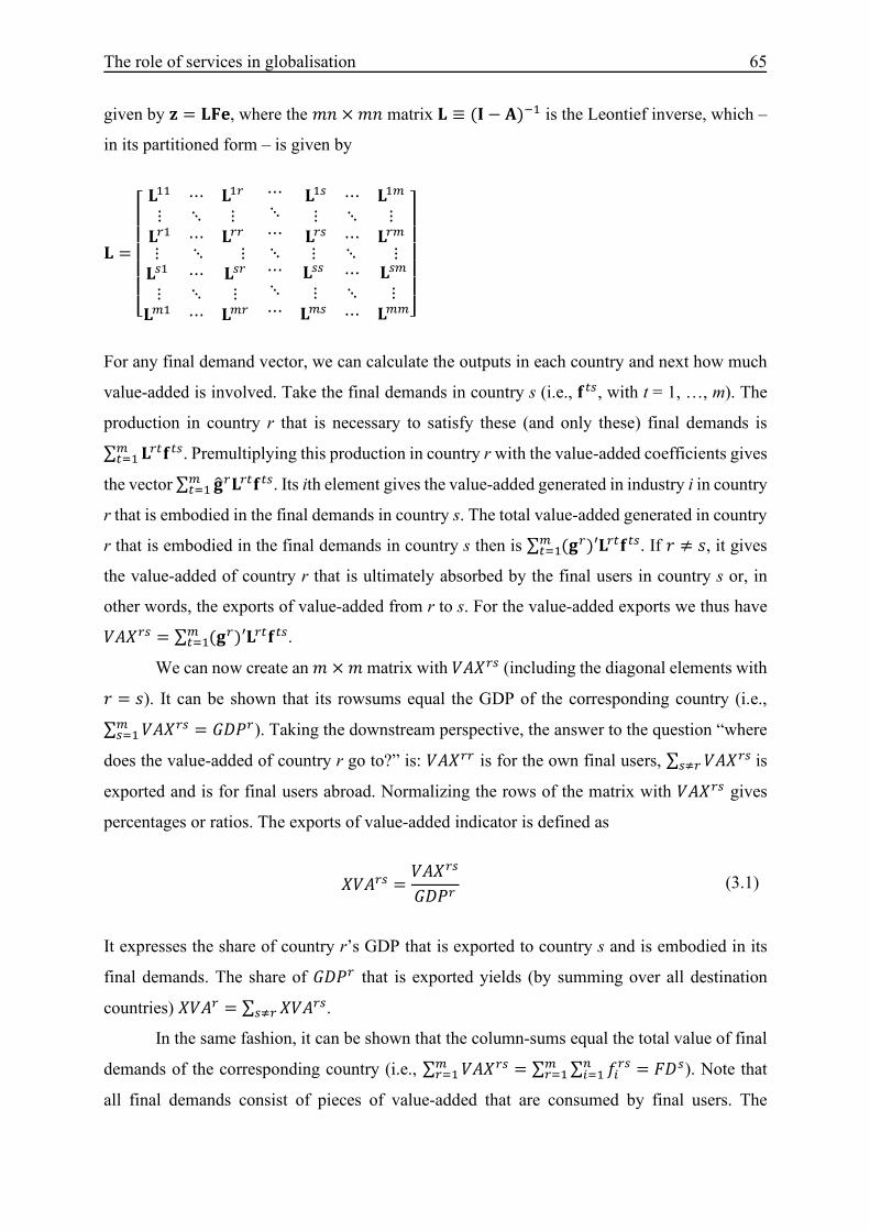
The role of services in globalisation 65
given by ® = ¾¦[, where the «¬ × «¬ matrix ¾ ≡ �J − G�KL is the Leontief inverse, which –
in its partitioned form – is given by
¾ =⎣⎢⎢⎢⎢⎢⎡ ¾LL ⋯ ¾L°⋮ ⋱ ⋮¾°L ⋯ ¾°°
⋯⋱⋯ ¾L± ⋯ ¾L¸⋮ ⋱ ⋮¾°± ⋯ ¾°¸ ⋮ ⋱ ⋮ ⋱ ⋮ ⋱ ⋮¾±L ⋯ ¾±° ⋮ ⋱ ⋮¾¸L ⋯ ¾¸°⋯⋱⋯ ¾±± ⋯ ¾±¸ ⋮ ⋱ ⋮¾¸± ⋯ ¾¸¸⎦⎥⎥
⎥⎥⎥⎤
For any final demand vector, we can calculate the outputs in each country and next how much
value-added is involved. Take the final demands in country s (i.e., 8À±, with t = 1, …, m). The
production in country r that is necessary to satisfy these (and only these) final demands is ∑ ¾°À8À±ÀkL . Premultiplying this production in country r with the value-added coefficients gives
the vector ∑ ¼¶ °¾°À8À±ÀkL . Its ith element gives the value-added generated in industry i in country
r that is embodied in the final demands in country s. The total value-added generated in country
r that is embodied in the final demands in country s then is ∑ �¼°�′¾°À8À±ÀkL . If Á ≠ Ã, it gives
the value-added of country r that is ultimately absorbed by the final users in country s or, in
other words, the exports of value-added from r to s. For the value-added exports we thus have ÄÅÆ°± = ∑ �¼°�′¾°À8À±ÀkL .
We can now create an « × « matrix with ÄÅÆ°± (including the diagonal elements with Á = Ã). It can be shown that its rowsums equal the GDP of the corresponding country (i.e., ∑ ÄÅÆ°±±kL = ÇÈÉ°). Taking the downstream perspective, the answer to the question “where
does the value-added of country r go to?” is: ÄÅÆ°° is for the own final users, ∑ ÄÅÆ°±±Y° is
exported and is for final users abroad. Normalizing the rows of the matrix with ÄÅÆ°± gives
percentages or ratios. The exports of value-added indicator is defined as
ÆÄÅ°± = ÄÅÆ°±ÇÈÉ° (3.1)
It expresses the share of country r’s GDP that is exported to country s and is embodied in its
final demands. The share of ÇÈÉ° that is exported yields (by summing over all destination
countries) ÆÄÅ° = ∑ ÆÄÅ°±±Y° .
In the same fashion, it can be shown that the column-sums equal the total value of final
demands of the corresponding country (i.e., ∑ ÄÅÆ°±°kL = ∑ ∑ ¹³°±Ê³kL°kL = Ëȱ). Note that
all final demands consist of pieces of value-added that are consumed by final users. The

66 Chapter 3
upstream perspective thus asks “where does the consumed value-added in country s come
from?” and the answer is: ÄÅƱ± is by the own producers, ∑ ÄÅÆ°±°Y± is imported (and is thus
generated by producers abroad). Normalizing the columns of the matrix with ÄÅÆ°± gives the
shares again. The imports of value-added indicator is defined as:
ÌÄÅ°± = ÄÅÆ°±Ëȱ (3.2)
It expresses the share of country s’s total value of final demand (FD) that is imported from and
generated by country r. In other words, the value-added imports from r as a share of total final
demands in country s.
To assess whether services travel further than manufactured goods (Section 3.4.2), it is
necessary to distinguish between dependence on intraregional and interregional trade. In the
empirical application we will focus on three regions: EU, which consists of all 28 members of
the European Union; North America, which consists of the three NAFTA countries Canada,
Mexico and the United States; and East Asia, which consists of China, Japan, Korea and
Taiwan. These are also the regions analysed in the two studies most closely related to this paper,
Los et al. (2015) and Baldwin and Lopez-Gonzalez (2015).
The XVA and MVA indicators are split into intraregional and interregional components.
Let us indicate a region with a capital letter. Then, the intraregional XVA for region R is
obtained by summing the value-added exports of all members of R to all other countries in R,
and taken as a share of regional GDP. Hence, for the intraregional XVA we have:
ÍÎÆÄÅÏ = ∑ ∑ �ÄÅÆ°± − ÄÅÆ°°�±∈Ï°∈Ï ∑ ÇÈÉ°°∈Ï (3.3)
The interregional XVA (IRXVA) measures the value-added exports to countries outside the
region. We have:
ÍÐÆÄÅÏ = ∑ ∑ ÄÅÆ°±±∉Ï°∈Ï∑ ÇÈÉ°°∈Ï (3.4)
Note that ÍÎÆÄÅÏ + ÍÐÆÄÅÏ = ÆÄÅÏ, with:
ÆÄÅÏ = ∑ ∑ �ÄÅÆ°± − ÄÅÆ°°�±°∈Ï ∑ ÇÈÉ°°∈Ï (3.5)

The role of services in globalisation 67
The split of the MVA indicator into an intraregional and an interregional component is
similar. That is, ÍÎÌÄÅÏ = ∑ ∑ �ÄÅÆ°± − ÄÅÆ°°�±∈Ï°∈Ï / ∑ Ëȱ±∈Ï and ÍÐÌÄÅÏ =∑ ∑ ÄÅÆ°±±∈Ï°∉Ï / ∑ Ëȱ±∈Ï .
When discussing the results, we will distinguish between the contributions of three sectors
to trade flows in value-added and dependency shares. These are: manufacturing, services and
other production. Recall that ∑ ¼¶ °¾°À8À±ÀkL is an n-element vector and its ith element gives the
value-added generated in industry i in country r that is embodied in the final demands in country
s. Denote this by ÄÅƳ°±. Then, we can split ÆÄÅÏ for region R as: ÆÄÅÒÓÊÔÕÏ + ÆÄÅÖװسÙ×±Ï +ÆÄÅÚÀÛ×°Ï , with, for example,
ÆÄÅÒÓÊÔÕÏ = ∑ ∑ ∑ �ÄÅƳ°± − ÄÅƳ°°�³∈ÒÓÊÔÕ±°∈Ï ∑ ÇÈÉ°°∈Ï (3.6)
There is a set of Appendix tables (Tables 3.A2–A7) that contain the results at industry level.
We use the 2016 release of the World Input-Output Database (WIOD) (Timmer et al.,
2015). This database contains annual time-series of WIOTs for the period 2000–14. The
consistent and harmonised tables include detailed data for 43 countries (including all 28 EU
members and the major advanced and emerging economies) and 56 industries. In this paper,
services are defined in a broad sense and include financial services; real estate; business
services; transport services; post and telecommunications; education; public administration;
health and social work; and wholesale trade and retail trade services. According to this broad
definition, 29 of the 56 industries in the database are considered services industries. These 29
industries—numbered 28–56 in Table 3.A1—are considered part of the services sector in this
analysis.65 The 2016 release of the WIOD is an update of the 2013 version of the database,
which covered 40 countries and a slightly earlier timeframe. The 2016 version offers more
industry-level detail than the initial WIOD release. For example, the new version includes a
disaggregation of business services. Reliable and detailed data for business services are useful,
because business services are known to play a key role in global value chains (Berry et al.,
2016).
Services data are the weakest part of current trade databases. This is because of the
intangible characteristic of services output and the resulting challenge in capturing services
trade flows. These challenges also hold for the WIOD and certain balancing procedures and
65 Industries numbered 5–23 in Appendix Table 3.A1 are considered part of the manufacturing sector; and industries numbered 1–4 and 24–27 are considered part of the other production sector.

68 Chapter 3
assumptions were necessary for the construction of internally consistent tables. Services data
in the WIOD use alternative data sources than standard balance of payments statistics (customs
information) because the database builds on international supply-use tables, which are
sometimes regarded as providing more reliable data for services (Miroudot and Shepherd,
2016). For these reasons, the WIOD is regarded as a comprehensive, reliable and consistent
database.
3.4 Empirical results This section investigates evolving dependencies of the European Union, North American and
East Asian regions on trade in value-added by applying the XVA and MVA indicators. Section
3.4.1 examines the extent to which trade of value-added in services industries is (or is not)
becoming more important relative to trade of value-added in manufactured goods industries
over time. This involves deriving sectoral shares of both value-added based indicators. Section
3.4.2 considers whether services or manufactured goods travel “further” in value-added trade.
The results based on gross exports (from the same database) serve as a benchmark.
3.4.1 Identifying the relative importance of services over time Table 3.2 reports the indicators XVA and MVA for the European Union’s, North American and
East Asian trade in value-added. The exports of value-added as a share of regional GDP were
given by Equation (3.6), and the imports of value-added as a share of regional final demand are
obtained from using a similar equation. The results are given for the years 2000 and 2014, and
by sector. The sectors (that account for the entire economy) are: manufacturing (M), services
(S) and other production (O), which includes agriculture, mining and quarrying, electricity and
construction. The two years are the first and last year in the database.66
Using Equation (3.5), we have (note that XVA is a weighted average of the XVAs of the
individual countries):
ÆÄÅÏ = & _& �ÄÅÆ°± − ÄÅÆ°°�±°∈Ï /ÇÈÉ°` ÇÈÉ°∑ ÇÈÉ°°∈Ï = & ÆÄÅ°°∈ÏÇÈÉ°∑ ÇÈÉ°°∈Ï (3.7)
Table 3.2 shows that the average EU country exported 23.3% of its GDP in 2000, which rose
to 27.6% in 2014, an increase of 4.3 percentage points (p.p.). That is, foreign final users
66 Only the results for 2000 and 2014 are displayed and the results are aggregated on a regional level to illustrate the most important trends. However, results for individual countries within each region and for all 15 years are available upon request.

The role of services in globalisation 69
(responsible for household consumption, private investments and government expenditures)
generate approximately one quarter of an EU country’s GDP. The “earnings” triggered by
foreign final demand is further split into the value-added generated in each sector. The exports
of value-added generated by services amounted for the average EU country to 11.3% of its GDP
in 2000 but to 15.0% in 2014, an increase of 3.7 percentage points. The results for all 56
industries are given in Appendix Table 3.A2. From these tables, it appears that approximately
two-thirds of the overall increase (of 4.3 p.p.) in XVA was attributable to business services (1.8
p.p.) and wholesale/retail trade (0.9 p.p.).67 The export of value-added has remained more or
less constant for the sectors manufacturing and other production in the average EU country.
Services have thus become more important over time for the generation of value-added
triggered by foreign final demand.
Table 3.2. Trade in value-added and gross exports for three regions (European Union, North America and East Asia) and sectors
European Union North America East Asia
M S O T M S O T M S O T
XVA
2000 10.0 11.3 2.1 23.3 3.7 4.3 0.9 9.0 7.4 5.0 1.0 13.3
2014 10.2 15.0 2.4 27.6 3.6 5.5 1.8 10.8 9.6 7.1 2.3 19.0
Change 0.2 3.7 0.4 4.3 -0.2 1.2 0.9 1.9 2.2 2.2 1.2 5.7
MVA
2000 9.3 9.9 3.3 22.5 5.1 4.1 1.8 11.1 4.3 4.0 2.4 10.8
2014 8.7 11.5 4.3 24.6 5.0 4.8 2.7 12.6 5.2 5.5 4.7 15.4
Change -0.6 1.6 1.0 2.0 -0.1 0.7 0.9 1.5 0.9 1.5 2.3 4.6
XGT
2000 23.7 8.4 1.8 33.9 7.9 3.3 0.9 12.0 13.8 3.0 0.2 17.1
2014 27.2 14.0 2.3 43.5 8.0 4.5 1.7 14.1 21.5 4.2 0.3 26.1
Change 3.5 5.6 0.5 9.6 0.0 1.2 0.8 2.1 7.7 1.2 0.1 9.0 Notes: The European Union includes all 28 EU members, North America includes Canada, Mexico and the United States, and East Asia consists of China, Japan, Korea and Taiwan. The sectors are: M = manufacturing; S = services; O = other production; and T = total/sum of all sectors. XVA refers to value-added exports as a share of GDP, averaged over the countries in the region. MVA refers to value-added imports as a share of total final demand, averaged over the countries in the region. XGT refers to total gross exports as a share of GDP, averaged over the countries in the region. Note that all data are rounded to the nearest tenth.
Whereas the XVAs indicate the foreign dependence on EU production, inputs and value-
added, the MVAs indicate the EU dependence on foreign value-added. Of the total final demand
in the average EU country, 22.5% was accounted for by foreign value-added in 2000, increasing
67 The following industries make up business services: “Legal and accounting activities, activities of head offices, management and consultancy activities” (M69/M70); “Architectural and engineering activities, technical testing and analysis” (M71); “Scientific R&D” (M72); “Advertising and market research” (M73); “Other professional, scientific and technological activities, veterinary activities” (M74/M75); “Administrative and support service activities” (N), and “Computer programming, consultancy and related activities; information service activities”
(J62/63). See Appendix Table 3.A1 for the classification of all services industries.

70 Chapter 3
to 24.6% in 2014. Observe that the dependence on manufacturing value-added declined (with
0.6 p.p.) and the largest increase was for services (with 1.6 p.p.). Also the increase in other
production was substantial (1.0 p.p.), and it turns out that this was largely due to mining and
quarrying. It was the industry responsible for the single largest percentage point increase in
dependence (0.6 p.p.). This reflects a greater reliance of EU’s final demands on natural resource
imports. The growing importance of the other production sector (and of the mining and
quarrying industry in particular) might be partly explained by higher commodity prices and not
only by volume changes.
Returning to Question 1 (“Has trade of value-added in services industries become more
important relative to trade of value-added in manufactured goods industries between 2000 and
2014?”), the answer is clearly affirmative for the European Union. The rising contributions of
services industries to trade in value-added could be a reflection of the growing importance of
services overall in the EU and other developed regions. This development may systematically
boost the trade triggered by services industries. Another explanation may be the liberalisation
of services trade during the time period, such as via services trade negotiations, which have led
to the rise of services-related GVCs (Heuser and Mattoo, 2017).
The bottom part of Table 3.2 gives the results for the gross export figures. These data have
the advantage of providing the industry of the products actually crossing the border (both
intermediates and final). The products exported by these industries may contain value-added
created in other industries or sectors, but only the industry of the actually exported products is
reflected in the data. Let �°± = ∑ °±[±Y° + ∑ 8°±±Y° indicate the vector of gross exports from
country r to country s, and define �°° = 0 for all r. For example, ÆÇÜÒÓÊÔÕÏ =∑ ∑ ∑ ݳ°±³∈ÒÓÊÔÕ±°∈Ï / ∑ ÇÈÉ°°∈Ï then gives, for the average EU country, its gross exports as
a share of its GDP. Observe in Table 3.2 that the role of manufacturing is much more important
than the role of services when exports are measured directly (as is the case with XGT). The role
of services is to a large extent indirect. Still, also when using the direct export figures it is true
that exports in services have become more important relative to exports in manufactured goods.
For North America, the findings are similar but not as pronounced as for the EU. The trade
in value-added has grown more for value-added created in the services sector than in
manufacturing (which has even fallen). The same applies to the services trade itself (see XGT).
However, the changes were not very large. For instance, total exports of value-added nudged
up from 9.0% to 10.8% as a share of GDP between 2000 and 2014. Furthermore, the sector
other production (agriculture, mining and quarrying, construction, and electricity) contributed

The role of services in globalisation 71
almost equally to this change. This is almost exclusively due to mining and quarrying, which
was the single industry that had the greatest impact on the increases in trade in value-added.
Rising commodity prices in the mining and quarrying industry may play a role, which reinforces
the decision to focus the comparison on the services and manufacturing sectors. Both the XVA
and the MVA of mining and quarrying grew by +0.7 p.p. over the time period. In explaining
the increased importance of services, business services and wholesale trade were particularly
influential, just as they were for the EU.
In East Asia, exports of value-added are still dominated by manufacturing although
services catches up. The percentage point changes in XVA were 2.2 for both sectors. Value-
added abroad triggered by final demands in the East Asian countries sketches a different picture.
Imports of foreign value-added (MVA) increased considerably (on average with 4.6 p.p.), but
the increase was the largest for value-added created in other production and the smallest for
manufacturing. The findings with regards to the XVA indicator are in line with the idea of
Factory East Asia. The region is still dependent for its value-added creation on exporting
manufactured goods, although the indirect contribution of services grows steadily.
Business services played a relative large role in explaining rising dependencies of the three
regions on trade. On the import side, this may be related to the increased domestic offshoring
of business services activities in developed countries to emerging and developing countries.
Balance of payments data provides some information on disaggregated trade flows in the
business services industries, which corroborates what we find using WIOD. For example, the
United States and Germany outsourced especially in the computer services, business consulting,
advertising and market research, R&D, and legal services sectors (Berry et al., 2016). Emerging
and developing countries have increased their world export share in these business services
categories between 2002 and 2012. At the same time, however, business services exports by
developed countries have also increased in importance. This indicates that countries may be
increasingly specialising in different types of business services.
Finally, two remarks are relevant. First, the results highlight the increasing disparities
between indicators for trade in value-added and for gross exports. In Table 3.2, the XVA
outcomes for services are always larger than the XGT outcomes. For manufacturing, the
differences are in the opposite direction and larger than for services. Indicators largely based
on direct trade (like XGT) overestimate manufactured goods (which embody more services)
compared to indicators that fully account for indirect trade (like XVA).

72 Chapter 3
Second, almost all indicators are the largest for the EU and the smallest for North America.
One should be careful to give too much weight to this observation, as it depends on the number
of countries that are included in a region.
3.4.2 Did services travel further than manufactured goods? This section addresses the question whether trade of value-added in services industries travelled
further than trade of value-added in manufactured goods industries in 2014. This is measured
by the share of services vis-a-vis manufacturing in intraregional and interregional trade in value
added. The intraregional XVA (ÍÎÆÄÅÏ) was defined in Equation (3.3). Just like the ÆÄÅÏ in
(5) was split into ÆÄÅÏ = ÆÄÅÒÓÊÔÕÏ + ÆÄÅÖװسÙ×±Ï + ÆÄÅÚÀÛ×°Ï , we now have ÍÎÆÄÅÏ = ÍÎÆÄÅÒÓÊÔÕÏ + ÍÎÆÄÅÖװسÙ×±Ï + ÍÎÆÄÅÚÀÛ×°Ï . The results in Table 3.3 then
report the shares, that is, ÍÎÆÄÅÖװسÙ×±Ï /ÍÎÆÄÅÏ for example. Of the total value-added
(created in the average EU country) that was embodied in the final demands of all other EU
countries, 50.6% was created in the services sector and 39.2% in the manufacturing sector.
Similar calculations and interpretations apply to interregional trade in value-added. For
example, 57.1% of the value-added in the average EU country that was embodied in final
demands outside the EU was created in the services sector. The services sector in the EU thus
had a larger share in the interregional exports of value-added than in the intraregional exports
of value-added (i.e., IR > IN) and the opposite held for the manufacturing sector (IR < IN). We
conclude that exports of value-added in EU services industries travelled further than exports of
value-added in EU manufacturing industries. It should be noted that this is a de facto,
aggregated result because the findings may vary depending on the geographic and structural
orientation of countries in trade.
Of the total value-added (created in the average EU country) that was embodied in the final
demands of all other EU countries, 50.6% was created in the services sector and 39.2% in the
manufacturing sector. Similar calculations and interpretations apply to interregional trade in
value-added. For example, 57.1% of the value-added in the average EU country that was
embodied in final demands outside the EU was created in the services sector. The services
sector in the EU thus had a larger share in the interregional exports of value-added than in the
intraregional exports of value-added (i.e., IR > IN) and the opposite held for the manufacturing
sector (IR < IN). We conclude that exports of value-added in EU services industries travelled
further than exports of value-added in EU manufacturing industries. It should be noted that this

The role of services in globalisation 73
is a de facto, aggregated result because the findings may vary depending on the geographic and
structural orientation of countries in trade.
Table 3.3. Shares for sectors in total, intraregional, and interregional trade in value-added for three regions in 2014
European Union North America East Asia
M S O T M S O T M S O T
XVA
IN 39.2 50.6 10.2 100 42.3 32.4 25.3 100 58.9 30.6 10.4 100
IR 35.4 57.1 7.6 100 28.5 59.1 12.4 100 48.9 39.0 12.1 100
TOT 37.0 54.2 8.7 100 32.8 50.7 16.5 100 50.6 37.6 11.8 100
MVA
IN 39.2 50.6 10.2 100 42.3 32.4 25.3 100 58.9 30.6 10.4 100
IR 31.4 43.2 25.4 100 39.1 40.8 20.1 100 27.6 36.8 35.6 100
TOT 35.4 47.0 17.6 100 40.0 38.6 21.5 100 34.0 35.7 30.3 100
XGT
IN 66.8 26.6 6.5 100 74.4 7.7 17.9 100 94.0 5.2 0.8 100
IR 57.5 38.5 4.0 100 45.0 47.2 7.9 100 79.3 19.2 1.4 100
TOT 62.5 32.1 5.4 100 56.4 31.8 11.8 100 82.5 16.2 1.3 100
Notes: Calculations are based on the World Input-Output Database. The European Union includes all 28 EU members, North America includes Canada, Mexico and the United States, and East Asia consists of China, Japan, Korea and Taiwan. Shares are rounded to the nearest tenth. XVA refers to VA exports of a particular sector (M = manufacturing; S = services; O = other production) as a share of all VA exports contributions (T = total/sum of all sectors = 100). MVA refers to VA imports as share of all VA import contributions. XGT refers to regional gross exports as a share of regional GDP. IN = intraregional trade in value-added (or gross exports), IR = interregional trade in value-added (or gross exports), TOT = total trade in value-added (or gross exports).
The row TOT gives the shares of the sectors in XVAR. For example, for the services sector,
we have ÆÄÅÖװسÙ×±Ï /ÆÄÅÏ = 15.0/27.6 = 0.542, where the 15.0 and 27.6 are from Table
3.2. The results are only for 1 year (2014) because the outcomes for other years sketch a similar
picture.68
The observation for the EU’s exports of value-added (i.e., services travelled further than
manufactured goods) also holds for the exports of value-added of the other two regions. For the
imports of value-added (MVA), the story is slightly different in the case of the EU even if the
conclusions are the same. Both for the services and the manufacturing sector, the share of
interregional trade is smaller than the share of intraregional trade (IR < IN). This is due to the
role of the sector other production. Comparing IR with IN, we find IR/IN = 43.2/50.6 = 0.85
for services and IR/ IN = 31.4/39.2 = 0.80 for manufacturing. Also for imports of value-added
by the EU, it is thus true that services value-added travelled further than manufacturing value-
added. For North America and East Asia, the findings for the imports (through MVA) are
similar to the findings for exports of value-added (through XVA).69 Hence, for every region
and indicator (including the EU MVA indicator), the result held that trade in value-added
68 The results for 2014 for the full 56-industry classification are provided in Appendix Tables 3.A5–A7. 69 Note that intraregional imports of value-added (MVA) by definition sum up to the intraregional exports of value-added (XVA) for each region. Hence, INXVA and INMVA values are identical in Table 3.3.

74 Chapter 3
created by services industries travelled further than trade in value-added created by
manufacturing industries. We add that transport services, which could be expected to increase
the share of services in interregional trade, only explain a small share of the more global nature
of services. The four transport industries together (land, water and air transport, and support
activities) accounted for less than a quarter of the increased importance of services in the EU’s
interregional exports of value-added relative to intraregional exports of value-added. The 2000
figures (not shown in the table) reveal similar patterns.
The distributions of the intraregional and interregional shares of the sectors in XVA and
MVA appear to be time invariant. The only observable difference over time was that services
grew as a share of total trade. One possible explanation for the lack of a stronger interregional
pattern over time for services could be that the ICT revolution increased more generally the
services content of manufactured goods. Given that the majority of exports of value-added
created in services industries are embodied in products traded by other sectors (e.g., in
manufacturing), there is less reason to believe an interregional trend in services would
predominate relative to manufactured goods over time. This is because changes in the
geographic orientation of manufactured goods trade would trigger (corresponding) changes in
the geographic orientation of services trade. Another explanation could be that the effect of an
expanded geographic scope of production fragmentation on services might have been offset by
regulatory convergence in services if convergence has been the strongest within regions.
Observe that the sector other production plays a substantial role in the case of imports of
value added (MVA). The industry-level results (see Appendix Tables 3.A5–A7) reveal that this
was overwhelmingly due to mining and quarrying, for which interregional imports of value-
added embodied in final demand were much more important than intraregional imports (except
for North America). This shows that Europe and East Asia were relatively dependent on raw
materials imported from outside the own region.
The sectoral embodiments of gross exports (intraregional, interregional and total) of the
three regions were also calculated for total gross exports (XGT). The trade of value-added in
services is typically indirect, because services are embodied in the gross exports of
manufactured goods (Heuser and Mattoo, 2017). The XVA and MVA indicators capture both
the direct and indirect services linkages. Direct export figures using the XGT approach may
provide additional insights because these data only report services and manufactured goods that
cross the border, aggregated by sector, and are not embodied indirectly in products traded by
other sectors. Two conclusions can be drawn when comparing the results for XGT with those
for XVA. First, gross exports were dominated by manufacturing. Services were considerably

The role of services in globalisation 75
more important in value-added terms relative to gross exports in each of the regions. Second,
also for gross exports it was the case that services travelled further than manufacturing.
Observe that there are significant differences in the intraregional vs. interregional shares of
services. The services share in intraregional exports of value-added was between two and six
times higher than the services share in gross intraregional exports in each region. However,
discrepancies between the share of services in interregional value-added exports and gross
interregional exports were considerably less. This provides an additional motivation for an
analysis of services trade based on value-added. The role of services is already understated
when gross exports are considered, but it is even more underrepresented when gross
intraregional exports are employed.
3.5 Conclusion and discussion
This study employed several trade indicators and different levels of industry aggregation to
study the role of services in globalisation patterns. This was done by examining the cases of the
European Union, North America and East Asia between 2000 and 2014, and distinguishing
between intraregional, interregional and total trade. There are two key findings. First, in Europe
and North America trade of value-added in services industries rose more than trade of value-
added in manufactured goods industries. In relative terms, this was also the case in East Asia.
Second, by comparing intraregional and interregional trade in value-added on a sectoral level,
value-added created in services industries always travelled further than value-added created in
manufacturing industries.
Our results also underscored the increasing disparity between gross exports and exports of
value-added over time (supporting the original finding of Johnson and Noguera, 2012), which
is especially acute for services. This greater discrepancy for services reflects the fact that gross
trade only captures direct but not indirect services exports—understating their importance. That
could cause one to misinterpret where value is created. Disparities between the services share
in gross exports and the services share in value-added exports were considerably larger within
regions than between regions. The results also indicated that world trade is more global when
measured in value-added terms than in gross exports. Although analysing trade in value-added
is extremely useful in exposing indirect dependencies, actual trade is the action that takes place.
Thus, gross export statistics remain important themselves and are also necessary to determine
the trade in value-added figures.

76 Chapter 3
The importance of services is even greater in interregional trade than in intraregional trade.
This has policy implications. First, trade policy should explicitly be aimed at lifting services
barriers (Berry et al., 2016; Saez et al., 2014). The Trade in Services Agreement (TiSA) that is
currently being negotiated by 23 members of the World Trade Organization (representing 50
countries) is a positive step in this direction. Research based on firm-level data finds that
allowing for the participation of foreign services providers improves the performance of
downstream manufacturing firms (Arnold et al., 2011; Duggan et al., 2013). Second, it is
important to improve the regulatory environment for domestic services because services are
embodied in the output of other sectors. Regulatory reform in the services sector can contribute
in establishing comparative advantage for firms relying on services inputs (Van der Marel,
2016). Improved access to services, which may accompany trade liberalisation and domestic
policy reform efforts, raises competitiveness and productivity of manufacturing industries
(Arnold et al, 2008; Arnold et al., 2016) and contributes to economic growth (Mattoo et al.,
2006).
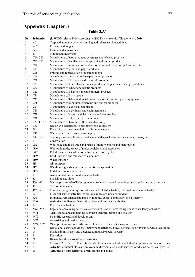
The role of services in globalisation 77
Appendix Chapter 3 Table 3.A1
Nr. Industries (in WIOD release 2016 according to ISIC Rev. 4, see also Timmer et al., 2016)
1 A01 Crop and animal production hunting and related service activities
2 A02 Forestry and logging
3 A03 Fishing and aquaculture
4 B Mining and quarrying
5 C10-C12 Manufacture of food products, beverages and tobacco products
6 C13-C15 Manufacture of textiles, wearing apparel and leather products
7 C16 Manufacture of wood and of products of wood and cork, except furniture; etc.
8 C17 Manufacture of paper and paper products
9 C18 Printing and reproduction of recorded media
10 C19 Manufacture of coke and refined petroleum products
11 C20 Manufacture of chemicals and chemical products
12 C21 Manufacture of basic pharmaceutical products and pharmaceutical preparations
13 C22 Manufacture of rubber and plastic products
14 C23 Manufacture of other non-metallic mineral products
15 C24 Manufacture of basic metals
16 C25 Manufacture of fabricated metal products, except machinery and equipment
17 C26 Manufacture of computer, electronic and optical products
18 C27 Manufacture of electrical equipment
19 C28 Manufacture of machinery and equipment n.e.c.
20 C29 Manufacture of motor vehicles, trailers and semi-trailers
21 C30 Manufacture of other transport equipment
22 C31, C32 Manufacture of furniture; other manufacturing
23 C33 Repair and installation of machinery and equipment
24 D Electricity, gas, steam and air conditioning supply
25 E36 Water collection, treatment and supply
26 E37-E39 Sewerage; waste collection, treatment and disposal activities; materials recovery; etc.
27 F Construction
28 G45 Wholesale and retail trade and repair of motor vehicles and motorcycles
29 G46 Wholesale trade, except of motor vehicles and motorcycles
30 G47 Retail trade, except of motor vehicles and motorcycles
31 H49 Land transport and transport via pipelines
32 H50 Water transport
33 H51 Air transport
34 H52 Warehousing and support activities for transportation
35 H53 Postal and courier activities
36 I Accommodation and food service activities
37 J58 Publishing activities
38 J59, J60 Motion picture/video/TV programme production, sound recording/music publishing activities; etc.
39 J61 Telecommunications
40 J62, J63 Computer programming, consultancy and related activities; information service activities
41 K64 Financial service activities, except insurance and pension funding
42 K65 Insurance, reinsurance and pension funding, except compulsory social security
43 K66 Activities auxiliary to financial services and insurance activities
44 L Real estate activities
45 M69, M70 Legal and accounting activities; activities of head offices; management consultancy activities
46 M71 Architectural and engineering activates: technical testing and analysis
47 M72 Scientific research and development
48 M73 Advertising and market research
49 M74, M75 Other professional, scientific and technical activities; veterinary activities
50 N Rental and leasing activities, Employment activities, Travel services, security and services to building
51 O Public administration and defence; compulsory social security
52 P Education
53 Q Human health and social work activities
54 R-S Creative, Arts, Sports, Recreation and entertainment activities and all other personal service activities
55 T Activities of households as employers; undifferentiated goods/services-producing activities - own use
56 U Activities of extra-territorial organisations and bodies

78 Chapter 3
Table 3.A2
European Union: decomposition of dependency indicators by industry (2000-2014)
(in percent; change between 2000 and 2014 in percentage points and percent change)
Industry / ISIC rev. 4
XVA MVA
2000 2000 2000 2000 2000 2014 14-00 Δ (%)
Crop and animal production 0.5 0.6 0.0 9.2 0.8 1.0 0.2 26.9
Forestry and logging 0.1 0.1 0.0 19.8 0.1 0.1 0.0 -11.9
Fishing and aquaculture 0.0 0.0 0.0 -15.0 0.1 0.1 0.0 10.4
Mining and quarrying 0.5 0.5 -0.1 -12.0 1.4 2.1 0.6 45.1
Food products 0.6 0.8 0.2 33.1 0.6 0.8 0.2 30.3
Textile products 0.6 0.4 -0.2 -26.6 0.7 0.6 -0.1 -13.5
Wood products 0.2 0.1 0.0 -11.6 0.2 0.1 0.0 -12.6
Paper products 0.3 0.2 -0.1 -28.8 0.3 0.2 -0.1 -33.8
Printing products 0.2 0.1 -0.1 -37.5 0.1 0.1 -0.1 -39.9
Refined petroleum products 0.1 0.1 0.0 -4.9 0.2 0.3 0.1 50.1
Chemical products 0.9 0.8 0.0 -4.5 0.8 0.7 -0.1 -8.2
Pharmaceutical products 0.5 0.7 0.2 43.3 0.4 0.6 0.2 44.6
Rubber and plastics 0.5 0.5 0.0 7.4 0.4 0.4 0.0 -5.6
Other nonmetallic minerals 0.3 0.2 -0.1 -18.4 0.2 0.2 0.0 -17.5
Basic metals 0.5 0.4 -0.1 -17.3 0.5 0.5 -0.1 -16.5
Fabricated metals 0.8 0.9 0.1 10.7 0.6 0.6 0.0 -8.0
Computer, electronic and optical products 1.0 0.7 -0.4 -36.4 1.3 0.9 -0.4 -28.3
Electronic equipment 0.6 0.6 0.0 0.1 0.5 0.5 -0.1 -11.6
Machinery and equipment n.e.c. 1.1 1.4 0.3 24.1 0.8 0.8 0.0 2.0
Motor vehicles, trailers and semi-trailers 1.0 1.2 0.2 19.2 0.8 0.7 -0.1 -6.8
Other transport equipment 0.4 0.4 0.0 4.7 0.4 0.3 -0.1 -14.2
Furniture; other manufacturing 0.4 0.4 0.1 15.3 0.4 0.4 0.0 0.0
Repair, installation of machinery/equipment 0.2 0.3 0.1 32.9 0.1 0.1 0.0 15.2
Electricity and gas 0.4 0.5 0.1 24.7 0.5 0.6 0.0 8.1
Water 0.0 0.0 0.0 23.6 0.0 0.0 0.0 -1.4
Waste and water management 0.2 0.3 0.1 63.8 0.2 0.2 0.1 34.0
Construction 0.3 0.4 0.1 51.0 0.2 0.3 0.1 38.1

The role of services in globalisation 79
Table 3.A2 (continued)
Industry / ISIC rev. 4
XVA MVA
2000 2014 14-00 Δ (%) 2000 2014 14-00 Δ (%)
Wholesale and retail trade/repair of vehicles 0.2 0.4 0.2 84.5 0.2 0.3 0.1 35.4
Wholesale trade, except of vehicles 1.6 2.3 0.7 46.1 1.6 2.0 0.4 27.3
Retail trade, except of vehicles 0.8 0.6 -0.2 -28.5 0.7 0.5 -0.1 -18.7
Inland transport 0.7 0.9 0.2 24.6 0.7 0.8 0.1 15.3
Water transport 0.2 0.2 0.0 1.8 0.1 0.1 0.0 -15.8
Air transport 0.2 0.2 0.0 3.1 0.2 0.1 0.0 -12.6
Support activities for transportation 0.6 0.8 0.2 42.3 0.4 0.6 0.1 31.5
Post 0.2 0.2 0.0 -1.1 0.1 0.1 0.0 -12.5
Hotels and restaurants 0.2 0.3 0.1 41.0 0.3 0.3 0.0 -4.7
Publishing activities 0.2 0.2 0.0 14.4 0.2 0.2 0.0 -6.6
Video, television, music, and casting 0.1 0.2 0.0 8.9 0.1 0.1 0.0 3.2
Telecommunications 0.3 0.3 0.0 -0.9 0.3 0.3 0.0 -5.0
Computer programming, consultancy, IT 0.4 0.9 0.5 121.5 0.3 0.5 0.2 77.7
Fin services, not insurance/pension funding 0.9 1.1 0.2 28.4 0.8 0.9 0.1 16.6
Insurance, reinsurance and pension funding 0.2 0.2 0.1 54.3 0.1 0.1 0.0 4.4
Other fin. services activities 0.2 0.3 0.1 47.5 0.1 0.2 0.0 30.4
Real estate activities 0.6 0.8 0.2 40.9 0.5 0.6 0.1 17.9
Legal and accounting; consultancy 0.9 1.4 0.5 55.7 0.7 1.0 0.3 37.8
Architectural and engineering activities 0.4 0.5 0.1 32.0 0.3 0.3 0.1 20.5
Scientific research and development 0.3 0.1 -0.2 -58.5 0.2 0.2 -0.1 -29.7
Advertising and market research 0.2 0.2 0.0 10.0 0.2 0.2 0.0 2.9
Other prof./scientific/technical activities 0.2 0.2 0.1 45.2 0.2 0.2 0.0 22.4
Admin and support service activities 1.1 1.7 0.5 44.1 1.1 1.3 0.2 19.2
Public admin 0.2 0.3 0.1 42.7 0.2 0.2 0.0 11.5
Education 0.2 0.2 0.1 34.4 0.1 0.1 0.0 13.9
Health and social work 0.0 0.1 0.1 119.5 0.0 0.1 0.0 30.1
Other services 0.2 0.3 0.1 27.0 0.3 0.3 0.0 15.9
Household consumption 0.0 0.0 0.0 -5.3 0.0 0.0 0.0 -56.0
Extraterritorial organizations and bodies 0.0 0.0 0.0 0.0 0.0 0.0 0.0 0.0
Manufacturing 10.0 10.2 0.2 2.3 9.3 8.7 -0.6 -6.4
Services 11.3 15.0 3.7 32.6 9.9 11.5 1.6 16.1
Other 2.1 2.4 0.4 17.7 3.3 4.3 1.0 31.1
Total 23.3 27.6 4.3 18.3 22.5 24.6 2.0 9.0 Source: Own calculations based on the World Input-Output Database. Shares are rounded to the nearest tenth. Notes: All 28 members of the European Union are aggregated. Industries are assigned to sectors. XVA refers to VA-exports as share of total regional value-added production. MVA refers to VA-imports as share of total regional final demand.

80 Chapter 3
Table 3.A3
North America: decomposition of dependency indicators by industry (2000-2014)
(in percent; change between 2000 and 2014 in percentage points and percent change)
Industry / ISIC rev. 4
XVA MVA
2000 2014 14-00 Δ (%) 2000 2014 14-00 Δ (%)
Crop and animal production 0.2 0.3 0.1 71.0 0.3 0.5 0.2 77.7
Forestry and logging 0.0 0.0 0.0 -2.8 0.1 0.1 0.0 -18.2
Fishing and aquaculture 0.0 0.0 0.0 72.4 0.0 0.0 0.0 67.7
Mining and quarrying 0.5 1.2 0.7 156.4 1.0 1.7 0.7 65.1
Food products 0.2 0.2 0.1 34.2 0.2 0.3 0.1 60.6
Textile products 0.1 0.1 -0.1 -57.1 0.4 0.4 -0.1 -16.4
Wood products 0.1 0.0 0.0 -30.3 0.1 0.1 0.0 5.7
Paper products 0.1 0.1 0.0 -35.2 0.1 0.1 0.0 -24.0
Printing products 0.1 0.0 0.0 -28.7 0.1 0.0 0.0 -44.3
Refined petroleum products 0.1 0.2 0.1 211.4 0.1 0.2 0.1 59.7
Chemical products 0.3 0.4 0.1 38.9 0.4 0.4 0.1 14.0
Pharmaceutical products 0.1 0.2 0.0 32.7 0.2 0.2 0.0 17.8
Rubber and plastics 0.1 0.1 0.0 -6.1 0.2 0.2 0.0 5.0
Other nonmetallic minerals 0.1 0.1 0.0 -14.9 0.1 0.1 0.0 -16.2
Basic metals 0.2 0.2 0.0 24.2 0.3 0.4 0.0 4.1
Fabricated metals 0.2 0.2 0.0 -7.6 0.3 0.3 0.0 0.1
Computer, electronic and optical products 0.8 0.5 -0.3 -34.3 0.9 0.7 -0.2 -18.3
Electronic equipment 0.1 0.1 0.0 -13.9 0.3 0.2 0.0 -10.1
Machinery and equipment n.e.c. 0.3 0.3 0.0 -5.1 0.4 0.5 0.0 5.8
Motor vehicles, trailers and semi-trailers 0.4 0.3 -0.1 -19.3 0.6 0.6 0.0 -6.3
Other transport equipment 0.3 0.3 0.0 1.7 0.1 0.1 0.0 0.3
Furniture; other manufacturing 0.2 0.1 0.0 -11.0 0.3 0.2 0.0 -14.5
Repair, installation of machinery/equipment 0.0 0.0 0.0 -23.0 0.0 0.0 0.0 -11.6
Electricity and gas 0.1 0.1 0.0 -13.6 0.3 0.3 0.0 11.2
Water 0.0 0.0 0.0 81.0 0.0 0.0 0.0 -4.1
Waste and water management 0.0 0.1 0.0 68.4 0.1 0.1 0.0 23.3
Construction 0.0 0.1 0.0 23.2 0.1 0.1 0.0 35.7

The role of services in globalisation 81
Table 3.A3 (continued)
Industry / ISIC rev. 4
XVA MVA
2000 2014 14-00 Δ (%) 2000 2014 14-00 Δ (%)
Wholesale and retail trade/repair of vehicles 0.1 0.1 0.0 -8.4 0.1 0.1 0.0 -3.7
Wholesale trade, except of vehicles 1.0 1.2 0.2 18.6 0.7 0.8 0.2 23.0
Retail trade, except of vehicles 0.1 0.1 0.0 4.1 0.3 0.3 0.0 -4.7
Inland transport 0.3 0.3 0.1 22.5 0.3 0.3 0.0 13.6
Water transport 0.0 0.0 0.0 -16.0 0.1 0.0 0.0 -24.6
Air transport 0.1 0.1 0.0 23.4 0.1 0.1 0.0 -9.1
Support activities for transportation 0.1 0.1 0.0 28.7 0.1 0.1 0.0 29.7
Post 0.1 0.1 0.0 -9.6 0.0 0.0 0.0 -8.1
Hotels and restaurants 0.1 0.1 0.0 11.0 0.1 0.1 0.0 22.4
Publishing activities 0.1 0.2 0.1 44.2 0.0 0.0 0.0 -5.0
Video, television, music, and casting 0.1 0.1 0.0 49.0 0.0 0.0 0.0 14.1
Telecommunications 0.1 0.1 0.0 0.9 0.1 0.1 0.0 -5.9
Computer programming, consultancy, IT 0.1 0.2 0.1 108.0 0.1 0.2 0.1 68.2
Fin services, not insurance/pension funding 0.3 0.4 0.1 43.9 0.3 0.4 0.1 39.8
Insurance, reinsurance and pension funding 0.1 0.1 0.1 55.4 0.1 0.2 0.1 64.9
Other fin. services activities 0.1 0.2 0.1 71.3 0.0 0.0 0.0 26.3
Real estate activities 0.2 0.2 0.0 15.2 0.2 0.2 0.0 18.5
Legal and accounting; consultancy 0.4 0.5 0.1 37.4 0.2 0.4 0.1 56.2
Architectural and engineering activities 0.1 0.2 0.1 43.8 0.1 0.1 0.0 35.3
Scientific research and development 0.1 0.1 0.0 54.2 0.1 0.1 0.0 -22.8
Advertising and market research 0.1 0.1 0.0 59.6 0.0 0.0 0.0 12.8
Other prof./scientific/technical activities 0.0 0.0 0.0 37.4 0.1 0.1 0.1 73.5
Admin and support service activities 0.5 0.6 0.1 22.6 0.7 0.7 -0.1 -7.2
Public admin 0.1 0.2 0.0 20.4 0.1 0.1 0.0 13.9
Education 0.0 0.0 0.0 59.6 0.0 0.0 0.0 28.4
Health and social work 0.0 0.0 0.0 54.0 0.0 0.0 0.0 16.6
Other services 0.1 0.1 0.0 5.5 0.1 0.1 0.0 31.9
Household consumption 0.0 0.0 0.0 -18.1 0.0 0.0 0.0 -51.4
Extraterritorial organizations and bodies 0.0 0.0 0.0 0.0 0.0 0.0 0.0 0.0
Manufacturing 3.7 3.6 -0.2 -5.1 5.1 5.0 -0.1 -2.4
Services 4.3 5.5 1.2 27.4 4.1 4.8 0.7 17.0
Other 0.9 1.8 0.9 94.8 1.8 2.7 0.9 51.6
Total 9.0 10.8 1.9 20.7 11.1 12.6 1.5 13.5 Source: Own calculations based on the World Input-Output Database. Shares are rounded to the nearest tenth. Notes: The 3 North American countries (Canada, Mexico, and US) are aggregated. Industries are assigned to sectors. XVA refers to VA-exports as share of total regional value-added production. MVA refers to VA-imports as share of total regional final demand.

82 Chapter 3
Table 3.A4
East Asia: decomposition of dependency indicators by industry (2000-2014)
(in percent; change between 2000 and 2014 in percentage points and percent change)
Industry / ISIC rev. 4
XVA MVA
2000 2014 14-00 Δ (%) 2000 2014 14-00 Δ (%)
Crop and animal production 0.3 0.7 0.5 184.9 0.4 0.7 0.3 63.8
Forestry and logging 0.0 0.1 0.0 42.9 0.1 0.1 0.0 14.5
Fishing and aquaculture 0.0 0.1 0.0 31.8 0.0 0.0 0.0 -15.9
Mining and quarrying 0.3 0.9 0.6 218.8 1.4 3.1 1.7 120.3
Food products 0.2 0.4 0.2 137.0 0.3 0.3 0.0 13.5
Textile products 0.6 0.9 0.3 44.0 0.3 0.3 -0.1 -16.4
Wood products 0.0 0.1 0.1 201.6 0.1 0.1 0.0 12.9
Paper products 0.1 0.1 0.0 7.2 0.0 0.0 0.0 -16.9
Printing products 0.1 0.1 0.0 -13.5 0.0 0.0 0.0 -22.9
Refined petroleum products 0.2 0.3 0.1 77.8 0.1 0.2 0.1 35.6
Chemical products 0.6 0.8 0.1 19.6 0.4 0.5 0.1 12.9
Pharmaceutical products 0.0 0.1 0.0 100.2 0.1 0.2 0.1 93.8
Rubber and plastics 0.3 0.4 0.0 13.6 0.2 0.2 0.0 16.4
Other nonmetallic minerals 0.2 0.3 0.1 56.1 0.1 0.1 0.0 12.7
Basic metals 0.6 0.8 0.2 32.5 0.4 0.4 0.1 14.7
Fabricated metals 0.4 0.5 0.1 16.8 0.2 0.3 0.0 13.0
Computer, electronic and optical products 1.8 2.2 0.4 24.3 0.9 1.1 0.2 21.9
Electronic equipment 0.5 0.6 0.1 16.4 0.3 0.3 0.0 8.5
Machinery and equipment n.e.c. 0.6 0.8 0.2 43.0 0.4 0.5 0.1 23.9
Motor vehicles, trailers and semi-trailers 0.7 0.7 0.0 1.0 0.1 0.3 0.2 120.3
Other transport equipment 0.2 0.3 0.1 80.5 0.1 0.2 0.1 47.1
Furniture; other manufacturing 0.2 0.3 0.1 40.3 0.2 0.2 0.1 35.9
Repair, installation of machinery/equipment 0.0 0.0 0.0 -31.4 0.0 0.0 0.0 34.3
Electricity and gas 0.3 0.4 0.1 29.2 0.3 0.4 0.2 58.0
Water 0.0 0.0 0.0 -8.6 0.0 0.0 0.0 12.1
Waste and water management 0.0 0.0 0.0 91.0 0.0 0.1 0.0 108.7
Construction 0.1 0.1 0.0 36.7 0.1 0.1 0.1 101.0

The role of services in globalisation 83
Table 3.A4 (continued)
Industry / ISIC rev. 4
XVA MVA
2000 2014 14-00 Δ (%) 2000 2014 14-00 Δ (%)
Wholesale and retail trade/repair of vehicles 0.1 0.1 0.0 -27.3 0.1 0.1 0.0 36.6
Wholesale trade, except of vehicles 1.4 2.2 0.8 57.6 0.7 1.1 0.3 41.0
Retail trade, except of vehicles 0.3 0.5 0.2 90.0 0.3 0.3 0.1 25.9
Inland transport 0.4 0.6 0.2 46.5 0.3 0.4 0.1 49.0
Water transport 0.3 0.2 0.0 -12.0 0.1 0.1 0.0 -19.6
Air transport 0.1 0.1 0.0 -20.7 0.1 0.1 0.0 25.2
Support activities for transportation 0.2 0.2 0.0 21.3 0.1 0.2 0.1 46.3
Post 0.0 0.0 0.0 -5.0 0.0 0.0 0.0 5.6
Hotels and restaurants 0.2 0.2 0.0 18.9 0.2 0.2 0.0 -14.3
Publishing activities 0.0 0.0 0.0 -27.3 0.0 0.0 0.0 -0.5
Video, television, music, and casting 0.1 0.0 0.0 -26.6 0.0 0.0 0.0 4.1
Telecommunications 0.1 0.2 0.0 8.8 0.1 0.1 0.0 4.6
Computer programming, consultancy, IT 0.1 0.1 0.0 4.3 0.1 0.2 0.1 68.1
Fin services, not insurance/pension funding 0.5 0.9 0.4 67.4 0.3 0.5 0.2 73.1
Insurance, reinsurance and pension funding 0.1 0.1 0.0 3.9 0.1 0.1 0.0 5.8
Other fin. services activities 0.0 0.0 0.0 13.6 0.0 0.1 0.0 27.8
Real estate activities 0.1 0.3 0.2 114.8 0.2 0.2 0.1 48.6
Legal and accounting; consultancy 0.1 0.4 0.3 318.8 0.3 0.5 0.2 91.2
Architectural and engineering activities 0.0 0.1 0.0 47.0 0.1 0.1 0.0 32.5
Scientific research and development 0.1 0.1 0.0 6.7 0.1 0.1 0.0 10.5
Advertising and market research 0.1 0.0 0.0 -65.4 0.0 0.0 0.0 -11.3
Other prof./scientific/technical activities 0.3 0.3 0.0 13.6 0.1 0.1 0.0 7.7
Admin and support service activities 0.1 0.2 0.0 14.2 0.3 0.4 0.1 30.2
Public admin 0.1 0.1 0.0 16.7 0.1 0.1 0.0 27.5
Education 0.0 0.0 0.0 106.6 0.0 0.1 0.0 40.4
Health and social work 0.0 0.0 0.0 29.6 0.0 0.0 0.0 66.1
Other services 0.1 0.2 0.1 74.2 0.1 0.2 0.1 69.4
Household consumption 0.0 0.0 0.0 -77.4 0.0 0.0 0.0 15.8
Extraterritorial organizations and bodies 0.0 0.0 0.0 0.0 0.0 0.0 0.0 0.0
Manufacturing 7.4 9.6 2.2 30.4 4.3 5.2 0.9 20.8
Services 5.0 7.1 2.2 44.4 4.0 5.5 1.5 36.4
Other 1.0 2.3 1.2 119.5 2.4 4.7 2.3 93.9
Total 13.3 19.0 5.7 42.4 10.8 15.4 4.6 43.0 Source: Own calculations based on the World Input-Output Database. Shares are rounded to the nearest tenth. Notes: 4 East Asian countries (China, Japan, Korea, and Taiwan) are aggregated. Industries are assigned to sectors. XVA refers to VA-exports as share of total regional value-added production. MVA refers to VA-imports as share of total regional final demand.

84 Chapter 3
Table 3.A5
European Union: Share of each industry in total, intraregional, and interregional trade
(2014)
(Percentage)
Industry / ISIC rev. 4 XVA MVA
IN IR TOT IN IR TOT
Crop and animal production 3.0 1.3 2.0 3.0 5.1 4.0
Forestry and logging 0.3 0.3 0.3 0.3 0.3 0.3
Fishing and aquaculture 0.1 0.0 0.1 0.1 0.4 0.2
Mining and quarrying 1.9 1.6 1.7 1.9 15.6 8.5
Food products 4.2 2.0 3.0 4.2 1.9 3.1
Textile products 1.6 1.4 1.5 1.6 3.1 2.3
Wood products 0.6 0.4 0.5 0.6 0.5 0.6
Paper products 1.0 0.7 0.8 1.0 0.5 0.8
Printing products 0.3 0.4 0.4 0.3 0.3 0.3
Refined petroleum products 0.4 0.3 0.4 0.4 1.7 1.0
Chemical products 3.1 2.9 3.0 3.1 2.8 3.0
Pharmaceutical products 2.8 2.2 2.5 2.8 1.7 2.3
Rubber and plastics 2.2 1.6 1.8 2.2 1.1 1.6
Other nonmetallic minerals 1.0 0.8 0.9 1.0 0.7 0.8
Basic metals 1.5 1.6 1.5 1.5 2.2 1.8
Fabricated metals 3.1 3.1 3.1 3.1 1.3 2.3
Computer, electronic and optical products 2.4 2.4 2.4 2.4 5.2 3.8
Electronic equipment 2.3 2.1 2.2 2.3 1.4 1.9
Machinery and equipment n.e.c. 4.3 5.3 4.9 4.3 2.3 3.4
Motor vehicles, trailers and semi-trailers 4.3 4.1 4.2 4.3 1.6 3.0
Other transport equipment 1.0 1.8 1.4 1.0 1.5 1.2
Furniture; other manufacturing 1.9 1.4 1.6 1.9 1.5 1.7
Repair, installation of machinery/equipment 0.9 1.0 0.9 0.9 0.1 0.5
Electricity and gas 2.0 1.7 1.9 2.0 2.8 2.4
Water 0.2 0.1 0.2 0.2 0.2 0.2
Waste and water management 1.2 1.0 1.1 1.2 0.5 0.8
Construction 1.6 1.5 1.6 1.6 0.7 1.2

The role of services in globalisation 85
Table 3.A5 (continued)
Industry / ISIC rev. 4 XVA MVA
IN IR TOT IN IR TOT
Wholesale and retail trade and repair of vehicles 1.6 1.5 1.5 1.6 0.5 1.1
Wholesale trade, except of vehicles 8.7 8.2 8.4 8.7 7.5 8.2
Retail trade, except of vehicles 2.2 2.0 2.1 2.2 2.2 2.2
Inland transport 3.1 3.2 3.2 3.1 3.4 3.3
Water transport 0.3 1.3 0.9 0.3 0.6 0.4
Air transport 0.5 0.7 0.6 0.5 0.7 0.6
Support activities for transportation 2.9 3.1 3.0 2.9 1.6 2.3
Post 0.5 0.6 0.6 0.5 0.3 0.4
Hotels and restaurants 0.7 1.1 0.9 0.7 1.6 1.2
Publishing activities 0.6 0.9 0.8 0.6 0.7 0.7
Video, television, music, and casting 0.5 0.6 0.6 0.5 0.6 0.6
Telecommunications 1.3 1.1 1.2 1.3 1.2 1.2
Computer programming, consultancy, IT 2.2 3.9 3.1 2.2 1.9 2.0
Fin services, except insurance and pension funding 3.1 4.8 4.1 3.1 4.1 3.6
Insurance, reinsurance and pension funding 0.5 1.1 0.9 0.5 0.7 0.6
Other fin. services activities 0.8 1.5 1.2 0.8 0.5 0.6
Real estate activities 2.9 3.1 3.0 2.9 1.5 2.2
Legal and accounting; consultancy 5.0 5.0 5.0 5.0 3.4 4.2
Architectural and engineering activities 1.6 2.0 1.8 1.6 0.9 1.2
Scientific research and development 0.6 0.4 0.5 0.6 0.8 0.7
Advertising and market research 0.9 0.8 0.9 0.9 0.4 0.7
Other professional, scientific and technical activities 0.9 0.8 0.8 0.9 0.9 0.9
Admin and support service activities 6.0 6.0 6.0 6.0 4.2 5.2
Public admin 1.0 1.2 1.1 1.0 1.0 1.0
Education 0.7 0.8 0.8 0.7 0.3 0.5
Health and social work 0.3 0.4 0.3 0.3 0.2 0.3
Other services 1.1 1.0 1.1 1.1 1.3 1.2
Household consumption 0.0 0.0 0.0 0.0 0.0 0.0
Extraterritorial organizations and bodies 0.0 0.0 0.0 0.0 0.0 0.0
Manufacturing 39.2 35.4 37.0 39.2 31.4 35.4
Services 50.6 57.1 54.2 50.6 43.2 47.0
Other 10.2 7.6 8.7 10.2 25.4 17.6
Total 100 100 100 100 100 100
Source: Own calculations based on the World Input-Output Database. Shares are rounded to the nearest tenth. Notes: All 27 members of the European Union are aggregated. Industries are assigned to sectors. XVA refers to VA-exports as share of all value-added exports contributions. MVA refers to VA-imports as share of all value-added import contributions.

86 Chapter 3
Table 3.A6
North America: Share of each industry in total, intraregional, and interregional trade
(2014)
(Percentage)
Industry / ISIC rev. 4 XVA MVA
IN IR TOT IN IR TOT
Crop and animal production 3.6 2.4 2.8 3.6 3.8 3.7
Forestry and logging 0.5 0.3 0.3 0.5 0.6 0.6
Fishing and aquaculture 0.2 0.2 0.2 0.2 0.3 0.3
Mining and quarrying 18.5 7.2 10.8 18.5 11.2 13.1
Food products 3.0 1.5 2.0 3.0 1.8 2.1
Textile products 1.2 0.3 0.6 1.2 3.6 3.0
Wood products 0.7 0.3 0.4 0.7 0.6 0.6
Paper products 1.2 0.6 0.8 1.2 0.7 0.8
Printing products 0.4 0.3 0.4 0.4 0.3 0.3
Refined petroleum products 1.9 1.9 1.9 1.9 1.1 1.3
Chemical products 3.7 3.7 3.7 3.7 3.4 3.5
Pharmaceutical products 1.3 1.7 1.6 1.3 1.6 1.5
Rubber and plastics 2.2 0.8 1.2 2.2 1.6 1.8
Other nonmetallic minerals 1.0 0.4 0.6 1.0 0.9 0.9
Basic metals 3.2 1.6 2.1 3.2 2.7 2.8
Fabricated metals 2.8 1.7 2.1 2.8 2.2 2.4
Computer, electronic and optical products 4.4 4.7 4.6 4.4 6.0 5.6
Electronic equipment 1.7 0.9 1.1 1.7 1.9 1.8
Machinery and equipment n.e.c. 3.9 2.4 2.9 3.9 3.5 3.6
Motor vehicles, trailers and semi-trailers 6.0 1.2 2.7 6.0 4.1 4.6
Other transport equipment 1.8 3.3 2.9 1.8 0.9 1.2
Furniture; other manufacturing 1.8 1.1 1.3 1.8 2.0 1.9
Repair, installation of machinery/equipment 0.0 0.0 0.0 0.0 0.3 0.2
Electricity and gas 1.4 1.0 1.1 1.4 2.7 2.3
Water 0.1 0.0 0.1 0.1 0.2 0.2
Waste and water management 0.5 0.8 0.7 0.5 0.5 0.5
Construction 0.5 0.5 0.5 0.5 0.8 0.7

The role of services in globalisation 87
Table 3.A6 (continued)
Industry / ISIC rev. 4 XVA MVA
IN IR TOT IN IR TOT
Wholesale and retail trade and repair of vehicles 1.1 0.5 0.7 1.1 0.7 0.8
Wholesale trade, except of vehicles 5.8 13.1 10.8 5.8 7.0 6.6
Retail trade, except of vehicles 2.1 0.7 1.1 2.1 2.2 2.2
Inland transport 2.3 3.2 2.9 2.3 2.6 2.5
Water transport 0.1 0.4 0.3 0.1 0.5 0.4
Air transport 0.6 1.4 1.1 0.6 0.7 0.7
Support activities for transportation 0.6 1.4 1.2 0.6 1.2 1.0
Post 0.3 0.9 0.7 0.3 0.2 0.2
Hotels and restaurants 1.0 0.9 1.0 1.0 0.9 0.9
Publishing activities 0.2 2.2 1.6 0.2 0.3 0.3
Video, television, music, and casting 0.5 1.3 1.0 0.5 0.3 0.4
Telecommunications 0.7 1.4 1.2 0.7 0.8 0.8
Computer programming, consultancy, IT 0.7 2.1 1.7 0.7 1.7 1.5
Fin services, except insurance and pension funding 1.9 4.2 3.5 1.9 3.8 3.3
Insurance, reinsurance and pension funding 0.7 1.7 1.4 0.7 1.8 1.5
Other fin. services activities 0.3 2.0 1.5 0.3 0.3 0.3
Real estate activities 1.2 2.3 2.0 1.2 1.5 1.4
Legal and accounting; consultancy 3.2 5.2 4.6 3.2 2.7 2.8
Architectural and engineering activities 1.2 2.1 1.8 1.2 1.1 1.2
Scientific research and development 0.6 1.2 1.0 0.6 0.5 0.5
Advertising and market research 0.3 1.1 0.8 0.3 0.4 0.4
Other professional, scientific and technical activities 0.3 0.4 0.4 0.3 1.2 1.0
Admin and support service activities 4.4 5.8 5.4 4.4 5.9 5.5
Public admin 1.0 2.0 1.7 1.0 0.6 0.7
Education 0.2 0.4 0.3 0.2 0.4 0.4
Health and social work 0.3 0.2 0.2 0.3 0.2 0.2
Other services 0.6 0.8 0.7 0.6 1.0 0.9
Household consumption 0.0 0.0 0.0 0.0 0.0 0.0
Extraterritorial organizations and bodies 0.0 0.0 0.0 0.0 0.0 0.0
Manufacturing 42.3 28.5 32.8 42.3 39.1 40.0
Services 32.4 59.1 50.7 32.4 40.8 38.6
Other 25.3 12.4 16.5 25.3 20.1 21.5
Total 100 100 100 100 100 100
Source: Own calculations based on the World Input-Output Database. Shares are rounded to the nearest tenth. Notes: The 3 North American countries (Canada, Mexico, and US) are aggregated. Industries are assigned to sectors. XVA refers to VA-exports as share of all value-added exports contributions. MVA refers to VA-imports as share of all value-added import contributions.

88 Chapter 3
Table 3.A7
East Asia: Share of each industry in total, intraregional, and interregional trade (2014)
(Percentage)
Industry / ISIC rev. 4 XVA MVA
IN IR TOT IN IR TOT
Crop and animal production 3.7 3.8 3.8 3.7 4.9 4.6
Forestry and logging 0.3 0.4 0.3 0.3 0.9 0.7
Fishing and aquaculture 0.3 0.3 0.3 0.3 0.3 0.3
Mining and quarrying 3.3 4.8 4.5 3.3 24.9 20.4
Food products 2.3 1.8 1.9 2.3 2.2 2.2
Textile products 3.9 4.7 4.5 3.9 1.1 1.7
Wood products 0.5 0.7 0.7 0.5 0.6 0.6
Paper products 0.8 0.7 0.7 0.8 0.6 0.0
Printing products 0.4 0.4 0.4 0.4 0.2 0.2
Refined petroleum products 1.8 1.6 1.6 1.8 1.2 1.3
Chemical products 5.3 3.7 4.0 5.3 2.6 3.2
Pharmaceutical products 0.5 0.4 0.4 0.5 1.1 1.0
Rubber and plastics 2.2 2.0 2.0 2.2 0.9 1.2
Other nonmetallic minerals 1.6 1.3 1.3 1.6 0.6 0.8
Basic metals 4.8 4.1 4.2 4.8 2.3 2.8
Fabricated metals 2.8 2.5 2.5 2.8 1.5 1.8
Computer, electronic and optical products 18.8 10.0 11.5 18.8 3.8 7.1
Electronic equipment 4.0 3.1 3.2 4.0 1.3 1.9
Machinery and equipment n.e.c. 4.9 4.1 4.2 4.9 3.1 3.5
Motor vehicles, trailers and semi-trailers 2.4 4.3 3.9 2.4 1.8 2.0
Other transport equipment 0.8 1.8 1.7 0.8 1.1 1.0
Furniture; other manufacturing 1.1 1.7 1.6 1.1 1.4 1.4
Repair, installation of machinery/equipment 0.1 0.1 0.1 0.1 0.3 0.2
Electricity and gas 2.0 2.0 2.0 2.0 3.1 2.9
Water 0.2 0.1 0.1 0.2 0.2 0.2
Waste and water management 0.3 0.2 0.2 0.3 0.4 0.4
Construction 0.4 0.5 0.4 0.4 1.0 0.8

The role of services in globalisation 89
Table 3.A7 (continued)
Industry / ISIC rev. 4 XVA MVA
IN IR TOT IN IR TOT
Wholesale and retail trade and repair of vehicles 0.5 0.3 0.3 0.5 0.6 0.6
Wholesale trade, except of vehicles 7.7 12.2 11.5 7.7 6.6 6.8
Retail trade, except of vehicles 2.6 2.7 2.7 2.6 1.9 2.1
Inland transport 2.4 3.1 3.0 2.4 3.0 2.9
Water transport 0.6 1.4 1.3 0.6 0.6 0.6
Air transport 0.5 0.5 0.5 0.5 0.9 0.8
Support activities for transportation 0.9 1.0 1.0 0.9 1.3 1.3
Post 0.1 0.1 0.1 0.1 0.3 0.2
Hotels and restaurants 1.2 1.3 1.3 1.2 1.4 1.4
Publishing activities 0.2 0.1 0.1 0.2 0.3 0.3
Video, television, music, and casting 0.3 0.2 0.2 0.3 0.2 0.3
Telecommunications 0.7 0.8 0.8 0.7 0.9 0.8
Computer programming, consultancy, IT 0.5 0.6 0.6 0.5 1.4 1.2
Fin services, except insurance and pension funding 3.9 4.8 4.6 3.9 3.3 3.4
Insurance, reinsurance and pension funding 0.3 0.4 0.4 0.3 0.6 0.5
Other fin. services activities 0.1 0.1 0.1 0.1 0.4 0.3
Real estate activities 1.3 1.8 1.7 1.3 1.5 1.5
Legal and accounting; consultancy 1.4 2.4 2.2 1.4 3.8 3.3
Architectural and engineering activities 0.3 0.3 0.3 0.3 0.6 0.6
Scientific research and development 0.4 0.4 0.4 0.4 0.5 0.5
Advertising and market research 0.2 0.1 0.1 0.2 0.3 0.3
Other professional, scientific and technical activities 2.0 1.6 1.6 2.0 0.7 1.0
Admin and support service activities 1.0 0.8 0.8 1.0 2.7 2.3
Public admin 0.4 0.4 0.4 0.4 0.8 0.7
Education 0.2 0.2 0.2 0.2 0.4 0.4
Health and social work 0.2 0.1 0.1 0.2 0.1 0.1
Other services 0.9 1.1 1.1 0.9 1.5 1.3
Household consumption 0.0 0.0 0.0 0.0 0.3 0.2
Extraterritorial organizations and bodies 0.0 0.0 0.0 0.0 0.0 0.0
Manufacturing 58.9 48.9 50.6 58.9 27.6 34.0 Services 30.6 39.0 37.6 30.6 36.8 35.7
Other 10.4 12.1 11.8 10.4 35.6 30.3
Total 100 100 100 100 100 100
Source: Own calculations based on the World Input-Output Database. Shares are rounded to the nearest tenth. Notes: 4 East Asian countries (China, Japan, Korea, and Taiwan) are aggregated. Industries are assigned to sectors. XVA refers to VA-exports as share of all value-added exports contributions. MVA refers to VA-imports as share of all value-added import contributions.

90 Chapter 3

91
This chapter is based on Bohn et al. (2019).
Chapter 4
Who’s afraid of Virginia WU? The
labor composition and labor gains of
trade
ABSTRACT
There are various ways to indicate the importance of international trade. In this paper, we use the ‘labor footprint’ concept to gain new insights into the implications of trade for employment. We focus on the US, but also provide information on 39 other, mostly developed, countries for the period 1995-2008. We show that US consumption increasingly depends on foreign workers. At the same time, US labor has benefited from new jobs generated by the world economy, especially in the services sector. Next we compare labor footprints with labor endowments to evaluate the capacity of countries to be self-sufficient in terms of labor in a hypothetical situation of autarky and perfect labor mobility. This counterfactual exercise reveals that most countries in our study are able to produce all output for consumption themselves. However, once the assumption that labor is perfectly mobile across skill levels and that all unemployed workers accept a job when offered one is relaxed, most countries can no longer be self-sufficient. That is, these countries would not be able to sustain their current consumption pattern.

92 Chapter 4
4.1 Introduction The famous play “Who’s afraid of Virginia Woolf” by Edward Albee is about a married couple
that take refuge in illusion and addresses the question “who’s afraid of living life without false
illusions?”. This paper is about the fear of foreign workers, or a proverbial Chinese Virginia
Wu, taking away domestic jobs, which for some countries turns out to be a false illusion. In this
paper we investigate the issue whether foreign workers are a threat to domestic workers by
using an empirical model that has become possible with the availability of global input-output
tables: global labor footprints.
A country’s global labor footprint measures the global amount of labor that is embodied in
the final products that this country consumes. The idea behind labor footprints is simple. Trade
enables countries to use foreign labor, as embodied in imported goods and services. Not only
the foreign labor that is embodied directly in the import of a – final or intermediate − product
should be accounted for, but also the foreign labor that goes into the inputs that go into the
production of this particular product. And the labor that goes into the inputs that go into the
inputs, and so forth. This is the labor that is indirectly embodied. The international
fragmentation of production processes has increased in importance (Baldwin, 2006), which had
two consequences. First, the contribution to the footprint of labor that is indirectly embodied
has probably increased. Second, calculating labor footprints is difficult because international
fragmentation has led to longer global supply chains. However, using global input-output tables
allows us to include all indirectly embodied labor. We can thus trace global supply chains and
calculate the labor footprint more precisely than is possible without these data.
As Rodrik (2017) indicates, the analysis is also related to the often observed worries that
foreign workers take away domestic jobs. The perceived threat to domestic jobs has increased,
now that production processes and value chains have become global (Hummels et al., 2001).
These developments have been associated with well-publicized outsourcing and offshoring
concerns in advanced economies. Many policymakers fear the consequences of the increased
international trade for ‘local jobs’. The negative effects of offshoring of US jobs to low income
countries was a major topic in the 2016 US presidential election. After the election in 2016, the
US has initiated a renegotiation of NAFTA, withdrew from the Trans-Pacific Partnership
(TPP), and put the negotiations on the Transatlantic Trade and Investment Partnership (TTIP)
on hold. Also the import penetration from China has revived the question ‘are the gains of trade
positive for the US?’. Recent studies document possible negative effects of Chinese import
exposure on the US labor market (Acemoglu et al., 2016; Autor et al., 2014; Ebenstein et al.,

The labor composition and labor gains of trade 93
2012; Pierce and Schott, 2016). Autor et al. (2013), for instance, find that Chinese supply shocks
accounted for 44% of total decline in US manufacturing jobs between 1990 and 2007. Import
exposure also led to higher unemployment, lower wages in non-manufacturing sectors, and
sizable transfer payments.
The labor footprint concept provides an alternative way of looking at the trade effects of
import competition. The analysis covers 14 consecutive years from 1995 to 2008 and we focus
mostly on the labor footprint of the US. We define the labor footprint as the number of workers,
worldwide, required to produce the entire bundle of final products (goods and services)
consumed in a certain country (e.g., the US) and year. This method allows us to calculate how
much labor (of different skill-types and different origins) are currently at work. We measure
the number of domestic workers that go into US consumption and the number of workers that
are imported. On the flip side, we consider the number of US workers that are exported, i.e.,
are embodied in foreign consumption of final products. We compare this situation with the
amount and type of workers required in autarky and take labor endowments into account (using
unemployment data).
The analysis then answers the question whether ‘lost’ jobs would have been saved in case
there was no trade with the condition that the country would still sustain its current level of
consumption. This approach is (partially) linked to the gains-of-trade literature (see Dixit and
Norman, 1980, or Feenstra, 2016, for comprehensive surveys of the concept). The standard
gains-of-trade analyses show that countries are better off with trade than without. Our analysis
should not be interpreted as a complete picture of the gains of trade because we focus only on
one component: labor. Labor gains of trade occur if the consumption of a country would need
more workers under autarky than current employment. In other words, the currently employed
workers would only allow a reduced consumption under autarky. The reduction reflects the
labor gains of trade.
We provide three measures related to what we call the labor benefits of trade. Firstly, we
define the worker surplus as the labor endowments minus the footprint. A negative surplus
indicates that a country “consumes” more workers than it actually endows. This has become
possible through trade, so that a negative worker surplus (as a share of the labor force) is seen
as a benefit from trade. We introduce worker productivity differences across countries in order
to assess the self-sufficiency prospects of the US and other countries more properly (under a
strong ceteris paribus assumption). Secondly, we calculate the footprint in autarky and the
corresponding worker surplus. A negative surplus indicates that a country has a labor force that
is not large enough to sustain its current consumption level and pattern in autarky. Also this can

94 Chapter 4
be viewed as a benefit of trade for the current, actual situation (because absence of trade would
hamper consumption). Thirdly, we define the labor gains of trade as the footprint in autarky
minus the number of employed workers, as a share of the employed workers. For example, an
outcome of 0.1 indicates that the same consumption bundle would require 10% more workers
in autarky than in the actual situation. The same number of workers can thus reach in autarky
(10/11=) 91% of the consumption that workers in the actual situation can.
Our findings indicate that nearly half of all workers embodied in US consumption were
foreign workers in 2008. The share of foreign workers in the US labor footprint grew 7.8
percentage points between 1995 and 2008. This may seem like a heavy dependence of domestic
consumption on foreign labor. However, labor productivity differences have to be taken into
account. Whereas the ‘raw’ share of Chinese workers in the 2008 US labor footprint was 14.2%,
it was 1.5% after adjusting for efficiency differences between US and foreign workers. At the
same time, nearly one million new jobs in services were created in the US to serve foreign
demand – mitigating the negative effect of import competition.
Our main finding is that domestic US workers could have produced the entire US
consumption bundle (which applies to every year in the period 1995-2008) in a situation of
autarky. This, however, only holds if we assume: (i) perfect substitutability between domestic
workers of different skill-types; and (ii) all unemployed workers are able and willing to accept
a job if offered. If imperfect substitutability is allowed, the US would have showed a shortage
of low-skilled workers in most years. Medium- and high-skilled workers would have needed to
be re-allocated to low-skilled tasks. This implies that the US could not have been self-sufficient
in autarky under realistic assumptions. We also find positive labor gains of trade for the US
throughout the time period. The US consumed between 1.3% and 4.2% more in the actual trade
structure between 1995 and 2008 than what would be possible in autarky with the same number
of workers - even before accounting for imperfect labor mobility.
We use the US as an illustration, but the analysis covers 40 different countries. The paper
is organised as follows. First, we provide the context and literature in Section 4.2, then we
present the methodology in Section 4.3 and the data sources in Section 4.4. Subsequently, we
discuss the results in Sections 4.5 and 4.6, and finalize our analysis with a conclusion in Section
4.7.

The labor composition and labor gains of trade 95
4.2 Literature Footprint indicators are becoming increasingly popular in research, policy- and decision-
making (Gomez-Paredes et al., 2015). They have been used in a diverse context including for
the analysis of issues related to ecology, energy, water usage, land, biodiversity, wages and
inequality. The concept captures both direct and indirect repercussions along production and
distribution chains (Cucek et al., 2012). Not only the direct impact of a particular final product
is calculated, but also the indirect impact of supplying (foreign) intermediate products and
supplying the intermediates for producing the intermediates et cetera. Footprints are computed
by using input-output analysis (Gomez-Paredes et al., 2015; Arto et al., 2014; Wiedmann et al.,
2006). The labor footprint builds on this concept and can be used to track the global flows of
labor that ends up in the consumption of final products (i.e., final demand) of a particular
country.
4.2.1 The labor footprint
The labor footprint is constructed by linking employment accounts to trade flows using
international input-output tables. It accounts for all workers, in whatever country, engaged in
producing the final consumption bundle of country R, e.g., the US. All labor footprints together
yield the global use of labor. Our empirical analysis can be split into two parts.
First, we use labor footprints to calculate the different types and origins of labor embodied
in final consumption. We measure the exports of domestic labor (i.e., domestic labor embodied
in foreign final demand) and the imports of foreign labor (i.e., foreign labor embodied in
domestic final demand). We consider whether the imports of labor (reflecting the dependency
of a country on foreign workers) increased between 1995 and 2008. Second, we compare the
structure of the labor footprint in actual trade to the corresponding labor footprint in autarky.
We check whether labor endowments were sufficient to sustain actually observed consumption
levels, using various assumptions. We include both temporal and country-level comparisons.
We consider a country to gain from trade in terms of labor if its overall levels of
consumption in the actual trade structure could not be obtained in a situation of autarky (with
the same number of employed workers). Hence, autarky then implies residents must sacrifice
part of their current consumption. The magnitude of the labor gains of trade in our
measurements is given by the extra labor a country would need in a counterfactual situation of
autarky to sustain the same consumption levels as in the actual situation (including the actual
trade structure). To compare the labor gains of trade across time in the US, the number of

96 Chapter 4
workers the US would be in surplus of (or be short of) in autarky is taken as a percentage of the
actually employed workers.
4.2.2 Factor content of trade
This paper fits into the recent discussion on trade in factor services, which is an approach that
has been used for counterfactual analysis and to measure the gains from trade (Costinot and
Rodriquez-Clare, 2018). The approach is based on the framework proposed by Adao et al.
(2017). Trade in factor services includes all factors such as labor, capital, land, and so on that
are embodied in the production of goods and services that are traded. Our analysis focusses on
a specific element of trade in factor services: labor.70
The calculations for the labor footprints are also related to the extensive literature on the
factor content of trade. Studies on this topic have long provided a method to compute the factors
embodied in trade. Just like the labor footprint concept, also the factor content of trade analyses
are based on input-output (IO) models.71 This literature goes back to the Hecksher-Ohlin (HO)
prediction, extended by Vanek (1968), which hypothesizes that countries export (import) their
relatively abundant (scarce) factors. Numerous studies attempted to empirically confirm the
Heckscher-Ohlin-Vanek theorem (HOV) but their models performed poorly when confronted
with the data. The most famous example is the ‘Leontief paradox’ (1953). Subsequent studies
extended HOV by relaxing certain assumptions to allow for technology differences,
intermediate trade, and alternative assumptions on the preferences across countries.
One of the challenges in extensions to HOV was to account for cross-country productivity
differences, which is an issue highly relevant to our study. Leontief (1953) and other early work
had insufficient data on the production techniques of foreign trading partners and resorted to
US technology to estimate labor and capital embodied in imports from abroad. A widely cited
study by Trefler (1993) introduced factor-augmenting productivity differences across countries
into the HOV model. He imputed international productivity differences to make the HOV
theorem perfectly fit the data on trade and endowments, then determined they strongly
correlated to cross-country variation in factor prices. However, there were two limitations in
his study. First, Trefler (1993) used the US IO-matrix to measure the factor content of trade
globally for all countries. Reliance on technology coefficients of a highly developed and capital-
abundant country to serve as a reference is problematic as it leads to a (downward) bias in the
70 The analysis is limited to labor because our focus is on the labor footprint; hence the counterfactual analysis can be considered a partial analysis of the gains of trade. 71 For an overview, see Foster and Stehrer (2010).

The labor composition and labor gains of trade 97
factor content of exports by countries with less efficient technologies (Davis and Weinstein,
2001). That is, most countries would need less of each factor to produce their exported output
using the US technology matrix than what they employ in reality. Second, Trefler (1993) did
not account for trade in intermediate products, which became important with the global
integration of production and the ongoing international fragmentation.
Subsequent studies have addressed the shortcomings, both through improved
methodologies and better data. Davis and Weinstein (2001) used the OECD database to
introduce the use of intermediates into the theoretical HOV model and to take into account
productivity differences. Reimer (2006) extended the approach of Davis and Weinstein (2001)
by using a world IO-matrix to measure the factor content of trade when production technologies
differ across countries and intermediate inputs are traded. A more recent contribution that
employs international IO tables is Trefler and Zhu (2010). They used the global GTAP database
and a method consistent with Vanek’s factor content predictions to determine a high correlation
between relative factor endowments and the factor content of trade. Stehrer et al. (2012) found
similar results using WIOD data. However, some authors (Fisher and Marshall, 2015; Zhang
2015) have criticized the approach of Trefler and Zhu (2010) as being “logically correct but
economically misleading” due to double-counting of re-exported intermediates in complex
trade structures.
4.2.3 Our approach Our approach draws upon the insights of the factor content literature to account for both
intermediate goods trade and differing production techniques across countries. To do so we use
an IO-method and the same global database as in Stehrer et al. (2012) and H. Zhang (2015).
However, our study differs from the factor content research in three respects. First, our focus is
on labor footprints, not on testing the validity of the HOV model. Second, in order to avoid the
double-counting of labor inputs in trade, we draw upon the ‘trade in value-added’ concept
(Johnson, 2014). This means we trace the domestic factors embodied in domestic production
that is directly or indirectly contained in the final consumption of partner countries (even in the
absence of direct bilateral trade between them). This demand based perspective distinguishes
our method from related studies such as Groshen et al. (2005) and Stehrer and Stöllinger (2014),
both of whom used IO tables to compare the number of jobs embodied in exports with the

98 Chapter 4
hypothetical number of jobs required to produce imports.72 Third, rather than focussing on the
factor content of trade (which is –by definition– zero if there is no trade between two countries),
we are interested in the trade in factors (i.e., how much factor content is embodied in the entire
consumption bundle of another country). In this respect, we draw upon the footprints approach
and want to know all the origins (including ‘home’) of the factors embodied in final
consumption. We describe the data we use after the methodology section.
4.3 Methodology
The analysis is global and we work with a world IO table (also known as a Global Multiregional
Input-Output table, see Tukker and Dietzenbacher, 2013, for an overview). For the ease of
exposition but without loss of generality, suppose that the world consists of only three countries
(R, S, and T). In this case, the world IO table looks as follows.73
Table 4.1. The world input-output table
Intermediate use in: Final use in: Total R S T R S T output Product flows from country R 5ÏÏ 5ÏÖ 5Ïã 8ÏÏ 8ÏÖ 8Ïã äÏ
country S 5ÖÏ 5ÖÖ 5Öã 8ÖÏ 8ÖÖ 8Öã äÖ country T 5ãÏ 5ãÖ 5ãã 8ãÏ 8ãÖ 8ãã äã Value added �¯Ï�´ �¯Ö�´ �¯ã�´ Total inputs �äÏ�´ �äÖ�´ �äã�´ Labor inputs �æÏ�´ �æÖ�´ �æã�´
Assuming n industries in each country, 5ÏÖ is the ¬ × ¬ matrix with intermediate deliveries
and its element ²³µÏÖ gives the delivery of goods and services (expressed in million US$) that
industry i in country R sells to industry j in country S. The element ¹³ÏÖ of the vector 8ÏÖ gives
the delivery of goods and services from industry i in country R for household consumption and
other domestic final demand purposes (including private investments, government consumption
and investments, and changes in stocks) in country S. These are the exports from R to S in
industry i. For simplicity, we use the term consumption in this paper to refer to the total of all
final demand categories. The element ç³Ï of the vector äÏ gives the total output (or value of
72 See also Steher (2012) who compares the demand-based measure of value added flows (‘trade in value added’) with the supply-based approach (‘value added in trade’) and applies them using the WIOD. 73 This follows standard IO methodology (see Miller and Blair, 2009). Bold-faced lower-case letters are used to indicate vectors, bold-faced capital letters indicate matrices, italic lower-case letters indicate scalars (including elements of a vector or matrix). Subscripts indicate industries and superscripts indicate countries. Vectors are columns by definition, row vectors are obtained by transposition, denoted by a prime (e.g., ä′). Diagonal matrices are denoted by a circumflex (e.g., ä¶).

The labor composition and labor gains of trade 99
production) by industry i in country R. In country S, the element ºµÖ of the (row) vector �¯Ö�´ gives the value added (including wages and salaries, employers’ contributions, capital
depreciation, indirect taxes, price-decreasing subsidies, and operating surplus or other income)
generated in industry j in country S. Additionally, the element èµÖ of the (row) vector �æÖ�´ gives
the input of labor in industry j in country S. Labor is measured in thousands of workers (not
corrected for productivity differences). Note that there are no separate column vectors with
exports nor separate row vectors with imports included in Table 4.1. This is because there are
no other countries in this world than R, S and T.
The labor footprint gives the amount of work worldwide that is necessary for the final
demands of a country (say R). Define
G = <GÏÏ GÏÖ GÏãGÖÏ GÖÖ GÖãGãÏ GãÖ Gãã@, é = �éÏéÖéã�
where GÏÖ = 5ÏÖ�ä¶ Ö�KL is the ¬ × ¬ matrix of input coefficients »³µÏÖ = ²³µÏÖ/çµÖ, and éÏ =æÏ�ä¶Ï�KL is the vector of labor inputs per US$ of output, i.e., ωµÏ = èµÏ/çµÏ. The vector with (in
this case three) labor footprints is then given by
�ëÏ ëÖ ëã�= ��éÏ�′ �éÖ�′ �éã�′� <ìÏÏ ìÏÖ ìÏãìÖÏ ìÖÖ ìÖãìãÏ ìãÖ ìãã@ <8ÏÏ 8ÏÖ 8Ïã8ÖÏ 8ÖÖ 8Öã8ãÏ 8ãÖ 8ãã@
(4.1)
where M is the multiplier matrix �J − G�KL, known as the Leontief inverse (or total
requirements matrix). Element «³µÏÖ of the matrix ìÏÖ indicates how much output from industry
i in country R is directly and indirectly required per unit of final demand for the products
produced by industry j in country S. ëÏ gives the labor footprint for country R, which gives the
amount of labor worldwide that is necessary to sustain the consumption pattern of country R.
Note that
ëÏ = �éÏ�′ & ìÏí8íÏ +íkÏ,Ö,ã �éÖ�′ & ìÖí8íÏ + �éã�� ∑ ìîï8ïðïsð,ñ,îíkÏ,Ö,ã (4.2)
The first term on the right-hand side gives the labor in country R that is embodied in the entire
consumption bundle of country R. The second and third term give the labor in countries S and
T, again, embodied in the consumption by R. The latter two terms give the imports of labor.

100 Chapter 4
The question is whether the labor footprint ëÏ in country R is larger (or smaller) than the
actual labor force in this country. If larger, country R can be said to consume more labor than
it actually has (given the current trade structure). The actual labor force is given by the number
of workers employed in country R (i.e., �æÖ�´[, with [ the summation vector consisting of ones)
and unemployment in workers. Unemployed workers are workers not currently engaged in
productive activities but actively searching for a job. The difference between the labor footprint
and the number of employees (excluding unemployed workers) is equivalent to the imports of
labor minus the exports of labor. (In a follow-up analysis, we also take worker productivity into
account. Differences in production technologies across countries are then assumed to be
perfectly reflected by differences in factor costs.)
The next step is to assume that country R acts under autarky, i.e., without any trade
relations. In that case, the labor footprint equals
�éÏ�′�J − GòÏ�KL8Ï (4.3) where GòÏ = ∑ GíÏíkÏ,Ö,ã is the matrix with technical input coefficients. For instance, it gives
how many dollars of steel are necessary for one dollar of car production, irrespective of the
origin of the steel. In a situation of autarky, a country has to produce everything itself, including
the inputs that go into the production (and the inputs that go into the inputs, etcetera). Similarly, 8Ï = ∑ 8íÏíkÏ,Ö,ã gives the consumption in country R under the assumption that all goods and
services are now produced at home. Note that in autarky all the labor involved in producing for
other countries in the current trade structure is released. It is now available for domestic
production, including production to substitute for ‘lost’ imports.
4.4 Data sources Our primary data source is the 2013 version of the World-Input-Output Database (WIOD). This
database contains a time-series of World Input-Output Tables (WIOTs) for the period 1995-
2011.74 There are 40 countries and 35 industries included, covering more than 85% of world
GDP, in addition to the ‘Rest of World’.75 The WIOTs were compiled by harmonizing national
supply-use tables (or national input-output tables) and combining them with detailed
74 Although a new version of the WIOD was released in 2016 (with a time-period from 2000-2014, and which includes three more countries), we use the 2013 release because the socio-economic accounts accompanying the 2016 release did not update employment data by skill levels, which is crucial for our analysis. 75 A list of all countries is provided in Table 4.A1 of the appendix. The 35 industries are based on the NACE revision 1, which corresponds to ISIC revision 3.

The labor composition and labor gains of trade 101
international trade data. This provides a single and consistent source of global trade linkages
involving intermediate and final trade flows between all industries and countries.76 The
WIOD’s socio-economic accounts (SEAs) give additional information on employment and
wage shares of three skill categories of workers. Note that employment is defined as ‘all persons
engaged’, which includes paid employees, the self-employed, part-time, and informal workers
(the latter has been estimated). This disaggregated employment and factor payment data are
available for every industry and country.77 All data have been harmonized to ensure
international comparability and compatibility with the WIOTs. Differences in labor
productivity across countries will be proxied in our study by the factor cost data at the industry
and skill level.
To estimate the labor force (or domestic labor endowment), we need data on unemployed
workers, which are then added to the number of employees engaged. For unemployment data,
we use the International Labor Organization (ILO) database. In most cases unemployment data
was based on Labor Force Surveys (LFSs). Whenever the ILO provided multiple data sources
for unemployment, the LFS was preferred over official national sources because LFSs use a
consistent methodology across countries. The ILO also provides unemployment data as
unemployment ratios, which we use later as a robustness check. In this way we were able to
obtain data for nearly all countries and years in the WIOD database.
Although the data covers the years 1995-2011, our analysis focusses on the period until
2008 for two reasons. First, labor and capital compensation data are not available for non-EU
countries in 2010 and 2011. This precludes productivity comparisons between EU and non-EU
countries based on using factor costs as a proxy of worker productivity. Second, 2009 and 2010
were the years most influenced by the financial crisis and thus may taint our results because of
the general contraction of trade. This could imply that the worker composition of the
consumption bundle became less diversified, with a higher share of domestic workers compared
to previous years.
Employment data in numbers of workers also reflect labor participation rates, which are to
some extent culturally determined and may differ across countries. For this reason we
considered using hours worked (instead of workers) as our unit of measurement. This
76 The WIOD is available for free at www.wiod.org. For more details on its construction, see Dietzenbacher et al. (2013) and Timmer et al. (2015). 77 Industry-level employment for the ‘Rest of World’ aggregate (making up 15% of world GDP but more in employment terms) is not included in the publicly released SEAs; however, confidential estimations, including a breakdown by skill-level, were gratefully provided by Gaaitzen de Vries. He was involved in the development of the WIOD satellite accounts. For more details on the construction of the satellite accounts, see Erumban et al. (2012).

102 Chapter 4
information is also provided by the SEAs, but data in hours are incomplete because only the
EU, US, Japan, and other advanced countries (with the exception of China) have reliable data
on this variable. The SEA creators derived data on hours worked for all other countries
contained in the WIOD directly from employment data in numbers of workers (which does thus
provide the same information). In addition, data on hours worked in the ‘Rest of World’ is not
provided by the SEAs and would be difficult to estimate. Therefore, we use workers – initially
without any cross-country productivity adjustment – as our baseline unit of measurement.
4.5 Results: US case study We begin our analysis with a case study of the United States. This includes determining the
composition of the US labor footprint (i.e., answering the question “who contributes how much
labor to the US consumption bundle?”) and evaluating the self-sufficiency of US labor in
autarky, followed by robustness and sensitivity checks. In Section 4.6, we move beyond the US
and analyze the situation of 39 more countries by comparing each country’s labor footprint with
its labor endowment. In each case we also examine the labor gains of trade.
4.5.1 US labor footprint
We first employ the labor footprint concept to compute the number of workers directly and
indirectly embodied in the consumption bundle of the United States (in 1995 and 2008). The
calculation is similar to what is done in equation (4.2) for a world with three countries. The first
term on the right-hand side gives the domestic workers embodied in the consumption bundle of
country R (i.e., in this case US workers embodied in US consumption), the second and third
terms give the embodied foreign workers (from S and T).
Table 4.2 displays the worker composition of the US labor footprint. The table shows the
number (and share) of domestic (i.e., US) workers embodied in US consumption and the
numbers (and shares) of ‘imported workers’. In 1995, approximately 203 million workers were
worldwide engaged, directly and indirectly, to produce the goods and services consumed in the
US in that year. 124 million (61.1%) of them were domestic US workers and almost 79 million
(38.9%) were foreign workers. Of all workers in the US labor footprint, only 9 million workers
(4.5%) were from advanced nations (EU-27 and other advanced nations), while the remaining
nearly 70 million foreign workers (34.3%) were from all other countries (including mostly

The labor composition and labor gains of trade 103
developing and emerging countries).78 China alone provided more than 25 million workers or
12.6% of all the labor required to produce the US consumption bundle.
In 2008, the year just preceding the economic crisis, 264 million workers were embodied
in US consumption (+61 million workers). The share of workers originating from developing
countries (i.e., China, Other emerging, and ‘Rest of World’) rose. The total share of foreign
workers increased by 7.8 percentage points, but the share of workers from emerging and
developing countries increased by 8.4 percentage points. This implies that the share of workers
from all advanced countries decreased by 8.4 percentage points (7.8 percentage points in the
US itself, 0.6 percentage points in the EU-27 and Other advanced countries). While the number
of domestic US workers increased in absolute terms, from 124 to 140 million, the share of US
workers in all embodied workers decreased to 53.3% in 2008. This is indicative of large and
increasing net labor imports.79 The share of US workers increased a few percentage points
during the financial crisis (2009-2011; not shown here). World trade contracted and the trend
towards greater US dependence on foreign labor temporarily reversed.
Table 4.2. US labor footprint, by region A. Workers embodied in US consumption (in thousands of workers)
1995 2008 Change
US workers (1) 124106 140874 16768
All foreign workers (2) 78931 123472 44541
EU-27 workers 4066 5004 938
Other advanced 5157 5428 271
China 25562 37607 12046
Other emerging 15638 22283 6644
Rest of World 28508 53150 24642
Footprint (3) = (1) + (2) 203037 264346 61309
B. Workers embodied in US consumption (as percentage of all embodied workers)
1995 2008 Change
US workers (1) 61.1 53.3 -7.8
All foreign workers (2) 38.9 46.7 7.8
EU-27 workers 2.0 1.9 -0.1
Other advanced 2.5 2.1 -0.5
China 12.6 14.2 1.6
Other emerging 7.7 8.4 0.7
Rest of World 14.0 20.1 6.1
Total 100 100 0
78 Other advanced countries include Australia, Canada, Japan, Korea, and Taiwan; Other emerging countries (i.e., other than China) include Brazil, India, Indonesia, Mexico, Russia, and Turkey; the ‘Rest of World’ aggregate combines all other countries in the world not included in any of the other categories, such that the labor footprint covers all countries. 79 As shown in Table 4.3, net imports were greatest in manufacturing and ‘other’ categories.

104 Chapter 4
There are two observations. First, the workers involved in producing for US consumption
diversified over the period because reliance on domestic workers declined (in relative terms).
This is consistent with the increasing international specialization patterns in trade in that period.
Although the US ‘lost’ jobs overseas, it ‘gained’ jobs because more US workers were involved
in producing foreign consumption (not captured in Table 4.2). What matters in this respect is
the net trade of workers. In addition, foreign workers, while large in number, may be less
productive than domestic US workers. We return to this issue in the counterfactual exercises,
in Section 4.5.2. The second observation is that the share of Chinese workers did not increase
substantially in the period of observation.
The current debate on US job losses is focused on lost jobs in manufacturing. Table 4.3
therefore splits the workers according to the industry group (manufacturing, services, other)
they are working in. It gives the US manufacturing workers embodied in the US consumption
bundle, the imports of manufacturing workers (i.e., foreign manufacturing workers embodied
in US consumption), and the export of manufacturing workers (i.e., US manufacturing workers
embodied in foreign consumption).
The number of US manufacturing jobs in US consumption shrank by 4 million between
1995 and 2008. This large reduction in US manufacturing jobs was only marginally
compensated by new US manufacturing jobs in foreign consumption. At the same time, 15
million manufacturing jobs were created overseas to directly or indirectly serve US
consumption. The number of services jobs in US consumption increased by almost 33 million.
Nearly 20 million of them were newly created US jobs and 13 million were newly offshored
services jobs.
Focusing on the number of US workers embodied in foreign consumption bundles, the
results show that in 2008 nearly 11 million US workers were involved in this – more than 6
million of which in services. The changes in these numbers over time indicate that nearly 1
million new services jobs were induced by exporting related activities between 1995 and 2008.
These 1 million new jobs could contribute to (partially) replace domestic jobs that may have
been lost to globalization and import competition. Thus, the perspective of lost jobs in
manufacturing is – in the debate – incomplete because in a GVC context these can (and are)
offset by gains in other sectors. The data strongly suggest that this is propelled by a transition
from manufacturing to services jobs. This supports a study by Timmer et al. (2013), which
found that advanced nations were increasing their competitiveness by transitioning to (high-
skilled) services activities. Note that the numbers do not yet reveal anything about the skill-type

The labor composition and labor gains of trade 105
(quality) of jobs gained or lost by US and foreign workers. We discuss skill-distributions next
to check the activities in which advanced nations specialize within production networks.
Table 4.4 splits all workers embodied in the US consumption bundle into two groups:
domestic workers and foreign workers. For each of the workers we distinguish three skill levels.
They are defined by educational attainment categories using skill-shares provided in the SEAs
(medium and high-skilled workers typically correspond to workers having at least a secondary
education, e.g., High School and vocational training). In 1995, 89% of US workers involved in
US consumption were either medium or high skilled, compared to only 29% of the foreign
workers. The numbers 2008 were 91% and 37%, respectively. Among all workers embodied in
US consumption, domestic US workers were highly educated relative to their foreign peers.
Highly skilled workers typically have better salaries, and in Ricardian theory cross-country
income differences are expected to reflect differences in labor productivity. This suggests that
there may be significant productivity discrepancies between domestic and foreign workers.
These discrepancies may, when properly accounted for, influence the capacity of US labor to
be self-sufficient in autarky. We use this insight to take a deeper look at the impact of
productivity in Section 4.5.2.
Table 4.3. Who works for whom? (in thousands of workers)
1995 2008 Change
Manufacturing
US workers for US consumption 14873 10674 -4200
Import of foreign workers 26307 41405 15098
Export of US workers 3744 3852 107
Services
US workers for US consumption 98919 118405 19485
Import of foreign workers 15351 28770 13420
Export of US workers 5364 6305 942
Other
US workers for US consumption 10313 11795 1482
Import of foreign workers 37273 53297 16024
Export of US workers 766 712 -53
Total
US workers for US consumption 124106 140874 16768
Import of foreign workers 78931 123472 44541
Export of US workers 9873 10869 996

106 Chapter 4
Table 4.4. US domestic and foreign workers in US consumption by skill-level (as percent of all domestic and foreign employment, respectively, embodied in US consumption)
1995 2008 Change
Domestic workers
Low-skilled (1) 10.9 9.0 -1.9
Medium-skilled (2) 64.0 60.1 -3.9
High-skilled (3) 25.1 30.9 5.8
Total 100 100
Foreign workers
Low-skilled (1) 70.6 62.8 -7.8
Medium-skilled (2) 25.0 29.5 4.5
High-skilled (3) 4.5 7.7 3.3
Total 100 100
4.5.2 Counterfactual exercises Next we compare the labor that is necessary to sustain the US consumption bundle with the US
labor endowments (or labor force). Table 4.5 displays the US labor endowment and the total
number of workers embodied in US consumption (i.e., the US labor footprint). The difference
(endowment minus footprint) gives the worker surplus and equals the difference between US
exports of labor (US workers embodied in foreign consumption) plus all unemployed US
workers in the labor force on the one hand and US imports of labor (foreign workers embodied
in US consumption) on the other hand. For 1995, for example, we find: endowment (141383)
minus footprint (203037) equals –61654 for the worker surplus. This is the same as exports of
US labor (9873, in Table 4.3) plus unemployment (7404) minus imports of labor (78931, also
in Table 4.3).
The footprints for 1995 and 2008 are the same as the ones in the previous section, but now
we consider additional years. In 1995, there was a discrepancy between endowment and
footprint of 62 million workers. In other words, there was a negative worker surplus, which was
–43.6% of the US labor force. This labor deficit grew to –80.8% by 2006, meaning that US
consumers became even more dependent on imports of labor over time. Clearly, the US
consumed more labor than it had available and could not be self-sufficient in terms of labor if
workers have the same productivity across countries. Thus, there were positive benefits from
trade in both cases (of 43.6% and 80.8%, respectively). However, given our insights from
standard trade theory and the literature, the assumption that all workers have the same
productivity across countries is an overly simplistic assumption because there are productivity
differences.

The labor composition and labor gains of trade 107
In the first scenario we consider the case of autarky. We assume the US produces
everything it consumes using its own technology and labor. This includes the production of the
current imports and all foreign indirect inputs into the US production process. On the other
hand, all US workers that were previously embodied in foreign consumption bundles are freed
up now. We use equation (4.3) for the calculations. The US labor footprint in this case shows
that almost 136 million US workers would be required in 1995, which is about 6 million less
than the US labor endowment of that year. The results imply that if the US used all of its workers
in an optimal way, including unemployed workers, the US would have a slight 4.0% labor
surplus (as a share of its labor force). In other words, unemployment would have fallen to 4.0%
and the US could have sustained the same consumption levels it actually achieved that year.
This worker surplus declined to 0.5% in 2006. This means that in a situation of autarky, the US
would only manage to be self-sufficient if at least 90% of all unemployed workers would accept
a job.80 This would assume little to no frictional unemployment.
In the second scenario we return to the actual trade structure and take a closer look at the
foreign workers embodied in US consumption and account for productivity differences. The
socio-economic accounts in the WIOD database allow us to calculate the wage rates by dividing
the labor payments and the number of workers. We have done this for all 35 industries in 41
countries (including the ‘Rest of World’) and for three skill types. Using these wage rates we
‘translate’ the imports of foreign workers into so-called US-efficient workers. To illustrate how
this works, suppose that we find that US consumption requires 360 high-skilled local workers
in the Indian automobile industry. Suppose also that the wage rate of high-skilled workers in
the US automobile industry is twice the corresponding wage rate in India. Then, the amount of
money that is paid for the 360 Indian high-skilled workers would have paid for only 180 US
workers. We thus assume that the output produced by two high-skilled Indian workers in the
automobile industry (using Indian technology) can be replaced by output produced by one US
worker (using US technology). Dividing the number of high-skilled Indian workers in the
automobile industry by two gives the number of US-efficient workers. This procedure is
repeated for the foreign workers of all skill types, industries and countries. It is expected to
work well if labor payments perfectly reflect differences in labor productivity.81
80 The worker surplus reduces to 729 thousand workers, which is 10.4% of the number of unemployed workers. Hence, 89.6% of the currently unemployed workers would have to accept a job offer. 81 As an alternative, we also used overall average wages (i.e., not distinguishing between high-, medium-, and low-skilled workers) to proxy productivity. The results using this more aggregated data did not differ much from the results in Table 4.5 (which are more precise).

108 Chapter 4
In Table 4.5 we see that the US had a labor surplus of 3.5% in 1995 (declining to 0.3% in
2006) when using US-efficient workers. The imports of 78931 thousand workers (Table 4.3) is
equivalent to only 12273 US-efficient workers. This implies that US workers are found to be
on average 6.4 times as productive as foreign workers. The import of US-efficient workers was
only a little larger than the export of US workers, implying that trade was fairly balanced (when
compared to the unadjusted numbers of workers).
As percentage of the US labor endowment, the US import of workers in 2008 was 10.5%
when measured in US-efficient workers instead of 46.7% in unadjusted workers. The share of
Chinese workers in 2008 was only 1.5% when measured in US-efficient workers, rather than
14.2% in case the numbers had not been adjusted for efficiency or productivity differences. In
absolute numbers, the import of Chinese workers in 2008 was equivalent to 2.3 million US
workers whereas the export of US workers to China was 0.8 million workers. US-China trade
created 548 thousand new US jobs (i.e., the increase in US exports) between 1995 and 2008.
The number of jobs created in China was equivalent to 1656 thousand new US-efficient
workers. Hence, while trade with China may have cost net US jobs, the numbers are not as
impressive as conventional studies like Autor et al. (2013) suggest.
Table 4.5. Labor footprints and endowments (top part, in thousands of workers), the worker surpluses (as percentage of the labor force, middle part), and the labor gains of trade (bottom part) 1995 2000 2005 2006 2007 2008
(1) Employed workers 133979 147717 148903 151319 152567 151743
(2) Unemployed workers 7404 5692 7591 7001 7078 8924 (3) Labor endowment (employed + unemployed)
141383 153409 156494 158320 159645 160667
(4) US labor footprint (using the actual trade structure)
203037 256722 282337 286191 274698 264346
(5) US labor footprint under autarky 135753 152547 155188 157591 158066 157151 (6) US labor footprint (after efficiency adjustments)
136379 152236 155944 157909 158268 157528
Worker surpluses (as share of (3)) (7) Actual trade structure (no adjustments)
-43.6 -67.3 -80.4 -80.8 -72.1 -64.5
(8) Autarky 4.0 0.6 0.8 0.5 1.0 2.2 (9) Actual trade structure (incl. efficiency adjustments)
3.5 0.8 0.4 0.3 0.9 2.0
(10) Labor gains of trade 1.3 3.3 4.2 4.1 3.6 3.6 Notes: (3) = (1) + (2); (7) = 100×[(3) - (4)]/(3); (8) = 100×[(3) - (5)]/(3); (9) = 100×[(3) - (6)]/(3); (10) = 100×[(5) - (1)]/(1).
The last row in Table 4.5 gives the labor gains of trade which are defined as the footprint
in autarky minus the number of employed workers, as a share of the employed workers. The
1995 consumption bundle requires in the actual situation with the current trade structure 134

The labor composition and labor gains of trade 109
million US workers. Some of these workers are exported and traded for foreign workers.
Through this trade in embodied workers, the US is able to consume its 1995 bundle. In autarky,
however, the same bundle would require 136 million workers. The current 134 million
employed workers would generate a consumption bundle is only 98.7% (≈ 134/136). The labor
gains of trade then state that the current bundle is 1.3% larger than the bundle that would be
possible in autarky. The labor gains of trade were even larger in later years – as high as 4.2%
in 2005, meaning the same consumption bundle would require 4.2% more workers in autarky
than in the actual situation.
4.6 Extensions The key finding of our counterfactual exercises is that the labor force (or labor endowment) in
the US is large enough to enable the country to achieve the same consumption levels in autarky
as in the current situation with trade. This result rests on a strong ceteris paribus clause and two
key assumptions however. First, any unemployed worker is assumed to be available for the
labor market and, second, there is perfect substitutability of workers across industries and skill-
types. In particular the assumption that a high-skilled worker can be replaced by a low-skilled
worker is implausible. This section will assume no substitutability across skill-types, which
implies that we redo the counterfactual exercises for each skill level. A second extension in this
section is to consider the results for the other countries in the WIOD database.
4.6.1 Sectoral substitutability and worker endowments The assumption of perfect worker substitutability between industry and skill-types is unlikely
to be satisfied in the short-term. Restructuring takes time and efforts (e.g., retraining or re-
educating workers), which will have consequences. If workers have different aptitudes
(comparative advantages) for jobs of different skill levels and are not easily retrained, then
moving them around is not possible or will seriously reduce productivity. Transitioning
between skill-specific tasks requires a lot of time and is costly so it is plausible to expect less
than full substitutability, at least in the short term (e.g., Borjas et al., 2008).
Instead of assuming perfect worker substitutability between industries and skill levels (in
autarky), we now posit that in the short-term workers are mobile only between industries, but
not between skills. This implies that – for each skill-type – we have labor endowments and that
we calculate how many US workers are necessary under autarky for the US consumption
bundle. The labor endowment is obtained by summing the employed and unemployed workers

110 Chapter 4
in each industry for each skill-type. The unemployed workers have been estimated by allocating
the total amount of unemployed workers in an industry proportionally to skill categories. This
implies that for each industry we assume identical unemployment rates across skill-types.
Table 4.5 in the previous section showed that the worker surplus was 862 thousand workers
in 2000 (i.e., row (3) minus row (5)). So, if a large part (i.e., 84.9%) of the 5692 thousand
unemployed workers would have been willing and able to accept a job, the US could have
sustained its consumption. The question, however, is whether this also holds if workers cannot
(or will not) switch to a job with another skill-level. Table 4.6 shows that in 2000 the US would
have lacked 169 thousand low-skilled workers if it had produced its own consumption under
autarky. This shortage rose to 233 thousand workers by 2006. At the same time, the US would
have had a surplus of medium- and high-skilled workers throughout the period (fluctuating but
generally decreasing over time). For instance, there would have been a surplus of 568 thousand
medium-skilled workers and 394 thousand high-skilled workers in 2006. As the US generally
had a surplus in highly skilled workers and a deficit in low-skilled workers, there was a skills-
mismatch in terms of workers available and required. Because the low-skilled worker deficit
was small compared to the surpluses of medium- and high-skilled workers in all years, the more
highly qualified workers could have been able to compensate the low-skilled worker shortage
(if redeployed to low-skilled tasks) - even when factoring in a small productivity loss.
Table 4.6. United States - employment, endowments, and labor footprints by skill-level (in thousands of workers) 1995 2000 2005 2006 2007 2008 Low-skilled workers employed (1) 14636 15265 15083 15234 14655 13723 unemployed (2) 809 588 769 705 680 807 US labor footprint under autarky (3) 15085 16022 15989 16172 15482 14521 surplus of workers (4) 360 -169 -137 -233 -147 9 Medium-skilled workers employed (1) 85757 92163 90683 91401 92014 91232 unemployed (2) 4739 3551 4623 4229 4269 5365 US labor footprint under autarky (3) 86733 95093 94370 95062 95233 94408 surplus of workers (4) 3763 621 936 568 1050 2189 High-skilled workers employed (1) 33587 40289 43137 44685 45898 46789 unemployed (2) 1856 1552 2199 2067 2129 2752 US labor footprint under autarky (3) 33935 41432 44828 46358 47350 48223 surplus of workers (4) 1508 409 508 394 677 1318
Notes: (4) = (1) + (2) – (3).
The second assumption that we have made and that is not realistic is that all unemployed
workers are willing and able to accept a job if so required. This is overly optimistic because
there will always be at least some frictional unemployment. The numbers in row (1) of Table

The labor composition and labor gains of trade 111
4.5 show that 152 million workers (of all skill-types) were employed in the US in 2008, but it
follows from row (5) that 157 million workers would have been required to be self-sufficient
in autarky. This implies that more than 5 million (of the 9 million, see row (2)) unemployed
workers would have needed to take up a job. That would be no problem under the assumptions
that we have made. If, however, we assume a natural unemployment rate of 5% as most
economists do, only 1 million workers would be able to accept a job.82 Consequently, there
would have been a true shortage of 4 million workers in 2008, implying that the US would not
have been able to produce its consumption bundle.
The data shows that for all years between 1995 and 2008, the number of US workers
required in autarky was always larger than the number of employed workers. The difference
(between currently employed workers and required workers under autarky, i.e., row (5) minus
row (1) in Table 4.5), however, was also always smaller than the number of unemployed
workers. We have already seen that this is not true for low-skilled jobs if they cannot be carried
out by medium- or high-skilled workers. For medium- and high-skilled jobs we see that the
number of workers required in autarky almost matched the number of actually employed
workers.83 The gross worker deficit of medium- and high-skilled workers in autarky would
never have been more than four million and two million, respectively, in any year. The deficits
were always smaller than the number of unemployed workers. However, there was a significant
shortage of low-skilled workers employed relative to the low-skilled workers required under
autarky. In other words, the US would not have been able to perform enough low-skill functions
as required to sustain the consumption bundle. So, in the absence of substitutability between
skill-types, a reversion to autarky would be impossible.
4.6.2 Sensitivity analysis In this section we modify the way unemployment data are obtained and cross-country
productivities are measured. So far, we have used ILO unemployment estimates in persons.
Now we draw upon unemployment rates, which are also readily available from the ILO. We
derive unemployed workers by combining the rates with data on the number of employed
workers provided by the WIOD’s satellite accounts.84 Note that employment data from the
82 That is, (160,667 thousand)*0.05 = 8 million persons remain unemployed under autarky, where 160,667 thousand is from (3) in Table 4.5. This indicates only 1 million of the 9 million currently unemployed workers are employed under autarky, leaving a 5 – 1 = 4 million worker shortage under autarky in 2008. 83 That is, (3) – (1) in Table 4.6. 84 Specifically, let e = employed workers, u = unemployed workers, L = labor force = e + u, and α = unemployment ratio = u/L. Then u = α(e+u), which yields u = [α/(1- α)]e.
112 Chapter 4
satellite accounts is not identical to the ILO employment data due to the former being
harmonized with the world IOTs. Hence the new estimates for unemployment in persons and
resulting labor endowments differ somewhat from the original estimates. For example, for
2008, we now find 9.3 million unemployed workers in the US instead of 8.9 million (see Table
4.5). The alternative estimate is less than 5% higher than the original number. The modification
only slightly increases resulting labor endowment levels and does not meaningfully affect the
results. The 2008 case for the US is indicative for other countries and years, suggesting that the
results are robust to this alternative measure of unemployment.
Next, we use an alternative estimation for the productivity of the ‘Rest of World’ (ROW)
for the scenario based on the actual trade structure with efficiency adjustments (i.e., used to
produce rows (6) and (9) in Table 4.5). It is important to check for robustness because the US
labor footprints showed large shares of embodied ROW workers (before any efficiency
adjustments). This indicates the role of ROW in this respect. The productivity was measured
by the per-person wage-rate. In the analysis so far, the wage rates in ROW were obtained in the
same way they were obtained for the other countries: by dividing the labor payments in ROW
by the number of workers (for low-, medium-, and high-skilled workers, respectively). Then
these wage rates were used to ‘translate’ the imports of foreign workers from ROW into US-
efficient workers. However, employment figures for ROW were obtained confidentially from
the WIOD creators and are based on estimation techniques. This data was not part of the
officially released satellite accounts. As so many countries and workers are reflected in the
aggregated number of ROW workers, the employment data for ROW could be expected to be
more approximated than for the individual countries included in the WIOD.
Now we take the unweighted average per-person labor payment of the 7 largest emerging
countries included in WIOD (Brazil, China, India, Indonesia, Mexico, Russia, and Turkey) to
proxy ROW productivity (that is, the per-person labor payments in each country are summed
up and divided by 7) and use this to replace the productivity of ROW workers in the original
specification. The discrepancy between the original worker surplus shares for the US (i.e., row
(9) in Table 4.5) and the modified surplus shares based on adjustments to ROW worker
productivity was less than 1.5 percentage points in all years before 2005. For example, The US
worker surplus in the original specification was 6.4 million workers in 1995 (or 3.5% of the
labor force) compared to 5.6 million workers using the alternative proxy for ROW’s
productivity in the same year (2.9% of the labor force).
The situation is slightly different in later years. Table 4.5 reported a surplus (endowment
in row (3) minus footprint after efficiency adjustments in row (6)) of 3.1 million workers (or

The labor composition and labor gains of trade 113
2.0% of the labor force) in 2008. Using the alternative proxy for ROW productivity, however,
would have yielded a shortage of 1.6 million workers (-1.0% of the labor force) in 2008. This
larger discrepancy in more recent years is because the new estimates for the wage rate in ROW
are based on the wage rates in emerging countries. These have grown more rapidly than the
original estimates of ROW’s wage rates. Because the wage rate is used to proxy productivity,
the productivity gaps between ROW workers using emerging country wage rates and US
workers narrowed. This caused the US labor surplus to decline and even change into a shortage.
Similar findings were observed for other years and other advanced countries. We feel that the
original ROW estimates seem more suitable than the alternative. This is because ROW includes
many developing countries that are not yet emerging countries. Their productivity (i.e., wage
rate) did not increase as much and as fast as the wage rate of the largest emerging countries.
We feel that the alternative overestimates the wage rate in ROW. The alternative should
therefore be viewed as a ‘worst case scenario’ (for the US).
4.6.3 Comparative perspective of the other countries in WIOD Now we expand the analysis to track the hypothetical self-sufficiency prospects and labor gains
of trade of all 40 countries in the WIOD database. We calculate a country’s ability to sustain
its consumption bundle in autarky using only domestic workers. This follows the same method
as before for the US, using equation (4.3) leading to the results in row (5) in Table 4.5.85 As in
Section 4.5.2, we assume (i) perfect worker substitutability between skill-types and industries
(based on effective use of each country’s production technology), and (ii) that unemployed
workers are able and willing to accept at any time a job if offered one. The exercise examines
which countries are most dependent on foreign workers to sustain consumption levels and how
this dependence changes over time in the period 1995-2008. This also puts the case of the US
into a broader context.
Table 4.7 displays all 40 countries, 34 of which had complete data (with unemployment
data available in 1995 and 2008). The surplus is displayed in the same way as in row (8) in
Table 4.5 for the US. That is, the labor endowment (currently employed plus unemployed
workers) minus the number of workers required under autarky, expressed as a percentage of the
labor endowment. Serious sacrifices would be necessary in cases where a country’s labor
85 The counterfactual method employed in this section hypothetically modifies the underlying trade structure. The second counterfactual exercise in Section 4.5 corrected for efficiency differences of workers across countries and estimated efficiency equivalent workers based on labor payments. Results based on the application of this second counterfactual method to the 40 WIOD countries are similar to the results with the first method for the same country and are available upon request.

114 Chapter 4
endowment is less than the number of workers required in autarky (i.e., a shortage). For
instance, Bulgaria had an estimated surplus of 16.1% in 1995, meaning that its domestic labor
endowment would have easily been sufficient to produce everything itself without trade that
year. However, Bulgaria would have had a deficit of 6.1% in 2008, implying that autarky would
necessarily entail reduced consumption, even in the most ideal circumstances (i.e., perfect
substitutability and all unemployed workers can and will accept the jobs they are offered).
The results reveal two notable insights. First, nearly all countries in our analysis could have
been self-sufficient in terms of producing everything for themselves using only their own
domestic labor. In the year 1995, 32 of 35 countries had an excess in labor endowments (all
except Estonia, Greece and Portugal); in 2008 still 28 out of 39 countries would have had a
labor surplus. Second, a clear majority of countries became less able to be self-sufficient over
time (25 of 34).
Table 4.7. Self-sufficiency measured by the labor ‘surplus’ or ‘deficit’ in hypothetical autarky
Country Suplus
1995 Surplus
2008 Change (08-95) Country
Surplus 1995
Surplus 2008
Change (08-95)
Bulgaria 16.1 -6.1 -22.2 Netherlands 12.0 10.0 -2.0 Lithuania 13.1 -2.8 -16.0 USA 4.0 2.2 -1.8 Spain 19.3 4.9 -14.4 Sweden 15.4 13.7 -1.8 Finland 22.7 9.2 -13.6 India 11.5 10.4 -1.1 Ireland 21.4 8.2 -13.1 Korea 5.0 5.0 0.0 Romania 6.0 -5.7 -11.8 Japan 3.8 4.0 0.3 Greece -4.5 -15.7 -11.1 Hungary 6.5 7.7 1.2 Poland 17.7 6.6 -11.1 China 6.7 10.4 3.7 Mexico 7.8 0.0 -7.8 Indonesia 6.5 10.8 4.2 Italy 14.3 7.0 -7.3 Germany 9.5 14.6 5.1 France 13.3 6.0 -7.3 Austria 1.4 8.0 6.6 Canada 11.6 4.4 -7.2 Taiwan 6.8 16.2 9.4 Slovenia 4.7 -1.5 -6.2 Luxembourg 6.7 17.4 10.7 Denmark 12.3 6.5 -5.7 Estonia -9.7 3.6 13.3 Belgium 15.9 10.2 -5.7 Brazil 6.5 n/a n/a Slovakia 13.4 8.3 -5.0 Australia n/a 1.8 n/a Great Britain 8.9 4.3 -4.6 Cyprus n/a -23.4 n/a Turkey 9.0 4.6 -4.4 Czech Republic n/a 10.3 n/a Portugal 0.0 -4.2 -4.2 Latvia n/a -4.3 n/a Russia 0.8 -2.6 -3.4 Malta n/a -1.8 n/a
Notes: The first two columns give the labor endowment (i.e., employed plus unemployed workers) minus the workers required to sustain the consumption bundle in autarky, expressed as percentage of the labor endowment. If the result is positive we have a ‘surplus’, if negative a ‘deficit’. The third column gives the percentage point changes between 1995 and 2008. The countries are ranked by largest decrease (in percentage points) over time.
The number of countries still in position to be self-sufficient in 2008 may appear surprising.
The next-best case scenario assumes that unemployed workers cannot immediately accept a job
The labor composition and labor gains of trade 115
and that the number of unemployed workers cannot fall. In that scenario, only 24 of 35 countries
had sufficient labor in 1995 and 18 of 39 in 2008 (which also means that unemployment had
increased in these countries). Under realistic circumstances, the share of hypothetically self-
sufficient countries would probably be lower. This is because worker substitutability between
sectors and industries is not perfect, the unemployment is underreported in certain countries,
and innumerable other factors are not fully captured (such as efficiency losses related to the
lack of import competition). In addition, small open economies simply do not have certain
industries. In autarky, they thus could not possibly produce the same diversity of inputs and
products as they currently consume. This is an important caveat and makes this exercise appear
more reasonable for large and independent countries like the US than for small and trade-
dependent countries.
The labor gains of trade were also calculated for the WIOD countries (see Table 4.A2 of
the Appendix for full results). As could be expected with the trend towards declining worker
surpluses in the counterfactual autarky situation over time in most countries, the labor gains of
trade increased in 27 of the 40 countries between 1995 and 2008. The labor gains of trade rose
in nearly all countries that became less self-sufficient in the period, and countries that were not
able to be self-sufficient in autarky (as shown in Table 4.7) enjoyed the highest overall labor
gains of trade.
Figure 4.1 gives the labor endowment, the number of employed workers, and the number
of workers that would be required under autarky. The numbers are for the ‘Triad’, i.e., the first
15 members of the EU, Japan, and the United States and are given for the years from 1995 to
2009. Our motivation to highlight these countries is two-fold. First, they are commonly
perceived to be the countries that are at greatest risk of job loss through outsourcing
arrangements and import competition. Second, their unemployment estimates are readily
available for every year in all countries and their employment data in general are probably more
reliable than that of emerging and developing countries (which tend to have major urban/rural
divides). Note that although the results of the 17 countries have been aggregated it is still
assumed that each separate country operates alone in autarky and does not trade with any
country – whether inside or outside of the group. The total Triad labor endowment (including
all employed and unemployed workers, and marked by the blue line in Figure 4.1) clearly
exceeded the number of workers cumulatively required in the Triad countries to maintain their
combined consumption bundle in any of the years (the grey line). However, comparing the
employed workers (the orange line) with the number of workers required under autarky shows

116 Chapter 4
an almost perfectly parallel movement. The Triad countries were thus able to sustain their
current consumption levels with the currently employed workers.
Finally, it is worth noting the sudden change in 2009 (Figure 4.1). This paper’s analysis
does not cover the crisis years, primarily because these years were a clear aberration from the
norm. There was a general collapse of trade, higher levels of unemployment, and declining
labor endowments. Little change occurred in 2009 in the relative abilities of countries to sustain
consumption levels in autarky with the currently employed workers (as the orange and grey
lines dipped in tandem). But when unemployment (which has seriously risen in 2009) is
included as part of the labor endowment, we observe an increase in the labor surplus in 2009
(blue minus grey lines).
Figure 4.1. The Triad (European Union-15, Japan, and United States) – labor endowments (which includes unemployed), employed workers (excluding unemployed), and domestic workers required in autarky (in millions of workers)
Notes: The EU-15 (members prior to May 1, 2004) consists of Austria, Belgium, Denmark, Finland, France, Germany, Greece, Ireland, Italy, Luxembourg, Netherlands, Portugal, Spain, Sweden, and the United Kingdom.
320
340
360
380
400
420
440
Labor endowments (whichincludes unemployed)
Employed workers (excl.unemployed)
Workers required in autarky

The labor composition and labor gains of trade 117
4.7 Conclusions and Evaluation In this paper, we began by describing a way of computing labor footprints based on standard
input-output methodology. The aim was twofold: first, to explore how much labor of different
types is embodied in the labor footprint of the US, and second, to provide an alternative
perspective on the labor benefits of trade and the popular debate over lost jobs due to
globalization. Labor footprints are defined as the total number of workers (domestic and
foreign) directly or indirectly involved in producing all final goods and services consumed in a
country. While the labor footprint concept is not novel by itself, this is to our knowledge the
first time it has been combined with employment data to systematically evaluate the
(hypothetical) self-sufficiency of domestic labor. These insights help shed new light into the
employment implications of trade – including the dependence of countries on foreign labor and
the threat of foreign workers for domestic jobs. The analysis was focused on the US but covered
40 countries and 14 consecutive years.
In the US case study, we showed that the share of foreign workers in the US labor footprint
grew steadily over time. The trend was largely driven by workers induced in emerging and
developing countries. This does not necessarily imply a net US job loss because new jobs were
created in export-related activities. We find that many new jobs were gained especially in the
services industries. Furthermore, most of the foreign workers were shown to be low-skilled.
We considered two counterfactual exercises and determined that US labor would have been
able to produce enough to sustain the domestic consumption bundle all by itself (i.e., in autarky)
in most years between 1995 and 2008. Despite the worker surplus possible in autarky, there
were still positive labor gains of trade for the US when these labor gains are defined as the
footprint in autarky minus the number of employed workers as a share of the employed workers.
Employed workers achieved a consumption bundle that was 1.3% larger in 1995 and 3.6%
larger in 2008 in the actual situation than the consumption bundle that would be possible in
autarky.
The second counterfactual exercise was based on the idea that wage rate differences
between countries reflected differences in productivity. US workers and US production
technology are more efficient than the foreign workers ending up in US consumption (in the
current trade structure). Correcting for the differences in productivity levels showed that the
enormous amounts of imports of foreign workers would be equivalent to much less US workers.
The US labor footprint (in US-efficient workers) was thus fairly close to the autarkic US labor

118 Chapter 4
requirements. These results were upheld using different sources for unemployment data and, to
a lesser extent, a different proxy for the productivity of the ‘Rest of World’ workers.
However, if we drop the assumption of perfect substitutability between sectors and skill-
levels it becomes clear that US labor cannot be self-sufficient (which would also increase the
labor gains of trade). In fact, the US would face an acute shortage of low-skilled workers in
autarky, and the US was no longer able to be self-sufficient in any year.
Dropping additional assumptions in the analysis would almost certainly further emphasize
that US labor cannot be self-sufficient (in terms of maintaining consumption levels). For
instance, price effects are important. If the US did not import from China and Mexico, many
consumer goods would have been much more expensive for US consumers. They would buy
less and US employment would be lower. In other words, consumption is not exogenous to
trade as implied in our analysis; employment and imports can also be positively correlated.
Second, in a world with internationally fragmented production processes, US export
competitiveness is also determined by finding the cheapest, most reliable, and most flexible
suppliers of intermediate inputs, which are often not located in the US itself. Therefore, factor
prices (and hence input coefficients) will differ in autarky due to the switch from foreign to
possibly less efficient domestic suppliers of intermediate inputs. Domestic inputs may not be
perfect substitutes of foreign inputs even if differences in the production technologies between
countries are accounted for.86 Of course, these caveats are even more applicable to smaller
countries with higher dependencies on trade and foreign suppliers – in an extreme case when
they lack certain industries or factor endowments entirely. Related to this point, consumption
bundles in autarky may be less diverse in most if not all countries even if it were possible to
produce the required industry-level output levels.87 This implies less product varieties available
to consumers.
We did not incorporate additional constraining factors in the analysis - such as the possible
endogeneity of consumption to trade - for two reasons. First and foremost, our goal was not to
simulate autarky. This would not be possible with our input-output approach; a different type
of analysis would have been required and this would go beyond the scope of our paper. Further
86 For instance, foreign suppliers may be able to produce more cheaply due to economies of scale or country-specific idiosyncrasies e.g., cultural factors, which are not accounted for by production technology. In addition, it has been shown that exporting firms are more productive and pay higher wages than non-exporters (Bernard et al. 2007). In autarky, all firms would be non-exporters. World IOTs are not currently detailed enough to distinguish between exporters and non-exporters, precluding any consideration of this in our analysis. 87 We cannot test this because of database limitations. Labor payments, employment figures, and footprint contributions are aggregated to the industry level (35 industries in the case of WIOD) and it is not possible to differentiate between product varieties within these industries.

The labor composition and labor gains of trade 119
refinements and/or alternative approaches are avenues for future research, for instance through
use of computable general equilibrium models. Second, the inability of the US to be self-
sufficient after dropping the assumption of perfect labor market mobility for workers of
different skill-levels already confirms the hypothesis. Additional evidence would hence
corroborate but not overturn the main conclusions. The finding that the US cannot maintain the
same consumption levels in autarky using only domestic workers already sends an important
policy message: protectionism has clear drawbacks and some of the rhetoric in the public sphere
from politicians and the popular press is misleading. At the same time, it should be noted that
efficiency losses related to protectionism (due primarily to lack of competition and
disincentives for innovation and optimal resource allocation) do still matter and would reinforce
the findings (i.e., there would be even bigger sacrifices necessary in autarky).
Lastly, we return to the specific case of the perceived threat of China for US jobs. We
highlighted this issue at the start as it was one of the motivating factors for the paper. Despite
widespread fears of a growing China rapidly taking away US jobs, we found that the share of
Chinese workers embodied in the US labor footprint increased by only 1.6 percentage points
between 1995 and 2008 (from 12.6% of the labor force to 14.2%). Just shy of half of this
increase involved manufacturing jobs, which potentially reflects import competition in that
sector. While the overall share of 14.2% in 2008 is not insignificant, this number too may
exaggerate the impact. To demonstrate this, we convert all Chinese workers reflected in the
labor footprint to US efficiency equivalents. Our analysis based on wage differences (at
industry- and skill-levels) between US and foreign workers as a proxy of productivity
differences showed that the efficiency-adjusted share of Chinese workers in the US labor
footprint amounted to only 1.5% in 2008!
Thus, while the evidence does suggest that some US jobs involved in producing for US
consumption have been outsourced to China, we do not find that China had a particularly large
negative impact on US jobs (and the same holds true for other developing countries). This is
underscored by looking at the reverse perspective. US trade with China was responsible for the
largest US job gains in terms of export-related activities between 1995 and 2008 (548,000 new
jobs), providing nearly 800,000 US jobs overall in 2008. Therefore, it is equally important to
consider how US labor has integrated in the world economy and the jobs that have been gained
due to globalization. The threat of China is therefore exaggerated and the US has relatively little
to fear.

120 Chapter 4
Appendix Chapter 4
Table 4.A1
Names and abbreviations of all countries included in the World Input-Output Database
AUT = Australia ITA = Italy
AUT = Austria JPN = Japan
BEL = Belgium KOR = South Korea
BGR = Bulgaria LTU = Lithuania
BRA = Brazil LUX = Luxembourg
CAN = Canada LVA = Latvia
CHN = China MEX = Mexico
CYP = Cyprus MLT = Malta
CZE = Czech Republic NLD = The Netherlands
DEU = Germany POL = Poland
DNK = Denmark PRT = Portugal
ESP = Spain ROU = Romania
EST = Estonia RUS = Russia
FIN = Finland SVK = Slovak Republic
FRA = France SVN = Slovenia
GBR = Great Britain SWE = Sweden
GRC = Greece TUR = Turkey
HUN = Hungary TWN = Taiwan
IDN = Indonesia USA = United States
IND = India ROW = Rest of World
IRL = Ireland

The labor composition and labor gains of trade 121
Table 4.A2
Labor gains (LG) of trade (Percentage of employed workers)
Country LG of
trade 1995 LG of
trade, 2008 Change (08-95) Country
LG of trade 1995
LG of trade, 2008
Change (08-95)
Bulgaria -2.7 11.7 14.4 Slovakia 0.0 2.0 2.1
Latvia 0.6 12.6 11.9 Great Britain -0.8 1.0 1.8
Greece 14.2 24.7 10.6 Lithuania 7.2 8.7 1.5
Turkey -1.9 7.1 9.0 Korea -3.1 -1.9 1.2
Ireland -10.8 -2.1 8.8 Russia 8.0 8.9 0.8
Romania 3.5 12.2 8.7 Japan -0.7 0.0 0.7
Poland -5.0 0.5 5.5 India -2.9 -2.8 0.1
Portugal 7.4 12.6 5.2 Sweden -7.3 -7.8 -0.5
Spain 2.5 7.1 4.6 Indonesia -2.3 -3.2 -0.9
Mexico -1.2 3.2 4.4 Netherlands -5.5 -7.5 -1.9
Canada -2.6 1.7 4.2 China -5.6 -8.7 -3.1
Cyprus 23.8 28.0 4.2 Brazil -1.2 -4.5 -3.3
Finland -7.2 -3.0 4.2 Hungary 3.2 -0.3 -3.5
Belgium -7.4 -3.5 3.9 Germany -1.8 -8.0 -6.2
Slovenia 2.3 6.2 3.8 Austria 3.1 -4.3 -7.4
France -2.1 1.4 3.5 Taiwan -5.2 -12.6 -7.4
Italy -4.0 -0.9 3.1 Czech Republic 3.3 -6.4 -9.7
Denmark -5.5 -3.2 2.3 Luxembourg -4.6 -15.0 -10.4
USA 1.3 3.6 2.2 Malta 19.4 8.1 -11.3
Australia 0.3 2.5 2.1 Estonia 21.5 1.9 -19.5 Notes: The labor gains of trade are defined as the footprint in autarky minus the number of employed workers, expressed as percentage of employed workers. The last columns give the percentage point changes between 1995 and 2008. The countries are ranked by largest increase (in percentage points) in their gains of trade over time.

122 Chapter 4
Table 4.A3
Unemployment by country
(in thousands of persons) 1995 2000 2001 2002 2003 2004 2005 2006 2007 2008
AUS n/a n/a n/a n/a 592 n/a 524 508 478 474
AUT 167 181 154 187 188 223 223 212 200 172
BEL 391 290 266 301 337 329 390 383 353 333
BGR 565 556 686 619 458 406 334 306 240 200
BRA 4198 n/a 7644 7724 8453 8083 8747 8024 7853 n/a
CAN 1394 1082 1162 1269 1283 1232 1169 1106 1077 1112
CHN 7900 19070 10870 12120 11750 10260 14730 13370 12100 14820
CYP n/a 15 13 11 14 15 19 17 15 15
CZE n/a 449 407 357 384 419 410 372 277 230
DEU 3179 3123 3078 3362 3894 4261 4571 4245 3601 3136
DNK 196 127 118 122 154 151 140 114 111 101
ESP 3664 2469 1856 2103 2216 2248 1934 1841 1846 2596
EST 68 90 88 66 76 69 54 41 32 38
FIN 413 297 276 280 281 275 220 204 183 172
FRA 2941 2631 2231 2276 2308 2488 2432 2432 2223 2064
GBR 2475 1606 1357 1470 1416 1363 1434 1642 1623 1753
GRC 381 519 493 474 454 507 493 448 418 388
HUN 417 267 232 230 241 241 302 318 312 326
IDN 3918 8005 9132 9531 10251 11899 10932 10011 9395 8963
IND 36742 41343 41996 41173 41390 40457 39348 41465 39974 39112
IRL 172 75 66 78 84 86 89 94 105 146
ITA 2639 2545 2268 2206 2146 1913 1877 1654 1481 1664
JPN 2100 3220 3390 3570 3510 3130 2950 2770 2570 2640
KOR 419 979 897 752 818 860 888 827 783 770
LTU 347 269 278 212 218 171 130 88 64 88
LUX 5 4 3 5 7 10 9 10 9 11
LVA n/a 156 150 153 131 127 108 78 68 88
MEX 2379 989 981 1137 1188 1528 1470 1367 1495 1584
MLT n/a 10 11 11 12 12 11 11 11 10
NLD 523 220 175 214 303 395 402 336 278 243
POL 2279 2830 3208 3432 3281 3225 3045 2344 1619 1211
PRT 336 199 203 243 333 342 414 421 441 418
ROU 968 816 758 862 700 776 704 728 641 576
RUS 6710 7699 6423 5700 5959 5676 5264 5311 4588 4793
SVK 324 491 509 486 448 491 430 355 296 256
SVN 68 66 55 58 62 60 66 61 50 46
SWE 396 239 215 227 256 309 351 337 298 305
TUR 1610 1498 1969 2466 2493 2498 2520 2329 2361 2605
TWN 165 291 452 515 503 454 429 410 417 450
USA 7404 5692 6801 8378 8774 8149 7591 7001 7078 8924
Source: International Labor Organization (ILOSTAT 2015), http://www.ilo.org/ilostat/

The labor composition and labor gains of trade 123
Table 4.A4
Labor endowments (or labor force) by country
(all workers gainfully employed, including informal workers, plus unemployed workers; in
thousands of persons) 1995 2000 2001 2002 2003 2004 2005 2006 2007 2008
AUS n/a n/a n/a n/a 10111 n/a 10552 10797 11036 11336
AUT 3884 4112 4113 4146 4159 4209 4255 4302 4361 4472
BEL 4258 4399 4431 4460 4498 4528 4648 4692 4731 4783
BGR 4083 3795 3900 3842 3775 3810 3830 3918 3967 3959
BRA 77744 n/a 87189 90353 92488 96335 99653 101271 102567 n/a
CAN 14987 16130 16361 16837 17185 17398 17574 17783 18124 18598
CHN 688550 739920 741120 749520 756070 762260 772980 777370 782000 789620
CYP n/a 330 335 339 355 369 386 389 400 406
CZE n/a 5389 5369 5348 5307 5359 5402 5460 5500 5579
DEU 40780 42267 42394 42458 42620 43141 43406 43320 43325 43586
DNK 2748 2840 2861 2868 2868 2848 2867 2897 2972 3009
ESP 17233 18880 18786 19441 20094 20757 21201 21863 22475 23172
EST 701 663 666 651 670 664 661 687 687 698
FIN 2466 2590 2600 2626 2628 2632 2609 2638 2669 2713
FRA 25635 26963 26995 27195 27259 27465 27547 27794 27952 28009
GBR 30388 31223 31281 31576 31824 32066 32524 33040 33225 33426
GRC 4512 4774 4754 4831 4862 5021 5044 5149 5201 5335
HUN 4442 4518 4464 4453 4468 4407 4458 4500 4481 4395
IDN 91189 101326 102569 103186 104574 106595 106396 107891 112744 114716
IND 417529 458226 474372 465379 490413 498357 509125 513233 500204 502491
IRL 1457 1772 1814 1857 1899 1957 2051 2142 2228 2322
ITA 24480 25475 25662 26000 26295 26169 26273 26528 26669 26942
JPN 68958 68473 68150 67318 67047 66807 66867 66967 67008 65685
KOR 20817 22115 22454 22904 22935 23394 23718 23960 24201 24331
LTU 1827 1668 1624 1607 1644 1596 1591 1575 1593 1619
LUX 220 268 282 293 300 309 317 329 342 381
LVA n/a 1097 1103 1134 1131 1140 1140 1157 1186 1209
MEX 35507 40214 41085 42095 42844 44561 45171 46636 47575 51278
MLT n/a 155 160 162 163 160 162 165 170 174
NLD 7678 8336 8457 8538 8586 8606 8654 8728 8884 8981
POL 17014 17847 17403 17199 16887 16998 17120 16874 16793 16994
PRT 4867 5229 5324 5395 5455 5459 5514 5621 5639 5636
ROU 10471 11587 11416 10436 10269 10187 9972 10059 10006 9942
RUS 81774 81425 81150 80628 81755 81950 82167 82687 82940 83481
SVK 2431 2516 2545 2525 2508 2547 2519 2488 2473 2518
SVN 986 971 964 981 981 983 986 995 1012 1040
SWE 4525 4539 4607 4620 4624 4647 4700 4759 4822 4847
TUR 22196 23078 23493 23820 23640 24230 24476 23421 23099 23799
TWN 9533 9888 9835 9969 10077 10238 10372 10523 10709 10854
USA 141383 153409 153619 153777 153963 155014 156494 158320 159645 160667
Source: International Labor Organization (ILOSTAT 2015) for unemployment; WIOD satellite accounts for employment data.

124 Chapter 4
Table 4.A5
Current trade structure: labor footprints by country
(in thousands of persons; includes total number of domestic and foreign workers without
efficiency adjustments) 1995 2000 2001 2002 2003 2004 2005 2006 2007 2008
AUS 13906 15264 15058 16214 17262 19433 20421 20253 21700 21569
AUT 6580 6538 6576 6431 6850 7044 7123 7211 7308 7435
BEL 7413 8243 8254 8555 9525 9919 10112 10281 10310 10706
BGR 2950 2569 2619 2588 2729 2851 3055 3134 3307 3465
BRA 72860 76858 75177 75724 76502 78858 82877 86771 90269 93913
CAN 19327 22301 23154 23536 25308 25647 27596 29464 29682 29942
CHN 577903 628115 641626 639211 633498 630546 621570 617768 623743 645381
CYP 484 558 597 604 636 632 623 650 683 817
CZE 4782 4719 4879 5142 5231 5311 5297 5436 5625 5953
DEU 64686 65492 64364 62285 66056 66720 65647 66446 68160 68303
DNK 4552 4442 4531 4640 4815 5198 5263 5480 5573 5634
ESP 19750 24780 25861 26760 28799 31349 32972 34676 36302 34968
EST 504 624 662 767 837 818 779 867 906 858
FIN 3383 3533 3494 3545 3883 3998 4156 4329 4469 4847
FRA 34637 37810 39030 39747 41748 43114 43693 43460 44698 45432
GBR 40623 48614 49451 50584 51681 58127 59722 60579 60484 57059
GRC 5544 6484 6530 6917 7195 7402 7325 7642 8105 8858
HUN 3792 4155 4204 4394 4616 4580 4501 4400 4396 4318
IDN 80054 80145 80382 83397 83998 84093 83981 88434 93841 96146
IND 351789 376220 392496 381642 407842 411106 423897 420806 412902 416739
IRL 1719 2497 2581 2923 3087 3268 3360 3867 4031 4047
ITA 31936 35118 36505 37731 39794 40455 40479 41814 41670 41838
JPN 114618 106906 105275 101527 102555 104903 106047 103881 98147 96090
KOR 27423 30135 30113 32400 33029 33406 33579 34447 35138 33417
LTU 1305 1464 1436 1503 1607 1585 1644 1697 1798 1879
LUX 387 480 469 488 540 606 639 810 639 585
LVA 826 889 931 970 1014 1080 1088 1203 1323 1287
MEX 30053 38056 40044 41356 41855 43684 44911 46870 47559 50906
MLT 216 240 237 234 247 226 234 280 280 252
NLD 18039 19957 20370 21044 21095 20042 19874 19235 18652 19465
POL 13491 15133 14280 13947 13590 13932 14435 15126 16202 17615
PRT 5732 6489 6700 6654 6647 6860 6752 6751 6898 7094
ROU 8355 9303 9441 8219 8504 8502 8761 9155 9653 9613
RUS 72837 63009 67193 68805 71773 75021 78651 79782 88152 91550
SVK 1976 1929 2030 2059 2118 2383 2522 2631 2860 3026
SVN 1056 1103 1098 1152 1238 1205 1204 1226 1327 1573
SWE 6185 6856 6652 6993 7341 7526 7513 7678 8068 8108
TUR 21188 23342 21274 21907 22990 24379 25302 25011 25659 32489
TWN 11900 13023 12245 12451 12292 13047 13042 12759 12231 12468
USA 203037 256722 257448 260723 263466 272848 282337 286191 274698 264346
Source: Author’s calculations based on the World Input-Output Database (WIOD)

The labor composition and labor gains of trade 125
Table 4.A6
Current trade structure: labor endowment minus labor footprint
(without efficiency adjustments; surplus or deficit expressed as percent share of given
country’s labor force) 1995 2000 2001 2002 2003 2004 2005 2006 2007 2008
AUS n/a n/a n/a n/a -70.7 n/a -93.5 -87.6 -96.6 -90.3
AUT -69.4 -59.0 -59.9 -55.1 -64.7 -67.3 -67.4 -67.6 -67.6 -66.3
BEL -74.1 -87.4 -86.3 -91.8 -111.8 -119.0 -117.5 -119.1 -117.9 -123.8
BGR 27.8 32.3 32.9 32.6 27.7 25.2 20.2 20.0 16.6 12.5
BRA 6.3 n/a 13.8 16.2 17.3 18.1 16.8 14.3 12.0 n/a
CAN -29.0 -38.3 -41.5 -39.8 -47.3 -47.4 -57.0 -65.7 -63.8 -61.0
CHN 16.1 15.1 13.4 14.7 16.2 17.3 19.6 20.5 20.2 18.3
CYP n/a -69.0 -78.3 -78.1 -79.2 -71.4 -61.6 -66.8 -70.7 -101.4
CZE n/a 12.4 9.1 3.9 1.4 0.9 1.9 0.4 -2.3 -6.7
DEU -58.6 -54.9 -51.8 -46.7 -55.0 -54.7 -51.2 -53.4 -57.3 -56.7
DNK -65.6 -56.4 -58.4 -61.8 -67.9 -82.5 -83.6 -89.2 -87.5 -87.2
ESP -14.6 -31.2 -37.7 -37.6 -43.3 -51.0 -55.5 -58.6 -61.5 -50.9
EST 28.2 5.9 0.6 -17.9 -25.0 -23.2 -17.8 -26.3 -31.9 -22.9
FIN -37.2 -36.4 -34.4 -35.0 -47.7 -51.9 -59.3 -64.1 -67.4 -78.6
FRA -35.1 -40.2 -44.6 -46.2 -53.2 -57.0 -58.6 -56.4 -59.9 -62.2
GBR -33.7 -55.7 -58.1 -60.2 -62.4 -81.3 -83.6 -83.4 -82.0 -70.7
GRC -22.9 -35.8 -37.4 -43.2 -48.0 -47.4 -45.2 -48.4 -55.8 -66.1
HUN 14.6 8.0 5.8 1.3 -3.3 -3.9 -1.0 2.2 1.9 1.7
IDN 12.2 20.9 21.6 19.2 19.7 21.1 21.1 18.0 16.8 16.2
IND 15.7 17.9 17.3 18.0 16.8 17.5 16.7 18.0 17.5 17.1
IRL -18.0 -40.9 -42.3 -57.4 -62.6 -67.0 -63.8 -80.5 -80.9 -74.3
ITA -30.5 -37.9 -42.3 -45.1 -51.3 -54.6 -54.1 -57.6 -56.3 -55.3
JPN -66.2 -56.1 -54.5 -50.8 -53.0 -57.0 -58.6 -55.1 -46.5 -46.3
KOR -31.7 -36.3 -34.1 -41.5 -44.0 -42.8 -41.6 -43.8 -45.2 -37.3
LTU 28.6 12.2 11.6 6.5 2.2 0.7 -3.3 -7.8 -12.8 -16.1
LUX -75.7 -79.0 -66.5 -66.9 -80.0 -95.9 -101.6 -146.4 -87.1 -53.3
LVA 0.0 19.0 15.5 14.5 10.3 5.2 4.6 -4.0 -11.6 -6.4
MEX 15.4 5.4 2.5 1.8 2.3 2.0 0.6 -0.5 0.0 0.7
MLT n/a -54.8 -48.2 -43.8 -52.0 -40.7 -44.6 -69.4 -64.7 -44.9
NLD -134.9 -139.4 -140.9 -146.5 -145.7 -132.9 -129.7 -120.4 -109.9 -116.7
POL 20.7 15.2 17.9 18.9 19.5 18.0 15.7 10.4 3.5 -3.7
PRT -17.8 -24.1 -25.8 -23.3 -21.9 -25.7 -22.4 -20.1 -22.3 -25.9
ROU 20.2 19.7 17.3 21.2 17.2 16.5 12.1 9.0 3.5 3.3
RUS 10.9 22.6 17.2 14.7 12.2 8.5 4.3 3.5 -6.3 -9.7
SVK 18.7 23.3 20.2 18.4 15.6 6.4 -0.1 -5.8 -15.7 -20.2
SVN -7.1 -13.6 -13.9 -17.5 -26.1 -22.7 -22.1 -23.2 -31.1 -51.3
SWE -36.7 -51.0 -44.4 -51.3 -58.8 -62.0 -59.9 -61.3 -67.3 -67.3
TUR 4.5 -1.1 9.4 8.0 2.8 -0.6 -3.4 -6.8 -11.1 -36.5
TWN -24.8 -31.7 -24.5 -24.9 -22.0 -27.4 -25.7 -21.2 -14.2 -14.9
USA -43.6 -67.3 -67.6 -69.5 -71.1 -76.0 -80.4 -80.8 -72.1 -64.5
Source / notes: Author’s calculations based on the World Input-Output Database (WIOD). Difference between actual number of employees available and labor footprint: [(Export of Labor + Unemployed Workers) - (Imports of labor)] / [Workforce]

126 Chapter 4
Table 4.A7
Autarky trade structure: labor footprints by country
(in thousands of persons) 1995 2000 2001 2002 2003 2004 2005 2006 2007 2008
AUS 8316 9098 9247 9622 9774 10115 10396 10656 11041 11128
AUT 3832 3902 3928 3846 3890 3887 3912 3923 3975 4115
BEL 3583 3862 3889 3813 3843 3894 4008 4041 4115 4296
BGR 3425 3242 3279 3220 3363 3489 3696 3819 4056 4201
BRA 72671 77434 76466 77227 77694 80221 83308 86553 89246 91884
CAN 13246 14216 14420 14917 15429 15616 16077 16496 17005 17781
CHN 642630 681524 692438 691857 697421 701775 692826 689246 691088 707370
CYP 367 398 400 408 423 432 438 453 480 501
CZE 5317 5018 5030 5007 4942 4831 4743 4845 4891 5004
DEU 36914 38308 37916 36805 36680 36443 36396 36487 36611 37221
DNK 2411 2558 2568 2594 2549 2590 2635 2717 2813 2813
ESP 13914 17331 17770 18088 18705 19632 20639 21589 22302 22046
EST 769 599 605 625 628 639 638 696 708 673
FIN 1905 2113 2132 2146 2203 2221 2303 2343 2388 2465
FRA 22223 24037 24421 24499 24652 24834 25175 25501 25984 26320
GBR 27697 29763 30193 30512 30712 31134 31659 31904 32073 31989
GRC 4716 5114 5181 5280 5323 5379 5421 5655 5896 6170
HUN 4155 4502 4365 4334 4418 4331 4289 4269 4159 4057
IDN 85239 88172 89054 89655 89492 90390 90550 93343 99111 102363
IND 369640 394497 411906 401109 429735 438786 454481 453916 444607 450308
IRL 1146 1627 1648 1691 1685 1743 1866 1961 2055 2132
ITA 20975 22504 22871 23343 23781 23871 24145 24758 24958 25046
JPN 66357 64385 64384 63014 62645 62625 63201 63646 63723 63035
KOR 19769 19905 20498 21335 21166 21191 21694 22238 22513 23106
LTU 1587 1465 1388 1457 1479 1517 1542 1587 1645 1664
LUX 206 272 283 288 283 285 292 287 290 315
LVA 1547 1547 1547 1547 1547 1547 1547 1547 1547 1547
MEX 32740 39899 40773 41598 42386 43900 44466 46055 46972 51284
MLT 166 169 170 165 167 170 163 175 178 177
NLD 6758 7605 7759 7750 7744 7600 7554 7750 7905 8086
POL 14004 15509 14228 13766 13445 13514 13567 14184 15063 15866
PRT 4868 5666 5767 5699 5592 5661 5697 5731 5737 5875
ROU 9838 11094 11202 9922 10215 10087 10054 10258 10551 10512
RUS 81097 70560 74401 76782 77952 78193 79977 80339 84512 85666
SVK 2106 2054 2195 2157 2062 2081 2129 2172 2150 2309
SVN 940 948 933 926 943 960 953 964 1009 1056
SWE 3827 3986 4071 4076 4048 3966 3993 4048 4159 4185
TUR 20194 21859 20753 21279 21272 22071 22402 21753 21490 22703
TWN 8883 9006 8525 8461 8580 8994 9039 8988 9010 9097
USA 135753 152547 151549 150449 150543 152676 155188 157591 158066 157151
Source: Author’s calculations based on the World Input-Output Database (WIOD)

The labor composition and labor gains of trade 127
Table 4.A8
Autarky trade structure: labor endowment minus labor footprint
(surplus or deficit expressed as percent share of given country’s workforce) 1995 2000 2001 2002 2003 2004 2005 2006 2007 2008 AUS n/a n/a n/a n/a 3.3 n/a 1.5 1.3 0.0 1.8
AUT 1.4 5.1 4.5 7.2 6.5 7.7 8.1 8.8 8.8 8.0
BEL 15.9 12.2 12.2 14.5 14.6 14.0 13.8 13.9 13.0 10.2
BGR 16.1 14.6 15.9 16.2 10.9 8.4 3.5 2.5 -2.2 -6.1
BRA 6.5 n/a 12.3 14.5 16.0 16.7 16.4 14.5 13.0 n/a
CAN 11.6 11.9 11.9 11.4 10.2 10.2 8.5 7.2 6.2 4.4
CHN 6.7 7.9 6.6 7.7 7.8 7.9 10.4 11.3 11.6 10.4
CYP n/a -20.5 -19.4 -20.4 -19.2 -17.2 -13.4 -16.2 -19.9 -23.4
CZE n/a 6.9 6.3 6.4 6.9 9.8 12.2 11.3 11.1 10.3
DEU 9.5 9.4 10.6 13.3 13.9 15.5 16.1 15.8 15.5 14.6
DNK 12.3 9.9 10.2 9.6 11.1 9.1 8.1 6.2 5.3 6.5
ESP 19.3 8.2 5.4 7.0 6.9 5.4 2.7 1.3 0.8 4.9
EST -9.7 9.6 9.1 4.0 6.3 3.7 3.5 -1.3 -3.1 3.6
FIN 22.7 18.4 18.0 18.3 16.2 15.6 11.7 11.2 10.6 9.2
FRA 13.3 10.9 9.5 9.9 9.6 9.6 8.6 8.2 7.0 6.0
GBR 8.9 4.7 3.5 3.4 3.5 2.9 2.7 3.4 3.5 4.3
GRC -4.5 -7.1 -9.0 -9.3 -9.5 -7.1 -7.5 -9.8 -13.4 -15.7
HUN 6.5 0.3 2.2 2.7 1.1 1.7 3.8 5.1 7.2 7.7
IDN 6.5 13.0 13.2 13.1 14.4 15.2 14.9 13.5 12.1 10.8
IND 11.5 13.9 13.2 13.8 12.4 12.0 10.7 11.6 11.1 10.4
IRL 21.4 8.2 9.2 8.9 11.3 10.9 9.0 8.4 7.8 8.2
ITA 14.3 11.7 10.9 10.2 9.6 8.8 8.1 6.7 6.4 7.0
JPN 3.8 6.0 5.5 6.4 6.6 6.3 5.5 5.0 4.9 4.0
KOR 5.0 10.0 8.7 6.9 7.7 9.4 8.5 7.2 7.0 5.0
LTU 13.1 12.2 14.5 9.3 10.0 5.0 3.1 -0.7 -3.2 -2.8
LUX 6.7 -1.6 -0.6 1.5 5.6 7.8 7.9 12.5 15.1 17.4
LVA n/a 9.3 6.5 3.0 -1.8 -9.7 -17.3 -16.2 -14.2 -4.3
MEX 7.8 0.8 0.8 1.2 1.1 1.5 1.6 1.2 1.3 0.0
MLT n/a -9.0 -6.6 -1.3 -2.6 -6.1 -0.4 -6.1 -4.9 -1.8
NLD 12.0 8.8 8.3 9.2 9.8 11.7 12.7 11.2 11.0 10.0
POL 17.7 13.1 18.2 20.0 20.4 20.5 20.8 15.9 10.3 6.6
PRT 0.0 -8.4 -8.3 -5.6 -2.5 -3.7 -3.3 -2.0 -1.7 -4.2
ROU 6.0 4.3 1.9 4.9 0.5 1.0 -0.8 -2.0 -5.4 -5.7
RUS 0.8 13.3 8.3 4.8 4.7 4.6 2.7 2.8 -1.9 -2.6
SVK 13.4 18.3 13.8 14.5 17.8 18.3 15.5 12.7 13.0 8.3
SVN 4.7 2.4 3.2 5.6 3.9 2.3 3.4 3.1 0.3 -1.5
SWE 15.4 12.2 11.6 11.8 12.5 14.7 15.0 14.9 13.8 13.7
TUR 9.0 5.3 11.7 10.7 10.0 8.9 8.5 7.1 7.0 4.6
TWN 6.8 8.9 13.3 15.1 14.9 12.2 12.9 14.6 15.9 16.2
USA 4.0 0.6 1.3 2.2 2.2 1.5 0.8 0.5 1.0 2.2
Source: Author’s calculations based on the World Input-Output Database (WIOD).

128 Chapter 4

129
This chapter is co-authored with Steven Brakman and Erik Dietzenbacher.
Chapter 5
From trade in value added to trade in
income
ABSTRACT
This paper investigates how much value added generated in a country translates into income gains for this country’s residents as opposed to income gains for foreign suppliers of capital and labor. First, we deconstruct the GDP of 42 countries plus an aggregate for the rest of the world in the year 2014 into bilateral transfers of income by making novel use of the Balance of Payments, national accounts, and data on cross-border investment positions. The resulting matrix indicates the share of GDP that is contained in the same country’s national income and indicates what shares end up as part of the national income of partner countries. The relation between GDP and GNI reveals that highly developed countries are the main beneficiaries of income transfers, receiving much income from developing and emerging countries. Second, we use the constructed GDP-GNI matrix and supplemental trade in value added data to estimate the income of a country contained in the final demands of other countries. We compare the income generated by the final demands of all other countries, what we call exports of income, with the more conventional exports of value-added measure. We find that US exports of income (i.e., the contribution of foreign final demand to US GNI) were US$ 763 billion higher than US exports of value-added (i.e., the contribution of foreign final demand to US GDP). Furthermore, we find that the US had almost no trade deficit in income in the year 2014. The US trade balance of income was -0.2% as compared to the US trade balance of value-added of -2.5% (as shares of US GDP) and as compared to the US balance of gross trade of -2.8%. The results across all countries show that the discrepancy between GDP and GNI matters for who ultimately gains from income transfers and from the final demand exerted by foreign countries. The national income implications of international integration should thus be given greater attention by trade economists and policymakers.

130 Chapter 5
5.1 Introduction US President Trump frequently points to US trade deficits with China, Japan, Germany, and
other countries in justifying new trade tariffs and his complaints of unfair trade practices. Trump
proclaimed in May 2019 that the US “has been losing, for many years, 600 to 800 billion Dollars
a year on Trade”. 88 He has cited similar trade deficit figures more than 50 times since 2015
(Qiu, 2018). Although the numbers are exaggerated (reflecting the US trade deficit in goods but
not the US trade surplus in services), it is true that the US has long had large trade deficits with
its most important trading partners.89 The overall US trade deficit and its bilateral deficits
continue to play a prominent role in political discourse and US policymaking.
However, policymakers and the public can be misled by bilateral trade balances if they
interpret the data as relating to the net income a country gains from its trade partners. This may
not be correct. Consider the classic example of China’s exports of iPhones to the US. China
uses intermediate inputs from Japan and South Korea in the iPhones it assembles for export.
This means that US imports from China do not only embody value added created in China. The
money that China receives from the US for its exports overstates the actual value-added benefit
of these exports to China’s economy. Furthermore, part of the value added generated by the
exports of iPhones or their components goes as profit to Apple, which may be repatriated to the
US. Hence, there may be misleading inferences regarding China’s iPhone exports and who
gains the income. These developments are closely related to the well-documented rise of global
supply chains, but so far, the resulting cross-border transfers of income have not been analyzed
to the same degree (due to a lack of data). This is an important motivation for the paper.
In general, it is necessary to make two corrections to assess how much income the US truly
loses to (or gains from) China and other countries due to trade. The first correction is assessing
trade from the standpoint of value added instead of gross exports. The trade in value added
literature has revealed that gross exports overstate to varying degrees the domestic value-added
generated from trade (Johnson, 2014). This is attributed to the growing use of foreign inputs in
the production process, double counting of intermediate inputs in global trade data, and
globalization patterns, which have made the world more interconnected. As a result, bilateral
trade balances based on trade in value added, measured by the domestic value-added contained
88 https://twitter.com/realdonaldtrump/status/1125356705787850753 89 The Department of Commerce reported a total trade deficit of more than $627 billion in 2018, which includes a trade surplus in services: https://www.bea.gov/data/intl-trade-investment/international-trade-goods-and-services

From trade in value added to trade in income 131
in the final demands of another country, differ from trade balances based on gross exports. The
bilateral US trade deficit with China is reduced when this is calculated using value-added data.90
The second correction involves moving beyond value added to consider so-called exports
of income. We define exports of income as income generated in a country that is attributed to
purchases of final products in other countries. In motivating this next step, consider the more
general, related issue: how much value added of a country translates into income gains for this
country’s residents as opposed to income gains for foreign suppliers of capital and labor? In the
past, this distinction was not as consequential because factor incomes generated from value-
added production generally corresponded to income for this country’s residents. However,
cross-border investment complicates this relationship. This is characterized by the growth of
global value chains (to a large extent driven by multinational firms), foreign-owned capital, and
profit-shifting strategies. Moreover, the increasing mobility of people and regional initiatives
such as the EU’s Schengen Area have resulted in more cross-border workers. The income
earned by these workers does not stay in the country to which they are contributing value added.
These developments result in income transferred abroad. Therefore, a country’s gross domestic
product (GDP) does not correspond to its gross national income (GNI).
Income transfers from one country to another may be related to trade, but not necessarily.
Consider the iPhone example. China’s exports of value-added related to the assembly of
iPhones may generate US income via profit shifting by US multinational firms operating in
China. However, if Apple sells iPhones produced in China to final consumers in China, there
may be no exports of value-added, but China could still be transferring income to the US. This
implies that final demand from China may generate US income in the absence of a direct or
even indirect trade relationship between the two countries. In a second example, a cross-border
worker may only be involved in the non-traded sector of another country but repatriate his/her
income, which also generates transfers of income. Financial globalization and global
interconnectedness could lead the US to depend more on the final demand of other countries in
terms of generating its income than value added. It is also plausible that the US could have a
lower trade deficit in terms of income than in terms of value-added when bilateral income
linkages through the investment, employment, and trade channels are fully accounted for.
90 The bilateral US trade deficit with China was 15% lower in value-added terms than in gross terms in 2014. China’s exports of value-added to the US does not include inputs from third countries that are embodied in China’s bilateral gross exports. It does, however, include the value of Chinese inputs in other countries’ bilateral gross exports to the US. The trade gap is narrowed in part because differences in the former exceed the latter. Source: World Input-Output Database (Timmer et al., 2015).

132 Chapter 5
While this concept is simple, data on bilateral transfers of income do not currently exist
and it is difficult to obtain the numbers on a country-by-country basis. The first part of this
paper fills this gap by creating a matrix that relates countries’ GDP to their GNI (the ‘GDP-
GNI’ matrix). We decompose the GDP’s of 42 countries and a ‘Rest of World’ aggregate for
2013 and 2014 into two components: a national income component and a bilateral income
component, representing the transfers of income. Transfers of income are essentially what the
System of National Accounts (SNA) defines as primary incomes payable to non-resident units.
The GDP-GNI matrix answers the question “how much income generated domestically leaves
a country?”. This refers to the value added of a country that goes to the national income of
another country. It also addresses the question “where does the income that leaves end up?”
This helps to identify to whom income is transferred due to repatriation. The second part of this
paper (the analysis) combines these insights with input-output analysis to derive and cast light
on the income that is generated in a country due to foreign final demand. We ask: “how much
income (as a share of GNI) do different countries export?”.
To do the decomposition in the first part, we make novel use of the Balance of Payments
(BoP) and national accounts data, focusing on the primary income accounts part of the current
account. We also draw upon databases from the IMF and World Bank to proxy the bilateral
shares of income transfers that are attributed to returns on direct investments, portfolio
investment holdings, and employee compensation. As part of this process, we use a new type
of foreign direct investment statistics (where available) that identifies the ‘ultimate’ investor.
Data by ultimate investor captures the ultimate beneficiary of returns on FDI, including FDI
that might otherwise be attributed to investors from tax havens in conventional bilateral FDI
statistics. Hence, our analysis accounts for all MNE profit shifting activities, also including
payments for the use of intellectual property. These data are available from central banks,
national statistical offices, and the OECD International Direct Investment Statistics database.
To do the analysis in the second part, we construct a new matrix of trade in income (the
‘GNIX’ matrix), which we derive from the GDP-GNI matrix by using additional trade in value
added data from world input-output tables. The GNIX matrix indicates the income that is earned
by a country due to domestic and foreign final demand. As compared to transfers of income in
the GDP-GNI matrix, exports of income involve linkages that are less tangible. Hence, French
gross exports to final users in Japan generate Chinese value added and US income.
The GDP-GNI matrix reveals certain bilateral dependencies of countries. While income
transferred by the European Union (EU15) and the US mainly ended up in the EU15 and the
US themselves, other regions generated a lot of national wealth, via transfers of income, in the

From trade in value added to trade in income 133
EU15 and the US. Overall, while geographical proximity played a role in explaining where
transfers of income went to, the EU15 and US received a disproportionate amount of income
from other countries. About a third of all exported income transfers in 2014 worldwide were by
emerging countries and the Rest of World aggregate, which mostly includes developing
economies. More than half of this income ended up in the GNI of the EU15 or US. Hence, one
can conclude that poorer countries are earning the money for rich, developed countries like the
US.
The role of the US as a large net receiver of income is reflected by a higher dependence of
the country on income induced by foreign final demand than on exports of value-added induced
by foreign final demand. We estimate that the US earned US$ 763 billion more national income
due to foreign final demand in 2014 than domestic value-added in the US generated by foreign
final demand. The discrepancy may partly be attributed to US investment in foreign countries
that leads to repatriated income even when no US exports of value-added are generated (e.g.,
value-added production by US subsidiaries in a foreign country that is consumed by the host-
country). Another key finding is that the US was not an exception: every country in our sample
exported a higher share of their GNI than their GDP. This suggests that the world is more
globalized in terms of a country’s dependence on foreign final demand from the new exports
of income perspective than is the case for value-added exports. Finally, we show how (bilateral)
trade balances of income differ from (bilateral) trade balances of value-added, which lead to a
reconsideration of bilateral positions between countries. The results indicate that the US had
almost no trade deficit in income (as compared to a considerable trade deficit in value-added).
Although most countries exported more income than value added, the US alongside other highly
developed countries benefited most from this new perspective in relative terms. Hence, while
conventional trade balances might misleadingly suggest that the US loses (much) more income
to other countries than it gains due to higher imports relative to exports, our balance of income
measure shows that, when accounting for income transfers, this is much less the case.
The paper is structured as follows. Section 5.2 motivates the analysis by highlighting the
current statistical challenges in greater detail and using the issue of trade in value added as an
illustration. Sections 5.3 and 5.4 present the methodology and data sources for creating the
GDP-GNI matrix. Sections 5.5.1 and 5.5.2 discuss and interpret the GDP-GNI matrix: the
diagonal values of the matrix (i.e., the value added that goes to the national income of the same
country), and the off-diagonal values of the matrix (i.e., value added of a country that becomes
part of the national income of another country). Sections 5.5.3 and 5.5.4 build on the previous
findings by formalizing the trade in income concept. First, we explain how the GNIX matrix of

134 Chapter 5
trade in income is derived and how exports of income differ from transfers of income. This is
followed by an analysis of the income implications of foreign final demand with respect to
countries’ exports of incomes and trade balances of income.
5.2 Statistical challenges: three questions One feature of globalization, which we characterize as the increasing cross-border movements
of goods, services, labor, and capital, is the fragmentation of production. This was facilitated
by greatly reduced transportation and communication costs in the last few decades and is related
to the emergence of so-called global value chains (GVCs), which now dominate world trade.
There are at least three empirical questions concerning trade that are raised by these new
developments, which are briefly introduced in this section. These issues present statistical
challenges that have only partially been addressed in previous research. They are an important
motivation for creating the GDP-GNI and GNIX matrices to document income flows. Note that
while the first part of this section is focused on the relationship between income and the trade
of goods and services to illustrate key issues, transfers (and exports) of income involve not just
trade related activities. For example, they may involve the income earned by cross-border
workers for providing a non-tradable service. Or they may involve income earned by residents
on portfolio investments abroad. The scope of the trade in income concept is thus broader.
The first question is: what are a country’s exports of value-added (as opposed to its gross
exports)? In part related to the rise of GVCs, a country’s gross output contains a rising share
of foreign inputs. A high dependence of a country on gross exports as a share of GDP is
perceived as a sign of export success and a country’s competitiveness in international trade.
This is especially the case when the exports involve high-tech products, such as iPhones
exported by China to the US. However, this can lead to misleading inferences if the share of
foreign value-added in gross exports is large and domestic contributions, which could primarily
involve low-skilled tasks, do not add much to the exporter’s GDP. Moreover, production inputs
passing through more than one country are double counted in the aggregate in international
trade statistics. This poses a statistical problem and distorts the true nature of interconnectedness
between countries. Input-output analysis and the recent development of global input-output
databases provide researchers with tools to determine how much direct and indirect domestic
value-added a country generates in the production for foreign final consumption (Johnson,
2014). These are known as the exports of value-added. A large and growing research field has
emerged to consider these issues. For details on methodological aspects, we refer to Ahmad et

From trade in value added to trade in income 135
al. (2017). This is a guide for measuring trade and fragmentation in global production networks
using both gross export- and value-added-based approaches.
The second question is: how much income do countries gain from their domestic value-
added production? This statistical challenge is subtler but none less important. Not all domestic
value-added generated in a country becomes part of its national income and ultimately benefit
its people. Consider for example the rise of GVCs, which tend to involve multinational
enterprises (MNEs) that make large direct investments abroad. A recent report published by the
OECD found that MNEs accounted for more than one-half of international trade, almost one-
third of global output and GDP, and one-fourth of total employment in 2014 (Cadestin et al.,
2019). Furthermore, it is estimated that MNE-coordinated GVCs in 2010 accounted for 80% of
world trade in gross terms (OECD et al, 2013). At the same time, a large and growing share of
MNE generated income involves intangible capital (e.g., intellectual property rights), which is
less easily attributable to a specific country (Chen et al., 2018).
These developments raise the question of where the profits of MNE activities go to. About
50% of all returns earned by foreign affiliates are reinvested in foreign markets (UNCTAD,
2018). This occurs when income that is transferred home is sent back to the host country as
FDI. Other profits may never leave the host country if there are strict capital controls. But the
high presence of MNEs and foreign-owned capital in many countries suggests that profit
shifting activities occur as well that result in income being repatriated or permanently
transferred from one country to another. In the context of trade, a country may export value-
added but gain little income or, conversely, gain income from the exports of value-added of
another country. This is one way in which the domestic value-added in a country induced by
foreign final demand may differ from the (GNI) income induced in the same country. This issue
has not been resolved by the growing availability of statistics on trade in value added, which
are all based on GDP, because data are lacking.
The third question is related to the first two: where does domestic value-added (including
the share that is exported) that is not contained in the same country’s national income due to
repatriation of income end up? Tracing the income that a country does not retain from domestic
production is not a trivial exercise due to limitations of BoP statistics. This issue is detailed
below for the general case involving the distinction between GDP and GNI, which involves all
value added - not just the part contained in another country’s final demands.
GDP and GNI are used as benchmarks to summarize the performance and magnitude of an
economy. GDP is typically defined according to the production approach, expenditure
approach, and income approach (CBS, 2017). The production approach sums up the gross value

136 Chapter 5
added at each stage of production (at basic prices) from all institutional units residing in the
economy, plus taxes and less subsidies on products. Value added refers to output minus
intermediate use (the sum of required inputs of goods and services). The expenditure approach
sums up all final uses of goods and services by resident institutional units (final consumption
and gross capital formation), plus exports and minus imports of goods and services. The income
approach compiles GDP as the sum of primary incomes generated in the production process
that are distributed by resident producer units (EC et al., 2009). GNI is based on the location of
owners of income. GNI indicates the sum of the primary incomes (wages and salaries, profits,
net receipts of interest and dividend) earned by the residents of a country, whether originating
within or outside of its borders (CBS, 2017). GNI equals GDP minus primary incomes payable
to non-resident units plus primary incomes receivable from non-resident units (EC et al., 2009).
That is, GNI is GDP plus the balance of net primary incomes received from and paid to residents
in all other countries (the ‘world’).
GDP and GNI data are readily available for almost all countries. But data on primary
incomes, which account for the discrepancy between GDP and GNI, are aggregated across all
partner countries. This aggregation masks differences in incomes payable and receivable
between counterpart economies and thus the relative importance of partner countries to the
aggregated (net) primary income balance. This bilateral part is not typically provided by
statistical agencies. Only a handful of countries provide publicly an official, geographical
disaggregation of the BoP, including the primary income account component. These differ in
coverage (in terms of geographical detail), years (typically only a few) and most importantly
method (income sent to intermediary entities may play a role, creating issues with so-called
pass-through income. Pass-through income is discussed in Section 5.3). Hence, even for the
few countries that do release fragmentary data on the bilateral part, such as the Netherlands, it
is based on different sources. The data are not easily comparable, and it is difficult to discern
the assumptions and modelling that were employed. This is to some extent also confidential.
On the aggregate, global GDP equals gross world income (or global GNI). However, GDP
and GNI only coincide on a country-level in two improbable cases. In the first case, this can
occur if a country prevents all movement of capital across its borders. This would imply that
there are no foreign investments and no cross-border workers. In the second case, this can occur
when all income that residents earn in foreign countries and repatriate home (= primary income
credits) precisely matches all income earned by non-residents domestically and repatriated
abroad (= primary income debits). But even in the second case, it is still interesting to know
where the transfers of income go to in order to shed light on the interconnectedness between

From trade in value added to trade in income 137
countries. In addition, countries like Ireland have a large foreign MNE presence and pay
considerably more income to non-residents than the incomes they receive from abroad. Hence
Ireland’s GNI was 14.7% smaller than its GDP in 2014 (according to World Bank World
Development Indicators).
Therefore, this paper focusses on the bilateral part involving transfers of (primary)
incomes. This involves splitting up the BoP data on a from-whom-to-whom basis to create a
matrix that relates countries’ GDP to their GNI. The novel GDP-GNI matrix of income transfers
is used together with trade in value added data to derive a second matrix showing countries’
trade in income. Note the important distinction between transfers of income (first matrix) and
exports of income (second matrix). Transfers of income involve the tangible repatriation of
income from one country to another and are not necessarily induced by foreign demand. Exports
of income are less tangible and measure the income of a country embodied in the final demands
of another country. Sections 5.3 and 5.4 focus on deriving bilateral transfers of income. The
analysis in Section 5.5 addresses both transfers and exports of income.
5.3 Methodology The novel aspect of this study is the relation of GDP to GNI by creating a matrix of bilateral
trade in income containing a breakdown of GDP in the rows and GNI in the columns.
We consider a world that consists of N countries and the relation between GDP and GNI
is shown in Table 5.1. The rows show “where does GDP go to?” and the columns show “where
does income come from?”. GDP³ is country i’s gross domestic product; GNI³ is country i’s gross
national income; GDP³,³ is the value added of i that is also part of i’s GNI; and GDP³,µ is the
value added of i that goes to j becomes part of j’s GNI. Note that WORLD = ∑ GNI³³ =∑ GDPµµ .
Table 5.1. GDP embodied in home and foreign country GNI
Destination country
Ori
gin
coun
try
1 … i … j … N Total 1 GDPL,L … GDPL,³ … GDPL,µ … GDPL,õ GDPL … … … … … … i GDP³,L … GDP³,³ … GDP³,µ … GDP³,õ GDP³ … … … … … … j GDPµ,L … GDPµ,³ … GDPµ,µ … GDPµ,õ GDPµ
… … … … … … N GDPõ,L … GDPõ,³ … GDPõ,µ … GDPõ,õ GDPõ
Total GNIL … GNI³ … GNIµ … GNIõ WORLD

138 Chapter 5
Data for GDP³ and GNI³ are publicly available. The first task is to calculate GDP³,³ with the help
of publicly available Balance of Payments (BoP) data from the World Bank (WB) and by
making an adjustment for so-called pass-through income. This is explained in step 1 (Section
5.3.3). This implies that we then have an estimate for ∑ GDP³,µµY³ . The second task is to
determine GDP³,µ, which is the novel aspect and main aim of the exercise, separately. This will
be done by making use of additional information on bilateral investment positions and
employee compensation, as will be explained in step 2 (Section 5.3.4). Before proceeding with
the two steps we provide background principles in Section 5.3.1 and discuss our general
strategy, which involves two preliminary steps, in Section 5.3.2.
5.3.1 Background principles From Table 5.1 we have:
GDP³,³ = GDP³ − & GDP³,µµY³ = GDP³ − PID³ (5.1)
GDP³,³ = GNI³ − & GDPµ,³µY³ = GNI³ − PIC³ (5.2)
where PID³ (=∑ GDP³,µµY³ ) are country i’s total primary income debits and PIC³ (= ∑ GDPµ,³µY³ )
are country i’s total primary income credits. Primary income debits are incomes earned in
country i and payable to residents in another country (i.e., “exported transfers of incomes”).
Primary income credits are incomes received by residents of country i from another country
(i.e., “imported transfers of incomes”). Combining (5.1) and (5.2) gives
GDP³ − & GDP³,µµY³ = GNI³ − & GDPµ,³µY³ (5.3)
which reflects the definitions in the System of National Accounts. That is, GNI³ equals GDP³ plus the balance of primary incomes (GNI³ = GDP³ + PIC³ − PID³).
The estimation of GDP³,³ would be simple and would follow from (5.1) if data for PID³ were available. This is not the case. Information on primary incomes is available in the IMF’s
BoP and International Investment Position (IIP) statistics. We will indicate these data by PID³öÒ÷ and PIC³öÒ÷. The main difference with PID³ and PIC³ is that the IMF data include
possible pass-through incomes (described below). To account for this, our method in step 1
(Section 5.3.3) corrects IMF information on primary incomes for pass-through incomes.

From trade in value added to trade in income 139
Pass-through incomes are closely related to the internationalization of capital markets,
which has made it easier for individuals and firms from country k to make investments in
country j indirectly via intermediary entities in a third country i. This implies that the returns
on these investments (which are primary incomes) run from j to k, via i. The transfer from i to
k (which is included in PID³öÒ÷) is not contained in GDP³. It is therefore not included in GDP³,ø
and in PID³. In the same fashion, the transfer from j to i is part of PIC³öÒ÷ but does not wind up
in GNI³. It thus should not be included in GDPµ,³ and in PIC³. This is an example of income
debits and income credits that pass through country i but have no effect on the real economy
(i.e., the GDP and GNI) of i. They should thus be removed from the IMF data.
In general, pass-through income is defined as income that originates outside of the country
and ultimately ends up outside of the country. Pass-through income shows up as income on
both the credit (PIC³öÒ÷) and debit (PID³öÒ÷) sides of a country’s primary income account. Their
values are identical and offset each other.91 For instance, suppose a German resident receives
interest income on a Spanish bond held in an account in Luxembourg. For Luxembourg, the
external nature of the source and destination of the transactions means that any income related
to them are part of PIDùúûöÒ÷ and PICùúûöÒ÷ , but do not factor into GDPùúû and GNIùúû.
Therefore, the IMF information on primary incomes is corrected for pass-through incomes
by subtracting pass-through incomes from the IMF data. That is,
PID³ = PID³öÒ÷ − PT³ (5.4) where PT³ is estimated pass-through income in country i.
5.3.2 Road map In order to be able to calculate the diagonal (GDP³,³) elements in Table 5.1, which are necessary
to estimate the off-diagonal elements (GDP³,µ), we begin with two preliminary steps. The first
preliminary step is to attribute all primary (factor) incomes to labor and capital on the basis of
IMF data. The reason is that issues involving pass-through income mainly involve the capital
part. Our second preliminary step is to estimate the capital and labor components of GDP³ and GNI³.This means that Table 5.1 can be split into a version for labor and a version for capital.
Also, the identities in Section 5.3.1 apply for labor and for capital. Step 1 (Section 5.3.3) uses
information derived from these two preliminary steps to estimate the diagonal elements for
91 For this reason, the net income credits and debits (i.e., the balance of primary incomes) is unaffected by pass-through income.

140 Chapter 5
capital and labor separately. Step 2 (Section 5.3.4) explains how we estimate the off-diagonal
elements, again separately for capital and labor. The last parts of steps 1 and 2 combine the
capital and labor components (e.g., GDP³,³ = GDP³,³ù + GDP³,³ü).
Preliminary step 1
To calculate GDP³,³ù = GDP³ù − PID³ù, our first preliminary step is to estimate PID³öÒ÷,ù (and also PID³öÒ÷,ü) on the basis of IMF data. If we then correct this for pass-through income we have—
according to (5.4)—our estimate for PID³ù (and thus GDP³,³ù ).
The IMF distinguishes three categories of primary incomes. These are the raw data that we
start with: primary capital income debits, denoted PID³öÒ÷,ü,°Óý; primary labor income debits,
denoted PID³öÒ÷,ù,°Óý; and other primary income debits, denoted PID³öÒ÷,Úþö,°Óý.92 Capital
income debits relate to the returns on foreign investment. For example, this could be the income
generated by US-owned capital in China that is repatriated. Labor income debits relates to the
compensation of cross-border employees. (See Annex I for a more detailed discussion of the
relevant subcomponents included in the primary income account).
The common strategy to compile estimates of GDP in national accounts data is to allocate
all factor incomes to capital and labor. We use a similar strategy to estimate PID³. Because no
other information is available on PID³öÒ÷,Úþö,°Óý, the component other income is subsumed into
the other two. This component is either zero or very small as a share of all debits for most
countries. (See Annex II for the shares of PID³öÒ÷,ù,°Óý, PID³öÒ÷,ü,°Óý and PID³öÒ÷,Úþö,°Óý
in their
total, for 42 countries based on the reported IMF data.) Hence, PID³öÒ÷,ù,°Óý and PID³öÒ÷,ü,°Óý
are increased proportionately to incorporate PID³öÒ÷,Úþö,°Óý whenever PID³öÒ÷,Úþö,°Óý is non-
zero. This yields for the estimates of the primary labor and capital incomes from the IMF:
PID³öÒ÷,ù = PID³öÒ÷,ù,°Óý (PID³öÒ÷,ù,°Óý + PID³öÒ÷,ü,°Óý + PID³öÒ÷,Úþö,°ÓýPID³öÒ÷,ù,°Óý + PID³öÒ÷,ü,°Óý ) (5.5)
PID³öÒ÷,ü = PID³öÒ÷,ü,°Óý (PID³öÒ÷,ù,°Óý + PID³öÒ÷,ü,°Óý + PID³öÒ÷,Úþö,°ÓýPID³öÒ÷,ù,°Óý + PID³öÒ÷,ü,°Óý ) (5.6)
The same procedure also yields PIC³öÒ÷,ü, which is used in preliminary step 2.
92 The category ‘other income’ is necessary because it exists in the data published by the IMF. Otherwise there is no full accounting of PID³.

From trade in value added to trade in income 141
Preliminary step 2
Our second preliminary step is to estimate GDP³ù and GNI³ù, and GDP³ü and GNI³ü. The
Conference Board (CB) publishes data for the ratio �³��, which we use to derive these four
components. Although this ratio is termed by the CB as ‘labor share of GDP’ (suggesting GDP³ù/GDP³) it actually is calculated as GNI³ù/GDP³. The separate information on the GNI³ù and GDP³ used by CB is not available though. Therefore, we combine the ratios �³�� with GDP data
from the World Bank (WB) to estimate the GNI components for labor and capital. That is,
GNI³ù = �³��GDP³�� and GNI³ü = GNI³�� − �³��GDP³�� (5.7) Next we use the ‘labor-version’ and the ‘capital-version’ of equation (5.3) in connection with
the estimates determined in preliminary step 1. This yields
GDP³ü = GNI³ü + PID³öÒ÷,ü − PIC³öÒ÷,ü and the residual GDP³ù = GDP³�� − GDP³ü
5.3.3 Step 1: estimation of the diagonal elements of the matrix Diagonal labor income elements
From equation (5.4) we know that the estimate PID³öÒ÷,ù needs to be corrected for pass-through
income (i.e., PID³ù = PID³öÒ÷,ù − PT³ù). We assume that there is no pass-through component in
the case of labor incomes (i.e., PT³ù = 0). This seems a reasonable assumption because labor
income relates to the earnings of cross-border workers. The income debits that arise from
German residents earning income in France is, by definition, part of the French GDP and cannot
originate from another country’s GDP. Similarly, income credits that arise from German
residents earning income in France are unlikely to end up in another country’s GNI than the
German (because these are the earnings of private citizens and not MNE- or investment related).
Given that labor income (compensation of employees, including the earnings of cross-border
workers) typically only make up a small share of a country’s primary income account, but a
considerable share of its GDP, this component of GDP is mostly expected to stick to the local
economy and become part of its GNI. Hence primary labor income is usually not pass-through
even in countries with large capital movements. This implies that our estimate for the total
primary labor income debits is given by PID³ù = PID³öÒ÷,ù. The estimate for the diagonal
elements (in the case of labor) is given by GDP³,³ù = GDP³ù − PID³ù.
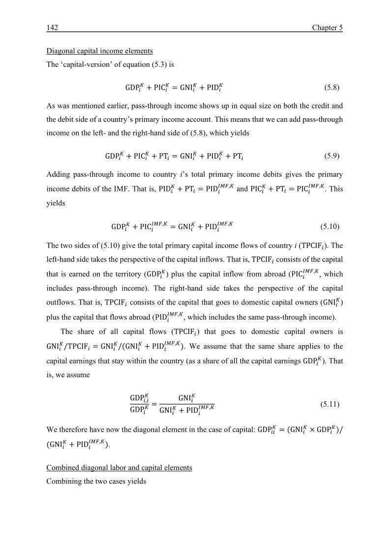
142 Chapter 5
Diagonal capital income elements
The ‘capital-version’ of equation (5.3) is
GDP³ü + PIC³ü = GNI³ü + PID³ü (5.8) As was mentioned earlier, pass-through income shows up in equal size on both the credit and
the debit side of a country’s primary income account. This means that we can add pass-through
income on the left- and the right-hand side of (5.8), which yields
GDP³ü + PIC³ü + PT³ = GNI³ü + PID³ü + PT³ (5.9) Adding pass-through income to country i’s total primary income debits gives the primary
income debits of the IMF. That is, PID³ü + PT³ = PID³öÒ÷,ü and PIC³ü + PT³ = PIC³öÒ÷,ü. This
yields
GDP³ü + PIC³öÒ÷,ü = GNI³ü + PID³öÒ÷,ü (5.10) The two sides of (5.10) give the total primary capital income flows of country i (TPCIF³). The
left-hand side takes the perspective of the capital inflows. That is, TPCIF³ consists of the capital
that is earned on the territory (GDP³ü) plus the capital inflow from abroad (PIC³öÒ÷,ü, which
includes pass-through income). The right-hand side takes the perspective of the capital
outflows. That is, TPCIF³ consists of the capital that goes to domestic capital owners (GNI³ü)
plus the capital that flows abroad (PID³öÒ÷,ü, which includes the same pass-through income).
The share of all capital flows (TPCIF³) that goes to domestic capital owners is GNI³ü/TPCIF³ = GNI³ü/�GNI³ü + PID³öÒ÷,ü�. We assume that the same share applies to the
capital earnings that stay within the country (as a share of all the capital earnings GDP³ü). That
is, we assume
GDP³,³üGDP³ü = GNI³üGNI³ü + PID³öÒ÷,ü (5.11)
We therefore have now the diagonal element in the case of capital: GDP³³ü = �GNI³ü × GDP³ü�/�GNI³ü + PID³öÒ÷,ü�.
Combined diagonal labor and capital elements
Combining the two cases yields

From trade in value added to trade in income 143
GDP³,³ = GDP³,³ù + GDP³,³ü = �GDP³ù − PID³ù� + GNI³üGNI³ü + PID³öÒ÷,ü GDP³ü (5.12)
Its complement (which is distributed in the next subsection over the countries of destination) is
given by
PID³ = & GDP³,µµY³ = GDP³ − GDP³,³ = PID³ù + PID³öÒ÷,üGNI³ü + PID³öÒ÷,ü GDP³ü (5.13)
5.3.4 Step 2: estimation of the off-diagonal elements of the matrix The next task is to obtain the off-diagonal elements GDP³,µ of the matrix relating GDP to GNI.
Each is divided into labor and capital components, GDP³,µ = GDP³,µù + GDP³,µü . We know that ∑ GDP³,µùµY³ = PID³öÒ÷,ù as estimated in (5.6) and from (5.13) it follows that
& GDP³,µüµY³ = PID³ü = PID³öÒ÷,üGNI³ü + PID³öÒ÷,ü GDP³ü (5.14)
The next task is to allocate ∑ GDP³,µùµY³ and ∑ GDP³,µüµY³ to the separate countries of destination
(i.e., determine GDP³,µù and GDP³,µü ).
Off-diagonal labor income elements
For labor, the allocation is done on the basis of data on compensation of employees. The share
of the total compensation paid by country i that is received by country j is given by CE³µ/ ∑ CE³µµY³ , where CE³µ denotes compensation of employees residing in country j and paid
for by country i. This implies
GDP³,µù = CE³µ∑ CE³µµY³ PID³öÒ÷,ù (5.15)
Data on CE³µ are drawn from a bilateral database on remittances. These remittances
include: compensation of employees (= primary labor incomes); worker’ remittances; and
migrants’ transfers. (Further details are given in Annex III).
Off-diagonal capital income elements
For capital, (5.14) states that ∑ GDP³,µüµY³ = PID³ü, where PID³ü is estimated using PID³öÒ÷,ü. In
its turn, PID³öÒ÷,ü is estimated in (5.6), using PID³öÒ÷,ü,°Óý. These are data on capital primary

144 Chapter 5
incomes and are obtained directly from the IMF. PID³öÒ÷,ü,°Óý consists of three components:
income from returns on direct investments (DI), on portfolio investment (POI), and on other
investments (OI). That is, PID³öÒ÷,ü,°Óý = PID³öÒ÷,�ö + PID³öÒ÷,þÚö + PID³öÒ÷,Úö. We split PID³öÒ÷,ü,°Óý into a DI-part and a POI-part on the basis of their sizes and we assume that the
same split also applies to PID³ü. That is,
PID³�ö,Ó�ÓTÀ = PID³öÒ÷,�öPID³öÒ÷,�ö + PID³öÒ÷,þÚö PID³ü
PID³þÚö,Ó�ÓTÀ = PID³öÒ÷,þÚöPID³öÒ÷,�ö + PID³öÒ÷,þÚö PID³ü
Note that PID³�ö,Ó�ÓTÀ + PID³þÚö,Ó�ÓTÀ = PID³ü = ∑ GDP³,µüµY³ . The reason to subsume the OI-
part of PID³öÒ÷,ü,°Óý under the other two parts is that bilateral data are available for the
investment positions of DI and POI, but not for OI. This bilateral information will be used to
allocate PID³�ö,Ó�ÓTÀ and PID³þÚö,Ó�ÓTÀ to countries of destination.
The component PID³�ö,Ó�ÓTÀ is allocated on the basis of data on foreign direct investment
positions. Let DIµ³ denote the value of country j’s direct investment in i and ∑ DIµ³µY³ gives the
total stock of foreign direct investment in country i. Then we assume that the income from
returns are allocated accordingly. That is, if for instance 10% of all direct investments in country
i are by country j (DIµ³ ∑ DIµ³µY³⁄ = 0.1), then it is assumed that 10% of country i’s transfers of
direct investment income consists of income payments sent to investors in j. Hence,
GDP³,µü,�ö = DIµ³∑ DIµ³µY³ PID³�ö,Ó�ÓTÀ (5.16)
Data on PID³�ö is available from the IMF. Data on DIµ³ are available from bilateral FDI statistics
(Further details are given in Annex IV).
Finally, component PID³þÚö,Ó�ÓTÀ is allocated on the basis of data on foreign portfolio
holdings. Let POIµ³ denote the value country j’s portfolio holdings in country i and ∑ POIµ³µY³
gives the total foreign portfolio holdings in country i. Then we assume that the income from
returns are allocated accordingly. That is,
GDP³,µü,þÚö = POIµ³∑ POIµ³µY³ PID³þÚö,Ó�ÓTÀ (5.17)
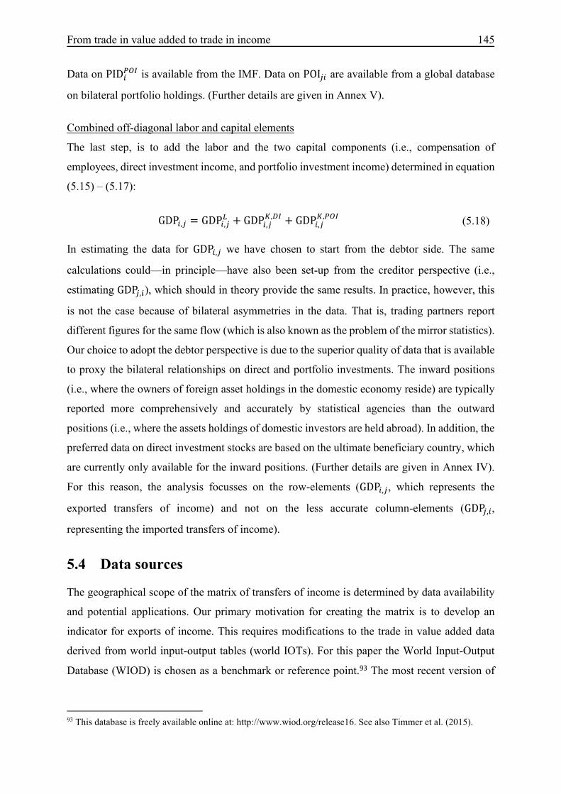
From trade in value added to trade in income 145
Data on PID³þÚö is available from the IMF. Data on POIµ³ are available from a global database
on bilateral portfolio holdings. (Further details are given in Annex V).
Combined off-diagonal labor and capital elements
The last step, is to add the labor and the two capital components (i.e., compensation of
employees, direct investment income, and portfolio investment income) determined in equation
(5.15) – (5.17):
GDP³,µ = GDP³,µù + GDP³,µü,�ö + GDP³,µü,þÚö (5.18)
In estimating the data for GDP³,µ we have chosen to start from the debtor side. The same
calculations could—in principle—have also been set-up from the creditor perspective (i.e.,
estimating GDPµ,³), which should in theory provide the same results. In practice, however, this
is not the case because of bilateral asymmetries in the data. That is, trading partners report
different figures for the same flow (which is also known as the problem of the mirror statistics).
Our choice to adopt the debtor perspective is due to the superior quality of data that is available
to proxy the bilateral relationships on direct and portfolio investments. The inward positions
(i.e., where the owners of foreign asset holdings in the domestic economy reside) are typically
reported more comprehensively and accurately by statistical agencies than the outward
positions (i.e., where the assets holdings of domestic investors are held abroad). In addition, the
preferred data on direct investment stocks are based on the ultimate beneficiary country, which
are currently only available for the inward positions. (Further details are given in Annex IV).
For this reason, the analysis focusses on the row-elements (GDP³,µ, which represents the
exported transfers of income) and not on the less accurate column-elements (GDPµ,³, representing the imported transfers of income).
5.4 Data sources The geographical scope of the matrix of transfers of income is determined by data availability
and potential applications. Our primary motivation for creating the matrix is to develop an
indicator for exports of income. This requires modifications to the trade in value added data
derived from world input-output tables (world IOTs). For this paper the World Input-Output
Database (WIOD) is chosen as a benchmark or reference point.93 The most recent version of
93 This database is freely available online at: http://www.wiod.org/release16. See also Timmer et al. (2015).

146 Chapter 5
the WIOD, released in 2016, contains annual time-series of world IOTs for the period 2000 to
2014. The consistent and harmonized tables include detailed data for 43 countries, including all
28 EU members and several major advanced and emerging economies.94 The IOTs account for
all inter-country and inter-industry transactions in 56 industries, distinguishing between
intermediate and final goods and services.
We incorporate all WIOD countries into the matrix except for one: Taiwan, which is
excluded from almost all data sources that are drawn upon to construct it. Therefore, the matrix
has a dimension of 43 × 43 (42 countries plus the Rest-of-World aggregate ROW, which now
includes also Taiwan) and is constructed for the years 2013 and 2014. This represents a “proof
of concept” that can be drawn upon to extend the time-frame in follow-up work. These two
years were chosen due to the quality of the available data. The data sources used to construct
the matrix, detailed below, contain almost no missing data in these two years for any of the 42
countries.
The source for GDP and GNI data, which give the respective row-wise sums and column-
wise sums for every country in the matrix, is the World Development Indicators dataset from
the World Bank.95,96 The BoP data used to compute the main diagonals of the matrix (GDP³,³) is from the IMF’s Balance of Payments and International Investment Position (IIP) statistics.97
The Conference Board (CB) provides the labor shares, i.e., the ratios �³�� = GNI³ù/GDP³, in the
Total Economy Database, which we use to estimate GDP³ù, GNI³ù, GDP³ü and GNI³ü.98
The most data intensive step involves the estimation of the diagonal elements, i.e., the
exported transfers of income to partner countries (GDP³,µ). The calculations use disaggregated
Alternative reference world IOTs include the OECD/WTO TiVA and Eora databases. The 2018 edition of the OECD/WTO TiVA database has a larger country coverage than the WIOD (64 economies) with a 2005-2015 timeframe. The Eora covers even more countries but relies more on extrapolations and estimations than WIOD. 94 Non-EU countries in the WIOD include Australia, Brazil, Canada, Switzerland, China, Indonesia, India, Japan, Korea, Mexico, Norway, Russia, Turkey, Taiwan, and the US. 95 This database is freely available online at: http://data.worldbank.org. 96 World GDP is reported to be slightly different than world GNI. We ensure that both values are the same in the matrix by basing global totals on world GDP. The only adjustment this implies for the matrix is to ROW’s column-wise sum (= ROW’s GNI), which we estimate by subtracting the sums of the reported GNIs of the 42 countries from world GDP. 97 This database is freely available online at: http://data.imf.org/?sk=7A51304B-6426-40C0-83DD-CA473CA1FD52. For mainland China, only aggregated investment income data are available after 2004 and not the breakdown into direct investment, portfolio investment, and other investment. Therefore, we assume the shares of each category in total investment in the years 2013-2014 are the same as the corresponding shares in the most recent available year (2004). 98 This database is freely available online at: https://www.conference-board.org/data/economydatabase/. To approximate factor shares for Rest of World (ROW), we sum up the weighted factor shares of all countries in the database but not among the 42 in the GDP-GNI matrix based on �³�� (the weighted shares are obtained by multiplying the factor shares �³�� by the GDP of each ROW country). The procedure used to average mainland China, Hong Kong, and Macao’s factor shares is similar.

From trade in value added to trade in income 147
BoP data. The main components of the primary income account include compensation to
employees, direct investment income, and portfolio investment income. (See Annex I for details
and definitions.) The IMF provides data on primary income debits (PID³öÒ÷) and credits �PIC³öÒ÷) for all 42 countries in 2013 and 2014 and, to the extent applicable or available for a
given country, data for each of the (sub-) components mentioned in the methodology section: PID³öÒ÷,ù,°Óý, PID³öÒ÷,ü,°Óý (= PID³öÒ÷,�ö,°Óý + PID³öÒ÷,þÚö,°Óý + PID³öÒ÷,Úö,°Óý� and PID³öÒ÷,Úþö,°Óý.
We use data from the IMF, World Bank, and national statistical agencies to make the
following two approximations. The bilateral shares of PID³ù (= PID³öÒ÷,ù) correspond to
employee compensation. The bilateral shares of PID³ü �= PID³öÒ÷,ü − PT³� correspond to direct
investment (PID³�ö,Ó�ÓTÀ) and portfolio investment (PID³þÚö,Ó�ÓTÀ). For these approximations,
we employ intercountry databases. These are: the World Bank’s Bilateral Remittances Database
(WBRM), the IMF’s Coordinated Direct Investment Survey (CDIS), and the IMF’s
Coordinated Portfolio Investment Survey (CPIS). For about half of the countries, we use a new
and preferred type of FDI data. When available, this data gives FDI by ultimate investing
country. This data is obtained from central banks, national statistical offices, and the OECD
International Direct Investment Statistics database. We use it instead of the CDIS to make the
calculations for bilateral direct investment shares. See Annexes III-V for details on all
databases.
Unique data challenges relate to greater China. While the final matrix combines mainland
China, Hong Kong, and Macao into one entity (to be consistent with the WIOD database), all
data sources that we use provide only data for each entity individually. The main issue is
ensuring that internal income transfers and internal investments/labor payments between the
three entities are excluded before making any calculations. For example, if BoP data for the
three are summed up with no adjustments, then our approach may erroneously attribute some
internal flows (which are part of China’s national income, i.e., part of GDP��õ,��õ) as income
transfers by greater China to the other 42 countries/ROW. Annex VI explains in detail how we
combine data for mainland China, Hong Kong, and Macao into aggregated data for greater
China.
A complete matrix also includes a row-vector and a column-vector for the ROW aggregate.
It should be noticed that the calculations for the column-vector ROW (the elements contributing
to ROW’s GNI) are straightforward given that the matrix is constructed from the debtor’s
perspective. By definition, GDP³,ÏÚ� gives the exported transfers of income that are not already

148 Chapter 5
accounted for by transfers to the other 41 countries. Based on equation (5.15), we define CE³,ÏÚ� = ∑ CE³µµY³ − ∑ CE³µµY³,ÏÚ� , which then implies GDP³,ÏÚ�ù = PID³öÒ÷,ù −∑ GDP³,µùµY³,ÏÚ� . In the same way we define GDP³,ÏÚ�ü,�ö and GDP³,ÏÚ�ü,þÚö. It should be mentioned
that the implication is that ROW is the “sink” of any errors in the bilateral estimations for other
countries.
The row-vector ROW poses a different issue. Simply deriving the missing ROW elements GDPÏÚ�,³ as the difference between GNI³ and the column-wise sum (that is, GNI³ −∑ GDPµ³µYÏÚ� ), leads to negative values of GDPÏÚ�,³ for some countries.99 Therefore, a
different strategy is used. First, we approximate the share of ROW’s GDP that is part of
ROW’s national income, GDPÏÚ�,ÏÚ� GDPÏÚ�⁄ , by taking the simple average of the
corresponding shares that were obtained for the largest six emerging countries in the matrix:
Brazil, India, Indonesia, Mexico, Russia, and Turkey.100 These are the countries that best
approximate ROW because they share similar characteristics in terms of development status
(e.g., GDP per capita).
Instead of taking the average of emerging countries to also proxy the off-diagonal elements GDPÏÚ�,³ GDPÏÚ�⁄ , we use a global database on direct investments developed by Damgaard
and Elkjaer (2017). This database provides estimates of the bilateral inward investment
positions of 116 countries on an ultimate investing country basis in 2015. 101,102 We start with a 42 × 74 matrix where the rows represent the FDI stocks of each of the 42 WIOD countries in
the 74 ROW countries contained in the database. Next, all columns are collapsed to create a
single 42 × 1 column-vector representing the direct investments of each of the 42 WIOD
countries in the ROW (proxied by the 74 ROW countries covered by the database). Normalizing
99 Negative values for income transfers are not possible. The cases where this occurred were residuals for countries with much pass-through income (e.g., Luxemburg, Cyprus, and Great Britain). This is likely attributed to an overestimation of the incomes transferred to them from non-ROW countries, resulting in an underestimation for the income transferred from ROW (i.e., the residual). 100 That is,
e6oð,ðe6oð = �e6o�ð�,�ð�e6o�ð� + e6o ��, ��e6o ��+ e6o ��, ��e6o �� + e6o���,���e6o���
+ e6oð�ñ,ð�ñe6oð�ñ + e6oî�ð,î�ðe6oî�ð �/6. An
alternative approach to derive GDPÏÚ�,ÏÚ� is to subtract the aggregated income debits of all 100+ ROW countries (countries not in the matrix) from ROW’s GDP. However, this requires the additional step of removing all income going from ROW countries to other ROW countries from the BoP data (as these would be considered pass-through or internal), which would be nearly impossible to estimate. 101 See Damgaard and Elkjaer (2017) for details on the methodology used to construct the database. The data are publicly available here and we assume the data are the same for 2014: https://www.imf.org/en/Publications/WP/Issues/2017/11/17/The-Global-FDI-Network-Searching-for-Ultimate-Investors-45414 102 Even if the approximations based on this data relate only to the direct investment component of the BoP, we consider them more detailed and accurate than taking the average of emerging countries to proxy ROW’s off-diagonal elements.

From trade in value added to trade in income 149
this column yields the 42 shares (adding up to 1). Each share tells which part of all ROW income
transfers that go to WIOD countries is received by a specific WIOD country. This gives the
estimated, offsetting shares of income transferred by ROW to each of the 42 WIOD countries
(excluding intra-ROW transfers). Each of the 42 shares is then multiplied by 1 −�GDPÏÚ�,ÏÚ� GDPÏÚ�⁄ � to obtain GDPÏÚ�,³ GDPÏÚ�⁄ .103 These represent shares of ROW’s
GDP that end up in the national income of each country in the matrix. Finally, each of the 43
shares, now including the diagonal share �GDPÏÚ�,ÏÚ� GDPÏÚ�⁄ �, is multiplied by GDPÏÚ� to
determine the actual values of GDPÏÚ�,ÏÚ�, GDPÏÚ�,³ (for i = 1, …, 42) in the 43rd row.
Finally, although all row-wise sums now correctly add up to the GDP of each
country/ROW in the matrix, the column-wise sums do not precisely add up to the GNI of each
country/ROW. This is due to reporting discrepancies related to the issue of mirror statistics
discussed in Section 5.3. Therefore, a matrix balancing technique is employed (Miller and Blair,
2009). It follows the generalized RAS (GRAS) algorithm from Lenzen et al. (2007) and uses a
Matlab program written by Temurshoev et al. (2013). The GRAS variant has the advantage of
also being able to make adjustments for rows that have elements with negative signs even if the
aggregated constraints are positive, which in some cases is true for our matrix.104 The balancing
technique thus ensures that all rows and columns of the final matrix add up properly.
The balancing procedure is applied to two matrices separately. The GDP-GNI matrix is
split into a matrix of transfers of labor income and a matrix of transfers of capital income
(including also the diagonals that reflect ‘transfers’ of income within the same country). The
reason the labor and capital parts are separated before applying RAS is that labor income is not
subject to significant data problems (i.e., pass-through income). Most of the data problems are
contained in the capital side. Therefore, any adjustments by RAS related to the matrix involving
only labor components are expected to be smaller than the adjustments by RAS related to the
matrix involving capital components.
Note that prior to applying RAS, the row-wise sums of the matrix of transfers of labor
income add up to the labor part of GDP of each country, GDP³ù, and the column-wise sums
should (but do not) add up to the labor part of GNI of each country, GNI³ù. The same applies to
103 If we denote the 42 shares obtained from normalization by ¬³, we have ¬³ = ÇÈÉÏÚ�,³/ ∑ ÇÈÉÏÚ�,³³ . Next,
note that 1 − $GDPÏÚ�,ÏÚ� GDPÏÚ�⁄ % = �GDPÏÚ� − GDPÏÚ�,ÏÚ��/GDPÏÚ� = ∑ ÇÈÉÏÚ�,³³ /GDPÏÚ�. Hence, ¬³�1 − $GDPÏÚ�,ÏÚ� GDPÏÚ�⁄ %� = ÇÈÉÏÚ�,³/GDPÏÚ�. 104 This is possible because of some negative data in the CDIS database used to estimate bilateral shares of direct investment incomes. Negative data can occur when there are negative retained earnings or for other reasons, see: http://datahelp.imf.org/knowledgebase/articles/484342-what-is-the-meaning-of-negative-data-in-the-coordi

150 Chapter 5
GDP³ü for the row sums and GNI³ü for the column sums. RAS is then applied separately to each
matrix and the results are added.
5.5 Results The analysis is organized in two parts. The first part uses the matrix that relates countries’ GDP
to their GNI (i.e., the GDP-GNI matrix) to explore the characteristics of incomes that are
transferred. First, we discuss the diagonal elements of the matrix (Section 5.5.1). Then we
analyze the off-diagonal elements from the standpoint of understanding the to-whom geography
of income transfers (Section 5.5.2). In the second part we derive the global trade in income
through GNI exports in the GNIX matrix. The columns of the GNIX matrix show for each
country their GNI footprint (i.e., the income imported and consumed by a country,
disaggregated by counterpart country) and the rows show for each country the part of their
income contained in the final demands of other countries. The analysis compares the share of a
country’s GNI that is exported (which are the exports of income) with the share of GDP that is
exported by the same country (which are the exports of value-added) (Section 5.5.3). Finally,
we discuss trade balances of income and how they differ from trade balances of value-added
(Section 5.5.4.)
5.5.1 Diagonal elements of the matrix The diagonal elements of the GDP-GNI matrix indicate the value added generated from
domestic production that ends up as part of the national income of the same country (GDP³,³). This was computed using equation (5.12) in the methodology section. Table 5.2 displays the
diagonal values for each country as a percent share of the country’s GDP.
The percent share of countries’ GDP that went to their own people was upwards of 90%
for all but six countries. High diagonal shares could be expected given that GDP and GNI
overlap to a large extent and are often of a similar magnitude. The share of GDP that went to
the same country reached more than 98% in four larger economies (China, Japan, Turkey, and
Korea). This implies a very large share of the value added of these countries represented income
gains for their residents. By contrast, the residual shares were higher (i.e., diagonal values were
relatively smaller) in business-friendly economies and tax havens. Luxembourg, Ireland,
Cyprus, Malta, and the Netherlands, which are the five countries that had the lowest diagonal
shares, are known to attract large numbers of multinational firms and/or foreign investors. Even
amongst these four, Luxembourg was an outlier with an exceptionally low share of GDP,

From trade in value added to trade in income 151
33.3%, that it retained as income. Two-thirds of Luxembourg’s GDP thus represented income
gains to residents of another country. This is consistent with Luxembourg’s integration in
international capital markets and its dependence on cross-border workers. Luxembourg is also
the largest investment fund center in Europe.105 Hence, the estimates indicate that a large share
of Luxembourg’s GDP embodies foreign-owned capital and/or payments to foreign factors.
Table 5.2. The percent share of GDP that is part of the national income of each country, 2014
CHN 98.9 DEU 96.5 PRT 94.7 CZE 91.6 JPN 98.8 LTU 96.5 LTA 94.7 BEL 91.2 TUR 98.7 BGR 96.2 AUS 94.6 GBR 90.9 KOR 98.5 IDN 95.9 NOR 94.4 HUN 90.4 IND 97.8 RUS 95.9 HRV 94.2 CHE 87.2 GRC 97.8 DNK 95.8 AUT 94.2 NLD 80.7 ROM 97.6 ESP 95.7 SWE 94.2 MLT 65.6 BRA 97.5 FRA 95.5 FIN 94.2 CYP 65.0 USA 97.4 SVN 95.1 CAN 94.0 IRL 63.2 ITA 97.2 SVK 95.0 ROW 93.8 LUX 33.3 MEX 96.7 POL 94.9 EST 92.8
Notes: Calculations are based on: 100�GDP�,�e6o� � and are after applying the RAS procedure. See Annex VII for the
names of the countries that ISO country codes refer to.
It is noteworthy that the diagonal shares in the years 2013 (not shown) and 2014 were
similar for the same country. This supports the robustness of the results and consistency of the
data sources used. Percent change in the diagonal shares of a country between these two years
(i.e.,100_�GDP³,³��L�/GDP³��L��/�GDP³,³��L�/GDP³��L�� − 1`) were less than 2% for every
country in the GDP-GNI matrix. Large fluctuations between consecutive years might have
raised some concerns about the data, but this is not the case. For this reason, only results for the
year 2014 will be discussed in the remainder of the analysis (Sections 5.5.1-5.5.4). The changes
that did occur to the diagonal shares were, in three-fifths of all countries, negative percentage
point changes. Even if this finding is based on two consecutive years only, it is consistent with
the idea that globalization and the increasingly complex activities of investors and multinational
firms are gradually leading to a less robust relationship between a country’s value-added
production and the share of income that this generates domestically.
Next, we consider the pass-through income in each country to assess the extent of pass-
through investment and its impact on the diagonal shares of the GDP-GNI matrix. Table 5.3,
105 Source: Central Bank of Luxembourg: https://www.banquedeluxembourg.com/de/bank/corporate/luxembourg-key-advantages-for-investment-funds

152 Chapter 5
column (1) shows the monetary value (in millions) of all income debits reported by the IMF
(PID³öÒ÷, the raw capital income debits plus labor income debits and other income debits).
Column (2) shows the monetary value of the income debits after adjusting for pass-through
income (PID³öÒ÷ − PT³ = PID³). The adjustments are based on the methodology explained in
Section 5.3.3. Column (2) thus shows the row-wise sums of non-diagonal elements representing
the transfers of income to other countries. For easier interpretability, each column shows all
debits before applying the RAS balancing procedure (hence, PID³öÒ÷ − PT³ ≠ ∑ GDP³,µµY³ in the
GDP-GNI matrix).106 Column (3) reports the ratio between the unadjusted and adjusted figures
(= PID³öÒ÷/�PID³öÒ÷ − PT³�). The countries are ranked based on this ratio from low to high.
Table 5.3. Income debits (PID³öÒ÷) and adjustments for pass-through income (PID³öÒ÷ − PT³�, 2014
PID³öÒ÷
(1) PID³öÒ÷ − PT³
(2) �1�/�2�
(3)
PID³öÒ÷
(1) PID³öÒ÷ − PT³
(2) �1�/�2�
(3)
IDN 31832 31719 1.0 PRT 15679 14251 1.1 HRV 2987 2976 1.0 CAN 100228 90519 1.1 BRA 57160 56811 1.0 ESP 74852 67526 1.1 TUR 13113 13012 1.0 JPN 72854 65410 1.1 IND 37581 37229 1.0 AUT 29992 26868 1.1 ROM 5899 5823 1.0 USA 606150 541750 1.1 MEX 41905 41336 1.0 HUN 20142 17817 1.1 BGR 2383 2335 1.0 DEU 177694 157027 1.1 LTU 1711 1672 1.0 NOR 31373 27383 1.1 LVA 1679 1634 1.0 FRA 146923 127328 1.2 KOR 22666 21896 1.0 FIN 20232 17468 1.2 POL 34095 32909 1.0 DNK 20528 17631 1.2 SVN 2016 1942 1.0 GBR 302328 256793 1.2
CHN 234515 225872 1.0 SWE 50746 42388 1.2 RUS 115135 110263 1.0 BEL 64223 52118 1.2 CZE 20043 19132 1.0 CYP 6541 4377 1.5 SVK 5909 5614 1.1 CHE 150653 99489 1.5 AUS 79434 74484 1.1 IRL 116897 74582 1.6 ITA 83092 77448 1.1 NLD 342512 183462 1.9 EST 2262 2098 1.1 MLT 14293 4345 3.3 GRC 9391 8591 1.1 LUX 263601 39242 6.7
Notes: own calculations derived from official data from the IMF (see Section 5.3.3). (1) and (2) are in millions. PID³öÒ÷ − PT³ would be equal to ∑ GDP³,µµY³ in the GDP-GNI matrix after applying the RAS balancing procedure.
106 Note that Table 5.3 is the only part of the analysis that shows data prior to the RAS method. All other results in Section 5.5 are after applying RAS to the GDP-GNI matrix.

From trade in value added to trade in income 153
The ranking of countries based on the estimations of their pass-through income appears
plausible. Luxembourg and Malta, which one would expect to have considerable pass-through
income due to their attractiveness to foreign investors, are at the bottom of column (3). This
implies that these two countries had the biggest relative discrepancies between the unadjusted
values in column (1) and the corresponding adjusted values in column (2). Luxembourg sent
income abroad at a magnitude of approximately four times its GDP in the year 2014 (i.e., PIDùúûöÒ÷ = 4 ∗ GDPùúû). This also implies that, following equation (5.1), the diagonal element
for Luxembourg (giving how much of Luxembourg’s GDP goes to itself) would be negative
in the case of no adjustments for pass-through income (i.e., GDPùúû,ùúû = GDPùúû − PIDùúûöÒ÷ ≈GDPùúû − 4 ∗ GDPùúû < 0). The example reinforces the need to correct for pass-through
income. At the same time, pass-through income appears, in general, not to be a major or
pervasive issue. Most countries had diagonal shares exceeding 90% of their GDP even before
adjusting for their pass-through income (not shown in Table 5.3). In addition, all but 7 countries
had adjusted values for their diagonals that differed by two percentage points or less from their
unadjusted diagonal values.
5.5.2 Off-diagonal elements of the matrix This section assesses the bilateral part of the GDP-GNI matrix. A subset of the matrix relating
countries’ GDP to their GNI is shown in Table 5.4 for the European Union (EU15 countries)
and in Tables 5.5 and 5.6 for North America and East Asia, respectively. The tables provide the
shares (in percent) of all exported income transferred by the row countries to each column
country. The percent share of country i’s transfers of income to country j is obtained with 100�GDP³,µ/ ∑ GDP�,��≠� �.107 This is domestic value-added that represents income gains to
residents of other countries j. The diagonal values GDP³,³, which are not considered exported
transfers of income, were taken out of all tables in this analysis. Only shares of the bilateral
component of GDP are reported. The full matrix is broken down into regional blocs for easier
interpretability. Our application of the data considers to what extent geographical proximity
explains transfers of income between countries. It could be that, like the trade of goods and
services, gravity is important and there is less income repatriated between countries that are
further apart.108
107 To obtain GDP³,µ, multiply share GDP³,µ/ ∑ GDP³,µµY³ from Tables 5.4-5.7 with denominator ∑ GDP³,µµY³ (the pass-through adjusted transfers of income from country i). Data on ∑ GDP³,µµY³ , are available from the author. 108 In the case of labor payments associated with cross-border workers, though accounting for only a small share of total primary income debits, it is almost by design only possible for income to end up in neighboring countries.

154 Chapter 5
We begin by analyzing the situation for the EU15 countries, which form a natural
geographic bloc. The first observation is that the average EU15 country sent about half of its
transfers of income (49.1%) to another EU15 country. This is obtained by the sum of the income
transferred by all members of the EU15 to all other countries in the EU15 as a share of the
region’s total transfers of income. Geography thus played an important role in determining
where Europe’s transfers of income went to. That is, half of this income contributed to the
national income of other EU15 countries. Returns on direct investment accounted for most of
the income that was transferred by countries in the entire matrix of 42 countries plus ROW.109
Firms exercise caution when making direct investments, which are a deep and sometimes risky
form of international commitment. Direct investments in neighboring EU countries may be
perceived as relatively safe and uncomplicated in the common market relative to investments
in other regions, which could explain the importance of geography in determining where the
income of the EU15 ended up.
Table 5.4. European Union (EU15): transfers of income by row-country as share of total transfers of income, 2014 (shares of each country to EU15 + US + Other = 100)
AUT BEL DEU DNK ESP FIN FRA GBR GRC IRL ITA LUX NLD PRT SWE EU15 US Other
AUT - 2.3 28.2 0.4 0.9 0.7 8.7 2.9 0.2 0.8 7.0 0.6 7.2 0.3 0.5 60.7 9.6 29.8
BEL 0.7 - 7.3 0.6 0.1 0.8 28.2 0.7 0.3 0.5 1.3 3.8 32.7 -0.1 2.6 79.4 6.2 14.4
DEU 3.1 1.7 - 1.9 1.9 1.0 7.4 10.1 0.1 1.8 4.4 1.2 7.8 0.4 1.8 44.4 23.2 32.3
DNK 0.5 0.9 9.1 - 0.9 6.8 3.2 4.8 0.0 1.2 0.6 1.0 6.6 0.1 17.7 53.6 23.1 23.3
ESP 0.8 1.9 14.7 0.6 - 0.4 16.6 8.3 0.7 2.2 10.5 1.0 4.9 1.9 1.1 65.5 16.2 18.4
FIN 1.1 0.9 11.0 4.4 0.4 - 4.6 4.9 0.0 1.9 1.1 0.7 10.2 0.2 22.4 63.8 15.8 20.4
FRA 0.9 5.2 14.5 0.7 2.1 0.7 - 9.2 0.1 2.7 5.7 1.3 7.2 0.5 0.8 51.6 20.0 28.4
GBR 0.3 0.7 6.8 0.8 2.0 0.4 7.5 - 0.6 4.8 1.6 0.7 5.8 0.2 1.3 33.6 37.7 28.7
GRC 1.9 2.9 14.6 0.4 1.0 0.3 12.7 19.4 - 1.9 8.6 1.2 6.1 3.7 1.3 76.0 20.5 3.5
IRL 0.4 1.0 5.2 0.6 1.1 0.9 3.7 7.3 0.0 - 3.7 0.5 2.4 0.4 0.6 28.0 59.8 12.2
ITA 1.8 2.4 16.1 0.9 6.3 0.5 21.2 7.2 1.4 4.5 - 1.6 4.7 1.3 0.5 70.4 11.0 18.6
LUX 0.8 17.5 10.2 1.1 1.7 1.1 6.4 5.0 1.2 2.0 7.6 - 6.4 2.3 2.5 65.8 13.2 21.0
NLD 0.6 6.9 12.6 1.8 1.7 0.9 8.8 12.1 0.1 2.5 1.7 1.8 - 0.3 1.5 53.3 19.6 27.1
PRT 1.1 2.5 11.8 1.1 17.1 0.0 13.4 5.9 1.0 2.7 4.8 1.7 15.2 - 0.3 78.7 9.6 11.7
SWE 0.9 0.8 9.2 7.8 0.8 9.9 3.6 9.9 0.0 2.0 0.6 1.6 12.7 0.1 - 59.7 18.3 22.0
EU15 1.0 3.2 9.4 1.3 2.0 1.0 8.5 6.4 0.4 2.7 3.3 1.2 6.5 0.5 1.8 49.1 26.1 24.8
Notes: own calculations based on GDP³,µ/�∑ GDP³,µµY³ �. The average, weighted share of EU15 to EU15 is based
on the equation ∑ GDPÛ,µ/ ∑ ∑ GDP³,øøY³³∈�úÛYµ,Û∈�ú , where EU indicates the EU15 region. Two notable outliers among the EU15 countries were Ireland and Great Britain. Ireland
sent only 28.0% of its transfers of income to another EU15 country and 59.8% to the US (more
than twice the weighted average of 26.1% for EU15 countries to the US). This can be best
109 Table 5.A2 (Annex II) shows that direct investment income debits accounted for a plurality (45.3%) of total income debits of the average country in the GDP-GNI matrix (as calculated using raw IMF data before any adjustments to pass-through income).

From trade in value added to trade in income 155
explained by tax incentives in Ireland that have attracted large numbers of US multinational
firms. Great Britain similarly transferred more income to the US (37.7%) than to another EU
country (33.6%). This is probably related to the strong historical and cultural ties between the
two countries. The contributions of Ireland and Great Britain to other countries’ GNIs were thus
less influenced by geographical proximity as compared to other EU15 countries because of the
key role played by the US.
Geographical proximity mattered less for the transfers of income from North America
(defined as the US, Canada, and Mexico). Observe in Table 5.5 that only 21.3% of all income
transferred by the three countries remained in the region (60.1% for Canada, 9.0% for the US,
and 53.1% for Mexico). North America, and especially the US, seemed lucrative to EU
investors – because almost 40% of US transfers of income contributed to the GNI of EU15
countries. Although more than half of Mexico’s and Canada’s transfers of income went to the
US, indicating the importance of US direct investments and US portfolio holdings in the
neighboring countries, these investments were dwarfed by those of investors in countries
outside of the region (notably Europe) investing in the US. The European influence is thus part
of the reason why North America’s transfers of income, especially by the US, did not depend
as much on geographical proximity.
The US may be an interesting case because two-thirds of all US transfers of income
involved returns on portfolio investments. The ratio of transfers of portfolio income to total
transfers of income (i.e., ∑ GDPúÖ�,µü,þÚöµYúÖ� / ∑ GDPúÖ�,µµYúÖ� ) was higher for the US than for
almost every other country in the GDP-GNI matrix.110 This is relevant because portfolio
holdings are probably less dependent on geography than are direct investments. They do not
require the same type of up-front and deep commitments or knowledge of the local market as
do direct investments. If most foreign investors holding portfolios in the US reside far away
from the US, then US transfers of income representing the returns on these investments
necessarily also end up further away (outside the region). This could help to explain why almost
all US transfers of income (91.0%) contributed to the national income of countries outside of
North America.
110 Table 5.A2 (Annex II) shows that 63.5% of US transfers of income were considered portfolio investment incomes, which is much higher than the weighted average of 45.5% for all countries in the full matrix.

156 Chapter 5
Table 5.5. North America (NA): transfers of income by row-country as share of total transfers of income, 2014
Notes: own calculations based on GDP³,µ/�∑ GDP³,µµY³ �. NA = North America (Canada + USA + Mexico)
Geographical proximity was least important for the transfers of income from Japan and
South Korea as compared to countries in the other two regions. Japan and South Korea seem to
be heavily dependent on investments from the US and EU because more than one-half (South
Korea) and two-thirds (Japan) of all income transferred by those countries ended up in the
national income of either the US or EU.
Table 5.6. East Asia: transfers of income by row-country as share of total transfers of income, 2014
Notes: own calculations based on GDP³,µ/�∑ GDP³,µµY³ �.
A key takeaway so far is that the EU15 countries and the US were important recipients of
incomes transferred from countries in the three regions. Next, we check whether this finding
also holds for incomes sent by countries outside of the three regions. Table 5.7 shows the
transfers of income by emerging and developing countries (China, Brazil, India, Indonesia,
Mexico, Russia, and Turkey, and ROW). Observe that about 22.5% of all income transfers from
those countries went to the EU15 and 38.6% to the US. Furthermore, the full GDP-GNI matrix
of 42 countries plus ROW shows that more than a third (35.6%) of all transfers of income
worldwide were by the countries contained in Table 5.7. Poorer and emerging countries thus
appear to send a relatively large share of their GDP to rich, developed regions like Europe and
North America (despite greater geographical distance). The findings show the importance of
the US, followed by the EU, as the major players in foreign investment worldwide. This also
indicates the global reach of US direct investments and US portfolio holdings abroad, which
account for almost all repatriated income.
CAN USA MEX CHN EU15 Other NA TOT
CAN - 59.7 0.4 6.1 14.0 19.7 60.1 100
USA 8.2 - 0.7 2.3 39.2 49.5 9.0 100
MEX 2.9 50.2 - 0.5 33.8 12.7 53.1 100
NA 6.4 14.3 0.6 2.9 34.3 41.5 21.3 100
CHN JPN KOR USA EU15 Other TOT
CHN - 9.8 3.3 9.7 13.6 63.6 100
JPN 8.6 - 3.1 44.6 25.7 18.0 100
KOR 10.4 19.7 - 32.2 20.1 17.8 100
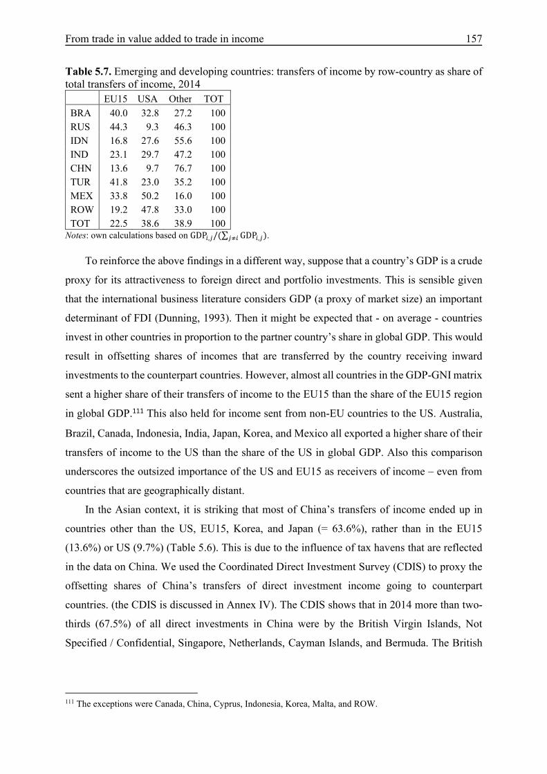
From trade in value added to trade in income 157
Table 5.7. Emerging and developing countries: transfers of income by row-country as share of total transfers of income, 2014
Notes: own calculations based on GDP³,µ/�∑ GDP³,µµY³ �.
To reinforce the above findings in a different way, suppose that a country’s GDP is a crude
proxy for its attractiveness to foreign direct and portfolio investments. This is sensible given
that the international business literature considers GDP (a proxy of market size) an important
determinant of FDI (Dunning, 1993). Then it might be expected that - on average - countries
invest in other countries in proportion to the partner country’s share in global GDP. This would
result in offsetting shares of incomes that are transferred by the country receiving inward
investments to the counterpart countries. However, almost all countries in the GDP-GNI matrix
sent a higher share of their transfers of income to the EU15 than the share of the EU15 region
in global GDP.111 This also held for income sent from non-EU countries to the US. Australia,
Brazil, Canada, Indonesia, India, Japan, Korea, and Mexico all exported a higher share of their
transfers of income to the US than the share of the US in global GDP. Also this comparison
underscores the outsized importance of the US and EU15 as receivers of income – even from
countries that are geographically distant.
In the Asian context, it is striking that most of China’s transfers of income ended up in
countries other than the US, EU15, Korea, and Japan (= 63.6%), rather than in the EU15
(13.6%) or US (9.7%) (Table 5.6). This is due to the influence of tax havens that are reflected
in the data on China. We used the Coordinated Direct Investment Survey (CDIS) to proxy the
offsetting shares of China’s transfers of direct investment income going to counterpart
countries. (the CDIS is discussed in Annex IV). The CDIS shows that in 2014 more than two-
thirds (67.5%) of all direct investments in China were by the British Virgin Islands, Not
Specified / Confidential, Singapore, Netherlands, Cayman Islands, and Bermuda. The British
111 The exceptions were Canada, China, Cyprus, Indonesia, Korea, Malta, and ROW.
EU15 USA Other TOT
BRA 40.0 32.8 27.2 100
RUS 44.3 9.3 46.3 100
IDN 16.8 27.6 55.6 100
IND 23.1 29.7 47.2 100
CHN 13.6 9.7 76.7 100
TUR 41.8 23.0 35.2 100
MEX 33.8 50.2 16.0 100
ROW 19.2 47.8 33.0 100
TOT 22.5 38.6 38.9 100

158 Chapter 5
Virgin Islands, the largest investor, by itself made 38.6% of all direct investments in China. All
these countries are well-known tax havens.
Given that nearly all transfers of income by China were attributed to returns on direct
investments (see Table 5.A2, Annex II), these tax havens then accounted for a great majority
of the income that China sent to ‘Other’ as reflected in Table 5.6. This shows that tax havens
can have a big impact on bilateral investment statistics if the data are based on the immediate
investing country. Although we used direct investment shares based on the ultimate beneficiary
country for more than half of all countries in the GDP-GNI matrix to minimize the impact of
tax havens, such data was not available for China. Hence, it could still well be that the US and
EU15 were the biggest investors in China if they operate there indirectly via intermediaries (tax
havens). China was the most extreme example of the apparent distortions in the data related to
tax havens. Most countries in the study had more reasonable (smaller) shares of their transfers
of income going to the ‘ROW’ countries not separately included in the matrix.
5.5.3 Analysis: exports of GNI In this section, we use the GDP-GNI matrix to help derive estimates of incomes that are
generated in a country due to demand for final goods and services. The analysis covers all types
of income contributing to a country’s GNI – e.g., the income a country gains from profit-shifting
by MNEs, the income sent home by cross-border workers, and the income a country’s citizens
earn from portfolio investments in another country. The sum of the income generated from all
sources of final demand, foreign and domestic, equals the country’s GNI. The main contribution
of this analysis is to differentiate between income that is induced by domestic final demand and
income that is induced by foreign final demand. We consider the income that is generated in a
country but induced by final demand abroad to be this country’s exports of income or exports
of GNI (hence GNIX). As part of the analysis we compare a country’s exports of income to its
exports of value-added (or VAX). The latter is the domestic value-added induced in one country
due to final demand in foreign countries. Exports of income contribute to a country’s GNI and
exports of value-added contribute to a country’s GDP.
The goal of the comparison is to investigate the extent to which a country is more (or
less) dependent on foreign consumption of final products in terms of the generation of its own
income compared to the generation of domestic value-added. This provides a better portrayal
of the income benefits of final demand from abroad to a country’s residents than the exports of
value-added indicator because part of the value added might be transferred to foreign countries
and vice versa.

From trade in value added to trade in income 159
So, it is important to observe the differences between the different types of exports.
These are gross exports, exports of value-added, and exports of income. An example is
illustrative. French consumers buy agricultural goods from the Netherlands, the production of
which uses German fertilizers. The German fertilizer factory also employs cross-border
workers from Poland (i.e., people who work in Germany but reside in Poland). In this case, the
delivery of Dutch agricultural products to French consumers are part of the Dutch gross exports
to France. These exported Dutch agricultural products also embody inputs of German
fertilizers. The labor and capital used in the German fertilizer factory is part of the German
value added. Hence, Germany exports value added to France. The earnings of the Polish cross-
border workers are part of the German value added but are transferred to Poland and become
part of Poland’s income (GNI). This means that Poland exports income to France. The possible
gross export, value added, and income linkages are illustrated in Table 5.8a.
Note that while exports of value-added and exports of income are the same in the
aggregate in Table 5.8a (summed up across the four countries), this is not necessarily the case
in every supply chain. The illustration in Table 5.8b now assumes that: i) the Dutch consume
all the agricultural goods themselves instead of French people, and ii) a Spanish firm owns the
farmland used to grow the agricultural products in the Netherlands, and repatriates part of the
profits it makes from selling the goods to Dutch consumers back to Spain. All other assumptions
are carried over from the first illustration. Then it is possible, as shown in Table 5.8b, that the
aggregated exports of income (from Poland, Germany, and Spain to the Netherlands) exceed
the exports of value-added (from just Germany to the Netherlands).
Table 5.8a. Illustration: gross exports, exports of value-added, and exports of income (in $)
Gross exports (GE³) Exports of value-added (VAX³) Exports of income (GNIX³) POL 0 0 2 (POL FRA) DEU 5 (DEU NLD) 5 (DEU FRA) 3 (DEU FRA) NLD 10 (NLD FRA) 5 (NLD FRA) 5 (NLD FRA) FRA 0 0 0
TOT 15 10 10 Table 5.8b. Illustration: gross exports, exports of value-added, and exports of income (in $)
Gross exports (GE³) Exports of value-added (VAX³) Exports of income (GNIX³) POL 0 0 2 (POL NLD) DEU 5 (DEU NLD) 5 (DEU NLD) 3 (DEU NLD) NLD 0 5 (internal, NLD NLD) 3 (internal, NLD NLD)
ESP 0 0 2 (ESP NLD)
TOT 5 5 7 Notes: POL = Poland; DEU = Germany; NLD = Netherlands; FRA = France; ESP = Spain.

160 Chapter 5
The two main components in the calculations for exports of income are the 43 × 43
GDP-GNI matrix, denoted ÇÈÉ, and a 43 × 43 matrix with exports of value-added, denoted ÄÅÆ. The matrix ÇÈÉ was given in Table 5.1 and was constructed according to Sections 5.3-
5.4. Its elements GDP³,µ give the transfer of incomes, i.e., the value added of i that goes to j and
becomes part of j’s GNI. The ÇÈÉ matrix covers only 43 countries (instead of 44) because our
definition of ROW includes Taiwan.
The ÄÅÆ matrix is derived in two steps from the 2014 world IOT in the WIOD database.
There are 56 industries included in the WIOT for each of the 44 countries.112 Let º denote the 2464 × 1 vector of value-added coefficients; Å the 2464 × 2464 matrix with input
coefficients; Í the 2464 × 2464 identity matrix; and Ë is the 2464 × 44 matrix of final
demands. Value added includes wages and salaries, employers’ contributions, capital
depreciation, indirect taxes, price-decreasing subsidies, and operating surplus or other income.
Final demands include private investments, government consumption and investments, and
changes in stocks. The full 2464 × 44 value-added exports matrix is given by
ÄÅÆÕÔ�� = º¶�Í − Å�KLË (5.19) where a ‘hat’ is used to indicate the diagonal matrix based on º. The second term in equation
(5.19) is also known as the Leontief inverse (or multiplier matrix). The typical element VAX³,µÕÔ�� gives the value added generated in country-industry i (= 1, …, 2464) necessary for all 2464
final demands by country j (= 1, …, 44). The first step is to aggregate the 2464 (= 44 × 56)
results for country-industries into the totals for the 44 countries (by summing over the 56
industries for each country). This yields a 44 × 44 matrix. The second step is to aggregate the
results for ROW-TWN and Taiwan, which yields the 43 × 43 matrix ÄÅÆ. Its typical element VAX³,µ gives the value added generated in country i necessary for all final demands in country
j, with i, j = 1, …, 43 and ROW (which now includes Taiwan) is country 43. The off-diagonal
elements of ÄÅÆ give exports of value-added.
Similar to ÄÅÆ, the matrix ÇÎÍÆ gives in its off-diagonal elements the exports of
income. ÇÎÍÆ is derived as follows. The final demands of country j induce value added (and
thus a contribution to GDP) in country i to the amount of VAX³,µ. The share of country i’s GDP
that becomes part of country k’s income (GNI) equals h³,ø = GDP³,ø/ ∑ GDP³,µµ = GDP³,ø/GDP³.
112 These are the 42 individual countries in the ÇÈÉ matrix; the 43rd country is Taiwan (included separately); and the 44th country is ROW-TWN. For the purposes of deriving ÄÅÆÕÔ�� in equation (5.19) only, the rest of world aggregate exceptionally is not combined with Taiwan.

From trade in value added to trade in income 161
This share gives the part of an average dollar of GDP in i that is transferred to the GNI of k. In
that case, the income transfer of VAX³,µ as part of GDP in country i to the GNI in country k
equals h³,øVAX³,µ. This gives the GNI in k that is due to final demands in j and which runs
through GDP in i. Clearly, country i is not the only transmission channel. All GNI in k that is
due to final demands in j is given by
GNIXø,µ = ∑ h³,øVAX³,µ³
Using matrix algebra, we have
ÇÎÍÆ = !�ÄÅÆ (5.20) where !� denotes the transposed matrix of !.
The rows of ÇÎÍÆ refer to income-generating countries and the columns refer to
income-consuming countries. The income generated in country k that is embodied in all final
demands consumed abroad (or total exports of income) is ∑ GNIXø,µµYø . It can be shown that
the sum of row k of ÇÎÍÆ equals the GNI of country k.113 The columns of ÇÎÍÆ give GNI
footprints and show all pieces of income (and where it comes from) that are consumed by final
users. ∑ GNIXø,µøYµ gives the imported income. It can be shown that the column sums equal
the sum of final demands in the corresponding country.114
Table 5.9 compares countries’ gross exports, exports of value-added, and exports of income
in 2014. To facilitate ease of interpretation and to show the relative impact exerted by foreign
final demand, all values are divided by GDP³ or GNI³. We report gross exports as a share of
GDP in column (1), GE³/GDP³ (=∑ GE³,µµY³ /GDP³), the share of GDP³ that was exported in
column (2), VAX³/GDP³ (=∑ VAX³,µµY³ /GDP³), and the share of GNI³ that was exported in
column (3), GNIX³/GNI³ (=∑ GNIX³,µ/GNI³µY³ ), for each of the 42 countries plus ROW. All
shares are multiplied by 100 to express the ratios in percent. Column (4) shows the percentage
point difference between (2) and (3), �eOld�eOl� − "#d�e6o�� ∗ 100, and column (5) shows the ratio
113 Taking the row sums of ÄÅÆÕÔ�� in (5.20) yields the values-added in each country-industry. Taking the appropriate sums for countries implies ∑ VAX³,µµ = GDP³. Hence ∑ GNIXø,µµ = ∑ ∑ h³,øVAX³,µ³µ = ∑ h³,øGDP³³ =∑ GDP³,ø³ = GNIø as follows from Table 5.1. 114 Let $′ denote the row summation vector consisting of ones, i.e., $� = �1, … ,1�. For the value-added coefficients it holds that º� = $′�Í − Å�. Therefore we have $′ÄÅÆÕÔ�� = $′Ë, which means that the column sums of ÄÅÆÕÔ�� equal the total amount of final demands in each country. Next, ∑ GNIXø,µø = ∑ ∑ h³,øVAX³,µ³ø = ∑ VAX³,µ³ , because ∑ h³,øø = 1. ∑ VAX³,µ³ equals the sum of all final products consumed in country j.
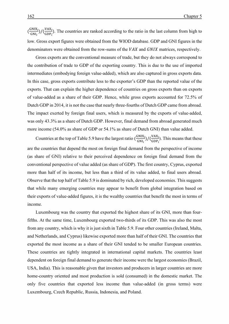
162 Chapter 5
�eOld�eOl� �/�"#d�e6o��. The countries are ranked according to the ratio in the last column from high to
low. Gross export figures were obtained from the WIOD database. GDP and GNI figures in the
denominators were obtained from the row-sums of the ÄÅÆ and ÇÎÍÆ matrices, respectively.
Gross exports are the conventional measure of trade, but they do not always correspond to
the contribution of trade to GDP of the exporting country. This is due to the use of imported
intermediates (embodying foreign value-added), which are also captured in gross exports data.
In this case, gross exports contribute less to the exporter’s GDP than the reported value of the
exports. That can explain the higher dependence of countries on gross exports than on exports
of value-added as a share of their GDP. Hence, while gross exports accounted for 72.5% of
Dutch GDP in 2014, it is not the case that nearly three-fourths of Dutch GDP came from abroad.
The impact exerted by foreign final users, which is measured by the exports of value-added,
was only 43.3% as a share of Dutch GDP. However, final demand from abroad generated much
more income (54.0% as share of GDP or 54.1% as share of Dutch GNI) than value added.
Countries at the top of Table 5.9 have the largest ratio �eOld�eOl� �/�"#d�e6o�). This means that these
are the countries that depend the most on foreign final demand from the perspective of income
(as share of GNI) relative to their perceived dependence on foreign final demand from the
conventional perspective of value added (as share of GDP). The first country, Cyprus, exported
more than half of its income, but less than a third of its value added, to final users abroad.
Observe that the top half of Table 5.9 is dominated by rich, developed economies. This suggests
that while many emerging countries may appear to benefit from global integration based on
their exports of value-added figures, it is the wealthy countries that benefit the most in terms of
income.
Luxembourg was the country that exported the highest share of its GNI, more than four-
fifths. At the same time, Luxembourg exported two-thirds of its GDP. This was also the most
from any country, which is why it is just sixth in Table 5.9. Four other countries (Ireland, Malta,
and Netherlands, and Cyprus) likewise exported more than half of their GNI. The countries that
exported the most income as a share of their GNI tended to be smaller European countries.
These countries are tightly integrated in international capital markets. The countries least
dependent on foreign final demand to generate their income were the largest economies (Brazil,
USA, India). This is reasonable given that investors and producers in larger countries are more
home-country oriented and most production is sold (consumed) in the domestic market. The
only five countries that exported less income than value-added (in gross terms) were
Luxembourg, Czech Republic, Russia, Indonesia, and Poland.

From trade in value added to trade in income 163
Table 5.9. Gross exports (% share of GDP), exports of value-added (% share of GDP), and exports of income (% share of GNI), 2014
GE³/GDP³ (1)
VAX³/GDP³ (2)
GNIX³/GNI³ (3)
(3)-(2) (4)
(3)/(2) (5)
CYP 44.4 30.6 51.4 20.8 1.7 USA 11.1 8.9 13.0 4.1 1.5 MLT 141.9 47.2 63.9 16.6 1.4 JPN 18.4 13.5 17.7 4.1 1.3 GBR 28.2 21.4 27.2 5.8 1.3 LUX 203.3 65.4 82.4 17.0 1.3 NLD 72.5 43.3 54.1 10.8 1.2 FRA 29.9 20.0 24.6 4.6 1.2 CHE 51.8 37.1 45.0 7.9 1.2 IRL 115.4 55.9 67.7 11.7 1.2 FIN 42.8 26.0 31.1 5.1 1.2 NOR 41.9 32.7 38.5 5.9 1.2 SWE 46.4 31.3 36.8 5.5 1.2 ESP 30.9 20.0 23.2 3.2 1.2 DNK 56.8 33.6 38.9 5.4 1.2 GRC 27.0 17.5 19.9 2.5 1.1 BEL 80.4 40.2 45.8 5.6 1.1 AUS 21.2 17.6 20.0 2.4 1.1 CAN 33.6 24.7 28.1 3.4 1.1 AUT 54.1 32.8 36.8 4.0 1.1 PRT 38.0 23.6 26.4 2.8 1.1 DEU 48.3 32.3 35.9 3.5 1.1 ITA 30.6 21.2 23.4 2.2 1.1 LTA 53.0 34.8 38.0 3.3 1.1 ROW 35.5 23.8 26.0 2.2 1.1 HRV 48.3 32.6 35.5 2.9 1.1 HUN 99.8 43.3 46.4 3.1 1.1 EST 78.1 40.9 43.5 2.7 1.1 IND 18.5 13.5 14.3 0.8 1.1 SVN 72.0 41.9 44.4 2.5 1.1 MEX 30.0 19.3 20.4 1.1 1.1 BGR 64.2 36.5 38.4 1.9 1.1 SVK 90.1 42.3 44.4 2.1 1.1 BRA 13.0 10.0 10.5 0.5 1.1 CHN 23.6 18.7 19.6 0.9 1.0 KOR 54.2 32.4 33.6 1.3 1.0 POL 51.9 33.6 34.7 1.2 1.0 IDN 24.2 19.6 20.2 0.6 1.0 ROM 44.0 30.0 30.9 0.8 1.0 RUS 30.4 26.1 26.8 0.7 1.0 LTU 74.8 44.7 45.9 1.2 1.0 CZE 86.8 42.8 43.8 1.0 1.0 TUR 35.1 23.2 23.6 0.4 1.0 SUM-W 27.7 19.3 22.2 2.9 1.2
Notes: Rounded to the nearest tenth. Weighted averages are based on (1) ∑ GE³/ ∑ GDP³³³ ; (2) ∑ VAX³/ ∑ GDP³³³ ; and (3) ∑ GNIX³/ ∑ GNI³³³ . GE³ are i’s gross exports, VAX³ are i’s value-added exports, and GNIX³ are i’s exports of income.

164 Chapter 5
Observe in Table 5.9 that percentage point differences in column (4) were positive in every
country, �eOld�eOl� � − �"#d�e6o�� > 0, and that the related ratio in column (5) always exceeded 1
(including the unrounded ratios of the countries at the bottom displaying a rounded ‘1.0’). In
other words, the share of GNI a country exported was always larger than the share of GDP
exported by the same country. Overall, global exports of income exceeded global exports of
value-added by 15.0%. This tells us that the world is more globalized and/or interconnected in
terms of countries' dependence on foreign demand from the perspective of income exports than
from the perspective of value-added exports.
This finding could be explained by the rapid pace of financial globalization. Consider that
cross-border direct investment activities can contribute to the exports of income of the investing
country via profit shifting whenever income is generated through foreign consumption. Cross-
border direct investments increased globally by 18.2% between 2011 and 2014 (source: CDIS
database), which are the years following the 2007/2008 financial crisis recovery period. On the
other hand, global exports of value-added increased by only 4.8% in the same period (source:
WIOD database). This is consistent with an analysis by Timmer et al. (2016) that international
production fragmentation only increased marginally since the financial crisis and that the
slowdown in global trade may be part of a longer trend. Hence new cross-border investment
activities greatly exceeded the pace of increased trade in value added in recent years.115 This
pattern held to a lesser extent also for the longer period from 2001-2014 as cross-border direct
investment increased by 239% (source: UNCTAD (2019) bilateral FDI database) and value-
added exports increased by 186% (source: WIOD database, 2016 release). These developments
suggest that final demand sometimes induced exports of income without inducing any
corresponding exports of value-added (e.g., along the lines of the illustration in Table 5.8b
where Dutch final demand induced more exports of income than exports of value-added).116
This is possible when the production processes used by subsidiaries of multinational firms are
more capital intensive, involve home-country or cross-border workers, use few foreign inputs,
and primarily serve final consumers in the host-country market.
115 This trend also holds for portfolio investments and remittances. Cross-border portfolio investments increased globally by 23.9% (CPIS database) and remittances increased by 13.7% (WBRM database) in 2011-2014. 116 Note that the reverse is also possible: exports of value-added that do not translate into exports of income for the same or another country. Suppose a US multinational firm outsources all production to a subsidiary in Ireland (e.g., for tax avoidance purposes or to lower production costs) but markets their products solely to US consumers. This generates Irish exports of value-added that are consumed by final users in the US. Then there may be substantially fewer exports of income than exports of value-added if all profits are shifted to the US (especially if production is capital-intensive). However, given that GNIX�%°�� > VAX�%°�� , this type of scenario is less frequent (on balance).

From trade in value added to trade in income 165
Although all countries depended more on foreigners to generate their income (GNI) than
to generate their domestic value-added (GDP), this occurred to varying degrees. The largest
percentage point difference in the two indicators, based on column (4), were in Cyprus (+20.8
p.p.), Luxembourg (+17.0 p.p.), Malta (+16.6 p.p.), Ireland (+11.7 p.p.), and the Netherlands
(+10.8 p.p.). Note that the big percentage point difference in the case of Luxembourg does not
contradict the previous finding that it exported less income than value-added (in gross terms).
This is because Luxembourg’s GDP was much higher than its GNI, which are the denominators
of the shares underlying the calculations in column (4). Meanwhile, the differences for 13 other
countries were less than two percentage points.
5.5.4 Analysis: trade balance of income In this section we use information obtained from the trade in income matrix, ÇÎÍÆ, to examine
trade balances of income. The goal is to cast more light on the impact of foreign final demand
on income by considering a country’s (bilateral) income surplus or deficit. We compare trade
balances that are conventionally based on gross exports, and more recently analyzed from the
perspective of value added, with trade balances of income. Note that the trade in income data
used to calculate a country’s income balance has the same broad scope as before. That is,
exports of income involve not just the income generated by foreign final demand that relate
directly or indirectly to the physical cross-border flows of goods and services. The exports may
also arise due to profit shifting in relation to domestic supply chains where no intermediary
inputs or final products cross the border.
We obtain the trade balance of income as follows:
Trade balance of income³ = & GNIX³,µµY³ − & GNIXµ,³µY³ (5.21)
Where GNIX³,µ denotes country i’s exports of income to country j and GNIXµ,³ denotes country
i’s imports of income from country j. ∑ GNIX³,µµY³ are country i’s exports of income to all
countries j (� ≠ �) and ∑ GNIXµ,³µY³ are country i’s imports of income from all countries j (� ≠�). The trade balances of value-added and gross exports are constructed similarly (i.e., by
replacing GNIX with VAX or GE in equation (5.21).
Table 5.10 shows the trade balances for each country in the year 2014. Column (1) reports
the (gross) trade balance for all countries as a share of GDP. Column (2) reports the trade
balance in value-added terms as a share of GDP. Column (3) is the novel part, showing the
trade balance of income as a share of GDP. For example, Ireland had a large (gross) trade

166 Chapter 5
surplus. Gross exports minus gross imports amounted to 22.7% of Irish GDP. This surplus was
1.4 percentage points smaller from the perspective of value-added exports minus value-added
imports (21.3%). Ireland had a much lower trade surplus in income (7.6% as share of GDP).
On the one hand, this implies that Ireland exported more income than it consumed from abroad.
That is, the income induced by non-Irish final demand that ended up in Ireland exceeded the
income Irish consumers sent abroad to satisfy their own domestic final demand. However, the
discrepancy between Ireland’s value-added and income surpluses is relatively large. This could
be explained by the prevalence of multinational activities in Ireland, which results in the
repatriation of income and is likely related to the influential role of the US.117
Table 5.10. Trade balances (surplus/deficit) as percent share of GDP, 2014
Gross trade balance
(1)
Value-added balance
(2)
Income balance
(3)
Gross trade balance
(1)
Value-added balance
(2)
Income balance
(3) AUS -0.1 -0.1 -2.7 IRL 22.7 21.3 7.6 AUT 4.2 3.9 4.1 ITA 3.6 3.2 3.3 BEL 5.8 4.2 5.0 JPN -1.6 -1.6 2.1 BGR -5.8 -6.9 -7.8 KOR 10.5 8.6 9.0 BRA -2.3 -3.2 -5.2 LTU 5.2 3.7 2.3 CAN 1.1 1.2 -0.3 LUX 27.1 25.2 -9.0 CHE 12.8 12.4 12.2 LTA -3.1 -2.9 -3.1 CHN 5.7 5.7 5.8 MEX 0.5 0.5 -1.5 CYP -8.2 -7.8 -14.9 MLT -1.7 -1.5 -5.6 CZE 10.4 8.0 1.3 NLD 15.6 14.6 14.5 DEU 11.2 10.8 12.9 NOR 13.9 12.8 16.2 DNK 8.9 8.2 12.4 POL 3.9 3.3 0.0 ESP 0.5 0.2 -0.2 PRT -3.3 -4.7 -6.3 EST 0.7 -0.5 -3.3 ROM 0.2 -0.5 -1.8 FIN 1.3 0.6 1.8 RUS 7.1 6.1 2.9 FRA -0.7 -1.1 0.4 SVK 7.8 5.1 3.9 GBR -0.7 -0.9 -2.6 SVN 5.1 3.8 3.3 GRC -8.7 -8.9 -8.2 SWE 6.2 5.9 8.3 HRV 0.7 -0.3 -1.8 TUR 2.8 1.9 1.1 HUN 9.4 6.4 2.0 USA -2.8 -2.5 -0.2 IDN 0.9 1.1 -2.3 ROW -10.6 -9.5 -12.7 IND -0.1 -1.0 -2.2
Notes: Rounded to the nearest tenth. (1) reports trade balances based on gross exports, �GE³ − GI³�/GDP³, where GI³ are i’s gross imports. (2) reports trade balance based on value added, �∑ XAX³µµY³ − ∑ VAXµ³µY³ �/ GDP³. (1) and (2) were obtained from the WIOD database. (3) reports trade balances of income, �∑ GNIX³µµY³ −∑ GNIXµ³µY³ �/ GDP³.
In general, the more developed economies had a higher income surplus (or a lower income
deficit) relative to their value-added surplus (or deficit). The opposite was true for many
117 The role of the US in terms of Ireland’s income exports was demonstrated by the GDP-GNI matrix, which showed that 59.8% of Ireland’s exported income transfers (=∑ GDPöÏù,µ/GDPöÏùµYöÏù ) went to the US in 2014.

From trade in value added to trade in income 167
emerging and developing countries. The ROW aggregate for all countries not in the GNIX
matrix, which arguably demonstrates this pattern the best, had not only the largest deficit in
value-added terms (-9.5%) but, after Cyprus, also the largest deficit in terms of income (-12.7%)
as share of GDP. This represents (for ROW) an income deficit that was US$ 354bn larger than
its value-added deficit. These patterns make sense given that developed countries tend to invest
more in developing countries than the other way around. Returns on investments, which account
for much of the discrepancy between the GNIX and VAX indicators, result in higher net exports
of income for those wealthier countries. Compared to the trade balances of value-added (which
in most cases did not differ much from the corresponding gross trade balances for each country),
the trade balances of income not just in Ireland but also Luxembourg, Cyprus, and the Czech
Republic were much less positive and/or more negative.
As mentioned in the introduction, US President Trump often complains about the bilateral
US trade deficit in goods with other countries and cites this as a justification for tariffs and other
protectionist measures. However, the analysis thus far portrays a story that may counter such
concerns about ‘fairness’ by showing how much the US truly lost (or benefitted) from an open
trade and investment climate vis-à-vis counterpart countries. First, US investors are major
players in foreign investment worldwide. This is related to the analysis of the GDP-GNI matrix
in Section 5.5.2, which indicated that a large share of many countries’ transfers of income ended
up in the US, even from countries that are geographically distant from the US. The US had a
positive primary income balance with a GNI that exceeded GDP. Second, the analysis in
Section 5.5.3 indicated that US exports of income (US$ 2308bn) were nearly 50% higher than
its exports of value-added (US$ 1545bn), and higher too than its gross exports (US$ 1927bn).
Although most countries exported more income than value-added, none (except for Cyprus)
exported so much more as a percent difference in the export volumes. Thus, the US benefitted
more in terms of the income it earned from foreign consumption than in terms of the value
added that was generated.
The data in Table 5.10 shows that the US trade deficit in income was much lower than its
trade deficit in value-added. The US income deficit was only 0.2% as share of US GDP. This
compares to a 2.5% deficit in value-added trade and a 2.8% deficit in gross exports trade as
shares of US GDP. Thus, the US income generated after accounting for all activities that US
workers, firms, and investors were involved in to satisfy foreign final demands, irrespective of
whether those activities generated value added in the US, almost matched the income the US
paid to foreigners to satisfy its own final demands. The US income deficit was US$34bn, which
was US$ 394bn smaller than its deficit in value-added (= US$ 428bn). Any arguments for

168 Chapter 5
protectionism to hinder the cross-border movements of labor, capital, goods and services are
thus weaker if not misleading given the large amounts of income the US is earning. At the same
time, it is worth noting a caveat to the results that applies not just to the US. The (investment)
income generated from final demand is not equally distributed over all citizens but might end
up in the hands of only a few. This ties into the discussion on rising income equality within
countries, which is observed worldwide, and which has also become a key political issue.
Figure 5.1 compares the bilateral US trade balances in gross terms, value-added terms, and
income terms with the ten countries with whom the latter two balances differed the most.
Bilateral US trade balances in income are defined as exports of income from the US to each
‘trading’ partner minus the trading partner’s exports of income to the US. This is obtained by
selecting only one element in the row-vector and one element in the column-vector of a given
country in the GNIX matrix that pertain to the same counterpart country. A long-standing
debate in the public and policy circles concerns who benefits the most from bilateral trade in
the US-Mexican trade relationship, and about what can be done to make trade more ‘balanced’.
The US had a US$ 88bn bilateral gross trade deficit with Mexico. This deficit was already much
smaller in terms of value-added (US$ 58bn), which can partly be attributed to the large amount
of intermediate goods that are traded across the border. Mexico imports many intermediates
from the US, which may contain US value added, and (re-) exports intermediates to the US,
which may then be turned into final products by US workers (Amiti et al., 2017). However, this
story is still incomplete. From the perspective of income, the US bilateral trade deficit with
Mexico is reduced an additional 30% to just US$ 40bn. The reason is the dominance of US-led
supply chains and US-owned production facilities (e.g., US subsidiaries) in Mexico, which not
only assemble products that contains US value added, but also repatriate Mexican value added
as income to the US. Hence, the bilateral US trade deficit in income is half of the bilateral US
trade deficit in gross terms. Trade is thus more balanced than it may appear at first glance.
The data show that the bilateral US income surplus was larger (or the bilateral US income
deficit was smaller) than the corresponding value-added surplus or deficit with 38 of 43
countries, including ROW. This included 18 economies with whom the US had a bilateral
income surplus whilst having a bilateral value-added deficit.118 Overall, from the conventional
GDP perspective, the US had a bilateral trade deficit in value-added with 31 of 42 countries. In
contrast, from the GNI perspective, the US had a bilateral trade deficit in income with only 14
countries. The fact that the US still had a small overall deficit from the perspective of income
118 Those 18 countries were Bulgaria, Czech Republic, Spain, Estonia, Finland, Great Britain, Croatia, Hungary, India, Ireland, Lithuania, Netherlands, Poland, Portugal, Romania, Slovakia, Slovenia, and Turkey.

From trade in value added to trade in income 169
is explained by bilateral deficits with large economic players such as China (US$ -179bn),
Japan (US$ -84bn), Germany (US$ -46bn), Mexico (US$ -41bn), and Korea (US$ -26bn), even
if they were for the most part less than the corresponding deficits in value-added. For example,
the largest bilateral US deficit from both the value-added and income perspectives was with
China, though the income deficit with China was US$ 20bn smaller. The one notable exception
was the bilateral US deficit with Japan, which was about twice as large in terms of income than
in terms of value-added. Hence, the income perspective casts bilateral US trade deficits in a
new light and its position vis-à-vis counterpart countries appears much stronger in this way
(except for with Japan).
Figure 5.1. Comparison of US bilateral trade balances, in billions of US$, 2014
For China the respective value-added (5.7%) and income (5.8%) surpluses as shares of its
GDP were almost identical. This reflects that foreign final demand induced slightly higher
levels of income than value added in China. Although the larger surplus in income may come
as a surprise given the extent of foreign investment activities in China, there are some possible
explanations. First, China was a net receiver of income transfers because its GNI was slightly
higher than its GDP. This may be related to China being one of the world’s biggest players in
outward FDI (UNCTAD, 2018), which would result in a large influx of income from the returns
on investment. Thus, profit shifting goes in both directions. Second, notoriously strict capital
controls might incentivize foreign multinationals operating in China to reinvest rather than to
repatriate more of their profits. Third, 98.9% of China’s GDP ended up in China, which was
the highest share of any country in the GDP-GNI matrix. This means China had the fewest
-100
-90
-80
-70
-60
-50
-40
-30
-20
-10
0
10
20
30
40
50
60
70
80
90
100
AU
S
BR
A
CA
N
CH
N
GB
R
IND
IRL
JPN
ME
X
RO
W
Gross export balance
Value-added balance
Income balance
ROW: (55.6,
65.1, 282.5)
China: (-235.3,
-199.7, -179.4)

170 Chapter 5
transfers of income relative to the size of its economy, which limits the extent to which the
subsequent calculations result in exports of income figures that differ from exports of value-
added.
Those results are interesting in light of a case study by Duan et al. (2012). The authors
found that 85.6% of the domestic value-added generated by China’s exports went to China’s
GNI in 2007. This was attributed to the role of foreign invested enterprises involved in China’s
exports. Although their method involves a decomposition of gross exports and thus does not
directly compare to our final demand approach, the finding suggests that a considerable part of
the value added induced in China by trade does not end up in China. However, we show that
China’s capital income ‘losses’ to other countries in a broader sense may be offset by income
that flows into China from abroad due to final demand in other countries. This depicts a much
more favorable perspective for China in terms of how it benefits from globalization.
In summary, the countries that benefitted the most from the income perspective in terms of
having a lower income deficit or a higher income surplus relative to the value-added deficit or
surplus were, as measured by the percentage point difference in the respective shares in their
GDP (and multiplied by 100): Denmark (+4.3 p.p.), Japan (+3.8 p.p.), Norway (+3.4 p.p.),
Sweden (+2.4 p.p.), the US (+2.3 p.p.), Germany (+2.1 p.p.), and France (+1.5 p.p.). All of
them are highly industrialized countries. The US, followed by Japan, were by far the biggest
‘winners’ in gross terms, which makes sense given the size of their economies. The data
indicates that the 14 ‘winners’ that had higher net exports of income than net exports of value-
added, including those 7, were particularly influential because they collectively ‘gained’ as
much (net) income as the other 28 other countries plus ROW collectively ‘lost’. This pattern of
a large number of developing and emerging countries earning income for a small group of
(investors in) highly developed countries can also be interpreted as being consistent with the
high levels of income inequality we see today.
5.6 Conclusion The emergence of multinational firms is closely linked to (and indeed, is arguably driving) the
growing fragmentation of production processes (Cadestin et al., 2018). While the activities of
multinational firms and their subsidiaries within global value chains have been instrumental to
the increasing levels of cross-border trade and investment around the world, they also raise new
questions with respect to the implications for income. What part of value added does a country
lose through the repatriation of income to other countries? How much income does a country

From trade in value added to trade in income 171
gain from value-added production at home and abroad? And more generally, as it relates to
trade and investment, what is the impact of foreign demand on a country’s GNI?
The focus of recent efforts has been on developing trade in value added indicators. These
indicators capture the contributions of foreign final demand to a country’s GDP more accurately
than gross export statistics. Databases currently used to analyze trade, such as the WIOD, are
constructed on a GDP-based framework due to data constraints. However, the value-added
indicators do not reveal the impact of foreign final demand in terms of income gains to a
country’s residents. For example, Mexico’s automotive exports to final users in France generate
Chinese value added and US income. This distinction between value added and income is
relevant in the era of the multinational firm and global value chains, which enable the
repatriation of earnings (UNCTAD, 2013). Domestic value-added induced abroad may end up
in another country through profit-shifting (e.g., from China to the US), and the income induced
by final users (e.g., in France) directly impacts countries’ consumption possibilities (GNI) (e.g.,
of the US). The income measure is thus arguably the more relevant perspective in terms of how
much a country relies on (and/or benefits from) foreign demand.
This paper has contributed to the current literature in two ways. First, we constructed a 43 × 43 GDP-GNI matrix with a breakdown of GDP for 42 countries plus ROW into bilateral
transfers of income. This decomposition of value added showed how much of GDP goes to the
producing country itself and how much goes to each of the other 42 countries in the matrix.
Second, we built on these insights by using supplementary trade in value added data to create a
GNIX matrix of trade in income. We then used the GNIX matrix to analyze the income
implications of final demand in 42 countries plus ROW.
US President Trump views some aspects of globalization skeptically and points to trade
balances to suggest that the US ‘loses’ much more money than it ‘gains’ in important bilateral
relationships. However, a deeper analysis into the income repercussions of final demand, which
incorporates not just trade linkages but also investment linkages, cross-border work, and the
resulting capital flows, provides much needed context. We show that conventional indicators
understate the extent to which the US benefitted from foreign consumption. The US exported
US$ 763bn more income than value-added in the year 2014. The analysis showed that all 42
countries plus ROW depended relatively more on foreign final demand to generate their income
(i.e., GNI) than value added (i.e., GDP). This indicates that the world is more interdependent
in terms of income than value added, which likely reflects financial globalization. However, no
country benefited from the new perspective as much as the US. The large US trade deficits in
goods and (to a lesser extent) in value-added vanished almost completely in terms of income (-

172 Chapter 5
0.2% as a share of US GDP). Bilateral US deficits with many countries, including China, were
lower from the standpoint of income. At the same time, there is some debate about how the
SNA and BoP treat incomes related to intangible capital, which our analysis (based on official
data) does not address (Bruner et al., 2018). For example, the incomes of U.S. foreign affiliates
related to the use of intellectual property are considered returns on US foreign direct investment
abroad and reflected as such in the primary income account. However, if these incomes were
reattributed to the US operating surplus and considered US services exports, US output (and
GDP) would increase, and the US would receive fewer primary incomes from the rest of the
world. This would likely imply a reduction in the US exports of income found in our analysis.
Most other industrialized countries, especially Japan, also earned (much) more income
from foreigners than value added. They generally had lower income deficits or higher income
surpluses as compared to value-added. Much of this extra net income came from emerging and
developing countries, which sent more than half of their exported income transfers to the US
and EU15. In contrast to the wealthy regions, poorer countries tended to have lower net exports
of income relative to their net exports of value-added.
The paper addresses calls by the WTO and OECD to move beyond ‘trade in value added’,
based on the local of production of income (GDP), towards a ‘trade in income’ approach that
is focused on the location of owners of income (GNI) (Ahmad and Ribarsky, 2014). As our
study showed, the income ‘captured’ by a domestic economy through final demand linkages is
not the same as its value-added contribution. Apart from the implications for trade, the paper
relates to the literature strand on Global Flow of Funds (N. Zhang, 2015; Errico et al., 2013;
Shrestha et al., 2012). It is also in line with recent efforts by the IMF to encourage the collection
and dissemination of more from-whom-to-whom cross-border data, with the aim of better
tracking cross country investment positions by individual counterpart economy and shedding
more light on globalization patterns.119
More generally, the data provided in the GDP-GNI and GNIX matrices cast new light on
the bilateral interdependencies of countries in times of ever-growing financial
interconnectedness. It is beneficial for policymakers to know who they are depending on for
investments in their country (whether directly or indirectly via intermediary countries), which
may help with the formulation of bilateral policy agreements. A better understanding of bilateral
capital flows can help with financial stability monitoring (Cowan, 2013; Milesi-Ferretti et al.,
119 See Errico et al. (2013) for more information on the efforts of the IMF to break down the aggregate data in the ‘rest-of-the-world’ account of the national accounts into data by bilateral counterpart country, of which the CDIS and CPIS databases are two of the key initiatives with respect to the international investment position components.

From trade in value added to trade in income 173
2010). Especially emerging countries depend on capital inflows to finance increased
consumption and investment. A better understanding of the interdependencies between
countries also can assist researchers to better predict the spillover effects of external shocks on
the domestic economy - such as those resulting from an economic crisis abroad.
The quality of the GDP-GNI matrix (which directly impacts the GNIX matrix of trade in
income that is derived from it) depends crucially on the data that is available to proxy bilateral
transfers of income (e.g., inward FDI positions, portfolio assets, etc.). It is expected that more
countries will soon release FDI data by ultimate investing country in line with the
recommendations in the 4th edition of the OECD Benchmark Definition of Foreign Direct
Investment (BMD4). Given the challenges involving tax havens and SPEs, data based on the
ultimate investor would improve the estimates for bilateral transfers of direct investment
income. Estimates for the bilateral transfers of portfolio investment income would similarly
benefit if data were made available that is based on the ultimate (rather than intermediate)
counterpart. Many portfolio investments go through intermediate international financial
centers, and this intermediary is often different from the final investment destination. While the
databases used in the development of the GDP-GNI matrix represent an important first step,
new/different data sources can be incorporated in future work to refine the estimations further
and provide an even more precise geographic decomposition. Data limitations also concern the
BoP data. Official estimations of pass-through incomes and/or more details about the residual
categories ‘other investment income’ and ‘other income’ would improve the respective
weighting of these categories and the allocations of income to partner countries.
Data constraints also impacted the scope of the analysis. Although it is theoretically
possible to extend the analysis to before the 2013-2014 timeframe, the data are worse and/or
incomplete for some countries, especially for the years that entirely predate the CDIS and CPIS
databases. GDP-GNI matrix replications for earlier years (and/or efforts to incorporate more
countries) would require entirely different databases or methods to proxy the bilateral income
outflows. A longer timeframe would nonetheless help to identify trends over a longer period.
This might show how much more important pass-through income was in 2013-2014 relative to
earlier years, how the role of the US and European countries as beneficiaries of income transfers
has evolved, and whether any countries have experienced rapid growth in their exports of
income and/or changes to their trade balances of income over time. An even more ambitious
extension of the GDP-GNI matrix could involve going beyond the country-level by splitting up
the transfers of income to and from different industries within countries.

174 Chapter 5
The GDP-GNI matrix was set up from the debtor perspective. Future research could use
similar techniques to construct a matrix from the creditor perspective and estimate more
precisely the countries that are responsible for generating a country’s GNI (i.e., the imported
transfers of income by counterpart country). That would better address the question: how much
of GNI can be attributed to transfers of income from different countries? However, due to
bilateral data asymmetries in official data, constructing the matrix in this way is much more
difficult and is unlikely to result in the same precision as the GDP decomposition in our study.
Finally, we encourage future research to focus more on the mechanisms that underpin
income repatriation. Although it is clear that at least some firms and investors repatriate part of
the income they earn abroad, what share of all MNEs and investors do repatriate income? Does
a small group of influential investors explain most income transfers? And what are the different
investor types involved in the repatriation of income? Addressing such questions could help to
more accurately distinguish immediate counterpart investors from the ultimate counterparts, as
well as to show how susceptible the GDP-GNI relations are to changes to investment behavior
and to external economic shocks.

From trade in value added to trade in income 175
Appendix Chapter 5 Annex I. The primary income account: key definitions
This annex discusses the IMF’s Balance of Payments BoP and International Investment
Position (IIP) statistics, from which all data on primary incomes was obtained.120 This dataset
provides a year-by-year breakdown of the current account for each country into the trade of
goods and services, the primary income account, and the secondary income account (each
subdivided into multiple components). That is, the dataset shows for each component all credits
received by residents of a country from another country (the “world”) and all debits payable by
residents of a country to another country, but without a disaggregation by partner country. Table
5.A1 shows these different components and the relationships between them within the context
of the current account. Only the primary income account part of the current account, providing
the balance of primary incomes, is relevant to the creation of the GDP-GNI matrix. In line with
the definitions in the System of National Accounts, this is the only part of the BOP that is
relevant with respect to accounting for the difference between GDP and GNI.
Primary income transactions involve the compensation of employees and investment
income. Compensation of employees is defined as income for the contribution of labor inputs
in the production process (= credits (1) and debits (1) in Table 5.A1). These are the earnings
(salaries and benefits) of individuals for work performed in another economy and paid for by
residents of the foreign economy. For example, this includes income earned by cross-border
workers. Employee compensation is not subject to significant pass-through issues because the
country where the individuals reside is typically the main beneficiary. Hence, these workers
typically contribute to the labor part of GDP in the country in which they work and to the GNI
of their home country. Labor income in equation (5.5) (e.g., PID³öÒ÷,ù,°Óý) are defined as
incomes involving debits (1).
Investment income is the return on foreign investments and holdings of financial assets
abroad (i.e., not the investments themselves). They include returns on direct investment (credits
(2) and debits (2)), portfolio investment (credits (3) and debits (3)), other investment (credits
(4) and debits (4)), and reserve assets (credits (5)). Direct investments themselves contribute to
the GDP of the country receiving the investment (assuming no pass-through capital). The
returns on direct investment, which is the important part reflected in the IMF data, increase the
120 The data are available for free at: http://data.imf.org/?sk=7A51304B-6426-40C0-83DD-CA473CA1FD52. For more detailed information about the different components, see the Balance of Payments and International Investment Position Manual published by the IMF (IMF, 2009).

176 Chapter 5
GNI of the country where the ultimate beneficiary owner resides. Portfolio investment incomes
reflect the return on debt securities, dividends on equity, and interest payments. Capital income
in equation (5.6) (e.g., PID³öÒ÷,ü,°Óý) are defined as incomes involving debits (2+3+4).
For some countries there is also a ‘other primary income’ component (= debits (6), or PID³öÒ÷,Úþö,°Óý). Income in this component is proportionally allocated to PID³öÒ÷,ù,°Óý and PID³öÒ÷,ü,°Óý
in the calculations as explained in the methodology section.
According to the accounting identities discussed in Section 5.3.1, GNI³ = GDP³ + PIC³ −PID³ (the balance of primary incomes) and, in following, GDP³ − PID³ = GNI� − PIC³. The
statistical discrepancies with respect to the left-hand-side and right-hand side of these two
identities when using IMF data (i.e., PIC³öÒ÷ and PID³öÒ÷) are very small. In fact, when using
GDP and GNI data from the World Development Indicators in combination with the reported
BOP data from the IMF, the statistical discrepancies in the second identity were less than one
percent for 35 of 42 countries in the GDP-GNI matrix in 2014 (and less than four percent for
the remainder).121
121 Though in theory the discrepancy should be zero, the discrepancies could be due to the WDI’s GDP and/or GNI data not being perfectly harmonized with GDP/GNI data the IMF uses to match to the BoP (possibly due to different methods of converting GDP into US dollars). The IMF does not publish GNI data.

From trade in value added to trade in income 177
Table 5.A1. Current account – overview and proxies for bilateral relationships
Current account
Goods and services
Primary income account
Compensation of employees (proxy: World Bank
remittances database.
See note*)
Credits (1) Debits (1)
Investment income (proxy: IMF CDIS and
CPIS databases; FDI
statistics by ultimate
investor; OECD
statistics. See note**)
Direct investments
Credits (2) Debits (2)
Portfolio investments
Credits (3) Debits (3)
Other investments
Credits (4) Debits (4)
Reserve assets
Credits (5)
Other primary income (proportionately
allocated to the other
two components.)
Credits (6) Debits (6)
Secondary income account
TOTAL (Primary income account)
PIC³öÒ÷ = Credits (1+2+3+4+5+6) PID³öÒ÷ = Debits (1+2+3+4+6) Net = PIC³öÒ÷ − PID³öÒ÷ GNI³ = PIC³öÒ÷ − PID³öÒ÷ + GDP³
*The proxy in the case of compensation of employees are the bilateral shares of all remittances sent by a country, which we use to estimate the allocation of primary labor income debits over the destination countries. See equation (5.15). **The proxy in the case of investment income are the bilateral shares of different countries in total foreign investment in a country, not the investments themselves, which we use to estimate the allocation of primary investment income debits (i.e., the returns on these investments) over the destination countries. See equations (5.16) and (5.17). ***Note that the secondary income accounts are not relevant for this analysis. They would only be incorporated if constructing a GDNI (gross disposable national income) based matrix. Reserve assets are provided on a gross basis and include all fees and interest payments. The IMF reports reserve assets only as credits or, if not available for publication, includes them under other investments (Credits (4)).

178 Chapter 5
Annex II. The primary income account: IMF data Table 5.A2 summarizes the IMF’s BoP data with respect to shares of primary incomes
corresponding to labor income (i.e., compensation of employees), capital income (i.e., direct
investment, portfolio investment, and other investment), and other primary income for all 42
countries in 2014.122 Columns (1) - (5) show the shares before correcting for pass-through
income and are based on the raw IMF data. Columns (7) – (9) show the shares after correcting
for pass-through income and reflect the scaled-up shares of columns (1) – (3) for compensation
of employees, direct investment income, and portfolio investment income. This means that the
last columns also incorporate the residual components ‘other investment income’ (from column
4) and ‘other primary income’ (from column 5), as described in Section 5.3 (methodology). All
numbers are in percent.
The weighted average of each category in Table 5.A2 (W-AVG) is obtained by summing
up the income debits corresponding to this category for all 42 countries and dividing by the
total income debits of the 42 countries, e.g., for column (1): W − AVG = 100�∑ PID³*� ∑ PID³�⁄ �.
The simple average of each category (S-AVG) is obtained by summing up the percent shares
of all 42 countries in the corresponding column and dividing by 42.
This depiction of primary income shares indicates which components are particularly
important and deserve the most attention when estimating the bilateral part. It also shows
whether the lack of a proxy for the bilateral part of the residual categories in columns (4) and
(5) may pose an issue. Observe that income debits attributed to the compensation of employees
accounted for 4.1% of all income debits for the average country (column 1). The largest
category was direct investment income debits, accounting for 45.3% of all income debits
(column 2). Portfolio investment income debits accounted for 40.7% (column 3); other
investment income debits for 9.0% (column 4); and other primary income debits for 0.9%
(column 5) of all income debits in the average country. The residual categories in columns (4)
and (5) constituted only small shares of all income debits. The lack of suitable proxies for these
categories is thus seen as less of a concern.
122 The actual debits corresponding to the shares in Table 5.A2 can be determined as follows: the column of interest with shares in Table 5.A2 is multiplied by the column of total debits in Table 5.3 (Section 5.5.1). Columns (1)-(5) in Table 5.A2 would be multiplied by column (1) in Table 5.3. Columns (7)-(9) would be multiplied by column (2) in Table 5.3.

From trade in value added to trade in income 179
Table 5.A2. Primary income account– component debits as percent share of all income debits (2014)
PID³ùPID³
(1)*
PID³�öPID³
(2)*
PID³þÚöPID³
(3)*
PID³ÚöPID³
(4)*
PID³ÚþöPID³
(5)*
Sum (1-5)
(6)
PID³öÒ÷,ùPID³öÒ÷ − PT³ (7)
PID³�ö,Ó�ÓTÀPID³öÒ÷ − PT³ (8)
PID³þÚö,Ó�ÓTÀPID³öÒ÷ − PT³ (9)
Sum (7-9) (10)
AUS 7.2 38.0 48.1 6.6 0.1 100 7.7 40.8 51.6 100 AUT 13.2 21.9 48.5 14.6 1.8 100 15.1 26.4 58.5 100 BEL 5.9 59.9 26.7 5.0 2.6 100 7.4 64.0 28.6 100 BGR 6.9 63.5 3.3 25.4 1.0 100 7.1 88.4 4.5 100 BRA 0.3 48.8 37.7 13.2 0.0 100 0.3 56.3 43.4 100 CAN 3.3 47.7 42.0 7.0 0.0 100 3.7 51.2 45.1 100 CHE 17.2 53.3 21.8 7.7 0.0 100 26.0 52.5 21.5 100 CHN 0.2 81.2 4.3 14.3 0.0 100 0.2 94.7 5.1 100 CYP 1.4 50.7 7.0 40.5 0.5 100 2.1 86.1 11.8 100 CZE 4.1 81.7 8.5 4.3 1.3 100 4.4 86.6 9.1 100 DEU 8.7 30.2 44.9 12.9 3.3 100 10.2 36.1 53.7 100 DNK 15.4 32.5 44.5 4.9 2.6 100 18.5 34.4 47.1 100 ESP 0.5 37.3 47.3 12.2 2.7 100 0.6 43.8 55.6 100 EST 3.2 86.4 4.8 3.9 1.8 100 3.6 91.4 5.0 100 FIN 3.8 33.3 54.0 6.0 2.9 100 4.5 36.5 59.0 100 FRA 1.0 19.9 67.3 10.0 1.8 100 1.2 22.6 76.3 100 GBR 0.8 29.2 51.4 16.9 1.6 100 1.0 35.8 63.2 100 GRC 6.9 5.4 30.3 52.3 5.1 100 8.0 14.0 78.0 100 HRV 1.5 38.2 32.8 27.5 0.0 100 1.5 53.0 45.5 100 HUN 3.6 73.3 16.3 5.9 0.9 100 4.1 78.4 17.5 100 IDN 4.4 61.1 25.5 9.0 0.0 100 4.4 67.4 28.1 100 IND 7.7 37.3 19.3 34.6 1.1 100 7.8 60.8 31.4 100 IRL 0.8 45.9 42.8 10.2 0.3 100 1.2 51.1 47.6 100 ITA 3.0 20.2 66.9 6.5 3.3 100 3.3 22.4 74.2 100 JPN 0.3 36.0 53.3 8.9 1.5 100 0.3 40.1 59.5 100 KOR 5.4 52.6 37.3 4.7 0.0 100 5.6 55.3 39.2 100 LTU 9.4 34.3 39.3 10.3 6.7 100 10.3 41.8 47.9 100 LUX 4.8 46.0 46.2 3.0 0.0 100 32.4 33.7 33.9 100 LVA 4.0 63.8 14.5 14.9 2.8 100 4.2 78.1 17.7 100 MEX 0.0 51.3 42.5 6.2 0.0 100 0.0 54.7 45.3 100 MLT 0.6 85.5 0.3 12.8 0.8 100 1.9 97.9 0.3 100 NLD 2.2 71.7 21.1 4.1 0.9 100 4.1 74.1 21.8 100 NOR 18.9 32.2 13.1 35.7 0.0 100 21.7 55.6 22.7 100 POL 5.8 65.4 19.5 7.6 1.7 100 6.1 72.3 21.6 100 PRT 2.3 28.7 41.2 25.8 2.0 100 2.5 40.0 57.5 100 ROU 1.4 42.0 21.2 33.0 2.4 100 1.4 65.5 33.1 100 RUS 12.3 59.6 11.8 16.2 0.1 100 12.9 72.7 14.4 100 SVK 3.2 69.1 20.0 4.8 2.8 100 3.5 74.8 21.7 100 SVN 7.5 -1.3 58.5 12.7 22.6 100 10.1 -2.1 92.0 100 SWE 2.2 49.1 44.0 3.0 1.7 100 2.6 51.4 46.0 100 TUR 6.2 17.9 32.9 42.9 0.0 100 6.3 33.0 60.7 100 USA 2.8 32.6 62.3 2.3 0.0 100 3.1 33.3 63.5 100
W-AVG 4.1 45.3 40.7 9.0 0.9 100 5.3 49.2 45.5 100
S-AVG 5.0 46.0 32.7 14.3 1.9 100 6.5 54.0 39.5 100
*The numerators in columns (1)-(5) reflect the raw IMF data (e.g., PID³ù = PID³öÒ÷,ù,°Óý and PID³�ö = PID³öÒ÷,�ö).
Columns show shares of income debits from row-countries reflecting: employee compensation (1); direct investments (2); portfolio investments (3); other investments (4); and other primary income (5). Scaled shares (7), (8), and (9) incorporate residual categories (4) and (5) and have been adjusted for pass-through income.

180 Chapter 5
On the creditor’s side - not shown in Table 5.A2 – the income shares for the average
country were 4.0% for employee compensation; 50.9% for direct investment income; 32.7%
for portfolio investment income; and 12.3% of the remainder.123 Note that the shares on the
debtor and creditor sides do not coincide precisely because only income credits and debits for
countries in the matrix (not all countries in the world) are reflected in the data in Table 5.A2.
Nevertheless, direct and portfolio investment incomes were by far the largest categories from
both perspectives and accounted for more than 85% of the discrepancy between GDP and GNI.
Annex III. Allocating labor compensation incomes to partner countries This annex discusses the World Bank Bilateral Remittance Matrix (WBRM).124 We allocate
transfers of income relating to employee compensation to the GNIs of counterpart countries
based on bilateral shares of remittance payments in the WBRM (see equation (5.15) for details).
The WBRM was created to obtain a global picture of the size of remittances flowing from
one country to another. Matrices in the WBRM have been constructed annually for the years
2010-2017. These provide the total amount of remittances of each country (= ∑ CE³µµY³ in
equation (5.15)) and the bilateral remittances between country-pairs (= CE³µ in equation
(5.15)). The World Bank uses two datasets to derive the data in the matrix (see Ratha and Shaw
2007, upon which the WB methodology is inspired). The first is UN Population Division
estimates of migrant stock by country of origin and destination. The second dataset is remittance
inflows data. A country’s total remittance inflows in a given year were allocated to its emigrant
stocks, adjusting for the migrant sending and receiving countries’ per capita income. The
remittance inflows data that can properly be interpreted as transfers of funds from migrants
were constructed as the sum of three components in the IMF’s Balance of Payments Statistics:
(i) compensation of employees, (ii) workers’ remittances, and (iii) migrants’ transfers.
The definition of remittances used to construct the WBRM (= i + ii + iii) is thus broader
than compensation of employees (= i only). However, compensation of employees (= i) is the
only component of the three relevant in terms of analyzing the difference between GDP and
GNI. Hence ideally this should be the only part of the data embedded in the WBRM to be
considered when allocating labor incomes to partner countries (i.e., GDP³,µù ). Workers’
remittances (ii), which refer to current transfers between residents of different countries by
123 A full breakdown of the creditor side is available upon request. 124 The data is available for free at: http://www.worldbank.org/en/topic/migrationremittancesdiasporaissues/brief/migration-remittances-data For more information, see the Frequently Asked Questions document accompanying the database.

From trade in value added to trade in income 181
migrants who are employed in new economies and considered residents there (nonresidents of
the home economy), are technically part of the current transfers in the secondary income
account. This goes towards computing gross disposable national income but not gross national
income. And migrants’ transfers (iii), which relate to capital account changes caused by a
change in residence of a household, belong to capital transfers in the capital account.
A disaggregation of the matrix output data into (i), (ii) and (iii) is unfortunately not
currently available, but the WBRM should still serve as an adequate representation for the
‘compensation of employees’ component that is relevant. This assumes the relative importance
of these three flows (i), (ii), and (iii) are the same across different country-pairs. For instance,
if country i sends 20% of its total remittances to country j (based on the WBRM), we assume
that this approximates the share of i’s total labor compensation payments going to j. This may
not necessarily be the case if workers’ remittances and migrants’ transfers over-proportionally
represent the remittances flows from i to j for this country-pair and the share of all employee
compensation payments from i to j is less than 20%.
Data from the WBRM on remittances payments is available for all 42 countries contained
in the matrix in 2013 and 2014.
Annex IV. Allocating direct investment incomes to partner countries We allocate transfers of direct investment income to the investing countries based on bilateral
shares that are obtained from data on direct investment positions (see equation (5.16) for
details). This annex first discusses data issues related to conventional measures of direct
investment positions and why they are problematic for the construction of the matrix relating
GDP to GNI. Then we explain how our selection of novel and newly released data on direct
investment positions based on the ultimate beneficiary investor mitigates or even resolves this
issue for most countries. Lastly, we introduce the Coordinated Direct Investment Survey
(CDIS) database, which we use as an alternative when the preferred type of data is unavailable.

182 Chapter 5
Data issues
Bilateral breakdowns of inward direct investment (or FDI) are available for nearly all countries
from OECD, UNCTAD, Eurostat, and IMF databases.125 This data is conventionally based on
the immediate (or direct) counterpart country, which sheds light on the immediate source of
direct investment funding. 126 However, due to the complex behaviors and financing structures
of MNEs in a globalized world, it is no longer the case that the immediate investors are also the
ultimate investors. This development has been driven by “the need of MNEs to manage global
production networks”, and their “desire to reduce tax and regulatory burdens” (OECD, 2015).
In many cases the immediate counterpart and ultimate investing country (where the
beneficiaries of the returns on direct investment reside) is the same. However, the distinction
can matter greatly in certain investment relations, especially when the immediate counterpart
is a tax haven.
There are two well-known issues related to conventional bilateral FDI statistics (reported
on an immediate or direct counterpart basis) (see Damgaard and Elkjaer, 2017 for a thorough
discussion of these issues): 1) the role of special purpose entities (SPEs) and of tax havens more
generally, and 2) “round-tripping”, to be described below. Both SPEs and round-tripping are
related to the pass-through income issues discussed in Section 5.3 (methodology). They may
indeed go a long way towards explaining the very existence of pass-through capital.
Special purpose entities are firms (or “entities”) that typically have few or no employees
and little or no physical presence in the country in which they operate. Colloquially called
“mailbox” companies, their existence is typically attributed to jurisdictions that provide low or
concessional tax rates to foreign investors. MNEs may channel their investments through SPEs
before reaching their intended destination. Luxembourg and the Netherlands are two examples
of countries that host large numbers of SPEs, but there are many more. Suppose that FDI is
reported by the intermediary country, e.g., Luxembourg, as inward investment from the US.
Because the investment only “passes through” to, say Germany, then Luxembourg may appear
to receive substantial foreign investments when in fact it only plays the role of a conduit to
125 For example, bilateral FDI statistics from UNCTAD are available for free at: https://unctad.org/en/Pages/DIAE/FDI%20Statistics/FDI-Statistics-Bilateral.aspx 126 The IMF defines and operationalizes direct investment as follows: “Direct investment arises when a unit resident in one economy, which is called direct investor, makes an investment that gives control or a significant degree of influence on the management of an enterprise that is resident in another economy which is called direct investment enterprise. There is a significant degree of influence when a direct investor owns equity that entitles it to 10 percent or more of the voting power in the direct investment enterprise”. This definition is from the Frequently Asked Questions document accompanying the IMF’s Coordinated Direct Investment Survey database, available at: http://data.imf.org/?sk=40313609-F037-48C1-84B1-E1F1CE54D6D5&sId=1390288795525

From trade in value added to trade in income 183
pass-through capital. This pass-through capital could distort the perceived role of FDI on
Luxembourg’s economy and more generally reduce the analytical interpretability of bilateral
FDI data.
The potential for misinterpretation of FDI statistics extends to the country of the intended
recipient (Germany), which registers the direct investment as originating from the direct
counterpart (Luxembourg) and not the ultimate investor (US). Thereby the perceived role of
the intermediary on the German economy is overstated while the perceived role of the ultimate
investor is understated. Although the stock of genuine FDI is not inflated in the intended
destination (unlike the case of an intermediary country with SPEs), some FDI stocks may be
misattributed. Despite having long been identified as a problem by disseminators of FDI
statistics, this is an issue that persists in nearly all databases providing bilateral FDI positions.
These issues make it difficult for policymakers to discern who is genuinely investing in their
country and, crucially for our analysis, where the returns on investment (the primary income)
may end up.
The second issue is round-tripping. Round-tripping refers to foreign investments that
represent funds that have been channeled abroad by resident investors, such as through SPEs,
and returned to the domestic economy in the form of FDI (Aykut et al., 2017). In this circular
form of investing, the intended recipient of FDI may be the same country from where the
investment originates. Many factors can cause round-tripping, but the most common are tax,
regulatory or other incentives provided by a foreign country that encourage an investor to re-
locate their company abroad. If the investor still resides and invests from the home country,
then this investment may show up as FDI in conventional statistics when in fact it should be
regarded as a round-tripping investment (but is not identified as such). Investors may also
pursue round-tripping as a reaction to capital market restrictions and inefficiencies at home to
gain flexibility, or to conceal their identity.
Round-tripping means that the overall stock of genuine FDI would be overstated for all
receiving countries. Round-trip investments should not be considered genuine FDI because
receiving countries do not reap any of the additional benefits of FDI (e.g., in terms of finance,
knowledge, technology transfers, and access to foreign distribution networks). Round-tripping
also contributes to the general multiple counting of cross-border capital flows.
The problem of round-tripping for the creation of the GDP-GNI matrix is essentially the
same as the issue of direct investment stocks in countries with SPEs: these investments do not
necessarily have an impact on the real economy (GDP and GNI) of the intermediary.
Fortunately, pass-through incomes are not a large issue in most countries of the matrix (see

184 Chapter 5
Section 5.5.1, Table 5.3). But the allocations of (pass-through adjusted) transfers of income to
partner countries should only consider where the returns of investments ultimately end up. That
is, transfers of income should not be attributed as going to an intermediary country if they do
not become part of this country’s national income (GNI). This distinction is highly relevant for
the calculations underlying equation (5.16).
FDI data by ultimate investing country and excluding special purpose entities
Considering the issues involving SPEs and round-tripping, it is best to use bilateral FDI data
that excludes SPEs or, even better, identifies the ultimate investing country. Data on inward
FDI that distinguishes between SPEs and non-SPEs and/or that is based on the ultimate
investing country was almost non-existent before the year 2013. The OECD developed the
fourth edition of its Benchmark Definition of Foreign Direct Investment (BMD4) in part to
provide more meaningful FDI measures and illuminate more light on the prevalence of pass-
through capital and round-tripping. The BMD4 encourages the collection of this type of data
and recommends that countries compile statistics on inward FDI by the ultimate investing
country. The OECD noted that only a handful of countries provided these statistics by March
2015: Austria, Estonia, Finland, France, Poland, and the United States (OECD, 2015). Since
then, more countries released similar statistics and additional ultimate investing country-based
data was obtained for Canada, Czech Republic, Germany, Hungary, Iceland, Italy, Lithuania,
Switzerland, and Turkey.
Given that all OECD countries are being encouraged to produce these new statistics, we
searched for data from central banks and national statistical offices, including annual
investment reports, of all 42 countries in the GDP-GNI matrix to ascertain whether more data
by ultimate investing country had been compiled but not (yet) been provided to the OECD. In
this way, additional estimations were obtained for Australia, Brazil, Spain, Great Britain, India,
Ireland, Japan, and Slovenia. In all, FDI data by ultimate investing country was available for
more than half (22/42) of all countries in the matrix. This is the data that was used to determine
bilateral stocks of direct investment, DIµ³, and total investment positions, ∑ DIµ³µY³ , for those 22
countries in equation (5.16).
All countries with FDI data by ultimate investing country are listed in Table 5.A3 along
with the source of the data and the years it is available. Table 5.A4 reports the extent of round-
tripping in the same 22 countries as a share of total inward investment in 2014 (if available). It
should be noticed from Table 5.A4 that round-tripping shares were relatively small in most
countries. Round-tripping was less than 10% in all but 2 of the 18 countries that reported data

From trade in value added to trade in income 185
and less than 5% in 10 of these 18 countries. Yet this still suggests that, in many of the countries
reporting round-tripping, one of the largest ‘foreign’ investors in a country is - indirectly - the
same country receiving those investments.
The total investment positions are in principle unaffected when using data by ultimate
investing country because the new perspective only (potentially) redistributes inward direct
investments based on the direct counterpart to the ultimate investing country. However, FDI
that could be attributed to round-tripping based on the ultimate investing country perspective
was first taken out of the raw data (in all 18 countries included in Table 5.A4). More
specifically, in countries with information on round-tripping, suppose ∑ DIµ³µ denotes the
reported or ‘gross’ stock of inward direct investments and DI³³ denotes the round-tripping
components of these investments (which are the direct investments in i that are attributed to i).
Then ∑ DIµ³µY³ = ∑ DIµ³µ − DI³³ (Hence this small modification to the raw data results in the
true value of ∑ DIµ³µY³ in these countries).
This correction is necessary because FDI related to round-tripping does not contribute
much (if at all) to another country’s GNI and should not be used to allocate transfers of income
to partner countries (which necessarily increase the GNI of another country). Another
consequence of removing round-tripping is that the relative importance of all other countries
investing in country i increases slightly (that is, share DIµ³ ∑ DIµ³µY³⁄ in the case of country j is
larger than DIµ³ ∑ DIµ³µ⁄ ).
In addition, several countries reported FDI statistics that excluded SPEs. All countries in
the matrix for which inward FDI positions excluding SPEs differed from inward FDI positions
including SPEs are listed in Table 5.A5 (all data from the OECD). The table provides the inward
direct investments in these countries that did not involve SPEs as a share of total FDI (hence,
the residual share is likely to reflect pass-through investment). There is also information
provided on whether a bilateral disaggregation of FDI data excluding SPEs was available and,
if so, for which years. One can see that the influence of SPEs varied widely but was generally
small in most countries. SPEs were most influential in the so-called tax havens. Notably,
Luxembourg and the Netherlands, which we found to be the countries that had the most pass-
through income as a share of the total income debits reported by the IMF (see Section 5.5.1,
Table 5.3), recorded 93% (Luxembourg) and 82% (Netherlands) of FDI stocks in their
respective countries as going to SPEs. It should be noticed that the countries providing FDI data
excluding SPEs were generally the ones most affected by SPEs. OECD statistics indicate that
the inward FDI positions of 15 more countries in the matrix did not differ depending on the

186 Chapter 5
inclusion of SPEs. Hence it can be assumed that SPEs play a minor to no role in most of the
countries in the GDP-GNI matrix that are not included in Table 5.A5.127
Six countries in Table 5.A5 (Estonia, Great Britain, Hungary, Poland, Spain, and
Switzerland) also provided the preferred data by ultimate investing country. For this reason, the
data excluding SPEs was not needed to proxy the shares of their transfers of direct investment
income going to partner countries. Two other countries in the table (Luxembourg and Sweden)
did not provide a bilateral breakdown of inward FDI excluding SPEs. Hence this data could not
be used. However, six of the countries in the table did provide a bilateral breakdown of inward
FDI excluding SPEs but did not provide FDI data by ultimate investing country (Belgium,
Denmark, South Korea, Netherlands, Norway, and Portugal). The bilateral inward FDI data
excluding SPEs was thus used for allocating the transfers of direct investment income from
these six countries to partner countries.
In summary, three types of data are used to proxy the shares of transfers of direct
investment income going from one country to another: 1) the first preference is bilateral inward
FDI data by the ultimate investing country (i.e., for the 22 countries in Table 5.A3); 2) if
bilateral FDI data excluding SPEs existed for a country, but there was no additional data
identifying the ultimate investor, then this is used as a second-best solution (for 6 additional
countries); 3) in the absence of both FDI data identifying the ultimate beneficiary and FDI data
differentiating between SPEs and non-SPEs, the IMF’s Coordinated Direct Investment Survey
(CDIS) was drawn upon (for the remaining 14 countries). The next section discusses the CDIS
database. A complete overview of the sources used for all 42 countries is shown in Table 5.A6.
127 According to data reported by the OECD, countries where SPEs play little to no role include Austria, Czech Republic, Germany, Finland, France, Greece, Italy, Japan, Lithuania, Latvia, Mexico, Slovakia, Slovenia, Turkey, and the US (OECD International Direct Investment Statistics database).

From trade in value added to trade in income 187
Table 5.A3. Countries that publish bilateral FDI statistics by ultimate investing country
Country Source Years available
Australia Australian Bureau of Statistics, Economic Activity of Foreign Owned Businesses in Australia, 2014-15.
2014 only
Austria OECD International Direct Investment Statistics database 2012-2016
Brazil Central Bank of Brazil, Census of Foreign Capitals 2010-2016 Canada OECD International Direct Investment Statistics database 2014-2016
Czech Republic OECD International Direct Investment Statistics database 2013-2016
Estonia OECD International Direct Investment Statistics database 2013-2016 Finland OECD International Direct Investment Statistics database 2013-2016
France OECD International Direct Investment Statistics database 2011-2016 Germany OECD International Direct Investment Statistics database 2013-2016 Great Britain Office for National Statistics, Dataset on inward foreign
direct investment involving UK companies: inward 2014-2016
Hungary OECD International Direct Investment Statistics database 2014-2016 India Independent study by Rao and Dhar (2016) 2014 only Ireland Central Statistics Office of Ireland (CSO), Foreign Direct
Investment in Ireland 2015 2015 only
Italy OECD International Direct Investment Statistics database 2013-2016
Japan Bank of Japan, Ministry of Finance 2015 only
Lithuania OECD International Direct Investment Statistics database 2015-2016
Poland OECD International Direct Investment Statistics database 2013-2016
Slovenia Central Bank of Slovenia (2017) 2014-2016 Spain Spain’s Ministry of Industry, Trade, and Tourism,
DataInvex-MINCOTUR database 2010-2016
Switzerland OECD International Direct Investment Statistics database 2014-2016
Turkey OECD International Direct Investment Statistics database 2016 only
USA OECD International Direct Investment Statistics database 2011-2016
Table 5.A4. Round-tripping as percent share of total FDI positions in selected countries, 2014
Country Share Country Share Ireland 13.15* Poland 4.17 Lithuania 10.36* Great Britain 3.62
Finland 9.29 Brazil 3.43
Germany 8.00 USA 2.98 Estonia 6.84 Austria 1.71 Italy 6.67 Slovenia 1.62*
Czech Republic 6.15 Hungary 0.60 France 5.03 Canada 0.82
Spain 4.46 Turkey 0.06* Notes: Data are based on the sources in Table 5.A3. *The data for Ireland, Lithuania, and Slovenia is from 2015 and data for Turkey is from 2016. **The ultimate investing country data provided by Switzerland is very aggregated and does not provide estimates of round-tripping. Data sources used for Australia, India, and Japan also do not report round-tripping.

188 Chapter 5
Table 5.A5. Ratio of FDI positions excluding SPEs to total FDI positions, 2014
Notes: A ratio of 0 means that all reported inward FDI is SPE-related; a ratio of 1 means that none of the reported inward FDI is SPE-related. The source for all countries is the OECD International Direct Investment Statistics database.
FDI data by direct counterpart country (CDIS)
The Coordinated Direct Investment Survey (CDIS) provides inward and outward investment
positions by bilateral counterpart country.128 The data is constructed on the basis of the
immediate investor (i.e., direct investment into the reporting economy) and immediate
investment (i.e., direct investment abroad by the reporting economy).129 The IMF considers the
database an important tool in capturing world totals and the geographic distribution for direct
investment positions in a coordinated matter. This builds on the successes of initiatives such as
the UNCTAD, OECD and Eurostat bilateral FDI databases. The IMF conducts the CDIS
annually (starting in 2009) across a wide range of countries, uses consistent definitions, and
encourages best practices in compiling and disseminating quality, harmonized data on direct
investment positions. One advantage of using CDIS data is that the concepts and principles in
the sixth edition of the IMF’s Balance of Payments and International Investment Position
Manual (BPM6) and the fourth edition of the OECD Benchmark Definition of Foreign Direct
Investment (BMD4) are used as the basis of compiling data reported in the CDIS. It is therefore
better harmonized to the BoP data that we use to create the matrix that relates countries’ GDP
128 The data is available for free at: http://data.imf.org/cdis 129 For more information on the construction of this database, see the IMF’s comprehensive “Coordinated Direct Investment Survey Guide” (IMF, 2015) and accompanying Frequently Asked Questions document. These are accessible at: http://data.imf.org/?sk=40313609-F037-48C1-84B1-E1F1CE54D6D5&sId=1390288795525
Country Ratio Bilateral FDI data excluding SPEs?
Belgium 0.89 Yes, 2013-2016 Denmark 0.77 Yes, 2013-2016 Estonia 0.97 Yes, 2015-2016
Great Britain 0.72 Yes, 2013-2016 Hungary 0.45 Yes, 2011-2016 Luxembourg 0.07 No Netherlands 0.18 Yes, 2013-2016
Norway 0.99 Yes, 2013-2016
Poland 0.99 Yes, 2013-2016
Portugal 0.86 Yes, 2011-2016
South Korea 0.99 Yes, 2013-2016 Spain 0.98 Yes, 2013-2016 Sweden 0.92 No
Switzerland 0.87 No

From trade in value added to trade in income 189
to their GNI. Investment positions in the CDIS are also broken down into equity and debt
instruments. For our purposes the type of instrument is not consequential and only the
aggregated data is used.
CDIS data is used to proxy the shares of transfers of direct investment income going to
partner countries for the 14 countries identified in Table 5.A6 (which provide neither bilateral
FDI positions by ultimate investing country nor bilateral FDI positions that exclude SPEs). Data
is available for all 14 countries in 2013 and 2014.
Table 5.A6. Summary: data sources used to proxy bilateral shares of transfers of direct investment income (2014)
Country Data source Country Data source
Australia UIC** Italy UIC
Austria UIC Japan UIC*
Belgium non-SPE Latvia CDIS Brazil UIC Lithuania UIC*
Bulgaria CDIS Luxembourg CDIS
Canada UIC Malta CDIS
China CDIS Mexico CDIS
Croatia CDIS Netherlands non-SPE
Cyprus CDIS Norway non-SPE
Czech Republic UIC Poland UIC Denmark non-SPE Portugal non-SPE
Estonia UIC Romania CDIS
Finland UIC Russia CDIS
France UIC Slovakia CDIS
Germany UIC Slovenia UIC*
Great Britain UIC South Korea non-SPE Greece CDIS Spain UIC
Hungary UIC Sweden CDIS
India UIC Switzerland UIC Indonesia CDIS Turkey UIC*
Ireland UIC* USA UIC Notes: UIC refers to direct investments by ultimate investing country (using the underlying sources in Table 5.A4). Non-SPE refers to FDI data that excludes FDI related to SPE activities (using OECD Statistics). CDIS refers to the IMF’s Coordinated Direct Investment Survey. *In Ireland, Japan, Lithuania and Slovenia, UIC data is only available for 2015; in Turkey only for 2016. The bilateral FDI shares are assumed to be the same for these five countries in 2014. **In Australia, UIC data is based on the Australian Taxation Office Businesses Income Tax dataset (ATO BIT). This provides information on the country of ownership on the Ultimate Holding Company (where the ultimate investor of foreign-owned assets is located).

190 Chapter 5
Annex V. Allocating portfolio investment incomes to partner countries This annex discusses the Coordinated Portfolio Investment Survey (CPIS).130 We allocate
transfers of portfolio income to the investing countries by using information from the CPIS on
foreign portfolio holdings (see equation (5.17) for details).
The CPIS is a sister database of the CDIS and is also published by the IMF. It is currently
the only global survey available on portfolio investment holdings. The CPIS provides data
collected from reporting economies on the holdings of asset stock positions by bilateral
counterpart country, as well as derived (mirror) liabilities for all economies.131 The data is
available from 2001 onwards. The type of equity or security is, as is the case with the CDIS,
not consequential for the creation of the GDP-GNI matrix. Only the aggregated data is used.
The data reported in the CPIS is augmented with data from two companion surveys: Securities
Held as Foreign Exchange Reserves (SEFER), and Securities Held by International
Organizations (SSIO). SEFER and SSIO provides geographic and instrument detail on
securities that are held as reserve assets and held by international organizations, respectively.
Data from the CPIS and SSIO surveys provide comprehensive information on holdings of
portfolio investment securities. The IMF used data from those two surveys together with data
from the SEFER survey to capture better geographic detail and derive estimates of portfolio
investment liabilities for every economy. It should be noted that the SEFER data is reported by
individual economies but delivered only confidentially to the IMF; these data are released only
in aggregate form.
The IMF derives liabilities for all economies - not just those participating in the CDIS
survey. Hence the country coverage is particularly wide in scope and bilateral data by economy
of liability (which uniquely incorporates data from the SEFER and SSIO) are available for all
42 countries contained in the matrix in 2013 and 2014. Therefore, foreign portfolio holdings by
counterpart country (POIµ³) and total foreign portfolio holdings (∑ POIµ³µY³ ) in equation (5.17)
are based on the derived (mirror) liabilities statistics contained in the CPIS.
130 The data is available for free at: http://data.imf.org/cpis 131 For more information on the construction of this database, see the IMF’s comprehensive “Coordinated Portfolio Investment Survey Guide” (IMF, 2017) and accompanying Frequently Asked Questions document. These are accessible here: http://data.imf.org/?sk=B981B4E3-4E58-467E-9B90-9DE0C3367363&ss=1481574691948

From trade in value added to trade in income 191
Annex VI. Greater China data issues The GDP-GNI matrix includes Greater China as one country. Greater China represents
mainland China (CN-ML), Hong Kong (CN-HK), and Macao (CN-MO). However, GDP and
GNI data and data from the IMF, WBRM, CDIS, and CPIS databases used to create the matrix
are only provided in disaggregated form for CN-ML, CN-HG, and CN-MO.
GDP and GNI data are summed up for the three entities. Although there may be internal
factor payments between CN-ML, CN-HK, and CN-MO, they cancel out when aggregated.
Hence Greater China’s GDP and GNI are exact functions of the published data and not
estimated.
A simple aggregation is more problematic in the case of primary incomes reported by the
IMF. Although net income is unaffected through aggregation (“internal” credits and debits
offset each other), this approach could lead to an underestimation of the share of Greater
China’s GDP that is part of the national income of either CN-ML, CN-HK, or CN-MO and an
overestimation of Greater China’s transfers of income. To see how, suppose for illustrative
purposes that there is no pass-through capital income between greater China, which has a GDP
of $100 in this example, and the world. If CN-ML has $5, CN-HK $4, and CN-MO $1 in
income debits, then following equation (5.1) the diagonal element is GDP��õ,��õ = GDP��õ −PID��õ = $100 − $5 − $4 − $1 = $90. However, suppose that reflected in the same income
debits are $3 from CN-ML that end up in CN-HK and $2 from CN-HK that end up in CN-ML.
As internal incomes are still part of greater China’s GNI, they should not be included as part of
its transfers of income (PID��õ). Therefore, the correct calculation of the diagonal is GDP��õ,��õ = $100 − $2 − $2 − $1 = $95.
The approach for Greater China requires an adjustment. We estimate the share of income
internal to greater China based on information from the WBRM, CDIS, and CPIS databases.
Suppose that all debits in the example above are direct investment incomes and the CDIS shows
that total FDI in greater China is $10, the bilateral investments of CN-HK in CN-ML are $3,
and the bilateral investments of CN-ML in CN-HK are $2. Then the share of internal direct
investments is 0.5 [($3+$2)/10]. To estimate internal income, we multiply 0.5 with the
combined debits reported by the IMF, which in the example is 0.5 ∗ �$5 + $4 + $1� = $5.
Finally, we subtract $5 from the reported debits of the three entities, $10 − $5 = $5, to estimate
direct investment income debits that are not internal. Using $5 as the new estimate for PID��õ,
we proceed with the standard approach to obtain the diagonal. This is GDP��õ,��õ = $100 −$5 = $95 (which is the same result as above).

192 Chapter 5
The approach of using the WBRM, CDIS, and CPIS databases to determine true shares of
off-diagonal elements CE��õ,µ ∑ CE��õ,µµY��õ⁄ (equation 5.15), DIµ,��õ ∑ DIµ,��õµY��õ⁄
(equation 5.16), and POIµ,��õ ∑ POIµ,��õµY��õ⁄ (equation 5.17) (i.e., to ensure that � ≠ -!Î)
is also adjusted slightly. Greater China is again treated as a region consisting of CN-ML, CN-
HK, and CN-MO. For example, from equation (5.16) we have GDP³,µü,�ö =�DIµ³ ∑ DIµ³µY³⁄ �PID³�ö,Ó�ÓTÀ where j is one of the countries in the matrix and i is Greater China.
Then the numerator refers to j’s direct investments in greater China. This is the sum of all direct
investments by j in CN-ML, CN-HK, and CN-MO. The total stock of direct investments in
Greater China, ∑ DIµ,��õµY��õ , is equal to the sum of direct investments by all countries in CN-
ML, CN-HK, and CN-MO minus the internal investments between CN-ML, CN-HK, and CN-
MO (∑ DIµ,��õµY��õ = ∑ DIµ,��õµ − DI��õ,��õ). Therefore, when internal investments are
nonzero, the share DIµ,��õ ∑ DIµ,��õµY��õ⁄ is larger after removing these investments from the
data than before the adjustments (which is similar to the outcome of removing round-tripping
investments for other countries, see Annex IV.) Hence, adjustments are made to ensure that the
right-hand side of GDP��õ,µü,�ö = �DIµ,��õ ∑ DIµ,��õµY��õ⁄ �PID��õ�ö,Ó�ÓTÀ (equation (5.16)) is
correct and gives the true GDP��õ,µü,�ö .

From trade in value added to trade in income 193
Annex VII. Names and abbreviations of all countries included in the matrix AUS = Australia IRL = Ireland AUT = Austria ITA = Italy BEL = Belgium JPN = Japan BGR = Bulgaria KOR = South Korea BRA = Brazil LTU = Lithuania CAN = Canada LUX = Luxembourg CHE = Switzerland LVA = Latvia CHN = China MEX = Mexico CYP = Cyprus MLT = Malta CZE = Czech Republic NLD = The Netherlands DEU = Germany NOR = Norway DNK = Denmark POL = Poland ESP = Spain PRT = Portugal EST = Estonia ROU = Romania FIN = Finland RUS = Russia FRA = France SVK = Slovak Republic GBR = Great Britain SVN = Slovenia GRC = Greece SWE = Sweden HRV = Croatia TUR = Turkey HUN = Hungary USA = United States IDN = Indonesia ROW = Rest of World IND = India

194 Chapter 5

195
Chapter 6
Summary and conclusions This thesis considered different ways of looking at trade. The globalization of the world
economy raises new questions with respect to how services activities, the foreign workers
embodied in a country’s imports of goods and services, and the role of foreign factors of
production influence the economic benefits a country obtains from open trade and investment
policies. Suitable (and in some cases new) approaches are necessary to address these questions.
Therefore, Chapter 2 provided a methodological overview of techniques used to assess trade in
the context of globally fragmented production. I discussed several indicators that aim to shed
light on a country’s position in international production networks. These included indicators
that were developed to overcome the analytical limitations of gross export statistics. In Chapters
3-5, I addressed different GVC-relevant questions (mostly at the country-level) by using
existing and newly developed approaches. In general, I identified three factors that affect the
extent to which a country benefits from trade: the competitiveness of its services sector,
access/availability of foreign labor to produce the goods and services that its residents consume,
and its income and investment linkages with other countries. This concluding chapter
summarizes the main findings of my research, considers some caveats, suggests policy
implications, and proposes ideas for future research.
In Chapter 3, I employed value-added export and gross export indicators to explore the role
of services in globalization. First, I investigated whether services activities are becoming more
important in trade relative to manufacturing activities in the EU-15, North America, and East
Asia. Second, I analyzed whether trade in services has a more intraregional or interregional
character. Based on the World Input-Output Database, I found that, in general, the share of
services in exports of value-added grew over time between 2000 and 2014, whilst the share of
manufacturing remained constant (or grew relatively less). Furthermore, the results showed that
throughout the entire period, services had a larger share in interregional exports of value-added
than in intraregional exports of value-added, whilst the opposite was true for manufacturing.
Hence, trade in services was more global than trade in manufacturing. I also concluded that,
because of the interregional characteristic of services and the underrepresentation of services in

196 Chapter 6
gross exports, trade is more global when measured in value added terms than in terms of gross
exports.
These insights suggest that policymakers should consider focusing their efforts towards
promoting services industries. This requires a strong regulatory framework and a level playing
field. The international competitiveness of firms that produce goods for export depends in large
part on their ability to source the most efficient services inputs (both domestic and imported).
Policymakers need to be aware of this and should not solely focus on promoting exported
manufactured goods without considering the upstream activities that go into their production.
Suppliers of services inputs in the context of exported goods are often small and medium-sized
enterprises (SMEs) (Maurer et al., 2016). SMEs tend to specialize in niche functions within the
value-chain and sell their services to exporting MNEs. Therefore, identifying, supporting and
encouraging these SMEs may be one way for governments to increase the amount of embodied
(indirect) services in trade. At the country-level, some countries may in fact have a comparative
advantage and/or create most of their value added in services even if (according to gross export
statistics) they seem to rely heavily on manufacturing exports. In this context, the merchandise
trade balance, which does not include services but is often cited by policymakers as an indicator
of international competitiveness, is less instructive with respect to the benefits of trade.
Finally, services should receive more attention in trade policy beyond their roles in the
World Trade Organization’s General Agreement on Trade in Services (GATS) and ongoing
plurilateral negotiations of the Trade in Services Agreement (TiSA). The overall importance of
trade in services and the global nature of services reinforces the need for bilateral and
multilateral efforts to reduce the high levels of behind-the-border barriers to trade in services.
As underscored by the OECD Services Trade Restrictiveness Index (STRI) database, measures
could include improving market access (i.e., dealing with national treatment and foreign entry
barriers), reducing discriminatory measures against foreign services providers, and promoting
pro-competitive regulations and global best practices. Progress in these areas would not only
boost the direct cross-border trade of services, but also improve competitiveness of the
manufacturing supply chains and products relying on the domestic outsourcing of services.
There are several avenues for future work to build upon this research. First, what are the
sources or drivers of a country’s rising dependence on trade in services over time (relative to
manufacturers)? To address this from an economic point of view, it is necessary to look at the
role of transaction costs affecting trade. This could include incorporating the roles of transport
and communication costs, tariffs, non-tariff barriers, trade agreements, and cultural distance
into a broader analysis. For example, countries which belong to regional agreements may have

Summary and conclusions 197
higher levels of convergence and thus export more services. Follow-up work could analyze the
extent to which price level changes in services (rather than volume changes) played a role in
their increasing embodiment in trade over time. It is possible that the prices of services remained
relatively high compared to manufacturers if there were sectoral (or interindustry) differences
in productivity growth. Second, my analysis used trade in value added indicators that do not
distinguish between embodied (e.g., non-tradable) and direct services exports. By applying a
vertical specialization approach (instead of a demand-side absorption approach), it would be
possible to decompose gross exports into the direct and indirect value-added contributions of
services, thus separating out these components. However, with this approach we do not learn
who is consuming the services, and thus would know less about how far they travel.
One issue that could complicate the estimations of trade in services, not addressed in this
thesis, involves the emergence of so-called “factoryless goods producers”, or FGPs (Bernard
and Fort, 2013; Kamal, 2018). FGPs are plants and firms that are traditionally considered to be
outside of the manufacturing sector in official statistics. Yet FGPs such as Apple Inc. or Philips
are heavily involved in manufacturing-related activities, including in the design and
engineering of products and in coordinating production activities. There may be repercussions
for the relative importance of manufacturing and services activities in trade if FGP
establishments were reclassified as part of the manufacturing sector (and thus also the value
added generated by them as reflected in WIOD data). However, there is no consensus on how
to define FGPs, and moreover, it is far from simple to identify them. Bernard and Fort (2013),
using US Census Bureau microdata, find that reattributing the output of FGPs in the wholesale
sector to manufacturing would have increased US manufacturing output by between 5.2%
(lower bound) and 16.8% (upper bound) in 2007, depending on the method used to measure
FGPs. Therefore, even if it were feasible to account for the role of FGPs, it appears unlikely
that the reallocation of value added would be enough to overturn the conclusions of the analysis
in Chapter 3.
Chapters 4 and 5 provided new perspectives on the benefits of international trade by turning
to the implications of trade for jobs, the consumption bundle, and income. These last two
chapters were motivated by growing concerns in both developed and developing areas of the
world about how international trade is now structured, including the dominating role of MNEs.
In Chapter 4, I used the labor footprint concept to assess how much countries rely on
foreign labor to sustain their current consumption patterns and standards in the period 1995-
2008. I analyzed the composition of the US labor footprint. I also compared labor footprints
with labor endowments to evaluate the capacity of the US and 39 other countries to be self-

198 Chapter 6
sufficient in terms of labor in a hypothetical situation of autarky and perfect labor mobility.
There were three key findings. First, I showed that US consumption increasingly depended on
foreign workers. The analysis showed that the possible adverse impact of China with respect to
job losses (at the national level) may be exaggerated. The share of jobs from China embodied
in US consumption of final products was just 1.5% in 2008 after accounting for differences in
labor productivities between US and Chinese workers. At the same time, US labor has
benefitted from new jobs generated by the world economy, especially high-skilled jobs in the
services sector. This also held in relation to US jobs induced by final demand in China.
Second, the counterfactual autarky exercises revealed that most countries in the study were
able to produce all output for consumption themselves (by using only their own production
technology and labor). However, once the assumptions that labor is perfectly mobile across
skill levels and that all unemployed workers accept a job when offered one were relaxed, most
countries could no longer be self-sufficient. That is, these countries would not be able to sustain
their current consumption pattern. Third and finally, I concluded that there were positive labor
gains of trade for most countries. That is, in no year could US consumption in the actual trade
structure be sustained in a counterfactual situation of autarky by just using currently employed
US workers.
The analysis in Chapter 4 builds on Chapter 3 by reinforcing the important role of services
also for job creation. Although the results indicated a large increase of manufacturing jobs that
were ‘imported’ by the US from abroad in the same period (i.e., foreign workers embodied in
the US consumption bundle), which may have replaced US manufacturing jobs, this focus is
misleading because these losses were offset by new US jobs generated in the services sector.
The counterfactual analysis showed that the US benefited from trade not just by specializing in
services and services-related jobs, but also from access to the global labor market with cheap
and/or efficient foreign workers and suppliers. The main policy implication is that barriers to
trade (e.g., a tariff war between the US and China) and an emphasis on ‘lost’ manufacturing
jobs is misguided because a reversion to autarky, even if it were to lead to full employment,
would require sacrifices in consumption. As Baldwin (2016) observes, the labor market is
becoming global; therefore, labor footprint analyses will become more important.
A few caveats are appropriate. First, the counterfactual analysis was at the national level,
which implies that what happens within a country (i.e., distribution across industries) is not
covered. Overall labor gains in trade would do little to console the manufacturing worker who
is out of a job. Second, the analysis only considered the factor labor. This was by design
because the focus was on the labor footprint itself. This means that there are only partial links

Summary and conclusions 199
to the trade in factor services literature and the gains of trade literature. One direction for future
research could involve employing a dynamic general equilibrium framework that introduces
physical capital and/or land. The substitution between labor and capital could be as important
as the substitution between domestic and foreign workers or the substitution between skilled
and unskilled labor. Although data on capital are included in the WIOD database, which would
make it possible to replicate the study for other production factors, the assumptions involved in
the data construction are more severe. CGE models are an interesting alternative approach to
address the impact of policy decisions, but they typically start off with specific questions and
heavy data requirements, with outcomes that are sensitive to the models and economic
parameters that are chosen. Input-output measures are more straightforward and provide the
best numbers.
Follow-up research may wish to consider the role of automation. A substitution of domestic
or foreign labor for machines would change the labor footprint without any change in trade.
Automation may lower the US labor force participation rate and change input coefficients. This
would mechanically increase the share of foreign labor compared to domestic labor. On the
other hand, automation may decrease the role of trade if machines become more substitutable
to foreign labor. The goal of a follow-up analysis could be to tease out which of trade and
automation is the most important factor in explaining changes to the labor footprint and/or self-
sufficiency prospects. However, this again would require a different, more dynamic, type of
study. The goal of Chapter 4 was not to simulate autarky, but rather to highlight the implications
for labor and consumption, as well as the potential use of labor footprints in empirical research.
There is also considerable potential to incorporate the insights of the growing literature on
‘functional specialization’ into labor footprint analyses. Countries’ exports increasingly reflect
a specialization in functions or sets of tasks carried out by occupational classes, which do not
necessarily align with industries (Grossman and Rossi-Hansberg, 2008; Timmer et al., 2019).
Industry-level analyses are thus imperfect indicators of comparative advantage or specialization
patterns in trade. This caveat applies to the analysis of the US labor footprint in Chapter 4.
Timmer et al. (2019) use a new dataset of occupations to subdivide labor income at the industry-
level into income earned by workers performing four distinct functions: R&D, management,
marketing, and fabrication. The authors, who have made this data publicly available, find some
evidence that links different functions (e.g., R&D) with different types of countries (e.g., high-
income). This type of data can be used to extend our study and the application of footprint
analyses more generally to include insights into the type of work performed by domestic
workers versus the workers that are imported (of different countries and industries).
200 Chapter 6
Functional specialization suggests that US workers may perform different activities than
foreign workers within the same industry, and that these functions also differ in their propensity
to be relocated. Thus, one might argue that our industry-level wage comparison of US and
foreign workers to determine US-efficiency equivalents in the counterfactual autarky exercises
is not fine-tuned enough. However, Chapter 4 distinguished between workers with three
different skill-levels (based on educational attainment). Timmer et al. (2019) find that education
is to some extent related to functions. R&D activities in the US are mostly performed by college
educated workers, while fabrication activities are overwhelmingly performed non-college
educated workers. Therefore, we already have a rough proxy with respect to these two functions
with the breakdown of skills. The results of our counterfactuals also did not meaningfully
change when workers were not distinguished by skill-level and only industries were used. This
suggests that differentiating workers by function instead of skill-type would not have a big
impact on baseline outcomes with respect to the ability of the US to be self-sufficient in autarky.
In Chapter 5, I introduced a gross national income (GNI)-based trade framework as the
next step compared to value added. This was motivated by the large capital investments linked
to MNEs’ foreign affiliates. The returns (profits) on foreign-owned investments and intangible
assets may be repatriated to investors in another country despite contributing to host-country
GDP. By making novel use of the Balance of Payments, national accounts, and data on cross-
border investment positions, I deconstructed the GDP of 42 countries plus ‘the rest of the world’
to create a 43 × 43 matrix of exported transfers of income for the year 2014. The relation
between GDP and GNI revealed that most transfers of income went to the US and the EU-15.
Next, the GDP-GNI matrix was used together with trade in value added data derived from world
input-output tables to generate a novel 43 × 43 matrix of trade in income. This matrix allowed
me to estimate the national income of one country that is embodied in the final demands of
other countries. While all countries exported a higher share of their income (GNI) than value-
added (GDP) to final users abroad, the results showed that highly developed countries
benefitted the most in relative terms from the income perspective. That is, their economic
dependence on foreign consumption of final products appeared higher. Finally, perhaps the
most interesting discovery was that the large US trade deficit in gross terms and in terms of
value-added disappeared almost entirely when measured in terms of income. The trade deficits
of several other highly developed countries were also less negative in terms of income.
Based on the results, I encourage trade policy analysts to think beyond value added and
consider the national income implications of the activities that their country is engaged in or is
promoting. Although upgrading into higher, more attractive value-added activities within

Summary and conclusions 201
GVCs (e.g., R&D) is generally perceived as desirable and a way of capturing more domestic
value-added via trade, these activities may generate profits that end up in other countries. The
country-level benefits of attracting MNE investment and integrating into the global economy
may thus be smaller in terms of what they mean for GNI than the corresponding contributions
in terms of GDP. Therefore, the true benefits of a country’s participation in GVCs also depend
on how much income it retains from the earnings of foreign-owned production factors (labor
and capital) at home plus the income that it earns from domestically-owned factors abroad.
The perspective of income also places some of the previous findings in the GVC literature
in context, including my own findings in Chapter 3 on services. While Chapters 2 and 3 showed
that correctly measuring domestic value-added contained in foreign consumption is one way to
measure the impact of trade on the economy, Chapter 5’s focus on the income channel is
perhaps just as relevant (especially given the role of MNE foreign affiliates in generating the
majority of world trade). GNI is an equally important indicator of the economy because this
income represents national wealth for a country’s people. At the same time, in interpreting the
results, one should remember that not everybody benefits equally. Owners of capital (perhaps
a small subset of the population) may earn a large share of the GVC-income. This characteristic
of GVCs could be linked to the well-documented rise of income inequality within countries.
Given that this is a novel approach, there is much potential for additional analysis and
improvements in the data. First, I constructed matrices for 2013 and 2014 only. This period
should be extended once additional data becomes available and/or by using by using alternative
databases. A more ambitious extension could involve splitting up the transfers of income on the
industry- rather than country-level. Second, it would be interesting to set the matrix up from the
creditor’s perspective. This approach could yield a different decomposition than what is derived
using the debtor approach of Chapter 5 because of bilateral asymmetries in the data reported by
counterpart economies. For example, I used inward FDI stocks to proxy the bilateral shares of
returns on direct investment incomes going to (and thus generating GNI in) other countries.
However, the outward FDI of the counterparts (with the returns generating their GNI) may be
reported differently in mirror statistics. The creditor perspective would provide more reliable
estimates of the breakdown of a country’s GNI into domestic and foreign value-added
components. Third, I would have preferred that the investment data used to proxy offsetting
transfers of income would only capture the ultimate investors and not the immediate counterpart
investors. Data by ultimate counterpart country was not always available, but the IMF and
OECD are encouraging the collection of this type of data. These efforts could lead to future
improvements of the matrix.

202 Chapter 6
The analyses of trade in jobs in Chapter 4 and trade in income in Chapter 5 may themselves
inspire future extensions to the GVC indicators guide in Chapter 2. Although Chapter 2
provided an overview of many GVC-based measures of trade, it is not exhaustive and did not
include a jobs or income component. International organizations such as the OECD have shown
an interest in measuring these two components.132 Therefore, the inclusion of indicators related
to the labor footprint or based on GNI could be a reasonable next step in extending the guide.
In general, my research suggested some channels through which developed countries like
the US gain from the liberalization of trade and investment. Chapters 3 and 4 demonstrated that
most of the value added and newly generated jobs generated via trade were in services and due
to service-related inputs into the production process. Chapter 4 showed that the aggregate
impact of China on US jobs in the context of the US-China relationship was small. Despite the
role China likely played in the decline of US manufacturing, these losses were offset by new
US jobs in services. Furthermore, I found in Chapter 5 that the US received much income from
countries like China due to US-owned intangible assets (which include services) and investment
activities abroad. This investment nexus reduces the interpretability of the US-China trade
deficit given that part of the US ‘deficit’ reflects US income or income that belongs neither to
the US nor to China. These insights make tariff wars with China even more counterproductive
from the US perspective. Finally, all chapters showed how gross exports – and following
Chapter 5, even the exports of value-added with respect to the national income generated - are
incomplete indicators of a country’s economic benefits from trade. Relying solely on gross
trade statistics or any one GVC indicator create misperceptions as to what sectors to prioritize.
I urge policymakers to consider a more diverse set of indicators in assessing the benefits of
trade and in crafting strategies of how to best position their country in the new global economy.
The analytical limitations of conventional (i.e., gross) trade balances have also been
underscored in this thesis. Adam Smith observed (in 1776) that, in countering the perceived
threat of mercantilism, “nothing, however, can be more absurd than this whole doctrine of the
balance of trade”. This assertion is not only still true today, but arguably even more so. The
election of President Trump led to a resurgence of interest in and debate about the US trade
balance. Although policymakers and the media still pay close attention to gross export figures
and bilateral trade balances as indicators of the impact of trade on the economy, most
132 The OECD discusses these future ambitions in the official background note accompanying the TiVA database, stating that “measuring these [trade in jobs and trade in income] flows will form an important part of the research programme in coming years”: http://www.oecd.org/sti/ind/TIVA_FAQ_Final.pdf The OECD already provides data on trade in employment here: http://www.oecd.org/sti/ind/TIVA_FAQ_Final.pdf

Summary and conclusions 203
economists would agree that the trade balance is relatively unimportant. Indeed, as my research
indicated, the current phase of globalization has made traditional trade balance indicators even
less meaningful. The current fixation on bilateral asymmetries in trade is misguided because
trade balances bear little relation to the competitiveness or health of the economy, and do not
adequately reflect the true nature of economic interdependencies between countries.
Lastly, my research depended heavily on the WIOD database and input-output techniques.
Chapter 2 (subsection 2.3.5) outlined general data constraints, the proportionality assumption,
and other limitations inherent in IO-analysis, which also apply to my analyses. Looking
forward, the OECD is committed to continue extending its own Trade in Value Added (TiVA)
database by adding new countries, years, and indicators (e.g., involving trade in emissions and
employment). As of 2018, TiVA covered 64 economies, 36 industries, and a period from 2005
to 2015. The next steps of my research could involve doing sensitivity checks by replicating
the analyses using other multiregional input-output tables like TiVA or Eora. Beyond more
detailed country- and industry-coverage, there are also efforts underway to separate input-
output tables for export-processing vs. non-processing firms and domestic vs. foreign-owned
firms. This requires data broken down by firm type. Opening the ‘black-box’ of firm
heterogeneity would be fruitful for my analyses because foreign-owned firms (e.g., MNE
affiliates) are likely to repatriate income. Foreign-owned (or export-oriented) firms also have
different production structure than the average domestic firm. They use different technologies
and produce exports with a higher than average imported input intensity relative to the output
of domestic (or non-exporting) firms. I strongly endorse the above-mentioned initiatives as well
as other ongoing or potential initiatives of the input-output community (see also Los (2017) and
Johnson (2018) for reflections related to improving IO-data and methods). Additional analytical
tools would allow for a deeper analysis into the topics I explored in this thesis.
In conclusion, the structure of trade has changed. The growing importance of intermediates
in trade and the liberalization of capital and labor markets are driving a wedge (at the country
level) between gross exports, the domestic value-added generated by exports, and the national
income sustained by foreign final demand. New measures of trade based on value added,
employment, and income are now much more relevant in terms of assessing the benefits of
trade. Therefore, before drawing conclusions with respect to the importance of different sectors
in trade, the repercussions of trade for employment, trade balances, trade and investment
policies, and many other issues that are currently being debated and headlining the news, one
has to measure what crosses borders in the correct way.

204 Chapter 6

205
References
Acemoglu, D., Autor, D.H., Dorn, D., Hanson, G.H., & Price, B. (2016). Import competition and the great U.S. employment sag of the 2000s. Journal of Labor Economics 34(S1), S141-S198.
Adao, R., Costinot, A., & Donaldson, D. (2017). Nonparametric counterfactual predictions in
neoclassical models of international trade. American Economic Review 107(3), 633-689. Ahmad, N. (2015). Measuring trade in value-added and beyond. In S.N. Houseman, & M.
Mandel (Eds.), Measuring Globalization: Better Trade Statistics for Better Policy (pp. 165-204). Kalamazoo, MI: W.E. Upjohn Institute for Employment Research.
Ahmad, N., Bohn, T., Mulder, N., Vaillant, M., & Zaclicever, D. (2017). Indicators on global
value chains: A guide for empirical work (OECD Statistics Working Papers, 2017/08, No. 84). Paris, France: OECD.
Ahmad, N., & Ribarsky, J. (2014). Trade in value added, jobs and investment. Paper prepared
for the IARIW 33rd General Conference. Rotterdam, The Netherlands. Albee, E. (1962). Who’s afraid of Virginia Woolf? New York, NY: Atheneum.
Amador, J., & Cabral, S. (2009). Vertical specialization across the world: A relative measure. North American Journal of Economics and Finance 20(3), 267-280.
Amador, J., & Cabral, S. (2014). Global value chains: surveying drivers, measures and impacts.
(Banco de Portugal Working Paper No. 03/2014). Amiti, M., Freund, C., & Bodine-Smith, T. (2017, April 19). Why renegotiating NAFTA could
disrupt supply chains. Liberty Street Economics (blog). Retrieved from https://libertystreeteconomics.newyorkfed.org/2017/04/why-renegotiating-nafta-could-disrupt-supply-chains.html
Anderson, J., Milot, C., & Yotov, Y. (2014). How much does geography deflect services trade?
Canadian answers. International Economic Review 53(3), 791-818. Andrew, R.M., & Peters, G.P. (2013). A multi-region input-output table based on the global
trade analysis project database (GTAP-MRIO). Economic Systems Research 25(1), 99-121. Antràs, P., Chor, D., Fally, T., & Hillberry, R. (2012). Measuring the upstreamness of
production and trade flows. American Economic Review: Papers & Proceedings 102(3), 412-416.
Arnold, J.M., Javorcik, B.S., Lipscomb, M., & Mattoo, A. (2016). Services reform and
manufacturing performance: Evidence from India. Economic Journal 126(590), 1-39. Arnold, J.M., Javorcik, B.S., & Mattoo, A. (2011). Does services liberalization benefit
manufacturing firms? Evidence from the Czech Republic. Journal of International Economics
85(1), 136-46.

206 References
Arnold, J.M., Mattoo, A., & Narciso, G. (2008). Services inputs and firm productivity in Sub-Saharan Africa: Evidence from firm-level data. Journal of African Economies 17(4), 578-99.
Arto, I., Rueda-Cantuche, J., & Peters, G.P. (2014). Comparing the GTAP-MRIO and WIOD
databases for carbon footprint analysis. Economics Systems Research 26(3), 327-353.
Autor, D.H., Dorn, D., & Hanson, G.H. (2013). The China syndrome: Local labor market effects of import competition in the United States. American Economic Review 103(6), 2121-2168.
Autor, D.H., Dorn, D., Hanson, G.H., & Song, J. (2014). Trade adjustment: Worker-level
evidence. The Quarterly Journal of Economics 129(4), 1799-1860. Aykut, D., Sanghi, A., & Kosmidou, G. (2017). What to do when foreign direct investment is
not direct or foreign: FDI round-tripping (World Bank Policy Research Working Paper No. 8046). Washington, DC: World Bank.
Balassa, B. (1965). Trade liberalization and “revealed” comparative advantage. The
Manchester School 33(2), 99-123. Baldone, S., Sdogati, F., & Tajoli, L. (2007). On some effects of international fragmentation of
production on comparative advantages, trade flows and the income of countries. World
Economy 30(11), 1726-1769. Baldwin, R.E. (2006). Globalisation: The great unbundling(s). Economic Council of Finland
20(3), 5-47.
Baldwin, R.E. (2016). The Great Convergence: Information Technology and the New
Globalization. Cambridge, MA: Belknap Press of Harvard University Press.
Baldwin, R.E., & Lopez-Gonzalez, J. (2015). Supply-chain trade: A portrait of global patterns and several testable hypotheses. World Economy 38(11), 1682-1721.
Baldwin, R.E., & Venables, A.J. (2013). Spiders and snakes: Offshoring and agglomeration in
the global economy. Journal of International Economics 90(2), 245-254.
Bank of Slovenia (2017). Direct Investment 2016. Ljubljana, Slovenia: Bank of Slovenia. Bernard, A., Jensen, B., Redding, S., & Schott, P. (2007). Firms in international trade. Journal
of Economic Perspectives 21(3), 105-130. Bernard, A.B., & Fort, T.C. (2013). Factoryless goods producers in the US (NBER Working
Paper Series No. 19396). National Bureau of Economic Research. Berry, A., Bohn, T., & Mulder, N. (2016). The changing landscape of business services global
trade and value chains: Are emerging economies taking over? In M. Roy, & P. Sauve (Eds.), Research Handbook on Trade in Services (pp. 448-477). Cheltenham, UK: Edward Elgar.
Bhagwati, J.N., Panagariya, A., & Srinivasan, T.N. (1998). Lectures on International Trade,
2nd ed.. Boston, MA: MIT Press.

References 207
Bohn, T., Brakman, S., & Dietzenbacher, E. (2018). The role of services in globalisation. World
Economy 41(10), 2732-2749. Bohn, T., Brakman, S., & Dietzenbacher, E. (2019). Who’s afraid of Virginia WU? The labor
composition and labor gains of trade (CESIFO Working Paper No. 7527). Munich, Germany: Center for Economic Studies and IFO Institute.
Borjas, G.J., Grogger, J., & Hanson, G. (2008). Imperfect substitution between immigrants and
natives: A reappraisal (NBER Working Paper No. 13887). National Bureau of Economic Research.
Broussolle, D. (2014). Service, trade in services and trade of services industries. Journal of
World Trade 48(1), 31-58. Broussolle, D. (2015). The emerging new concept of services in the System of National
Accounts and the Balance of Payments. The Review of Income and Wealth 61(3), 573-586. Brülhart, M. (2002). Marginal intra-industry trade: Towards a measure of non-disruptive trade
expansion. In P.J. Lloyd, & H.-H. Lee (Eds.), Frontiers of Research in Intra-Industry Trade (pp. 109-130). London, UK: Palgrave Macmillan.
Bruner, J., Rassier, D.G., & Ruhl, K.J. (2018). Multinational profit shifting and measures
throughout economic accounts (NBER Working Paper No. 24915). National Bureau of Economic Research.
Cadestin, C., De Backer, K., Desnoyers-James, I., Miroudot, S., Rigo, D., & Ye, M. (2018).
Multinational enterprises and global value chains: New insights on the trade-investment
nexus (OECD Science, Technology and Industry Working Papers No. 2018/05). Paris, France: OECD.
Cadestin, C., De Backer, K., Miroudot, S., Moussiegt, L., Rigo, D., and Ye, M. (2019).
Multinational enterprises in domestic value chains (OECD Science, Technology and Industry Policy Papers, 2019/03, No. 63). Paris, France: OECD.
Cattaneo, O., Gereffi, G., Miroudot, S., & Taglioni, D. (2013). Joining, upgrading and being
competitive in global value chains: A strategic framework (World Bank Policy Research Working Paper No. 6406). Washington, DC: World Bank.
CBS (2017). National accounts of the Netherlands 2017. The Hague/Heerlen, The Netherlands:
Statistics Netherlands.
Chen, W., Los, B., & Timmer, M.P. (2018). Factor incomes in global value chains: The role
of intangibles (NBER Working Paper No. 25242). National Bureau of Economic Research. Costinot, A., & Rodriquez-Clare, A. (2018). The US gains from trade: Valuation using the
demand for foreign factor services. Journal of Economic Perspectives 32(2), 3-24. Cowan, K. (2013). Bilateral data on capital flows: Role in financial stability monitoring. Paper
prepared for the First IMF Statistical Forum. Washington, DC.

208 References
Cucek, L., Klemes, J.J., & Kravanja, Z. (2012). A review of footprint analysis tools for monitoring impacts on sustainability. Journal of Cleaner Production 34, 9-20.
Damgaard, J., & Elkjaer, T. (2017). The global FDI network: Searching for ultimate investors
(IMF Working Paper No. 17/258). Washington, DC: International Monetary Fund. Davis, D.R., & Weinstein, D.E. (2001). An account of global factor trade. American Economic
Review 91(5), 1423-1453. De Backer, K., & Miroudot, S. (2014). Mapping global value chains (ECB Working Paper No.
1677). Frankfurt, Germany: European Central Bank. De Backer, K., & Yamano, N. (2012). International comparative evidence on global value
chains (OECD Science, Technology and Industry Working Papers No. 2012/03). Paris, France: OECD.
Dietzenbacher, E., Los, B., Stehrer, R., Timmer, M.P., & de Vries, G.J. (2013). The
construction of world input-output tables in the WIOD project. Economic Systems Research
25(1), 71-98. Dietzenbacher, E., & Romero, I. (2007). Production chains in an interregional framework:
Identification by means of average propagation lengths. International Regional Science
Review 30(4), 362-382. Dixit, A.K., & Norman, V. (1980). Theory of International Trade: A dual, general equilibrium
approach. Cambridge, UK: Cambridge University Press. Drake-Brockman, J., & Stephenson, S. (2012). Implications for 21st century trade and
development of the emergence of services value chains. Paper prepared for IADB and ICTSD
E-15 experts dialogue on GVCs. Geneva, Switzerland: ICTSD. Duan, Y., Yang, C., Zhu, K., & Chen, X. (2012). Does the domestic value added induced by
China’s exports really belong to China? China & World Economy 20(5), 83-102. Duggan, V., Rahardja, S., & Varela, G.J. (2013). Service sector reform and manufacturing
productivity: evidence from Indonesia (World Bank Policy Research Paper No. 6349). Washington, DC: World Bank.
Dullien, S. (2010). Integração produtiva na União Européia: uma perspectiva alemã. In R.
Alvarez, R. Baumann, & M. Wohlers (Eds.), Integração Produtiva: Caminhos para o
Mercosul (pp. 156-219). Brasilia, Brazil: Agência Brasileira de Desenvolvimento Industrial (ABDI).
Dunning, J.H. (1993). Multinational Enterprises and the Global Economy. Wokingham, UK: Addison-Wesley.
Ebenstein, A., McMillan, M., Zhao, Y., & Zhang, C. (2012). Understanding the role of China
in the ‘decline’ of US manufacturing. Unpublished manuscript, Hebrew University of Jerusalem.

References 209
Egger, H., & Egger, P. (2005). The determinants of EU processing trade. World Economy
28(2), 147-168. Errico, L., Walton, R., Hierro, A., AbuShanab, H., & Amidzic, G. (2013). Global flow of funds:
mapping bilateral geographic flows. Proceedings of the 59th World Statistics Congress
(WSC). Hong Kong: International Statistical Institute (ISI). Erumban, A.A., Gouma, R., de Vries, G., de Vries, K., & Timmer, M.P. (2012). WIOD Socio-
Economic Accounts (SEA): Sources and Methods. WIOD report, April. Groningen, The Netherlands.
Escaith, H. (2014a). Exploring the policy dimensions of trade in value-added (MPRA paper
59891). Munich, Germany: University Library of Munich. Escaith, H. (2014b). Mapping global value chains and measuring trade in tasks. In B. Ferrarini,
& D. Hummels (Eds.), Asia and Global Production Networks: Implications for Trade,
Incomes and Economic Vulnerability. Cheltenham, UK: Co-published by the Asian Development Bank and Edward Elgar Publishing.
EC, IMF, OECD, UN, & World Bank (2009). System of National Accounts 2008. New York,
NY: European Commission, International Monetary Fund, Organization for Economic Cooperation and Development, United Nations, and World Bank.
Fally, T. (2012a). On the fragmentation of production in the US. Unpublished manuscript,
University of Colorado-Boulder. Fally, T. (2012b). Production staging: Measurement and facts. Unpublished manuscript,
University of Colorado-Boulder. Feenstra, R.C. (2016). Advanced International Trade: Theory and Evidence. Princeton, NJ:
Princeton University Press. Feenstra, R.C., Hanson, G.H., & Swenson, D.L. (2000). Offshore assembly from the United
States: Production characteristics of the 9802 program. In R.C. Feenstra (Ed.), The Impact of
International Trade on Wages (pp. 85-125). Chicago, IL: University of Chicago Press.
Fisher, E.O., & Marshall, K.G. (2015). Testing the Heckscher-Ohlin-Vanek paradigm in a
world with cheap foreign labor. Unpublished manuscript, California Polytech State University.
Foster, N., & Stehrer, R. (2010). The factor content of trade: A survey of the literature.
Unpublished manuscript, The Vienna Institute for International Economic Studies. Gereffi, G. (1999). International trade and industrial upgrading in the apparel commodity chain.
Journal of International Economics 48(1), 37-70. Gereffi, G., & Fernandez-Stark, K. (2016). Global Value Chain Analysis: A Primer. Durham,
NC: Center on Globalization, Governance & Competitiveness (CGGC).

210 References
Gomez-Paredes, J., Yamasue, E., Okumura, H., & Ishihara, K. (2015). The labour footprint: A framework to assess labour in a complex economy. Economic Systems Research 27(4), 415-439.
Groshen, E.L., Hobijn, B., & McConnell, M.M. (2005). U.S. jobs gained and lost through trade:
A net measure. Current Issues in Economics and Finance 11(8). New York, NY: Federal Reserve Bank of New York.
Grossman, G.M., & Rossi-Hansberg, E. (2008). Trading tasks: A simple theory of offshoring.
American Economic Review 98(5), 1978-1997.
Hausmann, R., Hwang, J., & Rodrik, D. (2007). What you export matters. Journal of
Economic Growth 12(1), 1-25. Heuser, C., & Mattoo, A. (2017). Services trade and global value chains (World Bank Policy
Research Working Paper No. 8126). Washington, DC: World Bank. Hidalgo, C.A. (2009). The dynamics of economic complexity and the product space over a 42
year period (CID Working Paper No. 189). Cambridge, MA: Kennedy School of Government at Harvard University.
Hidalgo, C.A., & Hausmann, R. (2009). The building blocks of economic complexity.
Proceedings of the National Academy of Sciences of the United States of America 106(26), 10570-10575.
Hummels, D., Ishii, J., & Yi, K.-M. (2001). The nature and growth of vertical specialization in
world trade. Journal of International Economics 54(1), 75-96.
Johnson, R.C. (2014). Five facts about value-added exports and implications for macroeconomics and trade research. Journal of Economic Perspectives 28(2), 119-142.
Johnson, R.C. (2018). Measuring global value chains. Annual Review of Economics 10(1), 207-
236. Johnson, R.C., & Noguera, G. (2012). Accounting for intermediates: Production sharing and
trade in value added. Journal of International Economics 86(2), 224-236. Jones, R., & Kierzkowski, H. (2001). A framework for fragmentation. In S. Arndt, & H.
Kierzkowski (Eds.), Fragmentation: New Production Patterns in the World Economy (pp. 17-34). New York, NY: Oxford University Press.
IMF (2009). Balance of Payments and International Investment Position Manual, Sixth Edition
(BPM6). Washington, D.C.: International Monetary Fund. IMF (2015). Coordinated Direct Investment Survey Guide. Washington, D.C.: International
Monetary Fund. IMF (2017). Coordinated Portfolio Investment Survey Guide, Third Edition. Washington, D.C.:
International Monetary Fund.

References 211
Kamal, F. (2018). A portrait of US factoryless goods producers (NBER Working Paper Series No. 25193). National Bureau of Economic Research.
Kelly, T. (2012, October 10). Boeing gets grip on 787 supply chain with upsized jumbos. Reuters. Retrieved from http://www.reuters.com/article/us-boeing-dreamliner-production-idUSBRE89910320121010
Koopman, R., Powers, W., Wang, Z., & Wei, S.-J. (2011). Give credit to where credit is due:
Tracing value added in global production chains (NBER Working Paper Series No. 16426). National Bureau of Economic Research.
Koopman, R., Wang, Z., & Wei, S.-J. (2014). Tracing value-added and double counting in gross
exports. American Economic Review 104(2), 459-494. Lenzen, M., Moran, D., Kanemoto, K., & Geschke, A. (2013). Building eora: A global multi-
regional input-output database at high country and sector resolution. Economic Systems
Research 25(1), 20-49. Lenzen, M., Wood, R., & Gallego, B. (2007). Some comments on the GRAS method. Economic
Systems Research 19(4), 461-465. Leontief, W. (1936). Quantitative input-output relations in the economic system of the United
States. Review of Economics and Statistics 18(3), 105-125. Leontief, W. (1953). Studies in the Structure of the American Economy. New York, NY: Oxford
University Press. Los, B. (2017). Input-output analysis of international trade. In T. ten Raa (Ed.), Handbook of
Input-Output Analysis (pp. 227-328). Cheltenham, UK: Edward Elgar. Los, B., Timmer, M.P., & de Vries, G.J. (2015). How global are global value chains? A new
approach to measure international fragmentation. Journal of Regional Science 55(1), 66-92. Low, P. (2013). The role of services in global value chains. In D.K. Elms, & P. Low (Eds.),
Global Value Chains in a Changing World (pp. 61-82). Geneva, Switzerland: WTO Publications.
Mattoo, A., Rathindran, R., & Subramanian, A. (2006). Measuring services trade liberalization
and its impact on economic growth: An illustration. Journal of Economic Integration 21, 64-98.
Maurer, A., Magdeleine, J., & Lanz, R. (2016). Measuring trade in services in a world of global
value chains. In M. Roy, & P. Sauve (Eds.), Research Handbook on Trade in Services (pp. 42-65). Cheltenham, UK: Edward Elgar.
Milesi-Ferretti, G.M., Tamirisa, N., & Strobbe, F. (2010). Bilateral financial linkages and
global imbalances: A view on the eve of the financial crisis (IMF Working Paper No. 10/257). Washington, DC: International Monetary Fund.
212 References
Miller, R.E., & Blair, P.D. (2009). Input-Output Analysis: Foundations and Extensions. New York, NY: Cambridge University Press.
Miroudot, S., & Cadestin, C. (2017). Services in global value chains: From inputs to value-
creating activities (OECD Trade Policy Papers, 2017/03, No. 197). Paris, France: OECD. Miroudot, S., Sauvage, J., & Shepherd, B. (2013). Measuring the cost of international trade in
services. World Trade Review 12(4), 719-735. Miroudot, S., & Shepherd, B. (2016). Trade costs and global value chains in services. In M.
Roy, & P. Sauve (Eds.), Research Handbook on Trade in Services (pp. 66-84). Cheltenham, UK: Edward Elgar.
National Board of Trade (2012). Everybody is in services. The impact of servicification in
manufacturing on trade and trade policy. Kommerskollegium 2012:6. Stockholm, Sweden: National Board of Trade.
Nordas, H., and Rouzet, D. (2017). The impact of services trade restrictiveness on trade flows: First estimates. World Economy 40(6), 1155-1183.
OECD (2015). Implementing the latest international standards for compiling foreign direct
investment statistics: FDI statistics by the ultimate investing country. Note prepared by the
OECD Investment Division. Washington, DC: International Monetary Fund. OECD (2019). Trade in value added [database]. OECD statistics on trade in value added.
Retrieved from https://doi.org/10.1787/data-00648-en (accessed on 03. August 2019). OECD-World Bank Group (2015). Inclusive global value chains: Policy options in trade and
complementary areas for GVC integration by small and medium enterprises and low-income developing countries. OECD and World Bank Group report prepared for submission to the
G20 Trade Ministers Meeting. Istanbul, Turkey.
OECD-WTO (2013). Trade in value-added: Concepts, methodologies and challenges. Joint OECD-WTO Note. Paris, France: OECD.
OECD, WTO, and UNCTAD (2013). Implications of global value chains for trade, investment,
development and jobs. Joint report of the OECD, WTO, and UNCTAD for the G20 Leaders’
Summit. Saint Petersburg, Russian Federation.
O’Rourke, K.H., & Williamson, J.G. (2002). When did globalization begin? European Review
of Economic History 6(1), 23-50.
Pierce, J.R., & Schott, P.K. (2016). The surprisingly swift decline of U.S. manufacturing employment. American Economic Review 106(7), 1632-1662.
Qiu, L. (2018, March 6). President Trump’s exaggerated and misleading claims on trade. New
York Times. Retrieved from https://www.nytimes.com/2018/03/06/us/politics/07dc-tradefacts.html

References 213
Rao, K.S., & Dhar, B. (2016). Analysis of India’s FDI inflows during 2004-05 to 2013-14. In India’s Inward FDI Experience during the Post-liberalisation Period with Emphasis on the
Manufacturing Sector. A project report submitted to the Indian Council of Social Science Research (ICSSR). New Delhi, India: Institute for Studies in Industrial Development.
Ratha, D., & Shaw, W. (2007). South-south migration and remittances (World Bank Working
Paper No. 102). Washington, DC: World Bank. Reimer, J.J. (2006). Global production sharing and trade in the services of factors. Journal of
International Economics 68(2), 384-408. Rodrik, D. (2017). Straight Talk on Trade: Ideas for a Sane World Economy. Princeton, NJ:
Princeton University Press. Saez, S., Taglioni, D., van der Marel, E., & Zavacka, V. (2014). Valuing services in trade: A
toolkit for competitiveness diagnostics. Washington, DC: World Bank. Shrestha, M., Mink, R., & Fassler, S. (2012). An integrated framework for financial positions
and flows on a from-whom-to-whom basis: Concepts, status, and prospects (IMF Working Paper No. 12/57). Washington, DC: International Monetary Fund.
Smith, A. (1776). An Inquiry into the Nature and Causes of the Wealth of Nations. Edited by R.H. Campbell, & A.S. Skinner. 2 vols. Oxford, UK: Oxford University Press.
Stehrer, R. (2012). Trade in value added and the value added in trade (Wiiw Working Paper No. 81). Vienna, Austria: The Vienna Institute for International Economic Studies.
Stehrer, R., Foster, N., & de Vries, G. (2012). Value added and factors in trade: A
comprehensive approach (Wiiw Working Paper No. 80). Vienna, Austria: The Vienna Institute for International Economic Studies.
Stehrer, R., & Stöllinger, R. (2014). Trade in jobs: A counterfactual exercise (Wiiw Monthly
Report No. 3/2014). Vienna, Austria: The Vienna Institute for International Economic Studies.
Sturgeon, T.J., & Memedovic, O. (2010). Mapping global value chains: Intermediate goods
trade and structural change in the world economy (ISID Working Paper No. 05/2010). Vienna, Austria: United Nations Industrial Development Organization.
Swenson, D.L. (2005). Overseas assembly and country sourcing choices. Journal of
International Economics 66(1), 107-130. Temurshoev, U., Miller, R.E., & Bouwmeester, M.C. (2013). A note on the GRAS method.
Economic Systems Research 25(3), 361-367. Timmer, M.P. (Ed.) (2012). The World Input-Output Database (WIOD): Contents, sources and
methods (WIOD Working Paper No. 10).

214 References
Timmer, M.P., Dietzenbacher, E., Los, B., Stehrer, R., & de Vries, G.J. (2015). An illustrated user guide to the world input-output database: The case of global automotive production. Review of International Economics 23(3), 575-605.
Timmer, M.P., Los, B., Stehrer, R., & de Vries, G.J. (2013). Fragmentation, incomes, and jobs:
An analysis of European competitiveness. Economic Policy 28(76), 613-661. Timmer, M.P., Los, B., Stehrer, R., & de Vries, G.J. (2016). An anatomy of the global trade
slowdown based on the WIOD 2016 release (GGDC Research Memorandum No. 162). Groningen, The Netherlands: Groningen Growth and Development Centre.
Timmer. M.P., Miroudot, S., & de Vries, G.J (2019). Functional specialisation in trade. Journal
of Economic Geography 19(1), 1-30. Trefler, D. (1993). International factor price differences: Leontief was right! Journal of
Political Economy 101(6), 961-987. Trefler, D., & Zhu, S. (2010). The structure of factor content predictions. Journal of
International Economics 82(2), 195-207. Tsigas, M., Wang, Z., & Gehlhar, M. (2012). How a global inter-country input-output table
with processing trade account can be constructed from GTAP database. Paper prepared for
the 15th GTAP Conference on Global Economic Analysis. Geneva, Switzerland. Tukker, A., de Koning, A., Wood, R., Hawkins, T., Lutter, S., & Acosta, J. (2013). EXIOPOL–
development and illustrative analyses of a detailed global MR EE SUT/IOT. Economic
Systems Research 25(1), 50-70. Tukker, A., & Dietzenbacher, E. (2013). Global multiregional input-output frameworks: An
introduction and outlook. Economic Systems Research 25(1), 1-19. UNCTAD (2013). World Investment Report 2013 - Global Value Chains: Investment and Trade
for Development. New York, NY and Geneva, Switzerland: United Nations. UNCTAD (2018). World Investment Report 2018 - Investment and New Industrial Policies.
New York, NY and Geneva, Switzerland: United Nations. Van der Marel, E. (2016). Ricardo does services: Service sector regulation and comparative
advantage in goods. In M. Roy, & P. Sauve (Eds.), Research Handbook on Trade in Services
(pp. 85-106). Cheltenham, UK: Edward Elgar. Vanek, J. (1968). The factor proportions theory: The N-factor case. Kyklos 21(4), 749-756. Wiedmann, T., Minx, J., Barrett, J., & Wackernagel, M. (2006). Allocating ecological
footprints to final consumption categories with input-output analysis. Ecological Economics
56(1), 28-48.
Yi, K.-M. (2003). Can vertical specialization explain the growth of world trade? Journal of
Political Economy 111(1), 52-102.

References 215
Zhang, H. (2015). Methods of computing the factor content of trade using the international input-output model. Paper prepared for the 23rd International Input-Output Conference. Mexico City, Mexico.
Zhang, N. (2015). Measuring global flow of funds and integrating real and financial accounts:
data sources and approaches. Paper Prepared for the IARIW-OECD Special Conference:
“W(h)ither the SNA?”. Paris, France.

216 References

217
Dutch summary –
Nederlandse samenvatting
In dit proefschrift worden verschillende manieren behandeld om naar handel te kijken. De
globalisering van de wereldeconomie roept nieuwe vragen op over hoe diensten, de
buitenlandse arbeid vervat in de import van goederen en diensten van een land, en de rol van
buitenlandse productiefactoren van invloed zijn op de economische voordelen van een open
handels- en investeringsbeleid voor een land. Om deze vragen te kunnen beantwoorden, zijn
passende (en in sommige gevallen nieuwe) benaderingen nodig. Hoofdstuk 2 biedt hiertoe een
methodologisch overzicht van technieken die worden gebruikt om handel te evalueren binnen
de context van wereldwijd gefragmenteerde productie. Ik bespreek verschillende indicatoren
die licht werpen op de positie van een land binnen internationale productienetwerken,
waaronder indicatoren die zijn ontwikkeld om de analytische beperkingen van bruto
exportcijfers te ondervangen. In hoofdstuk 3 tot en met 5 behandel ik verschillende vragen die
de mondiale waardeketens (vooral op landniveau) betreffen, waarbij ik gebruikmaak van
bestaande en nieuw ontwikkelde benaderingen. Globaal heb ik drie factoren geïdentificeerd die
van invloed zijn op de mate waarin een land profiteert van handel: de concurrentiekracht van
de dienstensector, de toegang tot/beschikbaarheid van buitenlandse arbeidskrachten voor de
productie van goederen en diensten die de inwoners van dat land gebruiken, en de
verstrengeling van inkomsten en investeringen met die van andere landen.
In hoofdstuk 3 heb ik indicatoren voor export van toegevoegde waarde en bruto export
gebruikt om de rol van diensten in globalisering te onderzoeken. Ik heb eerst binnen de EU-15,
Noord-Amerika en Oost-Azië onderzocht of diensten voor de handel belangrijker zijn
geworden in verhouding tot productiegoederen. Vervolgens heb ik gekeken of de handel in
diensten meer intraregionaal of interregionaal is. Op basis van de World Input-Output Database
heb ik ontdekt dat het aandeel van diensten in export van toegevoegde waarde in de periode van
2000 tot en met 2014 is gegroeid, terwijl het aandeel van productiegoederen in deze periode
constant is gebleven (of relatief minder is gegroeid). Bovendien is uit de resultaten gebleken
dat diensten gedurende deze hele periode een groter aandeel vormden van de interregionale
export van toegevoegde waarde dan van de intraregionale export van toegevoegde waarde,
terwijl voor productiegoederen het tegenovergestelde gold. Hieruit blijkt dat de handel in

218 Dutch summary – Nederlandse samenvatting
diensten mondialer was dan de handel in productiegoederen. Een andere conclusie is bovendien
dat handel, vanwege het interregionale karakter van diensten en de ondervertegenwoordigung
van diensten en bruto export, mondialer is als deze wordt gemeten in termen van export van
toegevoegde waarde in plaats van bruto export.
In hoofdstuk 4 heb ik het concept van de arbeidsvoetafdruk gebruikt om te bepalen in
hoeverre landen, in de periode van 1995 tot en met 2008, afhankelijk waren van buitenlandse
arbeidskrachten om hun consumptiepatroon en -standaarden in stand te houden. Ik heb de
compositie van de Amerikaanse arbeidsvoetafdruk geanalyseerd. Daarnaast heb ik de
arbeidsvoetafdruk vergeleken met de arbeidscapaciteit om in een hypothetische situatie van een
autarkie en perfecte arbeidsmobiliteit de capaciteit van de Verenigde Staten en 39 andere landen
te bepalen om zichzelf in alle arbeid te voorzien. Hieruit zijn drie bevindingen voortgekomen.
Ten eerste heb ik aangetoond dat de Amerikaanse consumptie steeds meer afhankelijk is
geworden van buitenlandse arbeidskrachten. De analyse laat zien dat de mogelijke negatieve
invloed van China voor wat betreft banenverlies (op nationaal niveau) waarschijnlijk wordt
overdreven. Het aandeel van banen in China in de Amerikaanse consumptie van eindproducten
bedroeg slechts 1,5% in 2008, waarbij rekening is gehouden met verschillen in
arbeidsproductiviteit tussen Amerikaanse en Chinese arbeiders. Tegelijkertijd heeft de
Amerikaanse arbeidsmarkt geprofiteerd van nieuwe banen die zijn gecreëerd door de
wereldeconomie, met name hoogopgeleide banen in de dienstensector. Dit geldt ook voor
Amerikaanse banen die zijn gecreëerd door eindvraag in China.
Ten tweede blijkt uit de contrafeitelijke autarkiesimulaties dat de meeste landen in het
onderzoek alle output voor consumptie zelf konden produceren (door alleen van hun eigen
productietechnologie en arbeid gebruik te maken). Zodra de veronderstellingen werden
losgelaten dat arbeid volledig mobiel is tussen verschillende opleidingsniveaus en dat alle
werkloze arbeiders elke baan accepteren, waren de meeste landen echter niet meer
zelfvoorzienend. Met andere woorden, deze landen zouden hun huidige consumptiepatroon niet
meer kunnen handhaven. Ten slotte heb ik geconcludeerd dat handel voor de meeste landen tot
positieve arbeidsvoordelen leidt. Zo kon de Amerikaanse consumptie binnen de daadwerkelijke
handelsstructuur in het geval van een contrafeitelijke autarkie in geen enkel jaar door enkel
huidige Amerikaanse arbeiders worden gehandhaafd.
In hoofdstuk 5 introduceer ik een op het bruto nationaal inkomen (bni) gebaseerd
handelskader als de volgende stap vergeleken met toegevoegde waarde. Dit is ingegeven door
de grote kapitaalinvesteringen die zijn gelinkt aan de buitenlandse partners van multinationals
(MNE’s). De winst op investeringen en immateriële activa in buitenlandse handen kunnen

Dutch summary – Nederlandse samenvatting 219
worden gerepatrieerd naar investeerders in andere landen, ondanks dat ze bijdragen aan het
bruto binnenlands product (bbp) van het land van herkomst. Door op een nieuwe manier gebruik
te maken van de betalingsbalans, nationale rekeningen en gegevens over grensoverschrijdende
investeringsposities, heb ik het bbp van 42 landen plus ‘de rest van de wereld’ gedeconstrueerd
en een 43 × 43-matrix gecreëerd van geëxporteerde overdracht van inkomsten gedurende de
periode 2013-2014. De relatie tussen het bbp en het bni laat zien dat de meeste overdrachten
van inkomsten naar de VS en de EU-15 gingen. Vervolgens is de bbp-bni-matrix gebruikt in
combinatie met gegevens over export van toegevoegde waarde uit World Input-Output-tabellen
om een nieuwe 43 × 43-matrix te genereren van handel in inkomsten. Met deze matrix kon ik
het nationaal inkomen inschatten van één land, vervat in de eindvraag van andere landen.
Terwijl alle landen een hoger aandeel van hun inkomen (bni) dan toegevoegde waarde (bbp)
exporteerden naar eindgebruikers in het buitenland, laten de resultaten zien dat
hoogontwikkelde landen relatief meer profiteerden vanuit het perspectief van inkomsten. Met
andere woorden, hun economische afhankelijkheid van buitenlandse consumptie van
eindproducten leek hoger te zijn. Misschien wel de interessantste ontdekking, ten slotte, is dat
het hoge handelstekort van de VS in bruto export en in export van toegevoegde waarde vrijwel
geheel verdween als het werd berekend op basis van inkomsten. De handelstekorten van
verschillende andere hoogontwikkelde landen waren ook lager in termen van inkomsten.
De conclusie is dat de structuur van handel is veranderd. Het groeiende belang van
tussenpersonen in de handel en de liberalisering van de kapitaal- en arbeidsmarkt drijven (op
landniveau) een wig tussen de bruto export, de nationale toegevoegde waarde die door export
wordt gegenereerd, en het nationale inkomen dat in stand wordt gehouden door buitenlandse
eindvraag. Nieuwe handelsmaatregelen op basis van toegevoegde waarde, werkgelegenheid en
inkomsten zijn nu veel relevanter als het gaat om het evalueren van de voordelen van handel.
Voordat er conclusies worden getrokken over het belang van de verschillende sectoren voor de
handel, de gevolgen van handel voor de werkgelegenheid, handelsbalansen, handels- en
investeringsbeleid en vele andere aspecten waar momenteel over wordt gediscussieerd en
gesproken in de media, moet dus eerst op de juiste manier worden gemeten wat er de grenzen
overgaat.