Finite Element Dynamic Model Updating Using Modal Thermoelastic Fields

Journal of Sound and <ibration (1999) 228(2), 397}420Article No. jsvi.1999.2411, available online at http://www.idealibrary.com on

FINITE ELEMENT DYNAMIC MODEL UPDATINGUSING MODAL THERMOELASTIC FIELDS

L. HUMBERT, F. THOUVEREZ AND L. JEZEQUEL

Ecole Centrale de ¸yon, Mechanical Engineering Department ;MR 5513,36 avenue Guy de Collongue, ¸yon 69131, France

(Received 14 December 1998, and in ,nal form 1 June 1999)

In this paper, the use of thermoelastic measurements to improve a "nite elementmodel is investigated. The originality of the procedure lies in the use of this stresssum "eld measurement and in the new solution method of the modelling errorlocation stage. Measurement inaccuracies and expansion errors are taken intoaccount through an inequality constraint. Finally, the correction stage is doneowing to a variable metric Gauss}Newton method. This updating process has beenapplied to modal thermoelastic measurements carried out on a thin plate bendingwith di!erent kinds of defects ( 1999 Academic Press

1. INTRODUCTION

During the last 20 years, "nite element model updating has focused much research,especially in the aeronautical and automotive industries. Many techniques havebeen proposed, but they were sometimes limited by the available experimental data.The development of high-performance acquisition systems, allowing an accurateand wide investigation of structure behaviour, revives the interest in this subject. Inthis paper, the thermoelastic measurement technique that provides theexperimental dilatation "eld measurement for structures under harmonic loading[1, 2] will be considered. Despite its high sensitivity to local defects and itsachievement of a stress "eld measurement, this technique is not yet widespread.This is mainly due to di$culties in the interpretation of such data.

Stress experimental values are rarely used for "nite element model improvement,because of the di$culty to introduce stress data in standard updating schemes.Standard "nite element models are built only with an approximation of thedisplacement "eld. The stresses are a posteriori computed by a derivation anda smoothing of the displacement "eld [3]. To bypass this di$culty, a mixed "niteelement approach, based on simultaneous approximation of displacement andstress "elds [3, 4] has been chosen. This non-standard modelling allows easyhandling of the thermoelastic measurement as well as all kinds of stress value in theiterative updating process.

Updating schemes can be classi"ed into two categories [5]: direct correctionmethods and iterative correction methods. In the "rst one, models are onlymass and sti!ness matrices, which are adjusted in one step by a mathematical

0022-460X/99/470397#24 $30.00/0 ( 1999 Academic Press

398 L. HUMBERT E¹ A¸.

approach [6, 7]. Models corrected in this manner have lost their physical meaningas well as their predictivity based on the updated frequency domain. In iterativemethods, models are de"ned by a set of physical parameters on the "nite elementmesh. The updating is then achieved by an iterative two-step process, composed ofan ill-modelled areas location and a correction of the corresponding parameters.These methods are heavier to implement, but preserve the physical meaning of themodel. The most crucial step is the parameter choice which will determine the goodor bad conditioning of the correction process. To help this choice some modellingerror indicators have been developed, usually based on the equilibrium equationresidual term [8] or the constitutive law error [9].

However, these procedures are quite sensitive to measurement errors orinaccuracies due to the usual resolution in a modal subspace [10]. A new approachto the error location problem is suggested in which these errors are managed by aninequality constraint on the measured data. The problem is solved by an interactivelinearization of the distance between analytical and experimental data. In order tomake the parameter selection easier, a correlation of the several modal errorindicators is introduced. Finally, the correction stage is achieved owing toa variable metric Gauss}Newton method with a polynomial line search [11],applied to a cost function involving thermoelastic data and eigenfrequencies.Modal parameter sensitivities are computed by Fox's modal superposition method[12] adapted to the mixed "nite element model.

The previously described approach has been applied to measurements carriedout on thin plate bending with di!erent kinds of defects. After a short description ofthe thermoelastic measurement, the error location results are discussed. Thein#uence of the a priori error estimation is investigated, and the location of its rangeis reached. Lastly, the model is corrected towards mass parameters and boundarysti!nesses.

2. FINITE ELEMENT MODELLING

The mixed model used in this paper is built with a Hellinger}Reissner principleinvolving simultaneously the displacement and stress "elds. It consists in "ndingthe real "elds (u

i, p

ij) which make the following function steady:

FR(u

i, p

ij)"PX

(!=c(p

ij)!f

iui#1/2p

ij(u

i,j#u

j, i)!1/2ou2u2

i) dX

!PCp

t0tuidCp!PC

6

pijnj(u

i!u0

i) dC

6. (1)

This principle describes explicitly the equilibrium equation, the constitutive lawand all the boundary conditions which can be restored by di!erentiating the aboveexpression. It must be underlined that, in the standard displacement formulation,the only explicit relations are the equilibrium equation and the kinematic boundaryconditions. All other mechanical relations are implicitly used but are not enforcedby the variational principle and thus will not be represented by a "nite elementrelation.

MODEL UPDATING USING THERMOELASTIC DATA 399

Once the structure has been discretized with "nite elements, the mechanical "eldsare approximated on each element (e) owing to their values (degrees of freedom) atthe nodes n by

u(e)(x, y, z)"+n

N(e)un

(x, y, z)uN (e)n

, p(e)(x, y, z)"+n

N(e)pn (x, y, z)pN (e)n

.

In these relationships, Nu, Np are appropriate shape functions and uN , pN the

corresponding displacement and stress degrees of freedom vectors, that have to bedetermined. The substitution of approximated "elds in the Hellinger}Reissnerprinciple and its computation for each "nite element provide a quadratic matrixfunction. Finally, the steady state conditions of this function versus displacementand stress degrees of freedom provide the following equations which respectivelycorrespond to the equilibrium equation and the constitutive law:

A!u2M K

1Kt

1K

2BA

u6r6 B"A

F0B. (2)

All of the elementary matrices needed to build this system are given in Appendix A.This set of equations is rarely solved in this form, especially for the eigenvectorscomputation. The constitutive law can be used to express stresses in terms ofdisplacements:

p6 "HDu6 "!K~12

K51u6 (3)

and then, after substituting relation (3) into relation (2), the standard eigenvalueequation is obtained:

(K!u2M)u6 "0 with K"!K1K~1

2K5

1. (4)

These relationships only involve diagonal or very sparse matrices, which make thecomputation quite easy. Relation (4) allows one to compute eigenmodes (u

k, /

k)

and by using equation (3) the corresponding stress vectors Rk.

3. THERMOELASTIC EFFECT

The so-called thermoelastic e!ect is the adiabatic temperature change due to thematerial dilatation. It was investigated by Lord Kelvin over a hundred years ago,but the infrared camera technology has allowed one to measure it for only 20 years.The thermoelasticity in comparison with the elasticity, requires an additionalvariable, the temperature, which introduces additional e!ects. Thermoelasticequations consist of the motion equation (5), whose expression is alreadyunchanged, and the heat conduction equation (6):

oL2u

iLt2

"pij,j

#fi

(5)

oceLhLt

"r#kh,ii!3Ka¹

Leii

Lt(6)


with a linear elastic and isotropic constitutive law

pij"je

kkdij#2ke

ij!3Kahd

ij. (7)

The r and kh,ii

terms denote the external heat supply and the heat conductivity.They can be neglected by assuming that an elementary material particle hasa quasi-adiabatic behaviour when frequency is beyond a few Hertz [2].Furthermore, as one is dealing with small changes around ambient temperature,the temperature term in the constitutive law (7) can also be neglected. The heatequation may be simpli"ed as follows:

oceLhLt

"!3Ka¹Le

iiLt

. (8)

The expression of the temperature change in terms of the sum of the principalstresses or the sum of the principal strains is given by

Dh"!

3Ka¹oce

Dtr e"!

a¹ocp

Dtr p. (9)

This measurement has been investigated in detail in references [1, 2]. More detailsabout the measurement system, discrimination capacity and accuracy will be givenin the experimental part of this paper. Before being used in the updating process,this measure of a physical phenomenon must be transformed into "nite elementdata.

The thermoelastic "eld Dh is given on a rectangular grid of discrete measurementpoints p

ion the structure top surface (Figure 1). So, an e$cient use of full-"eld

experimental data requires a preliminary correlation between the tested structureand the modelled geometry. Once the measured "eld has been located on the mesh,the measurement can be projected on to the model. This is achieved by minimizingthe distance between the experimental values and the corresponding "nite elementapproximated "eld:

mintrpm

+piKK!

ocpa¹

Dh(pi)!Np(xpi, y

pi, z

pi) trN p

m KK (10)

or

mintrem

+piKK!

oce3Ka¹

Dh(pi)!Ne (xpi, y

pi, z

pi) trN e

m KK (11)

The mesh re"nement must be suited to the measurement point density to obtaina well-conditioned problem. Now the "nite element vectors trN e

mor trN p

mare

considered as being the experimental data and can be handled with "nite elementgoverning equations. This projection smooths in part measurement inaccuracies.

4. MODELLING ERROR LOCATION

The measurement provides only limited experimental information, whereas thestructure is modelled by a number of parameters (elementary mass and sti!ness,geometry parameters, boundary sti!nesses, etc.). The parameter choice is a crucial

Figure 1. Thermoelastic measurement Dh(K).


step which will determine the good or bad conditioning of the optimizationproblem. To help the user in this choice, some modelling error location techniquesexist, often based on residual forces in the equilibrium equation or on theconstitutive law error.

4.1. STANDARD ERROR LOCATION TECHNIQUES

The "nite element model is characterized by the equilibrium relationship, theso-called eigenvalue equation:

(K!u2kM)/

k"0. (12)

If the measurement provides the experimental circular eigenfrequency ukm

and thefull deformation shape /

km, one can substitute these values into the previous

relationship:

(K!u2km

M)/km"R

k. (13)

The equilibrium is not satis"ed yet and a residual term Rkappears, representing the

loading that has to be applied to the modelled structure to obtain the experimental


deformation shape. This vector can be straight linked to the mass and sti!nesscorrection matrices by

Rk"(!DK!u2

kmDM)/

km. (14)

Thus, this residual term may be used to locate the modelling inaccuracies.However, mode shapes are usually only measured at some discrete points and inparticular directions of the experimental structure. Before the error location step,a reduction of the model for the measured degrees of freedom or an expansion ofthe experimental results for the whole model must be carried out [5]. Reductiontechniques modify the model connectivity and lead to a propagation of the error inthe whole matrices [8]. An expansion is, in the present case, far more suitable [5].For a displacement u

mmeasured at some discrete points, the location problem is

generally achieved by minimizing a cost function involving the residual forces andmeasured values:

minu

E(K!u2mM)u6 E2#p DDDP

mu6 !u6

mDDD2. (15)

Norms E2E2 and DDD2DDD2 usually have the physical meaning of the strain energyand so both terms have a similar weight. The weighting parameter p allows themeasured data to be more or less enforced, depending on their reliability. Thesolution of this problem provides the expanded displacement vector u6 and, bysubstituting it in the equilibrium equation (13), the residual vector for all degrees offreedom. Then an error indicator can be computed by estimating the residual forcesfor each "nite element or substructure (e):

g(e)k"ER

kE2(e)"R(e)t

k;(e)

kwith KU

k"R

k. (16)

This method is often considered to be very sensitive to measurement errors andconditioning problems [8].

Another widely used technique for detecting modelling inaccuracies is theconstitutive law error method, developed by Ladeveze [9]. Its strong physicalmeaning gives it a good robustness to measurement error. The constitutive lawerror is de"ned as follows:

E2(u, p)"PX

Er!HDuE2dX"PX

(r!HDu) : DudX, (17)

u3V(X )"Mu regular, u"0 on C6N,

r3S (u, X)"Mr"0 on Cp , divr"ouK N.

This estimator provides the distance between the statistically admissible stressr and the one computed with the constitutive law from the kinematical admissibledisplacement "eld u. For the Hellinger}Reissner mixed model (3), its expression isgiven by

E2(uN , pN )"(r6 #K~12

K51u6 )5K5

1uN (18)


withK

1p6 !u2Mu6 "0 (19)

The statistical admissibility of the stress "eld introduces a relationship (19) betweenstress and displacement vectors: the equilibrium equation. Usually, a displacement"eld v is assigned to the stress "eld r using the constitutive law.

r"HDvNr6 "!K~12

K51v6 (20)

Thus, the expression of constitutive law error (18) becomes

E2 (uN , vN )"Eu6 !v6 E2"(u6 !v6 )5K(u6 !v6 ) (21)

As in the previous approach, the location problem can be expressed asa minimization problem involving the constitutive law error and the experimentaldata:

minu6 ,v6

Eu6 !v6 E2#p DDDPmu6 !u

mDDD2

with

Kv6 !u2mMu6 "0 (22)

After the solution of this problem, the location is done using an element by elementlocation of the constitutive law error:

g(e)k"Eu6 !v6 E2

(e)"(u6 (e)

k!v6 (e)

k) 5K(e)(u6 (e)

k!v6 (e)

k). (23)

In the literature [8], both approaches are often contrasted, according to criteriasuch as robustness and accuracy. It can easily be demonstrated that if the normE2E2 is built with the sti!ness matrix, both problems are similar. For a givendisplacement vector u6 , the equilibrium equation residual vector and the constitutivelaw error are de"ned as follows:

R"(K!u2mM )u6 ,

E2 (u6 , v6 )"(u6 !v6 ) 5K (u6 !v6 ),

with

Kv6 "u2mMu6

from which one can deduce that the constitutive law error is equal to the energy ofthe residual forces:

R"K(u6 !v6 )NR5K~1R"E2 (u6 , v6 ). (24)

4.2. ERROR LOCATION USING THERMOELASTIC DATA

For a standard "nite element model dealing with stress values is tricky, becausethere exists no "nite element relationship linking these data to the displacement


vector. But using the constitutive law operator built with a Hellinger}Reissnermodel (3), experimental stress values can be easily introduced into this locationprocess. For thermoelastic measurement the constitutive law error problem can beexpressed as follows:

minu6 ,v6

Eu6 !v6 E2#p DDDPm¹r HDv6 !trN r

mDDD2 with Kv6 !u2

mMu6 "0. (25)

Experimental data are as usual introduced by a weighting factor that allowsthem to be more or less applicable. The solution is directly determined by thisparameter, which has no physical meaning and whose choice, according to themeasurement reliability, is not straightforward. The most natural way to manageexperimental data is to constrain them with the estimated measurement error e

m.

The location problem, then becomes, a minimization problem with an inequalityconstraint.

minu6 ,v6

(u6 !v6 ) 5K(u6 !v6 ) with Kv6 !u2mMu6 "0, (26)

The norm here is a Euclidian one. Measurement inaccuracies mainly depend on themeasurement technique and the care taken in measuring. They can reach 5}20%.For industrial models, the solution of problems (25) or (26) with respect to alldegrees of freedom can sometimes be very cumbersome. So location problems areusually solved in the subspace of the q "rst analytical modes.

u6 "Ua"q+i/1

/iai, v6 "Ub"

q+i/1

/ibi, (27)

/5jK/

i"d

ij, /5

jM/

i"

dij

u2i

.

The unknown parameters are now the modal coe$cients aiand b

i. However, this

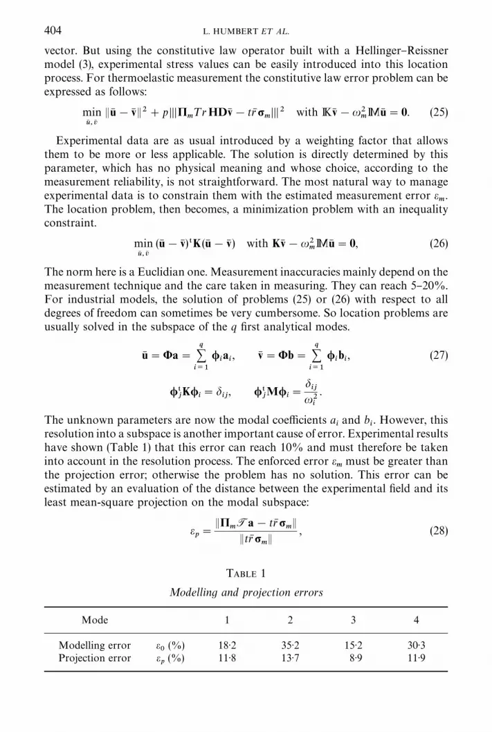
resolution into a subspace is another important cause of error. Experimental resultshave shown (Table 1) that this error can reach 10% and must therefore be takeninto account in the resolution process. The enforced error e

mmust be greater than

the projection error; otherwise the problem has no solution. This error can beestimated by an evaluation of the distance between the experimental "eld and itsleast mean-square projection on the modal subspace:

ep"

EPmTa!trN r

mE

EtrN rmE

, (28)

TABLE 1

Modelling and projection errors

Mode 1 2 3 4

Modelling error e0

(%) 18)2 35)2 15)2 30)3Projection error e

p(%) 11)8 13)7 8)9 11)9


with

a"(T 5P5mP

mT)~1(P

mT)5trN r

m, T"¹rHDU"¹r R .

T denotes the stress sum matrix of the q "rst modes. By substituting equation (27)into equation (26) and using the orthogonal properties of the modes, the locationproblem can be expressed only in terms of coe$cients a

i:

mina

q+i/1

a2i A1!

u2m

u2iB2

withEP

mTa!trN r

mE

EtrN rmE

)em. (29)

This kind of optimization is much more di$cult to solve than a single functionminimization. All standard methods are described in reference [11]: the Lagrangemultiplier approach, the gradient projection and reduced gradient methods, as wellas the feasible direction method. These techniques with n parameters are quitecumbersome. However, particularities of the location problem allows one tosimplify it and to develop an e$cient solution method.

It must be underlined that this new expression of the location problem involvesonly the stress eigenvectors and can be adapted to a classical displacement "niteelement model.

4.3. PARTICULARITIES OF THE CONSTRAINED LOCATION PROBLEM

Gafka and Zimmerman [13] have shown that the constrained error locationproblem (29) has some interesting properties:

f The cost function is convex.f The experimental "eld is close to the analytical eigenmode because only the

matched modes are used in the location process.f The solution is reached on the boundary of the inequality constraint [11]. Hence,

the inequality constraint can be replaced by an equality constraint.

This last assumption can easily be demonstrated. The constraint is either activeor inactive. Consider these two cases.

Case 1: ¹he constraint is inactive

EPmTa!trN r

mE

EtrN rmE

(em.

The solution is in the admissible domain. The constraint has no in#uence on thesolution computation and can be disregarded. The solution of the problem is thenthe analytical mode. This solution is only acceptable if the estimated error e

mis

greater than the distance e0

between the analytical and experimental data. In thiscase the updating process is not helpful.

Case 2: ¹he constraint is active

EPmTa!trN r

mE

EtrN rmE

"em.


The solution is on the boundary of the admissible domain. This is the onlypossibility when the "rst one is ruled out. The constraint compels the solution totend towards experimental values.

Using previous particularities, the error location problem can be written:

mina

F(a) with G (a, em)"0, (30)

F(a)"a5Qa"q+i/1

a2i A1!

u2m

u2iB2,

G(a, e)"EPmTa!trN r

mE2!e2EtrN r

mE2.

4.3. A NEW SOLUTION PROCESS

The distance between analytical and experimental data e is now considered asa parameter of the optimization process. To each particular value e

mof e, only one

solution a corresponds. So instead of solving problem (30), the distance e is forcedto tend towards e

m. The constrained minimization (30) can be transformed into

a single minimization by introducing a Lagrange's multiplier j:

mina,j

F(a)#jG (a, e). (31)

The steady state condition towards j sets the constraint on the measured data:

LLj

(F#jG )"0NG(a, e)"0. (32)

The steady state condition towards modal coe$cients a provides the relationship

LLa

(F#jG)"0N gradF(a)"!j grade/cst

G (a, e). (33)

From this relationship, one can deduce that j has to be positive; otherwise theconstraint will not be active. Furthermore, this relationship allows one to expressthe parameters a in terms of j:

a (j)"j(Q#j(PmT)5 (P

mT))~1(P

mT )5 trN r

m. (34)

By substituting this relation into equation (32), the minimization problem (31) canbe transformed into solving equation (35) versus j:

G(a (j), em)"0. (35)

This equation can also be written as

e (j)"EP

mTa(j)!trN r

mE

EtrN rmE

"em. (36)


This equation will "nally be solved in terms of an iterative linearization of thedistance e versus Lagrange's multiplier. To improve the regularity of e(j) and usingthe fact that j was to be positive, the multiplier j is replaced by 10k, with k in]!R,#R[. The expression of the modal coe$cients becomes

a(k)"10k(Q#10k(PmT )5(P

mT ))~1(P

mT )5 trN r

m. (37)

For each experimental mode k, one has to solve the iterative problem de"ned by

e(ki~1

)#(ki!k

i~1) A

LeLkBki~1

"em. (38)

The initial point k0

is computed with the analytical mode, normalized towards theexperimental data:

k0"log A

EQa0E

E(PmT )5(P

mTa

0!tr r

m)EB with a( j )

0"

(PmT

k)5 trN r

m(P

mT

k)5(P

mT

k)djk

.

The solution of equation (38) requires the sensitivity computation of e versus k.De"ne

A(k)"(Q#10k(PmT) 5(P

mT)), (39)

LA~1

Lk"!A~1

LALk

A~1NLA~1

Lk"!ln (10)10kA~1 (P

mT)5(P

mT)A~1.

(40)

The sensitivity expression is then

LeLk

"

12e

Le2Lk

, (41)

Le2Lk

"2(P

mTa!trN r

m)5P

mT

trN r5m

trN rm

LaLk

, (42)

LaLk

"ln (10)10kA~1(I!10k(PmT )5(P

mT )A~1) (P

mT )5trN r

m. (43)

Even if the previous expression seems to be complex, it involves only smallmatrices of order n (length of the modal basis). The solution of this new locationproblem is very fast and the convergence is achieved in a few steps (see Figure 2).Error indicators are then computed using expressions (16) or (23). The key point ofthis method is the choice of the measurement error e

m, according to the projection

error ep

and the initial distance between analytical and experimental data e0. The

in#uence of this choice on the error location will be investigated later.

5. OPTIMIZATION PROCESS

The ability to understand all possible error causes requires experience inupdating problems, as well as good knowledge of the modelling hypothesis and

Figure 2. Solution for the "rst mode.


the mechanical behaviour of the experimental structure. Error indicators do notgive any information about the kind of modelling error. However, depending on thestructure area highlighted by error indicators, it is often possible to guessparameters that a!ect the modelling most.

The mass and sti!ness of the "nite element or group of elements, as well asboundary sti!nesses have been taken as optimization parameters. All geometricalparameters can be managed in this way:

M"M0#

2

+i/1

pM

iM (i), K"K

0#

2

+i/1

pK

iK (i). (44)

The choice of the cost function has been widely discussed in the literature[5, 11, 14]. This function can involve the error between analytical and experimentaleigenfrequencies or mode shapes, modal analysis criterion coe$cients, residualforces, constitutive law error or a linear combination of this data. Thermoelasticmode shapes and eigenfrequencies have been introduced by means of the distancebetween analytical and experimental data. The advantage of this choice is toimprove the model using untreated data, but supplying a highly non-linear costfunction.

F(pMi

, pKi)"

m+k/1

EPm¹rR

k!trN r

kmE

EtrN rkm

E#

Eu2k!u2

kmE

u2km

. (45)

The minimization of this cost function is achieved by means of a metric variablequasi-Newton process [11] with a polynomial line search. The gradient iscomputed using a modal parameter sensitivity method. As the function is non-linear and the parameters may have di!erent rank orders, the gradient is correctedthrough iterative estimation of the Hessian with the Davidon Fletcher Powell


method. Then the minima in this direction are searched through polynomialapproximation of the correction step length. When the minima are reached,another search direction is computed. If there are no local minima the algorithmmust converge [15]. To avoid convergence problems due to local minima someregularization methods have been developed [14]. In the present case, it is assumedthat the amount of experimental thermoelastic data and the summation on manymodes provides a regular enough function. However, to avoid a divergence of the"nite element solution, the parameter changes have been limited to a prioriestimated range. This optimization method, based on an iterative linearizationof the cost function, calls for modal parameter derivatives versus structuralparameters:

LFLp

"

LFLR

k

LRk

Lp#

LFLu2

k

Lu2k

Lp. (46)

For a standard model, the derivatives of the modal stresses can be computed onlyby "nite di!erence methods, which require a lot of model evaluations. The use ofa mixed model allows quick computation of these derivatives. The modalparameter sensitivities versus structural parameters are obtained by di!erentiatingthe governing mixed equations (47) and (48) versus these parameters:

A!u2

kM

K 51

K1

K2BA

/k

RkB"A

00B . (47)

with /5kM/

h"d

kh(48)

N!u2kM

L/k

Lp#K

1

LRk

Lp!

Lu2k

LpM/

k"u2

k

LMLp

/k!

LK1

LpR

k, (49)

K51

L/k

Lp#K

2

LRi

Lp"!

LK1

Lp/

k!

LK2

LpRk, (50)

/5k

LMLp

/k#2/5

kM

L/k

Lp"0. (51)

For single eigenvalues, previous relationships are su$cient to determine modalsensitivities. The exact solution by means of Nelson's method has a too highcomputational cost to be applied. So the Fox's modal superposition method [12],which consists of representing the displacement and stress sensitivities bycontributions of the q "rst eigenvectors has been adapted:

L/k

Lp"Ua,

LRk

Lp"Rb. (52)

The coe$cients aiand b

i(i in [1, n]) are determined by premultiplying equations

(49)}(51) with /iand R

i, and using the orthogonality properties. The "nal outcome


is that

Lu2k

Lp"!/5

kf1!R 5

kf2, (53)

ai"G

/5kf1#R 5

kf2

u2i!u2

k

, iOk,

!1/2/5k

LMLp

/k, i"k,

(54)

bi"a

i!

/5if2

u2i

. (55)

with

f1"u2

k

LMLp

/k!

LK1

LpR

kand f

2"!

LK51

Lp/

k!

LK2

LpR

k.

This method requires very little computation, but has frequently been shown to beinaccurate due to the use of an incomplete set of eigenvectors in the expansion [12].Other techniques, such as the Zhang and Zerva iterative method or preconditionedconjugate projected gradient iterative technique [12], allow one to improvederivative calculation but introduce high computation. Nevertheless, the accuracyof Fox's method can be improved by increasing the number of eigenvectors.Moreover, as the correction is done by using an iterative method, one assumes thathigh accuracy is not necessary.

6. EXPERIMENTAL RESULTS

6.1. THERMOELASTIC MEASUREMENT OF THIN PLATE BENDING

The measurement of the dilatation temperature change is made without contact,at room temperature, by means of a thermographic camera (SPATE 4000Ometron) "tted with a mirror scanning system. It allows one to obtain a wideexperimental "eld on the tested structure area at "xed frequencies (here theeigenmode thermoelastic "elds). The thermoelastic information, which is about0)01}0)5 K, is extracted from the other room temperature changes througha frequential analytical "ltering. The measurement is fully controlled by a computer(see Figure 3).

All physical phenomena involved in this measurement technique, such as theinfrared emissivity, the gaseous media absorption, the radiation detection, as wellas the thermoelastic signal calibration, were investigated in detail in reference [2].The accuracy of temperature measurement reaches almost 0)001 K, whichcorresponds to a stress level of about 1)0 MPa for steel and 0)4 MPa for aluminium.The main limitation of this technique is the stress level one is able to generate,especially for high frequencies.

Thermoelastic modal measurements were carried out on a thin aluminium plate,with free-clamped boundary conditions (Figure 4). Di!erent kinds of defects were

Figure 3. Experimental set-up.

Figure 4. Experimental structure.


tested, successively: a 38 g mass located at di!erent positions, a material damage(a set of little borings) reducing the sti!ness by about 30%, and releasing of clampedboundary conditions. For the latter defect some screws were removed. Theexcitation was realized with a shaker controlled by a frequency analyzer. A modalanalysis was carried out in order to detect the "rst modes of the plate with a highaccuracy. The thermoelastic measurement does not allow modal extraction.However, as the modes are well separated and the damping is small, one canconsider that the measured shape can be compared with its mode shape.

Figure 1 shows the thermoelastic modal measurements for the "rst four modes.The experimental "elds have been obtained on a mesh involving 36 * 74 points and


are quite smooth. The thermoelastic "eld was calibrated by a strain gauge stuck onthe rear side of the plate.

6.2. KIRCHOFF'S THIN PLATE MODELLING

The plate can be modelled with a di!erent kind of approach [3, 4]. A choice wasmade to model it with a two-"eld Hellinger}Reissner formulation and Kircho! 'sthin plate hypothesis. Major assumptions of this theory are that: plane sectionsremain plane during deformation, the bending and membrane behaviours can bedealt separately, the direct stress in the normal direction p

zis small enough to be

neglected, together with the shear deformation. The behaviour of the plate can thenbe described by the normal displacement u of the middle plane and the bendingmoments (pJ

x, pJ

y,pJ

xy):

pN "Pe@2

~e@2

zpdz"ApNx

pNy

pNxyB . (56)

The "nite element mesh (Figure 5) is composed of 231 rectangular elements withfour nodes per element. Convergence problems of mixed formulations are discussedin reference [3]. They lead to some requirements linking the respective number ofdisplacement and stress degrees of freedom. To avoid this di$culty the same orderapproximation that requires four degrees of freedom per element was taken forall displacements and stress components. So, four degrees of freedom are de"nedfor each node: one displacement uN and three bending moments pN

xpNy

pNxy

. Thismodelling leads to a set of equations which have the same expression as (2).

The clamped edge is generally obtained by setting corresponding generalizeddegrees of freedom to zero. Nevertheless, a real clamping never has in"nite rigidity.

Figure 5. Finite element model.


So it was modelled by a set of linear springs k0, that will be updated in the

correction step. These springs are introduced in the mixed formulation by means oftheir potential energy k

0u2 and will "nally appear as k

0diagonal terms associated

with the corresponding displacement degrees of freedom.For bending deformation the stress distribution is linear; so bending moments

can be directly related to the top area stresses by

p(z/e@2)

"$e/2pJ (57)

N tr pJm"$2/e tr p

m. (58)

The thermoelastic values were then projected on to the mesh using the "niteelement shape functions (10), to obtain corresponding degrees of freedom tr eN

m.

6.3. ERROR LOCATION

The previous model has been used to compute 30 displacement and stress summode shapes (u

i, /

i, T

i), useful for the location process. Before beginning the

updating, the distance between experimental and analytical values as well as theerror introduced by the modal subspace (28) were estimated. Table 1 shows thesedata for the "rst mass defect.

The expansion error is about 10% and is thus signi"cant, in comparison with themodelling error. The convergence rate of the modal projection is very low anda basis of 50 modes only reduces this error by 1 or 2%. The measurement error isestimated a priori to be around 5%, to which is added the expansion error e

pto

obtain the constraint em. The convergence of the constrained location method is

very fast and is reached in a few steps, as shown in Figure 2. On this curve, thedistance e in terms of k and successive iterations of the resolution were plotted.When k increases, it enforces the experimental term of equation (31) and e tendstoward e

p.

Figure 6 shows modal error location for the "rst mass defect. The locationis not very good. Not only has the mass been located, but also other parts of thestructure.

Due to expansion or measurement errors the ill-modelled area is never locatedby a single peak. The modelling error may not a!ect all modes or can be hidden bymeasurement errors or be "ltered by the modal basis. Furthermore, the e!ect of anerroneous parameter on the dynamic response varies with the frequency domainand the parameter type.

The ill-modelled parameter detection consists in "nding areas appearing onmany indicators. This is quite easy in the case of a numerical simulation especiallywhen the modelling error is known, but proves much more di$cult in a real case.Usually, the normalized indicators are simply added (59) and provide a globalindicator for all the modes:

s(e)1"

m+k/1

g(e)k

EgkE

. (59)

Figure 6. Error location for the mass defect.


In reference [16], the author suggests weighting the frequency location indicatorsby the dissipated energy. Another approach has been chosen which uses acorrelation between all modal indicators (60), which highlights errors occurring onmany indicators:

s(e)2"

m+

k,h/1 kOh

g(e)k

g(e)h

EgkEEg

hE

. (60)

Figure 7 shows the indicator s2

carried out for all considered defects, with the"rst four thermoelastic measurements. All kinds of defects are located with goodaccuracy. However, it is noteworthy that the excitation area is detected too. Thistechnique is very interesting when experimental information is available for a lot offrequency points and when the measurement error is signi"cant. The discriminationcapacity of these correlated indicators is greater than the standard ones.

The solution of the location process is directly determined by the enforced errorem. This parameter seems to be very important, but it cannot be estimated with

high accuracy. It is usually given a priori, according to the measurement quality.Hence, the sensitivity of the location versus this parameter has been investigated. InFigure 8, is plotted the constitutive law error versus the multiplier k and versus e

m,

and the location of its approximate domain is achieved.The location is achieved for a quite large domain of k and e

m. However, these

domains are not the same for each mode. When k becomes too great, the energyE2(u6 , v6 ) increases quickly and the location fails. This corresponds to a decrease inthe distance between experimental and analytical data, e, which tends towards e

p.

Figure 7. Error location using s2.

Figure 8. Constitutive law error ("rst mode).


The parameter k enforces the measurement inaccuracies too. Since measurementerrors have a greater deformation energy than modelling errors, the constitutivelaw error increases faster. Thus, the optimal measurement expansion is obtained forthe upper bound of k's location domain.

6.4. MODEL OPTIMIZATION

Now consider the results of the model correction for the "rst mass defect. Thisdefect is represented by mass m at the position located by indicator s

2(Figure 7).

The clamped edge is split into three parts with a sti!ness parameter aifor each one.


Boundary sti!nesses were introduced using power parameters to improve theirlinearity,

k@0i"10aik

0i. (61)

The optimization requires 12 sensitivity computations and about 40 evaluationsof the "nite element model. It leads to a cost function monotonic decrease of 56%.But as shown in Figures 9(b) and 9(c), di!erent terms of the cost function (45) have

Figure 9. Correction of the mass defect: (a) cost function; (b) error on thermoelastic "elds; (c) error oneigenfrequencies; (d) mass parameter m (10~3 kg); (e) boundary sti!nesses k

0i(N/m).

TABLE 2

Correction of modal parameters

Mode 1 2 3 4

Eigenfrequency (%) 98 87 71 98Thermoelastic data (%) 52 53 14 34


a less regular trend. The observable chaotic and irregular behaviours are due to thestrong cost function non-linearities. The correction ratio of modal eigenfrequenciesand thermoelastic data are given in Table 2.

The mass defect is updated by about 85% and the boundary sti!nesses arereduced from the 106 Nm~1 initial value to about 105 Nm~1. The residual erroron thermoelastic modal "elds is due to either thermoelastic measurementinaccuracies or physical phenomena which have not been modelled. Nevertheless,the model improvement is quite signi"cant and shows the usefulness ofthermoelastic data in the correction step.

7. CONCLUSION

The aim of this paper was not to promote thermoelasticity as the bestexperimental information for "nite element updating, but to show that it canbe successfully used to achieve this goal. Measurements are usually the laststage of the design process and are rarely planned for updating purposes.So the user cannot choose the experimental data, which could be displacementas well as stress values. Moreover, "nite element models are usually usedto predict the stress level; it can also be interesting to update them with respect tothis kind of data.

So far the lack of experimental data has put a curb on updating methods, butmodern experimental techniques enable now a wide and accurate measure of thereal behaviour of mechanical structures. The new approach of the modelling errorlocation has a better accuracy and robustness to measurement errors than thestandard one. The single parameter of the location problem is now the a priorimeasurement error which is easier to estimate than the former weighting factor andhas a physical meaning. Moreover, the introduction of a correlation between modalerror indicators already improves the detection of ill-modelled parameters. Thisshould be stressed.

The use of non-standard mixed models could be a drawback because this kindof modelling is not available in industrial "nite element softwares. However, thesolution by means of a modal superposition technique involves only stresseigenvectors (see equation (29)) which can be estimated with most of the classicalsoftwares. Nevertheless, the so obtained stress vectors are generally less accuratethan those computed using a mixed model and do not necessarily satisfy static


boundary conditions. Finally, it must be underlined that the present developmentsare not limited to the use of thermoelastic data. The new solution techniqueproposed can be applied to any standard expansion and location methods based onthe constitutive law error or the residual forces.

REFERENCES

1. A. S. KOBAYASHI 1998 Handbook on Experimental Mechanics, 581}597. SEM.2. N. HARWOOD and W. M. CUMMINGS 1986 NE¸ Report No. 705. Calibration and

Qualitative Assesment of the SPATE stress measurement system.3. O. C. ZIENKIEWICZ and R. L. TAYLOR 1994 ¹he Finite Element Method. New York:

McGraw-Hill.4. F. BREZZI and M. FORTIN 1991 Mixed and Hybrid Finite Element Methods. Berlin:

Springer-Verlag.5. M. I. FRISWELL and J. E. MOTTERSHEAD 1995 Finite Model ;pdating in Structural

Dynamics. Dordrecht: Kluwer Academic Publishers.6. M. BARUCH 1978 AIAA Journal 16. Optimisation procedure to correct sti!ness and#exibility matrices using vibration data.

7. A. M. KABE 1985 AIAA Journal 23. Sti!ness matrix adjustment using modal data.8. F. M. HEMEZ and C. FARHAT 1995 Journal of Modal Analysis 10, 152}166. Structural

damage detection via "nite element model updating methodology.9. P. LADEVEZE and M. REYNIER 1989 12th ASME Mech. <ibration and Noise Conference,

Montreal. A localization method of sti!ness errors for adjustment of "nite elementmodels.

10. P. COLLIGNON and J. C. GOLINVAL 1995 Proceedings of Congres M<2. Comparison ofexperimental eigenvector expansion methods for failure detection.

11. R. T. HAFTKA, Z. GURDAL and M. P. KAMAT 1990 Element of Structural Optimisation.Dordrecht: Kluwer Academic Publishers.

12. K. F. ALVIN 1998 Proceedings of IMAC Conferences, 652}659. E$cient computation ofeigenvector sensitivities for structural dynamics via conjugate gradients.

13. G. K. GAFKA and D. C. ZIMMERMAN 1997 Proceedings IMAC, 1278}1284. Modelupdating using constrained eigenstructure assignment.

14. A. TARANTOLA 1987 Inverse Problem ¹heory, Methods for Data Fitting and ModelParameter Estimation. Amsterdam: Elsevier.

15. G. H. T. NG and J. E. MOTTERSHEAD 1995 Proceedings of IMAC Conferences, 1282}1288.Model updating by a two level Gauss}Newton approach with line searching.

16. A. CHOUAKI 1997 Ph.D. ¹hesis, ¸M¹ ENS Cachan, France. Une meH thode de recalagedes modeles dynamiques des structures avec amortissement.

APPENDIX A: HELLINGER}REISSNER MIXED MODEL

The approximated mechanical "elds are given for each element (e) versus degreesof freedom at every node n by

u(e)(x, y, z)"+n

N(e)un

(x, y, z)uN (e)n"N (e)

uu6 (e),

p(e)(x, y, z)"+n

N(e)pn (x, y, z)pN (e)n"N (e)p p6 (e).


For a two-"eld (u!r) formulation, Zienkiewicz and Taylor [3] express the generalexpression of elementary mass and sti!ness matrices:

M(e)"PXe

oN (e)u

N (e)5u

dx dy,

K (e)1"PX

e

N (e)p DN (e)5u

dxdy,

K (e)2"!PX

e

N (e)p H~1N (e)5p dxdy,

F (e)"PCe

t0N (e)5u

ds.

For the thin plate model used in the experimental part, both displacement andstress approximations are based on the same Lagrange's shape function order 1(N(e)

u"N(e)p "N ). The plate has been modelled by means of four-node rectangular

elements with four-degrees-of-freedom per node: one normal displacement uNnand

three bending moments pNxn

, pNyn

, pNxyn

. The particular expression of the elementarymass and sti!ness matrices are then given by

M (e)(ij )

"PXe

oeN (e)i

N (e)j

dxdy,

K (e)1"(K (e)

11K (e)

12K (e)

13),

K (e)2"A

K (e)22

K (e)23

0

K (e)23

K (e)33

0

0 0 K (e)44B

with

K (e)11(i j )

"PXe

LNi

LxLN

jLx

dxdy, K (e)12(ij )

"PXe

LNi

LyLN

jLy

dx dy

K (e)13(i j )

"PXeALN

iLx

LNj

Ly#

LNi

LyLN

jLx B dxdy

K (e)22(i j )

"!S22 PX

e

NiN

jdxdy, K (e)

23(ij )"S

12 PXe

NiN

jdx dy

K (e)33(i j )

"!S11 PX

e

NiN

jdxdy, K (e)

44(ij )"!S~1

33 PXe

NiN

jdx dy

S"H~1"12(1!l2)

e3E A1 l 0l 1 00 0 1/2(1!l) B

~1

and e the thickness of the plate.


APPENDIX B: NOMENCLATURE

ce , cp speci"c heat coe$cientsD spatial di!erentiation operatorE Young's modulusH Hooke's elasticity matrixk heat conductionK"j#2

3k bulk modulus

K, M sti!ness and mass matricesr external heat supplytrr

mthermoelastic measurement

trr, tr e sum of the principal stresses, sum of the principal strains¹ absolute temperature¹r

sum of the principal componentsui, e

ij, p

ijdisplacement, strain and stress "elds

=(eij) strain energy

=c(p

ij) complementary energy

Greek charactersa dilatation coe$cienth temperature changej, k Lame's coe$cientsl The Poisson ratioP

mmeasurement location matrix

U, R matrices of the q "rst modal deformation shapes and stress vectoro mass density(u

k, /

k) kth analytical mode

(ukm

, ukm

) kth experimental mode

Documents

Finite Element Dynamic Model Updating Using Modal Thermoelastic Fields