arX

iv:c

ond-

mat

/030

4461

v2 [

cond

-mat

.sta

t-m

ech]

13

Jun

2003

Heat capacity of square-well fluids of variable width

J. Largo∗ and J. R. Solana†

Departamento de Fısica Aplicada, Universidad de Cantabria, 39005 Santander, Spain

L. Acedo‡ and A. Santos§

Departamento de Fısica, Universidad de Extremadura, 06071 Badajoz, Spain

(Dated: February 2, 2008)

We have obtained by Monte Carlo NVT simulations the constant-volume excess heat capacity ofsquare-well fluids for several temperatures, densities and potential widths. Heat capacity is a ther-modynamic property much more sensitive to the accuracy of a theory than other thermodynamicquantities, such as the compressibility factor. This is illustrated by comparing the reported simu-lation data for the heat capacity with the theoretical predictions given by the Barker–Hendersonperturbation theory as well as with those given by a non-perturbative theoretical model based onBaxter’s solution of the Percus–Yevick integral equation for sticky hard spheres. Both theories giveaccurate predictions for the equation of state. By contrast, it is found that the Barker–Hendersontheory strongly underestimates the excess heat capacity for low to moderate temperatures, whereasa much better agreement between theory and simulation is achieved with the non-perturbative the-oretical model, particularly for small well widths, although the accuracy of the latter worsens forhigh densities and low temperatures, as the well width increases.

I. INTRODUCTION

Thermodynamic and structural properties of square-well (SW) fluids have been profusely studied both from theoryand from computer simulation [1]–[38]. From the theoretical side, the first few virial coefficients have been obtained[1, 2, 37] and the radial distribution function has been evaluated from numerical solutions of integral equation theories,such as Percus–Yevick [6, 7, 8, 30, 38], Yvon–Born–Green [14], HNC [10], MSA [16, 30], Rogers–Young [28], ORPA[28], and HRT [35]. Simpler analytical approximations have also been proposed [11, 12, 19, 20, 21, 22, 34]. Thethermodynamic properties have been derived from the theoretical structure functions as well as from perturbationtheory [3, 4, 9, 13, 23, 27]. Access to the “experimental” properties of SW fluids has been made possible viamolecular dynamics and Monte Carlo simulations [5, 10, 13, 16, 17, 18, 26, 36, 38]. Special attention has receivedthe determination of the critical point of SW fluids [6, 7, 8, 13, 18, 23, 25, 26, 29, 33, 34, 35, 38], both from thetheoretical and simulational viewpoints. The main reason for this wide interest lies in the fact that a SW fluid isperhaps the simplest one whose particles have attractive as well as repulsive interactions. In general, theories areeasier to apply to SW fluids than to other fluids with more realistic potentials. In addition, the SW potential seemsto be particularly sensitive to the performance of a theory. Therefore, this kind of fluid is an excellent testing-groundfor many theories of fluids and so the study of SW fluids can be considered as a first step towards our understandingof the properties of fluids with more sophisticated interactions. There is an additional reason explaining the recentrevival of interest in SW fluids. The SW potential possesses, besides the diameter of the hard core and the depth ofthe well, an additional parameter measuring the width of the well. This makes the SW potential with a small widthespecially suited to model the effective interactions among colloidal particles [16, 28, 30, 31, 38]. In this context, theglass transition [30, 31] and a solid-to-solid isostructural transition [24] have been studied for narrow SW systems.

Despite the extensive number of studies devoted to the SW fluid, relatively little attention has been paid to severalthermodynamic properties. This is the case for the heat capacity. To the best of our knowledge, there are available[5, 10] only a few simulation data of this property for SW fluids. Theoretical calculations of the same quantity areequally scarce [10]. In the present paper we have carried out Monte Carlo simulations of the constant-volume excessheat capacity CE

V of SW fluids for several values of the potential width and, for each of them, for several densitiesand temperatures. Moreover, in order to put clear the sensitivity of this property to the accuracy of a theory, thesimulation data are compared with the results obtained from the Barker–Henderson (BH) [39, 40] perturbation theory

∗Electronic address: largoju@unican.es†Electronic address: solanajr@unican.es; Author to whom correspondence should be addressed‡Electronic address: acedo@unex.es§Electronic address: andres@unex.es

2

and with those derived from the theoretical model proposed by Yuste and Santos [22], recently simplified by Acedoand Santos [34].

The paper is organized as follows. In the next section, we summarize the theoretical foundations of the MC procedureused and we describe the simulations performed and the results obtained. In Section III, we present an outline of theabove-mentioned theories. Finally, in the last section the theoretical results are compared with simulation data anddiscussed.

II. MONTE CARLO SIMULATIONS

In a square-well (SW) fluid, particles interact by means of a potential of the form

u (r) =

{

∞ if r ≤ σ−ǫ if σ < r ≤ λσ0 if r > λσ

(1)

where λ is the potential width in units of the particle diameter σ and ǫ is the potential depth.Constant-volume averaged excess heat capacity per particle in a SW fluid can be expressed in the form [5]:

CEV

Nk=

1

T ∗2

⟨

(M − 〈M〉)2⟩

N, (2)

where N is the number of particles, k is the Boltzmann constant, T ∗ = kT/ǫ is the reduced temperature, and M isthe number of pairs of interacting particles, that is, the number of pairs of particles whose centers lie separated by areduced distance r∗ = r/σ ≤ λ.

The averages involved in equation (2) can be calculated by Monte Carlo (MC) simulations in the NVT ensemble.Therefore, we have proceeded to calculate by means of MC NVT the constant-volume averaged excess heat capacityper particle for SW fluids with well widths λ ranging from 1.1 to 1.5. For each value of λ, CE

V has been evaluated forseveral densities along isotherms. To this end, a system consisting of 512 particles placed in a cubic box with periodicboundary conditions was used. Particles were initially placed in a regular configuration and then the system wasallowed to equilibrate for 2× 104 cycles, each of them consisting of an attempt move per particle, the first 104 cyclesat a very high temperature and the remaining ones at the desired temperature. The calculation of CE

V was performedby averaging over the next 5× 105 cycles, performing partial averages every 104 cycles with the aim of estimating thestatistical error from the standard deviation. The use of such a huge number of cycles in the calculations was motivatedby the need of ensuring that the values of CE

V converged to a constant value, apart from statistical fluctuations. Infact, we realized that for low values of the number of cycles used in the calculations, the values of CE

V increase withthe number of cycles used.

The results are shown in Table I. We have considered four isotherms for λ = 1.1, 1.2, 1.3 and three isotherms for λ =1.5. The lowest temperature in each case is larger than the estimated critical temperature [13, 18, 23, 25, 26, 33, 34, 35]:T ∗

c ≃ 0.5, 0.6, 0.8, 1.2 for λ = 1.1, 1.2, 1.3, 1.5, respectively.

III. THEORY

A. Barker–Henderson perturbation theory

In the second-order Barker–Henderson perturbation theory [39, 40], the free energy is expressed in the form

F

NkT=

F0

NkT+

F1

NkT

1

T ∗+

F2

NkT

1

T ∗2 , (3)

where F0 is the free energy of the hard-sphere (HS) reference system and F1 and F2 are the first- and second-orderperturbative terms, respectively. According to this theory, the constant-volume excess heat capacity per particle isgiven by

CEV

Nk= −

2

T ∗2

F2

NkT, (4)

3

where

F2

NkT= −πρkT

(

∂ρ

∂P

)

0

∫ ∞

0

[u∗1 (r)]

2g0 (r) r2dr (5)

in the so-called macroscopic compressibility approximation, whereas

F2

NkT= −πρkT

∫ ∞

0

[u∗1 (r)]

2

{

∂ [ρg0 (r)]

∂P

}

0

r2dr (6)

in the so-called local compressibility approximation. In Eqs. (5) and (6), ρ = N/V is the number density, u∗1(r) =

u1(r)/ǫ is the perturbative contribution to the potential function, which in a SW potential is u∗1(r) = −1 for σ < r <

λσ, P is the pressure, and g0(r) is the radial distribution function (r.d.f.) of the hard-sphere reference fluid.In recent years, several analytical and very accurate expressions for the r.d.f. g0(r) of the HS fluid have been

proposed [41, 42, 43]. They can be used to determine F2 in expressions (5) and (6). Regarding (∂ρ/∂P )0, whichappears explicitly in expression (5) and implicitly in (6), it can be obtained from the well-known Carnahan–Starling[44] equation of state

Z0 =P0V

NkT=

1 + η + η2 − η3

(1 − η)3 , (7)

where η = (π/6)ρσ3 is the packing fraction.

B. Yuste–Acedo–Santos model

The internal energy can be obtained from the r.d.f g(r) through the energy equation

U =3

2NkT + 2πNρ

∫ ∞

0

u (r) g (r) r2dr, (8)

whence

CEV

Nk=

2πρ

k

∫ ∞

0

u (r)

[

∂g (r)

∂T

]

V

r2dr. (9)

In the special case of the SW potential (1), Eqs. (8) and (9) become

U =3

2NkT − 12Nǫη

∫ λ

1

g (r∗) r∗2dr∗, (10)

CEV

Nk= −12η

∫ λ

1

[

∂g (r∗)

∂T ∗

]

η

r∗2dr∗, (11)

respectively. The r.d.f g(r∗) of the SW fluid depends on the packing fraction η, the reduced temperature T ∗ and,parametrically, on the well width λ. In principle, one has to resort to numerical solutions of integral equation theories.On the other hand, particularly suitable for the purpose of obtaining the heat capacity is the heuristic model proposedby Yuste and Santos [22] and recently simplified by Acedo and Santos [34], which is analytical and fairly accurate.Henceforth we will refer to this model as the Yuste–Acedo–Santos (YAS) model. It is based on expressing the Laplacetransform G(t) of r∗g(r∗) in the form

G (t) = tF (t) e−t

1 + 12ηF (t) e−t=

∞∑

n=1

(−12η)n−1 t [F (t)]n e−nt, (12)

where the auxiliary function F (t) is assumed to have the form [22, 34]

F (t) = −1

12η

e1/T∗

+ K1t −(

e1/T∗

− 1 + K2t)

e−(λ−1)t

1 + S1t + S2t2 + S3t3. (13)

4

The coefficients K1, K2, S1, S2 and S3 are explicit functions of η, T ∗ and λ determined from consistency conditions.We refer the interested reader to Refs. [22, 34] for further details. The YAS model (13) reduces to the exact solutionsof the Percus–Yevick (PY) equation in the limit of hard spheres (λ → 1 or T ∗ → ∞) [45, 46], as well as in the limitof sticky hard spheres (λ → 1 and T ∗ → 0 with T ∗ ∼ −1/ ln(λ− 1)) [47]. From that point of view, the approximation(13) can be seen as a simple extension to finite widths of Baxter’s solution of the PY equation for sticky hard spheres.

Upon Laplace inversion of Eq. (12), the final expression of the r.d.f. reads

g (r∗) = r∗−1∞∑

n=1

(−12η)n−1

fn (r∗ − n)Θ (r∗ − n), (14)

where the functions fn(r∗) are the inverse Laplace transforms of t[F (t)]n and Θ(r∗) is Heaviside’s step function.Therefore, to determine the r.d.f. for r∗ < n + 1 only the first n terms in the summation (14) are needed. Inparticular, for the values of λ ≤ 2 considered in this paper, one has

g(r∗) = −r∗−1

12η

3∑

i=1

zie1/T∗

+ K1zi

S1 + 2S2zi + 3S3z2i

ezi(r∗−1), 1 < r∗ ≤ λ, (15)

where zi (i = 1, 2, 3) are the three roots of the cubic equation 1 + S1t + S2t2 + S3t

3 = 0. Inserting Eq. (15) into Eq.(11), we finally get

CEV

Nk=

∂

∂T ∗

3∑

i=1

e1/T∗

+ K1zi

S1 + 2S2zi + 3S3z2i

[

z−1i − 1 + (λ − z−1

i )ezi(λ−1)]

. (16)

The heat capacity can also be obtained from the YAS r.d.f. by following the virial and compressibility routes tothe equation of state. The reason for the choice of the energy route (8) is two-fold. First, it is obviously the mostdirect route to determine the heat capacity. Second, we have checked that the other routes yield results that presentlarger deviations from the simulation data. This latter observation is consistent with the case of the PY theory forsticky hard spheres [48] and for SW fluids [7, 8].

IV. RESULTS AND DISCUSSION

Results obtained for CEV from the second-order Barker–Henderson perturbation theory within the local compress-

ibility approximation as well as within the macroscopic compressibility approximation are compared in Figs. 1–4 withthe simulation data of Table I. We can see that although the local compressibility approximation provides a betteragreement with simulation data, both approximations are rather poor at low temperatures. This might be due eitherto the insufficient accuracy of both the local compressibility and the macroscopic compressibility approximations orto the fact that higher order terms, beyond the second one, in the expansion of the Helmholtz free energy in powerseries of the inverse of the reduced temperature, have a nonnegligible contribution to the heat capacity. In order todetermine which of these two possibilities is the right one, we can use for F2 in Eq. (4) simulation data, thus avoidingtheoretical approximations. These simulations were performed by Barker and Henderson [49] who reported the resultsin terms of a function depending on forty five parameters for each density. These parameters were determined froma least squares fitting of their simulation data. Since the use of that fitting is somewhat tedious, we have preferredto use directly simulation data for F2, which are available for several densities and well widths [50], to determine CE

Vfrom Eq. (4). As one can see in Figs. 1–4, results thus obtained are much closer to the theoretical results derivedfrom the BH second-order perturbation theory than to the values of CE

V obtained from direct simulations, except inthe high density limit. This means that the main reason of the failure of the Barker-Henderson perturbation theoryin predicting the heat capacity of SW fluids arises in the truncation of the perturbative series at the level of thesecond order term, the higher order terms having a nonnegligible contribution. This is in contrast with the situationfor the equation of state [39, 51], which is accurately given by the second-order BH perturbation theory even atrelatively low temperatures for wide ranges of densities and potential wells. The reason is that, as pointed before,the constant-volume excess heat capacity is a thermodynamic property particularly sensitive to the performance of atheory and therefore the influence of higher order terms, which is small in the equation of state, may be important inthe heat capacity. This is particularly true for low values of the potential width, since the lower the potential width,the slower the convergence of the BH perturbation theory at low temperatures [15].

A much better agreement is obtained with YAS theory, Eq. (16), at low to moderate densities, as shown in thesame figures. This theory, in contrast to the BH theory, provides a better agreement with the simulation data of CE

V

5

as the potential width decreases. This is consistent with the fact that, as said before, the YAS model is an extensionto λ > 1 of the PY solution for sticky hard spheres and hence it is expected to be as accurate as the PY theory atleast for small λ − 1. The structural properties predicted by the YAS model for the SW fluid also exhibits a goodagreement with simulation data for low values of λ − 1 whereas the accuracy worsens as λ increases [22, 34]. Figures1–4 show that, given a well width λ, the YAS values of CE

V are more accurate as the temperature increases and/orthe density decreases.

In conclusion, we have performed Monte Carlo simulations of the constant-volume excess heat capacity of SWfluids of variable width for a wide range of densities and at several characteristic temperatures. This thermodynamicquantity vanishes for hard spheres and so it represents an important measure of the influence of attractive forces onthe state of the fluid. Moreover, the heat capacity seems to provide a rather stringent test to assess the accuracy oftheoretical approaches. In this paper we have compared the simulation data with the Barker–Henderson perturbationtheory [39, 40] and with a non-perturbative theory developed by Yuste, Acedo, and Santos [22, 34]. While the formertheory presents a poor performance, which can be attributed to the truncation of the perturvative series to secondorder rather than the inaccuracy of the theory itself, the non-perturbative theory does a fairly good job, especiallyfor narrow wells, except at low temperatures and high densities. Although a potential well of λ = 1.5 is appropriatefor many simple fluids, SW fluids with lower values of λ may be of interest because the properties of certain colloidalsuspensions are well reproduced by considering SW interactions with narrow potential widths. Therefore, as severaltheories for SW fluids have achieved a considerable accuracy for the equation of state and the pair correlation functionof SW fluids, the constant volume excess heat capacity seems to be a suitable thermodynamic property to discriminatebetween them. In this context, we expect that our simulation data can stimulate other studies on the heat capacityof SW fluids of variable width and can be used to check the reliability of other approximations.

The present work has been partially supported by the Spanish Direccion General de Investigacion (DGI) undergrants No. BFM2000-0014 (J.L. and J.R.S) and No. BFM2001-0718 (L.A and A.S.).

[1] Katsura, S., 1959, Phys. Rev. 115, 1417.[2] Barker, J. A., and Henderson D., 1967, Can. J. Phys. 44, 3959.[3] Smith, W. R., Henderson, D., and Barker, J. A., 1970, J. Chem. Phys. 53, 508.[4] Smith, W. R., Henderson, D., and Barker, J. A., 1971, J. Chem. Phys. 55, 4027.[5] Alder, B. J., Young, D. A., and Mark, M. A., 1972, J. Chem. Phys. 56, 3013.[6] Tago, Y., 1973, J. Chem. Phys. 58, 2096.[7] Tago, Y., 1973, Phys. Lett. A 44, 43.[8] Tago, Y., 1974, J. Chem. Phys. 60, 1528.[9] Henderson, D., Barker, J. A., and Smith, W. R., 1976, J. Chem. Phys. 64, 4244.

[10] Henderson, D., Madden, W. G., and Fitts, D. D., 1976, J. Chem. Phys. 64, 5026.[11] Nezbeda, I., 1977, Czech. J. Phys. B 27, 247.[12] Sharma, R. V., and Sharma, K. C., 1977, Physica A 89, 213.[13] Henderson,D., Scalise, O. H., and Smith, W. R., 1980, J. Chem. Phys. 72, 2431.[14] Jones, G. L., Kozak, J. J., Lee, E., Fishman, S., and Fisher, M. E., 1981, Phys. Rev. Lett. 46, 795.[15] Henderson, D., 1983, J. Chem. Phys. 79, 6430.[16] Huang, J. S., Safran, S. A., Kim, M. W., and Grest, G. S., 1984, Phys. Rev. Lett. 53, 592.[17] de Lonngi, D. A., Longgi, P. A., and Alejandre, J., 1990, Mol. Phys. 71, 427.[18] Vega, L., de Miguel, E., Rull, L. F., Jackson, G., and McLure, I. A., 1992, J. Chem. Phys. 96, 2296.[19] Tang, Y., and Lu, B. C.-Y., 1993, J. Chem. Phys. 99, 9828.[20] Tang, Y., and Lu, B. C.-Y., 1994, J. Chem. Phys. 100, 3079.[21] Tang, Y., and Lu, B. C.-Y., 1994, J. Chem. Phys. 100, 6665.[22] Yuste, S. B., and Santos, A., 1994, J. Chem. Phys. 101, 2355.[23] Chang, J., and Sandler, S. I., 1994, Mol. Phys. 81, 745.[24] Likos, C. N., and Senatore, G., 1995, J. Phys.: Condens. Matter 7, 6797.[25] Brilliantov, N. V., and Valleau, J. P., 1998, J. Chem. Phys. 108, 1123.[26] Elliott, J. R., and Hu, L., 1999, J. Chem. Phys. 110, 3043.[27] Benavides, A. L., and Gil-Villegas, A., 1999, Mol. Phys. 97, 1225.[28] Lang, A., Kahl, G., Likos, C. N., Lowen, H., and Watzlawek, M., 1999, J. Phys.: Condens. Matter 11, 10143.[29] Noro, M. G., and Frenkel, D., 2000, J. Chem. Phys. 113, 2941.[30] Dawson, K., Foffi, G., Fuchs, M., Gotze, W., Sciortino, F., Sperl, M., Tartaglia, P., Voigtmann, Th., and

Zaccarelli, E., 2001, Phys. Rev. E 63, 011401.

6

[31] Zaccarelli, E., Foffi, G., Dawson, K. A., Sciortino, F., and Tartaglia, P., 2001, Phys. Rev. E 63, 031501.[32] Acedo, L., 2000, J. Stat. Phys. 99, 707.[33] Vliegenthart, G. A., and Lekkerkerker, H. N. W., 2000, J. Chem. Phys. 112, 5364.[34] Acedo, L., and Santos, A., 2001, J. Chem. Phys. 115, 2805.[35] Reiner, A., and Kahl, G., 2002, J. Chem. Phys. 117, 4925.[36] Largo, J., and Solana, J. R., 2002, Fluid Phase Equilib. 193, 277.[37] Vlasov, A. Y., You, X.-M., and Masters, A. J., 2002, Mol. Phys. 100, 3313.[38] Zaccarelli, E., Foffi, G., Dawson, K. A., Buldyrev, S. V., Sciortino, F., and Tartaglia, P., 2003, J. Phys.:

Condens. Matter 15, S367.[39] Barker, J. A., and Henderson, D., 1967, J. Chem. Phys. 47, 2856.[40] Barker, J. A., and Henderson, D., 1967, J. Chem. Phys. 47, 4714.[41] Yuste, S. B., and Santos, A., 1991, Phys. Rev. A 43, 5418.[42] Yuste, S. B., Lopez de Haro, M., and Santos, A., 1996, Phys. Rev. E 53, 4820.[43] Tang, Y., and Lu, B. C.-Y., 1995, J. Chem. Phys. 103, 7463.[44] Carnahan, N. F., and Starling, K. E., 1969. J. Chem. Phys. 51, 635.[45] Wertheim, M. S., 1963, Phys. Rev. Lett. 10, 321.[46] Thiele, E., 1963, J. Chem. Phys. 39, 474.[47] Baxter, R. J., 1968, J. Chem. Phys. 49, 2770.[48] Wats, R. O., Henderson, D., and Baxter, R. J., 1971, Adv. Chem. Phys. 21, 421.[49] Barker, J. A., and Henderson, D., 1972, Ann. Rev. Phys. Chem. 21, 421. 23, 439.[50] Largo, J., and Solana, J. R., 2003, Molecular Simulation. In press.[51] Largo, J., and Solana, J. R., unpublished work.

7

TABLE I: MC simulation data for CE

V /Nk. The numbers enclosed between parentheses indicate the statistical uncertainty inthe last decimal places.

ρ∗ T ∗ = 0.7 T ∗ = 1.0 T ∗ = 1.5 T ∗ = 2.0 T ∗ = 2.5

λ = 1.1

0.1 0.527(3) 0.1731(8) 0.0580(2)

0.2 0.94(1) 0.319(1) 0.1109(3) 0.0556(2)

0.3 1.25(2) 0.431(3) 0.1588(8)

0.4 1.40(2) 0.525(5) 0.1979(9) 0.1033(4)

0.5 1.51(3) 0.603(7) 0.230(1)

0.6 1.50(3) 0.630(7) 0.252(2) 0.1361(7)

0.7 1.42(3) 0.612(7) 0.261(3)

0.8 1.38(2) 0.595(6) 0.256(3) 0.142(1)

0.9 1.15(3) 0.534(7) 0.241(4)

λ = 1.2

0.1 0.367(2) 0.1155(3) 0.0559(1)

0.2 3.11(17) 0.621(7) 0.1988(6) 0.0979(3)

0.3 0.77(1) 0.2568(9) 0.1288(6)

0.4 3.68(22) 0.83(1) 0.282(2) 0.1463(6)

0.5 0.82(1) 0.295(2) 0.1528(6)

0.6 3.01(14) 0.743(9) 0.282(3) 0.1459(8)

0.7 0.657(8) 0.253(2) 0.1351(7)

0.8 1.35(5) 0.530(8) 0.222(2) 0.1209(9)

0.9 0.463(6) 0.195(2) 0.111(1)

λ = 1.3

0.1 0.1846(6) 0.0864(2) 0.0504(1)

0.2 1.17(1) 0.303(2) 0.1423(7) 0.0834(3)

0.3 0.359(4) 0.1720(5) 0.1016(4)

0.4 1.35(2) 0.363(2) 0.178(1) 0.1060(6)

0.5 0.340(3) 0.1688(8) 0.1019(7)

0.6 0.90(2) 0.289(3) 0.151(1) 0.0918(3)

0.7 0.251(2) 0.1350(9) 0.0838(5)

0.8 0.512(8) 0.226(2) 0.126(1) 0.0807(6)

0.9 0.219(2) 0.122(1) 0.078(1)

λ = 1.5

0.1 0.426(3) 0.1724(4) 0.0952(3)

0.2 0.705(5) 0.263(2) 0.1426(8)

0.3 0.719(9) 0.277(2) 0.1495(7)

0.4 0.563(5) 0.239(2) 0.1339(8)

0.5 0.401(6) 0.190(2) 0.1142(6)

0.6 0.295(2) 0.161(1) 0.1027(5)

0.7 0.270(2) 0.1513(6) 0.0977(6)

0.8 0.235(3) 0.136(1) 0.0894(9)

0.9 0.188(2) 0.109(2) 0.0716(6)

8

List of figures

0.0

0.5

1.0

1.5

2.0

0.0

Cv/N

k

0.2 0.4 0.6 0.8 1.0

E

ρ∗

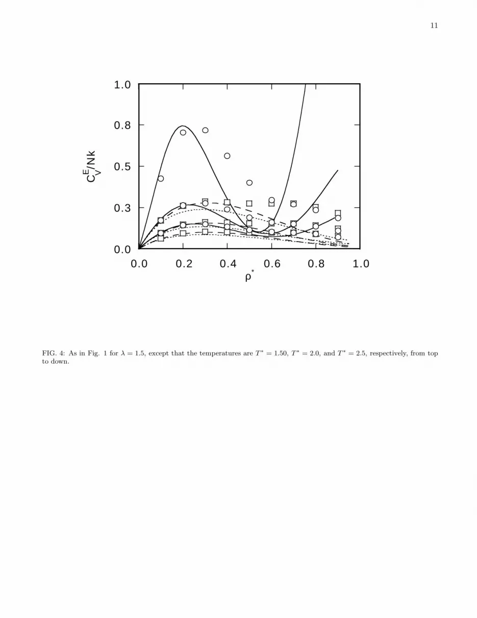
FIG. 1: Constant-volume excess heat capacity for a SW fluid with λ = 1.1 as a function of the reduced density ρ∗. Circles:simulation data from Table I for T ∗ = 0.7, T ∗ = 1.0, and T ∗ = 1.5, respectively, from top to down. Squares: values obtainedfrom Eq. (4) using the simulation data of F2 reported in [50]. Continuous curve: YAS model. Dashed curve: BH perturbationtheory in the local compressibility approximation. Dotted curve: BH perturbation theory in the macroscopic compressibilityapproximation.

9

0.0

0.2

0.4

0.6

0.8

1.0

0.0

Cv/N

k

0.2 0.4 0.6 0.8 1.0

E

ρ∗

FIG. 2: As in Fig. 1 for λ = 1.2, except that the temperatures are T ∗ = 1.0, T ∗ = 1.5, and T ∗ = 2.0, respectively, from top todown.

10

0.0

0.1

0.2

0.3

0.4

0.0

Cv/N

k

0.2 0.4 0.6 0.8 1.0

E

ρ∗

FIG. 3: As in Fig. 1 for λ = 1.3, except that the temperatures are T ∗ = 1.50, T ∗ = 2.0, and T ∗ = 2.5, respectively, from topto down.

11

0.0

0.3

0.5

0.8

1.0

0.0 0.2

CV

/Nk

0.4 0.6 0.8 1.0

E

ρ∗

FIG. 4: As in Fig. 1 for λ = 1.5, except that the temperatures are T ∗ = 1.50, T ∗ = 2.0, and T ∗ = 2.5, respectively, from topto down.