Embed Size (px)
Citation preview

INAUGURAL -DISSERTATIONzur
Erlangung der Doktorwurdeder
Naturwissenschaftlich-MathematischenGesamtfakultat
derRuprecht-Karls-Universitat
Heidelberg
vorgelegt vonDipl.-Phys. Daniel Andreas Finkaus Stuttgart-Bad Cannstatt
Tag der mundlichen Prufung: 23. Januar 2014


Improving the Selectivity of theISOLDE Resonance Ionization Laser Ion Sourceand In-Source Laser Spectroscopy of Polonium
Gutachter: Prof. Dr. Klaus Blaum
Prof. Dr. Selim Jochim


Zusammenfassung
Exotische Atomkerne weit ab der Stabilitat sind faszinierende Studienobjekte in vielenwissenschaftlichen Feldern, wie zum Beispiel der Atom-, Kern- und Astrophysik. Da essich bei diesen meist um kurzlebige Isotope handelt, ist es wichtig, deren Produktion mitder sofortigen Extraktion und Weiterleitung zu den Experimenten zu koppeln. Dies istdas Einsatzfeld des Isotopenseparators ISOLDE am CERN. Ein wichtiger Teil dieserGroßforschungsanlage ist die Resonanzionisations-Laserionenquelle (RILIS), da dieseein schnelles und hochselektives Mittel zur Ionisation der Reaktionsprodukte darstellt.Zusatzlich dient diese Technik auch als empfindlicher Aufbau fur die Entwicklung undVerbesserung von Elektronenanregungsschemata zur resonanten Laserphotoionisationund fur die Laserspektroskopie zur Untersuchung der Kernstruktur oder fundamentaleratomphysikalischer Eigenschaften.In der hier vorgelegten Arbeit werden alle diese verschiedenen Aspekte der RILIS be-handelt: Ein neuartiges Gerat zur Unterdruckung von oberflachenionisierten Kontami-nationen in RILIS Ionenstrahlen, bekannt als die Laserionenquelle und -falle (LIST),wurde an die ISOLDE angepasst, weiterentwickelt und charakterisiert; ein neues Elek-tronenanregungsschema zur Laserionisation von Kalzium wurde entwickelt; die Ionisa-tionsenergie von Polonium wurde mittels Rydbergspektroskopie mit hochster Prazisiongemessen; und schließlich fuhrte die erste Anwendung der hochselektiven LIST zurBestimmung von Kernstruktureigenschaften von 217Po mittels der Resonanzionisati-onsspektroskopie in der Ionenquelle.
Abstract
Exotic atomic nuclei far away from stability are fascinating objects to be studied inmany scientific fields such as atomic-, nuclear-, and astrophysics. Since these are oftenshort-lived isotopes, it is necessary to couple their production with immediate extrac-tion and delivery to an experiment. This is the purpose of the on-line isotope separatorfacility, ISOLDE, at CERN. An essential aspect of this laboratory is the Resonance Ion-ization Laser Ion Source (RILIS) because it provides a fast and highly selective means ofionizing the reaction products. This technique is also a sensitive laser-spectroscopy toolfor the development and improvement of electron excitation schemes for the resonantlaser photoionization and the study of the nuclear structure or fundamental atomicphysics.Each of these aspects of the RILIS applications are subjects of this thesis work: anew device for the suppression of unwanted surface ionized contaminants in RILIS ionbeams, known as the Laser Ion Source and Trap (LIST), was implemented into theISOLDE framework, further developed and characterized; a new electron-excitationscheme for the laser ionization of calcium was developed; the ionization energy of polo-nium was determined by high-precision Rydberg spectroscopy; and finally, the firstever on-line physics operation of the highly selective LIST enabled the study of nuclearstructure properties of 217Po by in-source resonance ionization spectroscopy.

Contents
List of figures ix
List of tables xi
Abbreviations and acronyms xiii
1 Introduction 1
I Theory and methods 5
2 Interaction of light with atoms 7
2.1 Electronic structure of atoms . . . . . . . . . . . . . . . . . . . . . . . . . . 72.1.1 One-electron systems . . . . . . . . . . . . . . . . . . . . . . . . . . . 7
2.1.2 Rydberg atoms . . . . . . . . . . . . . . . . . . . . . . . . . . . . . . 8
2.1.3 Multi-electron atoms . . . . . . . . . . . . . . . . . . . . . . . . . . . 10
2.2 The influence of the nucleus on the atomic structure . . . . . . . . . . . . . 11
2.2.1 Isotope shift . . . . . . . . . . . . . . . . . . . . . . . . . . . . . . . . 11
2.2.2 Hyperfine structure . . . . . . . . . . . . . . . . . . . . . . . . . . . . 14
2.3 Absorption and emission of light . . . . . . . . . . . . . . . . . . . . . . . . 16
2.3.1 The Einstein probability coefficients . . . . . . . . . . . . . . . . . . 16
2.3.2 Resonance excitation of atoms . . . . . . . . . . . . . . . . . . . . . 18
2.3.3 Spectral linewidth . . . . . . . . . . . . . . . . . . . . . . . . . . . . 182.3.4 Selection rules for allowed transitions . . . . . . . . . . . . . . . . . . 22
3 Radioactive ion beam production 23
3.1 The ISOL process at ISOLDE . . . . . . . . . . . . . . . . . . . . . . . . . . 25
3.1.1 The driver beam . . . . . . . . . . . . . . . . . . . . . . . . . . . . . 25
3.1.2 The target and front-end . . . . . . . . . . . . . . . . . . . . . . . . 25
3.1.3 The target materials . . . . . . . . . . . . . . . . . . . . . . . . . . . 27
3.1.4 The reaction mechanisms . . . . . . . . . . . . . . . . . . . . . . . . 29
3.1.5 Atom thermalization and transport . . . . . . . . . . . . . . . . . . . 29
3.1.6 Ionization processes . . . . . . . . . . . . . . . . . . . . . . . . . . . 293.1.7 Mass separation . . . . . . . . . . . . . . . . . . . . . . . . . . . . . 29
3.1.8 Production rates and total transport efficiency . . . . . . . . . . . . 30
3.2 Ionization mechanisms and ion sources at ISOLDE . . . . . . . . . . . . . . 31
3.2.1 Surface ionization . . . . . . . . . . . . . . . . . . . . . . . . . . . . 31
3.2.2 Electron impact ionization . . . . . . . . . . . . . . . . . . . . . . . . 33
iii

Contents
3.2.3 Resonance laser ionization . . . . . . . . . . . . . . . . . . . . . . . . 34
3.3 The Resonance Ionization Laser Ion Source at ISOLDE . . . . . . . . . . . 38
3.3.1 The ISOLDE RILIS setup . . . . . . . . . . . . . . . . . . . . . . . . 40
3.3.2 RILIS installations at off-line mass separators . . . . . . . . . . . . . 43
3.4 Ion beam detection at ISOLDE . . . . . . . . . . . . . . . . . . . . . . . . . 43
3.4.1 The ISOLDE tape station detector for beta- and gamma-decayingisotopes . . . . . . . . . . . . . . . . . . . . . . . . . . . . . . . . . . 43
3.5 Ion beam manipulation and transport usinglinear radiofrequency quadrupole ion guides . . . . . . . . . . . . . . . . . . 46
3.5.1 The ideal RFQ ion guide and mass filter . . . . . . . . . . . . . . . . 46
3.5.2 The real RFQ ion guide and mass filter . . . . . . . . . . . . . . . . 49
II Improvement of the selectivity of the Resonance Ionization LaserIon Source 51
4 The Laser Ion Source and Trap 53
4.1 LIST developments and achievements prior to this work . . . . . . . . . . . 54
4.1.1 First proposal . . . . . . . . . . . . . . . . . . . . . . . . . . . . . . . 54
4.1.2 LIST A . . . . . . . . . . . . . . . . . . . . . . . . . . . . . . . . . . 56
4.1.3 LIST B . . . . . . . . . . . . . . . . . . . . . . . . . . . . . . . . . . 56
4.1.4 LIST C . . . . . . . . . . . . . . . . . . . . . . . . . . . . . . . . . . 57
4.1.5 Objective of this thesis . . . . . . . . . . . . . . . . . . . . . . . . . . 58
4.2 The Laser Ion Source and Trap at ISOLDE . . . . . . . . . . . . . . . . . . 59
4.2.1 Specifications of LIST D, LIST 1 and LIST 2 . . . . . . . . . . . . . . 59
4.2.2 On-line runs and target specifications . . . . . . . . . . . . . . . . . 61
4.2.3 Implementation of the LIST at ISOLDE . . . . . . . . . . . . . . . . 62
4.3 Characterization of the performance of the LIST at ISOLDE . . . . . . . . 71
4.3.1 Different modes of operation . . . . . . . . . . . . . . . . . . . . . . 71
4.3.2 Parameters of the LIST performance and measurement methods . . 72
4.3.3 Transmission through the RFQ ion guide . . . . . . . . . . . . . . . 74
4.3.4 Surface ion suppression . . . . . . . . . . . . . . . . . . . . . . . . . 75
4.3.5 Laser ionization efficiency . . . . . . . . . . . . . . . . . . . . . . . . 80
4.3.6 Selectivity . . . . . . . . . . . . . . . . . . . . . . . . . . . . . . . . . 84
4.3.7 Comparison of lineshapes of resonances obtained in LIST mode, ionguide mode and normal RILIS operation . . . . . . . . . . . . . . . . 85
4.3.8 Time structure of LIST ion bunches . . . . . . . . . . . . . . . . . . 86
4.3.9 Improving the selectivity of the Laser Ion Source and Trap . . . . . 93
5 A new laser ionization scheme for calcium 95
5.1 Experimental setup . . . . . . . . . . . . . . . . . . . . . . . . . . . . . . . . 97
5.2 Analysis of the spectra . . . . . . . . . . . . . . . . . . . . . . . . . . . . . . 98
5.2.1 Alternative second intermediate states . . . . . . . . . . . . . . . . . 98
5.2.2 Excitation from the alternative intermediate state 1 . . . . . . . . . 100
5.2.3 Excitation from the alternative intermediate state 2 . . . . . . . . . 101
iv

Contents
5.3 The new laser ionization scheme for calcium . . . . . . . . . . . . . . . . . . 104
III In-source laser spectroscopy of polonium 109
6 Precision measurement of the ionization energy of polonium 1116.1 Experimental setup . . . . . . . . . . . . . . . . . . . . . . . . . . . . . . . . 1126.2 Rydberg scans . . . . . . . . . . . . . . . . . . . . . . . . . . . . . . . . . . 1146.3 Analysis of the Rydberg spectra . . . . . . . . . . . . . . . . . . . . . . . . 116
6.3.1 Identification of the subseries and peaks in the Rydberg scans . . . . 1166.3.2 Fitting . . . . . . . . . . . . . . . . . . . . . . . . . . . . . . . . . . . 118
6.4 Evaluation of Rydberg peak position . . . . . . . . . . . . . . . . . . . . . . 1196.4.1 Correction for the systematic shift of the spectra due to the DAQ
delay . . . . . . . . . . . . . . . . . . . . . . . . . . . . . . . . . . . . 1196.4.2 Evaluation procedure for the determination of the peak positions . . 120
6.5 Detailed analysis of the ionization energy of polonium . . . . . . . . . . . . 1226.5.1 Substitution of principal quantum number and quantum defect . . . 1236.5.2 Visualization of the Rydberg series . . . . . . . . . . . . . . . . . . . 1246.5.3 Determination of the ionization energy with respect to the second
excited state . . . . . . . . . . . . . . . . . . . . . . . . . . . . . . . 1256.5.4 Final result of the ionization energy of polonium . . . . . . . . . . . 1296.5.5 Assignment of subseries . . . . . . . . . . . . . . . . . . . . . . . . . 1296.5.6 Summary and discussion . . . . . . . . . . . . . . . . . . . . . . . . . 131
7 First experiments with the LIST: laser spectroscopy of neutron-richpolonium 1337.1 A brief review of the physics around the closed proton shell at Z =82 . . . . 1337.2 Status of the ISOLDE experiment IS456 . . . . . . . . . . . . . . . . . . . . 1357.3 Experimental setup and data taking . . . . . . . . . . . . . . . . . . . . . . 136
7.3.1 Measurement cycle . . . . . . . . . . . . . . . . . . . . . . . . . . . . 1377.4 The alpha-decay energy spectra . . . . . . . . . . . . . . . . . . . . . . . . . 139
7.4.1 Alpha-decay energy spectrum for mass A=217 . . . . . . . . . . . . 1397.4.2 Alpha-decay energy spectrum for mass A=218 . . . . . . . . . . . . 141
7.5 Laser resonance spectra and fitting . . . . . . . . . . . . . . . . . . . . . . . 1427.6 Results and discussion . . . . . . . . . . . . . . . . . . . . . . . . . . . . . . 144
7.6.1 Isotope shifts and mean square charge radii . . . . . . . . . . . . . . 1447.6.2 Electromagnetic moments . . . . . . . . . . . . . . . . . . . . . . . . 146
8 Summary and outlook 147
Appendices 151
A Fit results for the analysis of the systematic shift of the Rydberg scansdue to the DAQ delay 153
B Table of observed Rydberg levels of polonium 155
v

Contents
Bibliography 161
Acknowledgements 175
vi

List of figures
1.1 The chart of nuclei . . . . . . . . . . . . . . . . . . . . . . . . . . . . . . . . 2
2.1 Schematic of the hyperfine structure of an electronic level with I = 3/2 andJ = 2 . . . . . . . . . . . . . . . . . . . . . . . . . . . . . . . . . . . . . . . 14
2.2 An illustration of the three possible processes involved in a transition ofan electron between two electron levels with their corresponding Einsteinprobability coefficients . . . . . . . . . . . . . . . . . . . . . . . . . . . . . . 16
2.3 Lineshapes of power or Doppler broadened transitions . . . . . . . . . . . . 20
3.1 A sketch of the three different principles of radioactive ion beam facilities . 243.2 A drawing of the ISOLDE facility and its main components . . . . . . . . . 263.3 An illustration of the CERN accelerator complex with all major facilities . 273.4 A cross-sectional drawing of an ISOLDE target unit . . . . . . . . . . . . . 283.5 Theoretically expected production cross-sections at ISOLDE . . . . . . . . . 283.6 Surface ionization efficiencies in a hot cavity source . . . . . . . . . . . . . . 323.7 An illustration of different excitation schemes that may be applied for res-
onance laser ionization . . . . . . . . . . . . . . . . . . . . . . . . . . . . . . 343.8 A schematic of the first RILIS setup at ISOLDE . . . . . . . . . . . . . . . 393.9 A schematic layout of the most important elements of the RILIS setup . . . 403.10 The wavelength tuning range after the dual RILIS upgrade . . . . . . . . . 413.11 A schematic of the ISOLDE tape station . . . . . . . . . . . . . . . . . . . . 443.12 A schematic of the “Windmill” detector setup . . . . . . . . . . . . . . . . . 453.13 a) Geometry of the ideal, hyperbolic radiofrequency quadrupole. b) equipo-
tential lines in the x-z-plane. c) areas of x- and z-stability. . . . . . . . . . 473.14 Area of stability of first order of the ideal linear RFQ . . . . . . . . . . . . 483.15 Areas of stability for a linear RFQ in the V -U -space . . . . . . . . . . . . . 50
4.1 An illustration of the LIST target operated at the ISOLDE mass separatorfacility . . . . . . . . . . . . . . . . . . . . . . . . . . . . . . . . . . . . . . . 54
4.2 Illustration of the initial LIST design . . . . . . . . . . . . . . . . . . . . . . 554.3 A transverse schematic of the relative dimensions and alignments of the
RF-rods of LIST A and LIST B . . . . . . . . . . . . . . . . . . . . . . . . . 564.4 Schematic of LIST C . . . . . . . . . . . . . . . . . . . . . . . . . . . . . . . 574.5 A drawing of the LIST design and its most important parameters . . . . . . 604.6 Different stages of the assembly of the LIST 1 target . . . . . . . . . . . . . 604.7 Operating parameters of LIST target 1 and LIST target 2 . . . . . . . . . . 614.8 A schematic of the electronic supplies and the RF-transmission system from
the high voltage cage to the LIST . . . . . . . . . . . . . . . . . . . . . . . . 63
vii

List of figures
4.9 The radiation-hard coaxial copper line installed at the ISOLDE GPS front-end 64
4.10 Target assembly 1 with LIST 1 before the first on-line run in May 2011 . . . 64
4.11 On-line/off-line comparison of the calibration of the RF-amplitude as afunction of the RF-control voltage . . . . . . . . . . . . . . . . . . . . . . . 65
4.12 Photographs taken during the robot test of the LIST target 1 at the GPSfront-end . . . . . . . . . . . . . . . . . . . . . . . . . . . . . . . . . . . . . 67
4.13 Illustration of the remote control system of the LIST . . . . . . . . . . . . . 68
4.14 Laser ionization schemes for ytterbium, magnesium and polonium as usedduring the experiments with the LIST . . . . . . . . . . . . . . . . . . . . . 69
4.15 Schematic of the RILIS installation at the off-line mass separator for thetesting and characterization of the LIST with ytterbium . . . . . . . . . . . 70
4.16 Photograph of the laser installation at the off-line mass separator . . . . . . 70
4.17 LIST 1 repeller scan of 174Yb . . . . . . . . . . . . . . . . . . . . . . . . . . 72
4.18 Measurements of the ion transmission through the LIST RFQ ion guideconducted at the ISOLDE off-line separator with LIST 2 . . . . . . . . . . . 74
4.19 Surface ionized 48Ti ion current as a function of the repeller voltage mea-sured with LIST 1 under on-line conditions at ISOLDE . . . . . . . . . . . . 76
4.20 Wide range mass scans taken at the off-line separator with LIST 2 . . . . . 77
4.21 Ion rates of surface ionized 26Na and 46K and laser ionized 30Mg as a func-tion of the repeller voltage of the LIST 2 measured on-line at ISOLDE usinga tape station . . . . . . . . . . . . . . . . . . . . . . . . . . . . . . . . . . . 79
4.22 LIST 1 laser ionization efficiency measurement of ytterbium . . . . . . . . . 81
4.23 On-line measurement of the LIST 1 laser ionization efficiency of magnesium 82
4.24 Comparison of the resonance of the second intermediate step of the polo-nium scheme obtained in LIST mode, ion guide mode and in standardRILIS mode . . . . . . . . . . . . . . . . . . . . . . . . . . . . . . . . . . . . 85
4.25 Time structure of the LIST ion bunches of laser ionized 24Mg . . . . . . . . 87
4.26 Longitudinal potential inside the LIST . . . . . . . . . . . . . . . . . . . . . 88
4.27 Simplified model of the diverging atomic beam . . . . . . . . . . . . . . . . 91
4.28 Calculated LIST time structure . . . . . . . . . . . . . . . . . . . . . . . . . 91
4.29 Comparison of the measured and calculated appearance of the main peakin LIST time structure . . . . . . . . . . . . . . . . . . . . . . . . . . . . . . 91
4.30 LIST ion bunch time structure for the repeller voltage of Urep = 7 V fordifferent ranges of starting positions z0 . . . . . . . . . . . . . . . . . . . . . 91
4.31 Ion intensity of 212Fr in ion guide mode and LIST mode and 196Po in LISTmode as a function of the hot cavity temperature . . . . . . . . . . . . . . . 94
5.1 Previously used laser ionization schemes for calcium . . . . . . . . . . . . . 96
5.2 Target specifications for calcium on-line experiments at ISOLDE . . . . . . 97
5.3 Laser scans for the development of a new laser ionization scheme for calcium 99
5.4 Asymmetric autoionizing state of calcium with Fano fit . . . . . . . . . . . 102
5.5 The new laser ionization schemes for calcium . . . . . . . . . . . . . . . . . 105
5.6 Saturation curves for the atomic transitions used in the new calcium schemes106
viii

List of figures
6.1 a) Operational parameters of the ISOLDE target used during the measure-ments of the ionization energy. b) Ionization scheme for polonium as usedfor the Rydberg spectroscopy. . . . . . . . . . . . . . . . . . . . . . . . . . . 113
6.2 The three Rydberg scans of 208Po, obtained during the measurement cam-paign. . . . . . . . . . . . . . . . . . . . . . . . . . . . . . . . . . . . . . . . 115
6.3 Rydberg spectrum recorded in scan 3 with the multi-peak fit to all well-resolved peaks . . . . . . . . . . . . . . . . . . . . . . . . . . . . . . . . . . . 117
6.4 A representative example of the determination of the systematic shift dueto the DAQ delay . . . . . . . . . . . . . . . . . . . . . . . . . . . . . . . . . 119
6.5 a) The excitation energy of the well-resolved peaks of series Σ as a functionof the group number g. b) Remainder of the quantum defect δ′ as a functionof the minimum principle quantum number n′ . . . . . . . . . . . . . . . . . 124
6.6 Fit of the Rydberg formula to the combined series of Θ, ΠΘ and ΠΘΣΩΦfrom method 1. . . . . . . . . . . . . . . . . . . . . . . . . . . . . . . . . . . 126
6.7 Residuals for each Rydberg series obtained by a global fit method 3 . . . . . 1286.8 Histograms of the distributions of the quantum defects of the Rydberg levels
of polonium and the electron levels found in literature for sulphur, seleniumand tellurium . . . . . . . . . . . . . . . . . . . . . . . . . . . . . . . . . . . 130
7.1 Changes in mean square radii for even-Z isotopes in the lead-region . . . . 1347.2 Laser ionization scheme for polonium in-source spectroscopy and a schematic
of the hyperfine structure . . . . . . . . . . . . . . . . . . . . . . . . . . . . 1367.3 Sequence of logical steps to validate the start of the measurement cycle for
laser spectroscopy of polonium. . . . . . . . . . . . . . . . . . . . . . . . . . 1387.4 Measurement cycle for laser spectroscopy of polonium . . . . . . . . . . . . 1387.5 “Windmill” α-decay energy spectra of the polonium laser scans for mass
A = 217 and mass A = 218. . . . . . . . . . . . . . . . . . . . . . . . . . . . 1407.6 Laser spectra of 216,217,218,219Po and fits . . . . . . . . . . . . . . . . . . . . 1437.7 Changes in mean square radii for polonium isotopes . . . . . . . . . . . . . 145
ix

List of figures
x

List of tables
3.1 Operating parameters of the RILIS pump lasers . . . . . . . . . . . . . . . . 423.2 Typical parameters of the tunable RILIS lasers . . . . . . . . . . . . . . . . 42
4.1 LIST suppression factors for stable and radioactive isotopes . . . . . . . . . 784.2 LIST loss factors LLFs and laser ionization efficiencies ε measured for with
LIST 1 and LIST 2 . . . . . . . . . . . . . . . . . . . . . . . . . . . . . . . . 834.3 Comparison of the different LIST parameters obtained on-line by LIST and
LIST 2 . . . . . . . . . . . . . . . . . . . . . . . . . . . . . . . . . . . . . . . 85
5.1 Transitions from the 4p6s 1S0 intermediate state to autoionizing states incalcium . . . . . . . . . . . . . . . . . . . . . . . . . . . . . . . . . . . . . . 101
5.2 Transitions from the 3p64p2 1D2 intermediate state to autoionizing statesin calcium . . . . . . . . . . . . . . . . . . . . . . . . . . . . . . . . . . . . . 103
5.3 Saturation parameters of transitions of new laser ionization scheme for calcium107
6.1 Experimental values and theoretical predictions for the first ionization en-ergy of polonium available prior to the work described in this thesis . . . . 112
6.2 Scanning speeds for the obtained Rydberg spectra and estimated resolution 1146.3 Characteristics of the three different Rydberg scans and the fitting results . 1186.4 Details of the systematic shift due to the time delay in the DAQ . . . . . . 1206.5 Results of the separate Rydberg fits to each individual Rydberg series and
weighted average of the ionization energy . . . . . . . . . . . . . . . . . . . 1266.6 Quantum defects obtained by the global fit of the Rydberg formula to all
series with a shared ionization energy with respect to the second excitedstate, W ′′lim,global. . . . . . . . . . . . . . . . . . . . . . . . . . . . . . . . . . . 127
6.7 Comparison of the ionization energy of polonium obtained during the workon this thesis, at TRIUMF and by recent theoretical calculations with theliterature values . . . . . . . . . . . . . . . . . . . . . . . . . . . . . . . . . . 132
7.1 Isotope shifts and mean square charge radii of 216,217,218Po . . . . . . . . . . 144
A.1 Fit results for the analysis of the systematic DAQ-shift of the Rydberg scans154
B.1 Observed Rydberg levels of polonium . . . . . . . . . . . . . . . . . . . . . . 155
xi

List of tables
xii

Abbreviations and acronyms
AC . . . . . . . Alternating currentAIS . . . . . . Auto-ionizing stateAl . . . . . . . . AluminiumAt . . . . . . . . AstatineAu . . . . . . . GoldBi . . . . . . . . BismuthBN . . . . . . . Boron nitrideCa . . . . . . . CalciumCERN . . . . European Organization for Nuclear ResearchCPO . . . . . Charged Particle Optics c©
Cs . . . . . . . . CesiumCW . . . . . . Continuous wave (laser)DAQ . . . . . Data-acquisitionDC . . . . . . . Direct currentDCM . . . . . 4-dicyanomethylene-2-methyl-6-p-dimethylaminostyryl-4H-pyranDM . . . . . . Droplet modelEBIS . . . . . Electron beam ion sourcesEOM . . . . . Equation of motionFC . . . . . . . Faraday cupFiS . . . . . . . Field shiftFr . . . . . . . . FranciumFS . . . . . . . Fine structureGANIL . . . Grand Accelelerateur National d’Ions Lourds, Caen, FranceGPS . . . . . . General Purpose SeparatorGSI . . . . . . Gesellschaft fur Schwerionenforschung GmbH, Darmstadt, GermanyHFS . . . . . . Hyperfine structureHg . . . . . . . MercuryHRS . . . . . High Resolution SeparatorHV . . . . . . . High voltageIE . . . . . . . . Ionization energyIG . . . . . . . . Ion guideIP . . . . . . . . Ionization potentialIR . . . . . . . . InfraredIRIS . . . . . . Investigation of Radioactive Isotopes on Synchrocyclotron, Gatchina, RussiaIS . . . . . . . . Isotope shiftISOL . . . . . Isotope separator on-lineLC . . . . . . . Inductor-capacitorLIST . . . . . Laser Ion Source and Trap
xiii

List of tables
LLF . . . . . . LIST loss factorLQF . . . . . LIST quality factorLSF . . . . . . LIST suppression factorMCP . . . . . Micro channel plateMg . . . . . . . MagnesiumMR-TOF . Multi-reflection time-of-flightMS . . . . . . . Mass shiftNa . . . . . . . SodiumNB . . . . . . . Narrow bandNBI . . . . . . Niels Bohr Institute of PhysicsNd:YAG . . Neodymium-doped yttrium aluminum garnetNMS . . . . . Normal mass shiftOBE . . . . . Optical Bloch equationsPb . . . . . . . LeadPIPS . . . . . Passivated implanted planar siliconPNPI . . . . Petersburg Nuclear Physics InstitutePo . . . . . . . Poloniumpp . . . . . . . . Peak to peakPSB . . . . . . Proton Synchrotron BoosterPt . . . . . . . . PlatinumR6G . . . . . . Rhodamine 6GRB . . . . . . . Rhodamin BRe . . . . . . . RheniumRF . . . . . . . Radio-frequencyRFQ . . . . . Radio-frequency quadrupoleRIB . . . . . . Radioactive ion beamRIKEN . . . Rikagaku Kenkyujo; Japanese for: the institute of physical and chemical
researchRILIS . . . . Resonance Ionization Laser Ion SourceRn . . . . . . . RadonS . . . . . . . . . SelectivityS . . . . . . . . . SulphurSC . . . . . . . supercycleSe . . . . . . . . SeleniumSiC . . . . . . . Silicon carbideSMS . . . . . Specific mass shiftSn . . . . . . . . TinTa . . . . . . . . TantalumTe . . . . . . . . TelluriumTi . . . . . . . . TitaniumTi:Sa . . . . . Titanium:sapphireTiO . . . . . . Titanium oxideTl . . . . . . . . ThalliumTm . . . . . . . ThuliumTRIUMF . Tri University Meson Facility, National laboratory for particle and nuclear
xiv

List of tables
physics, Vancouver, CanadaUC2 . . . . . . Uranium carbideUV . . . . . . . UltravioletW . . . . . . . . TungstenWM . . . . . . WavemeterYb . . . . . . . Ytterbium
xv

List of tables
xvi

1 Introduction
From the perspective of our habitable corner of the universe, i.e. the Earth, matter seemsto be fairly stable. Yet, our existence relies on so-called “exotic atomic nuclei”, as thesenuclei are often a stepping stone in the nucleosynthesis processes, responsible for the cre-ation of the elements. Exotic nuclei are radioactive because they have an unusual ratioof protons and neutrons compared to that of the stable nuclei that surround us. Many ofthese exist only for a very short time in our sun or in extreme conditions far away in theuniverse such as neutron stars or supernovae. Besides their fundamental role in nature,they are extremely interesting objects to be studied in many fields from atomic to nuclearphysics and from solid-state to medical and biophysics.
Very few exotic nuclei occur naturally and most of our knowledge about the propertiesof these short-lived and volatile objects stems from their artificial production. To datemore than 3000 nuclei have been discovered of which, to put this into a context, only 284are stable. They can be illustrated in the chart of nuclei, as shown in Figure 1.1, whereeach combination of a number Z of protons with a number N of neutrons represents onespecific nucleus. The nuclear and atomic properties of these isotopes∗ may vary greatlyand their theoretical description still remains an extremely challenging task in nuclearphysics, despite the power of modern computers. Nuclei, heaver than the lightest hy-drogen isotope 1H, are many-body systems, and except for the very lightest nuclei, anab initio calculation, i.e. a calculation relying on the fundamental forces, is impossible.It is therefore a common approach to search for macroscopic trends and patterns acrossthe nuclear chart. The most obvious observation is the line of stable nuclei, known asthe valley of stability. Another macroscopic observation is the unusual stability of nucleiconsisting of certain numbers of protons or neutrons, known as the magic numbers: 2, 8,20, 28, 50, 82 and 126 (see Figure 1.1). A microscopic model that is able to reproducethe magic numbers is the nuclear shell model [73], which, in a simplified picture, assumesthe nucleons (protons and neutrons) to be arranged into energy shells within the nucleus,analogous to the concept of electron shells in atomic physics. Nevertheless, it is now clearthat these concepts need to be refined for isotopes far away from stability. Magic numbers,for instance, are known to disappear for imbalanced proton and neutron numbers, whilenew ones may appear[82, 174]. The recently discovered new magic number at N = 34 inthe neutron-rich isotope 54Ca is a good example [165]. However, the study of these exoticnuclei is an experimental challenge due to their short half-lives of typically of the orderof seconds to milliseconds. A high production yield and fast separation, extraction andtransport to the experimental setup is therefore essential.
∗Isotopes are atoms of the same element (same proton number, Z), but different number of neutrons(neutron number, N).
1

1 Introduction
N
Z
Chart of nuclei
N=2
Z=2
8
20
28
508
2028
50
82
128
82
In-source resonanceionization spectroscopy of polonium
New laser ionization scheme for calcium
Figure 1.1: The chart of nuclei (x-axis neutron number N, y-axis proton number P) and theregions of interest for this thesis. The red solid lines indicate elements, for which RILISlaser ionization schemes exist, while magic numbers are indicated with the dashed lines.Different tones of gray correspond to different radioactive decay channels.
One type of apparatus that is able to address all these demands is the “radioactive ionbeam facility” [75], whose proof of principle was demonstrated at the Niels Bohr Instituteof Physics (NBI) in Copenhagen, Denmark [91]. One prominent example is the ISOLDEfacility [85] at the European Organization for Nuclear Research (CERN) in Switzerland,where the results, reported in this thesis, were obtained. The ISOLDE radioactive ionbeam facility is based on the Isotope Separator On-Line (ISOL) process, where an accel-erator is combined with a mass separator to irradiate a suitable target material with ahigh-energy driver beam to produce a multitude of different nuclei of all kinds and masses.These are almost instantly released from the target, ionized and mass separated by mag-nets to be sent as ion beams to the experiments. In the fastest cases, all these events arehappening in a time-span of only a few milliseconds, as it was for instance demonstratedfor 14Be, which has a half-life of only 4.35 ms [84]. For radioactive ion beam production,one of the most important and difficult aspects is the ionization process as all experimentson exotic nuclei often rely on highest beam purity and intensity.
2

The ion source, which most closely meets these requirements is the Resonance IonizationLaser Ion Source (RILIS). First design studies were presented by V.S. Letokhov and V.I.Mishin [103] in 1984 and by H.-J. Kluge et al. in 1985 [90] and for the first time op-erated by Alkhazov et al. [1, 2] at the IRIS∗ facility at the Petersburg Nuclear PhysicsInstitute (PNPI) in Gatchina, Russia in 1989. The RILIS is based on the principle ofthe selective laser photoionization [102], where several lasers are wavelength-tuned to theelement-unique electron transitions of the atom for the stepwise excitation of the weakestbound electron above the ionization threshold. By principle, this technique is absolutelyelement-selective and ionization efficiencies of more than 10 % are possible. The RILISat ISOLDE [57] was operated for the first time in 1992 [119] and has now become themost often used ion source at ISOLDE. In total, laser ionization schemes for more than30 elements were developed and RILIS installations are operated at many radioactive ionbeam facilities worldwide. For a comprehensive discussion of the developments in this fieldduring the last decades, I refer to the review article of V.N. Fedosseev, Yu. Kudryavtsevand V.I. Mishin [58]. The regions on the nuclear chart, which are currently accessible bythe RILIS technique are indicated by the red bars in Figure 1.1 and the expansion of theavailable elements is subject to ongoing research.
Despite the element-selective principle of the RILIS, the beam purity may be reduceddue to ionization processes which take place in parallel. This is especially the case forthe ISOLDE RILIS, where the laser photoionization takes place in a hot metallic cavity.The hot cavity also provides the conditions for the process of surface ionization, where anatom may lose an electron during the contact with a hot surface. This process can be veryefficient for elements with low ionization energies, such as alkali or alkaline earth metals.The resolution of the separator magnets is not sufficient to efficiently suppress isobars (i.e.isotopes of the same mass, but from different elements) and thus, the selectivity of theRILIS, defined as the ratio of the ion beam intensity of the isotope of interest over theion beam intensity of the isobaric contaminants, may be greatly reduced. In some cases,the contamination is so strong that foreseen experiments are hampered or may even beharmed. An important aspect of the technical developments for the RILIS are thereforeaimed at improving the selectivity.
In addition to providing radioactive ion beams with high intensities and high purity to theexperiments at ISOLDE, the RILIS is also a powerful and sensitive resonance ionizationspectroscopy tool for ionization scheme development, fundamental atomic physics experi-ments and nuclear structure studies [1].
In this thesis all of these aspects of RILIS operation are performed: improvement of the se-lectivity of the RILIS by implementing a new device, the Ion Source and Trap (LIST), intothe ISOLDE framework; laser ionization scheme development for calcium; determinationof the ionization energy for polonium; and in-source resonance ionization spectroscopy ofneutron-rich polonium.
∗IRIS is the abbreviation for “Investigation of Radioactive Isotopes on Synchrocyclotron”.
3

1 Introduction
The outline of the thesis is as follows:Part I, “Theory and Methods”, aims at introducing all theoretical and experimental as-pects necessary for the understanding of the experiments and results reported in thisthesis. Chapter 2, “Interaction of light with atoms”, describes the electronic structure ofthe atoms as well as different aspects of laser spectroscopy. In Chapter 3, the relevanttheoretical and experimental principles of the “Radioactive ion beam production” are in-troduced: the ISOL process, the ionization processes, the RILIS setup and ion detectionmethods, and the principles of radiofrequency ion guides.Part II, “Improvement of the selectivity of the resonance ionization laser ion source”, de-scribes two approaches for the improvement of the selectivity. Chapter 4 reports on thetechnical implementation into the ISOLDE framework, development work and experimen-tal characterization of a device known as the Laser Ion Source and Trap (LIST). TheLIST is a novel type of ion source for ISOLDE and was proposed by H.-J. Kluge and firstdescribed by K. Blaum et al. in 2003 [14, 176]. It consists in its present form of an elec-trostatic surface ion repelling electrode and a radiofrequency quadrupole (RFQ) ion guidelocated immediately downstream of the cavity. The problem of the unwanted isobaric con-tamination in RILIS beams is tackled directly as ions created before the LIST structureare blocked by the positively charged repeller electrode whilst neutral atoms may enter thelaser/atom interaction region inside the RFQ, where the element-selective resonance ion-ization takes place. After development work at the Mainz University [14, 74, 152, 176, 178]prior to the work described in this thesis, extensive off-line tests and the first two on-lineruns at ISOLDE allowed the characterization and the improvement of the performancein terms of selectivity and ionization efficiency. Following these, a first on-line physicsexperiment to use the LIST took place at ISOLDE/CERN in September 2012.In Chapter 5, a new laser ionization scheme for calcium will be introduced that increasesthe laser ionization efficiency by a factor of about 20 compared to the previous existinglaser ionization scheme. During the on-line period in 2012, the new laser ionization schemefor calcium was in use for two experiments [11, 96] and enabled the study of the exotic53,54Ca isotopes for the first time by the ISOLTRAP experiment [177].Part III, “In-source laser spectroscopy of polonium”, covers fundamental atomic and nu-clear structure studies of polonium isotopes. Chapter 6, is about the “precision measure-ment of the ionization energy of polonium”. Laser scans over the ionization energy ofpolonium revealed a rich spectrum with many Rydberg states (highly excited electronstates), which enabled the determination of the ionization energy with more than 50 timeshigher precision than the value known from literature [149]. Chapter 7 is devoted to thein-source laser spectroscopy of polonium isotopes using the RILIS. This is a fitting con-clusion to the work described in this thesis since the isotope of interest, 217Po, was onlyaccessible due to the strong suppression of francium isotopes achieved by using the LIST.The results obtained give a valuable insight into the evolution of nuclear structure for thisregion of the nuclear chart, whilst the success of the experiment is a demonstration ofthe LIST as a viable ion source option for high purity ion beam production and in-sourceresonance ionization spectroscopy.
4

Part I
Theory and methods
5


2 Interaction of light with atoms
This chapter describes the basic principles of the interactions between light and atoms,which are essential to understand the experimental methods and physics described in thisthesis. The basic concept of atomic physics is briefly introduced by the most simple atomicstructure, the one-electron systems. A similar behavior of the energy levels is observed inso-called Rydberg-atoms, whose spectra can be described by the Rydberg-Ritz formula. Itwill be used to determine the ionization potential of polonium later in this work. Buildingupon the discussion of the one-electron system, the fine-structure of multi-electron atomsand important parameters such as the quantum numbers that describe the atomic structureare summarized. One important part of this work is the observation and description of thehyperfine-structures and isotope shifts of exotic polonium nuclei. These phenomena aredescribed in the last part of Section 2.1, which deals with atomic spectra. In Section 2.3,the fundamental principles of the emission and absorption of light are discussed since theyare essential to the understanding of the technique of laser spectroscopy. The chapter endswith the fundamental formulae which describe the atomic spectral lineshapes and widths.The discussion follows the descriptions given in [42, 48, 164, 167], if not otherwise identified.
2.1 Electronic structure of atoms
2.1.1 One-electron systems
The precise calculation of the discrete energy levels of the two body system of one-electronatoms, such as the hydrogen atom (H) and hydrogen-like atoms (He+, Li++, etc.), isone of the greatest achievements of quantum physics theory. In fact, these are the onlyatomic systems in non-relativistic quantum theory, which have an exact solution and theytherefore serve as an important basis for the further understanding of the electron-structureof multi-electron atoms.A one-electron atom consists of an electron with charge −e and mass me and an atomicnucleus with charge Ze and mass M . Its stationary states are solutions of the time-independent Schrodinger equation:
HΨ(r) = E Ψ(r) , (2.1)
where H = Hkin +HCoulomb is the Hamilton energy operator and Ψ(r) the eigenfunctionof the one-electron atom as a function of the position variable r∗. The calculation can besimplified by placing the nucleus into the origin of the two-body system and by replacingme with the reduced mass µ = meM/ (me +M) to study the relative motion of theelectron to the nucleus. Then, the Schrodinger equation of the one-electron atom writes
∗In this work, vectors are denoted in bold letters for improved readability.
7

2 Interaction of light with atoms
as follows: (− ~2
2µ∇2 − Ze2
4πε0r
)Ψ(r) = E Ψ(r) . (2.2)
The spherical symmetry of the Coulomb potential suggests the use of spherical coordinates(r, θ, and φ), which leads after transformation of the Laplace operator ∇2 to a separationansatz since the Coulomb potential depends solely on r:
Ψ (r, θ, φ) = R(r)Y (θ, φ) . (2.3)
Solutions to the separable terms in Equation. 2.3 are the radial eigenfunctions Rn,l andthe spherical harmonics Y m
l , which introduce the quantum numbers: principal quantumnumber n, angular momentum l and magnetic quantum number m. The energy eigenvaluesEn are then given by
En = −1
2
e4µ
(4πε0)2 ~2
Z2
n≡ −RM
Z2
n2, (2.4)
where RM is the Rydberg constant of the one-electron system with reduced mass µ. RMcan also be rewritten as
RM = R∞µ
me= R∞
M
M +me(2.5)
where RM is the fundamental Rydberg constant R∞ = 109737.32 cm−1. En is the energyof the excited state with principal quantum number n below the ionization limit, defined byElim = 0 cm−1. The resulting energy levels are therefore negative. In atomic spectroscopyhowever, it is common practice to note the electron levels as the excitation energy Wn,defined as the energy of the excited level to the ground state, Wn = En − Elim. Theminimum energy that is required to remove one electron from the atom with respect tothe lowest energy configuration of the electrons (the atomic ground-state) is given byWlim = IE = Elim − E0 = |E0| = eφ1 and is called the first ionization energy (IE )and φ1 the first ionization potential (IP)∗. This work mainly discusses the case, when oneelectron is removed from the neutral atom. Therefore, these measures are simply calledthe ionization energy and the ionization potential in the following.The energy eigenvalues En describe the gross structure of the one-electron system and donot depend on the quantum numbers l and m. The energy level En of the one-electronsystem is therefore n2-fold degenerate. For a full description of the one-electron system,Equation (2.2) needs to be further corrected for relativistic effects (fine structure, FS andthe interaction of the electron with the nucleus (hyperfine structure, HFS, which leads to asplitting and shifting of the degenerate states. These effects are discussed for multi-electronatoms later in this chapter.
2.1.2 Rydberg atoms
In the first order for any multi-electron atom, the distribution of the states with a highprincipal quantum number, n is analogous to that of the one electron atom. The energy of
∗In literature, the usage of these terms is not always consistent and often the term ionization potentialrefers to the ionization energy. In this work, the term ionization energy is used.
8

2.1 Electronic structure of atoms
these so-called Rydberg states converge to the ionization limit or to ionic states similarlyto the excited states of the one-electron atom described by Equation (2.4).This similarity can be qualitatively explained by the screening of the total nuclear chargeZ by the N − 1 inner electrons (N = Z for neutral atoms, N − 1 for a singly ionized ion,etc.) of the atom. Thus, the effective charge acting on the highly excited outer electronis ζ = Z − (N − 1) and the energy of the excited state can be calculated in first order by
En = −RMζ2
n2. (2.6)
However, there is a non-negligible probability that the electron penetrates the inner core ofthe electron shell. In this case, screening is not complete and the outer electron interactswith the larger charge of the nucleus and the inner N−1 electrons. The shift of the energylevels compared to the one-electron atom can be described by correcting the principalquantum number n through the use of the quantum defect δn,l and an effective quantumnumber n∗ = n − δn,l. The energy levels in the Equation (2.6) are then given by
En = − RMζ2
(n− δn,l)2 = −RMζ2
(n∗)2 . (2.7)
The quantum effect varies with the angular momentum l due to the l-dependent pene-tration of the inner core. The probability to find an s-electron (l = 0) close to the innercore is higher than for electrons with larger l and thus, the s-electron will experience anuclear potential that shows a stronger deviation from the point-like Coulomb potentialof the one-electron atom.The quantum defect δ is constant for high principal quantum numbers n and Equation (2.7)is a good approximation of the highly excited Rydberg states close to the ionization po-tential. However, the quantum defect shows also a small dependency on the principalquantum number n, which gets stronger for smaller n. These higher order effects can bedescribed by the Ritz expansion:
δ = δ0 +δ1
n∗+
δ2
(n∗)2 + · · · , (2.8)
which can be approximated in the second order to
δ(n) = A+B
(n−A)2 , (2.9)
where A and B are newly introduced constants to take account for the n-dependency ofδ(n).Combining Equation (2.7) and Equation (2.9) leads to the the Rydberg-Ritz formula [83]:
En = − RMζ2(
n−A+ B(n−A)2
)2 . (2.10)
9

2 Interaction of light with atoms
The Rydberg formula and Rydberg-Ritz formula (Equations 2.7 and 2.10) can be used todetermine the ionization energy of an element very precisely, provided that the energiesof several members of a Rydberg series (Energy levels En with same quantum defect δn,l)are known.
2.1.3 Multi-electron atoms
The Hamilton operator of a multi-electron atom with N electrons and a nuclear charge ofZe takes the form
H =
N∑i=1
(− ~
2m∇2i −
Ze2
4πε0ri
)+
N∑i<j=1
e2
4πε0rij+
N∑i=1
ξ(ri) (li · si) . (2.11)
The first term in Equation (2.11) describes the kinetic energy and interaction of eachelectron with the Coulomb potential of the nucleus. The second term describes the con-tribution to the potential energy from the electrostatic repulsion between the electrons.The third term is due to the interaction of the intrinsic electron spin s (quantum numberss = ±1
2) with the dipole moment due to its orbital angular momentum l and is known asthe spin-orbit interaction.There exists no exact solution for the Schrodinger equation of multi-electron atoms andthe wave-functions have to be approximated. However, it turns out that the non-centralelectrostatic interaction depends on the total orbital angular momentum L =
∑Ni = li
and the total spin S =∑N
i = si. Their associated quantum numbers L, S, ML, and MS
replace the individual quantum numbers ml and ms of each electronThe spin-orbit interaction leads to a splitting of the formerly degenerate gross-structureinto separated energy-levels, called the fine structure. The appropriate method of eval-uating the spin-orbit interaction depends on the relative interaction strength of the in-dividual electron spin with its own magnetic dipole moment. Two limiting cases can bedistinguished: the pure LS-coupling, which is a good description for light atoms and thejj -coupling, which occurs in heavier atoms.
LS-coupling
In case of LS -coupling, the interaction between the orbital moments Wli,lj = aijlilj andbetween the spin magnetic moments Wsi,sj = bijsisj are strong compared to the inter-action between the orbital magnetic moment and the spin magnetic moment of the sameelectron ei: Wli,si = ciilisi. Then, the orbital magnetic moments and spin magneticmoments couple to the total angular momentum J = L + S. It has the correspondingquantum number J with values of
J = L+ S, L+ S − 1, · · · , |L− S| . (2.12)
The value of J is then given by |J | = ~√J (J + 1). Pure LS -coupling results in a well
separated fine splitting of the energy levels of the one-electron energies E(n,L, S), forwhich the individual fine structure component is then denoted as n2S+1LJ .
10

2.2 The influence of the nucleus on the atomic structure
jj-coupling
The pure jj -coupling is the opposite extreme, where the interaction between the orbitalmagnetic moment and the spin magnetic moment of the same electron Wli,si is dominat-ing. Then the angular momentum li and spin si of each electron couple to the resultantangular momentum ji = li + si and form the total angular momentum J =
∑Ni=1 ji. In
this case, the fine splitting is no longer well resolved in the spectrum and L and S cannotbe treated as a “good” quantum number. The only remaining “strong” quantum numberto describe the spectrum is the total angular momentum J.
2.2 The influence of the nucleus on the atomic structure
Such is the precision of laser spectroscopy measurements that perturbations or splittingsof the atomic energy levels due to the non-point like nature of the nucleus may be resolved,even though the correction on the energy levels are orders of magnitudes smaller than thecontributions of the gross and fine structure. Two effects are of importance in this work:a small shift of the fine structure energy levels for different isotopes of the same element,called the isotope shift (IS), and a further splitting of the fine structure into the so-calledhyperfine structure. The isotope shift is caused by the nuclear mass, volume and chargedistribution. The hyperfine structure is the result of the interaction of the higher ordercomponents of the electromagnetic multipole field with the electrons.The measurement of the isotope shift and the hyperfine structure are important observ-ables in laser spectroscopy because they contain information related to the nuclear chargedistribution and moments.
2.2.1 Isotope shift
The mass and the charge distribution inside the nucleus changes along an isotope chaindue to the different number of neutrons. This shifts the energy levels of the atom, as theinteraction between the electrons and the nucleus is affected. The total shift of one finestructure energy level Ei between two isotopes with mass mass MA and MA′ is called theisotope shift and is defined as
∆EIS,i = EA′
i − EAi . (2.13)
Two effects are responsible for the isotope shift: the change of the kinetic energy of theelectrons due to the change of the finite nuclear mass (mass shift, MS) and the change ofthe Coulomb potential due the non-point-like structure of nucleus, which changes volumeand shape (field shift, FiS):
∆EAA′
IS,i = ∆EA′
MS,i + ∆EA′
FiS,i . (2.14)
Mass shift
The mass shift, which dominates the isotope shift of light nuclei (Z < 30), is caused bythe difference in kinetic energy ∆EAA
′kin of the electrons of two isotopes with mass number
11

2 Interaction of light with atoms
A and mass number A′, respectively. It can be calculated by
∆EAA′
kin,i = EA′
kin,i − EAkin,i =1
2
MA′ −MA
MA′MA′
N∑i=1
p2i +
N∑i>j
pipj , (2.15)
where p is the momentum of the electrons. The two terms in Equation (2.15) can betreated separately: term one describes the sum over the change in the single electronenergies due to the change in mass and is called the normal mass shift (NMS), while thesecond term describes the changes in the electron-electron correlations and is called thespecific mass shift (SMS). It follows that NMS and SMS have the same mass dependencyand the total mass shift can be written as:
∆EAA′
MS,i = ∆EAA′
NMS,i + ∆EAA′
SMS,i = (KNMS,i +KSMS,i)MA′ −MA
MAMA′, (2.16)
where KNMS,i is calculated easily by me · EFiS,i. KSMS,i is not analytically solvable formulti-electron systems and have to be derived by theoretical calculations [33]. However,the calculations are very difficult to obtain and therefore limit the accuracy of the infor-mation derived from the isotope-shift measurements.
Field shift
The field shift ∆EA′
FiS dominates the isotope shift of heavier elements since the mass shiftis approximately inversely proportional toMAMA′ . It can be written as
∆EAA′
FiS = Fi · λAA′
= Ei · f(Z) · λAA′ , (2.17)
where Ei is the electronic factor, f(Z) is a function which takes into account the finitesize of the nucleus and λAA
′is the change of the nuclear charge parameter. The electronic
factor is proportional to the change of the total non-relativistic electron-charge density atthe nucleus ∆ |Ψ(0)|2 and is given by
∆EAA′
FiS =πa0
Z∆ |Ψ(0)|2 . (2.18)
The determination of the electronic factor E for heavier isotopes relies on empirical data,since its precise calculation, based only on fundamental interactions, is only possible foratomic systems with up to three electrons [65, 76]. The function f(Z) increases with Zand takes into account the finite nuclear charge distribution and corrects the electronicfactor Ei for relativistic effects. The nuclear charge parameter λAA
′can be expressed as
a power series of the changes in the mean charge radius δ〈r2i〉AA′ :
λAA′
= δ〈r2〉AA′ +∞∑i=2
CiC1〈r2i〉AA′ , (2.19)
12

2.2 The influence of the nucleus on the atomic structure
where Ci are the Seltzer-coefficients. They can be found in literature for most elementstogether with the relations between the higher order of the changes in the mean squarecharge radius δ〈r2i〉AA′ and the mean square charge radius 〈r2〉AA′ [161]. The Seltzercoefficients are decreasing rapidly with higher orders and thus, higher powers of the meansquare radii do not contribute much. In case of polonium, literature values for Ci andδ〈r2i〉AA′
δ〈r2〉AA′ lead to λAA′ ≈ 0.932 · δ〈r2〉AA′ .
Obtaining nuclear properties from isotope shift measurements
A careful analysis of the isotope shift gives access to the changes in the mean-squarecharge radius δ〈r2〉AA′ . Its accuracy is limited by the precision of the determination ofthe constants KNMS, KSMS, E, and f(Z). As has been discussed, the electronic factor andthe value of KSMS rely on atomic calculations or supplementary experimental data. Inheavier nuclei, the mass shift becomes less important since it is proportional to 1
AA′ . Onthe other hand, the field shift is proportional to Z, which makes the determination of thechanges in the mean square charge radius δ〈r2〉AA′ easier for heavier nuclei such as polo-nium. However, an alternative way to determine the electronic factor E and the specificmass constant KSMS is the so-called King plot, if additional independent information (e.g.from e− scattering, muonic decay, or K x-ray experiments) about isotope shifts in othertransitions is available [88]. It allows a separation of the field and mass shifts and givesinformation about the consistency of the data. In preparing a King plot, the isotope shiftsof a measured transition and a reference transition are put into relation by introducingthe modified isotope shift defined by
∆EmodIS,i = (∆EIS,i −∆ENMS,i)
AA′
A′ −A(2.20)
to remove its mass dependency. The modified isotope shift of the reference transitionbecomes the x-axis and the modified isotope shift of the measured optical transition be-comes the y-axis of the King plot. Then, the pairs of the modified isotope shifts fall ona straight line, where the slope is the ratio between the two electronic factors E of thetransitions and the interception with the y-axis is the difference of the mass-shift factors.For a detailed description of this procedure, I refer to [76, 88, 128]. A King plot usingrecent data for the even-even polonium isotopes can be found in [39].
13
2 Interaction of light with atoms
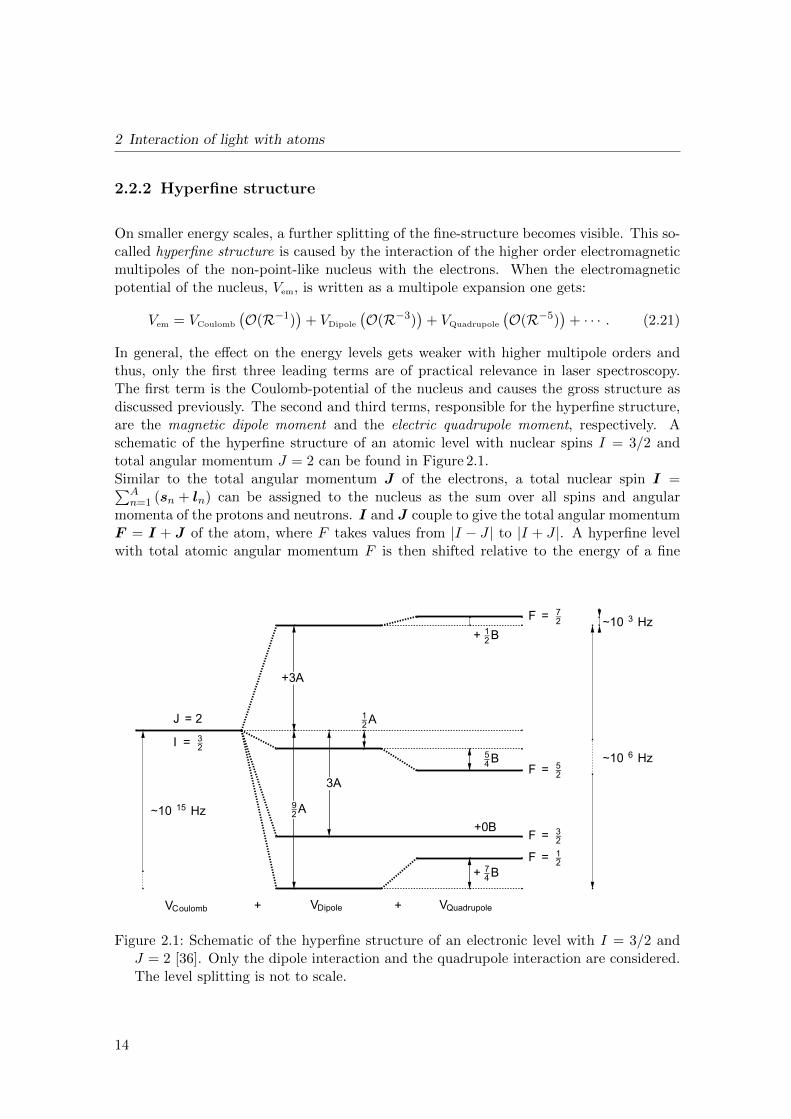
2.2.2 Hyperfine structure
On smaller energy scales, a further splitting of the fine-structure becomes visible. This so-called hyperfine structure is caused by the interaction of the higher order electromagneticmultipoles of the non-point-like nucleus with the electrons. When the electromagneticpotential of the nucleus, Vem, is written as a multipole expansion one gets:
Vem = VCoulomb
(O(R−1)
)+ VDipole
(O(R−3)
)+ VQuadrupole
(O(R−5)
)+ · · · . (2.21)
In general, the effect on the energy levels gets weaker with higher multipole orders andthus, only the first three leading terms are of practical relevance in laser spectroscopy.The first term is the Coulomb-potential of the nucleus and causes the gross structure asdiscussed previously. The second and third terms, responsible for the hyperfine structure,are the magnetic dipole moment and the electric quadrupole moment, respectively. Aschematic of the hyperfine structure of an atomic level with nuclear spins I = 3/2 andtotal angular momentum J = 2 can be found in Figure 2.1.Similar to the total angular momentum J of the electrons, a total nuclear spin I =∑A
n=1 (sn + ln) can be assigned to the nucleus as the sum over all spins and angularmomenta of the protons and neutrons. I and J couple to give the total angular momentumF = I + J of the atom, where F takes values from |I − J | to |I + J |. A hyperfine levelwith total atomic angular momentum F is then shifted relative to the energy of a fine
VCoulomb
J = 2
I = 32
∼10 15 Hz
+ VDipole
92 A
3A
12 A
+3A
+ VQuadrupole
+ 74 B
F = 12
+0BF = 3
2
54 B
F = 52
+ 12 B
F = 72
∼10 6 Hz
∼10 3 Hz
Figure 2.1: Schematic of the hyperfine structure of an electronic level with I = 3/2 andJ = 2 [36]. Only the dipole interaction and the quadrupole interaction are considered.The level splitting is not to scale.
14

2.2 The influence of the nucleus on the atomic structure
structure energy level n2S+1LJ by
∆EF =A
2· C +B ·
34C (C + 1)− I (I + 1) J (J + 1)
2 (2I − 1) (2J − 1) I · J, (2.22)
where C = F (F + 1)− J (J + 1)− I (I + 1) is the Casimir factor [28].A is the magnetic dipole constant and describes the interaction of the nuclear magneticmoment µI with the magnetic field at the nucleus caused by the total angular momentumJ of the electrons HJ(0):
A =µIHJ(0)
I · J. (2.23)
Note that the nuclear magnetic moment, given by µI = gIe
2mpI is smaller than the mag-
netic moment of the electron spin µS = gSe
2meS by the factor of me
mp≈ 1
1836 . This is thereason why the hyperfine structure splittings is typically 3 orders of magnitude smallerthan the fine structure splitting. Furthermore, the nuclear spin of ground state nucleiwith even numbers of protons and neutrons (ee-nuclei) is I = 0 (except for very few lightnuclei) and thus, the magnetic dipole interaction is only observed for nuclei with either anodd number of nucleons (eo-, or oe-nuclei, where I is a half-integer) or an odd number ofproton and neutron (oo-nuclei, where I is an integer).B is the electric-quadrupole coupling constant and describes the interaction of the electricfield gradient ∂2V/∂2z|z=0 at the nucleus with the spectroscopic quadrupole moment Qs:
B =
(∂2V
∂2z
)∣∣∣∣z=0
eQs . (2.24)
Qs is usually expressed in terms of the deformation parameter, β, and is a measure of thedeviation of the nuclear charge distribution from a spherical distribution. The electric-quadrupole interaction is therefore strongest for deformed nuclei and its sign depends onthe deformation of the nucleus: Q > 0, if the nucleus is elongated along the direction ofI (prolate shape) and Q < 0, if the nucleus is flattened (oblate shape). The shift due tothe electric quadrupole requires a non-zero Q and a non-zero electrical field gradient atthe nucleus, which leads to I, J ≥ 1.Higher order components of the HFS are beyond the resolution power of the techniquesused in this work and are therefore neglected in the following. For further reading, I referto the literature [19].
15

2 Interaction of light with atoms
2.3 Absorption and emission of light
Valence (or outer shell) electrons can interact with photons in various ways. Essentialfor laser spectroscopy is the absorption and emission of photons, whereby an electronundergoes a transition between two energy levels Ei and Ej (with i < j). Energy mustbe conserved and thus, the energy of the photon is Eij = Ei−Ej . A photon which fulfillsthis criteria is then called resonant with this transition. Eij is directly proportional to thefrequency ν and inversely proportional to the wavelength in vacuum E12 = hν12 = hc/λ. Inoptical spectroscopy however, it is common practice to note a transition by its wavenumberdefined by ν = ν/c = 1/λ.In the following, the basic principles of absorption and emission of light are described firstby the Einstein coefficients. The spectral linewidth, lifetime and broadening mechanismsof a transition between two atomic states are then discussed.
2.3.1 The Einstein probability coefficients
The processes involved in a transition of one electron between two energy levels Ei and Ej(i < j) were first described by Albert Einstein [54]. Einstein identified three fundamentalprocesses, which govern the emission and absorption of light and assigned each of them anintrinsic probability coefficient: resonant absorption (Einstein coefficient Bij), stimulatedemission (Einstein coefficient Bji), and spontaneous emission (Einstein coefficient Aji).In the following discussion of the Einstein coefficients, an ensemble of idealized non-degenerated two-level atoms with energy states E2 > E1 is assumed as shown in Fig-ure 2.2. First we can state that secondary transition channels are absent and that thetotal occupation Ntot of the energy states should then be constant:
N1 +N2 = Ntot = const. , (2.25)
where N1 and N2 are numbers of electrons in the lower and upper level, respectively.
E2
E1
DE = -E1E = hn12 2 12
A21 B12 B21
Figure 2.2: An illustration of the three possible processes involved in a transition of anelectron between two electron levels with their corresponding Einstein probability coef-ficients: spontaneous emission (A21), absorption (B12), and stimulated emission (B21).
16

2.3 Absorption and emission of light
Resonant absorption
Resonant absorption occurs, when a resonant photon with frequency ν12 excites an electronfrom the lower state to the upper state. If the ensemble is exposed to a radiation fieldwith density ρ (ν), the number of electrons in the lower state N1 is then reduced with arate N1 proportionally to the amount of photons with ν12:
N1 ≡∂N1
∂t= −B12ρ (ν12)N1 . (2.26)
Stimulated emission
In the stimulated absorption, electrons in the excited state may jump with probability(B12) to the lower state in the presence of a radiation field ρ (ν12):
N2 = −B21ρ (ν12)N2 . (2.27)
Spontaneous emission
While the former two effects only occur in a radiation field, spontaneous emission is purelystatistical and may occur also without the presence of a radiation field. An electron inthe excited state releases its energy with probability A21. The rate of this process is thengiven by:
N2 = −A21N2 . (2.28)
Spontaneous emission defines the natural lifetime of an excited atomic and can be observed,for instance, in an excited medium as fluorescence.
Einstein’s relations
While absorption and stimulated emission can in principle be explained by a semiclassicalapproach using time-dependent quantum mechanic wavefunctions and classical electro-magnetic theory, spontaneous emission cannot be explained this way, because it involvesstatistical processes. It therefore requires the theory of quantum electrodynamics (QED)for a full description. Luckily no knowledge about wavefunctions is necessary to derive therelations between the different Einstein coefficients. In fact, Einstein derived the relationsbetween the probability coefficients from considerations based entirely on the principles ofthermodynamics by describing the processes for an idealized two-level atom in a blackbodyenclosure.The ensemble is then exposed to a radiation field, which follows the Planck relation:
ρ (ν, T ) dν =8πν2
c3dν
1
ehν/kT − 1hν , (2.29)
where k is the Boltzmann constant.
17

2 Interaction of light with atoms
The population ratio is given by the Boltzmann relation if the ensemble is in thermalequilibrium with an environment with temperature T :
N2
N1=g2
g1e−
hν12kT , (2.30)
where g2/g1 is the degeneracy of the energy levels E2. For the idealized non degeneratesystem, the ratio becomes E1. g2/g1 = 1. In addition, the population of the lower andexcited state is constant (N1 = N2 = 0) in thermal equilibrium and the total rate ofresonant absorption must equal the rate of emission:
A21N2 +B21ρ (ν12)N2 = B12ρ (ν12)N1 . (2.31)
Rearranging Equation (2.31) and using the Boltzmann relation in Equation (2.30) leads to
ρ (ν12) =A21
B12 (g1/g2) ehν12/kT −B21. (2.32)
This must be equal to the Planck relation given in Equation (2.29) and by comparison oneobtains the Einstein relations for the Einstein probability coefficients
g1B12 = g2B21 and A21 =8πhν3
12
c3B21 . (2.33)
2.3.2 Resonance excitation of atoms
The Einstein probability coefficients for the transition between two states are intrinsicproperties of the atom. They are thus also valid for atoms, which are taken out of theideal blackbody enclosure and exposed to a photon flux Φ
[cm2s−1
](for example from
a laser). Instead of using the absorption coefficient B12 it is more common to use theevidently related absorption cross section σ12 of the transition. The rate of the absorptionis then given by
N2 = Φσ12 . (2.34)
In a many-level atom, higher levels can then be successively populated from the excitedlevel by the same principle using several light sources, which match the energy of thehigher-lying transitions. The overall process is then governed by the probabilities (orcross-sections) for absorption and emission of all involved transitions and will eventuallyreach an equilibrium, where the rates of absorption and emission are equal. This is theunderlying mechanism of resonance laser ionization and in-source laser spectroscopy.
2.3.3 Spectral linewidth
An elegant way to describe the interaction of electromagnetic waves with the electrons ofan atom, involving statistical processes such as spontaneous emission, is the density matrixformalism, which leads to the optical Bloch equations (OBE). A thorough treatment ofthis approach is given in [16, 162]. In short, the solutions of the OBEs for a two-leveltransition between two states Ei and Ej (with i < j) lead to the saturation parameter,
18

2.3 Absorption and emission of light
S, and the resonant saturation parameter, S0, given by:
S =S0
1 + 4δ2
γ2
, and S0 =I
Isat
with Isat =πhc
3λ2γ , (2.35)
where γ is the damping parameter. In the simple two-level atom, this can be interpretedas the spontaneous emission γ = A. δ is the detuning of the frequency with respect to theresonance frequency of the transition. I is the intensity of the laser radiation of wavelengthλ. Isat is the saturation intensity at which a population of the excited state Ej reaches itsmaximum of 50%, provided that g1 = g2. An excited state population of more than 50%is called a population inversion and is only possible for excitation schemes with more thantwo levels.The lineshape of a transition has a Lorentzian form with a linewidth (FWHM∗) of
δνp =γ
2π
√1 + S0 . (2.36)
The natural linewidth observed, if the transition is not saturated (I < Ip). In this case,the linewidth is given by the damping parameter γ or by the inverse of the lifetime τ ofthe transition†:
δνnat =γ
2π=
1
2πτ. (2.37)
For a two-level atom, the natural linewidth is simply the Einstein coefficient A21 of thetransition and its lifetime τ = 1
A21by its inverse. For more realistic multi-level atoms, the
lifetime has to be corrected for the additional lower states, to which the excited electronwith Ej can decay. Then, the total decay probability to all N = k lower levels is the sumof the corresponding Einstein coefficients and the total lifetime calculates to:
τj =1∑k
k=1Ajk. (2.38)
The line profile of the lower state Ei is also naturally broadened due to contribution of theline profiles of all transitions to the total linewidth. This leads in turn to a Lorentzianshape with an overall natural linewidth of this transition of
δνnat,ij = δνnat,j + δνnat,i =1
2πτj+
1
2πτi. (2.39)
Typical lifetimes of non-metastable excited states are of the order of 10−8 s with corre-sponding typical natural linewidths of 100 MHz. The resolution of these narrow transitionsby laser spectroscopy is very complicated and requires special Doppler-free or Doppler-reduced techniques such as collinear laser spectroscopy [13, 87] and collinear resonanceionization spectroscopy [135]. For in-source laser spectroscopy as used in this work, thenatural linewidth cannot be resolved since the other broadening mechanisms dominate the
∗Full width at half maximum†The natural linewidth of a transition can be obtained alternatively by the Heisenberg uncertainty
principle (∆E · ∆t ≥ ~2).
19

2 Interaction of light with atoms
Figure 2.3: Lineshapes of power or Doppler broadened transitions. The power broadenedtransitions have a Lorentzian shape with intensity dependent widths. In contrast, theDoppler broadened transitions are Gaussian and depend on the temperature of theatomic vapour.
spectral lineshape. The most important of these are power broadening, Doppler broadening,and pressure broadening, which will be discussed in the following.
Power broadening
If the laser intensity I approaches or exceeds the saturation intensity Isat, the lineshapestill remains Lorentzian, but a broadening of the natural linewidth is observed. Thiscan be understood by looking at the formula for the linewidth in Equation (2.36): if thelaser frequency is in resonance with the transition (ν = ν0, δ = 0), the population of theexcited state cannot exceed 50%. On the other hand, if the laser frequency is off resonance(ν 6= ν0, δ 6= 0), the population maximum is not yet reached and the population can thusfurther increase with increasing laser intensity resulting in a flatter slope of the Lorentzianlineshape.
Pressure broadening
If ionization takes place in a buffer gas, in a dense vapour, or in the presence of chargedparticles such as ions and electrons, the energy and lifetime of an excited state can bealtered. A shifting, broadening, and mixing of the energy levels can therefore occur. Theseeffects are due to interactions between the excited atom and the buffer gas atoms. For
20

2.3 Absorption and emission of light
example, collisions of the excited atom with particles may reduce the lifetime of a stateand thus broaden the lineshape (collisional broadening). Additionally, the Stark effect,which results in a shift of the resonance frequency, may be observed, if the excited atom isperturbed by an electric field of charged particles nearby. This effect can be significant incase the ionization takes place in gas cells, where the pressure is many orders of magnitudehigher than in the hot cavity, which was used for the experiments described in this work.A full description of these effects is given in the reference [167].
Doppler broadening
For in-source laser spectroscopy in a hot cavity, the lineshape is dominated by Dopplerbroadening. This is due to the velocity distribution of a hot vapour with atomic mass mA
and temperature T, which follows the Maxwell-Boltzmann distribution:
dN(vx)
N=
1√π
exp(−v2
x/v20
)with v0 =
(2kbT
mA
)1/2
, (2.40)
where vx is the velocity of a single atom, v0 is the “most probable velocity” and kb is theBoltzmann constant. The transition frequency ν of a single atom which propagates withvelocity vz in opposite direction (z-direction) of the laser light becomes Doppler shiftedto the transition frequency ν0 at rest:
ν = ν0 (1 + vz/c) . (2.41)
The overall lineshape follows the Maxwell-Boltzmann distribution from equation (2.40),which results in the Gaussian intensity profile
I (ν) = I (ν0) exp
[−(c (ν − ν0)
ν0v0
)2]
with I (ν0) =c√πν0vo
. (2.42)
The contribution to the total broadening by the Doppler broadening δνD is
δνD = 2√
ln 2ν0v0
c= ν0
√8kbT ln 2
mAc2. (2.43)
In addition, the center frequency has to be corrected for the expected Doppler shift. Thisis especially the case for highly directional atomic flow jets.For laser ionization in hot cavities as performed in this work, Doppler broadening canbe of the order of several GHz. However, to account for a Gaussian and a Lorentziancontribution, one can use the so-called Voigt function, which is a convolution of a GaussianIG (ν) and a Lorentzian line profile IL (ν):
I (ν) = IG (ν) ∗ IL (ν) =
∫ ∞−∞
dν ′IG
(ν ′)IL
(ν − ν ′
). (2.44)
Although, the integral in Equation (2.44) cannot be solved analytically, modern comput-ers and data analysis programs can generate Voigt functions and perform least-squares
21

2 Interaction of light with atoms
fitting very rapidly. In case of in-source laser spectroscopy in hot cavities, a Gaussianapproximation is often sufficient for determining the centroids of a transition due to thestrong Doppler broadening.
2.3.4 Selection rules for allowed transitions
Not all transitions between atomic states show the same probability or are observed innature. Whether a transition is ‘allowed’ or ‘forbidden’ is based on the rules of momentumconservation and symmetry (parity σ). To first order dipole approximation, the dipoleoperator only acts on the angular momentum and not on the electron spin. Therefore∆l = ±1, ∆s = 0 and parity changes by σ = ±1. In case of LS -coupling, where L, S, andJ are good quantum numbers one gets the following rules for allowed dipole transitions:
∆S = 0,∆L = 0,±1 and ∆J = 0,±1, where J = 0 6=⇒ J = 0 . (2.45)
Similar expressions can be derived for transitions between hyperfine structure levels:
∆J = 0,±1 and ∆F = 0,±1, whereF = 0 6=⇒ F = 0 . (2.46)
The word ‘forbidden’ is misleading as higher order multipole transitions may still occur,albeit with much smaller transition probabilities and cross-sections (several orders of mag-nitudes). Also, LS -coupling is not always pure and lines and formerly forbidden dipolelines appear. Nevertheless, the selection rules given in Equation (2.45) and Equation (2.46)are good guides to analyze atomic spectra and for finding new laser excitation schemes.
22

3 Radioactive ion beam production
The production of exotic isotopes far away from stability enables the study of a largevariety of phenomena in fields such as fundamental atomic-, astro-, nuclear-, and solid statephysics. Some exotic nuclei are found to be deformed, decay in unexpected manner, or aresuitable for medical applications. Determining their properties gives answers to questionssuch as the origin of elements (nucleosynthesis), nuclear structure and the chemistry ofsynthetic elements. It is also a very useful tool to explore new applications in fields suchas nuclear medicine and material science.Since the advent of radioactive ion beam (RIB) facilities in the 1950, more than 3000isotopes have been discovered and studied [85] and many more isotopes are expected tobe in reach.Several concepts for the production of radioactive ion beams exist, but common for themajority of the techniques are a driver (particle) beam (also called primary beam), whoseparticles collide with the target material and cause nuclear reactions for the productionof exotic nuclei, and a mass spectrometer to separate and select the reaction product ofinterest.The production of nuclei far from stability comes with several difficulties:
• low production cross-sections and low ion yields of the isotope of interest.
• short half-lives of many isotopes.
• non-selective production inside the target and possible contamination with unwantedspecies.
Therefore, all types of RIB facilities require an efficient atom and ion release from thetarget, highly selective elements for beam purification, and efficient beam transportation.Most RIB facilities follow two fundamental concepts: the Isotope Separator On-Line(ISOL) technique and the In-Flight Fragment Separator technique. ISOL facilities canbe further divided into two categories: those that use thick targets for production andthermalization∗ and rely on thermal motion for transport to the ion source; and facilitiesthat use thin targets for production and gas catchers to stop the reaction products. Anoverview of the different types of RIB facilities is given in Figure 3.1 and in [18].ISOL facilities are the most effective means of producing high intensity, low emittancebeams of isotopes with a half-life greater than 10 - 100 ms. In contrast, the In-Flight Frag-ment Separator method uses heavy projectiles to react with a thin target. This process isextremely fast, chemistry independent and results in a high energy, high emittance beamof ions in a variety of charge states. Extremely exotic and short lived species are therefore
∗Stopping and neutralization of the reaction products until the particles eventually reach thermalequilibrium with the target material.
23

3 Radioactive ion beam production
321
Legend:
Driver beam
Thicktarget
Thintarget
Reactionproducts
Gascatcher
Ionsource
Extractionelectrode
Massspectrometer
Beam ofchosenisotope
Figure 3.1: A sketch of the three different principles of radioactive ion beam facilities [113]:1) ISOL method using a thick target and an ion source as used at ISOLDE/CERN,Meyrin, Switzerland. 2) ISOL facility with thin target plus gas catcher as used atIGISOL, Jyvaskyla, Finland. 3) In-flight fragment separation method as used at GSI,Darmstadt, Germany.
accessible but the production yield of any chosen isotope is typically much lower than itcan be achieved at an ISOL facility. Examples for ISOL facilities are ISOLDE at CERN,Switzerland, the RIB facility in Louvain-la-Neuve, Belgium and the IGISOL facility inJyvaskyla, Finland. In-Flight Fragment Separator facilities are found at the Gesellschaftfur Schwerionenforschung (GSI) in Darmstadt, Germany, at the Grand Accelerateur Na-tional d’Ions Lourds (GANIL) in Caen, France and at the the Japanese Institute of Physicaland Chemical Research (RIKEN∗) in Wako, Japan. For further reading about the differentfacilities and methods, I refer to the several review papers [17, 18, 52].Of the three different types of RIB facilities, only a thick target type ISOL facility requiresnecessarily a dedicated ion source for standard operation. Most commonly used are ionsources based on surface ionization, resonance laser ionization, electron impact ionizationand plasma ionization. The right choice for the type of ion sources is crucial in planningan experiment and is made depending on the nuclear- (half-life), the atomic- (ionizationenergy, atomic levels, etc.) and the chemical properties of the element. The most im-portant characteristics of an ion source at a RIB facility are the ionization efficiency εion
defined as
εion =# of atoms ionized
total # of atoms released from the target(3.1)
∗RIKEN is an abbreviation of Rikagaku Kenkyujo, which translates from Japanese to English to “theinstitute of physical and chemical research”.
24
3.1 The ISOL process at ISOLDE
and the selectivity, S, defined as
S =Ion intensity of isotope of interest
Total ion intensity on the given mass of contaminants and isotope of interest.
(3.2)A lot of effort is continuously invested in the development of new techniques to improvethese two parameters. One of the primary goals of the work described in this thesis wasto improve the selectivity and efficiency of the Resonance Ionization Laser Ion Source(RILIS) at the ISOLDE facility.This chapter will focus on the aspects of the radioactive ion beam production process atISOLDE which are relevant to this work. A description of the ionization techniques withemphasis on resonance laser ionization is given. The status of the RILIS installation andits application as a spectroscopy tool is then discussed in the last part of the chapter.
3.1 The ISOL process at ISOLDE
This section discusses the ISOL process at ISOLDE, which includes the production ofthe exotic nuclei, the thermalization of the reaction products, the transport of the atomsto the ion source, the ionization, and the mass separation. The optional stages of ionbeam cooling and bunching, charge-state breeding and post-acceleration were not usedduring this work and are therefore omitted. Figure 3.2 gives an overview of the differentcomponents and their location at ISOLDE: the driver beam enters ISOLDE through theproton beam line and impinges on the target installed at one of the target front-ends,where the exotic atoms are produced in nuclear reactions. The atoms are then transferredto an ion-source, extracted into the beam-line and mass separated by one of the separatormagnets.
3.1.1 The driver beam
ISOLDE is integrated into the CERN accelerator complex as shown in Figure 3.3. It usesthe bunched, 1.4 GeV proton beam from the CERN Proton Synchrotron Booster (PSB) asa driver beam, which is sent through the proton beam line towards the target front-end.PSB Proton bunches are of 1.66µs length, contain up to 3 ·1013 protons, and are separatedby 1.2 s. The proton bunch distribution between the various users (ISOLDE, nTOF, LHCetc.), follows a repetitive sequence, known as the super-cycle, which typically containsof the order of 39 pulses. The maximum proton current that can be sent to ISOLDE islimited to 2µA due to radio-protection constraints.
3.1.2 The target and front-end
A cross-section of a standard ISOLDE target unit for surface or resonance laser ionizationis shown in Figure 3.4. It comprises a target cylinder filled with the target material, atransfer line for atom transport from the target to the source and a hot cavity, whichserves as surface ion source or as the laser-atom interaction region for resonance laser
25

3 Radioactive ion beam production
HR
S
GP
S
HR
S fron
ten
d
GP
S fron
ten
d
pro
ton
be
am lin
e
locatio
n R
ILIS
La1
locatio
n Tap
e statio
n
REX
Figu
re3.2
:A
draw
ing
ofth
eIS
OL
DE
facilityan
dits
main
comp
onen
ts:1.4
GeV
proton
driver
beam
,G
PS
-an
dH
RS
targetfron
ten
ds
with
target,tra
nsfer
line,
ionso
urce
and
extraction
electrod
e,an
dth
etw
om
asssep
aratorsG
PS
and
HR
S.
Op
tionally
the
bea
mfro
mth
eH
RS
separato
rm
agnet
canb
efu
rther
cooled
and
bu
nch
ed,
charge
stateb
red,
and
post-accelerated
tou
pto
3.1
MeV
/u.
Exp
erimen
tsare
loca
tedat
the
end
ofth
ed
ifferen
tb
eam-lin
esin
the
ISO
LD
Eex
perim
ental
hall.
Th
eR
ILIS
ionsou
rceis
located
inth
eex
perim
ental
hall
above
the
HR
Sm
asssep
arator.P
icture
adap
tedfrom
[21].
26

3.1 The ISOL process at ISOLDE
Figure 3.3: An illustration of the CERN accelerator complex with all major facilities. Theproton bunches are accelerated by the LINCAC 2 and Booster (in the text referred toas the Proton Synchrotron Booster, PSB) to 1.4 GeV before they are sent to ISOLDE[30].
ionization. Resistive heating of the target container and the hot cavity to up to 2000 Cenables the transport and ionization of atoms.The target can be installed at one of the two front-ends at ISOLDE (see Figure 3.2).These correspond to the beam-lines of the two mass separators General Purpose Separator(GPS) and High Resolution Separator (HRS). Ions are extracted from the hot cavity intothe ISOLDE beam-line by a potential difference between the target and front-end on ahigh-voltage (+30 keV and +60 keV) and an extraction electrode on ground potential,which is installed approximately 60 mm away from the exit of the ion source.
3.1.3 The target materials
The choice of the correct target material is crucial for highest production rates of theisotope of interest. For the work described in this thesis, rolled foils of titanium (Ti)or pellets of uranium-carbide (UC2) were used as a target material. As illustrated byFigure 3.5, a range of isotopes of many different elements are produced. The actual ex-perimental cross-sections for each isotope are difficult to obtain, but can be calculatedtheoretically by the ABRABLA code [109]. These production cross-sections were verifiedat GSI, but are expected to be similar to the production cross-sections at ISOLDE. Dueto the non-selective reaction reaction processes, a degree of selectivity must be thus intro-duced during the subsequent processes of atom transport, ionization, and ion transport toextract an isotopically pure beam.
27

3 Radioactive ion beam production
1.4 GeV Protons
Ion beam
1) Target
cylinder 2) Transfer line
and ion source
Figure 3.4: A cross-sectional drawing of an ISOLDE target unit equipped with a tantalumionizer cavity for surface or laser ionization. The main elements are: 1) The thicktarget container filled with the target material. 2) The transfer line for atom transportand a hot cavity for surface ionization and laser ionization [117].
Calculation
Cross section: Z
N
Figure 3.5: Theoretically expected production cross-sections at ISOLDE for 1 GeV protonson 238U [109].
28

3.1 The ISOL process at ISOLDE
3.1.4 The reaction mechanisms
The 1.4 GeV proton beam from the PSB travels through the target cylinder as shown inFigure 3.4 and undergoes nuclear reactions with the target material. Three productionchannels are present: proton induced fragmentation, spallation, and fission. Fragmenta-tion and spallation dominate the production at the neutron-deficient side of the nuclearchart and fission is mainly responsible for the production of neutron-rich nuclei. However,all channels are usually present and the exact production process is not always clearlydistinguishable.It is possible to give preference to the fission reaction channel by the use of a neutronconverter [108]. This is a solid tungsten cylinder, positioned adjacent to the target. Ifthe protons are directed onto the converter then a portion of the spallation neutrons areemitted into the target material and induce fission reactions.
3.1.5 Atom thermalization and transport
The initial kinetic energies of radioactive isotopes right after the production inside thetarget is in general quite high. Fission reaction products, for example, have kinetic energiesof about 200 MeV. At ISOLDE, these atoms are stopped inside the target matrix itselfand cooled down to the target temperature (typically ≈ 2000 C), which corresponds toa kinetic energy of ≈ 300 meV [52]. Depending on the vapor pressure of the element,the atoms are able to diffuse through the porous target material and eventually reach theaperture to a transfer line, which guides the atoms to the ion source. The transfer line isthe first opportunity to introduce chemical selectivity by inserting a quartz transfer lineto delay alkali metals and thus reducing the contamination by decay [23].
3.1.6 Ionization processes
The ionization region is located immediately after the transfer line. Depending on theproperties of the isotope of interest, one can choose between surface ionization, laserionization, electron impact and plasma ionization. The first three of these ionizationmechanisms that are relevant to the work described in here are discussed in more detaillater in this chapter in section 3.2. After the ionization, the ions are then accelerated bythe potential difference between the target assembly on a high-voltage (between -30 kVand -60 kV) and an extraction electrode on ground potential.
3.1.7 Mass separation
Each of the two ISOLDE target frontends has a corresponding dipole magnet mass spec-trometer: the General Purpose Separator (GPS) and the High Resolution Separator(HRS), respectively. When the beam enters the dipole magnet, ions of a different mass-to-charge ratio are bent with different radii. For a mono-energetic beam with kinetic energyT, atomic mass m, and particle charge q in a magnetic dipole field with field strength B,
29

3 Radioactive ion beam production
the bending radius ρ of the ion beam is given by:
ρ =1
B·
√2mT
q. (3.3)
The overall resolving power, R, of such a mass separator for a given mass m is defined as
R =m
∆m, (3.4)
where ∆m is the FWHM of the ion beam with mass m in the focal plane of the separator.The resolving power of the GPS mass separator (singly staged 90 analyzing magnet) isR ≈ 2500 and thus, is less strong than the resolving power of the HRS mass separator(two subsequent analyzing magnets with 90 and 60 respectively) with R ≈ 7000, but canachieve higher transport efficiency and is easier and faster to tune. In addition, the GPShas the advantage that it can enable transmission of up to three masses simultaneouslywithin a mass range of 15% (low mass, central mass, and high mass). The HRS beam-line,however, is also equipped with an RFQ ion cooler and buncher for further improvementof the beam quality/emittance.
3.1.8 Production rates and total transport efficiency
The intensity of a radioactive ion beam at an ISOL facility is given by
I = σ ·Ntarget · Φ · ε , (3.5)
where σ is the cross-section of the relevant production process for the isotope of interest(see Figure 3.5), N the number of atoms inside the target material, Φ the flux of the driverbeam, and ε the transport and ionization efficiency from the target to the experiment. Thetotal transport and ionization efficiency consists of the transport efficiency from the targetto the ion source εrelease, the ionization efficiency εionization, and the transport efficiencythrough the analyzing magnets and the beam line to the experiments εtransport:
ε = εrelease · εionization · εtransport . (3.6)
This work puts its emphasis on the improvement of the ionization efficiency of the ionsources.
30

3.2 Ionization mechanisms and ion sources at ISOLDE
3.2 Ionization mechanisms and ion sources at ISOLDE
An ion is defined as a nucleus with a number of shell-electrons Ne, which is smalleror greater than the number of protons Np = Z, where Z is the atomic number. Itis therefore either positively charged (Ne < Z, “positive ions”) or negatively charged(Ne > Z, “negative ions”). Almost all experiments at ISOLDE are performed with positiveions and thus, in the context of this work, the word “ion” is used to refer to a singlypositively charged ion. The ionization methods described below are therefore techniques,which remove one electron from a neutral atom.All ionization methods must provide a reaction energy which is at least greater than theionization energy E > IE = eφ1, where φ1 is the ionization potential, to remove oneelectron from the atomic shell (see Chapter 2.1). If this energy is supplied to a confinedsample, then a plasma of electrons, ions and neutral atoms is generated. The ion sourcetherefore needs to be optimized in terms of extraction and emittance of the ion beam tomatch the special requirements of the beam-line, of the post-accelerators, and the specificexperiment.The different ion sources at ISOLDE fall into four main categories: surface ionization∗,resonance laser ionization, electron impact ionization and plasma ionization. Each type ofion source has advantages for specific elements in terms of efficiency and selectivity. Surfaceionization is highly efficient for elements with low ionization energies such as alkali andalkaline-earth metals. Resonance laser ionization is highly efficient and element-selective,but requires good knowledge and extensive investigations about the atomic structure ofthe element as well as a series of transitions between atomic levels that are accessible withthe available laser system. Electron impact ionization and plasma ionization are rathernon-selective, but give access to elements with high ionization energies, such as noblegases, or to elements with an atomic structure that makes laser ionization impractical orinefficient, such as the halogens. In the following, the ionization mechanisms relevant tothis thesis, surface, laser and electron impact ionization are discussed.
3.2.1 Surface ionization
Surface ion sources are the standard choice for elements with low ionization energies atISOLDE. Surface ionization may occur when a neutral atom with ionization energy IE =eφi interacts with a surface of a material with a work function W . The least electron maythen tunnel into the Fermi band of the material.Following Meghnad Saha’s description of the ionization in hot gases, Irving Langmuir firstdescribed the relation between the ionization probability of a vapor by contact with asurface by considering the ratios between neutral atoms, ions, and electrons on the surface[98, 148]. The so-called Langmuir-Saha formula gives the ratio αs between the number ofions Ni and number of neutral atoms N0 with ionization energy eφi on the surface withtemperature T and work function W in thermal-equilibrium:
αs =Ni
N0=gig0
exp
(−eφ−W
kT
), (3.7)
∗Or contact ionization. The denotation depends on the literature.
31

3 Radioactive ion beam production
Figure 3.6: Surface ionization efficiencies in a hot cavity ion source obtained by experiments[89] and by simulations [170].
where gi and g0 are the degeneracy of states∗ for the ions and neutral atoms, respectively.The probability to ionize one atom on the surface is then given by
β =Ni
N0 +Ni= αs
(1
1 + αs
). (3.8)
As it follows from Equation (3.7), the surface ionization efficiency benefits from a hightemperature, a low ionization energy and a high work function†. Therefore, the highestionization efficiencies are obtained for alkaline metals with low ionization energies from5.1 eV (sodium, Na) to 3.9 eV (cesium, Cs and francium, Fr) in combination with contactmaterials with high working functions such as tantalum, Ta (W=3.7−4.9 eV)‡, tungsten,W (W=4.5−4.8 eV) or rhenium, Re (W≈5 eV) [3, 4].The ionization efficiency obtained by an ISOLDE-type hot-cavity surface ion source actu-ally exceeds the value that is implied by Equation (3.7) [89]. This is due to a combinationof effects: multiple atom-wall interactions per atom, a plasma potential, which is formedinside the hot cavity by the emitted electrons, and a penetrating extraction field. Theplasma potential is neutral close to the axis of the source and positive towards the wallsof the hot cavity. This leads to a confinement of the positive ions inside the hot cavityand to a reduced neutralization at the walls [100].However, a quantity to describe the overall enhancement of the ionization efficiency βs
∗g is the degeneracy of states, given by g = 2J + 1, where J is the total angular momentum in theground state of the atom or ion.
†For the production of negative ions, the opposite, high electron affinity and low work function, applies.‡The work function depends on the surface orientation, in case of crystalline elements.
32

3.2 Ionization mechanisms and ion sources at ISOLDE
to the ionization probability β predicted in Equation (3.8) is given by the amplificationfactor η:
η =βsβ. (3.9)
Recently, the surface ionization efficiency for several elements has been successfully sim-ulated and compared to experimental values [89, 170]. The experimental values and theresults from the simulation are shown in Figure 3.6. As expected, the ionization efficiencydepends strongly on the ionization energies. Ionization efficiencies of about 100 % areobtained for alkaline metals such as potassium, but decrease sharply for elements withhigher ionization efficiencies.
3.2.2 Electron impact ionization
Electron impact ionization is the ionization principle of the plasma ion source, the electronbeam ion sources (EBIS), and the electron beam ion traps. Free electrons with kineticenergies above the ionization potential (E ≥ IE ) may remove an electron from the electroncloud of an atom or an ion with a certain probability. This process is described by thefollowing reaction:
e− +Aq+ → A(q+1)+ + 2e− , (3.10)
where A is the atom with initial charge state q. The overall ionization rate R in a volumeV with target particle (atoms or ions) densities Ni and electron densities Ne is given by
R =
∫ ∫NiNeσi (ve,i) dve,i dV , (3.11)
where ve,i is the relative velocity between the electrons and the target particles and σi (ve,i)the velocity dependent cross-section of the process. In general, the reaction cross-sectionis zero for electron energies below the ionization threshold and reaches its maximum atelectron energies at about three to four times the ionization energy. The cross-section asa function of the energy can be described by several semi-empirical formulas [107, 126],but close to the ionization-threshold, the cross-section can be approximated by
σi = α (Ee − eφi)n , (3.12)
where α is a constant and n depends on whether the target is an atom (n = 1.1269)or an ion (n = 1.056). The cross-section declines for higher electron energies since theinteraction time gets shorter.If the ionization takes place in a hot plasma, the velocity distribution of the electrons isgiven by the Maxwell distribution (Equation (2.40)). In this case, ionization occurs dueinteraction with the electrons in the higher energy tail of the velocity distribution. Usingelectron impact ion sources, the electron energy can be precisely tuned to the maximumof the cross section of the reaction. A suitable increase in the electron beam energy makesit possible to ionize the ions to higher charge states.In contrast to surface ionization, electron impact ionization can be applied for elements
33

3 Radioactive ion beam production
with high ionization potentials such as halogens or noble gases. However, the process isnot selective since the maximum of the cross-section is rather broad and thus, isobariccontamination can be a problem in radioactive ion beams. Provided that the chosenisotope is a volatile element, a degree of selectivity can be achieved through the use of acooled transfer line to transport the reaction products to the ion source.
3.2.3 Resonance laser ionization
A very efficient and element selective ionization technique is the resonance laser ionization[92, 102]. Here, electrons are excited from the ground state above the ionization energyusing several subsequent electron transitions. These must be in reach of the tuning rangeof the available lasers. The final step of ionization can be achieved by either non-resonantexcitation into the continuum, by an excitation to a so-called auto-ionizing state abovethe ionization energy or by an excitation to a highly excited Rydberg-state close to theionization energy. In the latter, the atom can then be efficiently ionized by external effectssuch as a strong field gradient, blackbody radiation or collisions. An overview over thedifferent ways to ionize an atom by resonance laser ionization is shown in Figure 3.7. Theseso-called ionization schemes are discussed in more detail later in this section.The process of resonance laser ionization is completely element-selective due to the element-unique atomic structure. In some cases, even isotope or isomer selectivity is possible ifthe laser line-width is sufficiently narrow to resolve isotope- or isomer shifts. Moreover
Exci
tati
on
en
erg
y
a) b) c)
d)e)
f)Continuum
Ground level
st1 excited level
st nd1 or 2 excited level
Rydberg level
IP
Figure 3.7: An illustration of different excitation schemes that may be applied for resonancelaser ionization: intermediate states can be populated resonantly by a) one or b) twophotons or by c) two-photon excitation through a virtual level. Ionization is possibleby d) non-resonant ionization into the continuum or resonance excitation to e) auto-ionizing states or f) Rydberg levels followed by field or laser ionization.
34

3.2 Ionization mechanisms and ion sources at ISOLDE
high ionization efficiencies of up to 30 % can be achieved, and due to the very short ion-ization process, no additional significant delay is introduced into the production process.The resonance laser ionization is the technique of choice for most ion beams produced atISOLDE [59] (see Figure 1.1).In the following section, the principle and the basic requirements for an efficient laserionization are discussed. For a thorough analysis of the laser ionization process, I refer to[81, 102]. The description below follows the discussion found in [51].
Laser ionization efficiency
For a given ionization scheme several conditions must be satisfied to maximize the ioniza-tion efficiency:
Minimum photon energy: The sum of all of the electron transition energies,Ei (i = 1, · · · , k), has to exceed the ionization energy:
i=k∑i=1
Ei ≥ eφi = IE . (3.13)
The minimum photon energy required to ionize the elements with lowest ionizationenergies (cesium and francium) must be greater than E ≈ 3.9 eV, which correspondsto ultraviolet light of about 320 nm. The expected efficiency in this case will be verylow due to the low laser power available for UV light and the low cross-section fornon-resonant ionization. Generally, two to four lasers are therefore used to providea step-wise resonance ionization scheme.
Flux condition: the depopulation rate of the excited state due to resonant or non-resonant absorption, given by the product of the photon flux, Φ
[cm−2s−1
], and the
cross-section, σi, has to be greater than the loss rate due to de-excitation β[s−1]
ofthe level to meta-stable levels or energy levels that don’t match part of the excitationscheme∗. This is the so-called flux condition and can be expressed by
σi · Φ β . (3.14)
Fluence condition: For this discussion the photon fluence is calculated as the photonflux multiplied by the useful interaction time. For continuous wave lasers (CWlasers) the interaction time would be defined by the lifetime of the excited state.For efficient ionization for a given average laser power it is therefore preferable touse a laser with a pulse length that is less than the excited state lifetime. If this isthe case then the useable photon fluence, φ [cm−2] is simply the flux times the laserpulse length:
φ = Φ · τl . (3.15)
∗These levels are often colloquially referred to as “dark states” as they are “invisible” to the photonsthat are provided by the lasers.
35
3 Radioactive ion beam production
To ensure that enough photons are delivered within the suitable time period to ionizeall excited atoms, the fluence condition is then given by:
σi · φ ·g2
g1 + g2 1 , (3.16)
where g1 and g2 are the statistical weights of the ground and excited state of theatom, respectively.
A transition between two states is called saturated, if both, the flux condition and thefluence condition hold and in turn the maximum ionization rate is achieved if this isseparately valid for each involved transition. Typical values for the spontaneous emissionrate of β = 10−6 s−1 and for the cross-section of the weakest transition of σi = 10−17cm2
require a photon flux of more than 1021 photons/s [51]. This corresponds to a 500 W CWlaser power or to a pulsed laser with a pulse energy of much more than 5µJ/pulse. AtISOL facilities, only the latter is practical.The repetition rate of the pulsed lasers has to be chosen with respect to the averagetransport time of the atoms through the hot cavity of roughly 10µs, which leads to arepetition rate of 10 kHz and in turn defines together with the flux and fluence conditionthe pulse energy. If any transition remains unsaturated, the achievable ionization efficiencyis directly proportional to either the laser laser power or the cross-section for the transition.However, the ionization cross-section can vary by several orders of magnitude, dependingon whether the ionization is non-resonant above the ionization energy or resonant to anauto-ionizing state or Rydberg-level.
Non-resonant laser photo-ionization
Non-resonant laser photo-ionization occurs, when an electron of an atom is excited abovethe ionization energy into the ionization continuum. This is illustrated in Figure 3.7d. Itrequires a photon energy, which is higher than the energy from the intermediate state tothe ionization energy. The cross-section for non-resonant laser ionization is only 10−17cm2
to 10−19cm2. Although the maximum residual power of the non-tunable pump laser isusually used for a non-resonant ionization step, the transition is in most cases difficult tosaturate.
Ionization via auto-ionizing states
Strong resonances with high cross-sections are observed above the ionization energy in thespectra of many elements. These cross-sections can be several orders of magnitudes higherthan for non-resonant transitions to the continuum. In some cases (e.g. gadolinium [12, 24]and manganese [115]), the spectrum of bound states above the ionization energy can beextremely rich. These resonances can be interpreted as a resonant two-electron excitation,for which the combined excitation energies of both electrons exceeds the ionization energy.It is then possible that one electron decays back to a lower state, while the energy of thiselectron is transmitted directly to the other excited electron. In case of the latter, theexcited electron has then enough energy to escape the atom. The process is known asauto-ionization and the corresponding bound state an auto-ionizing state (AIS).
36
3.2 Ionization mechanisms and ion sources at ISOLDE
The line-shape of such a transition can differ from resonances below the ionization energy.It can be rather asymmetric due to interference effects with the continuum and fits with aVoigt function (see Equation (2.44)) may not be suitable for fitting any more. A theory forthe line-shape of these auto-ionizing states was first described by Ugo Fano [56]. Here, anauto-ionizing process is described by two scattering processes, which interfere with eachother: the excitation to a discrete level (resonant scattering) and the scattering within acontinuum of states (background scattering). If the excitation energy is varied around thecentral energy of the auto-ionizing resonance, the background process varies only slowly,while the amplitude and the phase of the resonant process changes rapidly. The variationof the phase leads to the asymmetric line-shape.The total cross-section σai follows a function of the Fano factor q and the so-called reducedenergy ε:
σai = σa · F (q, ε) + σb with F (q, ε) =(q + ε)2
(1 + ε2)and ε =
E − E0
Γ/2. (3.17)
σa is the part of the continuum cross-section, which interacts with the discrete level, σb
is the non-interacting constant background cross-section and Γ is the line-width of theresonance. The Fano factor q can then be interpreted as a quantity for the amplitudesof the resonant scattering and the background scattering and determines the shape of theresonance.On resonance (ε = 1/q), the amplitude is given by σai,max = σa ·
(1 + q2
)+ σb, which leads
in case of q2 1 toσai ≈ q2 · σa . (3.18)
Typical values of σa are similar to the cross-sections of the non-resonant ionization(10−17cm2 − 10−19cm2). In combination with Equation (3.18), it is obvious that for highFano factors q, the gain in laser ionization efficiency due to ionization through auto-ionizingstates can be several orders of magnitudes compared to the non-resonant laser ionization.Line-widths of auto-ionizing states can vary strongly and resonances were observed withline-widths ranging from MHz to THz (see Chapter 5). However, in most cases, tunablelasers are needed to excite to auto-ionizing states. The higher cross section of transitionsto an autoionizing state results in a reduced laser power requirement and, for the typicaloutput power of a tunable laser of the laser ion source, this transition may be saturated. Ifthis is not the benefit of using an autoionizing state, the usage of non-resonant ionizationhas to be carefully evaluated, taking into account the higher power and greater convenienceof using a non-tunable laser for a transition to the continuum.
Ionization via Rydberg levels
It is possible to excite to high-lying Rydberg levels (see Chapter 2.1.2) for efficient ioniza-tion. The resonant photo-absorption cross-sections of these Rydberg states can be as highas ≈ 10−14 cm−2. The binding energies of the electrons in these states is only of the orderof meV. This is very small, when compared to the binding energy of the valence electronof typically several eV. In addition, the volume∗ of a Rydberg atom is large and their
∗The radius increases approximately proportionally to the cube of the effective quantum number.
37

3 Radioactive ion beam production
life-times can be very long (several µs) [68]. These properties make them very sensitive toionization due to external disturbances:
Strong field gradients: Field ionization may occur when the Rydberg atom is ex-posed to a sufficiently strong field gradient.
Collision: The long life-time and large volume results in a high probability of collisionswith other particles in the atomic vapour or plasma. Furthermore, the cross-sectionfor ionization due to energy transfer during the collision is high because the electronis weakly bound.
Photo-ionization: In a hot cavity, the photon flux from the hot walls due to blackbodyradiation can be high and can lead to an excitation of the electron from high-lyingn-state into the continuum [9].
The study of a Rydberg series can be used to precisely determine the ionization energyof elements using the Rydberg-Ritz formula (Equation (2.10)). This has been recentlydemonstrated for astatine at ISOLDE [143, 144] and was performed as part of this thesis forpolonium (see Chapter 6). The study of a Rydberg series can be used to precisely determinethe ionization energy of elements using the Rydberg-Ritz formula (Equation (2.10)). Thishas been recently demonstrated for astatine at ISOLDE [143, 144] and was performed aspart of this thesis for polonium (see Chapter 6).
3.3 The Resonance Ionization Laser Ion Source at ISOLDE
The Resonance Ionization Laser Ion Source (RILIS) has become the most often used ionsource at ISOLDE. After first design studies were presented by V.S. Lethokov and V.I.Mishin [103] in 1984 and by H.-J. Kluge et al. in 1985 [90], the first ion source of this typeat an ISOL facility was established at the IRIS facility at the Petersburg Nuclear PhysicsInstitute (PNPI) in Gatchina, Russia in 1991 [1]. A similar installation was constructed atISOLDE [57] and for the first time operated on-line by Mishin, Fedosseev and colleagues[119] in 1992.Figure 3.8 is a schematic of the laser beam delivery to the ISOLDE target, taken from thefirst publication that referred to the ISOLDE RILIS [119]. Whilst the laser system haschanged from that of the original RILIS, this figure is still representative of the ISOLDEsetup, and closely matches the configuration methods used at several facilities worldwide.Mishin et al. reported laser ionization of ytterbium (Yb), thulium (Tm), and tin (Sn)with efficiencies of up to 10 % to 20 % [119].In the standard configuration, the ISOLDE RILIS uses the hot cavity surface ion source asa laser/atom interaction region. The hot cavity has proven to be efficient and convenientfor two reasons: 1) full overlap in time and space of the lasers with all atoms effusingfrom the target and 2) the cavity plasma potential that provides transverse confinement,and therefore enhances the survival of laser-ions during their drift towards the extractionregion, as described in Section 3.2.1.Many factors must be considered for the optimization of the geometry and characteristicsof the hot-cavity:
38

3.3 The Resonance Ionization Laser Ion Source at ISOLDEal.
Figure 3.8: A schematic of the first RILIS setup at ISOLDE. Picture taken from [119].Its basic principle is still valid for the RILIS at ISOLDE and exemplary for similarsetups at RIB facilities with thick targets world-wide. Atoms released from the targetare laser-ionized inside the hot cavity (here: the ionizer) extracted into the ISOLDEbeam-line and mass separated by the separator magnets. Laser beams are sent througha quartz window and the magnet into the hot cavity.
Duty cycle: the cavity should provide confinement of the atoms long enough for eachatom to be irradiated by at least one laser pulse. A long cavity therefore results ina lower repetition rate requirement for the laser system.
Decay losses: conversely, for short-lived isotopes, the effusion time should be minimizedto avoid decay losses. In this case, the cavity length should be short. For thestandard 30 mm cavity, the mean effusion time is about 100µs, corresponding to arequired repetition rate of 10 kHz
Diameter: to maximize the photon flux per unit area, the laser beams should be focusedto a spot size as small as possible. In this case the atom confinement, or cavitydiameter, should be equal to the laser spot diameter. For the long laser pathsused at ISOLDE and, due to the inaccessibility of the optics outside of the laserinstallation, the typical laser focal spot diameter at the source is 3 mm.
Material and temperature: for maximum ionization efficiency, minimum effusion timeand highest laser-ion survival, the cavity should be a high temperature material and athermionic electron emitter. Refractory metals such as tungsten, tantalum, rhenium
39

3 Radioactive ion beam production
are ideal in this respect.
The efficiency of the resonance laser ionization inside a hot cavity using a laser systemwith repetition rate f can be approximated by [119]
εRILIS =fεphoto
fεphoto + dv4L2
, (3.19)
where εphoto is the efficiency of the applied resonance laser ionization scheme, v is thethermal velocity of the atoms, and L and d are the length and the diameter of the hotcavity, respectively. The ISOLDE RILIS uses lasers with a repetition rate of f = 10 kHzand the hot cavity dimensions are L = 30 mm and d = 3 mm.During the last 20 years, the RILIS was gradually upgraded to improve the stability,efficiency and reliability. Now, it operates more than 2000 hours/year and has deliveredion beams of 28 elements [113]. The current laser setup is described in the followingsection, followed by a description of the modes of operation that were used during theexperiments described in this thesis.
3.3.1 The ISOLDE RILIS setup
A schematic of the current RILIS setup including the different detectors which were usedduring this work is shown in Figure 3.9. The laser setup went through two major up-grades during the last 5 years. First, the tunable dye-lasers and copper-vapor pump lasers(CVL) from the Russian Academy of Sciences were replaced by two commercial dye lasersfrom Credo c© and two commercial neodymium-doped yttrium aluminum garnet (Nd:YAG)pump lasers from Edgewave GmbH. One tunable narrow band (NB) dye-laser remainedin the system for spectroscopy purposes. A summary of these upgrades can be found in[115] and [59]. In the second stage, a complementary solid-state laser system, consisting of
Edgewave Nd:YAG Dye 1
Dye 2 SHG
SHG
RILIS Dye Laser System
‘windmill’ (a-detector)
60 kV
GPS/HRS
Protons
Target
Hot cavity
l - meter
Photonics Nd:YAG (NB-)Ti:Sa 1
Ti:Sa 2 FHGSHG
RILIS Ti:Sa Laser System
l-meter
Master clock
Delay Generator
pA – meter
Faraday cup
UU
UUU
U
K CaTl
Fr AuU
UU
UFrU
U
Xe
AtPoPo Po Po
LabVIEW based DAQ
Ti:Sa 3
(NB-)Dye 3
U
UAtPo
Photonics Nd:YAG
195
+
Po
208
+
Po
217
+
Po
208 +Po
THG
Alternative detectors:
- tapestation (b,g detector) - MCP (time structure)
Figure 3.9: A schematic layout of the most important elements of the RILIS setup [143].
40

3.3 The Resonance Ionization Laser Ion Source at ISOLDE
1
10
100
1000
10000
100000
200 300 400 500 600 700 800 900 1000
Po
we
r (m
W)
Wavelength (nm)
TiSaFHG DyeTHG
UV-pumpedDyeSHG DyeSHG
TiSaTHG TiSaSHG
UV-pumpedDyeFundamental DyeFundamental
TiSafundamental
Figure 3.10: The wavelength tuning range after the dual RILIS upgrade, including all tun-able dye and Ti:Sa lasers and second (SHG), third (THG), and fourth (FHG) harmonicgeneration [113].
three tunable Mainz design titanium:sapphire (Ti:Sa) lasers and two commercial Nd:YAGpump-lasers from Photonics Industries were installed [143, 145]. One of the Ti:Sa laserswas further modified for narrow-band operation [144] by inserting a second etalon into theTi:Sa cavity to narrow the laser linewidth to below 1 GHz. Furthermore, the tuning of theNB-Ti:Sa was automatized and integrated into the RILIS control system [142].If needed, non-linear crystals can be used for frequency multiplication of the fundamentalbeams of the lasers. Second, third and fourth harmonic generation can be achieved. Thespecifications of the pump and tunable lasers are given in Tables 3.1 and 3.2, respectively.Each tunable laser is coupled via fibers into wavemeters (WM) (WS6 and WS7 fromHighFinesse GmbH [78, 79]) for wavelength measurement and data-acquisition (DAQ).Automatic scanning is possible for the dye lasers and the NB-Ti:Sa laser. The full tuningrange of the RILIS lasers, including frequency-multiplication of the dye and Ti:Sa laserbeams is shown in Figure 3.10.A system of optical elements (mirrors, lenses, prisms, etc.) steers, converges and focusesthe laser beams from the RILIS laser setup through the separator magnets into the cavityof the target. Due to the wide laser wavelength range and inaccessibility of the opticsoutside of the laser installation, broadband optics must be used for beam transport. Forthis uncoated quartz prisms, windows and reference plates are used for beam transportand sampling. The losses due to Fresnel reflections are therefore approximately 4 % forevery optical surface in the beam path. Hence, the power delivered to the source is signif-icantly lower than the measured power on the laser table. A commercial automatic beamstabilization unit (Aligna R©, by TEM Messtechnik GmbH ) was recently installed to im-
41

3 Radioactive ion beam production
Table 3.1: Operating parameters of the RILIS pump lasers. Usually the dye lasers arepumped by different outputs (A, B, C) of one of the Edgewave Nd:YAG lasers. Ifneeded, beam A can be directly sent to the ion source for non-resonant ionization.
laser Dye A Dye B Dye C Ti:Sa 1 Ti:Sa 2
Manufacturer Edgewave Edgewave Edgewave Photonics Photonics
Harmonic Nd:YAG 2nd 2nd 3rd 2nd 2nd
Wavelength (nm) 532 nm 532 nm 355 nm 532 nm 532 nm
Repetition rate (kHz) 10 10 10 10 10
Average power (W) 0 - 80 0 - 40 0 - 20 0 -74 0 - 72
Pulse duration (ns) 8 8 6 128 170
Pulse jitter (ns) 3 3 3 9.3 8
Divergence (mRad) 0.2 0.2 0.3 7.6 6.4
Beam quality(M2)
< 1.3 - - ≈ 30 ≈ 30
Table 3.2: Typical parameters of the tunable RILIS lasers. In total two broadband (BB)Credo type dye lasers, one narrow band (NB) dye laser, two BB Ti:Sa laser, and one NBTi:Sa laser are available.
laser Dye “Credo” Dye NB Ti:Sa
Manufacturer Sirah GmbH DMK CERN / Mainz University
Tuning range (nm) 390− 860 390− 860 680− 950
Line-width BB/NB (GHz) 9/− 15/0.8 5/0.8
Maximal power (W)
- Fundamental 20 10 6
- 2nd harmonics 2.5 1 1
- 3rd harmonics 0.2 0.2 0.15
- 4th harmonics 0.15
Pulse duration (ns) 7 10 35
Divergence (mRad) < 1 < 1 < 1
42

3.4 Ion beam detection at ISOLDE
prove the stability of the ion beam production rate by correcting for any rapid or gradualdrifts of the laser beam positions. For a full description of the RILIS setup it is referredto [113] and for a thorough description of the solid-state laser system it is referred to [143].
3.3.2 RILIS installations at off-line mass separators
The off-line∗ mass separators at ISOLDE and in Mainz can be equipped with temporaryRILIS setups for ion source and ionization scheme tests [122, 153]. An all solid-state Ti:Sabased system is preferable for a temporary installation due to their smaller size and easeof use and cleanliness. A detailed description of the laser setup which was installed at theISOLDE off-line mass separator will be given in Chapter 4.2.3.Both off-line mass separators are very similar and differ only in terms of specific details ofthe electronics, the ion optics, and the control system and their design follows the principalsetup shown in Figure 3.8. Their target frontends are compatible to the ISOLDE targetsand therefore offer a realistic testing environment. Ions are usually extracted at 30 kV andthe 60 magnets are used for mass separation.
3.4 Ion beam detection at ISOLDE
ISOLDE has a wide variety of different ion detection methods. Faraday cups (FC), wirescanners and wire grids are installed at several locations along the ISOLDE beam line [63].These detectors are usually used for beam tuning with intense ion beams above the back-ground noise of the detection electronics (≈ 0.2 pA), but can be also used for experimentswith radioactive isotopes, if the ion beam intensities are high enough. Micro-channel plate(MCP) detectors are suitable for the detection of low intensity ion beams, particularlyfor stable or long lived isotopes whose activity is too low for detection at a decay station[180]. The fast response of MCP detectors makes them capable of measuring the timestructure of laser-ion bunches with ns precision. These measurements are important forthe understanding of the ion production process and optimization and development of ionsources.However, in most cases, Faraday cups and MCPs are not suited for the characterization ofradioactive ion beams due to their non-selective detection principles and particle identifi-cation is usually performed by the study of the radioactive decay channels. At ISOLDE,β-emitters can be studied by a tape station and α-emitters by a so-called “Windmill”-detector setup. Both detectors can be also used for γ-emitters.
3.4.1 The ISOLDE tape station detector for beta- and gamma-decayingisotopes
The local tape station detector at ISOLDE is a device for the detection of short-lived β-and γ-decaying nuclei. Its primary use at ISOLDE is the study of the radioactive ionyields and the measurement of the release times from the ISOLDE targets, but can be
∗The term “off-line” setup refers to an experimental installation, which is not attached to a driverbeam accelerator.
43

3 Radioactive ion beam production
(β - detection)4 π scintillator
X+ ionbeam
Geγ − detector
tape transport system
transport delay, T
Figure 3.11: A schematic of the ISOLDE tape station, consisting of a beam gate, transporttape, and detectors for γ- and β-emitters.
also used for nuclear decay spectroscopy. An illustration of the tape station is shownin Figure 3.11. It consists of a beam gate, a transport tape (MylarR© with an aluminumlayer), a 4π scintillator for β-detection, and a germanium (Ge) detector for γ-detection.After opening the beam gate, the ions with kinetic energies of up to 60 keV are implantedinto the tape, which is then moved to the detectors. Measurements with the tape stationare limited to nuclei with half-lives above the transport time of ≈ 100 ms. Clearly, theimplantation of intense beams of long-lived isotopes (several hours or more) should beavoided to prevent long-term contamination.
The KU Leuven “Windmill” detector for α- and γ-decaying isotopes
The “Windmill” detector from the KU Leuven is a highly sensitive α- and γ-detector,which can be installed at one of the free ISOLDE beam lines [55]. For the experimentsreported here, the ”Windmill” setup was installed at the end of the LA1 beam line (seeFigure 3.2) for the measurements of the HFS and IS of 216−219Po (see Chapter 7).Figure 3.12 shows the main components of the windmill setup. The ions are implantedwith up to 60 keV energy into one of the 10 carbon foils (10 mm diameter, 20µg/cm2,from the GSI target laboratory [106]), which is moved into the axis of the ion beam. Here,silicon detector system 1 (detectors C1 and C2 in Figure 3.12) surround the carbon foil.These are the detectors used for registering the alpha-emitting polonium isotopes thatwere studied as part of this thesis. Detector C1 is a passivated implanted planar silicon(PIPS) detector with 300 mm2 active surface and is installed as close as possible behind
44

3.4 Ion beam detection at ISOLDE
A
B
C
D
B F
C1
E
60kV X+ beam
C2
E
G
H
Figure 3.12: A schematic of the Windmill detector setup [37]. It consists of a rotatingwheel (D), equipped with 10 thin carbon discs (A) rotatable by a stepping motor (F),Si α-detectors (C1, C2, and B), a collimator (G), a Faraday cup (E), and a 214Amsource (H).
the carbon foil. Detector C2 is a cylindrical surface barrier detector with 350 mm2 surfaceand is placed in front of the foil. Its aperture of 6 mm diameter allows the ion beam to passthrough the detector to the carbon foil for implantation. The best solid angle coverage(≈ 51%) of the escaping α-particles is achieved if this detector is placed 4mm away fromthe carbon foil [36]. A collimator (element G in Figure 3.12) with an aperture of 5 mmprotects the detector C2 from ions that diverge from the beam axis. After implantationof the ion beam and after finishing the data taking, the wheel can be rotated to move aclean carbon foil into the ion beam.The alpha spectra recorded by C1 and C2 differ slightly due to the different geometry andlocation of the detectors, which needs to be considered during the analysis. The ions areimplanted closer to the detector C2 than to detector C1. Therefore, the α-particles travelthrough more material to reach the detector C1 and thus, the observed α-energy peak atdetector C1 is shifted and has a stronger tail towards lower energies. C2 gives a highercount rate because of the better solid angle coverage.Silicon detector system 2 (detector pair B in Figure 3.12) is mainly used for backgroundchecks and decay-spectroscopy of isotopes with longer half-lives. This detector pair sur-rounds a different foil position on the windmill wheel and consists of two PIPS detectorssimilar to the PIPS detector C1.It is further possible to move a Faraday cup in front of detector C2 for ease of stable beamtuning to the foil position. To calibrate and test the detectors, the rotating wheel is alsoequipped with a 30-50 Bq 241Am source, which can be moved between the detectors. How-ever, the α-calibration is slightly shifted because of the implantation depth of the ISOLDEbeam. Therefore a calibration using an ion beam of an isotope with a well-known α-lineis preferable.
45

3 Radioactive ion beam production
3.5 Ion beam manipulation and transport usinglinear radiofrequency quadrupole ion guides
The concept of linear quadrupole ion guides is based upon the groundbreaking work ofWolfgang Paul, for which he received the Nobel Prize in Physics in 1989 [129]. WolfgangPaul developed a technique to confine charged particles radially and to filter these depend-ing on their mass to charge ratio by applying alternating electrical fields to four hyperbolicrods [130, 131, 132]. Later, this concept was extended to the trapping of charged particlesin three dimensions [62].Nowadays, these so-called radio-frequency quadrupole (RFQ) mass filters and ion guidesare used in a wide range of research, e.g. mass spectrum analysis in chemistry or as an ionstorage device for quantum computing. At ISOLDE and at RIB facilities, devices knownas “ion cooler and buncher” combine an RFQ ion guide with segmented radio-frequencyrods (RF-rods) and with injected buffer gas for the confinement in radial direction, bunch-ing and cooling of the ion beams [77, 111]. Also the Laser Ion Source and Trap (LIST),which will be discussed in detail in Chapter 4, makes use of a linear RFQ structure to guidelaser ionized ions. The basic principles of linear RFQ ion guides are therefore introducedin the following. In order to limit the discussion, only the two-dimensional confinement inradial direction is discussed. For further reading and a more fundamental mathematicaltreatment of the theory, I refer to the literature [15, 44, 69, 110, 129].
3.5.1 The ideal RFQ ion guide and mass filter
The general three-dimensional time-dependent quadrupole potential can be described inCartesian coordinates∗ by:
Φ(x, y, z, t) = Φ0(t) ·(ax2 + by2 + cz2
), (3.20)
where Φ0(t) is the time-dependent voltage amplitude and a, b and c are geometrical pa-rameters. Assuming that no space-charge effects disturb the pure quadrupole potential,the Laplace-equation ∆Φ = 0 leads to the condition a + b + c = 0. The solution for aconfinement of charged particles in radial direction† is:
a = −c and b = 0 . (3.21)
A possible geometry is a quadrupole, which consists of four hyperbolic rods with infinitelength as shown in Figure 3.13 a. In this case, the coefficients can be normed toa = −c = 1
r20, where r0 is the free field radius, defined as the distance from the longitudinal
axis to the vertexes of the hyperbolic rods.Confinement of ions, which are traveling through the RFQ, is achieved by applying analternating potential, Φ0(t), phase-shifted by 180 between neighboring rods. One generalsolution using sine-functions is of the form Φ0(t) = U + V · cos (ωt), where U is the static
∗I follow the conventions for the Cartesian coordinates used in [129]: x and z are in radial direction, yis the axial direction. It may differ in alternative literature, where z is the axial direction.
†Confinement in all three dimensions is given, if the coefficients fulfill a = b and c = −2a.
46

3.5 Ion beam manipulation and transport usinglinear radiofrequency quadrupole ion guides
a) b) c)
Figure 3.13: a) Geometry of the ideal, hyperbolic radiofrequency quadrupole. b) Equipo-tential lines in the x-z-plane. c) Areas of x- and z-stability. All figures were taken from[129]
direct-current (DC) potential, V the amplitude of the alternating-current (AC) potentialand ω the frequency of the alternating potential.Together with Equation (3.20), the overall potential of an RFQ with four hyperbolic RF-rods is then given by:
Φ(x, z, t) = (U + V · cos (ωt)) ·(x2 − z2
)2r2
0
. (3.22)
The resulting equipotential lines in the x-z-plane are shown in Figure 3.13 b. The inhomo-geneity of the quadrupole potential of Equation (3.22) leads to a weak net force towardsthe center of the RFQ, where the electrical field is the weakest. For certain applied volt-ages, U and V , the longitudinal motion becomes stable and the charged particle can travelthrough the RFQ without hitting the RF-rods. However, the resulting equation of motions(EOMs) of charged particles inside a linear RFQ are:
x+q
mr20
(U + V · cos (ωt)) · x = 0
y = 0
z − q
mr20
(U + V · cos (ωt)) · z = 0 ,
(3.23)
where q = e for singly charged ions and m is the mass of the charged particle. The EOMsin x- and z-direction are types of Mathieu equations [118] and can be brought into thestandardized form of
d2x
dτ2+ (a+ 2q · cos (2τ)) · x = 0
d2z
dτ2− (a+ 2q · cos (2τ)) · z = 0
(3.24)
by introducing dimensionless parameters a = 4qUmr2
0ω2 , q = 2qV
mr20ω
2 and τ = ωt2 . The solution
to the Mathieu equations is a superposition of two movements of the charged particle: aslow oscillating macro-movement and a faster micro-movement with a higher frequency but
47

3 Radioactive ion beam production
smaller amplitude. Depending on the applied voltages, U and V , and the correspondingdimensionless parameters, a and q, respectively the EOMs have two types of solutions:
Unstable motion: the amplitudes of the oscillating charged particles grow exponentiallyand the particles will eventually get lost.
Stable motion: the amplitudes of the oscillations are limited and the charged particletravels through the RFQ.
Note that in case of the ideal RFQ the stability of the charged particle motion dependsentirely on the value of a and q and not on the initial parameters, such as the velocity orthe direction of the motion. The conditions for stable solutions can be illustrated in a a-qstability diagram as shown in Figure 3.13c, where the hashed areas mark the combinationsof a- and q values for which x or z stability exists. However, only where the areas ofx- and z- stability overlap with each other exists stability throughout the motion of thecharged particle through the RFQ. The most important area of x-z-stability is shown inFigure 3.14, where stability is given for 0 < q < 0.92 and corresponding a-values.A so-called operation line for different masses, m1 < m2 < m3, defined by a
q = 2UV = const.
and fixed r0 and ω illustrates the operation principle of the linear RFQ mass filter. Onlythe masses m1 and m2 are inside the range of stability (range ∆q in Figure 3.14) and havestable motions. A further improvement of the mass-resolution, R, of the linear mass filteris possible by steepening the operation line (e.g. increasing V ).The same principle is illustrated in Figure 3.15, where the stability diagram and the op-eration line is transformed into the V -U -space. In this case, the dimension of the area ofstability depend on the mass of the charged particle and the operation line cuts through
Figure 3.14: q-a area of stability of first order. For q-a pairs inside the area of stability,the motion is stable in x- and z-direction. For fixed values of r0, ω, U , and V , differentmasses with m1 < m2 < m2 lie on the operation line, of which only m1 and m2 arestable. Figure taken from [129].
48

3.5 Ion beam manipulation and transport usinglinear radiofrequency quadrupole ion guides
the tips of the areas of stability. Figure 3.15b shows the corresponding mass spectra (filledareas). However, the only mode of operation of the LIST is the RF -only mode (U = 0) [43].In this mode of operation, the RFQ works as an ion-guide for all masses 2eV
qr20ω
2 < m <∞,
which can be easily derived from the stability-condition 0 < q < 0.92. The correspondingmass spectra is illustrated in Figure 3.15b by the empty areas. Both masses, m1 and m2,are transmitted until the maximum RF-amplitude V of the area of stability of m1 (dashedline). For higher RF-amplitudes, only m2 is transmitted, until the end of the area ofstability of m2 is reached.
3.5.2 The real RFQ ion guide and mass filter
The potential inside the real RFQ ion guide and mass filter differs from the ideal hyperbolicRFQ due to several reasons:
• Non-hyperbolic RF-rods.
• The RF-rods are of finite lengths.
• Slightly misaligned RF-rods.
• Field disturbances by external fields (e.g. nearby electrodes).
• Space charge effects due to the interaction between the stored charged particles.
• A disturbed RF-signal at the RF-rods.
The deviations from the ideal RFQ potential lead to so called non-linear resonances, whichare unstable a-q-combinations inside the area of stability [45]. Usually, these non-linearresonances are observed as losses in the mass spectra for certain RF-voltage settings. How-ever, in the experiments with the LIST, described in here, no such non-linear resonanceswere observed. Figure 3.15c shows a possible mass spectra without non-linear resonancesof a real linear RFQ. In general, the mass peaks of a real RFQ mass filter show a decreasedefficiency towards the limits of the RF-potential, V . In contrast, the mass peaks may tailover the limits of the RF-potential. This is due to the finite length, which only allowsa certain number of oscillations. For charged particles with masses close to the area ofstability, the defocusing effect may not be strong enough and the charged particles mayeventually pass the RFQ without getting lost.
49

3 Radioactive ion beam production
V
U
m1
m2
Ion
Cu
rre
nt
V
UV
=a2q
Ion
Cu
rre
nt
V
a)
b)
c)
Figure 3.15: a) Areas of stability in the V -U -space. b) Ion signal as a function of theapplied RF-voltage. The filled areas represent the mass spectra, when the RFQ isoperated as a mass filter U > 0 and the empty areas represent the mass spectra of theion guide mode of operation (RF-only, U = 0). In all figures, red lines belong to massm1 and blue lines belong to m2. The dashed black line is the total ion current. c) Massspectra of the real RFQ.
50
Part II
Improvement of the selectivity ofthe Resonance Ionization Laser
Ion Source
51


4 The Laser Ion Source and Trap
The Laser Ion Source and Trap (LIST) is a novel approach to improve the selectivity ofthe RILIS. It combines the highly element-selective RILIS with an electrostatic repellingelectrode that is installed shortly after the exit of the hot cavity to suppress surface ionizedisobaric contaminants. Additionally, an RFQ ion guide (IG) is used to provide transverseconfinement of ions inside the LIST as they drift towards the extraction region.Figure 4.1 is an illustration of the LIST, combined with a typical target/ion source andmass separator configuration of ISOLDE. Two modes of operation can be distinguished:in LIST mode, a positive voltage is applied to the repeller electrode and thus, positiveions coming from the hot cavity are repelled and only neutral atoms are able to effuse intothe RFQ ion guide, where the atoms of interest are subsequently ionized by the RILISlasers. The ions are radially confined by the transverse RFQ potential and drift towardsthe aperture of the LIST end-electrode and the penetrating field of the high voltage (HV)extraction electrode. In LIST mode losses in efficiency compared to standard RILIS op-eration are expected, while the selectivity, i.e. the beam purity, is expected to improvestrongly. Alternatively, the LIST can be operation in ion guide mode: in this mode of op-eration, a negative voltage is applied to the repeller electrode allowing all ions to pass therepeller electrode. This results in a lower selectivity, but allows for ionization efficiencies,comparable to normal RILIS operation, which is typically of the order of 10 % (Furtherexplanations of the LIST mode and ion guide mode are given in Section 4.3.1).The LIST was proposed as a new type of ion source for RIB facilities in 2003 [14, 176]and was built and designed at the University of Mainz [14, 74, 152, 176, 178]. The testingand development of the LIST was carried out as a collaboration between the Universityof Mainz and ISOLDE [150, 151].This thesis describes the characterization and implementation of the LIST in the ISOLDEenvironment, further development work towards a higher selectivity and the first on-lineapplications of the LIST. The LIST was tested extensively at the off-line separators ofISOLDE and Mainz University [140] before it was further adapted and modified to matchthe special requirements of the on-line physics operation at ISOLDE. In May 2011, theLIST was for the first time operated with proton irradiation during an ISOLDE on-linetarget development run. This allowed for first studies of the LIST performance with ra-dioactive isotopes.Based on the results of these experiments, a new slightly modified LIST was designed toimprove the ionization efficiency, and was tested off-line. The first on-line application ofthe LIST took place in September 2012. Its goal was the suppression of surface-ionizedfrancium in polonium beams for the study of the hyperfine structure and isotope shifts ofneutron-rich polonium isotopes. The results of this experiment are described in Chapter 7.To put this doctoral work into context, this chapter starts with a short summary of theprevious development stages and achievements. A detailed explanation of the final exper-
53

4 The Laser Ion Source and Trap
Target
Hotcavity
Transferline
LIST ExtractorPrism
Quartzwindow
Detector
Separator magnet
Lasers
Protons
Ions
HV-platform (+30 kV to +60 kV)
Repeller
RFQion guide
Ground potential
Figure 4.1: An illustration of the LIST target operated at the ISOLDE mass separatorfacility. The LIST (repeller electrode, RFQ) is attached to the target assembly (targetcontainer, transfer line, hot cavity). Protons are irradiate the target and the reactionproducts effuse through the target into the LIST RFQ, where the atoms are ionized bythe lasers. After extraction by the extractor electrode, the ions are sent through themass separator towards the detector or the experiment.
imental setup is then given together with the technical aspects, methods and parametersrequired to assess the LIST performance. A dedicated section addresses the different mod-ifications of the LIST target-assembly and electronics, necessary for the implementationinto the ISOLDE environment and for the preparation of the on-line runs. The results ofthe characterization of the performance from the ISOLDE off-line and on-line operationare given at the end of the chapter∗.
4.1 LIST developments and achievements prior to this work
4.1.1 First proposal
The Laser Ion Source and Trap was first proposed by H.-J. Kluge and first described byK. Blaum, C. Geppert, H.-J. Kluge, M. Mukherjee, S. Schwarz and K. Wendt in 2003 [14].Its initial design concept is illustrated in Figure 4.2. An ion-repelling electrode (colloqui-ally called the “repeller” or the “repeller electrode”) is installed downstream of the exitof the transfer line of the target. Its function is to hinder the surface-ionized ions fromentering the laser/atom interaction region behind the repeller electrode. The free atoms,which are able to pass the repelling potential undisturbed, interact with the RILIS laserbeams which are tuned to ionize only the element of interest.Without a shielding enclosure, the strong field gradient of several keV/cm towards theextraction electrode would lead to a wide energy spread of the ion beam and high losses
∗This chapter comprises parts that were published in [60].
54
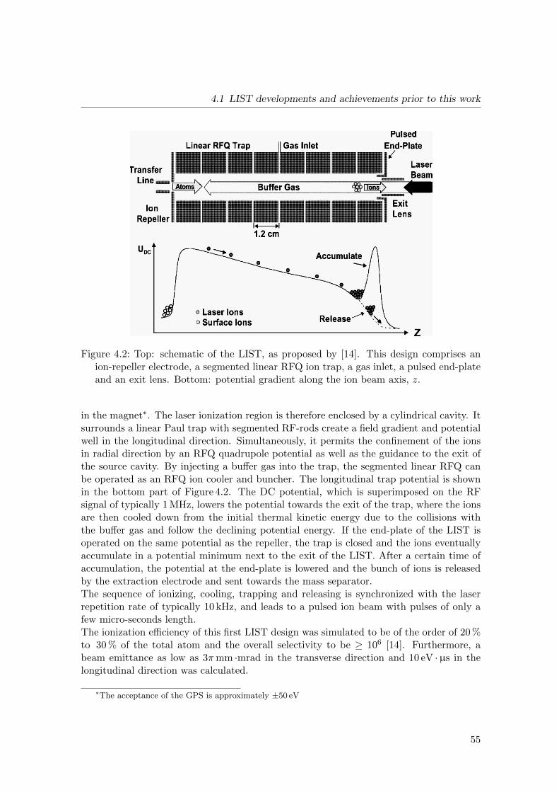
4.1 LIST developments and achievements prior to this work
Figure 4.2: Top: schematic of the LIST, as proposed by [14]. This design comprises anion-repeller electrode, a segmented linear RFQ ion trap, a gas inlet, a pulsed end-plateand an exit lens. Bottom: potential gradient along the ion beam axis, z.
in the magnet∗. The laser ionization region is therefore enclosed by a cylindrical cavity. Itsurrounds a linear Paul trap with segmented RF-rods create a field gradient and potentialwell in the longitudinal direction. Simultaneously, it permits the confinement of the ionsin radial direction by an RFQ quadrupole potential as well as the guidance to the exit ofthe source cavity. By injecting a buffer gas into the trap, the segmented linear RFQ canbe operated as an RFQ ion cooler and buncher. The longitudinal trap potential is shownin the bottom part of Figure 4.2. The DC potential, which is superimposed on the RFsignal of typically 1 MHz, lowers the potential towards the exit of the trap, where the ionsare then cooled down from the initial thermal kinetic energy due to the collisions withthe buffer gas and follow the declining potential energy. If the end-plate of the LIST isoperated on the same potential as the repeller, the trap is closed and the ions eventuallyaccumulate in a potential minimum next to the exit of the LIST. After a certain time ofaccumulation, the potential at the end-plate is lowered and the bunch of ions is releasedby the extraction electrode and sent towards the mass separator.The sequence of ionizing, cooling, trapping and releasing is synchronized with the laserrepetition rate of typically 10 kHz, and leads to a pulsed ion beam with pulses of only afew micro-seconds length.The ionization efficiency of this first LIST design was simulated to be of the order of 20 %to 30 % of the total atom and the overall selectivity to be ≥ 106 [14]. Furthermore, abeam emittance as low as 3πmm ·mrad in the transverse direction and 10 eV ·µs in thelongitudinal direction was calculated.
∗The acceptance of the GPS is approximately ±50 eV
55
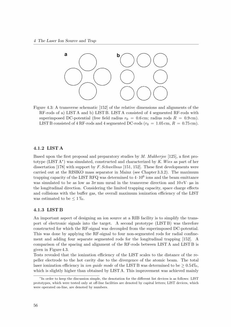
4 The Laser Ion Source and Trap
Figure 4.3: A transverse schematic [152] of the relative dimensions and alignments of theRF-rods of a) LIST A and b) LIST B. LIST A consisted of 4 segmented RF-rods withsuperimposed DC-potential (free field radius r0 = 0.6 cm; radius rods R = 0.9 cm).LIST B consisted of 4 RF-rods and 4 segmented DC-rods (r0 = 1.05 cm, R = 0.75 cm).
4.1.2 LIST A
Based upon the first proposal and preparatory studies by M. Mukherjee [125], a first pro-totype (LIST A∗) was simulated, constructed and characterized by K. Wies as part of herdissertation [178] with support by F. Schwellnus [151, 152]. These first developments werecarried out at the RISIKO mass separator in Mainz (see Chapter 3.3.2). The maximumtrapping capacity of the LIST RFQ was determined to 4 ·106 ions and the beam emittancewas simulated to be as low as 3πmm ·mrad in the transverse direction and 10 eV ·µs inthe longitudinal direction. Considering the limited trapping capacity, space charge effectsand collisions with the buffer gas, the overall maximum ionization efficiency of the LISTwas estimated to be ≤ 1 h.
4.1.3 LIST B
An important aspect of designing an ion source at a RIB facility is to simplify the trans-port of electronic signals into the target. A second prototype (LIST B) was thereforeconstructed for which the RF-signal was decoupled from the superimposed DC-potential.This was done by applying the RF-signal to four non-segmented rods for radial confine-ment and adding four separate segmented rods for the longitudinal trapping [152]. Acomparison of the spacing and alignment of the RF-rods between LIST A and LIST B isgiven in Figure 4.3.Tests revealed that the ionization efficiency of the LIST scales to the distance of the re-peller electrode to the hot cavity due to the divergence of the atomic beam. The totallaser ionization efficiency in ion guide mode of the LIST B was determined to be ≥ 0.54h,which is slightly higher than obtained by LIST A. This improvement was achieved mainly
∗In order to keep the discussion simple, the denotation for the different list devices is as follows: LISTprototypes, which were tested only at off-line facilities are denoted by capital letters; LIST devices, whichwere operated on-line, are denoted by numbers.
56

4.1 LIST developments and achievements prior to this work
0;5mm
Figure 4.4: A schematic of the LIST C [150] in a) a sideways perspective, displaying therepeller electrode and enclosing cavity and b) plan view inside the LIST, displaying thefour RF-rods.
by reducing the distance between the LIST and the exit of the hot cavity from 3 mm to1 mm, which led to a greater overlap of the laser beam with the atoms.During the diploma work of T. Gottwald, the RISIKO mass separator was equipped withan emittance meter for the study of the emittance of the LIST beam [74]. The experimen-tally determined beam emittance showed a surprisingly low emittance obtained withoutcooling and bunching of only ≈ 1πmm ·mrad.
4.1.4 LIST C
The design of LIST B was modified and adapted for the special technical restrictions at thetarget fronted at ISOLDE during the dissertation of F. Schwellnus [150]. For this purpose,the complexity of the third LIST prototype (LIST C) was reduced for several reasons:
1. Limited available volume for the LIST inside the ISOLDE target.
2. Limited number of available vacuum feedthroughs for the transport of the electronicsignals into the target.
3. Harsh conditions at the target front-end: radioactivity of up to kGy/h during oper-ation and temperatures exceeding 2000C.
4. Technical difficulties and safety considerations concerning the usage of buffer gas atthe ISOLDE target front-end.
These restrictions, together with the promising results of the LIST B emittance withoutbuffer gas, justified the reduction of the RFQ cooler and buncher to a linear RFQ ionguide without segmented rods and buffer gas cooling. A schematic of the LIST C design isshown in Figure 4.4. The LIST C was developed in a collaboration between the Universityof Mainz and ISOLDE and was successfully tested and operated at the ISOLDE off-line
57

4 The Laser Ion Source and Trap
mass separator under realistic conditions. It was then further simulated and characterizedat the University of Mainz.The minimum suppression of surface-ionized ions by the LIST C repeller electrode was ofthe order of 105, and the laser ionization efficiency could be increased to ≈ 0.14h∗. Evenwithout buffer gas, the LIST C pulse length of one laser pulse was smaller than 6µs andthe estimated transverse emittance was about 2πmm ·mrad.These promising results led to an ongoing continuation of the collaboration between theUniversity of Mainz and ISOLDE for further development of the LIST, towards the firston-line test at ISOLDE. A first solution for the transport of the RF-signal into the targetwas proposed and additional tests of the resulting LIST D at the ISOLDE off-line massseparator were scheduled for October 2010.
4.1.5 Objective of this thesis
The work on this doctoral thesis started in September 2010, directly prior the scheduledoff-line test of the LIST D at the ISOLDE off-line mass separator. It first aimed at charac-terizing the performance of the LIST at the off-line mass separator and then, if successful,eventually prepare and organize the first on-line test of the LIST at ISOLDE. The re-search work was carried out in a joint effort with Sven Richter (PhD student, Universityof Mainz [140]), within a collaboration between the RILIS group of Dr. Valentin Fedosseevand the target group of Dr. Thierry Stora at ISOLDE, the LARISSA working group ofProf. Dr. Klaus Wendt of Mainz University and the Division of Prof. Dr. Klaus Blaum atthe Max-Planck Institut fur Kernphysik in Heidelberg. This approach was compelled bythe combined knowledge of design and construction in Mainz, and ISOLDE for the suc-cessful implementation of the LIST into the ISOLDE environment and the preparation ofthe off-line and on-line experiments. Additionally, the project benefited of complementary,independent tests at ISOLDE and at the RISIKO mass separator in Mainz. Based on theprevious developments of the LIST described above, the objectives of this thesis are:
Establish a test setup at the ISOLDE off-line mass separator:Setting-up a temporary RILIS installation at the ISOLDE off-line mass separator;setting up and testing the electronics and developing of a remote control program;the adaptation and modification of an ISOLDE target unit for the installation of theLIST.
Preparatory tests at the ISOLDE off-line mass separator:Characterizing the LIST in terms of selectivity and ionization efficiency; testing anautomatic RF-coupling system; commissioning of the ISOLDE target prior to theon-line target development test.
Implementation of the LIST into the ISOLDE environmentConstructing an on-line target; developing a technical solution for the transporta-tion of an RF-signal into the target; installing the LIST power supplies and remotecontrols at the ISOLDE high voltage platform.
∗Note that this increase was achieved in the LIST mode (repeller on positive potential), while the laserionization efficiencies of LIST A and LIST B were obtained in ion guide mode.
58

4.2 The Laser Ion Source and Trap at ISOLDE
On-line testing, optimization, further developments and operation of the LISTOrganizing a first on-line run; characterizing the LIST using radioactive nuclides;first on-line application of LIST for physics experiments at ISOLDE, in the case ofa successful first on-line test.
4.2 The Laser Ion Source and Trap at ISOLDE
Three LIST devices were constructed and used for the experiments described here: LIST Dfor the initial tests at the ISOLDE off-line separator from October 2010 to February 2011,LIST 1 for the first on-line target development test at ISOLDE in May 2011 and LIST 2,which was used in September 2012 for the spectroscopy of neutron-rich polonium. Allthree LIST versions are based on the design of LIST C (repeller, RFQ ion guide, no cool-ing nor bunching), but were slightly altered between the different versions to optimize theperformance. They were built at the workshop of the physics institute of the Universityof Mainz and the corresponding target assemblies were designed and constructed by theISOLDE workshop.
4.2.1 Specifications of LIST D, LIST 1 and LIST 2
An illustration of the final LIST design is given in Figure 4.5 and photographs of thedifferent stages of the assembling and installing of the LIST are shown in Figure 4.6. Inorder to improve the performance, the dimensions of some components were changed fromLIST D to LIST 2. To simplify the description in the following, the LIST D values are usedas default. For components that were modified for each LIST version, the dimensions aregiven in parenthesise with indexes referring to the specific LIST model. Further detailedtechnical drawings will be given in [140].The LIST consists of two annular electrodes with an outer diameter of do = 35 mm andan aperture diameter of da = 7 mm (da,6 = 11 mm) located at each end of a cylindricalchamber made of stainless steel with a length of lc = 100 mm (lc,5,6 = 90 mm) and adiameter of dc = 38 mm. Four RF-rods of lRF = 98 mm (lRF,5,6 = 88 mm length) anddRF = 10 mm diameter are fixed parallel with the axis of the LIST and equally spacedaround a radius of rRF = 15 mm from the center of the device to form the RFQ ionguide. Each of these elements are made of stainless steel and are separated by boron-nitride (BN) ceramic insulators, chosen for its high melting point of T = 2973 C and itsresistance against radioactivity.The two electrodes (repeller and end-electrode) and the chamber shield the ionizationregion from the strong electric field of the ISOLDE extraction electrode; thereby providinga longitudinally field-free region, such that ions created inside the LIST will be extractedwith a small energy spread.A voltage of up to VRF = ± 500 V can be applied to the repeller electrode. The repellervoltage polarity determines the mode of operation of the LIST. A positive voltage repelsions that are created inside the hot cavity (“LIST mode”) permitting only neutral atomsto enter the LIST RFQ ion guide. A negative voltage enables passage of the hot cavityions and the LIST RFQ acts as an ion guide only (“ion guide mode”). The RFQ ion guide
59

4 The Laser Ion Source and Trap
1 cm
a
b
c
dd
V = repeller +/- 500 V V = 0 - 500 Vrf
f ~ 1 MHzrf
Df = 180°
-F-F
F
F
Figure 4.5: Left: a drawing of the LIST design and its most important parameters [140]:a) repeller, b) RF-rods, c) LIST holder and d) housing. A voltage of Vrepeller = ± 500 Vcan be applied to the repeller electrode. Right: the RF-signal (VRF = 0 − 500 V,fRF ≈ 1 MHz) is applied to the RF-rods in opposite phase between neighboring rods.
is necessary for transverse confinement of ions within the LIST as they drift towards theextraction potential (see Chapter 3.5). A sinusoidal RF-signal with fRF = 1 MHz frequency(fRF,5 = 1.2 MHz, fRF,6 = 1.15 MHz) and up to VRF = 500 Vpp amplitude from peak to peak(pp) is applied to the RF-rods, in opposite phase between neighboring rods to generate atrapping potential.
Figure 4.6: Left: Overview of the LIST 1 components. Center: assembled LIST. Therepeller electrode, the LIST chamber, the LIST holder and the RF-contacts are visible.Right: LIST 1 installed into an ISOLDE target.
60

4.2 The Laser Ion Source and Trap at ISOLDE
4.2.2 On-line runs and target specifications
One target was assembled for each on-line run and for the corresponding off-line test. Bothwere ISOLDE targets in standard configuration, as shown in Figure 3.4. They consistedof a target container (l = 202 mm, d = 20 mm), tantalum transfer line (l = 41 mmfrom target, d = 5 mm) and a hot cavity (l = 34 mm, d = 3.1 mm inner diameter). Theindividual target and operation parameters of the two LIST targets are given in Figure 4.7.
LIST target 1: off-line characterization October 2010 until May 2011 andon-line run May 2011
The first on-line target development run of the LIST was scheduled from May 5-7, 2011 atthe beginning of the on-line period in 2011. The goal was the first on-line characterizationof the LIST at ISOLDE, comprising measurements of the suppression and laser ionizationefficiency of radioactive isotopes. Its long-term reliability under on-line conditions was alsoto be assessed. In addition, the feasibility of using the LIST to reduce contamination ofsurface ionized sodium and aluminium (Al) in magnesium (Mg) beams in the mass rangefrom 21 u to 27 u was tested. For the production of these light exotic nuclei, the target(ISOLDE target #442) was filled with rolls of titanium-foils (25µm thickness, 56 g totalweight) as the target material.The initial tests at the off-line separator were carried out with the LIST D. Due to spaceconstrains inside the target, LIST 1 was built with a 1 cm shorter overall length. LIST Dand LIST 1 were installed 5 mm downstream of the hot cavity. This was the closest possibleposition ascertaining that the LIST would not come into contact with the hot cavity or theprotecting heat shields. An overview over the operating parameters of the LIST target 1(ISOLDE target # 442) is given in Figure 4.7 a.
Ta 516A
270 A Ta
0.3 -1.1mA
50 kV
#442
GPS
TiTa 570A
-630A
290 A Ta
0.3 -1.1mA
50 kV
#488
GPS
UCX
b)a)
LIS
T 1
LIS
T 2
Figure 4.7: An illustration of the operating parameters of a) LIST target 1 and b) LISTtarget 2. From top to bottom: target number #, target material, typical target andhot cavity currents in A, proton intensities in µA, LIST symbol, extraction voltage andfront-end. Design of schematics adopted from [143].
61

4 The Laser Ion Source and Trap
LIST target 2: off-line commissioning August 2012 and on-line runSeptember 2012
The LIST was used for its first real on-line physics application in September 2012. The goalwas suppression of surface ionized francium in polonium beams in order to subsequentlyperform laser spectroscopy on neutron-rich polonium isotopes (see Chapter 7). For thispurpose a uranium-carbide UCc was used. Due to a possible coating of the BN insulatorsbecause of the outgassing of material from the uranium-carbide target, the LIST wasinitially tested with silicon carbide (SiC) target to investigate this issue at the ISOLDEoff-line mass separator.A slightly altered design of the RF-rods insulators and the repeller electrode allowed forthe LIST to be mounted 2.5 mm closer to the hot cavity than for the previous target,resulting in an overall distance of only 2.5 mm. This geometry leads to a greater overlapof the lasers with free atoms behind the repeller, possibly leading to a higher ionizationefficiency. The operating parameters of the LIST target 2 (ISOLDE target #488) are givenin Figure 4.7 b.
4.2.3 Implementation of the LIST at ISOLDE
The on-line operation of an electronic device such as the LIST in the ISOLDE environmentrequired several technical modifications of the LIST, the target, and the GPS-front-enddue to several constraints:
1. Previously there were no dedicated RF-feedthroughs or RF-cabling installed fortransport of electronic signals over the distance of about 20 m from the high-voltagecage to the target. This necessitated:
→ the installation of a new radiation-hard RF-coax line from the high-voltage cageto the target.
→ the minimization of losses due to the transport of the RF-signal by sending alow-amplitude signal to the front-end as well as by transforming and splittingof the RF-signal into two RF-signals of opposite phase at the target using atransducer unit (“transducer box”).
→ the minimization of losses due to the transport of the RF-signal by sending alow-amplitude signal to the front-end as well as by transforming and splittingof the RF-signal into two RF-signals of opposite phase at the target using atransducer unit (“transducer box”).
2. Harsh conditions during operation due to high radiation levels and high temperatureswere overcome by:
→ radiation hard insulators, cables and a transducer box.
3. Automatic handling of the targets by robots demanded:
→ the design of the mount to hold the transducer box on the target assembly.
→ the construction of an automatic RF-coupling from the front-end to the target.
62

4.2 The Laser Ion Source and Trap at ISOLDE
4. No access to the target or to the front-end and only limited access to electronics onthe high-voltage platform is possible during operation. This required a
→ remote control for the LIST operating parameters.
→ automatic data acquisition system.
Transport of the RF-signal
Due to the absence of a dedicated RF-cable and an RF-feedthrough to the target, severalmodifications to the GPS front-end and the target unit were necessary prior to the firston-line run. In order to avoid power losses during the transport of the RF-signal fromthe high-voltage cage to the target over a distance of about 20 m, a two-stage transportand transformation system was initially designed by K.-P. Holdtke from the Universityof Mainz [150]. The final design for the adaption to ISOLDE is shown schematically inFigure 4.8.The RF-signal of about 1 MHz is generated by a function generator (“TTi”, 0.001 Hz to10 MHz, 0 Vpp to 7 Vpp) and amplified to up to 60 V by a pre-amplifier unit designed andbuilt by the University of Mainz. The pre-amplifier can be tuned remotely by an analog0 V to 10 V DC-voltage signal (RF-control voltage), provided by a “Keithley 6487” powersupply.The RF-signal was then sent down from the high-voltage cage to the target through a newlydeveloped radiation hard coaxial line. It was designed in parallel for the first on-line testof a HELICON type ion source by Pekka Suominen from the ISOLDE target group andinstalled at the ISOLDE GPS front-end during the ISOLDE shutdown period in spring2011 [97]. This line consisted of a 20 m radiation hard coaxial cable (50 Ω, 75.9 pF/m) ofthe company Huber+Suhner, a 0.7 m home-built coaxial copper line to bridge the high-radiation area close to the target, and an automatic RF-coupling to transport the signal tothe target. This RF-coupling allows the automatic connection of the target to the coaxial
RF-pre amplifier“University Mainz”
1MHz,0-59 VppFunction generator
“TTi TG2000"sine,1MHz, 0-10 Vpp
RF-control voltage“Keithley 6487"
0-10 V
Repeller voltage“Keithley 6487"
+/- 500 V
Transducer box“University Mainz”
1MHz,0-500Vpp
Coaxial line + RF-coupling“ISOLDE/CERN”20m, 75.9 pF/m
Df = 180°
Figure 4.8: A schematic of the electronic supplies and the RF-transmission system from thehigh-voltage cage to the LIST. The RF-supply system consists of a function generator,a DC-control unit, a pre-amplifier, a radiation hard coaxial line including the RF-coupling and a transducer box. The DC-voltage for the repeller is provided by a powersupply and transmitted through a standard feed-through to the target.
63

4 The Laser Ion Source and Trap
Figure 4.9: a) A picture of the radiation-hard coaxial copper line installed at the ISOLDEGPS front-end and a close-up of the RF-coupling [166].
RF-coupling
Target container
Transducer Box
Mount
LIST
Figure 4.10: Target assembly 1 with LIST 1 before the first on-line run in May 2011. Thetransducer box, mount of transducer box, RF-coupling, LIST 1 and target containerare visible.
64

4.2 The Laser Ion Source and Trap at ISOLDE
0 2 4 6 8 1 00
1 0 0
2 0 0
3 0 0
4 0 0
O f f - l i n e L I S T 5 O n - l i n e L I S T 5
RF-am
plitud
e (V pp
)
R F - c o n t r o l v o l t a g e ( V )
1 8.2,
, =−
−
l i n eo np p
l i n eo f fr fUU
Figure 4.11: Calibration of the RF-amplitude as a function of the RF-control voltage at the off-line separatorand at the GPS front-end before theon-line run 2011. The function gener-ator was set to a sine-signal with anamplitude of 3 Vpp. The signal at theGPS front-end is reduced by a factorof 2.18.
copper line when the robot attaches the target to the front-end. A drawing of the coaxialcopper line and the RF-coupling at the GPS front-end is given in Figure 4.9 [166].After passing the RF-coupling, the RF-signal is transported to a transducer box, whichis mounted above the target assembly. A technical drawing of the transducer box andfurther details can be found in [139, 140]. The transducer consists of an inductor-capacitor(LC) circuit with tunable capacitors to match the LC circuit to the 50 Ω coaxial line.All elements were made of radiation hard materials (PEEK) to protect the electricalcomponents from the radioactive environment. If the frequency of the RF-signal is inresonance with the LC-circuit, the transducer transforms the signal to up to 500 Vpp togenerate a sufficient trapping potential. The resonance frequency was 1.15 MHz for thetransducer box of the LIST target 1 and 1.2MHz for the transducer box 2. The differencebetween these two transducer boxes was due to small differences of the LC-components.Furthermore, the transducer box output is split into RF-signals of opposite phase forthe neighboring rods of the RFQ (see Figure 4.5). The RF-signals are then transferred bystandard vacuum feedthroughs from the transducer into the target continuing to the LIST.A picture of the final target assembly of the LIST 1 with transducer box and RF-couplingis shown in Figure 4.10.After each attachment of the target assembly to the frontend, the RF-amplitudes at theLIST RF-rods need to be calibrated for the applied RF-control voltage. Figure 4.11 showsthe calibration of the RF-control voltage to the RF-amplitude at the RF-rods of the of theLIST 1. The calibration at the ISOLDE off-line separator is compared to the calibrationat the ISOLDE GPS front-end before the first on-line run in 2011. For each individualcalibration, the RF-signal from the function generator was set to 3 Vpp and the tunablecapacitors were set such that signal strength at neighboring rods was symmetrical. Thedependency of the RF-amplitude to the RF-control voltage showed a linear behavior inboth cases. However, a difference of the strengths of the RF-signals of a factor of 2.18was observed between the off-line separator and the GPS front-end. For instance, atthe off-line separator, the maximum obtained amplitude at 10 V RF-control voltage was436pp, while at the GPS frontend, the amplitude was only 198 Vpp. Despite the losses, themaximum RF-amplitude at the GPS front-end was believed to be enough to transport
65

4 The Laser Ion Source and Trap
all ions through the RFQ according to the preparatory tests performed at the off-lineseparator (see Chapter 4.3.3). If necessary, it would have been possible to increase thesignal strength further by increasing the amplitude of the RF-function generator to 7 Vpp.The losses at the GPS front-end can be explained by the different RF-cables and RF-couplings, which were used at the off-line separator and the on-line separator. Since theLIST transducer box cannot be fine tuned at the front-end due to safety constraints, thetransducer box could only be tuned at the off-line separator prior to the on-line run leadingto a possible mismatch at the GPS-frontend. In order to limit the losses during the nextLIST experiments, an identically constructed coaxial copper line and cable was installedat the off-line separator for a better matching of the transducer box prior to the secondon-line run with the LIST 2 in 2012. The results of the calibration of the transducer boxof the corresponding LIST target 2 are similar to the calibration line of the transducer boxof LIST target 1 shown in Figure 4.11, but no direct measurements at the GPS frontendwere possible prior the second on-line run due to safety constraints.
Handling and coupling of a target by robots
The modified LIST target assembly with the transducer box and the cabling adds spaceand weight to the standard ISOLDE target. Thus, the correct placement of the LISTtransducer box and the automatic RF-coupling had to be investigated in order to balancethe target during the transport by the robots, and to avoid contact with the elements of thetarget front-end. For this purpose, a mount for the LIST transducer box was designed.The handling of the target by the robot was successfully tested at the GPS front-endduring the ISOLDE shutdown in April 2011. In addition, these tests provided importantinformation about the correct placement of the transducer box on the mount with respectto the cabling at the front-end. Figure 4.12 gives an impression of the different stages ofthe handling phases by the robot: grabbing, transporting and attaching.
Remote control system
Remote control of the repeller voltage and the RF-settings is essential for optimizing theLIST operating parameters. To serve this purpose, a LabVIEW based control systemfor the LIST has been developed and integrated into the RILIS control system [142].The system provided independent control of the RF-function generator “TTi TG2000”(RF-frequency), the RF-control voltage supply “Keithley 6487” (RF-amplitude) and therepeller voltage supply “Keithley 6487”. A schematic of the control system is shown inFigure 4.13.Glass fibers were passed from the RILIS laboratory into the HV-cage to allow the remotecontrol of the electronic units. RS232-to-ethernet and fiber-to-ethernet converters trans-lated the signal from and to the HV-cage. The electronics were integrated into the CERNtechnical network as shown in Figure 4.13, which were in turn accessible by the RILIScontrol computer. Additionally, the Faraday cup signal could be accessed by the controlsystem to allow for optimizing and scanning of the ion current as a function of the repellervoltage and the RF-amplitude.This setup was also used during the preparatory tests of the LIST at the ISOLDE off-line
66

4.2 The Laser Ion Source and Trap at ISOLDE
Figure 4.12: Photographs taken during the robot test of the LIST target 1 at the GPSfront-end. Left: Richard Catherall controls the grabbing of the target by the robotarm. Location and balancing the weight of the transducer box is crucial. Right top:the robot lifts and moves the target towards the front-end. The design of the holderallows to move the robot freely. Bottom right: target attached to GPS front-end.Cabling of transducer box needs to be considered for the final placement of the thetransducer box. It is noted that the transducer box was altered between this test andthe on-line run (see Figure 4.10).
67

4 The Laser Ion Source and Trap
Technical network CERN
8-port ethernet switch
Ethernet to optical fiber Fiber to Ethernet
Ethernet to RS232
RF-transducer
RF-function generator
‘TTi TG2000’
RILIS Laboratory
Optical fiber
RF-control voltage
‘Keithley 6487’
RF-coupling
Pre-amplifier
‘University Mainz’
High-voltage platform 30 kV – 60 kV
Repeller voltage
‘Keithley 6487’
Scope
‘Tectronix’
Figure 4.13: Illustration of the remote control system of the LIST. Glass fibers were passedfrom the RILIS laboratory to the HV-cage for remote control of the electronics. TheRF-function generator, the RF-control supply and the repeller voltage supply are inte-grated and controlled via the technical network of CERN.
mass separator, except that the devices were not integrated into the technical network,but controlled via an USB-to-RS232 converter directly by the control computer.
Off-line laser system
A RILIS setup was installed at the ISOLDE off-line mass separator for the off-line tests.A sketch of the setup is shown in Figure 4.15. It consisted of two Ti:Sa solid-state lasers,which were pumped by a Nd:YAG 532 nm pump laser from Photonics industry and onefrequency tripling unit. The pump laser beam was split by two tunable beam-splitters(λ/2-plate + beam-splitter cube), which allowed separate tuning of the pumping powerof the two Ti:Sa lasers. A small fraction of the output from each of the Ti:Sa lasers waspicked up by 4% beam splitters and sent to a wavemeter for monitoring. Laser optics forinfrared (IR) and ultraviolet (UV) light - consisting of mirrors, telescopes and periscopes- guided and focused the laser beams through a metal tube and a quartz-window into theseparator magnet and beam-line towards the LIST and the hot cavity.The tests at the off-line mass separator were conducted with ytterbium (Yb) because ofits efficient two-step laser ionization scheme, with wavelengths within the tuning range ofthe Ti:Sa lasers. The ionization scheme of ytterbium is shown in Figure 4.14a. Addition-
68

4.2 The Laser Ion Source and Trap at ISOLDE
-1IE: 67 860 cm
255.80 nm
843.37 nm
532 nm
Po
-1IE: 61 671.05 cm
532 nm
Mg-1
0 cm
6 2 12p 3s S0
285.21 nm 08 -1A = 4.91e s
552.84 nm 07 -1 A = 1.39e s
-135 051.26 cm
13s3p P1
o
-153 134.64 cm
13s4d D2
-1AIS: 50 989.2 cm -1
IE: 50 443.2 cm
736.45 nm
Yb-1
0 cm
14 2 14f 6s S0
-137 414.59 cm
13 2 o 24f ( F )5d 6s P1
1 o
267.20 nm 08 -1A = 1.43e s
-10 cm
4 36p P2
-139 081.19 cm
3 4 56p ( S )7s S2
o o
-150 934.89 cm
3 46p ( S )7p
o 5P2
a) b) c)
Figure 4.14: Laser ionization schemes for a) ytterbium (Yb), b) magnesium (Mg) and c)polonium (Po), as used during the experiments with the LIST. Ytterbium was ionizedvia an intermediate state to an autoionizing state. Magnesium and polonium wereionized via two intermediate transitions non-resonantly into the continuum. The secondstep of polonium was provided by a tunable NB Ti:Sa laser for the measurement of theHFS and the IS of that transition. Wavenumbers and configuration of the atomic levelsand wavelengths and the transition probabilities are given if known from literature [94].
ally, ytterbium has a significant surface ionization efficiency, which allows to study thesuppression of surface ionized ions and laser ionization efficiency in parallel.
On-line laser system
For the first on-line run, the RILIS laser system was tuned to the ionization scheme formagnesium, as shown in Figure 4.14b. A detailed description of the RILIS setup is givenin Chapter 3.3.1. Two Sirah Credo dye lasers were used for the first two resonant transi-tions and the residual output power of the dye pump laser (frequency doubled EdgewaveNd:YAG) was used for the non-resonant ionization step. The target was prepared withone uncalibrated magnesium mass marker for initial testing and optimization of the laserbeams and one calibrated magnesium mass marker (1100 nAh) for a laser ionization effi-ciency measurement.During the first part of the 2012 run, the RILIS was tuned to magnesium to compare theLIST 2 to LIST 1 from the 2011 run. The setup of the RILIS was similar to the setupdescribed above. In the second part of the 2012 on-line run, the setup was reconfiguredto ionize polonium (Po) for the study of neutron-rich polonium isotopes (see Chapter 7).The laser ionization scheme [41] of polonium is shown in Figure 4.14c. The first resonantstep was provided by the third harmonic of a Sirah dye laser, while the second step wasprovided by the fundamental of a tunable, narrow-band Ti:Sa laser for scanning of thespectroscopic transition. For the third transition above the ionization energy, the radiationof the frequency doubled Edgewave Nd:YAG dye pump-laser was used.
69

4 The Laser Ion Source and Trap
Wavemeter
Ti:Sa 2 Ti:Sa 1
Nd:YAG
Tripler unit M
M
UV Periscope
Telescope
l/2+cube l/2+cube
BD BD
50:50M
MM 4%
Telescope
4%
M
M
M
M
M
M
M
M
Periscope
M
MFiber couplerFiber coupler
Fiber couplerFiber
Fiber
To off-line mass separator
Legend:M: mirrorBD: beam dump4%: 4% beam splitter
l/2: l/2 plate
Figure 4.15: Schematic of the RILIS installation at the off-line mass separator for thetesting and characterization of the LIST with ytterbium. The main components area Nd:YAG 532 nm pump laser from Photonics industries, two Ti:Sa solid-state lasers,one tripler unit, a wavemeter and laser beam transport optics. The laser path is givenby straight colored lines with arrows indicating the direction. The beams are finallymixed together at the last periscope and sent to the off-line separator.
Figure 4.16: Photograph of the laser installation at the off-line mass separator (fromthe bottom right edge of the laser table in Figure 4.15). The two Ti:Sa lasers, theNd:YAG pump laser and the optics are visible. The laser beams are transported bytwo periscopes into the metal beam pipe towards the quartz-window of the mass sep-arator and the target.
70

4.3 Characterization of the performance of the LIST at ISOLDE
4.3 Characterization of the performance of the LIST atISOLDE
This section discusses the results of the two on-line runs and their preparatory tests at theoff-line separator. Prior to the results, the most important terms, parameters and methodsare defined to enable a better understanding. These are discussed with the help of Fig-ure 4.17, which shows the different dependency of the ionization efficiency of laser ionized174Yb and surface ionized 174Yb on the applied repeller voltage. For these measurements,the repeller voltage was scanned automatically from Urep = −215 V to Urep = +215 V,while the ion current was measured by a Faraday cup. These so-called, repeller scans,were conducted with the LIST 1 at the ISOLDE off-line separator as part of the prepara-tory measurements for the first on-line run.
4.3.1 Different modes of operation
Depending on the repeller voltage setting, the LIST can be operated in the selective LISTmode or in the ion guide mode with a selectivity and efficiency similar to normal RILISoperation:
LIST mode: In LIST mode, a positive repeller voltage is applied and surface ions aresuppressed. Only laser-ions created inside the LIST are extracted. The repellervoltage setting in LIST mode is defined as the positive voltage for which maximumsuppression of surface ions is achieved.The effect of a positive repeller voltage to the ion current of 174Yb is shown inFigure 4.17. When scanning across zero repeller voltage, the surface ion currentdecreases strongly and eventually reaches the background level of the Faraday cup ataround Urep = +5 V. Despite of some fluctuations of the Faraday cup noise level, thesurface ion current then remains indistinguishable from the Faraday cup backgroundnoise of 0.08 pA for higher repeller voltages, while the laser ion current remains wellabove the Faraday cup noise level. On the other hand, higher repeller voltages leadto the loss of laser ions due to an increased initial energy of ions created close to therepeller, which is detrimental for their transmission through the LIST. To take thiseffect into account, a range of suitable repeller voltages for the operation in LISTmode was determined from Urep = +7 V to Urep = +12 V.
Ion guide mode: In ion guide mode a negative voltage is applied to the repeller electrodeand the positive ions, which were created in the hot cavity, may enter the LISTRFQ undisturbed. The overall extraction efficiency depends on the penetration ofthe negative repeller voltage into the source and thus, the ion guide mode is definedas the negative repeller voltage for which the laser ionization efficiency is highest.In Figure 4.17, the ion guide mode for 174Yb is between Urep = −25 V to Urep =−55 V.
The exact values of the repeller voltage settings for LIST mode and ion guide mode needto be determined separately for each isotope and may differ, depending on the mass and
71

4 The Laser Ion Source and Trap
- 2 0 0 - 1 5 0 - 1 0 0 - 5 0 0 5 0 1 0 0 1 5 0 2 0 0
1 E - 1 3
1 E - 1 2
1 E - 1 1
1 E - 1 0
1 E - 9
1 E - 8
Ion
Curre
nt (A)
R e p e l l e r V o l t a g e ( V )
1 7 4 Y b L a s e r O N 1 7 4 Y b L a s e r O F F
L L F
L S F
a )
b )c )
d )
I G m o d e L I S T m o d e
O f f - l i n e :
Figure 4.17: Ion current of laser ions (dashed red line, laser on) and surface ions (solid blackline, laser off) of 174Yb as a function of the repeller voltage, measured at the ISOLDEoff-line separator with LIST 1. The hatched fields correspond to the repeller voltagesfor ion guide mode (IG) and LIST mode. The LIST loss factor, LLF, is indicated bythe red arrow from the laser ion current in IG mode (a) and in LIST mode (b) andthe LIST suppression factor, LSF, is indicated by the black arrow from the surface ioncurrent in IG mode (c) and in LIST mode (d).
the level of contamination. However, in case of radioactive isotopes with low productionyields a repeller scan is either impracticable or impossible. For these isotopes, the optimalLIST settings need to be extrapolated from the settings of stable isotopes.
4.3.2 Parameters of the LIST performance and measurement methods
The performance of the LIST can be characterized by five parameters: the selectivity, S ,the LIST suppression factor, LSF , the laser ionization efficiency ε, the LIST loss factor,LLF , and the LIST quality factor LQF . Corresponding measurement methods, which wereused throughout these experiments, are described when applicable.
Selectivity, S : The selectivity∗ is a measure of the purity of the ion beam and can bedefined as:
S =Ion intensity of isotope of interest
Total ion intensity on the given mass of contaminants and isotope of interest.
(4.1)
∗The selectivity has already been introduced in Equation 3.2 in Chapter 3 but is here given for com-pleteness.
72

4.3 Characterization of the performance of the LIST at ISOLDE
LIST suppression factor, LSF : The suppression in LIST mode can be described bythe LIST suppression factor, LSF, which is given by:
LSF =Ion intensity of contaminant in ion guide mode
Ion intensity of contaminant in LIST mode. (4.2)
If the ion intensity of the contaminant is above the detection limit of the Faradaycup, the LIST suppression factor can be determined by a repeller scan as demon-strated in Figure 4.17. It is calculated by comparing the maximum intensity in ionguide mode mode and the minimum intensity in LIST mode. For radioactive iso-topes, for which a repeller scan is not easily achievable, the suppression factor isthen derived by calculating the ratio between ion intensity in ion guide mode andin LIST mode using the predefined repeller settings for LIST mode and ion guidemode, which were obtained by extrapolation from the values of stable isotopes.The LSF for 174Yb, shown in Figure,4.17 has been determined to be ≈ 400 consid-ering the background noise of 0.08 pA. Note that for this measurement, the Faradaycup noise was a lower limit and a measurement of the absolute LSF would requirea detector with higher sensitivity (i.e. a SEM).
Laser ionization efficiency, εion: The ionization efficiency, εion, of an ion source can bedefined as:
εion =# atoms in sample ionized
total # atoms in sample. (4.3)
This is most reliably evaluated by measuring the integrated ion current after thetotal evaporation of a carefully calibrated sample of the element of interest. How-ever, the absolute efficiency measurement is restricted to stable isotopes and is timeconsuming, which limits its applicability during on-line runs.
LIST loss factor, LLF : A more practical means of assessing the laser ionization effi-ciency of the LIST is to compare the LIST mode and ion guide mode ion intensity,using the predefined repeller voltage settings. The efficiency loss, LLF, due to thereduced atom/laser overlap in LIST mode is given by:
LLF =Laser ion intensity in ion guide
Laser ion intensity in LIST mode. (4.4)
As an example, Figure 4.17 shows a LFF value of ≈ 50 for 174Yb with LIST 1.
LIST quality factor, LQF : Combining the LIST suppression factor, LSF, and the LISTloss factor, LLF, it is possible to characterize the LIST performance using the LISTquality factor, LQF, defined as:
LQF =LSF
LLF. (4.5)
The value of LQF is intended as a guide to determine the typical LIST performanceunder standard conditions and is an important tool for comparing different LIST
73

4 The Laser Ion Source and Trap
units. For specific isotopes that suffer from poor isobaric suppression, due to isotopedependent sources of contamination, the target and LIST ion source assembly maybe operated in non-standard conditions. In these cases, the LIST quality factor doesnot apply.If the efficiency in ion guide mode is comparable to the efficiency of the normal RILISoperation, the LIST quality factor LQF is the gain in selectivity due to the use ofthe LIST compared to the RILIS.
4.3.3 Transmission through the RFQ ion guide
The RF amplitude at the rods, for which the transmission efficiency is highest, depends onthe mass (see Chapter 3.5). This dependency was studied systematically at the ISOLDEoff-line separator with several surface ionized isotopes, namely 23Na, 40Ca, 85Rb and 133Csin ion guide mode with a repeller voltage settings of URep = −43 V. Laser ionized 174Ybwas studied in both, LIST mode and ion guide mode with repeller voltage settings ofURep = +7 V and URep = −100 V, respectively.Figure 4.18 shows the normalized ion current of these isotopes as a function of the RF-amplitude obtained by LIST 2. In the left graph, the behavior of the surface ionizedisotopes are shown. The transition curves of the different isotopes have similar shapes:a steep increase from URF = 0 Vpp to a mass-dependent maximum, from which the ioncurrent slowly decreases to about a third of the maximum ion current and in case of thelightest studied isotope, 23Na eventually drops to zero. This corresponds to the end ofthe stability diagram (see Figure 3.15 in Chapter 3.5). An approximate proportionality ofthe RF amplitudes for which the ion current is highest to the mass can be observed. For
0 5 0 1 0 0 1 5 0 2 0 0 2 5 0 3 0 0 3 5 00 . 1
1
I o n g u i d e m o d e ( U r e p = - 5 0 V ) :
Norm
alized
Ion C
urren
t
R F - A m p l i t u d e ( V p p )
S u r f a c e i o n i z e d i s o t o p e s 2 3 N a 4 0 C a 8 5 R b 1 3 3 C s
0 5 0 1 0 0 1 5 0 2 0 0 2 5 0 3 0 0 3 5 0
0 . 1
1I o n g u i d e m o d e v s . L I S T m o d e :
Norm
alized
Ion c
urren
t
R F - A m p l i t u d e ( V p p )
L a s e r i o n i z e d 1 7 4 Y b : L I S T m o d e ( U r e p = + 7 V ) I o n g u i d e m o d e ( U r e p = - 1 0 0 V )
Figure 4.18: Measurements of the ion transmission through the LIST RFQ ion guideconducted at the ISOLDE off-line separator with LIST 2. The normalized ion currentis given as a function of the RF voltage applied to the rods of the RFQ ion guide. Left:surface ionized 23Na, 40Ca, 85Rb and 133Cs in ion guide mode (Urep = −50 V).Right: laser ionized 174Yb in LIST mode (Urep = +7 V, dotted line) compared to ionguide mode (Urep = −100 V, dashed line).
74

4.3 Characterization of the performance of the LIST at ISOLDE
the heavier of the studied isotopes, the available maximum RF-amplitude was not highenough to observe the limit of transmission. These curves clearly deviate from a transmis-sion curve of an ideal RFQ ion guide, for which the ion current should remain stable overthe full range of the stability diagram. The differences can be ascribed to the changes ofthe quadrupole potential compared to an ideal RFQ due to the finite and non-hyperbolicRF-rods and field disturbances due to the repeller voltage.The difference in RF-amplitude dependence of laser ionized 174Yb in ion guide mode andin LIST mode is shown in the right graph of Figure 4.18. In ion guide mode, the transmis-sion curve is similar to the curves of the surface ionized ions. This is easily understandablesince in ion guide mode, most atoms are ionized inside the hot cavity and the initial con-ditions of the ions are similar to those of the surface ionized isotopes. In contrast, the ioncurrent in LIST mode remains constant for the full range of the applied RF-amplitudesafter it reached its maximum ion current. This may be explained by the different initialconditions between ions created inside the hot cavity and inside the LIST RFQ and thedifferent repeller voltage settings. The latter may also explain the disproportional shift ofthe maximum ion current between LIST and ion guide mode.The dependency of the transmission through the LIST RFQ on the RF-amplitude, therepeller voltage and the mass of the ion therefore requires a careful determination of theoptimal settings before studying the efficiency and performing any experiment. For ra-dioactive isotopes, for which a scan of the RF-amplitude is difficult to perform, the optimalsettings for the transmission through the RFQ need to be extrapolated from the valuesobtained with stable isotopes.
4.3.4 Surface ion suppression
Suppression: LIST 1
A repeller scan of 174Yb measured off-line with the LIST 1 is shown in Figure 4.17 andrevealed an LSF of about 400 (see Section 4.3.2). In contrast, Figure 4.19 shows a repellerscan, which was conducted for 48Ti during the on-line test using LIST 1 in 2011. This mea-surement allowed the predefinition of the repeller voltages for LIST mode to Urep = +7 Vand for ion guide mode to Urep = −50 V. The overall suppression of 48Ti was determinedas LSF = 4400 by taking into account the Faraday cup background noise of ≈ 0.1 pA.However, in contrast to the repeller scan of the surface ionized 174Yb from Figure 4.17,the ion current increases for repeller voltages higher than the optimum LIST setting ofUrep = +7 V by more than one order of magnitude. A possible explanation of this is thepoor vacuum condition related to the outgassing from the on-line target and electron im-pact ionization in this regime within the LIST structure.Using the predefined repeller settings, ionization of radiogenic isotopes was studied usinga tape station, which was equipped with a β- and γ-detector (see Chapter 3.4.1). For stan-dard RILIS operation, a desired magnesium ion beam in this mass range may suffer fromisobaric sodium and aluminum contamination. The suppression of the possible isobariccontaminants, 21,26Na, was determined using the β-detector of the ISOLDE tape station,revealing a suppression of more than 3 orders of magnitude for both.
75

4 The Laser Ion Source and Trap
- 1 0 0 - 8 0 - 6 0 - 4 0 - 2 0 0 2 0 4 0 6 01 E - 1 3
1 E - 1 2
1 E - 1 1
1 E - 1 0
1 E - 9
1 E - 8
Ion Cu
rrent
(A)
R e p e l l e r V o l t a g e ( V )
s u r f a c e i o n i z e d 4 8 T i
I G m o d e L I S T m o d e
O n - L i n e
Figure 4.19: Surface ionized 48Ti ion current as a function of the repeller voltage measuredwith LIST 1 under on-line conditions at ISOLDE. A suppression of 4400 is observed inLIST mode (Urep ≈ 8 V) compared to ion guide mode (Urep ≈ −50 V) with a strongincrease of interfering contamination for a higher positive repeller potential.
An overview of the LSF of the studied isotopes obtained by the LIST is given in Table 4.1.For most isotopes, namely 21Na, 23Na, 26Na, 48Ti (off-line), and 174Yb, the measurementof the actual LIST suppression factor was not possible since the ion intensity in LISTmode was indistinguishable from the background level of the detectors. In these cases,a lower limit for the suppression factor was calculated as the ion rate in ion guide modedivided by the statistical uncertainty
√N of the background measurement. However, this
does not apply to 39K, for which the absolute suppression factor was determined to onlyLSF = 230. In this case, the reduced suppression factor can be ascribed to additionalionization effects such as electron impact ionization as described above for 48Ti. Theseisotope specific reductions of the LSF will be discussed in the next session in more detail.Using the individually determined LSFs from above, a conservative general value ofLSF > 1000 can be expected.
Suppression: LIST 2
Figure 4.20 shows wide range mass scans for 20 u < m < 75 u and 125 u < m < 180 utaken at the off-line separator with LIST 2. The upper graph shows a mass scan in ionguide mode and the lower graph shows a mass scan in LIST mode. In ion guide mode,23Na, 27Al, 39,41K, 40Ca, 46−50Ti, 52,53Cr, 69,71Ga, 133Cs, 134−138Ba, and 168,170−174,176Ybare observed as well as titanium oxide (TiO) and some unidentified molecular ion beamsin the mass region of 34 u to 45 u. In LIST mode only the alkaline elements sodium, potas-sium, cesium, and a reduced molecular ion signal around 34 u remain above the detectionlimit of the Faraday cup.
76
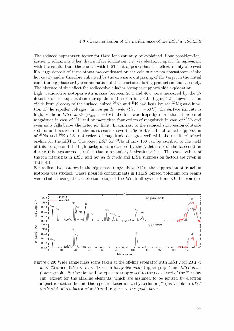
4.3 Characterization of the performance of the LIST at ISOLDE
The reduced suppression factor for these ions can only be explained if one considers ion-ization mechanisms other than surface ionization, i.e. via electron impact. In agreementwith the results from the studies with LIST 1, it appears that this effect is only observedif a large deposit of these atoms has condensed on the cold structures downstream of thehot cavity and is therefore enhanced by the extensive outgassing of the target in the initialconditioning phase or by contamination of the structures during production and assembly.The absence of this effect for radioactive alkaline isotopes supports this explanation.Light radioactive isotopes with masses between 26 u and 46 u were measured by the β-detector of the tape station during the on-line run in 2012. Figure 4.21 shows the ionyields from β-decay of the surface ionized 26Na and 46K and laser ionized 30Mg as a func-tion of the repeller voltages. In ion guide mode (URep = −50 V), the surface ion rate ishigh, while in LIST mode (URep = +7 V), the ion rate drops by more than 3 orders ofmagnitude in case of 46K and by more than four orders of magnitude in case of 26Na andeventually falls below the detection limit. In contrast to the reduced suppression of stablesodium and potassium in the mass scans shown in Figure 4.20, the obtained suppressionof 26Na and 46K of 3 to 4 orders of magnitude do agree well with the results obtainedon-line for the LIST 1. The lower LSF for 30Na of only 130 can be ascribed to the yieldof this isotope and the high background measured by the β-detectors of the tape stationduring this measurement rather than a secondary ionization effect. The exact values ofthe ion intensities in LIST and ion guide mode and LIST suppression factors are given inTable 4.1.For radioactive isotopes in the high mass range above 212 u, the suppression of franciumisotopes was studied. These possible contaminants in RILIS ionized polonium ion beamswere studied using the α-detector setup of the Windmill system from KU Leuven (see
1 E - 1 31 E - 1 21 E - 1 11 E - 1 0
1 E - 91 E - 8
2 0 3 0 4 0 5 0 6 0 7 0 1 3 0 1 4 0 1 5 0 1 6 0 1 7 01 E - 1 31 E - 1 21 E - 1 11 E - 1 0
1 E - 91 E - 8
Y b
Ion Cu
rrent
(A)
L a s e r O F F L a s e r O N
Y bC s2 3 N a
I o n g u i d e m o d e
4 1 K7 1 G a
6 9 G a
4 0 C a
5 2 C r
Ion Cu
rrent
(A)
M a s s ( a m u )
2 3 N a2 7 A l
3 9 K T i
T i O C s B a
L I S T m o d e3 9 K
4 1 K
Figure 4.20: Wide range mass scans taken at the off-line separator with LIST 2 for 20 u <m < 75 u and 125 u < m < 180 u, in ion guide mode (upper graph) and LIST mode(lower graph). Surface ionized isotopes are suppressed to the noise level of the Faradaycup, except for the alkaline elements, which are assumed to be ionized by electronimpact ionization behind the repeller. Laser ionized ytterbium (Yb) is visible in LISTmode with a loss factor of ≈ 50 with respect to ion guide mode.
77

4 The Laser Ion Source and Trap
Table 4.1: Ion intensities in ion guide mode and LIST mode and LIST suppression factors(LSF ) of several stable and radioactive isotopes obtained by using LIST 1 (off-line,on-line) and LIST 2 (on-line). Half-lives of radioactive isotopes are given in brackets.Stable isotopes as well as 220Fr were measured by a Faraday cup (FC) and ion intensitiesare given in pA. β-emitters were measured with the tape station (TS) and ion intensitiesare given in counts per µC protons, while α-emitters were measured by the α-detectorsof the Windmill setup and ion intensities are given in counts / supercycle. If the ionintensity was below the background (bgnd) level of the Faraday cup detector system,a conservative value of the LIST ion intensity was estimated from the backgroundfluctuations in case of the Faraday cup or the statistical uncertainty (
√N , given in
brackets) of the α or β counts. Values are implied with their significant numbers.
Isotope Detector IIG ILIST bgnd unit LSF
LIST 1
Off-line
23Na FC 75 0.4 0.08 pA 230
48Ti FC 145 0.08 0.08 pA ≥ 1800
174Yb FC 3.15 0.08 0.08 pA ≥ 300
On-line
21Na(22.5 s) TS 16000 · 105 100 100(10) counts/µC ≥ 1.6 · 104
23Na FC 85 0.4 0.1 pA 280
26Na(1.07 s) TS 3900 · 104 100 100(10) counts/µC ≥ 3.9 · 103
39K FC 410 2 0.1 pA 230
48Ti FC 3500 0.9 0.1 pA 4400
LIST 2
On-line
26Na(1.07 s) TS 75000 50 50(7) counts/µC ≥ 10700
30Na(48 ms) TS 1437 125 125(11) counts/µC ≥ 130
46K(105 s) TS 13000 50 50(7) counts/µC ≥ 1850
205Fr(3.97 s) WM 63520 25 0 counts / supercycle 2540
212Fr(20.0 min) FC 80 2 0.85 pA 70
220Fr(27.4 s) WM 15379 412 412(20) counts / supercycle ≥ 770
78

4.3 Characterization of the performance of the LIST at ISOLDE
- 5 0 0 - 4 0 0 - 3 0 0 - 2 0 0 - 1 0 0 0 1 0 0 2 0 0 3 0 0
1 0 2
1 0 3
1 0 4
1 0 5 i o n g u i d e : 8 0 0 0 0
Beta
Inten
sity (c
ounts
/µC)
R e p e l l e r V o l t a g e ( V )
3 0 M g 2 6 N a 4 6 K
b a c k g r o u n d : 5 0
L I S T : 4 0 0 0
I S O L D E O n - l i n e , 2 0 1 2
Figure 4.21: Ion rates of surface ionized 26Na and 46K and laser ionized 30Mg as a functionof the repeller voltage of the LIST 2 measured on-line at ISOLDE using a tape station.The background level was 50 counts per 1µC proton irradiation. If LIST mode isapplied, the surface ion intensity drops below the detection limit, while the intensityof the laser ionized ions drops only by a factor of 20.
Chapter 3.4.1). Table 4.1 lists the results for the studied isotopes. While the LIST sup-pression factors of 205Fr and 220Fr agree well with the LSFs obtained for the lighter masses,an LSF of only 70 was measured for 212Fr. Since the LIST mode 212Fr intensity was abovethe α-detection limit, the low LSF for this particular francium isotope indicates that thereis an isotope dependent ionization mechanism.A suggested explanation is the presence of the 212Fr ions inside the LIST RFQ ion guidedue to the radioactive decay of precursors that have passed the repeller electrode as neu-tral atoms and condensed on the relatively cold structures of the LIST. In the case of212Fr, neutral 212Ra is a possible predecessor, which may have decayed by β+ decay (15%branching ratio) on the RF-rods inside the LIST RFQ. Also observed were weak, butdetectable, ion beams of 216At and 217Rn which, due to their short half-lives (< 1 ms),cannot be direct in-target reaction products, but similar to the case of 212Fr be producedby the decay from precursors at the RFQ rods. The α-spectra of these isotopes and pos-sible corresponding production mechanisms will be discussed in Chapter 7.4.1.In summary, an absolute LSF measurement was only possible for 26Na (10700), 205Fr(2540) and 212Fr (70). However, in the absence of secondary ionization mechanisms aminimum LSF of 1000 is obtained for LIST 2. This is similar to the results obtainedby LIST 1, meaning that the repeller electrode of LIST 2, with a reduced distance of therepeller to the hot cavity of 2.5 mm, suppresses surface ions with the same efficiency asthe repeller electrode of the LIST 1, with a distance of 5 mm.
79

4 The Laser Ion Source and Trap
4.3.5 Laser ionization efficiency
Laser ionization efficiency: LIST 1
At the off-line separator, the LIST 1 loss factor for 174Yb was determined to be LSF = 50by the repeller scan shown in Figure 4.17 and as it was discussed in Section 4.3.2.For determination of the absolute laser ionization efficiency of 174Yb in LIST and ionguide mode a calibrated mass marker of 6.9 · 1014 atoms of natural ytterbium was used.Taking into account the 31.8 % abundance of 178Yb, this corresponds to an atomic sam-ple of 174Yb of 2.2 · 1014 atoms, or a maximum (100% efficient ionization) integrated ioncurrent of 10 nAh. Figure 4.22 shows the 174Yb ion current in LIST mode during the ef-ficiency measurement as a function of time. The atoms were evaporated during a periodof approximately 4 hours by stepwise increasing the mass marker temperature. The stepsand spikes in the data-set correspond to occasional blocking of the lasers for backgrounddetermination as well as for switching from LIST to ion guide mode for verifying thestability of the LIST’s performance during the measurement.The LIST 1 ionization efficiency was calculated by interpolating the ion current over theperiods, when the LIST was in ion guide mode or when the lasers were blocked for back-ground measurements. A total number of 4.4 · 1011 was then compared to the originalsample size to give a LIST mode ionization efficiency of εLIST = 0.2 %. This is about twiceas high as obtained in previous studies on gallium at the RISIKO off-line separator inMainz [151]. Multiplying by the LIST loss factor of LLF = 50 as extracted from Fig-ure 4.22, the efficiency in ion guide mode reaches εIG = 10 %, which is in good agreementwith the efficiency typically obtained for standard RILIS operation.For verification, a similar procedure was implemented into the on-line test measurementsof LIST 1 for the determination of the overall LIST ionization efficiency. A calibrated sam-ple of 2.47 · 1016 atoms of the stable magnesium (1100 nAh singly ionized ion current at100% 1+ ionization efficiency) was released during a period of about 12 hours. Figure 4.23shows the 24Mg ion current as a function of time with the measurement predominantlyperformed in ion guide mode. Occasional measurements in LIST mode are visible in Fig-ure 4.23 as sharp drops in the ion signal corresponding to the LLF. The measurement hadto be stopped before the sample was fully evaporated due to time constraints. The gapsin the data-set correspond to the use of the ion beam by another experiment. To evaluatethe integrated ion current, the latter was interpolated between the periods of data taking,once again with the assumption of an exponential decline of the ion rate with time.1.5 hours at the start of the measurement, were required to optimize the lasers and thedata acquisition system and data could not be taken. Therefore, the ion current wasextrapolated by an exponential decay to the start of the measurement. In addition, aconservative extrapolation of the starting ion rate was made using a constant ion rate,which corresponds to the initially measured maximum value. The extrapolation beyondthe measurement time was omitted. In this way, a lower limit of the ionization efficiencyis εIG = 2.5 % in ion guide and εLIST = 0.08 % in LIST mode.The fitted exponential decay curves depended on the background level. From the mea-sured ion currents and the fitted curves it seems that the ion current does not drop tothe background level of the Faraday cup. This excess is most likely due to atoms, which
80

4.3 Characterization of the performance of the LIST at ISOLDE
0 1 2 3 41 E - 1 4
1 E - 1 3
1 E - 1 2
1 E - 1 1
1 E - 1 0
1 E - 9
f ) f )
c , d , e )c , d , e )
c , d , e )
b )
f )b )
g )f )
c , d , e )
b )a )
Ion Cu
rrent
(A)
T i m e ( h )Figure 4.22: LIST 1 laser ionization efficiency measurement of a Yb-sample by full sample
evaporation during 4 hours. The steps visible in the trace are due to the followingactions: a) initial temperature increase of mass marker, b) laser blocking for Faradaycup background determination, c) switching to ion-guide mode for comparison, d) laserblocking in ion guide mode for surface ion background determination, e) return to LISTmode, f) mass marker temperature increase and g) intentional mass marker temperaturedecrease for test of reproducibility.
accumulated at a cold spot inside the target assembly. For the determination of the ex-ponential decay curves of the ion current, the background levels were kept fixed for LISTmode and ion guide mode at 2.4 pA and 140 pA, respectively. These background ions dostem from the same sample and may explain the reduced laser ionization efficiency of mag-nesium obtained on-line, when compared to the laser ionization efficiency measurement ofytterbium at the ISOLDE off-line mass separator.In Figure 4.23, a slight dependence of the loss factor on the ion current is evident withlower LIST loss factors of typically LLF 1 = 33(1), measured for ion currents of almost10 nA that were reached at the start of the measurement in ion guide mode. This is sig-nificantly smaller than the typical LIST loss factor, whereas later, when the ion currenthad reduced to below 1nA, a LLF = 51(1) was measured. The evolution of the loss factoris documented in Table 4.2, with values corresponding to the LIST loss factors, LLF 1 toLLF 4, illustrated in Figure 4.23.This is attributed to space charge effects that occur when the ion load in the hot cavityis high [89]. In this case, the laser ion density starts to screen the penetrating extrac-tion voltage of the repeller electrode as well as the guiding RF field and reduces the iontransport accordingly. A reduction of the laser ionization efficiency is only observed in ionguide mode. In the case of high ion current, the obtained LIST loss factors are thereforeunreliable. Correspondingly, the extracting negative repeller voltage should be chosen as
81
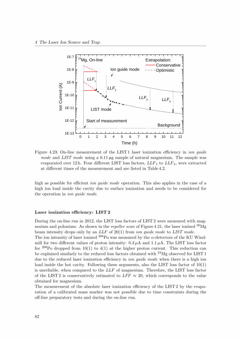
4 The Laser Ion Source and Trap
0 1 2 3 4 5 6 7 8 9 1 0 1 1 1 21 E - 1 3
1 E - 1 2
1 E - 1 1
1 E - 1 0
1 E - 9
1 E - 8
1 E - 7
L L F 2
L L F 4
E x t r a p o l a t i o n : C o n s e r v a t i v e O p t i m i s t i c
S t a r t o f m e a s u r e m e n t
Ion Cu
rrent
(A)
T i m e ( h )
B a c k g r o u n d
L I S T m o d e
I o n g u i d e m o d eL L F 1
2 4 M g , O n - l i n e
L L F 3
Figure 4.23: On-line measurement of the LIST 1 laser ionization efficiency in ion guidemode and LIST mode using a 0.11µg sample of natural magnesium. The sample wasevaporated over 12 h. Four different LIST loss factors, LLF 1 to LLF 4, were extractedat different times of the measurement and are listed in Table 4.2.
high as possible for efficient ion guide mode operation. This also applies in the case of ahigh ion load inside the cavity due to surface ionization and needs to be considered forthe operation in ion guide mode.
Laser ionization efficiency: LIST 2
During the on-line run in 2012, the LIST loss factors of LIST 2 were measured with mag-nesium and polonium. As shown in the repeller scan of Figure 4.21, the laser ionized 30Mgbeam intensity drops only by an LLF of 20(1) from ion guide mode to LIST mode.The ion intensity of laser ionized 208Po was measured by the α-detectors of the KU Wind-mill for two different values of proton intensity: 0.3µA and 1.1µA. The LIST loss factorfor 208Po dropped from 10(1) to 4(1) at the higher proton current. This reduction canbe explained similarly to the reduced loss factors obtained with 24Mg observed for LIST 1due to the reduced laser ionization efficiency in ion guide mode when there is a high ionload inside the hot cavity. Following these arguments, also the LIST loss factor of 10(1)is unreliable, when compared to the LLF of magnesium. Therefore, the LIST loss factorof the LIST 2 is conservatively estimated to LFF ≈ 20, which corresponds to the valueobtained for magnesium.The measurement of the absolute laser ionization efficiency of the LIST 2 by the evapo-ration of a calibrated mass marker was not possible due to time constraints during theoff-line preparatory tests and during the on-line run.
82

4.3 Characterization of the performance of the LIST at ISOLDE
Table 4.2: LIST loss factors LLFs and laser ionization efficiencies ε measured for withLIST 1 and LIST 2. Ion intensities in LIST and ion guide mode, which were usedfor the calculation of the LLFs together with the detector type and the backgroundlevels are given. Half-lives of radioactive isotopes are noted next to the isotopes inbrackets. 24Mg, 174Yb and 208Po were measured with the Faraday cup (FC) 30Mg withthe tape station (TS) and results are given in pA and counts/µC, respectively. The fourLIST suppression factors (LLF1 to LLF4) correspond to the LIST suppression factors,LSFs, illustrated in Figure 4.23. The proton intensities (Ip) for the the two 208Pomeasurements are listed in the left column. Values are implied with their significantnumbers.
Isotope Detector IIG ILIST bgnd unit LLF εIG/εLIST
LIST 1
Off-line
174Yb FC 1280 25 0.1 pA 51 10 / 0.2
On-line
23Mg(11.3 s) TS 1.0 · 106 3.5 · 103 100 counts/µC 294 -
24Mg FC 0.1 pA ≥ 2.5 /≥ 0.08
LLF1 7200 220 33
LLF2 3200 75 43
LLF3 360 7.4 49
LLF4 250 4.9 51
27Mg(9.46 min) TS 2.5 · 106 4.5 · 104 100 counts/µC 56 -
LIST 2
On-line
30Mg(335 ms) TS 80000 4000 50 20 -
208Po(2.898 y) FC -0.1 pA -
Ip=0.3µA 3 0.2 10
Ip=1.1µA 3 0.6 4
83

4 The Laser Ion Source and Trap
Laser ionization efficiency: discussion
In total, absolute ionization efficiencies were determined for 24Mg and 174Yb and LISTloss factors were measured for 23,24,27Mg, 174Yb and 208Po and the results are summarizedin Table 4.2.The absolute laser ionization efficiency of ≈ 10 % of 174Yb in ion guide mode obtained atthe off-line separator agrees with the expectation for a standard RILIS mode ionizationefficiency. The slightly lower ionization efficiency for 24Mg obtained on-line can be ex-plained by the inability to completely evaporate the sample during the limited availablemeasurement time. A series of ionization efficiency measurements is necessary to improvethe statistics, but unfortunately, the scheduling restrictions of the testing facilities makethis impractical and an increase of the reliance is based on regular checks of the LIST lossfactor.The results indicate that under optimal conditions and at low ion currents, the ion guideefficiency is comparable with the efficiency of the normal RILIS operation (≈ 10 %) andthus, the LIST loss factor can be also applied to compare the efficiency of the selectiveLIST mode to normal LIST operation.The loss in ion guide mode efficiency at high ion loads is regained by increasing the ex-traction voltage, which is currently limited to Urep = −500 V or by optimizing the designof the repeller electrode.The LIST loss factors for lower ion currents were of the order of 50 for LIST 1 and aroundonly 20 for LIST 2. The improvement can be ascribed to the reduced distance of theLIST 2 repeller electrode to the hot cavity of only 2.5 mm, which leads to an improvedspatial overlap of the lasers and the free atoms inside the LIST RFQ. The overall efficiencyof the LIST would benefit, if the distance of the repeller electrode to the hot cavity couldbe reduced further.
4.3.6 Selectivity
The LIST selectivity, defined in Equation (4.1), is difficult to determine exactly since itrequires the simultaneous measurement of the ion intensities of the isotope of interest andthe contaminant. A suitable pair of isotopes and corresponding detection system was notavailable during the on-line tests described here. Instead it was possible to assess the per-formance of each LIST using the LIST quality factor, defined in Equation (4.5), assumingthat the ion guide mode efficiency is comparable to normal RILIS operation.Table 4.3 summarizes the LIST parameters obtained in standard operation. The minimumLIST quality factor of LIST 1 is LQF = 88 and of LIST 2 is LQF = 127. These valueswere calculated by taking into account the absolute LIST suppression factor and the typ-ical LIST loss factors. The results indicate that the selectivity was increased due to theimproved laser ionization efficiency of the LIST 2.However, the limited detection efficiency and high background levels made it difficult todetermine the absolute suppression factor for some isotopes. Following the LIST suppres-sion factors of at least 4 orders of magnitude in the case of 26Na, a maximum LIST qualityfactor of the order of more than 200 can be expected with the LIST 1 and more than 500with the LIST 2.
84

4.3 Characterization of the performance of the LIST at ISOLDE
Table 4.3: Comparison of the different LIST parameters obtained on-line by LIST andLIST 2: minimum suppression factor (LSF min), maximum LIST loss factor (LSF max),representative LIST loss factor LLF, and corresponding minimum and maximum LISTquality factors (LQF min and LQF max ) are given. Values are implied with their signif-icant numbers.
LIST LSFmin LSFmax LLF LQFmin LQFmax
LIST 1 4400 ≥ 10000 50 88 ≥ 200
LIST 2 2540 ≥ 10000 20 127 ≥ 500
4.3.7 Comparison of lineshapes of resonances obtained in LIST mode,ion guide mode and normal RILIS operation
The LIST is an important option for resonance ionization spectroscopy (RIS) (see Chap-ter 7). Any differences in terms of line-shape (width, asymmetry) and center frequenciesof the observed atomic lines compared to those measured during in-source RIS in stan-dard hot-cavity RILIS mode need to be examined. Therefore, several measurements ofthe resonance profile of the second step transition for 208Po, which were taken during theexperiments, were compared retrospectively. The profiles were obtained by scanning the
0 . 6 0 0 . 6 5 0 . 7 0 0 . 7 5 0 . 8 0
0 . 0
0 . 2
0 . 4
0 . 6
0 . 8
1 . 0
L I S T m o d e I o n g u i d e m o d e R I L I S
Norm
alized
Ion C
urren
t
( W a v e n u m b e r - 1 1 8 5 3 ) ( c m - 1 )
2 0 8 P o : s c a n o f 2 n d t r a n s i t i o n
Figure 4.24: Comparison of the resonances of the second intermediate step of the polonium(Po) scheme (50934.89 cm−1, 6p3(4S)7p) obtained in LIST mode, ion guide mode andin standard RILIS mode, respectively. The transition was scanned by tuning a narrowband Ti:Sa laser across the resonance and fitted by a Voigt profile. Ion intensities werenormalized for better comparison.
85

4 The Laser Ion Source and Trap
NB Ti:Sa laser (about 1 GHz linewidth, WS7 wavemeter) for several operating modes:LIST 2 in ion guide mode (2 scans), LIST 2 in LIST mode (3 scans) and standard RILISmode (4 scans during the measurement of the ionization potential of polonium during thefollowing run at the HRS target. See Chapter 6.1). The laser power for the spectroscopictransition was attenuated to reduce the degree of saturation broadening.The left graph in Figure 4.24 shows one of these resonances for each of the different modesof operation, LIST mode, ion guide mode and standard RILIS mode. By trend, it seemsthat the width of the resonance in normal RILIS operation (FWHM = 0.053 cm−1 =1.59 GHz) is slightly narrower than in LIST mode (FWHM = 0.073 cm−1 = 2.19 GHz)and in ion guide mode (FWHM = 0.086 cm−1 = 2.58 GHz). In addition, no significantasymmetry nor shift in the frequency was obtained within the standard uncertainty of thewavemeter of 0.2 cm−1 , but it is difficult to make conclusions about the comparison of theline widths and the centroid positions, since the measurement conditions (saturation, tar-get temperature) were different. A more reliable comparison would require more statisticsand better target control and is therefore best performed at an off-line separator facility.
4.3.8 Time structure of LIST ion bunches
The measurement of the time-structure of a pulsed ion source is an ideal probe for theunderstanding of the ionization process. The time-structure of the LIST bunches of laserionized 24Mg was measured during the first on-line run with the LIST 1. An MCP detectorwas installed about 18 m downstream within the ISOLDE beam line and the data was takenby a Teledyne LeCroy Waverunner 104 Mxi scope, which was synchronized to the 10 kHzlaser pulses of the Nd:YAG pump laser. The time of flight was then measured with respectto the laser pulses for several seconds to provide enough statistics.The time structure was measured for several positive repeller voltages, spanning the typicaloperation range of the LIST, namely 7 V, 10 V, 20 V, 30 V, 40 V, 70 V, 100 V, 120 V and200 V. Figure 4.25 depicts the time structure for repeller voltages of 7 V, 10 V and 40 V.Three distinct structures are visible in each spectra:
Peak (A): a narrow, repeller-voltage independent peak at 29.725µs.
Peak (B): an intense peak with a repeller voltage dependent position and width.
Tail (C): the long, flat tail of peak (B) for which the substructure is slightly dependenton the repeller voltage.
The width of peak (B) decreases from 3.43(7)µs for a repeller voltage of 7 V to 1.56(5)µsand 0.37(3)µs for a repeller voltage of 10 V and 40 V, respectively. For the maximumrepeller voltage of 200 V the FWHM gets as small as 0.08(1)µs.In order to understand the different features observed in Figure 4.25, the time structure ofthe LIST ion bunches was calculated . The following section discusses the mathematicalmodel that was used for the calculations and the results will be discussed and comparedto the experimental results in the last subsection.
86

4.3 Characterization of the performance of the LIST at ISOLDE
0 1 0 2 0 3 0 4 0 5 0 6 00 . 0
0 . 5
1 . 0
1 . 5
2 . 0
2 . 5
3 . 0
Norm
alized
Coun
ts
( T i m e o f F l i g h t - 2 9 . 7 2 5 ) ( µs )
R e p e l l e rv o l t a g e :
7 V 1 0 V 4 0 V
T i m e s t r u c t u r e L I S T i o n p u l s e2 4 M g , o n - l i n e
( A )
( B )
( C )
Figure 4.25: Time structure of LIST ion bunches of laser ionized 24Mg for repeller voltages,7 V (red line), 10 V (black line) and 40 V (blue line). Three distinct features are visiblewithin each spectra: (A), a narrow, repeller-voltage independent peak; (B) a broader,more intense, repeller-voltage dependent peak; (C), the tail towards longer flight times.The time of flight is given with respect to peak (A) at 29.725µs.
A model for the calculation of the LIST time structure
Prior to this work, simulations were performed using Monte-Carlo methods and the ion-tracking software SIMION c© [150, 163]. For the work described in this thesis, a comple-mentary approach was used that calculates the time of flight for ions with different initialconditions (position z0, thermal velocity v0) alongside the longitudinal potential inside theLIST. The potential was simulated by the Charged Particle Optics c© (CPO c©) software,a software for the accurate simulation of electrostatic potentials of ion optical elementsusing the Boundary Element Method [138]. For simplicity, the time-dependent potentialof the RF-rods was not considered during the simulations. In turn, the calculation of thetime of flights of the ions was implemented into a code that was written in the Pythonprogramming language. Figure 4.26 shows the overall shape of the calculated longitudinalpotential for repeller voltages of 7 V and 40 V. Additional calculations were performed forrepeller voltages of Urep = 10 V, 100 V and 200 V, which showed a similar behaviour.For the calculation of the time of flights, the potential was approximated by purely em-pirical functions. Their purpose were merely to give an estimation of the longitudinalpotential gradient inside the LIST that can be implemented into the calculations. Severaldifferent functions, e.g. exponential functions and polynomials, were tested. The bestresults for the description of the asymmetric shape of the potential close to the repellerelectrode were obtained by hyperbolic tangent functions that were shifted to z = 0 andnormalized to the calculated effective repeller voltage at z = 0 mm, U0(Urep). The drop of
87

4 The Laser Ion Source and Trap
0 10 20 30 40 50 60 70 80 90
Urep
Distance from repeller electrode (mm)
z =31.75b z =max 85.3
Pote
ntia
l (V
)
I II IV VIII V VI
-40
-30
-20
-10
0
10
20
30
40
7.5 60
Repellerpotential U :rep
7V
40V
0
U(4
0V
)0
U(7
V)
0
z =160extr
VII
Figure 4.26: Longitudinal potential inside the LIST cavity as a function of the distance tothe repeller electrode calculated by the CPO c© program. Ranges on the longitudinalaxis, which are discussed in the text, are indicated by the Roman numbers. Thepotential defined by Equation (4.6) is fitted to the simulated data
the potential close to the exit of the LIST could be approximated by an exponential func-tion. The potential drop from U = −50 V at zmax = −85.3 mm to the extraction electrodewas approximated by a linear function and the potential behind the extraction electrodewas assumed to be constant. The functions that were fitted to the repeller potentials ofUrep = 7 V, 10 V, 40 V, 100 V and 200 V and that were used for the calculations are:
U(z) =
U0(Urep)
1 + tanh (a)· (1 + tanh (b · z + a)) for z < 0
U0(Urep)
1 + tanh (c)· (1− tanh (d · z + c))−B · exp (e · (x− xb)) for 0 ≤ z < zmax
U(zmax) + (x− zmax) · Uextr
zextr − zmax
for zmax ≤ z < zextr
Uextr for z > zextr ,(4.6)
where zb = 31.75 mm is the position at which the potential drops to 0 V, zmax = 85.3 mmis the position at which the potential reaches −50 V and zextr = 160 mm is the position ofthe extraction electrode operated at Uextr = −50 kV (see Figure 4.26 for an illustration).Only the effective repeller potential at z = 0, U0(Urep), depends on the applied repellervoltage and this dependency was obtained by a linear fit to the U0(Urep) for each repellervoltage:
U0(Urep) = 0.575(1) · Urep . (4.7)
88

4.3 Characterization of the performance of the LIST at ISOLDE
The constant parameters a = 1.775, b = 0.565 mm−1, c = 0.650, d = 0.185 mm−1, e =0.400 mm−1 and B = 1.872·10−8 V are the averaged parameters of the fits of Equation (4.6)to the potential gradients of the different repeller voltages. Overall, the fits describe thelongitudinal potential well and the representative fits to the repeller voltages of Urep = 7 Vand Urep = 40V are shown in Figure 4.26.A simplified model of the atomic beam was used, where the atomic beam was assumedto evaporate divergently with a constant angle Θ = constant . The geometry is illustratedin Figure 4.27. For the calculations, the angle of the divergence was chosen to be 3.8
according to the calculations for a hot cavity of 34 mm length described in [163]. Forsimplicity, the atom distribution within the cylindrical volume
VR = π ·R(z0,Θ)2 ·∆z (4.8)
for a given starting position z0 and corresponding atomic beam radius R(z0,Θ) = z0 ·tan Θwas assumed to be uniform:
VR · ρ(z0,Θ) = constant , (4.9)
where ρ(z0,Θ) is the atomic density at z0. Then, the number of atoms, N , which areionized by the laser with radius r and ionization efficiency εion in in the correspondingvolume Vr = πr2∆z can be calculated by:
N = N0 ·VrVR
= N0εion ·πr2∆z
πR(z0)2∆z= N0
r2
(z0 · tan(Θ))2 , (4.10)
where N0 is the number of atoms within the volume VR. With r, εion,Θ = constant, thenumber of atoms as a function of the initial position is then proportional to the square ofthe starting position (i.e. the distance to the hot cavity): N ∝ 1
z20.
The time of flight was calculated for different starting positions, −5 mm ≤ z0 ≤ 85.3 mm,with ∆z0 = 0.01 mm between each starting position and different initial velocities, 5m/s ≤v0 ≤ 3500 m/s, increasing in steps of ∆v0 = 5 m/s. The velocity was weighted by theMaxwell velocity distribution given in Equation (2.40) and by an additional weightingfactor∗ of 903/v0 m/s to consider the higher probability of slower atoms to interact withthe 10 kHz laser pulses before leaving the LIST RFQ.To match the time of flight of the calculated values to the experimental values, it wasnecessary to introduce an off-set, ∆U0, to the effective potential U0:
U ′0(Urep) = 0.575(1) · Urep + ∆U0 . (4.11)
The best overall agreement with the measured time of flights was obtained for a reductionof the effective potential of ∆U0 = −2.1(1). Interestingly this offset is not dependent onthe magnitude of the repeller voltage and its significance is not yet understood. A possibleexplanation are perturbations by the RF-potential, which were not considered for thesecalculations.
∗903 m/s is the velocity, for which the atom is interacting with one laser pulse, when traveling fromthe hot cavity z = −5 mm to the maximum allowed position zmax = 85.3 mm
89

4 The Laser Ion Source and Trap
Calculated LIST time structure and comparison to the experiment
Figure 4.28 shows the calculated LIST time structure for Urep = 7 V, 10 V, 40 V with re-spect to peak (A). The countrate was normalized to the peak (A) similar to the measuredtime structure from Figure 4.25. Overall, the simulation reproduces the main features,peak (A), peak (B) and tail (C) of the measured time structure. The dependency of theposition and the width of peak (B) on the repeller voltage are similar to the measuredvalues. In contrast, the intensity of tail (C) and the background of the calculations areoverestimated, but can be ascribed to the simplified model of the atomic beam, whichdoes not take into account any angle-preference of the intensity nor the acceptance of theRFQ. The calculated strictly growing intensity of peak (A) for increasing repeller voltageswas not observed in the measured time structures. This can be ascribed to a differentstatistic for each of these measurements and ion optics effects that depend on the initialenergies (e.g. energy tolerance of the GPS magnet). The substructure observed in thetail (C) was not reproduced, but can be explained by perturbations of the potential alongthe longitudinal axis due to the influence of the RF-potential. The calculated positionsof peak (B) with respect to peak (A) for different repeller voltages agree well with theexperiment as shown in Figure 4.29. A small shift is observed for low repeller voltages,but can be explained by the unknown correction, ∆U0, to the effective repeller voltagedescribed by Equation (4.11).
The origin of the different features of the LIST time structure
In order to understand the features, peak (A), peak (B) and tail (C), observed in the spectrashown in Figure 4.25 and Figure 4.28, the time structure was calculated for 7 differentranges of starting positions, z0, along the longitudinal axis, z. These ranges, denoted withRoman numbers, represent distinguishable features of the longitudinal potential as shownin Figure 4.26. The calculated time structures for the relevant ranges I − V that allowfor kinetic energies within the energy acceptance ±50 of the GPS mass separator [70]are shown in Figure 4.30. Using the separate calculations of the time structure, peak (A),peak (B) and peak (C) can be understood as follows:
Range I, −5 mm ≤ z < 0 mm: the longitudinal potential is rising from 0 V at the exitof the hot cavity (z = −5 mm) to the maximum potential at the position of therepeller electrode (z = 0). Only ions with sufficient initial velocities in forwarddirection can pass the repeller barrier. Ions created in range I contribute to peak(B).
Range II, 0 mm ≤ z < 7.5 mm: the longitudinal potential decreases rapidly by 75 %from its maximum value at the position of the repeller electrode z = 0 mm to z =7.5 mm. Assuming that the atomic beam is divergent, the atom density inside theLIST RFQ is highest in range I and thus most atoms are ionized close to the repellerelectrode. The strong potential gradient and the drift time in the following rangeslead to a focusing and the formation of peak (B).
Range III, 7.5 mm ≤ z < 31.75 mm: the longitudinal potential decreases slowly from25 % of its initial value at z = 7.5 mm to 0 V at around z = 31.75 mm. Ions created
90

4.3 Characterization of the performance of the LIST at ISOLDE
rR
Q
Repeller electrode
Hot cavity
Atomic beam Laser beam
Dz
z0 z=0z
Vr
VR
Figure 4.27: Simplified model of the diverging atomic beam with angle Θ. Vr = πr2∆zis the volume in which the atoms at z0 interact with the laser beam of radius r.VR = πR(z0)2∆z is the corresponding volume of the total atomic beam with radiusR(z0) = z0 · tan(Θ).
0 1 0 2 0 3 0 4 0 5 0 6 00123456789
1 01 1
( C )
C a l c u l a t e d t i m e s t r u c t u r e o f 2 4 M g L I S T l a s e r i o n p u l s e
R e p e l l e rv o l t a g e :
7 V 1 0 V 4 0 V
Norm
alized
Coun
ts
T i m e o f F l i g h t ( µs )
( A )
( B )
Figure 4.28: Calculated LIST time struc-ture for Urep = 7 V, 10 V and 40 V. Thetime of flight is given with respect topeak (A). The notation is similar to Fig-ure 4.25.
0 5 0 1 0 0 1 5 0 2 0 00
5
1 0
1 5
2 0
2 5A p p e a r a n c e o f p e a k ( B ) w i t h r e s p e c t t o p e a k ( A )
E x p e r i m e n t C a l c u l a t i o n
Tim
e of F
light (µ
s)
R e p e l l e r V o l t a g e ( V )
Figure 4.29: Comparison of the mea-sured and calculated appearance ofthe main peak (peak (B)) in the LISTtime structure with respect to peak (A).
0 2 0 4 0 6 00
1
2
3
Norm
alized
Coun
ts
T i m e o f F l i g h t ( µs )
, " I " , " I I " , " I I I " , " I V " , " V "
00 <z5.70 0 <≤ z
2 5.3 15.7 0 <≤ z6 02 5.3 1 0 <≤ z3.8 56 0 0 ≤≤ z
C a l c u l a t e d t i m e s t r u c t u r e f o r d i f f e r e n t r a n g e s o f s t a r t i n g p o s i t i o n s , z 0 ( m m ) :
Figure 4.30: LIST ion bunch time structure for the repeller voltage of Urep = 7 V for differ-ent ranges of starting positions z0, corresponding to the ranges defined in Figure 4.26and Section 4.3.8.
91

4 The Laser Ion Source and Trap
in range III form the tail (C).
Range IV, 31.75 mm ≤ z < 60 mm: the longitudinal potential is not affected by therepeller voltage or the extraction field of the extraction electrode on a high potentialand the longitudinal potential is constant at around 0 V. The time of flight of the ionscreated in range III is therefore entirely defined by the initial conditions (positionz0, thermal velocity, ν0).
Range V, 60 mm ≤ z < 85.3 mm: the longitudinal potential starts to drop due to theinfluence of the extraction potential of -50 kV at the extraction electrode at z =160 mm and a potential of -50 V is reached at z = zmax = 85.3 mm. Ions created inrange V form the peak (A) due to the strong potential gradient and the drift timetowards the experiments.
Range VI, 85.3 mm ≤ z < 160 mm Ions created after z = 85.3 mm have an energydifference of more than 50 eV compared to ions created inside the LIST, which ex-ceeds the acceptance of the GPS separator magnet and their contribution is thereforenegligible. The potential drops by -50000 kV to the ground potential at the extrac-tion electrode at z = −160 mm.
Range VII, z ≥ 160 mm: the potential remains constant after the extraction electrodeand the ions drift to the experiment with the velocity corresponding to their kineticenergy.
In summary, peak (A) stems from the atoms ionized next to the exit of the LIST (range V),peak (B) are the ions produced close to the repeller electrode (range I and II), the tail (C)are the atoms ionized further away from the repeller electrode (range III) and the back-ground is produced by ions produced in the nearly field free zone (range IV).An important result of these calculations for the laser ionization efficiency of the LISTis that the dominant peak (B) stems mainly from ions created very close to the repellerelectrode. Consequently, a reduction of the distance of the repeller electrode to the hotcavity should thus correlate with an increased laser ionization efficiency. This conclusionis supported by the improved ionization efficiency of a factor of 2,5 from LIST 1 to LIST 2,for which the distance was reduced by 2.5 mm.
92

4.3 Characterization of the performance of the LIST at ISOLDE
4.3.9 Improving the selectivity of the Laser Ion Source and Trap
In the following, possibilities are discussed to improve the LIST selectivity for futureapplications at ISOLDE.
Improving the laser ionization efficiency
Improving the laser ionization efficiency increases directly the ratio of the intensity of theisotopes of interest over the intensity of the contaminants.
1. Improvement of the laser/atom overlap: a higher laser/atom overlap can beachieved by further reducing the distance of the LIST to the hot cavity. The reduc-tion from 5 mm for LIST 1 to 2.5 mm for LIST 2 led to a significant improvement ofthe laser ionization efficiency of a factor of 2.5. This is also supported by the analysisand calculation of the time structure, which indicate that the atomic beam is dens-est close to the repeller. However, a further reduction is difficult to be mechanicallyconstructed due to possible shortcuts with the heat shield of the hot cavity. Onepossibility could be to use the heat shield itself as a repeller, which would reducethe distance to about 1 mm, but possible complications need to be ruled out duringlong-term off-line tests.Additionally, the laser/atom overlap could be increased by improving the atom beamcollimation by different hot cavity designs (e.g. increased length).
2. Improvement of the laser ionization scheme: if all steps would be stronglysaturated, the laser beam radii could be expanded to interact with more atoms.
3. Reducing the duty cycle: atoms with the largest transverse velocity componentmay have a short (< 100µs) residence time inside the LIST laser interaction region.In this case an increased laser repetition rate would reduce duty cycle losses providedthat the pulse energy stays the same, which is practically difficult.
Time dependence of laser ions
As it was discussed in Section 4.3.8, the laser ion pulse produced by the LIST has adistinct pattern with one dominant peak (B) corresponding to the ions produced close tothe repeller electrode. For the standard repeller voltage setting of Irep = 7V , the FWHMwas determined to be 3.43(7)µs. Using a beam gate could thus increases the selectivitysignificantly. For example, a gating time of 10µs around peak (B) would allow ≈ 60 % ofall ions to pass, whilst cutting of 90 %∗ of the pulse-independent contaminants leading toan overall selectivity gain of 6. Depending on the required laser ionization efficiency thegate could be increased at the cost of the reduction of the contamination and vice versa.
∗The duty cycle for a 10 kHz laser is approximately 100µs. With a gating time of only 10µs, only the10 % contaminants produced within this time interval could pass the beam gate.
93

4 The Laser Ion Source and Trap
Temperature dependency of contamination
Figure 4.31 shows that the ion rate of 212Fr, which is a LIST mode contaminant of unknownorigin∗, has a stronger cavity temperature dependency than laser ionized 196Po in LISTmode or the surface ionized 212Fr in ion guide mode. It is therefore possible to improve theselectivity for LIST mode laser ionized 212Po by a reduction of the hot cavity temperature.It should be noted that this method only applies to isotopes, which have a reasonable longlifetime to not be affected by the longer transport time through the hot cavity in case oflower temperatures. 196Po has a half-live of T1/2 = 5.8 s and an application for isotopeswith similar half-lives should be feasible.One possible future application is the resonance ionization spectroscopy of the poloniumisomers 211mPo and 211mPo. Due to their relatively long half-lives of T1/2 = 25.2 s andT1/2 = 45.1 s, respectively, the hot cavity temperature dependency of these isotopes is thesame or even less than the hot cavity temperature dependency of 196Po.
1 6 0 0 1 7 0 0 1 8 0 0 1 9 0 0 2 0 0 00 . 00 . 10 . 20 . 30 . 40 . 50 . 60 . 70 . 80 . 91 . 0
Norm
alized
Ion I
ntens
ity
H o t C a v i t y T e m p e r a t u r e ( ° C )
L I S T m o d e : 1 9 6 P o , l a s e r i o n i z a t i o n
I o n g u i d e m o d e : 2 1 2 F r , s u r f a c e i o n i z a t i o n
2 1 2 F r , u n k n o w n s o u r c e
Figure 4.31: Ion intensity of 212Fr (T1/2 = 20 min) in ion guide mode and LIST modeand 196Po (T1/2 = 5.8 s) in LIST mode as a function of the hot cavity temperature.The ion intensity is normalized to the maximum intensity measured for each isotope atT = 2000 C. 196Po was laser ionized and 212Fr in ion guide mode was surface ionized.The exact source and ionization mechanism of 212Fr in LIST mode is still unknown.
∗In Chapter 4.3.4, the in-trap β-decay of neutral 212Ra to 212Fr at the RF-rods was discussed as apossible explanation for the contamination.
94

5 A new laser ionization scheme forcalcium
More than 30 elements are currently available for the resonance laser ionization with theRILIS at ISOLDE and efforts are being continuously made to extend this further∗ [113].For many laser ionization schemes, only non-resonant final steps have been applied andtheir relatively low ionization cross-sections of only 10−17cm2 − 10−19cm2 require often alaser powers in excess of the power available from the Nd:YAG pump laser.Thus, finding efficient autoionizing states (AIS) may improve the ionization efficiency. Thegeneral approach to improve the laser ionization schemes for elements with stable isotopesis to conduct this studies at off-line facilities such as the LARIS laboratory at CERN [115].This allows for extended studies of the resonances without the scheduling constraints ofthe ISOLDE on-line facility. However, a very convenient and time-efficient alternativeapproach to improve existing laser ionization schemes is to perform the measurementsduring scheduled on-line runs at ISOLDE. The recent upgrade of the RILIS to a dual-RILISsystem of 6 tunable lasers (see Chapter 3.3.1) has made opportunistic ionization schemedevelopments possible during the normal on-line operation of the system [143, 145].Calcium (Ca) is one of those elements, which was ionized via a non-resonant last stepduring previous experiments [25, 127]. Figures 5.1 a,b show the existing laser ionizationschemes: a) two-step scheme with one blue laser beam to the intermediate step and oneUV laser beam for non-resonant ionization, and b), a three step scheme consisting of oneblue laser beam, one infrared laser beam for the excitation to the intermediate steps and ofone of the 532 nm pump lasers for the step above the ionization energy† of 49305.924 cm−1
[120]. Of these two laser ionization schemes, only the latter is applicable since the laserpower provided by a UV laser beam is usually not sufficient to approach saturation in thecase of non-resonant ionization.Two calcium experiments were scheduled for 2012: Experiment IS529, “measurements ofspins, moments and charge radii beyond 48Ca” by collinear laser spectroscopy with theCOLLAPS experiment in April 2012 [11] and experiment IS532 for mass measurements ofexotic calcium with the ISOLTRAP experiment in June 2012 [96], for which the resultswere recently published in Nature [177]. Both experiments relied on a high ionizationefficiency for the study of very exotic calcium isotopes and thus, investigations towards animprovement of the existing calcium laser ionization scheme was integrated into the setupprocedure and maintenance work of these two on-line runs.In the following I report on the results of the resonance ionization spectroscopy study, the
∗A RILIS web-database (http://riliselements.web.cern.ch) was recently developed to summarizeand share the latest results of RILIS scheme developments at facilities worldwide [143].
†Transition energies and excitation energies are given in the unit of wavenumbers throughout thischapter.
95

5 A new laser ionization scheme for calcium
-1IE: 49 305.924 cm
< 390 nm
Ca
-123 652.304 cm 422.67 nm
08 -1A = 2.18e s
532 nm
2 14s S0
-10 cm
1 o4s4p P1
-123 652.304 cm
14s4d D2
-137 298.287 cm -113 645.983 cm 732.61 nm
A = ?
a) b) c)
AIS
l2
l3
Figure 5.1: a) Two-step scheme using one resonant transition. b) Three-step scheme usingtwo resonant transitions and one non-resonant ionization step. Both originally from[25, 127]. c) Illustration of the scanning regions for an alternative second intermediatestep and the search for autoionizing states above the ionization region. The wavelengthsare referred to as λ2 and λ3 for the second and third step, respectively.
analysis of the spectra and the discussion of possible new ionization schemes. It shouldbe noted that these measurements aimed on the development of a new laser ionizationscheme rather than a comprehensive and decisive study of the atomic spectrum of calcium.I therefore restrict the discussion to the relevant information such as relative peak heights,ion intensities, widths and saturation and refer to possible future experiments at off-linelaser facilities for an in-depth study of the resonances and features in the spectra.
96

5.1 Experimental setup
5.1 Experimental setup
The search for an alternative laser ionization scheme was performed during maintenancebreaks of the IS529 experiment and during the laser setup and optimization procedure forthe IS532 experiment. Experiment IS529 used a UCx target (ISOLDE target # 471) witha hot cavity made of rhenium (Re) and experiment IS532 used a UCx target (# 480) witha hot cavity made of tantalum. Typical target specifications and operation parametersare given in Figure 5.2.
Re 690A
<279 A Re
<1.8mA
40 kV
#471
HRS
UCx
Ta 660A
<291 A Ta
<2 mA
30 kV
#480
HRS
UCx
b)a)
Figure 5.2: Target specifications of the targets used for the Ca-Spectroscopy. a) UCx target# 471 with rhenium (Re) hot cavity for experiment IS529 and b) UCx target # 480 withtantalum (Ta) hot cavity for experiment IS532. From top to bottom: target number,target material, typical target and hot cavity currents, proton intensities, extractionvoltage and type of front-end. Note that these values represent maximum values andcan differ for certain measurements. Design of schematics adopted from [143].
During the two experimental periods several scans of the calcium atomic spectrum wererecorded. The scan ranges for the search of an alternative intermediate step and resonantlast step are indicated in Figure 5.1 c with λ2 and λ3, respectively. For the search ofalternative intermediate states, a dye laser, operated with a Rhodamin B (RB)-ethanolsolution, was scanned from 16250 cm−1 to 17250 cm−1 (579.7 nm to 615.4 nm) from thefirst intermediate state 4s4p 1P o
1 at 23652.304 cm−1 , while a 532 nm Nd:Yag was used forthe last step. Two levels were found in the range from 17030 cm−1 to 17070 cm−1. Usingthese alternative intermediate levels, additional scans were performed with a dye-laserusing a DCM∗-ethanol solution in the range from 14700 cm−1 to 16300 cm−1 (613.5 nm to680.2 nm). Various autoionizing states were observed and studied during several scans.Due to time constraints during the experiment IS529, the scans were repeated during thesecond experiment, IS532, where the setup was tuned from the beginning to the alternativeintermediate steps and the autoionizing states.In order to compensate possible frequency shifts due to time-delays in the DAQ-system,the scans for the relevant levels (intermediate levels, strongest autoionizing states) wereperformed in forward and backward direction as appropriate.
∗DCM is the abbreviation for 4-dicyanomethylene-2-methyl-6-p-dimethylaminostyryl-4H-pyran.
97

5 A new laser ionization scheme for calcium
5.2 Analysis of the spectra
Figure 5.3 shows the relevant segments of the scans: a) alternative second intermediatestates; b) autoionizing states from the lower lying intermediate state (3p64s6s 1S0, denotedby the term symbol 1S0); c) autoionizing states from the higher lying intermediate state(3p64p2 1D2, denoted by the term symbol 1D2); d) and e), zooms into the spectra ofthe autoionizing states reached from the two second intermediate steps, 1S0 and 1D2,respectively.
5.2.1 Alternative second intermediate states
The alternative second intermediate states were found in the energy range from 17035 cm−1
and 17080 cm−1 relative to the first intermediate state 3p64s4p 1P o1 at 23652.3 cm−1 asshown in Figure 5.3 a. The first structure appears at around 17037 cm−1 and the secondstructure is at around 17067 cm−1. Both structures show unresolved substructures, whichare due to strong saturation and the presence of additional laser frequency side bands.To determine the transition energies E, a single Voigt-profile was fitted to the main res-onance of the first structure and a superposition of two Voigt profiles was fitted to thesecond structure. The results from the forward and backward scans were averaged to cal-culate the final value of the transition energy, E. The transition energies were then addedto the literature value for the first intermediate step 3p64s4p 1P o
1 with energy 23652.3 cm−1
[94].The statistical uncertainties of the fits are dominated by the uncertainty from the waveme-ter of ∆Estat,WM = 0.02 cm−1 [79]. A systematic uncertainty arises from the wavemeterWS7, which was determined in [143] to ∆Esys,WM = 0.03 cm−1 . Additionally, a systematicuncertainty of ∆Esys,WM = 0.3 cm−1 is conservatively added to resonance 1 because of theunresolved substructure.Taking the systematic uncertainty of 0.33 cm−1 into account, the main resonance in thefirst structure with energy 40690.26(2) cm−1 can be assigned to the literature value at40690.435(1) cm−1 with configuration 3p64s6s 1S. The highest lying resonance, reso-nance 2, in the second structure with energy 40719.87(2)cm−1 corresponds to the literaturevalue of an atomic state at 40719.847 cm−1 with configuration 3p64p2 1D [94]. The peak inthe lower energy flank of the main resonance with energy 40718.32(3) cm−1 is not knownin literature. It is impossible that it can be assigned to an isotope shift of the secondmost abundant isotope 44Ca, whose natural abundance of only 2 % does not correspond tothe peak height. It is therefore likely to be a laser related effect as discussed above. Thedisappearance of this peak in a reduced power (close to saturation intensity) scan wouldconfirm this but this was not feasible due to time constraints. The results for resonance 1and resonance 2 are given in Table 5.1 and Table 5.2, respectively, together with the cor-responding subsequent transitions to autoionizing states. The energy position of the twoobserved intermediate states enables a search for autoionizing states through the use of avisible dye laser for the third step in the ionization scheme.
98

5.2 Analysis of the spectra
17035 17040 17045 17050 17055 17060 17065 17070
0
10
20
30
40
50
60
Ion
Cu
rre
nt(p
A)
Wavenumber (cm -1)
15200 15250 15300 15850 15900 15950 16000 16050
0
50
100
150
200
250
300
350
400
450
Ion
Cu
rre
nt(p
A)
Wavenumber (cm -1)
0
100
200
300
400
500
600
15220 15240 15260 15280
Ion
Cu
rre
nt(p
A)
Wavenumber (cm -1)
0
50
100
150
200
250
300
350
15180 15200 15220 15240 15260 15280 15300
Ion
Cu
rre
nt
Wavenumber (cm -1)
(pA
)
0
100
200
300
400
500
15200 15300 15800 15900 16000
Ion
Cu
rre
nt
Wavenumber (cm -1)
1st intermediate state-1 6 1 o
(23652.3 cm ,3p 4s4p P )1
Ground state -1 6 2 1(0 cm ,3p 4s S )0
2nd harmonic Ti:Sa (422.67 nm)
Scan dye Rhodamin B (579nm to 619 nm)
Scan dye DCM from (613.5 nm to 680 nm)
1S0 Scan dye DCM from (613.5 nm to 680 nm)
1D2
6 2 13p 4p D2
6 13p 4s6s S0
i-vi
vii
viii
i
ii
iii
iv
v
vi
I-X
XI
XII
XIII
I
II
III
IV
V
VI
VII
VIIIIX
X
a)
c)b)
d) e)
(pA
)
nd2 intermediate states
1Autoionizing states from S0
1Autoionizing states from D2
33d4f D1
13d6p P1
33d4f P1 33d4f D1
33d4f F 13d4f P1
33d6p P1
33d4f D
1
2
13d6p P (?)
Figure 5.3: Overview of the different scans conducted for the search for a new laser ion-ization scheme for calcium: a) alternative second intermediate levels. b) and c), au-toionizing states found in the scans from the second intermediate levels. d) and e):zooms to the most interesting resonances from the point of view of laser ionizationefficiency in the spectra shown in b) and c), respectively, and the corresponding Voigt-fits (blue: individual line-shape; red: cumulative fit). Used dyes, scanning ranges andconfigurations, are given, if known from literature.
99

5 A new laser ionization scheme for calcium
5.2.2 Excitation from the alternative intermediate state 1
A broad low-resolution scan (0.7cm−1/s→ 14 measurements/cm−1) over all observed tran-sitions to autoionizing states from the 4p6s 1S0 state is shown in Figure 5.3 b. In total 8resonances, denoted by small Roman number, could be identified for transition energiesbetween 15175 cm−1 to 16100 cm−1. Of these, a pairing of the transitions i to vi wasobserved similar to the case of the resonance 2 observed in the scan for the search of theintermediate states described above. It is likely that these peaks are due to a similar laserside band, i.e. a saturation effect, as was discussed earlier.A slower scan with higher resolution (0.1cm−1/s → 100 measurements/cm−1) over thestrongest lines (resonances i - vi) from 15200 cm−1 to 15300 cm−1 is shown in Figure 5.3 d).These resonances are highly symmetrical and were therefore fitted with Voigt fits as shownin Figure 5.3 d), where the individual fits are the solid blue lines and the cumulative fitis the red line. The Gaussian widths due to hot cavity temperature of T ≈ 2000 C(Doppler broadening) and the laser linewidth of 9 - 12 GHz of the broad-band Credo dyelasers[59, 113] was estimated to be 0.4 cm−1 and was kept fixed during the fits. The scanwas performed with the maximum available laser power (≈ 1 W in the source). The prior-ity was given to maximizing the ionization efficiency, rather than extracting spectroscopicinformation, was made and thus, no attempt was made to reduce the degree of saturationand subsequent power broadening of the transitions. Similar to the transitions to theintermediate states, the statistical uncertainties are dominated by the statistical uncer-tainties of the wavemeter and are 0.02 cm−1 . The results are listed in Table 5.1.
The two resonances, vii and viii, shown in Figure 5.3 b are less intense than the reso-nances, i to vi. Resonance vii is significantly narrower (≈ 0.2 cm−1) than the resonancesi-vi and shows a certain asymmetry and a further unresolved substructure. However, notenough data was available to study this structure precisely, but the excitation energy ofthe centroid of W = 56531.98(20) cm−1 (transition energy of 15841.55 cm−1 ) is close toan autoionizing state known in literature (3p63d6p 3P1) with energy 56532.6 cm−1 [94]. Incontrast, the structure viii, for which no literature value is known, is extremely broad andsignificantly asymmetric. A Fano-fit (see Equation (3.17) in Chapter 3.2.3) was performedto resonance viii, to give the center of the resonance of 15977.12(50)(3) cm−1 with a widthof 23.5(3) cm−1 (720 GHz). However, the asymmetry factor q depended on the choice ofthe background level and could not be determined unambiguously and the observed strongasymmetry could instead stem from an unresolved substructure. This idea is supportedby a value known in literature with configuration 3d6p 1P and total excitation energy of56651.0 [94], which would be observed at a transition energy of 15960.7 cm−1 . This agreeswell to the small perturbation of the left flank of resonance viii [94]. No correspondingstates could be found in literature for the resonances i, v, and viii.For the strongest resonances, ii, iv and vi, the ratio of the absolute height to the backgrounddue to surface ionization (Laser on/off) was determined in with all lasers in saturation fora realistic comparison to normal operation conditions.For the strongest line ii, the overall gain in efficiency compared to surface ionization (Laseroff) is 290. The slightly lower height of resonance ii in Figure 5.3 d), when compared toresonance vi, is misleading and can be explained by fluctuations of the laser power duringthe scan.
100

5.2 Analysis of the spectra
Table 5.1: Parameters of the transition to the first intermediate step, 4p6s 1S0 (reso-nance 1), and subsequent transitions to autoionizing states (resonances i-viii): numberof resonance (Res.), transition energies E, total excitation energies from the ground-state W and corresponding literature values Wlit, electron configuration, term valueand total angular momentum J , FWHM and relative ionization efficiency compared tosurface ionization (Laser on/off). The literature values of the 3d4f 3P o could not beunambiguously assigned to either resonance iii or iv and are marked with (∗). Statis-tical and systematic uncertainties of the measured transition energies E are given inthe first and second parentheses, respectively, and are identical for the total excitationenergy W . The other values are implied with their significant numbers.
Res. E W W lit Config. Term J FWHM Laser
cm−1 cm−1 cm−1 cm−1/GHz on/off
1 17037.96(2)(33) 40690.26 40690.44 3p64s6s 1S 0
i 15210.55(2)(3) 55900.99 1 0.3/8.8
ii 15211.91(2)(3) 55902.35 55902.8 3d4f 3Do 1 0.9/28.1 290
iii 15256.00(2)(3) 55946.43 55946.6∗ 3d4f∗ 3P o∗ 1 0.4/11.9
iv 15257.37(2)(3) 55947.80 55946.6∗ 3d4f∗ 3P o∗ 1 0.6/17.7 190
v 15290.95(2)(3) 55981.38 1 0.9/27.3
vi 15292.33(2)(3) 55982.77 55982.3 3d6p 1P o 1 0.9/27.3 260
vii 15841.55(20)(3) 56531.98 56532.6 3d6p 3P o 1 ≈ 0.2/6
viii 15977.12(50)(3) 56667.55 1 ≈ 24/720
5.2.3 Excitation from the alternative intermediate state 2
The broad low-resolution scan (0.5cm−1/s → 20 measurements/cm−1) from the 4p2 1D2
intermediate state at 40719.847 cm−1 [94] is shown in Figure 5.3 c). In total 13 reso-nances, denoted by capital Roman numbers, were found in the range from 15150 cm−1 to16000 cm−1 . The spectrum of autoionizing states shows some similarities to the spectrumexplored from the 4p6s 1S0 intermediate state shown in Figure 5.3 b): several intense andrather narrow resonances at lower excitation energies, resonances I to X, and a very broadstructure next to weaker resonances at higher excitation energies (between 15700 cm−1 and16000 cm−1 ). In contrast to the spectrum of the excitation from the 4p6s 1S0 intermediatestate, more peaks are visible. This can be explained by the higher L- and J -value of the4p2 1D2 intermediate, which allows for more possible transitions. Moreover, no systematicpairing of the peaks is visible.The determination of the centroids of the resonances was similar to the analysis of the res-onances found in the scan from the 4p6s 1S0 intermediate state described in the previoussection: Voigt profiles were fitted with a fixed Gaussian linewidth of 0.4 GHz to the sym-metrical resonances (I to X) and to the weak resonance XI and Fano-profiles to the higherexcited resonances at higher energies 15700 cm−1 and 16000 cm−1 (resonance XII and res-
101

5 A new laser ionization scheme for calcium
15800 15805 15810 15815 15820 15825
0
10
20
30
40
50
60Io
nC
urr
en
t(p
A)
Wavenumber (cm -1)
Peak XII
q = -3.86
Figure 5.4: Resonance XII with transition energy 15812.89(3)(3) cm−1 (56532.76 cm−1 totalexcitation energy) accessed from the 4p2 1D2 intermediate state. A Fano-profile wasfitted (red solid line) to the asymmetric lineshape of the resonance.
onance XIII). Figure 5.3 e shows a scan with higher resolution 0.2cm−1/s → 50 measure-ments/ cm−1 for the resonances I to X, together with individual fits (solid blue lines) andthe cumulative fit (red line). It was difficult to resemble the peaks heights with the multi-peak Voigt fit, which can be explained by possible asymmetries of some of the peaks.Nevertheless, the transition energies could be determined and the fitting results for thebackward and forward scan were averaged to obtain the transition energies.Similar to the broad structure in the scan from the 4p6s 1S0 intermediate state, a fit witha Fano profile to the resonance XIII showed a strong dependency of the asymmetry factorq on the chosen fitting range and an unambiguous determination of q was not possible. Afurther discussion is therefore omitted. However, the strongly pronounced asymmetry inresonance XII is shown in figure 5.4 together with the fitted Fano profile (red solid line)and the corresponding Fano factor of q = −3.86(8).Center energies and widths of all resonances are given in Table 5.2 together with corre-sponding values and configurations of levels found in literature [66, 94] together with therelative intensities compared to surface ionization (Laser on/off) of the strongest lines, V,VIII, IX and X.. No corresponding states could be found for resonances I, III, VI-VIII,X, XI and XIII and are possibly newly discovered autoionizing resonances. Comparingthe transitions from both intermediate steps listed in Table 5.1 and Table 5.2, each pair,ii and II, vi and IX and vii and XII correspond to the same autoionizing state. Of thesetransitions, resonance IX with configuration 3d6p 3P o resulted in the highest recorded ion-ization efficiency with an overall gain in efficiency of a factor of 300 compared to surfaceionization.
102

5.2 Analysis of the spectra
Table 5.2: Parameters of the transition to the second intermediate step, 3p64p2 1D2 (res-onance 2), and subsequent transitions to autoionizing states (resonances I-XIII). Thenotation of the parameters is similar to those given in Table 5.1. Statistical and sys-tematic uncertainties of the measured transition energies E are given in the first andsecond parentheses, respectively, and are identical for the total excitation energy W .The other values are implied with their significant numbers.
Res. E W W lit Config. Term J FWHM Laser
cm−1 cm−1 cm−1 cm−1/GHz on/off
2 17067.56(2)(3) 40719.87 40719.85 3p64p2 1D 2
I 15175.00(2)(3) 55894.85 0 1.19/35.7
II 15182.46(2)(3) 55902.30 55902.8 3d4f 3Do 1 0.62/18.5
III 15187.17(2)(3) 55907.01 1,2,3 4.7/139.3
IV 15194.79(2)(3) 55914.64 55915 3d4f 3D 2.3 2.2/65.0
V 15230.72(2)(3) 55950.56 55951 3d4f 3F 1,2,3 4.5/142.1 240
VI 15238.84(2)(3) 55958.69 1,2,3 1.0/30.9
VII 15246.76(2)(3) 55966.61 1,2,3 1.7/50.8
VIII 15256.32(2)(3) 55976.17 1,2,3 3.5/105.0 275
IX 15262.93(2)(3) 55982.78 55982.3 3d4f 1P o 1 0.5/16.3 300
X 15287.56(2)(3) 56007.41 1,2,3 4.0/121.1 250
XI 15735.04(4)(3) 56454.89 1,2,3 0.3/8.8
XII 15812.89(3)(3) 56532.74 56532.63 3d6p 3P o 1 0.3/8.8
XIII 15933.51(30)(3) 56653.35 1,2,3 0.3/8.8
103

5 A new laser ionization scheme for calcium
5.3 The new laser ionization scheme for calcium
With the available dye laser power in the source of P ≈ 1 W, many of the observedautoionizing states, namely ii, iv and vi from intermediate step 1So
0 and V, VIII, IXand X from intermediate step 1Do
2, could serve as potential candidates for an efficientlast step for a new calcium laser ionization scheme. However, of these, the transitions iiand IX were the easiest to saturate. Figure 5.5 shows the laser ionization schemes fromthe first intermediate step 4s4p 1P 0
1 at 23652.304 cm−1 through a) the intermediate step4s4p 1S0 at 40690 cm−1 to the autoionizing state ii (3d4f 3Do
1, 55902.8 cm−1 ) and throughb) the intermediate step 4p2 1Do
2 at 40719 cm−1 to the autoionizing state IX (3d4f 1P o,55982.3 cm−1 ).
Saturation of the transitions
Figure 5.6 demonstrates the saturation for each transition shown in Figure 5.5 by showingthe ion current as a function of the laser power inside the hot cavity. The latter wasestimated based on simultaneous measurements of the laser power on the laser table. Theratio of the measured power to the laser power inside the hot cavity can be estimatedby measuring the ratio to the 4 % reflection∗ of the laser beam at a quartz plate that isin the beam path at 50 % of the path length to the target. For the measurement of thesaturation, the laser power was attenuated by inserting neutral density filters in the laserbeam path. The other involved transitions were kept saturated during each measurement.The ion current IC as a function of the power P was then fitted by a saturation curve,defined by
IC = IC 0 + IC sat ·PPsat
PPsat
+ 1, (5.1)
where IC 0 is the background of the ion current from the non-resonant ionization, I sat is themaximum ion current in saturation and Psat is the saturation parameter. The extractedsaturation parameters are listed in Table 5.3 for each transition. The estimated typicalavailable laser power in the hot cavity during the experiments IS529 and IS532 was about175 mW for the first step provided by the frequency-doubled Ti:Sa output, 500 mW forthe second step provided by the Credo dye filled with Rhodamin B and 1125 mW for thethird steps provided by the Credo dye laser filled with DCM. The excess of the laser poweravailable simplifies the maintenance of the RILIS performance because it makes the overallefficiency less sensitive to small changes of the power (aging of the dye, change of laserspot position) or small shifts of the wavelengths.
∗The laser spot of the reflection at the quartz plate is usually used as the reference spot to observe thebeam position during operation.
104

5.3 The new laser ionization scheme for calcium
-1IE: 49 305.924 cm
Ca
-123 652.304 cm 422.67 nm
08 -1A = 2.18e s
2 14s S0
-10 cm
1 o4s4p P1
-123 652.304 cm
3 o 3d4f D1 (Peak ii)-1
55902.3 cm
14s6s S0 (Peak 1)-1
40 690.435 cm
1 o3d4f P1 (Peak IX)-1
55 982.8 cm
2 14p D2 (Peak 2)-1
40 719.847 cm
-117 038.131 cm 586.75 nm
-117 067.543 cm 585.74 nm
-115 262.453 cm 655.01 nm
-115 212.365 cm 657.17 nm
a) b)
Figure 5.5: The new laser ionization schemes for calcium developed on-line at ISOLDE.From the first intermediate step at 23652 cm−1 with configuration 4s4p 1P o
1 , twoequally strong ionization schemes are accessible: a) via the second intermediate step40690 cm−1 with configuration 4s4p 1P1 to the autoionizing state at 55902.8 cm−1
with configuration 3d4f 3Do1 (resonance ii) and b) via the second intermediate step
40719.847 cm−1 with configuration 4p2 1D2 to the autoionizing state at 55982.8 cm−1
with configuration 3d4f 1P o (resonance IX). Excitation energies, transition energies andwavelengths are taken or calculated from values listed in [94]. Wavelengths are givenfor air. Peak numbers correspond to these defined in Figure 5.3.
105

5 A new laser ionization scheme for calcium
0 20 40 60 80 100 120 140 160 180
0
100
200
300
400
500
600
700
800
900
Ion
Cu
rre
nt(p
A)
Power (mW)
Saturation: 3rd step to Peak IX
4p2 1D2 3d4f 1Po
1
l = 655.01 nm
Etrans
= 15 262.453 cm-1
0 20 40 60 80 100 120 140 160 180
0
100
200
300
400
500
600
700
800
900
Ion
Cu
rre
nt(p
A)
Power (mW)
Saturation: 3rd step to Peak ii
4s6s 1S0 3d4f 3Do
1
l = 657.17 nm
Etrans
= 15 212.365 cm-1
0 2 4 6 8 10 12 14 16
0
1000
2000
3000
4000
5000
6000
7000
8000
9000
Ion
Cu
rre
nt(p
A)
Power (mW)
Saturation: 1st step to 4s4p 1Po
1
4s2 1S0 4s4p 1Po
1
l = 422.67 nm
Etrans
= 23 652.304 cm-1
0 10 20 30 40 50 60
0
100
200
300
400
500
600
700
800
900
Ion
Cu
rre
nt(p
A)
Power (mW)
Saturation: 2nd step to 4s6s 1S0
4s4p 1Po
1 4s6s 1S
0
l = 586.75 nm
Etrans
= 17 038.131 cm-1
0 10 20 30 40 50 60
0
100
200
300
400
500
600
700
800
900
Ion
Cu
rre
nt(p
A)
Power (mw)
Saturation: 2nd step to 4p2 1D2
4s4p 1Po
1 4p2 1D
2
l = 585.74 nm
Etrans
= 17 067.543 cm-1
a)
b) c)
d) e)
Figure 5.6: Saturation curves for the atomic transitions used in the new calcium schemes.The ion current of each involved transition is given as a function of the estimated laserpower inside the hot cavity. a) transition to the first excited state 4s4p 1P o
1 , b) secondexcited state 4s4p 1S0 (resonance 1), c) second excited state 4p2 1Do
2 (resonance 2), d) tothe autoionizing state 3d4f 3Do
1 (resonance ii) and e) to the autoionizing state 3d4f 1P o
(resonance IX). For each saturation measurement, the other involved transitions weresaturated. Note that the saturation of the first transition was measured at a differenttime with different oven settings and thus, the total ion current differs from the othermeasurements.
106

5.3 The new laser ionization scheme for calcium
Table 5.3: Saturation parameters, Psat, of transitions of the new laser ionization schemesfor calcium. Electron configuration of involved atomic levels of the transitions andwavelengths are given. The values correspond to the fits shown in Figure 5.6 and areorganized following the two schemes to either the autoionizing state (AIS) ii (3d4f 3Do
1)or to autoionizing state IX (3d4f 1P o
1 ). Wavelengths are calculated from the literaturevalues of the level energies listed in [94] and are implied with their significant numbers.
Step Transition Wavelength (nm) P sat (mW)
1st 4s2 1S0 → 4s4p 1P o0 422.67 0.5(1)
To AIS ii :
2nd 4s4p 1P o0 → 4s6s 1S0 586.75 9.6(29)
3rd 4s6s 1S0 → 3d4f 3Do1 657.17 18.2(11)
To AIS IX :
2nd 4s4p 1P o0 → 4p2 1D2 585.74 0.5(1)
3rd 4p2 1D2 → 3d4f 1P o1 655.0.1 5.5(2)
Conclusion
The saturation parameters of the transitions in the laser ionization scheme to the au-toionizing state IX shown in Figure 5.5b are smaller than for the ionization scheme tothe autoionizing state ii shown in Figure 5.5 a). Moreover, the autoionizing state IXwith FWHM = 16 GHz is narrower than the autoionizing state ii with FWHM = 28.1 GHz.Thus, the ionization through the autoionizing state IX is the best candidate for a newcalcium ionization scheme.The laser ON/Off ratio for ionization through the autoionizing state IX was measured toabout ≈ 300 for a hot cavity heating current of 279 A (T ≈ 2000 C) during the experi-ment IS532. Under similar conditions (hot cavity heating current of 279 A, T ≈ 2000 C)during experiment IS529, the laser on/off ratio for the previously used ionization scheme(Figure 5.1) was determined to about ≈ 14. This implies an overall improvement of thelaser ionization efficiency of calcium of about ≈ 20 with the new calcium scheme. Thisis a remarkable improvement as it shortens the measurement time by at least∗ the samefactor of 20 and surely the experiments at COLLAPS (IS529) and at ISOLTRAP (IS532)benefited greatly from the improved yields. Moreover, the newly developed laser ioniza-tion scheme for calcium will enable future experiments on highly exotic calcium isotopesfar away from stability due to the higher ion yield, which were not possible prior to thiswork.The experiments illustrate the necessity of a highly efficient ionization scheme for the studyof exotic isotopes. At ISOLTRAP, the masses of the exotic calcium isotopes, 53,54Ca, weremeasured using a newly developed multi-reflection time-of-flight (MR-TOF) mass sepa-rator [181] leading to the discovery of a shell closure at neutron number N = 32 [177].
∗The reduction of the measurement time depends on the measurement conditions. For a backgrounddominated measurement, the reduction of the measurement time can be even stronger.
107

5 A new laser ionization scheme for calcium
These isotopes have extremely low production yields, e.g. in the case of 54Ca the ioncount rate was only a few ions per second. In this case, one measurement cycle tookmore than one hour even with the newly developed ionization scheme for calcium. Themeasurement would not have been possible within the allocated time period without theefficiency improvement of the new ionization scheme.
108

Part III
In-source laser spectroscopy ofpolonium
109


6 Precision measurement of theionization energy of polonium
The ionization energy∗ (IE) is one of the most important parameters of an element. Itdetermines chemical properties such as the reactivity and the stability of its bonds withina chemical compound.Polonium (Po) is one of the rarest elements in the Earth’s crust and mainly appears inuranium ores as an intermediate product of the 238U decay chain (also called the uranium-or radium series). The amount of 210Po in these ores is estimated to be as little as0.1µg per ton [154], which makes the study of naturally occurring polonium extremelychallenging. A more effective source of polonium for study by experiments is artificialproduction at radioactive isotope production facilities such as ISOLDE.Thus, only very few experiments have investigated the atomic spectrum of polonium sofar [31, 32, 93]. A first prediction for the ionization energy of polonium was given by W.Finkelnburg and F. Stern [61]. They estimated the IE of polonium to be 8.4 ± 0.3 eVby taking into account the regularities of the screening constant s = Z − Zeff in theperiodic table and interpolating the ionization energy between the neighboring elements.Charles et al. [31, 32] confirmed this value by semi-empirical calculations following themethod of Russel [147] and by trying to associate some few lines in the spectra to Rydbergseries. This allowed for calculating the ionization energy by applying the Rydberg-Ritzformulas from Equation (2.7) and Equation (2.10). Sansonetti et al. lists a literature valueof the polonium ionization energy of IElit = 67860(30) cm−1, which is the averaged valueof the values given in [32] and [31]. Additionally, several theoretical predictions for theionization energy of polonium have been published with values ranging from 7.90 eV to8.575 eV [99, 133, 141, 155, 182]. A summary of the experimental and theoretical valuescan be found in Table 6.1. However, these values are not within close agreement and adetermination of the ionization energy of polonium down to a precision of few or below1 cm−1 had not been achieved.A very precise method of determining the ionization energy is the spectroscopy of a high-lying series of Rydberg levels, which in turn allows the precise calculation of the ionizationenergy by fitting the Rydberg-Ritz formulas to the obtained members of these series. AtISOLDE, this method has been recently applied to determine the ionization energy ofastatine for the first time [144].A series of Rydberg levels in the spectrum of polonium has been measured at ISOLDE byresonance ionization spectroscopy using the RILIS. The obtained value of the ionizationenergy is over two orders of magnitude more precise than that listed in [149].The following chapter describes the experimental setup, the data taking, and the analysisof these Rydberg levels and the determination of the IE of polonium. The newly obtained
∗In literature it is often alternatively referred to as the ionization potential (IP)
111
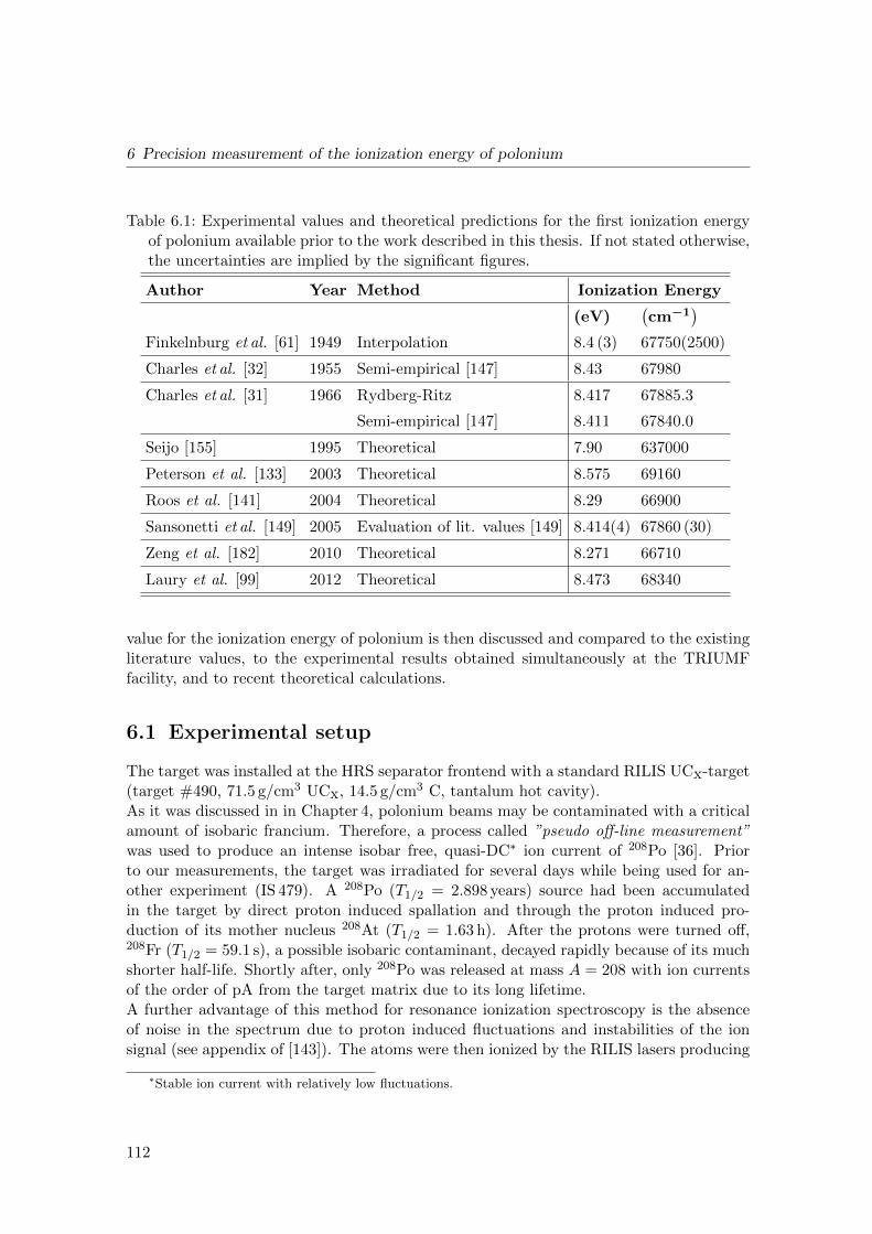
6 Precision measurement of the ionization energy of polonium
Table 6.1: Experimental values and theoretical predictions for the first ionization energyof polonium available prior to the work described in this thesis. If not stated otherwise,the uncertainties are implied by the significant figures.
Author Year Method Ionization Energy
(eV)(cm−1
)Finkelnburg et al. [61] 1949 Interpolation 8.4 (3) 67750(2500)
Charles et al. [32] 1955 Semi-empirical [147] 8.43 67980
Charles et al. [31] 1966 Rydberg-Ritz 8.417 67885.3
Semi-empirical [147] 8.411 67840.0
Seijo [155] 1995 Theoretical 7.90 637000
Peterson et al. [133] 2003 Theoretical 8.575 69160
Roos et al. [141] 2004 Theoretical 8.29 66900
Sansonetti et al. [149] 2005 Evaluation of lit. values [149] 8.414(4) 67860 (30)
Zeng et al. [182] 2010 Theoretical 8.271 66710
Laury et al. [99] 2012 Theoretical 8.473 68340
value for the ionization energy of polonium is then discussed and compared to the existingliterature values, to the experimental results obtained simultaneously at the TRIUMFfacility, and to recent theoretical calculations.
6.1 Experimental setup
The target was installed at the HRS separator frontend with a standard RILIS UCx-target(target #490, 71.5 g/cm3 UCx, 14.5 g/cm3 C, tantalum hot cavity).As it was discussed in in Chapter 4, polonium beams may be contaminated with a criticalamount of isobaric francium. Therefore, a process called ”pseudo off-line measurement”was used to produce an intense isobar free, quasi-DC∗ ion current of 208Po [36]. Priorto our measurements, the target was irradiated for several days while being used for an-other experiment (IS 479). A 208Po (T1/2 = 2.898 years) source had been accumulatedin the target by direct proton induced spallation and through the proton induced pro-duction of its mother nucleus 208At (T1/2 = 1.63 h). After the protons were turned off,208Fr (T1/2 = 59.1 s), a possible isobaric contaminant, decayed rapidly because of its muchshorter half-life. Shortly after, only 208Po was released at mass A = 208 with ion currentsof the order of pA from the target matrix due to its long lifetime.A further advantage of this method for resonance ionization spectroscopy is the absenceof noise in the spectrum due to proton induced fluctuations and instabilities of the ionsignal (see appendix of [143]). The atoms were then ionized by the RILIS lasers producing
∗Stable ion current with relatively low fluctuations.
112

6.1 Experimental setup
Ta 635A/650A
290 A Ta
no p
30 kV
#490
HRS
UCx
(a)
67 860 cm-1
-139 081.2 cm
-150 934.9 cm
l = 255.80 nm
l = 843.37 nm
-10 cm
l = 588 nm to 604 nm
Po
IE literature
3 56p 7s S 2
3 56p 7p P 2
4 36p P 2
(b)
Figure 6.1: a) Operational parameters of the ISOLDE target used during the measurementsof the ionization energy. Design of schematics adopted from [143]. b) Ionization schemefor polonium as used for the Rydberg spectroscopy. The first step was provided by afrequency-tripled dye-laser, the second step by the fundamental output of a Ti:Sa laserand the region around the ionization energy was scanned by a tunable dye laser operatedwith R6G in ethanol.
an ion current, which was stable over the whole measurement period and which was highenough to be measured directly by the Faraday cup (≥ 0.1 pA).Figure 6.1b shows the ionization scheme of polonium as used for the measurement. Theintermediate steps are the same as those described in Chapter 4.2.3 and [41]: the first step(λ = 255.80 nm) was provided by a frequency-tripled dye-laser (dye: styryl 8, P ≈ 40 mWin the hot cavity) and the second intermediate step (λ = 843.37 nm) by the fundamentalbeam of a Ti:Sa laser (P ≈ 1 W in the hot cavity). The ionizing step, which is usuallyprovided by the 532 nm output of a Nd:YAG pump laser, was replaced by a tunable dye-laser (dye: rhodamine 6G (R6G)) for scanning across the expected ionization energy at67860 (30) cm−1 [149]. The laser was scanned over a range of 585 nm - 605 nm (16530 cm−1
to 17100 cm−1, respectively), equivalent to a scan across the ionization threshold from67460 cm−1 to 68030 cm−1. The wavelength was measured by the WS7 wavemeter [79].The power output power of the dye laser is wavelength-dependent and thus, the intensityof the ion signal varies while scanning along the tuning range of the dye. This affects therelative intensities of the different Rydberg levels and has to be considered when compar-ing the relative heights of the peaks.The background signal at the Faraday cup HRS.FC690 was of the order of -0.08 pA. Thisnegative offset is due to the decay of radioactive isotopes, which are deposited on theFaraday cup.
113
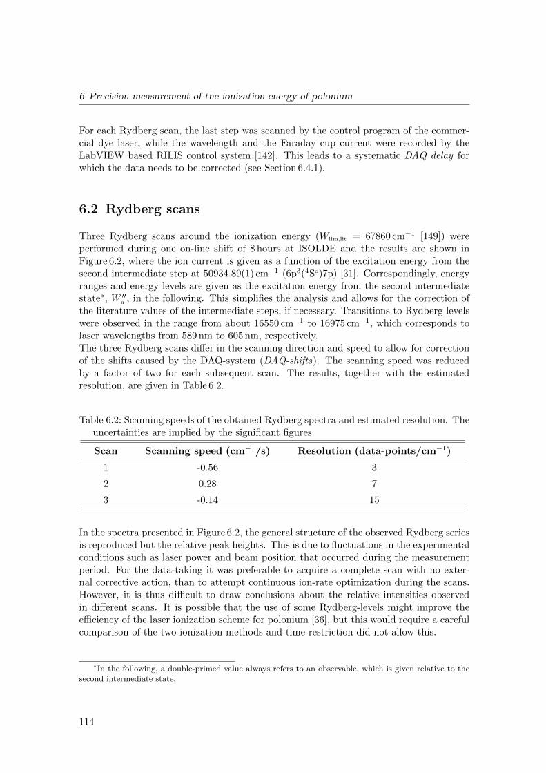
6 Precision measurement of the ionization energy of polonium
For each Rydberg scan, the last step was scanned by the control program of the commer-cial dye laser, while the wavelength and the Faraday cup current were recorded by theLabVIEW based RILIS control system [142]. This leads to a systematic DAQ delay forwhich the data needs to be corrected (see Section 6.4.1).
6.2 Rydberg scans
Three Rydberg scans around the ionization energy (Wlim,lit = 67860 cm−1 [149]) wereperformed during one on-line shift of 8 hours at ISOLDE and the results are shown inFigure 6.2, where the ion current is given as a function of the excitation energy from thesecond intermediate step at 50934.89(1) cm−1 (6p3(4So)7p) [31]. Correspondingly, energyranges and energy levels are given as the excitation energy from the second intermediatestate∗, W ′′n , in the following. This simplifies the analysis and allows for the correction ofthe literature values of the intermediate steps, if necessary. Transitions to Rydberg levelswere observed in the range from about 16550 cm−1 to 16975 cm−1, which corresponds tolaser wavelengths from 589 nm to 605 nm, respectively.The three Rydberg scans differ in the scanning direction and speed to allow for correctionof the shifts caused by the DAQ-system (DAQ-shifts). The scanning speed was reducedby a factor of two for each subsequent scan. The results, together with the estimatedresolution, are given in Table 6.2.
Table 6.2: Scanning speeds of the obtained Rydberg spectra and estimated resolution. Theuncertainties are implied by the significant figures.
Scan Scanning speed (cm−1/s) Resolution (data-points/cm−1)
1 -0.56 3
2 0.28 7
3 -0.14 15
In the spectra presented in Figure 6.2, the general structure of the observed Rydberg seriesis reproduced but the relative peak heights. This is due to fluctuations in the experimentalconditions such as laser power and beam position that occurred during the measurementperiod. For the data-taking it was preferable to acquire a complete scan with no exter-nal corrective action, than to attempt continuous ion-rate optimization during the scans.However, it is thus difficult to draw conclusions about the relative intensities observedin different scans. It is possible that the use of some Rydberg-levels might improve theefficiency of the laser ionization scheme for polonium [36], but this would require a carefulcomparison of the two ionization methods and time restriction did not allow this.
∗In the following, a double-primed value always refers to an observable, which is given relative to thesecond intermediate state.
114

6.2 Rydberg scans
1655
016
600
1665
016
700
1675
016
800
1685
016
900
1695
0
0.00
0.25
0.50
0.75
1.00
0.00
0.25
0.50
0.75
1.00
0.00
0.25
0.50
0.75
1.00
Excita
tion E
nergy
Abov
e 2nd
Excite
d Stat
e (cm
-1 )
Scan
3Sc
annin
g spe
ed =
-0.14
cm-1 /s
Ion Current (pA)
Scan
2
Scan
ning s
peed
= 0.2
8 cm-1 /s
Scan
1
Scan
ning s
peed
= -0.
56 cm
-1 /sIE lite
rature
Fig
ure
6.2:
Th
eth
ree
Ryd
ber
gsc
ans
of
208P
o,w
hic
hw
ere
obta
ined
du
rin
gth
em
easu
rem
ent
cam
pai
gn.
Th
ew
aven
um
ber
sco
rres
pon
dto
the
ener
gy
from
the
last
inte
rmed
iate
step
at50
934.
9cm−
1w
ith
con
figu
rati
on6p
3(4
So)7
p[3
1].
Th
efi
rst
an
dth
eth
ird
Ryd
ber
gsc
an
sco
vere
da
regi
onw
hic
hcr
osse
dth
eli
tera
ture
valu
eof
the
ion
izat
ion
ener
gyof
6786
0cm−
1
(16925
.1cm−
1fr
omth
ese
con
dst
ep)
tow
ell
bel
owth
eio
niz
atio
nen
ergy
[149
].S
can
2w
assc
ann
edin
the
opp
osit
ed
irec
tion
.T
he
scan
nin
gsp
eed
of
all
thre
esc
ans
diff
ered
from
each
oth
er,
wh
ich
led
toa
diff
eren
tre
solu
tion
.V
aria
tion
sin
pea
kh
eigh
tsd
uri
ng
asc
an
may
orig
inate
from
the
chan
gein
lase
rb
eam
pos
itio
nin
sid
eth
eca
vit
y.D
iffer
ence
sb
etw
een
the
scan
sin
dic
ate
slig
htl
yd
iffer
ent
con
dit
ion
sof
the
RIL
ISor
the
ISO
LD
Eta
rget
.
115

6 Precision measurement of the ionization energy of polonium
6.3 Analysis of the Rydberg spectra
Each obtained Rydberg spectrum was analyzed individually. In the following the proce-dure is explained using Rydberg scan 3 as an example, but Rydberg scans 1 and 2 wereanalyzed similarly. Figure 6.3 a shows the detailed structure of scan 3. In total 93 peakscould be resolved. The spectrum contains a repetitive substructure of 5 peaks, each be-longing to a separate Rydberg series. These subseries converge eventually to the centerof gravity of the group for higher energies towards the ionization energy. The five peaks,which all have the same principal quantum number n, are referred to as one group (g).
6.3.1 Identification of the subseries and peaks in the Rydberg scans
Figure 6.3 b shows a zoom into the spectrum of a low-lying group (g = 7) of Rydberg statesfrom 16746 cm−1 to 16757 cm−1. Each peak is well-resolved and belongs to one of the fivesubseries. The labeling with arbitrary names from the lowest-lying series to the highestlying series is as follows: Π, Θ, Σ, Ω, and Φ. Within one group, the second subseries Θis the strongest and the first subseries Π and the isolated subseries Ω in the middle ofthe group are about half as strong as subseries Θ. The fourth subseries Ω and the fifthsubseries Φ are much weaker than the others.These subseries converge towards higher energies and become unresolved in an envelopingpeak, which are then treated as a new individual subseries. The different stages of themerging of the subseries are shown in Figure 6.3 b-d: in Figure 6.3 c, the first two sub-series and the last two subseries become indistinguishable and are denoted as ΠΘ and ΩΦ;then, the third subseries Σ merges with the first two subseries to become subseries ΠΘΣ;Figure 6.3 c shows the subseries very close to the ionization energy; all series convergeeventually to the center of gravity of the group, which is then denoted as the subseriesΠΘΣΩΦ.The point from which the subseries start to merge depends on the resolution of the scanand consequently more Rydberg levels were resolved for scan 3 since it has the highestresolution due to the slow scanning speed.In total 97 resonances were resolved in scan 1 and 93 resonances were resolved in scan 2and scan 3. In scan 1 and scan 2, the peaks belong to 39 identified groups and in scan 3to 48 identified groups. Each group is numbered, starting with g = 1 for the lowest-lyingRydberg group of scan 1 and 2 visible in Figure 6.2. Correspondingly the lowest lyinggroup visible in scan 3 is g = 6.
116
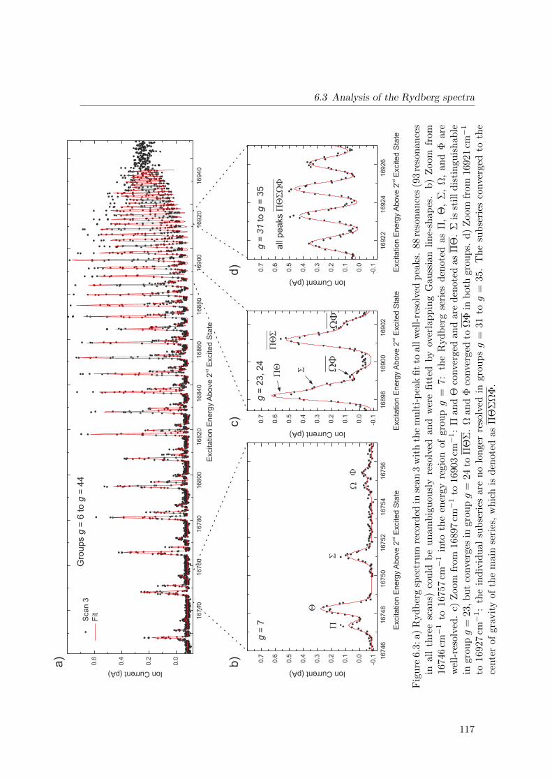
6.3 Analysis of the Rydberg spectra
a)
b)
c)d
)
16740
16760
16780
16800
16820
16840
16860
16880
16900
16920
16940
0.0
0.2
0.4
0.6
Scan 3
Fit
Ion Current (pA)
Gro
up
s g
= 6
to
g =
44
16746
16748
16750
16752
16754
16756
-0.1
0.0
0.1
0.2
0.3
0.4
0.5
0.6
0.7
Ion Current (pA)
P
Q
S
WF
g =
7
nd
Exci
tatio
n E
nerg
y A
bove
2 E
xcited S
tate
16898
16900
16902
-0.1
0.0
0.1
0.2
0.3
0.4
0.5
0.6
0.7
Ion Current (pA)
PQ S
PQS
WF
WF
g =
23
, 2
4
nd
Exci
tation E
nerg
y A
bove 2
Exci
ted S
tate
16
922
16
924
16
926
-0.1
0.0
0.1
0.2
0.3
0.4
0.5
0.6
0.7
Ion Current (pA)
all
pe
aks PQSWF
g =
31
to
g =
35
nd
Exc
itatio
n E
nerg
y A
bove 2
Exc
ited S
tate
nd
Excita
tion E
nerg
y A
bove 2
Excite
d S
tate
Fig
ure
6.3:
a)R
yd
ber
gsp
ectr
um
reco
rded
insc
an3
wit
hth
em
ult
i-p
eak
fit
toal
lw
ell-
reso
lved
pea
ks.
88re
son
ance
s(9
3re
son
ance
sin
all
thre
esc
ans)
cou
ldb
eu
nam
big
uou
sly
reso
lved
and
wer
efi
tted
by
over
lap
pin
gG
auss
ian
lin
e-sh
apes
.b
)Z
oom
from
16746
cm−
1to
167
57
cm−
1in
toth
een
ergy
regi
onof
grou
pg
=7:
the
Ryd
ber
gse
ries
den
oted
asΠ
,Θ
,Σ
,Ω
,an
dΦ
are
wel
l-re
solv
ed.
c)Z
oom
from
168
97
cm−
1to
1690
3cm−
1:
Πan
dΘ
conve
rged
and
are
den
oted
asΠ
Θ.
Σis
stil
ld
isti
ngu
ish
able
ingro
upg
=23,
bu
tco
nve
rges
ingr
oupg
=24
toΠ
ΘΣ
.Ω
and
Φco
nve
rged
toΩ
Φin
bot
hgr
oup
s.d
)Z
oom
from
1692
1cm−
1
to1692
7cm−
1:
the
ind
ivid
ual
sub
seri
esar
en
olo
nge
rre
solv
edin
grou
psg
=31
tog
=35
.T
he
sub
seri
esco
nve
rged
toth
ece
nte
rof
grav
ity
ofth
em
ain
seri
es,
wh
ich
isd
enot
edas
ΠΘ
ΣΩ
Φ.
117

6 Precision measurement of the ionization energy of polonium
6.3.2 Fitting
The fitting was performed using the Origin Pro c© 9.0 analysis software. To determine thecenter of each well-resolved peak, one or more groups were fitted simultaneously with amultipeak fit of superposed Gaussians for each scan. The equation describing this is:
F (ν) = y0 +N∑i=1
Ai
wi√π/2· e−2
(ν−νc,i)2
w2i , (6.1)
where y0 is the FC background level, which is kept constant for each scan, Ai is the areaunder the ith peak, wi = 2σi is the peak width, and νc,i is the wavenumber of the center ofpeak i. The common background level y0 was determined for each scan before the multi-peak fit by fitting a straight line to the background signal well below the ionization energyand was then kept fixed during the actual fitting. The peak width of the well-resolvedresonances was on average FWHM ≈ 0.4 cm−1 . This was taken as a lower limit and, fora single fully resolved peak, it corresponds to the expected Doppler broadening in the hotcavity. No upper limit was set in order to take into account the merging of the subseriesand the corresponding broadening.The groups below 16740 cm−1 (see Figure 6.2) were considered to be independent of theneighboring groups and were fitted individually by a multipeak fit. All groups from16740 cm−1 to about 16940 cm−1 were fitted by one multi-peak fit to take potential su-perpositions of the peaks of neighboring groups into account. For these cases, the highnumber of fitting parameters made it necessary to fit in several stages: first, the wavenum-bers of the peak centers were initialized and the width was shared for all peaks during thefirst fit. Then, the width was fitted freely with a lower limit of 0.4 cm−1 . If necessary,centroids and widths were slightly varied until the fit converged by X2-minimization. Theoverall uncertainty of each peak centroid is between 0.01 cm−1 and 0.1 cm−1 dependingon the statistics and how well resolved the individual peak is. Table 6.3 gives an overviewabout the most important parameters of the analysis.Note that the obtained values for the centroid of the peaks show a systematic shift betweenthe scans due to the different scanning speeds caused by a delay in the DAQ system.
Table 6.3: Characteristics of the three different Rydberg scans and the fitting results: peaksand groups that were identified, Faraday cup background levels and wavenumbers ofthe first and the last identified peak. The levels are not yet corrected for the systematicshift of the spectra due to the DAQ delay.
Scan # peaks Range groups Background First peak Last peak
gmin-gmax (pA) (cm−1) (cm−1)
1 97 1− 39 −0.0896 (6) 16565.09 (9) 16924.54 (3)
2 93 1− 39 −0.0895 (6) 16565.49 (2) 16924.91 (6)
3 93 6− 48 −0.0847 (2) 16703.86 (6) 16934.41 (2)
118

6.4 Evaluation of Rydberg peak position
6.4 Evaluation of Rydberg peak position
6.4.1 Correction for the systematic shift of the spectra due to the DAQdelay
A systematic shift of the peak positions is observed between the different scans. This isillustrated in Figure 6.4a which shows the Rydberg state series Σ in group g = 7. The peakposition of scan 1 is shifted towards lower wavenumbers compared to scan 3, while the peakposition of scan 2 is shifted towards higher wavenumbers compared to scan 3. It is further-more observed that the lineshape broadens slightly for faster scan speeds (see Figure 6.4a).Both effects can be explained by the different acquisition speeds of the wavemeter and theFaraday cup: while the wavenumber is measured about 28 times per second, the Faraday-cup DAQ integrates the ion current over a half a second and thus measures only 2 valuesper second. This results in a systematic shift of the measured wavenumber. Additionally,the lineshape is broadened due to the increased ion current that is recorded on rising andfalling peak flanks.The overall systematic DAQ-shift of the peaks was determined by calculating the weightedaverage of the systematic shifts of several well-resolved and undisturbed peaks of series Σ,
1 6 7 5 0 . 0 1 6 7 5 0 . 4 1 6 7 5 0 . 8 1 6 7 5 1 . 2 1 6 7 5 1 . 6- 0 . 1
0 . 0
0 . 1
- 0 . 1
0 . 0
0 . 1
- 0 . 1
0 . 0
0 . 1
E x c i t a t i o n E n e r g y A b o v e 2 n d E x c i t e d S t e p ( c m - 1 )
s c a n 3 : - 0 . 1 4 c m - 1 / s
s c a n 2 : 0 . 2 8 c m - 1 / s
s c a n 1 : - 0 . 5 6 c m - 1 / s
Ion Cu
rrent
(pA)
S e r i e s G r o u p g = 7
Σ
(a)
- 0 . 8 - 0 . 6 - 0 . 4 - 0 . 2 0 . 0 0 . 2 0 . 4
S e r i e s SG r o u p g = 7
Excita
tion E
nergy
Abov
e 2nd
Excite
d Step
(cm-1 )
S c a n n i n g S p e e d ( c m - 1 / s )
S c a n 1 S c a n 2 S c a n 3 F i t d S c a n 2
d S c a n 1
1 6 7 5 1 . 1 1
1 6 7 5 1 . 0 2
1 6 7 5 0 . 8 0
1 6 7 5 1 . 2 7
d S c a n 2
(b)
Figure 6.4: A representative example of the determination of the systematic shift due tothe DAQ delay, conducted for the resonance of series Σ in group g = 7. a) Plot and fitof the resonance of series for the three Rydberg scans. The estimated real position ofthe peak is given by the red solid line and the shifts to the measured peak positions areindicated with the arrows. b) The peak position as a function of the scanning speedand a fit to the data (red solid line). The real position of the centroid is defined as theintercept of the straight line with the abscissa (scanning speed of 0 cm−1/s).
119

6 Precision measurement of the ionization energy of polonium
for which it was certain that no superposition with neighboring series could disturb thepeak. In total, 13 of such resonances (g = 7 to g = 19) appear in each scan.As shown in Figure. 6.4b, the systematic shift, δν, of the peaks is proportional to the scan-ning speed. This allows for the determination of the real peak position at a scanning speedof 0 cm−1/s by fitting a straight line to the data and interpolating to the intercept. Thisprocedure was repeated for the other 12 undisturbed peaks of the series Σ and the resultsof all fits are given in Table A.1 in the Appendix A. No systematic wavenumber-dependenttrend in the DAQ-shifts was observed. The correction factor was then determined bycalculating the weighted average of all the individual DAQ-shifts, for which the fitting un-certainty was taken as the weighting factor. The uncertainty of the systematic DAQ-shiftwas obtained by calculating the standard deviation of the scans to the weighted average.Table 6.4 lists the systematic DAQ-shifts of the peaks obtained for each scan.
Table 6.4: Details of the systematic shift due to the time delay in the DAQ. Differentfrequency steps, measured scanning speeds and corresponding systematic DAQ-shift,δν obtained by the fit and the uncertainty of the DAQ-shift, ∆δν.
Scan Steps size Scanning speed δν ∆δν
(cm−1) (cm−1/s) (cm−1/s) (cm−1/s)
1 0.02 -0.56 -0.275 0.073
2 0.01 0.28 0.138 0.047
3 0.005 -0.14 -0.074 0.045
6.4.2 Evaluation procedure for the determination of the peak positions
The final values of the transition wavenumbers to the Rydberg levels were calculated bycorrecting the measured peak values in each scan for the systematic DAQ-shift and aver-aging the results from the individual analysis of the three Rydberg scans. The procedureis summarized in the following and the final results for each observed level can be foundin Table B.1 in Appendix B.1.
Correction of the fit results for the systematic DAQ-shift due to the DAQ delay:In order to obtain the DAQ-shift corrected centroids ν ′i,j,k, the DAQ-shifts δνk ofeach Rydberg scan given in Table 6.4 were added to each centroid νi,j,k (i: Rydbergseries, j: group number, k: scan number):
ν ′i,j,k = νi,j,k − δνk (6.2)
Calculation of the uncertainties of the DAQ-shift corrected peaks: The statisti-cal error of the DAQ-shift corrected centroid is given by the uncertainty of the mul-tipeak fit and the statistical uncertainty of the wavemeter ∆WM = 0.02 cm−1 [79].In addition, a systematic error due to the DAQ-shift ∆δνk needs to be added. Thesystematic error of the wavemeter will be added later to the final combined values
120

6.4 Evaluation of Rydberg peak position
of the centroids and to the uncertainty of the evaluated ionization energy since thissystematic is a property of the combined values of all three scans. Thus, the totalerror of the DAQ-shift corrected centroids calculates to:
∆ν ′i,j,k =
√(∆νi,j,k)
2 + (∆WM)2 + ∆δνk (6.3)
The position of the Rydberg levels: The calculation of the final value of the com-bined centroids depends on the number of scans in which the individual Rydberg levelwas resolved. Most peaks were resolved in at least two or three scans (N = 2, 3).In these cases, the final values of the Rydberg levels were obtained by calculatingthe weighted mean for each Rydberg level W ′′i,j :
W ′′i,j =
N=k∑k=1
ν ′i,j,kwi,j,k
N=k∑k=1
wi,j,k
with wi,j,k =1
∆ν ′i,j,k, (6.4)
where wi,j,k is the weighting factor. If a Rydberg level was only resolved in one scan(N = 1), the DAQ-shift corrected value from Equation (6.2) was taken:
W ′′i,j = ν ′i,j,k . (6.5)
The excitation energy of the Rydberg level with respect to the ground state is thengiven by
Wi,j = W ′′ +W ′′i,j , (6.6)
where W ′′ is the total excitation energy with respect to the energy of the secondexcited state in the ionization scheme.
Final error of Rydberg levels: In case the Rydberg state W ′′i,j was observed in at leasttwo Rydberg scans (N ≥ 2), the final statistical uncertainty is given by the standarddeviation σi,j of the DAQ-shift corrected fit values ν ′i,j,k around the weighted meanof the Rydberg level W ′′i,j . If a Rydberg level was only resolved in one peak (N = 1),the error of the DAQ-shift corrected value ∆ν ′i,j,k was taken. In order to treat theerrors conservatively, a lower limit for the statistical uncertainty of the Rydberg levelwas estimated by calculating the average standard deviation, σ = 0.06 cm−1, of allRydberg levels. This can be summarized by:
∆Wi,j =
σi,j if N ≥ 2 and σi,j > σ
∆ν ′i,j,k if N = 1 and ∆ν ′i,j,k > σ .
σ = 0.06 cm−1 if σi,j ,∆ν′i,j,k ≤ σ
(6.7)
For the final valuesWi,j of all observed Rydberg levels (see Table B.1 in Appendix B.1)the systematic uncertainty of the wavemeter was added.
121

6 Precision measurement of the ionization energy of polonium
6.5 Detailed analysis of the ionization energy of polonium
The ionization energy of polonium was calculated by fitting the Rydberg formula (Equa-tion (2.7)) and Rydberg-Ritz formula (Equation (2.10)) to the final values of the Rydberglevel from Table B.1.For practical reasons, the ionization energy is calculated with respect to the second excitedstate W ′′lit = 50934.89 cm−1 [31] throughout the rest of the chapter and will be denoted asW ′′lim. This allows for a simpler correction of the total ionization energy Wlim, in case theliterature value of the second step is measured more precisely in the future. The ionizationenergy can then be calculated by:
Wlim = W ′′lit +W ′′lim . (6.8)
Using the conventions defined in Chapter 2.1.2 for the excitation energy Wn and the energyEn of an intermediate atomic level, Wn = En − E0, the excitation energies W ′′n of theRydberg levels can then be calculated to the first order by using the Rydberg formula(Equation (2.7)) and setting the charge to ζ = 1 for a singly ionized ion:
W ′′n = W ′′lim −RM
(n∗)2 = W ′′lim −RM
(n− δn,l)2 , (6.9)
where n∗ is the effective quantum number, n the principal quantum number and δn,lthe quantum defect. The reduced-mass Rydberg constant for 208Po is calculated toRM = 109737.0262385 (8) by Equation (2.5) using the values for the Rydberg constantand electron mass recommended in CODATA [121] and the mass of 208Po given in theAME2012 [173].If the ionization energy W ′′lim is known, the effective quantum number n∗ can be calculatedfrom Equation (6.9) by
n∗ =
√RM
W ′′lim −W ′′n. (6.10)
In the case of a dependency of the quantum defect on the principal quantum number n asdescribed in Chapter 2.1.2, the ionization energy is calculated to second order using theRydberg-Ritz formula (Equation (2.10)):
W ′′n = W ′′lim −RM(
n−A+ B(n−A)2
)2 . (6.11)
The ionization energy, W ′′lim, with respect to the excitation energy of the second excitedstate, W ′′lim, is obtained by a fit of Equation (6.9) or Equation (6.11) to a series of Rydberglevels.
122

6.5 Detailed analysis of the ionization energy of polonium
6.5.1 Substitution of principal quantum number and quantum defect
In practice it can be difficult to assign the real principle quantum number n to high-lying Rydberg levels. An unambiguous allocation of a principal quantum number to eachRydberg level is only possible, if the head∗ of the Rydberg series, or other members ofthe same Rydberg series, are described in the literature. A possible assignment of theprinciple quantum numbers to the Rydberg levels will be discussed in Chapter 6.5.5.However, to keep the following calculation and discussions free from speculations on thereal principal quantum number, the principal quantum number n and the quantum defectδ are substituted in the following:
n→ n′: The principal quantum number n must be larger than the effective quantumnumber n∗ = n − δ since δ > 0. Hence, n is substituted by the minimum value forthe principal quantum number n′, which can be expressed by:
n′ = int [n∗] + 1 . (6.12)
Alternatively, n′ can be defined by introducing an integer ∆n, which is the differencebetween n′ and the principal quantum number n:
n′ := n−∆n . (6.13)
δ → δ′: The quantum defect δ can be substituted by the remainder of the quantum defectδ′, which is calculated by:
δ′ = mod1 [δ]
= mod1 [n− n∗]= mod1 [−n∗] .
(6.14)
Similar to n′, δ′ can be alternatively defined using an integer ∆δ, which is thedifference between the remainder of the quantum defect δ′ and the quantum defectδ:
δ′ := δ −∆δ . (6.15)
It can be easily verified that ∆n ≡ ∆δ:
δ′ = n′ − n∗ |δ′ = δ −∆δ, n′ = n−∆n
δ −∆δ = n−∆n− n∗ | − nδ −∆δ − n = −∆n− n∗ |n∗ = n− δ
∆δ ≡ ∆n .
(6.16)
Once it is possible to allocate the data unambiguously, this approach allows for a simplecorrection to the obtained values of n′ and δ′ for ∆n and ∆δ, respectively.The calculation of the value of the ionization energy by Equation (6.9) and Equation (6.11)is independent of the choice of the principal quantum number and the quantum defect.
∗Low-lying members of a Rydberg series, for which the principal quantum number n is known.
123
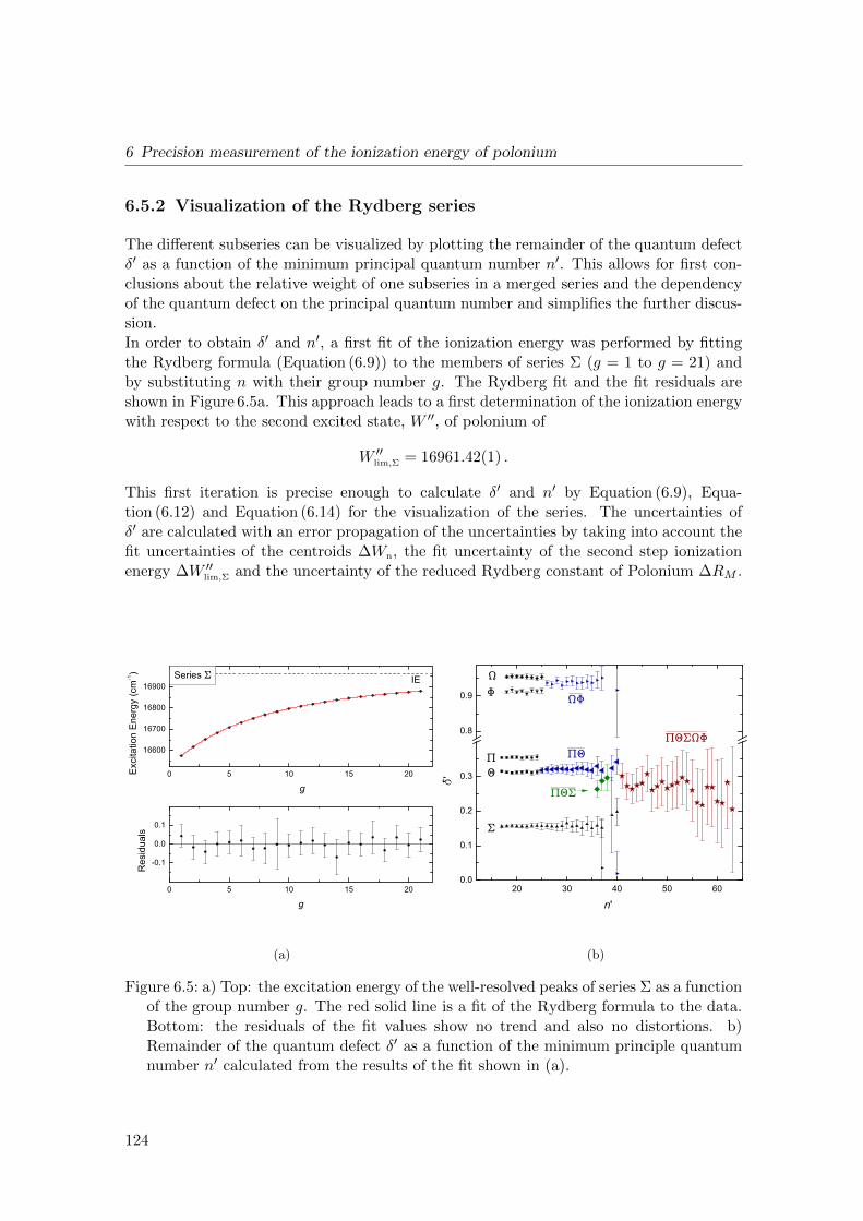
6 Precision measurement of the ionization energy of polonium
6.5.2 Visualization of the Rydberg series
The different subseries can be visualized by plotting the remainder of the quantum defectδ′ as a function of the minimum principal quantum number n′. This allows for first con-clusions about the relative weight of one subseries in a merged series and the dependencyof the quantum defect on the principal quantum number and simplifies the further discus-sion.In order to obtain δ′ and n′, a first fit of the ionization energy was performed by fittingthe Rydberg formula (Equation (6.9)) to the members of series Σ (g = 1 to g = 21) andby substituting n with their group number g. The Rydberg fit and the fit residuals areshown in Figure 6.5a. This approach leads to a first determination of the ionization energywith respect to the second excited state, W ′′, of polonium of
W ′′lim,Σ = 16961.42(1) .
This first iteration is precise enough to calculate δ′ and n′ by Equation (6.9), Equa-tion (6.12) and Equation (6.14) for the visualization of the series. The uncertainties ofδ′ are calculated with an error propagation of the uncertainties by taking into account thefit uncertainties of the centroids ∆Wn, the fit uncertainty of the second step ionizationenergy ∆W ′′lim,Σ and the uncertainty of the reduced Rydberg constant of Polonium ∆RM .
(a)
(b)
Figure 6.5: a) Top: the excitation energy of the well-resolved peaks of series Σ as a functionof the group number g. The red solid line is a fit of the Rydberg formula to the data.Bottom: the residuals of the fit values show no trend and also no distortions. b)Remainder of the quantum defect δ′ as a function of the minimum principle quantumnumber n′ calculated from the results of the fit shown in (a).
124

6.5 Detailed analysis of the ionization energy of polonium
The corresponding n′-δ′ plot for the observed Rydberg levels is shown in Figure 6.5b. Eachsubseries and merged series are distinguishable by comparing the corresponding δ′-values.The δ′ of the lower n′ do not change significantly, when compared to the δ′ of the reso-nances with higher principal quantum numbers, n.For some resonances, δ′, differs slightly to the overall trend of the corresponding series.This mainly occurs for peaks in which the individual subseries are visible, but not clearlyresolved from the neighboring series and thus, these peaks were omitted from the fit.
6.5.3 Determination of the ionization energy with respect to the secondexcited state
The final value of the ionization energy with respect to the second excited state at W ′′ =50934.89(1) cm−1 was determined by three different methods:
Method 1: Rydberg fit to only the strongest peaks of each group.
Method 2: Individual Rydberg fits for all resolved Rydberg series and merged series.W′′lim was calculated by the weighted average.
Method 3: Global fit to all Rydberg series with the ionization energy as a shared fittingparameter.
For each method, the Rydberg formula Equation (6.9) and the Rydberg-Ritz formula ofsecond order in Equation (6.11) were fitted. However, the fits with the Rydberg-Ritzformula led to an unrealistic value for the parameter B with uncertainties as large orlarger than the value. Additionally, the ionization energy showed a dependency on theparameter B. Therefore, a further use of the Rydberg-Ritz formula was omitted and onlythe Rydberg formula was used for the calculation of the ionization energy in the following.
Method 1: Rydberg fit to strongest peaks
As shown in Figure 6.5b, the strongest observed peaks in each group are the members ofthe subseries Θ and the corresponding merged series ΠΘ. The full range of the Rydbergscan is then covered by Θ, ΠΘ and the center of gravity series ΠΘΣΩΦ for a combinedRydberg fit with the Rydberg formula as shown in Figure 6.6.With method 1, the ionization energy with respect to the second excited state is W ′′lim,M1 =16961.45(1) and the common remainder of the quantum defect is δ′ = 0.3149(9). Thisvalue differs slightly to the one obtained from the fit of the well-resolved peaks of seriesΣ.However, the residuals are not uniformly continuous and show jumps of up to 0.2 cm−1
between the individual series. This illustrates the need of an individual fit with a free δfor each subseries, as it was performed for method 2 and method 3.
125

6 Precision measurement of the ionization energy of polonium
Figure 6.6: The fit of the Rydberg formula to the combined series of Θ, ΠΘ and ΠΘΣΩΦfrom method 1. The symbols used for the individual series are the same as introducedin Figure 6.5b. Jumps of the residuals are visible where a new series begins.
Method 2: weighted mean of individual fits to all series.
In a second approach, each subseries was analyzed separately and the final value of theionization energy was determined by calculating the weighted average of all individuallyobtained ionization energies, for which the fit uncertainties were taken as weighting factors.The results are given in Table 6.5.It should be noted that not all the peaks of each series were used, since peaks, which werenot fully resolved or for which the residuals were diverging from the fit were not takeninto account. Table 6.5 gives the range of the corresponding n′-values for the Rydberg
Table 6.5: Results of the separate Rydberg fits to each individual Rydberg series andweighted average of the ionization energy.
Series Range n’ δ′ (cm−1) W”lim (cm−1)
Π 17 - 24 0.3544(8) 16961.41(2)
Θ 17 - 24 0.3145(17) 16961.47(5)
Σ 17 - 37 0.1559(5) 16961.42(1)
Ω 18 -21, 23 - 25 0.9580(16) 16961.50(4)
Φ 18, 20, 21, 23 - 25 0.9113(29) 16961.33(5)
ΠΘ 25 - 37, 39, 40 0.3165(19) 16961.38(2)
ΩΦ 26 - 37 0.9331(45) 16961.37(4)
ΠΘΣΩΦ 41 - 65 0.30153(11) 16961.47(2)
Weighted average 16961.415(7)
126

6.5 Detailed analysis of the ionization energy of polonium
resonances, which were used. The uncertainty was determined by calculating the standarddeviation of the difference of the individual results of each series to the weighted average.The obtained ionization energy with respect to the second excited state of W” lim,M2 =16961.415 (7) cm−1 agrees with the value from method 1 within the uncertainties. Theuncertainty however, is significantly higher due to the scattering of the individual values,but the uncertainty of Method 1 is most likely underestimated.
Method 3: global fit to all individual series.
In a third attempt, the Rydberg formula was globally fitted to the individual Rydbergseries, where the ionization energy with respect to the second excited state, W ′′lim, was ashared parameter. Only the remainder of the quantum defect δ′ was an individual fittingparameter. The ranges of the n′ of the used Rydberg levels correspond to the ranges usedin method 2.This approach has the advantage that it uses all the available statistics in one fit for thedetermination of the ionization energy, while taking into account the different quantumdefects of each individual subseries. Table 6.6 lists the fit results for δ′ and Figure 6.7shows the residuals for each Rydberg series. The residuals are stable for the whole rangeof Rydberg levels and the obtained ionization energy with respect to the second excitedstate obtained by the global fit is:
W ′′lim,M3 = 16961.420(8) cm−1.
This value agrees well with the result from method 2, but differs from the result obtainedby method 1.
Table 6.6: Quantum defects obtained by the global fit of the Rydberg formula to all serieswith a shared ionization energy with respect to the second excited state, W ′′lim,global.
Series Range n’ δ′
Π 17 - 24 0.3548(87)
Θ 17 - 24 0.3130(5)
Σ 17 - 37 0.1561(5)
Ω 18 -21, 23 - 25 0.9548(7)
Φ 18, 20, 21, 23 - 25 0.9145(7)
ΠΘ 25 - 37, 39, 40 0.3204(15)
ΩΦ 26 - 37 0.9384(14)
ΠΘΣΩΦ 41 - 65 0.3204(15)
127

6 Precision measurement of the ionization energy of polonium
Figure 6.7: Residuals for each Rydberg series obtained by the global fit of method 3: aglobal fit to all series for which the ionization energy with respect to the second excitedstate was a shared fit parameter.
128

6.5 Detailed analysis of the ionization energy of polonium
6.5.4 Final result of the ionization energy of polonium
The total ionization energy of polonium from the ground-state, Wlim, is given by theexcitation energy of the second excited state, W ′′, and the ionization energy with respectto the second excited state, W ′′lim:
Wlim = W ′′ +W ′′lim . (6.17)
The second step, W ′′ = 50934.89(1) cm−1, was taken from [31] and the result of method 3for the ionization from the second state, Wlim,M3 = 16961.420(8) cm−1 was taken for thefinal value since it combines the advantage of taking the whole data set in one fit intoaccount and no shifts of residuals.Several uncertainties have to be considered in the calculation of the total ionization energy:
Statistical uncertainties: The uncertainty of the literature value of the second ex-cited step is of the order of ∆W ′′lit = 0.01 cm−1 according to [31] an the fit uncer-tainty of the ionization energy with respect to the second excited state is ∆W ′′lim =0.008 cm−1. The overall statistical uncertainty then calculates by error propagationto ∆Wlim,stat = 0.012 cm−1.
Systematic uncertainty: Systematic uncertainties arise from the wavemeter and theDAQ system. The systematic uncertainty of the HighFinesse WS7 wavemeter wasestimated to ∆νWM = 0.03 cm−1 in [143] by comparing the output of wavemeterWS7 to the output of wavemeter WS6.
The final result of the ionization energy of polonium is therefore given by:
Wlim = W ′′lit +W ′′lim
= 50934.89(1) cm−1 + 16961.420(8)(30) cm−1
= 67896.310(13)(30) cm−1 .
(6.18)
In alternative units, the ionization energy of polonium can be written as
Wlim = 67896.310(13)(30) cm−1
= 8.418069(2)(4) eV
= 147.28341(3)(7) nm .
(6.19)
6.5.5 Assignment of subseries
It is possible to allocate the members of a Rydberg series to a specific principal quantumnumber by comparing the quantum defect of similar homologous elements. For this pur-pose, the quantum defects of the literature values of the known atomic levels of sulphur(S) [116], selenium (Se) [123] and tellurium (Te) [27, 124, 146] were calculated.The second intermediate state of the polonium excitation scheme has the configuration6p37p5P2. Excitation from the second intermediate state is therefore only possible to ans-state (l = 0) or a d-state (l = 2). Therefore, odd-parity s- or d-states of sulphur, sele-nium or tellurium were taken into account for the comparison of the quantum defects. In
129

6 Precision measurement of the ionization energy of polonium
05
1 0
2=∆
2=∆
1=∆
3=∆
0=∆
S n s - s e r i e s1=∆
05
1 01 5
S n d - s e r i e s
02468
1 0
S e n s - s e r i e s
051 01 52 02 5
Coun
ts / 0
.5 S e n d - s e r i e s
05
1 0
T e n s - s e r i e s
∆−
05
1 0
T e n d - s e r i e s
0 . 0 0 . 1 0 . 2 0 . 3 0 . 4 0 . 5 0 . 6 0 . 7 0 . 8 0 . 9 1 . 0051 01 52 02 53 0
P o a l l l e v e l s
ΠΣ ΦΘ Ω
Figure 6.8: Histograms of the distributions of the quantum defects of the Rydberg levelsof polonium (Po) and the electron levels found in literature for sulphur (S), selenium(Se) and tellurium (Te). The quantum defects are substituted by δ −∆δ for a bettercomparison and the calculated ∆δ-values are given in the corresponding histograms.For Rydberg levels, δ−∆δ values can be identified with the δ′-values: δPo−∆δPo ≡ δ′Po
. A general trend is observed that δ−∆δ values of the ns-series (green) tend to be ≈ 1,while the δ − ∆δ values of nd-series (red) tend to accumulate between 0.05 and 0.5.Correspondingly, it can be thus assumed that the Rydberg series Ω and Φ of poloniumare ns-series and Σ, Π and Θ of polonium are nd-series. The ∆δ values increase by+1 from sulphur to selenium and to tellurium following the increase of the periods ofthe homologous elements. Polonium ns-levels should thus have ∆δ = 4 and poloniumnd-levels should have ∆δ = 3.
130

6.5 Detailed analysis of the ionization energy of polonium
addition, only quantum defects for levels with high n were taken into account for whichthe quantum defects don’t show any dependency on the principal quantum number.In contrast to polonium, the configurations and quantum numbers of the levels of sulphur,selenium and tellurium were known and therefore, ∆δ could be extracted for each of thes- and d-levels individually and subtracted from the total quantum defect: δ−∆δ. Theseresulting values where then compared to the remainder of the quantum defect of the polo-nium isotopes, for which δ′ ≡ δ −∆δ.Figure 6.8 shows the histograms of the δ − ∆δ values. The distribution of the quantumdefects of the s-levels (green) and d-levels (red) of sulphur, selenium and tellurium areclearly separated. The s-states tend to be in the range δ − ∆δ ≈ 0.9 − 1.1, while thed-states scatter between 0.05 and 0.5. Based on these assumptions, the series Ω and Φof polonium are identified as transitions to s-states, while Σ, Π and Θ are transitions tod-states.Following the evolution of the ∆δ values of sulphur, selenium and tellurium and adding oneadditional electron shell for Po, it becomes conclusive that ∆δs(Po) = 4 and ∆δd(Po) = 3.These results are nicely confirmed by a comparison with the 7 atomic states with odd par-ity found in [31], of which the listed ns states have quantum defects ranging from 4.9 to 5.05like the series Ω and Φ and the listed np-values have quantum defects scattering around3.3 like the series Π. The latter might also be valid for the series Θ since the quantumdefects of lower lying members of a Rydberg series have slightly different quantum defectsdue to the stronger interaction with the nucleus. No corresponding levels were found forthe series Σ, but this is most likely due to the low number of known levels in literature.For the ns-states, it is even possible to conclude that the series Σ corresponds to stateswith J = 1 and the series Φ corresponds to states with J = 2.The values of ∆δ ≡ ∆n can then be added to the n′ and δ′ values obtained in Chapter 6.5.3and an estimation for the n and δ values for the polonium series can be made. Table B.1 inAppendix B lists the complete list of the observed transitions to Rydberg states togetherwith the corresponding excitation energies and the suggested quantum numbers.
6.5.6 Summary and discussion
In this work, the ionization energy of polonium has been determined by fitting the Rydbergformula (Equation (2.7)) to a set of Rydberg series, which led to final value of:
IE Po = 67896.310(13)(30) cm−1 (6.20)
= 8.418069(2)(4) eV . (6.21)
This value is more than 50 times more precise than the literature value of 67860(30) cm−1
given in [149]. Moreover, the ionization energy determined in this work differs by morethan 10 cm−1 from the value of 67885.3 cm−1, which was obtained by a Rydberg-Ritz anal-ysis in [31]. However, in [31], only 3 low-lying levels were allocated to a Rydberg series,which limits the accuracy of the determination. Additionally, 93 new resonances in thepolonium spectra were observed, of which 57 resonances could be assigned to unambigu-ously resolved atomic states as listed in Table B.1 in the Appendix B.
131

6 Precision measurement of the ionization energy of polonium
At the same time of the measurements of the polonium Rydberg series at ISOLDE inSeptember 2012, a team at the Tri University Meson Facility (TRIUMF) in Vancouver,Canada, measured Rydberg series of polonium with the TRILIS setup [134]. Here, analternative two-step ionization scheme was used: a frequency-tripled Ti:Sa UV-laser beamwith wavelength of 245.08 nm to the first intermediate step at 39081.19 cm−1 (6p3(4S)7s5So2) and a frequency-doubled tunable Ti:Sa laser for the scan of the region around theionization energy.These measurements provided a complementary determination of the polonium ionizationenergy with different Rydberg series of levels with even parity in contrast to these mea-surements, for which Rydberg levels with odd parity were measured. The measurements atTRIUMF led to a value for the ionization energy of polonium of IE=67896.35(17)(20) cm−1
[136], which is in excellent agreement with the value measured in this work. In addition,a new theoretical value of 67790(129) cm−1 has been calculated by A. Borschevsky [22],which also agrees well with the new experimental values. The new value for the ionizationenergy of polonium obtained by Rydberg spectroscopy at ISOLDE and TRIUMF and theresults from the theoretical calculations by A. Borschevsky will be published in a jointarticle [137]. An overview of the values obtained in this work, at TRIUMF and by newtheoretical calculations are given in Table 6.7 and compared to the literature values.
Table 6.7: Comparison of the ionization energy of polonium obtained during the workon this thesis, at TRIUMF and by recent theoretical calculations with the literaturevalues. Values indicated with ∗ should be taken as preliminary. The values given in[31, 32] are implied with significant numbers.
Origin Method Ionization energy
(eV)(cm−1
)This work Rydberg analysis 8.418069(2)(4) 67896.310(13)(30)
S. Raeder et al. [136] Rydberg analysis 8.418074(21)(25)∗ 67896.35(17)(20)∗
A. Borschevsky [22] Theoretical 8.405(16)∗ 67790(129)∗
Charles et al. [32] Semi-empirical [147] 8.43 67980
Charles et al. [31] Rydberg-Ritz 8.417 67885.3
Semi-empirical [147] 8.411 67840.0
Sansonetti et al. [149] Evaluation of lit. values 8.414(4) 67860 (30)
132
7 First experiments with the LIST: laserspectroscopy of neutron-rich polonium
During the LIST on-line run in 2012 at ISOLDE, the mean square charge radii andhyperfine-structures of neutron-rich polonium (A > 210) isotopes were studied by in-source laser resonance spectroscopy using the LIST for the suppression of the strong fran-cium contamination in this mass region. The goal was to fill the gaps in the isotope chainvisible in Figure 7.1 and to investigate the properties of the odd-A neutron-rich poloniumisotopes. Due to the remaining contamination of 212Fr (see Chapter 4.3.4), a measurementof the polonium isotopes near the shell-closure N = 126 was omitted. However, the iso-tope shift and the hyperfine-structure of 217Po were successfully measured for the first timetogether with the neighboring isotopes 216,218Po as reference isotopes. In addition, a firstglimpse into the hyperfine-structure of 219Po was possible, demonstrating the feasibilityof the LIST for the study of this isotope.A brief review over the physics around the closed proton shell at Z = 82 and a summaryof the previous experiments on polonium at ISOLDE will put the work described in hereinto context, before the experiment and the results will be discussed.
7.1 A brief review of the physics around the closed protonshell at Z=82
The isotopes of elements close to the magic proton and neutron numbers (see Figure 1.1in Chapter 1) are of particular interest for nuclear structure studies. Fundamental prop-erties∗, such as the binding energies of the nucleons or the changes in the mean squarecharge radii, δ
⟨r2⟩A,Aref
, are sensitive to the interactions of few nucleons around an in-
ert core. The region around the closed proton shell Z = 82 of lead (Pb) is no strangerto this and unveils a variety of interesting phenomena. It hosts for example the stabledoubly-magic (Z = 82, N = 126) isotope 208Pb, which consequently is the heaviest stableisotope found in nature (ignoring “virtually” stable nuclei, such as 209Bi, which has ahalf-live of 1.9(2) · 1019 years [46]). Close to the neutron shell closure at N = 126, theground-state shapes of lead-isotopes (Iπ = 0+) are observed as spherical [39]. Furtheraway from the shell-closure to the neutron-deficient side an effect called shape-coexistencewas observed close to the ground states of mid-shell isotones (nuclei with same numberof neutrons, but different proton numbers) of N = 104. Shape-coexistence occurs whendifferent quantum configurations give rise to states with distinct nuclear shapes within
∗In order to keep this discussion concise, I refer to the dedicated literature and text books. An overviewof nuclear structure can be found in [29, 95]. For the discussion of the charge radii and moments, I referto [128].
133

7 First experiments with the LIST: laser spectroscopy of neutron-rich polonium
1 0 0 1 1 0 1 2 0 1 3 0 1 4 0 1 5 0
l o w s p i n h i g h s p i n r e f e r e n c e
δ<
r2 >
N
fm2
N = 12
6
N = 10
4
P t
H g
P b
P o
R n
R a
Figure 7.1: Changes in mean square radii, δ⟨r2⟩A,A’
, for even-Z isotopes in the lead-region
(Z = 82): platinum (78Pt) [101], mercury (80Hg) [171], lead (82Pb) [6, 47, 50, 53],polonium (84)Po [39, 159], radon (86Rn) and radium (88Ra) [64]. The reference isotopesare indicated by the large circles.
the same energy range and the same spin and parity. The proximity of those quantumconfigurations may result in configuration mixing, whereby the shape of the state becomesdifficult to determine. A remarkable example is 186Pb, which was found to have the threelowest states in a Iπ = 0+ configuration within a range of 700 keV and its shape wasinterpreted as a mixing of the corresponding spherical-, oblate-, and prolate shapes [5].Shape-coexistence was also found for the neutron-deficient isotopes of platinum (Pt) [101]and mercury (Hg) [171]. For the latter, also a specifically large odd-even staggering inthe mean square charge radii was observed, where the odd-N nuclei have a systematicallylarger mean square charge radii than the trend set out by the even-N isotopes. This canbe interpreted by a systematically stronger deformation of the odd-A nuclei. Figure 7.1shows these mean square charge radii.On the neutron-rich side of the shell closure (N > 126), it is of particular interest to mapthe existence of octupolar deformation∗ and inverted odd-even staggering as observed forisotopes of radon (Rn) [20], francium (Fr) [35] and radium (Ra) [67]. The inverted odd-even staggering refers to the odd-A isotopes being systematically smaller than the trendfor the even-A isotopes and is considered to be a fingerprint for octupolar deformation.Additionally, a kink in the mean square charge radii was observed departing from theneutron shell closure for lead, radon and radium [64] as shown in Figure 7.1.
∗Octupolar deformed nuclei have pear-like shapes. An illustration can be found in [67]
134

7.2 Status of the ISOLDE experiment IS456
During the last years, the systematics in the lead region were studied at ISOLDE bythe means of the in-source resonance ionization spectroscopy. This technique enables todetermine the isotope shift and the hyperfine structure and thus allows the determina-tion of the changes of the mean square charge radii and the electric dipole and magneticquadrupole moments, respectively. So far, lead- [47, 157, 158], bismuth- (Bi) [112], andpolonium-isotopes (Po) [39, 159] were studied. This list was recently extended to isotopesof thallium (Tl), gold (Au) and astatine (At) [114, 143].
7.2 Status of the ISOLDE experiment IS456: “Study ofpolonium ground state properties by simultaneousatomic- and nuclear-spectroscopy”
The experiment described in here is part of the IS456 experiment [38] aimed at the “Studyof polonium ground state properties by simultaneous atomic- and nuclear-spectroscopy”.Polonium has Z = 84 protons and is the first even-Z element being above the magicproton shell-closure with Z = 82 and having no stable isotopes. Prior to experimentIS456, evidence for shape coexistence close to the mid-shell at N = 104 arose from α-decayspectroscopy of radon and polonium [10, 175] and from in-beam studies [86]. However,the extent and onset of the ground-state deformation was still unknown until the neutron-deficient polonium isotopes were studied during two on-line runs at ISOLDE in 2007 and2009 [39, 159]. The results are shown in Figure 7.1. An astonishing result was the earlydeviation from the spherical shape compared to the mercury or the platinum chain [39]. Acomparison of the even isotopes to the odd isotopes did not show any pronounced odd-evenstaggering as observed for mercury [159]. On the neutron-rich side, a kink of the meancharge radii is visible, starting for isotopes heavier than 210Po with the neutron magicnumber N = 126, similar to the neutron-rich lead, radon and radium isotopes [64].However, the overwhelming contamination of the beam with francium above N > 126and the very short half-lives made the study of most isotopes on the neutron-rich sideimpossible during the first two runs. 212,213Fr and 220,222Fr are the strongest contaminantsin the polonium chain. The latter leaked into the beams of the lower masses due theasymmetric shape of the mass peaks after the GPS mass separator [52] and were observeddown to the mass A = 216. Only 216Po and 218Po could be measured on the neutron-richside using the ”pseudo off-line measurement” method described in [36] and in Chapter 6.1.The neutron-rich odd-A polonium isotopes remain still unstudied and the measurementsdescribed in here aim at shedding light on the unknown border of octupolar deformationin this region, colloquially called “the island of octupolar deformation”.
135

7 First experiments with the LIST: laser spectroscopy of neutron-rich polonium
-1IE: 67 860 cm
255.80 nm
843.37 nm
532 nm
Po-10 cm
4 36p P2
-139 081.19 cm
3 4 56p ( S )7s S2
o o
-150 934.89 cm
3 46p ( S )7p o 5 P2
a) b) Hyperfine structure: 5 o 57s S 7p P2 2
I = 13/2 I = 1/2I =9/2
17/2
15/2
13/2
11/2
F = 9/2
3/2
5/2
F = I + J
57p P2
5 o7s S2
13/2
11/2
9/2
7/2
5/2
17/2
15/213/211/29/2
13/2
11/29/27/25/2
3/2
5/2
3/2
5/23/2
Figure 7.2: a) Three-step laser ionization scheme for polonium. b) Zoom on the possiblehyperfine levels for nuclear spins Iπ = 13/2+, 9/2+, 1/2− with total angular momen-tum F and corresponding transitions (red solid lines) for the studied transition fromthe 7s 5So
2 state to the 7p 5P2 state. The hyperfine structure is not to scale.
7.3 Experimental setup and data taking
The polonium isotopes with mass A > 210 were produced∗ at ISOLDE in the spallation re-action of 238U induced by the impingement of a 1.4 GeV proton of typically 1.1µA intensityfrom the CERN PS-Booster onto a LIST-UCx target (ISOLDE target #488, 50 g/cm2).The reaction products effused into the tantalum transfer line and the hot cavity, bothkept on a temperature of T ≈ 2300 K and enter the LIST. Surface ionized contaminants,such as francium isotopes were separated from the neutral atomic beam by the repellerelectrode of the LIST operating on a positive potential of typically 7 V. Polonium was thenelement-selectively ionized inside the LIST RFQ structure by a three-step laser ionizationscheme [41]. It consisted of a frequency-tripled dye laser of 255.8 nm (P ≈ 20 mW) forthe transition to the 6p3(4So)7s 5So
2 first state, a tunable 0.8 GHz narrowband (NB) Ti:Salaser of ≈ 843.37 nm (P ≈ 3 mW) for the scan of the transition to the 6p3(4So)7p 5P2 sec-ond state and the 532 nm (P > 10 W) second harmonic output of a Nd:YAG pump laserfor the non-resonant transition over the ionization energy into the continuum. The outputpower of the NB-Ti:Sa for the second transition was reduced to avoid power broadening.Figure 7.2 shows the laser ionization scheme together with possible transitions betweenhyperfine levels of the 7s 5So
2 first state to the 7p 5P2 second state for different nuclearspins I = 13/2, 9/2, 1/2. After leaving the LIST RFQ, the ions were then accelerated to
∗For a detailed description of the nuclear reactions, the target specifications, the laser setup and thetechnical aspects of the LIST, I refer to the corresponding sections in Chapter 3 and Chapter 4.
136

7.3 Experimental setup and data taking
50 keV, mass separated by the GPS dipole magnet and sent to the KU Leuven “Wind-mill” detector setup [55, 160], where the ions were implanted into one of the 10 carbonfoils (10 mm diameter, 20µg/cm2, from the GSI target laboratory) [106]) mounted on arotating wheel. The 10 foils are divided into two sets of 5 foils so that different sets wereused for different isotopes. Two passivated implanted planar silicon (PIPS) detectors, C1and C2 (see Figure 3.12 in Chapter 3.4.1), surround the carbon foil and are placed into theion beam axis, whereas C1 is placed in front of the foil and has an 8 mm aperture for beamtransport to the foil and C2 is placed behind the carbon foil. Together, these detectorscover 51% of the total angular solid angle. After each implantation and data acquisition(DAQ) cycle, the rotating wheel was turned and a fresh carbon foil was moved betweenthe detectors into the axis of the ion beam. Once the narrow band scanning laser was setto a new wavelength, a new measurement cycle could begin.
7.3.1 Measurement cycle
The control systems of the setup and data acquisition of the RILIS (tunable NB-laser andcorresponding wavemeters) and the “Windmill” (Implantation and DAQ) were combinedand synchronized to the proton bunches of the proton supercycle (SC).A measurement cycle was started once the desired laser frequency was set and stabilizedand the “Windmill” setup was ready. Figure 7.3 shows a simplified logical sequence for theinitialization of a measurement cycle: once, the operational state of the RILIS lasers andthe DAQ of the Windmill were confirmed, the system was waiting for a trigger signal of theproton supercycle to start the new measurement cycle. An additional clock is introducedto take into account for the time delay of 535 ms [36] between the trigger signal and thearrival of the first bunch of the proton supercycle.The total measurement cycle for one scan over the studied transition is shown in Fig-ure 7.4a. As soon as, the new laser frequency was set and the “Windmill”-setup was ready(set-up time of typically a fraction m = 0.3 of proton supercycle) data were taken andintegrated over a fraction n = 0.7 of a proton supercycle. Figure 7.4b shows a typicalmeasurement cycle: The sequence of 9 proton bunches out of the total proton supercycle(39 proton bunches, spaced by 1.2 s) were sent to the ISOLDE target. The overall protonsequence adds up to an average proton current of ≈ 1.02µA, which was identical for eachmeasurement presented in this chapter. Of these 9 proton pulses, 7 fall into the time ofthe data taking. Figure 7.4c illustrates the measurement sequence between each protonpulse. Elements with a fast release from the target matrix and isotopes with very shorthalf-lives will see their production peak shortly after the proton impact on the target. Thisis the case of the francium contaminants [109], while the polonium beams have a moregradual release profile [41]. Thus, the beam-gates were closed for 100 ms during and afterthe proton pulse.Laser frequency scans were recorded for the GPS mass separator and set to mass A = 217and mass A = 218. Due to the relatively broad energy acceptance of the GPS separatormagnet (≈ 50 eV), 216Po was observed simultaneously in the scans for mass A = 217,making a specific scan for mass A = 216 unnecessary. A further advantage of having twoisotopes in one mass spectra is that it allows a direct measurement of the isotope shifts
137

7 First experiments with the LIST: laser spectroscopy of neutron-rich polonium
Trigger proton SC
RILIS ready
Windmill ready
&
& Delay Start measurement cycle
Figure 7.3: Sequence of logical steps to validate the start of the measurement cycle withthe RILIS lasers and the “Windmill” α-detector setup.
DAQ
Change DAQ Change
Protons in SC:
Proton bunches to ISOLDE:
Implantation and alpha counting
lmovewheel
Beam gate: closed open closed
n SC m SCn SCm SC
lmovewheel
a) Measurement cycle:
b) Proton sequence:
c) DAQ cycle for each proton pulse:
4 8 12 16 21 29 34 39Proton bunch :Number
proton bunch
24
Figure 7.4: a) Total measurement cycles for one isotope. For each frequency step, data istaken and integrated over n proton supercycles (SC). In between the measurements,the laser frequency is changed and the “Windmill” wheel moves a fresh carbon foil intothe beam axis. Proton pulses are shown as red bars. b) Proton delivery to ISOLDE.c) Measurement sequence for each proton pulse.
138

7.4 The alpha-decay energy spectra
of these two isotopes in one scan under the same conditions. In this case, 216Po servesas a reference isotope without possible laser related shifts or systematic uncertainties dueto the DAQ system. One scan was performed for mass A = 219 but time constraints didnot allow to accumulate enough statistics to extract information about the isotope shiftand the hyperfine structure and thus, 219Po is not further discussed. However, the decayenergy spectra revealed an unknown α-line, which is assigned to 219Po. This represents thefirst information about the decay properties and the lifetime of 219Po and will be subjectof a separate publication [40].Using these measurement routines, a specific α-decay energy spectrum can now be as-signed to each set laser wavelength and the laser scan is constructed plotting the integralof the gated α-spectrum for each scan step.
7.4 The alpha-decay energy spectra
Figure 7.5 shows one representative α-decay energy spectrum obtained by the C2-silicondetector of the Windmill (see Figure 3.12 in Chapter 3.4.1) for a) mass A = 217 and forb) mass A = 218. The insets are zoomed to the peaks of the polonium isotopes andthe corresponding energy ranges (red lines), which represent the gate that is applied forevaluating the polonium counts for each laser wavelength position. The structure of the α-decay energy spectra obtained by the C1-silicon detector is similar but the wide low-energytails of the α-decay peaks, which arises from the straggling of the α-particles through thecarbon foil, is less pronounced. This is because the isotopes are implanted in the first25 mm of the 90 mm-thick-foil. The discrepancy between C1 and C2 in this experimentare greater than in previous studies of the neutron-rich polonium isotopes [49]. C1 and C2were therefore analyzed separately and their data were combined later during the off-lineanalysis.Despite the selectivity enhancement provided by the LIST, additional α-decay energy lineswere observed in the spectra. These non-laser related contaminants are discussed∗ in thefollowing sections for each mass separately. Nevertheless, a significant consequence of theLIST operation is the absence of 213,220,221Fr α-decay lines in the α-decay energy spectraat A = 217 and A = 218, in contrast to the previous experiments [36].
7.4.1 Alpha-decay energy spectrum for mass A=217
The α-decay energy spectrum for mass A = 217 is shown in Figure 7.5a. The two strongestlines belong to laser-ionized 217Po (Eα = 6536(4) keV) and 216Po (Eα = 6778.2(5) keV).The next significant peak is 217At (Eα = 7069.9(15) keV), which is produced by β−-decay(5 % branch) from 217Po. In the same decay-chain, 213Po (Eα = 8375.9(25) keV) is pro-
duced from 217Atα→ 213Bi
β→ 213Po or by 217Poα→ 213Pb
β→ 213Biβ→ 213Po.
Traces of 217Rn (Eα = 7741(2) keV) and 216At (Eα = 7802(3) keV) are also visible. Incontrast to 217At and 213Po, which stem from the decay of 217Po in the carbon foils, 216Atand 217Rn are not daughter products of the ion beam components and their presenceindicates that these isotopes were extracted as low intensity ion beams ( 0.1 counts/s).
∗The energies of the α-lines are taken from the WWW table of radioactive isotopes database [34].
139

7 First experiments with the LIST: laser spectroscopy of neutron-rich polonium
Energy (keV)
Co
un
ts p
er
1 k
eV
5000 5500 6000 6500 7000 7500 8000 8500 90000
40
80
120
160
200
0
50
100
150
200
250
300
350
400
6400 6500 6600 6700 6800 6900
Energy (keV)C
ou
nts
pe
r 1
ke
V
217Po
217Po
216Po
217At
217Rn/ 216At
213Po
216Po
a-spectrumm = 217u
5000 5500 6000 6500 7000 7500 8000 8500 90000
50
100
150
200
250
Energy (keV)
Counts
per
1 k
eV
5900 5950 6000 6050 61000
50
100
150
200
250
Co
un
ts p
er
1 k
eV
Energy (keV)
218Po
218Po
214Po
217 218At/ Rn 213Po
a-spectrumm = 218u
a)
b)
Figure 7.5: α-decay energy spectra (countrate per 1 keV bin) for a) mass A = 217 and b)mass A = 218 obtained by the C2-silicon detector of the Windmill and integrated overall frequency steps of the laser scan for 216,217Po and 218Po, respectively. The smallgraphs show the alpha-energy gating that was applied for determining the poloniumcounts at each scan step.
140

7.4 The alpha-decay energy spectra
Given the sub-millisecond lifetime of these, in-target production is an unlikely source duethe typical release time from the target of > 100 ms [52]. A possible explanation is theproduction by radioactive decay inside the LIST RFQ from precursor nuclei, which passedthe repeller electrode as neutral atoms and condensed to the RF-rods. A similar scenariowas discussed for 212Fr in Chapter 4.3.4, where the high intensity in LIST mode was as-cribed to β-decay of 212Ra inside the LIST RFQ. Possible processes for the production of217Rn are α-decay of 221Ra or β-decay (< 0.01 % β−-decay branch) of 217At∗, originatingfrom the α-decay of 221Fr. The only possible production process for 216At is α-decay of220Fr. However, the recoil energy of 216At (≈ 145 keV†) from the α-decay would exceedthe trapping potential of the LIST (≈ 10 eV) and the acceptance of the mass separator.The exact nature of this process is therefore not understood and will be studied duringfuture on-line experiments with the LIST. One should note that prior to this observation,the shortest lived ion beam that was measured at ISOLDE was 14Be, with a half-life of4.35 ms [84].Apart from the rather weak peaks of 213Po, 216,217At and 217Rn, no further dominant linesare visible and the peaks of 216Po and 217Po are well isolated.
7.4.2 Alpha-decay energy spectrum for mass A=218
Figure 7.5b shows the α-decay energy spectrum for mass A = 218 recorded by the C2silicon detector with a well-isolated peak of 218Po (Eα = 6002.35(9) keV). The secondstrongest peak arises from α-decay of 214Po (Eα = 7686.82(7) keV), which is produced in
the carbon foils in the direct decay chain of 218Po: 218Poα→ 214Pb
β→ 214Biβ→ 214Po.
In contrast, 213Po (Eα = 8375.9(25) keV) is left-over contamination from the laser scansof mass A = 217 and the decay-chains of 217At and 217Po as described in previoussubsection. Within these decay-chains 213Bi serves as a waiting point due to its rela-tively long half-life of 45.59 min. The weaker peaks, 217At (Eα = 7066.9(1) keV) and218Rn (Eα = 7129.2(12) keV), are most likely produced inside the LIST RFQ by β-decayfrom 217Po and 218At, respectively. Additionally, traces of 216Po (Eα = 6778.2(5) keV),218At (Eα = 6693(3) keV) and 217Po (Eα = 6536(4) keV) are observed between 217Po and217At.
∗It should be mentioned that this is no indication for β−-decay inside the carbon foils as the intensityratio between 217At and 217Rn is far too small and does not reflect the β−-decay branch.
†The recoil energy is calculated by considering the conservation of the momentum. This leads to akinetic energy, Ekin,rec., of the recoiled nucleus with mass mrec of Ekin,rec. = mα
mrec·Eα. Using mrec ≈ 216 u
for 216At and mα ≈ 4 u, this calculates to Ekin,rec. ≈ 145 keV.
141

7 First experiments with the LIST: laser spectroscopy of neutron-rich polonium
7.5 Laser resonance spectra and fitting
Integrating the counts in the determined energy ranges for every laser frequency step re-veals the laser spectrum. Figure 7.6 shows the laser resonance spectra for the neutron-richpolonium isotopes 216,217,218,219Po. 219Po was analyzed by T.E. Cocolios [40] and is onlyshown for completeness. The even-even isotopes, 216,218Po, show the single resonance forthe ground-state configuration I = 0+ and a clear isotope shift with respect to each other,while the even-odd isotopes, 217,219Po, show a rich hyperfine structure. Even though thestatistics for 219Po is not sufficient for a further analysis, the visible structure in the spec-tra of 219Po indicates the feasibility of the LIST for laser spectroscopy of 219Po in futureexperiments provided that more beam time is available.
The frequency of each hyperfine component, νF,F′
0 (or alternatively the wavenumber,
νF,F′
0 = νF,F′
0 /c, where cn is the speed of light.) is defined relative to the central transitionfrequency of the transition 7s 5S0
2 → 7s 5P 02 :
νFF′
0 = ν0 + ∆νFF′
(7.1)
where ν0 is the center of gravity of the hyperfine structure and ∆νF,F′
= ∆νF′ − ∆νF
the overall shift of the lower level, ∆νF , and the upper level, ∆νF′
with total angu-lar momentum F = I + J and F ′ = I + J ′, respectively. Using Equation (2.22) fromChapter 2.2.2, the centroid can be calculated by:
νFF′
= ν0 +A′
2· C ′ +B′ ·
34C′ (C ′ + 1)− I (I + 1) J ′ (J ′ + 1)
2 (2I − 1) (2J ′ − 1) I · J ′
−A2· C −B ·
34C (C + 1)− I (I + 1) J (J + 1)
2 (2I − 1) (2J − 1) I · J(7.2)
where A and B are the magnetic dipole and electric quadrupole hyperfine constants, re-spectively and C = F (F + 1) − J (J + 1) − I (I + 1). The primed parameters belong tothe upper level.The fitting of the spectra was performed by M.D. Seliverstov of the Petersburg NuclearPhysics Institute in Gatchina, Russia [156]. The fitting routine that was applied is spe-cially adapted to in-source resonance ionization spectroscopy using the RILIS lasers andwavemeters and is described in detail in [39, 157, 160, 179]. In summary, each laser scanwas fitted by a superposition of the individual lineshapes of the resonances. In turn, eachindividual lineshape consists of a Gaussian Doppler profile and a deformed Lorentzian pro-file, which takes into account the asymmetry of the laser lineshape. The Doppler widthwas calculated for a hot-cavity temperature of T ≈ 2300 K and is fixed during the fitting(see Equation (2.43)). The degree of saturation of the three transitions of the ionizationscheme (shown in Figure 7.2) was taken into account by solving the rate equations fol-lowing the method discussed in [7]. During the fitting process, ν0, A and B were freeparameters, while the ratios for the hyperfine constants, A′/A and B′/B were fixed [160].The final fits are shown together with the data in Figure 7.6.
142

7.5 Laser resonance spectra and fitting
0
5 0
1 0 0
1 5 0
02 0 04 0 06 0 08 0 0
2 1 9 P o
2 1 8 P o , I = 0 +
05 0
1 0 01 5 02 0 0 2 1 7 P o , I = 9 / 2 +
Coun
ts
1 1 8 5 3 . 0 1 1 8 5 3 . 1 1 1 8 5 3 . 2 1 1 8 5 3 . 3 1 1 8 5 3 . 4 1 1 8 5 3 . 5 1 1 8 5 3 . 60
1 0 0
2 0 0
3 0 0 2 1 6 P o , I = 0 +
W a v e n u m b e r ( c m - 1 )Figure 7.6: Laser spectra of the neutron-rich 116,117,118,119Po isotopes. Uncertainties are
given by the standard deviation. The red curves are the fits to the data [156]. Thespectrum of 219Po was analyzed by T.E. Cocolios [40].
143

7 First experiments with the LIST: laser spectroscopy of neutron-rich polonium
7.6 Results and discussion
7.6.1 Isotope shifts and mean square charge radii
The simultaneous measurement of 216Po and 217Po allows the determination of the iso-tope shift of 217Po, without any systematic uncertainties from a possible wavemeter driftor from the DAQ system. The individual results of each scan were averaged to give thefinal value: δν217,216 = −1.060(150) GHz. For comparison with the data obtained duringprevious runs, the isotope shift of 217Po to the reference mass 210Po, the isotope shiftδν217,210 , was calculated using the isotope shift of 216Po, δν216,210 = −8.820(110) GHz, from[39]. In the case of 218Po, the isotope shift was first calculated relative to 216Po, δν218,216,and then relative to 210Po in the same manner as described for 217Po. An overview ofthe results is given in Table 7.1 together with the corresponding values from [39]. Theslightly higher statistical uncertainties compared to the values from the previous measure-ments arise from the combined statistical uncertainty of 217Po and of the reference isotope216Po. The small shift to the previous measurements is within the statistical uncertain-ties, but could stem from a drift in the wavemeter calibration. The changes in the meansquare charge radii with respect to 210Po, δ
⟨r2⟩
A,210, were extracted from the isotope
shifts by the formulae discussed in Chapter 2.2.1 and by using the same parameters usedfor the analysis of previous ISOLDE runs on polonium [39, 159]. The electronic factor,F , for the studied transition and the constant of the specific mass shift, KSMS were cal-culated by large-scale atomic calculations for polonium to F = −12.786 (1900) GHz/fm2
and KSMS = −51 (13), respectively [33, 39]. The corrections for the higher moments were0.932 (see Equation (2.19)) [169]. Table 7.1 gives an overview of the changes in the meansquare radii from this experiment and from the previous runs [39].The left graph in Figure 7.7 shows the changes in the mean square charge radii of 217Poand the polonium isotopes measured during the previous runs at ISOLDE [39, 159]. Here,the mean square charge radii are compared to the predictions from the droplet model (DM)[172], calculated by the second parametrization from [8] and the theoretical predictionsof a SKk4 from a Skyrme-Hartree-Fock model with the skl4-parametrization, which wasrecently benchmarked for the neutron-rich even lead and polonium isotopes [71, 72]. The
Table 7.1: Isotope shifts and mean square radii of 216,217,218Po. The results for 216,218Pofrom the previous runs are shown for comparison [36]. Statistical uncertainties aregiven in parentheses and systematic uncertainties originating from the are given in thecurly brackets.
Previous runs [39] This work
Isotope I π δνA,210 δ⟨r2⟩A,210
δνA,210 δ⟨r2⟩A,210
GHz fm2 GHz fm2
216Po 0+ -8.820(110) 0.733(10)5 -
- 217Po 9/2+ - - -9.880(200) 0.821(17)8218Po 0+ -11.524(125) 0.958(10)7 -11.406(150) 0.948(10)7
144

7.6 Results and discussion
1 1 0 1 2 0 1 3 0
- 1 . 0
- 0 . 5
0 . 0
0 . 5
1 . 0 2 1 7 P o , t h i s w o r k l o w s p i n h i g h s p i n D M S k y r m e ( S k I 4 )
<r2 > A,2
10 (fm
2 )
N
N = 12
6
C h a n g e s i n t h e m e a n s q u a r e c h a r g e r a d i i f o r p o l o n i u m
1 2 4 1 2 6 1 2 8 1 3 0 1 3 2 1 3 40
2
4
6
8
1 0
1 2 R e l a t i v e c h a n g e s i n t h e m e a n s q u a r e c h a r g e r a d i i P o R n R a
δ<r2 > N,1
24/δ<
r2 > 122,1
24N
Figure 7.7: Left: changes in mean square charge radii, δ⟨r2⟩
A,210, for polonium isotopes
with respect to the reference isotope, 210Po. 217Po (star) is shown among the otherisotopes (low spin, circle; high spin, triangle) measured during the previous runs atISOLDE [39, 159]. The predictions from the droplet model (DM) [8] and the SkI4-parametrization of the Skyrme-Hartree-Fock model [71, 72] are given by the black lineand the blue squares, respectively. Right: comparison of the relative changes in themean square charge radii, δ
⟨r2⟩
N,124/δ⟨r2⟩
122,124, of Po (this work and [39, 159]), Rn,
and Ra [64]. The connections between the data are to guide the eyes only.
changes in the mean square charge radii, δ⟨r2⟩
A,210, do only agree with the predictions
of the FRDM for 115 ≤ N ≤ 126. The departure from sphericity for light poloniumisotopes (107 ≤ N ≤ 115) was discussed in detail in [39] and was explained by shape-coexistence. The reproduction of the kink at the closed neutron shell of N = 126 by theSkI4-parametrization of the Skyrme-Hartree-Fock model was ascribed to the occupancyof the 1i11/2 neutron orbital, which invokes a change in the evolution of the charge radiisystematics [72].The right graph in Figure 7.7 shows the comparison of the relative changes in the meansquare charge radii, δ
⟨r2⟩
N,126/δ⟨r2⟩
122,124, of polonium (this work and [39, 159]), radon,
and radium [64]. δ⟨r2⟩
N,126/δ⟨r2⟩
122,124was calculated according to the formalism de-
scribed in [26, 80] by and normalizing the δ⟨r2⟩
N,124in each isotopic chain to δ
⟨r2⟩
122,124.
217Po clearly reveals the normal odd-even staggering. This can be quantified with a mod-
ified odd-even staggering parameter, γ, [157, 168] for 217Po of γ217 = 1 −2δ〈r 2〉
216,217
δ〈r 2〉216,218=
0.22(10), for which in general, a higher modified odd-even staggering parameter refers toa stronger staggering. The normal odd-even staggering of 217Po is in contrast to the re-versed odd-even staggering, which was observed for the even-Z elements radon and radiumisotopes of the same N [20, 35] shown in the right graph of Figure 7.7 and for neutron-richfrancium [35]. Thus, polonium marks a lower limit of the end of the region of invertedodd-even staggering.
145

7 First experiments with the LIST: laser spectroscopy of neutron-rich polonium
7.6.2 Electromagnetic moments
From the fits, the hyperfine-structure constants of 217Po, were determined toA = −0.437(20) GHzand B = 0.10(40) GHz. These values enable the extraction of the magnetic dipole moment,µ, and the spectroscopic electrical quadrupole moment, QS , using scaling relations to thereference isotope 207Po derived from Equations (2.23) and (2.24) and by disregarding anyhyperfine anomaly:
µ =A · I · µ0
A0 · I0; QS =
B ·QS0
B0(7.3)
with the corresponding values of 207Po of I0 = 5/2, A0 = 564(1) MHz, B0 = 367(7) MHz,µ0 = 0.793(55) n.m. and QS0 = 0.28(3) e·b [31, 93]. The latter needs to be corrected for
the Sternheimer effect by QcorrS =
QnlS1−Rnl with an estimation of the quadrupole shielding
factor of R6p = 0.20(5) [160].The spin-assignment of 217Po is controversial. From the α-decay spectroscopy of 221Rn,217Po was first believed to be octupolar deformed as is its mother nuclide with a corre-sponding nuclear spin assignment of Iπ = 11/2+ [105]. Later, the same authors refinedtheir conclusion and suggested a spherical Iπ = 9/2+ groundstate, based on the studyof the α-decay of 217Po to 213Pb. The octupolar deformed Iπ = 11/2+ state is insteadbelieved to be a low-lying excited state with excitation energy of only 9.5 keV or 19.8 keV[104]. It should be noted that the nuclear spin cannot be unambiguously determined inour experiment from the analysis from the hyperfine-structure due to a low resolution.However, the magnetic dipole and electric quadrupole moments for the spin-assignmentof 9/2+ are µ = −1.106(50)40 n.m. and QS = 0.06(30)2, respectively. The magneticmoment µ agrees well with the magnetic moment of 211Po of µ(211Po) = −1.196(58) n.m.[49, 160] with a spin-assignment of 9/2+. This shows that 217Po and 211Po have similarquantum configurations, supporting the spin-assignment of 9/2+ made in [104]. In turn,this leads to the conclusion about the absence of octupole deformation, which is in agree-ment with the observed “normal” odd-even staggering, contradictory to the expectedinverted odd-even staggering, which would be a fingerprint for octupolar deformation.Polonium thus marks the end of the “island of octupolar deformation”.This debate would benefit greatly from future studies on the relative positions of the 9/2+
state with respect to the 11/2+ state in the 217Po isotope.
146

8 Summary and outlook
This work comprises various aspects of the Resonance Ionization Laser Ion Source (RILIS)at the radioactive ion beam facility ISOLDE at CERN, ranging from the development ofnew techniques for the improvement of the selectivity, to experiments in atomic and nu-clear physics by the means of the in-source resonance ionization spectroscopy.
To tackle the problem of unwanted isobaric contamination in RILIS beams, a new device,the Laser Ion Source and Trap (LIST), was successfully implemented into the ISOLDEframework, operated on-line and further developed to optimize the performance. This wasachieved due to successfully addressing the many pre-requisites for on-line operation ofthe LIST: thorough testing with a realistic off-line laser ion source setup; preparation ofthe LIST for compatibility with the harsh conditions at the target frontend of ISOLDEthrough the use of radiation-hard and heat-resistant materials; a dedicated transport andremote control system for the electronic signals (repeller voltage, RF-signal).Throughout the course of this thesis, two off-line and two on-line runs were conducted.The latter, conducted in 2012, was the first ISOLDE physics experiment to use the LIST.The LIST was characterized extensively in terms of suppression of contaminants, laserionization efficiency and selectivity. A surface-ion suppression of at least three to fourorders of magnitude was observed. In its final configuration (LIST 2), a loss of the laserionization efficiency of LSF = 20(1) compared to normal RILIS operation was determined;an improvement of a factor of 2.5 compared to the first tests. A LIST quality factor, i.e.the improvement of the LIST selectivity over the RILIS selectivity, was conservativelyestimated to be 50, but higher values of up to 500 can be expected.The feasibility of the LIST as a tool for in-source resonance ionization spectroscopy wasdemonstrated. The temporal profile of the LIST ion bunches were measured on-line anddescribed by a mathematical model that reproduces the main features of the time struc-ture. Several possibilities for the further improvement of the selectivity of the LIST wereproposed. In conclusion, the LIST is now an established ion-source option at ISOLDEand further on-line experiments are expected.
The ionization efficiency for calcium was improved by developing a new laser ionizationscheme. Alternative intermediate and ionizing steps were explored and characterized.Several autoionizing states were observed that were unknown in the literature. Using thestrongest observed transitions, a 20-fold improvement of the laser ionization efficiency wasachieved. During the ISOLDE on-line period in 2012, the increased ionization efficiencyallowed the ISOLTRAP experiment to measure the masses of 53,54Ca for the first time[177]. These measurements demonstrated the new opportunities enabled by the recentupgrade of the RILIS laser system [143] to perform ionization scheme developments as anintegrated part of the tuning and maintenance routine of ongoing on-line experiments.
147

8 Summary and outlook
For polonium, a rich spectrum of Rydberg resonances close to the ionization thresholdwere measured in an on-line experiment. These enabled the first precise determinationof the first ionization energy. The resonances were classified and five separate Rydbergseries could be identified. Possible spin assignments of these individual Rydberg serieswere discussed by comparing the remainders of the quantum defects to the homologouselements sulphur, selenium and tellurium. It was shown that these subseries belong to nsand nd-series, which is supported by the analysis of polonium levels found in literature.Fitting the Rydberg formula globally to these individual subseries led to a final value ofthe ionization energy of IE Po = 67896.310(13)(30) cm−1. This is more than two ordersmore precise than the literature value [149] and is shifted by more than 10 cm−1 fromthe value reported in [31]. The new value is in excellent agreement with complementarymeasurements that were performed at the TRIUMF facility in Vancouver, Canada [136]and will be published together with theoretical calculations [22] in a joint publication [137].
Finally, and this is where we return to the first on-line application of the LIST, thegroundstate properties of 216,217,218,219Po were investigated by the means of in-source res-onance ionization spectroscopy. Due to the strong suppression of francium isotopes bythe LIST, the isotope shift and the hyperfine structure of 217Po were measured for thefirst time. This enabled the determination of the change in the mean-square charge radiiwith respect to 210Po and the electromagnetic moments to δ
⟨r2⟩A,210
= 0.821(17) cm−1
, µ = −1.106(50)40 n.m. and QS = 0.06(30)2 e·b, respectively. The observation ofnormal odd-even staggering and the strongly suggested 9/2+spin assignment leads to theconclusion of the absence of octupolar deformation, in contrast to the neutron-rich isotopesof radon, francium and radium. Polonium thus marks the end of the “island of octupolardeformation”.
Future activities concerning the LIST will focus on a further improvement of the LISTselectivity as well as a reduction of the LIST loss factor. Several possibilities, such as theimprovement of the laser ionization schemes, the laser/atom overlap and the gating onthe LIST ion pulses were discussed in Chapter 4.3.9. The best possible LIST efficiencyrequires the minimum possible gap between the LIST RFQ and the hot cavity exit. Thiscan be realized if the hot cavity itself can act as an ion repeller by operating with aninverted, but easily switchable, resistive heating polarity. This option is currently underinvestigation and would benefit from a successful outcome of the ongoing tests of highresistance cavity materials and novel heating methods.Laser ionization scheme development is an ongoing process and a lot of effort is currentlymade at off-line laboratories to further extend the list of the elements available for RILIS.This could be accompanied by complementary on-line laser ionization scheme developmentwork, as it was demonstrated for calcium in this thesis.In-source laser resonance spectroscopy and laser-assisted α-spectroscopy will continue tobe an essential part of the atomic and nuclear physics program at ISOLDE. Experimentsin the near future may aim to the study of the electron affinity∗ of astatine and polonium
∗The electron affinity is the energy required to attach an electron to a neutral atom
148

[143].In nuclear physics, the program to map the nuclear properties in the lead region will becontinued. Many ion beams of isotopes in this region are highly contaminated by surfaceionized contaminants such as francium isotopes. In these cases, the Laser Ion Source andTrap would be the ideal tool to enable the measurements. In the case of polonium, thedebate about the ground state spin-assignment of 217Po would benefit greatly of a futureexperiment, for which the LIST would be an essential part of the setup. In addition,the feasibility of the study of 219Po and other exotic isotopes with similar experimentalchallenges was demonstrated using the LIST.
149

8 Summary and outlook
150

Appendices
151


A Fit results for the analysis of thesystematic shift of the Rydberg scansdue to the DAQ delay
153

A Fit results for the analysis of the systematic shift of the Rydberg scans due to the DAQ delay
Tab
leA
.1:L
istof
the
fit
results
for
the
analy
sisof
the
system
aticD
AQ
-shift
ofth
eR
yd
berg
scans
fromC
hap
ter6.4.1
ofth
elin
ear
fits
toth
ecen
troids
ofm
emb
ersof
seriesΣ
with
group
nu
mb
ersran
ging
fromg
=7
tog
=19
asa
fun
ctionof
the
scan
nin
gsp
eed(S
can1:
-0.56cm−
1/s,scan
2:0.28
cm−
1/s,scan
3:-0.15
cm−
1/s).T
he
calculated
realp
ositionof
the
centroid
isfo
un
dat
scann
ing
speed
0cm−
1/s
(intercep
t).T
he
centroid
position
sof
eachscan
,th
ein
tercept
with
the
abscissa
and
the
slop
eof
the
linea
rfi
tare
given.
scan
1sc
an
2sc
an
3
gC
entro
id∆
Centro
idC
entro
id∆
Centro
idC
entro
id∆
Centro
idIn
terc
ep
t∆
Inte
rcep
tS
lop
e∆
Slo
pe
cm−
1cm−
1cm−
1cm−
1cm−
1cm−
1cm−
1cm−
1cm−
1/s
cm−
1/s
7167
50.80
0.0516
751.27
0.0316751.02
0.0316751.11
0.010.57
0.02
8167
68.10
0.1016
768.54
0.0416768.19
0.1416768.38
0.030.55
0.11
9167
83.18
0.0416
783.84
0.0316783.55
0.0316783.63
0.020.77
0.07
10
16796.83
0.0416
797.26
0.0316797.03
0.0316797.11
0.010.51
0.03
11
16808.81
0.0516
809.32
0.0416809.05
0.0316809.14
0.010.60
0.03
12
16819.69
0.0516
820.06
0.0316819.76
0.0316819.89
0.050.52
0.18
13
16829.31
0.0516
829.61
0.0316829.45
0.0316829.51
0.010.37
0.02
14
16837.97
0.0516
838.21
0.0216838.10
0.0316838.13
0.010.28
0.02
15
16845.82
0.0316
846.27
0.0316845.95
0.0316846.08
0.050.51
0.14
16
16852.95
0.0716
853.37
0.0516853.09
0.0316853.19
0.030.54
0.13
17
16859.48
0.0516
859.96
0.0516859.58
0.0316859.72
0.080.54
0.25
18
16865.33
0.0516
865.70
0.0316865.51
0.0316865.57
0.010.44
0.01
19
16870.84
0.1616
871.19
0.0416871.00
0.0316871.06
0.010.44
0.02
154

B Table of observed Rydberg levels ofpolonium
Table B.1: A table of the parameters of all observed peaks in the spectra obained duringthe Rydberg scans discussed in Chapter 6: minimum value of the principal quantumnumber n′, series notation used throughout this thesis, energy of the observed transitionW” to the Rydberg states from the second step at 39081.19 cm−1 , total excitation en-ergy of the resonance W and corresponding statistical uncertainty, estimated quantumdefect δ and corresponding statistical uncertainty and estimated term configuration forthe unambiguously identified atomic states. The statistical uncertainty of the transitionenergies ∆W ′′ is the same of the statistical uncertainty of the total excitation energy∆W . An additional systematic uncertainty of 0.3 cm−1 caused by the wavemeter mustbe taken into account for the transition energies and the total excitation energies.
n′ Series W” W ∆W δ ∆δ Configuration
[cm−1] [cm−1] [cm−1]
17 Π 16565.36 67500.25 0.06 3.354 0.002 6p3(4S) 20d
17 Θ 16567.24 67502.13 0.06 4.315 0.002 6p3(4S) 20d
17 Σ 16574.68 67509.57 0.06 4.155 0.003 6p3(4S) 20d
18 Φ 16583.71 67518.60 0.12 4.955 0.004 6p3(4S) 22s 5S2?
18 Ω 16585.58 67520.47 0.13 4.913 0.004 6p3(4S) 22s 3S1?
18 Π 16608.99 67543.88 0.07 3.354 0.003 6p3(4S) 21d
18 Θ 16610.67 67545.56 0.06 4.312 0.003 6p3(4S) 21d
18 Σ 16616.76 67551.65 0.06 4.156 0.003 6p3(4S) 21d
19 Φ 16624.36 67559.25 0.23 4.957 0.007 6p3(4S) 23s 5S2?
19 Ω 16625.75 67560.64 0.27 4.919 0.008 6p3(4S) 23s 3S1?
19 Π 16645.74 67580.63 0.06 3.355 0.003 6p3(4S) 22d
19 Θ 16647.24 67582.13 0.07 4.311 0.004 6p3(4S) 22d
19 Σ 16652.34 67587.23 0.06 4.157 0.004 6p3(4S) 22d
20 Φ 16658.84 67593.73 0.06 4.956 0.004 6p3(4S) 24s 5S2?
20 Ω 16660.23 67595.12 0.10 4.912 0.004 6p3(4S) 24s 3S1?
20 Π 16677.06 67611.95 0.06 3.355 0.004 6p3(4S) 23d
Continued on next page
155

B Table of observed Rydberg levels of polonium
Table B.1 – Continued from previous page
n′ Series W” W ∆W δ ∆δ Configuration
[cm−1] [cm−1] [cm−1]
20 Θ 16678.32 67613.21 0.09 4.312 0.005 6p3(4S) 23d
20 Σ 16682.75 67617.64 0.06 4.156 0.004 6p3(4S) 23d
21 Φ 16688.31 67623.20 0.06 4.955 0.004 6p3(4S) 25s 5S2?
21 Ω 16689.39 67624.28 0.06 4.915 0.004 6p3(4S) 25s 3S1?
21 Π 16703.99 67638.88 0.08 3.353 0.005 6p3(4S) 24d
21 Θ 16705.00 67639.89 0.06 4.313 0.005 6p3(4S) 24d
21 Σ 16708.85 67643.74 0.06 4.156 0.005 6p3(4S) 24d
22 Φ 16713.64 67648.53 0.13 4.955 0.007 6p3(4S) 26s 5S2?
22 Ω 16714.77 67649.66 0.14 4.907 0.007 6p3(4S) 26s 3S1?
22 Π 16727.19 67662.08 0.06 3.355 0.005 6p3(4S) 25d
22 Θ 16728.08 67662.97 0.06 4.314 0.005 6p3(4S) 25d
22 Σ 16731.46 67666.35 0.08 4.155 0.006 6p3(4S) 25d
23 Φ 16735.64 67670.53 0.06 4.954 0.006 6p3(4S) 27s 5S2?
23 Ω 16736.40 67671.29 0.06 4.917 0.006 6p3(4S) 27s 3S1?
23 Π 16747.44 67682.33 0.06 3.354 0.006 6p3(4S) 26d
23 Θ 16748.25 67683.14 0.06 4.311 0.006 6p3(4S) 26d
23 Σ 16751.11 67686.00 0.06 4.157 0.006 6p3(4S) 26d
24 Φ 16754.86 67689.75 0.06 4.951 0.007 6p3(4S) 28s 5S2?
24 Ω 16755.52 67690.41 0.06 4.914 0.007 6p3(4S) 28s 3S1?
24 Π 16765.12 67700.01 0.06 3.356 0.007 6p3(4S) 27d
24 Θ 16765.84 67700.73 0.06 4.313 0.007 6p3(4S) 27d
24 Σ 16768.38 67703.27 0.08 4.158 0.008 6p3(4S) 27d
25 Φ 16771.62 67706.51 0.06 4.955 0.007 6p3(4S) 29s 5S2?
25 Ω 16772.22 67707.11 0.06 4.917 0.007 6p3(4S) 29s 3S1?
25 ΠΘ 16781.29 67716.18 0.06 4.318 0.008
25 Σ 16783.62 67718.51 0.13 4.156 0.012 6p3(4S) 28d
26 ΦΩ 16786.72 67721.61 0.06 4.937 0.008
26 ΠΘ 16795.01 67729.90 0.06 4.320 0.009
26 Σ 16797.11 67732.00 0.06 4.157 0.009 6p3(4S) 29d
27 ΦΩ 16799.91 67734.80 0.06 4.934 0.009
Continued on next page
156
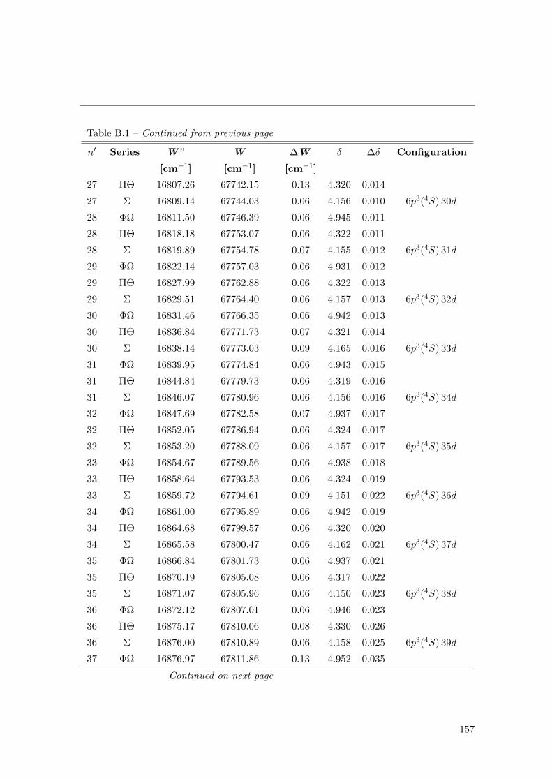
Table B.1 – Continued from previous page
n′ Series W” W ∆W δ ∆δ Configuration
[cm−1] [cm−1] [cm−1]
27 ΠΘ 16807.26 67742.15 0.13 4.320 0.014
27 Σ 16809.14 67744.03 0.06 4.156 0.010 6p3(4S) 30d
28 ΦΩ 16811.50 67746.39 0.06 4.945 0.011
28 ΠΘ 16818.18 67753.07 0.06 4.322 0.011
28 Σ 16819.89 67754.78 0.07 4.155 0.012 6p3(4S) 31d
29 ΦΩ 16822.14 67757.03 0.06 4.931 0.012
29 ΠΘ 16827.99 67762.88 0.06 4.322 0.013
29 Σ 16829.51 67764.40 0.06 4.157 0.013 6p3(4S) 32d
30 ΦΩ 16831.46 67766.35 0.06 4.942 0.013
30 ΠΘ 16836.84 67771.73 0.07 4.321 0.014
30 Σ 16838.14 67773.03 0.09 4.165 0.016 6p3(4S) 33d
31 ΦΩ 16839.95 67774.84 0.06 4.943 0.015
31 ΠΘ 16844.84 67779.73 0.06 4.319 0.016
31 Σ 16846.07 67780.96 0.06 4.156 0.016 6p3(4S) 34d
32 ΦΩ 16847.69 67782.58 0.07 4.937 0.017
32 ΠΘ 16852.05 67786.94 0.06 4.324 0.017
32 Σ 16853.20 67788.09 0.06 4.157 0.017 6p3(4S) 35d
33 ΦΩ 16854.67 67789.56 0.06 4.938 0.018
33 ΠΘ 16858.64 67793.53 0.06 4.324 0.019
33 Σ 16859.72 67794.61 0.09 4.151 0.022 6p3(4S) 36d
34 ΦΩ 16861.00 67795.89 0.06 4.942 0.019
34 ΠΘ 16864.68 67799.57 0.06 4.320 0.020
34 Σ 16865.58 67800.47 0.06 4.162 0.021 6p3(4S) 37d
35 ΦΩ 16866.84 67801.73 0.06 4.937 0.021
35 ΠΘ 16870.19 67805.08 0.06 4.317 0.022
35 Σ 16871.07 67805.96 0.06 4.150 0.023 6p3(4S) 38d
36 ΦΩ 16872.12 67807.01 0.06 4.946 0.023
36 ΠΘ 16875.17 67810.06 0.08 4.330 0.026
36 Σ 16876.00 67810.89 0.06 4.158 0.025 6p3(4S) 39d
37 ΦΩ 16876.97 67811.86 0.13 4.952 0.035
Continued on next page
157

B Table of observed Rydberg levels of polonium
Table B.1 – Continued from previous page
n′ Series W” W ∆W δ ∆δ Configuration
[cm−1] [cm−1] [cm−1]
37 ΠΘ 16879.87 67814.76 0.06 4.317 0.026
37 Σ 16880.60 67815.49 0.06 4.151 0.027 6p3(4S) 40d
37 ΦΩ 16881.11 67816.00 0.59 5.036 0.138
38 ΠΘΣ 16884.15 67819.04 0.06 4.314 0.029
39 ΦΩ 16885.43 67820.32 0.48 4.999 0.122
39 ΠΘ 16888.06 67822.95 0.10 4.324 0.037
39 Σ 16888.57 67823.46 0.40 4.188 0.109 6p3(4S) 42d
40 ΦΩ 16889.58 67824.47 0.48 4.917 0.133
40 ΠΘ 16891.64 67826.53 0.08 4.343 0.036
40 Σ 16892.15 67827.04 0.10 4.198 0.040 6p3(4S) 43d
40 ΦΩ 16892.77 67827.66 0.20 5.019 0.065
41 ΠΘΣΦΩ 16895.17 67830.06 0.06 4.302 0.036
42 ΠΘΣΦΩ 16898.40 67833.29 0.06 4.273 0.039
43 ΠΘΣΦΩ 16901.33 67836.22 0.06 4.264 0.042
44 ΠΘΣΦΩ 16904.02 67838.91 0.07 4.274 0.047
45 ΠΘΣΦΩ 16906.55 67841.44 0.06 4.280 0.048
46 ΠΘΣΦΩ 16908.86 67843.75 0.06 4.308 0.051
47 ΠΘΣΦΩ 16911.19 67846.08 0.09 4.261 0.063
48 ΠΘΣΦΩ 16913.25 67848.14 0.07 4.272 0.062
49 ΠΘΣΦΩ 16915.18 67850.07 0.09 4.285 0.070
50 ΠΘΣΦΩ 16917.05 67851.94 0.06 4.266 0.066
51 ΠΘΣΦΩ 16918.77 67853.66 0.06 4.275 0.070
52 ΠΘΣΦΩ 16920.39 67855.28 0.06 4.282 0.074
53 ΠΘΣΦΩ 16921.91 67856.80 0.06 4.297 0.078
54 ΠΘΣΦΩ 16923.38 67858.27 0.06 4.286 0.083
55 ΠΘΣΦΩ 16924.80 67859.69 0.06 4.260 0.088
56 ΠΘΣΦΩ 16926.15 67861.04 0.07 4.224 0.097
57 ΠΘΣΦΩ 16927.39 67862.28 0.07 4.217 0.103
58 ΠΘΣΦΩ 16928.49 67863.38 0.07 4.270 0.108
59 ΠΘΣΦΩ 16929.61 67864.50 0.07 4.269 0.113
Continued on next page
158

Table B.1 – Continued from previous page
n′ Series W” W ∆W δ ∆δ Configuration
[cm−1] [cm−1] [cm−1]
60 ΠΘΣΦΩ 16930.70 67865.59 0.07 4.228 0.120
61 ΠΘΣΦΩ 16931.71 67866.60 0.07 4.223 0.127
62 ΠΘΣΦΩ 16932.61 67867.50 0.07 4.283 0.133
63 ΠΘΣΦΩ 16933.59 67868.48 0.13 4.205 0.181
159

B Table of observed Rydberg levels of polonium
160

Bibliography
[1] G. Alkhazov, L. Batist, A. Bykov, V. Vitman, V. Letokhov, V. Mishin, V. Pan-teleyev, S. Sekatsky, and V. Fedoseyev. Application of a high efficiency selectivelaser ion source at the IRIS facility. Nucl. Instrum. Meth. A, 306:400 – 402, 1991.
[2] G. D. Alkhazov, V. S. Letokhov, V. I. Mishin, V. N. Panteleyev, V. I. Romanov,S. K. Sekatskii, and V. Fedoseyev. High-performance z-selective photoionization ofatoms in hot metal cavity with following electrostatic ion retention. Pis’ma Zh.Tekhn. Fiz., 15:63–67 (in Russian), 1989.
[3] G. Alton. Semi-empirical mathematical relationships for electropositive adsorbateinduced work function changes. Surf. Sci., 175:226 – 240, 1986.
[4] G. Alton. Ion sources for accelerators in materials research. Nucl. Instrum. Meth.B, 73:221 – 288, 1993.
[5] A. N. Andreyev, M. Huyse, P. Van Duppen, L. Weissman, D. Ackermann, J. Gerl,F. Hessberger, S. Hofmann, A. Kleinbohl, G. Munzenberg, S. Reshitko, H. Schlegel,C. Schaffner, P. Cagarda, M. Matos, S. Saro, A. Keenan, C. Moore, C. D. O’Leary,R. D. Page, M. Taylor, H. Kettunen, M. Leino, A. AU Lavrentiev, and K. Wyss,R. Heyde. A triplet of differently shaped spin-zero states in the atomic nucleus186Pb. Nature, 405:430, 2000.
[6] M. Anselment, W. Faubel, S. Goring, A. Hanser, G. Meisel, H. Rebel, and G. Schatz.The odd-even staggering of the nuclear charge radii of Pb isotopes. Nucl. Phys. A,451:471 – 480, 1986.
[7] H. Backe, A. Dretzke, S. Fritzsche, R. Haire, P. Kunz, W. Lauth, M. Sewtz, andN. Trautmann. Laser spectroscopic investigation of the element fermium (Z = 100).Hyperfine Interact., 162:3–14, 2005.
[8] D. Berdichevsky and F. Tondeur. Nuclear core densities, isotope shifts, and theparametrization of the droplet model. Z. f. Phys. A, 322:141–147, 1985.
[9] I. Beterov, D. Tretyakov, I. Ryabtsev, V. Entin, A. Ekers, and N. Bezuglov. Ioniza-tion of Rydberg atoms by blackbody radiation. New J. Phys., 11:013052, 2009.
[10] N. Bijnens, P. Decrock, S. Franchoo, M. Gaelens, M. Huyse, H. Y. Hwang, I. Reusen,J. Szerypo, J. von Schwarzenberg, J. Wauters, J. G. Correia, A. Jokinen, andP. Van Duppen. Intruder states and the onset of deformation in the neutron-deficienteven-even polonium isotopes. Phys. Rev. Lett., 75:4571, 1995.
161

Bibliography
[11] M. Bissell, K. Blaum, I. Budincevic, N. Frommgen, R. Garcia Ruiz, C. Gep-pert, M. Hammen, M. Kowalska, K. Kreim, P. Lievens, R. Neugart, G. Neyens,W. Nortershauser, J. Papuga, M. Rajabali, and D. Yordanov. Spins, moments andcharge radii beyond 48Ca. Technical Report CERN-INTC-2011-049. INTC-P-313,CERN, 2011.
[12] K. Blaum, B. A. Bushaw, W. Nortershauser, and K. Wendt. High-resolution,three-step resonance ionization mass spectrometry of gadolinium. AIP Conf. Proc.,584:141–144, 2001.
[13] K. Blaum, J. Dilling, and W. Nortershauser. Precision atomic physics techniquesfor nuclear physics. Phys. Scrip., T152:014017, 2013.
[14] K. Blaum, C. Geppert, H.-J. Kluge, M. Mukherjee, S. Schwarz, and K. Wendt. Anovel scheme for a highly selective laser ion source. Nucl. Instrum. Meth. B, 204:331– 335, 2003.
[15] K. Blaum, C. Geppert, P. Muller, W. Nortershauser, E. Otten, A. Schmitt, N. Traut-mann, K. Wendt, and B. Bushaw. Properties and performance of a quadrupole massfilter used for resonance ionization mass spectrometry. Int. J. Mass Spectrom., 181:67– 87, 1998.
[16] K. Blum. Density Matrix Theory and Applications, volume 64 of Springer Series onAtomic, Optical and Plasma Physics. Springer-Verlagand Berlin Heidelberg, 2012.
[17] Y. Blumenfeld. Radioactive ion beam facilities in Europe. Nucl. Instrum. Meth. B,266:4074 – 4079, 2008.
[18] Y. Blumenfeld, T. Nilsson, and P. V. Duppen. Facilities and methods for radioactiveion beam production. Physi. Scrip., 2013:014023, 2013.
[19] N. Bohr and V. Weisskopf. The influence of nuclear structure on the hyperfinestructure of heavy elements. Phys. Rev., 77:94–98, Jan 1950.
[20] W. Borchers, R. Neugart, E. Otten, H. Duong, G. Ulm, and K. Wendt. Hyper-fine structure and isotope shift investigations in 202−222Rn for the study of nuclearstructure beyond z = 82. Hyperf. Interact., 34:25, 1987.
[21] C. Borgmann. Private communication, 2013.
[22] A. Borschevsky. Private communication, 2013.
[23] E. Bouquerel, R. Catherall, M. Eller, J. Lettry, S. Marzari, T. Stora, and I. thecollaboration. Purification of a Zn radioactive ion beam by alkali suppression in aquartz line target prototype. Eur. J. Phys. Spec. Top., 150:277–280, 2007.
[24] B. Bushaw, W. Nortershauser, K. Blaum, and K. Wendt. Studies of narrow autoion-izing resonances in gadolinium. Spectrochim. Act. B, 58:1083, 2003.
162

Bibliography
[25] B. Bushaw, W. Nortershauser, and K. Wendt. Lineshapes and optical selectivity inhigh-resolution double-resonance ionization mass spectrometry. Spectrochim. ActaB, 54:321 – 332, 1999.
[26] P. Campbell, J. Billowes, J. Behr, G. Gwinner, G. Sprouse, and F. Xu. Isotopeshifts of the neutron-deficient bismuth isotopes: charge radii systematics across thez = 82 shell closure. Phys. Lett. B, 346:21, 1995.
[27] A. Cantu, M. Mazzoni, and Y. Joshi. Rydberg series in the absorption spectrum ofTe I limiting on 5s2 5p3 4S o3/2 ionization limit. Phys. Scr., 27:261, 1983.
[28] H. Casimir. On the interaction between atomic nuclei and electrons. Archives dumusee Teyler. F. Bohn, 1936.
[29] R. F. Casten. Nuclear Structure from a Simple Perspective. Oxford University Press,USA, 1990.
[30] CERN, 2013.
[31] G. Charles. Spectra of 208Po and the hyperfine structure of 209Po. J. Opt. Soc. Am.,56:1292–1297, 1966.
[32] G. W. Charles, D. Hunt, G. Pish, and D. Timma. Preliminary description andanalysis of the spectrum of polonium. J. Opt. Soc. Am., 45:869–872, 1955.
[33] B. Cheal, T. E. Cocolios, and S. Fritzsche. Laser spectroscopy of radioactive isotopes:Role and limitations of accurate isotope-shift calculations. Phys. Rev. A, 86:042501,2012.
[34] S. Chu, L. Ekstrom, and R. Firestone. WWW table of radioactive isotopes, 2013.
[35] A. Coc, C. Thibault, F. Touchard, H. Duong, P. Juncar, S. Liberman, J. Pinard,J. Lerme, J. Vialle, S. Buttgenbach, A. Mueller, and A. Pesnelle. Hyperfine struc-tures and isotope shifts of 207−213,220−228Fr; possible evidence of octupolar deforma-tion. Phys. Lett. B, 163:66 – 70, 1985.
[36] T. Cocolios. Single-particle and collective properties around closed shells probed byin-source laser spectroscopy. PhD thesis, Katholieke Universiteit Leuven and GroepWetenschap & Technologie and Arenberg Doctoraatsschool, 2010.
[37] T. Cocolios. Private communication, 2013.
[38] T. Cocolios, A. Andreyev, A. Barzakh, J. Billowes, D. Fedorov, V. Fedosseev,S. Franchoo, G. Huber, M. Huyse, A. Ionan, U. Koster, Y. Kudryavtsev, F. L.Blanc, S. Lesher, B. Marsh, I. Mukha, M. Seliverstov, J. V. de Walle, P. V. Duppen,and Y. Volkov. Study of polonium isotopes ground state properties by simulta-neous atomic- and nuclear-spectroscopy. Technical Report CERN-INTC-2007-003.INTC-P-222, CERN, 2007.
163

Bibliography
[39] T. Cocolios, W. Dexters, M. Seliverstov, A. Andreyev, S. Antalic, A. Barzakh,B. Bastin, J. Buscher, I. Darby, D. Fedorov., V. Fedosseyev, K. Flanagan, S. Fran-choo, S. Fritzsche, G. Huber, M. Huyse, M. Keupers, U. Koster, Y. Kudryavtsev,E. Mane, B. Marsh, P. Molkanov, R. Page, A. Sjoedin, I. Stefan., J. V. de Walle,P. V. Duppen, M. Venhartv, S. Zemlyanoy, M. Bender, and P.-H. Heenen. Earlyonset of ground state deformation in neutron deficient polonium isotopes. Phys.Rev. Lett., 106:052503, Feb 2011.
[40] T. Cocolios, D. Fink, A. Andreyev, S. Antalic, A. Barzakh, B. Bastin, K. Blaum,D. Fedorov, V. Fedosseev, K. Flanagan, L. Ghys, A. Gottberg, M. Huyse, N. Lecesne,K. Lynch, B. Marsh, D. Pauwels, E. Rapisarda, S. Richter, S. Rothe, M. Seliverstov,A. Sjodin, C. V. Beveren, P. V. Duppen, and K. Wendt. First decay spectroscopyof 219Po with the LIST. In preparation, 2014.
[41] T. Cocolios, B. Marsh, V. Fedosseev, S. Franchoo, G. Huber, M. Huyse, A. Ionan,K. Johnston, U. Koster, Y. Kudryavtsev, M. Seliverstov, E. Noah, T. Stora, andP. V. Duppen. Resonant laser ionization of polonium at RILIS-ISOLDE for thestudy of ground- and isomer-state properties. Nucl. Instrum. Meth. B, 266:4403 –4406, 2008.
[42] R. Cowan. The theory of atomic structure and spectra. University of California Pressand Ltd. and Berkeley and Los Angeles, 1919.
[43] P. Dawson. Performance characteristics of an r.f.-only quadrupole. Int. J. MassSpectrom. and I. Proc., 67(3):267 – 276, 1985.
[44] P. Dawson. Quadrupole Mass Spectrometry and Its Applications. American VacuumSociety Classics. American Inst. of Physics, 1997.
[45] P. Dawson and N. Whetten. Non-linear resonances in quadrupole mass spectrom-eters due to imperfect felds. ii. the quadrupole mass filter and the monopole massspectrometer. Int. J. Mass Spectrom. Ion. Phys., 3:1, 1969.
[46] P. de Marcillac, N. Coron, G. Dambier, J. Leblanc, and J.-P. Moalic. Experimentaldetection of α-particles from the radioactive decay of natural bismuth. Nature,422:876, 2003.
[47] H. De Witte, A. N. Andreyev, N. Barre, M. Bender, T. E. Cocolios, S. Dean, D. Fe-dorov, V. N. Fedoseyev, L. M. Fraile, S. Franchoo, V. Hellemans, P. H. Heenen,K. Heyde, G. Huber, M. Huyse, H. Jeppessen, U. Koster, P. Kunz, S. R. Lesher,B. A. Marsh, I. Mukha, B. Roussiere, J. Sauvage, M. Seliverstov, I. Stefanescu,E. Tengborn, K. Van de Vel, J. Van de Walle, P. Van Duppen, and Y. Volkov.Nuclear charge radii of neutron-deficient lead isotopes beyond N = 104 midshellinvestigated by in-source laser spectroscopy. Phys. Rev. Lett., 98:112502, 2007.
[48] W. Demtroder. Atoms, Molecules and Photons: an Introduction ao Atomic-andMolecular- and Quantum-Physics. Springer Verlagand Berlin, 2006.
164

Bibliography
[49] W. Dexters. Neutron-rich polonium isotopes studied with in-source laser spec-troscopy. Master’s thesis, Katholieke Universiteit Leuven, 2010.
[50] U. Dinger, J. Eberz, G. Huber, R. Menges, S. Schroder, R. Kirchner, O. Klepper,T. Kuhl, D. Marx, and G. Sprouse. Nuclear moments and change in the charge-radiiof neutron deficient lead isotopes. Z. Phys. A, 328:253, 1987.
[51] P. V. Duppen. Laser ion sources for on-line isotope separators. Nucl. Instrum. Meth.B, 126:66, 1997.
[52] P. V. Duppen. Isotope separation on line and post acceleration. Lect. Notes Phys,700:37–77, 2006.
[53] S. Dutta, R. Kirchner, O. Klepper, T. Kuhl, D. Marx, G. Sprouse, R. Menges,U. Dinger, G. Huber, and S. Schroder. Measurement of isotope shift and hyperfinesplitting of 190,191,193,197Pb isotopes by collinear laser spectroscopy. Z. Phys. A,341:39–45, 1991.
[54] A. Einstein. Zur Quantentheorie der Strahlung. Physikalische Z., 18:121 – 128, 1917.
[55] J. Elseviers, A. N. Andreyev, M. Huyse, P. Van Duppen, S. Antalic, A. Barzakh,N. Bree, T. E. Cocolios, V. F. Comas, J. Diriken, D. Fedorov, V. N. Fedosseev,S. Franchoo, L. Ghys, J. A. Heredia, O. Ivanov, U. Koster, B. A. Marsh, K. Nishio,R. D. Page, N. Patronis, M. D. Seliverstov, I. Tsekhanovich, P. Van den Bergh,J. Van De Walle, M. Venhart, S. Vermote, M. Veselsky, and C. Wagemans. β-delayed fission of 180tl. Phys. Rev. C, 88:044321, 2013.
[56] U. Fano. Effects of configuration interaction on intensities and phase shifts. Phys.Rev., 124:1866–1878, 1961.
[57] V. Fedoseev, Y. Kudryavtsev, V. Letokhov, V. Mishin, H. Ravn, S. Sundell,H. Kluge, and F. Scheerer. A laser ion-source for on-line isotope separation. InProceedings of the Fifth International Symposium on Resonance Ionization Spec-troscopy and its Applications, RIS -90, Varese, Italy, 1990.
[58] V. Fedosseev, Y. Kudryavtsev, and V. Mishin. Resonance laser ionization of atomsfor nuclear physics. Phys. Scripta, 85:058104, 2012.
[59] V. N. Fedosseev, L.-E. Berg, D. V. Fedorov, D. Fink, O. J. Launila, R. Losito,B. Marsh, R. E. Rossel, S. Rothe, M. D. Seliverstov, A. M. Sjodin, and K. D. A.Wendt. Upgrade of the resonance ionization laser ion source at ISOLDE on-lineisotope separation facility: New lasers and new ion beams. Rev. Sci.. Instrum.,83:02A903, 2012.
[60] D. Fink, S. Richter, B. Bastin, K. Blaum, R. Catherall, T. Cocolios, D. Fedorov,V. Fedosseev, K. Flanagan, L. Ghys, A. Gottberg, N. Imai, T. Kron, N. Lecesne,K. Lynch, B. Marsh, T. Mendonca, D. Pauwels, E. Rapisarda, J. Ramos, R. Rossel,S. Rothe, M. Seliverstov, M. Sjodin, T. Stora, C. V. Beveren, and K. Wendt. First ap-plication of the laser ion source and trap (LIST) for on-line experiments at ISOLDE.Nucl. Instrum. Meth. B, 317, Part B:417 – 421, 2013.
165

Bibliography
[61] W. Finkelnburg and F. Stern. Electron screening and ionization potentials of neutraland singly ionized atoms. Phys. Rev., 77:303–303, 1950.
[62] E. Fischer. Die dreidimensionale Stabilisierung von Ladungstragern in einem Vier-polfeld. Z. Phys., 156:1, 1959.
[63] G. Focker, F. Hoekemeijer, O. Jonsson, E. Kugler, and H. Ravn. The beam obser-vation system of the ISOLDE facility. AIP Conf. Proc., 333:196, 1995.
[64] G. Fricke and K. Heilig. Nuclear Charge Radii. Springer Berlin-Heidelberg, 2005.
[65] S. Fritzsche. Large-scale accurate structure calculations for open-shell atoms andions. Physica Scripta, T100:37, 2002.
[66] J. Gaardsted, T. Andersen, H. Haugen, J. Hansen, and N. Vaeck. Multiphotonspectroscopy of doubly excited autoionizing states of Ca. J. Phys. B, 24:4363, 1991.
[67] L. P. Gaffney, P. A. Butler, M. Scheck, A. B. Hayes, F. Wenander, M. Albers,B. Bastin, C. Bauer, A. Blazhev, S. Bonig, N. Bree, J. Cederkall, T. Chupp,D. Cline, T. E. Cocolios, T. Davinson, H. De Witte, J. Diriken, T. Grahn, A. Herzan,M. Huyse, D. G. Jenkins, D. T. Joss, N. Kesteloot, J. Konki, M. Kowalczyk,T. Kroll, E. Kwan, R. Lutter, K. Moschner, P. Napiorkowski, J. Pakarinen, M. Pfeif-fer, D. Radeck, P. Reiter, K. Reynders, S. V. Rigby, L. M. Robledo, M. Rudigier,S. Sambi, M. Seidlitz, B. Siebeck, T. Stora, P. Thoele, P. Van Duppen, M. J. Ver-meulen, M. von Schmid, D. Voulot, N. Warr, K. Wimmer, K. Wrzosek-Lipska, C. Y.Wu, and M. Zielinska. Studies of pear-shaped nuclei using accelerated radioactivebeams. Nature, 497:199, 2013.
[68] T. F. Gallagher, S. A. Edelstein, and R. M. Hill. Radiative lifetimes of the s and dRydberg levels of Na. Phys. Rev. A, 11:1504, 1975.
[69] P. Ghosh. Ion Traps. Oxford science publications. Oxford University Press, Incor-porated, 1995.
[70] T. Giles. Private communication, 2013.
[71] P. M. Goddard. Private communication, 2013.
[72] P. M. Goddard, P. D. Stevenson, and A. Rios. Charge radius isotope shift acrossthe n=126 shell gap. Phys. Rev. Lett., 110:032503, 2013.
[73] M. Goeppert-Mayer. Nuclear configurations in the Spin-Orbit Coupling Model. I.empirical evidence. Phys. Rev., 78:16, 1950.
[74] T. Gottwald. Messung der Emittanz der Laserionenquellenfalle LIST am RISIKOMassenseparator. Master’s thesis, Johannes Gutenberg-Universitat Mainz, 2007.
[75] P. G. Hansen. Experiments with beams of rare isotopes: A fifty-year perspective1951-2001. Nucl Phys. News, 11:31, 2001.
166

Bibliography
[76] K. Heilig and A. Steudel. Changes in mean-square nuclear charge radii from opticalisotope shifts. Atomic Data and Nuclear Data Tables, 14:613 – 638, 1974.
[77] F. Herfurth, J. Dilling, A. Kellerbauer, G. Bollen, S. Henry, H.-J. Kluge, E. Lamour,D. Lunney, R. Moore, C. Scheidenberger, S. Schwarz, G. Sikler, and J. Szerypo. Alinear radiofrequency ion trap for accumulation, bunching, and emittance improve-ment of radioactive ion beams. Nucl. Instrum. Meth. A, 469:254, 2001.
[78] HighFinesse GmbH. WS6 product sheet, 2013.
[79] HighFinesse GmbH. WS7 product sheet, 2013.
[80] R. J. Hull and H. H. Stroke. Nuclear moments and isotope shifts of Tl199, Tl200,Tl201, Tl202, and Tl204 - isotope shifts in odd-odd nuclei. Phys. Rev., 122:1574, 1961.
[81] G. S. Hurst, M. G. Payne, S. D. Kramer, and J. P. Young. Resonance ionizationspectroscopy and one-atom detection. Rev. Mod. Phys., 51:767, 1979.
[82] R. Janssens. Unexpected doubly magic nucleus. Nature, 459:1069, 2009.
[83] R. Jastrow. On the Rydberg-Ritz formula in quantum mechanics. Phys. Rev.,73:60–67, 1948.
[84] H. Jeppesen, U. Bergmann, M. Borge, J. Cederkall, V. Fedoseyev, H. Fynbo,V. Hansper, B. Jonson, K. Markenroth, V. Mishin, T. Nilsson, G. Nyman, K. Riis-ager, O. Tengblad, and K. Rolander. Search for beta-delayed charged particles fromthe halo nucleus 14Be. Nucl. Phys. A, 709:119, 2002.
[85] B. Jonson and A. Richter. More than three decades of ISOLDE physics. Hyperf.Interact., 129:1, 2000.
[86] R. Julin, K. Helariutta, and M. Muikku. Intruder states in very neutron-deficientHg, Pb and Po nuclei. J. Phys. G, 27:R109, 2001.
[87] S. Kaufman. High-resolution laser spectroscopy in fast beams. Optics Commun.,17:309 – 312, 1976.
[88] W. King. Isotope shifts in atomic spectra. Plenum Press and New York and London,1984.
[89] R. Kirchner. On the thermoionization in hot cavities. Nucl. Instrum. Meth. A,292:203, 1990.
[90] H.-J. Kluge, F. Ames, W. Ruster, and K. Wallmeroth. Laser ion sources. In L. Buch-mann and J. D’Auria, editors, Proceedings of the Accelerated Radioactive BeamsWorkshop, page 119. TRIUMF Proceedings TRI-85-1, Canada, 1985.
[91] O. Kofeod-Hansen and K. O. . Nielsen. Measurements on short-lived radioactivekrypton isotopes from fission after isotopic separation. Dan. Mat. Fys. Medd., 56-7:1, 1951.
167
Bibliography
[92] U. Koster. Resonance ionization laser ion sources. Nucl. Phys. A, 701:441, 2002.
[93] D. Kowalewska, K. Bekk, S. Goring, A. Hanser, W. Kalber, G. Meisel, and H. Rebel.Isotope shifts and hyperfine structure in polonium isotopes by atomic beam laserspectroscopy. Phys. Rev. A, 44:R1442, 1991.
[94] A. Kramida, Y. Ralchenko, J. Raeder, and N. A. TEAM. NIST Atomic SpectraDatabase (version 5.1), Thursday, 26 September 2013.
[95] K. Krane. Introductory Nuclear Physics. Wiley, 1987.
[96] S. Kreim. Seeking the purported magic number N = 32 with high-precision massspectrometry. Technical Report CERN-INTC-2011-053. INTC-P-317, CERN, 2011.
[97] M. Kronberger, A. Gottberg, T. Mendonca, J. Ramos, C. Seiffert, P. Suominen, andT. Stora. Production of molecular sideband radioisotope beams at CERN-ISOLDEusing a Helicon-type plasma ion source. Nucl. Instrum. Meth. B, 317, Part B:438 –441, 2013.
[98] I. Langmuir and K. Kingdon. Thermionic effects caused by vapours of alkali metals.Proc. R. Soc. Lond. A, 107:61, 1925.
[99] M. Laury and A. Wilson. Examining the heavy p-block with a pseudopotential-basedcomposite method: Atomic and molecular applications of rp-ccCA. J. Chem. Phys.,137:214111, 2012.
[100] J. Lawson. Particle beams and plasmas. CERN Report, 76-09:1–93, 1976.
[101] F. Le Blanc, D. Lunney, J. Obert, J. Oms, J. Putaux, B. Roussiere, J. Sauvage,S. Zemlyanoi, J. Pinard, L. Cabaret, H. T. Duong, G. Huber, M. Krieg, V. Sebastian,J. E. Crawford, J. K. P. Lee, M. Girod, S. Peru, J. Genevey, and J. Lettry. Large odd-even radius staggering in the very light platinum isotopes from laser spectroscopy.Phys. Rev. C, 60:054310, 1999.
[102] V. Letokhov. Laser photoionization spectroscopy. Academic Press, Orlando, 1987.
[103] V. Letokhov and V. Mishin. Laser photoionization pulsed source of radioactiveatoms. In Abstracts from the Workshop on the ISOLDE programme: on-line in1985 and Beyond, Zinal, Switzerland, 1984.
[104] C. Liang, P. Paris, R. Sheline, and P. Alexa. Alpha decay of 221Rn and 217Po; levelstructure of 217Po and the 213Pb ground state. Czech. J. Phys, 54:189–198, 2004.
[105] C. F. Liang, P. Paris, and R. K. Sheline. Level structure of 217Po and the spin ofthe previously proposed 213Pb ground state. Phys. Rev. C, 56:2324, 1997.
[106] B. Lommel, W. Hartmann, B. Kindler, J. Klemm, and J. Steiner. Preparation ofself-supporting carbon thin films. Nucl. Instrum. Meth. A, 480:199 – 203, 2002.
[107] W. Lotz. An empirical formula for the electron-impact ionization cross-section. Z.Phys., 206:205–211, 1967.
168

Bibliography
[108] R. Luis, J. Marques, T. Stora, P. Vaz, and L. Zanini. Optimization studies of theCERN-ISOLDE neutron converter and fission target system. Eur. J. Phys. A, 48:90,2012.
[109] S. Lukic, F. Gevaert, A. Kelic, M. Ricciardi, K.-H. Schmidt, and O. Yordanov.Systematic comparison of ISOLDE-SC yields with calculated in-target productionrates. Nucl. Instrum. Meth. A, 565:784 – 800, 2006.
[110] F. Major, V. Gheorghe, and G. Werth. Charged Particle Traps: Physics and Tech-niques of Charged Particle Field Confinement. Charged Particle Traps. Springer,2005.
[111] E. Mane, J. Billowes, K. Blaum, P. Campbell, B. Cheal, P. Delahaye, K. Flanagan,D. Forest, H. Franberg, C. Geppert, T. Giles, A. Jokinen, M. Kowalska, R. Neu-gart, G. Neyens, W. Nortershauser, I. Podadera, G. Tungate, P. Vingerhoets, andD. Yordanov. An ion cooler-buncher for high-sensitivity collinear laser spectroscopyat ISOLDE. Nucl. Instrum. Meth. A, 42:503–507, 2009.
[112] B. Marsh. In-Source Laser Resonance Ionization at ISOL Facilities. PhD thesis,The University of Manchester, 2007.
[113] B. Marsh. Resonance ionization laser ion sources. In CERN accelerator school, 2013.
[114] B. Marsh, B. Andel, A. Andreyev, S. Antalic, D. Atanasov, A. Barzakh, B. Bastin,C. Borgmann, L. Capponi, T. Cocolios, T. D. Goodacre, M. Dehairs, X. Derkx,H. D. Witte, D. Fedorov, V. Fedosseev, G. Focker, D. Fink, K. Flanagan, S. Fran-choo, L. Ghys, M. Huyse, N. Imai, Z. Kalaninova, U. Koster, S. Kreim, N. Kesteloot,Y. Kudryavtsev, J. Lane, N. Lecesne, V. Liberati, D. Lunney, K. Lynch, V. Manea,P. Molkanov, T. Nicol, D. Pauwels, L. Popescu, D. Radulov, E. Rapisarda, M. Rosen-busch, R. Rossel, S. Rothe, L. Schweikhard, M. Seliverstov, S. Sels, A. Sjodin,V. Truesdale, C. V. Beveren, P. V. Duppen, K. Wendt, F. Wienholtz, R. Wolf,and S. Zemlyanoy. New developments of the in-source spectroscopy method atRILIS/ISOLDE. Nucl. Instrum. Meth. B, 317, Part B:550 – 556, 2013.
[115] B. Marsh, L.-E. Berg, D. Fedorov, V. Fedosseev, O. Launila, M. Lindroos, R. Losito,F. Osterdahl, T. Pauchard, I. Pohjalainen, U. Sassenberg, M. Seliverstov, A. Sjodin,and G. Transtromer. The ISOLDE RILIS pump laser upgrade and the LARISLaboratory. Hyperf. Interact., 196:129–141, 2010.
[116] W. Martin, R. Zalubas, and A. Musgrove. Energy levels of sulfur, S i through SXVI. J. Phys. Chem. Ref. Data, 19:821, 1990.
[117] S. Marzari. Private communication, 2013.
[118] N. McLachlan. Theory and application of Mathieu functions. Clarendon Press,Oxford, 1947.
[119] V. Mishin, V. Fedoseyev, H.-J. Kluge, V. Letokhov, H. Ravn, F. Scheerer, Y. Shi-rakabe, S. Sundell, and O. Tengblad. Chemically selective laser ion-source for the
169

Bibliography
CERN-ISOLDE on-line mass separator facility. Nucl. Instrum. Meth. B, 73:550 –560, 1993.
[120] M. Miyabe, C. Geppert, M. Kato, M. Oba, I. Wakaida, K. Watanabe, and K. Wendt.Determination of ionization potential of calcium by high-resolution resonance ion-ization spectroscopy. J. Phys. Soc. Jpn., 75:034302, 2006.
[121] P. Mohr, B. Taylor, and D. Newell. The 2010 CODATA recommended values of thefundamental physical constants, 2011.
[122] L. Monz, R. Hohmann, H.-J. Kluge, S. Kunze, J. Lantzsch, E. Otten, G. Passler,P. Senne, J. Stenner, K. Stratmann, K. Wendt, K. Zimmer, G. Herrmann, N. Traut-mann, and K. Walter. Fast, low-level detection of strontium-90 and strontium-89 inenvironmental samples by collinear resonance ionization spectroscopy. Spectrochim.Act. B, 48:1655 – 1671, 1993.
[123] C. Moore. Atomic energy levels as derived from the analysis of optical spectra -chromium through niobium. Nat. Stand. Ref. Data Ser., 11:230, 1971.
[124] C. Morillon and J. Verges. Observation et classification du spectre d’arc du tellure(Te) entre 3678 et 11761 cm−1. Phys. Scr., 12:129, 1975.
[125] M. Mukherjee. The mass of 22Mg and a concept for a novel laser ion source trap.PhD thesis, Karl Ruprecht-Universitat Heidelberg, 2004.
[126] A. Muller, E. Salzborn, R. Frodl, R. Becker, H. Klein, and H. Winter. Absoluteionisation cross sections for electrons incident on O+, Ne+, Xe+ and Ar+ (i=1,...,5)ions. J. Phys. B, 13:1877, 1980.
[127] W. Nortershauser, N. Trautmann, K. Wendt, and B. Bushaw. Isotope shifts andhyperfine structure in the 4s2 1S0 → 4s4p 1P1 → 4s4d 1D2 transitions of stablecalcium isotopes and calcium-41. Spectrochim. Acta B, 53:709 – 721, 1998.
[128] E. Otten. Spectra, radii and moments of unstable isotopes. Springer Verlag andBerlin, 1989.
[129] W. Paul. Electromagnetic traps for charged and neutral particles. Rev. Mod. Phys.,62:531–540, 1990.
[130] W. Paul and M. Raether. Das elektrische Massenfilter. Z. Phys., 140(3):262–273,1955.
[131] W. Paul, H. Reinhard, and U. Zahn. Das elektrische Massenfilter als Massenspek-trometer und Isotopentrenner. Z. Phys., 152:143–182, 1958.
[132] W. Paul and H. Steinwedel. Ein neues Massenspektrometer ohne Magnetfeld. Z.Naturforschung A, 8:448, 1953.
[133] K. A. Peterson. Systematically convergent basis sets with relativistic pseudopoten-tials. I. correlation consistent basis sets for the post-d group 13–15 elements. J.Chem. Phys., 119:11099–11112, 2003.
170

Bibliography
[134] E. Prime, J. Lassen, T. Achtzehn, D. Albers, P. Bricault, T. Cocolios, M. Domb-sky, F. Labrecque, J. Lavoie, M. Pearson, T. Stubbe, N. Lecesne, C. Geppert, andK. Wendt. TRIUMF resonant ionization laser ion source. Hyperf, Interact., 171:127–134, 2006.
[135] T. Procter and K. Flanagan. First on-line results from the CRIS (Collinear ResonantIonisation Spectroscopy) beam line at ISOLDE. Hyperfine Interactions, 216:89–93,2013.
[136] S. Raeder. Private Communication, 2013.
[137] S. Raeder, D. Fink, A. Borschevsky, et al. Preliminary title: The first ionizationenergy of polonium. In preparation, 2014.
[138] F. Read, A. Adams, and J. Soto-Montiel. Electrostatic cylinder lenses i: Two elementlenses. J. Phys. E., 4:625, 1971.
[139] S. Richter. The setup of the laser ion source and trap. to be published as a technicalnote, 2013.
[140] S. Richter. PhD thesis, University of Mainz, to be submitted, 2014.
[141] B. Roos, R. Lindh, P. Malmqvist, V. Veryazov, and P. Widmark. Main groupatoms and dimers studied with a new relativistic ANO basis set. J. Phys. Chem.,108:2851–2858, 2004.
[142] R. Rossel, V. Fedosseev, B. Marsh, D. Richter, S. Rothe, and K. Wendt. Dataacquisition, remote control and equipment monitoring for ISOLDE RILIS. Nucl.Instrum. Meth. B, 317, Part B:557 – 560, 2013.
[143] S. Rothe. An all-solid state laser system for the laser ion source RILIS and in-sourcelaser spectroscopy of astatine at ISOLDE, CERN. PhD thesis, Johannes Gutenberg-Universitat Mainz, 2012.
[144] S. Rothe, A. Andreyev, S. Antalic, A. Borschevsky, L. Capponi, T. Cocolios, H. D.Witte, E. Eliav, V. F. D.V. Fedorov and, D. Fink, S. Fritzsche, L. Ghys, M. Huyse,N. Imai, U. Kaldor, Y. Kudryavtsev, U. Koster, J. Lane, J. Lassen, V. Liberati,K. Lynch, B. Marsh, K. Nishio, D. Pauwels, V. Pershina, L. Popescu, T. Procter,D. Radulov, S. Raeder, M. Rajabali, E. Rapisarda, R. Rossel, K. Sandhu, M. Se-liverstov, A. Sjodin, P. V. den Bergh, P. V. Duppen, M. Venhart, Y. Wakabayashi,and K. Wendt. Measurement of the first ionization potential of astatine by laserionization spectroscopy. Nat. Commun., 4:1835, 2013.
[145] S. Rothe, B. Marsh, C. Mattolat, V. Fedosseev, and K. Wendt. A complementarylaser system for ISOLDE RILIS. J. Phys. Conf. Ser., 312:052020, 2010.
[146] J. E. Ruedy. Series and term values in the arc spectrum of tellurium. Phys. Rev.,41:588–594, 1932.
171

Bibliography
[147] H. Russel. The arc and spark spectra of gadolinium. J. Opt. Soc. Am., 40:550–554,1950.
[148] M. Saha. Ionization in the solar chromosphere. Pli. Mag. Ser. 6, 40:472, 1920.
[149] J. Sansonetti and W. Martin. Handbook of basic atomic spectroscopic data. J.Phys. Chem. Ref. Data, 34:1559, 2005.
[150] F. Schwellnus. Entwicklung von Ionenquellen zur Optimierung von Selektivitat undEffizienz bei der resonanten Laserionisation. PhD thesis, Johannes Gutenberg-Universitat Mainz, 2010.
[151] F. Schwellnus, K. Blaum, R. Catherall, B. Crepieux, V. Fedosseev, T. Gottwald,H.-J. Kluge, B. Marsh, C. Mattolat, S. Rothe, T. Stora, and K. Wendt. The laserion source trap for highest isobaric selectivity in online exotic isotope production.Rev. Sci. Instrum., 81:02A515, 2010.
[152] F. Schwellnus, K. Blaum, C. Geppert, T. Gottwald, H.-J. Kluge, C. Mattolat,W. Nortershaeuser, K. Wies, and K. Wendt. The laser ion source and trap (LIST):A highly selective ion source. Nucl. Instrum. Meth. B, 266:4383 – 4836, 2008.
[153] F. Schwellnus, R. Catherall, B. Crepieux, V. Fedosseev, B. Marsh, C. Mattolat,M. Menna, F. Osterdahl, S. Raeder, T. Stora, and K. Wendt. Study of low workfunction materials for hot cavity resonance ionization laser ion sources. Nucl. In-strum. Meth. B, 267:1856 – 1861, 2009.
[154] J. Sedlet. Actinium, Astatine, Francium, Polonium, and Protactinium, volume 6of Treatise on analytical chemistry. Part II: Analytical chemistry of the elements.Wiley & Sons, USA, 1964.
[155] L. Seijo. Relativistic ab initio model potential calculations including spin–orbiteffects through the Wood–Boring Hamiltonian. J. Chem. Phys., 102:8078–8088,1995.
[156] M. Seliverstov. Private communication, 2013.
[157] M. Seliverstov, A. Andreyev, N. Barre, A. Barzakh, S. Dean, H. De Witte, D. Fe-dorov, V. Fedoseyev, L. Fraile, S. Franchoo, J. Genevey, G. Huber, M. Huyse,U. Koster, P. Kunz, S. Lesher, B. Marsh, I. Mukha, B. Roussiere, J. Sauvage, I. Ste-fanescu, K. Van de Vel, P. Van Duppen, and Y. Volkov. Charge radii and magneticmoments of odd-A 183−189Pb isotopes. Eur. Phys. J. A, 41:315–321, 2009.
[158] M. Seliverstov, A. Andreyev, N. Barre, H. Witte, D. Fedorov, V. Fedoseyev, S. Fran-choo, J. Genevey, G. Huber, M. Huyse, U. Koster, P. Kunz, S. Lesher, B. Marsh,B. Roussiere, J. Sauvage, P. Duppen, and Y. Volkov. Study of the neutron defi-cient 182−190Pb isotopes by simultaneous atomic- and nuclear-spectroscopy. Hyperf.Interact., 171:225–231, 2006.
172

Bibliography
[159] M. Seliverstov, T. Cocolios, W. Dexters, A. Andreyev, S. Antalic, A. Barzakh,B. Bastin, J. Buscher, I. Darby, D. Fedorov, V. Fedoseyev, K. Flanagan, S. Fran-choo, S. Fritzsche, G. Huber, M. Huyse, M. Keupers, U. Koster, Y. Kudryavtsev,B. Marsh, P. Molkanov, R. Page, A. Sjodin, I. Stefan, J. V. de Walle, P. V. Duppen,M. Venhart, and S. Zemlyanoy. Charge radii of odd-A 191−211Po isotopes. Phys.Lett. B, 719:362 – 366, 2013.
[160] M. Seliverstov, T. Cocolios, W. Dexters, A. Andreyev, S. Antalic, A. Barzakh,B. Bastin, J. Buscher, I. Darby, D. Fedorov, V. Fedoseyev, K. Flanagan, G. Huber,M. Huyse, M. Keupers, U. Koster, Y. Kudryavtsev, B. Marsh, P. Molkanov, R. Page,A. Sodin, I. Stefan, J. V. de Walle, P. V. Duppen, M. Venhart, and S. Zemlyanoy.Electromagnetic moments of odd-a 191−211Po isotopes. in preparation, 2014.
[161] E. C. Seltzer. K X-ray isotope shifts. Phys. Rev., 188:1916–1919, Dec 1969.
[162] B. Shore and P. Berman. Theory of coherent atomic excitation. Phys. Today, 44:71,1991.
[163] V. Sonnenschein. Untersuchung zum Abdampf- und Atomisationsverhalten ver-schiedener Elemente zur Steigerung der Effizienz bei HR-RIMS und LIST. Master’sthesis, Johannes Gutenberg-Universitat Mainz, 2008.
[164] R. Stebbings and F. Dunning. Rydberg states of atoms and molecules. CambridgeUniversity Pressand Cambridge, 1983.
[165] D. Steppenbeck, S. Takeuchi, N. Aoi, P. Doornenbal, M. Matsushita, H. Wang,H. Baba, N. Fukuda, S. Go, M. Honma, J. Lee, K. Matsui, S. Michimasa, T. Mo-tobayashi, D. Nishimura, T. Otsuka, H. Sakurai, Y. Shiga, P.-A. Soderstrom,T. Sumikama, H. Suzuki, R. Taniuchi, Y. Utsuno, J. J. Valiente-Dobon, andK. Yoneda. Evidence for a new nuclear ‘magic number’ from the level structureof 54Ca. Nature, 502:207, 2013.
[166] P. Suominen. Private communication, 2013.
[167] A. Thorne, U. Litzıen, and S. Johansson. Spectrophysics: Principles and Applica-tions. Springer Verlagand Berlin, 1999.
[168] W. Tomlinson and H. Stroke. Nuclear moments and isotope and isomer shifts ofneutron-deficient mercury isotopes 195, 195m, 194, 193, 193m and 192. Nucl. Phys.,60:614 – 633, 1964.
[169] G. Torbohm, B. Fricke, and A. Rosen. State-dependent volume isotope shifts oflow-lying states of group-II a and -II b elements. Phys. Rev. A, 31:2038–2053, 1985.
[170] M. Turek, A. Drozdziel, K. Pyszniak, D. Maczka, and B. S. owinski. Simulations ofionization in a hot cavity surface ion source. Rev .Sci. Instrum., 83:023303, 2012.
[171] G. Ulm, S. Bhattacherjee, P. Dabkiewicz, G. Huber, H.-J. Kluge, T. Kuhl,H. Lochmann, E.-W. Otten, K. Wendt, S. Ahmad, W. Klempt, and R. Neugart.
173
Bibliography
Isotope shift of 182Hg and an update of nuclear moments and charge radii in theisotope range 181Hg-206Hg. Z. Phys. A, 325:247, 1986.
[172] C. von Weizsacker. Zur Theorie der Kernmassen. Z. Phys., 96:431–458, 1935.
[173] M. Wang, G. Audi, A. Wapstra, F. Kondev, M. MacCormick, X. Xu, and B. Pfeiffer.The AME2012 atomic mass evaluation. Chinese Phys. C, 36:1603, 2012.
[174] D. Warner. Not-so-magic numbers. Nature, 430:517, 2004.
[175] J. Wauters, P. Dendooven, M. Huyse, G. Reusen, P. Van Duppen, and P. Lievens.α-decay properties of neutron-deficient polonium and radon nuclei. Phys. Rev. C,47:1447, 1993.
[176] K. Wendt, K. Blaum, K. Brueck, C. Geppert, H.-J. Kluge, M. Mukherjee, G. Passler,S. Schwarz, S. Sirotzki, and K. Wies. A highly selective laser ion source for bunched,low emittance beam release. Nucl. Phys. A, 746:47 – 53, 2004.
[177] F. Wienholtz, D. Beck, K. Blaum, C. Borgmann, M. Breitenfeldt, R. Cakirli,S. George, F. Herfurth, J. Holt, M. Kowalska, S. Kreim, D. Lunney, V. Manea,J. Menendez, D. Neidherr, M. Rosenbusch, L. Schweikhard, A. Schwenk, J. Simo-nis, J. Stanja, R. Wolf, and K. Zuber. Masses of exotic calcium isotopes pin downnuclear forces. Nature, 498:346, 2013.
[178] K. Wies. Entwicklung des Laserionenquellen- und fallenprojekts LIST fur Ul-traspurendetektion und Grundlagenforschung. PhD thesis, Johannes Gutenberg-Universitat Mainz, 2006.
[179] H. D. Witte. Probing the nuclear structure along the Z=82 closed shell: decay- andlaser spectroscopic studies of exotic Pb, Bi and Po nuclei. PhD thesis, KatholiekeUniversiteit Leuven, 2004.
[180] J. Wiza. Microchannel plate detectors. Nucl. Instrum. Meth., 162:587 – 601, 1979.
[181] R. Wolf, D. Beck, K. Blaum, C. Bohm, C. Borgmann, M. Breitenfeldt, F. Herfurth,A. Herlert, M. Kowalska, S. Kreim, D. Lunney, S. Naimi, D. Neidherr, M. Rosen-busch, L. Schweikhard, J. Stanja, F. Wienholtz, and K. Zuber. On-line separationof short-lived nuclei by a multi-reflection time-of-flight device. Nucl. Instrum. Meth.A, 686:82 – 90, 2012.
[182] T. Zeng, D. Fedorov, and M. Klobukowski. Multireference study of spin-orbit cou-pling in the hydrides of the 6p-block elements using the model core potential method.J. Chem. Phys., 132:074102, 2010.
174

Acknowledgements
Being amongst all the modern alchemists∗ at ISOLDE for the last few years, I finally feelable to consider myself to be one of them. It has been a challenging, but also a very ex-citing time (although, for the sake of my blood pressure, I would not have minded a littleless excitement during the on-line runs). There is no doubt that the successful outcome ofthis thesis was entirely dependent on the help of numerous people and I want to expressmy gratitude to:
My university supervisor Professor Klaus Blaum for offering me the opportunity to workwith him on this interesting project at ISOLDE, for the scientific advice, for all the prac-tical and financial support throughout the project and for always lending an ear to mysmaller and bigger problems.
My local supervisor at CERN, Bruce Marsh, whose initiatives in the lab and the MacGyver-like problem-solving capabilities were key to the success of my Ph.D. project. I am es-pecially grateful for all the discussions, the exceptional help with the manuscript and thefun at the various conferences.
The whole RILIS team, which I had the pleasure to be part of: section leader ValentinFedosseev for giving me the opportunity to be a part of his team, for the financial supportand for the scientific advice; Sebastian Rothe for the unofficial co-supervision, the fruitfuldiscussions and the great time in Japan; Ralph Rossel for help with the electronics and theremote control system; Maxim Seliverstov for the help with fitting of the polonium laserscans; and Dmitry Fedorov, Thomas Day Goodacre, Nobuaki Imai, and Pavel Molanov forthe various discussions and the good times in the labs.
The LARISSA working group of the University of Mainz for the close collaboration forthe LIST project and in particular: the LIST project leader Professor Klaus Wendt forallowing me to coordinate the LIST project at CERN, the financial support of the project,and the scientific advice and discussions; Sven Richter for the coordination of the LISTdevelopments at the University of Mainz, the technical drawings and construction of theLIST and transducer box, and the great team-work before, during and after the off-lineand on-line experiments; and of course the former and present members of the team thatsupported the LIST project during my time: Tobias Kron, Christoph Mattolat, SebastianRaeder, Fabian Schneider and Fabio Schwellnus and let me not forget to mention the restof the team for the fun during my stays in Mainz and at the various conferences.
∗Although modern alchemist (i.e. scientists at ISOLDE) possess the power to synthesize gold, theirintentions are purely scientific.
175

Acknowledgements
The members of the ISOLDE technical and target team that contributed to the LISTproject in various ways: Ermanno Barbero, Richard Catherall, Tim Giles, Matthias Kron-berger, Stefano Marzari, Tania Mendonca, Michael Owen, Emiliano Piselli, Joao Ramos,Erwin Siesling, Thierry Stora; and in particular Bernard Crepieux for the technical sup-port at the off-line mass separator and with the targets; Alexander Gottberg for our suc-cessful day-and-night debugging session at ISOLDE that saved the second LIST on-linerun; and Pekka Suominen for the design of the coaxial copper line.
The mechanical workshop of the University of Mainz physics institute for machining theLIST and Michael Boessenecker and Herr Lenk for the construction of the LIST trans-ducer box.
All members of the IS456 collaboration that contributed to the second LIST on-line run.Of all these, I would like to especially thank: Thomas Cocolios for arranging the firston-line application of the LIST, the supervision of the data analysis and discussion of theresults; Elisa Rapisarda for the personal ROOT course; and Anatoly Barzakh for input tothe discussion of the results.
The German doctoral student programme at CERN (Wolfgang-Gentner scholarships) ofthe Deutsches Bundesministerium fur Bildung und Forschung, supervised by MichaelHauschild, for financial support.
My friends, whether they are in Geneva, Mundelsheim, Zurich or in another corner of theworld for reminding me that there is a life besides working on a Ph.D. thesis and for notgiving up on contacting me. I hereby promise I’ll become a social animal again. I hopewe’ll ride the mountains again sooner rather than later, Christoph.
Der Familie, meinen Eltern Judith und Burghard und meiner Schwester Bigna. Eure men-tale und praktische Unterstutzung war in jeder Hinsicht super. Auch an die Unterstutzungvon Helga mochte ich mich da noch einmal erinnern.
Min siste takk gar til den utrolige kvinnen, som ikke bare fant Higgs-bosonet og klatreti Himalaya, men som ogsa er kvinnen jeg ble kjent med den første dagen jeg begynte padoktorgraden, og som na er min fantastiske kjæreste. Din talmodighet og ro var en storstyrke og hjelp i avslutningen av prosjektet. Du inspirerer meg hver dag.
... “For(;;) printf( ”Takk! ”); til Lillian! ”
Cartman: Stan, don’t you know the first law of physics?
Anything that’s fun costs at least eight dollars!
from South Park (season 9, episode 12)
176