Embed Size (px)
Citation preview

1
MORPHOLOGICAL EVOLUTION
AND MODULARITY OF THE
AMPHIBIAN SKULL
Carla Michelle Bardua
Department of Genetics, Evolution and Environment
University College London (UCL)
Thesis submitted for the degree of Doctor of Philosophy (PhD)

2

3
I, Carla Michelle Bardua, confirm that the work presented in this
thesis is my own. Where information has been derived from other
sources, I confirm that this has been indicated in the thesis.

4

ABSTRACT
5
ABSTRACT
Lissamphibia, the only extant, non-amniote tetrapod clade, are morphologically incredibly
diverse. However, to date, studies of morphological evolution, phenotypic integration
(covariation) and modularity (the division of a structure into sets of integrated traits) have
concentrated overwhelmingly on amniotes. In this thesis I quantified cranial morphological
variation across two lissamphibian clades, with representative specimens from every extant
genus (caecilians) and family (frogs). Shape was captured in detail, using a high-dimensional
surface-based geometric morphometric approach, to test alternative models of cranial
organisation and reconstruct cranial evolution across caecilians and frogs.
I found both frog and caecilian crania are highly modular, and the pattern of cranial integration
is strongly conserved across the clades. Of particular interest is the highly integrated, fast-
evolving jaw suspensorium region of both frogs and caecilians, suggesting feeding mechanics
may be driving cranial evolution in these clades. In addition, ecology exerts a stronger influence
on morphology than developmental strategy for both clades. Fossorial, semi-fossorial, and
aquatic species are the most disparate and fastest-evolving among frogs, while aquatic caecilian
species are the fastest-evolving for that clade. Ossification sequence timing significantly
influences integration, evolutionary rate, and disparity across frogs, and there is no simple
relationship between integration and evolutionary rate or disparity.
Finally, to extend the study of morphological evolution into deep time, I investigated influences
on cranial morphology for fossil and extant frogs from the Early Cretaceous to the Recent.
Given the extremely dorso-ventrally compressed nature of fossil frogs, I collected two-
dimensional cranial outline data for 42 fossil and 93 extant frogs. Phylogeny exerts the strongest
influence on cranial morphology, with allometry and developmental strategy acting as only
weak influences on cranial outlines.
This thesis represents a significant advance in the study of cranial modularity and
morphological evolution across frogs and caecilians, unrivalled in shape description, in
taxonomic sampling, and in the in-depth exploration of hypotheses of modularity and
macroevolutionary patterns.

ABSTRACT
6

IMPACT STATEMENT
7
IMPACT STATEMENT
This thesis investigates patterns of phenotypic integration and drivers of morphological
evolution across frog and caecilian crania. I address questions of interest to evolutionary and
developmental biologists, using a novel dataset and cutting-edge macroevolutionary analyses
for two understudied clades of vertebrates. This is the most comprehensive investigation into
cranial integration and morphological evolution across frogs and caecilians to date, in terms of
its quantification of morphology, its taxonomic sampling and its exploration of modular
structure. Understanding how integration influences morphological evolution could have
significant ramifications for analyses of evolution which assume trait independence (e.g.,
cladistic analyses), but our current understanding is skewed towards mammals and therefore
unrepresentative of tetrapods as a whole. Work from this thesis may therefore facilitate the
development of more accurate models of evolution. The extensive taxonomic and
morphological sampling of frog and caecilian crania has also produced the most detailed
analyses to date of how ecology, development, phylogeny and allometry influence cranial
morphology across these clades, thereby improving our understanding of how these factors may
interact and how the magnitude of each influence varies across different cranial regions. This
will help researchers understand the diversity of extant morphology, as well as revealing
insights into how extinct morphologies may have been shaped by past selection pressures and
constraints.
This thesis has culminated in the dissemination of research, with two chapters published in
internationally recognised journals and the remaining chapters ready for submission. I have
supervised four postgraduate projects and one internship, comprising intraspecific studies of
modularity across two caecilian, one frog and one salamander species, as well as a clade-wide
analysis of integration across the frog mandible. One project has led to publication. The
extensive use of the morphometric methods implemented in this thesis has further contributed to
two additional publications advancing our understanding of: (1) how to collect high-
dimensional data (Bardua et al. 2019a) and (2) the benefits and pitfalls of using these data
(Goswami et al. 2019). The first paper is a practical guide which details the steps necessary for
collecting semilandmarks, including advancements which facilitate their collection across
extremely diverse datasets. These data are used across a wide range of disciplines, so this paper
should serve as a useful guide to a range of researchers. In addition, I have contributed to data
sharing projects, whereby 130 frog skull meshes that I reconstructed are now available on
www.morphosource.org, with the remaining frog skull meshes to be published on
www.phenome10k.org for use by other researchers. Finally, the work in this thesis has been

IMPACT STATEMENT
8
presented to scientific audiences at 12 national and international conferences, as well as to the
public through Nature Live shows at the Natural History Museum, London.
This thesis therefore represents an important contribution to our understanding of the drivers
and patterns of morphological evolution across two understudied tetrapod clades. I hope this
research, disseminated by means of publications, conferences presentations and public
engagement, and the methods implemented herein (and detailed in Bardua et al. 2019a), provide
valuable resources to the next generation of morphometricians.

TABLE OF CONTENTS
9
TABLE OF CONTENTS
ABSTRACT 5
IMPACT STATEMENT 7
TABLE OF CONTENTS 9
LIST OF FIGURES AND TABLES 13
ACKNOWLEDGEMENTS 19
CHAPTER 1. INTRODUCTION 21
1.1 Morphological evolution 21
1.2 Modularity and integration 22
1.3 Introduction to amphibians 25
1.3.1 Study group one: caecilians 28
1.3.2 Study group two: frogs 28
1.4 The cranium 29
1.4.1 Amphibian cranial anatomy 30
1.4.2 Caecilian crania 32
1.4.3 Frog crania 33
1.5 Quantifying morphology 34
1.6 Research aims and outline 36
1.6.1 Thesis overview 36
1.6.2 Overview of methods applied in this thesis 37
1.6.3 Three-dimensional approach 38
1.6.4 Two-dimensional approach 41
1.6.5 Data analyses 42
1.6.6 Thesis outline 43
1.6.7 Further considerations 45
CHAPTER 2. MORPHOLOGICAL EVOLUTION AND MODULARITY OF THE
CAECILIAN SKULL
47
2.1 Abstract 47
2.2 Introduction 48
2.3 Materials and methods 52
2.3.1 Specimens 52
2.3.2 Phylogeny 55
2.3.3 Ecology 57

TABLE OF CONTENTS
10
2.3.4 Morphometric data collection 58
2.3.5 Data analyses 65
2.4 Results 69
2.4.1 Modularity 69
2.4.2 Cranial morphology 72
2.4.3 Evolutionary rates and disparity 81
2.5 Discussion 85
2.5.1 Modularity 85
2.5.2 Phylogeny and allometry 86
2.5.3 Ecology 87
2.5.4 Within-module analyses 88
2.5.5 How integration influences evolutionary rates and disparity 89
2.5.6 The quadrate-squamosal module 90
2.6 Conclusion 91
CHAPTER 3. EVOLUTIONARY INTEGRATION OF THE FROG CRANIUM 93
3.1 Abstract 93
3.2 Introduction 93
3.3 Materials and methods 98
3.3.1 Specimens 98
3.3.2 Phylogeny 98
3.3.3 Development 100
3.3.4 Morphometric data collection 100
3.3.5 Data analyses 102
3.4 Results 108
3.4.1 Phylogenetic and allometric signal 108
3.4.2 Modularity 108
3.4.3 Evolutionary rates and disparity 111
3.4.4 Ossification sequence timing 114
3.5 Discussion 115
3.5.1 Highly modular anuran crania 115
3.5.2 The macroevolutionary consequences of trait integration 117
3.6 Conclusion 119

TABLE OF CONTENTS
11
CHAPTER 4. DRIVERS OF MORPHOLOGICAL EVOLUTION ACROSS
ANURAN (FROG) SKULLS
121
4.1 Abstract 121
4.2 Introduction 122
4.3 Materials and methods 126
4.3.1 Specimens 126
4.3.2 Phylogeny 126
4.3.3 Morphometric data collection 126
4.3.4 Ecology 129
4.3.5 Development 129
4.3.5.1 Developmental strategy 129
4.3.5.2 Ossification sequence timing 130
4.3.6 Data analyses 130
4.4 Results 133
4.4.1 Cranial morphology 133
4.4.2 Evolutionary rates and disparity 141
4.5 Discussion 158
4.6 Conclusion 164
CHAPTER 5. PHYLOGENY, ECOLOGY AND DEEP TIME: 2D OUTLINE
ANALYSIS OF ANURAN SKULLS FROM THE EARLY CRETACEOUS TO
THE RECENT
165
5.1 Abstract 165
5.2 Introduction 166
5.3 Materials and methods 168
5.3.1 Specimens 168
5.3.2 Morphometric data collection 169
5.3.3 Phylogenies 170
5.3.4 Ecological and developmental data 172
5.3.5 Allometry 173
5.3.6 Data analyses 173
5.4 Results 177
5.4.1 Elliptical Fourier analysis 177
5.4.2 Principal components analysis 177
5.4.3 Sensitivity analyses 178
5.4.4 Phylogenetic signal 179

TABLE OF CONTENTS
12
5.4.5 Ecological and developmental influences on shape 179
5.4.6 Allometry 180
5.4.7 Morphospace occupation through time 180
5.5 Discussion 180
5.6 Conclusion 184
CHAPTER 6. CONCLUSION 185
6.1 Broader context 185
6.2 Data type 186
6.3 Key findings 187
6.3.1 Conservation of patterns of integration 187
6.3.2 Influences on morphology, disparity and evolutionary rate 188
6.3.2.1 Phylogeny and allometry 188
6.3.2.2 Development 189
6.3.2.3 Ecology 189
6.3.3 Evolutionary rates and disparity 189
6.3.4 Summary of key findings 190
6.4 Future directions 190
6.4.1 Additional influences on morphological evolution 190
6.4.2 Intraspecific level 191
6.4.3 Ontogenetic level 191
6.4.4 Extant diversity as a key to the past 192
6.4.5 Postcranial morphology 192
6.4.6 Salamanders 193
6.4.7 Amphibian ancestors 193
6.5 Conclusion 195
REFERENCES. 197
APPENDICES. 227
Appendix 1. Bardua et al. 2019 227
Appendix 2. Chapter 2 appendix 281
Appendix 3. Chapter 3 appendix 331
Appendix 4. Chapter 4 appendix 399
Appendix 5. Chapter 5 appendix 435

LIST OF FIGURES AND TABLES
13
LIST OF FIGURES AND TABLES
CHAPTER 1.
Figure 1.1. Two frameworks for morphological trait evolution 23
Figure 1.2. Types of modularity 24
Figure 1.3. Different hypothesised modular structures 25
Table 1.1. Family, genera and species counts for Lissamphibia 26
Figure 1.4. Lissamphibian phylogeny 27
Figure 1.5. Representative caecilian and frog crania, illustrating cranial anatomy 31
Figure 1.6. Subset of caecilian crania used in this thesis 33
Figure 1.7. Subset of frog crania used in this thesis 34
Figure 1.8. Comparison of full semi/landmark data with landmark-only data 36
Figure 1.9. Procedure for collecting high-dimensional data 39
Figure 1.10. Flow chart illustrating the main steps for collecting high dimensional data 40
Figure 1.11. Example of elliptical Fourier analysis 42
Figure 1.12. Sex differences in shape for two caecilian species 46
CHAPTER 2.
Table 2.1. Specimens used in this study 53
Figure 2.1. Time-calibrated phylogeny of caecilians used in this study 56
Figure 2.2. Landmarks and semilandmarks colour coded by the 16 cranial regions 59
Figure 2.3. Landmark and semilandmark data, coloured by type 61
Table 2.2. Landmarks used in this study 62
Figure 2.4. The ten-module model identified from the 16 cranial regions 71
Figure 2.5. Morphospace constructed using the entire semi/landmark dataset 73
Figure 2.6. Shape variation for each cranial module 75
Figure 2.7. Influence of phylogeny and allometry across the ten cranial modules 76
Table 2.3. Results for each of the cranial modules 77
Figure 2.8. Whole cranial morphology at minimum and maximum size 78
Figure 2.9. Module morphologies at minimum and maximum size 79
Figure 2.10. The occipital module morphology at minimum and maximum size 80
Figure 2.11. Evolutionary rate of individual landmarks and semilandmarks 82
Figure 2.12. Disparity of individual landmarks and semilandmarks 83
Figure 2.13. The relationship of integration with disparity and evolutionary rate 84
LIST OF FIGURES AND TABLES
14
CHAPTER 3.
Figure 3.1. Defined cranial regions displayed on skulls across the anuran phylogeny 99
Figure. 3.2. Landmark and semilandmark data, coloured by type 101
Table 3.1. Alternative models of modular organisation tested in EMMLi analysis 106
Figure 3.3. The 13-module model identified from the 19 cranial regions 109
Figure 3.4. The relationship of integration with disparity and evolutionary rate 112
Table 3.2. Results for each of the cranial modules 113
Figure 3.5. Influence of ossification sequence timing on integration 114
CHAPTER 4.
Figure 4.1. Landmarks and semilandmarks colour coded by the 15 cranial regions 128
Figure 4.2. Cranial morphological changes along PC1, PC2, PC3 and PC4 134
Figure 4.3. Phylomorphospace of all 173 anuran specimens 135
Figure 4.4. Shape variation for each cranial region defined in this study 137
Table 4.1. Results for each of the 15 cranial regions 138
Figure 4.5. Cranial morphology at minimum and maximum size 139
Figure 4.6. Relationship between cranial bone loss and centroid size 140
Figure 4.7. Phylogeny colour graded by rate, and microhabitat use displayed 142
Figure 4.8. Phylogeny colour graded by rate, and developmental strategy displayed 143
Figure 4.9. Phylogenies colour graded by rate for Qj, Sq, St, Occ, PS and Vo regions 146
Figure 4.10. Disparity and rate for the cranium, for the seven microhabitats 149
Figure 4.11. Disparity and rate for the seven microhabitats, for cranial regions 150
Figure 4.12. Disparity and rate for the two developmental strategies, for cranial regions 152
Figure 4.13. Relationship between ossification sequence timing, disparity and rate 153
Figure 4.14. Rate through time for the cranium 154
Figure 4.15. Rate through time for each of the 15 cranial regions 155
Figure 4.16. Evolutionary rate of individual landmarks and semilandmarks 157
Figure 4.17. Disparity of individual landmarks and semilandmarks 158
CHAPTER 5.
Figure 5.1. Photo of Aerugoamnis paulus FMNH PR2384 169
Figure 5.2. The outline of Adelotus brevis KU 56242 170
Figure 5.3. Composite phylogenetic tree of sampled extant and extinct anurans 172
Figure 5.4. The outline of Adelotus brevis demonstrating sensitivity analyses 176
Figure 5.5. Morphospace occupation of 125 frog skull outlines through time 178

LIST OF FIGURES AND TABLES
15
APPENDIX 2.
Figure S2.1. Network graphs displaying results from EMMLi analyses 281
Figure S2.2. Network graphs from EMMLi and CR analyses of the ten-module model 282
Figure S2.3. Reconstructed morphologies along PC1 283
Figure S2.4. Reconstructed morphologies along PC2 284
Figure S2.5. Reconstructed morphologies along PC3 285
Figure S2.6. Morphospace of all specimens 286
Figure S2.7. Phylomorphospace of all specimens 287
Figure S2.8. Morphospace of the parietal module 288
Figure S2.9. Morphospace of the frontal module 289
Figure S2.10. Morphospace of the quadrate-squamosal module 290
Figure S2.11. Morphospace of the stapes module 291
Figure S2.12. Morphospace of the pterygoid module 292
Figure S2.13. Morphospace of the nasopremaxilla (dorsal) module 293
Figure S2.14. Morphospace of the maxillopalatine module 294
Figure S2.15. Morphospace of the nasopremaxilla (palatal) module 295
Figure S2.16. Morphospace of the occipital module 296
Figure S2.17. Morphospace of the ventral os basale-vomer module 297
Figure S2.18. Distribution of specimens in morphospace, colour coded by centroid size 298
Table S2.1. Ecological data for all specimens in this study 299
Table S2.2. Definitions for the 16 cranial regions analysed in this study 301
Table S2.3. Curve definitions used in this study 304
Table S2.4. Number of surface points projected onto each of the cranial regions 313
Table S2.5. Alternative models of modular organisation tested in EMMLi analysis 314
Table S2.6. Results of EMMLi analysis for the 16 cranial regions 315
Table S2.7. Results of EMMLi analysis using subsampled data 316
Table S2.8. Results of EMMLi analysis using landmark-only data 317
Table S2.9. Results of EMMLi analysis using allometry-corrected data 318
Table S2.10. Results of EMMLi analysis using phylogenetically-corrected data 319
Table S2.11. Covariance Ratio results for the 16 cranial regions 320
Table S2.12. Covariance Ratio results, using landmark-only data 321
Table S2.13. Covariance Ratio results, using allometry-corrected data 322
Table S2.14. Covariance Ratio results, using phylogenetically-corrected data 323
Table S2.15. Results of EMMLi analysis for the ten identified cranial modules 324
Table S2.16. Covariance Ratio results for the ten identified cranial modules 325
Table S2.17. Summary of the PC axes for the full landmark and semilandmark dataset 326

LIST OF FIGURES AND TABLES
16
Table S2.18. Centroid size for each specimen 327
Table S2.19. Differences in the observed means of disparity between the ten modules 328
Table S2.20. Significance values for differences in rates of morphological evolution 329
APPENDIX 3.
Figure S3.1. Network graphs displaying results from EMMLi and CR analyses 331
Figure S3.2. Network graphs displaying results from landmark-only EMMLi and CR 332
Figure S3.3. Network graph displaying results from EMMLi excluding absent regions 333
Figure S3.4. Effect of developmental strategy on trait integration 334
Table S3.1. Specimen information 335
Table S3.2. Developmental information for each specimen 343
Table S3.3. Definitions for the 19 cranial regions analysed in this study 350
Table S3.4. Regions classed as absent across the specimens 354
Table S3.5. Landmark definitions used in this study 361
Table S3.6. Curve definitions used in this study 365
Table S3.7. Number of surface points within each cranial region 369
Table S3.8. Centroid size for each specimen 370
Table S3.9. Results of EMMLi analysis for the 19 cranial regions 373
Table S3.10. Results of EMMLi analysis using phylogenetically-corrected data 374
Table S3.11. Results of EMMLi analysis using allometry-corrected data 375
Table S3.12. Results of EMMLi analysis using subsampled data 376
Table S3.13. Results of EMMLi analysis using landmark-only data 377
Table S3.14. Results of EMMLi using phylogenetically-corrected landmark-only data 378
Table S3.15. Results of EMMLi analysis using allometry-corrected landmark-only data 379
Table S3.16. Results of EMMLi analysis excluding specimens with an absent region 380
Table S3.17. Covariance Ratio results for the 19 cranial regions 381
Table S3.18. Covariance Ratio results using phylogenetically-corrected data 382
Table S3.19. Covariance Ratio results using allometry-corrected data 383
Table S3.20. Covariance Ratio results using landmark-only data 384
Table S3.21. Covariance Ratio using phylogenetically-corrected landmark-only data 385
Table S3.22. Covariance Ratio results using allometry-corrected landmark-only data 386
Table S3.23. EMMLi results for biphasic species 387
Table S3.24. EMMLi results for biphasic species, using subsampled data 388
Table S3.25. Results of EMMLi analysis for direct-developing species 389
Table S3.26. Covariance Ratio results for biphasic species 390
Table S3.27. Covariance Ratio results for biphasic species, using subsampled data 391

LIST OF FIGURES AND TABLES
17
Table S3.28. Covariance Ratio results for direct developing species 392
Table S3.29. Significance values for differences in rates of morphological evolution 393
APPENDIX 4.
Figure S4.1. Example of checking parameter convergence for MCMC analyses 399
Figure S4.2. PC3-PC4 phylomorphospace of all 173 anuran specimens 400
Figure S4.3. Distribution of specimens in morphospace, colour coded by centroid size 400
Figure S4.4. Phylomorphospace colour graded by developmental strategy 401
Figure S4.5. Phylogeny colour graded by rate, including species names 402
Figure S4.6. Phylogeny colour graded by rate, for the FP, Max, Na, Neo, Otic and PM 403
Figure S4.7. Phylogeny colour graded by rate, for the Pt, Sph (d) and Sph (v) 404
Figure S4.8. Rate through time for each of the 15 cranial regions from 221 Ma- Recent 405
Table S4.1. Ecological data for the 173 species used in this study 405
Table S4.2. pPC scores for each cranial region and the cranium 411
Table S4.3. Parameters used for MCMC analyses 412
Table S4.4. Summary of the PC axes for the full landmark and semilandmark dataset 413
Table S4.5. Pairwise p values for differences in disparity for the 7 microhabitats 416
Table S4.6. Pairwise p values for differences in rate for the 7 microhabitats 422
Table S4.7. Differences in cranial disparity and rate according to developmental
strategy
428
APPENDIX 5.
Figure S5.1. The outlines of the 125 specimens used in analyses 435
Figure S5.2. Morphospace of 38 fossil specimens in this study, colour coded by
species
436
Figure S5.3. Morphospace of 86 specimens, colour coded by microhabitat use 436
Figure S5.4. Morphospace of 66 specimens, colour coded by environment 437
Figure S5.5. Morphospace of 78 specimens, colour coded by developmental strategy 437
Figure S5.6. Morphospace of extant and fossil specimens coloured by size 438
Figure S5.7. Phylomorphospace of 125 specimens used in this study 438
Table S5.1. Table of extant frog images used in this study 439
Table S5.2. Table of fossil frog images used in this study 446

LIST OF FIGURES AND TABLES
18

ACKNOWLEDGEMENTS
19
ACKNOWLEDGEMENTS
I am incredibly grateful for the support and guidance I have received throughout the course of
my PhD, and for the friendships I have gained along the way.
To my supervisor, Anjali Goswami, thank you for believing in me and for helping me to
achieve my best. The last four years have been an amazing experience and I am incredibly lucky
to have been a member of your lab. To my second supervisor, Susan Evans, thank you for your
help with frog cranial anatomy.
To Christophe Soligo and Marcello Ruta, thank you very much for a stimulating discussion
throughout the viva and for the thoughtful suggestions which have helped to improve this thesis.
Thank you to the wonderful people who facilitated my data collection in Paris and Berlin.
Specifically, thank you to Anne-Marie Ohler and Anthony Herrel for help with CT scanning at
the MNHN collection, Paris, and Kristin Mahlow, Nadia Fröbisch, Frank Tillack, Johannes
Müller and Mark-Oliver Rödel for facilitating the CT scanning at the MfN, Berlin. Also, a huge
thank you to David Blackburn and Edward Stanley who kindly hosted me for two weeks in
Florida for reconstructing CT scans of frogs. I would also like to say a big thank you to my
collaborators, especially Mark Wilkinson and David Gower who taught me everything I know
about caecilians. In addition, thank you to the grants that have helped fund my data collection
trips and conference attendances; thank you to the SYNTHESYS (Synthesis of Systematic
Resources) Grant, the Society of Vertebrate Paleontology Jackson Travel Grant and the SLMS
Graduate Student Conference Fund.
Thank you to my friends in academia who have guided and supported me through the last four
years. To Ryan Felice, you have taught me most of what I know today. Thank you for guiding
me through the last four years with endless patience and enthusiasm. I will forever appreciate it.
To Marcela Randau, Anne-Claire Fabre and Eve Noirault, thank you for giving me confidence
when I really needed it, and for the continued support. I would also like to say a special thank
you to the following people for their invaluable friendships, and for the fun times outside the
lab: Ellen Coombs, Heather White, Julien Clavel, Margot Bon, Ashleigh Marshall, Akinobu
Watanabe, Joao Leite, Tom Raven, Andrew Cuff and Thomas Halliday.
Finally, to my husband Ben, not much more needs saying here that hasn’t been said before- so
I’ll just say thank you and I love you. I would not have got through the last four years without
you.

ACKNOWLEDGEMENTS
20

CHAPTER 1 INTRODUCTION
21
CHAPTER 1
INTRODUCTION
“The morphologists, however, can argue interminably over theories and never, or hardly ever,
come to the same conclusion”- Snodgrass (1951)
Morphological evolution
The Ancient Greek philosopher Aristotle was the first to understand the notion of form as
distinct from function in biology (Physics II 3, see Charlton 1984). It was not until the late 18th
Century that the study of morphology became an established scientific discipline, first
developed by von Goethe (see Amrine et al. 1987). Morphology, the understanding of form, or
shape, (‘morphé’: form, ‘lógos’: word), can be described as “attempting to discover structural
homologies and to explain how animal organization has come to be as it is” (Snodgrass 1951).
Since the 1800s this field has progressed exponentially, through methodological advances for
quantifying and analysing morphological variation across clades. Understanding the main
factors promoting differences in organismal shape has therefore long captured the attention of
scientists and is still of great interest today.
A myriad of complex, often competing, factors influence the evolution of morphology. From
functional demands to developmental constraints to phylogenetic history, deciphering the major
influences on shape still poses a significant challenge. Some studies have found that patterns of
morphological evolution across a clade can be driven by convergence, where similar selection
pressures can drive parallel morphologies in distantly related taxa. For example, fossoriality can
result in convergence in skull (Da Silva et al. 2018) and limb (Vidal-García & Keogh 2017)
shape. In contrast, different morphologies can attend to similar functional roles - a principle
known as ‘many-to-one mapping’ - such as was demonstrated across labrid fish jaws
(Wainwright et al. 2005). Evolutionary conservatism (i.e. phylogenetic constraint) may also be
a major player in shaping morphology, as shown in the crania of Triturus newts (Ivanović &
Arntzen 2014) where closely related taxa resemble one another. Furthermore, size can strongly
constrain shape, as in the case of the cranial evolutionary allometry identified across many
mammalian clades, where the relatively bigger braincases of smaller species is likely a
constraint arising from minimum brain size (Cardini & Polly 2013; Cardini et al. 2015).
Valuable insights into the drivers behind macroevolutionary-scale trends can therefore be
gained by investigating patterns of morphological evolution across diverse clades.
The drivers of evolutionary rate can also be investigated through the study of morphological
evolution across large clades. Many studies have found that different microhabitats can promote
faster rates of evolution. For example, body shape evolves faster in terrestrial than rock-

CHAPTER 1 INTRODUCTION
22
dwelling dragon lizards (Collar et al. 2010), faster in reef-dwelling than non-reef dwelling
haemulid fish (Price et al. 2011, 2012), and the shells of gliding scallops evolve faster than
those of cementing scallops (Sherratt et al. 2017). Developmental strategy has also been found
to influence the rate of morphological evolution, with paedomorphic salamanders exhibiting
faster rates of evolution than biphasic or direct developing species for the vertebral column
(Bonett & Blair 2017; Bonett et al. 2018) and limbs (Ledbetter & Bonett 2019). Whilst whole
biological structures (e.g., crania, limb bones, shells) have been the focus of many evolutionary
studies, limited studies have investigated how morphological evolution may vary within these
structures.
Modularity and integration
The underlying concept of phenotypic integration (the covariation of phenotypic traits)
originated with Darwin (1859), but the modern formalisation was not developed until the 1950s
(Olson & Miller 1958). This work hypothesised that traits with strong functional, developmental
or genetic relationships may covary more strongly than distantly related traits. It is only in the
past few decades that this concept has been studied in greater depth and advances made in the
understanding of integration. Modularity has also seen growing popularity in evolutionary
studies. Modularity posits that structures can be divided up into subsets of correlated
(integrated) traits that may evolve in a coordinated fashion. Within a modular network,
modules can be recognised as having strong intra-module integration and weak inter-module
integration (Olson & Miller 1958; Wagner & Altenberg 1996). This regionalisation of traits is
thought to maintain biologically important connections whilst weakening unnecessary ones.
Specifically, functional modules may evolve to have similar genetic and developmental
pathways. Selection for functional integration may cause traits linked by pleiotropy to decouple
through time whilst traits linked by function become more genetically integrated (Wagner 1988;
Klingenberg 2005; Young & Hallgrímsson 2005). This has been suggested as a mechanism
responsible for producing a modular genotype-phenotype map that has most pleiotropic effects
occurring among characters sharing common functions (Wagner & Altenberg 1996) (Fig. 1.1).
The concept of developmental mapping (Fig. 1.1) expands on this by incorporating the role of
genetic factors in modulating developmental system pathways, which then affect phenotypic
traits (Klingenberg 2004a). Morphological data can therefore help to reveal genetic and
developmental information in fossils. The potential to infer this information from fossils has
huge implications for advancing evolutionary studies, which rely on accurate reconstructions of
past diversity.

CHAPTER 1 INTRODUCTION
23
Figure 1.1. Two frameworks for morphological trait evolution. Firstly, the genotype-phenotype map
(Wagner 1996; Wagner & Altenberg 1996), where genetic effects (red arrows) link genes (red squares)
with phenotypic traits (black circles). Secondly, developmental mapping, where genetic factors influence
phenotypic traits by modulating developmental system pathways (blue arrows). Environmental factors
and their effects (yellow squares and arrows) can also play a part. Source: Klingenberg (2008a).
The study of integration and modularity links many different domains of biology (including
genetics, developmental biology and morphology), across many levels of study [at the
population, ontogenetic and evolutionary levels, see Klingenberg (2013)]. The influences that
different types of modularity (genetic, developmental, functional and evolutionary) exert on
each other creates a complex network of interactions (Fig. 1.2). Evolutionary modularity is
evident when partitions of a structure evolve (semi)independently from one another, and is a
result of the associations between traits’ evolutionary divergences (Klingenberg 2008).
Developmental modularity influences genetic and functional modularity through controlling the
amount of morphological variation available, and genetic and functional modularity influence
developmental modularity by the genetic modulation of development and tissue remodelling,
respectively. Functional and genetic modularity influence each other through natural selection
within a population. Finally, genetic and functional modularity influence evolutionary
modularity through evolution by selection/drift, and performance selection, respectively. A
growing number of studies are demonstrating that integration may have a significant influence
on morphological evolution (see Klingenberg 2013), violating the crucial assumption of trait
independence in most analyses of evolution (such as cladistics analyses). The study of
phenotypic integration and modularity consequently offers an opportunity to create more
accurate evolutionary models as well as uniting diverse fields of biology.

CHAPTER 1 INTRODUCTION
24
Figure 1.2. Types of modularity. Genetic, developmental and functional modularity are based on
processes occurring within individuals or populations, and evolutionary modularity is a result of the
divergence history across an entire clade. These modularity types influence each other through processes
at the individual (blue arrows) and population (red arrows) level. Source: Klingenberg (2008a).
Integration has been found to facilitate (e.g., Claverie and Patek 2013; Parr et al. 2016; Randau
and Goswami 2017b), constrain (e.g., Goswami and Polly 2010b; Felice and Goswami 2018) or
both facilitate and constrain evolution (Goswami et al. 2014; Felice et al. 2018). Modularity
appears to create paths of least resistance in morphospace, facilitating evolutionary shifts along
these preferred directions but hindering deviation into different subspaces of morphospace.
Homoplasy is therefore expected to emerge as organisms follow similar evolutionary
trajectories. Simulations of the influence of phenotypic integration on an organism's response to
selection have demonstrated that both direction and magnitude, but not rate, of the response are
influenced (Goswami et al. 2014; Felice et al. 2018). Integrated structures achieve more
extreme morphologies only in the preferred regions of morphospace, leaving many regions
unsampled.
Patterns of modularity in the cranium are relatively conservative across mammalian clades and
through ontogeny (for a review of mammalian studies see Klingenberg 2013). A six module
model has the highest support in carnivorans (Goswami and Polly 2010b), rhesus macaques
(Cheverud 1982) through ontogeny in the primate cranium (Goswami & Finarelli 2016), and
across therians (Goswami 2006a) (Fig. 1.3). Furthermore, conservative covariation patterns in
cranial morphology have been found across human and non-human primates (Singh et al. 2012),

CHAPTER 1 INTRODUCTION
25
and across wild dingoes, pet dogs and hybridised breeds (Parr et al. 2016). Only recently is the
mammalian prevalence in modularity and integration studies starting to be addressed, with
macro-evolutionary studies of squamates (Watanabe et al. 2019), birds (Felice & Goswami
2018) and archosaurs (Felice et al. 2019) suggesting the crania of non-mammalian amniote
clades are highly modular. Outside of amniotes however, modularity and integration across
amphibians is considerably less studied. A functional two-module model of modularity has been
recovered across caecilian crania (Sherratt 2011), and mixed support has been found for
functional, developmental and hormonal models of three to five modules across toad crania
(Simon & Marroig 2017). However, studies of myobatrachid frogs (Vidal-García & Keogh
2017), species of Triturus salamanders (Ivanović & Arntzen 2014) and the alpine newt
(Ivanović & Kalezić 2010) have recovered no strong support for modular structure.
Furthermore, cranial integration has been shown to differ between closely related salamander
species (Ivanović et al. 2005) and show high variation through ontogeny in anuran larvae
(Chipman 2002), suggesting patterns of modularity and integration may not be as conserved as
they are across mammals. However, these amphibian studies did not investigate a wide range of
modular structures, and sampling of frogs has not yet been attempted at the clade-wide level,
creating avenues of research that require further investigation.
Figure 1.3. Different hypothesised modular structures. Phenotypic landmarks on a macaque cranium
demonstrating A) no modularity; B) two modules; C) six modules. Coloured circles are module
associations, with strong intra-module integration (coloured solid lines) and weak inter-module
integration (white dotted lines). Source: Modified from Goswami and Finarelli (2016).
Introduction to amphibians
Lissamphibia comprises three living clades: frogs (Anura); salamanders (Caudata); and
caecilians (Gymnophiona) (Fig. 1.4), referred to as Salientia, Urodela and Apoda, respectively,
with the inclusion of stem taxa, although the crown and total group names are often used
interchangeably (Frost et al. 2006). There are 8080 extant species of Lissamphibia identified to
date (Table 1.1) (AmphibiaWeb 2019).

CHAPTER 1 INTRODUCTION
26
Table 1.1. Family, genera and species counts for Lissamphibia (AmphibiaWeb 2019).
Family count Genera count Species count
Frogs 54 452 7130
Salamanders 10 68 737
Caecilians 10 33 213
Lissamphibia (total) 74 553 8080
Interest in lissamphibians continually grows as their incredibly diverse life histories and unique
abilities are uncovered. Capacities such as their regeneration of limbs (Yun et al. 2014) make
them of great interest to medical studies, and study of their non-amniotic eggs has contributed
much to the fields of vertebrate embryology and development (e.g., Barlow & Northcutt 1998;
Warkman & Krieg 2007). Their ease of breeding in the lab has made them an ideal choice for
the study of hybridisation and speciation (e.g., Parris 1999), as well as for understanding
developmental processes (e.g., Voss et al. 2009). Developmental strategy is diverse; whilst most
undergo a biphasic life history (metamorphosis), many skip the larval stage (direct
development, e.g., Eleutherodactylus) or never reach adult morphology (paedomorphosis, e.g.,
Siren lacertina). Lissamphibians have diverse ecological adaptations and near global
distribution (Duellman 1999), so the study of ecological and biogeographical influences on
lissamphibian morphology may have interesting implications for other taxa. Most analyses date
the origin of Lissamphibia at between 359 and 252 Ma (San Mauro et al. 2005; Marjanović &
Laurin 2007; Pyron 2011), and the fossil record reveals considerable diversity across the
amphibian lineage through deep time since their divergence from amniotes. Despite continued
debate, there is now growing consensus that Lissamphibia is a monophyletic clade, with an
origin within Temnospondyli (Ruta et al. 2003; Ruta & Coates 2007; Sigurdsen & Green 2011;
Maddin & Anderson 2012; Schoch 2019). With around 300 species, Temnospondyli is known
from ~ 330 – 115 Ma and had a near-global distribution (Schoch 2013). This clade occupied a
wide range of ecological niches and exhibited a large size range from ~ 0.5 – 6 m (Schoch
2013). Competing lissamphibian-origin hypotheses include an origin within Lepospondyli
(Laurin & Reisz 1997; Laurin 1998; Vallin & Laurin 2004; Pyron 2011; Marjanović & Laurin
2013), or different origins of the three clades, in various combinations (Romer 1945; Carroll
2007; Anderson et al. 2008), and one recent study even recovered many temnospondyls as
nested within crown Lissamphibia (Pardo et al. 2017). The long evolutionary history of
lissamphibians coupled with their consistently widespread distribution make Lissamphibia an
ideal clade for understanding how the interplay of intrinsic and extrinsic factors influences the
patterns and processes of evolution. Furthermore, as the only extant non-amniote tetrapod clade,
Lissamphibia provide an interesting case study for comparing morphological trends and

CHAPTER 1 INTRODUCTION
27
observing convergences across Tetrapoda over a long time scale. This thesis focuses on the
most and least diverse of the lissamphibian clades, the caecilians and frogs.
Figure 1.4. Lissamphibian phylogeny. Simplified representation of a phylogeny generated using a
supermatrix approach for 2871 amphibian species, with tips representing families (bold) and subfamilies.
Source: (Pyron & Wiens 2011).

CHAPTER 1 INTRODUCTION
28
Study group one: caecilians
Caecilians are the least studied and least diverse clade of Lissamphibia. Caecilians are elongate
and limbless, ranging in length from 60 – 1500 mm, with a typical diet of arthropods and
earthworms. This clade has varied reproductive strategies (viviparity and oviparity; Kupfer et al.
2016) and parental care strategies (e.g., maternal dermatophagy; Kupfer et al. 2008), and is the
only amphibian clade (along with one frog) that has internal fertilisation (Gower & Wilkinson
2002). The best known species is Atretochoana eiselti (Wilkinson & Nussbaum 1997), which is
the world’s largest lungless tetrapod, reaching 70 cm long (Wilkinson et al. 1998). Caecilian
habitat in the tropics is primarily fossorial, residing entirely underground or in leaf litter and
burrowing in loose wet soil. Secondarily aquatic caecilians are found in freshwater systems and
are restricted to the family Typhlonectidae (Vitt & Caldwell 2014). As in their extant diversity,
caecilian fossils are the least abundant of the three extant lissamphibian clades. The best known
fossil is the apodan Eocaecilia (Jenkins Jr & Walsh 1993) from the Early Jurassic (~ 189 Ma),
represented by many complete specimens and revealing the presence of some crown group
characters. Stem-group caecilians have been found from the Triassic (Chinlestegophis jenkinsi;
Pardo et al. 2017) and the Lower Cretaceous (Rubricaecilia monbaroni; Evans and Sigogneau-
Russell 2001) and crown-group caecilians from the Cretaceous and Tertiary, but these comprise
only isolated bones (e.g., Estes & Wake 1972; Wake et al. 1999), with the exception of
Chinlestegophis jenkinsi.
Caecilians were historically all placed into a single family, Caeciliidae. Since 1968 authors have
organised them into between three (Frost et al. 2006) and ten (Lescure et al. 1986) families.
Paraphyly has been a consistent issue and this has been primarily resolved by synonymy,
although this only shifts the problem of paraphyly from family to subfamily level. A recent
detailed analysis suggests a subdivision into nine families of caecilians (Wilkinson et al. 2011),
with all families believed to have originated in the Cretaceous or earlier.
Study group two: frogs
Anurans (frogs) are the most speciose and diverse clade of Lissamphibia, both in terms of extant
and fossil species. They are found in a variety of ecological niches with a near worldwide
distribution. Frogs have extreme examples of body size, reproductive strategies, physiologies
and morphologies. The largest frog, Conraua goliath, weighs 3.2 kg, whilst Paedophryne
amauensis is the world’s smallest vertebrate (Rittmeyer et al. 2012). Reproductive strategies
include gastric brooding as seen in the recently extinct frog, Rheobatrachus, which modified its
stomach to serve as a functional uterus (Corben et al. 1974). Just as bizarre is the Surinam frog,
Pipa pipa, which safeguards its developing young in layers of skin over its back, out of which
the developed young finally emerge (Rabb & Snedigar 1960). Diet also varies drastically; whilst
most frogs are insectivores, some eat crabs (Fejervarya cancrivora), or vertebrates such as

CHAPTER 1 INTRODUCTION
29
rodents and small birds (e.g., Ceratophrys). Salientia are present from the Early Triassic (e.g.,
Triadobatrachus, ~ 250 Ma Piveteau 1936; Ascarrunz et al. 2016), but likely originated in the
Permian (Ruta & Coates 2007), and a greater abundance of fossils is seen in the fossil record
from the Early Jurassic, including the stem-anurans Prosalirus (Shubin & Jenkins Jr 1995) and
Vieraella (Estes & Reig 1973). The origin of crown group frogs is still debated, with most
studies recovering an origin sometime between the Late Permian and Late Triassic (Roelants &
Bossuyt 2005; San Mauro et al. 2005; Pyron & Wiens 2011; Zhang et al. 2013). The first crown
group anuran is Eodiscoglossus (family: Discoglossidae; Hecht 1970) dating from the Mid to
Late Jurassic and also extending into the Cretaceous (Evans et al. 1990; Báez & Gómez 2016).
It is likely that some other modern families had evolved by the start of the Cretaceous, including
Pipidae (e.g., Estes et al. 1978). The K-Pg mass extinction caused an explosive radiation of
frogs, with three species-rich clades (Hyloidea, Microhylidae, and Natatanura), comprising ~
88% of anuran species, rapidly diversifying across this boundary, and many families with
arboreal species originating near this boundary (Feng et al. 2017). The current distribution of
Anura is thought to be a result of the breakup of Pangaea followed by the fragmentation of
Gondwana (Feng et al. 2017).
Frogs can be traditionally divided into the “Archaeobatrachia” (later including
“Mesobatrachia”), and the “Neobatrachia”. Various definitions for these groups have been used
(Hoegg et al. 2004) but they generally separate the more primitive frogs (Archaeobatrachia)
from the more advanced frogs (Neobatrachia), although these names have now been largely
discarded. Recently, the number of anuran families described has been steadily increasing as
well as the number of species. The most recent, large scale phylogenies suggest the division of
frogs into over 50 families (Pyron & Wiens 2011; Feng et al. 2017; Jetz & Pyron 2018),
although the precise pattern of relationships among these families is still debated.
The cranium
The cranium is a complex structure, experiencing competing demands from feeding, housing
the brain and sensory systems, and interacting with the environment or with conspecifics. This
structure is also developmentally complex, with cranial bones exhibiting different types of
ossifications (endochondral and intramembranous) and embryonic origins (neural crest and
paraxial mesoderm). The cranium is of great interest to palaeontologists as it can reveal
information on past ecology or environment, and there is a bias of vertebrates towards cranial
material, for example Temnospondyli (Schoch 2013), resulting from selective collecting and
preservation biases. Furthermore, the functional and developmental complexities of the cranium
make this an ideal structure for investigating patterns of trait integration, as the cranium can be
partitioned into individual cranial bones or regions with potentially divergent function or
development.

CHAPTER 1 INTRODUCTION
30
Amphibian cranial anatomy
Frog and caecilian crania are extremely disparate, making generalisations regarding their
morphology a challenge (for textbooks, see Duellman & Trueb 1986; Trueb 1993; Heatwole &
Davies 2003; de Iuliis & Pulerà 2007; Vitt & Caldwell 2014). Frog crania are generally very
wide and open, with thin, rod-like bones, whereas caecilian crania are generally robust and
elongate. However, both clades vary widely from these typical morphologies (for cranial
anatomical descriptions, see Fig. 1.5, and example caecilian and frog crania are illustrated in
Fig. 1.6 and 1.7). Both frog and caecilian crania exhibit extreme variability in the pattern of
fusion/absence of various bones, meaning quantifying morphology across both of these clades
represents a considerable challenge. Most cranial bones are found across both clades, but
differences also exist, for example the variable fusion of the nasal and premaxilla in caecilians
to form the nasopremaxilla, and the absence of separate frontal and parietal ossifications in
frogs. Numerous foramina/blind pits can also texture the surfaces of caecilian and frog crania,
creating additional challenges for quantifying cranial morphology across these clades. The
extreme variation exhibited across the crania of both Anura and Gymnophiona offers a
benchmark for in-depth analyses of cranial evolution.

CHAPTER 1 INTRODUCTION
31
Figure 1.5. Representative caecilian and frog crania, illustrating cranial anatomy. Caecilian skull,
Ichthyophis bombayensis BMNH 88.6.11.1, with cranial bones labelled, in (A) lateral, (B) dorsal and (C)
ventral aspect. The mesethmoid is absent in this species, so the inset in (B) shows the mesethmoid of
Siphonops annulatus BMNH 1956.1.15.88, with an arrow indicating its common position. The orbit (red
circle) and tentacular foramen (blue circle) are also illustrated (note their positions vary widely across
taxa). Also note the surface holes texturing the cranial bones, especially on the maxillopalatine. Frog skull
Adenomus kelaartii FMNH 1580, with cranial bones labelled, in (D) lateral, (E) dorsal and (F) ventral
aspect. The occipital region of frogs comprises the exoccipital and opisthotic bones, and is variably fused
to the prootic (of which the otic region comprises) (Alcalde & Basso 2013).

CHAPTER 1 INTRODUCTION
32
Caecilian crania
Caecilian crania exhibit surprising diversity, despite the low diversity of this clade (213 species)
(AmphibiaWeb 2019). The crania are heavily ossified and wedge-shaped, and the skin is co-
ossified to the skull in most taxa, and many of the dermal bones overlap extensively, bound by
connective tissue fibres (Wake 2003) (Fig. 1.6). These are considered to be adaptations to their
mostly fossorial lifestyles (e.g., Taylor 1969; Nussbaum 1983; Nussbaum & Wilkinson 1989;
Gower et al. 2004), although one family is secondarily fully aquatic (Typhlonectidae, Vitt and
Caldwell 2014). One major aspect of cranial variation across this clade is the stegokrotaphic
(open) or zygokrotapic (closed) nature of the skull, determined by the presence or absence of a
temporal foramen, thought to be linked to burrowing (Taylor 1969; Nussbaum 1983; Wake
2003; but see Kleinteich et al. 2012). In addition, the orbit is variably covered by bone and
varies in relative position, and the tentacular foramen also varies in position. Caecilian crania
comprise the following paired bones: the frontal, parietal, squamosal, quadrate, maxillopalatine
and vomer. The os basale is a compound bone, formed from the fusion of many ossification
centres including the occipitals and parasphenoid (Wake 2003). In addition, the nasal,
premaxilla and septomaxilla bones (when present) are variably fused, forming the
nasopremaxilla (Wake & Hanken 1982; Müller et al. 2005). The pterygoid (or ‘ectopterygoid’-
see Müller et al. (2005) for a discussion) is absent in some species, as is the stapes. The
prefrontal fuses to the maxillopalatine in most species (Wake & Hanken 1982; Müller et al.
2005) and the postfrontal is mostly absent across caecilians, probably fused to a neighbouring
bone through development. The mesethmoid is also variably present across caecilians.

CHAPTER 1 INTRODUCTION
33
Figure 1.6. Subset of caecilian crania used in this thesis, providing examples of the cranial diversity
across Gymnophiona. (A) Siphonops annulatus, (B) Scolecomorphus kirkii, (C) Ichthyophis bombayensis,
(D) Idiocranium russeli, (E) Atretochoana eiselti, and (F) Herpele squalostoma.
Frog crania
Frog diversity greatly exceeds that of the other two amphibian orders together (Trueb 1993),
with cranial bones varying widely in presence, shape and topology (for detailed anatomical
descriptions, see Ecker 1889; Duellman & Trueb 1986; Trueb 1993; Heatwole & Davies 2003;
de Iuliis & Pulerà 2007; Vitt & Caldwell 2014) (Fig. 1.7). However, compared with
salamanders and caecilians, the crania of frogs are reduced in terms of their cranial bone count,
with many bones uniformly absent including the lacrimal, prefrontal and postfrontal, and the
fusion of the opisthotic with the exoccipital to form the oto-occipital bone (Alcalde & Basso
2013). The following, paired bones are always present across Anura: the premaxilla, maxilla,
nasal, septomaxilla, frontoparietal (although these are not paired in for example Pipidae),
squamosal, pterygoid and oto-occipital bones (the latter are variably fused to the prootic bones).
The parasphenoid exists as a single, medial ossification. Across frogs, the vomer, neopalatine,
quadratojugal, sphenethmoid and stapes (columella) are variably present, through failure to
ossify or fusion (Trueb 1973; Schoch 2014; Pereyra et al. 2016). The vomer can have two
ossification centres (e.g., Rhombophryne nilevina Lambert et al. 2017), and the vomer and
neopalatine can fuse to form the vomeropalatine (e.g., Scaphiopus intermontanus; Hall &
Larsen 1998). Novel bones have also arisen in some taxa, including the parotic plate of
Brachycephalus ephippium (Campos et al. 2010) and the prenasal of Triprion petasatus (Trueb
1970). Both hypo-ossified and hyperossified skulls are found in frogs, from the reduced skull of

CHAPTER 1 INTRODUCTION
34
Ascaphus truei to the heavily ossified skull of Ceratophrys dorsata. In addition, frog crania can
exhibit ornamentation (e.g., Triprion petasatus), spikes (e.g., Anotheca spinosa), and the skin
can be co-ossified to the underlying cranial bones, forming a casqued head (e.g., Corythomantis
greeningi, Jared et al. 2005).
Figure 1.7. Subset of frog crania used in this thesis, providing examples of the cranial diversity across
Anura. (A) Pipa pipa, (B) Rhinoderma darwinii, (C) Nasikabatrachus sahyadrensis, (D) Conraua
goliath, (E) Triprion petasatus, and (F) Ceratobatrachus guentheri.
Quantifying morphology
Biologists have long held an interest in quantifying morphology, from Cope’s analyses of body
size evolution (Cope 1887) to D’Arcy Thompson’s splines of morphological deformation
through ontogeny (Thompson 1917). Improving the characterisation of morphology has
received considerable interest over the last century, as the accuracy of these characterisations
directly impacts the accuracy of studies on which they are based. Recent technological advances
in 3D imaging have expanded the possibilities for quantifying morphology, and recent
development and extension of the geometric morphometric tool box has enhanced the study of
diverse organisms (Bookstein 1991; Rohlf & Marcus 1993; Dryden & Mardia 1998; Lele &
Richtsmeier 2001; Adams et al. 2004, 2013; Zelditch et al. 2004; Gunz et al. 2005; Slice 2005;
Mitteroecker & Gunz 2009; Lawing & Polly 2010). Geometric morphometric methods involve

CHAPTER 1 INTRODUCTION
35
the use of landmarks to characterise the shape of a structure, which are discrete 2D or 3D
coordinates that represent ideally biologically homologous (‘Type I’) or geometrically
homologous (‘Type II’) positions across structures (Bookstein 1991). Landmarks have been
successfully applied to thousands of structures, including felid vertebrae (Randau et al. 2016),
dog crania (Drake & Klingenberg 2010), lacertid skulls (Urošević et al. 2018) and mouse
mandibles (Siahsarvie et al. 2012). Landmarks are generally suitable for capturing the gross
shape of structures, but only when sufficient numbers of landmarks can be identified, which can
be challenging for highly diverse datasets (or for structures like limb bones with limited discrete
homologous points). Furthermore, landmarks typically leave large regions of morphology
unsampled, such as along curves and across surfaces, which have no clear points of homology.
Consequently, further developments of geometric morphometrics have expanded the
quantification of morphology, from the addition of curve and surface sliding semilandmarks
(defined by relative positions, originally referred to as ‘Type III’ landmarks, Bookstein 1991;
see also Gunz et al. 2005; Gunz & Mitteroecker 2013) to the use of pseudolandmark or
landmark-free methods (Boyer et al. 2011, 2015; Pomidor et al. 2016). These methods densely
sample morphology, sampling evenly over structures. Pseudolandmark methods involve the
automatic generation of data points, greatly speeding up data collection and removing issues of
subjectivity in landmark placement. However, these methods do not retain correspondence
between data points, preventing the partitioning of data points into regions of interest.
Semilandmark methods in contrast allow the designation of data points into regions, facilitating
the study of patterns of trait integration across structures. Surface and curve sliding
semilandmark methods have gained considerable interest recently and have been used to capture
a wide range of morphologies, including crania/heads (Gunz et al. 2009; Cornette et al. 2013,
2015; Dumont et al. 2015; Segall et al. 2016; Fabre et al. 2018b), limb bones (Fabre et al.
2013b, a, 2014, 2015a, 2017, 2018a, 2019; Botton-Divet et al. 2016; Wölfer et al. 2019), brains
(Aristide et al. 2016), palates (Pavonia et al. 2017) and shells (Sherratt et al. 2016). Using
semilandmark datasets, it has also been shown recently that structures typically require a higher
number of (semi)landmarks than is typical of a landmark-only dataset. By comparing the fit
(Procrustes distance) between subsampled datasets and an original, full landmark and
semilandmark dataset (‘LaSEC’ method, Watanabe 2018), it can be shown that ~ 12 - 55
(semi)landmarks are necessary to capture the morphology of individual cranial bones or regions
(Fig. 1.8) (Appendix 1, Bardua et al. 2019a; Goswami et al. 2019). Thus, the study of complex
structures such as crania may require the collection of high-dimensional data that samples
surfaces and curves in addition to landmarks.

CHAPTER 1 INTRODUCTION
36
Figure 1.8. Comparison of full landmark and semilandmark data with landmark-only data. (A) Sampling
curve from performing LaSEC (Watanabe 2018) on the frontal region of caecilians, where the grey lines
indicate fit values from each iteration of subsampling and the dark line denotes median fit value at each
number of landmarks. The presence of a plateau indicates robust shape characterisation, with a fit of 0.95
achieved at 21 landmarks. (B) Full landmark and semilandmark data and (C) landmark-only data, both
colour-graded by the mean variance of each landmark/semilandmark, displayed on the caecilian
Siphonops annulatus BMNH 1956.1.15.88. The pattern of variance is similar across both datasets, but the
landmark-only data misses patterns of variance within each cranial region. For further discussion, see
Appendix 1 (Bardua et al. 2019a) and Goswami et al. (2019).
Research aims and outline
Thesis overview
I am interested in the morphological evolution and modularity of the amphibian cranium. Here I
focus on the most speciose, and the least speciose, clades of Lissamphibia: frogs and caecilians.
These represent the two extreme clades in terms of cranial morphology. Work on salamanders is
in progress. I implement a high-dimensional approach to quantifying cranial morphology, based
on our recently published guide (Appendix 1, Bardua et al. 2019a). Data are labelled high-
dimensional when the number of variables describing a phenotype exceeds the number of
phenotypes under study (Collyer et al. 2015). Using high-dimensional shape data, I investigate
patterns of trait integration across cranial partitions of frogs and caecilians, and use these trait
integrations to identify regions (‘modules’) comprising highly integrated phenotypic traits.
Using phylogenetic comparative methods I assess the influences of phylogeny, allometry,
ecology and development on morphology for the crania and for integrated cranial regions, as
well as investigating how evolutionary rates and disparity vary, and if they are influenced by
strength of integration. This high-dimensional, multivariate approach requires the crania to be
three-dimensionally preserved, with at least one bilateral half complete and undeformed.
Consequently, the poor nature of the fossil record of frogs and caecilians prevents the inclusion
of fossils (except one Eocene frog) in the high-dimensional analyses. For example, the vast

CHAPTER 1 INTRODUCTION
37
majority of fossil frog crania, whilst well preserved, are extremely flat. However, to take
advantage of these fossils, and to complement the analyses of extant taxa, I perform a 2D
outline analysis of these fossil frog crania (along with extant frog crania for comparison). I
investigate influences on cranial evolution, as well as observing whether morphospace
occupation has shifted through time.
I focus on the following four questions throughout this thesis:
1. What is the pattern of trait integration (i.e. the modular structure) across frog and
caecilian crania, and is this pattern conserved across these two clades?
2. How do the following factors influence the morphological evolution of frog and
caecilian crania and cranial regions?
a. Phylogeny
b. Allometry
c. Ecology (microhabitat use)
d. Development (developmental strategy and ossification sequence timing)
3. How do evolutionary rates and disparity vary across frog and caecilian crania?
4. How does the strength of integration influence evolutionary rates and disparity?
Overview of methods applied in this thesis
The collection of high-dimensional data for Chapters 2-4 necessitated the creation of three-
dimensional surfaces of the crania of frogs and caecilians. Spirit-preserved specimens were
computed tomography (CT) scanned and a surface mesh of each specimen’s cranium was then
created from each CT scan. The surface meshes were manually processed to remove noise
introduced during CT scanning, as well as decimating the meshes to an appropriate resolution
and removing surface foramina that may hinder the collection of semilandmarks (for details
refer to Appendix 1, Bardua et al. 2019a). The CT scanning, as well as the surface mesh
reconstruction and processing, was performed by myself as well as by collaborators.
Specifically, I CT scanned, reconstructed and processed the crania of 21 specimens at the
Natural History Museum, London, 22 specimens at the Muséum national d'Histoire naturelle,
Paris, and 20 specimens at the Museum für Naturkunde, Berlin. In order to achieve a sampling
of every anuran family, I also reconstructed and processed surface meshes from CT scans
created by other researchers. I visited the University of Florida in 2016 to reconstruct and
process surface meshes from CT scans of the crania of 145 anuran specimens. I also
reconstructed a further 16 CT scans created by researchers at this institution, which were made
available on the digital repository MorphoSource.org. Furthermore, I reconstructed the crania of
18 specimens from CT scans requested from the online digital repository DigiMorph.org.
However, anuran crania can be very fragile, and museum specimens are often internally

CHAPTER 1 INTRODUCTION
38
damaged. In addition, the thin nature of most anuran cranial bones makes CT scanning a
challenge, as the thinnest bones are frequently not visible in the CT scans. Therefore, not all
specimens scanned and reconstructed were used in this thesis. All available surface meshes were
compared and the meshes of the largest crania (as long as these were clean and complete) were
selected for my dataset. For a list of anuran specimens used in Chapters 3-4, see Appendix 3,
Table S3.1 (with the addition of a published scan of the mummified Eocene Thaumastosaurus
gezei MNHN QU 17279). Surface meshes of caecilian crania used in Chapter 2 were collected
by Emma Sherratt and processed by myself to prepare them for landmark and semilandmark
collection. Photographs and diagrams used in Chapter 5 were collected from the primary
literature, as well as some original photos (detailed in Appendix 5, Tables S5.1-5.2).
Three-dimensional approach
The approach implemented in Chapters 2-4 of this thesis is a high-density approach that
samples evenly over the morphology of each cranium, and is summarised in Fig. 1.9.
Specifically, Type I and Type II landmarks (Bookstein 1991) are placed manually onto each
cranium, followed by the manual placement of curve sliding semilandmarks between the
landmarks, typically following bone margins and muscle ridges to outline different cranial
regions. These curve points are then resampled so they are placed equidistantly from one
another. The same distribution of landmarks and curves are also placed onto a template (a
hemispherical mesh), and surface points are also applied manually onto each region of the
template. This template is then used to semi-automatically project the surface points onto each
specimen’s cranium. Following this, bending energy of the curve and surface points is
minimised. Procrustes alignment is applied to the data, to remove non-shape aspects (rotation,
scaling and position) (Gower 1975). The data are mirrored only for this alignment step and then
the mirrored data are removed before analyses, because aligning one-sided data can exaggerate
midline shape variation (Cardini 2016a, b). These data are then ready for phylogenetic,
multivariate analyses. This method of collecting high-dimensional data is discussed in detail in
Appendix 1 (Bardua et al. 2019a), with specifics relevant to each dataset discussed in the
relevant chapters. A summary of the steps taken in this thesis is provided in Fig. 1.10.

CHAPTER 1 INTRODUCTION
39
Figure 1.9. Procedure for collecting high-dimensional data across frog and caecilian crania. (A-E) a
representative frog, Ceratobatrachus guentheri and (F-J) a representative caecilian, Siphonops annulatus.
(A,F) surface meshes of the crania are digitally reconstructed from CT scans and processed; (B,G)
landmarks (red points) are applied manually across the crania; (C,H) curve sliding semilandmarks (yellow
points) are manually applied between landmarks, defining regions of interest. These are later resampled to
ensure points are equidistant; (D,I) surface sliding semilandmarks (blue points) are applied across each
region using a semi-automated procedure in R. Surface and curve sliding semilandmarks are then slid to
minimise bending energy across all specimens; (E,J) landmarks, curves and surface points are designated
into different cranial regions to test a range of different modular structures. The designation displayed
here represents the maximum possible partitioning of the crania.

CHAPTER 1 INTRODUCTION
40
Figure 1.10. Flow chart illustrating the main steps involved in collecting high-dimensional data from
complex morphologies. For details on each step, please see the relevant pages from Bardua et al. (2019a).

CHAPTER 1 INTRODUCTION
41
Two-dimensional approach
A two-dimensional approach is implemented for a dataset comprising the crania of fossil and
extant taxa (Chapter 5). Two-dimensional shape data, such as landmarks (e.g., Wund et al.
2012), linear measurements (e.g., Jojić et al. 2012) or outlines (e.g., Zhan & Wang 2012), can
serve as an appropriate proxy to three-dimensional shape (Rayfield 2005; Cardini 2014). Since
homologous landmarks were absent or very few in number across most of my dataset, an outline
analysis was selected as the most suitable 2D data analysis (Temple 1992). Outline analyses
include eigenshape analysis (Lohmann 1983), polar Fourier analysis (e.g., Kaesler & Waters
1972), perimeter-based Fourier analysis (Foote 1989) and the most common analysis: elliptical
(or ‘elliptic’) Fourier analysis (EFA) (see Rohlf & Archie 1984; Temple 1992). The Fourier
series, first developed by Josep Fourier, is used in EFA to describe the shapes of closed curves
(Giardina & Kuhl 1977; Kuhl & Giardina 1982). Specifically, the complex waveform of the
outline can be decomposed into simple sinusoidal waves (of varying magnitudes and periods),
allowing us to extract the main aspects of shape and hence reduce the dimensionality of the
dataset (by removing harmonics to achieve a desired degree of precision, Fig. 1.11). Elliptical
Fourier analysis, unlike the other outline analyses, does not require the even spacing of points
along the outlines, allowing more complex regions to be represented with more points.
Furthermore, homologous landmarks are not required for EFA (Crampton 1995). Elliptical
Fourier analysis has been shown to successfully capture 2D shape across a wide range of
structures, including water basin shapes (Bonhomme et al. 2013), leaves (Andrade et al. 2010),
caudal skeletal morphology of birds (Felice & O’Connor 2014) and human crania (Frieß &
Baylac 2003), so it is an appropriate method of characterising the two-dimensional shape of
fossil and extant frog crania.
To apply EFA on the fossil and extant frog crania, the outlines are traced by manually placing
100 points along each outline, starting in the same position for each cranium (anteromedial
extreme). All crania are oriented the same, and the outlines are scaled and translated to remove
non-shape aspects of the data. Elliptical Fourier analysis is applied to the outlines, and then
harmonic coefficients are retained that cumulatively describe 99% of the shape data.

CHAPTER 1 INTRODUCTION
42
Figure 1.11. Example of elliptical Fourier analysis (EFA). Here, sclerite shape has been characterised
using elliptical Fourier analysis. The original shape can be compared to results from EFA, retaining
between one and 200 harmonics. Sixteen harmonics are sufficient to successfully delineate species.
Source: (Carlo et al. 2011).
Data analyses
All datasets in this thesis are analysed under a phylogenetic comparative framework in order to
understand patterns of morphological evolution whilst accounting for phylogenetic history
(Felsenstein 1985). Published phylogenies are pruned and modified to match the species in each
of the datasets in this thesis for investigating phylogenetic signal and correcting data for
phylogeny when necessary. Large multivariate datasets such as the datasets presented herein
introduce statistical and analytical challenges, since the number of variables (trait dimensions,
‘p’) far exceeds the observations (number of specimens, ‘N’). This is because multivariate data
such as 3D landmarks and semilandmarks cannot be analysed independently, and they each
have three dimensions, quickly escalating the number of variables. Parametric procedures (e.g.,
multivariate regression and MANOVA) have decreasing statistical power as the number of trait
dimensions increase (Collyer et al. 2015), and many parametric tests are non-computable when
variable number exceeds specimen number. This is because many tests rely on the inverse of the
covariance matrix, which cannot be calculated when p > N as the covariance matrix is singular.
However, reducing the number of variables severely limits the quantification of morphology, as
organismal shape is inherently multidimensional (Collyer et al. 2015), presenting a paradoxical
situation where the ability to detect patterns decreases as trait dimensionality increases.
CHAPTER 1 INTRODUCTION
43
Furthermore, model fitting can be problematic with even moderately-sized trait datasets (Adams
& Collyer 2017).
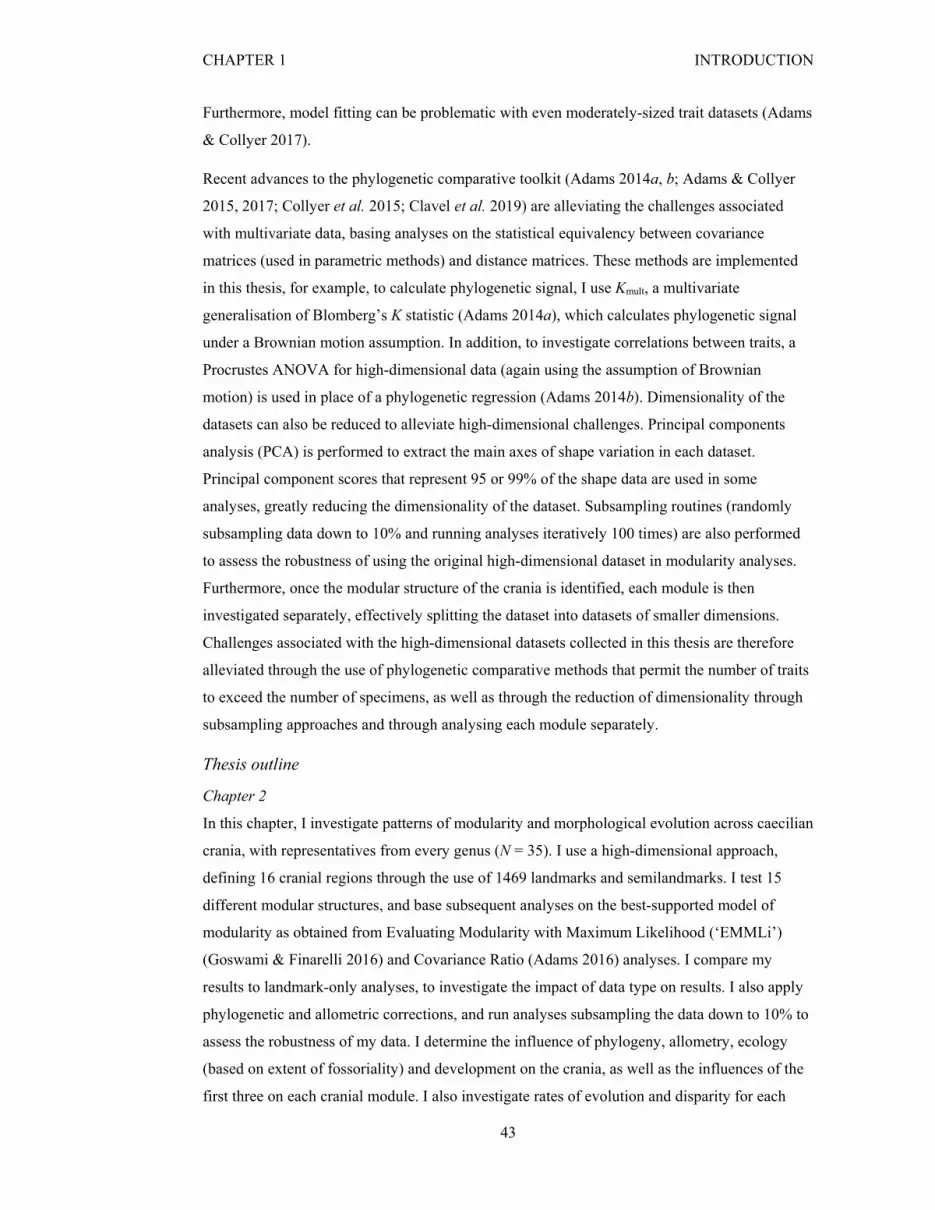
Recent advances to the phylogenetic comparative toolkit (Adams 2014a, b; Adams & Collyer
2015, 2017; Collyer et al. 2015; Clavel et al. 2019) are alleviating the challenges associated
with multivariate data, basing analyses on the statistical equivalency between covariance
matrices (used in parametric methods) and distance matrices. These methods are implemented
in this thesis, for example, to calculate phylogenetic signal, I use Kmult, a multivariate
generalisation of Blomberg’s K statistic (Adams 2014a), which calculates phylogenetic signal
under a Brownian motion assumption. In addition, to investigate correlations between traits, a
Procrustes ANOVA for high-dimensional data (again using the assumption of Brownian
motion) is used in place of a phylogenetic regression (Adams 2014b). Dimensionality of the
datasets can also be reduced to alleviate high-dimensional challenges. Principal components
analysis (PCA) is performed to extract the main axes of shape variation in each dataset.
Principal component scores that represent 95 or 99% of the shape data are used in some
analyses, greatly reducing the dimensionality of the dataset. Subsampling routines (randomly
subsampling data down to 10% and running analyses iteratively 100 times) are also performed
to assess the robustness of using the original high-dimensional dataset in modularity analyses.
Furthermore, once the modular structure of the crania is identified, each module is then
investigated separately, effectively splitting the dataset into datasets of smaller dimensions.
Challenges associated with the high-dimensional datasets collected in this thesis are therefore
alleviated through the use of phylogenetic comparative methods that permit the number of traits
to exceed the number of specimens, as well as through the reduction of dimensionality through
subsampling approaches and through analysing each module separately.
Thesis outline
Chapter 2
In this chapter, I investigate patterns of modularity and morphological evolution across caecilian
crania, with representatives from every genus (N = 35). I use a high-dimensional approach,
defining 16 cranial regions through the use of 1469 landmarks and semilandmarks. I test 15
different modular structures, and base subsequent analyses on the best-supported model of
modularity as obtained from Evaluating Modularity with Maximum Likelihood (‘EMMLi’)
(Goswami & Finarelli 2016) and Covariance Ratio (Adams 2016) analyses. I compare my
results to landmark-only analyses, to investigate the impact of data type on results. I also apply
phylogenetic and allometric corrections, and run analyses subsampling the data down to 10% to
assess the robustness of my data. I determine the influence of phylogeny, allometry, ecology
(based on extent of fossoriality) and development on the crania, as well as the influences of the
first three on each cranial module. I also investigate rates of evolution and disparity for each

CHAPTER 1 INTRODUCTION
44
cranial module, and for each landmark and semilandmark, and determine the relationship
between these metrics and integration.
Chapter 3
Here I investigate patterns of phenotypic integration across the anuran (frog) skull, sampling
across every frog family (N = 172). I quantify the morphology of 19 cranial regions, including
seven which are variably present across taxa. This is achieved using 995 landmarks and
semilandmarks. I test 27 functional, developmental and hormonal models of modularity, and use
EMMLi and Covariance Ratio to determine which model has the most support. I also run
modularity analyses separately on direct and indirect developing species, to observe the impact
metamorphosis may have on patterns and strength of cranial integration. I determine whether
integration influences evolutionary rate or disparity across frog crania, and whether ossification
sequence timing influences rates of evolution or disparity.
Chapter 4
This chapter focusses on the drivers of cranial morphological evolution across frogs. Using the
morphological data collected in Chapter 3, with the addition of a fossil frog (the mummified
Eocene Thaumastosaurus gezei) to the dataset, I explore influences on the morphological
evolution of the crania and of 15 defined cranial regions. I categorise species based on
developmental strategy and ecology (microhabitat), and quantify their influences on
morphology, as well as calculating the influence of phylogeny and allometry on morphology. I
observe whether species with different ecologies or developmental strategies occupy distinct
regions of morphospace. For the crania and the 15 defined cranial regions, I determine the
influence of ecology and developmental strategy on cranial disparity and on rate of evolution,
and I observe whether shifts in rate of evolution coincide with the emergence of any
developmental strategies or ecologies. I visualise the rate of evolution through time for the 15
cranial regions, as well as visualising how evolutionary rate and disparity vary across the
cranium at the level of the individual semi/landmark. Finally, I calculate the relationship
between ossification sequence timing and both disparity and rate of evolution.
Chapter 5
In this final data chapter, I implement a 2D outline approach to study morphological evolution
across fossil and extant frog taxa. Fossil frog crania, when preserved, are extremely flat,
necessitating this approach. I quantify the morphology of 42 fossil and 93 extant frog crania,
and, following sensitivity analyses, determine whether morphospace occupation has changed
through time. I also investigate phylogenetic, allometric, ecological and developmental
influences on cranial morphology. This chapter offers an understanding of frog cranial evolution
through deep time, as the high-dimensional analyses are restricted to extant taxa (plus just one

CHAPTER 1 INTRODUCTION
45
Eocene frog). For reasons of data availability, the data presented for Chapter 5 were collected
and analysed prior to the previous chapters. However, the position of this research as Chapter 5
is most appropriate as it extends the study of cranial morphology through deep time through the
inclusion of fossils, complementing the previous chapters which limit their taxonomic sampling
to extant taxa (with the exception of one Eocene fossil).
Chapter 6
In the final chapter, I summarise the findings from this thesis. Specifically, I compare results
from frog and caecilian crania, to reveal conserved and divergent patterns of modularity and
macro-evolutionary trends. I discuss the implications of my results, and place them into the
broader context. Lastly, I discuss the future directions that could stem from my work.
Further considerations
There are inevitably caveats associated with every study. Here, patterns of morphological
evolution and modularity are studied across the clades of Anura and Gymnophiona, but
intraspecific variation is not investigated. This is a result of time constraints; priority was given
to sampling as many genera as possible across the two clades. It was also not possible to create
a single-sex dataset for either frogs or caecilians. This is because sex information was missing
for many specimens in the collections and on the digital libraries used to collect data.
Furthermore, some specimens are exceptionally rare, but equally important to include in the
dataset. This includes the exceedingly ‘evolutionarily distinct’ frog Nasikabatrachus
sahyadrensis (Jetz & Pyron 2018), and the largest lungless tetrapod, the caecilian Atretochoana
eiselti (Wilkinson & Nussbaum 1997), which has extreme cranial morphology and is
represented by only six specimens (Wilkinson & Nussbaum 1997; Wilkinson et al. 1998;
Hoogmoed et al. 2011). A mixed sex sample was therefore necessary to fully maximise the
taxonomic sampling for these studies.
Intraspecific integration, variation, and sexual shape dimorphism is therefore outside the scope
of this thesis, but these were explored as a Master’s project for two species of caecilian
(Marshall et al. in prep; Marshall et al. 2019) and in a Master’s project and ongoing
collaborations for two species of frogs. For the intraspecific caecilian studies, we investigated
sexual shape dimorphism using a high-dimensional dataset, a landmark-only dataset, as well as
these two datasets corrected for allometry. Of the eight analyses (two species, four datasets),
only two were significant (non-corrected high-dimensional and landmark data for Boulengerula
boulengeri), with all analyses for Idiocranium russeli revealing no significant influence of sex
on shape (Fig. 1.12). It can be seen that interspecific variation far exceeds intraspecific variation
for the two caecilian species (Fig. 1.12), with preliminary analyses revealing 77% of shape
variation (Procrustes ANOVA, R2 = 0.78, p = 0.001) is explained by interspecific differences,

CHAPTER 1 INTRODUCTION
46
whilst sex differences were not significant (Procrustes ANOVA, R2 = 0.018, p = 0.23). This has
also been found across other caecilians (Sherratt et al. 2014). Whilst sexual shape dimorphism
does occur across some frogs and caecilians, intergeneric and interfamilial variation is typically
far greater than intraspecific variation (e.g., Sherratt et al. 2014). Furthermore, the more
prevalent sexual size dimorphism (e.g., see Shine 1979; Kupfer 2009) did not influence our
characterisation of shape because we removed size information from each specimen during
Procrustes alignment. Future studies should further investigate the influence of sex on shape
across these two clades, but this was not the focus of this thesis and is likely at most a minor
factor in studies at the macroevolutionary level. Owing to the importance of capturing as much
diversity across each clade as possible, increasing taxonomic sampling across frogs and
caecilians was determined to be the greater priority.
Figure 1.12. Sex differences in shape for two caecilian species. Morphospaces showing sex differences in
shape for (A) Idiocranium russeli and (B) Boulengerula boulengeri, and (C) a morphospace
demonstrating interspecific variation between Idiocranium russeli and Boulengerula boulengeri. Sex
differences in shape were only significant for Boulengerula boulengeri. Source: Marshall et al. (in prep).

CHAPTER 2 CAECILIAN CRANIAL EVOLUTION
47
CHAPTER 2
MORPHOLOGICAL EVOLUTION AND MODULARITY
OF THE CAECILIAN SKULL
Published as:
Bardua C., Wilkinson, M., Gower, D. J., Sherratt, E., Goswami, A. 2019. Morphological
evolution and modularity of the caecilian skull. BMC Evolutionary Biology. 19:1–24.
Abstract
Caecilians (Gymnophiona) are the least speciose extant lissamphibian order, yet living forms
capture approximately 250 million years of evolution since their earliest divergences. This long
history is reflected in the broad range of skull morphologies exhibited by this largely fossorial,
but developmentally diverse, clade. However, this diversity of form makes quantification of
caecilian cranial morphology challenging, with highly variable presence or absence of many
structures. Consequently, few studies have examined morphological evolution across caecilians.
This extensive variation also raises the question of degree of conservation of cranial modules
(semi-autonomous subsets of highly-integrated traits) within this clade, allowing us to assess the
importance of modular organisation in shaping morphological evolution. We used a high-
density surface geometric morphometric approach to quantify cranial morphological variation
across all 32 extant caecilian genera. We defined 16 cranial regions using 53 landmarks and 687
curve and 729 surface sliding semilandmarks. With these unprecedented high-dimensional data,
we analysed cranial shape and modularity across caecilians assessing phylogenetic, allometric
and ecological influences on cranial evolution, as well as investigating the relationships among
integration, evolutionary rate, and morphological disparity. We found highest support for a ten-
module model, with greater integration of the posterior skull. Phylogenetic signal was
significant (Kmult = 0.87, p < 0.01), but stronger in anterior modules, while allometric influences
were also significant (R2 = 0.16, p < 0.01), but stronger posteriorly. Reproductive strategy and
degree of fossoriality were small but significant influences on cranial morphology (R2 = 0.03 –
0.05), after phylogenetic (p < 0.03) and multiple-test (p < 0.05) corrections. The quadrate-
squamosal ‘cheek’ module was the fastest-evolving module, perhaps due to its pivotal role in
the unique dual jaw-closing mechanism of caecilians. Highly integrated modules exhibited both
high and low disparities, and no relationship was evident between integration and evolutionary
rate. Our high-dimensional approach robustly characterises caecilian cranial evolution and
demonstrates that caecilian crania are highly modular and that cranial modules are shaped by
differential phylogenetic, allometric, and ecological effects. More broadly, and in contrast to

CHAPTER 2 CAECILIAN CRANIAL EVOLUTION
48
recent studies, this work suggests that there is no simple relationship between integration and
evolutionary rate or disparity.
Introduction
A thorough understanding of the morphological evolution of a clade requires considering both
intrinsic (e.g., developmental) and extrinsic (e.g., environmental) influences. Examining
morphological evolution through clade history can reveal disparate patterns, from phylogenetic
conservatism (e.g., Ivanović & Arntzen 2017; Vidal-García & Keogh 2017) to repeated
convergent evolution through adaptation (e.g., Stayton & Ruta 2006; Felice & O’Connor 2014;
McLaughlin & Stayton 2016; Randau et al. 2016) or directional evolution (Bergmann et al.
2009; Sherratt et al. 2016). Quantification of these patterns can demonstrate that different
biological structures, or different parts of structures, may deviate in their patterns of evolution.
Individual structures may have divergent localised functions or different developmental origins
and therefore be subject to different constraints. However, each structure also contributes to the
functionality and, ultimately, to the fitness of the whole organism. For example, multiple levels
of functional and developmental interactions have been demonstrated within Felidae, from the
level of the individual vertebrae (Randau and Goswami 2017b), to different vertebral regions
(Randau and Goswami 2017a), to the level of the presacral vertebral column (Randau &
Goswami 2018). This hierarchy of interactions across the presacral vertebral column of felids
demonstrates how multiple levels of organisation shape the morphological evolution of a
complex structure.
The complex hierarchy of functional, developmental or genetical relationships among traits
underlies the concepts of modularity and integration. Integration refers to the covariation or
correlation amongst traits, while modularity refers to the partitioning of highly integrated traits
into semi-independent subsets (modules). Modular structures can be identified as those that can
be divided into subunits, or modules, that exhibit strong within-module integration (trait
covariation) and weaker between-module integration (Wagner 1996; Wagner and Altenberg
1996; Klingenberg 2004b). Trait regionalisation in modular networks is hypothesised to
promote evolvability (Clune et al. 2013), allowing strongly related traits to covary, and
coevolve, with relative autonomy from other regions. Strong integration within modules has
been found to facilitate (e.g., Claverie and Patek 2013; Parr et al. 2016; Randau and Goswami
2017b), constrain (e.g., Goswami and Polly 2010b; Felice and Goswami 2018) or both facilitate
and constrain (Goswami et al. 2014) evolution, affecting the magnitude and direction of an
organismal lineage’s response to selection (Marroig et al. 2009; Porto et al. 2009; Goswami et
al. 2014; Larouche et al. 2018). More specifically, integration directs evolutionary shifts to
favoured regions of morphospace, i.e. along paths of least resistance, which may promote

CHAPTER 2 CAECILIAN CRANIAL EVOLUTION
49
homoplasy as organismal evolution is directed along similar evolutionary trajectories defined by
the underlying architecture of trait interactions (Goswami et al. 2014; Melo et al. 2016; Felice et
al. 2018). Identifying the structure of these trait interactions through quantitative analysis is thus
central to advancing understanding of morphological evolution.
The focus of many studies of phenotypic integration and modularity is the vertebrate cranium, a
complex structure with multiple layers of functional and developmental patterning
(Hallgrímsson et al. 2009). Housing many important parts of the sensory, feeding, respiratory,
and communication systems, the cranium has been shaped by numerous, often competing,
demands. The cranium is also developmentally complex, with different embryonic origins
(neural crest and paraxial mesoderm) and types of ossifications (endochondral and
intramembranous) across the cranial bones. Previous studies have identified a complex modular
cranial structure in some vertebrate clades, reflecting this functional and developmental
complexity. A six-module model has been identified in carnivorans (Goswami and Polly
2010b), macaques (Cheverud 1982; Goswami & Finarelli 2016), and across therians (Goswami
2006a), suggesting this model may be conserved across a range of mammals. Modularity has
also been studied across 15 orders of Mammalia (Porto et al. 2009), and similar patterns of trait
correlations were found, suggesting a common covariance structure of the mammalian cranium.
Avian crania have been proposed to have seven distinct modules (Felice & Goswami 2018),
with some concordance with mammalian modules (vault, basicranium) as well as some novel
modules (e.g., nares). Several studies have limited analysis to a higher level division of the
neurocranium and facial modules, and this model also has strong support (Drake and
Klingenberg 2010; Goswami and Polly 2010a). Previous work on cranial modularity has been
strongly biased towards amniotes (especially mammals). In contrast, studies of modularity and
integration in non-amniotes (amphibians) are rare, limiting our understanding of the diversity of
patterns of modularity and our ability to reconstruct evolutionary trends in those clades.
As the only extant non-amniote tetrapod clade, Lissamphibia represents a unique lineage for
comparison with patterns of modularity and integration identified in amniote crania.
Evolutionary modularity has been explored in salamander crania using cranial ossification
sequences, and support was found for two (or four) developmental modules in terms of
coordinated timing of development (Laurin 2014). However, landmark studies suggest
salamander crania may be highly integrated, with no distinct modules across the cranium of the
alpine newt (Ivanović & Kalezić 2010) or the crania of species of Triturus (Ivanović & Arntzen
2014). Modularity has also been studied in frogs, comparing morphological evolution and
covariation in limbs and crania across the Myobatrachidae (Vidal-García & Keogh 2017).
Alternative two or three-module models were tested, but no strong support was found for any
modular structure. Similarly, only weak support was found for models of three to five

CHAPTER 2 CAECILIAN CRANIAL EVOLUTION
50
developmental, functional and hormonal modules (Simon & Marroig 2017) in crania of the
anuran Rhinella granulosa complex. In a previous investigation, Sherratt (2011) found support
for a two-module model in caecilian crania, with independence of the snout relative to the rest
of the cranium. While these studies have laid the groundwork for the study of modularity in
Lissamphibia, advances in data capture and analytical approaches allow us to expand this work
with high dimensional data that better represent the diversity of cranial morphology and directly
compare support for a broad range of alternative patterns of modularity. Thus, novel approaches
implemented in recent studies of mammalian (e.g., Goswami & Finarelli 2016) and avian
(Felice & Goswami 2018) crania can be applied to lissamphibian crania.
Caecilians are the least studied and least speciose major clade (order) of Lissamphibia
(Wilkinson et al. 2011; Kamei et al. 2012; Frost 2018). Elongate and limbless, ranging in adult
size from approximately 60 mm (e.g., Idiocranium russelli, Gower et al. 2015) to over 1700
mm (Caecilia thompsoni, Arredondo 2007), caecilians may superficially resemble snakes or
earthworms. Fertilisation is internal, and caecilians are the only amphibians (with the exception
of the tailed frog Ascaphus truei) where males have a copulatory organ (Gower & Wilkinson
2002). Both viviparity and oviparity are evident in this clade (Kupfer et al. 2016) and precocial
feeding (on maternal oviducts, or skin, or their secretions) using specialised, vernal dentitions
occurs in at least some viviparous species (Wake 1977; Exbrayat 1988) and in some direct
developing oviparous species (Kupfer et al. 2008), respectively. Caecilians possess two sets of
jaw-closing muscles (Nussbaum 1983), a mechanism unique among vertebrates. The jaw joint is
kinetic (Summers & Wake 2005), which may enhance bite force (Kleinteich et al. 2008).
Caecilians are predominantly found in tropical subsurface habitats, spending most of their time
as adults in leaf litter and moist soil (e.g., Gower & Wilkinson 2005). Secondarily aquatic
caecilians are found in freshwater systems of the neotropics and are restricted to the family
Typhlonectidae (e.g., Vitt & Caldwell 2014). Head first burrowing has long been thought to
influence cranial morphology (Taylor 1969; e.g., Nussbaum 1983; Nussbaum & Wilkinson
1989; Gower et al. 2004) because many caecilians exhibit stegokrotaphic (closed),
approximately conical crania with a subterminal mouth (see Taylor 1969; Wake 2003 but also;
Kleinteich et al. 2012). Additional aspects of being endogeic (living in soil), are also thought to
influence caecilian cranial morphology, for example by restricting gape size and perhaps
promoting rotational feeding (Measey & Herrel 2006). Although insufficient observational data
exist to confirm an absolute link between endogeicity and burrowing in caecilians, they are
presumed to be highly correlated in this clade, because no caecilian has ever been reported using
another organism’s burrow. Here we use the term fossorial to communicate both active
burrowing and more generally living in soil. Miniaturisation has been documented in some
caecilians (e.g., Wake 1986; Theska et al. 2018), although the extent to which this might be

CHAPTER 2 CAECILIAN CRANIAL EVOLUTION
51
causally linked to fossoriality is unknown. An extensive study of cranial shape evolution across
caecilians using 3D cranial landmarks across 141 species (Sherratt et al. 2014) showed that,
following an early expansion of morphospace, caecilian cranial evolution was both divergent
(clades occupying distinct areas of morphospace) and convergent (similarities attributed to
dedicated fossoriality in distantly related taxa). Sherratt et al.’s (2014) study represents the
largest quantitative examination of morphological evolution across Gymnophiona to date and
demonstrated the complexity of cranial evolution in caecilians, though cranial regions were not
analysed separately, such that anatomically-localised patterns were not investigated.
Caecilian crania exhibit great variation in the number, size and position of cranial bones as a
result of extensive and variable fusion of bones (Wake 2003; Müller et al. 2005). Consequently,
it is more difficult to quantify and compare cranial morphology across Gymnophiona than in
most other vertebrate orders, which largely have relatively conservative crania, in terms of bone
presence, such as mammals or birds. The highly variable nature of caecilian crania makes
traditional landmarking approaches challenging, because this approach would not allow shape
in all variably present or variably fused bones to be quantified. This is because all landmarks
must be present across all specimens. For these reasons we utilise a surface-based geometric
morphometric approach, which allows inclusion of individual elements and grouped elements,
with grouping of elements based on developmental and/or presumed functional relationships.
Hence, variably present elements (e.g., mesethmoid) can be grouped with other adjacent,
functionally or developmentally-related, and consistently present elements (e.g., frontal) so as
not to exclude them from analyses. This method offers several benefits, including better
representation of complex and variable structures and reduction in dependence on a limited
number of homologous landmarks that would exclude much of the variation across caecilians.
This approach has proven successful in recent studies of cranial morphology in mammals and
birds (e.g., Gunz et al. 2005; Gunz & Mitteroecker 2013; Dumont et al. 2015; Parr et al. 2016;
Felice & Goswami 2018). Using this approach, we quantify cranial morphological variation
across Gymnophiona, sampling all extant genera. Our study also represents the first study to
investigate a wide range of potentially modular structures within caecilian crania. We identify
the best-supported model of cranial modularity and quantify morphological variation for each
module. We test the relative strength of phylogenetic, allometric and ecological influences on
morphology for each module. Finally, we investigate morphological diversity (disparity) and
rates of morphological evolution for each module and across individual landmarks and
semilandmarks, and test whether integration of traits facilitates or constrains evolution of the
caecilian cranium.

CHAPTER 2 CAECILIAN CRANIAL EVOLUTION
52
Materials and methods
Specimens
We generated and analysed data from the crania of 35 caecilian species (one specimen per
species), sampling all 32 extant genera and ten families (Table 2.1), to capture a broad range of
phylogenetic and ecological diversity. All specimens were spirit-preserved and were CT
scanned by Emma Sherratt at the Natural History Museum (NHM) with a Nikon (Metris) X-Tek
HMX ST 225 System and volumes were digitally dissected to create 3D isosurface models
(.ply) of cranial bone using VG Studio MAX v.2.0 (Volume Graphics 2001), as described by
Sherratt (2011). All specimens were adults and of mixed sex, because a single-sex sample for
the analysed species was not available and because interspecific variation far exceeds sex-
specific variation (Sherratt et al. 2014). Models were cleaned and prepared for morphometric
analysis in Geomagic Wrap (3D Systems). Specifically, the external surfaces of caecilian crania
are textured by neurovascular foramina and blind pits, the latter serving as attachment points for
the skin (Wake 2003; Jared et al. 2018). Small foramina hinder the application of semi-
automated morphometric methods such as that used here, so these foramina were digitally filled
on the cranial reconstructions using Geomagic Wrap.
Models were decimated in Geomagic Wrap down to approximately 700,000 faces, reducing
computational demands for morphometric data collection (detailed below) without
compromising detail. Mirroring of models was implemented for specimens whose right-hand
side was damaged (Praslinia cooperi, Epicrionops bicolor), using the ‘mirror’ function in
Geomagic Wrap, and subsequent data collection was performed on only the right side of the
cranium.

CHAPTER 2 CAECILIAN CRANIAL EVOLUTION
53
Table 2.1. Specimens used in this study. Specimens are from the following institutions: American
Museum of Natural History, New York, USA (AMNH), Natural History Museum, London, UK (BMNH),
Delhi University, New Delhi, India (DU), Institut royal des Sciences naturelles de Belgique, Brussels,
Belgium (IRSNB), University of Kansas, Museum of Natural History, Lawrence, USA (KUH), Museu de
Ciências e Tecnologia da PUCRS, Porto Alegre, Brazil (MCP), Muséum national d’Histoire naturelle,
Paris, France (MNHN), Museum of Vertebrate Zoology, Berkeley, USA (MVZ), Naturhistorisches
Museum, Zoologische Abtheilung, Vienna, Austria (NHMW), National Museum of Sri Lanka, Colombo,
Sri Lanka (NMSL), University of Kerala, Thiruvananthapuram, India (UK), University of Michigan
Museum of Zoology, Ann Arbor, USA (UMMZ).
Species Family Specimen number Sex Total length
(mm)
Atretochoana eiselti Typhlonectidae NHMW 9144 F 735
Boulengerula
boulengeri
Herpelidae BMNH 2000.474 ?F 165
Brasilotyphlus
braziliensis
Siphonopidae AMNH A51751 M 260
Caecilia tentaculata Caeciliidae BMNH field tag
MW3945
M 533
Chikila fulleri Chikilidae DU field tag
SDB1304
F 212
Chthonerpeton
indistinctum
Typhlonectidae MCP field tag
MW16
M 325
Crotaphatrema
bornmuelleri
Scolecomorphidae NHMW 14859 M 275
Crotaphatrema lamottei Scolecomorphidae BMNH field tag
MW5741
M 265
Dermophis mexicanus Dermophiidae MVZ 179395 M 415
Epicrionops bicolor Rhinatrematidae BMNH 78.1.25.48 F 230
Gegeneophis carnosus Indotyphlidae UK field tag
MW295
M 155
Geotrypetes seraphini Dermophiidae BMNH field tag
MW4543
M 195
Grandisonia alternans Indotyphlidae BMNH
1956.1.13.39
M 220
Gymnopis multiplicata Dermophiidae BM1907.10.9.10 M 460
Herpele squalostoma Herpelidae BMNH field tag
MW4534
M 345

CHAPTER 2 CAECILIAN CRANIAL EVOLUTION
54
Hypogeophis rostratus Indotyphlidae UMMZ 179847 F 225
Ichthyophis
bombayensis
Ichthyophiidae BMNH 88.6.11.1 M 320
Ichthyophis glutinosus Ichthyophiidae NMSL field tag
MW1773
F 401
Ichthyophis nigroflavus Ichthyophiidae BMNH 1967.2775 M 420
Idiocranium russeli Indotyphlidae BMNH 1946.9.5.80 F 95
Indotyphlus cf.
battersbyi
Indotyphlidae AMNH 89788 ? 202
Luetkenotyphlus
brasiliensis
Siphonopidae BMNH 1930.4.4.1 F ?
Microcaecilia albiceps Siphonopidae MCZ A-58412 ? 181
Mimosiphonops
vermiculatus
Siphonopidae KUH 93271 ?F 185
Nectocaecilia petersii Typhlonectidae BMNH 61.9.2.6 F 590
Oscaecilia
ochrocephala
Caeciliidae MCZ 4268 F 330
Potomotyphlus kaupii Typhlonectidae IRNSB 12447 ? 355
Praslinia cooperi Indotyphlidae BMNH
1907.10.15.154
F 165
Rhinatrema bivittatum Rhinatrematidae BMNH field tag
MW2395
F 229
Schistometopum
gregorii
Dermophiidae MCZ 20143 F 300
Scolecomorphus kirkii Scolecomorphidae BMNH 2005.1388 F 380
Siphonops annulatus Siphonopidae BMNH
1956.1.15.88
M 340
Sylvacaecilia
grandisonae
Indotyphlidae BMNH 1969.1589 F 259
Typhlonectes
compressicauda
Typhlonectidae BMNH field tag
MW5820
M 305
Uraeotyphlus oxyurus Ichthyophiidae MNHN 1994.419 M 256

CHAPTER 2 CAECILIAN CRANIAL EVOLUTION
55
Phylogeny
Phylogenetic relationships and relative divergence dates among sampled taxa are important for
reconstructing evolutionary modularity and macroevolutionary patterns. A phylogeny was
constructed (Fig. 2.1) for our taxon sampling by modifying San Mauro et al.’s (2014) Bayesian
relaxed-clock timetree (see Supplementary Figure S2 from San Mauro et al. 2014) that sampled
20 of the species used in the present study. The following modifications were made. Seven
species were directly swapped with their monophyletic corresponding congener sampled in San
Mauro et al.’s (2014) tree: we added Microcaecilia albiceps, Grandisonia alternans,
Indotyphlus cf. battersbyi, Gegeneophis carnosus, Typhlonectes compressicauda,
Scolecomorphus kirkii and Crotaphatrema bornmuelleri in place of M. sp, G. alternans, I.
maharashtraensis, G. ramaswamii, T. natans, S. vittatus and C. lamottei, respectively.
Ichthyophis nigroflavus replaced (I. bannanicus + I. asplenius) and E. bicolor replaced E. cf.
marmoratus. Gymnopis is paraphyletic in San Mauro et al.’s tree, so we added Gymnopis
multiplicata as sister to Dermophis arbitrarily halfway along the equivalent branch to where San
Mauro et al.’s two Gymnopis specimens join the tree. The remaining species in our dataset lack
congeners in San Mauro et al.’s tree, so were placed into the phylogeny as follows:
Atretochoana eiselti was added as sister to (Typhlonectes + Potomotyphlus) based on Maciel et
al. (2017), arbitrarily three-quarters of the way along the branch subtending (Typhlonectes +
Potomotyphlus); Nectocaecilia petersii was then added as sister to (Typhlonectes +
Potomotyphlus + Atretochoana) based on Wilkinson & Nussbaum (1999), arbitrarily halfway
along the internal branch subtending that clade; Brasilotyphlus braziliensis was added as sister
to Microcaecilia (see Wilkinson et al. 2011, 2013), placed halfway (arbitrarily) between M.
albiceps and the split between that species and its divergence from other (non-Brasilotyphlus)
siphonopids; Mimosiphonops vermiculatus was added (halfway, arbitrarily) between the
Siphonops-Luetkenotyphlus divergence and their divergence from Microcaecilia +
Brasilotyphlus (based on Wake & Donnelly 2010; Wilkinson et al. 2011); Sylvacaecilia
grandisonae was added as sister to [(Indotyphlus + Gegeneophis) + (Praslinia + Hypogeophis +
Grandisonia)] based on Wilkinson et al. (2011) halfway (arbitrarily) between the internal
branch subtending that clade and its split from Idiocranium.

CHAPTER 2 CAECILIAN CRANIAL EVOLUTION
56
Figure 2.1. Time-calibrated phylogeny of caecilians used in this study. Modified from a Bayesian
relaxed-clock timetree based on a mitogenomic dataset (see Supplementary Fig. S2 from San Mauro et al.
2014). Scale is in million years. Node ages are based on point divergences (means) rather than confidence
ranges. Vertical lines refer to rate shifts tested in our study, corresponding to (A) obligate aquatic niche,
(B) viviparity and (C) direct development, the data for which can be found in Appendix 2, Table S2.1.
Note the re-emergence of biphasic development (C2).

CHAPTER 2 CAECILIAN CRANIAL EVOLUTION
57
Ecology
Due to their secretive, mostly endogeic lifestyles and mostly tropical distributions, caecilians
are seldom encountered and rank among the most poorly-known orders of extant vertebrates.
Many species are known from very few specimens and there is very little published ecological
information and no compilations of trait data to draw upon when investigating caecilian ecology
or ecological correlates (e.g., Gower & Wilkinson 2005; Wilkinson 2012). Probably all species
of caecilian are capable of some burrowing but in the general absence of quantitative data on
caecilian burrowing abilities and on other aspects of endogeicity we divided caecilians into five
mutually exclusive categories of presumed increasing degree of fossoriality (reflecting
burrowing ability and other aspects of endogeic adaptation) on the basis of a combination of
basic ecological and morphological data. The analytically unordered categories are: 0. aquatic
species (which sometimes burrow in soft substrates); 1. tailed species (which have relatively
short and stout bodies and zygokrotaphic skulls); 2. tailless species with zygokrotaphic skulls; 3.
tailless species with stegokrotaphic skulls and open orbits; and 4. tailless species with closed
orbits. Terrestrial species more likely to be found in leaf litter and on the surface (and not only
in deeper soils) belong to categories 1-3. This simple and unambiguous categorisation
corresponds with our intuition based on the unparalleled experience of Mark Wilkinson and
David Gower with different caecilian species (including representatives of all ten families and
all but seven of the 32 currently recognised genera) in the field, and is consistent with what little
ecological data have been published (Gower et al. 2004), but it merits further critical testing. To
the extent that the definitions of some of these categories are based on cranial morphological
features there is the potential for a degree of circularity in our analyses but since our analyses
are based on much more than these specific features we do not consider the circularity to be
vicious. We also categorised species based on terrestrial versus aquatic adults, recognising only
three obligate aquatic species in our sample (A. eiselti, Potomotyphlus kaupii and T.
compressicauda from Typhlonectidae).
Data on reproductive strategy (oviparity versus viviparity) and life history (with or without a
larval stage) were taken from San Mauro et al. (see Fig. 4 and Supplementary Fig. S2, both
from San Mauro et al. 2014) supplemented by personal observations of Mark Wilkinson and
David Gower (Appendix 2, Table S2.1). Species-level data were not always available, so we
categorised 13 and 14 species for life history and reproductive strategy respectively based on
traits known for congeners or other closest relatives (see Appendix 2, Table S2.1).
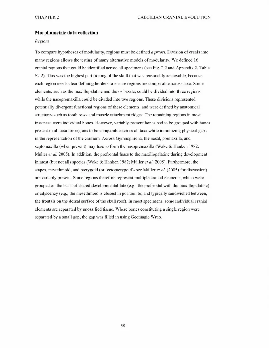
CHAPTER 2 CAECILIAN CRANIAL EVOLUTION
58
Morphometric data collection
Regions
To compare hypotheses of modularity, regions must be defined a priori. Division of crania into
many regions allows the testing of many alternative models of modularity. We defined 16
cranial regions that could be identified across all specimens (see Fig. 2.2 and Appendix 2, Table
S2.2). This was the highest partitioning of the skull that was reasonably achievable, because
each region needs clear defining borders to ensure regions are comparable across taxa. Some
elements, such as the maxillopalatine and the os basale, could be divided into three regions,
while the nasopremaxilla could be divided into two regions. These divisions represented
potentially divergent functional regions of these elements, and were defined by anatomical
structures such as tooth rows and muscle attachment ridges. The remaining regions in most
instances were individual bones. However, variably-present bones had to be grouped with bones
present in all taxa for regions to be comparable across all taxa while minimizing physical gaps
in the representation of the cranium. Across Gymnophiona, the nasal, premaxilla, and
septomaxilla (when present) may fuse to form the nasopremaxilla (Wake & Hanken 1982;
Müller et al. 2005). In addition, the prefrontal fuses to the maxillopalatine during development
in most (but not all) species (Wake & Hanken 1982; Müller et al. 2005). Furthermore, the
stapes, mesethmoid, and pterygoid (or ‘ectopterygoid’- see Müller et al. (2005) for discussion)
are variably present. Some regions therefore represent multiple cranial elements, which were
grouped on the basis of shared developmental fate (e.g., the prefrontal with the maxillopalatine)
or adjacency (e.g., the mesethmoid is closest in position to, and typically sandwiched between,
the frontals on the dorsal surface of the skull roof). In most specimens, some individual cranial
elements are separated by unossified tissue. Where bones constituting a single region were
separated by a small gap, the gap was filled in using Geomagic Wrap.

CHAPTER 2 CAECILIAN CRANIAL EVOLUTION
59
Figure 2.2. Landmarks and semilandmarks in (A) lateral, (B) dorsal and (C) ventral views, colour coded
by the 16 cranial regions defined in our study, shown on Siphonops annulatus. Regions are as follows:
NPM(d) (green): nasal, premaxilla (or nasopremaxilla) and septomaxilla when present, dorsal surface;
Fr (light pink): frontal, and mesethmoid when present; Pa (black): parietal; Sq (dark blue): squamosal,
and postfrontal when present; Max(l) (orange): maxillopalatine (lateral surface), and prefrontal when
present; Qu (light green): quadrate (lateral surface); JJ (red): quadrate (jaw joint articulation); Occ
(light purple): occipital (otic) region of os basale (excluding occipital condyle); Co (aqua): occipital
condyle; BS (purple): Ventral surface of os basale; NPM(p) (gold): palatal surface of nasopremaxilla, or
the anterior projection of the vomer; Vo (white): vomer; Max(i) (grey): interdental plate of
maxillopalatine; Max(p) (hot pink): palatine shelf (maxillary plate) of maxillopalatine; Pt (light blue):
pterygoid, and/or pterygoid process of quadrate; St (yellow): stapes.

CHAPTER 2 CAECILIAN CRANIAL EVOLUTION
60
Landmarks and curve semilandmarks
Type I and Type II landmarks (Bookstein 1991) and sliding semilandmarks (points regularly
spaced along ‘curves’, Gunz et al. 2005) were placed manually onto each reconstructed
caecilian cranium (see Fig. 2.3) in IDAV Landmark Editor v.3.6 (Wiley et al. 2005), to define
the 16 regions (as detailed above and in Fig. 2.2 and Appendix 2, Table S2.2). Fifty-three
landmarks were placed on the right-hand side of the cranium, three of which were along the
midline (Table 2.2). Curves were placed around large apertures (orbit, tentacular foramen,
choana, naris) to exclude these regions during surface point digitisation (details below). Curves
were also placed along tooth rows on the maxillopalatine, premaxilla, and vomer in order to
exclude them from regions because of their variable presence across genera (pterygoid teeth,
where present, were removed digitally in Geomagic Wrap). Fifty-seven curves were placed on
the right-hand side of each cranium, anchored by landmarks, with each curve composed of
between one and ten regularly-spaced semilandmarks (Appendix 2, Table S2.3). This resulted in
277 semilandmarks placed on each cranium. Curves were later resampled to between three and
30 semilandmarks each, with the number of semilandmarks reflecting our attempt to best
capture shape [for code and a description see SI in Botton-Divet et al. (2016)]. This approach
resulted in a total of 687 semilandmarks equidistantly placed along curves. During the sliding
procedure, the semilandmarks were slid to minimise bending energy.

CHAPTER 2 CAECILIAN CRANIAL EVOLUTION
61
Figure 2.3. Landmark and semilandmark data. Landmarks and semilandmarks in (A) lateral, (B) dorsal
and (C) ventral views, shown on Siphonops annulatus. Points are coloured as follows: landmarks (red),
curve semilandmarks (yellow) and surface semilandmarks (blue).

CHAPTER 2 CAECILIAN CRANIAL EVOLUTION
62
Table 2.2. Landmarks used in this study. 74 landmarks were placed onto the right-hand side of the
cranium of each specimen. 21 landmarks (*) were removed prior to analyses as they were not
homologous across all specimens. These 21 landmarks were used to fix curves around structures such as
foramina.
Landmark
number
Landmark position
1 Nasopremaxilla, palatal surface: medial extreme of tooth row
2 Maxillopalatine, lateral surface: posterior extreme
3 Nasopremaxilla, dorsal surface: anteromedial position
4 Nasopremaxilla, dorsal surface: medial suture with frontal
5 Frontal: most lateral suture position with nasal
6 Parietal: suture with os basale along midline
7 Os basale: dorsal extreme of foramen magnum
8 Vomer: posterior extreme, medial to the choana
9 Os basale: ventral extreme of foramen magnum
10 Os basale, ventral surface: anteromedial extreme on the anteriorly projecting
process
11 Quadrate: medial extreme of jaw joint articular surface
12 Quadrate: lateral extreme of jaw joint articular surface
13 Nasopremaxilla: lateral suture with frontal
14 Maxillopalatine, interdental plate: anteromedial extreme of tooth row
15 Maxillopalatine, interdental plate: posterolateral extreme
16 Maxillopalatine, interdental plate: anteromedial extreme
17 Maxillopalatine, maxillary plate: anterior extreme
18 Maxillopalatine, maxillary plate: posterior extreme of tooth row
19 Maxillopalatine, maxillary plate: inflection point where bone splits to
surround the choana
20 Nasopremaxilla, palatal surface: lateral extreme of tooth row
21 Nasopremaxilla, palatal surface: posteromedial extreme
22 Vomer: medial extreme of tooth row
23 Vomer: lateral extreme of tooth row
24 Os basale, ventral surface: medial position on the muscle ridge
25 Os basale, ventral surface: lateral position on the muscle ridge
26 Os basale, ventral surface: closest position to vomer
27 Os basale: dorsal extreme of occipital condyle
28 Os basale: ventral extreme of occipital condyle

CHAPTER 2 CAECILIAN CRANIAL EVOLUTION
63
29 Os basale: posterior extreme of fenestra ovalis
30 Os basale: lateral extreme along suture with parietal
31 Squamosal: anteromedial extreme
32 Squamosal: ventral extreme along suture with maxillopalatine
33 Squamosal: posteromedial extreme
34 Squamosal: posteroventral extreme
35 Frontal: suture with nasal along midline
36 Frontal: suture with parietal along midline
37 Frontal: lateral extreme suture with parietal
38 Parietal: suture with frontal along midline
39 Parietal: anterolateral position of parietal
40 Parietal: posterolateral extreme*
41 Maxillopalatine, lateral surface: anterior extreme of tooth row (dorsal)
42 Maxillopalatine, lateral surface: posterior extreme of tooth row, behind last
tooth
43 Nasopremaxilla, dorsal surface: posterolateral extreme above tooth row
44 Nasopremaxilla, dorsal surface: anterior extreme of nares opening
45 Nasopremaxilla, dorsal surface: dorsal extreme of nares opening
46 Nasopremaxilla, dorsal surface: lateral extreme of nares opening
47 Nasopremaxilla, dorsal surface: ventral extreme of nares opening
48 Quadrate, lateral surface: anterolateral extreme
49 Maxillopalatine, interdental plate: anterolateral to the most posterior tooth
50 Os basale: anteromedial suture with parietal
51 Maxillopalatine, maxillary plate: posterior extreme of choanal rim
52 Maxillopalatine, maxillary plate: anterior extreme of choanal rim
53 Quadrate, lateral surface: anteromedial extreme
54 Quadrate, lateral surface: maximum curvature of jaw joint articular surface
55 Stapes, lateral aspect: anterior extreme of the rod, positioned midway
dorsoventrally*
56 Stapes: position adjacent to posterior extreme of fenestra ovalis*
57 Stapes: position adjacent to anterior extreme of fenestra ovalis*
58 Stapes: position adjacent to dorsal extreme of fenestra ovalis*
59 Stapes: position adjacent to ventral extreme of fenestra ovalis*
60 Pterygoid process of quadrate (or if absent, pterygoid): posteromedial
extreme of ventral surface*

CHAPTER 2 CAECILIAN CRANIAL EVOLUTION
64
61 Pterygoid process of quadrate (or if absent, pterygoid): posterolateral extreme
of ventral surface*
62 Pterygoid process of quadrate (or if absent, pterygoid): anteromedial extreme
of ventral surface*
63 Maxillopalatine, lateral surface: posterodorsal suture with squamosal*
64 Maxillopalatine, lateral surface: anterodorsal extreme*
65 Maxillopalatine: if tentacular groove present, suture with nasal and frontal*
66 Maxillopalatine: tentacular groove (if present), anterior extreme*
67 Maxillopalatine: tentacular groove (if present), posterior extreme*
68 Maxillopalatine: tentacular groove (if present), ventral extreme*
69 Mesethmoid (if absent, frontal): anteromedial extreme*
70 Mesethmoid (if absent, frontal): posteromedial extreme*
71 Postfrontal (if absent, squamosal): antero-dorsal extreme*
72 Pterygoid (if present): posteromedial extreme of ventral surface*
73 Pterygoid (if present): posterolateral extreme of ventral surface*
74 Pterygoid (if present): anteromedial extreme of ventral surface*
Surface semilandmarks
While all landmarks and curves were placed manually onto each specimen, a template was used
to fit the surface semilandmarks (‘surface points’). The template used was a generic
hemispherical mesh onto which all specimen landmarks and curves were placed manually.
Surface points were then placed systematically across each region, in evenly spaced rows
parallel to the region margins. A semi-automated procedure in the Morpho package v.2.5.1
(Schlager 2017) in R v.3.4.3 (R Core Team 2017) was used to apply surface points onto each
specimen (Fig. 2.3). During this patching procedure, the template was warped to the shape of
each specimen based on the shared landmarks and curves, so had to be of sufficient resolution
(18,000 triangles in this instance). The template’s surface points were then projected onto each
specimen, and these were translated along their normals until they contacted the surface of the
specimen. Following this process, the curve and surface points were slid to minimise bending
energy. Each region was patched globally when possible, allowing bending energy to be
minimised across the whole dataset. A total of 729 surface points were placed onto each
specimen (Appendix 2, Table S2.4).
Three regions required patching across subsets of specimens. The lateral surface of the
maxillopalatine was variably subdivided into two in cases where the tentacular canal is open
laterally. The pterygoid region consisted of either one or two surfaces (pterygoid and/or

CHAPTER 2 CAECILIAN CRANIAL EVOLUTION
65
pterygoid process of the quadrate) or was absent completely (S. kirkii and C. bornmuelleri), and
the stapes was absent in three of the sampled taxa (S. kirkii, C. bornmuelleri and Crotaphatrema
lamottei). An additional 21 landmarks (Table 2.2, *landmarks) and 18 curves (Appendix 2,
Table S2.3) were placed on each specimen, to aid the patching of surface points for these highly
variable regions. These were not globally homologous across specimens so were removed
following patching of surface points, prior to analyses, leaving only surface points for these
regions in the final dataset. Absent regions were represented by one cranial landmark (whose
position best represented the location of the missing region), replicated to achieve an array of
the same dimension as the surface point dataset from other specimens. A missing region is
therefore captured as an infinitesimal surface, with the same dimensions as present regions. A
similar approach has previously been suggested to allow for incorporation of novel structures in
geometric morphometric studies (Klingenberg 2008b) and here this allowed us to retain all
specimens and regions for analyses. After global Procrustes alignment, missing regions had
non-zero (but negligible) size. The multiple templates for each of the maxillopalatine, pterygoid,
and stapes had an identical number of surface points and an analogous surface point
distribution. Unless otherwise specified, the term ‘semilandmarks’ refers to all sliding curve and
surface semilandmarks.
Data analyses
Generalised Procrustes Analysis
Generalised Procrustes analysis (Gower 1975) removes non-shape aspects from landmark
coordinate data (Rohlf & Slice 1990) and is considered the most powerful method currently for
quantifying and analysing shape (see Rohlf 2000 for a discusion of alternate methods). Curves
and surface points were mirrored prior to Procrustes analysis using the mirrorfill function in the
R package paleomorph v.0.1.4 (Lucas & Goswami 2017), because a bilaterally symmetrical
structure results in a more successful alignment than using only one side (Cardini 2016a).
Procrustes analysis was then performed using the geomorph R package v.3.0.5 (Adams et al.
2017). Mirrored data were then manually removed from the dataset following the Procrustes
alignment, such that all analyses were conducted on data representing only the midline and
right-side.
Modularity
To assess patterns of modularity we used two methods, both implemented in R: a maximum
likelihood approach (Evaluating Modularity with Maximum Likelihood, ‘EMMLi’) and the
covariance ratio (CR). First, we used EMMLi with the trait correlation matrix (congruence
coefficients) (Goswami & Finarelli 2016). This approach allows alternative hypotheses of
modularity to be tested, with the advantage that models with different numbers of modules can

CHAPTER 2 CAECILIAN CRANIAL EVOLUTION
66
be directly compared. We used the ‘EMMLi’ function in the R package EMMLi to test 15
different model structures (Appendix 2, Table S2.5), ranging from one module (entirely
integrated cranium) to a 16-module model (each of the 16 regions was a separate module). The
models we assessed included multiple two-module models (e.g., division of the cranium into
anterior and posterior modules, dorsal and ventral modules, and medial and lateral modules), a
six-module model analogous to the therian mammal six-module model (Goswami 2006a) and
extensions of this model by further partitioning some of the original six modules into small
subunits. We also investigated models from Sherratt’s (2011) study of caecilian crania, testing
the cheek region combined with either the snout, the braincase, or as its own module.
As a result of the low specimen-to-landmark (including semilandmarks) ratio in our dataset, we
assessed the robustness of our results in multiple ways. First, we analysed patterns of
modularity using only landmarks (excluding the regions detailed above as being represented
only by surface points). Second, we applied a random jackknife resampling of our
morphometric data down to 10% (Nlmks = 147) of the original dataset (N = 1469), using the
‘subSampleEMMLi’ function in EMMLiv2 (https://github.com/hferg/EMMLiv2/) with results
averaged over 100 iterative runs. We further analysed patterns of modularity with EMMLi after
correcting our data for phylogenetic and allometric effects. To correct for allometry we
performed a Procrustes ANOVA using the ‘procD.lm’ function in geomorph with log centroid
size as a factor, and extracted the residuals from this analysis. Centroid size is the square root of
the sum of squared distances of landmarks from the structure’s centroid (centre). To account for
the evolutionary relationships among species, we used phylogenetic independent contrasts of
shape in these analyses (Felsenstein 1985).
In addition, there is a tendency for analyses of densely sampled semilandmarks to favour highly
parameterised models, and not all possible groupings of modules can be assessed in EMMLi
analysis at present. We therefore followed Felice and Goswami (2018) and assessed the within-
and between-region trait correlations for the best-supported model from EMMLi analysis to
determine whether any regions could be reasonably combined into larger modules. We merged
regions into modules when the difference between the between-region correlation and the
lowest within-region correlation was 0.2 or lower. We based this cut-off on observation of the
pattern and distribution of region correlations.
We further applied a second method to assess modularity: we calculated the covariance ratio
(Adams 2016) for the complete dataset, landmark-only, allometry-corrected and
phylogenetically-corrected data using the ‘modularity.test’ function in geomorph.

CHAPTER 2 CAECILIAN CRANIAL EVOLUTION
67
Phylogenetic, allometric and other factors influencing shape
We used principal components analysis (PCA) to identify the major axes of shape variation
across caecilians for the whole cranium and for individual cranial modules. Principal
components analysis converts a dataset into a set of statistically uncorrelated variables, which
represent the principal axes of shape variation in a given dataset. Representations of
morphologies defining the extremes of the significant PC axes were then used to visualise the
main components of morphological variation across the cranium and cranial modules.
We quantified phylogenetic signal (the degree of similarity explained by shared ancestry) in our
shape data using the Kmult statistic (Adams 2014a), a multivariate generalisation of the K
statistic, which calculates phylogenetic signal under the assumption of Brownian motion
(Blomberg et al. 2003). Kmult was calculated using the ‘physignal’ function in geomorph for all
cranial modules separately and for the entire cranium, using our modified phylogeny. We also
estimated phylogenetic signal in our centroid size data.
The amount of shape variation explained by allometry (size-related shape change) was
visualised for the cranium using a multivariate regression implemented in the ‘procD.allometry’
function in geomorph (Drake & Klingenberg 2008). Individual module morphologies at
maximum and minimum sizes were also visualised, by partitioning the globally aligned shape
data into each module’s landmarks and semilandmarks, and investigating allometry with cranial
centroid size as the factor. Global Procrustes alignment retains relative positional and scaling
information, whilst local Procrustes loses this information (see Baab (2013) for a discussion).
Evolutionary allometry was quantified using a phylogenetic generalised least squares analysis
for high-dimensional data (Adams 2014b) (‘procD.pgls’ function in geomorph), for the cranium
and for each individual module. Global Procrustes alignment was performed, because we
wanted to retain information about relative positional and scaling information of modules.
Statistical significance of the factors (here, centroid size) in the model is assessed by
permutation of the phenotypic data across the tips of the phylogeny, for 1,000 iterations.
We performed phylogenetic ANOVAs to assess the influences of fossoriality, life history and
reproductive strategies on skull shape evolution, and of the influence of degree of fossoriality
for each individual module. Specimens with data lacking were removed from the relevant
analyses (see Appendix 2, Table S2.1). We applied Benjamini-Hochberg corrections (Benjamini
& Hochberg 1995) for the phylogenetic ANOVAs and rate shifts, to account for elevated false
positive rates. The influences of life history and reproductive strategies were not explored for
each module because increased numbers of statistical tests decreases statistical power.

CHAPTER 2 CAECILIAN CRANIAL EVOLUTION
68
Evolutionary rates and disparity
Disparity was quantified by Procrustes variance and calculated using the ‘morphol.disparity’
function in geomorph, for the entire cranium and for each individual cranial module.
Differences in disparity between cranial modules were evaluated using the ‘TukeyHSD’
function in R, which calculates the differences in observed means, with p-values adjusted for
multiple tests. We divided each module’s disparity by the number of landmarks and
semilandmarks included in analysis for that module to correct for landmark/semilandmark
number, which affects variance estimates, and to render our results more comparable across
modules. Using the dated phylogenetic tree described earlier, we then calculated net rates of
morphological evolution for each module under a Brownian motion model using the
‘compare.multi.evol.rates’ function (Denton & Adams 2015) in geomorph, which is an
extension of the ‘compare.evol.rates’ function (Adams 2014c) to allow comparison across
multiple phenotypic traits. This approach allows the direct comparison of rates across a high-
dimensional modular structure, using the ratio of the maximum to minimum rate as a test
statistic. Significance is evaluated through phylogenetic simulation, by obtaining tips data using
a global evolutionary rate and comparing simulation rate ratios to the observed ratio (see Denton
& Adams 2015). We investigated the relationship between magnitude of integration, disparity,
and rate of morphological evolution for each cranial module by plotting regressions of disparity
and rates on magnitude of integration (estimated within-module trait correlation, ρ).
We further determined the disparity (as measured by variance) and rate of morphological
evolution of each individual landmark and semilandmark (through modification of the
‘compare.evol.rates’ function in geomorph) and colour graded a representative caecilian
cranium’s landmarks and semilandmarks according to these metrics. Although the sliding of
semilandmarks and Procrustes analysis imposes some covariance on individual data points, this
approach allows for clear visualisation of concentrations of unusual rate or disparity in cranial
regions. We also plotted the regression of disparity on evolutionary rate for each individual
landmark and semilandmark, in order to conduct a more detailed assessment of these attributes
across the caecilian cranium. We compared the observed relationship between variance and
evolutionary rate to a simulated expectation of variance for each given evolutionary rate.
Specifically, we calculated the evolutionary rate for each landmark and semilandmark and
simulated trait evolution under a model of Brownian motion, assuming no trait covariation. We
ran 100 simulations, using the ‘sim.char’ function in the R package geiger v.2.0.6 (Harmon et
al. 2008). We determined the mean variance of each landmark and semilandmark across these
100 simulations and fitted a linear regression of calculated evolutionary rate to simulated
variance. We also generated a 95% prediction interval using the ‘predict’ function in R and

CHAPTER 2 CAECILIAN CRANIAL EVOLUTION
69
noted which of our landmarks and semilandmarks fell outside the expected variance range for
each given evolutionary rate.
We also tested whether shifts in rates of morphological evolution were correlated with major
transitions in ecology and life history across the tree. We compared net rates of morphological
evolution among obligate aquatic species and non-obligate species, among direct and indirect
developers and finally among viviparous and oviparous species (Fig. 2.1). This was
implemented in the ‘compare.evol.rates’ function in geomorph (Adams 2014c), which
calculates rates of evolution under a Brownian motion model of evolution for each group, and
obtains a rate ratio. Significance was assessed in the same way as with
‘compare.multi.evol.rates’ (see Denton & Adams 2015). Within caecilians, obligate aquatic
adults probably evolved only once (within Typhlonectidae), while among our sampled taxa
direct development has possibly arisen at least twice, and viviparity three times (Fig. 2.1). We
applied Benjamini-Hochberg corrections for multiple comparisons (Benjamini & Hochberg
1995) for rate shifts.
Results
Modularity
EMMLi analysis of the full trait correlation matrix identified the most parameterised model, the
16-module model, as the best fitting. Comparisons of within- and between-region trait
correlations for the non-corrected data resulted in five of the defined cranial regions then being
combined with other regions to form multi-region modules, (see Appendix 2, Table S2.6),
resulting in a ten-module model of modularity. The ten modules were: maxillopalatine
(combining lateral, interdental plate, and palatine shelf regions of the maxillopalatine), quadrate
(combining lateral and jaw joint surfaces), occipital (combining occipital region and occipital
condyle), frontal-nasopremaxilla, ventral os basale-vomer, parietal, pterygoid, stapes,
squamosal, and nasopremaxilla (palatal surface) (see Fig. 2.2 for region definitions).
A very similar pattern of trait correlations was obtained following jackknife resampling of our
shape data down to 10% of our original landmark and semilandmark dataset, with the mean
result proving near-identical to the full run using all shape data (Appendix 2, Fig. S2.1a and
Table S2.7). EMMLi analysis using only landmarks yielded a broadly similar pattern of
modularity to the complete dataset (Appendix 2, Fig. S2.1b and Table S2.8), although there
were some differences worth noting. Some between-region trait correlations were higher (e.g.,
between the frontal and parietal), which was expected because the sampled landmarks were
largely located along sutures with neighbouring bones and thus were likely to recover greater
integration of those elements. In addition, within-region trait correlations were generally

CHAPTER 2 CAECILIAN CRANIAL EVOLUTION
70
smaller, which was a result of the landmarks typically occupying extreme positions (e.g.,
sutures) within each region. These trait correlations therefore likely underestimated within-
region trait correlations and exaggerated between-region trait correlations, because they may not
have been representative of the entire surface, or the entire shape, of a region. Consequently, the
landmark-only analysis suggested the caecilian crania were more integrated than the analysis
with the complete dataset.
Analyses conducted after accounting for allometric and phylogenetic effects resulted in similar
patterns of trait correlation among cranial regions (Appendix 2, Fig. S2.1c-d and Tables S9-10).
The same ten-module model was recovered as best fitting (following our post-hoc combining of
some regions) from the allometry-corrected EMMLi analysis. However, the phylogenetically-
corrected analysis recovered a slightly different ten-module model, in which the frontal and
nasopremaxilla (dorsal surface) were in separate modules, but the squamosal was grouped with
the lateral and jaw joint surfaces of the quadrate (Fig. 2.4). The ten modules for the
phylogenetically-informed model were therefore the following: maxillopalatine (combining
lateral, interdental plate, and palatine shelf regions of the maxillopalatine), quadrate-squamosal
(combining lateral and jaw joint surfaces of the quadrate, and the squamosal), occipital
(combining occipital region and occipital condyle), frontal, ventral os basale-vomer, parietal,
pterygoid, stapes, nasopremaxilla (dorsal surface) and nasopremaxilla (palatal surface). We
based our subsequent analyses on this ten-module model.

CHAPTER 2 CAECILIAN CRANIAL EVOLUTION
71
Figure 2.4. The ten-module model identified from the 16 cranial regions. (A) Network graph of the
results from phylogenetically-corrected EMMLi analysis, showing the 16 cranial regions defined in this
study, colour coded by the ten identified modules. Regions were grouped into modules when the between-
region trait correlation (represented by line thickness) was within 0.2 of the lowest internal trait
correlation (represented by circle size). The resulting ten modules are visualised on Siphonops annulatus
in (B) dorsal, (C) ventral and (D) lateral views. The ten modules comprised the following grouping of
regions (see Fig. 2.2 for region definitions): Fr (light pink): frontal (Fr); Pa (black): parietal (Pa);
NPM(d) (green): nasopremaxilla (dorsal) (NPM(d)); Max (orange): maxillopalatine [lateral surface
(Max(l)), interdental plate (Max(i)), palatine shelf (Max(p))]; Occ (light purple): os basale (occipital
region (Occ) and occipital condyle (Co)); Qu-Sq (red): quadrate (lateral surface (Qu) and jaw joint
articular surface (JJ)) and squamosal (Sq); BS-Vo (purple): ventral surface of os basale (BS) and vomer
(Vo); NPM(p) (gold): palatal surface of nasopremaxilla; Pt (light blue): pterygoid (Pt); St (yellow):
stapes (St).
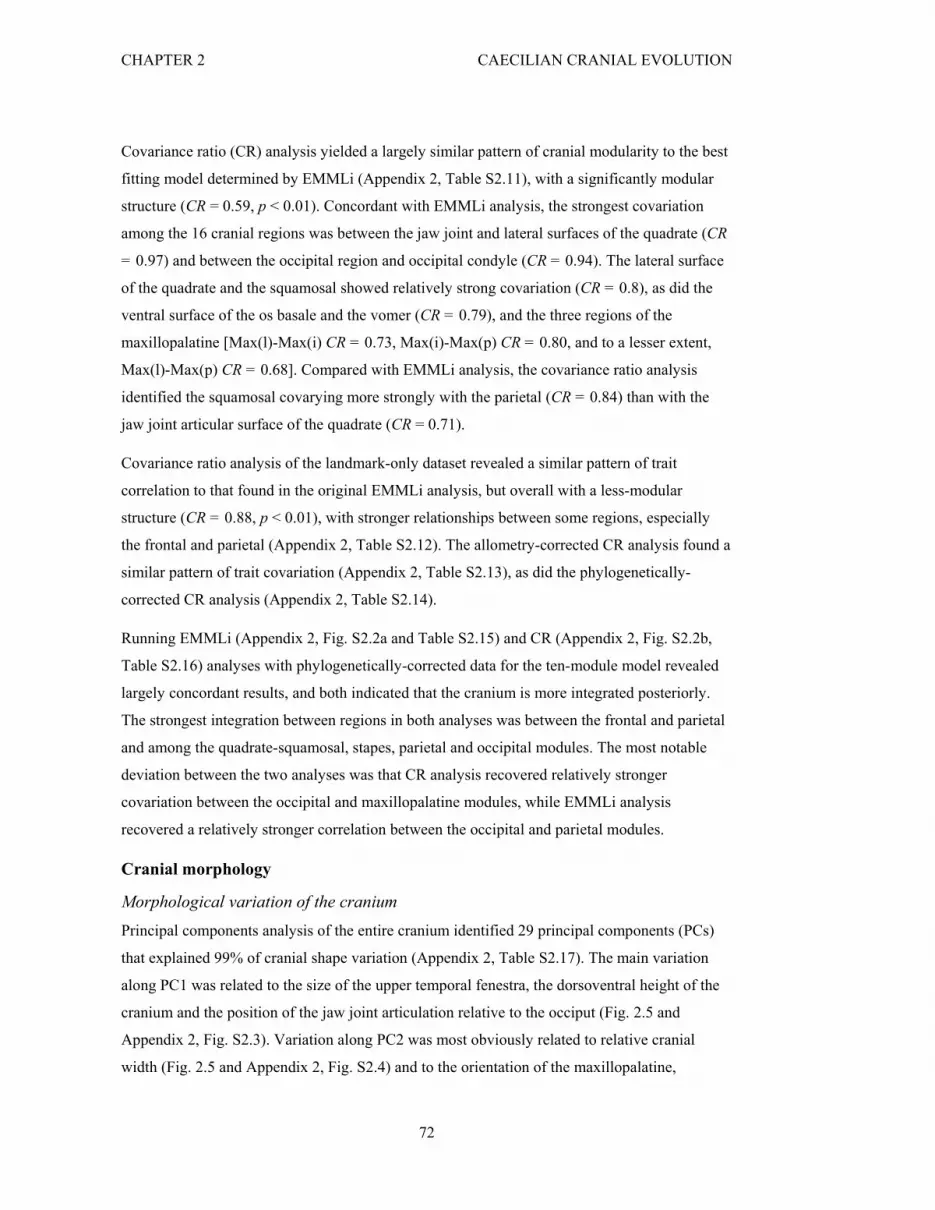
CHAPTER 2 CAECILIAN CRANIAL EVOLUTION
72
Covariance ratio (CR) analysis yielded a largely similar pattern of cranial modularity to the best
fitting model determined by EMMLi (Appendix 2, Table S2.11), with a significantly modular
structure (CR = 0.59, p < 0.01). Concordant with EMMLi analysis, the strongest covariation
among the 16 cranial regions was between the jaw joint and lateral surfaces of the quadrate (CR
= 0.97) and between the occipital region and occipital condyle (CR = 0.94). The lateral surface
of the quadrate and the squamosal showed relatively strong covariation (CR = 0.8), as did the
ventral surface of the os basale and the vomer (CR = 0.79), and the three regions of the
maxillopalatine [Max(l)-Max(i) CR = 0.73, Max(i)-Max(p) CR = 0.80, and to a lesser extent,
Max(l)-Max(p) CR = 0.68]. Compared with EMMLi analysis, the covariance ratio analysis
identified the squamosal covarying more strongly with the parietal (CR = 0.84) than with the
jaw joint articular surface of the quadrate (CR = 0.71).
Covariance ratio analysis of the landmark-only dataset revealed a similar pattern of trait
correlation to that found in the original EMMLi analysis, but overall with a less-modular
structure (CR = 0.88, p < 0.01), with stronger relationships between some regions, especially
the frontal and parietal (Appendix 2, Table S2.12). The allometry-corrected CR analysis found a
similar pattern of trait covariation (Appendix 2, Table S2.13), as did the phylogenetically-
corrected CR analysis (Appendix 2, Table S2.14).
Running EMMLi (Appendix 2, Fig. S2.2a and Table S2.15) and CR (Appendix 2, Fig. S2.2b,
Table S2.16) analyses with phylogenetically-corrected data for the ten-module model revealed
largely concordant results, and both indicated that the cranium is more integrated posteriorly.
The strongest integration between regions in both analyses was between the frontal and parietal
and among the quadrate-squamosal, stapes, parietal and occipital modules. The most notable
deviation between the two analyses was that CR analysis recovered relatively stronger
covariation between the occipital and maxillopalatine modules, while EMMLi analysis
recovered a relatively stronger correlation between the occipital and parietal modules.
Cranial morphology
Morphological variation of the cranium
Principal components analysis of the entire cranium identified 29 principal components (PCs)
that explained 99% of cranial shape variation (Appendix 2, Table S2.17). The main variation
along PC1 was related to the size of the upper temporal fenestra, the dorsoventral height of the
cranium and the position of the jaw joint articulation relative to the occiput (Fig. 2.5 and
Appendix 2, Fig. S2.3). Variation along PC2 was most obviously related to relative cranial
width (Fig. 2.5 and Appendix 2, Fig. S2.4) and to the orientation of the maxillopalatine,

CHAPTER 2 CAECILIAN CRANIAL EVOLUTION
73
squamosal, and quadrate. Along PC3, relative cranial width also varied, as well as the curvature
of the ventral rim of the cranium in lateral view (Appendix 2, Fig. S2.5).
The plot of the first two PCs (Fig. 2.5) most clearly separated E. bicolor and Rhinatrema
bivittatum (the two sampled members of Rhinatrematidae, the sister group to all other
caecilians) from the lungless (and morphologically highly disparate, Wilkinson & Nussbaum
1999) typhlonectid Atretochoana eiselti. Along PC3, A. eiselti was again representative of one
extreme, with sampled Ichthyophiidae at the other extreme (Appendix 2, Fig. S2.6). The
distribution of taxa in a phylomorphospace (Appendix 2, Fig. S2.7) suggested that variation in
cranial morphology was somewhat phylogenetically structured, discussed further below,
although close relatives were often not positioned close together.
Figure 2.5. Morphospace of all 35 specimens constructed using the entire landmark and semilandmark
dataset. Extreme shapes representing the positive and negative extremes along PC1 and PC2 are
displayed, which were created by mirroring the landmark and semilandmark data and warping these data
along PC1 and PC2. For a morphospace of PC1-PC3, see Appendix 2, Fig. S2.6. For extreme shapes for
PC1, PC2 and PC3 in dorsal, ventral, lateral, anterior and posterior aspects see Appendix 2, Figs. S2.3-
2.5.

CHAPTER 2 CAECILIAN CRANIAL EVOLUTION
74
Morphological variation of individual cranial modules
Distributions in morphospace varied across the individual cranial modules, and the number of
PCs required to explain 99% of the variation ranged from six (stapes) to 24 (maxillopalatine).
Atretochoana eiselti was generally the furthest from the remaining species in morphospace,
most evidently for the quadrate-squamosal, stapes and occipital modules. However, A. eiselti
occupied a similar position to other species for the nasopremaxilla (palatal surface), the
pterygoid and the ventral os basale-vomer modules. Specimens of Rhinatrematidae (E. bicolor
and R. bivittatum) occupied similar, extreme positions in morphospace for most cranial modules
(including the parietal, quadrate-squamosal, and ventral os basale-vomer modules).
Shape variation for each module was assessed from the extreme shapes along PC1 (Fig. 2.6),
and specimens closest to each extreme were identified (see Appendix 2, Figs. S2.8-2.17, for
module morphospaces and extreme shapes). The main variation in the parietal module
(Appendix 2, Fig. S2.8) represented the bony enclosure of the vault, from a stegokrotaphic
(closed) cranium (e.g., M. vermiculatus), to a zygokrotaphic cranium (with a large upper
temporal fenestra, e.g., E. bicolor). The frontal module varied in shape from having
approximately parallel anterior and posterior margins (e.g., A. eiselti) to laterally diverging
anterior and posterior margins (Ichthyophis nigroflavus) (Appendix 2, Fig. S2.9). The quadrate-
squamosal module (Appendix 2, Fig. S2.10) varied from an anteroposteriorly elongate
squamosal and lateral surface of the quadrate, and transversely oriented jaw joint surface (e.g.,
A. eiselti), to a dorsoventrally taller squamosal, anteroposteriorly compressed lateral surface of
the quadrate and more dorsoventrally oriented jaw joint (e.g., P. kaupii). The latter two species
also represented the extremes for the shape of the stapes module (after removing specimens in
which this module is absent, Appendix 2, Fig. S2.11), from projecting posteriorly (A. eiselti) to
anteriorly (P. kaupii). The pterygoid module (after removing specimens in which this module is
absent) varied in the number of surfaces, from one (e.g., Oscaecilia ochrocephala) to two (e.g.,
Ichthyophis bombayensis), because this region was represented by the pterygoid and/or
pterygoid process of the quadrate (Appendix 2, Fig. S2.12). The main axis of variation for the
dorsal surface of the nasopremaxilla module related to a relatively smaller naris and larger bony
surface lateral to the naris at one extreme (e.g., B. braziliensis) and a relatively larger naris and
smaller bony surface lateral to the naris at the other extreme (e.g., C. lamottei) (Appendix 2,
Fig. S2.13). The depth of this module lateral to the naris revealed the variable presence of the
tentacular foramen occupying this position. The maxillopalatine module (Appendix 2, Fig.
S2.14) has changed shape in response to its housing of the orbit or tentacular foramen (or both).
A large maxillopalatine laterally was associated with a narrower ventral surface and larger
contribution of the palatine shelf to the choana (e.g., E. bicolor), with A. eiselti at the other
extreme. The palatal surface of the nasopremaxilla (Appendix 2, Fig. S2.15) varied in

CHAPTER 2 CAECILIAN CRANIAL EVOLUTION
75
anteroposterior depth, from deeper (e.g., C. bornmuelleri) to less tall (E. bicolor). The
anteroposterior elongation of the fenestra ovalis was reflected in the lateral margin of the
occipital module (Appendix 2, Fig. S2.16), which varied from elongate anteroposteriorly (e.g.,
Boulengerula boulengeri) to approximately circular (e.g., A. eiselti). This module also
incorporated variation in the position of the occipital condyle, likely reflecting differences in the
orientation of the cranial-vertebral articulation. For the ventral os basale-vomer module
(Appendix 2, Fig. S2.17), the posterior process of the vomer extended further posteriorly and
partially overlaid the ventral surface of the os basale at one extreme (e.g., O. ochrocephala),
whereas at the other extreme the posterior process of the vomer was more lateral to the ventral
surface of the os basale (e.g., E. bicolor).
Figure 2.6. Shape variation for each cranial module. Exploded view of positive (+) and negative (-) shape
extremes for each cranial module along PC1 (see Fig. 2.4 for module definitions). Siphonops annulatus is
also presented in lateral (left) and ventral (right) aspect, with the landmarks and semilandmarks coloured
by module. Extreme shapes were generated from individual module PCAs, so PC axes do not align and
direction is arbitrary. All modules are presented in one view, except the maxillopalatine module (two
views). Aspect of modules is consistent with cranial aspect, except for the occipital (posterior view) and
the parietal and frontal (dorsal view). Specimens lacking a pterygoid or stapes module were removed
from these PCAs, for visualisation purposes only.
Phylogeny
Significant phylogenetic signal in cranial shape was found (Kmult = 0.87, p < 0.01). The degree
of phylogenetic signal varied across cranial modules, being weaker for the posterior of the
cranium (Fig. 2.7a and Table 2.3). Shape was not explained by phylogeny for one posterior
module: the occipital (Kmult = 0.66, p = 0.06). For the stapes and quadrate-squamosal modules,

CHAPTER 2 CAECILIAN CRANIAL EVOLUTION
76
phylogenetic signal was significant but relatively low (Kmult = 0.70, p = 0.04 and Kmult = 0.72,
p= 0.02 respectively). Shape variation for all remaining cranial modules had stronger
phylogenetic signal (Kmult = 0.87 – 1.16, p < 0.01 for all). The considerably weaker phylogenetic
signal observed posteriorly in the cranium was, at least in part, explained by A. eiselti, because
of its particularly extreme quadrate, squamosal and stapes morphologies. Results of analyses
with and without this species are reported in Table 2.3. Variation in cranial size, as measured by
centroid size (Appendix 2, Table S2.18), was not significantly phylogenetically structured (Kmult
= 0.65, p = 0.18).
Figure 2.7. Influence of phylogeny and allometry across the ten cranial modules. Network graphs from
EMMLi analysis of the ten-module model. Modules are graded low (yellow) to high (red) based on (A)
phylogenetic signal (Kmult) and (B) evolutionary allometry (R2). Circle size is proportional to internal trait
correlation; line thickness is proportional to between-module trait correlation. Layout corresponds
approximately to a cranium in right lateral view. See Fig. 2.4 for module definitions.

CHAPTER 2 CAECILIAN CRANIAL EVOLUTION
77
Table 2.3. Evolutionary rate, disparity, and integration and allometric, phylogenetic, and ecological
signal in caecilian cranial modules. Results for the ten identified cranial modules, where the within-
module correlations are taken from EMMLi analysis using phylogenetically-corrected data. Significance
of results for the last four columns is as follows: p values significant at the following alpha levels: * ≤
0.05, ** ≤ 0.01, *** ≤ 0.001. A ‘/’ indicates significance before/after correction for multiple tests for
differences in module shape related to fossoriality. (See Fig. 2.4 for module definitions).
Mod
ule
Rate σ
2mu
lt (×10
-8)
Disp
arity (Procru
stes
variance) (×
10-6)
With
in-m
odu
le
correlation
Evolu
tionary allom
etry
(R2)
Ph
ylogenetic sign
al
(Km
ult )
Ph
ylogenetic sign
al
(Km
ult ), exclu
din
g
Atretoch
oana
Fossoriality p
hylogen
etic
AN
OV
A (R
2)
Frontal 1.33 6.32 0.70 0.05 0.87*** 1.02*** 0.045*/
Parietal 1.67 8.43 0.71 0.22*** 1.05*** 1.32*** 0.102***
/**
Nasopremaxilla
(dorsal)
1.19 5.86 0.49 0.06* 0.93*** 0.97*** 0.027/
Maxillopalatine 1.64 7.84 0.50 0.19*** 0.93*** 0.97*** 0.046**/*
Occipital 1.25 4.71 0.73 0.37*** 0.66 0.75** 0.034/
Quadrate-
Squamosal
2.73 10.24 0.71 0.21*** 0.72* 1.12*** 0.059*/*
Ventral os
basale-vomer
0.91 4.97 0.46 0.12** 0.99*** 1.03*** 0.038/
Nasopremaxilla
(palatal)
0.97 5.51 0.79 0.11* 1.16*** 1.20*** 0.056*/
Pterygoid 1.65 10.60 0.78 0.11* 1.13*** 1.21*** 0.014/
Stapes 1.28 4.76 0.87 0.19*** 0.70* 1.05*** 0.033/

CHAPTER 2 CAECILIAN CRANIAL EVOLUTION
78
Allometry
Visual inspection of morphological changes of the cranium associated with allometry revealed
that a smaller cranial size was associated with a narrower, more elongate cranium, an absence of
an upper temporal fenestra, and anterior placement of the jaw joint (Fig. 2.8, and see Appendix
2, Fig. S2.18, for a morphospace colour-graded by centroid size). Reconstructed morphologies
were also generated for changes associated with size for each module (see Fig. 2.9). Smaller
size of the occipital module was associated with relatively larger otic capsules (see Fig. 2.10).
Evolutionary allometry (accounting for phylogeny) for the entire cranium accounted for 16% of
the shape variation (R2 = 0.16, p < 0.01). Allometry was not found to influence all cranial
modules equally, with a stronger influence generally observed in posterior modules (Fig. 2.7b
and Table 2.3). The occipital module was the most strongly influenced by allometry (R2 = 0.37,
p < 0.01). Only the frontal module was nonsignificant for the allometric influence on
morphology (R2 = 0.05, p = 0.14). Allometry accounted for 6–22% of the shape variation in the
remaining modules.
Figure 2.8. Whole cranial morphology at (A) minimum and (B) maximum size.

CHAPTER 2 CAECILIAN CRANIAL EVOLUTION
79
Figure 2.9. Module morphologies at minimum (left) and maximum (right) size. Allometry was
investigated using global Procrustes alignment. The occipital module was the most influenced by
allometry and can be seen in Fig. 2.10. Remaining modules are in descending order of strength of
allometry: (A) parietal, (B) quadrate-squamosal, (C) maxillopalatine, (D) stapes, (E) ventral os basale-
vomer, (F) pterygoid, (G) nasopremaxilla (palatal surface), (H) nasopremaxilla (dorsal surface). The
frontal module is excluded because it did not display significant allometric signal.

CHAPTER 2 CAECILIAN CRANIAL EVOLUTION
80
Figure 2.10. The occipital module morphology (posterior view), at (A) minimum and (B) maximum size.
Note the ‘bulging’ of this module dorsally at minimum size, in the position of the otic capsule, suggesting
smaller species have relatively larger otic capsules.
Ecology
Reproductive strategy (N = 33) and degree of fossoriality (N = 35) were found to be small but
significant influences on cranial shape after phylogenetic correction (R2 = 0.03, p = 0.02 and R2
= 0.05, p < 0.01 respectively), and remained significant after multiple-test correction (p = 0.04
and p = 0.01 respectively). Life history strategy (N = 34) was not found to be significantly
associated with variation in cranial shape (R2 = 0.05, p = 0.08).
For the analyses of individual modules, phylogenetic ANOVAs found that five of the ten cranial
modules exhibited a significant influence of degree of fossoriality on morphology (the parietal,
quadrate-squamosal, nasopremaxilla (palatal surface), maxillopalatine and frontal modules- see
Table 2.3). Multiple-test correction on the phylogenetic ANOVAs retained the parietal,
quadrate-squamosal and maxillopalatine modules as exhibiting a significant influence of degree
of fossoriality on morphology (Table 2.3).
Rate shifts associated with major ecological transitions
A significant shift in rate of morphological evolution coincided with the emergence of obligate
aquatic adults (observed rate ratio of obligate to non-obligate aquatic species: 5.28, p < 0.01),
although this result was explained largely by the morphologically highly disparate, viviparous
(and aquatic) A. eiselti: a significant rate shift here was not recovered when this species was
excluded. Rate shifts in morphological evolution were also identified coincident with the
evolutionary origin of direct development (observed rate ratio of direct to indirect developers:
1.42 p = 0.04) and of viviparity (observed rate ratio of viviparous to oviparous species: 2.20, p

CHAPTER 2 CAECILIAN CRANIAL EVOLUTION
81
= 0.01), with faster rates of morphological evolution occurring after each innovation. After
multiple-test correction, all rate shifts remained significant (p < 0.05).
Evolutionary rates and disparity
Individual landmark and semilandmark disparity and rate
When mean rate of morphological evolution (Fig. 2.11) and disparity (Fig. 2.12) of individual
landmarks and semilandmarks were visualised, high rates and disparity were found consistently
for landmarks and semilandmarks close to apertures. The maxillopalatine was found to have
highest disparity and evolutionary rates laterally, where the orbit and tentacular foramen are
variably housed. For the palatine shelf of the maxillopalatine, the highest disparity and rates
were found on its post-choanal process, reflecting the variable contribution of this bone to the
choanal rim. The nasopremaxilla had highest rates and disparity laterally, coinciding with the
area variably involved in housing the tentacular foramen. The parietal landmarks and
semilandmarks with the highest disparity and rate of morphological evolution were typically
close to the variably present upper temporal fenestra. Some localised areas within modules were
found to have little variation in the disparity and rate of morphological evolution of individual
landmarks and semilandmarks, exhibiting consistently high (jaw joint articulation) or low
(occipital condyle) values.
Analyses of landmarks and semilandmarks within cranial modules found a wide spread of rates
and disparity, with overall strong but variable correlation between these. Although most
landmarks and semilandmarks followed the relationship expected for evolutionary rate and
disparity under a Brownian motion model (Fig. 2.11), some pterygoid and parietal landmarks
and semilandmarks exhibited higher disparity than expected given their reconstructed
evolutionary rates. Conversely, most quadrate-squamosal module landmarks and semilandmarks
(and a few stapes landmarks and semilandmarks) exhibited lower disparity than expected given
their rate.

CHAPTER 2 CAECILIAN CRANIAL EVOLUTION
82
Figure 2.11. Evolutionary rate of individual landmarks and semilandmarks. (A) Regression of disparity
on evolutionary rate for each landmark and semilandmark, colour coded by module. The red line is the
regression for the entire cranium. The blue line is the Brownian motion prediction, with shaded 95%
interval. (B-F) Landmarks and semilandmarks on the sampled Siphonops annulatus cranium, colour
coded by evolutionary rate from low (purple) to high (red) in (B) dorsal, (C) anterior, (D) ventral, (E)
posterior, and (F) lateral aspect.

CHAPTER 2 CAECILIAN CRANIAL EVOLUTION
83
Figure 2.12. Disparity of individual landmarks and semilandmarks. Landmarks and semilandmarks
displayed on Siphonops annulatus and colour coded by magnitude of disparity, measured as Procrustes
variance, from low (purple) to high (red), in (A) dorsal, (B) anterior, (C) ventral, (D) posterior, and (E)
lateral aspect.
Module integration, disparity and rate
Disparity was found to be greatest in the most kinetic modules of the (generally akinetic)
caecilian cranium (Table 2.3), with the pterygoid module exhibiting the highest disparity (1.06
×10-5), followed by the quadrate-squamosal module (1.02 × 10⁻⁵). The occipital and stapes
modules had the lowest disparity (4.71 × 10⁻⁶, 4.76 × 10⁻⁶ respectively). Most modules had
significantly different disparities (Appendix 2, Table S2.19). Of the 45 pairwise differences
between the modules, 32 were significant (p < 0.05, of which 24 were highly significant, p <
1.00 × 10⁻⁷) and 13 were not (p > 0.05). The three largest differences were the pterygoid module
with the occipital, stapes and ventral os basale-vomer modules, respectively. There was a
nonsignificant relationship between integration and disparity (Fig. 2.13a) (Multiple R2 < 0.01, p
= 0.90). The pterygoid and quadrate-squamosal modules had high integration and disparity.
However, the stapes, nasopremaxilla (palatal surface) and occipital modules all had high
integration but very low disparity. Low integration and disparity was found for both the dorsal
surface of the nasopremaxilla and the ventral os basale-vomer modules. A nonsignificant
relationship was also evident from the regression of rates against integration (Fig. 2.13b)
(Multiple R2 < 0.01, p = 0.91). The quadrate-squamosal module had a significantly faster

CHAPTER 2 CAECILIAN CRANIAL EVOLUTION
84
evolutionary rate than the occipital, ventral os basale-vomer and both nasopremaxilla modules,
and the parietal had a significantly higher rate than the nasopremaxilla (palatal surface) module.
No other rates were significantly different (see Appendix 2, Table S2.20).
Figure 2.13. The relationship of integration with disparity and evolutionary rate. Regressions of
magnitude of integration (estimated within-module correlation) on (A) disparity and (B) evolutionary rate
for each cranial module (See Fig. 2.4 for module definitions). All relationships were non-significant.
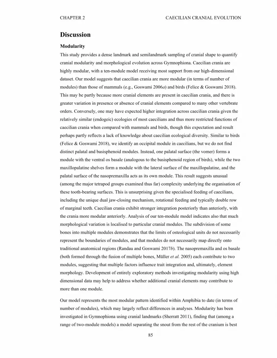
CHAPTER 2 CAECILIAN CRANIAL EVOLUTION
85
Discussion
Modularity
This study provides a dense landmark and semilandmark sampling of cranial shape to quantify
cranial modularity and morphological evolution across Gymnophiona. Caecilian crania are
highly modular, with a ten-module model receiving most support from our high-dimensional
dataset. Our model suggests that caecilian crania are more modular (in terms of number of
modules) than those of mammals (e.g., Goswami 2006a) and birds (Felice & Goswami 2018).
This may be partly because more cranial elements are present in caecilian crania, and there is
greater variation in presence or absence of cranial elements compared to many other vertebrate
orders. Conversely, one may have expected higher integration across caecilian crania given the
relatively similar (endogeic) ecologies of most caecilians and thus more restricted functions of
caecilian crania when compared with mammals and birds, though this expectation and result
perhaps partly reflects a lack of knowledge about caecilian ecological diversity. Similar to birds
(Felice & Goswami 2018), we identify an occipital module in caecilians, but we do not find
distinct palatal and basisphenoid modules. Instead, one palatal surface (the vomer) forms a
module with the ventral os basale (analogous to the basisphenoid region of birds), while the two
maxillopalatine shelves form a module with the lateral surface of the maxillopalatine, and the
palatal surface of the nasopremaxilla acts as its own module. This result suggests unusual
(among the major tetrapod groups examined thus far) complexity underlying the organisation of
these tooth-bearing surfaces. This is unsurprising given the specialised feeding of caecilians,
including the unique dual jaw-closing mechanism, rotational feeding and typically double row
of marginal teeth. Caecilian crania exhibit stronger integration posteriorly than anteriorly, with
the crania more modular anteriorly. Analysis of our ten-module model indicates also that much
morphological variation is localised to particular cranial modules. The subdivision of some
bones into multiple modules demonstrates that the limits of osteological units do not necessarily
represent the boundaries of modules, and that modules do not necessarily map directly onto
traditional anatomical regions (Randau and Goswami 2017b). The nasopremaxilla and os basale
(both formed through the fusion of multiple bones, Müller et al. 2005) each contribute to two
modules, suggesting that multiple factors influence trait integration and, ultimately, element
morphology. Development of entirely exploratory methods investigating modularity using high
dimensional data may help to address whether additional cranial elements may contribute to
more than one module.
Our model represents the most modular pattern identified within Amphibia to date (in terms of
number of modules), which may largely reflect differences in analyses. Modularity has been
investigated in Gymnophiona using cranial landmarks (Sherratt 2011), finding that (among a
range of two-module models) a model separating the snout from the rest of the cranium is best

CHAPTER 2 CAECILIAN CRANIAL EVOLUTION
86
supported across three levels of variation (fluctuating asymmetry, within-, and among-species).
For the anuran Rhinella granulosa complex, a range of best supported patterns of modularity
across species has been found, including models based on functional, hormonal-regulated and
developmental modules (Simon & Marroig 2017). No significant modular structure was found
for the anuran family Myobatrachidae (Vidal-García & Keogh 2017). These studies did not
investigate highly modular models, limiting exploration to two- (Sherratt 2011), three- (Vidal-
García & Keogh 2017) and three- and five-module (Simon & Marroig 2017) models. Our
inclusion of semilandmark data in addition to landmarks allows a denser sampling of
morphology across cranial regions and reduced reliance on landmarks located predominantly at
bone or region boundaries, thus facilitating a more extensive investigation of a wider range of
modular structures. Previous studies of other taxa using semilandmarks have identified more
modular systems (e.g., Parr et al. 2016; Felice & Goswami 2018), suggesting, perhaps
unsurprisingly, that high density morphometric data generally recover evidence for more
modular structures, which may be expected in complex systems such as crania. Increasing
numbers of landmarks or testing more modular patterns with landmark-only datasets may also
result in more modular patterns, but this result is also likely due to the sampling of morphology
that is not limited to boundaries or discrete structures. Analysis of our landmark-only dataset
finds stronger correlations among adjacent cranial regions (e.g., the frontal and parietal) when
compared with our full dataset, consistent with the hypothesis that integration between regions
can be overestimated when using only landmarks, as these largely represent the shared
boundaries of elements rather than their overall structure.
Phylogeny and allometry
Our investigation into phylogenetic and allometric influences on caecilian cranial morphology
produces broadly concurrent results to those of Sherratt et al. (2014), with evolutionary
allometry accounting for 14–16% of the morphological variation in both datasets. Strong
phylogenetic structure is found in both studies, but our study finds greater overlap among clades
in morphospace (although our morphospace distribution is not allometry-corrected). This
comparison demonstrates that both approaches (landmarks and surface-based methods) recover
broadly similar patterns of macroevolution but surface-based methods may provide distinct
insights. Our surface-based method also reveals the interplay of phylogenetic and allometric
constraints across caecilian crania. The quadrate-squamosal, occipital and stapes modules
exhibit relatively weak phylogenetic signal. This low phylogenetic signal in posterior modules
is partly driven by one species, A. eiselti, which exhibits particularly extreme quadrate,
squamosal and stapes morphologies, compared with its closest relatives. Atretochoana eiselti is
positioned especially far from P. kaupii in a PC1- PC2 morphospace (Fig. 2.5), revealing
extreme morphological divergence. Atretochoana eiselti is also the only lungless caecilian,

CHAPTER 2 CAECILIAN CRANIAL EVOLUTION
87
which has been interpreted as causally linked to its unique cranial shape (Wilkinson &
Nussbaum 1997). Shape variation for the occipital module has low phylogenetic signal even
when excluding the highly disparate A. eiselti, but exhibits the highest influence of allometry on
shape. The size of the semi-circular canals, and their distance from the centre of the organism, is
associated with improved balance (Jones & Spells 1963), which is considered important for
fossorial predators with reduced reliance on visual cues (Gans 1974). Maintaining a minimum
size of the otic capsules may explain the strong influence of allometry observed for this module,
as can be seen in the shape changes associated with allometry (Fig. 2.1). Most posterior cranial
modules, although exhibiting low phylogenetic signal in shape variation, bear the strongest
indications of the influence of allometry. Conversely, modules with the strongest phylogenetic
signal [nasopremaxilla (palatal surface) and pterygoid] show relatively little effect of allometry
(second and third lowest across the cranium, respectively). These contrasting patterns of
phylogeny and allometry suggest that cranial module size is not generally phylogenetically
structured, an interpretation supported by centroid size lacking significant phylogenetic signal
(Kmult = 0.65, p = 0.18).
Ecology
Reproductive strategy and degree of fossoriality are found to be small but significant influences
on gross cranial morphology in caecilians, even after correcting for multiple tests. Life history is
not found to be a significant influence on cranial shape. Degree of fossoriality has the strongest
influence on the shape of the parietal and quadrate-squamosal modules, consistent with the
understanding that more dedicated fossoriality in caecilians is associated with a more solidly
constructed, stegokrotaphic cranium (e.g., Nussbaum 1977; Gower et al. 2004; though see
Kleinteich et al. 2012). A closed, stegokrotaphic cranium in caecilians is characterised by the
contact of the parietal and squamosal bones and the covering of the jaw adductor muscles. In
Gymnophiona, the interhyoideus posterior muscle has become a novel jaw-closing muscle,
allowing a compensatory reduction in size of the ancestral jaw adductors and closure of the
upper temporal fenestra in some species (Nussbaum 1983). This rearrangement of jaw-closing
muscles across caecilians influences the morphology of the jaw joint articular surface of the
quadrate. Surprisingly, signal for the influence of degree of fossoriality on the shape of the
snout (the dorsal surface of the nasopremaxilla) is relatively weak, despite the snout’s role in
head-first burrowing. On a larger scale, the main axes of cranial shape variation across caecilian
crania are associated with solidity (closed temporal fenestra, PC1) and elongation (bullet-shaped
cranium, PC2), which are both considered to correlate with burrowing ability (e.g., Nussbaum
1977; Gower et al. 2004), although may also be related to miniaturisation (because similarly-
sized specimens cluster in morphospace). This investigation into the influences on cranial
morphology is limited by the scarcity of ecological data (e.g., Gower & Wilkinson 2005;

CHAPTER 2 CAECILIAN CRANIAL EVOLUTION
88
Wilkinson 2012) and the lack of current understanding concerning the relationships among
endogeicity, burrowing ability and miniaturisation for caecilians, highlighting the requirement
for additional fieldwork and studies of natural history. In addition, improved knowledge of
caecilian ecology would enable future studies to better characterise degree of fossoriality,
without partial reliance on cranial characters.
Atretochoana eiselti is a clear outlier in morphospace. Our analyses concur with Wilkinson and
Nussbaum’s (1999) cladistic analysis, which used 141 morphological characters to resolve
evolutionary relationships within Typhlonectidae, finding the terminal branch subtending A.
eiselti to exhibit the fastest rate of morphological evolution. Together, these analyses contribute
clear quantitative support for the qualitative documentation and interpretation of the extremely
divergent cranial morphology of A. eiselti (Nussbaum & Wilkinson 1995; Wilkinson &
Nussbaum 1997). As the largest lungless tetrapod and only known lungless caecilian (Wilkinson
& Nussbaum 1997; Wilkinson et al. 2014), the constraint of respiratory buccal pumping has
been lifted, and this release (along with a reduction of constraints associated with fossoriality) is
reflected in cranial morphology, with a uniquely large gape and cheek architecture (Wilkinson
& Nussbaum 1997; Wilkinson et al. 1998). Atretochoana eiselti is a member of a clade
including the three obligate aquatic typhlonectid species in our dataset, and the significant
increase in the rate of cranial module shape evolution along the stem of this lineage suggests
that this ecological transition promoted a faster rate of cranial evolution (although the signal for
this is caused to a substantial degree by A. eiselti). The faster rates of cranial module shape
evolution associated with the emergence of direct development and viviparity (and the
significant influence of reproductive strategy on cranial morphology) indicates a role for early
life history mode substantially influencing adult cranial morphology.
Within-module analyses
Using a surface-based approach, morphological variation can be visualised and quantified in
great detail, and disparity and rates of morphological evolution can be investigated within
cranial modules. Landmarks are difficult to identify consistently in the most disparate regions of
caecilian crania, thus these regions would be underrepresented using traditional landmarking
approaches. Observation of the extreme morphologies along the main axes of variation for each
individual cranial module allows a quantification of anatomical variation across caecilians. In
addition to quantifying morphological variation within modules, disparity and rate of
morphological evolution can be compared within and across modules. Disparity and rate of
cranial morphological evolution are strongly correlated in Gymnophiona, and vary widely
within each cranial module, with high disparity and rates particularly evident in areas associated
with major cranial fenestrae and foramina. Comparing the relationship between observed
landmark and semilandmark evolutionary rates and disparities with that expected under a

CHAPTER 2 CAECILIAN CRANIAL EVOLUTION
89
Brownian motion model reveals that most quadrate-squamosal (and some stapes) landmarks and
semilandmarks are less disparate than expected. The quadrate-squamosal module exhibits the
third lowest phylogenetic signal, and the stapes second lowest, suggesting that these modules
may have undergone convergent evolution.
How integration influences rates and disparity
Our results do not support a strong relationship between magnitude of integration and either
evolutionary rate or disparity. This is similar to findings from the comparison of the crania of
domestic dogs to other Carnivora, which showed that domestic dog crania are incredibly
disparate (a similar magnitude to the disparity across the entire order), and yet integration and
modularity of the cranium appear relatively conserved throughout domestication (Drake &
Klingenberg 2010). In our study, highly integrated modules have both more (e.g., quadrate-
squamosal and pterygoid) and less (e.g., stapes and occipital) disparity than do weakly
integrated modules. Among cranial modules with strong integration, the cheek region modules
(quadrate-squamosal, pterygoid) display the highest disparity but the otic region modules
(occipital, stapes) display the lowest. We interpret this dichotomy as indicating that integration
may promote evolutionary exploration of morphospace for some cranial modules but constrain
it for others, or that integration may not impact morphological disparity to any substantial
degree. The caecilian cheek region is variably kinetic (Wilkinson & Nussbaum 1997; Summers
& Wake 2005), with feeding function perhaps varying among species according to diet and
habitat. The otic region however may be more constrained in shape evolution, as a result of
minimum requirements associated with the functionality of the sensory system housed in the
otic capsules. The otic region may also be constrained by a narrower spectrum of more
fundamental function in cranial-skeletal articulation. Whereas previous studies have found some
support for greater integration of traits constraining morphological evolution and limiting
disparity (e.g., Felice & Goswami 2018), others have found support for greater integration
facilitating specialisation (Randau and Goswami 2017b) or a mixed pattern (Goswami and Polly
2010b). These differences may depend on the alignment of each module’s direction of selection
with the path that integration facilitates in morphospace (Hansen & Houle 2008; Goswami et al.
2014; Linde-Medina et al. 2016; Felice et al. 2018). Our results suggest that integration may
variably limit or promote morphological evolution (or have little effect), and studies of more
systems are required before general patterns might be detected and exceptions explained.
We are unable to detect any significant relationship between evolutionary rate and integration,
providing further evidence that integration may not necessarily influence the rate of
morphological evolution (Goswami et al. 2014; Felice et al. 2018). Not all modules have
significantly different evolutionary rates, in concordance with a previous study that found the
best-supported model of modularity is not necessarily fully congruent with the partitioning of
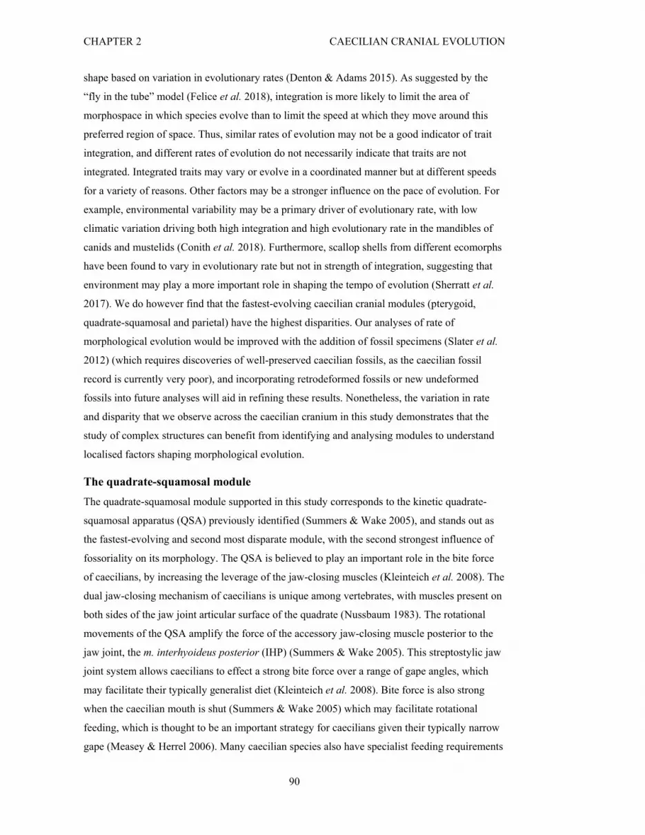
CHAPTER 2 CAECILIAN CRANIAL EVOLUTION
90
shape based on variation in evolutionary rates (Denton & Adams 2015). As suggested by the
“fly in the tube” model (Felice et al. 2018), integration is more likely to limit the area of
morphospace in which species evolve than to limit the speed at which they move around this
preferred region of space. Thus, similar rates of evolution may not be a good indicator of trait
integration, and different rates of evolution do not necessarily indicate that traits are not
integrated. Integrated traits may vary or evolve in a coordinated manner but at different speeds
for a variety of reasons. Other factors may be a stronger influence on the pace of evolution. For
example, environmental variability may be a primary driver of evolutionary rate, with low
climatic variation driving both high integration and high evolutionary rate in the mandibles of
canids and mustelids (Conith et al. 2018). Furthermore, scallop shells from different ecomorphs
have been found to vary in evolutionary rate but not in strength of integration, suggesting that
environment may play a more important role in shaping the tempo of evolution (Sherratt et al.
2017). We do however find that the fastest-evolving caecilian cranial modules (pterygoid,
quadrate-squamosal and parietal) have the highest disparities. Our analyses of rate of
morphological evolution would be improved with the addition of fossil specimens (Slater et al.
2012) (which requires discoveries of well-preserved caecilian fossils, as the caecilian fossil
record is currently very poor), and incorporating retrodeformed fossils or new undeformed
fossils into future analyses will aid in refining these results. Nonetheless, the variation in rate
and disparity that we observe across the caecilian cranium in this study demonstrates that the
study of complex structures can benefit from identifying and analysing modules to understand
localised factors shaping morphological evolution.
The quadrate-squamosal module
The quadrate-squamosal module supported in this study corresponds to the kinetic quadrate-
squamosal apparatus (QSA) previously identified (Summers & Wake 2005), and stands out as
the fastest-evolving and second most disparate module, with the second strongest influence of
fossoriality on its morphology. The QSA is believed to play an important role in the bite force
of caecilians, by increasing the leverage of the jaw-closing muscles (Kleinteich et al. 2008). The
dual jaw-closing mechanism of caecilians is unique among vertebrates, with muscles present on
both sides of the jaw joint articular surface of the quadrate (Nussbaum 1983). The rotational
movements of the QSA amplify the force of the accessory jaw-closing muscle posterior to the
jaw joint, the m. interhyoideus posterior (IHP) (Summers & Wake 2005). This streptostylic jaw
joint system allows caecilians to effect a strong bite force over a range of gape angles, which
may facilitate their typically generalist diet (Kleinteich et al. 2008). Bite force is also strong
when the caecilian mouth is shut (Summers & Wake 2005) which may facilitate rotational
feeding, which is thought to be an important strategy for caecilians given their typically narrow
gape (Measey & Herrel 2006). Many caecilian species also have specialist feeding requirements

CHAPTER 2 CAECILIAN CRANIAL EVOLUTION
91
early in ontogeny, with intraoviducal feeding in viviparous species and maternal dermatophagy
(Kupfer et al. 2008) in some oviparous species. Functionally, the cheek region is therefore
critical in both precocial feeding of young and generalist feeding as adults. The pivotal roles of
the quadrate and squamosal in the unique dual jaw-closing mechanism may have driven the
formation of the quadrate-squamosal module. This module is likely a prime target of selection,
reflected in shape variation by its high disparity, rate of morphological evolution, and ecological
signal, and its weak phylogenetic signal.
Conclusion
Our high-dimensional morphological data have enabled us to quantitatively identify patterns
within and across modules and across the cranium, which has provided insights into the
hierarchical organisation and evolution of the caecilian cranium. Our analyses demonstrate that
caecilian crania are highly modular, and that shape evolution of caecilian crania is influenced by
reproductive strategy and degree of fossoriality, but the strength of this latter effect, along with
the extent of phylogenetic and allometric constraints, varies across the ten identified modules.
The unique dual jaw-closing mechanism and complex feeding mode of caecilians has likely
driven the formation of a highly disparate and fast-evolving quadrate-squamosal ‘cheek’
module, which appears a key target of selection within caecilian crania. Overall, magnitude of
module integration is not consistently associated with higher or lower shape disparity or rate of
morphological evolution, suggesting that strong integration of traits variably promotes or
restricts (or has little effect upon) morphological evolution of caecilian cranial modules.

CHAPTER 2 CAECILIAN CRANIAL EVOLUTION
92

CHAPTER 3 FROG CRANIAL INTEGRATION
93
CHAPTER 3
EVOLUTIONARY INTEGRATION OF THE FROG
CRANIUM
Abstract
Anurans (frogs) are the most species-rich living amphibian order, numbering over 7100 species,
and exhibiting a range of cranial forms that pose significant challenges for quantifying cranial
morphology across the clade. Most previous studies of cranial variation in frogs have been
limited in either taxonomic or morphological sampling, hindering investigations encompassing
the full diversity of ecologies or developmental modes. Here, we focus on cranial integration, or
the interactions among cranial traits, and do so by quantifying anuran cranial morphology using
high-dimensional morphometrics for 172 anuran species, including representatives of every
extant anuran family. This is the most comprehensive dataset of anuran cranial morphology to
date, in terms of both taxonomic sampling and shape description. We investigate patterns of
evolutionary integration and modularity in cranial morphology using 995 landmarks and sliding
semilandmarks subjected to maximum likelihood and covariance ratio analysis. Both analytical
approaches support the anuran cranium as being highly modular, comprising 13 modules
including a multi-bone, functional ‘suspensorium’ module. This pattern is strikingly similar to
that identified previously for caecilian crania in Chapter 2, suggesting conservation of cranial
integration across these two lissamphibian clades. Developmental processes have a small
influence on cranial integration in frogs, with stronger integration observed in direct developers,
compared to those exhibiting metamorphosis with a feeding larval stage. Ossification sequence
timings also influence integration, with higher integration observed in late-ossifying bones.
Contrary to some studies, a consistent relationship between degree of integration and either
evolutionary rate or disparity was not observed in the anuran cranium.
Introduction
Phenotypic integration describes the covariation or correlation of traits and is an inherent
property of any biological system (Olson & Miller 1958). Phenotypic integration can result
from genetic, developmental or functional interactions, and it is thought that patterns of genetic
and developmental integration may evolve adaptively to promote functional integration (Riedl
1978; Cheverud 1984; Wagner & Altenberg 1996). However, our understanding of how
integration may influence evolution is incomplete. Studies have found that high levels of
integration can constrain morphological diversity (disparity) and/or evolutionary rate (Goswami
and Polly 2010b; Felice and Goswami 2018). Conversely, the opposite effect has also been
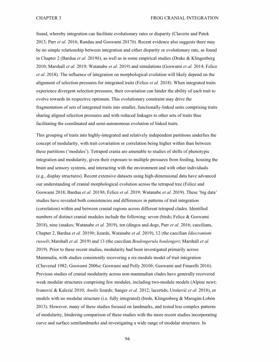
CHAPTER 3 FROG CRANIAL INTEGRATION
94
found, whereby integration can facilitate evolutionary rates or disparity (Claverie and Patek
2013; Parr et al. 2016; Randau and Goswami 2017b). Recent evidence also suggests there may
be no simple relationship between integration and either disparity or evolutionary rate, as found
in Chapter 2 (Bardua et al. 2019b), as well as in some empirical studies (Drake & Klingenberg
2010; Marshall et al. 2019; Watanabe et al. 2019) and simulations (Goswami et al. 2014; Felice
et al. 2018). The influence of integration on morphological evolution will likely depend on the
alignment of selection pressures for integrated traits (Felice et al. 2018). When integrated traits
experience divergent selection pressures, their covariation can hinder the ability of each trait to
evolve towards its respective optimum. This evolutionary constraint may drive the
fragmentation of sets of integrated traits into smaller, functionally-linked units comprising traits
sharing aligned selection pressures and with reduced linkages to other sets of traits thus
facilitating the coordinated and semi-autonomous evolution of linked traits.
This grouping of traits into highly-integrated and relatively independent partitions underlies the
concept of modularity, with trait covariation or correlation being higher within than between
these partitions (‘modules’). Tetrapod crania are amenable to studies of shifts of phenotypic
integration and modularity, given their exposure to multiple pressures from feeding, housing the
brain and sensory systems, and interacting with the environment and with other individuals
(e.g., display structures). Recent extensive datasets using high-dimensional data have advanced
our understanding of cranial morphological evolution across the tetrapod tree (Felice and
Goswami 2018; Bardua et al. 2019b; Felice et al. 2019; Watanabe et al. 2019). These ‘big data’
studies have revealed both consistencies and differences in patterns of trait integration
(correlation) within and between cranial regions across different tetrapod clades. Identified
numbers of distinct cranial modules include the following: seven (birds; Felice & Goswami
2018), nine (snakes; Watanabe et al. 2019), ten (dingos and dogs, Parr et al. 2016; caecilians,
Chapter 2, Bardua et al. 2019b; lizards, Watanabe et al. 2019), 12 (the caecilian Idiocranium
russeli; Marshall et al. 2019) and 13 (the caecilian Boulengerula boulengeri; Marshall et al.
2019). Prior to these recent studies, modularity had been investigated primarily across
Mammalia, with studies consistently recovering a six-module model of trait integration
(Cheverud 1982; Goswami 2006a; Goswami and Polly 2010b; Goswami and Finarelli 2016).
Previous studies of cranial modularity across non-mammalian clades have generally recovered
weak modular structures comprising few modules, including two-module models (Alpine newt;
Ivanović & Kalezić 2010; Anolis lizards; Sanger et al. 2012; lacertids; Urošević et al. 2018), or
models with no modular structure (i.e. fully integrated) (birds, Klingenberg & Marugán-Lobón
2013). However, many of these studies focused on landmarks, and tested less complex patterns
of modularity, hindering comparison of these studies with the more recent studies incorporating
curve and surface semilandmarks and investigating a wide range of modular structures. In

CHAPTER 3 FROG CRANIAL INTEGRATION
95
combination with landmarks, semilandmarks allow one to test many hypotheses of modularity,
given the high number of data points that can be placed into many alternate hypothesised
modules (Appendix 1, Bardua et al. 2019a). Patterns of trait integration recovered from ‘big
data’ studies across major non-mammalian clades have, so far, revealed some striking
similarities. For example, the occipital region and jaw joint region are consistently strongly
integrated across caecilians (Chapter 2, Bardua et al. 2019b), birds (Felice & Goswami 2018),
squamates (Watanabe et al. 2019) and crocodylomorphs and non-avian dinosaurs (Felice et al.
2019). Whilst the numbers of identified modules may vary across clades, the concordance of the
patterns suggests some conservation of integration patterns across tetrapods. Identifying shifts
in patterns of trait integration across the tetrapod tree however requires more coverage of non-
amniote clades.
Patterns of trait integration across Lissamphibia remain largely unexplored. A range of
functional, hormonal and developmental models of modularity have been tested across crania of
the frog species complex Rhinella granulosa, finding weak support for some models (Simon &
Marroig 2017). Functional models of cranial modularity have also been tested across the frog
family Myobatrachidae (Vidal-García & Keogh 2017), finding no strong support for cranial
modules. Similarly, no distinct modules were recovered for the crania of species of newts within
the genus Triturus (Ivanović & Arntzen 2014) or Ichthyosaura (Ivanović & Kalezić 2010). The
generally low support for modular structure recovered from morphometric analyses thus far for
frog and salamander crania is based upon only a handful of studies, with none to date exploring
modularity with datasets spanning multiple family-level clades, nor using high-dimensional
shape data. In contrast, the strong modular structure identified across caecilian crania in Chapter
2 (Bardua et al. 2019b) is the result of a clade-wide analysis exploring a wide range of models
using high-density shape data. The range of morphometric approaches used in studies thus far,
including linear measurements (Simon & Marroig 2017), 2D (Ivanović & Kalezić 2010) and 3D
(Vidal-García & Keogh 2017) geometric morphometrics, and high-dimensional surface-based
approaches (Chapter 2, Bardua et al. 2019b), as well as the variation in taxonomic and
morphological coverage across these studies, hinders the comparison of modular structures
across Lissamphibia. Identifying shifts in cranial integration patterns and modularity across
Lissamphibia would require the collection of high-dimensional phenotypic data across the
orders. Thus, increasing the density of shape data, as well as expanding the taxonomic sampling
and testing a greater number of modular structures would provide a more robust framework
from which to identify shifts of trait integration across lissamphibian crania.
Among living amphibians, anurans have posed challenges for collecting high-dimensional
morphological data. As Trueb described, “the diversity of modifications of anuran crania is as
numerous as the species” (Trueb 1993). With currently 7130 species (AmphibiaWeb 2019),

CHAPTER 3 FROG CRANIAL INTEGRATION
96
frogs are nearly ten times more species-rich than salamanders (737 species), and over 30 times
more speciose than caecilians (213 species). Anurans are also the most diverse in larval and
adult cranial structure of the extant amphibian orders (Trueb 1993). Many cranial bones are
variably lost across anurans (vomer, neopalatine, quadratojugal, sphenethmoid and stapes
(columella)), through failure to ossify (by truncation of development) or fusion of primordia
(Trueb 1973; Schoch 2014; Pereyra et al. 2016). The palate is particularly variable: the vomer
and neopalatine are both variably present and can also fuse to form a composite bone
(vomeropalatine) in taxa such as the scaphiopodids and asterophrynine microhylids (e.g., Hall
& Larsen 1998). The vomer can also have two centres of ossification, prechoanal and
postchoanal (e.g., Rhombophryne nilevina Lambert et al. 2017). Novel bones have arisen,
including the prenasal of Triprion petasatus (Trueb 1970) and the parotic plate of
Brachycephalus ephippium (Campos et al. 2010). Traditional morphometric approaches would
fail to capture this extensive variation of these variably present bones. A high-dimensional
approach allows inclusion of this extreme variation in bone morphology and occurrence, as this
variation may have a crucial influence on patterns of trait integration and modularity across
Anura.
Unlike other tetrapod clades in which modularity has been more extensively investigated,
anurans provide a unique opportunity to investigate patterns of cranial integration across
lineages varying strongly in life history, including the repeated loss of a free-living and feeding
larval stage (i.e. direct development). The different developmental strategies of amphibian
lineages seem to have driven heterochronic shifts in ossification sequence timings, where
anurans (the vast majority of which undergo drastic morphological restructuring during
metamorphosis) exhibit relatively later ossification of bones associated with adult feeding than
do temnospondyls, salamanders and caecilians (that undergo more minor morphological
restructuring) (Harrington et al. 2013). This is likely because early ossification of the bones
involved in adult feeding would hinder the function of larval mouthparts, since the feeding of
anuran larvae and adults greatly differs. However, direct developing frogs represent a partial
reversal of this trend, where the cranial bones associated with adult feeding ossify earlier
relative to those in biphasic frogs, probably due to their need to feed like adults immediately
following hatching (Hanken et al. 1992; Kerney et al. 2007; Harrington et al. 2013).
Developmental strategy therefore appears to influence ossification sequence timings across
Anura. Furthermore, because cranial ossification sequences vary widely across Anura
(Weisbecker & Mitgutsch 2010), and even intraspecifically (Reiss 2002; Moore & Townsend Jr
2003), the anuran skull may exhibit weak developmental integration (Weisbecker & Mitgutsch
2010), and the strength of integration may be influenced by developmental strategy.

CHAPTER 3 FROG CRANIAL INTEGRATION
97
The varying influence of thyroid hormone (TH) and the varying contribution of cranial neural
crest (CNC) streams to cranial bones may also impact the resulting pattern of trait integration
across Anura. Thyroid hormone is thought to trigger the ossification of bones during
metamorphosis (Rose & Reiss 1993), and at least some direct developing frogs have even been
shown to undergo TH-dependent metamorphosis before hatching (e.g., Callery & Elinson 2000;
Ziermann & Diogo 2013). This thyroid hormone dependency may constrain adult morphology,
and cranial bones with similar sensitivities to TH may be developmentally integrated (Schlosser
2005; Simon & Marroig 2017). Derivation from different CNC streams may also result in
developmental modules (Felice & Goswami 2018). The pattern of the contribution of CNC
streams to the osteocranium is considerably different for the frog Xenopus than for axolotl (a
salamander) or for amniotes (Hanken & Gross 2005; Gross & Hanken 2008; Piekarski et al.
2014), suggesting a possible deep divergence in the pattern of cranial development between
frogs and other tetrapod clades. Consequently, frogs may deviate from other clades in their
pattern of cranial trait integration. These developmental and hormonal influences may have
different impacts on the resulting patterns of trait integration across the adult anuran cranium,
depending on developmental strategy. The presence of a larval stage may drive the decoupling
of genetic and developmental traits with functional traits, as the distinct, divergent selection
pressures associated with larval and adult ecological niches may drive low genetic correlations
between these two life history stages (‘adaptive decoupling hypothesis’, Ebenman 1992; Moran
1994). Frogs with a free-living, feeding larval stage may therefore experience fewer
developmental or genetic constraints than direct developing frogs, which may influence the
resulting patterns of trait integration across the anuran skull.
We quantify cranial morphology across 172 anuran species, sampling every family and an
extensive range of ecologies and developmental strategies. We implement a high-density data
approach (detailed in Bardua et al. 2019a), which was proved successful in Chapter 2 in
capturing morphology across caecilians (Bardua et al. 2019b), as well as a range of other
structures and clades (Dumont et al. 2015; Parr et al. 2016; Felice & Goswami 2018; Watanabe
et al. 2019). With these shape data, we determine the pattern of evolutionary integration across
anuran crania considering phylogenetic and allometric effects. In doing so, we also assess
support for a modular structure, for the complete dataset as well as separately for taxa with or
without a feeding larval stage. We further analyse the relationship between ossification
sequence timing and integration and then investigate how integration may have impacted the
evolution of the anuran skull, specifically morphological diversity (disparity) and evolutionary
rate.

CHAPTER 3 FROG CRANIAL INTEGRATION
98
Materials and methods
Specimens
The dataset consists of the crania of 172 extant anuran specimens, representing 172 anuran
species, encompassing representatives from 153 genera and all 54 families of frogs (Appendix
3, Table S3.1). All specimens were spirit-preserved. Determining juvenile from adult specimens
can be difficult as adult crania are variably ossified across Anura (Trueb 1973; Nishikawa
2000), so the largest specimen available in the collections visited for each species was selected.
Due to lack of data or availability of specimens, we did not control for sex in data collection,
but it is unlikely that sex-related shape dimorphism would significantly affect results at this
scale of macroevolutionary analysis. Specimens were micro-CT scanned and 3D isosurface
models (‘meshes’) were created from segmenting the volumes using Avizo v.9.3 (FEI,
Hillsboro, OR, USA) and VG Studio MAX v.2.0 (Volume Graphics 2001). Meshes were
prepared and cleaned in Geomagic Wrap (3D Systems) by removing the mandible from each
specimen and removing small foramina on the skull surface, since these hinder the collection of
surface semilandmarks (Appendix 1, Bardua et al. 2019a). Surface reconstructions of all
analysed skulls will be available at Phenome10k.org or MorphoSource.org (upon publication,
Appendix 3, Table S3.1). Data were taken from the right side of each cranium, so 11 specimens
were mirrored as this side was incomplete or damaged (Appendix 3, Table S3.1).
Phylogeny
Anuran phylogenetic relationships have been the subject of extensive recent investigation. In
order to incorporate evolutionary relationships into analyses, we used the most recent, most
comprehensive phylogeny of Anura (Jetz & Pyron 2018) (Fig. 3.1). All of the 172 anuran
species that we sampled are present in this phylogeny, and 140 of these have a phylogenetic
position based on direct analysis of molecular data. The consensus phylogeny from Jetz and
Pyron (2018) was pruned using the ‘drop.tip’ function in the R package ape (Paradis et al.
2004). Four specimens did not have species assignment, so these were added to the phylogeny
at the appropriate position for their genus, to allow inclusion in the phylogenetically-informed
analyses (Raorchestes sp., Dendrobates sp., Capensibufo sp., and Xenorhina sp. were added as
Raorchestes anili, Dendrobates auratus, Capensibufo rosei, and Xenorhina varia respectively).

CHAPTER 3 FROG CRANIAL INTEGRATION
99
Figure 3.1. Defined cranial regions displayed on representative skulls across the anuran phylogeny. (A)
Phylogeny modified from Jetz and Pyron (2018), for the 172 species included in this study. Landmarks
and semilandmarks, coloured by cranial region, visualised on ten skulls (lateral aspects) to illustrate the
diversity of cranial shape across Anura. (B) Landmarks and semilandmarks, coloured by cranial region,
displayed on Adenomus kelaartii (FMNH 1580) in (i). dorsal, (ii). ventral, (iii). lateral, (iv). posterior and
(v). anterior aspect. Regions are as follows: Co (aqua): occipital condyle; Occ (light purple): oto-
occipital, excluding condyle; FP (black): frontoparietal; JJ (red): quadratojugal (jaw joint articulation);
Max(d) (orange): maxilla (dorsal/lateral surface); Max(v) (grey): maxilla (ventral/palatal surface); Na
(green): nasal; Neo (hot pink): neopalatine; Otic (lime green): prootic; Pm(d) (pale green): premaxilla
(dorsal/anterior surface, i.e. alary process); Pm(v) (gold): premaxilla (ventral/palatal surface); PS

CHAPTER 3 FROG CRANIAL INTEGRATION
100
(purple): parasphenoid; Pt (light blue): pterygoid; Qj(l) (light green): quadratojugal (lateral surface,
maxillary process); Sph(d) (brown): sphenethmoid (dorsal surface); Sph(v) (light pink): sphenethmoid
(ventral surface); Sq (blue): squamosal; St (yellow): stapes; Vo (white): vomer. Grey and white alternate
bands represent time bins of 25 million years.
Development
There is a high degree of variation in developmental strategy across Anura (Duellman & Trueb
1986), with nearly 40 reproductive modes defined based on the site of egg development
(Haddad & Prado 2005). We coded specimens by developmental strategy in terms of direct and
biphasic development (Appendix 3, Table S3.2). More specifically, we defined direct
developers as those species having larvae provisioned solely with yolk (‘endotrophic’, referred
to herein as ‘non-feeding’), and biphasic developers as having larvae that fed on external food
sources (‘exotrophic’, or ‘feeding’), as discussed previously (McDiarmid & Altig 1999; Scott
2005). This categorisation distinguishes larvae that interact with their environment (and
presumably experience strong environmental pressures as larvae), from those that do not or do
so in a limited way.
Morphometric data collection
Regions
We divided the right side of each frog cranium into 19 regions, which represented the maximum
reasonable partitioning of the cranial morphology (Fig. 3.1). In most cases, regions were simply
whole bone surfaces, but in some cases bones could be further divided into two distinct regions
each (premaxilla, maxilla, oto-occipital, quadratojugal and sphenethmoid, see Appendix 3,
Table S3.3 for details). All regions were defined by clear anatomical structures and mostly
represented homologous regions, although functionally analogous regions had to be combined
in rare cases, for example when novel bones were present (Appendix 3, Table S3.3). In addition,
the oto-occipital (exoccipital and opisthotic) can in some cases indistinguishably fuse with the
prootic, so for these specimens the ‘occipital’ (oto-occipital) and ‘otic’ (prootic) regions were
divided along the posterior epiotic ridge, which best represented the location of the suture.
Some regions are variably present across frog crania. Approximately half of our specimens have
at least one missing region, and over one-third of the regions are variably present. Removing
regions that are variably present (or specimens lacking these regions) would greatly impact
either our quantification of morphology or our sample size (Appendix 3, Table S3.4). To
incorporate the full range of skull variation in our analyses we represented absent regions as
‘negligible regions’, i.e. a position of zero size (or near-zero following Procrustes Alignment),
described below and previously in Chapter 2 (Bardua et al. 2019b).

CHAPTER 3 FROG CRANIAL INTEGRATION
101
Landmarks and curve semilandmarks
Each cranial region was defined by Type I and Type II landmarks (Bookstein 1991) linked by
‘curves’ (consisting of sliding semilandmarks; Gunz et al. 2005) (Fig. 3.2). Landmarks and
curves were digitised in IDAV Landmark Editor v.3.6 (Wiley et al. 2005). Fifty-eight
landmarks and 59 curves (ranging from two to 12 semilandmarks, see Appendix 3, Tables S3.5-
S3.6) were placed on the right side of each cranium to define all regions present across all
specimens. These curves were resampled (for a description and code see SI in Botton-Divet et
al. 2016), resulting in a total of 410 curve semilandmarks. An additional 24 landmarks and 24
curves were used to define variably present regions in specimens that had those regions
represented.
Figure. 3.2. Landmark and semilandmark data. Landmarks and semilandmarks in (a) lateral, (b) dorsal
and (c) ventral views, shown on Adenomus kelaartii (FMNH 1580). Points are coloured as follows:
landmarks (red), curve semilandmarks (yellow) and surface semilandmarks (blue).

CHAPTER 3 FROG CRANIAL INTEGRATION
102
Surface semilandmarks
A semi-automated procedure in the R package Morpho v.2.5.1 (Schlager 2017) was used to
project surface semilandmarks from a template onto each present cranial region, as described by
Schlager (2017) and previously implemented (Felice & Goswami 2018; Marshall et al. 2019;
Watanabe et al. 2019). Variably present regions were patched as normal when present, with the
additional landmarks and curves defining these regions. These landmarks and curves were then
removed prior to analyses, so that these regions were represented only by surface
semilandmarks. When variably present regions were absent, these regions were represented by
one coordinate position (that best represented the location of each missing region), replicated to
achieve an array of dimensions matching that of present regions. This method was successfully
implemented in Chapter 2 (Bardua et al. 2019b), and a similar method was suggested for
incorporating novel structures (See Fig 1B from Klingenberg 2008b). Variably present regions
were thus represented only by surface points. A total of 527 surface semilandmarks were
applied evenly across each cranium (see Appendix 3, Table S3.7).
Data analyses
Procrustes alignment
Non-shape aspects of our data (translation, rotation, scale) were removed through Procrustes
Alignment, using the ‘gpagen’ function in the R package geomorph v.3.0.5 (Adams & Otárola-
Castillo 2013; Adams et al. 2017). Our data were mirrored prior to alignment, as a bilaterally
symmetrical structure aligns more successfully (Cardini 2016a). Anuran crania only have two
midline landmarks (anterior and posterior extremes of the parasphenoid), so additional midline
positions were created by finding the midpoint of two bilaterally symmetrical landmarks
(anteromedial and posteromedial extremes of the frontoparietal). Data were mirrored using the
‘mirrorfill’ function in paleomorph v.0.1.4 (Lucas & Goswami 2017). Following alignment, the
mirrored data were removed, as these data were redundant.
Phylogenetic signal and correction
We calculated Kmult, the phylogenetic signal in our shape data under the assumption of
Brownian motion, using the ‘physignal’ function in the R package geomorph (Adams 2014a). A
phylogenetic correction was applied to our shape data to account for shared evolutionary history
and presumed increased similarity between more closely related species. We computed
phylogenetic independent contrasts (Felsenstein 1985) for our shape data and used these in
further analyses.
Allometric signal and correction
Size-related shape changes were investigated by quantifying evolutionary allometry in our
shape data. We used the ‘procD.pgls’ function in geomorph, which conducts a phylogenetic

CHAPTER 3 FROG CRANIAL INTEGRATION
103
generalised least squares analysis using log centroid size. Centroid size is the square root of the
sum of squared distances of all landmarks from the centre (centroid) of a structure. For the
centroid size of each crania, see Appendix 3, Table S3.8. We also visualised size-related shape
changes using the ‘procD.allometry’ function in geomorph.
To account for size-related shape changes, we corrected our shape data for allometry. We
performed a Procrustes ANOVA using the ‘procD.lm’ function in the R package geomorph,
with log centroid size as a factor, and used the residuals from this analysis in modularity
analyses.
Modularity
Modularity hypotheses
We hypothesised 27 different model structures, ranging from a fully integrated cranium (one
‘module’), to every bone or every region as its own module (14 or 19 modules) (see Table 3.1).
We compared a range of functional, developmental and hormonal models, including models
modified from previous studies (Simon et al. 2016; Vidal-García & Keogh 2017). These include
models based on the contribution of cranial neural crest streams to cranial bones, the relative
sensitivity of cranial bones to thyroid hormone (thought to trigger metamorphosis), and various
divisions of the cranium based on hypothesised functional units. We also included a model
analogous to the ten-module model recovered across caecilian crania in Chapter 2 (Bardua et al.
2019b).
The developmental model was based on the contributions of three cranial neural crest streams
(branchial, hyoid and mandibular) to each cranial bone of Xenopus laevis (Piekarski et al.
2014). We tested six variations of the developmental model to allow for the designation of the
frontoparietal to all three contributions in turn, and the parasphenoid/sphenethmoid to the
mandibular or the hyoid stream, since these bones are derived from more than one stream. The
following regions were marked as ‘NA’ as developmental data were not available: neopalatine,
stapes and sphenethmoid (dorsal).
The hormonal model was a modified version of one previously explored across toads (Simon &
Marroig 2017), which was based on the differential sensitivity of cranial bones to thyroid
hormone (split into three categories- high, mid and low sensitivity). Thyroid hormone triggers
metamorphosis, so differential sensitivity to this hormone may contribute to a modular signal.
Additional bones were added to modules in this model based on their timing of ossification
(Weisbecker & Mitgutsch 2010), with late-ossifying bones assumed to be less sensitive to
thyroid hormone (Simon & Marroig 2017). Regions with late ossification and low sensitivity to
thyroid hormone were the following: stapes, quadratojugal (jaw joint and lateral process),

CHAPTER 3 FROG CRANIAL INTEGRATION
104
vomer and sphenethmoid (dorsal and ventral). The prootic (otic region) was added as a mid
ossification, mid sensitivity region.
Functional models included a modified version of a functional model tested across toads (Simon
& Marroig 2017), which divided the skull into five modules. These modules were: (1)
neurocranium (brain protection, sound reception); (2) skull roof (protection from predators and
desiccation); (3) snout (detection of chemical and water-borne cues); (4) suspensorium (opening
of the mandible); (5) orbital (visualisation). The orbit module was excluded in our analyses as
none of our regions corresponded to this module, and we added the vomer to the snout, the
sphenethmoid (dorsal) to the roof, the quadratojugal (jaw joint and lateral process) to the
suspensorium, and the stapes and sphenethmoid (ventral) to the neurocranium. Six variations of
this mode were tested, with the nasal in the snout or roof module, and the frontoparietal in the
roof, neurocranium or suspensorium module. Other functional models included the five
functional models tested across myobatrachid frogs (Vidal-García & Keogh 2017), dividing the
skull into two- and three-module partitions: (1) snout/rest, (2) snout/squamosal/rest, (3)
snout/brain region/rest, (4) snout/posterior/medial, (5) dorsal/ventral.
Modularity analyses
We investigated patterns of trait integration and modularity using two methods: Evaluating
Modularity with Maximum Likelihood (EMMLi) (Goswami & Finarelli 2016) and Covariance
Ratio (CR) analysis (Adams 2016), both of which have been implemented in Chapter 2 (Bardua
et al. 2019b) as well as in previous analyses of modularity using high-dimensional shape data
(Felice & Goswami 2018; Marshall et al. 2019; Watanabe et al. 2019). EMMLi is a maximum
likelihood approach that allows the testing of multiple hypotheses of modularity, each of which
can vary in its number of modules. This is implemented using the ‘EMMLi’ function in the
EMMLi R package (Goswami & Finarelli 2016). We tested our 27 different model structures
with the shape data, as well as with the phylogenetically- and allometry-corrected shape data.
To assess the robustness of our results, we subsampled our shape data down to 10% (using
random jackknife resampling), and ran EMMLi iteratively 100 times with these subsampled
data using the ‘subSampleEMMLi’ function in EMMLiv2
(https://github.com/hferg/EMMLiv2/). We compared the average results from these 100 runs to
the results from the original analysis. We also ran EMMLi with the landmark-only dataset to
compare results using different data types. The landmark-only dataset excluded variably present
regions, as these were represented only by surface points. To test whether the creation of
‘negligible regions’ imposed artificially high integration on variably present regions (since
surface points occupied identical positions in negligible regions), we ran phylogenetically-
corrected EMMLi analysis for just the specimens that have every region present (N = 83). We

CHAPTER 3 FROG CRANIAL INTEGRATION
105
compared the pattern of trait integration from this analysis to the original analysis, as well as
determining whether within-region trait correlations were different.
We observed the pattern of trait correlations between each region for the best-supported model.
In addition, EMMLi is not exhaustive in its comparison of models and previous analyses of
large datasets such as high-density semilandmarks suggest that EMMLi tends to favour more
highly parameterised models. As such, we used the estimated within- and between- region
estimated correlations (ρ) for the best-supported model and grouped highly-integrated regions
into larger modules as previously described in Chapter 2 (Bardua et al. 2019b) and in other
recent studies (Felice & Goswami 2018; Marshall et al. 2019), to construct an alternative model
of modularity for further analysis with Covariance Ratio analysis. As in Chapter 2, we grouped
regions when the between-module correlation for two modules was within 0.2 of the lowest
within-module correlation (Bardua et al. 2019b).

CHAPTER 3 FROG CRANIAL INTEGRATION
106
Table 3.1. Alternative models of modular organisation tested in EMMLi analysis. Module hypotheses are
as follows (parentheses after each hypothesis denotes number of modules): A. fully integrated; B. variable
presence; C. functional (snout/rest); D. functional (dorsal/ventral); E. hormonal (T3+++/++/+); F.
developmental (hyoid/mandibular/branchial CNC); G. functional (snout/rest/squamosal); H. functional
(snout/posterior/medial); I. functional (snout/rest/brain region); J. functional
(snout/neurocranium/suspensorium/roof); K. functional (facial/sphenoid/cheek/cranial
vault/palate/occipital); L. functional (caecilian model); M. by bone (but 1 large occipital region); N. by
bone; O. by region. Hypotheses C,D,G-I modified from Vidal-García and Keogh (2017). Hypotheses E
and J modified from Simon and Marroig (2017). Hypothesis F modified from Piekarski et al. (2014). †
tested six versions of this model, allowing for different module designations of the frontoparietal and
parasphenoid/sphenethmoid. Occipital and otic region could have also been coded as ‘none’ but this was
not investigated. ‡ tested six versions of this model, allowing for different module designations of the
nasal and frontoparietal. § also tested the frontoparietal region in the parietal module of the caecilian
model. For region definitions see Fig. 3.1.
A
(1)
B
(2)
C
(2)
D
(2)
E
(3)
F†
(3)
G
(3)
H
(3)
I
(3)
J‡
(4)
K
(6)
L§
(9)
M
(13)
N
(14)
O
(19)
Pm (d) 1 1 1 1 1 1 1 1 1 1 1 1 1 1 1
Max (d) 1 1 1 2 1 2 1 1 1 1 1 2 2 2 2
PS 1 1 2 1 2 2 2 2 2 2 2 3 3 3 3
Sq 1 1 2 2 1 2 3 2 2 3 3 4 4 4 4
Pt 1 1 2 2 3 2 2 2 2 3 3 5 5 5 5
FP 1 1 2 1 2 1 2 3 3 4 4 6 6 6 6
Pm (v) 1 1 1 2 1 2 1 1 1 1 5 7 1 1 7
Max (v) 1 1 1 2 1 2 1 1 1 1 5 2 2 2 8
Na 1 1 1 1 1 1 1 1 1 4 1 1 7 7 9
Occ 1 1 2 1 2 3 2 2 3 4 6 8 8 8 10
Co 1 1 2 1 2 3 2 2 3 4 6 8 8 8 11
Otic 1 1 2 1 1 3 2 2 2 2 6 8 8 9 12
Neo 1 2 1 1 3 NA 1 1 1 1 5 2 9 10 13
St 1 2 2 2 3 NA 2 2 2 2 3 9 10 11 14
Qj (l) 1 2 2 2 3 2 2 2 2 3 3 4 11 12 15
JJ 1 2 2 2 3 2 2 2 2 3 3 4 11 12 16
Sph (d) 1 2 2 1 3 NA 2 3 3 4 4 6 12 13 17
Vo 1 2 1 1 3 1 1 1 1 1 5 3 13 14 18
Sph (v) 1 2 1 1 3 2 2 3 2 2 2 3 12 13 19

CHAPTER 3 FROG CRANIAL INTEGRATION
107
Covariance Ratio analysis compares the overall covariation between hypothesised modules to
the covariation within those modules, and is considered more appropriate for investigating
modular structure than the RV coefficient, as the latter is sensitive to the sample size and
number of variables (see Adams 2016 for a discussion). We conducted CR analysis (Adams
2016) for the model identified from EMMLi analysis as described above, using the
‘modularity.test’ function in geomorph, to observe whether both methods support similar
patterns of modularity. Specifically, we ran this analysis six times: for the non-corrected,
allometry-corrected, and phylogenetically-corrected complete datasets, as well as for the non-
corrected, allometry-corrected, and phylogenetically-corrected landmark-only datasets.
We ran EMMLi and CR analyses on subsets of specimens, divided into presence or absence of a
feeding larval stage. We split the dataset into species possessing ‘feeding’ and ‘non-feeding’
larvae prior to Procrustes alignment, so that both datasets were aligned separately. We then
performed phylogenetically-informed EMMLi and CR analyses for each subset. However, our
imbalance in the number of species with (N = 124) and without (N = 39) a feeding larval stage
may affect strength of integration. We therefore also ran EMMLi and CR analyses iteratively
100 times each on subsets of the larger ‘feeding larvae’ group (N = 124), taking 39 specimens at
random each time. We then calculated the mean estimated correlations/covariations from these
100 runs and compared these results to the results from the original complete ‘feeding larvae’
dataset (N = 124), and to the results from the smaller ‘non-feeding larvae’ group (N = 39).
Disparity and evolutionary rate
Disparity (morphological diversity) of each cranial module was defined as Procrustes variance
(calculated using the ‘morphol.disparity’ function in geomorph), divided by module
landmark/semilandmark number, to correct for landmark/semilandmark number (as this affects
variance). Evolutionary rate of each cranial module was determined through the
‘compare.multi.evol.rates’ function (Denton & Adams 2015) in geomorph, which assumes
Brownian motion. Regressions of disparity and evolutionary rate on the magnitude of
integration were conducted to understand the influence of the latter on the former.
Ossification sequence
The median rank position within the frog cranial ossification sequence was taken for each
cranial bone from Weisbecker and Mitgutsch (2010). The stapes was excluded as ossification
sequence information was absent for this bone, and the ‘suspensorium’ module was split into its
individual bones (quadratojugal, squamosal and pterygoid). The Spearman’s rank correlation
coefficient was then calculated between the magnitude of integration (within-module ρ) and the
median ossification position for each cranial bone, to determine the relationship between these
two metrics.

CHAPTER 3 FROG CRANIAL INTEGRATION
108
Results
Phylogenetic and allometric signal
The anuran crania exhibited significant phylogenetic signal (Kmult = 0.66, p = 1 × 10⁻⁴).
Evolutionary allometry was found to be significant, albeit weak (R2 = 0.12, p = 1 × 10⁻⁴).
Modularity
EMMLi analyses for the uncorrected, phylogenetically-corrected and allometry-corrected data
all recovered the most parametrised model (the 19-region model) as the best-supported. In all
three analyses, very similar patterns of trait integration were identified between cranial regions
(Fig. 3.3, Appendix 3, Fig. S3.1 and Tables S3.9–S3.11). For the reasons noted above,
comparisons of within- and between-region trait correlations were conducted, resulting in a
novel 13-module model recovered from all three analyses. This new model resulted in the
construction of the following multi-region modules: (1) a suspensorium module [quadratojugal
(jaw joint and lateral process), pterygoid and squamosal]; (2) a maxilla module (both dorsal and
ventral regions); (3) a premaxilla module (both dorsal and ventral regions); and (4) an occipital
module (occipital region and occipital condyle). All remaining regions formed single-region
modules: parasphenoid, frontoparietal, nasal, otic, neopalatine, stapes, sphenethmoid (dorsal),
sphenethmoid (ventral) and vomer.

CHAPTER 3 FROG CRANIAL INTEGRATION
109
Figure 3.3. The 13-module model identified from the 19 cranial regions. Network graphs of the results
from (A) phylogenetically-corrected EMMLi analysis and (B) phylogenetically-corrected Covariance
Ratio analysis, showing the 19 cranial regions defined in this study, colour-coded by the 13 identified
modules. Regions were grouped into modules when the between-region trait correlations identified from
EMMLi analysis (represented by line thickness in (A)) was within 0.2 of the lowest internal trait
correlation (represented by circle size in (A)). Line thickness in (B) relates to the covariance ratio for each
region pairing, and circle size is held constant. The resulting 13 modules are visualised on Adenomus
kelaartii (FMNH 1580) in (C) dorsal, (D) ventral and (E) lateral aspect. Modules are as follows: FP
(black): frontoparietal; Max (orange): maxilla (dorsal and ventral surfaces); Na (green): nasal; Neo (hot
pink): neopalatine; Occ (light purple): oto-occipital (Occ) and occipital condyle (Co); Otic (light
green): prootic; PS (purple): parasphenoid; Pm (pale green): premaxilla (dorsal and ventral surfaces);
Sph(d) (brown): sphenethmoid (dorsal surface); Sph(v) (light pink): sphenethmoid (ventral surface); St
(yellow): stapes; Susp (red): suspensorium (squamosal, pterygoid, and both quadratojugal regions); Vo
(white): vomer. For region definitions see Appendix 3, Table S3.3.

CHAPTER 3 FROG CRANIAL INTEGRATION
110
Resampling our data down to 10% and taking the mean of 100 runs returned very similar results
to the full run. The pattern of trait integration was the same, and the identical 13-module model
was recovered following the steps outlined above (Appendix 3, Fig. S3.1 and Table S3.12).
The landmark-only EMMLi analyses (uncorrected, phylogenetically-corrected, and allometry-
corrected) showed very similar results to one another with only subtle differences (Appendix 3,
Fig. S3.2 and Tables S3.13–3.15). Two highly integrated modules were recovered for all three
landmark-only EMMLi analyses: (1) an occipital module (the occipital region and occipital
condyle) and (2) a ‘facial module’, consisting of both regions of both the maxilla and
premaxilla. Besides these two modules, the within-module trait correlations observed for all
landmark-only analyses were considerably lower than for the complete shape data analyses, and
extremely low for the nasal, frontoparietal and maxilla (dorsal) (0.14, 0.23, 0.27 respectively).
Between-module trait correlations were also lower, but only slightly, so that in some cases the
between-module correlations were actually higher than the within-module correlations (e.g.,
occipital within: 0.57, frontoparietal within: 0.23, between: 0.32). Many within-module and
between-module trait correlations were below 0.3, and the effect of this was that most regions
did not stand out as independent modules, nor could they be grouped with other regions as being
strongly integrated. Most of the cranium therefore appeared unintegrated, with the exception of
the occipital and facial modules. The suspensorium module identified in the complete dataset
analyses could not be investigated here, as two of these regions (the quadratojugal regions) were
not present in the landmark-only data.
Re-running EMMLi analysis excluding all specimens with any ‘negligible regions’ revealed a
near-identical pattern of trait integration to that recovered from the entire dataset for
phylogenetically-corrected data (Appendix 3, Fig. S3.3). For this analysis, the within-region
trait correlations for the variably present regions were either unchanged, or only marginally
different (Appendix 3, Table S3.16) to analysis using the complete dataset. The quadratojugal
regions exhibited no change in within-region trait correlations, and the largest difference was a
0.05 decrease in within-region trait integration (stapes and sphenethmoid (ventral) regions). We
recovered a modular structure from this analysis that was identical to the model recovered using
the complete dataset. The use of the ‘negligible region’ method therefore did not artificially
exaggerate within-region trait integration for regions that are variably present.
All three complete shape data CR analyses (using uncorrected, phylogenetically-, and
allometry-corrected datasets) recovered significant modular signal (CR = 0.52, 0.48, 0.49
respectively, p = 0.001 for all). When pairwise CR values were investigated, the pattern of trait
relationships was extremely similar to the results from EMMLi for all three analyses of the
complete dataset (Appendix 3, Fig. S3.1). For all three analyses, the strongest covariances

CHAPTER 3 FROG CRANIAL INTEGRATION
111
between regions were those within the identified occipital module (CR = 0.97 – 0.99),
premaxilla module (CR = 0.95 – 0.97), and suspensorium module (CR = 0.78 – 0.96) (Appendix
3, Tables S3.17–S3.19). The maxilla module also shows strong covariation (CR = 0.73 – 0.8),
although the maxilla (dorsal) covaries more strongly with the occipital than the maxilla (ventral)
using phylogenetically-corrected data and also more strongly with the occipital condyle using
uncorrected data.
Conducting CR analysis for the landmark-only datasets (uncorrected, phylogenetically- and
allometry-corrected) revealed weaker, but still significant, modular signal compared with the
full datasets (CR = 0.82, 0.77, 0.78 respectively, p = 0.001 for all). The pattern of integration
observed for these datasets was similar to the landmark-only EMMLi analyses; there was strong
covariation within the occipital module (CR = 1.14, CR (phylo-cor) = 1.12, CR (allom-cor) =
1.17, respectively) and strong covariations between the four regions comprising the ‘facial’
module (CR = 1.04 – 1.34, CR (phylo-cor) = 0.95 – 1.31, CR (allom-cor) = 1.03 – 1.17),
although the two maxilla regions also covaried strongly with some other regions (Appendix 3,
Fig. S3.2 and Tables S3.20–3.22).
Species with and without a feeding larval stage exhibited similar patterns of trait integration, but
specimens without a feeding larval stage had slightly more strongly integrated crania, as
recovered from both phylogenetically-informed EMMLi and CR analyses (Appendix 3, Fig.
S3.4 and Tables S3.23–S3.28). Both analyses revealed a higher magnitude of integration
between most cranial regions for species without a feeding larval stage, although subsampling
the ‘feeding larvae’ group down to 39 specimens and finding the average of running
phylogenetically-informed EMMLi and CR analyses iteratively 100 times did largely reduce
this signal.
Evolutionary rates and disparity
Evolutionary rate was lowest in the parasphenoid (1.70 × 10⁻⁸) and occipital (2.20 × 10⁻⁸)
modules and highest in the stapes (5.99 × 10⁻⁸) and suspensorium (5.26 × 10⁻⁸) modules (Table
3.2, and Appendix 3, Table S3.29 for significance values). Disparity was also lowest in the
parasphenoid (6 × 10⁻⁶) and occipital (7.20 × 10⁻⁶) modules, and highest in the sphenethmoid(v)
(1.95 × 10⁻⁵), neopalatine (1.91 × 10⁻⁵), stapes (1.90 × 10⁻⁵) and suspensorium (1.76 × 10⁻⁵)
modules (Table 3.2). Magnitude of integration was not significantly correlated with disparity
(Multiple R2 = 0.05, p = 0.47) or rate of evolution (Multiple R2 = 0.03, p = 0.58) (Fig. 3.4).

CHAPTER 3 FROG CRANIAL INTEGRATION
112
Figure 3.4. Magnitude of integration versus disparity and evolutionary rate. Regression of strength of
integration (estimated within-module correlation) against (A) disparity (Procrustes variance) and (B)
evolutionary rate (σ2mult) for each cranial module.

CHAPTER 3 FROG CRANIAL INTEGRATION
113
Table 3.2. Strength of integration (within-module correlation), evolutionary rate and disparity for each
cranial module. Results for the 13 identified cranial modules. Integration (within-module correlation) is
taken from the phylogenetically-corrected EMMLi analysis.
Module Integration
(phylogenetically-
corrected)
Rate of evolution,
σ2mult (× 10−8)
Disparity
(Procrustes
variance) (× 10-6)
Frontoparietal 0.58 3.44 1.04
Maxilla 0.57 3.71 1.35
Nasal 0.67 3.48 1.07
Neopalatine 0.93 4.12 1.91
Occipital 0.75 2.20 7.20
Otic 0.66 3.79 1.13
Parasphenoid 0.64 1.70 6.00
Premaxilla 0.87 2.53 8.93
Sphenethmoid(d) 0.87 4.43 1.29
Sphenethmoid(v) 0.7 3.63 1.95
Stapes 0.97 5.99 1.90
Suspensorium 0.58 5.26 1.76
Vomer 0.9 2.52 9.89

CHAPTER 3 FROG CRANIAL INTEGRATION
114
Ossification sequence timing
There was a significant relationship observed between ossification sequence position and
magnitude of integration for individual cranial bones (Spearman's rank correlation rho = 0.59, p
= 0.027) (Fig. 3.5).
Figure 3.5. Influence of ossification sequence timing on integration, using the median rank position
within the frog cranial ossification sequence for each cranial bone (Weisbecker & Mitgutsch 2010).
Spearman’s rank correlation analysis supported a significant positive relationship between ossification
sequence timing and integration (within-module correlation) (Spearman's rho = 0.59, p = 0.027). The
‘suspensorium’ module was split into its constituent bones (quadratojugal, squamosal and pterygoid) and
the stapes was excluded. The occipital region corresponds to the oto-occipital bone, and the otic region to
the prootic bone.

CHAPTER 3 FROG CRANIAL INTEGRATION
115
Discussion
Highly modular anuran crania
We find anuran crania are highly modular, with a 13-module model supported from EMMLi
and CR analyses, contrasting previous analyses recovering only weak support for modularity
across frog crania (Simon & Marroig 2017; Vidal-García & Keogh 2017). Our study suggests
anuran crania comprise many semi-independent units of selection, as well as tight functional
modules. No developmental or hormonal model received support from our analyses. Further,
examination of estimated between-region correlations reveals no evidence of strong
relationships among regions sharing contributions from cranial neural crest streams or with
similar thyroid sensitivity. However, frogs (as shown for Xenopus) exhibit a considerably
different pattern of CNC contributions to cranial elements compared with salamanders and other
vertebrates (Hanken & Gross 2005; Gross & Hanken 2008; Piekarski et al. 2014). The pattern
of CNC contributions therefore appears evolutionarily labile (Hanken & Gross 2005) and may
have been changing throughout anuran evolution, which is not captured in the CNC model of
modularity hypothesised in this study. Functional models investigated in previous studies
(Simon & Marroig 2017; Vidal-García & Keogh 2017) comprising four or fewer modules also
did not receive support from our study. Our analyses instead suggest a more complex model,
with many regions acting as semi-independent units of selection. Osteological units were
recovered as modules in some cases (premaxilla, maxilla), but some bones comprised more than
one module (sphenethmoid). One multi-region module, the ‘suspensorium’, comprised three
bones (quadratojugal, squamosal, pterygoid). This grouping of different osteological units into
one module suggests function related to adult feeding may be driving this module more than
development (i.e. tissue origin).
The suspensory apparatus that braces and suspends the jaws against the neurocranium for
autosystylic jaw suspension has been recognised as an important functional unit in frogs (Trueb
1973). The squamosal and pterygoid act to protect and strengthen the cartilaginous system
(including the quadrate) (Trueb 1973). The quadrate ossifies only in some species (e.g., the
ascaphids, pelobatids, and Brachycephalus, Trueb 1973), but it is often invaded by the ossified
quadratojugal (Trueb 1973). The suspensorium likely acts as a functional unit of selection with
studies noting coordinated change in this unit. For example, the suspensorium has been found to
be more vertically oriented in miniaturised anuran species, in which a more rostrally positioned
jaw joint articulation leads to a smaller gape size (Yeh 2002a). Also, direct developing species
have been shown to have accelerated appearance of the jaw and suspensorium bones through
their cranial bone formation (Hanken et al. 1992; Kerney et al. 2007; Vassilieva 2017),
demonstrating coordinated changes of the suspensorium module due to heterochronic
repatterning. The range of feeding mechanisms across frogs associated with different

CHAPTER 3 FROG CRANIAL INTEGRATION
116
environments [e.g., aquatic suction feeding (Carreño & Nishikawa 2010; Fernandez et al. 2017),
and hydrostatic elongation in fossorial species (e.g., Trueb & Gans 1983; Nishikawa et al.
1999)] may have been facilitated by an integrated jaw suspensorium module, allowing these
mechanisms to arise convergently multiple times (Nishikawa 2000).
Our 13-module model is one of the most modular structures recovered thus far across tetrapod
crania, with the number of modules being similar to that recovered in Chapter 2 for caecilian
crania (10, Bardua et al. 2019b) and to that recovered intraspecifically within two caecilian
species (12-13, Marshall et al. 2019). These highly modular structures recovered across
lissamphibian clades are higher than those recovered using high-dimensional data for clade-
wide analyses of birds (7, Felice & Goswami 2018) and squamates (9–10, Watanabe et al.
2019), suggesting a possible amniote-amphibian divergence in cranial modular structure. Given
the more highly integrated crania recovered for direct developing frogs in our study, perhaps the
simplified life histories of amniotes (lacking a free-living, feeding larval stage) may have driven
more strongly integrated crania compared with lissamphibians. However, there are clearly
conserved elements between Anura and other tetrapod clades. The patterns of integration are
similar overall, with frog crania exhibiting highly integrated occipital and jaw-joint regions,
mirroring the result found across caecilian crania in Chapter 2 (Bardua et al. 2019b). This is
also similar to that found for other tetrapod clades (Felice & Goswami 2018; Felice et al. 2019;
Watanabe et al. 2019). The pattern of integration recovered is remarkably similar across frog
and caecilian crania, although a direct comparison is hindered by morphological differences
(e.g., the fusion of the premaxilla and nasal for most caecilians, and the absence of separate
frontal and parietal ossifications in frogs). Recovered multi-region modules in both frog and
caecilian crania include an occipital module and a maxilla module. Frog and caecilian crania
also both exhibit large, multi-region modules associated with feeding and prey capture (the
‘cheek’ (caecilian) and ‘suspensorium’ (frog) modules), comprising the lateral and articular
surfaces of the quadrate/quadratojugal, and the squamosal (and the pterygoid in frogs). These
shared, large, multi-region modules suggest a conserved tight functional unit associated with
feeding. Conservation of modularity from static to evolutionary level across caecilians has
already been demonstrated (Marshall et al. 2019), and now this study suggests possible
conservation of these patterns of integration across Amphibia.
The absence of a feeding larval stage resulted in a slightly more integrated cranium in frogs.
The need of biphasic frogs to adapt to two environments, each with unique functional pressures
(Reiss 2002), results in major morphological restructuring of the cranium between life history
stages (Rose & Reiss 1993). This restructuring includes middle ear formation, remodelling of
the nose, ossification of the cranial bones, lengthening of the jaws, and formation of the tongue
(Reiss 2002). These numerous morphological transformations may have driven the decreased

CHAPTER 3 FROG CRANIAL INTEGRATION
117
integration of the cranium for biphasic developers, allowing regions to change more
independently. In contrast, direct developers may have weaker selection towards a modular
structure, explaining the slightly stronger integration observed across their crania. In addition, a
complex life cycle (i.e. the presence of a larval stage) may have arisen in order to break up the
genetic correlations between larval and adult traits (Ebenman 1992), representing an adaptive
mechanism through which to decouple the developmental processes driving morphological
evolution across different life history stages (Moran 1994). Indeed, tadpoles and frogs can
evolve independently, responding to antagonistic selection pressures (Sherratt et al. 2017), and
different tadpole morphologies can lead to the same adult morphology (Bragg & Bragg 1958;
Pfennig 1990). Biphasic species may therefore be less developmentally constrained than direct
developers, as a result of this adaptive decoupling, consistent with the results here suggesting
slightly stronger cranial integration in direct developers.
An additional developmental influence on the pattern of cranial integration may be the timing of
bone ossification. Ossification sequence position correlated positively with the strength of
integration within cranial bones, with the latest-ossifying cranial bones exhibiting stronger
internal integration. Cranial ossification sequences are highly evolvable across Anura
(Weisbecker & Mitgutsch 2010), with large variation in the relative timing of cranial bone
ossification. We found intermediate-ossifying bones to have a broader range of magnitudes of
integration compared to the earliest-ossifying bones (and to a lesser extent, the latest-ossifying
bones), possibly reflecting the observation that the earliest- and latest-ossifying bones are
generally the most conserved in ossification sequence position (Weisbecker & Mitgutsch 2010;
Vassilieva 2017). Direct and indirect developers differ most in the relative timing of
intermediate-ossifying bones (Vassilieva 2017). The wide range of positions that the
intermediate-ossifying bones can occupy across taxa may therefore have weakened the
relationship between ossification and integration across these bones. The latest-ossifying bones,
which show the highest magnitudes of integration in this study, are also those that are lost in
many taxa, possibly due to paedomorphosis (Weisbecker & Mitgutsch 2010). High within-
element integration may have been selected for in these latest-ossifying bones, where the bones
act as semi-autonomous units which are frequently lost and gained throughout anuran evolution.
The macroevolutionary consequences of trait integration
Integration does not show a strong or consistent relationship with either evolutionary rate or
disparity in the anuran cranium. This is similar to findings in Chapter 2 from caecilian crania,
where integration does not significantly influence evolutionary rate (Bardua et al. 2019b) or
disparity (Bardua et al. 2019b; Marshall et al. 2019). Likewise, squamate crania do not exhibit a
significant relationship between magnitude of integration and either disparity or evolutionary
rate (Watanabe et al. 2019). Evolutionary rate and magnitude of integration are also not strongly

CHAPTER 3 FROG CRANIAL INTEGRATION
118
associated in carnivoran crania (Goswami et al. 2014), although there is some support for a
relationship between magnitude of integration and disparity in carnivorans and other mammals
(Goswami and Polly 2010b). Indeed, integration is hypothesised to have a stronger influence on
the direction of evolution, rather than its pace (Goswami et al. 2014; Linde-Medina et al. 2016;
Felice et al. 2018), as demonstrated empirically across bird crania (Bright et al. 2016). This
effect has been visualised as a ‘fly in a tube’ (Goswami et al. 2014; Felice et al. 2018), whereby
traits (‘flies’) can evolve at any speed within a distinct region of morphospace (‘tube’), and the
influence of integration on morphological evolution depends on the alignment of the direction
of selection with the path that integration facilitates in morphospace. For example, we found
both strongly (e.g., stapes) and weakly (e.g., suspensorium) integrated modules exhibit high
disparity and fast evolutionary rate, suggesting that for these modules, their directions of
selection may be aligned with the selection vectors (i.e. lines of least resistance) facilitated in
morphospace. The relationship integration has with evolutionary rates and disparity is therefore
probably complex and specific to each structure, rather than following a single simple
relationship.
Finally, on a more practical note, comparing landmark-only analyses to our analyses of more
complete descriptions of cranial shape highlights the benefits of implementing a surface-based
approach for investigating modularity across frog crania. The potential for landmarks to amplify
between-region trait correlations for adjacent regions and understate within-region correlations
(Bardua et al. 2019b; Marshall et al. 2019) may result in the cranium appearing less modular,
and more integrated, than when incorporating curve and surface information. This effect may
reflect adjacent regions sharing some landmark positions (inevitably supporting integration
between those regions), as well as landmarks not representing the full surface morphologies of
each region. In addition, crucially, landmarks fail to capture seven cranial regions in anurans,
since these are variably present across the clade. This exclusion of seven regions from
modularity analyses would mean patterns of integration cannot be comprehensively explored
across the whole cranium, as key structures are missed, such as the jaw articular surface and
palatal bones. We assigned ‘negligible regions’ in taxa with absent regions (implemented in
Bardua et al. 2019b, detailed in Appendix 1, a), and our comparison of analyses including or
excluding these taxa demonstrate that these ‘negligible regions’ do not affect the observed
pattern of integration, as results are near-identical with and without taxa lacking those regions.
Thus, our high-dimensional surface-based approach allows a more representative quantification
of trait integration and cranial morphological evolution across frogs.

CHAPTER 3 FROG CRANIAL INTEGRATION
119
Conclusion
We implemented a high-density approach to quantify anuran crania across the entire clade, with
extensive sampling of taxonomy and morphology. We thoroughly investigated patterns of
phenotypic integration using a range of methods, recovering a preferred 13-module model.
Direct developers had slightly more strongly integrated crania than did biphasic developers,
suggesting the presence of a feeding larval stage may fragment developmental associations
among regions. Later-ossifying bones were more integrated than earlier-ossifying bones,
suggesting high within-element integration may facilitate the frequent loss and gain of these
later-ossifying bones. Magnitude of integration did not have a significant relationship with
either disparity or evolutionary rate, supporting recent studies suggesting that integration may
influence the direction of evolution, but not its speed. Finally, we have illustrated the utility of
this high-dimensional approach, for quantifying cranial morphology across every frog family,
regardless of whether regions were absent in some specimens. Applying a similar high-
dimensional approach to other extremely diverse clades, many of which are currently
undersampled, could facilitate the study of phenotypic integration in these clades and allow
broader comparisons across the tree of life.

CHAPTER 3 FROG CRANIAL INTEGRATION
120

CHAPTER 4. FROG MORPHOLOGICAL EVOLUTION
121
CHAPTER 4
DRIVERS OF MORPHOLOGICAL EVOLUTION ACROSS
ANURAN (FROG) SKULLS
Abstract
The most speciose lissamphibian clade, Anura (frogs), is morphologically very diverse. Frogs
are found on every continent except Antarctica, occupying a wide variety of microhabitats from
fully aquatic to fossorial. Frogs also exhibit a range of developmental strategies, from the
typical biphasic life history to direct development, and a wide range of body sizes, from a snout-
to-vent length of under 8 mm to over 300 mm. Anura is therefore a key clade for investigating
the interplay of ecological, developmental, phylogenetic, and size influences on cranial
morphology. Sampling across the entire phylogeny, with full coverage of extant families (and
one fossil frog), we quantified cranial morphology using a high-dimensional 3D surface-based
approach in 173 taxa. Each cranium was represented by 995 landmarks and semilandmarks,
which were allocated to 15 cranial regions that were analysed separately as well as within a
whole skull analysis. We also categorised species based on microhabitat use and developmental
strategy to identify patterns related to ecology and life history. Ecology was a stronger influence
on cranial morphology than developmental strategy in anurans, with microhabitat use
influencing both cranial disparity and the rate of cranial evolution. Specifically, fossorial, semi-
fossorial and aquatic species had the fastest-evolving and most disparate crania, as well as
occupying relatively distinct regions of morphospace. Our study thus suggests the invasion of
frogs into fossorial and fully aquatic microhabitats promoted morphological evolution (in terms
of increased disparity and evolutionary rates), with each of these microhabitats likely associated
with distinct, opposing selection pressures. These environments may have induced particularly
strong selection and fast rates of evolution for novel/specialised feeding morphologies, as
evidenced by the exaggerated differences in evolutionary rate and disparity across microhabitats
for the jaw suspensorium cranial regions. Allometry and phylogeny were also significant
influences on cranial morphology, with these influences varying across the cranial regions, and
taxa with larger crania did not exhibit cranial bone loss to as great an extent as taxa with smaller
crania. Later-ossifying cranial bones were more disparate and faster-evolving than early-
ossifying ones, suggesting earlier-ossifying bones experience greater constraints on their
morphological evolution.

CHAPTER 4. FROG MORPHOLOGICAL EVOLUTION
122
Introduction
Patterns of morphological evolution can be driven by a multitude of processes, including
convergence towards similar form (as a result of similar selection pressures), or evolutionary
conservatism, where phylogenetic history defines the resulting range of morphologies.
Morphological convergence that results from shared ecological niches is of great interest to
biologists and has already been investigated across many biological systems. For example,
microhabitat (‘localised habitat’, although a term often used synonymously with habitat) has
been shown to influence body shape. Rock-dwelling, arboreal, semi-arboreal and terrestrial
dragon lizards differ in body and limb shape (Collar et al. 2010), and fossorial snakes and
lizards converge on similar cranial morphologies, distinct from those belonging to species that
show other ecological adaptations (Da Silva et al. 2018). Head posture and orbit orientation are
similar across crania of musteloid carnivorans sharing the same habitat (Dumont et al. 2015),
and the morphologies of the humerus, ulna and radius of musteloid carnivorans are also
influenced by habitat (Fabre et al. 2015b). Interestingly, this study of forelimb bones also
revealed species from different habitats (aquatic and arboreal) converging on similar aspects of
their forelimb morphologies to improve grasping and manipulation which are behaviours
required for both habitats (Fabre et al. 2015b). Many studies also demonstrate the complexity of
evolutionary processes, including the evolution of turtle shell shape which is driven both by
convergence and differentiation (McLaughlin & Stayton 2016), and frog body shape which is
shaped by both convergence and evolutionary conservatism (Moen et al. 2013). However, most
published studies do not sample the full diversity of a clade, and rarely is the full biological
form of a structure captured. The influence of ecology on morphology, relative to other factors
such as phylogenetic or developmental constraints, remains an interesting and unanswered
question for many clades, and is topical given the drastic changes in environment experienced
by many clades today.
Ecology can also influence the tempo (rate) of morphological evolution, and transitions between
ecological niches have been shown to induce notable shifts in evolutionary rate. Ecological
specialisation can induce elevated rates of phenotypic change, such as found for head shape
evolution in specialist boa species relative to generalist boa species (Reynolds et al. 2016).
However, in contrast, losing specialist capabilities can also promote morphological evolution
through a release of constraints, as seen in terrestrial and burrowing Pachydactylus geckos that
have reduced or lost adhesive capabilities (Higham et al. 2015). Rapid changes in environment
can also induce an increase in evolutionary rate, as shown in island dwelling versus mainland
mammals (Millien 2006), and novel environments have typically been found to induce faster
rates of phenotypic evolution. For example, recent colonisation of an artificial cave by a
population of the Italian plethodontid salamander (Hydromantes strinatii) resulted in elevated

CHAPTER 4. FROG MORPHOLOGICAL EVOLUTION
123
rates of evolution of foot shape and foot area relative to the closely related, nearby forest floor-
dwelling populations (Salvidio et al. 2015). Environments with strong selection pressures can
result in elevated evolutionary rate, such as the environment experienced by gliding scallops
(Sherratt et al. 2017) and streams with high predation risk (guppies reach maturity at an earlier
age and smaller size when in high predation streams; Reznick et al. 1997). Geographically
restricted species such as salamanders within Plethodon have also been shown to have faster
rates of morphological evolution, which is likely a result of their reduced ranges (Adams
2014c). Finally, terrestrial dragon lizards exhibit faster morphological evolution than arboreal
and rock-dwelling dragon lizards (Collar et al. 2010), and living in coral reefs has been found to
promote the rate of evolution across fish (Price et al. 2011, 2012). Finally, Ecology can
therefore be a key driver of morphological evolution.
Influences of developmental strategy on morphological evolution, whilst considerably less
studied than those of ecology, can also be important. Life cycle complexity has been found to
impact the rate of evolution considerably more than larval ecology for the vertebral column,
adult body form and larval body form of salamanders (Bonett & Blair 2017). Trunk vertebral
number evolves at a ~ 50 fold higher rate, adult body form evolves at a ~ 18 fold higher rate and
larval body form evolves at a ~ 3.5 fold higher rate in paedomorphic salamanders (those with
only an aquatic life stage) compared with biphasic species (those with two life stages) (Bonett &
Blair 2017). Direct developers also have faster rates of adult body form evolution than biphasic
species, although not as fast as paedomorphic species (Bonett & Blair 2017). At the population
level too, the salamander vertebral column has been found to evolve faster, and increase in
vertebral count more frequently, for paedomorphic than biphasic individuals (Bonett et al.
2018). Furthermore, paedomorphic salamanders have been shown to exhibit faster rates of limb
evolution (Ledbetter & Bonett 2019). In another lissamphibian clade, caecilians, I demonstrated
in Chapter 2 that the origin of direct development is associated with a faster rate of cranial
evolution (Bardua et al. 2019b). Developmental strategy can therefore be a significant influence
on morphological evolution, and Lissamphibia represents a key clade for investigating the
relative strength of developmental and ecological influences.
Anura exhibit a rich spectrum of ecologies and developmental strategies. With a near-global
distribution, frogs have invaded most environments, even brackish (e.g., Fejervarya cancrivora,
Gordon et al. 1961; Hopkins & Brodie 2015) and arid (e.g., Breviceps) environments. Frogs
also occupy nearly every microhabitat, including fossorial (e.g., Hemisus), aquatic (e.g., Pipa)
and arboreal (e.g., Cruziohyla calcarifer). There is also astonishing variation in developmental
strategy across Anura, with nearly 40 reproductive modes defined (based on the site of egg
development) (Haddad & Prado 2005). Anuran tadpoles can develop within a parental pouch
(Gastrotheca), a foam nest (Chiromantis), or vocal sacs (Rhinoderma), and the free-living,

CHAPTER 4. FROG MORPHOLOGICAL EVOLUTION
124
feeding larval stage can also be lost entirely (‘direct development’, e.g., Eleutherodactylus).
Direct development has arisen multiple times across Anura, and microhabitat specialists have
evolved repeatedly across this clade (Moen et al. 2013, 2016), with convergence due to
microhabitat use found to have dominated phenotypic evolution of Anura over the last 150
million years (My) (Moen et al. 2016). Anura is therefore an important clade for investigating
patterns of morphological evolution relative to ecological convergence, developmental shifts,
and evolutionary conservatism.
Previous research has already shown than anuran morphological evolution has been shaped by
both ecological convergence (Moen et al. 2013, 2016), and evolutionary conservatism (Moen et
al. 2013). Convergent evolution has also been demonstrated across Madagascan and Asian ranid
frogs, where frogs occupying the same adaptive zones (i.e. the same microhabitats, for example
the torrential microhabitat) shared both larval and adult characters (Bossuyt & Milinkovitch
2000a). Parallel evolution was also found between larval and adult characters for some frog
species, where both life stages had adapted to the same habitat but by evolving different
morphological characters (Bossuyt & Milinkovitch 2000a). Other studies have revealed a
myriad of factors influencing the morphological evolution of frogs. Studies of Australo-Papuan
frogs have revealed that both phylogeny and ecology influence body shape (Vidal-García et al.
2014), phylogeny and diet influence cranial morphology (Vidal-García & Keogh 2017), and
limb morphology is shaped by diet, locomotion, and burrowing (Vidal-García & Keogh 2017).
However, no study to date has investigated patterns of morphological evolution across the entire
anuran clade, nor has morphology been defined using high dimensional data, which could
provide additional insights into the influences on anuran morphological evolution.
The anuran skull is amenable to analyses of macroevolutionary patterns, given its complexity
and variation. Anurans exhibit extremely high cranial morphological diversity, in part from their
variable extent of cranial ossification (Trueb 1993). Anuran crania can be hypo-ossified (e.g.,
Ascaphus truei), hyperossified (e.g., Ceratophrys), the skin can co-ossify to the underlying
bones in casque-headed tree frogs (e.g., Corythomantis greeningi), and some frogs have
ornamentation such as cranial spikes (e.g., Anotheca spinosa). The extreme morphological
diversity is reflected in individual cranial bones, and the following cranial bones are variably
absent across the clade: the neopalatine, stapes, vomer, quadratojugal and sphenethmoid either
fail to ossify or their primordia fuse in some species (Trueb 1973; Schoch 2014; Pereyra et al.
2016). Ossification sequence timing also varies widely across Anura, between and even with
species (Reiss 2002; Yeh 2002b; Moore and Townsend Jr 2003; Weisbecker and Mitgutsch
2010). In addition, the extreme variation in size across Anura, from < 8 mm to > 300 mm, as
well as the multiple instances of miniaturisation (Yeh 2002a) and cranial bone loss also make
this an interesting clade for investigating the influence of evolutionary allometry on

CHAPTER 4. FROG MORPHOLOGICAL EVOLUTION
125
morphological evolution. The link between cranial size and cranial bone loss is not yet fully
resolved, with studies finding miniaturisation may (Trueb & Alberch 1985; Hanken & Wake
1993) or may not (Yeh 2002a) be correlated to cranial bone loss, and cranial bone loss does not
only occur in miniaturised species (Trueb 1973, 1993; Yeh 2002a). The anuran cranium is
therefore an ideal structure for investigating how size may influence both the shape and the
number of cranial bones, as well as the broader evolutionary mechanics of miniaturisation
across other clades.
The structural complexity of the cranium also makes it ideal for assessing multiple influences
on morphological evolution. The overlaying webs of genetic, developmental and allometric
effects can create intricate patterns of connectivity across structures comprising multiple
osteological units. The anuran cranium, for example, comprises multiple bones with different
embryonic origins (neural crest and paraxial mesoderm) and with different types of ossifications
(endochondral and intramembranous), and my research in Chapter 2 has already demonstrated
the varying strength of phylogenetic and allometric constraints across these bones in caecilians
(Bardua et al. 2019b). Given this intricate network of trait interactions across structures such as
crania, the study of these complex structures as single units of selection could be seen as a gross
simplification. The origin and history of each bone can influence its ability to respond to
functional, environmental or ecological selection pressures, and so the study of complex
structures should consider the constituent elements comprising such structures. Coined ‘mosaic
evolution’ (Gould & Eldredge 1977), this organisation of traits into semi-independently
evolving units, or modules (exhibiting high internal integration, Olson & Miller 1958) has been
recognised across many systems including mammalian brains (Barton & Harvey 2000), anuran
neural development (Schlosser 2003), and tetrapod crania (Felice & Goswami 2018; Felice et
al. 2019; Watanabe et al. 2019), as well as the famous Archaeopteryx (Owen 1863) and
tetrapod-like fishes (e.g., Tiktaalik, Daeschler et al. 2006; Gogonasus, Long et al. 2006).
Mosaic evolution of the anuran cranium was investigated in Chapter 3, which revealed how the
frog skull comprises multiple semi-independently evolving modules. Understanding the
morphological evolution of the anuran cranium therefore requires studying the evolution of
individual cranial regions, which likely experience different selection pressures.
To determine the main drivers of phenotypic evolution across Anura, we capture cranial
morphology across 173 anuran species and assess ecological, developmental, phylogenetic and
allometric influences on cranial morphological evolution. We comprehensively sample
morphology (defining 15 cranial regions) and phylogeny (with representatives from every
extant family), and we include the full range of ecologies and developmental strategies across
Anura. We categorise species based on microhabitat use and developmental strategy. Using
these data, we assess shape variation across our dataset for the cranium and for individual

CHAPTER 4. FROG MORPHOLOGICAL EVOLUTION
126
cranial regions, as well as investigating phylogenetic, allometric, ecological and developmental
influences on morphology. We also determine whether cranial size influences the extent of
cranial bone loss. We reconstruct evolutionary rates in the whole cranium and individual cranial
regions across the anuran phylogeny and through the ~ 220 million year (Pyron 2014)
evolutionary history of frogs, identifying shifts in evolutionary rate through time. We then
directly compare magnitude of disparity and evolutionary rate across cranial regions and
determine whether microhabitat use or developmental strategy has influenced either aspect, and
we further determine the relationship between ossification sequence timing and both
evolutionary rate and disparity. Finally, we compare evolutionary rate and disparity across
individual landmarks and semilandmarks relative to a Brownian expectation to determine
whether there is evidence of convergence or constraints on anuran cranial evolution. With this
comprehensive set of analyses, we reconstruct the evolution of anuran cranial shape and assess
the major factors that have influenced its diversity of form.
Materials and methods
Specimens
MicroCT scans of 173 crania, representing 173 anuran species, were compiled, including
representatives from all extant frog families. This dataset comprises the specimens used in
Chapter 3 (Appendix 3, Table S3.1), with the addition of the mummified Eocene
Thaumastosaurus gezei MNHN QU 17279 (Laloy et al. 2013). A recent phylogenetic analysis
suggests Thaumastosaurus gezei is a ranoid with African affinities (Laloy et al. 2013), nested
within the Natatanura clade from Frost et al. (2006).
Phylogeny
The most recent, most comprehensive phylogeny of Anura (Jetz & Pyron 2018) was pruned to
match our species sample using the ‘drop.tip’ function in the R package ape (Paradis et al.
2004), and modified as previously detailed in Chapter 3 (by adding four specimens without
species assignments to their respective genera within the phylogeny). In addition, the fossil
specimen Thaumastosaurus gezei was added as sister taxon to the clade comprising
Ceratobatrachus, Aubria and Pyxicephalus as recovered from a recent phylogenetic analysis
(Laloy et al. 2013).
Morphometric data collection
As previously explained in Chapter 3, 19 cranial regions were defined using 58 landmarks, 410
curve semilandmarks, and 527 surface semilandmarks, the last of which were applied to each
cranium semi-automatically using the R package Morpho (Schlager 2017) (see Fig. 3.2 in
Chapter 3). I followed the method described previously in Chapters 2 and 3 and detailed in

CHAPTER 4. FROG MORPHOLOGICAL EVOLUTION
127
Appendix 1 (Bardua et al. 2019a). Semilandmarks were slid to minimise bending energy
globally, then all data were mirrored to improve Procrustes alignment (Cardini 2016a), with
only the right side data retained for analyses to reduce redundant dimensionality (as also
implemented in Felice & Goswami 2018; Felice et al. 2019; Marshall et al. 2019; Watanabe et
al. 2019). Previous investigation (Chapter 3) in which some bones could be consistently
separated into multiple regions (e.g., dorsal and ventral premaxilla) revealed the strong
integration of cranial regions from the same osteological unit (premaxilla, maxilla, oto-occipital,
quadratojugal), with the exception of the sphenethmoid, so each bone except the sphenethmoid
was analysed separately, resulting in 15 cranial regions mostly consisting of individual bones
(Fig. 4.1).
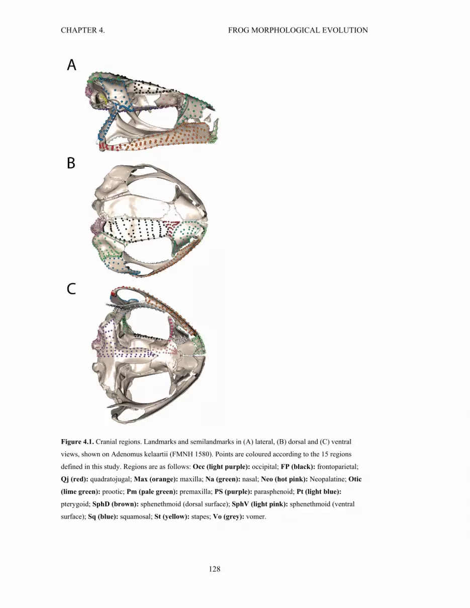
CHAPTER 4. FROG MORPHOLOGICAL EVOLUTION
128
Figure 4.1. Cranial regions. Landmarks and semilandmarks in (A) lateral, (B) dorsal and (C) ventral
views, shown on Adenomus kelaartii (FMNH 1580). Points are coloured according to the 15 regions
defined in this study. Regions are as follows: Occ (light purple): occipital; FP (black): frontoparietal;
Qj (red): quadratojugal; Max (orange): maxilla; Na (green): nasal; Neo (hot pink): Neopalatine; Otic
(lime green): prootic; Pm (pale green): premaxilla; PS (purple): parasphenoid; Pt (light blue):
pterygoid; SphD (brown): sphenethmoid (dorsal surface); SphV (light pink): sphenethmoid (ventral
surface); Sq (blue): squamosal; St (yellow): stapes; Vo (grey): vomer.

CHAPTER 4. FROG MORPHOLOGICAL EVOLUTION
129
Ecology
Microhabitat use was divided into the following seven broad categories: aquatic, semi-aquatic,
arboreal, semi-arboreal, fossorial, semi-fossorial and terrestrial, based on adults outside of the
breeding season (in line with Moen et al. 2016). This categorisation reflects the four main
microhabitats identified across frogs (Laurent 1964), with the recognition that intermediate
ecological types also exist (Laurent 1964). In addition, these categories are in line with previous
studies using habitat categories (Bossuyt & Milinkovitch 2000b; Young et al. 2005; Moen et al.
2013, 2016; Portik & Blackburn 2016). Data from the primary literature were used, as well as
categories established in previous studies (Moen et al. 2013, 2016) (Appendix 4, Table S4.1).
Ecological categories were based on predominant (or partial for ‘semi-’ categories) use of a
substrate (water for aquatic, vegetation for arboreal, and soil for fossorial) compared with land
(terrestrial). Whilst fossorial species can dig head-first, forelimb first or hindlimb first, and
whilst some species found in burrows may not actively burrow, this information is not always
available, and we do not have sufficient numbers of representatives from each category. We
therefore grouped these subcategories into broader ‘fossorial’ (and ‘semi-fossorial’) categories,
as this would capture general selection pressures associated with endogeicity (living in soil), as
previously discussed in Chapter 2 for caecilians (Bardua et al. 2019b). Furthermore, studies
have recognised that whilst some fossorial frogs may burrow backwards, fossorial frogs move
forward underground and excavate termite colonies by using their crania to penetrate the tunnels
(e.g., Rhinophrynus dorsalis, Trueb & Gans 1983). Therefore, head-first, forelimb first and
hindlimb first burrowers would likely experience similar selection pressures underground. For a
detailed investigation into burrowing influences on morphological evolution in myobatrachid
frogs, see Vidal-García and Keogh (2017).
Development
Developmental strategy
Species were categorised according to developmental strategy, using the following definitions,
as previously discussed (Chapter 3; McDiarmid & Altig 1999): direct development
(endotrophic/‘non-feeding’ larvae, i.e. solely provisioned with yolk) and biphasic development
(exotrophic/‘feeding’ larvae, i.e. exploiting external food sources). Data were taken from the
primary literature (see Appendix 3, Table S3.1). This categorisation removes ambiguity, and
distinguishes frogs experiencing extrinsic selection pressures from two environments (larval and
adult), to those experiencing only pressures from the adult environment. Whilst direct
developers can vary in their ontogenetic pathways, all are assumed to be endotrophic (Scott
2005). Species exhibiting trophic egg feeding or feeding on skin secretions were both counted
as ‘feeding’ larval forms.
CHAPTER 4. FROG MORPHOLOGICAL EVOLUTION
130
Ossification sequence timing
The median rank position in the ossification sequence was taken from Weisbecker and
Mitgutsch (2010) for each cranial bone (although this information is missing for the stapes). The
occipital region defined in this study corresponds to the oto-occipital bone, and the otic region
corresponds to the prootic bone (Appendix 3, Table S3.3).
Data analyses
Cranial shape
Morphological variation of the cranium
Principal components analysis (hereafter, PCA) was used to assess the primary aspects of shape
variation and morphospace occupation for the cranium, using the ‘plotTangentSpace’ function
in geomorph (Adams & Otárola-Castillo 2013). Morphologies representing the extreme shapes
along those principal component (PC) axes that each summarized over 5% of the variation were
also visualised.
Morphological variation of individual cranial regions
The major aspects of shape variation (along the first principal component, PC1) were described
for each cranial region by conducting PCAs using the ‘plotTangentSpace’ function in
geomorph. Specimens occupying extreme positions along PC1 were also identified. For these
descriptions of morphological variation, only specimens with the relevant region present were
retained in PCAs, since here we were limiting our description to shape, and not
presence/absence. The directionality of the PC axes was arbitrary, as the PCAs were conducted
on individual cranial regions.
Phylogenetic signal
Phylogenetic signal (Kmult) was determined for the crania and for each cranial region using the
‘physignal’ function in geomorph. We also created a phylomorphospace, which is a projection
of the phylogeny onto a morphospace (Sidlauskas 2008). This reveals the history of a clade’s
morphological diversification and provides a visualisation of how similar closely-related taxa
are in morphology. We created a phylomorphospace for the first two PC axes, using the
‘phylomorphospace’ function in phytools v0.6-60 (Revell 2012).
Allometry
Centroid size of each cranium was used as a measure of cranial size, as discussed previously
(Chapters 2 and 3). For specimen centroid sizes, see Appendix 3, Table S3.8, with the addition
of Thaumastosaurus gezei (centroid size = 473.83). Evolutionary allometry was calculated for
the crania and for each cranial region using the ‘procD.pgls’ function in geomorph, and shape
changes associated with allometry were visualised for the crania using the ‘procD.allometry’

CHAPTER 4. FROG MORPHOLOGICAL EVOLUTION
131
function in geomorph. Specimens were also colour-graded based on their centroid sizes, and
phylogenetic signal of the centroid size was calculated to determine whether size is
phylogenetically structured. Finally, to investigate the link between cranial size and cranial bone
loss, Spearman’s rank correlation was calculated between cranial centroid size and number of
cranial regions. This non-parametric test statistic was chosen as the number of cranial region
data are likely not normally distributed.
Ecology and developmental strategy
The influences of ecology and development on cranial morphology were quantified by
performing phylogenetic ANOVAs (pANOVA) on the landmark and semilandmark data for the
crania and for each cranial region, grouping taxa according to the ecological and developmental
categories listed above. To correct for multiple tests, Benjamini-Hochberg corrections were
applied (Benjamini & Hochberg 1995). The occupation of cranial morphospace was also
visualised for the different ecologies and developmental strategies.
Disparity and evolutionary rate
Pattern of whole skull and regional evolutionary rate
Evolutionary rate through time was investigated using BayesTraitsV3
(http://www.evolution.rdg.ac.uk/), by inputting phylogenetic principal component (pPC) scores
(calculated through the ‘phyl.pca’ function in phytools) that represented 95% of the shape
variation for the whole cranium and for each region. Thus 54 pPC scores were required for the
whole cranium, and between three and 17 for regions (Appendix 4, Table S4.2). We ran variable
rates Brownian motion models using a Markov Chain Monte Carlo (MCMC) algorithm. Two
chains were run for each cranial region and the cranium, and convergence of the chains was
assessed to ensure the chains were stationary. Variable rates models are complex and chains
may not quickly converge, so trace plots were assessed visually (e.g., Appendix 4, Fig. S4.1) as
well as using Gelman and Rubin’s convergence diagnostic through the ‘gelman.diag’ function,
which is implemented in the R package coda (Plummer et al. 2006). Effective sample size
(ESS) of the posterior samples was also assessed (ESS > 100), using the effectiveSize function
in the R package coda. If the runs had not converged, longer MCMC chains were ran. Once
convergence had been achieved, the most stable run with the highest likelihood was chosen as
the model of trait evolution. Each analysis was run for 100 – 500 million iterations, with the
first 12.5 – 50 million of these deleted as burn-in, sampling every 10 – 50 thousand iterations
(Appendix 4, Table S4.3). Additional iterations were removed as burn-in when necessary, on
observation of the chains. The average evolutionary rate for each branch of the phylogeny was
estimated using the ‘rjpp’ function in BTRTools (https://github.com/hferg/btrtools) R package
for the cranium and each cranial region, and visualised using the ‘plotBranchbyTrait’ function
in phytools. We assessed whether changes in evolutionary rate across taxa were associated with

CHAPTER 4. FROG MORPHOLOGICAL EVOLUTION
132
a change in ecology or developmental strategy, for the cranium and for individual cranial
regions.
The location of rate shifts on nodes and branches (scaled by their posterior probability) was
visualised for the cranium using the ‘plotShifts’ function in the R package BTRTools. Only rate
shifts with a posterior probability equal or greater to 0.9 were visualised. These rate shifts were
compared to the locations of shifts in microhabitat use and developmental strategy to determine
whether there was a correlation between shifts in evolutionary rate and either microhabitat use
or developmental strategy.
Comparing rate and disparity across cranial regions
To directly compare magnitudes of evolutionary rate and disparity across cranial regions,
disparity (Procrustes variance) was calculated for each cranial region using the
‘morphol.disparity’ function in the R package geomorph v.3.0.5 (Adams & Otárola-Castillo
2013), and corrected by dividing this by the number of landmarks/semilandmarks in each
cranial region. Evolutionary rate was calculated for each cranial region through the
‘compare.multi.evol.rates’ function in geomorph. Disparity and evolutionary rate of the crania
and cranial regions were also calculated for species grouped according to their microhabitat use
and their developmental strategy. In addition, Spearman’s rank correlation analyses were
performed between disparity and ossification sequence timing and between evolutionary rate
and ossification sequence timing, to determine the relationship between ossification sequence
timing and these two metrics.
Rate through time
The evolutionary rate through time was plotted for the cranium and for each cranial region,
using the ‘geoscalePlot’ function in the geoscale R package (Bell 2015). The mean rate of all
branches within one million-year time bins was computed for each cranial region, and these
were then divided by the maximum rate across all time bins for each cranial region. Correcting
for maximum rate facilitated the comparison of the temporal dynamics of the evolutionary rate
of each region (absolute rate values can not be compared as the rates were reconstructed from
separate datasets).
Individual landmark and semilandmark disparity and rate
Disparity (measured as variance) and evolutionary rate (measured by modifying the
‘compare.evol.rates’ function in geomorph) were calculated for each individual landmark and
semilandmark. Cranial landmarks and semilandmarks were colour-graded using these metrics to
visualise the spread of disparity and evolutionary rate across the anuran skull. A regression of
disparity on evolutionary rate for landmarks/semilandmarks was also plotted to visualise the
relationship between these metrics within and across cranial regions. This relationship was also

CHAPTER 4. FROG MORPHOLOGICAL EVOLUTION
133
compared to that expected under a Brownian motion model with no trait covariation, by taking
the evolutionary rate for each landmark/semilandmark and simulating trait evolution under
Brownian motion (running 100 simulations) using the ‘sim.char’ function in the geiger v.2.0.6
R package (Harmon et al. 2008). The estimated mean variances for each
landmark/semilandmark were taken from this simulation and a regression of evolutionary rate
on simulated variance was plotted. A 95% prediction interval was also calculated, to determine
which landmarks/semilandmarks exhibited higher or lower variance given their evolutionary
rate.
Results
Cranial morphology
Morphological variation of the cranium
The first four PC scores each accounted for over 5% of the morphological variation, and 46 PC
scores were necessary to capture 95% of the morphological variation (Appendix 4, Table S4.4).
The first PC axis accounted for 28% of the morphological variation. The main shape changes
along this axis (going from negative to positive) were the dorsoventral lengthening of the
cranium, the lateral extension of the frontoparietal, the reduction of the maxillary arcade, and
the shortening of the anterior process of the squamosal (Fig. 4.2A-B). The second PC axis
accounted for 14%, with the positive extreme associated with a dorsoventrally taller maxilla, a
larger nasal, and an anteroposteriorly compressed frontoparietal, as well as a taller, wider
cranium (Fig. 4.2C-D). The third PC axis accounted for 8%, with the main shape changes (from
negative to positive) including the reduction of the maxillary arcade and the expansion of the
pterygoid (Fig. 4.2E-F). Finally, the fourth PC axis accounted for 5% of the shape variation,
with the negative extreme associated with wider premaxillary and maxillary palatal shelves and
a relatively larger pterygoid (Fig. 4.2G-H). For the PC1-PC2 morphospace occupation of the
crania see Fig. 4.3, and for a PC3-PC4 morphospace see Appendix 4, Fig. S4.2.

CHAPTER 4. FROG MORPHOLOGICAL EVOLUTION
134
Figure 4.2. Cranial morphological changes along PC1, PC2, PC3 and PC4. Reconstructed morphologies
represented by positive (A) and negative (B) ends of PC1, positive (C) and negative (D) ends of PC2,
positive (E) and negative (F) ends of PC3, and positive (G) and negative (H) ends of PC4, all shown in
ventral (left) and dorsal (right) aspects. Each reconstruction is coloured by cranial region, as follows: Occ
(light purple): occipital; FP (black): frontoparietal; Qj (red): quadratojugal; Max (orange): maxilla; Na
(green): nasal; Neo (hot pink): Neopalatine; Otic (lime green): prootic; Pm (pale green): premaxilla;
PS (purple): parasphenoid; Pt (light blue): pterygoid; SphD (brown): sphenethmoid (dorsal); SphV
(light pink): sphenethmoid (ventral); Sq (blue): squamosal; St (yellow): stapes; Vo (grey): vomer. PC
axes accounted for 28%, 14%, 8% and 5% of the morphological variation respectively.
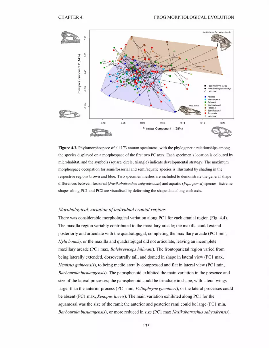
CHAPTER 4. FROG MORPHOLOGICAL EVOLUTION
135
Figure 4.3. Phylomorphospace of all 173 anuran specimens, with the phylogenetic relationships among
the species displayed on a morphospace of the first two PC axes. Each specimen’s location is coloured by
microhabitat, and the symbols (square, circle, triangle) indicate developmental strategy. The maximum
morphospace occupation for semi/fossorial and semi/aquatic species is illustrated by shading in the
respective regions brown and blue. Two specimen meshes are included to demonstrate the general shape
differences between fossorial (Nasikabatrachus sahyadrensis) and aquatic (Pipa parva) species. Extreme
shapes along PC1 and PC2 are visualised by deforming the shape data along each axis.
Morphological variation of individual cranial regions
There was considerable morphological variation along PC1 for each cranial region (Fig. 4.4).
The maxilla region variably contributed to the maxillary arcade; the maxilla could extend
posteriorly and articulate with the quadratojugal, completing the maxillary arcade (PC1 min,
Hyla boans), or the maxilla and quadratojugal did not articulate, leaving an incomplete
maxillary arcade (PC1 max, Balebreviceps hillmani). The frontoparietal region varied from
being laterally extended, dorsoventrally tall, and domed in shape in lateral view (PC1 max,
Hemisus guineensis), to being mediolaterally compressed and flat in lateral view (PC1 min,
Barbourula busuangensis). The parasphenoid exhibited the main variation in the presence and
size of the lateral processes; the parasphenoid could be triradiate in shape, with lateral wings
larger than the anterior process (PC1 min, Peltophryne guentheri), or the lateral processes could
be absent (PC1 max, Xenopus laevis). The main variation exhibited along PC1 for the
squamosal was the size of the rami; the anterior and posterior rami could be large (PC1 min,
Barbourula busuangensis), or more reduced in size (PC1 max Nasikabatrachus sahyadrensis).
CHAPTER 4. FROG MORPHOLOGICAL EVOLUTION
136
The pterygoid varied in the size of the medial ramus; the medial ramus could be thin (PC1 max,
Myobatrachus gouldii) or expanded anteroposteriorly (PC1 min, Pipa parva). The nasal could
extend far ventrally, contacting the maxilla (PC1 max, Ceratophrys aurita) or the nasal could be
reduced in size and isolated from other ossified material (PC1 min, Rheobatrachus silus). The
occipital region could be mediolaterally expanded (PC1 min, Hemiphractus proboscideus) or
mediolaterally compressed (PC1 max, Pipa parva), and the otic region varied from having a
concave surface (PC1 max, Ceratobatrachus guentheri) to a convex surface (PC1 min,
Brachycephalus ephippium). Along PC1, the quadratojugal varied from possessing an elongate
maxillary process and wide articular surface (PC1 min, Conraua beccarii), to possessing a
shorter, taller maxillary process, and a less ossified articular surface (PC1 max,
Nasikabatrachus sahyadrensis). The vomer region varied from being anteroposteriorly elongate
(PC1 max, Xenorhina sp.), to anteroposteriorly compressed, with the anterior process positioned
more laterally (PC1 min, Ameerega parvula). The sphenethmoid (dorsal) region varied in the
extent of its anterior projection, from projecting anteriorly in between the paired nasals (PC1
max, Anhydrophryne rattrayi) to remaining posterior to the nasals (PC1 min, Hemiphractus
proboscideus). The sphenethmoid (ventral) region also varied in its anterior projection, from
being present only lateral to the parasphenoid (PC1 min, Myobatrachus gouldii) to projecting
anteriorly to the parasphenoid (PC1 max, Arthroleptella lightfooti). For the remaining cranial
regions, the orientation (relative to the cranium) was a major aspect of the variation along PC1.
The stapes varied from a mediolateral orientation (PC1 max, Thaumastosaurus gezei) to the
lateral tip of the stapes pointing anteroventrally (PC1 min, Pipa pipa and Myobatrachus
gouldii). The premaxilla region exhibited the main variation in the orientation of the alary
process, from the tip orienting anterodorsally (PC1 min, Balebreviceps hillmani) to dorsally
(PC1 max, Pristimantis chiastonotus). Finally, the neopalatine was reduced in width with an
anterolaterally oriented tip at one extreme of PC1 (PC1 min, Hyla boans), and relatively wider
with a laterally oriented tip at the other extreme (PC1 max, Stumpffia pygmaea).

CHAPTER 4. FROG MORPHOLOGICAL EVOLUTION
137
Figure 4.4. Shape variation along PC1 for each cranial region defined in this study. The landmark and
semilandmark data are coloured by cranial region and displayed on Adenomus kelaartii (FMNH 1580) in
(A) ventral and (B) lateral aspects. The positive (+) and negative (-) shape extremes for each cranial
region are displayed in (A) ventral and (B) lateral aspects, with the exception of the frontoparietal (FP),
sphenethmoid (dorsal) (SphD) and otic (Otic) regions (dorsal aspect) and the occipital (Occ) region
(posterior aspect). All regions are displayed in one view, except the maxilla, premaxilla and
quadratojugal, which are displayed in both lateral and ventral views. Extreme shapes along PC1 were
generated from individual region PCAs, so the PC axes do not align and directionality is arbitrary, and the
extreme shapes are not to scale. Specimens with an absent region were removed from the PCAs for the
relevant cranial regions, for visualisation purposes only. Regions are as follows: Occ (light purple):
occipital; FP (black): frontoparietal; Qj (red): quadratojugal; Max (orange): maxilla; Na (green): nasal;
Neo (hot pink): Neopalatine; Otic (lime green): prootic; Pm (pale green): premaxilla; PS (purple):
parasphenoid; Pt (light blue): pterygoid; SphD (brown): sphenethmoid (dorsal surface); SphV (light
pink): sphenethmoid (ventral surface); Sq (blue): squamosal; St (yellow): stapes; Vo (grey): vomer.

CHAPTER 4. FROG MORPHOLOGICAL EVOLUTION
138
Phylogeny
Frog crania exhibited significant phylogenetic signal (Kmult = 0.66, p = 1 × 10⁻⁴). This effect
varied in strength across the skull, and the neopalatine stood out as considerably more
constrained by phylogeny than other regions (Kmult = 1.87, p = 1 × 10⁻⁴, see Table 4.1). The
phylomorphospace (Fig 4.3) showed some clustering of species based on phylogeny, but also
considerable overlap of families.
Table 4.1. Results for each of the 15 cranial regions. Disparity was corrected for semi/landmark number.
Significance of results for phylogenetic signal, evolutionary allometry, influence of microhabitat and
influence of developmental strategy is as follows: p values significant at the following alpha levels: * ≤
0.05, ** ≤ 0.01, *** ≤ 0.001. A ‘/’ indicates significance before/after correction for multiple tests.
pANOVA = phylogenetic ANOVA. For region definitions, see Fig. 4.1.
Cran
ial region
Ph
ylogenetic sign
al
(Km
ult )
Evolu
tionary allom
etry
(R2)
Disp
arity (Procru
stes
variance) (×
10-5)
Evolu
tionary rate,
σ2m
ult, (×
10-8)
Microh
abitat in
fluen
ce,
pA
NO
VA
(R2)
Develop
men
tal strategy
influ
ence, p
AN
OV
A (R
2)
Ossification
sequen
ce
FP 0.59*** 0.11*** 1.04 3.43 0.09**/* 0.016*/ 2
Max 0.74*** 0.17*** 1.35 3.71 0.08*/* 0.002 6
Na 0.57*** 0.07*** 1.07 3.49 0.11***/** 0.009 7
Neo 1.87*** 0.06*** 1.91 4.10 0.05 0.004 12
Occ 0.59*** 0.32*** 0.72 2.20 0.06 0.009 3
Otic 0.54*** 0.09*** 1.13 3.78 0.06 0.006 4
PS 0.79*** 0.10*** 0.60 1.69 0.08*/ 0.010 1
Pm 0.72*** 0.06*** 0.89 2.52 0.07 0.007 5
Pt 0.61*** 0.08*** 1.20 3.68 0.10**/** 0.006 10
Qj 0.65*** 0.16*** 2.92 8.47 0.12**/** 0.009 11
Sph(d) 0.54*** 0.07*** 1.29 4.41 0.07 0.011 13
Sph(v) 0.56*** 0.07*** 1.96 3.62 0.06 0.015*/ 13
Sq 0.62*** 0.08*** 1.81 5.41 0.10**/** 0.035***/* 8
St 0.70*** 0.02 1.86 5.99 0.03 0.004 NA
Vo 0.72*** 0.02* 0.99 2.51 0.13**/** 0.018*/ 9

CHAPTER 4. FROG MORPHOLOGICAL EVOLUTION
139
Allometry
Allometry had a significant effect on morphology (R2 = 0.13, p = 1 × 10⁻⁴). Larger species had
wider, more triangular-shaped skulls with relatively smaller cranial vaults (i.e. frontoparietal
and parasphenoid) and occipital regions (Fig. 4.5). The suspensory apparatus (pterygoid,
squamosal and quadratojugal) was more verticalised in smaller species. Evolutionary allometry
was a significant influence on shape for all cranial regions except the stapes (R2 = 0.02, p =
0.07). All remaining regions had an influence of allometry ranging from R2 = 0.02 to 0.17,
except for the occipital region, which exhibited a considerably stronger influence of size on
shape (R2 = 0.32, p = 1 × 10⁻⁴, see Table 4.1). A morphospace colour-graded by centroid size
(Appendix 4, Fig. S4.3) revealed a general trend of larger species clustering towards the
negative end of PC1. Size was not phylogenetically structured (Kmult = 0.39, p = 0.27). A
significantly positive correlation was recovered between cranial centroid size and number of
cranial regions from Spearman’s rank (rho = 0.17, p = 0.02) correlation, and plotting the
relationship revealed taxa with larger crania did not lose as many cranial regions as those with
smaller skulls did (Fig. 4.6).
Figure 4.5. Cranial morphology at minimum (A,C,E) and maximum (B,D,F) size, shown in (A,B) dorsal,
(C,D) ventral, (E,F) lateral aspects.

CHAPTER 4. FROG MORPHOLOGICAL EVOLUTION
140
Figure 4.6. Relationship between cranial bone loss and centroid size. Specimens range from having all of
the 15 cranial regions defined in this study present, to having only 11 present. The cranial regions lost in
some specimens were the stapes, quadratojugal, vomer, sphenethmoid (dorsal) and sphenethmoid
(ventral).
Ecology
Microhabitat significantly influenced cranial morphology (pANOVA R2 = 0.08, p = 0.002), and
the strength of influence of microhabitat varied across the cranium (Table 4.1). Phylogenetic
ANOVAs revealed the vomer exhibited the strongest influence of ecology on cranial shape (R2
= 0.13, p = 0.003), followed by the quadratojugal (R2 = 0.12, p = 0.002). The nasal, pterygoid,
squamosal, frontoparietal, maxilla and parasphenoid also all exhibited significant influences of
microhabitat on morphology (R2 = 0.08 - 0.11, p = 0.03 - 0.001), although after correction for
multiple tests, the parasphenoid was no longer significantly associated with cranial shape (p =
0.06). The remaining cranial regions showed no significant influence of microhabitat on
morphology.
The morphospace distribution for different microhabitats revealed an interesting pattern (Fig.
4.3). Semi/fossorial frogs were generally associated with dorsoventrally tall crania. From one
extreme of morphospace (PC1min/PC2min) to the other (PC1max/PC2max) there was a general
trend from aquatic, to semi-aquatic, to semi-fossorial, to fossorial, with limited overlap of

CHAPTER 4. FROG MORPHOLOGICAL EVOLUTION
141
semi/aquatic species with semi/fossorial species. Terrestrial and semi/arboreal species generally
occupied the centre of the morphospace, largely overlapping with one other.
Developmental strategy
Developmental strategy had a very small but significant influence on cranial morphology
(pANOVA R2 = 0.01, p = 0.03). Developmental strategy had little to no significant influence on
the morphology of cranial regions (Table 4.1). Four regions had significant but very weak
influences, with the strongest influence on the squamosal (R2 = 0.04, p < 0.01), and after
correction for multiple tests only the squamosal was still significant. Developmental strategies
completely overlapped in morphospace, with no clear separation in adult cranial morphology
between direct and biphasic developers (Fig. 4.3, and Appendix 4, Fig. S4.4).
Evolutionary rates and disparity
Pattern of evolutionary rate across the entire cranium
Evolutionary rates were low to moderate on the basal branches of the anuran phylogeny, with
the highest rates observed largely on terminal branches (Fig. 4.7). The ‘basal’ families exhibited
relatively low to moderate evolutionary rates (‘Archaeobatrachia’ - Leiopelmatidae, Ascaphidae
and Alytidae, although this term and the terms ‘Mesobatrachia’ ('transitional frogs’) and
‘Neobatrachia’ ('advanced frogs’) are outdated, Frost et al. 2006). Other clades exhibited
consistently fast rates of evolution (e.g., Pipidae, Brevicipitidae, Microhylidae and
Ceratophryidae). Hyperossified taxa typically exhibited the fastest evolutionary rates along their
terminal branches (e.g., Hemiphractus proboscideus, Triprion petasatus and Brachycephalus
ephippium). We did not find a strong link between microhabitat use and branch-specific rates of
evolution, although some minor differences were evident (Fig. 4.7). Fossorial species mostly
exhibited fast evolutionary rates along their terminal branches (e.g., the species representing
Hemisotidae, Nasikabatrachidae, Rhinophrynidae and Ceratophryidae), as did aquatic species
(e.g., the species representing Calyptocephalellidae and the three species representing Pipidae).
Terrestrial species, however, had a wider range of evolutionary rates, such as the range
displayed across the species of Strabomantidae. Arboreal species generally had moderate rates
of cranial evolution, as seen in the family Rhacophoridae. Semi-arboreal species had a wide
range of evolutionary rates, semi-aquatic species generally exhibited low to moderate
evolutionary rates, and semi-fossorial species had moderate to high evolutionary rates.
However, there was no clear pattern of branch-specific rates of evolution and developmental
strategy across the cranium (Fig. 4.8). For example, direct developing species exhibited a large
range of rates of evolution in the whole skull analysis, as exemplified by the species
representing Strabomantidae. Biphasic species also exhibited a wide range of evolutionary rates,
from high (e.g., the species within Conrauidae) to low (the species representing Ranixalidae).

CHAPTER 4. FROG MORPHOLOGICAL EVOLUTION
142
Figure 4.7. Phylogeny of the 173 species in this study, with branches colour graded by rate of evolution
for the whole skull. Microhabitat categories for each species are displayed by each terminal branch.
Phylogeny modified from Jetz and Pyron (2018). Families are indicated for each species. White and grey
triangles indicate rate shifts at nodes and branches respectively. The threshold of posterior probability for
the rate shifts was set to 0.9. For the phylogeny with species names labelled, see Appendix 4, Fig. S4.5.

CHAPTER 4. FROG MORPHOLOGICAL EVOLUTION
143
Figure 4.8. Phylogeny of the 173 species in this study, with branches colour graded by rate of evolution
for the whole skull. Developmental strategy for each species is displayed by each terminal branch.
Phylogeny modified from Jetz and Pyron (2018). Families are indicated for each species. White and grey
triangles indicate rate shifts at nodes and branches respectively. The threshold of posterior probability for
the rate shifts was set to 0.9. For the phylogeny with species names labelled, see Appendix 4, Fig. S4.5.
Multiple rate shifts at nodes and branches were identified across the phylogeny, and rate shifts
with a posterior probability of > 0.9 were visualised on the phylogeny (Fig. 4.7). Rate shifts
occurred at the split of Leiopelmatidae and Ascaphidae, as well as at the split of Alytidae and
Bombinatoridae and the split of Rhinophrynidae and Pipidae. Rate shifts also often occurred on
terminal branches, for example on the terminal branches of both representatives of Ranidae
(Rana sylvatica and Rana clamitans). In addition, rate shifts occurred frequently along terminal
branches of hyperossified taxa (e.g., Hemiphractus proboscideus, Triprion petasatus and
Brachycephalus ephippium). Shifts in whole skull evolutionary rate were variably associated
with shifts in microhabitat. A rate shift occurred at the split between the terrestrial species of
Leiopelmatidae and the semi-aquatic species of Ascaphidae, and some more basal shifts
occurred at the split of species exhibiting a range of microhabitats (for example, at the split of

CHAPTER 4. FROG MORPHOLOGICAL EVOLUTION
144
the families Scaphiopodidae, Pelodytidae, Pelobatidae and Megophryidae that have both
fossorial and terrestrial species). Rate shifts also occurred with no associated shift in
microhabitat use. For example, rate shifts occurred at the base of Rhacophoridae, represented
here by only arboreal species, at the base of Ceratophryidae, represented here by only fossorial
species, and at the base of Hylodidae, represented here by only terrestrial species. Rate shifts in
cranial morphological evolution also did not noticeably coincide with shifts in developmental
strategy, with a couple of exceptions. One rate shift coincided with the split of the direct
developing species of Ceratobatrachidae with their sister clade Nyctibatrachidae (represented by
a biphasic species), and a shift was also detected at the split of the direct developing species of
Brevicipitidae with the biphasic species of Hemisotidae. There was also a rate shift at the split
of the direct developing representative of Leiopelmatidae with the biphasic species of
Ascaphidae. However, the majority of transitions between developmental strategies were not
associated with rate shifts, for example the splits of the direct developing and biphasic species
within Myobatrachidae and also within Leptodactylidae. Furthermore, many rate shifts occurred
at the split of species with the same developmental strategy, for example there was a shift at the
base of the biphasic species within Hylodidae, between two biphasic species of Pyxicephalidae,
and at the base of the split between the biphasic species of Allophrynidae and Centrolenidae.
Pattern of evolutionary rate for individual cranial regions
We investigated in detail how evolutionary rate changed through time for the three fastest-
evolving cranial regions (the quadratojugal, stapes and squamosal), as well as the three slowest-
evolving regions (the parasphenoid, occipital and vomer) (Fig. 4.9). The quadratojugal (Fig.
4.9A) exhibited the fastest evolutionary rates in Triprion petasatus, Paracassina obscura and
Duttaphrynus dodsoni. Evolutionary rate of the quadratojugal generally varied within families,
although some families had consistently low rates of evolution (e.g., Rhacophoridae,
Mantellidae, Ranidae and Dicroglossidae) and some families had generally higher rates (e.g.,
Nasikabatrachidae and Alsodidae). The squamosal (Fig. 4.9B) was considerably slower in
evolutionary rate in the ‘basal’ families Leiopelmatidae, Ascaphidae and Alytidae, with no other
family exhibiting as low evolutionary rate on any terminal branch. The fastest rates of evolution
for the squamosal were in three species of Bufonidae and in Leptopelis spiritusnoctis and
Hemiphractus proboscideus. Evolutionary rate was generally conserved within some families
for the squamosal, for example low evolutionary rate was exhibited across Leptodactylidae,
Centrolenidae and Hyperoliidae, and high rate of evolution was exhibited across
Ceratophryidae. High evolutionary rate was concentrated in a few anuran families for the stapes
(Fig. 4.9C). The highest evolutionary rates of the stapes were found in the families
Brevicipitidae and Hemisotidae. High evolutionary rate of the stapes was also recovered
consistently across the more ‘basal’ families (Leiopelmatidae, Ascaphidae, Alytidae,

CHAPTER 4. FROG MORPHOLOGICAL EVOLUTION
145
Bombinatoridae, Rhinophrynidae and Pipidae), as well as Bufonidae. Other clades had either
consistently low rates of evolution for the stapes (e.g., Arthroleptidae), or a broad range of rates
(e.g., Pyxicephalidae).
For the relatively slowly-evolving regions, the occipital region (Fig. 4.9D) exhibited the lowest
rates of evolution in the ‘Archaeobatrachia’ families- Leiopelmatidae, Ascaphidae and Alytidae.
All species representing Pipidae had consistently high rates of evolution of the occipital region,
as well as species in Brevicipitidae and Hemisotidae. A conserved, high rate of evolution was
evident across the Pipidae and Rhinophrynidae families for the parasphenoid region (Fig. 4.9E),
whereas evolutionary rate of the parasphenoid was invariably low across families of
‘Archaeobatrachia’. A consistently moderate rate of evolution was recovered for some families,
including Bufonidae, Centrolenidae and Hyperoliidae. Finally, the rate of evolution of the
vomer (Fig. 4.9F) was generally low across many anuran families (e.g., Dicroglossidae,
Alsodidae and Pyxicephalidae), with high rates exhibited in just a few lineages, specifically
Brachycephalus ephippium and Myobatrachus gouldii.

CHAPTER 4. FROG MORPHOLOGICAL EVOLUTION
146

CHAPTER 4. FROG MORPHOLOGICAL EVOLUTION
147
Figure 4.9. Phylogenies of the 173 species in this study, with branches colour graded by rate of evolution
for the following cranial regions: (A) quadratojugal, (B) squamosal, (C) stapes, (D) occipital and (E)
parasphenoid and (F) vomer. Evolutionary rates are not comparable across different cranial regions, as the
rates analyses were conducted on separate datasets and the scales are not consistent. (A) Microhabitat use
and (B) developmental strategy are displayed next to the terminal branches for each species.
The relationship between microhabitat use and evolutionary rate was not consistent across these
cranial regions (Fig. 4.9). A range of evolutionary rates was recovered across fossorial, aquatic,
terrestrial and arboreal species for the quadratojugal, whereas generally relatively lower rates
were recovered for semi-fossorial, semi-aquatic, and semi-arboreal species. There was a wide
range of evolutionary rates of the squamosal for aquatic, fossorial and arboreal species. Semi-
aquatic species generally had relatively low rates of evolution of the squamosal and semi-
fossorial species generally had moderate evolutionary rates. Terrestrial and semi-arboreal
species mainly exhibited low evolutionary rates of the squamosal, with the main exception
being terrestrial members of Bufonidae. Semi-aquatic and semi-arboreal species generally
exhibited relatively low evolutionary rates of the occipital region, whereas arboreal, aquatic,
fossorial, semi-fossorial and terrestrial exhibited a wider range of evolutionary rates for this
region. Species from all microhabitats exhibited a range of evolutionary rates of the stapes.
Finally, species in most microhabitats exhibited relatively low evolutionary rates of the
parasphenoid and vomer with some faster-evolving taxa in each microhabitat category, although
a wider range of evolutionary rates was recovered for the vomer across aquatic species, and for
the parasphenoid across fossorial species.
Developmental strategy did not have a notable influence on rate of evolution for any cranial
region. There was a wide spread of evolutionary rates of the squamosal, stapes, quadratojugal,
parasphenoid and occipital regions for both biphasic and direct developing species. Direct
developers generally exhibited slow evolutionary rate of the vomer, with the exception of
Brachycephalus ephippium and Myobatrachus gouldii. Biphasic species exhibited a greater
spread of evolutionary rates, with more species exhibiting relatively fast rates, although the
imbalanced sample sizes hinders direct comparison of the two developmental strategies. There
was therefore no strong, consistent relationship between microhabitat use or developmental
strategy and branch-specific rates of evolution for any individual cranial region (see Fig. 4.9).
For the remaining cranial regions, the rate of evolution is briefly described (see Appendix 4,
Figs. S4.6-7). A low evolutionary rate was recovered for the ‘basal’ families (Leiopelmatidae,
Ascaphidae, Alytidae) for most cranial regions, except the neopalatine, otic and sphenthethmoid
(dorsal). The ‘transitional’ frog families (‘Mesobatrachia’ - Rhinophrynidae, Pipidae,
Scaphiopodidae, Pelodytidae, Pelobatidae and Megophryidae) exhibited relatively low rates of
CHAPTER 4. FROG MORPHOLOGICAL EVOLUTION
148
evolution in the frontoparietal, maxilla and sphenethmoid (dorsal), relatively high rates of
evolution in the nasal, neopalatine and pterygoid, and moderate evolutionary rate in the otic,
premaxilla and sphenethmoid (ventral). Of the ‘advanced’ anuran families (‘Neobatrachia’), the
pattern of evolutionary rate varied across the cranial regions. Bufonidae exhibited relatively
high rates of evolution in the frontoparietal, nasal, otic and pterygoid. Ceratophryidae exhibited
a relatively fast-to-moderate rate of evolution for every cranial region. Brevicipitidae exhibited
a relatively fast rate of evolution of the sphenethmoid (dorsal), otic and frontoparietal regions.
Evolutionary rate generally varied within families, with fast-evolving taxa often nested within
relatively slowly-evolving families.
Comparing rate and disparity across cranial regions
Evolutionary rate was highest in the quadratojugal (8.47 × 10⁻⁸), stapes (5.99 × 10⁻⁸), and
squamosal (5.41 × 10⁻⁸) regions and lowest in the parasphenoid (1.69 × 10⁻⁸), occipital (2.20 ×
10-8), and vomer (2.51 × 10⁻⁸) regions (Table 4.1). Disparity revealed a similar pattern to
evolutionary rate across the cranial regions. Disparity was also highest in the quadratojugal
region (2.92 × 10⁻⁵) and also lowest in the parasphenoid (6.00 × 10⁻⁶) and occipital (7.20 × 10⁻⁶)
regions, but the sphenethmoid (ventral) (1.96 × 10⁻⁵) and neopalatine (1.91 × 10⁻⁵) regions had
higher disparity than the stapes (1.86 × 10⁻⁵) and squamosal (1.81 × 10⁻⁵) regions.
When evolutionary rate and disparity were directly compared across cranial regions, the crania
of fossorial, semi-fossorial, and aquatic species all exhibited high disparity (Procrustes variance
= 0.02 for all), and these were all significantly more disparate than the crania of terrestrial
(0.009), arboreal (0.01), semi-arboreal (0.009) and semi-aquatic (0.008) species (p = 0.001 -
0.018 for all pairs) (Fig. 4.10). Fossorial, semi-fossorial, and aquatic species also exhibited the
highest disparities for most individual cranial regions, especially the quadratojugal (Fig. 4.11A).
The crania of fossorial, semi-fossorial and aquatic species also exhibited the highest rates of
evolution (σ2mult = 1.50 - 1.58 × 10⁻⁶) (Fig. 4.10). Cranial evolutionary rates for the remaining
microhabitats were considerably slower, with semi-aquatic species exhibiting the slowest rates
(6.98 × 10⁻⁷). Fossorial, semi-fossorial, and aquatic species exhibited the fastest rates of
evolution across most individual cranial regions, especially the quadratojugal, squamosal and
pterygoid regions (and the stapes for semi/fossorial species) (Fig. 4.11B). Pairwise differences
between fast-evolving/highly disparate semi/fossorial and aquatic species and slow-
evolving/less disparate terrestrial, semi/arboreal and semi-aquatic species were significant in
most cases (Appendix 4, Tables S4.5-4.6). Semi-arboreal and semi-aquatic species generally
exhibited the slowest rates of evolution across most cranial regions.
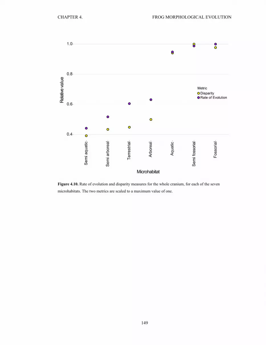
CHAPTER 4. FROG MORPHOLOGICAL EVOLUTION
149
Figure 4.10. Rate of evolution and disparity measures for the whole cranium, for each of the seven
microhabitats. The two metrics are scaled to a maximum value of one.
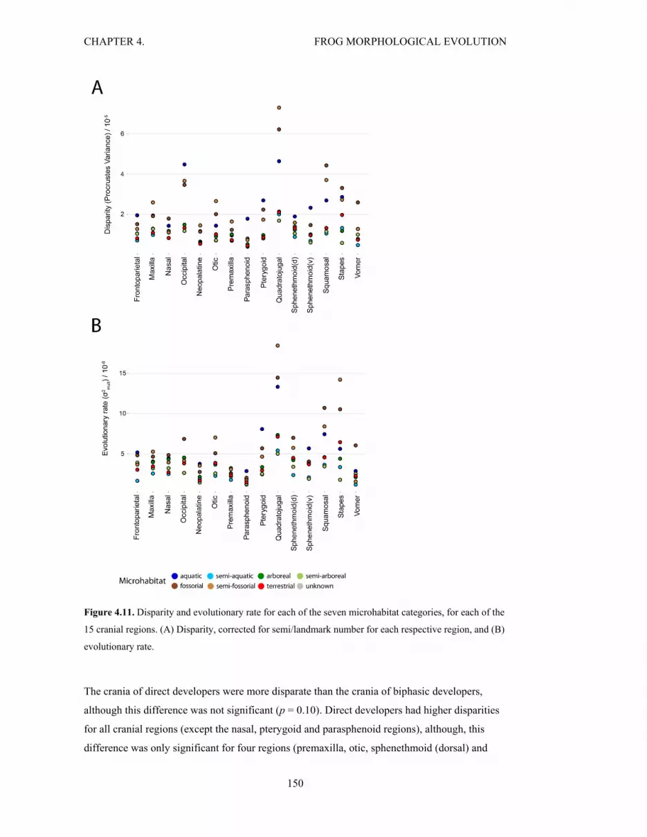
CHAPTER 4. FROG MORPHOLOGICAL EVOLUTION
150
Figure 4.11. Disparity and evolutionary rate for each of the seven microhabitat categories, for each of the
15 cranial regions. (A) Disparity, corrected for semi/landmark number for each respective region, and (B)
evolutionary rate.
The crania of direct developers were more disparate than the crania of biphasic developers,
although this difference was not significant (p = 0.10). Direct developers had higher disparities
for all cranial regions (except the nasal, pterygoid and parasphenoid regions), although, this
difference was only significant for four regions (premaxilla, otic, sphenethmoid (dorsal) and

CHAPTER 4. FROG MORPHOLOGICAL EVOLUTION
151
vomer) (Fig. 4.12A, Appendix 4, Table S4.7). No significant difference was found between the
rate of cranial evolution for direct (1.11 × 10⁻⁶) and biphasic (1.06 × 10⁻⁶) developers (rate ratio
= 1.06, p = 1). Analysis of individual cranial regions also revealed mixed results; direct
developers exhibited faster rates of evolution for the neopalatine, otic, sphenethmoid (ventral),
squamosal, stapes and vomer regions, whilst biphasic species exhibited faster rates of evolution
for the frontoparietal, maxilla, nasal, occipital, premaxilla, parasphenoid, pterygoid,
sphenethmoid (dorsal) and quadratojugal regions (Fig. 4.12B). The magnitude of differences
varied across the regions, and only two differences were significant: direct developers had
significantly faster-evolving otic and vomer regions (Appendix 4, Table S4.7).
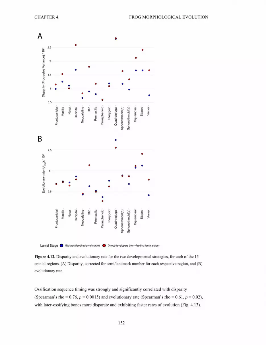
CHAPTER 4. FROG MORPHOLOGICAL EVOLUTION
152
Figure 4.12. Disparity and evolutionary rate for the two developmental strategies, for each of the 15
cranial regions. (A) Disparity, corrected for semi/landmark number for each respective region, and (B)
evolutionary rate.
Ossification sequence timing was strongly and significantly correlated with disparity
(Spearman’s rho = 0.76, p = 0.0015) and evolutionary rate (Spearman’s rho = 0.61, p = 0.02),
with later-ossifying bones more disparate and exhibiting faster rates of evolution (Fig. 4.13).

CHAPTER 4. FROG MORPHOLOGICAL EVOLUTION
153
Figure 4.13. Relationship between ossification sequence timing and disparity and evolutionary rate for
each cranial region. Spearman’s rank correlations of (A) disparity (corrected for semi/landmark number)
and (B) evolutionary rate with ossification sequence timing were significant (disparity: Spearman’s rho =
0.76, p = 0.0015, evolutionary rate: Spearman’s rho = 0.61, p = 0.02).
Rate through time
There was an initial peak in evolutionary rate at the base of the anuran phylogeny, which likely
reflected the splitting of major clades (Fig. 4.14). More specifically, higher evolutionary rates
from ~ 220 – 200 million years ago (Ma) coincides with the splitting of major clades: first the
splitting of the ‘primitive’ frog clades (‘Archaeobatrachia’ - Leiopelmatidae, Ascaphidae,
Alytidae and Bombinatoridae) and then the splitting of the traditionally ‘transitional’ frog clades
(‘Mesobatrachia’ - Rhinophrynidae, Pipidae, Scaphiopodidae, Pelodytidae, Pelobatidae and
Megophryidae) from the remaining ‘advanced’ frog clades (‘Neobatrachia’). From 200 Ma,
there was a general trend of the rate of cranial evolution steadily increasing to the Recent. Peaks
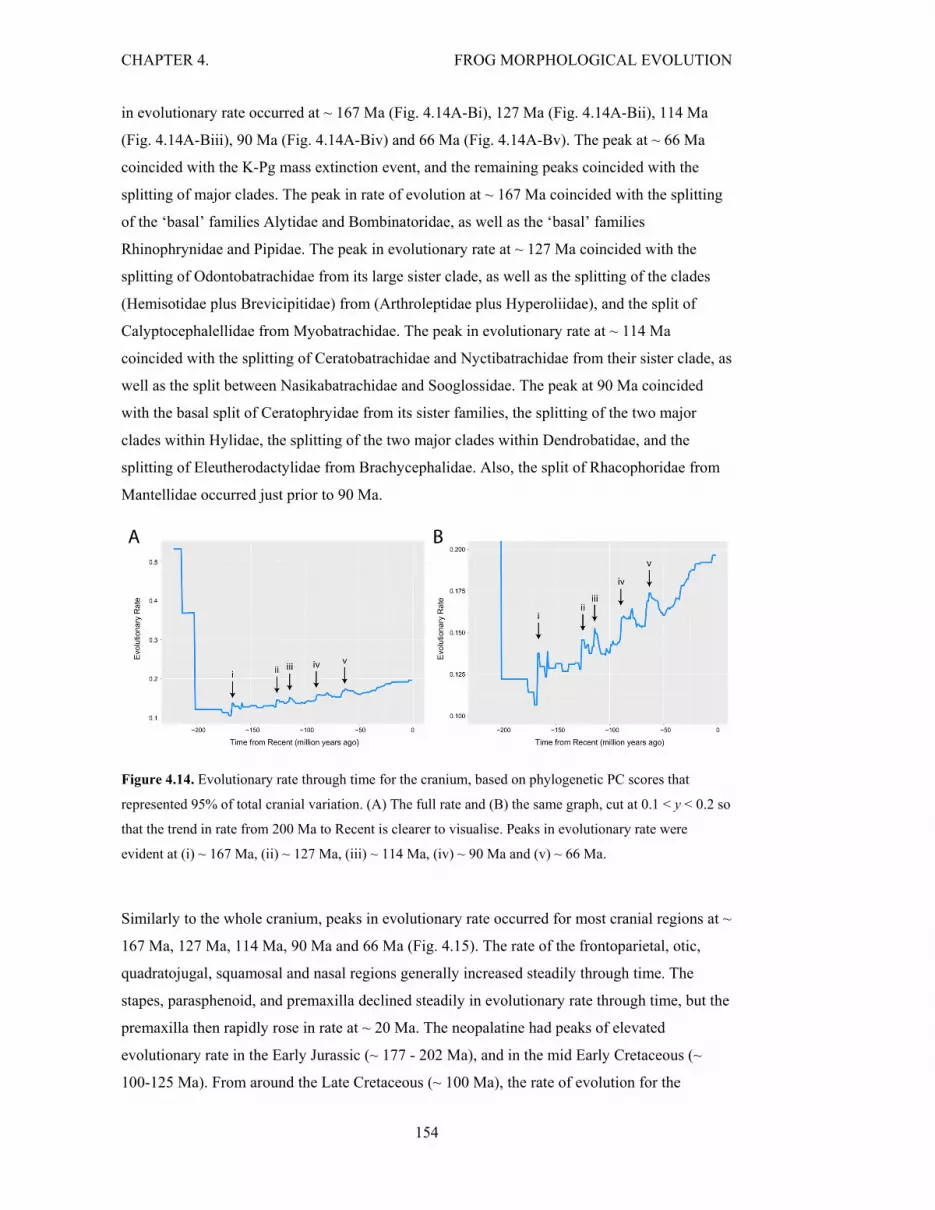
CHAPTER 4. FROG MORPHOLOGICAL EVOLUTION
154
in evolutionary rate occurred at ~ 167 Ma (Fig. 4.14A-Bi), 127 Ma (Fig. 4.14A-Bii), 114 Ma
(Fig. 4.14A-Biii), 90 Ma (Fig. 4.14A-Biv) and 66 Ma (Fig. 4.14A-Bv). The peak at ~ 66 Ma
coincided with the K-Pg mass extinction event, and the remaining peaks coincided with the
splitting of major clades. The peak in rate of evolution at ~ 167 Ma coincided with the splitting
of the ‘basal’ families Alytidae and Bombinatoridae, as well as the ‘basal’ families
Rhinophrynidae and Pipidae. The peak in evolutionary rate at ~ 127 Ma coincided with the
splitting of Odontobatrachidae from its large sister clade, as well as the splitting of the clades
(Hemisotidae plus Brevicipitidae) from (Arthroleptidae plus Hyperoliidae), and the split of
Calyptocephalellidae from Myobatrachidae. The peak in evolutionary rate at ~ 114 Ma
coincided with the splitting of Ceratobatrachidae and Nyctibatrachidae from their sister clade, as
well as the split between Nasikabatrachidae and Sooglossidae. The peak at 90 Ma coincided
with the basal split of Ceratophryidae from its sister families, the splitting of the two major
clades within Hylidae, the splitting of the two major clades within Dendrobatidae, and the
splitting of Eleutherodactylidae from Brachycephalidae. Also, the split of Rhacophoridae from
Mantellidae occurred just prior to 90 Ma.
Figure 4.14. Evolutionary rate through time for the cranium, based on phylogenetic PC scores that
represented 95% of total cranial variation. (A) The full rate and (B) the same graph, cut at 0.1 < y < 0.2 so
that the trend in rate from 200 Ma to Recent is clearer to visualise. Peaks in evolutionary rate were
evident at (i) ~ 167 Ma, (ii) ~ 127 Ma, (iii) ~ 114 Ma, (iv) ~ 90 Ma and (v) ~ 66 Ma.
Similarly to the whole cranium, peaks in evolutionary rate occurred for most cranial regions at ~
167 Ma, 127 Ma, 114 Ma, 90 Ma and 66 Ma (Fig. 4.15). The rate of the frontoparietal, otic,
quadratojugal, squamosal and nasal regions generally increased steadily through time. The
stapes, parasphenoid, and premaxilla declined steadily in evolutionary rate through time, but the
premaxilla then rapidly rose in rate at ~ 20 Ma. The neopalatine had peaks of elevated
evolutionary rate in the Early Jurassic (~ 177 - 202 Ma), and in the mid Early Cretaceous (~
100-125 Ma). From around the Late Cretaceous (~ 100 Ma), the rate of evolution for the

CHAPTER 4. FROG MORPHOLOGICAL EVOLUTION
155
neopalatine decreased rapidly and stayed relatively low until the Recent. The maxilla increased
in rate steadily through time, apart from a pronounced peak in rate at ~ 159-167 Ma. The
evolutionary rate of the sphenethmoid (dorsal) region steadily decreased until it reached a
minimum rate at ~ 100 Ma, and then it steadily increased. The pterygoid, sphenethmoid
(ventral), occipital, and vomer regions exhibited extremely elevated rates at ~ 220 Ma which
then rapidly dropped at 200 My (Appendix 4, Fig. S4.8). However, only the time period from 0
to 200 My is displayed in Fig. 4.15, and each region’s rate was corrected by its maximum rate
between 0 and 200 My, so that the trend across these four regions could be visible on a scale
comparable to the evolutionary rates exhibited across the other cranial regions. After ~ 200 Ma,
the rates of evolution of the pterygoid and sphenethmoid (ventral) generally increased. The
evolutionary rate of the vomer increased in rapid bursts until ~ 88 Ma and then steadily fell until
the Recent. The evolutionary rate of the occipital reached a peak at ~ 158 Ma, then steadily
decreased until ~ 100 Ma and then rose steadily until the Recent.
Figure 4.15. Rate through time for each of the 15 cranial regions. Rate was corrected by the maximum
rate for comparison of trends through time, as absolute values are not comparable. The time period 222
Ma – 200 Ma was excluded from this graph for ease of visualisation; the pterygoid, sphenethmoid
(ventral), occipital and vomer regions exhibited elevated rates at ~ 220 Ma that dropped rapidly (see
Appendix 4, Fig. S4.8). The rate was therefore corrected by maximum rate just in the time interval of 0 –
200 Ma.

CHAPTER 4. FROG MORPHOLOGICAL EVOLUTION
156
Individual landmark and semilandmark disparity and rate
Rate of evolution varied across, and within, cranial regions (Fig. 4.16). Evolutionary rate was
highest in the quadratojugal region, as well as surfaces near to this region. Specifically, high
rates were found for the posterior extreme of the maxilla, the tip of the posterior ramus of the
pterygoid and the tips of the zygomatic (anterior) and ventral ramii of the squamosal.
Concentrations of fast evolutionary rate were also found laterally in the neopalatine, and
anteriorly in the stapes, dorsal sphenethmoid and ventral sphenethmoid. The occipital,
parasphenoid and premaxilla regions exhibited consistently low rates of evolution. The pattern
of disparity across the crania was very similar (Fig. 4.17). Observation of the relationship
between evolutionary rate and disparity revealed that, whilst most neopalatine and maxilla
semi/landmarks exhibited the expected disparity given their evolutionary rates (assuming
Brownian motion), the semi/landmarks of most other cranial regions were less disparate than
expected (Fig. 4.16).

CHAPTER 4. FROG MORPHOLOGICAL EVOLUTION
157
Figure 4.16. Evolutionary rate and disparity for semi/landmarks. (A) Regression of disparity on the rate
of evolution for each individual semi/landmark, colour-coded by region designation. The overall
regression for the entire cranium is also displayed (red line), as well as the Brownian motion prediction,
with shaded 95% interval (blue line). The evolutionary rate of each semi/landmark across Anura is also
displayed by colour-grading each landmark and displaying these on a representative skull, Adenomus
kelaartii (FMNH 1580), in (B) dorsal, (C) anterior, (D) ventral, (E) posterior and (F) lateral aspect.
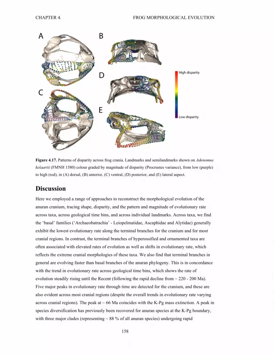
CHAPTER 4. FROG MORPHOLOGICAL EVOLUTION
158
Figure 4.17. Patterns of disparity across frog crania. Landmarks and semilandmarks shown on Adenomus
kelaartii (FMNH 1580) colour graded by magnitude of disparity (Procrustes variance), from low (purple)
to high (red), in (A) dorsal, (B) anterior, (C) ventral, (D) posterior, and (E) lateral aspect.
Discussion
Here we employed a range of approaches to reconstruct the morphological evolution of the
anuran cranium, tracing shape, disparity, and the pattern and magnitude of evolutionary rate
across taxa, across geological time bins, and across individual landmarks. Across taxa, we find
the ‘basal’ families (‘Archaeobatrachia’ - Leiopelmatidae, Ascaphidae and Alytidae) generally
exhibit the lowest evolutionary rate along the terminal branches for the cranium and for most
cranial regions. In contrast, the terminal branches of hyperossified and ornamented taxa are
often associated with elevated rates of evolution as well as shifts in evolutionary rate, which
reflects the extreme cranial morphologies of these taxa. We also find that terminal branches in
general are evolving faster than basal branches of the anuran phylogeny. This is in concordance
with the trend in evolutionary rate across geological time bins, which shows the rate of
evolution steadily rising until the Recent (following the rapid decline from ~ 220 - 200 Ma).
Five major peaks in evolutionary rate through time are detected for the cranium, and these are
also evident across most cranial regions (despite the overall trends in evolutionary rate varying
across cranial regions). The peak at ~ 66 Ma coincides with the K-Pg mass extinction. A peak in
species diversification has previously been recovered for anuran species at the K-Pg boundary,
with three major clades (representing ~ 88 % of all anuran species) undergoing rapid

CHAPTER 4. FROG MORPHOLOGICAL EVOLUTION
159
diversification at this time (Feng et al. 2017). The remaining peaks in evolutionary rate in the
Mid Jurassic and Mid Cretaceous do not noticeably coincide with shifts in palaeoclimate (e.g.,
Cramer et al. 2011; Korte et al. 2015), and instead appear predominantly associated with the
splitting of major anuran clades. This therefore suggests peaks in morphological diversification
coincide with peaks in species diversification. These peaks in evolutionary rate through time can
also be linked to the pattern of rate across taxa. For example, the peak in evolutionary rate
identified at ~ 114 Ma coincides with the split of Nasikabatrachidae and Sooglossidae as well as
the splitting of the clade ‘Ceratobatrachidae plus Nyctibatrachidae’ with its sister clade. In both
cases, the rate of evolution can be seen to increase after these splits. Analyses across taxa and
across time bins therefore together reveal the pattern of evolutionary tempo across Anura.
Across individual semi/landmarks, we can investigate the mode (process) of evolution as well
as the tempo. We find large differences in evolutionary rate and disparity across cranial regions,
with high disparity and evolutionary rate concentrated in the quadratojugal and low disparity
and evolutionary rate concentrated in the vomer. All cranial regions exhibit disparity equal or
lower to that expected given their evolutionary rate (under the assumption of Brownian motion),
suggesting that most regions are experiencing considerable evolutionary constraints and/or
convergence, possibly in response to experiencing similar selection pressures associated with
microhabitat use or biomechanics. We find no regions exhibit higher disparity than expected
given their evolutionary rate, suggesting there is no evidence for the rare scenario of disruptive
selection or facilitation (Felice et al. 2018), which was recovered only for some pterygoid and
parietal semilandmarks of caecilians in Chapter 2 (Bardua et al. 2019b). This analysis of
individual semi/landmarks across the anuran skull, along with the analyses of evolutionary rate
across the phylogeny and through time, reveals the complex pattern of evolutionary tempo and
mode for the anuran cranium.
We find strong evidence that ecology is a primary influence on cranial morphological variation
across Anura. Aquatic and fossorial species occupy largely distinct, minimally-overlapping
regions of morphospace, whilst terrestrial species occupy a more central position, partially
overlapping the regions of both aquatic and fossorial species, supporting the intermediate
morphology of terrestrial species (as suggested by Laurent 1964). However, arboreal species
overlap strongly with terrestrial species in cranial morphospace, suggesting these two habitats
may impose similar selection pressures on cranial morphology as defined in our study. Our
findings therefore partially agree with Moen and colleagues (Moen et al. 2013) who found that
arboreal as well as fossorial and semi/aquatic species had more distinct morphologies than
terrestrial species. Microhabitat also influences the speed and magnitude of cranial
morphological evolution across Anura. Semi/fossorial and aquatic species are considerably
more disparate and faster-evolving than terrestrial, semi/arboreal, and semi-aquatic species, over

CHAPTER 4. FROG MORPHOLOGICAL EVOLUTION
160
the entire cranium and for most individual cranial regions. Furthermore, whilst shifts in
microhabitat use do not seem to coincide with shifts in evolutionary rate, direct comparisons of
magnitude show that fossorial, semi-fossorial and aquatic species exhibit higher rates of
evolution and disparity than the other microhabitat specialists. The aquatic habitat has
previously been shown in Chapter 2 to have accelerated rates of evolution across the crania of
caecilians (Bardua et al. 2019b), as well as accelerated rates across the crania of lizards and
snakes (Watanabe et al. 2019) and the limbs of salamanders (Ledbetter & Bonett 2019), and
fossorial habitats have been shown to have fast evolutionary rate for lizards (Watanabe et al.
2019). In addition, African puddle frog species with a high water dependence have been found
to have higher rates of diversification than terrestrial species (Zimkus et al. 2012). The high
cranial disparity of fossorial and aquatic species suggests similar selection pressures may result
in different morphologies (many-to-one mapping, Wainwright et al. 2005), although the
morphologies are constrained to distinct regions of morphospace. Interestingly, crania of semi-
aquatic species were the least disparate and slowest-evolving, suggesting that, whilst fully
aquatic species experience strong selection pressures, the more generalist niche of semi-aquatic
species may impose weaker selection pressures. We find multiple approaches support the
conclusion that ecology is a major influence on cranial morphological variation and evolution
across Anura, with semi/aquatic and semi/fossorial species displaying distinct cranial
morphologies, and semi/fossorial and aquatic species exhibiting faster rates of evolution and
higher disparity than terrestrial, semi/arboreal, and semi-aquatic species.
This influence of ecology varies across the cranium. The jaw articulation region of frogs
(quadratojugal) is evolving the fastest, mirroring the finding from Chapter 2 for caecilians, and
for snakes (Bardua et al. 2019b; Watanabe et al. 2019), and it is also the most disparate cranial
region. This result suggests feeding mechanics may be a driving force behind cranial
morphological evolution of frogs. In addition, of the five regions most strongly influenced by
microhabitat, three of these are the regions involved in the jaw suspensorium (quadratojugal,
pterygoid, squamosal), along with the nasal and vomer. Changes associated with a fossorial
lifestyle are evident in the extreme morphologies along PC1 for these regions; for example, the
reduction in size of the anterior and medial rami of the squamosal and the expansion of the nasal
have previously been identified in fossorial frogs (Trueb 1973; Trueb & Cannatella 1982;
Senevirathne et al. 2016). Furthermore, the dichotomy observed between the fast-evolving
crania of semi/fossorial and aquatic species, versus the slower-evolving crania of terrestrial,
semi/arboreal and semi-aquatic species is most evident for the cranial regions involved in the
jaw suspensorium, as well as the stapes. Together, these results suggest cranial morphological
evolution across frogs is driven predominantly by the evolution of the jaw suspensorium, most
notably for aquatic and semi/fossorial species, which is likely related to the large diversity of

CHAPTER 4. FROG MORPHOLOGICAL EVOLUTION
161
feeding mechanisms across different microhabitats that have arisen convergently multiple times
across Anura (Nishikawa 2000).
Whilst the bones and muscles comprising the feeding apparatus are similar across frogs, the
morphology and size of individual elements vary considerably (Nishikawa 2000), and feeding
mechanisms are variably linked to the jaw suspensorium. Inertial elongation is highly dependent
on the speed of jaw opening, as the force from this propels the tongue forward (Nishikawa &
Gans 1996). However, the hydrostatic elongation mechanism predominantly observed across
fossorial frogs (e.g., Rhinophrynus dorsalis, Trueb & Gans 1983; Hemisus marmoratum,
Nishikawa et al. 1999) requires only minimal jaw opening, where only the lingual tip need leave
the mouth (Trueb & Gans 1983). This, and the small prey size (i.e. ants, termites) of fossorial
species (e.g., Trueb & Gans 1983; Nishikawa et al. 1999; Van Dijk 2001; Henrici 2015), means
a wide gape is not necessary, allowing the jaw suspensorium to move anteriorly. This anterior
shift in the jaw suspensorium in turn allows an anterior shift of the pectoral girdle, which
effectively eliminates the neck region, facilitating the application of forces to the snout which
are associated with a fossorial lifestyle (Trueb & Gans 1983; Henrici 2015). In contrast, large
prey specialists require wide skulls (Emerson 1985), and the suction feeding of aquatic species
(e.g., Carreño & Nishikawa 2010; Fernandez et al. 2017) also requires a wide skull, resulting in
a more lateralised jaw suspensorium. Second in evolutionary rate only to the quadratojugal, the
large differences in rate across the different microhabitats for the stapes region may be linked to
the convergent losses, reappearances, and re-losses of this structure, as previously documented
(Pereyra et al. 2016), and may reflect the different acoustic potentials from each substrate
(Hetherington 1992). Whilst the shape of the stapes remains relatively conserved across PC1,
the changing orientation of the stapes tip from lateral to anterolateral may reflect different
mechanical requirements associated with hearing in different microhabitats. The study of
individual cranial regions therefore allows us to understand which regions are driving the
evolution of the cranium as a whole.
In contrast to the strong influence of ecology on cranial evolution in anurans, cranial
morphology appears to be only very weakly influenced by developmental strategy, with
biphasic and direct developing species overlapping very strongly in cranial morphospace. The
crania of direct developing frogs are slightly more disparate and faster-evolving than those of
biphasic frogs, but these differences are not significant. In addition, whilst most individual
cranial regions are more disparate for direct developing species, only four of these differences
are significant (otic, vomer, sphenethmoid (dorsal) and premaxilla regions). A mixed pattern is
evident for evolutionary rate, with six regions faster-evolving for direct developers and nine
regions faster for biphasic species, and only two of these results are significant (the otic and
vomer regions evolve significantly faster for direct developing frogs). Biphasic species therefore

CHAPTER 4. FROG MORPHOLOGICAL EVOLUTION
162
appear slightly more constrained in disparity, and the influence of developmental strategy on
rate of evolution appears very weak and specific to each region. These results suggest the
presence of a larval stage may very slightly constrain the resulting adult morphology,
contrasting with the adaptive decoupling hypothesis (Ebenman 1992; Moran 1994) which
hypothesises that a larval stage may have evolved to break genetic and developmental
constraints, promoting the ability for adult morphologies to respond to selection pressures. As I
report in Chapter 3, direct developing frogs had slightly more strongly integrated crania,
suggesting the coordinated evolution of traits across the crania may have promoted slightly
increased disparity for direct developing crania, although the effect is very small. Overall,
developmental strategy does not appear to strongly influence cranial morphology or
morphological evolution in frogs.
It has long been accepted that early developmental stages are more evolutionarily conservative
than late developmental stages (e.g., Fink 1982; Strathmann 1988). The production of traits
from later developmental stages is considered dependent on the traits from earlier
developmental stages, imposing constraints on the earlier developmental stages (e.g., Smith
1983). Similarly, we find strong evidence that the earliest-ossifying regions (parasphenoid,
frontoparietal and occipital) have low evolutionary rates and disparities, whilst the highest rates
and disparity are found in the variably-present, latest-ossifying regions (neopalatine,
quadratojugal and sphenethmoid (dorsal)). This result suggests the early onset of ossification
constrains evolution. The parasphenoid, frontoparietal, and occipital regions (the latter
comprising the oto-occipital bone) are involved in the protection of the brain and otic capsules
(Duellman & Trueb 1986; Heatwole & Davies 2003), and so probably experience strong and
similar constraints on their morphology due to this conserved, essential function. These early-
ossifying bones are also found in areas of the skull that experience the least restructuring during
metamorphosis (Harrington et al. 2013). In contrast, later-ossifying bones are generally variably
present across Anura (possibly a result of paedomorphosis; Weisbecker & Mitgutsch 2010) and
undergo greater morphological changes during metamorphosis (Harrington et al. 2013),
suggesting their functions are not so essential and their morphologies are less constrained.
Ossification sequence timing is thus probably linked to functional demands (Heatwole & Davies
2003), with the earlier-ossifying bones more functionally conservative and therefore more
constrained in morphology.
Frog crania exhibit significant allometric and phylogenetic constraints, and the strength of these
influences varies across cranial regions. The neopalatine is strikingly more constrained by
phylogeny than the remaining cranial regions, more so than would be expected under the
assumption of Brownian motion. This suggests the frequent loss and gain of this structure is
strongly phylogenetically constrained. However, other variably present regions do not show

CHAPTER 4. FROG MORPHOLOGICAL EVOLUTION
163
especially high phylogenetic signal, such as the dorsal and ventral sphenethmoid regions (Kmult
= 0.54, 0.56), suggesting their losses and gains convergently arise across distantly related
clades. As well as phylogenetic constraints, allometric constraints vary in strength across the
cranial regions. For example, we find the occipital region is the most strongly influenced by size
(R2 = 0.32), mirroring results from caecilian crania (Chapter 2, Bardua et al. 2019b), which may
be partly related to size constraints associated with the cranial-neck articulation. The relatively
larger occipital regions we recover for smaller species, as well as the relatively larger cranial
vaults, otic regions, and more verticalised suspensory apparatuses, help to maintain the
minimum space requirements for the brain and sensory organs (e.g, the otic capsules) of smaller
species (previously demonstrated in miniaturised frogs, Yeh 2002a). This reveals how
constraints related to the nervous and sensory systems appear to have a relatively greater
influence on the cranial morphology of smaller frog species. Our finding that larger species
have proportionally smaller braincases is concordant with findings from mammals (Cardini et
al. 2015). However, our results diverge from the generally recognised ‘big size-long face’ rule
of cranial evolutionary allometry found across mammals (Cardini & Polly 2013; Cardini et al.
2015), and rather support the big size/wide skull pattern found across caecilians in Chapter 2
(Bardua et al. 2019b). This result suggests a possible common allometric pattern influencing
both frogs and caecilians, and perhaps may be a broader macro-evolutionary trend characteristic
of amphibians. Cranial size and phylogeny therefore both significantly influence anuran cranial
morphology.
Cranial size is also found to be associated with cranial bone loss. Cranial bone loss occurs
frequently across Anura, and miniaturisation, thought to arise though the early truncation of
development (i.e. paedomorphosis, Hanken 1984), also occurs repeatedly across this clade
(Clarke 1996). Miniaturisation can result in extreme morphological changes, or no evident
changes (Trueb & Alberch 1985). Miniaturisation has been found both correlated (Trueb &
Alberch 1985; Hanken & Wake 1993) and uncorrelated (Yeh 2002a) to cranial bone loss, and
cranial bone loss is not necessarily restricted to miniaturised species (Trueb 1973, 1993; Yeh
2002a). Here, we find a weak positive relationship between cranial centroid size and the number
of cranial regions, revealing that smaller species on average have fewer cranial bones.
Specifically, whilst smaller and larger crania alike can have a complete set of cranial bones,
only the smaller crania tend to lose two or more cranial regions. In particular, only the very
smallest crania have four regions absent. This finding suggests there may be no constraint on
the number of cranial bones in species with small crania, but rather species with large crania are
less able to lose cranial bones through evolution. Finally, in terms of ossification,
hyperossification has previously been found to occur regardless of body size (Trueb & Alberch
1985; Trueb 1993), and this is supported in our study by the weak influence of allometry for

CHAPTER 4. FROG MORPHOLOGICAL EVOLUTION
164
regions involved in hyperossification, such as the frontoparietal. This however requires further
investigation with a dataset more focused on hyperossified taxa. Cranial size therefore
influences cranial bone loss to a degree, but the influence of cranial size on the extent of
ossification is less clear and requires additional study.
Conclusion
Morphological variation, evolutionary rates, and disparity of the anuran cranium are all
significantly influenced by microhabitat, but in general not by developmental strategy.
Semi/fossorial and semi/aquatic species occupy distinct regions of cranial morphospace,
although they both overlap strongly with semi/arboreal and terrestrial species, suggesting
semi/arboreal and terrestrial species are more generalist in cranial morphology. Phylogeny and
allometry are also both significant influences on cranial morphology, with smaller size
associated with narrower crania and on average, fewer cranial bones. The crania of fossorial,
semi-fossorial, and aquatic species exhibit the highest rates of evolution and are the most
disparate, whist terrestrial, semi/arboreal and especially semi-aquatic species have considerably
less disparate and slower-evolving crania. The jaw suspensorium and the stapes in particular are
evolving the fastest for fossorial, semi-fossorial and aquatic species, probably reflecting strong
selection for specialised feeding modes (jaw suspensorium) and adaptation to substrates with
different acoustic potentials (stapes) across different microhabitats. Despite these differences in
rate and disparity across ecological categories, shifts in rate are not generally associated with
shifts in ecology. Ossification sequence timing significantly influences evolutionary rate and
disparity, with later-ossifying bones exhibiting faster rates of evolution and higher disparity.
Finally, evolutionary rate generally increases through time, and disparity is lower than expected
in most cranial regions (assuming Brownian motion), suggesting evidence of convergent
evolution. This study highlights the complex morphological evolution of the anuran cranium,
revealing the varying influences of phylogeny, allometry, ecology, and development, and
revealing how the tempo and pattern of cranial evolution varies across taxa, across time bins,
and across individual landmarks and semilandmarks.

CHAPTER 5 2D OUTLINE ANALYSIS OF FROGS
165
CHAPTER 5
PHYLOGENY, ECOLOGY AND DEEP TIME: 2D
OUTLINE ANALYSIS OF ANURAN SKULLS FROM THE
EARLY CRETACEOUS TO RECENT
Published as:
Bardua, C., Evans, S. E. and Goswami, A. 2018. Phylogeny, ecology and deep time: 2D outline
analysis of anuran skulls from the Early Cretaceous to Recent. Palaeontology. 62:417-431.
Bardua, C., Evans, S. E. and Goswami, A. 2018. Data from: Phylogeny, ecology and deep time:
2D outline analysis of anuran skulls from the Early Cretaceous to Recent. Dryad Digital
Repository. https://doi.org/10.5061/dryad.2gf6910.
Abstract
Anurans have a long fossil record, spanning from the Early Jurassic to Recent. However,
specimens are often severely flattened, limiting their inclusion in quantitative analyses of
morphological evolution. We performed a two-dimensional morphometric analysis of anuran
skull outlines, incorporating 42 Early Cretaceous to Miocene species, as well as 93 extant
species in 32 families. Outlines were traced in tpsDig2 and analysed with elliptical Fourier
analysis. Fourier coefficients were used in MANOVAs, phylogenetic MANOVAs (as
significant phylogenetic signal was found) and disparity analyses across multiple ecological and
life history groupings. The Neotropical realm showed higher disparity than the Australian,
Palearctic and Oriental realms (p = 0.007, 0.013, 0.038, respectively), suggesting concordance
of disparity and diversity. Developmental strategy had a weak effect on skull shape (R2 = 0.02, p
= 0.039), and disparity was similar in metamorphosing and direct developing frogs.
Microhabitat use was a significant discriminator of skull shape (F = 1.43, p = 0.004), but not
after phylogenetic correction. Evolutionary allometry had a small but significant influence on
the cranial outlines of the combined extant and fossil dataset (R2 = 0.05, p = 0.004). Finally,
morphospace occupation appears to have changed over time (F = 1.59, p = 5 × 10⁻¹⁰). However,
as with ecological signal, this shift appears to be largely driven by phylogeny and was not
significant after phylogenetic correction (R2 = 0.26, p = 0.22). This study thus suggests that frog
skull evolution is shaped more by phylogenetic constraints than by ecology.

CHAPTER 5 2D OUTLINE ANALYSIS OF FROGS
166
Introduction
Anurans (frogs), both extant and extinct, are the most speciose and diverse clade of
Lissamphibia. Currently numbering 7130 species (AmphibiaWeb 2019), frogs are found in a
variety of microhabitats with a near worldwide distribution. Anurans have a long fossil history
with impressive past diversity, ranging from the monstrous Beelzebufo ampinga (Evans et al.
2008) to the tiny Indobatrachus pusillus (Owen 1847). Salientia, stem and crown group
anurans, are present in the fossil record from the Early Triassic (e.g., Triadobatrachus, ca. 250
million years ago, hereafter Ma, Piveteau 1936; Ascarrunz et al. 2016), but likely originated in
the Permian (Ruta & Coates 2007). A greater abundance of fossils is seen from the Early
Jurassic, including the stem-anurans from the genera Prosalirus (Shubin & Jenkins Jr 1995) and
Viaerella (Estes & Reig 1973). The first crown group anuran is Eodiscoglossus oxoniensis
dating from the Middle to Late Jurassic and may be the earliest member of Discoglossoidea
(Evans et al. 1990). Eodiscoglossus is represented by many Early Cretaceous fossils. It is likely
that some other modern clades had evolved by the start of the Cretaceous, including Pipidae
(e.g., Estes et al. 1978). The majority of fossil occurrences are based on isolated or
disarticulated bone fragments (Sanchíz 1998), but rare cases of exceptional preservation
including soft tissue are known, including Eleutherodactylus from the Eocene amber of the
Dominican Republic (Poinar & Cannatella 1987) and a mummified specimen of
Thaumastosaurus gezei from the Eocene (Laloy et al. 2013). Despite the remarkable
preservation of some fossil anurans, three-dimensionally preserved specimens remain rare. The
vast majority of complete specimens are severely flattened, which may be partially attributable
to their thin rod- like cranial bones. Consequently, morphological evolution has not been well
studied across fossil frogs, as morphological studies are limited primarily to descriptions of
individual specimens (see Estes & Reig 1973) and not comparisons across taxa.
Preservational and sampling biases can strongly influence the completeness of a clade’s fossil
record. Temnospondyls, with their generally large size and robust skulls, have an extensive
fossil record, with around 300 species identified (Schoch 2013) and a near global distribution.
Temnospondyl diversity can be tracked from the Lower Carboniferous to the Lower Cretaceous
(McHugh 2012) and includes many complete skulls. However, their descendants, in particular
the anurans, are considerably more affected by preservational biases, being generally small
organisms in ecosystems which do not preserve readily, such as tropical forests (e.g., Duellman
1999). In fact, despite a present day species ratio of 2:3, there is a mammal to amphibian fossil
record ratio of > 5:1 during the Paleocene (Benson et al. 2016). This is likely a combination of
less intensive sampling efforts, less robust skeletons of amphibians, and many fossil mammals
named based on isolated teeth, and highlights the difficulty of inferring past diversity from
present. Throughout their history there is a clear bias towards amphibians preserved from

CHAPTER 5 2D OUTLINE ANALYSIS OF FROGS
167
freshwater systems compared with terrestrial systems (Schoch 2014), but both systems preserve
considerably less readily than marine settings. There is also disproportionate representation of
amphibian fossils from Lagerstätten, creating a biased picture of past amphibian diversity
(Schoch 2014). The under-represented nature of amphibians in the fossil record therefore
stresses the importance of incorporating all suitable fossils into morphological studies.
The quantification of morphology allows us to explore how environmental, developmental and
functional pressures can influence organismal shape. Recent decades have seen many advances
in the study of morphology, in particular in the field of three-dimensional shape analysis, with
anatomy captured using a range of approaches from anatomical landmarks (e.g., Goswami
2006b) to entire surfaces represented by sliding semi-landmarks (described by Bookstein 1997;
Gunz et al. 2005; and implemented by, for example, Fabre et al. 2014; Felice and Goswami
2018). High density surface-based approaches have already been demonstrated in Chapters 2-4,
where the morphological evolution of caecilian and frog crania were investigated. However,
methods such as this require high quality data if subsequent analyses are to be robust.
Specimens must have well-preserved and undeformed morphology, which are highly
constraining requirements for most fossil specimens. Thus, many studies choose to exclude
fossils instead of compromising the strength of morphological analyses (as seen in Chapters 2-4,
with the exception of one Eocene fossil frog included in Chapter 4). In addition to Chapters 2-4,
many previous macroevolutionary studies have explored morphological evolution across large
clades, including Gymnophiona (Sherratt et al. 2014); Aves (Cooney et al. 2017; Felice &
Goswami 2018); and the anuran family Myobatrachidae (Vidal-García & Keogh 2017), but
these clades (and many others) suffer from a fossil record largely inadequate for inclusion in
comprehensive, quantitative morphological studies. Past diversity has been studied in clades
such as temnospondyls (Stayton & Ruta 2006; Angielczyk & Ruta 2012), but these datasets
represent clades with unusually abundant fossils available for study. Nonetheless, these fossil
studies highlight the rich and varied past diversity of clades such as amphibians. This then leads
to the inevitable decision as to whether to prioritise the capture of morphological data
(subsequently sacrificing unsuitable specimens), or to use a more inclusive approach, reducing
sampling of morphology but representing more of past and present diversity.
The cranium is a particularly informative osteological structure for inferring anuran ecology and
behaviour (e.g., Jared et al. 2005; Senevirathne et al. 2016). Whilst some consider the anuran
limb system to be the most unique feature of this clade, anuran skulls exhibit extreme
morphological variation, from hypo-ossification (e.g., Bombina) to heavily ossified and
ornamented skulls (e.g., Ceratophrys), as well as the presence of novel cranial bones (e.g., the
prenasal of the casque-headed Triprion petasatus). Previous studies have explored three-
dimensional morphological variation in the anuran cranium (e.g., Vidal-García et al. 2014;

CHAPTER 5 2D OUTLINE ANALYSIS OF FROGS
168
Vidal-García & Keogh 2017) but fossils have not been included in these studies as three-
dimensional specimens are exceptionally rare. However, biological information can still be
extracted from two-dimensional anuran cranial morphology, especially as frog skulls are
reasonably dorsoventrally compressed relative to the crania of other tetrapods (p. 311 Trueb
1993). Pipoid and non-pipoid frogs have been compared using two-dimensional cranial and
lower mandible landmarks (Yeh 2002b), which revealed that pipoids differ ontogenetically from
salamanders, but are more similar to them morphologically than non-pipoids are. Two-
dimensional cranial landmarks were used by another study (Yeh 2002a) to compare skull shapes
of miniaturised frogs and closely related larger species. Miniaturised frogs were found to have
relatively larger braincases and reduction of some bone elements. Despite these promising
studies demonstrating that two-dimensional data successfully discriminates skull shape in extant
frogs, this approach has not yet been applied to fossil frogs.
Here, we quantify the two-dimensional morphology of extant and fossil anuran skulls to take
advantage of the many exceptionally preserved yet severely flattened fossil specimens. Because
of the difficulty in consistently identifying homologous landmarks in many fossil frog
specimens, we apply elliptical Fourier analysis to the outlines of anuran skulls. Using these data,
we assess whether phylogeny, development, or ecology is a greater influence on anuran skull
morphology, and quantify how anuran skull morphology changes through time. First, we
evaluate ecological and developmental signal in extant frog skull shape and compare disparities
across groupings based on these factors. We then combine data from the extant and fossil
datasets to measure phylogenetic signal and evaluate the influence of size on skull shape across
all frogs. Finally, we examine shifts in frog skull shape through time and differences in disparity
among temporal groupings of frogs in order to provide a comprehensive analysis of frog skull
shape evolution, as quantified by two-dimensional outlines.
Materials and methods
Specimens
Photos, diagrams, and reconstructions of 93 extant and 65 fossil frog skulls were obtained either
from the published literature or from original specimens (Appendix 5, Tables S5.1-5.2, and see
Fig. 5.1 for an example of a fossil frog). Phylogenetic and ecological diversity is well sampled
within the dataset, with 32 extant families represented, ranging from the aquatic Pipidae to the
fossorial Pyxicephalidae, and from the tiny Eleutherodactylus pipilans (Snout-vent length, SVL,
reaching 29.4 mm, AmphibiaWeb 2018), to the world’s largest frog, Conraua goliath (SVL up
to 320 mm, AmphibiaWeb 2018). This study also has temporal coverage spanning most of
anuran evolution, with 65 specimens of 42 fossil species ranging in age from the Middle-Late
Jurassic stem-anuran Notobatrachus degiustoi (176-145 Ma, Báez & Nicoli 2004) to fossil

CHAPTER 5 2D OUTLINE ANALYSIS OF FROGS
169
members of living genera, such as early Middle Miocene Rana (Roček et al. 2011). Adult
specimens were chosen to the best of our ability, but it can be difficult to discern between adult
and sub-adult fossil specimens. Fossil specimens were included if at least one bilateral half of
the skull was traceable, and this traceable half was mirrored when required (Appendix 5, Table
S5.2). Initially, multiple specimens of each fossil species were included in the main dataset to
assess the effect of deformation qualitatively, but the final analyses used only the least deformed
specimen or best reconstruction for each species. Subsets of this dataset were used for different
analyses, depending on the ecological, life history and body size traits available for each
species, as detailed below. Taxa with unknown or ambiguous phylogenetic position were
removed from phylogenetic analyses.
Figure 5.1. Aerugoamnis paulus FMNH PR2384 from the Early Eocene of Green River Formation,
Wyoming, demonstrating the dorso-ventral flattened preservation typical of specimens in this study
[photo used with permission from Henrici et al. (2013)]. Scale bar is 3 mm.
Morphometric data collection
Outlines were taken as the largest tracing around the skull, which in some cases meant that
ventral attributes were being traced in dorsal aspect. However, in most cases, it was not possible
to discern details beyond the largest outline. The program tpsUtil (Rohlf 2013) was used to
build a tps file from images, and this file was loaded into tpsDig2 (Rohlf 2015). The outline of
each image was traced using the closed curve function in tpsDig2 and this curve was then
resampled to 100 points. The starting point of each curve was the anteromedial extreme of the
skull, which was oriented to face towards the top of the image. Individual points were then slid

CHAPTER 5 2D OUTLINE ANALYSIS OF FROGS
170
around the outline, as points did not need even spacing because the analyses conducted on the
outlines only considered the outline not the individual points. Consequently, areas of high detail
could be represented by more points than areas of conserved curvature (Fig. 5.2). Some fossils
did not have scales included in the published images, but this did not affect their inclusion in
analyses because scale, as well as position, are non-shape aspects that were removed prior to
analysis. Once all images had been outlined in the tps file, the curves were appended to
landmarks using tpsUtil. These landmarks were then imported into R (R Core Team 2017) for
analyses.
Figure 5.2. The outline of Adelotus brevis KU 56242, an extant specimen used in this study (see
Appendix 5, Table S5.1).(see Bardua <i>et al.</i> 2018, Table S1) (A) traced using tpsDig2 and
resampled to 100 curve points; and (B) generated using the Momocs package, using the 100 resampled
curve points. Scale bar is 20 mm.
Extant-only phylogeny
The phylogenetic tree used for the extant frog dataset was adapted from the molecular
phylogenetic analysis and divergence estimates of 2871 amphibians (Pyron & Wiens 2011).
This was the most comprehensive phylogeny at the time of writing available for living
amphibians. The R packages geiger (Harmon et al. 2008), ape (Paradis et al. 2004) and phytools

CHAPTER 5 2D OUTLINE ANALYSIS OF FROGS
171
(Revell 2012) were used to prune this tree and add 28 extant species by assigning them to the
positions of their respective genera. Polytomies were randomly resolved in Mesquite (Maddison
& Maddison 2016). Six species were excluded from phylogenetic analyses, due to uncertain
phylogenetic positions, including Crossodactylodes pintoi and Zachaenus parvulus which are
both assigned to Incertae sedis in Hyloidea (Pyron & Wiens 2011).
Extant and fossil phylogeny
Fossil anuran species in our study were manually added to the extant phylogeny for our
combined analyses (Fig. 5.3). The topology for the fossil species was based on a recent
composite tree analysis (Marjanović & Laurin 2014), which collated many fossil lissamphibian
species and placed them within the framework of the extant amphibian phylogeny we used
(Pyron & Wiens 2011). Incongruences exist between the Marjanović and Laurin (2014) tree and
more focused phylogenetic studies; for example, Beelzebufo ambinga has been variably placed
within Calyptocephalidae (Agnolín 2012; Marjanović & Laurin 2014) or Ceratophryidae (Laloy
et al. 2013; Evans et al. 2014). However, since the Marjanović and Laurin (2014) tree has
considered all major attempts to place fossil lissamphibians into trees and is congruent with the
extant topology used in this study (Pyron & Wiens 2011), this composite tree topology was
further modified for the combined analyses.
A composite tree was created by manually inserting extinct species into our extant phylogeny,
using branch lengths that we first calculated by creating a topology of just the extinct species.
To create the extinct species topology, the positions of 28 extinct species in our study were
exactly replicated from the Marjanović and Laurin (2014) tree. Eight species (mainly
Liaobatrachus and Rana specimens) were not included in that work, but congeneric species
were represented, so they were placed within their respective genera, resolving polytomies at
random. For taxa without representatives in the Marjanović and Laurin (2014) tree, their
placement was estimated based on other recent studies. These taxa include Thaumastosaurus
gezei (Laloy et al. 2013) and Aerugoamnis paulus (Henrici et al. 2013). Four specimens with
unknown phylogenetic placement were removed from the phylogenetic analyses; Eupsophus
sp., Lutetiobatrachus gracilis and two specimens of Anura indet. This topology was then dated
using the R package Paleotree (Bapst 2012). The first and last occurrence dates of each fossil
taxon were taken from the literature, and each was placed into five million-year time bins. The
sampling rate was set at a low value of 0.01, as much of the frog fossil record consists of
isolated bones that could not be included in the study. Speciation and extinction rates were
assumed equal (Foote et al. 1999). The cal3 dating method (Bapst 2013) created 1000 dated
trees; the average branch lengths from these trees were then used to create the composite tree.

CHAPTER 5 2D OUTLINE ANALYSIS OF FROGS
172
To combine our extant and fossil phylogenies, fossil taxa were manually added to the cropped
extant phylogeny, using their calculated branch lengths as guidance. However, specific branch
lengths could not easily and completely be superimposed due to some variation in topology, so
some nodes required manual manipulation in Mesquite to ensure all branches and taxa were
aged as accurately as possible with the current information on phylogenetic relationships and
occurrences.
Figure 5.3. Composite phylogenetic tree of sampled extant and extinct anurans. Alternate colour bands
indicate periods of 50 million years, with the outer extreme at Recent.
Ecological and developmental data
Ecological data were compiled from the literature and online databases (IUCN 2016; Myers et
al. 2017; AmphibiaWeb 2018) on microhabitat use, environment, zoogeographic realm
occupation, IUCN Red List Status and developmental strategy (Appendix 5, Table S5.1).

CHAPTER 5 2D OUTLINE ANALYSIS OF FROGS
173
Microhabitat use (N = 86) was divided into seven categories: terrestrial (ground dwelling), fast
aquatic (rivers and streams), slow aquatic (lakes and ponds), semi-aquatic, fossorial
(underground), arboreal, and semi-arboreal, and species were excluded with broad microhabitats
or no available microhabitat information. Environment (N = 66) was defined as: ‘arid open’,
‘temperate forest’, ‘temperate open’, ‘tropical forest’ and ‘tropical open’. Frogs inhabiting a
range of environments were excluded from this analysis. The zoogeographic realm (N = 85) was
divided into the following: Afrotropical; Australo-Papuan; Nearctic; Neotropical; Oriental;
Palearctic and Widespread (Duellman 1999). Widespread was defined as species found in more
than one realm. Extinction risk (N = 78) was classified by the Red List Index (IUCN 2016) with
the following list: 1 (Least Concern), 2 (Near Threatened), 3 (Vulnerable), 4 (Endangered), 5
(Critically Endangered). ‘Data deficient’ specimens were removed from this analysis. Extinction
risk was treated as an ordered factor in analyses. Finally, developmental strategy (N = 78)
distinguished between species that undergo metamorphosis (biphasic, or indirect, development)
or not (direct development).
Allometry
Snout-vent length (SVL) was taken as the measurement for body size as it was the most readily
available measurement for fossil frogs and is the standard body measurement for extant frogs
(see Fig. 17 from Roček et al. 2010). Fossil frog SVL was taken from the literature as the
measured or estimated SVL of the specimen, or the maximum SVL found for a specimen of that
species. SVL for extant frogs was taken as the maximum female SVL, as females are generally
the larger sex in frogs (Shine 1979), or the upper limit of any SVL range given. SVL data were
available for 112 of the sampled species, 29 of which were fossil frog taxa and 83 were extant
frog taxa.
Data analyses
Two-dimensional shape- elliptical Fourier analysis
Two-dimensional projections of three-dimensional shapes can be effective correlates of overall
shape, potentially introducing only small error into the data (for a review see Cardini 2014).
Two-dimensional shape can be described by landmarks (e.g., Wund et al. 2012), linear
measurements (e.g., Jojić et al. 2012) or by outline (e.g., Zhan & Wang 2012). It is generally
accepted that outline analysis is preferable for capturing shape information when homologous
landmarks are missing (see Temple 1992). Outline approaches include eigenshape analysis
(Lohmann 1983), polar Fourier analysis (e.g., Kaesler & Waters 1972) and perimeter-based
Fourier analysis (Foote 1989) but the most common approach is elliptical Fourier analysis (see
Rohlf & Archie 1984; Temple 1992). The Fourier series was first developed by Joseph Fourier
(1768-1830), who demonstrated that a complex waveform can be expressed as a sum of

CHAPTER 5 2D OUTLINE ANALYSIS OF FROGS
174
trigonometric functions. This approach was later developed to apply this mathematics as a tool
for quantifying shape in biological studies. Elliptical Fourier analysis (EFA) uses the Fourier
series to describe the shape of a closed curve (Giardina & Kuhl 1977; Kuhl & Giardina 1982).
Decomposing a complex, closed waveform into a series of simpler, sinusoidal waves of varying
period and magnitude allows us to understand the primary aspects of shape, as well as reducing
dataset dimensionality. Elliptical Fourier analysis has been used to study shape in a variety of
subjects, from assessing shape differences in forest fragment populations of leaves (Andrade et
al. 2010) to comparing water basin shapes (Bonhomme et al. 2013). It has also been used in
morphological studies, from comparing bird caudal skeletal morphology across the ecological
spectrum (Felice & O’Connor 2014) to assessing artificial cranial deformation in human crania
(Frieß & Baylac 2003). Thus, EFA has been shown to be a successful method for assessing two-
dimensional shape in a range of akinetic biological shapes.
Outline analysis was used to capture the shape of anuran skulls. Unlike other outline
approaches, EFA does not require landmarks or a biological centre to the outline which is
homologous throughout the sample (Crampton 1995). In addition, evenly spaced points are not
a requirement, allowing increased sampling from areas of high curvature to better represent the
full outline. Elliptical Fourier (herein EF) coefficients provide an efficient measure of the major
aspects of shape to a desired degree of precision, reducing the dimensionality of the dataset by
removing unnecessary harmonics (as determined by those cumulatively representing less than a
set proportion of the shape).
Tps files were loaded into R and analysed using the Momocs package (Bonhomme et al. 2014).
The data were firstly converted into a ‘Coo’ object, which is the format required to analyse the
outlines. These outlines were then centred and scaled to remove all non-shape data from the
analyses. Elliptical Fourier analysis was applied to the outlines using the ‘efourier’ function in
Momocs. Normalisation was not performed in this step, as the outlines (being symmetrical and
roughly circular) are at risk of bad alignment. Orientation effects had already been considered
by orienting all images with the snout facing upwards. The Fourier coefficients were then
extracted to use as high dimensional variables in analyses. Each harmonic n is represented by
four coefficients, two from each of the x and y projections, so that the total number of
coefficients is 4n. The number of harmonic coefficients required for the outline analysis was
determined by choosing the number which corresponded to a cumulative sum harmonic power
of 99%. We therefore used 14 EF coefficients for the extant dataset and 12 for the fossil dataset.
Although the number of extra harmonics nearly doubled for 99% compared to 95% cumulative
power, the extra harmonics were necessary to accurately represent all the high detailed
information in the posterior region of the skull. This reduced dimensionality of the dataset down

CHAPTER 5 2D OUTLINE ANALYSIS OF FROGS
175
from 200 (100 two-dimensional coordinates) to 56 and 48 dimensions for the extant and fossil
datasets respectively.
Principal components analysis
To further reduce dimensionality, principal components analysis (PCA) was conducted in the R
package Momocs on the EF coefficients which represented 99% cumulative power. Principal
components analysis allows a large dataset to be represented by far fewer variables, making
multivariate analyses tractable. Principal components should not be analysed separately as
univariate variables, and a sufficient number of Principal components should be retained, as
using just the first few components can introduce biases into analyses (Uyeda et al. 2015).
Principal component (PC) scores that described 99% of the shape were retained and used in
subsequent analyses.
Sensitivity analyses
We first conducted a series of sensitivity analyses to assess the effects of pooling photos, figures
and reconstructions, and including specimens preserved in different aspects or with different
degrees of completeness. Some diagrams of fossil specimens depicted the outline more clearly
than a photo. To test that diagrams from the literature were accurate representatives of the true
skull shape, PC scores of skull outlines from diagrams and corresponding photos of 33 species
were compared with a MANOVA using the ‘MANOVA’ function in Momocs. As well as
diagrams, many authors have reconstructed the skull in two-dimensions, using one or multiple
specimens as reference (e.g., Báez & Nicoli 2004). As these reconstructions attempt to eliminate
the deformation present in the original specimens, they may provide a better representation of
the true skull shape. To assess the validity of using reconstructions, all specimens along with the
reconstruction for each species were outlined and compared to see whether reconstructions plot
in the same region of morphospace as the specimens. In addition, specimens of fossil frogs
commonly exist either in dorsal or ventral aspect but not always as both part and counterpart. To
test whether aspect is an important factor for skull outline shape variation, photos of extant frog
skulls from 27 species were outlined both in dorsal and ventral view. As noted above, outlines
were traced as the largest outline as it would look from a shadow projection and not by
following bones from purely the dorsal or ventral side, as individual bones could not be
determined in most fossil frog images.
Finally, deformation and crushing evident in fossil frog specimens introduces distortions in
quantification of the true skull shape. The posterior outline of the fossil frog skull generally
appeared worst affected, likely due to the higher-level detail here which is more easily affected
by crushing. In particular, the squamosal and pterygoid regions were occasionally difficult to
trace, and the occipital section was frequently difficult to decipher because of the overlapping of

CHAPTER 5 2D OUTLINE ANALYSIS OF FROGS
176
vertebrae. To assess the sensitivity of results to inaccuracy in outlining the posterior skull, a
sample of 32 species was outlined three times, firstly completely (‘D1’), secondly by
deliberately removing information about the posteromedial section by replacing this with a
straight-line perpendicular to the anteroposterior plane (‘D2’), and thirdly by removing the
posterolateral information similarly (‘D3’) (Fig. 5.4). The ‘D2’ outlines therefore exclude the
occipital region, and the ‘D3’ outlines exclude the pterygoid region. PC scores from the three
outlines for each specimen were then compared through pairwise MANOVAs. We could
therefore assess the degree to which uncertainty in the outline tracings can affect the analyses.
These extreme examples of incomplete outlines create realistic maximum values for the
difference between true and observed outlines.
Figure 5.4. The outline of Adelotus brevis KU 56242, outlined (A) completely, (B) deliberately removing
posteromedial information, and (C) deliberately removing posterolateral information, for sensitivity
analyses assessing the effect of missing or degraded posterior morphology on results. Scale bar is 20 mm.
Phylogenetic signal
Phylogenetic signal of the PC scores was evaluated using the Kmult statistic (Adams 2014a),
which is a multivariate generalisation of the K statistic (Blomberg et al. 2003), implemented in
the geomorph package (Adams & Otárola-Castillo 2013) in R. Closely related species are likely
to have similar traits due to shared ancestry, and this signal of phylogeny is measured relative to
expectations under a model of Brownian motion. Non-independence of data points means that,
once phylogenetic signal is detected, it is necessary to apply a phylogenetic correction to the
shape data to investigate evolutionary differences.
Ecological and developmental influences on shape
Ecological and developmental data from extant species only were used in MANOVAs
(‘MANOVA’ function in Momocs) and phylogenetic MANOVAs (herein pMANOVAs,
‘procD.pgls’ function in geomorph), to assess multiple potential factors influencing skull shape.
Whilst these two tests differ in their assessment of significance (the ‘procD.pgls’ function is

CHAPTER 5 2D OUTLINE ANALYSIS OF FROGS
177
non-parametric and the ‘MANOVA’ function is parametric), results are comparable. The Pillai-
Bartlett trace was used as it is considered the most robust test statistic (see Johnson & Field
1993). A correction was applied to the MANOVAs and pMANOVAs to account for an elevated
false-positive rate with increased number of tests (Benjamini & Hochberg 1995). Morphological
disparity (as measured by Procrustes variance) was also compared across ecological groupings,
using the ‘morphol.disparity’ function in geomorph.
Allometry
Allometric shape changes for the combined fossil and extant dataset were visualised by plotting
the predicted Procrustes residuals at minimum and maximum size using the ‘procD.allometry’
function in geomorph. Specimens were also plotted on a morphospace, colour coded by SVL, to
display the distribution of cranial sizes along the main axes of shape variation. The influence of
evolutionary allometry (shape correlates of size among species) was assessed using
pMANOVAs (‘procD.pgls’ function in geomorph) for both the extant only and the combined
extant and fossil dataset, with log-transformed SVL set as a factor against PC scores. Log-
transformed size variables better fitted a normal distribution.
Morphospace occupation through time
To assess differences in morphospace occupation based on species age, a MANOVA and
pMANOVA were applied to PC scores using species age as a factor. For fossil frogs, this was
the first occurrence date within the fossil record, and, for extant species, this was the first
occurrence date of that species if it had a fossil record, or “Present” if no fossil record exists.
The full dataset was binned into time bins of five million years.
Results
Elliptical Fourier analysis
Elliptical Fourier analysis successfully captured the frog skull outlines in terms of a series of
ellipses which reduced the dimensionality of the dataset down to 12 (fossil frogs) or 14 (extant
frogs, and combined dataset) harmonics, to an accuracy of 99% cumulative power (Appendix 5,
Fig. S5.1). Seven harmonics would have been sufficient to describe 95% of the shape in both
extant and fossil frogs but the last 4% of shape information was important for capturing
appropriate detail in the posterior region of the skull.
Principal components analysis
Principal component scores were retained in each analysis so that 99% of the shape was
described, resulting in 22 - 24 PC scores retained for extant frog analyses (depending on the
subset of data), and 15 - 17 for the fossil subsets. For the combined dataset of extant and fossil
frog outlines, 25 PC scores were retained. The first principal component of the combined

CHAPTER 5 2D OUTLINE ANALYSIS OF FROGS
178
dataset accounted for 37.7% of the variation and PC2 accounted for a further 18.1%. Similar
values were found for the extant (PC1 = 38.3%, PC2 = 18.3%) and fossil (PC1 = 40.5%, PC2 =
19.4%) only datasets. In the combined extant and fossil dataset, PC1 corresponded to the
relative length ratio of the skull; one extreme shape was antero-posteriorly longer than it was
wide, whereas the other extreme was wider than it was long (Fig. 5.5). The negative extreme of
PC2 corresponded to a more triangular outline, whereas the positive extreme was more circular.
Figure 5.5. Morphospace occupation of 125 frog skull outlines through time. Points are coloured from
purple (youngest) to red (oldest) in five million-year bins based on species first appearances. Extreme
outline shapes representing the positive and negative extremes along PC1 and PC2 are displayed.
Sensitivity analyses
Sensitivity analyses supported the pooling of all data types, and allowed us to visualise the
information lost from the posterior region of the skull. Dorsal and ventral outlines were shown
not to be significantly different (MANOVA, approx. F = 0.42, p = 0.98). They were also shown
CHAPTER 5 2D OUTLINE ANALYSIS OF FROGS
179
to have similar morphological disparity as illustrated by comparing Procrustes variances
(Procrustes variance, dorsal = 0.002, ventral = 0.002, p = 0.73) so that one aspect did not
capture more morphological variation. The outlines of frog skulls taken from photos and their
corresponding diagrams were also not significantly different from one another (MANOVA, F =
1.11, p = 0.37) and morphological disparity was similar (photo = 0.0002, diagram = 0.0002, p =
0.70). Outlines of fossil reconstructions were compared to outlines of original specimens.
Morphological disparity within each species was small (range 0.003 to 0.022), except for
Notobatrachus degiustoi which had a Procrustes variance significantly larger than all other
species (disparity = 0.037), which may reflect greater deformation in these specimens. These
results, and a visualisation of morphospace (Appendix 5, Fig. S5.2), suggested deformation did
significantly influence the outline shape, with some specimens of the same species showing
large morphospace distributions. Lastly, in a pairwise MANOVA taking Outline (D1/2/3) as a
factor, the partial outlines (D2 and D3) were both significantly different to the complete outline
(D1-D2 approx F = 19.19, p = 2.22 × 10⁻¹⁵, D1-D3 approx F = 2.74, p = 0.003). This analysis
revealed the importance of tracing the posterior region as accurately as possible, which justifies
the use of EFA instead of radial or tangent Fourier analysis since a greater sampling of points is
allowed in regions of greater complexity. Results from the various sensitivity analyses therefore
supported the inclusion of diagrams, reconstructions and both dorsal and ventral aspect outlines
in further analyses. However, caution had to be taken for fossils whose outlines were hard to
trace; some fossils were consequently rejected from the study (Appendix 5, Table S5.2), and
reconstructions were prioritised over photos.
Phylogenetic signal
The observed phylogenetic signal of the shape data (using PC scores) was significant for both
the extant frog dataset (N = 87, 24 PCs, Kmult = 0.49, p = 0.001) and combined dataset (N = 125,
25 PCs, Kmult = 0.48, p = 0.001). These results suggested closely related species resembled each
other, but phenotypically less than expected under a Brownian motion model.
Ecological and developmental influences on shape
Microhabitat use was a significant discriminator of skull shape (MANOVA, 24 PCs, F = 1.43, p
= 0.004), even after multiple-test correction (p = 0.02), but not after phylogenetic correction
(pMANOVA, 24 PCs, R2 = 0.09, p = 0.37) (Appendix 5, Fig. S5.3). Procrustes variances for
crania from all microhabitats were similar and non-significantly different, ranging from 0.011 to
0.039. Frogs inhabiting the five categories of environment were not found to have significantly
different skull outlines (Appendix 5, Fig. S5.4), before or after phylogenetic correction
(MANOVA, 22 PCs, F = 0.94, p = 0.62, pMANOVA, R2 = 0.07, p = 0.87), nor did they display
different morphological disparities (Procrustes variance range 0.029 to 0.045, no significant
differences). There was no significant difference in the outline shapes of the different

CHAPTER 5 2D OUTLINE ANALYSIS OF FROGS
180
zoogeographic realms, in either a MANOVA (23 PCs, F = 0.87, p = 0.84), or a pMANOVA,
(R2 = 0.05, p = 0.53). Disparity in zoogeographic realms in decreasing order was Widespread
(0.044), Neotropical (0.041), Nearctic (0.035), Australo-Papuan (0.022), Afrotropical (0.019),
Palearctic (0.018) and Oriental (0.009). The Neotropical realm showed significantly higher
disparity than the Australian, Palearctic and Oriental realms (p = 0.007, 0.013, 0.038,
respectively). The other differences in Procrustes variances were non-significant. There was no
significant difference in outline shape between the different levels of extinction risk
(MANOVA, 23 PCs, F = 0.84, p = 0.83, pMANOVA, R2 = 0.06, p = 0.61), as defined by the
IUCN Red List status. Finally, developmental strategy was a significant discriminator of frog
skull shape (MANOVA, 23 PCs, F = 2.04, p = 0.016) even after correcting for multiple-tests (p
= 0.04) and phylogeny (R2 = 0.02, p = 0.039), although not after correcting for both (p = 0.20)
(Appendix 5, Fig. S5.5). Disparity was similar in metamorphosing and direct developing frogs
(Procrustes variance: direct = 0.033; biphasic = 0.001, p = 0.85).
Allometry
Evolutionary allometry had a small but significant effect on the extant frog skull outlines (R2 =
0.08, p = 0.0004). Pooling extant and fossil frog data showed a smaller but still significant
allometric effect (R2 = 0.05, p = 0.004). Visualising morphospace distribution with size set as a
factor revealed an overlapping distribution, with a general trend of larger species having shorter,
wider skulls and smaller species having narrower skulls (Appendix 5, Fig. S5.6).
Morphospace occupation through time
A MANOVA illustrated a significant difference between taxa based on their age of first
appearance (25 PCs, F = 1.59, p = 5 × 10⁻¹⁰), binned into five million-year time bins, but not
once phylogeny was incorporated (R2 = 0.26, p = 0.22). A visualisation of the morphospace
occupation (Fig. 5.5, and see Appendix 5, Fig. S5.7 for a phylomorphospace) along the first two
principal components revealed a distribution seemingly independent of species age. Triprion
petasatus (extant) and Beelzebufo ampinga (fossil) had the most extreme skull outlines along
PC1 and Shelania pascuali (fossil) and Rana basaltica (fossil) represented the extremes along
the PC2 axis.
Discussion
The anuran skull is highly reduced relative to the ancestral condition in terms of the size and
number of cranial bones. This reduced cranial morphology is already seen in stem anurans (e.g.,
Notobatrachus degiustoi), after which the skull appears relatively unchanged. This qualitative
assessment was confirmed quantitatively in our study, which found that morphospace
occupation remained similar from the Middle-Late Jurassic until the present day, as measured
by fossil and extant frog skull outlines (Fig. 5.5). The small change observed in morphospace

CHAPTER 5 2D OUTLINE ANALYSIS OF FROGS
181
occupation is phylogenetically structured and most likely reveals a preservational bias rather
than truly changing morphospace, from the absence of some taxa in the fossil record (e.g.,
Centrolenidae) and abundance of others (e.g., Pipidae).
With a widespread distribution and adaptations to many diverse environments, frogs
successfully occupy many microhabitats in zoogeographic realms across the globe. It has long
been known that the Neotropical realm is the most diverse region for flora and fauna, boasting
the highest diversity of frogs (Duellman 1999), with over 2500 recorded species, 97% of which
are endemic to this region (Bolaños et al. 2008). This is thought to be greatly underestimated
(Fouquet et al. 2007), with a suggested 170 - 460 frog species unrecognised in this realm. Its
consistent moist and warm climates with little seasonal temperature change are conducive to
diversity. Although frogs have adapted to extreme environments such as brackish water
(Lepidobatrachus asper) and deserts (Craugastor augusti), their requirements of moisture and
warmth have meant that diversity is highest in areas satisfying these requirements. Results have
demonstrated that, as measured by skull outlines, the Neotropical realm is the most disparate
realm, indicating possible concordance of disparity and diversity in frogs. Convergence of body
shape has been found in anuran species with similar microhabitat use, including similar toe
morphology in arboreal species and an association of body rotundity with fossoriality
(Duellman & Trueb 1986; Wells 2007). However, ecological and environmental signals in our
dataset appeared weak in extant anuran cranial outlines (Appendix 5, Figs. S5.3-S5.4). Frogs
from different environments showed no significant differences in skull outline, and the
influence of microhabitat use on skull outline was only significant before phylogenetic
correction. Simplification and categorisation of ecosystem data may dilute any ecological
signals, as environments and ecologies exist on a continuous scale and are hard to discretise, but
it is also possible that skull outline does not capture ecological differences among anurans. For
example, the degree of ossification is thought to be related to certain feeding and life habits (p.
332 Trueb 1993), but cranial outline may not capture differences in ossification. Incorporation
of skull depth may therefore provide further insights into ecological influences on cranial
morphology.
Developmental strategy is easier to discretise, and was found to have a weak effect on cranial
morphology, but no effect on cranial morphological disparity (Appendix 5, Fig. S5.5). Tadpole
morphology has been postulated to impose constraints on the resulting adult morphology, for
example the loss of a free-living larval stage may have influenced the high morphological
diversity of plethodontid salamanders (Wake & Hanken 1996). This ontogenetic constraint
hypothesis can be contrasted with the idea of antagonistic selection creating pressure for
different ontogenetic life stages to evolve independently, allowing them to respond to different
environments and requirements. A larval stage does not appear to impose constraints on the

CHAPTER 5 2D OUTLINE ANALYSIS OF FROGS
182
body morphology of Australian anurans, with a recent study finding adult morphology was
shaped strongly by phylogenetic signal and tadpole morphology influenced more by homoplasy
(Sherratt et al. 2017). Sherratt et al. (2017) illustrates how developmental strategy is only one
aspect of development; tadpole morphology can evolve independently from adult morphology
in at least Australian anuran species. Incorporation of tadpole specimens in studies of cranial
morphology may therefore aid the understanding of how development influences adult cranial
shape. Our analyses of extant anurans found cranial disparity was not significantly different
between direct and biphasic developers, further suggesting that anuran morphology is not
restricted by metamorphosis, despite the prerequisite of a tadpole morphology. Developmental
strategy did significantly discriminate frogs based on skull shape, but accounted for only a small
amount of the shape variation, suggesting life history does not greatly influence the adult skull
shape. Our study therefore finds the existence of a free-living larval stage to neither greatly
facilitate nor constrain adult morphology, in terms of cranial outline.
Instead, our study found morphology is more driven by phylogenetic relationships than
ecological or developmental influences (Appendix 5, Figs. S5.3-S5.5). Ecological and
developmental signal, when significant, were often erased by correcting for phylogenetic signal.
This result suggests closely related species share similar microhabitats and lifestyles, despite
resembling each other phenotypically less than expected under a Brownian motion model.
Phylogenetic conservatism has been found previously in Australian anurans, in both skull
morphology (Vidal-García & Keogh 2017) and body shape and size (Vidal-García et al. 2014),
suggesting the prevalence of a phylogenetic signal in anuran morphology. Furthermore, a study
of toad skulls has revealed that evolutionary constraints can restrict morphological responses to
past climate changes (Simon et al. 2016). Fossil amphibian studies have had similar findings:
evidence has been found for morphological convergence within groups, and divergence between
groups, both for Paleozoic temnospondyls (Angielczyk & Ruta 2012) and Mesozoic
stereospondyls (Stayton & Ruta 2006). Our results are therefore concordant with previous
studies on extant and fossil amphibians, suggesting the prevalence of phylogenetic constraints
on anuran evolution through deep time.
Allometry can be studied across individuals of a given age (static), across different life stages
(ontogenetic) and across a phylogeny (evolutionary). Craniofacial evolutionary allometry has
been studied in placentals and marsupials, with a general trend of small species exhibiting
shorter faces (e.g., Cardini & Polly 2013; Cardini et al. 2015). This trend has, however, been
found to be variably present across tetrapods, evidenced in temnospondyls (Angielczyk & Ruta
2012), with a small size being associated with a short, broad snout and large orbits in some
clades but not others. Our study found allometry was a significant influence on anuran cranial
outlines through deep time, although the effect was small. Visualisation of the morphospace

CHAPTER 5 2D OUTLINE ANALYSIS OF FROGS
183
(Appendix 5, Fig. S5.6) showed that larger species appeared to have relatively wider skulls,
whilst smaller species had narrower skulls, reflecting the results from caecilian and frog crania
in Chapters 2 and 4. This result suggests that the pattern of craniofacial evolutionary allometry
across mammals may not be true outside of amniotes, or indeed Mammalia. Our findings
therefore suggest that size-dependent selection pressures or constraints on cranial morphology
may differ between anurans and mammals.
Beyond anuran evolution and biology, our results have implications for future studies of fossil
anurans, as well as other taxa. We described the complex outline of extant and fossil frog skulls
by a series of simple curves, and showed that whilst extant frogs required 14 harmonics to
describe 99% of the shape, fossil frogs only required 12 (although we used 14 for both in the
combined analysis). The additional two harmonics required to explain the extant frog skull
outlines highlight how the high order detail may have been lost from the fossils, since the fossil
skull outlines can be described using more simple curves. It has been shown experimentally by
studying the decay of Amphioxus and ammocoete larvae (Sansom et al. 2010) that higher detail
is more vulnerable to loss of information through decay. The most phylogenetically useful
information is more susceptible to loss in the fossil record whilst the plesiomorphic characters
are more robust. This results in fossils being interpreted as more basal than their true
phylogenetic position. This stemward slippage (Sansom et al. 2010) is suggested to be an
important bias often overlooked in the fossil record. In a similar fashion, higher frequency
harmonics are more readily lost to noise than the lower frequency harmonics. Comparing
harmonic requirements in extant and fossil datasets using EFA may therefore help to illustrate
the missing information in fossils in future studies.
The potential caveats of an outline study on fossil specimens (the inclusion of a variety of data
types and different levels of deformation) were addressed in this study through sensitivity
analyses, but require further investigation. Sensitivity analyses supported the inclusion of fossils
in both dorsal and ventral aspects as well as the use of diagrams and reconstructions. This may
have implications for the study of similarly flattened fossils, although the amount of shape
information captured in different two-dimensional aspects will be strongly dependent on the
fossil. A method has been developed which allows the comparison of two- and three-
dimensional shape (Cardini 2014), providing both of these data can be collected from the same
dataset. At the time of conducting this research for Chapter 5, the 3D dataset used in Chapters 4
and 5 was not available, but a useful avenue for further work could be to compare two- and
three-dimensional shape captured from this same subset of specimens. This study also begins to
assess the impact of variable deformation within a dataset, and future studies should further
explore these effects where possible. Our study did find significant differences between fossil
specimens of the same species (Appendix 5, Fig. S5.2), but the similarity observed in

CHAPTER 5 2D OUTLINE ANALYSIS OF FROGS
184
morphospace occupation between extant and fossil frog skulls suggests deformation in fossil
frog skull outlines was likely not introducing excessive noise into our results.
Conclusion
The flattened nature of most fossil anuran skulls renders a three-dimensional analysis
incorporating most fossil taxa currently unachievable. Whilst the incorporation of skull depth
information would better illustrate the morphospace occupation of fossil and extant frogs, this
requires three-dimensional reconstructions of flattened fossils, or the discovery of better
preserved fossil anurans. Elliptical Fourier analysis was therefore used to quantify two-
dimensional extant and extinct frog skull shape. This study compared extant and fossil frog
morphologies to evaluate phylogenetic, ecological and developmental signals. We found that
phylogeny overrode most ecological or developmental signals, and the observed change in
morphospace occupation through time appears to have been phylogenetically driven as well.
This study aimed to highlight the possibility of including less-well preserved specimens in
studies of morphology. This increased inclusivity does sacrifice the robustness of results to
some extent, but it means greater temporal breadth and the inclusion of many fossil specimens
which would otherwise remain excluded from morphological studies, limiting the sampling of
past diversity.

CHAPTER 6 CONCLUSION
185
CHAPTER 6
CONCLUSION
Broader context
The study of morphology is central to our understanding of extant and extinct diversity. From
sexual selection, to form-function relationships, to evolutionary arms races, a vast range of
topics are tackled by biologists interested in quantifying morphology and understanding how
and why shape varies in the manner observed across the history of life (e.g., Shine 1979;
Arnqvist & Rowe 1995; Banavar et al. 2014; Stanyon & Bigoni 2014). The study of
morphology can help to unravel genetic, developmental, or evolutionary influences on
organisms, and understanding the relationships between morphology and these influences across
extant taxa can have great implications for our understanding of taxa for which we only have
morphological information, i.e. fossils. Morphology can reveal how organisms evolve, how they
respond to ecological selection pressures, and how they may be constrained by biotic factors
(e.g., development). However, to fully understand the drivers of morphological evolution,
knowledge of how phenotypic traits correlate across a structure is vital, as these trait
correlations can impede or promote exploration of shape space (Goswami et al. 2014; Felice et
al. 2018). Linking the study of morphological evolution with an investigation into how
phenotypic traits interact is therefore critical in order to gain a more accurate understanding of
how and why shapes evolve.
The fields of morphological evolution and phenotypic integration are receiving growing interest
as scan data are becoming readily more available and methods to quantify shape are steadily on
the rise. Until now, these fields have been explored mainly with amniote (and in particular,
mammal) datasets (e.g., Cheverud 1982; Goswami 2006b; Goswami and Polly 2010b; Singh et
al. 2012; Goswami and Finarelli 2016; Parr et al. 2016), and very few studies have sampled
morphologies across entire clades. However, only with increased study of lissamphibians, the
sole extant tetrapod clade outside of Amniota, can we gain a comprehensive, unbiased
understanding of tetrapod cranial evolution. Whilst one study thus far has explored modularity
and evolution of caecilian crania across the entire clade (Sherratt 2011), no study has yet
examined modularity and cranial evolution across the full clade diversity of the most speciose
amphibians, anurans. Furthermore, previous studies of integration and modularity across frogs
and caecilians have focused their investigations of modular structure on two to five modules,
and collected either traditional landmark or linear distance data (Sherratt 2011; Simon &
Marroig 2017; Vidal-García & Keogh 2017), with no frog or caecilian studies to date

CHAPTER 6 CONCLUSION
186
investigating a range of highly modular structures, or sampling densely across the cranial
morphologies.
This thesis aimed to address the predominantly amniote-centric view of phenotypic integration
and morphological evolution of the cranium, by thoroughly investigating these concepts across
mainly extant species of two of the three lissamphibian clades, as well as exploring frog cranial
evolution through deep time. I comprehensively sampled 3D cranial morphology across datasets
boasting generic (caecilians, Chapter 2) and familial (frogs, Chapters 3-4) coverage, and I
further captured the 2D cranial morphology of 42 fossil and 93 extant frogs (Chapter 5). I used
these shape data to investigate the modular structure of frog and caecilian crania, as well as
exploring the patterns of cranial variation and the factors shaping its morphological evolution.
In this final chapter, I summarise my main findings and draw comparisons across my three
amphibian datasets (2D and 3D frog cranial data, 3D caecilian cranial data), as well as
discussing possible future directions for further study.
Data type
Cranial morphology was quantified using the following two types of data, each appropriate to
the dataset under study: high-dimensional 3D landmarks and semilandmarks (Chapters 2-4) and
2D outlines (Chapter 5). Extant frog and caecilian crania are extremely disparate, with cranial
bones that vary widely in relative positions, sizes, shapes and even presence. These datasets
therefore required a high-density 3D approach to fully capture this variation. The high-
dimensional morphometric approach implemented in Chapters 2-4 successfully captured the
complex and diverse cranial morphologies of frogs and caecilians, sampling every family of
frogs and every genus of caecilian. We described this method, and detailed how to overcome the
many challenges associated with the collection of this data, in a recently published study
(Appendix 1, Bardua et al. 2019a). Using this method, cranial morphology was quantified using
~1000 (frogs) and ~1500 (caecilians) landmarks and semilandmarks. I devised a method to
capture the morphology of variably present regions (termed the ‘negligible region’ method),
since traditional landmarking approaches would not capture these regions. Given the
considerable loss of elements in some frog and caecilian crania, this ‘negligible region’ method
prevented the loss of morphological information, and/or the exclusion of taxa with absent
regions. Furthermore, comparison of our high-dimensional landmarks/semilandmarks to
landmark-only analyses revealed important discrepancies between the two methods. Landmark-
only analyses for both frogs and caecilians exaggerated between-region trait correlations
relative to within-region trait correlations, portraying the crania to be more integrated than when
sampling evenly over the entire surface. This boundary bias is a result of landmarks being
typically situated at sutures, immediately adjacent to corresponding landmarks on neighbouring
regions (Goswami et al. 2019). The surface-based approach I used therefore better represented

CHAPTER 6 CONCLUSION
187
the morphology of the crania, and provided a more accurate reflection of the biological patterns
of trait integration. Defining 16 (caecilians) and 19 (frogs) cranial regions, I investigated the
modular structure of amphibian crania, and explored cranial morphological evolution across the
two clades.
However, this high-dimensional surface based approach required the crania to be three-
dimensionally preserved, complete and undeformed. Fossil frog crania are extremely flat and
internal anatomy is often obscured, resulting in their exclusion from the high-dimensional
analyses of cranial evolution. In order to incorporate these fossil specimens into an analysis of
cranial evolution, a 2D outline approach was necessary. Elliptical Fourier analysis successfully
captured the outline shape of 42 fossil frog crania, as well as 93 extant frog crania in order to
gain an understanding of morphospace occupation through time. However, these 2D data did
not allow the investigation of patterns of trait integration, or the study of individual cranial
regions. Furthermore, the weaker influences of ecology, allometry and phylogeny recovered
across this dataset relative to the high-dimensional dataset of frog crania probably reflect the
loss of morphological information in 2D outlines compared with the high-density 3D shape
data. Thus, whilst the 2D outline approach does not capture cranial morphology as effectively as
the 3D high-dimensional approach utilised for the extant taxa, it does permit the study of the
flattened fossil frog crania, which would otherwise have remained unsampled.
Key findings
Conservation of patterns of integration
Anuran and caecilian crania have diverged greatly in morphology, with frog skulls generally
wide and open, and caecilian skulls elongate and robust. However, despite the great
morphological differences, I found that the underlying pattern of trait integration was strikingly
similar. This suggests conservation of modularity since the divergence of lissamphibians in the
Paleozoic or Early Mesozoic (San Mauro et al. 2005; Zhang et al. 2005). The highly modular
structure may have facilitated the great morphological diversity exhibited across both clades,
with functionally distinct regions able to evolve semi-independently from one another. In both
datasets, the suspensorium/ ‘cheek’ region of the skull (i.e. quadrate/quadratojugal, squamosal,
and in frogs, the pterygoid) formed a large, highly integrated functional module, possibly to
facilitate coordinated changes in response to feeding pressures. The two occipital regions
defined in both frogs and caecilians formed a module, and a maxilla/maxillopalatine module
was also recovered from both frogs and caecilians, comprising two and three regions
respectively. However, whilst the vomer formed a module with the os basale (ventral) in
caecilian crania, the vomer did not form a module with the analogous region in frogs (the
parasphenoid). Slight differences in morphology also prevent the exact comparison of some

CHAPTER 6 CONCLUSION
188
regions across frogs and caecilians, including the fusion of the nasal and premaxilla in most
caecilians (= nasopremaxilla), and (probable) fusion of the frontal and parietal in frogs (=
frontoparietal). Overall, the crania of both clades were more modular anteriorly than posteriorly,
with anterior regions possibly responding more to highly localised selection pressures.
Patterns of trait integration recovered across frogs and caecilians can also be compared with
other published datasets. A study we published recently (Marshall et al. 2019) found an
extremely similar pattern of trait integration within two intraspecific samples of caecilian crania,
which was also strongly congruent with the pattern recovered across the caecilian clade
(Chapter 2). These datasets together therefore suggest a highly conservative pattern of trait
integration from the static to evolutionary level, at least across caecilians. These findings can
also be compared to recently published studies investigating patterns of trait integration across
amniotes using high-density data (birds, Felice & Goswami 2018; archosaurs, Felice et al. 2019;
squamates, Watanabe et al. 2019). Comparison of amphibian and amniote modularity patterns
reveals conserved features (e.g., strongly integrated jaw joint regions) as well as divergent
features (e.g., amphibian crania are more modular), suggesting a shifting of the pattern of
integration from the amniote-anamniote split. Our data therefore suggest that patterns of
modularity may be strongly conserved within Lissamphibia, but less conserved across
Tetrapoda as a whole.
Influences on morphology, disparity and evolutionary rate
Phylogeny and allometry
Phylogeny and allometry significantly influenced frog and caecilian crania, and these influences
varied across cranial regions. The strength of phylogenetic signal varied from Kmult = 0.48
(extant and fossil frog outlines, Chapter 5), to Kmult = 0.66 (frog crania, Chapters 3-4), to Kmult
= 0.87 (caecilian crania, Chapter 2), suggesting caecilian crania are more constrained by
phylogeny than frog crania. Evolutionary allometry accounted for 5% (frog outlines, Chapter 5),
13% (frog crania, Chapters 3-4) and 16% (caecilian crania, Chapter 2) of the shape variation,
suggesting caecilian cranial morphology was also more influenced by size than was frog cranial
morphology. A large cranial size was associated with wider, more triangular shaped skulls for
all frog and caecilian datasets (Chapters 2-5). This suggests there may be a common
macroevolutionary trend of ‘big size-wide skull’ across amphibians, in contrast to the ‘big size-
long face’ rule recognised across mammals (Cardini & Polly 2013; Cardini et al. 2015). Across
both frogs and caecilians (Chapters 2-4), the occipital region of the skull was relatively large in
smaller taxa and exhibited the strongest influence of allometry, possibly a result of minimum
space requirements associated with the otic capsules and cranial-neck articulation muscles.
Phylogenetic and allometric influences varied across frog and caecilian cranial regions,

CHAPTER 6 CONCLUSION
189
supporting the finding from both frogs and caecilians that size was not phylogenetically
structured.
Development
Developmental influences on morphological evolution were investigated for frog and caecilian
crania. Developmental strategy was a very weakly significant or a non-significant influence on
cranial morphology for all three datasets (Chapters 2,4,5). Developmental strategy also did not
significantly influence disparity (Chapters 4,5) or the rate of evolution (Chapter 4) of frog
crania. No rate shifts were associated with shifts in life history for frogs (Chapter 4), although a
significant rate shift was recovered for caecilian crania coinciding with the origin of direct
development (Chapter 2). Together, these results suggest developmental strategy was not a
major influence on cranial morphological evolution for frogs or caecilians. Ossification
sequence timing, however, appeared to be a strong significant influence on strength of
integration, evolutionary rates, and disparity for frog crania (Chapters 3-4), with late-ossifying
bones more disparate, faster-evolving, and more integrated than earlier-ossifying bones. This
suggests the relative timing of ossification of cranial bones has a considerable impact on the
morphological evolution of the anuran skull.
Ecology
This thesis found ecology to be a stronger influence on morphology than was development.
Across frogs and caecilians, ecology was a significant influence on cranial morphology
(Chapters 2,4). For frogs, semi/fossorial and semi/aquatic species occupied largely distinct
regions of morphospace, suggesting these two habitats imparted divergent selection pressures
on crania. In addition, fossorial, semi-fossorial and aquatic frog species had significantly faster
rates of evolution, and were more disparate, than terrestrial, semi/arboreal and semi-aquatic
species (Chapter 4). Aquatic caecilian species also exhibited faster rates of evolution (Chapter
2). From Chapter 2 and previous studies (e.g., Taylor 1969; Nussbaum 1983; Nussbaum &
Wilkinson 1989; Gower et al. 2004) it is thought that a fossorial lifestyle has shaped the
evolution of caecilian crania, but the influence of fossoriality on caecilian cranial morphology
was hard to quantify in this thesis as the vast majority of caecilian species are fossorial to some
extent, hindering comparisons to alternative habitats. Fossorial and aquatic niches appeared to
exert considerable influences on cranial shape evolution of both frogs and caecilians, driving
faster rates of evolution and increased disparity for frogs and to some extent, caecilians.
Evolutionary rates and disparity
Evolutionary rates and disparity were correlated across both frog and caecilian crania, with both
metrics varying across and within cranial regions (Chapters 2,4). The highest disparities and
rates of evolution were found on the jaw joint articular surface of both frogs and caecilians, as

CHAPTER 6 CONCLUSION
190
well as posteriorly on the maxillopalatine (caecilians)/maxilla (frogs). Across frogs, high rates
and disparity were also found anteriorly on the stapes and ventral sphenethmoid, laterally on the
neopalatine and ventrally on the squamosal. For both frog and caecilian crania, strength of
integration showed no linear relationship with either evolutionary rates or disparity (Chapters 2,
3). This supports the recent hypothesis that integration is a stronger influence on direction,
rather than the speed, of evolution (Felice et al. 2018). Integration can drive both higher and
lower disparity than expected from an unintegrated structure (Goswami et al. 2014).
Specifically, the influence of integration may depend on the alignment of each region’s
selection with the path that integration facilitates through morphospace.
Summary of key findings
I investigated modularity and morphological evolution across two of the three amphibian clades.
Frog and caecilian crania were both highly modular, exhibiting a pattern of phenotypic trait
integration that appears highly conserved across the two clades. Specifically, both frog and
caecilian crania exhibited a highly integrated ‘jaw suspensorium’ region (the ‘cheek’ module in
caecilians) and a highly integrated ‘occipital’ region. Evolutionary rate and disparity were
correlated, and varied across the crania, but showed no linear relationship to strength of
integration. However, ossification sequence timing correlated strongly with integration,
evolutionary rate, and disparity for frogs. Phylogeny and allometry both influenced cranial
morphology, and ecology was a stronger influence on morphology than developmental strategy.
Specifically, fossorial and aquatic niches appeared to be strong drivers of morphological
evolution for both frogs and caecilians, providing a foundation for future study of both
influences on amphibian morphological evolution and broader questions on the causes and
consequences of phenotypic integration.
Future Directions
Additional influences on morphological evolution
Future field work efforts and targeted taxonomic sampling could facilitate the investigation into
additional influences shaping frog or caecilian morphological evolution. Diet, for example, can
be a significant influence on cranial morphology (e.g., Emerson 1985; Goswami 2006b; Slater
and Van Valkenburgh 2009; Baab et al. 2014; Dumont et al. 2015). Diet data are unavailable
for most frog and caecilian species, but sampling of select frog species with dietary information
could better reveal how diet influences anuran cranial morphology. I would expect that small
prey specialists may have smaller, narrower crania than large prey specialists, as previously
described (e.g., Toft 1981; Emerson 1985). Locomotion (hopping, walking, swimming) may
also influence anuran cranial morphology. I would hypothesise that hopping ability (and the
distance covered) would correlate with reduced, perhaps hypo-ossified crania, to minimise the

CHAPTER 6 CONCLUSION
191
weight of the skull. Finally, large-scale extrinsic factors such as climatic niche position (e.g.,
tropical or temperate climate) and geographical distribution may influence cranial
morphological evolution. The possible concordance of cranial disparity (as measured by 2D
outlines) and species diversity identified across frog crania in Chapter 5 could be expanded
upon by testing whether the Neotropical realm is the most disparate in cranial morphology (as
measured by 3D high-density data) as well as being the most speciose of the zoogeographic
realms (Duellman 1999).
Intraspecific level
My thesis has concentrated on patterns of integration at the evolutionary level. The study of
integration at the intraspecific (static) level can reveal genetic relationships across the cranium.
This can be compared to the evolutionary level to understand whether these relationships are
maintained across species and have formed a persistent constraint on cranial evolution. Indeed,
we have investigated this across caecilian crania, finding highly congruent patterns across two
species of caecilian (Marshall et al. 2019), both of which are very similar to the pattern
recovered at the evolutionary level. This suggests genetic modularity may have evolved
adaptively to match functional modularity. Increased intraspecific sampling across caecilians
would reveal the pervasiveness of our finding, and comparisons of modular structure across
species with different developmental strategies, reproductive strategies, and ecologies may
reveal the influences these factors exert on the strength and pattern of phenotypic integration.
Similarly, intraspecific studies for frog species would reveal firstly whether frogs are similarly
conserved from static to evolutionary level, and secondly would provide additional insight into
the influence developmental strategy and ecology may have on the strength and patterns of
integration. This is work in progress as ongoing collaborations for two species of frogs.
Ontogenetic level
Investigating patterns of phenotypic integration through ontogeny would reveal how integration
patterns change from larvae to adult. A previous study has found a possible decoupling of the
morphological evolution of frog larvae and adults for species with a complex life cycle (Sherratt
et al. 2017). This provides support for the adaptive decoupling hypothesis, which hypothesises
that the presence of a larval stage arises to weaken genetic and developmental constraints,
allowing adults to respond more easily to functional demands (Ebenman 1992; Moran 1994).
Comparisons of morphometric traits between larval and post-metamorphic frogs (Johansson et
al. 2010), as well as between metamorphosed juvenile and adult wood frogs (Philips 1998) also
provide support for this hypothesis, where trait correlations across life stages are weak.
However, other studies have recovered strong correlations across life stages (e.g., Blouin 1992;
Watkins 2001; Wilson & Krause 2012), especially size-dependent (Watkins 2001) or
behavioural (Wilson & Krause 2012) traits. In this thesis, I have already shown that direct

CHAPTER 6 CONCLUSION
192
developers had slightly more highly integrated crania, and biphasic developers were more
modular, weakly supporting the adaptive decoupling hypothesis (Chapter 3). However, the
study of patterns of integration across larvae and across adults for select biphasic species would
greatly enhance our understanding of whether patterns of integration are conserved through
development. I hypothesise that the crania of larval frogs are more integrated than adult crania,
with the crania more modular following metamorphosis.
Extant diversity as a key to the past
Many lissamphibian bones are preserved as isolated, disarticulated material (e.g., Sanchíz
1998), which can prohibit taxonomic identification. This is in part because it is not known how
phylogenetically conserved the morphologies are, and whether distantly related taxa have
converged on similar phenotypes. The large morphological datasets collected in this thesis for
individual cranial bones across frogs and caecilians (following the partitioning of the crania)
may help the taxonomic identification of frog and caecilian cranial bones in the fossil record.
Determining the phylogenetic signal of each bone reveals the bones that have experienced the
most convergence, and the bones with the highest phylogenetic signal. Bones exhibiting high
phylogenetic signal may therefore be more appropriate for taxonomic identification, whereas
bones with convergent morphologies could be treated with caution. Furthermore, future
morphological datasets of isolated fossil cranial material of frogs or caecilians may be combined
with my datasets of extant cranial bones to gain a more in-depth understanding of how each
cranial bone has evolved from deep time to the present. This could be similar to my analysis of
anuran cranial outlines through deep time (Chapter 5). Similar studies targeting commonly
found fossil bones across different clades may aid future identification of fossils.
Postcranial morphology
Future studies could investigate patterns of trait integration and morphological evolution across
postcranial bones of amphibians. The three-dimensional studies in my thesis (Chapters 2-4)
required the crania to be complete, articulated and minimally deformed, hence restricting my
dataset to extant taxa (and only one fossil frog), since the fossil record comprises predominantly
disarticulated bones, with the few articulated specimens generally only preserved in two
dimensions (Sanchíz 1998). This exclusion of three-dimensionally preserved isolated fossil
cranial material from my thesis limits the understanding of cranial evolution to extant diversity
(but see Chapter 5). Future study of isolated postcranial bones could result in a dataset that
includes both extant and fossil species, facilitating the study of morphological evolution through
deep time. For example, limbs have been shown to be influenced by fossorial habitats and
locomotion across Australian frogs (Vidal-García & Keogh 2017), and so further investigation
into how ecology and locomotion influence limb morphology across the entire clade may allow
interpretation of past frog ecologies, which may help the reconstruction of past environments.
CHAPTER 6 CONCLUSION
193
Salamanders
A similar investigation into patterns of phenotypic integration across salamanders, the third
extant amphibian clade, would facilitate the assessment of macroevolutionary trends across
Lissamphibia. This is work currently being undertaken in collaboration with international
researchers, which involves sampling across every salamander genus (Fabre et al. in rev.).
Salamanders number 731 species (AmphibiaWeb 2019), ranging in size from 23 mm (Thorius;
Parra-Olea et al. 2016) to 1800 mm (Andrias davidianus, Hayes 2007). In addition to the direct
and biphasic developmental strategies observed across Anura, some salamanders exhibit a third
main strategy, paedomorphosis, where individuals retain larval characteristics as adults and do
not undergo metamorphosis. Paedomorphic salamanders include the blind cave olm Proteus
anguinus, which can survive eight years without sustenance (Gadeau de Kerville 1926), and the
well-known axolotl, Ambystoma mexicanum (Schreckenberg & Jacobson 1975), both of which
retain feathery, external gills.
Observation of the pattern of trait integration across salamander crania revealed that the highly
conserved pattern of trait integration observed thus far for frog and caecilian crania was also
conserved across salamanders, with strikingly similar patterns identified across all three clades.
In particular, salamander crania were also highly modular, with a highly integrated jaw
suspensorium region. This suggests a deep-rooted conservation of modularity across
Lissamphibia. Furthermore, with the addition of a third main developmental strategy
(paedomorphosis), salamanders serve as a key clade for additional investigation into the
influences of developmental strategy on cranial morphology. In contrast to anurans,
developmental strategy was found to be a strong influence on cranial morphology and
evolutionary rate across salamanders, with rate shifts coinciding with transitions between life
cycle strategies. Furthermore, salamanders inhabiting aquatic microhabitats exhibited the
fastest-evolving cranial morphologies, suggesting this microhabitat may be a key habitat for
promoting morphological evolution across amphibians. Our ongoing study of salamanders is
therefore extending the investigation of patterns of trait integration and morphological evolution
to understand macroevolutionary trends across the entire lissamphibian clade.
Amphibian ancestors
Owing to the poor preservation of frog and caecilian fossils, our high dimensional analyses were
restricted to extant taxa (with the exception of one frog from the Eocene). Fossil frogs were
studied through the use of 2D outlines, but these data did not allow the study of modularity as
crania could not be subdivided into different regions. Consequently, our current understanding
of patterns of modularity across amphibians is based primarily on extant taxa. Investigating
modularity within a clade of amphibian ancestors would allow us to understand how (and if)
patterns of modularity have changed through time, possibly confirming or opposing the current

CHAPTER 6 CONCLUSION
194
hypothesis that modularity increases through time (Wagner & Altenberg 1996; Goswami et al.
2014).
The ancestry of Lissamphibia remains a debated topic, with three main contending hypotheses:
a Temnospondyli origin (Ruta et al. 2003; Ruta & Coates 2007; Sigurdsen & Green 2011;
Maddin & Anderson 2012; Schoch 2019), a Lepospondyli origin (Laurin & Reisz 1997; Laurin
1998; Vallin & Laurin 2004; Pyron 2011; Marjanović & Laurin 2013), and a diphyletic origin,
where anurans evolved from dissorophoids (temnospondyls), gymnophionans evolved from
microsaurs (lepospondyls) and caudates are sister group to either Anura (Carroll 2007;
Anderson et al. 2008) or Gymnophiona (Romer 1945). A recent study also recovered different
origins of the three amphibian clades within Temnospondyli; Batrachia nested within
Dissorophoidea and Gymnophiona nested within Stereospondyli (Pardo et al. 2017). These
hypotheses have significantly different ramifications for the reconstruction of evolutionary
patterns and processes leading to the modern clades. The temnospondyl hypothesis would
suggest that miniaturisation is the main pathway from temnospondyls to modern day
amphibians (Fröbisch & Schoch 2009), whilst the lepospondyl hypothesis implies neoteny
played a large role, as lysorophians strongly resemble some larval salamanders (proteids and
sirenids) (Schoch & Milner 2004). The diphyly hypothesis suggests fossoriality evolved in
microsaurs as a condition for the emergence of caecilians. Miniaturisation, neoteny and
fossoriality are so pervasive within Lissamphibia, however, that convergence is almost certainly
a major issue and characters attributed to these evolutionary pathways may indeed be
homoplastic (Schoch & Milner 2004).
Whilst this debate is still ongoing, it is accepted by most authors that Temnospondyli is the
ancestral amphibian clade. Temnospondyls emerged in the lower Carboniferous, ~ 330 Ma, and
radiated into a huge variety of ecological niches. Their numbers were drastically cut by the
Permo-Triassic mass extinction, ~ 250 Ma, but some taxa recovered (particularly
Stereospondyli) and another massive radiation occurred in the Triassic (McHugh 2012). They
are known until the lower Cretaceous, 115 Ma. Around 300 species of temnospondyls have
been identified (Schoch 2013), with a near worldwide distribution. Temnospondyls had an
impressive size range, from the largest non-amniote tetrapods (6 m long stereospondyls) to the
miniaturised amphibamids (~ 0.05 m) (Schoch 2013). Holophyly of Temnospondyli has been
long proposed (e.g., Romer 1945) and has since been strongly supported in phylogenetic
analyses (e.g., Schoch 2013).
Temnospondyl crania are heavily ossified, and differ greatly in morphology from extant
amphibian crania. Frog and caecilian cranial bones diverge from temnospondyl cranial bones in
their relative positioning and individual morphologies (Schoch 2014a), as well as in number

CHAPTER 6 CONCLUSION
195
(lissamphibians retain only 19 of the 41 elements of the dermal skull of temnospondyls, Schoch
2014b). Identifying the pattern of integration across the crania of temnospondyls may shed light
on how each cranial region has evolved and how modularity has changed through time.
Furthermore, the inclusion of temnospondyls in evolutionary rates analyses could improve our
understanding of how and when amphibian morphologies have changed through time, since
fossils improves estimates of rate (Quental & Marshall 2010).
Extending the sampling further through time, the study of patterns of integration across stem
and early tetrapod crania would provide additional insights into macroevolutionary trends along
this lineage. Stem tetrapods were the first vertebrates to make the transition from water to land,
evidenced by a gradual loss of “fish” characteristics and the emergence of terrestrial adaptations
(Ahlberg & Milner 1994; Clack 2006). As such, they represent the ancestral condition for all
living tetrapods, including both amphibians and amniotes (Clack 1998). Well known taxa
include Acanthostega (Coates 1996), Ichthyostega (Ahlberg et al. 2005) and Tiktaalik
(Daeschler et al. 2006). Whilst the precise relationships of early tetrapods are still contentious,
the study of these taxa would allow the evolutionary history of amphibians to be traced from the
pivotal water-to-land transition until present day.
Conclusion
With the collection of high-density cranial shape data for representative species across every
caecilian genus and every frog family, this thesis presents the first thorough investigation into
patterns of phenotypic integration and the factors influencing morphological evolution at a
macroevolutionary scale across these two clades. Cranial shape was captured in unprecedented
detail, using and advancing a cutting-edge method that permits the comparison of extremely
disparate shapes. These shape data revealed the highly conserved, highly modular structure of
phenotypic integration across frog and caecilian crania, as well as highlighting the roles
ecology, development, phylogeny and allometry played in driving the morphological evolution
of these two clades. Partitioning the crania into highly integrated, semi-autonomous groupings
of traits allowed the investigation of evolutionary rates and disparity across distinct cranial
regions, and revealed the relationship integration has with these two metrics as well as with
ossification sequence timing. The work presented in this thesis attempts to alleviate the current
amniote bias in studies of phenotypic integration and morphological evolution, providing a
more representative insight into tetrapod cranial evolution. This work should serve as a useful
resource for future researchers interested in the mosaic evolution of the tetrapod skull, as well as
those interested more broadly in the interplay of influences shaping cranial morphological
evolution at a macroevolutionary scale. The rapid advancements in geometric morphometric
methods and the increasing ease of data acquisition have catapulted the study of
macroevolutionary trends across entire clades, providing exciting avenues for future study, and I

CHAPTER 6 CONCLUSION
196
hope research efforts will continue to focus on narrowing the gap between amniotes and their
incredibly diverse sister clade.

REFERENCES
197
REFERENCES
Adams, D. C. 2014a. A generalized K statistic for estimating phylogenetic signal from shape and
other high-dimensional multivariate data. Syst. Biol. 63:685–697.
Adams, D. C. 2014b. A method for assessing phylogenetic least squares models for shape and other
high-dimensional multivariate data. Evolution. 68:2675–2688.
Adams, D. C. 2014c. Quantifying and comparing phylogenetic evolutionary rates for shape and
other high-dimensional phenotypic data. Syst. Biol. 63:166–177.
Adams, D. C. 2016. Evaluating modularity in morphometric data: challenges with the RV coefficient
and a new test measure. Methods Ecol. Evol. 7:565–572.
Adams, D. C., and M. L. Collyer. 2015. Permutation tests for phylogenetic comparative analyses of
high-dimensional shape data: what you shuffle matters. Evolution. 69:823–829.
Adams, D. C., and M. L. Collyer. 2017. Multivariate phylogenetic comparative methods:
evaluations, comparisons, and recommendations. Syst. Biol. 67:14–31.
Adams, D. C., M. L. Collyer, A. Kaliontzopoulou, and E. Sherratt. 2017. Geomorph: software for
geometric morphometric analyses. R package version 3.0.5.
Adams, D. C., and E. Otárola-Castillo. 2013. geomorph: an R package for the collection and analysis
of geometric morphometric shape data. Methods Ecol. Evol. 4:393–399.
Adams, D. C., F. J. Rohlf, and D. E. Slice. 2013. A field comes of age: geometric morphometrics in
the 21st century. Hystrix, Ital. J. Mammal. 24:7–14.
Adams, D. C., F. J. Rohlf, and D. E. Slice. 2004. Geometric morphometrics: ten years of progress
following the ‘revolution.’ Ital. J. Zool. 71:5–16.
Agnolín, F. L. 2012. A new Calyptocephalellidae (Anura, Neobatrachia) from the Upper Cretaceous
of Patagonia, Argentina, with comments on its systematic position. Stud. Geol.
Salamanticensia 48:129–178.
Ahlberg, P. E., J. A. Clack, and H. Blom. 2005. The axial skeleton of the Devonian tetrapod
Ichthyostega. Nature. 437:137–140.
Ahlberg, P. E., and A. R. Milner. 1994. The origin and early diversification of tetrapods. Nature.
368:507–514.
Alcalde, L., and N. G. Basso. 2013. Old and new hypotheses about the homology of the compound
bones from the cheek and otico-occipital regions of the anuran skull. Zoology 116:232–45.
AmphibiaWeb. 2019. AmphibiaWeb: Information on amphibian biology and conservation

REFERENCES
198
<https://amphibiaweb.org>. University of California, Berkeley, CA, USA. Accessed 10
January 2019.
AmphibiaWeb. 2018. AmphibiaWeb: Information on amphibian biology and conservation
<https://amphibiaweb.org>. University of California, Berkeley, CA, USA. Accessed 11 June
2018.
Amrine, F., F. J. Zucker, and H. Wheeler (eds). 1987. Goethe and the sciences: a reappraisal. Kluwer
Academic Publishers, Dordrecht, Holland. 422 pp.
Anderson, J. S., R. R. Reisz, D. Scott, N. B. Fröbisch, and S. S. Sumida. 2008. A stem batrachian
from the Early Permian of Texas and the origin of frogs and salamanders. Nature. 453:515–
518.
Andrade, I. M., S. J. Mayo, D. Kirkup, and C. Van den Berg. 2010. Elliptic fourier analysis of leaf
outline shape in forest fragment populations of Anthurium sinuatum and A. pentaphyllum
(Araceae) from Northeast Brazil. Kew Bull. 65:3–20.
Angielczyk, K. D., and M. Ruta. 2012. The roots of amphibian morphospace: a geometric
morphometric analysis of Paleozoic temnospondyls. Fieldiana Life Earth Sci. 5:40–58.
Aristide, L., S. Furtado dos Reis, A. C. Machado, I. Lima, R. T. Lopes, and S. I. Perez. 2016. Brain
shape convergence in the adaptive radiation of New World monkeys. PNAS. 113:2158–2163.
Arnqvist, G., and L. Rowe. 1995. Sexual conflict and arms races between the sexes: a morphological
adaptation for control of mating in a female insect. Proc. R. Soc. B Biol. Sci. 261:123–127.
Arredondo, J. C. 2007. Caecilia thompsoni (Thompson’s caecilian). Maximum body size. Herpetol.
Rev. 38:444–445.
Ascarrunz, E., J. Rage, P. Legreneur, and M. Laurin. 2016. Triadobatrachus massinoti, the earliest
known lissamphibian (Vertebrata: Tetrapoda) re-examined by µCT scan, and the evolution of
trunk length in batrachians. Contrib. to Zool. 85:201–234.
Baab, K. L. 2013. The impact of superimposition choice in geometric morphometric approaches to
morphological integration. J. Hum. Evol. 65:689–692.
Baab, K. L., J. M. G. Perry, F. J. Rohlf, and W. L. Jungers. 2014. Phylogenetic, ecological, and
allometric correlates of cranial shape in malagasy lemuriforms. Evolution. 68:1450–1468.
Báez, A. M., and L. Nicoli. 2004. A new look at an old frog: the Jurassic Notobatrachus Reig from
Patagonia. Ameghiniana. 41:257–270.
Báez, A. M., and R. O. Gómez. 2016. Revision of the skeletal morphology of eodiscoglossus
santonjae, an early cretaceous frog from northeastern spain, with comments on its phylogenetic
placement. Foss. Impr. 72:67–77.

REFERENCES
199
Banavar, J. R., T. J. Cooke, A. Rinaldo, and A. Maritan. 2014. Form, function, and evolution of
living organisms. Proc. Natl. Acad. Sci. U. S. A. 111:3332–3337.
Bapst, D. W. 2013. A stochastic rate-calibrated method for time-scaling phylogenies of fossil taxa.
Methods Ecol. Evol. 4:724–733.
Bapst, D. W. 2012. paleotree: an R package for paleontological and phylogenetic analyses of
evolution. Methods Ecol. Evol. 3:803–807.
Bardua, C., S. E. Evans, and A. Goswami. 2018. Data from: Phylogeny, ecology and deep time: 2D
outline analysis of anuran skulls from the Early Cretaceous to Recent. Dryad Digital
Repository. https://doi.org/10.5061/dryad.2gf6910.
Bardua, C., R. N. Felice, A. Watanabe, A.-C. Fabre, and A. Goswami. 2019a. A practical guide to
sliding and surface semilandmarks in morphometric analyses. Integr. Org. Biol.
Bardua, C., M. Wilkinson, D. J. Gower, E. Sherratt, and A. Goswami. 2019b. Morphological
evolution and modularity of the caecilian skull. BMC Evol. Biol. 19:1–23.
Barlow, L. A., and R. G. Northcutt. 1998. The role of innervation in the development of taste buds:
insights from studies of amphibian embryos. Ann. New York Acad. Sci. 855:58–69.
Barton, R. A., and P. H. Harvey. 2000. Mosaic evolution of brain structure in mammals. Nature.
405:1055–1058.
Bell, M. A. 2015. geoscale: geological time scale plotting. R package version 2.0.
Benjamini, Y., and Y. Hochberg. 1995. Controlling the false discovery rate: a practical and powerful
approach to multiple testing. J. R. Stat. Soc. Ser. B 57:289–300.
Benson, R. B. J., R. J. Butler, J. Alroy, P. D. Mannion, M. T. Carrano, and G. T. Lloyd. 2016. Near-
stasis in the long-term diversification of Mesozoic tetrapods. PLOS Biol. 14:e1002359.
Bergmann, P. J., J. J. Meyers, and D. J. Irschick. 2009. Directional evolution of stockiness coevolves
with ecology and locomotion in lizards. Evolution. 63:215–227.
Blomberg, S. P., T. J. Garland, and A. R. Ives. 2003. Testing for phylogenetic signal in comparative
data: behavioral traits are more labile. Evolution. 57:717–745.
Blouin, M. S. 1992. Genetic correlations among morphometric traits and rates of growth and
differentiation in the green tree frog, Hyla cinerea. Evolution. 46:735-744
Bolaños, F., F. Castro, C. Cortez, I. de la Riva, T. Grant, S. B. Hedges, R. Heyer, R. Ibañez, E. La
Marca, E. O. Lavilla, D. Leite Silvano, S. Lotters, G. Parra-Olea, S. Reichle, R. Reynolds, L.
Rodriguez, G. Santos Barrera, N. Scott, C. Ubeda, A. Veloso, M. Wilkinson, and B. Young.
2008. Chapter 9: Amphibians of the Neotropical realm. P. 93 pp in S. Stuart, M. Hoffmann, J.

REFERENCES
200
Chanson, N. Cox, R. Berridge, P. Ramani, and B. Young, eds. Threatened Amphibians of the
World. Lynx Edicions, Barcelona.
Bonett, R. M., and A. L. Blair. 2017. Evidence for complex life cycle constraints on salamander
body form diversification. PNAS. 114:9936–9941.
Bonett, R. M., J. G. Phillips, N. M. Ledbetter, S. D. Martin, and L. Lehman. 2018. Rapid phenotypic
evolution following shifts in life cycle complexity. Proc. R. Soc. B Biol. Sci. 285:20172304.
Bonhomme, V., R. Frelat, and C. Gaucherel. 2013. Application of elliptical Fourier analysis to
watershed boundaries: a case study in Haiti. Géomorphologie Reli. Process. Environ. 1:17–26.
Bonhomme, V., S. Picq, C. Gaucherel, and J. Claude. 2014. Momocs: outline analysis using R. J.
Stat. Softw. 56:1–24.
Bookstein, F. L. 1997. Landmark methods for forms without landmarks: morphometrics of group
differences in outline shape. Med. Image Anal. 1:225–243.
Bookstein, F. L. 1991. Morphometric tools for landmark data: geometry and biology. Cambridge
University Press, Cambridge. 456 pp.
Bossuyt, F., and M. C. Milinkovitch. 2000. Convergent adaptive radiations in Madagascan and
Asian ranid frogs reveal covariation between larval and adult traits. PNAS. 97:6585–90.
Botton-Divet, L., R. Cornette, A.-C. Fabre, A. Herrel, and A. Houssaye. 2016. Morphological
analysis of long bones in semi-aquatic mustelids and their terrestrial relatives. Integr. Comp.
Biol. 56:1298–1309.
Boyer, D. M., Y. Lipman, E. St. Clair, J. Puente, B. A. Patel, T. Funkhouser, J. Jernvall, and I.
Daubechies. 2011. Algorithms to automatically quantify the geometric similarity of anatomical
surfaces. PNAS. 108:18221–18226.
Boyer, D. M., J. Puente, J. T. Gladman, C. Glynn, S. Mukherjee, G. S. Yapuncich, and I.
Daubechies. 2015. A new fully automated approach for aligning and comparing shapes. Anat.
Rec. 298:249–276.
Bragg, A. N., and W. N. Bragg. 1958. Variations in the mouth parts in tadpoles of Scaphiopus
(Spea) bombifrons Cope (Amphibia: Salientia). Southwest. Nat. 3:55–69.
Bright, J. A., J. Marugán-Lobón, S. N. Cobb, and E. J. Rayfield. 2016. The shapes of bird beaks are
highly controlled by nondietary factors. PNAS. 113:5352–5357.
Callery, E. M., and R. P. Elinson. 2000. Thyroid hormone-dependent metamorphosis in a direct
developing frog. PNAS. 97:2615–2620.
Campos, L. A., H. R. Da Silva, and A. Sebben. 2010. Morphology and development of additional

REFERENCES
201
bony elements in the genus Brachycephalus (Anura: Brachycephalidae). Biol. J. Linn. Soc.
99:752–767.
Cardini, A. 2016a. Left, right or both? Estimating and improving accuracy of one-side-only
geometric morphometric analyses of cranial variation. J. Zool. Syst. Evol. Res. 55:1–10.
Cardini, A. 2016b. Lost in the other half: improving accuracy in geometric morphometric analyses
of one side of bilaterally symmetric structures. Syst. Biol. 65:1096–1106.
Cardini, A. 2014. Missing the third dimension in geometric morphometrics: how to assess if 2D
images really are a good proxy for 3D structures? Hystrix, Ital. J. Mammal. 25:73–81.
Cardini, A., and P. D. Polly. 2013. Larger mammals have longer faces because of size-related
constraints on skull form. Nat. Commun. 4:2458.
Cardini, A., P. D. Polly, R. Dawson, and N. Milne. 2015. Why the long face? Kangaroos and
wallabies follow the same “rule” of cranial evolutionary allometry (CREA) as placentals. Evol.
Biol. 42:169–176.
Carlo, J. M., M. S. Barbeitos, and H. R. Lasker. 2011. Quantifying complex shapes: elliptical Fourier
analysis of octocoral sclerites. Biol. Bull. 220:224–237.
Carreño, C. A., and K. C. Nishikawa. 2010. Aquatic feeding in pipid frogs: the use of suction for
prey capture. J. Exp. Biol. 213:2001–2008.
Carroll, R. L. 2007. The Palaeozoic ancestry of salamanders, frogs and caecilians. Zool. J. Linn. Soc.
150:1–140.
Charlton, W. 1984. Aristotle physics- books I and II. Clarendon Press, Oxford. 170 pp.
Cheverud, J. M. 1982. Phenotypic, genetic, and environmental morphological integration in the
cranium. Evolution. 36:499–516.
Cheverud, J. M. 1984. Quantitative genetics and developmental constraints on evolution by
selection. J. Theor. Biol. 110:155–171.
Chipman, A. D. 2002. Variation, plasticity and modularity in anuran development. Zoology. 105:97–
104.
Clack, J. A. 1998. A new Early Carboniferous tetrapod with a melange of crown-group characters.
Nature. 394:66.
Clack, J. A. 2006. The emergence of early tetrapods. Palaeogeogr. Palaeoclimatol. Palaeoecol.
232:167–189.
Clarke, B. T. 1996. Small size in amphibians: its ecological and evolutionary implications. Symp.
Zool. Soc. L. 69:201–224.

REFERENCES
202
Clavel, J., L. Aristide, and H. Morlon. 2019. A penalized likelihood framework for high-dimensional
phylogenetic comparative methods and an application to New-World monkeys brain evolution.
Syst. Biol. 68:93–116.
Claverie, T., and S. N. Patek. 2013. Modularity and rates of evolutionary change in a power-
amplified prey capture system. Evolution. 67:3191–3207.
Clune, J., J.-B. Mouret, and H. Lipson. 2013. The evolutionary origins of modularity. Proc. R. Soc.
B Biol. Sci. 280:20122863.
Coates, M. I. 1996. The Devonian tetrapod Acanthostega gunnari Jarvik: postcranial anatomy, basal
tetrapod interrelationships and patterns of skeletal evolution. Trans. R. Soc. Edinburgh.
87:363–421.
Collar, D. C., J. A. Schulte, B. C. O’Meara, and J. B. Losos. 2010. Habitat use affects morphological
diversification in dragon lizards. J. Evol. Biol. 23:1033–1049.
Collyer, M. L., D. J. Sekora, and D. C. Adams. 2015. A method for analysis of phenotypic change
for phenotypes described by high-dimensional data. Heredity. 115:357–365.
Conith, A. J., M. A. Meagher, and E. R. Dumont. 2018. The influence of climatic variability on
morphological integration, evolutionary rates, and disparity in the Carnivora. Am. Nat.
191:704–715.
Cooney, C. R., J. A. Bright, E. J. R. Capp, A. M. Chira, E. C. Hughes, C. J. A. Moody, L. O. Nouri,
Z. K. Varley, and G. H. Thomas. 2017. Mega-evolutionary dynamics of the adaptive radiation
of birds. Nature. 542:344–347.
Cope, E. D. 1887. The origin of the fittest: essays on evolution. D. Appleton and Company, New
York. 526 pp.
Corben, C. J., I. G.J, and M. J. Tyler. 1974. Gastric Brooding: unique form of parental care in an
Australian frog. Science. 186:946–947.
Cornette, R., M. Baylac, T. Souter, and A. Herrel. 2013. Does shape co-variation between the skull
and the mandible have functional consequences? A 3D approach for a 3D problem. J. Anat.
223:329–336.
Cornette, R., A. Tresset, and A. Herrel. 2015. The shrew tamed by Wolff’s Law: do functional
constraints shape the skull through muscle and bone covariation? J. Morphol. 276:301–309.
Cramer, B. S., K. G. Miller, P. J. Barrett, and J. D. Wright. 2011. Late Cretaceous-Neogene trends in
deep ocean temperature and continental ice volume: Reconciling records of benthic
foraminiferal geochemistry (δ18O and Mg/Ca) with sea level history. J. Geophys. Res. Ocean.
116:1–23.

REFERENCES
203
Crampton, J. S. 1995. Elliptic Fourier shape analysis of fossil bivalves: some practical
considerations. Lethaia. 28:179–186.
Da Silva, F. O., A.-C. Fabre, Y. Savriama, J. Ollonen, K. Mahlow, A. Herrel, J. Müller, and N. Di-
Poï. 2018. The ecological origins of snakes as revealed by skull evolution. Nat. Commun. 9:1–
11.
Daeschler, E. B., N. H. Shubin, and F. A. Jenkins Jr. 2006. A Devonian tetrapod-like fish and the
evolution of the tetrapod body plan. Nature. 440:757–763.
Darwin, C. 1859. On the origin of species by means of natural selection. J. Murray, London. 502 pp.
De Iuliis, G., and D. Pulerà. 2007. The dissection of vertebrates; a laboratory manual. Elsevier Inc.,
London.
Denton, J. S. S., and D. C. Adams. 2015. A new phylogenetic test for comparing multiple high-
dimensional evolutionary rates suggests interplay of evolutionary rates and modularity in
lanternfishes (Myctophiformes; Myctophidae). Evolution. 69:2425–2440.
Drake, A. G., and C. P. Klingenberg. 2010. Large-scale diversification of skull shape in domestic
dogs: disparity and modularity. Am. Nat. 175:289–301.
Drake, A. G., and C. P. Klingenberg. 2008. The pace of morphological change: historical
transformation of skull shape in St Bernard dogs. Proc. R. Soc. B Biol. Sci. 275:71–76.
Dryden, I. L., and K. V Mardia. 1998. Statistical Shape Analysis. Wiley, New York. 376 pp.
Duellman, W. E. 1999. Patterns of distribution of amphibians: a global perspective. Johns Hopkins
University Press, Baltimore, 633 pp.
Duellman, W. E., and L. Trueb. 1986. Biology of the amphibians. McGraw-Hill publishing
company, New York. 670 pp.
Dumont, M., C. E. Wall, L. Botton-Divet, A. Goswami, S. Peigné, and A.-C. Fabre. 2015. Do
functional demands associated with locomotor habitat, diet, and activity pattern drive skull
shape evolution in musteloid carnivorans? Biol. J. Linn. Soc. 117:858–878.
Ebenman, B. 1992. Evolution in organisms that change their niches during the life cycle. Am. Nat.
139:990–1021.
Ecker, A. 1889. The anatomy of the frog. Clarendon Press, Oxford. 449 pp.
Emerson, S. B. 1985. Skull shape in frogs: correlations with diet. Herpetologica. 41:177–188.
Estes, R., and O. A. Reig. 1973. The early fossil record of frogs: a review of the evidence. Pp. 11–63
in J. L. Vial, ed. Evolutionary biology of the anurans: contemporary research on major
problems. University of Missouri Press, Columbia.

REFERENCES
204
Estes, R., Z. V. Špinar, and E. Nevo. 1978. Early Cretaceous pipid tadpoles from Israel (Amphibia:
Anura). Herpetologica. 34:374–393.
Estes, R., and M. H. Wake. 1972. The first fossil record of caecilian amphibians. Nature. 239:228–
231.
Evans, S. E., J. R. Groenke, M. E. H. Jones, A. H. Turner, and D. W. Krause. 2014. New material of
Beelzebufo, a hyperossified frog (Amphibia: Anura) from the Late Cretaceous of Madagascar.
PLoS One. 9:e87236.
Evans, S. E., M. E. H. Jones, and D. W. Krause. 2008. A giant frog with South American affinities
from the Late Cretaceous of Madagascar. PNAS. 105:2951–2956.
Evans, S. E., A. R. Milner, and F. Mussett. 1990. A discoglossid frog from the Middle Jurassic of
England. Palaeontology. 33:299–311.
Evans, S. E., and D. Sigogneau-Russell. 2001. A stem group caecilian (Lissamphibia:
Gymnophiona) from the Lower Cretaceous of North Africa. Palaeontology. 44:259–273.
Exbrayat, J.-M. 1988. Croissance et cycle des voies génitales femelles de Typhlonectes
compressicaudus (Duméril et Bibron, 1841) amphibien apode vivipare. Amphibia-Reptilia.
9:117–134.
Fabre, A.-C., C. Bardua, M. Bon, J. Clavel, R. N. Felice, J. W. Streicher, J. Bonnel, E. L. Stanley, D.
C. Blackburn, and A. Goswami. in review. Developmental strategies and the evolution of
morphological diversity in salamanders.
Fabre, A.-C., R. Cornette, A. Goswami, and S. Peigné. 2015a. Do constraints associated with the
locomotor habitat drive the evolution of forelimb shape? A case study in musteloid
carnivorans. J. Anat. 226:596–610.
Fabre, A.-C., R. Cornette, S. Peigné, and A. Goswami. 2013a. Influence of body mass on the shape
of forelimb in musteloid carnivorans. Biol. J. Linn. Soc. 110:91–103.
Fabre, A.-C., R. Cornette, G. J. Slater, C. Argot, S. Peigné, A. Goswami, and E. Pouydebat. 2013b.
Getting a grip on the evolution of grasping in musteloid carnivorans: a three-dimensional
analysis of forelimb shape. J. Evol. Biol. 26:1521–1535.
Fabre, A.-C., A. Goswami, S. Peigné, and R. Cornette. 2014. Morphological integration in the
forelimb of musteloid carnivorans. J. Anat. 225:19–30.
Fabre, A.-C., M. C. Granatosky, J. B. Hanna, and D. Schmitt. 2018a. Do forelimb shape and peak
forces co-vary in strepsirrhines? Am. J. Phys. Anthropol. 167:602–614.
Fabre, A.-C., J. Marigó, M. C. Granatosky, and D. Schmitt. 2017. Functional associations between
support use and forelimb shape in strepsirrhines and their relevance to inferring locomotor
REFERENCES
205
behavior in early primates. J. Hum. Evol. 108:11–30.
Fabre, A.-C., L. Peckre, E. Pouydebat, and C. E. Wall. 2019. Does the shape of forelimb long bones
co-vary with grasping behaviour in strepsirrhine primates? Biol. J. Linn. Soc. 127:649–660.
Fabre, A.-C., J. M. G. Perry, A. Hartstone-Rose, A. Lowie, A. Boens, and M. Dumont. 2018b. Do
muscles constrain skull shape evolution in Strepsirrhines? Anat. Rec. 310:291–310.
Fabre, A.-C., M. J. Salesa, R. Cornette, M. Antón, J. Morales, and S. Peigné. 2015b. Quantitative
inferences on the locomotor behaviour of extinct species applied to Simocyon batalleri
(Ailuridae, Late Miocene, Spain). Sci. Nat. 102:1–13.
Felice, R. N., and A. Goswami. 2018. Developmental origins of mosaic evolution in the avian
cranium. PNAS. 115:555–560.
Felice, R. N., and P. M. O’Connor. 2014. Ecology and caudal skeletal morphology in birds: the
convergent evolution of pygostyle shape in underwater foraging taxa. PLoS One 9:e89737.
Felice, R. N., M. Randau, and A. Goswami. 2018. A fly in a tube: Macroevolutionary expectations
for integrated phenotypes. Evolution. 72:2580–2594.
Felice, R. N., A. Watanabe, A. R. Cuff, E. Noirault, D. Poll, L. M. Witmer, M. A. Norell, P. M.
O’Connor, and A. Goswami. 2019. Evolutionary integration and modularity in the archosaur
cranium. Integr. Comp. Biol. 59:371–382.
Felsenstein, J. 1985. Phylogenies and the Comparative Method. Am. Nat. 125:1–15.
Feng, Y., D. C. Blackburn, D. Liang, D. M. Hillis, D. B. Wake, and D. C. Cannatella. 2017.
Phylogenomics reveals rapid, simultaneous diversification of three major clades of Gondwanan
frogs at the Cretaceous – Paleogene boundary. PNAS. 114:5864–5870.
Fernandez, E., F. Irish, and D. Cundall. 2017. How a frog, Pipa pipa, succeeds or fails in catching
fish. Copeia. 105:108–119.
Fink, W. L. 1982. The conceptual relationship between ontogeny and phylogeny. Paleobiology.
8:254–264.
Foote, M. 1989. Perimeter-based Fourier analysis: a new morphometric method applied to the
trilobite cranidium. J. Paleontol. 63:880–885.
Foote, M., J. P. Hunter, C. M. Janis, and J. J. Sepkoski Jr. 1999. Evolutionary and preservational
constraints on origins of biologic groups: divergence times of eutherian mammals. Science.
283:1310–1314.
Fouquet, A., A. Gilles, M. Vences, C. Marty, M. Blanc, and N. J. Gemmell. 2007. Underestimation
of species richness in Neotropical frogs revealed by mtDNA analyses. PLoS One. 2:e1109.

REFERENCES
206
Frieß, M., and M. Baylac. 2003. Exploring artificial cranial deformation using elliptic Fourier
analysis of procrustes aligned outlines. Am. J. Phys. Anthropol. 122:11–22.
Fröbisch, N. B., and R. R. Schoch. 2009. The largest specimen of Apateon and the life history
pathway of neoteny in the Paleozoic temnospondyl family Branchiosauridae. Foss. Rec.
12:83–90.
Frost, D. R. 2018. Amphibian species of the world 6.0: an online reference (accessed 23 October
2018). Electronic Database accessible at
http://research.amnh.org/herpetology/amphibia/index.html. American Museum of Natural
History, New York, USA.
Frost, D. R., T. Grant, N. Faivovich, R. H. Bain, A. Haas, C. F. B. Haddad, R. O. De Sá, A.
Channing, M. Wilkinson, S. C. Donnellan, C. J. Raxworthy, J. A. Campbell, B. L. Blotto, P. E.
Moler, R. C. Drewes, R. A. Nussbaum, J. D. Lynch, D. M. Green, and W. C. Wheeler. 2006.
The amphibian tree of life. Bull. Am. Museum Nat. Hist. 1–370.
Gadeau de Kerville, H. 1926. Note sur un protée anguillard (Proteus anguinus Laur.) ayant vécu huit
ans sans aucune nourriture. Bull. Soc. Zool 51:81–84.
Gans, C. 1974. Biomechanics: an approach to vertebrate biology. Lippincott, Philadelphia. 261 pp.
Giardina, C. R., and F. Kuhl. 1977. Accuracy of curve approximation by harmonically related
vectors with elliptical loci. Comput. Graph. Image Process. 6:277–285.
Gordon, M. S., K. Schmidt-Nielsen, and H. M. Kelly. 1961. Osmotic regulation in the crab-eating
frog (Rana cancrivora). J. Exp. Biol. 38:659–678.
Goswami, A. 2006a. Cranial modularity shifts during mammalian evolution. Am. Nat. 168:270–280.
Goswami, A. 2006b. Morphological integration in the carnivoran skull. Evolution. 60:169–183.
Goswami, A., and J. A. Finarelli. 2016. EMMLi: A maximum likelihood approach to the analysis of
modularity. Evolution. 70:1622–1637.
Goswami, A., and P. D. Polly. 2010a. Methods for studying morphological integration and
modularity. Pp. 213–243 in J. Alroy and G. Hunt, eds. Quantitative methods In paleobiology.
Paleontological Society Special Publications, Boulder, Colorado.
Goswami, A., and P. D. Polly. 2010b. The influence of modularity on cranial morphological
disparity in Carnivora and primates (Mammalia). PLoS One 5:e9517.
Goswami, A., J. B. Smaers, C. Soligo, and P. D. Polly. 2014. The macroevolutionary consequences
of phenotypic integration: from development to deep time. Philos. Trans. R. Soc. Lond. B.
Biol. Sci. 369:20130254.
REFERENCES
207
Goswami, A., A. Watanabe, R. N. Felice, C. Bardua, A.-C. Fabre, and P. D. Polly. 2019. High-
density morphometric analysis of shape and integration: the good, the bad, and the not-really-
a-problem. Integr. Comp. Biol.
Gould, S. J., and N. Eldredge. 1977. Punctuated equilibria: the tempo and mode of evolution
reconsidered. Paleobiology. 3:115–151.
Gower, D. J., M. T. Kouete, T. M. Doherty-Bone, E. S. Ndeme, and M. Wilkinson. 2015.
Rediscovery, natural history, and conservation status of Idiocranium russeli Parker, 1936
(Amphibia: Gymnophiona: Indotyphlidae). J. Nat. Hist. 49:233–253.
Gower, D. J., S. P. Loader, C. B. Moncrieff, and M. Wilkinson. 2004. Niche separation and
comparative abundance of Boulengerula boulengeri and Scolecomorphus vittatus (Amphibia:
Gymnophiona) in an East Usambara forest, Tanzania. African J. Herpetol. 53:183–190.
Gower, D. J., and M. Wilkinson. 2005. Conservation biology of caecilian amphibians. Conserv.
Biol. 19:45–55.
Gower, D. J., and M. Wilkinson. 2002. Phallus morphology in caecilians (Amphibia, Gymnophiona)
and its systematic utility. Bull. Nat. Hist. Museum Zool. 68:143–154.
Gower, J. C. 1975. Generalized procrustes analysis. Psychometrika. 40:33–51.
Gross, J. B., and J. Hanken. 2008. Segmentation of the vertebrate skull: neural-crest derivation of
adult cartilages in the clawed frog, Xenopus laevis. Integr. Comp. Biol. 48:681–696.
Gunz, P., and P. Mitteroecker. 2013. Semilandmarks: A method for quantifying curves and surfaces.
Hystrix, Ital. J. Mammal. 24:103–109.
Gunz, P., P. Mitteroecker, and F. L. Bookstein. 2005. Chapter three: semilandmarks in three
dimensions. Pp. 73–98 in D. E. Slice, ed. Modern Morphometrics in Physical Anthropology.
Kluwer Academic/Plenum, New York.
Gunz, P., P. Mitteroecker, S. Neubauer, G. W. Weber, and F. L. Bookstein. 2009. Principles for the
virtual reconstruction of hominin crania. J. Hum. Evol. 57:48–62.
Haddad, C. F. B., and C. P. A. Prado. 2005. Reproductive modes in frogs and their unexpected
diversity in the Atlantic forest of Brazil. Bioscience. 55:207–217.
Hall, J. A., and J. H. Larsen. 1998. Postembryonic ontogeny of the Spadefoot Toad, Scaphiopus
intermontanus (Anura: Pelobatidae): skeletal morphology. J. Morphol. 238:179–244.
Hallgrímsson, B., H. Jamniczky, N. M. Young, R. Campbell, T. E. Parsons, J. C. Boughner, and R.
S. Marcucio. 2009. Deciphering the palimpsest: studying the relationship between
morphological integration and phenotypic covariation. Evol. Biol. 36:355–376.

REFERENCES
208
Hanken, J. 1984. Miniaturization and its effects on cranial morphology in plethodontid salamanders,
genus Thorius (Amphibia: Plethodontidae). I. Osteological variation. Biol. J. Linn. Soc. 23:55–
75.
Hanken, J., and J. B. Gross. 2005. Evolution of cranial development and the role of neural crest:
insights from amphibians. J. Anat. 207:437–446.
Hanken, J., M. W. Klymkowsky, C. H. Summers, D. W. Seufert, and N. Ingebrigtsen. 1992. Cranial
ontogeny in the direct-developing frog, Eleutherodactylus coqui (Anura: Leptodactylidae),
analyzed using whole-mount lmmunohistochemistry. J. Morphol. 211:95–118.
Hanken, J., and D. B. Wake. 1993. Miniaturization of body size: organismal consequences and
evolutionary significance. Annu Rev Ecol Systemat. 24:501–519.
Hansen, T. F., and D. Houle. 2008. Measuring and comparing evolvability and constraint in
multivariate characters. J. Evol. Biol. 21:1201–1219.
Harmon, L. J., J. T. Weir, C. D. Brock, R. E. Glor, and W. Challenger. 2008. GEIGER: Investigating
evolutionary radiations. Bioinformatics. 24:129–131.
Harrington, S. M., L. B. Harrison, and C. A. Sheil. 2013. Ossification sequence heterochrony among
amphibians. Evol. Dev. 15:344–364.
Hayes, T. 2007. Cryptobranchid update: Eastern hellbender/Ozark hellbender ''North America’s
largest salamander". Endanger. Species Updat. 4:42–45.
Heatwole, H., and M. Davies (eds). 2003. Amphibian Biology (Volume 5), Osteology. Surrey Beatty
& Sons. 1497-2019.
Hecht, M. K. 1970. The morphology of Eodiscoglossus, a complete Jurrasic frog. Am. Museum
Novit. 2424:1–17.
Henrici, A. C. 2015. Digging through the past: the evolutionary history of burrowing and
underground feeding in rhinophrynid anurans. Palaeobiodiversity and Palaeoenvironments.
96:97–109.
Henrici, A. C., A. M. Báez, and L. Grande. 2013. Aerugoamnis paulus, new genus and new species
(Anura: Anomocoela): first reported anuran from the Early Eocene (Wasatchian) Fossil Butte
Member of the Green River Formation, Wyoming. Ann. Carnegie Museum 81:295–309.
Hetherington, T. E. 1992. The effects of body size on the evolution of the amphibian middle ear. Pp.
421–437 in D. B. Webster, R. R. Fay, and A. N. Popper, eds. The evolutionary biology of
hearing. Springer, New York.
Higham, T. E., A. V. Birn-Jeffery, C. E. Collins, C. D. Hulsey, and A. P. Russell. 2015. Adaptive
simplification and the evolution of gecko locomotion: morphological and biomechanical

REFERENCES
209
consequences of losing adhesion. PNAS. 112:809–814.
Hoegg, S., M. Vences, H. Brinkmann, and A. Meyer. 2004. Phylogeny and comparative substitution
rates of frogs inferred from sequences of three nuclear genes. Mol. Biol. Evol. 21:1188–1200.
Hoogmoed, M. S., A. O. Maciel, and J. T. Coragem. 2011. Discovery of the largest lungless
tetrapod, Atretochoana eiselti (Taylor, 1968) (Amphibia: Gymnophiona: Typhlonectidae), in
its natural habitat in Brazilian Amazonia. Bol. do Mus. Para. Emílio Goeldi. Ciências Nat.
6:241–262.
Hopkins, G. R., and E. D. Brodie. 2015. Occurrence of amphibians in saline habitats: a review and
evolutionary perspective. Herpetol. Monogr. 29:1–27.
IUCN. 2016. The IUCN Red List of Threatened Species. Version 2016-1
<http://www.iucnredlist.org>. Downloaded on 05 November 2016.
Ivanović, A., and J. . W. Arntzen. 2014. Evolution of skull and body shape in Triturus newts
reconstructed from three-dimensional morphometric data and phylogeny. Biol. J. Linn. Soc.
113:243–255.
Ivanović, A., and J. W. Arntzen. 2017. Evolution of skull shape in the family Salamandridae
(Amphibia: Caudata). J. Anat. 232:359–370.
Ivanović, A., and M. L. Kalezić. 2010. Testing the hypothesis of morphological integration on a
skull of a vertebrate with a biphasic life cycle: a case study of the alpine newt. J. Exp. Zool.
Part B Mol. Dev. Evol. 314B:527–538.
Ivanović, A., M. L. Kalezić, and I. Aleksić. 2005. Morphological integration of cranium and
postcranial skeleton during ontogeny of facultative paedomorphic European newts (Triturus
vulgaris and T. alpestris). Amphibia-Reptilia. 26:485–495.
Jared, C., M. M. Antoniazzi, C. A. Navas, E. Katchburian, E. Freymüller, D. V. Tambourgi, and M.
T. Rodrigues. 2005. Head co-ossification, phragmosis and defence in the casque-headed tree
frog Corythomantis greeningi. J. Zool. 265:1–8.
Jared, C., P. L. Mailho-Fontana, R. Marques-Porto, J. M. Sciani, D. C. Pimenta, E. D. Brodie, and
M. M. Antoniazzi. 2018. Skin gland concentrations adapted to different evolutionary pressures
in the head and posterior regions of the caecilian Siphonops annulatus. Sci. Rep. 8:1–7.
Jenkins Jr, F. A., and D. M. Walsh. 1993. An Early Jurassic caecilian with limbs. Nature. 365:246–
250.
Jetz, W., and R. A. Pyron. 2018. The interplay of past diversification and evolutionary isolation with
present imperilment across the amphibian tree of life. Nat. Ecol. Evol. 2:850–858.
Johansson, F., B. Lederer, and M. I. Lind. 2010. Trait performance correlations across life stages
REFERENCES
210
under environmental stress conditions in the common frog, Rana temporaria. PLoS One
5:e11680.
Johnson, C. R., and C. A. Field. 1993. Using fixed-effects model multivariate analysis of variance in
marine biology and ecology. Oceanogr. Mar. Biol. an Annu. Rev. 31:177–221.
Jojić, V., J. Blagojević, and M. Vujošević. 2012. Two-module organization of the mandible in the
yellow-necked mouse: a comparison between two different morphometric approaches. J. Evol.
Biol. 25:2489–2500.
Jones, G. M., and K. E. Spells. 1963. A theoretical and comparative study of the functional
dependence of the semicircular canal upon its physical dimensions. Proc. R. Soc. B Biol. Sci.
157:403–19.
Kaesler, R. L., and J. A. Waters. 1972. Fourier analysis of the ostracode margin. Geol. Soc. Am.
Bull. 83:1169–1178.
Kamei, R. G., D. San Mauro, D. J. Gower, I. Van Bocxlaer, E. Sherratt, A. Thomas, S. Babu, F.
Bossuyt, M. Wilkinson, and S. D. Biju. 2012. Discovery of a new family of amphibians from
northeast India with ancient links to Africa. Proc. R. Soc. B Biol. Sci. 279:2396–2401.
Kerney, R., M. Meegaskumbura, K. Manamendra-Arachchi, and J. Hanken. 2007. Cranial ontogeny
in Philautus silus (Anura: Ranidae: Rhacophorinae) reveals few similarities with other direct-
developing anurans. J. Morphol. 268:715–725.
Kleinteich, T., A. Haas, and A. P. Summers. 2008. Caecilian jaw-closing mechanics: integrating two
muscle systems. J. R. Soc. Interface. 5:1491–1504.
Kleinteich, T., H. C. Maddin, J. Herzen, F. Beckmann, and A. P. Summers. 2012. Is solid always
best? Cranial performance in solid and fenestrated caecilian skulls. J. Exp. Biol. 215:833–844.
Klingenberg, C. P. 2005. Developmental constraints, modules, and evolvability. Pp. 219–247 in
Variation|Var. Elsevier BV.
Klingenberg, C. P. 2004a. Dominance, nonlinear developmental mapping and developmental
stability. Pp. 37–51 in R. Veitia, ed. The Biology of Genetic Dominance. Landes Bioscience,
Austin, TX.
Klingenberg, C. P. 2004b. Integration, modules, and development: molecules to morphology to
evolution. Pp. 213–230 in M. Pigliucci and K. Preston, eds. Phenotypic integration: studying
the ecology and evolution of complex phenotypes. Oxford University Press, New York.
Klingenberg, C. P. 2008a. Morphological integration and developmental modularity. Annu. Rev.
Ecol. Evol. Syst. 39:115–132.
Klingenberg, C. P. 2008b. Novelty and “homology-free” morphometrics: what’s in a name? Evol.

REFERENCES
211
Biol. 35:186–190.
Klingenberg, C. P. 2013. Cranial integration and modularity : insights into evolution and
development from morphometric data. Hystrix, Ital. J. Mammal. 24:43–58.
Klingenberg, C. P., and J. Marugán-Lobón. 2013. Evolutionary covariation in geometric
morphometric data: analyzing integration, modularity, and allometry in a phylogenetic context.
Syst. Biol. 62:591–610.
Korte, C., S. P. Hesselbo, C. V. Ullmann, G. Dietl, M. Ruhl, G. Schweigert, and N. Thibault. 2015.
Jurassic climate mode governed by ocean gateway. Nat. Commun. 6:10015.
Kuhl, F. P., and C. R. Giardina. 1982. Elliptic Fourier features of a closed contour. Comput. Graph.
Image Process. 18:236–258.
Kupfer, A. 2009. Sexual size dimorphism in caecilian amphibians: analysis, review and directions
for future research. Zoology. 112:362–369.
Kupfer, A., E. Maxwell, S. Reinhard, and S. Kuehnel. 2016. The evolution of parental investment in
caecilian amphibians: a comparative approach. Biol. J. Linn. Soc. 119:4–14.
Kupfer, A., M. Wilkinson, D. J. Gower, H. Müller, and R. Jehle. 2008. Care and parentage in a skin-
feeding caecilian amphibian. J. Exp. Zool. Part A Ecol. Genet. Physiol. 309A:460–467.
Laloy, F., J.-C. Rage, S. E. Evans, R. Boistel, N. Lenoir, and M. Laurin. 2013. A re-interpretation of
the Eocene anuran Thaumastosaurus based on MicroCT examination of a “mummified”
specimen. PLoS One. 8:e74874.
Lambert, S. M., C. R. Hutter, and M. D. Scherz. 2017. Diamond in the rough: a new species of
fossorial diamond frog (Rhombophryne) from Ranomafana National Park, southeastern
Madagascar. Zoosystematics Evol. 93:143–155.
Larouche, O., M. L. Zelditch, and R. Cloutier. 2018. Modularity promotes morphological divergence
in ray-finned fishes. Sci. Rep. 8:7278.
Laurent, R. F. 1964. Adaptive modifications in frogs of an isolated highland fauna in Central Africa.
Evolution. 18:458–467.
Laurin, M. 2014. Assessment of modularity in the urodele skull: An exploratory analysis using
ossification sequence data. J. Exp. Zool. Part B Mol. Dev. Evol. 322B:567–585.
Laurin, M. 1998. The importance of global parsimony and historical bias in understanding tetrapod
evolution. Part I. Systematics, middle ear evolution and jaw suspension. Ann. des Sci. Nat. -
Zool. Biol. Anim. 19:1–42.
Laurin, M., and R. R. Reisz. 1997. A new perspective on tetrapod phylogeny. Pp. 9–59 in S. Sumida

REFERENCES
212
and K. Martin, eds. Amniote origins: completing the transition to land. Academic Press, San
Diego.
Lawing, A. M., and P. D. Polly. 2010. Geometric morphometrics: recent applications to the study of
evolution and development. J. Zool. 280:1–7.
Ledbetter, N. M., and R. M. Bonett. 2019. Terrestriality constrains salamander limb diversification:
implications for the evolution of pentadactyly. J. Evol. Biol. 32:642–652.
Lele, S. R., and J. T. Richtsmeier. 2001. An invariant approach to statistical analysis of shapes.
Chapman and Hall/CRC, New York. 308 pp.
Lescure, J., S. Renous, and J.-P. Gasc. 1986. Proposition d’une nouvelle classification des
amphibiens gymnophiones. Mémoires la Sociét Zool. Fr. 43:145–177.
Linde-Medina, M., J. C. Boughner, S. E. Santana, and R. Diogo. 2016. Are more diverse parts of the
mammalian skull more labile? Ecol. Evol. 6:2318–2324.
Lohmann, G. P. 1983. Eigenshape analysis of microfossils: a general morphometric procedure for
describing changes in shape. J. Int. Assoc. Math. Geol. 15:659–672.
Long, J. A., G. C. Young, T. Holland, T. J. Senden, and E. M. G. Fitzgerald. 2006. An exceptional
Devonian fish from Australia sheds light on tetrapod origins. Nature. 444:199–202.
Lucas, T., and A. Goswami. 2017. paleomorph: geometric morphometric tools for paleobiology. R
package version 0.1.4.
Maciel, A. O., M. I. C. Sampaio, M. S. Hoogmoed, and H. Schneider. 2017. Phylogenetic
relationships of the largest lungless tetrapod (Gymnophiona, Atretochoana) and the evolution
of lunglessness in caecilians. Zool. Scr. 46:255–263.
Maddin, H. C., and J. S. Anderson. 2012. Evolution of the amphibian ear with implications for
lissamphibian phylogeny: insight gained from the caecilian inner ear. Fieldiana Life Earth Sci.
5:59–76.
Maddison, W. P., and D. R. Maddison. 2016. Mesquite: a modular system for evolutionary analysis.
Version 3.04. http://mesquiteproject.org.
Marjanović, D., and M. Laurin. 2014. An updated paleontological timetree of lissamphibians, with
comments on the anatomy of Jurassic crown-group salamanders (Urodela). Hist. Biol. 26:535–
550.
Marjanović, D., and M. Laurin. 2007. Fossils, molecules, divergence times, and the origin of
lissamphibians. Syst. Biol. 56:369–388.
Marjanović, D., and M. Laurin. 2013. The origin(s) of extant amphibians: a review with emphasis on

REFERENCES
213
the “lepospondyl hypothesis.” Geodiversitas. 35:207–272.
Marroig, G., L. T. Shirai, A. Porto, F. B. de Oliveira, and V. de Conto. 2009. The evolution of
modularity in the mammalian skull II: evolutionary consequences. Evol. Biol. 36:136–148.
Marshall, A. F., C. Bardua, D. J. Gower, M. Wilkinson, E. Sherratt, and A. Goswami. 2019. High-
density three-dimensional morphometric analyses support conserved static (intraspecific)
modularity in caecilian (Amphibia: Gymnophiona) crania. Biol. J. Linn. Soc. 126:721–742.
McDiarmid, R. W., and R. Altig (eds). 1999. Tadpoles: the biology of anuran larvae. University of
Chicago Press, Chicago. 548 pp.
McHugh, J. B. 2012. Temnospondyl ontogeny and phylogeny, a window into terrestrial ecosystems
during the Permian-Triassic mass extinction. PhD (Doctor of Philosophy) thesis. University of
Iowa.
McLaughlin, C. J., and C. T. Stayton. 2016. Convergent evolution provides evidence of similar
radiations in shell shape in the turtle families Emydidae and Geoemydidae. Herpetologica.
72:120–129.
Measey, G. J., and A. Herrel. 2006. Rotational feeding in caecilians: putting a spin on the evolution
of cranial design. Biol. Lett. 2:485–487.
Melo, D., A. Porto, J. M. Cheverud, and G. Marroig. 2016. Modularity: genes, development, and
evolution. Annu. Rev. Ecol. Evol. Syst. 47:463–486.
Millien, V. 2006. Morphological evolution is accelerated among island mammals. PLoS Biol.
4:1863–1868.
Mitteroecker, P., and P. Gunz. 2009. Advances in geometric morphometrics. Evol. Biol. 36:235–
247.
Moen, D. S., D. J. Irschick, and J. J. Wiens. 2013. Evolutionary conservatism and convergence both
lead to striking similarity in ecology, morphology and performance across continents in frogs.
Proc. R. Soc. B Biol. Sci. 280:1–9.
Moen, D. S., H. Morlon, and J. J. Wiens. 2016. Testing convergence versus history: convergence
dominates phenotypic evolution for over 150 million years in frogs. Syst. Biol. 65:146–160.
Moore, M. K., and V. R. Townsend Jr. 2003. Intraspecific variation in cranial ossification in the
tailed frog, Ascaphus truei. J. Herpetol. 37:714–717.
Moran, N. A. 1994. Adaptation and constraint in the complex life cycles of animals. Annu. Rev.
Ecol. Syst. 25:573–600.
Müller, H., O. V. Oommen, and P. Bartsch. 2005. Skeletal development of the direct-developing

REFERENCES
214
caecilian Gegeneophis ramaswamii (Amphibia: Gymnophiona: Caeciliidae). Zoomorphology
124:171–188.
Myers, P., R. Espinosa, C. S. Parr, T. Jones, G. S. Hammond, and T. A. Dewey. 2017. The Animal
Diversity Web (online). https://animaldiversity.org. Accessed 10th February 2017.
Nishikawa, K. C. 2000. Feeding in frogs. Pp. 117–148 in Schwenk K, ed. Feeding: form, function
and evolution in tetrapod vertebrates. Academic Press, San Diego.
Nishikawa, K. C., and C. Gans. 1996. Mechanisms of tongue protraction and narial closure in the
marine toad Bufo marinus. J. Exp. Biol. 199:2511–2529.
Nishikawa, K. C., W. M. Kier, and K. K. Smith. 1999. Morphology and mechanics of tongue
movement in the African pig-nosed frog Hemisus marmoratum: a muscular hydrostatic model.
J. Exp. Biol. 202:771–80.
Nussbaum, R. A. 1977. Rhinatrematidae: a new family of caecilians (Amphibia: Gymnophonia).
Occas. Pap. Museum Zool. Univ. Michigan 682:1–30.
Nussbaum, R. A. 1983. The evolution of a unique dual jaw closing mechanism in caecilians:
(Amphibia: Gymnophiona) and its bearing on caecilian ancestry. J. Zool. 199:545–554.
Nussbaum, R. A., and M. Wilkinson. 1995. A new genus of lungless tetrapod: a radically divergent
caecilian (Amphibia: Gymnophiona). Proc. R. Soc. B Biol. Sci. 261:331–335.
Nussbaum, R. A., and M. Wilkinson. 1989. On the classification and phylogeny of caecilians
(Amphibia: Gymnophiona), a critical review. Herpetol. Monogr. 3:1–42.
Olson, E. C., and R. L. Miller. 1958. Morphological integration. University of Chicago Press.
Chicago. 376 pp.
Owen, R. 1863. On the Archaeopteryx of Von Meyer, with a description of the fossil remains of a
long-tailed species from the lithographic stone of Solnhofen. Philos Trans R Soc L. 153:33–47.
Owen, R. 1847. On the Batracholites, indicative of a small species of frog (Rana pusilla, Ow).
Addendum to the communication from G. T. Clark, Esq., Bombay. Q. J. Geol. Soc. London
3:224–225.
Paradis, E., J. Claude, and K. Strimmer. 2004. APE: analyses of phylogenetics and evolution in R
language. Bioinformatics. 20:289–290.
Pardo, J. D., B. J. Small, and A. K. Huttenlocker. 2017. Stem caecilian from the Triassic of Colorado
sheds light on the origins of Lissamphibia. PNAS. 114:E5389–E5395.
Parr, W. C. H., L. A. B. Wilson, S. Wroe, N. J. Colman, M. S. Crowther, and M. Letnic. 2016.
Cranial shape and the modularity of hybridization in dingoes and dogs; hybridization does not

REFERENCES
215
spell the end for native morphology. Evol. Biol. 43:171–187.
Parra-Olea, G., S. M. Rovito, M. García-París, J. A. Maisano, D. B. Wake, and J. Hanken. 2016.
Biology of tiny animals: three new species of minute salamanders (Plethodontidae: Thorius)
from Oaxaca, Mexico. PeerJ. 4:e2694.
Parris, M. J. 1999. Hybridization in leopard frogs (Rana pipiens complex): larval fitness components
in single-genotype populations and mixtures. Evolution. 53:1872–1883.
Pavonia, C., V. Paolonib, L. T. H. Ghislanzonic, G. Laganà, and P. Cozza. 2017. Geometric
morphometric analysis of the palatal morphology in children with impacted incisors: a three-
dimensional evaluation. Angle Orthod. 87:404–408.
Pereyra, M. O., M. C. Womack, J. S. Barrionuevo, B. L. Blotto, D. Baldo, M. Targino, J. J. Ospina-
Sarria, J. M. Guayasamin, L. A. Coloma, K. L. Hoke, T. Grant, and J. Faivovich. 2016. The
complex evolutionary history of the tympanic middle ear in frogs and toads (Anura). Sci. Rep.
6:1–9.
Pfennig, D. 1990. The adaptive significance of an environmentally-cued developmental switch in an
anuran tadpole. Oecologia. 85:101–107.
Philips, P. C. 1998. Genetic constraints at the metamorphic boundary: morphological development in
the wood frog, Rana sylvatica. J. Evol. Biol. 11:453–463.
Piekarski, N., J. B. Gross, and J. Hanken. 2014. Evolutionary innovation and conservation in the
embryonic derivation of the vertebrate skull. Nat. Commun. 5:1–9.
Piveteau, J. 1936. Origine et évolution morphologique des amphibiens anoures. Comptes rendus
l’Académie Sci. 103:1084–1086.
Plummer, M., N. Best, K. Cowles, and K. Vines. 2006. CODA: convergence diagnosis and output
analysis for MCMC. R News. 6:7–11.
Poinar, G. O., and D. C. Cannatella. 1987. An Upper Eocene frog from the Dominican republic and
its implication for Caribbean biogeography. Science. 237:1215–1216.
Pomidor, B. J., J. Makedonska, and D. E. Slice. 2016. A landmark-free method for three-
dimensional shape analysis. PLoS One. 11:e0150368.
Portik, D. M., and D. C. Blackburn. 2016. The evolution of reproductive diversity in Afrobatrachia:
A phylogenetic comparative analysis of an extensive radiation of African frogs. Evolution.
70:2017–2032.
Porto, A., F. B. de Oliveira, L. T. Shirai, V. De Conto, and G. Marroig. 2009. The evolution of
modularity in the mammalian skull I: morphological integration patterns and magnitudes. Evol.
Biol. 36:118–135.
REFERENCES
216
Price, S. A., R. Holzman, T. J. Near, and P. C. Wainwright. 2011. Coral reefs promote the evolution
of morphological diversity and ecological novelty in labrid fishes. Ecol. Lett. 14:462–469.
Price, S. A., J. J. Tavera, T. J. Near, and P. C. Wainwright. 2012. Elevated rates of morphological
and functional diversification in reef-dwelling haemulid fishes. Evolution. 67:417–428.
Pyron, R. A. 2014. Biogeographic analysis reveals ancient continental vicariance and recent oceanic
dispersal in amphibians. Syst. Biol. 63:779–797.
Pyron, R. A. 2011. Divergence time estimation using fossils as terminal taxa and the origins of
Lissamphibia. Syst. Biol. 60:466–481.
Pyron, R. A., and J. J. Wiens. 2011. A large-scale phylogeny of Amphibia including over 2800
species, and a revised classification of extant frogs, salamanders, and caecilians. Mol.
Phylogenet. Evol. 61:543–583.
Quental, T. B., and C. R. Marshall. 2010. Diversity dynamics: Molecular phylogenies need the fossil
record. Trends Ecol. Evol. 25:435–441.
R Core Team. 2017. R: A language and environment for statistical computing. R Foundation for
Statistical Computing. v 3.4.3. Vienna, Austria.
Rabb, G., and R. Snedigar. 1960. Observations on breeding and development of the Surinam toad,
Pipa pipa. Copeia. 1960:40–44.
Randau, M., and A. Goswami. 2017a. Morphological modularity in the vertebral column of Felidae
(Mammalia, Carnivora). BMC Evol. Biol. 17:1–12.
Randau, M., and A. Goswami. 2018. Shape covariation (or the lack thereof) between vertebrae and
other skeletal traits in felids: the whole is not always greater than the sum of parts. Evol. Biol.
45:196–210.
Randau, M., and A. Goswami. 2017b. Unravelling intravertebral integration, modularity and
disparity in Felidae (Mammalia). Evol. Dev. 19:85–95.
Randau, M., A. Goswami, J. R. Hutchinson, A. R. Cuff, and S. E. Pierce. 2016. Cryptic complexity
in felid vertebral evolution: Shape differentiation and allometry of the axial skeleton. Zool. J.
Linn. Soc. 178:183–202.
Rayfield, E. J. 2005. Aspects of comparative cranial mechanics in the theropod dinosaurs
Coelophysis, Allosaurus and Tyrannosaurus. Zool. J. Linn. Soc. 144:309–316.
Reiss, J. O. 2002. The phylogeny of amphibian metamorphosis. Zoology. 105:85–96.
Revell, L. J. 2012. phytools: An R package for phylogenetic comparative biology (and other things).
Methods Ecol. Evol. 3:217–223.

REFERENCES
217
Reynolds, R. G., D. C. Collar, S. A. Pasachnik, M. L. Niemiller, A. R. Puente-Rolón, and L. J.
Revell. 2016. Ecological specialization and morphological diversification in Greater Antillean
boas. Evolution. 70:1882–1895.
Reznick, D. N., F. H. Shaw, F. H. Rodd, and R. G. Shaw. 1997. Evaluation of the rate of evolution in
natural populations of guppies (Poecilia reticulata). Science. 275:1934–1937.
Riedl, R. 1978. Order in living organisms. John Wiley & Sons, New York. 313 pp.
Rittmeyer, E. N., A. Allison, M. C. Gründler, D. K. Thompson, and C. C. Austin. 2012. Ecological
guild evolution and the discovery of the world’s smallest vertebrate. PLoS One. 7:e29797.
Roček, Z., L. Dong, T. Přikryl, C. Sun, J. Tan, and Y. Wang. 2011. Fossil frogs (Anura) from
Shanwang (Middle Miocene; Shandong Province, China). Geobios. 44:499–518.
Roček, Z., J. G. Eaton, J. D. Gardner, and T. Přikryl. 2010. Evolution of anuran assemblages in the
Late Cretaceous of Utah, USA. Palaeobiodiversity and Palaeoenvironments. 90:341–393.
Roelants, K., and F. Bossuyt. 2005. Archaeobatrachian paraphyly and pangaean diversification of
crown-group frogs. Syst. Biol. 54:111–126.
Rohlf, F. J. 2000. Statistical power comparisons among alternative morphometric methods. Am. J.
Phys. Anthropol. 111:463–478.
Rohlf, F. J. 2013. tps Utility Program, version 1.44, Department of Ecology and Evolution, State
University of New York at Stony Brook. New York.
Rohlf, F. J. 2015. tpsDig, digitize landmarks and outlines, version 2.2, Department of Ecology and
Evolution, State University of New York at Stony Brook. New York.
Rohlf, F. J., and J. W. Archie. 1984. A comparison of Fourier methods for the description of wing
shape in mosquitoes (Diptera: Culicidae). Syst. Zool. 33:302–317.
Rohlf, F. J., and L. F. Marcus. 1993. A revolution in morphometrics. Trends Ecol. Evol. 8:129–132.
Rohlf, F. J., and D. E. Slice. 1990. Extensions of the Procrustes method for the optimal
superimposition of landmarks. Syst. Zool. 39:40–59.
Romer, A. S. 1945. Vertebrate Paleontology. 2nd ed. Chicago University Press, Chicago. 687 pp.
Rose, C. S., and J. O. Reiss. 1993. Metamorphosis and the vertebrate skull: ontogenetic patterns and
developmental mechanisms. Pp. 289–346 in J. Hanken and B. K. Hall, eds. The skull volume
1: development. The University of Chicago Press, Chicago, IL.
Ruta, M., and M. I. Coates. 2007. Dates, nodes and character conflict: addressing the lissamphibian
origin problem. J. Syst. Palaeontol. 5:69–122.

REFERENCES
218
Ruta, M., M. I. Coates, and D. L. J. Quicke. 2003. Early tetrapod relationships revisited. Biol. Rev.
Camb. Philos. Soc. 78:251–345.
Salvidio, S., F. Crovetto, and D. C. Adams. 2015. Potential rapid evolution of foot morphology in
Italian plethodontid salamanders (Hydromantes strinatii) following the colonization of an
artificial cave. J. Evol. Biol. 28:1403–1409.
San Mauro, D., D. J. Gower, H. Müller, S. P. Loader, R. Zardoya, R. A. Nussbaum, and M.
Wilkinson. 2014. Life-history evolution and mitogenomic phylogeny of caecilian amphibians.
Mol. Phylogenet. Evol. 73:177–189.
San Mauro, D., M. Vences, M. Alcobendas, R. Zardoya, and A. Meyer. 2005. Initial diversification
of living amphibians predated the breakup of Pangaea. Am. Nat. 165:590–599.
Sanchíz, B. 1998. Handbuch der Paläoherpetologie/Encyclopedia of Paleoherpetology. Part 4.
Salientia. Dr. Friedrich Pfeil, München. 275 pp.
Sanger, T. J., D. L. Mahler, A. Abzhanov, and J. B. Losos. 2011. Roles for modularity and constraint
in the evolution of cranial diversity among anolis lizards. Evolution. 66:1525–1542.
Sansom, R. S., S. E. Gabbott, and M. A. Purnell. 2010. Non-random decay of chordate characters
causes bias in fossil interpretation. Nature. 463:797–800.
Schlager, S. 2017. Morpho and Rvcg - Shape Analysis in R. Pp. 217–256 in G. Zheng, S. Li, and G.
Szekely, eds. Statistical Shape and Deformation Analysis. Academic Press.
Schlosser, G. 2005. Amphibian variations: the role of modules in mosaic evolution. Pp. 143–180 in
W. Callebaut and D. Rasskin-Gutman, eds. Modularity: understanding the development and
evolution of natural complex systems. MIT Press books, Cambridge, Massachusetts.
Schlosser, G. 2003. Mosaic evolution of neural development in anurans: acceleration of spinal cord
development in the direct developing frog Eleutherodactylus coqui. Anat. Embryol. 206:215–
227.
Schoch, R. R. 2014a. Amphibian Evolution: The Life of Early Land Vertebrates. Amphib. Evol. Life
Early L. Vertebr. 1–264.
Schoch, R. R. 2014b. Amphibian skull evolution: the developmental and functional context of
simplification, bone loss and heterotopy. J. Exp. Zool. Part B Mol. Dev. Evol. 322B:619–630.
Schoch, R. R. 2014c. Chapter 10: Macroevolution. Pp. 234–259 in Amphibian Evolution: The Life
of Early Land Vertebrates. John Wiley & Sons, Ltd.
Schoch, R. R. 2013. The evolution of major temnospondyl clades: an inclusive phylogenetic
analysis. J. Syst. Palaeontol. 11:673–705.
REFERENCES
219
Schoch, R. R. 2019. The putative lissamphibian stem-group: phylogeny and evolution of the
dissorophoid temnospondyls. J. Paleontol. 93:137–156.
Schoch, R. R., and A. R. Milner. 2004. Structure and implications of theories on the origins of
lissamphibians. Pp. 345–377 in Recent Advances in the Origin and Early Radiation of
Vertebrates.
Schreckenberg, G. M., and A. G. Jacobson. 1975. Normal stages of development of the Axolotl,
Ambystoma mexicanum. Dev. Biol. 42:391–400.
Scott, E. 2005. A phylogeny of ranid frogs (Anura: Ranoidea: Ranidae), based on a simultaneous
analysis of morphological and molecular data. Cladistics. 21:507–574.
Segall, M., R. Cornette, A.-C. Fabre, R. Godoy-Diana, and A. Herrel. 2016. Does aquatic foraging
impact head shape evolution in snakes? Proc. R. Soc. B Biol. Sci. 283:20161645.
Senevirathne, G., A. Thomas, R. Kerney, J. Hanken, S. D. Biju, and M. Meegaskumbura. 2016.
From clinging to digging: the postembryonic skeletal ontogeny of the Indian Purple frog,
Nasikabatrachus sahyadrensis (Anura: Nasikabatrachidae). PLoS One. 11:e0151114.
Sherratt, E. 2011. Evolution of the Caecilian Skull. PhD Thesis. Manchester, UK.
Sherratt, E., A. Alejandrino, A. C. Kraemer, J. M. Serb, and D. C. Adams. 2016. Trends in the sand:
directional evolution in the shell shape of recessing scallops (Bivalvia: Pectinidae). Evolution.
70:2061–2073.
Sherratt, E., D. J. Gower, C. P. Klingenberg, and M. Wilkinson. 2014. Evolution of cranial shape in
caecilians (Amphibia: Gymnophiona). Evol. Biol. 41:528–545.
Sherratt, E., J. M. Serb, and D. C. Adams. 2017a. Rates of morphological evolution, asymmetry and
morphological integration of shell shape in scallops. BMC Evol. Biol. 17:1–11.
Sherratt, E., M. Vidal-García, M. Anstis, and J. S. Keogh. 2017b. Adult frogs and tadpoles have
different macroevolutionary patterns across the Australian continent. Nat. Ecol. Evol. 1:1385–
1391.
Shine, R. 1979. Sexual selection and sexual dimorphism in the Amphibia. Copeia. 1979:297–306.
Shubin, N. H., and F. A. Jenkins Jr. 1995. An Early Jurassic jumping frog. Nature. 377:49-52
Siahsarvie, R., J. C. Auffray, J. Darvish, H. Rajabi-Maham, H. T. Yu, S. Agret, F. Bonhomme, and
J. Claude. 2012. Patterns of morphological evolution in the mandible of the house mouse Mus
musculus (Rodentia: Muridae). Biol. J. Linn. Soc. 105:635–647.
Sidlauskas, B. 2008. Continuous and arrested morphological diversification in sister clades of
characiform fishes: a phylomorphospace approach. Evolution. 62:3135–3156.

REFERENCES
220
Sigurdsen, T., and D. M. Green. 2011. The origin of modern amphibians: A re-evaluation. Zool. J.
Linn. Soc. 162:457–469.
Simon, M. N., F. A. Machado, and G. Marroig. 2016. High evolutionary constraints limited adaptive
responses to past climate changes in toad skulls. Proc. R. Soc. B Biol. Sci. 283:20161783.
Simon, M. N., and G. Marroig. 2017. Evolution of a complex phenotype with biphasic ontogeny:
contribution of development versus function and climatic variation to skull modularity in
toads. Ecol. Evol. 7:10752–10769.
Singh, N., K. Harvati, J. Hublin, and C. P. Klingenberg. 2012. Morphological evolution through
integration: a quantitative study of cranial integration in Homo, Pan, Gorilla and Pongo. J.
Hum. Evol. 62:155–164.
Slater, G. J., L. J. Harmon, and M. E. Alfaro. 2012. Integrating fossils with molecular phylogenies
improves inferences of trait evolution. Evolution. 66:3931–3944.
Slater, G. J., and B. Van Valkenburgh. 2009. Allometry and performance: the evolution of skull
form and function in felids. J. Evol. Biol. 22:2278–2287.
Slice, D. E. 2005. Modern morphometrics in physical anthropology. Kluwer Academic/Plenum,
New York. 383 pp.
Smith, J. M. 1983. The genetics of stasis and punctuation. Ann. Rev. Genet. 17:11–25.
Snodgrass, R. E. 1951. Anatomy and morphology. J. New York Entomol. Soc. 59:71–73.
Stanyon, R., and F. Bigoni. 2014. Sexual selection and the evolution of behavior, morphology,
neuroanatomy and genes in humans and other primates. Neurosci. Biobehav. Rev. 46:579–590.
Stayton, C. T., and M. Ruta. 2006. Geometric morphometrics of the skull roof of stereospondyls
(Amphibia: Temnospondyli). Palaeontology. 49:307–337.
Strathmann, R. R. 1988. Larvae, phylogeny, and von Baer’s Law. Pp. 53–68 in C. R. C. Paul and A.
B. Smith, eds. Echinoderm phylogeny and evolutionary biology. Clarendon Press, Oxford.
Summers, A. P., and M. H. Wake. 2005. The retroarticular process, streptostyly and the caecilian
jaw closing system. Zoology. 108:307–315.
Taylor, E. H. 1969. Skulls of Gymnophiona and their significance in the taxonomy of the group.
Univ. Kansas Sci. Bull. 48:585–687.
Temple, J. T. 1992. The progress of quantitative methods in palaeontology. Palaeontology. 35:475–
484.
Theska, T., M. Wilkinson, D. J. Gower, and H. Mueller. 2018. Musculoskeletal development of the
Central African caecilian Idiocranium russeli (Amphibia: Gymnophiona: Indotyphlidae) and

REFERENCES
221
its bearing on the re-evolution of larvae in caecilian amphibians. Zoomorphology. 138:137–
158.
Thompson, D. 1917. On Growth and Form. Cambridge University Press., Cambridge, UK. 793 pp.
Toft, C. A. 1981. Feeding ecology of Panamanian litter anurans: patterns in diet and foraging mode.
J. Herpetol. 15:139–144.
Trueb, L. 1973. Bones, frogs, and evolution. Pp. 65–132 in J. L. Vial, ed. Evolutionary biology of
the anurans: contemporary research on major problems. University of Missouri Press,
Columbia.
Trueb, L. 1970. Evolutionary relationships of headed tree frogs with co-ossified skulls (Family
Hylidae). Univ. Kansas Publ. Museum Nat. Hist. 18:547–716.
Trueb, L. 1993. Patterns of cranial diversity among the Lissamphibia. Pp. 255–338 in J. Hanken &
B. K. Hall (Eds.), The skull: patterns of structural and systematic diversity. The University of
Chicago Press, Chicago.
Trueb, L., and P. Alberch. 1985. Miniaturization and the anuran skull: a case study of heterochrony.
Pp. 113–121 in H. R. Duncker and G. Fleischer, eds. Functional morphology of the vertebrates.
Gustav Fischer Verlag, New York.
Trueb, L., and D. C. Cannatella. 1982. The cranial osteology and hyolaryngeal apparatus of
Rhinophrynus dorsalis (Anura: Rhinophrynidae) with comparisons to recent pipid frogs. J.
Morphol. 171:11–40.
Trueb, L., and C. Gans. 1983. Feeding specializations of the Mexican burrowing toad, Rhinophrynus
dorsalis (Anura: Rhinophrynidae). J. Zool. 199:189–208.
Urošević, A., K. Ljubisavljević, and A. Ivanović. 2018. Multilevel assessment of the lacertid lizard
cranial modularity. J. Zool. Syst. Evol. Res. 57:1–14.
Uyeda, J. C., D. S. Caetano, and M. W. Pennell. 2015. Comparative analysis of principal
components can be misleading. Syst. Biol. 64:677–689.
Vallin, G., and M. Laurin. 2004. Cranial morphology and affinities of Microbrachis, and a
reappraisal of the phylogeny and lifestyle of the first amphibians. J. Vertebr. Paleontol. 24:56–
72.
Van Dijk, D. E. 2001. Osteology of the ranoid burrowing African anurans Breviceps and Hemisus.
African Zool. 36:137–141.
Vassilieva, A. B. 2017. Heterochronies in the cranial development of Asian tree frogs (Amphibia:
Anura: Rhacophoridae) with different life histories. Dokl. Biol. Sci. 473:110–113.

REFERENCES
222
Vidal-García, M., P. G. Byrne, J. D. Roberts, and J. S. Keogh. 2014. The role of phylogeny and
ecology in shaping morphology in 21 genera and 127 species of Australo-Papuan
myobatrachid frogs. J. Evol. Biol. 27:181–192.
Vidal-García, M., and J. S. Keogh. 2017. Phylogenetic conservatism in skulls and evolutionary
lability in limbs – morphological evolution across an ancient frog radiation is shaped by diet,
locomotion and burrowing. BMC Evol. Biol. 17:1–15.
Vitt, L. J., and J. P. Caldwell. 2014. Herpetology: an introductory biology of amphibians and
reptiles. 4th ed. Academic Press, San Diego. 776 pp.
Volume Graphics. 2001. VGStudio MAX version 2.0. Volume Graphics GmbH. Germany.
Voss, S. R., H. H. Epperlein, and E. M. Tanaka. 2009. Ambystoma mexicanum, the axolotl: a
versatile amphibian model for regeneration, development, and evolution studies. Cold Spring
Harb. Protoc. 4:1–9.
Wagner, G. P. 1996. Homologues, natural kinds and the evolution of modularity. Am. Zool. 36:36–
43.
Wagner, G. P. 1988. The influence of variation and of developmental constraints on the rate of
multivariate phenotypic evolution. J. Evol. Biol. 1:45–66.
Wagner, G. P., and L. Altenberg. 1996. Perspective: complex adaptations and the evolution of
evolvability. Evolution. 50:967–976.
Wainwright, P. C., M. E. Alfaro, D. I. Bolnick, and C. D. Hulsey. 2005. Many-to-one mapping of
form to function: a general principle in organismal design? Integr. Comp. Biol. 45:256–262.
Wake, D. B., and J. Hanken. 1996. Direct development in the lungless salamanders: what are the
consequences for developmental biology, evolution and phylogenesis? Int. J. Dev. Biol.
40:859–869.
Wake, M. H. 1977. Fetal maintenance and its evolutionary significance in the Amphibia:
Gymnophiona. J. Herpetol. 11:379–386.
Wake, M. H. 1986. The morphology of Idiocranium russeli (Amphibia: Gymnophiona), with
comments on miniaturization through heterochrony. J. Morphol. 189:1–16.
Wake, M. H. 2003. The osteology of caecilians. Pp. 1809– 1876 in H. Heatwole and M. Davies, eds.
Amphibian biology, vol. 5, Osteology. Surrey Beatty and Sons, Chipping Norton, Australia.
Wake, M. H., and M. A. Donnelly. 2010. A new lungless caecilian (Amphibia: Gymnophiona) from
Guyana. Proc. R. Soc. B Biol. Sci. 277:915–922.
Wake, M. H., and J. Hanken. 1982. Development of the skull of Dermophis mexicanus (Amphibia:

REFERENCES
223
Gymnophiona), with comments on skull kinesis and amphibian relationships. J. Morphol.
173:203–223.
Wake, T. A., M. H. Wake, and R. G. Lesure. 1999. First Quaternary fossil record of caecilians from
a Mexican archaeological site. Quat. Res. 52:138–140.
Warkman, A. S., and P. A. Krieg. 2007. Xenopus as a model system for vertebrate heart
development. Semin Cell Dev Biol. 18:46–53.
Watanabe, A. 2018. How many landmarks are enough to characterize shape and size variation?
PLoS One. 13:e0198341.
Watanabe, A., A.-C. Fabre, R. N. Felice, J. Maisano, J. Müller, A. Herrel, and A. Goswami. 2019.
Ecomorphological diversification in squamates from conserved pattern of cranial integration.
PNAS. 116:14688–14697.
Watkins, T. B. 2001. A quantitative genetic test of adaptive decoupling across metamorphosis for
locomotor and life-history traits in the pacific tree frog, Hyla regilla. Evolution. 55:1668–
1677.
Weisbecker, V., and C. Mitgutsch. 2010. A large-scale survey of heterochrony in anuran cranial
ossification patterns. J. Zool. Syst. Evol. Res. 48:332–347.
Wells, K. D. 2007. The ecology and behavior of amphibians. University of Chicago Press, Chicago,
1148 pp.
Wiley, D. F., N. Amenta, G. Alcantara, Dan A. Deboshmita, Y. J. Kil, E. Delson, W. Harcourt-
Smith, F. J. Rohlf, K. St. John, and B. Hamann. 2005. Evolutionary morphing. Proc. IEEE Vis.
2005 431–438. University of California, Davis.
Wilkinson, M. 2012. Caecilians. Curr. Biol. 22:668–669.
Wilkinson, M., P. J. R. Kok, F. Ahmed, and D. J. Gower. 2014. Caecilita Wake & Donnelly, 2010
(Amphibia: Gymnophiona) is not lungless: implications for taxonomy and for understanding
the evolution of lunglessness. Zootaxa. 3779:383–388.
Wilkinson, M., and R. A. Nussbaum. 1997. Comparative morphology and evolution of the lungless
caecilian Atretochoana eiselti (Taylor) (Amphibia: Gymnophiona: Typhlonectidae). Biol. J.
Linn. Soc. 62:39–109.
Wilkinson, M., and R. A. Nussbaum. 1999. Evolutionary relationships of the lungless caecilian
Atretochoana eiselti (Amphibia: Gymnophiona: Typhlonectidae). Zool. J. Linn. Soc. 126:191–
223.
Wilkinson, M., A. O ’Connor, and R. A. Nussbaum. 2013. Taxonomic status of the Neotropical
caecilian genera Brasilotyphlus Taylor, 1968, Microcaecilia Taylor, 1968 and Parvicaecilia

REFERENCES
224
Taylor, 1968 (Amphibia: Gymnophiona: Siphonopidae). Occas. Pap. Museum Zool. Univ.
Michigan 744:1–12.
Wilkinson, M., D. San Mauro, E. Sherratt, and D. J. Gower. 2011. A nine-family classification of
caecilians (Amphibia: Gymnophiona). Zootaxa. 2874:41–64.
Wilkinson, M., A. Sebben, E. N. F. Schwartz, and C. A. Schwartz. 1998. The largest lungless
tetrapod: report on a second specimen of Atretochoana eiselti (Amphibia: Gymnophiona:
Typhlonectidae) from Brazil. J. Nat. Hist. 32:617–627.
Wilson, A. D. M., and J. Krause. 2012. Personality and metamorphosis: is behavioral variation
consistent across ontogenetic niche shifts? Behav. Ecol. 23:1316–1323.
Wölfer, J., E. Amson, P. Arnold, L. Botton-Divet, A.-C. Fabre, A. H. van Heteren, and J. A.
Nyakatura. 2019. Femoral morphology of sciuromorph rodents in light of scaling and
locomotor ecology. J. Anat. 234: 731-747.
Wund, M. A., S. Valena, S. Wood, and J. A. Baker. 2012. Ancestral plasticity and allometry in
threespine stickleback fish reveal phenotypes associated with derived, freshwater ecotypes.
Biol. J. Linn. Soc. 105:573–583.
Yeh, J. 2002a. The effect of miniaturized body size on skeletal morphology in frogs. Evolution.
56:628–641.
Yeh, J. 2002b. The evolution of development: two portraits of skull ossification in pipoid frogs.
Evolution. 56:2484–2498.
Young, J. E., K. A. Christian, S. C. Donnellan, C. R. Tracy, and D. Parry. 2005. Comparative
analysis of cutaneous evaporative water loss in frogs demonstrates correlation with ecological
habits. Physiol. Biochem. Zool. 78:847–856.
Young, N. M., and B. Hallgrímsson. 2005. Serial homology and the evolution of mammalian limb
covariation structure. Evolution. 59:2691–704.
Yun, M. H., P. B. Gates, and J. P. Brockes. 2014. Sustained ERK activation underlies
reprogramming in regeneration-competent salamander cells and distinguishes them from their
mammalian counterparts. Stem Cell Reports. 3:15–23.
Zelditch, M. L., D. L. Swiderski, H. D. Sheets, and W. L. Fink. 2004. Geometric morphometrics for
biologists: a primer. Elsevier, Amsterdam. 443 pp.
Zhan, Q. Bin, and X. L. Wang. 2012. Elliptic Fourier analysis of the wing outline shape of five
species of antlion (Neuroptera: Myrmeleontidae: Myrmeleontini). Zool. Stud. 51:399–405.
Zhang, P., H. Zhou, Y.-Q. Chen, Y.-F. Liu, and L.-H. Qu. 2005. Mitogenomic perspectives on the
origin and phylogeny of living amphibians. Syst. Biol. 54:391–400.

REFERENCES
225
Zhang, P., D. Liang, R. Mao, D. M. Hillis, D. B. Wake, and D. C. Cannatella. 2013. Efficient
sequencing of anuran mtDNAs and a mitogenomic exploration of the phylogeny and evolution
of frogs. Mol. Biol. Evol. 30:1899–1915.
Ziermann, J. M., and R. Diogo. 2013. Cranial muscle development in frogs with different
developmental modes: direct development versus biphasic development. J. Morphol. 275:398–
413.
Zimkus, B. M., L. Lawson, S. P. Loader, and J. Hanken. 2012. Terrestrialization, miniaturization and
rates of diversification in African puddle frogs (Anura: Phrynobatrachidae). PLoS One.
7:e35118.

REFERENCES
226

APPENDIX 1
227
APPENDIX 1. A PRACTICAL GUIDE TO SLIDING AND
SURFACE SEMILANDMARKS IN MORPHOMETRIC
ANALYSES
This appendix is the unmodified manuscript for the following publication:
Bardua, C., R. N. Felice, A. Watanabe, A.-C. Fabre, and A. Goswami. 2019. A practical guide to sliding
and surface semilandmarks in morphometric analyses. Integr. Org. Biol.
https://doi.org/10.1093/iob/obz016
Abstract Advances in imaging technologies, such as computed tomography (CT) and surface scanning, have
facilitated the rapid generation of large datasets of high-resolution 3D specimen reconstructions in recent
years. The wealth of phenotypic information available from these datasets has the potential to inform our
understanding of morphological variation and evolution. However, the ever-increasing ease of compiling
3D datasets has created an urgent need for sophisticated methods of capturing high-density shape data
that reflect the biological complexity in form. Landmarks often do not take full advantage of the rich
shape information available from high-resolution 3D specimen reconstructions, as they are typically
restricted to sutures or processes that can be reliably identified across specimens and exclude most of the
surficial morphology. The development of sliding and surface semilandmark techniques has greatly
enhanced the quantification of shape, but their application to diverse datasets can be challenging,
especially when dealing with the variable absence of some regions within a structure. Using
comprehensive 3D datasets of crania that span the entire clades of birds, squamates and caecilians, we
demonstrate methods for capturing morphology across incredibly diverse shapes. We detail many of the
difficulties associated with applying semilandmarks to comparable regions across highly disparate
structures, and provide solutions to some of these challenges, while considering the consequences of
decisions one makes in applying these approaches. Finally, we analyse the benefits of high-density sliding
semilandmark approaches over landmark-only studies for capturing shape across diverse organisms and
discuss the promise of these approaches for the study of organismal form.
Introduction Recent advances in specimen digitisation have led to rapid accumulation of high-resolution phenotypic
data. Specifically, computed tomography (CT) and surface scanning have allowed the efficient creation of
digital specimen reconstructions, providing rich morphological datasets with relative ease (Davies et al.
2017). This revolution in high quality data has driven demand for new methods which more
comprehensively capture phenotypic diversity (disparity), ultimately permitting more accurate and precise
representation of organismal morphology.

APPENDIX 1
228
Quantifying morphology has been a cornerstone of biology for centuries, from Cope’s analyses of body
size evolution across living and fossil taxa (Cope 1887) and D’Arcy Thompson’s splines of shape
deformation through ontogeny (Thompson 1917). Through this long history, there has been great
attention paid to improving the accuracy of representations of organismal form and incorporating those
representations into models of evolutionary and developmental dynamics. Over the last few decades, the
field of morphometry has blossomed through the development and extensions of the geometric
morphometric paradigm (Bookstein 1991; Rohlf and Marcus 1993; Dryden and Mardia 1998; Lele and
Richtsmeier 2001; Adams et al. 2004; Zelditch et al. 2004; Gunz et al. 2005; Slice 2005; Mitteroecker and
Gunz 2009). Geometric morphometric methods (Bookstein 1991; Zelditch et al. 2004; Lawing and Polly
2010; Adams et al. 2013) typically involve the use of two- or three-dimensional coordinate points to
quantify shape that is independent of differences in position, rotation, and isometry. Numerous recent
reviews cover the breadth and utility of geometric morphometric methods, which are now widely used
across the biological sciences, from translational studies of developmental anomalies (e.g., Waddington et
al. 2017) to detailed estimates of long-extinct ancestral morphologies (Da Silva et al. 2018). The
expansion of the geometric morphometric toolkit and increasing ease of applying these approaches to
diverse datasets has greatly enhanced the study of organismal morphology.
However, landmark-based geometric morphometrics still suffers from limitations in its representation of
organismal form, specifically due to reliance on merely discrete points for comparisons across specimens.
These discrete landmarks bring two major constraints. First, they are typically limited in number due to
their reliance on clear biological homology across specimens (levels of homology and landmark
categorisation are discussed further below). These points of clear homology can quickly diminish in
numbers even in closely related taxa, meaning that representations of morphology become increasingly
poor when studying more subtle variations in form (e.g., intraspecific variation) or when other major
sources of morphological differences are not characterized by existing landmarks. This is especially a
problem when many biological structures lack the discrete points of clear homology that define most
geometric morphometric landmarks. Studies of limb bones, for example, will often leave large regions
unsampled by any landmarks. This loss of morphological information is clearly undesirable as geometric
morphometrics continues to expand in applications to deep-time and broad comparative studies. The
second drawback is that landmarks, by definition, fail to characterize the shape between landmarks. Even
structures formed from many elements and that provide many sutures and processes for consistent
placement of landmarks will bear regions without any discrete points, such as the cranial vault. To
address these issues, recent years have seen further expansions of geometric morphometrics to include the
use of semilandmarks to capture shape along curves and surfaces (Gunz et al. 2005; Gunz and
Mitteroecker 2013), pseudolandmark methods (Boyer et al. 2011, 2015), or landmark-free methods
(Pomidor et al. 2016). These approaches greatly improve the representation of morphology and alleviate
both of the issues noted above, by densely sampling the regions that may not have many discrete points of
homology within or between them but represent homologous structures across specimens.
Pseudolandmark methods have been developed to transform surface meshes into clouds of points that are
then subjected to a blind Procrustes superimposition (e.g., cPDist Boyer et al. 2011, auto3dgm 2015).

APPENDIX 1
229
These methods remove subjectivity in placing landmarks, as well as massively reducing time required to
gather morphometric data. However, pseudolandmark methods do not allow the allocation of points into
different biologically defined regions and cannot ensure points are positioned in anatomically equivalent
positions throughout a dataset, limiting the ability to link patterns of variance to specific mechanisms of
interest (e.g. developmental tissues). For a discussion surrounding the limitations of pseudolandmark
methods, see (Gao et al. 2017), and for similar methods see a landmark-free approach (Pomidor et al.
2016) and eigensurface analysis (which transforms each specimen’s mesh into a grid of regularly spaced
points, Polly and MacLeod 2008). The ability to retain correspondence between data points is important
for many morphological studies, especially to compare morphology across different regions of a structure,
as in studies of modularity, and thus sliding semilandmark approaches may be particularly useful for
studies that are concerned with questions other than differences in overall shape among specimens.
Semilandmarks (Bookstein 1991; Gunz et al. 2005; Gunz and Mitteroecker 2013) offer, in a sense, an
intermediate characterization between homology-based landmark approaches and homology-free
pseudolandmark methods. They maintain comparability of biologically informed parts across specimens
by optimizing fit, by minimizing either bending energy or Procrustes distance and resulting in geometric
homology of semilandmarks (Bookstein 1991; Gunz et al. 2005, 2009). Curve sliding semilandmarks
define outlines, such as the margins of bones or fins and anatomical ridges, so they represent a significant
increase in shape capture compared to landmark-only datasets (Bookstein 1997). These semilandmarks
have been used successfully to quantify a vast array of organismal morphology, including beak shape
(Cooney et al. 2017), the inner ear of xenarthrans (Billet et al. 2015), fish fins (Larouche et al. 2018),
turtle shells (Vitek 2018), ostracod valves (Wrozyna et al. 2016), ant bodies (Yazdi 2014), and human
corpus callosum shape (Bookstein et al. 2002). The further addition of surface sliding semilandmarks
(defining entire surfaces which are demarcated by landmarks and curves) results in an even denser, more
comprehensive quantification of shape. In particular, combining landmarks, curve sliding semilandmarks,
and surface semilandmarks allows for defining regions within a structure as well as capturing the complex
morphology of 3D surfaces (Adams et al. 2013).
The application of 3D surface semilandmarks (in addition to landmarks and curve semilandmarks) is only
a recent advancement in the field of geometric morphometrics (Gunz et al. 2005; Mitteroecker and Gunz
2009; Gunz and Mitteroecker 2013), but already its utility has been demonstrated through the detailed
quantification of shape across a wide array of taxa. However, whilst curve sliding semilandmarks are
placed manually onto specimens, the application of surface sliding semilandmarks using a template is less
intuitive. With this approach, surface sliding semilandmarks are not placed manually onto each specimen;
they are applied to surfaces in a semi-automated approach, constrained in their placement by landmarks
and curves delimiting the boundaries of each region onto which they are applied (although see
Niewoehner 2005 for an alternative, manual, method). This method has been successfully applied to
capture the morphology of, for example, bivalve scallops (Sherratt et al. 2016), hominin crania (Gunz et
al. 2009), head shape of snakes (Segall et al. 2016), the skull (Dumont et al. 2015) and forelimb (Fabre et
al. 2013b,a, 2014, 2015) of musteloid carnivorans, the skull and mandible of the greater white-toothed
shrew (Cornette et al. 2013, 2015) and primates (Fabre et al. 2018b), the femur of sciuromorph rodents

APPENDIX 1
230
(Wölfer et al. 2019), the long bones of mustelids (Botton-Divet et al. 2016) and primates (Fabre et al.
2017, 2018a, 2019), the brain of New World monkeys (Aristide et al. 2016) and the palate of human
children (Pavonia et al. 2017). Methods combining curve and surface sliding semilandmarks are therefore
starting to be applied to a wide range of datasets and are emerging as one of the most promising
approaches for taking advantage of the high-resolution information on morphology offered by 3D image
data.
Despite being used in analyses for over a decade, detailed descriptions of sliding semilandmark methods,
in particular as applied to surfaces, tend to focus on the underlying mathematics rather than on the step-
by-step procedure for implementing these approaches. Consequently, this lack of guidance has prevented
the collection of surface semilandmark data from becoming a more widespread and implemented method.
For this reason, here we provide a practical guide to 3D sliding and surface semilandmark data collection,
in combination with 3D landmarks, using recently developed toolkits. We describe in detail the steps and
decisions required in applying this high-dimensional data approach, drawing on examples from
intergeneric datasets that span limbed vertebrate diversity. We identify several challenges we encountered
from applying this procedure to datasets spanning considerable disparity in form, provide a range of
solutions, and assess the consequences of different approaches for troubleshooting. As these high-density
approaches will be useful for many researchers taking advantage of the new possibilities allowed by 3D
datasets, we hope that this guide will prove useful and informative for the next generation of studies
quantifying organismal form in 3D.
Brief overview of landmarking approach
The method discussed in this paper involves the manual placement of anatomically-defined landmarks
and sliding semilandmarks (the latter forming ‘curves’ between landmarks (Gunz et al. 2005) onto
specimens, defining regions of interest on a structure (Figs 1, 2). Surface semilandmarks are semi-
automatically projected onto each specimen using a template (Gunz et al. 2005; Schlager 2017). The
construction of the template requires a surface mesh (the ‘template mesh’) onto which landmarks and
curves are placed which match those of the specimens, with the addition of surface semilandmarks that
will be projected semi-automatically onto each specimen during the ‘patching’ step (Fig. 3). Landmarks
and sliding semilandmarks are placed onto specimens and the template using IDAV Landmark Editor
v.3.6 (Wiley et al. 2005) or Checkpoint (Stratovan, Davis, CA, USA), using the ‘single point’ and ‘curve’
options respectively. These landmarks and curves delimit different regions within the structure. Surface
semilandmarks are then manually placed onto each region of the template (using the ‘single point’ option
in Landmark Editor), and the template is used in a semi-automated procedure in R (R Core Team 2017)
for placing these surface points onto each region of each specimen. Surface points can be generated
automatically for entire surfaces (e.g., Aristide et al. 2016), but this approach is not as transferable for
structures with multiple regions because the distribution and number of points in each cranial region
cannot be controlled. During the patching procedure, the template is warped to the shape of each
specimen and the surface points are projected onto each specimen. The points are expanded outwards by a
specified amount along their normals to prevent these points from being stuck inside the mesh surfaces.
Then, they are ‘deflated’ along their normals until they come in contact with a mesh surface. The surface

APPENDIX 1
231
points are then slid to minimise total bending energy of a thin plate spline across all specimens.
Subdividing a structure allows the researcher to investigate a wide-range of shape-related questions, such
as exploring how specific regions of morphology have evolved. This ‘patching’ procedure is implemented
in the R packages Morpho (Schlager 2016) and geomorph (Adams and Otárola-Castillo 2013), as well as
in Edgewarp (Bookstein and Green 1994), Mathematica routines (Wolfram Research, Champaign,
Illinois), MorphoDig (http://morphomuseum.com/morphodig (Lebrun and Orliac 2017)) and EVAN
toolbox (Phillips et al. 2010), although only Morpho and geomorph will be discussed here. For a practical
comparison of Morpho and Edgewarp, see (Botton-Divet et al. 2015). We refer to the Morpho package
literature (Schlager 2017) for detailed code to implement the patching and sliding procedures. The main
functions discussed here are for the patching procedure (placePatch) and a sliding procedure (slider3d) in
the Morpho R package (Schlager 2017). Table 1 lists the main programs and packages mentioned in this
guide, and Table 2 lists the terms used and their definitions.
Effective application of this semi-automated patching procedure requires coordination of many
interdependent steps, each with their own discussion points and potential pitfalls. These include (A) the
selection and preparation of 3D meshes for the specimens and template, (B) designing a landmark
scheme, and (C) implementing the patching procedure, sliding of semilandmark points, and Procrustes
alignment. Here, we provide guidance for each of these steps and solutions to common issues. For a
suggested work flow see Figure 4.
Figure 1. (This is a 3D figure, please follow this sketchfab link: https://sketchfab.com/3d-models/carla-
bardua-figure-1-add35e2e8af94839b1f577bfcee32e54). Landmark and semilandmark data displayed on
the caecilian Siphonops annulatus BMNH 1956.1.15.88. Points are coloured as follows: landmarks (red),
sliding semilandmarks (‘curve points’, yellow) and surface semilandmarks (‘surface points’, blue). For
information regarding each cranial region, see (Bardua et al. 2019). BMNH, Natural History Museum,
London, UK.

APPENDIX 1
232
Figure 2. (This is a 3D figure, please follow this sketchfab link: https://sketchfab.com/3d-models/carla-
bardua-figure-2-f6c4e6a649be48079a8747b80a52e40d). Landmark and semilandmark data displayed on
the squamate Sceloporus variabilis FMNH 122866. Points are coloured as follows: landmarks (red),
sliding semilandmarks (‘curves points’, yellow) and surface semilandmarks (‘surface points’, blue). For
information regarding each cranial region, see (Watanabe et al. in press). FMNH, Field Museum of
Natural History, Chicago, IL, USA.
Figure 3. (This is a 3D figure, please follow this sketchfab link: https://sketchfab.com/3d-models/carla-
bardua-figure-3-88cf8af1d00343729ffb7d4627a08df7). An example of a template used to apply surface
semilandmarks onto specimens. Here, landmarks (red), sliding semilandmarks (yellow) and surface
semilandmarks (blue) are manually placed onto a hemispherical mesh. This template is used to apply the
surface semilandmarks onto specimens. This template was used in a recent study of bird crania (Felice
and Goswami 2018).

APPENDIX 1
233
Figure 4. Suggested work flow for collecting high-dimensional shape data, summarising the main steps
and challenges that may arise during this process.
Table 1. Useful software and functions.
Name Specific function Use
IDAV Landmark (or
Stratovan Checkpoint)
(Wiley et al. 2005)
Single points Placing landmarks on specimens, placing
landmarks and surface semilandmarks on
template
Curves Placing sliding semilandmarks on specimens
and template
Meshlab (Cignoni et al. Quadric Edge Mesh decimation

APPENDIX 1
234
2008) Collapse Decimation
Create New Mesh
Layer
Simple template creation
Geomagic Wrap (3D
Systems, Rock Hill)
Fill single Filling in surface holes and sutures (after
material has first been manually removed to
create a break in the mesh surface).
Remove spikes Remove rugosity, smooth surface of mesh
Decimate Mesh decimation
Mesh Doctor Repairs imperfections in mesh
Move to origin Move mesh to origin, to facilitate rotation of
mesh when landmarking
Mirror Reflect specimen if desired side is damaged
Blender v2.79
(www.blender.org)
Various functions
(e.g., Create Sphere,
Sculpt)
3D mesh editing and creation of meshes to serve
as the template
Morpho R package (Schlager
2017)
createAtlas Creates an atlas from the template mesh,
landmarks, curves and surface points. For use in
placePatch.
placePatch The placement of surface points onto each
specimen, using a template
relaxLM Sliding of semilandmarks to minimise bending
energy or Procrustes distance across a dataset
using the template as a reference
slider3d Sliding of semilandmarks to minimise bending
energy or Procrustes distance across a dataset
using the Procrustes consensus as a reference
checkLM Check correct placement of landmarks and
sliding semilandmarks on meshes
geomorph R package
(Adams and Otárola-Castillo
2013)
findMeanSpec Identify specimen closest to the mean
mshape Estimate the mean shape for a set of aligned
specimens
shapes R package (Ian L.
Dryden 2017)
shapes3d Visualise landmarks and semilandmarks
rgl R package (Adler et al.
2018)
shade3d Visualise mesh
texts3d Visualise the numbers of each landmark and
semilandmark in the correct positions for each

APPENDIX 1
235
specimen. Used to identify erroneously placed
semilandmarks.
LaMBDA R package
(Watanabe 2018)
lasec Assess whether sufficient number of landmarks
have been sampled to characterise shape
variation
paleomorph R package
(Lucas and Goswami 2017)
mirrorfill Fill missing symmetrical landmarks
Rvcg R package (Schlager
2017)
vcgImport
vcgPlyWrite
Mesh file format conversion
Table 2. Definitions for the terms used in this guide.
Term Definition
Landmark Discrete point, ideally representing a biologically
homologous position on a structure.
Curve A series of sliding semilandmarks constrained to a
defined outline, starting and ending at landmarks.
Curve point A single sliding semilandmark on a curve.
Surface point A single semilandmark placed on the surface of a
structure defined by landmarks and curves.
Meshes Three-dimensional reconstructions of specimens
from CT scans and surface scans, typically stored
in PLY or STL format.
Template A surface mesh with landmarks, curves, and
densely sampled single points within anatomical
regions that is used to place surface semilandmarks
on meshes of specimens.
Patching success The placement of surface points onto a defined
region, in the desired manner (e.g., achieving an
even distribution of surface points, an absence of
points falling outside the desired region, and an
absence of points falling onto the incorrect side of
the material).
Example datasets
We use empirical datasets to illustrate the requirements and recommendations for collecting high-
dimensional data. These include three intergeneric studies sampling a wide range of diversity across
archosaurs with 352 extant bird species (Felice & Goswami 2018), squamates with 181 species
(Watanabe et al. in press), caecilians with 35 extant species (Bardua et al. 2019), as well as frogs and
salamanders. Many of the surface meshes used in these studies are available on phenome10k.org.

APPENDIX 1
236
Preparation of surface meshes
Surface mesh resolution (Fig. 4, cell 1A)
The optimal surface mesh resolution (i.e., number of polygons) depends on the amount of variation
present in the dataset and the aim of the study. The resolution should retain the geometrical features of the
original structure, whilst not impeding the memory load (Souter et al. 2010). We found that surface
meshes greater than ~ 50 Mb in size would significantly slow down Landmark Editor (although this is
less of an issue if using Stratovan Checkpoint). For our intergeneric study of caecilian crania, surface
meshes were simplified to approximately 700,000 polygons (Bardua et al. 2019), and our frog dataset has
a range of ~200,000 - 2,000,000 polygons depending on the complexity of the mesh (since ornamented
surface require a higher number of polygons). Landmark-based morphometric studies will require
resolutions sufficient for observing sutures, and high dimensional methods sampling entire surfaces will
benefit from adequate surface detail being captured. Intraspecific datasets will typically require higher
resolutions than interspecific datasets, as the former tend to exhibit smaller scale variation. Subtle
differences between specimens in an intraspecific dataset may not be detected with decreasing resolution
and will be more affected by digitisation error. In contrast, much of the variation will still be detected
with poorer resolution scans for datasets exhibiting relatively large variation. In a study comparing low-
resolution surface scans to high-resolution CT scans, it was found that low-resolution was adequate for
capturing variation in interspecific studies, whereas high-resolution was required for studies of
asymmetry, as smaller biological signal can be heavily masked by noise (Marcy et al. 2018). Surface
meshes can be decimated to an appropriate number of polygons using the ‘decimate’ tool in Geomagic
(3D Systems, Rock Hill) or the ‘Quadric Edge Collapse Decimation’ tool in Meshlab (Cignoni et al.
2008).
Fill surface holes (Fig. 4, cell 1B)
Each region onto which surface points are placed should largely be one continuous surface. Surface
points can fall through holes during the patching procedure, so large foramina should be excluded from
regions by placing curves to ‘fence off’ these areas (e.g. the orbit within the maxillopalatine bone of some
caecilians, Fig. 5). However, this is impractical when a specimen has many small, naturally occurring
surface holes. Skulls are often textured by numerous blind pits and neurovascular foramina, which vary in
number and position across the clade. Small foramina such as these can be manually filled on the cranial
reconstructions using Geomagic Wrap, providing this procedure does not alter gross morphology (Fig. 6).
The decision to manually fill foramina should be based on the biological importance of the foramina for
the research question.

APPENDIX 1
237
Figure 5. Fenestrae or large foramina can be excluded from a region by placing landmarks and curves
around them, to prevent surface points sliding inside. Here, the orbit is excluded from the maxillopalatine
region of Gymnopis multiplicata BMNH 1907.10.9.10 (viewed in lateral aspect). BMNH, Natural History
Museum, London, UK.
Figure 6. Removing foramina from surface meshes. Idiocranium russeli BMNH 1946.9.5.80, lateral
view, before (A) and after (B) processing in Geomagic Wrap to remove the neurovascular foramina.
BMNH, Natural History Museum, London, UK.
Fill sutures within a region (Fig. 4, cell 1C)
Whereas many adjacent cranial bones are fused in clades such as Aves, bones are sometimes separated by
unossified tissue, resulting in non-continuous surfaces across a structure in skeletal reconstructions based
on standard CT scans. An example of this is the caecilian skull; most specimens have at least some
individual cranial elements separated by unossified tissue. These gaps prohibit the patching of several
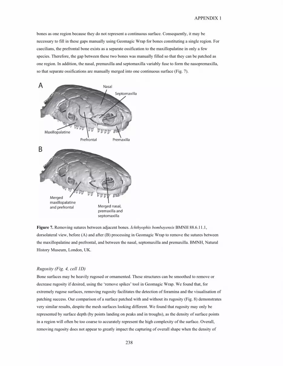
APPENDIX 1
238
bones as one region because they do not represent a continuous surface. Consequently, it may be
necessary to fill in these gaps manually using Geomagic Wrap for bones constituting a single region. For
caecilians, the prefrontal bone exists as a separate ossification to the maxillopalatine in only a few
species. Therefore, the gap between these two bones was manually filled so that they can be patched as
one region. In addition, the nasal, premaxilla and septomaxilla variably fuse to form the nasopremaxilla,
so that separate ossifications are manually merged into one continuous surface (Fig. 7).
Figure 7. Removing sutures between adjacent bones. Ichthyophis bombayensis BMNH 88.6.11.1,
dorsolateral view, before (A) and after (B) processing in Geomagic Wrap to remove the sutures between
the maxillopalatine and prefrontal, and between the nasal, septomaxilla and premaxilla. BMNH, Natural
History Museum, London, UK.
Rugosity (Fig. 4, cell 1D)
Bone surfaces may be heavily rugosed or ornamented. These structures can be smoothed to remove or
decrease rugosity if desired, using the ‘remove spikes’ tool in Geomagic Wrap. We found that, for
extremely rugose surfaces, removing rugosity facilitates the detection of foramina and the visualisation of
patching success. Our comparison of a surface patched with and without its rugosity (Fig. 8) demonstrates
very similar results, despite the mesh surfaces looking different. We found that rugosity may only be
represented by surface depth (by points landing on peaks and in troughs), as the density of surface points
in a region will often be too coarse to accurately represent the high complexity of the surface. Overall,
removing rugosity does not appear to greatly impact the capturing of overall shape when the density of

APPENDIX 1
239
surface points is coarser than the rugosity (especially when capturing shape over a disparate dataset).
However, if rugosity is of specific interest, we suggest a high density of surface points to capture this
complex surface. Semilandmarks have been shown to be capable of capturing ornamentation if desired,
and they outperformed landmark data and outline data (elliptical Fourier analysis, see Giardina and Kuhl
1977; Kuhl and Giardina 1982) for capturing the shape of ornamented gastropod shells (Van Bocxlaer
and Schultheiß 2010).
Figure 8. Effect of rugosity on patching. The frontoparietal of the frog Anotheca spinosa UF 137287,
dorsal view, (a) with rugosity retained and (b) rugosity removed through use of the ‘remove spikes’
function in Geomagic Wrap. (c) This density of surface points did not capture the rugose morphology, as
surface points from the smoothed (green) and non-smoothed (blue) bones appear similar in distribution.
Removing rugosity makes surface holes easier to identify, which can affect patching. UF, University of
Florida, Gainesville, FL, USA.
Centre each surface mesh (Fig. 4, cell 1E)
Each surface mesh should be centred, to facilitate the rotation of the mesh when placing landmarks and
curves in Landmark Editor (or Checkpoint Stratovan). This can be done using the ‘move to origin’
function in Geomagic Wrap, or in the ‘Transform: Move, Rotate, Center’ dialog box of Meshlab.
Format of surface meshes (Fig. 4, cell 1F)
Most meshes created from surface renderings of CT or surface scans are stored in Stanford Polygon
Format (PLY) or Stereolithography (STL) format. Landmark Editor, as well as our analyses in R, require
meshes to be in PLY format. Specifically, the PLY files must be in ASCII, not binary format, for
subsequent steps in R. To convert from STL or binary PLY to ASCII PLY, it is possible to import meshes
into R using the function ‘vcgImport’ from the R package Rvcg (Schlager 2017), and then export them
using the function ‘vcgPlyWrite’ from the Rvcg R package, specifying “binary=FALSE”. A common

APPENDIX 1
240
cause for the patching step failing to run is that meshes are stored as binary PLY files, not ASCII PLY
files.
Dividing a structure into regions
Overview
Dividing a structure into regions allows us to examine variation in potentially independent elements or
modules and to investigate differential or localised influences on morphology such as allometry and
ecological factors. However, the variable presence and fusion of bones within a dataset complicates the
division of a structure into regions, as specimens must all have the same regions defined across the
structure of interest if analyses under a unified framework are to be run. There are two options for bones
that are variably present or variably fused across the sample (assuming we do not exclude them from the
dataset altogether, which would create gaps in the physical representation of the structure). First, the
bones could be placed into regions that are globally present across the dataset, based on shared
development or function. Alternatively, they could be defined as individual regions, so that specimens
lacking a region are designated an artificial ‘missing’ region of negligible size (see below). Another
complication is dealing with highly disparate regions. To define such a region, it may be necessary to use
different landmarks and curves for subsets of specimens and use different templates to patch this region
separately for each landmark and curve configuration. In this case, landmarks and curves can be removed
after patching and only the surface points are retained for analyses, as the landmarks and curves would
not be comparable across all specimens.
Variably-present bones: 1. Designate to common regions (Fig. 4, cell 2A)
Variably-present or variably-fused bones (or regions) can be designated to regions globally present across
all specimens. We recommend this procedure when there is a clear understanding of shared development
or function, so that the merging is biologically informed. For example, the prefrontal bone in caecilians
exists as a separate ossification in only some species, and thus it must be put into a region common to all
caecilians. We place the prefrontal into a ‘midface’ region along with the maxillopalatine (Fig. 9), as
these two bones fuse in some species through development (Wake and Hanken 1982; Müller et al. 2005).
Therefore, this region exists as the prefrontal and maxillopalatine for some species, and just the
maxillopalatine for other species. Additionally, the nasal, premaxilla and septomaxilla of caecilians can
be placed into one ‘rostrum’ region, as these all variably fuse to form the nasopremaxilla in some species.
Thus, the rostrum region can be represented by one, two or three separate ossifications.
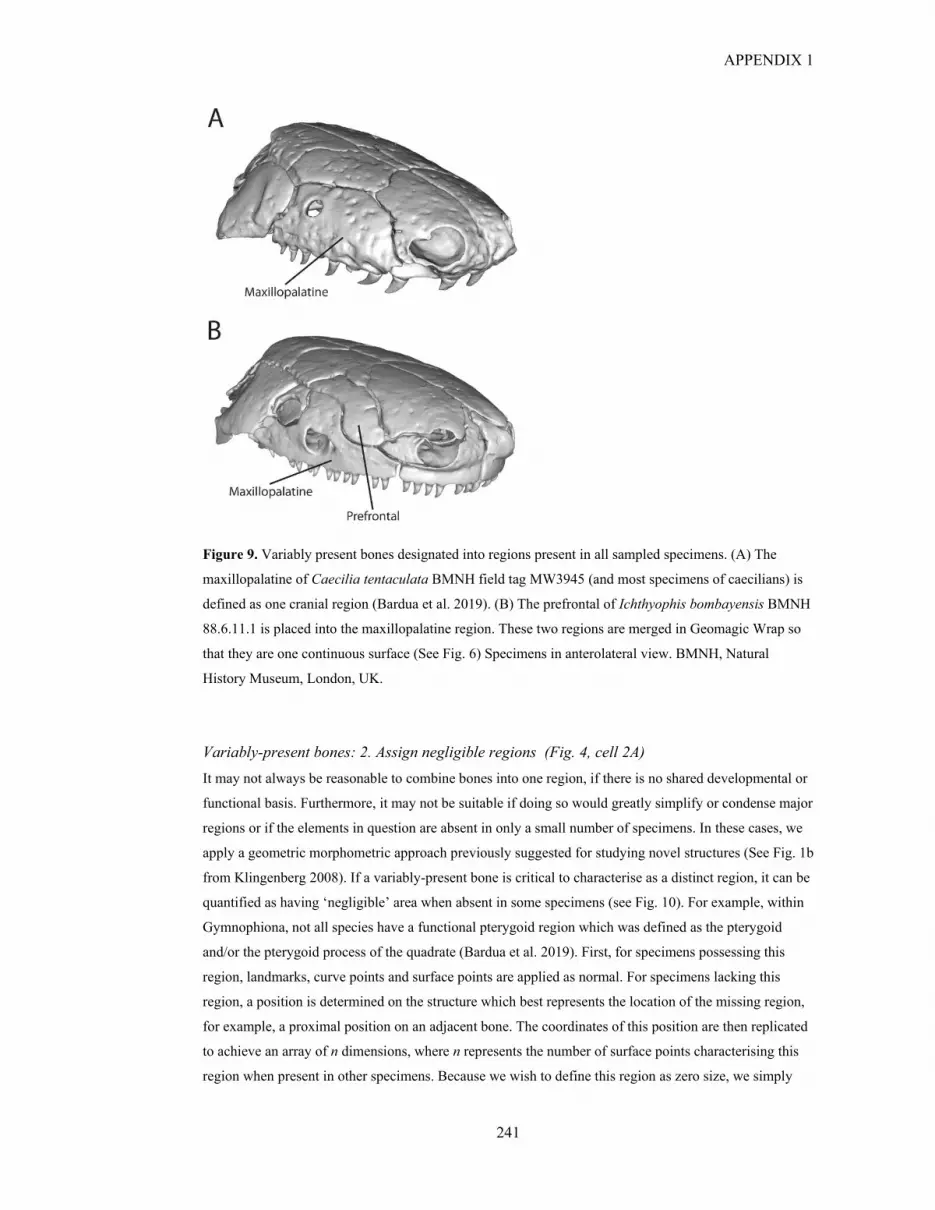
APPENDIX 1
241
Figure 9. Variably present bones designated into regions present in all sampled specimens. (A) The
maxillopalatine of Caecilia tentaculata BMNH field tag MW3945 (and most specimens of caecilians) is
defined as one cranial region (Bardua et al. 2019). (B) The prefrontal of Ichthyophis bombayensis BMNH
88.6.11.1 is placed into the maxillopalatine region. These two regions are merged in Geomagic Wrap so
that they are one continuous surface (See Fig. 6) Specimens in anterolateral view. BMNH, Natural
History Museum, London, UK.
Variably-present bones: 2. Assign negligible regions (Fig. 4, cell 2A)
It may not always be reasonable to combine bones into one region, if there is no shared developmental or
functional basis. Furthermore, it may not be suitable if doing so would greatly simplify or condense major
regions or if the elements in question are absent in only a small number of specimens. In these cases, we
apply a geometric morphometric approach previously suggested for studying novel structures (See Fig. 1b
from Klingenberg 2008). If a variably-present bone is critical to characterise as a distinct region, it can be
quantified as having ‘negligible’ area when absent in some specimens (see Fig. 10). For example, within
Gymnophiona, not all species have a functional pterygoid region which was defined as the pterygoid
and/or the pterygoid process of the quadrate (Bardua et al. 2019). First, for specimens possessing this
region, landmarks, curve points and surface points are applied as normal. For specimens lacking this
region, a position is determined on the structure which best represents the location of the missing region,
for example, a proximal position on an adjacent bone. The coordinates of this position are then replicated
to achieve an array of n dimensions, where n represents the number of surface points characterising this
region when present in other specimens. Because we wish to define this region as zero size, we simply

APPENDIX 1
242
replicate the one position coordinate and use this as raw coordinate data, instead of applying the patching
procedure for these specimens. Because this negligible region is not represented by landmarks and curves
(only surface points), landmarks and curves used to define this region when present on other specimens
are removed after the patching and sliding of the surface points for these specimens. This region is
therefore only represented by surface points for analyses. Global Procrustes alignment will slightly adjust
surface point positions such that the ‘negligibly sized region’ is no longer zero size, but it remains near-
zero in size and is still considered ‘negligible’. Although one could argue for exclusion of these variably-
present structures, that approach would greatly limit the elements that could be considered in large-scale
cross-taxon analyses and would result in inaccurate representation of the real biological variation in the
sample of interest.
Figure 10. Negligible region method. The pterygoid region in two specimens, in ventral aspect: (A)
Epicrionops bicolor BMNH 78.1.25.48 and (B) Scolecomorphus kirki BMNH 2005.1388. The negligible
pterygoid region of Scolecomorphus kirki is represented by the same number of surface points (blue), all
occupying the same position. The area for this negligible region is therefore zero, or near zero, but it
retains positional information. The position represents the likely location where this region would have
been, if present. Landmarks (red points) and curves (yellow points) are removed before analyses for
specimens with a present pterygoid region. BMNH, Natural History Museum, London, UK.
Biological foramina variably present: Negligible hole method (Fig. 4, cell 2B)
As mentioned above, the patching procedure requires surfaces to be a largely continuous surface, so
biologically important holes, including the orbit and nares, must be “fenced” off with curves. Problems
arise when only some specimens in the dataset have a fossa or foramen in the region to be patched. In
these cases, specimens lacking a hole can be given a “negligibly-sized hole”, using the same landmarks
and curves to fence off a miniscule area. This hole is approximately the size of one surface point, and our
tests demonstrate that it does not affect patching (i.e. it does not create an empty space where the
“negligibly-sized hole” was placed). This approach allows all specimens to be patched together as they all

APPENDIX 1
243
have the same landmark and curve configuration. The non-comparable landmarks and curves can then be
removed before analyses (including Procrustes alignment).
For comparing across specimens with and without fossae, one should ensure that surface point placement
is not appreciably affected by the presence of the “negligible” hole. To demonstrate, we tested patching
with and without a negligibly-sized hole on ten pyramidal 3D models of varying proportions using
Blender v2.79 (www.blender.org). On four of the ten models, we placed a circular “fossa” on one face
(Fig. 11). An additional pyramidal model was produced to serve as a template mesh (Fig. 11A) (for more
information regarding templates, please see the Template creation and use section). We placed landmarks
on each vertex and curves along each edge. Landmarks and curves were digitised around the perimeter of
the fossa (Fig. 11B) and corresponding curves were placed as a negligibly-sized hole on meshes lacking a
fossa (Fig. 11C). On the template mesh, we digitised 90 surface points on a single face. Surface points
were projected onto the ten target specimens. The negligibly-sized hole technique allows surface points to
be projected evenly on the surface of specimens lacking a fossa (Fig. 11C) and prevents surface points
from being erroneously projected inside the fossa when present (Fig. 11B). We evaluated the effects of
the negligibly-sized hole on the placement of surface points by repeating the patching procedure on the
six pyramid meshes without fossae with the fossa landmarks and curves removed from the template and
target meshes before patching. We then removed the fossa landmarks and curves from the original 10
specimen dataset and subjected all 16 specimens to a common Procrustes alignment and principal
components analysis (PCA).
The first four principal component axes account for 96% of the cumulative shape variance in the
dataset. The first principal component (PC1) describes the ratio of the base of the pyramid to its height,
PC2 represents the angle of the face with surface points, PC3 is associated with variation in the angles of
the corners of the base, and PC4 is correlated with the size of the fossa. Critically, pairs of identical
pyramid shapes patched with and without the negligibly-sized hole share adjacent positions in
morphospace (Fig 11D). This illustrates that this process for placing patches of surface points does not
introduce undesirable artefacts in quantifying shape while also facilitating shapes with different
anatomical features to be compared directly.

APPENDIX 1
244
Figure 11. “Negligibly-sized hole” method for patching surfaces with variably present features. (A)
Landmarks (red), curves (yellow), and surface points (blue) are digitised on a template mesh. (B, C)
Surface points are projected on to target meshes. On meshes with “fossa,” curves are placed around the
perimeter of this region. On specimens lacking the “fossa,” corresponding landmarks are placed
extremely close together, forming a “hole” of negligible size (C). We subjected these data to a Procrustes
alignment and principal components analysis (D). When that same specimen (numbered points) is
patched with (solid circle) and without (solid square) the negligibly sized region corresponding to the
“fossa,” these specimens share adjacent positions in morphospace.
A biological example of this situation occurs in the maxillopalatine of caecilians. This bone can have an
orbit or tentacular foramen partially or completely enclosed within the bone. Complete enclosure of a
foramen requires curves to “fence-off” this hole, whereas partial enclosure does not require a hole.
However, to patch all specimens together, a negligibly-sized area was fenced off in the latter specimens,
so that landmarks and curves were kept consistent (Fig. 12). One template can subsequently be used for
these specimens.
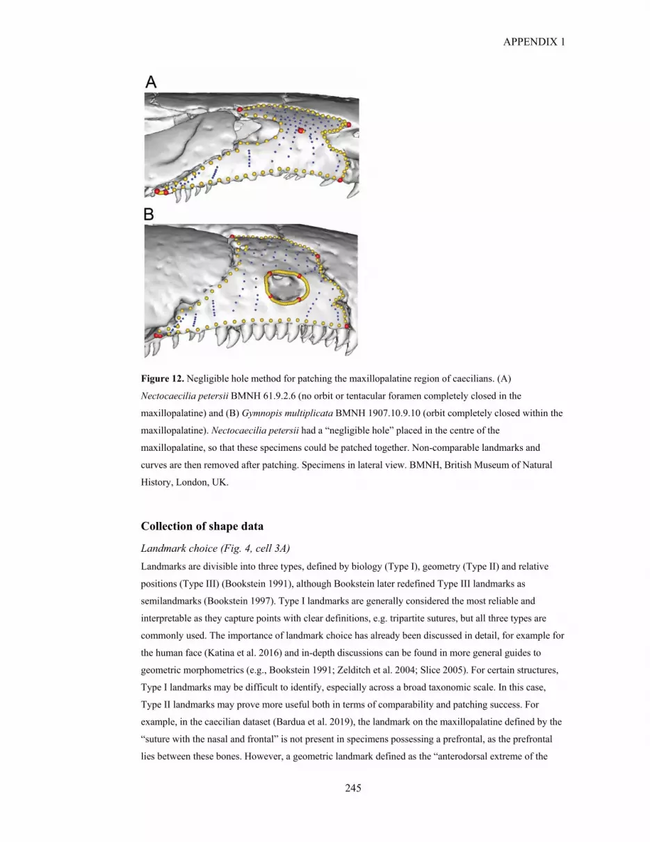
APPENDIX 1
245
Figure 12. Negligible hole method for patching the maxillopalatine region of caecilians. (A)
Nectocaecilia petersii BMNH 61.9.2.6 (no orbit or tentacular foramen completely closed in the
maxillopalatine) and (B) Gymnopis multiplicata BMNH 1907.10.9.10 (orbit completely closed within the
maxillopalatine). Nectocaecilia petersii had a “negligible hole” placed in the centre of the
maxillopalatine, so that these specimens could be patched together. Non-comparable landmarks and
curves are then removed after patching. Specimens in lateral view. BMNH, British Museum of Natural
History, London, UK.
Collection of shape data
Landmark choice (Fig. 4, cell 3A)
Landmarks are divisible into three types, defined by biology (Type I), geometry (Type II) and relative
positions (Type III) (Bookstein 1991), although Bookstein later redefined Type III landmarks as
semilandmarks (Bookstein 1997). Type I landmarks are generally considered the most reliable and
interpretable as they capture points with clear definitions, e.g. tripartite sutures, but all three types are
commonly used. The importance of landmark choice has already been discussed in detail, for example for
the human face (Katina et al. 2016) and in-depth discussions can be found in more general guides to
geometric morphometrics (e.g., Bookstein 1991; Zelditch et al. 2004; Slice 2005). For certain structures,
Type I landmarks may be difficult to identify, especially across a broad taxonomic scale. In this case,
Type II landmarks may prove more useful both in terms of comparability and patching success. For
example, in the caecilian dataset (Bardua et al. 2019), the landmark on the maxillopalatine defined by the
“suture with the nasal and frontal” is not present in specimens possessing a prefrontal, as the prefrontal
lies between these bones. However, a geometric landmark defined as the “anterodorsal extreme of the

APPENDIX 1
246
maxillopalatine” can be identified in all specimens. In addition, we find that an important consideration
when determining landmarks for studies involving patching should be finding landmarks which do not
vary widely in position across the sample. This is because surface point placement is the most successful
when the landmark and curve configurations are similar across specimens. High variability in landmark
position across specimens can make it difficult to find a template landmark distribution that will
successfully place surface points onto every specimen. For example, a landmark defining the palatal
surface of the caecilian maxillopalatine results in less variation in landmark position across specimens,
which facilitates the placement of surface points (Fig. 13). Patching success is adversely affected by
structures that are not strongly conserved in shape across specimens, so we advocate the use of landmarks
which are the most conserved across specimens, in presence and position.
Figure 13. Landmark choice can affect patching success. Landmarks (red points) and curves (yellow
points) are manually placed onto each specimen, and a template is used to semi-automatically place
surface points (blue) onto each region. The success of this surface point placement can be affected by
landmark choice. Here, a template (A) is used to patch the palatal surface of the maxillopalatine in (B, D)
Idiocranium russeli BMNH 1946.9.5.80 and (C, E) Luetkenotyphlus brasiliensis BMNH 1930.4.4.1,
using different landmarks (labelled ‘LM1’ and ‘LM2’) to delimit the posterior extreme of this surface. (B,
C) Landmark 1 (alveolus of ultimate tooth) may vary widely in position, making patching difficult, as the

APPENDIX 1
247
template can only resemble one morphology. (D, E) Landmark 2 (posterolateral extreme of the
maxillopalatine) may improve patching success if they show less variation in landmark position, making
the patching more successful. All specimens are viewed in ventral aspect, with anterior facing upwards.
BMNH, Natural History Museum, London, UK.
Curve semilandmark placement (Fig. 4, cell 3B)
It is important to ensure that the landmarks and curves accurately follow the outline of the desired region.
When placing curve points in the IDAV Landmark Editor (or Stratovan Checkpoint) program, we
recommend that they are placed on a flat surface, instead of on the sides of regions of interest. In other
words, the normal of the landmarks and curve points should be consistent with the intended normal of the
surface points. Although the normals of landmarks and curve points do not necessarily impact the
placement of surface points, placing the anchoring curve points on the side may cause the additional
curve points placed between these anchors by the program to be irregular in spacing. The extreme case is
if the path between the anchored curve points deviates or falls from the perimeter of the region. This leads
to incorrect placement of curve points.
Curve resampling (Fig. 4, cell 3C)
Because the placement of curve points on each specimen is done manually in Landmark Editor (or
Stratovan Checkpoint), points are not usually evenly spaced along each curve, and the number of curve
points initially chosen may not be ideally representative across the entire dataset. Curves are therefore
resampled for even spacing before being slid during alignment (for code see SI in Botton-Divet et al.
2016). Sliding the curves after resampling is a crucial step, as equally spaced semilandmarks cannot be
treated as optimally placed (See Fig 1 from Gunz et al. 2005). For the caecilian dataset (Bardua et al.
2019), we tested how many points were optimal for resampling, by comparing over-representation of
each curve (50 points per curve), under-representation (5 points per curve) and a vector of points which
allocated more points to longer curves. We predicted that resampling curves to a high number of points
would help constrain surface points to each region, as this leaves fewer “gaps” between adjacent
semilandmarks through which points can “escape”. However, even with 50 curve points per curve,
surface points can still fall outside of the region of interest (Fig. 14). In addition, having five points per
curve did not adversely affect patching success compared to the oversampled scheme. Increasing the
number of curve points actually seems to result in more specimens failing to patch (i.e. errors messages
returned for these specimens) (see ‘placePatch’ function). When the ‘relax.patch’ argument is set as true
(relax.patch=TRUE) in the ‘placePatch’ function, patching success is considerably higher when curves
are resampled to five points per curve (only one specimen failed to patch for our caecilian dataset of 35
specimens) instead of 50 (11 specimens failed to patch). This outcome suggests that oversampling of
curve points can actually impede the patching process. Our recommendation is to resample the curves
based on their original length, but in most cases to limit each curve to no more than ca. 20–30 points. This
level of sampling results in curves that are well represented in typical cases, without compromising
patching. Furthermore, we recommend that the density of curve points is similar to the density of surface
points to achieve even coverage of the structure.
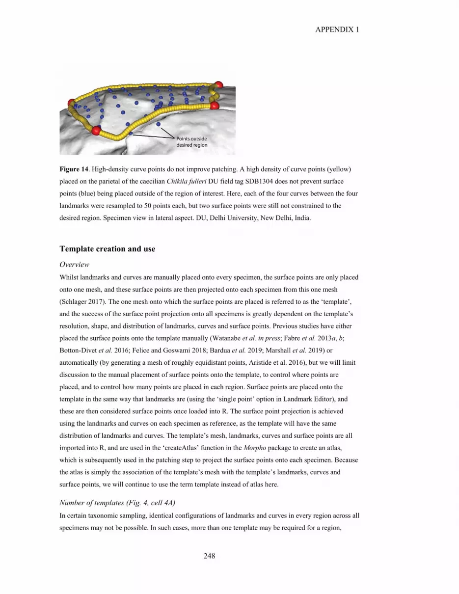
APPENDIX 1
248
Figure 14. High-density curve points do not improve patching. A high density of curve points (yellow)
placed on the parietal of the caecilian Chikila fulleri DU field tag SDB1304 does not prevent surface
points (blue) being placed outside of the region of interest. Here, each of the four curves between the four
landmarks were resampled to 50 points each, but two surface points were still not constrained to the
desired region. Specimen view in lateral aspect. DU, Delhi University, New Delhi, India.
Template creation and use
Overview
Whilst landmarks and curves are manually placed onto every specimen, the surface points are only placed
onto one mesh, and these surface points are then projected onto each specimen from this one mesh
(Schlager 2017). The one mesh onto which the surface points are placed is referred to as the ‘template’,
and the success of the surface point projection onto all specimens is greatly dependent on the template’s
resolution, shape, and distribution of landmarks, curves and surface points. Previous studies have either
placed the surface points onto the template manually (Watanabe et al. in press; Fabre et al. 2013a, b;
Botton-Divet et al. 2016; Felice and Goswami 2018; Bardua et al. 2019; Marshall et al. 2019) or
automatically (by generating a mesh of roughly equidistant points, Aristide et al. 2016), but we will limit
discussion to the manual placement of surface points onto the template, to control where points are
placed, and to control how many points are placed in each region. Surface points are placed onto the
template in the same way that landmarks are (using the ‘single point’ option in Landmark Editor), and
these are then considered surface points once loaded into R. The surface point projection is achieved
using the landmarks and curves on each specimen as reference, as the template will have the same
distribution of landmarks and curves. The template’s mesh, landmarks, curves and surface points are all
imported into R, and are used in the ‘createAtlas’ function in the Morpho package to create an atlas,
which is subsequently used in the patching step to project the surface points onto each specimen. Because
the atlas is simply the association of the template’s mesh with the template’s landmarks, curves and
surface points, we will continue to use the term template instead of atlas here.
Number of templates (Fig. 4, cell 4A)
In certain taxonomic sampling, identical configurations of landmarks and curves in every region across all
specimens may not be possible. In such cases, more than one template may be required for a region,

APPENDIX 1
249
because a single template can only patch specimens with identical landmark and curve configurations.
Variable regions should be represented using as few landmark and curve configurations as possible. One
template should be used to patch each region when possible, so that bending energy can then be
minimised across all specimens in the subsequent sliding step. However, when more than one template is
required for a region, specimens with regions that have each landmark and curve configuration are
patched as groups. Landmarks and curves are removed if necessary (when these are not consistent across
the dataset), and then the remaining landmarks and curves and the surface points from each variable
region are added to the data collected for the globally present regions. When more than one template is
used, the surface points are only slid as groups and not globally, so it is important to be careful about
where the points are placed on the template. Surface points on different templates should be placed in
analogous ways, so that the data are comparable. Once all coordinate data have been collated from all
templates, Procrustes alignment is applied to the complete dataset prior to any further analyses.
Caecilian crania are highly variable and require the use of multiple templates (Bardua et al. 2019;
Marshall et al. 2019). As an example, the pterygoid region in caecilians was defined in our study to be the
pterygoid process of the quadrate, and/or the pterygoid (ectopterygoid) when present. One template could
not represent both variations, so specimens with one bone present were patched together, and specimens
with both bones present were patched together (Fig. 15). The ordering and distribution of surface points
were analogous across the two templates, with the posteriorly positioned surface points on the ‘single
bone’ specimens corresponding to the surface points placed on the posterior bone in the ‘two bones’
specimens (and similarly with the anterior surface points). Pterygoid landmarks and curves were removed
from the resulting datasets as these differed across the morphologies, so only the surface points were
retained. Similarly, when the tentacular fossa runs the entire length of the maxillopalatine in caecilian
crania, the maxillopalatine must be patched as two regions, dorsal and ventral to this fossa (Fig. 16).
Specimens whose maxillopalatine has a tentacular foramen completely enclosed within the bone however
are better represented by a template with one region and a hole. Surface points were placed on each of
these two maxillopalatine templates such that the first half were dorsal to the tentacular fossa/foramen,
and the second half were ventral, with analogous distributions.

APPENDIX 1
250
Figure 15. Multiple template used for highly disparate regions. The pterygoid region as defined by this
study, in ventral aspect, for Praslinia cooperi BMNH 1907.10.15.154 (A) and Epicrionops bicolor
BMNH 78.1.25.48 (B). Because this region consists of either one (B) or two (A) bones, landmarks and
curves are not consistent in number or position across specimens. Here, landmarks and curves are used to
constrain the regions, and the pterygoid region is patched separately in specimens with one or two bones.
Curves and landmarks are removed after patching, while keeping the surface points. BMNH, Natural
History Museum, London, UK.
Figure 16. Multiple template used for highly disparate regions. The maxillopalatine can have a tentacular
foramen completely enclosed within the bone (Gymnopis multiplicata BMNH 1907.10.9.10, A), or a
tentacular fossa passing through its entire length (Chthonerpeton indistinctum MCP field tag MW16, B)
or neither. These require different patching approaches, but once patched, the curves and landmarks can

APPENDIX 1
251
be removed and the surface points analysed. Specimens in lateral aspect. BMNH, British Museum of
Natural History, London, UK; MCP, Museu de Ciências e Tecnologia da PUCRS, Porto Alegre, Brazil.
Template shape (Fig. 4, cell 4B)
The most suitable template shape depends on the variation observed across the dataset. Previous studies
have used a specimen from the dataset (e.g., Aristide et al. 2016; Botton-Divet et al. 2016; Marshall et al.
2019), a non-sample specimen (Wölfer et al. 2019), or a geometrically simplified representation of the
structure under question (e.g., Fabre et al. 2014; Felice and Goswami 2018; Bardua et al. 2019).
Intraspecific datasets typically exhibit smaller variation in morphology. As such, template shape which
represents the actual morphology of the species will likely result in a successful placement of surface
points (Souter et al. 2010; Marshall et al. 2019). The specimen closest to the average morphology can be
determined through use of the ‘findMeanSpec’ function in the geomorph R package. The surface mesh of
this specimen can be used to create the template with the full configuration of landmarks and
semilandmarks. Alternatively, a specimen can be picked at random to use as the template if the
morphological variation is especially small. However, the use of a specimen as a template may not be
appropriate for broad taxonomic studies because its morphology may not be generalizable across the
entire breadth of shape variation. A study comparing the most suitable template shapes for two datasets
found that the dataset exhibiting extreme morphological variation (theropod pelvic girdles) required a
considerably geometrically simpler mesh than the dataset exhibiting only small morphological variation
(shrew skulls) (Souter et al. 2010). No one specimen’s morphology in the theropod pelvic girdle dataset
would have sufficiently represented the morphology captured across the entire dataset. It was found that
the greater the morphological variation, the simpler the template should be. This is because the template
is warped (see ‘Warping of template’ section below), so that whilst a specimen’s mesh will warp
accurately to other specimens’ meshes when the morphologies are similar, this is more difficult when the
morphologies are very different, as a complex shape has to transform into another complex shape (Souter
et al. 2010). A simpler shape in this case will warp better to each specimen’s morphology. For our studies
of caecilians, squamates and birds, we found that a generic hemispherical mesh as the template was
effective at placing patch semilandmarks (see ‘Warping of template’ section). A hemisphere was more
successful than a sphere with respect to accuracy in patching, as the former better represents the shape of
a skull (with the ventral cranial surface as the flat surface of the hemisphere, and the tooth row following
the base of the hemisphere). These template shapes can be created in programs including Meshlab and
Blender.
Template resolution (Fig. 4, cell 4C)
The resolution of the template mesh is equally as important as the template shape. Surface points are
projected from the warped mesh onto the target specimen. Therefore, patching accuracy is partially
dependent on how well the warped template mesh fits with the topology of the target mesh. It is essential
that the template mesh has sufficiently high resolution (i.e., consists of enough triangles), so that the
template can be warped to accurately reflect each specimen’s morphology. The number of polygons limits
the degree to which the template mesh can be deformed (Fig. 17). Very low-resolution meshes thus
produce poor correspondence between template and target specimens. The template must therefore have a

APPENDIX 1
252
high-resolution but does not have to resemble the specimen morphology. The necessary number of faces
for the template mesh will vary based on the complexity of the morphology being quantified, but
hemispherical templates with around 18,000 faces have proven suitable for vertebrate skulls.
Figure 17: Warping template meshes of different resolutions. (A) Low polygon (1,802 faces) and (B)
high polygon (18,024 faces) hemispherical meshes warped to the shape of the bird Alca torda (NHMUK
1897.2.25.1), ventral view. The warped low-resolution template is a poor fit with the landmark
configuration of the target specimen, producing areas where the contours of the mesh do not correspond
to the curves (black arrows). In contrast, the shape of the warped high-resolution mesh exhibits more
detailed shape deformation and greater correspondence with target configuration. This improves the
performance of the projection step of the patching method.
Template landmarks and curves (Fig. 4, cell 4D)
How regions are defined on the template can impact patching success. For datasets with small amounts of
variation, the landmark and curve positions on the template can follow a pattern based on the average
shapes of each region in the target specimens. However, interspecific studies encounter considerably
more variation in morphology. An inevitable result of studying shape variation across a diverse dataset is
that extreme shapes and sizes form part of the dataset. The template’s landmarks and curves must
therefore be suitable for these extreme shapes as well, and an average shape may not be the optimal
solution. For regions exhibiting large size variation, we found the most success when the template
represented the morphology of the smaller-sized regions. Surface points could successfully fill a large
region on a specimen when the template represented a small shape, with densely clustered surface points,
but issues arose when widely distributed points from the template were patched onto a small region.
Surface points would often fall outside the desired region.
One example is the parietal of caecilians (Fig. 18). For the purposes of analysing external bone surfaces,
the adductor muscle ridge was taken as the lateral margin of the parietal when a squamosal-parietal
fenestra is present. Whereas most taxa exhibit an approximately rectangular-shaped parietal, two species
(Rhinatrema bivitattum and Epicrionops bicolor) have a more triangular-shaped external surface of the
parietal. We found that a triangular-shaped template outperformed a rectangular-shaped parietal by
keeping the surface points inside the desired region. Therefore, despite most specimens having a

APPENDIX 1
253
rectangular-shaped parietal, the template that was the most globally successful imitated the shape of the
parietal in Rhinatrema bivitattum and Epicrionops bicolor. A rectangular template resulted in posteriorly
positioned points falling outside the parietal for Rhinatrema bivitattum. Surprisingly, a triangular shaped
template configuration for this region successfully patched every specimen. This suggests the patching
procedure is more successful at enlarging the spaces between points, than at decreasing spaces between
points (compare posterolateral points). Hence, the use of mean shape is not necessarily the most effective
template for patching.
Figure 18. Effect of template shape on patching success. The external surface of the parietal is
rectangular in shape for most caecilian species (seen here in dorsal aspect, with anterior facing upwards),
but can appear more triangular in some species. To illustrate the effect of template shape on patching
success, two templates were used to patch the parietal for two caecilian species. (A) A triangular-shaped
template successfully patches the parietal of both (B) Microcaecilia albiceps MCZ A-58412 and (C)
Rhinatrema bivitattum BMNH field tag MW2395, whereas (D) a rectangular-shaped template patches (E)
Microcaecilia albiceps well but (F) Rhinatrema bivitattum poorly (surface points have fallen outside the
desired region). In this case, the most globally successful template was not the one resembling the most
common morphology, but the one resembling the extreme morphology. BMNH, Natural History
Museum, London, UK; MCZ, Museum of Comparative Zoology, Cambridge, MA, USA.

APPENDIX 1
254
Number of surface points (Fig. 4, cell 4E)
The optimum number of surface points to place onto the template depends on the complexity and the size
of each defined region. More points may better represent a region, but we found this also increases the
likelihood of some points falling outside the region of interest. In addition, over-representation of a region
unnecessarily increases the dimensionality of the dataset, which could lessen power of the analyses that
follow (for a discussion on the optimal number of landmarks/semilandmarks, see Watanabe 2018). For
regions exhibiting large size variation, the number should be high enough to allow the largest region to be
represented. For our interspecific cranial datasets, we used ~500 - 1000 surface points to represent the
entire cranium. Regions varied from having ~20 to ~100 surface points. The occipital condyle for
example has a small and simple surface so was generally represented by ~20 surface points, whereas the
maxillopalatine is a large region and was represented by 48 surface points. The numbers of surface points
are within the range of previous studies, which have used 24 surface points to capture the articular surface
of the humerus (Fabre et al. 2014), 225 for musteloid crania (Dumont et al. 2015), 265 for the surface of
the entire humerus of primates (Fabre et al. 2017), 268 for monkey endocasts (Aristide et al. 2016), 800
for shrew crania (Cornette et al. 2013) and over 800 surface points for shrew mandibles (Cornette et al.
2013).
At present, it is not possible to determine a priori how many surface points are necessary to fully capture
the shape variation. However, it is possible to retrospectively examine how many (semi) landmarks are
required to capture the shape of a region, through implementation of the ‘lasec’ function in the R package
LaMDBA (Watanabe 2018). This function subsamples the original dataset by randomly selecting 3, 4, 5,
… N points, determining the fit of each reduced dataset to the complete dataset, and repeating this for a
selected number of iterations. Fit is based on Procrustes distance between the full and subsampled
datasets with respect to position of the specimens in high-dimensional morphospace (i.e., not the spatial
position of the landmarks). We performed LaSEC for landmarks and semilandmarks (curve and surface
points) for the caecilian and squamate datasets, for individual cranial regions. The function generates a
sampling curve, where a plateau in the curve signifies stationarity in characterization of shape variation
and absence or fewer landmarks than the occurrence of plateau indicates inadequate characterization. The
curves from each cranial region (e.g., Fig. 19) clearly show that enough landmarks and semilandmarks
had been sampled due to a robust plateau in the curve.
We also determined the number of landmarks and semilandmarks that would have been sufficient for
each region, given a required fit of 0.9, 0.95 and 0.99 between the reduced and complete datasets (Tables
3, 4). These results could be used as a guide for estimating how many landmarks/semilandmarks should
be taken for comparably sized regions. As a general guide for cranial regions, we suggest 12+
landmarks/semilandmarks for small and topologically simple regions (e.g. jaw joint articular surface), and
~ 70 landmarks/semilandmarks for larger and morphologically complex regions (e.g. occipital region).
Use of LaSEC revealed that we did capture shape accurately in all datasets, and that fewer
landmarks/semilandmarks would have still captured shape in great detail. However, this cannot be
determined in advance, and so we suggest it is preferable to oversample a structure and later downsample
if necessary. We therefore suggest placing a relatively high density of surface points onto each region of

APPENDIX 1
255
the template, and then use LaSEC to guide downsampling if required. Because surface points should be
placed evenly across structures, it is necessary to also consider which region may require the highest
density of surface points (i.e., which region may be particularly complex and varying in morphology). If
one region requires a high density of points to characterise shape, the remaining regions should have a
similar density of surface points in order to ensure even coverage of the entire structure of interest.
Figure 19. Sampling curve from performing LaSEC on the frontal region of the caecilian dataset. Each
grey line indicates fit values from one iteration of subsampling. Thick, dark line denotes median fit value
at each number of landmarks. The presence of a plateau indicates robust shape characterisation.
Table 3. Results from performing LaSEC with 1000 iterations on individual cranial partitions of the
extant caecilian dataset. Values for Fit = 0.9, 0.95, and 0.99 denote the median number of randomly
subsampled landmarks degree of fit (0 to 1) of randomly subsampled landmark configurations and fixed-
only datasets to the respective full high-dimensional coordinate data. For definitions of cranial regions,
see (Bardua et al. 2019).
Dataset Number of
landmarks
Total number of
landmarks and
semilandmarks
Fit =
0.90
Fit =
0.95
Fit =
0.99
Fit of
landmark-
only dataset
Basisphenoid
region
4 155 15 25 69 0.583
Frontal 4 125 13 21 61 0.617
Jaw joint 3 50 13 19 37 0.306
Maxillopalatine
(interdental
shelf)
4 110 13 19 52 0.782

APPENDIX 1
256
Maxillopalatine
(lateral surface)
3 134 14 23 64 0.238
Maxillopalatine
(palatal surface)
5 75 13 19 44 0.602
Nasopremaxilla
(dorsal surface)
7 148 13 21 61 0.684
Nasopremaxilla
(palatal surface)
3 59 8 12 29 0.770
Occipital
condyle
2 34 11 15 27 NA (only
two
landmarks)
Occipital region 5 153 16 27 73 0.605
Parietal 3 126 11 18 51 0.361
Pterygoid 0 50 7 10 24 NA
Quadrate (lateral
surface)
2 57 12 18 38 NA (only
two
landmarks)
Squamosal 4 104 15 25 61 0.574
Stapes 0 20 10 12 17 NA
Vomer 3 69 12 18 41 0.538
Total
Table 4. Results from performing LaSEC with 1000 iterations on individual cranial partitions of the
extant squamate dataset. Values for Fit = 0.9, 0.95, and 0.99 denote the median number of randomly
subsampled landmarks degree of fit (0 to 1) of randomly subsampled landmark configurations and fixed-
only datasets to the respective full high-dimensional coordinate data.
Dataset Number of
landmarks
Total number of
landmarks and
semilandmarks
Fit = 0.90 Fit = 0.95 Fit = 0.99 Fixed-only
Premaxilla 4 78 15 23 49 0.713
Nasal 4 86 15 25 54 0.664
Maxilla 5 162 16 27 74 0.696

APPENDIX 1
257
Jugal 3 94 13 20 51 0.645
Frontal 4 130 14 25 66 0.721
Parietal 4 98 16 28 64 0.647
Squamosal 3 52 17 25 43 0.452
Jaw joint 4 42 20 27 38 0.484
Supraoccipital 5 132 30 55 90 0.597
Occipital
condyle
2 37 22 27 34 NA
Basioccipital 4 122 14 26 66 0.805
Pterygoid 3 53 14 21 39 0.421
Palatine 4 64 16 23 45 0.457
Surface point distribution (Fig. 4, cell 4E)
The distribution of surface points placed on the template will depend on the shape variation of each
region, across all specimens. Considering the most appropriate distribution for each region is crucial, as
this can strongly affect the patching process. Where possible, we recommend a systematic distribution,
consisting of rows of evenly spaced surface points parallel to the curves defining each region. One should
place surface points away from curve points, to reduce the risk of points falling outside the desired region.
Use of more than one template requires additional consideration, as surface points from corresponding
regions should always be equivalent in position.
Warping of template (Fig. 4, cell 4C)
The patching procedure implemented in the R package Morpho semi-automatically projects surface
points on to a target mesh (Fig. 20A) from a template mesh upon which surface landmarks have been
digitised (Fig. 20B). An essential part of this process is the warping of the template mesh via thin plate
spline (TPS) deformation based on the curves shared between the template and target specimens (Fig.
20B-E, Fig. 21). To prevent the surface points from being misplaced within the target mesh, the surface
points are “inflated” along their normals (Fig. 22) and then projected back until each landmark contacts
the target mesh (Fig. 23).

APPENDIX 1
258
Figure 20. Projecting patch points from template to specimen. Morphology of a specimen (A, Alca torda,
NHMUK 1897.2.25.1) is quantified coarsely with 3D landmark data (red: anatomical landmarks, yellow:
curve points). Corresponding landmarks and curves are digitised on a template mesh, along with high-
density surface points (blue) which will be transferred from the template to the target specimen (B). The
template is then morphed to the shape of the specimen (C-D), generating the intermediate model with
surface points (E). Surface points are projected from the intermediate model on to the specimen (F),
producing dense representation of entire surface of interest. NHMUK, Natural History Museum, London,
UK
Figure 21. Video illustrating how the template is warped to the shape of each specimen. A simple
hemispherical template can be warped to complex morphologies, such as a bird skull. [See online version
for the video (MP4 format)].

APPENDIX 1
259
Figure 22. Video illustrating inflation of surface points. The position of the surface points is adjusted
along the normal of the warped template before being projected onto the target specimen to ensure that all
surface points are placed on the outer surface of the target specimen. [See online version for the video
(MP4 format)].
Figure 23. Video illustrating how the surface points are projected onto each specimen. [See online
version for the video (MP4 format)].
Patching procedure
Failed surface point projection (Fig. 4, cell 5A)
The patching of some specimens in a dataset can fail (i.e. an error message is returned). This can happen
both when the relax.patch argument is set to TRUE or to FALSE when running the ‘placePatch’ function
in Morpho. This specifies whether to minimise bending energy toward the atlas (the template). We found
the likelihood of specimens failing to patch was increased when relax.patch was set to TRUE. The
specimens that fail often have some curve points that are ‘floating’ and are not completely sitting on the
surface of the mesh (Fig. 24). However, these ‘floating’ points can be difficult to notice as they can be
just above the mesh surface. This can be a consequence of curves being defined incorrectly, or curves
being placed too near the edge of a bone and then sliding off the surface. For specimens whose patching

APPENDIX 1
260
fails, we recommend checking the placement of the curve points carefully.
Figure 24. Incorrect and correct placement of curves (yellow points) on a salamander, Bolitoglossa
adspersa ZMB 71710 (A) One curve has been defined incorrectly, so some curve points have fallen off of
the bone. The floating curve points may then result in the patching step failing. (B) When correctly
defined, this curve traces the anterior margin of the nasal. Specimens in anterior aspect. ZMB, Zoological
Museum of Berlin, Berlin, Germany.
Inflate value (Fig. 4, cell 5B)
During patching, it is possible that points are not always placed onto the external bone surface, especially
if the bone material is thin. Points may instead fall onto the internal bone surface. This can be corrected
by increasing the “inflate” value of the ‘placePatch’ function in Morpho (Fig. 25).
Conversely, if the “inflate” value is too high, it is possible for surface points to fall outside of the region
of interest, with surface points projected onto nearby surfaces outside of the defined region (Fig. 25). This
appears to pose the greatest problem when the desired region is in close proximity to another surface.
When patching the palate, nearby teeth are especially problematic as their surface is often nearby and
parallel to the normal vector of the surface points. This issue can normally be fixed by reducing the
“inflate” value just for the palate, although teeth may have to be removed if an optimal inflate value
cannot be found that places the surface points neither on the internal bone surface, nor on nearby surfaces.

APPENDIX 1
261
Figure 25. The effect of adjusting the inflate value during the patching step, using the vomer of the
caecilian Epicrionops bicolor BMNH 78.1.25.48 as an example. (A) Here, all surface points have been
correctly placed onto the outer surface of the vomer (I = 0). (B) When the inflate value is too high,
surface points can jump outside the region of interest, onto nearby bone (teeth in this case) (I = 1). (C)
When the inflate value is too low, surface points can be placed on the internal surface, as seen through the
nares in (D) where the points are now on the underside of the vomer (I = - 0.1). Specimen displayed in
(A-C) ventromedial and (D) anterior aspect. Ideal inflate values will vary for each region, and possibly
each specimen. BMNH, Natural History Museum, London, UK.
Ideally, the same inflate value would be used to patch all specimens. In practice, this may not be possible
due to the complexity of the structure and the magnitude of phenotypic disparity (Fig. 26). If this is the
case, subsets of specimens can be patched with different inflate values. We argue that more accurate
placement of surface points is a far more biologically sound characterization of morphology than spurious
placement. The coordinate data from all specimens can then be slid together, to minimise bending energy
globally.

APPENDIX 1
262
Figure 26. Optimal inflate value can vary across specimens for the patching step. The optimal inflate
value (I) may vary across the dataset, as can be seen for the frontal bone across caecilians. (A) and (C)
show the patching result using I = 0 for Scolecomorphus kirkii BMNH 2005.1388 and Schistometopum
gregori MCZ 20143 respectively. (B) and (D) show the patching result using I = 1 for Scolecomorphus
kirkii and Schistometopum gregori respectively. Scolecomorphus kirkii patches best with I = 0, but
Schistometopum gregori patches best for I = 1. In these cases it may be necessary to patch some
specimens separately, and recombine the dataset prior to sliding. Specimens displayed in dorsal aspect,
with anterior to the right. BMNH, Natural History Museum, London, UK; MCZ, Museum of
Comparative Zoology, Cambridge, MA, USA.
Partial mesh removal (Fig. 4, cell 5C)
During the projection of surface points from the template onto the specimen, surface points tend to be
projected onto the first surface they encounter. This situation often occurs with CT scans due to the
presence of internal surfaces on which surface points can be “stuck” inside the external mesh surface. One
way to avoid this is to remove internal surfaces using Geomagic Wrap. External elements can be selected,
then this selection can be inverted and all the internal surfaces deleted.
Another potential issue involves external surfaces which are adjacent to the surface targeted for patching.
As a solution, problematic areas of the mesh can be removed (Fig. 27). Once surface points are correctly
patched on the modified surface scan, patched data can be saved and the mesh can be replaced with the
unaltered mesh in order to proceed to the sliding step.

APPENDIX 1
263
Figure 27. Patching success can be affected by nearby material. Here, the premaxilla (anterior aspect) of
the salamander Bolitoglossa adspersa ZMB 71710 is being patched, with landmarks (red points) and
curves (yellow points) defining the target surface. (A) Surface points (blue) can fall outside of the desired
region, instead landing on nearby material. (B) Removing nearby material from the mesh can result in the
surface points patching onto the correct material. Once the patching step has been completed, the original,
complete mesh can be used for subsequent steps. ZMB, Zoological Museum of Berlin, Berlin, Germany.
Piecemeal patching (Fig. 4, cell 5C)
For complex anatomical structures, such as skulls, the quality of patching may suffer from attempting to
map the surface points on structures based on all landmarks and curves. With the skull of snakes
(Watanabe et al. in press), for example, the placement of surface points on the premaxilla, nasal, and the
frontal was uneven and erroneously placed on the other side (Fig. 28A). In contrast, when patching is
performed on individual regions or small group of neighbouring regions, then the placement of patching
improves considerably for those specific regions (Fig. 28B). We recommend a piecemeal patching
protocol where individual regions are patched separately and subsequently combined to create a single
dataset comprising all patched regions. Because surface points can fall onto the incorrect regions,
piecemeal patching makes it easier to visually confirm all surface points were correctly placed. In
addition, different parameters for the patching procedure can be used for each region. We found that
convex surfaces generally required higher inflate values than concave surfaces (e.g. occipital region,
parietal required I ~ 1 and palatal surfaces required I ~ 0 for the clade-wide caecilian study (Bardua et al.
2019), and intraspecific caecilian datasets required I = 0.3 for dorsal (convex) surfaces and I = 0.05 for
ventral (concave) surfaces (Marshall et al. 2019)). Increasing or reducing the number of landmarks and

APPENDIX 1
264
curve points used for mapping the template surface points within a localized region (e.g., cranial element)
did not yield observable differences in the placement of surface points.
Figure 28. Global and piecemeal patching of surface points on the skull of Bitis ZMB 16732. (A),
Surface points after patching based on the position of all landmarks (red) and curve points (yellow). Note
unequal and erroneous placement of surface (blue) points on the nasal and frontal bones. (B), Surface
points after patching based on the position of landmarks and curve points of the nasal bone. Note the
equal distribution of surface points entirely on the nasal bone. (C), Final landmark and semilandmark data
after merging localized patching across cranial partitions. Note the equal distribution of surface points
within regions and lack of erroneous placement of surface points. ZMB, Zoological Museum of Berlin,
Berlin, Germany.
Face inversion (Fig. 4, cell 5D)
Due to fewer landmarks anchoring the mapping of the template surface points onto meshes, a potential
issue that arises from piecemeal patching is that the ‘placePatch’ function may have difficulty identifying
the orientation of the surface points with respect to the polygon faces of the mesh. Consequently, surface
points may be placed on the reverse side of the polygons for some specimens. When this occurs, we
suggest patching with an additional region to prevent inversion of faces. For instance, the frontal and
parietal may be patched together if the ‘placePatch’ function has difficulty placing surface points on
either the frontal or the parietal separately. Alternately, including just the landmarks and curves from
additional regions also seems to prevent face inversion. For example, to patch the frontal, the vomer
landmarks and curves could be retained on the specimens and template to act as anchors (without the
vomer itself being patched). We found that altering the number of landmarks used to map the template
surface points onto meshes of specimens within a localized region did not resolve the issue of face
inversion.

APPENDIX 1
265
Sliding and alignment
Overview
Following the patching step, all curve and surface points are slid. This allows these points to be
positioned ‘optimally’, maximising geometric or biological correspondence across all semilandmarks.
The sliding step is important, as the initial arbitrary placement of semilandmarks can impose strong
statistical artefacts (Gunz and Mitteroecker 2013). Curves are slid along their tangent vectors, and surface
points within their tangent planes, and they are slid either to minimise bending energy or Procrustes
distance (Bookstein 1991, 1997; Andresen et al. 2000; Bookstein et al. 2002; Gunz et al. 2005, 2009).
Sliding datasets exhibiting large morphological variation using either bending energy or Procrustes
distance has shown both alignment criteria to yield results with negligible differences, whilst these two
sliding approaches can create large differences in results for datasets exhibiting small morphological
variation (Perez et al. 2006). For these latter datasets, it may be necessary to investigate the impacts that
alignment criteria have on results. For sliding 3D data there are two functions in the Morpho R package:
‘slider3d’ (sample-wide relaxing of semilandmarks) and ‘relaxLM’ (relaxing a reference configuration
against a target). For detailed descriptions and examples of these sliding procedures, see (Schlager 2017).
Adjusting stepsize for sliding curves (Fig. 4, cell 6A)
Curves, when slid, should only slide along their predefined paths, and the amount they slide can be
dampened by adjusting the stepsize parameter in the ‘placePatch’ function in Morpho (Schlager 2017).
We found that if the stepsize parameter was set too high, the curve points sometimes deviated from their
correct trajectories (Fig. 29). By decreasing the stepsize value to 0.1 (Bardua et al. 2019; Marshall et al.
2019), this problem was alleviated. However, a small stepsize value limits the amount of movement that
all curve and surface points can make, so doing so may limit the extent to which bending energy can be
minimised.
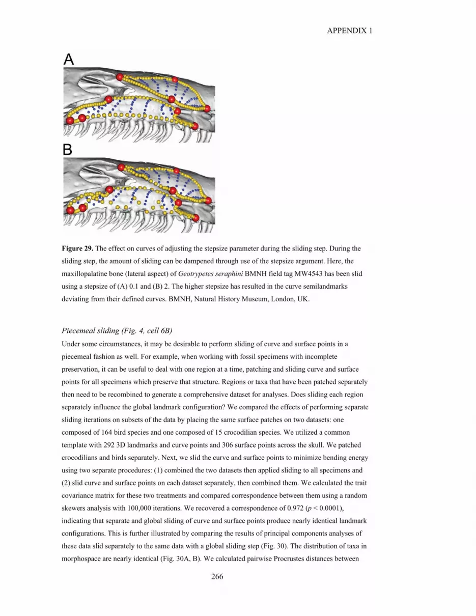
APPENDIX 1
266
Figure 29. The effect on curves of adjusting the stepsize parameter during the sliding step. During the
sliding step, the amount of sliding can be dampened through use of the stepsize argument. Here, the
maxillopalatine bone (lateral aspect) of Geotrypetes seraphini BMNH field tag MW4543 has been slid
using a stepsize of (A) 0.1 and (B) 2. The higher stepsize has resulted in the curve semilandmarks
deviating from their defined curves. BMNH, Natural History Museum, London, UK.
Piecemeal sliding (Fig. 4, cell 6B)
Under some circumstances, it may be desirable to perform sliding of curve and surface points in a
piecemeal fashion as well. For example, when working with fossil specimens with incomplete
preservation, it can be useful to deal with one region at a time, patching and sliding curve and surface
points for all specimens which preserve that structure. Regions or taxa that have been patched separately
then need to be recombined to generate a comprehensive dataset for analyses. Does sliding each region
separately influence the global landmark configuration? We compared the effects of performing separate
sliding iterations on subsets of the data by placing the same surface patches on two datasets: one
composed of 164 bird species and one composed of 15 crocodilian species. We utilized a common
template with 292 3D landmarks and curve points and 306 surface points across the skull. We patched
crocodilians and birds separately. Next, we slid the curve and surface points to minimize bending energy
using two separate procedures: (1) combined the two datasets then applied sliding to all specimens and
(2) slid curve and surface points on each dataset separately, then combined them. We calculated the trait
covariance matrix for these two treatments and compared correspondence between them using a random
skewers analysis with 100,000 iterations. We recovered a correspondence of 0.972 (p < 0.0001),
indicating that separate and global sliding of curve and surface points produce nearly identical landmark
configurations. This is further illustrated by comparing the results of principal components analyses of
these data slid separately to the same data with a global sliding step (Fig. 30). The distribution of taxa in
morphospace are nearly identical (Fig. 30A, B). We calculated pairwise Procrustes distances between

APPENDIX 1
267
taxa in both versions of the analysis and plotted the relationship between them (Fig. 30C). A linear
regression reveals an extremely strong fit between pairwise distances in the two treatments (R2 = 0.9975,
p < 0.001). Because global vs separate sliding of curve and surface point subsets has little appreciable
influence on data distributions, it is expected that sliding regions separately is an appropriate workflow
for dealing with high-dimensional 3D surface landmark datasets.
Figure 30. Comparing sliding curve and surface points globally vs sliding subsets separately and
combining data. With a dataset of 598 total landmarks, curve and surface points, with 164 bird and 15
crocodilian skulls, we slid curve and surface points to minimize bending energy with two workflows. In
one procedure, we slid curve and surface points for all specimens together, then subjected the data to
generalized Procrustes analysis (GPA) and
PCA (A). In the second treatment, we conducted sliding on the two clades separately, then combined
them before carrying out GPA and PCA (B). These procedures produce nearly identical morphospace
distributions. Comparing pairwise distances between taxa for each treatment further demonstrates
extremely good fit (C).
Asymmetric sampling of bilaterally symmetric structures (Fig. 4, cell 6C)
Coordinate data of bilaterally symmetric structures, such as the skull, often comprise landmarks from
only one side due to redundant shape information that exists on the other side. In addition, sampling only
one side substantially reduces the time required for data collection, which is relevant for the time-
intensive acquisition of high-dimensional morphometric data. However, performing generalized
Procrustes alignment on one-sided data produces exaggerated shape variation along the anatomical
midline while reducing the variation off the midline (Table 5) (Cardini 2016a,b). Following previous
studies, we recommend imputation of the missing side through mirroring of existing side along the
midline plane prior to mirroring, then removing the mirrored landmarks subsequent to alignment of
coordinate data. While previous studies highlighting these artefacts focused on data with only landmarks,
here, we investigated which components of high-dimensional coordinates––landmarks, curve points, and
surface points—should be mirrored to sufficiently minimize spurious characterization of shape variation.
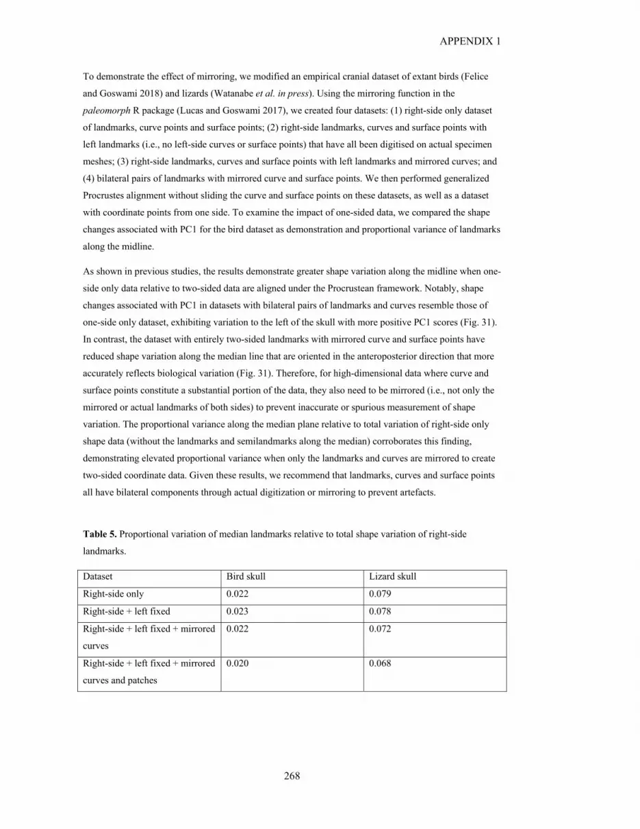
APPENDIX 1
268
To demonstrate the effect of mirroring, we modified an empirical cranial dataset of extant birds (Felice
and Goswami 2018) and lizards (Watanabe et al. in press). Using the mirroring function in the
paleomorph R package (Lucas and Goswami 2017), we created four datasets: (1) right-side only dataset
of landmarks, curve points and surface points; (2) right-side landmarks, curves and surface points with
left landmarks (i.e., no left-side curves or surface points) that have all been digitised on actual specimen
meshes; (3) right-side landmarks, curves and surface points with left landmarks and mirrored curves; and
(4) bilateral pairs of landmarks with mirrored curve and surface points. We then performed generalized
Procrustes alignment without sliding the curve and surface points on these datasets, as well as a dataset
with coordinate points from one side. To examine the impact of one-sided data, we compared the shape
changes associated with PC1 for the bird dataset as demonstration and proportional variance of landmarks
along the midline.
As shown in previous studies, the results demonstrate greater shape variation along the midline when one-
side only data relative to two-sided data are aligned under the Procrustean framework. Notably, shape
changes associated with PC1 in datasets with bilateral pairs of landmarks and curves resemble those of
one-side only dataset, exhibiting variation to the left of the skull with more positive PC1 scores (Fig. 31).
In contrast, the dataset with entirely two-sided landmarks with mirrored curve and surface points have
reduced shape variation along the median line that are oriented in the anteroposterior direction that more
accurately reflects biological variation (Fig. 31). Therefore, for high-dimensional data where curve and
surface points constitute a substantial portion of the data, they also need to be mirrored (i.e., not only the
mirrored or actual landmarks of both sides) to prevent inaccurate or spurious measurement of shape
variation. The proportional variance along the median plane relative to total variation of right-side only
shape data (without the landmarks and semilandmarks along the median) corroborates this finding,
demonstrating elevated proportional variance when only the landmarks and curves are mirrored to create
two-sided coordinate data. Given these results, we recommend that landmarks, curves and surface points
all have bilateral components through actual digitization or mirroring to prevent artefacts.
Table 5. Proportional variation of median landmarks relative to total shape variation of right-side
landmarks.
Dataset Bird skull Lizard skull
Right-side only 0.022 0.079
Right-side + left fixed 0.023 0.078
Right-side + left fixed + mirrored
curves
0.022 0.072
Right-side + left fixed + mirrored
curves and patches
0.020 0.068

APPENDIX 1
269
Figure 31. Diagram, in dorsal view, showing shape variation associated with positive PC1 scores of each
bird skull dataset highlighting the differences in variation along the midline (blue line). The black lines
indicate the magnitude and direction of shape changes from mean shape to shape at maximum PC1 score
observed in the sampled specimens for right-side only dataset (A); right-side with left landmarks (B);
right side with left landmarks and mirrored curve points (C); and right side with left landmarks and
mirrored curve and surface points (D). Note the shape variation towards the left side of the skull for
landmarks along the median plane (blue line) in datasets aligned without the full set of bilateral
landmarks, curve points and surface points.
Conclusions The collection of semilandmark data (curves and surface points) can be both difficult and time-
consuming, so is it worth it? There are many factors to consider when deciding data type, including the
intended sample size, complexity of the structure, and the desired resolution of the shape data. Landmarks
are considerably faster to collect than semilandmark data, meaning greater taxonomic sampling is easier
to achieve. Although pseudolandmarks are also fast to collect, landmarks may be preferred when specific
aspects of morphology are of interest, instead of capturing the entire morphology. Thousands of studies to
date have successfully captured the shape of structures using 2D or 3D landmark data (domestic dog
crania, Drake and Klingenberg 2010; mouse mandibles, Siahsarvie et al. 2012; caecilian crania, Sherratt
et al. 2014; felid vertebrae, Randau et al. 2016; lacertid skulls, Urošević et al. 2018). However, the recent
explosion of scan data and the accompanying advances in technology have facilitated the collection of

APPENDIX 1
270
higher-resolution shape information, improving the sampling of shape across a broader range of taxa, and
expanding the toolkit for testing a wider range of hypotheses.
Structures with few identifiable landmarks (e.g., limb bones, fused crania) may not be suitable for
landmark-only data collection, as this can leave large areas of morphology unsampled. Similarly,
sampling over a large, diverse clade may drastically reduce the number of shared landmarks across taxa
(Bardua et al. 2019). In these cases, the addition of semilandmarks can greatly improve the
characterisation of shape. For our caecilian and squamate datasets, landmark-only data can be compared
to complete landmark and semilandmark data, by aligning both separately and observing the fit between
the two aligned datasets using the ‘protest’ function in the vegan R package (Oksanen et al. 2018). A very
poor fit was observed between the landmark-only data and the full data for each cranial region for the
caecilian and squamate datasets, reflecting the shape information that is lost when only landmarks are
used (Tables 3, 4). Limiting datasets to landmarks would therefore mean capturing an exceptionally small
amount of the morphological variation across our sample, even within each of the clades of interest. For
comparing across clades, the number of Type I and Type II landmarks that can be identified consistently
plummets; for example, our estimate of cranial landmarks with unambiguous homology across Tetrapoda
numbers approximately 12. Thus, for the purposes of accurately capturing morphological variation, and
reconstructing the evolution of form, our results demonstrate that semilandmarks are a vast improvement
on landmark-only geometric morphometrics. Accurate analyses of evolutionary processes shaping form
require accurate data on morphological variation, and this is not achievable across large clades without
moving beyond Type I and Type II landmarks.
Curve semilandmarks expand the quantification of shape to include the morphology of outlines (e.g.,
bone or fin margins) and ridges. Curve semilandmarks may be sufficient for some structures whose shape
is strongly characterised by curves, with relatively conserved surface geometries in between curves (e.g.,
semi-circular canals, Billet et al. 2015; or bird beaks, Cooney et al. 2017). These data may also be suitable
for datasets with moderate levels of surface deformation or incomplete morphologies. The collection of
surface semilandmarks can impose strict criteria on the condition of the mesh, since surfaces must be
complete and undeformed. Consequently, it may be more practical to collect curve sliding semilandmarks
for structures whose surfaces are damaged or incomplete (but whose bone margins or outline information
is preserved), but whose morphology would be undersampled using only landmarks.
For studies where the shape of the entire structure is of interest, rather than needing to segregate a
structure into component parts, it may be appropriate to capture the shape of surfaces through the use of
pseudolandmarks (Vitek et al. 2017). Pseudolandmarks sample over the entire surface of a structure, so
the structures must be complete and undeformed. Since they are automatic, these methods facilitate the
study of extensive datasets, meaning very large sample sizes can be achieved with relatively little manual
input. These methods have been demonstrated using datasets of teeth (Boyer et al. 2011; Vitek et al.
2017) and primate calcanei (Boyer et al. 2015). However, the lack of user control in these methods means
that structures cannot be subdivided into different regions, and structures must be treated in their entirety,
so questions are limited to looking at gross morphology. Furthermore, complex structures may include
areas which should be excluded from shape capture, such as the teeth on a mandible. Since automatic

APPENDIX 1
271
methods cannot distinguish between wanted and unwanted areas of morphology, unwanted regions would
have to be manually removed from each structure beforehand. A study comparing the effectiveness of
automatic pseudolandmark and semi-automated semilandmark approaches (Gonzalez et al. 2016) found
both methods were successful for simple, smooth shapes with high levels of variation across the dataset.
However, semiautomatic methods were more successful at discriminating group differences for more
complex and irregular shapes (and datasets exhibiting lower levels of morphological variation). This may
be because pseudolandmark approaches sample evenly over a structure so cannot focus on specific
regions of interest which may be the key to between-group differences (Gonzalez et al. 2016). However,
choice of alignment settings can affect the success of pseudolandmark approaches, and increased numbers
of pseudolandmarks can improve the detection of group differences, suggesting this approach may be
suitable for datasets with small amounts of variation (although sensitivity analyses should be run for each
dataset) (Vitek et al. 2017). Pseudolandmark approaches are therefore most appropriate for relatively
simple structures when large sample size is desired and biological questions are centred around gross
morphology.
Surface semilandmark approaches as described here provide an intermediate between lower-density
landmark-based studies and extremely high-density pseudolandmark studies. Semilandmarks are able to
discriminate group morphology for diverse datasets (Gonzalez et al. 2016). Furthermore, use of
semilandmarks allows detection of subtle morphological variation, making them crucial for
morphologically restricted studies (e.g., intraspecific or within-population studies). Critically, the method
described allows for demarcation of regions that correspond to homologous structures, e.g. the frontal
bone or the rostrum (Figs 32,33), meaning that relationships among regions or differential patterns of
variation across regions can be assessed. Although the specific sutures defining a region, or even the
elements comprising a structure may vary across large (or even small) clades, they can be compared in a
biologically meaningful manner using semilandmarks. Therefore, whilst automated procedures may be
suitable for capturing the overall morphology of some structures, semi-automated procedures may be
better suited to investigating localised shape variation (Gonzalez et al. 2016). Furthermore, the
relationships among regions, i.e. integration and modularity, can be examined using this approach,
because the surface point positions are informed by landmarks and curves that have been placed with user
input, rather than an entirely automated process. Surface semilandmarks also facilitate the warping of one
structure’s morphology to another, for use in fossil reconstructions and hypothetical model construction
(e.g., Gunz et al. 2009; O’Higgins et al. 2011). Both semilandmark and pseudolandmark approaches,
therefore, offer promising and complementary paths forward for comparing across disparate organisms or
for comparing structures that may not have many clear landmarks.

APPENDIX 1
272
Figure 32. (This is a 3D figure, please follow this sketchfab link: https://sketchfab.com/3d-models/carla-
bardua-figure-31-b3db492d35964e0282a81179972e5083): Landmarks and semilandmarks, colour coded
by the 16 cranial regions defined in (Bardua et al. 2019), shown on the caecilian Siphonops annulatus
BMNH 1956.1.15.88. Regions are as follows: nasal, premaxilla (or nasopremaxilla) and septomaxilla
when present, dorsal surface (green); frontal, and mesethmoid when present (light pink); parietal (black);
squamosal, and postfrontal when present (dark blue); maxillopalatine (lateral surface), and prefrontal
when present (orange); quadrate (lateral surface) (light green); quadrate (jaw joint articulation) (red);
occipital (otic) region of os basale (excluding occipital condyle) (light purple); occipital condyle (aqua);
Ventral surface of os basale (purple); palatal surface of nasopremaxilla, or the anterior projection of the
vomer (gold); vomer (white); interdental plate of maxillopalatine (grey); palatine shelf (maxillary plate)
of maxillopalatine (hot pink); pterygoid, and/or pterygoid process of quadrate (light blue); stapes
(yellow). BMNH, Natural History Museum, London, UK.
Figure 33. (This is a 3D figure, please follow this sketchfab link: https://sketchfab.com/3d-models/carla-
bardua-figure-32-b046136256904b4293b630272f2134b8). Landmarks and semilandmarks, colour coded
by the 13 cranial regions defined in (Watanabe et al. in press), shown on the lizard Sceloporus variabilis

APPENDIX 1
273
FMNH 122866. Regions are as follows: premaxilla (red), nasal (dark blue), maxilla (dark green), jugal
(purple), frontal (orange), parietal (yellow), squamosal (brown), jaw joint (pink), supraoccipital (gray),
basioccipital (light blue), pterygoid (light green), palatine (tan), and occipital condyle (black). FMNH,
Field Museum of Natural History, Chicago, IL, USA
Of course, using high-density approaches such as those described here may create issues with data
dimensionality, and this effect should be considered and checked in downstream analyses. There is also
the additional problem that many existing analytical tools cannot cope with large datasets at present
(Adams and Collyer 2017), although new methods are in continuous development to solve these issues
(Clavel et al. 2019). One approach that we have implemented is to subsample down to 10-20% of the full
landmark and semilandmark dataset and rerun analyses to check consistency of results. For our analyses
of trait correlation structure (integration and modularity), we subsampled our datasets of birds, squamates,
and caecilians down to 10% of the full dataset and compared results from 100 iterations to that for the full
dataset. Results were consistently nearly identical across subsamples and the full datasets (Watanabe et
al. in press; Felice and Goswami 2018; Bardua et al. 2019; Marshall et al. 2019), indicating that they are
robust to landmark sampling, but this should be checked separately for every dataset. This effect has also
been demonstrated for high-dimensional shape data for musteloid limbs, finding subsampled data lead to
the same results (Fabre et al. 2014). Randomly subsampling from the complete dataset (and running
analyses iteratively) offers the additional benefit of enabling sampling from the whole of morphology,
achieving dimensionality similar to that of landmark-only datasets but without restricting the shape data
to sutures and other Type I and Type II landmarks, which tend to be limited to the boundaries of
structures.
Biological variation is inherently high-dimensional (Collyer et al. 2015). In order to best reconstruct and
examine morphological variation and morphological evolution, it is imperative to accurately measure
organismal form. The past few decades have brought extraordinary new abilities to image organisms with
more speed and resolution than previously possible, and many current initiatives are focused on digitizing
biological diversity at scales that would have been unimaginable when geometric morphometric
approaches were first being applied to macroevolutionary questions. These new datasets bring challenges,
but they also provide unprecedented opportunities to identify the fundamental rules shaping evolution
across disparate species. To do so will require further expansion and development of tools that can
capture and leverage this new information to its fullest potential. We hope that this practical guide to
applying surface sliding semilandmark methods across a wide diversity of forms will prove useful in
advancing the fields of quantitative evolutionary and comparative biology towards that goal.

APPENDIX 1
274
References Adams, D. C., and M. L. Collyer. 2017. Multivariate phylogenetic comparative methods: evaluations,
comparisons, and recommendations. Syst. Biol. 67:14–31.
Adams, D. C., and E. Otárola-Castillo. 2013. geomorph: an R package for the collection and analysis of
geometric morphometric shape data. Methods Ecol. Evol. 4:393–399.
Adams, D. C., F. J. Rohlf, and D. E. Slice. 2013. A field comes of age: geometric morphometrics in the
21st century. Hystrix, Ital. J. Mammal. 24:7–14.
Adams, D. C., F. J. Rohlf, and D. E. Slice. 2004. Geometric morphometrics: ten years of progress
following the ‘revolution.’ Ital. J. Zool. 71:5–16.
Adler, D., D. Murdoch, and E. Al. 2018. rgl: 3D Visualization Using OpenGL. R package version
0.99.16. https://CRAN.R-project.org/package=rgl.
Andresen, P. R., F. L. Bookstein, K. Conradsen, B. K. Ersbøll, J. L. Marsh, and S. Kreiborg. 2000.
Surface-bounded growth modeling applied to human mandibles. I E E E Trans. Med. Imaging
19:1053–1063.
Aristide, L., S. Furtado dos Reis, A. C. Machado, I. Lima, R. T. Lopes, and S. I. Perez. 2016. Brain shape
convergence in the adaptive radiation of New World monkeys. Proc. Natl. Acad. Sci. USA
113:2158–2163.
Bardua, C., M. Wilkinson, D. J. Gower, E. Sherratt, and A. Goswami. 2019. Morphological evolution and
modularity of the caecilian skull. BMC Evol. Biol. 19:1–23.
Billet, G., L. Hautier, and R. Lebrun. 2015. Morphological diversity of the bony labyrinth (inner ear) in
extant xenarthrans and its relation to phylogeny. J. Mammal. 96:658–672.
Bookstein, F. L. 1997. Landmark methods for forms without landmarks: morphometrics of group
differences in outline shape. Med. Image Anal. 1:225–243.
Bookstein, F. L. 1991. Morphometric tools for landmark data: geometry and biology. Cambridge
University Press., Cambridge.
Bookstein, F. L., and W. Green. 1994. Edgewarp: a flexible program package for biometric image
warping in two dimensions; Pp. 135–147 in Bookstein FL, Green WD. Visualization in biomedical
computing. vol. 2359. International society for optics and photonics.
Bookstein, F. L., A. P. Streissguth, P. D. Sampson, P. D. Connor, and H. M. Barr. 2002. Corpus Callosum
Shape and Neuropsychological Deficits in Adult Males with Heavy Fetal Alcohol Exposure.
Neuroimage 15:233–251.
Botton-Divet, L., R. Cornette, A.-C. Fabre, A. Herrel, and A. Houssaye. 2016. Morphological analysis of
long bones in semi-aquatic mustelids and their terrestrial relatives. Integr. Comp. Biol. 56:1298–
1309.

APPENDIX 1
275
Botton-Divet, L., A. Houssaye, A. Herrel, A.-C. Fabre, and R. Cornette. 2015. Tools for quantitative form
description; an evaluation of different software packages for semi-landmark analysis. PeerJ 3.
Boyer, D. M., Y. Lipman, E. St. Clair, J. Puente, B. A. Patel, T. Funkhouser, J. Jernvall, and I.
Daubechies. 2011. Algorithms to automatically quantify the geometric similarity of anatomical
surfaces. PNAS 108:18221–18226.
Boyer, D. M., J. Puente, J. T. Gladman, C. Glynn, S. Mukherjee, G. S. Yapuncich, and I. Daubechies.
2015. A new fully automated approach for aligning and comparing shapes. Anat. Rec. 298:249–
276.
Cardini, A. 2016a. Left, right or both? Estimating and improving accuracy of one-side-only geometric
morphometric analyses of cranial variation. J. Zool. Syst. Evol. Res. 55:1–10.
Cardini, A. 2016b. Lost in the other half: improving accuracy in geometric morphometric analyses of one
side of bilaterally symmetric structures. Syst. Biol. 65:1096–1106.
Cignoni, P., M. Corsini, and G. Ranzuglia. 2008. Meshlab: an open-source 3d mesh processing system.
ERCIM News 73:47–48.
Clavel, J., L. Aristide, and H. Morlon. 2019. A penalized likelihood framework for high-dimensional
phylogenetic comparative methods and an application to New-World monkeys brain evolution.
Syst. Biol. 68:93–116.
Collyer, M. L., D. J. Sekora, and D. C. Adams. 2015. A method for analysis of phenotypic change for
phenotypes described by high-dimensional data. Heredity (Edinb). 115:357–365.
Cooney, C. R., J. A. Bright, E. J. R. Capp, A. M. Chira, E. C. Hughes, C. J. A. Moody, L. O. Nouri, Z. K.
Varley, and G. H. Thomas. 2017. Mega-evolutionary dynamics of the adaptive radiation of birds.
Nature 542:344–347.
Cope, E. D. 1887. The origin of the fittest: essays on evolution. D. Appleton and Company, New York,
526 pp.
Cornette, R., M. Baylac, T. Souter, and A. Herrel. 2013. Does shape co-variation between the skull and
the mandible have functional consequences? A 3D approach for a 3D problem. J. Anat. 223:329–
336.
Cornette, R., A. Tresset, and A. Herrel. 2015. The shrew tamed by Wolff’s Law: do functional constraints
shape the skull through muscle and bone covariation? J. Morphol. 276:301–309.
Da Silva, F. O., A.-C. Fabre, Y. Savriama, J. Ollonen, K. Mahlow, A. Herrel, J. Müller, and N. Di-Poï.
2018. The ecological origins of snakes as revealed by skull evolution. Nat. Commun. 9:1–11.
Davies, T. G., I. A. Rahman, S. Lautenschlager, J. A. Cunningham, R. J. Asher, P. M. Barrett, K. T.
Bates, S. Bengtson, R. B. J. Benson, D. M. Boyer, J. Braga, J. A. Bright, L. P. A. M. Claessens, P.
G. Cox, X. P. Dong, A. R. Evans, P. L. Falkingham, M. Friedman, R. J. Garwood, A. Goswami, J.

APPENDIX 1
276
R. Hutchinson, N. S. Jeffery, Z. Johanson, R. Lebrun, C. Martínez-Pérez, J. Marugán-Lobón, P. M.
O’Higgins, B. Metscher, M. J. Orliac, T. B. Rowe, M. Rücklin, M. R. Sánchez-Villagra, N. H.
Shubin, S. Y. Smith, J. M. Starck, C. Stringer, A. P. Summers, M. D. Sutton, S. A. Walsh, V.
Weisbecker, L. M. Witmer, S. Wroe, Z. Yin, E. J. Rayfield, and P. C. J. Donoghue. 2017. Open
data and digital morphology. Proc. R. Soc. B Biol. Sci. 284:20170194.
Drake, A. G., and C. P. Klingenberg. 2010. Large‐scale diversification of skull shape in domestic dogs:
disparity and modularity. Am. Nat. 175:289–301.
Dryden, I. L., and K. V Mardia. 1998. Statistical Shape Analysis. Wiley, New York.
Dumont, M., C. E. Wall, L. Botton-Divet, A. Goswami, S. Peigné, and A.-C. Fabre. 2015. Do functional
demands associated with locomotor habitat, diet, and activity pattern drive skull shape evolution in
musteloid carnivorans? Biol. J. Linn. Soc. 117:858–878.
Fabre, A.-C., R. Cornette, S. Peigné, and A. Goswami. 2013a. Influence of body mass on the shape of
forelimb in musteloid carnivorans. Biol. J. Linn. Soc. 110:91–103.
Fabre, A.-C., R. Cornette, G. J. Slater, C. Argot, S. Peigné, A. Goswami, and E. Pouydebat. 2013b.
Getting a grip on the evolution of grasping in musteloid carnivorans: a three-dimensional analysis
of forelimb shape. J. Evol. Biol. 26:1521–1535.
Fabre, A.-C., A. Goswami, S. Peigné, and R. Cornette. 2014. Morphological integration in the forelimb of
musteloid carnivorans. J. Anat. 225:19–30.
Fabre, A.-C., M. C. Granatosky, J. B. Hanna, and D. Schmitt. 2018a. Do forelimb shape and peak forces
co-vary in strepsirrhines? Am. J. Phys. Anthropol. 167:602–614.
Fabre, A.-C., J. Marigó, M. C. Granatosky, and D. Schmitt. 2017. Functional associations between
support use and forelimb shape in strepsirrhines and their relevance to inferring locomotor behavior
in early primates. J. Hum. Evol. 108:11–30.
Fabre, A.-C., L. Peckre, E. Pouydebat, and C. E. Wall. 2019. Does the shape of forelimb long bones co-
vary with grasping behaviour in strepsirrhine primates? Biol. J. Linn. Soc. 127:649–660.
Fabre, A.-C., J. M. G. Perry, A. Hartstone-Rose, A. Lowie, A. Boens, and M. Dumont. 2018b. Do
muscles constrain skull shape evolution in Strepsirrhines ? Anat. Rec. 310:291–310.
Fabre, A.-C., M. J. Salesa, R. Cornette, M. Antón, J. Morales, and S. Peigné. 2015. Quantitative
inferences on the locomotor behaviour of extinct species applied to Simocyon batalleri (Ailuridae,
Late Miocene, Spain). Sci. Nat. 102:1–13.
Felice, R. N., and A. Goswami. 2018. Developmental origins of mosaic evolution in the avian cranium.
Proc. Natl. Acad. Sci. USA 115:555–560.
Gao, T., G. S. Yapuncich, I. Daubechies, S. Mukherjee, and D. M. Boyer. 2017. Development and
assessment of fully automated and globally transitive geometric morphometric methods , with

APPENDIX 1
277
application to a biological comparative dataset with high interspecific variation. Anat. Rec.
301:636–658.
Giardina, C. R., and F. Kuhl. 1977. Accuracy of curve approximation by harmonically related vectors
with elliptical loci. Comput. Graph. Image Process. 6:277–285.
Gonzalez, P. N., J. Barbeito-Andrés, L. A. D’Addona, V. Bernal, and S. I. Perez. 2016. Technical note:
performance of semi and fully automated approaches for registration of 3D surface coordinates in
geometric morphometric studies. Am. J. Phys. Anthropol. 160:169–178.
Gunz, P., and P. Mitteroecker. 2013. Semilandmarks: A method for quantifying curves and surfaces.
Hystrix, Ital. J. Mammal. 24:103–109.
Gunz, P., P. Mitteroecker, and F. L. Bookstein. 2005. Chapter three: semilandmarks in three dimensions.
Pp. 73–98 in D. E. Slice, ed. Modern Morphometrics in Physical Anthropology. Kluwer
Academic/Plenum, New York.
Gunz, P., P. Mitteroecker, S. Neubauer, G. W. Weber, and F. L. Bookstein. 2009. Principles for the
virtual reconstruction of hominin crania. J. Hum. Evol. 57:48–62.
Ian L. Dryden. 2017. shapes: Statistical Shape Analysis. R package version 1.2.1. https://CRAN.R-
project.org/package=shapes.
Katina, S., K. Mcneil, A. Ayoub, B. Guilfoyle, B. Khambay, P. Siebert, F. Sukno, M. Rojas, L. Vittert, J.
Waddington, P. F. Whelan, and A. W. Bowman. 2016. The definitions of three-dimensional
landmarks on the human face: an interdisciplinary view. J. Anat. 228:355–365.
Klingenberg, C. P. 2008. Novelty and “homology-free” morphometrics: what’s in a name? Evol. Biol.
35:186–190.
Kuhl, F. P., and C. R. Giardina. 1982. Elliptic Fourier features of a closed contour. Comput. Graph.
Image Process. 18:236–258.
Larouche, O., M. L. Zelditch, and R. Cloutier. 2018. Modularity promotes morphological divergence in
ray-finned fishes. Sci. Rep. 8:7278.
Lawing, A. M., and P. D. Polly. 2010. Geometric morphometrics: recent applications to the study of
evolution and development. J. Zool. 280:1–7.
Lebrun, R., and M. J. Orliac. 2017. MorphoMuseuM: an online platform for publication and storage of
virtual specimens. Paleontol. Soc. Pap. 22:183–195.
Lele, S. R., and J. T. Richtsmeier. 2001. An invariant approach to statistical analysis of shapes. Chapman
and Hall/CRC, New York.
Lucas, T., and A. Goswami. 2017. paleomorph: geometric morphometric tools for paleobiology. R
package version 0.1.4.

APPENDIX 1
278
Marcy, A. E., C. Fruciano, M. J. Phillips, K. Mardon, and V. Weisbecker. 2018. Low resolution scans can
provide a sufficiently accurate, cost- and time-effective alternative to high resolution scans for 3D
shape analyses. PeerJ 6:e5032.
Marshall, A. F., C. Bardua, D. J. Gower, M. Wilkinson, E. Sherratt, and A. Goswami. 2019. High-density
three-dimensional morphometric analyses support conserved static (intraspecific) modularity in
caecilian (Amphibia: Gymnophiona) crania. Biol. J. Linn. Soc. 126:721–742.
Mitteroecker, P., and P. Gunz. 2009. Advances in geometric morphometrics. Evol. Biol. 36:235–247.
Müller, H., O. V. Oommen, and P. Bartsch. 2005. Skeletal development of the direct-developing caecilian
Gegeneophis ramaswamii (Amphibia: Gymnophiona: Caeciliidae). Zoomorphology 124:171–188.
Niewoehner, W. A. 2005. A Geometric Morphometric Analysis of Late Pleistocene Human Metacarpal 1
Base Shape. Pp. 285–298 in D. E. Slice, ed. Modern Morphometrics in Physical Anthropology.
Kluwer Academic/Plenum, New York.
O’Higgins, P., S. N. Cobb, L. C. Fitton, F. Gröning, R. Phillips, J. Liu, and M. J. Fagan. 2011. Combining
geometric morphometrics and functional simulation: an emerging toolkit for virtual functional
analyses. J. Anat. 218:3–15.
Oksanen, J., F. G. Blanchet, M. Friendly, R. Kindt, P. Legendre, D. McGlinn, P. R. Minchin, R. B.
O’Hara, G. L. Simpson, P. Solymos, M. H. H. Stevens, E. Szoecs, and H. Wagner. 2018. vegan:
Community Ecology Package. R package version 2.5-2.
Pavonia, C., V. Paolonib, L. T. H. Ghislanzonic, G. Laganà, and P. Cozza. 2017. Geometric
morphometric analysis of the palatal morphology in children with impacted incisors: a three-
dimensional evaluation. Angle Orthod. 87:404–408.
Perez, S. I., V. Bernal, and P. N. Gonzalez. 2006. Differences between sliding semi-landmark methods in
geometric morphometrics, with an application to human craniofacial and dental variation. J. Anat.
208:769–784.
Phillips, R., P. O’Higgins, F. L. Bookstein, B. (ed) Green, H. (ed) Gunnarson, Y. (ed) Shady, V. (ed)
Dalge, R. (ed) Gowigati, and O. (ed) Ben Ali. 2010. EVAN (European Virtual Anthropology
Network) toolbox. European Virtual Anthropology Network - EVAN (www.evan.at) and the
EVAN-Society.
Polly, P. D., and N. MacLeod. 2008. Locomotion in fossil Carnivora: an application of eigensurface
analysis for morphometric comparison of 3D surfaces. Palaeontol. Electron. 11:1–13.
Pomidor, B. J., J. Makedonska, and D. E. Slice. 2016. A landmark-free method for three- dimensional
shape analysis. PLoS One 11:e0150368.
R Core Team. 2017. R: A language and environment for statistical computing. R Foundation for
Statistical Computing. v 3.4.3. Vienna, Austria.

APPENDIX 1
279
Randau, M., A. Goswami, J. R. Hutchinson, A. R. Cuff, and S. E. Pierce. 2016. Cryptic complexity in
felid vertebral evolution: Shape differentiation and allometry of the axial skeleton. Zool. J. Linn.
Soc. 178:183–202.
Rohlf, F. J., and L. F. Marcus. 1993. A revolution in morphometrics. Trends Ecol. Evol. 8:129–132.
Schlager, S. 2016. Morpho: Calculations and Visualisations Related to Geometric Morphometrics.
Schlager, S. 2017. Morpho and Rvcg - Shape Analysis in R. Pp. 217–256 in G. Zheng, S. Li, and G.
Szekely, eds. Statistical Shape and Deformation Analysis. Academic Press.
Segall, M., R. Cornette, A.-C. Fabre, R. Godoy-Diana, and A. Herrel. 2016. Does aquatic foraging impact
head shape evolution in snakes? Proc. R. Soc. B Biol. Sci. 283:20161645.
Sherratt, E., A. Alejandrino, A. C. Kraemer, J. M. Serb, and D. C. Adams. 2016. Trends in the sand:
directional evolution in the shell shape of recessing scallops (Bivalvia: Pectinidae). Evolution.
70:2061–2073.
Sherratt, E., D. J. Gower, C. P. Klingenberg, and M. Wilkinson. 2014. Evolution of cranial shape in
caecilians (Amphibia: Gymnophiona). Evol. Biol. 41:528–545.
Siahsarvie, R., J. C. Auffray, J. Darvish, H. Rajabi-Maham, H. T. Yu, S. Agret, F. Bonhomme, and J.
Claude. 2012. Patterns of morphological evolution in the mandible of the house mouse Mus
musculus (Rodentia: Muridae). Biol. J. Linn. Soc. 105:635–647.
Slice, D. E. 2005. Modern morphometrics in physical anthropology. Kluwer Academic/Plenum, New
York.
Souter, T., R. Cornette, J. Pedraza, J. R. Hutchinson, and M. Baylac. 2010. Two applications of 3D semi-
landmark morphometrics implying different template designs: the theropod pelvis and the shrew
skull. Comptes Rendus Palevol 9:411–422.
Thompson, D. 1917. On Growth and Form. Cambridge University Press., Cambridge, UK.
Urošević, A., K. Ljubisavljević, and A. Ivanović. 2018. Multilevel assessment of the Lacertid lizard
cranial modularity. J. Zool. Syst. Evol. Res. 57:1–14.
Van Bocxlaer, B., and R. Schultheiß. 2010. Comparison of morphometric techniques for shapes with few
homologous landmarks based on machine-learning approaches to biological discrimination.
Paleobiology 36:497–515.
Vitek, N. S. 2018. Delineating modern variation from extinct morphology in the fossil record using shells
of the Eastern Box Turtle (Terrapene carolina). PLoS One 13:e0193437.
Vitek, N. S., C. L. Manz, T. Gao, J. I. Bloch, S. G. Strait, and D. M. Boyer. 2017. Semi-supervised
determination of pseudocryptic morphotypes using observer-- free characterizations of anatomical
alignment and shape. Ecol. Evol. 7:5041–5055.

APPENDIX 1
280
Waddington, J. L., S. Katina, C. M. P. O’Tuathaigh, and A. W. Bowman. 2017. Translational genetic
modelling of 3D craniofacial dysmorphology: elaborating the facial phenotype of
neurodevelopmental disorders through the “prism” of schizophrenia. Curr. Behav. Neurosci.
Reports 4:322–330. Current Behavioral Neuroscience Reports.
Wake, M. H., and J. Hanken. 1982. Development of the skull of Dermophis mexicanus (Amphibia:
Gymnophiona), with comments on skull kinesis and amphibian relationships. J. Morphol. 173:203–
223.
Watanabe, A. 2018. How many landmarks are enough to characterize shape and size variation? PLoS One
13:e0198341.
Watanabe, A., A.-C. Fabre, R. N. Felice, J. Maisano, J. Müller, A. Herrel, and A. Goswami. 2019.
Ecomorphological diversification in squamates from conserved pattern of cranial integration. Proc.
Natl. Acad. Sci. USA 116:14688–14697.
Wiley, D. F., N. Amenta, G. Alcantara, Dan A. Deboshmita, Y. J. Kil, E. Delson, W. Harcourt-Smith, F.
J. Rohlf, K. St. John, and B. Hamann. 2005. Evolutionary morphing. Proc. IEEE Vis. 2005 431–
438. University of California, Davis.
Wölfer, J., E. Amson, P. Arnold, L. Botton-Divet, A.-C. Fabre, A. H. van Heteren, and J. A. Nyakatura.
2019. Femoral morphology of sciuromorph rodents in light of scaling and locomotor ecology. J.
Anat.
Wrozyna, C., T. A. Neubauer, J. Meyer, and W. E. Piller. 2016. Shape variation in neotropical
Cytheridella (Ostracoda) using semilandmarks-based geometric morphometrics: a methodological
approach and possible biogeographical implications. PLoS One 11:e0168438.
Yazdi, A. B. 2014. Application of geometric morphometrics to analyse allometry in two species of the
genus Myrmica (Hymenoptera : Formicidae). Soil Org. 86:77–84.
Zelditch, M. L., D. L. Swiderski, H. D. Sheets, and W. L. Fink. 2004. Geometric morphometrics for
biologists: a primer. Amsterdam.

CHAPTER 2 APPENDIX 2
281
APPENDIX 2
CHAPTER 2 APPENDIX
Figure S2.1. Network graphs displaying results from EMMLi analyses using (A) 10% subsampled, (B)
anatomical landmarks only, (C) allometry-corrected, and (D) phylogenetically-corrected data. Layout
approximately corresponds to a skull in lateral view, with the anterior to the right. Circle size is
proportional to within-module trait correlation (ρ), and line thickness is proportional to between-module
trait correlation. The stapes and pterygoid are missing from the landmark-only graph, as these are not
represented by any anatomical landmarks (semilandmarks only). For abbreviations see Figure 2.2.
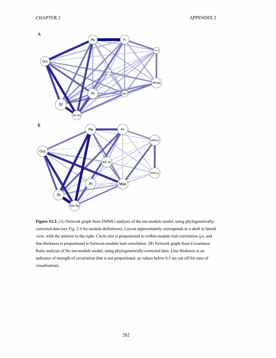
CHAPTER 2 APPENDIX 2
282
Figure S2.2. (A) Network graph from EMMLi analysis of the ten-module model, using phylogenetically-
corrected data (see Fig. 2.4 for module definitions). Layout approximately corresponds to a skull in lateral
view, with the anterior to the right. Circle size is proportional to within-module trait correlation (ρ), and
line thickness is proportional to between-module trait correlation. (B) Network graph from Covariance
Ratio analysis of the ten-module model, using phylogenetically-corrected data. Line thickness is an
indicator of strength of covariation (but is not proportional, as values below 0.5 are cut off for ease of
visualisation).

CHAPTER 2 APPENDIX 2
283
Figure S2.3. Reconstructed morphologies represented by positive (left) and negative (right) ends of PC1,
in dorsal, ventral, lateral, anterior, and posterior views from top to bottom.
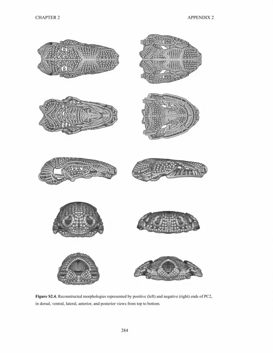
CHAPTER 2 APPENDIX 2
284
Figure S2.4. Reconstructed morphologies represented by positive (left) and negative (right) ends of PC2,
in dorsal, ventral, lateral, anterior, and posterior views from top to bottom.

CHAPTER 2 APPENDIX 2
285
Figure S2.5. Reconstructed morphologies represented by positive (left) and negative (right) ends of PC3,
in dorsal, ventral, lateral, anterior, and posterior views from top to bottom.

CHAPTER 2 APPENDIX 2
286
Figure S2.6. Morphospace of all 35 specimens based on the complete landmark and semilandmark
dataset, with PC1 on the x-axis and PC3 on the y-axis. Shapes represented by the positive and negative
end of each axis are displayed in dorsal view.

CHAPTER 2 APPENDIX 2
287
Figure S2.7. Phylomorphospace of all specimens in this study, with time in millions of years on the
vertical axis (present day at the top).
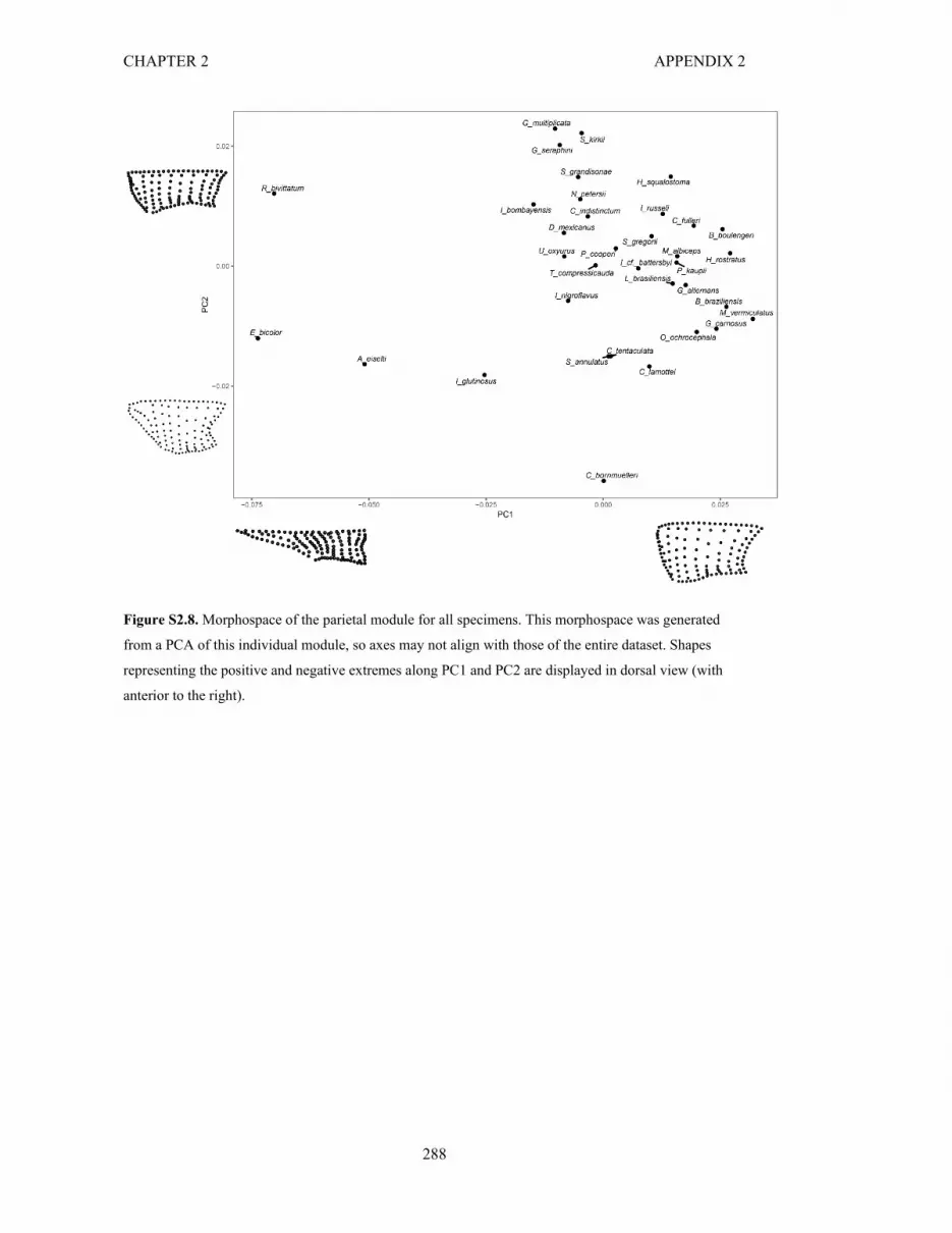
CHAPTER 2 APPENDIX 2
288
Figure S2.8. Morphospace of the parietal module for all specimens. This morphospace was generated
from a PCA of this individual module, so axes may not align with those of the entire dataset. Shapes
representing the positive and negative extremes along PC1 and PC2 are displayed in dorsal view (with
anterior to the right).

CHAPTER 2 APPENDIX 2
289
Figure S2.9. Morphospace of the frontal module for all specimens. This morphospace was generated
from a PCA of this individual module, so axes may not align with those of the entire dataset. Shapes
representing the positive and negative extremes along PC1 and PC2 are displayed in dorsal view (with
anterior to the right).

CHAPTER 2 APPENDIX 2
290
Figure S2.10. Morphospace of the quadrate-squamosal module for all specimens. This morphospace was
generated from a PCA of this individual module, so axes may not align with those of the entire dataset.
Shapes representing the positive and negative extremes along PC1 and PC2 are displayed in lateral view
(with anterior to the right).

CHAPTER 2 APPENDIX 2
291
Figure S2.11. Morphospace of the stapes module for all specimens. This morphospace was generated
from a PCA of this individual module, so axes may not align with those of the entire dataset. Shapes
representing the positive and negative extremes along PC1 and PC2 are displayed in ventral view (with
lateral to the left). ‘Tip’ refers to position of the lateral tip of the stapes.

CHAPTER 2 APPENDIX 2
292
Figure S2.12. Morphospace of the pterygoid module for all specimens. This morphospace was generated
from a PCA of this individual module, so axes may not align with those of the entire dataset. Shapes
representing the positive and negative extremes along PC1 and PC2 are displayed in ventral view (with
anterior to the right).
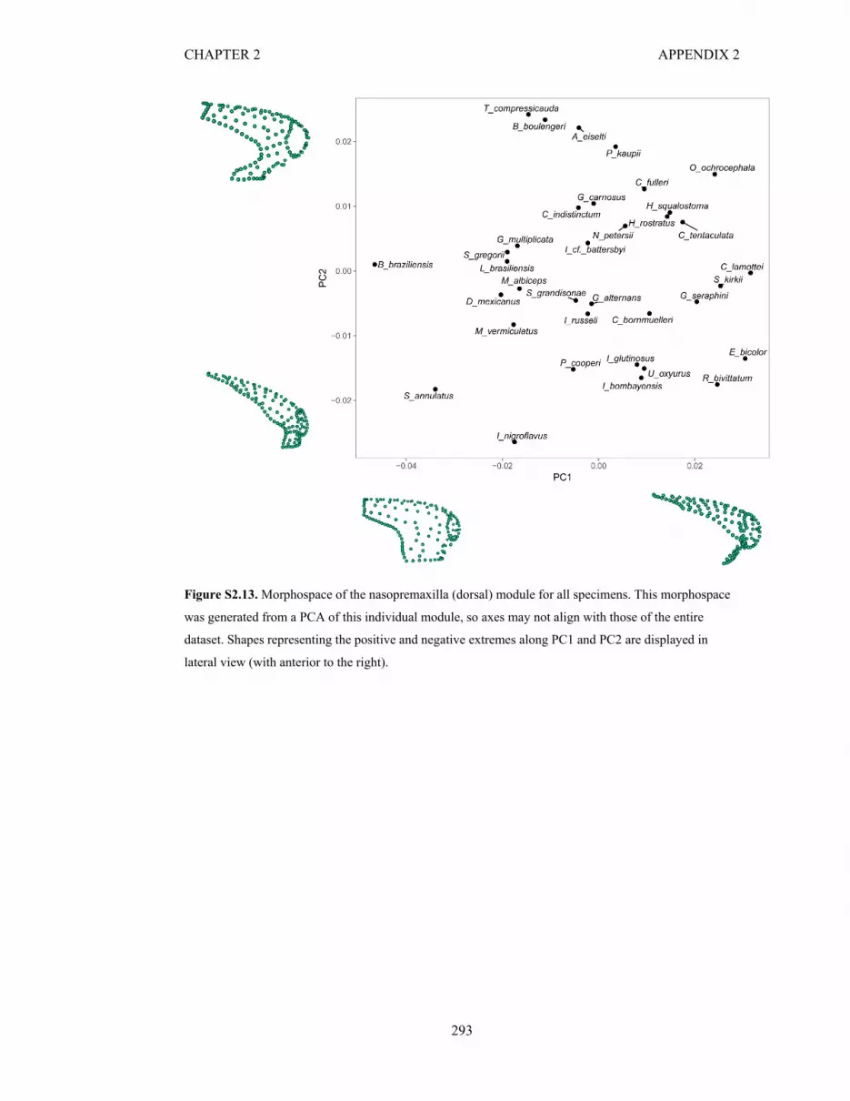
CHAPTER 2 APPENDIX 2
293
Figure S2.13. Morphospace of the nasopremaxilla (dorsal) module for all specimens. This morphospace
was generated from a PCA of this individual module, so axes may not align with those of the entire
dataset. Shapes representing the positive and negative extremes along PC1 and PC2 are displayed in
lateral view (with anterior to the right).

CHAPTER 2 APPENDIX 2
294
Figure S2.14. Morphospace of the maxillopalatine module for all specimens. This morphospace was
generated from a PCA of this individual module, so axes may not align with those of the entire dataset.
Shapes representing the positive and negative extremes along PC1 and PC2 are displayed in lateral view
(with anterior to the right).

CHAPTER 2 APPENDIX 2
295
Figure S2.15. Morphospace of the nasopremaxilla (palatal) module for all specimens. This morphospace
was generated from a PCA of this individual module, so axes may not align with those of the entire
dataset. Shapes representing the positive and negative extremes along PC1 and PC2 are displayed in
ventral view (with medial to the right).

CHAPTER 2 APPENDIX 2
296
Figure S2.16. Morphospace of the occipital module for all specimens. This morphospace was generated
from a PCA of this individual module, so axes may not align with those of the entire dataset. Shapes
representing the positive and negative extremes along PC1 and PC2 are displayed in posterior view (with
lateral to the right).
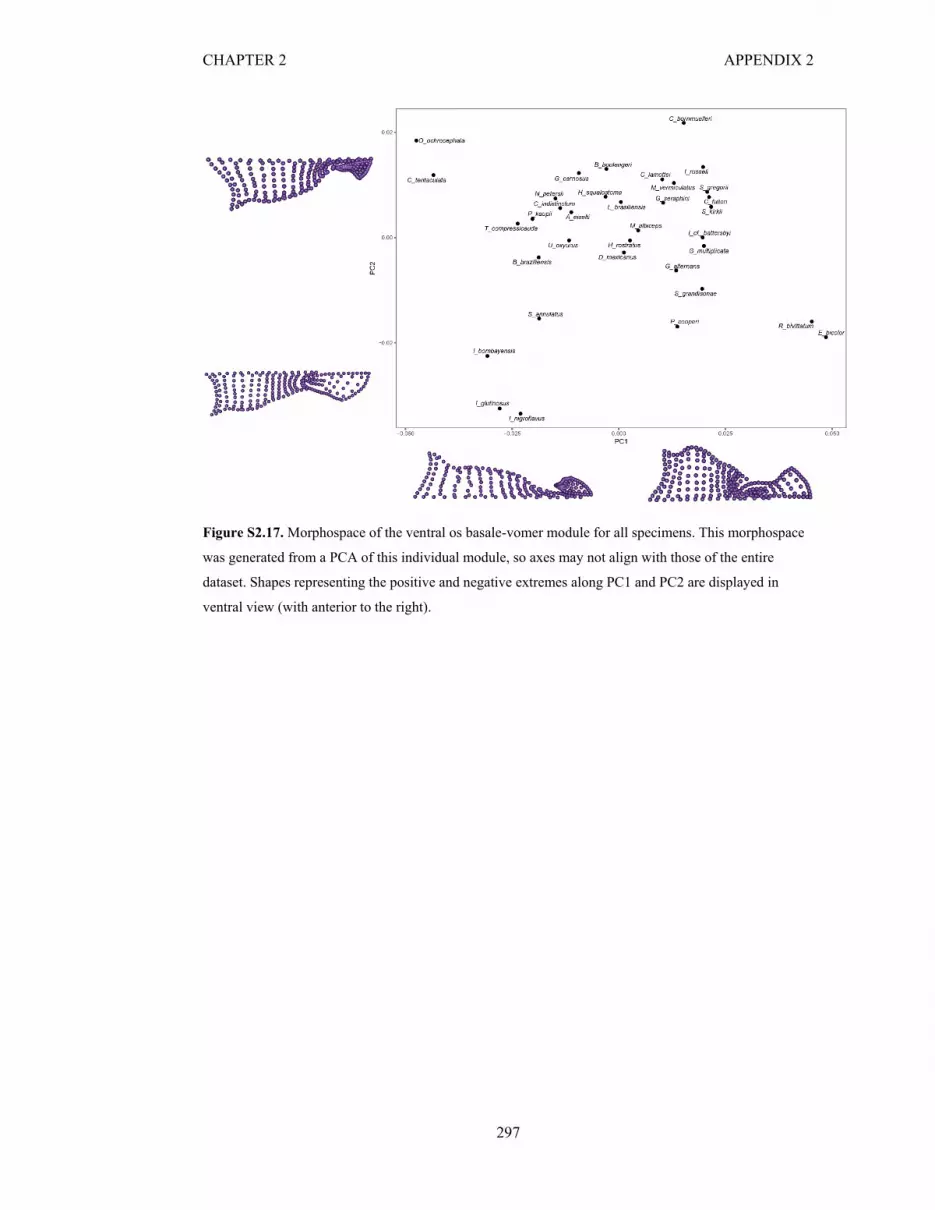
CHAPTER 2 APPENDIX 2
297
Figure S2.17. Morphospace of the ventral os basale-vomer module for all specimens. This morphospace
was generated from a PCA of this individual module, so axes may not align with those of the entire
dataset. Shapes representing the positive and negative extremes along PC1 and PC2 are displayed in
ventral view (with anterior to the right).

CHAPTER 2 APPENDIX 2
298
Figure S2.18. Distribution of specimens in morphospace, colour-coded by centroid size, binned into 10
bins of equal size.

299
APPEN
DIX
2 C
HA
PTER 2
Table S2.1. Ecological data for all species sampled in this study. For degree of fossoriality, the categories are: 0, aquatic species (which sometimes burrow in soft
substrates); 1, tailed species (which have relatively short and stout bodies and zygokrotaphic skulls); 2, tailless species with zygokrotaphic skulls; 3, tailless species with
stegokrotaphic skulls and open orbits; and 4, tailless species with closed orbits. All larval stage and reproductive mode information was taken from San Mauro et al (2014)
except for * species, whose data was based on nearest relatives. ** information is from personal observation (Mark Wilkinson). Data collected for Indotyphlus cf.
battersbyi was based on Indotyphlus battersbyi.
Species Degree of fossoriality as adult (0,1,2,3,4)
Life history strategy (larval stage absent/present)
Reproductive mode
Atretochoana eiselti 0 absent* viviparous* Boulengerula boulengeri 4 absent oviparous Brasilotyphlus braziliensis 4 absent* oviparous* Caecilia tentaculata 3 absent* oviparous* Chikila fulleri 4 absent oviparous Chthonerpeton indistinctum 2 absent viviparous Crotaphatrema bornmuelleri 4 absent* NA Crotaphatrema lamottei 4 absent* NA Dermophis mexicanus 3 absent viviparous Epicrionops bicolor 1 present* oviparous* Gegeneophis carnosus 4 absent* oviparous* Geotrypetes seraphini 2 absent viviparous Grandisonia alternans 3 NA oviparous* Gymnopis multiplicata 4 absent viviparous Herpele squalostoma 4 absent oviparous Hypogeophis rostratus 3 absent oviparous Ichthyophis bombayensis 1 present oviparous Ichthyophis glutinosus 1 present oviparous Ichthyophis nigroflavus 1 present* oviparous*

300
CH
APTER
2 A
PPEND
IX 2
Idiocranium russeli 3 absent oviparous Indotyphlus cf. battersbyi 3 absent* oviparous* Luetkenotyphlus brasiliensis 3 absent* oviparous* Microcaecilia albiceps 4 absent* oviparous* Mimosiphonops vermiculatus 3 absent* oviparous* Nectocaecilia petersii 2 absent** viviparous** Oscaecilia ochrocephala 4 absent* oviparous* Potomotyphlus kaupii 0 absent viviparous Praslinia cooperi 3 present oviparous* Rhinatrema bivitattum 1 present oviparous Schistometopum gregorii 3 absent viviparous Scolecomorphus kirkii 2 absent** viviparous** Siphonops annulatus 3 absent oviparous Sylvacaecilia grandisonae 3 present** oviparous** Typhlonectes compressicauda 0 absent** viviparous** Uraeotyphlus oxyurus 1 present oviparous*

301
APPEN
DIX
2 C
HA
PTER 2
Table S2.2 Definitions for the 16 cranial regions analysed in this study, corresponding to coloured regions in Fig. 2.2.
Region colour in Fig. 2.2 Region Region description Purple Os basale
(ventral) The ventral surface of the os basale, separated from the occipital region by a curve tracing the posterior muscle ridge. This is analogous to the basisphenoid module previous identified in birds (Felice and Goswami 2018).
Pale pink Frontal
Intraspecific analyses (Marshall et al. 2019) have found the mesethmoid shape to correlate most strongly with the frontal, so the mesethmoid and frontal were patched as one region. The whole frontal and mesethmoid (down its midline).
Red Quadrate (jaw joint)
The articular surface of the quadrate.
Grey Maxillopalatine (interdental plate)
The ventral surface of the maxillopalatine immediately posterior to the primary tooth row.
Orange Maxillopalatine (lateral)
The prefrontal was included in the lateral maxillopalatine region, because it has been shown to fuse with the maxillopalatine through development (Wake and Hanken 1982) and not with the frontal as was previously believed (Marcus et al. 1935). This region was the most difficult to landmark, because of its large variation in shape and housing of sensory openings. The maxillopalatine can house the orbit, the tentacular foramen, both or neither. The orbit, when present, is either housed completely within the maxillopalatine or sits between the maxillopalatine and squamosal. The tentacular foramen is either in the maxillopalatine or between the maxillopalatine and nasopremaxilla. The tentacle and orbit openings can be connected or separated. In addition, the tentacular opening can be a foramen (closed hole) or a fossa (a groove passing through the entire length of the maxillopalatine). This huge variation means defining homologous landmarks and curves is very difficult. Consequently, landmarks and curves were used as “fences” to constrain the regions for patching, but most were then removed before analyses. This way, we could use just two templates for patching these regions, one template with a defined hole (a negligibly sized hole was used for maxillopalatines with no hole) and one template that separated the maxillopalatine into regions dorsal and ventral to the tentacular fossa.
Hot pink Maxillopalatine (palatine shelf)
The ventral surface posterior to the secondary tooth row is known as the palatine shelf (or maxillary plate) and partially or completely borders the choana. When closed, the two landmarks defining the

302
CH
APTER
2 A
PPEND
IX 2
anterior and posterior border extremes of the choana were adjacently placed, reflecting the closing of the choana.
Green Nasopremaxilla (dorsal)
The dorsal surface of the nasopremaxilla (or nasal and premaxilla), and septomaxilla when present.
Gold Nasopremaxilla (palatal)
The ventral (palatal) surface of the nasopremaxilla posterior to the tooth row. The ventral surface consists of the naso/premaxilla in most specimens, but can be partially (e.g. Geotrypetes seraphini) or completely (Scolecomorphus kirkii and Crotaphatrema lamottei) covered by an anterior projection of the vomer. These bones were patched as one region, defined as the bone surface between the anterior first and second rows of teeth.
Aqua Occipital condyle
The occipital condyle. The occipital condyle was separated from the occipital region by two curves defining its border.
Pale purple Os basale (occipital)
Occipital region of the os basale, excluding occipital condyle. Ventrally, this region ended at the muscle ridge.
Black Parietal
We are interested in the external bone surface, so when a parietal-squamosal fenestra was present, we excluded the parietal region covered by the adductor musculature in life. This region is covered in fasciae so is considered internal. The parietal region was therefore defined by the parietal’s medial, anterior, and posterior margins, and the lateral margin was defined by the adductor ridge. For specimens Rhinatrema bivittatum and Epicrionops bicolor, which represent the extreme (primitive) condition of a large adductor muscle, this region is especially small.
Pale blue Pterygoid There is current debate surrounding bone homology for the pterygoid region of caecilians. There is a putative pterygoid (also referred to as the ectopterygoid) in some specimens, and all (except Scolecomorphus kirkii and Crotaphatrema bornmuelleri) have an anterior projection of the quadrate in ventral view, resembling the pterygoid in both shape and position. This is postulated to function as a pterygoid. Given the variable presence of the pterygoid and the pterygoid process of the quadrate, we defined the pterygoid region as both bones. Separate patching across specimens was necessary, as this region variably includes only one of the bones, both, or neither. Scolecomorphus kirkii and Crotaphatrema bornmuelleri, which have neither bone, were given a negligibly sized pterygoid region on the ventral side of the quadrate.

303
APPEN
DIX
2 C
HA
PTER 2
Pale green Quadrate
(lateral)
The lateral surface of the quadrate was defined by its anterior, lateral and medial borders, and the posterior edge traced around the jaw joint and the stapes articulation, excluding both.
Dark blue Squamosal The postfrontal was present in only three specimens and was patched with the squamosal. The posterior orbit margin, when the orbit is not enclosed within the maxillopalatine, consists of the squamosal or the postfrontal. Although the depressor musculature attaches onto the squamosal, this region is not covered by fasciae so was considered external bone surface.
Yellow Stapes
The stapes is present in all but three of the caecilian dataset (Scolecomorphus kirkii, Crotaphatrema bornmuelleri and Crotaphatrema lamottei). For all species with a stapes present, the lateral surface of the stapes was captured.
White Vomer The surface of the vomer posterior to the second row of teeth.

304
CH
APTER
2 A
PPEND
IX 2
Table S2.3. Description of curves (consisting of sliding semilandmarks) placed onto each specimen. The manually-placed curve length refers to the amount of curve points
placed in Landmark Editor, but, when exported from Landmark Editor, each curve is converted into eight or nine curve points. Following this, we subsampled the curve
points to ensure all curve points were placed equidistantly along curves. These curve points were later slid to minimise bending energy across the specimens. Some curves
(curves 58-75) were placed onto some specimens in order to aid the patching process but were deleted prior to analyses as they were not present across all specimens.
Original curves placed in Landmark Editor
Curves retained for analyses
Description Bone Region Starting landmark
Ending landmark
Manually-placed curve length
Resampled curve length
SC1 SC1 Posteriorly, following midline of os basale
Os basale Ventral surface
10 24 7 15
SC2 SC2 Laterally, following ridge Os basale Ventral surface
24 25 4 10
SC3 SC3 Anteriorly, following lateral outline of os basale
Os basale Ventral surface
25 26 9 20
SC4 SC4 Anteriorly along anterior process of os basale
Os basale Ventral surface
26 10 3 10
SC5 SC5 Posteriorly to foramen magnum
Os basale Occipital 50 7 1 3
SC6 SC6 Following edge of foramen magnum
Os basale Occipital 7 27 5 10
SC7 SC7 Following lateral edge of occipital condyle
Os basale Occipital 27 28 5 10
SC8 SC8 Following foramen magnum medially to midline
Os basale Occipital 28 9 1 2

305
APPEN
DIX
2 C
HA
PTER 2
SC9 SC9 Ventrally to ridge Os basale Occipital 9 24 3 5
SC10 SC10 Follow outline of fenestra ovalis to maximum inflection point
Os basale Occipital 25 29 3 10
SC11 SC11 Following the muscle ridge and not the bone margin (excluding the anterior process)
Os basale Occipital 29 30 4 15
SC12 SC12 Following os basale-parietal suture to midline
Os basale Occipital 30 50 6 15
SC13 SC13 Following anterior jaw joint outline
Quadrate Jaw joint 11 12 3 6
SC14 SC14 Following posterior jaw joint outline
Quadrate Jaw joint 12 54 2 3
SC15 SC15 Following posterior jaw joint outline
Quadrate Jaw joint 54 11 2 3
SC16 SC16 Posteriorly, following medial edge of frontal
Frontal Frontal 69 70 4 15
SC17 SC17 Laterally, following frontal-parietal suture
Frontal Frontal 70 37 5 20
SC18 SC18 Anteriorly, along lateral frontal margin
Frontal Frontal 37 5 8 10
SC19 SC19 Medially, following frontal-nasal suture
Frontal Frontal 5 69 5 20
SC20 SC20 Posteriorly, following medial edge of parietal
Parietal Parietal 38 6 8 20

306
CH
APTER
2 A
PPEND
IX 2
SC21 SC21 Laterally, following parietal-os basale suture
Parietal Parietal 6 40 6 15
SC22 SC22 Anteriorly, along lateral parietal margin
Parietal Parietal 40 39 7 15
SC23 SC23 Medially, following parietal-frontal suture
Parietal Parietal 39 38 4 10
SC24 SC24 Posteriorly, following the edge of the tooth row
Maxillopalatine Interdental surface
14 15 8 20
SC25 SC25 Medially, along posterior edge
Maxillopalatine Interdental surface
15 49 2 5
SC26 SC26 Anteriorly, in front of second tooth row
Maxillopalatine Interdental surface
49 16 6 15
SC27 SC27 Laterally, following anterior edge
Maxillopalatine Interdental surface
16 14 2 5
SC28 SC28 Laterally, following edge of the tooth row
Nasopremaxilla Palatal surface
1 20 6 10
SC29 SC29 Following the edge of the naso/premaxilla posteriorly
Nasopremaxilla Palatal surface
20 21 5 15
SC30 SC30 Anteriorly following the medial edge of the naso/premaxilla
Nasopremaxilla Palatal surface
21 1 3 10
SC31 SC31 Laterally, following tooth row
Vomer Vomer 22 23 4 10
SC32 SC32 Posteriorly, following edge of vomer
Vomer Vomer 23 8 6 15

307
APPEN
DIX
2 C
HA
PTER 2
SC33 SC33 Anteriorly, following the medial edge of the vomer
Vomer Vomer 8 22 5 15
SC34 SC34 Posteriorly, following the edge of the tooth row
Maxillopalatine Palatine shelf
17 18 7 20
SC35 SC35 Following the bone margin Maxillopalatine Palatine shelf
18 19 5 15
SC36 SC36 Following the bone margin Maxillopalatine Palatine shelf
19 51 4 10
SC37 SC37 Following the margin of the choana
Maxillopalatine Palatine shelf
51 52 8 20
SC38 SC38 Laterally, following the edge of the bone margin
Maxillopalatine Palatine shelf
52 17 2 10
SC39 SC39 Ventrally, following the quadrate-squamosal suture
Quadrate Lateral surface
53 48 7 15
SC40 SC40 Posteriorly, following the lateral edge of the quadrate
Quadrate Lateral surface
48 12 4 5
SC41 SC41 Anteriorly, following the bone margin, tracing around where the stapes articulates with the quadrate
Quadrate Lateral surface
11 53 6 15
SC42 SC42 Posteriorly along the medial margin of the squamosal
Squamosal Squamosal 71 33 8 20
SC43 SC43 Ventrally, following the posterior margin of the squamosal
Squamosal Squamosal 33 34 6 15

308
CH
APTER
2 A
PPEND
IX 2
SC44 SC44 Anteriorly, following the lateral margin of the squamosal
Squamosal Squamosal 34 32 5 10
SC45 SC45 Dorsally, following the anterior margin of the squamosal
Squamosal Squamosal 32 71 7 20
SC46 SC46 Posteriorly, following the lateral edge of the maxillopalatine above the tooth row
Maxillopalatine Lateral surface
41 42 7 30
SC47 SC47 Following the lateral edge of the maxillopalatine
Maxillopalatine Lateral surface
42 2 2 5
SC48 SC48 Following the medial margin of the occipital condyle
Os basale Occipital condyle
28 27 4 10
SC49 SC49 Posteriorly, following the medial margin of the nasopremaxilla
Nasopremaxilla Dorsal surface
3 4 10 20
SC50 SC50 Laterally, following the nasopremaxilla-frontal suture
Nasopremaxilla Dorsal surface
4 13 4 10
SC51 SC51 Ventrally, following the edge of the nasopremaxilla
Nasopremaxilla Dorsal surface
13 43 7 20
SC52 SC52 Anteriorly, following the lateral edge of the nasopremaxilla, above the tooth row
Nasopremaxilla Dorsal surface
43 3 5 10
SC53 SC53 Following the outline of the Nasopremaxilla Dorsal 45 44 3 5

309
APPEN
DIX
2 C
HA
PTER 2
nares, from the dorsal to anterior extreme
surface
SC54 SC54 Following the outline of the nares, from the anterior to ventral extreme
Nasopremaxilla Dorsal surface
44 47 3 5
SC55 SC55 Following the outline of the nares, from the ventral to lateral extreme
Nasopremaxilla Dorsal surface
47 46 3 5
SC56 SC56 Following the outline of the nares, from the lateral to dorsal extreme
Nasopremaxilla Dorsal surface
46 45 3 5
SC57 SC57 Medially, following the ridge of the jaw joint
Quadrate Jaw joint 12 11 5 5
SC58 (removed) Laterally, following the base of the process (excluding the "stem")
Quadrate Pterygoid process
60 61 3 N/A
SC59 (removed) Anteriorly, following the lateral margin
Quadrate Pterygoid process
61 62 6 N/A
SC60 (removed) Posteriorly, following the medial margin
Quadrate Pterygoid process
62 60 5 N/A
SC61 (removed) Dorsally, following the posterior margin of the maxillopalatine
Maxillopalatine Lateral surface
2 63 9 N/A
SC62 (removed) Anteriorly, following the medial margin of the maxillopalatine
Maxillopalatine Lateral surface
63 64 5 N/A
SC63 (removed) Ventrally, following the Maxillopalatine Lateral 64 2 9 N/A

310
CH
APTER
2 A
PPEND
IX 2
anterior margin surface
SC61 (alternative)
(removed) Dorsally, following the posterior margin of the ventral section of maxillopalatine
Maxillopalatine Lateral surface
2 63 9 N/A
SC62 (alternative)
(removed) Anteriorly, following the medial margin of the ventral section of the maxillopalatine
Maxillopalatine Lateral surface
63 64 5 N/A
SC63 (alternative)
(removed) Ventrally, following the anterior margin of the ventral section of the maxillopalatine
Maxillopalatine Lateral surface
64 2 9 N/A
SC64 (removed) Following the base of the stapes, from posterior to dorsal extreme
Stapes Stapes 56 58 2 N/A
SC65 (removed) Following the base of the stapes, from dorsal to anterior extreme
Stapes Stapes 58 57 2 N/A
SC66 (removed) Following the base of the stapes, from anterior to ventral extreme
Stapes Stapes 57 59 2 N/A
SC67 (removed) Following the base of the stapes, from ventral to posterior extreme
Stapes Stapes 59 56 2 N/A
SC68 (removed) Following the main axes of the stapes rod, taking the most direct, lateral route whilst following any
Stapes Stapes 56 55 4 N/A

311
APPEN
DIX
2 C
HA
PTER 2
natural curve
SC69 (removed) Following the outline of the orbit/tentacular foramen, from posterodorsal to anterodorsal extreme
Maxillopalatine Lateral surface
65 66 5 N/A
SC70 (removed) Following the outline of the orbit/tentacular foramen, from anterodorsal to anteroventral extreme
Maxillopalatine Lateral surface
66 68 5 N/A
SC71 (removed) Following the outline of the orbit/tentacular foramen, from anteroventral to posteroventral extreme
Maxillopalatine Lateral surface
68 67 5 N/A
SC72 (removed) Following the outline of the orbit/tentacular foramen, from posteroventral to posterodorsal extreme
Maxillopalatine Lateral surface
67 65 5 N/A
SC69 (alternative)
(removed) Anteriorly, following the edge of the dorsal section of the maxillopalatine
Maxillopalatine Lateral surface
65 66 5 N/A
SC70 (alternative)
(removed) Posteriorly, following the edge of the dorsal section of the maxillopalatine
Maxillopalatine Lateral surface
66 68 5 N/A
SC71 (alternative)
(removed) Posteriorly, following the edge of the dorsal section of the maxillopalatine
Maxillopalatine Lateral surface
68 67 5 N/A
SC72 (alternative)
(removed) Anteriorly, following the edge of the dorsal section
Maxillopalatine Lateral surface
67 65 5 N/A

312
CH
APTER
2 A
PPEND
IX 2
of the maxillopalatine
SC73 (removed) Laterally along posterior margin of the pterygoid
Pterygoid Pterygoid 72 73 2 N/A
SC74 (removed) Anteriorly along lateral margin of the pterygoid
Pterygoid Pterygoid 73 74 6 N/A
SC75 (removed) Posteriorly along medial margin of the pterygoid
Pterygoid Pterygoid 74 72 5 N/A

313
APPEN
DIX
2 C
HA
PTER 2
Table S2.4. Number of surface points projected onto each of the cranial regions.
Cranial region Number of surface points Frontal 56 Parietal 63 Nasopremaxilla (dorsal) 60 Maxillopalatine (lateral) 96 Os basale (occipital) 88 Occipital condyle 12 Quadrate (jaw joint) 30 Squamosal 35 Quadrate (lateral) 20 Os basale (ventral) 96 Nasopremaxilla (palatal) 21 Vomer 26 Maxillopalatine (interdental plate) 26 Maxillopalatine (palatine shelf) 30 Pterygoid 50 Stapes 20 TOTAL 729

314
CH
APTER
2 A
PPEND
IX 2
Table S2.5. Alternative models of modular organisation tested in EMMLi analysis: 2A (1- not cheek, 2- cheek), 2B (1- anterior, 2-posterior), 2C (1-dorsal, 2-ventral), 2D
(1-snout&cheek, 2-braincase), 2E (1-snout, 2-cheek&braincase), 3 (1-snout, 2-braincase, 3-cheek), 6A (approx. analogous to 1-vault, 2-anterior oral-nasal, 3-orbit, 4-
basicranium, 5-zygomatic-pterygoid, 6-molar, see Goswami (2006)), 6B (1-vault, 2-facial, 3-occipital, 4-cheek, 5-sphenoid, 6-palate). For 8 modules and higher, different
groupings of the 16 cranial regions were tested.
Region No modules 2A 2B 2C 2D 2E 3 6A 6B 8 9A 9B 12 15 16
Frontal 1 1 1 1 1 1 1 1 1 1 1 1 1 1 1 Parietal 1 1 2 1 2 2 2 1 1 1 1 1 2 2 2 Nasopremaxilla (dorsal) 1 1 1 1 1 1 1 2 2 2 2 2 3 3 3 Maxillopalatine (lateral) 1 2 1 1 1 1 1 3 2 3 2 3 4 4 4 Os basale (occipital) 1 1 2 1 2 2 2 4 3 4 3 4 5 5 5 Occipital condyle 1 1 2 1 2 2 2 4 3 4 3 4 5 6 6 Quadrate (jaw joint) 1 2 2 2 1 2 3 5 4 5 4 5 6 7 7 Squamosal 1 2 2 1 1 2 3 5 4 5 5 5 6 8 8 Quadrate (lateral) 1 2 2 1 1 2 3 5 4 5 5 5 6 7 9 Os basale (ventral) 1 1 2 2 2 2 2 4 5 5 6 6 7 9 10 Nasopremaxilla (palatal) 1 1 1 2 1 1 1 2 6 6 7 7 8 10 11 Vomer 1 1 1 2 1 1 1 2 6 6 7 7 9 11 12 Maxillopalatine (interdental plate) 1 2 1 2 1 1 1 6 6 6 7 7 10 12 13 Maxillopalatine (palatine shelf) 1 2 1 2 1 1 1 6 6 6 7 7 10 13 14 Pterygoid 1 2 2 2 1 2 3 5 4 7 8 8 11 14 15 Stapes 1 1 2 1 2 2 2 5 4 8 9 9 12 15 16

315
APPEN
DIX
2 C
HA
PTER 2
Table S2.6. Results of EMMLi analysis for trait correlations (ρ) within and between 16 cranial regions.
Frontal
Parietal
Nasoprem
axilla (dorsal)
Maxillopalatine
(lateral)
Os basale
(occipital)
Occipital condyle
Quadrate (jaw
joint)
Squamosal
Quadrate (lateral)
Os basale (ventral)
Nasoprem
axilla (palatal)
Vom
er
Maxillopalatine
(interdental plate)
Maxillopalatine
(palatine shelf)
Pterygoid
Stapes
Frontal 0.70 Parietal 0.39 0.67 Nasopremaxilla (dorsal) 0.31 0.16 0.50 Maxillopalatine (lateral) 0.17 0.17 0.20 0.55 Os basale (occipital) 0.09 0.26 0.09 0.12 0.70 Occipital condyle 0.04 0.27 0.08 0.15 0.72 0.94 Quadrate (jaw joint) 0.17 0.34 0.10 0.28 0.42 0.54 0.97 Squamosal 0.12 0.20 0.11 0.33 0.12 0.22 0.53 0.74 Quadrate (lateral) 0.18 0.28 0.14 0.26 0.29 0.37 0.81 0.50 0.77 Os basale (ventral) 0.15 0.12 0.10 0.11 0.29 0.32 0.14 0.13 0.14 0.54 Nasopremaxilla (palatal) 0.18 0.20 0.26 0.20 0.13 0.06 0.10 0.17 0.13 0.13 0.83 Vomer 0.14 0.15 0.15 0.18 0.17 0.12 0.23 0.33 0.23 0.35 0.44 0.77 Maxillopalatine (interdental plate)
0.16 0.15 0.23 0.38 0.12 0.08 0.16 0.16 0.18 0.11 0.45 0.20 0.85
Maxillopalatine (palatine shelf)
0.11 0.12 0.18 0.23 0.18 0.15 0.14 0.11 0.16 0.22 0.30 0.36 0.54 0.70
Pterygoid 0.16 0.12 0.15 0.16 0.21 0.29 0.45 0.22 0.43 0.13 0.16 0.12 0.14 0.07 0.80 Stapes 0.09 0.22 0.11 0.19 0.32 0.26 0.46 0.32 0.42 0.17 0.25 0.25 0.15 0.12 0.19 0.86

316
CH
APTER
2 A
PPEND
IX 2
Table S2.7. Results of EMMLi analysis for trait correlations (ρ) within and between 16 cranial regions, for the 10% subsampled analyses, averaged over 100 iterations.
Frontal
Parietal
Nasoprem
axilla (dorsal)
Maxillopalatine
(lateral)
Os basale (occipital)
Occipital condyle
Quadrate (jaw
joint)
Squamosal
Quadrate (lateral)
Os basale (ventral)
Nasoprem
axilla (palatal)
Vom
er
Maxillopalatine
(interdental plate)
Maxillopalatine
(palatine shelf)
Pterygoid
Stapes
Frontal 0.69 Parietal 0.40 0.66 Nasopremaxilla (dorsal) 0.31 0.16 0.50 Maxillopalatine (lateral) 0.17 0.17 0.19 0.54 Os basale (occipital) 0.09 0.26 0.09 0.12 0.70 Occipital condyle 0.04 0.26 0.08 0.15 0.71 0.94 Quadrate (jaw joint) 0.17 0.34 0.10 0.27 0.42 0.55 0.97 Squamosal 0.12 0.21 0.11 0.33 0.12 0.22 0.52 0.74 Quadrate (lateral) 0.17 0.28 0.14 0.25 0.29 0.37 0.80 0.50 0.76 Os basale (ventral) 0.15 0.12 0.10 0.10 0.29 0.31 0.14 0.13 0.14 0.54 Nasopremaxilla (palatal) 0.18 0.20 0.25 0.20 0.13 0.05 0.10 0.17 0.13 0.14 0.83 Vomer 0.14 0.16 0.15 0.18 0.18 0.12 0.23 0.33 0.23 0.35 0.44 0.77 Maxillopalatine (interdental plate)
0.15 0.15 0.22 0.38 0.12 0.08 0.16 0.16 0.18 0.11 0.43 0.20 0.84
Maxillopalatine (palatine shelf)
0.11 0.12 0.18 0.23 0.18 0.15 0.14 0.11 0.16 0.22 0.30 0.36 0.53 0.69
Pterygoid 0.16 0.12 0.15 0.16 0.21 0.29 0.45 0.22 0.43 0.13 0.16 0.12 0.14 0.07 0.78 Stapes 0.09 0.21 0.11 0.19 0.32 0.26 0.45 0.31 0.41 0.17 0.26 0.26 0.15 0.12 0.19 0.85

317
APPEN
DIX
2 C
HA
PTER 2
Table S2.8. Results of EMMLi analysis for trait correlations (ρ) within and between 16 cranial regions, for the anatomical landmark only dataset. The stapes and pterygoid
regions are excluded from this analysis as they are only represented by semilandmarks.
Frontal
Parietal
Nasoprem
axilla (dorsal)
Maxillopalatine
(lateral)
Os basale (occipital)
Occipital condyle
Quadrate (jaw
joint)
Squamosal
Quadrate (lateral)
Os basale (ventral)
Nasoprem
axilla (palatal)
Vom
er
Maxillopalatine
(interdental plate)
Maxillopalatine
(palatine shelf)
Frontal 0.35 Parietal 0.54 0.17 Nasopremaxilla (dorsal) 0.33 0.14 0.37 Maxillopalatine (lateral) 0.2 0.15 0.25 0.34 Os basale (occipital) 0.1 0.34 0.09 0.17 0.5 Occipital condyle 0.07 0.28 0.07 0.2 0.69 0.86 Quadrate (jaw joint) 0.16 0.24 0.13 0.41 0.42 0.5 0.92 Squamosal 0.14 0.16 0.13 0.45 0.18 0.2 0.51 0.52 Quadrate (lateral) 0.19 0.2 0.15 0.28 0.25 0.29 0.52 0.44 0.12 Os basale (ventral) 0.13 0.19 0.1 0.16 0.33 0.46 0.18 0.14 0.18 0.24 Nasopremaxilla (palatal) 0.2 0.16 0.29 0.33 0.11 0.02 0.12 0.18 0.14 0.13 0.5 Vomer 0.15 0.19 0.15 0.21 0.14 0.12 0.18 0.24 0.15 0.31 0.46 0.34 Maxillopalatine (interdental plate)
0.16 0.14 0.2 0.46 0.12 0.09 0.21 0.21 0.15 0.13 0.44 0.24 0.54
Maxillopalatine (palatine shelf)
0.12 0.14 0.14 0.24 0.18 0.17 0.21 0.14 0.17 0.22 0.27 0.37 0.39 0.42

318
CH
APTER
2 A
PPEND
IX 2
Table S2.9. Results of EMMLi analysis for trait correlations (ρ) within and between 16 cranial regions, for the allometry-corrected data. Analyses were conducted on all 16
cranial regions.
Frontal
Parietal
Nasoprem
axilla (dorsal)
Maxillopalatine
(lateral)
Os basale
(occipital)
Occipital condyle
Quadrate (jaw
joint)
Squamosal
Quadrate (lateral)
Os basale (ventral)
Nasoprem
axilla (palatal)
Vom
er
Maxillopalatine
(interdental plate)
Maxillopalatine
(palatine shelf)
Pterygoid
Stapes
Frontal 0.69 Parietal 0.43 0.68 Nasopremaxilla (dorsal) 0.31 0.17 0.5 Maxillopalatine (lateral) 0.17 0.15 0.2 0.53 Os basale (occipital) 0.13 0.18 0.12 0.12 0.6 Occipital condyle 0.1 0.17 0.11 0.09 0.6 0.9 Quadrate (jaw joint) 0.24 0.27 0.1 0.23 0.25 0.4 0.97 Squamosal 0.13 0.16 0.11 0.3 0.14 0.13 0.49 0.74 Quadrate (lateral) 0.21 0.24 0.14 0.21 0.19 0.28 0.79 0.47 0.77 Os basale (ventral) 0.16 0.12 0.12 0.12 0.23 0.23 0.16 0.16 0.17 0.54 Nasopremaxilla (palatal) 0.17 0.2 0.26 0.19 0.18 0.12 0.08 0.17 0.12 0.18 0.83 Vomer 0.13 0.16 0.15 0.2 0.19 0.16 0.28 0.37 0.26 0.38 0.44 0.79 Maxillopalatine (interdental plate)
0.15 0.19 0.23 0.33 0.11 0.06 0.13 0.13 0.14 0.11 0.44 0.19 0.82
Maxillopalatine (palatine shelf)
0.13 0.19 0.19 0.19 0.13 0.11 0.14 0.15 0.17 0.21 0.29 0.37 0.46 0.66
Pterygoid 0.16 0.1 0.15 0.15 0.16 0.25 0.42 0.21 0.41 0.14 0.16 0.13 0.18 0.13 0.8 Stapes 0.12 0.21 0.1 0.2 0.32 0.21 0.44 0.35 0.41 0.2 0.22 0.26 0.17 0.09 0.18 0.87

319
APPEN
DIX
2 C
HA
PTER 2
Table S2.10. Results of EMMLi analysis for trait correlations (ρ) within and between 16 cranial regions, for the phylogenetically-corrected dataset. Analyses were
conducted on all 16 cranial regions.
Frontal
Parietal
Nasoprem
axilla (dorsal)
Maxillopalatine
(lateral)
Os basale (occipital)
Occipital condyle
Quadrate (jaw
joint)
Squamosal
Quadrate (lateral)
Os basale (ventral)
Nasoprem
axilla (palatal)
Vom
er
Maxillopalatine
(interdental plate)
Maxillopalatine
(palatine shelf)
Pterygoid
Stapes
Frontal 0.7 Parietal 0.47 0.71 Nasopremaxilla (dorsal) 0.25 0.13 0.49 Maxillopalatine (lateral) 0.18 0.19 0.19 0.55 Os basale (occipital) 0.15 0.39 0.1 0.2 0.71 Occipital condyle 0.12 0.37 0.11 0.21 0.73 0.95 Quadrate (jaw joint) 0.37 0.48 0.14 0.28 0.56 0.64 0.98 Squamosal 0.2 0.26 0.14 0.29 0.27 0.36 0.56 0.69 Quadrate (lateral) 0.31 0.4 0.15 0.25 0.43 0.51 0.85 0.53 0.81 Os basale (ventral) 0.12 0.11 0.07 0.11 0.22 0.25 0.2 0.13 0.17 0.5 Nasopremaxilla (palatal) 0.16 0.14 0.25 0.18 0.1 0.07 0.08 0.13 0.1 0.09 0.79 Vomer 0.12 0.1 0.13 0.13 0.09 0.1 0.26 0.25 0.23 0.3 0.46 0.77 Maxillopalatine (interdental plate)
0.19 0.21 0.2 0.4 0.19 0.16 0.28 0.27 0.26 0.14 0.36 0.22 0.83
Maxillopalatine (palatine shelf)
0.13 0.12 0.15 0.28 0.19 0.19 0.2 0.2 0.2 0.2 0.25 0.33 0.55 0.71
Pterygoid 0.12 0.16 0.12 0.19 0.28 0.33 0.41 0.24 0.4 0.12 0.09 0.11 0.16 0.17 0.78 Stapes 0.21 0.26 0.13 0.16 0.35 0.35 0.55 0.27 0.47 0.15 0.23 0.25 0.19 0.14 0.22 0.87

320
CH
APTER
2 A
PPEND
IX 2
Table S2.11. Covariance Ratio results for the full landmark and semilandmark dataset between each of the 16 cranial regions.
Frontal
Parietal
Nasoprem
axilla (dorsal)
Maxillopalatine
(lateral)
Os basale
(occipital)
Occipital condyle
Quadrate (jaw
joint)
Squamosal
Quadrate (lateral)
Os basale (ventral)
Nasoprem
axilla (palatal)
Vom
er
Maxillopalatine
(interdental plate)
Maxillopalatine
(palatine shelf)
Pterygoid
Parietal 0.72 Nasopremaxilla (dorsal) 0.71 0.54 Maxillopalatine (lateral) 0.67 0.71 0.72 Os basale (occipital) 0.48 0.59 0.44 0.64 Occipital condyle 0.34 0.49 0.37 0.59 0.94 Quadrate (jaw joint) 0.56 0.69 0.44 0.52 0.71 0.69 Squamosal 0.69 0.84 0.64 0.76 0.61 0.56 0.71 Quadrate (lateral) 0.62 0.73 0.56 0.6 0.7 0.66 0.97 0.8 Os basale (ventral) 0.58 0.45 0.49 0.59 0.67 0.63 0.35 0.56 0.46 Nasopremaxilla (palatal) 0.64 0.65 0.76 0.58 0.45 0.28 0.32 0.65 0.47 0.45 Vomer 0.62 0.63 0.54 0.51 0.42 0.31 0.35 0.64 0.46 0.79 0.73 Maxillopalatine (interdental plate)
0.59 0.57 0.69 0.74 0.7 0.62 0.46 0.65 0.57 0.6 0.7 0.45
Maxillopalatine (palatine shelf)
0.54 0.59 0.62 0.68 0.7 0.61 0.5 0.64 0.6 0.68 0.57 0.62 0.8
Pterygoid 0.45 0.33 0.53 0.43 0.49 0.44 0.52 0.49 0.59 0.44 0.43 0.37 0.48 0.42 Stapes 0.64 0.79 0.57 0.63 0.67 0.57 0.81 0.77 0.84 0.45 0.61 0.47 0.55 0.53 0.53

321
APPEN
DIX
2 C
HA
PTER 2
Table S2.12. Covariance Ratio results using only anatomical landmarks for 14 cranial regions. The stapes and pterygoid regions are excluded from this analysis as they are
only represented by semilandmarks.
Frontal
Parietal
Nasoprem
axilla (dorsal)
Maxillopalatine
(lateral)
Os basale
(occipital)
Occipital condyle
Quadrate (jaw
joint)
Squamosal
Quadrate (lateral)
Os basale (ventral)
Nasoprem
axilla (palatal)
Vom
er
Maxillopalatine
(interdental plate)
Parietal 1.40 Nasopremaxilla (dorsal) 1.16 0.80 Maxillopalatine (lateral) 1.14 1.07 1.09 Os basale (occipital) 0.70 0.94 0.66 0.92 Occipital condyle 0.54 0.80 0.54 0.88 1.15 Quadrate (jaw joint) 0.78 0.89 0.64 0.85 0.89 0.82 Squamosal 0.99 0.96 0.95 1.09 0.81 0.73 0.87 Quadrate (lateral) 1.03 1.00 1.05 1.09 0.98 0.93 1.10 1.22 Os basale (ventral) 0.96 0.96 0.72 0.91 0.89 1.04 0.51 0.81 0.89 Nasopremaxilla (palatal) 1.04 0.87 1.20 1.01 0.60 0.40 0.52 0.95 1.02 0.60 Vomer 0.94 0.96 0.79 0.74 0.61 0.49 0.42 0.85 0.77 0.93 1.12 Maxillopalatine (interdental plate)
0.97 0.92 1.06 1.17 0.85 0.77 0.62 0.93 1.01 0.75 1.18 0.75
Maxillopalatine (palatine shelf)
0.85 0.93 0.82 0.94 0.89 0.82 0.68 0.83 1.06 0.81 0.87 0.94 0.96

322
CH
APTER
2 A
PPEND
IX 2
Table S2.13. Covariance Ratio results for the full landmark and semilandmark dataset, corrected for allometry.
Frontal
Parietal
Nasoprem
axilla (dorsal)
Maxillopalatine
(lateral)
Os basale
(occipital)
Occipital condyle
Quadrate (jaw
joint)
Squamosal
Quadrate (lateral)
Os basale (ventral)
Nasoprem
axilla (palatal)
Vom
er
Maxillopalatine
(interdental plate)
Maxillopalatine
(palatine shelf)
Pterygoid
Parietal 0.75 Nasopremaxilla (dorsal) 0.72 0.58 Maxillopalatine (lateral) 0.71 0.72 0.75 Os basale (occipital) 0.60 0.61 0.54 0.58 Occipital condyle 0.46 0.41 0.45 0.45 0.85 Quadrate (jaw joint) 0.61 0.62 0.47 0.43 0.58 0.56 Squamosal 0.71 0.87 0.65 0.76 0.66 0.52 0.68 Quadrate (lateral) 0.67 0.71 0.59 0.55 0.63 0.56 0.96 0.78 Os basale (ventral) 0.62 0.57 0.51 0.57 0.64 0.56 0.35 0.60 0.49 Nasopremaxilla (palatal) 0.61 0.63 0.76 0.60 0.57 0.39 0.36 0.68 0.51 0.49 Vomer 0.60 0.67 0.53 0.53 0.50 0.37 0.42 0.66 0.51 0.82 0.71 Maxillopalatine (interdental plate)
0.62 0.60 0.73 0.70 0.58 0.42 0.37 0.66 0.55 0.52 0.74 0.43
Maxillopalatine (palatine shelf)
0.58 0.67 0.67 0.65 0.63 0.43 0.43 0.68 0.61 0.66 0.60 0.64 0.72
Pterygoid 0.46 0.34 0.54 0.45 0.50 0.43 0.53 0.51 0.58 0.47 0.46 0.38 0.50 0.47 Stapes 0.67 0.75 0.60 0.63 0.70 0.51 0.75 0.76 0.80 0.51 0.63 0.50 0.58 0.58 0.56

323
APPEN
DIX
2 C
HA
PTER 2
Table S2.14. Covariance Ratio results for the full landmark and semilandmark dataset, corrected for phylogeny.
Frontal
Parietal
Nasoprem
axilla (dorsal)
Maxillopalatine
(lateral)
Os basale
(occipital)
Occipital condyle
Quadrate (jaw
joint)
Squamosal
Quadrate (lateral)
Os basale
(ventral)
Nasoprem
axilla (palatal)
Vom
er
Maxillopalatine
(interdental shelf)
Maxillopalatine
(palatine shelf)
Pterygoid
Parietal 0.79 Nasopremaxilla (dorsal) 0.68 0.58 Maxillopalatine (lateral) 0.57 0.66 0.68 Os basale (occipital) 0.50 0.73 0.56 0.75 Occipital condyle 0.37 0.62 0.49 0.69 0.95 Quadrate (jaw joint) 0.73 0.83 0.52 0.58 0.82 0.75 Squamosal 0.72 0.86 0.62 0.69 0.79 0.75 0.85 Quadrate (lateral) 0.75 0.85 0.55 0.61 0.84 0.75 0.99 0.89 Os basale (ventral) 0.58 0.53 0.50 0.61 0.68 0.66 0.54 0.64 0.57 Nasopremaxilla (palatal) 0.60 0.60 0.75 0.54 0.50 0.37 0.41 0.55 0.44 0.43 Vomer 0.59 0.64 0.55 0.48 0.43 0.36 0.48 0.60 0.51 0.69 0.72 Maxillopalatine (interdental shelf)
0.55 0.67 0.71 0.78 0.80 0.75 0.62 0.70 0.65 0.63 0.62 0.48
Maxillopalatine (palatine shelf)
0.50 0.64 0.65 0.69 0.77 0.74 0.63 0.68 0.65 0.66 0.55 0.56 0.84
Pterygoid 0.45 0.48 0.50 0.52 0.61 0.57 0.57 0.58 0.61 0.56 0.35 0.48 0.54 0.56 Stapes 0.75 0.84 0.59 0.61 0.77 0.68 0.90 0.81 0.89 0.52 0.58 0.52 0.62 0.56 0.51
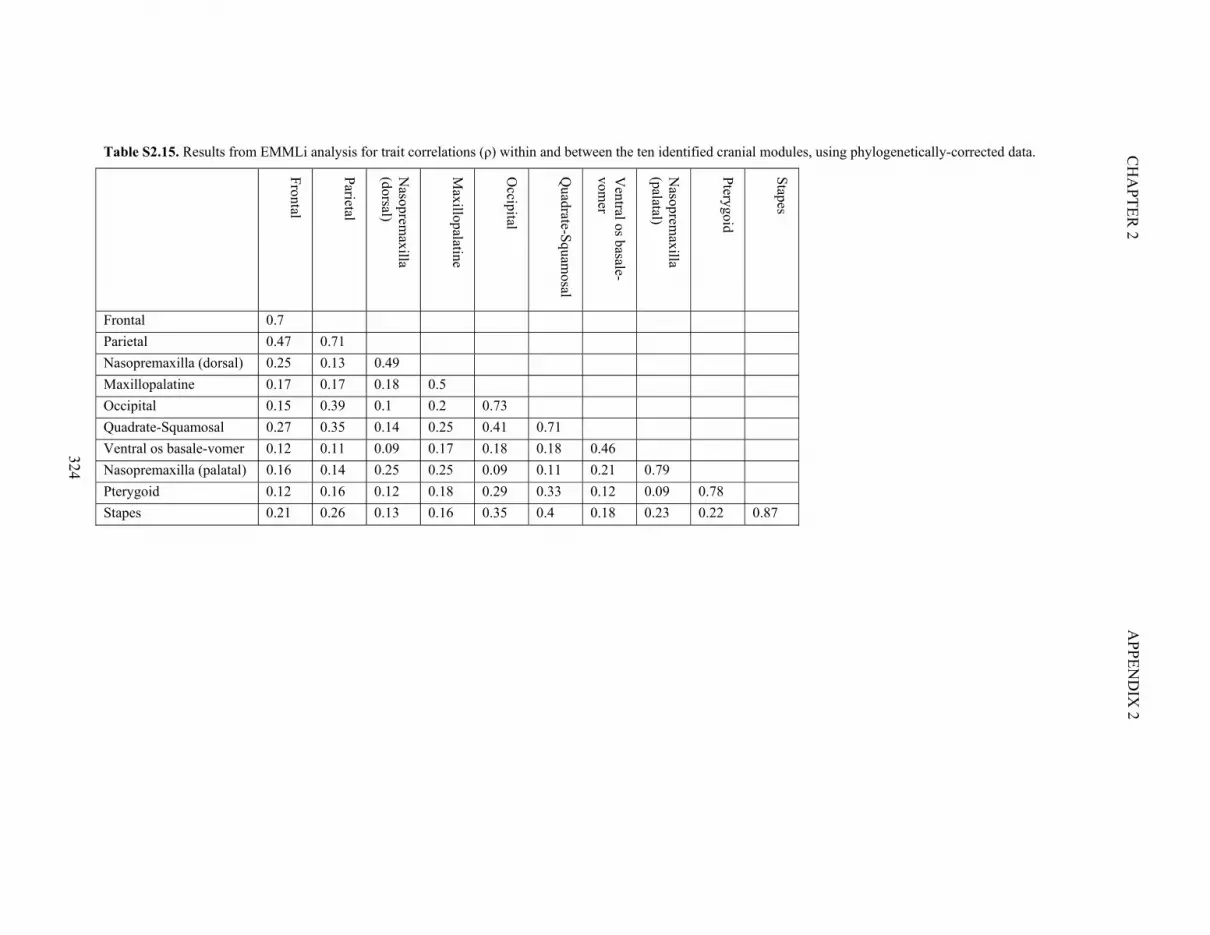
324
CH
APTER
2 A
PPEND
IX 2
Table S2.15. Results from EMMLi analysis for trait correlations (ρ) within and between the ten identified cranial modules, using phylogenetically-corrected data.
Frontal
Parietal
Nasoprem
axilla (dorsal)
Maxillopalatine
Occipital
Quadrate-Squam
osal
Ventral os basale-
vomer
Nasoprem
axilla (palatal)
Pterygoid
Stapes
Frontal 0.7 Parietal 0.47 0.71 Nasopremaxilla (dorsal) 0.25 0.13 0.49 Maxillopalatine 0.17 0.17 0.18 0.5 Occipital 0.15 0.39 0.1 0.2 0.73 Quadrate-Squamosal 0.27 0.35 0.14 0.25 0.41 0.71 Ventral os basale-vomer 0.12 0.11 0.09 0.17 0.18 0.18 0.46 Nasopremaxilla (palatal) 0.16 0.14 0.25 0.25 0.09 0.11 0.21 0.79 Pterygoid 0.12 0.16 0.12 0.18 0.29 0.33 0.12 0.09 0.78 Stapes 0.21 0.26 0.13 0.16 0.35 0.4 0.18 0.23 0.22 0.87

325
APPEN
DIX
2 C
HA
PTER 2
Table S2.16. Covariance Ratio results between each of the ten identified cranial modules, using phylogenetically corrected data.
Frontal
Parietal
Nasoprem
axilla (dorsal)
Maxillopalatine
Occipital
Quadrate-
squamosal
Ventral os basale-
vomer
Nasoprem
axilla (palatal)
Pterygoid
Parietal 0.79 Nasopremaxilla (dorsal) 0.68 0.58 Maxillopalatine 0.59 0.71 0.74 Occipital 0.48 0.72 0.55 0.82 Quadrate-squamosal 0.75 0.86 0.57 0.70 0.83 Ventral os basale-vomer 0.63 0.62 0.56 0.67 0.64 0.61 Nasopremaxilla (palatal) 0.60 0.60 0.75 0.60 0.48 0.47 0.61 Pterygoid 0.45 0.48 0.50 0.58 0.61 0.60 0.57 0.35 Stapes 0.74 0.84 0.59 0.64 0.76 0.90 0.56 0.58 0.51

326
CH
APTER
2 A
PPEND
IX 2
Table S2.17. Summary of the PC axes for the full landmark and semilandmark dataset. 29 (indicated in bold) of the 34 PC axes were required to explain 99% of cranial
shape variation.
PC1 PC2 PC3 PC4 PC5 PC6 PC7 PC8 PC9 PC10 Standard deviation 0.05224 0.04406 0.03181 0.03047 0.02475 0.02248 0.01988 0.01817 0.01757 0.01533 Proportion of Variance 0.25671 0.18265 0.09521 0.08737 0.05765 0.04755 0.03717 0.03107 0.02903 0.0221 Cumulative Proportion
0.25671 0.43936 0.53457 0.62194 0.67959 0.72713 0.7643 0.79537 0.82439 0.84649
PC11 PC12 PC13 PC14 PC15 PC16 PC17 PC18 PC19 PC20 Standard deviation 0.0144 0.01245 0.01183 0.01171 0.01078 0.009748 0.009577 0.008971 0.008639 0.007665 Proportion of Variance 0.0195 0.01458 0.01316 0.0129 0.01093 0.00894 0.00863 0.00757 0.00702 0.00553 Cumulative Proportion
0.866 0.88057 0.89374 0.90664 0.91757 0.92651 0.93514 0.94272 0.94974 0.95526
PC21 PC22 PC23 PC24 PC25 PC26 PC27 PC28 PC29 PC30 Standard deviation 0.007387 0.007118 0.007054 0.00661 0.006593 0.006075 0.005835 0.005472 0.005267 0.004982 Proportion of Variance 0.00513 0.00477 0.00468 0.00411 0.00409 0.00347 0.0032 0.00282 0.00261 0.00234 Cumulative Proportion
0.9604 0.96516 0.96984 0.97395 0.97804 0.98152 0.98472 0.98754 0.99015 0.99248
PC31 PC32 PC33 PC34 Standard deviation 0.004845 0.004573 0.004475 0.003938 Proportion of Variance 0.00221 0.00197 0.00188 0.00146 Cumulative Proportion
0.99469 0.99666 0.99854 1

327
APPEN
DIX
2 C
HA
PTER 2
Table S2.18. Centroid size of all specimens.
Species Centroid size Species Centroid size Atretochoana eiselti 429.83 Ichthyophis glutinosus 246.50 Boulengerula boulengeri 79.72 Idiocranium russeli 75.01 Brasilotyphlus braziliensis 115.38 Indotyphlus cf. battersbyi 86.15 Caecilia tentaculata 284.91 Luetkenotyphlus brasiliensis 103.13 Ichthyophis nigroflavus 255.15 Microcaecilia albiceps 111.87 Chikila fulleri 121.96 Mimosiphonops vermiculatus 142.57 Chthonerpeton indistinctum 237.84 Nectocaecilia petersii 251.04 Crotaphatrema bornmuelleri 156.99 Oscaecilia ochrocephala 126.26 Crotaphatrema lamottei 136.73 Potomotyphlus kaupii 161.32 Dermophis mexicanus 299.74 Praslinia cooperi 157.78 Epicrionops bicolor 197.55 Rhinatrema bivittatum 170.79 Gegeneophis carnosus 75.15 Schistometopum gregorii 163.21 Geotrypetes seraphini 146.92 Scolecomorphus kirkii 148.90 Grandisonia alternans 178.54 Siphonops annulatus 282.88 Gymnopis multiplicata 309.86 Sylvacaecilia grandisonae 209.00 Herpele squalostoma 192.55 Typhlonectes compressicauda 224.47 Hypogeophis rostratus 124.27 Uraeotyphlus oxyurus 152.94 Ichthyophis bombayensis 252.80

328
CH
APTER
2 A
PPEND
IX 2
Table S2.19. Differences (x10-6) in the observed means of disparity among the ten cranial modules. A negative value indicates the module in the column has a higher
disparity than the module in the row. Test performed using the ‘TukeyHSD’ function in R. * p ≤ 0.05, ** p ≤ 0.01, *** p ≤ 0.001, **** p ≤ 0.0000001.
Frontal
Parietal
Nasoprem
axilla (dorsal)
Maxillopalatine
Occipital
Quadrate-
Squamosal
Ventral os basale -
vomer
Nasoprem
axilla (palatal)
Pterygoid
Parietal 2.18**** Nasopremaxilla (dorsal)
-0.47 -2.64****
Maxillopalatine 1.57*** -0.61 2.04**** Occipital -1.66*** -3.84**** -1.19** -3.23**** Quadrate-Squamosal 4.04**** 1.86**** 4.51**** 2.47**** 5.70**** Ventral os basale-vomer
-1.39*** -3.57**** -0.92* -2.96**** 0.27 -5.43****
Nasopremaxilla (palatal)
-0.83 -3.01**** -0.36 -2.40**** 0.83 -4.87**** 0.56
Pterygoid 4.40**** 2.22*** 4.87**** 2.83**** 6.06**** 0.36 5.79**** 5.23**** Stapes -1.60 -3.78*** -1.13 -3.17*** 0.06 -5.64**** -0.21 -0.77 -6.00****

329
APPEN
DIX
2 C
HA
PTER 2
Table S2.20. Significance (p) values for differences in rates of morphological evolution among the ten cranial modules identified in this study. Results indicated in bold are
significant (p < 0.05).
Frontal
Parietal
Nasoprem
axilla (dorsal)
Maxillopalatine
Occipital
Quadrate-
Squamosal
Ventral os
basale-vomer
Nasoprem
axilla (palatal)
Pterygoid
Parietal 1 Nasopremaxilla (dorsal) 1 1 Maxillopalatine 1 1 0.093 Occipital 1 1 0.738 0.146 Quadrate-Squamosal 1 0.866 0.001 0.381 0.005 Ventral os basale-vomer 1 0.191 0.933 0.524 0.822 0.001 Nasopremaxilla (palatal) 1 0.003 1 0.999 1 0.002 0.989 Pterygoid 0.243 1 0.999 1 0.998 0.999 1 1 Stapes 1 1 1 1 1 1 1 1 1

CHAPTER 2 APPENDIX 2
330
References for Appendix 2 Felice, R. N., and A. Goswami. 2018. Developmental origins of mosaic evolution in the avian cranium.
PNAS. 115:555–560.
Goswami, A. 2006. Morphological integration in the carnivoran skull. Evolution. 60:169–183.
Marcus, H., E. Stimmelmayr, and G. Porsch. 1935. Beitrage zur Kenntnis der Gymnophionen. XXV. Die
Ossifikation des Hypogeophisschddels. Morphol. Jahrb 76:375–420.
Marshall, A. F., C. Bardua, D. J. Gower, M. Wilkinson, E. Sherratt, and A. Goswami. 2019. High-density
three-dimensional morphometric analyses support conserved static (intraspecific) modularity in
caecilian (Amphibia: Gymnophiona) crania. Biol. J. Linn. Soc. 126:721–742.
San Mauro, D., D. J. Gower, H. Müller, S. P. Loader, R. Zardoya, R. A. Nussbaum, and M. Wilkinson.
2014. Life-history evolution and mitogenomic phylogeny of caecilian amphibians. Mol.
Phylogenet. Evol. 73:177–189.
Wake, M. H., and J. Hanken. 1982. Development of the skull of Dermophis mexicanus (Amphibia:
Gymnophiona), with comments on skull kinesis and amphibian relationships. J. Morphol. 173:203–
223.
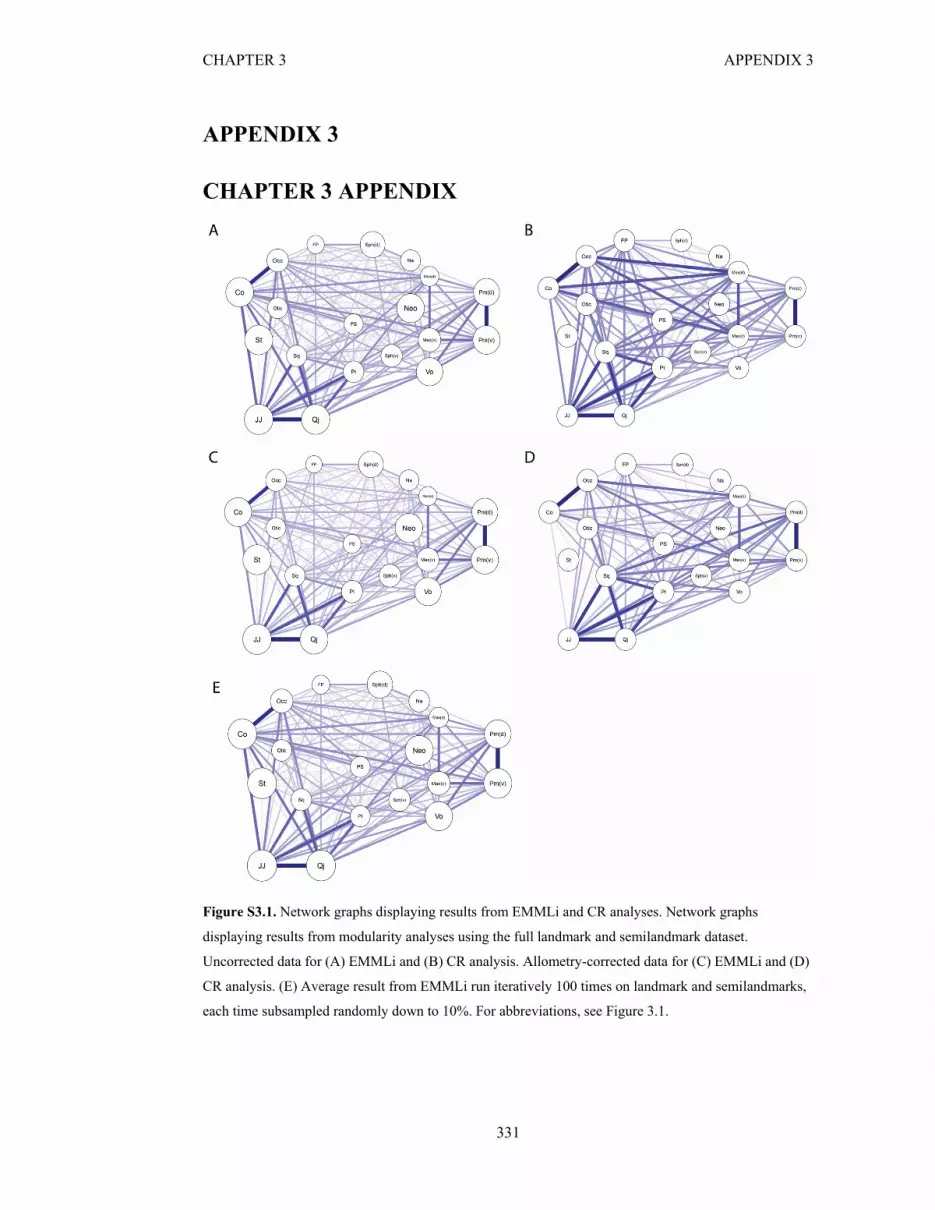
CHAPTER 3 APPENDIX 3
331
APPENDIX 3
CHAPTER 3 APPENDIX
Figure S3.1. Network graphs displaying results from EMMLi and CR analyses. Network graphs
displaying results from modularity analyses using the full landmark and semilandmark dataset.
Uncorrected data for (A) EMMLi and (B) CR analysis. Allometry-corrected data for (C) EMMLi and (D)
CR analysis. (E) Average result from EMMLi run iteratively 100 times on landmark and semilandmarks,
each time subsampled randomly down to 10%. For abbreviations, see Figure 3.1.

CHAPTER 3 APPENDIX 3
332
Figure S3.2. Network graphs displaying results from landmark-only EMMLi and CR analyses.
Phylogenetically-corrected data for (A) EMMLi and (B) CR analysis. Uncorrected data for (C) EMMLi
and (D) CR analysis. Allometry-corrected data for (E) EMMLi and (F) CR analysis. For abbreviations,
see Figure 3.1.

CHAPTER 3 APPENDIX 3
333
Figure S3.3. Network graph displaying results from EMMLi analysis excluding specimens with absent
regions. Network graph displaying results from EMMLi analysis using phylogenetically-corrected data,
excluding specimens with an absent region (N = 83).

CHAPTER 3 APPENDIX 3
334
Figure S3.4. Effect of developmental strategy on trait integration. (A,C,E) Phylogenetically informed CR
and (B,D,F) phylogenetically informed EMMLi analyses for (A-B) biphasic developers (species
possessing a feeding larval stage), from taking 39 specimens at random 100 times and computing the
mean estimated correlations from these runs, (C-D) biphasic species, on the full dataset (N = 124), and
(E-F) direct developers (species that do not possess a feeding larval stage) (N = 39). It can be seen that the
crania of direct developers are more integrated than those of metamorphosing species.

335
CH
AP
TE
R 3
AP
PE
ND
IX 3
Table S3.1. Specimen information. *random species from genus chosen to represent phylogenetic position. ^specimen was mirrored as the right side was damaged or
incomplete.
Specimen name Scientific Name (Jetz and Pyron 2018)
Specimen number Family Subfamily Scan location
Acanthixalus sonjae Acanthixalus sonjae ZMB 79329 Hyperoliidae Hyperoliinae MfN
Adenomera andreae Adenomera andreae UF 43260 Leptodactylidae Leptodactylinae FMNH Herpetology
Adenomus kelaartii Adenomus kelaartii FMNH 1580 Bufonidae Bufoninae FMNH Herpetology
Afrixalus auresus^ Afrixalus aureus ZMB 64929 Hyperoliidae Hyperoliinae MfN
Cophixalus darlingtoni^ Albericus darlingtoni MNHN 1970.1455 Microhylidae Asterophryninae MNHN
Allobates kingsburyi Allobates kingsburyi CAS H 10670 Dendrobatidae Dendrobatinae FMNH Herpetology
Allophryne ruthveni Allophryne ruthveni KU H 166716 Allophrynidae Allophryninae FMNH Herpetology
Alsodes nodosus Alsodes nodosus CM 63864 Alsodidae Alsodinae FMNH Herpetology
Altiphrynoides malcomi Altiphrynoides malcolmi CAS 162120 Bufonidae Bufoninae FMNH Herpetology
Alytes obstetricans Alytes obstetricans CAS SUA 21691 Alytidae Alytinae FMNH Herpetology
Ameerega parvula Ameerega parvula ZMB 75398 Dendrobatidae Dendrobatinae MfN
Amietophrynus regularis Amietophrynus regularis ZMB 74275 Bufonidae Bufoninae MfN
Anaxyrus fowleri^ Anaxyrus fowleri UF 3997-2 Bufonidae Bufoninae FMNH Herpetology
Anaxyrus quercicus Anaxyrus quercicus UF 124269 Bufonidae Bufoninae FMNH Herpetology
Anhydrophryne rattrayi Anhydrophryne rattrayi CAS H 156428 Pyxicephalidae Cacosterninae FMNH Herpetology
Anotheca spinosa Anotheca spinosa UF 137287 Hylidae Hylinae FMNH Herpetology
Ansonia mcgregori Ansonia mcgregori KU 334742 Bufonidae Bufoninae FMNH Herpetology
Aromobates alboguttatus Aromobates alboguttatus ZMB 18825 Dendrobatidae Dendrobatinae MfN
Arthroleptella lightfooti Arthroleptella lightfooti CAS H 157023 Pyxicephalidae Cacosterninae FMNH Herpetology
Arthroleptis bioko Arthroleptis bioko CAS 207285 Arthroleptidae Arthroleptinae FMNH Herpetology
Ascaphus truei Ascaphus truei UF 80664 Ascaphidae Ascaphinae FMNH Herpetology
Astylosternus diadematus Astylosternus diadematus CAS 254126 Arthroleptidae Astylosterninae FMNH Herpetology

CH
AP
TE
R 3
336
AP
PE
ND
IX 3
Astylosternus occidentalis Astylosternus occidentalis ZMB 77244 Arthroleptidae Astylosterninae MfN
Atelopus ignescens Atelopus ignescens UF 39140 Bufonidae Bufoninae FMNH Herpetology
Atelopus oxyrhynchus Atelopus oxyrhynchus UF 93190 Bufonidae Bufoninae FMNH Herpetology
Balebreviceps hillimani Balebreviceps hillmani CAS 167436 Brevicipitidae Brevicipitinae FMNH Herpetology
Barbourula busuangensis^ Barbourula busuangensis UF 70546 Bombinatoridae Bombinatorinae FMNH Herpetology
Barycholos pulcher Barycholos pulcher UF 68066 Strabomantidae Holoadeninae FMNH Herpetology
Batrachyla taeniata Batrachyla taeniata CAS 85253 Batrachylidae Batrachylinae FMNH Herpetology
Bombina maxima Bombina maxima UF 96648 Bombinatoridae Bombinatorinae FMNH Herpetology
Boophis boehmei Boophis boehmei CAS H 250237 Mantellidae Boophinae FMNH Herpetology
Brachycephalus ephippium Brachycephalus ephippium MCZ 108655 Brachycephalidae Brachycephalinae FMNH Herpetology
Brachytarsophrys carinensis
Brachytarsophrys carinense FLMNH 63888 Megophryidae Megophryinae FMNH Herpetology
Cacosternum namaquense Cacosternum namaquense CAS H 156975 Pyxicephalidae Cacosterninae FMNH Herpetology
Callulina kisiwamsitu Callulina kisiwamsitu CAS 168818 Brevicipitidae Brevicipitinae FMNH Herpetology
Caudiverbera caudiverbera Calyptocephalella gayi CAS SUA 10082 Calyptocephalellidae Calyptocephalellinae FMNH Herpetology
Capensibufo sp. Capensibufo rosei* CAS 156600 Bufonidae Bufoninae FMNH Herpetology
Cardioglossa elegans Cardioglossa elegans ZMB 77546 Arthroleptidae Arthroleptinae MfN
Cardioglossa manengouba Cardioglossa manengouba ZMB 77600 Arthroleptidae Arthroleptinae MfN
Centrolene buckleyi Centrolene buckleyi UF 30579 Centrolenidae Centroleninae FMNH Herpetology
Ceratobatrachus guentheri Ceratobatrachus guentheri ZMB 39175 Ceratobatrachidae Ceratobatrachinae MfN
Ceratophrys aurita Ceratophrys aurita CAS 84998 Ceratophryidae Ceratophryinae FMNH Herpetology
Ceuthomantis smaragdinus Ceuthomantis smaragdinus KU H 315000 Ceuthomantidae Ceuthomantinae FMNH Herpetology
Chacophrys pierotti Chacophrys pierottii KU 191932 Ceratophryidae Ceratophryinae FMNH Herpetology
Chiromantis rufescens Chiromantis rufescens MCZ A 136738 Rhacophoridae Rhacophorinae University of Texas
Chrysobatrachus cupreonitens
Chrysobatrachus cupreonitens
UF 27884 Hyperoliidae Hyperoliinae FMNH Herpetology
Cochranella granulosa Cochranella granulosa UF 137267 Centrolenidae Centroleninae FMNH Herpetology

337
CH
AP
TE
R 3
AP
PE
ND
IX 3
Conraua beccarii Conraua beccarii tc0314 Conrauidae Conrauinae FMNH Herpetology
Conraua crassipes Conraua crassipes CAS 258122 Conrauidae Conrauinae FMNH Herpetology
Conraua goliath Conraua goliath UF H 64720 Conrauidae Conrauinae FMNH Herpetology
Craugastor laticeps Craugastor laticeps UF 157233 Craugastoridae Craugastorinae FMNH Herpetology
Crossodactylus trachystomus
Crossodactylus trachystomus CM 2662 Hylodidae Hylodinae FMNH Herpetology
Agalychnis calcifer Cruziohyla calcarifer UF 137291 Hylidae Phyllomedusinae FMNH Herpetology
Cryptobatrachus boulengeri Cryptobatrachus boulengeri NHM 1916.4.4.21 Hemiphractidae Hemiphractinae NHM
Cryptothylax greshoffi Cryptothylax greshoffii ZMB 80650 Hyperoliidae Hyperoliinae MfN
Cycloramphus asper Cycloramphus asper CM 68338 Cycloramphidae Cycloramphinae FMNH Herpetology
Cyclorana longipes Cyclorana longipes UF 10923 Hylidae Pelodryadinae FMNH Herpetology
Dendrobates sp. Dendrobates auratus* ZMB 4795 Dendrobatidae Dendrobatinae MfN
Discodeles bufoniformis Discodeles bufoniformis KU 341127 Ceratobatrachidae Ceratobatrachinae UF Nanoscale Research Facility
Duttaphrynus dodsoni Duttaphrynus dodsoni CAS H 227515 Bufonidae Bufoninae FMNH Herpetology
Hyla tuberculosa Ecnomiohyla tuberculosa 43479 Hylidae Hylinae FMNH Herpetology
Eleutherodactylus glaphycompus
Eleutherodactylus glaphycompus
UF 56811 Eleutherodactylidae Eleutherodactylinae FMNH Herpetology
Eleutherodactylus johnstonei
Eleutherodactylus johnstonei UF 27911 Eleutherodactylidae Eleutherodactylinae FMNH Herpetology
Eupsophus roseus Eupsophus roseus CM 57175 Alsodidae Alsodinae FMNH Herpetology
Rana cancrivora^ Fejervarya cancrivora NHM 71 7 20 217 Dicroglossidae Dicroglossinae NHM
Minervarya nilgirica Fejervarya nilagirica MNHNRA 19842337
Dicroglossidae Dicroglossinae MfN
Fejervarya vittigera Fejervarya vittigera ZMB 56677 Dicroglossidae Dicroglossinae MfN
Fritziana gouldii Fritziana goeldii NHM 95 3 6 4 Hemiphractidae Hemiphractinae NHM
Gastrophryne carolinensis Gastrophryne carolinensis MNHN 0.5031 Microhylidae Gastrophryninae MNHN
Gastrotheca peruana Gastrotheca peruana UF 65783 Hemiphractidae Hemiphractinae FMNH Herpetology
Guibemantis liber Guibemantis liber CAS H 252002 Mantellidae Mantellinae UF Nanoscale Research
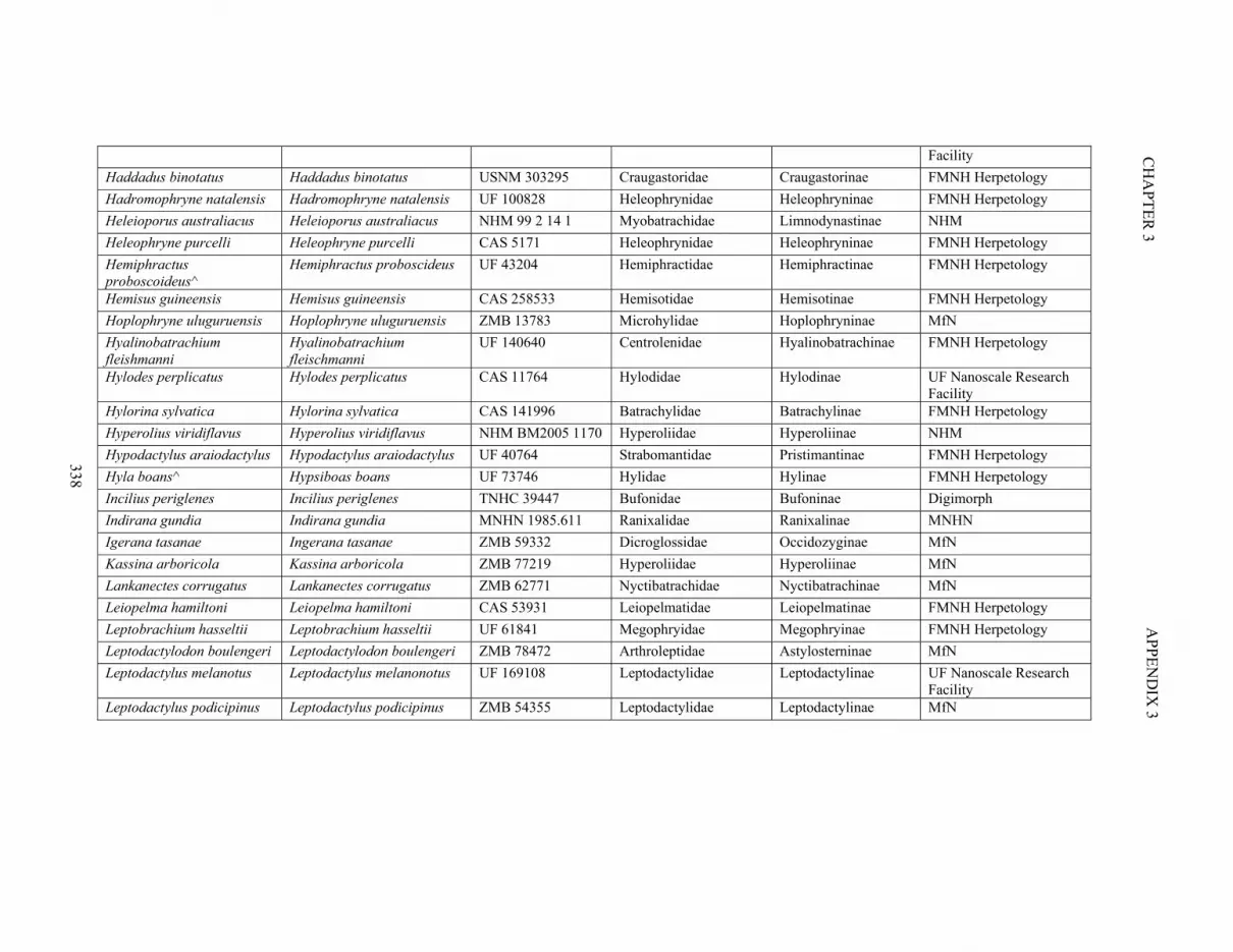
CH
AP
TE
R 3
338
AP
PE
ND
IX 3
Facility
Haddadus binotatus Haddadus binotatus USNM 303295 Craugastoridae Craugastorinae FMNH Herpetology
Hadromophryne natalensis Hadromophryne natalensis UF 100828 Heleophrynidae Heleophryninae FMNH Herpetology
Heleioporus australiacus Heleioporus australiacus NHM 99 2 14 1 Myobatrachidae Limnodynastinae NHM
Heleophryne purcelli Heleophryne purcelli CAS 5171 Heleophrynidae Heleophryninae FMNH Herpetology
Hemiphractus proboscoideus^
Hemiphractus proboscideus UF 43204 Hemiphractidae Hemiphractinae FMNH Herpetology
Hemisus guineensis Hemisus guineensis CAS 258533 Hemisotidae Hemisotinae FMNH Herpetology
Hoplophryne uluguruensis Hoplophryne uluguruensis ZMB 13783 Microhylidae Hoplophryninae MfN
Hyalinobatrachium fleishmanni
Hyalinobatrachium fleischmanni
UF 140640 Centrolenidae Hyalinobatrachinae FMNH Herpetology
Hylodes perplicatus Hylodes perplicatus CAS 11764 Hylodidae Hylodinae UF Nanoscale Research Facility
Hylorina sylvatica Hylorina sylvatica CAS 141996 Batrachylidae Batrachylinae FMNH Herpetology
Hyperolius viridiflavus Hyperolius viridiflavus NHM BM2005 1170 Hyperoliidae Hyperoliinae NHM
Hypodactylus araiodactylus Hypodactylus araiodactylus UF 40764 Strabomantidae Pristimantinae FMNH Herpetology
Hyla boans^ Hypsiboas boans UF 73746 Hylidae Hylinae FMNH Herpetology
Incilius periglenes Incilius periglenes TNHC 39447 Bufonidae Bufoninae Digimorph
Indirana gundia Indirana gundia MNHN 1985.611 Ranixalidae Ranixalinae MNHN
Igerana tasanae Ingerana tasanae ZMB 59332 Dicroglossidae Occidozyginae MfN
Kassina arboricola Kassina arboricola ZMB 77219 Hyperoliidae Hyperoliinae MfN
Lankanectes corrugatus Lankanectes corrugatus ZMB 62771 Nyctibatrachidae Nyctibatrachinae MfN
Leiopelma hamiltoni Leiopelma hamiltoni CAS 53931 Leiopelmatidae Leiopelmatinae FMNH Herpetology
Leptobrachium hasseltii Leptobrachium hasseltii UF 61841 Megophryidae Megophryinae FMNH Herpetology
Leptodactylodon boulengeri Leptodactylodon boulengeri ZMB 78472 Arthroleptidae Astylosterninae MfN
Leptodactylus melanotus Leptodactylus melanonotus UF 169108 Leptodactylidae Leptodactylinae UF Nanoscale Research Facility
Leptodactylus podicipinus Leptodactylus podicipinus ZMB 54355 Leptodactylidae Leptodactylinae MfN
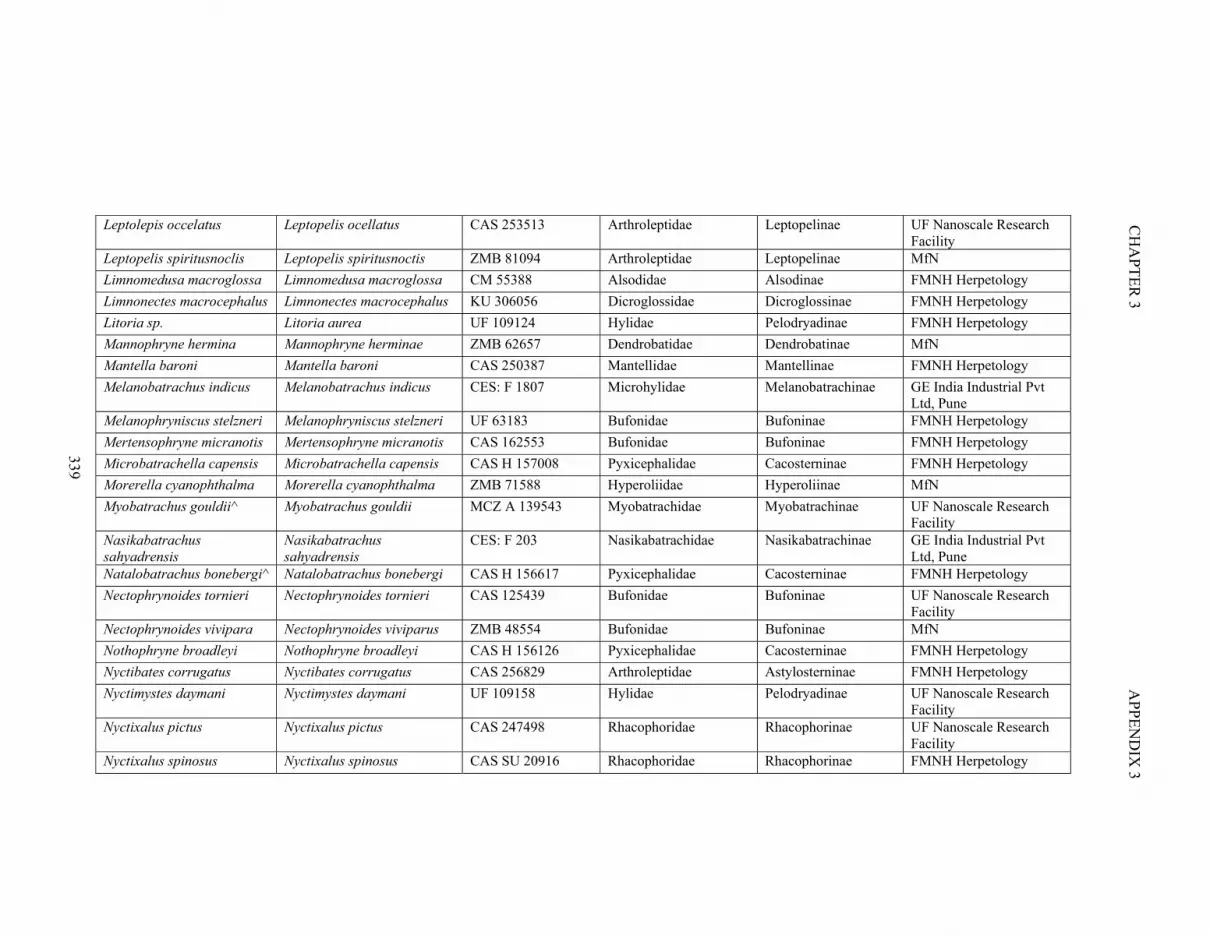
339
CH
AP
TE
R 3
AP
PE
ND
IX 3
Leptolepis occelatus Leptopelis ocellatus CAS 253513 Arthroleptidae Leptopelinae UF Nanoscale Research Facility
Leptopelis spiritusnoclis Leptopelis spiritusnoctis ZMB 81094 Arthroleptidae Leptopelinae MfN
Limnomedusa macroglossa Limnomedusa macroglossa CM 55388 Alsodidae Alsodinae FMNH Herpetology
Limnonectes macrocephalus Limnonectes macrocephalus KU 306056 Dicroglossidae Dicroglossinae FMNH Herpetology
Litoria sp. Litoria aurea UF 109124 Hylidae Pelodryadinae FMNH Herpetology
Mannophryne hermina Mannophryne herminae ZMB 62657 Dendrobatidae Dendrobatinae MfN
Mantella baroni Mantella baroni CAS 250387 Mantellidae Mantellinae FMNH Herpetology
Melanobatrachus indicus Melanobatrachus indicus CES: F 1807 Microhylidae Melanobatrachinae GE India Industrial Pvt Ltd, Pune
Melanophryniscus stelzneri Melanophryniscus stelzneri UF 63183 Bufonidae Bufoninae FMNH Herpetology
Mertensophryne micranotis Mertensophryne micranotis CAS 162553 Bufonidae Bufoninae FMNH Herpetology
Microbatrachella capensis Microbatrachella capensis CAS H 157008 Pyxicephalidae Cacosterninae FMNH Herpetology
Morerella cyanophthalma Morerella cyanophthalma ZMB 71588 Hyperoliidae Hyperoliinae MfN
Myobatrachus gouldii^ Myobatrachus gouldii MCZ A 139543 Myobatrachidae Myobatrachinae UF Nanoscale Research Facility
Nasikabatrachus sahyadrensis
Nasikabatrachus sahyadrensis
CES: F 203 Nasikabatrachidae Nasikabatrachinae GE India Industrial Pvt Ltd, Pune
Natalobatrachus bonebergi^ Natalobatrachus bonebergi CAS H 156617 Pyxicephalidae Cacosterninae FMNH Herpetology
Nectophrynoides tornieri Nectophrynoides tornieri CAS 125439 Bufonidae Bufoninae UF Nanoscale Research Facility
Nectophrynoides vivipara Nectophrynoides viviparus ZMB 48554 Bufonidae Bufoninae MfN
Nothophryne broadleyi Nothophryne broadleyi CAS H 156126 Pyxicephalidae Cacosterninae FMNH Herpetology
Nyctibates corrugatus Nyctibates corrugatus CAS 256829 Arthroleptidae Astylosterninae FMNH Herpetology
Nyctimystes daymani Nyctimystes daymani UF 109158 Hylidae Pelodryadinae UF Nanoscale Research Facility
Nyctixalus pictus Nyctixalus pictus CAS 247498 Rhacophoridae Rhacophorinae UF Nanoscale Research Facility
Nyctixalus spinosus Nyctixalus spinosus CAS SU 20916 Rhacophoridae Rhacophorinae FMNH Herpetology

CH
AP
TE
R 3
340
AP
PE
ND
IX 3
Occidozyga limba Occidozyga lima ZMB 56612 Dicroglossidae Occidozyginae MfN
Odontobatrachus natator Odontobatrachus natator CAS 230204 Odontobatrachidae Odontobatrachinae FMNH Herpetology
Odontophrynus americanus Odontophrynus americanus CM 147828 Odontophrynidae Odontophryninae FMNH Herpetology
Oreobates quixensis Oreobates quixensis CAS SU A 11453 Strabomantidae Pristimantinae FMNH Herpetology
Osteocephalus buckleyi Osteocephalus buckleyi NHM 1970 2034 Hylidae Hylinae NHM
Osteopilus septentrionalis^ Osteopilus septentrionalis UF 63656 Hylidae Hylinae FMNH Herpetology
Paracassina obscura Paracassina obscura CAS 145354 Hyperoliidae Hyperoliinae FMNH Herpetology
Pelobates fuscus Pelobates fuscus UF 36935 Pelobatidae Pelobatinae FMNH Herpetology
Pelodytes caucasicus Pelodytes caucasicus CAS H 94059 Pelodytidae Pelodytinae FMNH Herpetology
Peltophryne guentheri Peltophryne guentheri UF104862 Bufonidae Bufoninae FMNH Herpetology
Petropedetes palmipes Petropedetes palmipes ZMB 73891 Petropedetidae Petropedetinae MfN
Phlyctimantis boulengeri^ Phlyctimantis boulengeri ZMB 80664 Hyperoliidae Hyperoliinae MfN
Phrynobatrachus leveleve Phrynobatrachus leveleve HOLOTYPE 218901
Phrynobatrachidae Phrynobatrachinae FMNH Herpetology
Phyllomedusa azurea Phyllomedusa azurea MCZ A29952 Hylidae Phyllomedusinae FMNH Herpetology
Pipa parva Pipa parva UF37924 Pipidae Pipinae FMNH Herpetology
Pipa pipa Pipa pipa UF 64234 Pipidae Pipinae FMNH Herpetology
Platymantis polillensis Platymantis polillensis KU H 313722 Ceratobatrachidae Ceratobatrachinae FMNH Herpetology
Plethodontohyla notosticta Plethodontohyla notosticta NHM 1925 7 2 95 Microhylidae Cophylinae NHM
Polypedates macrotis Polypedates macrotis KU H 327008 Rhacophoridae Rhacophorinae FMNH Herpetology
Poyntonia paludicola Poyntonia paludicola CAS H 165936 Pyxicephalidae Cacosterninae FMNH Herpetology
Pristimantis chiastonotus Pristimantis chiastonotus MNHN 1979.7847 Paris
Strabomantidae Pristimantinae MNHN
Probreviceps macrodactylus Probreviceps macrodactylus UF 111075 Brevicipitidae Brevicipitinae FMNH Herpetology
Proceratophrys boiei Proceratophrys boiei CM 45985 Odontophrynidae Odontophryninae FMNH Herpetology
Pseudacris ornata Pseudacris ornata UF 159 19 Hylidae Hylinae FMNH Herpetology
Pseudis paradoxica Pseudis paradoxa ZMB 26104 Hylidae Hylinae MfN

341
CH
AP
TE
R 3
AP
PE
ND
IX 3
Ptychadena bibroni Ptychadena bibroni MNHN 1996.660 Ptychadenidae Ptychadeninae MNHN
Pyxicephalus adspersus Pyxicephalus adspersus UF 92094 Pyxicephalidae Pyxicephalinae FMNH Herpetology
Uperodon monatnus Ramanella montana UF 20016 Microhylidae Microhylinae FMNH Herpetology
Lithobates clamitans Rana clamitans UF 76511 Ranidae Raninae FMNH Herpetology
Rana sylvatica Rana sylvatica NHM 1976 55 Ranidae Raninae NHM
Raorchestes sp. Raorchestes anili* MNHN RA 1985482 Rhacophoridae Rhacophorinae MfN
Philautus glandulosus Raorchestes glandulosus Wien 3557 1 Rhacophoridae Rhacophorinae MfN
Rhacophorus reinwalti Rhacophorus reinwardtii S dec Rhacophoridae Rhacophorinae Digimorph
Rheobatrachus silus Rheobatrachus silus NHM 1982 131 Myobatrachidae Myobatrachinae NHM
Rhinoderma darwinii Rhinoderma darwinii MNHN 2006.2736 Rhinodermatidae Rhinodermatinae MNHN
Rhinophrynus dorsalis Rhinophrynus dorsalis CAS 71766 Rhinophrynidae Rhinophryninae FMNH Herpetology
Scaphiophryne madagascariensis
Scaphiophryne madagascariensis
ZMB 10423 Microhylidae Scaphiophryninae MfN
Scaphiopus holbrookii Scaphiopus holbrookii UF 9620S Scaphiopodidae Scaphiopodinae FMNH Herpetology
Semnodactylus weali Semnodactylus wealii ZMB 75815 Hyperoliidae Hyperoliinae MfN
Sooglossus sechellensis Sooglossus sechellensis CAS H 160084 Sooglossidae Sooglossinae FMNH Herpetology
Spea multiplicata Spea multiplicata UF 100788 Scaphiopodidae Scaphiopodinae FMNH Herpetology
Eleutherodactylus biporcatus
Strabomantis biporcatus CAS 119580 Strabomantidae Strabomantinae FMNH Herpetology
Eleutherodactuylus cornutus
Strabomantis cornutus CAS SU 11456 Strabomantidae Strabomantinae FMNH Herpetology
Strabomantis ingeri Strabomantis ingeri FMNH 81985 1 CNHM81915
Strabomantidae Strabomantinae FMNH Herpetology
Stumpffia pygmaea Stumpffia pygmaea UF 153631 Microhylidae Cophylinae FMNH Herpetology
Syncope antenori Syncope antenori UF H 68008 Microhylidae Gastrophryninae FMNH Herpetology
Telmatobius degener Telmatobius degener UF 39736 Telmatobiidae Telmatobiinae FMNH Herpetology
Telmatobius laticeps Telmatobius laticeps MNHN 1963.789 Telmatobiidae Telmatobiinae MNHN
Theloderma stellatum Theloderma stellatum FMNH 253619 Rhacophoridae Rhacophorinae Digimorph

CH
AP
TE
R 3
342
AP
PE
ND
IX 3
Thoropa miliaris Thoropa miliaris CM 68357 Cycloramphidae Cycloramphinae FMNH Herpetology
Tomopterna marmorata Tomopterna marmorata ZMB 76248 Pyxicephalidae Cacosterninae MfN
Trichobatrachus robustus Trichobatrachus robustus cas herp 254134 Arthroleptidae Astylosterninae FMNH Herpetology
Triprion petasatus Triprion petasatus UF98441S Hylidae Hylinae FMNH Herpetology
Bufo gariepensis Vandijkophrynus gariepensis ZMB 57846 Bufonidae Bufoninae MfN
Xenopus laevis Xenopus laevis XLAM_20 Pipidae Pipinae UCL
Xenorhina sp. Xenorhina varia* UF 121103 Microhylidae Asterophryninae FMNH Herpetology
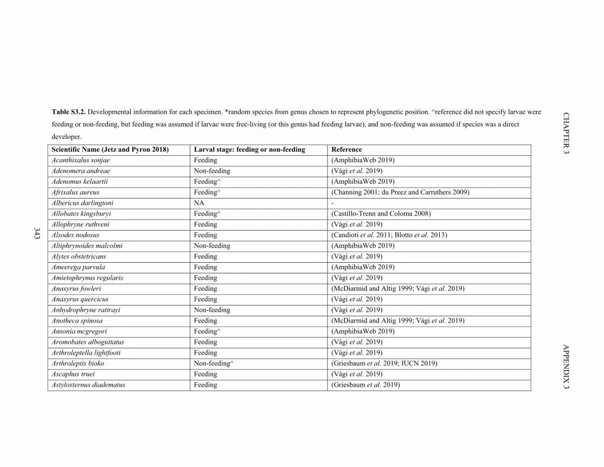
343
CH
AP
TE
R 3
AP
PE
ND
IX 3
Table S3.2. Developmental information for each specimen. *random species from genus chosen to represent phylogenetic position. ^reference did not specify larvae were
feeding or non-feeding, but feeding was assumed if larvae were free-living (or this genus had feeding larvae), and non-feeding was assumed if species was a direct
developer.
Scientific Name (Jetz and Pyron 2018) Larval stage: feeding or non-feeding Reference
Acanthixalus sonjae Feeding (AmphibiaWeb 2019)
Adenomera andreae Non-feeding (Vági et al. 2019)
Adenomus kelaartii Feeding^ (AmphibiaWeb 2019)
Afrixalus aureus Feeding^ (Channing 2001; du Preez and Carruthers 2009)
Albericus darlingtoni NA -
Allobates kingsburyi Feeding^ (Castillo-Trenn and Coloma 2008)
Allophryne ruthveni Feeding (Vági et al. 2019)
Alsodes nodosus Feeding (Candioti et al. 2011; Blotto et al. 2013)
Altiphrynoides malcolmi Non-feeding (AmphibiaWeb 2019)
Alytes obstetricans Feeding (Vági et al. 2019)
Ameerega parvula Feeding (AmphibiaWeb 2019)
Amietophrynus regularis Feeding (Vági et al. 2019)
Anaxyrus fowleri Feeding (McDiarmid and Altig 1999; Vági et al. 2019)
Anaxyrus quercicus Feeding (Vági et al. 2019)
Anhydrophryne rattrayi Non-feeding (Vági et al. 2019)
Anotheca spinosa Feeding (McDiarmid and Altig 1999; Vági et al. 2019)
Ansonia mcgregori Feeding^ (AmphibiaWeb 2019)
Aromobates alboguttatus Feeding (Vági et al. 2019)
Arthroleptella lightfooti Feeding (Vági et al. 2019)
Arthroleptis bioko Non-feeding^ (Griesbaum et al. 2019; IUCN 2019)
Ascaphus truei Feeding (Vági et al. 2019)
Astylosternus diadematus Feeding (Griesbaum et al. 2019)

CH
AP
TE
R 3
344
AP
PE
ND
IX 3
Astylosternus occidentalis Feeding (Rödel et al. 2012)
Atelopus ignescens Feeding
Atelopus oxyrhynchus Feeding (AmphibiaWeb 2019)
Balebreviceps hillmani Non-feeding^ (AmphibiaWeb 2019)
Barbourula busuangensis NA -
Barycholos pulcher Non-feeding (AmphibiaWeb 2019)
Batrachyla taeniata Feeding (Formas 1976)
Bombina maxima Feeding (Liu 1950; Vági et al. 2019)
Boophis boehmei Feeding (Randrianiaina et al. 2009)
Brachycephalus ephippium Non-feeding (Vági et al. 2019)
Brachytarsophrys carinense Feeding^ (IUCN 2019)
Cacosternum namaquense Feeding^ (IUCN 2019)
Callulina kisiwamsitu Non-feeding^ (AmphibiaWeb 2019)
Calyptocephalella gayi Feeding (Vági et al. 2019)
Capensibufo rosei* Feeding (Vági et al. 2019)
Cardioglossa elegans Feeding^ (Hirschfeld et al. 2012; Griesbaum et al. 2019)
Cardioglossa manengouba Feeding (Blackburn et al. 2008)
Centrolene buckleyi Feeding (Vági et al. 2019)
Ceratobatrachus guentheri Non-feeding (Kerney et al. 2007)
Ceratophrys aurita Feeding (Schalk 2016)
Ceuthomantis smaragdinus Non-feeding^ (AmphibiaWeb 2019)
Chacophrys pierottii Feeding (McDiarmid and Altig 1999)
Chiromantis rufescens Feeding (Vági et al. 2019)
Chrysobatrachus cupreonitens NA -
Cochranella granulosa Feeding (Vági et al. 2019)
Conraua beccarii Feeding^ (Kirschey 2017)

345
CH
AP
TE
R 3
AP
PE
ND
IX 3
Conraua crassipes Feeding (Channing et al. 2012)
Conraua goliath Feeding (Vági et al. 2019)
Craugastor laticeps Non-feeding (AmphibiaWeb 2019)
Crossodactylus trachystomus Feeding^ (Caramaschi and Kisteumacher 1989)
Cruziohyla calcarifer Feeding (AmphibiaWeb 2019)
Cryptobatrachus boulengeri Non-feeding (Vági et al. 2019)
Cryptothylax greshoffii Feeding^ (Portik and Blackburn 2016)
Cycloramphus asper Feeding (IUCN 2019)
Cyclorana longipes Feeding (Sherratt et al. 2018)
Dendrobates auratus* Feeding (Vági et al. 2019)
Discodeles bufoniformis Non-feeding (Scott 2005)
Duttaphrynus dodsoni Feeding^ (AmphibiaWeb 2019)
Ecnomiohyla tuberculosa NA (Santiago et al. 2016)
Eleutherodactylus glaphycompus Non-feeding (IUCN 2019)
Eleutherodactylus johnstonei Non-feeding (Vági et al. 2019)
Eupsophus roseus Non-feeding (Formas and Pugin 1978; Candioti et al. 2011; Blotto et al. 2013)
Fejervarya cancrivora Feeding (Vági et al. 2019)
Fejervarya nilagirica Feeding DC Blackburn pers comm
Fejervarya vittigera Feeding (Shuman-Goodier et al. 2017)
Fritziana goeldii Feeding (Duellman et al. 2011)
Gastrophryne carolinensis Feeding (Vági et al. 2019)
Gastrotheca peruana Feeding^ (Wake 2015)
Guibemantis liber Feeding (Vági et al. 2019)
Haddadus binotatus Non-feeding (Vági et al. 2019)
Hadromophryne natalensis Feeding (AmphibiaWeb 2019)
Heleioporus australiacus Feeding (Sherratt et al. 2018; Vági et al. 2019)

CH
AP
TE
R 3
346
AP
PE
ND
IX 3
Heleophryne purcelli Feeding (Vági et al. 2019)
Hemiphractus proboscideus Non-feeding (Vági et al. 2019)
Hemisus guineensis Feeding (Vági et al. 2019)
Hoplophryne uluguruensis Feeding (Vági et al. 2019)
Hyalinobatrachium fleischmanni Feeding (Vági et al. 2019)
Hylodes perplicatus Feeding^ (AmphibiaWeb 2019)
Hylorina sylvatica Feeding (Cárdenas-Rojas et al. 2007)
Hyperolius viridiflavus Feeding^ (Channing et al. 2012)
Hypodactylus araiodactylus Non-feeding (AmphibiaWeb 2019)
Hypsiboas boans Feeding (Vági et al. 2019)
Incilius periglenes Feeding^ (AmphibiaWeb 2019)
Indirana gundia Feeding^ (IUCN 2019)
Ingerana tasanae Non-feeding^ (IUCN 2019)
Kassina arboricola Feeding (Penner et al. 2013)
Lankanectes corrugatus Feeding (Meegaskumbura et al. 2015; Vági et al. 2019)
Leiopelma hamiltoni Non-feeding (Vági et al. 2019)
Leptobrachium hasseltii Feeding^ (AmphibiaWeb 2019)
Leptodactylodon boulengeri Feeding (IUCN 2019)
Leptodactylus melanonotus Feeding (Vági et al. 2019)
Leptodactylus podicipinus Feeding (Vági et al. 2019)
Leptopelis ocellatus Feeding^ (Channing et al. 2012)
Leptopelis spiritusnoctis Feeding (Penner et al. 2013)
Limnomedusa macroglossa Feeding (Kaefer et al. 2009)
Limnonectes macrocephalus Feeding^ (IUCN 2019)
Litoria aurea Feeding (Sherratt et al. 2018; Vági et al. 2019)
Mannophryne herminae Feeding (Vági et al. 2019)

347
CH
AP
TE
R 3
AP
PE
ND
IX 3
Mantella baroni Feeding^ (AmphibiaWeb 2019)
Melanobatrachus indicus NA (IUCN 2019)
Melanophryniscus stelzneri Feeding (Pereyra et al. 2011)
Mertensophryne micranotis Feeding (Vági et al. 2019)
Microbatrachella capensis Feeding (Vági et al. 2019)
Morerella cyanophthalma Feeding^ (IUCN 2019)
Myobatrachus gouldii Non-feeding (Anstis et al. 2007; Vági et al. 2019)
Nasikabatrachus sahyadrensis Feeding (Vági et al. 2019)
Natalobatrachus bonebergi Feeding (Vági et al. 2019)
Nectophrynoides tornieri Non-feeding (Wake 2015; Vági et al. 2019)
Nectophrynoides viviparus Non-feeding (Vági et al. 2019)
Nothophryne broadleyi Feeding^ (IUCN 2019)
Nyctibates corrugatus Feeding (Rödel et al. 2012; Vági et al. 2019)
Nyctimystes daymani NA (AmphibiaWeb 2019)
Nyctixalus pictus Feeding (Meegaskumbura et al. 2015)
Nyctixalus spinosus Feeding^ (IUCN 2019)
Occidozyga lima Feeding (Haas et al. 2014; Vági et al. 2019)
Odontobatrachus natator Feeding (Barej et al. 2014)
Odontophrynus americanus Feeding (Vági et al. 2019)
Oreobates quixensis Non-feeding (Vági et al. 2019)
Osteocephalus buckleyi Feeding (Vági et al. 2019)
Osteopilus septentrionalis Feeding (McDiarmid and Altig 1999)
Paracassina obscura Feeding^ (AmphibiaWeb 2019)
Pelobates fuscus Feeding (Vági et al. 2019)
Pelodytes caucasicus Non-feeding^ (AmphibiaWeb 2019)
Peltophryne guentheri Feeding^ (Incháustegui et al. 2014)

CH
AP
TE
R 3
348
AP
PE
ND
IX 3
Petropedetes palmipes Feeding^ (IUCN 2019)
Phlyctimantis boulengeri Feeding (Penner et al. 2013)
Phrynobatrachus leveleve Feeding^ (AmphibiaWeb 2019)
Phyllomedusa azurea Feeding (Rodrigues et al. 2007)
Pipa parva Feeding (Vági et al. 2019)
Pipa pipa Non-feeding (Vági et al. 2019)
Platymantis polillensis Non-feeding (AmphibiaWeb 2019)
Plethodontohyla notosticta Non-feeding (Vági et al. 2019)
Polypedates macrotis Feeding (Meegaskumbura et al. 2015)
Poyntonia paludicola Feeding (Vági et al. 2019)
Pristimantis chiastonotus Non-feeding (AmphibiaWeb 2019)
Probreviceps macrodactylus Non-feeding^ (AmphibiaWeb 2019)
Proceratophrys boiei Feeding^ (Do Nascimento et al. 2010)
Pseudacris ornata Feeding (Vági et al. 2019)
Pseudis paradoxa Feeding (Vági et al. 2019)
Ptychadena bibroni Feeding (Vági et al. 2019)
Pyxicephalus adspersus Feeding (Vági et al. 2019)
Ramanella montana NA (Krishna and Bosch 2017)
Rana clamitans Feeding (McDiarmid and Altig 1999)
Rana sylvatica Feeding (McDiarmid and Altig 1999)
Raorchestes anili* NA -
Raorchestes glandulosus Non-feeding (AmphibiaWeb 2019)
Rhacophorus reinwardtii Feeding (Vági et al. 2019)
Rheobatrachus silus Non-feeding (Vági et al. 2019)
Rhinoderma darwinii Feeding (Vági et al. 2019)
Rhinophrynus dorsalis Feeding (McDiarmid and Altig 1999; Vági et al. 2019)

349
CH
AP
TE
R 3
AP
PE
ND
IX 3
Scaphiophryne madagascariensis Feeding (Grosjean et al. 2007)
Scaphiopus holbrookii Feeding (McDiarmid and Altig 1999)
Semnodactylus wealii Feeding (Vági et al. 2019)
Sooglossus sechellensis Non-feeding (Vági et al. 2019)
Spea multiplicata Feeding (McDiarmid and Altig 1999; Vági et al. 2019)
Strabomantis biporcatus Non-feeding (Vági et al. 2019)
Strabomantis cornutus Non-feeding (AmphibiaWeb 2019)
Strabomantis ingeri Non-feeding (AmphibiaWeb 2019)
Stumpffia pygmaea Non-feeding^ (AmphibiaWeb 2019)
Syncope antenori Non-feeding (Krügel and Richter 1995)
Telmatobius degener Feeding^ (Aguilar and Lehr 2009)
Telmatobius laticeps Feeding^ (Barrionuevo and Ponssa 2008)
Theloderma stellatum Feeding (IUCN 2019)
Thoropa miliaris Feeding (Giaretta and Facure 2004)
Tomopterna marmorata Feeding (Vági et al. 2019)
Trichobatrachus robustus Feeding (Vági et al. 2019)
Triprion petasatus Feeding (Vági et al. 2019)
Vandijkophrynus gariepensis Feeding (Minter et al. 2004)
Xenopus laevis Feeding (McDiarmid and Altig 1999; Vági et al. 2019)
Xenorhina varia* NA -

CH
AP
TE
R 3
350
AP
PE
ND
IX 3
Table S3.3. Definitions for each of the 19 cranial regions defined in this study.
Region Definition Position when absent
Occipital condyle Occipital condylar surface of exoccipital.
NA
Occipital and Otic
The opisthotic fuses with the exoccipital through development (Alcalde and Basso 2013), forming the oto-occipital bone. The prootic is variably fused to the oto-occipital bone (Trueb 1993; Alcalde and Basso 2013). When the prootic is fused indistinguishably with the oto-occipital bone, it is not possible to determine the precise location of the original sutures. However, these bones could not be placed into one region, since they are separated by unossified tissue in many specimens (Trueb 1993). Furthermore, these bones likely have distinct functions (the oto-occipital is involved in cranial-neck articulation and the prootic is more invested in the otic region). The separation between the oto-occipital and prootic occurs in the dorsal region of the otic capsule (Trueb 1993), along or near the posterior epiotic ridge. Therefore, when necessary, we split the otoccipital region along this ridge, forming an ‘occipital’ region corresponding primarily to the exoccipital (and opisthotic), and an ‘otic’ region corresponding primarily to the prootic. This created distinct ‘back-of-skull’ and ‘otic’ functional regions.
Occipital region
‘Back-of-skull’ region, mostly corresponding to exoccipital and opisthotic bones. Curves were traced around the jugular foramen. This region excludes the occipital condyle as this is a separate region.
Otic
‘Otic’ region, most comprising the prootic. This region extends ventrally until the prootic foramen. Medially, this region is defined by a curve tracing the medial border of the epiotic eminence. In Brachycephalus ephippium, this region includes the parotic plate.
NA
Frontoparietal
External surface of frontoparietal, which for most specimens is simply the dorsal surface. However, the lateral margin of the frontoparietal can reach far ventrally (e.g. Peltophryne guentheri). Capturing the lateral surface of the frontoparietal allowed depth information to be captured, including the tall ridge present in some specimens (particularly hyperossified frogs, which typically have extremely dorsoventrally tall frontoparietals). A frontoparietal-squamosal arch (‘arcus postorbitalis’) can also be present in hyperossified frogs, where the lateral process of the frontoparietal extends far laterally and sutures with the squamosal, overlying the otic region. In these cases, the curves defining the frontoparietal pass underneath this arch, along the suture of the frontoparietal with the
NA

351
CH
AP
TE
R 3
AP
PE
ND
IX 3
otic region. In extremely ossified taxa with the posterolateral margin of the frontoparietal not visible, we placed this curve immediately medial to the anterior epiotic ridge, separating the frontoparietal from the otic region. The frontoparietal is a paired bone in most specimens. When unpaired, half of the bone is captured.
Maxilla (lateral) Lateral surface of maxilla, extending ventrally until reaching (but excluding) tooth row. NA
Maxilla (ventral) Palatal shelf (palatine process) of maxilla, posteromedial to the ‘pars dentalis’. NA
Nasal Exposed surface of nasal. The posterolateral border of this region traces the posterolateral margin of the nasal, so that the dorsoventral thickness of this bone is captured.
NA
Neopalatine and Vomer
The vomer and neopalatine can fuse in some specimens to form the vomeropalatine (e.g., Xenorhina sp.). In this case, the vomeropalatine was split into two regions which best divided this bone into the neopalatine and vomer regions. Specifically, the posterior process occupying the position of the neopalatine in other frogs was defined as the neopalatine region. The neopalatine and vomer are also variably fused with the sphenethmoid. When the original sutures were not discernable, osteological information from different species within that genus was used. For example, Atelopus oxyrynchus was landmarked as having a vomer and palatine because other Atelopus species do, and the region boundaries were inferred from other species.
Neopalatine
Ventral surface of neopalatine. In the rare case that teeth are present, these are manually removed. This region is absent in some specimens.
Vomer
Ventral surface of vomer, including anterior, prechoanal, postchoanal and dentigerous processes. The vomerine teeth in most specimens are situated on a ridge on the posterior margin of the vomer. In these cases, our defined region included the tooth ridge, but excluded the teeth themselves (e.g., Agalychnis). When teeth were situated in the middle and not the edge of the vomer, teeth were manually removed so that the entire surface of the vomer could still be captured (Kassina arboricola, Spea multiplicata, Rhacophorus reinwalti,, Chacophrys pierotti). The only exception to this was when occasionally a small area of bone was present posterior to the tooth ridge of the vomer, but the teeth were difficult to manually remove (Oreobates quixensis, Discodeles bufoniformis, Polypedates macrotis). In these cases this posteriorly located bone was excluded from the region.
Posteromedial extreme of vomer. If vomer is also absent: anterormedial tip of the parasphenoid (e.g., Brachycephalus ephippium).
Anteromedial tip of parasphenoid (e.g., Pipa pipa)
Parasphenoid The exposed surface of the parasphenoid. The pterygoid can variably overlie the parasphenoid, so that the parasphenoid curves trace around the pterygoid. For specimens where the parasphenoid has fused indistinguishably
NA

CH
AP
TE
R 3
352
AP
PE
ND
IX 3
to the sphenethmoid (e.g., Xenopus laevis), the lateral margin of the parasphenoid region was taken as the extreme of the ventral surface of fused bone.
Premaxilla (dorsal)
Anterior surface of premaxilla (dorsal to ‘pars dentalis’), including alary process. This region does not trace the dorsal surface of the ‘pars palatina’, since this is captured in the ventral region of the premaxilla.
NA
Premaxilla (ventral)
Palatine shelf (‘pars palatina’) of premaxilla, including the two posterior processes present in most specimens, but excluding the ‘pars dentalis’ (tooth shelf). This region does not capture the ventral surface of the alary process, since this is captured in the dorsal region of the maxilla.
NA
Pterygoid Ventral surface of pterygoid, capturing anterior ramus, medial ramus and posterior ramus morphology. NA
Quadratojugal (jaw joint articular surface)
The quadrate is cartilaginous, and ossifies only in some species (e.g., the ascaphids, pelobatids, and Brachycephalus, Trueb 1973). It is often invaded by the ossified quadratojugal (Trueb 1973). When no ossified material is present we class this region as absent. When it is partially ossified, we capture as much of this region as possible. The quadratojugal articulates with the pterygoid and the mandible (Ruiz-Monachesi et al. 2016). The jaw joint articular surface was often adjacent to the pterygoid articular surface, so to identify the jaw joint articular surface we referred to reconstructions of each skull in situ with the mandible.
Posteroventral extreme of the lateral surface of the quadrate (e.g., Limnomedusa macroglossa). When the lateral surface of the quadrate is also absent, the negligible region is placed on the anterolateral tip of the squamosal.
Quadratojugal (lateral)
We define the lateral surface of the quadratojugal as the maxillary process, as this contributes to the maxillary arcade and likely has a distinct function to the jaw joint articular surface. Only the exposed surface of the maxillary process of the quadratojugal is captured, so that this region is marked as absent in Triprion as in this species it is covered by the overlying maxilla.
Anterolateral tip of the squamosal.
Sphenethmoid (dorsal region)
This region captures the ossified region medial to the paired nasals or frontoparietals. This region is the dorsal surface of the sphenethmoid in most anurans, or the dermal sphenethmoid in some frogs (e.g., casque-headed hylids; Trueb 1973), as the dermal sphenethmoid overlies the dorsal sphenethmoid. This ossified region can either be paired (e.g., Alytes obstetricans) or not (e.g., Bombina maxima), where half of the region is captured in the latter case.
Anteromedial extreme of frontoparietal (e.g., Eleutherodactylus bicorpatus).
Sphenethmoid The exposed, ossified surface of the sphenethmoid in ventral and lateral aspects. At its largest, this region can extend anteriorly between the paired vomers, and it can extend far posteriorly, lateral to the parasphenoid. The
Anteromedial tip of
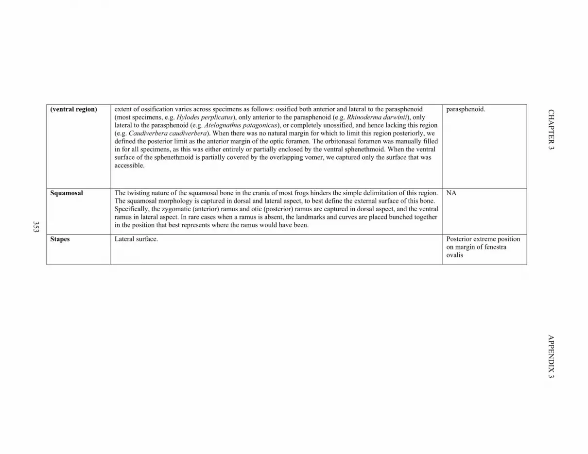
353
CH
AP
TE
R 3
AP
PE
ND
IX 3
(ventral region) extent of ossification varies across specimens as follows: ossified both anterior and lateral to the parasphenoid (most specimens, e.g. Hylodes perplicatus), only anterior to the parasphenoid (e.g. Rhinoderma darwinii), only lateral to the parasphenoid (e.g. Atelognathus patagonicus), or completely unossified, and hence lacking this region (e.g. Caudiverbera caudiverbera). When there was no natural margin for which to limit this region posteriorly, we defined the posterior limit as the anterior margin of the optic foramen. The orbitonasal foramen was manually filled in for all specimens, as this was either entirely or partially enclosed by the ventral sphenethmoid. When the ventral surface of the sphenethmoid is partially covered by the overlapping vomer, we captured only the surface that was accessible.
parasphenoid.
Squamosal The twisting nature of the squamosal bone in the crania of most frogs hinders the simple delimitation of this region. The squamosal morphology is captured in dorsal and lateral aspect, to best define the external surface of this bone. Specifically, the zygomatic (anterior) ramus and otic (posterior) ramus are captured in dorsal aspect, and the ventral ramus in lateral aspect. In rare cases when a ramus is absent, the landmarks and curves are placed bunched together in the position that best represents where the ramus would have been.
NA
Stapes Lateral surface. Posterior extreme position on margin of fenestra ovalis

CH
AP
TE
R 3
354
AP
PE
ND
IX 3
Table S3.4. Regions classed as absent across the specimens. ‘Absence’ includes absolute absence of a region, as well as unossified regions. Scientific (phylogenetic) name
indicates the species name according to the phylogeny used in this study (Jetz and Pyron 2018). *specimens without species assignment, so the name displayed here indicates
the position we assigned these specimens for phylogenetic analyses.
Specimen name Scientific (phylogenetic) name
Neopalatin
e
Stap
es
Vom
er
Qu
adratojugal
(lateral)
Qu
adratojugal
(jaw joint)
Sp
heneth
moid
(d
)
Sp
heneth
moid
(v)
Acanthixalus sonjae Acanthixalus sonjae
Adenomera andreae Adenomera andreae
Adenomus kelaartii Adenomus kelaartii
Afrixalus auresus Afrixalus aureus absent
Agalychnis calcifer Cruziohyla calcarifer absent
Allobates kingsburyi Allobates kingsburyi absent absent
Allophryne ruthveni Allophryne ruthveni absent absent
Alsodes nodosus Alsodes nodosus absent
Altiphrynoides malcomi Altiphrynoides malcolmi absent
Alytes obstetricans Alytes obstetricans absent
Ameerega parvula Ameerega parvula absent
Amietophrynus regularis Amietophrynus regularis absent
Anaxyrus fowleri Anaxyrus fowleri
Anaxyrus quercicus Anaxyrus quercicus absent
Anhydrophryne rattrayi Anhydrophryne rattrayi absent
Anotheca spinosa Anotheca spinosa
Ansonia mcgregori Ansonia mcgregori absent
Aromobates alboguttatus Aromobates alboguttatus

355
CH
AP
TE
R 3
AP
PE
ND
IX 3
Arthroleptella lightfooti Arthroleptella lightfooti
Arthroleptis bioko Arthroleptis bioko absent
Ascaphus truei Ascaphus truei absent absent absent absent absent
Astylosternus diadematus Astylosternus diadematus
Astylosternus occidentalis Astylosternus occidentalis absent
Atelopus ignescens Atelopus ignescens absent
Atelopus oxyrhynchus Atelopus oxyrhynchus absent
Balebreviceps hillimani Balebreviceps hillmani absent absent absent
Barbourula busuangensis Barbourula busuangensis absent
Barycholos pulcher Barycholos pulcher absent
Batrachyla taeniata Batrachyla taeniata
Bombina maxima Bombina maxima absent absent
Boophis boehmei Boophis boehmei
Brachycephalus ephippium Brachycephalus ephippium absent absent absent absent absent
Brachytarsophrys carinensis Brachytarsophrys carinense
Bufo gariepensis Vandijkophrynus gariepensis
Cacosternum namaquense Cacosternum namaquense absent absent
Callulina kisiwamsitu Callulina kisiwamsitu absent absent
Capensibufo sp. Capensibufo rosei* absent
Cardioglossa elegans Cardioglossa elegans absent
Cardioglossa manengouba Cardioglossa manengouba
Caudiverbera caudiverbera Calyptocephalella gayi absent absent
Centrolene buckleyi Centrolene buckleyi
Ceratobatrachus guentheri Ceratobatrachus guentheri absent
Ceratophrys aurita Ceratophrys aurita
Ceuthomantis smaragdinus Ceuthomantis smaragdinus absent

CH
AP
TE
R 3
356
AP
PE
ND
IX 3
Chacophrys pierotti Chacophrys pierottii absent
Chiromantis rufescens Chiromantis rufescens
Chrysobatrachus cupreonitens Chrysobatrachus cupreonitens absent
Cochranella granulosa Cochranella granulosa absent
Conraua beccarii Conraua beccarii absent
Conraua crassipes Conraua crassipes
Conraua goliath Conraua goliath
Cophixalus darlingtoni Albericus darlingtoni absent
Craugastor laticeps Craugastor laticeps
Crossodactylus trachystomus Crossodactylus trachystomus absent
Cryptobatrachus boulengeri Cryptobatrachus boulengeri absent
Cryptothylax greshoffi Cryptothylax greshoffii absent
Cycloramphus asper Cycloramphus asper absent
Cyclorana longipes Cyclorana longipes
Dendrobates sp. Dendrobates auratus* absent
Discodeles bufoniformis Discodeles bufoniformis absent
Duttaphrynus dodsoni Duttaphrynus dodsoni
Eleutherodactuylus cornutus Strabomantis cornutus absent
Eleutherodactylus biporcatus Strabomantis biporcatus absent absent
Eleutherodactylus glaphycompus Eleutherodactylus glaphycompus
Eleutherodactylus johnstonei Eleutherodactylus johnstonei
Eupsophus roseus Eupsophus roseus
Fritziana gouldii Fritziana goeldii absent
Gastrophryne carolinensis Gastrophryne carolinensis absent absent
Gastrotheca peruana Gastrotheca peruana
Guibemantis liber Guibemantis liber

357
CH
AP
TE
R 3
AP
PE
ND
IX 3
Haddadus binotatus Haddadus binotatus absent absent
Hadromophryne natalensis Hadromophryne natalensis
Heleioporus australiacus Heleioporus australiacus
Heleophryne purcelli Heleophryne purcelli
Hemiphractus proboscoideus Hemiphractus proboscideus
Hemisus guineensis Hemisus guineensis absent absent absent absent absent
Hoplophryne uluguruensis Hoplophryne uluguruensis absent absent absent
Hyalinobatrachium fleishmanni Hyalinobatrachium fleischmanni absent
Hyla boans Hypsiboas boans
Hyla tuberculosa Ecnomiohyla tuberculosa
Hylodes perplicatus Hylodes perplicatus
Hylorina sylvatica Hylorina sylvatica
Hyperolius viridiflavus Hyperolius viridiflavus absent
Hypodactylus araiodactylus Hypodactylus araiodactylus absent
Igerana tasanae Ingerana tasanae absent
Incilius periglenes Incilius periglenes absent absent
Indirana gundia Indirana gundia
Kassina arboricola Kassina arboricola
Lankanectes corrugatus Lankanectes corrugatus absent absent
Leiopelma hamiltoni Leiopelma hamiltoni absent absent absent absent
Leptobrachium hasseltii Leptobrachium hasseltii
Leptodactylodon boulengeri Leptodactylodon boulengeri
Leptodactylus melanotus Leptodactylus melanonotus
Leptodactylus podicipinus Leptodactylus podicipinus
Leptolepis occelatus Leptopelis ocellatus
Leptopelis spiritusnoclis Leptopelis spiritusnoctis

CH
AP
TE
R 3
358
AP
PE
ND
IX 3
Limnomedusa macroglossa Limnomedusa macroglossa absent absent
Limnonectes macrocephalus Limnonectes macrocephalus absent
Lithobates clamitans Rana clamitans
Litoria sp. Litoria aurea
Mannophryne hermina Mannophryne herminae
Mantella baroni Mantella baroni
Melanobatrachus indicus Melanobatrachus indicus absent absent absent absent
Melanophryniscus stelzneri Melanophryniscus stelzneri absent absent absent absent absent
Mertensophryne micranotis Mertensophryne micranotis absent
Microbatrachella capensis Microbatrachella capensis
Minervarya nilgirica Fejervarya nilagirica
Morerella cyanophthalma Morerella cyanophthalma absent
Myobatrachus gouldii Myobatrachus gouldii absent
Nasikabatrachus sahyadrensis Nasikabatrachus sahyadrensis absent absent
Natalobatrachus bonebergi Natalobatrachus bonebergi
Nectophrynoides tornieri Nectophrynoides tornieri
Nectophrynoides vivipara Nectophrynoides viviparus
Nothophryne broadleyi Nothophryne broadleyi
Nyctibates corrugatus Nyctibates corrugatus absent
Nyctimystes daymani Nyctimystes daymani
Nyctixalus spinosus Nyctixalus spinosus
Nyctixalus pictus Nyctixalus pictus
Occidozyga limba Occidozyga lima absent
Odontobatrachus natator Odontobatrachus natator absent
Odontophrynus americanus Odontophrynus americanus
Oreobates quixensis Oreobates quixensis

359
CH
AP
TE
R 3
AP
PE
ND
IX 3
Osteocephalus buckleyi Osteocephalus buckleyi
Osteopilus septentrionalis Osteopilus septentrionalis
Paracassina obscura Paracassina obscura
Pelobates fuscus Pelobates fuscus absent absent
Pelodytes caucasicus Pelodytes caucasicus absent
Peltophryne guentheri Peltophryne guentheri absent
Petropedetes palmipes Petropedetes palmipes
Philautus glandulosus Raorchestes glandulosus
Phlyctimantis boulengeri Phlyctimantis boulengeri absent
Phrynobatrachus leveleve Phrynobatrachus leveleve
Phyllomedusa azurea Phyllomedusa azurea
Pipa parva Pipa parva absent absent absent absent
Pipa pipa Pipa pipa absent absent absent absent
Platymantis polillensis Platymantis polillensis absent
Plethodontohyla notosticta Plethodontohyla notosticta absent
Polypedates macrotis Polypedates macrotis absent
Poyntonia paludicola Poyntonia paludicola
Pristimantis chiastonotus Pristimantis chiastonotus
Probreviceps macrodactylus Probreviceps macrodactylus absent absent
Proceratophrys boiei Proceratophrys boiei
Pseudacris ornata Pseudacris ornata
Pseudis paradoxica Pseudis paradoxa
Ptychadena bibroni Ptychadena bibroni absent
Pyxicephalus adspersus Pyxicephalus adspersus absent
Fejervarya vittigera Fejervarya vittigera
Rana cancrivora Fejervarya cancrivora

CH
AP
TE
R 3
360
AP
PE
ND
IX 3
Rana sylvatica Rana sylvatica
Raorchestes sp. Raorchestes anili*
Rhacophorus reinwalti Rhacophorus reinwardtii
Rheobatrachus silus Rheobatrachus silus
Rhinoderma darwinii Rhinoderma darwinii absent
Rhinophrynus dorsalis Rhinophrynus dorsalis absent absent absent
Scaphiophryne madagascariensis Scaphiophryne madagascariensis
Scaphiopus holbrookii Scaphiopus holbrookii absent
Semnodactylus weali Semnodactylus wealii
Sooglossus sechellensis Sooglossus sechellensis absent absent
Spea multiplicata Spea multiplicata absent
Strabomantis ingeri Strabomantis ingeri absent
Stumpffia pygmaea Stumpffia pygmaea absent absent
Syncope antenori Syncope antenori absent absent
Telmatobius laticeps Telmatobius laticeps
Telmatobius degener Telmatobius degener
Theloderma stellatum Theloderma stellatum
Thoropa miliaris Thoropa miliaris
Tomopterna marmorata Tomopterna marmorata
Trichobatrachus robustus Trichobatrachus robustus
Triprion petasatus Triprion petasatus absent
Uperodon monatnus Ramanella montana absent absent
Xenopus laevis Xenopus laevis absent absent absent
Xenorhina sp. Xenorhina varia* absent

361
CH
AP
TE
R 3
AP
PE
ND
IX 3
Table S3.5. Landmark definitions used in this study. 82 landmarks were placed onto the right-hand side of the cranium of each specimen. 24 landmarks (*) were removed
prior to analyses as they were not homologous across all specimens. These 24 landmarks were used in the patching procedure to place surface points onto variably present
regions.
Original landmark number
New landmark number
Landmark definition Region (see Table S3.3 for details)
1 1 Premaxilla: medial extreme above tooth row Premaxilla
2 2 Premaxilla: lateral extreme above tooth row Premaxilla
3 3 Premaxilla: tip of alary process ('pars alaris') Premaxilla
4 4 Premaxilla: posteromedial extreme at base of alary process Premaxilla
5 5 Premaxilla: posterolateral extreme at base of alary process Premaxilla
6 6 Maxilla: anteroventral extreme in lateral view, dorsal to the tooth row/palatal shelf Maxilla
7 7 Maxilla: posterior extreme in lateral aspect. Maxilla
8 8 Maxilla: anterodorsal extreme of maxilla in lateral view. Maxilla
9 9 Maxilla: tip of preorbital process of pars facialis, or if process absent, posterior-most suture with nasal Maxilla
10 10 Parasphenoid: anterior tip of cultriform process Parasphenoid
11 11 Parisphenoid: inflection point between anterior and lateral projections Parasphenoid
12 12 Parisphenoid: anterolateral extreme of lateral projection Parasphenoid
13 13 Parisphenoid: inflection point between lateral and posterior projections Parasphenoid
14 14 Parasphenoid: posterior extreme along midline Parasphenoid
15 15 Squamosal: posteromedial extreme on tip of otic (posterior) ramus Squamosal
16 16 Squamosal: medial extreme on tip of ventral ramus Squamosal
17 17 Squamosal: ventral extreme on tip of zygomatic (anterior) ramus Squamosal
18 18 Squamosal: inflection point between zygomatic (anterior) ramus and ventral ramus Squamosal
19 19 Squamosal: anterolateral tip of ventral ramus Squamosal
20 20 Squamosal: inflection point between ventral ramus and otic (posterior) ramus Squamosal
21 21 Pterygoid: lateral extreme of tip of posterior ramus Pterygoid

CH
AP
TE
R 3
362
AP
PE
ND
IX 3
22 22 Pterygoid: inflection point between medial ramus and posterior ramus on the ventral bone surface Pterygoid
23 23 Pterygoid: anteromedial extreme of tip of medial ramus Pterygoid
24 24 Pterygoid: anterior extreme of base of medial ramus Pterygoid
25 25 Pterygoid: anteromedial extreme of anterior ramus Pterygoid
26 26 Pterygoid: anterior extreme of base of posterior ramus Pterygoid
27 27 Frontoparietal: anterior extreme along medial margin Frontoparietal
28 28 Frontoparietal: anterior extreme along lateral margin Frontoparietal
29 29 Frontoparietal: most lateral suture with otic region Frontoparietal
30 30 Frontoparietal: posterolateral extreme, often adjacent to epiotic ridge Frontoparietal
31 31 Frontoparietal: suture with exoccipital along midline Frontoparietal
32 32 Premaxilla: anteromedial extreme position on palatal shelf ('pars palatina') (just posterior to the pars dentigera)
Premaxilla
33 33 Premaxilla: anterolateral extreme position on palatal shelf ('pars palatina') (just posterior to the pars dentigera)
Premaxilla
34 34 Premaxilla: posterolateral extreme of palatal shelf ('pars palatina') Premaxilla
35 35 Premaxilla: tip of palatine process on palatal shelf ('pars palatina'), in ventral aspect Premaxilla
36 36 Maxilla: anterior extreme of palatal shelf ('pars palatina') Maxilla
37 37 Maxilla: anteromedial extreme of palatal shelf ('pars palatina') Maxilla
38 38 Maxilla: posterolateral extreme of palatal shelf ('pars palatina') Maxilla
39 39 Nasal: anterior tip Nasal
40 40 Nasal: posterior extreme Nasal
41 41 Nasal: tip of maxillary process Nasal
42 NA (Deleted landmark)* NA
43 42 Parasphenoid: posterolateral extreme of lateral projection Parasphenoid
44 43 Occipital: anteromedial extreme suture with frontoparietal Occipital
45 44 Occipital: dorsal extreme of foramen magnum Occipital
46 45 Occipital: dorsal extreme of occipital condyle, along foramen magnum margin Occipital
47 46 Occipital: ventral extreme of occipital condyle, along foramen magnum margin Occipital

363
CH
AP
TE
R 3
AP
PE
ND
IX 3
48 47 Occipital: ventral extreme of foramen magnum Occipital
49 48 Occipital: in ventral aspect, posteromedial suture with parasphenoid Occipital
50 NA Stapes: dorsolateral extreme* Stapes
51 NA Stapes: ventrolateral extreme* Stapes
52 NA Stapes: dorsomedial extreme* Stapes
53 NA Stapes: ventromedial extreme* Stapes
54 NA Vomer: tip of anterior process (or anterior extreme)* Vomer
55 NA Vomer: tip of prechoanal process (or anterolateral extreme)* Vomer
56 NA Vomer: tip of postchoanal process (or posterolateral extreme)* Vomer
57 NA Vomer: posteromedial extreme* Vomer
58 49 Occipital: in ventral aspect, posterolateral extreme suture with parasphenoid Occipital
59 50 Occipital: ventral extreme of jugular foramen Occipital
60 51 Occipital: dorsal extreme of jugular foramen Occipital
61 52 Occipital: anterior extreme of epiotic ridge Occipital
62 53 Occipital: juncture of epiotic ridge and posterior margin of otic region Occipital
63 54 Otic region: anterior extreme of epiotic ridge Otic
64 55 Otic region: dorsolateral extreme of prootic foramen Otic
65 56 Otic region: anterolateral extreme, following anterior margin of otic region Otic
66 57 Otic region: posterolateral extreme Otic
67 58 Otic region: juncture of epiotic ridge and posterior margin of otic region Otic
68 NA Quadratojugal: articular surface, posterolateral extreme on hinge* Quadratojugal
69 NA Quadratojugal: articular surface, anterior extreme* Quadratojugal
70 NA Quadratojugal: articular surface, posteromedial extreme on hinge* Quadratojugal
71 NA Quadratojugal: maxillary process, anterodorsal tip* Quadratojugal
72 NA Quadratojugal: maxillary process, posterodorsal extreme* Quadratojugal
73 NA Quadratojugal: maxillary process, posteroventral extreme* Quadratojugal
74 NA Neopalatine: medial tip* Neopalatine
75 NA Neopalatine: anterior extreme of lateral tip* Neopalatine

CH
AP
TE
R 3
364
AP
PE
ND
IX 3
76 NA Neopalatine: posterior extreme of lateral tip* Neopalatine
77 NA Dorsal sphenethmoid: anteromedial extreme* Dorsal sphenethmoid
78 NA Dorsal sphenethmoid: posteromedial extreme* Dorsal sphenethmoid
79 NA Dorsal sphenethmoid: lateral extreme* Dorsal sphenethmoid
80 NA Ventral sphenethmoid: anteromedial extreme* Ventral sphenethmoid
81 NA Ventral sphenethmoid: posteromedial extreme, just anterior to the optic foramen* Ventral sphenethmoid
82 NA Ventral sphenethmoid: posterolateral extreme* Ventral sphenethmoid
83 NA Ventral sphenethmoid: anterolateral extreme, posterior to neopalatine when present* Ventral sphenethmoid

365
CH
AP
TE
R 3
AP
PE
ND
IX 3
Table S3.6. Curve definitions used in this study. Description of curve semilandmarks placed manually onto each specimen. Curves are each converted into eight or nine
curve points after they are exported from Landmark Editor, and then we subsampled curve points to a density reflecting the magnitude of variation along each curve. Curve
points are then slid to minimise bending energy across the dataset. Some curves were placed for use in patching the variably-present regions, but were removed prior to
analyses as these curves were not present across the entire dataset.
Curve number
New curve number
Description Region Starting landmark
Ending landmark
Manually-placed curve length
Resampled curve length
C1 C1 Directly to the base of the alary process ('pars alaris') then follow base
Premaxilla (dorsal) 1 4 3 3
C2 C2 Following posterior edge of alary process ('pars alaris') Premaxilla (dorsal) 4 3 4 3
C3 C3 Following posterior edge of alary process ('pars alaris') Premaxilla (dorsal) 3 5 4 3
C4 C4 Following base of alary process ('pars alaris'), then directly to landmark
Premaxilla (dorsal) 5 2 3 3
C5 C5 Medially, dorsal to tooth row Premaxilla (dorsal) 2 1 4 4
C6 C6 Laterally, posterior to tooth shelf ('pars dentigera') Premaxilla (ventral) 32 33 4 3
C7 C7 Following edge of palatal shelf of premaxilla Premaxilla (ventral) 33 34 3 3
C8 C8 Following edge of palatal shelf of premaxilla Premaxilla (ventral) 34 35 4 6
C9 C9 Following edge of palatal shelf of premaxilla Premaxilla (ventral) 35 32 4 3
C10 C10 Following bone margin Parasphenoid 10 11 10 10
C11 C11 Following bone margin Parasphenoid 11 12 5 6
C12 C12 Following bone margin Parasphenoid 12 43 6 4
C13 C13 Following bone margin Parasphenoid 43 13 5 5
C14 C14 Following bone margin Parasphenoid 13 14 3 4
C15 C15 Anteriorly along midline Parasphenoid 14 10 8 12
C16 C16 Following margin of ventral bone surface Pterygoid 21 22 6 5
C17 C17 Following margin of ventral bone surface Pterygoid 22 23 6 5
C18 C18 Following margin of ventral bone surface Pterygoid 23 24 5 5

CH
AP
TE
R 3
366
AP
PE
ND
IX 3
C19 C19 Following margin of ventral bone surface Pterygoid 24 25 8 8
C20 C20 Following margin of ventral bone surface Pterygoid 25 26 10 10
C21 C21 Following margin of ventral bone surface Pterygoid 26 21 6 5
C22 C22 Posteriorly along margin of palatal shelf, excluding tooth shelf
Maxilla (ventral) 36 38 10 15
C23 C23 Anteriorly along margin of palatal shelf Maxilla (ventral) 38 37 12 15
C24 C24 Laterally along margin Maxilla (ventral) 37 36 3 5
C25 C25 Tracing medial margin of dorsal surface Squamosal 15 17 8 10
C26 C26 Following margin of lateral bone surface Squamosal 17 18 6 10
C27 C27 Following margin of lateral bone surface Squamosal 18 19 6 10
C28 C28 Following bone margin Squamosal 19 16 3 5
C29 C29 Following medial extreme of the lateral bone surface in posterior view
Squamosal 16 20 6 8
C30 C30 Tracing bone margin to capture dorsal bone surface Squamosal 20 15 6 10
C31 C31 Anteriorly along margin Frontoparietal 27 28 4 5
C32 C32 Posteriorly along margin Frontoparietal 28 29 8 15
C33 C33 Posteriorly along margin Frontoparietal 29 30 5 5
C34 C34 Medially along margin Frontoparietal 30 31 6 5
C35 C35 Anteriorly along margin Frontoparietal 31 27 10 10
C36 NA Following anterior margin Neopalatine 74 75 6 5
C37 NA Following lateral margin Neopalatine 75 76 3 2
C38 NA Following posterior margin Neopalatine 76 74 6 5
C39 NA Following lateral margin, in lateral view Stapes 50 51 2 2
C40 NA Following ventral margin, in lateral view Stapes 51 53 4 5
C41 NA Following medial margin, in lateral view Stapes 53 52 3 3
C42 NA Following dorsal margin, in lateral view Stapes 52 50 4 5
C43 C36 Following midline to foramen magnum Occipital 44 45 3 3

367
CH
AP
TE
R 3
AP
PE
ND
IX 3
C44 C37 Tracing foramen magnum Occipital 45 46 5 5
C45 C38 Tracing lateral margin of occipital condyle Occipital 46 47 6 5
C46 C39 Tracing medial margin of occipital condyle Occipital 46 47 4 4
C47 C40 Tracing foramen magnum Occipital 47 48 3 3
C48 C41 Anteriorly along bone margin, or along midline if fused medially
Occipital 48 49 3 3
C49 C42 Laterally, tracing bine margin Occipital 49 58 6 5
C50 C43 Trace around posterior margin of fenestra ovalis, to the ventral extreme of the epiotic ridge, and then dorsally along ridge.
Occipital 58 62 8 10
C51 C44 Tracing along ridge dorsally Occipital 62 61 6 5
C52 C45 Medially tracing along bone margin Occipital 61 44 5 5
C53 C46 Laterally around jugular foramen Occipital 60 59 5 5
C54 C47 Medially around jugular foramen Occipital 59 60 5 5
C55 C48 Anteriorly, tracing medial side of ridge Otic 63 64 6 8
C56 C49 Laterally, following contour Otic 64 65 5 5
C57 C50 Posteriorly, tracing lateral margin of dorsal bone surface
Otic 65 66 5 15
C58 C51 Medially, following contour Otic 66 67 5 8
C59 C52 Tracing along epiotic ridge Otic 67 63 5 5
C60 C53 Posteriorly tracing bone margin Nasal 39 40 7 10
C61 C54 Laterally tracing bone margin, capturing bone depth Nasal 40 41 7 10
C62 C55 Anteriorly tracing bone margin Nasal 41 39 8 10
C63 NA Posteriorly tracing bone margin Vomer 54 55 8 6
C64 NA Posteriorly tracing bone margin Vomer 55 56 8 6
C65 NA Tracing posterior bone margin, onto tooth ridge (if present) but anterior to teeth
Vomer 56 57 8 8
C66 NA Anteriorly tracing bone margin Vomer 57 54 8 6

CH
AP
TE
R 3
368
AP
PE
ND
IX 3
C67 NA Posteriorly, tracing bone margin Quadratojugal (lateral) 71 72 6 5
C68 NA Ventrally, tracing bone margin Quadratojugal (lateral) 72 73 4 3
C69 NA Anteriorly, tracing bone margin Quadratojugal (lateral) 73 71 6 5
C70 NA Anteriorly, tracing articular surface only Quadratojugal (jaw joint articulation)
68 69 4 5
C71 NA Posteriorly, tracing articular surface only Quadratojugal (jaw joint articulation)
69 70 4 5
C72 NA Laterally, tracing articular surface only Quadratojugal (jaw joint articulation)
70 68 4 5
C73 C56 Posteriorly, tracing bone margin Maxilla (dorsal) 9 7 12 15
C74 C57 Anteriorly, tracing bone margin dorsal to tooth row Maxilla (dorsal) 7 6 12 15
C75 C58 Dorsally, tracing bone margin Maxilla (dorsal) 6 8 4 5
C76 C59 Posteriorly, tracing bone margin Maxilla (dorsal) 8 9 6 8
C77 NA Posteriorly, following midline Sphenethmoid (dorsal) 77 78 5 8
C78 NA Laterally, tracing bone margin Sphenethmoid (dorsal) 78 79 5 8
C79 NA Anteriorly, tracing bone margin Sphenethmoid (dorsal) 79 77 8 10
C80 NA Posteriorly, following midline Sphenethmoid (ventral) 80 81 8 10
C81 NA Dorsally, tracing posterior margin (or tracing anteriorly around optic foramen if bone extends posteriorly to this foramen)
Sphenethmoid (ventral) 81 82 4 5
C82 NA Tracing ventral bone surface Sphenethmoid (ventral) 82 83 8 10
C83 NA Tracing ventral bone surface Sphenethmoid (ventral) 83 80 10 15

369
CH
AP
TE
R 3
AP
PE
ND
IX 3
Table S3.7. Number of surface points within each cranial region. Surface points were distributed evenly over each region. Two templates were required for some regions
(*), as one template was not sufficient to successfully patch the regions across all specimens owing to the extreme morphological variation across the dataset.
Region Number of surface points
Premaxilla(d) 12
Premaxilla(v) 12
Parasphenoid* 40
Pterygoid 26
Maxilla(v) 20
Nasal 20
Maxilla(d) 48
Occipital condyle 12
Occipital 58
Otic 36
Frontoparietal* 64
Squamosal 26
Neopalatine 16
Stapes 16
Quadratojugal(l) 15
Quadratojugal(JJ)* 16
Sphenethmoid(d)* 29
Vomer 20
Sphenethmoid(v)* 41
TOTAL 527

CH
AP
TE
R 3
370
AP
PE
ND
IX 3
Table S3.8. Centroid size for each specimen.
Species Centroid Size
Species Centroid Size
Species Centroid Size
Species Centroid Size
Acanthixalus sonjae 237.72 Ceuthomantis smaragdinus
134.38 Indirana gundia 239.06 Raorchestes sp. 162.32
Adenomera andreae 164.23 Chacophrys pierottii 296.86 Kassina arboricola 221.03 Phlyctimantis boulengeri 259.43
Adenomus kelaartii 224.86 Chiromantis rufescens 270.11 Lankanectes corrugatus 251.26 Phrynobatrachus leveleve
107.95
Afrixalus aureus 115.68 Chrysobatrachus cupreonitens
139.73 Leiopelma hamiltoni 314.57 Phyllomedusa azurea 199.03
Cruziohyla calcarifer 399.60 Cochranella granulosa 157.39 Leptobrachium hasseltii 385.84 Pipa parva 182.19
Allobates kingsburyi 125.65 Conraua beccarii 719.35 Leptodactylodon boulengeri
251.60 Pipa pipa 684.80
Allophryne ruthveni 127.66 Conraua crassipes 358.00 Leptodactylus melanonotus
242.71 Platymantis polillensis 162.72
Alsodes nodosus 304.76 Conraua goliath 1550.81 Leptodactylus podicipinus
217.43 Plethodontohyla notosticta
184.04
Altiphrynoides malcolmi 189.81 Albericus darlingtoni 147.09 Leptopelis ocellatus 308.55 Polypedates macrotis 387.11
Alytes obstetricans 270.51 Craugastor laticeps 363.91 Leptopelis spiritusnoctis 283.40 Poyntonia paludicola 160.25
Ameerega parvula 146.92 Crossodactylus trachystomus
144.71 Limnomedusa macroglossa
328.62 Pristimantis chiastonotus 304.38
Amietophrynus regularis 371.85 Cryptobatrachus boulengeri
244.82 Limnonectes macrocephalus
593.85 Probreviceps macrodactylus
274.68
Anaxyrus fowleri 284.90 Cryptothylax greshoffii 262.53 Rana clamitans 384.28 Proceratophrys boiei 376.38
Anaxyrus quercicus 185.94 Cycloramphus asper 382.78 Litoria aurea 342.27 Pseudacris ornata 188.48
Anhydrophryne rattrayi 114.67 Cyclorana longipes 440.07 Mannophryne herminae 205.54 Pseudis paradoxa 397.48
Anotheca spinosa 390.13 Dendrobates sp. 122.40 Mantella baroni 136.16 Ptychadena bibroni 317.17
Ansonia mcgregori 241.60 Discodeles bufoniformis 1019.39 Melanobatrachus indicus 171.44 Pyxicephalus adspersus 722.04

371
CH
AP
TE
R 3
AP
PE
ND
IX 3
Aromobates alboguttatus 176.54 Duttaphrynus dodsoni 277.19 Melanophryniscus stelzneri
142.26 Fejervarya vittigera 251.55
Arthroleptella lightfooti 97.80 Strabomantis cornutus 304.52 Mertensophryne micranotis
111.76 Fejervarya cancrivora 451.26
Arthroleptis bioko 189.84 Strabomantis biporcatus 240.03 Microbatrachella capensis
100.86 Rana sylvatica 236.96
Ascaphus truei 233.25 Eleutherodactylus glaphycompus
223.67 Fejervarya nilagirica 240.19 Raorchestes anili 219.68
Astylosternus diadematus 333.78 Eleutherodactylus johnstonei
166.31 Morerella cyanophthalma
195.82 Rhacophorus reinwardtii 365.67
Astylosternus occidentalis
402.96 Eupsophus roseus 231.30 Myobatrachus gouldii 179.33 Rheobatrachus silus 267.76
Atelopus ignescens 198.07 Fritziana goeldii 247.60 Nasikabatrachus sahyadrensis
339.52 Rhinoderma darwinii 155.93
Atelopus oxyrhynchus 228.84 Gastrophryne carolinensis
117.41 Natalobatrachus bonebergi
205.93 Rhinophrynus dorsalis 230.76
Balebreviceps hillmani 177.80 Gastrotheca peruana 295.67 Nectophrynoides tornieri 169.97 Scaphiophryne madagascariensis
228.68
Barbourula busuangensis
524.14 Guibemantis liber 142.62 Nectophrynoides viviparus
235.83 Scaphiopus holbrookii 356.82
Barycholos pulcher 156.99 Haddadus binotatus 276.68 Nothophryne broadleyi 137.18 Semnodactylus wealii 171.72
Batrachyla taeniata 224.17 Hadromophryne natalensis
385.54 Nyctibates corrugatus 320.78 Sooglossus sechellensis 131.49
Bombina maxima 277.35 Heleioporus australiacus 307.36 Nyctimystes daymani 331.46 Spea multiplicata 310.25
Boophis boehmei 214.74 Heleophryne purcelli 280.68 Nyctixalus spinosus 263.65 Strabomantis ingeri 403.44
Brachycephalus ephippium
117.35 Hemiphractus proboscideus
414.43 Nyctixalus pictus 225.82 Stumpffia pygmaea 68.46
Brachytarsophrys carinense
662.91 Hemisus guineensis 151.91 Occidozyga lima 157.48 Syncope antenori 79.94
Vandijkophrynus gariepensis
350.28 Hoplophryne uluguruensis
96.48 Odontobatrachus natator 321.64 Telmatobius laticeps 346.74
Cacosternum namaquense
138.46 Hyalinobatrachium fleischmanni
130.73 Odontophrynus americanus
376.61 Telmatobius degener 284.82

CH
AP
TE
R 3
372
AP
PE
ND
IX 3
Callulina kisiwamsitu 270.94 Hypsiboas boans 522.28 Oreobates quixensis 304.03 Theloderma stellatum 228.62
Capensibufo sp. 171.18 Ecnomiohyla tuberculosa 484.74 Osteocephalus buckleyi 375.14 Thoropa miliaris 408.21
Cardioglossa elegans 173.11 Hylodes perplicatus 240.19 Osteopilus septentrionalis
433.96 Tomopterna marmorata 276.74
Cardioglossa manengouba
188.77 Hylorina sylvatica 381.32 Paracassina obscura 204.94 Trichobatrachus robustus
448.59
Calyptocephalella gayi 410.48 Hyperolius viridiflavus 200.08 Pelobates fuscus 338.04 Triprion petasatus 290.47
Centrolene buckleyi 171.83 Hypodactylus araiodactylus
171.84 Pelodytes caucasicus 260.82 Ramanella montana 135.96
Ceratobatrachus guentheri
553.66 Ingerana tasanae 244.63 Peltophryne guentheri 374.03 Xenopus laevis 378.54
Ceratophrys aurita 954.11 Incilius periglenes 285.05 Petropedetes palmipes 336.07 Xenorhina sp. 229.69

373
CH
AP
TE
R 3
AP
PE
ND
IX 3
Table S3.9. Results of EMMLi analysis for trait correlations (ρ) within and between 19 cranial regions using uncorrected full landmark and semilandmark data.
Frontoparietal
Maxilla(d)
Maxilla(v)
Nasal
Neopalatine
Occipital
Occipital condyle
Otic
Parasphenoid
Premaxilla(d)
Premaxilla(v)
Pterygoid
Quadratojugal(JJ)
Quadratojugal(l)
Sphenethmoid(d)
Sphenethmoid(v)
Squamosal
Stapes
Vom
er
Frontoparietal 0.6 0.13 0.12 0.21 0.1 0.2 0.18 0.2 0.1 0.14 0.18 0.14 0.21 0.26 0.33 0.16 0.15 0.11 0.08
Maxilla(d) 0.13 0.65 0.49 0.15 0.16 0.34 0.38 0.25 0.16 0.36 0.35 0.27 0.36 0.39 0.08 0.15 0.2 0.1 0.29
Maxilla(v) 0.12 0.49 0.78 0.09 0.16 0.29 0.34 0.2 0.14 0.45 0.51 0.27 0.3 0.31 0.12 0.12 0.19 0.08 0.28
Nasal 0.21 0.15 0.09 0.69 0.2 0.17 0.18 0.1 0.11 0.15 0.11 0.12 0.15 0.18 0.31 0.16 0.12 0.16 0.22
Neopalatine 0.1 0.16 0.16 0.2 0.95 0.14 0.09 0.23 0.1 0.1 0.03 0.12 0.11 0.16 0.14 0.11 0.24 0.1 0.31
Occipital 0.2 0.34 0.29 0.17 0.14 0.75 0.79 0.27 0.32 0.25 0.3 0.23 0.43 0.41 0.18 0.07 0.26 0.15 0.19
Occipital condyle 0.18 0.38 0.34 0.18 0.09 0.79 0.96 0.24 0.35 0.34 0.39 0.27 0.53 0.49 0.21 0.07 0.34 0.13 0.27
Otic 0.2 0.25 0.2 0.1 0.23 0.27 0.24 0.69 0.11 0.09 0.08 0.15 0.16 0.18 0.11 0.09 0.19 0.12 0.1
Parasphenoid 0.1 0.16 0.14 0.11 0.1 0.32 0.35 0.11 0.66 0.16 0.15 0.21 0.28 0.28 0.11 0.11 0.16 0.06 0.14
Premaxilla(d) 0.14 0.36 0.45 0.15 0.1 0.25 0.34 0.09 0.16 0.9 0.86 0.27 0.35 0.31 0.16 0.1 0.28 0.07 0.47
Premaxilla(v) 0.18 0.35 0.51 0.11 0.03 0.3 0.39 0.08 0.15 0.86 0.94 0.22 0.29 0.24 0.22 0.08 0.25 0.06 0.42
Pterygoid 0.14 0.27 0.27 0.12 0.12 0.23 0.27 0.15 0.21 0.27 0.22 0.71 0.6 0.55 0.1 0.12 0.39 0.11 0.24
Quadratojugal(JJ) 0.21 0.36 0.3 0.15 0.11 0.43 0.53 0.16 0.28 0.35 0.29 0.6 0.99 0.89 0.11 0.17 0.58 0.09 0.35
Quadratojugal(l) 0.26 0.39 0.31 0.18 0.16 0.41 0.49 0.18 0.28 0.31 0.24 0.55 0.89 0.98 0.17 0.17 0.58 0.11 0.39
Sphenethmoid(d) 0.33 0.08 0.12 0.31 0.14 0.18 0.21 0.11 0.11 0.16 0.22 0.1 0.11 0.17 0.86 0.27 0.1 0.17 0.09
Sphenethmoid(v) 0.16 0.15 0.12 0.16 0.11 0.07 0.07 0.09 0.11 0.1 0.08 0.12 0.17 0.17 0.27 0.74 0.07 0.06 0.22
Squamosal 0.15 0.2 0.19 0.12 0.24 0.26 0.34 0.19 0.16 0.28 0.25 0.39 0.58 0.58 0.1 0.07 0.7 0.18 0.3
Stapes 0.11 0.1 0.08 0.16 0.1 0.15 0.13 0.12 0.06 0.07 0.06 0.11 0.09 0.11 0.17 0.06 0.18 0.97 0.07
Vomer 0.08 0.29 0.28 0.22 0.31 0.19 0.27 0.1 0.14 0.47 0.42 0.24 0.35 0.39 0.09 0.22 0.3 0.07 0.92

CH
AP
TE
R 3
374
AP
PE
ND
IX 3
Table S3.10. Results of EMMLi analysis for trait correlations (ρ) within and between 19 cranial regions, for the phylogenetically-corrected full landmark and semilandmark
dataset.
Frontoparietal
Maxilla(d)
Maxilla(v)
Nasal
Neopalatine
Occipial
condyle
Occipital
Otic
Parasphenoid
Prem
axilla(d)
Prem
axilla(v)
Pterygoid
Quadratojugal
(JJ)
Quadratojugal
(l)
Sphenethm
oid(d)
Sphenethm
oid(v)
Squam
osal
Stapes
Vom
er
Frontoparietal 0.58 0.15 0.17 0.19 0.12 0.16 0.19 0.17 0.08 0.13 0.17 0.17 0.26 0.29 0.31 0.19 0.17 0.12 0.07
Maxilla(d) 0.15 0.63 0.44 0.14 0.19 0.3 0.27 0.21 0.15 0.3 0.28 0.26 0.34 0.39 0.09 0.08 0.19 0.07 0.21
Maxilla(v) 0.17 0.44 0.77 0.08 0.2 0.28 0.23 0.18 0.11 0.39 0.45 0.29 0.3 0.33 0.14 0.08 0.17 0.05 0.23
Nasal 0.19 0.14 0.08 0.67 0.21 0.17 0.15 0.09 0.12 0.16 0.11 0.11 0.11 0.15 0.25 0.2 0.11 0.17 0.25
Neopalatine 0.12 0.19 0.2 0.21 0.93 0.17 0.17 0.18 0.14 0.12 0.04 0.1 0.08 0.12 0.11 0.17 0.14 0.09 0.32
Occipial condyle 0.16 0.3 0.28 0.17 0.17 0.96 0.78 0.21 0.34 0.24 0.29 0.28 0.5 0.45 0.18 0.16 0.31 0.09 0.1
Occipital 0.19 0.27 0.23 0.15 0.17 0.78 0.73 0.23 0.33 0.16 0.2 0.23 0.41 0.38 0.13 0.12 0.24 0.1 0.04
Otic 0.17 0.21 0.18 0.09 0.18 0.21 0.23 0.66 0.1 0.07 0.06 0.14 0.18 0.2 0.14 0.1 0.16 0.11 0.07
Parasphenoid 0.08 0.15 0.11 0.12 0.14 0.34 0.33 0.1 0.64 0.1 0.08 0.17 0.27 0.26 0.1 0.13 0.14 0.06 0.09
Premaxilla(d) 0.13 0.3 0.39 0.16 0.12 0.24 0.16 0.07 0.1 0.87 0.83 0.2 0.2 0.23 0.17 0.07 0.2 0.09 0.43
Premaxilla(v) 0.17 0.28 0.45 0.11 0.04 0.29 0.2 0.06 0.08 0.83 0.94 0.18 0.15 0.16 0.21 0.08 0.18 0.06 0.39
Pterygoid 0.17 0.26 0.29 0.11 0.1 0.28 0.23 0.14 0.17 0.2 0.18 0.72 0.63 0.57 0.07 0.09 0.4 0.13 0.21
Quadratojugal(JJ) 0.26 0.34 0.3 0.11 0.08 0.5 0.41 0.18 0.27 0.2 0.15 0.63 0.99 0.88 0.1 0.1 0.54 0.13 0.23
Quadratojugal(l) 0.29 0.39 0.33 0.15 0.12 0.45 0.38 0.2 0.26 0.23 0.16 0.57 0.88 0.97 0.14 0.13 0.54 0.14 0.28
Sphenethmoid(d) 0.31 0.09 0.14 0.25 0.11 0.18 0.13 0.14 0.1 0.17 0.21 0.07 0.1 0.14 0.87 0.33 0.13 0.15 0.05
Sphenethmoid(v) 0.19 0.08 0.08 0.2 0.17 0.16 0.12 0.1 0.13 0.07 0.08 0.09 0.1 0.13 0.33 0.7 0.07 0.1 0.19
Squamosal 0.17 0.19 0.17 0.11 0.14 0.31 0.24 0.16 0.14 0.2 0.18 0.4 0.54 0.54 0.13 0.07 0.65 0.2 0.24
Stapes 0.12 0.07 0.05 0.17 0.09 0.09 0.1 0.11 0.06 0.09 0.06 0.13 0.13 0.14 0.15 0.1 0.2 0.97 0.09
Vomer 0.07 0.21 0.23 0.25 0.32 0.1 0.04 0.07 0.09 0.43 0.39 0.21 0.23 0.28 0.05 0.19 0.24 0.09 0.9

375
CH
AP
TE
R 3
AP
PE
ND
IX 3
Table S3.11. Results of EMMLi analysis for trait correlations (ρ) within and between 19 cranial regions, for the allometry-corrected full landmark and semilandmark
dataset.
Frontoparietal
Maxilla(d)
Maxilla(v)
Nasal
Neopalatine
Occipital
Occipital
condyle
Otic
Parasphenoid
Premaxilla(d)
Premaxilla(v)
Pterygoid
Quadratojugal
(JJ)
Quadratojugal
(l)
Sphenethmoid
(d)
Sphenethmoid
(v)
Squamosal
Stapes
Vom
er
Frontoparietal 0.57 0.1 0.08 0.19 0.09 0.19 0.16 0.15 0.11 0.11 0.15 0.13 0.24 0.26 0.3 0.14 0.14 0.08 0.08
Maxilla(d) 0.1 0.63 0.46 0.16 0.16 0.27 0.27 0.19 0.13 0.35 0.34 0.24 0.3 0.31 0.07 0.15 0.18 0.11 0.25
Maxilla(v) 0.08 0.46 0.77 0.09 0.16 0.24 0.28 0.15 0.11 0.45 0.51 0.24 0.24 0.24 0.11 0.11 0.17 0.09 0.26
Nasal 0.19 0.16 0.09 0.68 0.21 0.1 0.09 0.1 0.09 0.17 0.1 0.15 0.22 0.25 0.28 0.14 0.15 0.15 0.25
Neopalatine 0.09 0.16 0.16 0.21 0.95 0.13 0.07 0.24 0.11 0.11 0.04 0.13 0.16 0.21 0.13 0.1 0.26 0.1 0.34
Occipital 0.19 0.27 0.24 0.1 0.13 0.72 0.74 0.26 0.27 0.18 0.23 0.18 0.31 0.3 0.16 0.06 0.23 0.13 0.12
Occipital condyle 0.16 0.27 0.28 0.09 0.07 0.74 0.94 0.2 0.28 0.28 0.32 0.23 0.39 0.35 0.2 0.03 0.32 0.1 0.2
Otic 0.15 0.19 0.15 0.1 0.24 0.26 0.2 0.68 0.11 0.08 0.06 0.12 0.11 0.11 0.14 0.09 0.19 0.14 0.12
Parasphenoid 0.11 0.13 0.11 0.09 0.11 0.27 0.28 0.11 0.62 0.12 0.11 0.2 0.21 0.25 0.09 0.13 0.16 0.06 0.14
Premaxilla(d) 0.11 0.35 0.45 0.17 0.11 0.18 0.28 0.08 0.12 0.9 0.86 0.26 0.3 0.29 0.13 0.09 0.27 0.09 0.47
Premaxilla(v) 0.15 0.34 0.51 0.1 0.04 0.23 0.32 0.06 0.11 0.86 0.94 0.21 0.23 0.19 0.19 0.07 0.24 0.06 0.42
Pterygoid 0.13 0.24 0.24 0.15 0.13 0.18 0.23 0.12 0.2 0.26 0.21 0.73 0.6 0.55 0.12 0.12 0.39 0.11 0.22
Quadratojugal(JJ) 0.24 0.3 0.24 0.22 0.16 0.31 0.39 0.11 0.21 0.3 0.23 0.6 0.99 0.88 0.16 0.2 0.58 0.09 0.3
Quadratojugal(l) 0.26 0.31 0.24 0.25 0.21 0.3 0.35 0.11 0.25 0.29 0.19 0.55 0.88 0.97 0.2 0.18 0.57 0.11 0.33
Sphenethmoid(d) 0.3 0.07 0.11 0.28 0.13 0.16 0.2 0.14 0.09 0.13 0.19 0.12 0.16 0.2 0.86 0.25 0.11 0.15 0.08
Sphenethmoid(v) 0.14 0.15 0.11 0.14 0.1 0.06 0.03 0.09 0.13 0.09 0.07 0.12 0.2 0.18 0.25 0.75 0.08 0.05 0.22
Squamosal 0.14 0.18 0.17 0.15 0.26 0.23 0.32 0.19 0.16 0.27 0.24 0.39 0.58 0.57 0.11 0.08 0.7 0.18 0.27
Stapes 0.08 0.11 0.09 0.15 0.1 0.13 0.1 0.14 0.06 0.09 0.06 0.11 0.09 0.11 0.15 0.05 0.18 0.98 0.06
Vomer 0.08 0.25 0.26 0.25 0.34 0.12 0.2 0.12 0.14 0.47 0.42 0.22 0.3 0.33 0.08 0.22 0.27 0.06 0.92

CH
AP
TE
R 3
376
AP
PE
ND
IX 3
Table S3.12. Results of EMMLi analysis for trait correlations (ρ) within and between 19 cranial regions, for the 10% subsampled analyses, averaged over 100 iterations.
Frontoparieta
l Maxilla(d)
Maxilla(v)
Nasal
Neopalatine
Occipital
Occipital
condyle
Otic
Parasphenoid
Prem
axilla(d)
Prem
axilla(v)
Pterygoid
Quadratojuga
l(JJ)
Quadratojuga
l(l)
Sphenethm
oid(d)
Sphenethm
oid(v)
Squam
osal
Stapes
Vom
er
Frontoparietal 0.66 0.12 0.12 0.22 0.07 0.14 0.12 0.23 0.12 0.13 0.21 0.12 0.21 0.28 0.35 0.22 0.13 0.12 0.1
Maxilla(d) 0.12 0.59 0.49 0.16 0.16 0.36 0.41 0.24 0.14 0.39 0.4 0.27 0.4 0.4 0.05 0.13 0.19 0.06 0.3
Maxilla(v) 0.12 0.49 0.87 0.1 0.25 0.35 0.4 0.28 0.11 0.2 0.22 0.36 0.34 0.38 0.04 0.15 0.16 0.04 0.27
Nasal 0.22 0.16 0.1 0.72 0.13 0.15 0.13 0.07 0.09 0.27 0.1 0.14 0.18 0.23 0.33 0.17 0.13 0.13 0.27
Neopalatine 0.07 0.16 0.25 0.13 0.99 0.17 0.1 0.26 0.08 0.08 0.02 0.09 0.09 0.12 0.16 0.05 0.25 0.06 0.26
Occipital 0.14 0.36 0.35 0.15 0.17 0.74 0.82 0.26 0.23 0.22 0.34 0.21 0.43 0.39 0.22 0.08 0.23 0.1 0.17
Occipital condyle 0.12 0.41 0.4 0.13 0.1 0.82 0.96 0.26 0.21 0.26 0.4 0.26 0.52 0.47 0.2 0.09 0.3 0.05 0.25
Otic 0.23 0.24 0.28 0.07 0.26 0.26 0.26 0.68 0.08 0.07 0.07 0.13 0.17 0.2 0.08 0.11 0.2 0.09 0.09
Parasphenoid 0.12 0.14 0.11 0.09 0.08 0.23 0.21 0.08 0.59 0.13 0.12 0.24 0.29 0.28 0.12 0.13 0.14 0.04 0.14
Premaxilla(d) 0.13 0.39 0.2 0.27 0.08 0.22 0.26 0.07 0.13 0.83 0.81 0.29 0.34 0.29 0.11 0.09 0.25 0.09 0.42
Premaxilla(v) 0.21 0.4 0.22 0.1 0.02 0.34 0.4 0.07 0.12 0.81 0.95 0.26 0.3 0.24 0.23 0.09 0.27 0.07 0.37
Pterygoid 0.12 0.27 0.36 0.14 0.09 0.21 0.26 0.13 0.24 0.29 0.26 0.76 0.58 0.54 0.07 0.09 0.38 0.13 0.24
Quadratojugal(JJ) 0.21 0.4 0.34 0.18 0.09 0.43 0.52 0.17 0.29 0.34 0.3 0.58 0.99 0.88 0.13 0.15 0.5 0.12 0.34
Quadratojugal(l) 0.28 0.4 0.38 0.23 0.12 0.39 0.47 0.2 0.28 0.29 0.24 0.54 0.88 0.96 0.18 0.15 0.51 0.15 0.4
Sphenethmoid(d) 0.35 0.05 0.04 0.33 0.16 0.22 0.2 0.08 0.12 0.11 0.23 0.07 0.13 0.18 0.98 0.21 0.08 0.17 0.1
Sphenethmoid(v) 0.22 0.13 0.15 0.17 0.05 0.08 0.09 0.11 0.13 0.09 0.09 0.09 0.15 0.15 0.21 0.66 0.04 0.07 0.22
Squamosal 0.13 0.19 0.16 0.13 0.25 0.23 0.3 0.2 0.14 0.25 0.27 0.38 0.5 0.51 0.08 0.04 0.68 0.2 0.28
Stapes 0.12 0.06 0.04 0.13 0.06 0.1 0.05 0.09 0.04 0.09 0.07 0.13 0.12 0.15 0.17 0.07 0.2 0.99 0.1
Vomer 0.1 0.3 0.27 0.27 0.26 0.17 0.25 0.09 0.14 0.42 0.37 0.24 0.34 0.4 0.1 0.22 0.28 0.1 0.91

377
CH
AP
TE
R 3
AP
PE
ND
IX 3
Table S3.13. Results of EMMLi analysis for trait correlations (ρ) within and between 12 cranial regions, for the landmark-only dataset. The following variably-present
regions were excluded as these are only represented by semilandmarks: quadratojugal(jj), quadratojugal(l), sphenethmoid(d), sphenethmoid(v), squamosal, stapes, vomer.
Frontoparietal
Maxilla(d)
Maxilla(v)
Nasal
Occipital
Occipital
condyle
Otic
Parasphenoid
Premaxilla(d)
Premaxilla(v)
Pterygoid
Squamosal
Frontoparietal 0.23 0.16 0.19 0.16 0.32 0.32 0.21 0.15 0.13 0.17 0.14 0.17
Maxilla(d) 0.16 0.27 0.49 0.18 0.29 0.36 0.15 0.18 0.48 0.49 0.21 0.22
Maxilla(v) 0.19 0.49 0.56 0.13 0.31 0.38 0.15 0.18 0.67 0.74 0.21 0.24
Nasal 0.16 0.18 0.13 0.14 0.15 0.16 0.11 0.12 0.17 0.15 0.11 0.09
Occipital 0.32 0.29 0.31 0.15 0.57 0.7 0.24 0.35 0.22 0.27 0.17 0.24
Occipital condyle 0.32 0.36 0.38 0.16 0.7 0.83 0.23 0.36 0.29 0.33 0.22 0.33
Otic 0.21 0.15 0.15 0.11 0.24 0.23 0.36 0.15 0.11 0.11 0.15 0.19
Parasphenoid 0.15 0.18 0.18 0.12 0.35 0.36 0.15 0.39 0.16 0.16 0.19 0.17
Premaxilla(d) 0.13 0.48 0.67 0.17 0.22 0.29 0.11 0.16 0.77 0.82 0.21 0.24
Premaxilla(v) 0.17 0.49 0.74 0.15 0.27 0.33 0.11 0.16 0.82 0.83 0.17 0.22
Pterygoid 0.14 0.21 0.21 0.11 0.17 0.22 0.15 0.19 0.21 0.17 0.46 0.36
Squamosal 0.17 0.22 0.24 0.09 0.24 0.33 0.19 0.17 0.24 0.22 0.36 0.48

CH
AP
TE
R 3
378
AP
PE
ND
IX 3
Table S3.14. Results of EMMLi analysis for trait correlations (ρ) within and between 12 cranial regions, for the phylogenetically-corrected landmark-only dataset. The
following variably-present regions were excluded as these are only represented by semilandmarks: quadratojugal(jj), quadratojugal(l), sphenethmoid(d), sphenethmoid(v),
squamosal, stapes, vomer.
Frontoparietal
Maxilla(d)
Maxilla(v)
Nasal
Occipital
Occipital
condyle
Otic
Parasphenoid
Premaxilla(d)
Premaxilla(v)
Pterygoid
Squamosal
Frontoparietal 0.22 0.13 0.14 0.14 0.29 0.29 0.19 0.13 0.09 0.12 0.14 0.17
Maxilla(d) 0.13 0.23 0.42 0.18 0.21 0.29 0.12 0.13 0.41 0.42 0.19 0.18
Maxilla(v) 0.14 0.42 0.5 0.13 0.2 0.29 0.13 0.11 0.6 0.69 0.2 0.19
Nasal 0.14 0.18 0.13 0.14 0.13 0.15 0.11 0.13 0.19 0.17 0.09 0.09
Occipital 0.29 0.21 0.2 0.13 0.53 0.68 0.21 0.35 0.14 0.16 0.18 0.23
Occipital condyle 0.29 0.29 0.29 0.15 0.68 0.85 0.2 0.37 0.21 0.24 0.25 0.3
Otic 0.19 0.12 0.13 0.11 0.21 0.2 0.32 0.14 0.09 0.09 0.15 0.17
Parasphenoid 0.13 0.13 0.11 0.13 0.35 0.37 0.14 0.36 0.1 0.09 0.17 0.15
Premaxilla(d) 0.09 0.41 0.6 0.19 0.14 0.21 0.09 0.1 0.72 0.79 0.16 0.18
Premaxilla(v) 0.12 0.42 0.69 0.17 0.16 0.24 0.09 0.09 0.79 0.82 0.14 0.15
Pterygoid 0.14 0.19 0.2 0.09 0.18 0.25 0.15 0.17 0.16 0.14 0.47 0.37
Squamosal 0.17 0.18 0.19 0.09 0.23 0.3 0.17 0.15 0.18 0.15 0.37 0.43

379
CH
AP
TE
R 3
AP
PE
ND
IX 3
Table S3.15. Results of EMMLi analysis for trait correlations (ρ) within and between 12 cranial regions, for the allometry-corrected landmark-only dataset. The following
variably-present regions were excluded as these are only represented by semilandmarks: quadratojugal(jj), quadratojugal(l), sphenethmoid(d), sphenethmoid(v), squamosal,
stapes, vomer.
Frontoparietal
Maxilla(d)
Maxilla(v)
Nasal
Occipital
Occipital condyle
Otic
Parasphenoid
Premaxilla(d)
Premaxilla(v)
Pterygoid
Squamosal
Frontoparietal 0.22 0.13 0.16 0.16 0.31 0.3 0.19 0.16 0.11 0.15 0.13 0.17
Maxilla(d) 0.13 0.25 0.47 0.17 0.21 0.25 0.13 0.14 0.46 0.46 0.19 0.22
Maxilla(v) 0.16 0.47 0.54 0.11 0.26 0.32 0.12 0.15 0.66 0.73 0.19 0.23
Nasal 0.16 0.17 0.11 0.15 0.11 0.09 0.11 0.1 0.15 0.12 0.11 0.12
Occipital 0.31 0.21 0.26 0.11 0.54 0.65 0.25 0.32 0.16 0.2 0.14 0.22
Occipital condyle 0.3 0.25 0.32 0.09 0.65 0.76 0.2 0.32 0.22 0.26 0.16 0.31
Otic 0.19 0.13 0.12 0.11 0.25 0.2 0.36 0.15 0.09 0.09 0.13 0.17
Parasphenoid 0.16 0.14 0.15 0.1 0.32 0.32 0.15 0.34 0.13 0.12 0.18 0.16
Premaxilla(d) 0.11 0.46 0.66 0.15 0.16 0.22 0.09 0.13 0.76 0.81 0.2 0.24
Premaxilla(v) 0.15 0.46 0.73 0.12 0.2 0.26 0.09 0.12 0.81 0.82 0.16 0.21
Pterygoid 0.13 0.19 0.19 0.11 0.14 0.16 0.13 0.18 0.2 0.16 0.49 0.37
Squamosal 0.17 0.22 0.23 0.12 0.22 0.31 0.17 0.16 0.24 0.21 0.37 0.5

CH
AP
TE
R 3
380
AP
PE
ND
IX 3
Table S3.16. Results of EMMLi analysis for trait correlations (ρ) within and between 19 cranial regions, excluding specimens with an absent region. Data are
phylogenetically corrected.
Frontoparietal
Maxilla(d)
Maxilla(v)
Nasal
Neopalatine
Occipital
Occipital
condyle
Otic
Parasphenoid
Prem
axilla(d)
Prem
axilla(v)
Pterygoid
Quadratojugal
(JJ)
Quadratojugal
(l)
Sphenethm
oid(d)
Sphenethm
oid(v)
Squam
osal
Stapes
Vom
er
Frontoparietal 0.57 0.13 0.16 0.18 0.13 0.19 0.19 0.18 0.08 0.14 0.18 0.17 0.21 0.23 0.34 0.24 0.14 0.12 0.09
Maxilla(d) 0.13 0.61 0.43 0.15 0.27 0.25 0.29 0.17 0.18 0.31 0.29 0.28 0.37 0.44 0.1 0.1 0.21 0.15 0.21
Maxilla(v) 0.16 0.43 0.76 0.11 0.21 0.21 0.25 0.14 0.13 0.41 0.45 0.31 0.25 0.3 0.15 0.12 0.17 0.14 0.24
Nasal 0.18 0.15 0.11 0.72 0.32 0.19 0.2 0.13 0.14 0.18 0.14 0.15 0.15 0.16 0.24 0.22 0.11 0.22 0.26
Neopalatine 0.13 0.27 0.21 0.32 0.89 0.21 0.23 0.08 0.18 0.05 0.04 0.15 0.13 0.16 0.13 0.28 0.1 0.21 0.24
Occipital 0.19 0.25 0.21 0.19 0.21 0.71 0.77 0.27 0.38 0.17 0.18 0.25 0.35 0.35 0.22 0.21 0.2 0.17 0.07
Occipital condyle 0.19 0.29 0.25 0.2 0.23 0.77 0.96 0.25 0.37 0.26 0.28 0.29 0.41 0.4 0.27 0.27 0.27 0.18 0.11
Otic 0.18 0.17 0.14 0.13 0.08 0.27 0.25 0.63 0.12 0.09 0.09 0.13 0.19 0.21 0.17 0.14 0.15 0.27 0.07
Parasphenoid 0.08 0.18 0.13 0.14 0.18 0.38 0.37 0.12 0.67 0.09 0.07 0.21 0.34 0.3 0.14 0.14 0.15 0.15 0.09
Premaxilla(d) 0.14 0.31 0.41 0.18 0.05 0.17 0.26 0.09 0.09 0.9 0.87 0.26 0.19 0.23 0.18 0.1 0.2 0.24 0.44
Premaxilla(v) 0.18 0.29 0.45 0.14 0.04 0.18 0.28 0.09 0.07 0.87 0.94 0.24 0.11 0.17 0.21 0.12 0.16 0.2 0.39
Pterygoid 0.17 0.28 0.31 0.15 0.15 0.25 0.29 0.13 0.21 0.26 0.24 0.73 0.63 0.58 0.07 0.11 0.43 0.32 0.19
Quadratojugal(JJ) 0.21 0.37 0.25 0.15 0.13 0.35 0.41 0.19 0.34 0.19 0.11 0.63 0.99 0.9 0.08 0.1 0.54 0.29 0.2
Quadratojugal(l) 0.23 0.44 0.3 0.16 0.16 0.35 0.4 0.21 0.3 0.23 0.17 0.58 0.9 0.98 0.1 0.12 0.56 0.29 0.26
Sphenethmoid(d) 0.34 0.1 0.15 0.24 0.13 0.22 0.27 0.17 0.14 0.18 0.21 0.07 0.08 0.1 0.86 0.46 0.1 0.17 0.08
Sphenethmoid(v) 0.24 0.1 0.12 0.22 0.28 0.21 0.27 0.14 0.14 0.1 0.12 0.11 0.1 0.12 0.46 0.65 0.09 0.16 0.24
Squamosal 0.14 0.21 0.17 0.11 0.1 0.2 0.27 0.15 0.15 0.2 0.16 0.43 0.54 0.56 0.1 0.09 0.64 0.39 0.17
Stapes 0.12 0.15 0.14 0.22 0.21 0.17 0.18 0.27 0.15 0.24 0.2 0.32 0.29 0.29 0.17 0.16 0.39 0.92 0.16
Vomer 0.09 0.21 0.24 0.26 0.24 0.07 0.11 0.07 0.09 0.44 0.39 0.19 0.2 0.26 0.08 0.24 0.17 0.16 0.87

381
CH
AP
TE
R 3
AP
PE
ND
IX 3
Table S3.17. Covariance Ratio results for the full landmark and semilandmark dataset between each of the 19 cranial regions, using uncorrected data.
Frontoparietal
Maxilla(d)
Maxilla(v)
Nasal
Neopalatine
Occipital
Occipital
condyle
Otic
Parasphenoid
Premaxilla(d)
Premaxilla(v)
Pterygoid
Quadratojugal
(JJ)
Quadratojugal
(l)
Sphenethmoid
(d)
Sphenethmoid
(v)
Squamosal
Stapes
Vom
er
Frontoparietal 0 0.64 0.63 0.51 0.49 0.66 0.63 0.61 0.52 0.53 0.55 0.67 0.66 0.66 0.58 0.38 0.64 0.21 0.45
Maxilla(d) 0.64 0 0.80 0.47 0.57 0.83 0.80 0.68 0.54 0.64 0.63 0.65 0.70 0.71 0.44 0.35 0.69 0.26 0.55
Maxilla(v) 0.63 0.80 0 0.46 0.53 0.77 0.77 0.60 0.51 0.65 0.68 0.65 0.60 0.60 0.48 0.33 0.63 0.23 0.51
Nasal 0.51 0.47 0.46 0 0.30 0.40 0.41 0.30 0.37 0.37 0.36 0.53 0.44 0.50 0.51 0.37 0.51 0.26 0.43
Neopalatine 0.49 0.57 0.53 0.30 0 0.55 0.49 0.49 0.38 0.46 0.49 0.42 0.41 0.37 0.38 0.31 0.49 0.28 0.50
Occipital 0.66 0.83 0.77 0.40 0.55 0 0.99 0.65 0.66 0.57 0.59 0.61 0.69 0.66 0.44 0.33 0.67 0.25 0.44
Occipital condyle 0.63 0.80 0.77 0.41 0.49 0.99 0 0.61 0.65 0.53 0.56 0.58 0.67 0.63 0.41 0.31 0.63 0.22 0.40
Otic 0.61 0.68 0.60 0.30 0.49 0.65 0.61 0 0.48 0.63 0.60 0.63 0.67 0.64 0.44 0.40 0.72 0.25 0.55
Parasphenoid 0.52 0.54 0.51 0.37 0.38 0.66 0.65 0.48 0 0.49 0.48 0.62 0.60 0.65 0.28 0.35 0.60 0.20 0.46
Premaxilla(d) 0.53 0.64 0.65 0.37 0.46 0.57 0.53 0.63 0.49 0 0.97 0.67 0.68 0.62 0.33 0.27 0.71 0.24 0.64
Premaxilla(v) 0.55 0.63 0.68 0.36 0.49 0.59 0.56 0.60 0.48 0.97 0 0.61 0.62 0.54 0.39 0.27 0.66 0.25 0.59
Pterygoid 0.67 0.65 0.65 0.53 0.42 0.61 0.58 0.63 0.62 0.67 0.61 0 0.86 0.85 0.44 0.38 0.81 0.25 0.61
Quadratojugal(JJ) 0.66 0.70 0.60 0.44 0.41 0.69 0.67 0.67 0.60 0.68 0.62 0.86 0 0.96 0.30 0.40 0.86 0.24 0.60
Quadratojugal(l) 0.66 0.71 0.60 0.50 0.37 0.66 0.63 0.64 0.65 0.62 0.54 0.85 0.96 0 0.32 0.38 0.85 0.24 0.61
Sphenethmoid(d) 0.58 0.44 0.48 0.51 0.38 0.44 0.41 0.44 0.28 0.33 0.39 0.44 0.30 0.32 0 0.49 0.35 0.23 0.23
Sphenethmoid(v) 0.38 0.35 0.33 0.37 0.31 0.33 0.31 0.40 0.35 0.27 0.27 0.38 0.40 0.38 0.49 0 0.42 0.34 0.42
Squamosal 0.64 0.69 0.63 0.51 0.49 0.67 0.63 0.72 0.60 0.71 0.66 0.81 0.86 0.85 0.35 0.42 0 0.30 0.66
Stapes 0.21 0.26 0.23 0.26 0.28 0.25 0.22 0.25 0.20 0.24 0.25 0.25 0.24 0.24 0.23 0.34 0.30 0 0.21
Vomer 0.45 0.55 0.51 0.43 0.50 0.44 0.40 0.55 0.46 0.64 0.59 0.61 0.60 0.61 0.23 0.42 0.66 0.21 0

CH
AP
TE
R 3
382
AP
PE
ND
IX 3
Table S3.18. Covariance Ratio results for the phylogenetically-corrected full landmark and semilandmark dataset.
Frontoparietal
Maxilla(d)
Maxilla(v)
Nasal
Neopalatine
Occipital
Occipital
condyle
Otic
Parasphenoid
Prem
axilla(d)
Prem
axilla(v)
Pterygoid
Quadratojugal
(JJ)
Quadratojugal
(l)
Sphenethm
oid (d)
Sphenethm
oid (v)
Squam
osal
Stapes
Vom
er
Frontoparietal 0 0.61 0.60 0.48 0.48 0.63 0.58 0.54 0.41 0.44 0.46 0.63 0.65 0.63 0.56 0.44 0.61 0.19 0.34
Maxilla(d) 0.61 0 0.73 0.51 0.52 0.75 0.71 0.62 0.52 0.53 0.49 0.66 0.68 0.73 0.45 0.40 0.63 0.24 0.40
Maxilla(v) 0.60 0.73 0 0.43 0.51 0.71 0.71 0.58 0.46 0.56 0.59 0.68 0.62 0.61 0.46 0.42 0.56 0.21 0.40
Nasal 0.48 0.51 0.43 0 0.36 0.40 0.39 0.31 0.35 0.39 0.33 0.52 0.46 0.50 0.42 0.39 0.52 0.29 0.47
Neopalatine 0.48 0.52 0.51 0.36 0 0.51 0.47 0.43 0.42 0.38 0.36 0.46 0.41 0.42 0.39 0.41 0.42 0.23 0.44
Occipital 0.63 0.75 0.71 0.40 0.51 0 0.98 0.59 0.70 0.45 0.48 0.65 0.71 0.69 0.40 0.42 0.63 0.19 0.28
Occipital condyle 0.58 0.71 0.71 0.39 0.47 0.98 0 0.54 0.66 0.40 0.44 0.61 0.67 0.65 0.38 0.40 0.59 0.18 0.22
Otic 0.54 0.62 0.58 0.31 0.43 0.59 0.54 0 0.40 0.54 0.53 0.57 0.59 0.57 0.50 0.43 0.61 0.21 0.48
Parasphenoid 0.41 0.52 0.46 0.35 0.42 0.70 0.66 0.40 0 0.41 0.41 0.50 0.55 0.56 0.28 0.42 0.53 0.17 0.33
Premaxilla(d) 0.44 0.53 0.56 0.39 0.38 0.45 0.40 0.54 0.41 0 0.95 0.55 0.49 0.49 0.32 0.22 0.57 0.27 0.59
Premaxilla(v) 0.46 0.49 0.59 0.33 0.36 0.48 0.44 0.53 0.41 0.95 0 0.53 0.45 0.43 0.35 0.26 0.53 0.27 0.53
Pterygoid 0.63 0.66 0.68 0.52 0.46 0.65 0.61 0.57 0.50 0.55 0.53 0 0.85 0.81 0.41 0.44 0.78 0.27 0.53
Quadratojugal(JJ) 0.65 0.68 0.62 0.46 0.41 0.71 0.67 0.59 0.55 0.49 0.45 0.85 0 0.95 0.34 0.41 0.81 0.26 0.47
Quadratojugal(l) 0.63 0.73 0.61 0.50 0.42 0.69 0.65 0.57 0.56 0.49 0.43 0.81 0.95 0 0.34 0.43 0.81 0.28 0.50
Sphenethmoid(d) 0.56 0.45 0.46 0.42 0.39 0.40 0.38 0.50 0.28 0.32 0.35 0.41 0.34 0.34 0 0.57 0.35 0.20 0.16
Sphenethmoid(v) 0.44 0.40 0.42 0.39 0.41 0.42 0.40 0.43 0.42 0.22 0.26 0.44 0.41 0.43 0.57 0 0.39 0.28 0.33
Squamosal 0.61 0.63 0.56 0.52 0.42 0.63 0.59 0.61 0.53 0.57 0.53 0.78 0.81 0.81 0.35 0.39 0 0.33 0.57
Stapes 0.19 0.24 0.21 0.29 0.23 0.19 0.18 0.21 0.17 0.27 0.27 0.27 0.26 0.28 0.20 0.28 0.33 0 0.20
Vomer 0.34 0.40 0.40 0.47 0.44 0.28 0.22 0.48 0.33 0.59 0.53 0.53 0.47 0.50 0.16 0.33 0.57 0.20 0

383
CH
AP
TE
R 3
AP
PE
ND
IX 3
Table S3.19. Covariance Ratio results for the allometry-corrected full landmark and semilandmark dataset.
Frontoparietal
Maxilla(d)
Maxilla(v)
Nasal
Neopalatine
Occipital
Occipital
condyle
Otic
Parasphenoid
Premaxilla(d)
Premaxilla(v)
Pterygoid
Quadratojugal
(JJ)
Quadratojugal
(l)
Sphenethmoid
(d)
Sphenethmoid
(v)
Squamosal
Stapes
Vom
er
Frontoparietal 0 0.52 0.55 0.55 0.47 0.53 0.45 0.49 0.44 0.44 0.47 0.62 0.58 0.58 0.57 0.35 0.60 0.19 0.41
Maxilla(d) 0.52 0 0.74 0.45 0.59 0.73 0.67 0.59 0.45 0.65 0.63 0.61 0.64 0.64 0.39 0.36 0.65 0.24 0.57
Maxilla(v) 0.55 0.74 0 0.43 0.52 0.70 0.69 0.52 0.43 0.65 0.68 0.62 0.55 0.53 0.44 0.31 0.61 0.23 0.52
Nasal 0.55 0.45 0.43 0 0.28 0.36 0.33 0.33 0.37 0.45 0.42 0.57 0.52 0.53 0.48 0.33 0.52 0.23 0.44
Neopalatine 0.47 0.59 0.52 0.28 0 0.59 0.53 0.48 0.38 0.44 0.47 0.41 0.41 0.38 0.36 0.30 0.49 0.26 0.51
Occipital 0.53 0.73 0.70 0.36 0.59 0 0.97 0.58 0.55 0.53 0.55 0.54 0.58 0.54 0.39 0.29 0.65 0.26 0.49
Occipital condyle 0.45 0.67 0.69 0.33 0.53 0.97 0 0.48 0.51 0.46 0.50 0.50 0.51 0.45 0.36 0.25 0.59 0.22 0.43
Otic 0.49 0.59 0.52 0.33 0.48 0.58 0.48 0 0.40 0.58 0.55 0.56 0.59 0.54 0.41 0.40 0.68 0.24 0.56
Parasphenoid 0.44 0.45 0.43 0.37 0.38 0.55 0.51 0.40 0 0.45 0.45 0.59 0.52 0.59 0.27 0.35 0.57 0.18 0.43
Premaxilla(d) 0.44 0.65 0.65 0.45 0.44 0.53 0.46 0.58 0.45 0 0.97 0.67 0.68 0.64 0.31 0.25 0.74 0.27 0.65
Premaxilla(v) 0.47 0.63 0.68 0.42 0.47 0.55 0.50 0.55 0.45 0.97 0 0.60 0.61 0.56 0.37 0.24 0.69 0.28 0.60
Pterygoid 0.62 0.61 0.62 0.57 0.41 0.54 0.50 0.56 0.59 0.67 0.60 0 0.84 0.83 0.43 0.37 0.79 0.24 0.60
Quadratojugal(JJ) 0.58 0.64 0.55 0.52 0.41 0.58 0.51 0.59 0.52 0.68 0.61 0.84 0 0.95 0.27 0.41 0.85 0.22 0.61
Quadratojugal(l) 0.58 0.64 0.53 0.53 0.38 0.54 0.45 0.54 0.59 0.64 0.56 0.83 0.95 0 0.28 0.37 0.83 0.20 0.61
Sphenethmoid(d) 0.57 0.39 0.44 0.48 0.36 0.39 0.36 0.41 0.27 0.31 0.37 0.43 0.27 0.28 0 0.48 0.30 0.20 0.21
Sphenethmoid(v) 0.35 0.36 0.31 0.33 0.30 0.29 0.25 0.40 0.35 0.25 0.24 0.37 0.41 0.37 0.48 0 0.42 0.34 0.41
Squamosal 0.60 0.65 0.61 0.52 0.49 0.65 0.59 0.68 0.57 0.74 0.69 0.79 0.85 0.83 0.30 0.42 0 0.29 0.67
Stapes 0.19 0.24 0.23 0.23 0.26 0.26 0.22 0.24 0.18 0.27 0.28 0.24 0.22 0.20 0.20 0.34 0.29 0 0.21
Vomer 0.41 0.57 0.52 0.44 0.51 0.49 0.43 0.56 0.43 0.65 0.60 0.60 0.61 0.61 0.21 0.41 0.67 0.21 0

CH
AP
TE
R 3
384
AP
PE
ND
IX 3
Table S3.20. Covariance Ratio results for 12 cranial regions, for the uncorrected landmark-only dataset. The following variably-present regions were excluded as these are
only represented by semilandmarks: quadratojugal(jj), quadratojugal(l), sphenethmoid(d), sphenethmoid(v), squamosal, stapes, vomer.
Frontoparietal
Maxilla(d)
Maxilla(v)
Nasal
Occipital
Occipital condyle
Otic
Parasphenoid
Prem
axilla(d)
Prem
axilla(v)
Pterygoid
Squam
osal
Frontoparietal 0 0.99 0.97 0.82 0.89 0.90 0.77 0.73 0.65 0.69 0.89 0.84
Maxilla(d) 0.99 0 1.34 0.75 1.08 1.12 1.01 0.86 1.06 1.04 1.06 1.12
Maxilla(v) 0.97 1.34 0 0.69 0.99 1.05 0.92 0.79 1.10 1.14 0.94 0.97
Nasal 0.82 0.75 0.69 0 0.57 0.64 0.48 0.59 0.54 0.52 0.72 0.66
Occipital 0.89 1.08 0.99 0.57 0 1.14 0.77 0.79 0.61 0.63 0.73 0.78
Occipital condyle 0.90 1.12 1.05 0.64 1.14 0 0.77 0.81 0.60 0.64 0.75 0.79
Otic 0.77 1.01 0.92 0.48 0.77 0.77 0 0.63 0.72 0.69 0.78 0.87
Parasphenoid 0.73 0.86 0.79 0.59 0.79 0.81 0.63 0 0.62 0.58 0.84 0.80
Premaxilla(d) 0.65 1.06 1.10 0.54 0.61 0.60 0.72 0.62 0 1.08 0.79 0.81
Premaxilla(v) 0.69 1.04 1.14 0.52 0.63 0.64 0.69 0.58 1.08 0 0.73 0.75
Pterygoid 0.89 1.06 0.94 0.72 0.73 0.75 0.78 0.84 0.79 0.73 0 1.05
Squamosal 0.84 1.12 0.97 0.66 0.78 0.79 0.87 0.80 0.81 0.75 1.05 0

385
CH
AP
TE
R 3
AP
PE
ND
IX 3
Table S3.21. Covariance Ratio results for 12 cranial regions, for the phylogenetically-corrected landmark-only dataset. The following variably-present regions were
excluded as these are only represented by semilandmarks: quadratojugal(jj), quadratojugal(l), sphenethmoid(d), sphenethmoid(v), squamosal, stapes, vomer.
Frontoparietal
Maxilla(d)
Maxilla(v)
Nasal
Occipital
Occipital condyle
Otic
Parasphenoid
Premaxilla(d)
Premaxilla(v)
Pterygoid
Squamosal
Frontoparietal 0 0.97 0.93 0.80 0.84 0.82 0.70 0.63 0.55 0.56 0.83 0.81
Maxilla(d) 0.97 0 1.31 0.88 1.02 1.05 0.91 0.81 1.00 0.95 1.11 1.10
Maxilla(v) 0.93 1.31 0 0.67 0.91 0.99 0.86 0.69 1.05 1.11 0.97 0.92
Nasal 0.80 0.88 0.67 0 0.54 0.58 0.49 0.56 0.62 0.51 0.69 0.71
Occipital 0.84 1.02 0.91 0.54 0 1.12 0.72 0.86 0.49 0.49 0.76 0.76
Occipital condyle 0.82 1.05 0.99 0.58 1.12 0 0.66 0.83 0.48 0.49 0.76 0.75
Otic 0.70 0.91 0.86 0.49 0.72 0.66 0 0.56 0.59 0.57 0.71 0.74
Parasphenoid 0.63 0.81 0.69 0.56 0.86 0.83 0.56 0 0.51 0.47 0.69 0.70
Premaxilla(d) 0.55 1.00 1.05 0.62 0.49 0.48 0.59 0.51 0 1.07 0.68 0.67
Premaxilla(v) 0.56 0.95 1.11 0.51 0.49 0.49 0.57 0.47 1.07 0 0.64 0.62
Pterygoid 0.83 1.11 0.97 0.69 0.76 0.76 0.71 0.69 0.68 0.64 0 1.05
Squamosal 0.81 1.10 0.92 0.71 0.76 0.75 0.74 0.70 0.67 0.62 1.05 0

CH
AP
TE
R 3
386
AP
PE
ND
IX 3
Table S3.22. Covariance Ratio results for 12 cranial regions, for the allometry-corrected landmark-only dataset. The following variably-present regions were excluded as
these are only represented by semilandmarks: quadratojugal(jj), quadratojugal(l), sphenethmoid(d), sphenethmoid(v), squamosal, stapes, vomer
Frontoparietal
Maxilla(d)
Maxilla(v)
Nasal
Occipital
Occipital condyle
Otic
Parasphenoid
Prem
axilla(d)
Prem
axilla(v)
Pterygoid
Squam
osal
Frontoparietal 0 0.86 0.82 0.91 0.85 0.85 0.70 0.75 0.61 0.64 0.85 0.82
Maxilla(d) 0.86 0 1.17 0.73 0.95 0.98 0.91 0.80 1.07 1.03 0.96 1.07
Maxilla(v) 0.82 1.17 0 0.62 0.85 0.91 0.78 0.70 1.04 1.08 0.81 0.89
Nasal 0.91 0.73 0.62 0 0.50 0.55 0.45 0.62 0.60 0.55 0.77 0.70
Occipital 0.85 0.95 0.85 0.50 0 1.17 0.74 0.77 0.58 0.59 0.62 0.75
Occipital condyle 0.85 0.98 0.91 0.55 1.17 0 0.69 0.75 0.57 0.60 0.61 0.75
Otic 0.70 0.91 0.78 0.45 0.74 0.69 0 0.61 0.70 0.65 0.69 0.85
Parasphenoid 0.75 0.80 0.70 0.62 0.77 0.75 0.61 0 0.65 0.60 0.84 0.82
Premaxilla(d) 0.61 1.07 1.04 0.60 0.58 0.57 0.70 0.65 0 1.11 0.78 0.85
Premaxilla(v) 0.64 1.03 1.08 0.55 0.59 0.60 0.65 0.60 1.11 0 0.72 0.79
Pterygoid 0.85 0.96 0.81 0.77 0.62 0.61 0.69 0.84 0.78 0.72 0 1.01
Squamosal 0.82 1.07 0.89 0.70 0.75 0.75 0.85 0.82 0.85 0.79 1.01 0

387
CH
AP
TE
R 3
AP
PE
ND
IX 3
Table S3.23. Trait correlations (ρ) within and between 19 cranial regions using phylogenetically-corrected full landmark and semilandmark data, for species with a feeding
larval stage (N = 124).
Frontoparietal
Maxilla(d)
Maxilla(v)
Nasal
Neopalatine
Occipital
Occipital
condyle
Otic
Parasphenoid
Premaxilla(d)
Premaxilla(v)
Pterygoid
Quadratojugal
(JJ)
Quadratojugal
(l)
Sphenethmoid
(d)
Sphenethmoid
(v)
Squamosal
Stapes
Vom
er
Frontoparietal 0.56 0.13 0.15 0.2 0.16 0.2 0.18 0.16 0.09 0.13 0.18 0.18 0.25 0.27 0.3 0.23 0.17 0.13 0.1
Maxilla(d) 0.13 0.63 0.43 0.13 0.2 0.27 0.31 0.21 0.16 0.29 0.27 0.26 0.37 0.4 0.07 0.11 0.19 0.08 0.21
Maxilla(v) 0.15 0.43 0.77 0.08 0.21 0.23 0.27 0.16 0.11 0.38 0.46 0.29 0.29 0.31 0.12 0.12 0.16 0.06 0.22
Nasal 0.2 0.13 0.08 0.66 0.24 0.16 0.17 0.11 0.12 0.15 0.11 0.11 0.12 0.16 0.28 0.23 0.12 0.18 0.3
Neopalatine 0.16 0.2 0.21 0.24 0.92 0.2 0.22 0.17 0.15 0.08 0.02 0.12 0.1 0.14 0.18 0.21 0.14 0.11 0.29
Occipital 0.2 0.27 0.23 0.16 0.2 0.74 0.79 0.27 0.34 0.16 0.22 0.24 0.4 0.37 0.19 0.16 0.21 0.12 0.04
Occipital condyle 0.18 0.31 0.27 0.17 0.22 0.79 0.95 0.25 0.34 0.23 0.31 0.28 0.48 0.43 0.23 0.19 0.26 0.11 0.08
Otic 0.16 0.21 0.16 0.11 0.17 0.27 0.25 0.64 0.11 0.07 0.06 0.14 0.18 0.2 0.14 0.12 0.16 0.12 0.08
Parasphenoid 0.09 0.16 0.11 0.12 0.15 0.34 0.34 0.11 0.65 0.08 0.07 0.19 0.31 0.3 0.12 0.15 0.15 0.07 0.09
Premaxilla(d) 0.13 0.29 0.38 0.15 0.08 0.16 0.23 0.07 0.08 0.86 0.82 0.17 0.17 0.22 0.15 0.09 0.17 0.09 0.38
Premaxilla(v) 0.18 0.27 0.46 0.11 0.02 0.22 0.31 0.06 0.07 0.82 0.94 0.14 0.11 0.15 0.2 0.13 0.15 0.07 0.33
Pterygoid 0.18 0.26 0.29 0.11 0.12 0.24 0.28 0.14 0.19 0.17 0.14 0.71 0.63 0.58 0.08 0.1 0.39 0.09 0.18
Quadratojugal(JJ) 0.25 0.37 0.29 0.12 0.1 0.4 0.48 0.18 0.31 0.17 0.11 0.63 0.99 0.89 0.09 0.15 0.51 0.09 0.21
Quadratojugal(l) 0.27 0.4 0.31 0.16 0.14 0.37 0.43 0.2 0.3 0.22 0.15 0.58 0.89 0.97 0.12 0.18 0.52 0.1 0.3
Sphenethmoid(d) 0.3 0.07 0.12 0.28 0.18 0.19 0.23 0.14 0.12 0.15 0.2 0.08 0.09 0.12 0.87 0.39 0.14 0.15 0.11
Sphenethmoid(v) 0.23 0.11 0.12 0.23 0.21 0.16 0.19 0.12 0.15 0.09 0.13 0.1 0.15 0.18 0.39 0.69 0.12 0.15 0.22
Squamosal 0.17 0.19 0.16 0.12 0.14 0.21 0.26 0.16 0.15 0.17 0.15 0.39 0.51 0.52 0.14 0.12 0.62 0.16 0.24
Stapes 0.13 0.08 0.06 0.18 0.11 0.12 0.11 0.12 0.07 0.09 0.07 0.09 0.09 0.1 0.15 0.15 0.16 0.97 0.07
Vomer 0.1 0.21 0.22 0.3 0.29 0.04 0.08 0.08 0.09 0.38 0.33 0.18 0.21 0.3 0.11 0.22 0.24 0.07 0.89

CH
AP
TE
R 3
388
AP
PE
ND
IX 3
Table S3.24. Average trait correlations (ρ) within and between 19 cranial regions using phylogenetically-corrected full landmark and semilandmark data, for species with a
feeding larval stage (N = 124). EMMLi analyses were run for 100 random samples of 39 specimens, to match the sample size of the specimens lacking a feeding larvae.
Frontoparietal
Maxilla(d)
Maxilla(v)
Nasal
Neopalatine
Occipital
Occipital
condyle
Otic
Parasphenoid
Prem
axilla(d)
Prem
axilla(v)
Pterygoid
Quadratojugal
(JJ)
Quadratojugal
(l)
Sphenethm
oid (d)
Sphenethm
oid (v)
Squam
osal
Stapes
Vom
er
Frontoparietal 0.58 0.16 0.15 0.22 0.17 0.21 0.20 0.18 0.12 0.14 0.18 0.18 0.24 0.27 0.33 0.25 0.17 0.15 0.13
Maxilla(d) 0.16 0.65 0.45 0.16 0.20 0.30 0.33 0.24 0.18 0.32 0.30 0.28 0.39 0.43 0.11 0.15 0.22 0.10 0.25
Maxilla(v) 0.15 0.45 0.77 0.12 0.22 0.25 0.29 0.21 0.13 0.42 0.48 0.29 0.29 0.33 0.14 0.13 0.19 0.09 0.24
Nasal 0.22 0.16 0.12 0.68 0.24 0.18 0.19 0.14 0.14 0.17 0.13 0.13 0.14 0.18 0.34 0.25 0.14 0.18 0.30
Neopalatine 0.17 0.20 0.22 0.24 0.93 0.21 0.21 0.20 0.15 0.09 0.07 0.14 0.11 0.15 0.22 0.20 0.16 0.14 0.25
Occipital 0.21 0.30 0.25 0.18 0.21 0.75 0.80 0.29 0.35 0.20 0.25 0.25 0.40 0.38 0.22 0.15 0.24 0.15 0.11
Occipital condyle 0.20 0.33 0.29 0.19 0.21 0.80 0.96 0.28 0.37 0.28 0.33 0.29 0.48 0.45 0.26 0.18 0.29 0.14 0.15
Otic 0.18 0.24 0.21 0.14 0.20 0.29 0.28 0.65 0.14 0.09 0.09 0.17 0.20 0.22 0.14 0.12 0.19 0.14 0.10
Parasphenoid 0.12 0.18 0.13 0.14 0.15 0.35 0.37 0.14 0.66 0.12 0.12 0.20 0.31 0.30 0.15 0.16 0.17 0.11 0.11
Premaxilla(d) 0.14 0.32 0.42 0.17 0.09 0.20 0.28 0.09 0.12 0.88 0.84 0.21 0.23 0.27 0.16 0.13 0.22 0.10 0.39
Premaxilla(v) 0.18 0.30 0.48 0.13 0.07 0.25 0.33 0.09 0.12 0.84 0.94 0.17 0.16 0.18 0.21 0.15 0.19 0.10 0.33
Pterygoid 0.18 0.28 0.29 0.13 0.14 0.25 0.29 0.17 0.20 0.21 0.17 0.71 0.63 0.58 0.11 0.13 0.40 0.12 0.21
Quadratojugal(JJ) 0.24 0.39 0.29 0.14 0.11 0.40 0.48 0.20 0.31 0.23 0.16 0.63 0.99 0.89 0.11 0.17 0.52 0.11 0.24
Quadratojugal(l) 0.27 0.43 0.33 0.18 0.15 0.38 0.45 0.22 0.30 0.27 0.18 0.58 0.89 0.98 0.14 0.19 0.53 0.12 0.34
Sphenethmoid(d) 0.33 0.11 0.14 0.34 0.22 0.22 0.26 0.14 0.15 0.16 0.21 0.11 0.11 0.14 0.86 0.41 0.14 0.17 0.16
Sphenethmoid(v) 0.25 0.15 0.13 0.25 0.20 0.15 0.18 0.12 0.16 0.13 0.15 0.13 0.17 0.19 0.41 0.70 0.14 0.16 0.25
Squamosal 0.17 0.22 0.19 0.14 0.16 0.24 0.29 0.19 0.17 0.22 0.19 0.40 0.52 0.53 0.14 0.14 0.63 0.16 0.25
Stapes 0.15 0.10 0.09 0.18 0.14 0.15 0.14 0.14 0.11 0.10 0.10 0.12 0.11 0.12 0.17 0.16 0.16 0.97 0.13
Vomer 0.13 0.25 0.24 0.30 0.25 0.11 0.15 0.10 0.11 0.39 0.33 0.21 0.24 0.34 0.16 0.25 0.25 0.13 0.90

389
CH
AP
TE
R 3
AP
PE
ND
IX 3
Table S3.25. Results of EMMLi analysis for trait correlations (ρ) within and between 19 cranial regions using phylogenetically-corrected full landmark and semilandmark
data, for species without a feeding larval stage (N = 39).
Frontoparietal
Maxilla(d)
Maxilla(v)
Nasal
Neopalatine
Occipital
Occipital
condyle
Otic
Parasphenoid
Premaxilla(d)
Premaxilla(v)
Pterygoid
Quadratojugal
(JJ)
Quadratojugal
(l)
Sphenethmoid
(d)
Sphenethmoid
(v)
Squamosal
Stapes
Vom
er
Frontoparietal 0.61 0.18 0.22 0.16 0.09 0.19 0.11 0.22 0.1 0.19 0.19 0.15 0.19 0.26 0.3 0.14 0.17 0.09 0.16
Maxilla(d) 0.18 0.65 0.5 0.2 0.22 0.34 0.37 0.28 0.15 0.35 0.35 0.29 0.36 0.42 0.14 0.12 0.23 0.06 0.25
Maxilla(v) 0.22 0.5 0.78 0.14 0.22 0.26 0.32 0.28 0.13 0.44 0.48 0.32 0.37 0.37 0.25 0.12 0.22 0.09 0.3
Nasal 0.16 0.2 0.14 0.69 0.16 0.19 0.2 0.09 0.18 0.21 0.18 0.15 0.13 0.14 0.1 0.12 0.12 0.14 0.22
Neopalatine 0.09 0.22 0.22 0.16 0.95 0.1 0.03 0.27 0.11 0.26 0.22 0.12 0.12 0.14 0.05 0.09 0.26 0.03 0.49
Occipital 0.19 0.34 0.26 0.19 0.1 0.7 0.76 0.2 0.34 0.29 0.29 0.24 0.44 0.41 0.09 0.1 0.28 0.12 0.12
Occipital condyle 0.11 0.37 0.32 0.2 0.03 0.76 0.96 0.17 0.39 0.39 0.39 0.31 0.57 0.52 0.03 0.09 0.38 0.07 0.22
Otic 0.22 0.28 0.28 0.09 0.27 0.2 0.17 0.7 0.1 0.11 0.1 0.16 0.19 0.22 0.15 0.13 0.17 0.1 0.13
Parasphenoid 0.1 0.15 0.13 0.18 0.11 0.34 0.39 0.1 0.66 0.21 0.2 0.19 0.22 0.2 0.08 0.13 0.15 0.08 0.12
Premaxilla(d) 0.19 0.35 0.44 0.21 0.26 0.29 0.39 0.11 0.21 0.92 0.88 0.3 0.35 0.26 0.23 0.1 0.3 0.06 0.59
Premaxilla(v) 0.19 0.35 0.48 0.18 0.22 0.29 0.39 0.1 0.2 0.88 0.94 0.27 0.3 0.21 0.22 0.07 0.27 0.04 0.55
Pterygoid 0.15 0.29 0.32 0.15 0.12 0.24 0.31 0.16 0.19 0.3 0.27 0.76 0.65 0.56 0.09 0.12 0.39 0.26 0.28
Quadratojugal(JJ) 0.19 0.36 0.37 0.13 0.12 0.44 0.57 0.19 0.22 0.35 0.3 0.65 0.99 0.87 0.1 0.06 0.57 0.25 0.36
Quadratojugal(l) 0.26 0.42 0.37 0.14 0.14 0.41 0.52 0.22 0.2 0.26 0.21 0.56 0.87 0.97 0.18 0.06 0.6 0.25 0.29
Sphenethmoid(d) 0.3 0.14 0.25 0.1 0.05 0.09 0.03 0.15 0.08 0.23 0.22 0.09 0.1 0.18 0.87 0.17 0.13 0.21 0.08
Sphenethmoid(v) 0.14 0.12 0.12 0.12 0.09 0.1 0.09 0.13 0.13 0.1 0.07 0.12 0.06 0.06 0.17 0.77 0.07 0.05 0.14
Squamosal 0.17 0.23 0.22 0.12 0.26 0.28 0.38 0.17 0.15 0.3 0.27 0.39 0.57 0.6 0.13 0.07 0.68 0.3 0.36
Stapes 0.09 0.06 0.09 0.14 0.03 0.12 0.07 0.1 0.08 0.06 0.04 0.26 0.25 0.25 0.21 0.05 0.3 0.98 0.13
Vomer 0.16 0.25 0.3 0.22 0.49 0.12 0.22 0.13 0.12 0.59 0.55 0.28 0.36 0.29 0.08 0.14 0.36 0.13 0.93

CH
AP
TE
R 3
390
AP
PE
ND
IX 3
Table S3.26. Covariance Ratio results between 19 cranial regions using phylogenetically-corrected full landmark and semilandmark data, for species with a feeding larval
stage (N = 124).
Frontoparietal
Maxilla(d)
Maxilla(v)
Nasal
Neopalatine
Occipital
Occipital
condyle
Otic
Parasphenoid
Prem
axilla(d)
Prem
axilla(v)
Pterygoid
Quadratojugal
(JJ)
Quadratojugal
(l)
Sphenethm
oid(d)
Sphenethm
oid(v)
Squam
osal
Stapes
Vom
er
Frontoparietal 0 0.60 0.60 0.53 0.52 0.64 0.60 0.53 0.45 0.42 0.46 0.66 0.62 0.59 0.57 0.53 0.57 0.25 0.36
Maxilla(d) 0.60 0 0.73 0.51 0.56 0.78 0.75 0.63 0.55 0.55 0.49 0.67 0.70 0.72 0.44 0.47 0.64 0.24 0.45
Maxilla(v) 0.60 0.73 0 0.47 0.56 0.75 0.74 0.55 0.49 0.56 0.61 0.69 0.60 0.59 0.46 0.49 0.54 0.22 0.41
Nasal 0.53 0.51 0.47 0 0.39 0.40 0.38 0.34 0.37 0.41 0.34 0.51 0.47 0.50 0.46 0.46 0.51 0.31 0.56
Neopalatine 0.52 0.56 0.56 0.39 0 0.58 0.54 0.43 0.46 0.37 0.34 0.50 0.42 0.43 0.43 0.46 0.41 0.26 0.39
Occipital 0.64 0.78 0.75 0.40 0.58 0 0.98 0.64 0.69 0.44 0.49 0.66 0.70 0.67 0.44 0.50 0.60 0.22 0.27
Occipital condyle 0.60 0.75 0.74 0.38 0.54 0.98 0 0.61 0.65 0.40 0.47 0.62 0.66 0.63 0.42 0.48 0.56 0.20 0.22
Otic 0.53 0.63 0.55 0.34 0.43 0.64 0.61 0 0.46 0.56 0.53 0.58 0.60 0.58 0.50 0.48 0.62 0.25 0.43
Parasphenoid 0.45 0.55 0.49 0.37 0.46 0.69 0.65 0.46 0 0.39 0.39 0.53 0.58 0.60 0.31 0.50 0.53 0.19 0.32
Premaxilla(d) 0.42 0.55 0.56 0.41 0.37 0.44 0.40 0.56 0.39 0 0.94 0.54 0.46 0.49 0.31 0.25 0.56 0.29 0.55
Premaxilla(v) 0.46 0.49 0.61 0.34 0.34 0.49 0.47 0.53 0.39 0.94 0 0.52 0.42 0.42 0.35 0.31 0.51 0.29 0.48
Pterygoid 0.66 0.67 0.69 0.51 0.50 0.66 0.62 0.58 0.53 0.54 0.52 0 0.86 0.83 0.46 0.48 0.79 0.24 0.57
Quadratojugal(JJ) 0.62 0.70 0.60 0.47 0.42 0.70 0.66 0.60 0.58 0.46 0.42 0.86 0 0.95 0.34 0.46 0.80 0.25 0.50
Quadratojugal(l) 0.59 0.72 0.59 0.50 0.43 0.67 0.63 0.58 0.60 0.49 0.42 0.83 0.95 0 0.32 0.48 0.81 0.24 0.54
Sphenethmoid(d) 0.57 0.44 0.46 0.46 0.43 0.44 0.42 0.50 0.31 0.31 0.35 0.46 0.34 0.32 0 0.65 0.37 0.21 0.24
Sphenethmoid(v) 0.53 0.47 0.49 0.46 0.46 0.50 0.48 0.48 0.50 0.25 0.31 0.48 0.46 0.48 0.65 0 0.43 0.28 0.37
Squamosal 0.57 0.64 0.54 0.51 0.41 0.60 0.56 0.62 0.53 0.56 0.51 0.79 0.80 0.81 0.37 0.43 0 0.29 0.60
Stapes 0.25 0.24 0.22 0.31 0.26 0.22 0.20 0.25 0.19 0.29 0.29 0.24 0.25 0.24 0.21 0.28 0.29 0 0.20
Vomer 0.36 0.45 0.41 0.56 0.39 0.27 0.22 0.43 0.32 0.55 0.48 0.57 0.50 0.54 0.24 0.37 0.60 0.20 0

391
CH
AP
TE
R 3
AP
PE
ND
IX 3
Table S3.27. Average Covariance Ratio results between 19 cranial regions using phylogenetically-corrected full landmark and semilandmark data, for species with a
feeding larval stage (N = 124). CR analyses were run for 100 random samples of 39 specimens, to match the sample size of the specimens lacking a feeding larval stage.
Frontoparietal
Maxilla(d)
Maxilla(v)
Nasal
Neopalatine
Occipital
Occipital
condyle
Otic
Parasphenoid
Premaxilla(d)
Premaxilla(v)
Pterygoid
Quadratojugal
(JJ)
Quadratojugal
(l)
Sphenethmoid
(d)
Sphenethmoid
(v)
Squamosal
Stapes
Vom
er
Frontoparietal 0 0.66 0.65 0.61 0.56 0.67 0.62 0.61 0.54 0.52 0.53 0.71 0.65 0.64 0.63 0.60 0.64 0.37 0.48
Maxilla(d) 0.66 0 0.76 0.57 0.60 0.79 0.76 0.69 0.59 0.60 0.55 0.71 0.74 0.75 0.51 0.53 0.69 0.35 0.55
Maxilla(v) 0.65 0.76 0 0.54 0.60 0.76 0.75 0.62 0.55 0.63 0.66 0.72 0.62 0.63 0.54 0.55 0.60 0.31 0.50
Nasal 0.61 0.57 0.54 0 0.44 0.49 0.46 0.46 0.48 0.46 0.41 0.60 0.55 0.58 0.58 0.56 0.60 0.40 0.62
Neopalatine 0.56 0.60 0.60 0.44 0 0.61 0.58 0.51 0.49 0.44 0.43 0.56 0.48 0.47 0.46 0.48 0.49 0.34 0.45
Occipital 0.67 0.79 0.76 0.49 0.61 0 0.98 0.70 0.72 0.51 0.53 0.68 0.70 0.68 0.51 0.53 0.64 0.33 0.40
Occipital condyle 0.62 0.76 0.75 0.46 0.58 0.98 0 0.66 0.68 0.46 0.50 0.64 0.66 0.63 0.48 0.50 0.59 0.29 0.34
Otic 0.61 0.69 0.62 0.46 0.51 0.70 0.66 0 0.57 0.60 0.58 0.65 0.67 0.65 0.52 0.54 0.69 0.37 0.52
Parasphenoid 0.54 0.59 0.55 0.48 0.49 0.72 0.68 0.57 0 0.46 0.45 0.60 0.62 0.65 0.41 0.55 0.61 0.34 0.46
Premaxilla(d) 0.52 0.60 0.63 0.46 0.44 0.51 0.46 0.60 0.46 0 0.96 0.61 0.55 0.56 0.38 0.37 0.62 0.32 0.58
Premaxilla(v) 0.53 0.55 0.66 0.41 0.43 0.53 0.50 0.58 0.45 0.96 0 0.57 0.50 0.49 0.42 0.38 0.56 0.32 0.52
Pterygoid 0.71 0.71 0.72 0.60 0.56 0.68 0.64 0.65 0.60 0.61 0.57 0 0.86 0.84 0.55 0.55 0.82 0.36 0.63
Quadratojugal(JJ) 0.65 0.74 0.62 0.55 0.48 0.70 0.66 0.67 0.62 0.55 0.50 0.86 0 0.95 0.43 0.51 0.83 0.36 0.57
Quadratojugal(l) 0.64 0.75 0.63 0.58 0.47 0.68 0.63 0.65 0.65 0.56 0.49 0.84 0.95 0 0.42 0.52 0.84 0.35 0.62
Sphenethmoid(d) 0.63 0.51 0.54 0.58 0.46 0.51 0.48 0.52 0.41 0.38 0.42 0.55 0.43 0.42 0 0.71 0.48 0.32 0.38
Sphenethmoid(v) 0.60 0.53 0.55 0.56 0.48 0.53 0.50 0.54 0.55 0.37 0.38 0.55 0.51 0.52 0.71 0 0.51 0.38 0.48
Squamosal 0.64 0.69 0.60 0.60 0.49 0.64 0.59 0.69 0.61 0.62 0.56 0.82 0.83 0.84 0.48 0.51 0 0.40 0.66
Stapes 0.37 0.35 0.31 0.40 0.34 0.33 0.29 0.37 0.34 0.32 0.32 0.36 0.36 0.35 0.32 0.38 0.40 0 0.32
Vomer 0.48 0.55 0.50 0.62 0.45 0.40 0.34 0.52 0.46 0.58 0.52 0.63 0.57 0.62 0.38 0.48 0.66 0.32 0

CH
AP
TE
R 3
392
AP
PE
ND
IX 3
Table S3.28. Covariance Ratio results between 19 cranial regions using phylogenetically-corrected full landmark and semilandmark data, for species without a feeding larval
stage (N = 39).
Frontoparietal
Maxilla(d)
Maxilla(v)
Nasal
Neopalatine
Occipital
Occipital
condyle
Otic
Parasphenoid
Prem
axilla(d)
Prem
axilla(v)
Pterygoid
Quadratojugal
(JJ)
Quadratojugal
(l)
Sphenethm
oid(d)
Sphenethm
oid(v)
Squam
osal
Stapes
Vom
er
Frontoparietal 0 0.68 0.71 0.51 0.60 0.74 0.64 0.72 0.58 0.63 0.59 0.73 0.79 0.78 0.56 0.40 0.76 0.29 0.64
Maxilla(d) 0.68 0 0.81 0.54 0.59 0.79 0.72 0.71 0.53 0.62 0.60 0.68 0.70 0.79 0.56 0.40 0.73 0.31 0.52
Maxilla(v) 0.71 0.81 0 0.41 0.54 0.72 0.67 0.77 0.51 0.67 0.68 0.73 0.73 0.73 0.51 0.40 0.72 0.28 0.59
Nasal 0.51 0.54 0.41 0 0.45 0.54 0.50 0.38 0.52 0.46 0.41 0.55 0.48 0.53 0.46 0.42 0.63 0.41 0.43
Neopalatine 0.60 0.59 0.54 0.45 0 0.50 0.44 0.67 0.38 0.59 0.57 0.52 0.54 0.57 0.39 0.34 0.65 0.21 0.66
Occipital 0.74 0.79 0.72 0.54 0.50 0 0.96 0.67 0.72 0.63 0.61 0.68 0.77 0.77 0.51 0.41 0.76 0.29 0.50
Occipital condyle 0.64 0.72 0.67 0.50 0.44 0.96 0 0.56 0.72 0.56 0.53 0.60 0.70 0.71 0.44 0.33 0.70 0.20 0.41
Otic 0.72 0.71 0.77 0.38 0.67 0.67 0.56 0 0.46 0.64 0.60 0.73 0.69 0.70 0.56 0.45 0.70 0.24 0.71
Parasphenoid 0.58 0.53 0.51 0.52 0.38 0.72 0.72 0.46 0 0.63 0.63 0.62 0.59 0.57 0.37 0.50 0.63 0.27 0.47
Premaxilla(d) 0.63 0.62 0.67 0.46 0.59 0.63 0.56 0.64 0.63 0 0.99 0.68 0.64 0.56 0.47 0.41 0.71 0.24 0.76
Premaxilla(v) 0.59 0.60 0.68 0.41 0.57 0.61 0.53 0.60 0.63 0.99 0 0.63 0.59 0.52 0.44 0.39 0.69 0.22 0.71
Pterygoid 0.73 0.68 0.73 0.55 0.52 0.68 0.60 0.73 0.62 0.68 0.63 0 0.87 0.82 0.41 0.53 0.81 0.46 0.67
Quadratojugal(JJ) 0.79 0.70 0.73 0.48 0.54 0.77 0.70 0.69 0.59 0.64 0.59 0.87 0 0.95 0.43 0.43 0.85 0.38 0.64
Quadratojugal(l) 0.78 0.79 0.73 0.53 0.57 0.77 0.71 0.70 0.57 0.56 0.52 0.82 0.95 0 0.52 0.40 0.86 0.37 0.58
Sphenethmoid(d) 0.56 0.56 0.51 0.46 0.39 0.51 0.44 0.56 0.37 0.47 0.44 0.41 0.43 0.52 0 0.44 0.49 0.33 0.26
Sphenethmoid(v) 0.40 0.40 0.40 0.42 0.34 0.41 0.33 0.45 0.50 0.41 0.39 0.53 0.43 0.40 0.44 0 0.49 0.48 0.41
Squamosal 0.76 0.73 0.72 0.63 0.65 0.76 0.70 0.70 0.63 0.71 0.69 0.81 0.85 0.86 0.49 0.49 0 0.46 0.70
Stapes 0.29 0.31 0.28 0.41 0.21 0.29 0.20 0.24 0.27 0.24 0.22 0.46 0.38 0.37 0.33 0.48 0.46 0 0.20
Vomer 0.64 0.52 0.59 0.43 0.66 0.50 0.41 0.71 0.47 0.76 0.71 0.67 0.64 0.58 0.26 0.41 0.70 0.20 0

393
CH
AP
TE
R 3
AP
PE
ND
IX 3
Table S3.29. Significance (p) values for differences in rates of morphological evolution among the 13 cranial modules identified in this study. Results indicated in bold are
significant (p < 0.05).
Premaxilla
Maxilla
Parasphenoid
Quadrate/
Squam
osal/ P
terygoid
Frontoparietal
Nasal
Occipital
Prootic
Neopalatine
Stapes
Sphenethm
oid(d)
Vom
er
Maxilla 1 Parasphenoid 0.03 0.536 Quadrate/Squamosal/Pterygoid 1 0.573 0.639 Frontoparietal 0.978 1 0.001 1 Nasal 0.058 1 0.001 1 1 Occipital 1 0.006 0.999 0.024 0.004 1 Prootic 0.507 1 0.001 1 0.746 0.999 0.02 Neopalatine 1 1 0.999 1 1 1 1 1 Stapes 0.603 1 0.228 1 0.999 0.891 0.996 0.999 0.366 Sphenethmoid(d) 0.264 1 0.008 1 1 0.788 0.998 1 1 0.746 Vomer 1 1 1 1 1 1 1 1 0.005 0.008 0.904 Sphenethmoid(v) 0.321 1 0.006 1 1 0.923 1 1 1 0.713 0.41 1

CHAPTER 3 APPENDIX 3
394
References for Appendix 3
Aguilar, C., and E. Lehr. 2009. Tadpole of Telmatobius mayoloi (Anura: Ceratophryidae). J. Herpetol.
43:159–164.
Alcalde, L., and N. G. Basso. 2013. Old and new hypotheses about the homology of the compound bones
from the cheek and otico-occipital regions of the anuran skull. Zoology. 116:232–45.
AmphibiaWeb. 2019. AmphibiaWeb: Information on amphibian biology and conservation
<https://amphibiaweb.org>. University of California, Berkeley, CA, USA. Accessed 10 January
2019.
Anstis, M., D. J. Roberts, and R. Altig. 2007. Direct development in two Myobatrachid Frogs,
Arenophryne rotunda Tyler and Myobatrachus gouldii Gray, from Western Australia. Rec. Aust.
Museum 23:259–271.
Barej, M. F., A. Schmitz, R. Günther, S. P. Loader, K. Mahlow, and M. O. Rödel. 2014. The first
endemic West African vertebrate family - a new anuran family highlighting the uniqueness of the
Upper Guinean biodiversity hotspot. Front. Zool. 11:1–10.
Barrionuevo, J. S., and M. L. Ponssa. 2008. Decline of three species of the genus Telmatobius (Anura:
Leptodactylidae) from Tucumán Province, Argentina. Herpetologica 64:47–62.
Blackburn, D. C., J. Kosuch, A. Schmitz, M. Burger, P. Wagner, L. N. Gonwouo, A. Hillers, and M.-O.
Rödel. 2008. A New Species of Cardioglossa (Anura: Arthroleptidae) from the Upper Guinean
Forests of West Africa. Copeia 2008:603–612.
Blotto, B. L., J. J. Nuñez, N. G. Basso, C. A. Úbeda, W. C. Wheeler, and J. Faivovich. 2013.
Phylogenetic relationships of a Patagonian frog radiation, the Alsodes + Eupsophus clade (Anura:
Alsodidae), with comments on the supposed paraphyly of Eupsophus. Cladistics 29:113–131.
Candioti, M. F. V., J. J. Nuñez, and C. Úbeda. 2011. Development of the nidicolous tadpoles of
Eupsophus emiliopugini (Anura: Cycloramphidae) until metamorphosis, with comments on
systematic relationships of the species and its endotrophic developmental mode. Acta Zool. 92:27–
45.
Caramaschi, U., and G. Kisteumacher. 1989. O girino de Crossodactylus trachystomus (Reinhardt &
Luetken, 1862) (Anura, Leptodactylidae). Rev. Bras. Biol. 49:237–239.
Cárdenas-Rojas, D. R., F. Rabanal, and J. R. Formas. 2007. The tadpole of Hylorina sylvatica (Anura:
Cyclorhamphidae) in southern Chile. Zootaxa 1580:51–62.
Castillo-Trenn, P., and L. A. Coloma. 2008. Notes on behaviour and reproduction in captive Allobates
kingsburyi (Anura: Dendrobatidae), with comments on evolution of reproductive amplexus. Int.
Zoo Yearb. 42:58–70.
Channing, A. 2001. Amphibians of Central and Southern Africa. Cornell University Press, New York.
470 pp.

CHAPTER 3 APPENDIX 3
395
Channing, A., M.-O. Rödel, and Jenny Channing. 2012. Tadpoles of Africa: the biology and identification
of all known tadpoles in sub-Saharan Africa. Edition Chimaira, Frankfurt am Main. 402 pp.
Do Nascimento, F. A. C., B. S. Lisboa, G. O. Skuk, and R. O. De Sá. 2010. Description of the tadpole of
Proceratophrys renalis (Miranda-Ribeiro, 1920) (Anura: Cycloramphidae). South Am. J. Herpetol.
5:241–248.
du Preez, L., and V. Carruthers. 2009. Frogs of Southern Africa: a complete guide. Struik Nature, Cape
Town. 519 pp.
Duellman, W. E., K.-H. Jungfer, and D. C. Blackburn. 2011. The phylogenetic relationship of
geographically separated “Flectonotus” (Anura: Hemiphractidae), as revealed by molecular,
behavioral, and morphological data. Phyllomedusa 10:15–29.
Formas, J. R. 1976. Descriptions of Batrachyla (Amphibia, Anura, Leptodactylidae) tadpoles. J. Herpetol.
10:221–225.
Formas, J. R., and E. Pugin. 1978. Tadpoles of Eupsophus roseus and Bufo variegatus (Amphibia, Anura)
in Southern Chile. J. Herpetol. 12:243–246.
Giaretta, A. A., and K. G. Facure. 2004. Reproductive ecology and behavior of Thoropa miliaris (Spix,
1824) (Anura, Leptodactylidae, Telmatobiinae). Biota Neotrop. 4:1745–1758.
Griesbaum, F., M. Hirschfeld, M. F. Barej, A. Schmitz, M. Rohrmoser, M. Dahmen, F. Mühlberger, H. C.
Liedtke, N. L. Gonwouo, J. Doumbia, and M.-O. Rödel. 2019. Tadpoles of three western African
frog genera: Astylosternus Werner, 1898, Nyctibates Boulenger, 1904, and Scotobleps Boulenger,
1900 (Amphibia, Anura, Arthroleptidae). Zoosystematics Evol. 95:133–160.
Grosjean, S., J. Glos, M. Teschke, F. Glaw, and M. Vences. 2007. Comparative larval morphology of
Madagascan toadlets of the genus Scaphiophryne: phylogenetic and taxonomic inferences. Zool. J.
Linn. Soc. 151:555–576.
Haas, A., J. Pohlmeyer, D. S. McLeod, T. Kleinteich, S. T. Hertwig, I. Das, and D. R. Buchholz. 2014.
Extreme tadpoles II: The highly derived larval anatomy of Occidozyga baluensis (Boulenger,
1896), an obligate carnivorous tadpole. Zoomorphology 133:321–342.
Hirschfeld, M., M. F. Barej, N. L. Gonwouo, and M.-O. Rödel. 2012. Tadpole descriptions of three
Cardioglossa species from southwestern Cameroon (Amphibia: Anura: Arthroleptidae).
Salamandra 48:147–156.
Incháustegui, S. J., K. Ng, C. Marte, and L. M. Díaz. 2014. The tadpoles of the southern crested toad,
Peltophryne guentheri (Anura: Bufonidae), from Hispaniola. IRCF Reptil. Amphib. 21:125–129.
IUCN. 2019. The IUCN Red List of Threatened Species. version 2019-1. <http://www.iucnredlist.org>.
Downloaded on 1st February 2019.
Jetz, W., and R. A. Pyron. 2018. The interplay of past diversification and evolutionary isolation with

CHAPTER 3 APPENDIX 3
396
present imperilment across the amphibian tree of life. Nat. Ecol. Evol. 2:850–858.
Kaefer, Í. L., C. Both, and S. Z. Cechin. 2009. Breeding biology of the rapids frog Limnomedusa
macroglossa (Anura: Cycloramphidae) in southern Brazil. J. Nat. Hist. 43:1195–1206.
Kerney, R., M. Meegaskumbura, K. Manamendra-Arachchi, and J. Hanken. 2007. Cranial ontogeny in
Philautus silus (Anura: Ranidae: Rhacophorinae) reveals few similarities with other direct-
developing anurans. J. Morphol. 268:715–725.
Kirschey, T. 2017. Herpetofauna (Amphibia, Reptilia) at the Kafa Biosphere Reserve. Pp. 190–205 in
NABU, ed. NABU’s Biodiversity Assessment at the Kafa Biosphere Reserve, Ethiopia. NABU.
Krishna, S. N., and J. Bosch. 2017. The breeding behaviour and advertisement calls of the tree-hole
breeding frog Ramanella montana (Microhylidae) in the Western Ghats, S. India. Acta Zool. Sin.
53:575–578.
Krügel, P., and S. Richter. 1995. Syncope antenori: a bromeliad breeding frog with free-swimming,
nonfeeding tadpoles (Anura, Microhylidae). Copeia 4:955–963.
Liu, C. 1950. Amphibians of western China. Chicago Natural History Museum Press, Chicago. 400 pp.
McDiarmid, R. W., and R. Altig (eds). 1999. Tadpoles: the biology of anuran larvae. University of
Chicago Press, Chicago. 458 pp.
Meegaskumbura, M., G. Senevirathne, S. D. Biju, S. Garg, S. Meegaskumbura, R. Pethiyagoda, J.
Hanken, and C. J. Schneider. 2015. Patterns of reproductive-mode evolution in Old World tree
frogs (Anura, Rhacophoridae). Zool. Scr. 44:509–522.
Minter, L. R., M. Burger, J. A. Harrison, H. H. Braack, P. J. Bishop, and D. Kloepfer (eds). 2004. Atlas
and red data book of the frogs of South Africa, Lesotho and Swaziland. Smithsonian Institution,
Washington D.C.
Penner, J., G. B. Adum, M. T. McElroy, T. Doherty-Bone, M. Hirschfeld, L. Sandberger, C. Weldon, A.
A. Cunningham, T. Ohst, E. Wombwell, D. M. Portik, D. Reid, A. Hillers, C. Ofori-Boateng, W.
Oduro, J. Plötner, A. Ohler, A. D. Leaché, and M. O. Rödel. 2013. West Africa - A safe haven for
frogs? A sub-continental assessment of the chytrid fungus (Batrachochytrium dendrobatidis). PLoS
One 8:e56236.
Pereyra, L. C., J. N. Lescano, and G. C. Leynaud. 2011. Breeding-site selection by red-belly toads,
Melanophryniscus stelzneri (Anura: Bufonidae), in Sierras of Córdoba, Argentina. Amphibia-
Reptilia 32:105–112.
Piekarski, N., J. B. Gross, and J. Hanken. 2014. Evolutionary innovation and conservation in the
embryonic derivation of the vertebrate skull. Nat. Commun. 5:5661.
Portik, D. M., and D. C. Blackburn. 2016. The evolution of reproductive diversity in Afrobatrachia: A
phylogenetic comparative analysis of an extensive radiation of African frogs. Evolution. 70:2017–
CHAPTER 3 APPENDIX 3
397
2032.
Randrianiaina, R. D., R. N. Antúnez, J. Canitz, F. Forth, I. Lemme, B. Rodríguez, H. Rinas, R. Thänert,
P. Tröger, N. Westphal, A. Willim, K. C. Wollenberg, A. Strauß, and M. Vences. 2009. Vogue or
adaptive character? A tadpole’s goatee helps to distinguish two cryptic treefrog species of the genus
Boophis. Herpetol. Notes 2:165–173.
Rödel, M.-O., M. F. Barej, A. Hillers, A. D. Leaché, K. N.G., C. Ofori-Boateng, N. E. Assemian, B.
Tohé, P. J., M. Hirschfeld, J. Doumbia, L. N. Gonwouo, J. Nopper, C. Brede, R. Diaz, M. K. Fujita,
M. Gil, G. H. Segniagbeto, R. Ernst, and L. Sandberger. 2012. The genus Astylosternus in the
Upper Guinea rainforests, West Africa, with the description of a new species (Amphibia: Anura:
Arthroleptidae). Zootaxa 3245:1–29.
Rodrigues, D. J., M. Uetanabaro, and F. S. Lopes. 2007. Breeding biology of Phyllomedusa azurea Cope,
1862 and P. sauvagii Boulenger, 1882 (Anura) from the Cerrado, Central Brazil. J. Nat. Hist.
41:1841–1851.
Ruiz-Monachesi, M. R., E. O. Lavilla, and R. Montero. 2016. The skull of Phyllomedusa sauvagii
(Anura, Hylidae). Anat. Rec. 299:557–572.
Santiago, R. R., P. J. Venegas, H. M. Ortega-Andrade, G. Gagliardi-Urrutia, and P. E. Salerno. 2016.
Systematics of Ecnomiohyla tuberculosa with the description of a new species and comments on
the taxonomy of Trachycephalus typhonius (Anura, Hylidae). Zookeys 630:115–154.
Schalk, C. M. 2016. Community assembly of Neotropical frogs across ecological scales. PhD Thesis. 204
pp.
Scott, E. 2005. A phylogeny of ranid frogs (Anura: Ranoidea: Ranidae), based on a simultaneous analysis
of morphological and molecular data. Cladistics 21:507–574.
Sherratt, E., M. Anstis, and J. S. Keogh. 2018. Ecomorphological diversity of Australian tadpoles. Ecol.
Evol. 8:12929–12939.
Shuman-Goodier, M. E., G. R. Singleton, and C. R. Propper. 2017. Competition and pesticide exposure
affect development of invasive (Rhinella marina) and native (Fejervarya vittigera) rice paddy
amphibian larvae. Ecotoxicology 26:1293–1304. Springer US.
Simon, M. N., and G. Marroig. 2017. Evolution of a complex phenotype with biphasic ontogeny:
contribution of development versus function and climatic variation to skull modularity in toads.
Ecol. Evol. 7:10752–10769.
Trueb, L. 1973. Bones, frogs, and evolution. Pp. 65–132 in J. L. Vial, ed. Evolutionary Biology of the
Anurans: Contemporary Research on Major Problems. University of Missouri Press, Columbia.
Trueb, L. 1993. Patterns of cranial diversity among the Lissamphibia. Pp. 255–338 in J. Hanken & B. K.
Hall (Eds.), The Skull: Patterns of Structural and Systematic Diversity. Chicago: The University of
Chicago Press.

CHAPTER 3 APPENDIX 3
398
Vági, B., Z. Végvári, A. Liker, R. P. Freckleton, and T. Székely. 2019. Parental care and the evolution of
terrestriality in frogs. Proc. R. Soc. B Biol. Sci. 286:1–10.
Vidal-García, M., and J. S. Keogh. 2017. Phylogenetic conservatism in skulls and evolutionary lability in
limbs – morphological evolution across an ancient frog radiation is shaped by diet , locomotion and
burrowing. BMC Evol. Biol. 17:1–15. BMC Evolutionary Biology.
Wake, M. H. 2015. Fetal adaptations for viviparity in amphibians. J. Morphol. 276:941–960.
Weisbecker, V., and C. Mitgutsch. 2010. A large-scale survey of heterochrony in anuran cranial
ossification patterns. J. Zool. Syst. Evol. Res. 48:332–347.

CHAPTER 4 APPENDIX 4
399
APPENDIX 4
CHAPTER 4 APPENDIX
Figure S4.1. Example of checking parameter convergence for MCMC analyses. Phylogenetic Principal
Component scores were inputted into BayesTraitsV3 (http://www.evolution.rdg.ac.uk/) for the cranium,
and MCMC analysis was run twice for 200 million iterations. The outputs of the two runs (black and red
lines) were compared visually to ensure both had converged on similar parameter values.

CHAPTER 4 APPENDIX 4
400
Figure S4.2. Phylomorphospace of all 173 anuran specimens, with the phylogenetic relationships among
the species displayed on a morphospace of PC3 (x axis) and PC4 (y axis). Each specimen’s location is
coloured by microhabitat, and the symbols (square, circle, triangle) indicate developmental strategy.
Figure S4.3. Distribution of specimens in morphospace, colour-coded by centroid size, binned into 10
bins of equal size.

CHAPTER 4 APPENDIX 4
401
Figure S4.4. Phylomorphospace of all 173 anuran specimens, with the phylogenetic relationships among
the species displayed on a morphospace of the first two PC axes. Each specimen’s location is coloured by
developmental strategy. The maximum morphospace occupation for biphasic and direct developing
species is illustrated by shading in the respective regions blue and red. Two specimen meshes are
included to demonstrate the general shape differences between fossorial (top, Nasikabatrachus
sahyadrensis) and aquatic (bottom, Pipa parva) species. Extreme shapes along PC1 and PC2 are
visualised by deforming the shape data along each axis.

CHAPTER 4 APPENDIX 4
402
Figure S4.5. Phylogeny of the 173 species in this study, with branches colour graded by rate of evolution.
Species names are displayed on this phylogeny.

CHAPTER 4 APPENDIX 4
403
Figure S4.6. Phylogeny of the 173 species in this study, with branches colour graded by rate of evolution,
for six cranial regions. (A) frontoparietal (B) maxilla (C) nasal (D) neopalatine (E) otic (F) premaxilla.

CHAPTER 4 APPENDIX 4
404
Figure S4.7. Phylogeny of the 173 species in this study, with branches colour graded by rate of evolution,
for three cranial regions. (A) pterygoid (B) sphenethmoid (dorsal) and (C) sphenethmoid (ventral).
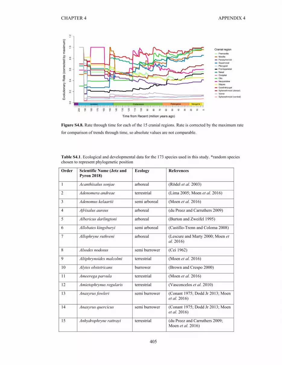
CHAPTER 4 APPENDIX 4
405
Figure S4.8. Rate through time for each of the 15 cranial regions. Rate is corrected by the maximum rate
for comparison of trends through time, so absolute values are not comparable.
Table S4.1. Ecological and developmental data for the 173 species used in this study. *random species chosen to represent phylogenetic position
Order Scientific Name (Jetz and Pyron 2018)
Ecology References
1 Acanthixalus sonjae arboreal (Rödel et al. 2003)
2 Adenomera andreae terrestrial (Lima 2005; Moen et al. 2016)
3 Adenomus kelaartii semi arboreal (Moen et al. 2016)
4 Afrixalus aureus arboreal (du Preez and Carruthers 2009)
5 Albericus darlingtoni arboreal (Burton and Zweifel 1995)
6 Allobates kingsburyi semi arboreal (Castillo-Trenn and Coloma 2008)
7 Allophryne ruthveni arboreal (Lescure and Marty 2000; Moen et al. 2016)
8 Alsodes nodosus semi burrower (Cei 1962)
9 Altiphrynoides malcolmi terrestrial (Moen et al. 2016)
10 Alytes obstetricans burrower (Brown and Crespo 2000)
11 Ameerega parvula terrestrial (Moen et al. 2016)
12 Amietophrynus regularis terrestrial (Vasconcelos et al. 2010)
13 Anaxyrus fowleri semi burrower (Conant 1975; Dodd Jr 2013; Moen et al. 2016)
14 Anaxyrus quercicus semi burrower (Conant 1975; Dodd Jr 2013; Moen et al. 2016)
15 Anhydrophryne rattrayi terrestrial (du Preez and Carruthers 2009; Moen et al. 2016)

CHAPTER 4 APPENDIX 4
406
16 Anotheca spinosa arboreal (Moen et al. 2016)
17 Ansonia mcgregori semi aquatic (Toledo-Bruno et al. 2017)
18 Aromobates alboguttatus semi aquatic (Moen et al. 2016)
19 Arthroleptella lightfooti terrestrial (du Preez and Carruthers 2009)
20 Arthroleptis bioko terrestrial (Blackburn et al. 2010)
21 Ascaphus truei semi aquatic (Moen et al. 2016; Hobbs et al. 2019)
22 Astylosternus diadematus semi aquatic (Moen et al. 2016)
23 Astylosternus occidentalis terrestrial (Rödel 2005; Hillers et al. 2008)
24 Atelopus ignescens terrestrial (Moen et al. 2016)
25 Atelopus oxyrhynchus terrestrial (Dole and Durant 1974; Simon and Toft 1991)
26 Balebreviceps hillmani semi burrower (Largen and Drewes 1989; Moen et al. 2016)
27 Barbourula busuangensis aquatic (Moen et al. 2016)
28 Barycholos pulcher terrestrial (Moen et al. 2016)
29 Batrachyla taeniata terrestrial (Moen et al. 2016)
30 Bombina maxima aquatic (Vitt and Caldwell 2014)
31 Boophis boehmei arboreal (Glaw and Vences 1994; Moen et al. 2016)
32 Brachycephalus ephippium terrestrial (Moen et al. 2016)
33 Brachytarsophrys carinense terrestrial (Tapley et al. 2017)
34 Cacosternum namaquense terrestrial (du Preez and Carruthers 2009; Moen et al. 2016; Rebelo and Measey 2019)
35 Callulina kisiwamsitu arboreal (Moen et al. 2016; IUCN 2019)
36 Calyptocephalella gayi aquatic (Moen et al. 2016)
37 Capensibufo rosei* terrestrial (du Preez and Carruthers 2009)
38 Cardioglossa elegans arboreal (Plath et al. 2004)
39 Cardioglossa manengouba terrestrial (Moen et al. 2016)
40 Centrolene buckleyi semi arboreal (Moen et al. 2016)
41 Ceratobatrachus guentheri terrestrial (Fuiten 2012)
42 Ceratophrys aurita burrower (Nomura et al. 2009)
43 Ceuthomantis smaragdinus semi arboreal (Moen et al. 2016)
44 Chacophrys pierottii burrower (Moen et al. 2016)
45 Chiromantis rufescens arboreal (Schiøtz 1999)
46 Chrysobatrachus terrestrial (Laurent 1964)

CHAPTER 4 APPENDIX 4
407
cupreonitens
47 Cochranella granulosa arboreal (Savage 2002; Moen et al. 2016)
48 Conraua beccarii aquatic (Moen et al. 2016)
49 Conraua crassipes semi aquatic (Plath et al. 2004; Moen et al. 2016)
50 Conraua goliath aquatic (Vitt and Caldwell 2014; Moen et al. 2016)
51 Craugastor laticeps terrestrial (Moen et al. 2016)
52 Crossodactylus trachystomus
terrestrial (Moen et al. 2016)
53 Cruziohyla calcarifer arboreal (Savage 2002; Moen et al. 2016)
54 Cryptobatrachus boulengeri semi aquatic (Moen et al. 2016)
55 Cryptothylax greshoffii arboreal (Moen et al. 2016)
56 Cycloramphus asper semi aquatic (Moen et al. 2016; IUCN 2019)
57 Cyclorana longipes terrestrial (Cogger 2000)
58 Dendrobates auratus* NA NA;
59 Discodeles bufoniformis semi aquatic (Fuiten 2012; Pikacha et al. 2016)
60 Duttaphrynus dodsoni terrestrial (AmphibiaWeb 2019)
61 Ecnomiohyla tuberculosa arboreal (Moen et al. 2016)
62 Eleutherodactylus glaphycompus
semi arboreal (IUCN 2019)
63 Eleutherodactylus johnstonei
semi arboreal (Ovaska 1991; Kaiser 1997)
64 Eupsophus roseus terrestrial (Moen et al. 2016)
65 Fejervarya cancrivora semi aquatic (Moen et al. 2016)
66 Fejervarya nilagirica terrestrial (IUCN 2019)
67 Fejervarya vittigera terrestrial (Shuman-Goodier et al. 2017)
68 Fritziana goeldii arboreal (IUCN 2019)
69 Gastrophryne carolinensis semi burrower (Conant 1975; Moen et al. 2016)
70 Gastrotheca peruana terrestrial (Hertwig and Sinsch 1995)
71 Guibemantis liber arboreal (Glaw and Vences 1994; Moen et al. 2016)
72 Haddadus binotatus terrestrial (Coco et al. 2014)
73 Hadromophryne natalensis semi aquatic (du Preez and Carruthers 2009; Moen et al. 2016)
74 Heleioporus australiacus semi burrower (Cogger 2000)
75 Heleophryne purcelli semi aquatic (du Preez and Carruthers 2009)

CHAPTER 4 APPENDIX 4
408
76 Hemiphractus proboscideus arboreal (Moen et al. 2016)
77 Hemisus guineensis burrower (Moen et al. 2016)
78 Hoplophryne uluguruensis arboreal (Moen et al. 2016)
79 Hyalinobatrachium fleischmanni
arboreal (Savage 2002)
80 Hylodes perplicatus terrestrial (Moen et al. 2016)
81 Hylorina sylvatica terrestrial (Moen et al. 2016)
82 Hyperolius viridiflavus arboreal (Moen et al. 2016)
83 Hypodactylus araiodactylus terrestrial (Duellman and Lehr 2009)
84 Hypsiboas boans arboreal (Lescure and Marty 2000)
85 Incilius periglenes burrower (Crump et al. 1992; Moen et al. 2016)
86 Indirana gundia terrestrial (Nair et al. 2012)
87 Ingerana tasanae terrestrial (Manthey and Grossmann 1997)
88 Kassina arboricola arboreal (Portik and Blackburn 2016)
89 Lankanectes corrugatus aquatic (Pethiyagoda et al. 2015)
90 Leiopelma hamiltoni terrestrial (Bell 1978)
91 Leptobrachium hasseltii terrestrial (Manthey and Grossmann 1997; Moen et al. 2016)
92 Leptodactylodon boulengeri terrestrial (Plath et al. 2004)
93 Leptodactylus melanonotus terrestrial (Savage 2002)
94 Leptodactylus podicipinus terrestrial (Martins 1996)
95 Leptopelis ocellatus arboreal (Schiøtz 1999)
96 Leptopelis spiritusnoctis arboreal (Rödel 2007)
97 Limnomedusa macroglossa terrestrial (Guerra et al. 2018)
98 Limnonectes macrocephalus semi aquatic (IUCN 2019)
99 Litoria aurea semi aquatic (Cogger 2000)
100 Mannophryne herminae terrestrial (Moen et al. 2016)
101 Mantella baroni terrestrial (Glaw and Vences 1994)
102 Melanobatrachus indicus terrestrial (Moen et al. 2016)
103 Melanophryniscus stelzneri terrestrial (IUCN 2019)
104 Mertensophryne micranotis arboreal (Grandison and Ashe 1983)
105 Microbatrachella capensis terrestrial (du Preez and Carruthers 2009; Moen et al. 2016)
106 Morerella cyanophthalma arboreal (Rödel et al. 2009)
107 Myobatrachus gouldii burrower (Cogger 2000)

CHAPTER 4 APPENDIX 4
409
108 Nasikabatrachus sahyadrensis
burrower (Radhakrishnan et al. 2019)
109 Natalobatrachus bonebergi semi arboreal (du Preez and Carruthers 2009; Rebelo and Measey 2019)
110 Nectophrynoides tornieri semi arboreal (Moen et al. 2016)
111 Nectophrynoides viviparus terrestrial (Moen et al. 2016)
112 Nothophryne broadleyi terrestrial (Conradie et al. 2018)
113 Nyctibates corrugatus terrestrial (Dewynter et al. 2017)
114 Nyctimystes daymani semi aquatic (Zweifel R.G 1958)
115 Nyctixalus pictus arboreal (Moen et al. 2016)
116 Nyctixalus spinosus arboreal (Alcala and Brown 1998)
117 Occidozyga lima semi aquatic (Manthey and Grossmann 1997)
118 Odontobatrachus natator semi aquatic (Barej et al. 2015)
119 Odontophrynus americanus burrower (Moen et al. 2016)
120 Oreobates quixensis terrestrial (Moen et al. 2016)
121 Osteocephalus buckleyi arboreal (Lescure and Marty 2000; Moen et al. 2016)
122 Osteopilus septentrionalis semi arboreal (Moen et al. 2016)
123 Paracassina obscura terrestrial (Schiøtz 1999)
124 Pelobates fuscus burrower (Moen et al. 2016)
125 Pelodytes caucasicus terrestrial (Moen et al. 2016)
126 Peltophryne guentheri terrestrial (Moen et al. 2016)
127 Petropedetes palmipes semi aquatic (Barej et al. 2010; Moen et al. 2016)
128 Phlyctimantis boulengeri arboreal (Schiøtz 1999)
129 Phrynobatrachus leveleve semi aquatic (Pollo 2018)
130 Phyllomedusa azurea arboreal (Moen et al. 2016)
131 Pipa parva aquatic (Moen et al. 2016)
132 Pipa pipa aquatic (Lescure and Marty 2000)
133 Platymantis polillensis arboreal (AmphibiaWeb 2019)
134 Plethodontohyla notosticta arboreal (Glaw and Vences 1994)
135 Polypedates macrotis arboreal (Manthey and Grossmann 1997; Moen et al. 2016)
136 Poyntonia paludicola terrestrial (du Preez and Carruthers 2009; Moen et al. 2016; Rebelo and Measey 2019)
137 Pristimantis chiastonotus terrestrial (Lescure and Marty 2000; Moen et al. 2016)

CHAPTER 4 APPENDIX 4
410
138 Probreviceps macrodactylus semi burrower (Moen et al. 2016)
139 Proceratophrys boiei semi burrower (Nomura et al. 2009; Moen et al. 2016)
140 Pseudacris ornata burrower (Conant 1975)
141 Pseudis paradoxa aquatic (Lescure and Marty 2000)
142 Ptychadena bibroni semi aquatic (Lamotte and A. 1997)
143 Pyxicephalus adspersus burrower (Moen et al. 2016; Rebelo and Measey 2019)
144 Ramanella montana arboreal Daniel 1963;
145 Rana clamitans semi aquatic (Conant 1975; Moen et al. 2016)
146 Rana sylvatica terrestrial (Moen et al. 2016)
147 Raorchestes anili* arboreal (AmphibiaWeb 2019)
148 Raorchestes glandulosus arboreal (Moen et al. 2016)
149 Rhacophorus reinwardtii arboreal (Manthey and Grossmann 1997; Moen et al. 2016)
150 Rheobatrachus silus aquatic (Cogger 2000)
151 Rhinoderma darwinii terrestrial (Moen et al. 2016)
152 Rhinophrynus dorsalis burrower (Trueb and Gans 1983; Moen et al. 2016)
153 Scaphiophryne madagascariensis
burrower (Glaw and Vences 1994; Moen et al. 2016)
154 Scaphiopus holbrookii burrower (Moen et al. 2016)
155 Semnodactylus wealii terrestrial (du Preez and Carruthers 2009)
156 Sooglossus sechellensis terrestrial (Boettger 1896; Moen et al. 2016)
157 Spea multiplicata burrower (Moen et al. 2016)
158 Strabomantis biporcatus terrestrial (Moen et al. 2016)
159 Strabomantis cornutus terrestrial (Moen et al. 2016)
160 Strabomantis ingeri terrestrial (Moen et al. 2016)
161 Stumpffia pygmaea terrestrial (Glaw and Vences 1994; Moen et al. 2016)
162 Syncope antenori semi arboreal (Moen et al. 2016)
163 Telmatobius degener aquatic (Moen et al. 2016)
164 Telmatobius laticeps aquatic (Moen et al. 2016)
165 Thaumastosaurus gezei NA (fossil) NA
166 Theloderma stellatum arboreal (Poyarkov et al. 2018)
167 Thoropa miliaris terrestrial (Giaretta and Facure 2004; Lutz 2016; Moen et al. 2016)

CHAPTER 4 APPENDIX 4
411
168 Tomopterna marmorata burrower (du Preez and Carruthers 2009)
169 Trichobatrachus robustus semi aquatic (Vitt and Caldwell 2014)
170 Triprion petasatus arboreal (Lee 1996; Moen et al. 2016)
171 Vandijkophrynus gariepensis
terrestrial (du Preez and Carruthers 2009)
172 Xenopus laevis aquatic (du Preez and Carruthers 2009; Moen et al. 2016)
173 Xenorhina varia* NA (ignore this specimen)
NA
Table S4.2. Phylogenetic Principal Component (pPC) scores that capture 95% of the variation for each
cranial region and for the cranium. These pPC scores were used in BayesTraitsV3
(http://www.evolution.rdg.ac.uk/) to investigate changes in evolutionary rate through time.
Region pPC scores for 95%
Cranium 54
Frontoparietal 17
Maxilla 13
Nasal 10
Neopalatine 4
Occipital 16
Otic 12
Parasphenoid 12
Premaxilla 8
Pterygoid 10
Quadratojugal 4
Sphenethmoid(d) 5
Sphenethmoid(v) 10
Squamosal 12
Stapes 3
Vomer 6

CHAPTER 4 APPENDIX 4
412
Table S4.3. Parameters used for MCMC analysis, using the program BayesTraitsV3
(http://www.evolution.rdg.ac.uk/).
Region Iterations / x 106
Original burn-in / x 106
Additional number of rows deleted as burn-in
Sample Stones (stones/iterations)
Cranium 200 25 2000 20000 500 / 5000
Frontoparietal 200 25 4000 20000 500 / 5000
Maxilla 100 12.5 0 10000 500 / 5000
Nasal 100 12.5 0 10000 500 / 5000
Neopalatine 100 12.5 0 10000 500 / 5000
Occipital 100 12.5 3757 10000 500 / 5000
Otic 200 25 0 20000 500 / 5000
Parasphenoid 100 12.5 0 10000 500 / 5000
Premaxilla 100 12.5 0 10000 500 / 5000
Pterygoid 500 50 0 50000 500 / 5000
Quadratojugal 100 12.5 0 10000 500 / 5000
Sphenethmoid(d) 500 50 4000 50000 500 / 5000
Sphenethmoid(v) 200 25 0 20000 500 / 5000
Squamosal 500 50 0 50000 500 / 5000
Stapes 100 12.5 0 10000 500 / 5000
Vomer 500 50 0 50000 500 / 5000

413
CH
AP
TE
R 4
AP
PE
ND
IX 4
Table S4.4. Summary of the PC axes for the full landmark and semilandmark dataset. 46 of the 172 PC axes were required to explain 95% of cranial shape variation.
PC1 PC2 PC3 PC4 PC5 PC6 PC7 PC8 PC9 PC10
Standard deviation 0.057274 0.040853 0.030468 0.024258 0.022726 0.020868 0.019555 0.017219 0.016978 0.016295
Proportion of Variance 0.2795 0.1422 0.0791 0.05014 0.044 0.0371 0.03258 0.02526 0.02456 0.02263
Cumulative Proportion 0.2795 0.4217 0.50079 0.55093 0.59494 0.63204 0.66462 0.68988 0.71444 0.73707
PC11 PC12 PC13 PC14 PC15 PC16 PC17 PC18 PC19 PC20
Standard deviation 0.014362 0.013588 0.013248 0.012549 0.011563 0.011173 0.010621 0.010396 0.010165 0.009781
Proportion of Variance 0.01757 0.01573 0.01495 0.01342 0.01139 0.01064 0.00961 0.00921 0.0088 0.00815
Cumulative Proportion 0.75464 0.77037 0.78533 0.79874 0.81014 0.82077 0.83038 0.83959 0.8484 0.85655
PC21 PC22 PC23 PC24 PC25 PC26 PC27 PC28 PC29 PC30
Standard deviation 0.009348 0.008902 0.008557 0.008326 0.007968 0.007853 0.007564 0.007383 0.007179 0.006862
Proportion of Variance 0.00745 0.00675 0.00624 0.00591 0.00541 0.00525 0.00488 0.00464 0.00439 0.00401
Cumulative Proportion 0.86399 0.87074 0.87698 0.88289 0.8883 0.89356 0.89843 0.90307 0.90747 0.91148
PC31 PC32 PC33 PC34 PC35 PC36 PC37 PC38 PC39 PC40
Standard deviation 0.006568 0.006222 0.005981 0.005891 0.005726 0.005619 0.005445 0.005408 0.005237 0.005092
Proportion of Variance 0.00368 0.0033 0.00305 0.00296 0.00279 0.00269 0.00253 0.00249 0.00234 0.00221
Cumulative Proportion 0.91515 0.91845 0.9215 0.92446 0.92725 0.92994 0.93247 0.93496 0.9373 0.93951
PC41 PC42 PC43 PC44 PC45 PC46 PC47 PC48 PC49 PC50
Standard deviation 0.00504 0.004889 0.004801 0.004755 0.004656 0.004591 0.004427 0.004353 0.00427 0.004188
Proportion of Variance 0.00216 0.00204 0.00196 0.00193 0.00185 0.0018 0.00167 0.00161 0.00155 0.00149
Cumulative Proportion 0.94167 0.94371 0.94567 0.9476 0.94944 0.95124 0.95291 0.95452 0.95608 0.95757
PC51 PC52 PC53 PC54 PC55 PC56 PC57 PC58 PC59 PC60
Standard deviation 0.004043 0.003942 0.003889 0.003784 0.003761 0.003684 0.003615 0.003523 0.00347 0.003442
Proportion of Variance 0.00139 0.00132 0.00129 0.00122 0.00121 0.00116 0.00111 0.00106 0.00103 0.00101
Cumulative Proportion 0.95897 0.96029 0.96158 0.9628 0.964 0.96516 0.96627 0.96733 0.96836 0.96937

414
CH
AP
TE
R 4
AP
PE
ND
IX 4
PC61 PC62 PC63 PC64 PC65 PC66 PC67 PC68 PC69 PC70
Standard deviation 0.003322 0.003278 0.003201 0.003144 0.003115 0.003095 0.003027 0.002925 0.002871 0.002861
Proportion of Variance 0.00094 0.00092 0.00087 0.00084 0.00083 0.00082 0.00078 0.00073 7.00E-04 7.00E-04
Cumulative Proportion 0.97031 0.97122 0.9721 0.97294 0.97376 0.97458 0.97536 0.97609 0.97679 0.97749
PC71 PC72 PC73 PC74 PC75 PC76 PC77 PC78 PC79 PC80
Standard deviation 0.002852 0.002757 0.002733 0.002713 0.002681 0.002648 0.002546 0.0025 0.002483 0.002465
Proportion of Variance 0.00069 0.00065 0.00064 0.00063 0.00061 6.00E-04 0.00055 0.00053 0.00053 0.00052
Cumulative Proportion 0.97818 0.97883 0.97947 0.98009 0.98071 0.9813 0.98186 0.98239 0.98291 0.98343
PC81 PC82 PC83 PC84 PC85 PC86 PC87 PC88 PC89 PC90
Standard deviation 0.002392 0.002356 0.00234 0.002301 0.002222 0.002205 0.002199 0.002168 0.002152 0.002117
Proportion of Variance 0.00049 0.00047 0.00047 0.00045 0.00042 0.00041 0.00041 4.00E-04 0.00039 0.00038
Cumulative Proportion 0.98392 0.98439 0.98486 0.98531 0.98573 0.98615 0.98656 0.98696 0.98735 0.98773
PC91 PC92 PC93 PC94 PC95 PC96 PC97 PC98 PC99 PC100
Standard deviation 0.002093 0.002053 0.002013 0.001968 0.001942 0.001919 0.0019 0.001874 0.001826 0.001797
Proportion of Variance 0.00037 0.00036 0.00035 0.00033 0.00032 0.00031 0.00031 3.00E-04 0.00028 0.00027
Cumulative Proportion 0.98811 0.98847 0.98881 0.98914 0.98946 0.98978 0.99008 0.99038 0.99067 0.99094
PC101 PC102 PC103 PC104 PC105 PC106 PC107 PC108 PC109 PC110
Standard deviation 0.001783 0.001758 0.001751 0.00172 0.001704 0.001687 0.001661 0.001641 0.001634 0.001606
Proportion of Variance 0.00027 0.00026 0.00026 0.00025 0.00025 0.00024 0.00024 0.00023 0.00023 0.00022
Cumulative Proportion 0.99121 0.99148 0.99174 0.99199 0.99224 0.99248 0.99272 0.99295 0.99317 0.99339
PC111 PC112 PC113 PC114 PC115 PC116 PC117 PC118 PC119 PC120
Standard deviation 0.001581 0.001555 0.001544 0.001541 0.001511 0.001486 0.001469 0.001442 0.00144 0.001429
Proportion of Variance 0.00021 0.00021 2.00E-04 2.00E-04 0.00019 0.00019 0.00018 0.00018 0.00018 0.00017
Cumulative Proportion 0.99361 0.99381 0.99401 0.99422 0.99441 0.9946 0.99478 0.99496 0.99514 0.99531

415
CH
AP
TE
R 4
AP
PE
ND
IX 4
PC121 PC122 PC123 PC124 PC125 PC126 PC127 PC128 PC129 PC130
Standard deviation 0.001401 0.001388 0.001357 0.00134 0.001324 0.001304 0.001284 0.001259 0.00125 0.001232
Proportion of Variance 0.00017 0.00016 0.00016 0.00015 0.00015 0.00014 0.00014 0.00014 0.00013 0.00013
Cumulative Proportion 0.99548 0.99564 0.9958 0.99595 0.9961 0.99625 0.99639 0.99652 0.99666 0.99678
PC131 PC132 PC133 PC134 PC135 PC136 PC137 PC138 PC139 PC140
Standard deviation 0.001204 0.001196 0.001179 0.001168 0.001161 0.001135 0.001121 0.001108 0.001095 0.001082
Proportion of Variance 0.00012 0.00012 0.00012 0.00012 0.00011 0.00011 0.00011 1.00E-04 1.00E-04 1.00E-04
Cumulative Proportion 0.99691 0.99703 0.99715 0.99726 0.99738 0.99749 0.9976 0.9977 0.9978 0.9979
PC141 PC142 PC143 PC144 PC145 PC146 PC147 PC148 PC149 PC150
Standard deviation 0.001069 0.001052 0.001036 0.001031 0.001016 0.000998 0.000986 0.000971 0.000969 0.000958
Proportion of Variance 1.00E-04 9.00E-05 9.00E-05 9.00E-05 9.00E-05 8.00E-05 8.00E-05 8.00E-05 8.00E-05 8.00E-05
Cumulative Proportion 0.998 0.99809 0.99819 0.99828 0.99836 0.99845 0.99853 0.99861 0.99869 0.99877
PC151 PC152 PC153 PC154 PC155 PC156 PC157 PC158 PC159 PC160
Standard deviation 0.000946 0.000931 0.000903 0.000902 0.000879 0.000868 0.000863 0.00085 0.000838 0.00083
Proportion of Variance 8.00E-05 7.00E-05 7.00E-05 7.00E-05 7.00E-05 6.00E-05 6.00E-05 6.00E-05 6.00E-05 6.00E-05
Cumulative Proportion 0.99885 0.99892 0.99899 0.99906 0.99913 0.99919 0.99925 0.99931 0.99937 0.99943
PC161 PC162 PC163 PC164 PC165 PC166 PC167 PC168 PC169 PC170
Standard deviation 0.000822 0.000809 0.000803 0.00078 0.000769 0.000751 0.000732 0.000722 0.000702 0.0007
Proportion of Variance 6.00E-05 6.00E-05 5.00E-05 5.00E-05 5.00E-05 5.00E-05 5.00E-05 4.00E-05 4.00E-05 4.00E-05
Cumulative Proportion 0.99949 0.99955 0.9996 0.99965 0.9997 0.99975 0.9998 0.99984 0.99988 0.99993
PC171 PC172
Standard deviation 0.000676 0.000648
Proportion of Variance 4.00E-05 4.00E-05
Cumulative Proportion 0.99996 1

416
CH
AP
TE
R 4
AP
PE
ND
IX 4
Table S4.5. Pairwise significance values for differences in cranial disparity for the seven microhabitats, for each cranial region. Bold values indicate significant (p < 0.05)
values.
Frontoparietal aquatic arboreal burrower semi aquatic semi arboreal semi burrower
aquatic
arboreal 0.01
burrower 0.24 0.11
semi aquatic < 0.01 0.20 0.01
semi arboreal 0.06 0.98 0.26 0.38
semi burrower 0.14 0.57 0.58 0.18 0.65
terrestrial < 0.01 0.27 0.01 0.70 0.53 0.20
Maxilla aquatic arboreal burrower semi aquatic semi arboreal semi burrower
aquatic
arboreal 0.09
burrower 0.95 0.09
semi aquatic 0.03 0.35 0.01
semi arboreal 0.19 0.97 0.19 0.51
semi burrower 0.26 0.01 0.22 < 0.01 0.03
terrestrial 0.02 0.42 0.02 0.71 0.67 0.01
Nasal aquatic arboreal burrower semi aquatic semi arboreal semi burrower
aquatic
arboreal 0.36
burrower 0.29 0.03
semi aquatic 0.07 0.16 0.01
semi arboreal 0.37 0.80 0.05 0.44

417
CH
AP
TE
R 4
AP
PE
ND
IX 4
semi burrower 0.38 0.83 0.08 0.42 0.99
terrestrial 0.03 0.06 < 0.01 0.98 0.35 0.40
Neopalatine aquatic arboreal burrower semi aquatic semi arboreal semi burrower
aquatic
arboreal < 0.01
burrower 0.36 0.02
semi aquatic 0.01 0.84 0.03
semi arboreal 0.01 0.80 0.05 0.90
semi burrower 0.55 0.06 0.86 0.07 0.09
terrestrial < 0.01 0.82 0.01 0.99 0.87 0.04
Occipital aquatic arboreal burrower semi aquatic semi arboreal semi burrower
aquatic
arboreal 0.05
burrower 0.93 0.05
semi aquatic 0.05 0.83 0.05
semi arboreal 0.09 0.79 0.08 0.92
semi burrower 0.42 0.03 0.37 0.03 0.04
terrestrial 0.02 0.53 0.01 0.79 0.94 0.01
Otic aquatic arboreal burrower semi aquatic semi arboreal semi burrower
aquatic
arboreal 0.25
burrower 0.30 0.03
semi aquatic 0.18 0.61 0.02
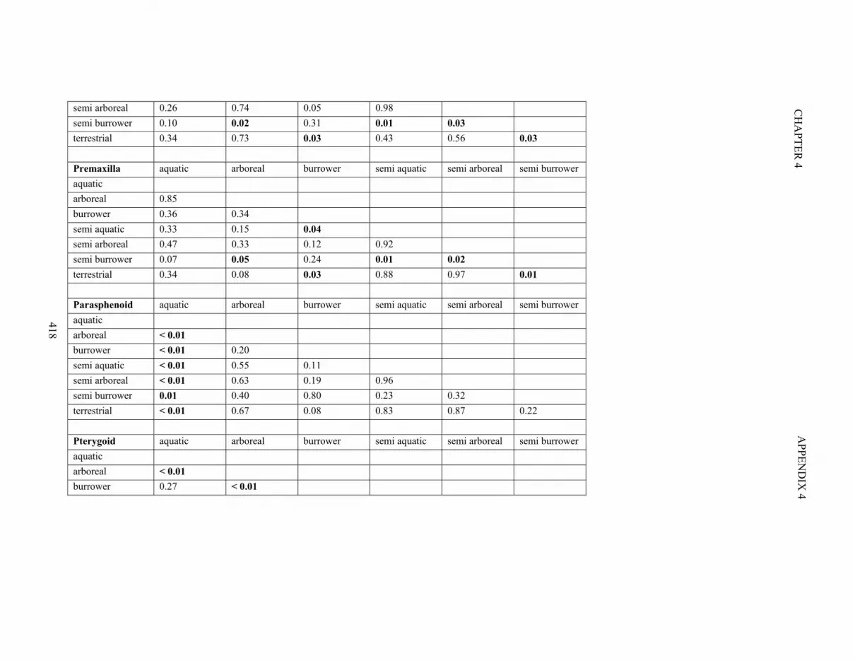
418
CH
AP
TE
R 4
AP
PE
ND
IX 4
semi arboreal 0.26 0.74 0.05 0.98
semi burrower 0.10 0.02 0.31 0.01 0.03
terrestrial 0.34 0.73 0.03 0.43 0.56 0.03
Premaxilla aquatic arboreal burrower semi aquatic semi arboreal semi burrower
aquatic
arboreal 0.85
burrower 0.36 0.34
semi aquatic 0.33 0.15 0.04
semi arboreal 0.47 0.33 0.12 0.92
semi burrower 0.07 0.05 0.24 0.01 0.02
terrestrial 0.34 0.08 0.03 0.88 0.97 0.01
Parasphenoid aquatic arboreal burrower semi aquatic semi arboreal semi burrower
aquatic
arboreal < 0.01
burrower < 0.01 0.20
semi aquatic < 0.01 0.55 0.11
semi arboreal < 0.01 0.63 0.19 0.96
semi burrower 0.01 0.40 0.80 0.23 0.32
terrestrial < 0.01 0.67 0.08 0.83 0.87 0.22
Pterygoid aquatic arboreal burrower semi aquatic semi arboreal semi burrower
aquatic
arboreal < 0.01
burrower 0.27 < 0.01

419
CH
AP
TE
R 4
AP
PE
ND
IX 4
semi aquatic < 0.01 0.78 < 0.01
semi arboreal < 0.01 0.67 0.01 0.87
semi burrower 0.11 0.10 0.29 0.11 0.11
terrestrial < 0.01 0.66 < 0.01 0.95 0.90 0.07
Quadratojugal aquatic arboreal burrower semi aquatic semi arboreal semi burrower
aquatic
arboreal 0.02
burrower 0.15 < 0.01
semi aquatic 0.02 0.87 < 0.01
semi arboreal 0.02 0.69 0.01 0.77
semi burrower 0.07 < 0.01 0.45 < 0.01 < 0.01
terrestrial 0.01 0.95 < 0.01 0.91 0.71 < 0.01
Sphenethmoid (dorsal)
aquatic arboreal burrower semi aquatic semi arboreal semi burrower
aquatic
arboreal 0.11
burrower 0.28 0.67
semi aquatic 0.03 0.28 0.19
semi arboreal 0.09 0.65 0.46 0.73
semi burrower 0.56 0.45 0.69 0.15 0.31
terrestrial 0.11 0.78 0.77 0.16 0.53 0.53

420
CH
AP
TE
R 4
AP
PE
ND
IX 4
Sphenethmoid (ventral)
aquatic arboreal burrower semi aquatic semi arboreal semi burrower
aquatic
arboreal < 0.01
burrower 0.04 0.15
semi aquatic < 0.01 0.27 0.03
semi arboreal < 0.01 0.29 0.05 0.86
semi burrower 0.01 0.92 0.27 0.51 0.46
terrestrial < 0.01 0.84 0.09 0.31 0.33 0.99
Squamosal aquatic arboreal burrower semi aquatic semi arboreal semi burrower
aquatic
arboreal 0.04
burrower 0.04 < 0.01
semi aquatic 0.04 0.66 < 0.01
semi arboreal 0.10 0.82 0.01 0.90
semi burrower 0.28 0.03 0.42 0.02 0.04
terrestrial 0.04 0.99 < 0.01 0.64 0.81 0.03
Stapes aquatic arboreal burrower semi aquatic semi arboreal semi burrower
aquatic
arboreal 0.08
burrower 0.70 0.01
semi aquatic 0.15 0.86 0.04
semi arboreal 0.08 0.58 0.02 0.53
semi burrower 0.92 0.17 0.64 0.25 0.15
terrestrial 0.33 0.21 0.10 0.41 0.17 0.51

421
CH
AP
TE
R 4
AP
PE
ND
IX 4
Vomer aquatic arboreal burrower semi aquatic semi arboreal semi burrower
aquatic
arboreal 0.34
burrower 0.05 < 0.01
semi aquatic 0.21 0.52 < 0.01
semi arboreal 0.58 0.69 0.04 0.37
semi burrower 1.00 0.34 0.10 0.23 0.61
terrestrial 0.27 0.90 < 0.01 0.56 0.61 0.31

422
CH
AP
TE
R 4
AP
PE
ND
IX 4
Table S4.6. Pairwise significance values for differences in rate of cranial evolution for the seven microhabitats, for each cranial region. Bold values indicate significant (p <
0.05) values.
Frontoparietal aquatic arboreal burrower semi aquatic semi arboreal semi burrower
aquatic
arboreal 0.91
burrower 0.81 0.78
semi aquatic < 0.01 < 0.01 < 0.01
semi arboreal 0.94 0.68 0.88 < 0.01
semi burrower 0.90 0.96 0.81 0.01 0.72
terrestrial 0.22 0.31 0.05 < 0.01 0.31 0.58
Maxilla aquatic arboreal burrower semi aquatic semi arboreal semi burrower
aquatic
arboreal 1.00
burrower 0.67 0.89
semi aquatic 0.30 0.06 0.02
semi arboreal 0.95 0.45 0.63 0.42
semi burrower 0.92 0.17 0.91 0.02 0.09
terrestrial 0.92 0.61 0.33 0.04 0.87 0.16
Nasal aquatic arboreal burrower semi aquatic semi arboreal semi burrower
aquatic
arboreal 1.00
burrower 0.80 0.92
semi aquatic 0.20 0.03 0.02
semi arboreal 0.88 0.27 0.56 0.48

423
CH
AP
TE
R 4
AP
PE
ND
IX 4
semi burrower 0.97 0.69 0.83 0.28 0.61
terrestrial 0.32 0.01 0.01 0.68 0.54 0.31
Neopalatine aquatic arboreal burrower semi aquatic semi arboreal semi burrower
aquatic
arboreal 1.00
burrower 0.23 0.44
semi aquatic 0.05 < 0.01 < 0.01
semi arboreal 0.68 0.14 0.09 0.29
semi burrower 0.94 0.67 0.38 0.09 0.46
terrestrial 0.91 0.63 0.08 < 0.01 0.35 0.95
Occipital aquatic arboreal burrower semi aquatic semi arboreal semi burrower
aquatic
arboreal 0.31
burrower 0.36 0.51
semi aquatic 0.17 0.90 0.31
semi arboreal 0.13 0.32 0.21 0.40
semi burrower 0.97 0.02 0.57 0.08 0.01
terrestrial 0.03 0.53 0.07 0.39 0.66 0.01
Otic aquatic arboreal burrower semi aquatic semi arboreal semi burrower
aquatic
arboreal 0.97
burrower 0.38 0.30
semi aquatic 0.32 0.30 0.01
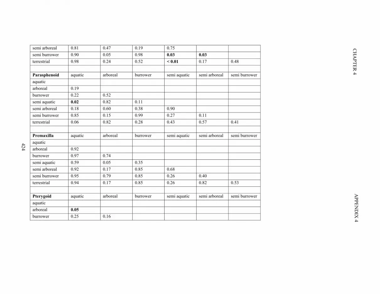
424
CH
AP
TE
R 4
AP
PE
ND
IX 4
semi arboreal 0.81 0.47 0.19 0.75
semi burrower 0.90 0.05 0.98 0.03 0.03
terrestrial 0.98 0.24 0.52 < 0.01 0.17 0.48
Parasphenoid aquatic arboreal burrower semi aquatic semi arboreal semi burrower
aquatic
arboreal 0.19
burrower 0.22 0.52
semi aquatic 0.02 0.82 0.11
semi arboreal 0.18 0.60 0.38 0.90
semi burrower 0.85 0.15 0.99 0.27 0.11
terrestrial 0.06 0.82 0.28 0.43 0.57 0.41
Premaxilla aquatic arboreal burrower semi aquatic semi arboreal semi burrower
aquatic
arboreal 0.92
burrower 0.97 0.74
semi aquatic 0.59 0.05 0.35
semi arboreal 0.92 0.17 0.85 0.68
semi burrower 0.95 0.79 0.85 0.26 0.40
terrestrial 0.94 0.17 0.85 0.26 0.82 0.53
Pterygoid aquatic arboreal burrower semi aquatic semi arboreal semi burrower
aquatic
arboreal 0.05
burrower 0.25 0.16

425
CH
AP
TE
R 4
AP
PE
ND
IX 4
semi aquatic < 0.01 0.30 < 0.01
semi arboreal 0.02 0.19 0.05 0.95
semi burrower 0.65 0.16 0.85 0.08 0.03
terrestrial < 0.01 0.44 < 0.01 0.53 0.65 0.09
Quadratojugal aquatic arboreal burrower semi aquatic semi arboreal semi burrower
aquatic
arboreal 0.30
burrower 0.83 0.04
semi aquatic 0.03 0.48 < 0.01
semi arboreal 0.15 0.38 0.03 0.90
semi burrower 0.80 < 0.01 0.74 < 0.01 < 0.01
terrestrial 0.20 0.75 0.01 0.19 0.31 0.01
Sphenethmoid (dorsal)
aquatic arboreal burrower semi aquatic semi arboreal semi burrower
aquatic
arboreal 0.98
burrower 0.14 0.19
semi aquatic 0.06 0.01 < 0.01
semi arboreal 0.91 0.69 0.19 0.12
semi burrower 0.94 0.35 0.72 0.01 0.28
terrestrial 0.98 0.58 0.15 < 0.01 0.45 0.71

426
CH
AP
TE
R 4
AP
PE
ND
IX 4
Sphenethmoid (ventral)
aquatic arboreal burrower semi aquatic semi arboreal semi burrower
aquatic
arboreal 0.67
burrower 0.24 0.92
semi aquatic < 0.01 < 0.01 < 0.01
semi arboreal 0.02 0.01 0.06 0.94
semi burrower 0.97 0.20 0.87 < 0.01 < 0.01
terrestrial 0.45 0.85 0.83 < 0.01 0.01 0.43
Squamosal aquatic arboreal burrower semi aquatic semi arboreal semi burrower
aquatic
arboreal 0.34
burrower 0.22 < 0.01
semi aquatic 0.08 0.89 < 0.01
semi arboreal 0.26 0.53 < 0.01 0.80
semi burrower 0.98 < 0.01 0.86 0.01 < 0.01
terrestrial 0.29 0.57 < 0.01 0.30 0.38 0.03
Stapes aquatic arboreal burrower semi aquatic semi arboreal semi burrower
aquatic
arboreal 0.77
burrower 0.13 0.02
semi aquatic 0.60 0.96 0.02
semi arboreal 0.20 0.11 < 0.01 0.18
semi burrower 0.22 < 0.01 0.62 0.01 < 0.01
terrestrial 0.78 0.04 0.24 0.07 0.01 0.07

427
CH
AP
TE
R 4
AP
PE
ND
IX 4
Vomer aquatic arboreal burrower semi aquatic semi arboreal semi burrower
aquatic
arboreal 0.79
burrower 0.02 < 0.01
semi aquatic 0.07 0.16 < 0.01
semi arboreal 0.94 0.38 0.08 0.09
semi burrower 0.52 0.41 < 0.01 0.69 0.19
terrestrial 0.85 0.43 < 0.01 0.01 0.83 0.22
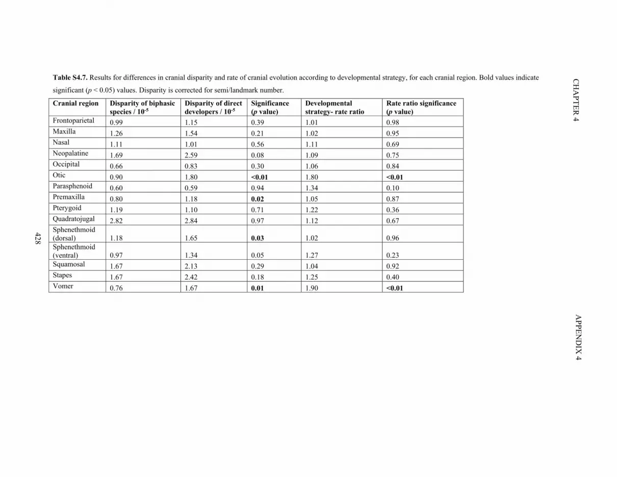
428
CH
AP
TE
R 4
AP
PE
ND
IX 4
Table S4.7. Results for differences in cranial disparity and rate of cranial evolution according to developmental strategy, for each cranial region. Bold values indicate
significant (p < 0.05) values. Disparity is corrected for semi/landmark number.
Cranial region Disparity of biphasic species / 10-5
Disparity of direct developers / 10-5
Significance (p value)
Developmental strategy- rate ratio
Rate ratio significance (p value)
Frontoparietal 0.99 1.15 0.39 1.01 0.98 Maxilla 1.26 1.54 0.21 1.02 0.95 Nasal 1.11 1.01 0.56 1.11 0.69 Neopalatine 1.69 2.59 0.08 1.09 0.75 Occipital 0.66 0.83 0.30 1.06 0.84 Otic 0.90 1.80 <0.01 1.80 <0.01 Parasphenoid 0.60 0.59 0.94 1.34 0.10 Premaxilla 0.80 1.18 0.02 1.05 0.87 Pterygoid 1.19 1.10 0.71 1.22 0.36 Quadratojugal 2.82 2.84 0.97 1.12 0.67 Sphenethmoid (dorsal) 1.18 1.65 0.03 1.02 0.96 Sphenethmoid (ventral) 0.97 1.34 0.05 1.27 0.23 Squamosal 1.67 2.13 0.29 1.04 0.92 Stapes 1.67 2.42 0.18 1.25 0.40 Vomer 0.76 1.67 0.01 1.90 <0.01

CHAPTER 4 APPENDIX 4
429
References for Appendix 4
Alcala, A. C., and W. C. Brown. 1998. Philippine amphibians: illustrated field guide. Bookmark, Inc.,
Philippines. 116 pp.
AmphibiaWeb. 2019. AmphibiaWeb: Information on amphibian biology and conservation
<https://amphibiaweb.org>. University of California, Berkeley, CA, USA. Accessed 10 January
2019.
Barej, M. F., J. Penner, A. Schmitz, and M.-O. Rödel. 2015. Multiple genetic lineages challenge the
monospecific status of the West African endemic frog family Odontobatrachidae. BMC Evol. Biol.
15:1-16.
Barej, M. F., M. Rödel, L. N. Gonwouo, O. S. G. Pauwels, W. Böhme, and A. Schmitz. 2010. Review of
the genus Petropedetes Reichenow, 1874 in Central Africa with the description of three new
species (Amphibia: Anura: Petropedetidae). Zootaxa 2340:1–49.
Bell, B. D. 1978. Observations on the ecology and reproduction of the New Zealand leiopelmid frogs.
Herpetologica 34:340–354.
Blackburn, D. C., V. Gvoždík, and A. D. Leaché. 2010. A new squeaker frog (Arthroleptidae:
Arthroleptis) from the mountains of Cameroon and Nigeria. Herpetologica 66:335–348.
Boettger, O. 1896. Neue Kriechthiere (Scelotes, Arthroleptis) von den Seychellen. Zool. Anz. 19:349–
351.
Brown, L. E., and E. G. Crespo. 2000. Burrowing behavior of the midwife toads Alytes cisternasii and
Alytes obstetricans (Anura, Discoglossidae). Alytes. 17. 101–113.
Burton, and Zweifel. 1995. A new genus of Genyophrine microhylid frogs from New Guinea. Am. Mus.
Novit. 3129:1–7.
Castillo-Trenn, P., and L. A. Coloma. 2008. Notes on behaviour and reproduction in captive Allobates
kingsburyi (Anura: Dendrobatidae), with comments on evolution of reproductive amplexus. Int.
Zoo Yearb. 42:58–70.
Cei, J. . 1962. Batracios de Chile. Universidad de Chile, Santiago. 128 pp.
Coco, L., V. N. T. Borges, L. A. Fusinatto, M. C. Kiefer, J. C. F. Oliveira, P. G. Araujo, B. M. Costa, M.
Van Sluys, and C. F. D. Rocha. 2014. Feeding habits of the leaf litter frog Haddadus binotatus
(Anura, Craugastoridae) from two Atlantic forest areas in Southeastern Brazil. An. Acad. Bras.
Cienc. 86:239–249.
Cogger, H. G. 2000. Reptiles and amphibians of Australia. CSIRO Publishing, Port Melbourne. 1033 pp.
Conant, R. 1975. A field guide to reptiles and amphibians of Eastern and Central North America.
Houghton Mifflin Co., Boston. 640 pp.
Conradie, W., G. B. Bittencourt-Silva, H. M. Farooq, S. P. Loader, M. Menegon, and K. A. Tolley. 2018.

CHAPTER 4 APPENDIX 4
430
New species of Mongrel frogs (Pyxicephalidae: Nothophryne) for northern Mozambique inselbergs.
African J. Herpetol. 67:61–85.
Crump, M. L., F. R. Hensley, and K. L. Clark. 1992. Apparent decline of the golden toad: underground or
extinct? Copeia 1992:413–420.
Dewynter, M., L. Chirio, F. Melki, J. Cordier, and T. Fretey. 2017. Premières données herpétologiques
(Amphibiens et Reptiles) sur le massif du Koumouna-Bouali (Gabon). Les Cah. la Fond. Biotope
11:1–42.
Dodd Jr, C. K. 2013. Frogs of the United States and Canada Volume 1. The John Hopkins University
Press, Baltimore. 460 pp.
Dole, J. I. M. W., and P. Durant. 1974. Movements and seasonal activity of Atelopus oxyrhynchus
(Anura: Atelopodidae) in a Venezuelan cloud forest. Copeia 1974:230–235.
du Preez, L., and V. Carruthers. 2009. Frogs of Southern Africa: a complete guide. Struik Nature, Cape
Town. 519 pp.
Duellman, W. E., and E. Lehr. 2009. Terrestrial breeding frogs (Strabomantidae) in Peru. Nature und Tier
Verlag, Münster, Germany. 382 pp.
Fuiten, A. M. 2012. Skeletal variation in Melanesian forest frogs (Anura: Ceratobatrachidae). Master's
Thesis. 64 pp.
Giaretta, A. A., and K. G. Facure. 2004. Reproductive ecology and behavior of Thoropa miliaris (Spix,
1824) (Anura, Leptodactylidae, Telmatobiinae). Biota Neotrop. 4:1745–1758.
Glaw, F., and M. Vences. 1994. A fieldguide to the amphibians and reptiles of Madagascar. Vences and
Glaw Verlag, Cologne. 480 pp.
Grandison, A. G. C., and S. Ashe. 1983. The distribution, behavioural ecology and breeding strategy of
the pygmy toad, Mertensophryne micranotis. Bull. Br. Mus. Nat. Hist. 45:85–93.
Guerra, V., R. Lingnau, B. de S. Barreto, A. Kwet, and R. P. Bastos. 2018. Vocalizations of
Limnomedusa macroglossa (Amphibia: Anura: Alsodidae). Salamandra 54:97–100.
Hertwig, I., and U. Sinsch. 1995. Comparative toe pad morphology in marsupial frogs (Genus
Gastrotheca): arboreal versus ground-dwelling species. Copeia 1995:38–47.
Hillers, A., M. Veith, and M.-O. Rödel. 2008. Effects of forest fragmentation and habitat degradation on
West African leaf-litter frogs. Conserv. Biol. 22:762–772.
Hobbs, J., J. M. Round, M. J. Allison, and C. C. Helbing. 2019. Expansion of the known distribution of
the coastal tailed frog, Ascaphus truei, in British Columbia, Canada, using robust eDNA detection
methods. PLoS One 14:e0213849.
IUCN. 2019. The IUCN Red List of Threatened Species. version 2019-1. <http://www.iucnredlist.org>.

CHAPTER 4 APPENDIX 4
431
Downloaded on 1st February 2019.
Kaiser, H. 1997. Origins and introductions of the Caribbean frog, Eleutherodactylus johnstonei
(Leptodactylidae): management and conservation concerns. Biodivers. Conserv. 6:1391–1407.
Lamotte, M., and O. A. 1997. Redécouverte de syntypes de Rana bibroni Hallowell, 1845, désignation
d’un lectotype et description d’une espèce nouvelle de Ptychadena (Amphibia, Anura). Zoosystema
19:531–543.
Largen, M. J., and R. C. Drewes. 1989. A new genus and species of brevicipitine frog (Amphibia Anura
Microhylidae) from high altitude in the mountains of Ethiopia. Trop. Zool. 2:13–30.
Laurent, R. F. 1964. Adaptive modifications in frogs of an isolated highland fauna in Central Africa.
Evolution. 18:458–467.
Lee, J. C. 1996. The amphibians and reptiles of the Yucatan Peninsula. Cornell University Press, Ithaca,
New York. 500 pp.
Lescure, J., and C. Marty. 2000. Atlas des amphibiens de Guyane. Collection patrimoines naturels,
Muséum national d’Histoire naturelle, Paris. 392 pp.
Lima, A. P. 2005. Guia de Sapos da Reserva Adolpho Ducke: Amazônia Central. Áttema Design
Editorial, Manaus. 168 pp.
Lutz, B. 2016. Trends towards non-aquatic and direct development in frogs. Copeia 1947:242–252.
Manthey, U., and W. Grossmann. 1997. Amphibien & Reptilien Sudostasiens. Natur und Tier, Germany.
512 pp.
Martins, I. A. 1996. Reproductive biology of Leptodactylus podicipinus (Cope, 1862) (Anura,
Leptodactylidae) in the northwest region of the State of Sao Paulo. Universidade Estadual Paulista,
Botucatu, Sao Paulo, Brasil. Master's Thesis.
Moen, D. S., H. Morlon, and J. J. Wiens. 2016. Testing convergence versus history: convergence
dominates phenotypic evolution for over 150 million years in frogs. Syst. Biol. 65:146–160.
Nair, A., S. V Gopalan, S. George, K. S. Kumar, A. G. F. Teacher, and J. Merilä. 2012. Endemic Indirana
frogs of the Western Ghats biodiversity hotspot. Ann. Zool. Fenn. 49:257–286.
Nomura, F., D. C. Rossa-Feres, and F. Langeani. 2009. Burrowing behavior of Dermatonotus muelleri
(Anura, Microhylidae) with reference to the origin of the burrowing behavior of Anura. J. Ethol.
27:195–201.
Ovaska, K. 1991. Reproductive phenology , population structure, and habitat use of the frog
Eleutherodactylus johnstonei in Barbados, West Indies. J. Herpetol. 25:424–430.
Pethiyagoda, R., K. Manamendra-Arachchi, and H. Sudasinghe. 2015. Underwater and terrestrial feeding
in the Sri Lankan wart-frog, Lankanectes corrugatus. Ceylon J. Sci. (Biological Sci). 43:79–82.

CHAPTER 4 APPENDIX 4
432
Pikacha, P., C. Filardi, C. Morrison, and L. Leung. 2016. Factors affecting frog species richness in the
Solomon Islands. Pacific Conserv. Biol. 22:223–235.
Plath, M., M. Solbach, and H.-W. Herrmann. 2004. Anuran habitat selection and temporal partitioning in
a montane and submontane rainforest in Southwestern Cameroon – first results. Salamandra
40:239–260.
Pollo, C. J. 2018. Guide of amphibians and reptiles of São Tomé and Príncipe. Smashwords. 118 pp.
Portik, D. M., and D. C. Blackburn. 2016. The evolution of reproductive diversity in Afrobatrachia: A
phylogenetic comparative analysis of an extensive radiation of African frogs. Evolution. 70:2017–
2032.
Poyarkov, N. A., I. I. Kropachev, S. S. Gogoleva, and N. L. Orlov. 2018. A new species of the genus
Theloderma Tschudi, 1838 (Amphibia: Anura: Rhacophoridae) from Tay Nguyen Plateau, central
Vietnam. Zool. Res. 39:158–184.
Radhakrishnan, C. ., K. . C. . Gopi, and M. J. Palot. 2019. Extension of range of distribution of
Nasikabatrachus sahyadrensis Biju & Bossuyt (Amphibia: Anura: Nasikabatrachidae) along
Western Ghats, with some insights into its bionomics. Curr. Sci. 92:213–216.
Rebelo, A. D., and J. Measey. 2019. Locomotor performance constrained by morphology and habitat in a
diverse clade of African frogs (Anura: Pyxicephalidae). Biol. J. Linn. Soc. 127:310–323.
Rödel, M.-O. 2007. The identity of Hylambates hyloides Boulenger, 1906 and description of a new small
species of Leptopelis from West Africa. Mitteilungen aus dem Museum für Naturkd. Berlin, Zool.
R. 83:90–100.
Rödel, M.-O., J. Kosuch, T. U. Grafe, R. Boistel, N. E. Assemian, N. G. Kouamé, B. Tohé, G. Gourène,
J. L. Perret, K. Henle, P. Tafforeau, N. Pollet, and M. Veith. 2009. A new tree-frog genus and
species from Ivory Coast, West Africa (Amphibia: Anura: Hyperoliidae). Zootaxa 2044:23–45.
Rödel, M.-O., J. Kosuch, M. Veith, and R. Ernst. 2003. First record of the genus Acanthixalus Laurent,
1944 from the Upper Guinean rain forest, West Africa, with the description of a new species. J.
Herpetol. 37:43–52.
Rödel, M. 2005. The amphibians of the forested parts of south-western Ghana. Salamandra 41:107–127.
Savage, J. M. 2002. The amphibians and reptiles of Costa Rica. University of Chicago Press, Chicago.
954 pp.
Schiøtz, A. 1999. Treefrogs of Africa. Chimaira. Frankfurt am Main. 350 pp.
Shuman-Goodier, M. E., G. R. Singleton, and C. R. Propper. 2017. Competition and pesticide exposure
affect development of invasive (Rhinella marina) and native (Fejervarya vittigera) rice paddy
amphibian larvae. Ecotoxicology 26:1293–1304. Springer US.
Simon, M. P., and C. A. Toft. 1991. Diet specialization in small vertebrates: mite-eating in frogs. Oikos

CHAPTER 4 APPENDIX 4
433
61:263–278.
Tapley, B., T. Cutajar, S. Mahony, C. T. Nguyen, V. Q. Dau, T. T. Nguyen, H. VAN Luong, and J. J. L.
Rowley. 2017. The Vietnamese population of Megophrys kuatunensis (Amphibia: Megophryidae)
represents a new species of Asian horned frog from Vietnam and southern China. Zootaxa
4344:465–492.
Toledo-Bruno, A. G., D. G. Macas, D. P. Buenavista, M. A. P. Medina, and R. R. C. Forten. 2017.
Amphibian and reptile diversity in Mt. Kalatungan Range Natural Park, Philippines. Environ. Exp.
Biol. 15:127–135.
Trueb, L., and C. Gans. 1983. Feeding specializations of the Mexican burrowing toad, Rhinophrynus
dorsalis (Anura: Rhinophrynidae). J. Zool. 199:189–208.
Vasconcelos, R., E. Froufe, J. C. Brito, S. Carranza, and D. J. Harris. 2010. Phylogeography of the
African common toad, Amietophrynus regularis, based on mitochondrial DNA sequences:
inferences regarding the Cape Verde population and biogeographical patterns. African Zool.
45:291–298.
Vitt, L. J., and J. P. Caldwell. 2014. Herpetology: an introductory biology of amphibians and reptiles. 4th
ed. Academic Press, San Diego. 776 pp.
Zweifel R.G. 1958. Frogs of the Papuan hylid genus Nyctimystes. Am. Museum Novit. 1896:1–51.

CHAPTER 4 APPENDIX 4
434

CHAPTER 5 APPENDIX 5
435
APPENDIX 5
CHAPTER 5 APPENDIX
Figure S5.1. The outlines of the 125 specimens used in analyses, created using 14 Elliptical Fourier
coefficients. Numbers refer to specimens as listed in Tables S5.1-5.2. Number 1-87 are extant specimens,
numbers 88 to 125 are fossil specimens.
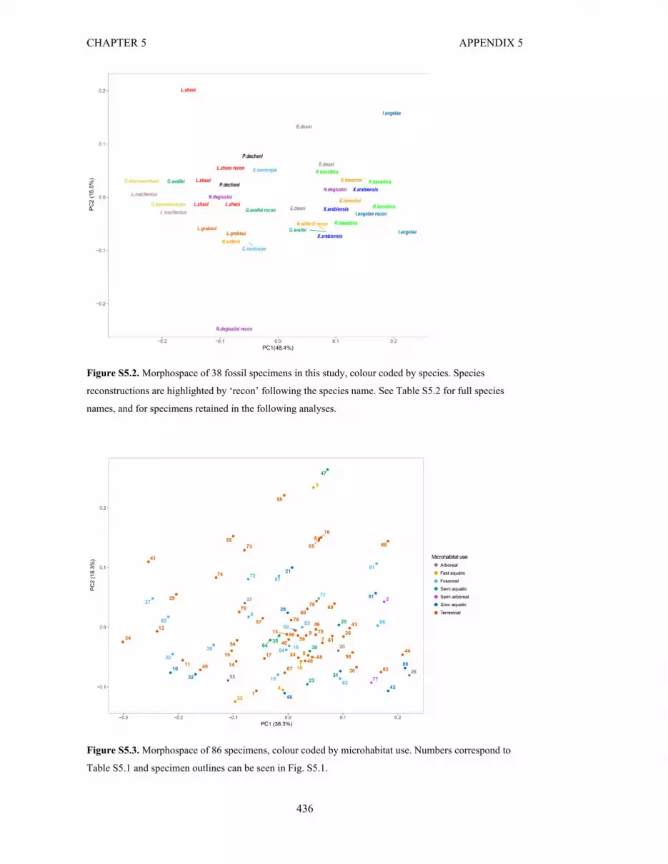
CHAPTER 5 APPENDIX 5
436
Figure S5.2. Morphospace of 38 fossil specimens in this study, colour coded by species. Species
reconstructions are highlighted by ‘recon’ following the species name. See Table S5.2 for full species
names, and for specimens retained in the following analyses.
Figure S5.3. Morphospace of 86 specimens, colour coded by microhabitat use. Numbers correspond to
Table S5.1 and specimen outlines can be seen in Fig. S5.1.

CHAPTER 5 APPENDIX 5
437
Figure S5.4. Morphospace of 66 specimens, colour coded by environment. Numbers correspond to Table
S5.1 and specimen outlines can be seen in Fig. S5.1.
Figure S5.5. Morphospace of 78 specimens, colour coded by developmental strategy. Numbers
correspond to Table S5.1 and specimen outlines can be seen in Fig. S.1.

CHAPTER 5 APPENDIX 5
438
Figure S5.6. Morphospace of extant and fossil specimens (N = 112), coloured gradationally by raw size
(snout-vent length). Outlines reveal allometric shapes associated with large (top) and small (bottom) size.
Figure S5.7. Phylomorphospace of 125 specimens used in this study (87 extant, 38 fossil). Two views of
the three-dimensional morphospace, showing PC1 (left) and PC2 (right) on the x-axis. Time is in million
years, with present day at the top.

439
CH
AP
TE
R 5
AP
PE
ND
IX 5
Table S5.1. Table of extant frog images used in this study.
Extant species-
*excluded
from
phylogenetic
analyses
Outline n
umb
er in F
igure S1
Aspect
Reference for
photo/diagram
Microhab
itat Use
Environm
ent
Zoogeograph
ic realm
Extin
ction risk
Develop
men
tal strategy
Maxim
um
snou
t-ven
t length (m
m)
5 My b
ins b
ased on first app
earance of
genus
Adelotus brevis 1 Dorsal Lynch 1971: p84 Terrestrial NA (broad)
Australo-Papuan
Near Threatened
Indirect 50 5
Allophryne ruthveni 2 Dorsal Fabrezi and Langone 2000
Semi-arboreal
Tropical forest
Neotropical Least Concern
NA 30 5
Ascaphus truei 3 Dorsal Trueb 1993: p324 Fast aquatic
Temperate forest
Nearctic Least Concern
Indirect 51 5
Barbourula busuangensis
4 Dorsal Trueb 1993: p324 Fast aquatic
Tropical forest
Oriental Vulnerable Indirect 100 5
Barycholos pulcher 5 Dorsal Lynch 1971: p191 Terrestrial Tropical forest
Neotropical Least Concern
Direct 30 5
Batrachyla leptopus 6 Dorsal Lynch 1971: p128 Terrestrial Temperate forest
Neotropical Least Concern
Indirect 39 5
Bombina orientalis 35 Dorsal Maglia and Pugener 1998: Fig.1A
Semi Aquatic
NA (broad)
Palearctic Least Concern
Indirect 80 5
Brachycephalus ferruginus
7 Dorsal Alves et al 2006: Fig.7
Terrestrial Tropical forest
Neotropical Data Deficient
Direct 54 5
Brachycephalus pombali
43 Dorsal Alves et al 2006: Fig. 8
Terrestrial Tropical forest
Neotropical Data Deficient
NA 15 5
Bufo granulosus 36 Dorsal Pramuk 2000: Fig.2B
Terrestrial NA (broad)
Neotropical Least Concern
Indirect 90 5
Bufo japonicus 8 Dorsal Line drawing of original (R. Matsumoto, NSM, Tokyo, NSM_PO_6)
Fossorial Temperate forest
Palearctic Least Concern
Indirect 176 5

440
CH
AP
TE
R 5
AP
PE
ND
IX 5
Bufo lemur 44 Dorsal Pramuk 2000: Fig.2C
Terrestrial Tropical forest
Neotropical Critically Endangered
Indirect 120 5
Bufo melanostictus 9 Dorsal Line drawing of original (R. Matsumoto, NSM, Tokyo, NSM_PO_11)
Terrestrial Temperate open
Oriental Least Concern
Indirect 150 5
Bufo spinulosus 46 Dorsal Trueb 1973: p73 Fig.2-2a
Terrestrial Temperate open
Neotropical Least Concern
Indirect 64 5
Bufo valliceps 45 Dorsal Pramuk 2000: Fig.2A
Terrestrial Tropical forest
Neotropical Least Concern
Indirect 130 5
Calluella guttulata 87 Dorsal McPartlin 2010: Fig. 3A
Fossorial Tropical forest
Palearctic Least Concern
Indirect 50 5
Calyptocephallela gayi
10 Dorsal Lynch 1971: p114 Slow aquatic
Temperate open
Neotropical Vulnerable Indirect 320 5
Ceratobatrachus guentheri
34 Dorsal Original, (Sean Wilcox, California State Polytechnic University, Pomona, see below for photo)
Terrestrial Tropical forest
Australo-Papuan
Least Concern
Direct 53 5
Ceratophrys aurita 11 Dorsal Lynch 1971: p107 Terrestrial Tropical forest
Neotropical Least Concern
Indirect 150 5
Ceratophrys calcarata
12 Dorsal Lynch 1982: Fig. 2E
Terrestrial Arid open Neotropical Least Concern
Indirect 150 5
Ceratophrys ornata 27 Dorsal Reig & Limeses 1963, p115 A, Col.3
Fossorial NA (broad)
Neotropical Near Threatened
NA 125 5
Chacophrys pierottii 38 Dorsal Reig & Limeses 1963, p115 A, Col.2
Fossorial NA (broad)
Neotropical Least Concern
NA 50 5
Conraua alleni 39 Dorsal Sheil 1999: Fig. 11E
Semi Aquatic
Tropical forest
Afrotropical Vulnerable Indirect 65 5
Conraua goliath 33 Dorsal Original, MEH Jones, Field Museum, Chicago,
Fast aquatic
Tropical forest
Afrotropical Endangered Indirect 320 5

441
CH
AP
TE
R 5
AP
PE
ND
IX 5
FMNH 15980
Craugastor augusti 57 Dorsal Lynch 1971: p154 Terrestrial Arid open Nearctic Least Concern
Direct 75 5
Crinia signifera 13 Dorsal Lynch 1971: p92 Terrestrial NA (broad)
Australo-Papuan
Least Concern
Indirect 28 5
Crossodactylus gaudichaudii
47 Dorsal Lynch 1971: p165 Semi Aquatic
Tropical forest
Neotropical Least Concern
Indirect 30 5
Cycloramphus eleutherodactylus
14 Dorsal Lynch 1971: p138 Terrestrial Tropical forest
Neotropical Data Deficient
Direct NA 5
Cyclorana australis 15 Dorsal Lynch 1971: p77 Fossorial Arid open Australo-Papuan
Least Concern
Indirect 100 5
Cyclorana dahli 48 Dorsal Lynch 1971: p77 Slow aquatic
Tropical open
Australo-Papuan
NA Indirect NA 5
Discoglossus nigriventer
82 Dorsal Biton et al 2013: Fig. 3AI
Terrestrial Temperate open
Palearctic Critically Endangered
Indirect 40 5
Discoglossus pictus 85 Dorsal Biton et al 2013: Fig. 3AV
Terrestrial NA (broad)
Palearctic Least Concern
Indirect 75 5
Edalorhina perezi 40 Dorsal Lynch 1971: p178 Terrestrial Tropical forest
Neotropical Least Concern
Indirect 37 5
Eleutherodactylus limbatus
78 Dorsal Lynch 1971: p158 Terrestrial NA (broad)
Neotropical Vulnerable Direct 12 5
Eleutherodactylus pipilans
75 Dorsal Lynch 1971: p159 Terrestrial Tropical forest
Neotropical Least Concern
Direct 29 5
Eupsophus roseus 16 Dorsal Lynch 1971: p125 Fossorial Temperate forest
Neotropical Near Threatened
Indirect 95 5
Gastrophryne carolinensis
81 Dorsal Trueb et al 2011: Fig.4A
Fossorial Temperate open
Nearctic Least Concern
Indirect 36 5
Gastrotheca carinaceps
17 Dorsal Duellman et al 2006: Fig. 3A
Terrestrial Tropical forest
Neotropical Data Deficient
Direct 80 5
Hadromophryne natalensis
18 Dorsal Lynch 1971: p104 Fast aquatic
Tropical forest
Afrotropical Least Concern
Indirect 63 5
Heleioporus eyeri 52 Dorsal Lynch 1971: p78 Fossorial Arid open Australo-Papuan
Least Concern
Indirect 65 5
Hemiphractus bubalus
53 Dorsal Trueb 1974: Fig 8 Arboreal Tropical forest
Neotropical Near Threatened
Direct 65 5

442
CH
AP
TE
R 5
AP
PE
ND
IX 5
Hemiphractus fasciatus
54 Dorsal Trueb 1974: Fig. 11
Terrestrial Tropical forest
Neotropical Near Threatened
Direct 59 5
Hemiphractus johnsoni
19 Dorsal Trueb 1974: Fig. 14
Terrestrial Tropical forest
Neotropical Endangered Direct 73 5
Holoaden bradei 55 Dorsal Lynch 1971: p152 Terrestrial Tropical open
Neotropical Critically Endangered
Direct 37 5
Hyalinobatrachium fleischmanni
37 Dorsal Trueb 1973: p73 Fig.2-2e
Arboreal Tropical forests
Neotropical Least Concern
Indirect 32 5
Hylodes asper 30 Dorsal Lynch 1971: p167 Terrestrial Tropical forest
Neotropical Least Concern
Indirect 50 5
Hylorina sylvatica 58 Dorsal Lynch 1971: p127 Terrestrial Temperate forest
Neotropical Least Concern
Indirect 66 5
Hypsiboas boans 20 Dorsal Line drawing of original (R. Matsumoto, NSM, Tokyo, NSM_PO_201)
Arboreal NA NA NA NA NA 5
Lechriodus fletcheri 56 Dorsal Lynch 1971: p85 Terrestrial Tropical forests
Australo-Papuan
Least Concern
Indirect 54 5
Lepidobatrachus asper
62 Dorsal Trueb 1973: p73 Fig.2-2d
Fossorial Arid open Neotropical Near Threatened
Indirect 90 5
Leptodactylus bolivianus
63 Dorsal Trueb 1973: p72 Fig.2-1
Fossorial NA (broad)
Neotropical Least Concern
Indirect 120 5
Leptodactylus quadrivittatus
31 Ventral Lynch 1971: p187 Slow aquatic
Tropical forest
Neotropical Least Concern
Indirect 50 5
Limnodynastes dorsalis
64 Dorsal Lynch 1971: p87 Semi aquatic
Temperate open
Australo-Papuan
Least Concern
Indirect 75 5
Limnomedusa macroglossa
65 Dorsal Lynch 1971: p175 Terresrial NA (broad)
Neotropical Least Concern
Indirect 63 5
Lithodytes lineatus 61 Dorsal Lynch 1971: p179 Terrestrial NA Neotropical Least Concern
Indirect 52 5
Megaelosia goeldii 67 Dorsal Lynch 1971: p169 Terrestrial Tropical forest
Neotropical Least Concern
Indirect 100 5
Melanophryniscus krauczuki
68 Dorsal Baldo and Basso 2004: Fig.2A
Terrestrial Tropical open
Neotropical Data Deficient
Indirect 20.5 5
Metacrinia nichollsi 69 Dorsal Lynch 1971: p99 Terrestrial Temperate Australo- Least Direct 25 5
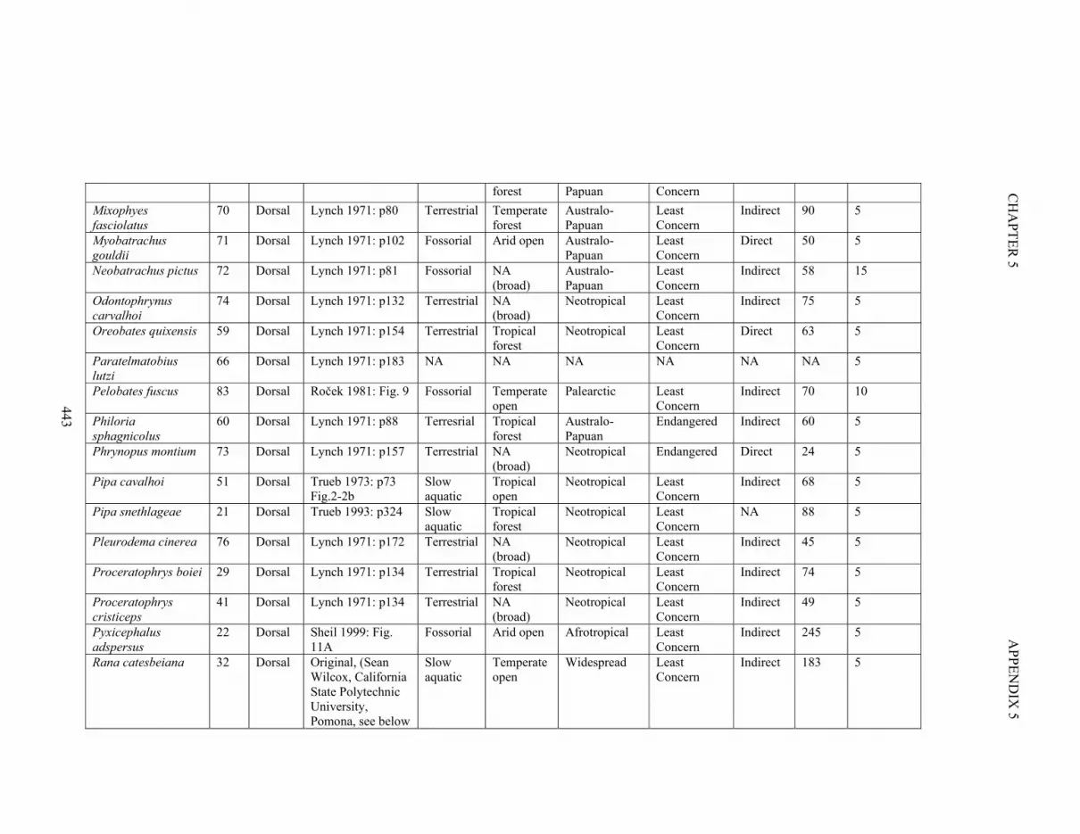
443
CH
AP
TE
R 5
AP
PE
ND
IX 5
forest Papuan Concern
Mixophyes fasciolatus
70 Dorsal Lynch 1971: p80 Terrestrial Temperate forest
Australo-Papuan
Least Concern
Indirect 90 5
Myobatrachus gouldii
71 Dorsal Lynch 1971: p102 Fossorial Arid open Australo-Papuan
Least Concern
Direct 50 5
Neobatrachus pictus 72 Dorsal Lynch 1971: p81 Fossorial NA (broad)
Australo-Papuan
Least Concern
Indirect 58 15
Odontophrynus carvalhoi
74 Dorsal Lynch 1971: p132 Terrestrial NA (broad)
Neotropical Least Concern
Indirect 75 5
Oreobates quixensis 59 Dorsal Lynch 1971: p154 Terrestrial Tropical forest
Neotropical Least Concern
Direct 63 5
Paratelmatobius lutzi
66 Dorsal Lynch 1971: p183 NA NA NA NA NA NA 5
Pelobates fuscus 83 Dorsal Roček 1981: Fig. 9 Fossorial Temperate open
Palearctic Least Concern
Indirect 70 10
Philoria sphagnicolus
60 Dorsal Lynch 1971: p88 Terresrial Tropical forest
Australo-Papuan
Endangered Indirect 60 5
Phrynopus montium 73 Dorsal Lynch 1971: p157 Terrestrial NA (broad)
Neotropical Endangered Direct 24 5
Pipa cavalhoi 51 Dorsal Trueb 1973: p73 Fig.2-2b
Slow aquatic
Tropical open
Neotropical Least Concern
Indirect 68 5
Pipa snethlageae 21 Dorsal Trueb 1993: p324 Slow aquatic
Tropical forest
Neotropical Least Concern
NA 88 5
Pleurodema cinerea 76 Dorsal Lynch 1971: p172 Terrestrial NA (broad)
Neotropical Least Concern
Indirect 45 5
Proceratophrys boiei 29 Dorsal Lynch 1971: p134 Terrestrial Tropical forest
Neotropical Least Concern
Indirect 74 5
Proceratophrys cristiceps
41 Dorsal Lynch 1971: p134 Terrestrial NA (broad)
Neotropical Least Concern
Indirect 49 5
Pyxicephalus adspersus
22 Dorsal Sheil 1999: Fig. 11A
Fossorial Arid open Afrotropical Least Concern
Indirect 245 5
Rana catesbeiana 32 Dorsal Original, (Sean Wilcox, California State Polytechnic University, Pomona, see below
Slow aquatic
Temperate open
Widespread Least Concern
Indirect 183 5

444
CH
AP
TE
R 5
AP
PE
ND
IX 5
for photo)
Rana pipiens 42 Dorsal Trueb 1973: p73 Fig.2-2f
Slow aquatic
NA (broad)
Nearctic Least Concern
Indirect 110 25
Rana temporaria 23 Dorsal Line drawing of original, (SE Evans, UCL, UK)
Semi Aquatic
Temperate forest
Palearctic Least Concern
Indirect 90 10
Rhamphophryne acrolopha
77 Dorsal Trueb 1973: p73 Fig.2-2c
Semi-arboreal
Tropical forest
Neotropical Data Deficient
NA 45 5
Rhinophrynus dorsalis
86 Dorsal Trueb and Cannatella 1982: Fig.2A
Fossorial Tropical forest
Neotropical Least Concern
Indirect 85 5
Scaphiopus hurterii 84 Dorsal Smith 1937: Fig. 6 Fossorial Arid open Nearctic Least Concern
Indirect 81 5
Strabomantis bufoniformis
49 Dorsal Lynch 1971: p147 Terrestrial Tropical forest
Neotropical Least Concern
Direct 94 5
Taudactylus acutirostris
24 Dorsal Lynch 1971: p96 Terrestrial Tropical forest
Australo-Papuan
Critically Endangered
Indirect 30 5
Telmatobius hautholi 28 Dorsal Lynch 1971: p119 Slow Aquatic
NA Neotropical Vulnerable Indirect 60 5
Thoropa lutzi 25 Dorsal Lynch 1971: p130 Semi Aquatic
Tropical forest
Neotropical Endangered Indirect 28 5
Triprion petasatus 26 Dorsal Trueb 1973: p73 Fig.2-2g
Arboreal Arid open Neotropical Least Concern
Indirect 75 5
Uperoleia rugosa 79 Dorsal Lynch 1971: p99 Terrestrial NA (broad)
Australo-Papuan
Least Concern
Indirect 30 5
Uperoleia russelli 50 Dorsal Lynch 1971: p97 Terrestrial Temperate open
Australo-Papuan
Least Concern
NA 33 5
Xenopus laevis 80 Dorsal Trueb and Hanken 1992: Fig.9 (upper)
Slow aquatic
Arid open Widespread Least Concern
Indirect 120 5
Batrachophrynus macrostomus*
NA Dorsal Lynch 1971: p122 Slow aquatic
Slow aquatic
Neotropical Endangered NA 138 NA
Crossodactylodes pintoi*
NA Dorsal Lynch 1971: p136 Terrestrial Tropical Neotropical Data Deficient
Indirect 18 NA
Euparkerella brasiliensis*
NA Dorsal Lynch 1971: p151 Terrestrial Tropical Neotropical Least Concern
NA 22 NA
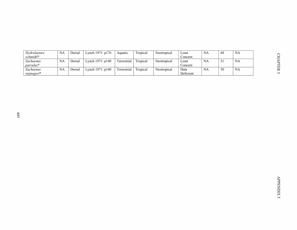
445
CH
AP
TE
R 5
AP
PE
ND
IX 5
Hydrolaetare schmidti*
NA Dorsal Lynch 1971: p176 Aquatic Tropical Neotropical Least Concern
NA 68 NA
Zachaenus parvulus*
NA Dorsal Lynch 1971: p140 Terrestrial Tropical Neotropical Least Concern
NA 31 NA
Zachaenus stejnegeri*
NA Dorsal Lynch 1971: p140 Terrestrial Tropical Neotropical Data Deficient
NA 30 NA

446
CH
AP
TE
R 5
AP
PE
ND
IX 5
Table S5.2. Table of fossil frog images used in this study.
Fossil species
*excluded
from p
hylogenetic
analyses
Ou
tline n
um
ber in
Fig. S1
Referen
ce for photo/d
iagram
Figu
re from referen
ce
Ad
dition
al specim
ens
excluded from m
ain analyses
following sen
sitivity analysses
Asp
ect
Recon
struction
?
Mirrored
?
Snou
t-vent len
gth (m
m) from
literatu
re
First ap
pearance or start of stage w
hen
first appeared
(M
a)
Last ap
pearance or en
d of
stage wh
en last ap
peared
(Ma)
5 My b
ins based
on first
appearan
ce
Aerugoamnis paulus 88 Henrici et al 2013 1C NA Dorsal No No 19.3 55.8 50.3 60
Beelzebufo ampinga 89 Evans et al 2014 4B NA Dorsal Yes No 193.0 72.1 66.0 75
Calyptocephalella pichileufensis
90 Gómez et al 2011 4 NA Dorsal Yes No 110.0 47.5 47.4 50
Cordicephalus gracilis
91 Trueb and Báez 2006
4A NA Dorsal Yes No 26.1 145.0 113.0 145
Eodiscoglossus santonjae
92 Hecht 1970 2 Fig.1 (part) Counterpart
No Yes 27.3 130.0 125.5 130
Eopelobates anthracinus
93 Estes 1970 8 NA Dorsal Yes No 40.0 28.4 23.0 30
Eopelobates bayeri 94 Roček et al 2014 3B NA Ventral No No 64.0 13.8 11.6 15
Eopelobates deani 95 Roček et al 2014 5C Fig.4C; 4D Dorsal No No 37.0 50.3 46.2 55
Eopelobates hinschei
96 Estes 1970 10 Fig.7B from Roček et al 2014
Unsure No Yes NA 44.3 44.3 45
Eoxenopoides reuningi
97 Báez and Trueb 1997;
16 (right)
NA Dorsal Yes No NA 72.1 59.2 75
Gobiates khermeentsavi
98 Špinar and Tatarinov 1986;
1C Fig. 2A Dorsal Schematic drawing
Yes 50.0 83.6 66.0 85
Gobiates sp. 99 Roček 2008 2A NA Dorsal Yes No 50.0 86.3 72.1 90

447
CH
AP
TE
R 5
AP
PE
ND
IX 5
Gracilibatrachus avallei
100 Báez 2013 6 Fig.5D; 7A Dorsal Yes No 23.0 130.0 125.5 130
Iberobatrachus angelae
101 Báez 2013 3 Fig.2A; 2B Dorsal Yes No 40.0 130.0 125.5 130
Latonia vertaizoni 102 Roček 1994 19 NA Unsure Schematic drawing
Yes 200.0 33.9 28.4 35
Liaobatrachus beipiaoensis
103 Dong et al 2013 4C-1 NA Unsure No Yes NA 129.4 122.5 130
Liaobatrachus grabaui
104 Dong et al 2013 3C-1 Fig.3B-1 Unsure No No 94.0 130.0 122.5 130
Liaobatrachus macilentus
105 Dong et al 2013 5B1 Fig.5B2 Ventral No Yes 62.0 130.0 122.5 130
Liaobatrachus zhaoi 106 Dong et al 2013 7A Fig. 6A,B,C,D Dorsal Yes No 80.0 130.0 122.5 130
Macropelobates osborni
107 Estes 1970 27 (right)
NA Dorsal Yes No NA 33.9 28.4 35
Neusibatrachus wilferti
108 Báez and Sanchiz 2007
2 Fig.3A1 Dorsal Yes No 21.0 129.4 125.0 130
Notobatrachus degiustoi
109 Báez and Nicoli 2004
2 Fig.4; 5C Dorsal Yes No 150.0 168.3 166.1 170
Palaeobatrachus cf. grandipes
110 Roček and Wuttke 2010;
5 NA Ventral No No 112.0 24.8 24.6 25
Pelobates cf. decheni
111 Roček and Wuttke 2010
7e NA Ventral No Yes NA 24.8 24.6 25
Pelobates decheni 112 Böhme et al 1982 2 NA Dorsal No No 85.0 28.4 23.0 30
Rana barani 113 Rückert–Ülkümen 2003;
Plate 1 Fig.1
NA Ventral No No 83.0 11.6 5.3 15
Rana basaltica 114 Roček et al 2011 7A-2 Fig.A2 Dorsal No Yes 46.0 17.0 15.2 20
Rana sp.1 115 Rückert–Ülkümen 2003;
Plate 2, Fig.1
NA Unsure No No 77.0 24.8 24.6 25
Rana sp 116 Roček and Wuttke 2010
9B NA Ventral No Yes NA 24.8 24.6 25
Saltenia ibanezi 117 Báez and Trueb 1997
18 (right)
NA Dorsal Yes No NA 83.6 72.1 85
Scaphiopus skinneri 118 Estes 1970 30a NA Dorsal No Yes NA 33.5 32.0 25

448
CH
AP
TE
R 5
AP
PE
ND
IX 5
Scaphiopus neuter 119 Kluge 1966 1 NA Dorsal No Yes 60.0 24.8 20.4 35
Shelania pascuali 120 Báez and Trueb 1997;
5 (left) NA Dorsal Yes No 100.0 47.8 41.3 50
Singidella latecostata
121 Báez and Harrison 2005
4A NA Dorsal Yes No 45.0 47.8 41.3 50
Thaumastosaurus gezei
122 Laloy et al 2013 3A NA Dorsal No No NA 40.4 33.9 45
Thoraciliacus rostriceps
123 Trueb 1999 3 (left) NA Dorsal Yes No 32.0 145.0 113.0 145
Vulcanobatrachus mandelai
124 Trueb et al 2005 9 (left) NA Dorsal Yes No 42.0 89.3 66.0 90
Xenopus arabiensis 125 Henrici and Báez 2001
3.2 Fig.4.1; 4.2 Dorsal Yes Yes 47.3 33.9 23.0 35
Anura indet IVPP V14266*
NA Roček et al 2011 5B-2 NA Ventral No No 52.4 17.0 15.2 NA
Anura indet JMSP H11.014*
NA Roček et al 2011 7F-2 NA Ventral No Yes 89.0 17.0 15.2 NA
Eupsophus sp* NA Nicoli 2012 Fig.3A NA Dorsal Yes No 30.0 NA NA NA
Lutetiobatrachus gracilis*
NA Wuttke 2012 Plate 2 Fig.1
Fig.1 Dorsal No No 29.2 NA NA NA

CHAPTER 5 APPENDIX 5
449
References for Appendix 5
Extant frog photos and diagrams
Alves, A. C. R., L. F. Ribeiro, C. F. B. Haddad, and S. F. dos Reis. 2006. Two new species of Brachycephalus (Anura: Brachycephalidae) from the Atlantic forest in Paraná State, Southern Brazil. Herpetologica. 62:221–233.
Baldo, D., and N. G. Basso. 2004. A new species of Melanophryniscus Gallardo, 1961 (Anura: Bufonidae), with comments on the species of the genus reported for Misiones, Northeastern Argentina. J. Herpetol. 38:393–403.
Biton, R., E. Geffen, M. Vences, O. Cohen, S. Bailon, R. Rabinovich, Y. Malka, T. Oron, R. Boistel, V. Brumfeld, and S. Gafny. 2013. The rediscovered Hula painted frog is a living fossil. Nat. Commun. 4:1–6.
Duellman, W. E., L. Trueb, and E. Lehr. 2006. A new species of Marsupial frog (Anura: Hylidae: Gastrotheca) from the Amazonian slopes of the Cordillera Oriental in Peru. Copeia 4:595–603.
Fabrezi, M., and J. A. Langone. 2000. Los caracteres morfológicos del controvertido Neobatrachia arborícola Allophryne ruthveni Gaige, 1926. Cuadernos. Cuad. Herpetol. 14:47–59.
Lynch, J. D. 1971. Evolutionary relationships, osteology, and zoogeography of leptodacyloid frogs. Univ. Kansas Museum Nat. Hist. Misc. Publ. 53:1–238.
Lynch, J. D. 1982. Relationships of the frogs of the genus Ceratophrys (Leptodactylidae) and their bearing on hypotheses of Pleistocene forest refugia in South America and punctuated equilibria. 31:166–179.
Maglia, A. M. ., and L. . A. Púgener. 1998. Skeletal development and adult osteology of Bombina orientalis (Anura: Bombinatoridae). Herpetologica 54:344–363.
McPartlin, C. A. 2010. Osteology of Calluella guttulata (Blyth 1855) and associated commentary on evolution in the family Microhylidae (Anura). Unpublished MA thesis. University of Kansas, Lawrence, Kansas.
Pramuk, J. B. 2000. Prenasal bones and snout morphology in West Indian bufonids and the Bufo granulosus. J. Herpetol. 34:334–340.
Reig, O. A., and C. E. Limeses. 1963. Un nuevo género de anuros ceratofrínidos del Distrito Chaqueño. Physis 24:113–128.
Roček, Z. 1981. Cranial anatomy of frogs of the family Pelobatidae stanius, 1859, with outlines of their phylogeny and systematics. Acta Univ. Carolinae- Biol. 1980:1–164.
Sheil, C. A. 1999. Osteology and skeletal development of Pyxicephalus adspersus (Anura: Ranidae: Raninae). J. Morphol. 240:49–75.
Smith, H. M. 1937. Notes on Scaphiopus hurterii Strecker. Herpetologica 1:104-105+107-108.
Trueb, L. 1973. Bones, frogs, and evolution. Pp. 65–132 in J. L. Vial, ed. Evolutionary biology of the anurans: contemporary research on major problems. University of Missouri Press, Columbia.
Trueb, L. 1993. Patterns of cranial diversity among the Lissamphibia. Pp. 255–338 in J. Hanken & B. K. Hall (Eds.), The skull: patterns of structural and systematic diversity. Chicago: The University of Chicago Press.
Trueb, L. 1974. Systematic relationships of neotropical horned frogs, genus Hemiphractus (Anura, Hylidae). Occas. Pap. Museum Nat. Hist. Univ. Kansas 29:1–60.
Trueb, L., and D. C. Cannatella. 1982. The cranial osteology and hyolaryngeal apparatus of Rhinophrynus dorsalis (Anura: Rhinophrynidae) with comparisons to recent pipid frogs. J. Morphol. 171:11–40.
Trueb, L., R. Diaz, and D. C. Blackburn. 2011. Osteology and chondrocranial morphology of Gastrophryne carolinensis (Anura: Microhylidae), with a review of the osteological diversity of

CHAPTER 5 APPENDIX 5
450
New World microhylids.
Trueb, L., and J. Hanken. 1992. Skeletal development in Xenopus laevis (Anura: Pipidae). J. Morphol. 214:1–41.
Fossil frog photos and diagrams
Báez, A. M. 2013. Anurans from the Early Cretaceous Lagerstätte of Las Hoyas, Spain: new evidence on the Mesozoic diversification of crown-clade Anura. Cretac. Res. 41:90–106.
Báez, A. M., and T. Harrison. 2005. A new pipine frog from an Eocene crater lake in North-Central Tanzania. Palaeontology 48:723–737.
Báez, A. M., and L. Nicoli. 2004. A new look at an old frog: the Jurassic Notobatrachus Reig from Patagonia. Ameghiniana 41:257–270.
Báez, A. M., and B. Sanchíz. 2007. A review of Neusibatrachus wilferti, an Early Cretaceous frog from the Montsec Range, northeastern Spain. Acta Palaeontol. Pol. 52:477–487.
Báez, A. M., and L. Trueb. 1997. Redescription of the Paleogene Shelania pascuali from Patagonia and its bearing on the relationships of fossil and recent pipoid frogs. Sci. Pap. Nat. Hist. Museum, Univ. Kansas 4:1–41.
Böhme, W., Z. Roček, and Z. V. Špinar. 1982. On Pelobates decheni Troschel, 1861, and Zaphrissa eurypelis Cope, 1866 (Amphibia: Salientia: Pelobatidae) from the Early Miocene of Rott near Bonn, West Germany. J. Vertebr. Paleontol. 2:1–7.
Dong, L., Z. Roček, Y. Wang, and M. E. H. Jones. 2013. Anurans from the Lower Cretaceous Jehol Group of Western Liaoning, China. PLoS One 8:e69723.
Estes, R. 1970. New fossil pelobatid frogs and a review of the genus Eopelobates. Bull. Museum Comp. Zool. 139:293–339.
Evans, S. E., J. R. Groenke, M. E. H. Jones, A. H. Turner, and D. W. Krause. 2014. New material of Beelzebufo, a hyperossified frog (Amphibia: Anura) from the Late Cretaceous of Madagascar. PLoS One 9:e87236.
Gómez, R. O., A. M. Báez, and P. Muzzopappa. 2011. A new helmeted frog (Anura: Calyptocephalellidae) from an Eocene subtropical lake in northwestern Patagonia, Argentina. J. Vertebr. Paleontol. 31:50–59.
Hecht, M. K. 1970. The morphology of Eodiscoglossus, a complete Jurrasic frog. Am. Museum Novit. 2424:1–17.
Henrici, A. C., and A. M. Báez. 2001. First occurrence of Xenopus (Anura: Pipidae) on the Arabian Peninsula: a new species from the Upper Oligocene of Yemen. J. Paleontol. 75:870–882.
Henrici, A. C., A. M. Báez, and L. Grande. 2013. Aerugoamnis paulus, new genus and new species (Anura: Anomocoela): first reported anuran from the Early Eocene (Wasatchian) Fossil Butte Member of the Green River Formation, Wyoming. Ann. Carnegie Museum 81:295–309.
Kluge, A. G. 1966. A new pelobatine frog from the Lower Miocene of South Dakota with a discussion of the evolution of the Scaphiopus-Spea complex.
Laloy, F., J.-C. Rage, S. E. Evans, R. Boistel, N. Lenoir, and M. Laurin. 2013. A re-interpretation of the Eocene anuran Thaumastosaurus based on MicroCT examination of a “mummified” specimen. PLoS One 8:e74874.
Nicoli, L. 2012. On the putative presence of Eupsophus (Anura: Cycloramphidae) in Central Patagonia during the Oligocene. Herpetologica 68:236–243.
Roček, Z. 1994. Taxonomy and distribution of Tertiary discoglossids (Anura) of the genus Latonia V. Meyer, 1843. Geobios 27:717–751.

CHAPTER 5 APPENDIX 5
451
Roček, Z. 2008. The Late Cretaceous frog Gobiates from Central Asia: its evolutionary status and possible phylogenetic relationships. Cretac. Res. 29:577–591.
Roček, Z., L. Dong, T. Přikryl, C. Sun, J. Tan, and Y. Wang. 2011. Fossil frogs (Anura) from Shanwang (Middle Miocene; Shandong Province, China). Geobios 44:499–518.
Roček, Z., and M. Wuttke. 2010. Amphibia of Enspel (Late Oligocene, Germany). Palaeobiodiversity and Palaeoenvironments 90:321–340.
Roček, Z., M. Wuttke, J. D. Gardner, and B. A. Singh Bhullar. 2014. The Euro-American genus Eopelobates, and a re-definition of the family Pelobatidae (Amphibia, Anura). Palaeobiodiversity and Palaeoenvironments 94:529–567.
Rückert-Ülkümen, N. 2003. Fossil ranids from Miocene deposits of Central Anatolia. Istanbul Üniv. Müh. Fak. Yerbilim. Derg. 16:71–74.
Špinar, Z. V., and L. P. Tatarinov. 1986. A new genus and species of discoglossid frog from the Upper Cretaceous of the Gobi Desert. J. Vertebr. Paleontol. 6:113–122.
Trueb, L. 1999. The Early Cretaceous pipoid anuran, Thoraciliacus: redescription, revaluation, and taxonomic status. Herpetologica 55:139–157.
Trueb, L., and A. M. Báez. 2006. Revision of the Early Cretaceous Cordicephalus from Israel and an assessment of its relationships among pipoid frogs. J. Vertebr. Paleontol. 26:44–59.
Trueb, L., C. F. Ross, and R. Smith. 2005. A new pipoid anuran from the Late Cretaceous of South Africa. J. Vertebr. Paleontol. 25:533–547.
Wuttke, M. 2012. Redescription of the Middle Eocene frog Lutetiobatrachus gracilis Wuttke in Sanchiz, 1998 (Lower Geiseltalian, »Grube Messel«, near Darmstadt, southern Hesse, Germany). Darmstädter Beiträge zur Naturgeschichte 18:29–41.


