. SIMULATION OF SPONTANEOUS IGNITION IN POROUS MEDIAP. CASTAÑEDA, D. MARCHESIN, AND J. BRUININGAbstra t. We study the stability of ombustion in a porous medium in a simplied modelthat takes into a ount the balan e between heat generation and heat losses. The tem-perature dependen e of heat generation is given by Arrhenius law. Heat losses are due to ondu tion to the ro k formation. The system evolution is des ribed by an innite numberof nonlinear modes. We show that its long time behavior is di tated by the two dominantmodes, whose phase diagram ontains two attra tors and a saddle, justifying the pi ture in lassi al hemi al engineering. 1. Introdu tionCombustion in-situ is an important methodology to extra t heavy oil from reservoirs, pro-vided ignition is sustained and ontrolled. The geometri al setting of the rea tion lo ationand of ondu tive heat losses is a very important matter. When heat losses be ome equalto a small rea tion heat rate, the system remains trapped in a slow rea tion mode; su ha mode is indistinguishable from extin tion. On the other hand, if heat losses are smallerthan the heat generated by the rea tion, the temperature and the heat losses will in rease,so we expe t that the system rea hes an equilibrium in a fast rea tion mode; this is ignition.Heat losses are strongly dependent on the geometry of the heat generating region. In thisarti le we will only dis uss the one-dimensional ase, however work in progress in ludes othergeometries.In Se . 2 we onstru t the rea tor model that we will study in this work and nondimen-sionalize it to enter, in Se . 3, in linear analysis of its equilibria. These steady-state solutionswill guide some of the numeri al analysis made in Se . 4. Finally, in Se . 5 we summarizeour results. 2. The rea tor model for one dimensional heat flowWe derive a set of equations that des ribe the onservation of energy in a porous mediumwhere thermal ow o urs. Fi k's law des ribes the transport of energy by ondu tion,and Arrhenius' law des ribes the rate of energy generated by the rea tion between oxygenand oke. Then the variation of heat in the domain is equal to that rea tion governed byArrhenius' law inside the domain plus Fi k's law, whi h involves the boundary. For a generaldomain Ω we have:d

dt

∫

Ω

QdV =

∫

Ω

∆H co ccA exp

(

−E

RT

)

dV +

∫

∂Ω

κ∇T · n dS, (1)where Q = Q(x, t) is the thermal energy density, ∆H denotes the rea tion enthalpy per unitmass of oxygen, co is the on entration of oxygen in the inje ted gas, cc is the on entrationof arbon (the fuel) in the porous media, A is the pre-exponential fa tor, E is the a tivationenergy, and κ denotes the thermal ondu tivity.Key words and phrases. 30o CILAMCE, Chemi al rea tor, Porous media, In-situ ombustion, Geometri alsetting, Heat losses. 1

2 CASTAÑEDA, MARCHESIN, AND BRUININGIn the one dimensional ase, the domain in x stret hes from 0 to L, and the rea tion takespla e is the subinterval from zero to a xed a < L. We assume that the thermal ondu tivityin the interval x ∈ [0, a) is mu h larger than in the region x ∈ (a, L]. Thus we an taketemperatures uniform in spa e for the rea ting interval, and we an simplify the governingequation.Noti e also, that in the interval x ∈ (a, L], there is no rea tion taking pla e, there is onlyheat ondu tion, co = 0 there, so Eq. (1) leads to the lassi al heat equation. In this way,the 1d equations are:ρece

∂T

∂t= κ

∂2T

∂x2x ∈ (a, L)

ρici∂T

∂t

∣

∣

∣

∣

x=a+

= ∆HcoA exp

(

−E

RT

)∣

∣

∣

∣

x=a+

+κ

a

∂T

∂x

∣

∣

∣

∣

x=a+

x ∈ [0, a].(2)We nondimensionalize with

x := ax, t := tRt, θ := TR/E, L := aL, (3)obtainingρecea

2

κtR

∂θ

∂t=

∂2θ

∂x2x ∈ (1, L)

ρicia2

κtR

∂θ

∂t

∣

∣

∣

∣

x=1+

=∆H coccAa

2R

κEexp

(

−1

θ

)∣

∣

∣

∣

x=1+

+∂θ

∂x

∣

∣

∣

∣

x=1+

x ∈ [0, 1].(4)Introdu ing

tR =ρicia

2

κ, E =

ρeceρici

and γ =∆HcoccAa

2R

κE, (5)and dropping the tildes, we rewrite the system in the form:

E∂θ

∂t=

∂2θ

∂x2x ∈ (1, L), t > 0

∂θ

∂t

∣

∣

∣

∣

x=1

= γ exp

(

−1

θ

)∣

∣

∣

∣

x=1

+∂θ

∂x

∣

∣

∣

∣

x=1+

x = 1, t > 0

θ(L, t) = θL t > 0θ(x, 0) = θi(x) x ∈ [0, L]θ(x, t) = θ(1, t) x ∈ [0, 1].

(6)Clearly, any solution of the PDE (6) is always onstant in x ∈ [0, 1]. Taking this fa t intoa ount, we an perform the analysis either in [0, L] or in [1, L].As we will see, there are two types of solutions for (6) as far as E is on erned. Therst one orresponds to E = 0 and the se ond one to E > 0. The rst one orrespondsto ρece ≪ ρici; in the se ond one, the pre ise value of E is irrelevant. Following data for hemi al ompounds in the work of Tyler (1985) and by Abu-Khamsin et al. (1988), we seethat γ = 7.0× 108.

SIMULATION OF SPONTANEOUS IGNITION IN POROUS MEDIA 33. Linear stability of equilibria in the rea tor modelThe steady-states are solutions of system (6) that satisfy

∂2

∂x2= 0 x ∈ (1, L)

γ exp

(

−1

)∣

∣

∣

∣

x=1

+∂

∂x

∣

∣

∣

∣

x=1+

= 0 x ≤ 1,

(7)with boundary ondition (L) = θL at the right, where θL is a non-negative temperature.Then, we look for a similar boundary ondition at the left, say (1) = θo, where even if θo isunknown, it represents a non-negative temperature.Clearly the solution of Eq. (7.a) for su h Diri hlet BCs is given by the ontinuous solution(x) =

θo x < 1(θo − θL)r(x) + θL x ∈ [1, L],

(8)with r(x) := (L− x)/d, x ∈ [1, L] and d := L− 1. (9)3.1. Finding the equilibria. Substituting the se ond equation from (8) into the Eq. (7.b)leads toγd = Ξ(θo), where Ξ(θ) :=

θ − θLexp(−1/θ)

. (10)Therefore L, θo, θL and γ are intimately related in steady-states. Equation (10) is the sameexpressions found in (Bruining et al., 2008) and means that we are interested in valuesθo > θL.Looking for the extrema of the fun tion Ξ, we see that

Ξ′(θ) =d

dθ

[

(θ − θL) exp

(

1

θ

)]

=θ2 − θ + θL

θ2exp

(

1

θ

)

. (11)Then Ξ′(θ) = 0 atθM =

1

2−

1

2

√

1− 4θL and θm =1

2+

1

2

√

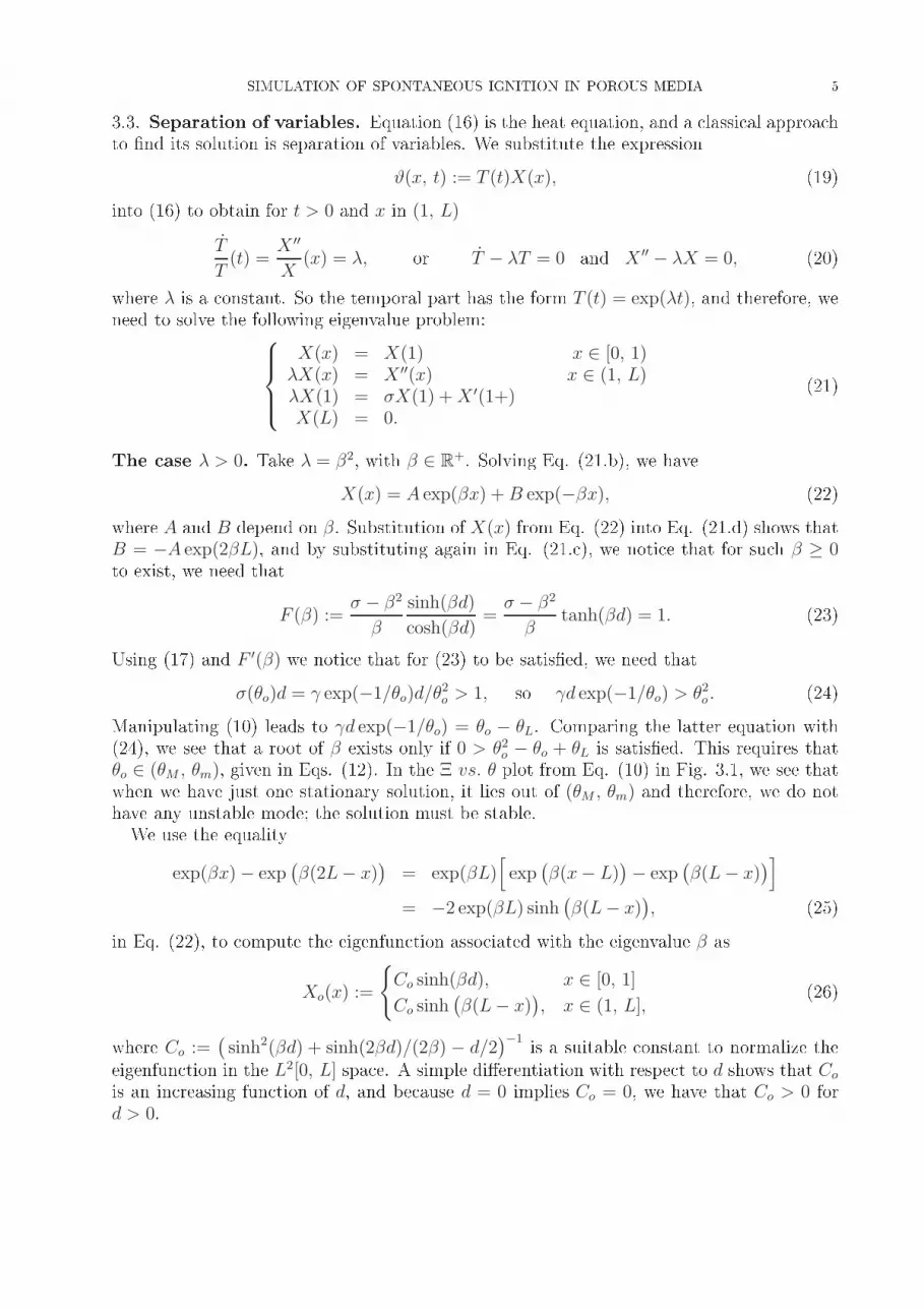
1− 4θL, (12)where m stands for minimum and M for maximum, see Fig. 3.1.In Fig. 3.1 we have θL = 0.17 for the solid urve, θL = 0.15, 0.19, 0.21, 0.23 for the dotted urves (from left to right), θL = 0.25 for the dotted-dashed urve. Noti e that when θLis smaller, the peak be omes larger. Noti e that the interse tion of ea h urve with the θaxis is the respe tive θL. Finally, noti e that for the solid urve with θL = 0.17 we mark,at the left of verti al axis, the regions where we have one or three solutions (with `1' or`3') of Ξ(θ) = γd. On the horizontal axis, we mark also the regions I, II, III where the orresponding θI , θII , θIII would be. We noti e that the rst equation in (10) always hasat least one root, whi h means that there is always a steady-state solution. In some ases,there are three dierent roots, and three dierent stationary solutions, related to the rootsθI , θII , θIII and noti e that θL < θI < θM < θII < θm < θIII .

4 CASTAÑEDA, MARCHESIN, AND BRUINING

Figure 3.1. Some Ξ(θ) versus θ.3.2. Linear stability analysis of equilibria. We have found the stationary solutions forthe Diri hlet ondition. We will study time dependent solutions that are lose to the sta-tionary solution (8) to determine under whi h onditions (x) is linearly stable.Noti e that when θ ≈ , using Taylor's formula, we an writeexp(−1/θ) ≈ exp(−1/)(1 + (θ − )/2). (13)Now using (13) on the rst term of the RHS of (6.b), adding and subtra ting x and t,re alling that t = 0 and (x = 1) satises Eq. (7.b), we have that (6.b) be omes

∂(θ − )

∂t

∣

∣

∣

∣

x=1

≈ γ exp(−1/)(θ − )/2∣

∣

x=1+

∂(θ − )

∂x

∣

∣

∣

∣

x=1+

. (14)We now examine how the solution of the evolution problem behaves when we perturb thestationary solution around the solution . To do so, we deneϑ(x, t) :≈ θ(x, t)− (x). (15)Sin e we have assumed onstant reservoir temperatures at the right boundary, we write thelinear model for the perturbation, from Eqs. (14) and the heat equation, as

ϑt = ϑxx x ∈ (1, L), t > 0ϑt

∣

∣

x=1= σϑ

∣

∣

x=1+ ϑx

∣

∣

x=1+x ≤ 1, t > 0

(16)whereσ = σ(θo) := γ exp(−1/θo)/θ

2o. (17)for (1) = θo. The homogeneous Diri hlet boundary and initial onditions are

ϑ(L, t) = 0 and ϑ(x, 0) = ϑo(x). (18)

SIMULATION OF SPONTANEOUS IGNITION IN POROUS MEDIA 53.3. Separation of variables. Equation (16) is the heat equation, and a lassi al approa hto nd its solution is separation of variables. We substitute the expressionϑ(x, t) := T (t)X(x), (19)into (16) to obtain for t > 0 and x in (1, L)

T

T(t) =

X ′′

X(x) = λ, or T − λT = 0 and X ′′ − λX = 0, (20)where λ is a onstant. So the temporal part has the form T (t) = exp(λt), and therefore, weneed to solve the following eigenvalue problem:

X(x) = X(1) x ∈ [0, 1)λX(x) = X ′′(x) x ∈ (1, L)λX(1) = σX(1) +X ′(1+)X(L) = 0.

(21)The ase λ > 0. Take λ = β2, with β ∈ R+. Solving Eq. (21.b), we have

X(x) = A exp(βx) +B exp(−βx), (22)where A and B depend on β. Substitution of X(x) from Eq. (22) into Eq. (21.d) shows thatB = −A exp(2βL), and by substituting again in Eq. (21. ), we noti e that for su h β ≥ 0to exist, we need that

F (β) :=σ − β2

β

sinh(βd)

cosh(βd)=

σ − β2

βtanh(βd) = 1. (23)Using (17) and F ′(β) we noti e that for (23) to be satised, we need that

σ(θo)d = γ exp(−1/θo)d/θ2o > 1, so γd exp(−1/θo) > θ2o . (24)Manipulating (10) leads to γd exp(−1/θo) = θo − θL. Comparing the latter equation with(24), we see that a root of β exists only if 0 > θ2o − θo + θL is satised. This requires that

θo ∈ (θM , θm), given in Eqs. (12). In the Ξ vs. θ plot from Eq. (10) in Fig. 3.1, we see thatwhen we have just one stationary solution, it lies out of (θM , θm) and therefore, we do nothave any unstable mode; the solution must be stable.We use the equalityexp(βx)− exp

(

β(2L− x))

= exp(βL)[

exp(

β(x− L))

− exp(

β(L− x))

]

= −2 exp(βL) sinh(

β(L− x))

, (25)in Eq. (22), to ompute the eigenfun tion asso iated with the eigenvalue β asXo(x) :=

Co sinh(βd), x ∈ [0, 1]

Co sinh(

β(L− x))

, x ∈ (1, L],(26)where Co :=

(

sinh2(βd) + sinh(2βd)/(2β)− d/2)

−1 is a suitable onstant to normalize theeigenfun tion in the L2[0, L] spa e. A simple dierentiation with respe t to d shows that Cois an in reasing fun tion of d, and be ause d = 0 implies Co = 0, we have that Co > 0 ford > 0.

6 CASTAÑEDA, MARCHESIN, AND BRUININGThe ase λ < 0. We now look for negative eigenvalues. Take λ = −α2 and noti e that αand −α give the same solution, so for onvenien e take α ∈ R−. From Eq. (21.b), we have

−α2X = X ′′, (27)it follows that X(x) is a linear ombination of sines and osines with argument αx. But fromEq. (21.d), we have X(L) = 0, so it is better to hooseX(x) = A sin(α(L− x)), (28)where A = A(α) is a onstant. By substituting (28) into Eq. (21. ) we get that −α mustsatisfy −(σ + α2)A sin(αd) = −Aα cos(αd). Then, we are looking for α ∈ R

− su h thatσ + α2

α=

cos(αd)

sin(αd)= cot(αd). (29)Comparing the plot of both sides of (29), we see that there is a root αn in ea h interval

(−(n + 1)π/d, −nπ/d) with n ∈ N . The roots form a ountable de reasing sequen e ofeigenvalues for our model. Ea h of these eigenvalues has an asso iated eigenfun tionXn(x) :=

Cn sin(αnd), x ∈ [0, 1]

Cn sin(

αn(L− x))

, x ∈ (1, L],(30)where Cn :=

(

sin2(αnd) − sin(2αnd)/(2αn) + d/2)

−1 are suitable positive normalizing on-stants for the eigenfun tions in the L2[0, L] spa e.We have used the negative sign for α just for onvenien e. In this way, we only emphasizethat the positive eigenvalue β orresponds to the unstable mode, while the negative eigen-values αn orresponds to the stable modes; if λ < 0 the solution (19) onverges exponentiallyto zero. This arrangement is also onvenient be ause it allows us to plot all the onditionsin a single graph.We an redene the fun tion in (23) as F (y) below, using positive y for β and negative yfor α, in this way:F (y) :=

(σ/y − y) tanh(

yd)

y > 0σd y = 0(σ/y + y) tan

(

yd)

y < 0.(31)Now the roots of F (y) = 1 are all the eigenvalues; negative values of y orrespond toeigenvalues λ = −y2, and positive values of y orrespond to eigenvalues λ = y2. The plot ofthis fun tion is in Fig. 3.2. From the limits

limy→0−

(σ/y + y) tan(

yd)

= σd, and limy→0+

(σ/y − y) tanh(

yd)

= σd, (32)we see that F (y) is a ontinuous fun tion at y = 0, for any σ or L. If we let σ and L move ontinuously so that σd be omes less than 1, then the positive eigenvalue no longer exists,be ause it be omes a negative eigenvalue. This is a very ni e property.It is possible also to show even more, the fun tion F (y) ∈ C∞(R) ex ept for y = nπ/d,where is not dened. Although, its rst derivative is ontinuous at y = 0.Noti e that for the unstable mode to exist we need σd > 1, whi h is false when γd is lessthat the riti al value σ∗ := 4 exp(1/2); a bifur ation o urs right at this value! Be ause theheight F (y = 0) in Fig. 3.2 hanges ontinuously for ontinuous variation of σ and d, we

SIMULATION OF SPONTANEOUS IGNITION IN POROUS MEDIA 7

Figure 3.2. Positive and negative eigenvalues, F (y) = 1. There exists atmost one positive eigenvalue.have that the bifur ation from one stable solution to the three steady-state solutions (oneunstable and two stable) is ontinuous dependent in su h parameters.3.4. Evolution of the linearized model. The solution ϑ(x, t) is obtained by superpositionof all modes given by Eq. (19). We saw that we have to pro eed dierently for eigenvaluesλ ≤ 0 and λ > 0. Therefore, with the superposition of the solutions in (26) and (30), wehave that the solution of the linearized model is

ϑ(x, t) = Ao exp(β2t) sinh

(

β(L− x))

+∑

n∈N

An exp(−α2nt) sin

(

αn(L− x))

, (33)where the oe ients An := 〈ϑo, Xn〉, ∀n ∈ N are obtained by omparing (33) at time zerowith the initial ondition ϑo(x). This superposition is all that we need due the ompletenessand orthonormality of the eigenfun tions in the region [0, L], the formal arguments are ontained in the thesis (Castañeda, 2010).Remark: Noti e that there exists one and only one positive eigenvalue when θo ∈ (θM , θm),with θM , θm given by (12). When 1 − 4θL < 0, there is no unstable equilibrium, and thetemperature of the reservoir goes to the (unique) stationary solution.4. Numeri al methodIn this se tion we dis uss a nite dieren e s heme that we used for the nonlinear problem(6), with E = 1. We implement the Crank-Ni olson method (CN). For the heat equation, inthe domain x ∈ [1, L] it would be:−µ

2vn+1m+1 + (1 + µ)vn+1

m −µ

2vn+1m−1 =

µ

2vnm+1 + (1− µ)vnm +

µ

2vnm−1, (34)where vnm = v(mh+ 1, nk) is the dis rete solution (then vno represents v(1, nk)), µ := k/h2,

h is the grid spa ing and k is the time interval. The CN method is of order O(h2, k2), andit is un onditionally stable.The right boundary ondition is governed by vn+1M = vnM , where M := (L− 1)/h. In orderto dis retize the left boundary, x = 1, where θt = γ exp

(

− 1/θ)

+ θx, we re all that one wayof deriving the dis retization of CN method utilizes an auxiliary grid point between two step

8 CASTAÑEDA, MARCHESIN, AND BRUININGtimes, namely (

1 +mh, (n + 12)k). For the sake of onsisten y we have to expand the timederivatives at the boundary around the auxiliary point (1, (n+ 1

2)k). Noti e that

θ(

1, (n + 1/2± 1/2)k)

= θ(

1, (n+ 1/2)k)

± 1/2θt(

1, (n+ 1/2)k)

+(k2/8)θtt(

1, (n + 1/2)k)

+O(k3). (35)By subtra ting the (+) equation from the (−) equation in (35), and dividing by k, we ndθt(

1, (n+ 1/2)k)

=θ(

1, (n+ 1)k)

− θ(1, nk)

k+O(k2). (36)We do something similar for the spatial derivative, but in this ase, we use spatial averageat two neighboring grid points by adding both Eqs. (35), the (−) and the (+), for θx insteadof θ. Noti e that θx(1, · ) = [θ(1 + h, · )− θ(1, · )]/h+O(h), then

θx(

1, (n+ 1/2)k)

=1

2

[

θ(

1 + h, (n+ 1)k)

− θ(

1, (n + 1)k)

h

+θ(1 + h, nk)− θ(1, nk)

h

]

+ O(h, k2). (37)Finally we an writeexp

(

−1

θ(

1, (n + 1/2)k)

)

=1

2

[

exp

(

−1

θ(

1, (n + 1)k)

)

+ exp

(

−1

θ(1, nk)

)]

+O(k2). (38)From these approximations, we get the nal form for the boundary ondition(

1 +λ

2

)

vn+1o −

λ

2vn+11 −

kγ

2exp

(

−1

vn+1o

)

=

(

1−λ

2

)

vno +λ

2vn1 +

kγ

2exp

(

−1

vno

)

. (39)Although this boundary s heme is of rst order in spa e in omparison to the former bases heme of se ond order, this is not a problem, be ause the stability and onvergen e of theoverall results are not impaired in the simulations. Moreover, the a ura y of the overalls heme is not altered; it is se ond order in spa e and time.4.1. Implementation of the numeri al method. Let h = (L − 1)/M be the size ofthe spatial grid and M + 1 the number of spatial nodes of the numeri al domain. Letvn := (vno , v

n1 , . . . , v

nM)T . We write the CN method as

Avn+1 − U(vn+1) = Bvn + U(vn), where U(vn) :=

(

kγ

2exp

(

−1

vno

)

, 0, . . . , 0

)T (40)andA :=

1 + λ2

−λ2

0−µ

21 + µ −µ

2. . . . . . . . .−µ

21 + µ −µ

20 0 1

, B :=

1− λ2

λ2

0µ

21− µ µ

2. . . . . . . . .µ

21− µ µ

20 0 1

.We want to solve ea h step of the implementation by Newton's method. Let be ωo := vnand we will iterate with ωl+1 := ωl + dl, where dl is a ve tor that orre ts the last predi tionωl. In this way we see how vn+1 is obtained from ωl.

SIMULATION OF SPONTANEOUS IGNITION IN POROUS MEDIA 9We are looking for dl su h that ωl+1 solves (40.a) instead of vn+1. Set K := Bvn +U(vn),that will remain xed for a given n. Assuming dlo small, we use Taylor's formula to expressexp

(

−1

ωl+1o

)

= exp

(

−1

ωlo + dlo

)

= exp

(

−1

ωlo

)(

1 +dlo

(ωlo)

2

)

+O(

(dlo)2)

, (41)so, we have the iterative equationAdl + U(ωl)

dlo(ωl

o)2= K −Aωl + U(ωl). (42)To solve this equation, let Ml := −Aωl + U(ωl) and

Λ :=

αl −λ2

0−µ

21 + µ −µ

2. . . . . . . . .−µ

21 + µ −µ

20 0 1

, (43)where αl = 1 + λ2− kγ

2(ωlo)

2 exp(

− 1ωlo

). Then, Eq. (42) is dl = Λ−1(K +Ml). At the start ofea h iteration, we take ωl+1 = ωl + dl and update Ml and Λ at O(1) ost. However, we needto solve a linear system with Λ in ea h iteration, whi h is expensive.Noti e that the matri es A and Λ dier only in the rst diagonal entry, whi h hangesat ea h step of Newton's method. Note that making an UL fa torization for the A matrixand the Λ matrix gives the same U matrix. However, the L matrix diers only in the rstdiagonal entry, the αl of Eq. (43). In shortΛ(l) = UL(l), (44)whi h means that Λ and L depend upon the iteration step. Then nding the inverse of U ,on e and for all, outside the iterative solver, improves the solver, and equation (42) be omes

L(l)dl = U−1(

K +Ml

)

. (45)Comparing (42) with (45), we see that we have repla ed the resolution of a tridiagonalsystem, in ea h step of the iterative solver, by the resolution of a lower bidiagonal system.This algorithm improves the ma hine time by almost 50%.4.2. Numeri al results. Re all that in Se . 2 we had γ = 7× 108. Using su h large valuesof γ in the numeri al method leads to slow onvergen e: in the nonlinear part, Eq. (39), theαl oe ient in the solver in reases and the solver requires a small step time k in order toguarantee onvergen e. Nevertheless, we are interested in simulating situations in the model ontaining three steady-state solutions and see the qualitative behavior of its solutions. Wedo so for relatively small values of γ.Even using a oarse mesh, we obtain good onvergen e to both stable stationary solutions.For k = 0.2 and h = 0.01 we get an error no larger than 10−2 in omparison to the a tual θIand θIII values.A good example of this behavior is the following. We set γ = 1/4, the reservoir temperatureθL = 0.2 and L = 10. For these parameters, the stationary left temperatures are θI ≈

10 CASTAÑEDA, MARCHESIN, AND BRUINING0.22803135, θII ≈ 0.47920158 and θIII ≈ 1.12500985. Furthermore, we set the grid numbersh = 0.05 and k = 0.2, and the initial ondition

uo(x) =(θL − θi)x+ θiL− θL

L− 1+ 0.4095 sin

(

0.6(L− x))

+ 0.5905 sin(

0.4(L− x))

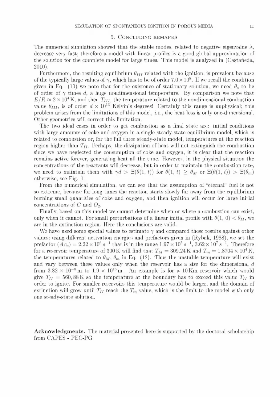
, (46)where θi = 0.4792015876. The results of simulation for the unstable stationary solutionagree with our intuition: the evolution of the numeri al solution approa hes the unstableequilibrium solution in a very short time, t ≈ 30. It remains lose to that solution forlong time: it diverges only for t > 800, and approa hes a stable stationary solution aroundt ≈ 1850. Noti e that using a bise tion method we an nd initial onditions that remain lose to the unstable solution for times as long as we please. This result is plotted at sometimes on Fig. 4.1 for CN. In this gure we also show results for the Ba kward Euler methodwith entral dierentiation (BE). Rening the grid numbers will show that the onvergen ehas to be, in both ases, to I(x).

Figure 4.1. The initial ondition, for time t = 0, given in (46) is plotted onthe top left. We plot with dark ir les the CN method and with light rossesthe BE method, the three linear plots are the three stationary solutions. Fortimes loser to t = 30 the solution obtained by both methods approximateasymptoti ally the unstable solution. Both solutions remain lose to it untilt = 800. The bifur ation starts leading CN to I(x) at t = 1600 and BE toIII(x) at t = 1850.Several simulations show that the behavior of any solution of the nonlinear model alwayshas a fast onvergen e to an almost linear prole, from whi h the solution will be driven toone of the stable stationary solutions. Su h separation between traje tories that onverge to

I(x) from those onverging to III(x) appears to o ur at a value θ(1, t) omparable to θII .

SIMULATION OF SPONTANEOUS IGNITION IN POROUS MEDIA 115. Con luding remarksThe numeri al simulation showed that the stable modes, related to negative eigenvalue λ,de rease very fast; therefore a model with linear proles is a good global approximation ofthe solution for the omplete model for large times. This model is analyzed in (Castañeda,2010).Furthermore, the resulting equilibrium θIII related with the ignition, is prevalent be auseof the typi ally large values of γ, whi h has to be of order 7.0×108. If we re all the onditiongiven in Eq. (10) we note that for the existen e of stationary solution, we need θo to beof order of γ times d, a huge nondimensional temperature. By omparison we note thatE/R ≈ 2×104K, and then TIII , the temperature related to the nondimensional ombustionvalue θIII , is of order d × 1013 Kelvin's degrees! Certainly this range is unphysi al; thisproblem arises from the limitations of this model, i.e., the heat loss is only one-dimensional.Other geometries will orre t this limitation.The two ideal ases in order to get ombustion as a nal state are: initial onditionswith large amounts of oke and oxygen in a single steady-state equilibrium model, whi h isrelated to ombustion or, for the full three steady-state model, temperatures at the rea tionregion higher than TII . Perhaps, the dissipation of heat will not extinguish the ombustionsin e we have negle ted the onsumption of oke and oxygen, it is lear that the rea tionremains a tive forever, generating heat all the time. However, in the physi al situation the on entrations of the rea tants will de rease, but in order to maintain the ombustion rate,we need to maintain them with γd > Ξ(θ(1, t)) for θ(1, t) ≥ θM or Ξ(θ(1, t)) > Ξ(θm)otherwise, see Fig. 1.From the numeri al simulation, we an see that the assumption of eternal fuel is notso extreme, be ause for long times the rea tion starts slowly far away from the equilibriumburning small quantities of oke and oxygen, and then ignition will o ur for large initial on entrations of C and O2.Finally, based on this model we annot determine when or where a ombustion an exist,only when it annot. For small perturbations of a linear initial prole with θ(1, 0) < θII , weare in the extin tion region. Here the on lusions are valid.We have used some spe ial values to estimate γ and ompared these results against othervalues; using dierent a tivation energies and prefa tors given in (Rybak, 1988), we set theprefa tor (Aco) = 2.22×106 s−1 that is in the range 1.97×105 s−1, 3.62×107 s−1. Thereforefor a reservoir temperature of 300K will nd that TM = 309.24K and Tm = 1.8704× 104K,the temperatures related to θM , θm in Eq. (12). Thus the unstable temperature will existand vary between these values only when the reservoir has a size for the dimensional dfrom 3.82 × 10−8m to 1.9 × 1015m. An example is for a 10Km reservoir whi h wouldgive TII = 560, 88K so the temperature at the boundary has to ex eed this value TII inorder to ignite. For smaller reservoirs this temperature would be larger, and the domain ofextin tion will grow until TII rea h the Tm value, whi h is the limit to the model with onlyone steady-state solution.A knowledgments. The material presented here is supported by the do toral s holarshipfrom CAPES - PEC-PG.

12 CASTAÑEDA, MARCHESIN, AND BRUININGReferen es[1 S.A. Abu-Khamsin, W.E. Brigham and H.J. Ramey (1988) Rea tion kineti s of fuel formationfor in-situ ombustion, SPE Reservoir Engineering 3:4: 13081316.[2 J. Bruining and D. Mar hesin (2008) Spontaneous ignition in porous media at long times, ECMORXI. 8-11 Sept., 11th European Conferen e on the Mathemati s of Oil Re overy. Bergen, Norway.[3 P. Castañeda (2010) Chemi al rea tors in porous media. (Defended on 4 January 2010.)[http://www.preprint.impa.br/ Do toral thesis, IMPA/Brasil.[4 W. Rybak (1988) Intrinsi rea tivity of petroleum oke under ignition onditions, Fuel 67: 16961702.[5 R.J. Tyler (1985) Intrinsi rea tivity of petroleum oke to oxygen, Fuel 65: 235240.Pablo CastañedaDan Mar hesinInstituto Na ional de Matemáti a Pura e Apli adaEstrada Dona Castorina, 110Rio de Janeiro, RJ 22460-320, BrazilE-mail address : astanedaimpa.brE-mail address : mar hesiimpa.brJohannes BruiningSe tion Geoengineering, Delft University of Te hnologyP.O. Box 5048, 2600 GA, Delft, The NetherlandsE-mail address : J.Bruiningtudelft.nl