Octane number prediction based on gas chromatographic analysis with non-linear regression techniques

Chemometrics and intelligent

ELSEVIER Chemometrics and Intelligent Laboratory Systems 25 (1994) 325-340

laboratory systems

Octane number prediction based on gas chromatographic analysis with non-linear regression techniques

J.A. van Leeuwen ap*, R.J. Jonker b, R. Gill ’ a Akzo Research Laboratories Arnhem, P. 0. Box 9300, 6800 SB Arnhem, The Netherlands

b Akzo ChemicaLs, Research Centre Amsterdam, P.O. Box 26223, 1002 GE Amsterdam, The Netherlands ’ Utrecht University, Department of Mathematics, P.O. Box 80010, 3508 TA Utrecht, The Netherlands

Received 5 March 1994; accepted 10 April 1994

Abstract

Most widely used techniques for multivariate modelling (principal component regression (PCR), partial least squares (PLS)) are based on linear relations between variables. They are also applied when the chemical or physical relations underlying the data are known to be of a non-linear nature which leads to sub-optimal models. In case of non-linearities possible alternatives are the use of projection pursuit regression and neural networks. Projection pursuit regression is based on a ‘projection’ of the independent variables on direction vectors that are found (‘pursued’) using a gradient descent optimization technique. The projected independent variables are smoothed to include any non-linearities. The smooths can be represented graphically which enables visual inspection of the non-linearities. Neural networks are based on simple processing units that contain a non-linear transformation function. Connecting a number of processing units and estimating the weight of each connection is the basis of the neural network. Estimating the weights by repeated adaption of their value after a number of example cases have been presented allows non-linear relations to be modelled. The non-linear techniques are applied to the results of gas chromatographic analysis of gasolines. The results of the mass distribution of the gasolines over numerous individual components are combined into so-called PIANO groups and related to octane numbers. The octane number of gasolines is known to depend non-linearly on the specific composition of the gasoline. A data set of 824 gasolines, each separated in 89 PIANO groups is used. For each gasoline, the octane number is known. It is shown that projection pursuit regression and neural networks can be used to model the relation between PIANO groups and the octane number.

1. Introduction

The key fuel-performance property of gasoline is its octane number (ON). The octane rating of a

* Corresponding author.

gasoline is determined by the measurement of a standard knock intensity in test engines, where the sample’s performance is compared to refer- ence fuel blends [l]. One of the critical points of this method is the consumption of 500 ml of naphtha per measurement. Another is that the minimal standard deviation of the test is 0.3 point. In practice, two octane numbers are used, the

0169-7439/94/$07.00 0 1994 Elsevier Science B.V. All rights reserved SSDZ 0169-7439(94)00042-H

326 J.A. uan Leeuwen et al. / Chemometrics and Intelligent Laboratory Systems 25 (1994) 325-340

motor octane number (MON) and the research octane number (RON), simulating different oper- ating conditions of the engine. The octane numbers differ in value. All statistical modelling described in this paper is done on the RON. The relation with the MON will be discussed briefly in the section on the data set.

Fluid catalytic cracking (FCC) is the most important and widely used refinery process for con- verting heavy oils into more valuable gasoline. In FCC catalyst research, test methods are used in which only small amounts of gasoline are ob- tained. The l-2 ml produced in these tests are far from the 500 ml required for the standard engine test. Apart from this, the precision of the engine test is so poor, that small improvements in the performance of the catalyst are not detected. Therefore, an indirect method for the measurement of the octane numbers needs to be developed.

The octane quality is determined by the gasoline’s composition. In principle, a compositional analysis of the gasoline should provide information from which the octane number can be calcu- lated. Unfortunately this task is complicated by the complexity of the gasoline mixture and the non-linear blending characteristics of the octane number properties of the individual components. In the past, spectroscopic techniques (Hi NMR 121, C,, NMR 131, IR [4] and NIR [51) have been used for ON prediction. A drawback of these spectroscopic methods is that they have to be applied to distillation fractions, because otherwise the structural information of the gasoline is contaminated with contributions from other boiling ranges in the sample.

Gas chromatography (GC) allows the detailed analysis of a naphtha even if it is mixed with other, higher boiling fractions. The technique was applied by Anderson et al. [6] for the calculation of octane numbers. A supplementary advantage of gas chromatography is, that it is a cheap, fast, precise method of analysis, capable of analyzing a large number of samples from small sample vol- umes.

Contrary to the standard method where the octane numbers are measured directly with the engine, this new method of analysis requires a

mathematical model to relate the GC results to the octane numbers of the naphtha. The determi- nation of an appropriate calibration model for the prediction of octane numbers from the gas chromatographic data is the subject of research described in this paper.

The models presented are based on a data set of some 800 gas chromatographic analyses and the corresponding octane numbers. At an earlier stage and with less samples, linear models were made using principal components regression (PCR) and multiple linear regression (MLR). From this investigation, suspicions are that non- linearities play a role in the model. With neither PCR nor MLR acceptable results were found unless by inclusion of a large number of variables (MLR) or principal components (PCR).

2. Software/hardware

The statistical programming package Splus is used for all calculations involving projection pursuit regression (Splus, Statistical Sciences Inc., Seattle, WA, USA).

The package NeuralWorks Professional II/ plus version 4.0 is used for all calculations involving a neural network (NeuralWorks Professional II/plus, NeuralWare Inc., Pittsburgh, PA, USA).

The version of Splus used was implemented on a Sun Spare workstation. The NeuralWorks software was implemented on an IBM RS6000 workstation.

3. Non-linear non-parametric modelling

Non-linear non-parametric modelling techniques are relatively new techniques. Subse- quently, little is known about their practical properties. In this study, two non-linear, non-parametric techniques are evaluated on their use for RON prediction. They are neural networks (NN) and projection pursuit regression (PPReg). Neu- ral networks and projection pursuit regression are similar in that they do not require a prespecified model that is tested for statistical relevance.

J.A. van Leeuwen et al. / Chemometrics and Intelligent Laboratory Systems 25 (1994) 325-340 327

PPReg is non-parametric in that it does not produce a model with estimated parameters. It produces smoothed predictions of the dependent variable. For the work presented here, a small addition to the original PPReg algorithm is intro- duced io allow prediction with a fixed model. It consists of a parameterization of the smooth.

The NN produces similar models although in this case many parameters (the weights of the neurons) are estimated. The procedure to get the parameter estimations through iterative learning procedures and minimizing local errors is different from normal regression techniques.

Both NN and PPReg are capable of including non-linearities in their models. In PPReg the non-linearities are accommodated by the smooth function, whereas in NN they are present in the so-called transfer function. An outline of both techniques is given first and then their application to the ON prediction problem is discussed.

3.1. Projection pursuit regression

Projection pursuit regression is a non-linear non-parametric multiple regression technique, developed by Friedman [7]. It is based on an iterative two-stage process of projection (reduction of parameter space) and smoothing (establishing non-linear relations). It produces a non- linear model of the regression surface by the summation of a number of smooths. The reduction of the parameter space is essential for the application of smoothing; smoothing in high-dimensional spaces quickly becomes impossible because of data sparsity [71. Projection pursuit regression basically fits the model:

y=Y+ c 4?&?J+%40 m=l

??I =xa,

where n = number of objects under investigation, p = number of explanatory variables, y = vector of response or dependent variable (n x 11, X = matrix of explanatory variables (n x p), QL, = mth projection vector (length p), 4, = smooth function for mth projection vector, M,, = number of incorporated smooths, eMO = residual error after

fitting Ma smooths, z, = vector of scores after projection of X on a, (length n>. In this case the response y is a vector because the dependent variable, RON, is a scalar. In case of multiple responses, the same line of reasoning applies to the matrix of responses.

The first step in the projection pursuit algorithm is to produce a projection a, vector for the first smooth. The projection vector projects the p-dimensional space of the original X matrix into a projected vector z, = Xa,. In fact, the projection vector reduces the p-dimensional variable space to a one-dimensional vector z. Selection of a suitable projection vector a is done by maximizing the criterion:

Z(a,) = 1 - i-l

L& i=l

m-l

ri m , =Yi-Y- C 4j(zij)

j=l

with xi = ith row of X. The criterion Z(a,), which is of the R* type, introduces the second step in projection pursuit regression, the smooth 4,. The projection vector a, and the corresponding smooth 4, are varied in an iterative process to maximize Z(a,).

For the first projection vector a, and the first smooth &, this comes down to finding zi and maximizing Z(a,), ri,l = yi - 5. Thus, the variance explained by smooth 4, of a1 * X is maximized.

It is clear that the maximization of Z(a,) through iteratively repeating a smoothing procedure is computationally intensive. The smoothing procedure applied to the projected variables is a symmetric k-nearest neighbours linear least squares procedure [9]. It has a variable span and uses local cross validation to find the optimal span. In the version of projection pursuit regression as implemented in Splus, the same smoothing procedure is applied to all projected objects, so minimization of Z(a,) is only dependent of the ai values and not of the c#+ values because for a given ai, +i is fixed.

The maximization procedure used in projec-

328 J.A. van Leeuwen et al. /Chemomettics and Intelligent Laboratory Systems 25 (1994) 325-340

tion pursuit regression as implemented in Splus is that of Rosenbrock [8]. This minimization procedure is based on gradient descent. Other gradient descent methods may give similar results.

The iterative part of projection pursuit regression now is that once a smooth bi and a corresponding projection vector QL~ are found, the residuals (y -9i) can again be submitted to the same process. So, a second smooth & can be found, based on a second projection vector CY~. After the first iteration the model was:

J=~++,(X*cu,) +&I

Finding +2 involves maximizing

I((y2) = 1_ [Y -“,“(_x~~‘~x”4”2’12 YY 1’Ul

After the second iteration the model is:

y=Y+ i 4m(x*%n)+E2 m=l

N

0

L

?h

9

Smooth 1 Smooth 2

/ 0’

. l * , .* .

.

-0.30 -0.20 -0.10 0.0

21

Smooth 3

.

* . .

ON . /

2

N 0.

9. r/- 9 /

0.02 0.03 0.04 0.05 0.06 0.07 0.06

23

This process can be extended to include more smooths. The number of smooths to include is a key issue in projection pursuit regression and is directly related to the chosen maximum value of ZGU,).

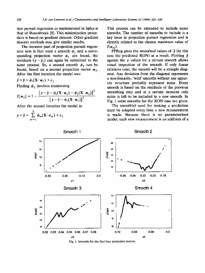
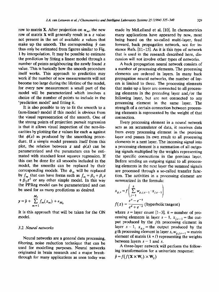
PPReg gives the smoothed values of 9 (in this case the predicted RON) as a result. Plotting 9 against the z values for a certain smooth allows visual inspection of the smooth. If only linear relations exist, the smooth will be a straight diagonal. Any deviation from the diagonal represents a non-linearity, ‘wild’ smooths without any appar- ent structure probably represent noise. Every smooth is based on the residuals of the previous smoothing step and at a certain moment only noise is left to be included in a new smooth. In Fig. 1 some smooths for the RON case are given.

The smooth(s) used for making a prediction must be adapted every time a new measurement is made. Because there is no parameterized model, each new measurement is an addition of a

aD

(0

PI zw N

N

0

-0.26 -0.24 -0.22 -0.20 -0.16

22

Smooth 4

Fig. 1. Smooths for the first four projection vectors.

J.A. van Leeuwen et al. /Chemometrics and Intelligent Laboratory Systems 25 (1994) 325-340 329

row to matrix X. After projection on (Y,,,, the new row of matrix X will generally result in a 2 value not present in the set of available z values that make up the smooth. The corresponding 9 can thus only be estimated from figures similar to Fig. 1 by interpolation. It may be possible to estimate the prediction by fitting a linear model through a number of points neighbouring the newly found z value. This is basically how the smooth procedure itself works. This approach to prediction may work if the number of new measurements will not become too large during the lifetime of the model, for every new measurement a small part of the model will be parameterized which involves a choice of the number of points to include in the ‘prediction model’ and fitting it.

made by McLelland et al. [lo]. In chemometrics many applications have appeared by now, most being based on the so-called multi-layer, feed forward, back propagation network, see for instance Refs. [ll-1.51. As it is this type of network that is used in the research described here, discussion will not involve other types of networks.

It is also possible to try to fit the smooth to a (non-linear) model if this model is obvious from the visual representation of the smooth. One of the strong points of projection pursuit regression is that it allows visual inspection of the non-linearities by plotting the z values for each QL against the 4(z) as produced by the smoothing procedure. If a simple model presents itself from this plot, the relation between z and 4(z) can be parameterized and the parameters can be estimated with standard least squares regression. If this can be done for all smooths included in the model, the smooths can be replaced by their corresponding models. The 4, will be replaced by f, that can have forms such as f, = p,, +&z +&z* or any other simple model. In this way the PPReg model can be parameterized and can be used for as many predictions as desired.

A back propagation neural network consists of a number of processing elements. The processing elements are ordered in layers. In many back propagation neural networks, the number of layers is limited to three. The processing elements that make up a layer are connected to all processing elements in the preceding layer and/or the following layer, but are not connected to any processing element in the same layer. The strength of a certain connection between processing elements is represented by the weight of that connection.

Every processing element in a neural network acts as an accumulator of data, it receives data from every processing element in the previous layer and passes its own result to all processing elements in a next layer. The incoming signal into a processing element is a summation of all outgoing signals multiplied by the weights representing the specific connections in the previous layer. Before sending an outgoing signal to all processing elements in the next layer the summed signals are processed through a so-called transfer function. The activities in a processing element are summarized in the formula:

x g,s =f i wg,j,s-l 'xj,s-l i i

MO \j=l I Y =J+ c fm(zm> +&MO

m=l

It is this approach that will be taken for the ON model.

3.2. Neural networks

Neural networks are a general data processing, filtering, noise reduction technique that can be used for modelling purposes. Neural networks originated in brain research and a major break- through for many applications as seen today was

ez - e-z

f(z) = eZ+e-* ~ (hyperbolic tangent)

where s = layer count [l-3], k = number of processing elements in layer s - 1, xjS_i = the output produced by the jth processing element in layer s - 1, xg,S = the output produced by the g th processing element in layer S, w~,~,~_ 1 = matrix element of matrix (k * I) representing the weights between layers s - 1 and S.

A three-layer network will perform the following transformation for a univariate response:

i=f(fwT) xw2)

330 J.A. uan Leeuwen et al. / Chenwmetrics and Intelligent Laboratory Systems 25 (1994) 325-340

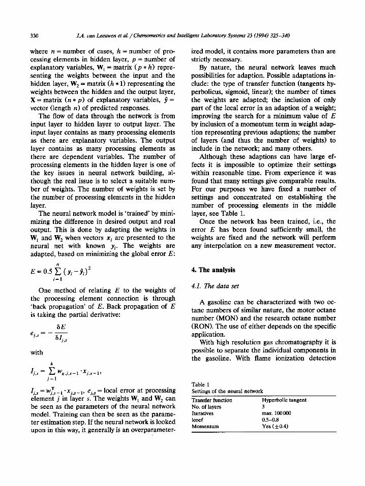
where IZ = number of cases, h = number of processing elements in hidden layer, p = number of explanatory variables, W, = matrix (p * h) representing the weights between the input and the hidden layer, W, = matrix (h * 1) representing the weights between the hidden and the output layer, X = matrix (n * p) of explanatory variables, 9 = vector (length n) of predicted responses.

The flow of data through the network is from input layer to hidden layer to output layer. The input layer contains as many processing elements as there are explanatory variables. The output layer contains as many processing elements as there are dependent variables. The number of processing elements in the hidden layer is one of the key issues in neural network building, although the real issue is to select a suitable number of weights. The number of weights is set by the number of processing elements in the hidden layer.

The neural network model is ‘trained’ by minimizing the difference in desired output and real output. This is done by adapting the weights in W, and W, when vectors xi are presented to the neural net with known yi. The weights are adapted, based on minimizing the global error E:

E=0.5 5 (&-ji)’ i=l

One method of relating E to the weights of the processing element connection is through ‘back propagation’ of E. Back propagation of E is taking the partial derivative:

6E ej*s = - “‘I,s

with

lj,s = It wg,j,s-l ‘xj,s-l~ j=l

Zj,s = wzs _ 1 * xj,s _ 1, ej,s = local error at processing element j in layer s. The weights W, and W, can be seen as the parameters of the neural network model. Training can then be seen as the parameter estimation step. If the neural network is looked upon in this way, it generally is an overparameter-

ized model, it contains more parameters than are strictly necessary.

By nature, the neural network leaves much possibilities for adaption. Possible adaptations include: the type of transfer function (tangents hy- perbolicus, sigmoid, linear); the number of times the weights are adapted; the inclusion of only part of the local error in an adaption of a weight; improving the search for a minimum value of E by inclusion of a momentum term in weight adaption representing previous adaptions; the number of layers (and thus the number of weights) to include in the network; and many others.

Although these adaptions can have large ef- fects it is impossible to optimize their settings within reasonable time. From experience it was found that many settings give comparable results. For our purposes we have fixed a number of settings and concentrated on establishing the number of processing elements in the middle layer, see Table 1.

Once the network has been trained, i.e., the error E has been found sufficiently small, the weights are fixed and the network will perform any interpolation on a new measurement vector.

4. The analysis

4.1. The data set

A gasoline can be characterized with two octane numbers of similar nature, the motor octane number (MON) and the research octane number (RON). The use of either depends on the specific application.

With high resolution gas chromatography it is possible to separate the individual components in the gasoline. With flame ionization detection

Table 1 Settings of the neural network

Transfer function Hyperbolic tangent No. of layers 3 Iteratives max. 100000 lcoef OS-O.8 Momentum Yes ( f 0.4)

JA van Leeuwen et al. / chemometrics and Intelligent Laboratory Systems 25 (1994) 325-340 331

Table 2 known RON and MON. For each gasoline the The PIANO groups GC analysis and classification in PIANO groups P Paraffines was available. The research described herein fo- I Iso-pa&fines A Aromates

cuses on the RON. The procedures for the MON

N Naphthenes are the same and give similar results. For an

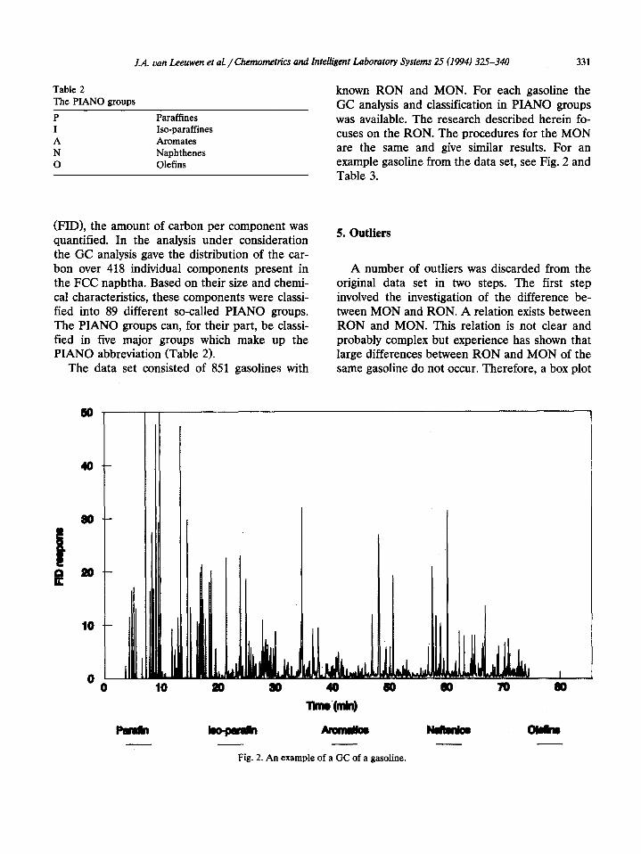
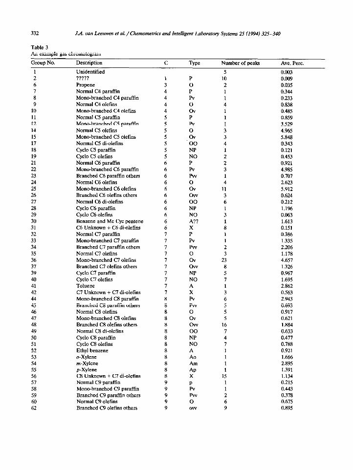
0 Olefins example gasoline from the data set, see Fig. 2 and Table 3.

(FID), the amount of carbon per component was quantified. In the analysis under consideration the GC analysis gave the distribution of the carbon over 418 individual components present in the FCC naphtha. Based on their size and chemical characteristics, these components were classi- fied into 89 different so-called PIANO groups. The PIANO groups can, for their part, be classi- fied in five major groups which make up the PIANO abbreviation (Table 2).

The data set consisted of 851 gasolines with

60

40

80

B B 20

10

Oo

5. Outliers

A number of outliers was discarded from the original data set in two steps. The first step involved the investigation of the difference between MON and RON. A relation exists between RON and MON. This relation is not clear and probably complex but experience has shown that large differences between RON and MON of the same gasoline do not occur. Therefore, a box plot

Fig. 2. An example of a GC of a gasoline.

332

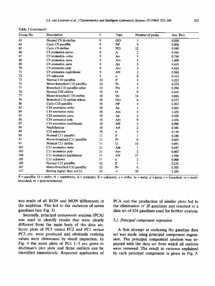
Table 3

J.A. van Leeuwen et al. / Chemometrics and Intelligent Laboratory Systems 25 (1994) 325-340

An examole was chromatogram

Group No. Description C Type Number of peaks Ave. Pert.

1 Unidentified 2 ????? 6 Propene 7 Normal C4 paraffin 8 Mono-branched C4 paraffin 9 Normal C4 olefins

10 Mono-branched C4 olefins 11 Norma1 C5 paraffin 12 Mono-branched C5 paraffin 14 Norma1 C5 olefins 15 Mono-branched C5 olefins 17 Norma1 C5 di-olefins 18 Cycle C5 paraffin 19 Cycle C5 olefins 21 Norma1 C6 paraffin 22 Mono-branched C6 paraffin 23 Branched C6 paraffin others 24 Norma1 C6 olefins 25 Mono-branched C6 olefins 26 Branched C6 olefins others 27 Normal C6 di-olefins 28 Cycle C6 paraffin 29 Cycle C6 olefins 30 Benzene and Me Cyc pentene 31 C6 Unknown + C6 di-olefins 32 Norma1 C7 paraffin 33 Mono-branched C7 paraffin 34 Branched C7 paraffin others 35 Normal C7 olefins 36 Mono-branched C7 olefins 37 Branched C7 olefins others 39 Cycle C7 paraffin 40 Cycle C7 olefins 41 Toluene 42 C7 Unknown + C7 di-olefins 44 Mono-branched C8 paraffin 45 Branched C8 paraffin others 46 Norma1 C8 olefins 47 Mono-branched C8 olefins 48 Branched C8 olefins others 49 Normal C8 di-olefins 50 Cycle C8 paraffin 51 Cycle C8 olefins 52 Ethyl benzene 53 o-Xylene 54 m-Xylene 55 p-Xylene 56 C8 Unknown + C7 di-olefins 57 Normal C9 paraffin 58 Mono-branched C9 paraffin 59 Branched C9 paraffin others 60 Normal C9 olefins 62 Branched C9 olefins others

1 3 4 4 4 4 5 5 5 5 5 5 5 6 6 6 6 6 6 6 6 6 6 6 7 7 7 7 7 7 7 7 7 7 8 8 8 8 8 8 8 8 8 8 8 8 8 9 9 9 9 9

P 0 P Pv 0 ov P Pv 0 ov 00 NP NO P Pv Pw 0 ov ow 00 NP NO A?? X P Pv Pw 0 Gv ow NP NO A X Pv Pw 0 ov ow 00 NP NO A Ao Am AP X

L Pw 0 ow

5 0.003 10 2 1

4 1 1 1 3 3 4 1 2 2 3 1 4

11 3 6 1 3 1 8

1 2 3

23 8 5

1 3 6 5 5 5

16 7 4 7

1 1 1

15 1

2 6 9

0.009 0.035 0.344 0.233 0.838 0.485 0.859 3.529 4.965 5.848 0.343 0.121 0.453 0.921 4.985 0.707 2.623 5.912 0.624 0.212 1.196 0.063 1.613 0.151 0.386 1.335 2.206 1.178 4.657 1.326 0.967 1.695 2.862 0.563 2.943 0.693 0.917 0.621 1.884 0.633 0.477 0.788 0.921 1.666 2.895 1.391 1.134 0.215 0.443 0.378 0.675 0.895

J.A. van Leeuwen et al. / Chemometrics and Intelligent Laboratory Systems 25 (1994) 325-340

Table 3 (continued)

Group No. Description C Type Number of peaks Ave. Pert.

333

63 Normal C9 di-olefins 64 Cycle C9 paraffin 65 ($10 C9 olefins 66 C9 aromatics mono 61 C9 aromatics ortho 68 C9 aromatics meta 69 C9 aromatics para 70 C9 aromatics poly 71 C9 aromatics naphthenic 72 C9 unknown 73 Normal Cl0 paraffin 74 Mono-branched Cl0 paraffin 75 Branched Cl0 paraffin other 76 Norma1 Cl0 olefins 77 Mono-branched Cl0 olefins 78 Branched Cl0 olefins others 80 Cycle Cl0 paraffin 83 Cl0 aromatics o&o 84 Cl0 aromatics meta 85 Cl0 aromatics para 86 Cl0 aromatics poly 87 Cl0 aromatics naphthenic 88 Naphthalene 89 Cl0 unknown 90 Normal Cl 1 paraffin 91 Mono-branched Cl1 paraffin 93 Norma1 Cl1 olefins 101 Cl1 aromatics meta 103 Cl1 aromatics pofy 104 Cl1 aromatics naphthenic 105 Cl1 unknown 106 Norma1 Cl2 paraffin 107 Mono-branched Cl2 paraffin 117 Boiling higher than n-Cl2

9 00 9 NP 9 NO 9 A 9 Ao 9 Am 9 AP 9 Aw 9 AN 9 X

10 P 10 Pv 10 Pw 10 0 10 ov 10 ow 10 NP 10 Ao 10 Am 10 AP 10 Aw 10 AN 10 AA 10 X

11 P 11 Pv 11 0 11 Am 11 Aw 11 AN 11 X

12 P 12 Pv 12 +

9 12 2 1 1

3 2 8 1 4 5 9

14 6 4 1 4 2 8 2 2 4 1 6

14

2 17 2

6 30

0.068 0.808 0.980 0.466 0.746 1.608 0.618 4.016 0.568 0.533 0.223 0.570 0.296 0.616 0.696 0.537 0.202 0.365 1.439 0.428 2.436 0.990 0.381 0.149 0.180 0.622 0.691 0.197 0.467 1.926 0.068 0.135 0.303 1.283

P = paraffin; 0 = olefin; N = naphthene; A = aromatic; X = unknown; o = ortho; m = meta; p = para; v = branched; w = multi- branched; w = poly-substituted.

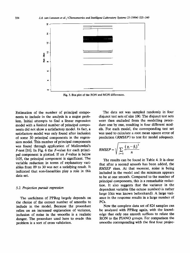
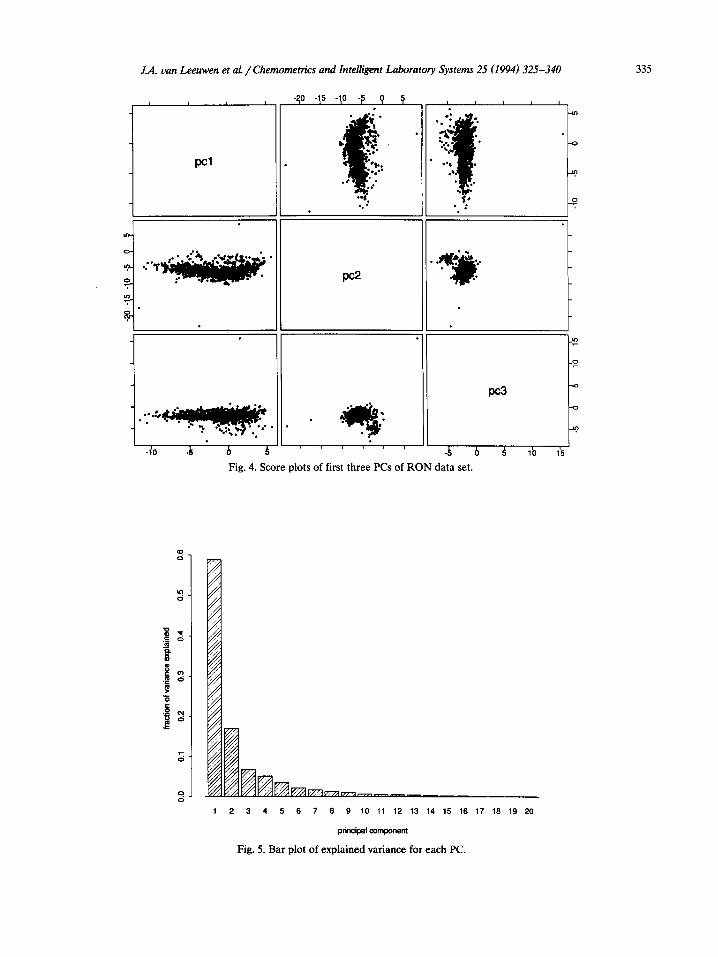
was made of all RON and MON differences in PCA and the production of similar plots led to the naphthas. This led to the exclusion of seven the elimination of 20 gasolines and resulted in a gasolines (see Fig. 3). data set of 824 gasolines used for further analysis.

Secondly, principal component analysis (PCA) was used to identify results that were clearly different from the main body of the data set. Score plots of PC1 versus PC2 and PC1 versus PC3 etc. were produced and obviously outlying values were eliminated by visual inspection. In Fig. 4 the score plots of PCs l-3 are given in draftman’s plot style and three outliers can be identified immediately. Repeated application of

5.1. Principal component regression

A first attempt at analyzing the gasoline data set was made using principal component regression. The principal component analysis was repeated with the data set from which all outliers were removed. The result in variance explained by each principal component is given in Fig. 5.

334 J.A. van Leeuwen et al. / Chemometrics and Intelligent Laboratory Systems 25 (1994) 325-340

a-

*-

N

Fig. 3. Box plot of the RON and MON differences.

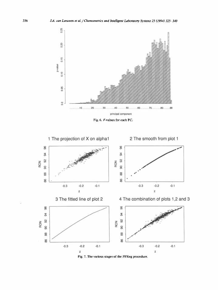
Estimation of the number of principal components to include in the analysis is a major problem. Initial attempts to find a linear regression model with a limited number of principal components did not show a satisfactory model. In fact, a satisfactory model was only found after inclusion of some 30 principal components in the regression model. This number of principal components was found through application of Malinowksi’s F-test [16]. In Fig. 6 the F-value for each principal component is plotted. If an F-value is below 0.05, the principal component is significant. The variable reduction in terms of explanatory variables from 89 to 30 was not a satisfying result. It indicated that non-linearities play a role in this data set.

5.2. Projection pursuit regression

The usefulness of PPReg largely depends on the choice of the correct number of smooths to include in the model. Because the procedure relies on an increased explanation of variance, inclusion of noise in the smooths is a realistic danger. The procedure used here to evade this problem is a sort of cross validation.

The data set was sampled randomly in four disjunct test sets of size 100. The disjunct test sets were then excluded from the modelling procedure one by one, resulting in four different models. For each model, the corresponding test set was used to calculate a root mean square error of prediction (RMSEP) to test for model adequacy.

RMsEp=

i

c (Yi-ji>’

i=l n

The results can be found in Table 4. It is clear that after a second smooth has been added, the RMSEP rises. At that moment, noise is being included in the model and the minimum appears to be at one smooth. Compared to the number of principal components, this is a remarkable reduction. It also suggests that the variance in the dependent variable (the octane number) is rather large (this was known beforehand). A large variance in the response results in a large number of PCs.

Now the complete data set of 824 samples can be analyzed with PPReg again, with the knowl- edge that only one smooth suffices to relate the RON to the PIANO groups. For comparison the smooths corresponding with the first four projec-

LA. van Leeuwen et al./Chemometrics and Intelligent Laboratory Systems 25 (1994) 325-340 335

. .

.

.

. .* :s... * .- .

PC3

Fig. 4. Score plots of first three PCs of RON data set.

1 2 3 4 5 6 7 6 9 10 11 12 13 14 15 16 17 16 19 20

Fig. 5. Bar plot of explained variance for each PC.


10 20 30 A0 54 60 70 80 B8

principal component

Fig. 6. F-values for each PC.

1 The projection of X on alpha1 2 The smooth from plot 1

_ -> +--

-x -- _ __

-0.3 -0.2 -0.1

z

3 The fitted line of plot 2 4 The combination of plots 1,2 and 3

-0.3 -0.2 -0.1

2

-0.3 -0.2 -0.1

z

8 Y -0.3 -0.2 -0.1

z

Fig. 7. The various stages of the PPReg procedure.

J.A. van Leeuwen et al. /Chemometrics and Intelligent Laboratory Systems 25 (1994) 325-340 331

8- 1 -0.2 -0.1 0.0 0.1

L

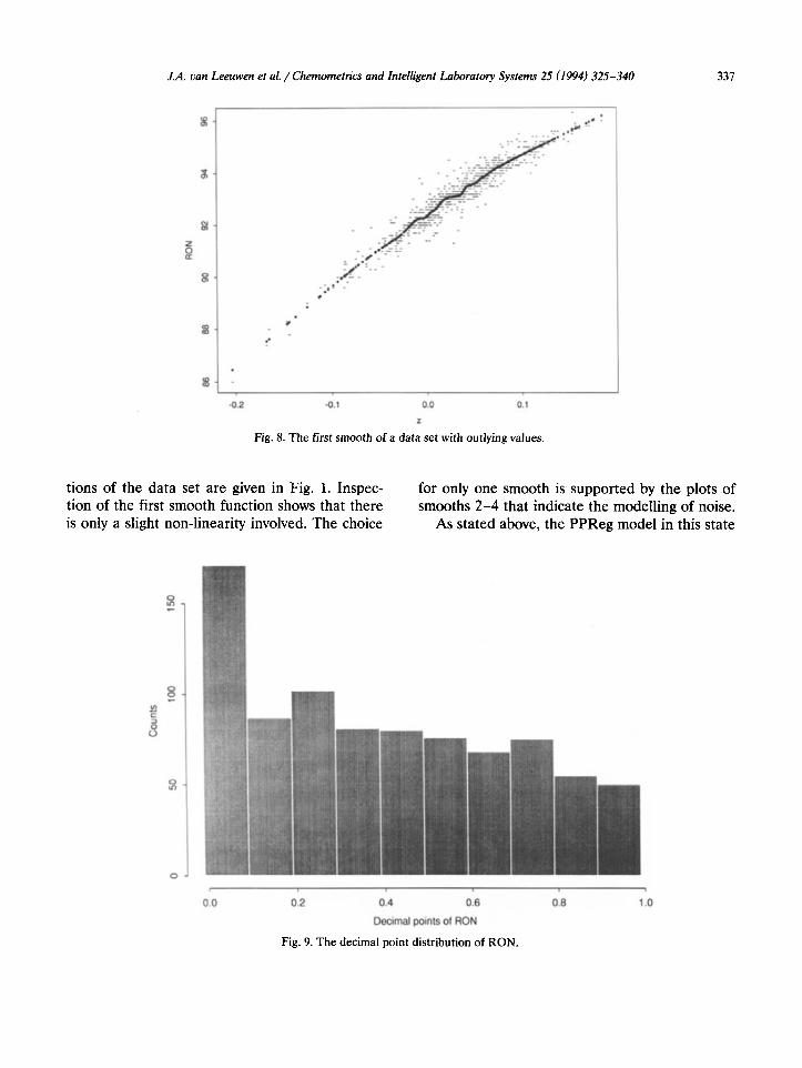
Fig. 8. The first smooth of a data set with outlying values.

tions of the data set are given in Fig. 1. Inspec- for only one smooth is supported by the plots of tion of the first smooth function shows that there smooths 2-4 that indicate the modelling of noise. is only a slight non-linearity involved. The choice As stated above, the PPReg model in this state

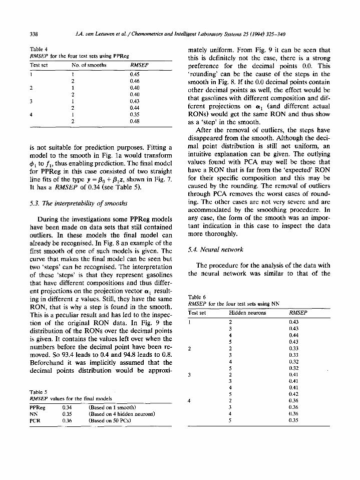
0.0 0.2 0.4 0.6

Decimal points of RON

Fig. 9. The decimal point distribution of RON.

, 0.6 1 .o


Table 4 RMSEP for the four test sets using PPReg

Test set No. of smooths RMSEP

1 1 0.45 2 0.46

2 1 0.40 2 0.40

3 1 0.43 2 0.44

4 1 0.35 2 0.48

is not suitable for prediction purposes. Fitting a model to the smooth in Fig. la would transform 4i to fi, thus enabling prediction. The final model for PPReg in this case consisted of two straight line fits of the type y = PO + &z, shown in Fig. 7. It has a RMSEP of 0.34 (see Table 5).

5.3. The interpretability of smooths

During the investigations some PPReg models have been made on data sets that still contained outliers. In these models the final model can already be recognised. In Fig. 8 an example of the first smooth of one of such models is given. The curve that makes the final model can be seen but two ‘steps’ can be recognised. The interpretation of these ‘steps’ is that they represent gasolines that have different compositions and thus different projections on the projection vector (pi resulting in different z values. Still, they have the same RON, that is why a step is found in the smooth. This is a peculiar result and has led to the inspection of the original RON data. In Fig. 9 the distribution of the RONs over the decimal points is given. It contains the values left over when the numbers before the decimal point have been removed. So 93.4 leads to 0.4 and 94.8 leads to 0.8. Beforehand it was implicitly assumed that the decimal points distribution would be approxi-

Table 5 RMSEP values for the final models

PPReg 0.34 (Based on 1 smooth) NN 0.35 (Based on 4 hidden neurons) PCR 0.36 (Based on 50 PCs)

mately uniform. From Fig. 9 it can be seen that this is definitely not the case, there is a strong preference for the decimal points 0.0. This ‘rounding’ can be the cause of the steps in the smooth in Fig. 8. If the 0.0 decimal points contain other decimal points as well, the effect would be that gasolines with different composition and different projections on (pi (and different actual RONs) would get the same RON and thus show as a ‘step’ in the smooth.

After the removal of outliers, the steps have disappeared from the smooth. Although the decimal point distribution is still not uniform, an intuitive explanation can be given. The outlying values found with PCA may well be those that have a RON that is far from the ‘expected’ RON for their specific composition and this may be caused by the rounding. The removal of outliers through PCA removes the worst cases of rounding. The other cases are not very severe and are accommodated by the smoothing procedure. In any case, the form of the smooth was an important indication in this case to inspect the data more thoroughly.

5.4. Neural network

The procedure for the analysis of the data with the neural network was similar to that of the

Table 6 RMSEP for the four test sets using NN

Test set Hidden neurons RMSEP

1 2 0.43 3 0.43 4 0.44 5 0.43

2 2 0.33 3 0.33 4 0.32 5 0.32

3 2 0.41 3 0.41 4 0.41 5 0.42

4 2 0.36 3 0.36 4 0.36 5 0.35

J.A. van Leeuwen et al. / Chemometrics and Intelligent Laboratory Systems 25 (1994) 325-340 339

projection pursuit regression technique. In fact, the same procedure of cross validation through test sets was used and the same test sets were used. In case of the neural network, the key issue is the number of hidden neurons.

The results (RMSEP) for an increasing number of neurons are given in Table 6. It is not so clear in this case what the optimal number of neurons should be. The choice has been made to include only a minimal number of neurons resulting in four hidden neurons. This decision is not undisputed, but there is no clear-cut way to de- cide on the number of neurons to include. After training the weights of the neural net are fixed. The neural net model can be used for prediction purposes now. The neural net with four hidden neurons results in an RMSEP of 0.35 (see Table 5).

6. Discussion

At the start of the investigation it was realized that the related model-building techniques (NN and PPReg) did not have well established guide- lines for use yet. During the investigation this idea was confirmed. For instance, in projection pursuit regression the number of smooths to include in the final model is not easily determined. A similar case is present in neural network model building, where the number of units in the middle (hidden) layer is often open to discussion. They are the most important parameter for each technique that must be found through trial and error. Many other parameters of less importance must also be set (especially in NN) without any theoretical basis for selecting the optimal setting. This makes the use of these techniques time-consum- ing for a non-experienced user.

Also the influence of the structure of the data set on the final model is not clear. In this particu- lar case, the design of the data set was a given fact and could not be changed otherwise than by deletion of observations. But even in case of designed experiments it is difficult to give an optimal experimental design, because the model being fitted is unknown. This makes application

of these techniques even more difficult, because in general use the techniques will require a large data set.

PPReg and NN have an entirely different theoretical basis. The NN is a combination of many elements with the same non-linear function as a basis. The combination allows virtually any non- linearity to be modelled because the neural net relies on overparameterizing the required model. PPReg is based on dimension reduction via projection. The projection score vector is smoothed to represent non-linearities. The parameterization by fitting the smooth scores suggested here is only a small step from the original algorithm. It adds the ‘model’ only in the final step and leaves complete freedom in the initial stages. With the NN, the model is fixed from the beginning but flexibility is gained through the many parameters (weights) in the model and the choice of the non-linear transfer function in the processing elements.

Despite the theoretical differences both techniques result in acceptable models and it seems that model flexibility is the unifying characteris- tic. It does not seem to matter whether flexibility is reached by non-parameterization or by over- parameterization.

7. Conclusions

The non-linear non-parametric techniques pro jection pursuit regression and neural network can be used to model the non-linear relation between RON and PIANO group. The RMSEP is near the inherent variance in the octane number. It appears that small non-linearities can be incorporated into the model using this type of modelling techniques.

Acknowledgments

The authors want to thank J. As for the contributions made to this research and on which he graduated from Utrecht University.

340 J.A. van Leeuwen et al. / Chemomettics and Intelligent Laboratory Systems 25 (1994) 325-340

References

[l] Test Method for Knock Characteristics of Motor Fuels by the Research Method ASTM Manual for Rating Mo- tor, Diesel and Aviation Fuels, ASTM Test Method D2699-70, American Society for Testing and Materials, Philadelphia, PA, 1971.

[2] R. Louis, Nuclear magnetic resonance analysis of gasolines, Erdol und Kohlen, Erdgas, Petrochemie, 19 (1966) 281-286.

[9] J.H. Friedman, A variable span smoother, Tech. Rept. No. 5, Laboratory for Computational Statistics, Depart- ment of Statistics, Stanford, CA, 1984.

[lo] J.L. McLe.lland, Parallel Distributed Processing, Part 1 and 2, MIT, Cambridge, MA, 1986.

[ll] M. Glick and G.M. Hieftje, Classification of allays with an artificial neural network and multivariate calibratrion of glow-discharge emission spectra, Applied Spectroscopy, 45 (1991) 1706.

[3] M.B. Meyers, J. Stollsteimer and A.M. Weins, Determi- nation of gasoline octane numbers from chemical composition, Analytical Chemistry, 47 (1975) 2301-2304.

[4] H. Luther and H.H. Oelert, Molecular spectroscopic group analysis for saturated hydrocarbons, Zeitschrift fur Analytische Chemie, 183 (1961) 161-172.

[5] J.J. Kelly, C.H. Narlow, T.M. Jinguji and J.B. Callis, Prediction of gasoline octane numbers from near-infrared spectral features in the range 660-1215 nm, Ana- lytical Chemistry, 61 (1989) 313-320.

[6] PC. Anderson, J.M. Sharkey and R.P. Walsh, Calcula- tion of the research octane number of motor gasoline quality control, Journal of the Institute of Petroleum, 58 (1972) 83-94.

[12] J.R. Long, V.G. Gregoriou and P.J. Gemperline, Spec- troscopic calibration and quantitation using artificial neural nets, Analytical Chemistry, 62 (1990) 1791.

[13] A.P. de Weyer, L. Buydens, G. Kateman and H.M. Heuvel, Neural networks used as a soft-modelling technique for quantitative description of the relation between physical structure and mechanical properties of poly(eth- ylene terephtalate) yarns, Chemometrics and Intelligent Laboratory Systems, 16 (1992) 77-86.

[7] J.H. Friedman and W. Stuetzle, Projection pursuit regression, Journal of the American Statistical Association, 76 (1981) 817.

[14] J.R.M. Smits, P. Schoenmakers, A. Stehmann, F. Sijster- mans and G. Kateman, Interpretation of infrared spectra with modular neural network systems, Chemometrics and Intelligent Laboratory Systems, 18 (1993) 27-39.

[15] J.R.M. Smits, L.W. Breedveld, M.W.J. Derksen, G. Kate- man, H.W. Balfoort, J. Snoek and J.W. Hofstraat, Pat- tern classification with artificial neural networks; classification of algae based upon flow cytometry data, Anaiytica Chimica Acta, 258 (1992) 11.

[8] H.H. Rosenbrock, An automatic method for finding the 1161 E.R. Malinowski, Statistical F-test for abstract factor greatest or least value of a function, The Computer Jour- analysis and target testing, Journal of Chemometrics, 3 nal, 3 (1960) 175. (1988) 49.

Documents

Octane number prediction based on gas chromatographic analysis with non-linear regression techniques