Embed Size (px)
Citation preview
i
OPTIMISATION OF BIOGAS PRODUCTION USING SOME PROCESS
PARAMETERS IN A FIXED DOME LABORATORY BIOREACTOR
BARASA HENRY MASINDE
A Thesis Submitted to the Graduate School in Partial Fulfillment of the Requirements for
the Doctor of Philosophy Degree in Agricultural Engineering of Egerton University
EGERTON UNIVERSITY
JANUARY 2021
ii
DECLARATION AND RECOMMENDATION
Declaration
I declare that this Thesis is my original work and has not been presented for the award of a
degree in any University.
Signature __ __ Date_07.01.2021__
Barasa Henry Masinde
BD11/0401/13
Recommendation
This thesis has been submitted with our approval as University supervisors.
Signature __ Date_09.01.2021__
Prof. Daudi M. Nyaanga, PhD.
Department of Agricultural Engineering, Egerton University
Egerton, Kenya.
Signature ___ _______________ Date_______09.01.2021_____
Dr. Musa R. Njue, PhD.
Department of Agricultural Engineering, Egerton University
Egerton, Kenya.
Signature Date 09.01.2021
Prof. Joseph W. Matofari, PhD.
Department of Dairy and Food Science and Technology, Egerton University
Egerton, Kenya.

iii
COPYRIGHT
© 2021 Barasa Henry Masinde
All rights are reserved. No part of this publication may be reproduced, stored in a retrieval
system or transmitted in any form or by any means; electronic, magnetic tape, mechanical,
photocopying, recording or otherwise, without due written permission from the author or
Egerton University.

iv
DEDICATION
This work is dedicated to my wife Christine, and my children Andrew, Eric, Margaret,
Richard, Moses, and Florence.
v
ACKNOWLEDGEMENTS
I give thanks to the Almighty God for giving me the life, strength, determination, and vision
to undertake and complete this work. I am very grateful to my supervisors Prof. Daudi M.
Nyaanga, Dr. Musa R. Njue, and Prof. Joseph W. Matofari for the constant guidance and
encouragement throughout this work.
It would not have been possible to perform this work without the funding from the National
Commission for Science, Technology and Innovation (NACOSTI) for fabricating a
laboratory bioreactor in which the experiments were done, and consequently the
documentation of this work. Many thanks to Egerton University for providing a secure and a
conducive environment for my studies; Graduate School under the leadership of Prof. Nzula
Kitaka, Dean of Faculty of Engineering and Technology Prof. Japheth Onyando, Chairman of
Agricultural Engineering (AGEN) Department Dr. Raphael Wambua, the Chairman of
Electrical Control and Instrumentation Engineering (ECIEN) Department Dr. Franklin
Manene, Dr. Peter Kundu, and Dr. Booker Osodo. I also appreciate the support from the
following staff: Mrs. Bernadette Misiko (Dairy, Food Science and Technology Department),
Meshack Korir, Peter Mecha, Patrick Wamalwa, A. Muyera, W. Tallam, and Napoo (all from
AGEN).
My thanks also go to the Vice Chancellor of Masinde Muliro University of Science and
Technology (MMUST) for granting me study leave to enable me complete this research
work. This was possible through the efforts made by Mrs. Brenda Simiyu of Mechanical and
Industrial Engineering (MIE) Department, and the Dean of the School of Engineering and
Built Environment (SOBE) Dr. Bernadette Sabuni. Encouragement by the late Prof. C K
Ndiema and Dr. Joel Chirchir (of MIE) is highly appreciated. A special mention goes to Dr.
Peter Cherop (MIE) for reading my work thereby assisting me to make appropriate
improvements.
Lastly thanks go to my family for allowing me to use their resources, and to my friends for
encouraging me to finish this work.
vi
ABSTRACT
Biogas is a renewable energy that has many applications including cooking, lighting
households among others. It is produced through the breakdown of organic matter in an air
tight compartment through a biochemical process which is generally termed digestion. This
technology involves various techniques through use of digesters or bioreactors and
operational parameters which could be predicted and must be optimised. A 0.15m3 capacity
fixed dome laboratory bioreactor was used to determine the effect of total solids, temperature,
and substrate retention time on biogas production rate. The feedstock was cow dung from
dairy cows managed under a free-range system during the day but held under a shed
overnight at Egerton University, Kenya. Three different experiments were conducted in a
batch feeding regime of the bioreactor. In the first one, the substrate at total solids of 6%, 7%,
8%, 9%, and 10% was digested at a constant temperature of 350C (using auto control system).
The second experiment was conducted at mesophilic temperatures of 250C, 300C, 350C, 400C,
and 450C using a cow dung substrate at total 8% solids. An evaluation of existing biogas
production prediction models was done. A third model (named the fixed dome temperature
model) was developed and tested. Biogas production rate was optimised with the help of
response surface methodology – in which a central composite design was applied. An
interaction of three variables namely total solids, temperature, and substrate retention time
were tested at five different levels. The highest average biogas production rate was 0.48 m3of
biogas per m3 of digester volume per day (m3/m3d) at 8% total solids. The highest average
result of 0.52 m3/m3d occurred at 400C. Lastly substrate retention time was observed while
the cow dung was at 8% total solids and 350C; and the highest average output was 0.68
m3/m3d at 11 days. Low Temperature Lagoon model and Toprak model suited the results
obtained in this research. The optimum output of 0.50 m3/m3d was achieved at a level of 8%
total solids, 43.410C, and 15 days. The optimal values were verified and found to be in
agreement with experimental results at an admissible tolerance of 6.6-10.7%. The above
conclusions can be transferred for adoption for field and industrial fixed dome digesters for
biogas production into operational guidelines for biogas stakeholders including designers and
operators.
vii
TABLE OF CONTENTS
DECLARATION AND RECOMMENDATION ................................................................ ii
COPYRIGHT ........................................................................................................................ iii
DEDICATION....................................................................................................................... iv
ACKNOWLEDGEMENTS .................................................................................................. v
ABSTRACT ........................................................................................................................... vi
TABLE OF CONTENTS .................................................................................................... vii
LIST OF TABLES ................................................................................................................. x
LIST OF FIGURES ............................................................................................................. xii
LIST OF SYMBOLS .......................................................................................................... xiii
LIST OF ACRONYMS/ABBREVIATIONS ..................................................................... xv
CHAPTER ONE .................................................................................................................... 1
GENERAL INTRODUCTION ............................................................................................. 1
1.1 Background ............................................................................................................... 1
1.2 Statement of the Problem .......................................................................................... 6
1.3 Objectives .................................................................................................................. 7
1.3.1 Broad Objective ................................................................................................. 7
1.3.2 Specific Objectives ............................................................................................ 7
1.4 Research Questions ................................................................................................... 7
1.5 Justification ............................................................................................................... 7
1.6 Scope and Limitations ............................................................................................... 8
1.6.1 Scope .................................................................................................................. 8
1.6.2 Limitations ......................................................................................................... 9
References ......................................................................................................................... 10
CHAPTER TWO ................................................................................................................. 15
LITERATURE REVIEW ................................................................................................... 15
2.1Biogas ............................................................................................................................ 15
2.2 Types of Biogas Systems ............................................................................................. 16
2.3 Anaerobic Digestion ..................................................................................................... 21
2.3.1 Microbial aspects of the anaerobic process ........................................................... 21
2.3.2 Factors affecting anaerobic digestion .................................................................... 23
2.3.3 Methods for enhancing biogas production ............................................................ 35
viii
2.4 Process Optimisation .................................................................................................... 46
2.5 Response Surface Methodology for Optimisation ....................................................... 49
2.6 Biogas Production Prediction Models .......................................................................... 54
References ......................................................................................................................... 56
CHAPTER THREE ............................................................................................................. 75
EFFECT OF TOTAL SOLIDS, TEMPERATURE AND SUBSTRATE RETENTION
TIME ON BIOGAS PRODUCTION ................................................................................. 75
Abstract .............................................................................................................................. 75
3.1 Introduction .................................................................................................................. 75
3.2 Materials and Methods ................................................................................................. 78
3.2.1 Experiment Set-up ................................................................................................. 78
3.2.2 Material Preparation .............................................................................................. 81
3.2.3 Temperature control .............................................................................................. 85
3.2.4 Substrate retention time ......................................................................................... 85
3.3 Results and Discussions ............................................................................................... 86
3.3.1. Effect of total solids on biogas production ........................................................... 86
3.3.2. Effect of temperature on biogas production ......................................................... 92
3.3.3. Effect of substrate retention time on biogas production at 8% TS and 350C ....... 95
3.4 Conclusions and Recommendation .............................................................................. 99
3.4.1 Conclusions ........................................................................................................... 99
3.4.2 Recommendation ................................................................................................... 99
References ....................................................................................................................... 101
CHAPTER FOUR .............................................................................................................. 108
EVALUATING BIOGAS PRODUCTION PREDICTION MODELS ......................... 108
Abstract ............................................................................................................................ 108
4.1 Introduction ................................................................................................................ 108
4.2 Materials and Methods ............................................................................................... 115
4.3 Results and Discussions ............................................................................................. 116
4.3.1 Low Temperature Lagoon Digester model .......................................................... 116
4.3.2 Modified Toprak Model ...................................................................................... 119
4.3.3 Proposed Fixed-dome-lab Temperature Model ................................................... 122
4.4 Conclusions and Recommendation ............................................................................ 127
4.4.1Conclusions .......................................................................................................... 127
ix
4.4.2 Recommendation ................................................................................................. 128
References ....................................................................................................................... 129
CHAPTER FIVE ............................................................................................................... 131
OPTIMISATION OF BIOGAS PRODUCTION ............................................................ 131
Abstract ............................................................................................................................ 131
5.1 Introduction ................................................................................................................ 131
5.2 Materials and Methods ............................................................................................... 133
5.3 Results and Discussions ............................................................................................. 138
5.4 Conclusions and Recommendation ............................................................................ 149
5.4.1 Conclusions ......................................................................................................... 149
5.4.2 Recommendation ................................................................................................. 150
References ....................................................................................................................... 151
CHAPTER SIX .................................................................................................................. 156
GENERAL DISCUSSION, CONCLUSIONS AND RECOMMENDATIONS ........... 156
6.1 General Discussion ..................................................................................................... 156
6.2 General Conclusions .................................................................................................. 159
6.3 General Recommendations ........................................................................................ 159
APPENDICES .................................................................................................................... 161
Appendix 1: Design Drawings, Calculations, Figures and Plates .................................... 161
A1.1 Design of a bioreactor and figures ....................................................................... 161
A1.2: Engineering drawings ......................................................................................... 166
A1.3: Plates of types of bioreactors .............................................................................. 168
Appendix 2: Biogas production data and analysis ........................................................... 171
A2.1 Biogas Production (litres per day) in the Egerton University Fixed Dome Lab
Digester ......................................................................................................................... 171
A2.2: Biogas prediction for 8% TS at 35 degrees Celsius for models based on 2018 and
2019 data....................................................................................................................... 173
Appendix 3: Copyright Form ........................................................................................... 175
Appendix 4: Abstracts of Publications ............................................................................. 179
Appendix 5: Research permit ........................................................................................... 182
x
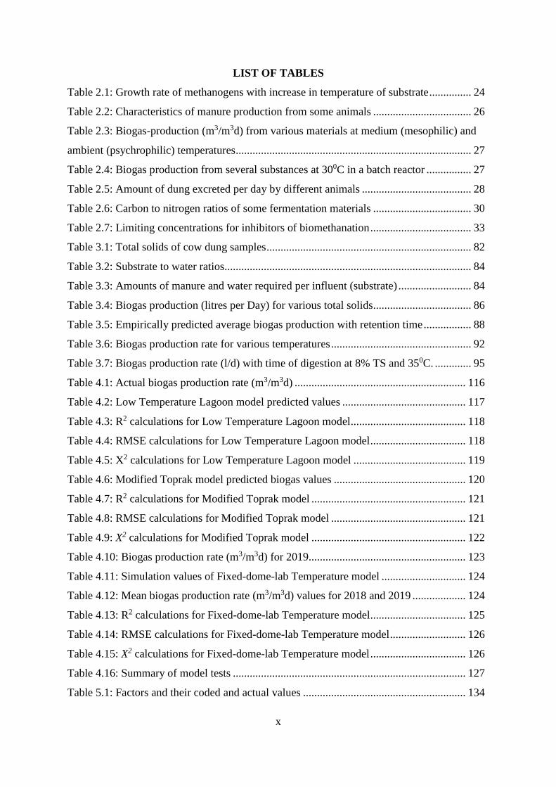
LIST OF TABLES
Table 2.1: Growth rate of methanogens with increase in temperature of substrate ............... 24
Table 2.2: Characteristics of manure production from some animals ................................... 26
Table 2.3: Biogas-production (m3/m3d) from various materials at medium (mesophilic) and
ambient (psychrophilic) temperatures.................................................................................... 27
Table 2.4: Biogas production from several substances at 300C in a batch reactor ................ 27
Table 2.5: Amount of dung excreted per day by different animals ....................................... 28
Table 2.6: Carbon to nitrogen ratios of some fermentation materials ................................... 30
Table 2.7: Limiting concentrations for inhibitors of biomethanation .................................... 33
Table 3.1: Total solids of cow dung samples ......................................................................... 82
Table 3.2: Substrate to water ratios........................................................................................ 84
Table 3.3: Amounts of manure and water required per influent (substrate) .......................... 84
Table 3.4: Biogas production (litres per Day) for various total solids................................... 86
Table 3.5: Empirically predicted average biogas production with retention time ................. 88
Table 3.6: Biogas production rate for various temperatures .................................................. 92
Table 3.7: Biogas production rate (l/d) with time of digestion at 8% TS and 350C. ............. 95
Table 4.1: Actual biogas production rate (m3/m3d) ............................................................. 116
Table 4.2: Low Temperature Lagoon model predicted values ............................................ 117
Table 4.3: R2 calculations for Low Temperature Lagoon model ......................................... 118
Table 4.4: RMSE calculations for Low Temperature Lagoon model .................................. 118
Table 4.5: X2 calculations for Low Temperature Lagoon model ........................................ 119
Table 4.6: Modified Toprak model predicted biogas values ............................................... 120
Table 4.7: R2 calculations for Modified Toprak model ....................................................... 121
Table 4.8: RMSE calculations for Modified Toprak model ................................................ 121
Table 4.9: X2 calculations for Modified Toprak model ....................................................... 122
Table 4.10: Biogas production rate (m3/m3d) for 2019........................................................ 123
Table 4.11: Simulation values of Fixed-dome-lab Temperature model .............................. 124
Table 4.12: Mean biogas production rate (m3/m3d) values for 2018 and 2019 ................... 124
Table 4.13: R2 calculations for Fixed-dome-lab Temperature model .................................. 125
Table 4.14: RMSE calculations for Fixed-dome-lab Temperature model ........................... 126
Table 4.15: X2 calculations for Fixed-dome-lab Temperature model .................................. 126
Table 4.16: Summary of model tests ................................................................................... 127
Table 5.1: Factors and their coded and actual values .......................................................... 134

xi
Table 5.2: Matrix of the experiments ................................................................................... 135
Table 5.3: Criteria. ............................................................................................................... 137
Table 5.4: Influent preparation ............................................................................................ 137
Table 5.5: Actual and predicted biogas yield ....................................................................... 138
Table 5.6: Analysis of variance ........................................................................................... 140
Table 5.7: Optimised and experimental results.................................................................... 149
xii
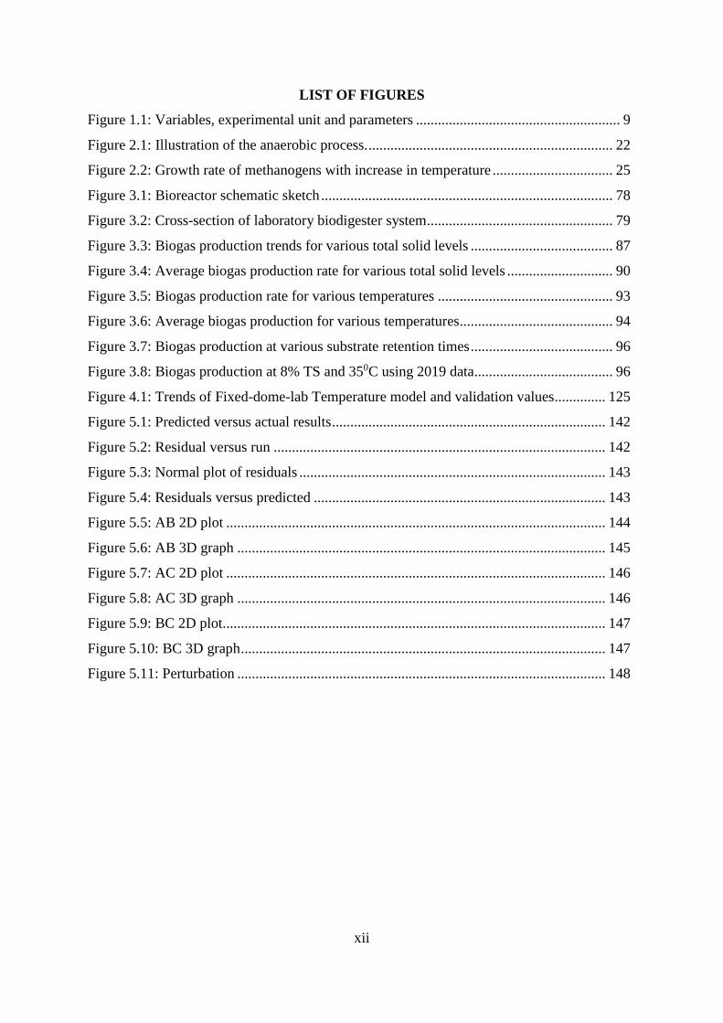
LIST OF FIGURES
Figure 1.1: Variables, experimental unit and parameters ........................................................ 9
Figure 2.1: Illustration of the anaerobic process. ................................................................... 22
Figure 2.2: Growth rate of methanogens with increase in temperature ................................. 25
Figure 3.1: Bioreactor schematic sketch ................................................................................ 78
Figure 3.2: Cross-section of laboratory biodigester system................................................... 79
Figure 3.3: Biogas production trends for various total solid levels ....................................... 87
Figure 3.4: Average biogas production rate for various total solid levels ............................. 90
Figure 3.5: Biogas production rate for various temperatures ................................................ 93
Figure 3.6: Average biogas production for various temperatures .......................................... 94
Figure 3.7: Biogas production at various substrate retention times ....................................... 96
Figure 3.8: Biogas production at 8% TS and 350C using 2019 data...................................... 96
Figure 4.1: Trends of Fixed-dome-lab Temperature model and validation values .............. 125
Figure 5.1: Predicted versus actual results ........................................................................... 142
Figure 5.2: Residual versus run ........................................................................................... 142
Figure 5.3: Normal plot of residuals .................................................................................... 143
Figure 5.4: Residuals versus predicted ................................................................................ 143
Figure 5.5: AB 2D plot ........................................................................................................ 144
Figure 5.6: AB 3D graph ..................................................................................................... 145
Figure 5.7: AC 2D plot ........................................................................................................ 146
Figure 5.8: AC 3D graph ..................................................................................................... 146
Figure 5.9: BC 2D plot......................................................................................................... 147
Figure 5.10: BC 3D graph .................................................................................................... 147
Figure 5.11: Perturbation ..................................................................................................... 148
xiii
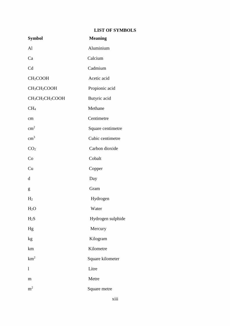
LIST OF SYMBOLS
Symbol Meaning
Al Aluminium
Ca Calcium
Cd Cadmium
CH2COOH Acetic acid
CH3CH2COOH Propionic acid
CH3CH2CH2COOH Butyric acid
CH4 Methane
cm Centimetre
cm2 Square centimetre
cm3 Cubic centimetre
CO2 Carbon dioxide
Co Cobalt
Cu Copper
d Day
g Gram
H2 Hydrogen
H2O Water
H2S Hydrogen sulphide
Hg Mercury
kg Kilogram
km Kilometre
km2 Square kilometer
l Litre
m Metre
m2 Square metre

xiv
m3 Cubic metre
Mg Magnesium
ml Millilitre
Na Sodium
0C Degree Celsius
Zn Zinc
xv
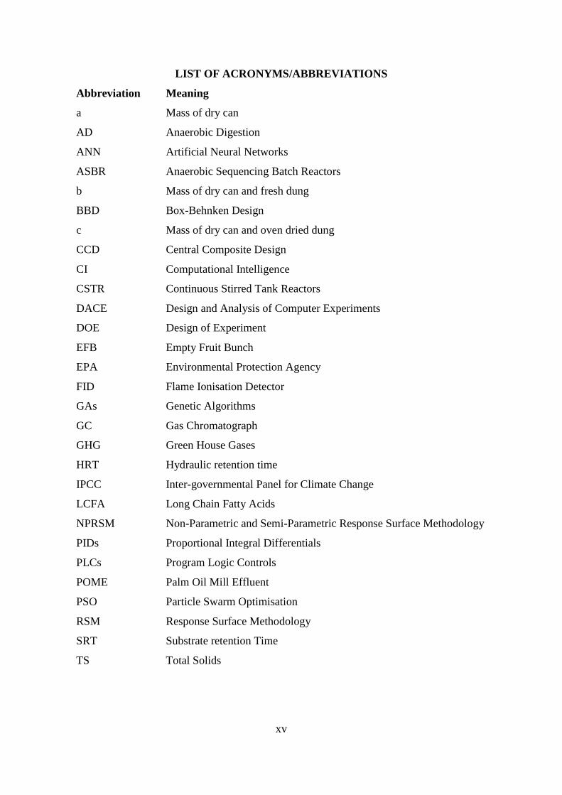
LIST OF ACRONYMS/ABBREVIATIONS
Abbreviation
a
AD
ANN
ASBR
b
BBD
c
CCD
CI
CSTR
DACE
DOE
EFB
EPA
FID
GAs
GC
GHG
HRT
IPCC
LCFA
NPRSM
PIDs
PLCs
POME
PSO
RSM
SRT
TS
Meaning
Mass of dry can
Anaerobic Digestion
Artificial Neural Networks
Anaerobic Sequencing Batch Reactors
Mass of dry can and fresh dung
Box-Behnken Design
Mass of dry can and oven dried dung
Central Composite Design
Computational Intelligence
Continuous Stirred Tank Reactors
Design and Analysis of Computer Experiments
Design of Experiment
Empty Fruit Bunch
Environmental Protection Agency
Flame Ionisation Detector
Genetic Algorithms
Gas Chromatograph
Green House Gases
Hydraulic retention time
Inter-governmental Panel for Climate Change
Long Chain Fatty Acids
Non-Parametric and Semi-Parametric Response Surface Methodology
Proportional Integral Differentials
Program Logic Controls
Palm Oil Mill Effluent
Particle Swarm Optimisation
Response Surface Methodology
Substrate retention Time
Total Solids

xvi
UASB
VFA
VS
Up-Flow Anaerobic Sludge Blanket Reactors
Volatile Fatty Acids
Volatile Solids
1
CHAPTER ONE
GENERAL INTRODUCTION
1.1 Background
Biogas is a renewable and an environmentally friendly form of energy which can substitute
wood and fossil fuels in a number of applications and thus mitigate the rising costs of
petroleum products and deforestation (Deublein and Steinhauser, 2008). Biogas is a
combination of gases produced during anaerobic decomposition of organic materials of plant
origin. It is produced from the organic wastes by a concerted action of various groups of
anaerobic bacteria (Boe, 2006). The main gaseous by-product is methane, with relatively less
carbon dioxide, ammonia and hydrogen sulphide (Saleh et al., 2012). Methane is the principal
constituent of natural gas and ranks first in the series of saturated hydrocarbons known as
alkanes (Khanal, 2008; Monnet, 2003). It is a light, colourless, odourless and highly
inflammable gas, second only to hydrogen in the energy released per gram of fuel burnt,
hence its potential as a household energy source (Nijaguna, 2006).
Biogas production was introduced in developing countries as a low-cost alternative source of
energy to alleviate acute energy shortage for households (Parawira and Mshandete, 2009).
However, few households currently use biogas. The poor adoption of this technology is
associated with the high cost of the digesters, lack of knowledge in installing and maintaining
them and frequent microbial failures (Ho et al., 2015). In Kenya, implementation of foreign
biogas systems has not only led to lower performance but also hampered local innovativeness
and scientific advancement in the field of renewable energy based on the local resources
(Nzila et al., 2012). Biogas technology provides an alternate source of energy in rural areas,
and is an appropriate technology that meets the basic need for cooking and lighting. The
biogas technology is adaptive and cheap because the gas burns clean, has high calorific value
and can be virtually produced anywhere using any locally available biodegradable material
like cattle waste, farm crop residues and other organic wastes (Bond and Templeton, 2011;
Nzila et al., 2012). A small household can use biogas for lighting and cooking without
causing air pollution, while large industrial systems can utilize it to generate electricity to run
their establishment and even sell the surplus to the National Grid (Rajendran et al., 2012).
The use of biogas offers a great opportunity towards the reduction in global warming gases
and climate change (Lippmann et al., 2003). Cooking with biogas can save women time
spent in harvesting wood and instead engage in other economic empowering activities,
reduces smoke which is a major cause of lung diseases and poor eye sight for rural women
2
and children who cook with firewood in poorly lit and ventilated spaces (Nzila et al., 2015).
Other applications include gas-powered refrigerators and chicken incubators than run on
biogas in Kenya (Laichena and Wafula, 1997; Sibisi and Green, 2005). In India and Nepal,
biogas is connected to toilets for lighting (Batzias et al., 2005).
Manure that is left to decompose releases two main gases that cause global climate change:
nitrous dioxide warms the atmosphere three hundred and ten (310) times more than carbon
dioxide (CO2), and methane (CH4) warms the atmosphere twenty one (21) times more than
CO2; therefore by converting cow manure into biogas instead of letting it decompose, it
would be able to reduce global warming gases by 99 million metric tons or 4% (EPA, 2005;
Saleh et al., 2012). Cattle dung is a complex and naturally occurring polymeric substrate
which consists of soluble and insoluble matter which can be used as a source of renewable
energy (Garcia-Ochoa et al., 1999). Improper management of this waste leads to many
environmental hazards including water pollution and greenhouse gases (GHS) emissions
(Kobayashi and Li, 2011). United States of America exclusively produces approximately two
hundred and thirty (230) million tonnes of dry matter of animal waste that cannot be applied
as local fertilizer (Karim et al., 2007), United Kingdom produces eighty eight (88) million
tonnes annually (Phillips et al., 2008), while China produces 1.07 billion tonnes of livestock
waste yearly (Chen et al., 2009). Anaerobic digestion (AD) has been found to be an efficient,
cheap and easy method to manage livestock waste (Nasir et al., 2014).
A bioreactor (also termed as a digester) is any manufactured device or installed or
constructed structure with associated facilities (henceforth termed system) in which a
biologically active biological cum chemical process (digestion and sometimes fermentation)
is carried out which involves microorganisms or biochemically active substances derived
from such organisms is supported (IUPAC, 2006). Bioreactors are commonly cylindrical,
with a capacity ranging from 10 millilitre (ml) bottles to several cubic metres (m3), and are
often made of stainless steel and are mainly small and precise for experimental laboratory
studies while digesters are larger field or industrial biomass digestion systems used to
produce biogas for use in the household, farm or industry (Arthur et al., 2011).
There are many designs of biogas plants but the most common ones in Kenya include the
lagoon, floating drum, fixed dome and flexible structure bio-digester models (Schön, 2010).
These designs have evolved over the years since the first digester was installed in Kenya
around the year 1959 (Nyaanga et al., 2015). The first field biogas systems were based on the
3
floating drum originating from India, and fixed Chinese systems which have since been
modified and advanced to meet the local conditions (Rupfa et al., 2017) by local engineers,
technologists, technicians and masons and accompanied by the introduction of portable
flexible bag digesters, being installed underground or above ground (Nyaanga et al., 2015).
Rupfa et al. (2017) suggests that the most suitable biodigester design for different
applications in Kenya should be based on user defined inputs, including energy and fertiliser
requirements; feedstock (type, amount, and rate of supply); water supply; land use (area, soil
type, ground water level); climate (temperature and rainfall); construction materials available
locally; and the priorities (based on sustainability criteria) of the intended biogas user. There
are many factors and hence there is need for long term and multi-agency corroboration. The
environmental, management, and civil designs including sizing of the digesters with the idea
of optimising the biogas production can be studied and decided on using appropriately
designed laboratory bioreactors that replicate the field systems (Nyaanga et al., 2015).
A fixed dome reactor has been used in this study. A fixed dome is a bioreactor which consists
of a digester with fixed, non-movable gas holder, which sits on the digester – it is the most
commonly used digester in China (Santerre and Smith, 1982) and also in Kenya. In terms of
absolute numbers, the fixed dome is by far the most common digester type in developing
countries (Gunaseelan, 1997). The Chinese fixed dome is the most popular and used most in
developing countries because of its reliability, low maintenance costs, a long lifespan, and
relatively minimal loss of the biogas yield (Ghimire, 2013; Huba et al., 2013).
A parameter is any of the factors that limit the way in which something can be done. In this
study, the parameters that have been considered are total solids, temperature, and substrate
retention time; and their effect on biogas production rate in a fixed dome bioreactor under
mesophilic laboratory conditions. Bioreactors operate at different environmental and
management conditions. There are three possible ranges of temperature in which the
anaerobic digestion (AD) process can be carried out. According to Comino et al. (2010),
psychrophilic temperature ranges from 150C to 250C, mesophilic temperature ranges from
300C to 400C, and thermophilic temperature ranges from 500C to 600C. Temperature and
substrate concentration may be the most important parameters determining the performance
and stability of the AD process (Chae et al., 2008). Together, they influence the microbial
community structure, the biochemical conversion pathways, the kinetics and thermodynamic
balance of the biochemical reactions, and the stoichiometry of the products formed (Arikan et
4
al., 2015). Because the formation and consumption of products can occur at different rates,
transient accumulation of potentially inhibitory substances is possible, particularly with
complex substrates (Labatut et al., 2014). Consequently, temperature is a critical factor
affecting anaerobic digestion because it influences both system heating requirements and
methane production (Ramaraj and Unpaprom, 2016). Other factors that affect the efficient
production of biogas include lack of feedstock, appropriate design of digesters, development
of inoculums, pH, organic loading rate, hydraulic retention time (HRT), Carbon to Nitrogen
(C:N) ratio, and volatile fatty acids (Nzila et al., 2010). Also defects in digester construction
and microbiological failure are the major areas of concern and are crucial for the optimisation
of biogas production technologies and their economic viability (Nijaguna, 2006).
The hydraulic retention time (HRT) refers to the duration that the substrate or the organic
matter compounds take to be digested or get bio-chemically decomposed in the absence of
oxygen, as they pass or traverse and move through the digester from the inlet (as influent) to
the exit (as effluent) (Nyaanga et al., 2015). Complex organic compounds require longer
retention times than simple compounds since the former are harder to breakdown (Singh et
al., 2017).
The retention time of the solids, which can also be termed as substrate retention time (SRT),
has been associated with the ability of a biological system (including fermentation and
digestion of organic matter) to reduce complex harmful compounds to safe levels and hence
meet the effluent standards or the allowed pollutants’ biodegradability levels for complete the
production of biogas (Nyaanga et al., 2015; Singh et al., 2017). Substrate retention time in
biogas production systems depends on the amount of substrate and nutrients available for
methanogenic bacteria to consume and complete to generate methane (Masinde et al., 2020).
Using this understanding, substrate retention time, can be defined as the time taken from
loading the digester or bioreactor with the influent and inoculum, to the time the substrate
stops yielding biogas. The SRT will be influenced by the given biogas system (size or
volume), type of substrate, prevailing operational conditions such as temperature and
agitation. In most cases, lay biogas stakeholders use the terms HRT and SRT interchangeably
despite the difference and similarity. Both SRT and HRT are used in the design of bio-
chemical reactors including biogas production systems which use bacteria and enzymes.
Stirring or agitation and feeding regime (frequency and amount fed into a bioreactor or a
digester) may lead to longer or shorter HRT or SRT or wash out (where excess microbial
5
mass is moved out of digester or digesters), respectively. Hence HRT and SRT depend on
digester volume or size, prevailing conditions, material type especially with respect to
digestibility in addition to factors such as pH, carbon to nitrogen ratio, microbial growth
inhibitors, among others. The anaerobic digesters, which are capable of owning prolonged
solid or substrate retention times (SRT) because of immobile or congested bacterial biomass,
operate rapidly with smaller hydraulic retention time (HRT) and decreased expenses (Singh
et al., 2017).
The biogas quantity and quality are greatly influenced by the range of temperature in the
process of anaerobic digestion. A sudden drop or increase of temperature causes temperature
shocks to the bacteria which might inhibit their performance or cause their death (Patharwat
et al., 2016). The same can happen in the event of insufficient or excess supply of their
specific food or nutrients. Singh et al. (2017) reported that naturally, the microorganisms
(specifically, the methanogenic kind of bacteria) that take part in anaerobic digestion are
largely categorized into three types as mesophiles, thermophiles and cryophiles or
psychrophiles. The elevated temperature of the thermophilic regime induces more
biochemical processes, causing massive production of methane (Leenawat et al., 2016).
Thermophilic regime consumes a large quantity of energy, and this is counterbalanced by the
huge biogas production.
A number of semi theoretical and empirical models have been proposed and used in the
mathematical estimation of the amount of biogas produced from a given biogas setup and
prevailing conditions. They include Plug Flow Digester, Lagoon Low Temperature, Toprak,
Chen and Hashimoto, and Scoff and Minott which involve hydraulic retention time, volatile
solids concentrations, bacteria growth rate, digester temperature, and daily substrate flow
rate. These are described and tested in later chapters in this thesis. A few other mathematical
models have been proposed. Delgadillo et al. (2018) proposed the model for the simulation of
biogas production using model parameters obtained by performing a sensitivity analysis,
using a sequential quadratic programming algorithm. They calibrated and validated the model
using experimental data obtained from a pilot-scaled plant and concluded that the model was
able to correctly predict the methane production dynamics from few key measurements.
Korolev and Maykov (2019) optimized a two-stage methanogenesis regime based on the
theory of the Pontryagin’s maximum principle and concluded that optimal control of the
biogas process can be estimated using a controlled algorithm.
6
Optimisation is the act of achieving the best possible result under given circumstances. The
aim is either to minimise the effort or to maximise benefit. The effort or benefit can be
expressed as a function of certain design variables. Hence optimisation is the process of
finding conditions that give the minimum or the maximum value of a function (Astolfi and
Praly, 2006). In this study, biogas production was maximised while the parameters were kept
in range. Some optimisation techniques associated with anaerobic digestion including basic
designs of single-stage or two-stage systems, environmental conditions within the reactors
such as temperature, pH and buffering capacity have been applied in Nigeria, Tanzania and
Zimbabwe among others in sub-Saharan Africa (Parawira and Mshandete, 2009). Response
surface methodology (RSM) is one of the most effective approaches for designing
experiments, for building models, and for determining optimal conditions on responses which
are influenced by several independent variables (Kang et al., 2016). Apart from defining the
influences of independent variables on the responses, RSM also determines the effect of
interaction between parameters to obtain the best performance on a system (Belwal et al.,
2016). Other optimisation techniques include Artificial Neural Networks (ANN) (Ghatak and
Ghatak, 2018), Genetic Algorithm (GA), and Taguchi.
1.2 Statement of the Problem
Biogas production is influenced by a number of process parameters including substrate
retention time, total solids, and temperature for different digester designs and management
regimes (including batch, semi continuous and continuous feeding of the organic matter) in
the field, and industrial, household and experimental or laboratory digesters or bioreactors.
The common biogas systems in Kenya including the fixed dome digesters are likely to
perform differently as per the manure characteristics and the management of some of the
operational parameters including dilution levels, retention time and digester temperature.
The dilution of feedstock to water used in Kenya is 1:1, leading to a variation of the total
solids in the influent due to the inherent amount of water in the feedstock including cow dung
or manure.
The effect of varying substrate retention time, total solids, and temperature on biogas
production in a batch bioreactor is not clearly articulated. The applicability of some of the
simpler empirical existing biogas production prediction models have not been tested on this
type fixed dome laboratory bioreactor for adoption. Optimisation using substrate retention
time, total solids, and temperature to maximise biogas production in a fixed dome bioreactor
7
using response surface method on the biogas production in a fixed dome lab bioreactor has
not been done. Therefore, there was need to carry out this study in order to fill these gaps in
the advancement of biogas technology in Kenya and other parts of the world.
1.3 Objectives
1.3.1 Broad Objective
The broad objective of this research was to optimise biogas production using some process
parameters in a fixed dome laboratory bioreactor.
1.3.2 Specific Objectives
The specific objectives were to:
i. Determine the effect of different total solids, temperature and substrate retention time on
biogas production for the fixed dome laboratory bioreactor.
ii. Evaluate existing biogas production prediction models that relate to total solids,
temperature and substrate retention time.
iii. Optimise biogas production based on total solids, temperature and substrate retention time
for the fixed dome laboratory bioreactor.
1.4 Research Questions
a) How is biogas production affected by total solids, temperature and substrate retention
time?
b) How do the existing biogas production prediction models that relate total solids,
temperature, and substrate retention time to biogas production with respect to the data
collected?
c) Has optimisation using total solids, mesophilic temperature, and substrate retention time
been employed to maximise biogas production for the fixed dome laboratory bioreactor?
1.5 Justification
The need to relate the field medium and small scale fixed dome digesters common in most
institutions such as universities, slaughter houses, large scale farms and small scale
households, has been identified that led to the development of a laboratory bioreactor
representing the fixed dome digesters by Nyaanga et al. (2015), however, the functioning of
8
the bioreactor has not been done. It is on this basis that this research’s objectives were
formulated.
The effect of varying the levels of total solids, temperature, and substrate retention time on
biogas production gives the optimal point at which each factor gives the highest amount of
biogas. This enables the application of the appropriate levels of each parameter by the biogas
producer. The relationship from such an evaluation can be adapted by biogas stakeholders
and producers to improve the technology and enhance its adoption.
Evaluation of models of biogas production is important because it helps to understand how a
system behaves when a parameter is varied. Models can be used to predict the level of input
at which maximum biogas can be produced. This helps in reducing the cost of production
while maximising on the output by identifying the appropriate settings of values of the
concerned parameters for different sized fixed dome digesters operated at varied conditions.
Optimisation of factors that affect biogas production helps in giving the level of combining
the inputs in order to achieve the best desired output. This knowledge assists in easing the
production process and the associated costs. In this particular case, the optimum temperature,
total solids and substrate retention time for the laboratory fixed dome bioreactor could be
scaled up to the field or industrial digesters.
1.6 Scope and Limitations
1.6.1 Scope
The cattle dung herein termed as the cow manure (used as a feedstock) was sourced from
semi free range cattle rearing system (where the animals are allowed to graze in the fields
during the day and come to the shed for milking and overnight) of Tatton Agricultural Park
(Farm), Egerton University, Kenya. Tap water at room temperature, was used to dilute the
manure to the required total solids before loading into the 0.15m3 fixed dome batch
laboratory reactor, designed and fabricated in the Agricultural Engineering workshop at
Egerton University. The factors considered in the research were temperature, total solids and
substrate retention time and their effects on biogas production and quality. The substrate
retention time of 11 to 18 days, a mesophilic temperature range of 250C to 450C at intervals
of 50C, and a total solids range from 6% to 10% were proposed for the research. Biogas
9
volume was measured by the water displacement method and validated by bag storage, while
the quality of the gas was verified by a Gas Chromatograph and visual blue flame.
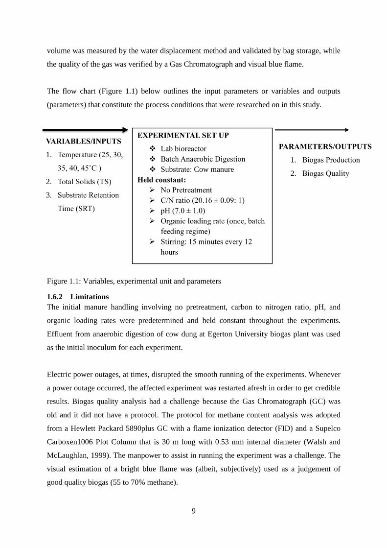
The flow chart (Figure 1.1) below outlines the input parameters or variables and outputs
(parameters) that constitute the process conditions that were researched on in this study.
Figure 1.1: Variables, experimental unit and parameters
1.6.2 Limitations
The initial manure handling involving no pretreatment, carbon to nitrogen ratio, pH, and
organic loading rates were predetermined and held constant throughout the experiments.
Effluent from anaerobic digestion of cow dung at Egerton University biogas plant was used
as the initial inoculum for each experiment.
Electric power outages, at times, disrupted the smooth running of the experiments. Whenever
a power outage occurred, the affected experiment was restarted afresh in order to get credible
results. Biogas quality analysis had a challenge because the Gas Chromatograph (GC) was
old and it did not have a protocol. The protocol for methane content analysis was adopted
from a Hewlett Packard 5890plus GC with a flame ionization detector (FID) and a Supelco
Carboxen1006 Plot Column that is 30 m long with 0.53 mm internal diameter (Walsh and
McLaughlan, 1999). The manpower to assist in running the experiment was a challenge. The
visual estimation of a bright blue flame was (albeit, subjectively) used as a judgement of
good quality biogas (55 to 70% methane).
EXPERIMENTAL SET UP
Lab bioreactor
Batch Anaerobic Digestion
Substrate: Cow manure
Held constant:
No Pretreatment
C/N ratio (20.16 ± 0.09: 1)
pH (7.0 ± 1.0)
Organic loading rate (once, batch
feeding regime)
Stirring: 15 minutes every 12
hours
PARAMETERS/OUTPUTS
1. Biogas Production
2. Biogas Quality
VARIABLES/INPUTS
1. Temperature (25, 30,
35, 40, 45˚C )
2. Total Solids (TS)
3. Substrate Retention
Time (SRT)
10
References
Arikan, O., Mulbry, W. and Lansing, S. (2015). Effect of temperature on methane
production from field-scale anaerobic digesters treating dairy manure. Waste
Management, 43( 2), 108-113.
Arthur, R., Baidoo, M. and Antwi, E. (2011). Biogas as a potential renewable energy source.
A Ghanaian case study. Renewable Energy, 36(5), 1510-1516.
doi:10.1016/j.renene.2010.11.012
Astolfi, A. and Praly, L. (2006). Global complete observability and output-to-state stability
imply the existence of a globally convergent observer. Mathematics of Control,
Signals and Systems, 18(1), 32-65.
Batzias, F., Sidiras, D. and Spyrou, E. (2005). Evaluating livestock manures for biogas
production: A GIS method. Renewable Energy, 30, 1161-1176.
Belwal, T., Dhyani, P., Bhatt, I. D., Rawal, R. S. and Pande, V. (2016). Optimization
extraction conditions for improving phenolic content and antioxidant activity in
Berberis asiatica fruits using response surface methodology (RSM). Food Chemistry,
207, 115-124.
Boe, K. (2006). On-line monitoring and control of the biogas process. (PhD), Technical
University of Denmark, Lyngby, Denmark.
Bond, T. and Templeton, M. (2011). History and future of domestic biogas plants in the
developing world. Energy for Sustainable Development, 15(4), 347-354.
doi:10.1016/j.esd.2011.09.003
Chae, K., Jang, A., Yim, S. and Kim, I. (2008). The effects of digestion temperature and
temperature shock on the biogas yields from the mesophilic anaerobic digestion of
swine manure. Bioresource Technology, 99, 1-6.
Chen, S., Li, R. and Li, X. (2009). Anaerobic co-digestion of kitchen waste and cattle
manure for methane production. Energy Sources, 31, 1848-1856.
Comino, E., Rosso, M. and Riggio, V. (2010). Investigation of increasing organic loading
rate in the co-digestion of energy crops and cow manure mix. Bioresource
Technology, 101(9), 3013-3019.
Delgadillo, L., Machado-Higuera, M. and Hernandez, M. (2018). Mathematical modelling
and simulation for biogas production from organic waste. International Journal of
Engineering Systems Modelling and Simulation, 10(2), 97-101.
doi:10.1504/IJESMS.2018.10013112.
11
Deublein, D. and Steinhauser, A. (2008). Biogas from Waste and Renewable Resources: An
Introduction. Weinheim, Germany.
EPA. (2005). Anaerobic Digestion: Benefits for Waste Management, Agriculture, Energy,
and the Environment. U.S. Environment Protection Agency.
Garcia-Ochoa, F., Santos, V., Naval, L., Guardiola, E. and Lopez, B. (1999). Kinetic
model for anaerobic digestion of livestock manure. Enzyme Microbiology and
Techology, 25, 55-60.
Ghatak, M. and Ghatak, A. (2018). Artificial neural network model to predict behavior of
biogas production curve from mixed lignocellulosic co-substrates. Fuel, 232, 178-
189.
Ghimire, P. (2013). SNV supported domestic biogas programmes in Asia and Africa.
Renewable Energy, 49, 90-94. doi:10.1016/j.renene.2012.01.058
Gunaseelan, V. (1997). Anaerobic digestion of biomass for methane production: A review.
Biomass and Bioenergy, 13(1-2), 83-114.
Ho, T. B., Roberts, T. K. and Lucas, S. (2015). Small-scale household biogas digesters as a
viable option for energy recovery and global warming mitigation—Vietnam case
study. Journal of Agricultural Science and Technology A, 5, 387-395.
Huba, E., Cheng, S., Li, Z. and Mang, H. (2013). A review of prefabricated biogas digesters
in China. Renewable and Sustainable Energy Review, 28, 738-748.
doi:10.1016/j.rser.2013.08.030
IUPAC. (2006). Compendium of Chemical Terminology (2nd ed.).
Kang, J., Kim, S. and Moon, B. (2016). Optimization by response surface methodology of
Lutein recovery from paprika leaves using accelerated solvent extraction. Food
Chemistry, 205, 140-145.
Karim, K., Klasson, K., Drescher, S., Ridenour, W., Borole, A. and Al-Dahhan, M.
(2007). Mesophilic digestion kinetics of manure slurry. Applied Biochemistry and
Biotechnology, 142, 231-242.
Khanal, S. (2008). Anaerobic Biotechnology for Bioenergy Production: Principles and
Applications (S.K. Khanal ed.). New York, USA: John Wiley and Sons
Kobayashi, T. and Li, Y.-Y. (2011). Performance and characteriztion of a newly developed
self-agitated anaerobic reactor with biological desulphurization. Bioresource
Technology, 102(10), 5580-5588. doi:10.1016/biortech.2011.01.077
12
Korolev, S. and Maykov, D. (2019). Optimization of two-stage methanogenesis regime
based on the Pontryagin’s maximum principle (English Abstract)
https://www.researchgate.net/publication/334126988.
Labatut, R., Angenent, L. and Scott, N. (2014). Conventional mesophilic vs. thermophilic
anaerobic digestion: a trade-off between performance stability? . Water
Research(53), 249-258.
Laichena, J. and Wafula, J. (1997). Biogas technology for rural households in Kenya. OPEC
Reviews, 21, 223-244.
Leenawat, A., Pasakorn, J., Atip, L., Rodriguez, J. and Khanita, K. (2016). Effect of
temperature on increasing biogas production from sugar industrial wastewater
treatment by UASB process in pilot scale. Paper presented at the 3rd International
Conference on Power and Energy Systems Engineering, CPESE, Kitakyushu, Japan.
Lippmann, M., Frampton, M., Schwartz, J., Dockery, D., Schlesinger, R., Koutrakis, P.,
Froines, J., Nel, A., Finkelstein, J. and Godleski, J. (2003). The US Environmental
Protection Agency Particulate Matter Health Effects Research Centers Program: a
midcourse report of status, progress, and plans. Environmental Health Perspectives,
111(8), 1074-1092.
Masinde, B. H., Nyaanga, D. M., Njue, M. R. and Matofari, J. W. (2020). Effect of Total
Solids on Biogas Production in a Fixed Dome Laboratory Digester Under Mesophilic
Temperature. Annals of Advanced Agricultural Sciences, 4(2), 26-33.
doi:10.22606/as.2020.42003
Monnet, F. (2003). An Introduction to Anaerobic Digestion of Organic Wastes. Scotland.
Nasir, I., Ghazi, T., Omar, R. and Idris, A. (2014). Bioreactor performance in anaerobic
digestion of cattle manure: A Review. Energy Source: Part A, 36, 1476-1483.
doi:10.1080/15567036.2010.542439
Nijaguna, B. (2006). Biogas Technology. New Delhi, India: New Age International.
Nyaanga, D., Barasa, H. and Gisemba, J. (2015, 11-15 May ). Current and future of biogas
contribution to the energy needs of Kenya. Paper presented at the NACOSTI
Proceedings of Conference, University of Nairobi.
Nzila, C., De Wulf, J., Spanjers, H., Kiriamiti, H. and Langenhove, H. (2010). Biowaste
energy potential in Kenya. Renewable Energy, 35(12), 2698-2704.
Nzila, C., De Wulf, J., Spanjers, H., Tuigong, D., Kiriamiti, H. and Van Langenhove, H.
(2012). Multi criteria sustainability assessment of biogas production in Kenya.
Applied Energy, 93, 496-506.
13
Nzila, C., Njuguna, D., Madara, D., Muasya, R., Githaiga, J., Muumbo, A. and Kiriamiti,
H. (2015). Characterization of agro-residues for biogas production and nutrient
recovery in Kenya. Journal of Emerging Trends in Engineering and Applied
Sciences, 6(5), 327-334.
Parawira, W. and Mshandete, A. (2009). Biogas technology research in selected sub-Saharan
African countries–A review. African Journal of Biotechnology, 8(2), 102-111.
Patharwat, I., Kumbhar, S., Hingalaje, P., Khurpe, A., Goudgaon, J. and Dhamangaonkar,
P. (2016). Analysis of optimum temperature and validity of biogas plant.
International Journal of Industrial Electronics and Electrical Engineering, 4(4), 76.
Phillips, K., Silgram, M., Newell-Price, P., Warret, M., Provey, G., Cottril, B. and
Newton, J. (2008). The environmental impact of livestock production. Report
ADAS 2007, Deffra FFG, 1-96.
Rajendran, K., Aslanzaden, S. and Taherzadeh, M. J. (2012). Household Biogas Digesters -
A Review. Energies, 5, 2911-2942. doi:10.3390/en5082911
Ramaraj, R. and Unpaprom, Y. (2016). Effect of temperature on the performance of biogas
production from Duckweed. Chemistry Research Journal, 1(1), 58-66.
Rupfa, G., Bahri, P., de Boer, K. and McHenry, M. (2017). Development of an optimal
biogas system design model for Sub-Saharan Africa with case studies from Kenya
and Cameroon. Renewable Energy, 109, 586-601. doi:10.1016/j.renene.2017.03.048
Saleh, A., Kamarudin, E., Yaacob, A., Yussof, A. and Abdullah, M. (2012). Optimization
of biomethane production by anaerobic digestion of palm oil mill effluent using
response surface methodology. Asia-Pacific Journal of Chemical Engineering(7),
353-360.
Santerre, M. and Smith, K. (1982). Measures of appropriateness: the resource requirements
of anaerobic digestion (biogas) systems. World Development, 10, 239-261.
Schön, M. (2010). Numerical modelling of anaerobic digestion processes in agricultural
biogas plants (Vol. 6): BoD–Books on Demand.
Sibisi, N. and Green, J. (2005). A floating dome biogas digester: perceptions of energising a
rural school in Maphephetheni, KwaZulu-Natal. Journal of Energy in Southern
Africa, 16(3), 45-52.
Singh, G., Jain, V. and Singh, A. (2017). Effect of temperature and other factors on
anaerobic digestion process responsible for biogas production. International Journal
of Theoretical and Applied Mechanics, 12(3), 637-657.

14
Walsh, K. and McLaughlan, R. (1999). Bubble extraction of dissolved gases from ground
water samples. Water, Air, and Soil Pollution, 115, 525-534.
15
CHAPTER TWO
LITERATURE REVIEW
2.1Biogas
With an overall human population growth of 70% between 1970 and 2004, the largest
contribution to global greenhouse gas (GHG) emissions has come from the energy supply
sector (EPA, 1992). Thus, innovations and improvements in this field can have major effects
on this issue and contribute to mitigate climate change and its accompanying effects. Among
other advantages, energy recovery from renewable sources can help to reduce GHG
emissions since - unlike combustion of natural gas, liquefied gas, oil and coal - energy
generation from biogas is an almost carbon-neutral way to produce energy from regional
available raw materials (Saleh et al., 2012).
Biogas comprises of gases that are produced during anaerobic digestion of organic materials
that originate from plants. It is produced from the organic wastes by a concerted action of
various groups of anaerobic bacteria (Boe, 2006). The main gaseous by-product is methane,
with relatively less carbon dioxide, ammonia and hydrogen sulphide (Saleh et al., 2012).
Methane is the principal constituent of natural gas and ranks first in the series of saturated
hydrocarbons known as alkanes (Khanal, 2008; Monnet, 2003). It is a light, colourless,
odourless and highly inflammable gas, second only to hydrogen in the energy released per
gram of fuel burnt, hence its potential as a household energy source (Nijaguna, 2006).
Besides hydro power, solar energy, biomass energy and wind energy, biogas plants are
important producers of electricity and heat from renewable energy sources (Lippmann et al.,
2003). However, there are some shortcomings. Major benefits of energy production with
biogas plants include utilisation of locally available, renewable resources; no supply costs in
the case of agricultural waste products utilisation; almost carbon-neutral energy supply; local
energy supply – no overland lines required; controllable performance – adjustable to demand;
capability to provide base load electricity; and improved fertilization quality compared to raw
agricultural wastes (EPA, 2005; Lippmann et al., 2003). Bio-slurry is used as a fertilizer to
promote the growth of crops and improve the crop yield (Gisemba and Barasa, 2019). Biogas
is used mainly for lighting, cooking and heating. Cooking with biogas can save women time
spent in harvesting wood and instead engage in other economic empowering activities,
reduces smoke which is a major cause of lung diseases and poor eye sight for rural women
16
and children who cook with firewood in poorly lit and ventilated spaces (Nzila et al., 2015).
Other applications include gas-powered refrigerators and chicken incubators than run on
biogas in Kenya (Laichena and Wafula, 1997; Sibisi and Green, 2005). In India and Nepal,
biogas is connected to toilets for lighting (Batzias et al., 2005).
Manure that is left to decompose releases two main gases that cause global climate change:
nitrous dioxide warms the atmosphere three hundred and ten (310) times more than carbon
dioxide (CO2), and methane (CH4) warms the atmosphere twenty one (21) times more than
CO2; therefore by converting cow manure into biogas instead of letting it decompose, we
would be able to reduce global warming gases by 99 million metric tons or 4% (EPA, 2005;
Saleh et al., 2012). Cattle dung is a complex and naturally occurring polymeric substrate
which consists of soluble and insoluble matter which can be used as a source of renewable
energy (Garcia-Ochoa et al., 1999). Improper management of this waste leads to many
environmental hazards including water pollution and greenhouse gases (GHS) emissions
(Kobayashi and Li, 2011). United States of America exclusively produces approximately two
hundred and thirty (230) million tonnes of dry matter of animal waste that cannot be applied
as local fertilizer (Karim et al., 2007), United Kingdom produces eighty eight (88) million
tonnes annually (Phillips et al., 2008), while China produces 1.07 billion tonnes of livestock
waste yearly (Chen et al., 2009). Anaerobic digestion (AD) has been found to be an efficient,
cheap and easy method to manage livestock waste (Nasir et al., 2014).
2.2 Types of Biogas Systems
Digesters provide anaerobic conditions for biogas generation from biomass. The digester
design and size vary depending on specific geographical conditions, substrate type, quantity
of substrate available, and availability of construction materials (Rajendran et al., 2012). The
main digester designs used in developing countries are; fixed dome, floating drum and plug
flow digesters.
Fixed dome digesters are non-portable two tank systems, usually built underground to protect
them from temperature fluctuations and to save space (Vögeli et al., 2014). Digester feeding
is through an inlet pipe that reaches the bottom level of the digester chamber, gas produced is
accumulated at the gas collection chamber just above before piping to a separate chamber,
while slurry is collected through the expansion chamber (Rajendran et al., 2012). Gas
pressure is created by level differences between the slurry in the digester and that in the
17
expansion chamber; this helps push the digested substrate out. This study employed the use
of a fixed dome laboratory batch digester. A fixed dome is a bioreactor which consists of a
digester with fixed, non-movable gas holder, which sits on the digester – it is the most
commonly used digester in China (Santerre and Smith, 1982) and also in Kenya. In terms of
absolute numbers, the fixed dome is by far the most common digester type in developing
countries (Gunaseelan, 1997). The Chinese fixed dome is the most popular and used most in
developing countries because of its reliability, low maintenance costs, a long lifespan, and
relatively minimal loss of the biogas yield (Ghimire, 2013; Huba et al., 2013).
Floating drum digesters may have a well-shaped underground digester unit with a movable
inverted drum acting as a gas holder or gas storage tank (Regattieri et al., 2018). They
produce gas at constant pressure and variable volume whereby the movable drum moves up
and down depending on the amount of gas generated in the digester (Green and Sibisi, 2002;
Rajendran et al., 2012). The drum’s weight also helps to pressurize gas flow through
pipelines for conveyance, distribution and use; its position above the digester also helps
indicate the amount of biogas held (Green and Sibisi, 2002). This design was developed in
India by Khadi and Village Industry Commission, generally referred to as the KVIC design
(Sooch and Singh, 2004). The mixing of the substrate is achieved in the digester during the
feeding time whereby the substrate moves along the wall, the digester is easy to operate, and
it has constant gas pressure because of the weight of the floating drum (Buysman, 2009). The
main disadvantage of this system is the high cost of the steel drum, and the corrosion of steel
caused by sulphide ions (Balasubramaniyam et al., 2008).
Plug flow digesters are constant volume portable digesters but produce biogas at variable
pressure (Green and Sibisi, 2002). They consist of a long, narrow, heated and insulated
cylindrical tank whereby substrates are fed from one end while the gas and digestate are
collected from the other end (Neibling and Chen, 2014); they may be partially or fully built
below the ground and covered by a flexible or rigid roof. They are inclined to produce a two-
phase system by facilitating the separation of acidogenesis from methanogenesis
longitudinally (Rajendran et al., 2012). This design is capable of achieving high temperatures
during the day due to the thin covering of the digester body because it is exposed to solar
radiation; but the digester experiences high heat loss at night and in the winter season
(Daxiong et al., 1990).
18
It was found that for the production of biogas by anaerobic digestion processes, residues from
livestock farming, food processing industries, waste water treatment sludge, and other
organic wastes can be utilised (Schön, 2010). Anaerobic digesters can be designed and
engineered to operate using a number of different variants and process configurations.
Anaerobic digestion processes can be classified according to the total solids content of the
slurry in the digester and categorized further on the basis of number of reactors used, into
single stage and multi stage (Monnet, 2003). In single stage reactors, the different stages of
anaerobic digestion occur in one reactor while multi stage processes make use of two or more
reactors that separate the steps in space.
Eder and Schulz (2006) have established that biogas reactors can either be designed to
operate at a high total solids content (greater than 20%), or at a low solids concentration.
Plants treating substrates with high solids content are referred to as dry fermentation reactors,
those with low solids content are called wet fermentation systems (Gray, 2004). Also, there
are combinations of both semi-dry and wet-dry. Low-solids digesters can transport material
through the system using standard pumps with a significantly lower energy input but require
more volume and area due to an increased liquid-to-feedstock ratio (Grady et al., 1999). The
dry fermentation process utilizes solid, stackable biomass and organic waste, which cannot be
pumped, and it is mainly based on a batch-wise operation with a high TS content ranging
from 20 to 50% at mesophilic temperatures (Schön, 2010). Dry fermentation systems are
operated in a variety of specifications with and without percolation in digesters having a box
or container shape accessible for loading machinery as well as in digesters formed by an air-
tight plastic sheeting filled with substrate without any further conditioning. Koettner (2002)
observed that digesters which solely work on the dry system with very little or no additional
liquid are inoculated with a digested substrate and thus, inoculants and fresh material have to
be mixed in suitable ratios beforehand. In dry–wet fermentation systems, the substrates don’t
need to be mixed or inoculated as bacteria rich percolation liquid re-circulated from the
digester effluent takes over the role of the bacterial inoculation and process starting. The
liquid that is heated in a heat exchanger, is either sprayed over the biomass from nozzles on
top of the tank or flooded into the reactor (Eder and Schulz, 2006).
Regarding the flow pattern of anaerobic digesters, two basic types can be distinguished: batch
and continuous. In continuous flow reactors the processes involved in anaerobic digestion
19
proceed spatially as well as temporarily in parallel steps whereas batch reactors exhibit
temporarily staggered sequences (Jegede et al., 2019). The operation of batch-type digesters
consists of loading the digester with organic materials and allowing it to digest; once the
digestion is complete, the effluent is removed and the process is repeated (Eder and Schulz,
2006). For example, covered lagoons and anaerobic sequencing batch reactors (ASBR) are
operated in batch mode.
A covered lagoon consists of a pond containing the organic wastes which is fitted with an
impermeable cover that collects the biogas. The cover can be placed over the entire lagoon or
over the part that produces the most methane. The substrate enters at one end of the lagoon
and the effluent is removed at the other. Cover lagoons are not heated and operate at ambient
temperature which implies seasonal variations in reaction and conversion rates, and have the
advantage of relatively low costs which are partly offset by lower energy yields and poor
effluent quality (Schön, 2010).
Anaerobic sequencing batch reactors (ASBR) are discontinuously operated in a fill and draw
mode. Filling of the tank is followed by a reaction period yielding biogas. During this stage
the substrate is allowed to settle to the bottom of the tank and the solids separate from the
effluent liquor. After that the supernatant and the digested substrate are withdrawn except a
small portion which is retained in the tank in order to inoculate the incoming feed with active
microorganisms.
In a continuous or quasi-continuous digester, organic material is constantly or regularly fed
into the digester where it is moved forward either mechanically or by the force of the new
feed pushing out digested material. Continuous digesters, unlike batch-type digesters,
produce biogas without the interruption of loading material and unloading effluent (Schön,
2010). Continuous digesters include plug-flow systems, continuous stirred tank reactors
(CSTR), and high-rate bio-film systems such as up-flow anaerobic sludge blanket reactors
(UASB).
In most cases, a plug-flow digester comprises a stirred and heated horizontal tank which is
fed at one end and the emptied at the other. By continuous feeding, a ‘plug’ of substrate is
slowly moved through the tank towards the effluent. This mode of operation has various
advantages that include the prevention of premature removal of fresh substrate through
20
hydraulic short-circuiting and a high sanitizing potential. Since the plug flow digester is a
growth based system where the biomass is not conserved, it is less efficient than a retained
biomass system and inoculation may be required (Eder and Schulz, 2006).
Basically, a CSTR consists of a closed vessel equipped with stirring devices providing
mixing of the content. The reactor is continuously fed with substrate and due to the mixing it
can be assumed that the concentrations of the compounds inside the vessel equal those at the
effluent. Also, there is no liquid-solid separation or stratification and, hence, the substrate
retention time (SRT) is the same as the hydraulic retention time (HRT). Since the biomass is
suspended in the main liquid and will be removed together with the effluent, relatively long
HRTs are required to avoid an outwash of the slow-growing methanogens (Batstone et al.,
2002).
Up-flow anaerobic sludge blanket reactors belong to the group of so-called high-rate
anaerobic reactors. The term “high-rate” refers to reactor configurations that provide
significant retention of active biomass, resulting in large differences between the SRT and the
HRT, and operate at relatively short HRTs, often on the order of two days or less (Grady et
al., 1999). In an UASB digester the influent is introduced into the bottom of the vessel with a
relatively uniform flow across the reactor cross section and distributed such that an upward
flow is created. In the upper portion of the tank a cone shape with a widening cross section is
introduced reducing the flow as it rises. As a consequence, combined with the flow rising
upward from the bottom, gradually descending sludge will be hold in equilibrium forming a
blanket which suspends in the tank. Small sludge granules begin to form whose surface area
is covered with aggregations of bacteria. Finally the aggregates form into dense compact bio-
films referred to as "granules". Substrate flows upwards through the blanket and is degraded
and converted to biogas by the anaerobic microorganisms. Treated effluent exits the granular
zone and flows upward into the gas-liquids-solids separator. There, the gas is collected in a
hood and the supernatant liquid is discharged while separated solids settle back to the
reaction zone. The combined effects of influent distribution and gas production result in
mixing of the influent with the granules. Some variants of bio-film reactors use up-flow
reactors provided with an internal packing to improve sludge blanket stability. The media
have a high specific surface and allow for the growth of attached biomass (Grady et al.,
1999).
21
Generally, choice of reactor type is determined by waste characteristics, especially particulate
solid contents. Consequently, the process must be able to convert solids to gas without
clogging the anaerobic reactor. Solids and slurry waste are mainly treated in CSTRs, while
soluble organic wastes are treated using high-rate bio-film systems such as UASB reactors
(Boe, 2006). As explained previously, these reactors have very low HRTs and bacteria are
retained in these reactors. The bacteria convert the soluble constituents to gas but have little
opportunity to hydrolyze and degrade the particulate solids, unless the solids become attached
to the biomass (Burke, 2001).
2.3 Anaerobic Digestion
Anaerobic process technologies initially intended for food and beverage production have
been developed and applied over many centuries (Batstone et al., 2002). With the
employment of anaerobic digestion for treatment of organic waste and biogas production, an
environmentally attractive technology has been established (Singh, 2017). Anaerobic
digestion has several environmental benefits with regard to waste treatment, pollution
reduction, production of CO2-neutral renewable energy and improvement of agricultural
practices by recycling of plant nutrients (Boe, 2006). Anaerobic digestion is a slow process,
and it normally takes at least 21 days for the microbes to adapt to a new condition when there
is a change of temperature or a substrate (Deublein and Steinhauser, 2008).
Björnsson et al. (2000) reported that the anaerobic degradation of complex organic matter
into methane and certain by-products is a complex multi-step process of metabolic
interactions performed by a well-organized community of microbial populations.
Accordingly, a variety of microorganisms coexist in anaerobic digesters even when a single
substrate is utilised, and their concerted activity is necessary for the complete bioconversion
of organic materials to methane, carbon dioxide as well as trace gases such as hydrogen
sulphide (H2S) and hydrogen (H2) (Boe, 2006). Maintaining a healthy bacterial population
heavily depends on the microbial status and suitable operating conditions (Björnsson et al.,
2000; Lee and Hajela, 1996).
2.3.1 Microbial aspects of the anaerobic process
Anaerobic digestion of organic matter can be subdivided into four phases, termed
hydrolysis/liquefaction, acidogenesis, acetogenesis and methanogenesis. These phases are a
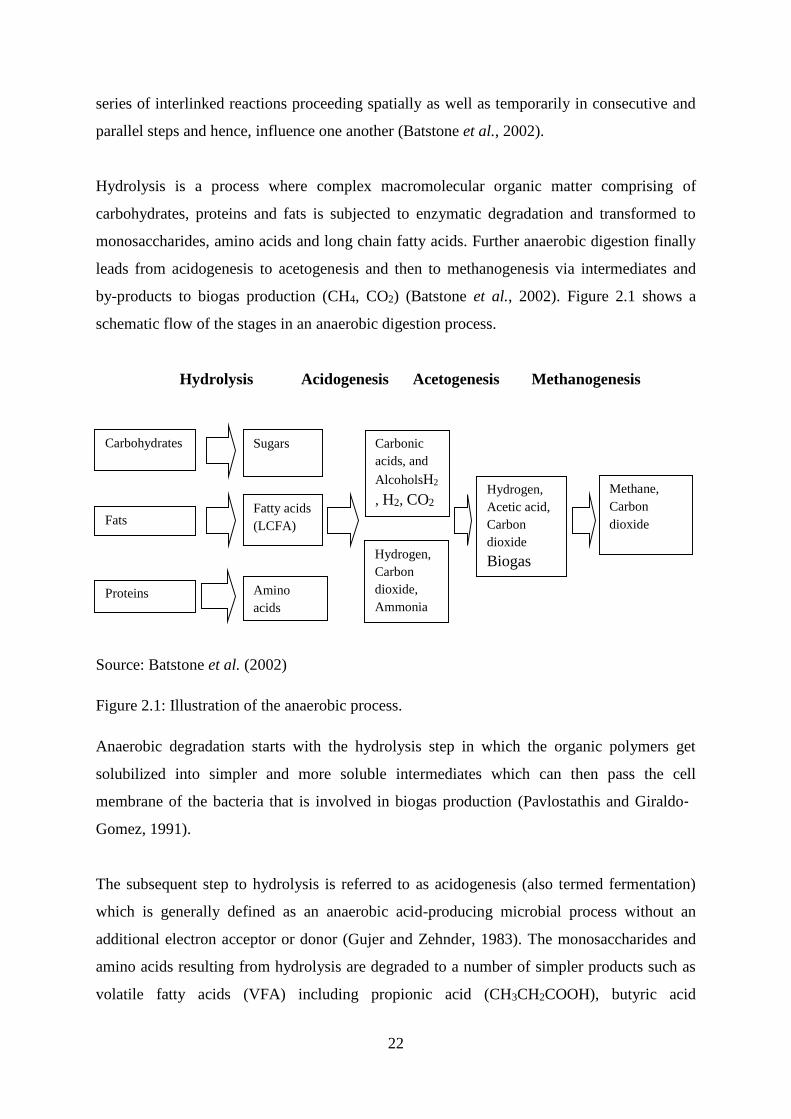
22
series of interlinked reactions proceeding spatially as well as temporarily in consecutive and
parallel steps and hence, influence one another (Batstone et al., 2002).
Hydrolysis is a process where complex macromolecular organic matter comprising of
carbohydrates, proteins and fats is subjected to enzymatic degradation and transformed to
monosaccharides, amino acids and long chain fatty acids. Further anaerobic digestion finally
leads from acidogenesis to acetogenesis and then to methanogenesis via intermediates and
by-products to biogas production (CH4, CO2) (Batstone et al., 2002). Figure 2.1 shows a
schematic flow of the stages in an anaerobic digestion process.
Hydrolysis Acidogenesis Acetogenesis Methanogenesis
Source: Batstone et al. (2002)
Figure 2.1: Illustration of the anaerobic process.
Anaerobic degradation starts with the hydrolysis step in which the organic polymers get
solubilized into simpler and more soluble intermediates which can then pass the cell
membrane of the bacteria that is involved in biogas production (Pavlostathis and Giraldo‐
Gomez, 1991).
The subsequent step to hydrolysis is referred to as acidogenesis (also termed fermentation)
which is generally defined as an anaerobic acid-producing microbial process without an
additional electron acceptor or donor (Gujer and Zehnder, 1983). The monosaccharides and
amino acids resulting from hydrolysis are degraded to a number of simpler products such as
volatile fatty acids (VFA) including propionic acid (CH3CH2COOH), butyric acid
Carbohydrates Sugars
Amino
acids
Hydrogen,
Acetic acid,
Carbon
dioxide
Biogas
(CH4,
CO2)
Fatty acids
(LCFA)
Hydrogen,
Carbon
dioxide,
Ammonia
Fats
Proteins
Methane,
Carbon
dioxide
Carbonic
acids, and
AlcoholsH2
, H2, CO2
23
(CH3CH2CH2COOH), and acetic acid (CH3COOH) (Batstone et al., 2002). These products
can not be utilised directly by the methanogens and must be degraded further in a subsequent
process that is referred to as acetogenesis (Björnsson et al., 2000). Acidogenesis is often the
quickest step in the anaerobic conversion of complex organic matter in liquid phase
digestions (Vavilin et al., 1996).
Acetogenesis is the degradation of higher organic acids formed in acidogenesis to yield
carbon dioxide and hydrogen (Batstone et al., 2002). This intermediate conversion is crucial
for the successful production of biogas. During methanogenesis, the fermentation products
such as acetate, H2 and CO2 are converted to CH4 and CO2 by methanogenic archaea which
are strict obligate anaerobes (Björnsson et al., 2000; Pavlostathis and Giraldo-Gomez, 1991).
2.3.2 Factors affecting anaerobic digestion
The metabolic activity involved in microbiological methanation is dependent on the
following factors: substrate temperature, available nutrients, retention time (flow-through
time), pH level, nitrogen inhibition and carbon to nitrogen ratio, substrate solid content and
agitation, and inhibitory factors (Grady et al., 1999). Each of the various types of bacteria
responsible for the four stages of the anaerobic digestion is affected differently by the above
parameters (Varma et al., 2009). Since interactive effects between the various determining
factors exist, no precise quantitative data on gas production as a function of the above factors
are available (Gray, 2004). Thus, optimisation was limited to the three selected factors
(temperature, substrate concentration and solid retention time) while holding the other factors
constant.
a) Temperature of substrate
Anaerobic fermentation is, in principle, possible between 30C and approximately 700C.
Differentiation is generally made between three temperature ranges: the psychrophilic
temperature range lies below 200C, the mesophilic temperature range lies between 200C and
400C, and the thermophilic temperature range from 400C to 650C (Eder and Schulz, 2006;
Grady et al., 1999; Patharwat et al., 2016). The best temperatures are 100C, 370C and 520C
for psychrophilic, mesophilic, and thermophilic bacteria respectively (Patharwat et al., 2016).
The rate of bacteriological methane production increases with temperature. Since, however,
the amount of free ammonia also increases with temperature, the bio-digestive performance
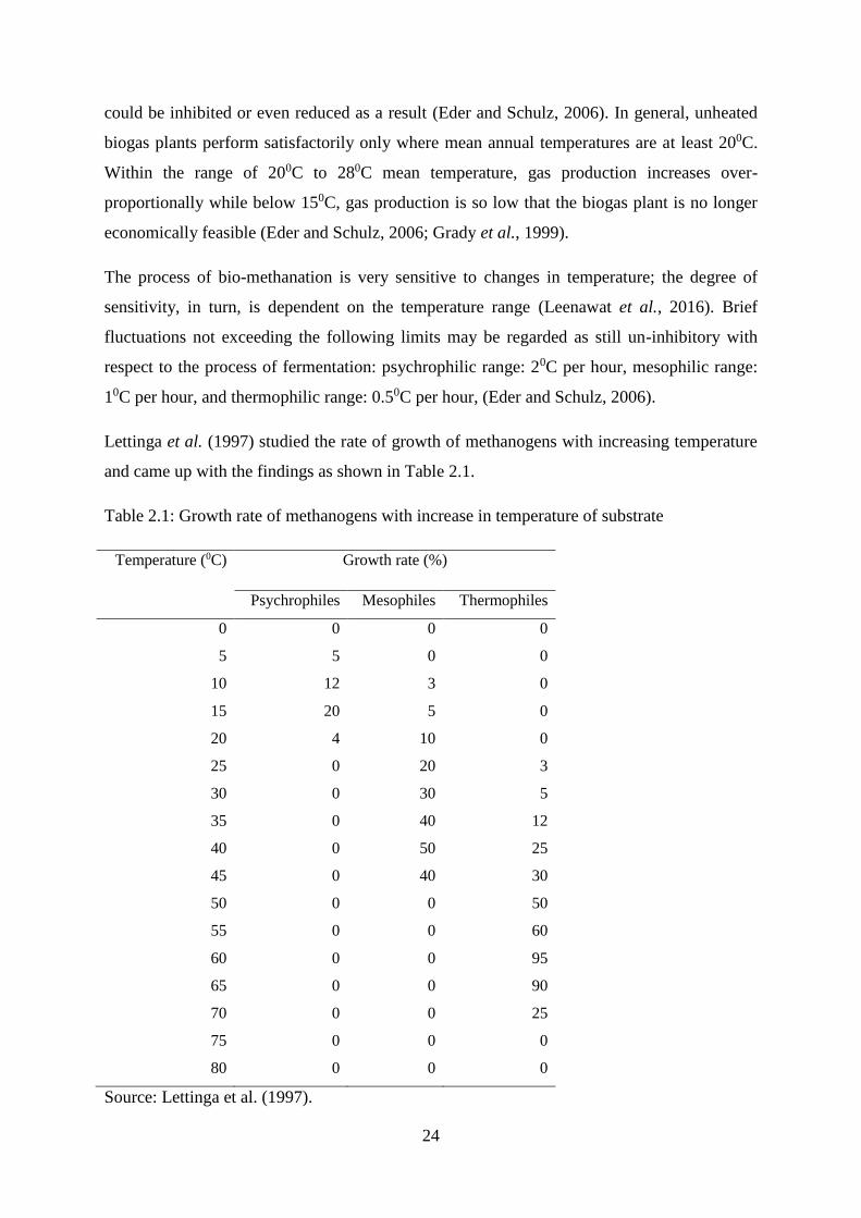
24
could be inhibited or even reduced as a result (Eder and Schulz, 2006). In general, unheated
biogas plants perform satisfactorily only where mean annual temperatures are at least 200C.
Within the range of 200C to 280C mean temperature, gas production increases over-
proportionally while below 150C, gas production is so low that the biogas plant is no longer
economically feasible (Eder and Schulz, 2006; Grady et al., 1999).
The process of bio-methanation is very sensitive to changes in temperature; the degree of
sensitivity, in turn, is dependent on the temperature range (Leenawat et al., 2016). Brief
fluctuations not exceeding the following limits may be regarded as still un-inhibitory with
respect to the process of fermentation: psychrophilic range: 20C per hour, mesophilic range:
10C per hour, and thermophilic range: 0.50C per hour, (Eder and Schulz, 2006).
Lettinga et al. (1997) studied the rate of growth of methanogens with increasing temperature
and came up with the findings as shown in Table 2.1.
Table 2.1: Growth rate of methanogens with increase in temperature of substrate
Temperature (0C) Growth rate (%)
Psychrophiles Mesophiles Thermophiles
0 0 0 0
5 5 0 0
10 12 3 0
15 20 5 0
20 4 10 0
25 0 20 3
30 0 30 5
35 0 40 12
40 0 50 25
45 0 40 30
50 0 0 50
55 0 0 60
60 0 0 95
65 0 0 90
70 0 0 25
75 0 0 0
80 0 0 0
Source: Lettinga et al. (1997).
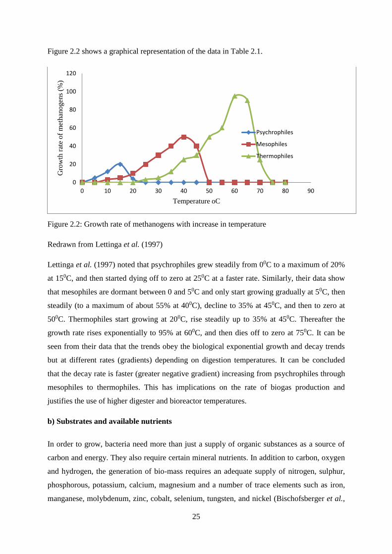
25
Figure 2.2 shows a graphical representation of the data in Table 2.1.
Figure 2.2: Growth rate of methanogens with increase in temperature
Redrawn from Lettinga et al. (1997)
Lettinga et al. (1997) noted that psychrophiles grew steadily from 00C to a maximum of 20%
at 150C, and then started dying off to zero at 250C at a faster rate. Similarly, their data show
that mesophiles are dormant between 0 and 50C and only start growing gradually at 50C, then
steadily (to a maximum of about 55% at 400C), decline to 35% at 450C, and then to zero at
500C. Thermophiles start growing at 200C, rise steadily up to 35% at 450C. Thereafter the
growth rate rises exponentially to 95% at 600C, and then dies off to zero at 750C. It can be
seen from their data that the trends obey the biological exponential growth and decay trends
but at different rates (gradients) depending on digestion temperatures. It can be concluded
that the decay rate is faster (greater negative gradient) increasing from psychrophiles through
mesophiles to thermophiles. This has implications on the rate of biogas production and
justifies the use of higher digester and bioreactor temperatures.
b) Substrates and available nutrients
In order to grow, bacteria need more than just a supply of organic substances as a source of
carbon and energy. They also require certain mineral nutrients. In addition to carbon, oxygen
and hydrogen, the generation of bio-mass requires an adequate supply of nitrogen, sulphur,
phosphorous, potassium, calcium, magnesium and a number of trace elements such as iron,
manganese, molybdenum, zinc, cobalt, selenium, tungsten, and nickel (Bischofsberger et al.,
0
20
40
60
80
100
120
0 10 20 30 40 50 60 70 80 90
Gro
wth
rat
e o
f m
eth
ano
gen
s (%
)
Temperature oC
Psychrophiles
Mesophiles
Thermophiles
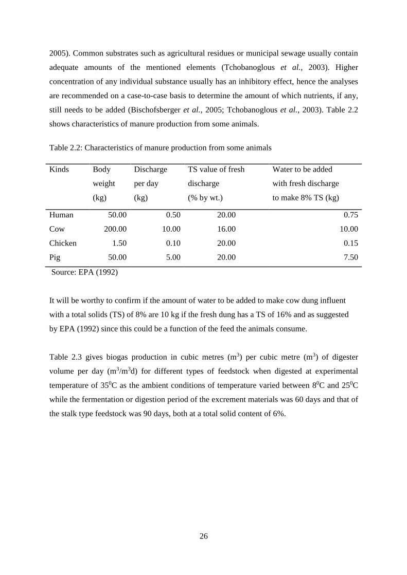
26
2005). Common substrates such as agricultural residues or municipal sewage usually contain
adequate amounts of the mentioned elements (Tchobanoglous et al., 2003). Higher
concentration of any individual substance usually has an inhibitory effect, hence the analyses
are recommended on a case-to-case basis to determine the amount of which nutrients, if any,
still needs to be added (Bischofsberger et al., 2005; Tchobanoglous et al., 2003). Table 2.2
shows characteristics of manure production from some animals.
Table 2.2: Characteristics of manure production from some animals
Kinds Body
weight
(kg)
Discharge
per day
(kg)
TS value of fresh
discharge
(% by wt.)
Water to be added
with fresh discharge
to make 8% TS (kg)
Human 50.00 0.50 20.00 0.75
Cow 200.00 10.00 16.00 10.00
Chicken 1.50 0.10 20.00 0.15
Pig 50.00 5.00 20.00 7.50
Source: EPA (1992)
It will be worthy to confirm if the amount of water to be added to make cow dung influent
with a total solids (TS) of 8% are 10 kg if the fresh dung has a TS of 16% and as suggested
by EPA (1992) since this could be a function of the feed the animals consume.
Table 2.3 gives biogas production in cubic metres (m3) per cubic metre (m3) of digester
volume per day (m3/m3d) for different types of feedstock when digested at experimental
temperature of 350C as the ambient conditions of temperature varied between 80C and 250C
while the fermentation or digestion period of the excrement materials was 60 days and that of
the stalk type feedstock was 90 days, both at a total solid content of 6%.
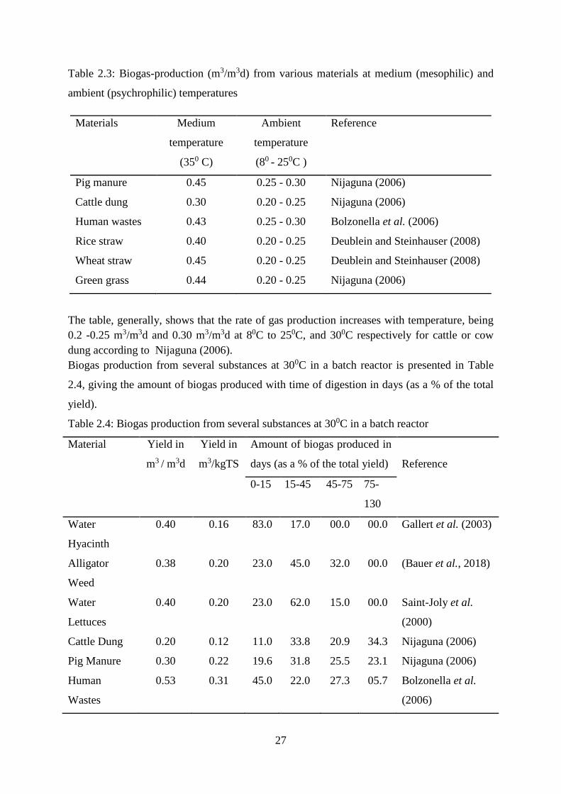
27
Table 2.3: Biogas-production (m3/m3d) from various materials at medium (mesophilic) and
ambient (psychrophilic) temperatures
Materials
Medium
temperature
(350 C)
Ambient
temperature
(80 - 250C )
Reference
Pig manure 0.45 0.25 - 0.30 Nijaguna (2006)
Cattle dung 0.30 0.20 - 0.25 Nijaguna (2006)
Human wastes 0.43 0.25 - 0.30 Bolzonella et al. (2006)
Rice straw 0.40 0.20 - 0.25 Deublein and Steinhauser (2008)
Wheat straw 0.45 0.20 - 0.25 Deublein and Steinhauser (2008)
Green grass 0.44 0.20 - 0.25 Nijaguna (2006)
The table, generally, shows that the rate of gas production increases with temperature, being
0.2 -0.25 m3/m3d and 0.30 m3/m3d at 80C to 250C, and 300C respectively for cattle or cow
dung according to Nijaguna (2006).
Biogas production from several substances at 300C in a batch reactor is presented in Table
2.4, giving the amount of biogas produced with time of digestion in days (as a % of the total
yield).
Table 2.4: Biogas production from several substances at 300C in a batch reactor
Material
Yield in
m3 / m3d
Yield in
m3/kgTS
Amount of biogas produced in
days (as a % of the total yield)
Reference
0-15 15-45 45-75 75-
130
Water
Hyacinth
0.40 0.16 83.0 17.0 00.0 00.0 Gallert et al. (2003)
Alligator
Weed
0.38 0.20 23.0 45.0 32.0 00.0 (Bauer et al., 2018)
Water
Lettuces
0.40 0.20 23.0 62.0 15.0 00.0 Saint-Joly et al.
(2000)
Cattle Dung 0.20 0.12 11.0 33.8 20.9 34.3 Nijaguna (2006)
Pig Manure 0.30 0.22 19.6 31.8 25.5 23.1 Nijaguna (2006)
Human
Wastes
0.53 0.31 45.0 22.0 27.3 05.7 Bolzonella et al.
(2006)
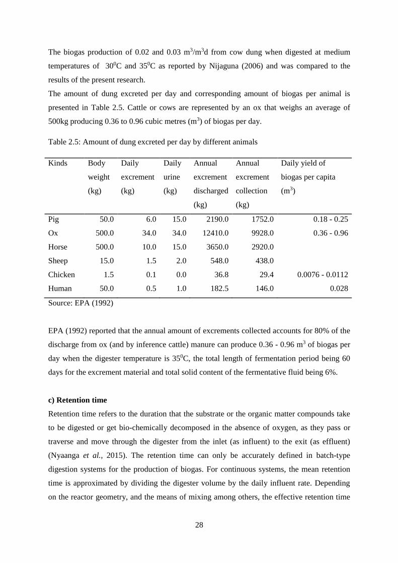
28
The biogas production of 0.02 and 0.03 m3/m3d from cow dung when digested at medium
temperatures of 300C and 350C as reported by Nijaguna (2006) and was compared to the
results of the present research.
The amount of dung excreted per day and corresponding amount of biogas per animal is
presented in Table 2.5. Cattle or cows are represented by an ox that weighs an average of
500kg producing 0.36 to 0.96 cubic metres (m3) of biogas per day.
Table 2.5: Amount of dung excreted per day by different animals
Kinds Body
weight
(kg)
Daily
excrement
(kg)
Daily
urine
(kg)
Annual
excrement
discharged
(kg)
Annual
excrement
collection
(kg)
Daily yield of
biogas per capita
(m3)
Pig 50.0 6.0 15.0 2190.0 1752.0 0.18 - 0.25
Ox 500.0 34.0 34.0 12410.0 9928.0 0.36 - 0.96
Horse 500.0 10.0 15.0 3650.0 2920.0
Sheep 15.0 1.5 2.0 548.0 438.0
Chicken 1.5 0.1 0.0 36.8 29.4 0.0076 - 0.0112
Human 50.0 0.5 1.0 182.5 146.0 0.028
Source: EPA (1992)
EPA (1992) reported that the annual amount of excrements collected accounts for 80% of the
discharge from ox (and by inference cattle) manure can produce 0.36 - 0.96 m3 of biogas per
day when the digester temperature is 350C, the total length of fermentation period being 60
days for the excrement material and total solid content of the fermentative fluid being 6%.
c) Retention time
Retention time refers to the duration that the substrate or the organic matter compounds take
to be digested or get bio-chemically decomposed in the absence of oxygen, as they pass or
traverse and move through the digester from the inlet (as influent) to the exit (as effluent)
(Nyaanga et al., 2015). The retention time can only be accurately defined in batch-type
digestion systems for the production of biogas. For continuous systems, the mean retention
time is approximated by dividing the digester volume by the daily influent rate. Depending
on the reactor geometry, and the means of mixing among others, the effective retention time
29
may vary widely for the individual substrate constituents. Selection of a suitable retention
time thus depends not only on the process temperature, but also on the type of substrate used
(Dong, 2004). Optimising the process parameters (retention time, process temperature,
substrate quality, and volumetric loading) ensures the cost efficiency of the biological
processes. But as each m3 digester volume has its price, heating equipment can be costly and
high quality substrates may have alternative uses, the cost-benefit optimum in biogas
production is almost always below the biological optimum (Nijaguna, 2006).
Gray (2004) reported that the approximate retention time in days for different liquid manures
undergoing fermentation in the mesophilic temperature range to produce biogas are 20-30
days for cow manure, 15-25 days for liquid pig manure, 20-40 days liquid chicken manure:,
and 50-80 days animal manure mixed with plant material. Another study also reported that if
the retention time is too short, the bacteria in the digester are "washed out" faster than they
can reproduce, so that the fermentation practically ceases but also notes that this problem
rarely occurs in agricultural biogas systems (Hamad et al., 1981; Jash and Gosh, 1990; Marti-
Herero, 2011). The current research used a batch reactor, mesophilic temperature range and
liquid cow manure, hence the retention time.
d) pH value
The methane-producing bacteria thrive best under neutral to slightly alkaline conditions
(Bischofsberger et al., 2005). Once the process of fermentation has stabilized under anaerobic
conditions, the pH will normally take on a value of between 7 and 8.5 (Boe, 2006). Due to the
buffer effect of Carbon dioxide-bicarbonate (CO2 - HCO3-) and ammonia-ammonium (NH3 -
NH4+) compounds, the pH level is rarely taken as an indicator of substrate acids and/or
potential biogas yield (Tchobanoglous et al., 2003). A digester containing a high volatile-acid
concentration requires a higher-than-normal pH value (Grady et al., 1999). If the pH value
drops below 6.2, the medium will have a toxic effect on the methanogenic bacteria (Grady et
al., 1999).
d) Nitrogen inhibition, and Carbon to Nitrogen ratio
All substrates contain nitrogen apart from carbon. Table 2.6 presents the nitrogen content of
various organic substances and the Carbon to Nitrogen (C:N) ratio. For higher pH values,
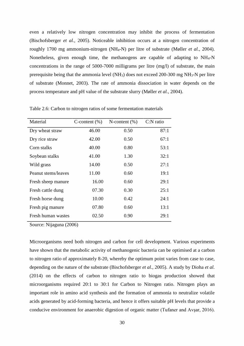
30
even a relatively low nitrogen concentration may inhibit the process of fermentation
(Bischofsberger et al., 2005). Noticeable inhibition occurs at a nitrogen concentration of
roughly 1700 mg ammonium-nitrogen (NH4-N) per litre of substrate (Møller et al., 2004).
Nonetheless, given enough time, the methanogens are capable of adapting to NH4-N
concentrations in the range of 5000-7000 milligrams per litre (mg/l) of substrate, the main
prerequisite being that the ammonia level (NH3) does not exceed 200-300 mg NH3-N per litre
of substrate (Monnet, 2003). The rate of ammonia dissociation in water depends on the
process temperature and pH value of the substrate slurry (Møller et al., 2004).
Table 2.6: Carbon to nitrogen ratios of some fermentation materials
Material C-content (%) N-content (%) C:N ratio
Dry wheat straw 46.00 0.50 87:1
Dry rice straw 42.00 0.50 67:1
Corn stalks 40.00 0.80 53:1
Soybean stalks 41.00 1.30 32:1
Wild grass 14.00 0.50 27:1
Peanut stems/leaves 11.00 0.60 19:1
Fresh sheep manure 16.00 0.60 29:1
Fresh cattle dung 07.30 0.30 25:1
Fresh horse dung 10.00 0.42 24:1
Fresh pig manure 07.80 0.60 13:1
Fresh human wastes 02.50 0.90 29:1
Source: Nijaguna (2006)
Microorganisms need both nitrogen and carbon for cell development. Various experiments
have shown that the metabolic activity of methanogenic bacteria can be optimised at a carbon
to nitrogen ratio of approximately 8-20, whereby the optimum point varies from case to case,
depending on the nature of the substrate (Bischofsberger et al., 2005). A study by Dioha et al.
(2014) on the effects of carbon to nitrogen ratio to biogas production showed that
microorganisms required 20:1 to 30:1 for Carbon to Nitrogen ratio. Nitrogen plays an
important role in amino acid synthesis and the formation of ammonia to neutralize volatile
acids generated by acid-forming bacteria, and hence it offers suitable pH levels that provide a
conducive environment for anaerobic digestion of organic matter (Tufaner and Avşar, 2016).
31
Cow manure has a C:N ratio of about 22.71:1 (Ardaji et al., 2016) and hence its suitability
for this research .
e) Agitation and its effect on total solids content
The mobility of the methanogens within the substrate is gradually impaired by increasing
solids content, and the biogas yield may suffer as a result. However, reports of relatively high
biogas yields from landfill material with high solids content are found in recent literature
(Hansen et al., 2004; Ras et al., 2007). No general valid guidelines can be offered with
regard to specific biogas production for any particular total solid percentage (Abbassi-
Guendouz et al., 2012).
Substrates and various modes of fermentation require some substrate agitation or mixing in
order to maintain process stability within the digester (Bridgeman, 2012; Lemmer et al.,
2013). The most important objectives of agitation include removal of the metabolites and gas
produced by the methanogens, mixing of fresh substrate and bacterial population
(inoculation), preclusion of scum formation and sedimentation, avoidance of pronounced
temperature gradients within the digester, provision of a uniform bacterial population density,
and prevention of the formation of dead spaces that would reduce the effective digester
volume (Halalsheh et al., 2011).
Bridgeman (2012) gives the following points to be considered while selecting or designing a
suitable means of agitation:
i. The process involves a symbiotic relationship between various strains of bacteria
namely, i.e. the metabolite from one species can serve as nutrient for the next species,
among others. Whenever the bacterial community is disrupted, the process of
fermentation will remain more or less unproductive until an equivalent new
community is formed. Consequently, excessive or too frequent mixing is usually
detrimental to the process. Slow stirring is better than rapid agitation.
ii. A thin layer of scum must not necessarily have an adverse effect on the process. For
systems in which the digester is completely filled with substrate, so that any scum
always remains sufficiently wet, there is little or no danger that the extraction of gas
could be impeded by the scum.
iii. Some types of biogas systems can function well without any mechanical agitation at
all. Such systems are usually operated either on substrates with such a high solid
32
content, that no stratification occurs, or on substrates consisting primarily of solute
substances.
Karapaju and Rintala (2008) reported biogas production for minimal and intermittent
agitation relative to the biogas yield from a continuously mixed system. An evaluation, done
by Ghanimeh et al. (2012), on the effect of mixing and organic loading rate on anaerobic
digestion of source-separated organic fraction of municipal solid waste that was continuously
and slowly mixed at 100 revolutions per minute (rpm) showed a superior digestion efficiency.
Since the results of agitation and mixing are highly dependent on the substrate in use, it is not
possible to achieve a sufficiently uniform comparative evaluation of various mixing systems
and/or intensity levels (Lemmer et al., 2013). Thus, each such system can only be designed
on the basis of empirical data. The current research has reported on the form of agitation and
mixing that was used.
f) Inhibitory metals
There are light as well as heavy metals. Light metals include sodium (Na), magnesium (Mg),
Potassium (K), and Calcium (Ca), while the heavy metals include chromium (Cr), cobalt
(Co), copper (Cu), cadmium (Cd), nickel (Ni) and zinc (Zn). The presence of heavy metal
ions in the substrate is a major cause of toxicity that inhibits biogas production from
anaerobic digestion (Jin et al., 1998; Sterrit and Lester, 1980; Swanwick et al., 1969). Vallee
and Ulner (1972) reported that these heavy metal ions disrupt enzymatic functioning by
binding the metals with the organic substrate or by replacing naturally occurring metals in
enzyme prosthetic groups. Also the presence of antibiotics (this may include bacitracin,
flavomycin, lasalocid, monensin, and spiramycin) and detergents used in livestock husbandry
can have an inhibitory effect on the process of bio-methanation (Bischofsberger et al., 2005).
Table 2.7 presents the limit of concentrations (mg/l) for various metal inhibitors (Møller et
al., 2004).
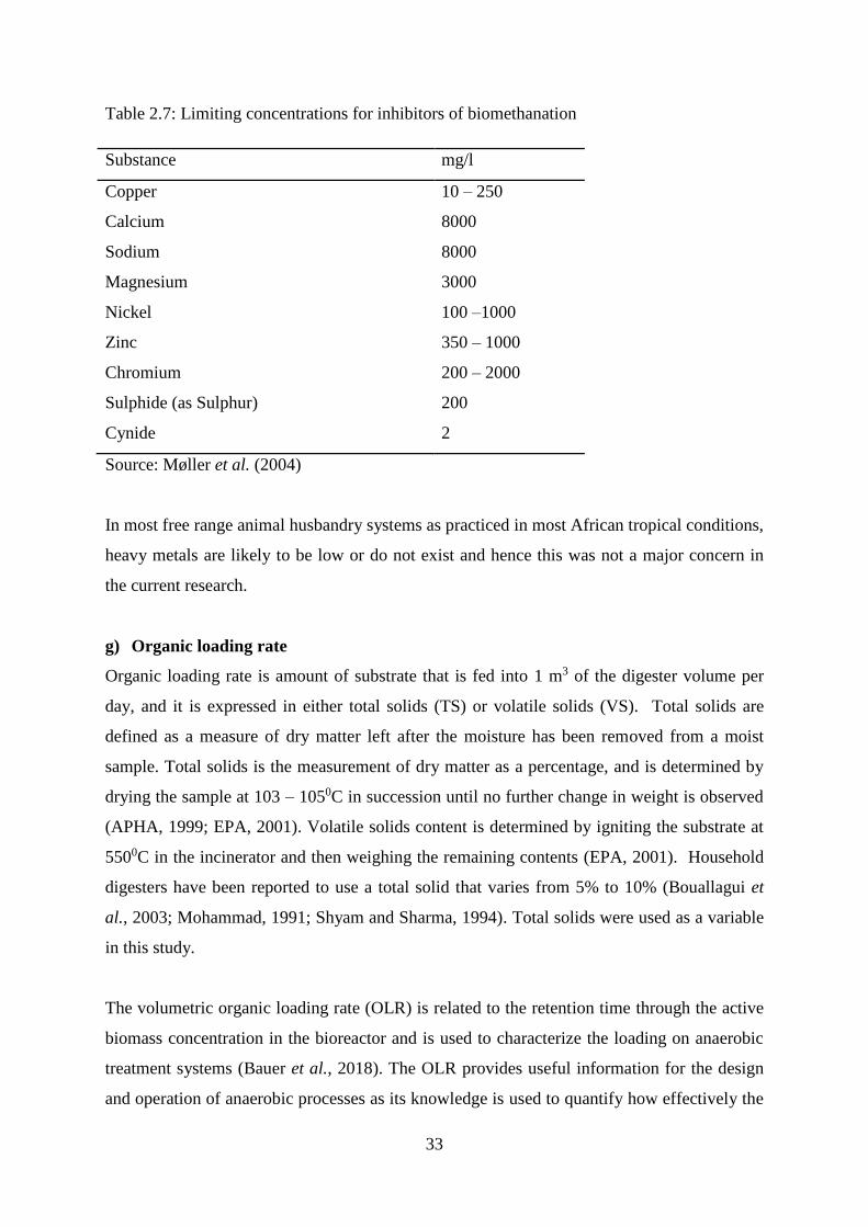
33
Table 2.7: Limiting concentrations for inhibitors of biomethanation
Substance mg/l
Copper 10 – 250
Calcium 8000
Sodium 8000
Magnesium 3000
Nickel 100 –1000
Zinc 350 – 1000
Chromium 200 – 2000
Sulphide (as Sulphur) 200
Cynide 2
Source: Møller et al. (2004)
In most free range animal husbandry systems as practiced in most African tropical conditions,
heavy metals are likely to be low or do not exist and hence this was not a major concern in
the current research.
g) Organic loading rate
Organic loading rate is amount of substrate that is fed into 1 m3 of the digester volume per
day, and it is expressed in either total solids (TS) or volatile solids (VS). Total solids are
defined as a measure of dry matter left after the moisture has been removed from a moist
sample. Total solids is the measurement of dry matter as a percentage, and is determined by
drying the sample at 103 – 1050C in succession until no further change in weight is observed
(APHA, 1999; EPA, 2001). Volatile solids content is determined by igniting the substrate at
5500C in the incinerator and then weighing the remaining contents (EPA, 2001). Household
digesters have been reported to use a total solid that varies from 5% to 10% (Bouallagui et
al., 2003; Mohammad, 1991; Shyam and Sharma, 1994). Total solids were used as a variable
in this study.
The volumetric organic loading rate (OLR) is related to the retention time through the active
biomass concentration in the bioreactor and is used to characterize the loading on anaerobic
treatment systems (Bauer et al., 2018). The OLR provides useful information for the design
and operation of anaerobic processes as its knowledge is used to quantify how effectively the
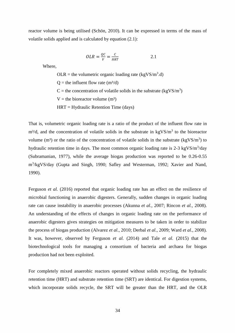
34
reactor volume is being utilised (Schön, 2010). It can be expressed in terms of the mass of
volatile solids applied and is calculated by equation (2.1):
𝑂𝐿𝑅 =𝑄𝐶
𝑉=
𝐶
𝐻𝑅𝑇 2.1
Where,
OLR = the volumetric organic loading rate (kgVS/m3.d)
Q = the influent flow rate (m³/d)
C = the concentration of volatile solids in the substrate (kgVS/m3)
V = the bioreactor volume (m³)
HRT = Hydraulic Retention Time (days)
That is, volumetric organic loading rate is a ratio of the product of the influent flow rate in
m³/d, and the concentration of volatile solids in the substrate in kgVS/m3 to the bioreactor
volume (m³) or the ratio of the concentration of volatile solids in the substrate (kgVS/m3) to
hydraulic retention time in days. The most common organic loading rate is 2-3 kgVS/m3/day
(Subramanian, 1977), while the average biogas production was reported to be 0.26-0.55
m3/kgVS/day (Gupta and Singh, 1990; Safley and Westerman, 1992; Xavier and Nand,
1990).
Ferguson et al. (2016) reported that organic loading rate has an effect on the resilience of
microbial functioning in anaerobic digesters. Generally, sudden changes in organic loading
rate can cause instability in anaerobic processes (Akunna et al., 2007; Rincon et al., 2008).
An understanding of the effects of changes in organic loading rate on the performance of
anaerobic digesters gives strategies on mitigation measures to be taken in order to stabilize
the process of biogas production (Alvarez et al., 2010; Derbal et al., 2009; Ward et al., 2008).
It was, however, observed by Ferguson et al. (2014) and Tale et al. (2015) that the
biotechnological tools for managing a consortium of bacteria and archaea for biogas
production had not been exploited.
For completely mixed anaerobic reactors operated without solids recycling, the hydraulic
retention time (HRT) and substrate retention time (SRT) are identical. For digestion systems,
which incorporate solids recycle, the SRT will be greater than the HRT, and the OLR
35
indicates both the anaerobic digester volume utilisation efficiency and the overall process
loading (Grady et al., 1999).
Retention time and organic loading rate are inversely proportional to each other and thus,
have to be aligned when designing the reactor layout. The maximum possible OLR depends
on both the process temperature and the retention time: the lower the temperature and the
longer the retention time, the higher the OLRs that can be processed (Grady et al., 1999).
This maximum value depends also on the specific digester/reactor type. The higher the OLR,
the higher the risk to exceed the optimum performance limit of the degrading biomass.
Feeding the system above its sustainable OLR results in low biogas yield due to accumulation
of inhibiting substances such as volatile fatty acids in the digester slurry (Bauer et al., 2018).
Typically, OLR ranges from 2 to 6 kgVS/m3d (Eder and Schulz, 2006) and these values were
compared to the results of the current research.
2.3.3 Methods for enhancing biogas production
Manipulations that the feedstock is subjected to before undergoing anaerobic digestion have
an effect of promoting the level of biogas production. The methods for enhancing the
production of biogas from biomass waste include co-digestion, pretreatment, and
hyperthermophilic anaerobic digestion.
a) Co-digestion
Co-digestion involves the use of two or more different feedstock in a bioreactor to undergo
anaerobic digestion process (Pannucharoenwong, 2018). Gashaw and Teshita (2014) define
co-digestion as the anaerobic treatment of a mixture of at least two different substrates with
the aim of improving the efficiency of an anaerobic digestion process. Some of the
advantages of anaerobic co-digestion include increased cost efficiency, increased
biodegradation of treated materials, and increased biogas yield (Gashaw and Teshita, 2014).
Co-digestion helps to mitigate inhibitory effects of unfavourable substrates, balances
nutrients and increases organic loading rate which result in a higher methane yield while
diversifying and synergizing the bacterial populations that carry out methanogenesis (Shah et
al., 2015). Apart from improving the reliability of the feedstock, co-digestion dilutes toxic
substances, synergizes microorganisms in the substrate, increases the load of biodegradable
matter, and increases methane yield per unit volume of the digester (Nkemka and Murto,
36
2010). Co-digestion is one of the methods for enhancing biogas production to as much as 25 -
400% over the mono-digestion of the same substrates (Fayyaz et al., 2015).
Gashaw and Teshita (2014) concluded that organic food wastes co-digested with cattle
manure improved the biogas potential compared to cattle manure alone. Neczaj et al. (2012)
reported anaerobic co-digestion of a mixture of a fraction of municipal solid waste,
agricultural residues, organic solid wastes, and sewage sludge. Tamrat et al. (2013) did co-
digestion of three mix ratios of rumen fluid inoculated cow manure with organic kitchen
waste and established a substantial increase in biogas yield of 24 – 47% compared to the
control. Biogas production from empty fruit bunches was compared with a co-digestion of
palm oil mill effluent, and found out that the two enhanced biodegradability with 25 – 32%,
and increased methane production by 98% (Sompong et al., 2012). A feasibility study on
anaerobic co-digestion of sewage sludge and sugar beet pulp lixiviation was assessed under
mesophilic and thermophilic conditions by Montanes et al. (2015) in which they established
that the net methane generation was higher in the mesophilic range on the biochemical
methane potential test.
Zielinski et al. (2017) reported that co-digestion of cow manure with energy rich substrates
like pig manure and chicken manure increases biogas yield. Sebola et al. (2015) concluded
that co-digestion of chicken droppings and cow manure enhanced biogas yield as compared
to their mono-digestion, with a maximum increase in biogas production of 50% being
attained at a mix ratio of 1:1under mesophilic temperature conditions. Afazeli et al. (2014)
reported that biogas production from co-digestion of chicken manure and cow manure under
continuous anaerobic digestion increased by 69.6%. Böjti et al. (2017) co-digested pretreated
maize silage with chicken manure in continuous anaerobic digestion at mesophilic conditions
of 37°C and recorded an increase of 24% in biogas production.
It was observed by Al Mamun and Torii (2015) that methane biogas yields can be improved
through co-digestion because this process is capable of creating a synergy between the
digesting medium and the supply of missing nutrients. Dahunsi and Orunsi (2013) did a
unique experiment that involved co-digestion of food waste and human excreta for 60 days
using a 40 litre digester, and the volume of gas generated from the mixture comprised of 58%
methane (CH4), 24% carbon dioxide (CO2), 19% hydrogen sulphide (H2S) and other
impurities. An experiment of co-digestion of cheese whey and cattle manure, based on
37
concentric acidogenesis using an innovative two-stage process and methanogenic phases, was
designed for reducing footprint and enhancing performance (Lorenzo et al., 2013). It showed
an improved yield; that the highest methane production was achieved when a co-digestion of
the above substrates was at a ratio of 1:1. Tong et al. (2013) conducted an anaerobic co-
digestion of goat manure, rice straw, corn stalks and wheat straw under different mixing
ratios at mesophilic temperature (350C) with a total solid concentration of 8%. They found
out that biogas yields improved significantly at all carbon to nitrogen ratios.
A review by Mata-Alvarez et al. (2010) on co-digestion practices and analysis included
models to be developed and thereafter standardization from laboratory scale anaerobic
digesters to an industrial scale. Full-scale plants with sewage sludge co-digestion cases are
worth mentioning. A study by Zipancic et al. (2008) at a waste water treatment plant
equipped with two digesters (each with a capacity of 2000m3), operating at a hydraulic
retention time of 20 days, and an average organic loading rate of 0.8 VSS/m3d and were
supplemented with organic fraction of municipal solid waste (OFMSW) to increase the
organic loading rate to 25% at Velenje in Slovenia. This resulted in an increased biogas
production by 80%, and a specific biogas production increased by over 53%. Another full-
scale study was reported by Zitomer et al. (2008) in which a waste water treatment plant
digester had five co-substrates including yeast waste; the synergistic effect increased biogas
production by over 50%.
Anaerobic co-digestion of chicken manure and corn stover was carried out in both a batch
reactor and a continuously stirred tank reactor (CSTR) whereby the batch co-digestion
experiment was done at an initial volatile solids (VS) concentration of 3g VS/L, carbon to
nitrogen ratio of 20 and a retention time of 30 days, whereas in the CSTR experiment, a
feeding concentration of total solids (TS) of 12%, a carbon to nitrogen ratio of 20 and organic
loading rates of 1-4g VS/L/d (Yeqing et al., 2014). The results showed that in the batch case,
the methane yield was 281±12 ml/g of VS added while the CSTR outcome was 223±7 ml/g
of VS added (Yeqing et al., 2014). Co-digestion in a batch reactor gives better results than
the CSTR by 26%.
b) Pretreatment of feedstock
Pretreatment of feedstock involves the initial manipulations or actions that the material is
subjected to facilitate subsequent processes that convert it to a desired product or products.
The manipulations may include thermal, biological, chemical, hydro or mechanical actions.
38
Most of these methods have high energy costs, and are unprofitable (Teghammar et al.,
2012). Different feedstocks have different types and degrees of limitations to optimal
performance of anaerobic digestion that can be solved by different pre-treatment mechanisms
(Carlsson et al., 2012). Conversion of biodegradable material to biogas is limited by the rate
and extent of hydrolysis. Animal manure contains a high lignocellulose content and therefore
pretreatment is important in increasing carbohydrate, protein and fatty acids accessibility
along with hydrolysis efficiency (Rusanowska et al., 2018). Pretreatment reduces feed stock
size to increase surface area and reduce cellulose crystals for improved hydrolysis yield by 5-
25%, to potentially enhance biogas yield and reduce retention time by about 23-59% (Kratky
and Jirout, 2011). Assefa et al. (2014) reported that there was no significant difference in pH
and organic matter content between poultry substrates subjected to different temperature and
sodium hydroxide (NaOH) pretreatments before anaerobic digestion.
i. Mechanical Pretreatment
Mechanical pretreatment involves disintegration, grinding, mincing, and milling or extrusion
of solid particles of the substrate into easily fermentable components through reduction in
resistance to flow and making mixing within the digester easier, and thus releasing cell
compounds and increasing the specific surface area (Elliot and Mahmood, 2012; Skiadas et
al., 2005). Knives and mills are used to break open the cellular structure to increase the
specific surface area for bacterial attack, especially for lignocellulosic substrates (Bochmann
and Montgomery, 2014). Shearing and compressive forces acting on biomass reduces its
crystallinity, particle size and increases specific surface area and bulk density (Kratky and
Jirout, 2011). Some of the advantages of mechanical pretreatment include better
dewaterability of the final anaerobic residue, no generation of odour, moderate energy
consumption and an easier implementation of subsequent processes (Toreci et al., 2009). The
disadvantages include insignificant effect on removal of pathogens, and the possibility of
scaling and clogging of equipment (Perez-Elvira et al., 2006).
Mechanical pretreatment methods include the rotary drum, lysis-centrifuge, liquid shear,
collision, high-pressure homogenizer, sonication, liquefaction, and maceration (Esposito et
al., 2011; Hartmann et al., 2000). The following discussion highlights findings that have been
made in mechanical pretreatment processes.
39
Rotary drum is one of the mechanical pretreatment methods that was used by Zhu et al.
(2009) and Subramani and Ponkumar (2012) for organic fraction of municipal solid waste
(OFMSW) separation pretreatment before anaerobic digestion, and it enhanced biogas
production by 18-36%. Davidson et al. (2007) studied the biomethane potential of source-
sorted OFMSW, and reported small variations in both methane yield per gram of volatile
solids, and content of methane in biogas while using different mechanical methods such as
the screw press, disc screen shredder, food waste disposer and piston press. In a similar
experiment, Zhang and Banks (2013) found no significant enhancement of biogas production.
Rusanowska et al. (2018) reported that mechanical pretreatment of lignocellulosic biomass
increased biogas production by about 22% and biomass degradation by about 6%. Izumi et al.
(2010) studied the effect of size reduction in food waste in anaerobic digestion and observed
that biogas production from food waste at sizes less than 0.7mm in mesophilic conditions
increased by 28%. A size reduction that is less than 0.7mm causes an accumulation of
volatile fatty acids (VFA) (Izumi et al., 2010) whereas methanogens are sensitive to acidic
intermediates (Park et al., 2011); this may result in a decreased anaerobic digestion
performance. Carlsson and Anox (2008) reported an increase in biogas production of 20-
40% when OFMSW was subjected to electroporation pretreatment. Liquifaction of OFMSW
was to yield biogas that was 15-26% higher (Carrère et al., 2010), while sonication on the
same material gave 16% more cumulative biogas compared to untreated substrates (Cesaro
and Belgiorno, 2013). Sonication involves the use of a probe in which the mechanical
vibration disrupts the cell structure and floc matrix (Elliot and Mahmood, 2007). The effect
of the vibration at low frequencies of 20-40 kHz sound waves is the reduction in particle size
(Chua et al., 2002). At high frequency sound waves, there is a formation of radicals such as
H*, OH*, and HO2* that cause oxidation of solid substances (Bougrier et al., 2006).
Sonication of the feedstock before anaerobic digestion has been reported to enhance biogas
production by 24-140% in batch systems, and 10-45% in continuous or semi-continuous
systems (Carrère et al., 2010). Studies on enhancement of volatile solids (VS) destruction and
higher biogas production in waste activated sludge (WAS) yielded negligible results (Cesaro
and Belgiorno, 2013; Sandino et al., 2005). It was concluded that extruders and colloid mills
are more suited to reducing sizes of materials that have over 15-20% moisture content while
hammer and knife mills are suited for dry biomass at 10-15% moisture content (Taherzadeh
and Karimi, 2008). The effectiveness and uniformity of grinding of a given feed stock
depends on its moisture content.
40
Generally, maceration enhances biogas production by 10-60% (Carrère et al., 2010).
Maceration has an effect of shearing rather than the cutting of fibres (Hartmann et al., 2000).
Angelidaki and Ahring (2000) macerated fibres in manure upto 2mm and it gave an increase
of 16% biogas production, while size reduction of down to 0.35mm yielded 20% increase,
and a negligible difference was observed when further reduction in size was made. High-
pressure homogenization (HPH) is another method of mechanical pretreatment. Barjenbruch
and Kopplow (2003) treated surplus sludge with HPH at a pressure of 600 bar and showed
that the filaments were completely disintegrated. A study on the effect of HPH on the
anaerobic digestion of sewage sludge showed an increase of 25% volatile solids reduction
(Engelhart et al., 2000). This development has necessitated a full scale application of HPH to
waste water treatment plants (WWTP), and has achieved 30% biogas enhancement and a
reduction in working volume of digesters by 23% (Carrère et al., 2010).
ii. Thermal pretreatment
Thermal pretreatment involves subjecting a given material to heat at given temperatures over
a period of time to achieve disintegration of cell membranes and tough bonds holding
material fibres together in order to increase solubilization of organic compounds, ease
bacterial attack and biodegradation (Ariunbaatar et al., 2014). This method is the most
studied, and has been applied at an industrial scale (Carlsson et al., 2012; Carrère et al., 2010;
Cesaro and Belgiorno, 2014). Thermal pretreatment helps to remove pathogens, improves
dewatering performance, lowers the viscosity of the digestate, and consequently enhance the
handling of the digestate (Carlsson et al., 2012; Edelmann et al., 2005; Shen et al., 2012; Val
del Rio et al., 2011). Heat helps break down the hydrogen bonds holding together the
cellulosic and lignocellulosic complexes, thereby making the feed stocks to increase in
specific surface area (Garrote et al., 1999). Pathogen removal and easy handling of the
digestate was also reported by Val del Rio et al. (2011) and Carlsson et al. (2012).
An increase in biogas yield occurs with an increase in temperature of pretreatment up to a
certain optimum temperature above which production decreases (Bochmann et al., 2010;
Jahng et al., 2011) because of xylose formation and lignin breakdown that become toxic to
anaerobic digestion bacteria (Bochmann and Montgomery, 2014). At high temperatures
(>1700C), materials form chemical bonds which agglomerate the particles (Bougrier et al.,
2006). An example is that of the Maillard reaction in which the carbohydrates and amino
41
acids form complex substrates that are difficult to biodegrade using anaerobic digestion
(Carrère et al., 2010; Elliot and Mahmood, 2012; Hendriks and Zeeman, 2009). Thermal
pretreatment is also known to cause a loss of organics and potential biogas production from
easily biodegradable substrates; depending on the feedstock and the range of temperature
applied (Panaud et al., 1999; Pinnekamp, 1989).
Thermal pretreatment at lower temperatures (<1100C) does not degrade complex molecules
but instead cause deflocculation of macromolecules (Protot et al., 2011). Barjenbruch and
Kopplow (2003) made a similar conclusion when they observed at 900C that the filaments
were not disintegrated but were only attacked by thermal pretreatment. Chamchoi et al.
(2011) and Gonzalez-Fernandez et al. (2012) pretreated household waste at 700C for 8 hours
and 60 minutes respectively, and reported no enhancement in the production of biogas.
Appels et al. (2010) reported a negligible increase in biogas production from sludge
pretreated at 700C for 60 minutes.
Biogas production improved 20 times when thermal pretreatment was applied to sludge for
60 minutes at 900C (Appels et al., 2010). Rafique et al. (2010) reported an enhancement of
78% biogas production with 60% methane content by thermal pretreatment at 700C. Ferrer et
al. (2008) reported a 30% increase in biogas production with 69% methane content.
Ariunbaatar et al. (2014) found out that at a temperature <110°C, thermal pretreatment and
subsequent anaerobic digestion of feed stocks achieved a more cost-effective performance
compared to other methods. Assefa et al. (2014) observed that thermally pre-treating poultry
litter-cow manure substrate at 80ºC increased gas production and VS removal by 46.3% and
26.1% respectively. Climent et al. (2007) reported an increase of 50% in biogas production
from organic solid waste subjected to 70°C thermal pretreatment prior to digestion at
thermophilic conditions. On a laboratory scale, thermal pretreatment can be done using
microwave heaters, pressure cookers and autoclaves (Bochmann and Montgomery, 2014).
Thermal pretreatment at a temperature of 1750C was studied by Liu et al on food waste and
fruit and vegetable waste, in which they reported 7.9% and 11.7% reduction in biomethane
yield respectively due to the formation of melanoidins (Shen et al., 2012). Ma et al. (2011)
pretreated food waste at 1200C and reported an increase in biogas production of 24%. A
lower biogas yield was obtained from pig manure that had been pretreated at a temperature
>1100C (Rafique et al., 2010).
42
iii. Hydro pretreatment
In hydro pretreatment, water is the main solution that is applied to the feed stock prior to
anaerobic digestion. An increase in biogas yield occurs with an increase in temperature of
pretreatment up to a certain optimum temperature above which production decreases
(Bochmann et al., 2010; Jahng et al., 2011) because of xylose formation and lignin
breakdown that become toxic to anaerobic digestion bacteria (Bochmann and Montgomery,
2014). Hydro pretreatment involves increasing specific surface area to volume ratio of feed
stocks prior to their digestion by soaking them in water for a given period of time to help
loosen their tough outer coatings. Bolaji et al. (2017) found that soaking maize in water for a
period up to 36 hours increased the specific surface area and sphericity of the grains. The
practice of soaking hard covered feedstocks like sheep, goat and chicken manure by farmers
in Kenya has been common in most rural areas although proper process details and
procedures of how to approach this pretreatment have not been documented (Smith et al.,
2013).
iv. Chemical pretreatment
Chemical pretreatment employs the use of strong alkalis, acids and oxidants to destroy
organic bonds in lignocellulosic and cellulosic feed stocks. For the production of biogas,
anaerobic digestion requires a pH of near neutral and hence alkali pretreatment is preferred
(Li et al., 2012). Pretreatments involving acids and oxidative methods such as ozonation are
not suited to feedstock that is easily biodegradable because they lead to an accumulation of
volatile fatty acids (VFA) which inhibits the production of biogas during the anaerobic
digestion process (Mattsson et al., 2011). However, the application of acids has a positive
effect on the substrates that contain lignin and cellulose (Fernandes et al., 2009).
In alkali pretreatment, sodium hydroxide (NaOH) is the most common component that is
used. The initial reactions that induce the swelling of solids include solvation and
saphonification (Carlsson et al., 2012), and these result in an increase in surface area that
enables easy accessibility by anaerobic microbes (Hendriks and Zeeman, 2009; Lopez-Torres
and Llorens, 2008; Molenbach and Nokes, 2012). Assefa et al. (2014) pretreated cow and
chicken manure with 0.45 g, 1.35 g, and 2.25 g of NaOH and recorded respective increase of
0.03%, 21% and 56% in cumulative biogas yield. Bochmann and Montgomery (2014)
observed that alkali pretreatment of substrates leads to an increase in system pH and if used
43
in continuous anaerobic process, this can result in the build-up of salts, mainly ammonium-
ammonia imbalance that may inhibit methane production during the anaerobic digestion
process.
Acid pretreatment involves use of acids like hydrochloric acid (HCl) and sulphuric acid
(H2SO4), in combination with heat, to lignocellulosic substrates not only to degrade lignin but
also the hydrolytic microbes are capable of acclimating to acidic conditions (Musoline et al.,
2012). Strong acidic pretreatments should be avoided because of the by-products that may
inhibit biogas production, loss of fermentable sugar, a high cost of acids and the associated
additional cost for neutralizing the acidic conditions before commencing the anaerobic
digestion (Molenbach and Nokes, 2012; Murphy and Kumar, 2011; Taherzadeh and Karimi,
2008).
Ozonation is an oxidative method that is applied in chemical pretreatment. It involves the use
of hydrogen peroxide or ozone that causes swelling of lignocelluloses to increase substrate
specific surface area and cause partial lignin solubilization for improved hydrolysis
(Kianmahr et al., 2010). Ozonation does not increase salt concentration, nor remainder of
chemical residues, but it disinfects pathogens (Weemaes et al., 2000). Ozone (O3) is a very
strong oxidant which decomposes itself into radicals and also reacts with organic substrates
(Sri et al., 2011). Ozonation was done on waste water and sludge in a waste water treatment
plant (WWTP) and established that the optimal ozone dose for enhancing anaerobic digestion
to produce biogas from a WWTP is 0.05-0.5 gO3/gTS (Carballa et al., 2007; Carrère et al.,
2010; Goel et al., 2003; Yoem et al., 2002).
A study by Monlau et al. (2012) on pretreatment of sunflower stalks with hydrochloric acid at
a temperature of 170°C showed in an increase of 20% methane yield. Cesaro and Belgiorno
(2013) reported an optimum ozone dose of 0.16 gO3/gTS for source-sorted OFMSW which
gave an increase of 37% biogas production. Lopez-Torres and Llorens (2008) applied
alkaline pretreatment on OFMSW and obtained an increased methane production of 11.5%.
Neves et al. (2006) pretreated barley waste with an alkaline (0.3 gNaOH/gTS) and reported
100% of the potential production of biogas.
Alkaline pretreatment was done on water hyacinth (which has a lower lignin content
compared to other plants) and recorded an insignificant effect relative to mechanical
44
pretreatment (Patil et al., 2011). Bochmann and Montgomery (2014) concluded that chemical
pretreatment should not be applied to substrates that contain low lignin, and that the high
costs associated with this pretreatment method is one of the factors preventing its large scale
adoption.
v. Biological pretreatment
Biological pretreatment method involves use of micro-organisms to aerobically or
anaerobically breakdown feed stock structures to increase their surface area for hydrolysis.
Enzymes may also be added to the anaerobic digestion system to enhance biogas production
(Ariunbaatar et al., 2014). Anaerobic microbiological pretreatment involves separation of the
first and second stages of anaerobic digestion (hydrolysis and acidogenesis) from
methanogenesis, also called two stage anaerobic digestion (Ge et al., 2010, 2011a, 2011b),
pre-acidification or dark fermentation (Bochmann and Montgomery, 2014). Aerobic
microbial pretreatment is done naturally using natural mixed cultures whereby the cultures
generate enzymes that help degrade cellulose, lignin and hemicellulose hence increasing the
surface area of substrate. A physical separation of acidogenic bacteria from methanogenic
bacteria results in a higher biogas yield and a higher efficiency in the removal of chemical
oxygen demand (COD) in a shorter hydraulic retention time (HRT) relative to conventional
single stage digesters (Hartmann and Ahring, 2006). It has been reported by Parawira et al.
(2005) that if the hydrolysis stage is optimized, it stimulates acidogenic bacteria to produce
more precise enzymes that accelerate the breakdown of the feedstock . Consequently, the first
step of the anaerobic digestion is assumed to be a pretreatment method.
In conventional biological pretreatment, the feedstock can undergo an aerobic pretreatment
such as composting or micro-aeration before anaerobic digestion in order to get a higher
production of hydrolytic enzymes that is induced by increased specific microbial growth
(Lim and Wang, 2013). A study by Fdez-Guelfo et al. (2011) on composting OFMSW
showed that specific microbial growth rate increased between 160-205% relative to thermo-
chemical pretreatment of OFMSW . Another observation by Lim and Wang showed that
aerobic pretreatment gives an increase in volatile fatty acid (VFA) formation because of the
enhanced activities of the hydrolytic and acidogenic bacteria (Lim and Wang, 2013).
Brummeler and Koster (1990), however, reported a loss of 19.5% volatile solids (VS) after
pre-composting treatment of OFMSW. A loss of potential for methane production when sisal
45
pulp waste was subjected to a longer duration of aerobic pretreatment was reported by
Mshandete A et al. (2005).
Miah et al. (2005) studied pretreatment of feedstock under aerobic thermophilic bacteria at
650C with fungus Geobacillus thermodenitrificans and reported the highest biogas production
of 70ml/gVS having 80-90% methane content. Melamane et al. (2007) pretreated wine
distillery wastewater with a fungus and obtained 53.3% removal of COD. Pure cultures of
fungus Trichoderma reseei aerobically pretreated for four days with sisal leaf decortication
residues gave 30-40% cumulative biogas (Muthangya et al., 2009).
vi. A combination of different pretreatments
Every pretreatment method has a specific mechanism of solubilizing organic matter, and
hence using a combination of different pretreatment methods can have a significant effect on
the biodegradability of biomass. This combination has been studied with an aim of enhancing
biogas production during anaerobic digestion (Lu et al., 2008; Valo et al., 2004).
Thermal-chemical pretreatment is one of the combinations. Shahriari et al. (2012) pretreated
OFMSW using a combination of microwave irradiation at temperatures higher than 1450C
and chemical pretreatments; and reported a decrease in biogas production caused by a large
component of refractory material per gram of chemical oxygen demand (gCOD). When pig
manure was pretreated with lime and heated to a temperature higher than 1100C, a similar
trend was observed courtesy of the Maillard reaction (Carrere et al., 2009; Rafique et al.,
2010).
Thermal-mechanical pretreatment has been studied to enhance anaerobic digestion of
OFMSW, although this combination is unpopular (Ariunbaatar et al., 2014). A high
enhancement of biogas production of 17% was reported when rice straw was ground to
10mm and heated to 1100C before undergoing anaerobic digestion (Melamane et al., 2007).
A study by Wett et al. (2010) (2010) on the disintegration of sludge pretreated at 19-21 bar
pressure and 160-1800C for 1 hour, and found out that biogas production increased by 75% at
steady state, dewatering characteristics of the digestate improved, and consequently reduced
the disposal cost by 25%.
46
2.4 Process Optimisation
Optimisation is the act of achieving the best possible result under given circumstances. In
design, construction, maintenance and operation, engineers have to make decisions. The aim
of such decisions is either to minimise the effort or to maximise benefit. The effort or benefit
can be expressed as a function of certain design and operation variables. Hence optimisation
is the process of finding conditions that give the minimum or the maximum value of a
function (Astolfi and Praly, 2006).
There is no single method available for solving all optimisation problems efficiently.
Therefore, a number of methods have been developed for solving different types of problems.
Optimum seeking methods are also called mathematical programming techniques, which are
a branch of operations research, comprising of the following areas (Du et al., 2008):
i) Mathematical programming methods which are useful in finding the minimum of a
function of several variables under a prescribed set of constraints.
ii) Stochastic process techniques that are used to analyse problems which are described
by a set of random variables of known distribution.
iii) Statistical methods often used in the analysis of experimental data, and in the
construction of empirical models.
The statement of an optimisation problem comprises of a design vector, constraints, and
objective functions and may include:
a) Any system is described by a set of quantities, some of which are viewed as
variables during the design process, and some are pre-assigned parameters or
imposed by the environment. All the quantities that can be treated as variables
are called design or decision variables, and are collected in the design vector x
(Nocedal and Wright, 1999).
b) Design variables cannot be selected arbitrarily, but have to satisfy certain
requirements. These requirements are called design constraints. Design
constraints may represent limitation on the performance or behavior of the
system. Constraints are side conditions that are used to specify the feasible set
C within real numbers R. The constraints can be categorized as (Nocedal and
Wright, 1999):
47
i. Equality constraints: Conditions of the form 𝑓𝑖(𝑥) = 𝑐𝑖 for certain
functions 𝑓𝑖 on R and constant 𝑐𝑖 in R.
ii. Inequality constraints: Conditions of the form 𝑓𝑖(𝑥) ≤ 𝑐𝑖 or 𝑓𝑖(𝑥) ≥ 𝑐𝑖
for certain functions 𝑓𝑖 on R and constants 𝑐𝑖 in R.
iii. Range constraints: Conditions restricting the values of some decision
variables to within certain closed intervals of R. They are important in
many situations, for instance the non-negativity constraints may only
allow variables that take values ≥0. Range constraints can also arise
from the desire to keep a variable between certain upper and lower
bounds.
iv. Linear constraints: Range constraints or conditions of the form 𝑓𝑖(𝑥) =
𝑐𝑖, 𝑓𝑖(𝑥) ≤ 𝑐𝑖 or 𝑓𝑖(𝑥) ≥ 𝑐𝑖 in which the function is linear in the
standard sense of being expressible as the sum of constant coefficients
times the variables 𝑥1 … … . . 𝑥𝑛.
v. Data parameters: General problem statements usually involve not only
decision variables but symbols designating known coefficients,
constants, or data elements. Conditions on such elements, such as the
non-negativity of a particular coefficient, are not among the constraints
in a problem of optimisation since the numbers in question are
supposed to be given and are not subject to choice.
c) The objective function aims at finding a design which satisfies the constraints.
In general, there are acceptable designs, and the purpose of optimisation is to
single out the best possible design. Thus, a criterion has to be selected for
comparing different designs. This criterion, when expressed as a function of
the design variables, is called an objective function (Nocedal and Wright,
1999).
An optimisation problem can be classified in several ways (Nocedal and Wright, 1999):
a) Constrained or unconstrained, depending on the presence or absence of constraints.
b) Linear, quadratic, polynomial or non-linear depending on the nature of the objective
functions and the constraints. This classification is important because computational
48
methods are usually selected on the basis of such classification i.e. the nature of the
functions involved dictate the type of procedure for finding the solution.
c) Integer or real valued, and deterministic or stochastic; depending upon the values
permitted for the design variables.
A number of optimisation methods have been used in biogas studies including techniques
such as Design of Experiment (DOE), Response Surface Methodology (RSM) with central
composite design (CCD) and Box-Behnken design (BBD), have been used (including in this
research) in the optimisation of agricultural and industrial biogas plants with respect to
external and internal system variations and their effect on the rate and quality of methane
produced from the fermentation and digestion of organic matter. Other techniques including
artificial neural networks (ANN), and Taguchi have also been applied.
Park and Lek (2016) conceptualised that artificial neural networks (ANN) are biologically
inspired computational networks based on the study of the brain and the nervous system, and
are used to solve many real complex problems. These computations are based on multilayer
perceptrons that involve a supervised procedure that consists of three layers namely the input,
hidden, and output layers. Artificial Neural Network (ANN) coupling Genetic Algorithm
(GA) was used by Kana et al. (2012) to model the non-linear behaviour of the anaerobic
process and optimise biogas production from mixed substrates that included cow dung. An
evaluation of the optimal profile showed an increase of 8.64% in biogas production over that
predicted by the optimised substrate profile. Production from the non-optimised profile
started on the 8th day, compared to that of the 3rd day from the optimised one. Basheer and
Hajmeer (2000) and Thuiller (2003) found the limitations of ANN that include lack of fixed
guidelines for optimal ANN architecture, its “black-box model” behavior, and insufficient
concepts of ecology and relations.
The optimisation and control of systems such as the biochemical digestion of organic matter
involving the use of microbial population with differing successions, poses challenges due to
the underlying highly non-linear and complex processes. However, the flexibility and power
of computational intelligence (CI) methods such as Genetic Algorithms (GAs) and Particle
Swarm Optimisation (PSO) have been employed beyond the simpler empirical models based
on accurate measurements and observations for modelling and simulation techniques.
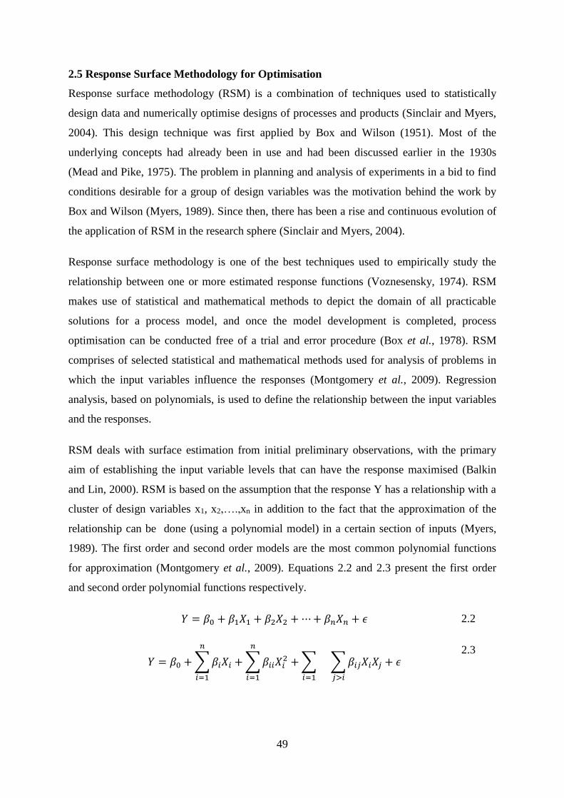
49
2.5 Response Surface Methodology for Optimisation
Response surface methodology (RSM) is a combination of techniques used to statistically
design data and numerically optimise designs of processes and products (Sinclair and Myers,
2004). This design technique was first applied by Box and Wilson (1951). Most of the
underlying concepts had already been in use and had been discussed earlier in the 1930s
(Mead and Pike, 1975). The problem in planning and analysis of experiments in a bid to find
conditions desirable for a group of design variables was the motivation behind the work by
Box and Wilson (Myers, 1989). Since then, there has been a rise and continuous evolution of
the application of RSM in the research sphere (Sinclair and Myers, 2004).
Response surface methodology is one of the best techniques used to empirically study the
relationship between one or more estimated response functions (Voznesensky, 1974). RSM
makes use of statistical and mathematical methods to depict the domain of all practicable
solutions for a process model, and once the model development is completed, process
optimisation can be conducted free of a trial and error procedure (Box et al., 1978). RSM
comprises of selected statistical and mathematical methods used for analysis of problems in
which the input variables influence the responses (Montgomery et al., 2009). Regression
analysis, based on polynomials, is used to define the relationship between the input variables
and the responses.
RSM deals with surface estimation from initial preliminary observations, with the primary
aim of establishing the input variable levels that can have the response maximised (Balkin
and Lin, 2000). RSM is based on the assumption that the response Y has a relationship with a
cluster of design variables x1, x2,….,xn in addition to the fact that the approximation of the
relationship can be done (using a polynomial model) in a certain section of inputs (Myers,
1989). The first order and second order models are the most common polynomial functions
for approximation (Montgomery et al., 2009). Equations 2.2 and 2.3 present the first order
and second order polynomial functions respectively.
𝑌 = 𝛽0 + 𝛽1𝑋1 + 𝛽2𝑋2 + ⋯ + 𝛽𝑛𝑋𝑛 + 𝜖 2.2
𝑌 = 𝛽0 + ∑ 𝛽𝑖𝑋𝑖
𝑛
𝑖=1
+ ∑ 𝛽𝑖𝑖𝑋𝑖2
𝑛
𝑖=1
+ ∑
𝑖=1
∑ 𝛽𝑖𝑗𝑋𝑖𝑋𝑗 + 𝜖
𝑗>𝑖
2.3
50
In general, the common error variance, σ2 assumption is made and the ordinary least squares
aids in the estimation of coefficients (Myers, 1989). According to Montgomery et al. (2009),
the effective estimation of model parameters depends on the correct use of experimental
designs for data collection. Response surface design is the terminology for designs used to fit
response surfaces. The most common response surface designs are the central composite
design (CCD), Box-Behnken design, and orthogonal design, which incorporates the fractional
and 2k factorial design points (Box and Behnken, 1960). The CCD was used during this
research study. Polynomial models generally give a sensible true functional relationship
approximation for a particular sub-area owing to its focus in a confined search space area.
The assumption is that if the true response function can adequately be approximated by the
fitted surface, then there is very little difference between the analysis of the fitted surface and
that of the actual system (Montgomery et al., 2009).
Response surface methodology has a sequential procedure and its aim is to quickly and
efficiently guide the experimenter to the overall optimum domain. During the initial stages, a
first-order model is fitted due to the fact that there is a likelihood that the domain being
investigated could be far from the optimum, and consequently there is small curvature
detection in the system. Consequently, the approach of steepest ascent is applied in order to
provide guidance in the search for an operability region that is most favourable.
The steepest ascent is in the direction that is perpendicular to the response which is fitted, and
matches with the direction which produces the most rapid increase in the fitted response. The
stages along the course are proportionate to the approximated regression coefficients. The
iteration of the procedure is carried out until the first order model lack of fit shows the
optimum condition domain (Montgomery et al., 2009).
After the location of the optimum region, the fitting of the second order model is conducted
before the analysis for location of the optima is carried out. In the course of the entire
procedure, the subsequent stage is planned using the information from the previous stage.
There may be need to conduct extra runs to get additional information about the response in
some sections of the domain that the initial design may have inadequately covered (Myers,
1989). Sequential design together with extra experimental runs fall in the design
augmentation concept (Myers, 1989).
51
Design and analysis of computer experiments (DACE) is a statistical technique that was
established by Sacks et al. (1989). DACE has found its application in the field of engineering
as a solution to problems associated with expensive optimisation of designs such as electronic
circuits design, computational fluid dynamics and analysis of finite elements (Bates, 1996;
Buche et al., 2005; Grierson and Pak, 1993; Lee and Hajela, 1996). Where processes are
complex such that physical experimentation is extremely expensive, time consuming, or even
impossible to conduct, then simulation of the system through mathematical modelling comes
in handy (Sacks et al., 1989). Although advances have been made in terms of computer
capacity improvement, exorbitant computational cost renders complex engineering
simulations impractical.
In DACE, data from an experimental design is used to build a surrogate or a metamodel (also
known as model of model) before being optimised. Consequently, a larger simulator is used
to model the physical process, and the computer code aids to directly conduct the
experiments (Bates, 1996). The behaviour of the system can either be approximated by a
deterministic or a stochastic model. For a stochastic simulation model, the experimentation,
presents a behaviour similar to that of a physical system (Montgomery et al., 2009).
Conversely, there is a difference between experimentation using a deterministic model and
experimentation of the physical system due to the fact there is no random error linked with
the output. Ultimately, when the code is run with unchanged inputs, identical response values
will be achieved (Sacks et al., 1989). Sacks et al. (1989) were among the first scholars to
introduce and pursue deterministic models, and they put forth the idea of using a statistical
model that views the response as if it were a stochastic process realisation.
Gaussian stochastic process model is the name given to the statistical model which Sacks et
al. (1989) adopted, with an advantage of providing fundamental statistics for computation of
an efficient response predictor at untried inputs, and hence it permits the estimation of the
uncertainty of the predictor. According to the proposal by Sacks et al. (1989), the concept is
to select a design with high response predictability at untried inputs of the experimental
domain and supplement it by use of extra design points. The aim of augmenting the design is
to lay emphasis on sampling that has high uncertainty of the predictor so that scrutiny can be
dedicated to the space parts that are not adequately explored (Jones et al., 1998). Computer
experiments, in contrast with conventional RSM, aims at finding a model for approximation
of true response surface in a much broader span (in some cases extending over the whole
52
operability domain) of the design parameters. This consequently requires models that have
more complexity in comparison with the first and second order polynomial models.
Non-parametric and semi-parametric response surface methodology (NPRSM) is best suited
to situations in which the polynomial models in the domain of operability do not
accommodate the response (Myers, 1989; Sinclair and Myers, 2004). This happens where
there is need to fit a model that covers a section of the space of the factor, which happens to
be bigger than the portion considered in the conventional RSM techniques (Sinclair and
Myers, 2004). ‘Non-parametric response surface methodology’ means that there is an
absence of a particular model, and that the analysis mainly focuses on prediction. This,
therefore, leads to the application of kernel-based methods of regression. Conversely, Semi-
parametric response surface methodology implies that there is the use of a model, but not of a
standard polynomial nature (Sinclair and Myers, 2004). According to Myers (1989), the
situations where Non-parametric and semi-parametric response surface methodology
(NPRSM) can be applied include:
i. Where optimum conditions are not required
ii. If the interest in the response surface appearance is greater than the interest in the
interpretative function
iii. Where the function exhibits nonlinearity, but not certainly well-behaved
iv. Where the designs must originate from a space-filling grid and do not have to honour
the ‘form of the model’
There exists a big difference in terms of various aspects (modelling, design and optimisation
approaches) between RSM and NPRSM. However, the difference between NPRSM and
Design and analysis of computer experiments (DACE) is not as clear. This is because the
development of DACE as one of the modelling techniques was to help address the issue of
high simulation costs of complex engineering processes (Sacks et al., 1989). NPRSM has
been used mainly in biotechnology and biopharmacy (Sinclair and Myers, 2004). At first,
sequential sampling and deterministic stochastic Gaussian process were used in DACE but
later, models like thin Plate splines and neural networks were developed. Henceforth, DACE
may be seen as a component of NPRSM.
53
Developments have been made with regard to NPRSM and DACE, in the field of
optimisation of algorithm parameters. Major techniques that have been introduced in this
field include sequential optimisation of parameters (Bartz-Beielstein et al., 2005) and
effective global optimisation (Jones et al., 1998). The main objective of these techniques is to
help to quantify the significance of each variable and interactions between variables. In the
case of multiple instances, these techniques provide a clear view of the interaction between
instance properties and the parameters. These techniques also support the performance of
interpolation within the variable settings as well as the extrapolation to parameter space
domains that were hitherto undetected. These techniques play an important role as far as
algorithm interpretation and enhancement is concerned (Hennink et al., 2010; Hutter et al.,
2009).
In NPRSM, conventional RSM designs like CCD and factorial designs are commonly used
(Myers et al., 2004). It is important, however, to note that conventional RSM designs are
suitable in cases where the design domain is regular or if the experimenter is interested in a
polynomial model. A regular domain of design can be depicted as a space surrounded by the
p-dimensional hypersphere or hypercube, where every point within or on the sphere or cube
is considered a possible design point. Due to practical problems associated with the
operability, availability and feasibility of the system under study, there may be need to create
holes in the design domain, slice portions of the sphere, or cut up the cube corners (Kennard
and Stone, 1969). Moreover, when the experiments are time-consuming or expensive, the
number of runs that can be achieved is reduced. This number of trials is relatively smaller
than the number of conceptually possible experiments.
In the cases where there is a fixed model as well as the number of achievable trials, most
RSM designs result in a big number of required replicates (Kennard and Stone, 1969). If
there is an occurrence of nonstandard conditions like unusual requirements of the sample size
or an irregular experimental domain, then computer-generated designs are preferable
(Montgomery et al., 2009). Computer-generated designs are commonly referred to as optimal
designs because of their optimality with respect to a particular criterion. G-optimality, A-
optimality and D-optimality are the commonly used optimality criteria (Montgomery et al.,
2009). D- and A-optimality focus on estimating the regression coefficients and use the
minimisation of a function of the covariance matrix of the parameters’ least squares estimates
(Montgomery et al., 2009; Santner et al., 2003). G-optimal designs focus on response
54
prediction and their aim is to reduce the variance of the maximum scaled prediction in the
design domain (Montgomery et al., 2009).
The common procedure in computer-generated designs is to define the model (usually a
polynomial model), establish the interest region, choose the number of runs to conduct,
define the criterion of optimality, and finally select the points of design (that would interest
the experimenter) from a group of preferred points. The preferred points are a network of
points that are spaced over the practicable design domain (Montgomery et al., 2009). With
the development of DACE, there has been introduction of other criteria-founded designs.
They are more complex to achieve in comparison with the designs mentioned earlier.
Typically, the Gaussian stochastic model is presumed and the design criteria has a functional
relationship with its unknown variables (Santner et al., 2003). For a set number of trials and
for a particular structure of correlation, these criteria of design aims at selecting a design that
will give the best response prediction at untried inputs in the experimental domain.
2.6 Biogas Production Prediction Models
A model is a simplified abstract view of a complex reality. A scientific model represents
empirical objects, phenomena, and physical processes in a logical way. For the scientist, a
model is also a way in which the human thought processes can be amplified (Stockburger,
2006). MacKay (2004) defined a mathematical model as a representation of the essential
aspects of an existing system which presents knowledge of that system in a usable form.
Mathematical models are used not only in the natural sciences (such as physics, biology,
earth science, meteorology) and engineering disciplines, but also in the social sciences (such
as economics, psychology, sociology and political science); physicists, engineers, computer
scientists, and economists use mathematical models most extensively.
A crucial part of the modeling process is the evaluation of whether or not a given
mathematical model describes a system accurately. Rolland and Pernici (1998) evaluated a
model by its consistency to empirical data and concluded that any model that is inconsistent
with reproducible observations must be modified or rejected. They argued that a fit to
empirical data alone was insufficient for a model to be accepted as valid; other factors
included ability to explain past observations, ability to predict future observations, cost of use
– especially in combination with other models, refutability, enabling estimation of the degree
of confidence in the model, and simplicity, or even aesthetic appeal.
55
Assessing the scope of a model, that is, determining the situations in which the model can be
applied can be straightforward. If the model was constructed based on a set of data, one must
determine for which systems or situations the known data is a ‘typical’ set of data (MacKay,
2004). It has been observed that biogas models have been formulated for specific designs of
digesters and conditions, and cannot be applied across board. Hence there is need to perform
tests in order to adapt the models to various working conditions.
Some of the mathematical models used to relate the inputs (factors) to the output in a biogas
system include:
a) Plug Flow Model
b) Chen and Hashimoto Model
c) Low Temperature Lagoon Digester Model
d) Toprak Model
e) Scoff and Minott Model
The application of some of these models was discussed and tested using available statistical
indicators in Chapter 4 of this thesis.
56
References
Abbassi-Guendouz, A., Brockmann, D., Trably, E., Dumas, C. and Delgenès, J. (2012).
Total solids content drives high solid anaerobic digestion via mass transfer limitation.
Bioresource Technology, 111, 55-61.
Afazeli, H., Jafari, A., Rafiee, S. and Nosrati, M. (2014). An investigation of biogas
production potential from livestock and slaughterhouse wastes. Renewable and
Sustainable Energy Reviews, 34, 380-386.
Akunna, J., Abdullahi, Y. and Stewart, N. (2007). Anaerobic digestion of municipal solid
wastes containing variable proportions of waste types. Water Science Technology,
50, 143-149.
Al Mamun, M. and Torii, S. (2015). Enhancement of production and upgrading of biogas
using different techniques - A Review. International Journal of Earth Sciences and
Engineering, 8(2), 877-892.
Alvarez, J., Otero, L. and Lema, J. (2010). A methodology for optimising feed composition
for anaerobic co-digestion of agro-industrial wastes. Bioresource Technology, 101,
1153-1158.
Angelidaki, I. and Ahring, B. (2000). Methods for increasing the biogas potential from the
recalcitrant organic matter contained in manure. Water Science Technology, 41, 189-
194.
APHA. (1999). Standard Methods for the Examination of Water and Wastewater. American
Public Health Association.
Appels, I., Degreve, J., Bruggen, B., Impe, J. and Dewil, R. (2010). Influence of low
temperature thermal pretreatment on sludge solubilization, heavy metal release and
anaerobic digestion. Bioresource Technology, 101, 5743-5748.
Ardaji, V., Radnezhad, H. and Nourouzi, M. (2016). Improving biogas production
performance from pomegranate waste, poultry manure and cow dung sludge using
thermophilic anaerobic digestion: Effect of total solids adjustment. Journal of Earth,
Environment and Health Sciences, 2(3), 97-109.
Ariunbaatar, J., Panico, A., Esposito, G., Pirozzi, F. and Lens, P. (2014). Pretreatment
methods to enhance anaerobic digestion of organic solid waste. Applied Energy, 123,
143-156.
57
Assefa, A., Egigu, M. and Kebede, A. (2014). Thermal and chemical pre-treatments of cow
dung and poultry litter enhance biogas production in batch fermentation.
International Journal of Scientific and Technology Research, 3, 165-170.
Astolfi, A. and Praly, L. (2006). Global complete observability and output-to-state stability
imply the existence of a globally convergent observer. Mathematics of Control,
Signals and Systems, 18(1), 32-65.
Balasubramaniyam, U., Zisengwe, L., Meriggi, N. and Buysman, E. (2008). Biogas
production in climates with long winters. WECF.
Balkin, S. D. and Lin, D. K. (2000). A neural network approach to response surface
methodology. Communications in Statistics-Theory and Methods, 29(9-10), 2215-
2227.
Barjenbruch, M. and Kopplow, O. (2003). Enzymatic, mechanical and thermal pretreatment
of surplus sludge. Advanced Environmental Resources, 7, 715-720.
Bartz-Beielstein, T., Lasarczyk, C. W. and Preuß, M. (2005). Sequential parameter
optimization. Paper presented at the 2005 IEEE congress on evolutionary
computation.
Basheer, I. and Hajmeer, M. (2000). Artificial neural networks: fundamentals, computing,
design, and application. Journal of Microbiological Methods, 43(1), 3-31.
Bates, D. S. (1996). Jumps and stochastic volatility: Exchange rate processes implicit in
deutsche mark options. The Review of Financial Studies, 9(1), 69-107.
Batstone, D. J., Keller, J., Angelidaki, I., Kalyuzhnyi, S., Pavlostathis, S., Rozzi, A.,
Sanders, W., Siegrist, H. and Vavilin, V. (2002). The IWA anaerobic digestion
model no 1 (ADM1). Water Science and Technology, 45(10), 65-73.
Batzias, F., Sidiras, D. and Spyrou, E. (2005). Evaluating livestock manures for biogas
production: A GIS method. Renewable Energy, 30, 1161-1176.
Bauer, A., Moeller, L., Wedwitschka, H., Stinner, W. and Zehnsdorf, A. (2018). Anaerobic
digestion of mixed silage of waterweed biomass and wheat straw in a long-term
semi-continuous biogas production process. Energy, Sustainability and Society, 8(4).
doi:10.1186/s13705-017-0145-9
Bischofsberger, W., Dichtl, N., Rosenwinkel, K., Seyfried, C. and Böhnke, B. (2005). A
description of hydrolysis kinetics in anaerobic degradation of particulate organic
matter. Bioresource Technology, 56(2-3), 229-237.
58
Björnsson, L., Murto, M. and Mattiasson, B. (2000). Evaluation of parameters for
monitoring an anaerobic co-digestion process. Applied Microbiology and
Biotechnology, 54(6), 844-849.
Bochmann, G., Drosg, B., Ortner, M., Schonlieb, M., Andres-Lainez, S., Kirchmayr, R.
and Braun, R. (2010). Influence of thermal pre-treatment to increase digestibility of
brewers’ spent grains. Paper presented at the 12th World Congress on Anaerobic
Digestion, Guadalajara.
Bochmann, G. and Montgomery, L. (2014). Pretreatment of Feedstock for Enhanced Biogas
Production. Retrieved from Paris, France.
Boe, K. (2006). On-line monitoring and control of the biogas process. (PhD), Technical
University of Denmark, Lyngby, Denmark.
Böjti, T., Kovács, K., Kakuk, B., Wirth, R., Rákhely, G. and Bagi, Z. (2017). Pretreatment
of poultry manure for efficient biogas production as monosubstrate or co-
fermentation with maize silage and corn stover. Anaerobe, 46, 138-145.
Bolaji, O., Awonorin, S., Shittu, T. and Sanni, L. (2017). Changes induced by soaking
period on the physical properties of maize in the production of Ogi. Cogent Food and
Agriculture, 3(1), 132-157.
Bolzonella, D., Pavan, P., Mace, S. and Cecchi, F. (2006). Dry anaerobic digestion of
differently sorted organic municipal solid waste: a full-scale experience. Water
Science Technology, 53, 23-32.
Bouallagui, H., Ben, C., Marouani, L. and Hamdi, M. (2003). Mesophilic biogas production
from fruit and vegetable waste in a tabular digester. Bioresource Technology, 86, 85-
89.
Bougrier, C., Albasi, C., Delgenes, J. and Carrere, H. (2006). Effect of ultrasonic, thermal
and ozone pretreatments on waste activated sludge solubilization and
biodegradability. Chemical Engineering Process, 45, 711-718.
Box, G. and Behnken, D. (1960). Simplex-sum designs: a class of second order rotatable
designs derivable from those of first order. The Annals of Mathematical Statistics,
31(4), 838-864.
Box, G., Hunter, W. and Hunter, J. (1978). Statistics for Experimenters.
Box, G. and Wilson, K. (1951). On the experimental attainment of optimum conditions.
Journal of the Royal Statistical Society: Series B (Methodological), 13(1), 1-38.
Bridgeman, J. (2012). Computational fluid dynamics modeling of sewage sludge mixing in
an anaerobic digester. Advances in Engineering Software, 44(1), 54-62.
59
Brummeler, E. and Koster, J. (1990). Enhancement of dry anaerobic batch digestion of
organic fraction of municipal solid waste. Biological Wastes, 31, 199-210.
Buche, D., Schraudolph, N. N. and Koumoutsakos, P. (2005). Accelerating evolutionary
algorithms with Gaussian process fitness function models. IEEE Transactions on
Systems, Man, and Cybernetics, Part C (Applications and Reviews), 35(2), 183-194.
Burke, D. (2001). Dairy waste anaerobic digestion handbook: Options for recovering
beneficial products from dairy manure.
Buysman, E. (2009). Anaerobic digestion for developing countries with cold climates. (MSc),
Wageningen, Netherlands.
Carballa, M., Monterola, G., Larrea, I., Temes, T., Omil, F. and Lema, J. (2007). Influence
of ozone pretreatment on sludge anaerobic digestion: removal of pharmaceutical and
personal care products. Chemosphere, 67, 1444-1452.
Carlsson, M. and Anox, K. (2008). Electroporation for enhanced methane yield from
municipal solid waste. Paper presented at the ORBIT 2008, Wageningen.
Carlsson, M., Lagerkvist, A. and Morgan-Sagastume, F. (2012). The effects of substrate
pretreatment on anaerobic digestion: a review. Waste Management, 32, 1634-1650.
Carrère, H., Dumas, C., Battimelli, A., Batstone, D., Delgenès, J., Steyer, J. and Ferrer, I.
(2010). Pretreatment methods to improve sludge anaerobic degradability: A review.
Journal of Hazardous Materials, 183, 1-15.
Carrere, H., Sialve, B. and Bernet, N. (2009). Improving pig manure conversion into biogas
by thermal and thermal-chemical pretreatments. Bioresource Technology, 100, 3690-
3694.
Cesaro, A. and Belgiorno, V. (2013). Sonolysis and ozonation as pretreatment for anaerobic
digestion of solid waste. Ultrason Solochem, 20, 931-936.
Cesaro, A. and Belgiorno, V. (2014). Pretreatment methods to improve anaerobic
biodegradability of organic municipal solid waste fractions. Chemical Engineering
Journal, 240, 24-37.
Chamchoi, N., Garcia, H. and Angelidaki, I. (2011). Methane potential of household waste:
batch assays determination. Journal of Environmental Resources, 33, 13-26.
Chen, S., Li, R. and Li, X. (2009). Anaerobic co-digestion of kitchen waste and cattle
manure for methane production. Energy Sources, 31, 1848-1856.
Chua, C., Lee, D., Chang, B.-V., You, C. and Tay, J. (2002). “Weak” ultrasonic pre-
treatment on anaerobic digestion of flocculated activated biosolids. Water Resources,
36, 2681-2688.
60
Climent, M., Ferrer, I., Del Mar Baeza, M., Artola, A., Vázquez, F. and Font, X. (2007).
Effects of thermal and mechanical pretreatments of secondary sludge on biogas
production under thermophilic conditions. Chemical Engineering Journal, 133(1-3),
335-342.
Dahunsi, S. and Orunsi, U. (2013). Co-digestion of food waste and human excreta for biogas
production. British Biotechnology Journal, 3(4), 485-499.
Davidson, A., Gruvberger, C., Christenssen, T., Hansen, T. and Jansen, J. (2007). Methane
yield in source-sorted organic fraction municipal solid waste. Waste Management,
27, 406-414.
Daxiong, Q., Shuhua, G., Baofen, L. and Gehua, W. (1990). Diffusion and innovation in the
Chinese biogas programme. World Development, 18(4), 555-563. doi:10.1016/0305-
750X(90)90071-5
Derbal, K., Bencheikh-Lehocine, M., Ceecchi, F., Meniai, A. and Pavan, P. (2009).
Application of the IWA ADM1 model to simulate anaerobic co-digestion of aorganic
waste with waste- activated sludge in mesophilic condition. Bioresource
Technology, 100, 1539-1543.
Deublein, D. and Steinhauser, A. (2008). Biogas from Waste and Renewable Resources: An
Introduction. Weinheim, Germany.
Dioha, I., Ikeme, C., Nafi’u, T., Soba, N. and Yusuf, M. (2014). Effect of carbon to
nitrogen ratio on biogas production. International Research Journal of Natural
Sciences, 1(3), 1-10.
Dong, R. (2004). Energy – The most important resource for social development. Paper
presented at the International Course on New Technology Popularizing Agricultural
Machinery, China Agricultural University, Beijing.
Du, D., Pardalos, P. and Wu, W. (2008). History of Optimization. In C. Floudas & P.
Pardalos (Eds.), Encyclopedia of Optimization (pp. 1538-1542). Boston: Spinger.
Edelmann, W., Baier, U. and Engeli, H. (2005). Environmental aspects of the anaerobic
digestion of organic fraction of municipal solid waste and agricultural waste. Water
Science Technology, 52, 553-559.
Eder, B. and Schulz, H. (2006). Biogas Praxis [in German] (3rd ed.).
Elliot, A. and Mahmood, T. (2007). Pretreatment technologies for advancing anaerobic
digestion of pulp and paper biotreatment residue. Water Resources, 41, 4273-4286.
61
Elliot, A. and Mahmood, T. (2012). Comparison of mechanical pretreatment methods for the
enhancement of anaerobic digestion of pulp and paper waste. Water Science
Technology, 84, 497-505.
Engelhart, M., Kruger, M., Kopp, J. and Dichtl, N. (2000). Effects of disintegration on
anaerobic digestion of sewage excess sludge in down-flow stationary fixed film
digesters. Water Science Technology, 41, 171-179.
EPA. (1992). Global methane emissions from livestock and poultry manure. United States
Environment Protection Agency, 400(1091).
EPA. (2001). Method 1684: Total, Fixed, and Volatile Solids in Water, Solids, and Biosolids.
U.S. Environmental Protection Agency.
EPA. (2005). Anaerobic Digestion: Benefits for Waste Management, Agriculture, Energy,
and the Environment. U.S. Environment Protection Agency.
Esposito, G., Frunzo, I., Panico, A. and Pirozzi, F. (2011). Modeling the effect of organic
loading rate and organic fraction of municipal solid waste particle size on
performances of an anaerobic co-digestion reactor. Process Biochemistry, 46, 557-
565.
Fayyaz, A., Qaisar, M., Naim, R., Arshid, P., Iftikhar, R. and Mohammad, M. (2015). Co-
digestion, pretreatment and digester design for enhanced methanogenesis. Renewable
and Sustainable Energy Reviews, 42, 627-642.
Fdez-Guelfo, L., Alvarez-Gallego, C., Sales, M. and Romero, G. (2011). The effect of
different pretreatments on biomethanation kinetics of industrial organic fraction of
municipal solid wastes (OFMSW). Chemical Engineering Journal, 171, 411-417.
Ferguson, R., Coulon, F. and Villa, R. (2016). Organic loading rate: A promising microbial
management tool in anaerobic digestion. Water Research, 100, 348-356.
Ferguson, R., Villa, R. and Coulon, F. (2014). Bioengineering options and strategies for
optimization of anaerobic digestion processes. Environmental Technology, 3, 1-14.
Fernandes, T., Klaasse Bos, B., Zeeman, G., Sander, J. and Lier, J. (2009). Effects of
thermal-chemical pretreatment on anaerobic biodegradability and hydrolysis of
lignocellulosic biomass. Bioresource Technology, 100, 2575-2579.
Ferrer, I., Ponsá, S., Vázquez, F. and Font, X. (2008). Increasing biogas production by
thermal sludge pre-treatment prior to thermophilic anaerobic digestion. Biochemical
Engineering Journal(42), 186-192.
Gallert, C., Henning, A. and Winter, J. (2003). Scale-up of anaerobic digestion of the
biowaste fraction from domestic wastes. Water Resources(37), 1433-1441.
62
Garcia-Ochoa, F., Santos, V., Naval, L., Guardiola, E. and Lopez, B. (1999). Kinetic
model for anaerobic digestion of livestock manure. Enzyme Microbiology and
Technology, 25, 55-60.
Garrote, G., Dominguez, H. and Parajo, J. (1999). Hydrothermal processing of
lignocellulosic materials. Holz als Roh-und Werkstoff, 57(3), 191-202.
Gashaw, A. and Teshita, A. (2014). Co-digestion of Ethiopian food waste with cow dung for
biogas production. International Journal of Research, 1(7), 475-500.
Ge, H., Jensen, P. and Batstone, D. (2010). Pre-treatment mechanisms during thermophilic–
mesophilic temperature phased anaerobic digestion of primary sludge. Water
Resources(44), 123-130.
Ge, H., Jensen, P. and Batstone, D. (2011a). Increased temperature in thermophilic stage in
temperature phased anaerobic digestion (TPAD) improves degradability of waste
activated sludge. Hazardous Material, 187, 355-361.
Ge, H., Jensen, P. and Batstone, D. (2011b). Temperature phased anaerobic digestion
increse apparent hydrlysis rate for waste activated sludge. Water Resources, 45,
1597-1606.
Ghanimeh, S., Fadel, M. and Saikaly, P. (2012). Mixing effect on thermophilic anaerobic
digestion of source-sorted organic fraction municipal solid waste. Bioresource
Technology, 117, 63-71.
Ghimire, P. (2013). SNV supported domestic biogas programmes in Asia and Africa.
Renewable Energy, 49, 90-94. doi:10.1016/j.renene.2012.01.058
Gisemba, J. and Barasa, M. (2019). Effect of bioslurry utilization and application methods
on the African stalk borer (Buseiola fusca) and yield of maize. International Journal
of Science and Nature, 10(3), 125-131.
Goel, R., Tokutomi, T., Yasui, H. and Noike, T. (2003). Optimal process configuration for
anaerobic digestion with ozonation. Water Science Technology, 8, 85-96.
Gonzalez-Fernandez, C., Salve, B., Bernet, N. and Steyr, J. (2012). Thermal pretreatment to
improve methane production of Scenedesmus biomass. Biomass Bioenergy, 40, 105-
111.
Grady, C., Daigger, G. and Lim, H. (1999). Biological wastewater treatment: Principles and
practice. New York: Marcel Dekker, New York.
Gray, N. (2004). Biology of waste water treatment (2nd ed.). London: Imperial College
Press.
Green, J. and Sibisi, M. (2002). Domestic biogas digesters: a comparative study.
63
Grierson, D. and Pak, W. (1993). Optimal sizing, geometrical and topological design using a
genetic algorithm. Structural Optimization, 6(3), 151-159.
Gujer, W. and Zehnder, A. (1983). Conversion processes in anaerobic digestion. Water
Science and Technology, 15, 127-167.
Gunaseelan, V. (1997). Anaerobic digestion of biomass for methane production: A review.
Biomass and Bioenergy, 13(1-2), 83-114.
Gupta, R. and Singh, N. (1990). Community biogas plants in India. Biological Wastes, 32,
149-153.
Halalsheh, M., Kassab, G., Yazajeen, H., Qumsieh, S. and Field, J. (2011). Effect of
increasing the surface area of primary sludge on anaerobic digestion at low
temperature. Bioresource Technology, 102(2), 748-752.
Hamad, M., Abdel-Dayem, A. and El-Halwagi, M. (1981). Evaluation of the performance of
two rural biogas units of Indian and Chinese design. Energy Agriculture, 1, 235-250.
Hansen, C., Schmidt, T., Angelidaki, J., Marca, I., Jansen, J., Mosbaek, H. and
Christensen, T. (2004). Method for determination of methane potentials of solid
organic waste. Waste Management, 24, 393-400.
Hartmann, H. and Ahring, B. (2006). Strategies for the anaerobic digestion of the organic
fraction of municipal solid waste: an overview. Water Science Technology, 53, 7-22.
Hartmann, H., Angelidaki, I. and Ahring, B. (2000). Increase of anaerobic degradation of
particulate organic matter in full-scale biogas plants by mecanical maceration. Water
Science Technology, 41, 145-153.
Hendriks, A. and Zeeman, G. (2009). Pretreatments to enhance the digestibility of
lignocellulosic biomass. Bioresource Technology, 100, 10-18.
Hennink, M., Hutter, I. and Bailey, A. (2010). Qualitative Research Methods: Sage.
Huba, E., Cheng, S., Li, Z. and Mang, H. (2013). A review of prefabricated biogas digesters
in China. Renewable and Sustainable Energy Review, 28, 738-748.
doi:10.1016/j.rser.2013.08.030
Hutter, F., Hoos, H. H., Leyton-Brown, K. and Stützle, T. (2009). ParamILS: an automatic
algorithm configuration framework. Journal of Artificial Intelligence Research, 36,
267-306.
Izumi, K., Okishio, Y., Nagao, N., Niwa, C., Yamamoto, S. and Toda, T. (2010). Effects
of particle size on anaerobic digestion of food waste. International Journal of Bio-
deterioration and Biodegradation, 64(7), 601-608.
64
Jahng, D., Lee, Y. and Zhang, L. (2011). Anaerobic co-digestion of food waste and piggery
wastewater: focusing on the role of trace elements. Bioresource Technology, 102(8),
5048-5059.
Jash, T. and Gosh, D. (1990). Studies on residence time distribution in cylindrical and
rectangular biogas digesters. Energy, 15, 987-991.
Jegede, A., Zeeman, G. and Bruning, H. (2019). A review of mixing, design and loading
conditions in household anaerobic digesters. Critical Reviews in Environmental
Science and Technology, 49(22), 2117-2153. doi:10.1080/10643389.2019.1607441
Jin, P., Bhattacharya, S., Williama, C. and Zhang, H. (1998). Effects of sulphide addition
on copper inhibition in methanogenic systems. Water Resources, 32, 977-988.
Jones, D., Schonlau, M. and Welch, W. (1998). Efficient global optimization of expensive
black-box functions. Journal of Global Optimisation, 13(4), 455-492.
Kana, E., Oloke, J., Lateef, A. and Adesiyan, M. (2012). Modeling and optimization of
biogas production on saw dust and other co-substrates using artificial neural network
and genetic algorithm. Renewable Energy, 46, 276-281.
Karapaju, P. and Rintala, J. (2008). Effect of solid-liquid separation on recovering residual
methane and nitrogen of a digested dairy cow manure. Bioresource Technology, 99,
120-127.
Karim, K., Klasson, K., Drescher, S., Ridenour, W., Borole, A. and Al-Dahhan, M.
(2007). Mesophilic digestion kinetics of manure slurry. Applied biochemistry and
biotechnology, 142, 231-242.
Kennard, R. W. and Stone, L. A. (1969). Computer aided design of experiments.
Technometrics, 11(1), 137-148.
Khanal, S. (2008). Anaerobic Biotechnology for Bioenergy Production: Principles and
Applications (S.K. Khanal ed.). New York, USA: John Wiley and Sons
Kianmahr, P., Parker, W. and Seto, P. (2010). An evaluation of prtocols for characterization
of ozone impacts on waste agricultural solids properties and digestibility.
Bioresource Technology, 101, 8565-8572.
Kobayashi, T. and Li, Y.-Y. (2011). Performance and characteriztion of a newly developed
self-agitated anaerobic reactor with biological desulphurization. Bioresource
Technology, 102(10), 5580-5588. doi:10.1016/biortech.2011.01.077
Koettner, M. (2002, 18-20 Sept 2002). Biogas and fertilizer production from solid waste and
biomass through dry fermentation in batch method. Paper presented at the 3rd
65
International Symposium on Anaerobic Digestion of Solid Wastes, Technical
University of Munich, Munich, Germany
Kratky, L. and Jirout, T. (2011). Biomass size reduction machines for enhancing biogas
production. Chemical Engineering and Technology, 34(3), 391-399.
Laichena, J. and Wafula, J. (1997). Biogas technology for rural households in Kenya. OPEC
Reviews, 21, 223-244.
Lee, J. and Hajela, P. (1996). Parallel genetic algorithm implementation in multidisciplinary
rotor blade design. Journal of Aircraft, 33(5), 962-969.
Leenawat, A., Pasakorn, J., Atip, L., Rodriguez, J. and Khanita, K. (2016). Effect of
temperature on increasing biogas production from sugar industrial wastewater
treatment by UASB process in pilot scale. Paper presented at the 3rd International
Conference on Power and Energy Systems Engineering, CPESE, Kitakyushu, Japan.
Lemmer, A., Naegele, H.-J. and Sondermann, J. (2013). How Efficient are Agitators in
Biogas Digesters? Determination of the Efficiency of Submersible Motor Mixers and
Incline Agitators by Measuring Nutrient Distribution in Full-Scale Agricultural
Biogas Digesters. Energies(6), 6255-6273. doi:10.3390/en6126255
Lettinga, G., Field, J., Van Lier, J., Zeeman, G. and Pol, L. H. (1997). Advanced anaerobic
wastewater treatment in the near future. Water Science and Technology, 35(10), 5-12.
Li, H., Li, C., Liu, W. and Zou, S. (2012). Optimized alkaline pretreatment of sludge before
anaerobic digestion. Bioresource Technology(123), 189-194.
Lim, J. and Wang, J.-Y. (2013). Enhanced hydrolysis and methane yield by applying micro
aeration pretreatment to anaerobic co-digestion of brown water and food waste.
Waste Management, 33, 813-819.
Lippmann, M., Frampton, M., Schwartz, J., Dockery, D., Schlesinger, R., Koutrakis, P.,
Froines, J., Nel, A., Finkelstein, J. and Godleski, J. (2003). The US Environmental
Protection Agency Particulate Matter Health Effects Research Centers Program: a
midcourse report of status, progress, and plans. Environmental Health Perspectives,
111(8), 1074-1092.
Lopez-Torres, M. and Llorens, M. (2008). Effect of alkaline pretreatment on anaerobic
digestion of solid wastes. Waste Management, 28, 2229-2234.
Lorenzo, B., Selene, G., Alessandro, S. and Fabio, F. (2013). Innovative two-stage
anaerobic process for effective co-digestion of cheese whey and cattle manure.
Bioresource Technology, 128, 779-783.
66
Lu, J., Gavala, H., Skiadas, I., Mladenovska, Z. and Ahring, B. (2008). Improving
anaerobic sewage sludge digestion by implimentation of hyper-thermophilic pre-
hydrolysis step. Journal of Environmental Management, 88, 881-889.
Ma, J., Duong, T., Smits, M., Vestraete, W. and Carballa, M. (2011). Enhanced
biomethanation of kitchen waste by different pretreatments. Bioresource Technology,
102, 592-599.
MacKay, D. (2004). Information Theory, Inference, and Learning Algorithms. Cambridge:
Cambridge University Press.
Marti-Herero, J. (2011). Reduced hydraulic times in low-cost tabular digesters: Two issues.
Biomass Bioenergy, 35, 4481-4484.
Mata-Alvarez, J., Dosta, J., Mace, S. and Astals, S. (2010). Co-digestio of solid wastes: A
review of its uses and perspectives including modeling. Critical Reviews in
Biotechnology, 1, 1-13. doi:10.3109/07388551.2010.525496
Mattsson, M., Wang, L., Rundstedt, J. and Karlson, N. (2011). Different pretreatments to
enhance biogas production. (Master of Science), Halmstad.
Mead, R. and Pike, D. (1975). A biometrics invited paper. A review of response surface
methodology from a biometric viewpoint. Biometrics, 31(4), 803-851.
Melamane, A., Tandlich, R. and Burgess, J. (2007). Anaerobic digestion of fungally
pretreated wine distillery waste water. African Journal of Biotechnology, 6, 1990-
1993.
Miah, M., Tada, C. and Yang, Y. (2005). Aerobic thermophilic bacteria enhance biogas
production. Journal of Material Cycles Waste Management, 7, 48-54.
Mohammad, N. (1991). Biogas plants construction technology for rural areas. Bioresource
Technology, 35, 283-289.
Molenbach, A. and Nokes, S. (2012). The use of high solids loading in biomass pretreatment
- A review. Biotechnology Bioenergy, 109, 1430-1442.
Møller, H., Sommer, S. and Ahring, B. (2004). Methane productivity of manure, straw and
solid fractions of manure. Biomass and Bioenergy, 26, 485-495.
Monlau, F., Barakat, A., Steyer, J. and Carrere, H. (2012). Comparison of seven types of
thermo-chemical pretreatments on the structural features and anaerobic digestion of
sunflower stalks. Bioresource Technology, 120, 241-247.
Monnet, F. (2003). An Introduction to Anaerobic Digestion of Organic Wastes. Scotland.
67
Montanes, R., Soleria, R. and Perez, M. (2015). Anaerobic co-digestion of sewage sludge
and sugar beet pulp lixiviation in batch reactors: Effect of temperature. Bioresource
Technology, 180, 177-184.
Montgomery, D. C., Runger, G. C. and Hubele, N. F. (2009). Engineering Statistics: John
Wiley and Sons.
Mshandete A, Björnsson, L., Kavaisi, A., Rubindamayugi, S. and Mattiasson, B. (2005).
Enhancement of anaerobic batch digestion of sisal pulp waste by mesophilic aerobic
pretreatment. Water Resources, 39, 1569-1575.
Murphy, G. and Kumar, D. (2011). Impact of pretreatment and downstream processing
technologies on economics and energy in cellulosic ethanol production.
Biotechnology for Biofuels, 4, 27-34.
Musoline, W., Esposito, G., Giordano, A. and Lens, P. (2012). Anaerobic digestion of rice
straw - a review. Critical Review in Environmental Science Technology, 12, 2605-
2611. doi:10.1080/10643389.627018
Muthangya, M., AM, M. and Kavaisi, A. (2009). Enhancement of anaerobic digestion of
sisal leaf decortication residues by biological pretreatment. APRN Journal of
Agricultural and Biological Sciences, 4, 66-73.
Myers, G. (1989). The pragmatics of politeness in scientific articles. Applied Linguistics,
10(1), 1-35.
Nasir, I., Ghazi, T., Omar, R. and Idris, A. (2014). Bioreactor performance in anaerobic
digestion of cattle manure: A Review. Energy Source: Part A, 36, 1476-1483.
doi:10.1080/15567036.2010.542439
Neczaj, E., Bien, J., Grosser, A., Worwag, M. and Kacprzak, M. (2012). Anaerobic
treatment of sewage sludge and grease trap sludge in continuous co-digestion.
Global NEST Journal, 14(2), 142-148.
Neibling, H. and Chen, L. (2014). Anaerobic Digestion Basics. (6). Moscow.
Neves, I., Ribeiro, R., Oliveira, R. and Alves, M. (2006). Enhancement of methane
production from barley waste. Biomass Bioenergy, 30, 599-603.
Nijaguna, B. (2006). Biogas Technology. New Delhi, India: New Age International.
Nkemka, V. and Murto, M. (2010). Evaluation of biogas production from seaweed in batch
tests and in UASB reactors combined with the removal of heavy metals. Journal of
Environmental Management, 91, 1573-1579.
Nocedal, J. and Wright, S. (1999). Numerical optimization. New York: Springer.
68
Nyaanga, D., Barasa, H. and Gisemba, J. (2015, 11-15 May ). Current and future of biogas
contribution to the energy needs of Kenya. Paper presented at the NACOSTI
Proceedings of Conference, University of Nairobi.
Nzila, C., Njuguna, D., Madara, D., Muasya, R., Githaiga, J., Muumbo, A. and Kiriamiti,
H. (2015). Characterization of agro-residues for biogas production and nutrient
recovery in Kenya. Journal of Emerging Trends in Engineering and Applied
Sciences, 6(5), 327-334.
Panaud, V., Delgenes, J. and Moletta, R. (1999). Thermal-chemical pretreatment of a
microbial biomass: influence of sodium hydroxide addition on solubilization and
biodegradability. Enzyme Microbiology and Techology, 25, 258-263.
Pannucharoenwong, N. (2018). Optimization of Bio-Methane Production from Mesophilic
Anaerobic Co-digestion of Pig Manure and Vegetable Residue. International Journal
of Applied Engineering Research, 13(4), 1988-1995.
Parawira, W., Murto, M., Read, J. and Mattiasson, B. (2005). Profile of hydrolyses and
biogas production during two stage mesophilic anaerobic digestion of solid potato
waste. Process Biochemistry, 40, 2945-2952.
Park, Y. and Lek, S. (2016). Artificial Neural Networks: Multilayer Perceptron for
Ecological Modeling. In Developments in environmental modeling. Elsevier., 28,
123-140.
Park, Y., Li, Y. and Zhu, J. (2011). Solid-state anaerobic digestion for methane production
from organic waste. Renewable and Sustainable Energy Review, 15, 821-826.
Patharwat, I., Kumbhar, S., Hingalaje, P., Khurpe, A., Goudgaon, J. and Dhamangaonkar,
P. (2016). Analysis of optimum temperature and validity of biogas plant.
International Journal of Industrial Electronics and Electrical Engineering, 4(4), 76.
Patil, J., AntonyRaj, M. and Gavimath, C. (2011). Study on effect of pretreatment methods
on biomethanation of water hyacinth. International Journal of Advanced
Biotechnology Resources, 2, 143-147.
Pavlostathis, S. and Giraldo-Gomez, E. (1991). Kinetics of anaerobic treatment. Water
Science and Technology, 24(8), 35-59.
Pavlostathis, S. and Giraldo‐ Gomez, E. (1991). Kinetics of anaerobic treatment: a critical
review. Critical Reviews in Environmental Science and Technology, 21(5-6), 411-
490.
Perez-Elvira, S., Nieto, D. and Fdz-Palanco, F. (2006). Sludge minimization technologies.
Reviews in Environmental Science and Biotechnology, 5, 375-398.
69
Phillips, K., Silgram, M., Newell-Price, P., Warret, M., Provey, G., Cottril, B. and
Newton, J. (2008). The environmental impact of livestock production. Report
ADAS 2007, Deffra FFG, 1-96.
Pinnekamp, J. (1989). Effects of thermal pretreatment of sewage sludge on anaerobic
digestion. Water Science Technology, 21, 97-108.
Protot, A., Julien, I., Christopher, D. and Patrick, I. (2011). Sludge disintegration during
heat treatment at low temperature: a better understanding of involved mechanisms
with a multi-parametric approach. Biochemical Engineering Journal, 54, 178-184.
Rafique, R., Poulse, T., Nizami, A.-S., Assam, Z., Murphy, J. and Kiely, G. (2010). Effect
of thermal, chemical, thermal-chemical pretreatments to enhance methane
production. Energy, 35, 4556-4561.
Rajendran, K., Aslanzadeh, S. and Taherzadeh, M. (2012). Household biogas digesters—A
review. Energies, 5(8), 2911-2942.
Ras, S., Veijanen, A. and Rintala, J. (2007). Trace compounds of biogas from different
biogas production plants. Journal of Energy, 32(8), 1375-1380.
Regattieri, A., Bortolini, M., Ferrari, E., Gamberi, M. and Piana, F. (2018). Biogas micro-
production from human organic waste—A research proposal. Sustainability, 10(2),
330-336.
Rincon, B., Borja, R., Gonzalez, J., Portillo, M. and Saiz-Jimenez, C. (2008). Influence of
organic loading rate and hydraulic retention time on the performance, stability, and
microbial communities of one-stage anaerobic digestion of a two-stage olive mill
solid residue. Biochemical Engineering Journal, 40, 253-261.
Rolland, C. and Pernici, T. (1998). A Comprehensive View of Process Engineering. Paper
presented at the 10th International Conference CAiSE’98, Pisa Italy.
Rusanowska, P., Zieliński, M., Dudek, M. and Dębowski, M. (2018). Mechanical
pretreatment of lignocellulosic biomass for methane fermentation in innovative
reactor with cage mixing system. Journal of Ecological Engineering, 19(5), 219-224.
Sacks, J., Welch, W. J., Mitchell, T. J. and Wynn, H. P. (1989). Design and analysis of
computer experiments. Statistical Science, 409-423.
Safley, L. and Westerman, P. (1992). Performance of a low temperature lagoon digester.
Bioresource Technology, 41, 167-175.
Saint-Joly, C., Desbois, S. and Lotti, J. (2000). Determinant impact of waste collection and
composition on anaerobic digestion performance: industrial results. . Water Science
Technology(41), 291-297.
70
Saleh, A., Kamarudin, E., Yaacob, A., Yussof, A. and Abdullah, M. (2012). Optimization
of biomethane production by anaerobic digestion of palm oil mill effluent using
response surface methodology. Asia-Pacific Journal of Chemical Engineering(7),
353-360.
Sandino, J., Santha, H., Rogowiski, S., Anderson, W., Sung, S. and Isik, F. (2005).
Applicability of ultrsound pre-conditioning of waste activated sludge to reduce
foaming potential in mesophilic digesters. Residuals Biosolids Management, 17, 819-
835.
Santerre, M. and Smith, K. (1982). Measures of appropriateness: the resource requirements
of anaerobic digestion (biogas) systems. World Development, 10, 239-261.
Santner, T. J., Williams, B. J. and Notz, W. (2003). The design and analysis of computer
experiments (Vol. 1): Springer.
Schön, M. (2010). Numerical modelling of anaerobic digestion processes in agricultural
biogas plants (Vol. 6): BoD–Books on Demand.
Sebola, M., Tesfagiorgis, H. and Muzenda, E. (2015). Methane production from anaerobic
co-digestion of cow dung, chicken manure, pig manure and sewage waste.
Shah, F., Mahmood, Q., Rashid, N., Pervez, A., Raja, I. and Shah, M. (2015). Co-
digestion, pretreatment and digester design for enhanced methanogenesis. Renewable
and Sustainable Energy Reviews(42), 627-642.
Shahriari, H., Warith, M., Hamoda, M. and Kennedy, K. (2012). Anarobic digestion of
organic fraction of municipal solid waste combining two pretreatment modalities:
high pressure microwaves and hydrogen peroxide. Waste Management, 32, 41-52.
Shen, R., Wang, W., Liu, X., Gao, X. and Zhou, Y. (2012). Effect of thermal pretreatment
on the physical and chemical properties of municipal biomass waste. Waste
Management, 32, 249-255.
Shyam, M. and Sharma, P. (1994). Solid-state anaerobic digestion of cattle dung and agro-
residues in small-capacity field digesters. Bioresource Technology, 48, 203-207.
Sibisi, N. and Green, J. (2005). A floating dome biogas digester: perceptions of energising a
rural school in Maphephetheni, KwaZulu-Natal. Journal of Energy in Southern
Africa, 16(3), 45-52.
Sinclair, S. L. and Myers, J. E. (2004). The relationship between objectified body
consciousness and wellness in a group of college women. Journal of College
Counseling, 7(2), 150-161.
71
Singh, M. (2017). Metal ion inhibitors and other inorganic toxicants in anaerobic biological
process of industrial effluents: A critical review. International Journal of Science and
Research, 6(5), 2353-2363.
Skiadas, I., Gavala, H., Lu, J. and Ahring, B. (2005). Thermal pre-treatment of primary and
secondary sludge at 70 0C prior to anaerobic digestion. Water Science
Technology(52), 161-166.
Smith, J., Apsley, A., Avery, L., Baggs, E., Balana, B., Bechtel, K. and Moris, K. (2013).
The potential of small scale biogas digesters to improve livelihoods and long term
sustainability of ecosystem services in Sub-Saharan Africa. Retrieved from
Department of International Development, United Kingdom.
Sompong, O., Boe, K. and Angelidaki, I. (2012). Thermophilic anaerobic co-digestion of oil
palm empty fruit bunches with palm oil mill effluent for efficient biogas production.
Applied Energy, 93, 648-654.
Sooch, S. and Singh, J. (2004). Comparative study of economics of different models of
family size biogas plants for state of Punjab, India. Energy Conversion and
Management, 45(9-10), 1329-1341.
Sri, B., Kalyaraman, C. and Thanasekaran, K. (2011). Effect of ozonation and
ultrasonication pretreatment processes on co-digestion of tannery solid wastes. Clean
Technology Environment Policy, 13, 517-525.
Sterrit, R. and Lester, J. (1980). Interaction of heavy metals with bacteria. Science Total
Environment, 14(5), 1-17.
Stockburger, D. (2006). Introductory Statistics: Concepts, Models and Applications.
Subramani, T. and Ponkumar, S. (2012). Anaerobic digestion of aerobic pretreated organic
waste. International Journal of Modern Engineering Resources, 2, 607-611.
Subramanian, S. (1977). Bio-Gas Systems in Asia. (11). New Delhi, India.
Swanwick, J., Shurben, D. and Jackson, S. (1969). A survey of sewage sludge digesters in
Great Britain. Journal of Water Pollution Control Federation, 68, 639-653.
Taherzadeh, M. and Karimi, K. (2008). Pretreatment of lignocellulosic wastes to improve
ethanol and biogas production: a review. International Journal of Molecular
Sciences, 9(9), 1621-1651.
Tale, V., Maki, J. and Zitomer, D. (2015). Bioaugimentation of overloaded anaerobic
digesters restores function and archaeal community. Water Resources, 70(1), 138-
147.
72
Tamrat, A., Mebeaselassie, A. and Amare, G. (2013). Co-digestion of cattle manure with
organic kitchen waste to inrease biogas production using rumen fluid as innoculums.
International Journal of Physical Science, 8(11), 443-450.
Tchobanoglous, G., Burton, F. and Stensel, H. (2003). Waste Water Engineering: Treatment
and Re-use (4th ed.): Tata McGraw-Hill Publishing Company Ltd.
Teghammar, A., Karimi, K., Horváth, I. and Taherzadeh, M. (2012). Enhanced biogas
production from rice straw, triticale straw and softwood spruce by NMMO
pretreatment. Biomass and Bioenergy, 36, 116-120.
Thuiller, W. (2003). BIOMOD–optimizing predictions of species distributions and projecting
potential future shifts under global change. Global Change Biology, 9(10), 1353-
1362.
Tong, Z., Linlin, L., Zilin, S., Guangxin, R., Yongzhong, F., Xinhui, H. and Gaihe, Y.
(2013). Biogas production by co-digestion of goat manure with three crop residues.
PLoS ONE, 8(6), 1-7.
Toreci, I., Kennedy, K. and Droste, R. (2009). Evaluation of continuous mesophilic
anaerobic sludge digestion after high temperature microwave pretreatment. Water
Resources, 43, 1273-1284.
Tufaner, F. and Avşar, Y. (2016). Effects of co-substrate on biogas production from cattle
manure: a review. International Journal of Environmental Science and Technology,
13(9), 2303-2312.
Val del Rio, A., Morales, N., Isanta, E., Mosquera-Corral, A., Campos, J. and Steyer, J.
(2011). Thermal pretreatment of aerobic granular sludge: impact on anaerobic
biodegradability. Water Resource, 45, 6011-6020.
Vallee, B. and Ulner, D. (1972). Biochemical effects of mercury, cadmium and lead. Annual
Reviews in Biochemistry, 41, 91-128.
Valo, A., Carrere, H. and Delgenes, J. (2004). Thermal, chemical and thermo-chemical
pretreatment of waste activated sludge for anaerobic digestion. Journal of Chemical
Technol0gy and Biotechnology, 79, 1197-1203.
Varma, R., Vesvikar, M., Karim, K., Hoffman, R., De Paoli, D., Klasson, K., Winterberg,
A. and Alexander, C. (2009). Bioenergy production from anaerobic digestion of
animal and farm wastes. Paper presented at the Energy Summit, Missouri University
of Science and Technology.
73
Vavilin, V., Lokshina, L., Rytov, S., Kotsyurbenko, O. and Nozhevnikova, A. (1996).
Modeling methanogenesis during anaerobic conversion of complex organic matter at
low temperatures. Water Science and Technology, 36(6-7), 531-538.
Vögeli, Y., Lohri, C., Gallardo, A., Diener, S. and Zurbrügg, C. (2014). Anaerobic
digestion of biowaste in developing countries. Retrieved from Dübendorf:
Voznesensky, V. (1974). Statistical Methods of Planning Experiment in Technicomechanical
Investigations. Moscow Izdatelstvo Statistic.
Ward, A., Hobbs, P., Holliman, P. and Jones, D. (2008). Optimising the anaerobic digestion
of agricultural resources. Bioresource Technology, 99, 7928-7940.
Weemaes, M., Grootaerd, H., Simens, F. and Verstraete, W. (2000). Anaerobic digestion of
ionized biosolids. Water Resources, 34, 2330-2336.
Wett, B., Phothilangka, P. and Eladawy, A. (2010). Systematic comparison of mechanical
and thermal sludge disintegration technologies. Waste Management, 30, 1057-1063.
Xavier, S. and Nand, K. (1990). A preliminary study on biogas production from cowdung
using fixed-bed digesters. Biological Wastes, 34, 161-165.
Yeqing, L., Ruihong, Z., Yanfeng, H., Chnyu, Z., Xiaoying, L. and Chang, C. (2014).
Anaerobic co-digstion of chicken manure and corn stover in batch and continuously
stirred tank reactor (CSTR). Bioresource Technology, 156, 342-347.
Yoem, I., Lee, K., Ahn, K. and Lee, S. (2002). Effects of ozone pretreatment on the
biodigestibility of sludge from municipal waste water treatment plants. Water
Science Technology, 46, 421-425.
Zhang, Y. and Banks, C. (2013). Impact of different particle side distributions on anaerobic
digestion of organic fraction of municipal solid waste. Waste Management, 33, 297-
307.
Zhu, B., Gikas, P., Zhang, R., Lord, J., Jenkins, B. and Li, X. (2009). Characteristics and
biogas production potential of municipal solid waste pretreated with rotary drum
reactor. Bioresource Technology, 100, 1122-1129.
Zielinski, M., Dębowski, M., Kisielewska, M., Nowicka, A., Rokicka, M. and Szwarc, K.
(2017). Comparison of ultrasonic and hydrothermal cavitation pretreatments of cattle
manure mixed with straw wheat on fermentative biogas production. Waste and
Biomass Valorization. doi:10.1007/ s12649–017–9977-y
Zipancic, G., Uranjek-Zevert, N. and Ros, M. (2008). Full-scale anaerobic co-digstion of
organic waste and municipal sludge. Biomass Bioenergy, 32, 162-167.
74
Zitomer, D., Adhikari, P., Heisel, C. and Dineen, D. (2008). Municipal anaerobic digesters
for co-digestion, energy recery, and greenhouse gas reductions. Water Environment
Research, 80, 229-237.
75
CHAPTER THREE
EFFECT OF TOTAL SOLIDS, TEMPERATURE AND SUBSTRATE RETENTION
TIME ON BIOGAS PRODUCTION
Abstract
Biogas production is influenced by a number of factors including total solids, temperature,
and substrate retention time, among others. The exact effect of these variables when digesting
Kenyan cow dung or liquid cattle manure was the aim of this study. Three experiments were
set-up to investigate the effect of total solids, temperature, and substrate retention time on
biogas production, respectively. Experiments were done on a laboratory scale in a batch
reactor of 0.15 m3 (or 150 litre) capacity. The substrate was dung from dairy cows managed
under a free-range system with an overnight holding yard. The substrate at total solids of 6%,
7%, 8%, 9%, and 10% were investigated at a constant temperature of 350C; and the mean
biogas production was 37.46, 45.67, 73.12, 42.94, and 36.66 litres per day (l/d), respectively.
Mesophilic temperature at 250C, 300C, 350C, 400C, and 450C were subjected to the substrate
having total solids of 8%; and the mean results were 25.52, 51.98, 73.12, 79.21, and 49.41
l/d, respectively. Substrate retention time observed while the dung was at 8% total solids and
350C; and the biogas production were 23.64, 61.38, 63.09, 79.88, 88.00, 102.00, 90.37, 86.00,
72.85, and 64.00 l/d for day 6, 7, 8, 9, 10, 11, 12, 13, 14, and 15, respectively. The highest
biogas production was attained at total solids of 8%, a temperature of 350C, and a substrate
retention time of 11 days. It was evident that total solids, temperature and retention time had
effect on the rate of biogas production. Generally, it was observed that the biogas production
increased with increase total solids, temperature and retention time until a maximum but
before the onset of a decrease.
3.1 Introduction
Biogas is an important form of renewable energy. It is stored in biological materials such as
straw, manure and other agricultural products; and it is one of the key options for mitigating
Green House Gas (GHG) emissions to replace fossil fuels (Elaiyaraju and Partha, 2016;
Sovacool, 2012). It can be used to generate heat, electricity, and produce transport fuel
(Taherzadeh and Karimi, 2008; Tricase and Lombardi, 2009). Each year, 590-880 million
tonnes of methane are exhausted worldwide into the atmosphere through microbial activity
and 90% of this comes from biogenic sources (Charlton et al., 2010).
76
Anaerobic digestion is the process by which organic matter is broken down in the absence of
oxygen to produce biogas, carbon dioxide and other traces of gases. The process of anaerobic
digestion takes place through four successive stages: hydrolysis, acidogenesis, acetogenesis,
and methanogenesis; and it is dependent on the interaction between diverse microorganisms
that are able to carry out the four aforementioned stages (Verma, 2002). In single stage batch
reactors, the substrate is loaded and the four processes are allowed to occur in the same
reactor sequentially; then the slurry is emptied after a predetermined retention time or the
cessation of biogas production (Verma, 2002).
Working under the assumption that all the substrate is converted to methane (CH4) and
carbon dioxide (CO2), and that the carbon (C), hydrogen (H2) and oxygen (O2) composition
of the substrate are known, one can use equation (3.1) and the general gas equation to find a
theoretical molar and volumetric output of CH4 (Buswell and Mueller, 1952).
𝐶𝑛𝐻𝑎𝑂𝑏 + (𝑛 −𝑎
4−
𝑏
2) 𝐻2𝑂 → (
𝑛
2−
𝑎
8+
𝑏
4) 𝐶𝑂2 + (
𝑛
2+
𝑎
8−
𝑏
4) 𝐶𝐻4 3.1
Under actual operating conditions, equation 3.1 was modified to account for the presence of
ammonia (NH3) and hydrogen sulphide (H2S) in the waste as given in equation 3.2 (Achinas
and Euverink, 2016).
𝐶𝑛𝐻𝑎𝑂𝑏𝑁𝑥𝑆𝑦 + (𝑛 −𝑎
4−
𝑏
2+
3𝑥
4+
𝑦
2) 𝐻2𝑂
→ (𝑛 −𝑎
4+
𝑏
2+
3𝑥
4+
𝑦
2) 𝐶𝑂2 + (𝑛 +
𝑎
4−
𝑏
2−
3𝑥
4−
𝑦
2) 𝐶𝐻4 + 𝑥𝑁𝐻3
+ 𝑦𝐻2𝑆 3.2
Parameters that affect biogas production include substrate concentration, temperature,
substrate retention time, carbon to nitrogen ratio, pH, organic loading rate, nutrients, and
toxicity (Parawira et al., 2005). The effects of these parameters are different on different
microbial groups as each microbial group has different physiological and nutritional needs;
and their imbalances cause instability (Dolud et al., 2005). An imbalance in the process
caused due to the disturbance in the hydrolysis stage will limit the activities in the subsequent
stages thereby reducing biogas production; a disturbance in methanogenesis will bring about
an accumulation of acids that have been formed in previous stages; changes in the process
such as reduced biogas production, accumulation of volatile fatty acids, decrease in pH, and
alkalinity are indicators of process instability (Barnes et al., 1989). In this study the effects of
77
substrate concentration, temperature, and substrate retention time were investigated in a
laboratory fixed dome batch reactor.
There are three main temperature regimes for anaerobic digestion: psychrophilic (< 250C),
mesophilic (30-400C) and thermophilic (50-700C) (Leenawat et al., 2016; Meegoda et al.,
2018; Patharwat et al., 2016). Mesophilic digestion operates in a lower temperature, is slower
and yields less biogas. However, mesophilic digesters remain attractive because of their
lower heater energy costs compared to thermophilic digesters (Moset et al., 2015). The
mesophilic range was used in this study. Thermophilic digestion, on the other hand, operates
at a higher temperature with a consequent increase in reaction rates leading to increased
biogas production (Franke-Whittle et al., 2014; Lettinga et al., 1997).
Substrate concentration can be determined in terms of volatile solids or total solids. Volatile
solids content is determined by igniting the substrate at 5500C in the incinerator and then
weighing the remaining contents (EPA, 2001). Total solids is the measurement of dry matter
as a percentage, and is determined by drying the sample at 103 – 1050C in succession until no
further change in weight is observed (APHA, 1999; EPA, 2001). Total solids were used as a
variable in this study.
Substrate retention time refers to the mean length of time that the material fed into the batch
digester takes before it is emptied (Kircher et al., 2014). Shorter retention times are known to
be associated with acidification especially fatty acid and can cause inhibitory effects (Hwu et
al., 1996). Nonetheless, shorter substrate retention times allow for increased process
efficiency and decreased capital costs, although longer substrate retention times are necessary
for the digestion of lignocellulosic wastes (Shi et al., 2017). Generally, mesophilic digestion
can be accomplished within 15 – 30 days (Mao et al., 2015).
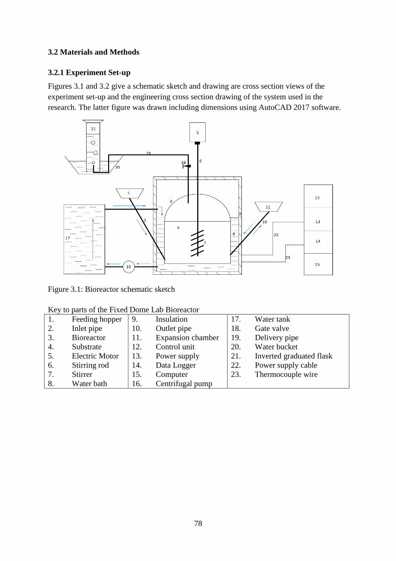
78
3.2 Materials and Methods
3.2.1 Experiment Set-up
Figures 3.1 and 3.2 give a schematic sketch and drawing are cross section views of the
experiment set-up and the engineering cross section drawing of the system used in the
research. The latter figure was drawn including dimensions using AutoCAD 2017 software.
Figure 3.1: Bioreactor schematic sketch
Key to parts of the Fixed Dome Lab Bioreactor
1. Feeding hopper
2. Inlet pipe
3. Bioreactor
4. Substrate
5. Electric Motor
6. Stirring rod
7. Stirrer
8. Water bath
9. Insulation
10. Outlet pipe
11. Expansion chamber
12. Control unit
13. Power supply
14. Data Logger
15. Computer
16. Centrifugal pump
17. Water tank
18. Gate valve
19. Delivery pipe
20. Water bucket
21. Inverted graduated flask
22. Power supply cable
23. Thermocouple wire
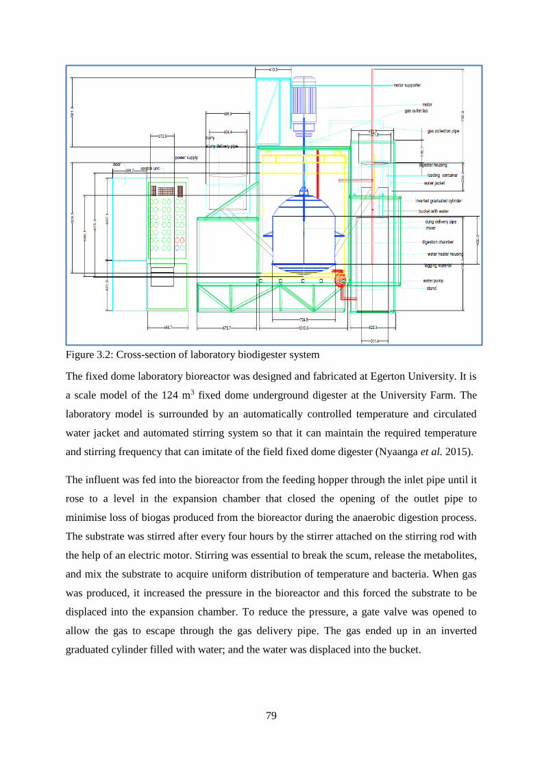
79
Figure 3.2: Cross-section of laboratory biodigester system
The fixed dome laboratory bioreactor was designed and fabricated at Egerton University. It is
a scale model of the 124 m3 fixed dome underground digester at the University Farm. The
laboratory model is surrounded by an automatically controlled temperature and circulated
water jacket and automated stirring system so that it can maintain the required temperature
and stirring frequency that can imitate of the field fixed dome digester (Nyaanga et al. 2015).
The influent was fed into the bioreactor from the feeding hopper through the inlet pipe until it
rose to a level in the expansion chamber that closed the opening of the outlet pipe to
minimise loss of biogas produced from the bioreactor during the anaerobic digestion process.
The substrate was stirred after every four hours by the stirrer attached on the stirring rod with
the help of an electric motor. Stirring was essential to break the scum, release the metabolites,
and mix the substrate to acquire uniform distribution of temperature and bacteria. When gas
was produced, it increased the pressure in the bioreactor and this forced the substrate to be
displaced into the expansion chamber. To reduce the pressure, a gate valve was opened to
allow the gas to escape through the gas delivery pipe. The gas ended up in an inverted
graduated cylinder filled with water; and the water was displaced into the bucket.
80
Temperature was regulated by a water bath that surrounded the bioreactor. Water was heated
by the electric immersion heaters in the hot water tank. Circulation of water was enabled by a
centrifugal pump. A power supply provided electricity to the system, through the power
cable, for heating the water and monitoring the temperature. A control unit had the
instrumentation that allowed water to be heated to a predetermined temperature only. A
computer was attached to the control unit via a digital data logger. Thermocouple wires from
the substrate in the bioreactor, water bath that surrounded the bioreactor, and the outside of
the experiment set-up were connected to the data logger. The data was downloaded by the
computer, and also real-time temperature was read on the screen of the computer. Foam
mattress pellets were used as an insulation material; they were placed in a casing that
surrounded the water bath to minimise heat loss.
Gas collection was by the water displacement method. A gas pipe was connected to an
inverted graduated cylinder filled with water, and placed in a bucket of water. A gate valve
was opened to allow the gas to displace water in the 500 millilitre capacity cylinder. This was
done several times until the gas was exhausted for the duration of production. The volume of
gas collected was then calculated to give biogas production rate in cubic metres per cubic
metre of digester volume per day (m3/m3d) (Mudhoo et al., 2012).
Biogas for analysis of methane content was collected in sampling bags and taken to a Gas
Chromatograph (Acer Varian 3400CX model). The model uses a flame ionisation detector
(FID). The protocol for methane content analysis was adopted from a Hewlett Packard
5890plus GC with an FID and a Supelco Carboxen1006 Plot Column that is 30 m long with
0.53 mm internal diameter (Walsh and McLaughlan, 1999). This protocol was adjusted to suit
the Acer Varian 3400CX model. The injector port was maintained at 2000C and 80kPa, while
the FID was maintained at 2000C. The oven program started with 350C for 1 minute followed
by a ramp of 200C per minute to 1800C, and the gas was held for 2 minutes. Manual gas
injection into the FID port was done using a tight 1μL syringe (Plate 3.11). The retention time
for methane was 1.5 minutes, with an analytical detection limit set at 0.1μg/L (Walsh and
McLaughlan, 1999). The carrier gas was nitrogen, and the combustion gases were hydrogen
and oxygen. The methane content was read from a print-out having a graph showing the
peaks of gas retention per minute. The results were then analysed for percentage methane
content in the sample.
81
3.2.2 Material Preparation
Total solids are defined as a measure of dry matter left after the moisture has been removed
from a moist sample. Dung from dairy cows, managed under a free-range system, was used
as a feedstock. Fresh cow dung was collected from Tatton Agricultural Park (teaching farm)
and Ngongogeri (commercial farm), all of Egerton University, and taken to the laboratory for
determining the total solids by percentage. At first, each can was cleaned and weighed while
empty by using an electronic balance. Then every can was loaded with fresh dung, weighed,
and then put in an air oven that was set at 1050C to heat the contents for 12 hours to attain a
constant weight. Thereafter, each can and its content was removed and taken to a desiccator
to cool down to room temperature. The desiccator had silica gel to ensure the hot dried dung
did not re-absorb moisture from the atmosphere during the cooling process. After the dry
samples attained room temperature, they were weighed again to determine their masses.
Three sets of experiments were done to take care of the variation in total solids content
because of the change from the dry season to the wet season. Each set had 11 samples. The
first two sets were done at the end of the dry season in the month of March, and the last set
was done during the wet season in month of May 2018. Then an average value of total solids
was used in subsequent calculations to prepare the influents.
Table 3.1 shows the data that was obtained and the associated calculations.
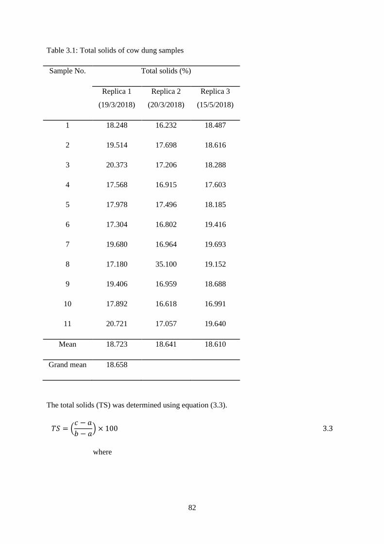
82
Table 3.1: Total solids of cow dung samples
Sample No. Total solids (%)
Replica 1
(19/3/2018)
Replica 2
(20/3/2018)
Replica 3
(15/5/2018)
1 18.248 16.232 18.487
2 19.514 17.698 18.616
3 20.373 17.206 18.288
4 17.568 16.915 17.603
5 17.978 17.496 18.185
6 17.304 16.802 19.416
7 19.680 16.964 19.693
8 17.180 35.100 19.152
9 19.406 16.959 18.688
10 17.892 16.618 16.991
11 20.721 17.057 19.640
Mean 18.723 18.641 18.610
Grand mean 18.658
The total solids (TS) was determined using equation (3.3).
𝑇𝑆 = (𝑐 − 𝑎
𝑏 − 𝑎) × 100 3.3
where
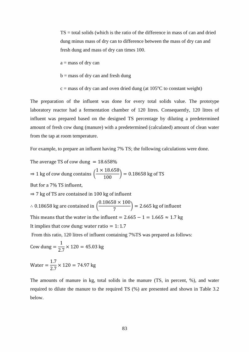
83
TS = total solids (which is the ratio of the difference in mass of can and dried
dung minus mass of dry can to difference between the mass of dry can and
fresh dung and mass of dry can times 100.
a = mass of dry can
b = mass of dry can and fresh dung
c = mass of dry can and oven dried dung (at 105oC to constant weight)
The preparation of the influent was done for every total solids value. The prototype
laboratory reactor had a fermentation chamber of 120 litres. Consequently, 120 litres of
influent was prepared based on the designed TS percentage by diluting a predetermined
amount of fresh cow dung (manure) with a predetermined (calculated) amount of clean water
from the tap at room temperature.
For example, to prepare an influent having 7% TS; the following calculations were done.
The average TS of cow dung = 18.658%
⇒ 1 kg of cow dung contains (1 × 18.658
100) = 0.18658 kg of TS
But for a 7% TS influent,
⇒ 7 kg of TS are contained in 100 kg of influent
∴ 0.18658 kg are contained in (0.18658 × 100
7) = 2.665 kg of influent
This means that the water in the influent = 2.665 − 1 = 1.665 ≈ 1.7 kg
It implies that cow dung: water ratio = 1: 1.7
From this ratio, 120 litres of influent containing 7%TS was prepared as follows:
Cow dung =1
2.7× 120 = 45.03 kg
Water =1.7
2.7× 120 = 74.97 kg
The amounts of manure in kg, total solids in the manure (TS, in percent, %), and water
required to dilute the manure to the required TS (%) are presented and shown in Table 3.2
below.
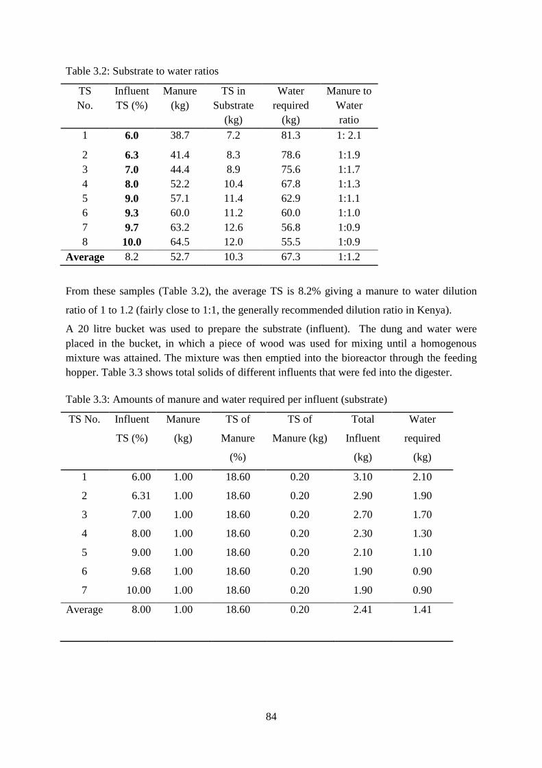
84
Table 3.2: Substrate to water ratios
TS
No.
Influent
TS (%)
Manure
(kg)
TS in
Substrate
(kg)
Water
required
(kg)
Manure to
Water
ratio
1 6.0 38.7 7.2 81.3 1: 2.1
2 6.3 41.4 8.3 78.6 1:1.9
3 7.0 44.4 8.9 75.6 1:1.7
4 8.0 52.2 10.4 67.8 1:1.3
5 9.0 57.1 11.4 62.9 1:1.1
6 9.3 60.0 11.2 60.0 1:1.0
7 9.7 63.2 12.6 56.8 1:0.9
8 10.0 64.5 12.0 55.5 1:0.9
Average 8.2 52.7 10.3 67.3 1:1.2
From these samples (Table 3.2), the average TS is 8.2% giving a manure to water dilution
ratio of 1 to 1.2 (fairly close to 1:1, the generally recommended dilution ratio in Kenya).
A 20 litre bucket was used to prepare the substrate (influent). The dung and water were
placed in the bucket, in which a piece of wood was used for mixing until a homogenous
mixture was attained. The mixture was then emptied into the bioreactor through the feeding
hopper. Table 3.3 shows total solids of different influents that were fed into the digester.
Table 3.3: Amounts of manure and water required per influent (substrate)
TS No. Influent
TS (%)
Manure
(kg)
TS of
Manure
(%)
TS of
Manure (kg)
Total
Influent
(kg)
Water
required
(kg)
1 6.00 1.00 18.60 0.20 3.10 2.10
2 6.31 1.00 18.60 0.20 2.90 1.90
3 7.00 1.00 18.60 0.20 2.70 1.70
4 8.00 1.00 18.60 0.20 2.30 1.30
5 9.00 1.00 18.60 0.20 2.10 1.10
6 9.68 1.00 18.60 0.20 1.90 0.90
7 10.00 1.00 18.60 0.20 1.90 0.90
Average 8.00 1.00 18.60 0.20 2.41 1.41
85
It can be noted that the manure samples handled had 1 kg of these Egerton cattle manure with
a TS of 18.6% ; had total solids amounting to 0.2 kg which would be digested by the bacteria
and hopefully converted to biogas in a given retention time in the batch laboratory digester.
Tchobanoglous et al. (2003) gave total solids (TS) range of 7 to 9%. Accordingly, 8% TS is
the average value. The step change is 1%. It is logical to apply the step change above and
below the range to obtain star values for investigation. Therefore, the effect of total solids on
biogas production was investigated by running the experiment at 6%, 7%, 8%, 9% and 10%
for 18 days each. All the results were recorded and analysed.
3.2.3 Temperature control
The reactor was put in a water bath of warm water. Water was heated in a water tank using
immersion heaters, and circulated by a centrifugal pump to ensure that the heated water
releases heat to the reactor until the set temperature was achieved. The immersion heaters
were regulated by a thermostat, which stopped the heating when the pre-set temperatures
were attained. The temperature control was enabled by use of the proportional differential
integrals (PIDs) and program logic controls (PLCs).
In the control experiment, the same batch system was used. The substrate to water dilution
was 1:1 as is usually done by biogas producers in Kenya (Nyaanga, 2011). The temperature
was left at room conditions. Stirring the substrate was done for two minutes after every four
hours at a speed of 15 revolutions per minute (Lemmer et al., 2013). The biogas volume
produced was recorded.
Mesophilic temperature ranges from 300C to 400C (Patharwat et al., 2016). The average
temperature of the range is 350C, and this gives a step change of 50C. A step change was
applied below and above the range to get the star values for investigation. Effect of
temperature was investigated by varying the runs at 250C, 300C, 350C, 400C, and 450C for 18
days each. Total solids were kept constant at 8% for all runs. The data was analysed and
results discussed in the relevant section below.
3.2.4 Substrate retention time
The effect of substrate retention time was investigated by making three runs while keeping
the concentration of the substrate at total solids of 8%, while the temperature was maintained
at 350C. The 8%TS and 350C were chosen because they were at the centre of the design space
in their respective ranges. An average value of biogas production was used for analysis.
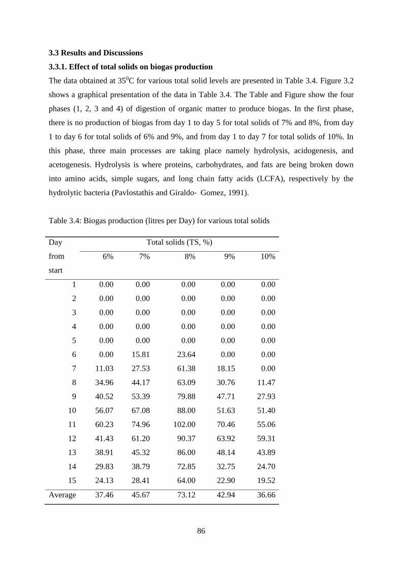
86
3.3 Results and Discussions
3.3.1. Effect of total solids on biogas production
The data obtained at 350C for various total solid levels are presented in Table 3.4. Figure 3.2
shows a graphical presentation of the data in Table 3.4. The Table and Figure show the four
phases (1, 2, 3 and 4) of digestion of organic matter to produce biogas. In the first phase,
there is no production of biogas from day 1 to day 5 for total solids of 7% and 8%, from day
1 to day 6 for total solids of 6% and 9%, and from day 1 to day 7 for total solids of 10%. In
this phase, three main processes are taking place namely hydrolysis, acidogenesis, and
acetogenesis. Hydrolysis is where proteins, carbohydrates, and fats are being broken down
into amino acids, simple sugars, and long chain fatty acids (LCFA), respectively by the
hydrolytic bacteria (Pavlostathis and Giraldo‐ Gomez, 1991).
Table 3.4: Biogas production (litres per Day) for various total solids
Day
from
start
Total solids (TS, %)
6% 7% 8% 9% 10%
1 0.00 0.00 0.00 0.00 0.00
2 0.00 0.00 0.00 0.00 0.00
3 0.00 0.00 0.00 0.00 0.00
4 0.00 0.00 0.00 0.00 0.00
5 0.00 0.00 0.00 0.00 0.00
6 0.00 15.81 23.64 0.00 0.00
7 11.03 27.53 61.38 18.15 0.00
8 34.96 44.17 63.09 30.76 11.47
9 40.52 53.39 79.88 47.71 27.93
10 56.07 67.08 88.00 51.63 51.40
11 60.23 74.96 102.00 70.46 55.06
12 41.43 61.20 90.37 63.92 59.31
13 38.91 45.32 86.00 48.14 43.89
14 29.83 38.79 72.85 32.75 24.70
15 24.13 28.41 64.00 22.90 19.52
Average 37.46 45.67 73.12 42.94 36.66
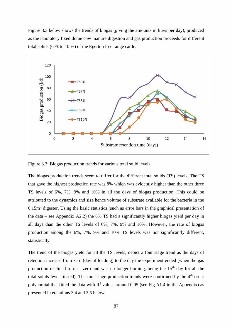
87
Figure 3.3 below shows the trends of biogas (giving the amounts in litres per day), produced
as the laboratory fixed dome cow manure digestion and gas production proceeds for different
total solids (6 % to 10 %) of the Egerton free range cattle.
Figure 3.3: Biogas production trends for various total solid levels
The biogas production trends seem to differ for the different total solids (TS) levels. The TS
that gave the highest production rate was 8% which was evidently higher than the other three
TS levels of 6%, 7%, 9% and 10% in all the days of biogas production. This could be
attributed to the dynamics and size hence volume of substrate available for the bacteria in the
0.15m3 digester. Using the basic statistics (such as error bars in the graphical presentation of
the data – see Appendix A2.2) the 8% TS had a significantly higher biogas yield per day in
all days than the other TS levels of 6%, 7%, 9% and 10%. However, the rate of biogas
production among the 6%, 7%, 9% and 10% TS levels was not significantly different,
statistically.
The trend of the biogas yield for all the TS levels, depict a four stage trend as the days of
retention increase from zero (day of loading) to the day the experiment ended (when the gas
production declined to near zero and was no longer burning, being the 15th day for all the
total solids levels tested). The four stage production trends were confirmed by the 4th order
polynomial that fitted the data with R2 values around 0.95 (see Fig A1.4 in the Appendix) as
presented in equations 3.4 and 3.5 below,
0
20
40
60
80
100
120
0 2 4 6 8 10 12 14 16
Bio
gas
pro
duct
ion (
l/d)
Substrate retention time (days)
TS6%
TS7%
TS8%
TS9%
TS10%
88
Y8% = 0.015x4 - 0.71x3 + 9.97x2 - 38.24x + 34.96; R2 = 0.96 3.4
Y6,7,9,10% = 0.0219x4 - 0.856x3 + 10.413x2 - 38.621x + 35.616, R² = 0.93 3.5
where
Y= biogas yield or production rate (litres per day) for given TS % and
x = day from start of the digestion process (days).
Using equations 3.4 and 3.5, the gas production beyond the 15th day (the day when the
experiment was stopped due low production and poor quality biogas which could not burn),
the gas production rate from the system was as presented in Table 3.5 below and Figure A2.5
in the Appendix.
Table 3.5: Empirically predicted average biogas production with retention time
*Avg YieldObs/Pred = average biogas production Observed or measured Data and Predicted or
simulated values using the empirical polynomial models.
The four stages in the digestion and gas production with time were evident in all levels of
total solids tested. Stage 1 had no gas produced for all levels of total solids being 5 to 7 days
depending on the TS used. The substrate of 8% and 7% total solids (TS) started producing
Retention
Time (Days)
Biogas Produced in litres per day
Avg YieldObs* for 6 -
10%TS
Avg YieldPred for 6
- 10%TS
YieldPred for 8%
TS
1 0 6.6 6.0
2 0 -6.5 -7.1
3 0 -7.9 -7.9
4 0 -1.4 0.0
5 4 9.5 13.8
6 14 22.2 30.8
7 30 34.5 48.6
8 42 44.5 65.3
9 57 51.1 79.4
10 65 53.7 89.5
11 56 52.1 94.8
12 44 46.6 94.8
13 32 38.2 89.2
14 24 28.3 78.3
15 26 18.9 62.5
16
12.5 42.7
17
12.0 20.2
18
21.0 -3.4
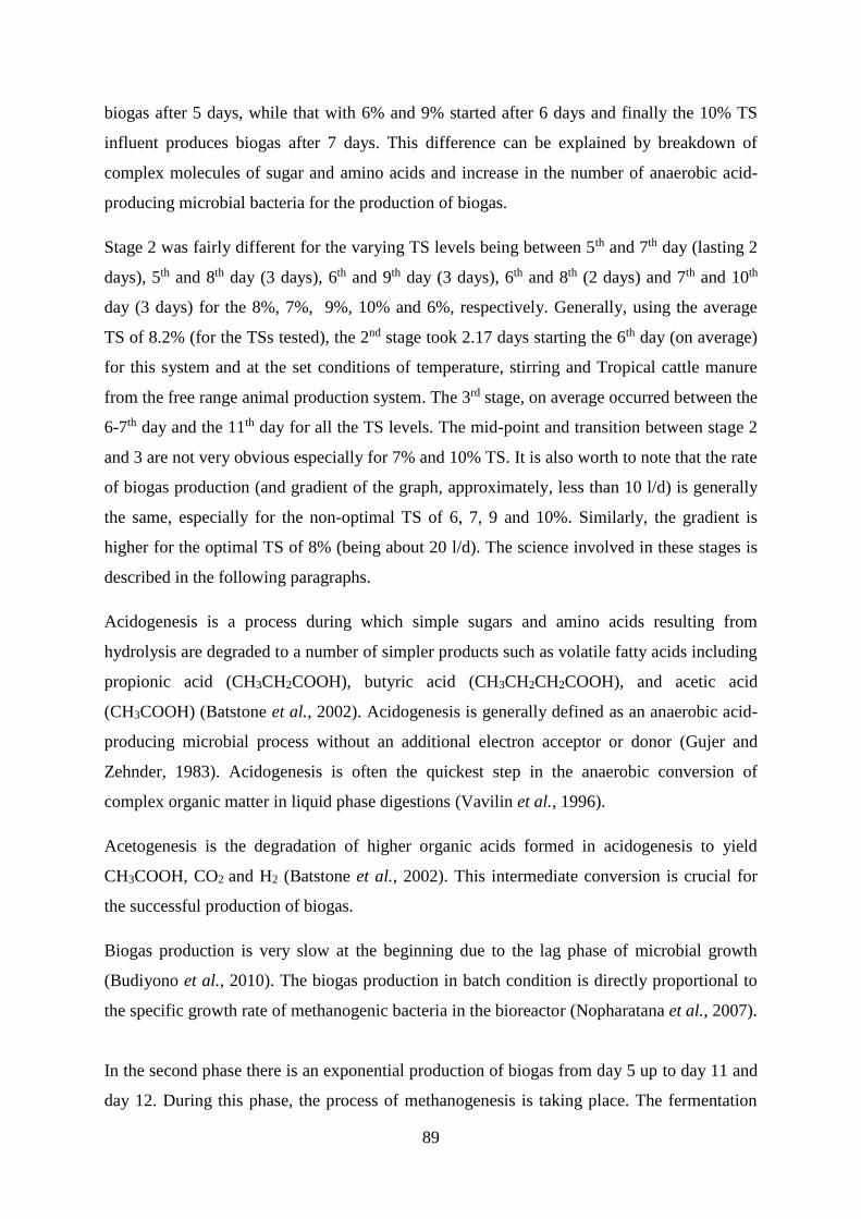
89
biogas after 5 days, while that with 6% and 9% started after 6 days and finally the 10% TS
influent produces biogas after 7 days. This difference can be explained by breakdown of
complex molecules of sugar and amino acids and increase in the number of anaerobic acid-
producing microbial bacteria for the production of biogas.
Stage 2 was fairly different for the varying TS levels being between 5th and 7th day (lasting 2
days), 5th and 8th day (3 days), 6th and 9th day (3 days), 6th and 8th (2 days) and 7th and 10th
day (3 days) for the 8%, 7%, 9%, 10% and 6%, respectively. Generally, using the average
TS of 8.2% (for the TSs tested), the 2nd stage took 2.17 days starting the 6th day (on average)
for this system and at the set conditions of temperature, stirring and Tropical cattle manure
from the free range animal production system. The 3rd stage, on average occurred between the
6-7th day and the 11th day for all the TS levels. The mid-point and transition between stage 2
and 3 are not very obvious especially for 7% and 10% TS. It is also worth to note that the rate
of biogas production (and gradient of the graph, approximately, less than 10 l/d) is generally
the same, especially for the non-optimal TS of 6, 7, 9 and 10%. Similarly, the gradient is
higher for the optimal TS of 8% (being about 20 l/d). The science involved in these stages is
described in the following paragraphs.
Acidogenesis is a process during which simple sugars and amino acids resulting from
hydrolysis are degraded to a number of simpler products such as volatile fatty acids including
propionic acid (CH3CH2COOH), butyric acid (CH3CH2CH2COOH), and acetic acid
(CH3COOH) (Batstone et al., 2002). Acidogenesis is generally defined as an anaerobic acid-
producing microbial process without an additional electron acceptor or donor (Gujer and
Zehnder, 1983). Acidogenesis is often the quickest step in the anaerobic conversion of
complex organic matter in liquid phase digestions (Vavilin et al., 1996).
Acetogenesis is the degradation of higher organic acids formed in acidogenesis to yield
CH3COOH, CO2 and H2 (Batstone et al., 2002). This intermediate conversion is crucial for
the successful production of biogas.
Biogas production is very slow at the beginning due to the lag phase of microbial growth
(Budiyono et al., 2010). The biogas production in batch condition is directly proportional to
the specific growth rate of methanogenic bacteria in the bioreactor (Nopharatana et al., 2007).
In the second phase there is an exponential production of biogas from day 5 up to day 11 and
day 12. During this phase, the process of methanogenesis is taking place. The fermentation
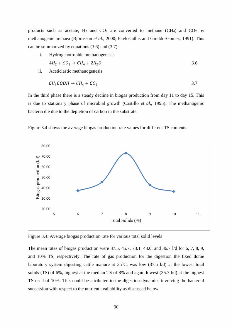
90
products such as acetate, H2 and CO2 are converted to methane (CH4) and CO2 by
methanogenic archaea (Björnsson et al., 2000; Pavlostathis and Giraldo-Gomez, 1991). This
can be summarized by equations (3.6) and (3.7):
i. Hydrogenotrophic methanogenesis
4𝐻2 + 𝐶𝑂2 → 𝐶𝐻4 + 2𝐻2𝑂 3.6
ii. Aceticlastic methanogenesis
𝐶𝐻3𝐶𝑂𝑂𝐻 → 𝐶𝐻4 + 𝐶𝑂2 3.7
In the third phase there is a steady decline in biogas production from day 11 to day 15. This
is due to stationary phase of microbial growth (Castillo et al., 1995). The methanogenic
bacteria die due to the depletion of carbon in the substrate.
Figure 3.4 shows the average biogas production rate values for different TS contents.
Figure 3.4: Average biogas production rate for various total solid levels
The mean rates of biogas production were 37.5, 45.7, 73.1, 43.0, and 36.7 l/d for 6, 7, 8, 9,
and 10% TS, respectively. The rate of gas production for the digestion the fixed dome
laboratory system digesting cattle manure at 35oC, was low (37.5 l/d) at the lowest total
solids (TS) of 6%, highest at the median TS of 8% and again lowest (36.7 l/d) at the highest
TS used of 10%. This could be attributed to the digestion dynamics involving the bacterial
succession with respect to the nutrient availability as discussed below.
20.00
30.00
40.00
50.00
60.00
70.00
80.00
5 6 7 8 9 10 11
Bio
gas
pro
duct
ion (
l/d)
Total Solids (%)
91
Anaerobic digestion process increased steadily from total solids of 6% to 8%. At low solids,
aceticlastic methanogens called methanosarcina play an important role, followed by
hydrogenotrophic methanoculleus and methanomicrobiales species (Yi et al., 2014).
Methanosarcina, a typical aceticlastic methanogen, has often been reported to be the
dorminant methanogen in anaerobic digestion (Demirel and Scherer, 2008). The ability of
genus methanosarcina having high growth rates and forming irregular cell clumps makes
them more tolerant to changing pH and high concentrations of toxic ionic agents (Conklin et
al., 2006). Methanosarcina produce methane from acetate (although some species are more
versatile and can also utilize hydrogen and carbon dioxide), methylated amines and methanol,
and also use both the aceticlastic and hydrogenotrophic methanogenesis pathways compared
to methanosaeta species (de Vrieze et al., 2012).
As the total solids increase from 8% to 10%, the biogas production rate declines steadily.
Increasing the total solids means a higher applied organic loading rate and more volatile
solids for microorganisms which results in higher volatile fatty acid concentrations (Yi et al.,
2014), and this favours the growth of methanosarcina species (de Vrieze et al., 2012). On the
other hand, methanoculleus species population decline in mesophilic anaerobic digesters with
an increase in total solids content (Bourque et al., 2008). The changing of microbial
communities in mesophilic anaerobic digestion of cow dung was responsible for the
performance exhibited in Figure 3.4.
This observation is similar to the work reported by Igoni et al. (2008) on a batch reactor. A
marginal increase in the percentage of total solids results in a geometric increase in the
volume of biogas produced, suggesting therefore (as seen in Figure 3.4) that a continual
increase in the percentage of total solids at some point becomes immaterial to the increasing
volume of biogas produced. This is possible because when percentage of total solids
increases, the amount of water decreases, thus reducing the level of microbial activity, which
then affects the amount of biogas, particularly at higher values of the TS% (Igoni et al.,
2008).
Itodo and Awulu (1999) showed that slurries of higher total solids concentrations were more
acidic than that of lower total solids concentrations, which is an additional reason why higher
total solids values would not significantly affect the increasing volume of biogas produced.
Abbassi-Guendouz et al. (2012) showed that the total methane production decreased with
total solids contents increasing from 10% to 25% in batch anaerobic digestion of cardboard
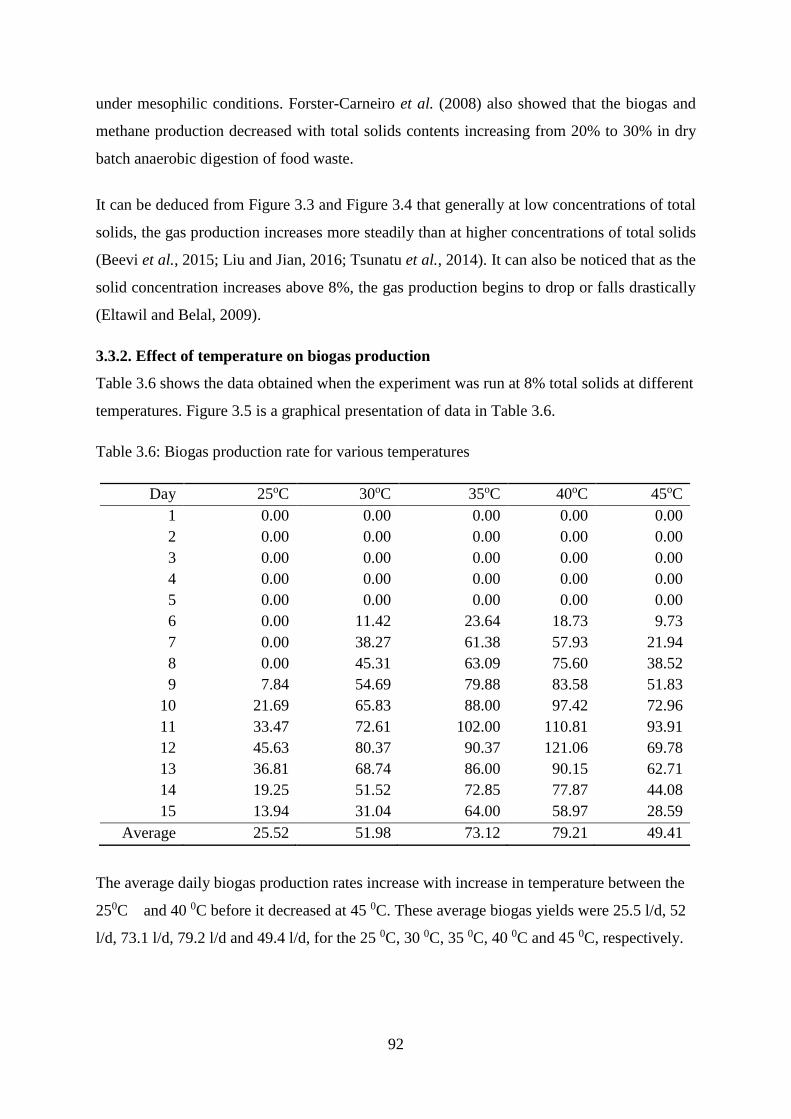
92
under mesophilic conditions. Forster-Carneiro et al. (2008) also showed that the biogas and
methane production decreased with total solids contents increasing from 20% to 30% in dry
batch anaerobic digestion of food waste.
It can be deduced from Figure 3.3 and Figure 3.4 that generally at low concentrations of total
solids, the gas production increases more steadily than at higher concentrations of total solids
(Beevi et al., 2015; Liu and Jian, 2016; Tsunatu et al., 2014). It can also be noticed that as the
solid concentration increases above 8%, the gas production begins to drop or falls drastically
(Eltawil and Belal, 2009).
3.3.2. Effect of temperature on biogas production
Table 3.6 shows the data obtained when the experiment was run at 8% total solids at different
temperatures. Figure 3.5 is a graphical presentation of data in Table 3.6.
Table 3.6: Biogas production rate for various temperatures
Day 25oC 30oC 35oC 40oC 45oC
1 0.00 0.00 0.00 0.00 0.00
2 0.00 0.00 0.00 0.00 0.00
3 0.00 0.00 0.00 0.00 0.00
4 0.00 0.00 0.00 0.00 0.00
5 0.00 0.00 0.00 0.00 0.00
6 0.00 11.42 23.64 18.73 9.73
7 0.00 38.27 61.38 57.93 21.94
8 0.00 45.31 63.09 75.60 38.52
9 7.84 54.69 79.88 83.58 51.83
10 21.69 65.83 88.00 97.42 72.96
11 33.47 72.61 102.00 110.81 93.91
12 45.63 80.37 90.37 121.06 69.78
13 36.81 68.74 86.00 90.15 62.71
14 19.25 51.52 72.85 77.87 44.08
15 13.94 31.04 64.00 58.97 28.59
Average 25.52 51.98 73.12 79.21 49.41
The average daily biogas production rates increase with increase in temperature between the
250C and 40 0C before it decreased at 45 0C. These average biogas yields were 25.5 l/d, 52
l/d, 73.1 l/d, 79.2 l/d and 49.4 l/d, for the 25 0C, 30 0C, 35 0C, 40 0C and 45 0C, respectively.
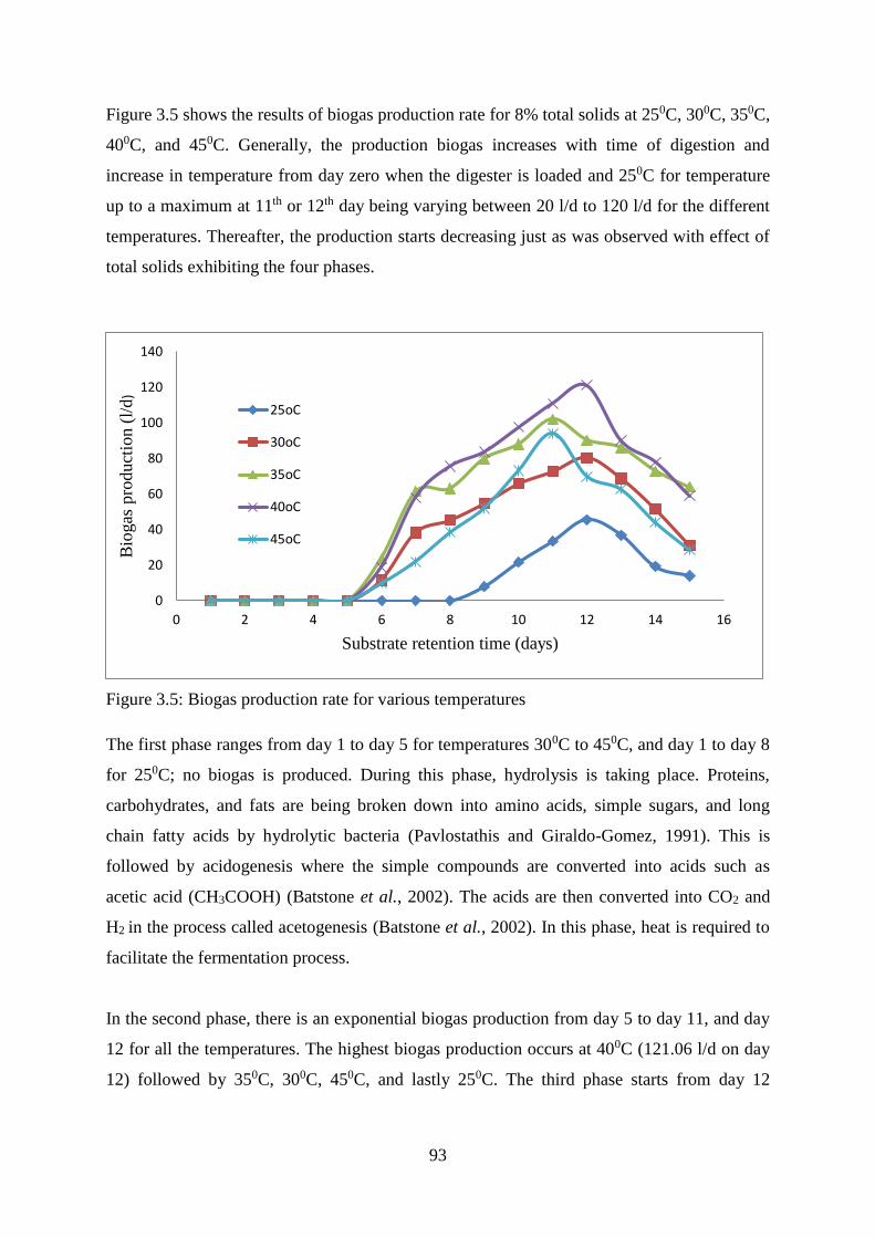
93
Figure 3.5 shows the results of biogas production rate for 8% total solids at 250C, 300C, 350C,
400C, and 450C. Generally, the production biogas increases with time of digestion and
increase in temperature from day zero when the digester is loaded and 250C for temperature
up to a maximum at 11th or 12th day being varying between 20 l/d to 120 l/d for the different
temperatures. Thereafter, the production starts decreasing just as was observed with effect of
total solids exhibiting the four phases.
Figure 3.5: Biogas production rate for various temperatures
The first phase ranges from day 1 to day 5 for temperatures 300C to 450C, and day 1 to day 8
for 250C; no biogas is produced. During this phase, hydrolysis is taking place. Proteins,
carbohydrates, and fats are being broken down into amino acids, simple sugars, and long
chain fatty acids by hydrolytic bacteria (Pavlostathis and Giraldo-Gomez, 1991). This is
followed by acidogenesis where the simple compounds are converted into acids such as
acetic acid (CH3COOH) (Batstone et al., 2002). The acids are then converted into CO2 and
H2 in the process called acetogenesis (Batstone et al., 2002). In this phase, heat is required to
facilitate the fermentation process.
In the second phase, there is an exponential biogas production from day 5 to day 11, and day
12 for all the temperatures. The highest biogas production occurs at 400C (121.06 l/d on day
12) followed by 350C, 300C, 450C, and lastly 250C. The third phase starts from day 12
0
20
40
60
80
100
120
140
0 2 4 6 8 10 12 14 16
Bio
gas
pro
duct
ion (
l/d
)
Substrate retention time (days)
25oC
30oC
35oC
40oC
45oC
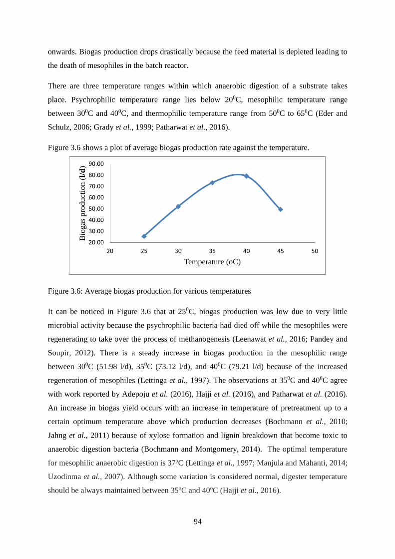
94
onwards. Biogas production drops drastically because the feed material is depleted leading to
the death of mesophiles in the batch reactor.
There are three temperature ranges within which anaerobic digestion of a substrate takes
place. Psychrophilic temperature range lies below 200C, mesophilic temperature range
between 300C and 400C, and thermophilic temperature range from 500C to 650C (Eder and
Schulz, 2006; Grady et al., 1999; Patharwat et al., 2016).
Figure 3.6 shows a plot of average biogas production rate against the temperature.
Figure 3.6: Average biogas production for various temperatures
It can be noticed in Figure 3.6 that at 250C, biogas production was low due to very little
microbial activity because the psychrophilic bacteria had died off while the mesophiles were
regenerating to take over the process of methanogenesis (Leenawat et al., 2016; Pandey and
Soupir, 2012). There is a steady increase in biogas production in the mesophilic range
between 300C (51.98 l/d), 350C (73.12 l/d), and 400C (79.21 l/d) because of the increased
regeneration of mesophiles (Lettinga et al., 1997). The observations at 350C and 400C agree
with work reported by Adepoju et al. (2016), Hajji et al. (2016), and Patharwat et al. (2016).
An increase in biogas yield occurs with an increase in temperature of pretreatment up to a
certain optimum temperature above which production decreases (Bochmann et al., 2010;
Jahng et al., 2011) because of xylose formation and lignin breakdown that become toxic to
anaerobic digestion bacteria (Bochmann and Montgomery, 2014). The optimal temperature
for mesophilic anaerobic digestion is 37oC (Lettinga et al., 1997; Manjula and Mahanti, 2014;
Uzodinma et al., 2007). Although some variation is considered normal, digester temperature
should be always maintained between 35oC and 40oC (Hajji et al., 2016).
20.00
30.00
40.00
50.00
60.00
70.00
80.00
90.00
20 25 30 35 40 45 50
Bio
gas
pro
du
ctio
n (
l/d
)
Temperature (oC)
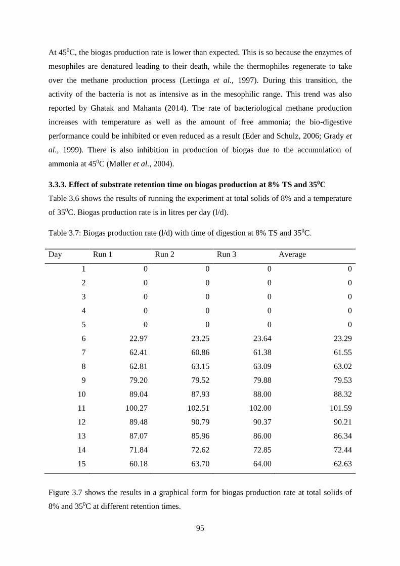
95
At 450C, the biogas production rate is lower than expected. This is so because the enzymes of
mesophiles are denatured leading to their death, while the thermophiles regenerate to take
over the methane production process (Lettinga et al., 1997). During this transition, the
activity of the bacteria is not as intensive as in the mesophilic range. This trend was also
reported by Ghatak and Mahanta (2014). The rate of bacteriological methane production
increases with temperature as well as the amount of free ammonia; the bio-digestive
performance could be inhibited or even reduced as a result (Eder and Schulz, 2006; Grady et
al., 1999). There is also inhibition in production of biogas due to the accumulation of
ammonia at 450C (Møller et al., 2004).
3.3.3. Effect of substrate retention time on biogas production at 8% TS and 350C
Table 3.6 shows the results of running the experiment at total solids of 8% and a temperature
of 350C. Biogas production rate is in litres per day (l/d).
Table 3.7: Biogas production rate (l/d) with time of digestion at 8% TS and 350C.
Day Run 1 Run 2 Run 3 Average
1 0 0 0 0
2 0 0 0 0
3 0 0 0 0
4 0 0 0 0
5 0 0 0 0
6 22.97 23.25 23.64 23.29
7 62.41 60.86 61.38 61.55
8 62.81 63.15 63.09 63.02
9 79.20 79.52 79.88 79.53
10 89.04 87.93 88.00 88.32
11 100.27 102.51 102.00 101.59
12 89.48 90.79 90.37 90.21
13 87.07 85.96 86.00 86.34
14 71.84 72.62 72.85 72.44
15 60.18 63.70 64.00 62.63
Figure 3.7 shows the results in a graphical form for biogas production rate at total solids of
8% and 350C at different retention times.
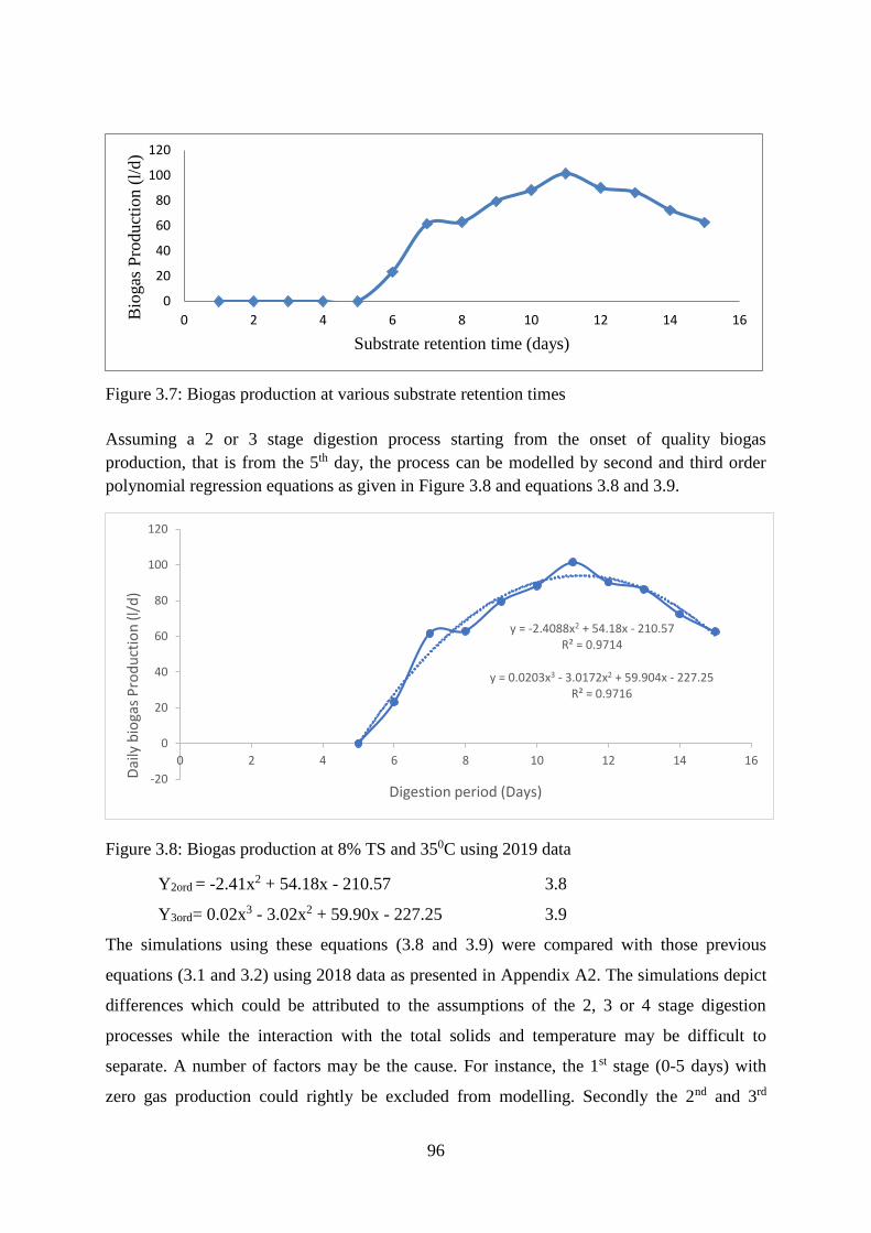
96
Figure 3.7: Biogas production at various substrate retention times
Assuming a 2 or 3 stage digestion process starting from the onset of quality biogas
production, that is from the 5th day, the process can be modelled by second and third order
polynomial regression equations as given in Figure 3.8 and equations 3.8 and 3.9.
Figure 3.8: Biogas production at 8% TS and 350C using 2019 data
Y2ord = -2.41x2 + 54.18x - 210.57 3.8
Y3ord= 0.02x3 - 3.02x2 + 59.90x - 227.25 3.9
The simulations using these equations (3.8 and 3.9) were compared with those previous
equations (3.1 and 3.2) using 2018 data as presented in Appendix A2. The simulations depict
differences which could be attributed to the assumptions of the 2, 3 or 4 stage digestion
processes while the interaction with the total solids and temperature may be difficult to
separate. A number of factors may be the cause. For instance, the 1st stage (0-5 days) with
zero gas production could rightly be excluded from modelling. Secondly the 2nd and 3rd
0
20
40
60
80
100
120
0 2 4 6 8 10 12 14 16Bio
gas
Pro
duct
ion (
l/d)
Substrate retention time (days)
y = 0.0203x3 - 3.0172x2 + 59.904x - 227.25R² = 0.9716
y = -2.4088x2 + 54.18x - 210.57R² = 0.9714
-20
0
20
40
60
80
100
120
0 2 4 6 8 10 12 14 16
Dai
ly b
ioga
s P
rod
uct
ion
(l/d
)
Digestion period (Days)
97
stages are difficult to separate since there is only half day difference between the 2. The only
model, therefore, suggested for the biogas prediction for the system between day 5 and about
day 17 when burnable gas (biogas) ceased, could be a 2nd order polynomial model though its
precision and statistical accuracy will require more data to enhance and generalize.
There was no biogas production from day 1 to day 5. This was attributed to three processes of
anaerobic digestion taking place: hydrolysis, acidogenesis and acetogensis respectively. The
first one was hydrolysis. Organic biomass contains complex polymers which are inaccessible
to microorganisms without being further broken down through hydrolysis (Gujer and
Zehnder, 1983). As a result, hydrolysis serves the purpose of rendering macromolecules into
its smaller components which in turn can be utlised by acidogenic bacteria (Meegoda et al.,
2018). During hydrolysis, hydrolytic bacteria are able to secrete extracellular enzymes that
can convert carbohydrates, lipids and proteins into simple sugars, long chain fatty acids and
amino acids respectively (Park et al., 2011). After enzymatic cleavage, the products of
hydrolysis are able to diffuse through the cell membranes of acidogenic microorganisms (van
Lier et al., 2008).
The second process was acidogenesis. Acidogenic bacteria are able to produce intermediate
volatile fatty acids (VFAs) and other products (Meegoda et al., 2018). Volatile fatty acids
constitute a class of organic acids such as acetates, and larger organic acids such as
propionate and butyrate (Bergman et al., 1990). As opposed to other stages, acidogenesis is
generally believed to proceed at a faster rate than all other processes of anaerobic digestion,
with acidogenic bacteria having a regeneration time fewer than 36 hours (Deublein and
Steinhauser, 2008). With the rapidity of this stage, the production of volatile fatty acids
creates direct precursors for the final stage of methanogenesis; Volatile fatty acid
acidification is widely reported to be a cause of digester failure (Akuzawa et al., 2011).
Acetogenesis is the third process during which higher volatile fatty acids (e.g. propionate and
butyrate) are converted into acetate and hydrogen (Hansen and Cheong, 2013). At the same
time, lipids undergo a separate pathway of acetogenesis through acidogenesis and β-
oxidation, where acidogenesis produces acetate from glycerol, while β-oxidation produces
acetate from LCFAs (Cirne et al., 2007).
98
The results and the observation of retention time made in this study may not be in total
agreement with (Varma et al., 2009) who reported that hydrolysis takes 2 days while
acidogenesis and acetogenesis take 3.6 days. This may be due to a different system (digester)
design and management (operational factors such as temperature, feeding and stirring
regimes) and substrate characteristics including type of feedstock, total solids among other
variables, apart from the data collection precision.
Methanogenesis marks the final stage of anaerobic digestion, where accessible intermediates
are consumed by methanogenic bacteria to produce methane (Ferry, 2010). Production of
biogas starts from day 5 and increases steadily to day 11 (102.00 l/d). Methanogenic bacteria
are confined to a small selection of substrates (Meegoda et al., 2018). Aceticlastic
methanogenesis from acetate accounts for nearly two thirds of the methane production while
the remaining one third comes from hydrogenotrophic methanogenesis (Belay et al., 1986;
Lovley and Klug, 1983).
However, it was noticed that biogas production stagnated from day 7 to day 8. This can be
attributed to excessive partial pressure of hydrogen produced by acetogenesis that deleted
acetogenic microorganisms (Dinopoulou et al., 1988). But due to the presence of
hydrogenotrophic methanogens, especially the methanosarcina species, hydrogen was able to
be rapidly consumed while maintaining partial pressure at a level favourable to acetogenesis
by creating an exergonic reaction (Stams and Plugge, 2009). During the stagnation period,
methanosarcina species, which tend to be robust and are capable of withstanding ammonia,
sodium, and acetate concentrations in addition to pH shocks at levels that would otherwise be
detrimental to other methanogenic bacteria, kept on producing biogas (de Vrieze et al., 2012).
Consequently, the steady production came on course from day 8 to day 11.
Methanogenic bacteria represent a group of obligate anaerobic archaea; as an acute
sensitivity, it was found that 99% of methanococcus voltae and methanococcus vannielli cells
had been killed within ten hours upon exposure to oxygen (Kiener and Leisinger, 1983).
Methanogens have a slower regeneration time than other bacteria in an anaerobic digestion;
at least 5 to 16 days (Deublein and Steinhauser, 2008). However, some hydrogenotrophic
species, such as methanococcus maripaludis, have a doubling time of only two hours
(Richards et al., 2016).
99
From day 11 onwards, biogas production started declining from 102 l/d to 62.63 l/d on day
15. This was caused by the depletion of nutrients in the substrate and the gradual death of the
methanogens. In batch reactors, the end of methanogenesis is determined when biogas
production stops, which can take about 40 days (Verma, 2002).
3.4 Conclusions and Recommendation
3.4.1 Conclusions
Biogas production rate varied with different total solid levels increasing from an average of
0.25 m3/m3d at 6% total solids (TS), through an average of 0.32 m3/m3d for 7% TS to reach a
maximum average of 0.48 m3/m3d at 8% TS (with a manure to water ratio of 1:1.3), and then
started decreasing steadily to 0.24 m3/m3d as the total solids increased to 10% through an
average of 0.32 m3/m3d for the other total solid levels of the cattle manure under free range
animal production system in Egerton, Kenya. The optimal TS for the laboratory fixed dome
digester is 8% when operation at a digester temperature of 25 to 45oC.
In the mesophilic range of temperature, biogas production increased with increase in
temperature, generally, moving from 0.25 m3/m3d at 25oC through 0.35 m3/m3d at 300C to
0.53 m3/m3d at 400C (optimal temperature), and then declined to 0.33 m3/m3d at 450C.
The biogas production increases with the retention time, being maximum of 0.68 m3/m3d
from the batch laboratory fixed dome digester at 11th day of digestion, having started biogas
production after 5 days for 8% TS cattle manure substrate being maintained at a temperature
of 350C.
Empirical models to simulate the biogas production with the temperature and total solid
ranges used are possible.
3.4.2 Recommendation
The above conclusions can be transferred with appropriate modifications and scale factors for
adoption for field and industrial fixed digesters for biogas production into operational
guidelines for biogas stakeholders including designers and operators.
Further research is recommended to determine:
1. Effect of feeding regimes (as batch and continuous bioreactor or digester) at varying
temperatures and stirring frequencies for different substrates

100
2. The effect of thermophilic and cryophilic (ambient and below) temperature ranges on
biogas production rate and quality for the laboratory fixed dome digester
3. Accuracy and precision of empirical models from experimental and observed data
from the biogas system.
101
References
Abbassi-Guendouz, A., Brockmann, D., Trably, E., Dumas, C. and Delgenès, J. (2012).
Total solids content drives high solid anaerobic digestion via mass transfer limitation.
Bioresource Technology, 111, 55-61.
Achinas, S. and Euverink, G. J. W. (2016). Theoretical analysis of biogas potential
prediction from agricultural waste. Resource-Efficient Technologies, 2(3), 143-147.
Adepoju, T., Olatunbosun, B. and Olawale, O. (2016). Statistical analysis of biogas
production from co-digestion of cornstalk with goat dung using a one factor design.
Chemistry Research Journal, 1(4), 1-10.
Akuzawa, M., Hori, T., Haruta, S., Ueno, Y., Ishii, M. and Igarashi, Y. (2011). Distinctive
responses of metabolically active microbiota to acidification in a thermophilic
anaerobic digester. Microbial Ecology, 61(3), 595-605.
APHA. (1999). Standard Methods for the Examination of Water and Wastewater. American
Public Health Association.
Barnes, R., Dhanoa, M. S. and Lister, S. J. (1989). Standard normal variate transformation
and de-trending of near-infrared diffuse reflectance spectra. Applied Spectroscopy,
43(5), 772-777.
Batstone, D. J., Keller, J., Angelidaki, I., Kalyuzhnyi, S., Pavlostathis, S., Rozzi, A.,
Sanders, W., Siegrist, H. and Vavilin, V. (2002). The IWA anaerobic digestion
model no 1 (ADM1). Water Science and Technology, 45(10), 65-73.
Beevi, B. S., Madhu, G. and Sahoo, D. K. (2015). Performance and kinetic study of semi-
dry thermophilic anaerobic digestion of organic fraction of municipal solid waste.
Waste Management, 36, 93-97.
Belay, N., Sparling, R. and Daniels, L. (1986). Relationship of formate to growth and
methanogenesis by Methanococcus thermolithotrophicus. Applied Environmental
Microbiology, 52(5), 1080-1085.
Bergman, H., Wichmann, T. and DeLong, M. R. (1990). Reversal of experimental
parkinsonism by lesions of the subthalamic nucleus. Science, 249(4975), 1436-1438.
Björnsson, L., Murto, M. and Mattiasson, B. (2000). Evaluation of parameters for
monitoring an anaerobic co-digestion process. Applied Microbiology and
Biotechnology, 54(6), 844-849.
Bochmann, G., Drosg, B., Ortner, M., Schonlieb, M., Andres-Lainez, S., Kirchmayr, R.
and Braun, R. (2010). Influence of thermal pre-treatment to increase digestibility of
102
brewers’ spent grains. Paper presented at the 12th World Congress on Anaerobic
Digestion, Guadalajara.
Bochmann, G. and Montgomery, L. (2014). Pretreatment of Feedstock for Enhanced Biogas
Production. Retrieved from Paris, France.
Bourque, J., Guiot, S. and Tartakovsky, B. (2008). Methane production in an UASB reactor
operated under periodic mesophilic-thermohilic conditions. Biotechnology
Bioengineering, 100, 1115-1121.
Budiyono, Widiasa, I., Johari, S. and Sunarso. (2010). The influence of total solid contents
on biogas yield from cattle manure using rumen fluid inoculum. Energy Research
Journal, 1(1), 6-11.
Buswell, A. and Mueller, H. (1952). Mechanism of methane fermentation. Industrial and
Engineering Chemistry, 44(3), 550-552.
Castillo, R.-T., Luengo, P. and Alvarez, J. M. (1995). Temperature effect on anaerobic of
bedding manure in a one phase system at different inoculums concentration.
Agriculture, Ecosystems and Environment, 54, 55-66.
Charlton, S., Dollmeyer, T. and Grana, T. (2010). Meeting the US heavy-duty EPA 2010
standards and providing increased value for the customer. SAE International Journal
of Commercial Vehicles, 3(2010-01-1934), 101-110.
Cirne, D., Paloumet, X., Björnsson, L., Alves, M. and Mattiasson, B. (2007). Anaerobic
digestion of lipid-rich waste—Effects of lipid concentration. Renewable Energy, 32,
965-975.
Conklin, A., Stensel, H. and Ferguson, J. (2006). Growth kinetics and competition between
Methanosarcina and Methanosaeta in mesophilic anaerobic digestion Water
Environment Research, 78, 486-496.
de Vrieze, J., Hennebel, T., Boon, N. and Verstraete, W. (2012). Methanosarcina: The
rediscovered methanogen for heavy duty biomethanation. Bioresource technology,
112, 1-9.
Demirel, B. and Scherer, P. (2008). The roles of acetotrophic and hydrogenotrophic
methanogens during anaerobic conversion of biomass to methane: a review. Reviews
in Environmental Science and Biotechnology, 7, 173-190.
Deublein, D. and Steinhauser, A. (2008). Biogas from Waste and Renewable Resources: An
Introduction. Weinheim, Germany.
103
Dinopoulou, G., Rudd, T. and Lester, J. (1988). Anaerobic acidogenesis of a complex
wastewater: The influence of operational parameters on reactor performance.
Biotechnology and Bioengineering, 31, 958-968.
Dolud, M., Andree, H. and Hügle, T. (2005). Rapid analysis of liquid hog manure using
near-infrared spectroscopy in flowing condition. Precision livestock farming ‘05.
Wageningen Academic Publications, Wageningen, The Netherlands, 115-122.
Eder, B. and Schulz, H. (2006). Biogas Praxis [in German] (3rd ed.).
Elaiyaraju, P. and Partha, N. (2016). Studies on biogas production by anaerobic process
using agroindustrial wastes. Research in Agricultural Engineering, 62(2), 73-82.
Eltawil, M. and Belal, E. (2009). Evaluation and scrubbing of biogas generation from
agricultural wastes and water hyacinth biological engineering. Miscillenous Journal
of Agricultural Engineering, 26(1), 534-560.
EPA. (2001). Method 1684: Total, Fixed, and Volatile Solids in Water, Solids, and Biosolids.
U.S. Environmental Protection Agency.
Ferry, J. (2010). The chemical biology of methanogenesis. Planet and Space Science, 58,
1775–1783.
Forster-Carneiro, T., Pérez, M. and Romero, L. (2008). Influence of total solid and
inoculum contents on performance of anaerobic reactors treating food waste
Bioresource Technology(99), 6994-7002.
Franke-Whittle, I. H., Walter, A., Ebner, C. and Insam, H. (2014). Investigation into the
effect of high concentrations of volatile fatty acids in anaerobic digestion on
methanogenic communities. Waste Management, 34(11), 2080-2089.
Ghatak, M. D. and Mahanta, P. (2014). Effect of temperature on anaerobic co-digestion of
cattle dung with lignocellulosic biomass. Journal of Advanced Engineering
Research, 1(1), 1-7.
Grady, C., Daigger, G. and Lim, H. (1999). Biological wastewater treatment: Principles and
practice. New York: Marcel Dekker, New York.
Gujer, W. and Zehnder, A. (1983). Conversion processes in anaerobic digestion. Water
Science and Technology, 15, 127-167.
Hajji, A., Rhachi, M., Garoum, M. and Laaroussi, N. (2016). The effects of pH, temperature
and agitation on biogas production under mesophilic regime. Paper presented at the
2016 3rd International Conference on Renewable Energies for Developing Countries
(REDEC).
104
Hansen, C. and Cheong, D. (2013). Agricultural Waste Management in Food Processing.
Cambridge, MA, USA: Academic Press.
Hwu, C.-S., Donlon, B. and Lettinga, G. (1996). Comparative toxicity of long-chain fatty
acid to anaerobic sludges from various origins. Water Science and Technology, 34(5-
6), 351-358.
Igoni, A. H., Abowei, M., Ayotamuno, M. and Eze, C. (2008). Effect of total solids
concentration of municipal solid waste on the biogas produced in an anaerobic
continuous digester. Agricultural Engineering International: CIGR Journal.
Itodo, I. and Awulu, J. (1999). Effects of total solids concentrations of poultry, cattle, and
piggery waste slurries on biogas yield. Transactions of the ASAE, 42(6), 1853-1855.
Jahng, D., Lee, Y. and Zhang, L. (2011). Anaerobic co-digestion of food waste and piggery
wastewater: focusing on the role of trace elements. Bioresource Technology, 102(8),
5048-5059.
Kiener, A. and Leisinger, T. (1983). Oxygen sensitivity of methanogenic bacteria. Systematic
and Applied Microbiology, 4, 305-312.
Kircher, M., Witten, D. M., Jain, P., O'Roak, B. J., Cooper, G. M. and Shendure, J. (2014).
A general framework for estimating the relative pathogenicity of human genetic
variants. Nature Genetics, 46(3), 310.
Leenawat, A., Pasakorn, J., Atip, L., Rodriguez, J. and Khanita, K. (2016). Effect of
temperature on increasing biogas production from sugar industrial wastewater
treatment by UASB process in pilot scale. Paper presented at the 3rd International
Conference on Power and Energy Systems Engineering, CPESE, Kitakyushu, Japan.
Lemmer, A., Naegele, H.-J. and Sondermann, J. (2013). How Efficient are Agitators in
Biogas Digesters? Determination of the Efficiency of Submersible Motor Mixers and
Incline Agitators by Measuring Nutrient Distribution in Full-Scale Agricultural
Biogas Digesters. Energies(6), 6255-6273. doi:10.3390/en6126255
Lettinga, G., Field, J., Van Lier, J., Zeeman, G. and Pol, L. H. (1997). Advanced anaerobic
wastewater treatment in the near future. Water Science and Technology, 35(10), 5-12.
Liu, Z. and Jian, L. (2016). The effect of total solids concentration and temperature on
biogas production by anaerobic digestion. Energy sources, Part A: Recovery,
utilization, and environmental effects, 38(23), 3534-3541.
doi:10.1080/15567036.2016.1183064
105
Lovley, D. and Klug, M. (1983). Methanogenesis from Methanol and Methylamines and
Acetogenesis from Hydrogen and Carbon Dioxide in the Sediments of a Eutrophic
Lake. Applied and Environmental Microbiology, 45, 1310-1315.
Manjula, D. and Mahanti, P. (2014). Effect of temperature on biogas production from
Lignocellulosic biomasses. Paper presented at the Proceedings of 1st International
Conference on non-conventional energy (ICONCE).
Mao, C., Feng, Y., Wang, X. and Ren, G. (2015). Review on research achievements of
biogas from anaerobic digestion. Renewable and Sustainable Energy Reviews, 45,
540-555.
Meegoda, J., Li, B., Patel, K. and Wang, L. (2018). A review of the processes, parameters,
and optimization of anaerobic digestion. International Journal of Environmental
Research and Public Health, 15(10), 2224.
Møller, H., Sommer, S. and Ahring, B. (2004). Methane productivity of manure, straw and
solid fractions of manure. Biomass and Bioenergy, 26, 485-495.
Moset, V., Poulsen, M., Wahid, R., Højberg, O. and Møller, H. B. (2015). Mesophilic
versus thermophilic anaerobic digestion of cattle manure: methane productivity and
microbial ecology. Microbial Biotechnology, 8(5), 787-800.
Mudhoo, A., Moorateeah, P. and Mohee, R. (2012). Effects of microwave heating on biogas
production, chemical oxygen demand, and volatile solids solubilization of food
residues. World Academy of Science, Engineering and Technology, 69.
Nopharatana, A., Pullammanappallil, P. C. and Clarke, W. P. (2007). Kinetics and dynamic
modelling of batch anaerobic digestion of municipal solid waste in a stirred reactor.
Waste Management, 27(5), 595-603.
Nyaanga, D. (2011). Performance of Tropical Biogas. Paper presented at the Egerton
University International Conference, Egerton University, Kenya.
Pandey, P. and Soupir, M. (2012). Impacts of temperatures on biogas production in dairy
manure anaerobic digestion. International Journal of Engineering and Technology, 4,
629-631.
Parawira, W., Murto, M., Read, J. and Mattiasson, B. (2005). Profile of hydrolyses and
biogas production during two stage mesophilic anaerobic digestion of solid potato
waste. Process Biochemistry, 40, 2945-2952.
Park, Y., Li, Y. and Zhu, J. (2011). Solid-state anaerobic digestion for methane production
from organic waste. Renewable and Sustainable Energy Review, 15, 821-826.
106
Patharwat, I., Kumbhar, S., Hingalaje, P., Khurpe, A., Goudgaon, J. and Dhamangaonkar,
P. (2016). Analysis of optimum temperature and validity of biogas plant.
International Journal of Industrial Electronics and Electrical Engineering, 4(4), 76.
Pavlostathis, S. and Giraldo-Gomez, E. (1991). Kinetics of anaerobic treatment. Water
Science and Technology, 24(8), 35-59.
Pavlostathis, S. and Giraldo‐ Gomez, E. (1991). Kinetics of anaerobic treatment: a critical
review. Critical Reviews in Environmental Science and Technology, 21(5-6), 411-
490.
Richards, M., Lie, T., Zhang, J., Ragsdale, S., Leigh, J. and Price, N. (2016). Exploring
hydrogenotrophic methanogenesis: A genome scale metabolic reconstruction of
methanococcus maripaludis. Journal of Bacteriology, 198, 3379-3390.
Shi, X., Dong, J., Yu, J., Yin, H., Hu, S., Huang, S. and Yuan, X. (2017). Effect of
hydraulic retention time on anaerobic digestion of wheat straw in the semi-
continuous continuous stirred-tank reactors. BioMed Research International.
Sovacool, B. K. (2012). The political economy of energy poverty: A review of key
challenges. Energy for Sustainable Development, 16(3), 272-282.
Stams, A. and Plugge, C. (2009). Electron transfer in syntrophic communities of anaerobic
bacteria and archaea. Nature Reviews Microbiology, 7, 568-577.
Taherzadeh, M. and Karimi, K. (2008). Pretreatment of lignocellulosic wastes to improve
ethanol and biogas production: a review. International Journal of Molecular
Sciences, 9(9), 1621-1651.
Tchobanoglous, G., Burton, F. and Stensel, H. (2003). Waste Water Engineering: Treatment
and Re-use (4th ed.): Tata McGraw-Hill Publishing Company Ltd.
Tricase, C. and Lombardi, M. (2009). State of the art and prospects of Italian biogas
production from animal sewage: technical-economic considerations. Renewable
Energy, 34(3), 477-485.
Tsunatu, D., Azuaga, I. and Agabison, J. (2014). Evaluation of the effect of total solids
concentration on biogas yields of agricultural wastes. International Research Journal
of Environment Sciences, 3(2).
Uzodinma, E., Ofoefule, A., Eze, J. and Onwuka, N. (2007). Biogas Production from
blends of Agro-industrial wastes. Trends in Applied Science Research, 2(6), 554-558.
van Lier, J., Mahmoud, N. and Zeeman, G. (2008). Anaerobic Wastewater Treatment. In
Biological Wastewater Treatment: Principles, Modelling and Design. International
Water Association, UK, 401-442.
107
Varma, R., Vesvikar, M., Karim, K., Hoffman, R., De Paoli, D., Klasson, K., Winterberg,
A. and Alexander, C. (2009). Bioenergy production from anaerobic digestion of
animal and farm wastes. Paper presented at the Energy Summit, Missouri University
of Science and Technology.
Vavilin, V., Lokshina, L., Rytov, S., Kotsyurbenko, O. and Nozhevnikova, A. (1996).
Modeling methanogenesis during anaerobic conversion of complex organic matter at
low temperatures. Water Science and Technology, 36(6-7), 531-538.
Verma, S. (2002). Anaerobic Digestion of Biodegradable Organics in Municipal Solid
Wastes.
Walsh, K. and McLaughlan, R. (1999). Bubble extraction of dissolved gases from ground
water samples. Water, Air, and Soil Pollution, 115, 525-534.
Yi, J., Dong, B., Jin, J. and Dai, X. (2014). Effect of Increasing Total Solids Contents on
Anaerobic Digestion of Food Waste under Mesophilic Conditions: Performance and
Microbial Characteristics Analysis. PLoS ONE, 9(7).
108
CHAPTER FOUR
EVALUATING BIOGAS PRODUCTION PREDICTION MODELS
Abstract
A number of biogas production prediction models have been proposed but they have not
been tested for the common Kenyan organic material, cow or cattle manure used to produce
biogas. They include the empirical plug flow digester model at fixed temperature, pH, and
loading rate and expressing biogas yield as a function substrate influent and effluent volatile
solids and hydraulic retention time. A modification of this model by Chen and Hashimoto
Model adds the influence of temperature and bacterial population. A simpler low
temperature lagoon model relates temperature to biogas production amount. This model has
been advanced to the Toprak model which made yield a function of the exponential of
temperature. Chen and Hashimoto Model and Scoff and Minott model are more involving
with more variables and hence more since they involve hydraulic retention time, volatile
solids concentrations, bacteria growth rate, digester temperature, and daily substrate flow
rate. These biogas production prediction models were evaluated using data observed while
producing biogas from a fixed dome digester set at selected temperatures and using cow and
liquid cattle manure from semi-free range animals of Tatton Farm, at Njoro in Kenya at 6, 8
and 10% total solids. Two (the Low Temperature Lagoon and the Toprak) out of the five
models tested, suited a fixed dome batch bioreactor data using a goodness of fit between the
predicted data by the models and that obtained from laboratory experiments. A third model
(named the Fixed dome Temperature model) relating temperature to the rate of biogas
production) was developed from experimental data, and validated using a set of observed
data from a different experiment conducted nearly a year later from the data used to develop
the model. The similarity among the Low Temperature Lagoon, modified Toprak and Fixed
dome Temperature models was observed while noting their simplicity and hence may not
fully explain the 3 or 4 stages of the biogas production fluctuations. The other models could
be applied in the digester system but with more in depth understanding and determination of
the bacterial population dynamics.
4.1 Introduction
Models are developed and used to help scientists, engineers, and decision makers to
understand and communicate about a system of interest with the ultimate aim of bringing a
positive change to how a system is built and/or managed. First, models must be a simplified
109
representation of the system and provide a cognitively-mediated environment to explain the
systemic behavior (Akbas and Ozdemir, 2018). Second, models are limited to the collective
cognitive complexity of the ‘mental models’ of those involved in model development: some
models are an inconsistent representation of a dynamic and complex system (Stockburger,
2006). These challenges are escalated on using models in deep uncertainty situations where
stakeholders do not know or cannot agree on the system structure, future scenarios, and
model parameters (Kwakkel and Pryut, 2013).
There are four types of models (Ali et al., 2016):
i. Physical models: these are smaller and simpler representations of the thing being
studied.
ii. Conceptual models: they tie together many ideas to explain a common phenomenon
or event.
iii. Mathematical models: are sets of equations that take into account many factors to
represent a phenomenon.
iv. Stochastic models: are tools for estimating probability distributions of potential
outcomes by allowing for random variation in one or more inputs over time.
In this study, mathematical models were used because integers and figures were involved in
relating the inputs (factors) to the output (biogas production rate).
Models for predicting biogas production include:
a) Plug Flow Model
The model was among the earliest suggested for predicting gas production in a plug
flow digester by Jewell et al. (1978). It is a simple empirical formula with many
parameters like temperature, pH, and organic loading rate remaining constant; and is
given as:
𝑌 = 0.5 (𝑆𝑏𝑜 − 𝑆𝑏𝑖
𝐻𝑅𝑇) 4.1
where,
Y = Biogas yield in litres/litre of digester per day
Sbo = Influent volatile solids
110
Sbi = Effluent volatile solids
HRT = Hydraulic retention time in days
If any of the fixed parameters changed, the model would not remain valid
(Jewell et al. (1978).
b) Chen and Hashimoto Model
Chen and Hashimoto (1978) improved on the Plug Flow model by incorporating
other parameters in their model to take care of digester temperature, bacterial growth
rate and volatile solid concentration of the substrate. The model is given as:
𝑌 =𝐵0𝑆0
𝐻𝑅𝑇{1 −
𝐾
𝐻𝑅𝑇(𝑢𝑚)−1+𝐾} 4.2
where,
Y = Biogas production in litres/litre of digester per day
Bo = Ultimate yield of gas in litres/gram of volatile solid (VS) added
So = Influent VS concentration in grams/litre
K = Kinetic parameter (dimensionless) = 0.6 + 0.0206e0.051So
HRT = Hydraulic Retention Time
um = 0.013T – 0.129 = Maximum bacteria growth rate in which T is
the temperature in degrees Celsius (0C)
T = Digester temperature in 0C
c) Low Temperature Lagoon Digester Model
Safley and Westerman (1992) developed a model to predict gas production from a
low temperature lagoon digester or pond digesters. It is based on the temperature of
the lagoon, and keeps all other parameters constant including substrate type, total
solids, feeding rate and hydraulic retention time among others. The linear Lagoon
model was given as
Y = 0.0093T + 0.216 4.3
where,
Y = Biogas production in m3/kg VS
111
T = Digester temperature in 0C
The temperature was measured at various points (horizontally and vertically) of the
lagoon while observing the ambient temperature.
d) Toprak model
Toprak (1995) developed a model for a pond digester as shown in equation (4.4).
𝑌 = 1.241𝑇𝑎1.127 4.4
where,
Y = Biogas production in L/m3 of digester per day
Ta = Ambient air temperature, 0C
This Pond Model, like the Lagoon model, used temperature (specifically ambient
temperature) giving the biogas production as an exponential of the temperature.
The advantages and disadvantages of these models to a laboratory reactor data are
likely to be varied and applicability may be low or high and hence the need to test
the models using the data from the fixed dome digester.
e) Scoff and Minott model
A more accurate model for plug flow digesters was developed by Minott (2002). It
considers hydraulic retention time, volatile solids concentrations, bacteria growth
rate, digester temperature, and daily substrate flow rate. It is given as:
Y =0.5
HRT{C0 − CT(x, t)v
Ta
T0} 4.5
where,
Y = Gas production in kg/day
HRT = Hydraulic Retention Time (days)
v = Daily flow rate of manure slurry into digester (m3/day)
C0 = 0.863TS (which is influent total volatile solids in kg/m3, TS = total
solids)
112
T0 = Constant temperature at which the digester is operated
Ta = 273.2 K
CT = Total substrate degradation in the digester (kg/m3. Total amount of
organic matter digested)
CT is given as:
𝐶𝑇(𝑥, 𝑡) =𝐶0𝐾𝑒(−1 𝐾⁄ )
𝑢𝑚2 𝑣𝑡
{(𝑢𝑚 − 2𝐾)[1 − 𝑒(−𝑢𝑚𝑡 𝐾⁄ )] + 𝑡𝑢𝑚[1 + 𝑒(−𝑢𝑚𝑡 𝐾⁄ )]} 4.6
where,
CT = Total substrate degradation
x = at given position
t = at given time
K = Hashimoto ideal plug flow constant = 1.26
um= 0.013T0 − 0.129 (which is the maximum bacterial growth rate)
T = maximum HRT for digestion up to a given point (days).
In this study, some of the above existing mathematical models for predicting biogas
production were tested to find out if they could relate the rate of biogas production from a
laboratory fixed dome batch bioreactor to some of the selected process or digestion
parameters. The tools for testing included:
a) Coefficient of determination, R2 (Sen, 2008).
𝑅2 =(∑ 𝐸𝑥𝑝𝑖𝑃𝑟𝑒𝑑𝑖
𝑁𝑖=1 )2
∑ 𝐸𝑥𝑝2𝑁𝑖=1 ∑ 𝑃𝑟𝑒𝑑2𝑁
𝑖=1
4.7
where,
Expi = Experimental value
Predi = Predicted value of the model
N = Number of observations
113
R2 varies from 0 to 1; the closer the value is to 1, the better is the relationship
between the experimental and predicted values.
b) Modelling Efficiency, EF (Lahsasni et al., 2004).
𝐸𝐹 =∑ (𝐸𝑥𝑝𝑖 − 𝐸𝑥𝑝𝑖 𝑚𝑒𝑎𝑛)2𝑁
𝑖=1 − ∑ (𝑃𝑟𝑒𝑑𝑖 − 𝐸𝑥𝑝𝑖)2𝑁
𝑖=1
∑ (𝐸𝑥𝑝𝑖 − 𝐸𝑥𝑝𝑖 𝑚𝑒𝑎𝑛)2𝑁𝑖=1
4.8
where,
Expi = Experimental value
Expi mean = Experimental mean value
Predi = Predicted value
N = Number of observations
EF varies from 0 to 1. The best fit comes when EF tends to 1.
c) Root Mean Square Error, RMSE (Eterkin and Firat, 2015).
𝑅𝑀𝑆𝐸 = [1
𝑁∑(𝐸𝑥𝑝𝑖 − 𝑃𝑟𝑒𝑑𝑖)
2
𝑁
𝑖=1
]
0.5
4.9
where,
Expi = Experimental value
Predi = Predicted value of the model
N = Number of observations
RMSE should tend to zero for a good fit between the experimental and predicted
values.
d) Chi Square, X2 (Hossain et al., 2007).
𝑋2 =∑ (𝐸𝑥𝑝𝑖 − 𝑃𝑟𝑒𝑑𝑖)
2𝑁𝑖=1
𝑁 − 𝑛 4.10
where,
114
Expi = Experimental value
Predi = Predicted value of the model
N = Number of observations
n = number of constants in the model
The X2 value tending towards zero gives a better goodness of fit.
Industrial and field biogas plants do not often operate at their optimum, and hence to attain a
higher efficiency it is necessary to know the limits for the anaerobic digestion process; these
can only be identified in laboratory experiments (Kowalczyk et al., 2011). To use the results
of laboratory scale experiments, it is essential to know whether the results are transferable to
industrial, institutional or household biogas systems and whether the experiments are
reproducible. Experiments at a laboratory scale are the most common way to study the
anaerobic digestion process.
Brunn et al. (2009) experimented with the reproducibility and transferability of laboratory
scale reactors to industrial scale; two identical 120 litre (L) reactors operating under the
same conditions were run in parallel, and compared to an industrial scale reactor with a
process volume of 4600m3. The results showed that the industrial scale reactor produced, on
average, 36% more gas than the laboratory scale reactors due to the different feeding
schedules and substrates; the laboratory scale reactors were fed three times per week while
the industrial scale reactor was fed daily, and the substrate for the reactors from different
plants. A good reproducibility for reactors of the same scale was found, but not for
transferability. This shows the importance of using similar process parameters for tests
relating to reproducibility and transferability.
Kowalczyk et al. (2011) researched the scalability of anaerobic digestion by analysing the
performance of three identical 22 L reactors and a single 390 L reactor, operating under
identical process conditions. The goal of the work was to serve as a “pre-study” to determine
the transferability of reactors of two different scales, as well as reproducibility between the
reactors of the same size. The results of the study showed a high level of correspondence
between the four reactors based on the measured parameters (biogas volume, biogas
composition, percentage of dry matter, and volatile solids. While studying the transferability
of experimental results, there must be a comparison between a laboratory scale reactor and
115
an industrial scale reactor in such a manner that all process parameters chosen must be as
identical as possible for synchronicity.
4.2 Materials and Methods
The Plug Flow, Chen and Hashimoto, and Scoff and Minnott models are only applied to
continuously-fed digesters as recommended by (Eder and Schulz, 2006) and hence they
cannot be used to analyse the anaerobic digestion process in a batch bioreactor as was the
case in this study. Consequently, the tests for goodness of fit were done on a Low
Temperature Lagoon Digester, Modified Toprak, and Fixed-dome-lab Temperature models.
4.2.1 Low Temperature Lagoon Digester model
The Low Temperature Lagoon Digester Model (equation 4.3) was tested using data found in
this research. The Toprak model was modified and tested to determine if it fitted the
situation of a laboratory fixed dome batch reactor; ambient air temperature was replaced
with digester temperature with the assumption that the digester could be operated at the
stated temperatures as being the prevailing ambient temperatures. The two models were run
at 8% total solids. All other factors were assumed to be constant. This was mainly done to
test the optimality of performance in terms of biogas yield per day. The Lagoon
Temperature model as presented in equation 4.3 after being converting biogas units in the
function from m3/kg VS by multiplying the experimental data gotten in this research with a
factor of 1 (since the ratio of TS/VS varies widely depending on the substrate and system
digestion conditions varying just below 1 and just above 2) and hence was used without any
modification as given in equation. This assumption was used in the evaluation and testing of
all the models in this chapter.
4.3.2 Modified Toprak model
Modified Toprak model
𝑌 = 1.241𝑇1.127 4.11
where,
Y = Biogas production in m3/m3 per day
T = Digester temperature, 0C.
This model was run at 250C, 300C, 350C, 400C and 450C.
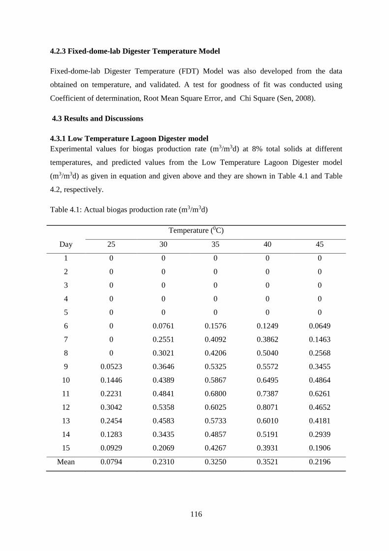
116
4.2.3 Fixed-dome-lab Digester Temperature Model
Fixed-dome-lab Digester Temperature (FDT) Model was also developed from the data
obtained on temperature, and validated. A test for goodness of fit was conducted using
Coefficient of determination, Root Mean Square Error, and Chi Square (Sen, 2008).
4.3 Results and Discussions
4.3.1 Low Temperature Lagoon Digester model
Experimental values for biogas production rate (m3/m3d) at 8% total solids at different
temperatures, and predicted values from the Low Temperature Lagoon Digester model
(m3/m3d) as given in equation and given above and they are shown in Table 4.1 and Table
4.2, respectively.
Table 4.1: Actual biogas production rate (m3/m3d)
Temperature (0C)
Day 25 30 35 40 45
1 0 0 0 0 0
2 0 0 0 0 0
3 0 0 0 0 0
4 0 0 0 0 0
5 0 0 0 0 0
6 0 0.0761 0.1576 0.1249 0.0649
7 0 0.2551 0.4092 0.3862 0.1463
8 0 0.3021 0.4206 0.5040 0.2568
9 0.0523 0.3646 0.5325 0.5572 0.3455
10 0.1446 0.4389 0.5867 0.6495 0.4864
11 0.2231 0.4841 0.6800 0.7387 0.6261
12 0.3042 0.5358 0.6025 0.8071 0.4652
13 0.2454 0.4583 0.5733 0.6010 0.4181
14 0.1283 0.3435 0.4857 0.5191 0.2939
15 0.0929 0.2069 0.4267 0.3931 0.1906
Mean 0.0794 0.2310 0.3250 0.3521 0.2196
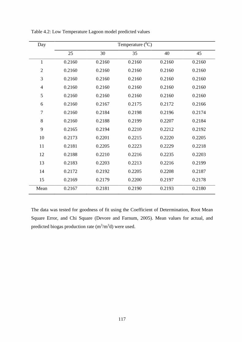
117
Table 4.2: Low Temperature Lagoon model predicted values
Day Temperature (0C)
25 30 35 40 45
1 0.2160 0.2160 0.2160 0.2160 0.2160
2 0.2160 0.2160 0.2160 0.2160 0.2160
3 0.2160 0.2160 0.2160 0.2160 0.2160
4 0.2160 0.2160 0.2160 0.2160 0.2160
5 0.2160 0.2160 0.2160 0.2160 0.2160
6 0.2160 0.2167 0.2175 0.2172 0.2166
7 0.2160 0.2184 0.2198 0.2196 0.2174
8 0.2160 0.2188 0.2199 0.2207 0.2184
9 0.2165 0.2194 0.2210 0.2212 0.2192
10 0.2173 0.2201 0.2215 0.2220 0.2205
11 0.2181 0.2205 0.2223 0.2229 0.2218
12 0.2188 0.2210 0.2216 0.2235 0.2203
13 0.2183 0.2203 0.2213 0.2216 0.2199
14 0.2172 0.2192 0.2205 0.2208 0.2187
15 0.2169 0.2179 0.2200 0.2197 0.2178
Mean 0.2167 0.2181 0.2190 0.2193 0.2180
The data was tested for goodness of fit using the Coefficient of Determination, Root Mean
Square Error, and Chi Square (Devore and Farnum, 2005). Mean values for actual, and
predicted biogas production rate (m3/m3d) were used.
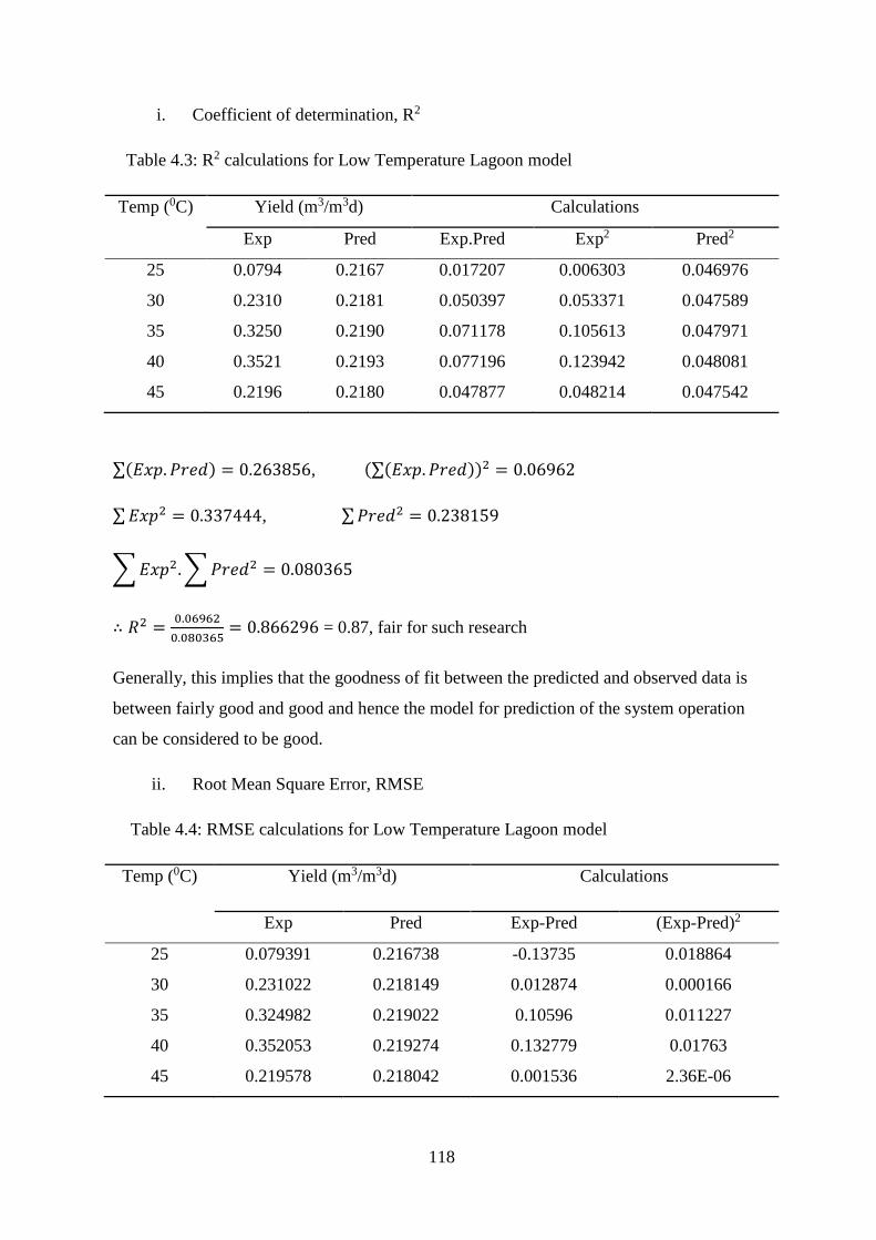
118
i. Coefficient of determination, R2
Table 4.3: R2 calculations for Low Temperature Lagoon model
Temp (0C) Yield (m3/m3d) Calculations
Exp Pred Exp.Pred Exp2 Pred2
25 0.0794 0.2167 0.017207 0.006303 0.046976
30 0.2310 0.2181 0.050397 0.053371 0.047589
35 0.3250 0.2190 0.071178 0.105613 0.047971
40 0.3521 0.2193 0.077196 0.123942 0.048081
45 0.2196 0.2180 0.047877 0.048214 0.047542
∑(𝐸𝑥𝑝. 𝑃𝑟𝑒𝑑) = 0.263856, (∑(𝐸𝑥𝑝. 𝑃𝑟𝑒𝑑))2 = 0.06962
∑ 𝐸𝑥𝑝2 = 0.337444, ∑ 𝑃𝑟𝑒𝑑2 = 0.238159
∑ 𝐸𝑥𝑝2. ∑ 𝑃𝑟𝑒𝑑2 = 0.080365
∴ 𝑅2 =0.06962
0.080365= 0.866296 = 0.87, fair for such research
Generally, this implies that the goodness of fit between the predicted and observed data is
between fairly good and good and hence the model for prediction of the system operation
can be considered to be good.
ii. Root Mean Square Error, RMSE
Table 4.4: RMSE calculations for Low Temperature Lagoon model
Temp (0C) Yield (m3/m3d) Calculations
Exp Pred Exp-Pred (Exp-Pred)2
25 0.079391 0.216738 -0.13735 0.018864
30 0.231022 0.218149 0.012874 0.000166
35 0.324982 0.219022 0.10596 0.011227
40 0.352053 0.219274 0.132779 0.01763
45 0.219578 0.218042 0.001536 2.36E-06
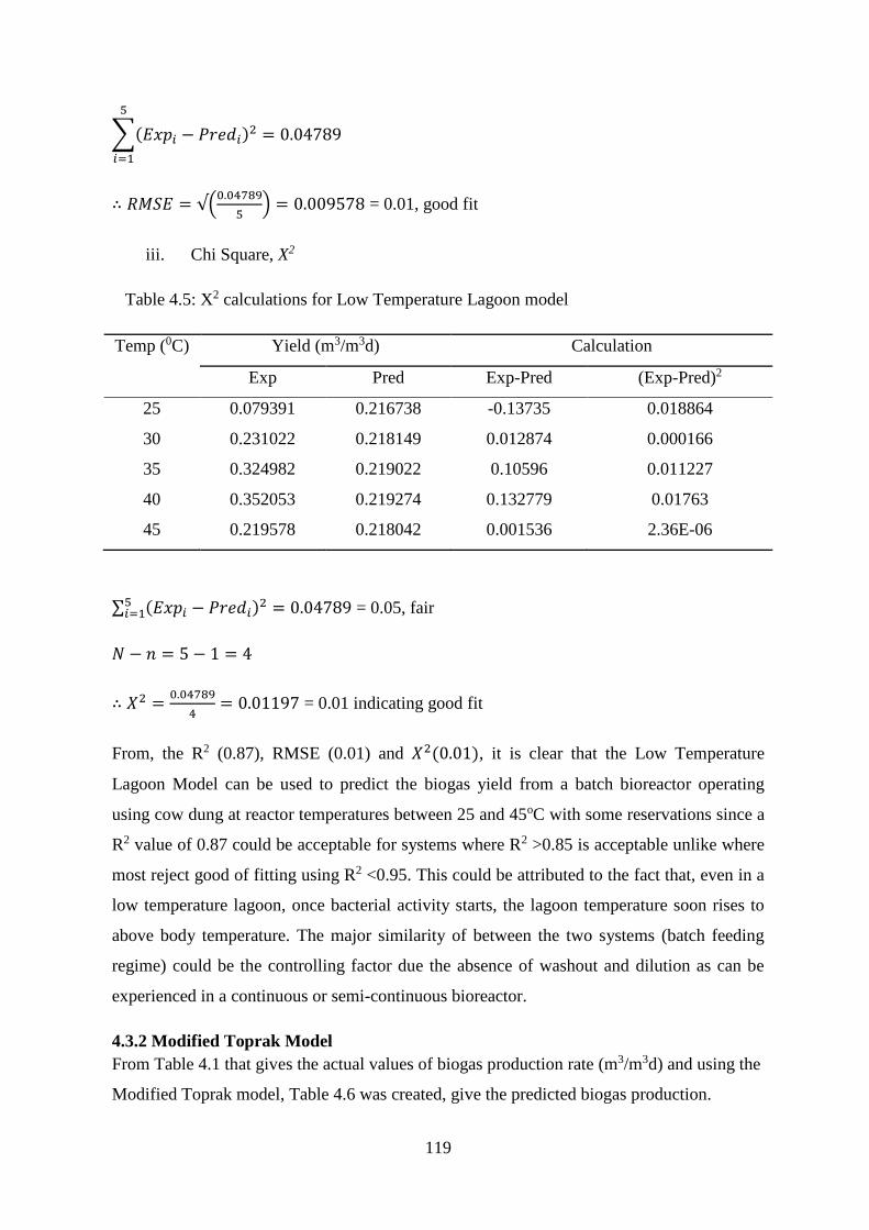
119
∑(𝐸𝑥𝑝𝑖 − 𝑃𝑟𝑒𝑑𝑖)2
5
𝑖=1
= 0.04789
∴ 𝑅𝑀𝑆𝐸 = √(0.04789
5) = 0.009578 = 0.01, good fit
iii. Chi Square, X2
Table 4.5: X2 calculations for Low Temperature Lagoon model
Temp (0C) Yield (m3/m3d) Calculation
Exp Pred Exp-Pred (Exp-Pred)2
25 0.079391 0.216738 -0.13735 0.018864
30 0.231022 0.218149 0.012874 0.000166
35 0.324982 0.219022 0.10596 0.011227
40 0.352053 0.219274 0.132779 0.01763
45 0.219578 0.218042 0.001536 2.36E-06
∑ (𝐸𝑥𝑝𝑖 − 𝑃𝑟𝑒𝑑𝑖)2 = 0.047895
𝑖=1 = 0.05, fair
𝑁 − 𝑛 = 5 − 1 = 4
∴ 𝑋2 =0.04789
4= 0.01197 = 0.01 indicating good fit
From, the R2 (0.87), RMSE (0.01) and 𝑋2(0.01), it is clear that the Low Temperature
Lagoon Model can be used to predict the biogas yield from a batch bioreactor operating
using cow dung at reactor temperatures between 25 and 45oC with some reservations since a
R2 value of 0.87 could be acceptable for systems where R2 >0.85 is acceptable unlike where
most reject good of fitting using R2 <0.95. This could be attributed to the fact that, even in a
low temperature lagoon, once bacterial activity starts, the lagoon temperature soon rises to
above body temperature. The major similarity of between the two systems (batch feeding
regime) could be the controlling factor due the absence of washout and dilution as can be
experienced in a continuous or semi-continuous bioreactor.
4.3.2 Modified Toprak Model
From Table 4.1 that gives the actual values of biogas production rate (m3/m3d) and using the
Modified Toprak model, Table 4.6 was created, give the predicted biogas production.
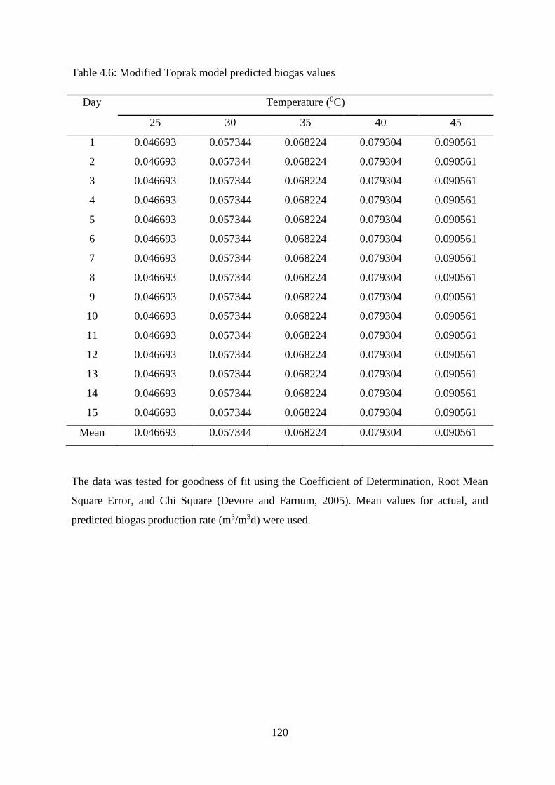
120
Table 4.6: Modified Toprak model predicted biogas values
Day Temperature (0C)
25 30 35 40 45
1 0.046693 0.057344 0.068224 0.079304 0.090561
2 0.046693 0.057344 0.068224 0.079304 0.090561
3 0.046693 0.057344 0.068224 0.079304 0.090561
4 0.046693 0.057344 0.068224 0.079304 0.090561
5 0.046693 0.057344 0.068224 0.079304 0.090561
6 0.046693 0.057344 0.068224 0.079304 0.090561
7 0.046693 0.057344 0.068224 0.079304 0.090561
8 0.046693 0.057344 0.068224 0.079304 0.090561
9 0.046693 0.057344 0.068224 0.079304 0.090561
10 0.046693 0.057344 0.068224 0.079304 0.090561
11 0.046693 0.057344 0.068224 0.079304 0.090561
12 0.046693 0.057344 0.068224 0.079304 0.090561
13 0.046693 0.057344 0.068224 0.079304 0.090561
14 0.046693 0.057344 0.068224 0.079304 0.090561
15 0.046693 0.057344 0.068224 0.079304 0.090561
Mean 0.046693 0.057344 0.068224 0.079304 0.090561
The data was tested for goodness of fit using the Coefficient of Determination, Root Mean
Square Error, and Chi Square (Devore and Farnum, 2005). Mean values for actual, and
predicted biogas production rate (m3/m3d) were used.
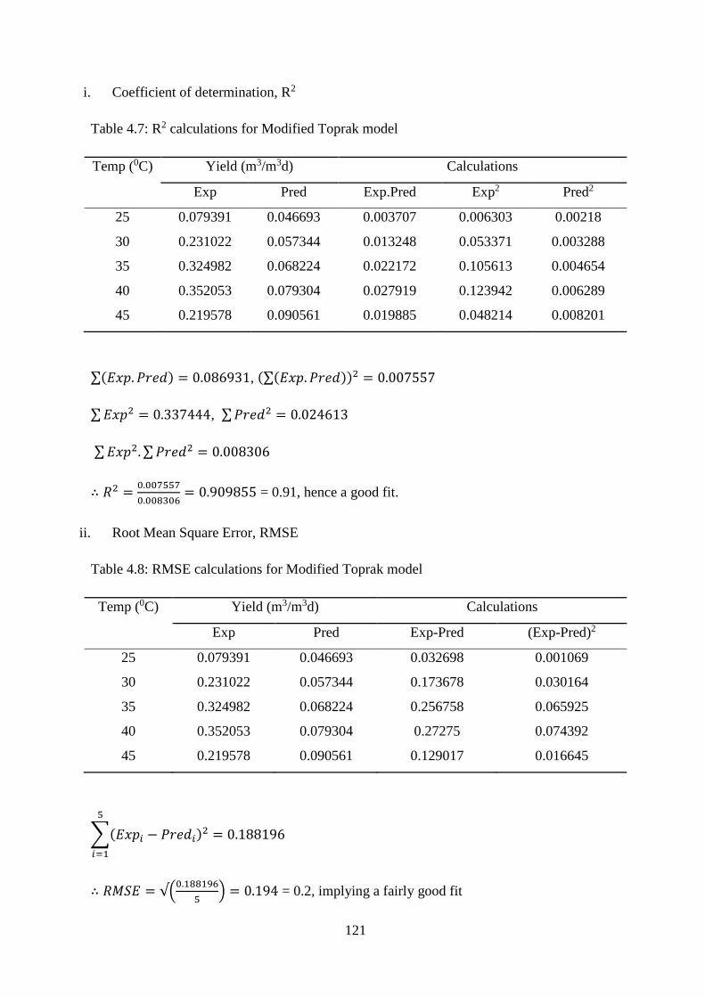
121
i. Coefficient of determination, R2
Table 4.7: R2 calculations for Modified Toprak model
Temp (0C) Yield (m3/m3d) Calculations
Exp Pred Exp.Pred Exp2 Pred2
25 0.079391 0.046693 0.003707 0.006303 0.00218
30 0.231022 0.057344 0.013248 0.053371 0.003288
35 0.324982 0.068224 0.022172 0.105613 0.004654
40 0.352053 0.079304 0.027919 0.123942 0.006289
45 0.219578 0.090561 0.019885 0.048214 0.008201
∑(𝐸𝑥𝑝. 𝑃𝑟𝑒𝑑) = 0.086931, (∑(𝐸𝑥𝑝. 𝑃𝑟𝑒𝑑))2 = 0.007557
∑ 𝐸𝑥𝑝2 = 0.337444, ∑ 𝑃𝑟𝑒𝑑2 = 0.024613
∑ 𝐸𝑥𝑝2. ∑ 𝑃𝑟𝑒𝑑2 = 0.008306
∴ 𝑅2 =0.007557
0.008306= 0.909855 = 0.91, hence a good fit.
ii. Root Mean Square Error, RMSE
Table 4.8: RMSE calculations for Modified Toprak model
Temp (0C) Yield (m3/m3d) Calculations
Exp Pred Exp-Pred (Exp-Pred)2
25 0.079391 0.046693 0.032698 0.001069
30 0.231022 0.057344 0.173678 0.030164
35 0.324982 0.068224 0.256758 0.065925
40 0.352053 0.079304 0.27275 0.074392
45 0.219578 0.090561 0.129017 0.016645
∑(𝐸𝑥𝑝𝑖 − 𝑃𝑟𝑒𝑑𝑖)2
5
𝑖=1
= 0.188196
∴ 𝑅𝑀𝑆𝐸 = √(0.188196
5) = 0.194 = 0.2, implying a fairly good fit
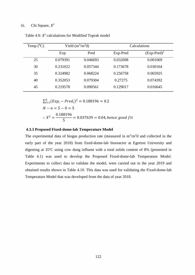
122
iii. Chi Square, X2
Table 4.9: X2 calculations for Modified Toprak model
Temp (0C) Yield (m3/m3d) Calculations
Exp Pred Exp-Pred (Exp-Pred)2
25 0.079391 0.046693 0.032698 0.001069
30 0.231022 0.057344 0.173678 0.030164
35 0.324982 0.068224 0.256758 0.065925
40 0.352053 0.079304 0.27275 0.074392
45 0.219578 0.090561 0.129017 0.016645
∑ (𝐸𝑥𝑝𝑖 − 𝑃𝑟𝑒𝑑𝑖)2 = 0.188196 = 0.25
𝑖=1
𝑁 − 𝑛 = 5 − 0 = 5
∴ 𝑋2 =0.188196
5= 0.037639 = 0.04, ℎ𝑒𝑛𝑐𝑒 𝑔𝑜𝑜𝑑 𝑓𝑖𝑡
4.3.3 Proposed Fixed-dome-lab Temperature Model
The experimental data of biogas production rate (measured in m3/m3d and collected in the
early part of the year 2018) from fixed-dome-lab bioreactor at Egerton University and
digesting at 35oC using cow dung influent with a total solids content of 8% (presented in
Table 4.1) was used to develop the Proposed Fixed-dome-lab Temperature Model.
Experiments to collect data to validate the model, were carried out in the year 2019 and
obtained results shown in Table 4.10. This data was used for validating the Fixed-dome-lab
Temperature Model that was developed from the data of year 2018.
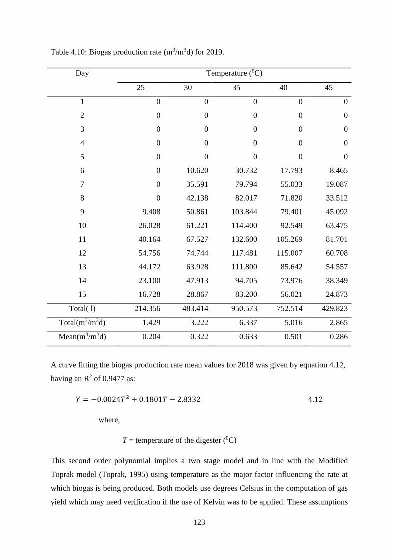
123
Table 4.10: Biogas production rate (m3/m3d) for 2019.
Day Temperature (0C)
25 30 35 40 45
1 0 0 0 0 0
2 0 0 0 0 0
3 0 0 0 0 0
4 0 0 0 0 0
5 0 0 0 0 0
6 0 10.620 30.732 17.793 8.465
7 0 35.591 79.794 55.033 19.087
8 0 42.138 82.017 71.820 33.512
9 9.408 50.861 103.844 79.401 45.092
10 26.028 61.221 114.400 92.549 63.475
11 40.164 67.527 132.600 105.269 81.701
12 54.756 74.744 117.481 115.007 60.708
13 44.172 63.928 111.800 85.642 54.557
14 23.100 47.913 94.705 73.976 38.349
15 16.728 28.867 83.200 56.021 24.873
Total( l) 214.356 483.414 950.573 752.514 429.823
Total(m3/m3d) 1.429 3.222 6.337 5.016 2.865
Mean(m3/m3d) 0.204 0.322 0.633 0.501 0.286
A curve fitting the biogas production rate mean values for 2018 was given by equation 4.12,
having an R2 of 0.9477 as:
𝑌 = −0.0024𝑇2 + 0.1801𝑇 − 2.8332 4.12
where,
T = temperature of the digester (0C)
This second order polynomial implies a two stage model and in line with the Modified
Toprak model (Toprak, 1995) using temperature as the major factor influencing the rate at
which biogas is being produced. Both models use degrees Celsius in the computation of gas
yield which may need verification if the use of Kelvin was to be applied. These assumptions
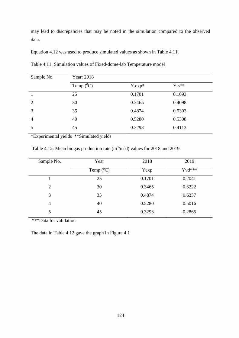
124
may lead to discrepancies that may be noted in the simulation compared to the observed
data.
Equation 4.12 was used to produce simulated values as shown in Table 4.11.
Table 4.11: Simulation values of Fixed-dome-lab Temperature model
Sample No. Year: 2018
Temp (0C) Y.exp* Y.s**
1 25 0.1701 0.1693
2 30 0.3465 0.4098
3 35 0.4874 0.5303
4 40 0.5280 0.5308
5 45 0.3293 0.4113
*Experimental yields **Simulated yields
Table 4.12: Mean biogas production rate (m3/m3d) values for 2018 and 2019
Sample No. Year 2018 2019
Temp (0C) Yexp Yvd***
1 25 0.1701 0.2041
2 30 0.3465 0.3222
3 35 0.4874 0.6337
4 40 0.5280 0.5016
5 45 0.3293 0.2865
***Data for validation
The data in Table 4.12 gave the graph in Figure 4.1
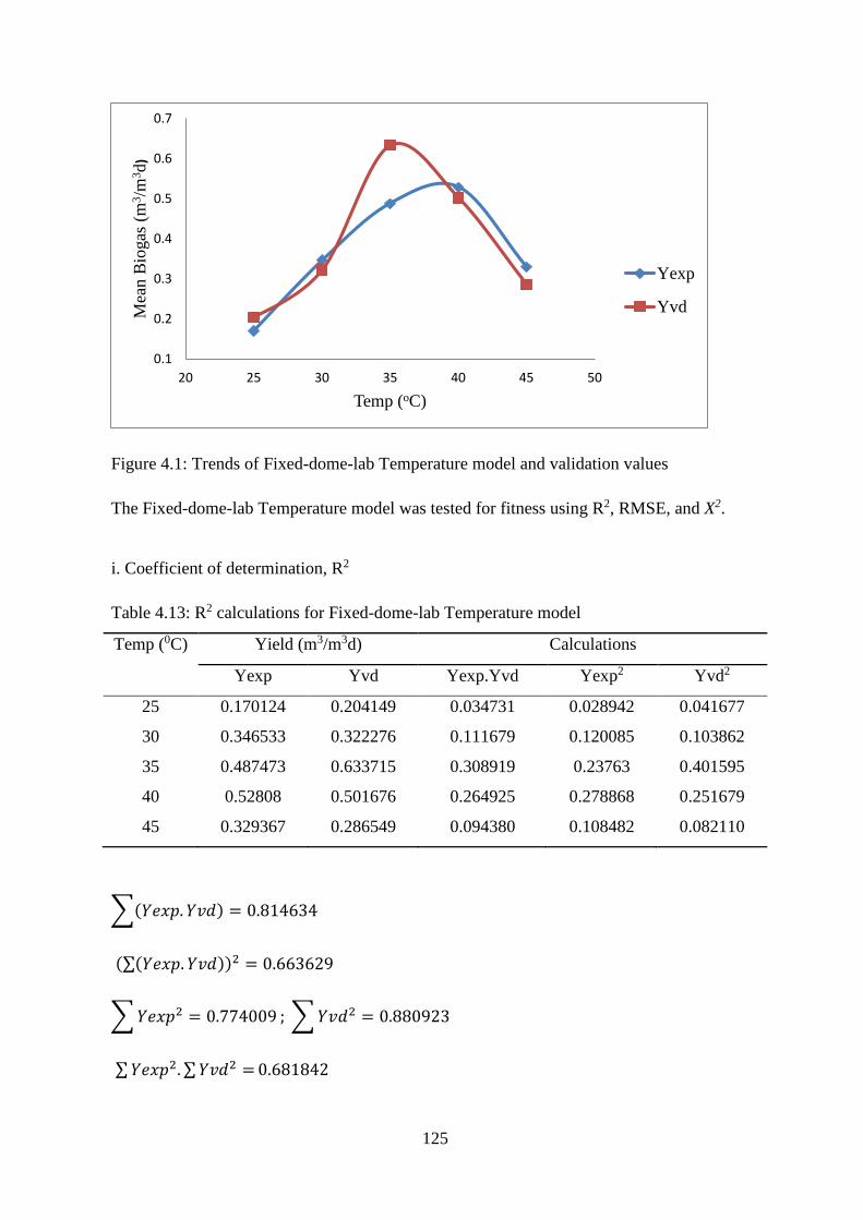
125
Figure 4.1: Trends of Fixed-dome-lab Temperature model and validation values
The Fixed-dome-lab Temperature model was tested for fitness using R2, RMSE, and X2.
i. Coefficient of determination, R2
Table 4.13: R2 calculations for Fixed-dome-lab Temperature model
Temp (0C) Yield (m3/m3d) Calculations
Yexp Yvd Yexp.Yvd Yexp2 Yvd2
25 0.170124 0.204149 0.034731 0.028942 0.041677
30 0.346533 0.322276 0.111679 0.120085 0.103862
35 0.487473 0.633715 0.308919 0.23763 0.401595
40 0.52808 0.501676 0.264925 0.278868 0.251679
45 0.329367 0.286549 0.094380 0.108482 0.082110
∑(𝑌𝑒𝑥𝑝. 𝑌𝑣𝑑) = 0.814634
(∑(𝑌𝑒𝑥𝑝. 𝑌𝑣𝑑))2 = 0.663629
∑ 𝑌𝑒𝑥𝑝2 = 0.774009 ; ∑ 𝑌𝑣𝑑2 = 0.880923
∑ 𝑌𝑒𝑥𝑝2. ∑ 𝑌𝑣𝑑2 = 0.681842
0.1
0.2
0.3
0.4
0.5
0.6
0.7
20 25 30 35 40 45 50
Mea
n B
iogas
(m
3/m
3d
)
Temp (oC)
Yexp
Yvd
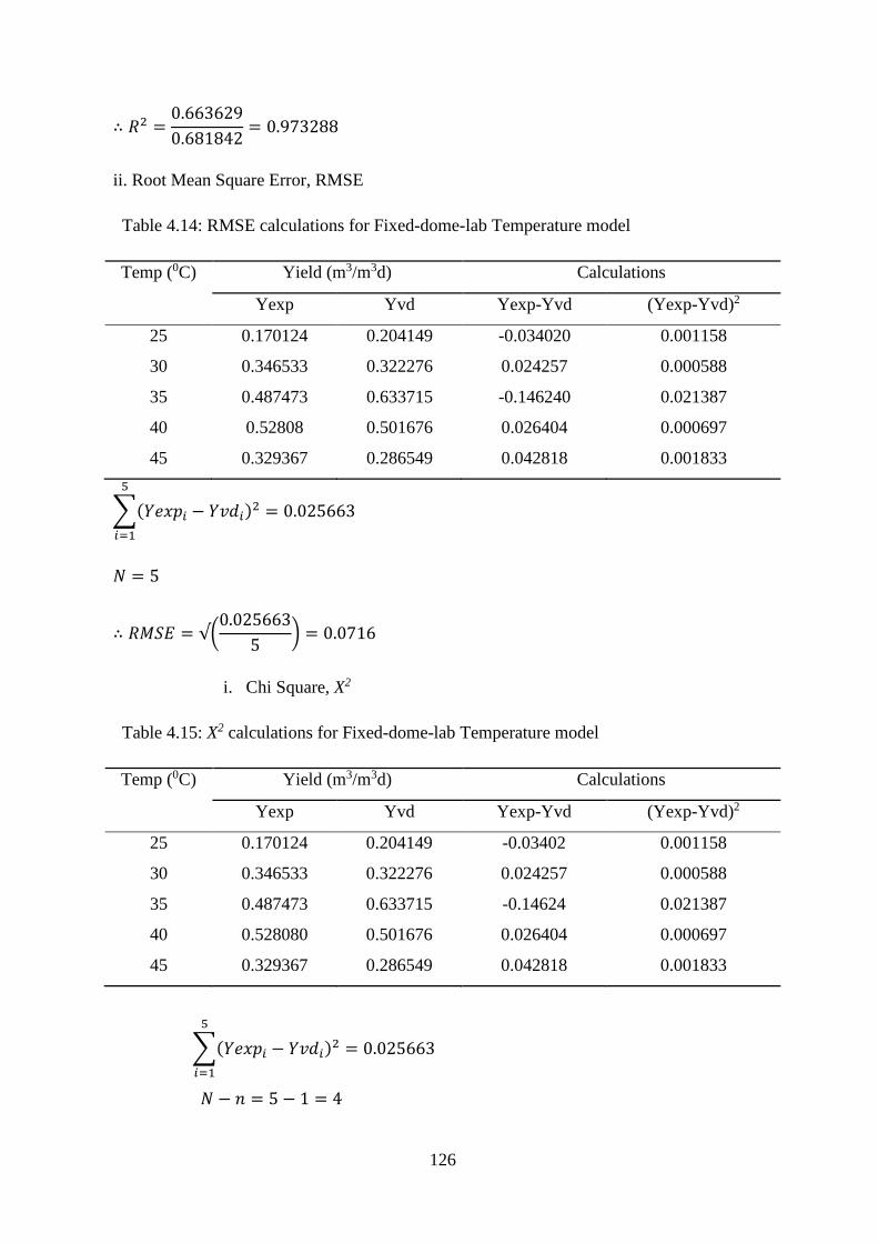
126
∴ 𝑅2 =0.663629
0.681842= 0.973288
ii. Root Mean Square Error, RMSE
Table 4.14: RMSE calculations for Fixed-dome-lab Temperature model
Temp (0C) Yield (m3/m3d) Calculations
Yexp Yvd Yexp-Yvd (Yexp-Yvd)2
25 0.170124 0.204149 -0.034020 0.001158
30 0.346533 0.322276 0.024257 0.000588
35 0.487473 0.633715 -0.146240 0.021387
40 0.52808 0.501676 0.026404 0.000697
45 0.329367 0.286549 0.042818 0.001833
∑(𝑌𝑒𝑥𝑝𝑖 − 𝑌𝑣𝑑𝑖)2
5
𝑖=1
= 0.025663
𝑁 = 5
∴ 𝑅𝑀𝑆𝐸 = √(0.025663
5) = 0.0716
i. Chi Square, X2
Table 4.15: X2 calculations for Fixed-dome-lab Temperature model
Temp (0C) Yield (m3/m3d) Calculations
Yexp Yvd Yexp-Yvd (Yexp-Yvd)2
25 0.170124 0.204149 -0.03402 0.001158
30 0.346533 0.322276 0.024257 0.000588
35 0.487473 0.633715 -0.14624 0.021387
40 0.528080 0.501676 0.026404 0.000697
45 0.329367 0.286549 0.042818 0.001833
∑(𝑌𝑒𝑥𝑝𝑖 − 𝑌𝑣𝑑𝑖)2 = 0.025663
5
𝑖=1
𝑁 − 𝑛 = 5 − 1 = 4
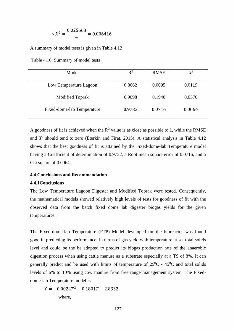
127
∴ 𝑋2 =0.025663
4= 0.006416
A summary of model tests is given in Table 4.12
Table 4.16: Summary of model tests
Model R2 RMSE X2
Low Temperature Lagoon 0.8662 0.0095 0.0119
Modified Toprak 0.9098 0.1940 0.0376
Fixed-dome-lab Temperature 0.9732 0.0716 0.0064
A goodness of fit is achieved when the R2 value is as close as possible to 1, while the RMSE
and X2 should tend to zero (Eterkin and Firat, 2015). A statistical analysis in Table 4.12
shows that the best goodness of fit is attained by the Fixed-dome-lab Temperature model
having a Coefficient of determination of 0.9732, a Root mean square error of 0.0716, and a
Chi square of 0.0064.
4.4 Conclusions and Recommendation
4.4.1Conclusions
The Low Temperature Lagoon Digester and Modified Toprak were tested. Consequently,
the mathematical models showed relatively high levels of tests for goodness of fit with the
observed data from the batch fixed dome lab digester biogas yields for the given
temperatures.
The Fixed-dome-lab Temperature (FTP) Model developed for the bioreactor was found
good in predicting its performance in terms of gas yield with temperature at set total solids
level and could be the be adopted to predict its biogas production rate of the anaerobic
digestion process when using cattle manure as a substrate especially at a TS of 8%. It can
generally predict and be used with limits of temperature of 250C - 450C and total solids
levels of 6% to 10% using cow manure from free range management system. The Fixed-
dome-lab Temperature model is
𝑌 = −0.0024𝑇2 + 0.1801𝑇 − 2.8332
where,
128
Y = Mean biogas produced in m3per m3of digester volume per day
(m3/m3d)
T = Digester temperature (0C)
4.4.2 Recommendation
Available mathematical models for the prediction of biogas production rate can be used with
a precaution ensuring the initial and final boundary conditions of the model are clear and
adhered to. In most cases, the scope and limitations for the models are not easily identified,
hence the caution.
It is further recommended that the following research be conducted:
i. Existing models should be validated with huge, replicated and similar experimental
data as ones used in their development.
ii. Models relating total solids and substrate retention time to biogas production rate
should be developed for a fixed dome laboratory bioreactor as batch and semi
continuous system that operates in a psychrophilic, mesophilic and thermophilic
temperature ranges.
iii. Compare the lab bioreactor performance with those of the field digester for the same
months or operating digestion temperatures.
129
References
Akbas, H. and Ozdemir, G. (2018). Prediction Modeling of Biogas Production with
Classification and Regression Tree at Wastewater Treatment Plants. Paper
presented at the The Eurasia Proceedings of Science, Technology, Engineering &
Mathematics (EPSTEM).
Ali, A., Rundong, L., Shah, F., Mahar, R. and WajidIjaz, M. (2016). Predictive Modeling
of Biogas Production from Anaerobic Digestion of Mixed Kitchen Waste at
Mesophilic Temperature. International Journal of Waste Resources, 6(3), 230.
doi:10.4172/2252-5211.1000230
Brunn, L., Dornack, C. and Bilitewski, B. (2009). Application of laboratory scale
experiments to industrial scale in case of anaerobic waste treatment. Fresenius
Environmental Bulletin, 18(2), 196-203.
Chen, Y. and Hashimoto. (1978). Kinetics of methane fermentation. Paper presented at the
Symposium on Biotechnology in Energy Production and Conservation, New York.
Devore, J. and Farnum, N. (2005). Applied Statistics for Engineers and Scientists. Belmont,
CA: Curt Hinrichs.
Eder, B. and Schulz, H. (2006). Biogas Praxis [in German] (3rd ed.).
Eterkin, C. and Firat, M. (2015). A comprehensive review of thin layer drying model used
in agricultural products. Critical Reviews in Food Science and Nutrition, 57(4), 701-
717.
Hossain, M., Woods, J. and Bala, B. (2007). Single layer drying characteristics and colour
kinetics of red Chilli. International Journal of Food Science and Technology,
42(11), 1367-1375.
Jewell, W., Carpener, H., Dell'orto, S., Fanfoni, K., Hayes, T., Leuschner, A., Miller, T.,
Sherman, D., Soest, P., Wolin, M. and Wujcik, W. (1978). Anaerobic fermentation
of agricultural residue: Potential for improvement and implementation - Final
Report (EY-76-S-02-2981-7). Retrieved from Cornell University.
Kowalczyk, A., Schwede, S., Gerber, M. and Span, R. (2011). Scale up of laboratory scale
to industrial scale biogas plants. Paper presented at the World Renewable Energy
Congress, Sweden.
Kwakkel, J. and Pryut, E. (2013). Exploratory Modelling and Analysis, an approach for
model-based foresight under deep uncertainty. Technological Forecasting and
Social Change, 80(3), 419-431.
130
Lahsasni, S., Kouhila, M., Marhouz, M. and Idlimam, A. (2004). Thin layer convective
solar drying and modeling of prickly pear peel. Energy, 29, 211-224.
Minott, S. (2002). Feasibility of fuel cells for energy conversion on the dairy farm. Cornell
University, New York.
Safley, L. and Westerman, P. (1992). Performance of a low temperature lagoon digester.
Bioresource Technology, 41, 167-175.
Sen, Z. (2008). Solar Energy Fundamentals and Modeling Techniques: Atmosphere,
Environment, Climate Change and Renewable Energy. Retrieved from London.
Stockburger, D. (2006). Introductory Statistics: Concepts, Models and Applications.
Toprak, H. (1995). Temperature and organic loading dependency of methane and carbon
dioxide emission rates of a full-scale anaerobic waste stabilization pond. Water
Research, 29(1), 1111-1119.
131
CHAPTER FIVE
OPTIMISATION OF BIOGAS PRODUCTION
Abstract
Optimisation was done by investigating the interaction effects of total solids, temperature,
and substrate retention time on biogas production in a batch bioreactor. Central composite
design (CCD) of Response Surface Methodology (RSM) was used to design the experiment.
Total solid levels were varied from 6.31% to 9.68%, temperature was from 26.590C to
43.410C, and substrate retention time was from 9.95 to 20.04 days. Analysis of results was
done using Design Expert software statistical package (version 10.0.0.3). It gave a coefficient
of determination of 0.9665 which indicated a high correlation between the variables. All the
variables had a significant effect. Contour plots, and three dimensional graphs were
discussed. The highest rate of 75.41litres/day was achieved at a level of 8% total solids total
solids, 43.410C, and 15 days.
5.1 Introduction
Optimisation is the act of achieving the best possible result under given circumstances. In
design, construction and maintenance, engineers have to make decisions. The aim of such
decisions is either to minimise the effort or to maximise benefit. The effort or benefit can be
expressed as a function of certain design variables. Hence optimisation is the process of
finding conditions that give the minimum or the maximum value of a function (Astolfi and
Praly, 2006). Efforts to maximise biogas production are currently being done by using
various feedstocks. Reungsang et al. (2012) used Response Surface Methodology (RSM)
with a Central Composite Design (CCD) to optimise the key factors affecting methane
production from the acidic effluent coming from the sugarcane juice hydrogen fermentation
process. The parameters studied were substrate concentration, ratio of NaHCO3 to substrate
concentration, and an initial pH. The maximum methane yield of 367 ml CH4/g-volatile solid
(VS) added was obtained at the optimum conditions of 13,823 mg-COD/l, an NaHCO3 to
substrate concentration ratio of 3.09, and an initial pH of 7.07. Methane yield was enhanced
4.4-fold in comparison to raw effluent. Sathish and Vivekanandan (2016) studied the optimal
conditions for biogas generation from anaerobic digestion of rice straw in a 1m3 floating
drum anaerobic digester using RSM. The parameters were temperature, pH, substrate
concentration, and agitation time. The highest level of biogas of 0.72m3 was produced at an
optimum temperature of 500C, pH 7.5, substrate concentration of 110.70 kg, and an agitation
time of 5 seconds, respectively. Saleh et al. (2012) investigated the effects of temperature,
132
palm oil mill effluent (POME) volume, inoculum volume, and co-substrate addition such as
oil palm empty fruit bunch (EFB) and palm kernel on the anaerobic digestion process for
biogas and methane production. RSM by Box-Behnken design verified that the specific
biogas production rate and methane yield were mainly affected by the operating temperature
and co-substrate addition. The optimal conditions for the maximum specific biogas
production rate (0.0574 m3/ kg chemical oxygen demand per day) and methane yield (25.6%)
were predicted by multiple response optimisation and verified experimentally at 47.80C
operating temperature, 50.4 ml POME volume, and 5.7 g EFB addition. Other similar works
have been reported by Pannucharoenwong (2018) among others.
Response surface methodology (RSM) is one of the most effective approaches for designing
experiments, for building models, and for determining optimal conditions on responses which
are influenced by several independent variables (Bezerra et al., 2008; Kang et al., 2016).
Apart from defining the influences of independent variables on the responses, RSM also
determines the effect of interaction between parameters to obtain the best performance on a
system (Belwal et al., 2016; Zaroual et al., 2009). RSM is a collection of statistical and
mathematical techniques used for developing, improving, and optimising processes
(Montgomery et al., 2009). The most extensive applications of RSM are in situations where
several input variables potentially influence some performance measure or quality
characteristic of a process; most applications of RSM are sequential in nature, and are
performed within some region of the independent variable space called the operability region
(Carley and Kamneva, 2004).
Two types of RSM are used in design of experiments: Box–Wilson, and Box–Behnken (Jain
et al., 2011). The Box–Wilson, which is also called central composite design (CCD), has
three different design points: edge points as in two-level designs (±1), star points at ±α that
take care of quadratic effects, and centre points (0) (Jiménez et al., 2014). Central composite
design does testing at five levels. The edge points are at the design limits, star points are at
some distance from the centre depending on the number of factors in the design; the star
points extend the range outside the low and high settings for all factors, the centre points
complete the design (Leiviskä, 2013). Central composite design provides high quality
predictions over the entire design space, and is suitable for fitting a quadratic surface, and
usually works well for process optimisation (Kousha et al., 2015).
133
Box-Behnken design is an independent quadratic design because it does not contain an
embedded factorial or fractional factorial design (Kong et al., 2016). In this design, the
treatment combinations are at the midpoints of edges of the process space and at the centre,
require three levels of each factor: –1, 0, and +1, and has fewer treatment combinations than
CCD (Leiviskä, 2013).
In this study, CCD was used. Experiments designed by using CCD have fewer runs, and also
give similar results which are comparable to a full-factorial design, and enables an effective
evaluation of interaction between individual factors to provide the best combination for
optimal performance (Jiménez et al., 2014; Khoobbakht et al., 2016). Central composite
design is robust; it makes the process consistent on target and is relatively insensitive to
factors that are difficult to control (Taguchi, 1986, 1987). .
5.2 Materials and Methods
All the protocol was the same as in chapter 3 except the experimental design and data
analysis.
a) Design of experiment
Central composite design was used to get the matrix of experiments with three factors, each
being tested at five different levels. The response was biogas production (Y). The factors
were: substrate retention time (x1), total solids (x2), and temperature (x3). Design Expert
software (version 10.0.0.3, Stat-Ease, Inc., Minneapolis, United States) statistical package
was used to generate Table 5.1 and Table 5.2 for the experiment. The levels of every factor
were as indicated in Table 5.1. In the design space, the highest level was coded as +1, the
centre point was 0, and the lowest level was coded as –1. The outer design space points
corresponding to α were ± 1.68179. α = 2k/4, where k is the number of factors (Ahmad, 2009;
Aslan, 2007). In this case, k = 3. There was a total of 20 runs of experiments; comprising of 6
centre points and 14 axial points. If a full factorial experiment were done, there would have
been 53 (or 125) runs of experiments.
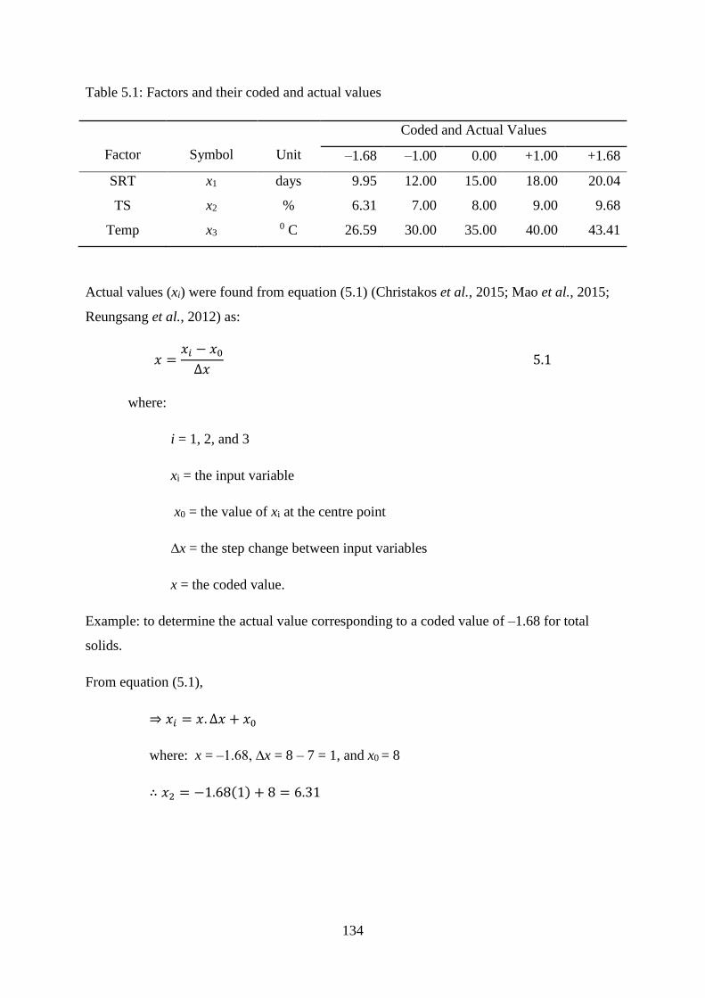
134
Table 5.1: Factors and their coded and actual values
Factor
Symbol
Unit
Coded and Actual Values
–1.68 –1.00 0.00 +1.00 +1.68
SRT x1 days 9.95 12.00 15.00 18.00 20.04
TS x2 % 6.31 7.00 8.00 9.00 9.68
Temp x3 0 C 26.59 30.00 35.00 40.00 43.41
Actual values (xi) were found from equation (5.1) (Christakos et al., 2015; Mao et al., 2015;
Reungsang et al., 2012) as:
𝑥 =𝑥𝑖 − 𝑥0
∆𝑥 5.1
where:
i = 1, 2, and 3
xi = the input variable
x0 = the value of xi at the centre point
∆x = the step change between input variables
x = the coded value.
Example: to determine the actual value corresponding to a coded value of –1.68 for total
solids.
From equation (5.1),
⇒ 𝑥𝑖 = 𝑥. ∆𝑥 + 𝑥0
where: x = –1.68, ∆x = 8 – 7 = 1, and x0 = 8
∴ 𝑥2 = −1.68(1) + 8 = 6.31
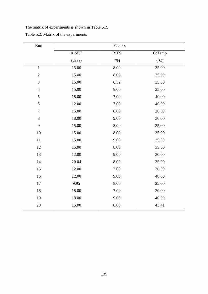
135
The matrix of experiments is shown in Table 5.2.
Table 5.2: Matrix of the experiments
Run Factors
A:SRT B:TS C:Temp
(days) (%) (oC)
1 15.00 8.00 35.00
2 15.00 8.00 35.00
3 15.00 6.32 35.00
4 15.00 8.00 35.00
5 18.00 7.00 40.00
6 12.00 7.00 40.00
7 15.00 8.00 26.59
8 18.00 9.00 30.00
9 15.00 8.00 35.00
10 15.00 8.00 35.00
11 15.00 9.68 35.00
12 15.00 8.00 35.00
13 12.00 9.00 30.00
14 20.04 8.00 35.00
15 12.00 7.00 30.00
16 12.00 9.00 40.00
17 9.95 8.00 35.00
18 18.00 7.00 30.00
19 18.00 9.00 40.00
20 15.00 8.00 43.41
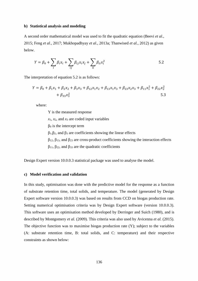
136
b) Statistical analysis and modeling
A second order mathematical model was used to fit the quadratic equation (Beevi et al.,
2015; Feng et al., 2017; Mukhopadhyay et al., 2013a; Thanwised et al., 2012) as given
below.
𝑌 = 𝛽0 + ∑ 𝛽𝑖𝑥𝑖
𝑖
+ ∑ 𝛽𝑖𝑗𝑥𝑖𝑥𝑗
𝑖𝑗
+ ∑ 𝛽𝑖𝑖𝑥𝑖2 5.2
𝑖𝑖
The interpretation of equation 5.2 is as follows:
𝑌 = 𝛽0 + 𝛽1𝑥1 + 𝛽2𝑥2 + 𝛽3𝑥3 + 𝛽12𝑥1𝑥2 + 𝛽13𝑥1𝑥3 + 𝛽23𝑥2𝑥3 + 𝛽11𝑥12 + 𝛽22𝑥2
2
+ 𝛽33𝑥32 5.3
where:
Y is the measured response
x1, x2, and x3 are coded input variables
β0 is the intercept term
β1,β2, and β3 are coefficients showing the linear effects
β12, β13, and β23 are cross-product coefficients showing the interaction effects
β11, β22, and β33 are the quadratic coefficients
Design Expert version 10.0.0.3 statistical package was used to analyse the model.
c) Model verification and validation
In this study, optimisation was done with the predictive model for the response as a function
of substrate retention time, total solids, and temperature. The model (generated by Design
Expert software version 10.0.0.3) was based on results from CCD on biogas production rate.
Setting numerical optimisation criteria was by Design Expert software (version 10.0.0.3).
This software uses an optimisation method developed by Derringer and Suich (1980), and is
described by Montgomery et al. (2009). This criteria was also used by Avicenna et al. (2015).
The objective function was to maximise biogas production rate (Y); subject to the variables
(A: substrate retention time, B: total solids, and C: temperature) and their respective
constraints as shown below:
137
Maximise
𝑌 = −901.41 + 15.21𝐴 + 183.25𝐵 + 7.74𝐶 − 0.56𝐴𝐵 + 0.04𝐴𝐶 + 0.06𝐵𝐶 − 0.41𝐴2
− 11.47𝐵2 − 0.11𝐶2 5.4
Subject to:
12 ≤ A ≤ 18; 7 ≤ B ≤ 9; 30 ≤ C ≤ 40
Table 5.3: Criteria.
Name Goal Lower limit Upper limit
A: SRT (days) In range 12.00 18.00
B: TS (%) In range 7.00 9.00
C: Temp (0C) In range 30.00 40.00
Y: Biogas production (litres/day) Maximise 33.01 75.41
This procedure generated Table 5.4.
Table 5.4: Influent preparation
TS (%) Cow dung : water dilution Cow dung (kg) Water (kg)
7.642 1:1.441 49.160 70.840
7.697 1:1.424 49.505 70.495
7.724 1:1.416 49.669 70.331
Influent preparation was done as follows: 1 kg of cow dung contains 0.18658 kg of total
solids (TS). In an influent of 7.642% TS, it implies that 7.642 kg of TS are contained in 100
kg of influent. Therefore 0.18658 kg of TS are contained in
(0.18658×100
7.642) which is equivalent to 2.441 kg of influent. This means that water in the
influent = 2.441 – 1 = 1.441 kg. Therefore cow dung : water ratio is 1:1.441
For an influent of 120 kg, Cow dung = 1×120
2.441= 49.160 𝑘𝑔; Water =
1.441×120
2.441= 70.840 𝑘𝑔
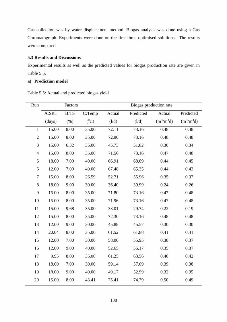
138
Gas collection was by water displacement method. Biogas analysis was done using a Gas
Chromatograph. Experiments were done on the first three optimised solutions. The results
were compared.
5.3 Results and Discussions
Experimental results as well as the predicted values for biogas production rate are given in
Table 5.5.
a) Prediction model
Table 5.5: Actual and predicted biogas yield
Run Factors Biogas production rate
A:SRT
(days)
B:TS
(%)
C:Temp
(0C)
Actual
(l/d)
Predicted
(l/d)
Actual
(m3/m3d)
Predicted
(m3/m3d)
1 15.00 8.00 35.00 72.11 73.16 0.48 0.48
2 15.00 8.00 35.00 72.90 73.16 0.48 0.48
3 15.00 6.32 35.00 45.73 51.82 0.30 0.34
4 15.00 8.00 35.00 71.56 73.16 0.47 0.48
5 18.00 7.00 40.00 66.91 68.89 0.44 0.45
6 12.00 7.00 40.00 67.48 65.35 0.44 0.43
7 15.00 8.00 26.59 52.71 55.96 0.35 0.37
8 18.00 9.00 30.00 36.40 39.99 0.24 0.26
9 15.00 8.00 35.00 71.80 73.16 0.47 0.48
10 15.00 8.00 35.00 71.96 73.16 0.47 0.48
11 15.00 9.68 35.00 33.01 29.74 0.22 0.19
12 15.00 8.00 35.00 72.30 73.16 0.48 0.48
13 12.00 9.00 30.00 45.88 45.57 0.30 0.30
14 20.04 8.00 35.00 61.52 61.88 0.41 0.41
15 12.00 7.00 30.00 58.00 55.95 0.38 0.37
16 12.00 9.00 40.00 52.65 56.17 0.35 0.37
17 9.95 8.00 35.00 61.25 63.56 0.40 0.42
18 18.00 7.00 30.00 59.14 57.09 0.39 0.38
19 18.00 9.00 40.00 49.17 52.99 0.32 0.35
20 15.00 8.00 43.41 75.41 74.79 0.50 0.49
139
The combination of factors which yielded the highest biogas production rate of 75.41 litres
per day (l/d) was a substrate retention time of 15 days, total solids of 8%, and a temperature
of 43.40C. This is the optimum combination of factors that gives the highest biogas
production rate of 0.50 cubic metres of biogas per cubic metre of biodigester volume per day
(m3/m3d), which is equivalent to 75.41 l/d.
A regression analysis was done based on the experimental results using the Design Expert
10.0.0.3 statistical package, and it yielded a relationship given by equation 5.4. This equation
was used to predict biogas production rate as shown in Table 5.5.
It was observed that the actual biogas production rates were in agreement with 0.4m3/m3d
reported by Nyaanga (2011), and Moog et al. (1997). This value also agrees reasonably with
0.42 m3/m3d that was observed by Ferrer et al. (2011). Consequently, the model can be
adopted for use under similar conditions of this experiment.
b) Analysis of variance (ANOVA)
The analysis of variance is necessary in order to determine the significance and adequacy of
the model (Thanwised et al., 2012). The statistical significance of the second-order
polynomial equation was checked by an F-test (ANOVA). Table 5.6 shows the statistics.
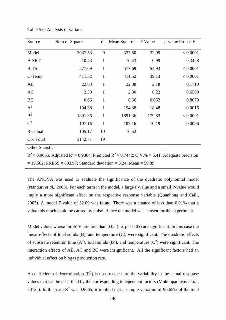
140
Table 5.6: Analysis of variance
Source Sum of Squares df Mean Square F Value p-value Prob > F
Model 3037.53 9 337.50 32.09 < 0.0001
A-SRT 10.43 1 10.43 0.99 0.3428
B-TS 577.69 1 577.69 54.93 < 0.0001
C-Temp 411.52 1 411.52 39.13 < 0.0001
AB 22.88 1 22.88 2.18 0.1710
AC 2.30 1 2.30 0.22 0.6500
BC 0.66 1 0.66 0.062 0.8079
A2 194.38 1 194.38 18.48 0.0016
B2 1891.36 1 1891.36 179.83 < 0.0001
C2 107.16 1 107.16 10.19 0.0096
Residual 105.17 10 10.52
Cor Total 3142.71 19
Other Statistics
R2 = 0.9665; Adjusted R2 = 0.9364; Predicted R2 = 0.7442; C.V.% = 5.41; Adequate precision
= 19.562; PRESS = 803.97; Standard deviation = 3.24; Mean = 59.89
The ANOVA was used to evaluate the significance of the quadratic polynomial model
(Nanduri et al., 2008). For each term in the model, a large F-value and a small P-value would
imply a more significant effect on the respective response variable (Quanhong and Caili,
2005). A model F-value of 32.09 was found. There was a chance of less than 0.01% that a
value this much could be caused by noise. Hence the model was chosen for the experiment.
Model values whose ‘prob>F’ are less than 0.05 (i.e. p < 0.05) are significant. In this case the
linear effects of total solids (B), and temperature (C), were significant. The quadratic effects
of substrate retention time (A2), total solids (B2), and temperature (C2) were significant. The
interaction effects of AB, AC and BC were insignificant. All the significant factors had an
individual effect on biogas production rate.
A coefficient of determination (R2) is used to measure the variability in the actual response
values that can be described by the corresponding independent factors (Mukhopadhyay et al.,
2013a). In this case R2 was 0.9665; it implied that a sample variation of 96.65% of the total
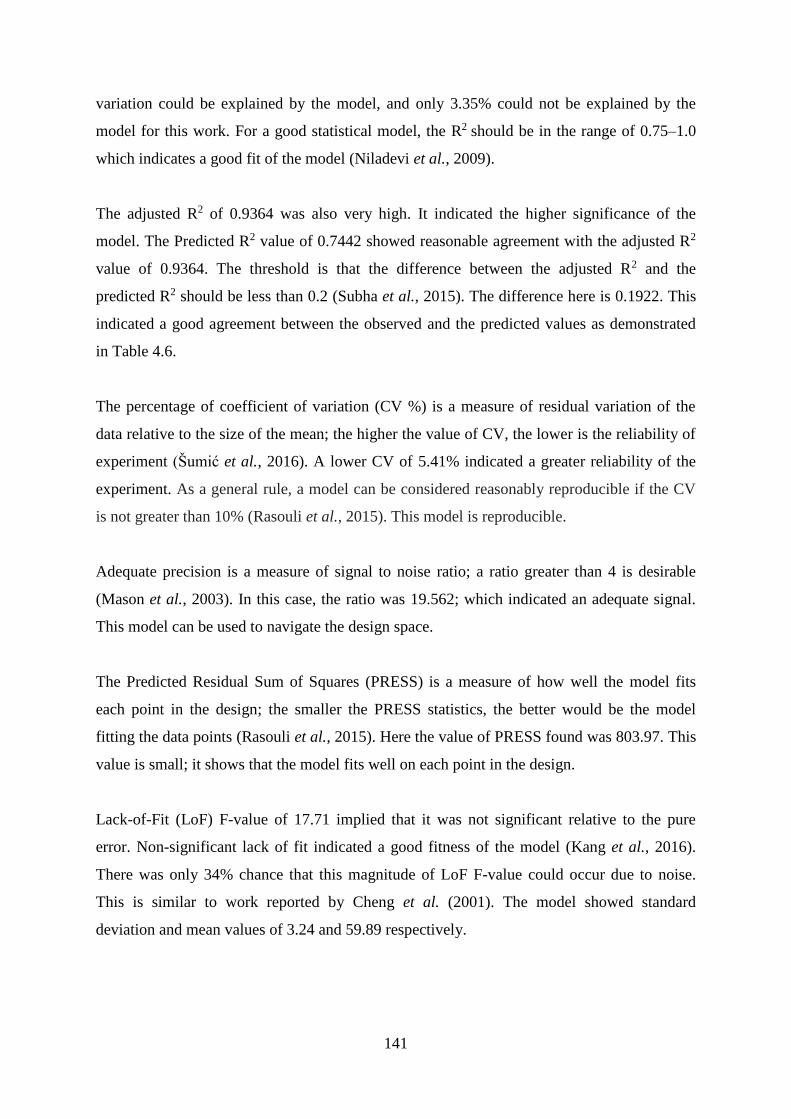
141
variation could be explained by the model, and only 3.35% could not be explained by the
model for this work. For a good statistical model, the R2 should be in the range of 0.75–1.0
which indicates a good fit of the model (Niladevi et al., 2009).
The adjusted R2 of 0.9364 was also very high. It indicated the higher significance of the
model. The Predicted R2 value of 0.7442 showed reasonable agreement with the adjusted R2
value of 0.9364. The threshold is that the difference between the adjusted R2 and the
predicted R2 should be less than 0.2 (Subha et al., 2015). The difference here is 0.1922. This
indicated a good agreement between the observed and the predicted values as demonstrated
in Table 4.6.
The percentage of coefficient of variation (CV %) is a measure of residual variation of the
data relative to the size of the mean; the higher the value of CV, the lower is the reliability of
experiment (Šumić et al., 2016). A lower CV of 5.41% indicated a greater reliability of the
experiment. As a general rule, a model can be considered reasonably reproducible if the CV
is not greater than 10% (Rasouli et al., 2015). This model is reproducible.
Adequate precision is a measure of signal to noise ratio; a ratio greater than 4 is desirable
(Mason et al., 2003). In this case, the ratio was 19.562; which indicated an adequate signal.
This model can be used to navigate the design space.
The Predicted Residual Sum of Squares (PRESS) is a measure of how well the model fits
each point in the design; the smaller the PRESS statistics, the better would be the model
fitting the data points (Rasouli et al., 2015). Here the value of PRESS found was 803.97. This
value is small; it shows that the model fits well on each point in the design.
Lack-of-Fit (LoF) F-value of 17.71 implied that it was not significant relative to the pure
error. Non-significant lack of fit indicated a good fitness of the model (Kang et al., 2016).
There was only 34% chance that this magnitude of LoF F-value could occur due to noise.
This is similar to work reported by Cheng et al. (2001). The model showed standard
deviation and mean values of 3.24 and 59.89 respectively.
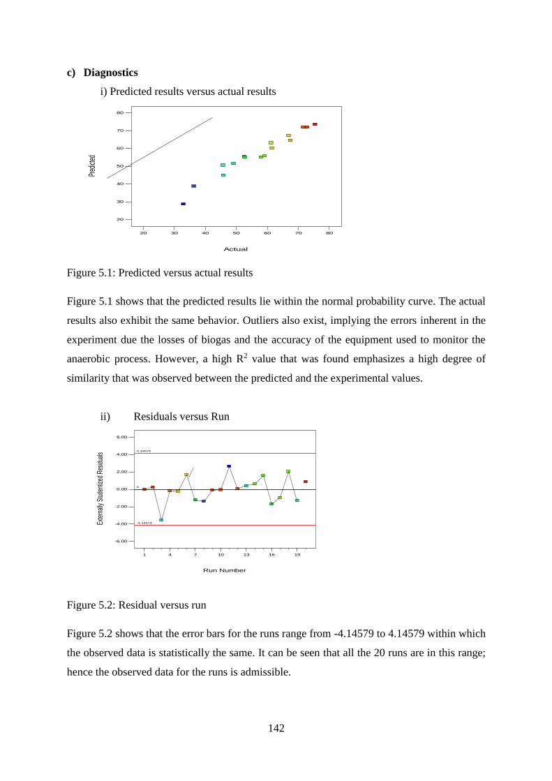
142
c) Diagnostics
i) Predicted results versus actual results
Figure 5.1: Predicted versus actual results
Figure 5.1 shows that the predicted results lie within the normal probability curve. The actual
results also exhibit the same behavior. Outliers also exist, implying the errors inherent in the
experiment due the losses of biogas and the accuracy of the equipment used to monitor the
anaerobic process. However, a high R2 value that was found emphasizes a high degree of
similarity that was observed between the predicted and the experimental values.
ii) Residuals versus Run
Figure 5.2: Residual versus run
Figure 5.2 shows that the error bars for the runs range from -4.14579 to 4.14579 within which
the observed data is statistically the same. It can be seen that all the 20 runs are in this range;
hence the observed data for the runs is admissible.
Design-Expert® SoftwareBiogas production rate
Color points by value ofBiogas production rate:
75.41
33.01
Actual
Pred
icted
Predicted vs. Actual
20
30
40
50
60
70
80
20 30 40 50 60 70 80
Design-Expert® SoftwareBiogas production rate
Color points by value ofBiogas production rate:
75.41
33.01
Run Number
Exte
rnal
ly St
uden
tized
Res
idua
ls
Residuals vs. Run
-6.00
-4.00
-2.00
0.00
2.00
4.00
6.00
1 4 7 10 13 16 19
4.14579
-4.14579
0
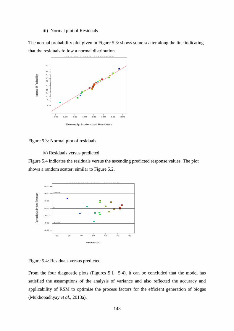
143
iii) Normal plot of Residuals
The normal probability plot given in Figure 5.3: shows some scatter along the line indicating
that the residuals follow a normal distribution.
Figure 5.3: Normal plot of residuals
iv) Residuals versus predicted
Figure 5.4 indicates the residuals versus the ascending predicted response values. The plot
shows a random scatter; similar to Figure 5.2.
Figure 5.4: Residuals versus predicted
From the four diagnostic plots (Figures 5.1– 5.4), it can be concluded that the model has
satisfied the assumptions of the analysis of variance and also reflected the accuracy and
applicability of RSM to optimise the process factors for the efficient generation of biogas
(Mukhopadhyay et al., 2013a).
Design-Expert® SoftwareBiogas production rate
Color points by value ofBiogas production rate:
75.41
33.01
Externally Studentized Residuals
Nor
mal
% P
roba
bilit
y
Normal Plot of Residuals
-4.00 -3.00 -2.00 -1.00 0.00 1.00 2.00 3.00
1
5
10
20
30
50
70
80
90
95
99
Design-Expert® SoftwareBiogas production rate
Color points by value ofBiogas production rate:
75.41
33.01
Predicted
Exte
rnall
y Stu
dent
ized
Resid
uals
Residuals vs. Predicted
-6.00
-4.00
-2.00
0.00
2.00
4.00
6.00
20 30 40 50 60 70 80
4.14579
-4.14579
0
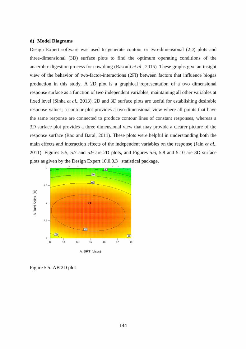
144
d) Model Diagrams
Design Expert software was used to generate contour or two-dimensional (2D) plots and
three-dimensional (3D) surface plots to find the optimum operating conditions of the
anaerobic digestion process for cow dung (Rasouli et al., 2015). These graphs give an insight
view of the behavior of two-factor-interactions (2FI) between factors that influence biogas
production in this study. A 2D plot is a graphical representation of a two dimensional
response surface as a function of two independent variables, maintaining all other variables at
fixed level (Sinha et al., 2013). 2D and 3D surface plots are useful for establishing desirable
response values; a contour plot provides a two-dimensional view where all points that have
the same response are connected to produce contour lines of constant responses, whereas a
3D surface plot provides a three dimensional view that may provide a clearer picture of the
response surface (Rao and Baral, 2011). These plots were helpful in understanding both the
main effects and interaction effects of the independent variables on the response (Jain et al.,
2011). Figures 5.5, 5.7 and 5.9 are 2D plots, and Figures 5.6, 5.8 and 5.10 are 3D surface
plots as given by the Design Expert 10.0.0.3 statistical package.
Figure 5.5: AB 2D plot
Design-Expert® SoftwareFactor Coding: ActualBiogas production rate (l/d)
Design Points75.41
33.01
X1 = A: SRTX2 = B: Total Solids
Actual FactorC: Temp = 35
12 13 14 15 16 17 18
7
7.5
8
8.5
9Biogas production rate (l/d)
A: SRT (days)
B: T
ota
l Solid
s (
%)
55
60
6565
65
70
6
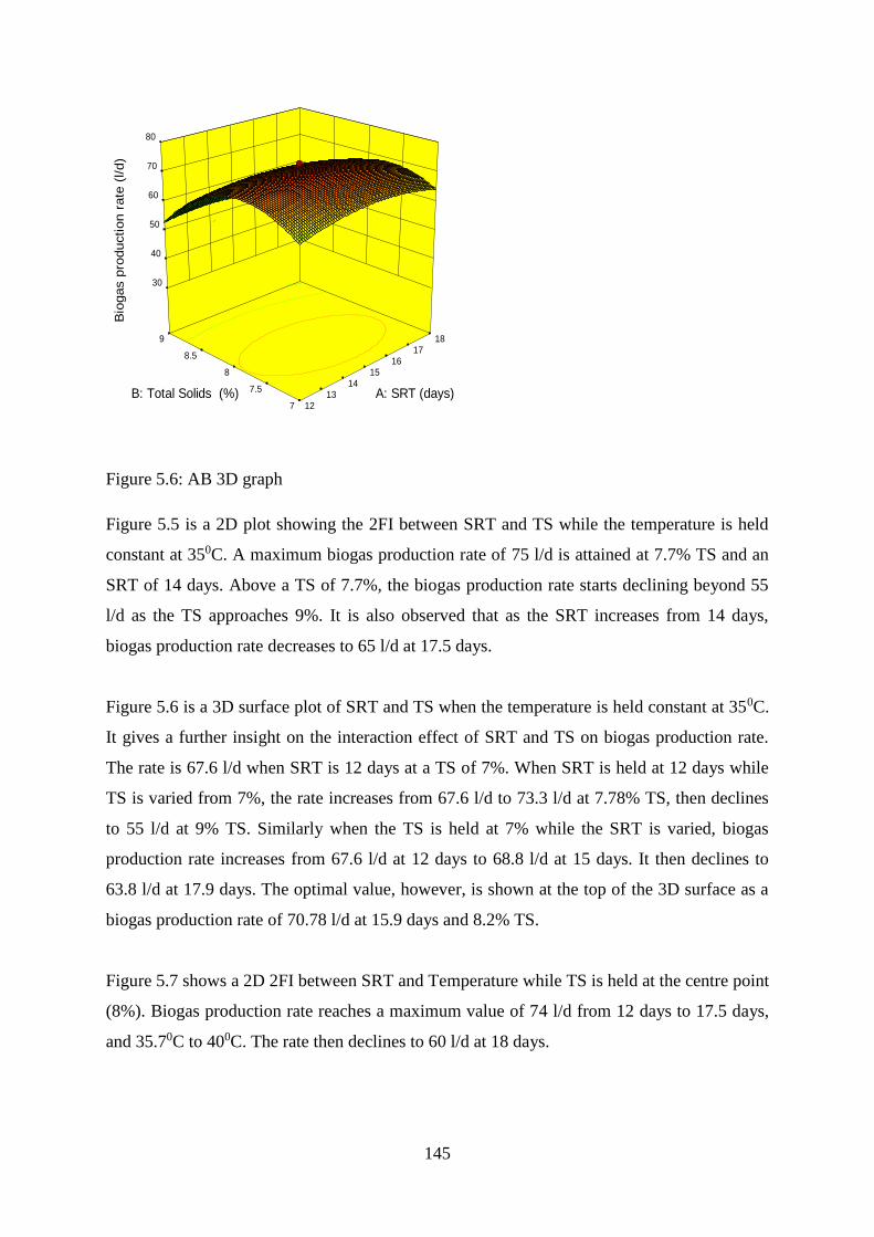
145
Figure 5.6: AB 3D graph
Figure 5.5 is a 2D plot showing the 2FI between SRT and TS while the temperature is held
constant at 350C. A maximum biogas production rate of 75 l/d is attained at 7.7% TS and an
SRT of 14 days. Above a TS of 7.7%, the biogas production rate starts declining beyond 55
l/d as the TS approaches 9%. It is also observed that as the SRT increases from 14 days,
biogas production rate decreases to 65 l/d at 17.5 days.
Figure 5.6 is a 3D surface plot of SRT and TS when the temperature is held constant at 350C.
It gives a further insight on the interaction effect of SRT and TS on biogas production rate.
The rate is 67.6 l/d when SRT is 12 days at a TS of 7%. When SRT is held at 12 days while
TS is varied from 7%, the rate increases from 67.6 l/d to 73.3 l/d at 7.78% TS, then declines
to 55 l/d at 9% TS. Similarly when the TS is held at 7% while the SRT is varied, biogas
production rate increases from 67.6 l/d at 12 days to 68.8 l/d at 15 days. It then declines to
63.8 l/d at 17.9 days. The optimal value, however, is shown at the top of the 3D surface as a
biogas production rate of 70.78 l/d at 15.9 days and 8.2% TS.
Figure 5.7 shows a 2D 2FI between SRT and Temperature while TS is held at the centre point
(8%). Biogas production rate reaches a maximum value of 74 l/d from 12 days to 17.5 days,
and 35.70C to 400C. The rate then declines to 60 l/d at 18 days.
Design-Expert® SoftwareFactor Coding: ActualBiogas production rate (l/d)
Design points above predicted valueDesign points below predicted value75.41
33.01
X1 = A: SRTX2 = B: Total Solids
Actual FactorC: Temp = 35
7
7.5
8
8.5
9
12 13
14 15
16 17
18
30
40
50
60
70
80
Bio
gas p
roduction r
ate
(l/d)
A: SRT (days)B: Total Solids (%)
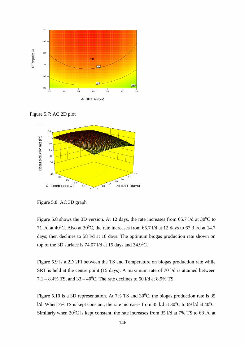
146
Figure 5.7: AC 2D plot
Figure 5.8: AC 3D graph
Figure 5.8 shows the 3D version. At 12 days, the rate increases from 65.7 l/d at 300C to
71 l/d at 400C. Also at 300C, the rate increases from 65.7 l/d at 12 days to 67.3 l/d at 14.7
days; then declines to 58 l/d at 18 days. The optimum biogas production rate shown on
top of the 3D surface is 74.07 l/d at 15 days and 34.90C.
Figure 5.9 is a 2D 2FI between the TS and Temperature on biogas production rate while
SRT is held at the centre point (15 days). A maximum rate of 70 l/d is attained between
7.1 – 8.4% TS, and 33 – 400C. The rate declines to 50 l/d at 8.9% TS.
Figure 5.10 is a 3D representation. At 7% TS and 300C, the biogas production rate is 35
l/d. When 7% TS is kept constant, the rate increases from 35 l/d at 300C to 69 l/d at 400C.
Similarly when 300C is kept constant, the rate increases from 35 l/d at 7% TS to 68 l/d at
Design-Expert® SoftwareFactor Coding: ActualBiogas production rate (l/d)
Design Points75.41
33.01
X1 = A: SRTX2 = C: Temp
Actual FactorB: Total Solids = 8
12 13 14 15 16 17 18
30
32
34
36
38
40Biogas production rate (l/d)
A: SRT (days)
C: T
emp
(deg
C)
6065
70
6
Design-Expert® SoftwareFactor Coding: ActualBiogas production rate (l/d)
Design points above predicted valueDesign points below predicted value75.41
33.01
X1 = A: SRTX2 = C: Temp
Actual FactorB: Total Solids = 8
30
32
34
36
38
40
12 13
14 15
16 17
18
30
40
50
60
70
80
Bio
gas
prod
uctio
n ra
te (
l/d)
A: SRT (days)C: Temp (deg C)
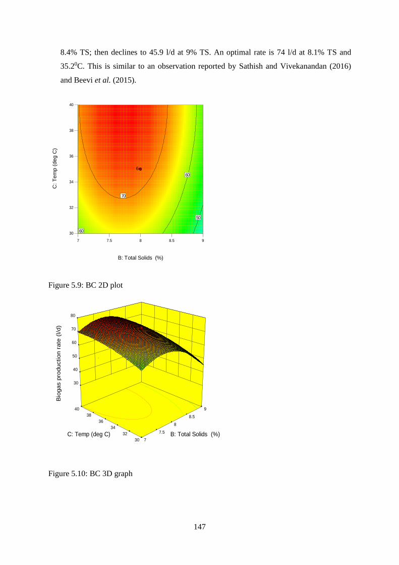
147
8.4% TS; then declines to 45.9 l/d at 9% TS. An optimal rate is 74 l/d at 8.1% TS and
35.20C. This is similar to an observation reported by Sathish and Vivekanandan (2016)
and Beevi et al. (2015).
Figure 5.9: BC 2D plot
Figure 5.10: BC 3D graph
Design-Expert® SoftwareFactor Coding: ActualBiogas production rate (l/d)
Design Points75.41
33.01
X1 = B: Total Solids X2 = C: Temp
Actual FactorA: SRT = 15
7 7.5 8 8.5 9
30
32
34
36
38
40Biogas production rate (l/d)
B: Total Solids (%)
C: T
em
p (
deg C
)
50
60
60
70
6
Design-Expert® SoftwareFactor Coding: ActualBiogas production rate (l/d)
Design points above predicted valueDesign points below predicted value75.41
33.01
X1 = B: Total Solids X2 = C: Temp
Actual FactorA: SRT = 15
30
32
34
36
38
40
7
7.5
8
8.5
9
30
40
50
60
70
80
Bio
gas p
roduction r
ate
(l/d)
B: Total Solids (%)C: Temp (deg C)
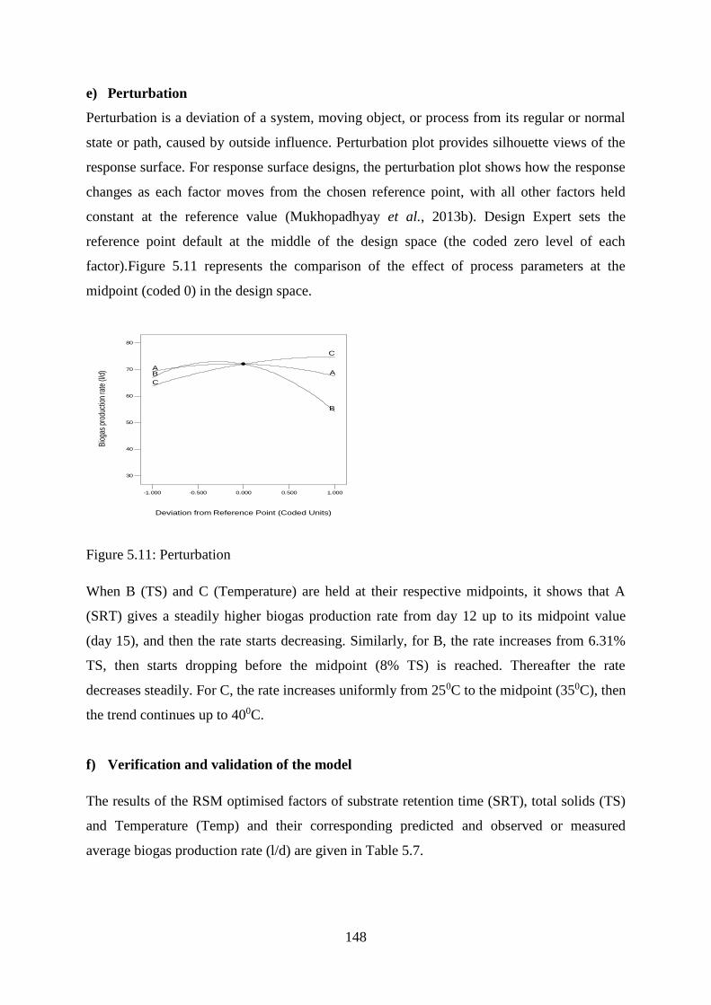
148
e) Perturbation
Perturbation is a deviation of a system, moving object, or process from its regular or normal
state or path, caused by outside influence. Perturbation plot provides silhouette views of the
response surface. For response surface designs, the perturbation plot shows how the response
changes as each factor moves from the chosen reference point, with all other factors held
constant at the reference value (Mukhopadhyay et al., 2013b). Design Expert sets the
reference point default at the middle of the design space (the coded zero level of each
factor).Figure 5.11 represents the comparison of the effect of process parameters at the
midpoint (coded 0) in the design space.
Figure 5.11: Perturbation
When B (TS) and C (Temperature) are held at their respective midpoints, it shows that A
(SRT) gives a steadily higher biogas production rate from day 12 up to its midpoint value
(day 15), and then the rate starts decreasing. Similarly, for B, the rate increases from 6.31%
TS, then starts dropping before the midpoint (8% TS) is reached. Thereafter the rate
decreases steadily. For C, the rate increases uniformly from 250C to the midpoint (350C), then
the trend continues up to 400C.
f) Verification and validation of the model
The results of the RSM optimised factors of substrate retention time (SRT), total solids (TS)
and Temperature (Temp) and their corresponding predicted and observed or measured
average biogas production rate (l/d) are given in Table 5.7.
Design-Expert® SoftwareFactor Coding: ActualBiogas production rate (l/d)
Actual FactorsA: SRT = 15B: Total Solids = 8C: Temp = 35
-1.000 -0.500 0.000 0.500 1.000
30
40
50
60
70
80
AAB
B
C
C
Perturbation
Deviation from Reference Point (Coded Units)
Bio
gas
prod
uctio
n ra
te (l
/d)
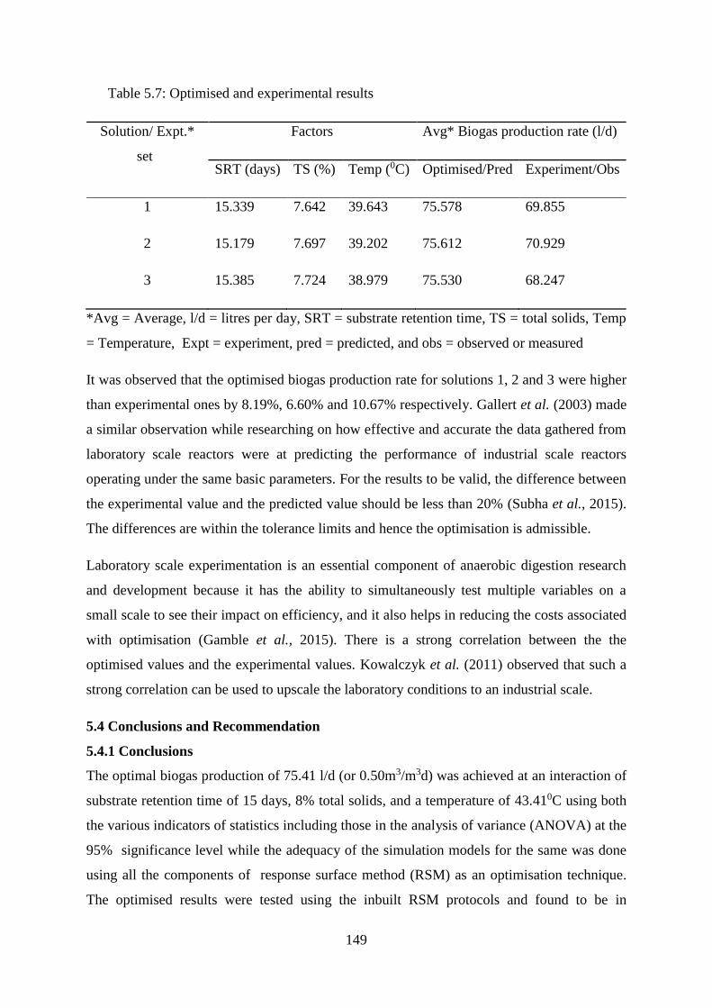
149
Table 5.7: Optimised and experimental results
Solution/ Expt.*
set
Factors Avg* Biogas production rate (l/d)
SRT (days) TS (%) Temp (0C) Optimised/Pred Experiment/Obs
1 15.339 7.642 39.643 75.578 69.855
2 15.179 7.697 39.202 75.612 70.929
3 15.385 7.724 38.979 75.530 68.247
*Avg = Average, l/d = litres per day, SRT = substrate retention time, TS = total solids, Temp
= Temperature, Expt = experiment, pred = predicted, and obs = observed or measured
It was observed that the optimised biogas production rate for solutions 1, 2 and 3 were higher
than experimental ones by 8.19%, 6.60% and 10.67% respectively. Gallert et al. (2003) made
a similar observation while researching on how effective and accurate the data gathered from
laboratory scale reactors were at predicting the performance of industrial scale reactors
operating under the same basic parameters. For the results to be valid, the difference between
the experimental value and the predicted value should be less than 20% (Subha et al., 2015).
The differences are within the tolerance limits and hence the optimisation is admissible.
Laboratory scale experimentation is an essential component of anaerobic digestion research
and development because it has the ability to simultaneously test multiple variables on a
small scale to see their impact on efficiency, and it also helps in reducing the costs associated
with optimisation (Gamble et al., 2015). There is a strong correlation between the the
optimised values and the experimental values. Kowalczyk et al. (2011) observed that such a
strong correlation can be used to upscale the laboratory conditions to an industrial scale.
5.4 Conclusions and Recommendation
5.4.1 Conclusions
The optimal biogas production of 75.41 l/d (or 0.50m3/m3d) was achieved at an interaction of
substrate retention time of 15 days, 8% total solids, and a temperature of 43.410C using both
the various indicators of statistics including those in the analysis of variance (ANOVA) at the
95% significance level while the adequacy of the simulation models for the same was done
using all the components of response surface method (RSM) as an optimisation technique.
The optimised results were tested using the inbuilt RSM protocols and found to be in
150
agreement with the experimental results with a tolerance of 6.6 – 10.7 %, hence they can be
used.
5.4.2 Recommendation
Analysis of variance (ANOVA) and response surface method (RSM) indicators can be used
to determine the optimal points of biogas production when dealing with varying factors; in
this case substrate retention time, total solids and temperature. The same can be applied to a
combination of other parameters (such as pH, organic loading rate, and agitation) that affect
biogas production in the psychrophilic, mesophilic and thermophilic ranges of biomass
digestion temperature for biogas production should be investigated to determine their optimal
level of biogas production rate.
151
References
Ahmad, S. (2009). Techniques for inducing accelerated corrosion of steel in concrete.
Arabian Journal for Science and Engineering, 34(2), 95.
Aslan, N. (2007). Application of response surface methodology and central composite
rotatable design for modeling the influence of some operating variables of a multi-
gravity separator for coal cleaning. Fuel, 86(5-6), 769-776.
Astolfi, A. and Praly, L. (2006). Global complete observability and output-to-state stability
imply the existence of a globally convergent observer. Mathematics of Control,
Signals and Systems, 18(1), 32-65.
Avicenna, Mela, M., Ihsan, S. and Setyobudi, R. (2015). Process Improvement of Biogas
Production from Anaerobic Co-digestion of Cow Dung and Corn Husk. Procedia
Chemistry, 14, 91-100.
Beevi, B. S., Madhu, G. and Sahoo, D. K. (2015). Performance and kinetic study of semi-
dry thermophilic anaerobic digestion of organic fraction of municipal solid waste.
Waste Management, 36, 93-97.
Belwal, T., Dhyani, P., Bhatt, I. D., Rawal, R. S. and Pande, V. (2016). Optimization
extraction conditions for improving phenolic content and antioxidant activity in
Berberis asiatica fruits using response surface methodology (RSM). Food Chemistry,
207, 115-124.
Bezerra, M. A., Santelli, R. E., Oliveira, E. P., Villar, L. S. and Escaleira, L. A. (2008).
Response surface methodology (RSM) as a tool for optimization in analytical
chemistry. Talanta, 76(5), 965-977.
Carley, K. M. and Kamneva, N. Y. (2004). A network optimization approach for improving
organizational design. Retrieved from Carnigie-Mellon Univ Pittsburg PA.
Cheng, H., Wang, Y. J., Edwards, R. L., An, Z., Wu, J., Shen, C. and Dorale, J. A.
(2001). A high-resolution absolute-dated late Pleistocene monsoon record from Hulu
Cave, China. Science, 294(5550), 2345-2348. doi:10.1126/science.1064618
Christakos, S., Dhawan, P., Verstuyf, A., Verlinden, L. and Carmeliet, G. (2015). Vitamin
D: metabolism, molecular mechanism of action, and pleiotropic effects.
Physiological Reviews, 96(1), 365-408.
Derringer, G. and Suich, R. (1980). Simultaneous optimization of several response variables.
Journal of Quality Technology, 12(4), 214-219.
152
Feng, J., Zhang, J., Zhang, J., He, Y., Zhang, R., Chen, C. and Liu, G. (2017). Enhanced
methane production of vinegar residue by response surface methodology (RSM).
Amb Express, 7(1), 89.
Ferrer, I., Garfí, M., Uggetti, E., Ferrer-Martí, L., Calderon, A. and Vel, E. (2011). Biogas
production in low-cost household digesters at t he Peruvian Andes. Biomass and
Bioenergy. doi:10.1016/j.biombioe.2010.12.036.
Gallert, C., Henning, A. and Winter, J. (2003). Scale-up of anaerobic digestion of the
biowaste fraction from domestic wastes. Water Resources(37), 1433-1441.
Gamble, K. J., Houser, J. B., Hambourger, M. S. and Hoepfl, M. C. (2015). Anaerobic
Digestion from the Laboratory to the Field: An Experimental Study into the
Scalability of Anaerobic Digestion. Paper presented at the ASEE Southeast Section
Appalachian State University.
Jain, M., Garg, V. and Kadrivelu, K. (2011). Investigation of Cr(VI) adsorption onto
Chemically treated Helianthus annus: optimization using Response Surface
Methodology. Bioresource Technology, 102, 600-605.
Jiménez, J., Guardia-Puebla, Y., Romero-Romero, O., Cisneros-Ortiz, M., Guerra, G.,
Morgan-Sagastume, J. and Noyola, A. (2014). Methanogenic activity optimization
using the response surface methodology, during the anaerobic co-digestion of
agriculture and industrial wastes Microbial community diversity. Biomass and
Bioenergy, 71, 84-97.
Kang, J., Kim, S. and Moon, B. (2016). Optimization by response surface methodology of
Lutein recovery from paprika leaves using accelerated solvent extraction. Food
Chemistry, 205, 140-145.
Khoobbakht, G., Najafi, G., Karimi, M. and Akram, A. (2016). Optimization of operating
factors and blended levels of diesel, biodiesel and ethanol fuels to minimize exhaust
emissions of diesel engine using response surface methodology. Applied Thermal
Engineering, 99, 1006-1017.
Kong, Z., Li, M., Chen, J., Bao, Y., Fan, B., Francis, F. and Dai, X. (2016). Processing
factors of triadimefon and triadimenol in barley brewing based on response surface
methodology. Food Control, 64, 81-86.
Kousha, M., Tavakoli, S., Daneshvar, E., Vazirzadeh, A. and Bhatnagar, A. (2015). Central
Composite design optimization of Acid Blue 25 dye biosorption using shrimp shell
biomass. Journal of Molecular Liquids, 207, 266–273.
153
Kowalczyk, A., Schwede, S., Gerber, M. and Span, R. (2011). Scale up of laboratory scale
to industrial scale biogas plants. Paper presented at the World Renewable Energy
Congress, Sweden.
Leiviskä, K. (2013). Introduction to Experiment Design. University of Oulu: Control
Engineering Laboratory.
Mao, C., Feng, Y., Wang, X. and Ren, G. (2015). Review on research achievements of
biogas from anaerobic digestion. Renewable and Sustainable Energy Reviews, 45,
540-555.
Mason, R., Gunst, R. and Hess, J. (2003). Statistical design and analysis of experiments,
eight applications to engineering and science (2nd ed.). New York: Wiley.
Montgomery, D. C., Runger, G. C. and Hubele, N. F. (2009). Engineering Statistics: John
Wiley and Sons.
Moog, H., Avilla, A., Agpaoa, E., Valenzuela, F. and Concepcion, F. (1997). Promotion
and utilization of polyethylene bio-digester in small-holder farming systems in the
Philippines. Livestock Research for Rural Development, 9(2).
Mukhopadhyay, D., Sarkar, J. P. and Dutta, S. (2013a). Optimization of process factors for
the efficient generation of biogas from raw vegetable wastes under the direct
influence of plastic materials using Taguchi methodology. Desalination and Water
Treatment, 51(13), 2781-2790.
Mukhopadhyay, D., Sarkar, J. P. and Dutta, S. (2013b). Optimization of process parameters
for the economical generation of biogas from raw vegetable wastes under the positive
influence of plastic materials using response surface methodology. Journal of
Biochemical Technology, 4(1), 549-553.
Nanduri, J., Yuan, G., Kumar, G. K., Semenza, G. L. and Prabhakar, N. R. (2008).
Transcriptional responses to intermittent hypoxia. Respiratory Physiology and
Neurobiology, 164(1-2), 277-281.
Niladevi, K., Sukumaran, R. K., Jacob, N., Anisha, G. and Prema, P. (2009). Optimization
of laccase production from a novel strain—Streptomyces psammoticus using
response surface methodology. Microbiological Research, 164(1), 105-113.
Nyaanga, D. (2011). Performance of Tropical Biogas. Paper presented at the Egerton
University International Conference, Egerton University, Kenya.
Pannucharoenwong, N. (2018). Optimization of Bio-Methane Production from Mesophilic
Anaerobic Co-digestion of Pig Manure and Vegetable Residue. International Journal
of Applied Engineering Research, 13(4), 1988-1995.
154
Quanhong, L. and Caili, F. (2005). Application of response surface methodology for
extraction optimization of germinant pumpkin seeds protein. Food Chemistry, 92(4),
701-706.
Rao, P. V. and Baral, S. S. (2011). Experimental design of mixture for the anaerobic co-
digestion of sewage sludge. Chemical Engineering Journal, 172(2-3), 977-986.
Rasouli, J., Ciric, B., Imitola, J., Gonnella, P., Hwang, D., Mahajan, K., Mari, E. R.,
Safavi, F., Leist, T. P. and Zhang, G.-X. (2015). Expression of GM-CSF in T cells
is increased in multiple sclerosis and suppressed by IFN-β therapy. The Journal of
Immunology, 194(11), 5085-5093.
Reungsang, A., Sakchai, P. and Sureewan, S. (2012). Optimization of key factors affecting
Methane production from acidic effluent coming from the sugarcane juice Hydrogen
fermentation process. Energies, 5, 4746-4757;. doi:10.3390/en5114746
Saleh, A., Kamarudin, E., Yaacob, A., Yussof, A. and Abdullah, M. (2012). Optimization
of biomethane production by anaerobic digestion of palm oil mill effluent using
response surface methodology. Asia-Pacific Journal of Chemical Engineering(7),
353-360.
Sathish, S. and Vivekanandan, S. (2016). Parametric optimization for floating drum
anaerobic bio-digester using Response Surface Methodology and Artificial Neural
Network. Alexandria Engineering Journal, 55(4), 3297-3307.
Sinha, K., Chowdhury, S., Saha, P. D. and Datta, S. (2013). Modeling of microwave-
assisted extraction of natural dye from seeds of Bixa orellana (Annatto) using
response surface methodology (RSM) and artificial neural network (ANN). Industrial
Crops and Products, 41, 165-171.
Subha, B., Song, Y. C. and Woo, J. H. (2015). Optimization of biostimulant for
bioremediation of contaminated coastal sediment by response surface methodology
(RSM) and evaluation of microbial diversity by pyrosequencing. Marine Pollution
Bulletin, 98(1-2), 235-246.
Šumić, Z., Vakula, A., Tepić, A., Čakarević, J., Vitas, J. and Pavlić, B. (2016). Modeling
and optimization of red currants vacuum drying process by response surface
methodology (RSM). Food Chemistry, 203, 465-475.
Taguchi, G. (1986). Introduction to Quality Engineering. UNIPUB, White Plains, NY: Asian
Productivity Organization.
Taguchi, G. (1987). System of Experimental Design: Engineering Methods to Optimize
Quality and Minimize Cost. White Plains, NY: UNIPUB/Kraus International.
155
Thanwised, P., Wirojanagud, W. and Reungsang, A. (2012). Effect of hydraulic retention
time on hydrogen production and chemical oxygen demand removal from tapioca
wastewater using anaerobic mixed cultures in anaerobic baffled reactor (ABR).
International Journal of Hydrogen Energy, 37(20), 15503-15510.
Zaroual, Z., Chaair, H., Essadki, A., El Ass, K. and Azzi, M. (2009). Optimizing the
removal of trivalent chromium by electrocoagulation using experimental design.
Chemical Engineering Journal, 148(2-3), 488-495.
156
CHAPTER SIX
GENERAL DISCUSSION, CONCLUSIONS AND RECOMMENDATIONS
6.1 General Discussion
The effect of total solids on biogas production rate was investigated in a fixed dome
laboratory digester of 0.15m3. Data was collected at a temperature of 350C for total solid
levels of 6 – 10%. There was no production of biogas from day 1 to day 5 for total solids of
7% and 8%, from day 1 to day 6 for total solids of 6% and 9%, and from day 1 to day 7 for
total solids of 10%. In this phase, three main processes are taking place namely hydrolysis,
acidogenesis, and acetogenesis. Hydrolysis is where proteins, carbohydrates, and fats are
being broken down into amino acids, simple sugars, and long chain fatty acids, respectively
by the hydrolytic bacteria. Acidogenesis is a process during which simple sugars and amino
acids resulting from hydrolysis are degraded to a number of simpler products such as volatile
fatty acids including propionic acid, butyric acid, and acetic acid. Acetogenesis is the
degradation of higher organic acids formed in acidogenesis to yield acetic acid, carbon
dioxide and hydrogen. This intermediate conversion is crucial for the successful production
of biogas.
In the second phase there was an exponential production of biogas from day 5 up to day 11
and day 12. During this phase, the process of methanogenesis was taking place. The
fermentation products such as acetate, hydrogen and carbon dioxide were converted to
methane and carbon dioxide by methanogenic archaea.
In the third phase there was a steady decline in biogas production from day 11 to day 15 due
to stationary phase of microbial growth. The methanogenic bacteria died due to the depletion
of carbon in the substrate. It was generally observed that the highest biogas production rate
was achieved by 8% total solids (0.68m3/m3d) on day 11, followed by 7%, 9%, 6%, and lastly
10% in a descending order. Anaerobic digestion process increased steadily from total solids
of 6% to 8%. At low solids, aceticlastic methanogens called methanosarcina play an
important role, followed by hydrogenotrophic methanoculleus and methanomicrobiales
species. As the total solids increase from 8% to 10%, the biogas production rate declines
steadily. Increasing the total solids means a higher applied organic loading rate and more
volatile solids for microorganisms which results in higher volatile fatty acid concentrations.
A marginal increase in the percentage of total solids results in a geometric increase in the
volume of biogas produced, suggesting therefore that a continual increase in the percentage
157
of total solids at some point becomes immaterial to the increasing volume of biogas
produced. This is possible because when the percentage of total solids increases, the amount
of water decreases. This reduces the level of microbial activity which then affects the yield of
biogas, particularly at higher values of the TS%.
Effect of mesophilic temperature was investigated. The experiment was run at a constant total
solid of 8%. The levels of temperature were 250C, 300C, 350C, 400C and 450C. The results
exhibited three phases. The first phase ranges from day 1 to day 5 for temperatures 300C to
450C, and day 1 to day 8 for 250C; no biogas was produced. During this phase, hydrolysis,
acidogenesis, and acetogenesis were taking place. In the second phase, there was an
exponential biogas production from day 5 to day 11, and day 12 for all the temperatures. The
highest biogas production occurred at 400C (0.807 m3/m3d on day 12) followed by 350C,
300C, 450C, and lastly 250C. The third phase started from day 12 onwards. Biogas production
dropped drastically because the feed material was depleted leading to the death of mesophiles
in the batch reactor.
There are three temperature ranges within which anaerobic digestion of a substrate can take
place. Psychrophilic temperature range lies below 200C, mesophilic temperature range
between 300C and 400C, and thermophilic temperature range from 500C to 750C. At the
beginning, biogas production was low due to very little microbial activity because the
psychrophilic bacteria had died off while the mesophiles were regenerating to take over the
process of methanogenesis. There was a steady increase in biogas production in the
mesophilic range between 300C (0.346m3/m3d), 350C (0.487m3/m3d), and 400C
(0.528m3/m3d) because of the increased regeneration of mesophiles. At 450C, the biogas
production rate is lower than expected. This is so because the enzymes of mesophiles are
denatured leading to their death. The rate of bacteriological methane production increases
with temperature as well as the amount of free ammonia. The accumulation of ammonia
inhibited biogas production.
The effect of substrate retention time on biogas production rate was investigated by running
the experiment at total solids of 8% and a temperature of 350C. There was no biogas
production from day 1 to day 5. This was attributed to three processes of anaerobic digestion
taking place namely hydrolysis, acidogenesis and acetogenesis, respectively.
158
Methanogenesis marks the final stage of anaerobic digestion, where accessible intermediates
are consumed by methanogenic bacteria to produce methane. Production of biogas starts from
day 5 and increases steadily to day 11 (0.68m3/m3d). However, it was noticed that biogas
production stagnated from day 7 to day 8. This can be attributed to excessive partial pressure
of hydrogen produced by acetogenesis that deleted acetogenic microorganisms. But due to
the presence of hydrogenotrophic methanogens, especially the methanosarcina species,
hydrogen was able to be rapidly consumed while maintaining partial pressure at a level
favourable to acetogenesis by creating an exergonic reaction. During the stagnation period,
methanosarcina species, which tend to be robust and are capable of withstanding ammonia,
sodium, and acetate concentrations in addition to pH shocks at levels that would otherwise be
detrimental to other methanogenic bacteria, kept on producing biogas. Consequently, the
steady production came on course from day 8 to day 11.
From day 11 onwards, biogas production started declining from 0.68 to 0.418m3/m3d on day
15. This was caused by the depletion of nutrients in the substrate and the gradual death of the
methanogens.
An evaluation of some existing biogas production prediction models was done. The models
included the Plug Flow, Chen and Hashimoto, Scoff and Minnot, Low Temperature Lagoon
Digester, and Toprak. The first three were found to be applicable to semi-continuously-fed
and continuously-fed digesters. The last two models were found to suit the batch-fed
digesters, and hence they were evaluated in this work. A test for the goodness of fit between
the experimental data and the predicted values from the models was done. The tools for
testing included the coefficient of determination (R2), root mean square error (RMSE), and
Chi square (X2). A Fixed-dome-lab Temperature model was developed and validated.
A goodness of fit is achieved when the R2 value is as close as possible to 1, while the RMSE
and X2 should tend to zero. A statistical analysis showed that the best goodness of fit was
attained by the Fixed-dome-lab Temperature model having R2 of 0.9732, RMSE of 0.0716,
and X2 of 0.0064.
Optimisation was done by investigating the interaction effects of total solids, temperature,
and substrate retention time on biogas production in a batch bioreactor. Central composite
design (CCD) of Response Surface Methodology was used to design the experiment.
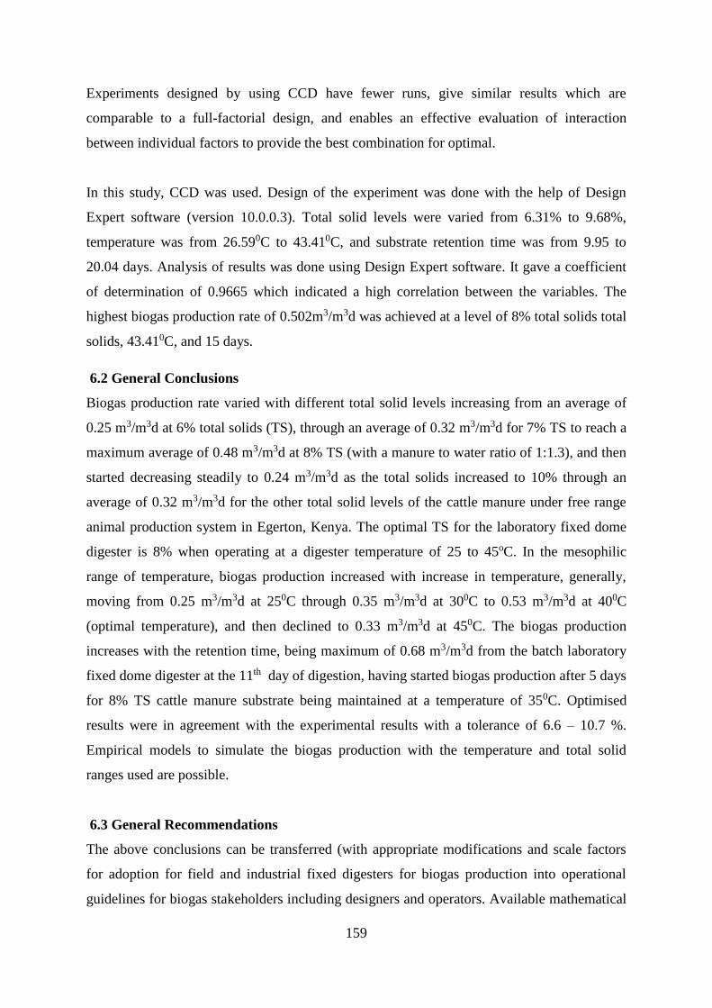
159
Experiments designed by using CCD have fewer runs, give similar results which are
comparable to a full-factorial design, and enables an effective evaluation of interaction
between individual factors to provide the best combination for optimal.
In this study, CCD was used. Design of the experiment was done with the help of Design
Expert software (version 10.0.0.3). Total solid levels were varied from 6.31% to 9.68%,
temperature was from 26.590C to 43.410C, and substrate retention time was from 9.95 to
20.04 days. Analysis of results was done using Design Expert software. It gave a coefficient
of determination of 0.9665 which indicated a high correlation between the variables. The
highest biogas production rate of 0.502m3/m3d was achieved at a level of 8% total solids total
solids, 43.410C, and 15 days.
6.2 General Conclusions
Biogas production rate varied with different total solid levels increasing from an average of
0.25 m3/m3d at 6% total solids (TS), through an average of 0.32 m3/m3d for 7% TS to reach a
maximum average of 0.48 m3/m3d at 8% TS (with a manure to water ratio of 1:1.3), and then
started decreasing steadily to 0.24 m3/m3d as the total solids increased to 10% through an
average of 0.32 m3/m3d for the other total solid levels of the cattle manure under free range
animal production system in Egerton, Kenya. The optimal TS for the laboratory fixed dome
digester is 8% when operating at a digester temperature of 25 to 45oC. In the mesophilic
range of temperature, biogas production increased with increase in temperature, generally,
moving from 0.25 m3/m3d at 250C through 0.35 m3/m3d at 300C to 0.53 m3/m3d at 400C
(optimal temperature), and then declined to 0.33 m3/m3d at 450C. The biogas production
increases with the retention time, being maximum of 0.68 m3/m3d from the batch laboratory
fixed dome digester at the 11th day of digestion, having started biogas production after 5 days
for 8% TS cattle manure substrate being maintained at a temperature of 350C. Optimised
results were in agreement with the experimental results with a tolerance of 6.6 – 10.7 %.
Empirical models to simulate the biogas production with the temperature and total solid
ranges used are possible.
6.3 General Recommendations
The above conclusions can be transferred (with appropriate modifications and scale factors
for adoption for field and industrial fixed digesters for biogas production into operational
guidelines for biogas stakeholders including designers and operators. Available mathematical
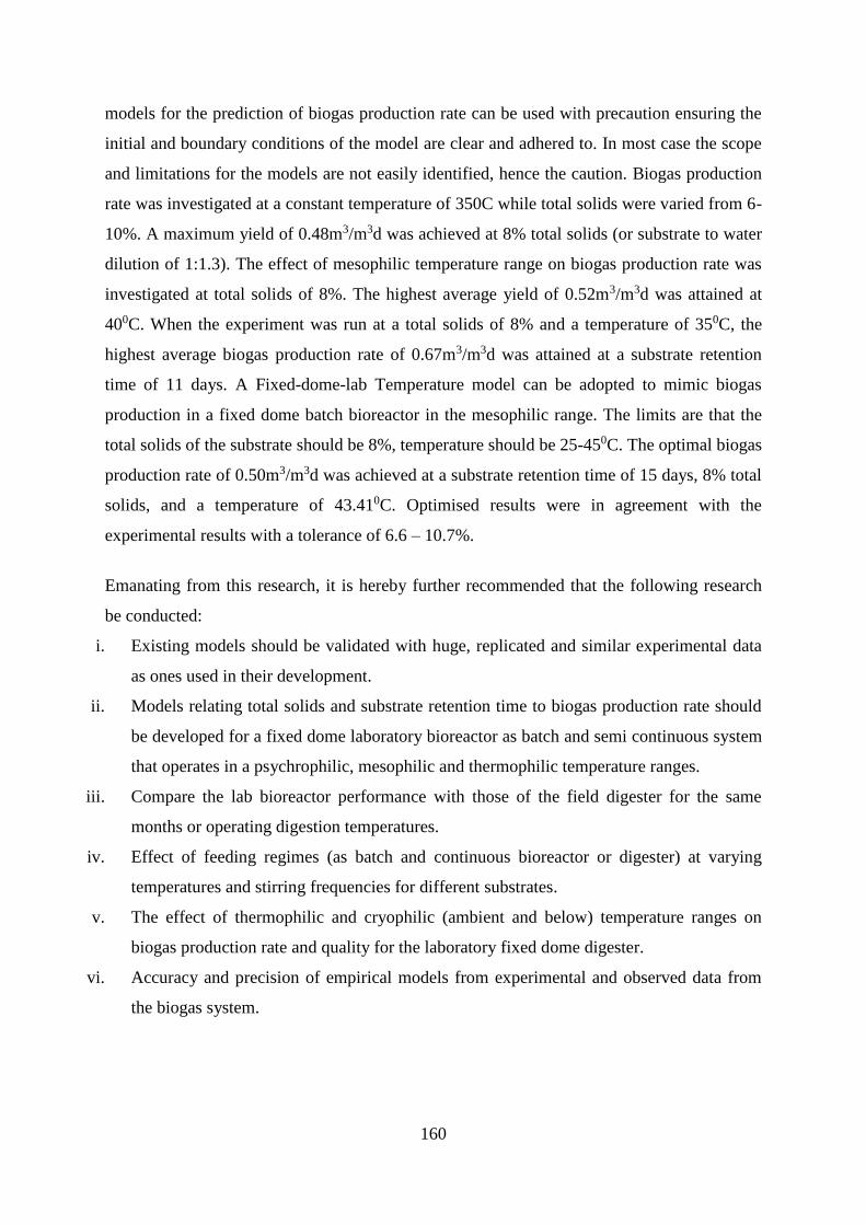
160
models for the prediction of biogas production rate can be used with precaution ensuring the
initial and boundary conditions of the model are clear and adhered to. In most case the scope
and limitations for the models are not easily identified, hence the caution. Biogas production
rate was investigated at a constant temperature of 350C while total solids were varied from 6-
10%. A maximum yield of 0.48m3/m3d was achieved at 8% total solids (or substrate to water
dilution of 1:1.3). The effect of mesophilic temperature range on biogas production rate was
investigated at total solids of 8%. The highest average yield of 0.52m3/m3d was attained at
400C. When the experiment was run at a total solids of 8% and a temperature of 350C, the
highest average biogas production rate of 0.67m3/m3d was attained at a substrate retention
time of 11 days. A Fixed-dome-lab Temperature model can be adopted to mimic biogas
production in a fixed dome batch bioreactor in the mesophilic range. The limits are that the
total solids of the substrate should be 8%, temperature should be 25-450C. The optimal biogas
production rate of 0.50m3/m3d was achieved at a substrate retention time of 15 days, 8% total
solids, and a temperature of 43.410C. Optimised results were in agreement with the
experimental results with a tolerance of 6.6 – 10.7%.
Emanating from this research, it is hereby further recommended that the following research
be conducted:
i. Existing models should be validated with huge, replicated and similar experimental data
as ones used in their development.
ii. Models relating total solids and substrate retention time to biogas production rate should
be developed for a fixed dome laboratory bioreactor as batch and semi continuous system
that operates in a psychrophilic, mesophilic and thermophilic temperature ranges.
iii. Compare the lab bioreactor performance with those of the field digester for the same
months or operating digestion temperatures.
iv. Effect of feeding regimes (as batch and continuous bioreactor or digester) at varying
temperatures and stirring frequencies for different substrates.
v. The effect of thermophilic and cryophilic (ambient and below) temperature ranges on
biogas production rate and quality for the laboratory fixed dome digester.
vi. Accuracy and precision of empirical models from experimental and observed data from
the biogas system.
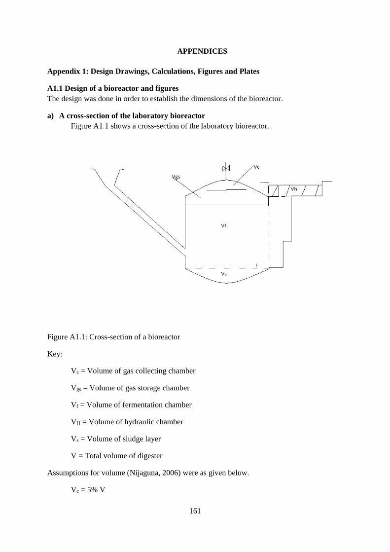
161
APPENDICES
Appendix 1: Design Drawings, Calculations, Figures and Plates
A1.1 Design of a bioreactor and figures
The design was done in order to establish the dimensions of the bioreactor.
a) A cross-section of the laboratory bioreactor
Figure A1.1 shows a cross-section of the laboratory bioreactor.
Figure A1.1: Cross-section of a bioreactor
Key:
Vc = Volume of gas collecting chamber
Vgs = Volume of gas storage chamber
Vf = Volume of fermentation chamber
VH = Volume of hydraulic chamber
Vs = Volume of sludge layer
V = Total volume of digester
Assumptions for volume (Nijaguna, 2006) were as given below.
Vc = 5% V
162
Vs = 15% V
Vgs + Vf = 80% V
Vgs = VH
Vgs = 0.5 ( Vgs + Vf + Vs ) K
V = Vc+ Vgs + Vf + Vs
where K = Gas production rate in m3 per m3 of digester volume per day.
For Bangladesh K = 0.4 m3/m3d (Moog et al., 1997).
b) Geometry of the bioreactor
Figure A1.2: Geometry of the reactor
Assumptions of geometrical dimensions (Nijaguna, 2006).
𝐷 = 1.3078𝑉1 3⁄
𝑉1 = 0.0827𝐷3, 𝑉2 = 0.05011𝐷3, 𝑉3 = 0.3142𝐷3
𝑅1 = 0.725𝐷, 𝑅2 = 1.0625𝐷
𝑓1 =𝐷
5 , 𝑓2 =
𝐷
8
𝑆1 = 0.911𝐷2, 𝑆2 = 0.8345𝐷2
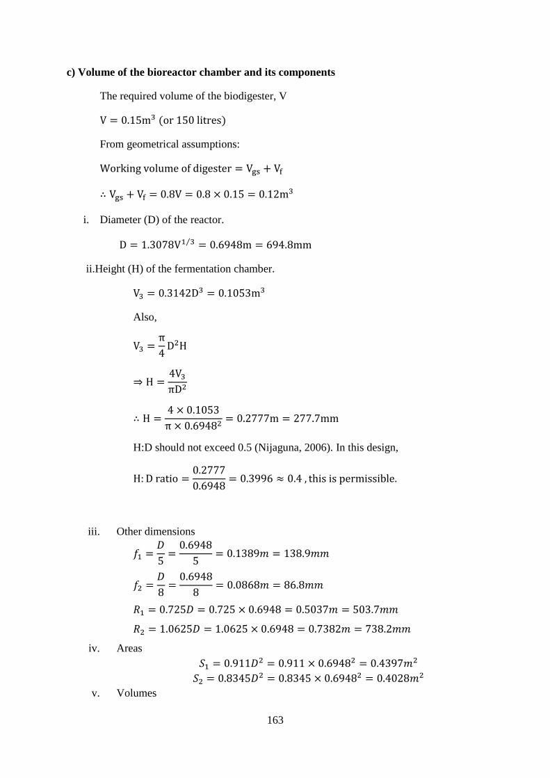
163
c) Volume of the bioreactor chamber and its components
The required volume of the biodigester, V
V = 0.15m3 (or 150 litres)
From geometrical assumptions:
Working volume of digester = Vgs + Vf
∴ Vgs + Vf = 0.8V = 0.8 × 0.15 = 0.12m3
i. Diameter (D) of the reactor.
D = 1.3078V1 3⁄ = 0.6948m = 694.8mm
ii.Height (H) of the fermentation chamber.
V3 = 0.3142D3 = 0.1053m3
Also,
V3 =π
4D2H
⇒ H =4V3
πD2
∴ H =4 × 0.1053
π × 0.69482= 0.2777m = 277.7mm
H:D should not exceed 0.5 (Nijaguna, 2006). In this design,
H: D ratio =0.2777
0.6948= 0.3996 ≈ 0.4 , this is permissible.
iii. Other dimensions
𝑓1 =𝐷
5=
0.6948
5= 0.1389𝑚 = 138.9𝑚𝑚
𝑓2 =𝐷
8=
0.6948
8= 0.0868𝑚 = 86.8𝑚𝑚
𝑅1 = 0.725𝐷 = 0.725 × 0.6948 = 0.5037𝑚 = 503.7𝑚𝑚
𝑅2 = 1.0625𝐷 = 1.0625 × 0.6948 = 0.7382𝑚 = 738.2𝑚𝑚
iv. Areas
𝑆1 = 0.911𝐷2 = 0.911 × 0.69482 = 0.4397𝑚2
𝑆2 = 0.8345𝐷2 = 0.8345 × 0.69482 = 0.4028𝑚2
v. Volumes
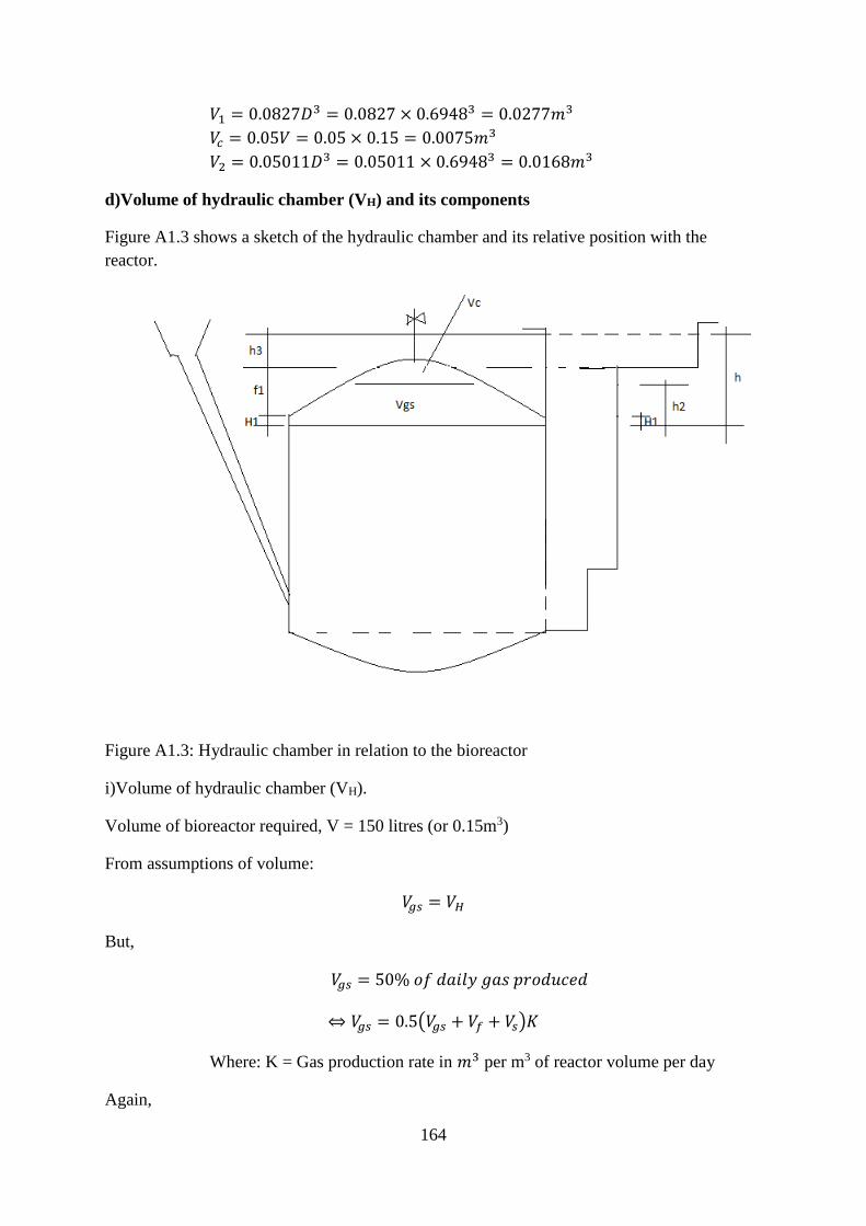
164
𝑉1 = 0.0827𝐷3 = 0.0827 × 0.69483 = 0.0277𝑚3
𝑉𝑐 = 0.05𝑉 = 0.05 × 0.15 = 0.0075𝑚3
𝑉2 = 0.05011𝐷3 = 0.05011 × 0.69483 = 0.0168𝑚3
d)Volume of hydraulic chamber (VH) and its components
Figure A1.3 shows a sketch of the hydraulic chamber and its relative position with the
reactor.
Figure A1.3: Hydraulic chamber in relation to the bioreactor
i)Volume of hydraulic chamber (VH).
Volume of bioreactor required, V = 150 litres (or 0.15m3)
From assumptions of volume:
𝑉𝑔𝑠 = 𝑉𝐻
But,
𝑉𝑔𝑠 = 50% 𝑜𝑓 𝑑𝑎𝑖𝑙𝑦 𝑔𝑎𝑠 𝑝𝑟𝑜𝑑𝑢𝑐𝑒𝑑
⇔ 𝑉𝑔𝑠 = 0.5(𝑉𝑔𝑠 + 𝑉𝑓 + 𝑉𝑠)𝐾
Where: K = Gas production rate in 𝑚3 per m3 of reactor volume per day
Again,
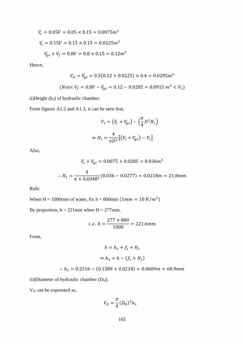
165
𝑉𝑐 = 0.05𝑉 = 0.05 × 0.15 = 0.0075𝑚3
𝑉𝑠 = 0.15𝑉 = 0.15 × 0.15 = 0.0225𝑚3
𝑉𝑔𝑠 + 𝑉𝑓 = 0.8𝑉 = 0.8 × 0.15 = 0.12𝑚3
Hence,
𝑉𝐻 = 𝑉𝑔𝑠 = 0.5(0.12 + 0.0225) × 0.4 = 0.0285𝑚3
(𝑁𝑜𝑡𝑒: 𝑉𝑓 = 0.8𝑉 − 𝑉𝑔𝑠 = 0.12 − 0.0285 = 0.0915 𝑚3 < 𝑉3)
ii)Height (h3) of hydraulic chamber.
From figures A1.2 and A1.3, it can be seen that,
𝑉1 = (𝑉𝑐 + 𝑉𝑔𝑠) − (𝜋
4𝐷2𝐻1)
⇒ 𝐻1 =4
𝜋𝐷2[(𝑉𝑐 + 𝑉𝑔𝑠) − 𝑉1]
Also,
𝑉𝑐 + 𝑉𝑔𝑠 = 0.0075 + 0.0285 = 0.036𝑚3
∴ 𝐻1 =4
𝜋 × 0.69482(0.036 − 0.0277) = 0.0218𝑚 = 21.8𝑚𝑚
Rule:
When H = 1000mm of water, fix h = 800mm (1𝑚𝑚 = 10 𝑁 𝑚2⁄ )
By proportion, h = 221mm when H = 277mm,
𝑖. 𝑒. ℎ =277 × 800
1000= 221.6𝑚𝑚
From,
ℎ = ℎ3 + 𝑓1 + 𝐻1
⇒ ℎ3 = ℎ − (𝑓1 + 𝐻1)
∴ ℎ3 = 0.2216 − (0.1389 + 0.0218) = 0.0609𝑚 = 60.9𝑚𝑚
iii)Diameter of hydraulic chamber (DH).
VH can be expressed as,
𝑉𝐻 =𝜋
4(𝐷𝐻)2ℎ3
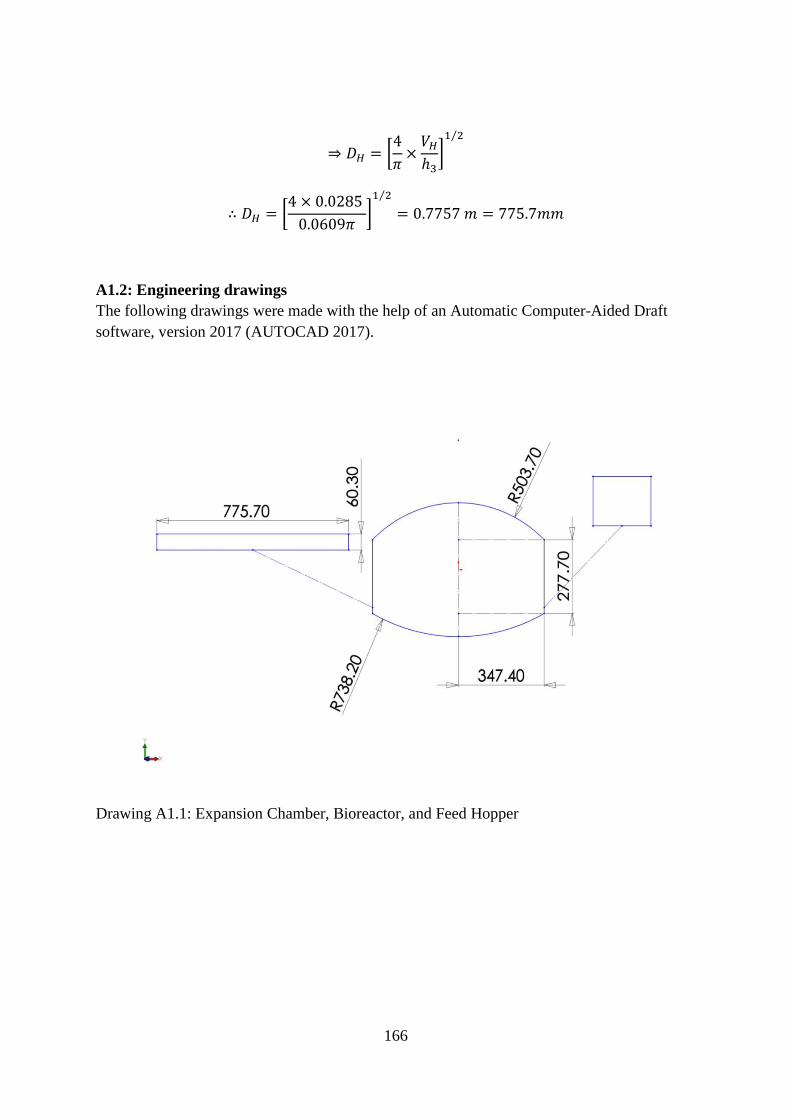
166
⇒ 𝐷𝐻 = [4
𝜋×
𝑉𝐻
ℎ3]
1 2⁄
∴ 𝐷𝐻 = [4 × 0.0285
0.0609𝜋]
1 2⁄
= 0.7757 𝑚 = 775.7𝑚𝑚
A1.2: Engineering drawings
The following drawings were made with the help of an Automatic Computer-Aided Draft
software, version 2017 (AUTOCAD 2017).
Drawing A1.1: Expansion Chamber, Bioreactor, and Feed Hopper
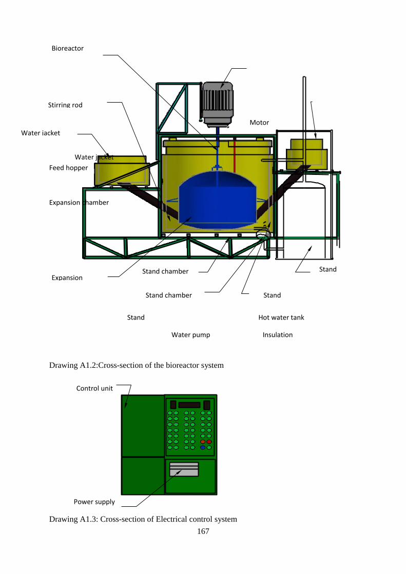
167
Motor
Water jacket
Feed hopper
Expansion chamber
Stand Hot water tank
Water pump Insulation
Drawing A1.2:Cross-section of the bioreactor system
Control unit
Power supply
Drawing A1.3: Cross-section of Electrical control system
Bioreactor
Stirring rod
Water jacket
Expansion
Stand chamber
Stand chamber Stand
Stand
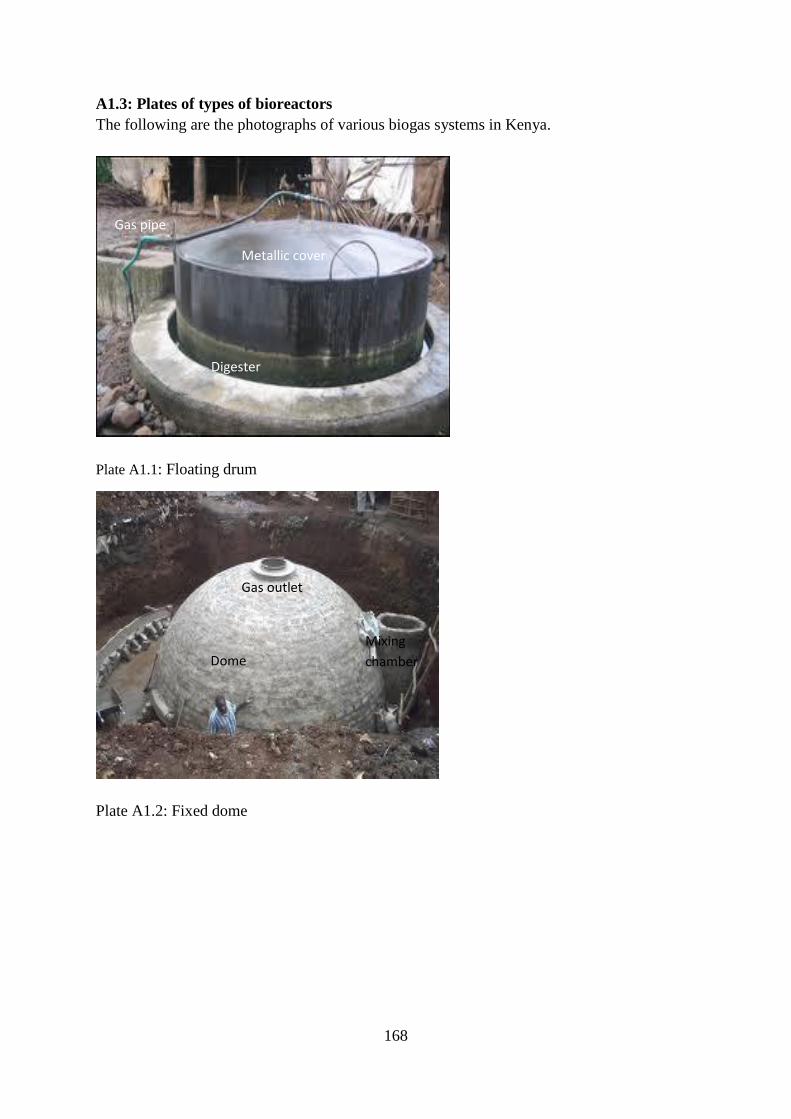
168
A1.3: Plates of types of bioreactors
The following are the photographs of various biogas systems in Kenya.
Plate A1.1: Floating drum
Plate A1.2: Fixed dome
Metallic cover
Digester
Gas pipe
Dome
Gas outlet
Mixing
chamber
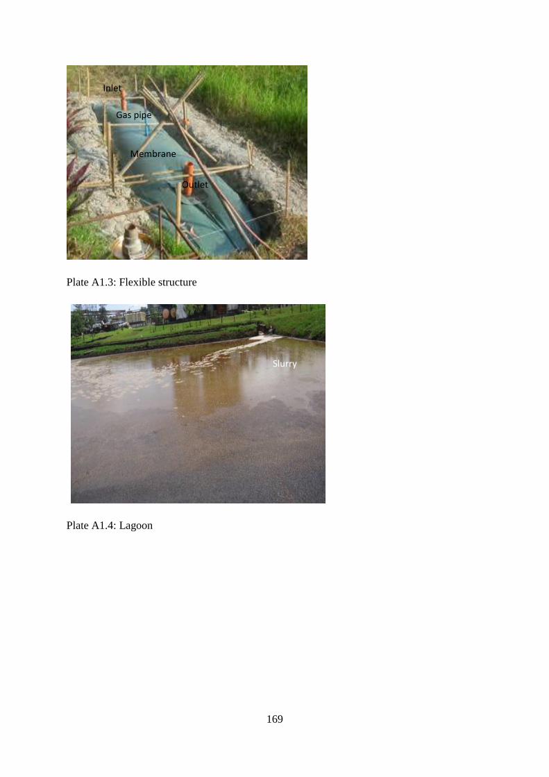
169
Plate A1.3: Flexible structure
Plate A1.4: Lagoon
Gas pipe
Inlet
Outlet
Membrane
Slurry
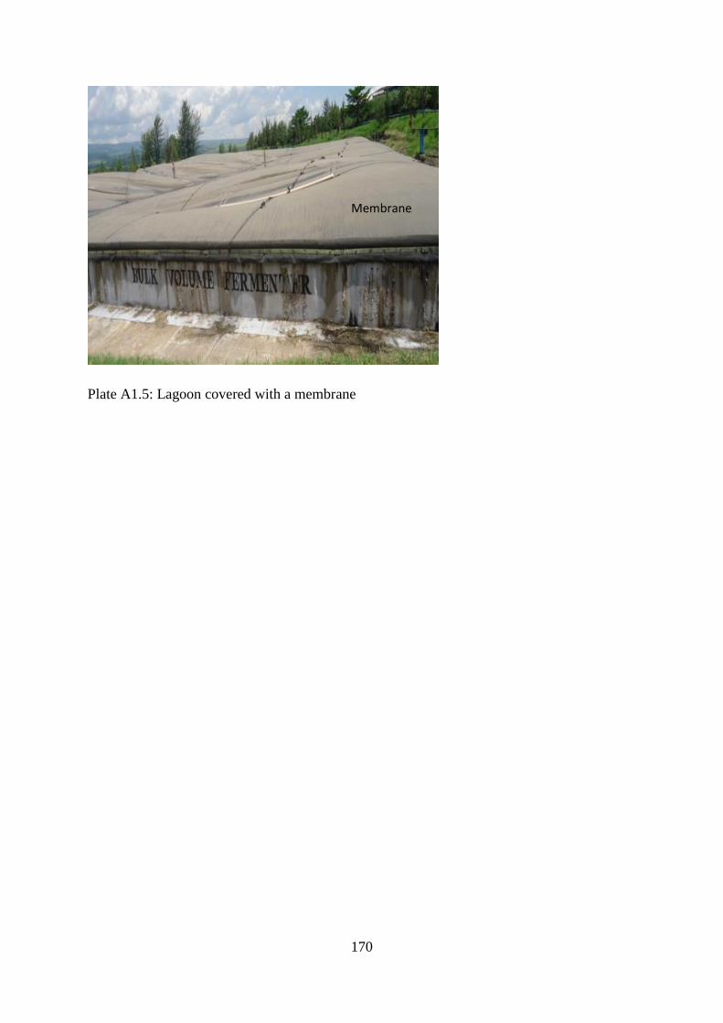
170
Plate A1.5: Lagoon covered with a membrane
Membrane
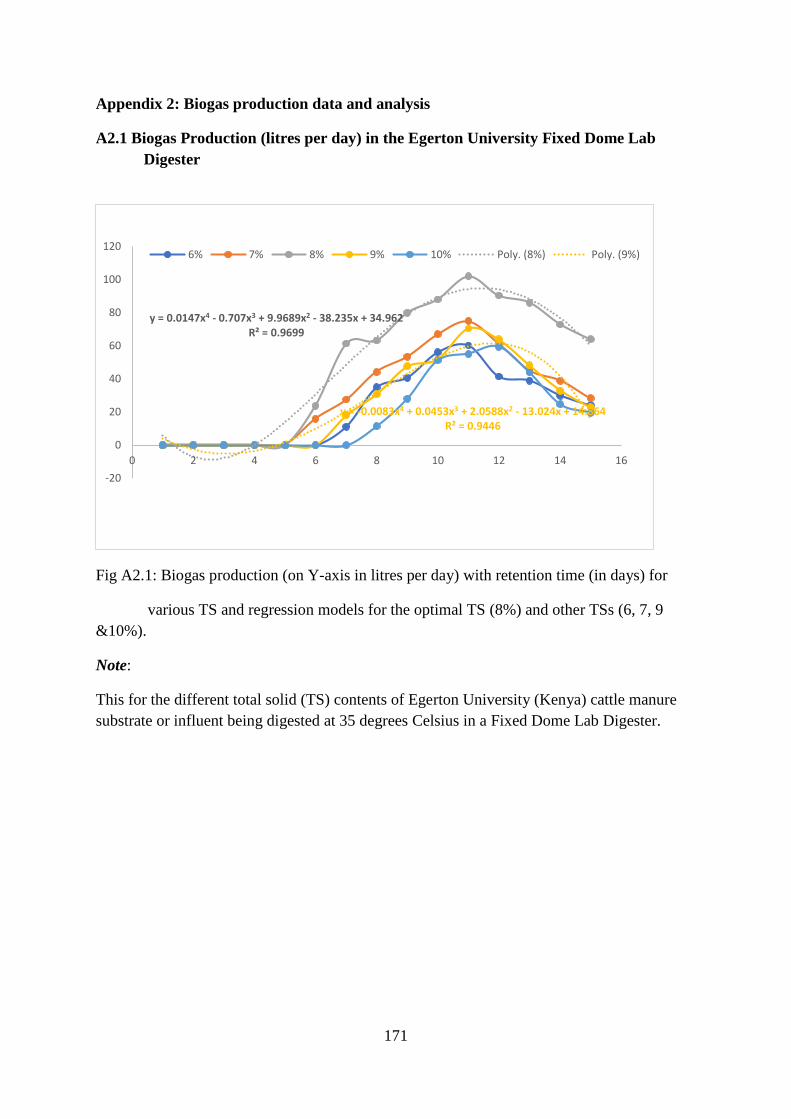
171
Appendix 2: Biogas production data and analysis
A2.1 Biogas Production (litres per day) in the Egerton University Fixed Dome Lab
Digester
Fig A2.1: Biogas production (on Y-axis in litres per day) with retention time (in days) for
various TS and regression models for the optimal TS (8%) and other TSs (6, 7, 9
&10%).
Note:
This for the different total solid (TS) contents of Egerton University (Kenya) cattle manure
substrate or influent being digested at 35 degrees Celsius in a Fixed Dome Lab Digester.
y = 0.0147x4 - 0.707x3 + 9.9689x2 - 38.235x + 34.962R² = 0.9699
y = -0.0083x4 + 0.0453x3 + 2.0588x2 - 13.024x + 14.864R² = 0.9446
-20
0
20
40
60
80
100
120
0 2 4 6 8 10 12 14 16
6% 7% 8% 9% 10% Poly. (8%) Poly. (9%)
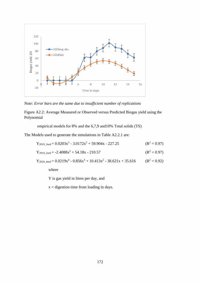
172
Note: Error bars are the same due to insufficient number of replications
Figure A2.2: Average Measured or Observed versus Predicted Biogas yield using the
Polynomial
empirical models for 8% and the 6,7,9 and10% Total solids (TS)
The Models used to generate the simulations in Table A2.2.1 are:
Y2019_3ord = 0.0203x3 - 3.0172x2 + 59.904x - 227.25 (R2 = 0.97)
Y2019_2ord = -2.4088x2 + 54.18x - 210.57 (R2 = 0.97)
Y2018_4ord = 0.0219x4 - 0.856x3 + 10.413x2 - 38.621x + 35.616 (R2 = 0.92)
where
Y is gas yield in litres per day, and
x = digestion time from loading in days.
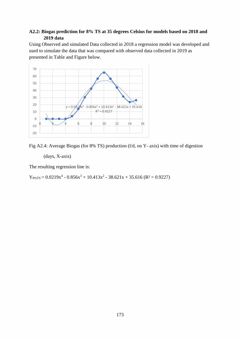
173
A2.2: Biogas prediction for 8% TS at 35 degrees Celsius for models based on 2018 and
2019 data
Using Observed and simulated Data collected in 2018 a regression model was developed and
used to simulate the data that was compared with observed data collected in 2019 as
presented in Table and Figure below.
Fig A2.4: Average Biogas (for 8% TS) production (l/d, on Y- axis) with time of digestion
(days, X-axis)
The resulting regression line is:
Y8%TS = 0.0219x4 - 0.856x3 + 10.413x2 - 38.621x + 35.616 (R² = 0.9227)
y = 0.0219x4 - 0.856x3 + 10.413x2 - 38.621x + 35.616R² = 0.9227
-20
-10
0
10
20
30
40
50
60
70
0 2 4 6 8 10 12 14 16
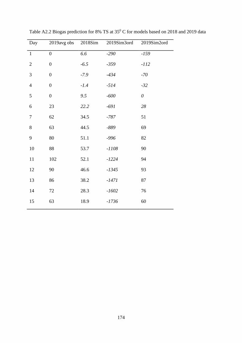
174
Table A2.2 Biogas prediction for 8% TS at 350 C for models based on 2018 and 2019 data
Day 2019avg obs 2018Sim 2019Sim3ord 2019Sim2ord
1 0 6.6 -290 -159
2 0 -6.5 -359 -112
3 0 -7.9 -434 -70
4 0 -1.4 -514 -32
5 0 9.5 -600 0
6 23 22.2 -691 28
7 62 34.5 -787 51
8 63 44.5 -889 69
9 80 51.1 -996 82
10 88 53.7 -1108 90
11 102 52.1 -1224 94
12 90 46.6 -1345 93
13 86 38.2 -1471 87
14 72 28.3 -1602 76
15 63 18.9 -1736 60
175
Appendix 3: Copyright Form
This is a copyright form from Isaac Scientific Publishing (ISP) for the first paper.
COPYRIGHT FORM
This form is provided for original papers submitted to the journals of Isaac Scientific
Publishing (ISP) and must be received by ISP before the paper is accepted for publication.
Please read this form carefully before signing.
Journal name: Annals of Advanced Agricultural Sciences.
Title of Paper: Effect of total solids on biogas production in a fixed dome laboratory digester
under mesophilic temperature.
Author(s): Barasa H. Masinde, Daudi M. Nyaanga, Musa R. Njue, and Joseph W. Matofari.
Affiliation(s): Masinde Muliro University of Science and Technology, Egerton University.
Copyright Transfer
The undersigned hereby assigns to the ISP all the rights under copyright that may exist in and
to the above Work, and any revised or expanded derivative works submitted to the above
mentioned journal by the undersigned based on the Work. The undersigned hereby warrants
that the Work is original and that he/she is the author of the Work; to the extent that the Work
incorporates passages, figures, data or other materials from the works of others, the
undersigned has obtained any necessary permission.
Retained Rights/Terms and Conditions
Authors/employers retain all proprietary rights in any process, procedure, or article of
manufacture described in this Work.
Authors/employers may reproduce or authorize others to reproduce the Work, materials
extracted verbatim from the Work, or derivative works for the author’s personal use or for the
company or organizational use, provided that the source and any ISP copyright notice are
indicated, the copies are not used in any way that implies ISP endorsement of a product or
service of any employer are not offered for sale.
Authors/employers may make limited distribution of all or portions of the Work prior to
publication if they inform the ISP in advance of the nature and extent of such limited
distribution.
176
ISP Copyright Ownership
It is the formal policy of the ISP to own the copyrights to all the copyrightable materials in its
technical publications and to the individual contributions contained therein, in order to
protect the interests of ISP, its authors and their employers, and, at the at the same time, to
facilitate the appropriate re-use of this material by others. The ISP distributes its technical
publications throughout the world and does so by various means such as hard copy and
electronic media. It also abstracts and may translate its publications, and articles contained
therein, for inclusion in various compendiums, collective works, databases and similar
publications.
Author/Employer Rights
If you are employed and prepared the Work on a subject within the scope of your
employment, the copyright in the Work belongs to your employer as a work-for-hire. In that
case, the ISP assumes that when you sign this Form, you are authorized to do so by your
employer and that your employer has consented to the transfer of copyright, to the
representation and warranty of publication rights, and to all other terms and conditions of this
Form as the author. In the event the above is not accepted and published by the ISP or is
withdrawn by the author(s) before acceptance by the ISP, the foregoing copyright transfer
shall become null and void and all materials embodying the Work submitted to the above
mentioned journal will be destroyed.
The author signs for and accepts responsibility for releasing this material on behalf of any
and all co-authors.
Author/Authorized Agent For Joint Authors Date (dd-mm-yy)
*Signed: BHM 08-02-2020
This is a copyright form from Isaac Scientific Publishing (ISP) for the second paper.
177
COPYRIGHT FORM
This form is provided for original papers submitted to the journals of Isaac Scientific
Publishing (ISP) and must be received by ISP before the paper is accepted for publication.
Please read this form carefully before signing.
Journal name: International Journal of Power and Energy Research.
Title of Paper: Optimisation of Biogas Production in a Batch Laboratory Digester using Total
Solids, Substrate Retention Time, and Mesophilic Temperature.
Author(s): Barasa H. Masinde, Daudi M. Nyaanga, Musa R. Njue, and Joseph W. Matofari.
Affiliation(s): Masinde Muliro University of Science and Technology, Egerton University.
Copyright Transfer
The undersigned hereby assigns to the ISP all the rights under copyright that may exist in and
to the above Work, and any revised or expanded derivative works submitted to the above
mentioned journal by the undersigned based on the Work. The undersigned hereby warrants
that the Work is original and that he/she is the author of the Work; to the extent that the Work
incorporates passages, figures, data or other materials from the works of others, the
undersigned has obtained any necessary permission.
Retained Rights/Terms and Conditions
Authors/employers retain all proprietary rights in any process, procedure, or article of
manufacture described in this Work.
Authors/employers may reproduce or authorize others to reproduce the Work, materials
extracted verbatim from the Work, or derivative works for the author’s personal use or for the
company or organizational use, provided that the source and any ISP copyright notice are
indicated, the copies are not used in any way that implies ISP endorsement of a product or
service of any employer are not offered for sale.
Authors/employers may make limited distribution of all or portions of the Work prior to
publication if they inform the ISP in advance of the nature and extent of such limited
distribution.
178
ISP Copyright Ownership
It is the formal policy of the ISP to own the copyrights to all the copyrightable materials in its
technical publications and to the individual contributions contained therein, in order to
protect the interests of ISP, its authors and their employers, and, at the at the same time, to
facilitate the appropriate re-use of this material by others. The ISP distributes its technical
publications throughout the world and does so by various means such as hard copy and
electronic media. It also abstracts and may translate its publications, and articles contained
therein, for inclusion in various compendiums, collective works, databases and similar
publications.
Author/Employer Rights
If you are employed and prepared the Work on a subject within the scope of your
employment, the copyright in the Work belongs to your employer as a work-for-hire. In that
case, the ISP assumes that when you sign this Form, you are authorized to do so by your
employer and that your employer has consented to the transfer of copyright, to the
representation and warranty of publication rights, and to all other terms and conditions of this
Form as the author. In the event the above is not accepted and published by the ISP or is
withdrawn by the author(s) before acceptance by the ISP, the foregoing copyright transfer
shall become null and void and all materials embodying the Work submitted to the above
mentioned journal will be destroyed.
The author signs for and accepts responsibility for releasing this material on behalf of any
and all co-authors.
Author/Authorized Agent For Joint Authors Date (dd-mm-yy)
*Signed: BHM 28-03-2020
179
Appendix 4: Abstracts of Publications
Two papers were published from this work:
a) Paper 1: Effect of total solids on biogas production in a fixed dome laboratory digester
under mesophilic temperature. Annals of Advanced Agricultural Sciences, Vol. 4, No. 2,
May 2020. https://dx.doi.org/10.22606/as.2020.42003
b) Paper 2: Optimisation of biogas production in a batch laboratory digester using total
solids, substrate retention time, and mesophilic temperature. International Journal of
Power and Energy Research, Vol. 4, No. 2, July 2020.
https://dx.doi.org/10.22606/ijper.2020.42001
The abstracts of the papers are as follows.
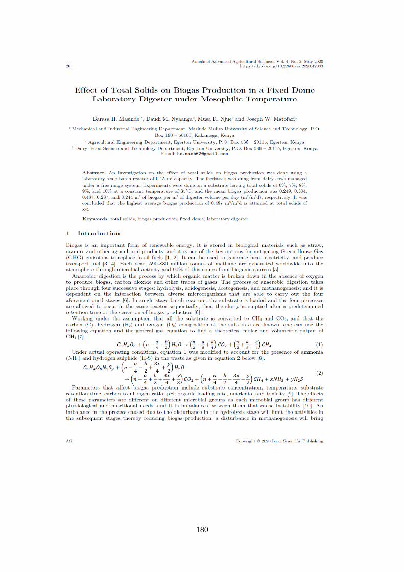
180
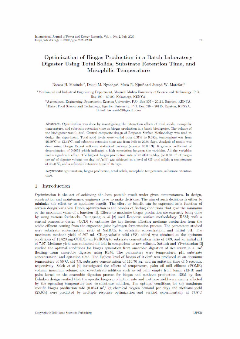
181

182
Appendix 5: Research permit