The shock structure in the protoplanetary nebula M1-92: imaging of atomic and H_2 line emission

Astron. Astrophys. 331, 361–371 (1998) ASTRONOMYAND

ASTROPHYSICS

The shock structure in the protoplanetary nebula M 1–92:imaging of atomic and H2 line emission⋆

V. Bujarrabal1, J. Alcolea1, R. Sahai2, J. Zamorano3, and A.A. Zijlstra4

1 Observatorio Astronomico Nacional (IGN), Apartado 1143, E-28800 Alcala de Henares, Spain (bujarrabal,[email protected])2 Jet Propulsion Laboratory, MS 183-900, 4800 Oak Grove Drive, Pasadena CA 91109, USA ([email protected])3 Departamento de Astrofısica, Facultad C. Fısicas, Universidad Complutense, E-28040 Madrid, Spain ([email protected])4 European Southern Observatory, Karl Schwarzschild Strasse 2, D-85748 Garching bei Munchen, Germany ([email protected])

Received 18 March 1997 / Accepted 19 September 1997

Abstract. We present HST imaging of continuum (5500 A) and

atomic line (Hα, [OI] 6300 A, [SII] 6717 and 6731 A, and

[OIII] 5007 A) emissions in the protoplanetary nebula M 1–92.

Ground based imaging of 2µm continuum and H2 ro-vibrational

(S(1) v=1-0 and v=2-1 lines) emission has been also performed.

The 5500 A continuum is due to scattering of the stellar light

by grains in a double-lobed structure comparable in extent and

total density with the molecular envelope detected at mm wave-

lengths, which consists of two empty shells with a clear axis of

symmetry. On the other hand, the optical line emission comes

mainly from two chains of shocked knots placed along the sym-

metry axis of the nebula and inside those cavities, for which

relatively high excitation is deduced (shock velocities of about

200 km s−1). The H2 emission probably comes from more ex-

tended regions with representative temperature and density of

1600 K and 6 103 cm−3, intermediate in location and excitation

between the atomic line knots and the very cold region detected

in CO emission. We argue that the chains of knots emitting in

atomic lines correspond to shocks taking place in the post-AGB

bipolar flow. The models for interstellar Herbig-Haro objects

seem to agree with the observations, at least qualitatively, ex-

plaining in particular that the atomic emission from the bipolar

flow dominates over that from shocks propagating in the AGB

shell. Models developed for protoplanetary nebula dynamics

fail, however, to explain the strong concentration of the atomic

emission along the symmetry axis.

Key words: circumstellar matter – stars: AGB and post-AGB

– planetary nebulae: individual: M 1–92 – shocks – infrared:

ISM: lines and bands

⋆ Based on observations made with the NASA/ESA Hubble Space

Telescope, obtained at the Space Telescope Science Institute, operated

by the Association of Universities for Research in Astronomy, Inc.,

under NASA contract NAS 5-2655

1. Introduction

M 1–92, Minkowski’s Footprint, is one of the best studied pro-

toplanetary nebulae (PPN), see e.g. Herbig (1975), Cohen and

Kuhi (1977), Solf (1994), Bujarrabal et al. (1994). The temper-

ature of the central star is about 20 000 K: this makes it a rela-

tively hot post-AGB star, well on its way to become a planetary

nebula. The coordinates of the central star are: right ascension

19:36:18.9, declination +29:32:50 (J2000), l = 64.1, b = 4.3.

The distance to M 1–92 has been studied by several authors.

Cohen and Kuhi (1977, see also Calvet and Cohen 1978) dis-

cussed possible values between 2.3 and 3.5 kpc, depending on

whether the object belongs to luminosity class V or III, but note

that this classification may be not meaningful for PPNe. Feibel-

man and Bruhweiler (1990) propose a distance between 1 and

2.5 kpc, from the possible values of the intervening extinction,

a range that was considered to be consistent with their analysis

of the ultraviolet emission of M 1–92. We will adopt a distance

of 2.5 kpc. For this value, the luminosity of M 1–92 is estimated

to be about 104 L⊙ (Cohen and Kuhi 1977), a value often found

in PPNe (e.g. Calvet and Cohen 1978).

The optical image (a reflection nebula of about 10′′ or 4 1017

cm), consists of two lobes, with a conspicuous symmetry axis

approximately oriented along the NW-SE direction. The much

brighter NW part points towards the observer. Optical spec-

troscopy observations (Herbig 1975, Solf 1994) have shown a

high-velocity bipolar outflow with velocities of about 200 - 300

km s−1, following the nebular axis. High-excitation gas, with

characteristics similar to those of Herbig-Haro objects and prob-

ably related to shocks, is identified in the two lobes (Solf 1994).

The gap between both lobes and the high extinction towards the

star indicate the existence of an oblate dust condensation in the

center. This is confirmed by the torus-like feature identified in

IR color images (Eiroa and Hodapp 1989).

The detection of OH maser emission in M 1–92 indicates

O-rich chemistry. High spatial resolution mapping of the OH

1667 MHz line (Seaquist et al. 1991) shows that the OH maser

362 V. Bujarrabal et al.: The shock structure in the protoplanetary nebula M 1–92: atomic and H2 line emission

probably arises from a flat, compact component, perpendicular

to the symmetry axis and slightly larger than the IR ring (3-4′′

versus 2-3′′), that probably corresponds to the same torus.

The 2′′-resolution mapping of the 12CO and 13CO line emis-

sion (Bujarrabal et al. 1994, 1997) shows a double, hollow shell

which covers the whole optical nebula. This shell was ejected

during the past AGB phase and contains most of the nebular ma-

terial (at least 1 M⊙). The molecular gas flows predominantly

in the axial direction with outward (deprojected) velocities as

high as 70 km s−1. Such a velocity, significantly higher than

typical AGB expansion velocities, and the hollow shape of the

CO lobes strongly suggest the effect of wind interaction between

the fast bipolar outflow (presently ejected by the star) and the

slow dense envelope (ejected during the past AGB phase). The

temperature of the emitting gas is very low, 15 - 20 K, indicating

that strong cooling took place after the shock acceleration.

M 1–92 is probably the PPN in which the structure and

properties of the wind interaction, the dominant dynamical pro-

cess for the formation of planetary nebulae, is being studied

in most detail. However, the comparison of the CO data and

the shocked gas observations in the optical has been less useful

due to the low spatial resolution of the optical spectroscopy. To

overcome such a limitation we have performed Hubble Space

Telescope (HST) imaging using several narrow filters in order

to select [SII], [OI], [OIII] and Hα emission, together with a

filter placed in a spectral region free from intense lines, in order

to measure the nebular continuum level and distribution. We

have also probed the intermediate excitation gas by means of

near infrared ground-based observations of H2 ro-vibrational

emission.

2. Observations and data analysis

2.1. Optical imaging with the Hubble Space Telescope

HST Wide Field Planetary Camera 2 (WFPC2) observations of

M 1–92 were obtained in May 1996 through a set of five fil-

ters, four of which isolate atomic line emission: F656N (Hα),

F631N ([OI] 6300 A), F673N ([SII] 6717 and 6731 A), and

F502N ([OIII] 5007 A). The fifth filter, F547M, is placed be-

tween 5211 and 5697 A, a spectral region in which the line

emission contribution to the total intensity is negligible (Tram-

mell et al. 1993), and is useful for measuring the continuum

intensity. Standard reduction procedures were applied. After

averaging the different exposures and rotating the images, the

actual angular resolution measured from stellar images is ∼ 0.1

arcsec, about twice the pixel size (0.05 arcsec). The units in the

images presented here are erg sec−1 cm−2 A−1 (per pixel). The

total exposure times for filters F673N, F631N, F502N, F656N,

F547M were respectively 1980, 2080, 2080, 760, 960 seconds.

In all cases several different exposures were done in order to

help in the analysis, in particular short exposures of about 100

seconds were performed to control any possible saturation.

The images in the continuum and line filters are quite sim-

ilar in flux distribution to a first approximation. Since the line

filter intensity includes line emission plus scattered light, the

contribution of scattering to the intensity distribution measured

with the narrow filters must be dominant. Our continuum 5500

A image was used to remove such a contribution. The contin-

uum level at 6730A is below the level measured in the 5500A

continuum filter due to the color index of the nebula. The dif-

ference is much smaller for the [OI] and [OIII] lines which are

closer in wavelength to the continuum filter. The color index

from photometry measurements (Cohen and Kuhi 1977) indi-

cates that the continuum level at 6700A is about 20-25% lower

compared to 5500A. This factor agrees with the estimate from

the HST images and was used to subtract the continuum. How-

ever, we note that the extinction varies across the nebula and

the correction factor is therefore only an average value. This

can leave a large-scale residual error in the [SII] image. From

the allowed range of correction factors, we estimate that the

uncertainty in the [SII] line emission strengths is about 30%.

The smooth component is especially uncertain. The outer lanes

visible in both lobes (almost parallel to the axis of the nebula

and strongest in the NW lobe; see Fig. 1) seem to be real: they

are slightly above the estimated uncertainty and also appear in

the [OI] differential image.

The intensity detected in the narrow Hα filter is mainly due

to the scattered stellar line emission. However, the scattered

light, whether it correspond to continuum or line emission from

the star, must present the same spatial distribution. Therefore,

our F547M image can still be useful for subtracting the scattered

light contribution, once we estimate an appropriate scaling fac-

tor. We use a factor that yields intensity close to zero (but not

negative) in the pixels that present very low emission in the [SII]

and [OI] lines. The used correction factor implies that the scat-

tered continuum level is only about 20% of the total scattered

light through the Hα filter, which is accurately coincident with

the fraction of the scattered light due to the stellar continuum

calculated from measurements of line and continuum lobe in-

tensity by Cohen and Kuhi (1977) and Trammell et al. (1993).

In any case, the scaling factor to be applied in the scattered light

subtraction is obviously more uncertain for our Hα image than

for [SII]. The extended structures found in the differential Hαimage are then not accurately measured, although the intensity

increase of the compact knots is reliable.

In Fig. 1 we show the images in the continuum at 5500 A

(a), with the Hα filter after subtracting the scattered light (b),

with the [OI] filter before (c) and after (d) subtraction of the

scattered light, with the [SII] filter (e) and with the [OIII] filter

(f) both after subtraction, see also Fig. 4. In Fig. 2 we show cuts

in three directions in the 5500 A continuum image (Sect. 3.1).

2.2. Ground-based imaging of near-infrared H2 line emission

The images were obtained at the Calar Alto 2.2 m telescope,

using the MAGIC camera (Herbst et al. 1993) in the high-

resolution mode. In this configuration, the NICMOSS3 2562

HgCdTe array images a 164-square-arcsec field of view at

0.63 ′′/pixel. The nebula was observed using three narrow-

band filters: H2 S(1) v=1-0 (centered at λc=2.122 µm, width

V. Bujarrabal et al.: The shock structure in the protoplanetary nebula M 1–92: atomic and H2 line emission 363

Fig. 1a–f. HST images of M 1–92. a: 5500 A

continuum; contours are 2.4, 4.8, 10, 24, 48,

100, 240, and 480 10−19 erg cm−2 s−1 A−1

(per pixel, pixel size: 0.046 arcsec). b Hα

emission after subtraction of scattered light.

c, d [OI] 6300 A emission respectively be-

fore and after subtraction of scattered light. e

[SII] 6700 A emission after continuum sub-

traction. f [OIII] 5000 A emission after con-

tinuum subtraction. See text for details on

the subtraction procedure.

of W=0.021 µm), H2 v=2-1 S(1) (λc=2.248 µm, W=0.022 µm)

and continuum at 2.260 µm (W=0.060µ).

Three independent images were taken in each filter, with

relative offsets of the order of 20′′. Each individual image is the

result of the coadd of 10 exposures of 0.7 s and 2.0 s for the

continuum and line filters respectively. Sky frames were taken

at the beginning and end of each filter series.

The data reduction process included bad pixel removal and

interpolation, dark subtraction, flat-fielding, sky subtraction,

and registration of all images. All the images in each filter were

combined, eliminating discrepant points like cosmic rays, resid-

ual stars in the sky frames, and a faint ghost image which ap-

peared in one of the frames.

Absolute flux calibration was obtained from observations

of the standard star Gl 748, which has K=6.305 and J-K=0.53

(Elias et al. 1982). The indicated Teff=4000K yields flux den-

sities at 2.122, 2.248 and 2.260 µm for this standard star of

0.1415 10−12; 0.1193 10−12 and 0.1174 10−12 erg cm−2 s−1

A−1, respectively. During the observations, the airmasses of the

standard star and of M 1–92 were 1.40 and 1.15, respectively.

A typical extinction of 0.088 mag/airmass was assumed. The

units of the final images are erg cm−2 s−1 µm−1 (per pixel).


Fig. 2. The surface brightness of the 5500 A continuum as a function

of radius in M 1–92, generated by taking cuts through the F547M HST

image along radial vectors passing through the central star. Three dif-

ferent cuts are shown, θ = 0◦ and 180◦ respectively corresponding to

polar directions along the major axis of the nebula in the northern and

southern lobe, and θ = 45◦ corresponding to a cut at an intermediate

latitude (θ is measured anti-clockwise from the polar axis). The inten-

sities for each cut have been normalized to a surface brightness of 13.2

mag arcsec−2. The dashed line shows for comparison an r−3 intensity

variation, expected for an inverse-square density variation.

We subtracted the continuum contribution to the intensity

measured in the narrow line filters. The worst case is the 2.122

µm filter, which is furthest in wavelength from the continuum

filter. Since we are interested in the lobe emission, instead of in

the stellar intensity, we have estimated the relative continuum

level between 2.122 and 2.260 µm wavelength from the total

nebula colors and relative reddening given by Eiroa and Hodapp

(1989) and Eiroa et al. (1983). The emission from the lobes is

relatively bluer than from the central ring surrounding the star.

This compensates the slightly larger intensity of the whole neb-

ula at 2.260µm, and we estimate that in the lobes the continuum

level must be comparable at 2.122 and 2.260 µm. We have then

directly subtracted the continuum level from the line images.

Fig. 3a shows the continuum image (see a previous compara-

ble image in Latter et al. 1995) and Fig. 3b the intrinsic v=1–0

emission after continuum subtraction. From the uncertainties in

this procedure, we estimate that the errors in the 2.122 µm line

emission in the lobes is of the order of 40%. In spite of this large

uncertainty, the line emission detected in both lobes at 2.122µm

is probably real, since to cancel such structures we would have

to assume that the lobes are half a magnitude bluer than the

average nebula emission, which is very improbable in view of

the relative reddening measured across the object by Eiroa and

Hodapp and the short difference in wavelength between both

filters.

In the case of the v=2-1 line the subtraction is straightfor-

ward since the wavelength difference with respect to the con-

tinuum filter is very short. The emission is weak in this line (as

usual in protoplanetary nebulae, see below); we report a tenta-

tive detection in this line at a level 5-10 times weaker than the

v=1-0 line.

The central M 1–92 ring is known to be relatively red (Eiroa

and Hodapp 1989), accordingly, the subtraction procedure used

here leads to negative contours in the differential 2.122 µm

image in this region. The results so obtained are then not mean-

ingful for such a ring and not displayed in Fig. 3b.

Since the seeing in our H2 ground-based observations is of

the order of 1 arcsec, much poorer than in the HST data, we

have improved the spatial resolution of the 2.122 µm differ-

ential image by deconvolving an empirical point spread func-

tion. The Lucy-Richardson algorithm implemented in the IRAF

STSDAS package (Lucy 1974) was used. Line and continuum

images were first subtracted before applying the algorithm. The

point spread function was taken from a portion of the continuum

image containing the bright (but unsaturated) star west of M 1–

92 (FWHM = 1.2 arcsec). The chi-square estimator provided by

the task reached a satisfactory value of 1.33 after 50 iterations,

with no significant change when more iterations are performed.

The resulting image is shown in Fig. 3c.

3. Results: HST data

Similar HST observations than those presented here have been

independently obtained and recently reported by Trammell and

Goodrich (1996). These authors observed about one month be-

fore us. The images of Hα, [OI] and [SII] emission given in

that paper also show the existence of a narrow line emission

structure in the center of both lobes. The exposure times of our

images are however higher by a factor 2 – 3 (except for the

F631N filter), which results in a better signal/noise ratio. Also

we present [OIII] maps, which allows the detection and study of

the high-excitation gas. As we will see, the HST data analysis is

quite different in both works. We have discussed more in detail

the scattered light spatial distribution and its subtraction from

the line filter images, also a fruitful comparison with emission

in H2 and CO lines is performed here; finally, our interpretation

of the origin of the atomic line emission is completely different.

3.1. Scattering of the stellar light

Most of the visible radiation from M 1–92 is the result of scat-

tering of stellar emission by nebular dust grains, as shown in

Sect. 2.1. The contribution of line emission in the wide filter

F547M, in which no intense nebular line is expected, is negli-

gible.

The morphology of the scattered light is best seen in the

F547M image in Fig. 1 (a). The image shows the presence of

substantial obscuration in a torus-like structure similar to that

found by Eiroa and Hodapp (1989). The inclination of the nebula

with respect to the plane of the sky (Sect. 1) leads to a system-

atically higher obscuration for the SE lobe. The F547M image

shows the presence of bright lanes which are almost parallel to

the axis and mostly seen in the northern lobe, that practically

envelop the whole nebula. Such bright lanes are almost coin-


Fig. 3a–c. H2 v=1-0 images. a continuum image at 2.26 µm. b H2 v=1-0 image after continuum subtraction. c H2 v=1-0 intensity image after

deconvolution of the point spread function. Contours, in logarithmic scale, are 4.5, 10, 22, 45, 100, etc, up to 10000 10−14 erg cm−2 s−1 µm−1

(per pixel, pixel size: 0.63 arcsec). Offsets are given in arc seconds.

cident with the lateral walls of the hollow, very dense shells

that constitute most of the CO nebula (Bujarrabal et al. 1994).

These lanes probably result from the relatively large density in

this shell with respect to the diffuse inner gas. At the lowest

intensity level, we note (a) the halo surrounding the bright NW

lobe, probably representing second order scattering of the lobe

light, and (b) the filament-like structures detected in both tips

of the nebula.

The magnitude and variation of scattered light, as a func-

tion of radius, can be used to make a rough estimate of the line-

of-sight optical depth. For an envelope with an inverse-square

density distribution, and optically-thin scattering, it can be eas-

ily shown that the surface brightness due to scattered light, S,

should vary as r−3 (r being the distance to the central star). In

M 1–92, the density structure of the envelope is complex, as

mentioned above, so S does not vary as r−3. This is shown in

cuts of the surface brightness, S, from the continuum image,

taken along three different radial vectors in Fig. 2. The dashed

line in the figure shows an r−3 variation for comparison.

The line-of-sight nebular scattering optical depth τ (λ)s,losat any point P, at a distance r from the central star, is related to

the surface brightness and the stellar flux incident at that point,

as follows (assuming no significant extinction of the starlight

from the star to P),

τ (λ)s,los/(4πφ2) =S(λ)

[L(λ)/(4πD2)],

where φ is the angular distance to P from the central star in

arcsec, S(λ) is the surface brightness per arcsec2, and D is the

distance to M 1–92 (see Sahai et al. 1998). We will assume

that Teff=20,000 K and Lbol=104 L⊙ for D=2500 pc. We find

that, e.g. at φ=4′′ in the NW lobe, the surface brightness is 15.6

mag arcsec−2, which gives τ (λ)s,los ∼ 0.32 at λ=0.55 µm. A

scattering opacity of 2.9 104 cm2g−1 (per unit mass of dust) will

be used to determine the mass in dust grains. Our assumption,

that the opacity along the path followed by the scattered light is

negligible, seems justified since we are measuring the scattered

light intensity in a low-density region, but we must keep in mind

that we are calculating a lower limit to the dust mass. We have

also assumed that most of the material along the line-of-sight is

localized at the same distance from the star, so that the incident

stellar flux does not vary significantly across the region which

contributes to the optical depth. In the case of an r−2 radial

density, accounting for the variation of the starlight and the

optical depth results in an increase in the derived optical depth

by a factor 2. If the density decreased more slowly (faster) than

r−2, this factor would be larger (smaller) than 2. In M 1–92,

we know that the material is more localized than expected from

such a dust density distribution, but the localization region is

not in the plane of the sky. We conservatively estimate that the

optical depth derived from the above equation is underestimated

by at most a factor 2 because of our simple treatment of the radial

density variation. If we further make the simplifying assumption

that the scattering material seen along the line-of-sight is the

same material which was originally part of the inverse-square

density AGB envelope along the same line-of-sight through P,

we can estimate that the dust mass-loss rate was larger than ∼

(3–6) 10−7 M⊙ yr−1.

An estimate of the dust mass-loss rate can also be de-

rived from modelling the IRAS far-infrared fluxes, using a

2-component dust emission model described by Sahai et al.(1991). The color-corrected IRAS fluxes used in this model

for M 1–92 are 14.5, 56.8, 124.9 and 71.1 Jy at 12, 25, 60,

and 100 µm, respectively. Assuming a dust emissivity of 150

cm2g−1 at 60 µm (Jura 1986), with a λ−p power-law variation

and p=1.1(1.5), we find that the masses and temperatures of

the 2 components are, respectively, 6.7(3.8) 10−3 and 2.1(1.2)

10−5 M⊙ and 61(71) and 158(183) K. An estimate to the time-

scale over which this mass of dust has been ejected is given

by the expansion time for CO, about 10000 yr (Bujarrabal et

al. 1997). We therefore find a dust mass-loss rate of about 6

10−7 M⊙ yr−1. We believe that the differing estimates of the

dust mass-loss rate from the IRAS and HST data are consistent

in view of the uncertainties of the assumptions, and adopt for

further discussion a value of the total mass in dust grains of 6

10−3 M⊙, corresponding to a mass-loss rate of about 6 10−7


M⊙ yr−1. The total gas mass derived from CO data by Bujarra-

bal et al. (1997) is about 1 M⊙, giving a gas-to-dust ratio of

about 160, comparable to the gas-to-dust ratio in O-rich AGB

envelopes (about 100–200).

3.2. Atomic line emission from the nebula

In Fig. 1 (c, d, e), we show the images obtained with filters

F631N ([OI] line) and F673N ([SII] lines). The original [OI] and

[SII] line emission images are clearly contaminated by scattered

stellar light, as we have mentioned, but they also show several

knots of emitting material that are not present in the continuum

map. Such clumps are mostly located in the axis of the neb-

ula and placed symmetrically at about 2.2 arcsec from the star

(NW and SE lobes) and at about 3.3 arcsec from the star to-

wards the SE. After subtraction of the contribution of scattering

(Sect. 2.1, Fig. 1 (d, e)), both lines show a very similar image

and the structure of these clumps is much more obvious. In

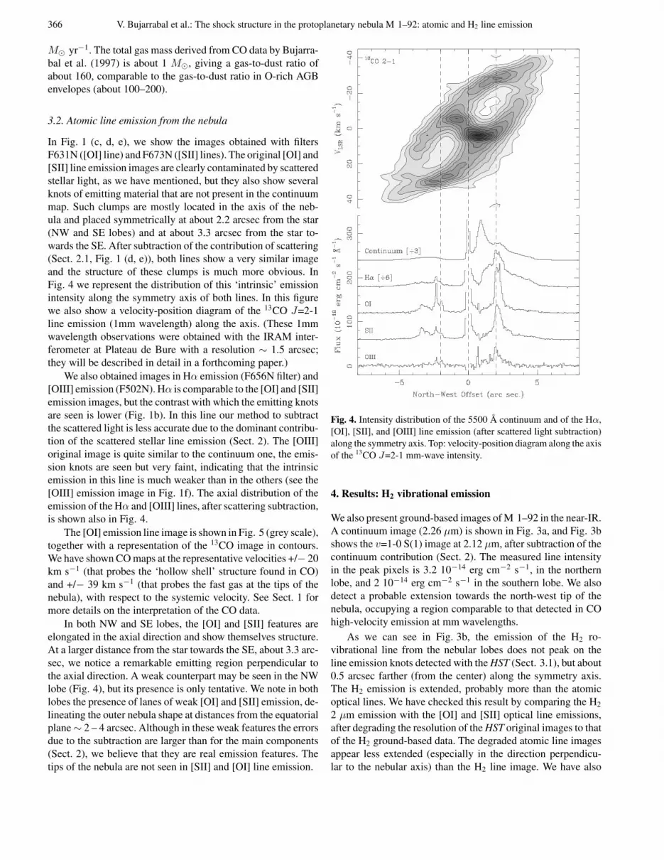
Fig. 4 we represent the distribution of this ‘intrinsic’ emission

intensity along the symmetry axis of both lines. In this figure

we also show a velocity-position diagram of the 13CO J=2-1

line emission (1mm wavelength) along the axis. (These 1mm

wavelength observations were obtained with the IRAM inter-

ferometer at Plateau de Bure with a resolution ∼ 1.5 arcsec;

they will be described in detail in a forthcoming paper.)

We also obtained images in Hα emission (F656N filter) and

[OIII] emission (F502N). Hα is comparable to the [OI] and [SII]

emission images, but the contrast with which the emitting knots

are seen is lower (Fig. 1b). In this line our method to subtract

the scattered light is less accurate due to the dominant contribu-

tion of the scattered stellar line emission (Sect. 2). The [OIII]

original image is quite similar to the continuum one, the emis-

sion knots are seen but very faint, indicating that the intrinsic

emission in this line is much weaker than in the others (see the

[OIII] emission image in Fig. 1f). The axial distribution of the

emission of the Hα and [OIII] lines, after scattering subtraction,

is shown also in Fig. 4.

The [OI] emission line image is shown in Fig. 5 (grey scale),

together with a representation of the 13CO image in contours.

We have shown CO maps at the representative velocities +/− 20

km s−1 (that probes the ‘hollow shell’ structure found in CO)

and +/− 39 km s−1 (that probes the fast gas at the tips of the

nebula), with respect to the systemic velocity. See Sect. 1 for

more details on the interpretation of the CO data.

In both NW and SE lobes, the [OI] and [SII] features are

elongated in the axial direction and show themselves structure.

At a larger distance from the star towards the SE, about 3.3 arc-

sec, we notice a remarkable emitting region perpendicular to

the axial direction. A weak counterpart may be seen in the NW

lobe (Fig. 4), but its presence is only tentative. We note in both

lobes the presence of lanes of weak [OI] and [SII] emission, de-

lineating the outer nebula shape at distances from the equatorial

plane ∼ 2 – 4 arcsec. Although in these weak features the errors

due to the subtraction are larger than for the main components

(Sect. 2), we believe that they are real emission features. The

tips of the nebula are not seen in [SII] and [OI] line emission.

Fig. 4. Intensity distribution of the 5500 A continuum and of the Hα,

[OI], [SII], and [OIII] line emission (after scattered light subtraction)

along the symmetry axis. Top: velocity-position diagram along the axis

of the 13CO J=2-1 mm-wave intensity.

4. Results: H2 vibrational emission

We also present ground-based images of M 1–92 in the near-IR.

A continuum image (2.26 µm) is shown in Fig. 3a, and Fig. 3b

shows the v=1-0 S(1) image at 2.12 µm, after subtraction of the

continuum contribution (Sect. 2). The measured line intensity

in the peak pixels is 3.2 10−14 erg cm−2 s−1, in the northern

lobe, and 2 10−14 erg cm−2 s−1 in the southern lobe. We also

detect a probable extension towards the north-west tip of the

nebula, occupying a region comparable to that detected in CO

high-velocity emission at mm wavelengths.

As we can see in Fig. 3b, the emission of the H2 ro-

vibrational line from the nebular lobes does not peak on the

line emission knots detected with the HST (Sect. 3.1), but about

0.5 arcsec farther (from the center) along the symmetry axis.

The H2 emission is extended, probably more than the atomic

optical lines. We have checked this result by comparing the H2

2 µm emission with the [OI] and [SII] optical line emissions,

after degrading the resolution of the HST original images to that

of the H2 ground-based data. The degraded atomic line images

appear less extended (especially in the direction perpendicu-

lar to the nebular axis) than the H2 line image. We have also


tried to deconvolve the point spread function from our 2.12 µm

line image (Sect. 2.2). The results are shown in Fig. 3c for the

H2 v=1-0 line image after continuum subtraction. As we see in

this figure, the deconvolution suggests a rich structure in the H2

line emission. In the north lobe, the H2 line comes from a re-

gion, surrounding the [OI] and [SII] emitting knots, that seems

intermediate between that probed by the atomic and CO line

emission. In the southern lobe, the H2 line emission peaks pre-

cisely between both main knots seen in [OI] or [SII], and shows

an extension much wider than the knots of atomic line emission.

We also observed the H2 v=2-1 line emission at 2.25 µm,

which is found to be much weaker than the v=1-0 line. After

subtraction of the continuum, we tentatively detect emission

at a level of about 4 10−15 erg cm−2 s−1. In the regions of

the M 1–92 lobes where we found the maximum of the v=1-

0 line, the intensity of the v=2-1 line is weaker by about a

factor 5–10.

4.1. Continuum emission at 2 µm wavelength

We have also applied the scattering analysis to the 2µm con-

tinuum emission from M 1–92. We used for this analysis our

2.26µm image, with a stellar PSF deconvolved following the

same procedure as for the line images. We find that the observed

surface brightness is significantly larger than the incident stellar

radiation in the nebular regions, e.g. the 2µm surface brightness

at a radius of 4′′ in the northern lobe (about 2.3 10−2 Jy arcsec−2)

is about 20 times larger than the value of the maximum possible

scattered intensity of the 2µm radiation from the central star

(the total flux from the northern and southern lobes is 0.36 and

0.09 Jy, respectively). We conclude that there must be a signifi-

cant increase in the 2µm flux from the central source, over that

contributed from the star, which probably results from thermal

emission from a compact, central region of hot dust. In support

of this hypothesis, we find that the total flux from the central

source as seen in the deconvolved image is about 3.5 Jy, roughly

a factor 20 larger than the expected 2µm black-body flux from

the central star. Adding a third high-temperature component to

the 2-component dust model described above (Sect. 3.1), we

find that a small mass of dust, <∼ 10−7 M⊙ (for p=1.1) to 10−8

M⊙ (for p=1.5), at T >∼ 600 K, can produce the observed 2µm

flux.

5. Shock interpretation of atomic and H2 line emission

5.1. HST atomic line observations

As already mentioned by several authors (Solf 1994, Trammell

et al. 1993, etc), the atomic line intensities found in M 1–92 cor-

respond to that expected from shocks with moderate excitation,

mainly for shock tracers as the [OI] and [SII] lines observed by

us. It is shown in Fig. 4 and 5 (Sect. 3.2) that the shocked mate-

rial probed by the atomic line emission is clearly placed inside

the molecular shell and associated to the symmetry axis of the

nebula. In fact, the shocked gas in our images is located in both

empty regions (‘holes’) left by the accelerated low-excitation

Fig. 5. Comparison of the [OI] emission (grey scale) with the 13CO

J=2-1 mm-wave intensity distribution at four representative velocities

with respect to the central one: +/− 20 km s−1 (that probes the ‘hollow

shell’ structure found in CO) and +/− 39 km s−1 (that probes the fast

CO ‘bipolar outflow’). The CO low velocity maps are represented by

the continuous contours at 30 and 70% of maximum; the high velocity

maps are given by the broken contours at half maximum intensity.

Positive/negative velocities are represented by thick/thin contours.

shell in the two lobes. Only the outer SE feature, with a charac-

teristic transverse shape (i.e. elongated perpendicularly to the

symmetry axis), reaches the CO shells. But very low [SII] or

[OI] emission is found in front of the molecular shell (i.e. close

to the axis and farther than 5 arcsec from the star). Since the CO

shell has certainly suffered strong shock acceleration (Sect. 1),

the leading bow-like shock must be located outwards. Such a

structure is not seen in our images. The shocks that are exciting

the line emission found in our observations must be propagating

in the bipolar post-AGB flow. In fact, the clumpy image of this

bipolar flow given by our images is similar to the sinuous chain

of knots often mapped in jets associated to young stellar objects

(e.g. Reipurth 1989, Heathcote et al. 1996).

The outermost SE feature, characterized by its transverse

shape, almost reaches the base of the CO axial tip. It cannot

be identified with the leading shock, but its position and shape

could be interpreted as indicating that the emitting gas is located

in the Mach disk, i.e. in the thin region in which the jet stops

and in which relatively strong excitation occurs. This interpre-

tation is also suggested by the finding of similar structures in

the interstellar medium, in which the Mach disk is identified as

the inner part of the boomerang-shaped structures at the end of

the jets (its outer part probably being the leading bow shock).

The fact that the emission from shocks inside the colliding

bipolar flow dominates over that coming from the leading bow

shock is expected from theoretical considerations. Shock fronts

are also expected in the jet due to variations in its direction and


velocity (Biro et al. 1995, Gouveia dal Pino and Benz 1994)

or, generally, to the development of conical shocks in it (e.g.Blondin et al. 1990). Such internal shocks are particularly in-

tense in the plane-parallel limit, in which they have being exten-

sively studied, see e.g. Frank and Mellema (1994). As shown by

Hartigan (1989) and Hartigan and Raymond (1993), the emis-

sion coming from the Mach disk and the shocks inside the jet is

expected to dominate over the emission from the leading bow

shock when the jet density is lower than the ambient gas density

(previous to shocks). The big contrast found in our observations

between the emission from the bipolar jet and the emission from

the bow leading shock indicates, if the above interpretation is

correct, that the jet density (prior to shocks) is smaller than that

of the AGB shell by a factor >∼ 10. The present mass loss rate

in PPNe is indeed believed to be low, in contrast to the high

mass-loss rate characteristic of the last AGB phases, which is

as high as 10−4 M⊙ yr−1 in the case of M 1–92 (Bujarrabal et

al. 1997). From these figures we estimate that the typical den-

sity (prior to shocks) of the impinging bipolar jet should be <∼

2 103 cm−3. Note that in interstellar Herbig-Haro objects it is

also possible to detect the leading bow shock, due to the high

density of the interstellar jets, that are thought to be denser than

the surrounding material.

We cannot rule out, as an alternative explanation to the ab-

sence of atomic emission from the leading shock, that this lead-

ing shock has entered a very diffuse region and is dissipating,

since the original density must strongly decrease with the dis-

tance to the star.

In the clumps in which the [SII] and [OI] emission arises,

[OIII] appears to be relatively weak but not negligible. If we

compare the flux intensities (after correcting for a visual ex-

tinction in the lobes of 3 mag, see Sect. 2) with predictions by

models (e.g. Hartigan et al. 1987), we deduce shock velocities

of about 200 km s−1, in agreement with previous works. Note

that the [OIII] emission is relatively weaker in the outermost

south-east condensation, which suggests a relatively lower ex-

citation. Although it is not clear whether or not in this case the

Mach disk is theoretically expected to show weaker [OIII] 5007

A emission than the countershocks in the jet (e.g. Icke et al.1992), the fact that this bar-like clump presents different exci-

tation conditions than the others supports its identification with

the Mach disk.

We then conclude that the model predictions mentioned

above are at least qualitatively in agreement with our results.

We must recall that such models have mainly been developed to

explain the interaction of jets from young stellar objects with the

ambient clouds and the emission from the leading bow-shock.

Therefore, their predictions cannot be safely applied to our case

and only a qualitative agreement is to be expected. The com-

parison of our images with detailed line emission models of

PPN shocks (e.g. Mellema 1993) is not satisfactory, since such

models do not predict emission along the symmetry axis (see

Sect. 6).

5.2. Ground-based H2 line observations

We have found that the distribution of the H2 ro-vibrational

emission is less compact than that of the atomic line emission,

and is located approximately between the atomic and the CO

emitting regions (Sect. 4). This result is compatible with the

excitation requirements of the H2 lines, as expected from the-

ory and confirmed by observations of interstellar Herbig-Haro

objects (see e.g. calculations by Raga et al. 1995 and observa-

tions by Noriega-Crespo and Garnavich 1994 and Davis et al.1994a,b). No detailed model for the vibrational H2 emission

from PPNe has been published.

We can estimate from our data the temperature and den-

sity in the shocked region responsible for the H2 emission. As

we have seen, the v=2-1 emission is significantly weaker than

that of the v=1-0 transition. H2 excitation by uv photon absorp-

tion and subsequent radiative cascades is therefore unlikely, and

the detected emission is probably due to collisional excitation

in shocked material (e.g. Shull and Beckwith 1982). This is

in agreement with results found in the protoplanetary nebulae

CRL2688 and CRL618 (see Hora and Latter 1994 and Beckwith

et al. 1984).

Our data do not rule out that the H2 emitting region is heated

by the stellar uv radiation and not by shocks, which is a possible

scenario (see Sternberg and Dalgarno, 1989) if the attenuation

of the stellar uv emission is low and the densities are larger

than 104 cm−3. The models also indicate, in certain intermedi-

ate cases with high uv fields and low kinetic temperatures, that

the excitation of the high-v H2 levels can be due to fluorescence,

though the density and collision probability are high enough to

dominate the deexcitation. Low S(1) v=2/v=1 ratios would be

then present, in spite of the radiative excitation, and this popula-

tion mechanism could also be compatible with our observations.

The existence of this composite excitation mechanism can only

be tested by comparing data on several rotational components of

each vibrational transition, which are not available for M 1–92.

However, we have discussed that the presence of intense shocks

in M 1–92 is almost certain and, moreover, that studies of the

similar nebulae CRL2688 and CRL618 show the excitation of

the high-v levels to be very probably collisional. Accordingly,

we favor the idea that the vibrational emission of H2 is due

to purely collisional excitation (in order to estimate the level

population) and that this situation takes place in a shocked en-

vironment (in order to compare the results with data from other

shocked regions in M 1–92).

Under this framework, the (collisional) excitation of the ob-

served transitions is relatively easy to formulate. The population

of the v=1 level is essentially given by excitation from the v=0

state. From the collisional rates in Draine et al. (1983), we can

see that the collisional vibrational excitation in this case is dom-

inated by the H–H2 interaction. We will assume that, in the H2

emitting region, about one half of the total number of particles

(n) are hydrogen atoms and that the other half are molecular

(e.g. Raga et al. 1995). For low-J levels, the collisional popula-

tion of the different rotational sublevels could be described by

the popular sudden approximation and, therefore, such excita-


tion rates are practically independent of the J level in the v=1

state. The a priori expected range of densities is ∼ 103 – 105

cm−3, from the values found by Bujarrabal et al. (1997) and

the discussion in Sect. 5.1. Under these conditions, we cannot

assume that the vibrational state populations are thermalized. In

the general case, it is easily shown that the population of a v=1

low-J level by collisions is given by

x1 = x0

nHC01

nHC10 + A10

.

Where x0 is the population (per magnetic sublevel) of the

low-J levels in the v=0 ground state, and C is the vibra-

tional excitation or deexcitation rate (taken from Draine et

al.); C01 and C10 are related by the usual reversibility relation,

C01 = C10exp(−6000/T ). Here the Einstein A-coefficient cor-

responds to the whole vibrational transition; it is taken to be 8.3

10−7 s−1 (Turner et al. 1977). Assuming that most molecules

are in the ground vibrational state and that the populations of

the rotational levels are thermalized to the kinetic temperature,

T (which is reasonable, given the very low probability of the

rotational radiative transitions), x0 is given by the inverse of the

partition function including the ortho and para species, i.e. x0

= 44/T (note that we are assuming that the relative population

of both H2 species is given by their statistical weights). We can

expect that the H2 emission is optically thin in actual cases, this

is due to the forbidden nature of such quadrupole transitions.

The number of photons emitted per second and unit volume

by an H2 v=1-0 transition is then

nph = x1gA10(J, J ′)nH2.

Where g is the degeneracy of the upperv=1J=3 level (for the ob-

served transition, g=21, taken into account the statistical weight

ratio for para/ortho molecular hydrogen), x1g is the population

of the upper level of the considered transition, A10(J, J ′) is its

Einstein A-coefficient for the observed component (taken from

Turner et al. 1977), and nH2is the local density of H2.

Combining the empirical data and the above formulation

we can derive the density and temperature in the H2 emitting

region. We deduce from our data that in the northern lobe there

is an emitting region with radius equal to 1 arcsec and an inte-

grated H2 v=1-0 S(1) flux equal to 3 10 −13 erg cm−2 s−1. In the

southern lobe, the corresponding radius and flux are 0.65 arcsec

and 1.5 10 −13 erg cm−2 s−1. The H2 v=2-1 S(1) emission is

much less well defined, we will assume that it comes from a

similar region and shows a flux 5 – 10 times weaker. Using the

adopted distance to M 1–92 (2.5 kpc, Sect. 1), we find from our

analysis of the H2 emission in M 1–92 a temperature T ∼ 1600

K and total densities n ∼ 6 103 cm−3. The physical conditions

determined from H2 emission are similar in both lobes since

the different sizes compensate the difference in flux. The total

mass of such regions is therefore ∼ 10−3 M⊙. The temperature

we derive is comparable to those deduced for the similar PPNe

CRL2688 and CRL618 by Hora and Latter (1994) and Beck-

with et al. (1982). However, these authors assume thermaliza-

tion of the vibrational states, which leads them to deduce some-

what smaller densities and total mass. For reasonable collisional

rates and the densities deduced from the calculations (from our

method or, still more clearly, from that followed for CRL2688

and CRL618) the collisions are clearly unable to thermalize the

vibrational state populations. The assumption of thermalization

in our case would lead to overestimations of the v=1 state by

about one order of magnitude.

In our calculations, the temperature is essentially given by

the v=1-0 / v=2-1 line ratio. Since the second line is poorly

measured, the derived temperature is not very accurate and may

represent an upper limit only. Unfortunately, the density deter-

mination is very dependent on the assumed temperature: if it is

equal to 1000 K, instead of 1600 K, the density should increase

by a factor ∼ 6. However, the temperature we have found is

characteristic of shocked H2 emitting gas in PPNe, as we have

seen, and we think that the given value can be considered as

reliable. On the other hand, once a value of the temperature is

assumed, the dependence of the estimated density on the ob-

served intensity is very smooth. (Note also that the collisional

population of the v=2 level is mainly done from the v=0 state,

which leads in our case to a v=2/v=1 population ratio much

higher than the v=1/v=0 ratio.)

The comparison of our results with the calculations for in-

terstellar shocks by Raga et al. (1995) appears very appealing,

although, as we will see, it must be performed with caution.

First, Raga et al. confirm the expected intermediate excitation

needed to detect H2 emission from shocked regions. These au-

thors also predict H2 emitting regions encircling the impinging

bipolar jet and defining a hood- or bow-shaped hollow structure,

which seems comparable to that observed in the M 1–92 north

lobe. However in the model by Raga et al., both optical and H2

lines come from (different regions of) the shocked ambient gas,

the equivalent of the accelerated AGB shell in a PPNe. (We must

recall here that our H2 maps are not very accurate; the map in

Fig. 3c has been obtained from a relatively uncertain differential

measurement and after applying a deconvolution process, see

Sect. 2.2.) In any case, our observations show that a detailed the-

oretical description of the protoplanetary wind interaction must

take into account the emission coming from shocks in both the

bipolar post-AGB flow and in the AGB shell.

6. Conclusions: the wind interaction processes in M 1–92

We present HST observations in the visible of atomic line

emission and ground-based observations in the near IR of H2

ro-vibrational emission. Our HST observations show that the

atomic line emission mainly comes from two chains of com-

pact spots placed inside the empty cavities detected in CO mi-

crowave emission (that are expected to represent the remnant

AGB shell accelerated by the passage of a shock front, Bujarra-

bal et al. 1997), see Figs. 1, 4, 5. Together with Hα, [OI] and

[SII] emission, we also find [OIII] 5007 A emission in such

spots; the intensity of this line, relative to the others, indicate

that the excitation conditions correspond to that of shocks with a

velocity of about 200 km s−1. The [OIII] emission is relatively

weaker in the southernmost bar-like clump, suggesting that the

excitation conditions in it are lower than for the others. H2 emis-


sion seems to come from more extended regions, intermediate

in excitation conditions between the regions emitting in CO and

in the atomic lines, see Fig. 3.

The spot chains in our HST data are clearly related to shocks

inside the post-AGB (very collimated) flow (Sect. 5.1). The out-

ermost bar-like clump in the south-east lobe shows a geometry

comparable to that expected in the Mach disk; this interpreta-

tion is in agreement with the different excitation state of this

clump. Our data do not support the interpretation of the atomic

line observations in M 1–92 by Trammell and Goodrich (1996).

These authors conclude that the emitting spots correspond to the

points in the outer shell where the bipolar jet impinges; the ob-

served position of these spots would be due to a large tilt of the

jet with respect to the symmetry axis, in the direction of the line

of sight. Their conclusions were in agreement with the popular

idea that shocked regions identified in PPNe correspond to the

spots in the dense AGB shell where the bipolar jet impinges

(e.g. Solf 1994), as well as with the fact that precession or wob-

bling seems to be relatively common in the collimated jets of

PNe and PPNe, producing well known point-symmetrical neb-

ulae (see Livio and Pringle 1996). In our images, however, the

coincidence of the spot alignment with the symmetry axis of the

nebula is so precise (Figs. 1, 5) and the spots are so accurately

placed in the center of the hollow molecular shell (Figs. 4, 5),

that it is very improbable that this distribution of the atomic line

spots is the result of a fortunate tilting angle of the jet.

Our atomic line results are in qualitative agreement with

shock models developed for Herbig-Haro interstellar knots

(Sect. 5.1). However, the most popular wind interaction the-

ory in protoplanetary and planetary nebulae does not seem to

be in agreement with our observations. Usual wind interaction

models for evolved star environments assume that the fast post-

AGB flow is little collimated (see Mellema and Frank 1995 and

references therein, see also the results from somewhat different

assumptions by Soker 1989). Although the predictions for the

distribution of atomic line emission intensity in these models

are not yet as developed as for the case of interstellar shocks

(Mellema and Frank 1995, Mellema 1993, 1995), it is clear

that they lead, as one could expect, to emitting regions extend-

ing well away from the symmetry axis and even close to the

equatorial plane. These results are very different from the knot

chains we have detected. (Such a predicted line emission dis-

tribution could in some way correspond to the relatively weak

lanes detected in the [OI] and [SII] images of M 1–92, mostly

in the NW lobe and parallel to the axis; as we have discussed in

Sect. 2, such lanes are probably real although their images can

be strongly affected by the continuum subtraction procedure.)

Other models (see Soker and Livio 1994 and references

therein) suggest the existence of very collimated jets in PPNe,

if there is an accretion disk around the central star(s). The the-

oretical line emission distribution in PPNe under the accreting

disk assumption has been scarcely developed; the predictions

cannot explain, in any case, our observations (see Cliffe et al.1995; note that in their results no emission from the shocks

propagating in the jet appears).

The H2 vibrational emission comes from a region less

strongly concentrated along the symmetry axis of the nebula

than for the optical lines, but it is still probably associated with

it. The H2 emission comes from regions intermediate in struc-

ture between the compact knots emitting in atomic lines and the

extended CO shell. In excitation conditions, the H2 emitting gas

is also intermediate between the very excited clumps emitting

in [SII], [OI], and [OIII] optical lines and the cold molecular

gas (that has been already accelerated but presents a kinetic

temperature as low as 15 – 20 K). These results are in good

agreement with predictions for H2 emission from shocks in in-

terstellar Herbig-Haro objects (Raga et al. 1995), that indicate

that H2 vibrational emission extend to wider regions than the

optical lines, due to its lower excitation requirements (although

the comparison between our observations and these calcula-

tions is not straightforward, see Sect. 5.2). Our H2 data allowed

to calculate the temperature and density in these intermediate

regions, assuming that collisions dominate the H2 vibrational

excitation. We find for them a temperature of about 1600 K

(confirming its middle excitation), a density ∼ 6 103 cm−3 and

a total mass ∼ 10−3 M⊙, much lower than the mass of the CO

shell (about 1 M⊙). The density of the H2 emitting region is

somewhat larger than the original average density expected for

the impinging bipolar jet (<∼ 2 103 cm−3, Sect. 5.1).

We conclude that models of the PPN dynamics must incor-

porate some new considerations in order to account for the new

experiments (at least for those calculations that include line in-

tensities and can be directly compared with our data). The main

difference between interstellar and PPN modelling studies is

that, in the interstellar models, the fast jets impinging on the

slow component are assumed to be very collimated (indepen-

dently of the ambient gas distribution) and the emission from the

shocks propagating in these jets is well studied. This yields the

prediction of the chain-like substructure often observed in inter-

stellar jets; in interstellar flows we can also observe the Mach

disk and the acceleration of the ambient gas by bow-shocks,

in agreement with theory. Precisely, these are also the most re-

markable observational characteristics of our data on M 1–92:

the jets appear collimated and structured similarly to the inter-

stellar case and the CO massive shell is probably accelerated

by wind interaction and very accurately shows a bow-shaped

structure (although in our images the leading bow-shock is not

detected). Also, models for interstellar shocks reproduce the

main properties of our H2 near-IR observations; but we must

note the lack of models predicting H2 vibrational emission for

the case of post-AGB shocks. We hope that it is possible to tune

the wind interaction models for PPNe in order to make their

predictions more compatible with observations. For instance,

the atomic line knots could correspond to features similar to

the axial chain of dense clumps predicted by Soker and Livio

(1989) and the hot axial clumps predicted by Icke et al. (1992),

from their models with collimated flows (note that these papers

do not include line intensity predictions).

These conclusions apply in principle for M 1–92, which re-

mains the best studied PPN at this respect. But we note that in

the other similar objects in which the observations are accurate


enough, like OH231.8+4.2 and He3-1475, the structure of the

jet emission (Reipurth 1987, Bobrowsky et al. 1995, Riera et

al. 1995) and of the accelerated molecular flows (Alcolea et al.1996) is quite comparable to that found in M 1–92. We accord-

ingly suggest that the picture of the wind interaction processes

depicted above may be a quite common characteristic of proto-

planetary evolution.

Acknowledgements. We are grateful to the anonymous referee of the

paper for his/her careful reading of the paper and fruitful comments. We

are particularly indebted to Alfonso Aragon-Salamanca for observing

and reducing the H2 NIR images for us at Calar Alto observatory. This

work has been partially supported by DGICYT, project number PB 93-

0048. RS is grateful for the partial support provided for this research

by NASA trough a grant from the STScI, operated by AURA, Inc.,

under NASA grant NAS 5-26555.

References

Alcolea J., Bujarrabal V., Sanchez Contreras C., 1996, A&A 312, 560

Beckwith S., Beck S.C., Gatley I., 1984, ApJ 280, 648

Biro S., Raga A.C., Canto J., 1995, MNRAS 275, 557

Blondin J.M., Fryxell B.A., Konigl A., 1990, ApJ 360, 370

Bobrowsky M., Zijlstra A.A., Grebel E.K., et al., 1995, ApJ 446, L89

Bujarrabal V., Alcolea J., Neri R., Grewing M., 1994, ApJ 436, L169

Bujarrabal V., Alcolea J., Neri R., Grewing M., 1997, A&A 320, 540

Calvet N., Cohen M., 1978, MNRAS 182, 687

Cliffe J.A., Frank A., Livio M., Jones T.W., 1995, ApJ 447, L49

Cohen M., Kuhi L.V., 1977, ApJ 213, 79

Davis C.J., Eisloffel J., Ray T.P., 1994a, ApJ 426, L93

Davis C.J., Mundt R., Eisloffel J., 1994b, ApJ 437, L55

Draine B.T., Roberge W.G., Dalgarno A., 1983, ApJ 264, 485

Elias J.H., Frogel J.A., Matthews K., Neugebauer G., 1982, AJ 87,

1029

Eiroa C., Hefele H., Qian Zhong-yu, 1983, A&ASS 54, 309

Eiroa C., Hodapp K.-W., 1989, A&A 223, 271

Feibelman W.A., Bruhweiler F.C., 1990, ApJ 354, 262

Frank A., Mellema G., 1994, A&A 289, 937

Gouveia Dal Pino E.M., Benz W., 1994, ApJ 435, 261

Hartigan P., Raymond J., Hartmann L., 1987, ApJ 316, 323

Hartigan P., 1989, ApJ 339, 987

Hartigan P., Raymond J., 1993, ApJ 409, 705

Heathcote S., Morse J.A., Hartigan P., et al., 1996, AJ 112, 1141

Herbig G.H., 1975, ApJ 200, 1

Herbst T.M., Beckwith S.V.W., Birk Ch., Hippler S., McCaughrean

M.J., Mannucci F., Wolf J., 1993, in ‘Infrared Detectors and Instru-

mentation’, SPIE Conference 1946, ed.: A.M. Fowler, page 605.

Hora J.L., Latter W.B., 1994, ApJ 437, 281

Icke V., Balick B., Frank A., 1992, A&A 253, 224

Jura M., 1986, ApJ 303, 327

Latter W.B., Kelly D.M., Hora J.L., Deutsch L.K., 1995, ApJSS 100,

159

Livio M., Pringle J.E., 1996, ApJ 465, L55

Lucy L.B., 1974, AJ 79, 745

Mellema G., 1993, PhD Thesis, Univ. Leiden

Mellema G., 1995, MNRAS 277, 173

Mellema G., Frank A., 1995, in ‘Asymmetrical Planetary Nebulae’,

Annals of the Israel Physical Society, Vol. 11, 229

Noriega-Crespo A., Garnavich P.M., 1994, AJ 108, 1432

Raga A.C., Taylor S.D., Cabrit S., Biro S., 1995, A&A 296, 833

Reipurth B., 1987, Nature 325, 787

Reipurth B., 1989, ESO Workshop on ‘Low Mass Star Formation and

Pre-Main Sequence Objects’, ed.: B. Reipurth, page 247

Riera A., Garcıa-Lario P., Manchado A., Pottasch S.R., Raga A.C.,

1995, A&A 302, 137

Sahai, R., Wootten, A., Scwharz, H.E., Clegg, R.E.S., 1991, A&A 251,

560

Sahai, R., Trauger, J.T., Watson, A.M., et al., 1998, ApJ, in press

Seaquist E.R., Plume R., Davis L.E., 1991, ApJ 367, 200

Shull J.M., Beckwith S., 1982, Ann. Rev. of A. & A. 20, 163

Soker N., 1989, ApJ 340, 927

Soker N., Livio M., 1989, ApJ 339, 268

Soker N., Livio M., 1994, ApJ 421, 219

Solf J., 1994, A&A 282, 567

Sternberg A., Dalgarno A., 1989, ApJ 338, 197

Trammell S.R., Dinerstein H.L., Goodrich R.W., 1993 , ApJ 402, 249

Trammell S.R., Goodrich R.W., 1996, ApJ 468, L107

Turner J., Kirby-Docken K., Dalgarno A., 1977, ApJSS 35, 281

This article was processed by the author using Springer-Verlag LaTEX

A&A style file L-AA version 3.

Documents

The shock structure in the protoplanetary nebula M1-92: imaging of atomic and H_2 line emission