VAYU MANDALBulletin ofIndianMeteorologicalSociety

VOL. 35&36 No.1-4 JANUARY-DECEMBER 2009 & 2010

VAYUMANDAL

Regd No. 21693/71 ISBN 0970 1397

JANUARY-DECEMBER 2009 & 2010

CONTENTS

1. A Study of ozone depletion trend & time series analysis of – Manas Kumar De 3

surface temperature over Maitri, Antarctica during the last

decade 1991-2000

2. Role of Agrometeorological Services in managing the drought – S.C. Bhan, S.D. Atrri and Surender Paul 12

of 2002 in Haryana and Punjab

3. On the variation of summer thermal stress over Kolkata – R. Bhattacharya, G. Biswas, R. Guha, 16

from 1995 to 2009 S. Pal and S. S. Dey

4. Utility of Global Positioning System derived integrated – H. R. Biswas, S. Bandyopadhyay, G. K. Das 22

precipitable water vapour on weather analysis and forecasting and S. N. Roy

5. Upper circulations anomaly during deficient and excess – D.P. Dubey 28

monsoon rainfall over Madhya Pradesh

6. Synoptic, satellite and thermodynamics perspective of a severe – G.K. Das, G. C. Debnath, H.R. Biswas, 32

hailstorm over Cooch Behar on 4th April, 2010 -A case study S. Bandyopadhyay and S. N. Roy

7. Online Monitoring of Indian Observations and their Impact – M. Das Gupta and S. Indira Rani 39

on NWP System

8. Weather variability and summer rice yield in wet monsoon – Surendra Singh, Hiambok Jones Syiemlieh and 46

environment of upper Brahmaputra valley Partha Pratim Dey

9. Precipitation and cloud radar reflectivity at millimeter wave – D.K. Tripathi and A.B. Bhattacharya 60

based on Mie's scattering formula

10. Study of Heat wave over Rajasthan during 1981-2001 – R.C. Vashisth, S. D. Attri and S. C. Bhan 63

11. Modern techniques of estimation of areal rainfall - A case – B. Amudha, R. Asokan and 70

study of rainfall in southern peninsular India K.V. Balasubramanian

during March 2008.

12. Extreme Temperatures Anomalies over Maharashtra. – T. P. Singh, R. R. Shende and S. F. Mulla 82

13. Analysis of squalls over New Delhi and forecasting of – Rahul Saxena, S. C. Bhan and B. P. Yadav 92

maximum probable gust speed

14. Wheat yield prediction using CERES-Wheat model for – K.K. Singh, A.K. Baxla, R.K. Mall, P.K. Singh, 97

decision support in agro-advisory. R. Balasubramanyam and Shikha Garg

15. Study of Erythemal exposure from Daily OMI – Seema Gupta, A. K. Mishra, R.K. Giri 110

data for Meerut City and Virendra Singh

16. Associated wind pattern, rainfall and Radius of Maximum – P.A. Subadra and V. Radhika Rani 115

Wind (RMW) in a Tropical Cyclone over Bay of Bengal–

a case study

Published by Dr. D.R. Pattanaik for the Indian Meteorological Society and Printed atFocus Impressions, New Delhi-110 003, focusimpressions@gmail.com

EDITORIAL COMMITTEE(Vayu Mandal)

Editors : Sh. D. R. Sikka

: AVM (Dr.) Ajit Tyagi

Executive Editor : Dr. D. R. Pattanaik

Editorial Board : Dr. P. C. Joshi : Dr. L. S. Rathore

: Prof. U.C. Mohanty

: Dr. R. R. Kelkar

: Prof. B. N. Goswami

: Dr. (Mrs) Swati Basu

: Prof. G. S. Bhat

: Dr. G. B. Pant

: Dr. M. Rajeevan

: Dr. V.U.M. Rao

: Dr. M. R. Ramesh Kumar

: Dr. M. Ravi Chandran

International Editors : Prof. T. N. Krishnamurti

: Prof. J. Shukla

: Dr. Rupa Kumar Kolli

: Dr. M. V. K. Siva Kumar

: Dr. Kamal Puri

Indian Metrological SocietyNational Council 2012 -2014

President

Dr. Shailesh Nayak

Immediate Past President

Dr L. S. Rathore

Vice- Presidents

Dr. P. C. Joshi

AVM (Dr.) Ajit Tyagi

Secretary

Dr. K. J. Ramesh

Jt. Secretary

Dr. S. C. Bhan

Treasurer

Dr. K. K. Singh

1. The Society was established in 1956 and was

registered on 26 May, 1972 Under the Societies

Registration Act of 1860 as amended by Punjab

Amendment Act 1957 and applicable to the Delhi

State. Registration No. of the Society is 5403.

2. Objectives of the Society

i) Advancement of Meteorological and allied

sciences in all their aspects

ii) Dissemination of knowledge of such sciences

both among the scientific workers and among

the public and

iii) Promotion of application of Meteorology and

allied sciences to various constructive human

activities.

3. The Society is a non-profit making organization and

none of its income of arrests accrue to the benefit of

its members.

4. Activities of the Society

i) To encourage and expand research activity.

ii) To organize meeting, discussions, symposia,

conferences etc.

iii) To arrange to publish suitable publications.

iv) To promote cooperation in scientific work as far as it

may be practicable between Government

Department, academic and other research

institutions, scientific societies and industries.

5. The Society's Headquarter is located at Delhi and its

local chapter are functional at various places in

India.

6. Any person who is interested in the aims of Societies

is eligible to become a member. The annual

subscription of membership is Rs.300 (U.S.$ 50).

Life membership subscription is Rs.3000 (U.S. $

500) for scientists from India (abroad). Admission fee

is Rs.50 (U.S. $ 15).

General Only original work should be submitted. It should not have been published earlier in any form or should not be under consideration elsewhere. Manuscripts should be sent, in duplicate, (with 2 sets of diagrams, on original and the other photocopy) to the Executive Editor, Vayu Mandal, C/o Mausam Bhawan ; Lodi Road, New Delhi – 110003.

Presentation Atricles should be as brief as full documentation allows. They should not usually exceed 5-6 printed pages (approx.. 4000 words) including diagrams. Invited articles can be upto 10 pages. Paper must be written clearly and concisely with consistency in style and spelling, and typed double spaced on good paper. The format is 'Abstract', 'Key words', 'Introduction', 'Data and Method', 'Discussion', 'Summary/Conclusion', 'Acknowledgements' (if any), and ' References',

Title Title should be specific, brief and informative of the subject discussed.

Key wordsUp to five key words should be provided.

Abstract The abstract should be typed on a separate page and should not exceed 100 words.

TextOnly standard abbreviations should be used.All measurement should be in SI units. Avoid beginning of a sentence with numbers.

Tables All tables must be numbered serially and be placed at the end. Tables should carry brief titles. Abbreviations used in the table should be defined at the bottom of the table.

Guidelines to Authors

IllustrationsA set of original drawing on transparency paper and

photocopies must be sent along with the manuscript. All

diagrams must be neatly labelled. maximum size of a

diagram can be A4 size.

References References in the text should be cited by author name and

year of publication. The references should contain the

author(s) name(s), year, title, name of the journal, (in

standard abbreviations), Vol. No. , and pages. References

to book should contain name of Editor, if any, preceded by,

Ed(s), place of publication, publisher, and year of

publication and chapter or pages referred to. References

to thesis should contain the degree, the year in which

submitted, the university and the place. Samples are given

below :

Mooley D.A. and Munot, A.A., 1993, 'Variation in

the relationship of the Indian Summer Monsoon

with global factors', Proc. Indian Acad. Sci., (Earth

Planet Sci.) Vol. 102, No. 1, pp. 89-104.

Ansari G.C., Tropical Metrology, Pune, 1993, pp

120-134.

Phillips N.A. The atmosphere in Motion', Ed. B.

Bolin, New York Rockfeller Inst. Press., 1959, pp

501-504.

Sing U.S., 'Some studies on Vertical Motion and

diabatic heating over the Indian Monsoon region',

Ph.D Thesis 1975, Banaras Hindu University,

India.

Executive Editor

1. Vayu Mandal, which is the official bulletin of the Indian Meteorological Society, is published twice a year. Price per copy is Rs.50. The annual subscription is Rs. 100. For Foreign Subscription the rates are US $20 (by air mail) and US$ 10 (by ordinary mail). Members of the Indian Meteorological Society receive a free electronic copy.

2. Correspondence and contribution to the Journal may be sent to the Executive Editor, Vayu Mandal c/o Mausam Bhawan, Lodi Road, New Delhi-10003. The papers should be typed in double spacing. The number of figure, photographs and tables should be kept to the minimum possible and they should be in a form ready for photo reproduction. Use of mathematical expressions may be minimized and lengthy list of references avoided. Subscription by Demand Draft/Local Cheque Payable to Indian Meteorological Society at Delhi may be sent to the Secretary

3. Authors will receive the copy of he issue of Vayu Mandal containing their contributions. Extra Copies can be provided on advance payment.

4. The society can use any material published in Vayu Mandal in other publications.

5. The editor and the society are not responsible for the views expressed by any author in their contribution published in Vayu Mandal.

DISCLAIMER & LIMITATIONS· The contents published in this bulletin have been

checked and authenticity assured within limitations of human errors.

· The geographical boundaries shown in this report do not necessarily correspond to the political boundaries.

Email : vayumandal.ims@gmail.com

Vayu Mandal Rates of Advertisement Per Issue

Half Page : Rs.10,000/-

Full Page : Rs. 15,000/-

Inner Book Cover (Colour) : Rs. 25,000/-

The Executive Editor VAYU MANDAL

C/o, Mausam Bhawan, Lodi Road, New Delhi – 110 003E-mail: vayumandal.ims@gmail.com

Council Members

Dr. Akhilesh Gupta

Prof. U. C. Mohanty

Dr. Rajkumar

Dr. A. K. Srivastava

Dr. Milind Mujumdar

Dr. D. Pradhan

Dr. M. Satya Kumar

Dr. D. R. Pattanaik

VAYU MANDALVOL. 35 & 36, No.1-4 JANUARY-DECEMBER

2009 & 2010

Indian Meteorological Society

2

Dear Readers,

It is my great pleasure to provide you the next issue of the Bulletin of Indian MeteorologicalSociety (IMS)-Vayu Mandal. The current National Council of IMS with the dedicated efforts of thecouncil members and the re-constituted “Editorial Committee” could able to bring out the backlogsof this Journal. Issues of Vayu Mandal for 2009 and 2010 are combined into one volume.

As this journal is the face of the IMS, its timely publication and quality of the papers are ofparamount importance. With the help of my Editorial Colleagues we shall be making every effortfor its timely publication and also to improve the quality of the papers covering all relevantcontemporary themes. I take this opportunity to call upon all the academicians, researchers,students, operational professionals etc. to contribute to this journal through reporting their mostrecent innovative endeavours. I assure you all about bringing out timely publication of this journalfrom now onwards.

My sincere thanks are due to the Editorial Committee for their dedicated efforts in bringingout this publication.

November, 2012 (Shailesh Nayak)President, IMS

PRESIDENT MESSAGE

3

1. IntroductionThe Scientific evidence accumulated over morethan two decades of study by the Internationalresearch community has shown that human madechemicals (CFC's) are responsible for the observeddepletion of ozone layer over Antarctica and likelyto play a major role in global losses. In view of this

Manas Kumar DeIndia Meteorological Department

New Delhiemail: manasde02@gmail.com

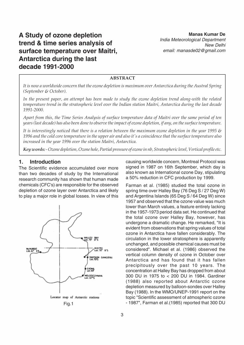
Fig.1

ABSTRACT

It is now a worldwide concern that the ozone depletion is maximum over Antarctica during the Austral Spring(September & October).

In the present paper, an attempt has been made to study the ozone depletion trend along-with the relatedtemperature trend in the stratospheric level over the Indian station Maitri, Antarctica during the last decade1991-2000.

Apart from this, the Time Series Analysis of surface temperature data of Maitri over the same period of tenyears (last decade) has also been done to observe the impact of ozone depletion, if any, on the surface temperature.

It is interestingly noticed that there is a relation between the maximum ozone depletion in the year 1995 &1996 and the cold core temperature in the upper air and also it's a coincidence that the surface temperature alsoincreased in the year 1996 over the station Maitri, Antarctica.

Key words: - Ozone depletion, Ozone hole, Partial pressure of ozone in nb, Stratospheric level, Vertical profile etc.

causing worldwide concern, Montreal Protocol wassigned in 1987 on 16th September, which day isalso known as International ozone Day, stipulatinga 50% reduction in CFC production by 1999.

Farman et al. (1985) studied the total ozone inspring time over Halley Bay (76 Deg S / 27 Deg W)and Argentina Islands (65 Deg S / 64 Deg W) since1957 and observed that the ozone value was muchlower than March values, a feature entirely lackingin the 1957-1973 period data set. He continued thatthe total ozone over Halley Bay, however, hasundergone a dramatic change. He remarked, "It isevident from observations that spring values of totalozone in Antarctica have fallen considerably. Thecirculation in the lower stratosphere is apparentlyunchanged, and possible chemical causes must beconsidered". Michael et al. (1986) observed thevertical column density of ozone in October overAntarctica and has found that it has fallenprecipitously over the past 10 years. Theconcentration at Halley Bay has dropped from about300 DU in 1975 to < 200 DU in 1984. Gardiner(1988) also reported about Antarctic ozonedepletion measured by balloon-sondes over HalleyBay (1988). In the WMO/UNEP-1991 report on thetopic "Scientific assessment of atmospheric ozone- 1987", Farman et al.(1985) reported that 300 DU

A Study of ozone depletiontrend & time series analysis ofsurface temperature over Maitri,Antarctica during the lastdecade 1991-2000

4

in 1960's over Antarctica station Halley Bay hasbeen reduced to 150 DU in 1990 in the month ofOctober. Again Farman (1994) in WMO/UNEP-1994 revealed that the trend in vertical column hasshown near total disappearance of Ozone from 12-20km altitude in September and October (Tiwari-1999). Besides Scientists, from IMD, viz., Tiwari(1999) has also shown that Ozone hole at Maitriwas quite severe in 1994-1995 and also in 1996with increase in area and depth and the cold corevortex in 1995 was very cold and persisted up toNov. Peshin et al. (1997) has also studied Ozonedepletion over Maitri during the spring month in theyear 1992 and found it centred around 16 kmextending between 12-23 km. Koppar and Nagrath(1991) has also studied ozone depletion during latewinter- early spring over Dakshin-Gangotri,Antarctica in the year 1987.

The present study aims at finding the ozonedepletion trend in the stratospheric level along-withstratospheric temperature characteristics overMaitri (WMO Index No 89514, Lat-70°45' 52"SLong-11°44' 03"E, elevation-117 metre) inAntarctica during the last decade 1991-2000 (Fig.1).Besides this, the surface temperature data of theplace during the same period has also beenanalysed.

2. Data and MethodologyData for the period of 1991-2000 has been collectedfrom National Data Centre , IMD - Pune. The verticalprofiles of ozone and temperature for the month ofSeptember, October & November for all the saidten years have been plotted.

Apart from this the Time Series Analysis of thesaid ten years surface temperature data have alsobeen done on finding out the mean monthlytemperature, mean annual temperature, annualextreme cold and warm temperature etc. Thegraphs in respect of mean monthly temperature ofthe summer and winter month, annual extremewarm and cold temperatures and mean annualtemperature daily maxima and daily minima duringthe ten years have plotted.

3. Result and Discussion3.1. Stratospheric ozone & upper air (Upper

troposphere & lower stratosphere)temperature

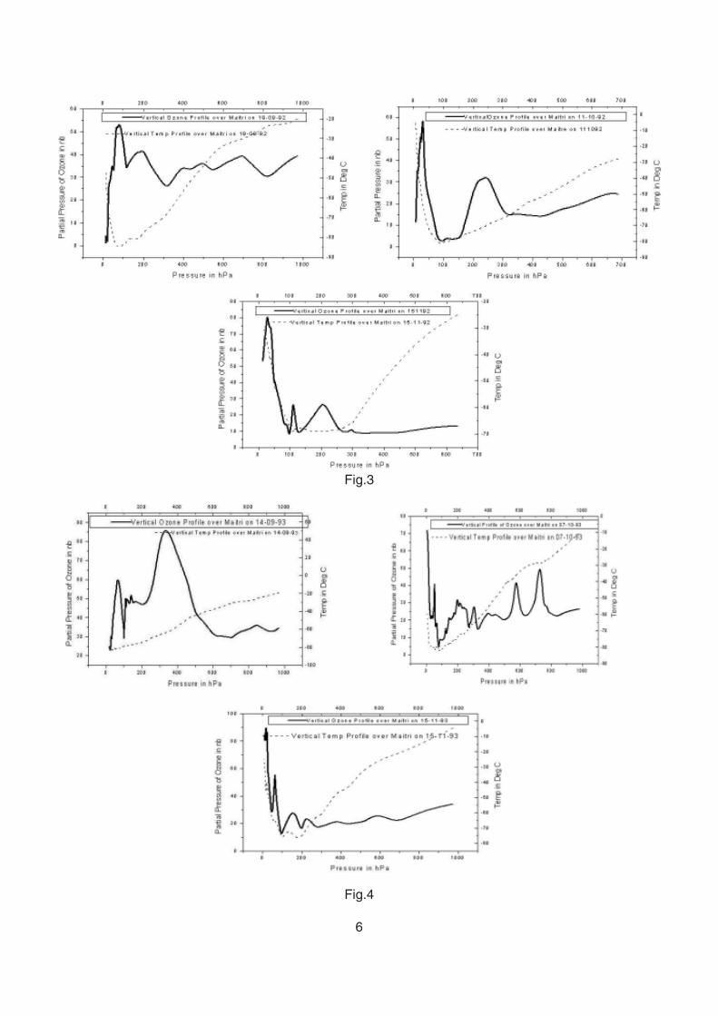
(i) During the last decade, 1991-2000, it isobserved that in the year 1992 (Fig.3) and in

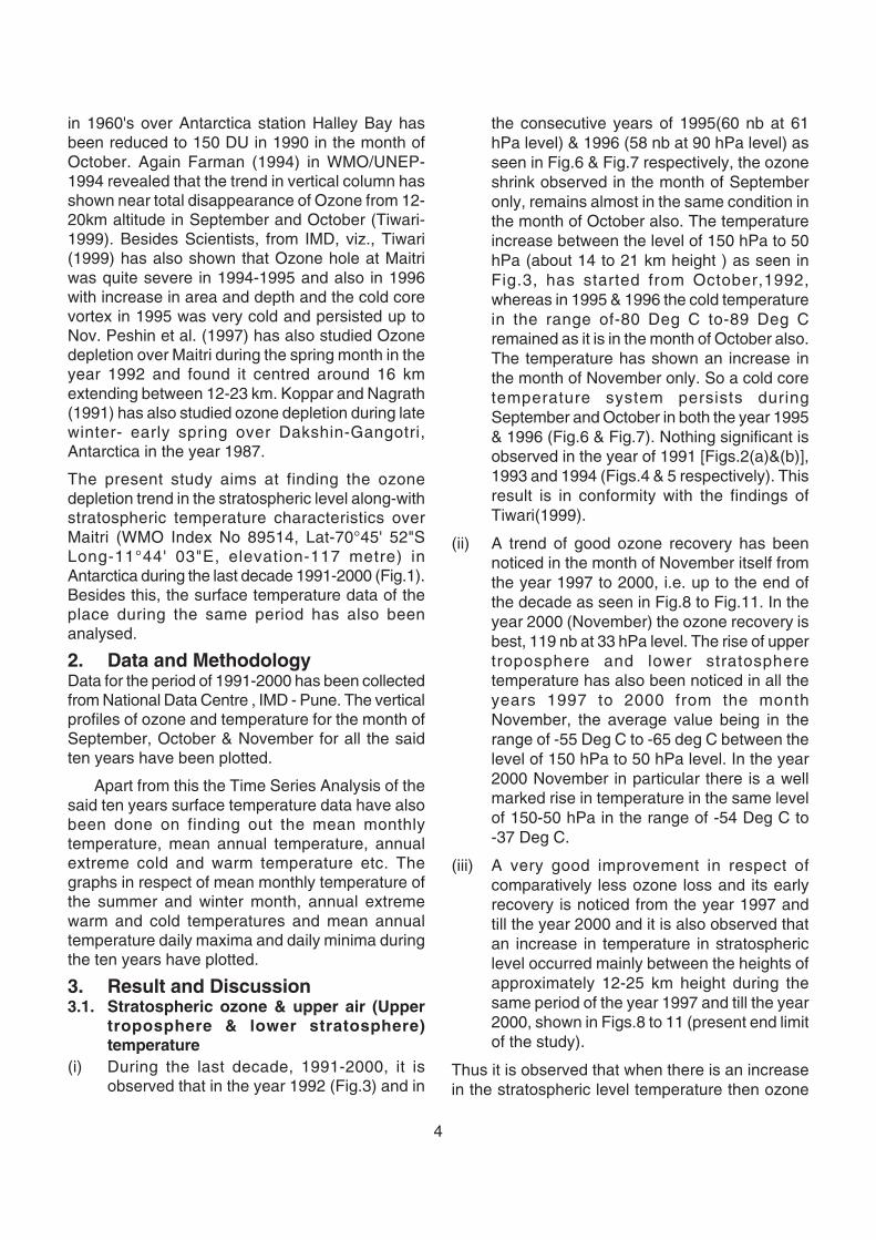
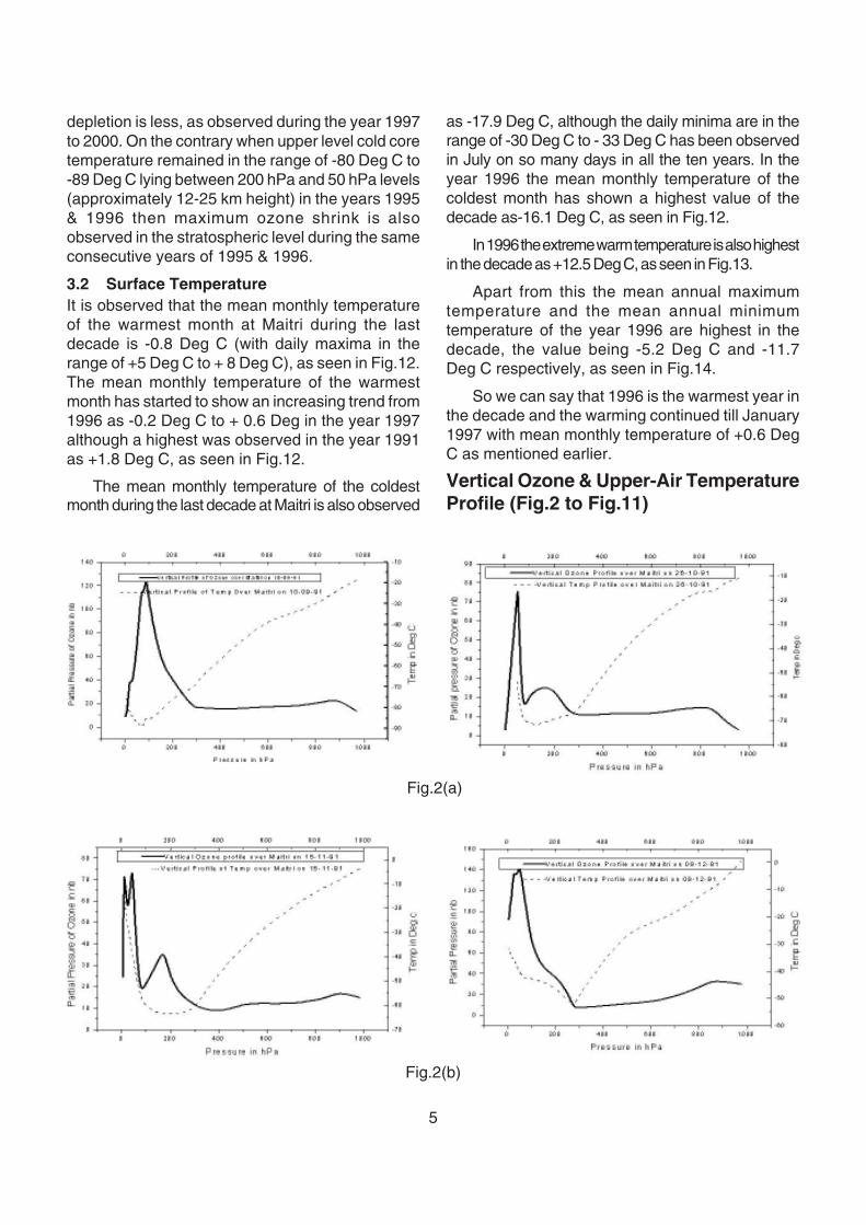
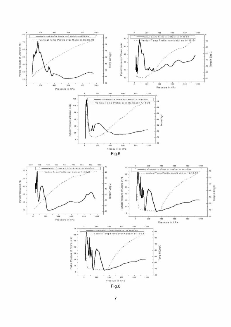
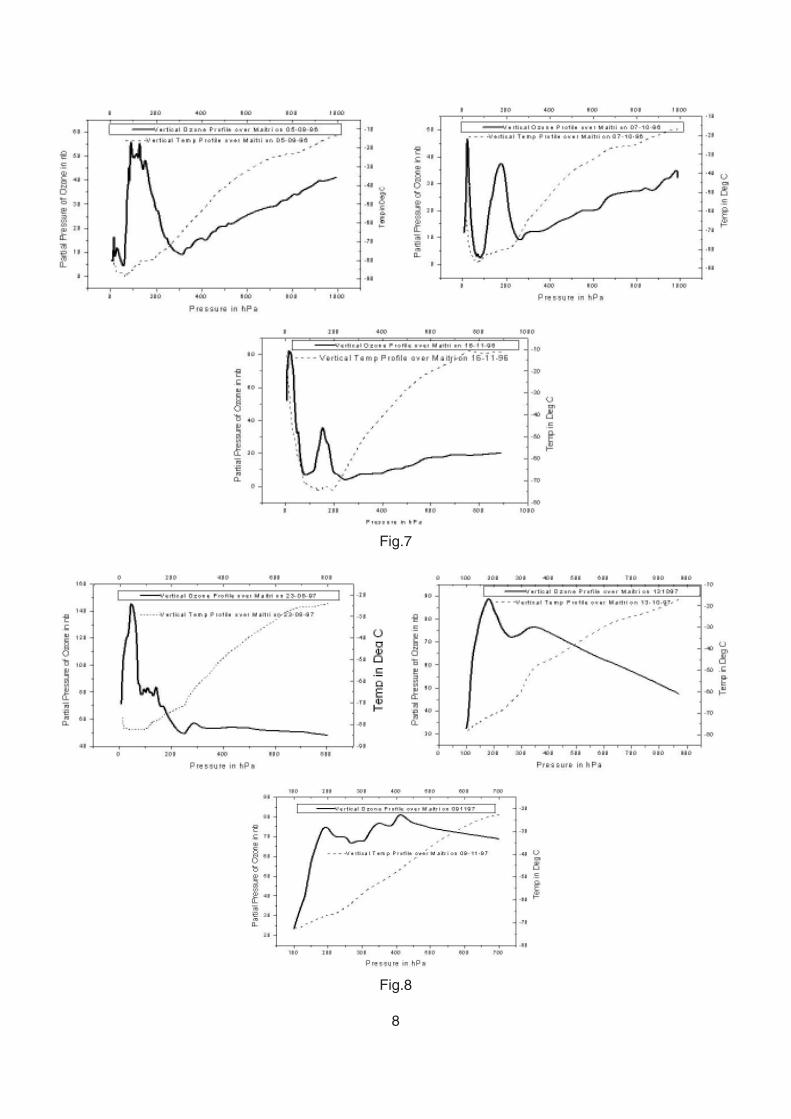
the consecutive years of 1995(60 nb at 61hPa level) & 1996 (58 nb at 90 hPa level) asseen in Fig.6 & Fig.7 respectively, the ozoneshrink observed in the month of Septemberonly, remains almost in the same condition inthe month of October also. The temperatureincrease between the level of 150 hPa to 50hPa (about 14 to 21 km height ) as seen inFig.3, has started from October,1992,whereas in 1995 & 1996 the cold temperaturein the range of-80 Deg C to-89 Deg Cremained as it is in the month of October also.The temperature has shown an increase inthe month of November only. So a cold coretemperature system persists duringSeptember and October in both the year 1995& 1996 (Fig.6 & Fig.7). Nothing significant isobserved in the year of 1991 [Figs.2(a)&(b)],1993 and 1994 (Figs.4 & 5 respectively). Thisresult is in conformity with the findings ofTiwari(1999).

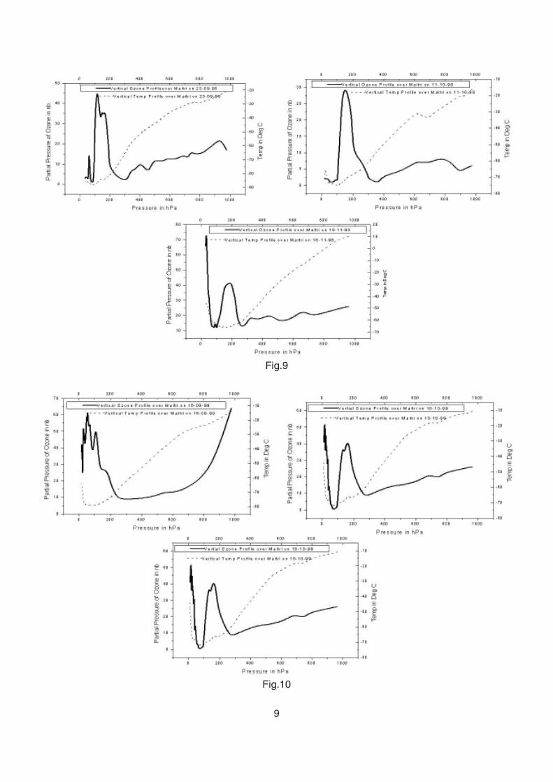
(ii) A trend of good ozone recovery has beennoticed in the month of November itself fromthe year 1997 to 2000, i.e. up to the end ofthe decade as seen in Fig.8 to Fig.11. In theyear 2000 (November) the ozone recovery isbest, 119 nb at 33 hPa level. The rise of uppertroposphere and lower stratospheretemperature has also been noticed in all theyears 1997 to 2000 from the monthNovember, the average value being in therange of -55 Deg C to -65 deg C between thelevel of 150 hPa to 50 hPa level. In the year2000 November in particular there is a wellmarked rise in temperature in the same levelof 150-50 hPa in the range of -54 Deg C to-37 Deg C.

(iii) A very good improvement in respect ofcomparatively less ozone loss and its earlyrecovery is noticed from the year 1997 andtill the year 2000 and it is also observed thatan increase in temperature in stratosphericlevel occurred mainly between the heights ofapproximately 12-25 km height during thesame period of the year 1997 and till the year2000, shown in Figs.8 to 11 (present end limitof the study).

Thus it is observed that when there is an increasein the stratospheric level temperature then ozone

5

depletion is less, as observed during the year 1997to 2000. On the contrary when upper level cold coretemperature remained in the range of -80 Deg C to-89 Deg C lying between 200 hPa and 50 hPa levels(approximately 12-25 km height) in the years 1995& 1996 then maximum ozone shrink is alsoobserved in the stratospheric level during the sameconsecutive years of 1995 & 1996.

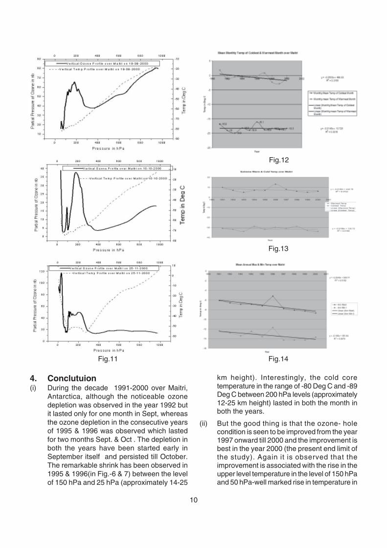
3.2 Surface TemperatureIt is observed that the mean monthly temperatureof the warmest month at Maitri during the lastdecade is -0.8 Deg C (with daily maxima in therange of +5 Deg C to + 8 Deg C), as seen in Fig.12.The mean monthly temperature of the warmestmonth has started to show an increasing trend from1996 as -0.2 Deg C to + 0.6 Deg in the year 1997although a highest was observed in the year 1991as +1.8 Deg C, as seen in Fig.12.

The mean monthly temperature of the coldestmonth during the last decade at Maitri is also observed

as -17.9 Deg C, although the daily minima are in therange of -30 Deg C to - 33 Deg C has been observedin July on so many days in all the ten years. In theyear 1996 the mean monthly temperature of thecoldest month has shown a highest value of thedecade as-16.1 Deg C, as seen in Fig.12.

In 1996 the extreme warm temperature is also highestin the decade as +12.5 Deg C, as seen in Fig.13.

Apart from this the mean annual maximumtemperature and the mean annual minimumtemperature of the year 1996 are highest in thedecade, the value being -5.2 Deg C and -11.7Deg C respectively, as seen in Fig.14.

So we can say that 1996 is the warmest year inthe decade and the warming continued till January1997 with mean monthly temperature of +0.6 DegC as mentioned earlier.

Vertical Ozone & Upper-Air TemperatureProfile (Fig.2 to Fig.11)

Fig.2(a)

Fig.2(b)

6

Fig.4

Fig.3

7

Fig.5

Fig.6

8

Fig.8

Fig.7

9

Fig.9

Fig.10

10

Fig.11 Fig.14

Fig.13

Fig.12

4. Conclutuion(i) During the decade 1991-2000 over Maitri,

Antarctica, although the noticeable ozonedepletion was observed in the year 1992 butit lasted only for one month in Sept, whereasthe ozone depletion in the consecutive yearsof 1995 & 1996 was observed which lastedfor two months Sept. & Oct . The depletion inboth the years have been started early inSeptember itself and persisted till October.The remarkable shrink has been observed in1995 & 1996(in Fig.-6 & 7) between the levelof 150 hPa and 25 hPa (approximately 14-25

km height). Interestingly, the cold coretemperature in the range of -80 Deg C and -89Deg C between 200 hPa levels (approximately12-25 km height) lasted in both the month inboth the years.

(ii) But the good thing is that the ozone- holecondition is seen to be improved from the year1997 onward till 2000 and the improvement isbest in the year 2000 (the present end limit ofthe study). Again it is observed that theimprovement is associated with the rise in theupper level temperature in the level of 150 hPaand 50 hPa-well marked rise in temperature in

11

Prasad, DDGM (Training), CTI, IMD Pune, for thenecessary support to take up the work.

I thank Dr. (Ms.) Medha Khole, Director of CTI& Mrs. S.S. Basarkar, Director of DDGM(SI) Unit,Pune for their helpful suggestions in the topics.Advanced Trg in Meteorology at CTI (IMD) Pune,during July-August 2005. I am also thankful to ShriAnil Verma, S.A. (APEC unit, at H.Q. New Delhi),and S/Shri Subhash Khurana, AM-II & DineshKhanna, S.A. (Publication unit, at H.Q. New Delhi)for helping me for the necessary computer workrequired to bring out the paper.

ReferencesFarman J. C.,Gardiner B.G., and Shanklin J.D.,1985, "Large losses of total ozone in Antarcticareveal seasonal ClO/NO interaction", (Nature-1985, Vol-315, pp 207-210,).

Gardiner B.G., 1988, Antarctic ozone depletionmeasured by balloon-sondes at Halley Bay",(Quadrennial ozone symposium, Germany, 4-13August 1988).

Kopper A.L. and Nagrath S.C., 1991, "Seasonalvariation in the vertical distribution of ozone overDakshin-Gangotri, Antarctica, Mausam, 42,3,pp.275-278.

Michael B. McElroy, Ross J. Salawitch, Stever C.Wofsy and Jennifer A. Logan, 1986, "Reductionsof Antarctic ozone due to Synergestics interactionsof Cl & Br (Chlorine & Bromine).

Peshin S.K., Rajesh Rao P. and Srivastava S.K.,1997, "Antarctica ozone depletion measured byballoon-sondes at Maitri-1992", Mausam, 48,3,pp.443-446.

Tiwari V.S., 1999, "Measurement of ozone atMaitri, Antarctica", Mausam, 50,2,pp. 203-210.

WMO/UNEP, 1991,"Scientific assessment ofstratospheric ozone, 1989", global ozone research andmonitoring project, Report No. 30, WMO, Geneva.

WMO/UNEP, 1994, "Scientific assessment ofozone depletion-1994" WMO, Geneva.

the level of 150-50 hPa in the range of -54 DegC to -37 Deg C.

(iii) The above two points are as per the earlierfindings by Antarctic Scientist Farman et al1.(1985) that stratospheric ozone depletion isassociated with the stratospheric temp, it ismore when upper air temperature isdecreased and less when upper airtemperature is increased.

(iv) Coincidentally it has also been observed thatthe year 1996 was the warmest year overMaitri in the decade. The reason may be dueto the impact of increased trace gases andconsequent green house warming during theconsecutive years of 1995 & 1996. Bothissues are clear examples of a "globalcommons" environment problem. The issueof ozone depletion & global warming, saysEPA Administrator Lee Thomas, areinexorably interconnected.

AcknowledgementThe author is thankful to Dr.Ajit Tyagi, DirectorGeneral of Meteorology for his constantencouragement and guidance to carry out theactivities in the field of Polar Sciences and finallydue to his inspiration it was possible to give a finalshape to the paper which I was trying since myAdvance Training Course (in 2005) at Pune.

I wish to place on records my sincere thanksto Dr. (Mrs.) N. Jayanthi, D.D.G.M. (W/F &Training) (Retired), for giving me an opportunityto undertake this work during my AdvanceTraining Course. It is a good fortune for me tohave the brilliant guidance of Dr. Somenath Dutta,Director (CTI, IMD, Pune). I acknowledge mygratefulness to him for his able guidance andcordial cooperation for doing this work and withoutthis it would not be possible for me to completethe job successfully, I am thankful to Shri S.K.

12

ABSTRACT

During some of the years when the south-west monsoon sweeps across India with less than its usual force,many states face a gloomy harvest and a year of food shortages and drought resulting in widespread cropdamage and economic loss. However, its severity can be minimized using agrometeorological services efficiently.This paper describes such strategy in managing drought of 2002 in major agrarian states of Punjab and Haryanaby making use of the services rendered by India Meteorological Department.

1. IntroductionThe country faced a severe drought during the year2002 when all-India monsoon rainfall was deficientby 19% with 29% area of the country undermoderate to severe drought conditions. Thedeficiency in the states of Haryana and Punjab was38% and 27%, respectively. The deficiency in Julyrainfall - the most crucial month from the agriculturalpoint of view - was 85% for Haryana and 62% forPunjab. Though paddy in both the states is grownas an irrigated crop, the rainfall during the monsoonseason plays an important role in determining theyield of the crop. Due to the concerted efforts ofthe Agrometeorological Advisory Services (AAS) ofthe Meteorological Centre at Chandigarh (capitalof both the states) and the agriculture departmentsof both the states, the productivity of paddy inHaryana increased by 2.7% during 2002 comparedto that during 2001; and there was a drop of just1% in Punjab. Haryana, in addition to achievinghigher productivity during a drought year, could alsoproduce excess fodder (which normally falls shortduring drought years) and a large quantity of fodderwas supplied to the adjoining state of Rajasthanwhich faced a severe drought. The role of theAgrometeorological Advisory Service (AAS) of IMDin managing the drought of 2002 with respect topaddy crop in the two states and the mode ofinteraction with the planners and the decision-making authorities at different levels are discussed.

2. Monsoon rainfall and its variability inthe two states

The normal monsoon rainfall (June-September) inthe two states is about 500 mm with July and August

Role of AgrometeorologicalServices in managing the droughtof 2002 in Haryana and Punjab

S.C. Bhan, S.D. Atrri andSurender Paul*

India Meteorological Department, New Delhi*Meteorological Centre, Chandigarh

email: scbhan@yahoo.comscbhan@gmail.com

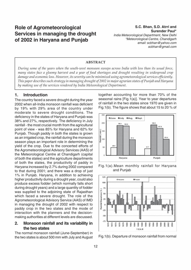
together accounting for more than 70% of theseasonal rains [Fig.1(a)]. Year to year departuresof rainfall in the two states since 1970 are given inFig.1(b). The figure shows that about 15 to 20 % of

Fig.1(b). Departure of monsoon rainfall from normal

Fig.1(a).Mean monthly rainfall for Haryana and Punjab

13

the years faced droughts (rainfall deficiency of>25%) indicating that the occurrence of droughtsin the two states is not uncommon. Earlier studiesalso show that the frequency of droughts in Haryanais 20% (IMD 1991) and in Punjab is 19% (IMD 1996;MoAg 2005).

2.1. Cultivation of paddy in the two statesThe states of Haryana and Punjab are primarilyagrarian economies with agriculture contributingabout 28% and 39%, respectively to the grossstate domestic product against the nationalaverage of about 22%. Paddy is one of the mostimportant kharif crops grown over an area ofabout 1050 thousand hectare in Haryana andabout 2650 thousand hectare in Punjab which isabout 28% and 60% of the net cultivated area ofthe two states, respectively. Both the states jointlycontr ibute about 44% of the total paddyprocurement of the country. Though the mean

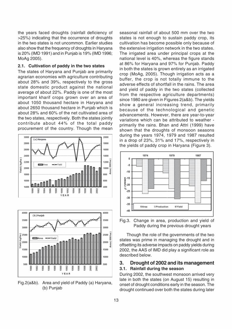
seasonal rainfall of about 500 mm over the twostates is not enough to sustain paddy crop, itscultivation has become possible only because ofthe extensive irrigation network in the two states.The irrigated area under principal crops at thenational level is 40%, whereas the figure standsat 86% for Haryana and 97% for Punjab. Paddyin both the states is grown entirely as an irrigatedcrop (MoAg, 2005). Though irrigation acts as abuffer, the crop is not totally immune to theadverse effects of shortfall in the rains. The areaand yield of paddy in the two states (collectedfrom the respective agriculture departments)since 1980 are given in Figures 2(a&b). The yieldsshow a general increasing trend, primarilybecause of the technological and geneticadvancements. However, there are year-to-yearvariations which can be attributed to weather -primarily the rains. Bhan and Attri (1999) haveshown that the droughts of monsoon seasonsduring the years 1974, 1979 and 1987 resultedin a drop of 23%, 31% and 17%, respectively inthe yields of paddy crop in Haryana (Figure 3).

Fig.2(a&b). Area and yield of Paddy (a) Haryana,(b) Punjab

Fig.3. Change in area, production and yield ofPaddy during the previous drought years

Though the role of the governments of the twostates was prime in managing the drought and inoffsetting its adverse impacts on paddy yields during2002, the AAS of IMD did play a significant role asdescribed below.

3. Drought of 2002 and its management3.1. Rainfall during the seasonDuring 2002, the southwest monsoon arrived verylate in both the states (on August 15) resulting inonset of drought conditions early in the season. Thedrought continued over both the states during later

14

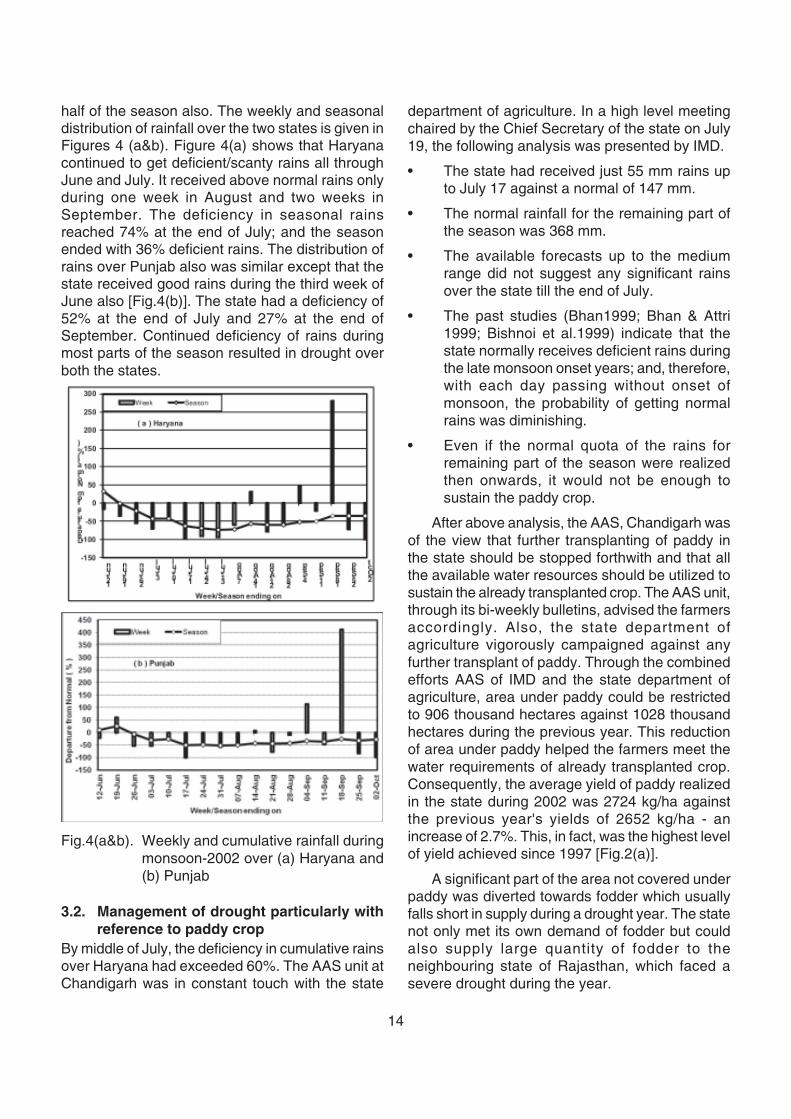
Fig.4(a&b). Weekly and cumulative rainfall duringmonsoon-2002 over (a) Haryana and(b) Punjab

half of the season also. The weekly and seasonaldistribution of rainfall over the two states is given inFigures 4 (a&b). Figure 4(a) shows that Haryanacontinued to get deficient/scanty rains all throughJune and July. It received above normal rains onlyduring one week in August and two weeks inSeptember. The deficiency in seasonal rainsreached 74% at the end of July; and the seasonended with 36% deficient rains. The distribution ofrains over Punjab also was similar except that thestate received good rains during the third week ofJune also [Fig.4(b)]. The state had a deficiency of52% at the end of July and 27% at the end ofSeptember. Continued deficiency of rains duringmost parts of the season resulted in drought overboth the states.

department of agriculture. In a high level meetingchaired by the Chief Secretary of the state on July19, the following analysis was presented by IMD.

• The state had received just 55 mm rains upto July 17 against a normal of 147 mm.

• The normal rainfall for the remaining part ofthe season was 368 mm.

• The available forecasts up to the mediumrange did not suggest any significant rainsover the state till the end of July.

• The past studies (Bhan1999; Bhan & Attri1999; Bishnoi et al.1999) indicate that thestate normally receives deficient rains duringthe late monsoon onset years; and, therefore,with each day passing without onset ofmonsoon, the probability of getting normalrains was diminishing.

• Even if the normal quota of the rains forremaining part of the season were realizedthen onwards, it would not be enough tosustain the paddy crop.

After above analysis, the AAS, Chandigarh wasof the view that further transplanting of paddy inthe state should be stopped forthwith and that allthe available water resources should be utilized tosustain the already transplanted crop. The AAS unit,through its bi-weekly bulletins, advised the farmersaccordingly. Also, the state department ofagriculture vigorously campaigned against anyfurther transplant of paddy. Through the combinedefforts AAS of IMD and the state department ofagriculture, area under paddy could be restrictedto 906 thousand hectares against 1028 thousandhectares during the previous year. This reductionof area under paddy helped the farmers meet thewater requirements of already transplanted crop.Consequently, the average yield of paddy realizedin the state during 2002 was 2724 kg/ha againstthe previous year's yields of 2652 kg/ha - anincrease of 2.7%. This, in fact, was the highest levelof yield achieved since 1997 [Fig.2(a)].

A significant part of the area not covered underpaddy was diverted towards fodder which usuallyfalls short in supply during a drought year. The statenot only met its own demand of fodder but couldalso supply large quantity of fodder to theneighbouring state of Rajasthan, which faced asevere drought during the year.

3.2. Management of drought particularly withreference to paddy crop

By middle of July, the deficiency in cumulative rainsover Haryana had exceeded 60%. The AAS unit atChandigarh was in constant touch with the state

15

Other departments involved in managing thedrought, particularly the irrigation and powerdepartments, were also provided the necessarymeteorological support to help them regulate waterand electricity supply to different parts of the state.Bhakhra and Beas Management Board (BBMB)which manage the Bhakhra Dam at river Satluj andthe Pong Dam at river Beas are the main authoritysupplying water and electricity to the states. Weatherforecasts and realized rainfall (both distribution andintensity) were regularly provided to the BBMB tohelp them objectively assess the quantum of waterand power required in both the basin states on thebasis of the rainfall received in the recent past andthe forecast for the immediate future. Also theoccurrence of rains; and its forecast for HimachalPradesh where major portions of the catchments ofthe two dams lie, helped the BBMB assess theexpected inflow into the dams and thus regulate itssupply downstream. Similar information was alsoprovided to the state departments of irrigation andpower for necessary decision-making. With all thesecombined efforts of the state government, the damauthorities and the AAS of IMD, the state couldachieve the highest level of productivity of paddy inpast 5 years despite a drought that persisted all mostall through the crop season.

In Punjab, a similar increase in the yield couldnot be achieved primarily because the area underpaddy during the year increased from 2487thousand hectare in 2001 to 2530 thousandhectares in 2002 - an increase of about 2 %. Thiswas because paddy is normally transplanted earlierin the state and also because the rainfall deficiencyas on July 10 was 26% compared to 43% deficiency

in Haryana for the corresponding period. However,due to the constant interaction of the AAS of lMDwith the departments of the state governmentresponsible for managing the drought and the damauthorities (as mentioned for Haryana), the drop inthe yield could be restricted to just 1% (from 3545kg/ha to 3510 kg/ha).

The above experience of managing the droughtof 2002 in Haryana and Punjab shows that theagrometeorological services can play an importantrole in minimizing the impacts of adverse weatherconditions and making agriculture more economic.

ReferencesIMD, 1991, Climate of Haryana and UnionTerritories of Delhi and Chandigarh. IndiaMeteorological Department, Pune. pp. 98.

IMD, 1996, Cl imate of Punjab. IndiaMeteorological Department, Pune. pp. 83.

MoAg, 2005. Agricultural Statistics at a Glance-2005. Ministry of Agriculture, Government ofIndia, New Delhi. pp. 241.

Bhan, S.C., 1999, Rainfall variability overwestern Haryana during early, normal and latecommencement of sowing rains. Proc. NationalSymposium on "Meteorology beyond 2000"(Tropmet -99) held at Chennai during February16-19, 1999. pp. 105-109.

Bhan, S.C. and Attri, S.D., 1999. Droughtimpacts on technologically advanced agriculturein Haryana. Vayu Mandal, 29(1-4): 417-421.

Bishnoi, O.P. Bhan, S.C. and Niwas, R, 1999,Predictive behaviour of seasonal rainfall at Hisarfor Pearlmillet production. Haryana Agric. Univ.J. Res., 21: 80-84.

16

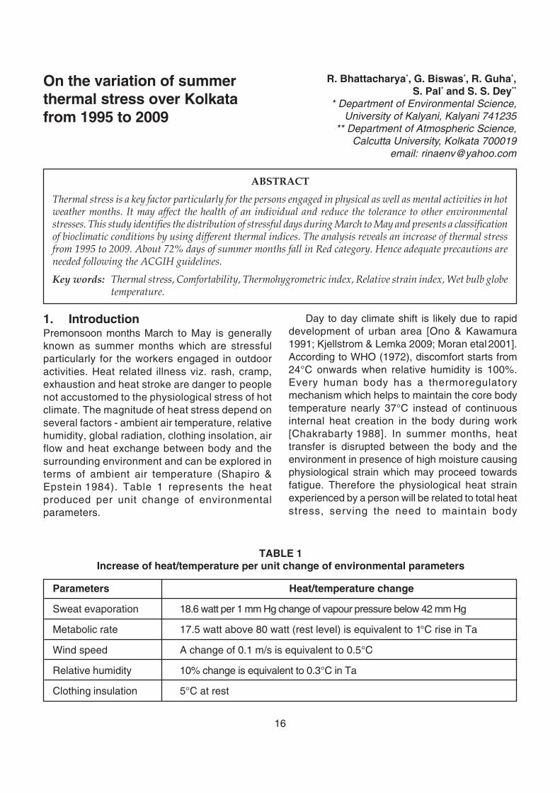
1. IntroductionPremonsoon months March to May is generallyknown as summer months which are stressfulparticularly for the workers engaged in outdooractivities. Heat related illness viz. rash, cramp,exhaustion and heat stroke are danger to peoplenot accustomed to the physiological stress of hotclimate. The magnitude of heat stress depend onseveral factors - ambient air temperature, relativehumidity, global radiation, clothing insolation, airflow and heat exchange between body and thesurrounding environment and can be explored interms of ambient air temperature (Shapiro &Epstein 1984). Table 1 represents the heatproduced per unit change of environmentalparameters.

Day to day climate shift is likely due to rapiddevelopment of urban area [Ono & Kawamura1991; Kjellstrom & Lemka 2009; Moran etal 2001].According to WHO (1972), discomfort starts from24°C onwards when relative humidity is 100%.Every human body has a thermoregulatorymechanism which helps to maintain the core bodytemperature nearly 37°C instead of continuousinternal heat creation in the body during work[Chakrabarty 1988]. In summer months, heattransfer is disrupted between the body and theenvironment in presence of high moisture causingphysiological strain which may proceed towardsfatigue. Therefore the physiological heat strainexperienced by a person will be related to total heatstress, serving the need to maintain body

R. Bhattacharya*, G. Biswas*, R. Guha*,S. Pal* and S. S. Dey**

* Department of Environmental Science,University of Kalyani, Kalyani 741235

** Department of Atmospheric Science,Calcutta University, Kolkata 700019

email: rinaenv@yahoo.com

On the variation of summerthermal stress over Kolkatafrom 1995 to 2009

ABSTRACT

Thermal stress is a key factor particularly for the persons engaged in physical as well as mental activities in hotweather months. It may affect the health of an individual and reduce the tolerance to other environmentalstresses. This study identifies the distribution of stressful days during March to May and presents a classificationof bioclimatic conditions by using different thermal indices. The analysis reveals an increase of thermal stressfrom 1995 to 2009. About 72% days of summer months fall in Red category. Hence adequate precautions areneeded following the ACGIH guidelines.

Key words: Thermal stress, Comfortability, Thermohygrometric index, Relative strain index, Wet bulb globetemperature.

TABLE 1Increase of heat/temperature per unit change of environmental parameters

Parameters Heat/temperature change

Sweat evaporation 18.6 watt per 1 mm Hg change of vapour pressure below 42 mm Hg

Metabolic rate 17.5 watt above 80 watt (rest level) is equivalent to 1°C rise in Ta

Wind speed A change of 0.1 m/s is equivalent to 0.5°C

Relative humidity 10% change is equivalent to 0.3°C in Ta

Clothing insulation 5°C at rest

17

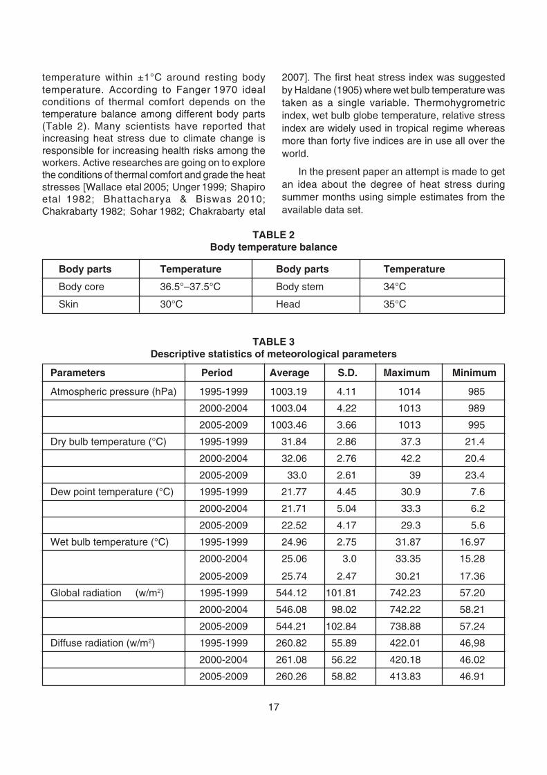
temperature within ±1°C around resting bodytemperature. According to Fanger 1970 idealconditions of thermal comfort depends on thetemperature balance among different body parts(Table 2). Many scientists have reported thatincreasing heat stress due to climate change isresponsible for increasing health risks among theworkers. Active researches are going on to explorethe conditions of thermal comfort and grade the heatstresses [Wallace etal 2005; Unger 1999; Shapiroetal 1982; Bhattacharya & Biswas 2010;Chakrabarty 1982; Sohar 1982; Chakrabarty etal

2007]. The first heat stress index was suggestedby Haldane (1905) where wet bulb temperature wastaken as a single variable. Thermohygrometricindex, wet bulb globe temperature, relative stressindex are widely used in tropical regime whereasmore than forty five indices are in use all over theworld.

In the present paper an attempt is made to getan idea about the degree of heat stress duringsummer months using simple estimates from theavailable data set.

TABLE 2Body temperature balance

Body parts Temperature Body parts Temperature

Body core 36.5°–37.5°C Body stem 34°C

Skin 30°C Head 35°C

TABLE 3Descriptive statistics of meteorological parameters

Parameters Period Average S.D. Maximum Minimum

Atmospheric pressure (hPa) 1995-1999 1003.19 4.11 1014 985

2000-2004 1003.04 4.22 1013 989

2005-2009 1003.46 3.66 1013 995

Dry bulb temperature (°C) 1995-1999 31.84 2.86 37.3 21.4

2000-2004 32.06 2.76 42.2 20.4

2005-2009 33.0 2.61 39 23.4

Dew point temperature (°C) 1995-1999 21.77 4.45 30.9 7.6

2000-2004 21.71 5.04 33.3 6.2

2005-2009 22.52 4.17 29.3 5.6

Wet bulb temperature (°C) 1995-1999 24.96 2.75 31.87 16.97

2000-2004 25.06 3.0 33.35 15.28

2005-2009 25.74 2.47 30.21 17.36

Global radiation (w/m2) 1995-1999 544.12 101.81 742.23 57.20

2000-2004 546.08 98.02 742.22 58.21

2005-2009 544.21 102.84 738.88 57.24

Diffuse radiation (w/m2) 1995-1999 260.82 55.89 422.01 46,98

2000-2004 261.08 56.22 420.18 46.02

2005-2009 260.26 58.82 413.83 46.91

18

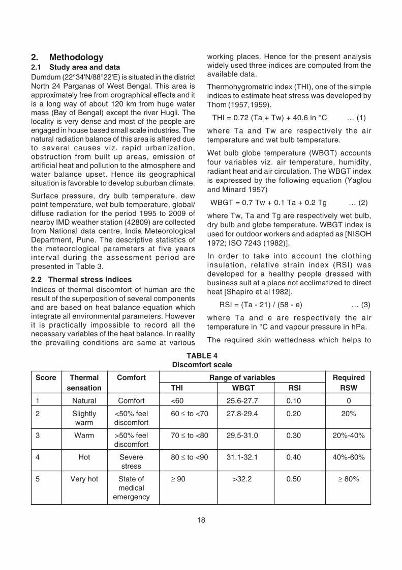
working places. Hence for the present analysiswidely used three indices are computed from theavailable data.

Thermohygrometric index (THI), one of the simpleindices to estimate heat stress was developed byThom (1957,1959).

THI = 0.72 (Ta + Tw) + 40.6 in °C … (1)

where Ta and Tw are respectively the airtemperature and wet bulb temperature.

Wet bulb globe temperature (WBGT) accountsfour variables viz. air temperature, humidity,radiant heat and air circulation. The WBGT indexis expressed by the following equation (Yaglouand Minard 1957)

WBGT = 0.7 Tw + 0.1 Ta + 0.2 Tg … (2)

where Tw, Ta and Tg are respectively wet bulb,dry bulb and globe temperature. WBGT index isused for outdoor workers and adapted as [NISOH1972; ISO 7243 (1982)].

In order to take into account the clothinginsulation, relative strain index (RSI) wasdeveloped for a healthy people dressed withbusiness suit at a place not acclimatized to directheat [Shapiro et al 1982].

RSI = (Ta - 21) / (58 - e) … (3)

where Ta and e are respectively the airtemperature in °C and vapour pressure in hPa.

The required skin wettedness which helps to

2. Methodology2.1 Study area and dataDumdum (22°34'N/88°22'E) is situated in the districtNorth 24 Parganas of West Bengal. This area isapproximately free from orographical effects and itis a long way of about 120 km from huge watermass (Bay of Bengal) except the river Hugli. Thelocality is very dense and most of the people areengaged in house based small scale industries. Thenatural radiation balance of this area is altered dueto several causes viz. rapid urbanization,obstruction from built up areas, emission ofartificial heat and pollution to the atmosphere andwater balance upset. Hence its geographicalsituation is favorable to develop suburban climate.

Surface pressure, dry bulb temperature, dewpoint temperature, wet bulb temperature, global/diffuse radiation for the period 1995 to 2009 ofnearby IMD weather station (42809) are collectedfrom National data centre, India MeteorologicalDepartment, Pune. The descriptive statistics ofthe meteorological parameters at five yearsinterval during the assessment period arepresented in Table 3.

2.2 Thermal stress indicesIndices of thermal discomfort of human are theresult of the superposition of several componentsand are based on heat balance equation whichintegrate all environmental parameters. Howeverit is practically impossible to record all thenecessary variables of the heat balance. In realitythe prevailing conditions are same at various

TABLE 4Discomfort scale

Score Thermal Comfort Range of variables Requiredsensation THI WBGT RSI RSW

1 Natural Comfort <60 25.6-27.7 0.10 0

2 Slightly <50% feel 60 ≤ to <70 27.8-29.4 0.20 20%warm discomfort

3 Warm >50% feel 70 ≤ to <80 29.5-31.0 0.30 20%-40%discomfort

4 Hot Severe 80 ≤ to <90 31.1-32.1 0.40 40%-60%stress

5 Very hot State of ≥ 90 >32.2 0.50 ≥ 80%medical

emergency

19

remove heat from body as a latent heat ofevaporation and keep the body in thermal comfortcan be obtained from the ratioE

req/E

max when thermal

balance is achieved. Ereq = Metabolic heat

production ± Heat exchange between body and

surrounding and Emax

is the maximum capacity of

evaporation [Kerslake 1972;Gonzalez et al 1978.The various stages of thermal sensation andphysiological zone of thermal discomfort withincreasing temperature are classified from surveyamong the various populations by several scientistsall over the globe in a five graded discomfort scale[Prasad and Power 1982; Mayer and Hoppe 1987;Epstein and Moran 2006] as shown in Table 4.Required skin wittedness at different stages ofdiscomfort is also presented in the same table.

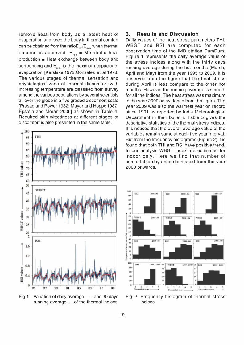
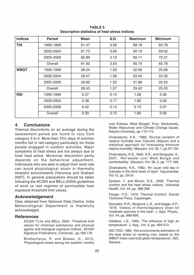
3. Results and DiscussionDaily values of the heat stress parameters THI,WBGT and RSI are computed for eachobservation time of the IMD station DumDum.Figure 1 represents the daily average value ofthe stress indices along with the thirty daysrunning average during the hot months (March,April and May) from the year 1995 to 2009. It isobserved from the figure that the heat stressduring April is less compare to the other hotmonths. However the running average is smoothfor all the indices. The heat stress was maximumin the year 2009 as evidence from the figure. Theyear 2009 was also the warmest year on recordsince 1901 as reported by India MeteorologicalDepartment in their bulletin. Table 5 gives thedescriptive statistics of the thermal stress indices.It is noticed that the overall average value of thevariables remain same at each five year interval.But from the frequency histograms (Figure 2) it isfound that both THI and RSI have positive trend.In our analysis WBGT index are estimated forindoor only. Here we find that number ofcomfortable days has decreased from the year2000 onwards.

Fig.1. Variation of daily average .......and 30 daysrunning average .....of the thermal indices

Fig. 2. Frequency histogram of thermal stressindices

20

TABLE 5Descriptive statistics of heat stress indices

Indices Period Mean S.D. Maximum Minimum

THI 1995-1999 81.47 3.58 89.18 65.78

2000-2004 81.73 3.66 90.19 69.02

2005-2009 82.89 3.13 89.11 72.31

Overall 81.92 3.55 90.19 65.78

WBGT 1995-1999 28.24 1.59 32.99 25.66

2000-2004 28.47 1.58 33.42 25.56

2005-2009 28.60 1.52 31.88 25.55

Overall 28.43 1.57 33.42 25.55

RSI 1995-1999 0.37 0.14 1.08 0.06

2000-2004 0.38 0.17 1.80 0.06

2005-2009 0.42 0.13 0.73 0.07

Overall 0.39 0.15 1.80 0.06

4. ConclusionsThermal discomforts on an average during theassessment period are found to vary fromcategory 3 to 4. More than 70% days of summermonths fall in red category particularly for thosepeople engaged in outdoor activities. Majorsymptoms of heat stress are not always due toheat load alone. Moreover discomfort partlydepends on the behavioral adjustment.Individuals who are able to adjust their work ratecan avoid physiological strain in thermallystressful environments [Veronica and Graham2007]. In general precautions should be takenfollowing the ACGlH and BELs (2004) guidelinesof work vs rest regimes of permissible heatexposure threshold limit values.

AcknowledgementData obtained from National Data Centre, IndiaMeteorological Department is thankful lyacknowledged.

ReferencesACGIH TLVs and BELs, 2004, 'Threshold limitvalues for chemical substances and physicalagents and biological exposure indices', ACGIHSignature Publications, Cincinnati, pp.168-176.

Bhattacharya, R. and Biswas, G., 2010,'Physiological stress during hot weather months

over Kolkata, West Bengal', Proc. Biodiversity,Water Resources and Climate Change Issues,Kalyani University, pp.110-115.

Chakrabarty, K.K., 1988, 'Diurnal variation ofrelative humidity over Calcutta (Alipore) and astatistical approach for forecasting minimumrelative humidity', Mausam, Vol. 39, 1, pp.97-102.

Chakrabarty, K.K., Nath, A.K., and Sengupta, S.,2007, 'Nor'wester over West Bengal andcomfortability', Mausam, Vol. 58, 2, pp. 177-188.

Chakrabarty, K.K., 1982, 'An usual cold day inCalcutta in the third week of April', Vayumandal,Vol.12, pp. 29-31.

Epstein, Y. and Moran, D.S., 2006, 'Thermalcomfort and the heat stress indices', IndustrialHealth, Vol. 44, pp. 388-398.

Fanger, P.O., 1970, 'Thermal Comfort', DanishTechnical Press, Copenhgen.

Gonzalez, R.R., Berglund, L.G., and Gagge, A.P.,1978, 'Indices of thermoregulatory strain formoderate exercise in the heat', J. Appl. Physio.,Vol. 44, pp. 889-899.

Haldane, J.S., 1905, 'The influence of high airtemperature', J. Hyg., Vol. 5, pp. 494-513.

ISO 7243, 1982, 'Hot environments-estimation ofthe heat stress on working man, based on theWBGT-index (wet bulb globe temperature)', ISO,Geneva.

21

Kjellstrom, T. and Lemke, B., 2009, 'Estimatingheat stress indices from routine weather stationdata; an important tool to support adaptionplanning', IOP Conf. Series:Earth andEnvironmental Science, Vol. 6, pp.39-40.

Kerslake, D.M., 1972, 'The stress of hot environment',Cambridge University Press, Cambridge.

Moran, D.S., Pandolf, K.B., Shapiro, Y., HeledY., Shani, Y., Mattfew, W.T. and Gonzales, R.R.,2001, 'An environmental stress index (ESI) as asubstitute for the wet bulb globe temperature(WBGT)', J. Thermal Biol., Vol. 26, pp. 427-431.

Mayer, H. and Hoppe, P., 1987, 'Thermalcomfort of man in different urban environments',Theor. Appl. Climatol., Vol. 38, pp. 43-49.

NIOSH, 1972, 'Occupational exposure to hotenvironment', National Institute for Occupationalsafety and Health, HSM 72-10269, Departmentof Health, Education and Welfare, Washington DC.

Ono, H.P. and Kawamura, T., 1991, 'Sensibleclimates in monsoon Asia', Int. J. Biometeorol.,Vol.35, pp. 39-47.

Prasad, S.K. and Power, B.C., 1982, 'Discomfortover Bombay during winter', Vayumandal, Vol.12, pp. 53-54.

Shapiro, Y. and Epstein, Y., 1984, 'Environmentalphysiology and indoor climate-thermo regulation andthermal comfort', Energy Build, Vol. 7, pp. 29-34.

Shapiro, Y., Pandolf, K.B. and Goldman, R.F.,1982, 'Predicting sweat loss response to exercise,

environment and clothing', Eur. J. Appl. Physiol.,Vol.48, pp. 83-96.

Sohar, E., 1982, 'Men, microclimate and society',Energy Build, Vol. 4, pp.149-154.

Thom, E.C., 1957, 'A new concept for coolingdegree days', Air Condit. Heat and Ventil., Vol.54,pp.73-80.

Thom, E.C., 1959, 'The discomfort index',Weatherwise, Vol.12, pp.57-60.

Unger, J., 1999, 'Comparison of urban and ruralbioclimatological conditions in the case of aCentral European city', Int. J. Biometeorol, Vol.43,pp.139-144.

Veronica, S. Miller and Graham, P. Bates, 2007,'The thermal work limit is a simple reliable heatindex for the protection of workers in thermallystressful environments', Ann. Occup. Hyg., Vol.51, pp. 553-561.

WMO, 1972, 'The assessment of human bioclimatic-A limited review of physical parameters',H.E. Landsberg, (ed.) WMO Technical note, Vol.123, pp. 2-16.

Wallace, R.F., Kriebel, D., Punnett, L., Weghman,D.H., Wenger C.B., Gardner J.W. and GonzalesR.R., 2005, 'The effects of continuous hot weathertraining on risk of exertional heat illness', Med.Sci. Sports Exerc., Vol. 37, pp. 84-90.

Yaglou, C.P. and Minard, D., 1957, 'Control of heatcasualties at military training centers', Am. Med.Ass. Arch. Ind. Hlth., Vol.16, pp.302-316.

22

1. IntroductionWater vapour is one of the key elements of theatmosphere as moisture and latent heat aretransported through water vapour phase. Also watervapour is a highly variable and not evenly distributedin the atmosphere. It plays an important role invarious atmospheric processes that act over a widerange of spatial and temporal scales starting fromglobal climate to micrometeorology. Thus accuratedense and frequent measurement of atmosphericwater vapour obviously has great use in day to dayweather forecasting as well as climate study.Atmospheric scientists have developed a varietyof means to measure the vertical and horizontaldistribution of water vapour. At present water vapouris measured using radiosondes and ground orspace base radiometer. Radiosondes provideaccurate water vapour profile data of theatmosphere which have great use in weatheranalysis and forecasting but spatial and temporalcoverage is rather poor. In the recent year a newtechnology on the basis of Global Positioning

System (GPS) is being applied worldwide to remotesensing water vapour in the atmosphere. IndiaMeteorological Department has installed groundbased GPS receiver with data processing systemat five cities including Kolkata, India to deriveintegrated precipitable water vapour (IPWV) in theaim of enhancement of meteorological observationover Indian region.

GPS derived IPWV data can be available on nearreal time basis with high temporal resolution (hourlyor even every 30 minutes). So it promises a greatapplication in improvement of short term weatherforecast especially during severe weather conditionviz., severe thunderstorm activity, flash flood eventetc. Application of IPWV data in meso scalenumerical weather model studied by Kuo et al.1993,1996 and they infer that GPS derived IPWVdata assure improvement in short term weatherforecasting. Besides short term weather prediction,GPS observations of atmospheric moisture can alsobe used to monitor climate change (Yuan et al.1993).Nowcasting of thunderstorm using GPS

ABSTRACT

In the recent year a new technology to remote sensing water vapour in the atmosphere is being applied worldwideon the basis of Global Positioning System (GPS). India Meteorological Department has installed ground basedGPS receiver with data processing system at five cities including Kolkata, India to derive integrated precipitablewater vapour (IPWV) in the aim of enhancement of meteorological observation over Indian region. In thepresent study hourly IPWV data derived from GPS at Kolkata for the peak pre-monsoon period (April - May)2008 has been analysed to explore the potentiality of this data in forecasting/nowcasting severe thunderstormevents namely Norwester’s and some other characteristic features related to water vapour contained of theatmosphere. Study reveals that GPS derived IPWV can be used as good predictor for nowcasting of severethunderstorm events and temporal variability of precipitable water vapour contained in the atmosphere. Timeof commencement of severe thunderstorms nearly coincided with time of attaining highest IPWV value with asharp increase on an average 1.6 mm/hr over a period of 7 - 8 hrs prior to occurrence of the thunderstorm event,however minimum and peak value depends upon the calendar day as significant positive trend of IPWV valueseen through advancement of the season. Statistical analyses indicate that a polynomial trend curve may beused for nowcasting 2 - 3 hrs prior to occurrence of the severe thunderstorm over Kolkata and neighbourhood.Time series analysis of daily averaged IPWV data of Kolkata shows that it could be useful to determine thetransition of two seasons and consequently advance of monsoon over a region.

Key words: Global Positioning System (GPS), IPWV, Forecasting, Kolkata.

Utility of Global PositioningSystem derived integratedprecipitable water vapour onweather analysis and forecasting

H. R. Biswas, S. Bandyopadhyay,G. K. Das and S. N. Roy

Regional Meteorological Centre, Kolkataemails: 786hrb@gmail.com,

hr.biswas@imd.gov.in

23

Meteorology has been studied conducting fieldexperiments by many authors in other countries. InIndia the estimation of IPWV using GPS has beeninitiated by Giri et al. (2006 ) for winter season. Giri etal.(2007) has also done the comparative study of GPSderived IPWV data with MODIS, NCEP andRadisonde data. Again as the thermo dynamicalproperties of tropical troposphere changes rapidlyapplication of thermodynamic diagram computedfrom Radiosonde data is having limitations onaccount of only two daily observations viz. 0000 UTCand 1200 UTC and present conventional synopticmanual weather observation recorded in three hourlyinterval with very low spatial resolution. Under suchcircumstances use of real time IPWV contentsrecorded at each hour by ground based GPS mayhave great advantages for short term forecasting(nowcasting) of severe thunderstorm events.

In the present study, an attempt has beenmade to explore the utility of IPWV data derivedfrom GPS installed at Kolkata in short termprediction and understanding of meteorologicalcharacteristic features of severe thunderstormevent over Kolkata and its vicinity. Also potentialityof the GPS derived IPWV data to explore someother characteristic features directly related watervapour contained of the atmosphere have beenexamined in this study.

2. Data and MethodologyThe main objective of this study is to reveal thepredictability value of IPWV data received at eachhour through GPS installed at RegionalMeteorological Center, Kolkata for nowcasting ofsevere thunderstorms events associated with squall,hailstorm, heavy showers etc which are also knownas Norwester's over Kolkata and neighbourhoodduring pre-monsoon season and also to find out thesalient characteristic features explored from IPWVdata with change of season or hours of a day. So,daily hourly IPWV data of 2008 for the peakpremonsoon period 16th April to 31st May andbeginning month of monsoon i.e. June 2008 hasbeen collected from India MeteorologicalDepartment, New Delhi. The weather information i.e.occurrence /non-occurrence of thunderstorm activityand associated weather over Kolkata during the peakpremonsoon period has been extracted frommeteorological report of Regional MeteorologicalCentre, Kolkata.

GPS signals are delayed by water vapour, dryair, hydrometeors and other particulates (Niell1996). The delay due to water vapour offers anopportunity for sensing water vapor with GPS (Beviset al. (1992), Rocken et al. (1993), Businger et al.(1996) and Duan et al. (1996). Also it is well knownfact that water vapour contained in atmosphererapidly changes with occurrence of severeconvective activity. So, hourly IPWV data for daysof severe thunderstorm and non-thunderstorm dayshas been analysed by means of basic statisticalparameters viz., Mean, variance and also statisticaltrend analysis. Diurnal variability of IPWV data hasbeen examined and the significant hours of a dayfor which IPWV data to be monitored for short termprediction of severe convective activity have beenidentified using K-mean cluster analysis. Timeseries analysis of daily average of hourly IPWV datahas been performed to see the variability of IPWVdata during transition of two seasons.

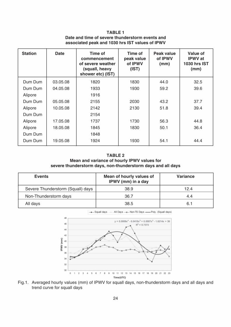
3. Results and DiscussionsSevere thunderstorm events over Kolkata during16th April to 31st May 2008 have been scrutinizedfrom daily weather data of two meteorologicalobservatories namely Alipore and Dum Dum withabout 20 km distance apart from each other anddate and time occurrence of these events has beentabulated in Table 1. Severe thunderstormassociated with Squall in 3 occasions andassociated with heavy shower occurred at Aliporeand 5 occasions of severe convective activityassociated with squall were reported by Dum Dum.Scrutinizing the hourly IPWV value interestingly ithas been noticed that time of peak value of IPWVnearly coincided with the time of commencementof the severe thunderstorm activity as shown inTable 1. Also Mean and variance of hourly IPWVvalues in a day for severe thunderstorm days, non-thunderstorm days and all days has been shown inTable 2 from which it indicates that varianceassociated with severe thunderstorm events (12.4)much higher than non-thunderstorm days(4.4). Theabove innovation motivate that hourly IPWV valuemay have good predictability of severethunderstorm events. Averaged hourly values (mm)of IPWV for squall days, non-thunderstorm daysand all days have been plotted in Fig.1. It is observedfrom Fig.1 that a significant change of IPWV valuesi.e. IPWV values sharply increased from latemorning (around 0500 UTC) to evening period when

24

TABLE 1Date and time of severe thunderstorm events andassociated peak and 1030 hrs IST values of IPWV

Station Date Time of Time of Peak value Value ofcommencement peak value of IPWV IPWV at

of severe weather of IPWV (mm) 1030 hrs IST(squall, heavy (IST) (mm)

shower etc) (IST)

Dum Dum 03.05.08 1820 1830 44.0 32.5

Dum Dum 04.05.08 1933 1930 59.2 39.6

Alipore 1916

Dum Dum 05.05.08 2155 2030 43.2 37.7

Alipore 10.05.08 2142 2130 51.8 39.4

Dum Dum 2154

Alipore 17.05.08 1737 1730 56.3 44.8

Alipore 18.05.08 1845 1830 50.1 36.4

Dum Dum 1848

Dum Dum 19.05.08 1924 1930 54.1 44.4

TABLE 2Mean and variance of hourly IPWV values for

severe thunderstorm days, non-thunderstorm days and all days

Events Mean of hourly values of VarianceIPWV (mm) in a day

Severe Thunderstorm (Squall) days 38.9 12.4

Non-Thunderstorm days 36.7 4.4

All days 38.5 6.1

Fig.1. Averaged hourly values (mm) of IPWV for squall days, non-thunderstorm days and all days andtrend curve for squall days

25

severe thunderstorm activity occurred and then itdecreased sharply, however no such features foundon non-thunderstorm days. K- Mean ClusterAnalysis suggested 0500 UTC to 1600 UTC datais most significant for indication of severeThunderstorm Event over Kolkata during pre-monsoon season. The peak values of IPWV in mmand values at 0500 UTC (1030 hrs IST) arepresented in Table 1. On an average 1.6 mm/hourincrease in IPWV value was noticed over a periodof 7 to 8 hours prior to the commencement of severethunderstorm activity over Kolkata. However theminimum and peak values of IPWV could not betaken as fixed single values for whole seasonbecause significant positive trend observed asseason advances. Trend analysis of averagedhourly IPWV value in a day for severe thunderstormevents of premonsoon 2008 indicated a fourth orderpolynomial curve fitted with good correlationcoefficient value as 0.86 (Fig.1). Comparingobservational hourly data with average polynomialcurve nowcasting of severe thunderstorm eventscan be done 2 to 3 hours prior to occurrence of theevent. However for estimation of the polynomialcurve a long period data series has to be analysed.

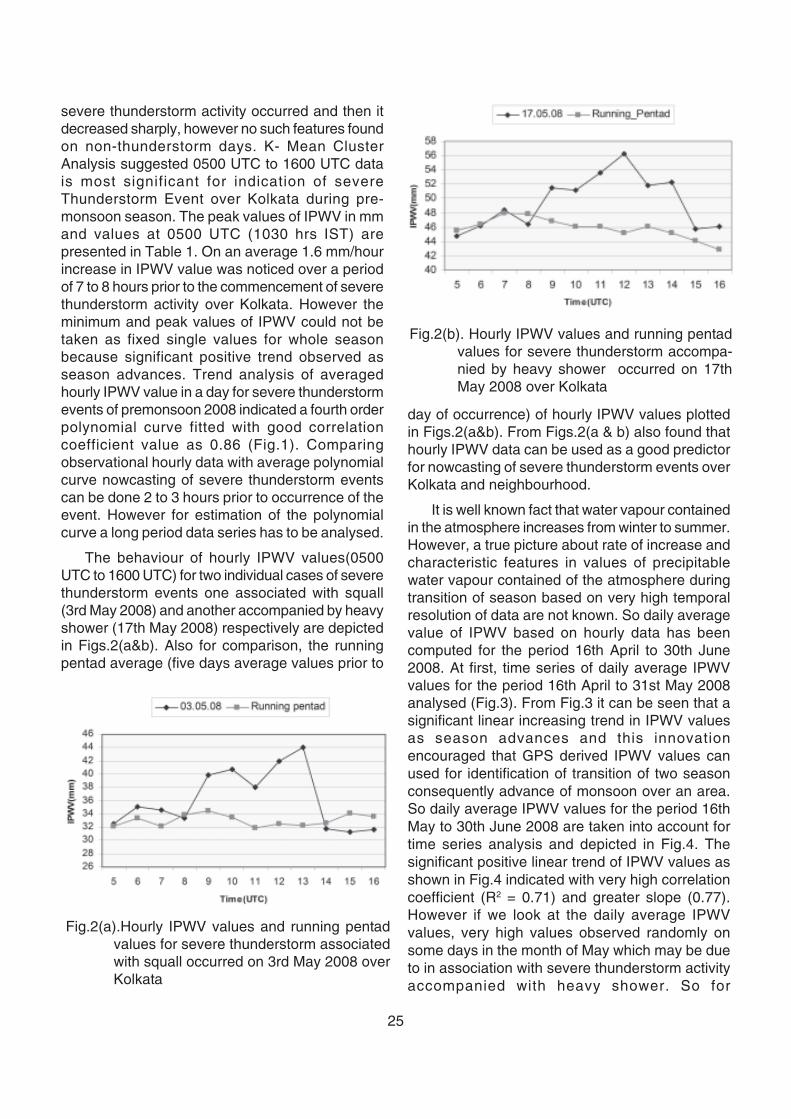
The behaviour of hourly IPWV values(0500UTC to 1600 UTC) for two individual cases of severethunderstorm events one associated with squall(3rd May 2008) and another accompanied by heavyshower (17th May 2008) respectively are depictedin Figs.2(a&b). Also for comparison, the runningpentad average (five days average values prior to

day of occurrence) of hourly IPWV values plottedin Figs.2(a&b). From Figs.2(a & b) also found thathourly IPWV data can be used as a good predictorfor nowcasting of severe thunderstorm events overKolkata and neighbourhood.

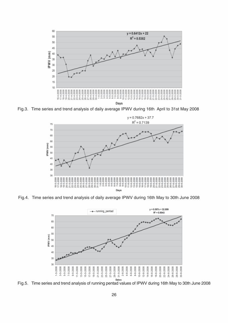
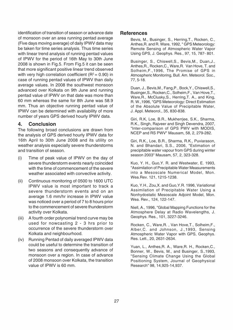
It is well known fact that water vapour containedin the atmosphere increases from winter to summer.However, a true picture about rate of increase andcharacteristic features in values of precipitablewater vapour contained of the atmosphere duringtransition of season based on very high temporalresolution of data are not known. So daily averagevalue of IPWV based on hourly data has beencomputed for the period 16th April to 30th June2008. At first, time series of daily average IPWVvalues for the period 16th April to 31st May 2008analysed (Fig.3). From Fig.3 it can be seen that asignificant linear increasing trend in IPWV valuesas season advances and this innovationencouraged that GPS derived IPWV values canused for identification of transition of two seasonconsequently advance of monsoon over an area.So daily average IPWV values for the period 16thMay to 30th June 2008 are taken into account fortime series analysis and depicted in Fig.4. Thesignificant positive linear trend of IPWV values asshown in Fig.4 indicated with very high correlationcoefficient (R2 = 0.71) and greater slope (0.77).However if we look at the daily average IPWVvalues, very high values observed randomly onsome days in the month of May which may be dueto in association with severe thunderstorm activityaccompanied with heavy shower. So for

Fig.2(a).Hourly IPWV values and running pentadvalues for severe thunderstorm associatedwith squall occurred on 3rd May 2008 overKolkata

Fig.2(b). Hourly IPWV values and running pentadvalues for severe thunderstorm accompa-nied by heavy shower occurred on 17thMay 2008 over Kolkata

26

Fig.3. Time series and trend analysis of daily average IPWV during 16th April to 31st May 2008

Fig.5. Time series and trend analysis of running pentad values of IPWV during 16th May to 30th June 2008

Fig.4. Time series and trend analysis of daily average IPWV during 16th May to 30th June 2008

27

identification of transition of season or advance dateof monsoon over an area running pentad average(Five days moving average) of daily IPWV data maybe taken for time series analysis. Thus time serieswith linear trend analysis of running pentad valuesof IPWV for the period of 16th May to 30th June2008 is shown in Fig.5. From Fig.5 it can be seenthat more significant positive linear trend observedwith very high correlation coefficient (R2 = 0.90) incase of running pentad values of IPWV than dailyaverage values. In 2008 the southwest monsoonadvanced over Kolkata on 9th June and runningpentad value of IPWV on that date was more than60 mm whereas the same for 8th June was 58.9mm. Thus an objective running pentad value ofIPWV can be determined with availability of morenumber of years GPS derived hourly IPWV data.

4. ConclusionThe following broad conclusions are drawn fromthe analysis of GPS derived hourly IPWV data for16th April to 30th June 2008 and its utility onweather analysis especially severe thunderstormsand transition of season.

(i) Time of peak value of IPWV on the day ofsevere thunderstorm events nearly coincidedwith the time of commencement of the severeweather associated with convective activity.

(ii) Continuous monitoring of 0500 to 1600 UTCIPWV value is most important to track asevere thunderstorm events and on anaverage 1.6 mm/hr increase in IPWV valuewas noticed over a period of 7 to 8 hours priorto the commencement of severe thunderstormactivity over Kolkata.

(iii) A fourth order polynomial trend curve may beused for nowcasting 2 - 3 hrs prior tooccurrence of the severe thunderstorm overKolkata and neighbourhood.

(iv) Running Pentad of daily averaged IPWV datacould be useful to determine the transition oftwo seasons and consequently advance ofmonsoon over a region. In case of advanceof 2008 monsoon over Kolkata, the transitionvalue of IPWV is 60 mm.

ReferencesBevis, M., Businger, S., Herring,T., Rocken, C.,Anthes,R. and R. Ware, 1992, " GPS Meteorology:Remote Sensing of Atmospheric Water VaporUsing GPS, J. Geophys. Res., 97, 15, 787- 801.

Businger, S., Chiswell,S., Bevis,M., Duan,J.,Anthes,R., Rocken,C., Ware,R. Van Hove, T. andSolheim,F.,1996, The Promise of GPS inAtmospheric Monitoring, Bull. Am. Meteorol. Soc.,77, 5-18.

Duan, J., Bevis,M., Fang,P., Bock,Y., Chiswell,S.,Businger,S., Rocken,C., Solheim,F., Van Hove,T.,Ware,R., McClusky,S., Herring,T. A., and King,R. W.,1996, "GPS Meteorology: Direct Estimationof the Absolute Value of Precipitable Water,J. Appl. Meteorol., 35, 830-838.

Giri, R.K, Loe, B.R., Mukherrjee, S.K., Sharma,R.K., Singh, Rajveer and Singh Devendra, 2007,"Inter-comparison of GPS PWV with MODIS,NCEP and RS PWV" Mausam, 58, 2, 279-282.

Giri, R.K., Loe, B.R., Sharma, R.K., Puviarason,N. and Bhandari, S.S., 2006, "Estimation ofprecipitable water vapour from GPS during winterseason 2003" Mausam, 57, 2, 323-328.

Kuo, Y. H., Guo,Y. R. and Westwater, E. 1993,"Assimilation of Precipitable Water Measurementsinto a Mesoscale Numerical Model, Mon.Wea.Rev. 121, 1215-1238.

Kuo, Y.H., Zou,X. and Guo,Y.R. 1996, VariationalAssimilation of Precipitable Water Using aNonhydostatic Mesoscale Adjoint Model, Mon.Wea. Rev., 124, 122-147.

Niell, A., 1996, "Global Mapping Functions for theAtmosphere Delay at Radio Wavelengths, J.Geophys. Res., 101, 3227-3246.

Rocken, C., Ware,R. , Van Hove,T., Solheim,F.,Alber,C. and Johnson, J.,1993, SensingAtmospheric Water Vapor with GPS, Geophys.Res. Lett., 20, 2631-2634.

Yuan, L., Anthes,R. A., Ware,R. H., Rocken,C.,Bonner, W., Bevis, M., and Businger, S.,1993,"Sensing Climate Change Using the GlobalPositioning System, Journal of GeophysicalResearch" 98, 14,925-14,937.

28

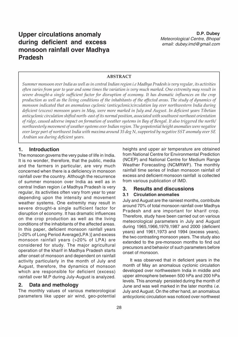
1. IntroductionThe monsoon governs the very pulse of life in India.It is no wonder, therefore, that the public, mediaand the farmers in particular, are very muchconcerned when there is a deficiency in monsoonrainfall over the country. Although the recurrenceof summer monsoon over India as well as incentral Indian region i.e Madhya Pradesh is veryregular, its activities often vary from year to yeardepending upon the intensity and movementweather systems. One extremity may result insevere drought-a single sufficient factor fordisruption of economy. It has dramatic influenceson the crop production as well as the livingconditions of the inhabitants of the affected areas.In this paper, deficient monsoon rainfall years[<20% of Long Period Average(LPA )] and excessmonsoon rainfall years (>20% of LPA) areconsidered for study. The major agriculturaloperation of the kharif in Madhya Pradesh startsafter onset of monsoon and dependent on rainfallactivity particularly in the month of July andAugust, therefore, the dynamics of monsoonwhich are responsible for deficient (excess)rainfall over M.P during July-August is analyzed.

2. Data and methologyThe monthly values of various meteorologicalparameters like upper air wind, geo-potential

heights and upper air temperature are obtainedfrom National Centre for Environmental Prediction(NCEP) and National Centre for Medium RangeWeather Forecasting (NCMRWF). The monthlyrainfall time series of Indian monsoon rainfall ofexcess and deficient monsoon rainfall is collectedfrom various publication of IMD.

3. Results and discussions3.1 Circulation anomaliesJuly and August are the rainiest months, contributearound 70% of total monsoon rainfall over MadhyaPradesh and are important for kharif crop.Therefore, study have been carried out on variousmeteorological parameters in July and Augustduring 1965,1966,1979,1987 and 2000 (deficientyears) and 1961,1973 and 1994 (excess years),the two contrasting monsoon years. The study alsoextended to the pre-monsoon months to find outprecursors and behavior of such parameters beforeonset of monsoon.

It was observed that in deficient years in themonth of May an anomalous cyclonic circulationdeveloped over northwestern India in middle andupper atmosphere between 500 hPa and 200 hPalevels. This anomaly persisted during the month ofJune and was well marked in the later months i.e.July and August. On the other hand, an anomalousanticyclonic circulation was noticed over northwest

ABSTRACT

Summer monsoon over India as well as in central Indian region i.e Madhya Pradesh is very regular, its activitiesoften varies from year to year and some times the variation is very much marked. One extremity may result insevere drought-a single sufficient factor for disruption of economy. It has dramatic influences on the cropproduction as well as the living conditions of the inhabitants of the affected areas. The study of dynamics ofmonsoon indicated that an anomalous cyclonic (anticyclonic)circulation lay over northwestern India duringdeficient (excess) monsoon years in May, were more marked in July and August. In deficient years Tibetiananticyclonic circulation shifted north- east of its normal position, associated with southwest northeast orientationof ridge, caused adverse impact on formation of weather systems in Bay of Bengal. It also triggered the north/northwesterly movement of weather systems over Indian region. The geopotential height anomalies were negativeover large part of northwest India with maxima around 35 deg N, supported by negative SST anomaly over SEArabian sea during deficient years.

D.P. Dubey Meteorological Centre, Bhopal

email: dubey.imd@gmail.com

Upper circulations anomalyduring deficient and excessmonsoon rainfall over MadhyaPradesh

29

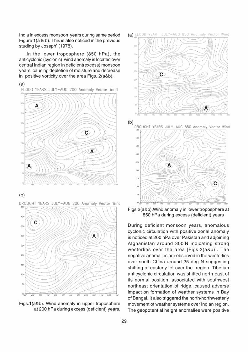
India in excess monsoon years during same periodFigure 1(a & b). This is also noticed in the previousstuding by Joseph’ (1978).

In the lower troposphere (850 hPa), theanticyclonic (cyclonic) wind anomaly is located overcentral Indian region in deficient(excess) monsoonyears, causing depletion of moisture and decreasein positive vorticity over the area Figs. 2(a&b).

(a)

(b)

Figs.1(a&b). Wind anomaly in upper troposphereat 200 hPa during excess (deficient) years.

(a)

(b)

Figs.2(a&b).Wind anomaly in lower troposphere at850 hPa during excess (deficient) years

During deficient monsoon years, anomalouscyclonic circulation with positive zonal anomalyis noticed at 200 hPa over Pakistan and adjoiningAfghanistan around 300°N indicating strongwesterlies over the area [Figs.3(a&b)]. Thenegative anomalies are observed in the westerliesover south China around 25 deg N suggestingshifting of easterly jet over the region. Tibetiananticyclonic circulation was shifted north-east ofits normal position, associated with southwestnortheast orientation of ridge, caused adverseimpact on formation of weather systems in Bayof Bengal. It also triggered the north/northwesterlymovement of weather systems over Indian region.The geopotential height anomalies were positive

A

C

A

A

C

A

C

A

A

C

30

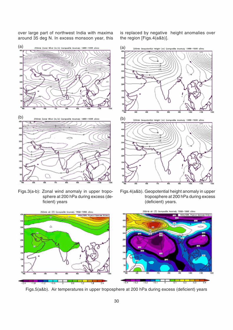
Figs.4(a&b). Geopotential height anomaly in uppertroposphere at 200 hPa during excess(deficient) years.

Figs.3(a-b): Zonal wind anomaly in upper tropo-sphere at 200 hPa during excess (de-ficient) years

(a)

(b)

(a)

(b)

over large part of northwest India with maximaaround 35 deg N. In excess monsoon year, this

is replaced by negative height anomalies overthe region [Figs.4(a&b)].

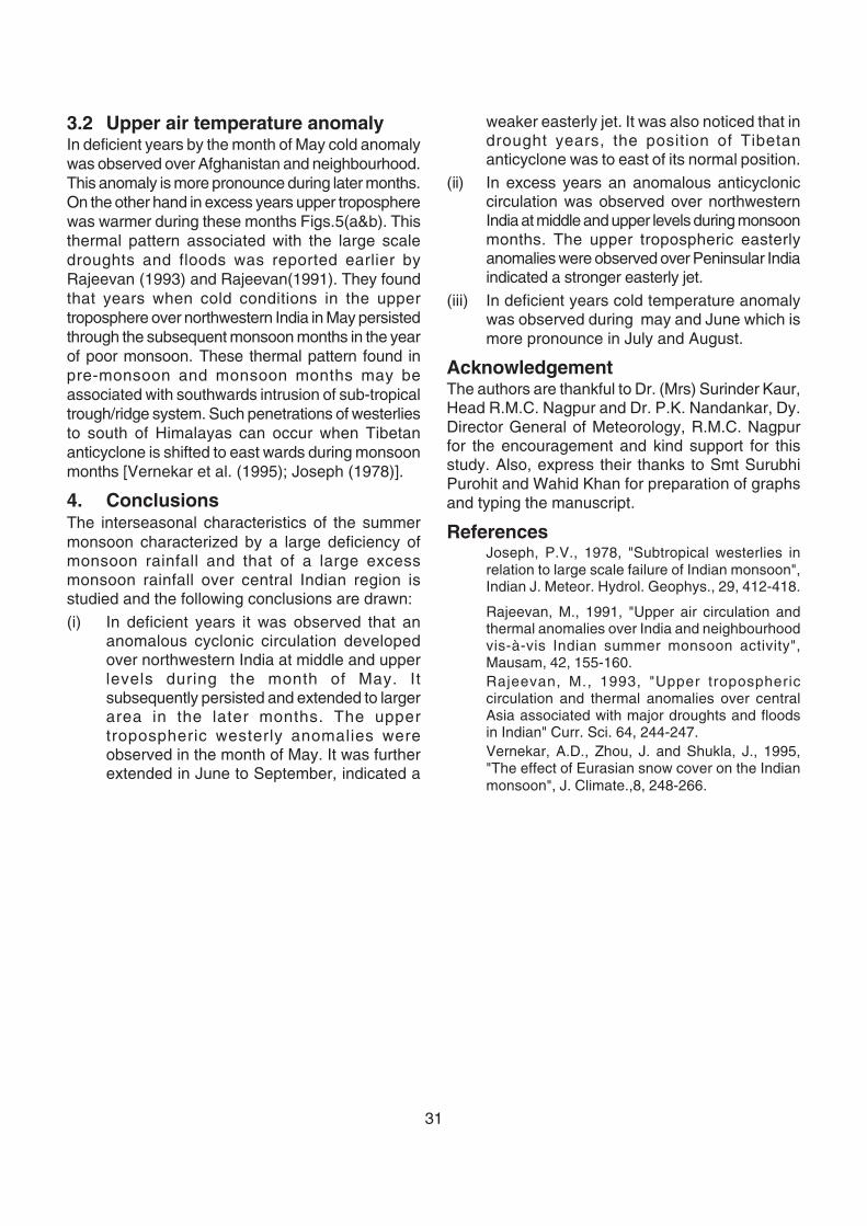
Figs.5(a&b). Air temperatures in upper troposphere at 200 hPa during excess (deficient) years

31

3.2 Upper air temperature anomalyIn deficient years by the month of May cold anomalywas observed over Afghanistan and neighbourhood.This anomaly is more pronounce during later months.On the other hand in excess years upper tropospherewas warmer during these months Figs.5(a&b). Thisthermal pattern associated with the large scaledroughts and floods was reported earlier byRajeevan (1993) and Rajeevan(1991). They foundthat years when cold conditions in the uppertroposphere over northwestern India in May persistedthrough the subsequent monsoon months in the yearof poor monsoon. These thermal pattern found inpre-monsoon and monsoon months may beassociated with southwards intrusion of sub-tropicaltrough/ridge system. Such penetrations of westerliesto south of Himalayas can occur when Tibetananticyclone is shifted to east wards during monsoonmonths [Vernekar et al. (1995); Joseph (1978)].

4. ConclusionsThe interseasonal characteristics of the summermonsoon characterized by a large deficiency ofmonsoon rainfall and that of a large excessmonsoon rainfall over central Indian region isstudied and the following conclusions are drawn:

(i) In deficient years it was observed that ananomalous cyclonic circulation developedover northwestern India at middle and upperlevels during the month of May. Itsubsequently persisted and extended to largerarea in the later months. The uppertropospheric westerly anomalies wereobserved in the month of May. It was furtherextended in June to September, indicated a

weaker easterly jet. It was also noticed that indrought years, the position of Tibetananticyclone was to east of its normal position.

(ii) In excess years an anomalous anticycloniccirculation was observed over northwesternIndia at middle and upper levels during monsoonmonths. The upper tropospheric easterlyanomalies were observed over Peninsular Indiaindicated a stronger easterly jet.

(iii) In deficient years cold temperature anomalywas observed during may and June which ismore pronounce in July and August.

AcknowledgementThe authors are thankful to Dr. (Mrs) Surinder Kaur,Head R.M.C. Nagpur and Dr. P.K. Nandankar, Dy.Director General of Meteorology, R.M.C. Nagpurfor the encouragement and kind support for thisstudy. Also, express their thanks to Smt SurubhiPurohit and Wahid Khan for preparation of graphsand typing the manuscript.

ReferencesJoseph, P.V., 1978, "Subtropical westerlies inrelation to large scale failure of Indian monsoon",Indian J. Meteor. Hydrol. Geophys., 29, 412-418.

Rajeevan, M., 1991, "Upper air circulation andthermal anomalies over India and neighbourhoodvis-à-vis Indian summer monsoon activity",Mausam, 42, 155-160.Rajeevan, M., 1993, "Upper troposphericcirculation and thermal anomalies over centralAsia associated with major droughts and floodsin Indian" Curr. Sci. 64, 244-247.Vernekar, A.D., Zhou, J. and Shukla, J., 1995,"The effect of Eurasian snow cover on the Indianmonsoon", J. Climate.,8, 248-266.

32

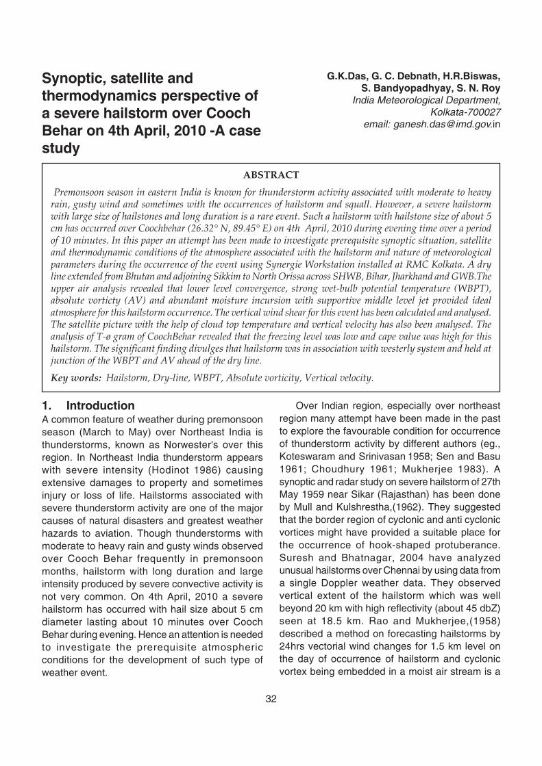
1. IntroductionA common feature of weather during premonsoonseason (March to May) over Northeast India isthunderstorms, known as Norwester's over thisregion. In Northeast India thunderstorm appearswith severe intensity (Hodinot 1986) causingextensive damages to property and sometimesinjury or loss of life. Hailstorms associated withsevere thunderstorm activity are one of the majorcauses of natural disasters and greatest weatherhazards to aviation. Though thunderstorms withmoderate to heavy rain and gusty winds observedover Cooch Behar frequently in premonsoonmonths, hailstorm with long duration and largeintensity produced by severe convective activity isnot very common. On 4th April, 2010 a severehailstorm has occurred with hail size about 5 cmdiameter lasting about 10 minutes over CoochBehar during evening. Hence an attention is neededto investigate the prerequisite atmosphericconditions for the development of such type ofweather event.

Over Indian region, especially over northeastregion many attempt have been made in the pastto explore the favourable condition for occurrenceof thunderstorm activity by different authors (eg.,Koteswaram and Srinivasan 1958; Sen and Basu1961; Choudhury 1961; Mukherjee 1983). Asynoptic and radar study on severe hailstorm of 27thMay 1959 near Sikar (Rajasthan) has been doneby Mull and Kulshrestha,(1962). They suggestedthat the border region of cyclonic and anti cyclonicvortices might have provided a suitable place forthe occurrence of hook-shaped protuberance.Suresh and Bhatnagar, 2004 have analyzedunusual hailstorms over Chennai by using data froma single Doppler weather data. They observedvertical extent of the hailstorm which was wellbeyond 20 km with high reflectivity (about 45 dbZ)seen at 18.5 km. Rao and Mukherjee,(1958)described a method on forecasting hailstorms by24hrs vectorial wind changes for 1.5 km level onthe day of occurrence of hailstorm and cyclonicvortex being embedded in a moist air stream is a

G.K.Das, G. C. Debnath, H.R.Biswas,S. Bandyopadhyay, S. N. Roy

India Meteorological Department,Kolkata-700027

email: ganesh.das@imd.gov.in

Synoptic, satellite andthermodynamics perspective ofa severe hailstorm over CoochBehar on 4th April, 2010 -A casestudy

ABSTRACT

Premonsoon season in eastern India is known for thunderstorm activity associated with moderate to heavyrain, gusty wind and sometimes with the occurrences of hailstorm and squall. However, a severe hailstormwith large size of hailstones and long duration is a rare event. Such a hailstorm with hailstone size of about 5cm has occurred over Coochbehar (26.32° N, 89.45° E) on 4th April, 2010 during evening time over a periodof 10 minutes. In this paper an attempt has been made to investigate prerequisite synoptic situation, satelliteand thermodynamic conditions of the atmosphere associated with the hailstorm and nature of meteorologicalparameters during the occurrence of the event using Synergie Workstation installed at RMC Kolkata. A dryline extended from Bhutan and adjoining Sikkim to North Orissa across SHWB, Bihar, Jharkhand and GWB.Theupper air analysis revealed that lower level convergence, strong wet-bulb potential temperature (WBPT),absolute vorticty (AV) and abundant moisture incursion with supportive middle level jet provided idealatmosphere for this hailstorm occurrence. The vertical wind shear for this event has been calculated and analysed.The satellite picture with the help of cloud top temperature and vertical velocity has also been analysed. Theanalysis of T-ø gram of CoochBehar revealed that the freezing level was low and cape value was high for thishailstorm. The significant finding divulges that hailstorm was in association with westerly system and held atjunction of the WBPT and AV ahead of the dry line.

Key words: Hailstorm, Dry-line, WBPT, Absolute vorticity, Vertical velocity.

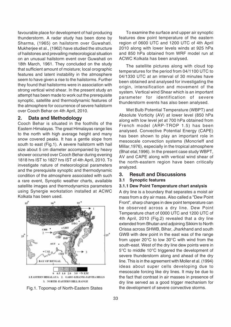
33

favourable place for development of hail producingthunderstorm. A radar study has been done bySharma, (1965) on hailstorm over Guwahati.Mukherjee et al., (1962) have studied the structureof hailstones and prevailing meteorological situationon an unusual hailstorm event over Guwahati on18th March, 1961. They concluded on the studythat sufficient amount of moisture; local orographicfeatures and latent instability in the atmosphereseem to have given a rise to the hailstorms. Furtherthey found that hailstorms were in association withstrong vertical wind shear. In the present study anattempt has been made to work out the prerequisitesynoptic, satellite and thermodynamic features ofthe atmosphere for occurrence of severe hailstormover Cooch Behar on 4th April, 2010.

2. Data and MethodologyCooch Behar is situated in the foothills of theEastern Himalayas. The great Himalayas range liesto the north with high average height and manysnow covered peaks. It has a gentle slope fromsouth to east (Fig.1). A severe hailstorm with hailsize about 5 cm diameter accompanied by heavyshower occurred over Cooch Behar during evening1818 hrs IST to 1827 hrs IST of 4th April, 2010. Toinvestigate nature of meteorological parametersand the prerequisite synoptic and thermodynamiccondition of the atmosphere associated with sucha rare event, Synoptic weather charts, availablesatellite images and thermodynamics parametersusing Synergie workstation installed at ACWCKolkata has been used.

To examine the surface and upper air synopticfeatures dew point temperature of the easternregion of 0600 UTC and 1200 UTC of 4th April2010 along with lower levels winds at 925 hPaand 850 hPa obtained from WRF model run atACWC Kolkata has been analysed.

The satellite pictures along with cloud toptemperatures for the period from 04/1100 UTC to04/1330 UTC at an interval of 30 minutes havebeen obtained and analysed for investigating theorigin, intensification and movement of thesystem. Vertical wind Shear which is an importantparameter for identi f icat ion of severethunderstorm events has also been analysed.

Wet Bulb Potential Temperature (WBPT) andAbsolute Vorticity (AV) at lower level (850 hPaalong with low level jet at 700 hPa obtained fromFrench model (ARP-TROP 1.5) has beenanalysed. Convective Potential Energy (CAPE)has been shown to play an important role inmesoscale convection systems (Moncrieff andMillar,1976), especially in the tropical atmosphere(Bhat etal,1996). In the present case study WBPT,AV and CAPE along with vertical wind shear ofthe north-eastern region have been criticallyanalyzed.

3. Result and Discussions3.1 Synoptic features3.1.1 Dew Point Temperature chart analysisA dry line is a boundary that separates a moist airmass from a dry air mass. Also called a "Dew PointFront", sharp changes in dew point temperature canbe observed across a dry line. Dew PointTemperature chart of 0000 UTC and 1200 UTC of4th April, 2010 (Fig.2) revealed that a dry lineextended from Bhutan and adjoining Sikkim to NorthOrissa across SHWB, Bihar, Jharkhand and southGWB with dew point in the east was of the rangefrom upper 20°C to low 30°C with wind from thesouth-east. West of the dry line dew points were in5°C to middle 10°C triggered the development ofsevere thunderstorm along and ahead of the dryline. This is in the agreement with Moller et al. (1994)ideas about super cells developing due tomesoscale forcing like dry lines. It may be due tothe fact that contrast in air masses in presence ofdry line served as a good trigger mechanism forthe development of severe convective storms.Fig.1. Topomap of North-Eastern States

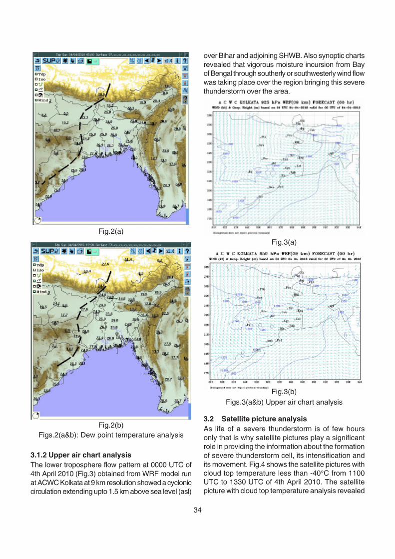
34

3.1.2 Upper air chart analysisThe lower troposphere flow pattern at 0000 UTC of4th April 2010 (Fig.3) obtained from WRF model runat ACWC Kolkata at 9 km resolution showed a cycloniccirculation extending upto 1.5 km above sea level (asl)

Figs.2(a&b): Dew point temperature analysisFig.2(b)

Fig.2(a)

over Bihar and adjoining SHWB. Also synoptic chartsrevealed that vigorous moisture incursion from Bayof Bengal through southerly or southwesterly wind flowwas taking place over the region bringing this severethunderstorm over the area.

Fig.3(a)

Fig.3(b)Figs.3(a&b) Upper air chart analysis

3.2 Satellite picture analysisAs life of a severe thunderstorm is of few hoursonly that is why satellite pictures play a significantrole in providing the information about the formationof severe thunderstorm cell, its intensification andits movement. Fig.4 shows the satellite pictures withcloud top temperature less than -40°C from 1100UTC to 1330 UTC of 4th April 2010. The satellitepicture with cloud top temperature analysis revealed

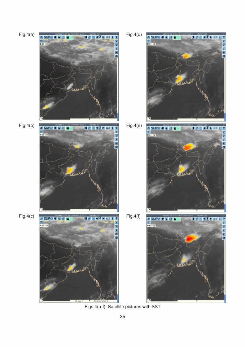
35

Fig.4(c)

Fig.4(a)

Fig.4(b)

Fig.4(d)

Figs.4(a-f): Satellite pictures with SST

Fig.4(f)

Fig.4(e)

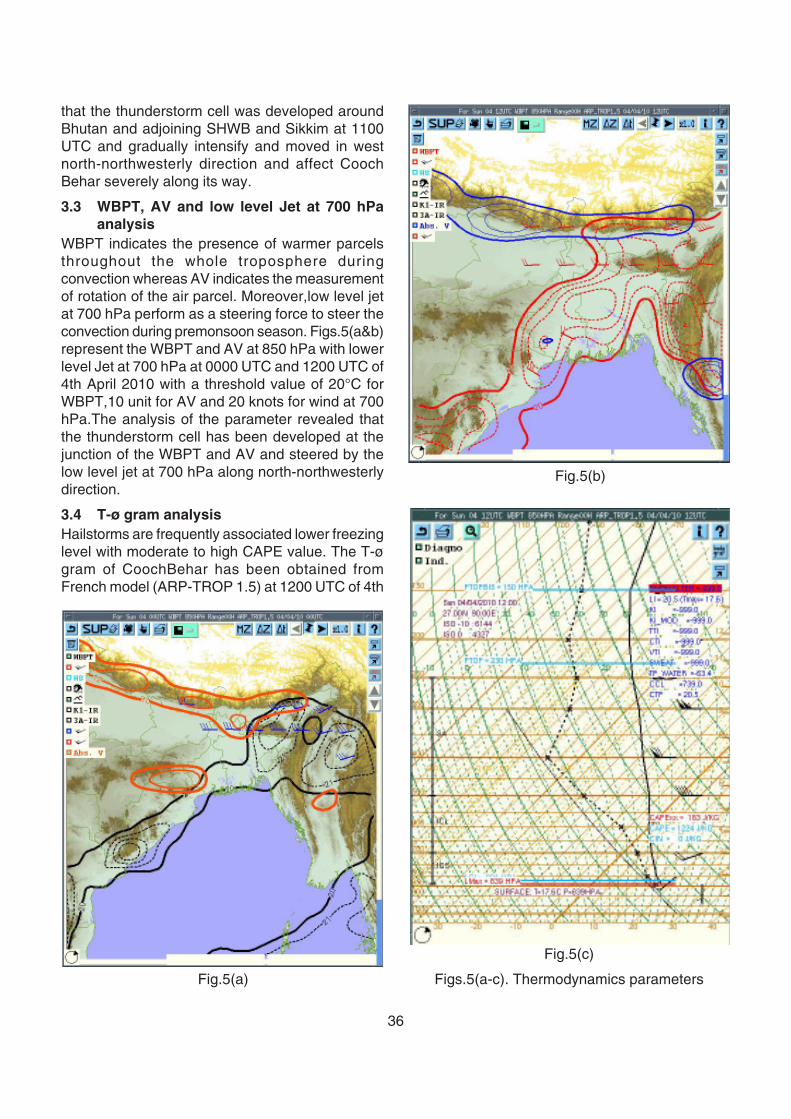
36

Fig.5(c)

Figs.5(a-c). Thermodynamics parametersFig.5(a)

Fig.5(b)

that the thunderstorm cell was developed aroundBhutan and adjoining SHWB and Sikkim at 1100UTC and gradually intensify and moved in westnorth-northwesterly direction and affect CoochBehar severely along its way.

3.3 WBPT, AV and low level Jet at 700 hPaanalysis

WBPT indicates the presence of warmer parcelsthroughout the whole troposphere duringconvection whereas AV indicates the measurementof rotation of the air parcel. Moreover,low level jetat 700 hPa perform as a steering force to steer theconvection during premonsoon season. Figs.5(a&b)represent the WBPT and AV at 850 hPa with lowerlevel Jet at 700 hPa at 0000 UTC and 1200 UTC of4th April 2010 with a threshold value of 20°C forWBPT,10 unit for AV and 20 knots for wind at 700hPa.The analysis of the parameter revealed thatthe thunderstorm cell has been developed at thejunction of the WBPT and AV and steered by thelow level jet at 700 hPa along north-northwesterlydirection.

3.4 T-ø gram analysisHailstorms are frequently associated lower freezinglevel with moderate to high CAPE value. The T-øgram of CoochBehar has been obtained fromFrench model (ARP-TROP 1.5) at 1200 UTC of 4th

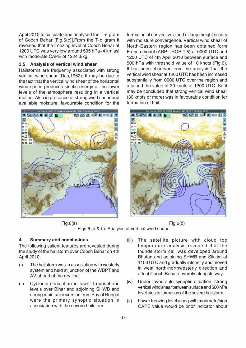
37

April 2010 to calculate and analysed the T-ø gramof Cooch Behar [Fig.5(c)].From the T-ø gram itrevealed that the freezing level of Cooch Behar at1200 UTC was very low around 595 hPa~4 km aslwith moderate CAPE of 1224 J/kg.

3.5 Analysis of vertical wind shearHailstorms are frequently associated with strongvertical wind shear (Das,1962). It may be due tothe fact that the vertical wind shear of the horizontalwind speed produces kinetic energy at the lowerlevels of the atmosphere resulting in a verticalmotion. Also in presence of strong wind shear andavailable moisture, favourable condition for the

formation of convective cloud of large height occurswith moisture convergence. Vertical wind shear ofNorth-Eastern region has been obtained formFrench model (ARP-TROP 1.5) at 0000 UTC and1200 UTC of 4th April 2010 between surface and500 hPa with threshold value of 10 knots (Fig.6).It has been observed from the analysis that thevertical wind shear at 1200 UTC has been increasedsubstantially from 0000 UTC over the region andattained the value of 30 knots at 1200 UTC. So itmay be concluded that strong vertical wind shear(30 knots or more) was in favourable condition forformation of hail.

Fig.6(a)Figs.6 (a & b). Analysis of vertical wind shear

Fig.6(b)

4. Summary and conclusionsThe following salient features are revealed duringthe study of the hailstorm over Cooch Behar on 4thApril 2010.

(i) The hailstorm was in association with westerlysystem and held at junction of the WBPT andAV ahead of the dry line.

(ii) Cyclonic circulation in lower troposphericlevels over Bihar and adjoining SHWB andstrong moisture incursion from Bay of Bengalwere the primary synoptic situation inassociation with the severe hailstorm.

(iii) The satellite picture with cloud toptemperature analysis revealed that thethunderstorm cell was developed aroundBhutan and adjoining SHWB and Sikkim at1100 UTC and gradually intensify and movedin west north-northwesterly direction andaffect Cooch Behar severely along its way.

(iv) Under favourable synoptic situation, strongvertical wind shear between surface and 500 hPalevel aids to formation of the severe hailstorm.

(v) Lower freezing level along with moderate/highCAPE value would be prior indicator about

38

impending severe thunderstorm associatedwith hail over Cooch Behar and its suburbs.

AcknowledgementThe authors are greatly thankful to all officers andstaff members of Regional Meteorological Centre,Kolkata for their logistic support for this study.

ReferencesBhat, G.S., Srinivasan, J. and Gadgil, S., 1996,Tropical deep convection Convective PotentialEnergy and Sea Surface Temperature,J.Meteor.Soc., Japan, 74, 155-166.

Chaudhury, A.K., 1961, Premonsoonthunderstorms in Assam, Tripura and Manipur,IJMG, 12,319 -321.

Das, P., 1962, Influence of wind shear on thegrowth of hail, J. Atmos. Sci., 19, 407-414.

Hodinot, M.H.O., 1986, Thunderstorm Observationsin West Bengal 1945-46, Weather, 41, 2-5.

Koteswaram, P. and Srinivasan, V., 1958,Thunderstorms over Gangetic West Bengal in thepremonsoon season and the synoptic factorsfavourable for their formation, IJMG, 9, 301-312.

Moller, A.R., Doswell, C.A., Foster, M.P. andWoodall G.R., 1994, The operational recognition of

supercell thunderstorm environment and stormstructures, Weather and For., 9, 327 - 347.

Moncrieff, M.W. and Millar, M.J., 1976, The dynamicsand simulation of tropical cumulonimbus and squalllines, Quart. J.Roy, Meteor. Soc., 102, 373-394.

Mukherjee A.K., Ghosh, S.K. and Arunachalam,G., 1962, Hailstorm at Guwahati on 18 March 1961,IJMG,13, 213-216.

Mukherjee A.K., 1983, Cloud dynamics in localsevere storms, Vayu Mandal, 1&2, 14-21.

Mull, S. and Kulshrestha, S.M., 1962, "The severehailstorm of 27 May 1959 near Sikar (Rajasthan):A synoptic and radar study" IJMG, 13, 81-94.

Rao, D. Venkateswara and Mukherjee, A.K., 1958,On forecasting hailstorms by method of vectorialwind changes", IJMG, 9, 313-322.

Sen, S. and Basu, S.C., 1961, Premonsoonthunderstorm in Assam and synoptic conditionsfavourable for their occurrence, Mausam, 12, 15-20.

Sharma, B.L., 1965, Radar study of a hailstorm overGuwahati on 17 April 1962, IJMG, 16,459-466.

Suresh, R. and Bhatnagar, A.K., 2004, Unusualhailstorms during May 2002 in Chennai and itssuburbs - A study using data from single Dopplerweather Radar, Mausam, 55, 655-670.

39

1. IntroductionNCMRWF is generating medium range weatherforecast in real time using global Numerical WeatherPrediction (NWP) models since last two decades. Itis well known that the quality of NWP outputs largelydepends on the quality of initial condition. Hence dataassimilation and associated observation monitoringis one of most important activity of any operationalNWP centre. The observing process is the mostimportant and expensive component of theforecasting system. IMD is deploying various newobservation platforms/techniques under itsmodernisation plan. It is expected that all theseobservations will help to improve the quality ofweather prediction over Indian region.

An online real-time observation monitoringsystem have recently been developed andimplemented at NCMRWF with special emphasison the monitoring of Indian observations. It runsfour times a day viz. (0000, 0600, 1200 and 1800UTC) along GDAS cycles. It generates the datacoverage plots for various types of observationsassimilated in GDAS. It also generates the timeseries plots for the availability of different types ofobservations for last 45 days.

Quality of Indian RS/RW observations is alwaysdoubted by various leading NWP centers of the

world as many of these observations are rejectedby data assimilation systems. Plots showing therejection of temperature and zonal windobservations at various levels of atmosphere byNCMRWF GDAS for Indian RS/RW observations(for 0000 and 1200 UTC) are also generated.Similar plots depicting the rejection of zonal windsfor Indian pilot balloon observations are alsogenerated for 0600 and 1800 UTC.

NCMRWF's Global Data Assimilation-ForecastSystem (GDAFS) is described in section 2.Monitoring of the quantity and coverage of varioustypes of observations received at NCMRWF, ingeneral, is described in section 3. Quality of Indianupper-air sonde observations is discussed insection 4. Numerical experiments carried outwithholding upper-air observation from 10 IndianGPS-sonde stations and their impacts on analyses-forecast system are presented in section 5.

2. Global Data Assimilation-Forecastsystem (GDAFS)

NCMRWF's GDAFS is six-hourly intermittentassimilation system, which runs four times a day(viz. 0000, 0600, 1200 and 1800 UTC), at T254L64resolution, an adapted version of NCEP's GlobalForecasting System (GFS) (Kalnay et al.1990). Itcomprises of (i) Data-preprocessing and Quality

Online monitoring of Indianobservations and their impacton NWP system

M. Das Gupta and S. Indira RaniNational Centre of Medium Range Weather

Forecasting (NCMRWF)A-50, Sector-62, NOIDA-201307email: munmun@ncmrwf.gov.in

ABSTRACT

An online real-time observation monitoring system has been developed recently and implemented at NCMRWFwith special emphasis on the monitoring of Indian observations. This system generates information about theavailability of various types of observations received at NCMRWF and their subsequent utilisation in globaldata assimilation system (GDAS). It also generates information regarding the rejection/acceptance ofobservations by GDAS, which in turn indicates the quality of observations. India Meteorological Department(IMD) recently introduced GPS-sonde at 10 stations out of its 40 upper-air radiosonde stations. It is noticedthe rejection of observations by GDAS for these 10 stations have been reduced drastically. Numerical experimentscarried out withholding these upper-air observations have shown deterioration in the quality of predictioncompared to that of operational run which utilizes these observations regularly.

Key words: Observation monitoring, GPS-sonde, Upper-air observations, Observation quality, Impact ofobservations.

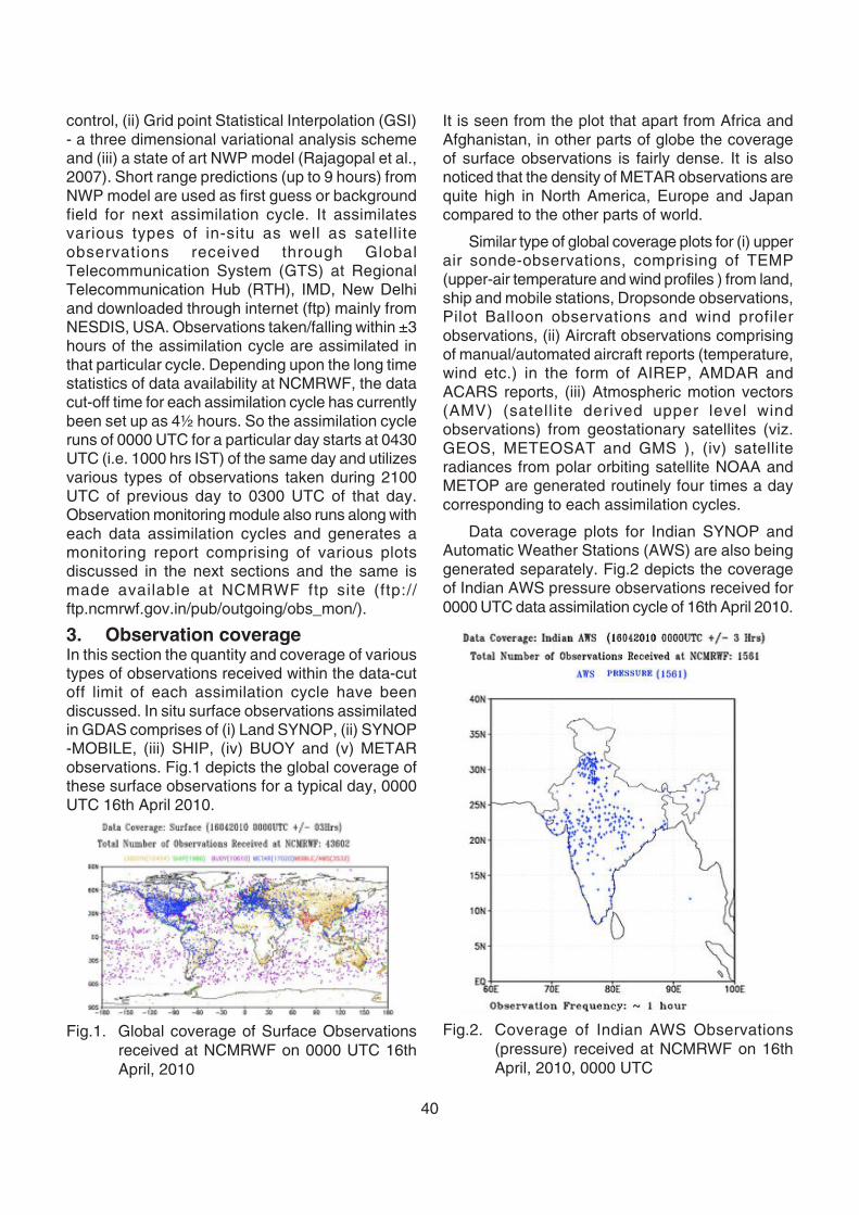
40

control, (ii) Grid point Statistical Interpolation (GSI)- a three dimensional variational analysis schemeand (iii) a state of art NWP model (Rajagopal et al.,2007). Short range predictions (up to 9 hours) fromNWP model are used as first guess or backgroundfield for next assimilation cycle. It assimilatesvarious types of in-situ as well as satelliteobservations received through GlobalTelecommunication System (GTS) at RegionalTelecommunication Hub (RTH), IMD, New Delhiand downloaded through internet (ftp) mainly fromNESDIS, USA. Observations taken/falling within ±3hours of the assimilation cycle are assimilated inthat particular cycle. Depending upon the long timestatistics of data availability at NCMRWF, the datacut-off time for each assimilation cycle has currentlybeen set up as 4½ hours. So the assimilation cycleruns of 0000 UTC for a particular day starts at 0430UTC (i.e. 1000 hrs IST) of the same day and utilizesvarious types of observations taken during 2100UTC of previous day to 0300 UTC of that day.Observation monitoring module also runs along witheach data assimilation cycles and generates amonitoring report comprising of various plotsdiscussed in the next sections and the same ismade available at NCMRWF ftp site (ftp://ftp.ncmrwf.gov.in/pub/outgoing/obs_mon/).

3. Observation coverageIn this section the quantity and coverage of varioustypes of observations received within the data-cutoff limit of each assimilation cycle have beendiscussed. In situ surface observations assimilatedin GDAS comprises of (i) Land SYNOP, (ii) SYNOP-MOBILE, (iii) SHIP, (iv) BUOY and (v) METARobservations. Fig.1 depicts the global coverage ofthese surface observations for a typical day, 0000UTC 16th April 2010.

Fig.1. Global coverage of Surface Observationsreceived at NCMRWF on 0000 UTC 16thApril, 2010

It is seen from the plot that apart from Africa andAfghanistan, in other parts of globe the coverageof surface observations is fairly dense. It is alsonoticed that the density of METAR observations arequite high in North America, Europe and Japancompared to the other parts of world.

Similar type of global coverage plots for (i) upperair sonde-observations, comprising of TEMP(upper-air temperature and wind profiles ) from land,ship and mobile stations, Dropsonde observations,Pilot Balloon observations and wind profilerobservations, (ii) Aircraft observations comprisingof manual/automated aircraft reports (temperature,wind etc.) in the form of AIREP, AMDAR andACARS reports, (iii) Atmospheric motion vectors(AMV) (satellite derived upper level windobservations) from geostationary satellites (viz.GEOS, METEOSAT and GMS ), (iv) satelliteradiances from polar orbiting satellite NOAA andMETOP are generated routinely four times a daycorresponding to each assimilation cycles.

Data coverage plots for Indian SYNOP andAutomatic Weather Stations (AWS) are also beinggenerated separately. Fig.2 depicts the coverageof Indian AWS pressure observations received for0000 UTC data assimilation cycle of 16th April 2010.

Fig.2. Coverage of Indian AWS Observations(pressure) received at NCMRWF on 16thApril, 2010, 0000 UTC

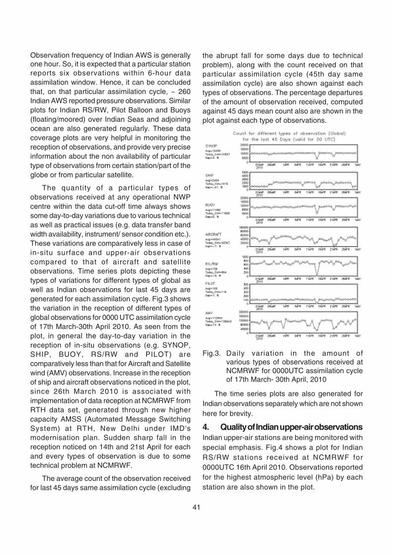
41

Observation frequency of Indian AWS is generallyone hour. So, it is expected that a particular stationreports six observations within 6-hour dataassimilation window. Hence, it can be concludedthat, on that particular assimilation cycle, ~ 260Indian AWS reported pressure observations. Similarplots for Indian RS/RW, Pilot Balloon and Buoys(floating/moored) over Indian Seas and adjoiningocean are also generated regularly. These datacoverage plots are very helpful in monitoring thereception of observations, and provide very preciseinformation about the non availability of particulartype of observations from certain station/part of theglobe or from particular satellite.

The quantity of a particular types ofobservations received at any operational NWPcentre within the data cut-off time always showssome day-to-day variations due to various technicalas well as practical issues (e.g. data transfer bandwidth availability, instrument/ sensor condition etc.).These variations are comparatively less in case ofin-situ surface and upper-air observationscompared to that of aircraft and satelliteobservations. Time series plots depicting thesetypes of variations for different types of global aswell as Indian observations for last 45 days aregenerated for each assimilation cycle. Fig.3 showsthe variation in the reception of different types ofglobal observations for 0000 UTC assimilation cycleof 17th March-30th April 2010. As seen from theplot, in general the day-to-day variation in thereception of in-situ observations (e.g. SYNOP,SHIP, BUOY, RS/RW and PILOT) arecomparatively less than that for Aircraft and Satellitewind (AMV) observations. Increase in the receptionof ship and aircraft observations noticed in the plot,since 26th March 2010 is associated withimplementation of data reception at NCMRWF fromRTH data set, generated through new highercapacity AMSS (Automated Message SwitchingSystem) at RTH, New Delhi under IMD'smodernisation plan. Sudden sharp fall in thereception noticed on 14th and 21st April for eachand every types of observation is due to sometechnical problem at NCMRWF.

The average count of the observation receivedfor last 45 days same assimilation cycle (excluding

the abrupt fall for some days due to technicalproblem), along with the count received on thatparticular assimilation cycle (45th day sameassimilation cycle) are also shown against eachtypes of observations. The percentage departuresof the amount of observation received, computedagainst 45 days mean count also are shown in theplot against each type of observations.

Fig.3. Daily variation in the amount ofvarious types of observations received atNCMRWF for 0000UTC assimilation cycleof 17th March- 30th April, 2010

The time series plots are also generated forIndian observations separately which are not shownhere for brevity.

4. Quality of Indian upper-air observationsIndian upper-air stations are being monitored withspecial emphasis. Fig.4 shows a plot for IndianRS/RW stations received at NCMRWF for0000UTC 16th April 2010. Observations reportedfor the highest atmospheric level (hPa) by eachstation are also shown in the plot.

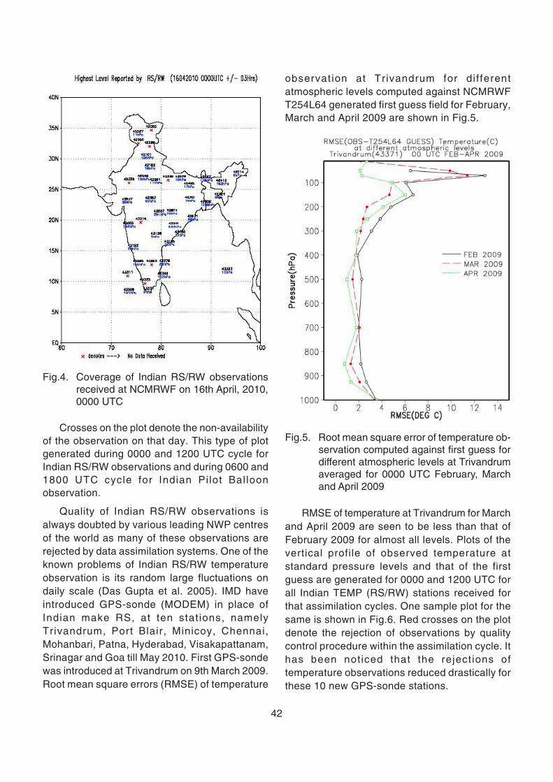
42

Fig.4. Coverage of Indian RS/RW observationsreceived at NCMRWF on 16th April, 2010,0000 UTC

Crosses on the plot denote the non-availabilityof the observation on that day. This type of plotgenerated during 0000 and 1200 UTC cycle forIndian RS/RW observations and during 0600 and1800 UTC cycle for Indian Pi lot Bal loonobservation.

Quality of Indian RS/RW observations isalways doubted by various leading NWP centresof the world as many of these observations arerejected by data assimilation systems. One of theknown problems of Indian RS/RW temperatureobservation is its random large fluctuations ondaily scale (Das Gupta et al. 2005). IMD haveintroduced GPS-sonde (MODEM) in place ofIndian make RS, at ten stat ions, namelyTrivandrum, Port Blair, Minicoy, Chennai,Mohanbari, Patna, Hyderabad, Visakapattanam,Srinagar and Goa till May 2010. First GPS-sondewas introduced at Trivandrum on 9th March 2009.Root mean square errors (RMSE) of temperature

observation at Trivandrum for dif ferentatmospheric levels computed against NCMRWFT254L64 generated first guess field for February,March and April 2009 are shown in Fig.5.

Fig.5. Root mean square error of temperature ob-servation computed against first guess fordifferent atmospheric levels at Trivandrumaveraged for 0000 UTC February, Marchand April 2009

RMSE of temperature at Trivandrum for Marchand April 2009 are seen to be less than that ofFebruary 2009 for almost all levels. Plots of thevertical profile of observed temperature atstandard pressure levels and that of the firstguess are generated for 0000 and 1200 UTC forall Indian TEMP (RS/RW) stations received forthat assimilation cycles. One sample plot for thesame is shown in Fig.6. Red crosses on the plotdenote the rejection of observations by qualitycontrol procedure within the assimilation cycle. Ithas been noticed that the rejections oftemperature observations reduced drastically forthese 10 new GPS-sonde stations.

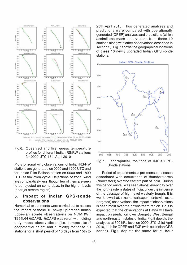
43

Fig.6. Observed and first guess temperatureprofiles for different Indian RS/RW stationsfor 0000 UTC 16th April 2010

Plots for zonal wind observations for Indian RS/RWstations are generated on 0000 and 1200 UTC andfor Indian Pilot Balloon station on 0600 and 1800UTC assimilation cycle. Rejections of zonal windare comparatively less, though few of them are seento be rejected on some days, in the higher levels(near jet stream region).

5. Impact of Indian GPS-sondeobservations

Numerical experiments were carried out to assessthe impact of these 10 newly up-graded Indianupper-air sonde observations on NCMRWFT254L64 GDAFS. GDAFS was rerun withholdingonly mass observations (i.e. temperature/geopotential height and humidity) for these 10stations for a short period of 10 days from 15th to

25th April 2010. Thus generated analyses andpredictions were compared with operationallygenerated (OPER) analyses and predictions (whichassimilates mass observations from these 10stations along with other observations described insection 2). Fig.7 shows the geographical locationsof these 10 newly upgraded Indian GPS sondestations.

Fig.7. Geographical Positions of IMD's GPS-Sonde stations

Period of experiments is pre-monsoon seasonassociated with occurrence of thunderstorms(Norwesters) over the eastern part of India. Duringthis period rainfall was seen almost every day overthe north-eastern states of India, under the influenceof the passage of high level westerly trough. It iswell known that, in numerical experiments with extra(targeted) observations, the impact of observationsis seen most over the downstream region. So it isexpected that the observations at Patna will haveimpact on prediction over Gangetic West Bengaland north-eastern states of India. Fig.8 depicts theanalyses at 500 hPa level on 0000 UTC, 21st April2010, both for OPER and EXP (with out Indian GPSsonde). Fig.9 depicts the same for 72 hour

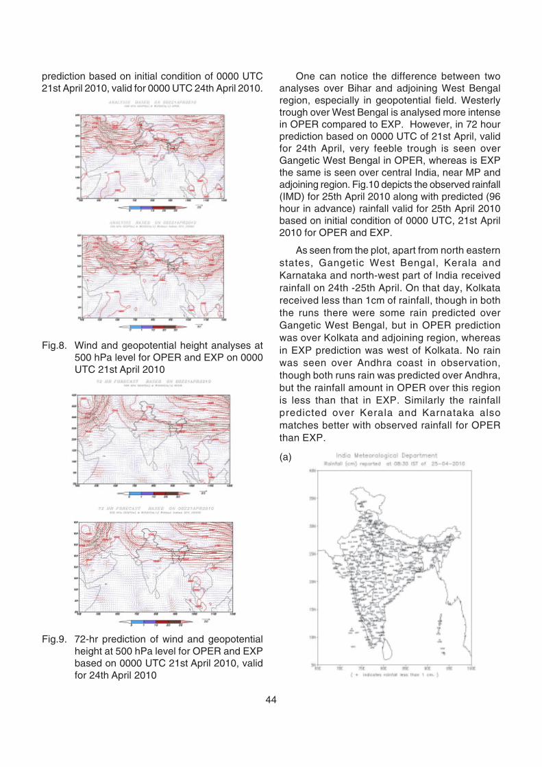
44

prediction based on initial condition of 0000 UTC21st April 2010, valid for 0000 UTC 24th April 2010.

Fig.8. Wind and geopotential height analyses at500 hPa level for OPER and EXP on 0000UTC 21st April 2010

Fig.9. 72-hr prediction of wind and geopotentialheight at 500 hPa level for OPER and EXPbased on 0000 UTC 21st April 2010, validfor 24th April 2010

One can notice the difference between twoanalyses over Bihar and adjoining West Bengalregion, especially in geopotential field. Westerlytrough over West Bengal is analysed more intensein OPER compared to EXP. However, in 72 hourprediction based on 0000 UTC of 21st April, validfor 24th April, very feeble trough is seen overGangetic West Bengal in OPER, whereas is EXPthe same is seen over central India, near MP andadjoining region. Fig.10 depicts the observed rainfall(IMD) for 25th April 2010 along with predicted (96hour in advance) rainfall valid for 25th April 2010based on initial condition of 0000 UTC, 21st April2010 for OPER and EXP.

As seen from the plot, apart from north easternstates, Gangetic West Bengal, Kerala andKarnataka and north-west part of India receivedrainfall on 24th -25th April. On that day, Kolkatareceived less than 1cm of rainfall, though in boththe runs there were some rain predicted overGangetic West Bengal, but in OPER predictionwas over Kolkata and adjoining region, whereasin EXP prediction was west of Kolkata. No rainwas seen over Andhra coast in observation,though both runs rain was predicted over Andhra,but the rainfall amount in OPER over this regionis less than that in EXP. Similarly the rainfallpredicted over Kerala and Karnataka alsomatches better with observed rainfall for OPERthan EXP.

(a)

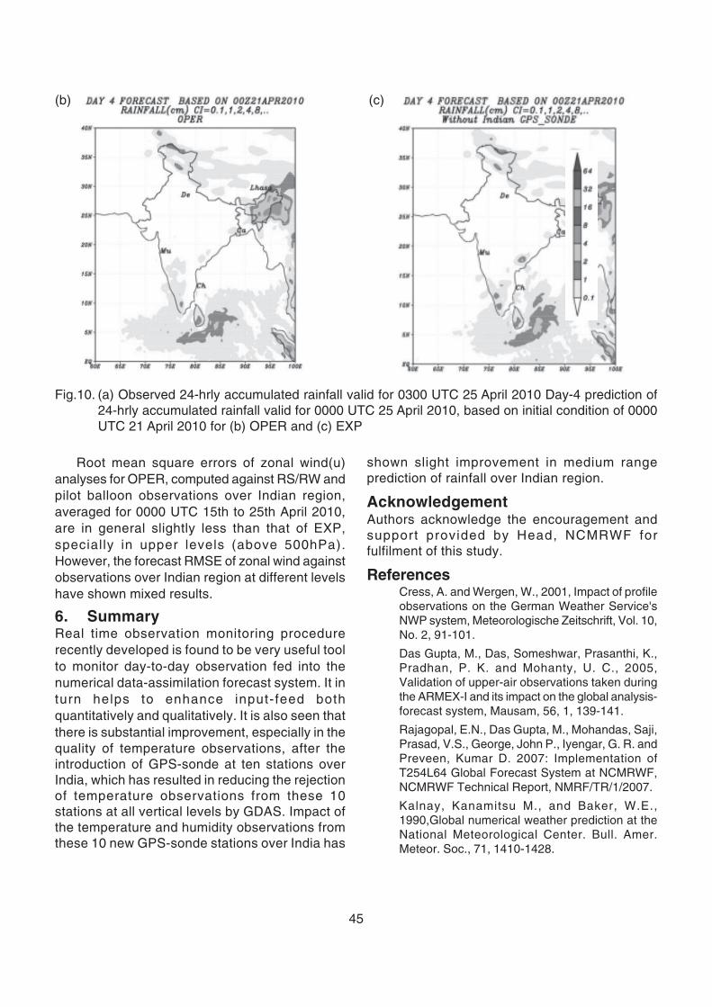
45

Root mean square errors of zonal wind(u)analyses for OPER, computed against RS/RW andpilot balloon observations over Indian region,averaged for 0000 UTC 15th to 25th April 2010,are in general slightly less than that of EXP,specially in upper levels (above 500hPa).However, the forecast RMSE of zonal wind againstobservations over Indian region at different levelshave shown mixed results.

6. SummaryReal time observation monitoring procedurerecently developed is found to be very useful toolto monitor day-to-day observation fed into thenumerical data-assimilation forecast system. It inturn helps to enhance input-feed bothquantitatively and qualitatively. It is also seen thatthere is substantial improvement, especially in thequality of temperature observations, after theintroduction of GPS-sonde at ten stations overIndia, which has resulted in reducing the rejectionof temperature observations from these 10stations at all vertical levels by GDAS. Impact ofthe temperature and humidity observations fromthese 10 new GPS-sonde stations over India has

Fig.10. (a) Observed 24-hrly accumulated rainfall valid for 0300 UTC 25 April 2010 Day-4 prediction of24-hrly accumulated rainfall valid for 0000 UTC 25 April 2010, based on initial condition of 0000UTC 21 April 2010 for (b) OPER and (c) EXP

(b) (c)

shown slight improvement in medium rangeprediction of rainfall over Indian region.

AcknowledgementAuthors acknowledge the encouragement andsupport provided by Head, NCMRWF forfulfilment of this study.

ReferencesCress, A. and Wergen, W., 2001, Impact of profileobservations on the German Weather Service'sNWP system, Meteorologische Zeitschrift, Vol. 10,No. 2, 91-101.

Das Gupta, M., Das, Someshwar, Prasanthi, K.,Pradhan, P. K. and Mohanty, U. C., 2005,Validation of upper-air observations taken duringthe ARMEX-I and its impact on the global analysis-forecast system, Mausam, 56, 1, 139-141.

Rajagopal, E.N., Das Gupta, M., Mohandas, Saji,Prasad, V.S., George, John P., Iyengar, G. R. andPreveen, Kumar D. 2007: Implementation ofT254L64 Global Forecast System at NCMRWF,NCMRWF Technical Report, NMRF/TR/1/2007.

Kalnay, Kanamitsu M., and Baker, W.E.,1990,Global numerical weather prediction at theNational Meteorological Center. Bull. Amer.Meteor. Soc., 71, 1410-1428.

46

1. IntroductionThere is a significant shift in the understanding ofcrop production systems (plant- soil- environmentalrelationship) from ecologically based simulationstudies on the phenological and physiologicaldimensions of crop growth (Baker et al. 1972, Reddyet al. 1985, Richie 1986, Aggarwal et al. 1994, Zhangand Dawes 1998, Kang et al. 2002, Kang et al. 2003)to technologically dependent crop yield assessmentusing the effects of High Yielding Varieties (HYVS)of seeds and irrigation crop parameters (Aigneret al. 1977, Subash et al. 2004). The explanation ofphysical processes such as photosynthesis,respiration, transpiration and carbohydratesassimilation were considered in crop yield modelingespecially in the last part of 20th Century when DeWitand his associates simulated the effects ofcarbohydrates for plant growth (DeWit et al. 1969).The crop growth modeling for different crops wererealized and the attempts were made to developdifferent models for different crops such as solarradiation based model (Reddy et al.1985),photothermal quotient model for wheat crop(Aggarwal et al. 1994), DeciBle software for wheatcrop management (Chatelin et al. 2005) and so on.On the other hand, economists also developeddifferent production functions such as classical Cobb-Dauglas production function and later on multipleerror term of agricultural production distribution

(Subash et al. 2004). In order to develop anintegrated crop yield modeling for simulating theeffects of both sets of parameters, physiological aswell as technological factors of production, anintegrated crop yield model that followed the 'law ofdiminishing return' was developed by Singh (2000);some of the parameters of which are dependent onbiophysical properties of land and fertilizer useefficiency for the assessment of crop yield (Singh et al.2006). In this modeling, agro-meteorologicalparameters were considered as most variable thatinfluence implicitly the crop yield (Fig.1).

The Commission for agro-meteorologicalservices for improvement in agricultural production,constituted in 2004 under Agro-meteorologicalProgramme of World Meteorological Organisation(WMO), recently implemented programme for agro-meteorological measurements and operationalagro-meteorological strategies for development ofsuitable crop models in response to needs offarmers (Commission for Agricultural Meteorology6

2006). However, it was also realized that agro-meteorological parameters and its related modulus/indexes are essential parts to incorporate in the cropyield modeling whether they are ecologically basedor meteorologically dependent models. Biophysical(soil and water) potentials of crop growth and

Weather variability and summerrice yield in wet monsoonenvironment of upperBrahmaputra valley

Surendra SinghHiambok Jones Syiemlieh

and Partha Pratim DeyNorth-Eastern Hill University,

Shillong-793 022

ABSTRACT

Weather variability is increasingly considered an important factor to determine the summer rice crop yield.Constructing weather indexes for calculation of potential productivity for rice crop, the variability of potentialproductivity of summer rice crop and weather variability were analysed to compare it with the trends ofexisting crop yield taking into account the monthly weather statistics for a period of 52 years (1952-2003). Itis found that potential productivity is more determined by growth factor and temperature efficiency of thereproductive phase of green biomass growth of rice crop. Excessive seasonal rainfall limits the potentialproductivity as well as crop yield because of floods and over land flow which damage the green biomass ofsummer rice crop in the Upper Brahmaputra valley. On account of highly variable weather parameters overtime, the realization factor of potential productivity becomes weak. However, less-variable weather conditionsat the time of ripening of the crop contribute towards grain size and its hardness. Hence, it increases yield ofsummer rice crop in the Upper Brahmaputra valley.

Key words: Crop yield, growth rate, potential productivity, summer rice yield, temperature efficiency, weathervariability.

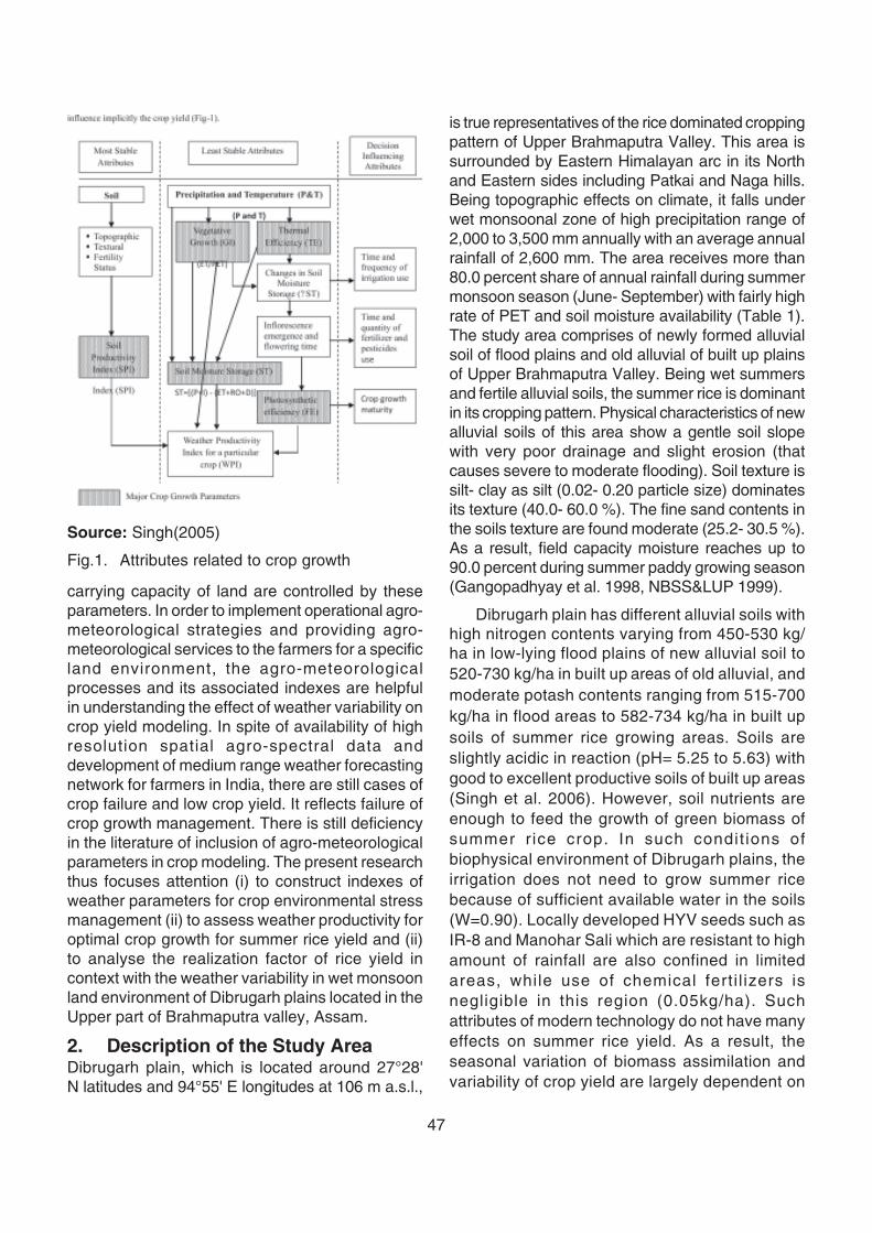
47

carrying capacity of land are controlled by theseparameters. In order to implement operational agro-meteorological strategies and providing agro-meteorological services to the farmers for a specificland environment, the agro-meteorologicalprocesses and its associated indexes are helpfulin understanding the effect of weather variability oncrop yield modeling. In spite of availability of highresolution spatial agro-spectral data anddevelopment of medium range weather forecastingnetwork for farmers in India, there are still cases ofcrop failure and low crop yield. It reflects failure ofcrop growth management. There is still deficiencyin the literature of inclusion of agro-meteorologicalparameters in crop modeling. The present researchthus focuses attention (i) to construct indexes ofweather parameters for crop environmental stressmanagement (ii) to assess weather productivity foroptimal crop growth for summer rice yield and (ii)to analyse the realization factor of rice yield incontext with the weather variability in wet monsoonland environment of Dibrugarh plains located in theUpper part of Brahmaputra valley, Assam.

2. Description of the Study AreaDibrugarh plain, which is located around 27°28'N latitudes and 94°55' E longitudes at 106 m a.s.l.,

is true representatives of the rice dominated croppingpattern of Upper Brahmaputra Valley. This area issurrounded by Eastern Himalayan arc in its Northand Eastern sides including Patkai and Naga hills.Being topographic effects on climate, it falls underwet monsoonal zone of high precipitation range of2,000 to 3,500 mm annually with an average annualrainfall of 2,600 mm. The area receives more than80.0 percent share of annual rainfall during summermonsoon season (June- September) with fairly highrate of PET and soil moisture availability (Table 1).The study area comprises of newly formed alluvialsoil of flood plains and old alluvial of built up plainsof Upper Brahmaputra Valley. Being wet summersand fertile alluvial soils, the summer rice is dominantin its cropping pattern. Physical characteristics of newalluvial soils of this area show a gentle soil slopewith very poor drainage and slight erosion (thatcauses severe to moderate flooding). Soil texture issilt- clay as silt (0.02- 0.20 particle size) dominatesits texture (40.0- 60.0 %). The fine sand contents inthe soils texture are found moderate (25.2- 30.5 %).As a result, field capacity moisture reaches up to90.0 percent during summer paddy growing season(Gangopadhyay et al. 1998, NBSS&LUP 1999).

Dibrugarh plain has different alluvial soils withhigh nitrogen contents varying from 450-530 kg/ha in low-lying flood plains of new alluvial soil to520-730 kg/ha in built up areas of old alluvial, andmoderate potash contents ranging from 515-700kg/ha in flood areas to 582-734 kg/ha in built upsoils of summer rice growing areas. Soils areslightly acidic in reaction (pH= 5.25 to 5.63) withgood to excellent productive soils of built up areas(Singh et al. 2006). However, soil nutrients areenough to feed the growth of green biomass ofsummer r ice crop. In such condit ions ofbiophysical environment of Dibrugarh plains, theirrigation does not need to grow summer ricebecause of sufficient available water in the soils(W=0.90). Locally developed HYV seeds such asIR-8 and Manohar Sali which are resistant to highamount of rainfall are also confined in limitedareas, while use of chemical ferti l izers isnegligible in this region (0.05kg/ha). Suchattributes of modern technology do not have manyeffects on summer rice yield. As a result, theseasonal variation of biomass assimilation andvariability of crop yield are largely dependent on

Source: Singh(2005)

Fig.1. Attributes related to crop growth

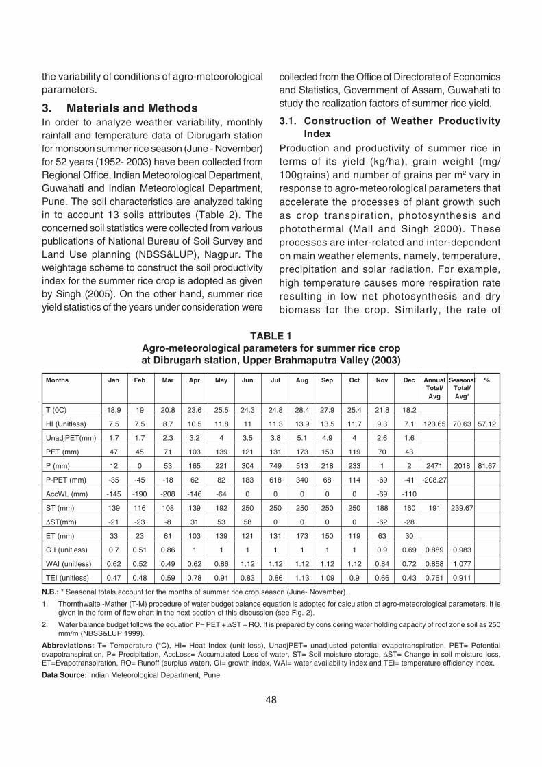
48

TABLE 1Agro-meteorological parameters for summer rice cropat Dibrugarh station, Upper Brahmaputra Valley (2003)

Months Jan Feb Mar Apr May Jun Jul Aug Sep Oct Nov Dec Annual Seasonal %Total/ Total/Avg Avg*

T (0C) 18.9 19 20.8 23.6 25.5 24.3 24.8 28.4 27.9 25.4 21.8 18.2

HI (Unitless) 7.5 7.5 8.7 10.5 11.8 11 11.3 13.9 13.5 11.7 9.3 7.1 123.65 70.63 57.12

UnadjPET(mm) 1.7 1.7 2.3 3.2 4 3.5 3.8 5.1 4.9 4 2.6 1.6

PET (mm) 47 45 71 103 139 121 131 173 150 119 70 43

P (mm) 12 0 53 165 221 304 749 513 218 233 1 2 2471 2018 81.67

P-PET (mm) -35 -45 -18 62 82 183 618 340 68 114 -69 -41 -208.27

AccWL (mm) -145 -190 -208 -146 -64 0 0 0 0 0 -69 -110

ST (mm) 139 116 108 139 192 250 250 250 250 250 188 160 191 239.67

ΔST(mm) -21 -23 -8 31 53 58 0 0 0 0 -62 -28

ET (mm) 33 23 61 103 139 121 131 173 150 119 63 30

G I (unitless) 0.7 0.51 0.86 1 1 1 1 1 1 1 0.9 0.69 0.889 0.983

WAI (unitless) 0.62 0.52 0.49 0.62 0.86 1.12 1.12 1.12 1.12 1.12 0.84 0.72 0.858 1.077

TEI (unitless) 0.47 0.48 0.59 0.78 0.91 0.83 0.86 1.13 1.09 0.9 0.66 0.43 0.761 0.911

N.B.: * Seasonal totals account for the months of summer rice crop season (June- November).

1. Thornthwaite -Mather (T-M) procedure of water budget balance equation is adopted for calculation of agro-meteorological parameters. It isgiven in the form of flow chart in the next section of this discussion (see Fig.-2).

2. Water balance budget follows the equation P= PET + ΔST + RO. It is prepared by considering water holding capacity of root zone soil as 250mm/m (NBSS&LUP 1999).

Abbreviations: T= Temperature (°C), HI= Heat Index (unit less), UnadjPET= unadjusted potential evapotranspiration, PET= Potentialevapotranspiration, P= Precipitation, AccLoss= Accumulated Loss of water, ST= Soil moisture storage, ΔST= Change in soil moisture loss,ET=Evapotranspiration, RO= Runoff (surplus water), GI= growth index, WAI= water availability index and TEI= temperature efficiency index.

Data Source: Indian Meteorological Department, Pune.

the variability of conditions of agro-meteorologicalparameters.

3. Materials and MethodsIn order to analyze weather variability, monthlyrainfall and temperature data of Dibrugarh stationfor monsoon summer rice season (June - November)for 52 years (1952- 2003) have been collected fromRegional Office, Indian Meteorological Department,Guwahati and Indian Meteorological Department,Pune. The soil characteristics are analyzed takingin to account 13 soils attributes (Table 2). Theconcerned soil statistics were collected from variouspublications of National Bureau of Soil Survey andLand Use planning (NBSS&LUP), Nagpur. Theweightage scheme to construct the soil productivityindex for the summer rice crop is adopted as givenby Singh (2005). On the other hand, summer riceyield statistics of the years under consideration were

collected from the Office of Directorate of Economicsand Statistics, Government of Assam, Guwahati tostudy the realization factors of summer rice yield.

3.1. Construction of Weather ProductivityIndex

Production and productivity of summer rice interms of its yield (kg/ha), grain weight (mg/100grains) and number of grains per m2 vary inresponse to agro-meteorological parameters thataccelerate the processes of plant growth suchas crop transpiration, photosynthesis andphotothermal (Mall and Singh 2000). Theseprocesses are inter-related and inter-dependenton main weather elements, namely, temperature,precipitation and solar radiation. For example,high temperature causes more respiration rateresulting in low net photosynthesis and drybiomass for the crop. Similarly, the rate of

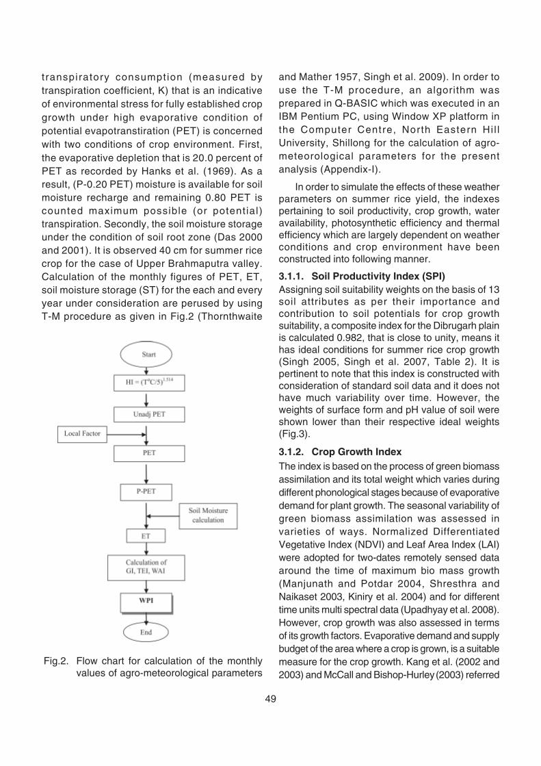
49

transpiratory consumption (measured bytranspiration coefficient, K) that is an indicativeof environmental stress for fully established cropgrowth under high evaporative condition ofpotential evapotranstiration (PET) is concernedwith two conditions of crop environment. First,the evaporative depletion that is 20.0 percent ofPET as recorded by Hanks et al. (1969). As aresult, (P-0.20 PET) moisture is available for soilmoisture recharge and remaining 0.80 PET iscounted maximum possible (or potential)transpiration. Secondly, the soil moisture storageunder the condition of soil root zone (Das 2000and 2001). It is observed 40 cm for summer ricecrop for the case of Upper Brahmaputra valley.Calculation of the monthly figures of PET, ET,soil moisture storage (ST) for the each and everyyear under consideration are perused by usingT-M procedure as given in Fig.2 (Thornthwaite

and Mather 1957, Singh et al. 2009). In order touse the T-M procedure, an algorithm wasprepared in Q-BASIC which was executed in anIBM Pentium PC, using Window XP platform inthe Computer Centre, North Eastern Hi l lUniversity, Shillong for the calculation of agro-meteorological parameters for the presentanalysis (Appendix-I).

In order to simulate the effects of these weatherparameters on summer rice yield, the indexespertaining to soil productivity, crop growth, wateravailability, photosynthetic efficiency and thermalefficiency which are largely dependent on weatherconditions and crop environment have beenconstructed into following manner.

3.1.1. Soil Productivity Index (SPI)Assigning soil suitability weights on the basis of 13soil attributes as per their importance andcontribution to soil potentials for crop growthsuitability, a composite index for the Dibrugarh plainis calculated 0.982, that is close to unity, means ithas ideal conditions for summer rice crop growth(Singh 2005, Singh et al. 2007, Table 2). It ispertinent to note that this index is constructed withconsideration of standard soil data and it does nothave much variability over time. However, theweights of surface form and pH value of soil wereshown lower than their respective ideal weights(Fig.3).

3.1.2. Crop Growth IndexThe index is based on the process of green biomassassimilation and its total weight which varies duringdifferent phonological stages because of evaporativedemand for plant growth. The seasonal variability ofgreen biomass assimilation was assessed invarieties of ways. Normalized DifferentiatedVegetative Index (NDVI) and Leaf Area Index (LAI)were adopted for two-dates remotely sensed dataaround the time of maximum bio mass growth(Manjunath and Potdar 2004, Shresthra andNaikaset 2003, Kiniry et al. 2004) and for differenttime units multi spectral data (Upadhyay et al. 2008).However, crop growth was also assessed in termsof its growth factors. Evaporative demand and supplybudget of the area where a crop is grown, is a suitablemeasure for the crop growth. Kang et al. (2002 and2003) and McCall and Bishop-Hurley (2003) referred

Fig.2. Flow chart for calculation of the monthlyvalues of agro-meteorological parameters

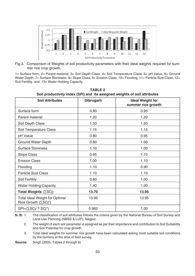
50

TABLE 2Soil productivity index (SPI) and its assigned weights of soil attributes

Soil Attributes Dibrugarh Ideal Weight forsummer rice growth

Surface form 0.80 0.95

Parent material 1.20 1.20

Soil Depth Class 1.50 1.50

Soil Temperature Class 1.15 1.15

pH Value 0.80 0.95

Ground Water Depth 0.80 1.00

Surface Stoniness 1.10 1.00

Slope Class 0.95 1.10

Erosion Class 1.00 1.10

Flooding 1.10 0.90

Particle Size Class 1.10 1.10

Soil Fertility 0.80 1.00

Water Holding Capacity 1.40 1.00

Total Weights (∑SCj) 13.70 13.95

Total Ideal Weight for Optimal 13.95 13.95Rice Growth (∑SCj*)

SPI=(∑SCj/ ? SCj*) 0.982 1.00

N. B: 1. The classification of soil attributes follows the criteria given by the National Bureau of Soil Survey andLand Use Planning (NBSS & LUP), Nagpur.

2. The weight of each soil parameter is assigned as per their importance and contribution to Soil Suitabilityand Soil Potential for crop growth.

3. Total ideal weights for summer rice growth have been calculated asking most suitable soil conditionsby the farmers at the time of field survey.

Source: Singh (2005, Tables 2 through 6)

Fig.3. Comparison of Weights of soil productivity parameters with their ideal weights required for sum-mer rice crop growth.

1= Surface form, 2= Parent material, 3= Soil Depth Class, 4= Soil Temperature Class, 5= pH Value, 6= GroundWater Depth, 7= Surface Stoniness, 8= Slope Class, 9= Erosion Class, 10= Flooding, 11= Particle Size Class, 12=Soil Fertility, and 13= Water Holding Capacity

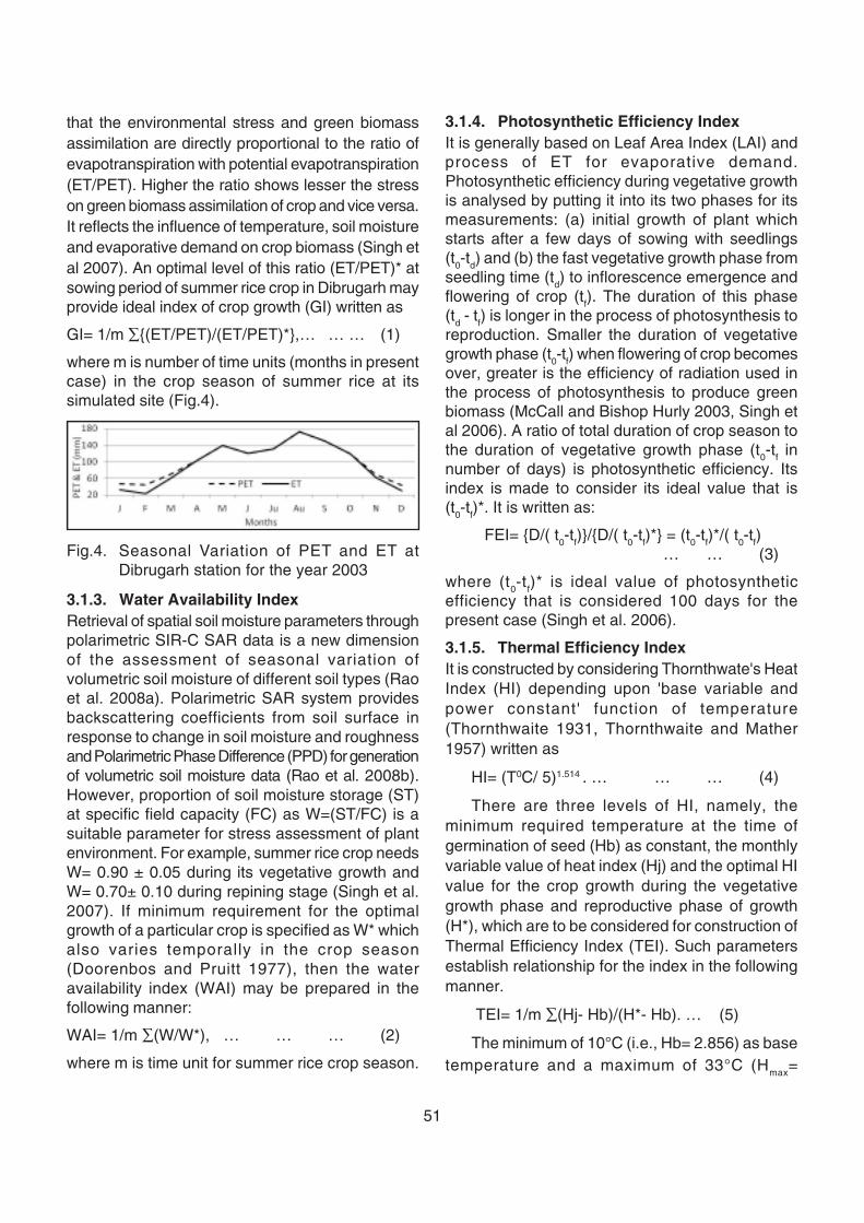
51

that the environmental stress and green biomassassimilation are directly proportional to the ratio ofevapotranspiration with potential evapotranspiration(ET/PET). Higher the ratio shows lesser the stresson green biomass assimilation of crop and vice versa.It reflects the influence of temperature, soil moistureand evaporative demand on crop biomass (Singh etal 2007). An optimal level of this ratio (ET/PET)* atsowing period of summer rice crop in Dibrugarh mayprovide ideal index of crop growth (GI) written as

GI= 1/m ∑{(ET/PET)/(ET/PET)*},… … … (1)

where m is number of time units (months in presentcase) in the crop season of summer rice at itssimulated site (Fig.4).

Fig.4. Seasonal Variation of PET and ET atDibrugarh station for the year 2003

3.1.3. Water Availability IndexRetrieval of spatial soil moisture parameters throughpolarimetric SIR-C SAR data is a new dimensionof the assessment of seasonal variation ofvolumetric soil moisture of different soil types (Raoet al. 2008a). Polarimetric SAR system providesbackscattering coefficients from soil surface inresponse to change in soil moisture and roughnessand Polarimetric Phase Difference (PPD) for generationof volumetric soil moisture data (Rao et al. 2008b).However, proportion of soil moisture storage (ST)at specific field capacity (FC) as W=(ST/FC) is asuitable parameter for stress assessment of plantenvironment. For example, summer rice crop needsW= 0.90 ± 0.05 during its vegetative growth andW= 0.70± 0.10 during repining stage (Singh et al.2007). If minimum requirement for the optimalgrowth of a particular crop is specified as W* whichalso varies temporally in the crop season(Doorenbos and Pruitt 1977), then the wateravailability index (WAI) may be prepared in thefollowing manner:

WAI= 1/m ∑(W/W*), … … … (2)

where m is time unit for summer rice crop season.

3.1.4. Photosynthetic Efficiency IndexIt is generally based on Leaf Area Index (LAI) andprocess of ET for evaporative demand.Photosynthetic efficiency during vegetative growthis analysed by putting it into its two phases for itsmeasurements: (a) initial growth of plant whichstarts after a few days of sowing with seedlings(t0-td) and (b) the fast vegetative growth phase fromseedling time (td) to inflorescence emergence andflowering of crop (tf). The duration of this phase(td - tf) is longer in the process of photosynthesis toreproduction. Smaller the duration of vegetativegrowth phase (t0-tf) when flowering of crop becomesover, greater is the efficiency of radiation used inthe process of photosynthesis to produce greenbiomass (McCall and Bishop Hurly 2003, Singh etal 2006). A ratio of total duration of crop season tothe duration of vegetative growth phase (t0-tf innumber of days) is photosynthetic efficiency. Itsindex is made to consider its ideal value that is(t0-tf)*. It is written as:

FEI= {D/( t0-tf)}/{D/( t0-tf)*} = (t0-tf)*/( t0-tf) … … (3)

where (t0-tf)* is ideal value of photosyntheticefficiency that is considered 100 days for thepresent case (Singh et al. 2006).

3.1.5. Thermal Efficiency IndexIt is constructed by considering Thornthwate's HeatIndex (HI) depending upon 'base variable andpower constant' function of temperature(Thornthwaite 1931, Thornthwaite and Mather1957) written as

HI= (T0C/ 5)1.514 . … … … (4)

There are three levels of HI, namely, theminimum required temperature at the time ofgermination of seed (Hb) as constant, the monthlyvariable value of heat index (Hj) and the optimal HIvalue for the crop growth during the vegetativegrowth phase and reproductive phase of growth(H*), which are to be considered for construction ofThermal Efficiency Index (TEI). Such parametersestablish relationship for the index in the followingmanner.

TEI= 1/m ∑(Hj- Hb)/(H*- Hb). … (5)

The minimum of 10°C (i.e., Hb= 2.856) as basetemperature and a maximum of 33°C (Hmax=

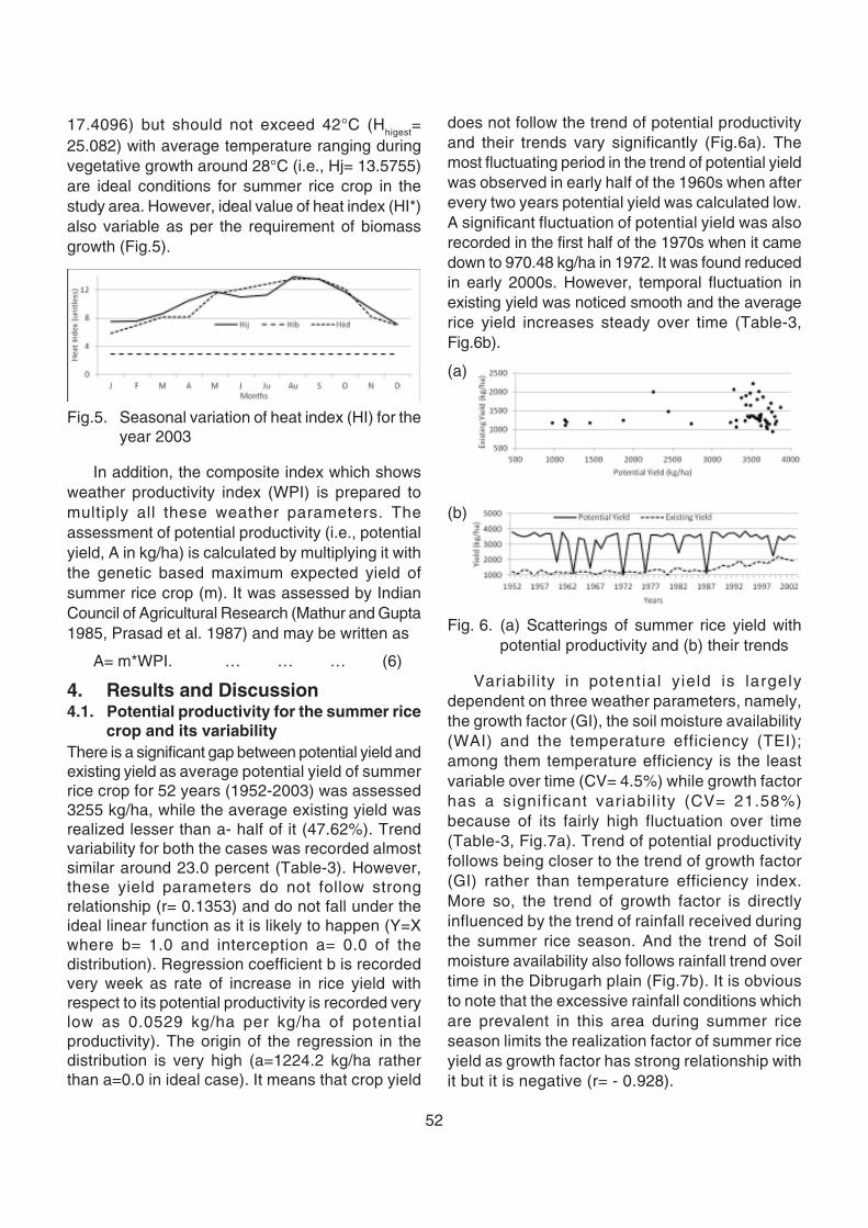
52

17.4096) but should not exceed 42°C (Hhigest

=25.082) with average temperature ranging duringvegetative growth around 28°C (i.e., Hj= 13.5755)are ideal conditions for summer rice crop in thestudy area. However, ideal value of heat index (HI*)also variable as per the requirement of biomassgrowth (Fig.5).

Fig.5. Seasonal variation of heat index (HI) for theyear 2003

In addition, the composite index which showsweather productivity index (WPI) is prepared tomultiply all these weather parameters. Theassessment of potential productivity (i.e., potentialyield, A in kg/ha) is calculated by multiplying it withthe genetic based maximum expected yield ofsummer rice crop (m). It was assessed by IndianCouncil of Agricultural Research (Mathur and Gupta1985, Prasad et al. 1987) and may be written as

A= m*WPI. … … … (6)

4. Results and Discussion4.1. Potential productivity for the summer rice

crop and its variabilityThere is a significant gap between potential yield andexisting yield as average potential yield of summerrice crop for 52 years (1952-2003) was assessed3255 kg/ha, while the average existing yield wasrealized lesser than a- half of it (47.62%). Trendvariability for both the cases was recorded almostsimilar around 23.0 percent (Table-3). However,these yield parameters do not follow strongrelationship (r= 0.1353) and do not fall under theideal linear function as it is likely to happen (Y=Xwhere b= 1.0 and interception a= 0.0 of thedistribution). Regression coefficient b is recordedvery week as rate of increase in rice yield withrespect to its potential productivity is recorded verylow as 0.0529 kg/ha per kg/ha of potentialproductivity). The origin of the regression in thedistribution is very high (a=1224.2 kg/ha ratherthan a=0.0 in ideal case). It means that crop yield

does not follow the trend of potential productivityand their trends vary significantly (Fig.6a). Themost fluctuating period in the trend of potential yieldwas observed in early half of the 1960s when afterevery two years potential yield was calculated low.A significant fluctuation of potential yield was alsorecorded in the first half of the 1970s when it camedown to 970.48 kg/ha in 1972. It was found reducedin early 2000s. However, temporal fluctuation inexisting yield was noticed smooth and the averagerice yield increases steady over time (Table-3,Fig.6b).

(a)

(b)

Fig. 6. (a) Scatterings of summer rice yield withpotential productivity and (b) their trends

Variability in potential yield is largelydependent on three weather parameters, namely,the growth factor (GI), the soil moisture availability(WAI) and the temperature efficiency (TEI);among them temperature efficiency is the leastvariable over time (CV= 4.5%) while growth factorhas a significant variabil ity (CV= 21.58%)because of its fairly high fluctuation over time(Table-3, Fig.7a). Trend of potential productivityfollows being closer to the trend of growth factor(GI) rather than temperature efficiency index.More so, the trend of growth factor is directlyinfluenced by the trend of rainfall received duringthe summer rice season. And the trend of Soilmoisture availability also follows rainfall trend overtime in the Dibrugarh plain (Fig.7b). It is obviousto note that the excessive rainfall conditions whichare prevalent in this area during summer riceseason limits the realization factor of summer riceyield as growth factor has strong relationship withit but it is negative (r= - 0.928).

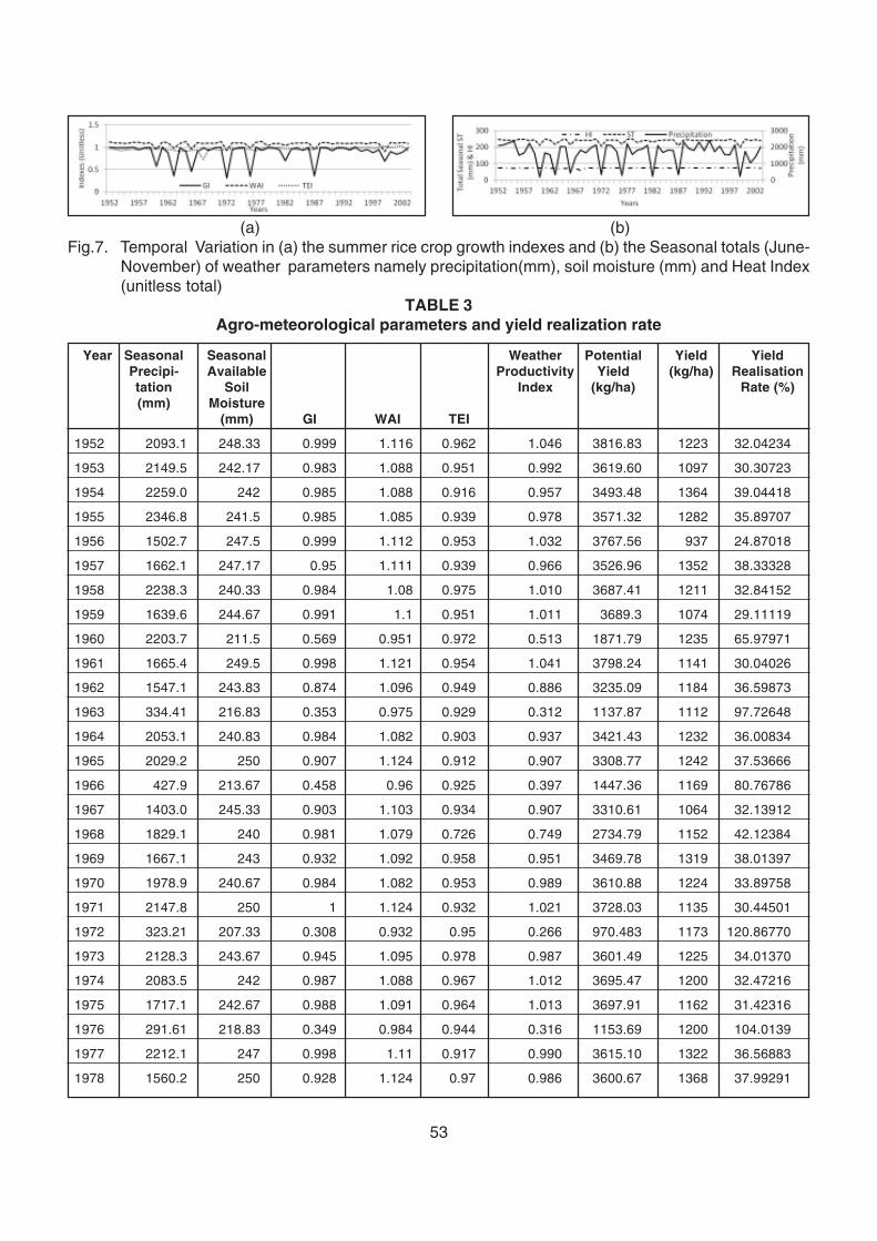
53

TABLE 3Agro-meteorological parameters and yield realization rate

Year Seasonal Seasonal Weather Potential Yield YieldPrecipi- Available Productivity Yield (kg/ha) Realisationtation Soil Index (kg/ha) Rate (%)(mm) Moisture

(mm) GI WAI TEI

1952 2093.1 248.33 0.999 1.116 0.962 1.046 3816.83 1223 32.04234

1953 2149.5 242.17 0.983 1.088 0.951 0.992 3619.60 1097 30.30723

1954 2259.0 242 0.985 1.088 0.916 0.957 3493.48 1364 39.04418

1955 2346.8 241.5 0.985 1.085 0.939 0.978 3571.32 1282 35.89707

1956 1502.7 247.5 0.999 1.112 0.953 1.032 3767.56 937 24.87018

1957 1662.1 247.17 0.95 1.111 0.939 0.966 3526.96 1352 38.33328

1958 2238.3 240.33 0.984 1.08 0.975 1.010 3687.41 1211 32.84152

1959 1639.6 244.67 0.991 1.1 0.951 1.011 3689.3 1074 29.11119

1960 2203.7 211.5 0.569 0.951 0.972 0.513 1871.79 1235 65.97971

1961 1665.4 249.5 0.998 1.121 0.954 1.041 3798.24 1141 30.04026

1962 1547.1 243.83 0.874 1.096 0.949 0.886 3235.09 1184 36.59873

1963 334.41 216.83 0.353 0.975 0.929 0.312 1137.87 1112 97.72648

1964 2053.1 240.83 0.984 1.082 0.903 0.937 3421.43 1232 36.00834

1965 2029.2 250 0.907 1.124 0.912 0.907 3308.77 1242 37.53666

1966 427.9 213.67 0.458 0.96 0.925 0.397 1447.36 1169 80.76786

1967 1403.0 245.33 0.903 1.103 0.934 0.907 3310.61 1064 32.13912

1968 1829.1 240 0.981 1.079 0.726 0.749 2734.79 1152 42.12384

1969 1667.1 243 0.932 1.092 0.958 0.951 3469.78 1319 38.01397

1970 1978.9 240.67 0.984 1.082 0.953 0.989 3610.88 1224 33.89758

1971 2147.8 250 1 1.124 0.932 1.021 3728.03 1135 30.44501

1972 323.21 207.33 0.308 0.932 0.95 0.266 970.483 1173 120.86770

1973 2128.3 243.67 0.945 1.095 0.978 0.987 3601.49 1225 34.01370

1974 2083.5 242 0.987 1.088 0.967 1.012 3695.47 1200 32.47216

1975 1717.1 242.67 0.988 1.091 0.964 1.013 3697.91 1162 31.42316

1976 291.61 218.83 0.349 0.984 0.944 0.316 1153.69 1200 104.0139

1977 2212.1 247 0.998 1.11 0.917 0.990 3615.10 1322 36.56883

1978 1560.2 250 0.928 1.124 0.97 0.986 3600.67 1368 37.99291

(a) (b)Fig.7. Temporal Variation in (a) the summer rice crop growth indexes and (b) the Seasonal totals (June-

November) of weather parameters namely precipitation(mm), soil moisture (mm) and Heat Index(unitless total)

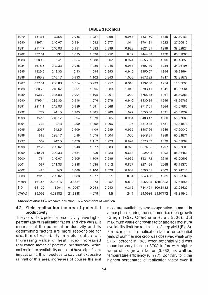
54

1979 1813.1 228.5 0.986 1.027 0.98 0.968 3531.60 1335 37.80161

1980 1897.4 240.67 0.984 1.082 0.977 1.014 3701.81 1022 27.60810

1981 2114.7 240.83 0.951 1.082 0.989 0.992 3621.61 1399 38.62924

1982 237.01 231 0.695 1.038 0.952 0.67 2444.09 1476 60.39066

1983 2089.3 241 0.954 1.083 0.967 0.974 3555.50 1296 36.45056

1984 1676.5 242.33 0.985 1.089 0.945 0.988 3607.39 1254 34.76195

1985 1826.6 243.33 0.93 1.094 0.953 0.945 3450.57 1354 39.23991

1986 1805.3 245.17 0.993 1.102 0.943 1.006 3672.32 1247 33.95678

1987 327.51 208.83 0.354 0.939 0.957 0.310 1132.08 1254 110.7693

1988 2305.2 243.67 0.991 1.095 0.983 1.040 3796.11 1341 35.32564

1989 1933.2 245.83 0.994 1.105 0.961 1.029 3756.38 1461 38.89383

1990 1796.4 239.33 0.918 1.076 0.976 0.940 3430.85 1656 48.26786

1991 2311.1 242.83 0.989 1.091 0.968 1.018 3717.01 1564 42.07682

1992 1772 241.5 0.985 1.085 0.986 1.027 3750.08 1691 45.09239

1993 2413 240.17 0.94 1.079 0.965 0.954 3483.17 1960 56.27066

1994 1737 243 0.99 1.092 1.006 1.06 3870.38 1581 40.84873

1995 2057 242.5 0.909 1.09 0.989 0.955 3487.26 1646 47.20040

1996 1562 239.17 0.95 1.075 1.004 1.000 3648.91 1859 50.94671

1997 1532 247.5 0.876 1.112 0.973 0.924 3373.02 1839 54.52084

1998 2126 239.67 0.943 1.077 0.989 0.979 3574.55 1797 50.27209

1999 240.01 200.33 0.684 0.9 1.029 0.618 2254.3 1992 88.36451

2000 1764 246.67 0.905 1.109 0.986 0.965 3521.72 2219 63.00903

2001 1057 241.33 0.838 1.085 1.012 0.897 3274.55 2068 63.15370

2002 1426 246 0.888 1.106 1.028 0.984 3593.01 2003 55.74710

2003 2018 239.67 0.983 1.077 0.911 0.94 3432.3 1901 55.38562

Mean 1640.6 238.676 0.8834 1.073 0.957 0.892 3255.05 1396.423 47.61656

S D 641.39 11.8904 0.19067 0.053 0.043 0.215 784.421 306.8182 22.05429

CV(%) 39.095 4.98182 21.5838 4.979 4.5 24.1 24.0986 21.97172 46.31642

Abbreviations: SD= standard deviation, CV= coefficient of variation

TABLE 3 (Contd.)

4.2. Yield realisation factors of potentialproductivity

The years of low potential productivity have higherpercentage of realization factor and vice versa. Itmeans that the potential productivity and itsdetermining factors are more responsible forcreation of variabil i ty in yield realization.Increasing value of heat index increasedrealization factor of potential productivity, whilesoil moisture availability does not have significantimpact on it. It is needless to say that excessiverainfall of this area increases of course the soil

moisture availability and evaporative demand inatmosphere during the summer rice crop growth(Singh 1999, Chaichana et al. 2006). Butmaximum value of growth factor and soil moistureavailability limit the realization of crop yield (Fig.8).For example, the realisation factor for potentialyield of summer rice crop was observed weak only27.61 percent in 1980 when potential yield wasrecorded very high as 3702 kg/ha with highervalue of its growth factor (0.983) as well astemperature efficiency (0. 977). Contrary to it, thehighest percentage of realization factor even if

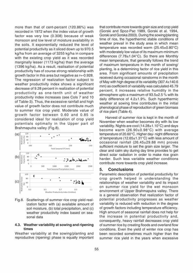
55

more than that of cent-percent (120.86%) wasrecorded in 1972 when the index value of growthfactor was very low (0.308) because of weakmonsoon and low level of moisture availability inthe soils. It exponentially reduced the level ofpotential productivity as it sliced down up to 970.5kg/ha from an average of 3255 kg/ha in comparewith the existing crop yield as it was recordedmarginally lesser (1173 kg/ha) than the average(1396 kg/ha). As a result, realisation of potentialproductivity has of course strong relationship withgrowth factor in this area but negative as r=-0.928.The regression of realization factor subject toweather productivity index shows a significantdecrease of 9.28 percent in realization of potentialproductivi ty as one-tenth unit of weatherproductivity index increases (see Cols 7 and 10of Table-3). Thus, the excessive rainfall and highvalue of growth factor does not contribute muchto summer rice crop yield. Moderate value ofgrowth factor between 0.60 and 0.85 isconsidered ideal for realization of crop yieldpotentials optimally in the Upper part ofBrahmaputra valley (Fig.8).

(a)

(b)

(c)

Fig.8. Scatterings of summer rice crop yield real-ization factor with (a) available amount ofsoil moisture, (b) total precipitation, and (c)weather productivity index based on sea-sonal data

4.3. Weather variability at sowing and ripeningtimes

Weather variability at the sowing/planting andreproductive (ripening) phase is equally important

that contribute more towards grain size and crop yield(Gorski and Spoz-Pac 1989, Gorski et al. 1994,Gorski and Gorska 2003). During the sowing/plantingtime of rice, the hyperthermic stable conditions ofweather prevail in the study area in which meantemperature was recorded warm (25.45±0.80°C)with moderately low value of its maximum-minimumdifferences (7.78±1.04°C). So there are Monthlymean temperature, that generally follows the trendof maximum temperature in the month of sowing/planting, is a determining factor of rice yield in thisarea. From significant amounts of precipitationreceived during occasional rainstorms in the monthof May with high degree of its variability (307.4±140.6mm) as coefficient of variability was calculated 45.79percent, it increases relative humidity in theatmosphere upto a maximum of 93.5±2.5 % with itsdaily difference of 4.2±1.9%. Such hyperthermicweather at sowing time contributes in the initialphenological phase of reproduction of green biomassof rice plant (Table 4).

Harvest of summer rice is kept in the month ofNovember when weather becomes dry with its lowvariability. Nights are cool (14.28±1.10°C) and daysbecome warm (26.90±0.98°C) with averagetemperature of 20.60°C. Higher day- night differenceof temperature (12.65±1.31°C) with less amount ofoccasional rainfall (26.45±29.88 mm) provessufficient moisture to set the grain size larger. Theclear and calm sky during day time provides to getdirect solar radiation in order to make rice grainharder. Such less variable weather conditionscontribute more towards crop yield increase.

5. ConclusionsParametric description of potential productivity forcrop growth helped in understanding therelationships of weather variability and its impacton summer rice yield for the wet monsoonenvironment of Upper Brahmaputra valley. Thereis a general observation that realization factor ofpotential productivity progresses as weathervariability is reduced with reduction in the degreeof growth factors including temperature efficiency.High amount of seasonal rainfall does not help forthe increase in potential productivity and,consequently, heavy rainfall decreases crop yieldof summer rice by creating floods and overland flowconditions. Even the yield of winter rice crop hasbeen recorded sometimes much higher than thesummer rice yield in the years when excessive

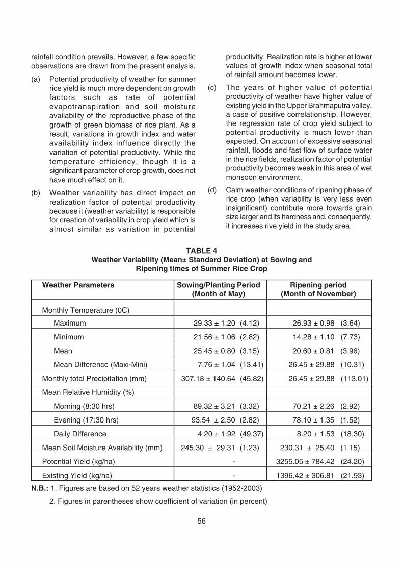
56

rainfall condition prevails. However, a few specificobservations are drawn from the present analysis.

(a) Potential productivity of weather for summerrice yield is much more dependent on growthfactors such as rate of potentialevapotranspiration and soil moistureavailability of the reproductive phase of thegrowth of green biomass of rice plant. As aresult, variations in growth index and wateravailability index influence directly thevariation of potential productivity. While thetemperature efficiency, though it is asignificant parameter of crop growth, does nothave much effect on it.

(b) Weather variability has direct impact onrealization factor of potential productivitybecause it (weather variability) is responsiblefor creation of variability in crop yield which isalmost similar as variation in potential

productivity. Realization rate is higher at lowervalues of growth index when seasonal totalof rainfall amount becomes lower.

(c) The years of higher value of potentialproductivity of weather have higher value ofexisting yield in the Upper Brahmaputra valley,a case of positive correlationship. However,the regression rate of crop yield subject topotential productivity is much lower thanexpected. On account of excessive seasonalrainfall, floods and fast flow of surface waterin the rice fields, realization factor of potentialproductivity becomes weak in this area of wetmonsoon environment.

(d) Calm weather conditions of ripening phase ofrice crop (when variability is very less eveninsignificant) contribute more towards grainsize larger and its hardness and, consequently,it increases rive yield in the study area.

TABLE 4Weather Variability (Mean± Standard Deviation) at Sowing and

Ripening times of Summer Rice Crop

Weather Parameters Sowing/Planting Period Ripening period(Month of May) (Month of November)

Monthly Temperature (0C)

Maximum 29.33 ± 1.20 (4.12) 26.93 ± 0.98 (3.64)

Minimum 21.56 ± 1.06 (2.82) 14.28 ± 1.10 (7.73)

Mean 25.45 ± 0.80 (3.15) 20.60 ± 0.81 (3.96)

Mean Difference (Maxi-Mini) 7.76 ± 1.04 (13.41) 26.45 ± 29.88 (10.31)

Monthly total Precipitation (mm) 307.18 ± 140.64 (45.82) 26.45 ± 29.88 (113.01)

Mean Relative Humidity (%)

Morning (8:30 hrs) 89.32 ± 3.21 (3.32) 70.21 ± 2.26 (2.92)

Evening (17:30 hrs) 93.54 ± 2.50 (2.82) 78.10 ± 1.35 (1.52)

Daily Difference 4.20 ± 1.92 (49.37) 8.20 ± 1.53 (18.30)

Mean Soil Moisture Availability (mm) 245.30 ± 29.31 (1.23) 230.31 ± 25.40 (1.15)

Potential Yield (kg/ha) - 3255.05 ± 784.42 (24.20)

Existing Yield (kg/ha) - 1396.42 ± 306.81 (21.93)

N.B.: 1. Figures are based on 52 years weather statistics (1952-2003)

2. Figures in parentheses show coefficient of variation (in percent)

57

ReferencesAggarwal, P. K., Kalran, N., Singh, A. K. andSinha, S. K. (1994). Analyzing the limitation setby climatic factors, genotype, water and nitrogenavailability on productivity of wheat: I- the modeldescription, parameterization and validation. FieldCrops Research. 38(1): 73-91.

Aigner, D .J., Lovell, C. A. K. and Schmidt, P.(1977), Formulation and estimation of stochasticfrontier production function. Journal ofEconometrics. 6: 21-37.

Baker, D. N., Hesketh, J. D. and Duncan, W. G.(1972), Simulation of growth in cotton: I- grossphotosynthesis, respiration and growth, CropScience. 12: 431-435.

Chaichana, T., Sumpun, C., Jompakdee, W. andDussadee, N. (2008), Engineering analysis of wetseason rice production in North Thailand. InternationalAgriculture Engineering Journal, 17(1-4): 1-17.

Chatelin, M. H., Aubry, C., Poussin, J.C., Meynard,J.M., Masse, J., Verjux, N., Gate, Ph. and LewBris (2005), DeciBle, a software package for wheatcrop management and simulation. AgriculturalSystems. 83(1): 77-99.

Commission for Agricultural Meteorology (2006),Weather and Climate Information, SustainableAgriculture and Adaption Strategies to ClimateChange, World Meteorological Organisation(WMO), Publication- 999, Geneva, Switzerland.

Das, H.P. (2000), Monitoring the incidence of largescale droughts in India. In D.A. Wilhite (ed):Drought- A Global Assessment. Vol. 1, Routeldge,London & New York, pp.181-195.

Das, H.P. (2001). On the assessment ofagricultural drought of dry land crop. Vayu Mandal.31(1-4): 98-102.

DeWit, C. T., Brouwer, R. and Vries, F. W. T .P.(1969), The simulation of photosynthesissystems:I- models and Methods. Proceedings,IPB/PP Technical Meeting, Pudoc, Wageningen.

Doorenbos, J. and Pruitt, W. O. (1977), Guidelinesfor Predicting Crop Water Requirements. FAOIrrigation and Drainage Paper 24, Food andAgriculture Organisation of the United Nations,Rome, Italy: p 145.

Gangopadhyay, S.K., Walia, C.S., Chamuah,G.S., Baruah, U. (1998), Rice growing soils ofupper Brahmaputra valley of Assam- their

characteristics and suitability. Journal of IndianSociety of Soil Sciences. 46: 103-109

Gorski, T., Demidowicz, G., Deputat, T., Gorska,K., Marcinkowska, I., Spoz-Pac, W. and Krakowiak,A. (1994), Agrometeorological quantification ofagricultural year in Poland. Zeszyty ProblemowePostepon Nauk Rolniczyh. 405: 81-87.

Gorski, T. and Gorska, K. (2003), The effects ofscale on crop yield variability. AgriculturalSystems. 78:425-434.

Gorski, T. and Spoz-Pac, W. (1989), A method forforecasting sugar beet yields in Poland. ZeszytyProblemowe Postepow Nauk Rolniczych. 369: 31-43

Hanks, J.K., Gardener, H. R. and Florian, R. L.(1969), Plant growth evapotranspiration relationsfor several crops in the central Great plains.Agronomic Journal.30-34.

Kang, S. Z., Lu, Zhang, Liang, Y. L. and Dawes,W. (2003), Simulation of winter wheat yield andwater use efficiency in the Loess plateau of Chinausing WAVES. Agricultural Systems. 78: 355-367.

Kang, S. Z., Zhang, L., Liang, Y. L. and Caia, H.J. (2002), Effects of limited irrigation on yield andwater use efficiency of winter wheat in the Loessplateau of China. Agricultural Water Management.55: 203-216.

Kiniry, J. R., Bean, B., Yun, Xie and Pei-yu, Chen(2004), Maize yield potential: critical processesand simulation modeling in a high yieldingenvironment. Agricultural Systems. 82(1): 45-56.

Mall, R. K. and Singh, K. K. (2000), Climaticvariability and wheat yield progress in Punjabusing CERES-wheat and WTGROWS models.Vayu Mandal, 30(3-4): 35-40.

Manjunath, K. R. and Potdar, M. B. (2004), Wheatgrowth profile: satellite monitoring and crop yieldmodeling. Journal of the Indian Society of RemoteSensing. 32(1): 91-102.

Mathur P. N. and Gupta M. P. (1985), NationalDemonstrations Project-An Overview, Publicationsand Information Division, Indian Council ofAgricultural Research, New Delhi, Table-4: p. 11

McCall, D. G. and Bishop-Hurley, G. J. (2003), Apasture growth model for use in a whole farm dairyproduction model. Agricultural Systems. 76(3):1183-1205.

NBSS & LUP (1999), Soils of Assam forOptimizing Land Use, NBSS Publ-66, Soils ofIndia Series, Nagpur.

58

Prasad, C., Choudhary, B. N. and Nayar, B.B.(1987), First-line Transfer of Technology Projects,Publication and Information Division, IndianCouncil of Agriculture Research, New Delhi

Rao, K.S., Rao, Y.S. and Jassar, H.K.A. (2008a),Retrieval of soil moisture using SIR-C polarimetricdata. Journal of the Indian Society of RemoteSensing. 36(2):109-122.

Rao, K.S., Rao, Y.S. and Jassar, H.K.A. (2008b),A study on the polarimetric properties variousfeatures using SIR-C data. Journal of the IndianSociety of Remote Sensing. 36(2):123-136.

Reddy, V.R., Baker, D. N. and Jenkins, J. N.(1985), Validation of GOSSYM: Part-II. Mississippiconditions, Agricultural Systems. 17: 133-154.

Ritchie, J. T. (1986), CERES-wheat: a generaldocumentation, USDA-ARS Grassland, Soil andWater Resources Laboratory, Temple, Texas.

Shrestha, R. P. and Naikaset, S. (2003), Agro-spectral models for estimating dry season riceyield in the Bangkok plain of Thailand. AsianJournal of Geo-informatics. 4(1): 11-19.

Singh, S. (1999), A Resource Atlas of ArunachalPradesh, Planning Division, Government ofArunachal Pradesh, Itanager,161 pp with 59Plates, 26 Tables and 27 Figures.

Singh, S. (2000), Modeling, structure and functionsof agricultural yield potential. Transactions of theInstitute of Indian Geographers. 22:1-15.

Singh, S. (2005), CSSM, Crop-ecologicalSustainability Simulation Model: A Spatio-Temporal Crop Yield Analysis Tool (version- 5.2),Monograph No GE/ SAP-UGC/3, Department ofGeography, North-Eastern Hill University,Shillong.

Singh, S., Sharma, B. and Dey, P. P. (2006),Predicting summer rice yield based on biophysicaland technological parameters on Monsoon landsof Brahmaputra valley. International AgriculturalEngineering Journal, 15(2-3): 91-107.

Singh, S., Starkel, L. and Syiemlieh, H. J. (2009),Land Degradation and Ecorestoration in theExtremely Wet Monsoon Environment ofCherrapunji Area, India, Bookwell Publications,Delhi (in press).

Singh, S., Syiemlieh, H. J. and Sharma, B. (2007),Biophysical attributes influencing the summer riceyield in Brahmaputra valley, Indian Journal of SoilConservation, 35(1): 30-35.

Subash, S., Bino-Paul, G. D. and Ramanathan, A.(2004), Technical efficiency in rice production - anapplication of stochastic frontier analysis. IndianJournal of Regional Science. XXXVI (1): 118-126.

Thornthwaite, C.W. (1931), Climates of NorthAmerica. Geographical Review. 21(4): 633-655.

Thornthwaite, C.W. and Mather, J.R. (1957).Instructions and Tables for Computing PotentialEvapotranspiration and Water Balance,Publications in Climatology Vol X(3), DrexelInstitute of Technology, Centerton, New Jersey.

Upadhyay, G., Ray, S.S. and Panigrahy, S. (2008),Derivation of crop phonological parameters usingmulti-data SPOT- VGT-NDVI data: a case forPunjab. Journal of the Indian society of RemoteSensing, 36(1): 37-50.

Zhang, L. and Dawes, W. (1998). WAVES - AnIntegrated Energy and Water Balance Model,CSIRO Land and Water, Technical Report No. 31/98, Canberra ACT 2601, Australia.

Appendix-I: Algorithm for Calculation ofAgro-meteorological Parameters1. Create UNADJPET(136,47) table from

UNADJPET.TXT file.

2. Create CORRFATC(2,12) table fromCORRFACT.TXT file.

3. Create T250(141,11) table from TAB250.TXT file.

4. Open input file DIBRU.OUT and output fileDIBRU.H.

5. (a) Create heat index for 12 months as (temp/5)1.514

(b) Generate sum of heat index for 12 months and6 months (June to November).

(c) Generate percentage of 6months value withrespect to 12 months value of heat index.

(d) The 12 heat indices, accumulated heat indexfor 12 months and 6 months and percentageheat index value are written to output file.

6. (a) Unadjusted Precipitation is generated bycomparing the temperature with the valuesstored in table UADJPET(136,47) and locatingthe corresponding value.

7. (a) PET is generated by multiplying unadjustedPrecipitation generated in step (6) withcorresponding CORRFACT (correction factor)which is then subtracted from precipitationvalue to generate P.PET values for 12corresponding months.

59

(b) The 12 PET values are written to output file.

8. (a) Precipitation of 12 months are added togetherinto TRF12.

(b) Precipitation for 6 months (june to Nov) areadded into TRF6.

(c) Percentage of TRF6 w.r.t TRF12 is generated.

(d) The 12 precipitations, TRF12, TRF6 andpercentage are written to output file.

9. (a) Add all the negative P.PET value to generateSum P

(b) The 12 P.PET values are written to output file.

10. Accumulate Wet Loss (ACCWL) Calculation:

(a) ACCWL for November is taken as P.PET forNovember.

(b) ACCWL for January is taken as sum ofACCWL for November and P.PET for January.

(c) For the months of February to June theACCWL is taken as sum of ACCWL of previousmonth and P.PET of the month.

(d) The positive ACCWL values are changed tozero.

(e) The 12 ACCWL values are written to outputfile.

11. ST Value calculation:(a) All negative accWL values are stored into

corresponding ST locations.

(b) The ST values are then changed intocorresponding value from T250 (141,11).

(a) Sum of 12 months ST values and 6 months(June to Nov) are stored into TST12, TST6respectively.

(b) The 12 ST values, TST12 and TST6 are writtento output file.

12. Delta ST value calculation:

(a) Delta ST value for January if the differencebetween ST value of January and December.

(b) Delta ST value for February to December is thedifference between ST values of thecalculating month and ST value of the previousmonth.

(c) The 12 Delta ST values are written to outputfile.

13. Evapotranspiration (ET) Calculation:

(a) If rainfall (precipitation) is greater than or equalto PET value then ET takes the PET value.

(b) If rainfall is less than PET value then ET istaken as difference between rainfall and DeltaST value.

(c) The 12 ET values are written to output file.

14. Growth Factor (GI) Calculation :

(a) GI is calculated as ratio of ET to PET value ofcorresponding month.

(b) Further 12 GI values are written to o/p file.

(c) The average GI value for 12 month and sixmonths (June to Nov) are generated andwritten to output file.

15. Water Use Efficiency (WUE) Calculation :

(a) WUE is calculated by diving corresponding STvalues by (250 x 0.89).

(b) The 12 WUE values are written to output file.

16. Temperature Efficiency Index (TEI) Calculation :

(a) TEI is calculated as (heat index at step (5) -2.856) / 9.79.

(b) The 12 TEI values along with Average annualTEI value and 6 months average TEI(June toNov) value are written to output file.

17. Photosynthetic Efficiency Index (FEI) Calculation:

(a) For all the 12 months FEI is taken as 1.

(b) The 12 FEIs along with 12 months average FEIand 6 months average FEI are written to outputfile.

The steps 5 to 17 are repeated for the year 1953 to 2003and output is generated.

60

1. IntroductionThe advantage of using radar for precipitationmeasurements is the coverage of a large area inreal time. In weather radar various informationare achieved by rotating an antenna with avariable vertical angle by suitable calibration. Theradar antenna in practice emits a short pulse ofe.m. radiation in a particular direction. Very smallfraction of this energy is reflected back by targets(here precipitating particles) to radar antenna.The back-scattered average power received bythe radar is proportional to the reflectivity factorZ. From knowledge of reflectivity and usingsuitable empirical Z-R relation one can determinethe meteorological quantities like rainfall rate andliquid water content. At higher millimeter wave thedrop size of cloud and precipitation particles arevery small, compared to the wavelength and thenRayleigh's scattering is no longer valid. In thiscase we consider the Mie scattering or opticalscattering [Arai et al. (2005)].

2. Theoretical background and resultsThe backscattering cross-section of a water dropin Rayleigh region is written as (Sen andBhattacharya 2009)

σ=∏5 D6 ⎢K ⎢2 / λ4 (1)

where | K|2 is complex index of refraction.

Then the cloud radar reflectivity η can be expressedas

η =( ∏5 ⎢Κ ⎢2 / λ4)∫ ν (D)dD (2)

The radar reflectivity factor Z is obtained from,

Z =Σ Ni Di6 =∫ N (D)D6 dD (3)

where Ni is the number of drops in a unit volume of

air with diameter Di and N(D) is the number of drops

having diameter between D and (D+dD). If there is

no vertical air motion then rate of rainfall is

expressed as,

R= — ∫ N (D)D3 Vt (D)dD (4)

where Vt (D) denotes the terminal velocity of thedrop whose diameter is D and can be expressedas,

V = 1400D1/2 (5)

We see from Eqs.(3) and (4) that it is the raindropsize distribution N(D) that ties Z to R.UsingMarshall-Palmer exponential drop sizedistribution in Eqs. (3) and (4) one may get arelation between radar reflectivity and rainfall rateof the form

Z = aRb (6)

where a is known as pre-factor and b is knownas exponent.

A frequently used relationship for Z-R, is of theform

Z=200 R1.6

One may derive the average power received by theradar antenna [Sen and Bhattacharya 2009] as

Pr= ——— — ⎢Κ ⎢2 Z (7)

where Pt = peak transmitted power in the pulser,G = antenna gain, h = pulse length in the space,λ = wave length, θ = beam width between halfpower points and r = range.

Precipitation and cloud radarreflectivity at millimeter wavebased on Mie's scatteringformula

D.K.Tripathi1, 2, and A.B.Bhattacharya1

1. Department of Physics, University ofKalyani-741235

and2. Department of Physics, Narula Institute of

Technology, Kolkata–700109

ABSTRACT

Fundamentals of Z-R relations are critically examined to find the variations in Z-R relations with latitude.It is found that the change in Z-R relations does not follow any special trend.

∞i=1

∞

0

PtG2 hθ2 Π3

730r2 λ2

∞

60Π

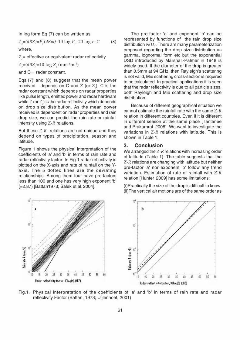
61

In log form Eq (7) can be written as,

Ze=(dBZ)=Pr (dBm)–10 log Pt+20 log r+C (8)

where,

Ze= effective or equivalent radar reflectivity

Ze=(dBZ)=10 log Ze (mm 6m–3)

and C = radar constant.

Eqs.(7) and (8) suggest that the mean powerreceived depends on C and Z (or Ze), C is theradar constant which depends on radar propertieslike pulse length, emitted power and radar hardwarewhile Z (or Ze) is the radar reflectivity which dependson drop size distribution. As the mean powerreceived is dependent on radar properties and raindrop size, we can predict the rain rate or rainfallintensity using Z-R relations.

But these Z-R relations are not unique and theydepend on types of precipitation, season andlatitude.

Figure 1 shows the physical interpretation of thecoefficients of 'a' and 'b' in terms of rain rate andradar reflectivity factor. In Fig.1 radar reflectivity isplotted on the X-axis and rate of rainfall on the Y-axis. The 5 dotted lines are the deviatingrelationships. Among them four have pre-factorsless than 100 and one has very high exponent ‘b’(=2.87) [Battan1973; Salek et al. 2004].

The pre-factor 'a' and exponent 'b' can berepresented by functions of the rain drop sizedistribution N(D). There are many parameterizationproposed regarding the drop size distribution asgamma, lognormal form etc but the exponentialDSD introduced by Marshall-Palmer in 1948 iswidely used. If the diameter of the drop is greaterthan 0.5mm at 94 GHz, then Rayleigh's scatteringis not valid, Mie scattering cross-section is requiredto be calculated. In practical applications it is seenthat the radar reflectivity is due to all particle sizes,both Rayleigh and Mie scattering and drop sizedistribution.

Because of different geographical situation wecannot estimate the rainfall rate with the same Z-Rrelation in different countries. Even if it is differentin different season at the same place [Tantaneeand Prakarnrat 2008]. We want to investigate thevariations in Z-R relations with latitude. This isshown in Table 1.

3. ConclusionWe arranged the Z-R relations with increasing orderof latitude (Table 1). The table suggests that theZ-R relations are changing with latitude but neitherpre-factor 'a' nor exponent 'b' follow any trendvariation. Estimation of rate of rainfall with Z-Rrelation [Hunter 2009] has some limitations:

(i)Practically the size of the drop is difficult to know.(ii)The vertical air motions are of the same order as

Fig.1. Physical interpretation of the coefficients of 'a' and 'b' in terms of rain rate and radarreflectivity Factor (Battan, 1973; Uijlenhoet, 2001)

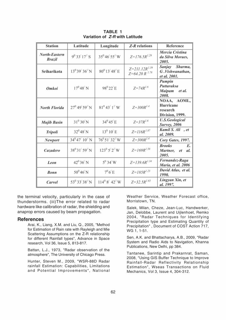
62

the terminal velocity, particularly in the case ofthunderstorms. (iii)The error related to radarhardware like calibration of radar, the shielding andanaprop errors caused by beam propagation.

ReferencesArai, K., Liang, X.M. and Liu, Q., 2005, "Methodfor Estimation of Rain rate with Rayleigh and MieScattering Assumptions on the Z-R relationshipfor different Rainfall types", Advance in Spaceresearch, Vol 36, Issue 5, 813-817.

Battan, L.J., 1973, "Radar observation of theatmosphere", The University of Chicago Press.

Hunter, Steven M., 2009, "WSR-88D Radarrainfall Estimation: Capabilities, Limitationsand Potent ia l Improvements" , Nat iona l

Weather Service, Weather Forecast office,Morristown, TN.

Salek, Milan, Cheze, Jean-Luc, Handwerker,Jan, Delobbe, Laurent and Uijlenhoet, Remko2004, "Radar Techniques for Identi fyingPrecipitation type and Estimating Quantity ofPrecipitation" , Document of COST Action 717,WG 1, 1-51.

Sen, A.K. and Bhattacharya, A.B., 2009, "RadarSystem and Radio Aids to Navigation, KhannaPublications, New Delhi, pp 384.

Tantanee, Sarintip and Prakarnrat, Saman,2008, "Using GIS Buffer Technique to ImproveRainfal l-Radar Reflect ivi ty Relat ionshipEstimation", Wseas Transactions on FluidMechanics, Vol 3, Issue 4, 304-312.

TABLE 1Variation of Z-R with Latitude

63

1. IntroductionWith the progressive northward movement of sunduring pre-monsoon months, the vast areas of landin the Northern Indian sub-continent is heated up byintense solar radiation from the sun. Depending uponthe nature of earth's surface, some parts becomerelatively more warmer as compared to other areas.May and June are excessively hot months duringwhich maximum temperature in the day rise to anabnormally high value in the northern belt particularlyin Rajasthan state. In the event of delayed onset ofmonsoon, abnormally high temperature continueeven up to the first week of July. Therefore, theobservations of maximum temperature and itsdeparture from the normal become significant duringthese months as the day- to-day human activitiesare affected. During April to June, the normalmaximum temperature of Rajasthan state is itselfvery high as compared to the adjoining areas. Furtherrise in maximum temperature from normal valuesometimes leads to heat wave situations. Due to longexposure of extreme hot spells and continuance ofheat wave over a particular region leads to severethermal strains, disastrous consequences and alsocasualties.

The phenomenon of heat wave is of greatconcern to agriculturist, water management, irrigationetc. particularly for Rajasthan state. Because of dryclimate and prolonged recurrence of heat wave over

this part cause fall in water level in major reservoirsand also reduces the underground water table andalso loss of human lives. Further, this phenomenonis likely to become more intense in view of globalwarming scenario and needs proper investigation toplan adaptation strategies.

2. Heat waveIn Annual Monsoon Review-2002, IndiaMeteorological Department has revised the criteriafor declaring of Heat wave as given in it's'Forecasting Manual IV' and made it effective w.e.f1st March, 2002. According to this:

(i) Heat wave need not be considered tillmaximum temperature of a station reachesat least 40°C for plains and at least 30°C forhilly regions.

(ii) When the normal maximum temperature of astation is less than or equal to 40°C:

• Heat Wave Departure from normal : 5°Cto 6°C

• Sever Heat Wave Departure from normal:7°C or more.

(iii) When the normal maximum temperature of astation is 40°C:

• Heat Wave Departure from normal is 4°Cto 5°C

ABSTRACT

An attempt has been made to study the spatial variation of maximum temperature over Rajasthan state duringpre-monsoon months from the data of daily maximum temperature of ten stations taken as a representation forEast and West Rajasthan for two consecutive decade i.e. 1981-91 and 1992-2001. The study revealed that twoheat wave prone region viz. one in the western part of the state near Jaisalmer and other in the Eastern part ofstate with its center near Bharatpur formed during hot weather season. The maximum duration, number ofspells and severity of heat waves were found in these two zones only. A significant increase in the frequency,persistency and spatial coverage of heat wave during decade 1992-2001 were also observed with span of time.These changes may be the manifestation of local/regional impact such as deforestation, urbanization and globalwarming / climate change.

Key words:- Heat wave, Spatial, Dust dune, Obscure, Terrestrial, Albedo

Study of heat wave overRajasthan during 1981-2001

R.C. Vashisth, S. D. Attri* and S. C. BhanRegional Met Centre, New Delhi

*India Meteorological Department,New Delhi

64

• Sever Heat Wave Departure from normalis 6°C or more

(iv) When actual maximum temperature remains45°C or more irrespective of normalmaximum temperature, Heat Wave shouldbe declared.

Heat wave move in general from west to east(i.e. migrate from one area to another) but theirmovement is not so systematic. They developsometimes insitu over Thar Desert of Pakistanand adjoining areas and move eastwardsaffecting Rajasthan, Uttar Pradesh, MadhyaPradesh, Vidarbha, Andhra Pradesh, Orissa,Jharkhand, Bihar and some times in some partsof West Bengal also. Thar desert region is themost favourable for the development of heatwaves. Sometimes heat wave also develops in-situ over parts of Rajasthan and move East wardsaffecting the regions of west Madhya Pradesh andWest Uttar Pradesh and extends further up tosouthern and eastern part of the country.

Rajasthan state is characterized by thepresence of loose sand and dust dunes. Thesuspended dust particles in the atmosphere areof the order of microns and at times completelyobscure the sun thus restricting the incoming shortwave radiation and allowing outgoing terrestriallong wave radiation to go in space. Secondly,deserts have high albedo. Both these factors resultin negative radiation balance between earth andthe atmosphere. Thus the area of Thar desert andadjoining west Rajasthan acts as a sink. There issinking of air in general in the middle and uppertroposphere i.e. between 2 to 12 Km. Thedescending air gets warm by compression.Raghavan (1966) made a detailed climatologicalstudy of severe heat waves in India.Subbaramayya and Suryanaryana Rao (1976)studied the occurrence of heat wave and cold wavethat prevailed over Indian sub continent. Desai etal (l999) studied heat wave conditions and madea comparative studies with different years.

The probable causes of generation andseverity of heat waves over Rajasthan during premonsoon months are detailed as under:

(i) Due to prevailing dry continental westerlyregime from Thar desert over Rajasthan andadjoining areas.

(ii) Lack of moistures, vegetation and inversionup to a height of about 1.5 km a.s.l. resultsubsidence over the region and thesubsidizing air gets warm due tocompression.

(iii) Absence of triggering mechanism as well asmoist air streams over Rajasthan state.

(iv) Suspended dust in air over parts ofRajasthan leads to negative radiationbalance, thereby enhance the cooling ofearth's atmosphere during night due to highalbedo of sand.

In this paper, authors have presented the detailedstudy and analysis of heat wave conditions inRajasthan. It's areas extent, severity and also themost favourable regions of its development fortwo decades (i.e.1981-1991 and 1992-2001) andmade a comparative analysis of heat waves.Decadal study indicate warming tendency in thelater decade.

3. DataThe temperature data for 5 selected stations of WestRajasthan viz. Churu, Ganganagar, Bikaner,Jaisalmer and Barmer and 5 selected stations fromEast Rajasthan viz. Bharatpur, Jaipur, Ajmer, Kotaand Udaipur have been used. The data from thesestations were tabulated and compiled from state dailyweather report (SDWR) and weekly weather report(WWR) for Rajasthan available at Meteorologicalcenter for the month of April, May, June and July forthe decade 1981-91 and 1992- 2001.

4. Analysis of data and discussionFor the purpose of present study, the tabulationand analysis of 10 selected stations of West andEast Rajasthan in the period 1981-91 and 1992-2001 have been carried out. Table 1(a) & 1(b)indicates the severity of heat wave determinedfrom the departure of maximum temperature fromthe normal value from that day. It may bementioned that although the departure fromnormal is large in the month of April but it doesnot necessarily represent the severity of heatwave because the normal maximum temperaturefor the month is below 40°C. However, in themonth of May and June the normal maximumtemperature over different stations in Rajasthan

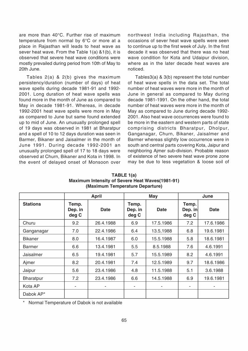
65

are more than 40°C. Further rise of maximumtemperature from normal by 6°C or more at aplace in Rajasthan will leads to heat wave assever heat wave. From the Table 1(a) &1(b), it isobserved that severe heat wave conditions weremostly prevailed during period from 10th of May to20th June.

Tables 2(a) & 2(b) gives the maximumpersistency/duration (number of days) of heatwave spells during decade 1981-91 and 1992-2001. Long duration of heat wave spells wasfound more in the month of June as compared toMay in decade 1981-91. Whereas, in decade1992-2001 heat wave spells were more in Mayas compared to June but same found extendedup to mid of June. An unusually prolonged spellof 19 days was observed in 1981 at Bharatpurand a spell of 10 to 12 days duration was seen inBarmer, Bikaner and Jaisalmer in the month ofJune 1991. During decade 1992-2001 anunusually prolonged spell of 17 to 18 days wereobserved at Churn, Bikaner and Kota in 1998. Inthe event of delayed onset of Monsoon over

northwest India including Rajasthan, theoccasions of sever heat wave spells were seento continue up to the first week of July. In the firstdecade it was observed that there was no heatwave condition for Kota and Udaipur division,where as in the later decade heat waves arenoticed.

Tables3(a) & 3(b) represent the total numberof heat wave spells in the data set. The totalnumber of heat waves were more in the month ofJune in general as compared to May duringdecade 1981-1991. On the other hand, the totalnumber of heat waves were more in the month ofMay as compared to June during decade 1992-2001. Also heat wave occurrences were found tobe more in the eastern and western parts of statecomprising distr icts Bharatpur, Dholpur,Ganganagar, Churn, Bikaner, Jaisalmer andBarmer whereas slightly low occurrence were insouth and central parts covering Kota, Jaipur andneighboring Ajmer sub-division. Probable reasonof existence of two severe heat wave prone zonemay be due to less vegetation & loose soil of

TABLE 1(a)Maximum Intensity of Severe Heat Waves(1981-91)

(Maximum Temperature Departure)

April May June

Stations Temp. Temp. Temp.Dep. in Date Dep. in Date Dep. in Datedeg C deg C deg C

Churu 9.2 26.4.1988 6.9 17.5.1986 7.2 17.6.1986

Ganganagar 7.0 22.4.1986 6.4 13.5,1988 6.8 19.6.1981

Bikaner 8.0 16.4.1987 6.0 15.5.1988 5.8 18.6.1981

Barmer 6.6 13.4.1981 5.5 8.5.1988 7.6 4.6.1991

Jaisalmer 6.5 19.4.1981 5.7 15.5.1989 8.2 4.6.1991

Ajmer 8.2 20.4.1981 7.4 12.5.1989 9.7 18.6.1986

Jaipur 5.6 23.4.1986 4.8 11.5.1988 5.1 3.6.1988

Bharatpur 7.2 23.4.1986 6.6 14.5.1988 6.9 19.6.1981

Kota AP - - - - - -

Dabok AP*

* Normal Temperature of Dabok is not available

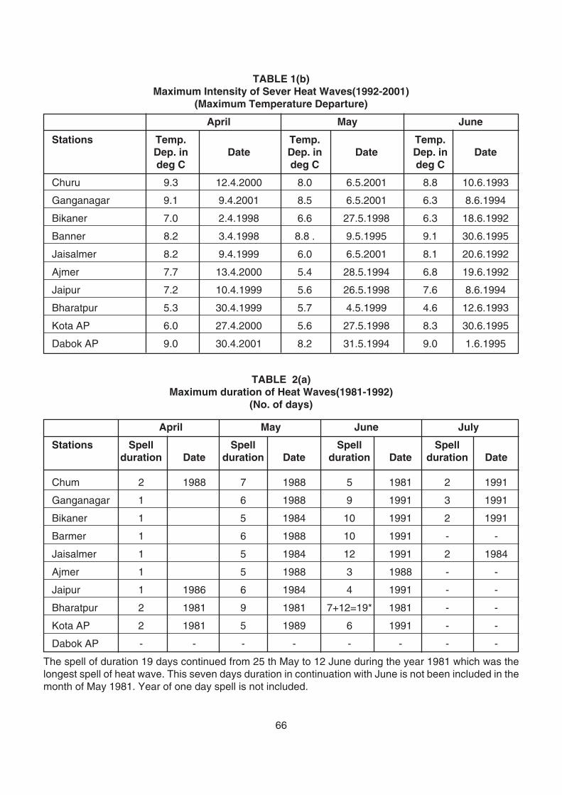
66

TABLE 1(b)Maximum Intensity of Sever Heat Waves(1992-2001)

(Maximum Temperature Departure)

April May June

Stations Temp. Temp. Temp.Dep. in Date Dep. in Date Dep. in Datedeg C deg C deg C

Churu 9.3 12.4.2000 8.0 6.5.2001 8.8 10.6.1993

Ganganagar 9.1 9.4.2001 8.5 6.5.2001 6.3 8.6.1994

Bikaner 7.0 2.4.1998 6.6 27.5.1998 6.3 18.6.1992

Banner 8.2 3.4.1998 8.8 . 9.5.1995 9.1 30.6.1995

Jaisalmer 8.2 9.4.1999 6.0 6.5.2001 8.1 20.6.1992

Ajmer 7.7 13.4.2000 5.4 28.5.1994 6.8 19.6.1992

Jaipur 7.2 10.4.1999 5.6 26.5.1998 7.6 8.6.1994

Bharatpur 5.3 30.4.1999 5.7 4.5.1999 4.6 12.6.1993

Kota AP 6.0 27.4.2000 5.6 27.5.1998 8.3 30.6.1995

Dabok AP 9.0 30.4.2001 8.2 31.5.1994 9.0 1.6.1995

TABLE 2(a)Maximum duration of Heat Waves(1981-1992)

(No. of days)

April May June July

Stations Spell Spell Spell Spellduration Date duration Date duration Date duration Date

Chum 2 1988 7 1988 5 1981 2 1991

Ganganagar 1 6 1988 9 1991 3 1991

Bikaner 1 5 1984 10 1991 2 1991

Barmer 1 6 1988 10 1991 - -

Jaisalmer 1 5 1984 12 1991 2 1984

Ajmer 1 5 1988 3 1988 - -

Jaipur 1 1986 6 1984 4 1991 - -

Bharatpur 2 1981 9 1981 7+12=19* 1981 - -

Kota AP 2 1981 5 1989 6 1991 - -

Dabok AP - - - - - - - -

The spell of duration 19 days continued from 25 th May to 12 June during the year 1981 which was thelongest spell of heat wave. This seven days duration in continuation with June is not been included in themonth of May 1981. Year of one day spell is not included.

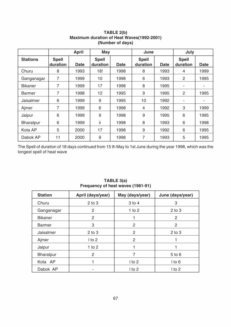
67

TABLE 2(b)Maximum duration of Heat Waves(1992-2001)

(Number of days)

April May June July

Stations Spell Spell Spell Spellduration Date duration Date duration Date duration Date

Churu 8 1993 18! 1998 8 1993 4 1999

Ganganagar 7 1999 10 1998 6 1993 2 1995

Bikaner 7 1999 17 1998 8 1995 - -

Barmer 7 1998 12 1995 9 1995 2 1995

Jaisalmer 6 1999 9 1995 10 1992 - -

Ajmer 7 1999 6 1998 4 1992 3 1999

Jaipur 6 1999 9 1998 9 1995 6 1995

Bharatpur 6 1999 ii 1998 8 1993 6 1998

Kota AP 5 2000 17 1998 9 1992 6 1995

Dabok AP 11 2000 9 1998 7 1993 5 1995

The Spell of duration of 18 days continued from 15 th May to 1st June during the year 1998, which was thelongest spell of heat wave

TABLE 3(a)Frequency of heat waves (1981-91)

Station April (days/year) May (days/year) June (days/year)

Churu 2 to 3 3 to 4 3

Ganganagar 2 1 to 2 2 to 3

Bikaner 2 1 2

Barmer 3 2 2

Jaisalmer 2 to 3 2 2 to 3

Ajmer l to 2 2 1

Jaipur 1 to 2 1 1

Bharatpur 2 7 5 to 6

Kota AP 1 l to 2 l to 6

Dabok AP - l to 2 l to 2

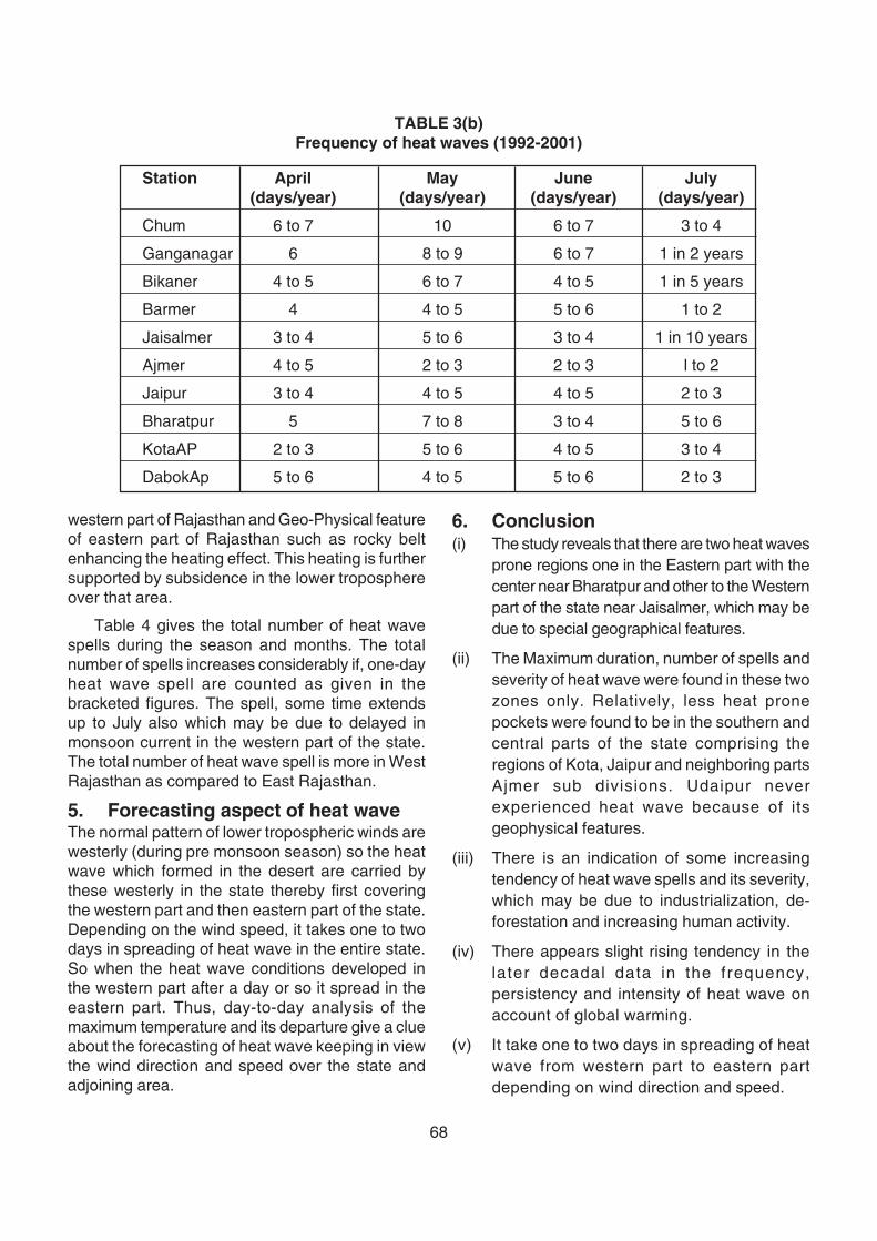
68

TABLE 3(b)Frequency of heat waves (1992-2001)

Station April May June July(days/year) (days/year) (days/year) (days/year)

Chum 6 to 7 10 6 to 7 3 to 4

Ganganagar 6 8 to 9 6 to 7 1 in 2 years

Bikaner 4 to 5 6 to 7 4 to 5 1 in 5 years

Barmer 4 4 to 5 5 to 6 1 to 2

Jaisalmer 3 to 4 5 to 6 3 to 4 1 in 10 years

Ajmer 4 to 5 2 to 3 2 to 3 l to 2

Jaipur 3 to 4 4 to 5 4 to 5 2 to 3

Bharatpur 5 7 to 8 3 to 4 5 to 6

KotaAP 2 to 3 5 to 6 4 to 5 3 to 4

DabokAp 5 to 6 4 to 5 5 to 6 2 to 3

western part of Rajasthan and Geo-Physical featureof eastern part of Rajasthan such as rocky beltenhancing the heating effect. This heating is furthersupported by subsidence in the lower troposphereover that area.

Table 4 gives the total number of heat wavespells during the season and months. The totalnumber of spells increases considerably if, one-dayheat wave spell are counted as given in thebracketed figures. The spell, some time extendsup to July also which may be due to delayed inmonsoon current in the western part of the state.The total number of heat wave spell is more in WestRajasthan as compared to East Rajasthan.

5. Forecasting aspect of heat waveThe normal pattern of lower tropospheric winds arewesterly (during pre monsoon season) so the heatwave which formed in the desert are carried bythese westerly in the state thereby first coveringthe western part and then eastern part of the state.Depending on the wind speed, it takes one to twodays in spreading of heat wave in the entire state.So when the heat wave conditions developed inthe western part after a day or so it spread in theeastern part. Thus, day-to-day analysis of themaximum temperature and its departure give a clueabout the forecasting of heat wave keeping in viewthe wind direction and speed over the state andadjoining area.

6. Conclusion(i) The study reveals that there are two heat waves

prone regions one in the Eastern part with thecenter near Bharatpur and other to the Westernpart of the state near Jaisalmer, which may bedue to special geographical features.

(ii) The Maximum duration, number of spells andseverity of heat wave were found in these twozones only. Relatively, less heat pronepockets were found to be in the southern andcentral parts of the state comprising theregions of Kota, Jaipur and neighboring partsAjmer sub divisions. Udaipur neverexperienced heat wave because of itsgeophysical features.

(iii) There is an indication of some increasingtendency of heat wave spells and its severity,which may be due to industrialization, de-forestation and increasing human activity.

(iv) There appears slight rising tendency in thelater decadal data in the frequency,persistency and intensity of heat wave onaccount of global warming.

(v) It take one to two days in spreading of heatwave from western part to eastern partdepending on wind direction and speed.

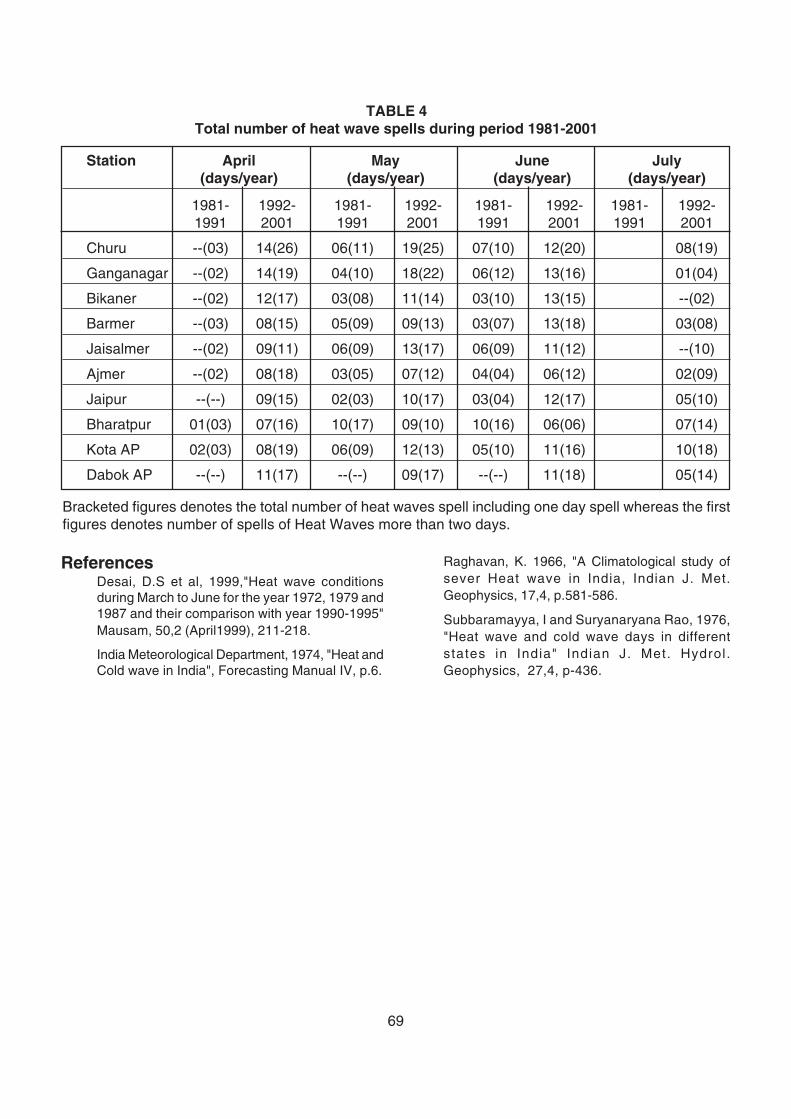
69

TABLE 4Total number of heat wave spells during period 1981-2001

Station April May June July(days/year) (days/year) (days/year) (days/year)

1981- 1992- 1981- 1992- 1981- 1992- 1981- 1992-1991 2001 1991 2001 1991 2001 1991 2001

Churu --(03) 14(26) 06(11) 19(25) 07(10) 12(20) 08(19)

Ganganagar --(02) 14(19) 04(10) 18(22) 06(12) 13(16) 01(04)

Bikaner --(02) 12(17) 03(08) 11(14) 03(10) 13(15) --(02)

Barmer --(03) 08(15) 05(09) 09(13) 03(07) 13(18) 03(08)

Jaisalmer --(02) 09(11) 06(09) 13(17) 06(09) 11(12) --(10)

Ajmer --(02) 08(18) 03(05) 07(12) 04(04) 06(12) 02(09)

Jaipur --(--) 09(15) 02(03) 10(17) 03(04) 12(17) 05(10)

Bharatpur 01(03) 07(16) 10(17) 09(10) 10(16) 06(06) 07(14)

Kota AP 02(03) 08(19) 06(09) 12(13) 05(10) 11(16) 10(18)

Dabok AP --(--) 11(17) --(--) 09(17) --(--) 11(18) 05(14)

Bracketed figures denotes the total number of heat waves spell including one day spell whereas the firstfigures denotes number of spells of Heat Waves more than two days.

ReferencesDesai, D.S et al, 1999,"Heat wave conditionsduring March to June for the year 1972, 1979 and1987 and their comparison with year 1990-1995"Mausam, 50,2 (April1999), 211-218.

India Meteorological Department, 1974, "Heat andCold wave in India", Forecasting Manual IV, p.6.

Raghavan, K. 1966, "A Climatological study ofsever Heat wave in India, Indian J. Met.Geophysics, 17,4, p.581-586.

Subbaramayya, I and Suryanaryana Rao, 1976,"Heat wave and cold wave days in differentstates in India" Indian J. Met. Hydrol.Geophysics, 27,4, p-436.

70

1. IntroductionThe pre-monsoon season (March-May) of India ischaracterised by intense heating of the land due tomaximum insolation and this season is a transitionperiod from winter to summer monsoon circulation.Due to increased heating, low pressure areas startdeveloping over the land in March itself. March 21/22nd is known as the Vernal Equinox when thesun's noon rays are vertical over the equator anddays and nights are equal. The rainfall activity issubdued during the month of March except forsporadic rainfall due to intense convection.Occasionally, during the pre-monsoon season,remnants of typhoons of Pacific Ocean travel acrosssoutheast Asia, enter into the Bay of Bengal aseasterly waves and sometimes trigger the formationof tropical cyclones (Kelkar4, 2007). Intense rainfallactivity associated with thunderstorms isexperienced in peninsular India during the passageof easterly waves.

An unprecedented heavy rainfall since the year1875 in the states of Tamil Nadu(TN), Kerala(KER),Karnataka(KAR) and Andhra Pradesh(AP)occurred during March 2008 and was confined tothe period between 12th and 27th. Two shallowdisturbances, one in the form of large amplitude

easterly waves (13-18 March) moving subsequentlynorthwards and the other as a low pressure area(20-22 March) at sea level in Commorin-Maldivesarea were the causative factors for such an excessrainfall in the four southern states of India. During20-27 March 2008, thundershower activity resultedfrom the high amplitude troughs in easterlies,embedded circulations and low level winddiscontinuities which led to formation of a lowpressure area in Cape-Comorin region off Sri Lanka(Mazumdar et al, 2009). Easterly waves move closeto the Inter-Tropical Convergence Zone (ITCZ) andare associated with considerable convectivecloudiness. With the advance of the summerseason, these easterly waves increase in intensity.The passage of deep easterly waves in theneighbourhood of ITCZ can and does enhance thedifferences in temperature and moisture content ofair masses on the two sides of ITCZ as well as onthe two sides of the deep trough associated withdeep easterly waves (Asnani, 2005). Negativeanomalies of Outgoing Longwave Radiation (OLR)imply increased cloudiness and likelihood ofenhanced precipitation. As the relationship betweenOLR anomaly and precipitation is most reliable intropical regions observed negative OLR anomalies

Modern techniques ofestimation of areal rainfall - Acase study of rainfall insouthern peninsular Indiaduring March 2008

B. Amudha, R. Asokan andK.V. Balasubramanian

Regional Meteorological Centre,India Meteorological Department,

Chennai 600 006email:amudha2308@gmail.com

ABSTRACT

An unprecedented all time record rainfall since the year 1875 in the states of Tamil Nadu, Kerala and Karnatakaoccurred during March 2008. Rainfall obtained from modern observational systems like Automatic WeatherStations (AWS), estimates of Integrated Precipitable Water Vapour (IPWV) through ground-based GPS systemsand upper air RS-RW ascents are indicators of the rainfall events. TRMM satellite-derived estimates andDoppler radar-derived precipitation accumulation in the 100 km range are modern tools for understanding thespatial and areal rainfall variabilities. After validating with observatory rainfall, AWS recorded rainfall of 20stations has been used as the yardstick to evaluate the rainfall estimates from other techniques. It is observedthat TRMM estimates of rainfall cannot exactly match the actual rainfall recorded at surface level by AWSand observatory. TRMM estimates are either overestimated or underestimated and vary with the location /altitude of the place. TRMM rainfall estimate is available only at 0.25 × 0.25 degrees resolution which isapproximately equal to an areal distance of around 25 km and hence errors are unavoidable in point-rainfallestimates. Effectiveness and utility of such data for operational use has been discussed.

Key words: Automatic Weather Stations, TRMM, IPWV, GPS, Doppler Weather Radar, Easterly waves

71

exceeding 20 W/m2 (CDBI, 2008) over peninsularIndia are indicators of the convective activity andsubsequent rainfall which occurred during March2008.

Tamil Nadu received a record rainfall of 176 mmduring March 2008 against the normal value of 19mm which is 806% above normal and if both thesubdivisions of TN and Puducherry are consideredas a whole the rainfall was 802% above normal.The monthly total rainfall for AP during March 2008was the second highest since 1875, the first onebeing in 1944. The area weighted average rainfallfor the southern peninsula was 915% of its LongPeriod Average value. Anomalous southwesterliesfrom the Arabian Sea and northeasterlies from thenorth Pacific Ocean converged over the southIndian Ocean during this period. These circulationfeatures might have contributed to widespreadconvective activity over south peninsula (CDBI,2008). Rainfall recorded by conventionalobservatories of the southern peninsula duringMarch 2008 and the associated synoptic featuresare reported and documented (Daily WeatherReports, 2008) by IMD for March 2008 and hencethey have not been included within the scope ofthis paper.

The objective of the present study is toemphasise the effectiveness and reliability ofutilising modern observing techniques in estimationof the areal rainfall. Modern techniques, no doubtenhance the ability of the weather forecaster anddependability is proven when adequate measuresare taken for maintenance and periodic calibrationof sensors. Awareness of the inherent limitationsand errors likely to occur in any state-of-artelectronic systems and efforts to minimise them willgo a long way in ensuring better forecasting ofsevere weather phenomena.

IMD had commissioned a dense surfaceobservational network network of 125 state-of-artsatellite-based Automatic Weather Stations (AWS)during the year 2007 (Ranalkar et al, 2008). As on31 July 2012, 550 more AWS have been installedand are operational. Many more are in the anvil toensure reliable and accurate data from remotespatially unrepresented data sparse locations. Inaddition to other meteorological parameters, AWSprovides crucial information about the rainfallrealised in hitherto meteorologically unrepresented

areas. Rainfall measured by the sensor in AWS hasbeen validated with the co-located observatory raingauge data wherever possible. AWS data is usedin this study as a yardstick to evaluate the rainfallestimates obtained from the Tropical RainfallMeasuring Mission(TRMM) satellites. The validationof AWS data yields promising results for its utility inmonitoring and nowcasting of severe weatherevents (Tyagi et al, 2010). Considering the vastspatial density of a network of AWS and ARGs,proving the dependability and worthiness of AWSin utilisation of the data during occurrences of suchextreme weather events like that of the current studypaves the way towards gradual switch-over to latesttechnology. Accurate rainfall data from AWS isobtained when periodic cleaning of the rain gaugeis done as part of preventive maintenanceschedules. Estimates of Integrated PrecipitableWater Vapour (IPWV) from ground-based GlobalPositioning System (GPS) equipments coupled withIPWV content of the upper atmosphere obtainedfrom the network of radiosonde-radiowind(RS-RW)stations provide valuable inputs on the possibleoccurrences of severe weather phenomena. Eachtechnology has its own advantages and limitationsbut overall, one complements the other inenhancing forecasting capabilities.

2. Data and methodologyi) The weekly rainfall normals for TN, for the

month of March for the period 1941-90calculated from the area weighted normalrainfall of 30 districts (Weekly WeatherReports, 2008).

ii) Cumulative rainfall data from 20 AWS (TN -8, AP - 10 and KAR - 2) in the southernpeninsular India installed during year 2007 forwhich uninterrupted data was available. TheAWS are Thiruchendur(TCD), Vedasandur(VDS), Karaikal(KKL), Chidambaram(CDM),Puducherry(PDY), Mailam(MLM), Kalavai(KLV), Chennai-Nungambakkam(NBK),Tirumala(TRM), Sriharikota(SHR), Nellore(NLR), Kavali(KVL), Bapatla(BPT), Darsi(DRS), Narsapur(NRP), Yellamanchilli(YMC),Bhimunipattinam(BHM), Vizianagaram(VZN),Bengaluru (BNG) and Bidar(BDR).

iii) Rainfall data of conventional surfaceobservatories which are co-located with AWS.Out of the 20 AWS, 9 (VDS, KKL, CDM, PDY,

72

NBK, KVL, BPT, NRP, BNG) have co-locatedobservatories and the rainfall recorded byAWS and conventional rain gauge in theobservatory(OBSY) has been compared andvalidated.

iv) Values of the hourly GPS-IPWV ( in mm) overNBK for March 2008 from IMD website (http://www.imd.gov.in).

v) IPWV (in mm) obtained from the RS-RW data(0000 and 1200 UTCs) of observatory atChennai Airport in Meenambakkam (MBK,12°59'N/80°10'E) for March 2008 has beentaken from the website of University of Wyoming(http://weather.uwyo.edu/ upperair/sounding.html). It has been compared with the GPS-derived IPWV of NBK which is located at adistance of 15 km from MBK to analyse thevariability in the moisture content over Chennaiand the corresponding impact on the actualrainfall realised over Chennai. RS-RW data hasbeen utilised to understand the upper airvariations in relative humidity and dew pointtemperature at freezing level during the unusualrainfall activity.

vi) TRMM satellite-derived precipitationestimates from the 3B42-V7 product yield thebest precipitation accumulation (mm) for threehourly periods. The gridded estimates havea 0.25° x 0.25° spatial resolution (http://www.trmm.gsfc.nasa.gov/. The daily rainfall datafor March 2008 for each of the 20 AWS attheir nearest Lat/Long positions has beenobtained from the site www.gdata1.sci.gsfc.

nasa.gov/daac-bin/G3 which is a Giovannionline user-friendly visualisation applicationfor analysis of Level-3 gridded TRMM data.The daily rainfall values have beendownloaded and cumulated to obtain themonthly total for March 2008 for each stationand compared with AWS rainfall data.

vii) Precipitation Accumulation (PAC) product fromthe Doppler Weather Radar (DWR) located atChennai at a distance of 5 km from NBK hasbeen used to understand the spatial rainfalldistribution in the 100 km range of the radar.

3. Results and discussionsThe excess rainfall of March 2008 was abnormal andis evident from the percentage departures(PD) ofrainfall from weekly normals for TN provided in Table1. The PD of 1525 during 13 to 19th and a PD of2329 during 20 to 26th quantify the rainfall activity ofTN. The isohyets analysis of the monthly rainfallnormals for March based on rainfall recorded duringthe period 1941-90 by 113 stations of IMD and thoseunder the Districtwise Rainfall MeasuringScheme(DRMS) in the area bounded by 6°N and22°N/70°E and 95°E revealed that the normal rainfallin the area ranged only from 0 to 70 mm and hencethe rainfall activity of March 2008 is unusual.

3.1 Spatial variability of rainfall through AWSand TRMM data

The characteristic spatial features of rainfall underthe influence of easterly waves are distinctlycaptured by the intercomparison of rainfall datarecorded by AWS, co-located surface observatoriesand TRMM estimates. Satellite-derived rainfall is

TABLE 1

Percentage departures from weekly normals forTamil Nadu (30 districts) for March 2008

Week Period Actual Weekly Percentage Departurerainfall (mm) Normal (mm) from weekly normal

1 26 Feb - 5th Mar 5.4 4.0 35

2 6 - 12 Mar 11.2 4.8 133

3 13 - 19 Mar 58.5 3.6 1525

4 20 -26 Mar 89.9 3.7 2329

5 27 Mar - 2 Apr 23.2 6.6 251

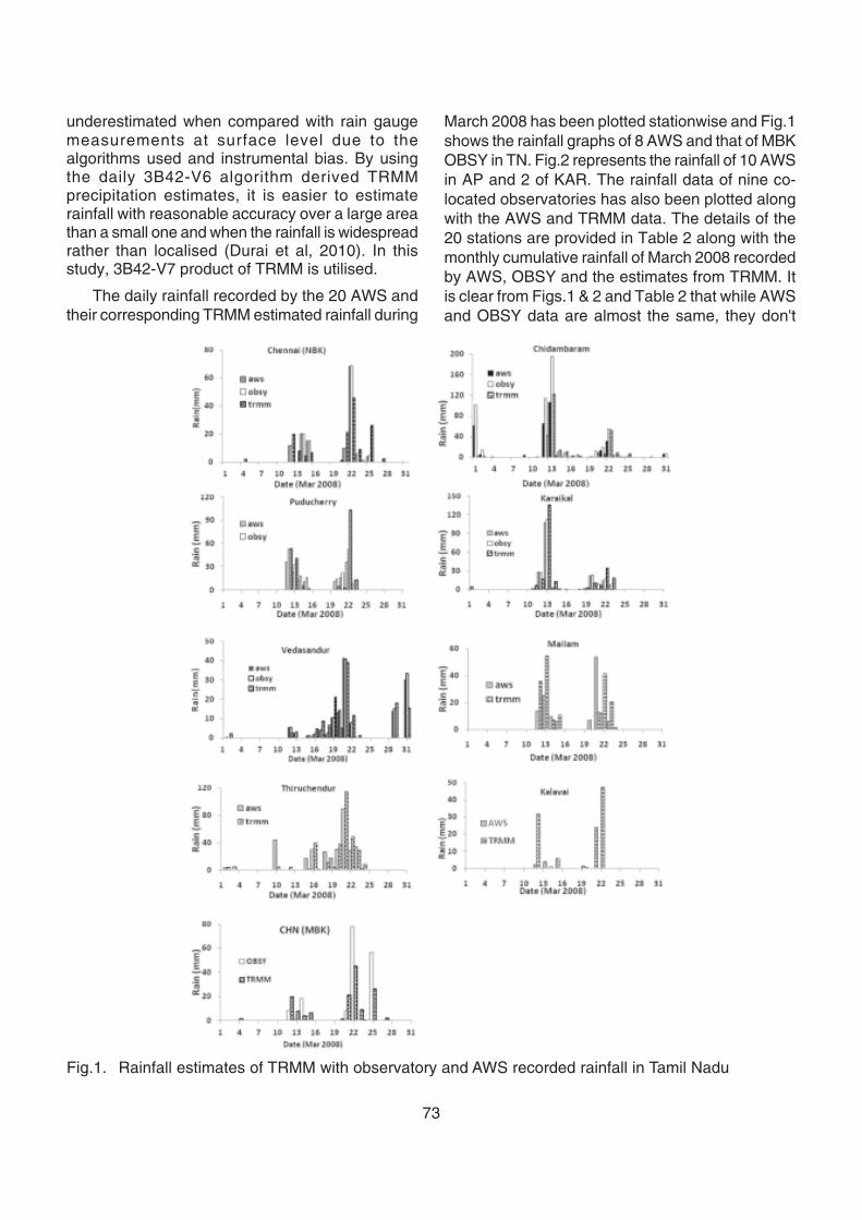
73

underestimated when compared with rain gaugemeasurements at surface level due to thealgorithms used and instrumental bias. By usingthe daily 3B42-V6 algorithm derived TRMMprecipitation estimates, it is easier to estimaterainfall with reasonable accuracy over a large areathan a small one and when the rainfall is widespreadrather than localised (Durai et al, 2010). In thisstudy, 3B42-V7 product of TRMM is utilised.

The daily rainfall recorded by the 20 AWS andtheir corresponding TRMM estimated rainfall during

March 2008 has been plotted stationwise and Fig.1shows the rainfall graphs of 8 AWS and that of MBKOBSY in TN. Fig.2 represents the rainfall of 10 AWSin AP and 2 of KAR. The rainfall data of nine co-located observatories has also been plotted alongwith the AWS and TRMM data. The details of the20 stations are provided in Table 2 along with themonthly cumulative rainfall of March 2008 recordedby AWS, OBSY and the estimates from TRMM. Itis clear from Figs.1 & 2 and Table 2 that while AWSand OBSY data are almost the same, they don't

Fig.1. Rainfall estimates of TRMM with observatory and AWS recorded rainfall in Tamil Nadu

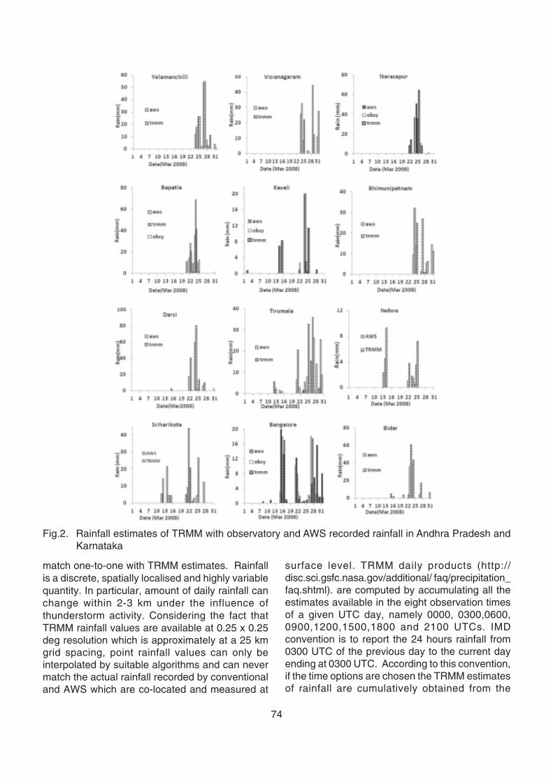
74

match one-to-one with TRMM estimates. Rainfallis a discrete, spatially localised and highly variablequantity. In particular, amount of daily rainfall canchange within 2-3 km under the influence ofthunderstorm activity. Considering the fact thatTRMM rainfall values are available at 0.25 x 0.25deg resolution which is approximately at a 25 kmgrid spacing, point rainfall values can only beinterpolated by suitable algorithms and can nevermatch the actual rainfall recorded by conventionaland AWS which are co-located and measured at

surface level. TRMM daily products (http://disc.sci.gsfc.nasa.gov/additional/ faq/precipitation_faq.shtml). are computed by accumulating all theestimates available in the eight observation timesof a given UTC day, namely 0000, 0300,0600,0900,1200,1500,1800 and 2100 UTCs. IMDconvention is to report the 24 hours rainfall from0300 UTC of the previous day to the current dayending at 0300 UTC. According to this convention,if the time options are chosen the TRMM estimatesof rainfall are cumulatively obtained from the

Fig.2. Rainfall estimates of TRMM with observatory and AWS recorded rainfall in Andhra Pradesh andKarnataka

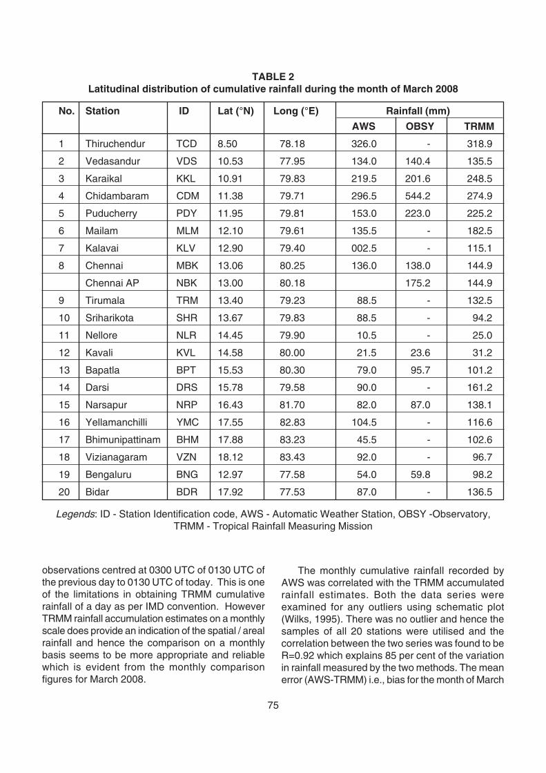
75

observations centred at 0300 UTC of 0130 UTC ofthe previous day to 0130 UTC of today. This is oneof the limitations in obtaining TRMM cumulativerainfall of a day as per IMD convention. HoweverTRMM rainfall accumulation estimates on a monthlyscale does provide an indication of the spatial / arealrainfall and hence the comparison on a monthlybasis seems to be more appropriate and reliablewhich is evident from the monthly comparisonfigures for March 2008.

The monthly cumulative rainfall recorded byAWS was correlated with the TRMM accumulatedrainfall estimates. Both the data series wereexamined for any outliers using schematic plot(Wilks, 1995). There was no outlier and hence thesamples of all 20 stations were utilised and thecorrelation between the two series was found to beR=0.92 which explains 85 per cent of the variationin rainfall measured by the two methods. The meanerror (AWS-TRMM) i.e., bias for the month of March

TABLE 2Latitudinal distribution of cumulative rainfall during the month of March 2008

No. Station ID Lat (°N) Long (°E) Rainfall (mm)

AWS OBSY TRMM

1 Thiruchendur TCD 8.50 78.18 326.0 - 318.9

2 Vedasandur VDS 10.53 77.95 134.0 140.4 135.5

3 Karaikal KKL 10.91 79.83 219.5 201.6 248.5

4 Chidambaram CDM 11.38 79.71 296.5 544.2 274.9

5 Puducherry PDY 11.95 79.81 153.0 223.0 225.2

6 Mailam MLM 12.10 79.61 135.5 - 182.5

7 Kalavai KLV 12.90 79.40 002.5 - 115.1

8 Chennai MBK 13.06 80.25 136.0 138.0 144.9

Chennai AP NBK 13.00 80.18 175.2 144.9

9 Tirumala TRM 13.40 79.23 88.5 - 132.5

10 Sriharikota SHR 13.67 79.83 88.5 - 94.2

11 Nellore NLR 14.45 79.90 10.5 - 25.0

12 Kavali KVL 14.58 80.00 21.5 23.6 31.2

13 Bapatla BPT 15.53 80.30 79.0 95.7 101.2

14 Darsi DRS 15.78 79.58 90.0 - 161.2

15 Narsapur NRP 16.43 81.70 82.0 87.0 138.1

16 Yellamanchilli YMC 17.55 82.83 104.5 - 116.6

17 Bhimunipattinam BHM 17.88 83.23 45.5 - 102.6

18 Vizianagaram VZN 18.12 83.43 92.0 - 96.7

19 Bengaluru BNG 12.97 77.58 54.0 59.8 98.2

20 Bidar BDR 17.92 77.53 87.0 - 136.5

Legends: ID - Station Identification code, AWS - Automatic Weather Station, OBSY -Observatory,TRMM - Tropical Rainfall Measuring Mission

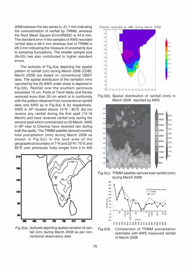
76

2008 between the two series is -31.7 mm indicatingthe overestimation of rainfall by TRMM, whereasthe Root Mean Square Error(RMSE) is 44.9 mm.The standard error in the samples of AWS recordedrainfall data is 66.4 mm whereas that of TRMM is28.5 mm indicating the measure of uncertainty dueto sampling fluctuations. The smaller sample size(N=20) has also contributed to higher standarderrors.

The isohyets of Fig.3(a) depicting the spatialpattern of rainfall (cm) during March 2008 (CDBI,March 2008) are based on conventional OBSYdata. The spatial distribution of the rainfall(in mm)reported by the 20 AWS under study is depicted inFig.3(b). Rainfall over the southern peninsulaexceeded 10 cm. Parts of Tamil Nadu and Keralareceived more than 20 cm which is in conformitywith the pattern obtained from conventional rainfalldata and AWS as in Fig.3(a) & (b) respectively.AWS in AP located above 15°N / 80°E did notreceive any rainfall during the first spell (13-18March) and have received rainfall only during thesecond spell which commenced on 20 March. AWSin AP near to Chennai have received rain duringboth the spells. The TRMM satellite-derived monthlytotal precipitation (mm) during March 2008 asshown in Fig.3(c) in the land area of thegeographical boundary of 7°N and 20°N / 75°E and85°E over peninsular India ranges from 0 to 400

Fig.3(a). Isohyets depicting spatial variation of rain-fall (cm) during March 2008 as per con-ventional observatory data

Fig.3(b). Spatial distribution of rainfall (mm) inMarch 2008 reported by AWS

Fig.3(c). TRMM satellite-derived total rainfall (mm)during March 2008

Fig.3(d). Comparison of TRMM precipitationestimates with AWS measured rainfallof March 2008

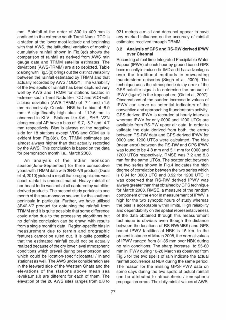
77

mm. Rainfall of the order of 300 to 400 mm isconfined to the extreme south Tamil Nadu. TCD isa station at the lower most latitude and beginningwith that AWS, the latitudinal variation of monthlycumulative rainfall shown in Fig.3(d) shows thecomparison of rainfall as derived from AWS raingauge data and TRMM satellite estimates. Thedeviations (AWS-TRMM) are also depicted. Table2 along with Fig.3(d) brings out the distinct variabilitybetween the rainfall estimated by TRMM and thatactually recorded by AWS / OBSY. The variabilityof the two spells of rainfall has been captured verywell by AWS and TRMM for stations located inextreme south Tamil Nadu like TCD and VDS witha bias/ deviation (AWS-TRMM) of -7.1 and +1.5mm respectively. Coastal NBK had a bias of -8.9mm. A significantly high bias of -112.6 mm isobserved in KLV. Stations like KVL, SHR, VZNalong coastal AP have a bias of -9.7, -5.7 and -4.7mm respectively. Bias is always on the negativeside for 18 stations except VDS and CDM as isevident from Fig.3(d). So, TRMM estimates arealmost always higher than that actually recordedby the AWS. This conclusion is based on the datafor premonsoon month i.e., March 2008.

An analysis of the Indian monsoonseason(June-September) for three consecutiveyears with TRMM data with 3B42-V6 product (Duraiet al, 2010) yielded a result that orographic and westcoast rainfall is underestimated. Heavy rainfall ofnortheast India was not at all captured by satellite-derived products. The present study pertains to onemonth of the pre-monsoon season, for the southernpeninsula in particular. Further, we have utilised3B42-V7 product for obtaining the rainfall fromTRMM and it is quite possible that some differencecould arise due to the processing algorithms butno definite conclusion can be drawn with resultsfrom a single month's data. Region-specific bias inmeasurement due to terrain and orographicfeatures cannot be ruled out. It is quite possiblethat the estimated rainfall could not be actuallyrealized because of the dry lower level atmosphericconditions which prevail during pre-monsoon andwhich could be location-specific(coastal / inlandstations) as well. The AWS under consideration arein the leeward side of the Western Ghats and theelevations of the stations above mean sealevel(a.m.s.l) are different for each of them. Theelevation of the 20 AWS sites ranges from 0.8 to

921 metres a.m.s.l and does not appear to haveany marked influence on the accuracy of rainfallestimates received through TRMM.

3.2 Analysis of GPS and RS-RW derived IPWVover Chennai

Recording of real time Integrated Precipitable WaterVapour (IPWV) at each hour by ground based GPSbeen recently introduced in IMD and it has advantagesover the traditional methods in nowcastingthunderstorm episodes (Singh et al, 2009). Thetechnique uses the atmospheric delay error of theGPS satellite signals to determine the amount ofIPWV (kg/m2) in the troposphere (Giri et al, 2007).Observations of the sudden increase in values ofIPWV can serve as potential indicators of theconvective and approaching thunderstorm activity.GPS-derived IPWV is recorded at hourly intervalswhereas IPWV for only 0000 and 1200 UTCs areavailable from RS-RW upper air data. In order tovalidate the data derived from both, the errorsbetween RS-RW data and GPS-derived IPWV for0000 and 1200 UTCs were calculated. The bias(mean error) between the RS-RW and GPS IPWVwas found to be 4.8 mm and 5.1 mm for 0000 and1200 UTCs respectively. RMSE was 7.2 and 8.3mm for the same UTCs. The scatter plot betweenthe two series shown in Fig.4 indicates the highdegree of correlation between the two series whichis 0.94 for 0000 UTC and 0.92 for 1200 UTC. Itwas observed that RS-RW derived IPWV wasalways greater than that obtained by GPS techniquefor March 2008. RMSE, a measure of the randomcomponent of the error in measurement of IPWV ishigh for the two synoptic hours of study whereasthe bias is acceptable within limits. High reliabilityand dependability on the spatial representativenessof the data obtained through this measurementtechnique is obvious even though the distancebetween the locations of RS-RW(MBK) and GPSbased IPWV facilities at NBK is 15 km. In thepresent instance of March 2008, the normal valuesof IPWV ranged from 31-35 mm over NBK duringno rain conditions. The sharp increase to 55-60mm in IPWV during 10-26 March as observed fromFig.5 for the two spells of rain indicate the actualrainfall occurrence at NBK during the same period.The reason for the missing GPS-IPWV data onsome days during the two spells of actual rainfallcan be attributed to atmospheric / ionosphericpropagation errors. The daily rainfall values of AWS,

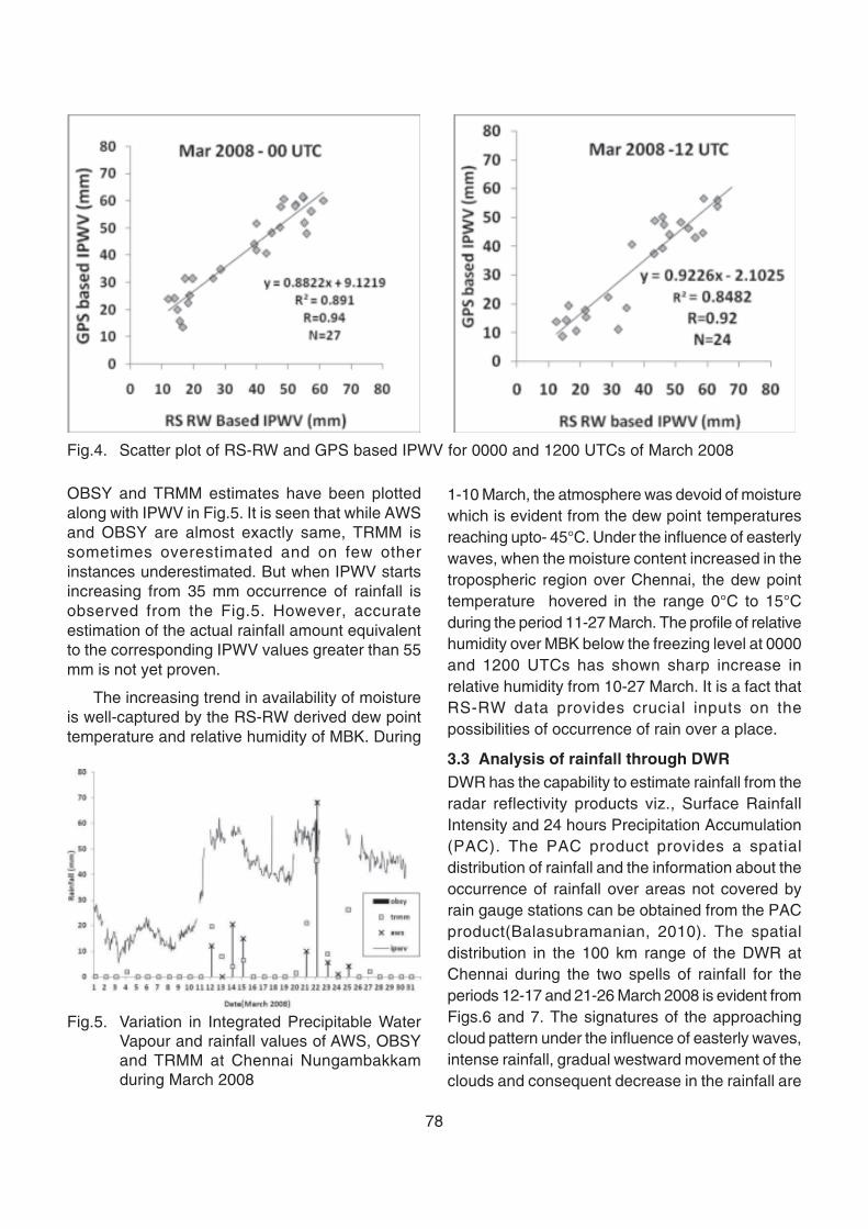
78

Fig.4. Scatter plot of RS-RW and GPS based IPWV for 0000 and 1200 UTCs of March 2008

OBSY and TRMM estimates have been plottedalong with IPWV in Fig.5. It is seen that while AWSand OBSY are almost exactly same, TRMM issometimes overestimated and on few otherinstances underestimated. But when IPWV startsincreasing from 35 mm occurrence of rainfall isobserved from the Fig.5. However, accurateestimation of the actual rainfall amount equivalentto the corresponding IPWV values greater than 55mm is not yet proven.

The increasing trend in availability of moistureis well-captured by the RS-RW derived dew pointtemperature and relative humidity of MBK. During

1-10 March, the atmosphere was devoid of moisturewhich is evident from the dew point temperaturesreaching upto- 45°C. Under the influence of easterlywaves, when the moisture content increased in thetropospheric region over Chennai, the dew pointtemperature hovered in the range 0°C to 15°Cduring the period 11-27 March. The profile of relativehumidity over MBK below the freezing level at 0000and 1200 UTCs has shown sharp increase inrelative humidity from 10-27 March. It is a fact thatRS-RW data provides crucial inputs on thepossibilities of occurrence of rain over a place.

3.3 Analysis of rainfall through DWRDWR has the capability to estimate rainfall from theradar reflectivity products viz., Surface RainfallIntensity and 24 hours Precipitation Accumulation(PAC). The PAC product provides a spatialdistribution of rainfall and the information about theoccurrence of rainfall over areas not covered byrain gauge stations can be obtained from the PACproduct(Balasubramanian, 2010). The spatialdistribution in the 100 km range of the DWR atChennai during the two spells of rainfall for theperiods 12-17 and 21-26 March 2008 is evident fromFigs.6 and 7. The signatures of the approachingcloud pattern under the influence of easterly waves,intense rainfall, gradual westward movement of theclouds and consequent decrease in the rainfall are

Fig.5. Variation in Integrated Precipitable WaterVapour and rainfall values of AWS, OBSYand TRMM at Chennai Nungambakkamduring March 2008

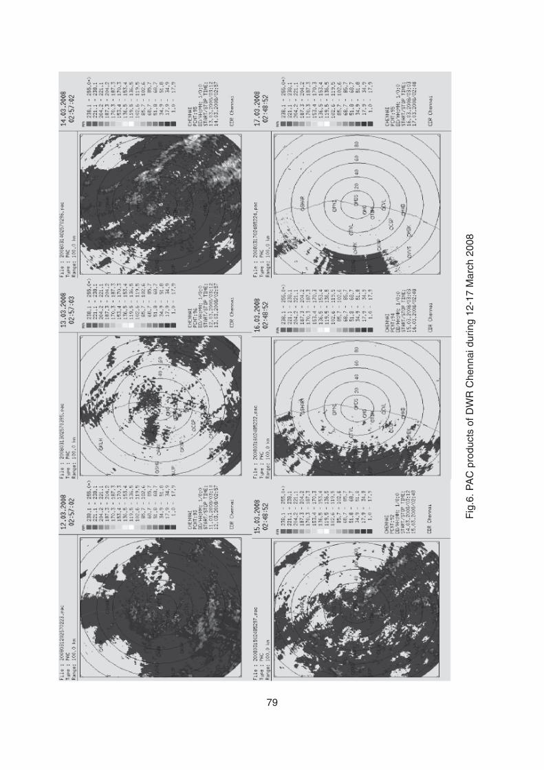
79

Fig

.6. P

AC

pro

duct

s of

DW

R C

henn

ai d

urin

g 12

-17

Mar

ch 2

008

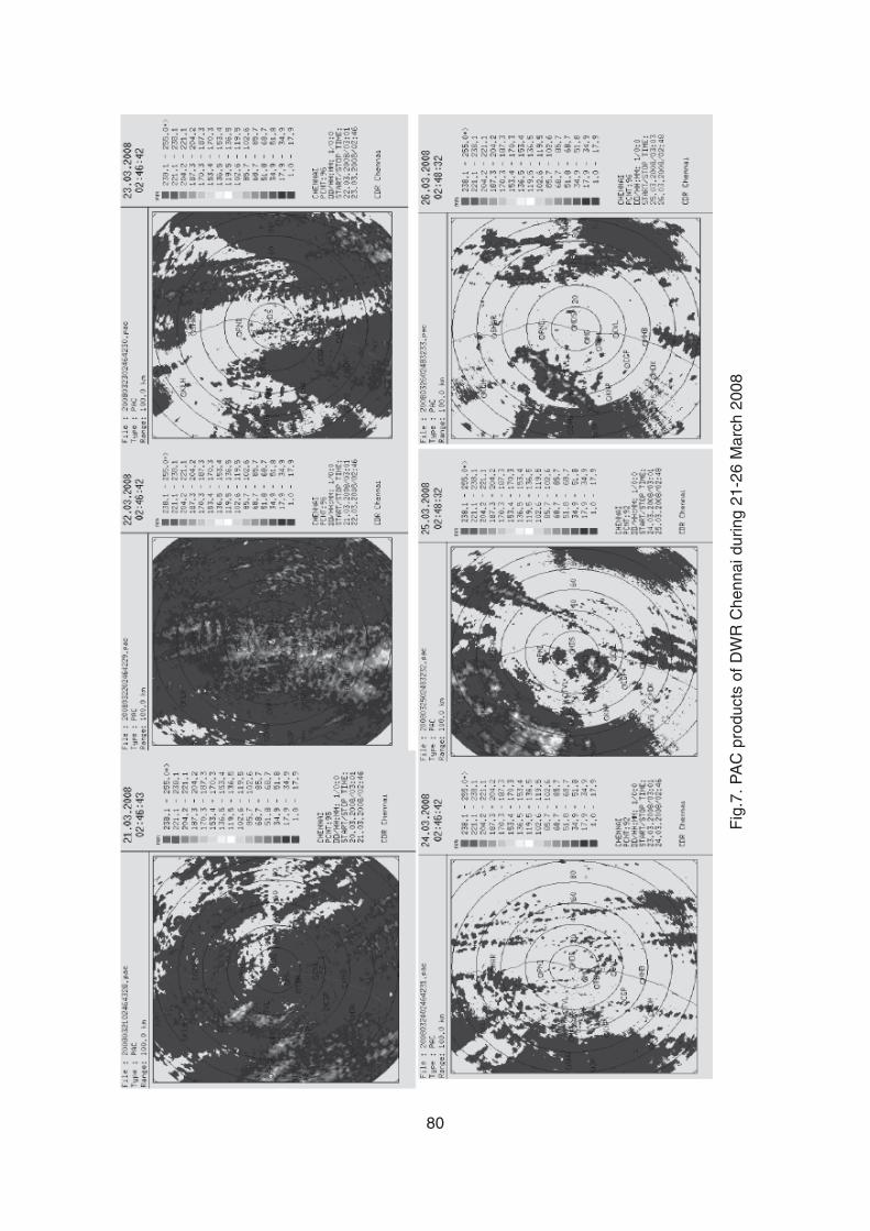
80

Fig

.7. P

AC

pro

duct

s of

DW

R C

henn

ai d

urin

g 21

-26

Mar

ch 2

008

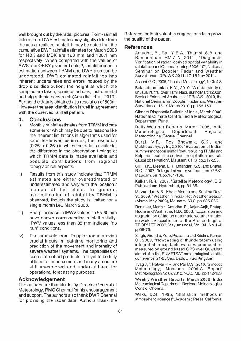
81

well brought out by the radar pictures. Point- rainfallvalues from DWR estimates may slightly differ fromthe actual realised rainfall. It may be noted that thecumulative DWR rainfall estimates for March 2008for NBK and MBK are 128 mm and 136.1 mmrespectively. When compared with the values ofAWS and OBSY given in Table 2, the difference inestimation between TRMM and DWR also can beunderstood. DWR estimated rainfall too hasinherent uncertainties and errors induced by thedrop size distribution, the height at which thesamples are taken, spurious echoes, instrumentaland algorithmic constraints(Amudha et al, 2010).Further the data is obtained at a resolution of 500m.However the areal distribution is well in agreementwith the observed rainfall pattern.

4. Conclusionsi) Monthly rainfall estimates from TRMM indicate

some error which may be due to reasons likethe inherent limitations in algorithms used forsatellite-derived estimates, the resolution(0.25° x 0.25°) in which the data is available,the difference in the observation timings atwhich TRMM data is made available andpossible contributions from regionaltopographical aspects.

ii) Results from this study indicate that TRMMestimates are either overestimated orunderestimated and vary with the location /altitude of the place. In general,overestimation of rainfall by TRMM isobserved, though the study is limited for asingle month i.e., March 2008.

iii) Sharp increase in IPWV values to 55-60 mmhave shown corresponding rainfall activity.IPWV values less than 35 mm indicate "norain" conditions.

iv) The products from Doppler radar providecrucial inputs in real-time monitoring andprediction of the movement and intensity ofsevere weather systems. The capabilities ofsuch state-of-art products are yet to be fullyutilised to the maximum and many areas arestill unexplored and under-utilised foroperational forecasting purposes.

AcknowledgementThe authors are thankful to Dy.Director General ofMeteorology, RMC Chennai for his encouragementand support. The authors also thank DWR Chennaifor providing the radar data. Authors thank the

Referees for their valuable suggestions to improvethe quality of the paper.

ReferencesAmudha, B., Raj, Y.E.A., Thampi, S.B. andRamanathan, RM.A.N, 2011., "DiagnosticVerification of radar -derived spatial variability inrainfall around Chennai during 2006-10", NationalSeminar on Doppler Radar and WeatherSurveillance, DRaWS-2011, 17-18 Nov 2011.

Asnani, G.C., 2005, "Tropical Meteorology", 1, Ch.4.8.

Balasubramanian, K.V., 2010, "A radar study ofunusual rainfall over Tamil Nadu during March 2008",Book of Extended Abstracts of DRaWS - 2010, theNational Seminar on Doppler Radar and WeatherSurveillance, 18-19 March 2010, pp.156-159.

Climate Diagnostic Bulletin of India, March 2008,National Climate Centre, India MeteorologicalDepartment, Pune.

Daily Weather Reports, March 2008, IndiaMeteorological Department, RegionalMeteorological Centre, Chennai.

Durai, V.R., Roy Bhowmik, S.K., andMukhopadhyay, B., 2010. "Evaluation of Indiansummer monsoon rainfall features using TRMM andKalpana-1 satellite derived precipitation and raingauge observation", Mausam, 61, 3, pp.317-336.

Giri, R.K., Meena, L.R., Bhandari, S.S. and Bhatia,R.C., 2007, "Integrated water vapour from GPS",Mausam, 58, 1,pp.101-106.

Kelkar, R.R., 2007, "Satellite Meteorology", B.S.Publications, Hyderabad, pp.84-85.

Mazumdar, A.B., Khole Medha and Sunitha Devi,S., 2009, "Weather in India - Hot Weather Season(March-May 2008), Mausam, 60,2, pp.235-266.

Ranalkar, Manish, Amudha, B., Anjan Anjit, Pratap,Rudra and Vashistha, R.D., 2008, "Expansion andupgradation of Indian automatic weather stationnetwork ", Special issue of the Proceedings ofTROPMET 2007, Vayumandal, Vol.34, No.1-4,pp69-76.

Singh, Virendra, Kore, Prasanna and Krishna Kumar,G., 2009, "Nowcasting of thunderstorm usingintegrated precipitable water vapour contentmeasured by ground based GPS over Guwahatiairport of India", EUMETSAT meteorological satelliteconference, 21-25 Sep, Bath, United Kingdom.

Tyagi Ajit, Hatwar H.R, and Pai, D.S., 2010, "SynopticMeteorology, Monsoon 2009-A Report"Met.Monograph No.09/2010, NCC, IMD, pp.142-153.

Weekly Weather Reports, March 2008, IndiaMeteorological Department, Regional MeteorologicalCentre, Chennai.

Wilks, D.S., 1995, "Statistical methods inatmospheric sciences", Academic Press, California.

82

1. IntroductionIn past two decades extreme weather events havebecome more severe and their occurrences havealso been experienced more in the world. Observedrecords indicate that the loss in biotic life andeconomy due to occurrence of these events, hasincreased significantly in recent years. Surfacetemperature is one of the most sensitivemeteorological parameters, which is responsible forcatastrophic weather events. Extreme maximumtemperature in summer months (April - June) andextreme minimum temperature in winter months(December - February) at surface level produceadverse effect on human body, plants andproduction of industries. Consequent upon extrememaximum temperature and extreme minimumtemperature are associated with heat wave and coldwave respectively. The maximum temperature isgenerally attained in the afternoon while minimumtemperature is attained in the morning hours of theday. The day's maximum and minimumtemperatures mainly depend upon the incomingshort wave radiation, outgoing long wave radiation,albedo, cloud condition, rainfall and wind condition.

The temperature data have always beenattractive for the study of global warming andclimate change. A long term variation in surface air

temperature has been studied by Hingane et al(1985), Jones et al (1986) and Rupakumar andHingane. (1988). Kothwale (1992) reported that themean annual maximum temperature in India hasincreased by about 0.5°C/100 years during the pastcentury. The trend in climate change over India hasbeen examined by Pramanik and Jagannathan.(1954), Srivastav et al. (1992) and Rao et al. (2005).Recent climatic study shows that average globalair surface temperature has increased by about0.74°C from 1906 to 2005 (Kothawale, 2007). Since1861 observational data indicate that the 1990s wasglobally the warmest decade and 1998 was thewarmest year. During last decades the change intemperature is mainly due to rapid increase inpopulation, industrialization, urbanization anddeforestation in large scale (Guhathakura andSrivastav 2004; IPCC, 2007).

In this present paper anomalies in extrememaximum temperature for summer months (April-June) and extreme minimum temperature for wintermonths (December-February) over Maharashtraduring the period 1981 - 2000 from: i) monthly meanmaximum temperature and monthly mean minimumtemperature and, ii) ever-recorded extrememaximum and minimum temperatures up to 1980,have been discussed. Monthly mean maximum &

ABSTRACT

Extreme weather events like- extreme temperatures, cyclones, severe rainstorms etc. become a cause of tremendoussocio-economic consequences. The extreme maximum temperature in summer months and extreme minimumtemperature in winter months are generally associated with heat wave and cold wave respectively which aremain cause of enormous loss of human life and property. The extreme maximum and minimum temperaturesdata for period 1981-2000 for summer months (April, May, June) and winter months (December, January,February) respectively have been used for study of extreme temperatures.

In the present paper anomalies of extreme maximum and minimum temperatures over Maharashtra during theperiod 1981 - 2000 from: (i) monthly mean maximum temperature and monthly mean minimum temperaturerespectively and, (ii) ever- recorded extreme maximum and minimum temperatures respectively up to 1980 forrespective months have been discussed.

Key words: Mean temperature, Extreme temperature, Ever-recorded extreme temperature, Anomaly.

Extreme temperaturesanomalies over Maharashtra

T. P. Singh, R. R. Shende and S. F. MullaIndia Meteorological Department, Pune

83

minimum temperatures and monthly ever- recordedextreme temperature have also been discussed.

2. Data and AnalysisMonthly record of daily maximum temperature anddaily minimum temperature are considered to decidethe extreme maximum and extreme minimumtemperatures for that month. These two values arethen compared with the earlier record of monthlyhighest and the lowest value of temperatures todecide the ever- recorded extreme maximumtemperature and extreme minimum temperaturerespectively for the month. Monthly extrememaximum temperature for summer months (April-June) and monthly extreme minimum temperaturefor winter months (December- February) data of 16well distributed stations over Maharashtra state forlast two decade (1981- 2000) have been taken. Toobtain ever-recorded temperatures month wise,extreme maximum temperature and extrememinimum temperature data have been scanned fora long period. The ever-recorded highest maximumand lowest minimum temperatures month-wise upto 1980 for these stations have been considered toexamine the anomaly in extreme temperatures inlast two decade. The monthly mean values ofmaximum and minimum temperatures for respectivemonths are also taken to examine the anomaly.Moreover, IDWRs have been scanned to examineweather conditions.

3. Results and discussionsThe maximum temperature of higher order in a yeargenerally occurs in the summer months - April, Mayand June, whereas the minimum temperature oflow order in a year occurs in December, Januaryand February.

From Table 1 during summer monthly meanmaximum temperature is high in May over allstations of Maharashtra state, except KLP, PNE andMWR where it is high in April. Monthly meanmaximum temperature in May is of higher order i.e.41.6° to 42.8° C at PRB, YOT, GND, AKL, NGP,JLG and CPR. In April it is up to 38.1°C at PNE,KLP and MWR. However, it is low i.e. 22.5° to31.0°C at hill station MWR in these months. It ismore or less equal at KLP, PNE and NSK inrespective months. During these months thevariation in the temperature at coastal stations-MUM, RTN and VNG is less about 3.1°C (range:30.2° to 33.3°C).

Ever-recorded extreme maximum temperatureup to 1980 is high in month May over all stationsexcept MUM, VNG, RTN and MWR. In May it isrecorded in higher order i.e. 45.6° to 48.3°C at thesestations- AGD, SLP, PRB, YOT, GND, NGP, AKL,JLG and CPR. It is high at MUM, VNG and MWR inmonth- April and RTN in June. However, it is highat PNE in April and May both months. It is up to42.2° C at coastal stations- MUM, RTN and VNGin months: April-June. It is in the range 39.4° C to43.3° C at NSK, PNE and KLP in these months.

It is seen from Figs.1(a-i) that extreme maximumtemperature anomaly from monthly mean maximumtemperature is high in month June over all stationsexcept MUM where it is high in April. The anomalyis found in higher order of 8° to 11°C at JLG, AKL,NGP, PRB, GND, SLP, YOT, CPR and AGD in June1995. Temperature over these stations attainedextremely high, because of more heatingcontinuous in a long spell as heat wave prevailedover Maharashtra and its neighbourhood regionsfrom 30th May to 7th June 1995. The onset ofsouthwest monsoon was also late by 8-10 days fromnormal date in June 1995. In June the anomaly atcoastal places; VNG, MUM and RTN in year 1991,1995 & 1998 respectively is found maximum inorder of 5.5° to 6.1°C, whereas it is maximum inorder of 9.1° to 10.9°C at PNE & NSK in year 1991and KLP in 1987. The highest anomaly in order of12.3° C is found at MWR in June 1993. In Aprilanomaly at MUM is large as 7.7°C in year 1984.The anomaly is higher over hilly area.

However, the anomaly is found negative at AGD(-0.1), AKL (-0.3), CRP (-0.8), GND (-0.8), YOT(-0.8) and NGP (-1.4) in May 1990. It means thatdaily maximum temperature at these places in May1990 is less than their monthly mean maximumtemperature respectively. In this month the persistentof low pressure, cyclonic storm and advancementof southwest monsoon by 10-15 days early overMaharashtra and its neighbourhood regionsproduced a good amount of rainfall, as synopticfeatures were most favourable for less heatingparticularly over Vidarbha and Marathwada regions.

It is seen from Figs.2(a-i) that extreme maximumtemperature anomaly from ever- recorded extrememaximum temperature up to 1980 is positive in June1995 over PRB (0.3), AKL (0.5), YOT (1.0), GND(1.5), AGD (2.0) and MUM (0.4). In month June

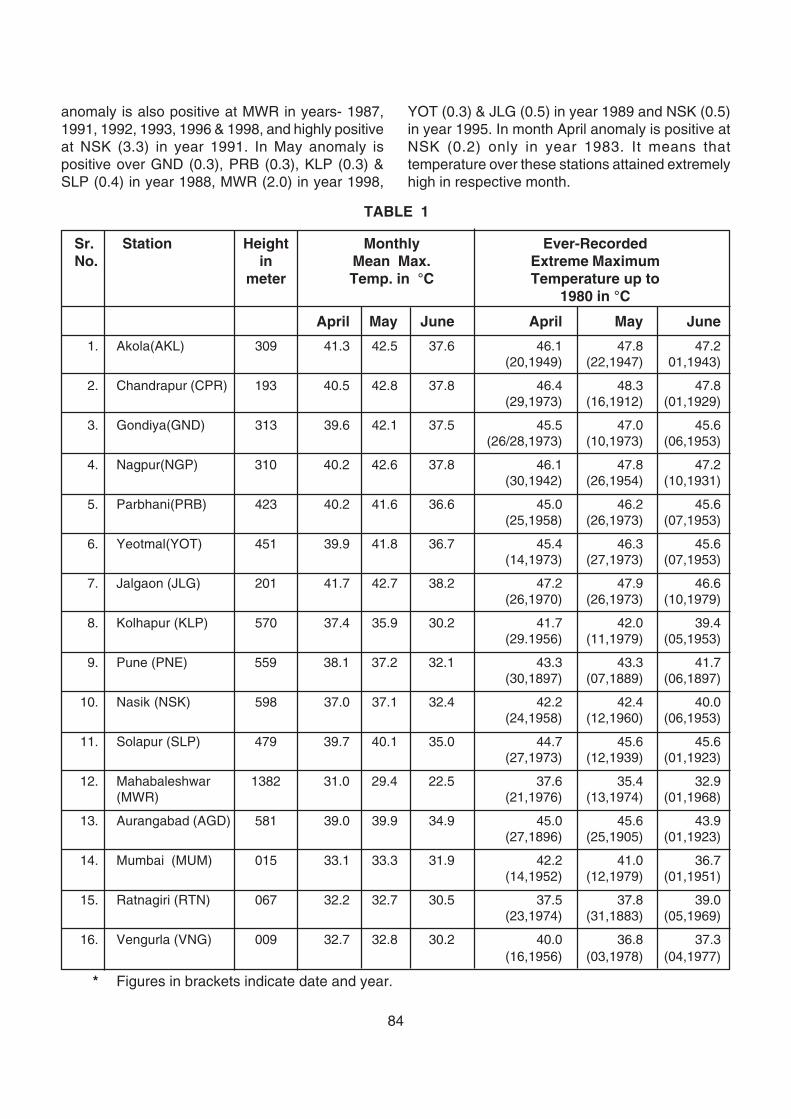
84

anomaly is also positive at MWR in years- 1987,1991, 1992, 1993, 1996 & 1998, and highly positiveat NSK (3.3) in year 1991. In May anomaly ispositive over GND (0.3), PRB (0.3), KLP (0.3) &SLP (0.4) in year 1988, MWR (2.0) in year 1998,

YOT (0.3) & JLG (0.5) in year 1989 and NSK (0.5)in year 1995. In month April anomaly is positive atNSK (0.2) only in year 1983. It means thattemperature over these stations attained extremelyhigh in respective month.

TABLE 1

Sr. Station Height Monthly Ever-RecordedNo. in Mean Max. Extreme Maximum

meter Temp. in °C Temperature up to1980 in °C

April May June April May June

1. Akola(AKL) 309 41.3 42.5 37.6 46.1 47.8 47.2(20,1949) (22,1947) 01,1943)

2. Chandrapur (CPR) 193 40.5 42.8 37.8 46.4 48.3 47.8(29,1973) (16,1912) (01,1929)

3. Gondiya(GND) 313 39.6 42.1 37.5 45.5 47.0 45.6(26/28,1973) (10,1973) (06,1953)

4. Nagpur(NGP) 310 40.2 42.6 37.8 46.1 47.8 47.2(30,1942) (26,1954) (10,1931)

5. Parbhani(PRB) 423 40.2 41.6 36.6 45.0 46.2 45.6(25,1958) (26,1973) (07,1953)

6. Yeotmal(YOT) 451 39.9 41.8 36.7 45.4 46.3 45.6(14,1973) (27,1973) (07,1953)

7. Jalgaon (JLG) 201 41.7 42.7 38.2 47.2 47.9 46.6(26,1970) (26,1973) (10,1979)

8. Kolhapur (KLP) 570 37.4 35.9 30.2 41.7 42.0 39.4(29.1956) (11,1979) (05,1953)

9. Pune (PNE) 559 38.1 37.2 32.1 43.3 43.3 41.7(30,1897) (07,1889) (06,1897)

10. Nasik (NSK) 598 37.0 37.1 32.4 42.2 42.4 40.0(24,1958) (12,1960) (06,1953)

11. Solapur (SLP) 479 39.7 40.1 35.0 44.7 45.6 45.6(27,1973) (12,1939) (01,1923)

12. Mahabaleshwar 1382 31.0 29.4 22.5 37.6 35.4 32.9(MWR) (21,1976) (13,1974) (01,1968)

13. Aurangabad (AGD) 581 39.0 39.9 34.9 45.0 45.6 43.9(27,1896) (25,1905) (01,1923)

14. Mumbai (MUM) 015 33.1 33.3 31.9 42.2 41.0 36.7(14,1952) (12,1979) (01,1951)

15. Ratnagiri (RTN) 067 32.2 32.7 30.5 37.5 37.8 39.0(23,1974) (31,1883) (05,1969)

16. Vengurla (VNG) 009 32.7 32.8 30.2 40.0 36.8 37.3(16,1956) (03,1978) (04,1977)

* Figures in brackets indicate date and year.

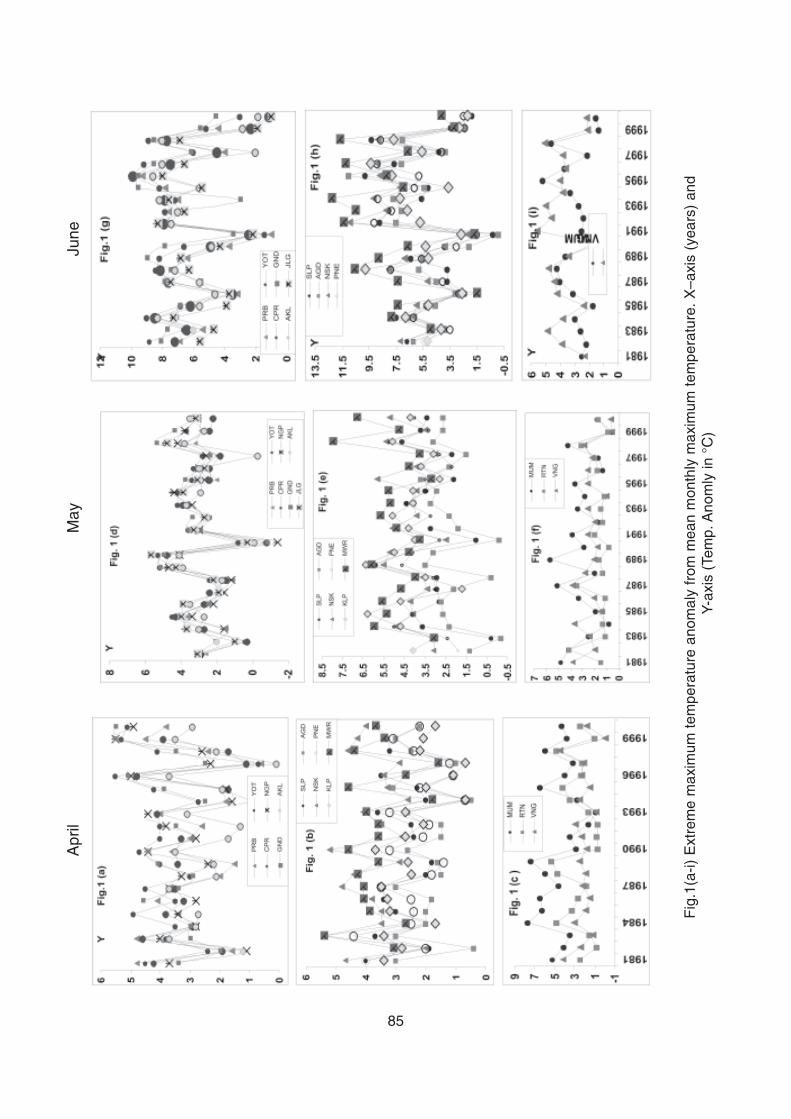
85

Fig

.1(a

-i) E

xtre

me

max

imum

tem

pera

ture

ano

mal

y fr

om m

ean

mon

thly

max

imum

tem

pera

ture

. X–a

xis

(yea

rs)

and

Y-a

xis

(Tem

p. A

nom

ly in

°C

)

Apr

il M

ayJu

ne

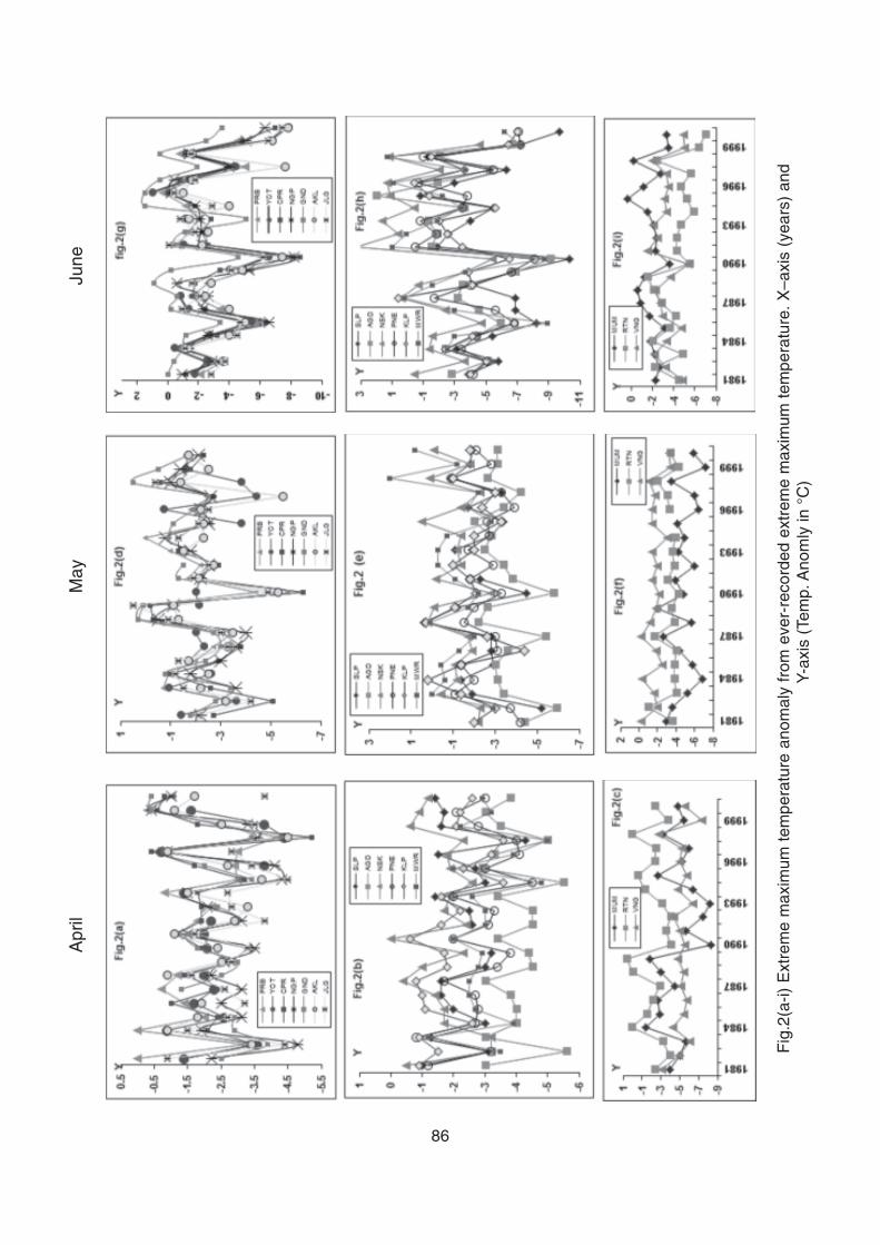
86

Fig

.2(a

-i) E

xtre

me

max

imum

tem

pera

ture

ano

mal

y fr

om e

ver-

reco

rded

ext

rem

e m

axim

um t

empe

ratu

re.

X–a

xis

(yea

rs)

and

Y-a

xis

(Tem

p. A

nom

ly in

°C

)

Apr

il M

ayJu

ne

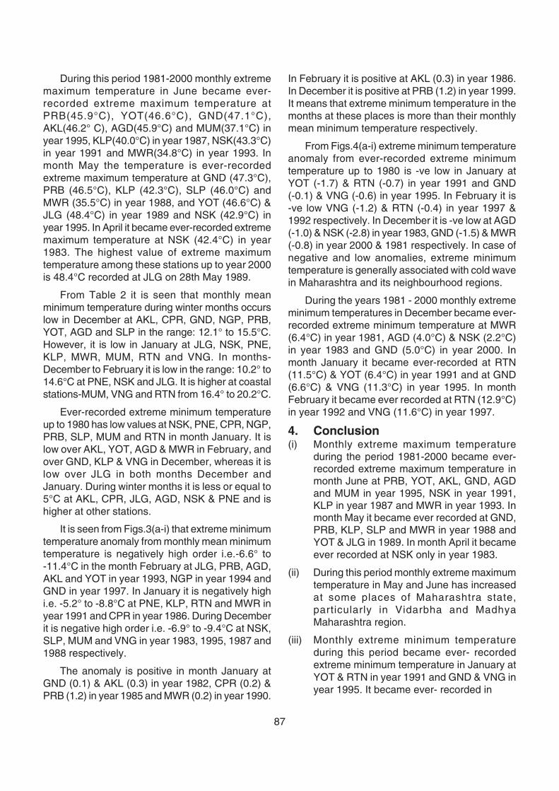
87

During this period 1981-2000 monthly extrememaximum temperature in June became ever-recorded extreme maximum temperature atPRB(45.9°C), YOT(46.6°C), GND(47.1°C),AKL(46.2° C), AGD(45.9°C) and MUM(37.1°C) inyear 1995, KLP(40.0°C) in year 1987, NSK(43.3°C)in year 1991 and MWR(34.8°C) in year 1993. Inmonth May the temperature is ever-recordedextreme maximum temperature at GND (47.3°C),PRB (46.5°C), KLP (42.3°C), SLP (46.0°C) andMWR (35.5°C) in year 1988, and YOT (46.6°C) &JLG (48.4°C) in year 1989 and NSK (42.9°C) inyear 1995. In April it became ever-recorded extrememaximum temperature at NSK (42.4°C) in year1983. The highest value of extreme maximumtemperature among these stations up to year 2000is 48.4°C recorded at JLG on 28th May 1989.

From Table 2 it is seen that monthly meanminimum temperature during winter months occurslow in December at AKL, CPR, GND, NGP, PRB,YOT, AGD and SLP in the range: 12.1° to 15.5°C.However, it is low in January at JLG, NSK, PNE,KLP, MWR, MUM, RTN and VNG. In months-December to February it is low in the range: 10.2° to14.6°C at PNE, NSK and JLG. It is higher at coastalstations-MUM, VNG and RTN from 16.4° to 20.2°C.

Ever-recorded extreme minimum temperatureup to 1980 has low values at NSK, PNE, CPR, NGP,PRB, SLP, MUM and RTN in month January. It islow over AKL, YOT, AGD & MWR in February, andover GND, KLP & VNG in December, whereas it islow over JLG in both months December andJanuary. During winter months it is less or equal to5°C at AKL, CPR, JLG, AGD, NSK & PNE and ishigher at other stations.

It is seen from Figs.3(a-i) that extreme minimumtemperature anomaly from monthly mean minimumtemperature is negatively high order i.e.-6.6° to-11.4°C in the month February at JLG, PRB, AGD,AKL and YOT in year 1993, NGP in year 1994 andGND in year 1997. In January it is negatively highi.e. -5.2° to -8.8°C at PNE, KLP, RTN and MWR inyear 1991 and CPR in year 1986. During Decemberit is negative high order i.e. -6.9° to -9.4°C at NSK,SLP, MUM and VNG in year 1983, 1995, 1987 and1988 respectively.

The anomaly is positive in month January atGND (0.1) & AKL (0.3) in year 1982, CPR (0.2) &PRB (1.2) in year 1985 and MWR (0.2) in year 1990.

In February it is positive at AKL (0.3) in year 1986.In December it is positive at PRB (1.2) in year 1999.It means that extreme minimum temperature in themonths at these places is more than their monthlymean minimum temperature respectively.

From Figs.4(a-i) extreme minimum temperatureanomaly from ever-recorded extreme minimumtemperature up to 1980 is -ve low in January atYOT (-1.7) & RTN (-0.7) in year 1991 and GND(-0.1) & VNG (-0.6) in year 1995. In February it is-ve low VNG (-1.2) & RTN (-0.4) in year 1997 &1992 respectively. In December it is -ve low at AGD(-1.0) & NSK (-2.8) in year 1983, GND (-1.5) & MWR(-0.8) in year 2000 & 1981 respectively. In case ofnegative and low anomalies, extreme minimumtemperature is generally associated with cold wavein Maharashtra and its neighbourhood regions.

During the years 1981 - 2000 monthly extrememinimum temperatures in December became ever-recorded extreme minimum temperature at MWR(6.4°C) in year 1981, AGD (4.0°C) & NSK (2.2°C)in year 1983 and GND (5.0°C) in year 2000. Inmonth January it became ever-recorded at RTN(11.5°C) & YOT (6.4°C) in year 1991 and at GND(6.6°C) & VNG (11.3°C) in year 1995. In monthFebruary it became ever recorded at RTN (12.9°C)in year 1992 and VNG (11.6°C) in year 1997.

4. Conclusion(i) Monthly extreme maximum temperature

during the period 1981-2000 became ever-recorded extreme maximum temperature inmonth June at PRB, YOT, AKL, GND, AGDand MUM in year 1995, NSK in year 1991,KLP in year 1987 and MWR in year 1993. Inmonth May it became ever recorded at GND,PRB, KLP, SLP and MWR in year 1988 andYOT & JLG in 1989. In month April it becameever recorded at NSK only in year 1983.

(ii) During this period monthly extreme maximumtemperature in May and June has increasedat some places of Maharashtra state,particularly in Vidarbha and MadhyaMaharashtra region.

(iii) Monthly extreme minimum temperatureduring this period became ever- recordedextreme minimum temperature in January atYOT & RTN in year 1991 and GND & VNG inyear 1995. It became ever- recorded in

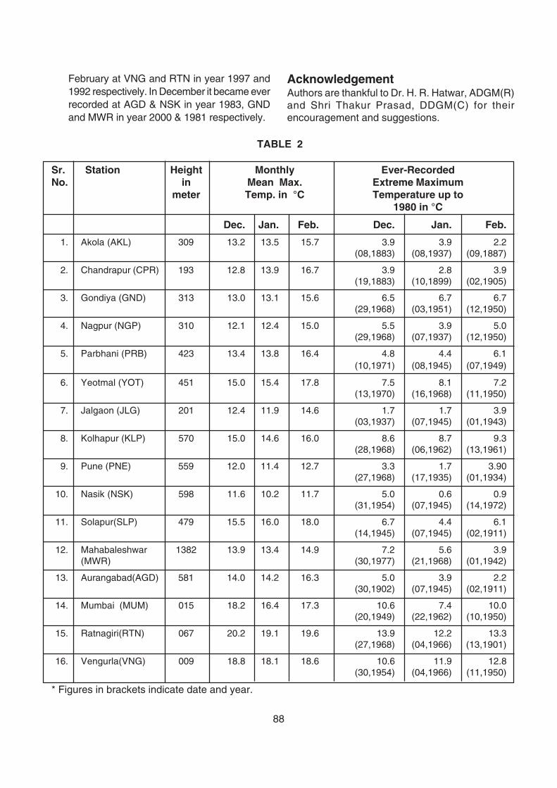
88

TABLE 2

Sr. Station Height Monthly Ever-RecordedNo. in Mean Max. Extreme Maximum

meter Temp. in °C Temperature up to1980 in °C

Dec. Jan. Feb. Dec. Jan. Feb.

1. Akola (AKL) 309 13.2 13.5 15.7 3.9 3.9 2.2(08,1883) (08,1937) (09,1887)

2. Chandrapur (CPR) 193 12.8 13.9 16.7 3.9 2.8 3.9(19,1883) (10,1899) (02,1905)

3. Gondiya (GND) 313 13.0 13.1 15.6 6.5 6.7 6.7(29,1968) (03,1951) (12,1950)

4. Nagpur (NGP) 310 12.1 12.4 15.0 5.5 3.9 5.0(29,1968) (07,1937) (12,1950)

5. Parbhani (PRB) 423 13.4 13.8 16.4 4.8 4.4 6.1(10,1971) (08,1945) (07,1949)

6. Yeotmal (YOT) 451 15.0 15.4 17.8 7.5 8.1 7.2(13,1970) (16,1968) (11,1950)

7. Jalgaon (JLG) 201 12.4 11.9 14.6 1.7 1.7 3.9(03,1937) (07,1945) (01,1943)

8. Kolhapur (KLP) 570 15.0 14.6 16.0 8.6 8.7 9.3(28,1968) (06,1962) (13,1961)

9. Pune (PNE) 559 12.0 11.4 12.7 3.3 1.7 3.90(27,1968) (17,1935) (01,1934)

10. Nasik (NSK) 598 11.6 10.2 11.7 5.0 0.6 0.9(31,1954) (07,1945) (14,1972)

11. Solapur(SLP) 479 15.5 16.0 18.0 6.7 4.4 6.1(14,1945) (07,1945) (02,1911)

12. Mahabaleshwar 1382 13.9 13.4 14.9 7.2 5.6 3.9(MWR) (30,1977) (21,1968) (01,1942)

13. Aurangabad(AGD) 581 14.0 14.2 16.3 5.0 3.9 2.2(30,1902) (07,1945) (02,1911)

14. Mumbai (MUM) 015 18.2 16.4 17.3 10.6 7.4 10.0(20,1949) (22,1962) (10,1950)

15. Ratnagiri(RTN) 067 20.2 19.1 19.6 13.9 12.2 13.3(27,1968) (04,1966) (13,1901)

16. Vengurla(VNG) 009 18.8 18.1 18.6 10.6 11.9 12.8(30,1954) (04,1966) (11,1950)

* Figures in brackets indicate date and year.

February at VNG and RTN in year 1997 and1992 respectively. In December it became everrecorded at AGD & NSK in year 1983, GNDand MWR in year 2000 & 1981 respectively.

AcknowledgementAuthors are thankful to Dr. H. R. Hatwar, ADGM(R)and Shri Thakur Prasad, DDGM(C) for theirencouragement and suggestions.

89

Fig

.3(a

-i) E

xtre

me

min

imum

tem

pera

ture

ano

mal

y fr

om m

ean

mon

thly

min

imum

tem

pera

ture

. X

–axi

s (y

ears

) an

dY

-axi

s (T

emp.

Ano

mly

in °

C)

Dec

embe

rJa

nuar

yF

ebru

ary

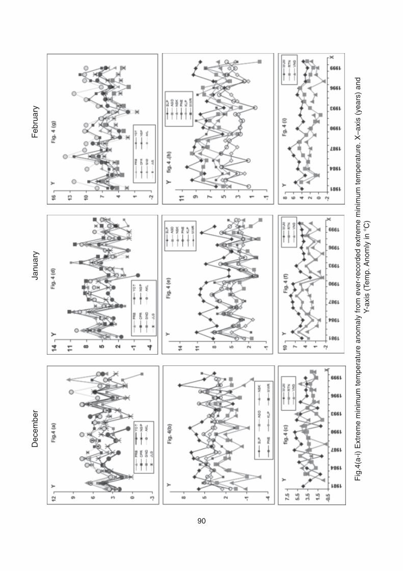
90

Dec

embe

rJa

nuar

yF

ebru

ary

Fig

.4(a

-i) E

xtre

me

min

imum

tem

pera

ture

ano

mal

y fr

om e

ver-

reco

rded

ext

rem

e m

inim

um t

empe

ratu

re.

X–a

xis

(yea

rs)

and

Y-a

xis

(Tem

p. A

nom

ly in

°C

)

91

ReferencesGuhathakurta, P. and Srivastav, A. K., 2004,"Evidence of climate jump in annual temperaturein India ", Mausam, Vol. 55, 3, pp. 419 - 428.

Hingane, L.S. Rupa Kumar, K. and RamanaMurthy B. V., 1985, "Long term trends of surfaceair temperature in India", J. Climatol, Vol. 5, pp.521 - 528.

Intergovernmental Panel on Climate Change,2007, (IPCC)'s 4th Assessment Report "TechnicalPaper VI." Chapter- 2, PP-3.

Jones, P. D., Raper S.C.B., Wigley, T.M.L. andWright, P.B., 1986, "Global temperature variationsbetween 1861-1984", Nature, Vol. 23, pp. 421-434.

Kothawale, D. R., 1992, "Surface temperature overIndia a Diagnostic Study", M.Sc. Thesis, Universityof Pune, pp 136.

Kothawale, D. R., 2007, "Temperature trends inrecent decade 1996-2005 over India", Tropmet2007, pp. 180-181.

Pramanik, S.K. and Jagannathan, P., 1954,"Climate Change in India - (II), temperature",Indian, J. Met. Geophysics, Vol. 5, pp. 29-47.

Rao, G. S. P., Murty, M. K. and Joshi, U.R., 2005,"Climate change over India as revealed by criticalextreme temperature analysis", Mausam, Vol. 56,No.3, pp. 601-608.

Rupa Kumar, K. and Hingane, L.S. 1988, "Longterm variations of Surface air temperature at majorindustrial cities of India", Climate Change, 13, pp287- 307.

Srivastav, H. N., Dewan, B.N., Dikshit, S. K., Rao,G.S.P, Singh, S.S. and Rao, K.R. 1992, "Decadaltrends in climate over India", Mausam, Vol. 43,No.1, pp. 7-20.

92

1. IntroductionThunderstorms are the most exhi larat ingphenomena occurring in the nature. It is one wayof restoring the stabilities in the atmosphere. Fromthe aviation point of view, it is of utmostimportance to study and analyze the weatherassociated with thunderstorms from its genesisto its dissipation. Thunderstorms are sometimesassociated with squalls of varying wind speedsand duration. Squall is defined as the suddenincrease in the mean wind speed in three stageson Beaufort scale upto 22 knots or more for atleast a minute. The gust of wind associated withthe thunderstorms has enough strength to causestructural damages. Basu and Mondal(2002)have tried to forecast squall propagation speedover Kolkata region during pre-monsoon seasonby correlating the radar echo positions with mid-troposphere (700-500hPa) winds and CAPE. Adynamic model by Betts et al. (1976) to simulatethe characteristics of squall line was foundeffective in determining the propagation speed ofsquall. The scope of this paper is to study theclimatology of squalls during different seasonsand forecast the probable gust wind associatedwith it.

2. Data analysisSurface data for the period 1993-2000 was takento find the instances of the squall occurrences atSafdarjung airport New Delhi. Daily WeatherReports of Regional Meteorological Center, Delhi

Analysis of squalls over NewDelhi and forecasting ofmaximum probable gust speed

Rahul Saxena, S. C. Bhan and B. P. YadavIndia Meteorological Department

Lodi Road, New Delhi

ABSTRACT

Thunderstorms are a frequent occurrence through out the year in the tropical regions. Many parts of India arealso affected by thunderstorms ranging from dust storms in Rajasthan to Nor'westers in West Bengal. Thundersqualls associated with the thunderstorms are significant micro scale phenomena in terms of their damagingpotential. Onset of squalls bring drastic changes in the basic meteorological parameters as well as other groundconditions like visibility and mean wind speed considerably affecting the aviation activities. In this paper,attempt has been made to analyse the physical characteristics of the squalls over Delhi and to forecast the windspeed associated with evening/night squalls using downrush temperature.

Key words: Squall, Gust, Downrush temperature, Gale, Peak velocity

were used to collect the data of occurrences ofsqualls. For each of the thunder-squall event,anemographs were studied to find:

a) Time of start and end of the gusty winds

b) Wind direction and speed in squall

c) Maximum gust speed associated with thesquall

The year has been divided in four seasons as perthe meteorological conventions into winter (Jan-Feb), pre monsoon (March-May), monsoon (June-Sept) and post monsoon (Oct-Dec). Month-wiseand season-wise analysis of squalls with respectto speed, direction and frequency has been carriedout.

3. Results and discussions3.1 Seasonal and diurnal distributionDuring the eight years under study, 92 squalls wererecorded averaging about 11-12 in a year. Premonsoon (45%) and Monsoon (49%) account formost of thunder squalls (Table 1). Maximumfrequency of squalls is in the month of May (24%)followed by June (20%), July (15%) and April (14%).November and December are devoid of any squallactivity (Fig.1). Majority of the squalls during premonsoon season occur during late evenings/night(18-21 and 21-24 hrs IST) but this activity is moreduring evening hours (15-18 hrs IST) in themonsoon season (Fig. 2).

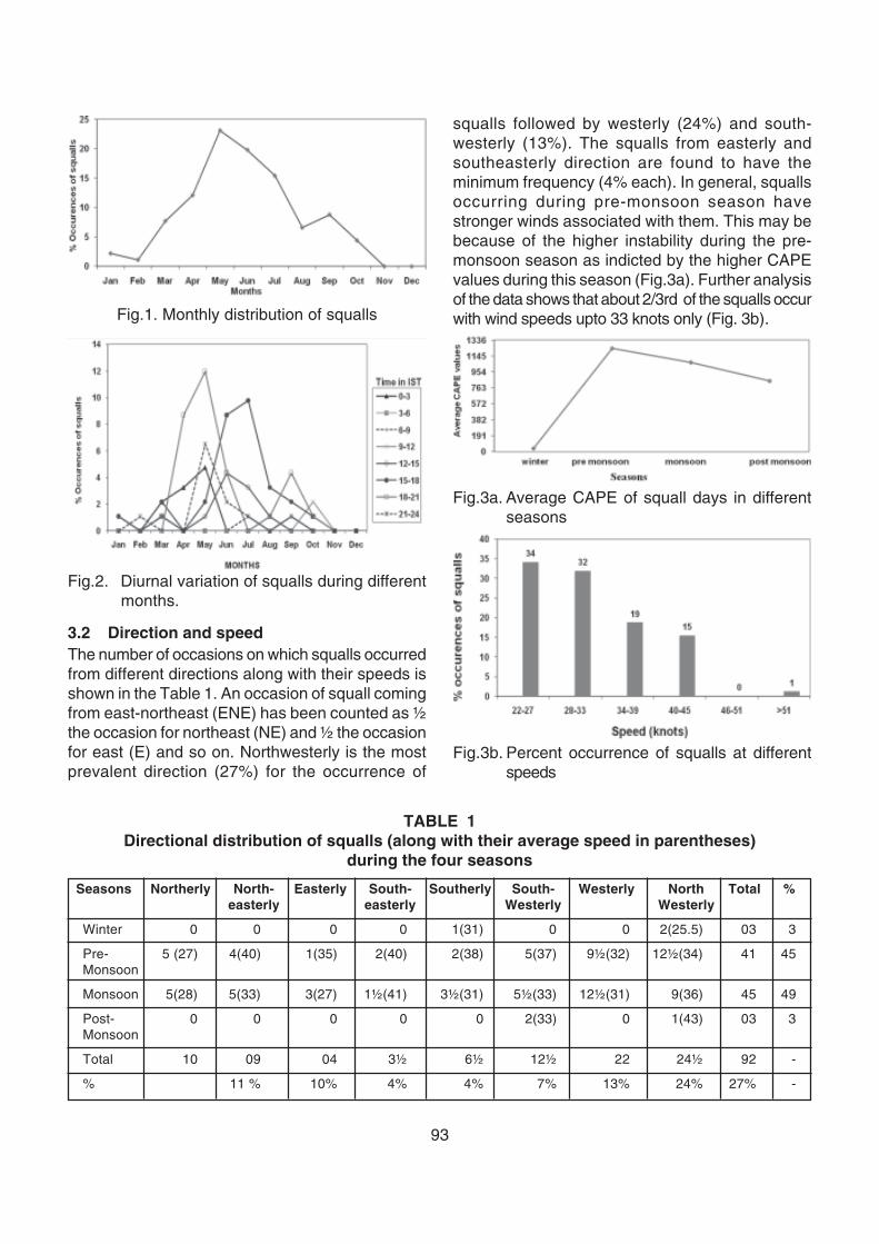
93

3.2 Direction and speedThe number of occasions on which squalls occurredfrom different directions along with their speeds isshown in the Table 1. An occasion of squall comingfrom east-northeast (ENE) has been counted as ½the occasion for northeast (NE) and ½ the occasionfor east (E) and so on. Northwesterly is the mostprevalent direction (27%) for the occurrence of

squalls followed by westerly (24%) and south-westerly (13%). The squalls from easterly andsoutheasterly direction are found to have theminimum frequency (4% each). In general, squallsoccurring during pre-monsoon season havestronger winds associated with them. This may bebecause of the higher instability during the pre-monsoon season as indicted by the higher CAPEvalues during this season (Fig.3a). Further analysisof the data shows that about 2/3rd of the squalls occurwith wind speeds upto 33 knots only (Fig. 3b).

Fig.2. Diurnal variation of squalls during differentmonths.

Fig.1. Monthly distribution of squalls

TABLE 1Directional distribution of squalls (along with their average speed in parentheses)

during the four seasons

Seasons Northerly North- Easterly South- Southerly South- Westerly North Total %easterly easterly Westerly Westerly

Winter 0 0 0 0 1(31) 0 0 2(25.5) 03 3

Pre- 5 (27) 4(40) 1(35) 2(40) 2(38) 5(37) 9½(32) 12½(34) 41 45Monsoon

Monsoon 5(28) 5(33) 3(27) 1½(41) 3½(31) 5½(33) 12½(31) 9(36) 45 49

Post- 0 0 0 0 0 2(33) 0 1(43) 03 3Monsoon

Total 10 09 04 3½ 6½ 12½ 22 24½ 92 -

% 11 % 10% 4% 4% 7% 13% 24% 27% -

Fig.3a. Average CAPE of squall days in differentseasons

Fig.3b. Percent occurrence of squalls at differentspeeds

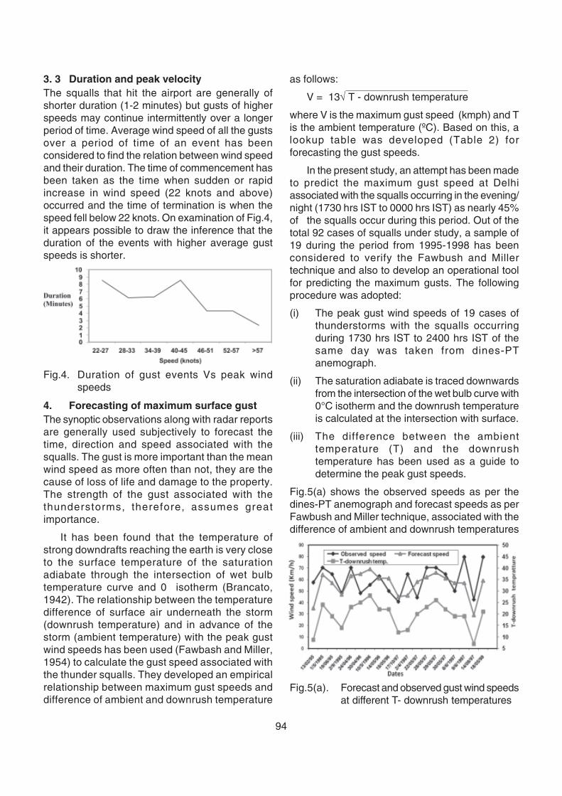
94

3. 3 Duration and peak velocityThe squalls that hit the airport are generally ofshorter duration (1-2 minutes) but gusts of higherspeeds may continue intermittently over a longerperiod of time. Average wind speed of all the gustsover a period of time of an event has beenconsidered to find the relation between wind speedand their duration. The time of commencement hasbeen taken as the time when sudden or rapidincrease in wind speed (22 knots and above)occurred and the time of termination is when thespeed fell below 22 knots. On examination of Fig.4,it appears possible to draw the inference that theduration of the events with higher average gustspeeds is shorter.

as follows:

V = 13√ T - downrush temperature

where V is the maximum gust speed (kmph) and Tis the ambient temperature (ºC). Based on this, alookup table was developed (Table 2) forforecasting the gust speeds.

In the present study, an attempt has been madeto predict the maximum gust speed at Delhiassociated with the squalls occurring in the evening/night (1730 hrs IST to 0000 hrs IST) as nearly 45%of the squalls occur during this period. Out of thetotal 92 cases of squalls under study, a sample of19 during the period from 1995-1998 has beenconsidered to verify the Fawbush and Millertechnique and also to develop an operational toolfor predicting the maximum gusts. The followingprocedure was adopted:

(i) The peak gust wind speeds of 19 cases ofthunderstorms with the squalls occurringduring 1730 hrs IST to 2400 hrs IST of thesame day was taken from dines-PTanemograph.

(ii) The saturation adiabate is traced downwardsfrom the intersection of the wet bulb curve with0°C isotherm and the downrush temperatureis calculated at the intersection with surface.

(iii) The difference between the ambienttemperature (T) and the downrushtemperature has been used as a guide todetermine the peak gust speeds.

Fig.5(a) shows the observed speeds as per thedines-PT anemograph and forecast speeds as perFawbush and Miller technique, associated with thedifference of ambient and downrush temperatures

Fig.4. Duration of gust events Vs peak windspeeds

4. Forecasting of maximum surface gustThe synoptic observations along with radar reportsare generally used subjectively to forecast thetime, direction and speed associated with thesqualls. The gust is more important than the meanwind speed as more often than not, they are thecause of loss of life and damage to the property.The strength of the gust associated with thethunderstorms, therefore, assumes greatimportance.

It has been found that the temperature ofstrong downdrafts reaching the earth is very closeto the surface temperature of the saturationadiabate through the intersection of wet bulbtemperature curve and 0 isotherm (Brancato,1942). The relationship between the temperaturedifference of surface air underneath the storm(downrush temperature) and in advance of thestorm (ambient temperature) with the peak gustwind speeds has been used (Fawbash and Miller,1954) to calculate the gust speed associated withthe thunder squalls. They developed an empiricalrelationship between maximum gust speeds anddifference of ambient and downrush temperature

Fig.5(a). Forecast and observed gust wind speedsat different T- downrush temperatures

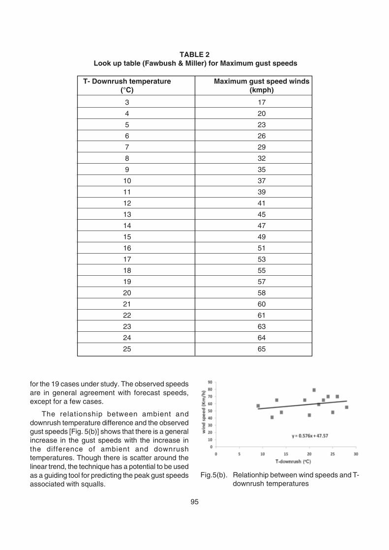
95

for the 19 cases under study. The observed speedsare in general agreement with forecast speeds,except for a few cases.

The relationship between ambient anddownrush temperature difference and the observedgust speeds [Fig. 5(b)] shows that there is a generalincrease in the gust speeds with the increase inthe difference of ambient and downrushtemperatures. Though there is scatter around thelinear trend, the technique has a potential to be usedas a guiding tool for predicting the peak gust speedsassociated with squalls.

Fig.5(b). Relationhip between wind speeds and T-downrush temperatures

TABLE 2 Look up table (Fawbush & Miller) for Maximum gust speeds

T- Downrush temperature Maximum gust speed winds(°C) (kmph)

3 17

4 20

5 23

6 26

7 29

8 32

9 35

10 37

11 39

12 41

13 45

14 47

15 49

16 51

17 53

18 55

19 57

20 58

21 60

22 61

23 63

24 64

25 65

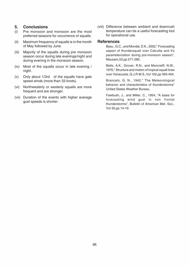
96

5. Conclusions(i) Pre monsoon and monsoon are the most

preferred seasons for occurrence of squalls.

(ii) Maximum frequency of squalls is in the monthof May followed by June.

(iii) Majority of the squalls during pre monsoonseason occur during late evenings/night andduring evening in the monsoon season.

(iv) Most of the squalls occur in late evening /night.

(v) Only about 1/3rd of the squalls have galespeed winds (more than 33 knots).

(vi) Northwesterly or westerly squalls are morefrequent and are stronger.

(vii) Duration of the events with higher averagegust speeds is shorter.

(viii) Difference between ambient and downrushtemperature can be a useful forecasting toolfor operational use.

ReferencesBasu , G.C., and Mondal, D.K., 2002," Forecastingaspect of thundersquall over Calcutta and it'sparameterization during pre-monsoon season",Mausam,53,pp 271-280.

Betts, A.K., Grover, R.N., and Moncreiff, N.W.,1976," Structure and motion of tropical squall linesover Venezuela, Q.J.R.M.S.,Vol 102,pp 395-404.

Brancato, G. N., 1942," The Meteorologicalbehavior and characteristics of thunderstorms"United States Weather Bureau.

Fawbush, J., and Miller, C., 1954, "A basis forforecasting wind gust in non frontalthunderstorms", Bulletin of American Met. Soc.,Vol 35,pp 14-19.

97

1. IntroductionWheat (Triticum aestivum L.), one of the importantstaple foods in India, is grown under diverse setsof agro-climatic conditions. It is grown in the regionwithin latitudes 15° to 32° N, and longitudes 72° to92°E both under irrigated and rainfed conditions.Punjab, Haryana, Uttar Pradesh, Uttaranchal,Madhya Pradesh, Rajasthan and Bihar are theleading states of India contributing more than 90per cent of the wheat for the country. India is nowthe 2nd largest wheat producer in the world afterChina. Wheat is sown during November toDecember and harvested during March to April. Thewheat-marketing season in India is assumed tobegin from April every year.

Increased climatic variabilities and weather

Wheat yield prediction usingCERES-Wheat model fordecision support in agro-advisory

K.K.Singh, A.K. Baxla, R.K. Mall*, P.K.Singh,R. Balasubramanyam** and Shikha Garg

*Bararas Hindu University, Varanasi** India Meterological Department, Pune

India Meteorology Department, New Delhi

ABSTRACT

Pre harvest yield estimate of the crop for the country is important for policy makers in the government forfurther course of action planning. In the present study efforts are made to estimate the wheat yield for the year2009-10 using CERES-Wheat crop growth simulator embedded in DSSAT v4.0. A methodology has beendeveloped and simulations were made under irrigated condition for the 15 wheat-growing locations representingdifferent agroclimatic zones of the country. Daily weather data on maximum and minimum temperatures,rainfall and bright sunshine hours were used for 15 locations for the two winter seasons, current season 2009-2010 and previous season 2008-09. Two dates of sowing representing normal and late sown conditions foreach zone were taken up for the study. Genetic coefficients required for running the CERES-Wheat V4.0 modelwere used for commonly grown cultivars i.e. PBW-343, RAJ-3765, Malviya-234, HUW-234 and C-306 atdifferent locations.

Simulated results indicate that wheat crop yield in Uttar Pradesh during the crop season 2009-10 is slightlyaffected due to rise in temperature encountered at grain filling stage in the month of March. Under normalsown condition wheat yield prediction during 2009-10 is ~1% less compared to 2008-09 in Uttar Pradeshwhile increase in grain yield by ~4% in North West India and ~18% in East India respectively.

In case of late sown condition, crop model shows reduction in grain yield in North West India and UttarPradesh and increase over East India. During March 2010 maximum and minimum temperature remainedabove normal almost throughout the month over most parts of the country. Maximum temperatures wereabove normal by 4-8°C over northwest, east, central and adjoining peninsular India. The predicted wheat yielddeviated from 2008-09 in North West India and Uttar Pradesh was ~ 4% and ~23% respectively. While thereis ~8% more yields in East India during 2009-10 compare to year 2008-09.

Key words: CERES-Wheat model, Genetic coefficients, Yield prediction, Climatic variability and extremeweather.

abnormalities like hailstorm, frost, high wind,extreme temperatures and foggy condition duringwheat growing (Rabi) season leads to naturaldisasters affecting wheat productivity. Over the pastfew years, the per hectare yield of wheat in Indiahas fallen due to the temperature rising steadily inJanuary, February and March, a time most crucialfor the wheat crop Singh et al, 2010, Singh et al,2011; Shantha 2002). During January and Februaryof 2006 temperatures kept rising steadily due toprolonged absence of rain. The average day andnight temperatures have been 4-6°C higher thanthe normal, most striking during February, in wheatsowing region of the country. With the raisedtemperatures, crop matures early. The responseto temperatures varies with the stage ofdevelopment, mainly booting (late ear

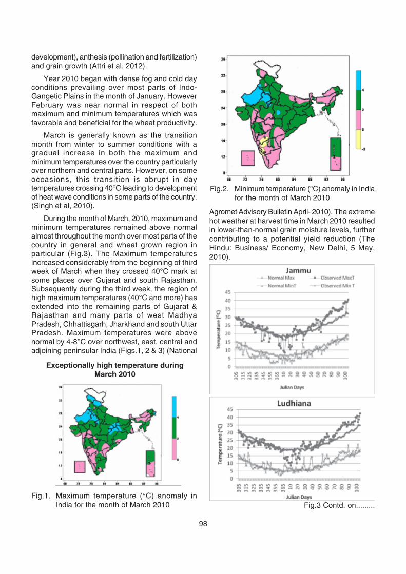
98

development), anthesis (pollination and fertilization)and grain growth (Attri et al. 2012).

Year 2010 began with dense fog and cold dayconditions prevailing over most parts of Indo-Gangetic Plains in the month of January. HoweverFebruary was near normal in respect of bothmaximum and minimum temperatures which wasfavorable and beneficial for the wheat productivity.

March is generally known as the transitionmonth from winter to summer conditions with agradual increase in both the maximum andminimum temperatures over the country particularlyover northern and central parts. However, on someoccasions, this transition is abrupt in daytemperatures crossing 40°C leading to developmentof heat wave conditions in some parts of the country.(Singh et al, 2010).

During the month of March, 2010, maximum andminimum temperatures remained above normalalmost throughout the month over most parts of thecountry in general and wheat grown region inparticular (Fig.3). The Maximum temperaturesincreased considerably from the beginning of thirdweek of March when they crossed 40°C mark atsome places over Gujarat and south Rajasthan.Subsequently during the third week, the region ofhigh maximum temperatures (40°C and more) hasextended into the remaining parts of Gujarat &Rajasthan and many parts of west MadhyaPradesh, Chhattisgarh, Jharkhand and south UttarPradesh. Maximum temperatures were abovenormal by 4-8°C over northwest, east, central andadjoining peninsular India (Figs.1, 2 & 3) (National

Exceptionally high temperature duringMarch 2010

Fig.1. Maximum temperature (°C) anomaly inIndia for the month of March 2010

Fig.2. Minimum temperature (°C) anomaly in Indiafor the month of March 2010

Agromet Advisory Bulletin April- 2010). The extremehot weather at harvest time in March 2010 resultedin lower-than-normal grain moisture levels, furthercontributing to a potential yield reduction (TheHindu: Business/ Economy, New Delhi, 5 May,2010).

Fig.3 Contd. on.........

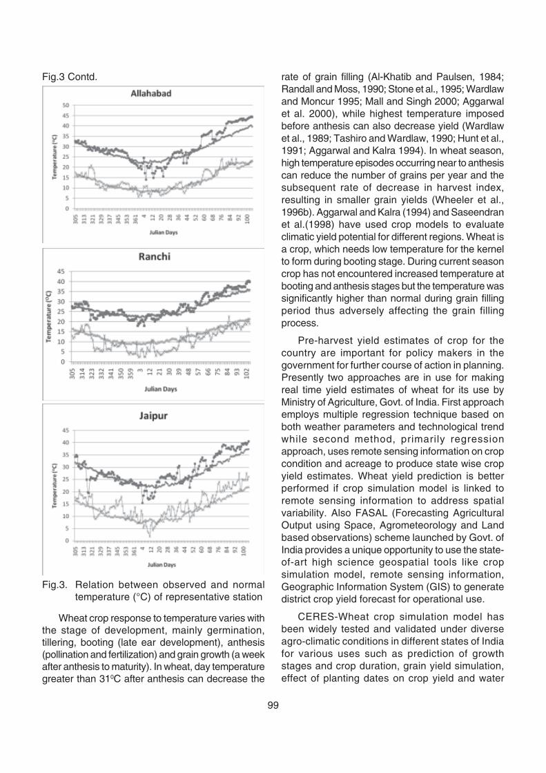
99

rate of grain filling (Al-Khatib and Paulsen, 1984;Randall and Moss, 1990; Stone et al., 1995; Wardlawand Moncur 1995; Mall and Singh 2000; Aggarwalet al. 2000), while highest temperature imposedbefore anthesis can also decrease yield (Wardlawet al., 1989; Tashiro and Wardlaw, 1990; Hunt et al.,1991; Aggarwal and Kalra 1994). In wheat season,high temperature episodes occurring near to anthesiscan reduce the number of grains per year and thesubsequent rate of decrease in harvest index,resulting in smaller grain yields (Wheeler et al.,1996b). Aggarwal and Kalra (1994) and Saseendranet al.(1998) have used crop models to evaluateclimatic yield potential for different regions. Wheat isa crop, which needs low temperature for the kernelto form during booting stage. During current seasoncrop has not encountered increased temperature atbooting and anthesis stages but the temperature wassignificantly higher than normal during grain fillingperiod thus adversely affecting the grain fillingprocess.

Pre-harvest yield estimates of crop for thecountry are important for policy makers in thegovernment for further course of action in planning.Presently two approaches are in use for makingreal time yield estimates of wheat for its use byMinistry of Agriculture, Govt. of India. First approachemploys multiple regression technique based onboth weather parameters and technological trendwhile second method, primarily regressionapproach, uses remote sensing information on cropcondition and acreage to produce state wise cropyield estimates. Wheat yield prediction is betterperformed if crop simulation model is linked toremote sensing information to address spatialvariability. Also FASAL (Forecasting AgriculturalOutput using Space, Agrometeorology and Landbased observations) scheme launched by Govt. ofIndia provides a unique opportunity to use the state-of-art high science geospatial tools like cropsimulation model, remote sensing information,Geographic Information System (GIS) to generatedistrict crop yield forecast for operational use.

CERES-Wheat crop simulation model hasbeen widely tested and validated under diverseagro-climatic conditions in different states of Indiafor various uses such as prediction of growthstages and crop duration, grain yield simulation,effect of planting dates on crop yield and water

Fig.3. Relation between observed and normaltemperature (°C) of representative station

Wheat crop response to temperature varies withthe stage of development, mainly germination,tillering, booting (late ear development), anthesis(pollination and fertilization) and grain growth (a weekafter anthesis to maturity). In wheat, day temperaturegreater than 310C after anthesis can decrease the

Fig.3 Contd.

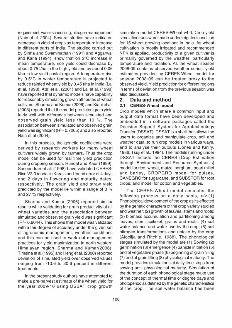
100

requirement, water scheduling, nitrogen management(Nain et al. 2004). Several studies have indicateddecrease in yield of crops as temperature increasein different parts of India. The studied carried outby Sinha and Swaminathan (1991) and Aggarwaland Karla (1994), show that on 2°C increase inmean temperature, rice yield could decrease byabout 0.75 t/ha in the high yield and by about 0.06t/ha in low yield costal region. A temperature riseby 0.5°C in winter temperature is projected toreduce rainfed wheat yield by 0.45 t/ha in India (Lalet al. 1998). Attri et al. (2001) and Lal et al. (1998)have reported that dynamic models have capabilityfor reasonably simulating growth attributes of wheatcultivars. Sharma and Kumar (2006) and Kiani et al.(2003) reported that the model predicted grain yieldfairly well with difference between simulated andobserved grain yield less than 10 %. Theassociation between simulated and observed grainyield was significant (R2= 0.7205) and also reportedNain et al (2004).

In this process, the genetic coefficients werederived by research workers for many wheatcultivars widely grown by farmers. Thus the cropmodel can be used for real time yield predictionduring cropping season. Hundal and Kaur (1999),Saseendran et al. (1998) have validated CERES-Rice V3.0 model in Kerala and found error of 4 daysand 2 days in flowering and maturity dates,respectively. The grain yield and straw yieldpredicted by the model lie within a range of 3 %and 27 % respectively.

Sharma and Kumar (2006) reported similarresults while validating for grain productivity of allwheat varieties and the association betweensimulated and observed grain yield was significant(R2= 0.8044). This shows that model was validatedwith a fair degree of accuracy under the given setof agronomic management, weather conditionsand this can be used to work out managementpractices for yield maximization in north westernHimalayan region. Sharma and Kumar(2006),Timsina et al.(1995) and Heng et al. (2000) reporteddeviation of simulated yield over observed valuesranging from -10.6 to 20.6 percent in differenttreatments.

In the present study authors have attempted tomake a pre-harvest estimate of the wheat yield forthe year 2009-10 using DSSAT crop growth

simulation model CERES-Wheat v4.0. Crop yieldsimulation runs were made under irrigated conditionfor 15 wheat-growing locations in India. As wheatcultivation is mostly irrigated and recommendedNPK is applied, productivity of a given cultivar isprimarily governed by the weather, particularlytemperature and radiation. As the wheat season2008-09 contains observed weather series, yieldestimates provided by CERES-Wheat model forseason 2008-09 can be treated proxy to theobserved yield. Yield prediction for different regionsin terms of deviation from the previous season wasalso discussed.2. Data and method2.1 CERES-Wheat modelCrop models which share a common input andoutput data format have been developed andembedded in a software packages called theDecision Support System for AgrotechnologyTransfer (DSSAT). DSSAT is a shell that allows theusers to organize and manipulate crop, soil andweather data, to run crop models in various ways,and to analyse their outputs (Jones and Kiniry,1986; Tsuji et al., 1994). The models running underDSSAT include the CERES (Crop Estimationthrough Environment and Resource Synthesis)model for rice, wheat, maize, sorghum, pearl milletand barley, CROPGRO model for pulses,CANEGRO for sugarcane, and SUBSTOR for rootcrops, and model for cotton and vegetables.

The CERES-Wheat model simulates thefollowing process on a daily basis, viz.(1)Phonological development of the crop as its effectedby the genetic characters of the crop variety studiedand weather; (2) growth of leaves, stems and roots;(3) biomass accumulation and partitioning amongleaves, stem, spikelet, grains and roots; (4) soilwater balance and water use by the crop; (5) soilnitrogen transformations and uptake by the crop(Alocilja and Ritchie, 1988). The phonologicalstages simulated by the model are (1) Sowing (2)germination (3) emergence (4) panicle initiation (5)end of vegetative phase (6) beginning of grain filling(7) end of grain filling (8) physiological maturity. Themodel provides simulations at daily time steps fromsowing until physiological maturity. Simulation ofthe duration of each phonological stage make useof the concept of thermal time or degree days andphotoperiod as defined by the genetic characteristicsof the crop. The soil water balance has been

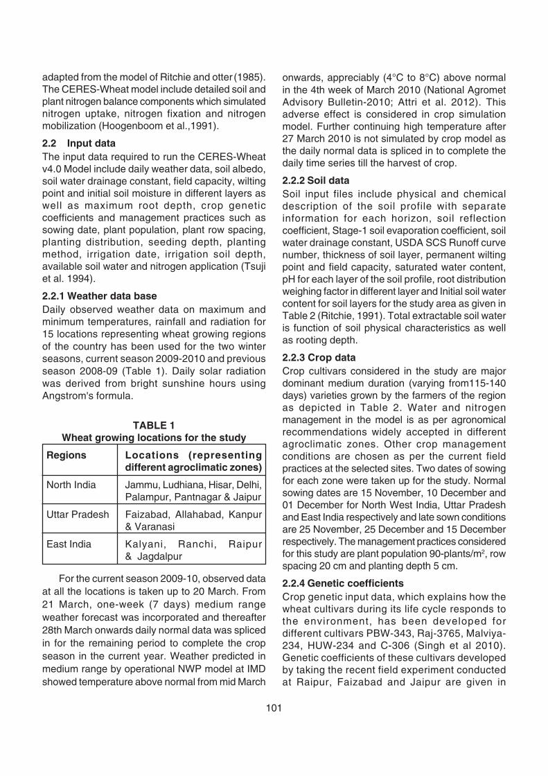
101

adapted from the model of Ritchie and otter (1985).The CERES-Wheat model include detailed soil andplant nitrogen balance components which simulatednitrogen uptake, nitrogen fixation and nitrogenmobilization (Hoogenboom et al.,1991).

2.2 Input dataThe input data required to run the CERES-Wheatv4.0 Model include daily weather data, soil albedo,soil water drainage constant, field capacity, wiltingpoint and initial soil moisture in different layers aswell as maximum root depth, crop geneticcoefficients and management practices such assowing date, plant population, plant row spacing,planting distribution, seeding depth, plantingmethod, irrigation date, irrigation soil depth,available soil water and nitrogen application (Tsujiet al. 1994).

2.2.1 Weather data baseDaily observed weather data on maximum andminimum temperatures, rainfall and radiation for15 locations representing wheat growing regionsof the country has been used for the two winterseasons, current season 2009-2010 and previousseason 2008-09 (Table 1). Daily solar radiationwas derived from bright sunshine hours usingAngstrom's formula.

onwards, appreciably (4°C to 8°C) above normalin the 4th week of March 2010 (National AgrometAdvisory Bulletin-2010; Attri et al. 2012). Thisadverse effect is considered in crop simulationmodel. Further continuing high temperature after27 March 2010 is not simulated by crop model asthe daily normal data is spliced in to complete thedaily time series till the harvest of crop.

2.2.2 Soil dataSoil input files include physical and chemicaldescription of the soil profile with separateinformation for each horizon, soil reflectioncoefficient, Stage-1 soil evaporation coefficient, soilwater drainage constant, USDA SCS Runoff curvenumber, thickness of soil layer, permanent wiltingpoint and field capacity, saturated water content,pH for each layer of the soil profile, root distributionweighing factor in different layer and Initial soil watercontent for soil layers for the study area as given inTable 2 (Ritchie, 1991). Total extractable soil wateris function of soil physical characteristics as wellas rooting depth.

2.2.3 Crop dataCrop cultivars considered in the study are majordominant medium duration (varying from115-140days) varieties grown by the farmers of the regionas depicted in Table 2. Water and nitrogenmanagement in the model is as per agronomicalrecommendations widely accepted in differentagroclimatic zones. Other crop managementconditions are chosen as per the current fieldpractices at the selected sites. Two dates of sowingfor each zone were taken up for the study. Normalsowing dates are 15 November, 10 December and01 December for North West India, Uttar Pradeshand East India respectively and late sown conditionsare 25 November, 25 December and 15 Decemberrespectively. The management practices consideredfor this study are plant population 90-plants/m2, rowspacing 20 cm and planting depth 5 cm.

2.2.4 Genetic coefficientsCrop genetic input data, which explains how thewheat cultivars during its life cycle responds tothe environment, has been developed fordifferent cultivars PBW-343, Raj-3765, Malviya-234, HUW-234 and C-306 (Singh et al 2010).Genetic coefficients of these cultivars developedby taking the recent field experiment conductedat Raipur, Faizabad and Jaipur are given in

TABLE 1Wheat growing locations for the study

Regions Locations (representingdifferent agroclimatic zones)

North India Jammu, Ludhiana, Hisar, Delhi,Palampur, Pantnagar & Jaipur

Uttar Pradesh Faizabad, Allahabad, Kanpur& Varanasi

East India Kalyani, Ranchi, Raipur& Jagdalpur

For the current season 2009-10, observed dataat all the locations is taken up to 20 March. From21 March, one-week (7 days) medium rangeweather forecast was incorporated and thereafter28th March onwards daily normal data was splicedin for the remaining period to complete the cropseason in the current year. Weather predicted inmedium range by operational NWP model at IMDshowed temperature above normal from mid March

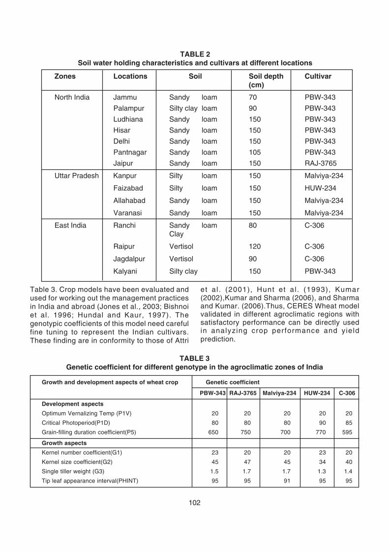
102

TABLE 3Genetic coefficient for different genotype in the agroclimatic zones of India

Growth and development aspects of wheat crop Genetic coefficient

PBW-343 RAJ-3765 Malviya-234 HUW-234 C-306

Development aspects

Optimum Vernalizing Temp (P1V) 20 20 20 20 20

Critical Photoperiod(P1D) 80 80 80 90 85

Grain-filling duration coefficient(P5) 650 750 700 770 595

Growth aspects

Kernel number coefficient(G1) 23 20 20 23 20

Kernel size coefficient(G2) 45 47 45 34 40

Single tiller weight (G3) 1.5 1.7 1.7 1.3 1.4

Tip leaf appearance interval(PHINT) 95 95 91 95 95

TABLE 2Soil water holding characteristics and cultivars at different locations

Zones Locations Soil Soil depth Cultivar(cm)

North India Jammu Sandy loam 70 PBW-343

Palampur Silty clay loam 90 PBW-343

Ludhiana Sandy loam 150 PBW-343

Hisar Sandy loam 150 PBW-343

Delhi Sandy loam 150 PBW-343

Pantnagar Sandy loam 105 PBW-343

Jaipur Sandy loam 150 RAJ-3765

Uttar Pradesh Kanpur Silty loam 150 Malviya-234

Faizabad Silty loam 150 HUW-234

Allahabad Sandy loam 150 Malviya-234

Varanasi Sandy loam 150 Malviya-234

East India Ranchi Sandy loam 80 C-306Clay

Raipur Vertisol 120 C-306

Jagdalpur Vertisol 90 C-306

Kalyani Silty clay 150 PBW-343

Table 3. Crop models have been evaluated andused for working out the management practicesin India and abroad (Jones et al., 2003; Bishnoiet al. 1996; Hundal and Kaur, 1997). Thegenotypic coefficients of this model need carefulfine tuning to represent the Indian cultivars.These finding are in conformity to those of Attri

et a l . (2001), Hunt et a l . (1993), Kumar(2002),Kumar and Sharma (2006), and Sharmaand Kumar. (2006).Thus, CERES Wheat modelvalidated in different agroclimatic regions withsatisfactory performance can be directly usedin analyzing crop performance and yieldprediction.

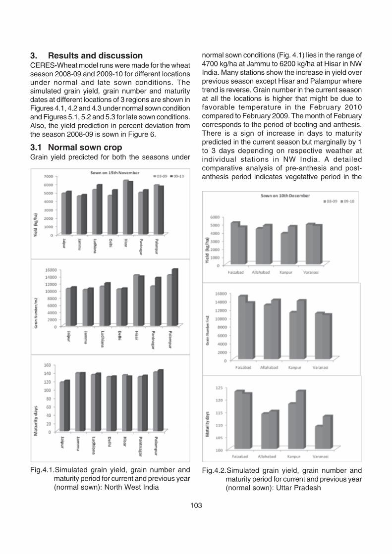
103

3. Results and discussionCERES-Wheat model runs were made for the wheatseason 2008-09 and 2009-10 for different locationsunder normal and late sown conditions. Thesimulated grain yield, grain number and maturitydates at different locations of 3 regions are shown inFigures 4.1, 4.2 and 4.3 under normal sown conditionand Figures 5.1, 5.2 and 5.3 for late sown conditions.Also, the yield prediction in percent deviation fromthe season 2008-09 is sown in Figure 6.

3.1 Normal sown cropGrain yield predicted for both the seasons under

normal sown conditions (Fig. 4.1) lies in the range of4700 kg/ha at Jammu to 6200 kg/ha at Hisar in NWIndia. Many stations show the increase in yield overprevious season except Hisar and Palampur wheretrend is reverse. Grain number in the current seasonat all the locations is higher that might be due tofavorable temperature in the February 2010compared to February 2009. The month of Februarycorresponds to the period of booting and anthesis.There is a sign of increase in days to maturitypredicted in the current season but marginally by 1to 3 days depending on respective weather atindividual stations in NW India. A detailedcomparative analysis of pre-anthesis and post-anthesis period indicates vegetative period in the

Fig.4.1.Simulated grain yield, grain number andmaturity period for current and previous year(normal sown): North West India

Fig.4.2.Simulated grain yield, grain number andmaturity period for current and previous year(normal sown): Uttar Pradesh

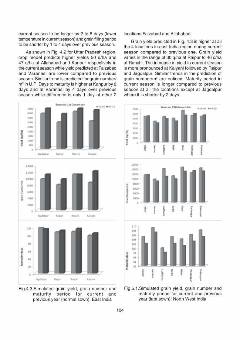
104

current season to be longer by 2 to 6 days (lowertemperature in current season) and grain filling periodto be shorter by 1 to 4 days over previous season.

As shown in Fig. 4.2 for Uttar Pradesh region,crop model predicts higher yields 50 q/ha and47 q/ha at Allahabad and Kanpur respectively inthe current season while yield predicted at Faizabadand Varanasi are lower compared to previousseason. Similar trend is predicted for grain number/m2 in U.P. Days to maturity is higher at Kanpur by 2days and at Varanasi by 4 days over previousseason while difference is only 1 day at other 2

locations Faizabad and Allahabad.

Grain yield predicted in Fig. 4.3 is higher at allthe 4 locations in east India region during currentseason compared to previous one. Grain yieldvaries in the range of 30 q/ha at Raipur to 46 q/haat Ranchi. The increase in yield in current seasonis more pronounced at Kalyani followed by Raipurand Jagdalpur. Similar trends in the prediction ofgrain number/m2 are noticed. Maturity period incurrent season is longer compared to previousseason at all the locations except at Jagdalpurwhere it is shorter by 2 days.

Fig.4.3.Simulated grain yield, grain number andmaturity period for current andprevious year (normal sown): East India

Fig.5.1.Simulated grain yield, grain number andmaturity period for current and previousyear (late sown): North West India

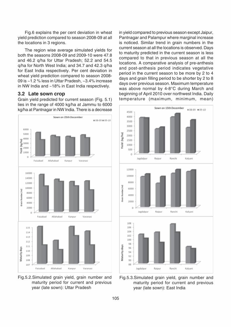
105

Fig.6 explains the per cent deviation in wheatyield prediction compared to season 2008-09 at allthe locations in 3 regions.

The region wise average simulated yields forboth the seasons 2008-09 and 2009-10 were 47.8and 46.2 q/ha for Uttar Pradesh; 52.2 and 54.5q/ha for North West India; and 34.7 and 42.3 q/hafor East India respectively. Per cent deviation inwheat yield prediction compared to season 2008-09 is ~1.2 % less in Uttar Pradesh, ~3.4% increasein NW India and ~18% in East India respectively.

3.2 Late sown cropGrain yield predicted for current season (Fig. 5.1)lies in the range of 4000 kg/ha at Jammu to 6000kg/ha at Pantnagar in NW India. There is a decrease

in yield compared to previous season except Jaipur,Pantnagar and Palampur where marginal increaseis noticed. Similar trend in grain numbers in thecurrent season at all the locations is observed. Daysto maturity predicted in the current season is lesscompared to that in previous season at all thelocations. A comparative analysis of pre-anthesisand post-anthesis period indicates vegetativeperiod in the current season to be more by 2 to 4days and grain filling period to be shorter by 2 to 8days over previous season. Maximum temperaturewas above normal by 4-8°C during March andbeginning of April 2010 over northwest India. Dailytemperature (maximum, minimum, mean)

Fig.5.2.Simulated grain yield, grain number andmaturity period for current and previousyear (late sown): Uttar Pradesh

Fig.5.3.Simulated grain yield, grain number andmaturity period for current and previousyear (late sown): East India

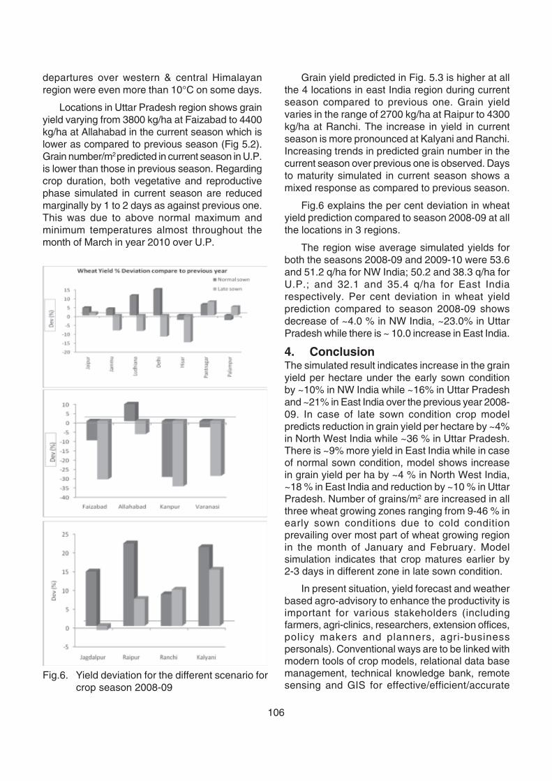
106

Fig.6. Yield deviation for the different scenario forcrop season 2008-09

departures over western & central Himalayanregion were even more than 10°C on some days.

Locations in Uttar Pradesh region shows grainyield varying from 3800 kg/ha at Faizabad to 4400kg/ha at Allahabad in the current season which islower as compared to previous season (Fig 5.2).Grain number/m2 predicted in current season in U.P.is lower than those in previous season. Regardingcrop duration, both vegetative and reproductivephase simulated in current season are reducedmarginally by 1 to 2 days as against previous one.This was due to above normal maximum andminimum temperatures almost throughout themonth of March in year 2010 over U.P.

Grain yield predicted in Fig. 5.3 is higher at allthe 4 locations in east India region during currentseason compared to previous one. Grain yieldvaries in the range of 2700 kg/ha at Raipur to 4300kg/ha at Ranchi. The increase in yield in currentseason is more pronounced at Kalyani and Ranchi.Increasing trends in predicted grain number in thecurrent season over previous one is observed. Daysto maturity simulated in current season shows amixed response as compared to previous season.

Fig.6 explains the per cent deviation in wheatyield prediction compared to season 2008-09 at allthe locations in 3 regions.

The region wise average simulated yields forboth the seasons 2008-09 and 2009-10 were 53.6and 51.2 q/ha for NW India; 50.2 and 38.3 q/ha forU.P.; and 32.1 and 35.4 q/ha for East Indiarespectively. Per cent deviation in wheat yieldprediction compared to season 2008-09 showsdecrease of ~4.0 % in NW India, ~23.0% in UttarPradesh while there is ~ 10.0 increase in East India.

4. ConclusionThe simulated result indicates increase in the grainyield per hectare under the early sown conditionby ~10% in NW India while ~16% in Uttar Pradeshand ~21% in East India over the previous year 2008-09. In case of late sown condition crop modelpredicts reduction in grain yield per hectare by ~4%in North West India while ~36 % in Uttar Pradesh.There is ~9% more yield in East India while in caseof normal sown condition, model shows increasein grain yield per ha by ~4 % in North West India,~18 % in East India and reduction by ~10 % in UttarPradesh. Number of grains/m2 are increased in allthree wheat growing zones ranging from 9-46 % inearly sown conditions due to cold conditionprevailing over most part of wheat growing regionin the month of January and February. Modelsimulation indicates that crop matures earlier by2-3 days in different zone in late sown condition.

In present situation, yield forecast and weatherbased agro-advisory to enhance the productivity isimportant for various stakeholders (includingfarmers, agri-clinics, researchers, extension offices,policy makers and planners, agri-businesspersonals). Conventional ways are to be linked withmodern tools of crop models, relational data basemanagement, technical knowledge bank, remotesensing and GIS for effective/efficient/accurate

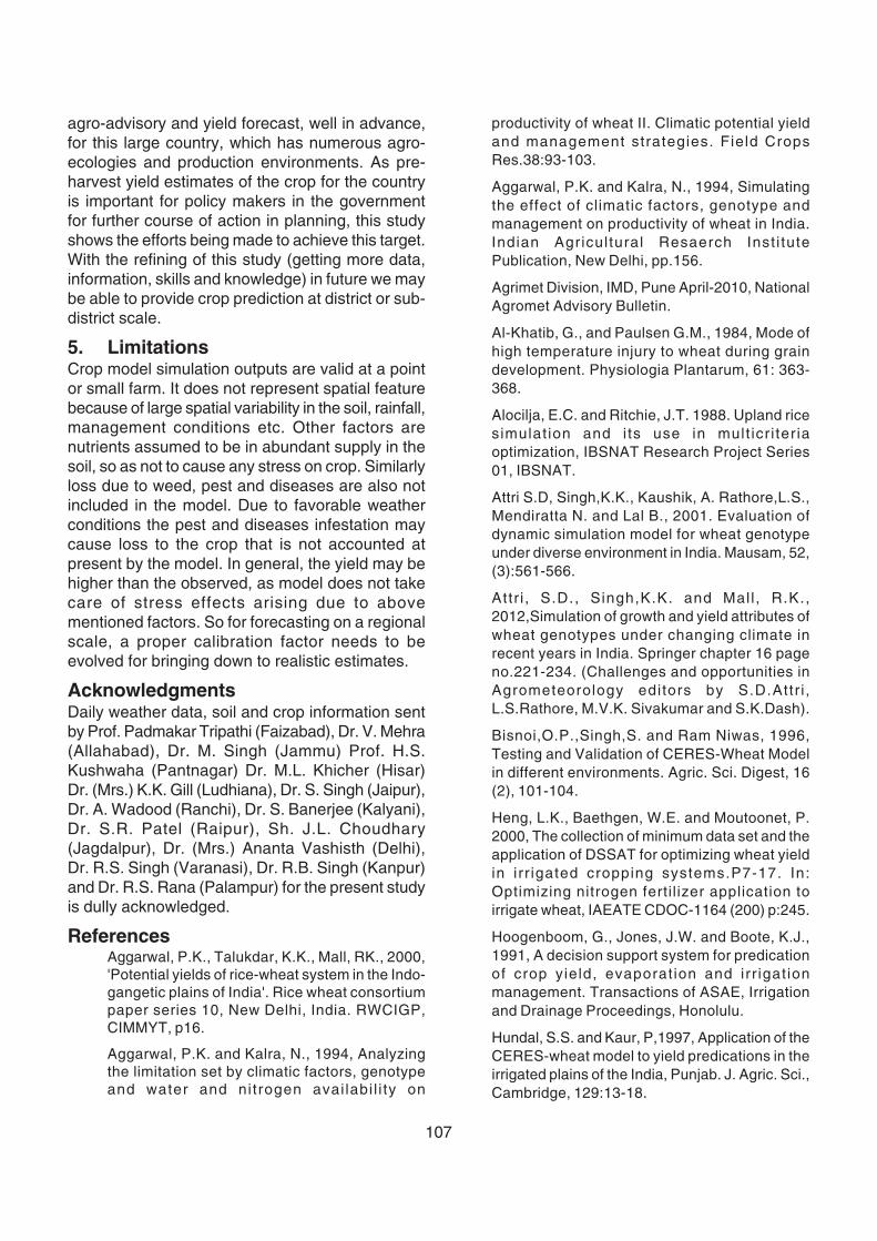
107

agro-advisory and yield forecast, well in advance,for this large country, which has numerous agro-ecologies and production environments. As pre-harvest yield estimates of the crop for the countryis important for policy makers in the governmentfor further course of action in planning, this studyshows the efforts being made to achieve this target.With the refining of this study (getting more data,information, skills and knowledge) in future we maybe able to provide crop prediction at district or sub-district scale.

5. LimitationsCrop model simulation outputs are valid at a pointor small farm. It does not represent spatial featurebecause of large spatial variability in the soil, rainfall,management conditions etc. Other factors arenutrients assumed to be in abundant supply in thesoil, so as not to cause any stress on crop. Similarlyloss due to weed, pest and diseases are also notincluded in the model. Due to favorable weatherconditions the pest and diseases infestation maycause loss to the crop that is not accounted atpresent by the model. In general, the yield may behigher than the observed, as model does not takecare of stress effects arising due to abovementioned factors. So for forecasting on a regionalscale, a proper calibration factor needs to beevolved for bringing down to realistic estimates.

AcknowledgmentsDaily weather data, soil and crop information sentby Prof. Padmakar Tripathi (Faizabad), Dr. V. Mehra(Allahabad), Dr. M. Singh (Jammu) Prof. H.S.Kushwaha (Pantnagar) Dr. M.L. Khicher (Hisar)Dr. (Mrs.) K.K. Gill (Ludhiana), Dr. S. Singh (Jaipur),Dr. A. Wadood (Ranchi), Dr. S. Banerjee (Kalyani),Dr. S.R. Patel (Raipur), Sh. J.L. Choudhary(Jagdalpur), Dr. (Mrs.) Ananta Vashisth (Delhi),Dr. R.S. Singh (Varanasi), Dr. R.B. Singh (Kanpur)and Dr. R.S. Rana (Palampur) for the present studyis dully acknowledged.

ReferencesAggarwal, P.K., Talukdar, K.K., Mall, RK., 2000,'Potential yields of rice-wheat system in the Indo-gangetic plains of India'. Rice wheat consortiumpaper series 10, New Delhi, India. RWCIGP,CIMMYT, p16.

Aggarwal, P.K. and Kalra, N., 1994, Analyzingthe limitation set by climatic factors, genotypeand water and nitrogen avai labi l i ty on

productivity of wheat II. Climatic potential yieldand management strategies. Field CropsRes.38:93-103.

Aggarwal, P.K. and Kalra, N., 1994, Simulatingthe effect of climatic factors, genotype andmanagement on productivity of wheat in India.Indian Agricultural Resaerch Inst i tutePublication, New Delhi, pp.156.

Agrimet Division, IMD, Pune April-2010, NationalAgromet Advisory Bulletin.

Al-Khatib, G., and Paulsen G.M., 1984, Mode ofhigh temperature injury to wheat during graindevelopment. Physiologia Plantarum, 61: 363-368.

Alocilja, E.C. and Ritchie, J.T. 1988. Upland ricesimulat ion and i ts use in mult icr i ter iaoptimization, IBSNAT Research Project Series01, IBSNAT.

Attri S.D, Singh,K.K., Kaushik, A. Rathore,L.S.,Mendiratta N. and Lal B., 2001. Evaluation ofdynamic simulation model for wheat genotypeunder diverse environment in India. Mausam, 52,(3):561-566.

Attr i , S.D., Singh,K.K. and Mall , R.K.,2012,Simulation of growth and yield attributes ofwheat genotypes under changing climate inrecent years in India. Springer chapter 16 pageno.221-234. (Challenges and opportunities inAgrometeorology editors by S.D.Attr i ,L.S.Rathore, M.V.K. Sivakumar and S.K.Dash).

Bisnoi,O.P.,Singh,S. and Ram Niwas, 1996,Testing and Validation of CERES-Wheat Modelin different environments. Agric. Sci. Digest, 16(2), 101-104.

Heng, L.K., Baethgen, W.E. and Moutoonet, P.2000, The collection of minimum data set and theapplication of DSSAT for optimizing wheat yieldin irr igated cropping systems.P7-17. In:Optimizing nitrogen fertil izer application toirrigate wheat, IAEATE CDOC-1164 (200) p:245.

Hoogenboom, G., Jones, J.W. and Boote, K.J.,1991, A decision support system for predicationof crop yield, evaporat ion and irr igat ionmanagement. Transactions of ASAE, Irrigationand Drainage Proceedings, Honolulu.

Hundal, S.S. and Kaur, P,1997, Application of theCERES-wheat model to yield predications in theirrigated plains of the India, Punjab. J. Agric. Sci.,Cambridge, 129:13-18.

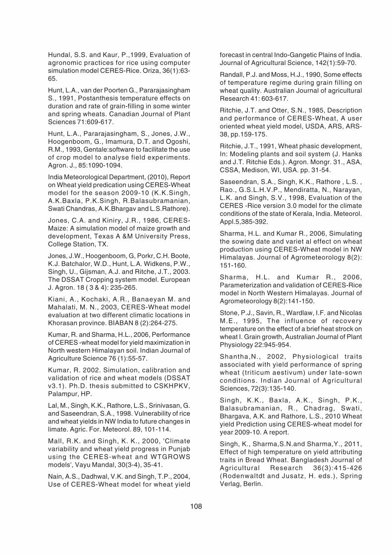
108

Hundal, S.S. and Kaur, P.,1999, Evaluation ofagronomic practices for rice using computersimulation model CERES-Rice. Oriza, 36(1):63-65.

Hunt, L.A., van der Poorten G., PararajasinghamS., 1991, Postanthesis temperature effects onduration and rate of grain-filling in some winterand spring wheats. Canadian Journal of PlantSciences 71:609-617.

Hunt, L.A., Pararajasingham, S., Jones, J.W.,Hoogenboom, G., Imamura, D.T. and Ogoshi,R.M., 1993, Gentale:software to facilitate the useof crop model to analyse field experiments.Agron. J., 85:1090-1094.

India Meteorological Department, (2010), Reporton Wheat yield predication using CERES-Wheatmodel for the season 2009-10 (K.K.Singh,A.K.Baxla, P.K.Singh, R.Balasubramanian,Swati Chandras, A.K.Bhargav and L.S.Rathore).

Jones, C.A. and Kiniry, J.R., 1986, CERES-Maize: A simulation model of maize growth anddevelopment, Texas A &M University Press,College Station, TX.

Jones, J.W., Hoogenboom, G, Porkr, C.H. Boote,K.J. Batchalor, W.D., Hunt, L.A. Widkens, P.W.,Singh, U., Gijsman, A.J. and Ritche, J.T., 2003.The DSSAT Cropping system model. EuropeanJ. Agron. 18 ( 3 & 4): 235-265.

Kiani, A., Kochaki, A.R., Banaeyan M. andMahalati, M. N., 2003, CERES-Wheat modelevaluation at two different climatic locations inKhorasan province. BIABAN 8 (2):264-275.

Kumar, R. and Sharma, H.L., 2006, Performanceof CERES -wheat model for yield maximization inNorth western Himalayan soil. Indian Journal ofAgriculture Science 76 (1):55-57.

Kumar, R. 2002. Simulation, calibration andvalidation of rice and wheat models (DSSATv3.1). Ph.D. thesis submitted to CSKHPKV,Palampur, HP.

Lal, M., Singh, K.K., Rathore, L.S., Srinivasan, G.and Saseendran, S.A., 1998. Vulnerability of riceand wheat yields in NW India to future changes inlimate. Agric. For. Meteorol. 89, 101-114.

Mall, R.K. and Singh, K. K., 2000, 'Climatevariability and wheat yield progress in Punjabusing the CERES-wheat and WTGROWSmodels', Vayu Mandal, 30(3-4), 35-41.

Nain, A.S., Dadhwal, V.K. and Singh, T.P., 2004,Use of CERES-Wheat model for wheat yield

forecast in central Indo-Gangetic Plains of India.Journal of Agricultural Science, 142(1):59-70.

Randall, P.J. and Moss, H.J., 1990, Some effectsof temperature regime during grain filling onwheat quality. Australian Journal of agriculturalResearch 41: 603-617.

Ritchie, J.T. and Otter, S.N., 1985, Descriptionand performance of CERES-Wheat, A useroriented wheat yield model, USDA, ARS, ARS-38, pp.159-175.

Ritchie, J.T., 1991, Wheat phasic development,In: Modeling plants and soil system (J. Hanksand J.T. Ritchie Eds.). Agron. Mongr. 31., ASA,CSSA, Medison, WI, USA. pp. 31-54.

Saseendran, S.A., Singh, K.K., Rathore , L.S. ,Rao., G.S.L.H.V.P., Mendiratta, N., Narayan,L.K. and Singh, S.V., 1998, Evaluation of theCERES -Rice version 3.0 model for the climateconditions of the state of Kerala, India. Meteorol.Appl.5,385-392.

Sharma, H.L. and Kumar R., 2006, Simulatingthe sowing date and variet al effect on wheatproduction using CERES-Wheat model in NWHimalayas. Journal of Agrometeorology 8(2):151-160.

Sharma, H.L. and Kumar R., 2006,Parameterization and validation of CERES-Ricemodel in North Western Himalayas. Journal ofAgrometeorology 8(2):141-150.

Stone, P.J., Savin, R., Wardlaw, I.F. and NicolasM.E., 1995, The inf luence of recoverytemperature on the effect of a brief heat strock onwheat I. Grain growth, Australian Journal of PlantPhysiology 22:945-954.

Shantha,N., 2002, Physiological trai tsassociated with yield performance of springwheat (trit icum aestivum) under late-sowncondit ions. Indian Journal of AgriculturalSciences, 72(3):135-140.

Singh, K.K., Baxla, A.K., Singh, P.K.,Balasubramanian, R., Chadrag, Swati ,Bhargava, A.K. and Rathore, L.S., 2010 Wheatyield Prediction using CERES-wheat model foryear 2009-10. A report.

Singh, K., Sharma,S.N.and Sharma,Y., 2011,Effect of high temperature on yield attributingtraits in Bread Wheat. Bangladesh Journal ofAgricultural Research 36(3):415-426(Rodenwaltdt and Jusatz, H. eds.), SpringVerlag, Berlin.

109

Sinha, S.K. and Swaminathan, M.S., 1991,Deformation, Climate change and sustainablenutrition security. Climate Change 16, 33-45.

Tashiro T., and Wardlaw I.F. 1990. The responseto high temperature shock and humidity changesprior to and during the early stages of graindevelopment in wheat. Australian Journal ofPlant Physiology 17:551-561.

Timsina, J., Singh, U., Singh, Y. and Lansigan,F.P. 1995. Addressing sustainability of rice -wheat system testing and application of CERESand SUCROS models. In proceedingInternational Rice Research Conference 13-17Feb., 1995, IRRI, Los Banos, Phil ippines,pp.633-656.

The Hindu: Business/ Economy, New Delhi, 5May, 2010.

Tsuji, G.Y., Uehara, G. and Balas, S.S. (Eds.).1994, DSSATv3. University of Hawaii, Honolulu,Hawaii, 284 p.

Wardlaw, I.F., and Moncur, L., 1995, The responseof wheat to high temperature following anthesis. I.The rate and duration of kernel filling. AustralianJournal of Plant Physiology, 22:391-397.

Wardlaw, I.F.,Dawson, I.A., Munibi, P. andFewster, R.,1989, The tolerance of wheat to hightemperature during reproductive growth. II.Survey procedures and general response patternsAustralian Journal of Plant Physiology 40:1-13.

Wheeler, T.R., Hong, T.D., Ellis, R.H., Batts,G.R., Morison, J.I.L. and Hadley, P. 1996b, Theduration and rate of grains growth and harvestindex of wheat (Triticum aestivum) in response totemperature and CO

2 Journal of Experimental

Botany, 47:623-630.

110

1. IntroductionMeerut (28.50 N, 77.0° E) is an ancient metropolitancity in the Indian state of Uttar Pradesh (U.P). It is apart of National Capital Region of India. Meerut isthe 63rd fastest growing urban area in the world(http://www.citymayors.com/statistics). OMI isonboard the NASA Earth Observing System (EOS)Aura spacecraft is a nadir-viewing spectrometer thatmeasures solar reflected and backscattered lightin a selected range of the ultraviolet and visiblespectrum. Ultraviolet radiation is divided into threecomponents: UV-A (315 to 400 nm), UV-B (280 to315 nm) and UV-C (240 to 280 nm). The shorterwavelengths that comprise UV-B are the harmfulportion of UV radiation that can reach ground level.Atmospheric ozone shields life at the surface frommost of the UV-B and almost all of the UV-C. UV-Aand UV-B are reduced by a small amount fromRayleigh scattering in the atmosphere. Cloud coverreduces all forms of UV radiation. Ozone stronglyabsorbs UVB, and UVB increased significantly atthe surface in the early 1990s because ofstratospheric ozone depletion (Kerr and McElory1993; Herman et al., 1996). Chemical processes inthe atmosphere can affect the amount of ozone,and therefore, the level of protection provided by

Seema Gupta, A. K. Mishra, R.K.Giri* andVirendra Singh*

Department of Chemistry, D.N. Post GraduateCollege, Meerut

*India Meteorological Department,Lodi Road, New Delhi

Study of Erythemal exposurefrom daily OMI data for Meerutcity

ABSTRACT

The data of erythemal flux, total ozone and aerosol optical depth obtained from the Ozone Monitoring Instrument(OMI) for the year of 2007-08 of Meerut have been examined. It has been observed that the value of Erythemalflux for winter and pre-monsoon season, approximately increase 12% and 1% and decrease of 7% for monsoonas well as post-monsoon season during the year 2008 as compared to the year 2007 respectively. The otherparameters like total ozone shows approximately 2% increase in winter and pre-monsoon season respectively.The total annual average ozone amount for monsoon season of 2007 & 2008 almost remain the same except itshows approximate 1% increase in the year of 2008 during post-monsoon season. The aerosol optical thicknessat 388 nm for winter, pre-monsoon, monsoon and post-monsoon season shows the 12%, 31%, 22% and 18%respectively for the year 2008 along with the overall annual 19% increase as compared to the year 2007. Theannual average trend of total ozone and erythemal flux for the year 2007-08 does not differ appreciably. Thepossible cause may be do rapid change in the urbanization or anthropogenic activities leads modifying thetemperature trend and weather activities.

Key words: Erythemal flux, aerosol optical depth, total ozone and ultraviolet (UV)

the ozone in the stratosphere and troposphere. Thisthinning of hte atmospheric ozone leads to elevatedlevels of UV-B at the earth's surface and increasesthe risks of DNA damage and other cellular damagein living organisms. The OMI instrument employshyper spectral imaging in a push-broom mode toobserve solar backscatter radiation in the visibleand ultraviolet. The hyper spectral capabilitiesimprove the accuracy and precision of the totalozone amounts and also allow for accurateradiometric and wavelength self calibration over thelong term. OMI continues the TOMS record for totalozone and other atmospheric parameters relatedto ozone chemistry and climate. An erythemal (orsunburn) action spectrum has been introduced torepresent the average skin response over the UVBand UVA spectral regions (McKinlay and Diffey,1987). Weighting the UVB and UVA irradiances bythe action spectrum yields the erythemal effectiveirradiance or "dose rate". This dose rate representsthe instantaneous amount of skin damaging UVradiation. OMI produces noontime surface spectralUV irradiance estimates at four wavelengths (305,310, 324, and 380 nm). UV-A radiation can alsoimprove health by spurring the production of Vitamin D,a substance that's critical for calcium absorption in

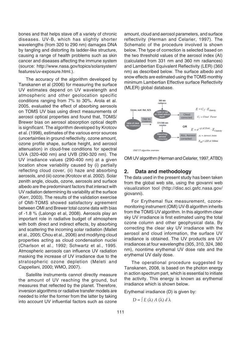
111

bones and that helps stave off a variety of chronicdiseases. UV-B, which has slightly shorterwavelengths (from 320 to 290 nm) damages DNAby tangling and distorting its ladder-like structure,causing a range of health problems such as skincancer and diseases affecting the immune system(source: http://www.nasa.gov/topics/solarsystem/features/uv-exposure.html.).

The accuracy of the algorithm developed byTanskanen et al (2006) for measuring the surfaceUV estimates depend on UV wavelength andatmospheric and other geolocation specificconditions ranging from 7% to 30%. Arola et al.2005, evaluated the effect of absorbing aerosolson TOMS UV bias using direct measurements ofaerosol optical properties and found that, TOMS/Brewer bias on aerosol absorption optical depthis significant. The algorithm developed by Krotcovet al. (1998), estimates of the various error sources(uncertainties in ground reflectivity, ozone amount,ozone profile shape, surface height, and aerosolattenuation) in cloud-free conditions for spectralUVA (320-400 nm) and UVB (290-320 nm). TheUV irradiance values (290-400 nm) at a givenlocation show variability caused by (i) partiallyreflecting cloud cover, (ii) haze and absorbingaerosols, and (iii) ozone (Krotcov et al. 2002). Solarzenith angle, clouds, ozone, aerosols and surfacealbedo are the predominant factors that interact withUV radiation determining its variability at the surface(Kerr, 2003). The results of the validation exerciseof OMI-TOMS showed satisfactory agreementbetween OMI and Brewer total ozone data with biasof -1.8 % (Lalongo et al, 2008). Aerosols play animportant role in radiative budget of atmospherewith both direct and indirect effects, by absorbingand scattering the incoming solar radiation (Malletet al., 2005; Chou et al., 2006) and modifying cloudproperties acting as cloud condensation nuclei(Charlson et al., 1992; Schwartz et al., 1995.Atmospheric aerosols can influence UV radiationmasking the increase of UV irradiance due to thestratospheric ozone depletion (Meleti andCappellani, 2000; WMO, 2007).

Satellite instruments cannot directly measurethe amount of UV reaching the ground, butmeasures that reflected by the planet. Therefore,inversion algorithms or radiative transfer models areneeded to infer the former from the latter by takinginto account UV influential factors such as ozone

amount, cloud and aerosol parameters, and surfacereflectivity (Herman and Celarier, 1997). TheSchematic of the procedure involved is shownbelow. The type of correction is selected based onthe two threshold values of the aerosol index (AI)(calculated from 331 nm and 360 nm radiances)and Lambertian Equivalent Reflectivity (LER) (360nm) as described below. The surface albedo andsnow effects are estimated using the TOMS monthlyminimum Lambertian Effective surface Reflectivity(MLER) global database.

OMI UV algorithm (Herman and Celarier, 1997, ATBD)

2. Data and methodologyThe data used in the present study has been takenfrom the global web site, using the giovanni webvisualization tool (http://disc.sci.gsfc.nasa.gov/giovanni).

For Erythemal flux measurement, ozone-monitoring instrument (OMI) UV-B algorithm inheritsfrom the TOMS UV algorithm. In this algorithm clearsky UV irradiance is first estimated using the totalozone column and other geophysical data. Bycorrecting the clear sky UV irradiance with theaerosol and cloud information, the surface UVirradiance is obtained. The UV products are UVirradiances at four wavelengths (305, 310, 324, 380nm), noontime erythemal UV dose rate and theerythemal UV daily dose.

The operational procedure suggested byTanskanen, 2008, is based on the photon energyin action spectrum part, which is essential to initiatethe activity. This energy is known as erythemalirradiance which is shown below.

Erythemal irradiance (D) is given by:

D = ∫ E (λ) A (λ) d λ

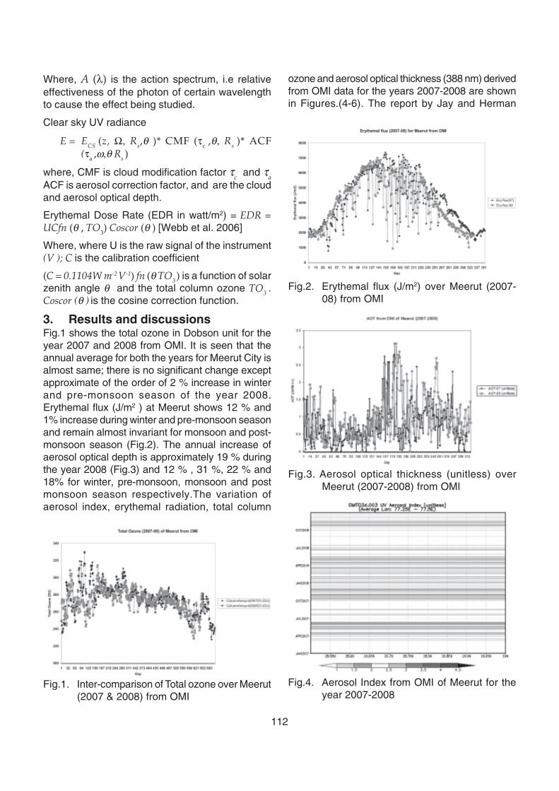
112

Fig.2. Erythemal flux (J/m2) over Meerut (2007-08) from OMI

Fig.3. Aerosol optical thickness (unitless) overMeerut (2007-2008) from OMI

Where, A (λ) is the action spectrum, i.e relativeeffectiveness of the photon of certain wavelengthto cause the effect being studied.

Clear sky UV radiance

E = ECS (z, Ω, Rs,θ )* CMF (τc ,θ, Rs )* ACF(τa ,ω,θ Rs )

where, CMF is cloud modification factor τc and τaACF is aerosol correction factor, and are the cloudand aerosol optical depth.

Erythemal Dose Rate (EDR in watt/m2) = EDR =UCfn (θ , TO3) Coscor (θ ) [Webb et al. 2006]

Where, where U is the raw signal of the instrument(V ); C is the calibration coefficient

(C = 0.1104W m-2 V-1) fn (θ TO3 ) is a function of solarzenith angle θ and the total column ozone TO3 .Coscor (θ ) is the cosine correction function.

3. Results and discussionsFig.1 shows the total ozone in Dobson unit for theyear 2007 and 2008 from OMI. It is seen that theannual average for both the years for Meerut City isalmost same; there is no significant change exceptapproximate of the order of 2 % increase in winterand pre-monsoon season of the year 2008.Erythemal flux (J/m2 ) at Meerut shows 12 % and1% increase during winter and pre-monsoon seasonand remain almost invariant for monsoon and post-monsoon season (Fig.2). The annual increase ofaerosol optical depth is approximately 19 % duringthe year 2008 (Fig.3) and 12 % , 31 %, 22 % and18% for winter, pre-monsoon, monsoon and postmonsoon season respectively.The variation ofaerosol index, erythemal radiation, total column

ozone and aerosol optical thickness (388 nm) derivedfrom OMI data for the years 2007-2008 are shownin Figures.(4-6). The report by Jay and Herman

Fig.1. Inter-comparison of Total ozone over Meerut(2007 & 2008) from OMI

Fig.4. Aerosol Index from OMI of Meerut for theyear 2007-2008

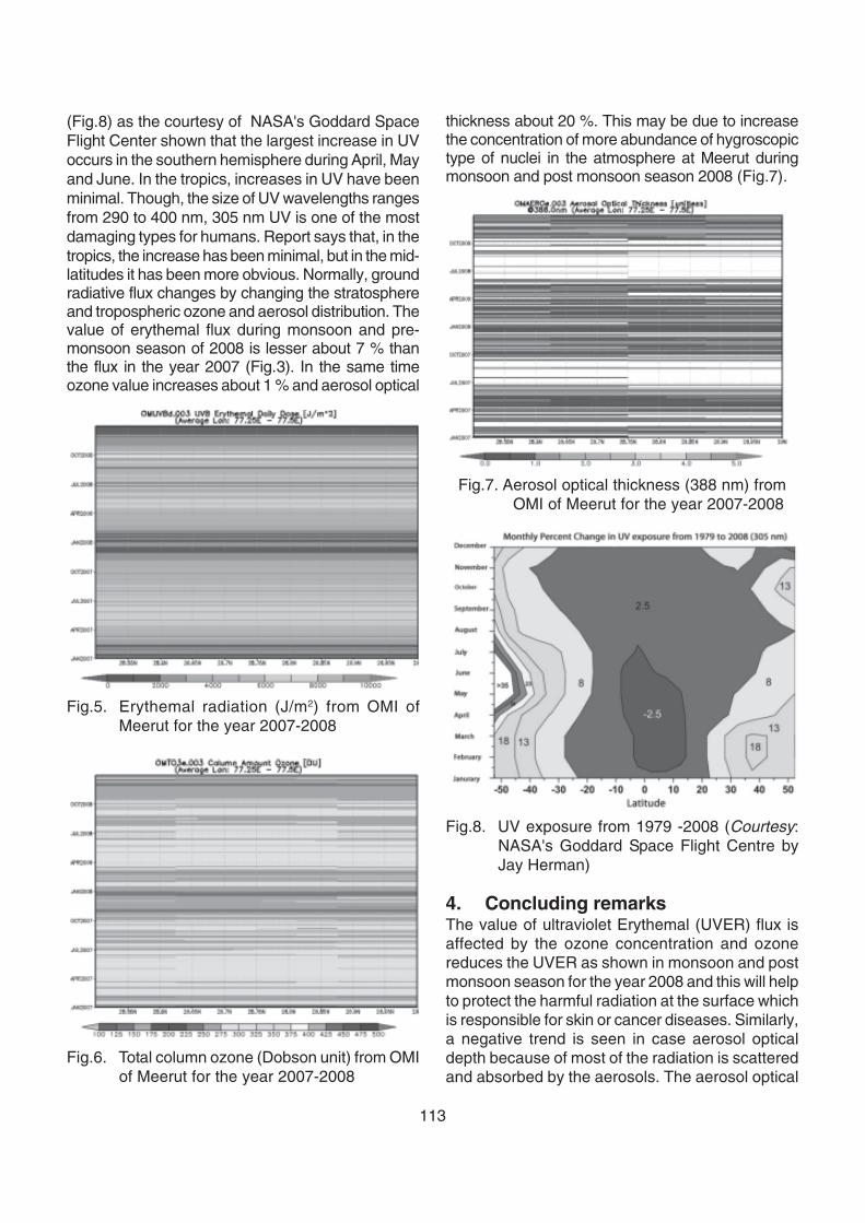
113

thickness about 20 %. This may be due to increasethe concentration of more abundance of hygroscopictype of nuclei in the atmosphere at Meerut duringmonsoon and post monsoon season 2008 (Fig.7).

Fig.6. Total column ozone (Dobson unit) from OMIof Meerut for the year 2007-2008

Fig.5. Erythemal radiation (J/m2) from OMI ofMeerut for the year 2007-2008

(Fig.8) as the courtesy of NASA's Goddard SpaceFlight Center shown that the largest increase in UVoccurs in the southern hemisphere during April, Mayand June. In the tropics, increases in UV have beenminimal. Though, the size of UV wavelengths rangesfrom 290 to 400 nm, 305 nm UV is one of the mostdamaging types for humans. Report says that, in thetropics, the increase has been minimal, but in the mid-latitudes it has been more obvious. Normally, groundradiative flux changes by changing the stratosphereand tropospheric ozone and aerosol distribution. Thevalue of erythemal flux during monsoon and pre-monsoon season of 2008 is lesser about 7 % thanthe flux in the year 2007 (Fig.3). In the same timeozone value increases about 1 % and aerosol optical

Fig.7. Aerosol optical thickness (388 nm) fromOMI of Meerut for the year 2007-2008

Fig.8. UV exposure from 1979 -2008 (Courtesy:NASA's Goddard Space Flight Centre byJay Herman)

4. Concluding remarksThe value of ultraviolet Erythemal (UVER) flux isaffected by the ozone concentration and ozonereduces the UVER as shown in monsoon and postmonsoon season for the year 2008 and this will helpto protect the harmful radiation at the surface whichis responsible for skin or cancer diseases. Similarly,a negative trend is seen in case aerosol opticaldepth because of most of the radiation is scatteredand absorbed by the aerosols. The aerosol optical

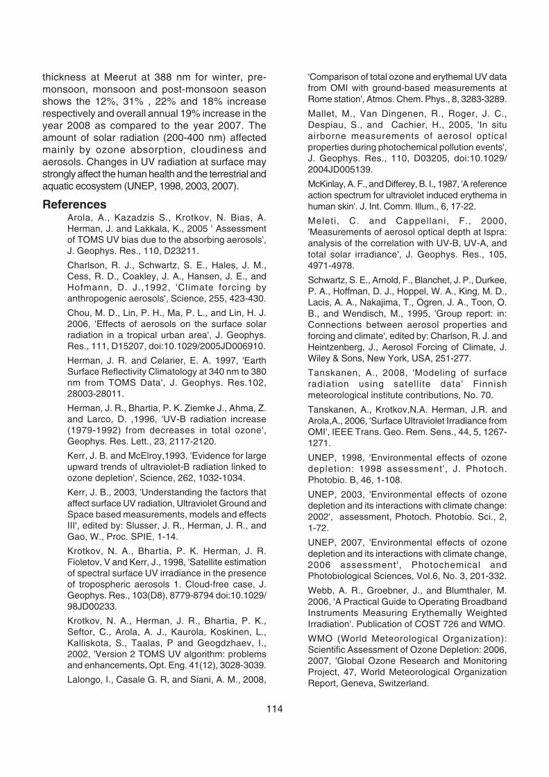
114

thickness at Meerut at 388 nm for winter, pre-monsoon, monsoon and post-monsoon seasonshows the 12%, 31% , 22% and 18% increaserespectively and overall annual 19% increase in theyear 2008 as compared to the year 2007. Theamount of solar radiation (200-400 nm) affectedmainly by ozone absorption, cloudiness andaerosols. Changes in UV radiation at surface maystrongly affect the human health and the terrestrial andaquatic ecosystem (UNEP, 1998, 2003, 2007).

ReferencesArola, A., Kazadzis S., Krotkov, N. Bias, A.Herman, J. and Lakkala, K., 2005 ' Assessmentof TOMS UV bias due to the absorbing aerosols',J. Geophys. Res., 110, D23211.

Charlson, R. J., Schwartz, S. E., Hales, J. M.,Cess, R. D., Coakley, J. A., Hansen, J. E., andHofmann, D. J.,1992, 'Climate forcing byanthropogenic aerosols', Science, 255, 423-430.

Chou, M. D., Lin, P. H., Ma, P. L., and Lin, H. J.2006, 'Effects of aerosols on the surface solarradiation in a tropical urban area', J. Geophys.Res., 111, D15207, doi:10.1029/2005JD006910.

Herman, J. R. and Celarier, E. A. 1997, 'EarthSurface Reflectivity Climatology at 340 nm to 380nm from TOMS Data', J. Geophys. Res.102,28003-28011.

Herman, J. R., Bhartia, P. K. Ziemke J., Ahma, Z.and Larco, D. ,1996, 'UV-B radiation increase(1979-1992) from decreases in total ozone',Geophys. Res. Lett., 23, 2117-2120.

Kerr, J. B. and McElroy,1993, 'Evidence for largeupward trends of ultraviolet-B radiation linked toozone depletion', Science, 262, 1032-1034.

Kerr, J. B., 2003, 'Understanding the factors thataffect surface UV radiation, Ultraviolet Ground andSpace based measurements, models and effectsIII', edited by: Slusser, J. R., Herman, J. R., andGao, W., Proc. SPIE, 1-14.

Krotkov, N. A., Bhartia, P. K. Herman, J. R.Fioletov, V and Kerr, J., 1998, 'Satellite estimationof spectral surface UV irradiance in the presenceof tropospheric aerosols 1. Cloud-free case, J.Geophys. Res., 103(D8), 8779-8794 doi:10.1029/98JD00233.

Krotkov, N. A., Herman, J. R., Bhartia, P. K.,Seftor, C., Arola, A. J., Kaurola, Koskinen, L.,Kalliskota, S., Taalas, P and Geogdzhaev, I.,2002, 'Version 2 TOMS UV algorithm: problemsand enhancements, Opt. Eng. 41(12), 3028-3039.

Lalongo, I., Casale G. R, and Siani, A. M., 2008,

'Comparison of total ozone and erythemal UV datafrom OMI with ground-based measurements atRome station', Atmos. Chem. Phys., 8, 3283-3289.

Mallet, M., Van Dingenen, R., Roger, J. C.,Despiau, S., and Cachier, H., 2005, 'In situairborne measurements of aerosol opticalproperties during photochemical pollution events',J. Geophys. Res., 110, D03205, doi:10.1029/2004JD005139.

McKinlay, A. F., and Differey, B. I., 1987, 'A referenceaction spectrum for ultraviolet induced erythema inhuman skin'. J. Int. Comm. Illum., 6, 17-22.

Meleti, C. and Cappellani, F., 2000,'Measurements of aerosol optical depth at Ispra:analysis of the correlation with UV-B, UV-A, andtotal solar irradiance', J. Geophys. Res., 105,4971-4978.

Schwartz, S. E., Arnold, F., Blanchet, J. P., Durkee,P. A., Hoffman, D. J., Hoppel, W. A., King, M. D.,Lacis, A. A., Nakajima, T., Ogren, J. A., Toon, O.B., and Wendisch, M., 1995, 'Group report: in:Connections between aerosol properties andforcing and climate', edited by: Charlson, R. J. andHeintzenberg, J., Aerosol Forcing of Climate, J.Wiley & Sons, New York, USA, 251-277.

Tanskanen, A., 2008, 'Modeling of surfaceradiation using satellite data' Finnishmeteorological institute contributions, No. 70.

Tanskanen, A., Krotkov,N.A. Herman, J.R. andArola,A., 2006, 'Surface Ultraviolet Irradiance fromOMI', IEEE Trans. Geo. Rem. Sens., 44, 5, 1267-1271.

UNEP, 1998, 'Environmental effects of ozonedepletion: 1998 assessment', J. Photoch.Photobio. B, 46, 1-108.

UNEP, 2003, 'Environmental effects of ozonedepletion and its interactions with climate change:2002', assessment, Photoch. Photobio. Sci., 2,1-72.

UNEP, 2007, 'Environmental effects of ozonedepletion and its interactions with climate change,2006 assessment', Photochemical andPhotobiological Sciences, Vol.6, No. 3, 201-332.

Webb, A. R., Groebner, J., and Blumthaler, M.2006, 'A Practical Guide to Operating BroadbandInstruments Measuring Erythemally WeightedIrradiation'. Publication of COST 726 and WMO.

WMO (World Meteorological Organization):Scientific Assessment of Ozone Depletion: 2006,2007, 'Global Ozone Research and MonitoringProject, 47, World Meteorological OrganizationReport, Geneva, Switzerland.

115

1. IntroductionIndian monsoon months are highly looked forwardto by agriculturists, meteorologists and otherresearchers so as to know about its performancein terms of rainfall during the season every year.Apart from the copious rainfall events, scope forformation of 'Monsoon Depressions(MDs)' over thenorth Bay of Bengal or Head Bay (north of 18½° NLatitude) exists. Generally MDs after having formedin the north Bay of Bengal travel in sea for a veryshort distance before crossing the land mass / ordecaying (Asnani 2005). Hence MDs, in general,do not attain highest intensity. However, it is veryinteresting to note that each MD, though formed ina very small region over Head Bay, follows differentpath while moving in the sea, in spite of a very shorttravel. The present study is aimed to understandthe movement of Cyclonic Storm (CS) Pyarr, whichdiverted its movement slightly in a southwesterly(SWly) direction, its associated wind structure andthe RMW terms of outputs obtained from QuikSCAT and TRMM data. Moreover CS Pyarrintensified into cyclonic storm over Bay of Bengalafter about eight years after the Severe CyclonicStorm of 23 September 1997, which crossed coast.

ABSTRACT

One of the main challenges in the study of tropical cyclones is to understand it right from its genesis, directionof movement and intensification. Earlier studies reveal that maximum potential intensity of a tropical cyclonecan be determined using the Radius of Maximum Wind (RMW) which is defined as the distance between thecentre of the cyclonic storm and its band of strongest winds. Yet another interesting information is that thetropical cyclones give abundant rainfall. The highest rainfall rates occur near the RMW. Efforts have beenmade in this study to analyse the direction of movement with regard to the region of RMW and the area ofmaximum rainfall in a cyclonic storm when the storm is at sea. The QuikSCAT sea wind data and thecorresponding images, Tropical Rainfall Measuring Mission (TRMM) three hourly precipitation data - 3B42V6 product and statistics obtained through Cyclone eAtlas of IMD in respect of Cyclonic Storm Pyarr werearchived and used in this study. The analyses of the details derived from the above data sets revealed that all theabove products supported the well established theory of intensification and occurrence of rainfall in a Tropicalcyclone and thus the modern products can provide valid details to the forecasters during real time situationvery well to aid better forecasting.

Key words: QuikSCAT, TRMM, Tropical Cyclone and Radius of Maximum Wind

2. Data and methodologyThe statistics on frequency of formation of cyclonicdisturbances(C&Ds) over Bay of Bengal for themonsoon period June to September was generatedthrough Cyclone eAtlas-IMD software 2008, withthe chosen basic input for the years 1891 - 2009.There had been 443 C&Ds which formed over Bayof Bengal during the above period for the giveninput. The statistics on frequency of C&Ds for themonth of September alone accounts for 163cyclonic disturbances. The area of the Bay ofBengal which falls to the north of 18½°N is referredto as North Bay of Bengal or Head Bay. Advancedoption 1 of eAtlas software was invoked to obtainthe details of tracks of C&Ds formed over this areai.e., bounded by latitudinal/ longitudinal area18-22°N/82-94°E and the software generated tracksof 78 C&Ds [67 Depressions(D), 10 CyclonicStorms(CS) and 1 Severe Cyclonic Storms(SCS)].

The frequency of C&Ds formed in specified areaof formation bounded by 18-20°N latitude and 91-92°E longitude. The following was obtained througheAtlas software three cyclonic disturbances hadoccurred during the entire period of 119 years.

Associated wind pattern, rainfalland radius of maximum wind(RMW) in a Tropical Cyclone overBay of Bengal - A case study

P. A. Subadra and V. Radhika RaniRegional Meteorological Centre,

India Meteorological Department,Chennai-600 006

email:subadra.imd@gmail.com

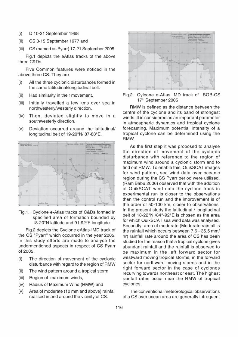
116

(i) D 10-21 September 1968

(ii) CS 8-15 September 1977 and

(iii) CS (named as Pyarr) 17-21 September 2005.

Fig.1 depicts the eAtlas tracks of the abovethree C&Ds.

Five Common features were noticed in theabove three CS. They are

(i) All the three cyclonic disturbances formed inthe same latitudinal/longitudinal belt.

(ii) Had similarity in their movement.

(iii) Initially travelled a few kms over sea innorthwesterly/westerly direction,

(iv) Then, deviated slightly to move in asouthwesterly direction.

(v) Deviation occurred around the latitudinal/longitudinal belt of 19-20°N/ 87-88°E.

RMW is defined as the distance between thecentre of the cyclone and its band of strongestwinds. It is considered as an important parameterin atmospheric dynamics and tropical cycloneforecasting. Maximum potential intensity of atropical cyclone can be determined using theRMW.

As the first step it was proposed to analysethe direction of movement of the cyclonicdisturbance with reference to the region ofmaximum wind around a cyclonic storm and tofind out RMW. To enable this, QuikSCAT imagesfor wind pattern, sea wind data over oceanicregion during the CS Pyarr period were utilised.(Ram Babu,2006) observed that with the additionof QuikSCAT wind data the cyclone track inexperimental run is closer to the observationsthan the control run and the improvement is ofthe order of 50-100 km, closer to observations.In the present study the latitudinal / longitudinalbelt of 18-22°N /84°-92°E is chosen as the areafor which QuikSCAT sea wind data was analysed.Secondly, area of moderate (Moderate rainfall isthe rainfall which occurs between 7.6 - 35.5 mm/hr) rainfall rate around the area of CS has beenstudied for the reason that a tropical cyclone givesabundant rainfall and the rainfall is observed tobe maximum in the left forward sector forwestward moving tropical storms, in the forwardsector for northward moving storms and in theright forward sector in the case of cyclonesrecurving towards northeast or east. The highestrainfall rates occur near the RMW of tropicalcyclones.

The conventional meteorological observationsof a CS over ocean area are generally infrequent

Fig.1. Cyclone e-Atlas tracks of C&Ds formed inspecified area of formation bounded by18-20°N latitude and 91-92°E longitude.

Fig.2. Cylcone e-Atlas IMD track of BOB-CS17th September 2005

Fig.2 depicts the Cyclone eAtlas-IMD track ofthe CS "Pyarr" which occurred in the year 2005.In this study efforts are made to analyse theundermentioned aspects in respect of CS Pyarrof 2005.

(i) The direction of movement of the cyclonicdisturbance with regard to the region of RMW

(ii) The wind pattern around a tropical storm

(iii) Region of maximum winds,

(iv) Radius of Maximum Wind (RMW) and

(v) Area of moderate (10 mm and above) rainfallrealised in and around the vicinity of CS.

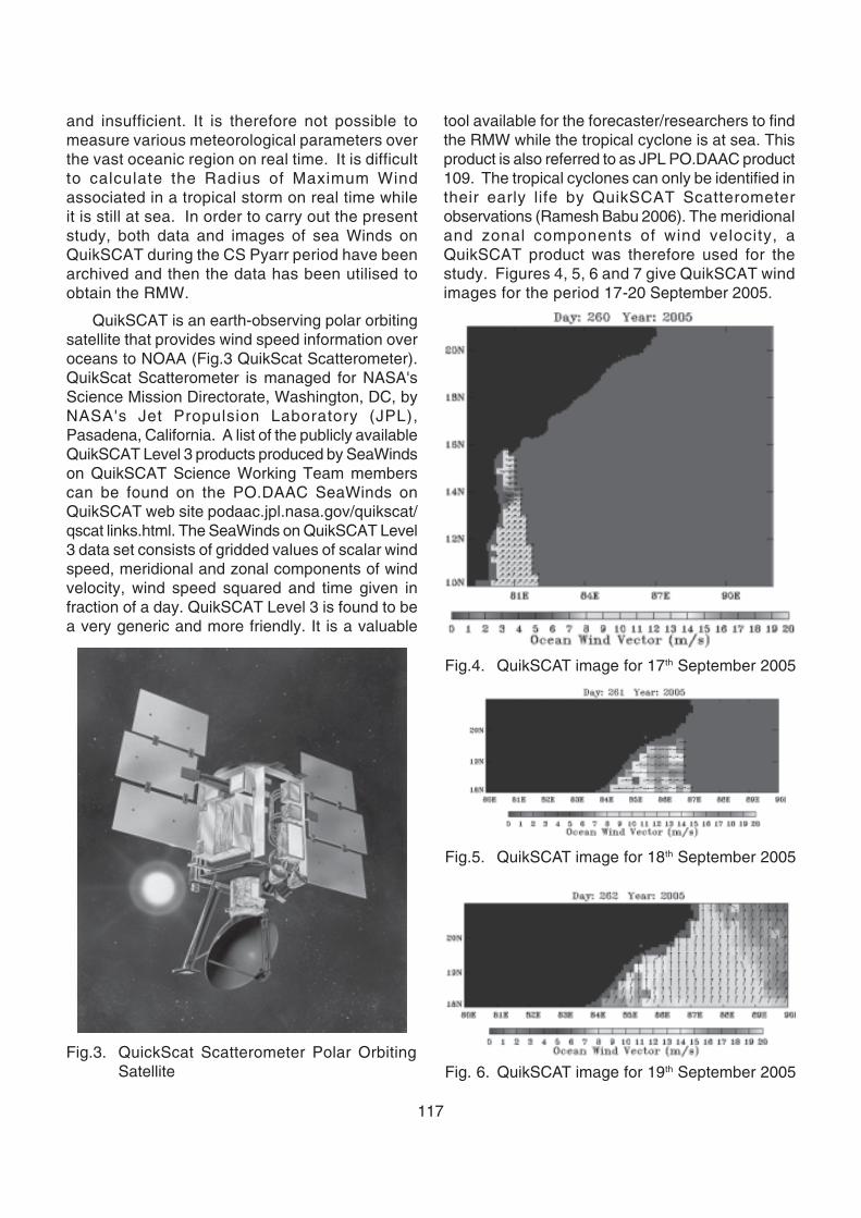
117

and insufficient. It is therefore not possible tomeasure various meteorological parameters overthe vast oceanic region on real time. It is difficultto calculate the Radius of Maximum Windassociated in a tropical storm on real time whileit is still at sea. In order to carry out the presentstudy, both data and images of sea Winds onQuikSCAT during the CS Pyarr period have beenarchived and then the data has been utilised toobtain the RMW.

QuikSCAT is an earth-observing polar orbitingsatellite that provides wind speed information overoceans to NOAA (Fig.3 QuikScat Scatterometer).QuikScat Scatterometer is managed for NASA'sScience Mission Directorate, Washington, DC, byNASA's Jet Propulsion Laboratory (JPL),Pasadena, California. A list of the publicly availableQuikSCAT Level 3 products produced by SeaWindson QuikSCAT Science Working Team memberscan be found on the PO.DAAC SeaWinds onQuikSCAT web site podaac.jpl.nasa.gov/quikscat/qscat links.html. The SeaWinds on QuikSCAT Level3 data set consists of gridded values of scalar windspeed, meridional and zonal components of windvelocity, wind speed squared and time given infraction of a day. QuikSCAT Level 3 is found to bea very generic and more friendly. It is a valuable

Fig.3. QuickScat Scatterometer Polar OrbitingSatellite

Fig.4. QuikSCAT image for 17th September 2005

Fig.5. QuikSCAT image for 18th September 2005

Fig. 6. QuikSCAT image for 19th September 2005

tool available for the forecaster/researchers to findthe RMW while the tropical cyclone is at sea. Thisproduct is also referred to as JPL PO.DAAC product109. The tropical cyclones can only be identified intheir early life by QuikSCAT Scatterometerobservations (Ramesh Babu 2006). The meridionaland zonal components of wind velocity, aQuikSCAT product was therefore used for thestudy. Figures 4, 5, 6 and 7 give QuikSCAT windimages for the period 17-20 September 2005.

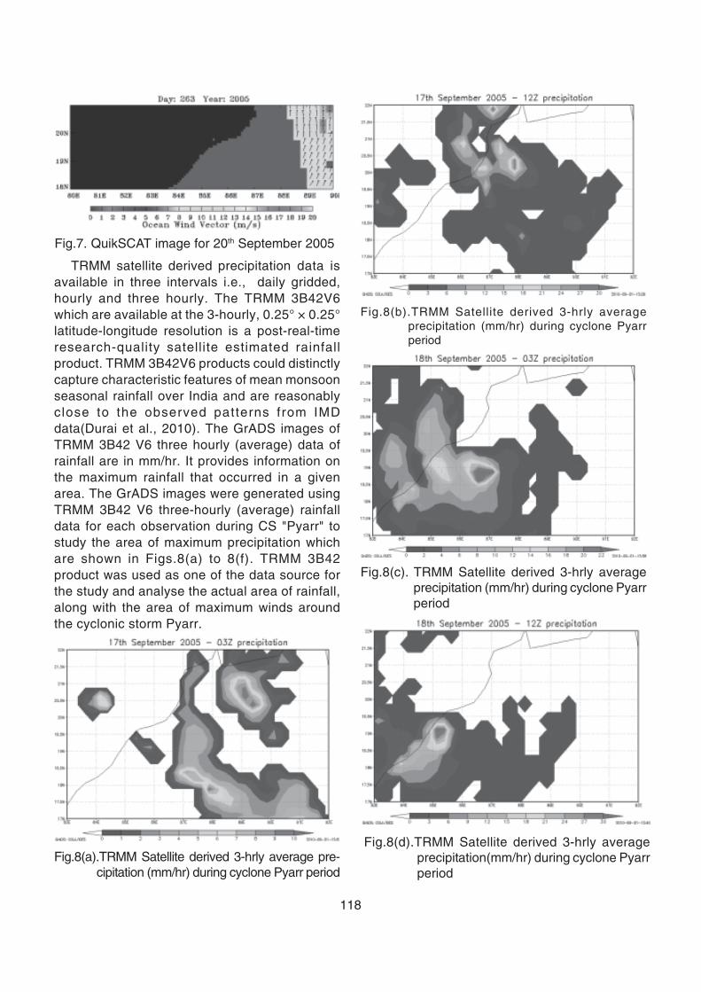
118

TRMM satellite derived precipitation data isavailable in three intervals i.e., daily gridded,hourly and three hourly. The TRMM 3B42V6which are available at the 3-hourly, 0.25° × 0.25°latitude-longitude resolution is a post-real-timeresearch-quality satellite estimated rainfallproduct. TRMM 3B42V6 products could distinctlycapture characteristic features of mean monsoonseasonal rainfall over India and are reasonablyclose to the observed patterns from IMDdata(Durai et al., 2010). The GrADS images ofTRMM 3B42 V6 three hourly (average) data ofrainfall are in mm/hr. It provides information onthe maximum rainfall that occurred in a givenarea. The GrADS images were generated usingTRMM 3B42 V6 three-hourly (average) rainfalldata for each observation during CS "Pyarr" tostudy the area of maximum precipitation whichare shown in Figs.8(a) to 8(f). TRMM 3B42product was used as one of the data source forthe study and analyse the actual area of rainfall,along with the area of maximum winds aroundthe cyclonic storm Pyarr.

Fig.7. QuikSCAT image for 20th September 2005

Fig.8(a).TRMM Satellite derived 3-hrly average pre-cipitation (mm/hr) during cyclone Pyarr period

Fig.8(d).TRMM Satellite derived 3-hrly averageprecipitation(mm/hr) during cyclone Pyarrperiod

Fig.8(c). TRMM Satellite derived 3-hrly averageprecipitation (mm/hr) during cyclone Pyarrperiod

Fig.8(b).TRMM Satellite derived 3-hrly averageprecipitation (mm/hr) during cyclone Pyarrperiod

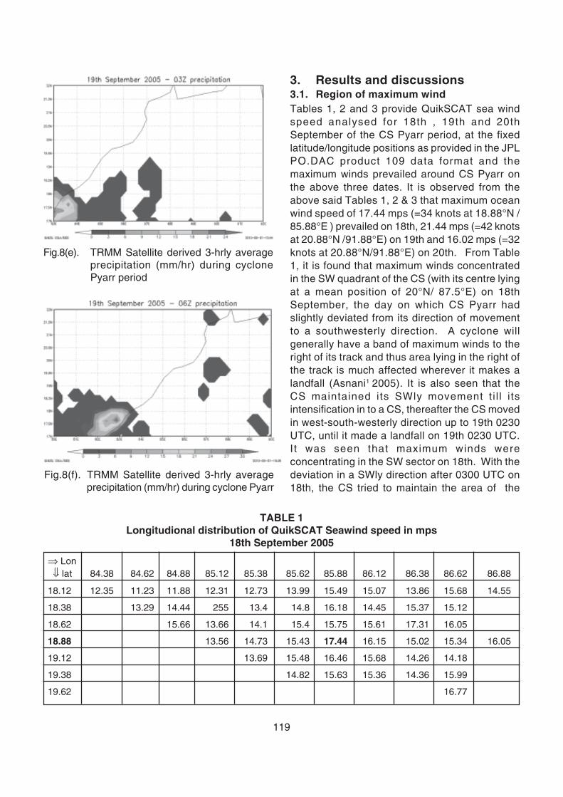
119

3. Results and discussions3.1. Region of maximum windTables 1, 2 and 3 provide QuikSCAT sea windspeed analysed for 18th , 19th and 20thSeptember of the CS Pyarr period, at the fixedlatitude/longitude positions as provided in the JPLPO.DAC product 109 data format and themaximum winds prevailed around CS Pyarr onthe above three dates. It is observed from theabove said Tables 1, 2 & 3 that maximum oceanwind speed of 17.44 mps (=34 knots at 18.88°N /85.88°E ) prevailed on 18th, 21.44 mps (=42 knotsat 20.88°N /91.88°E) on 19th and 16.02 mps (=32knots at 20.88°N/91.88°E) on 20th. From Table1, it is found that maximum winds concentratedin the SW quadrant of the CS (with its centre lyingat a mean position of 20°N/ 87.5°E) on 18thSeptember, the day on which CS Pyarr hadslightly deviated from its direction of movementto a southwesterly direction. A cyclone willgenerally have a band of maximum winds to theright of its track and thus area lying in the right ofthe track is much affected wherever it makes alandfall (Asnani1 2005). It is also seen that theCS maintained its SWly movement t i l l i tsintensification in to a CS, thereafter the CS movedin west-south-westerly direction up to 19th 0230UTC, until it made a landfall on 19th 0230 UTC.It was seen that maximum winds wereconcentrating in the SW sector on 18th. With thedeviation in a SWly direction after 0300 UTC on18th, the CS tried to maintain the area of the

Fig.8(e). TRMM Satellite derived 3-hrly averageprecipitation (mm/hr) during cyclonePyarr period

Fig.8(f). TRMM Satellite derived 3-hrly averageprecipitation (mm/hr) during cyclone Pyarr

TABLE 1Longitudional distribution of QuikSCAT Seawind speed in mps

18th September 2005

⇒ Lon ⇓ lat 84.38 84.62 84.88 85.12 85.38 85.62 85.88 86.12 86.38 86.62 86.88

18.12 12.35 11.23 11.88 12.31 12.73 13.99 15.49 15.07 13.86 15.68 14.55

18.38 13.29 14.44 255 13.4 14.8 16.18 14.45 15.37 15.12

18.62 15.66 13.66 14.1 15.4 15.75 15.61 17.31 16.05

18.88 13.56 14.73 15.43 17.44 16.15 15.02 15.34 16.05

19.12 13.69 15.48 16.46 15.68 14.26 14.18

19.38 14.82 15.63 15.36 14.36 15.99

19.62 16.77

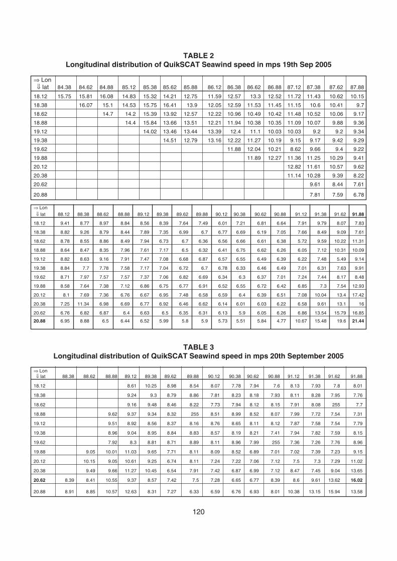
120

TABLE 2Longitudinal distribution of QuikSCAT Seawind speed in mps 19th Sep 2005

⇒ Lon ⇓ lat 84.38 84.62 84.88 85.12 85.38 85.62 85.88 86.12 86.38 86.62 86.88 87.12 87.38 87.62 87.88

18.12 15.75 15.81 16.08 14.83 15.32 14.21 12.75 11.59 12.57 13.3 12.52 11.72 11.43 10.62 10.15

18.38 16.07 15.1 14.53 15.75 16.41 13.9 12.05 12.59 11.53 11.45 11.15 10.6 10.41 9.7

18.62 14.7 14.2 15.39 13.92 12.57 12.22 10.96 10.49 10.42 11.48 10.52 10.06 9.17

18.88 14.4 15.84 13.66 13.51 12.21 11.94 10.38 10.35 11.09 10.07 9.88 9.36

19.12 14.02 13.46 13.44 13.39 12.4 11.1 10.03 10.03 9.2 9.2 9.34

19.38 14.51 12.79 13.16 12.22 11.27 10.19 9.15 9.17 9.42 9.29

19.62 11.88 12.04 10.21 8.62 9.66 9.4 9.22

19.88 11.89 12.27 11.36 11.25 10.29 9.41

20.12 12.82 11.61 10.57 9.62

20.38 11.14 10.28 9.39 8.22

20.62 9.61 8.44 7.61

20.88 7.81 7.59 6.78

⇒ Lon ⇓ lat 88.12 88.38 88.62 88.88 89.12 89.38 89.62 89.88 90.12 90.38 90.62 90.88 91.12 91.38 91.62 91.88

18.12 9.41 8.77 8.97 8.84 8.56 8.39 7.64 7.49 6.01 7.21 6.81 6.64 7.91 9.79 8.07 7.83

18.38 8.82 9.26 8.79 8.44 7.89 7.35 6.99 6.7 6.77 6.69 6.19 7.05 7.66 8.49 9.09 7.61

18.62 8.78 8.55 8.86 8.49 7.94 6.73 6.7 6.36 6.56 6.66 6.61 6.38 5.72 9.59 10.22 11.31

18.88 8.64 8.47 8.35 7.96 7.61 7.17 6.5 6.32 6.41 6.75 6.62 6.26 6.05 7.12 10.31 10.09

19.12 8.82 8.63 9.16 7.91 7.47 7.08 6.68 6.87 6.57 6.55 6.49 6.39 6.22 7.48 5.49 9.14

19.38 8.84 7.7 7.78 7.58 7.17 7.04 6.72 6.7 6.78 6.33 6.46 6.49 7.01 6.31 7.63 9.91

19.62 8.71 7.97 7.57 7.57 7.37 7.06 6.82 6.69 6.34 6.3 6.37 7.01 7.24 7.44 8.17 8.48

19.88 8.58 7.64 7.38 7.12 6.86 6.75 6.77 6.91 6.52 6.55 6.72 6.42 6.85 7.3 7.54 12.93

20.12 8.1 7.69 7.36 6.76 6.67 6.95 7.48 6.58 6.59 6.4 6.39 6.51 7.08 10.04 13.4 17.42

20.38 7.25 11.34 6.98 6.69 6.77 6.92 6.46 6.62 6.14 6.01 6.03 6.22 6.58 9.61 13.1 16

20.62 6.76 6.82 6.87 6.4 6.63 6.5 6.35 6.31 6.13 5.9 6.05 6.26 6.86 13.54 15.79 16.85

20.88 6.95 8.88 6.5 6.44 6.52 5.99 5.8 5.9 5.73 5.51 5.84 4.77 10.67 15.48 19.6 21.44

TABLE 3Longitudinal distribution of QuikSCAT Seawind speed in mps 20th September 2005

⇒ Lon ⇓ lat 88.38 88.62 88.88 89.12 89.38 89.62 89.88 90.12 90.38 90.62 90.88 91.12 91.38 91.62 91.88

18.12 8.61 10.25 8.98 8.54 8.07 7.78 7.94 7.6 8.13 7.93 7.8 8.01

18.38 9.24 9.3 8.79 8.86 7.81 8.23 8.18 7.93 8.11 8.28 7.95 7.76

18.62 9.16 9.48 8.46 8.22 7.73 7.94 8.12 8.15 7.91 8.08 255 7.7

18.88 9.62 9.37 9.34 8.32 255 8.51 8.99 8.52 8.07 7.99 7.72 7.54 7.31

19.12 9.51 8.92 8.56 8.37 8.16 8.76 8.65 8.11 8.12 7.87 7.58 7.54 7.79

19.38 8.96 9.04 8.95 8.84 8.83 8.57 8.19 8.21 7.41 7.94 7.82 7.59 8.15

19.62 7.92 8.3 8.81 8.71 8.89 8.11 8.96 7.99 255 7.36 7.26 7.76 8.96

19.88 9.05 10.01 11.03 9.65 7.71 8.11 8.09 8.52 6.89 7.01 7.02 7.39 7.23 9.15

20.12 10.15 9.05 10.61 9.25 6.74 8.11 7.24 7.22 7.06 7.12 7.5 7.3 7.29 11.02

20.38 9.49 9.66 11.27 10.45 6.54 7.91 7.42 6.87 6.99 7.12 8.47 7.45 9.04 13.65

20.62 8.39 8.41 10.55 9.37 8.57 7.42 7.5 7.28 6.65 6.77 8.39 8.6 9.61 13.62 16.02

20.88 8.91 8.85 10.57 12.63 8.31 7.27 6.33 6.59 6.76 6.93 8.01 10.38 13.15 15.94 13.58

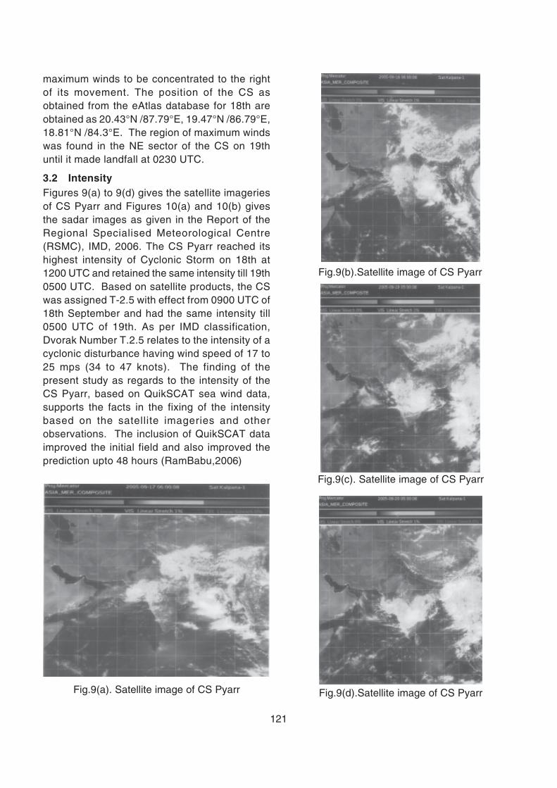
121

Fig.9(b).Satellite image of CS Pyarr

Fig.9(c). Satellite image of CS Pyarr

Fig.9(d).Satellite image of CS PyarrFig.9(a). Satellite image of CS Pyarr

maximum winds to be concentrated to the rightof its movement. The position of the CS asobtained from the eAtlas database for 18th areobtained as 20.43°N /87.79°E, 19.47°N /86.79°E,18.81°N /84.3°E. The region of maximum windswas found in the NE sector of the CS on 19thuntil it made landfall at 0230 UTC.

3.2 IntensityFigures 9(a) to 9(d) gives the satellite imageriesof CS Pyarr and Figures 10(a) and 10(b) givesthe sadar images as given in the Report of theRegional Specialised Meteorological Centre(RSMC), IMD, 2006. The CS Pyarr reached itshighest intensity of Cyclonic Storm on 18th at1200 UTC and retained the same intensity till 19th0500 UTC. Based on satellite products, the CSwas assigned T-2.5 with effect from 0900 UTC of18th September and had the same intensity till0500 UTC of 19th. As per IMD classification,Dvorak Number T.2.5 relates to the intensity of acyclonic disturbance having wind speed of 17 to25 mps (34 to 47 knots). The finding of thepresent study as regards to the intensity of theCS Pyarr, based on QuikSCAT sea wind data,supports the facts in the fixing of the intensitybased on the satellite imageries and otherobservations. The inclusion of QuikSCAT dataimproved the initial field and also improved theprediction upto 48 hours (RamBabu,2006)

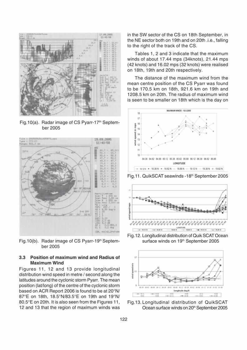
122

Fig.12. Longitudinal distribution of Quik SCAT Oceansurface winds on 19th September 2005

Fig.13. Longitudinal distribution of QuikSCATOcean surface winds on 20th September 2005

Fig.11. QuikSCAT seawinds -18th September 2005

in the SW sector of the CS on 18th September, inthe NE sector both on 19th and on 20th .i.e., fallingto the right of the track of the CS.

Tables 1, 2 and 3 indicate that the maximumwinds of about 17.44 mps (34knots), 21.44 mps(42 knots) and 16.02 mps (32 knots) were realisedon 18th, 19th and 20th respectively.

The distance of the maximum wind from themean centre position of the CS Pyarr was foundto be 170.5 km on 18th, 921.6 km on 19th and1208.5 km on 20th. The radius of maximum windis seen to be smaller on 18th which is the day on

Fig.10(b). Radar image of CS Pyarr-19th Septem-ber 2005

Fig.10(a). Radar image of CS Pyarr-17th Septem-ber 2005

3.3 Position of maximum wind and Radius ofMaximum Wind

Figures 11, 12 and 13 provide longitudinaldistribution wind speed in metre / second along thelatitudes around the cyclonic storm Pyarr. The meanposition (lat/long) of the centre of the cyclonic stormbased on ACR Report 2006 is found to be at 20°N/87°E on 18th, 18.5°N/83.5°E on 19th and 19°N/80.5°E on 20th. It is also seen from the Figures 11,12 and 13 that the region of maximum winds was

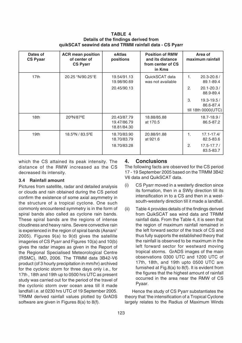
123

TABLE 4Details of the findings derived from

quikSCAT seawind data and TRMM rainfall data - CS Pyarr

Dates of ACR mean position eAtlas Position of RMW Area ofCS Pyaar of center of positions and its distance maximum rainfall

CS Pyarr from center of CSin Kms

17th 20.25 °N/90.25°E 19.54/91.13 QuickSCAT data 1. 20.3-20.6 /19.98/90.69 was not available 89.1-89.4

20.45/90.13 2. 20.1-20.3 /88.9-89.4

3. 19.3-19.5 /86.6-87.4

till 18th 0000(UTC)

18th 20ºN/87ºE 20.43/87.79 18.88/85.88 18.7-18.9 /19.47/86.79 at 170.5 86.5-87.218.81/84.30

19th 18.5ºN / 83.5ºE 18.70/83.90 20.88/91.88 1. 17.1-17.4/18.70/83.79 at 921.6 82.5-83.6

18.70/83.28 2. 17.5-17.7 /83.5-83.7

which the CS attained its peak intensity. Thedistance of the RMW increased as the CSdecreased its intensity.

3.4 Rainfall amountPictures from satellite, radar and detailed analysisor clouds and rain obtained during the CS periodconfirm the existence of some axial asymmetry inthe structure of a tropical cyclone. One suchcommonly encountered symmetry is in the form ofspiral bands also called as cyclone rain bands.These spiral bands are the regions of intensecloudiness and heavy rains. Severe convective rainis experienced in the region of spiral bands (Asnani1

2005). Figures 9(a) to 9(d) gives the satelliteimageries of CS Pyarr and Figures 10(a) and 10(b)gives the radar images as given in the Report ofthe Regional Specialised Meteorological Centre(RSMC), IMD, 2006. The TRMM data 3B42-V6product (of 3 hourly precipitation in mm/hr) archivedfor the cyclonic storm for three days only i.e., for17th , 18th and 19th up to 0500 hrs UTC as presentstudy was carried out for the period of the travel ofthe cyclonic storm over ocean area till it madelandfall i.e. at 0230 hrs UTC of 19 September 2005.TRMM derived rainfall values plotted by GrADSsoftware are given in Figures 8(a) to 8(f).

4. ConclusionsThe following facts are observed for the CS period17 - 19 September 2005 based on the TRMM 3B42V6 data and QuikSCAT data.

(i) CS Pyarr moved in a westerly direction sinceits formation, then in a SWly direction till itsintensification in to a CS and then in a west-south-westerly direction till it made a landfall.

(ii) Table 4 provides details of the findings derivedfrom QuikSCAT sea wind data and TRMMrainfall data. From the Table 4, it is seen thatthe region of maximum rainfall remained inthe left forward sector of the track of CS andthus fully supports the established theory thatthe rainfall is observed to be maximum in theleft forward sector for westward movingtropical storms. GrADS images of the mainobservations 0300 UTC and 1200 UTC of17th, 18th, and 19th upto 0500 UTC arefurnished at Fig.8(a) to 8(f). It is evident fromthe figures that the highest amount of rainfalloccurred in the area near the RMW of CSPyaar.

Hence the study of CS Pyarr substantiates thetheory that 'the intensification of a Tropical Cyclonelargely relates to the Radius of Maximum Winds

124

around it'. From the present study it is felt that theQuickSCAT sea wind data if available, for thetropical cyclone periods, on real time basis, will bean added tool for forecasting the movement ofCyclones and Depressions, in calculating RMWof CS and its distance along with the otherimportant tools which are being used at present.

Similar such studies for various aspects inrespect of different tropical cyclones usingQuikSCAT sea wind data may provide usefulinformation. A systematic study with TRMM datamay also provide vital information for forecasterson real time.

AcknowledgementThe authors are thankful to Deputy Director Generalof Meteorology, Regional Meteorological Centre,Chennai for providing opportunity and facility to carryout the study. They also express sincere thanks toMs.B.Amudha, Met.I, RMC Chennai who encouragedand offered suggestions for improving the study.Authors also acknowledge use of QuikSCAT andTRMM products of NASA, USA in this study.

ReferencesAsnani, G.C., 2005, 'Tropical Meteorology',Pune Vol.II,

http://www.poet.jpl.nasa.gov/.for QuikSCATseawinds over ocean surface.

http://trmm.gfsc.noaa.gov/ for TRMM 3B42V6products.

Cyclone e-Atlas, 2008, IMD software.

Durai,V.R., et al., 2010, 'Evaluation of Indiansummer monsoon rainfall features usingTRMM and KALPANA-1 satellite derivedprecipitation and rain gauge observation',Mausam,Vol.61,No.3,317-336.

Lorne, 2000, "The preliminary study of theimpact of QuikSCAT /Sea winds oceansurface winds data to the JMA global model",Fifth International Winds Workshopproceedings" , Australia, Tahara,Y.

Ram Babu,G.,2006, 'QuikSCAT scatterometerwind data impact on tropical cyclone forecastby a mesoscale model', Mausam, Vol.57, No.1,141-150.

Report on Annual Cyclone Review Meeting,2006, IMD.

Report of Regional Specialised MeteorologicalCentre, 2006, IMD.

RamBabu, G., 2004 "Impact of assimilationof QuikSCAT data in mesoscale modelingsystem' Seventh International WindsWorkshop proceeding, Finland, 2004.