Who Has Most Say in Cooking?

ASARC Working Paper 2009/19

Who Has Most Say in Cooking?

Raghav Gaiha, Faculty of Management Studies, University of Delhi,

Raghbendra Jha,

Arndt-Corden Division of Economics Research School of Pacific and Asian Studies

Australian National University,

&

Vani S. Kulkarni, Centre of South Asian Studies,

Yale University.

November 2009

ASARC WP 2009/19 2

Abstract

The present analysis seeks to build on household economics literature by focusing on who in fact has most say in cooking-the female spouse, the husband or a senior female member/ the mother-in-law-and how this role is shaped by a diversity of factors (e.g. caste, type of family, demographic characteristics, educational attainments, affluence, and location). A complex but not implausible pattern is revealed in which all these variables matter in varying degrees. To the extent that caste, type of family, number of male and female adults in paid employment, their educational attainments, and life- style differences matter, the familiar story of a more decisive role of women in paid employment in influencing household allocation of resources for food, health and education needs reexamination. More importantly, if the patterns of decision-making revealed by our analysis are associated with more varied nutritional and other health related outcomes, the policies designed to influence the latter are far from obvious-especially in light of the important roles of cultural values and evolving life style patterns.

Key words: cooking decisions, family structure, caste, affluence, location JEL codes: D10, D12, H31, Q12

ASARC WP 2009/19 3

Who Has Most Say in Cooking?1

Introduction

Towards a better understanding of nutritional outcomes, an attempt is made here to examine who has most say in cooking decisions-whether, for example, the female spouse, or the male spouse, or the mother-in-law. This may matter if their food preferences differ. Not just the amounts allocated for food but also its composition may be sensitive to who decides what will be cooked. Extant literature does not go beyond whether women have a greater say in allocation of household resources for food, education and health. Of particular significance are resources allocated for the benefit of children, and between male and female children. Household decision-making is formalised from two distinct perspectives: the neo-classical and the bargaining ones. In both formulations, women have a greater say in household allocation of resources depending on whether they are engaged in outside employment. In a more specialised formulation, the dowry that a married woman brings with her contributes to her baragaining power within a household. Our analysis goes a step beyond this literature in focusing on who has the most say in cooking, allowing for family type, education, adult male and female employment in paid work, caste affiliation, and socio-economic status. The focus is on the interplay of economic, social or cultural, and demographic characteristics as determinants of who has most say in cooking. In a sequel, an attempt will be made to link nutritional outcomes for both children and adults to who has most say in cooking, controlling for individual, household and other characteristics.

Intrahousehold Allocation

An important contribution is Becker’s (1981) common preference or altruistic model of household behaviour. It assumes a household utility function that reflects the preferences of all members. Maximising this subject to the budget constraint yields demand functions for goods and leisure. In this model, all household resources (capital, labour and land) are pooled and all expenditures are made with pooled income2. As its point of departure, the alternative model assumes differences in preferences among household members, which are resolved by a bargaining process. The bargaining generates an agreed, self-enforcing utility function. Using cooperative Nash, non-cooperative Nash and other related solutions, bargaining models of 1 This study is funded by the British government, under the Foresight Global Food and Farming Futures Project. Our appreciation is due to Raj Bhatia for his computational expertise, and to Woojin Kang for his superb mathematical skills. Discussions with Anil Deolalikar, L. Haddad and A. V. Subramanian were extremely useful in carrying out the analysis, as also some insightful but provocative remarks by Shylashri Shankar. We are grateful to Sonal Desai for furnishing the details of the University of Maryland-NCAER household survey.The views expressed are, however, the sole responsibility of the authors 2 For an admirably clear and comprehensive overview of models of household economics, see Behrman and Deolalikar (1995).

ASARC WP 2009/19 4

household behaviour are formulated (e.g. Sen, 1983, Manser and Brown, 1980, McElroy and Horney, 1981, Lundberg and Pollak, 1991). A key concept is the threat point (or fall-back position) which determines an individual’s bargaining power3. One major difficulty in choosing between the common preference and bargaining models is that they lead to similar predictions in many cases (Hoddinott, 1992). Suppose that an exogenous change occurs that increases the return to women’s labour outside the household. Both models predict that this may lead to changes in the allocation of women’s time. In the common preference model, the household head or benefactor may decide to reorganise household production so as to increase women’s labour market participation4. In a bargaining context, women may decide to renegotiate the conjugal contract on the basis of the enhanced earning opportunity. Further, increased women’s labour force participation may alter the distribution of income within the household and this could affect the pattern of household expenditure. But again, this would be predicted by both the models. In the common preference model, the change in expenditure may reflect the reallocation of members’ time. For example, households may purchase fuel rather than gather it. Alternatively, the increase in women’s earnings outside the household raises their bargaining power within it either because their threat point is higher or because their perceived contribution within the household is greater. However, there are pieces of evidence that lend greater plausibility to the bargaining models5. Monetary transfers in the common preference model, for example, would be negatively linked to the income or wealth of the recipient. The available evidence for Botswana (Lucas and Stark, 1985) and Kenya (Hoddinott, 1992) does not corroborate this. This could imply that donor-recipient relations are guided not so much by altruism as by self-interested exchange. Further, evidence available on the high incidence of physical violence within a family-a cross-cultural ethnographic study (Levinson, 1989) found that wife beating occurred in 84 per cent of the developing societies studied-is hardly reassuring from the point of view of altruistic household behaviour.6

3 Sen (1983) sketches a framework of household decision-making that combines elements of cooperation and conflict. Agarwal (1997) elaborates the cooperative-conflicts. 4 An important contribution, based on a sample of 1334 households in India in 1971, confirms a significant positive relationship between normal district rainfall and the probability of a woman being employed in rural India. The second stage confirms that the differential survival chance of the female child improves with a higher female employment rate or with a lower male-female earning differential (Rosenzweig and Schultz, 1982). 5 Whether dowry significantly influences a female spouse’s bargaining power and thereby alters the household expenditure allocation remains a neglected area of research. Rao (1993) offers an insightful analysis of dowry increases but stops short of their implications for household decision-making. 6 In a series of writings, Amartya Sen has drawn attention to the neglect of women that is alleviated by their employment and ownership of assets. As noted in his piece in the New York Times (1990):”It is certainly true that, for example, the status and power of women in the family differ greatly from one region to another, and there are good reasons to expect that these social features would be related to the economic role and independence of women. For example, employment outside the home and owning assets can both be important for women's economic independence and power; and these factors may have far-reaching effects on the divisions of benefits and chores within the family and can greatly influence what are implicitly accepted as women's "entitlements”. See also an insightful contribution by Basu (1992).

ASARC WP 2009/19 5

To the extent that the bargaining model is a more plausible representation of household behaviour, there is a case for shifting threat points for women, or, to use McElroy’s (1990) terminology, influencing extrahousehold environmental parameters7. In particular, assigning property rights to women on par with men (e.g. land rights), the promotion of female literacy and employment could make a substantial difference in ameliorating intrahousehold disparities(Gaiha, 1993)8. In the analysis that follows, we focus on probabilities of different households having most say in cooking, using a reduced form estimation. While it is not sufficiently detailed to allow us to distinguish between the Beckerian and bargaining models, it offers insights into the complexity of cooking decisions, conditional on individual, household and locational characteristics.

Data

Our analysis is based on a nationwide household survey, India Human Development Survey 2005 (IHDS), conducted jointly by University of Maryland and National Council of Applied Economic Research (NCAER). IHDS covers over 41000 households residing in rural and urban areas, selected from 33 states.9 The sample comprises 384 districts out of a total of 593 identified in 2001 census. Villages and urban blocks constituted the primary sampling unit from which households were selected. The rural sample contains about half the households that were interviewed initially by NCAER in 1993–94 in a survey entitled Human Development Profile of India-HDPI-and the other half of the sample households was drawn from both districts surveyed in HDPI as well as from districts located in the states and union territories not covered in HDPI. The original HDIP was a random sample of 33,230 households, located in 16 major states, 195 districts and 1765 villages. In states where the 1993–94 survey was conducted and recontact details were available, 13593 households were randomly selected for reinterview in 2005. About 82 per cent of the households were contactable for reinterview resulting in a resurvey of 11,153 original households as well as 2,440 households which had separated from the original households but were still living in the same village. In each district where reinterviews were conducted, two fresh villages were randomly selected using a probability proportional to size technique. In each village, 20 randomly selected households were selected. Additionally, 3,993 households were randomly selected from the states where the 1993–94 survey was not conducted, or where recontact information was not available.

7 See, in this context, two important contributions by Chiappori (1991, 1992). In the latter, the author develops an innovative approach to bridge the collective neoclassical case and the Nash-bargained framework while the former questions whether testable restrictions could be generated on demand functions in Nash bargaining model proposed by McElroy and Horney (1981).. 8 See in this context the empirical analysis of Panda and Agarwal (2005) confirming that access to immovable property such as housing and land are important not only for enhancing women’s livelihood options but also for reducing their risk of marital violence. 9 This is a summary of the material provided by Sonal Desai.

ASARC WP 2009/19 6

In order to draw a random sample of urban households, all urban areas in a state were listed in the order of their size with number of blocks drawn from each urban area allocated based on probability proportional to size. After determining the number of blocks, the enumeration blocks were selected randomly. From these enumeration blocks (of about 150—200 households), a complete household listing was obtained and a sample of 15 households was selected per block. The questions fielded in IHDS were organised into two questionnaires, household and women. The household questionnaires were administered to the individual most knowledgeable about income and expenditure, frequently the male household head; the questionnaire for health and education were administered to a woman in the household-typically the female spouse of the household head. Comparison of IHDS data with the National Sample Survey or NSS (2004–05), National Family Health Survey III (2005–06) and Census (2001) confirms the robustness of IHDS data. For example, IHDS sample distribution on urban residence, caste and religion is remarkably similar to NSS and NFHS-III, although all three surveys (IHDS, NSS and NFHS) have higher proportions of households claiming Scheduled Caste status than enumerated in Census (2001).

Cross-Tabulations

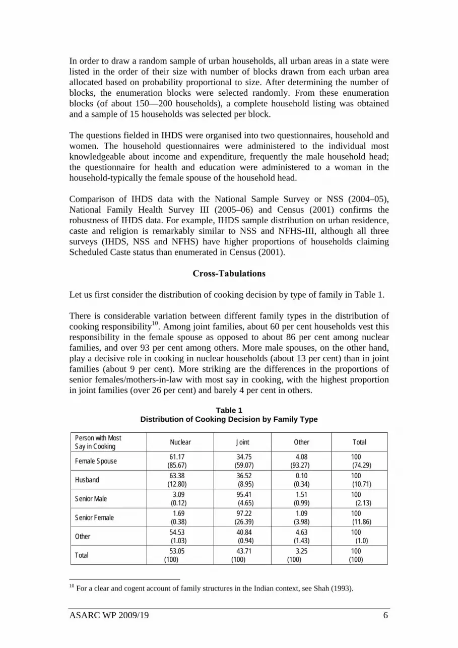
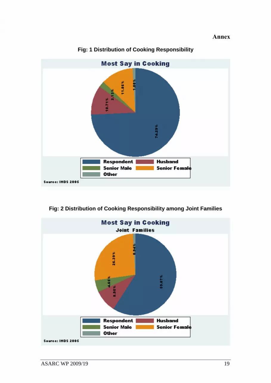
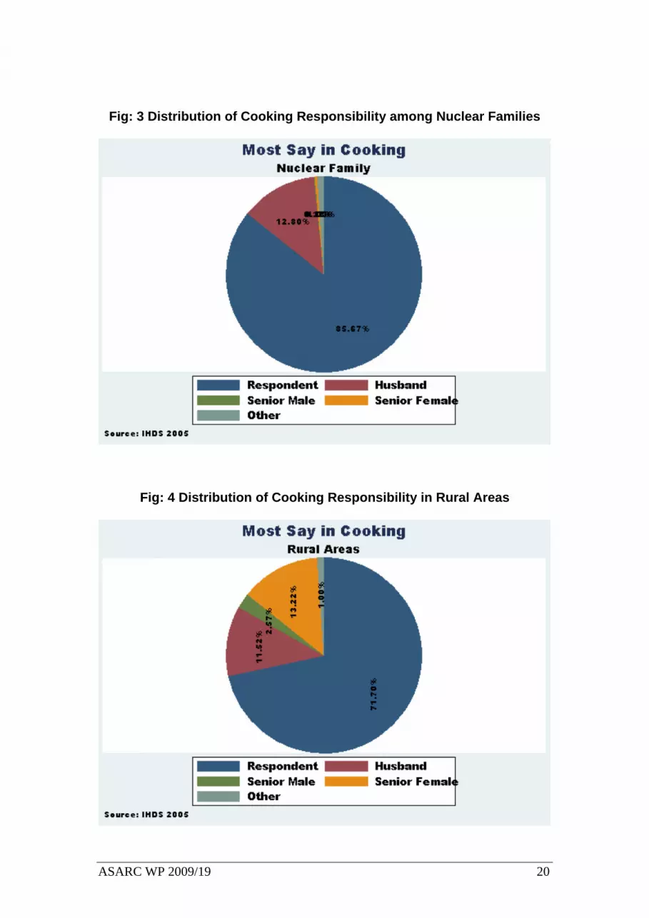
Let us first consider the distribution of cooking decision by type of family in Table 1. There is considerable variation between different family types in the distribution of cooking responsibility10. Among joint families, about 60 per cent households vest this responsibility in the female spouse as opposed to about 86 per cent among nuclear families, and over 93 per cent among others. More male spouses, on the other hand, play a decisive role in cooking in nuclear households (about 13 per cent) than in joint families (about 9 per cent). More striking are the differences in the proportions of senior females/mothers-in-law with most say in cooking, with the highest proportion in joint families (over 26 per cent) and barely 4 per cent in others.

Table 1

Distribution of Cooking Decision by Family Type

Person with Most Say in Cooking Nuclear Joint Other Total

Female Spouse 61.17 (85.67)

34.75 (59.07)

4.08 (93.27)

100 (74.29)

Husband 63.38 (12.80)

36.52 (8.95)

0.10 (0.34)

100 (10.71)

Senior Male 3.09 (0.12)

95.41 (4.65)

1.51 (0.99)

100 (2.13)

Senior Female 1.69 (0.38)

97.22 (26.39)

1.09 (3.98)

100 (11.86)

Other 54.53 (1.03)

40.84 (0.94)

4.63 (1.43)

100 (1.0)

Total 53.05 (100)

43.71 (100)

3.25 (100)

100 (100)

10 For a clear and cogent account of family structures in the Indian context, see Shah (1993).

ASARC WP 2009/19 7

Table 2 Distribution of Cooking Decision by Caste

Person with Most Say in Cooking SC ST OBC Others Total


8.03 (80.28)

35.45 (73.63)

34.08 (73.48)

100 (74.29)

Husband 25.72 (12.23)

5.82 (8.39)

36.75 (11.0)

31.71 (9.86)

100 (10.71)


2.46 (0.71)

41.86 (2.49)

37.84 (2.34)

100 (2.13)


6.02 (9.62)

36.20 (12.01)

38.45 (13.24)

100 (11.86)

Other 24.31 (1.09)

7.45 (1.01)

30.86 (0.87)

37.38 (1.09)

100 (1.0)

Total 22.34 (100)

7.43 (100)

35.77 (100)

34.46 (100)

100 (100)

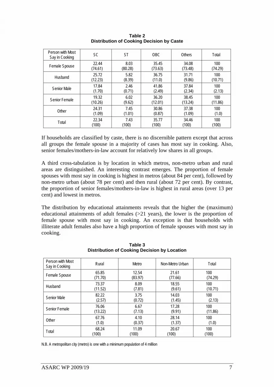
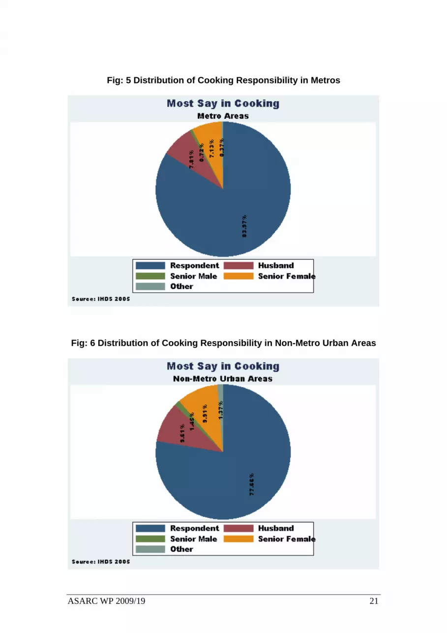
If households are classified by caste, there is no discernible pattern except that across all groups the female spouse in a majority of cases has most say in cooking. Also, senior females/mothers-in-law account for relatively low shares in all groups. A third cross-tabulation is by location in which metros, non-metro urban and rural areas are distinguished. An interesting contrast emerges. The proportion of female spouses with most say in cooking is highest in metros (about 84 per cent), followed by non-metro urban (about 78 per cent) and then rural (about 72 per cent). By contrast, the proportion of senior females/mothers-in-law is highest in rural areas (over 13 per cent) and lowest in metros. The distribution by educational attainments reveals that the higher the (maximum) educational attainments of adult females (>21 years), the lower is the proportion of female spouse with most say in cooking. An exception is that households with illiterate adult females also have a high proportion of female spouses with most say in cooking.

Table 3

Distribution of Cooking Decision by Location

Person with Most Say in Cooking Rural Metro Non-Metro Urban Total


12.54 (83.97)

21.61 (77.66)

100 (74.29)

Husband 73.37 (11.52)

8.09 (7.81)

18.55 (9.61)

100 (10.71)


3.75 (0.72)

14.03 (1.45)

100 (2.13)


6.67 (7.13)

17.28 (9.91)

100 (11.86)

Other 67.76 (1.0)

4.10 (0.37)

28.14 (1.37)

100 (1.0)

Total 68.24 (100)

11.09 (100)

20.67 (100)

100 (100)

N.B. A metropolitan city (metro) is one with a minimum population of 4 million

ASARC WP 2009/19 8

Table 4 Distribution of Cooking Decision by Highest Female Education Level

Person with Most Say in Cooking 0 year 1-5 years 6-10 years >10 years Total

Female Spouse 46.55 73.91

15.61 76.85

27.0 75.05

10.84 70.80

100 74.31

Husband 56.82 12.99

14.29 10.13

20.99 8.40

7.90 7.43

100 10.70


13.59 (1.89)

26.75 (2.10)

13.45 (2.48)

100 (2.10)


13.08 (10.31)

30.13 (13.40)

16.76 (17.52)

100 (11.89)

Other 39.76 (0.85)

12.20 (0.81)

27.92 (1.05)

20.12 (1.77)

100 (1.0)

Total 46.80 (100)

15.09 (100)

26.73 (100)

11.38 (100)

100 (100)

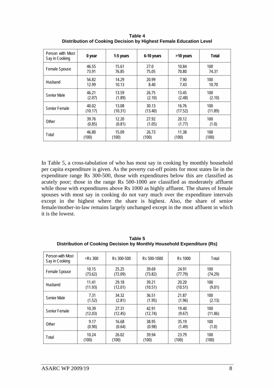
In Table 5, a cross-tabulation of who has most say in cooking by monthly household per capita expenditure is given. As the poverty cut-off points for most states lie in the expenditure range Rs 300-500, those with expenditures below this are classified as acutely poor; those in the range Rs 500-1000 are classified as moderately affluent while those with expenditures above Rs 1000 as highly affluent. The shares of female spouses with most say in cooking do not vary much over the expenditure intervals except in the highest where the share is highest. Also, the share of senior female/mother-in-law remains largely unchanged except in the most affluent in which it is the lowest.

Table 5 Distribution of Cooking Decision by Monthly Household Expenditure (Rs)

Person with Most Say in Cooking <Rs 300 Rs 300-500 Rs 500-1000 Rs 1000 Total


25.25 (72.09)

39.69 (73.82)

24.91 (77.79)

100 (74.29)

Husband 11.41 (11.93)

29.18 (12.01)

39.21 (10.51)

20.20 (10.51)

100 (9.01)


34.32 (2.81)

36.51 (1.95)

21.87 (1.96)

100 (2.13)


27.31 (12.45)

42.91 (12.74)

19.40 (9.67)

100 (11.86)

Other 9.17 (0.90)

16.68 (0.64)

38.95 (0.98)

35.19 (1.49)

100 (1.0)

Total 10.24 (100)

26.02 (100)

39.94 (100)

23.79 (100)

100 (100)

ASARC WP 2009/19 9

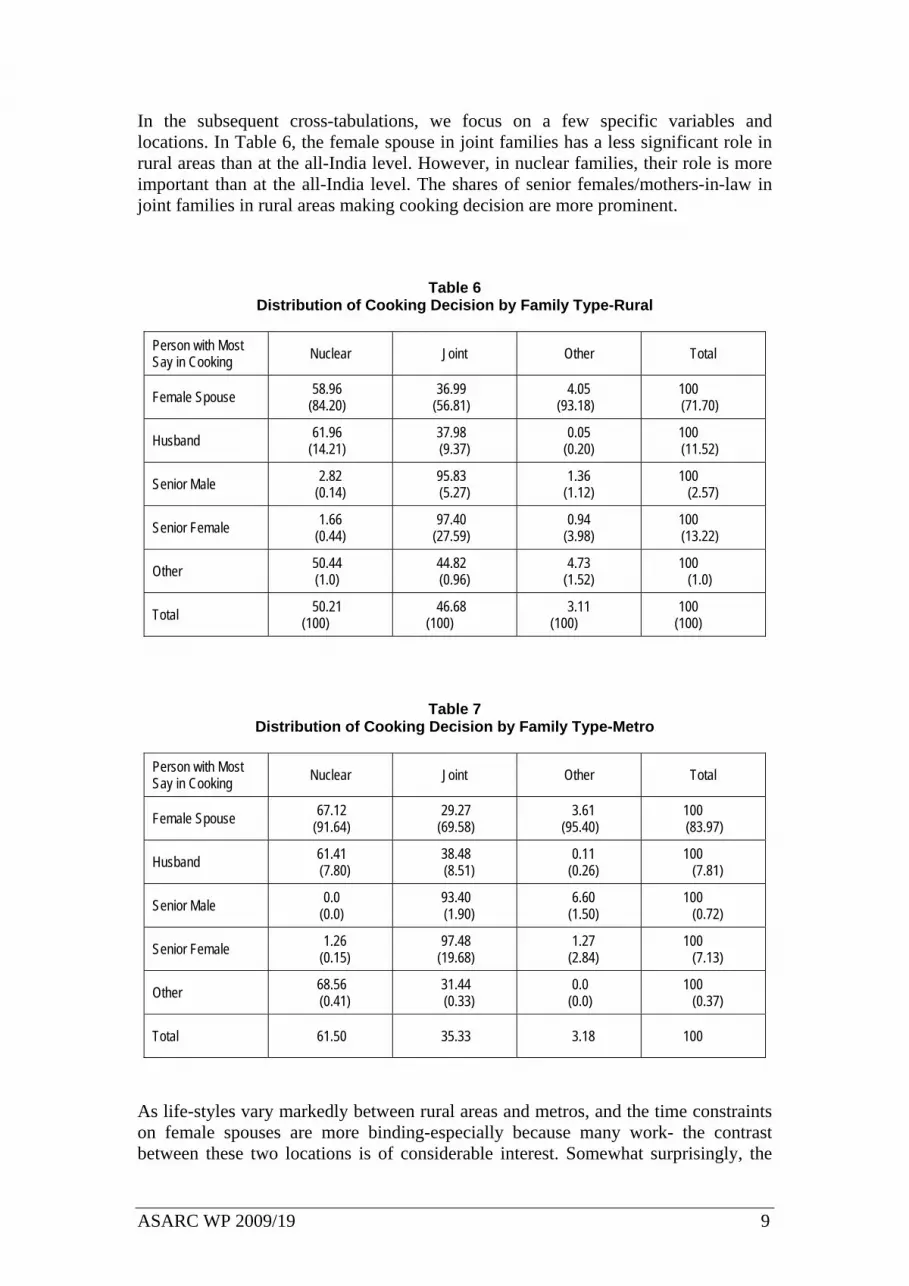
In the subsequent cross-tabulations, we focus on a few specific variables and locations. In Table 6, the female spouse in joint families has a less significant role in rural areas than at the all-India level. However, in nuclear families, their role is more important than at the all-India level. The shares of senior females/mothers-in-law in joint families in rural areas making cooking decision are more prominent.

Table 6 Distribution of Cooking Decision by Family Type-Rural



36.99 (56.81)

4.05 (93.18)

100 (71.70)

Husband 61.96 (14.21)

37.98 (9.37)

0.05 (0.20)

100 (11.52)


95.83 (5.27)

1.36 (1.12)

100 (2.57)


97.40 (27.59)

0.94 (3.98)

100 (13.22)

Other 50.44 (1.0)

44.82 (0.96)

4.73 (1.52)

100 (1.0)

Total 50.21 (100)

46.68 (100)

3.11 (100)

100 (100)

Table 7 Distribution of Cooking Decision by Family Type-Metro



29.27 (69.58)

3.61 (95.40)

100 (83.97)

Husband 61.41 (7.80)

38.48 (8.51)

0.11 (0.26)

100 (7.81)


93.40 (1.90)

6.60 (1.50)

100 (0.72)


97.48 (19.68)

1.27 (2.84)

100 (7.13)

Other 68.56 (0.41)

31.44 (0.33)

0.0 (0.0)

100 (0.37)

Total 61.50 35.33 3.18 100

As life-styles vary markedly between rural areas and metros, and the time constraints on female spouses are more binding-especially because many work- the contrast between these two locations is of considerable interest. Somewhat surprisingly, the

ASARC WP 2009/19 10

pattern is strikingly different. In the metros, the proportion of female spouses in nuclear families taking cooking decisions is markedly higher — about 92 per cent. In the joint families too, the proportion of female spouses is considerably higher in the metros compared with the rural areas ((about 70 per cent and 57 per cent, respectively). Also, the share of senior females/mothers-in-law in joint families responsible for cooking decisions is lower than in rural areas (about 20 per cent and 28 per cent, respectively).

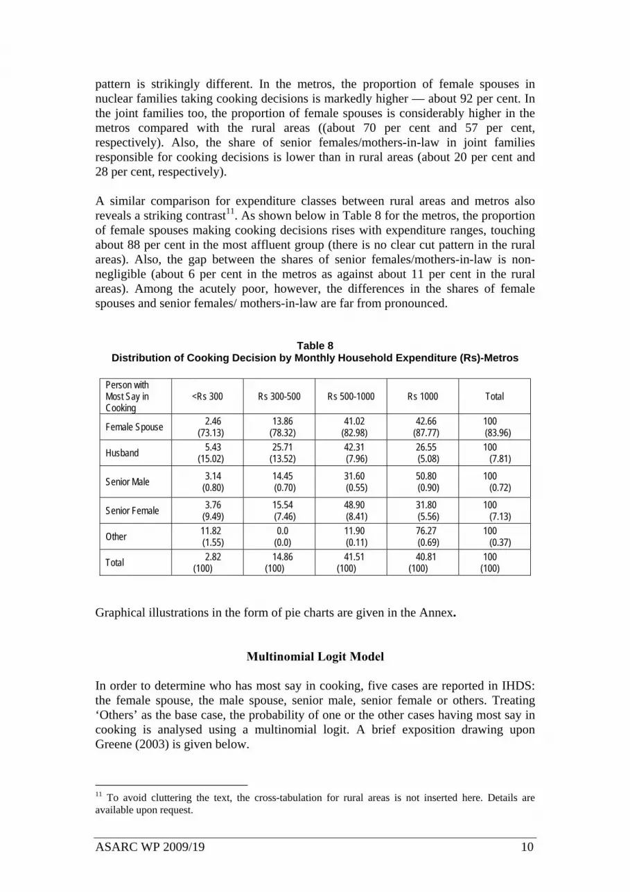
A similar comparison for expenditure classes between rural areas and metros also reveals a striking contrast11. As shown below in Table 8 for the metros, the proportion of female spouses making cooking decisions rises with expenditure ranges, touching about 88 per cent in the most affluent group (there is no clear cut pattern in the rural areas). Also, the gap between the shares of senior females/mothers-in-law is non-negligible (about 6 per cent in the metros as against about 11 per cent in the rural areas). Among the acutely poor, however, the differences in the shares of female spouses and senior females/ mothers-in-law are far from pronounced.

Table 8 Distribution of Cooking Decision by Monthly Household Expenditure (Rs)-Metros

Person with Most Say in Cooking

<Rs 300 Rs 300-500 Rs 500-1000 Rs 1000 Total


13.86 (78.32)

41.02 (82.98)

42.66 (87.77)

100 (83.96)

Husband 5.43 (15.02)

25.71 (13.52)

42.31 (7.96)

26.55 (5.08)

100 (7.81)


14.45 (0.70)

31.60 (0.55)

50.80 (0.90)

100 (0.72)


15.54 (7.46)

48.90 (8.41)

31.80 (5.56)

100 (7.13)

Other 11.82 (1.55)

0.0 (0.0)

11.90 (0.11)

76.27 (0.69)

100 (0.37)

Total 2.82 (100)

14.86 (100)

41.51 (100)

40.81 (100)

100 (100)

Graphical illustrations in the form of pie charts are given in the Annex.

Multinomial Logit Model In order to determine who has most say in cooking, five cases are reported in IHDS: the female spouse, the male spouse, senior male, senior female or others. Treating ‘Others’ as the base case, the probability of one or the other cases having most say in cooking is analysed using a multinomial logit. A brief exposition drawing upon Greene (2003) is given below.

11 To avoid cluttering the text, the cross-tabulation for rural areas is not inserted here. Details are available upon request.

ASARC WP 2009/19 11

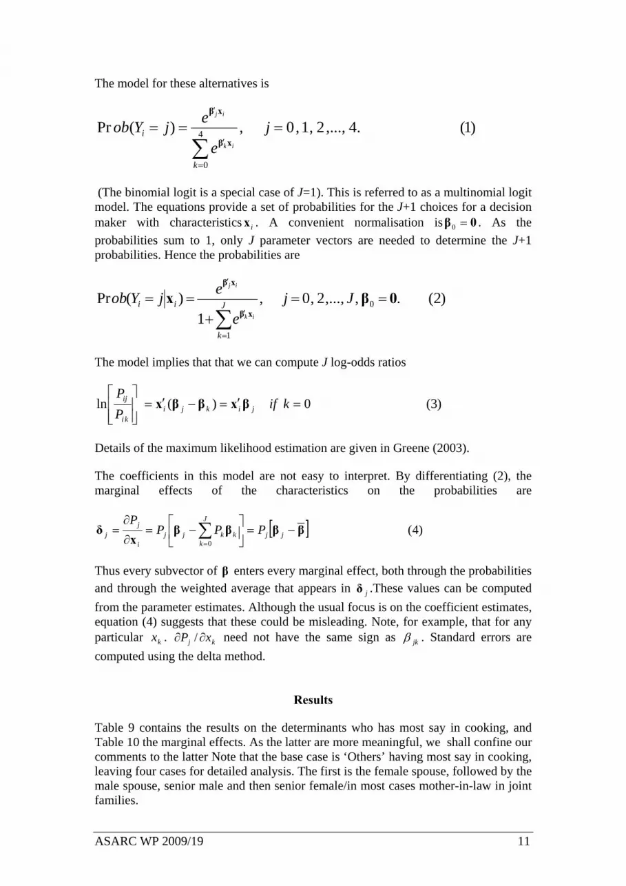
The model for these alternatives is

)1(.4,...,2,1,0,)(Pr 4

0

===

∑=

′

′

je

ejYob

k

iik

ij

xβ

xβ

(The binomial logit is a special case of J=1). This is referred to as a multinomial logit model. The equations provide a set of probabilities for the J+1 choices for a decision maker with characteristics ix . A convenient normalisation is 0β =0 . As the probabilities sum to 1, only J parameter vectors are needed to determine the J+1 probabilities. Hence the probabilities are

)2(.,,...,2,0,1

)(Pr 0

1

0βxxβ

xβ

==+

==

∑=

′

′

Jje

ejYob J

k

iiik

ij

The model implies that that we can compute J log-odds ratios

)3(0)(ln =′=−′=⎥⎥⎦

⎤

⎢⎢⎣

⎡kif

PP

jikjiki

ij βxββx

Details of the maximum likelihood estimation are given in Greene (2003). The coefficients in this model are not easy to interpret. By differentiating (2), the marginal effects of the characteristics on the probabilities are

[ ] )4(0

ββββx

δ −=⎥⎦

⎤⎢⎣

⎡−=

∂

∂= ∑

=jj

J

kkkjj

i

jj PPP

P

Thus every subvector of β enters every marginal effect, both through the probabilities and through the weighted average that appears in jδ .These values can be computed from the parameter estimates. Although the usual focus is on the coefficient estimates, equation (4) suggests that these could be misleading. Note, for example, that for any particular kx . kj xP ∂∂ / need not have the same sign as jkβ . Standard errors are computed using the delta method.

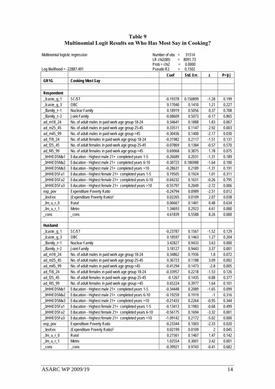
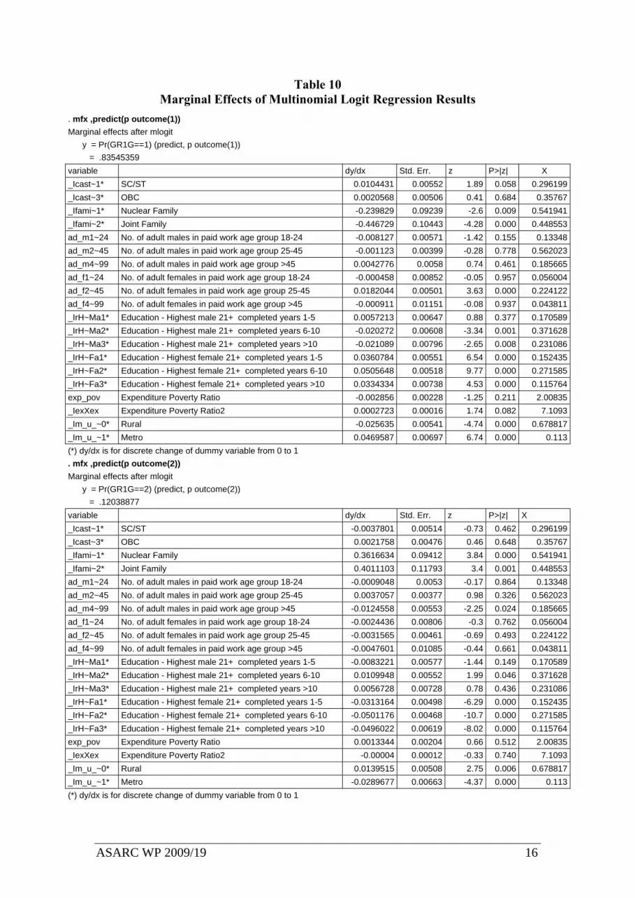
Results Table 9 contains the results on the determinants who has most say in cooking, and Table 10 the marginal effects. As the latter are more meaningful, we shall confine our comments to the latter Note that the base case is ‘Others’ having most say in cooking, leaving four cases for detailed analysis. The first is the female spouse, followed by the male spouse, senior male and then senior female/in most cases mother-in-law in joint families.

ASARC WP 2009/19 12

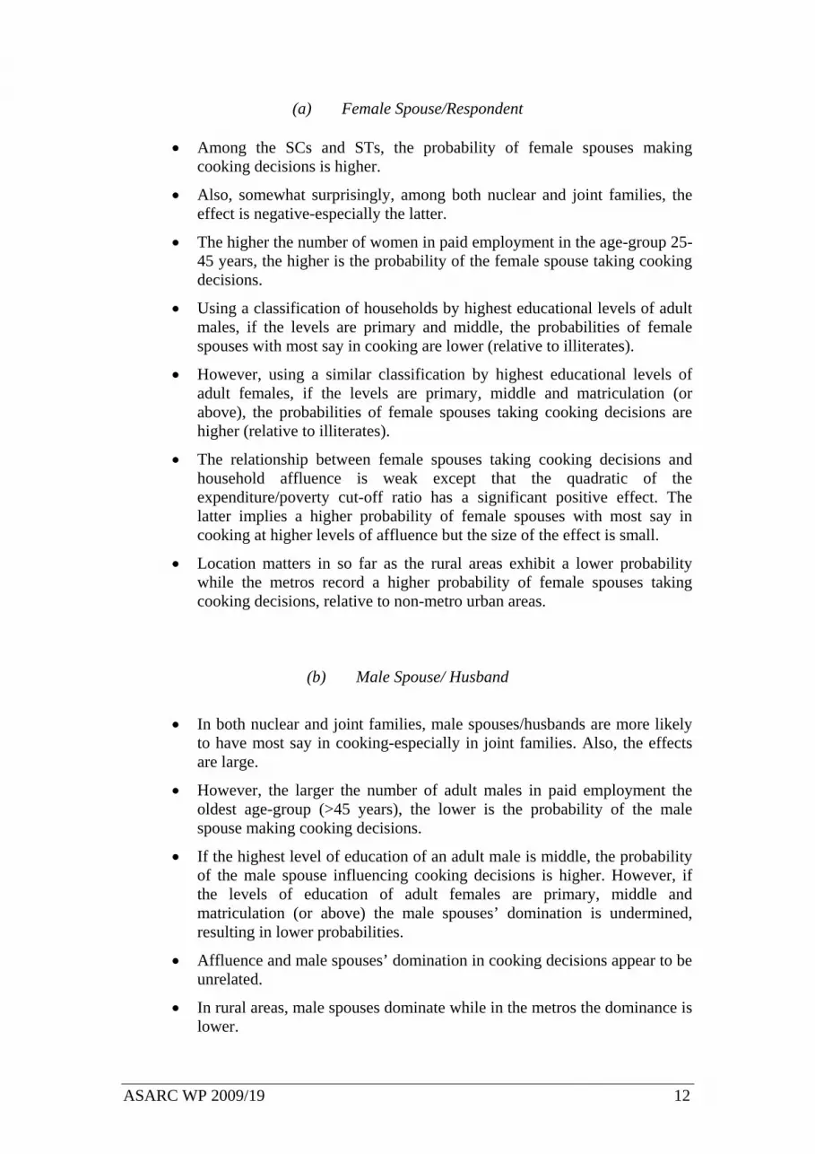
(a) Female Spouse/Respondent

• Among the SCs and STs, the probability of female spouses making cooking decisions is higher.

• Also, somewhat surprisingly, among both nuclear and joint families, the effect is negative-especially the latter.

• The higher the number of women in paid employment in the age-group 25-45 years, the higher is the probability of the female spouse taking cooking decisions.

• Using a classification of households by highest educational levels of adult males, if the levels are primary and middle, the probabilities of female spouses with most say in cooking are lower (relative to illiterates).

• However, using a similar classification by highest educational levels of adult females, if the levels are primary, middle and matriculation (or above), the probabilities of female spouses taking cooking decisions are higher (relative to illiterates).

• The relationship between female spouses taking cooking decisions and household affluence is weak except that the quadratic of the expenditure/poverty cut-off ratio has a significant positive effect. The latter implies a higher probability of female spouses with most say in cooking at higher levels of affluence but the size of the effect is small.

• Location matters in so far as the rural areas exhibit a lower probability while the metros record a higher probability of female spouses taking cooking decisions, relative to non-metro urban areas.

(b) Male Spouse/ Husband

• In both nuclear and joint families, male spouses/husbands are more likely to have most say in cooking-especially in joint families. Also, the effects are large.

• However, the larger the number of adult males in paid employment the oldest age-group (>45 years), the lower is the probability of the male spouse making cooking decisions.

• If the highest level of education of an adult male is middle, the probability of the male spouse influencing cooking decisions is higher. However, if the levels of education of adult females are primary, middle and matriculation (or above) the male spouses’ domination is undermined, resulting in lower probabilities.

• Affluence and male spouses’ domination in cooking decisions appear to be unrelated.

• In rural areas, male spouses dominate while in the metros the dominance is lower.

ASARC WP 2009/19 13

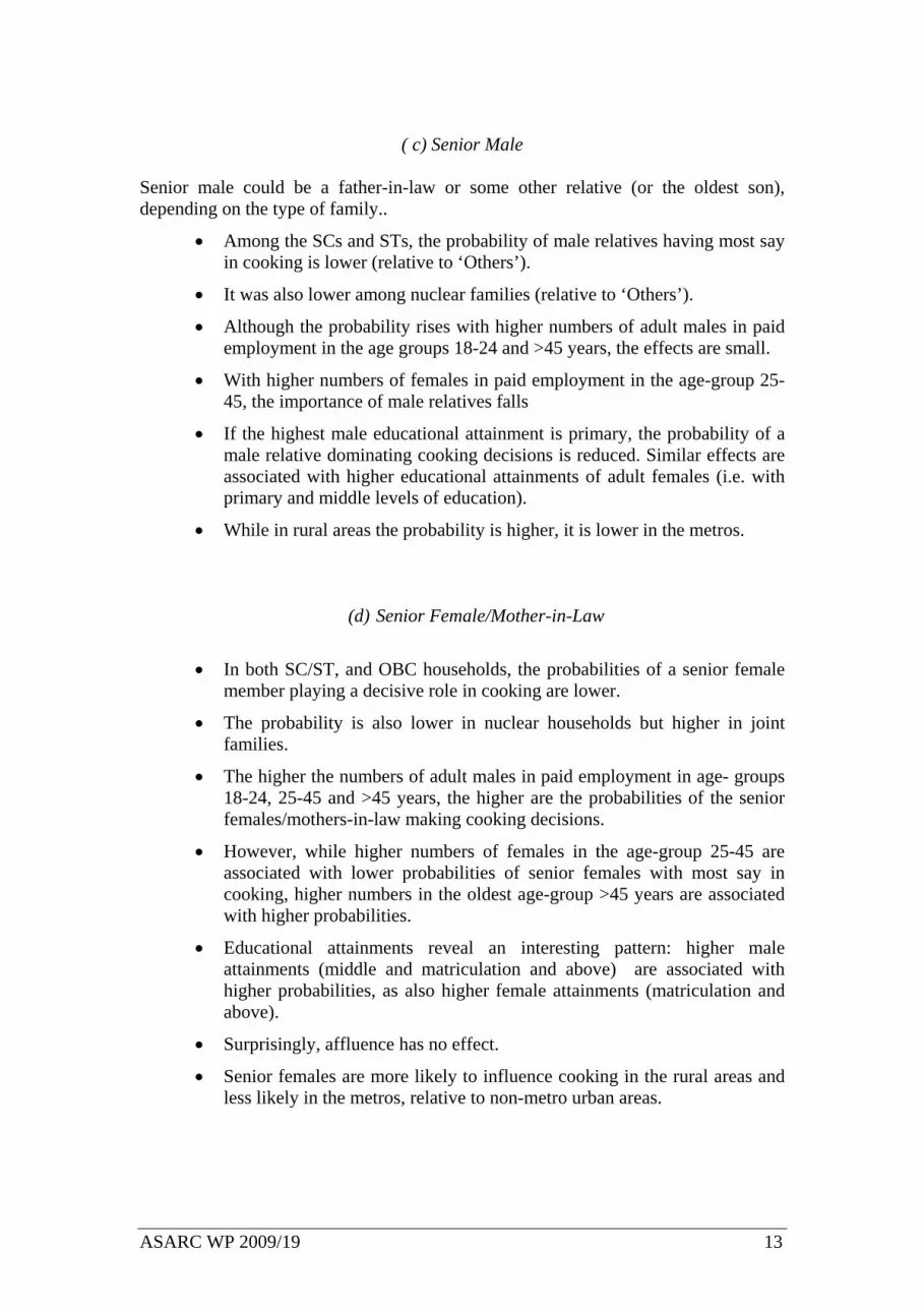
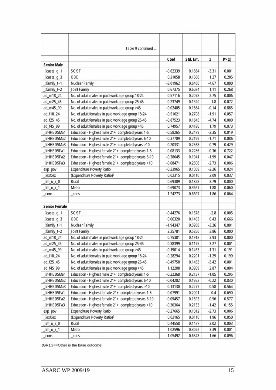
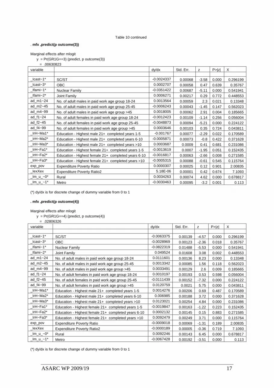
( c) Senior Male

Senior male could be a father-in-law or some other relative (or the oldest son), depending on the type of family..

• Among the SCs and STs, the probability of male relatives having most say in cooking is lower (relative to ‘Others’).

• It was also lower among nuclear families (relative to ‘Others’).

• Although the probability rises with higher numbers of adult males in paid employment in the age groups 18-24 and >45 years, the effects are small.

• With higher numbers of females in paid employment in the age-group 25-45, the importance of male relatives falls

• If the highest male educational attainment is primary, the probability of a male relative dominating cooking decisions is reduced. Similar effects are associated with higher educational attainments of adult females (i.e. with primary and middle levels of education).

• While in rural areas the probability is higher, it is lower in the metros.

(d) Senior Female/Mother-in-Law

• In both SC/ST, and OBC households, the probabilities of a senior female member playing a decisive role in cooking are lower.

• The probability is also lower in nuclear households but higher in joint families.

• The higher the numbers of adult males in paid employment in age- groups 18-24, 25-45 and >45 years, the higher are the probabilities of the senior females/mothers-in-law making cooking decisions.

• However, while higher numbers of females in the age-group 25-45 are associated with lower probabilities of senior females with most say in cooking, higher numbers in the oldest age-group >45 years are associated with higher probabilities.

• Educational attainments reveal an interesting pattern: higher male attainments (middle and matriculation and above) are associated with higher probabilities, as also higher female attainments (matriculation and above).

• Surprisingly, affluence has no effect.

• Senior females are more likely to influence cooking in the rural areas and less likely in the metros, relative to non-metro urban areas.

ASARC WP 2009/19 14

Table 9 Multinomial Logit Results on Who Has Most Say in Cooking?

Multinomial logistic regression Number of obs = 31514 LR chi2(80) = 8091.73 Prob > chi2 = 0.0000 Log likelihood = -22887.491 Pseudo R2 = 0.1502 Coef Std. Err. z P>|z| GR1G Cooking Most Say Respondent _Icaste_g_1 SC/ST -0.19378 0.150899 -1.28 0.199 _Icaste_g_3 OBC 0.17040 0.1410 1.21 0.227 _Ifamily_t~1 Nuclear Family 0.18919 0.5056 0.37 0.708 _Ifamily_t~2 Joint Family -0.08609 0.5073 -0.17 0.865 ad_m18_24 No. of adult males in paid work age group 18-24 0.34641 0.1888 1.83 0.067 ad_m25_45 No. of adult males in paid work age group 25-45 0.33511 0.1147 2.92 0.003 ad_m45_99 No. of adult males in paid work age group >45 -0.30436 0.1400 -2.17 0.030 ad_f18_24 No. of adult females in paid work age group 18-24 -0.31982 0.2117 -1.51 0.131 ad_f25_45 No. of adult females in paid work age group 25-45 -0.07869 0.1384 -0.57 0.570 ad_f45_99 No. of adult females in paid work age group >45 0.69068 0.3875 1.78 0.075 _IrHHED5Ma1 Education - Highest male 21+ completed years 1-5 -0.26689 0.2031 -1.31 0.189 _IrHHED5Ma2 Education - Highest male 21+ completed years 6-10 -0.30723 0.186988 -1.64 0.100 _IrHHED5Ma3 Education - Highest male 21+ completed years >10 -0.28631 0.2189 -1.31 0.191 _IrHHED5Fa1 Education - Highest female 21+ completed years 1-5 0.19505 0.1924 1.01 0.311 _IrHHED5Fa2 Education - Highest female 21+ completed years 6-10 -0.04232 0.1631 -0.26 0.795 _IrHHED5Fa3 Education - Highest female 21+ completed years >10 -0.55797 0.2049 -2.72 0.006 exp_pov Expenditure Poverty Ratio -0.24794 0.0989 -2.51 0.012 _IexXex (Expenditure Poverty Ratio)2 0.02265 0.0109 2.07 0.038 _Im_u_r_0 Rural 0.06667 0.1401 0.48 0.634 _Im_u_r_1 Metro 1.34693 0.2923 4.61 0.000 _cons _cons 4.61839 0.5588 8.26 0.000 Husband _Icaste_g_1 SC/ST -0.23787 0.1567 -1.52 0.129 _Icaste_g_3 OBC 0.18597 0.1463 1.27 0.204 _Ifamily_t~1 Nuclear Family 3.42827 0.9433 3.63 0.000 _Ifamily_t~2 Joint Family 3.18127 0.9443 3.37 0.001 ad_m18_24 No. of adult males in paid work age group 18-24 0.34862 0.1936 1.8 0.072 ad_m25_45 No. of adult males in paid work age group 25-45 0.36723 0.1188 3.09 0.002 ad_m45_99 No. of adult males in paid work age group >45 -0.41294 0.1473 -2.8 0.005 ad_f18_24 No. of adult females in paid work age group 18-24 -0.33957 0.2218 -1.53 0.126 ad_f25_45 No. of adult females in paid work age group 25-45 -0.1267 0.1435 -0.88 0.377 ad_f45_99 No. of adult females in paid work age group >45 0.65224 0.3977 1.64 0.101 _IrHHED5Ma1 Education - Highest male 21+ completed years 1-5 -0.34448 0.2089 -1.65 0.099 _IrHHED5Ma2 Education - Highest male 21+ completed years 6-10 -0.19259 0.1919 -1 0.316 _IrHHED5Ma3 Education - Highest male 21+ completed years >10 -0.21433 0.2264 -0.95 0.344 _IrHHED5Fa1 Education - Highest female 21+ completed years 1-5 -0.13413 0.1983 -0.68 0.499 _IrHHED5Fa2 Education - Highest female 21+ completed years 6-10 -0.56175 0.1694 -3.32 0.001 _IrHHED5Fa3 Education - Highest female 21+ completed years >10 -1.09142 0.2172 -5.02 0.000 exp_pov Expenditure Poverty Ratio -0.23344 0.1003 -2.33 0.020 _IexXex (Expenditure Poverty Ratio)2 0.02199 0.0109 2 0.045 _Im_u_r_0 Rural 0.21561 0.1467 1.47 0.142 _Im_u_r_1 Metro 1.02554 0.3001 3.42 0.001 _cons _cons -0.39921 0.9743 -0.41 0.682

ASARC WP 2009/19 15

Table 9 continued …

Coef Std. Err. z P>|z| Senior Male _Icaste_g_1 SC/ST -0.62339 0.1884 -3.31 0.001 _Icaste_g_3 OBC 0.21058 0.1660 1.27 0.205 _Ifamily_t~1 Nuclear Family -3.01962 0.6460 -4.67 0.000 _Ifamily_t~2 Joint Family 0.67375 0.6084 1.11 0.268 ad_m18_24 No. of adult males in paid work age group 18-24 0.57116 0.2078 2.75 0.006 ad_m25_45 No. of adult males in paid work age group 25-45 0.23749 0.1320 1.8 0.072 ad_m45_99 No. of adult males in paid work age group >45 -0.02405 0.1664 -0.14 0.885 ad_f18_24 No. of adult females in paid work age group 18-24 -0.51621 0.2708 -1.91 0.057 ad_f25_45 No. of adult females in paid work age group 25-45 -0.87523 0.1845 -4.74 0.000 ad_f45_99 No. of adult females in paid work age group >45 0.74957 0.4180 1.79 0.073 _IrHHED5Ma1 Education - Highest male 21+ completed years 1-5 -0.58265 0.2479 -2.35 0.019 _IrHHED5Ma2 Education - Highest male 21+ completed years 6-10 -0.37709 0.2199 -1.71 0.086 _IrHHED5Ma3 Education - Highest male 21+ completed years >10 -0.20331 0.2568 -0.79 0.429 _IrHHED5Fa1 Education - Highest female 21+ completed years 1-5 -0.08133 0.2286 -0.36 0.722 _IrHHED5Fa2 Education - Highest female 21+ completed years 6-10 -0.38645 0.1941 -1.99 0.047 _IrHHED5Fa3 Education - Highest female 21+ completed years >10 -0.68471 0.2506 -2.73 0.006 exp_pov Expenditure Poverty Ratio -0.23965 0.1059 -2.26 0.024 _IexXex (Expenditure Poverty Ratio)2 0.02315 0.0110 2.09 0.037 _Im_u_r_0 Rural 0.69309 0.1828 3.79 0.000 _Im_u_r_1 Metro 0.69073 0.3667 1.88 0.060 _cons _cons 1.24273 0.6697 1.86 0.064 Senior Female _Icaste_g_1 SC/ST -0.44276 0.1578 -2.8 0.005 _Icaste_g_3 OBC 0.06320 0.1463 0.43 0.666 _Ifamily_t~1 Nuclear Family -1.94347 0.5968 -3.26 0.001 _Ifamily_t~2 Joint Family 2.25781 0.5850 3.86 0.000 ad_m18_24 No. of adult males in paid work age group 18-24 0.75381 0.1918 3.93 0.000 ad_m25_45 No. of adult males in paid work age group 25-45 0.38399 0.1175 3.27 0.001 ad_m45_99 No. of adult males in paid work age group >45 -0.19014 0.1453 -1.31 0.191 ad_f18_24 No. of adult females in paid work age group 18-24 -0.28294 0.2201 -1.29 0.199 ad_f25_45 No. of adult females in paid work age group 25-45 -0.49758 0.1453 -3.42 0.001 ad_f45_99 No. of adult females in paid work age group >45 1.12208 0.3909 2.87 0.004 _IrHHED5Ma1 Education - Highest male 21+ completed years 1-5 -0.22368 0.2137 -1.05 0.295 _IrHHED5Ma2 Education - Highest male 21+ completed years 6-10 -0.04202 0.1952 -0.22 0.830 _IrHHED5Ma3 Education - Highest male 21+ completed years >10 0.13130 0.2277 0.58 0.564 _IrHHED5Fa1 Education - Highest female 21+ completed years 1-5 0.07991 0.2001 0.4 0.690 _IrHHED5Fa2 Education - Highest female 21+ completed years 6-10 -0.09457 0.1693 -0.56 0.577 _IrHHED5Fa3 Education - Highest female 21+ completed years >10 -0.30364 0.2133 -1.42 0.155 exp_pov Expenditure Poverty Ratio -0.27665 0.1012 -2.73 0.006 _IexXex (Expenditure Poverty Ratio)2 0.02165 0.0110 1.96 0.050 _Im_u_r_0 Rural 0.44558 0.1477 3.02 0.003 _Im_u_r_1 Metro 1.02596 0.3022 3.39 0.001 _cons _cons 1.05492 0.6343 1.66 0.096 (GR1G==Other is the base outcome)

ASARC WP 2009/19 16

Table 10 Marginal Effects of Multinomial Logit Regression Results

. mfx ,predict(p outcome(1)) Marginal effects after mlogit y = Pr(GR1G==1) (predict, p outcome(1)) = .83545359 variable dy/dx Std. Err. z P>|z| X _Icast~1* SC/ST 0.0104431 0.00552 1.89 0.058 0.296199_Icast~3* OBC 0.0020568 0.00506 0.41 0.684 0.35767_Ifami~1* Nuclear Family -0.239829 0.09239 -2.6 0.009 0.541941_Ifami~2* Joint Family -0.446729 0.10443 -4.28 0.000 0.448553ad_m1~24 No. of adult males in paid work age group 18-24 -0.008127 0.00571 -1.42 0.155 0.13348ad_m2~45 No. of adult males in paid work age group 25-45 -0.001123 0.00399 -0.28 0.778 0.562023ad_m4~99 No. of adult males in paid work age group >45 0.0042776 0.0058 0.74 0.461 0.185665ad_f1~24 No. of adult females in paid work age group 18-24 -0.000458 0.00852 -0.05 0.957 0.056004ad_f2~45 No. of adult females in paid work age group 25-45 0.0182044 0.00501 3.63 0.000 0.224122ad_f4~99 No. of adult females in paid work age group >45 -0.000911 0.01151 -0.08 0.937 0.043811_IrH~Ma1* Education - Highest male 21+ completed years 1-5 0.0057213 0.00647 0.88 0.377 0.170589_IrH~Ma2* Education - Highest male 21+ completed years 6-10 -0.020272 0.00608 -3.34 0.001 0.371628_IrH~Ma3* Education - Highest male 21+ completed years >10 -0.021089 0.00796 -2.65 0.008 0.231086_IrH~Fa1* Education - Highest female 21+ completed years 1-5 0.0360784 0.00551 6.54 0.000 0.152435_IrH~Fa2* Education - Highest female 21+ completed years 6-10 0.0505648 0.00518 9.77 0.000 0.271585_IrH~Fa3* Education - Highest female 21+ completed years >10 0.0334334 0.00738 4.53 0.000 0.115764exp_pov Expenditure Poverty Ratio -0.002856 0.00228 -1.25 0.211 2.00835_IexXex Expenditure Poverty Ratio2 0.0002723 0.00016 1.74 0.082 7.1093_Im_u_~0* Rural -0.025635 0.00541 -4.74 0.000 0.678817_Im_u_~1* Metro 0.0469587 0.00697 6.74 0.000 0.113(*) dy/dx is for discrete change of dummy variable from 0 to 1 . mfx ,predict(p outcome(2)) Marginal effects after mlogit y = Pr(GR1G==2) (predict, p outcome(2)) = .12038877 variable dy/dx Std. Err. z P>|z| X _Icast~1* SC/ST -0.0037801 0.00514 -0.73 0.462 0.296199_Icast~3* OBC 0.0021758 0.00476 0.46 0.648 0.35767_Ifami~1* Nuclear Family 0.3616634 0.09412 3.84 0.000 0.541941_Ifami~2* Joint Family 0.4011103 0.11793 3.4 0.001 0.448553ad_m1~24 No. of adult males in paid work age group 18-24 -0.0009048 0.0053 -0.17 0.864 0.13348ad_m2~45 No. of adult males in paid work age group 25-45 0.0037057 0.00377 0.98 0.326 0.562023ad_m4~99 No. of adult males in paid work age group >45 -0.0124558 0.00553 -2.25 0.024 0.185665ad_f1~24 No. of adult females in paid work age group 18-24 -0.0024436 0.00806 -0.3 0.762 0.056004ad_f2~45 No. of adult females in paid work age group 25-45 -0.0031565 0.00461 -0.69 0.493 0.224122ad_f4~99 No. of adult females in paid work age group >45 -0.0047601 0.01085 -0.44 0.661 0.043811_IrH~Ma1* Education - Highest male 21+ completed years 1-5 -0.0083221 0.00577 -1.44 0.149 0.170589_IrH~Ma2* Education - Highest male 21+ completed years 6-10 0.0109948 0.00552 1.99 0.046 0.371628_IrH~Ma3* Education - Highest male 21+ completed years >10 0.0056728 0.00728 0.78 0.436 0.231086_IrH~Fa1* Education - Highest female 21+ completed years 1-5 -0.0313164 0.00498 -6.29 0.000 0.152435_IrH~Fa2* Education - Highest female 21+ completed years 6-10 -0.0501176 0.00468 -10.7 0.000 0.271585_IrH~Fa3* Education - Highest female 21+ completed years >10 -0.0496022 0.00619 -8.02 0.000 0.115764exp_pov Expenditure Poverty Ratio 0.0013344 0.00204 0.66 0.512 2.00835_IexXex Expenditure Poverty Ratio2 -0.00004 0.00012 -0.33 0.740 7.1093_Im_u_~0* Rural 0.0139515 0.00508 2.75 0.006 0.678817_Im_u_~1* Metro -0.0289677 0.00663 -4.37 0.000 0.113(*) dy/dx is for discrete change of dummy variable from 0 to 1

ASARC WP 2009/19 17

Table 10 continued . mfx ,predict(p outcome(3)) Marginal effects after mlogit y = Pr(GR1G==3) (predict, p outcome(3)) = .00630823 variable dy/dx Std. Err. z P>|z| X _Icast~1* SC/ST -0.0024337 0.00068 -3.58 0.000 0.296199 _Icast~3* OBC 0.0002707 0.00058 0.47 0.639 0.35767 _Ifami~1* Nuclear Family -0.0351422 0.00687 -5.11 0.000 0.541941 _Ifami~2* Joint Family 0.0006271 0.00217 0.29 0.772 0.448553 ad_m1~24 No. of adult males in paid work age group 18-24 0.0013564 0.00059 2.3 0.021 0.13348 ad_m2~45 No. of adult males in paid work age group 25-45 -0.0006243 0.00043 -1.45 0.147 0.562023 ad_m4~99 No. of adult males in paid work age group >45 0.0018005 0.00062 2.91 0.004 0.185665 ad_f1~24 No. of adult females in paid work age group 18-24 -0.0012423 0.00109 -1.14 0.256 0.056004 ad_f2~45 No. of adult females in paid work age group 25-45 -0.0048873 0.00094 -5.21 0.000 0.224122 ad_f4~99 No. of adult females in paid work age group >45 0.0003646 0.00103 0.35 0.724 0.043811 _IrH~Ma1* Education - Highest male 21+ completed years 1-5 -0.001767 0.00077 -2.29 0.022 0.170589 _IrH~Ma2* Education - Highest male 21+ completed years 6-10 -0.0005871 0.00073 -0.8 0.422 0.371628 _IrH~Ma3* Education - Highest male 21+ completed years >10 0.0003687 0.0009 0.41 0.681 0.231086 _IrH~Fa1* Education - Highest female 21+ completed years 1-5 -0.0013619 0.0007 -1.95 0.051 0.152435 _IrH~Fa2* Education - Highest female 21+ completed years 6-10 -0.0016817 0.00063 -2.66 0.008 0.271585 _IrH~Fa3* Education - Highest female 21+ completed years >10 -0.0005315 0.00088 -0.61 0.545 0.115764 exp_pov Expenditure Poverty Ratio 0.0000307 0.00025 0.12 0.901 2.00835 _IexXex Expenditure Poverty Ratio2 5.18E-06 0.00001 0.42 0.674 7.1093 _Im_u_~0* Rural 0.0034263 0.00074 4.62 0.000 0.678817 _Im_u_~1* Metro -0.0030463 0.00095 -3.2 0.001 0.113 (*) dy/dx is for discrete change of dummy variable from 0 to 1

. mfx ,predict(p outcome(4)) Marginal effects after mlogit y = Pr(GR1G==4) (predict, p outcome(4)) = .02806326 variable dy/dx Std. Err. z P>|z| X _Icast~1* SC/ST -0.0063375 0.00139 -4.57 0.000 0.296199 _Icast~3* OBC -0.0028969 0.00123 -2.36 0.018 0.35767 _Ifami~1* Nuclear Family -0.0822319 0.01488 -5.53 0.000 0.541941 _Ifami~2* Joint Family 0.049524 0.01608 3.08 0.002 0.448553 ad_m1~24 No. of adult males in paid work age group 18-24 0.0111601 0.00136 8.23 0.000 0.13348 ad_m2~45 No. of adult males in paid work age group 25-45 0.0013342 0.00085 1.56 0.118 0.562023 ad_m4~99 No. of adult males in paid work age group >45 0.0033491 0.00129 2.6 0.009 0.185665 ad_f1~24 No. of adult females in paid work age group 18-24 0.0010197 0.00193 0.53 0.598 0.056004 ad_f2~45 No. of adult females in paid work age group 25-45 -0.0111439 0.00152 -7.32 0.000 0.224122 ad_f4~99 No. of adult females in paid work age group >45 0.0120759 0.0021 5.75 0.000 0.043811 _IrH~Ma1* Education - Highest male 21+ completed years 1-5 0.0014276 0.00206 0.69 0.487 0.170589 _IrH~Ma2* Education - Highest male 21+ completed years 6-10 0.006985 0.00188 3.72 0.000 0.371628 _IrH~Ma3* Education - Highest male 21+ completed years >10 0.0123021 0.00254 4.84 0.000 0.231086 _IrH~Fa1* Education - Highest female 21+ completed years 1-5 -0.0019847 0.00163 -1.22 0.223 0.152435 _IrH~Fa2* Education - Highest female 21+ completed years 6-10 0.0002132 0.00145 0.15 0.883 0.271585 _IrH~Fa3* Education - Highest female 21+ completed years >10 0.0092479 0.00249 3.71 0.000 0.115764 exp_pov Expenditure Poverty Ratio -0.0009018 0.00069 -1.31 0.189 2.00835 _IexXex Expenditure Poverty Ratio2 -0.0000189 0.00005 -0.36 0.719 7.1093 _Im_u_~0* Rural 0.0092246 0.00143 6.45 0.000 0.678817 _Im_u_~1* Metro -0.0067428 0.00192 -3.51 0.000 0.113 (*) dy/dx is for discrete change of dummy variable from 0 to 1

ASARC WP 2009/19 18

Concluding Observations

The main findings are summarised from a broad policy perspective. The household economics literature has drawn attention to changes in allocation of food and other resources between adult and children on the one hand, and between males and females on the other, depending on whether women have a role in supplementing household incomes by working outside. If they do, the allocation of resources changes in favour of health and education of children as well as in favour of girls and women. That, among the poor and in settings that favour sons, these biases or neglect of female children and women often take brutish forms has been widely documented. The present analysis’ sought to build on this literature by focusing on who in fact has most say in cooking-the female spouse, the husband or a senior female member-including the mother-in-law-and how this role is shaped by a diversity of factors (e.g. caste, type of family, demographic characteristics, educational attainments, affluence, and location). A complex but not implausible pattern is revealed in which all these variables matter in varying degrees. To the extent that caste, type of family, number of male and female adults, their educational attainments, and life style differences depending on their location matter, the familiar story of a more decisive role of women in paid employment in influencing household allocation of resources needs re-examination. More importantly, if the patterns of decision-making revealed by our analysis are associated with more varied nutritional and other health related outcomes, the policies designed to influence the latter are far from obvious-especially in light of the cultural values and evolving life style patterns.

ASARC WP 2009/19 19

Annex

Fig: 1 Distribution of Cooking Responsibility

Fig: 2 Distribution of Cooking Responsibility among Joint Families

ASARC WP 2009/19 20

Fig: 3 Distribution of Cooking Responsibility among Nuclear Families

Fig: 4 Distribution of Cooking Responsibility in Rural Areas

ASARC WP 2009/19 21

Fig: 5 Distribution of Cooking Responsibility in Metros

Fig: 6 Distribution of Cooking Responsibility in Non-Metro Urban Areas

ASARC WP 2009/19 22

References

Agarwal, B. (1997) “Bargaining and Gender Relations: Within and Beyond the Household”, Feminist Economics, vol. 3, no.1.,pp.1-51.

Basu, A (1992). Culture, the Status of Women and Demographic Behaviour. Oxford: Clarendon Press.

Becker, G. S. (1981) A Treatise on the Family, Cambridge, MA: Harvard University Press.

Behrman, J. R. and A. B. Deolalikar (1995) “Health and Nutrition”, in J. R. Behrman and T. N. Srinivasan (eds.) Handbook of Development Economics, vol. 3, Amsterdam: North Holland.

Chiappori, Pierre-Andre (1991) “Nash-Bargained Household Decisions: A Rejoinder”, International Economic Review, vol. 32, no. 3.pp.761-762.

Chiappori, Pierre-Andre (1991) “Collective Labour Supply and Welfare”, The Journal of Political Economy, vol. 100, no. 3, pp.437-467.

Gaiha, R. (1993) Design of Poverty Alleviation Strategy in Rural Areas, Rome: Food and Agriculture Organisation.

Hoddinott, J. (1992) “Household Economics and the Economics of Household”, Oxford, Trinity College, (mimeo).

Levinson, D. (1989) Family Violence in Cross-Cultural Perspective, Newbury Park, Sage.

Lucas, R. and O. Stark (1985) “Motivations to Remit”, Journal of Political Economy, vol. 93, no.5, pp. 901-918.

Lundberg, S. and R. Pollak (1991) “Separate Spheres: Bargaining and the Marriage Market”, Seattle: University of Washington, (mimeo).

McElroy, M. (1990) “The Empirical Content of Nash Bargained Household Behaviour”, Journal of Human Resources, vol. 25, no.3, pp. 559-583.

McElroy, M. and M. Horney (1981) “Nash Bargained Household decision: Toward a Generalisation of the Theory of Demand”, International Economic Review, vol. 22, no.2, pp. 333-349.

Manser, M., and M. Brown (1980) “Marriage and Household Decision-Making-A Bargaining Analysis”, International Economic Review, vol. 21, no.1, pp. 31-44.

Murasko, J. E. (2009) “Socioeconomic Status, Height and Obesity in Children”, Economics and Human Biology, vol. 7, no.3, pp.376-386.

Panda, P. and Bina Agarwal (2005) “Marital Violence, Human Development and Women’s Property Status in India”, World Development, vol. 33, no. 5, pp.823-850.

Rao, V. (1993) “The Rising Price of Husbands: A Hedonic Analysis of Dowry Increase in Rural India”, The Journal of Political Economy, vol. 101, no. 4, pp. 666-677.

Rosenzweig, M. and T. P. Schultz (1982) “Market Opportunities, Genetic Endowments, and Intrafamily Resource Distribution: Child Survival in Rural India”, American Economic Review, vol. 72, no. 3, pp. 803-815.

Sen, Amartya (1983) “Economics and the Family”, Asian Development Review, vol. 1.

Sen, Amartya (1990) “More than 100 Million Women are Missing”, New York Times, vol. 37, December.

Shah, A. M (1993). The Household Dimension of the Family in India, New Delhi: Orient Longman.

Documents

Who Has Most Say in Cooking?