Embed Size (px)
Citation preview

EVALUATION OF AN ACTUATING MECHANISM
FOR THE ELECTRICAL INDUSTRY
Ian David Wiggins
A research report submitted to the Faculty of Engineering and the Built Environment,
University of the Witwatersrand, Johannesburg, in partial fulfilment of the requirements for
the degree of Master of Science in Engineering.
Johannesburg, 2012

i
DECLARATION
I declare that this research report is my own unaided work.
It is being submitted to the Degree of Master of Science to the University of the
Witwatersrand, Johannesburg. It has not been submitted before for any degree or
examination to any other university.
--------------------------------------------------------
(Signature of candidate)
______________day of ________________ year________________

ii
ABSTRACT
A class of electrical devices reacts to fault conditions by disengaging from the circuit.
A particular sub-system of the device, the actuating mechanism, was identified as having
potential for improvement in the first pass yield achieved for its manufacturing and assembly
process. The critical characteristic of the actuating mechanism, its sensitivity or “lock load”,
was found to be within functional limits in 94% of mechanisms tested at the end of the
production line. An increase in this value to a tentative target of 99% was proposed. Such an
increase in first pass yield has typically been shown to translate into a financial advantage,
offsetting any investment required for its implementation. It was conjectured that a
modification to the actuating mechanism design might be indicated to enable the target to be
achieved.
In order to examine the feasibility of improving the process, models were developed to
represent two variations of the current actuating mechanism design. The models were
implemented by means of vector loop analysis, and were used to predict the lock load
distribution of the mechanisms. The accuracy of the models was first validated by comparison
with parametric CAD models of the mechanisms, and then with actual lock load distribution
data derived from measurement of production samples. An interactive computer application
was developed to facilitate the manipulation of individual model variables within their
tolerance bands, and to evaluate the effect of such manipulation on the calculated value of the
lock load. A Pareto analysis was conducted to identify the independent component variables
that were the most critical for control of the correct functioning of the mechanism, and thus
where the priorities lay for further optimisation.
The results were analysed, and a comparison of the strengths and weaknesses of the two
existing designs suggested that a third variation of the mechanism had the potential of
achieving the process yield target.
The mathematical model was adapted to predict the behaviour of the third actuating
mechanism variation. The first pass yield predicted by the new model was 99.36%. The
implementation costs of the new design were estimated, and offset against the potential
savings resulting from the improved first pass yield. A payback period of 2.7 years was
projected.
It was recommended that the accuracy of the critical data used in the analysis be refined by
means of larger scale testing, and that ancillary recommendations stemming from the Pareto
analysis be implemented. Finally it was concluded that based on the currently available data,
the design modifications proposed for the actuating mechanism were both financially and
practically feasible, and should be implemented.

iii
CONTENTS
ABSTRACT .......................................................................................................................................ii
LIST OF FIGURES ............................................................................................................................ vi
LIST OF TABLES ............................................................................................................................ viii
LIST OF SYMBOLS AND ABBREVIATIONS ....................................................................................... ix
NOMENCLATURE .......................................................................................................................... xii
1 INTRODUCTION ..................................................................................................................... 1
1.1 Overview ....................................................................................................................... 1
1.2 Literature survey. .......................................................................................................... 3
1.3 Objectives and Methodology ........................................................................................ 9
1.3.1 Analyse the design of actuating mechanism Option 1. ......................................... 9
1.3.2 Analyse the actual performance of the Option 1 mechanism. ........................... 10
1.3.3 Analyse the actual performance of the Option 2 mechanism. ........................... 10
1.3.4 Propose a design for a new Option 3 actuating mechanism. ............................. 11
2 DESCRIPTION OF THE ACTUATING MECHANISM ................................................................ 12
2.1 General principals of operation .................................................................................. 12
2.2 Actuating mechanism operation ................................................................................. 14
2.3 Control of catch face friction: Option 1 ...................................................................... 15
2.3.1 Force and moment diagrams. ............................................................................. 15
2.3.2 Description of forces and moments. ................................................................... 17
2.3.3 Control of forces and moments .......................................................................... 18
2.4 Control of catch face friction: Option 2 ...................................................................... 19
2.5 Control of catch face friction: Option 3 ...................................................................... 20
2.5.1 Option 3 design requirements and limitations ................................................... 20
3 ANALYSIS: MECHANISM OPTION 1 ..................................................................................... 22
3.1 Static analysis .............................................................................................................. 22
3.1.1 Positional analysis ............................................................................................... 23
3.1.2 Force analysis ...................................................................................................... 33
3.1.3 Determination of lock load. ................................................................................ 40
3.1.4 Evaluation of design tolerances .......................................................................... 41
3.1.5 Sensitivity Analysis .............................................................................................. 43
3.2 Model Validation: Option 1. ........................................................................................ 46

iv
3.2.1 Determination of catch face friction coefficient μcf ............................................ 46
3.2.2 Modelling of catch face defects and imperfections. ........................................... 49
3.2.3 Re-evaluation of the catch face friction coefficient distribution. ....................... 52
3.2.4 Derivation of values for catch face imperfections. ............................................. 53
3.2.5 Actual values of geometric variables. ................................................................. 55
3.2.6 Updated Monte Carlo analysis ............................................................................ 57
3.2.7 Measurement of actual lock loads for model verification. ................................. 59
3.2.8 Comparison of distributions. ............................................................................... 60
4 ANALYSIS: MECHANISM OPTION 2 ..................................................................................... 63
4.1 Static analysis .............................................................................................................. 63
4.1.1 Positional analysis ............................................................................................... 63
4.1.2 Force Analysis ...................................................................................................... 68
4.1.3 Determination of lock load. ................................................................................ 70
4.2 Model Validation: Option 2 ......................................................................................... 71
4.2.1 Determination of catch face friction coefficient μcf ............................................ 72
4.2.2 Modelling of catch face defects and imperfections. ........................................... 74
4.2.3 Derivation of values for catch face imperfections. ............................................. 76
4.2.4 Actual values of geometric variables. ................................................................. 78
4.2.5 Updated Monte Carlo analysis. ........................................................................... 78
4.2.6 Measurement of actual lock loads for model verification. ................................. 79
4.2.7 Comparison of distributions. ............................................................................... 80
4.3 Review of options 1 and 2. .......................................................................................... 82
5 PROPOSAL AND ANALYSIS: MECHANISM OPTION 3 ........................................................... 83
5.1 Proposal for option 3. ................................................................................................. 83
5.2 Static analysis. ............................................................................................................. 84
5.2.1 Determination of catch face friction coefficient µcf. ........................................... 84
5.2.2 Lock load prediction ............................................................................................ 86
6 COMPARISON OF RESULTS .................................................................................................. 88
6.1 Comparison of static analyses ..................................................................................... 88
7 DISCUSSION ......................................................................................................................... 90
8 CONCLUSIONS ..................................................................................................................... 93
9 RECOMMENDATIONS FOR FUTURE WORK. ........................................................................ 94
9.1 Accuracy of data. ......................................................................................................... 94
9.2 Suggested modifications to mechanism: Options 1, 2 and 3. ..................................... 94

v
REFERENCES ................................................................................................................................ 95
APPENDIX A: MECHANISM ANALYSIS OPTION 1 ......................................................................... 97
A1 Positional analysis ....................................................................................................... 97
A1.1 Determination of γ .............................................................................................. 97
A1.2 Determination of β .............................................................................................. 98
A1.3 Determination of ε ............................................................................................ 101
A1.4 Determination of α and δ .................................................................................. 101
A1.5 Determination of φ & ρ ..................................................................................... 108
A1.6 Determination of ξ & η ...................................................................................... 109
A1.7 Determination of ζ ............................................................................................ 112
A1.8 Determination of θ & λ ..................................................................................... 114
A2 Force analysis Option 1 ............................................................................................. 115
A2.1 Determination of fcf and fncf .............................................................................. 115
A2.3 Determination of τas .................................................................................................. 117
A2.4 Determination of W2 ......................................................................................... 118
A2.5 Determination of μcf .......................................................................................... 119
APPENDIX B: SURFACE IMPERFECTIONS ................................................................................... 122
B1 Modelling of surface imperfections .......................................................................... 122
APPENDIX C: MECHANISM ANALYSIS OPTION 2 ....................................................................... 129
C.1 Positional analysis ..................................................................................................... 129
C.1.1 Determination of β ............................................................................................ 129
C.1.2 Determination of α, δ, and δδ........................................................................... 131
C.1.3 Determination of remaining geometric variables. ............................................ 136
C.2 Force analysis Option 2 ..................................................................................... 136
C.2.1 Determination of fcf , fncf , fms, τas and W2........................................................... 136
C.2.2 Determination of μcf .......................................................................................... 136
APPENDIX D: MECHANISM ANALYSIS OPTION 3 ...................................................................... 139
D.1 Force analysis ............................................................................................................ 139
D.1.1 Determination of μcf .......................................................................................... 139

vi
LIST OF FIGURES
Figure 1.1 Device schematic showing main sub-systems. ............................................................ 1
Figure 2.1 Schematic view of actuating mechanism: Option 1. .................................................. 13
Figure 2.2 Actuating mechanism schematic view: Option 1. ...................................................... 14
Figure 2.3 Free body diagrams: system at equilibrium, at point of actuation. ........................... 16
Figure 2.4 Moments applied to the actuator: system at equilibrium, at point of actuation. ..... 17
Figure 2.5 Actuating mechanism schematic view: Option 2 ....................................................... 19
Figure 3.1 Assembly of Option 1 components, orientation of local coordinate systems (part 1). 23
Figure 3.2 Assembly of Option 1 components, orientation of local coordinate systems (part 2). 23
Figure 3.3 Dimensions of Option 1 components, part 1. ............................................................ 27
Figure 3.4 Dimensions of Option 1 components, part 2. ............................................................ 28
Figure 3.5 Option 1: Vector loop 1. ............................................................................................. 29
Figure 3.6 Option 1: Vector loop 2. ............................................................................................. 30
Figure 3.7 Option 1: Vector loop 3. ............................................................................................. 30
Figure 3.8 Option 1: Vector loop 4. ............................................................................................. 31
Figure 3.9 Option 1: Determination of γ. .................................................................................... 31
Figure 3.10 Static force vectors and moments acting on the torque link. .................................. 34
Figure 3.11 Force vectors acting on the actuator. ...................................................................... 35
Figure 3.12 Variables relating to actuator spring displacement. ................................................ 36
Figure 3.13 Variables relating to actuator spring flatness. ......................................................... 37
Figure 3.14 Predicted lock load distribution: Option 1. .............................................................. 42
Figure 3.15 Lock load manipulation spreadsheet. ...................................................................... 44
Figure 3.16 Relative effect of deviation of variables from nominal values. ............................... 45
Figure 3.17 General arrangement: lock load gauge. ................................................................... 47
Figure 3.18 Distribution: catch face friction coefficient: Option 1. (270 samples). .................... 49
Figure 3.19 Microscopic photograph of catch face surface imperfections: Option 1 actuator. . 49
Figure 3.20 Lock load data approximated by the sum of 3 normal distributions. ...................... 50
Figure 3.21 The Option 1 lock load distribution separated into its component parts. .............. 51
Figure 3.22 Monte Carlo analysis: Option 1, actual variable values, no imperfections.............. 53
Figure 3.23 Monte Carlo analysis: imperfection 1. ..................................................................... 54
Figure 3.24 Monte Carlo analysis: imperfection 2. ..................................................................... 54
Figure 3.25 Monte Carlo analysis: actual variable values, all imperfections: Option 1. ............. 58
Figure 3.26 Measured lock load distribution: Option 1 (340 samples)....................................... 60

vii
Figure 3.27 Measured lock load distribution vs predicted lock load distribution. ..................... 61
Figure 4.1 Assembly Option 2 components, orientation of local coordinate systems. .............. 64
Figure 4.2 Dimensions of Option 2 components, where differing from Option 1. ..................... 65
Figure 4.3 Option 2 derived dimensions, where differing from Option 1. ................................. 65
Figure 4.4 Option 2: Vector loop 1 .............................................................................................. 66
Figure 4.5 Option 2: Vector loop 2 .............................................................................................. 66
Figure 4.6 Force vectors and moments acting on the Option 2 torque link. .............................. 68
Figure 4.7 Force vectors acting on actuator type 2. ................................................................... 69
Figure 4.8 Predicted lock load distribution: Option 2 ................................................................. 71
Figure 4.9 Catch face friction coefficient distribution: Option 2 (240 samples). ........................ 72
Figure 4.10 Actuator catch face comparison: Option 1 (L) vs. Option 2 (R) ............................... 73
Figure 4.11 Torque link catch face comparison: Process A (L) vs. Process B (R)......................... 74
Figure 4.12 Lock load data approximated by the sum of 2 normal distributions: Option 2. ...... 74
Figure 4.13 The Option 2 lock load distribution separated into its component parts. .............. 75
Figure 4.14 Lock load distribution resulting from catch face friction coefficient distribution. .. 76
Figure 4.15 Lock load distribution resulting from defect 1. ........................................................ 77
Figure 4.16 Monte Carlo analysis: Option 2, actual variable values, all imperfections. ............. 79
Figure 4.17 Measured lock load distribution: Option 2 (200 samples)....................................... 80
Figure 4.18 Predicted lock load distribution vs. Measured lock load distribution: Option 2. .... 81
Figure 5.1 Catch face friction coefficient: actuator Option 2, torque link Option 1B ................. 85
Figure 5.2 Comparison: distribution of measured values vs normal distribution. ..................... 86
Figure 5.3 Predicted lock load distribution: actuator Option 2, torque link Option 2B. ............. 87
Figure 6.1 Comparison of lock load distribution predictions. ..................................................... 88
Figure B.1 The values of angle ά caused by imperfections of rounded profile. ....................... 123
Figure B.2 The values of angle ά caused by imperfections of rectangular profile. ................... 124
Figure B.3 The values of angle ά caused by imperfections of sinusoidal profile (case 1). ........ 125
Figure B. 4 The values of angle ά caused by imperfections of sinusoidal profile (case 2). ....... 125
Figure B.5 The effect of imperfections of rectangular profile on nominal lock load. ............... 127
Figure B.6 The effect of imperfections of rounded profile on nominal lock load. ................... 127
Figure B.7 The effect of imperfections of sinusoidal profile on nominal lock load ................. 128

viii
LIST OF TABLES
Table 3.1 Independent variables: mechanism Option 1. ............................................................ 25
Table 3.2 Dependent variables: mechanism Option 1. ............................................................... 26
Table 3.3 Definition of dependent variables for mechanism Option 1....................................... 32
Table 3.4 Definition of force variables: Option 1 ........................................................................ 38
Table 3.5 Variable distribution means (nominal). ....................................................................... 40
Table 3.6 Derivation of primary friction coefficient mean and standard deviation. .................. 52
Table 3.7 Comparison of values derived from model and from actual measurement. .............. 55
Table 3.8 Variable distribution means and standard deviations (actual). .................................. 56
Table 3.9 Measuring equipment used during experiments. ....................................................... 57
Table 3.10 Model predictions vs actual measurement: Option 1 ............................................... 62
Table 4.1 Variables not applicable to mechanism Option 2. ...................................................... 64
Table 4.2 New variables applicable to mechanism Option 2. ..................................................... 64
Table 4.3 Definition of Dependent Variables .............................................................................. 67
Table 4.4 Definition of force variables: Option 2 ........................................................................ 70
Table 4.5 Option 2 specific variable distribution means (actual). .............................................. 78
Table 4.6 Model predictions vs actual measurement: Option 2 ................................................. 81
Table 5.1 Variables relating to lock load measuring jig: Option 3. ............................................. 84
Table 6.1 Predicted first pass yield values per construction type. ............................................. 89
Table B.1 Formulae for the calculation of ά.............................................................................. 124
Table C.1 Dependent variables pertaining to actuator type 2. ................................................. 137

ix
LIST OF SYMBOLS AND ABBREVIATIONS
a1 Actuator shoulder to catch face (mm).
a2 Actuator catch face length (mm).
a3 Actuator catch face angle (°).
a4 Actuator shoulder to flange (mm).
a5 Actuator bend outer radius (mm).
a6 Actuator shoulder radius (mm).
a7 Actuator shoulder to roller centre (type 2) (mm).
a8 Actuator face to roller centre (type 2) (mm).
a9 Actuator roller radius (type 2) (mm).
a10 Actuator face step height (type 2) (mm).
b1 Shell base centres: location 1 to location 2 (local x) (mm).
b2 Shell base centres: location 1 to location 2 (local y) (mm).
b3 Shell base location 1 centre to actuator stop (local x) (mm).
b5 Shell base location 1 centre to fixed pressure pad (local x) (mm).
b6 Spring location centre (local x) (mm).
b7 Spring location centre (local y) (mm).
b8 Spring location centre (local y2) (mm).
b9 Spring location radius (mm).
c1 Engagement arm centres: pivot point to spring location (local x) (mm).
c2 Engagement arm centres: pivot point to spring location (local y) (mm).
c3 Engagement arm spring location centre to tip (radial dimension) (mm).
cp Engagement force (gf).
E Young’s modulus (GPa).
fcf Force vector applied by torque link on actuator at the point of engagement (N).
fncf Component of vector fcf acting perpendicular to catch face (N).
fmag Motive force vector acting on actuator (N).
fms Main spring force vector acting on torque link (N).
fT Reactive force vector acting on torque link at point T (N).
gf Gram-force.
H Flaw height (mm).
h1 Handle centres: pivot point to actuator location (local x) (mm).
h2 Handle centres: pivot point to actuator location (local y) (mm).

x
h3 Handle rest angle (“on” position) (°).
k Main spring rate. (N/mm)
L Actuator spring effective length (mm).
L1 Distance from end of active portion of actuator spring to the s7 position (mm).
L2 Actuator spring active length (mm).
m1 Link frame location centre to actuator location (local x) (mm).
m2 Link frame location centre to actuator location (local y) (mm).
p1 Bottom frame plate centres: location 1 to location 2 (local x) (mm).
p2 Bottom frame plate centres: location 1 to location 2 (local y) (mm).
p3 Bottom frame plate centres: location 1 to torque link pivot point (local x) (mm).
p4 Bottom frame plate centres: location 1 to torque link pivot point (local y) (mm).
p5 Bottom frame plate centres: location 1 to link frame location (local x) (mm).
p6 Bottom frame plate centres: location 1 to link frame location (local y) (mm).
p7 Bottom frame plate centres: location 1 to handle location (local x) (mm).
p8 Bottom frame plate centres: location 1 to handle location (local y) (mm).
R Flaw radius (mm).
s1 Main spring locations centre distance (global x) (mm).
s2 Main spring locations centre distance (global y) (mm).
s3 Main spring upper location (torque link) radius (mm).
s4 Main spring lower location (engagement arm) radius (mm).
s5 Actuator spring thickness (mm).
s6 Actuator spring width (mm).
s7 Actuator spring flatness (mm).
s Actuator spring displacement (mm).
sas Actuator spring rate (N/mm).
sf Main spring free length (mm).
std Standard.
t1 Torque link length (mm).
t2 Torque link tip radius (mm).
t3 Torque link centres: spring notch to pivot point (local x) (mm).
t4 Torque link centres: spring notch to pivot point (local y) (mm).
t5 Torque link pivot point radius (mm).
t6 Torque link length to root of angle (type 2)(mm).
t7 Torque link catch face angle (type 2) (°).

xi
w1 Actuator spring pre-displacement at centre due to the spring curvature (mm).
w2 Spring pre-displacement at the end of the active portion of the spring (mm).
w3 Spring pre-displacement at the extreme end of the spring (mm).
Mean of x.
α Torque link local to global coordinate system angle (°).
ά Local modification to catch face angle (°).
β Actuator local to global coordinate system angle (°).
γ Bottom frame plate local to global coordinate system angle (°).
δ Torque link / actuator catch overhang (mm).
δδ Torque link angle root to actuator contact point (mm).
ε Actuator / actuator stop tangent point (global y) (mm).
ζ Main spring length (loaded) (mm).
η Engagement arm / engagement pad tangent point (global y) (mm).
θ Main spring force vector angle 1 (°).
λ Torque link/main spring moment arm length (mm).
μ Friction coefficient estimator.
μcf Static friction coefficient of catch face interface.
μsh Static friction coefficient of actuator shoulder / link frame interface.
μtl Static friction coefficient of torque link / pivot pin interface.
μmc Static friction coefficient of engagement arm / handle interface.
ξ Engagement arm local to global coordinate system angle (°).
ρ Torque link/actuator moment arm length (mm).
2 Variance estimator.
τa Actuator torque derived from torque link acting on angled catch face (Nmm).
τcf Actuator torque derived from catch face friction (Nmm).
τsh Actuator torque derived from actuator shoulder friction (Nmm).
τas Actuator torque derived from the actuator spring (Nmm).
τLL Lock load torque (Nmm).
τT Torque link torque derived from pivot point friction (Nmm).
φ Catch force vector angle (°).
ψ Catch face angle force moment arm length (mm).
ω Catch face friction force moment arm length (mm).
ϟ Main spring force vector angle 2 (°).

xii
NOMENCLATURE
Actuation Mechanical operation whereby the engagement system of the mechanism is de-activated in the presence of a fault condition.
Actuating mechanism
Sub system which acts upon a signal from the motive unit to de-activate the engagement mechanism.
Actuator Moveable part of the actuating mechanism acted upon by the motive force applied by motive unit.
Actuator type 1 Actuator variation used in mechanism Option 1.
Actuator type 2 Actuator variation used in mechanism Option 2.
Base Plastic housing which encloses the mechanism, and locates the bottom frame and certain other components.
Bottom frame Metallic element which locates the link frame, torque link, and other components.
CAD Computer Aided Design.
Engagement arm Moveable element pivoting on a portion of the handle.
Engagement mechanism
Sub-system which maintains the device in an operational state by the application of pressure between a fixed and moving pressure pad.
Engagement pressure
The normal force exerted by the main spring via the moving pressure pad when the mechanism is in the ON position. Usually expressed as a gram-force.
First Pass Yield The percentage of production which is found to be completely defect free when first tested at the end of the production line, without having undergone any re-work or component replacement.
Lock Load Sum of all static torques, defined as a force vector acting through a moment arm of 25.0mm, which acts on the actuator and opposes the motive force applied by the motive unit at the point of actuation.
Link frame Portion of mechanism frame acting as anchor for the actuator.

xiii
Main spring Tension spring located within the mechanism which provides the engagement pressure as well as the motive force for the disengagement operation.
Motive unit Proprietary arrangement which detects the presence of a fault condition, and initiates the actuation operation by applying a motive force to the actuator.
Option 0 Obsolete catch face arrangement comprising actuator 1 and torque link 1A.
Option 1 Catch face arrangement comprising actuator 1 and torque link 1B.
Option 2 Catch face arrangement comprising actuator 2 and torque link 2A.
Option 3 Catch face arrangement comprising actuator 2 and torque link 2B.
Pressure pad Mechanism elements attached to the engagement arm and to a further element attached to the base. The pressure exerted between these pads maintains the device in an operational state.
Process A Proprietary metal forming process resulting in good component quality at economical cost. Used for torque link type 1A and 2A.
Process B Proprietary metal forming process resulting in excellent component quality at an increased cost. Used for torque link type 1B and 2B, and is the preferred process for production units.
RoHS Restriction of Hazardous Substances Directive: European Union directive controlling the use of hazardous substances in products.
Torque link Moveable part of the mechanism retained or released by movement of the actuator. Available in type 1 and 2, with alternative manufacturing processes A and B.
Torque link type 1 Torque link variation used in mechanism Option 1.
Torque link type 2 Torque link variation used in mechanism Option 2.

1
1 INTRODUCTION
1.1 Overview.
The subject of this study is a mass produced device, widely used in the electrical industry.1 The
device is comprised of several sub-systems, as shown in Figure 1.1. One of these sub-systems,
the motive unit, is configured to detect the presence of electrical fault conditions. When such
a fault condition is detected, a sequence of events occurs culminating in the operation of an
actuating mechanism. This actuating mechanism in turn releases an engagement mechanism,
thereby rendering the system safe.
Figure 1.1 Device schematic showing main sub-systems.
The device as a whole is somewhat variable in construction, but usually consists of
approximately fifty components. Most of these components are produced in-house by the
manufacturer, while a few are imported in finished or semi-finished form from specialized
suppliers. All of the components are fully defined in terms of geometry, material and
properties, with tolerances specified as deemed appropriate both to the requirements of the
assembly and to the capabilities of the applicable production processes. The actuating
mechanism is currently manufactured in two versions, which will be referred to in this study as
“Option 1” and “Option 2”. An obsolete variation “Option 0” is available if needed for
comparison purposes.
1 The mechanism in question has been subject to widespread imitation and trademark infringement by
companies specializing in reverse engineering. In order to protect the intellectual property rights of the
manufacturer, certain details of the mechanism and its manufacturing processes which do not affect the
outcome of this report have been expressed in generalized terms.
2
The actuating mechanism sub-system is also variable in component count, but an initial
examination shows that all variations can be represented by eight active components. The
interrelationship between these components is examined later in this report.
In-house component manufacture is controlled by means of a statistical process control
regime integrated into the manufacturing process, and pre-acceptance inspection procedures
are enforced for components and raw materials produced by outside suppliers.
Due to the device’s status as both a safety critical item and as a product certified to
international standards, it is subject to rigorous final assembly testing. One of the main
performance tests carried out on the device evaluates its “lock load” - the force required to
operate the actuating mechanism. This lock load has well defined functional limits. The upper
limit ensures that the force required to operate the mechanism is always lower than the
motive force supplied by the motive unit, while the lower limit prevents spurious actuation
caused by vibrations or rough handling. Actuating mechanisms whose lock load falls outside of
these limits are rejected, and moved to a re-work area for analysis and repair. This repair
process increases the manufacturing costs of the assembly line at a rate proportional to the
volume of re-work required.
In today’s highly competitive manufacturing environment there is continuous pressure to
improve quality and to reduce costs in order for any product to remain competitive. In the
case of the device being studied, one area which has been identified as having a significant
potential for cost reduction is in the costs associated with fault finding and re-work on the
assembly lines, and in the assembly process of the actuating mechanism in particular. The
specific area chosen for attention is the performance testing procedure which identifies units
with lock loads falling outside of the required specification limits. It is felt that the number of
devices that are rejected for having incorrect lock loads is excessive, and represents an
unnecessary cost to the company. The establishment of a realistic target for improvement in
this area is one of the first objectives of this study.
The obvious solution to the problem of reducing this cost is to reduce the need for re-work: in
other words to increase the first pass yield of the assembly process. This in turn implies the
need for an improvement to one or more elements of the actuating mechanism assembly.
Such elements could be component or process related, and might involve adjustment of
design tolerances or changes to process methods. The device is however a mature product,
and much work has already been done in optimizing component quality within the limits of the
existing manufacturing methods. Any significant changes to the components or processes
would therefore not be a trivial exercise, and would need to be fully justified in terms of cost
and benefit.
Note that merely tightening component tolerances in order to increase the first pass yield of
the assembly process might succeed in increasing the pass rate at the end of the line, but are
likely to imply a reduction in the first pass yield of the individual component manufacturing
processes. This further implies that changes would then be necessary to the manufacturing of
the components if the exercise was not to become one of merely shifting failure rates from

3
one department to another. Although the component first pass yields are not explicitly
included in this study, the interrelationship of the manufacturing and assembly processes were
kept in mind throughout.
In order to examine the feasibility of increasing the first pass yield of the assembly process for
this device, a number of questions needed to be answered. In particular, for any financial
analysis to be carried out it is necessary to know the current production cost per unit, including
any required re-work. This must then be compared to the predicted future production cost per
unit of an improved process or processes, and the difference offset against the cost required
to implement such improvement.
Most of the information required for such an analysis is already well known, or easily
obtainable. A brief examination of the problem revealed that there were four main questions
remaining unanswered.
It is accepted that the in-line process control system ensures that all components used
on the assembly line are manufactured within design tolerances. Therefore, if faulty
units are found at the end of the production line, does this mean that the design itself
is not capable of achieving a sufficiently high first pass yield?
Assuming this to be so, then where should attention be directed, in order to derive
maximum benefit in terms of first pass yield?
How can the theoretical answers obtained for the first two questions be translated
into a practical and feasible change to the specification of the assembly process, and /
or the design?
What is a realistic prediction for the improvement in first pass yield deriving from such
a proposed solution?
Further questions stemming from the answers to the above, such as the tooling costs
associated with any proposed changes, raw material costs, the costs of changing assembly
methods and so forth, can easily be determined once the details of the proposal have been
finalized and specified.
1.2 Literature survey.
An initial examination of the actuating mechanism showed it to be essentially planar and, due
to a tension spring forming part of the assembly, of closed form. Although the actuation of the
mechanism is a dynamic process, the limiting case of the lock load value occurs in the static
state immediately prior to actuation. Consequently, it was considered that a problem of this
sort was best examined with the help of a closed form planar static model.

4
The usual approach in problems of this nature is to describe the mechanism under evaluation
as a set of related vector loops. See for example Gau et al (1). Following the approach of Hansen
and Tortorelli (2), the independent geometric variables associated with each design element are
reduced by observation to the minimum necessary to specify the geometry of the mechanism.
These variables are specified in terms of the particular design element’s own local coordinate
system. The location and orientation of each local coordinate system is then parameterized in
terms of the global coordinate system, or possibly of an intermediate coordinate system as
appropriate.
After construction of the initial model, a number of equations describing dependent variables
are derived. These variables describe geometrical mechanism characteristics such as tangent
points, locations of joints on sliding surfaces, and the location and orientation of the local
coordinate systems. These equations are solved to express the dependent variables in terms of
the independent variables.
Several methods for solving such equations have been proposed, for example both an iterative
approach and the use of CAD models to solve for the dependent variables are suggested by
Chase and Parkinson (3). For this study it was preferred to solve the equations explicitly to
facilitate the later manipulation of the variables during the analysis. Such manipulation was
felt to be necessary in order to predict the effect of the accumulation of tolerances in the
assembly.
The solutions to the dependent variable equations can be complex, and should be checked
thoroughly. In order to check the validity of these solutions, a simple and convenient method
is to use the suggestions of Chase and Parkinson for a different purpose: that is to use an
accurate CAD model of the mechanism as a template for comparison with the results obtained
from the set of equation solutions. For this study a fully parameter driven CAD system
(Unigraphix NX) was available, thus the solutions could be checked and confirmed over a range
of input values.
Once the geometry of the system is fully described in terms of its factors, it is straightforward
to expand the definition to include the forces in the system. Unknown forces are found by
setting the net force within the system and the sum of the system moments to zero. As all
surfaces in the model are nominally homogeneous and the loads in the system are relatively
low, and only the static case is being considered, simple Coulomb friction was considered
adequate for use during the force analysis (4).
In order to adequately describe the real world situation, the elements of chance and
uncertainty must be introduced into the model. Rao and Reddy (5), in a related study of linkage
optimization methods, advocate the use of stochastic techniques in which “some or all of the
parameters are described by random variables rather than by deterministic quantities”. This
approach is echoed by Mallik and Dhande (6), who find stochastic approaches to be more
suitable for analysis of mechanical error than deterministic methods. Rao and Cao (7) expand
on this and treat each parameter as having a distribution which can be determined either by

5
measurement or alternatively approximated by the use of a normal distribution if the actual
distribution is unknown.
Once the facility for manipulation of variables is introduced, the sensitivity of the assembly to
changes in variable values can be examined. Such sensitivity analyses reveal which tolerances
have the most influence on the overall accuracy of the assembly, and direct where tolerance
tightening can most advantageously be applied. These analyses typically involve deriving an
assembly function to represent the mechanism, and expressing the sensitivity of the assembly
to variations in individual dimensions as a set of partial derivatives representing the sensitivity
of each variable (3).
Numerous techniques have been demonstrated which minimize mechanism error while
maximizing allowable tolerance. For example, if the variables are simultaneously set to the
appropriate limits of their tolerances, then the two “worst case scenarios” for the resultant
values on both sides of the mean can be determined. Mallik and Dhande (6) find however that
such deterministic worst-case analyses give highly conservative estimates of mechanism
functionality, and do not reflect the overall behaviour of mechanisms. In addition, such an
approach, if used for more than a few variables, tends to result in the component tolerances
becoming unrealistically small when the method is used in reverse to determine required
tolerances from a pre-defined result distribution (3). This is echoed by Wu and Rao (8), who
consider a statistical approach to be by far the most widely used in practical applications.
A statistical approach can be implemented in a number of ways. For example, the overall
tolerance can be calculated as the root sum squares of the product of the individual variable
tolerances and sensitivities. This method tends in practice to give overly optimistic results (3),
and so further refinements have been proposed such as the use of various correction factors
to accommodate mean shifts, biased distributions and the like.
The statistical approach can also be formulated as an optimization problem. For example, Shi (9)
takes the approach of minimizing a “cost function”, defined in terms of the reciprocals of a set
of tolerances, constrained by a “reliability function” which represents the minimum functional
requirements for the assembly. In a variation of this approach Sharfi and Smith (10) expand the
problem to describe the changes in variable sensitivity over time during a machine cycle.
A drawback of all of these statistical methods for determining the sensitivity of the mechanism
to dimensional or other tolerances is that they are mostly applicable to the design phase of a
project, where no tolerances have yet been implemented in practice. They pre-suppose that
the tolerances derived by the methods are free to be implemented, obtainable in practice, and
that there is a substantially linear relationship between tolerance and cost. In addition, the
geometry of the system and its associated dimensional tolerances are usually considered in
isolation, without reference to the effect of such geometrical variation on the forces within the
system. It is felt that in the context of a pre-existing system, where a resultant force is to be
examined as a function of geometric variation, an empirical approach is of more value.
6
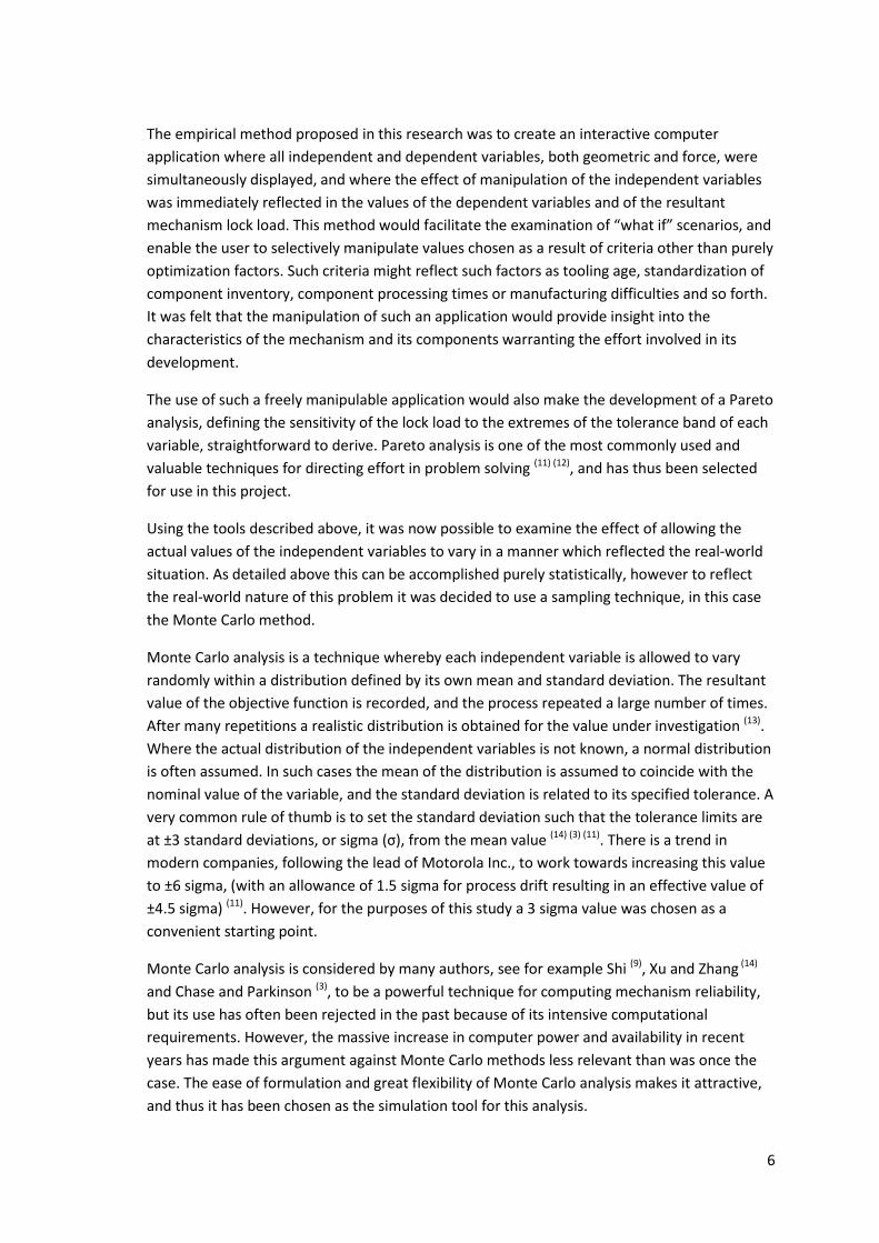
The empirical method proposed in this research was to create an interactive computer
application where all independent and dependent variables, both geometric and force, were
simultaneously displayed, and where the effect of manipulation of the independent variables
was immediately reflected in the values of the dependent variables and of the resultant
mechanism lock load. This method would facilitate the e amination of “what if” scenarios, and
enable the user to selectively manipulate values chosen as a result of criteria other than purely
optimization factors. Such criteria might reflect such factors as tooling age, standardization of
component inventory, component processing times or manufacturing difficulties and so forth.
It was felt that the manipulation of such an application would provide insight into the
characteristics of the mechanism and its components warranting the effort involved in its
development.
The use of such a freely manipulable application would also make the development of a Pareto
analysis, defining the sensitivity of the lock load to the extremes of the tolerance band of each
variable, straightforward to derive. Pareto analysis is one of the most commonly used and
valuable techniques for directing effort in problem solving (11) (12), and has thus been selected
for use in this project.
Using the tools described above, it was now possible to examine the effect of allowing the
actual values of the independent variables to vary in a manner which reflected the real-world
situation. As detailed above this can be accomplished purely statistically, however to reflect
the real-world nature of this problem it was decided to use a sampling technique, in this case
the Monte Carlo method.
Monte Carlo analysis is a technique whereby each independent variable is allowed to vary
randomly within a distribution defined by its own mean and standard deviation. The resultant
value of the objective function is recorded, and the process repeated a large number of times.
After many repetitions a realistic distribution is obtained for the value under investigation (13).
Where the actual distribution of the independent variables is not known, a normal distribution
is often assumed. In such cases the mean of the distribution is assumed to coincide with the
nominal value of the variable, and the standard deviation is related to its specified tolerance. A
very common rule of thumb is to set the standard deviation such that the tolerance limits are
at ±3 standard deviations, or sigma ( ), from the mean value (14) (3) (11). There is a trend in
modern companies, following the lead of Motorola Inc., to work towards increasing this value
to ±6 sigma, (with an allowance of 1.5 sigma for process drift resulting in an effective value of
±4.5 sigma) (11). However, for the purposes of this study a 3 sigma value was chosen as a
convenient starting point.
Monte Carlo analysis is considered by many authors, see for example Shi (9), Xu and Zhang (14)
and Chase and Parkinson (3), to be a powerful technique for computing mechanism reliability,
but its use has often been rejected in the past because of its intensive computational
requirements. However, the massive increase in computer power and availability in recent
years has made this argument against Monte Carlo methods less relevant than was once the
case. The ease of formulation and great flexibility of Monte Carlo analysis makes it attractive,
and thus it has been chosen as the simulation tool for this analysis.
7
A further question relating to Monte Carlo studies involves the appropriate number of
iterations needed to result in an accurate determination of, in this case, the distribution of lock
load values. Recommended iterations vary widely in the literature, ranging from 300 (14), 300-
3000 (15), right up to 100000-400000 (3). Once again, the optimum number seems to depend on
numerous factors, not least of which is the required accuracy of the derived distribution (16).
An approach which takes into account the required accuracy of the results is used by Dunn and
Shultis (17), who use the Weak Law of Large Numbers to derive the number of iterations
needed. It was decided to use this approach in this study. However, as computing power is not
expected to be an issue in this case, it was decided that whatever results were obtained would
be rounded up to a convenient figure, and possibly be further modified by examination of the
perceived smoothness of the resultant graphs. It was decided to consider this further once
initial results had been obtained.
A further question to be considered in this review was to define what could reasonably be
achieved by the application of these methods. The overall aim of tolerance analysis is defined
by Chase and Parkinson (3) as “design improvement… (by) systematically selecting tolerances
throughout an assembly to ensure that design requirements will be met.” What is not
mentioned in this definition is that the ideal situation, that of all products meeting all
requirements, is not always obtainable in practice. Instead, only a proportion of the
manufactured assemblies will typically be completely satisfactory on testing or inspection at
the end of the production line. This proportion is known as the first pass yield of the process.
The remaining non-complying production is usually re-worked or scrapped depending on the
characteristics of the product in question. This represents a significant cost to the
manufacturer; not only in the direct costs of fault finding and repair, but also in increased
product cycle time, delivery delays, and the cost of in-process inventory (18). According to
Pyzdek and Keller (19), companies operating at between three sigma and four sigma typically
spend 25-40% of their revenue fixing problems. In companies operating at six sigma this figure
comes down to 5%. These figures may be somewhat misleading, as no mention is made of the
complexity of the products being made. Final product failure rates are typically a function of
both component failure rates and component count. Nevertheless, it is clear that the point
made by the authors is still valid.
Other authorities have conducted research into first pass yield targets, and these vary widely
according to assembly complexity, number of variables, industry type and so forth. Some
examples are:
World class companies should have a first pass yield exceeding 99% (18).
A typical circuit board with around 1000 components has a benchmark first pass yield
of 97.5% (20).
The average first pass yield for “Best in Class” Engineering companies is around 91%
(although this figure includes rejects from the manufacture of the individual
components and reflects multiple processes running at an average of 5.04 sigma) (21).

8
After consideration of these figures, it was decided that the initial target for the first pass yield
of the device assembly, after optimization of the actuating mechanism, would be 99%.
Finally, particular note was taken of a series of reports prepared by Dr A. Hay, relating to the
mechanism under investigation as well as other similar mechanisms. In these reports,
investigations were conducted into various aspects of the definition and analysis of the
mechanism’s characteristics.
Hay first demonstrated (22) a method of determining the static friction coefficient of the torque
link / actuator interface by experimental methods. In his work the friction coefficient was
derived from lock load measurements performed using an apparatus of known dimensions.
This method was felt to be appropriate for the current study. His work, however, employed an
idealized representation of the mechanism, with a limited number of independent geometric
variables being used in the positional analysis. In addition, certain of the interfaces between
the components had been idealised, and no allowance was made for process capabilities in the
manufacture of the components. In particular, the number of samples measured in the trials
was very small compared to the likely variability in results, and all geometric dimensions were
set to their nominal value without reference to their manufacturing tolerances. For the current
study, the number of samples will be significantly enlarged to accurately describe the
geometry of the mechanism. The process capabilities used in the manufacture of components
and the variation of manufactured dimensions within tolerance bands will also be taken into
account.
In an extension to his work (23), Hay proposed a method for automating the generation of
solutions to a set of kinematic constraint equations defining a mechanism. Hay’s approach was
initially considered appropriate for the current project, but was ultimately not used. As
explained in the text, it was felt that deriving general solutions for the dependent variables
offered greater flexibility for subsequent manipulation of the system.
Hay finally applied the above developed techniques to perform a sensitivity analysis (24) on a
static model of a mechanism similar to the one under investigation in this project. The
variables thereby identified as having the most influence on the correct functioning of the
mechanism were then subjected (25) to a dynamic sensitivity analysis using MSC ADAMS.
These sensitivity analyses demonstrated the applicability of the various techniques described
in Hay’s earlier works. Several of the recommendations contained in these reports, such as the
use of vector analyses in the modelling phase and the experimental derivation of friction
coefficients, were thus adopted as a starting point for this project.
9
1.3 Objectives and Methodology.
Due to the complex nature of the mechanism under investigation it is appropriate to present
the objectives of the research and the detailed methodology together.
Two existing mechanism configurations will be considered initially. Once insights have been
gained, a third mechanism will be proposed and analysed.
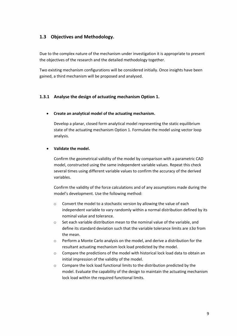
1.3.1 Analyse the design of actuating mechanism Option 1.
Create an analytical model of the actuating mechanism.
Develop a planar, closed form analytical model representing the static equilibrium
state of the actuating mechanism Option 1. Formulate the model using vector loop
analysis.
Validate the model.
Confirm the geometrical validity of the model by comparison with a parametric CAD
model, constructed using the same independent variable values. Repeat this check
several times using different variable values to confirm the accuracy of the derived
variables.
Confirm the validity of the force calculations and of any assumptions made during the
model’s development. Use the following method:
o Convert the model to a stochastic version by allowing the value of each
independent variable to vary randomly within a normal distribution defined by its
nominal value and tolerance.
o Set each variable distribution mean to the nominal value of the variable, and
define its standard deviation such that the variable tolerance limits are ±3 from
the mean.
o Perform a Monte Carlo analysis on the model, and derive a distribution for the
resultant actuating mechanism lock load predicted by the model.
o Compare the predictions of the model with historical lock load data to obtain an
initial impression of the validity of the model.
o Compare the lock load functional limits to the distribution predicted by the
model. Evaluate the capability of the design to maintain the actuating mechanism
lock load within the required functional limits.

10
Determine variable sensitivities.
Perform an empirical analysis to determine the sensitivity of the actuator mechanism
lock load to variation in the values of each independent variable. Develop an
application to facilitate this analysis. Set all independent variables individually to their
upper and lower limits, while fixing all other variables at their nominal values.
Ascertain the effect on the actuator mechanism lock load of each manipulation.
Analyse the sensitivity by means of a Pareto chart, and identify priorities for further
investigation.
1.3.2 Analyse the actual performance of the Option 1 mechanism.
Update the model to determine its behaviour using actual component distributions.
Obtain actual variable distributions for the components used in the assembly. These
may be obtained from historic statistical process control data or from direct
measurement, as appropriate.
Substitute the actual component variable distributions for the theoretical distributions
previously used in the model, and derive an updated prediction for the distribution of
the Option 1 actuating mechanism lock load.
Obtain actual performance data for the Option 1 actuator mechanism.
Obtain actual Option 1 lock load distribution data by direct measurement. Compare
this distribution with the predicted lock load distribution derived in the previous step.
Compare the model’s predictions to the actual performance and analyse the results.
Compare the two sets of results, and reconfirm the validity of the model now that
actual component variable distributions are used. Evaluate the distribution of the
actual actuator mechanism lock loads and compare to the target of 99% falling within
the functional limits.
1.3.3 Analyse the actual performance of the Option 2 mechanism.
Update the model.
Reconfigure the model to accommodate geometrical and other differences between
the Option 2 and Option 1 actuating mechanisms.

11
Validate the geometrical integrity of the model as previously accomplished for the
Option 1 variation.
Obtain additional actual component variable distribution data, where required.
Obtain actual performance data.
Obtain the predicted and actual performance data for the Option 2 actuating
mechanism in the same manner as for Option 1.
Compare the model’s predictions to the actual performance and analyse the results.
Compare the actual and predicted distributions for Option 2 and contrast these with
those previously obtained for Option 1.
Analyse any differences found. Evaluate the implications of the analysis, in particular
any design or performance insights to be gained from the exercise.
1.3.4 Propose a design for a new Option 3 actuating mechanism.
The following assumes that the results of the analysis of Options 1 and 2 indicate that a
modification to the design of the actuating mechanism has the potential to achieve the
targeted increase in first pass yield.
Develop a proposal for an improved design.
Use the insights and results obtained in Section 1.3.3 to propose a solution to the problem
of increasing the first pass yield of the actuating mechanism.
Predict the behaviour of the new design.
Using the models previously developed predict the behaviour, lock load distribution and
first pass yield of the proposed improvements.
Estimate financial implications.
Estimate the costs associated with implementation of the new design and the length of the
payback period.

12
2 DESCRIPTION OF THE ACTUATING MECHANISM
The following section presents an overall description of the purpose and design of the
actuating mechanism. The differences between the Option 1 and Option 2 actuating
mechanism variations are discussed, as well as general requirements and limitations imposed
on any future Option 3 proposal. The design of the obsolete “Option 0” variation is given for
comparison purposes.
2.1 General principals of operation.
As discussed in the introduction, and as shown in Figure 1.1, the presence of a fault condition
causes the motive unit to apply a force to the actuating mechanism. This motive force
overcomes the actuating mechanism’s lock load, triggering its actuation. This in turn causes
the engagement mechanism to collapse, thereby rendering the device into a safe mode.
The motive unit is considered for the purposes of this study to be a fully independent sub-
system having no influence on the performance of the actuating mechanism. In particular, the
motive force supplied by the motive unit is considered to be constant.
In contrast to this, the geometric details of the engagement mechanism contribute to the
position and orientation of elements of the actuating mechanism. In addition, the tolerances
applied to the housing base, the mechanism frame, the handle and various other elements all
contribute to the precise definition of the actuating mechanism’s geometry.
Consequently, this study is confined to the control of the actuating mechanism lock load, but
subject to the geometric and force influences of the device as a whole.
An overall schematic view of the device is given in Figure 2.1. Various sections of the
mechanism will be described and illustrated in more depth later in the study.

13
Figure 2.1 Schematic view of actuating mechanism Option 1.
Notes:
Revolute joints 1 and 2 are fixed relative to the base, subject to the tolerances on the boss
locations. The corresponding hole locations on the bottom frame are similarly subject to
tolerances. The precise relationship between the base and the bottom frame and their relative
orientation is thus tolerance dependent.
Revolute joints 3 and 4 are fixed relative to the bottom frame, subject once again to the
applicable tolerances in the location of the joints.
The knife edge joint 5 has, in practice, a small radius on the actuator shoulder. It is therefore
treated as a revolute joint, with a precise location subject to tolerances in the base, bottom
frame, and link frame.
Revolute joint 6, between the handle and the engagement arm, is free to move along a radius
centred on joint 3, limited by stop 8 and other limitations not relevant to this study.
The translational joint 7 is kept in engagement by the main spring.
Features 8 and 9 are located on the base, with their precise locations once again subject to
tolerance.

14
Item 10 is a pressure pad, and is part of the non-moving portion of the engagement
mechanism. For the purpose of this study it is assumed to be attached to the base, subject to
positional tolerances. The fixed and moving pressure pads are required to be held together by
a substantial force in order to maintain the device in an operative condition. The moving
pressure pad, item 11, is attached to the end of the engagement arm.
2.2 Actuating mechanism operation.
The actuation of the mechanism is achieved as follows.
Figure 2.2 Actuating mechanism schematic view: option 1.
(Note that the actuator return spring is omitted for clarity).
1. The actuator pivots on a knife-edge arrangement against the link frame. (Note that in practice there is a small radius on the actuator shoulder, thus rendering the actual joint position dependent on the radius value).
2. A spring loaded pivoting torque link is mechanically retained by the actuator. The spring additionally supplies the engagement force to the pressure pads.
3. When the actuator flange is attracted to the motive unit as described in Section 2.1, the catch face of the actuator slides upon the end of the torque link until the torque link disengages from the actuator.

15
4. The torque link is now free to move under the influence of the main spring, and the resultant movement of the torque link causes the engagement mechanism to collapse, rapidly opening the pressure pads.
5. The fault condition is cleared, the magnetic field collapses, and the actuator returns
under the influence of its own (weak) return spring to its rest position.
6. The mechanism is now ready to be reset when the handle (not shown) is next operated.
The design as detailed above is very efficient in terms of component count and thus cost, but
in situations such as this where certain components have several different functions, the
optimization of their design becomes challenging.
For example, a primary function of the torque link is to anchor and locate one end of the main
spring. This main spring has to be fairly strong, as it provides both the engagement force
applied by the pressure pad, and the motive force behind the acceleration of the engagement
arm upon actuation of the mechanism. Both the engagement force and engagement arm
acceleration should ideally be as large as possible for optimum functioning of the device. The
strong main spring results, however, in a large torque being applied to the torque link.
This large torque results in a large normal force being present in the translational joint
between the catch faces of the actuator and the torque link. Friction in this joint opposes the
action of the relatively weak magnetic force generated by the motive unit. This friction also
leads to wear in the catch faces which may have long term consequences. Long term effects
are not considered further as part of this study.
The control of the system of moments applied to the actuator is of paramount importance for
the correct operation of the actuation mechanism, and requires constant monitoring and
specialized manufacturing processes to achieve.
This design challenge has several potential solutions.
The two solutions which are currently used in production actuating mechanisms of the type
under consideration can be described as Option 1 and Option 2. The similarities and
differences between these two solutions are discussed in the next sections.
2.3 Control of catch face friction: Option 1.
2.3.1 Force and moment diagrams.
Free body diagrams of the active components of the actuation mechanism are shown below.
The following conventions are used in the diagram:

16
Constraint forces vectors: f3/1 = force vector exerted by body 3 on body 1. (fT )
f1/2 = force vector exerted by body 1 on body 2. (fms)
f2/3 = force vector exerted by body 2 on body 3.
External force vectors: fms = main spring force vector.
fmag = motive force vector.
fas = actuator spring force vector.
Moments τa = actuator torque from f1/2 acting on angled catch face.
τcf = actuator torque derived from catch face friction.
τsh = actuator torque from actuator shoulder friction.
τas = actuator torque derived from fas.
τLL = lock load torque.
τT = torque link torque derived from friction at point A.
All vector quantities are shown in bold face. The appro imate orientations of the components’
coordinate systems are indicated in the diagrams. The definition of these coordinate systems is
necessary for the vector loop analysis shown later in this study.
Figure 2.3 Free body diagrams: system at equilibrium, at point of actuation.
Note that certain of the constraint force vectors are assigned descriptive names later in the
study, where this is felt to aid in a better understanding of the model. The moments
experienced by body 2 are shown separately in Figure 2.4.
τT

17
From the forces shown in the above diagram, a group of moments are applied to the actuator.
These moments are illustrated in the following diagram.
Figure 2.4 Moments applied to the actuator: system at equilibrium, at point of actuation.
The forces and moments illustrated in Figures 2.3 and 2.4 are discussed in the following
section.
2.3.2 Description of forces and moments.
1. The torque link tip exerts a force f1/2 (from now on named fcf or catch face force) upon an angled catch face within the body of the actuator at point B. The force fcf is derived from the main spring force fms, reduced slightly by the reactive torque stemming from f3/1 (from now on named fT). This force vector fcf has a component fn
cf normal to the angled actuator catch face, which exerts an anti-clockwise reactive torque (τa) on the actuator. This torque is dependent both on the magnitude of the force fcf and on the length of the moment arm over which it acts. This moment arm length is itself dependent on the precise orientation of the angle catch face relative to the knife edge.
2. The friction in the joint between the actuator and torque link exerts a clockwise reactive torque (τcf) on the actuator when an attempt is made to rotate the actuator in an anti-clockwise direction towards the motive unit.
3. Similarly, friction in the actuator shoulder joint exerts a clockwise reactive torque (τsh) on
the actuator when an attempt is made to rotate the actuator anti-clockwise. 4. The actuator return spring exerts, in the static case, a constant clockwise torque (τas) on
the actuator. 5. The magnetic attraction between the actuator flange and the motive unit (fmag) exerts an
anticlockwise torque (τmag), which has to overcome the sum of the previous four moments in order to actuate the mechanism.
6. This overall arrangement is referred to as actuating mechanism “Option 1”.
τa τcf τsh τas
τmag
18
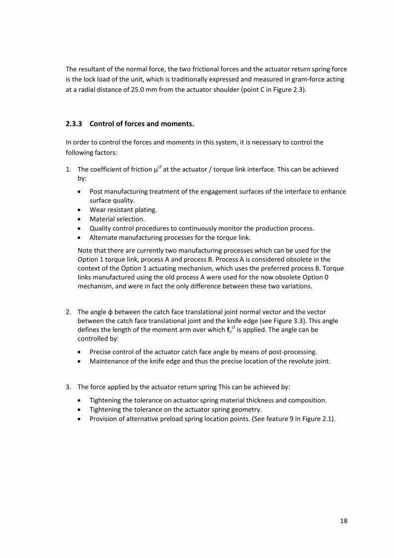
The resultant of the normal force, the two frictional forces and the actuator return spring force
is the lock load of the unit, which is traditionally expressed and measured in gram-force acting
at a radial distance of 25.0 mm from the actuator shoulder (point C in Figure 2.3).
2.3.3 Control of forces and moments.
In order to control the forces and moments in this system, it is necessary to control the
following factors:
1. The coefficient of friction μcf at the actuator / torque link interface. This can be achieved by:
Post manufacturing treatment of the engagement surfaces of the interface to enhance surface quality.
Wear resistant plating.
Material selection.
Quality control procedures to continuously monitor the production process.
Alternate manufacturing processes for the torque link.
Note that there are currently two manufacturing processes which can be used for the Option 1 torque link, process A and process B. Process A is considered obsolete in the context of the Option 1 actuating mechanism, which uses the preferred process B. Torque links manufactured using the old process A were used for the now obsolete Option 0 mechanism, and were in fact the only difference between these two variations.
2. The angle φ between the catch face translational joint normal vector and the vector between the catch face translational joint and the knife edge (see Figure 3.3). This angle defines the length of the moment arm over which fn
cf is applied. The angle can be controlled by:
Precise control of the actuator catch face angle by means of post-processing.
Maintenance of the knife edge and thus the precise location of the revolute joint.
3. The force applied by the actuator return spring This can be achieved by:
Tightening the tolerance on actuator spring material thickness and composition.
Tightening the tolerance on the actuator spring geometry.
Provision of alternative preload spring location points. (See feature 9 in Figure 2.1).

19
2.4 Control of catch face friction: Option 2.
The second actuating mechanism design, Option 2, is in fact a variation on the Option 1 design.
Figure 2.5 Actuating mechanism schematic view: option 2
In this variation, the angled actuator catch face is replaced by a stainless steel roller pin,
located within a housing mounted on the actuator. The translational joint angle, which defines
the moment arm length over which the catch face force acts and which was implemented on
the actuator catch face in mechanism Option 1, is now transferred to the torque link catch
face, while retaining a similar function. This arrangement is referred to as “Option 2”.
This solution is perceived to have the following advantages, the extent of which is examined
later in this study.
1. The surface finish of the stainless steel roller, and thus its coefficient of friction, is more consistent than the angled actuator catch face it replaces.
2. Variation in the quality of the wear resistant plating on the actuator catch face is avoided. 3. It is easier to accurately maintain the required angle on the torque link catch face (which is
formed directly from the tooling), than on the actuator catch face (where the angle is formed in a post manufacturing process).
There are, however, certain drawbacks to this design.

20
1. The assembly of the roller into its housing is time-consuming, labour-intensive and difficult to automate.
2. Without special surface treatments, wear in the torque link catch face where it engages the roller can become a problem.
3. As this solution is implemented on a small scale for specialized applications, the torque link
used for Option 2 cannot currently be manufactured using the preferred type B process
used for the Option 1 solution.
4. The production processes associated with this design are not currently optimised for high
volume production, and such optimisation would require significant capital investment.
2.5 Control of catch face friction: Option 3.
It is assumed at this point that the need for a third design option will become apparent during
the course of the study. Should this be the case, then consideration will have to be given to the
specification, requirements and limitations of the design.
Any hypothetical third option for the design of the actuating mechanism could potentially
involve increased costs. These might relate to increased component complexity or to increased
production or assembly costs. Such increased costs would have to be offset by some
advantage inherent in the updated design which led directly to an increase in first pass yield
for the actuating mechanism, and a corresponding reduction in the costs associated with
repair and re-work.
Alternatively, the third option could possibly have a reduced cost. In such a case, it would have
to be demonstrated that the quality of the final product would not be adversely affected by
the introduction of the new design.
These and other requirements and limitations pertaining to any proposed third option are
summarized as follows.
2.5.1 Option 3 design requirements and limitations.
The following requirements and limitations are imposed upon any potential design solution.
The functional limits for the distribution of the lock load values must be consistently
met.
No changes are allowed which may adversely affect the operation of the motive unit.
(Note that the actuator has a dual function, and is an integral component of both the
actuating mechanism and the motive unit).

21
No changes are allowed which would require the mechanism to be recertified to
national or international standards. The definition of how extensive a design change
would have to be to necessitate recertification is somewhat loose, but it is accepted
that any changes to the overall method of operation or substantial changes to
magnetic or electrical circuitry would require recertification.
All proposed changes are required to pass internal testing equivalent to certification
testing, even if formal recertification is not required.
The physical dimensions and overall profile of the mechanism housing must remain
unchanged.
All proposed changes to be RoHS compliant.
The cost of all proposed changes must be justified in terms of the cost savings
associated with the improved first pass yield of the actuating mechanism.
Although this study is focused upon the control of the actuating mechanism lock load,
it must be remembered that this is only one characteristic of a fairly complex device.
No changes are thus allowed that would impact on the performance of any other
attribute of the device’s internal systems.

22
3 ANALYSIS: MECHANISM OPTION 1
As stated in Section 1.3.1, it was decided to analyse the Option 1 actuating mechanism with
the aid of a static planar model. It was further decided to develop the geometric definition of
the model by means of vector loop analysis, in order to derive functions for all of the
dependent geometric variables. These functions were to be checked with the help of a
parametric CAD model of the mechanism.
The forces and moments were then to be introduced into the model to derive a definition of
the lock load as a function of the independent variables in the system.
The validity of the design was to be established with the aid of Monte Carlo analysis, and the
sensitivity of the design to changes in each independent variable to be investigated by use of
an empirical application.
Actual distributions for the independent variables were then to be introduced to evaluate the
performance of the model in a real-world situation in comparison with the actual performance
data.
3.1 Static analysis.
The relative positions of the components of the mechanism are determined by the nature of
their defined joints and by the physical sizes of the components.
The physical sizes are specified as:
The nominal dimensions of the components, and
The allowed tolerance in these dimensions.
The permitted variation in the sizes of the components causes variation in the orientation of
the mechanism. These positional variations in turn result in variation in the forces experienced
within the system. In particular, the force required to actuate the mechanism is influenced in
an as yet inadequately defined manner by such positional variations.
In order to determine the sensitivity of the lock load to the tolerance specified for each
dimension, and thus verify the suitability of the tolerances, it was first necessary to perform a
positional analysis of the mechanism by means of vector loop analysis.
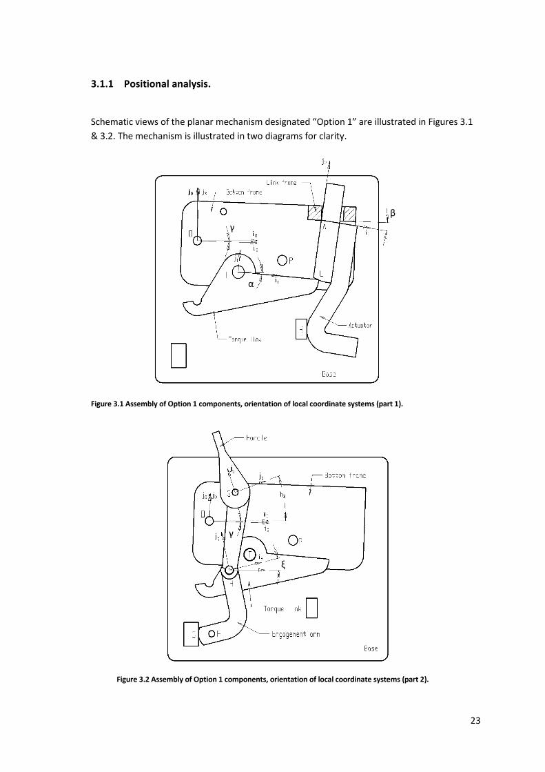
23
3.1.1 Positional analysis.
Schematic views of the planar mechanism designated “Option 1” are illustrated in Figures 3.1
& 3.2. The mechanism is illustrated in two diagrams for clarity.
Figure 3.1 Assembly of Option 1 components, orientation of local coordinate systems (part 1).
Figure 3.2 Assembly of Option 1 components, orientation of local coordinate systems (part 2).
γ
β
α
ξ
γ

24
Notes:
The mechanism illustrated above is somewhat unusual in that the location and
orientation of the coordinate systems of each component is not fixed, but can vary
according to the tolerances applied to the location of the joint positions on both
elements of each joint. For example, the angle γ between the nominally coincident
coordinate systems i0, j0 and i3, j3 represents the tolerances applied to the location
elements (or revolute joints) at O and P. Similarly, the exact positions of the nominally
fixed revolute joints at S, T, and A are tolerance dependent. The revolute joint at H and
the translational joint at C are allowed to move depending on the geometry and
position of their components. This is explained in more detail as follows.
The global coordinate system, indicated by the unit vectors (i0, j0), is by definition
coincident with the coordinate system of the base.
The bottom frame and link frame can, due to the method used in their assembly, be
considered as one part. The combined part “frame” then has a coordinate system
indicated by the unit vectors (i3, j3).
The frame locates onto the base via locating holes which engage with studs located on
the base at positions O and P.
The origins of the coordinate systems indicated by (i3, j3) and (i0, j0) are coincident.
The angle γ represents the tolerances in joints O and P, and has a nominal value of 0°.
The stop located at joint B is an integral part of the base.
Joint A is considered to be a revolute joint.
The coordinate system of the handle, indicated by the unit vectors (i5, j5), is
constrained at an angle h3 to the base by means of integral stops located in the shell.
This angle is considered have a tolerance of ±0.5° for the purposes of this study.
The fixed pressure pad G is considered to be integral with the base.
The coordinate systems of the engagement arm, torque link and actuator, indicated by
(i6, j6), (i1, j1), and (i2, j2), are at angles ξ, α and β respectively to the global coordinate
system. These angles are to be determined.
The co-ordinate system of the link frame (i4, j4) has been fixed relative to the bottom
frame and is thus not used further.
An analysis of the mechanism illustrated in Figures 3.1 & 3.2 indicated that the
mechanism’s configuration was defined by the following independent variables. (See
Figures 3.3 and 3.4)

25
Table 3.1 Independent variables: mechanism Option 1.
t1 torque link length (mm)
t2 torque link tip radius (mm)
t3 torque link centres: spring notch to pivot point (local x) (mm)
t4 torque link centres: spring notch to pivot point (local y) (mm)
t5 torque link pivot point radius (mm)
a1 actuator shoulder to catch face (mm)
a2 actuator catch face angle length (mm)
a3 actuator catch face angle value (°)
a4 actuator shoulder to flange length (mm)
a5 actuator bend outer radius (mm)
a6 actuator shoulder radius (mm)
p2 bottom frame plate centres: location 1 to location 2 (local y) (mm)
p3 bottom frame plate centres: location 1 to torque link pivot point (local x) (mm)
p4 bottom frame plate centres: location 1 to torque link pivot point (local y) (mm)
p5 bottom frame plate centres: location 1 to link frame location (local x) (mm)
p6 bottom frame plate centres: location 1 to link frame location (local y) (mm)
p7 bottom frame plate centres: location 1 to handle location (local x) (mm)
p8 bottom frame plate centres: location 1 to handle location (local y) (mm)
m1 link frame location centre to actuator location (local x) (mm)
m2 link frame location centre to actuator location (local y) (mm)
b1 shell base centres: location 1 to location 2 (local x) (mm)
b2 shell base centres: location 1 to location 2 (local y) (mm)
b3 shell base location 1 centre to actuator stop (local x) (mm)
b5 shell base location 1 centre to fixed pressure pad (local x) (mm)
b6 spring location centre (local x) (mm)
b7 spring location centre (local y) (mm)
b9 spring location radius
c1 engagement arm centres: pivot point to spring location (local x) (mm)
c2 engagement arm centres: pivot point to spring location (local y) (mm)
c3 engagement arm spring location centre to pressure pad (radial dimension) (mm)
h1 handle centres: pivot point to actuator location (local x) (mm)
h2 handle centres: pivot point to actuator location (local y) (mm)
h3 handle angle relative to base(in the “on” position) (°)
s3 main spring upper location (torque link) radius (mm)
s4 main spring lower location (engagement arm) radius (mm)
s5 actuator spring thickness (mm)
s6 actuator spring width (mm)
s7 actuator spring flatness (mm)

26
From the above independent variables, the following dependent variables were derived.
Table 3.2 Dependent variables: Mechanism Option 1.
α torque link local to global coordinate system angle (°)
β actuator local to global coordinate system angle (°)
γ bottom frame plate local to global coordinate system angle (°)
δ torque link / actuator catch overhang (mm)
ε actuator / actuator stop tangent point (global y) (mm)
ζ main spring length (loaded) (mm)
η engagement arm / engagement pad tangent point (global y) (mm)
θ main spring force vector angle 1 (°)
ϟ main spring force vector angle 2 (°)
ξ engagement arm local to global coordinate system angle (°)
λ torque link/main spring moment arm length (mm)
ρ torque link/actuator moment arm length (mm)
φ catch force vector angle (°)
ψ catch face angle force moment arm length (mm)
ω catch face friction force moment arm length (mm)
p1 bottom frame plate centres: location 1 to location 2 (local x) (mm)
Additional variables relating to the orientation of the fle ible member “actuator spring” will be
introduced later in the analysis.
3.1.1.1 Determination of mechanism configuration: Option 1.
Dimensions relevant to the alignment of the actuator and torque link are shown in Figure 3.3.

27
Figure 3.3 Dimensions of Option 1 components, part 1.
Dimensions pertaining to the positioning of the handle and engagement arm are
illustrated in Figure 3.4.
δ
φ
ε
ρ
ψ
ω

28
Figure 3.4 Dimensions of Option 1 components, part 2.
η
λ θ
ζ ϟ

29
In order to determine the dependent variables, various vector loops were defined.
The vector loops were constructed in such a way that they formed a closed chain of vectors,
each leg of which was defined in terms of the components’ independent variables plus one or
two of the dependent geometric variables. The applicable coordinate system was noted.
The notation used for the vectors was as follows:
r0AT indicates the vector to A from T, expressed in terms of coordinate system 0.
As many of the individual vectors were initially expressed in terms of other coordinate
systems, they had to be converted to the system used for the loop as a whole by means of a
transformation matrix (22).
Once all the vectors were transformed into the same coordinate system, the vector loop was
described by summing the vector equations. Two equations, representing the sums of the X
and Y coordinates respectively, were thereby obtained. These equations were set equal to
zero, describing the closed nature of the loops. The two equations now contained either one
or two unknowns, which were determined by individual or simultaneous solving of the
equations as appropriate.
The following vector loops were solved for this analysis.
Figure 3.5 Option 1: Vector loop 1.

30
Figure 3.6 Option 1: Vector loop 2.
Figure 3.7 Option 1: Vector loop 3.

31
Figure 3.8 Option 1: Vector loop 4.
Figure 3.9 Option 1: Determination of γ.
3.1.1.2 Determination of dependent variables.
Once the mechanism had been described in terms of the four vector loops and the diagnostic
diagram shown above, the vector loops were solved in order to determine values for the
dependent variables.
In his work examining a similar problem (23) Hay contends that “the most difficult and time
consuming part of performing an analytic static force analysis is determining a closed form
solution e pressing the mechanism assembly in terms of its factors”. He then demonstrates
the use of a Matlab algorithm using the Newton-Raphson method to solve a system of
nonlinear kinematic constraint equations.
γ1
γ2
γ

32
This approach was considered carefully for this project. It was however decided to solve for
each variable explicitly. Obtaining general solutions for the dependent variables was felt to
offer greater flexibility for further manipulation of the system than would be possible using
unique variable solutions. (See Figure 3.15). The further refinement of Hay’s Matlab program
for use as a design tool for problems of this sort remains as a future challenge.
A detailed derivation of the dependent variables in given in Appendix A.
The equations of the dependent variables are summarised in Table 3.3 below.
Table 3.3 Definition of dependent variables for mechanism Option 1
γ = -arctan (b2 / b1) + arctan (p2 / √
) (A.1)
β = (
√
) γ (
) (A.9)
ε = (p5 - m1 γ 6 - m2 o γ 5 β γ 5 - a4 o β γ (A.10)
α = (
√
)
X = t2 β γ - a3) -t1 + t2
Y = t1 - t2 β γ - a3) + t2
Z = A β γ -a3) – B
A = o γ 5–p3–m1) – γ 6+p4–m2) + t2 β γ-a3) + a1 β γ - a2 β γ 3
B = γ 5 – p3 – m1 o γ 6 + p4 – m2) – t2 o β γ - a3) - a1 o β γ + a2 o β γ 3
(A.30)
δ =
o α α – A
o β γ β γ
(A.20)
φ =
– β – γ ( α o α o β γ
o α α β γ )
(A.32)
ρ = √( o α α – β γ )
α o α o – β γ (A.31)

33
ξ =
( o γ γ o γ γ
√
)
o (
√
)
(A.40)
η = -p7 sin γ - p8 o γ 1 sin (h3 γ 2 cos (h3 γ 1 ξ 2 o ξ (A.41)
ζ = √
(A.50)
ϟ = arctan (s1 / s2) (A.51)
θ = ( α – o α o
o α α ) (
) (A.52)
λ = √ o α α
α – o α o (A.53)
The above equations were checked against several parametric CAD models of the mechanism,
and were found to hold for a range of input values extending well beyond the tolerances
specified for the independent variables.
The equations were thus considered to be free from derivation errors.
3.1.2 Force analysis.
With the planar geometry of the mechanism defined in terms of its variables, it was possible to
examine the force required to operate the mechanism.
This force is a function of the mechanism’s geometry, the force e erted by the main spring
(fms), the torque applied to the actuator by the actuator spring (τas), and the friction in the
mechanism’s joints.
This resultant force is known as the lock load (fLL) of the mechanism, and is historically
expressed as a gram-force value applied perpendicular to the primary axis of the actuator, at a
distance of 25.0 mm from point A. For the mechanism to operate, this force must be less than
the available motive force (fmag).

34
3.1.2.1 Determination of the static forces acting on the torque link.
Figure 3.10 illustrates the forces acting on the torque link, as well as certain of the geometric
variables which were used in the force calculations.
Figure 3.10 Static force vectors and moments acting on the torque link.
In Figure 3.10 the force applied by the main spring acts along the vector fms. A component of
that force, defined by the cosine of angle θ and the length of the moment arm λ, applies an
anticlockwise torque to the torque link. This torque is opposed by a moment of equal value
caused by the reactive force fcf applied by the actuator on the torque link,the reactive frictional
torque τT present in the revolute joint T and the reactive frictional moment at C. The
magnitude of fcf is primarily dependent on the original torque and the length of the moment
arm ρ. Note that the angles α and ϟ represent the angles between the force vectors and the
global coordinate system.
The two forces fms and fcf are balanced by the reactive force exerted by the bottom frame on
the torque link fT. This force, along with the radius t5 and µT,the static friction coefficient of the
revolute joint at point T define τT, the reactive frictional torque at T.
The derivation of solutions for the unknown forces in the system is shown in Appendix A, and
the force equations are summarised in Table 3.4.
θ
λ
ρ
α
ϟ
τT
µcf
φ
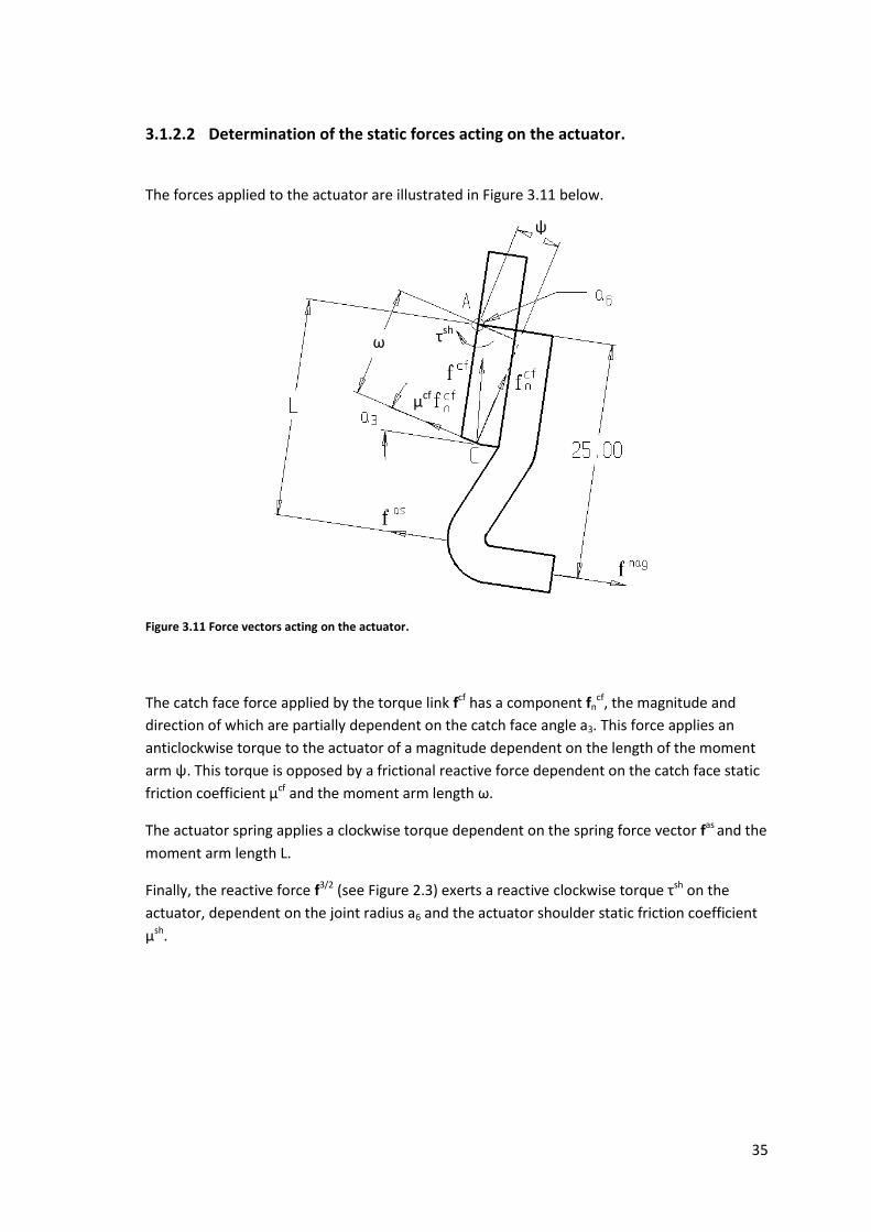
35
3.1.2.2 Determination of the static forces acting on the actuator.
The forces applied to the actuator are illustrated in Figure 3.11 below.
Figure 3.11 Force vectors acting on the actuator.
The catch face force applied by the torque link fcf has a component fncf, the magnitude and
direction of which are partially dependent on the catch face angle a3. This force applies an
anticlockwise torque to the actuator of a magnitude dependent on the length of the moment
arm ψ. This torque is opposed by a frictional reactive force dependent on the catch face static
friction coefficient µcf and the moment arm length ω.
The actuator spring applies a clockwise torque dependent on the spring force vector fas and the
moment arm length L.
Finally, the reactive force f3/2 (see Figure 2.3) exerts a reactive clockwise torque τsh on the
actuator, dependent on the joint radius a6 and the actuator shoulder static friction coefficient
µsh.
μcf
ψ
ω τsh

36
3.1.2.3 Determination of the static forces applied by the actuator spring.
Most of the variables shown in the Figure 3.12 below are self-explanatory. Factors not shown
are the actuator spring width s5, the actuator spring thickness s6, and a factor relating to the
actuator spring flatness W2.
Figure 3.12 Variables relating to actuator spring displacement.
The displacement s of the actuator spring causes the force vector fas to be applied to the
actuator. This force, acting over the moment arm length L, applies the clockwise moment τas to
the actuator at point A.
In the physical system there is an additional variation provided for the value of s, implemented
as a second spring location point, displaced along the local “x” vector from the point b6. This
variable (b8) was not considered further for this analysis.
β

37
3.1.2.4 Determination of actuator spring flatness.
In addition to the actuator spring displacement defined by b6 – b9, there was a further
variation to be considered, namely the effective addition or subtraction to the value of s
resulting from variations in the flatness of the actuator leaf spring, which either reduced the
effective displacement or induced a pre-load in the spring, depending on the orientation of the
curvature. This curvature was measured and limited by variable s7 below. This variable,
measured at the mid position of the actuator spring, resulted in an effective displacement w2
at the operating position.
Figure 3.13 Variables relating to actuator spring flatness.
Note that W3 refers to the displacement at the spring end and W2 refers to the displacement at
the spring actuation point.
The derivation of W2 is shown in Appendix A2.4, and was found to be 2.83 s7. This value was
checked against field observations, and was found to be consistent with the observed values.
Thus for all spring force calculations a value of 2.83 s7 was added to the value of s.
Note that the sign of s7 indicates whether the curvature of the spring is concave or convex. A
positive value indicates that the spring is convex, while a negative value indicates that the
spring is concave.

38
A detailed derivation of the forces variables is given in Appendix A.
The equations of the force variables in Appendix A are summarised in Table 3.4 below.
Table 3.4 Definition of force variables: Option 1
fcf = √
P = (ρ2 ρµcfsinφ μcf sinφ)2)- ((t5)2 ( μT)2)
where Q = -((t5)2 ( μT)2 2 fms (cos ϟ o α ϟ α – λ o θ fms ρ µcf sinφ)
R = λ o θ fms)2 - ((t5)2 ( μT)2 (fms)2)
(A.57)
fncf = f
cf cos(φ) (A.58)
fms = ζ – sf + 0.85) (A.59)
fas =
(A.60)
τas =
(A.61)
L = (p6 + b7 - m2) / cos β, (A.62)
s = b3 – b6 + b9 + W2, (A.63)
W2 = 2.83 s7 (A.69)
3.1.2.5 Determination of μcf, µtl and μsh.
The actual values for the three static friction coefficients are, as is often the case for
mechanical components, not explicitly specified. Their control is implicitly controlled by the
surface finishes, plating and other treatments specified for their manufacture. This was
considered to be inadequate for the purposes of this study, and an accurate determination of
the catch face friction coefficient was undertaken. (See Section 3.2.1). For the initial analysis
of nominal design values, historically accepted values of 0.15±0.03 for the catch face friction
coefficient and 0.20±0.10 for the torque link pivot point and actuator shoulder friction
coefficients were used.
With the values of μcf, fms, fas, fcf & fncf having been determined, it was now possible to
determine the theoretical lock load by evaluating the static forces acting upon the actuator.

39
3.1.2.6 Summary of the static forces acting on the actuator.
The moments acting on the actuator immediately before it begins to move are required to
have a vector sum of zero. (See Figure 2.4). This requirement can be expressed using
previously derived variables as:
τa + τLL - τcf - τas - τsh = 0 (3.1)
ie
ψ fncf + 25fLL = μcf ω fn
cf + τas + μsh a6fcf (3.2)
Where, to recap,
μcf is the coefficient of friction of the catch face between the actuator and the torque link,
μsh is the coefficient of friction of the actuator shoulder and link frame joint,
μtl is the coefficient of friction of the torque link revolute joint,
τas is the torque exerted on the actuator by the actuator spring (Nmm),
τa is the torque exerted on the actuator by the torque link via the actuator catch face
angle (Nmm),
τcf is the frictional torque of the catch faces (Nmm),
τsh is the frictional torque of the actuator shoulder (Nmm),
τLL is the lock load torque (Nmm),
Ψ is the angle force moment arm length (mm),
ω is the friction force moment arm length (mm),
a6 is the actuator shoulder radius (mm),
fcf is the catch force, ie the force exerted by the torque link on the actuator (N),
fncf is the component of the catch force normal to the actuator catch face (N), and
fLL is the lock load (N).

40
3.1.3 Determination of lock load.
From the values determined in the preceding sections, the force required to operate the
mechanism Option 1 could be expressed as:
(3.3) fLL = ((μcf ω)- ψ)fn
cf + τas+ μsh a6fcf
25
The independent variables considered in this analysis had the following nominal values with
respect to the mechanism Option 1.
Table 3.5 Variable distribution means (nominal).
Variable
Nominal value
Variable Nominal value
t1 17.60 b2 4.60
t2 0.08 b3 23.06
t3 5.15 b5 3.04
t4 5.80 b6 21.14
t5 0.80 b7 19.30
a1 10.30 b9 0.50
a2 1.20 c1 4.30
a3 4º c2 20.80
a4 26.00 c3 5.10
a5 2.10 h1 2.80
a6 0.05 h2 11.70
p2 4.60 h3 19.00
p3 6.92 s3 0.40
p4 3.77 s4 1.00
p5 25.20 s5 0.192
p6 6.31 s6 2.90
p7 4.26 s7 0.125
p8 5.00 μcf 0.15
m1 0.44 μsh 0.20
m2 0.80 μmc 0.20
b1 15.82 μtl 0.20

41
Solving Equation (3.3) resulted in:
fLL = 18.26 gf.
This agrees well with the historical values obtained on the production line, thus suggesting that
there are no major errors in the formulation of the model.
3.1.4 Evaluation of design tolerances.
It was indicated in Section 1.2 that the design tolerances would be evaluated by means of a
Monte Carlo analysis. Since the lock load had been expressed in terms of all the independent
variables (see Equation 3.3), it was possible to perform the Monte Carlo analysis by assuming
the following:
The variable values were normally distributed,
The variable mean values were equal to their nominal values, and
The standard deviation of each variable was such that the production tolerance of the
variable was equal to the generally accepted ±3 from the mean (3).
As mentioned above, the catch face friction coefficients are not explicitly specified as a
design variable, and were thus assumed to have the historically accepted value of 0.15
±0.03 for the catch face friction coefficient and 0.20±0.10 for the actuator shoulder
and the torque link pivot point.
When considering the number of iterations to perform for the analysis, the approach of Dunn
and Shultis (17) was used. Using their method, the Weak Law of Large Numbers can be
formulated as
o {| ̅ μ| } (
) δ
Where ̅ is the population mean, µ the sample mean, ϵ the error, the population variance,
δ the probability and N the sample size.
If the probability of the sample mean being within 0.1 of the population mean is required
(somewhat arbitrarily but based on Dunn and Shultis) to be 99.36%, then
δ =
=
=
Rounding this up as proposed in Section 1.2 resulted in a sample size of 50000.

42
A Monte Carlo analysis of the model was implemented, with the following results.
Figure 3.14 Predicted lock load distribution: Option 1.
As the functional limits for the lock load are defined to be 12 – 23 gf for the application
considered in this analysis, it can be seen that the predicted lock load distribution was fairly
well located between these limits, with a small portion of the distribution exceeding the upper
process limit.
The cumulative normal distribution calculated for the above mean and standard deviation
indicated that the samples exceeding the upper tolerance limit were expected to be around
0.56 per cent of production, while the samples exceeding the lower tolerance limit were
expected to be around 0.04 per cent. This agreed fairly well with a subjective view of the
distribution expected from experience with the real life production process.
The initial conclusions drawn from the Monte Carlo analysis were thus as follows:
The mean lock loads predicted by calculation and by the Monte Carlo analysis are
identical at the precision used, confirming the absence of formulation errors.
Closer inspection of historical records indicated that the model’s predictions were
somewhat optimistic, in terms of the proportion of production rejected for exceeding
both of the functional limits. It was decided that further clarity on this opinion was to
be obtained by experimentation and refinement of the model. (The results of such
model refinement can be seen in Figure 3.25, and lock load measurements from a
production sample are given in Section 3.2.7).

43
The tolerances specified for the independent variables seemed to be largely
appropriate for achieving a high first pass yield, but left little margin for error.
The model thus appeared to be adequate as a starting point, and the next stage of the project
was focused upon its refinement.
Note that the choice of 50000 as the number of iterations to be performed by the Monte Carlo
analysis has resulted in a graph having adequate smoothness without any excessive random
artefacts. A trial run using 200000 iterations was performed, and the values obtained were
identical to the previous results at the number of significant figures used. It was thus decided
to retain 50000 as the chosen iteration value for the rest of the analysis.
3.1.5 Sensitivity Analysis.
In order to ascertain the degree to which each variable contributed to the lock load
distribution, it was necessary to perform a sensitivity analysis.
A spreadsheet was developed as a means of manipulating individual variables within their
tolerance bands, in order to determine the relative effect of changes in the value of each
variable on the lock load. A screen shot of the application, with all variables set to their
nominal values, is shown in Figure 3.15.
The spreadsheet displays all factors relevant to the mechanism.
Each independent variable is equipped with a slider control, whereby its value can be adjusted
within a band defined by its tolerance limits. The independent variables are all initially set to
their nominal design values, and can be reset to these values by pressing the reset button
provided.
Manipulation of the independent variables, individually or in combination, causes an update in
the value of all affected dependent variables, up to and including the lock load. In this way all
the effects of adjusting the value of any variable or variables can immediately be seen.
Certain variables are de-activated on the sheet, as they are applicable only to the Option 2
actuating mechanism. A separate spreadsheet page is provided for the Option 2 variation,
where the appropriate variables are available for manipulation.
Certain values not directly applicable to this project, such as the engagement force between
the pressure pads, are provided for their utility value outside the context of this project. In
addition, a feature is included for examining the effects of specific classes of catch face surface
defect. (See Appendix B for further explanation).

44
Figure 3.15 Lock load manipulation spreadsheet.
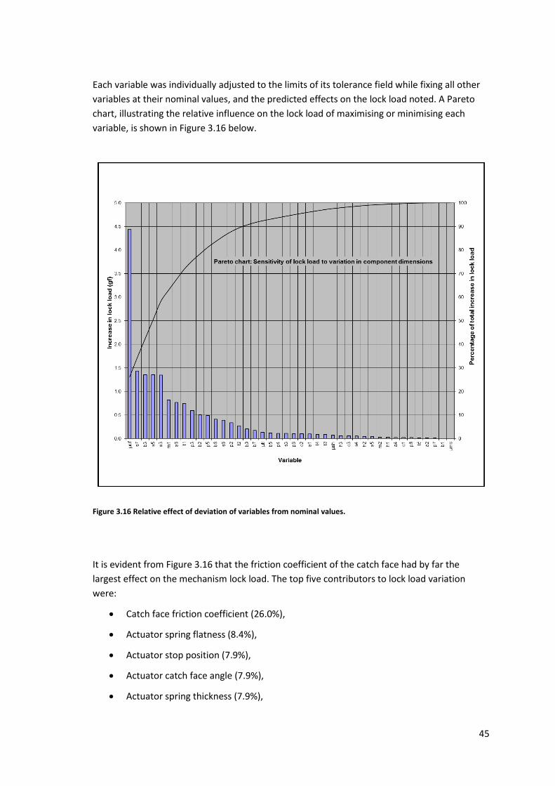
45
Each variable was individually adjusted to the limits of its tolerance field while fixing all other
variables at their nominal values, and the predicted effects on the lock load noted. A Pareto
chart, illustrating the relative influence on the lock load of maximising or minimising each
variable, is shown in Figure 3.16 below.
Figure 3.16 Relative effect of deviation of variables from nominal values.
It is evident from Figure 3.16 that the friction coefficient of the catch face had by far the
largest effect on the mechanism lock load. The top five contributors to lock load variation
were:
Catch face friction coefficient (26.0%),
Actuator spring flatness (8.4%),
Actuator stop position (7.9%),
Actuator catch face angle (7.9%),
Actuator spring thickness (7.9%),

46
These five variables alone together contributed nearly 60% of the lock load variation, and gave
a very good indication where future efforts regarding component manufacturing control
should be concentrated.
An initial examination of the definition of these five variables showed that the spring flatness
and thickness, the stop position and catch face angle were all well defined, and had been given
dimensional tolerances that were appropriate to the processes used in their manufacture and
their relative importance to the mechanism. While the tightening of these tolerances was
noted for future study, it was felt impractical to attempt such process changes in this project.
The catch face friction coefficient by contrast was less well defined and controlled, and with a
lock load variation contribution of 26.0% it was the obvious candidate to be addressed in order
to improve the first pass yield of the mechanism.
3.2 Model Validation: Option 1.
The method used to validate the model was as follows.
Actual values were obtained for the catch face friction coefficient. (After the initial
experimental results had been obtained, this section was expanded to include the
modelling of catch face surface imperfections).
Actual values were obtained for the mean and distribution of all geometric variables
used in the model.
These measured values were substituted into the model, replacing the values obtained
from the design parameters. The model then represented actual production
mechanisms, rather than the design.
A representative sample of production mechanisms was measured, and the
distribution of the measured lock loads plotted.
The measured lock load distribution was then compared to the predictions obtained
from the model.
3.2.1 Determination of catch face friction coefficient μcf.
It was mentioned in Section 3.1.2.5 that the coefficient of friction of the catch face was
assumed to be in the range 0.12-0.18.
Since it had been demonstrated how important this coefficient actually is, it was necessary to
determine the actual distribution of its value under production conditions.

47
3.2.1.1 Measurement method: catch face friction coefficient: Option 1.
The equation for determining the lock load derived in Section 3.1.3 could be used to determine
the catch face friction coefficient if all the other variables were known.
As the mechanism components were subject to dimensional variation as detailed in the
previous sections, it was necessary to substitute the majority of the mechanism with a gauge
of known and fixed size.
The gauge illustrated in Figure 3.17 (24) was developed prior to the commencement of this
project for the purpose of evaluating the interface between the catch faces of the torque link
and the actuator.
The gauge fulfilled all functions of the mechanism with the exception of the actuator, actuator
spring, main spring and torque link.
The dial gauge was located such that its measuring arm engaged directly with the actuator.
Rotation of the body of the gauge thus exerted a load on the actuator, substituting for the
motive force normally provided by the motive unit. The gauge was gradually rotated,
increasing the force applied to the actuator, until the mechanism disengaged. The force that
was required to trigger the specific actuator / torque link pair, its lock load, was then read
directly from the gauge.
Figure 3.17 General arrangement: lock load gauge.

48
The lock loads of 270 actuator / torque link pairs were measured by the above method over a
period of three months, in order to give as accurate a spread of results over time as possible.
(There is no significance to the number 270 other than the availability of samples for testing).
For each actuator / torque link pair the force required to begin to displace the actuator from
its rest position in the un-latched condition was also measured, thereby giving a direct
measurement for fas, and thence for τas. All other values, including fms, were measured directly
from the gauge.
(Note that the due to the use of process B in the manufacturing of the torque link, its
dimensions were very consistent. It was thus not necessary to perform profile measurements
on each individual component used in the exercise).
As shown in Equation (A.73) in Appendix A2.5, the coefficient of friction in the catch faces can
be calculated by:
μcf = 25 fLL - 25 fas + 0.1026
36.02
The coefficient of friction was calculated for each actuator / torque link pair, and a summary of
the results is shown in Figure 3.18 below.
3.2.1.2 Measurement results: catch face friction coefficient: Option 1.
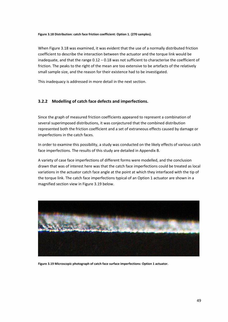
49
Figure 3.18 Distribution: catch face friction coefficient: Option 1. (270 samples).
When Figure 3.18 was examined, it was evident that the use of a normally distributed friction
coefficient to describe the interaction between the actuator and the torque link would be
inadequate, and that the range 0.12 – 0.18 was not sufficient to characterise the coefficient of
friction. The peaks to the right of the mean are too extensive to be artefacts of the relatively
small sample size, and the reason for their existence had to be investigated.
This inadequacy is addressed in more detail in the next section.
3.2.2 Modelling of catch face defects and imperfections.
Since the graph of measured friction coefficients appeared to represent a combination of
several superimposed distributions, it was conjectured that the combined distribution
represented both the friction coefficient and a set of extraneous effects caused by damage or
imperfections in the catch faces.
In order to examine this possibility, a study was conducted on the likely effects of various catch
face imperfections. The results of this study are detailed in Appendix B.
A variety of case face imperfections of different forms were modelled, and the conclusion
drawn that was of interest here was that the catch face imperfections could be treated as local
variations in the actuator catch face angle at the point at which they interfaced with the tip of
the torque link. The catch face imperfections typical of an Option 1 actuator are shown in a
magnified section view in Figure 3.19 below.
Figure 3.19 Microscopic photograph of catch face surface imperfections: Option 1 actuator.

50
Using this technique it was now possible to replicate the observed catch face friction
coefficient distribution by using a combination of an actual friction coefficient distribution and
one or more catch face imperfection distributions.
Note that this technique takes no cognisance of the shape, size or any other characteristic of
the defect itself, but merely on the effect that such defect has on the perceived catch face
friction coefficient.
Using the sample lock loads obtained in Section 3.2.1.1, the data was rearranged to represent
the lock load minus the actuator spring force, giving a distribution for the forces derived only
from the torque derived from the torque link.
It was now necessary to represent this data distribution as the optimized sum of several
discrete normal distributions.
These normal distributions were derived using the Matlab simplex search algorithm
fminsearch (25) to minimize the difference between the data and the summed normal
distributions.
The best optimisation results were obtained when using 3 discrete distributions as illustrated
in Figure 3.20. (Note: all lock loads are shown in gf).
Lock load (without actuator spring)
Figure 3.20 Lock load data approximated by the sum of 3 normal distributions.

51
The derived distribution (solid line) was more clearly illustrated when it was separated into its
component parts as shown in Figure 3.21.
Figure 3.21 The lock load distribution separated into its component parts.
The graphs shown in Figures 3.20 and 3.21 were interpreted as follows.
The primary distribution, representing variation in the friction coefficient, had a mean lock
load contribution of 3.739 grams with a standard deviation of 1.258 grams, and no influence
from catch face imperfections. This combination had a relative frequency of 0.521.
The remaining two distributions were attributable to the presence of catch face imperfections
or damage, and were interpreted as follows:
A minor defect resulting in an average of 2.926g being added to the 3.739g lock load,
with a total lock load standard deviation of 1.268 g and a relative frequency of 0.344;
and / or
A more severe defect resulting in an average of 6.621g being added to the lock load,
with a total standard deviation of 1.2589g and a relative frequency of 0.135.
Any of these defects may or may not occur in any particular mechanism.
Note that the use of algorithm fminsearch initially resulted in an even more accurate
approximation of the actual sample values of 3.1.6.1. However, an initial examination of the
results showed that the following constraints were required to keep the results realistic.
0
0.05
0.1
0.15
0.2
0.25
0.3
0.35
0 2 4 6 8 10 12 14 16
Main distribution
Defect 1
Defect 2
combined
Lock Load (without actuator spring)
Rel
ativ
e f
req
uen
cy

52
The standard deviation of each of the “lock load + defect” combinations was
constrained to be greater than or equal to the standard deviation of the lock load
alone, on the basis that the addition of a variable was unlikely to reduce the overall
standard deviation.
The frequency of any combination was constrained to be greater than or equal to zero.
The above graphs were optimized subject to these constraints.
3.2.3 Re-evaluation of the catch face friction coefficient distribution.
The primary lock load distribution was converted to a set of catch face friction coefficients by
means of Equation A.75 derived in Appendix A2.5.
μ and were then estimated by use of the following equations (26).
n n μ = = 1 n xi and 2 = 1 n (xi – )
2 i=1 i=1
Application of these formulae resulted in the values displayed in Table 3.6.
Table 3.6 Derivation of primary friction coefficient mean and standard deviation.
Lock
load
Rel
ativ
e
freq
uen
cy
Fric
tio
n
Co
effi
cien
t
Fric
tio
n c
oef
f.
x re
l. fr
eq.
(Fr.
coef
f - μ)2
(Fr.
coef
f - μ)2
x re
. fre
q
0 0.00382754 0.10255 0.000392514 0.000648661 2.48278E-06
1 0.02963926 0.109359663 0.00324134 0.000348165 1.03193E-05
2 0.12199635 0.116169325 0.014172234 0.000140411 1.71296E-05
3 0.26690584 0.122978988 0.03282381 2.54E-05 6.77941E-06
4 0.31038526 0.129788651 0.040284484 3.13227E-06 9.72209E-07
5 0.19185622 0.136598313 0.026207236 7.36075E-05 1.41221E-05
6 0.0630351 0.143407976 0.009039736 0.000236826 1.49283E-05
7 0.01100831 0.150217638 0.001653643 0.000492787 5.42475E-06
8 0.00102186 0.157027301 0.00016046 0.000841491 8.59885E-07
9 5.0419E-05 0.163836964 8.26047E-06 0.001282939 6.46843E-08
10 1.3223E-06 0.170646626 2.25644E-07 0.001817129 2.40277E-09
μ = 0.127983942 2 = 7.30855E-05

53
Thus the primary distribution of the friction coefficient had a mean of 0.128 and a standard
deviation of 0.00855.
3.2.4 Derivation of values for catch face imperfections.
The derived catch face friction distribution illustrated above was then substituted for the
theoretical values in the Monte Carlo analysis.
Running the updated Monte Carlo analysis resulted in the following graph.
Figure 3.22 Monte Carlo analysis: option 1, actual variable values, no imperfections.
The mean lock load predicted by the model (3.797g) differed from the value derived from the
actual measurements (3.739) by less than 0.06g; well within the measurement error of the
lock load data. The standard deviation was predicted to be 1.363g as opposed to the measured
1.258g; once again small when compared to the measurement error.
Following the approach of considering the catch face imperfections to be local variations in the
actuator catch face angle, it was possible to use an iterative method to derive means and
standard deviations for the two local effective catch face angles which resulted in lock load
distributions matching those measured in the three superimposed distributions illustrated
above.
Application of this method resulted in the graphs shown in Figures 3.23 and 3.24.

54
Figure 3.23 Monte Carlo analysis: imperfection 1.
Figure 3.24 Monte Carlo analysis: imperfection 2.
A comparison of the predicted and the measured values illustrated above is given in Table 3.7.

55
Table 3.7 Comparison of values derived from model and from actual measurement.
Values derived from
measured samples (gf)
Values derived
from model (gf)
Main distribution mean 3.739 3.797
Main distribution standard deviation 1.258 1.363
Imperfection 1 mean 6.665 6.657
Imperfection 1 standard deviation 1.279 1.279
Imperfection 1 mean 10.38 10.36
Imperfection 1 standard deviation 1.254 1.254
The following values for the distribution of the Option 1 catch face friction coefficient and for
the derived local variations to the catch face angle were used for the rest of this analysis.
Mean µcf: 0.128 : 0.00855
Mean catch face angle 4.04° : 0.154°
Defect 1 mean angle: 3.001° : 0.167° Probability: 34.4%
Defect 2 mean angle: 1.624° : 0.137° Probability: 13.5%
3.2.5 Actual values of geometric variables.
Samples of all applicable components were measured, and their variable distributions were
recorded. In most cases, random samples produced over a period of several years were
selected, in order to give as representative a sample as possible. The actuator and torque link
samples were taken from current production. The sample size was varied primarily according
to the relative importance of the variable being measured, but also on occasion due to such
factors as the relatively low probability of a particular variable changing in size over time. For
example, where the centre distance of two holes is fixed in a tool, it is of more value to obtain
the dimensions obtained from each individual tool set or mould cavity used in production,
than it is to examine the (non) change of such dimension over time. In such cases the value of
the dimension was obtained from the qualification measurements performed during the tool’s
commissioning.
The values obtained for all variables are shown in Table 3.8, with notes pertaining to the
measurement methods used and the sample sizes. The variables are listed in order of
importance as per the Pareto chart (Figure 3.16).
The actual variable distribution values and tolerances were used in all further analyses;
however their specific numerical values are not required outside of such analyses and are thus
not explicitly presented in Table 3.8.

56
Table 3.8 Variable distribution means and standard deviations (actual).
Theoretical Actual
Var.
Relative influence percent - rank
nominal tolerance mean Standard deviation
Derived tolerance (3σ)
Sample size, method
µCF
26.04% 1 0.15 * 0.128 * * 271 (a)
s7 8.43% 2 0.125 * 0.160 * * 45(d)
b3 7.95% 3 23.06 * 22.94 * * 16 (c)
a3 7.93% 4 4.0 * 4.040 * * 30 (f)
s5 7.90% 5 0.192 * 0.191 * * 50 (b)
m1 4.77% 6 0.44 * 0.482 * * 30 (d)
a6 4.50% 7 0.05 * 0.098 * * 30(f)
t1 4.38% 8 17.60 * 17.61 * * 36(e)
p3 3.49% 9 6.92 * 6.915 * * 20 (d)
b2 2.94% 10 4.60 * 4.620 * * 16 (c)
p5 2.87% 11 25.20 * 25.24 * * 20 (d)
b6 2.38% 12 21.14 * 21.04 * * 16(c)
s6 2.28% 13 2.90 * 2.906 * * 50 (e)
p2 1.97% 14 4.60 * 4.598 * * 20 (d)
t2 1.60% 15 0.08 * 0.103 * * 30(d)
b9 1.19% 16 0.50 * 0.505 * * 16(c)
b7 1.00% 17 19.30 * 19.38 * * 16(c)
µTL
0.78% 18 0.20 * - * * -
b5 0.66% 19 3.04 * 3.149 * * 16 (c)
p4 0.65% 20 3.77 * 3.801 * * 20 (d)
s3 0.63% 21 0.40 * 0.406 * * 20(d)
p6 0.62% 22 6.31 * 6.274 * * 20 (d)
c2 0.61% 23 20.80 * 20.85 * * 30(e)
a1 0.54% 24 10.30 * 10.38 * * 30 (d)
t4 0.54% 25 5.80 * 5.799 * * 20(d)
t3 0.51% 26 5.15 * 5.134 * * 20(d)
µSH
0.43% 27 0.20 * - - - -
h3 0.35% 28 19.00 * 17.04 * * 30(d)
c3 0.34% 29 5.10 * 5.157 * * 30(e)
s4 0.31% 30 1.00 * 0.963 * * 50 (e)
h2 0.28% 31 11.70 * 11.69 * * 30(c)
a5 0.26% 32 2.10 * 2.143 * * 30 (g)
m2 0.15% 33 0.80 * 0.794 * * 30 (b)
h1 0.15% 34 2.80 * 2.746 * * 30(c)
a4 0.14% 35 26.00 * 26.07 * * 50 (e)
c1 0.12% 36 4.30 * 4.347 * * 30(e)
p8 0.12% 37 5.00 * 4.987 * * 20 (d)
t5 0.10% 38 0.80 * 0.811 * * 20(d)
a2 0.08% 39 1.20 * 1.148 * * 20(d)
p7 0.02% 40 4.26 * 4.270 * * 20 (d)
b1 0.00% 41 15.82 * 15.80 * * 16 (c)
µMC
0.00% 42 0.20 * - - - -
b8 not used 18.90 *

57
The following equipment was used in obtaining measurements: (See Table 3.9).
Table 3.9 Measuring equipment used during experiments.
Reference Instrument type Make & model
a Catch force gauge E2316A
b Digital micrometer Mitotoyo 293-521N
c Digital 3D machine Aberlink Axiom
d Digital shadowgraph Sigma M HF500
e Digital vernier calliper Sylvac S225
f Video microscope Nikon SMZ800
g Radius gauge Mitotoyo 186-105
Note that no feasible method was found to measure the remaining friction coefficients µtl, µsh,
and µmc, thus their nominal design values were used for the remainder of the study. This was
justified due to their low effect on the lock load distribution: 0.78%, 0.43% and 0.00%
respectively.
3.2.6 Updated Monte Carlo analysis.
The value distributions of the independent variables measured in Section 3.2.5, and presented
in Table 3.8, were substituted into the Monte Carlo analysis derived in Section 3.1.4. These
actual distributions replaced the theoretical distributions used up until now.
In addition, the updated catch face friction coefficient distribution derived in Section 3.2.1 was
substituted for the previously assumed values.
Finally, a probability function regulating potential local catch face angle modification was
introduced to simulate the effects of catch face damage or imperfections, according to the
parameters derived in Section 3.2.4.
The resulting Monte Carlo graph represented a prediction for the results which should be
obtained when measuring the lock load distribution of a population of actual mechanisms.
The results of the Monte Carlo analysis are given in Figure 3.25.

58
Figure 3.25 Monte Carlo analysis: actual variable values, all imperfections: Option 1.
As is evident from Figure 3.25, the model predicted that a significant portion of the actuating
mechanism lock loads would exceed the upper functional limit, with a smaller portion
exceeding the lower limit. This had been expected, as the perception that the first pass yield of
this process was inadequate had been the reason, as explained in Section 1.1, that the
actuating mechanism lock load had been selected for investigation in this study.
Note that the predicted lock load and standard deviation shown in Figure 3.25 assumes a
normal distribution which, as can be seen, is not quite the case. First pass yield predictions
based on the mean and standard deviation must thus be used with care.
Taking first pass yield figures directly from the model run data, the model predicted a first pass
yield of 94.12%, with 4.95% falling above the maximum functional limit and 0.93% below the
minimum.
The ne t section compares the model’s prediction with measurements taken from actual
actuating mechanism samples.

59
3.2.7 Measurement of actual lock loads for model verification.
An initial sample of 200 mechanisms was selected from 22 batches having various housing
profiles, performance ratings and production dates ranging over the previous five years.
All mechanisms were manufactured to Option 1 specification, including torque links
manufactured using process B.
In addition, 140 new mechanisms were sampled directly from 3 different production lines in
assembly plants around the country.
Once again, the number 340 represent the availability of samples rather than any specific
sample size optimization.
The mechanisms were opened, and the lock loads measured using an adjustable tension gram-
force gauge. At this point, a potential problem was noted. It was realized that with the gauge
discrimination being at the level of one gram, the accuracy of the measurements could never
be more accurate than ±0.5 grams, compared to a bin width of 1.0 grams. In addition, the first
four or five times that the mechanism was actuated gave erratic readings for the lock load.
This was interpreted as being the effect of surface contamination / dust on the catch faces.
After several actuations, the lock load settled down to a consistent value, which was recorded
as the measurement for that particular actuator / torque link pair. All of the measurements for
all of the mechanism variations were carried out by one person (the author) in order to
minimise any subjectivity in the lock load readings. This was considered to be generally
satisfactory, but an area where improvement is recommended if further experimentation is
undertaken.
The distribution of the measured lock loads is shown below. Note that the frequency has been
scaled up by an appropriate factor to bring the scale in line with that of the Monte Carlo
analysis.

60
Figure 3.26 Measured lock load distribution: option 1 (340 samples).
The above measured samples had an actual first pass yield of 95.9%, with 2.6% of the samples
falling above the maximum functional limit and 1.5% below the minimum.
3.2.8 Comparison of distributions.
The distribution of the measured samples was superimposed over the distribution predicted
by the model.
The comparison is displayed in Figure 3.27.
Measured mean lock load: 17.11
Measured std. deviation: 3.356

61
Figure 3.27 Measured lock load distribution vs predicted lock load distribution.
The two graphs were compared using the following criteria:
Distribution essentially normal.
Small proportion of distribution below lower functional limit.
Larger proportion of distribution above upper functional limit.
Distortion in the graph to the right of the mean.
Shape of graph.
In addition, the specific predictions of the model were compared with the results obtained
from measurement. (See Table 3.10).

62
Table 3.10 Model predictions vs actual measurement: Option 1
Criteria
Model Actual
Mean lock load 17.53 gf 17.11 gf
Lock load std. deviation 2.888 gf 3.356 gf
First pass yield 94.12% 95.89%
Above maximum lock load 4.95% 2.64%
Below minimum lock load 0.93% 1.47%
When the error factor described in Section 3.2.7 is taken into account, the model and the
actual measurements correspond fairly well.
The catch face imperfections, although not completely understood at a fundamental level,
have been adequately accounted for in the two supplementary distributions, and their effect
in the model closely resembles the actual measurements.
The two graphs were thus considered to be a good match according to these criteria, and the
model was considered to be validated.

63
4 ANALYSIS: MECHANISM OPTION 2
The design of the second actuating mechanism, Option 2, was discussed in Section 2.4
To recap, the angled actuator catch face was replaced by a stainless steel roller pin, while the
translational joint angle was transferred to the torque link catch face.
The difficulties inherent in controlling the actuator catch face surface in the Option 1 design
have been demonstrated by the results obtained in Section 3. The advantages of using the
roller pin to eliminate actuator catch face imperfections have thus become more apparent.
There are however several drawbacks to implementing this design on a large scale, including
the difficulty of assembling the Option 2 actuator and the lack of the improved type B
production process on the Option 2 torque link.
In the next section, the Option 2 mechanism was analysed using the same methods that were
employed for the Option 1 mechanism. The mechanism configuration was defined in terms of
its independent variables, and the theoretical lock load was determined. A Monte Carlo
analysis was used to establish the lock load distribution predicted by the model, and the model
updated to include the actual variable distributions. In particular, the actual static friction
coefficient for the Option 2 catch face was determined and included in the model.
The model was again validated by comparison with actual production lock load data.
4.1 Static analysis.
4.1.1 Positional analysis.
A schematic view of the planar mechanism designated Option 2 is shown in Figure 4.1 below.
Note the design differences present at point E, where the roller now forms part of the actuator
assembly and the catch face angle becomes a feature of the torque link.

64
Figure 4.1 Assembly Option 2 components, orientation of local coordinate systems.
When the mechanism Option 2 was compared with Option 1, the following variables were
found to be no longer applicable. (See Table 4.1).
Table 4.1 Variables not applicable to mechanism Option 2.
t1 torque link length (mm)
t2 torque link tip radius (mm)
a1 actuator shoulder to catch face (mm)
a2 actuator catch face angle length (mm)
a3 actuator catch face angle value (°)
In the Option 2 configuration, these variables were replaced by: (See Table 4.2).
Table 4.2 New variables applicable to mechanism Option 2.
t6 torque link catch face root distance (mm)
t7 torque link catch face angle (°)
a7 actuator shoulder to roller centre (mm)
a8 actuator face to roller centre (mm)
a9 roller radius (mm)
a10 actuator face offset (mm)
γ β
α

65
The dependent variables were derived in a similar manner to those of Option 1, with the
following variations in the methods used.
4.1.1.1 Determination of Option 2 mechanism configuration.
Dimensions unique to the positioning of the Option 2 actuator and torque link are illustrated in
Figures 4.2 and 4.3 below.
Figure 4.2 Dimensions of Option 2 components, where differing from Option 1.
Figure 4.3 Option 2 derived dimensions, where differing from Option 1.
ψ
δδ
φ
ρ
ω

66
The vector loops for mechanism Option 2 were constructed similarly to those of Option 1, with
the following variations to accommodate the dimensional differences.
Figure 4.4 Option 2: Vector loop 1
Figure 4.5 Option 2: Vector loop 2

67
4.1.1.2 Determination of dependent variables.
The methods employed to evaluate the following variables are shown in more detail in
Appendix C.
The equations derived are summarised in the following table. (See Table 4.3).
Table 4.3 Definition of Dependent Variables
β =
β = (
√
) γ (
)
where = o γ 5 - m1) - γ 6-m2) -a5 - b3).
(C.8)
α =
α = (
√A ) (
A)
A = o γ 5 – p3 – m1) – γ 6 + p4 – m2) + a8 o β γ 7 β γ B = γ 5 – p3 – m1 o γ 6 + p4 – m2) + a8 β γ - a7 o β γ
(C.20)
δδ = cos t7 (A - t6 o α 9 α
(C.21) o α - t7)
δ = t1 – t6 – δδ (C.22)
ρ = t6 + δδ (C.23)
φ = t7 (C.24)
ψ = (a7 + a9 cos (β + φ - α)) sin (β + φ - α) + a8 – a9 sin (β + φ - α) – a6 –a6 sin β (C.25)
ω = (a7 + a9 cos (β + φ - α)) cos (β + φ - α) (C.26)
The remaining positional variables are derived as detailed in Section 3 and Appendix A. All
dependent variable derivations were verified using a parametric CAD model.

68
4.1.2 Force Analysis.
The force analysis was conducted using the methods developed for Option 1, adapted for the
slightly different geometry of Option 2.
4.1.2.1 Determination of the static forces acting on the torque link.
The following diagram illustrates the forces acting on the torque link, as well as certain of the
geometric variables which are used in the force calculations. (See Figure 4.6).
Figure 4.6 Force vectors and moments acting on the Option 2 torque link.
As shown in Section 3.1.2.1, the force applied by the main spring fms is balanced by the reactive
force fcf applied by the actuator on the torque link, the reactive force fT, the friction in the
revolute joint T, and the reactive frictional moment at E.
The derivation of solutions for the unknown forces in the system uses the same methods as
shown for Option 1. The force equations are summarised in Table 4.4.
θ
λ
ρ
α
ϟ
τT µcf
φ

69
4.1.2.2 Determination of the static forces acting on the actuator.
The forces applied to the Option 2 actuator are illustrated below. (See Figure 4.7).
Figure 4.7 Force vectors acting on actuator type 2.
As shown in Section 3.1.2.2, the catch force fcf is applied by the torque link to the actuator. In
the Option 2 case however, the direction of the normal force fncf is dependent on the angle φ,
which is itself partially dependent on the torque link catch face angle t7. All other force vectors
and moments are as detailed in 3.1.2.2.
The derivation of the unknown forces in the system are again as per Option 1, and the force
equations summarised in Table 4.4.
4.1.2.3 Determination of the static forces applied by the actuator spring.
The forces applied by the actuator spring, as modified by the tolerance on the spring’s flatness,
were derived in the same way as shown in Section 3.1.2.3 and 3.1.2.4 for the Option 1 actuator
spring.
For reference purpose the equations derived for the force calculations of Option 2 are
summarised in the Table 4.4. The equations are in fact identical to those used for the Option 1
case.
µcf
ω
ψ
φ

70
Table 4.4 Definition of force variables: Option 2
fcf = √
P = (ρ2 ρµcfsinφ μcf sinφ)2)- ((t5)2 ( μT)2)
where Q = -((t5)2 ( μT)2 2 fms (cos ϟ o α ϟ α – λ o θ fms ρ + µcf sinφ)
R = λ o θ fms)2 - ((t5)2 ( μT)2 (fms)2)
(A.57)
fncf = f
cf cos(φ) (A.58)
fms = ζ – sf + 0.85) (A.59)
fas =
(A.60)
τas =
(A.61)
L = (p6 + b7 - m2 o β, (A.62)
s = b3 – b6 + b9 + W2, (A.63)
W2 = 2.83 s7 (A.69)
4.1.3 Determination of lock load.
From the values determined in the preceding sections, and as illustrated in the case of the
Option 1 actuating mechanism (see Equation 3.3), the force required to operate mechanism
Option 2 can be expressed as:
(see Equation 3.3) fLL = ((μcf ω)- ψ)fn
cf + τas+ μsh a6fcf
25
With the information derived in the preceding sections, it was now possible to perform a
Monte Carlo analysis on the predicted lock load distribution for the Option 2 design. As was
the case for Option 1 a nominal value of 0.15±0.03 was used for the catch face static friction
coefficient. The results of the Monte Carlo simulation are shown in Figure 4.8 below.

71
Figure 4.8 Predicted lock load distribution: Option 2
As can be seen, the prediction for the Option 2 design was very similar to that for the Option 1
design. This was to be expected, as both variations were designed to perform the same
function; that is to comply with the same lock load range.
It was anticipated, however, that the differences between the two options would become
apparent once the actual distributions for the independent variables, and for the catch face
friction coefficient in particular, were substituted into the model.
Values for these distributions were therefore obtained, as detailed in the following sections.
4.2 Model Validation: Option 2.
The method used for validation of the Option 2 model followed the same steps as the Option 1
model, that is
Obtain actual values for the catch face friction coefficient distribution,
Obtain actual values for the geometric variable distributions,
Substitute these values into the model,
Obtain actual lock load distribution figures, and
Compare the actual lock load distribution to the predictions of the model.
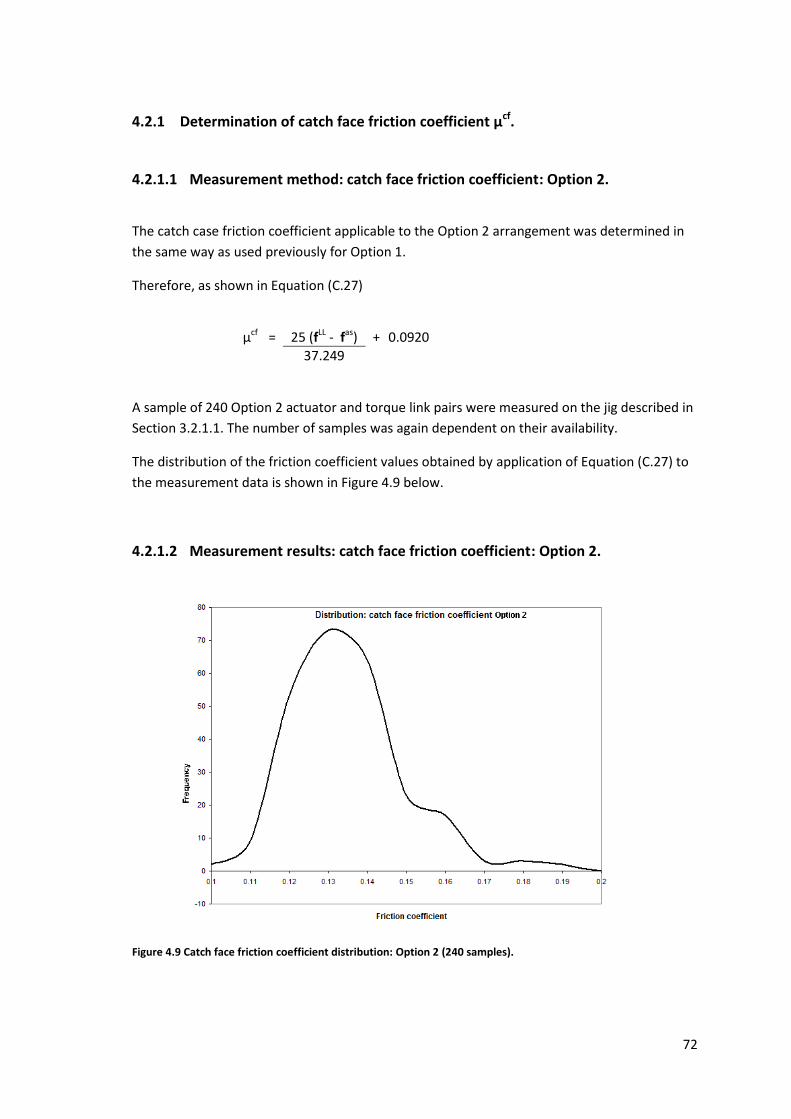
72
4.2.1 Determination of catch face friction coefficient μcf.
4.2.1.1 Measurement method: catch face friction coefficient: Option 2.
The catch case friction coefficient applicable to the Option 2 arrangement was determined in
the same way as used previously for Option 1.
Therefore, as shown in Equation (C.27)
μcf = 25 (fLL - fas) + 0.0920
37.249
A sample of 240 Option 2 actuator and torque link pairs were measured on the jig described in
Section 3.2.1.1. The number of samples was again dependent on their availability.
The distribution of the friction coefficient values obtained by application of Equation (C.27) to
the measurement data is shown in Figure 4.9 below.
4.2.1.2 Measurement results: catch face friction coefficient: Option 2.
Figure 4.9 Catch face friction coefficient distribution: Option 2 (240 samples).

73
The distribution shown in Figure 4.9 was closer to a normal distribution than had been the
case with Option 1.
The underlying reason for the difference in the Option 1 and Option 2 distribution patterns is
unclear. Option 1 features a high production volume actuator design with post-processed
catch face, together with a torque link manufactured using the preferred process B. “Option 2”
has a high quality but low volume roller type actuator, while its torque link is manufactured
with the less-preferred process A.
It appears that the actuator surface imperfections may be somewhat more complex than the
imperfections found on the torque link, presumably due to the post processing and
subsequent surface treatment applied to the actuator offering more opportunities for error
than is the case with the single manufacturing process of the torque link.
Microscopic photographs of the Option 1 and Option 2 actuator catch faces and torque link
catch faces manufactured using Process A and Process B are shown in Figures 4.10 and 4.11.
The differences in quality between the various production processes are clearly seen.
Note that all of the photographs were taken at the same magnification.
Figure 4.10 Actuator catch face comparison: Option 1 (L) vs. Option 2 (R)
In Figure 4.10 it can be seen that the stainless steel pin used for the Option 2 actuator has a
much finer surface finish than the post-processed actuator catch face used for Option 1. The
vertical striations of Option 1 in particular are thought to contribute significantly to the portion
of the lock load attributed to surface imperfections. These catch face defects have a somewhat
random effect, depending on the severity of the imperfections as well as their precise
orientation and location relative to the torque link tip.

74
Figure 4.11 Torque link catch face comparison: Process A (L) vs. Process B (R)
When the Option 1 and Option 2 torque link catch faces are compared, there is a similarity in
the overall type of surface finish present. The quality of the finish produced by Process B is
however noticeably finer than that produced by Process A, contributing to a lower incidence of
excessive lock loads in mechanisms featuring the Process B torque link.
4.2.2 Modelling of catch face defects and imperfections.
Following the method developed in Section 3.2.2, the measured lock load was split into
discrete distributions. The best results were obtained with just one catch face imperfection
distribution superimposed onto the frictional distribution.
The combined distribution is shown in Figure 4.12 below.
Figure 4.12 Lock load data approximated by the sum of 2 normal distributions: Option 2.

75
The combined distribution is shown separated into its component parts in Figure 4.13.
Figure 4.13 The Option 2 lock load distribution separated into its component parts.
The main lock load distribution was converted to a friction coefficient distribution as per the
method demonstrated in Section 3.2.3.
The friction coefficient was found to have a mean of 0.1299 and a standard deviation of
0.00877.
Substitution of this catch face static friction coefficient mean and standard distribution into the
Monte Carlo model resulted in the following prediction of the distribution for Option 2 lock
loads - without the actuator spring and without any influence from catch face imperfections.
The distribution shown is thus a prediction of the characteristics of the theoretical lock load
distribution if it was influenced by the catch face friction coefficient only, free of any catch face
imperfection effects. This distribution is shown in Figure 4.14.

76
Figure 4.14 Lock load distribution resulting from catch face friction coefficient distribution.
(Relative frequency 0.8804).
4.2.3 Derivation of values for catch face imperfections.
This distribution was again augmented by inclusion of the effects of the catch face
imperfections as previously described in Section 3.2.4. The local catch face angle variation
corresponding to the catch face imperfection distribution was determined iteratively, as
described in Section 3.2.4, and is illustrated in Figure 4.15.
This distribution modelled the effect that the manipulation of the derived local catch face
angle had on the predicted lock load, replicating the secondary distribution noted in Figures
4.12 and 4.13. This new distribution definition was now available for augmentation of the main
distribution illustrated in Figure 4.14 according to the relative frequency of defect occurrence
shown.

77
Figure 4.15 Lock load distribution resulting from defect 1.
(Relative frequency 0.120).
The following values for the distribution of the Option 2 catch face friction coefficient, and for
the derived local variations to the catch face angle for modelling of the Option 2 catch face
imperfections, were extracted from the above and used for the rest of this analysis.
Mean µcf: 0.1299 : 0.00877
Mean catch face angle 6.55° : 0.00518°
Defect 1 mean angle: 5.08° : 0.00517° Probability: 12.0%
It is interesting to note that the improved lock load distribution of Option 2 appears to be
almost entirely due to the reduced incidence of catch face imperfections in this arrangement.
In fact, the underlying friction coefficient has a slightly greater standard deviation in Option 2
than in Option 1. This is believed to be caused by the process A manufacturing process of the
Option 2 torque link providing a greater number of opportunities for deviation from the
optimal state.

78
4.2.4 Actual values of geometric variables.
Samples of all components that differed from the components examined for Option 1
were measured, and their variable distributions recorded. The measuring methods
shown in the right hand column refer to the list of measuring equipment referred to in
Table 3.9.
The mean values of the variables unique to Option 2 are shown in Table 4.5.
Table 4.5 Option 2 specific variable distribution means (actual).
Theoretical Actual
Var.
nominal tol. mean (or SD) Derived tolerance (3 )
sample size, method
µcf
0.15 * 0.127572 * * 241 (a)
t3 5.15 * 5.14395 * * 20 (d)
t4 5.80 * 5.74289 * * 20 (d)
t5 0.80 * 0.80027 * * 20 (d)
t6 16.38 * 16.41689 * * 20 (d)
t7 6.5° * 6.5512° * * 20 (d)
a4 26.10 * 26.09736 * * 20 (d)
a5 1.70 * 1.76872 * * 20 (d)
a6 0.05 * 0.079965 * * 20 (d)
a7 10.05 * 10.0186 * * 20 (d)
a8 0.30 * 0.250595 * * 20 (d)
a9 0.35 * 0.350225 * * 20 (d)
a10 0.40 * 0.41912 * * 20 (d)
All other variable distributions remained as per the standard catch face.
4.2.5 Updated Monte Carlo analysis.
The actual variable distributions and the measured catch face friction and surface imperfection
distributions derived in the previous sections were substituted for the nominal values
previously used in the Option 2 model. The methods used for the substitution were as
described in Section 3.2.6. Running a Monte Carlo simulation using the new data resulted in
the following prediction for the actual lock load distribution. (See Figure 4.16).

79
Figure 4.16 Monte Carlo analysis: option 2, actual variable values, all imperfections.
When the Option 2 lock load distribution shown in Figure 4.16 is compared with that of the
Option 1 distribution shown in Figure 3.25, it can immediately be seen that the proportion of
lock loads outside of the functional limits has been reduced substantially in Option 2.
The predicted first pass yield, taken directly from the Monte Carlo iteration data, is 98.69%,
with 1.08% falling above the maximum functional limit and 0.23% falling below the minimum.
The two distributions will be compared in more depth in Section 6.
4.2.6 Measurement of actual lock loads for model verification.
200 mechanism samples equipped with Option 2 actuating mechanisms were opened, and
their lock loads measured using an adjustable tension gram-force gauge. Again, the number of
samples measured reflects the availability of the samples.
The distribution of the measured lock loads is shown in Figure 4.17. Note that the frequency
has again been scaled up by a factor to bring the scale in line with that of the Monte Carlo
analysis, to which it will be compared.

80
Figure 4.17 Measured lock load distribution: Option 2 (200 samples).
The actual measurements resulted in a first pass yield of 97.5%, with 1.5% falling above the
maximum functional limit and 1% below the minimum.
4.2.7 Comparison of distributions.
The distribution of the measured samples was superimposed over the distribution predicted
by the model.
The comparison is displayed in Figure 4.18.
Measured mean lock load: 16.68
Measured std. deviation: 2.487
Low
er f
un
ctio
nal
lim
it
Up
per
fu
nct
ion
al li
mit

81
Figure 4.18 Predicted lock load distribution vs. Measured lock load distribution: Option 2.
The two distributions were compared using the same criteria as used in Section 3.2.8.
Once again there is a good match between the two distributions in terms of the locations of
their general features. The slight difference at the lower end of the lock load range is not
considered significant given the relatively small sample size used.
The comparison between the predicted and actual values is shown in Table 4.6.
Table 4.6 Model predictions vs actual measurement: Option 2
Criteria
Model Actual
Mean lock load 17.28 gf 16.38 gf
Lock load std. deviation 2.119 gf 2.487 gf
First pass yield 98.69% 97.50%
Above maximum lock load 1.08% 1.50%
Below minimum lock load 0.23% 1.00%
Once again the correspondence of the predicted and actual figures was fairly good. The Option
2 model was thus considered to be validated.

82
4.3 Review of options 1 and 2.
The analyses of options 1 and 2 were reviewed, and the following conclusions were noted.
The overall design of the actuating mechanism, as specified by the nominal sizes and
tolerances given in the design documentation, was capable of consistently producing
products having a lock load within functional limits. This statement was qualified
however due to the indirect specification of the friction coefficients in the system,
which added an element of uncertainty to the evaluation of the design. The predicted
performance of the actuating mechanism, subject to the friction coefficient
assumptions detailed in the text, is illustrated in Figures 3.14 and 4.8.
Most of the variable sizes pertaining to the design were well maintained within their
functional limits during manufacture.
The Pareto analysis revealed that the variable contributing by far the greatest amount
to variation in the lock load was the catch face friction coefficient.
The perceived friction coefficient included a component attributable to damage or
imperfection in one or both of the catch faces. These imperfections manifested
themselves in the distortions to the right of the mean in both of the lock load
distributions analysed, and have been modelled by means of local variation in the
effective catch face angles.
The Option 2 actuator appeared to have more consistent lock load measurements
than the Option 1 actuator, and the torque links manufactured by means of process B
appeared to have more consistent lock load measurements than those manufactured
by means of process A. The reasons for this are illustrated in Figures 4.10 and 4.11, and
discussed in Section 4.2.1.2.
The Option 1 actuating mechanism model predicted a first pass yield of 94.12%.
The Option 2 actuating mechanism model predicted a first pass yield of 98.69%.
From the above, it was clear that there was the potential to improve the first pass yield of the
manufacturing process by improving the consistency of the torque link / actuator interface.
The design of such improvement, as well as the quantification thereof is the subject of the next
section.

83
5 PROPOSAL AND ANALYSIS: MECHANISM OPTION 3
5.1 Proposal for option 3.
When the design constraints of Section 2.5.1 were considered, it became evident that there
was the potential for a major improvement in the torque link / actuator interface by combining
the Option 2 actuator with a modified Option 2 torque link having an improved catch face. This
upgraded torque link catch face could be provided by means of using the process B
manufacturing method.
This solution was perceived to comply with the following limitations:
No changes to the geometry of the existing design Option 2.
This implied very low risk in the introduction of the proposal.
No certification implications.
No implications for the motive unit.
The advantage inherent in this solution was anticipated to be an immediate increase in first
pass yield for the actuation unit assembly process, and consequently in the costs associated
with rework.
There were however certain perceived disadvantages. These included:
The introduction of this solution to those products currently using the Option 1
actuating mechanism would introduce the added assembly complexity of the Option 2
actuating mechanism across the product range.
This would imply increased costs, which would offset the gains associated with the
reduced rework.
Introducing the improved process B into the Option 2 torque link across the product
range would also increase costs.
The disadvantages of the proposed solution would have to be outweighed by the cost savings
associated with an increased first pass yield.
For the financial calculations to be performed, it would be necessary to establish a reliable
prediction for the magnitude of such a first pass yield increase.
In order to develop such a prediction, the proposed Option 3 was evaluated following the
same techniques employed for Options 1 and 2.
Note: To avoid clumsiness in terminology, the current Option 2 torque link manufactured using
process A will henceforth be referred to as the “Option 2A” torque link, while the same
component manufactured using process B will be referred to as the ”Option 2B” torque link.
Similarly, reference will be made to “Option 1A” and “Option 1B” torque links.

84
5.2 Static analysis.
The proposed Option 3 actuating mechanism had an identical geometrical arrangement to the
Option 2 mechanism.
For an examination of the predicted lock load distribution of such an arrangement, it was thus
not necessary to respecify the geometric arrangement of the mechanism, but only to establish
the distribution of its catch face friction coefficient and surface imperfections.
An Option 2 torque link manufactured using process B, and thus suitable for use with the
Option 2 actuator in order to embody the proposed Option 3 arrangement, does not currently
exist. It was however possible to use the “Option 1B” torque link in order to predict the friction
coefficient distribution of the “Option 2B” torque link.
The catch face angle of the Option 1 torque link was entirely inappropriate for use with the
Option 2 actuator. However the same methodology as previously employed could still be used
for determination of the friction coefficient, and extrapolated for a suitable torque link catch
face angle.
5.2.1 Determination of catch face friction coefficient µcf.
For the Option 2 actuator / Option 1B torque link combination the following values were used
with respect to the lock load measurement jig. (See Table 5.1).
Table 5.1 Variables relating to lock load measuring jig: option 3.
Variable (relating to roller catch actuator) Value
μcf = the coefficient of friction in the catch face Unknown
μsh = the coefficient of friction in the actuator shoulder 0.2
μT = the coefficient of friction in the torque link pivot 0.2
ψ = catch face angle force moment arm 0.0312 mm
ω = catch face friction force moment arm length 10.40 mm
fLL = lock load. To be measured
fas = actuator spring force To be measured

85
fms = main spring force 11.46 N
ρ = torque link/actuator moment arm length 17.24 mm
λ = torque link/main spring moment arm length 8.046 mm
θ = main spring force vector angle 1 47.28°
φ = catch force vector angle 0.1714°
ζ = main spring flexed length 19.20 mm
Using these values, the catch face friction was determined from the lock loads and spring
forces of 300 samples measured on the lock load jig as shown in Appendix D.
The catch face friction is calculated using Equation (D.1) as follows:
μcf = 25 (fLL - fas) + 0.00203
37.6277
The distribution of the friction coefficient values obtained by the use of the above equation is
shown in Figure 5.1 below.
Figure 5.1 Catch face friction coefficient: actuator Option 2, torque link Option 1B

86
The above distribution was compared with a true normal distribution having the same mean
and standard deviation. (See Figure 5.2).
Figure 5.2 Comparison: distribution of measured values vs normal distribution.
The catch face friction distribution shown in Figure 5.2 closely approximated a normal
distribution. This implied that the catch face imperfections, which tended to distort the
distribution to the right of the mean, were not present in this case. This further implied that
the combination of the Option 2 actuator with a torque link produced using process B largely
eliminated catch face imperfections from the system. This was the scenario that was hoped
would be achieved by this catch face combination. Attempts to define distributions for catch
face imperfections to model the slight discrepancy between the results and a true normal
distribution gave trivial results, and thus were not included in the model for Option 3.
5.2.2 Lock load prediction.
When the catch face friction distribution derived in Section 5.2.1 was substituted into the
Option 2 model, and the catch face angle adjusted to a more appropriate 6.1°, a model was
thereby created for the proposed Option 3 solution.
A Monte Carlo analysis of the new Option 3 model was performed, resulting in the following
prediction for the Option 3 lock load distribution. (See Figure 5.3).

87
Figure 5.3 Predicted lock load distribution: actuator Option 2, torque link Option 2B.
The shape of the distribution shown in Figure 5.3 is closer to a normal distribution than those
shown in Figures 3.25 and 4.16. In addition, a greater proportion of the distribution is situated
between the process limits.
The predicted first pass yield for the Option 3 variation is 99.36% with 0.09% falling above the
upper process limit and 0.55% below the minimum.
Using a preliminary costing for the estimated capital expenditure required to implement an
Option 3 solution across the entire product range of the device, offset against the cost saving
associated with the increased first pass yield, an estimated pay-back time of 2.7 years was
predicted.
A detailed comparison of the predictions for Option 3 and those of Options 1 and 2 is given in
the next section.

88
6 COMPARISON OF RESULTS
For the sake of completeness, the obsolete “Option 0” actuating mechanism arrangement
mentioned in Section 1.1 was analysed using the same methodology developed for Options 1,
2 and 3.
It is superfluous to repeat the details of the analysis in this report, so only the results are
included for comparison purposes.
6.1 Comparison of static analyses.
The histograms representing the Monte Carlo analyses of the various models developed in the
previous three sections were combined in the following graph. (See Figure 6.1).
The combined graph depicts individual line graphs derived from the previously developed
Monte Carlo analyses, and indicates the functional limits of the mechanism.
Figure 6.1 Comparison of lock load distribution predictions.
Type 1 actuator / type 1A torque link. (Option 0). Type 1 actuator / type 1B torque link. (Option 1). Type 2 actuator / type 2A torque link. (Option 2). Type 2 actuator / type 2B torque link. (Option 3).

89
It was evident from Figure 6.1 that the models predict a steady improvement in yield when
moving from the obsolete Option 0, through the currently employed Options 1 and 2 and on to
the proposed Option 3. While there was minimal improvement at the lower functional limit,
associated with spurious mechanism actuation, there was significant improvement at the
upper limit, associated with correct mechanism operation. This indicated that the rework rate
will be significantly improved.
The expected first pass yield values determined from the Monte Carlo models are summarised
in Table 6.1 below.
Table 6.1 Predicted first pass yield values per construction type.
Option 0 Option 1 Option 2 Option 3
Construction
Option 1
actuator,
Option 1A
torque link.
Option 1
actuator,
Option 1B
torque link.
Option 2
actuator,
Option 2A
torque link.
Option 2
actuator,
Option 2B
torque link.
Mean lock load (gf). 19.39 17.54 17.28 16.95
Lock load SD (gf). 3.680 2.889 2.119 1.946
Predicted below
minimum F.L. 2.24% 0.93% 0.23% 0.55%
Predicted above
maximum F.L. 16.32% 4.95% 1.08% 0.09%
Predicted first pass
yield . 81.45% 94.12% 98.69% 99.36%

90
7 DISCUSSION
The geometric models of the Option 1 and Option 2 versions of the actuating mechanism were
successfully constructed using vector loop analysis. It was found possible to express the
unknown dimensions and the position and orientation of the individual component coordinate
systems fully in terms of the independent variables.
The geometric models were checked against parametric CAD models of the mechanisms to
confirm that the results predicted by the model for the dependent variables were accurate.
The CAD parameters for the independent input variables were varied numerous times to
confirm the accuracy of the models over a range of input values. All results agreed, and the
geometric models were considered to be validated.
These models were then expanded to include the forces and reactive torques present in the
system. The two input forces (those supplied by the main spring and by the actuator spring),
were calculated from first principles and confirmed by direct measurement. The resultant and
reaction forces were calculated with all variables set to their nominal values, and the resultant
predicted lock loads derived. These predictions were compared with historical lock load data,
and found to be consistent with expectations.
An application was developed to facilitate the manipulation of the independent variables while
observing the effect on all the dependent variables, up to and including the lock load. Use of
the application enabled the sensitivity of the lock load to variations in each individual
dimension to be established. Examination of the Pareto chart developed from this data proved
to be enlightening in terms of the relative importance of certain variables to the lock load of
the mechanism. The overriding significance of the catch face friction coefficient was expected,
although the extent of its impact upon the lock load had not been fully anticipated. A
comparison of the relative importance of each variable to its specified tolerance and control
procedures highlighted several anomalous areas, which were noted for future evaluation and
study. The catch face friction coefficient was chosen as the focus for the rest of this project,
due to its relatively deficient specification combined with its overriding importance to the
mechanism’s function.
The models for the Option 1 and Option 2 versions of the actuating mechanism were then
modified to represent each independent variable as a distribution of values rather than as one
unique value. These distributions were assumed to be normal, to have a mean value
corresponding to the nominal value of the dimension, and to have a standard deviation equal
to one third of the allowed tolerance on the dimension. Note that certain of the dimensions
and tolerances required were not directly specified on the engineering documentation, and
had to be derived as the sum of two or more constituent dimensions and tolerances, with the
associated tolerance stacking implications. (These inadequately specified dimensions
represent examples of the anomalies discussed in the preceding paragraph). The discovery and
correction of certain non-optimal dimensioning on the engineering specifications was not
included in this project, but is of practical benefit to production.

91
A Monte Carlo analysis was then performed on the above model by allowing each dimension
to vary randomly within a normal distribution defined by its mean and standard deviation, and
recording the resultant lock load of the mechanism. 50 000 lock load calculation iterations
were performed for each Monte Carlo analysis, resulting in the derivation of a distribution for
the lock load values expected from the design.
This distribution showed that the design of the actuating mechanism appeared to be quite
reasonable in its overall specification, assuming that each component dimension could be
maintained within its plus or minus three standard deviation tolerance band. There was, as
mentioned earlier, one major omission from the theoretical model: the absence of a direct
specification for the static friction coefficient present in the catch face. This specification was
not entirely absent, but was indirectly specified in terms of the surface finish, post processing
and surface treatments applied to the catch face surfaces. A direct measurement of a
component’s friction coefficient is not practical to implement in a production environment,
and any measurement is in any event only valid for the particular actuator / torque link pair
being measured and thus cannot be used as part of a mass production component
manufacturing process in any meaningful way. An assumed mean and standard deviation was
used for the catch face friction coefficient in the Monte Carlo analysis which, given the
importance of this value, was not satisfactory.
Despite this failing, the model indicated that the theoretical design, as it stands, is capable of
producing a high proportion (around 99.4%) of functional products, subject to adequate
control of the catch face friction coefficient.
The next stage in the refinement of the models was to substitute the actual means and
standard deviations of the variable distributions for those derived from the engineering
specification. These were obtained by direct measurement of component samples, or from
historical records as appropriate to the individual dimension. Normal distributions continued
to be assumed for these values. The exception to this was in the catch face friction coefficient
distributions, where the shape of the distribution curves was not normal. In this case the
distributions were approximated as the sum of two or three discrete distributions, comprising
a main distribution corresponding to the catch face friction coefficient and an additional
distribution or distributions corresponding to catch face imperfections. These imperfections
were modelled as local variations in the effective catch face angle, the distributions of which
having their own means and standard deviations as well as a defined probability of occurring in
any one particular actuator / torque link pair. While the exact nature of the imperfections was
not considered, the effect of such imperfections on the measured lock load distributions was
described reasonably well by the model. The numbers of samples measured to obtain the
means and standard deviations of the components, as well as the characteristics of the catch
face angle variations, were considered adequate for this study. Follow up studies using larger
sample sizes are however recommended to improve the accuracy of the predictions.
Substitution of the actual variable values into the model resulted in a lock load distribution
prediction which attempted to model the real world scenario. When the model’s predictions
were compared to the results of measuring several hundred actuating mechanisms it was
92
found that there was a close match between the distributions, for both the Option 1 and
Option 2 mechanism variations. The first pass yields predicted by the model for the actuating
mechanism lock load were 94.12% for Option 1 and 98.69% for Option 2. The measured first
pass yields for the same mechanisms were 95.89% and 97.50% respectively. It was felt that a
closer match, and greater confidence in the results, could again have been obtained with a
larger sample of actual production units. This was not practical for this study, but should be
undertaken in the future before any decision is made regarding possible implementation of
the recommendations of this report. On the basis of the comparisons made using the available
data, it was accepted that the models gave reasonably accurate predictions of the first pass
yield of the assembly process, and would continue to do so when any of the parameters of the
model were adjusted.
The predictions of the models and the measured lock load distributions were below the
tentative 99% target set in Section 1.2., but provided a benchmark against which future
improvements could be measured.
The comparison between the performance of the two actuating mechanism versions indicated
that the Option 2 arrangement performed better in terms of catch face friction coefficient
consistency, and hence of maintaining the lock load distribution within the process limits.
Observation of the samples suggested that the increased yield was due to the improved design
of the Option 2 actuator, which overrode the negative effect of the sub-optimal process A used
for the Option 2 torque link.
The obvious design improvement implied by the above was an Option 2 arrangement that was
equipped with a torque link manufactured using the improved process B. This straightforward
proposal was named “Option 3”.
A torque link suitable for Option 2, but produced by means of process B, does not currently
exist. In order to predict the performance of this component, an Option 1 torque link with the
appropriate manufacturing process B was tested in combination with an Option 2 actuator.
The results of this test were extrapolated to predict the first pass yield for the Option 3
mechanism.
The results predicted a first pass yield for the Option 3 mechanism of 99.36%.
Using the preliminary costing for the estimated capital expenditure required to implement an
Option 3 solution across the entire production of this particular device, an estimated payback
period of 2.7 years was predicted. This figure was perhaps rather conservative, as it included a
quotation for the (difficult) automatic assembly of the option 2/3 actuator as it currently
stands, without any attention being paid to redesign of the actuator to facilitate automatic
assembly. Such a “design for assembly” study and subsequent redesign would be conducted
before any final decision was made regarding actual implementation, and would be aimed at
reducing the capital outlay required for such assembly equipment, and thus the payback
period required.

93
As this study was concerned with only one aspect of a complex device, the proposed Option 3,
being based upon the already proven Option 2, has the powerful advantage of not introducing
any changes which could potentially impact negatively on any other performance
characteristic of the device. The definition of the advantages inherent in performing this
optimisation exercise, in terms of the increased first pass yield and thus the monetary savings
associated with the implementation of Option 3 across the product range, has been addressed
in this study.
8 CONCLUSIONS
Models describing the existing actuating mechanism designs were developed using vector loop
analysis to determine the mechanism lock loads as a function of geometric and other variables.
The geometric predictions of the models were validated by comparison with parametric CAD
models of the mechanism. The force predictions were evaluated by comparison of the lock
load distributions predicted by the model with the functional limits for the mechanism, and
with historical records of actual mechanism performance. The models were found to be valid.
The models were re-implemented in a spreadsheet format to facilitate the manipulation of
independent variables within their tolerance band. By the use of this method, a Pareto analysis
of the sensitivity of the lock load to variation in each variable was developed. The catch face
friction coefficient was found to have by far the greatest influence on the lock load, and was
defined as the priority for further investigation.
Investigation of the catch face friction coefficient led to the development of a method for
more accurately defining the catch face friction. This was implemented as the combination of a
primary friction coefficient distribution combined with one or more supplementary
distributions representing imperfections or damage in the catch faces. This method of
describing the existing catch face friction was combined with the actual geometric variable
distributions derived from sample measurements to refine the models. The predictions of the
revised models, when compared with data taken from the measurement of production
samples, indicated that the models were capable of predicting the behaviour of the actual
mechanisms.
The insights gained from examination of the Option 1 and 2 models and performance data led
to the proposal of a new Option 3 design. The models were updated to predict the behaviour
of Option 3, and predicted a first pass yield of 99.36%. Preliminary analysis of the costs
involved in implementing the Option 3 design indicated a pay-back period of 2.7 years.
It is thus recommended that Option 3 should be formulated as a formal implementation
project.

94
9 RECOMMENDATIONS FOR FUTURE WORK.
During the course of this study, there were several occasions where it was evident that further
work to improve the accuracy of the results appeared to be desirable. It was not feasible to
undertake much of this additional work during the course of this study however, so the
proposals were noted for future evaluation. If it is desired to implement the recommendations
of this study, the resources of the company should be employed to complete a number of
supplementary studies. Recommended future work includes:
9.1 Accuracy of data.
The number of samples measured should be increased and the accuracy of such
measurements improved. Samples should be taken from all available toolsets or mould
cavities, and be representative of all variations that could occur in practice. In particular, the
actual catch face friction coefficient measurements should be done on a considerably larger
scale, and employ an automatic lock load measurement system to eliminate any subjectivity
from the measurements. In addition, it should be established if there is in fact any difference
evident in mechanical actuation of the mechanism with a force gauge compared to magnetic
actuation using the motive unit.
The gathering of data should be performed over a long enough period to accommodate any
long term trends in the component characteristics, particularly over the duration of the tooling
maintenance cycle.
The costs involved in introducing the Option 3 mechanism across the product range should
also be refined, to increase the accuracy of the predicted amortisation period.
9.2 Suggested modifications to mechanism: Options 1, 2 and 3.
It was evident from the Pareto analysis that there were a number of areas where the
specification of dimensional and other tolerances was not optimal. The tightening of
tolerances in certain areas, as well as the possible relaxation of tolerances in others, could be
undertaken in light of the information derived from the Pareto analysis.
The assembly of the Option 2 actuator should be thoroughly examined in light of the proposal
to introduce it across the product range. Automation of the assembly process, including the
possible re-design of the actuator with emphasis on “design for assembly”, should be
considered. Calculation of costs and pay back periods can be estimated more accurately using
the first pass yield predictions established in this study.

95
REFERENCES
1. Gao, J., Chase, K.W. and Magleby, S.P. (1998). Global coordinate method for determining
sensitivity in assembly tolerance analysis. Anaheim, California : Proceedings of the ASME
International Mechanical Engineering Conference and Exposition.
2. Hansen, J. M. and Tortorelli, D. A. (1996). An Efficient Method for Synthesis of Mechanisms
using an Optimization Method. The Netherlands : IUTAM Symposium on Optimization of
Mechanical Systems pp 129-138. Kluwer academic publishers.
3. Chase, Kenneth W. and Parkinson, Alan R. (1991). A Survey of Research in the Application of
Tolerance Analysis to the Design of Mechanical Assemblies. Utah, U.S.A. : Research in
Engineering Design vol3 pp23-37.
4. Dick, T. and Cailletaud, G. (2005). Analytic and FE based estimates of the coefficient of
friction of composite surfaces. United Kingdom : Elsevier Sciences Technology.
5. Rao, S. S. and Reddy, C. P. (1979). Mechanism Design by Chance Constrained Programming
Techniques. Great Britain : Mechanism and Machine Theory, vol 14 pp 413-424. Pergamon
Press Ltd.
6. Mallik, A. K. and Dhande, S. G. (1987). Analysis and Synthesis of Mechanical Error in Path-
Generating Linkages Using a Stochastic Approach. Great Britain : Mechanism and Machine
Theory, Vol.22 No.2 pp 115-123. Pergamon Press Ltd.
7. Rao, S. S. and Cao, L. (2002). Optimum Design of Mechanical Systems Involving Interval
Parameters. Miami, U.S.A. : Journal of Mechanical Design, Vol.124 pp 465-472. American
Society of Mechanical Engineers.
8. Wu, W. and Rao, S. S. (2004). Interval Approach for the Modeling of Tolerances and
Clearances in Mechanism Analysis. Miami, U.S.A. : Journal of Mechanical Design, Vol.126 pp
581-592. American Society of Mechanical Engineers.
9. Shi, Z. (1996). Synthesis of Mechanical Error in Special Linkages Based on Reliability Concept.
Great Britain : Mechanism and Machine Theory, Vol.32 No.2 pp255-259.Pergammon Press Ltd.
10. Sharfi, O. M. A, and Smith, M. R. (1982). A Simple Method for the Allocation of Appropriate
Tolerances and Clearances in Linkage Mechanisms. Great Britain : Mechanism and Machine
Theory, Vol.18 No.2 pp123-129. Pergamon Press Ltd.
11. Bicheno, J. and Catherwood, P. (1991). Six Sigma and the Quality Toolbox. First Edition.
Buckingham, England : Picsie Books.
12. Bicheno, J. and Holweg, M. (2009). The Lean Toolbox. Fourth Edition. Buckingham,
England : Picsie Books.

96
13. Holton G. A. (2004). Monte Carlo Method. [Online] Accessed October 2011 : s.n.
14. Xu, W. L. and Zhang, Q. X. (1989). Probabilistic Analysis and Monte Carlo Simulation of the
Kinematic Error in a Spatial Linkage. Great Britain : Mechanism and Machine Theory, Vol.24
No.1 pp 19-27. Pergamon Press Ltd.
15. Vose Software, (2007). Monte Carlo Simulation. [Online] Accessed September 2011.
16. Ata, M. Y. (2006). Determining the Optimal Size in Monte Carlo Experiments. Konya-Selcuk
University : International Conference in Modeling Simulation. AMSE '06. .
17. Dunn, W. L. and Shultis, J. K. (2006). Exploring Monte Carlo Methods. United Kingdom :
Elsevier Sciences Technology.
18. Buckley, R. L. (2003). Winning in a Highly Competitive Manufacturing Environment. San
Ramon, California : Falcon Books.
19. Pyzdek, T. and Keller, P. (2010). The Six Sigma Handbook 3rd Edition. s.l. : McGraw Hill.
20. Van Gastel, S. (2011). Improved Margins by Reducing Re-work - a Benchmark Comparison.
[Online] Accessed September 2011.
21. Littlefield, M. (2007). The Cost of Quality: Benchmarking Enterprise Quality Management.
[Online] Accessed October 2011 : s.n.
22. Hay, Alex M. (2005). Determination of catch face friction coefficients of mechanisms.
Johannesburg : Cibri Internal Publication 007-RT-ED-REP-2005001-00-A.
23. Boas, Mary L. (1966). Mathematical Methods in the Physical Sciences. Chicago : John Wiley
& Sons, Inc.
24. Lane, Shaun (2009). Lock load gauge. Johannesburg : Cibri Internal Publication E2316-A.
25. The MathWorks Inc. (2007). MATLAB function reference R2007a. Natick, Massachusetts :
The MathWorks, Inc.
26. Larson, Harold J. (1969). Introduction to Probability Theory and Statistical Inference.
Monterey, California : John Wiley & Sons, Inc.
27. Hay, Alex M. (2006). A MATLAB script for planar mechanism static sensitivity analyses.
Johannesburg : Cibri Internal Publication 000-RT-ED-TRM-2006003-00-A.
28. Hay, Alex M. (2006). Dynamic sensitivity analyses of actuating mechanisms. Johannesburg :
Cibri Internal Publication 010-RT-ED-SMR-2006002-00-A.
29. Hay, Alex M. (2006). Static sensitivity analyses of actuating mechanisms. Johannesburg :
Cibri Internal Publication 010-RT-ED-SMR-2006003-00-A.

97
APPENDIX A: MECHANISM ANALYSIS OPTION 1
Note: for convenience, where figures in the main text are referred to, the relevant portions of
the figures are repeated here.
A1 Positional analysis.
A1.1 Determination of γ.
Assuming that the frame plate is assembleable onto the base, i.e. the centre dimension of the studs
is equal to the centres of the holes, then from Figure 3.9:
=
The relative angles of the frame plate and the base are driven by the dimensions b2 & p2, therefore
for a given b1:
=
also, as shown in Figure 3.9,
γ1 = arctan (b2 / b1)
γ2 = arctan (p2 / p1) and
γ = -γ1 γ2
thus
γ = -arctan (b2 / b1) + arctan (p2 / √
) (A.1)
γ2
γ1
γ

98
A1.2 Determination of β.
From Figure 3.6,
= (A.2)
From Figure 3.3(c),
= [p5 - m1, p6 - m2]T
Using the two dimensional rotation matrix to transform to the global co-ordinate system (22),
=
o γ - γ (p5 – m1)
γ o γ (p6 - m2)
=
o γ 5 - m1) - γ 6 - m2) (A.3)
γ 5 - m1 o γ 6 - m2)

99
Similarly, from Figure 3.3(b), = [((a5 - a5 cos (-β -γ , -a4 + a5 – a5 sin (-β -γ ]T
Then
=
o β γ - β γ (a5 – a5 cos (-β -γ
β γ o β γ (-a4 + a5 – a5 sin (-β -γ
=
o β + γ 5 – a5 cos (-β -γ – β + γ -a4 + a5 – a5 sin (-β -γ
β + γ 5 – a5 cos (-β -γ o β + γ -a4 + a5 – a5 sin (-β -γ
=
a5 o β + γ - a5 cos2 β + γ 4 β + γ – a5 β + γ - a5 sin2 β + γ
a5 β + γ - a5 o β + γ β + γ - a4 o β + γ 5 o β + γ
+ a5 o β + γ β + γ
=
a5 o β + γ 4 – a5 β + γ - a5 (cos2 β + γ 2 β + γ
a5 β + γ 5 - a4 o β + γ 5 o β + γ β + γ
- a5 o β + γ β + γ
=
a5 o β + γ + (a4 – a5 β + γ - a5
a5 β + γ 5 - a4 o β + γ (A.4)
Finally, from Figure 3.3(e),
=
b3
-ε
(A.5)
ε

100
Thus from Equations (A.2, A.3, A.4 & A.5:
o γ 5 - m1) - γ 6 - m2) + a5 o β γ 4 – a5 β γ - a5 - b3 =
0 (A.6)
γ 5 - m1 o γ 6 - m2) + a5 β γ 5 - a4 o β γ ε 0 (A.7)
Using Equation (A.6 , l o γ 5 - m1) - γ 6 - m2) - a5 - b3) = K
Then a5 cos β + γ 4 – a5) sin β + γ = -K.
Dividing both sides by √
gives
a5 o β γ
+
(a4– a5 β γ
=
-K
√
√
√
(A.8)
Now let cosZ =
(a4– a5)
√
then sinZ =
a5
√
substituting in Equation(A.8):
o β γ + o β γ = -K
√
thus
β γ =
-K
√
and
β γ = arcsin -K
√
Therefore
√
a5
a4 - a5
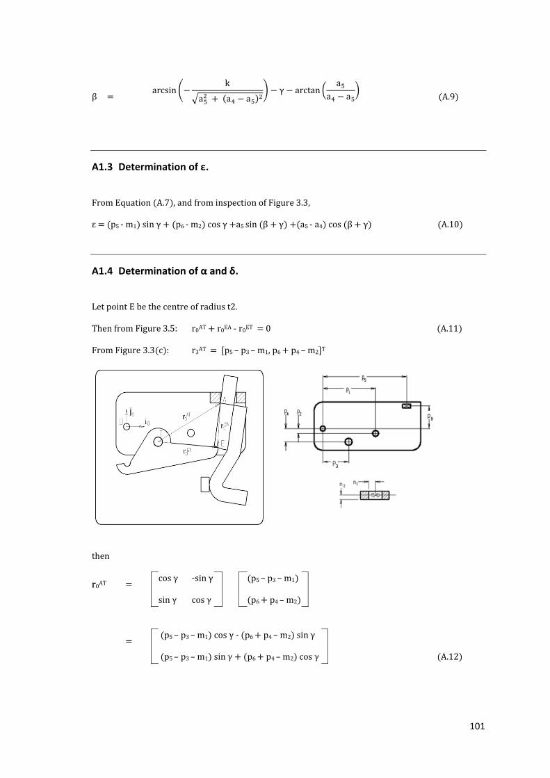
101
β = (
√
) γ (
) (A.9)
A1.3 Determination of ε.
From Equation (A.7), and from inspection of Figure 3.3,
ε = (p5 - m1) sin γ + (p6 - m2) cos γ +a5 sin β + γ 5 - a4) cos β + γ (A.10)
A1.4 Determination of α and δ.
Let point E be the centre of radius t2.
Then from Figure 3.5: r0AT + r0
EA - r0ET = 0 (A.11)
From Figure 3.3(c): r3AT = [p5 – p3 – m1, p6 + p4 – m2]T
then
r0AT =
o γ - γ (p5 – p3 – m1)
γ o γ (p6 + p4 – m2)
=
(p5 – p3 – m1 o γ - (p6 + p4 – m2 γ
(p5 – p3 – m1 γ 6 + p4 – m2 o γ (A.12)

102
From Figures 3.3(b) and 3.5:
r2EA = [ δ – t2 sin a3),(-a1 + (a2 - δ tan a3 - t2 cos a3)]T
r0EA =
o β γ - β γ δ – t2 sin a3
β γ o β γ -a1 + (a2 - δ tan a3 - t2 cos a3
=
δ – t2 sin a3 o β + γ – β + γ -a1 + (a2 - δ 3 - t2 cos a3)
δ –t2 sin a3 β + γ o β + γ -a1 + (a2 - δ 3 - t2 cos a3) (A.13)
From Figures 3.3(a) and 3.5:
r1ET = [(t1 - t2) , (-t2)] T
r0ET =
o α - α (t1 - t2)
α o α -t2
r0ET =
(t1 - t2 o α 2 α
(t1 - t2 α - t2 o α (A.14)
Then from Equations (A.11, A.12, A.13 & A.14):
o γ 5 – p3 – m1) – γ 6 + p4 – m2 δ – t2 sin a3 o β + γ
- β + γ -a1 + (a2 - δ 3 - t2 cos a3) - (t1 - t2 o α - t2 α
=
0
sin γ 5 – p3 – m1 o γ 6 + p4 – m2 δ – t2 sin a3 β + γ
o β + γ -a1 + (a2 - δ 3 - t2 cos a3) - (t1 - t2 α 2 o α
0
let
A = cos γ (p5 – p3 – m1) – γ (p6 + p4 – m2) - t2 sin a3 cos β + γ + a1 sin β + γ
– a2 sin β + γ tan a3 + t2 cos a3 sin β + γ
δ

103
then, as -t2 sin a3 cos β γ + t2 cos a3 sin β γ m l f d o t2 sin β γ-a3),
A = cos γ (p5–p3–m1) – sin γ (p6+p4–m2) + t2 sin β γ-a3) + a1 sin β γ - a2 sin β γ tan a3
then let
B = sin γ (p5 – p3 – m1) + cos γ (p6 + p4 – m2) – t2 sin a3 sin β + γ - a1 cos β + γ
+ a2 cos β + γ tana3 - t2 cos a3 cos β + γ
similarly to the above,
B = sin γ (p5 – p3 – m1) +cos γ (p6 + p4 – m2) – t2 cos β + γ - a3) - a1 o β + γ + a2 o β + γ tan a3
then
A δ o β + γ δ β + γ 3 - (t1 - t2 o α - t2 α =
0 (A.15)
δ β + γ – δ o β + γ 3 - (t1 - t2) α 2 o α 0 (A.16)
From Equation (A.15):
(t1-t2) cos α 2 sin α - A = δ (A.17)
cos β + γ β + γ tan a3
Substituting into Equation (A.16):
B + ((t1-t2 o α 2 α – A β γ - ((t1-t2 o α 2 α – A o β γ 3
o β γ β γ 3)
-(t1-t2 α 2 o α =
Then, re-arranging terms,
B + β γ 1-t2 o α β γ 2 α – A β γ -((t1-t2 o α 2 α – A o β γ 3
o β γ β γ 3)
-(t1-t2 α 2 o α =0
and, expanding factors,
B +
β + γ 1 - t2 ) o α β + γ 2 α – A β + γ - o β + γ 3 (t1 - t2 o α – o β + γ 3 t2 α A o β + γ 3
o β + γ β + γ 3)
- (t1-t2 α 2 o α =

104
Let
C = β + γ 1-t2)
D = β + γ 2
o β + γ β + γ 3 o β + γ β + γ 3
E = β + γ
F = o β + γ 3 (t1 - t2)
o β + γ β + γ 3 o β + γ β + γ 3
G = o β + γ 3 t2 H = o β + γ 3 o β + γ β + γ 3 o β + γ β + γ 3
Then
B +C cos α D sin α - A E – F cos α - G sin α A H - (t1-t2) sin α t2 cos α =
Collecting factors,
(C - F +t2) cos α D - G - t1 + t2) sin α – A E + A H + B = 0
Let (D - G - t1 + t2) = X
(C - F + t2) = Y
-A (H-E) - B = Z
Then X sin α cos α = Z
Dividing both sides by √
α +
o α = Z (A.18)
√ √ √
Let cos Q = X
√
then sin Q = Y
√
Substituting in Equation (A.18),
cos Q sin α Q cos α = Z
√

105
Thus sin α = Z
√
α =
arcsin
(
√ ) - Q
(A.19)
Substituting back into Equation (A.17),
δ = (t1 - t2) cos α 2 α - A (A.20)
cos β + γ β + γ tan a3
Note:
Experience has shown that the above equations need to be simplified in order to minimize
excessive rounding errors in calculations on an excel spreadsheet.
Therefore: Simplifying C,
C = (t1 - t2) sin ( β + γ
(cos β + γ β + γ tan a3)
D v d g o d o om y β γ g v
(t1 - t2) = cos β + γ + sin a3 cos β + γ cos a3
= (t1 - t2) sin β + γ o 3
cos β + γ cos a3 + sin β + γ sina3
C = (t1 - t2) sin β + γ o a3 (A.21)
cos β + γ - a3)
Similarly,
D = t2 sin β + γ o a3
and (A.22)
cos β + γ - a3)
E = sin β + γ o a3 (A.23) cos β + γ -a3)

106
Simplifying F:
F = cos β + γ tan a3 (t1 - t2)
cos β + γ β + γ tan a3
D v d g o d o om y o β γ g v
= (t1 - t2) tan a3
1 + tan β + γ tan a3)
(t1 - t2) sin a3 . cos β + γ o a3
= cos a3 cos β + γ cos a3 + sin β + γ sin a3
= (t1 - t2) sin a3 cos β + γ
cos β + γ cos a3 + sin β + γ sin a3
F = (t1- t2) sin a3 cos β + γ (A.24)
cos β + γ - a3)
Similarly,
G = t2 sin a3 cos β + γ
and (A.25)
cos β + γ - a3)
H = sin a3 cos β + γ (A.26) cos β + γ - a3)
Simplifying X,
X = D – G - t1 + t2
= t2 sin β + γ o a3
- t2 sin a3 cos β + γ
-t1+t2 cos β + γ - a3) cos β + γ - a3)
= t2 (sin β + γ cos a3 – sin a3 cos β + γ
-t1+t2 cos β + γ - a3)
= t2 sin β + γ - a3)
-t1 + t2 cos β + γ - a3)
X = t2 β γ - a3) -t1 + t2 (A.27)
similarly,

107
Y = t1 - t2 β γ - a3) + t2 (A.28)
Simplifying Z:
Z = -A (H-E) - B
Z = -A
( o β γ β γ o
o β γ ) - B
Z = -A
( β γ
o β γ ) - B
Z = A tan ( β + γ -a3) - B (A.29)
S m l fy g α,
α = arcsin
(
√ ) - Q
= arcsin
(
√ ) - arcsin (
√ )
= arcsin
(
√ √
√ √
)
= arcsin
(
√ √
√ √
)
= arcsin
(
√
)
α = arcsin
( √
) (A.30)

108
A1.5 Determination of φ & ρ.
From Figure 3.5, 3.3(a) and 3.3(b):
r0CT = r0
ET + [t2 sin (a3 – β - γ , t2 cos (a3 – β - γ ]T
= (t1 - t2) cos α t2 sin α + t2 sin (a3 – β - γ
(t1 - t2) sin α - t2 cos α t2 cos (a3 – β - γ
= (t1 - t2) cos α t2 sin α 2 sin (a3 – β - γ
(t1 - t2) sin α - t2 cos α 2 cos (a3 – β - γ
ρ = |r0CT|
thus
ρ = √ ((t1 - t2) o α t2 α 2 sin(a3 – β - γ 2 + ((t1 - t2)sin α - t2 o α 2 cos(a3 – β - γ 2
(A.31)
Also, from examination of Figure 3.3,
φ = a3 – β – γ ( α o α o β γ
o α α β γ ) (A.32)
ρ φ
β
α
γ
a3
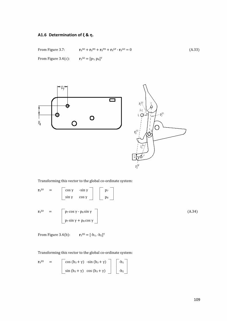
109
A1.6 Determination of ξ & η.
From Figure 3.7: r0SO + r0
HS + r0FH + r0
GF - r0GO = 0 (A.33)
From Figure 3.4(c): r3SO = [p7, p8]T
Transforming this vector to the global co-ordinate system:
r0SO = o γ - γ p7
γ o γ p8
r0SO = p7 o γ - p8 γ (A.34)
p7 γ 8 o γ
From Figure 3.4(b): r5HS = [-h1, -h2]T
Transforming this vector to the global co-ordinate system:
r0HS = cos (h3 + γ -sin (h3 + γ -h1
sin (h3 + γ cos (h3 + γ -h2

110
r0HS = -h1 cos (h3 + γ 2 sin (h3 + γ (A.35)
-h1 sin (h3 + γ – h2 cos (h3 + γ
From Figure 3.4(d): r6FH = [-c1, -c2]T
Transforming this vector to the global co-ordinate system results in
r0FH = o ξ - ξ -c1
ξ o ξ -c2
r0FH = -c1 o ξ 2 ξ
(A.36)
-c1 ξ – c2 o ξ
From Figure 3.7: r0GF= [-c3, 0]T (A.37)
and r0GO= [-b5, -η]T (A.38)
Thus from Equations (A.33 - A.38):
p7 o γ - p8 γ - h1 cos (h3 + γ 2 sin (h3 + γ - c1 o ξ c2 ξ - c3 + b5 = 0
p7 γ 8 o γ - h1 sin (h3 + γ – h2 cos (h3 + γ -c1 ξ – c2 o ξ η 0 (A.39)
Let p7 o γ - p8 γ - h1 cos (h3 + γ 2 sin (h3 + γ - c3 + b5 = X2
Then -c1 o ξ 2 ξ = -X2
Dividing both sides by √
ξ
√
-
o ξ
√
=
√
ξ

111
Now let cosQ2 =
c2
then sinQ2 =
c1
√
√
Then substituting in Equation (A.38):
ξ o 2 - o ξ 2 =
-X2
√
Thus
ξ - Q2) =
-X2
√
ξ = (
√
) +Q2
ξ = ( o γ γ o γ γ
√
) o (
√
)
(A.40)
Substituting back into Equation (A.39),
η = -p7 γ - p8 o γ 1 sin (h3 + γ 2 cos (h3 + γ 1 ξ 2 o ξ (A.41)

112
A1.7 Determination of ζ.
From Figure 3.8: r0TO + r0
JT + r0FJ + r0
GF - r0GO = 0 (A.42)
From Figure 3.3(c): r3TO = [p3, -p4]T
Transforming this vector to the global co-ordinate system:
r0TO = o γ - γ p3
γ o γ -p4
r0TO = p3 o γ 4 γ (A.43)
p3 γ – p4 o γ
From Figure 3.4(a):
r1
JT = [-t3, -t4]T
Transforming this vector to the global co-ordinate system:
r1JT = o α - α -t3
α o α -t4

113
r0JT = -t3 o α 4 α (A.44)
-t3 α – t4 o α
From Figure 3.8:
r0FJ = [-s1, -s2]T (A.45)
r0GF= [-c3, 0]T (A.46)
r0GO= [-b5, -η]T (A.47)
Thus from Equations (A.42 – A.47):
p3 o γ 4 γ -t3 o α 4 α - s1 - c3 + b5 =
0
p3 γ – p4 o γ - t3 α – t4 o α - s2 η 0
Therefore
s1 = p3 o γ 4 γ - t3 cos α 4 sin α - c3 + b5, and (A.48)
s2 = p3 γ – p4 o γ - t3 α – t4 cos α η (A.49)
Thus
ζ = √
- s3 + s4
(A.50)
In addition, ϟ can be defined as:
ϟ = arctan (s1 / s2) (A.51)

114
A1.8 Determination of θ & λ.
From the above, and from Figures 3.4(f) and 3.7: r0
KT = r0JT + r0
KJ
Thus r0KT = -t3 cos α 4 sin α + -s3 sin (arctan (s1/s2))
-t3 sin α – t4 cos α -s3 cos (arctan (s1/s2))
= -t3 cos α 4 sin α - s3 sin (arctan (s1/s2))
-t3 sin α – t4 cos α - s3 cos (arctan (s1/s2))
Therefore, from Figure 3.7:
θ = ( α – o α o
o α α ) (
) (A.52)
Similarly,
λ = √ o α α α – o α o
(A.53)
θ λ
ζ ϟ

115
A2 Force analysis Option 1.
A2.1 Determination of fcf and fncf.
Summing moments about T,
From Figure 3.10, using the previously derived geometric variables and τT = t5 fT μT :
λ cos θ fms = ρ fcf + t5 fT μT μcf fcf sinφ (A.54)
W μT is the coefficient of friction at point T,
fcf is the force vector at the catch face, and
fT is the force vector at point T, and
φ is the angle between fncf and fcf (see Figure 3.3)
Examining the X and Y components of the forces relative to the global coordinate system:
From Figure 3.10,
fms cos ϟ + fcf cos α = fXT and (A.55)
fms sin ϟ + fcf sin α = fYT (A.56)
using fT = √ (fXT )2 + (fY
T)2
and substituting in Equation (A.54),
λ cos θ fms = t5 μT √ (fms)2 + (fcf)2 + 2 fms cos ϟ fcf cos α fms sin ϟ fcf sin α + (ρ μcf sinφ) fcf
θ
λ
ρ
α
ϟ
ω
ψ
μcf τT
τsh
φ
μcf

116
λ cos θ fms - ρ μcf sinφ) fcf = t5 μT √ (fms)2 + (fcf)2 + 2 fms cos ϟ fcf cos α fms sin ϟ fcf sin α
λ o θ fms - ((ρ μcf sinφ) fcf))2 = (t5)2 ( μT)2
((fms)2 + (fcf)2 + 2fms cos ϟ fcf cos α fms sin ϟ fcf sin α
λ cos θ fms)2 + ρ2+ ρµcfsinφ+(μcf sinφ)2)( fcf)2 – 2 λ cos θ fms ρ µcf sinφ) fcf =
(t5)2 ( μT)2 (fms)2 + (t5)2 ( μT)2 (fcf)2 + (t5)2 ( μT)2 2 fms fcf (cos ϟ cos α ϟ sin α
rearranging factors:
ρ2 ρµcfsinφ μcf sinφ)2)- ((t5)2 ( μT)2))(fcf)2 - ((t5)2 ( μT)2 2 fms (cos ϟ cos α ϟ sin α
– (2λ cos θ fms ρ µcf sinφ) fcf λ cos θ fms)2 - ((t5)2 ( μT)2 (fms)2) = 0
thus
fcf = -Q √ Q2 – 4 P R (A.57) 2 P Where
P = (ρ2 ρµcfsinφ μcf sinφ)2)- ((t5)2 ( μT)2)
Q = -((t5)2 ( μT)2 2 fms (cos ϟ o α ϟ α – λ o θ fms ρ µcf sinφ)
R = λ o θ fms)2 - ((t5)2 ( μT)2 (fms)2)
(note: examination of the results determined that the negative root is applicable in this case).
It follows directly that fncf
= fcf cos(φ) (A.58)
where fncf is the component of vector fcf normal to the actuator catch face, and φ is the angle
between fncf and fcf (see Figure 3.3).
A2.2 Determination of fms.
(Force exerted by the main spring under the geometric conditions determined in 3.1.1)
The pre-load present in the tension spring varies according to the spring rate; however it has been
found that this pre-load consistently corresponds to an initial elongation of 0.85mm.
Thus
fms = ζ – sf + 0.85) (A.59) where k = spring rate, (1.75 N/mm) and sf = spring free length (13.5mm).

117
Note also that there are two main springs available for the mechanism, with differing rates and free
l g Fo udy o ly “ d d” m g ll u d
A2.3 Determination of τas.
(Torque exerted by actuator spring on the actuator)
As shown in Figure 3.12, the actuator spring acts as a simple cantilever where:
L = (p6 + b7 - m2 o β, (A.60)
s = b3 – b6 + b9 + w2, (A.61)
s5 and s6 are independent variables,
w2 is derived below, and
E = 120 GPa. (Standard for the grade of phosphor bronze used).
fas was then determined from the standard formula for leaf spring calculation, thus
fas = s E s6 s53
(A.62) 4 L3 The torque ul g f om d fl o of u o g τas is fas L
(A.63) thus τas = s E s6 s5
3 4 L2
β

118
A2.4 Determination of W2.
As shown in Figure 3.13, the following variables were used in the derivation of W2
L2 = spring active length,
S7 = curvature value measured at spring centre, ie length L3 from the spring end,
L1 = distance from end of active portion of spring to the s7 position
W1 = spring pre-displacement due to the spring curvature at the s7 position.
W2 = spring pre-displacement due to the spring curvature at the end of the active portion
of the spring.
W3 = spring pre-displacement due to the spring curvature at the end of the spring.
The torque on the actuator is constant, thus if fx is the force required to straighten the actuator
spring at point Lx then:
L1P1 = L2P2
ie L1 . 3 E I W1 = L2 . 3 E I W2
L13 L2
3
Thus W2 = L22
W1 (A.64)
L12
In the case under discussion
L1 = 10.4745, L2 = 25.0720 and L3 = 16.8

119
Thus W1 = 0.1745 W2 (A.65)
Now from the triangle described by the actuator, the actuator spring and length W3,
W3 = 2(W1 + s7). (A.66)
From Figure 3.13 it can be seen that
W2 = W3 (A.67)
L3 + (L2 - L1) 2 L3
Thus
W2 = W3 + W3 (L2 - L1)
2 2 L3
From Equation (A.62), substituting 2(W1 + s7) for W3:
W2 = W1 + s7 + (W1 + s7) (L2 - L1)
L3
thus
W2 = W1 + s7 + (W1) (L2-L1) + ( s7) (L2-L1) (A.68)
L3 L3
From Equation (A63), substituting W2 for W1 and values for L1 – L3:
W2 = 0.1745W2 + s7 + (0.1745w2)(0.89555) + 0.89555 s7
Thus W2 = 2.83 s7 (A.69)
A2.5 Determination of μcf.
The following is the method used for deriving the catch face friction coefficient distribution of the
standard actuator / fine blanked torque link combination.
From Equation (3.3):
fLL = ((μcf ω) - ψ fn
cf τas μsh a6 fcf 25
Thus
25 fLL - τas - μsh a6 fcf + ψ = μcf (A.70)
ω fncf ω

120
o τas is eliminated from the data during measurement, it is set to zero in the above equation.
Thus
25 fLL - μsh a6 fcf + ψ = μcf
ω fncf ω
Where
fcf = catch force = (disregarding torque link and catch face friction)
λ cos θ fms (A.71) ρ
fncf = catch force normal = fcf o φ (A.72)
The variables applicable to the above equations are given in the table below.
Values, where given, are the actual values relating to the measuring jig.
Table B.1 Variables relating to lock load jig: option 1.
Variable Value
μcf = the coefficient of friction in the catch face Unknown
μsh = the coefficient of friction in the actuator shoulder 0.2
ψ = catch face angle force moment arm 1.065 mm
ω = catch face friction force moment arm length 10.194 mm
fLL = the lock load. To be measured
fas = actuator spring force To be measured
fms = main spring force 11.436 N
ρ = torque link/actuator moment arm length 17.528 mm
λ = torque link/main spring moment arm length 8.046 mm
θ = main spring force vector angle 1 47.458°
φ = catch force vector angle 5.487°
ζ = main spring flexed length 19.185

121
Therefore:
fcf = 2 λ cos θ fms
ρ
= 124.427
35.056
= 3.549 N
then
fncf =
=
fcf o φ 3.533 N
thus
25 fLL - τas- μsh a6fcf + ψ = μcf
ω fncf ω
μcf = 25 (fLL – fas) - μsh a6 fcf + 1.065
10.194 * 3.533 10.194
Setting μsh to its nominal value of 0.2, and a6 to its measured mean value of 0.09763, the above
equation becomes:
μcf = 25 (fLL – fas) – 0.069298 + 0.1044732
36.015
μcf = 25 (fLL – fas) + 0.10255 (A.73) 36.015

122
APPENDIX B: SURFACE IMPERFECTIONS
B1 Modelling of surface imperfections.
The distribution of measured catch face friction coefficients derived in 3.2.2 indicated that the
actuator torque resulting from the friction in the actuator / torque link translational joint was
sometimes augmented by a further torque deriving from imperfections in the actuator catch
face. (Note once again that the possibility of imperfections in the torque link was disregarded,
due to the consistency of the type B process used in their manufacture).
Microscopic photographs of various catch face imperfections can be seen in Figures 3.19, 4.10
and 4.11.
It was proposed that these imperfections be considered to alter the catch force vector angle φ
by an angle ά, resulting from a localised change in the actuator torque link interface.
Various types of imperfection were considered, namely
wide shallow grooves with rounded profile,
narrow deep grooves with rounded profile,
ridges with rounded profile,
wide shallow grooves with rectangular profile,
narrow deep grooves with rectangular profile,
ridges with rectangular profile, and
wavy surfaces with sinusoidal profile.
Various assumptions were made with respect to the profiles, namely
the profiles were of perfect geometrical form, and
the profiles were positioned at the worst possible position with respect to an increase
in lock load.
From an e amination of the diagrams below, equations were derived for the value of ά.

123
Figure B.1 The values of angle ά caused by imperfections of rounded profile.
The derivation of the values of ά in the cases of the rounded ridges and grooves shown above,
and of the rectangular ridges and grooves shown below followed directly from the diagrams,
and are given in Table B.1
ά = arccos((R+r-H)/(R+r))
If
ά = √ 2-(R-H)2)/r)
If R > r
ά = o -H)/R)

124
Figure B.2 The values of angle ά caused by imperfections of rectangular profile.
Table B.1 Formulae for the calculation of ά.
Case Condition Equation
Grooves with rounded profile R > r ά = arcos((R-H)/R) (B.1)
Grooves with rounded profile r ≥ R ά = arcsin(√(R2-(R-H)2)/r) (B.2)
Ridges with rounded profile All ά = arcos((R+r-H)/(R+r)) (B.3)
Grooves with rectangular profile H2+(w/2)2-2RH > 0 ά = arcos((r-H)/ r) (B.4)
Grooves with rectangular profile H2+(w/2)2-2RH ≤ 0 ά = arcsin(W 2 r) (B.5)
Ridges with rectangular profile All ά = arcos((r-H)/ r) (B.6)
ά = o -H)/ r)
If H2+(w/2)2-2RH > 0
ά = o -H)/ r) If H2+(w/2)2-2RH ≤ 0
ά = arcsin(W 2 r)

125
Figure B.3 The values of angle ά caused by imperfections of sinusoidal profile (case 1).
Figure B. 4 The values of angle ά caused by imperfections of sinusoidal profile (case 2).
The case of the sinusoidal profile was more complex.
From Figure B.3,
tan(ά) = (2πA P)*sin(2πRsin(ά) P) (B.7)

126
Note: the above equation was solved for ά by means of an iterative algorithm implemented in
Matlab, and held true while tan (ά) < 2 π A/P.
If tan (ά) ≥ 2 π A P, then as shown in Figure B.4, άmax occurred when
ά = arctan (2 π A/P) (B.8)
With the value of ά known for various sizes and shapes of surface imperfections, the effect on
the lock load could now be determined.
The torque on the actuator resulting from the angle on the catch face τa was calculated by the
equation:
τa = fcf cos (φ) * ( (sin (a3)(a1 - a2 tan a3)) - a6 + δ
) (B.9) cos a3
Replacing φ with (φ- ά) and sin(a3) with sin (a3- ά)
τa = fcf cos φ - ά * ( (sin (a3 - ά 1-a2 tan a3))-a6 + δ
) (B.10) cos a3
Note:
The cos (a3) and tan (a3) terms establish overall position and are not localized force vectors,
thus they were not replaced by (a3 - ά)
Substituting (φ - ά) for φ and sin (a3 - ά) for sin (a3) as detailed above, and setting all other
variables to their nominal values, the following surface graphs of the lock loads resulting from
variations in the details of the actuator catch face imperfections were drawn.
The lock load modification effects caused by the presence of square grooves and square ridges
located on the actuator catch face, as illustrated in Figure B.5, demonstrate the following.
For square ridges, the increase in lock load is dependent entirely on the ridge height.
For wide, square grooves, the increase in lock load is entirely dependent on the groove
height.
For narrow grooves, the lock load increase is dependent on the groove width.
An examination of Figure B.2 suffices to confirm the validity of the above.

127
Figure B.5 The effect of imperfections of rectangular profile on nominal lock load.
Figure B.6 The effect of imperfections of rounded profile on nominal lock load.
The lock load modification effects caused by the presence of rounded grooves and ridges
located on the actuator catch face, as illustrated in Figure B.6, follow a similar pattern to that
of the square ridges and grooves. The transition between the regions of feature height
predominance and feature width predominance is however more gradual in the case of the
rounded features.

128
Figure B.7 The effect of imperfections of sinusoidal profile on nominal lock load
Finally, the imperfections of sinusoidal profile show an almost complete indifference to the
height (or Ra value) of the imperfections at short wave lengths, contrasting with the Ra value
being completely dominant at longer wavelengths. This is, in effect, a special case of the
rounded profile of Figure B.7, but with a much more gradual transition between the regions.
The above diagrams demonstrate that if the shape and size of any particular imperfection is
known, it is possible to predict its effect on the lock load by application of the above formulae
and / or consultation of the above graphs.
More importantly in this case, if the details of the imperfection are not known, then any
reasonable lock load increase, of any type, can be converted into a local catch face angle
variation having an equivalent effect on the lock load. The details of the actual form of the
imperfection are not in fact required in order to model their effects.
It was thus considered justified to treat all extraneous lock load effects as generic local catch
face angle variations.

129
APPENDIX C: MECHANISM ANALYSIS OPTION 2
C.1 Positional analysis.
C.1.1 Determination of β.
From Figure 4.4: r0AO + r0
BA – r0BO = 0 (C.1)
As in Appendix A:
r0AO = o γ 5 - m1) - γ 6 - m2) (C.2)
γ 5 - m1) + o γ 6 - m2)
From Figures 4.5 and 4.2: r2BA = [(a5 - a5cos(-β-γ 10),(-a4 + a5 – a5sin (-β-γ ]T

130
Then
r0BA = cos β γ -sin β γ (a5 – a5 cos(-β -γ a10)
sin β γ cos β γ (-a4 + a5 – a5 sin (-β -γ
= cos β + γ 5 – a5 cos (-β -γ a10) – sin β + γ -a4 + a5 – a5 sin (-β -γ
sin β + γ 5 – a5 cos (-β -γ a10)+ cos β + γ -a4 + a5 – a5 sin (-β-γ
= (a5 + a10) cos β + γ - a5 cos2 β + γ + a4 sin β + γ – a5 sin β + γ - a5 sin2 β γ
(a5 + a10) sin β + γ - a5 cos β + γ sin β + γ - a4 cos β + γ 5 cos β + γ
+ a5 cos β + γ sin β + γ
= (a5 + a10) cos β + γ 4 – a5) sin β + γ - a5 (cos2 β + γ 2 β + γ
(a5 + a10) β + γ 5 - a4) cos β + γ 5 cos β + γ sin β + γ
- a5 cos β + γ sin β + γ
r0BA = (a5 + a10) cos β + γ 4 – a5) sin β + γ - a5
(a5 + a10) β + γ 5 - a4) cos β + γ (C.3)
Finally, as in Appendix B:
r0BO =
b3
-ε (C.4)
Thus from Equations (C.1, C.2, C.3 & C4):
o γ 5 - m1) - γ 6 - m2) + (a5 + a10 o β γ 4 – a5 β γ
- a5 - b3
=
0 (C.5)
γ 5 - m1 o γ 6 - m2) + (a5 + a10 β γ 5 - a4 o β γ
ε
0 (C.6)
From Equation (C.5): l o γ 5 - m1) - γ 6 - m2) -a5 - b3) = K.
Then (a5 + a10) cos β + γ 4 – a5) sin β + γ = -K
Dividing both sides by √ ((a5+a10)2 + (a4-a5)2) gives

131
a5 cos β + γ + (a4 – a5) sin β + γ = -K
√ ((a5 + a10)2 + (a4 - a5)2) √ ((a5 + a10)2 + (a4 - a5)2) √ ((a5 + a10)2 + (a4 - a5)2) (C.7)
Now let cosZ =
(a4 – a5)
√ ((a5 + a10)2 + (a4 - a5)2)
then sinZ =
(a5 - a10)
√ ((a5 + a10)2 + (a4 - a5)2)
substituting in Equation (C.7): sin Z cos β + γ + cos Z sin β + γ = -K
√ ((a5 + a10)2 + (a4 - a5)2)
thus
sin β γ = -K √ ((a5 + a10)2 + (a4 - a5)2)
β γ = arcsin -K √ (a5 +a10)2 + (a4 - a5)2)
Therefore
β = (
√
) γ (
) (C8)
C.1.2 Determination of α, δ, and δδ.
Let point E be the centre of radius a9.
then from Figure 4.5: r0AT + r0
EA - r0ET = 0 (C.9)
As shown in Appendix B:
r0AT = cos γ (p5 – p3 – m1) – sin γ (p6 + p4 – m2)
sin γ (p5 – p3 – m1) + cos γ (p6 + p4 – m2) (C.10)
√((a5+a10)2 + (a4-a5)
2)
a5+a1
0
a4-a5

132
From Figure 4.2: r2
EA = [a8 , -a7]T
r0EA = cos β + γ -sin β + γ a8
sin β + γ cos β + γ -a7
= a8 cos β + γ 7 sin β + γ
a8 sin β + γ - a7 cos β + γ (C.11)
From Figure 4.2:
r1ET = [(t6 + δδ , -δδ tan t7 + a9/cos t7)] T
r0ET = cos α -sin α (t6 + δδ
sin α cos α (-δδ tan t7 + a9/cos t7)
r0ET = (t6 + δδ o α δδ tan t7 - a9/cos t7) sin α
(t6 + δδ α - δδ tan t7 - a9/cos t7) cos α (C.12)
Then from (C.9, C.10, C.11 & C.12):
o γ 5 – p3 – m1) – γ 6 + p4 – m2)+ a8 o β γ
+ a7 β γ - (t6 δδ o α - (-a9/cos t7 δδ 7 α
=
0
γ 5 – p3 – m1 o γ 6 + p4 – m2 + a8 β γ
- a7 o β γ - (t6 δδ α -a9/cos t7 δδ 7 o α
0
let A = cos γ (p5 – p3 – m1) – sin γ (p6 + p4 – m2) + a8 cos β + γ 7 sin β + γ
δδ

133
and let B = sin γ (p5 – p3 – m1) + cos γ (p6 + p4 – m2) + a8 sin β + γ - a7 cos β + γ
then
A - (t6 δδ o α 9 α o 7) – δδ 7 α =
0 (C13)
B - (t6 δδ α - (a9 o α o 7 δδ 7 o α 0 (C14)
From Equation (C.13):
A - (t6 + δδ o α a9 sin α
- δδ tan t7 sin α = 0 cos t7
Then
A - t6 cos α – δδ cos α a9 α
- δδ tan t7 sin α = 0 cos t7
and
A - t6 cos α a9 sin α
= δδ (tan t7 sin α o α cos t7
Solv g fo δδ g v :
A -
t6 cos α +
a9 sin α = δδ tan t7 sin α o α tan t7 sin α o α cos t7 (tan t7 sin α o α
thus
A cos t7 -
t6 cos α o 7 +
a9 sin α = δδ sin t7 sin α o 7 cos α sin t7 sin α o 7 cos α sin t7 sin α o 7 cos α
then
δδ = cos t7 (A - t6 cos α 9 sin α
(C.15) o α - t7)

134
Similarly, from Equation (C.14):
δδ = cos t7 (B - t6 sin α - a9 cos α
(C.16) α - t7)
Combining Equations (C.15 and C.16):
cos t7 (A - t6 cos α 9 sin α =
cos t7 (B - t6 sin α - a9 cos α
o α - t7) α - t7)
Cross-multiplying gives:
A cos t7 α - t7) - t6 cos α o 7 α - t7) + a9 α α - t7)= B cos t7 o α - t7) - t6 sin α o t7
o α - t7) - a9 cos α o α - t7)
Re-arranging terms:
a9 (sin α α - t7) + cos α o α - t7)) + cos t7 (A α - t7) – B o α - t7)) - t6 cos t7 α - t7)
cos α - o α - t7) sin α =
which gives:
a9 (cos α - α - t7))) + cos t7 (A α - t7) – B o α - t7)) - t6 cos t7 α - t7) - α =
and thus:
a9 cos t7 + cos t7 (A α - t7) – B o α - t7)) - t6 cos t7 sin t7 = 0
Re-arranging terms gives:
a9 cos t7 - t6 cos t7 sin t7 = - cos t7 (A α - t7) – B o α - t7))
thus:
a9 + t6 sin t7 = -A α - t7) – B o α - t7) (C.17)
Now let a9 + t6 sin t7 = -K
Then d v d g o d y √ A2+B2) gives:
A sin α - t7) +
B cos α - t7) = K (C.18) √ A2 + B2 √ A2 + B2 √ A2 + B2
Now let sinZ = B √ A2 + B2
then cos Z = A √ A2 + B2
Substituting in Equation (C.18):

135
cos Z sin α - t7) + sin Z cos α - t7) = K √ A2 + B2
Thus sin α - t7 ) = K √ A2+B2
α = (
√A ) (
A)
(C.19)
Substituting back into Equation (C20):
α = (
√A ) (
A)
(C.20)
and, from Equation (C.15):
δδ = cos t7 (A - t6 o α 9 α (C.21)
o α - t7)
D ly f om ov , ov g δ d m d y
δ = 1 – t6 – δδ (C.22)
The remaining positional variables were derived as detailed in Appendix B or directly from the
appropriate diagrams as detailed in the text.

136
C.1.3 Determination of remaining geometric variables.
Directly from Figure 4.3:
ρ = t6 δδ (C.23) and φ = 7 (C.24)
Similarly,
ψ = (a7 + a9 cos β + φ - α β + φ - α 8 – a9 sin β + φ - α – a6 –a6 sin β (C.25)
and
ω = 7 + a9 cos β + φ - α o β + φ - α (C.26)
C.2 Force analysis Option 2.
C.2.1 Determination of fcf , fncf , fms, τas and W2.
The above variables were determined in the same manner as employed for Option 1.
C.2.2 Determination of μcf.
As demonstrated in Equation (A.70)
25 fLL - τas - μsha6fcf + ψ = μcf
ω fncf ω
Where
τas = torque exerted on actuator by the actuator spring = 25 fas
ρ
φ
ψ
ω

137
fcf = catch force (disregarding torque link and catch face friction)
= λ o θ fms ρ
fncf = catch force normal = fcf o φ
The variables applicable to the above equations are listed in the table below. Values, where
specified, are the actual values pertaining to the measuring jig.
Table C.1 Dependent variables pertaining to actuator type 2.
Variable (relating to roller catch actuator) Value
μcf = coefficient of friction in the catch face Unknown
μsh = coefficient of friction in the actuator shoulder 0.2
μT = coefficient of friction in the torque link pivot 0.2
ψ = catch face angle force moment arm 0.9514 mm
ω = catch face friction force moment arm length 10.3412 mm
fLL = lock load. To be measured
fas = actuator spring force To be measured
fms = main spring force 11.4609 N
ρ = torque link/actuator moment arm length 17.2439 mm
λ = torque link/main spring moment arm length 8.0456 mm
θ = main spring force vector angle 1 47.2861°
φ = catch force vector angle 6.6803°
ζ = main spring flexed length 19.1991
o ov v l , du o d ff g om y “O o ” d “O o
”, l g ly d ff f om o d l d of “O o ”
Therefore:

138
fcf = λ o θfms ρ
=
62.5494 17.2439
= 3.627 N
then
fncf =
=
fcf o φ 3.602 N
Thus
μcf = 25 fLL - 25 fas - μsha6fcf + 0.9514
10.3412 * 3.602 10.3412
μcf = 25 (fLL - fas) – 0.07082 + 0.0920 37.249
μcf = 25 (fLL - fas) + 0.0920 (C.27) 37.249

139
APPENDIX D: MECHANISM ANALYSIS OPTION 3
D.1 Force analysis.
D.1.1 Determination of μcf.
Using Equation (A.70) and following the method shown in Appendix A2.5:
25 fLL - τas - μsh a6 fcf + ψ = μcf
ω fncf ω
Where
τas = torque exerted on actuator by the actuator spring
= 25 fas
fcf = catch force (disregarding torque link friction)
= λ o θ fms ρ
fn
cf = catch force normal
= fcf o φ
T fo …
fcf = λ o θ fms
ρ
=
62.5494 17.2932
= 3.617 N
then
fncf =
fcf o φ
Which remains 3.617N.
Thus
μcf = 25 fLL - 25 fas - μsh a6 fcf + 0.031117
10.4030 * 3.617 10.4030
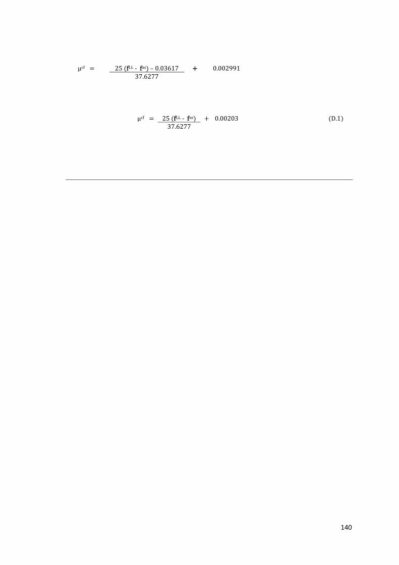
140
μcf = 25 (fLL - fas) – 0.03617 + 0.002991
37.6277
μcf = 25 (fLL - fas) + 0.00203 (D.1)
37.6277