tion

(17)

J<. satisfies

(18)

differential

s we used to lime interval for obtaining

~q. (18). But and volumes

• hat its rate of year. Suppose aused by past [ Lake Huron. : to reduce the

is the separable

(19)

(years).

1.5 Linear First-Order Equations 53

----- -- -----Mixture problem A 120-gallon (gal) tank initially contains 90 lb of salt dissolved in 90 gal of water. Brine containing 2lbj gal of salt flows into the tank at the rate of 4 gal/min, and the well-stirred mixture flows out of the tank at the rate of 3 gal/min. How much salt does the tank contain when it is full?

Solution The interesting feature of this example is that, due to the differing rates of inflow and outflow, the volume of brine in the tank increases steadily with V(t) = 90 + t gallons. The change !J.x in the amount x of salt in the tank from timet to timet + !J.t (minutes) is given by

Problems

!J.x ~ (4)(2) !J.t- 3 (-x-) !J.t, 90 + t

so our differential equation is dx 3 -+--x=8. dt 90 + t

An integrating factor is

p(x) = exp (/ -3

- dt) = e310(90+t) = (90 + t) 3 90+ t ,

which gives

Dt [ (90 + l )3 x J = 8(90 + t) 3

;

(90 + t) 3x = 2(90 + t) 4 +C.

Substitution of x (0) = 90 gives C = -(90) 4 , so the amount of salt in the tank at time t is

904 x(t)=2(90+t)-

3.

(90 + t)

The tank is full after 30 min, and when t = 30, we have

904 X (30) = 2(9(1 -1- 30) -

1203 ~ 202 (lb)

of salt in the tank.

-- _" __ _ Find general solutions of the differential equations in Prob­lems 1 through 25. If an initial condition is given, find the corresponding particular solution. Throughout, primes denote derivatives with respect to x.

19. y'+ycotx =COSX

20. y' = l -1- x + y -1- xy, y(O) = 0 21. xy' == 3y + x 4 cos x, y(2rr) = 0

22. y' = 2xy + 3x2 exp(x 2), y(O) = 5

1. y' + y = 2, y(O) = 0

3. y' + 3y = 2xe-3x

5. xy' + 2y = 3x, y(1) = 5

6. xy' + 5y = 7x2 , y(2) = 5

2. y'-2y = 3e2x, y(O) = 0 2

4. y' - 2x y = ex

23. xy' + (2x- 3)y = 4x4

24. (x 2 + 4)y' + 3xy = x, y(O) = 1

25. (x 2 + 1) ~~ + 3x 3 y = 6x exp ( -ix2 ), y(O) = I

•

7. 2xy' + y = 10-JX

9. xy'- Y = x, y(1) = 7 8. 3xy' + y = 12x

10. 2xy'- 3y = 9x3 Solve the differential equations in Problems 26 through 28 by regarding y as the independent variable rather than x.

xy' + Y = 3xy, y(1) = 0 xy' + 3y = 2x5 , y(2) = 1

y' -1- Y =ex , y(O) = 1

xy'- 3y = x3, y(l) = 10

y' + 2xy = x, y(O) = -2

= 0- y)cosx, y(rr) = 2

+ x)y' + Y = cosx, y(O) =I :::: 2y + x 3 cosx

26.

28.

dy (1- 4xy 2 )- = y 3

dx dy

(1 + 2xy)- = 1 + y 2 dx

dy 27. (x + yeY)- = I

dx

29. Express the general solution of dyjdx = 1 + 2xy in terms of the error function

2 rx 2 erf(x) = .j7r Jo e-

1 dt.

56 Chapter 1 First-Order Differential Equations

Fig. 1.5 .9, which approaches asymptotically the graph of the equilibrium solution x(t) = 20 that corresponds to the reservoir's long-term pollutant content. How long does it take the pollutant concentration in the reservoir to reach 10 Lj m3?

46. The incoming water has pollutant concentration c(t) = 10(1 + cost) L/ m3 that varies between 0 and 20, with an average concentration of 10 Lj m3 and a period of os­cillation of slightly over 6;\- months. Does it seem pre­dictable that the lake's pollutant content should ultimately oscillate periodically about an average level of 20 million liters? Verify that the graph of x(t) does, indeed, resemble the oscillatory curve shown in Fig. 1.5.9. How long does

it take the pollutant concentration in the reservoir to 10 L/ m3?

25 X

10 20 30 40 50 60

FIGURE 1.5.9. Graphs of solutions in Problems 45 and 46.

co Go to qoo. ql/QVuenz to download thjs application's computing resources including Maple/Mathematica!MATLABI Python.

For an interesting applied problem that involves the solution of a linear differen tial equation, consider indoor temperature osci'llations that are driven by outdoor temperature oscillations of the form

A(t) = ao + a 1 co~wt + b1 sinwt . (1)

If w = rr/12, then these oscillations have a period of 24 hours (so that the cycle of outdoor temperatures repeats itself daily) and Eq. (1) provides a realistic model for the temperature outside a house on a day when no change in the overall day-to-day weather pattern is occurring. For instance, for a typical July day in Athens, Georgia with a minimum temperature of 70°F when t = 4 (4 A.M.) and a maximum of 90°F when t = 16 (4 P.M.), we would take

A(t) = 80- 10 cos w(t- 4) = 80- 5 cos wt - 5.J3 sin wt. (2)

We derived Eq. (2) by using the identity cos(a - {3) = cos a cos f3 + sin a sin f3 to get a0 = 80, a1 = -5, and b1 = -5.J3 in Eq. (1).

If we write Newton's law of cooling (Eq. (3) of Section 1.1) for the corre­sponding indoor temperature u(t) at time t , but with the outside temperature A(t) given by Eq. {1) instead of a constant ambient temperature A, we get the linear

FIG RE 1.5. given by Eq. ( uo = 65,68,

first-order differential equation 100

that is,

du dt = -k(u - A(t));

du + ku = k(a0 + a 1 coswt + b1 sinwt) dt

(3)

with coefficient functions P(t) = k and Q(t ) = kA(t). Typical values of the propor­tionality constant k range from 0.2 to 0.5 (although k might be greater than 0.5 for a poorly insulated building with open windows, or less than 0.2 for a well-insulated building with tightly sealed windows).

95

90

~ 85 OJ)

2. 80

"' 75

J(

FIGURE 1.5. indoor and ou oscillations.

70 Chapter 1 First-Order Differential Equations

Problems --- ----

Find general solutions of the differential equations in Prob­lems 1 through 30. Primes denote derivatives with respect to x throughout.

1. (x + y)y' = x- y

3. xy' = y + 2fo 5. x(x + y)y' = y(x- y) 7. xy2y' = x3 + y3

9. x 2y'=xy+y2

11. (x2 - y 2)y1 = 2xy r---c~~

12. xyy' = y 2 + xJ4x2 + y2

13. xy' = y + J x2 + y2

14. yy' +x = Jx2 + y2

15. x(x + y)y' + y(3x + y) = 0 16. y' = v'x + y + 1 18. (x + y)y' = 1 20. y 2 y' + 2xy 3 = 6x

22. x 2 y' + 2xy = 5y4

24. 2xy' + y 3e-2x = 2xy

25. y 2(xy' + y)(l + x 4 ) 112 = x 26. 3y2y' + y 3 =e-x

27. 3xy2 y' = 3x4 + y3 28. xeY y' = 2(eY + x 3e2x)

2. 2xyy' = x 2 + 2y2

4. (x- y)y' = x + y

6. (x + 2y)y' = y 8. x 2y' = xy + x 2eY!x

10. xyy' = x 2 + 3y2

17. y' = (4x + y)2

19. x 2y' + 2xy = 5y 3

21. y' = y + y 3

23. xy' + 6y = 3xy413

29. (2x sin y cos y)y' = 4x2 + sin2 y 30. (x + eY)y' = xe-Y - 1

In Problems 31 through 42, verify that the given differential equation is exact; then solve it.

31. (2x + 3y) dx + (3x + 2y) dy = 0

32. (4x- y) dx + (6y- x) dy = 0

33. (3x2 + 2y2) dx + (4xy + 6y2) dy = 0

34. (2xy2 + 3x2) dx + (2x 2y + 4y 3) dy = 0

35. (x3+;)dx+(y2 +lnx)dy=O

36. (1 + yexY) dx + (2y + xeXY) dy = 0

37. (cosx+lny)dx+ (~ +eY)dy =0

x+y 38. (x + tan- 1 y) dx + --2

dy = 0 1+ y

39. (3x2

y 3 + y 4) dx + (3x 3 y 2 + y 4 + 4xy 3) dy = 0

40. (ex siny + tany) dx +(ex cosy+ x sec2 y) dy = 0

41. (

2x- 3y2) dx + (2y - x2 +_I_) dy = 0 y x4 x3 y2 ,;y

2x5/ 2 _ 3y5/ 3 3y5/ 3 _ 2x5/ 2 42

· 5/ 2 2/ 3 dx + 3/ 2 5/ 3 dy = 0 2x y 3x y

Find a general solution of each reducible second-order differ­ential equation in Problems 43-54. Assume x, y and/or y' positive where helpful (as in Example 11 ).

43. xy" = y' 44. yy" + (y')2 = 0

-45. y" + 4y = 0 46. xy" + y' = 4x 47. y" = (y'f 48. x 2y" + 3xy' = 2 49. yy" + (y') 2 = yy' 50. y" = (x + y')2

51. y" = 2y(y')3 52. y 3y" = 1 53. y" = 2yy' 54. yy" = 3(y'f

55. Show that the substitution v = ax + by + c transforms the differential equation dyjdx = F(ax +by +c) into a separable equation.

56. Suppose that n f. 0 and n f. 1. Show that the sub­stitution v = y l - n transforms the Bernoulli equation dy/dx + P(x) y = Q(x)yn into the linear equation

dv dx + (1- n)P(x) v (x) =(I- n)Q(x).

57. Show that the substitution v = In y transforms the differ­ential equation dyjdx + P(x)y = Q(x)(y ln y) into the linear equation dvjdx + P(x) = Q(x)v(x) .

58. Use the idea in Problem 57 to solve the equation

dy 2 x --4x y+2y ln y=O.

dx

59. Solve the differ·~ntial equation

dy X- y- I

dx x + y + 3

by finding h and k so that the substitutions x = u + h, y = v + k transform it into the homogeneous equation

dv u- v

du = u + v

60. Use the metho in Problem 59 to solve the differential equation

61.

62.

63.

dy 2y -x + 7

dx 4x-3y-l8

Make an appropriate substitution to find a solution of the equation dyjdx = sin(x- y). Does this general solution contain the linear solution y(x) = x- n /2 that is readily verified by substitution in the differential equation?

Show that the solution curves of the differential equation

dy y(2x 3 - y 3)

dx x(2y3- x3)

areoftheform x 3 + y 3 = Cxy .

The equation dyjdx = A(x)y2 + B(x)y + C(x) is called a Riccati equation. Suppose that one particular solution Yl (x) of this equation is known. Show that the substitu-tion

1 Y = Yl +­

v transforms the Ri.ccati equation into the linear equation

dv -- + (B + 2Ayi)v =-A. dx

Use the method of Problem 63 to solve the equations in Prob­lems 64 and 65, given that Yl (x) = x is a solution of each.

66. An equ

is call1 paramf

is a ge1 67. Consid

forwh

is tang

Explai tion of and th< illustr::

Fl of ec th

'*·I co c download computin~

Maple/Ma

ansforms c) into a

the sub­equation on

the differ­) into the

1

= u + h, :quation

differential

ution of the :ral solution at is readily ttion? a! equation

(x) is called ular solution the substitu-

tr equation

ions in Prob­•n of each.

dy 2 64. - + y 2 = 1 + X

dx

dy 2 65. - + 2xy = 1 + x 2 + y

dx

66. An equation of the form

67.

y = xy' + g(y') (37)

is called a Clairaut equation. Show that the one­parameter family of straight lines described by

y(x) = Cx + g(C)

is a general solution of Eq. (37) . Consider the Clairaut equation

y = xy'- t(y')2

(38)

for which g(y') = -! (y')2 in Eq. (37). Show that the line

y = Cx- -!C 2

is tangent to the parabola y = x 2 at the point (! C, ! C 2 ) .

Explain why this implies that y = x 2 is a singular solu­tion of the given Clairaut equation. This singular solution and the one-parameter family of straight line solutions are illustrated in Fig. 1.6.10.

FIGURE 1.6.10. Solutions of the Clairaut equation of Problem 67. The "typical" straight line with equation y = Cx -lC2 is tangent to the parabola at the point C!C, lC 2 ) .

1 .6 Substitution Methods and Exact Equations 71

68. Derive Eq. (18) in this section from Eqs. (16) and (17).

69. Flight trajectory In the situation of Example 7, suppose that a = 100 mi, vo = 400 mi/ h, and w = 40 mi/ h. Now how far northward does the wind blow the airplane?

70. Flight trajectory As in the text discussion, suppose that an airplane maintains a heading toward an airport at the origin. If vo = 500 mi/ h and w = 50 mi/ h (with the wind blowing due north), and the plane begins at the point (200, 150) , show that its trajectory is described by

71. River crossing A river 100 ft wide is flowing north at w feet per second. A dog starts at (100, 0) and swims at vo = 4 ft/ s, always heading toward a tree at (0, 0) on the west bank directly across from the dog 's starting point. (a) If w = 2 ft/ s, show that the dog reaches the tree. (b) If w ,= 4 ft/ s, show that the dog reaches instead the point on the west bank 50 ft north of the tree. (c) If w = 6 ft/s, show that the dog never reaches the west bank.

72. In the calculus of plane curves, one learns that the curva­ture K of the curve y = y(x) at the point (x , y) is given by

ly''(x)l K = ---'-'---'-'-'....,--,,.,-

(1 + y'(x)2]3/ 2 '

and that the curvature of a circle of radius r is K = 1/ r . [Se:e Example 3 in Section 11.6 of Edwards and Penney, Calculus: Early Transcendentals, 7th edition, Hoboken, NJ : Pearson, 2008.] Conversely, substitute p = y' to derive a general solution of the second-order differential equation

(with r constant) in the form

Thus a circle of radius r (or a part thereof) is the only plane curve with constant curvature 1/r.

1.6 Application Com uter Algebra Solutions

C[] Go to qoo.ql/tLcVCl to download this application's computing resources including Maple!Mathematica!MATLAB.

Computer algebra systems typically include commands for the "automatic" solution of differential equations. But two different such systems often give different results whose equivalence is not clear, ~md a single system may give the solution in an overly complicated form. Consequently, computer algebra solutions of differential equations often require considerable "processing" or simplification by a human user in order to yield concrete and applicable information. Here we illustrate these issues using the interesting differential equation

dy . ( ) -- = sm x- y dx

(1)

82 Chapter 2 Mathematical Models and Numerical Methods

Solution To solve the equation in (14), we separate the variables and integrate. We get

p

FIGURE 2.1.6. Typical solution curves for the explosion/extinction equation P' = kP(P - M) .

lfJI Problems

J P(/~ 150) = J 0.0004dt ,

__ I_ j (2_ - 1 ) dP = j 0.0004 dt [partial fractions],

150 p p - 150

In IPI-ln IP- 1501 = -0.061 + C ,

--=--p-,- = ±ec e-0.061 = B e-0.061 p -150

[where B = ±ec].

(a) Substitution oft = 0 and P = 200 into (15) gives B = 4. With this value of B we Eq. (15) for

600e-0.061 P(t) = 4e- 0.061 - I .

Note that, as t increases and approaches T = ln (4)/0.06 ~ 23.105, the positive u~:o••u"u"'''u' on the right in (16) decreases and approaches 0. Consequently P(t) ~ +oo as t ~ r- . This is a doomsday situation-a real population explosion. (b) Substitution oft = 0 and P = 100 into (15) gives B = -2. With this value of B we solve Eq. (15) for

300e-0 ·061 300 P(t) = 2e 0.061 + 1~ = 2 + e0.061 · (17)

Note that, as t increases without bound, the positive denominator on the right in (16) ap­proaches +oo. Consequently, P(t) ~ 0 as t ~ +oo. This is an (eventual) extinction situa­tion . •

Thus the population in Example 7 either explodes or is an endangered species threatened with extinction, depending on whether or not its initial size exceeds the threshold population M = 150. An approximation to this phenomenon is sometimes observed with animal populations, such as the alligator population in certain areas of the southern United States.

Figure 2.1.6 shows typical solution curves that illustrate the two possibilities for a population P(t) satisfying Eq. (13). If Po = M (exactly!), then the popula­tion remains constant. However, this equili rium situation is very unstable. If Po exceeds M (even slightly), then P(t) rapidly increases without bound, whereas if the initial (positive) population is less than M (however slightly), then it decreases (more gradually) toward zero as t ~ +oo. See Problem 33.

Separate variables and use partial fractions to solve the initial value problems in Problems 1-8. Use either the exact solution or a computer-generated slope field to sketch the graphs of sev­eral solutions of the given differential equation, and highlight the indicated particular solution.

d£ 7. dt =4x(7- x ),x(O) =II

dx 8. dt = ?x(x- 13) , x(O) = 17

9. Population growth The time rate of change of a rabbit population P i proportional to the square root of P . At timet = 0 (months) the population numbers 100 rabbits and is increasi g at the rate of 20 rabbits per month. How many rabbits will there be one year later?

dx 1. - = X - x 2 X (0) = 2

dt '

dx 3. dt = 1 - x 2 , x (0) = 3

dx 5. dt = 3x(5- x), x(O) = 8

dx 6. dt = 3x(x- 5), x(O) = 2

dx 2. dt = 10x-x2 ,x(O) = 1

dx 4. - = 9-4x 2 x(O) = 0

dt ' 10. Extinction by disease Suppose that the fish population

P(t) in a lake is attacked by a disease at timet = 0, with the result that the fish cease to reproduce (so that the birth rate is f3 = 0) and the death rate 8 (deaths per week per

fish) is I tially 9( bow lor

u. Fish p< stocked both im

where k there ar 1 year?

12. Popula tor pop1 of P. '

two dm tors in t

13. Birth r : of rabb: pro port (a) She

Note th (b) Su~ after te1

14. Death 1

\em 13 populat

15. Limitir isfying B=aP is the r< is P(O) month; populat

16. Limitir satisfyi initial ~ month how m; the lirni

17. Limith satisfyi initial ~ month howm; the limi

18. Thresh isfying bP,wh andD = populat

(15)

' B we solve

(16)

denominator ~ r- . This

,f B we solve

(17)

1t in (16) ap­tinction situa-

• ;ered species . exceeds the is sometimes certain areas

, possibilities 1 the popula­tstable. If Po d, whereas if n it decreases

fish) is thereafter proportional to 1/./P. If there were ini­tially 900 fish in the lake and 441 were left after 6 weeks, how long did it take all the fish in the lake to die?

11. Fish population Suppose that when a certain lake is stocked with fish, the birth and death rates f3 and 8 are both inversely proportional to .JP. (a) Show that

P(t) = (ikt + /Po) 2,

where k is a constant. (b) If Po = 100 and after 6 months there are 169 fish in the lake, how many will there be after 1 year?

12. Population growth The time rate of change of an alliga­tor population P in a swamp is proportional to the square of P. The swamp contained a dozen alligatOjS in 1988, two dozen in 1998. When will there be four dozen alliga­tors in the swamp? What happens thereafter?

13. Birth rate exceeds death rate Consider a prolific breed of rabbits whose birth and death rates, f3 and o, are each proportional to the rabbit population P = P (t) , with f3 > 8. (a) Show that

Po P(t) = 1 - kP

0t ' k constant.

Note that P(t) ~ +oo as t ~ lj(kPo) . This is doomsday. (b) Suppose that Po = 6 and that there are nine rabbits after ten months. When does doomsday occur?

14. Death rate exceeds birth rate Repeat part (a) of Prob­lem 13 in the case f3 < 8. What now happens to the rabbit population in the long run?

15. Limiting population Consider a population P(t) sat­isfying the logistic equation dPfdt = aP- bP 2 , where B = aP is the time rate at which births occur and D = bP 2

is the rate at which deaths occur. If the initial population is P(O) = Po , and Eo births per month and Do deaths per month are occurring at time t = 0, show that the limiting population isM= EoPo/Do .

16. Limiting population Consider a rabbit population P(t) satisfying the logistic equation as in Problem 15. If the initial population is 120 rabbits and there are 8 births per month and 6 deaths per month occurring at time t = 0, how many months does it take for P(t) to reach 95% of the limiting population M?

7. Limiting population Consider a rabbit population P(t) satisfying the logistic equation as in Problem 15. If the initial population is 240 rabbits and there are 9 births per month and 12 deaths per month occurring at time t = 0, bow many months does it take for P(t) to reach 105% of the limiting population M?

~.'lu:eshold population Consider a population P(t) sat­isfying the extinction-explosion equation dPfdt = aP 2 -

where B = a P 2 is the time rate at which births occur D == bP is the rate at which deaths occur. If the initial

is P(O) = Po and Bo births per month and Do

2.1 Population Models 83

deaths per month are occurring at time t = 0, show that the threshold population is M = Do Po/ Eo.

19. Th1reshold population Consider an alligator population P(t' ) satisfying the extinction-explosion equation as in Problem 18. If the initial population is 100 alligators and there are 10 births per month and 9 deaths per month oc­curring at time t = 0, how many months does it take for P (1) to reach 10 times the threshold population M ?

20. Th1reshold population Consider an alligator population P (1) satisfying the extinction-explosion equation as in Problem 18. If the initial population is 110 alligators and the e are 11 births per month and 12 deaths per month oc­curring at time t = 0, how many months does it take for P (1) to reach 10% of the threshold population M?

21. Lo;~stic model Suppose that the population P(t) of a country satisfies the differential equation dPfdt = kP(200- P) with k constant. Its population in 1960 was 100 million and was then growing at the rate of 1 million per year. Predict this country's population for the year 2020.

22. Lo;~istic model Suppose that at time t = 0, half of a "lo­gistic" population of 100,000 persons have heard a certain rumor, and that the number of those who have heard it is then increasing at the rate of 1000 persons per day. How long will it take for this rumor to spread to 80% of the pop­ulation? (Suggestion: Find the value of k by substituting P(O) and P 1(0) in the logistic equation, Eq. (3) .)

23. Solution rate As the salt KN03 dissolves in methanol, the number x(t) of grams of the salt in a solution af­ter t seconds satisfies the differential equation dxfdt =

2 ' 0.8x - 0.004x .

(a) What is the maximum amount of the salt that will ever dissolve in the methanol?

(b) If x = 50 when t = 0, how long will it take for an additional 50 g of salt to dissolve?

24. Spread of disease Suppose that a community contains 15,000 people who are susceptible to Michaud's syn­drome, a contagious disease. At time t = 0 the number N(t ) of people who have developed Michaud's syndrome is 5000 and is increasing at the rate of 500 per day. As­sume that N 1 (t) is proportional to the product of the num­bers of those who have caught the disease and of those who have not. How long will it take for another 5000 peo­ple to develop Michaud's syndrome?

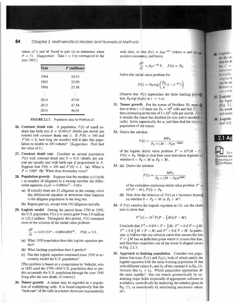
25. Logistic model The data in the table in Fig. 2.1. 7 are given for a certain population P(t) that satisfies the logis­tic equation in (3). (a) What is the limiting population M ? (Suggestion: Use the approximation

p I (t) ~ _P__:.( t_+____:h )~--:--P-'--(1_-_h_;_) 2h

with h = 1 to estimate the values of P 1 (t) when P = 25.00 and when P = 47.54. Then substitute these values in the logistic equation and solve for k and M .) (b) Use the

84 Chapter 2 Mathematical Models and Numerical Methods

values of k and M found in part (a) to determine when P = 75. (Suggestion: Take I = 0 to correspond to the year 1965.)

Year P (millions)

1964 24.63

1965 25.00

1966 25.38

2014 47 .04

2015 47.54

2016 48.04

FIGURE 2.1.7. Population data for Problem 25.

26. Constant death rate A population P (t) of small ro­dents has birth rate f3 = (0.001)P (births per month per rodent) and constant death rate 8. If P(O) = 100 and P' (0) = 8, how long (in months) will it take this popu­lation to double to 200 rodents? (Suggestion: First find the value of 8.)

27. Constant death rate Consider an animal population P(l) with constant death rate 8 = 0.01 (deaths per ani­mal per month) and with birth rate f3 proportional to P . Suppose that P(O) = 200 and P'(O) = 2. (a) When is P = 1000? (b) When does doomsday occur?

28. Population growth Suppose that the number x(t) (with 1 in months) of alligators in a swamp satisfies the differ­ential equation dxjdt = 0.000lx2 - O.Olx.

(a) If initially there are 25 alligators in the swamp, solve this differential equation to determine what happens to the alligator population in the long run.

(b) Repeat part (a), except with 150 alligators initially.

29. Logistic model During the period from 1790 to 1930, the U.S. population P(t ) (t in years) grew from 3.9 million to 123.2 million . Throughout this period, P(t) remained close to the solution of the initial value problem

~~ = 0.03135P- 0.0001489P 2, P(O) = 3.9.

(a) What 1930 population does this logistic equation pre­dict?

(b) What limiting population does it predict?

(c) Has this logistic equation continued since 1930 to ac-curately model the U.S. population?

[This problem is based on a computation by Verhulst, who in 1845 used the 1790-1840 U.S. population data to pre­dict accurately the U.S. population through the year 1930 (long after his own death, of course).]

30. Thmor growth A tumor may be regarded as a popula­tion of multiplying cells. It is found empirically that the "birth rate" of the cells in a tumor decreases exponentially

with time, so that {3(1) = f3 0e-a 1

positive constants), and hence

dP -at d = f3oe P, P(O) = Po.

Solve this initial value problem for

Observe that P(t) approaches the finite limiting popula­tion Po exp (f3o/a) as 1 -+ +oo.

31. Thmor growth For the tumor of Problem 30, suppose that at time 1 = 0 there are Po = 106 cells and that P(t) is then increasing at the rate of 3 x 105 cells per month . After 6 months the tumor has doubled (in size and in number of cells). Solve numerically for a, and then find the limiting population of the tumor.

32. Derive the solu ·on

P(t ) = MPo . Po + (M - Po)e-kMt

of the logistic initial value problem P' = kP(M - P), P(O) = P0 . Make it clear how your derivation depends on whether 0 < Po < M or Po > M .

33. (a) Derive the solution

P(t) = MPo Po + (M - Po )ekMt

of the extinc 'on-explosion initial value problem P' = kP(P- M) , P(O) = P0 .

(b) How does the behavior of P(t) as 1 increases depend on whether 0 < Po < M or Po > M?

34. If P(t) satisfies the logistic equation in (3), use the chain rule to show that

P"(t) = 2k 2 P(P- iM)(P- M).

Conclude that P" > 0 ifO < P < !M; P" = 0 if P = !M;

P" < 0 if i M < .P < M; and P" > 0 if P > M . In partic­ular, it follows that any solution curve that crosses the line P = ! M has an inflection point where it crosses that line, and therefore res .rubles one of the lower S-shaped curves in Fig. 2.1.3.

35. Approach to limiting population Consider two popu­lation functions .P1 (1) and .P2(1), both of which satisfy the logistic equation with the same limiting population M but with different val es k1 and kz of the constant kin Eq. (3). Assume that k1 < kz. Which population approaches M the most rapidly? You can reason geometrically by ex­amining slope fields (especially if appropriate software is available), symbolically by analyzing the solution given in Eq. (7), or numerically by substituting successive values oft.

J6. Logistic · for the va tion forth for x2 = pressions is readily original e can be us· ulation v; spaced ti1

37. Logistic the logist (Fig. 2.1 . the result and actua

38. Logistic tual U.S.

Co cot download this computing re' Maple/Mathe1

t and ~o are

uting popula-

1 30, suppose 1d that P (t) is ·month. After in number of

d the limiting

kP(M- P), on depends on

problem P' =

;reases depend

1, use the chain

M).

=OifP=!M; > M. In partie­crosses the line rosses that line, :-shaped curves

;ider two popu­'hich satisfy the lpulation M but :ant k in Eq. (3).

approaches M etrically by ex­riate software is .olution given in 1ccessive values

2. 1 Population Models 85

36. Logistic modeling To solve the two equations in ( 1 0) for the values of k and M , begin by solving the first equa­tion for the quantity x = e- sokM and the second equation for x2 = e-lOOkM . Upon equating the two resulting ex­pressions for x 2 in terms of M, you get an equation that is readily solved for M. With M now known, either of the original equations is readily solved fork . This technique can be used to "fit" the logistic equation to any three pop­ulation values Po, P1, and P2 corresponding to equally spaced times to = 0, t1, and t2 = 211.

1930, and 1960. Solve the resulting logistic equation, then compare the predicted and actual populations for the years 1980, 1990, and 2000.

39. Periodic growth rate Birth and death rates of animal opulations typically are not constant; instead, they vary

periodically with the passage of seasons. Find P(t) if the population P satisfies the differential equation

dP - = (k + b cos 2:rrt)P, dt

37. Logistic modeling Use the method of Problem 36 to fit the logistic equation to the actual U.S. population data (Fig. 2.1.4) for the years 1850, 1900, and 1950. Solve the resulting logistic equation and compare the predicted and actual populations for the years 1990 and 2000.

where t is in years and k and b are positive constants. Thus the growth-rate function r (t) = k + b cos 2:rr t varies peri­odically about its mean value k . Construct a graph that contrasts the growth of this population with one that has the same initial value Po but satisfies the natural growth equation P ' = kP (same constant k). How would the two populations compare after the passage of many years?

38. Logistic modeling Fit the logistic equation to the ac­tual U.S. population data (Fig. 2.1.4) for the years 1900,

2.1 Application

co Go to qoo . ql/s3nZZ3 to download this application's computing resources including /Haple!Mathematica!M ATLAB.

Logistic Modeling of Population Data These investigations deal with the problem of fitting a logistic model to given pop­ulation data. Thus we want to determine the numerical constants a and b so that the solution P(t) of the initial value problem

dP - = aP + bP 2

, P(O) =Po dt

(1)

approximates the given values Po, P 1, ... , Pn of the population at the times to = 0, t 1, . .. , ln. If we rewrite Eq. (1) (the logistic equation with kM = a and k = -b) in the form

then we see that the points

1 dP --- =a+bP p dt '

( P' (t;))

P(t;) , P (t;) , i=0, 1, 2, .. . ,n ,

(2)

should all lie on the straight line with y-intercept a and slope b (as determined by the function of P on the right-hand side in Eq. (2)).

This observation provides a way to find a and b. If we can determine the ap­proximate values of the derivatives P{, P~ , . .. corresponding to the given population data, then we can proceed with th following agenda:

• First plot the points (P1, P{/PI), (P2 , P~/ P2), .. . on a sheet of graph paper with horizontal P -axis.

• Then use a ruler to draw a straight line that appears to approximate these points well.

• Finally, measure this straight line's y-intercept a and slope b.

But where are we to find the needed 'lalues of the derivative P' (t) of the (as yet) unknown function P? It is easiest to use the approximation

(3)

n measure-

gives

(2lb)

= 0, r = R

both (2la) ignition by

= 1.78187 X

r 26 miles). 1 mjs at the

•

1e question )f the earth :cessary for its velocity aw'ay from

:nter at time

(22)

X 1024 (kg) 6.378 X 106

1 Example 4

! solution for

(23)

as a function

2.3 Acceleration-Velocity Models 101

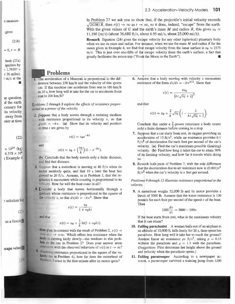
In Problem 27 we ask you to show that, if the projectile's initial velocity exceeds J2GM/ R, then r(t) ---+ oo as t ---+ oo, so it does , indeed, "escape" from the earth. With the given values of G and the earth's mass M and radius R, this gives v0 ~

11,180 (m/s) (about 36,680 ft/s, about 6.95 mi js, about 25,000 rni/ h).

Remark Equation (24) gives the escape velocity for any other (spherical) planetary body when we use its mass and radius. For instance, when we use the mass M and radius R for the moon given in Example 4, we find that escape velocity from the lunar surface is vo ~ 2375 mj s. This is just over one-fifth of the escape velocity from the earth's surface, a fact that greatly faci litates the return trip ("From the Moon to the Earth"). •

Problems 1. The acceleration of a Maserati is proportional to the dif­

ference between 250 km/ h and the velocity of this sports car. If this machine can accelerate from rest to 100 km/ h in 10 s, how long will it take for the car to accelerate from rest to 200 km/ h?

Problems 2 through 8 explore the effects of resistance propor­tional to a power of the velocity.

2. Suppose that a body moves through a resisting medium with resistance proportional to its velocity v, so that dvjdt = -kv . (a) Show that its velocity and position at timet are given by

v(t) = voe-k 1

and x(t) = xo + (:0 ) (1- e-kr).

(b) Conclude that the body travels only a finite distance, and find that distance.

3. Suppose that a motorboat is moving at 40 ft j s when its motor suddenly quits, and that 10 s later the boat has slowed to 20 ftjs. Assume, as in Problem 2, that the re­sistance it encounters while coasting is proportional to its velocity. How far will the boat coast in all?

4. Consider a body that moves horizontally through a medium whose resistance is proportional to the square of the velocity v, so that dvjdt = -kv2 . Show that

vo v (t) = _J_+_v_o_k_t

and that 1

x(t) = xo +kIn(!+ vokt).

Note that, in contrast with the result of Problem 2, x (t) ---+

+oo as t ---+ +oo. Which offers less resistance when the body is moving fairly slowly-the medium in this prob­lem or the one in Problem 2? Does your answer seem consistent with the observed behaviors of x(t) as t ---+ oo?

5. Assuming resistance proportional to the square of the ve­locity (as in Problem 4), how far does the motorboat of Problem 3 coast in the first minute after its motor quits?

6. Assume that a body moving with velocity v encounters resistanceoftheformdv/dt = -kv312 . Show that

4v0 v(t) = 2

(kt.ji!O + 2)

and that

Conclude that under a ~-power resistance a body coasts only a finite distance before coming to a stop.

7. Suppose that a car starts from rest, its engine providing an acceleration of 10 ft j s2 , while air resistance provides 0.1 ftjs2 of deceleration for each foot per second of the car's velocity. (a) Find the car's maximum possible (limiting) velocity. (b) Find how long it takes the car to attain 90% of its limiting velocity, and how far it travels while doing so.

8. Rew rk both parts of Problem 7, with the sole difference that the deceleration due to air resistance now is (0.001)v 2

ft js2 when the car's velocity is v feet per second.

Problems 9 through 12 illustrate resistance proportional to the velocity.

9. A motorboat weighs 32,000 lb and its motor provides a thrust of 5000 lb. Assume that the water resistance is 100 pounds for each foot per second of the speed v of the boat. The

dv 1000- = 5000- 100v.

dt

If the boat starts from rest, what is the maximum velocity that it can attain?

10. Falling parachutist A woman bails out of an airplane at anal 'tude of 10,000 ft, falls freely for 20 s, then opens her parachute. How long will it take her to reach the ground? Assume linear air resistance pv ft js2 , taking p = 0.15 without the parachute and p = 1.5 with the parachute. (Suggestion: First determine her height above the ground and velocity when the parachute opens.)

11. Falling paratrooper According to a newspaper ac­count, a paratrooper survived a training jump from 1200

1 02 Chapter 2 Mathematical Models and Numerical Methods

ft when his parachute failed to open but provided some re­sistance by flapping unopened in the wind. Allegedly he hit the ground at 100 mi/ h after falling for 8 s. Test the ac­curacy of this account. (Suggestion: Find pin Eq. (4) by assuming a terminal velocity of 100 mi/ h. Then calculate the time required to fall1200 ft.)

12. Nuclear waste disposal It is proposed to dispose of nu­clear wastes-in drums with weight W = 640 lb and vol­ume 8 ft3-by dropping them into the ocean (vo = 0). The force equation for a drum falling through water is

dv m-=-W+B+FR

dt '

where the buoyant force B is equal to the weight (at 62.5 lb/ ft3 ) of the volume of water displaced by the drum (Archimedes' principle) and F R is the force of water resis­tance, found empirically to be I lb for each foot per second of the velocity of a drum. If the drums are likely to burst upon an impact of more than 75 ft/s, what is the maximum depth to which they can be dropped in the ocean without likelihood of bursting?

13. Separate variables in Eq. (12) and substitute u = v /Pii to obtain the upward-motion velocity function given in Eq. (13) with initial condition v(O) = vo.

14. Integrate the velocity function in Eq. (13) to obtain the upward-motion position function given in Eq. (14) with initial condition y(O) = yo.

15. Separate variables in Eq. (15) and substitute u = v /Pfi to obtain the downward-motion velocity function given in Eq. (16) with initial condition v(O) = vo.

16. Integrate the velocity function in Eq. (16) to obtain the downward-motion position function given in Eq. (17) with initial condition y(O) = YO·

Problems 17 and 18 apply Eqs. (12)-(17) to the motion of a crossbow bolt.

17. Consider the crossbow bolt of Example 3, shot straight upward from the ground (y = 0) at time t = 0 with initial velocity v0 = 49 m js. Take g = 9.8 m/s2 and p = 0.0011 in Eq. (12). Then use Eqs. (13) and (14) to show that the bolt reaches its maximum height of about 108.47 min about 4.61 s.

18. Continuing Problem 17, suppose that the bolt is now dropped (vo = 0) from a height of Yo = 108.47 m. Then use Eqs. (16) and (17) to show that it hits the ground about 4.80 slater with an impact speed of about 43.49 m/s.

Problems 19 through 23 illustrate resistance proportional to the square of the velocity.

19. A motorboat starts from rest (initial velocity v(O) = vo = 0). Its motor provides a constant acceleration of 4 ft/ s2 ,

but water resistance causes a deceleration of v2 /400 ft/ s2 .

Find v when t = 10 s, and also find the limiting velocity as t ~ +oo (that is, the maximum possible speed of the boat).

20. An arrow is shot straight upward from the ground an initial velocity of 160 ft/s. It experiences both the celeration of gravity and deceleration v2/800 due to resistance. How high in the air does it go?

21. If a ball is projected upward from the ground with initial velocity v0 and resistance proportional to v2 , deduce Eq. (14) that the maximum height it attains is

Ymax = - In 1 + - . 1 ( pv~ ) 1p g

22. Suppose that p = 0.075 (in fps units, with g = 32 ftjs2) in Eq. (15) for a paratrooper falling with parachute open. If he jumps from an altitude of 10,000 ft and opens his parachute immediately, what will be his terminal speed? How long will it take him to reach the ground?

23. Suppose that the paratrooper of Problem 22 falls freely for 30 s with p = 0.00075 before opening his parachute. How long will it now take him to reach the ground?

Problems 24 through 30 explore gravitational acceleration and escape velocity.

24. The mass of the sun is 329,320 times that of the earth and its radius is 109 times the radius of the earth. (a) To what radius (in meters) would the earth have to be compressed in order for itt become a black hole-the escape velocity from its surface equal to the velocity c = 3 x 108 m/ s of light? (b) Repeat part (a) with the sun in place of the earth.

25. (a) Show that if a projectile is launched straight upward from the surface of the earth with initial velocity vo less than escape velocity ,j1GM/R , then the maximum dis­tance from the center of the earth attained by the projectile is

1GMR r - ------,.. max - 1GM- R v2 '

0

where M and R are the mass and radius of the earth, re­spectively. (b) With what initial velocity vo must such a projectile be launched to yield a maximum altitude of 100 kilometers above the surface of the earth? (c) Find the maximum distance from the center of the earth, expressed in terms of earth radii, attained by a projectile launched from the surface of the earth with 90% of escape velocity.

26. Suppose that you are stranded-your rocket engine has failed--on an asteroid of diameter 3 miles, with density equal to that of the earth with radius 3960 miles. If you have enough spring in your legs to jump 4 feet straight up on earth while wearing your space suit, can you blast off from this asteroid using leg power alone?

27. (a) Suppose a projectile is launched vertically from the surface r == R of the earth with initial velocity vo = ,j1GM/ R , so v~ = k 2/ R where k 2 = 2GM. Solve the differential equation dr/dt = k/.,fi (from Eq. (23) in this section) explicitly to deduce that r(t) ~ oo as t ~00.

(b) Ifthe 1ocit)

Why 28. (a) Suppc

tance ro is dvjd t ' reaches tl

t =

(Suggesti

f Jr/(ro of 1000 I is neg1ec speed wi:

29. Suppose surface o Then its value pre

y

d2;

dt~

"' I c

FIGURE2.3.

·ound with oth the de­due to air

with initial ~duce from

= 32 ft/s2)

chute open. d opens his tina! speed?

?

lls free! y for tchute. How

acceleration

he earth and (a) To what

, compressed ;ape velocity >< 108 m/s of place of the

aight upward locity vo less taximum dis­the projectile

(b) If the projectile is launched vertically with initial ve­locity v0 > J2GM/R, deduce that

dr = Jk2 +a>..!:..__

dt r vfr

Why does it again follow that r(t) ~ oo as t ~ oo? 28. (a) Suppose that a body is dropped (vo = 0) from a dis­

tance ro > R from the earth's center, so its acceleration is dvfd t = -GMfr2 . Ignoring air resistance, show that it reaches the height r < ro at time

t=J ro (Jrro-r 2 +rocos-1 ~)-2GM y-;:;;

(Suggestion: Substitute r = ro cos2 8 to evaluate J J r f(ro - r) d r .) (b) If a body is dropped from a height of 1000 k.rn above the earth's surface and air resistance is neglected, how long does it take to fall and with what speed will it strike the earth's surface?

29. Suppose that a projectile is fired straight upward from the surface of the earth with initial velocity vo < J2GM/R. Then its height y (t) above the surface satisfies the initial value problem

d2y

dt 2

GM (y + R)2 '

2.3 Application

y(O) = 0, y1(0) = VQ.

Rocket Pro ulsion

2.3 Acceleration-Velocity Models 103

Substitute dvfdt = v(dvfdy) and then integrate to obtain

2GMy v2 = v5 - ---'--

R(R + y)

for the velocity v of the projectile at height y. What maxi­mum altitude does it reach if its initial velocity is I km/s?

30. In Jules Verne's original problem, the projectile launched from the surface of the earth is attracted by both the earth and the moon, so its distance r(t) from the center of the earth satisfies the initial value problem

d 2 r GMe GMm 1

d('i = ----;z- + (S _ r)2 ; r(O) = R , r (0) = vo

where Me and Mm denote the masses of the earth and the moon, respectively; R is the radius of the earth and S = 384,400 k.rn is the distance between the centers of the earth and the moon. To reach the moon, the projectile must only just pass the point between the moon and earth where its net acceleration vanishes. Thereafter it is "under the control" of the moon, and falls from there to the lunar surface. Find the minimal launch velocity vo that suffices for the projectile to make it "From the Earth to the Moon."

Suppose that the rocket of Fig. 2.3.5 blasts off straight upward from the surface of

F

I Ill I c

the earth at timet = 0. We want to calculate its height y and velocity v = dyjdt at time t. The rocket is propelled by exhaust gases that exit (rearward) with constant speed c (relative to the rocket). Because of the combustion of its fuel, the mass m = m(t) of the rocket is variable.

To derive the equation of motion of the rocket, we use Newton's second law in the form

dP dt = F, (1)

where P is momentum (the product of mass and velocity) and F denotes net external force (gravity, air resistance, etc.). If the mass m of the rocket is constant so m' (t) = 0-when its rockets are turned off or burned out, for instance-then Eq. (1) gives

which (with dvfdt =a) is the more familiar form F = ma of Newton's second law. But herem is not constant. Suppose m changes tom+ D.m and v to v + D.v

during the short time interval from t tot + D.t. Then the change in the momentum of the rocket itself is

D.P ~ (m + D.m)(v + D.v) - mv = m D.v + v D.m + D.m D.v .

But the system also includes the exhaust gases expelled during this time interval, with mass - D.m and approximate velocity v -c. Hence the total change in momen-

1en solve

;onvenient

(18)

g generates ¥S the three ;traight line

•

a1 equation

sfy a given

solution of

nstants. An 1es two ini-

vith the two

~quation

n

I.

Problems Jn each of Problems 1-22, use the method of elimination to determine whether the given linear system is consistent or in­consistent. For each consistent system, find the solution if it is unique; otherwise, describe the infinite solution set in terms of an arbitrary parameter t (as in Examples 5 and 7).

1. X+ 3y = 9 2. 3x + 2y = 9 2x + y=8 X- y =8

3. 2x + 3y = 1 4. 5x- 6y = l 3x + 5y = 3 6x- 5y = 10

5. X+ 2y = 4 6. 4x- 2y = 4 2x + 4y = 9 6x- 3y = 7

7. x-4y=- i0 8. 3x- 6y = 12 -2x + 8y = 20 2x- 4y = 8

9. X+ 5y + z =2 10. x + 3y + 2z = 2 2x + y -2z = l 2x + 7y + 7z = - 1

x + 7y + 2z = 3 2x + 5y + 2z = 7

n. 2x + 7y + 3z = 11 12. 3x + 5y - z = 13 x + 3y + 2z = 2 2x + 7y + z = 28

3x + 7y + 9z = - 12 x + 7y + 2z = 32

13. 3x + 9y + 7z = 0 14. 4x + 9y + 12z = - 1 2x + 7y + 4z = 0 3x + y + 16z = -46 2x + 6y + 5z = 0 2x + 7y + 3z = 19

15. x + 3y + 2z = 5 16. x- 3y + 2z = 6 x- y + 3z = 3 X+ 4y- z= 4

3x + y + 8z = 10 5x + 6y + z = 20

17. 2x - y + 4z = 7 18. x+ 5y + 6z = 3 3x + 2y- 2z = 3 5x + 2y - !Oz =I Sx + y + 2z = 15 8x + 17y + 8z = 5

X -2y + z = 2 20. 2x + 3y + 7z = 15 2x- y- 4z = 13 X+ 4y + z = 20 X- y- z = 5 x + 2y + 3z = 10

x+y - z = 5 22. 4x- 2y + 6z = 0 3x + y + 3z = 11 x- y- z= O 4x + y + 5z = 14 2x- y + 3z = 0

of Problems 23-30, a second-order differential equa­its general solution y(x) are given. Determine the A and B so as to find a solution of the differen­

that satisfies the given initial conditions involving ll1ld y' (0).

+ 4y = 0, y(x) = A cos 2x + B sin 2x, == 3, y'(O) = 8

- 9y == 0, y(x) = A cosh 3x + B sinh 3x, == 5, y' (0) == 12

-25y == 0, y(x) = Aesx + Be-sx , == 10, y' (0) = 20

l2ly == 0, y(x) = Aellx + Be- ll x, == 44, y' (O) = 22

2y' -15y == 0, y(x) = Ae3x + Be-5x, == 40, y' (0) == -16

lOy'+ 21y == 0, y(x ) = Ae3x +Be 7x' 15, y' (0) == 13

3.1 Introduction to Linear Systems 145

29. 6y" - 5y' + y = 0, y(x) = Aexf2 + Bex f3, y(O) = 7, y'(O) = 11

30. 15y'' + y' -28y = 0, y(x) = Ae4x f3 + Be-7x/5, y(O) = 41, y'(O) = 164

31. A system of the form

a1 x + b1y = 0

a2x + b2 y = 0,

in which the constants on the right-hand side are all zero, is said to be homogeneous. Explain by geometric rea­soning why such a system has either a unique solution or infinitely many solutions. In the former case, what is the uni ue solution?

32. Consider the system

a1x+b1 y+c1z=d1

a2x + b2 y + C2 Z = d2

of two equations in three unknowns.

(a) Use the fact that the graph of each such equation is a plane in xyz-space to explain why such a system al­ways has either no solution or infinitely many solu­tions.

(b) Explain why the system must have infinitely many so­lutions if d 1 = 0 = d2.

33. The linear system

a1x + b1 y = Cl

a2x + b2y = C2

a3X + b3 y = C3

of three equations in two unknowns represents three lines L 1, L2, and L 3 in the xy-plane. Figure 3 .1.5 shows six possible configurations of these three lines. In each case describe the solution set of the system.

34. Consider the linear system

a1x + b1 y + c1z = d1

a2x + b2 y + C2Z = d2

a3X + b3 y + C3Z = d3

of three equations in three unknowns to represent three planes P1, P2, and P3 in xyz-space. Describe the solution set of the system in each of the following cases.

(a) The three planes are parallel and distinct.

(b) The three planes coincide-PI = P2 = P3 .

(c) P1 and P2 coincide and are parallel to P3 .

(d) P1 and P2 intersect in a line L that is parallel to P3.

(e) P1 and P2 intersect in a line L that lies in P3.

(f) P1 and P2 intersect in a line L that intersects P3 in a single point.

146 Chapter 3 Linear Systems and Matrices

(a) (b) (c)

(d) (t)

FIGURE 3.1.5. Three lines in the plane (Problem 33).

MfJ Matrices and Gaussian Elimination

In Example 6 of Section 3.1 we applied the method of elimination to solve the linear system

lx + 2y + l z = 4 3x + Sy + 7<: = 20

2x + 7 y + 9z = 23.

(1)

There we employed elementary operations to transform this system into the equiv­alent system

l x + 2y + l z = 4 Ox+ ly + 2z = 4 Ox + Oy + l z = 3,

(2)

which we found easy to solve by back substitution. Here we have printed in color the coefficients and constants (including the Os and ls that would normally be omitted) because everything else-the symbols x, y, and z for the variables and the+ and = signs-is excess baggage that means only extra writing, for we can keep track of these symbols mentally. In effect, in Example 6 we used an appropriate sequence of operations to transform the array

2 1 8 7 7 9

2~] 23

of coefficients and constants in (1) into the anay

of constants and coefficients in (2).

(3)

(4)

154 Chapter 3 Linear Systems and Matrices

Problems

as follows:

x 1 = 5 + 2s- 3t

X2 = S

X3 = -3-- 2t

X4 = 7 + 4t

xs = t.

Thus, the substitution of any two specific values for sand tin (19) yields a particular (x 1 , x 2, x3 , x4, x 5 ) of the system, and each of the system's infinitely many different is the result of some such substitution.

Examples 3 and 5 illustrate the ways i which Gaussian elimination can in either a unique solution or infinitely rna y solutions. On the other hand, if reduction of the augmented matrix to echelon form leads to a row of the form

0 0 0 0 *·

where the asterisk denotes a nonzero entry in the last column, then we have an inconsistent equation,

Ox, +Ox2 + ···+ 0xn = *· and therefore the system has no solution.

Remark We use algorithms such as the back substitution and Gaussian elimination algo­rithms of this section to outline the basic computational procedures of linear algebra. In modem numerical work, these procedures often are implemented on a computer. For in­stance, linear systems of more than four equations are usually solved in practice by using a computer to carry out the process of Gaussian elimination. •

The linear systems in Problems 1- 10 are in echelon form. Solve each by back substitution.

10. Xi - 5x2 + 2x3 - 7x4 + llxs = 0 x2 - 13x3 + 3x4 - 7xs = 0

x 4 - 5xs = 0 1. Xi + X2 + 2X3 = 5

x2 + 3x3 = 6 X3 = 2

3. x, - 3x2 + 4x3 = 7 x2 - 5x3 = 2

5. Xi + X2- 2X3 + X4 = 9 X2 - X3 + 2X4 = 1

X3 - 3x4 = 5

6. XJ - 2x2 + 5x3 - 3x4 = 7 x2 - 3x3 + 2x4 = 3

X4 = - 4

7. XJ + 2x2 + 4x3 - 5x4 = 17 X2 - 2X3 + 7 X4 = 7

2. 2x 1 - 5x2 + X3 = 2 3x2 - 2x3 = 9

X3 = -3

4. x , - 5x2 + 2x3 = 10 X2 - 7X3 = 5

8. XJ - 10x2 + 3x3 - 13x4 = 5 x3 + 3x4 = 10

9. 2XJ + X2 + X3 + X4 = 6 3x2 - X3 - 2x4 = 2

3x3 + 4x4 = 9 X4 = 6

In Problems 11-22, use elementary row operations to trans­form each augmented coefficient matrix to echelon form. Then solve the system by back substitution.

11. 2x, + 8x2 + 3x3 = 2 12. XI + 3x2 + 2x3 = 5

2XJ + 7X2 + 4X3 = 8

13. XJ + 3x2 + 3x3 = 13 14. 2x, + 5x2 + 4x3 = 23 2x, + 7x2 + 8x3 = 29

15. 3x, + x2 - 3x3 = - 4 16. Xi+ X2 + X3 = 1

5x 1 + 6x2 + 8x3 = 8

17. XJ - 4x2 - 3x3 - 3x4 = 4 2x 1 - 6x2 - 5x3 - 5x4 = 5 3xl - x2 - 4x3 - 5x4 = -7

18. 3XJ - 6x2 + X3 + 13x4 = 15 3x, - 6x2 + 3x3 + 21x4 = 21 2x, - 4x2 + 5x3 + 26x4 = 23

3x, + x2 - 3x3 = 6

2x1 + 7x2 + X3 = -9 2x, + 5x2 = -5

3x, - 6x2 - 2x3 = 2x,- 4x2 + X3 = 17

XJ - 2x2 - 2x3 = -9

2x1 + 5x2 + 12x3 = 6 3x, + X2 + 5x3 = 12 5x, + 8x2 + 21x3 = 17

t9. 3Xi + · Xi- 2.

4Xi + · lt). 2Xi + 4.

Xi+ 3. 5XI + 8.

21. Xi+ 2XJ -2. 3XJ

4XJ - 2.

22. 4x, -2. 2XJ -2.

4Xt + 3Xt

fn Problems rem has (a) many solutio

23. 3x + 2y 6x + 4y

25. 3x + 2} 6x + k}

27. X+ 2} 2x- } 4x + 3}

28. Under\\ system

Co Go download th: computing n Maple/Math<

(19)

ar solution t solutions

• can result md, if the form

.;e have an

ination algo­. algebra. In uter. For in­ce by using a

•

}9. 3X! + X2 + X3 + 6x4 = 14 XI - 2x2 + Sx3 - Sx4 = -7

4XI + X2 + 2X3 + 7X4 = 17 20. 2x1 + 4x2 - x3 - 2x4 + 2xs = 6

XI + 3x2 + 2x3 - ?x4 + 3xs = 9 Sx1 + 8x2 - ?x3 + 6x4 + xs = 4

21. X! + X2 + X3 6 2x1 - 2x2 - Sx3 = -13 3X! + X3 + X4 = 13 4XI - 2x2 - 3x3 + X4 = I

22. 4X! - 2X2 - 3X3 + X4 = 3 2x1 - 2x2 - Sx3 = - 10 4XJ + X2 + 2X3 + X4 = 17 3X! + X3 + X4 = 12

Jn Problems 23-27, determine for what values of k each sys­tem has (a) a unique solution; (b) no solution; (c) infinitely

many solutions.

23. 3x + 2y = 1 6x + 4y = k

25. 3x + 2y = 11 6x + ky = 21

27. X + 2y + Z = 3 2x- y- 3z = 5 4x + 3y - z = k

24.

26.

3x + 2y = 0 6x + ky = 0 3x + 2y = 1 ?x + Sy = k

28. Under what condition on the constants a, b, and c does the system

2x- y + 3z =a

X+ 2y + Z = b

?x + 4y + 9z = c

3.2 Matrices and Gaussian Elimination 155

have a unique solution? No solution? Infinitely many so­lutions?

29. This problem deals with the reversibility of elementary row operations.

(a) If the elementary row operation cRp changes the ma­trix A to the matrix B, show that (1/c) Rp changes B to A.

(b) If SWAP(Rp . Rq) changes A to B, show that SWAP(Rp . Rq) also changes B to A .

(c) If cRp + Rq changes A to B, show that (-c)Rp + Rq changes B to A.

(d) Conclude that if A can be transformed into B by a fi­nite sequence of elementary row operations, then B can similarly be transformed into A.

30. This problem outlines a proof that two linear systems LS 1

and LS2 are equivalent (that is, have the same solution set) if their augmented coefficient matrices A 1 and A2 are row equivalent.

(a) If a single elementary row operation transforms A1 to A2 , show directly-considering separately the three cases-that every solution of LS 1 is also a solution of LS2.

(b) Explain why it now follows from Problem 29 that ev­ery solution of either system is also a solution of the other system; thus the two systems have the same so­lution set.

Automated Row Reduction

Computer algebra systems are often used to ease the labor of matrix computations, including elementary row operations. The 3 x 4 augmented coefficient matrix of Example 3 can be entered with the Maple command

with(linalg): A := array( [ [ 1, 2, 1 , 4] 1

[3, 8, 7 , 20], [2, 7, 9 , 23]] ) ;

or the Mathematica command

A = { {1, 2, 1, 4}, {3, 8, 7, 20}, {2, 7, 9, 23}}

or the MATLA B command

A = [1 2 1 4 3 8 7 20 2 7 9 23]

The Maple linalg package has built-in elementary row operations that can be used to carry out the reduction f A exhibited in Example 3, as follows:

162 Chapter 3 Linear Systems and Matrices

Such a (square) matrix, with ones on its principal diagonal (the one upper left to lower right) and zeros elsewhere, is called an identity matrix reasons given in Section 3.4). For instance, the 2 x 2 and 3 x 3 identity matrices

[~ n and u ! n The matrix in (9) is the n x n identity matrix. With this terminology, the pn~ceom!l~ argument establishes the following theorem.

THEOREM 4 Homogeneous Systems with Unique Solutions

Let A be an n x n matrix. Then the homogeneous system with coefficient matrix A has only the trivial solution if and only if A is row equivalent to the n x n identity matrix.

ll•u!J.!tJOJ The computation in Example 2 (disregarding the fourth column in each matrix there) shows that the matrix

Problems

hU~iJ is row equivalent to the 3 x 3 identity matrix. Hence Theorem 4 implies that the homogeneous system

X ] + 2X2 + X3 = 0

3X] + 8x2 + 7X3 = 0

2xl + 7x2 + 9x3 = 0

with coefficient matrix A has only the trivial solution XJ = x 2 = x3 = 0. •

Find the reduced echelon form of each of the matrices given in Problems 1-20. 1~~~~-TT -'• l ~ -7 19 -~ J

1. [~ . n 3

. u ~ :n [21 2 -11] s. 3 -19

7• u ~ n

9. [~4 2 18] I 1~

ll. u ~ _; l "·U !l!l

19] 70

16. [ ~ ! ~~ ~ ] 2 7 34 17

17. u -: =l -: ~n

18. [ 221 -523 - 5 - 12 1]

~~ ~: 1 i 19. [ ~I ~ -~~ ~~ I~]

0 2 I 3

20. [l 21-30.

I~ ~ 1 ~ !~] 4 5 9 26

Use the method of Gauss-Jordan elimination (trans­forming the augmented matrix into reduced echelon form) to solve Problems 11-20 in Section 3.2.

31. ShoW that tl 10 the 3 x 3 each other).

32. Show that t

is row equi· ad -be =!=

33. List all pos trix, using <

zero or nor 34. List all pos

trix, using · zero or nor

35. Consider tl

(a) If x = numb a solu

(b) If X = tions, sol uti

CO cote download this computing res Maple/Mathen

[1 2 I 4]

• 38720 .. 2 7 9 23

• r-ref( a)

MDI] MIIIN Ub

FIGURE3.3 row-echelon 1

calculator.

me from trix (for trices are

preceding

lS

nt matrix then x n

there) shows

1omogeneous

31. Show that the two matrices in (1) are both row equivalent to the 3 x 3 identity matrix (and hence, by Theorem 1, to each other).

32. Show that the 2 x 2 matrix

A=[~ ! ] is row equivalent to the 2 x 2 identity matrix provided that ad- be"/= 0.

33. List all possible reduced row-echelon forms of a 2 x 2 ma­trix, using asterisks to indicate elements that may be either zero or nonzero.

34. List all possible reduced row-echelon forms of a 3 x 3 ma­trix, using asterisks to indicate elements that may be either zero or nonzero.

35. Consider the homogeneous system

ax+ by= 0

ex+ dy = 0.

(a) If x = xo and y = yo is a solution and k is a real number, then show that x = kxo andy =kyo is also a solution.

(b) If x = Xt, y = Y t and x = x2, y = Y2 are both solu­tions, then show that x = Xt + x2, y = Y t + Y2 is a solution.

3.3 Reduced Row-Echelon Matrices 163

36. Suppose that ad -be "/= 0 in the homogeneous system of Problem 35. Use Problem 32 to show that its only solution is the! trivial solution.

37. Show that the homogeneous system in Problem 35 has a nontrivial solution if and only if ad - be = 0.

38. Use the result of Problem 37 to find all values of e for which the homogeneous system

(e + 2)x + 3y = 0

2x + (e- 3)y = 0

has a nontrivial solution.

39. Consider a homogeneous system of three equations in three unknowns. Suppose that the third equation is the sum of some multiple of the first equation and some mul­tiple of the second equation. Show that the system has a nontrivial solution.

40. Let :E be an echelon matrix that is row equivalent to the matrix A. Show that E has the same number of nonzero rows as does the reduced echelon formE* of A. Thus the number of nonzero rows in an echelon form of A is an "in­vari~mt" of the matrix A. Suggestion: Consider reducing E toE* .

3.3 Application Automated Row Reduction Most computer algebra systems include commands for the immediate reduction of matrices to reduced echelon form. For instance, if the matrix

2 8 7

1 4] 7 20 9 23

of Example 2 has been entered-as illustrated in the 3.2 Application-then the Maple command

with(linalg): R := r r ef(A);

or the Mathematica command

R = RowReduce[A] // MatrixForm

or the MATLAB command

R = rref (A)

or the Wolfram I Alpha query

row reduce ( ( 11 2 1 11 4) 1 ( 3 I 8 I 7 1 2 0) I ( 2 I 7 I 9 I 2 3) )

produces the reduced echelon matrix

0 1 0

0 0

that exhibits the solution of the linear system having augmented coefficient matrix A . The same calculation is illustrated in the calculator screen of Fig. 3.3.1. Solve

~ebra . In general,

natrix is

clear that

tees appear .umber 0 in

rules .

tl -3 J

1·

\·

3.4 Matrix Operations 173

then AI = lA = A. For instance, the element in the second row and third column of AI is

(a21)(0) + (a22)(0) + (a23)(1) =an

If a is a nonzero real number and b = a- 1 , then ab = ba = 1. Given a nonzero square matrix A, the question as to whether there exists an inverse matrix B, one such that AB = BA = I , is more complicated and is investigated in Section 3.5.

Problems Jn Problems 1-4, two matrices A and B and two numbers c and dare given. Compute the matrix cA +dB.

1. A = [ ~ -~ l B = [ - ~ -~ l c = 3, d = 4

2. A =[-~ ~ -~ }n=[ -~ ~ !} c=5,d=-3

3. A = [ ~ ~ ] , B = [ -~ ; ] , c = -2, d = 4 3 - 1 7 4

4. A = [ ~ - ~ - ~ ] , B = [ ~ - ~ =~ ] , c = 7, d = 5 5 -2 7 0 7 9

Problems 5-12, two matrices A and B are given. Calculate 'c..,irl"'ll"r of the matrices AB and BA is defined.

-1] = [ -4 2] 2 ' B 1 3

-l -n B ~ u -: -n 2 3J. B ~ m

~[;_: !].n~[ -l n = [ -n· B = [ ~ -~ J

-4 5

[2 1] [-1 o 45] .. 4 3 ' B = 3 -2

_ 5 J B = [ 2 7 5 6 ] , - 1 4 2 3

0 3 -2) B = [ 2 -7 5] , 3 9 lO

13-16, three matrices A , B, and Care given. Ver­of both sides the associative law A(BC) =

3 I] [ 2 -1 4 , B = -3

-I), B = [ 2 -3

15. A = [ ~ ] , B : [ -1 - -- 1- 2 j, ~ ~[ ~ u 16. A~ u nB ~ [: =a

C=U 0 -1 2] 2 0 1

1n Problems 17-22, first write each given homogeneous system in the matrix form Ax = 0. Then find the solution in vector form, as in Eq. (9).

17. XJ - 5x3 + 4x4 = 0 X2 + 2X3 - 7 X4 = 0

18. x 1 - 3x2 + 6x4 = 0 x3 + 9x4 = 0

19. x 1 + 3x4 - xs = 0 x2 - 2x4 + 6xs = 0

x3 + x4 - 8xs = 0

20. XJ - 3x2 + 7xs = 0 x3 - 2xs = 0

X4 - IOxs = 0

21. XJ x3 + 2x4 + 7xs = 0 x2 + 2x3 - 3x4 + 4xs = 0

22. x 1 - xz + 7x4 + 3xs = 0 x3 - x4 - 2xs = 0

Problems 23 through 26 introduce the idea-developed more fully in the next section-of a multiplicative inverse of a square matrix.

23. Let

B =[a b] c d '

and

I = u ~l Find B so that AB = I = BA as follows: First equate en­tries on the two sides of the equation AB = I . Then solve the resulting four equations for a, b, c, and d. Finally verify at BA = I as well.

24. Repeat Problem 23, but with A replaced by the matrix

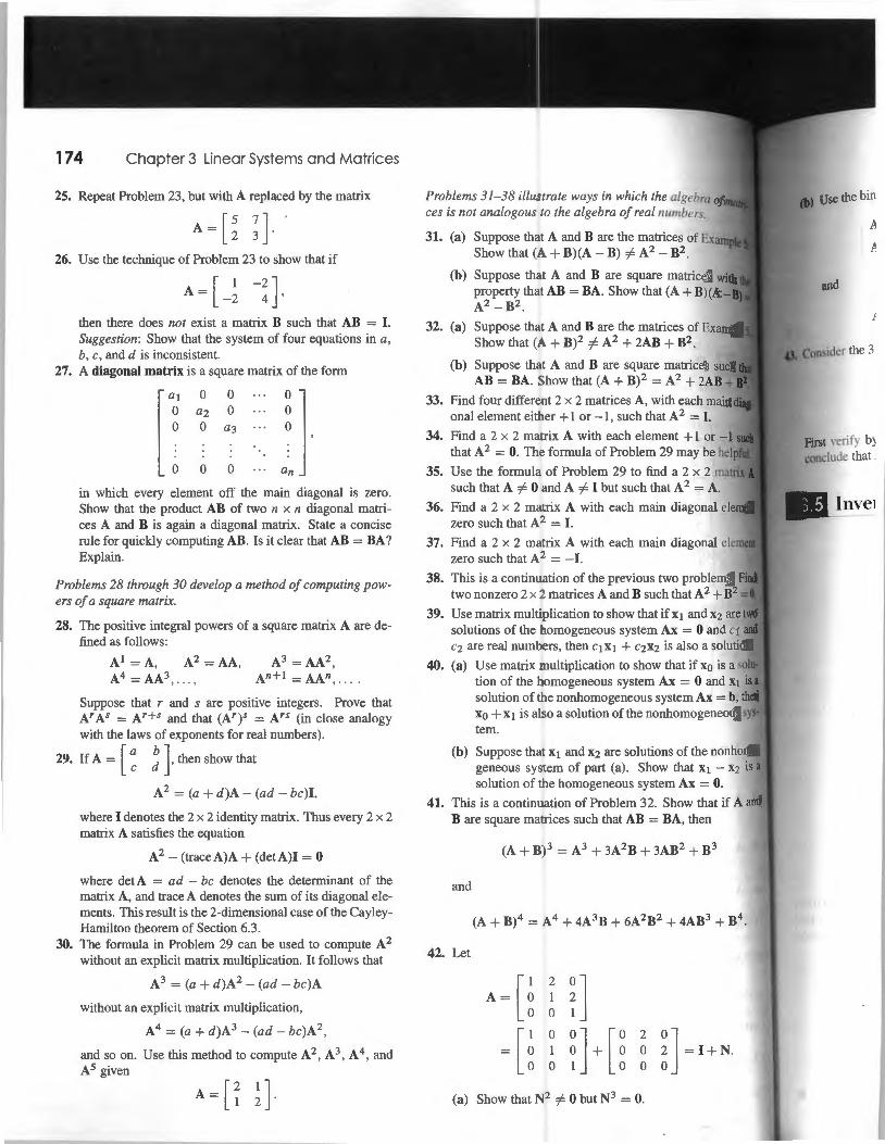
174 Chapter 3 Linear Systems and Matrices

25. Repeat Problem 23, but with A replaced by the matrix

A=[~ ;J . 26. Use the technique of Problem 23 to show that if

A= [ 1 -2

-2] 4 ,

then there does not exist a matrix B such that AB = I. Suggestion: Show that the system of four equations in a, b, c, and d is inconsistent.

27. A diagonal matrix is a square matrix of the form

0 0 n in which every element off the main diagonal is zero. Show that the product AB of two n x n diagonal matri­ces A and B is again a diagonal matrix. State a concise rule for quickly computing AB. Is it clear that AB = BA? Explain.

Problems 28 through 30 develop a method of computing pow­ers of a square matrix.

28. The positive integral powers of a square matrix A are de­fined as follows:

A 1 =A, A2 =AA, A3 =AA2, A4=AA3 , ... , An+t=AAn , ....

Suppose that r and s are positive integers. Prove that A' As = Ar+s and that (A')s = A's (in close analogy with the laws of exponents for real numbers).

29. If A = [ ~ ~ l then show that

A 2 =(a+ d)A- (ad- bc)I ,

where I denotes the 2 x 2 identity matrix. Thus every 2 x 2 matrix A satisfies the equation

A2 - (traceA)A + (detA)I = 0

where det A = ad - be denotes the determinant of the matrix A, and trace A denotes the sum of its diagonal ele­ments. This result is the 2-dimensional case of the Cayley­Hamilton theorem of Section 6.3.

30. The formula in Problem 29 can be used to compute A 2

without an explicit matrix multiplication. It follows that

A 3 =(a+ d)A2- (ad- bc)A

without an explicit matrix multiplication,

A 4 =(a+ d)A 3 - (ad - bc)A2,

and so on. Use this method to compute A 2, A 3, A 4, and A5 given

A=[~ ~l

Problems 31-38 illustrate ways in which the algebra ces is not analogous to the algebra of real numbers.

31. (a) Suppose that A and B are the matrices of Show that (A + B)(A- B) c:j= A2 - B2.

(b) Suppose that A and B are square matrices property that AB = BA. Show that (A+ B)(A A2 - B2.

32. (a ) Suppose that A and B are the matrices of Show that (A+ B)2 # A2 + 2AB + B2.

(b) Suppose that A and B are square matrices AB = BA. Show that (A+ B)2 = A2 + 2AB +

33. Find four different 2 x 2 matrices A, with each main anal element either + 1 or -1 , such that A 2 = I.

34. Find a 2 x 2 ma1rix A with each element + 1 or -1 that A 2 = 0. The formula of Problem 29 may be

35. Use the formula of Problem 29 to find a 2 x 2 such that A ¥= 0 and A ¥= I but such that A 2 = A.

36. Find a 2 x 2 matrix A with each main diagonal zero such that A 2 = I .

37. Find a 2 x 2 matrix A with each main diagonal zero such that A 2 = -I.

38. This is a continuation of the previous two problems. two nonzero 2 x 2 matrices A and B such that A 2 + B2

39. Use matrix multiplication to show that ifxt and x2 are solutions of the homogeneous system Ax = 0 and Ct c2 are real numbers, then c1 x 1 + c2x2 is also a

40. (a) Use matrix multiplication to show that if xo is a tion of the homogeneous system Ax = 0 and Xt solution of the nonhomogeneous system Ax= b, x0 + x 1 is also a solution of the nonhomogeneous tern.

(b) Suppose that. x 1 and x2 are solutions of the uu•u•v"'Vl

geneous system of part (a). Show that x 1 - x2 is solution of the homogeneous system Ax = 0.

41. This is a continuation of Problem 32. Show that if A B are square matrices such that AB = BA, then

and

(A+ B)4 = A 4 + 4A3B + 6A2B2 + 4AB3 + B4.

42. Let

A~[! 2

n 1

0

~[! 0 n+u 2

n~I+N 1 0 0 0

(a) Show that N2 ¥= 0 but N3 = 0.

and

ofmatri-

. xample 5.

s with the 1(A-B) =

Example S.

:s such that ~AB +B1

1 main diag-1.

or -1 such ' be helpful.

ow that if A ~.then

3.5 Inverses of Matrices 175

(b) Use the binomial formulas of Problem 41 to compute 44. Let A = [a hi ], B = [ biJ ], and C = [ c Jk ] be matrices of sizes m x n, n x p, and p x q, respectively. To establish the associative law A(BC) = (AB)C, proceed as follows . By Equation (16) the hjth element of AB is

and

A 2 = (I + N)2 = I + 2N + N2,

A 3 = (I + N)3 = I + 3N + 3N2 ,

I

n

l:_ahibiJ . i=!

43. Consider the 3 x 3 matrix

By another application of Equation ( 16), the hkth element of (AE:)C is

A~ [ =i ~~ =i]. First verify by direct computation that A2 = 3A. Then conclude that An+ 1 = 3n A for every positive integer n.

Show similarly that the double sum on the right is also equal to the hkth element of A(BC) . Hence them x q ma­trices (AB)C and A(BC) are equal.

Inverses of Matrices Recall that the n x n identity matrix is the diagonal matrix

I 0 0 0 1 0

I= 0 0

0 0 0

0 0 0 (1)

having ones on its main diagonal and zeros elsewhere. It is not difficult to deduce directly from the definition of the matrix product that I acts like an identity for matrix multiplication:

AI = A and IB = B (2)

if the sizes of A and B are such that the products AI and IB are defined. It is, nevertheless, instructive to derive the identities in (2) formally from the two basic facts about matrix multiplication that we state below. First, recall that the notation

A = [ a1 .a2 a3 · · · an J (3)

expresses the m x n matrix A in terms of its column vectors a 1, a2, a3, ... , an.

Fact 1 Ax in terms of columns of A

If A = [ a1 a2 · · · an ) and x = (x1 , x2, ... , Xn) is ann-vector, then

Ax= x 1a1 + xzaz + · · · + Xn an . (4)

The reason is that when each row vector of A is multiplied by the column vector x, its j th element is multiplied by x J.

Fact 2 AB in terms of columns of B

If A is an m x n matrix and B = [ b 1 b2 · · · bp J is ann x p matrix, then

AB=[Ab 1 Ab2 ... Abp) · (5)

That is, the j th column of AB is the product of A and the j th column of B. The reason is that the elements of the j th column of AB are obtained by multiplying the individual rows of A by the j th column of B.

'e already ~ of these e proof by

ty (d), and,

;ays that (a)

,mique solu-

every b, we f the identity that

(20)

Problems Jn Problems 1-8, first apply the formulas in (9) to find A -I. Then use A - I (as in Example 5) to solve the system Ax = b.

LA =[! ~Jb= UJ 2.A =[~ ~Jb=[-~] 3. A= [ ~ n. b = [ -n 4.A =[~ ~~ J b = [ n 5. A= [; ~Jb= [~] 6.A =[~ ~ J b = [ 1n

7. A= [ ~ ;Jb= [n 8. A = D ~~ J b = [ n

In Problems 9-22, use the method of Example 7 to find the inverse A - 1 of each given matrix A.

9. [ ~ ~] 10. [~ ~]

u 5

~] u 3 :] 5 12. 8 7 10

u 7

n [l 5

n 3 14. 4 7 3

u '] h -3 -q 4 13 16. l 2 12 -3 -3

H -3 -!] [i -2

n 2 18. 0 -2 - 1

4

ll [: 0 -n 4 20. 0 5 1

0 "1 [i 0 1

~1 0 0 0 3 I 2 0 22.

1 2 0 0 I 2 4

3.5 Inverses of Matrices 185

5 1 2 0 1 26. A= 2 -2 , B= 0 3 0

1 7 2 1 0 2

27.hu -2

nB~u 0 l i] 1 0

2 0 1

28. h [l 5

nB~ [ -: 0

~] 3 3 5 4 0

29. Verify parts (a) and (b) of Theorem 3.

Problems 30 through 37 explore the properties of matrix in­verses.

30. Suppose that A, B, and C are invertible matrices of the same size. Show that the product ABC is invertible and that (ABC)- 1 = c-1B- 1A-I.

31. Suppose that A is an invertible matrix and that r and s are negative integers. Verify that Ar A s = Ar+s and that (Ar)s = Ars.

32. Prove that if A is an invertible matrix and AB = AC, then B = C . Thus invertible matrices can be canceled.

33. Let A be an n x n matrix such that Ax = x for every n­vector x. Show that A = I.

34. Show that a diagonal matrix is invertible if and only if each diagonal element is nonzero. In this case, state concisely how the inverse matrix is obtained.

35. Let A be an n x n matrix with either a row or a column consisting only of zeros. Show that A is not invertible.

36. Show that A = [ : ! J is not invertible if ad -be = 0.

37. Suppose that ad- be # 0 and A - 1 is defined as in Equa­tion (9). Verify directly that AA - I =A - I A= I.

Problems 38 through 40 explore the effect of multiplying by an elementary matrix.

38. Let E be the elementary matrix E 1 of Example 6. If A is a 2 x 2 matrix, show that EA is the result of multiplying the first row of A by 3.

39. Let E be the elementary matrix E2 of Example 6 and sup­pose that A is a 3 x 3 matrix. Show that EA is the result upon adding twice the first row of A to its third row.

40. Let E be the elementary matrix E3 of Example 6. Show that EA is the result of interchanging the first two rows of the matrix A.

Problems 41 and 42 complete the proof of Eq. (2).

41. Show that the ith row of the product AB is Ai B, where Ai is the i th row of the matrix A.

42. Apply the result of Problem 41 to show that if B is an m x n matrix and I is the m X m identity matrix, then m = B.

43. Suppose that the matrices A and Bare row equivalent. Use Theore 5 to prove that B = GA, where G is a product of elementary matrices.

186 Chapter 3 Linear Systems and Matrices

44. Show that every invertible matrix is a product of elemen­tary matrices.

such that AB = I , then A and B are invertible. 46. Deduce from the result of Problem 45 that if A

square matrices whose product AB is invertible, and B are themselves invertible.

45. Extract from the proof of Theorem 7 a self-contained proof of the following fact: If A and B are square matrices

3.5 Application Automated Solution of Linear Systems

Co Go to goo.gl/rcsRzKto download this application's computing resources including Maple/Mathematica!M ATLAB.

[3 •2 7 5] -1 [585] 2 4 ·1 6 435

• 5 I 7 ·3 - 286

4 ·6 -s 9 445 UDIIUTD

[

59 13 17

47

FIGURE 3.5.2. TI-89 solution of a linear system Ax = b.

Linear systems with more than two or three equations are most frequently with the aid of calculators or computers. If an n x n linear system is written in matrix form Ax = b , then we need to calculate first the inverse matrix A -I then the matrix product x = A - 1 b. Suppose the n x n matrix A and the vector b have been entered (as illustrated in the 3.2 Application). If A is · then the inverse matrix A - 1 is calculated by the Maple command with { 1 inverse {A) , the Mathematica command Inverse [A] , or the MATLAB

inv {A) . Consequently, the solution vector x is c lculated by the Maple cornrn:m

with { linalg) : x : = multiply { invt:!rse {A) I b) ;

or the Mathematica command

x = Inverse[A] .b

or the MATLAB command

x = inv{A)*b

Figure 3.5.2 illustrates a similar calculator solution of the linear system

3x1 - 2x2 + 7x3 + 5x4 = 505

2x 1 + 4x2 - x3 + 6x4 = 435

Sx, + x2 + 7x3 - 3x4 = 286

4x 1 - 6x2 - 8x3 + 9x4 = 445

for the solution x 1 = 59, x2 = 13, x3 = 17, x 4 = 47. This solution is also given by the WolframiAlpha query

A {{3 1 -2 1 1 1 5) 1 (2 1 4 1 -1 1 6) 1 {5 1 1 1 1 1 -3) 1 (41 -61 -81 9)) 1

b {5051 4351 2861 445) 1

inv {A) .b

Remark Whereas the preceding commands illustrate the handy use of conveniently avail· able inverse matrices to solve linear systems, it might be mentioned that modern computer systems employ direct methods-involving Gaussian elimi ation and still more sophisticated techniques-that are more efficient and numerically reliable to solve a linear system Ax == b without first calculating the inverse matrix A - I. I

Use an available calculator or computer system to solve the linear systems in Problems 1-6 of the 3.3 Application. The applied problems below are elementary in character-resembling the "word problems" of high school algebra-but might illustrate the practical advantages of automated solutions.

1. You are walking down the street minding your own business when you spot a small but heavy leather bag lying on the sidewalk. It turns out to contain U.S. Mint American Eagle gold coins of the following types:

• One-half ounce gold coins that sell for $285 each, • One-quarter ounce gold coins that sell for $150 each, and

!asured by number of xpansions. m requires ;h of these ;e four 3 x these 2 x 2 )tal number

determinant

n our opera­of a 25 x 25

: 1025 opera­r second this nillion years! mcomparably m)-to scientific and )00 (or mes with

Problems Use cofactor expansions to evaluate the determinants in Prob­lems J-6. Expand along the row or column that minimizes the amount of computation that is required.

1.

3.

0 0 3 4 0 0 0 5 0

0 0 0 2 0 5 0 3 6 9 8 4 0 10 7

0 0 1 0 0 2 0 0 0 0

5. 0 0 0 3 0 0 0 0 0 4 0 5 0 0 0

3 0 11 -5 0 -2 4 13 6 5

6. 0 0 5 0 0 7 6 -9 17 7 0 0 8 2 0

2.

4.

2 1 2 0

5 11 3 -2 0 0 0 4

0

2

8 7 6 23 0 -3 0 17

In Problems 7-12, evaluate each given determinant after first simplifying the computation (as in Example 6) by adding an appropriate multiple of some row or column to another.

1 2 2 2 3 3 3

-2 5 5 17

-4 12

2 3 4 5 6 7 0 8 9 4 6 9

2 3 4 8. -2 -3 1

10.

12.

3 2 7

-3 6 5 -2 - 4

2 -5 12

2 0 0

-4

0 0 -3 11 12

0 5 13 0 0 7

the method of elimination to evaluate the determinants in 13-20.

4 -1 4 2 -2 -2 2 14. 3 -5

4 3 -5 -4 3

5 4 2 4 -2 3 16. -5 -4 - 1 4 5 -4 2

3 3 3 -3

-I -3 -3 2

4 4 1 -2 2

I 4 -3 -2

19.

20.

- 1 0 0 0 -2

-2 3 -2 0 -3 3 ~I

2 - 1 2 0

3 3 -2 3

- 1 4 -2 4

3.6 Determinants 201

Use Cramer's rule to solve the systems in Problems 21-32.

21. 3x + 4y = 2 5x + 7y = 1

23. 17x+7y=6 12x + 5y = 4

25. 5x + 6y = 12 3x + 4y = 6

27. 5xl + 2xz - 2x3 = x 1 + 5xz - 3x3 = -2

5x l -- 3xz + 5x3 = 2

28. 5xl + 4xz - 2x3 = 4 2x1 + 3x3 = 2 2X! - Xz -1- X3 = 1

29. 3x l - xz - 5x3 = 3 4xl -- 4xz - 3x3 = -4

x 1 - 5x3 = 2

30. x 1 -- 4xz + 2x3 = 3 4xl -'- 2xz + X3 = 1 2x1 -- 2xz - 5x3 = -3

31. 2x1 - 5x3 = -3 4x l - 5xz + 3x3 = 3

-2X J -1- Xz -1- X3 = 32. 3xl + 4xz - 3x3 = 5

3xl -- 2xz + 4x3 = 7 3x 1 + 2xz - X3 = 3

22. 5x + 8y = 3 8x + 13y = 5

24. 11 x + 15y = 10 8x + 11y = 7

26. 6x + 7y = 3 8x + 9y = 4

Apply Theorem 5 to find the inverse A - I of each matrix A given in Problems 33-40.

[ -: -2

-n [ -~ 0

n 33. 5 34. -4

-3 - I

[ _; 5 _; ] [ -; 4 -i] 35. 3 36. - 1 -5 0 -5 0 -5

[ -4 _l] [_l 4 -3 ] 37. -2 4 38. 2 - 1 -3 -3 2 -4

[ -l -2 _n u 4 -3 ] 39. 3 40. -3 - 1

3 0 -3

41. Show that (AB)T = BT AT if A and B are arbitrary 2 x 2 matrices.

202 Chapter 3 Linear Systems and Matrices

42. Consider the 2 x 2 matrices

A = [ ~ : J and B = [ ; ].

where x andy denote the row vectors of B. Then the prod­uct AB can be written in the form

AB = [ ax + by J . cx+dy

Use this expression and the properties of determinants to show that

detAB =(ad- be) I ; I = (detA)(det B).

Thus the determinant of a product of 2 x 2 matrices is equal to the product of their determinants.

Each of Problems 43-46 lists a special case of one of Property 1 through Property 5. Verify it by expanding the determinant on the left-hand side along an appropriate row or column.

kau G)2 al3 au GJ2 al3 43. ka21 a22 a23 =k a21 a22 a23

ka31 a32 a33 a31 a32 a33 a21 a22 a23 au a12 al3

44. au a12 al3 a2 1 a22 a23 a31 a32 G33 a31 a32 a33 G) bl CJ +d1 a1 bl C) G) bl dl

45. a2 b2 C2 + d2 a2 b2 C2 + a2 b2 d2 a3 b3 C3 + d3 a3 b3 C3 a3 b3 d3 au+ ka12 a12 GJ3 au GJ2 al3

46. a21 + ka22 a22 a23 a21 a22 a23 a31 + ka32 a32 a33 a31 a32 a33

Problems 47 through 49 develop properties of matrix trans­poses.

47. Suppose that A and B are matrices of the same size. Show that: (a) (AT)T = A; (b) (cA)T = cAT ; and (c) (A+ B)T =AT + BT .

48. Let A and B be matrices such that AB is defined. Show that (AB) T = B TAT . Begin by recalling that the ijth ele­ment of AB is obtained by multiplying elements in the i th row of A with those in the jth column of B. What is the ijth element of BT AT ?

49. Let A = [ aij ] be a 3 x 3 matrix . Show that det(AT) =

det A by expanding det A along its first row and det(A T) along its first column.

50. Suppose that A2 =A. Prove that IAI = 0 or lA I = I.

51. Suppose that An = 0 (the zero matrix) for some positive integer n. Prove that lA I = 0.

52. The square matrix A is called orthogonal provided that AT = A - l . Show that the determinant of such a matrix must be either +I or - 1.

53. The matrices A and B are said to be similar provided that A = p-l BP for some invertible matrix P . Show that if A and Bare similar, then IA I = IB I.

54. Deduce from Theorems 2 and 3 that if A and B invertible matrices, then AB is invertible if and both A and B are invertible.

55. Let A and B be n x n matrices . Suppose it is either AB = I or BA = I. Use the result of Problem conclude that B = A - l.

56. Let A be ann x n matrix with detA = 1 and with aU ments of A integers .

(a) Show that - l has only integer entries. (b) Suppose that b is an n-vector with only integer

tries. Show that the solution vector x of Ax == b only integer entries.

57. Let A be a 3 x 3 upper triangular matrix with nonzero terminant. Show by explicit computation that A -l is upper triangular.

58. Figure 3.6.2 shows an acute triangle with angles A, B, C and opposite sides a, b, and c. By dropping a dicular from each vertex to the opposite side, derive equations

59.

60.

c cos B + b cos C = a

c cos A + a cos C = b

a cos B + b cos A = c.

Regarding these as linear equations in cos A, cosB, and cosC, use Cramer's rule to derive law of cosines by solving for

b2 + c2- a2 cos A= b

2 c Thus

a2 = b

2 + c

2 -2bccosA. Note that the case A = :rr/2 (90°) reduces to the Pythago­rean theorem.

c

FIGURE 3.6.2. The triangle of Problem 58.

Show that

u ~ I = 3

2 0 and 1 2 1 =4.

0 2

Consider then x n determinant

2 0 0 0 0 1 2 1 0 0 0 0 2 0 0

Bn =

0 0 0 0 2 0 0 0 0 2

in which each en y on the main diagonal is a 2, each entry on the two adjacent diagonals is a 1, and every other entry is zero.

V(a , b, .

61 Tbeformu of the gem

The case r

V(XJ,)

Prove thi1 cubic pol:

L

y

FIGURE3.7 interpolating given data po

re n x n l only if

own that em 54 to

JJ. allele-

1teger en­~=bhas

)nzero de­,-l is also

; A, B, and ~a perpen­derive the

: unknowns o derive the

tem58.

0 0 0

2

(a) Expand along the first row to show that

Bn = 2Bn- 1 - Bn-2 ·

(b) Prove by induction on n that Bn = n + I for n :=: 2.

Problems 61-64 deal with the Vandermonde determinant

Xi x2 n- 1 I x ,

X2 x2 n-1 2 x2

V(XJ ,X2, ... ,Xn) =

Xn x2 n-1 n Xn

that will play an important role in Section 3. 7.

61. Show by direct computation that V(a , b) = b- a and that

I a a2

V(a,b ,c)= I b b2 =(b-a)(c-a)(c-b). I c c2

62. The formulas in Problem 61 are the cases n = 2 and n = 3 of the general formula

n

i,j= I i > j

The case n = 4 is

V(x1,X2 ,X3,x4) = (x2 -xl)(x3 -x1)(x3 -x2)

x (x4 - xJ)(x4- x2)(x4 - x3).

Prove this as follows. Given x 1, x 2 , and x3 , define the cubic polynomial P(y) to be

XI x2 I

x3 I

X2 x2 x3 P(y) = 2 2 (26)

x2 x3 X3 3 3 y y2 y3

3.7 Linear Equations and Curve Fitting 203

Because P(xi) = P(x2) = P(x3) = 0 (why?), the roots of P (y) are x 1, x2, and X3. It follows that

P(y) = k(y- XJ)(y- x2)(y- x3),

where k is the coefficient of y 3 in P(y). Finally, ob­serve that expansion of the 4 x 4 determinant in (26) along its last row gives k = V(x 1, x2 , x 3) and that V(x1 ,x2,X3,x4) = P(x4).

63. Generalize the argument in Problem 62 to prove the for­mula i (25) by induction on n . Begin with the (n- l)st­degree polynomial

Xi x2 n-1 I x ,

X2 x2 n-1 2 x2

P(y ) =

Xn- 1 x~- 1 n-1 xn-1

y y2 yn-1

64. Use the formula in (25) to evaluate the two determinants given next.

I

(a) 2 4 8 3 9 27 4 16 64

- 1 -1 2 4 8

- 2 4 -8 (b)

3 9 27

Linear Equations and Curve Fitting_ __ _

y = f(x)

(x;,Y;)

X

.1. A curve y = f(x) ~that is, passing through)

pomts.

Linear algebra has important applications to the common scientific problem of rep­resenting empirical data by means of equations or functions of specified types. We give here only a brief introduction to this extensive subject.

Typically, we begin with a collection of given data points (x0 , y0 ), (x 1 , yi), . .. , (xn, Yn) that are to be represented by a specific type of function y = f(x ). For instance, y might be the volume of a sample of gas when its temperature is x. Thus the given data points are the results of experiment or measurement, and we want to determine the curve y = f(x) in the ;~.y-plane so that it passes through each of these points; see Figure 3.7 .1. Thus we speak of "fitting" the curve to the data points.

We will confine our attention largely to polynomial curves. A polynomial of degree n is a function of the form

(1)

where the coefficients ao , a 1, a2 , ... , an are constants. The data point (xi , Yi) lies on the curve y = f(x) provided that f(x i) = Yi. The condition that this be so for each