Embed Size (px)
Citation preview
A Structural Approach to the Mapping Problem in
Parallel Discrete Event Logic Simulations
Mark Davoren
July 21, 1989
Ph.D.
University of Edinburgh
1989
Abstract
It is shown that traditional techniques are inadequate for mapping irregular asyn-
chronous problems to distributed-memory parallel architectures. It is also shown
that by using problem specific knowledge, such as the problem's structure, rea-
sonable mappings can be produced.
Parallel discrete event simulation of digital logic circuits is used as an appli-
cation to study various mapping algorithms. The structural approach uses the
structure of the problem, in this case the design hierarchy of the circuit, to pro-
duce a locality tree which is an approximation of the communication behaviour of a
problem. An algorithm is presented which generates mappings from such locality
trees onto a grid of processors.
A conservative parallel discrete event simulator was implemented on a grid
of Transputers. Analysis of experimental results shows that for sufficiently sized
problems, the structural approach produces mappings which result in relatively low
inter-processor communication and within limits of load balancing better overall
performance.

1
Acknowledgements
I would like to thank my friends without whom I would probably not have finished
this thesis. They introduced me to the highlands, gliding and above all to Scottish
music and dancing. For the latter, I am especially grateful to everybody at New
Scotland; they kept me happy allowing me to concentrate on my work.
To everybody who helped me with my work, I also give thanks. In particular,
I would like to thank Rob Pooley for all the help he gave me in our friendly and
fruitful conversations, my supervisor, Roland Ibbett, for his time and patience and
the Goths who bailed me out of system problems on numerous occasions.
This work was, in part funded by a University of Edinburgh Postgraduate
Studentship.
Finally, I give thanks to Juliet for the love and support she has given to me.
Declaration
I declare that this thesis was composed by myself and that all the work presented
as original is my own.
Table of Contents
1. The Mapping problem 1.
1.1 Introduction ................................. 1
1.1.1 Inter-Module Communication ................... 2
1.2 Problem representation ............................ 5
• 1.2.1 A graph based description .................... 5
• 1.2.2 Problem metrics and constraints ............... 8
1.2.3 Optimisation goals ....................... 10
1.3 Problem solutions ............................. 12
1.3.1 Problem complexity ....................... 13
1.3.2 Restricted optimal solutions .................. 14
1.3.3 Approximate solutions ..................... 18
1.4 Annotations ................................ 29
1.5 Conclusion ............................... 33
2. A structural approach 35
2.1 Introduction ...............................35
2.2 Locality trees ..............................36
11
Table of Contents 111
2.2.1 Simple trees . 37
2.2.2 Cross linked trees ........................37
2.2.3 Locality tree operations ....................40
2.3 Mapping locality trees .........................43
2.3.1 Slicing ..............................45
2.3.2 Load balancing control .....................50
2.3.3 Arranging ............................51
2.3.4 Allocation ............................55
3. Parallel Simulation
57
3.1 Motivation ...............................57
3.2 What is a simulator? ..........................58
3.3 The process model ...........................60
3.3.1 A parallel implementation ...................61
3.3.2 Time ...............................62
3.3.3 The simulation mechanism ...................64
3.4 Deadlock and Failure to proceed ...................66
3.5 Deadlock avoidance and recovery ...................68
3.5.1 Null messages ..........................69
3.5.2 2 phase approach ........................72
3.6 Optimistic schemes ............................73
3.7 Digital logic simulation .........................75
3.8 Summary ................................76
Table of Contents lv
The implementation of a simulator
4.1 Overview ................................78
4.2 The master process ...........................80
4.3 The slave process ..............................82
4.3.1 Structure ............................82
4.3.2 The simulation engine .....................83
4.3.3 The event queue manager ...................88
4.3.4 The controller process ......................88
4.4 The network ..................................93
4.4.1 Routing .............................93
4.4.2 Deadlock ..............................94
4.4.3 Congestion ...........................99
Results and Discussion 101
5.1 An analysis of performance ......................102
5.1.1 Implementation derived delays ..................104
5.1.2 Simulation derived delays ...................105
5.2 A quantitative analysis of a simple circuit ..............iWi.
5.2.1 The simulation phase of X, Y and Z .............108
5.2.2 The Waiting phase ........................112
5.2.3 Conclusions of the simple analysis ..............114
5.2.4 Lessons for a new implementation ..............115
5.3 A qualitative analysis of a complex circuit ..............116.
Table of Contents V
5.3.1 The circuit . 118
5.3.2 The mappings .........................118
5.4 The measurements ...........................121
5.5 Comparison of mappings ........................ 123
5.6 General Performance ..........................126
6. Summary and Conclusions 134
6.1 Future Directions ............................139
A. Published paper 150
Chapter 1
The Mapping problem
1.1 Introduction
To implement software on a parallel computer requires the software to be parti-
tioned into components. These components are then assigned or mapped to
the various processors. This mapping involves both where and when a component
is to be executed. Deciding what such a mapping is to be, is often referred to as
the mapping problem.
The study of the mapping problem has its origins in the job scheduling required
in multi-process operating systems. A number of algorithms have been developed
to determine the order in which jobs are to be executed on a single processor. This
is now a reasonably well understood topic [16][49, Chap 4].
When the problem of mapping to multiple processors is considered the task
becomes considerably more complex. Not only must the order of execution be de-
cided, but so too, the location. The mapping problem as opposed to the scheduling
problem is assumed to be set in the context of a multi-processor environment.
The term module will be used to refer to a component of the software being
mapped, ie. an object of the mapping. A component of the hardware to which is
being mapped, ie. a target of the mapping, will be referred to as a processor.
1
Chapter 1. The Mapping problem
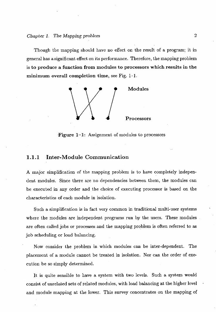
Though the mapping should have no effect on the result of a program; it in
general has a significant effect on its performance. Therefore, the mapping problem
is to produce a function from modules to processors which results in the
minimum overall completion time, see Fig. 1-1.
Modules
Processors
Figure 1-1: Assignment of modules to processors
1.1.1 inter-Module Communication
A major simplification of the mapping problem is to have completely indepen-
dent modules. Since there are no dependencies between them, the modules can
be executed in any order and the choice of executing processor is based on the
characteristics of each module in isolation.
Such a simplification is in fact very common in traditional multi-user systems
where the modules are independent programs run by the users. These modules
are often called jobs or processes and the mapping problem is often referred to as
job scheduling or load balancing.
Now consider the problem in which modules can be inter-dependent. The
placement of a module cannot be treated in isolation. Nor can the order of exe-
cution be so simply determined.
It is quite sensible to have a system with two levels. Such a system would
consist of unrelated sets of related modules, with load balancing at the higher level
and module mapping at the lower. This survey concentrates on the mapping of
Chapter I. The Mapping problem 3
related modules. The mappings described ignore external effects of any enclosing
system; they assume that only a single set of inter-dependent modules is being
assigned to an empty set of processors.
This inter-dependence between modules is realised as inter-module commu-
nication, IMC. IMC is often expressed in terms of message passing, where one
module sends messages to another which receives them. Although there are
other models of IMC such as the procedural and memory access models, message
passing makes explicit the separate, independent existence of the modules, which
is the basis of a mapping.
C
A
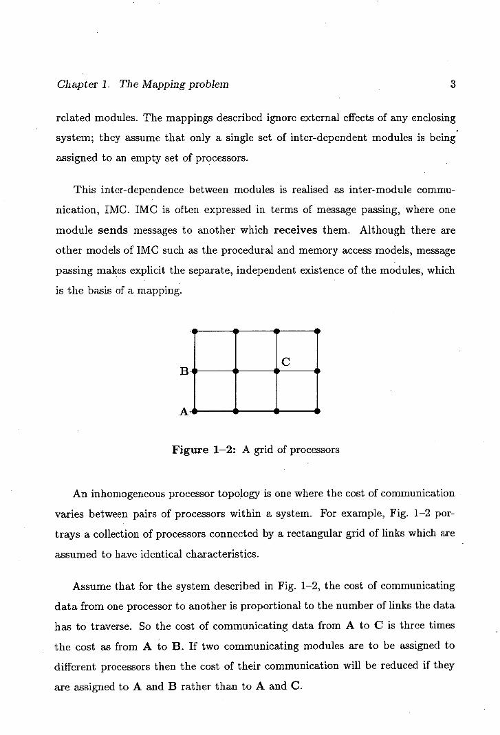
Figure 1-2: A grid of processors
An inhomogeneous processor topology is one where the cost of communication
varies between pairs of processors within a system. For example, Fig. 1-2 por-
trays a collection of processors connected by a rectangular grid of links which are
assumed to have identical characteristics.
Assume that for the system described in Fig. 1-2, the cost of communicating
data from one processor to another is proportional to the number of links the data
has to traverse. So the cost of communicating data from A to C is three times
the cost as from A to B. If two communicating modules are to be assigned to
different processors then the cost of their communication will be reduced if they
are assigned to A and B rather than to A and C.
Chapter 1. The Mapping problem 4
The mapping algorithm is now being pulled in two directions. To optimise
communication costs, all modules should be placed on the same processor, but
to optimise computation time, the modules should be spread evenly amongst the
processors to gain the benefits of parallelism. Such goals of the mapping algorithm
are discussed later.
A particular pattern of IMC which has been very much studied is one where
a module only communicates at the beginning and end of its execution. After
receiving all of its inputs, it goes into a compute-only phase, then passes its results
onto other waiting modules and finally terminates. In this case, a module is
basically a procedure which can be executed on a possibly different processor to
that of the calling module.
Such patterns arise especially when programs written in sequential languages
such as Fortran are partitioned into modules. The partitioning is often at the
procedural level or sometimes at the level of single statements.
Since enormous amounts of effort have been invested in such existing soft-
ware, it is desirable that these programs should be automatically partitioned and
executed on parallel machines with the ensuing performance benefits.
Much of the research into mapping algorithms has assumed this pattern of
IMC, eg. [54,14,15]. However, such an approach ignores the extremely large class
of problems where the pattern of communication is less restricted. There are many
problems which require a module to engage in IMC during its lifetime and not
just at its initiation and completion.
In particular, for programs written in languages with explicit parallel and IMC
constructs, the assumption of a restricted IMC is invalid. Therefore the mapping
algorithms cited from the literature are inapplicable to the modules of programs
written in languages such as OCCAM [41], POOL [1] or any other language with
explicit IMC constructs available to the programmer.
Chapter 1. The Mapping problem 5
It will be shown that traditional mapping mechanisms are also inapplicable in
the case of digital logic simulation where a logic gate is mapped to a processor
and has to handle many separate events during its lifetime.
1.2 Problem representation
When the pattern of IMC is reasonably stable the system is said to have a static
structure. In such systems the number of modules and their relationship can be
determined before execution begins. This allows the mapping to be completely
determined before run time. The alternative is a dynamic structure where map-
ping decisions can be made only during execution as modules are created and their
relationships become known.
This survey will concentrate on mapping static structures of modules to fixed
topologies of processors. Though the dynamic structure is more general it can
often be viewed as a series of phases where each phase can be considered as static.
In addition, it seems likely that a dynamic mapping would give better results if it
is preceded by an optimising static mapping. This has been demonstrated in the
case of pipelines of modules by Iqbal et al. [30].
There are two common forms of representing the mapping problem; graph
theoretic and number theoretic. The former allows a structural description of the
problem and can make use of the wealth of graph theory available. The latter
allows the easier introduction of restrictions, but can only describe facets of the
problem which can be given a numeric value.
1.2.1 A graph based description
The following is one possible representation in graph theoretic terms which is
used by Stone [54] and Bokhari [10], amongst others. The structure of the modules
Chapter 1. The Mapping problem 6
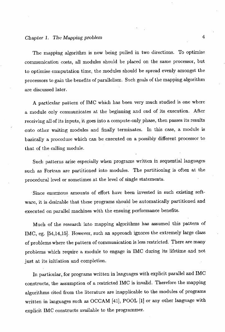
Figure 1-3: A module graph
is represented by a module graph Gm = (Vm , Em ). In this graph, the nodes or
vertices, Vm , represent the modules and two nodes i, j E V are connected by an
edge (i,j) E Em if and only if their corresponding modules communicate or have
the potential to do so during the execution of the program. Such a structure is
presented in Fig. 1--3.
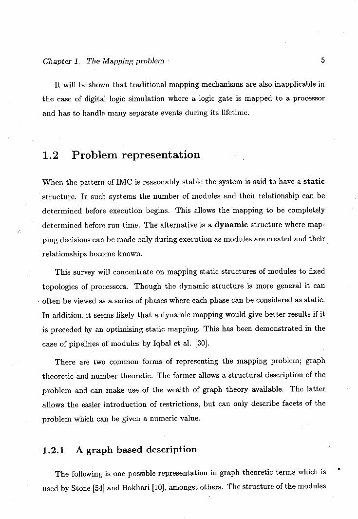
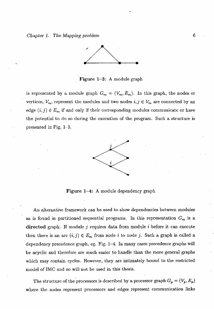
Figure 1-4: A module dependency graph
An alternative framework can be used to show dependencies between modules
as is found in partitioned sequential programs. In this representation Gm is a
directed graph. If module j requires data from module i before it can execute
then there is an arc (i, j) E Em from node i to node j. Such a graph is called a
dependency precedence graph, eg. Fig. 1-4. In many cases precedence graphs will
be acyclic and therefore are much easier to handle than the more general graphs
which may contain cycles. However, they are intimately bound to the restricted
model of IMC and so will not be used in this thesis.
The structure of the processors is described by a processor graph G = (V,, E)
where the nodes represent processors and edges represent communication links
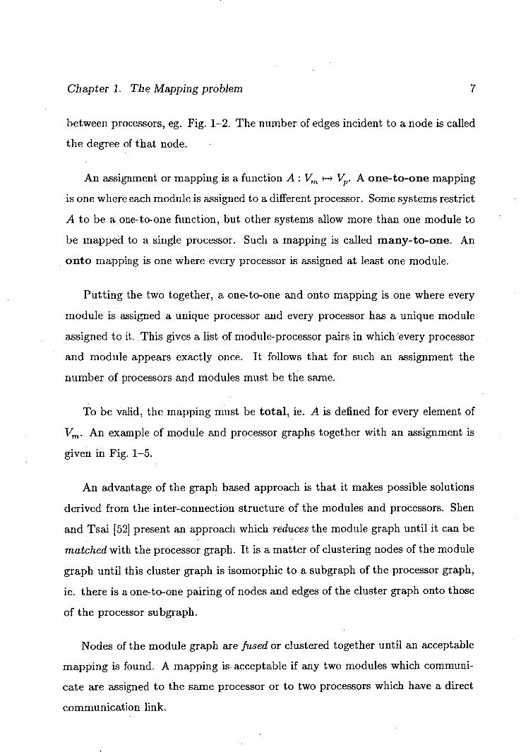
Chapter 1. The Mapping problem 7
between processors, eg. Fig. 1-2. The number of edges incident to a node is called
the degree of that node.
An assignment or mapping is a function A: Vm V. A one-to-one mapping
is one where each module is assigned to a different processor. Some systems restrict
A to be a one-to-one function, but other systems allow more than one module to
be mapped to a single processor. Such a mapping is called many-to-one. An
onto mapping is one where every processor is assigned at least one module.
Putting the two together, a one-to-one and onto mapping is one where every
module is assigned a unique processor and every processor has a unique module
assigned to it. This gives a list of module-processor pairs in which -'every processor
and module appears exactly once. It follows that for such an assignment the
number of processors and modules must be the same.
To be valid, the mapping must be total, ie. A is defined for every element of
Vm . An example of module and processor graphs together with an assignment is
given in Fig. 1-5.
An advantage of the graph based approach is that it makes possible solutions
derived from the inter-connection structure of the modules and processors. Shen
and Tsai [52] present an approach which reduces the module graph until it can be
matched with the processor graph. It is a matter of clustering nodes of the module
graph until this cluster graph is isomorphic to a subgraph of the processor graph,
ie. there is a one-to-one pairing of nodes and edges of the cluster graph onto those
of the processor subgraph.
Nodes of the module graph are fused or clustered together until an acceptable
mapping is found. A mapping is acceptable if any two modules which communi-
cate are assigned to the same processor or to two processors which have a direct
communication link.
Chapter 1. The Mapping problem
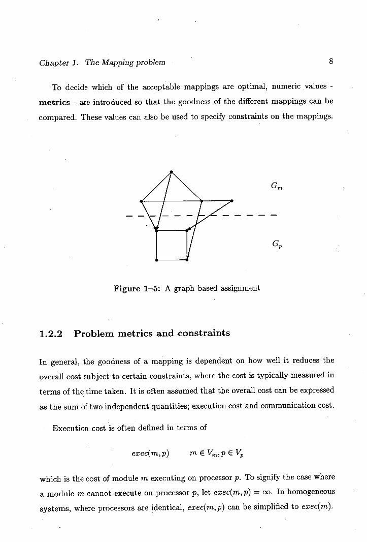
To decide which of the acceptable mappings are optimal, numeric values -
metrics - are introduced so that the goodness of the different mappings can be
compared. These values can also be used to specify constraints on the mappings.
Gm
G
Figure 1-5: A graph based assignment
1.2.2 Problem metrics and constraints
In general, the goodness of a mapping is dependent on how well it reduces the
overall cost subject to certain constraints, where the cost is typically measured in
terms of the time taken. It is often assumed that the overall cost can be expressed
as the sum of two independent quantities; execution cost and communication cost.
Execution cost is often defined in terms of
exec(m,p) m E V,p E VP
which is the cost of module m executing on processor p. To signify the case where
a module m cannot execute on processor p, let exec(m, p) = 00. In homogeneous
systems, where processors are identical, exec(m, p) can be simplified to exec(m).
Chapter 1. The Mapping problem 9
Communication cost is similarly defined in terms of
cornm(m 1 , m 2 , Pi, P2) m 1 , m 2 E Vm , P1, P2 E Vp
which is the cost of module m 1 communicating with m2 when m 1 is mapped to p1
and m2 mapped to P2 Iffm 1 and m2 are mapped to the same processor p then it
is typical to let comm(m 1 ,m2 ,p,p) = 0 since the ultra-processor costs are usually
negligible in comparison with inter-processor costs.
Some proposals express comm as the product of the inter-module communica-
tion cost and the inter-processor communication cost;
c0mm(m 1 , in2, Pi, P2) = IMc0st(m 1 , m2) x IPc0st(p 1 ,p2 )
If a graph theoretic representation is used then each edge (i, i) E Em of the module
graph is weighted with IMcost(i, j) and each edge (k, 1) e EP of the processor
graph is weighted with IPcost(k, 1).
This can be further simplified for bus and fully-connected topologies where
inter-processor communication costs are a constant, ie. IPcost(p1 ,p2 ) = 1 when
expressed in appropriate units.
It is important to recognise the limitations of these metrics. To specify the
execution time of a module assumes that this value is independent of the rest of
the system. That it does not depend on the execution costs of other modules. Nor
does it depend on any delays due to synchronisation or resource control. From
this, it follows that for an execution cost to be meaningful there can be no IMC
during the execution of a module, it can only occur at the beginning or at the end
of that module's execution.
Of course, this assumes that the module's execution does in fact have a begin-
ning and an end and is not a permanently executing module such as a server or a
filter. The basic pattern assumed in many proposals is that the module executes
once, with no intermediate IMC, then disappears.
Chapter 1. The Mapping problem 10
This is the functional patterh of IMC referred to above. It is this limitation
which prevents many of the published mapping proposals from working with lan-
guages which allow explicit IMC.
Similarly, to specify a communication cost assumes that it too is independent of
the rest of the system. As Lee and Aggarwal [39] have noted, unless every module
edge maps to a unique processor edge then there can be interference which affects
the IPcost due to bandwidth interference.
Finally, to state that the overall cost is the sum of execution costs and commu-
nication costs is to assume that these two quantities are independent. However in
many systems, execution and communication are overlapped. In the case of time
taken, the overall time will be less than the sum of the execution and communi-
cation times.
Other metrics that have been considered are the likelihood of processors failing
and the cost of recovery [14].
In addition to the above metrics, some systems consider constraints on the
problem. In particular, the memory requirements of all the modules mapped to a
given processor must not exceed that processor's memory capacity [4,50].
1.2.3 Optimisation goals
For M modules and P processors there are P M valid mappings. We need some
objective function by which to judge the myriad mappings. In a real sense, as long
as a program satisfies its requirements, the only true objective function is the time
it takes to complete its tasks. It has been traditional to relate this completion
time to a function of simpler parameters which are more easily determined and
controlled. Inspite of the problems discussed in the previous section it is this latter
function which is used as the objective function.
Chapter 1. The Mapping problem 11
There is a class of problems for which the goodness of a solution is based
solely on the value of an objective function applied to that solution and where an
optimal solution is one which has a minimal or maximal value. This is the class
of optimisation problems.
One of the simplest objective functions is based on the Quadratic Assignment
Problem, QAP, which was first formulated by Koopmans and Beckmann [36].
Hanan and Kurtzberg present a review of QAP and other related assignment
problems in [25].
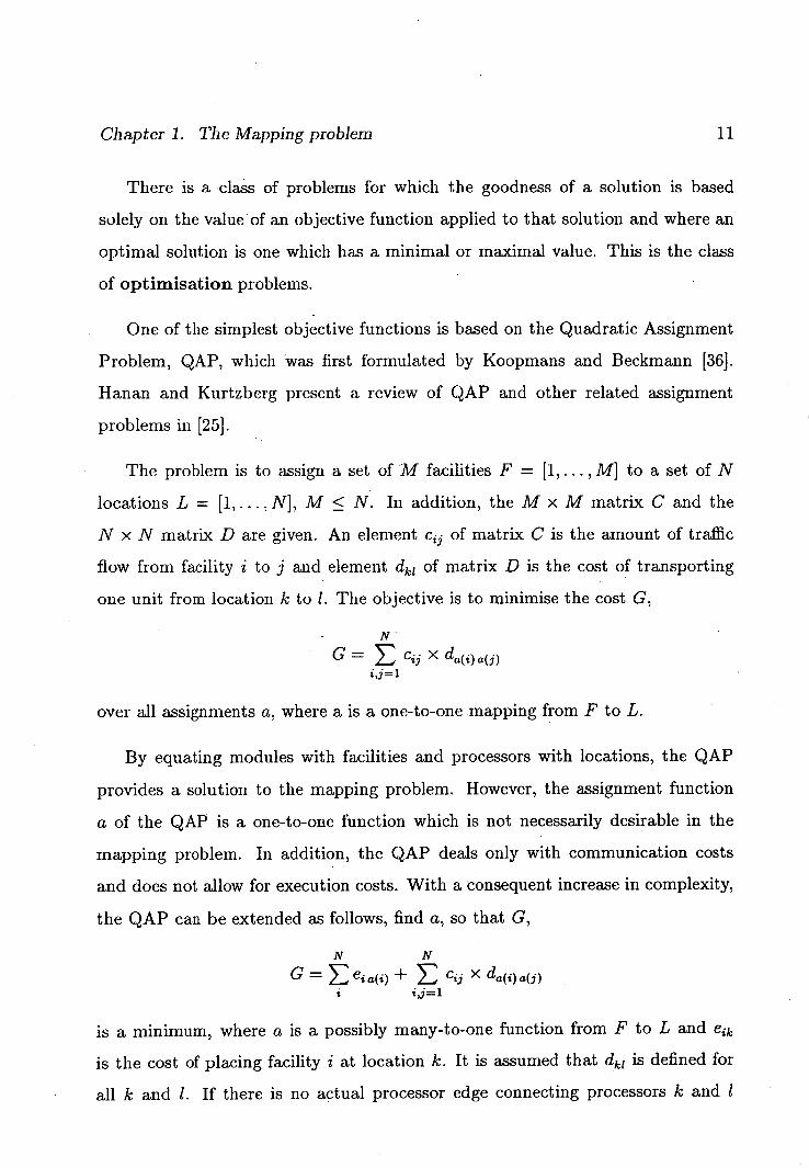
The problem is to assign a set of M facilities F = [1,. . . , M] to a set of N
locations L = [1.....N], M < N. In addition, the M x M matrix C and the
N x N matrix D are given. An element cij of matrix C is the amount of traffic
flow from facility i to j and element dkl of matrix D is the cost of transporting
one unit from location k to 1. The objective is to minimise the cost G,
N
G = Cij X a(j)
over all assignments a, where a is a one-to-one mapping from F to L.
By equating modules with facilities and processors with locations, the QAP
provides a solution to the mapping problem. However, the assignment function
a of the QAP is a one-to-one function which is not necessarily desirable in the
mapping problem. In addition, the QAP deals only with communication costs
and does not allow for execution costs. With a consequent increase in complexity,
the QAP can be extended as follows, find a, so that G,
N N
C = > eia(i) + E Ci X da(i) a(j) i i,j=1
is a minimum, where a is a possibly many-to-one function from F to L and 6jk
is the cost of placing facility i at location k. It is assumed that dkl is defined for
all k and 1. If there is no actual processor edge connecting processors k and 1
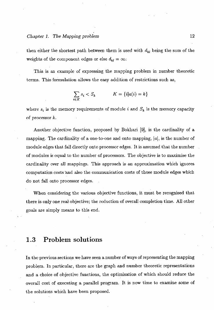
Chapter 1. The Mapping problem 12
then either the shortest path between them is used with dkj being the sum of the
weights of the component edges or else dkl = 00;
This is an example of expressing the mapping problem in number theoretic
terms. This formulation allows the easy addition of restrictions such as,
Si < Sk K = { ila(i) = k} iE K
where s2 is the memory requirements of module i and Sjç, is the memory capacity
of processor k.
Another objective function, proposed by Bokhari [9], is the cardinality of a
mapping. The cardinality of a one-to-one and onto mapping, IaI, is the number of
module edges that fall directly onto processor edges. It is assumed that the number
of modules is equal to the number of processors. The objective is to maximise the
cardinality over all mappings. This approach is an approximation which ignores
computation costs and also the communication costs of those module edges which
do not fall onto processor edges.
When considering the various objective functions, it must be recognised that
there is only one real objective; the reduction of overall completion time. All other
goals are simply means to this end.
1.3 Problem solutions
In the previous sections we have seen a number of ways of representing the mapping
problem. In particular, there are the graph and number theoretic representations
and a choice of objective functions, the optimisation of which should reduce the
overall cost of executing a parallel program. It is now time to examine some of
the solutions which have been proposed.
Chapter I. The Mapping problem
13
The simplest solution is to enumerate every possible mapping, evaluate the
objective function and choose a mapping which gives an optimal value - there
may be more than one which does so. Unfortunately, for any more than a handful
of modules and processors, this is enormously time consuming.
1.3.1 Problem complexity
Complexity theory defines P to be the class of decision problems which can be
solved in polynomial time. Decision problems are ones with a solution of either
"yes" or "no" and they often take the form of a search for a pattern or structure
which satisfies certain. problem specific properties. A problem can be solved in
polynomial time if the time taken to solve it is less than a polynomial function of
the size of the problem's parameters.
The class NP, is the class of decision problems which can be solved in poly-
nomial time if the solution pattern is magically guessed straight away, or alterna-
tively, if all patterns are tried simultaneously.
NP includes P, but it is unknown whether there are any other problems in NP
which are not in P or whether P = NP. It has been shown that there is a class of
problems within NP such that if they are in P then so too are all the problems in
NP and therefore they all can be solved in polynomial time. This special class of
the hardest problems in NP is called NP-Complete [22].
It is widely assumed, but as yet unproved that P :A NP and that the lower
time bound for NP-Complete problems is exponential.
When the mapping problem is re-phrased as a decision problem it is NP-
Complete. So too are the QAP and many other problems in numeric optimisation
and graph theory, such as the subgraph isomorphism problem mentioned in section
1.2.1. So unless there is a major breakthrough in complexity theory, which is
now seen as unlikely, the mapping problem is fundamentally an expensive (non-
Chapter 1. The Mapping problem 14
polynomial) problem to solve. Typically, the time required to find an optimal
mapping is an exponential function of the number of modules and processors.
The mapping problem must be solved whenever a parallel program is run on
a parallel machine. So a compromise must be made to produce a mapping within
an acceptable time. There are number of alternatives.
1.3.2 Restricted optimal solutions
Up until now we have considered mapping arbitrary module graphs to arbitrary
processor graphs and found that optimal mappings are particularly difficult to
produce within a reasonable time. One way to avoid this impasse is to restrict
the problem being tackled. By constraining the number of nodes or the inter-
communication topology allowed in the module and processor graphs a number of
fast optimal solutions have been developed.
Perhaps the most noted mapping algorithm published to date is due to Stone
[54]. He presented a description of the mapping problem in terms of commodity
flow graphs. These usually take the form of a set of source nodes which produce
goods and a set of sink nodes which consume them. Goods flow from sources to
sinks via a network. The edges of this network are weighted with a capacity which
is the maximum amount of goods which can flow along that edge. A common
question asked of commodity networks is what is the maximum flow of goods
from sources to sinks.
A cut set of a commodity graph is a set of edges which when removed discon-
nects the source nodes from the sink nodes. Thus all the goods which flow from
source to sink must flow through the cutset. No proper subset of a cutset is .a
cutset. The capacity of a cutset is equal to the sum of the capacities of the edges
in that cutset.
Chapter 1. The Mapping problem ii;i
This capacity is the maximum flow of goods through the cutset and therefore
is a limit on that flow. The cutset with the lowest capacity is the bottleneck of the
whole network and its weight is the maximum possible flow through the network.
This minimum cutset, mm-cut, can be found in polynomial time.
In Stone's method, a source node and a sink node are just two special nodes of
which there can be many, one for each processor. Every cutset which disconnects
each of the special nodes from the other special nodes, corresponds to a partition;
the mm-cut corresponding to the optimal mapping. Using the polynomial time
solution for standard commodity flow networks, Stone produced an optimal map-
ping algorithm for two processors. He later extended this to solve in polynomial
time, the three processor case [55].
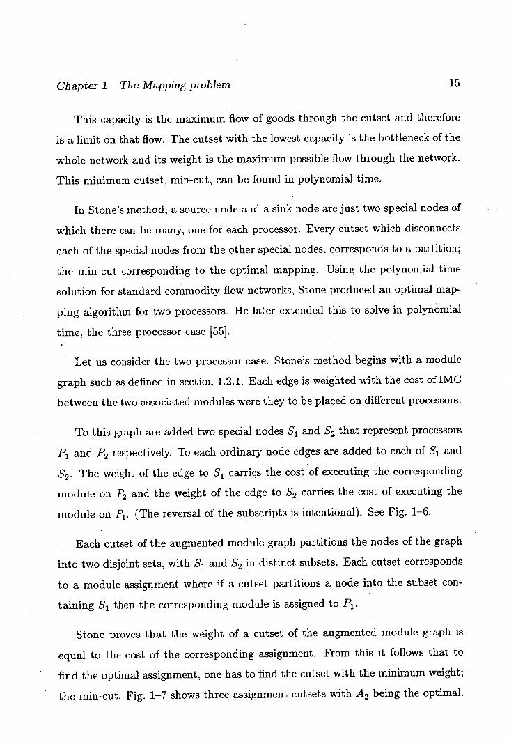
Let us consider the two processor case. Stone's method begins with a module
graph such as defined in section 1.2.1. Each edge is weighted with the cost of IMC
between the two associated modules were they to be placed on different processors.
To this graph are added two special nodes S 1 and S2 that represent processors
P1 and P2 respectively. To each ordinary node edges are added to each of S 1 and
S2 . The weight of the edge to S 1 carries the cost of executing the corresponding
module on P2 and the weight of the edge to S 2 carries the cost of executing the
module on P1 . (The reversal of the subscripts is intentional). See Fig. 1-6.
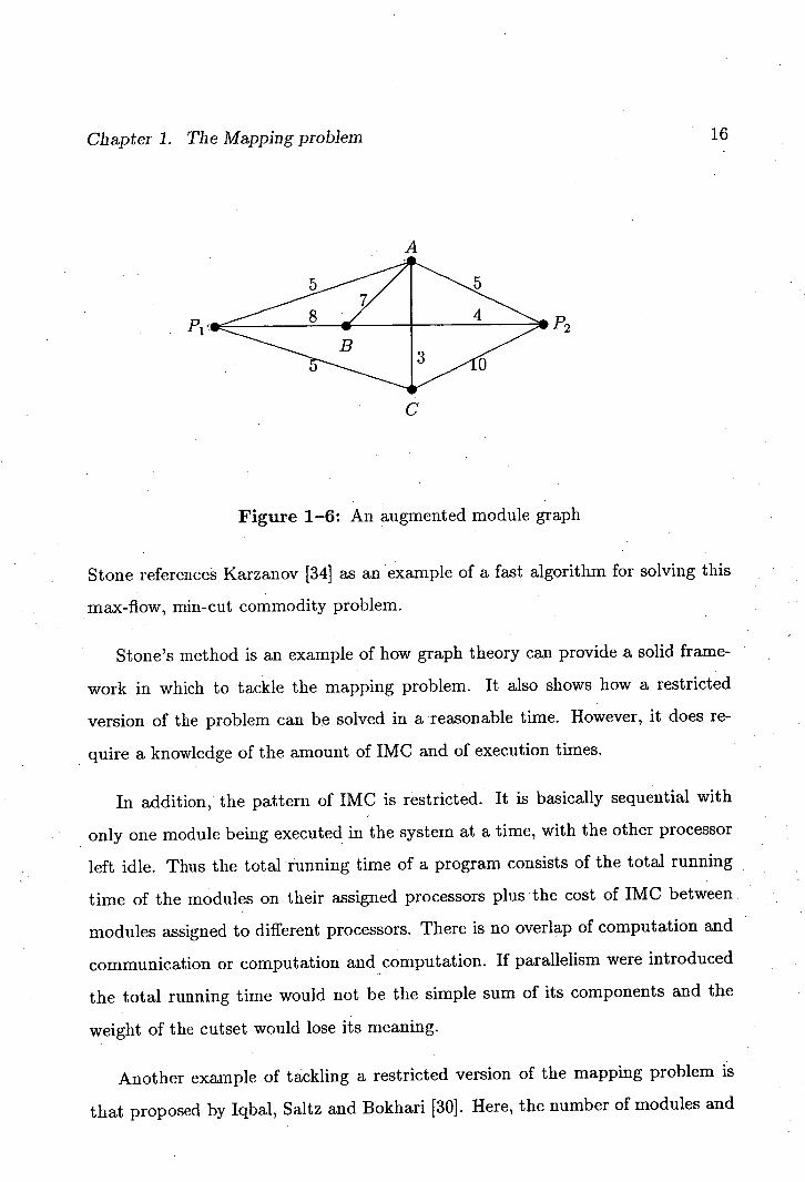
Each cutset of the augmented module graph partitions the nodes of the graph
into two disjoint sets, with S1 and 52 in distinct subsets. Each cutset corresponds
to a module assignment where if a cutset partitions a node into the subset con-
taming S then the corresponding module is assigned to P1 .
Stone proves that the weight of a cutset of the augmented module graph is
equal to the cost of the corresponding assignment. From this it follows that to
find the optimal assignment, one has to find the cutset with the minimum weight;
the mm-cut. Fig. 1-7 shows three assignment cutsets with A 2 being the optimal.
Chapter 1. The Mapping problem 16
A
C
Figure 1-6: An augmented module graph
Stone references Karzanov [34] as an example of a fast algorithm for solving this
max-flow, mm-cut commodity problem.
Stone's method is an example of how graph theory can provide a solid frame-
work in which to tackle the mapping problem. It also shows how a restricted
version of the problem can be solved in a reasonable time. However, it does re-
quire a knowledge of the amount of IMC and of execution times.
In addition, the pattern of IMC is restricted. It is basically sequential with
only one module being executed in the system at a time, with the other processor
left idle. Thus the total running time of a program consists of the total running
time of the modules on their assigned processors plus the cost of IMC between
modules assigned to different processors. There is no overlap of computation and
communication or computation and computation. If parallelism were introduced
the total running time would not be the simple sum of its components and the
weight of the cutset would lose its meaning.
Another example of tackling a restricted version of the mapping problem is
that proposed by Iqbal, Saltz and Bokhari [30]. Here, the number of modules and
Chapter 1. The Mapping problem 17
P.91
P1 P2
A, ('1!) ,q2(47)
Figure 1-7: An augmented module graph with cuts
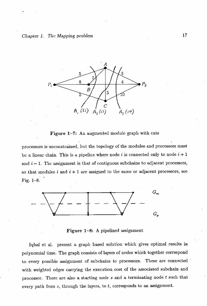
processors is unconstrained, but the topology of the modules and processors must
be a linear chain. This is a pipeline where node i is connected only to node i + 1
and i - 1. The assignment is that of contiguous subchains to adjacent processors,
so that modules i and i + 1 are assigned to the same or adjacent processors, see
Fig. 1-8.
Iv- V GP
Figure 1-8: A pipelined assignment
Iqbal et al. present a graph based solution which gives optimal results in
polynomial time. The graph consists of layers of nodes which together correspond
to every possible assignment of subchains to processors. These are connected
with weighted edges carrying the execution cost of the associated subchain and
processor. There are also a starting node s and a terminating node t such that
every path from s, through the layers, to t, corresponds to an assignment.
Chapter 1. The Mapping problem UP
The edge with the highest weight in a path corresponds to the most heavily
loaded processor, ie. the bottleneck on performance. The optimal assignment
has the path with the minimum maximum weight - the bottleneck path. An
algorithm for m modules and n processors is presented which finds an optimal
path in O(m 3n) time.
A third example of a restricted optimal solution is presented by Bokhari [9]. In
this approach, the module graph is restricted to being a tree and the IMC pattern
constrained to a procedure call hierarchy. In Bokhari's algorithm, each node in
the module tree is expanded into a layer of nodes. This layer consists of one node
for each possible assignment of the module to a processor. Each node is linked
to the nodes in the layers of the original node's parent and children and the links
are weighted with execution and communication costs. The optimal assignment
corresponds to the minimum weight tree which connects the root to the leaves.
1.3.3 Approximate solutions
Rather than restricting the problem to achieve an optimal solution, an alternative
is to accept a solution to the general problem which is possibly not optimal.
Approximation algorithms can provide very good solutions, but often they cannot
guarantee to do so every time. However, they do produce their results, good or
bad, quickly.
If we have to accept a suboptimal solution it would be desirable if it can be
guaranteed to be close to the optimal. Let OPT(A) be the cost of an optimal
assignment and APPROX(A), the cost of an assignment produced by an approx-
imation algorithm, then APPROX(A) is an €-approximation algorithm if
OPT(A) - APPROX(A)
OPT(A)
for some fixed (hopefully small) e. That is, the approximate solution is guaranteed
to be within a fixed percentage of the optimal solution [27, Pg.5611.
Chapter 1. The Mapping problem 19
Sahni and Gonzalez [51] have shown that unfortunately the existence of a
polynomial solution to such an approximation for the QAP would imply P =
NP which is considered very unlikely. So if we are to have a polynomial time
approximation algorithm then we cannot guarantee that it will produce good
results for all cases, though it may be unlikely that the worst-case results occur in
practice.
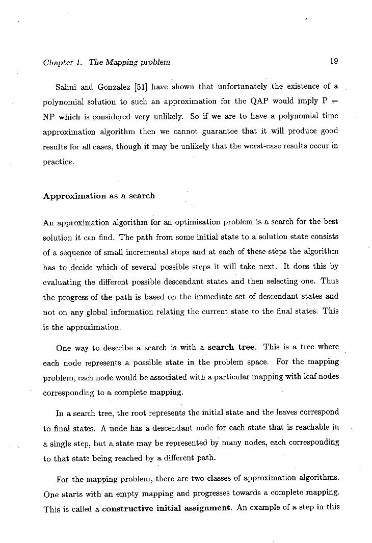
Approximation as a search
An approximation algorithm for an optimisation problem is a search for the best
solution it can find. The path from some initial state to a solution state consists
of a sequence of small incremental steps and at each of these steps the algorithm
has to decide which of several possible steps it will take next. It does this by
evaluating the different possible descendant states and then selecting one. Thus
the progress of the path is based on the immediate set of descendant states and
not on any global information relating the current state to the final states. This
is the approximation.
One way to describe a search is with a search tree. This is a tree where
each node represents a possible state in the problem space. For the mapping
problem, each node would be associated with a particular mapping with leaf nodes
corresponding to a complete mapping.
In a search tree, the root represents the initial state and the leaves correspond
to final states. A node has a descendant node for each state that is reachable in
a single step, but a state may be represented by many nodes, each corresponding
to that state being reached by a different path.
For the mapping problem, there are two classes of approximation algorithms.
One starts with an empty mapping and progresses towards a complete mapping.
This is called a constructive initial assignment. An example of a step in this
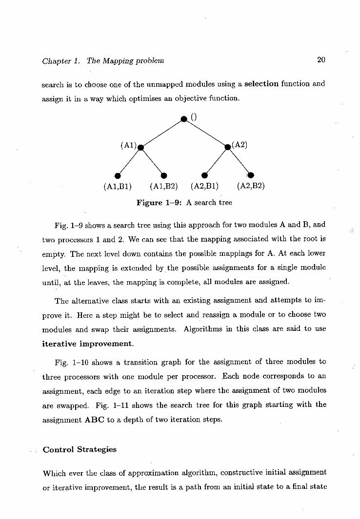
Chapter 1. The Mapping problem 20
search is to choose one of the unmapped modules using a selection function and
assign it in a way which optimises an objective function.
(A1,B1) (A1,132) (A2,13 1) (A2,B2)
Figure 1-9: A search tree
Fig. 1-9 shows a search tree using this approach for two modules A and B, and
two processors 1 and 2. We can see that the mapping associated with the root is
empty. The next level down contains the possible mappings for A. At each lower
level, the mapping is extended by the possible assignments for a single module
until, at the leaves, the mapping is complete, all modules are assigned.
The alternative class starts with an existing assignment and attempts to im-
prove it. Here a step might be to select and reassign a module or to choose two
modules and swap their assignments. Algorithms in this class are said to use
iterative improvement.
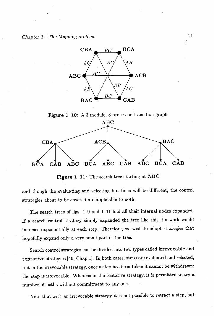
Fig. 1-10 shows a transition graph for the assignment of three modules to
three processors with one module per processor. Each node corresponds to an
assignment, each edge to an iteration step where the assignment of two modules
are swapped. Fig. 1-11 shows the search tree for this graph starting with the
assignment ABC to a depth of two iteration steps.
Control Strategies
Which ever the class of approximation algorithm, constructive initial assignment
or iterative improvement, the result is a path from an initial state to a final state
Chapter 1. The Mapping problem 21
CBA... RO .BCA
AC! \AC/ \AB
BACW WCAB
Figure 1-10: A 3 module, 3 processor transition graph
ABC
CBA
BCA CAB ABC BCA ABC CAB ABC BCA CAB
Figure 1-11: The search tree starting at ABC
and though the evaluating and selecting functions will be different, the control
strategies about to be covered are applicable to both.
The search trees of figs. 1-9 and 1-11 had all their internal nodes expanded.
If a search control strategy simply expanded the tree like this, its work would
increase exponentially at each step. Therefore, we wish to adopt strategies that
hopefully expand only a very small part of the tree.
Search control strategies can be divided into two types called irrevocable and
tentative strategies [46, Chap.11. In both cases, steps are evaluated and selected,
but in the irrevocable strategy, once a step has been taken it cannot be withdrawn;
the step is irrevocable. Whereas in the tentative strategy, it is permitted to try a
number of paths without commitment to any one.
Note that with an irrevocable strategy it is not possible to retract a step, but
Chapter 1. The Mapping problem 22
in some cases its effect may be undone by later steps. If the searching step is to
swap two modules then to undo a swap, simply repeat it.
Horowitz and Sahni [27, Chap.41 present a general irrevocable control strategy
which they call the greedy method. It is used as the basis for a number of
constructive initial assignment algorithms.
Tentative strategies can be further divided into two groups, those that allow
backtracking and those that perform a graph-search.
The backtracking strategy is a depth first traversal of the search tree. It allows
a path to be tried, but if it is later found to be a poor choice then it can be
"forgotten" and another path tried instead. As the algorithm traverses down the
search tree, it remembers the nodes on the path back to the root. Should the
current line of search prove fruitless, the algorithm retraces its steps - backtracks -
until it finds a node with untried alternatives and chooses one of these. Obviously,
the better the algorithm chooses its alternatives, the less backtracking that occurs
and the search is more efficient.
The more general graph-search approach allows a number of paths to be tried
concurrently. At each step, the most promising state is selected and its descendant
states are added to the list of states to be considered for the next step. The manner
in which the new states are inserted into the list determines the route of the search.
If new nodes are always added to the head of the list, the graph-search degenerates
into a depth first search.
An analogy
One can imagine the search for an optimum as being like climbing a mountain
in heavy cloud to find the height of its peak, armed with only an altimeter. At
various points of the trek, there will be a number of paths from which to choose
the way forward, but because of the cloud, one cannot tell which path leads to the

Chapter 1. The Mapping problem 23
top. Often it will never be certain that the top has been found just that there is
nowhere further to go, but down.
If the mountain is a simple hump or cone, it is called convex. For such convex
problems it is easy to produce a quick optimal algorithm; always choose a path
which goes up. The most efficient algorithm being always to choose the steepest
path up. This is the greedy method of Horowitz and Sahni[27].
However, like nature, the optimisation mountains usually have foothills, ridges
and plateaus, not to mention cliffs and the greedy algorithm quickly runs into
problems.
Consider our intrepid cloud bound mountaineer. If he always chooses an up-
wards path he may unwittingly find himself stuck at the top of a foothill perhaps
even concluding that this is indeed the top of the mountain.
Another possibility our climber might face is to be on the crest of a ridge which
extends upwards in front of him, but the only paths he can see lead down the sides
of the ridge. Perhaps these paths meet others which lead to points further up the
ridge, but this is unknown.
Depending on the strategy used, the problems of foothills and ridges may result
in the climber stopping at what he thinks is the mountain peak when in fact it
isn't. He has found what is called a local optimum, a maximum in this case.
To escape foothills and ridges, the climber needs to adopt a tentative strategy
or to take a risk by possibly choosing a level or even downward path. The risk is
that the search may go on forever.
Our questing climber might discover a flat, level plateau where all the paths
he can see neither go up nor down. Unless he notes all the points he has visited
so as to avoid them later, he could wander in circles forever searching.
Chapter 1. The Mapping problem 24
Irrevocable strategies
Whereas tentative strategies, by their nature, can avoid foothills and ridges, but
at the cost of wasted time, an irrevocable strategy can do so only with a suitable
choice of selection functions and allowable search steps.
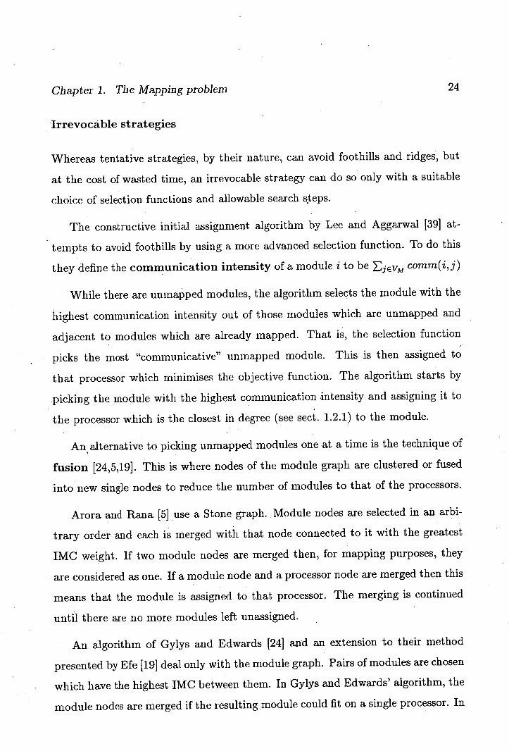
The constructive initial assignment algorithm by Lee and Aggarwal [39] at-
tempts to avoid foothills by using a more advanced selection function. To do this
they define the communication intensity of a module ito be FliEVm comm(i,j)
While there are unmapped modules, the algorithm selects the module with the
highest communication intensity out of those modules which are unmapped and
adjacent to modules which are already mapped. That is, the selection function
picks the most "communicative" unmapped module. This is then assigned to
that processor which minimises the objective function. The algorithm starts by
picking the module with :the highest communication intensity and assigning it to
the processor which is the closest in degree (see sect. 1.2.1) to the module.
An alternative to picking unmapped modules one at a time is the technique of
fusion [24,5,19]. This is where nodes of the module graph are clustered or fused
into new single nodes to reduce the number of modules to that of the processors.
Arora and Rana [5] use a Stone graph. Module nodes are selected in an arbi-
trary order and each is merged with that node connected to it with the greatest
IMC weight. If two module nodes are merged then, for mapping purposes, they
are considered as one. If a module node and a processor node are merged then this
means that the module is assigned to that processor. The merging is continued
until there are no more modules left unassigned.
An algorithm of Gylys and Edwards [24] and an extension to their method
presented by Efe [19] deal only with the module graph. Pairs of modules are chosen
which have the highest IMC between them. In Gylys and Edwards' algorithm, the
module nodes are merged if the resulting. module could fit on a single processor. In
Chapter 1. The Mapping problem 25
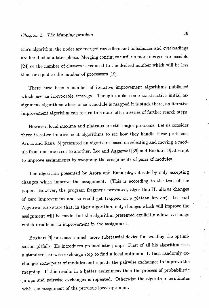
Efe's algorithm, the nodes are merged regardless and imbalances and overloadings
are handled in a later phase. Merging continues until no more merges are possible
[24] or the number of clusters is reduced to the desired number which will be less
than or equal to the number of processors [19].
There have been a number of iterative improvement algorithms published
which use an irrevocable strategy: Though unlike some constructive initial as-
signment algorithms where once a module is mapped it is stuck there, an iterative
improvement algorithm can return to a state after a series of further search steps.
However, local maxima and plateaus are still major problems. Let us consider
three iterative improvement algorithms to see how they handle these problems.
Arora and Rana [5] presented an algorithm based on selecting and moving a mod-
ule from one processor to another. Lee and Aggarwal [39] and Bokhari [9] attempt
to improve assignments by swapping the assignments of pairs of modules.
The algorithm presented by Arora and Rana plays it safe by only accepting
changes which improve the assignment. (This is according to the text of the
paper. However, the program fragment presented, algorithm II, allows changes
of zero improvement and so could get trapped on a plateau forever). Lee and
Aggarwal also state that, in their algorithm, only changes which will improve the
assignment will be made, but the algorithm presented explicitly allows a change
which results in no improvement in the assignment.
Bokhari [9] presents a much more substantial device for avoiding the optimi-
sation pitfalls. He introduces probabilistic jumps. First of all his algorithm uses
a standard pairwise exchange step to find a local optimum. It then randomly ex-
changes some pairs of modules and repeats the pairwise exchanges to improve the
mapping. If this results in a better assignment then the process of probabilistic
jumps and pairwise exchanges is repeated. Otherwise the algorithm terminates
with the assignment of the previous local optimum.
Chapter 1. The Mapping problem Nei
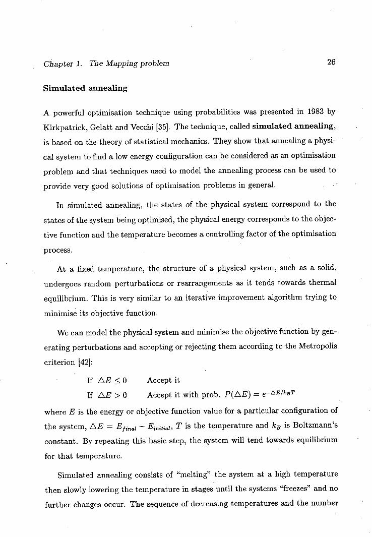
Simulated annealing
A powerful optimisation technique using probabilities was presented in 1983 by
Kirkpatrick, Gelatt and Vecchi [35]. The technique, called simulated annealing,
is based on the theory of statistical mechanics. They show that annealing a physi-
cal system to find a low energy configuration can be considered as an optimisation
problem and that techniques used to model the annealing process can be used to
provide very good solutions of optimisation problems in general.
In simulated annealing, the states of the physical system correspond to the
states of the system being optimised, the physical energy corresponds to the objec-
tive function and the temperature becomes a controlling factor of the optimisation
process.
At a fixed temperature, the structure of a physical system, such as a solid,
undergoes random perturbations or rearrangements as it tends towards thermal
equilibrium. This is very similar to an iterative improvement algorithm trying to
minimise its objective function.
We can model the physical system and minimise the objective function by gen-
erating perturbations and accepting or rejecting them according to the Metropolis
criterion [42]:
If /2E < 0 Accept it
If z~ E > 0 Accept it with prob. P(E) = e_/lcBT
where E is the energy or objective function value for a particular configuration of
the system, LE = Ejnai - Ejnjtjai, T is the temperature and kB is Boltzmann's
constant. By repeating this basic step, the system will tend towards equilibrium
for that temperature.
Simulated annealing consists of "melting" the system at a high temperature
then slowly lowering the temperature in stages until the systems "freezes" and no
further changes occur. The sequence of decreasing temperatures and the number
Chapter 1. The Mapping problem 27
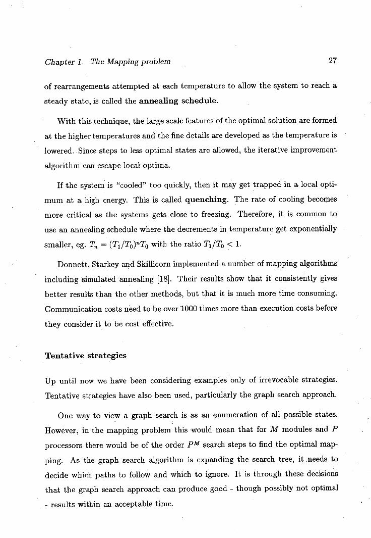
of rearrangements attempted at each temperature to allow the system to reach a
steady state, is called the annealing schedule.
With this technique, the large scale features of the optimal solution are formed
at the higher temperatures and the fine details are developed as the temperature is
lowered. Since steps to less optimal states are allowed, the iterative improvement
algorithm can escape local optima.
If the system is "cooled" too quickly, then it may get trapped in a local opti-
mum at a high energy. This is called quenching. The rate of cooling becomes
more critical as the systems gets close to freezing. Therefore, it is common to
use an annealing schedule where the decrements in temperature get exponentially
smaller, eg. T = (T1 /T0)'T0 with the ratio T1 1T0 < 1.
Donnett, Starkey and Skillicorn implemented a number of mapping algorithms
including simulated annealing [18]. Their, results show that it consistently gives
better results than the other methods, but that it is much more time consuming.
Communication costs need to be over 1000 times more than execution costs before
they consider it to be cost effective.
Tentative strategies
Up until now we have been considering examples only of irrevocable strategies.
Tentative strategies have also been used, particularly the graph search approach.
One way to view a graph search is as an enumeration of all possible states.
However, in the mapping problem this would mean that for M modules and P
processors there would be of the order P m search steps to find the optimal map-
ping. As the graph search algorithm is expanding the search tree, it .needs to
decide which paths to follow and which to ignore. It is through these decisions
that the graph search approach can produce good - though possibly not optimal
- results within an acceptable time.
Chapter 1. The Mapping problem 28
Shen and Tsai [52] have used Nilsson's A* algorithm [46] as part of a construc-
tive initial assignment algorithm. This involves expanding the search tree using
an evaluation function to select promising nodes.
This evaluation function consists of two parts:
f(n) = g(n) + h(n)
where g(n) is the traditional objective function presented earlier which quantifies
the "goodness" of the partial mapping so far. The second term, h(n) is a heuristic
function which is an estimate of h*(n), the cost of the minimal cost path from this
partial mapping to an optimal mapping.
If h(n) < h*(n) for all ii, ie. a lower bound, then this algorithm is guaranteed
to find an optimal solution. In a degenerate case, where g(n) is the length of the
current path and h(n) = 0 then the algorithm is a breadth first search. The higher
the value of h(n) the more branches that will be ignored and therefore the more
efficient the search, but if h(n) is not a lower bound on h*(n), it is possible for
optimal solutions to be missed.
A variation on the graph search approach is the branch and bound algorithm.
This technique is a depth first search which incorporates constraints to eliminate
parts of the search tree. Since eliminating a branch means that the entire subtree
from that branch is ignored, potentially enormous savings can be made.
Ma, Lee and Tsuchiya [40] present a mapping algorithm based on the branch
and bound method. They use bounds such as the memory capacity of the pro-
cessors. They can constrain modules to be on particular processors. In addition,
pairs of modules can be constrained to be on different processors. Using these
constraints and others they reduced the number of iterations required in their
application from an upper bound of 0(100) down to 0(10).
Chapter 1. The Mapping problem 29
1.4 Annotations
In recent years, a number of explicitly parallel language models, such as Occam[41]
and POOL [1], have been developed. These language models allow arbitrary com-
munication patterns between the modules. Since most of the techniques discussed
in the literature assume the limited functional model of IMC, more general map-
ping algorithms are needed.
Given the difficult nature of automated mappings, the solution adopted in
Occam, POOL and the parallel functional language ParAlfl[29} is to have the pro-
grammer specify the mapping manually. This is done by annotating the modules
with a reference to the processor on which they are to be executed.
Occam
Occam[41] is based on Hoare's model of communicating sequential processes,
CSP[26]. It allows the programmer to specify a static hierarchy of modules, which
are called processes. A process can be either a primitive process such as as-
signment or an I/O operation or it can consist of a collection of further processes
which are executed either in parallel or sequentially. In addition, there are chan-
nels which provide a one-way communication link between pairs of processors.
Processes declared at the top level of a program can be annotated with a place-
ment expression. This expression, which is evaluated at compile time, specifies
the processor on which that process and all its component processes are to be
executed. The processors are referred to by some machine dependent name such
as a unique fixed processor ID.
For example, the following program fragment declares 10 processes; a host
process, a master process and 8 slave processes. It allocates each to a separate
Chapter 1. The Mapping problem 30
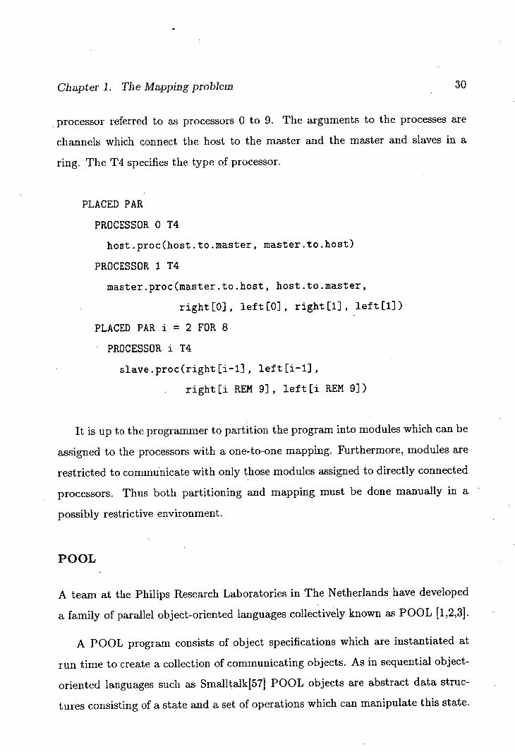
processor referred to as processors 0 to 9. The arguments to the processes are
channels which connect the host to the master and the master and slaves in a
ring. The T4 specifies the type of processor.
PLACED PAR
PROCESSOR 0 T4
host.proc(host.to .master, master.to .host)
PROCESSOR 1 T4
master.proc(master.to .host, host.to .master,
right [0] , left [0] , right [1] , left [1])
PLACED PAR i = 2 FOR 8
PROCESSOR i T4
slave.proc(right[i-11, left[i-1]
right [i REM 91, left [1 REM 9])
It is up to the programmer to partition the program into modules which can be
assigned to the processors with a one-to-one mapping. Furthermore, modules are
restricted to communicate with only those modules assigned to directly connected
processors. Thus both partitioning and mapping must be done manually in a
possibly restrictive environment.
POOL
A team at the Philips Research Laboratories in The Netherlands have developed
a family of parallel object-oriented languages collectively known as POOL [1,2,3].
A POOL program consists of object specifications which are instantiated at
run time to create a collection of communicating objects. As in sequential object-
oriented languages such as Smalltalk[57] POOL objects are abstract data struc-
tures consisting of a state and a set of operations which can manipulate this state.
Chapter 1. The Mapping problem 31
In addition, POOL also allows each object to have an active component which can
execute independently of requests to invoke an object's operations. This active
component requires that the object be mapped to a processor for its execution.
A proposal has been presented by Augusteijn et al. [6] to allow the programmer
to assign objects to virtual nodes. These virtual nodes are then to be assigned
to physical nodes in an as yet undefined manner except that there will be at most
one virtual, node assigned to a physical node. Thus the programmer is specifying
a partitioning rather than a mapping.
The proposal defines two object classes; Nodes and Node-set. The operations
of these classes allow an object to find out what node itself or another object is
executing on. It can also convert an integer into a node reference allowing the
calculation of the node at run time. The pragmas annotating object creations and
copyings .take an instance of Node-set as their arguments.
'ParAlfi
ParAlfi is a para-functional language developed by Paul Hudak and colleagues at
Yale university[29,28]. It is a functional language which has been extended with
annotations to provide more control over the parallel evaluation process.
In a referentially transparent language such as ParAlfi, the arguments to a
function can be evaluated concurrently without any fear of them interfering with
each other. These function evaluations can be treated 'as modules in a dynamic
structure.
In ParAffi, expressions can be annotated with $on E, where E has the value of
a processor identifier. For example, in the expression f(a) $on go, go is evaluated
first to decide where 1(a) should be evaluated. If an expression is unannotated
then it is executed on the processor of its parent expression; the current processor.
ParAlfi provides the $self primitive which has the value of the current processor
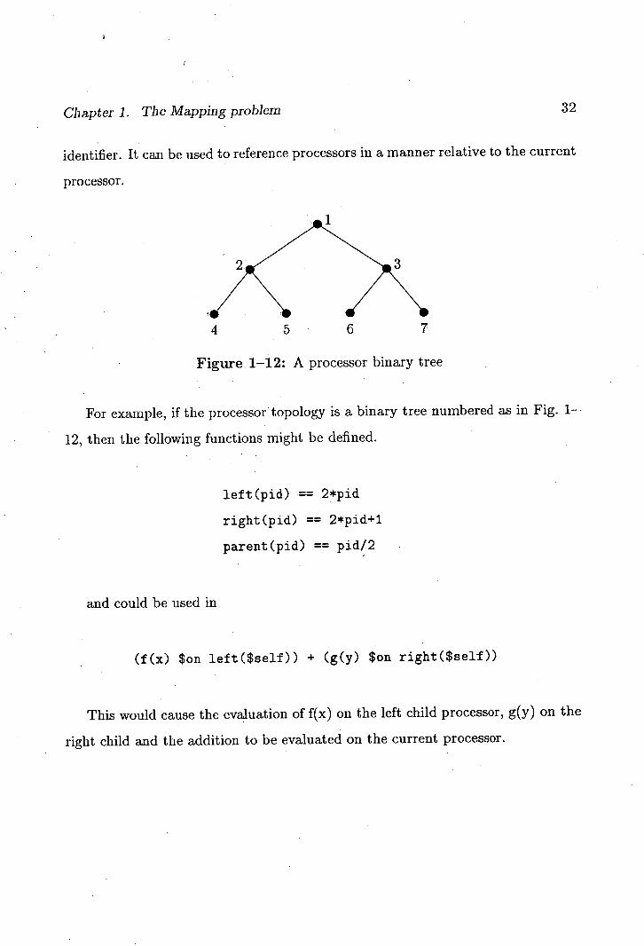
Chapter 1. The Mapping problem 32
identifier. It can be used to reference processors in a manner relative to the current
processor.
1
4 5 6 7
Figure 1-12: A processor binary tree
For example, if the processor topology is a binary tree numbered as in Fig. 1-
12, then the following functions might be defined.
left(pid) == 2*pid
right(pid) 2*pid+1
parent(pid) pidl2
and could be used in
(f(x) $on left($self)) + (g(y) $on right($self))
This would cause the evaluation of 1(x) on the left child processor, g(y) on the
right child and the addition to be evaluated on the current processor.
Chapter 1. The Mapping problem 33
1.5 Conclusion
When implementing any parallel algorithm on a parallel architecture one must
always solve the mapping problem - to decide which processor should execute
which module. Not only is it a necessity, but it can have a dramatic effect on the
performance of the system.
A survey of several approaches to solving the mapping problem has been pre-
sented. The approaches fall into two categories; manual, where the programmer
specifies the mapping completely and automatic where an algorithm produces a
mapping given various parameters of the program and the architecture.
Manual mechanisms such as annotations and placements are practical for small
or simple systems, especially when the physical topology is suited to the logical
topology. There are several examples showing how to map large synchronous
systems which have a very regular structure and simple communication model [20].
However, as the systems become larger and more complex and good mappings are
no longer intuitively obvious, an automated mapping mechanism is desired.
The automatic mappings are all based on the underlying assumption that
the various parameters used in the objective function are meaningful and can be
determined. For this to be so the automatic methods surveyed rely on a restricted
pattern of interaction - the functional non-overlapping model. Even with this
restricted model it is often difficult to determine the value of such metrics as
simple execution and communication costs and even if they can be determined
the possibly enormous amounts of data can make their processing impractical.
The problems are more fundamental when a less restrictive pattern of commu-
nication is allowed. When the time taken for a task to complete depends on more
than the communication and execution costs, but also depends on synchronisation
Chapter 1. The Mapping problem
34
delays, the overlapping of computation and communication and network conges-
tion then the traditional objective functions no longer relate to the completion
time and are meaningless.
These new costs are not static or independent variables, but depend on the
interaction between modules executing in a real system in real time. In all but
trivial cases it is impossible to quantify these costs. Therefore, mapping methods
based on objective functions will always be inadequate for complex asynchronous
systems. They give the impression of precision and yet are approximate and even
inaccurate.
A new approach is needed; one that is not based on incomplete or unmeasurable
quantities, but on a fuller understanding of the behaviour of complex systems.
This thesis presents a new approach which utilises problem specific knowledge
and structure to guide the generation of a mapping.
Chapter 2
A structural approach
2.1 Introduction
As was concluded in the previous chapter there is a need for a mechanism which
can generate a good mapping without the need for a detailed knowledge of the
system's computation and communication costs. These costs are difficult to obtain
and process, sometimes ill-defined and the final result is usually an approximation
anyway.
Increasingly, systems are being designed hierarchically. Such an approach
places a superstructure over the otherwise ad hoc collection of component activi-
ties. Before any existing mapping mechanisms can be applied, such superstructure
must be removed leaving a simple flattened process graph (section 1.2.1). It will
be shown that rather than being something to be eliminated, this superstructure
provides valuable information.
This thesis shows that in certain applications, the hierarchical design structure
of a system can be used as an approximation to the system's communication
behaviour and can be used to produce a better mapping. As a consequence, it is
demonstrated that in these applications a principle of locality is at work where
locality is defined by the hierarchical design structure.
35
Chapter 2. A structural approach
36
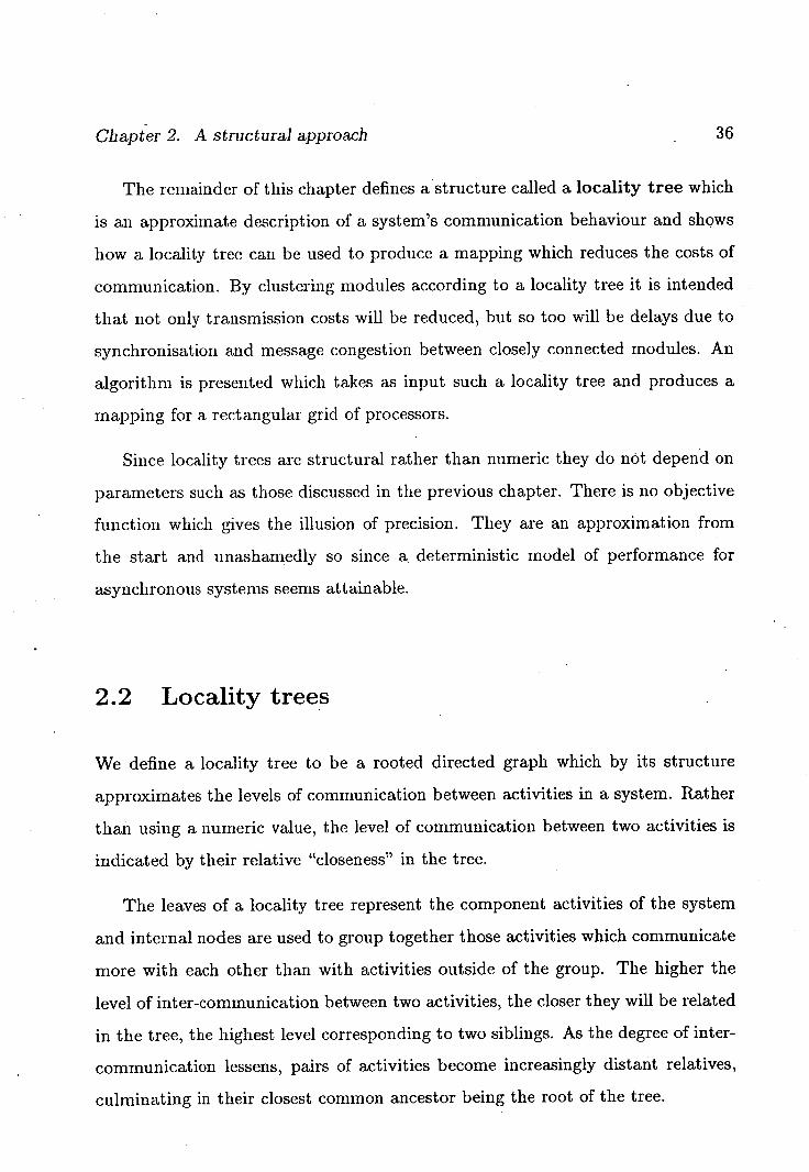
The remainder of this chapter defines a structure called a locality tree which
is an approximate description of a system's communication behaviour and shows
how a locality tree can be used to produce a mapping which reduces the costs of
communication. By clustering modules according to a locality tree it is intended
that not only transmission costs will be reduced, but so too will be delays due to
synchronisation and message congestion between closely connected modules. An
algorithm is presented which takes as input such a locality tree and produces a
mapping for a rectangular grid of processors.
Since locality trees are structural rather than numeric they do not depend on
parameters such as those discussed in the previous chapter. There is no objective
function which gives the illusion of precision. They are an approximation from
the start and unashamedly so since a. deterministic model of performance for
asynchronous systems seems attainable.
2.2 Locality trees
We define a locality tree to be a rooted directed graph which by its structure
approximates the levels of communication between activities in a system. Rather
than using a numeric value, the level of communication between two activities is
indicated by their relative "closeness" in the tree.
The leaves of a locality tree represent the component activities of the system
and internal nodes are used to group together those activities which communicate
more with each other than with activities outside of the group. The higher the
level of inter-communication between two activities, the closer they will be related
in the tree, the highest level corresponding to two siblings. As the degree of inter-
communication lessens, pairs of activities become increasingly distant relatives,
culminating in their closest common ancestor being the root of the tree.
Chapter 2. A structural approach
37
In contrast to the actual level of inter-communication which is basically a
continuous variable, the approximation uses an arbitrary discrete scale with the
number of divisions equal to twice the height of the tree. The level of inter-
communication between two activities is approximated by the length of the short-
est path between the two corresponding leaf nodes.
There is, however, no arithmetic relation between the levels, simply an order-
ing. If one pair of activities has twice the inter-node path length than another
pair, this does not imply that there is half the amount of communication. All it
represents is that the former pair communicates less than the latter.
2.2.1 Simple trees
K
A B C D E F G H
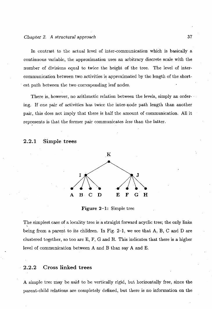
Figure 2-1: Simple tree
The simplest case of a locality tree is a straight forward acyclic tree; the only links
being from a parent to its children. In Fig. 2-1, we see that A, B, C and D are
clustered together, so too are E, F, G and H. This indicates that there is a higher
level of communication between A and B than say A and E.
2.2.2 Cross linked trees
A simple tree may be said to be vertically rigid, but horizontally free, since the
parent-child relations are completely defined, but there is no information on the
Chapter 2. A structural approach
relationship between siblings, cousins, etc. To provide horizontal rigidity, simple
trees can be extended by allowing cross links.
A cross link between any two nodes expresses a higher level of communication
than would otherwise be indicated by their position in a simple tree. This allows
nodes to be pulled together laterally. It represents an attraction between siblings,
cousins, etc. and allows the expression of finer degrees of communication levels by
describing the relation between particular pairs rather than whole families. Not
just leaves, but internal nodes may also be cross linked. Thus expressing a higher
level of communication between all of the leaf activities of one subtree and those
of the other.
Since cross links exist to express extra information on top of a simple local-
ity tree, it is meaningless for a node to be cross linked to one of its ancestors,
descendants or itself as such linkage is already expressed by the simple tree.
In order to preserve the meaning of the locality tree, two types of cross links
are distinguished. To connect two siblings together, an junk is used. An junk is
an internal link within a parent-children nuclear family. It extends the information
in the locality tree by allowing a node to be more closely related to one sibling
than to the others. Junks always come in pairs since cross linking is a symmetrical
relation, but they are usually considered as single bi-directional links.
RN
A B C D E F G H
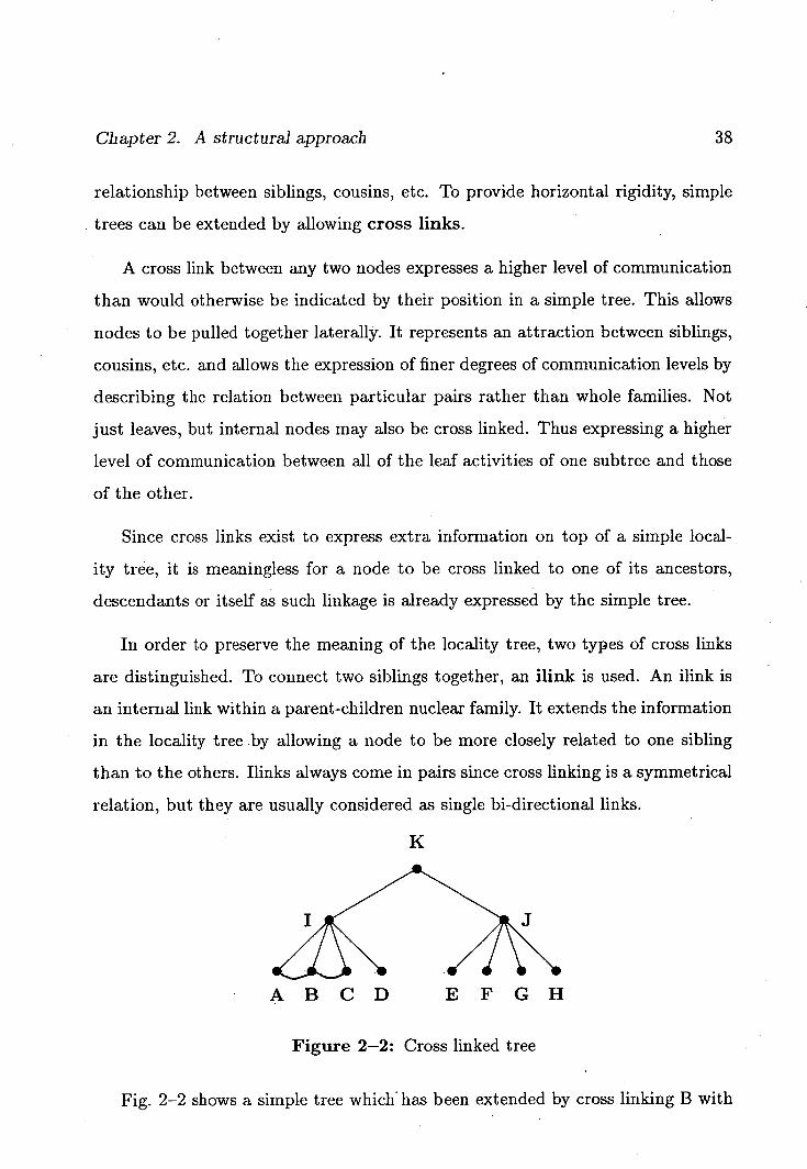
Figure 2-2: Cross linked tree
Fig. 2-2 shows a simple tree which has been extended by cross linking B with
Chapter 2. A structural approach 39
A and C. As B and A, and B and C are sibling relations ilink pairs are used. Such
a tree indicates that B has a higher level of communication with A, C and D than
with E, F, G or H. Furthermore, it shows that B is particularly communicative
with A and C.
For more distantly related nodes an external link or elink is used. Elinks are
used to express external forces on the children of a family caused by the rest of
the locality tree. However, they will never override the family structure. They
allow particular children within a family to be drawn towards other parts of the
locality tree. Having this second type of link allows emphasis to be given to the
hierarchical structure of the locality tree, but still to recognise connections across
that hierarchy.
As with their sibling counterparts, two non-sibling nodes will be cross linked
with a pair of links, in this case elinks. In addition, uni-directional elinks are used
to express how the family as a whole as represented by its parent is also drawn
towards the remotely cross linked node. For example, in Fig. 2-2, if a descendant
of C was cross linked with a descendant of D, then the locality tree should reflect
this increased degree of communication between the two families by cross linking
C and D.
z
A B
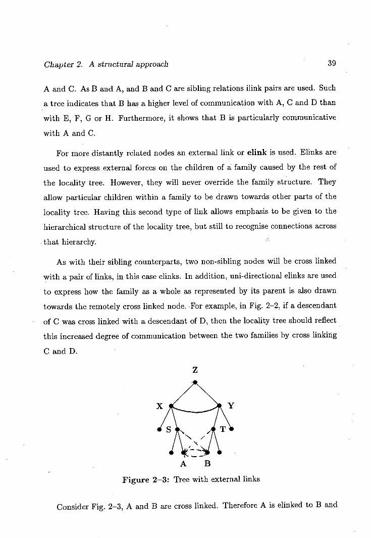
Figure 2-3: Tree with external links
Consider Fig. 2-3, A and B are cross linked. Therefore A is elinked to B and
Chapter 2. A structural approach 40
vice versa. Furthermore, A's parent, S, needs an elink to B so that when the
children of X are considered for mapping, S and therefore A is pulled towards B.
A similar argument requires an elink from T to A. If there were any other ancestor
nodes between S and X or T and Y then they too would be elinked. In the case
of X and Y, the greatest uncles of B and A respectively, they are simply ilinked
to indicate a special closeness between the two families.
In general, if A and B have as their closest common ancestor Z, and X and Y,
children of Z, are ancestors of A and B respectively then all the ancestors from
A up to, but excluding X are elinked to B. If A and X are the same node then
there is no clink to B. Siñiilarly, all the ancestors from B up to, but excluding Y
are clinked to A. In addition, X and Y are junked. If we consider a node to be
an ancestor of itself then this definition reduces to an ordinary pair of ilinks when
the two nodes to be cross linked are siblings. It follows from this definition that a
node will never have an clink to any of its parents' descendants.
2.2.3 Locality tree operations
There are times when it is necessary to broaden or narrow a locality tree. Part of
the mapping algorithm described later requires that the number of children of a
parent be "matched" to the number of processors available. The actual number of
descendant leaf activities remains constant, but the children of a node are grouped
differently in order to increase or decrease the number of nodes at the level below
the parent.
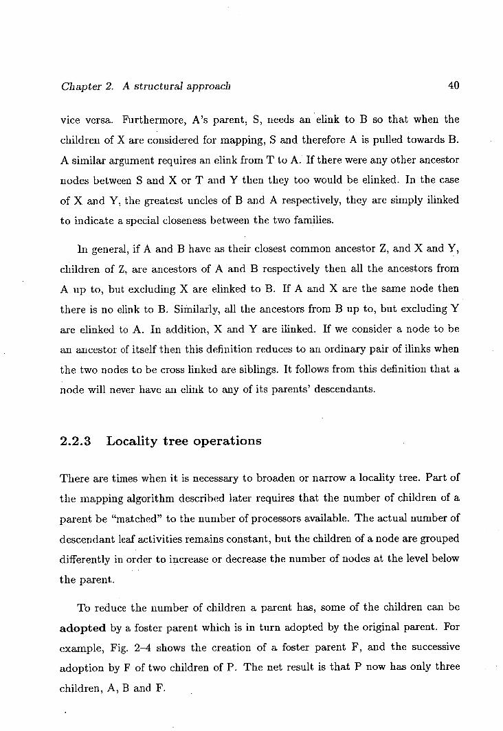
To reduce the number of children a parent has, some of the children can be
adopted by a foster parent which is in turn adopted by the original parent. For
example, Fig. 2-4 shows the creation of a foster parent F, and the successive
adoption by F of two children of P. The net result is that P now has only three
children, A, B and F.
F F
links must be considered when C is adopted.
19
. - B/ /C
A B\
-
E C
Chapter 2. A structural approach
41
IN
F
D CD
Figure 2-4: Child adoption
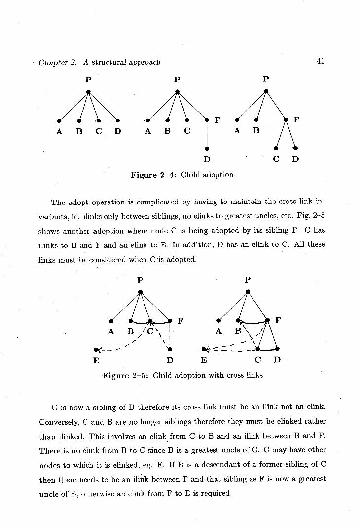
The adopt operation is complicated by having to maintain the cross link in-
variants, ie. junks only between siblings, no elinks to greatest uncles, etc. Fig. 2-5
shows another adoption where node C is being adopted by its sibling F. C has
junks to B and F and an clink to E. In addition, D has an elink to C. All these
Figure 2-5: Child adoption with cross links
C is now a sibling of D therefore its cross link must be an junk not an clink.
Conversely, C and B are no longer siblings therefore they must be clinked rather
than junked. This involves an clink from C to B and an junk between B and F.
There is no clink from B to C since B is a greatest uncle of C. C may have other
nodes to which it is clinked, eg. E. If E is a descendant of a former sibling of C
then there needs to be an junk between F and that sibling as F is now a greatest
uncle of E, otherwise an clink from F to E is required..
Chapter 2. A structural approach 42
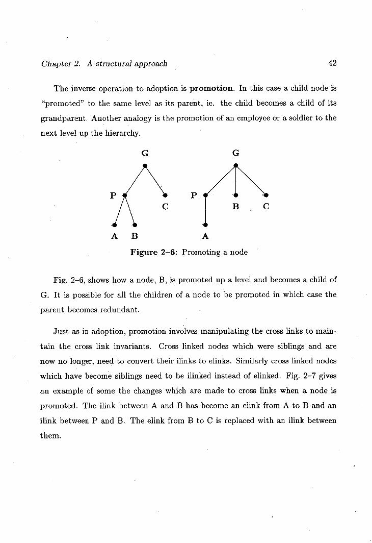
The inverse operation to adoption is promotion. In this case a child node is
"promoted" to the same level as its parent, ie. the child becomes a child of its
grandparent. Another analogy is the promotion of an employee or a soldier to the
next level up the hierarchy.
G G
A B A
Figure 2-6: Promoting a node
Fig. 2-6, shows how a node, B, is promoted up a level and becomes a child of
G. It is possible for all the children of a node to be promoted in which case the
parent becomes redundant.
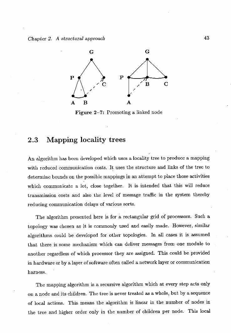
Just as in adoption, promotion involves manipulating the cross links to main-
tain the cross link invariants. Cross linked nodes which were siblings and are
now no longer, need to convert their ilinks to elinks. Similarly cross linked nodes
which have become siblings need to be junked instead of elinked. Fig. 2-7 gives
an example of some the changes which are made to cross links when a node is
promoted. The ilink between A and B has become an elink from A to B and an
ilink between P and B. The elink from B to C is replaced with an ilink between
them.
Chapter 2. A structural approach
43
G G
HE
A B A
Figure 2-7: Promoting a linked node
2.3 Mapping locality trees
An algorithm has been developed which uses a locality tree to produce a mapping
with reduced communication costs. It uses the structure and links of the tree to
determine bounds on the possible mappings in an attempt to place those activities
which communicate a lot, close together. It is intended that this will reduce
transmission costs and also the level of message traffic in the system thereby
reducing communication delays of various sorts.
The algorithm presented here is for a rectangular grid of processors. Such a
topology was chosen as it is commonly used and easily made. However, similar
algorithms could be developed for other topologies. In all cases it is assumed
that there is some mechanism which can deliver messages from one module to
another regardless of which processor they are assigned. This could be provided
in hardware or by a layer of software often called a network layer or communication
harness.
The mapping algorithm is a recursive algorithm which at every step acts only
on a node and its children. The tree is never treated as a whole, but by a sequence
of local actions. This means the algorithm is linear in the number of nodes in
the tree and higher order only in the number of children per node. This local
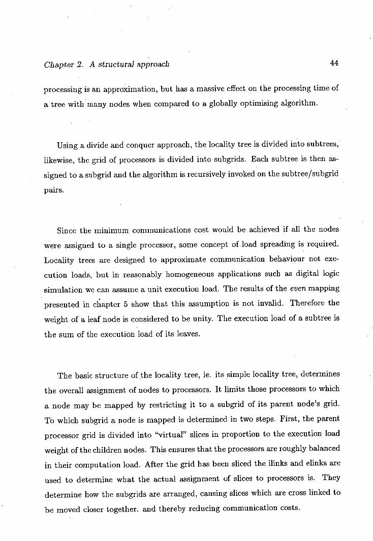
Chapter 2. A structural approach 44
processing is an approximation, but has a massive effect on the processing time of
a tree with many nodes when compared to a globally optimising algorithm.
Using a divide and conquer approach, the locality tree is divided into subtrees,
likewise, the grid of processors is divided into subgrids. Each subtree is then as-
signed to a subgrid and the algorithm is recursively invoked on the subtree/subgrid
pairs.
Since the minimum communications cost would be achieved if all the nodes
were assigned to a single processor, some concept of load spreading is required.
Locality trees are designed to approximate communication behaviour not exe-
cution loads, but in reasonably homogeneous applications such as digital logic
simulation we can assume a unit execution load. The results of the even mapping
presented in chapter 5 show that this assumption is not invalid. Therefore the
weight of a leaf node is considered to be unity. The execution load of a subtree is
the sum of the execution load of its leaves.
The basic structure of the locality tree, ie. its simple locality tree, determines
the overall assignment of nodes to processors. It limits those processors to which
a node may be mapped by restricting it to a subgrid of its parent node's grid.
To which subgrid a node is mapped is determined in two steps. First, the parent
processor grid is divided into "virtual" slices in proportion to the execution load
weight of the children nodes. This ensures that the processors are roughly balanced
in their computation load. After the grid has been sliced the ilinks and elinks are
used to determine what the actual assignment of slices to processors is. They
determine how the subgrids are arranged, causing slices which are cross linked to
be moved closer together. and thereby reducing communication costs.
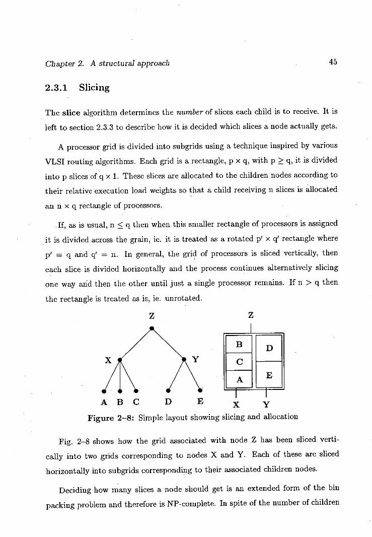
Chapter 2. A structural approach
45
2.3.1 Slicing
The slice algorithm determines the number of slices each child is to receive. It is
left to section 2.3.3 to describe how it is decided which slices a node actually gets.
•A processor grid is divided into subgrids using a technique inspired by various
VLSI routing algorithms. Each grid is a rectangle, p x q, with p ~! q, it is divided
into p slices of q x 1. These slices are allocated to the children nodes according to
their relative execution load weights so that a child receiving n slices is allocated
an n x q rectangle of processors.
If, as is usual, n < q then when. this smaller rectangle of processors is assigned
it is divided across the grain, ie. it is treated as a rotated p' x q' rectangle where
P' = q and q' = n. In general, the grid of processors is sliced vertically, then
each slice is divided horizontally and the process continues alternatively slicing
one way and then the other until just a single processor remains. If n > q then
the rectangle is treated as is, ie. unrotated.
Z z
ABC D E * Figure 2-8: Simple layout showing slicing and allocation
Fig. 2-8 shows how the grid associated with node Z has been sliced verti-
cally into two grids corresponding to nodes X and Y. Each of these are sliced
horizontally into subgrids corresponding to their associated children nodes.
Deciding how many slices a node should get is an extended form of the bin
packing problem and therefore is NP-complete. In spite of the number of children

Chapter 2. A structural approach 46
often being small, it cannot be guaranteed that it is always so and therefore an
approximation algorithm is used.
A child should receive a number of slices proportional to its fraction of the
total execution load of all the children of the parent. Associated with each child is
a standardised weight which represents how worthy the child is of receiving more
slices than it currently has. The weight is an integer between -100 and 100, ie.
.a signed whole number percentage which is a percentage of the total number of
slices being shared out.
As a child starts off with no slices, its initial standardised weight is set to the
percentage it deserves. As slices are allocated to a node, its weight is decreased
by the percentage of the total number of slices which have been allocated to it. If
the standardised weight is positive then the child still deserves more slices, if it is
negative then it has been oversupplied. If child i of node n has a real weight of r1
and has been allocated t2 slices out of a possible p then its standardised weight is
given by,
si flOOr\ (loot.
= TNT ( - TNT ( " Sn I \ p
To distribute the slices, the children nodes are placed in decreasing standard-
ised weight and are allocated their share of the slices in turn. Due to the rounding
errors of integer arithmetic and the granularity of the slices, it is quite likely that
some nodes will receive more than their share and some will receive less, possibly
none.
After the initial allocation, those nodes which have not been allocated any
slices are associated with those with more than their fair share. All of the poor
nodes which have been associated with a particular wealthy benefactor node are
removed from their parent and adopted by a child minder. The child minder and
the benefactor are then merged under one node which is adopted by the original
parent.

Chapter 2. A structural approach
47
Figure 2-9: Matching children to slices
Fig. 2-9 shows a family of four nodes, A, B, C and D which have execution
load weights of 14, I, 4 and 1, respectively. This gives a total of 20. They are to
be mapped to a grid containing 3 slices. So they deserve 2.1, 0.15, 0.6 and 0.15
slices respectively.
As it is not possible to allocate fractions of slices, the nodes must be regrouped
in a way which reduces internal fragmentation. The standardised weight of each
node is calculated and the nodes are placed in order of decreasing weight; A (70),
C (20), B (5), D (5). The nodes are taken in order and allocated slices where each
slice has a standardised weight of 33. While there are still slices, a node is given
a minimum of 1 slice and up to, but not more than its weight's worth. In our
example, the list now looks like;
B has 0 slices and weight 5
D has 0 slices and weight 5
A has 2 slices and weight 4
C has 1 slice and weight -13
Note that due to rounding errors, the sum of standardised weights does not nec-
essarily equal zero.
Unfortunately, B and D have not been allocated any slices. So they have to be
merged with the more successful nodes. Each deprived child is taken in turn and
associated with that node which has the most spare capacity. In this example, B
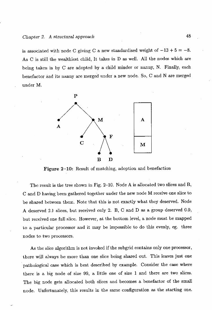
Chapter 2. A structural approach 48
is associated with node C giving C a new standardised weight of —13 + 5 = —8.
As C is still the wealthiest child, It takes in D as well. All the nodes which are
being taken in by C are adopted by a child minder or nanny, N. Finally, each
benefactor and its nanny are merged under a new node. So, C and N are merged
under M.
A
M
B D
Figure 2-10: Result of matching, adoption and benefaction
The result is the tree shown in Fig. 2-10. Node A is allocated two slices and B,
C and D having been gathered together under the new node M receive one slice to
be shared between them. Note that this is not exactly what they deserved. Node
A deserved 2.1 slices, but received only 2. B, C and D as a group deserved 0.9,
but received one full slice. However, at the bottom level, a node must be mapped
to a particular processor and it may be impossible to do this evenly, eg. three
nodes to two processors.
As the slice algorithm is not invoked if the subgrid contains only one processor,
there will always be more than one slice being shared out. This leaves just one
pathological case which is best described by example. Consider the case where
there is a big node of size 99, a little one of size 1 and there are two slices.
The big node gets allocated both slices and becomes a benefactor of the small
node. Unfortunately, this results in the same configuration as the starting one.
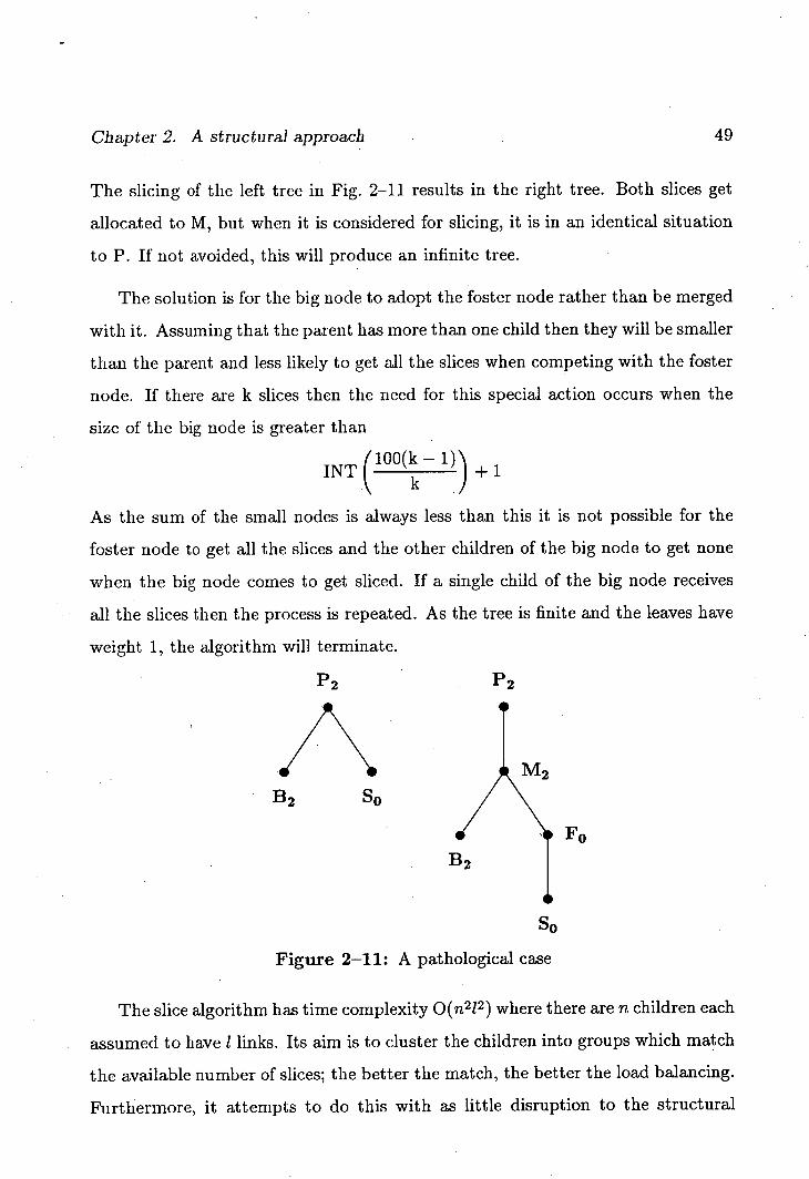
Chapter 2. A structural approach 49
The slicing of the left tree in Fig. 2-11 results in the right tree. Both slices get
allocated to M, but when it is considered for slicing, it is in an identical situation
to P. If not avoided, this will produce an infinite tree.
The solution is for the big node to adopt the foster node rather than be merged
with it. Assuming that the parent has more than one child then they will be smaller
than the parent and less likely to get all the slices when competing with the foster
node. If there are k slices then the need for this special action occurs when the
size of the big node is greater than
flOO(k - i)\ INT(%
k ) +1
As the sum of the small nodes is always less than this it is not possible for the
foster node to get all the slices and the other children of the big node to get none
when the big node comes to get sliced. If a single child of the big node receives
all the slices then the process is repeated. As the tree is finite and the leaves have
weight 1, the algorithm will terminate.
22
-40
B2 so
FO
so
Figure 2-11: A pathological case
The slice algorithm has time complexity O(n2 1 2 ) where there are n children each
assumed to have 1 links. Its aim is to cluster the children into groups which match
the available number of slices; the better the match, the better the load balancing.
Furthermore, it attempts to do this with as little disruption to the structural
Chapter 2. A structural approach 50
information as possible. Except for the pathological case just described, poor
children are adopted by a nanny rather than the benefactor directly in order to
keep them separate from the benefactor's children. It also combines poor children
into a bigger family which will have a better chance of receiving slices in its own
right. Finally, the resulting tree tends towards being tall and thin which reduces
the time taken to process a family, a quadratic function, at the cost of traversing
more nodes, a linear function.
2.3.2 Load balancing control
If nodes received exactly the number of slices they deserved then all the processors
would be evenly loaded given our assumption of unit execution load. However, as
we saw in the previous example there can be a discrepancy between what a node
deserves and what a node gets. This will cause uneveness in the load balancing of
the processors.
The slicing algorithm was extended to allow control over the level of permitted
load imbalance. A limit, p, can be imposed which prevents the production of a
mapping which has allocated too many or too few activities to a grid of processors
in comparison with the overall average load.
An evenly balanced load, /3 is equal to the real weight of the whole tree divided
by the number of processors. Load imbalance is measured in terms of deviation
from 3. A value of p = 1 corresponds to a deviation from 3 by /3, ie. double the
average load.
After the slices have been divided up amongst the children, a check is made
to see whether any node has been under allocated by more than an allowable
amount. A node i, with real weight r1 and t2 slices of size q has been unacceptably
underpowered if
r2 > /3tq(1 + p)
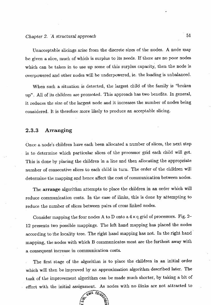
Chapter 2. A structural approach
611
Unacceptable slicings arise from the discrete sizes of the nodes. A node may
be given a slice, much of which is surplus to its needs. If there are no poor nodes
which can be taken in to use up some of this surplus capacity, then the node is
overpowered and other nodes will be underpowered, ie. the loading is unbalanced.
When such a situation is detected, the largest child of the family is "broken
up". All of its children are promoted. This approach has two benefits. In general,
it reduces the size of the largest node and it increases the number of nodes being
considered. It is therefore more likely to produce an acceptable slicing.
2.3.3 Arranging
Once a node's children have each been allocated a number of slices, the next step
is to determine which particular slices of the processor grid each child will get.
This is done by placing the children in a line and then allocating the appropriate
number of consecutive slices to each child in turn. The order of the children will
determine the mapping and hence affect the cost of communication between nodes.
The arrange algorithm attempts to place the children in an order which will
reduce communication costs. In the case of ilinks, this is done by attempting to
reduce the number of slices between pairs of cross linked nodes.
Consider mapping the four nodes A to D onto a 4 x q grid of processors. Fig. 2-
12 presents two possible mappings. The left hand mapping has placed the nodes
according to the locality tree. The right hand mapping has not. In the right hand
mapping, the nodes with which B communicates most are the furthest away with
a consequent increase in communication costs.
The first stage of the algorithm is to place the children in an initial order
which will then be improved by an approximation algorithm described later. The
task of the improvement algorithm can be made much shorter, by taking a bit of
effort with the initial assignment. As nodes with no ilinks are not attracted to
'$'
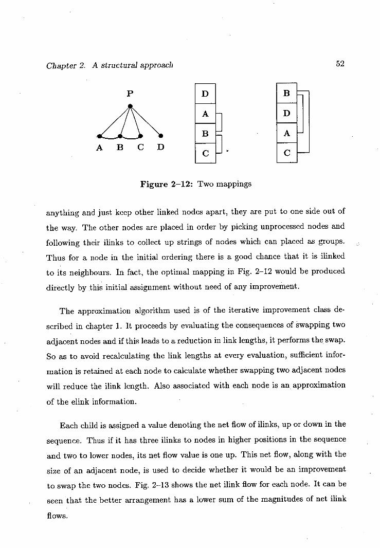
Chapter 2. A structural approach
52
Figure 2-12: Two mappings
anything and just keep other linked nodes apart, they are put to one side out of
the way. The other nodes are placed in order by picking unprocessed nodes and
following their ilinks to collect up strings of nodes which can placed as groups.
Thus for a node in the initial ordering there is a good chance that it is junked
to its neighbours. In fact, the optimal mapping in Fig. 2-12 would be produced
directly by this initial assignment without need of any improvement.
The approximation algorithm used is of the iterative improvement class de-
scribed in chapter 1. It proceeds by evaluating the consequences of swapping two
adjacent nodes and if this leads to a reduction in link lengths, it performs the swap.
So as to avoid recalculating the link lengths at every evaluation, sufficient infor-
mation is retained at each node to calculate whether swapping two adjacent nodes
will reduce the junk length. Also associated with each node is an approximation
of the elink information.
Each child is assigned a value denoting the net flow of ilinks, up or down in the
sequence. Thus if it has three junks to nodes in higher positions in the sequence
and two to lower nodes, its net flow value is one up. This net flow, along with the
size of an adjacent node, is used to decide whether it would be an improvement
to swap the two nodes. Fig. 2-13 shows the net ilink flow for each node. It can be
seen that the better arrangement has a lower sum of the magnitudes of net junk
flows.
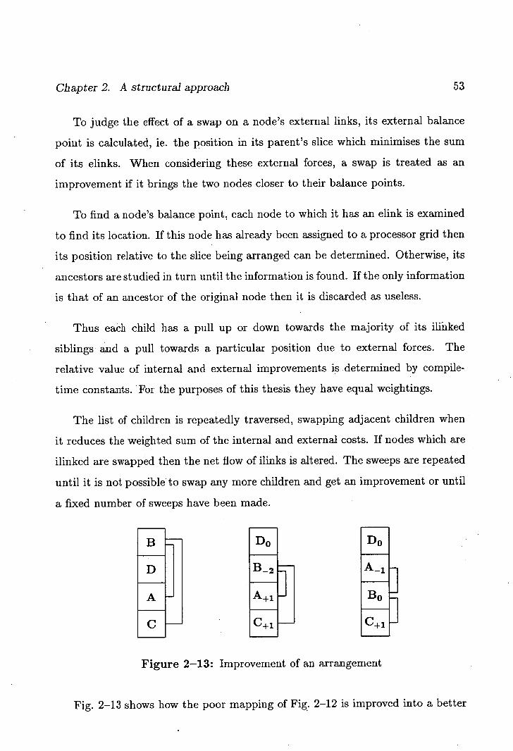
Chapter 2. A structural approach
53
To judge the effect of a swap on a node's external links, its external balance
point is calculated, ie. the position in its parent's slice which minimises the sum
of its elinks. When considering these external forces, a swap is treated as an
improvement if it brings the two nodes closer to their balance points.
To find a node's balance point, each node to which it has an elink is examined
to find its location. If this node has already been assigned to a processor grid then
its position relative to the slice being arranged can be determined. Otherwise, its
ancestors are studied in turn until the information is found. If the only information
is that of an ancestor of the original node then it is discarded as useless.
Thus each child has a pull up or down towards the majority of its junked
siblings and a pull towards a particular position due to external forces. The
relative value of internal and external improvements is determined by compile-
time constants. For the purposes of this thesis they have equal weightings.
The list of children is repeatedly traversed, swapping adjacent children when
it reduces the weighted sum of the internal and external costs. If nodes which are
ilinked are swapped then the net flow of ilinks is altered. The sweeps are repeated
until it is not possible' to swap any more children and get an improvement or until
a fixed number of sweeps have been made.
LIki
J_J
Do Do
[1H _
rF _
Figure 2-13: Improvement of an arrangement
Fig. 2-13 shows how the poor mapping of Fig. 2-12 is improved into a better
Chapter 2. A structural approach 54
one. In this example, each of the nodes has been allocated a single slice and there
are no elinks.
The first step is to allocate those nodes with no ilinks. For this reason D is
placed in slot 0, out of the way. Next, an unprocessed node is chosen and allocated
to slot 1. Normally, a node with just 1 ilink is chosen if it exists in an attempt to
straighten out tangles in the iliuk graph. However, for the sake of example, node
B is chosen to go into slot 2. Those nodes to which B has an junk are examined
and the first unprocessed node found is allocated to the next slot. In this case, it is
A. The junks of A are checked, but all its links are to processed nodes. Therefore
another node, C, is chosen from the list of unprocessed nodes and allocated to the
next slot. As all of the nodes are allocated, the initial assignment is complete.
Before the improvement algorithm can commence, the net ilink flow is calcu-
lated for each node. This is just the number of ilinks to nodes in higher positions
minus the number of iliiiks to nodes in lower ones. The net flows are shown in the
middle mapping of Fig. 2-13.
As there are no elinks, D will never move. So the first swap to be considered
is that of B and A. Moving B down a slot would improve the mapping by +2
(B's net flow times the size of A, ie. 1) and moving A up would improve it by
+1 (A's net flow times the size of B) From the total of +3 is subtracted 2 (the
sum of their sizes) as the two adjacent nodes are ilinked and the swapping does
not affect that ilink. As +1 > 0, the swap is done giving the right hand mapping
in the figure. In the next sweep through the nodes, no improvement is found and
the algorithm terminates. Swapping A and B or B and C gives an improvement
of -1 and therefore these swaps are discarded.
The combination of a simple initial assignment with an improvement algorithm
produces good results. For small numbers of nodes it is possible to evaluate the
objective function for every arrangement of nodes in every possible topology. This
Chapter 2. A structural approach 55
was done and an optimal mapping for each combination of links for a given number
of nodes was found.
For each combination, the optimal mapping was compared with the mapping
found by the algorithm presented above. It was found that the algorithm found
an arrangement equal to the optimal in all topologies of four nodes, over 95% of
topologies with five nodes and over 2/3 of the topologies with 6 nodes.
The time complexity of the algorithm is linear in the product of the number of
nodes and the number of ilinks; evaluating and executing a swap takes constant
time.
2.3.4 Allocation
After the nodes have been sliced and arranged they are allocated in turn to the
subgrids of the parent node's grid according to whether the grid is sliced verti-
cally or horizontally. Finally the mapping algorithm is invoked on each of the
node/subgrid pairs.
The tree is traversed in a depth-first manner for the sake of convenience, but
it is important that each child of a family is allocated to a specific processor
grid before any of the child subtrees are processed. This provides a node being
assigned with a general indication of the location, in relation to its own processor
grid, of any node to which its children have an elink. This is enough information
to determine the external balance points of the children nodes.
The mapping algorithm is an approximation algorithm and is not guaranteed
to give the optimal arrangement. However, it is the intention that tall, thin trees
are used with a small number of children per node. In these cases, very good results
for each node are likely within a short amount of time. The mapping algorithm is
0(m2 ), but the proof of the pudding is in the eating so the remaining chapters of

Chapter 2. A structural approach
56
this thesis present an implementation in which to test this new approach and the
results of using it.
Chapter .3
Parallel Simulation
3.1 Motivation
One application which displays the properties required by the structural mapping
approach is that of the simulation of digital logic circuits. It is becoming more
common for logic circuits to be designed hierarchically and yet they do not have
a regular structure which allows their simulation to be easily mapped.
The trend in circuit design is to use hardware description languages (HDLs)
such as Ella [45] and Model [38] and computer aided design environments such as
SOLO 1000 [38], which promote a structural approach to the design of circuits.
Apart from its suitability as an application for a structural mapping, there is a
growing demand for more powerful logic simulators. A parallel approach has the
potential for significant performance improvements.
57
Chapter 3. Parallel Simulation
RRI
3.2 What is a simulator?
A simulator is a tool which given a description of a system can, within the limita-
tions of the description, behave like that system. Thus the simulator implements
an abstraction of the described system where the state of the simulation at a given
simulation time corresponds to the state of the real system at the corresponding
real time. We say a simulation is correct if this correspondence is indeed the case.
Simulators can be divided into two classes. In one, simulation time progresses
smoothly. Such simulators are called continuous and are often implemented
using analogue techniques. They are typically used when the system is described in
terms of continuous equations such as the wave equation or the laws of gravitation.
The alternative is for simulation time to progress in a series of steps. Sim-
ulators which have such a quantised time are called discrete and are typically
implemented using a digital computer. This thesis is concerned only in the latter
class of discrete simulators.
To say simulation time proceeds as a series of steps means that the state of the
simulation is calculated only at specific points in the simulation time continuum.
For such a simulation to be correct, the simulation designer needs to ensure that
the simulation does not miss any state changes during such time steps.
In time-driven simulators, the series is regular; there is a constant time
interval between state calculations, eg., simulating a digital circuit in 1 ns steps.
In this case, it is necessary to ensure that the value of signals do not change then
change again within less than 1 ns otherwise the simulator would miss all but the
last change.
Another pitfall of the time-driven approach is that if the time interval is much
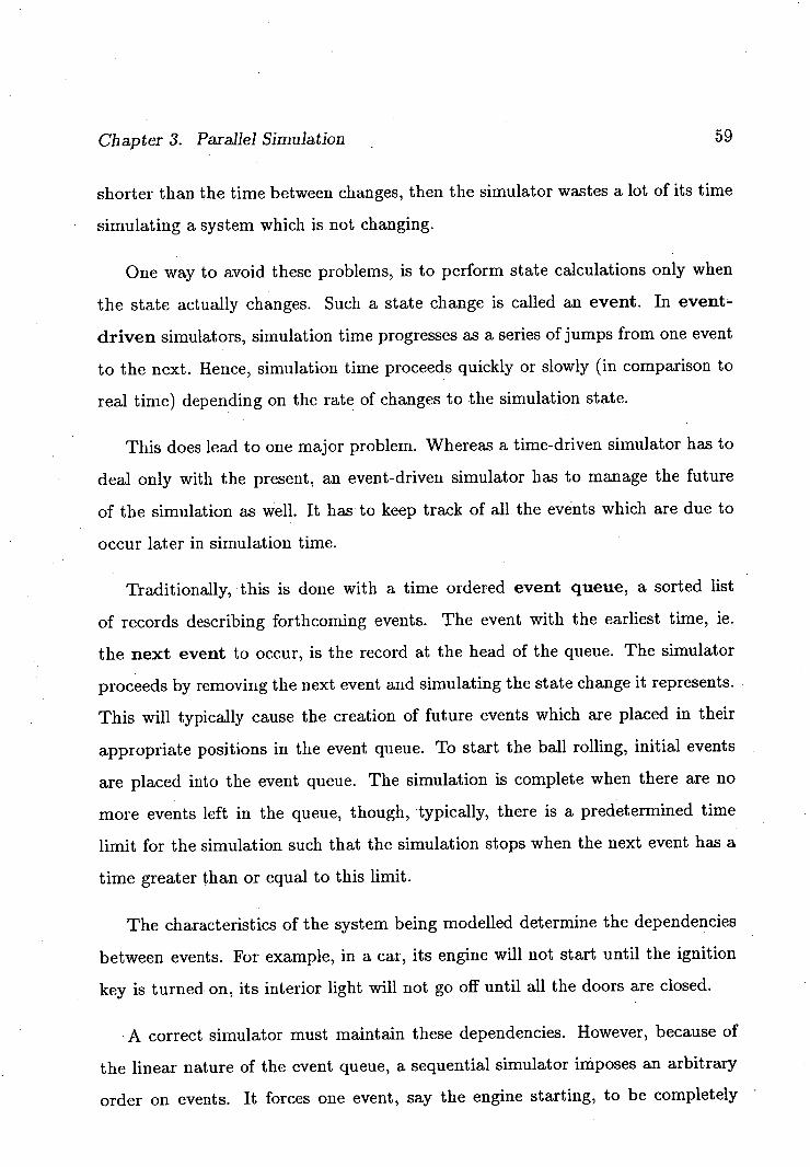
Chapter 3. Parallel Simulation 59
shorter than the time between changes, then the simulator wastes a lot of its time
simulating a system which is not changing.
One way to avoid these problems, is to perform state calculations only when
the state actually changes. Such a state change is called an event. In event-
driven simulators, simulation time progresses as a series of jumps from one event
to the next. Hence, simulation time proceeds quickly or slowly (in comparison to
real time) depending on the rate of changes to the simulation state.
This does lead to one major problem. Whereas a time-driven simulator has to
deal only with the present, an event-driven simulator has to manage the future
of the simulation as well. It has to keep track of all the events which are due to
occur later in simulation time.
Traditionally, this is done with a time ordered event queue, a sorted list
of records describing forthcoming events. The event with the earliest time, ie.
the next event to occur, is the record at the head of the queue. The simulator
proceeds by removing the next event and simulating the state change it represents.
This will typically cause the creation of future events which are placed in their
appropriate positions in the event queue. To start the ball rolling, initial events
are placed into the event queue. The simulation is complete when there are no
more events left in the queue, though, typically, there is a predetermined time
limit for the simulation such that the simulation stops when the next event has a
time greater than or equal to this limit.
The characteristics of the system being modelled determine the dependencies
between events. For example, in a car, its engine will not start until the ignition
key is turned on, its interior light will not go off until all the doors are closed.
• A correct simulator must maintain these dependencies. However, because of
the linear nature of the event queue, a sequential simulator imposes an arbitrary
order on events. It forces one event, say the engine starting, to be completely
Chapter 3. Parallel Simulation 60
simulated before or after another, eg. the interior light going off, even though
they are totally independent and could be simulated in parallel. Thus the use of
the event queue destroys any natural parallelism that might be present in the real
system by forcing a serial execution of the simulation.
3.3 The process model
Often, a natural way to describe a system is to describe the behaviour of its com-
ponents and how they interact. The process or scenario model as it is called by
Franta [21] views a. system as a collection of interacting activities; a network of
processes where each process is a.separate, independently existing agent. Typi-
cally, but not necessarily, an agent maintains some local state information.
Such an approach is similar to that of the object model [33] where the state of
the system is described in terms of the states of its components. Here, the system
is described as a collection of objects; an object being some local, private state
information and a well-defined set of operations on that state which other objects
can invoke. For example, in Smalltalk80 [57], objects are accessed by invoking
their operations using a restricted form of message passing similar to a procedure
call.
The essential difference between the two is that the process model emphasises
the activities within the system. Its basic unit is an active component, perhaps
with no state at all, a pure function. The object model focuses on the state of the
system and systems are described in terms of passive components.
Typically, as is the case in Smalltalk80, objects are active only when they are
handling requests. On the other hand, processes are not so restricted, making the
process model more powerful. In those object based systems such as POOL [3,
Chapter 3. Parallel Simulation 61
1] where objects can be active between requests the distinction between models
becomes quite blurred.
3.3.1 A parallel implementation
Independently, Bryant at MIT [11] and Chandy at a series of lectures at the
University of Waterloo and later in conjunction with Misra [12,13,44] proposed
mechanisms for successfully implementing a process based simulation on a parallel
processing system.
In their approach, each of the physical components or processes in the real sys-
tern is simulated by an autonomous logical process in the simulator. For example,
there would be a logical process for each gate in a circuit or each unit volume in a
model of the weather. The interaction between two physical processes is simulated
by the sending of messages between the two corresponding logical processes.
More strictly, a physical system can be simulated by associating a separate
logical process (ip) with each physical process (pp) where 1p i simulates the actions
of pp• If ppi affects pp, then let there be a channel or link from 1pi to lp3 . If
an ip knows the initial state and all the events that occur to its corresponding pp
up to time t then it can simulate the actions of the pp up to at least that time t
and possibly beyond.
As an example consider the simulation of a doctors' surgery, as described in
Fig. 3-1. Patients enter the surgery and go into the waiting room. When a doctor
becomes free, the patient who has been waiting the longest is sent to see him.
After consultation, the (hopefully) cured patient leaves via the exit.
Fig. 3-1 is an annotated interconnection graph (as described in section 1.2.1) of
a doctor's surgery system. Each of the nodes represent a physical process such as a
queueing of waiting patients or a doctor's consultation with a patient. The arrows
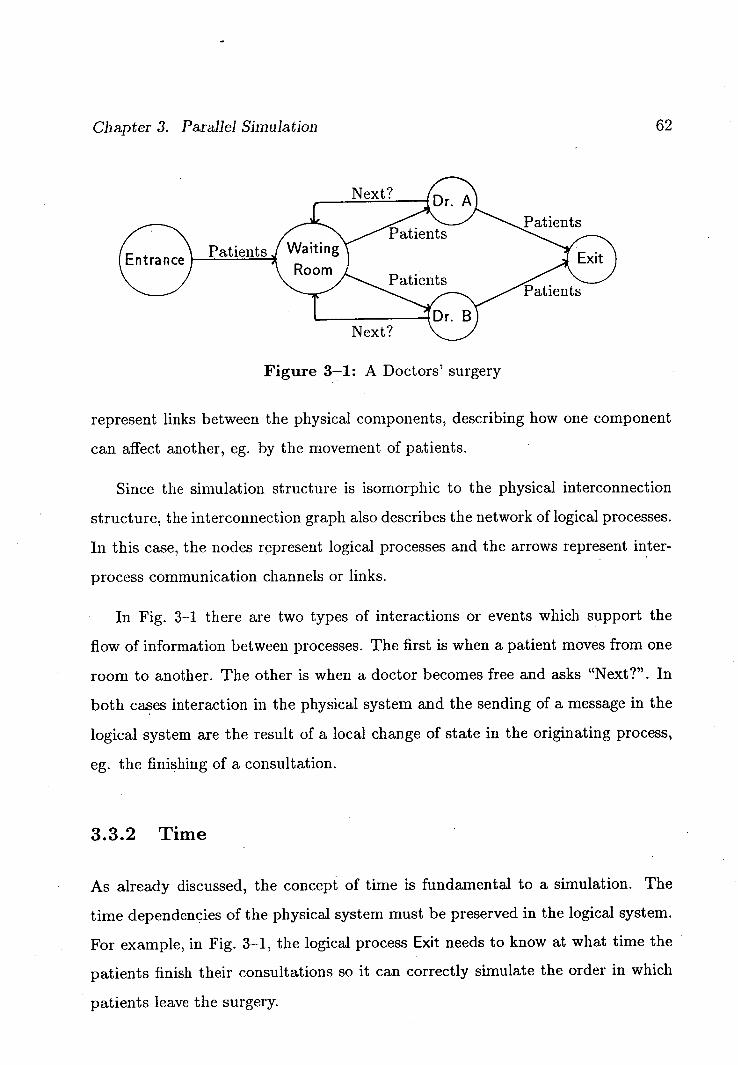
Chapter 3. Parallel Simulation 62
t? [Dr. A ients
Waitin Patients
•Exit Entralv ~~
PatientsRoom
Patients
ts
Patients
Next?
Figure 3-1: A Doctors' surgery
represent links between the physical components, describing how one component
can affect another, eg. by the movement of patients.
Since the simulation structure is isomorphic to the physical interconnection
structure, the interconnection graph also describes the network of logical processes.
In this case, the nodes represent logical processes and the arrows represent inter-
process communication channels or links.
In Fig. 3-1 there are two types of interactions or events which support the
flow of information between processes. The first is when a patient moves from one
room to another. The other is when a doctor becomes free and asks "Next?". In
both cases interaction in the physical system and the sending of a message in the
logical system are the result of a local change of state in the originating process,
eg. the finishing of a consultation.
3.3.2 Time
As already discussed, the concept of time is fundamental to a simulation. The
time dependencies of the physical system must be preserved in the logical system.
For example, in Fig. 3-1, the logical process Exit needs to know at what time the
patients finish their consultations so it can correctly simulate the order in which
patients leave the surgery.
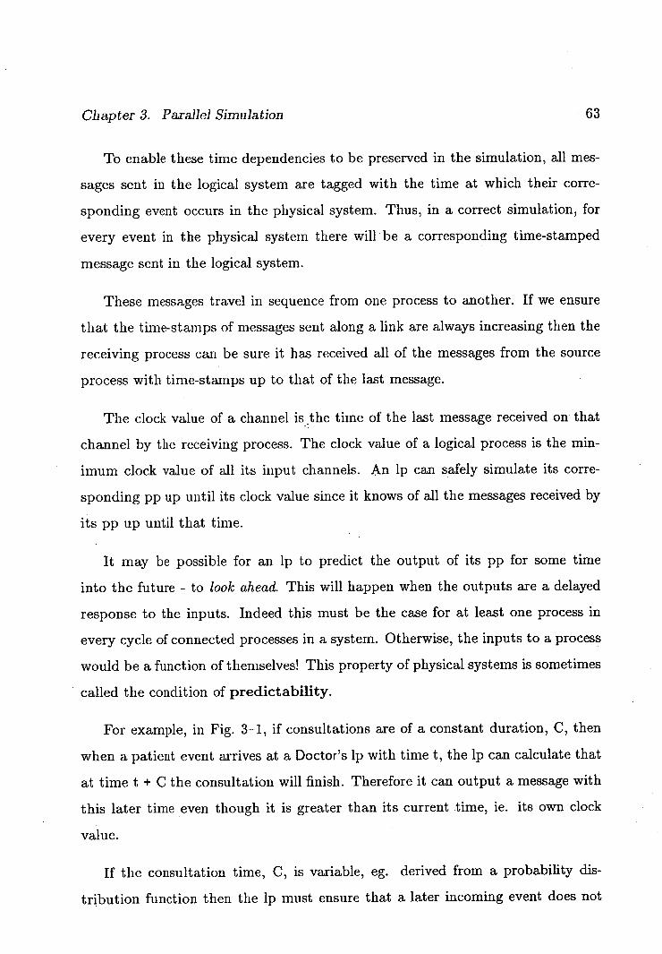
Chapter 3. Parallel Simulation
63
To enable these time dependencies to be preserved in the simulation, all mes-
sages sent in the logical system are tagged with the time at which their corre-
sponding event occurs in the physical system. Thus, in a correct simulation, for
every event in the physical system there will be a corresponding time-stamped
message sent in the logical system.
These messages travel in sequence from one process to another. If we ensure
that the time-stamps of messages sent along a link are always increasing then the
receiving process can be sure it has received all of the messages from the source
process with time-stamps up to that of the last message.
The clock value of a channel is the time of the last message received on that
channel by the receiving process. The clock value of a logical process is the min-
imum clock value of all its input channels. An ip can safely simulate its corre-
sponding pp up until its clock value since it knows of all the messages received by
its pp up until that time.
It may be possible for an lp to predict the output of its pp for some time
into the future - to look ahead. This will happen when the outputs are a delayed
response to the inputs. Indeed this must be the case for at least one process in
every cycle of connected processes in a system. Otherwise, the inputs to a process
would be a function of themselves! This property of physical systems is sometimes
called the condition of predictability.
For example, in Fig. 3-1, if consultations are of a constant duration, C, then
when a patient event arrives at a Doctor's ip with time t, the ip can calculate that
at time t + C the consultation will finish. Therefore it can output a message with
this later time even though it is greater than its current time, ie. its own clock
value.
If the consultation time, C, is variable, eg. derived from a probability dis-
tribution function then the lp must ensure that a later incoming event does not
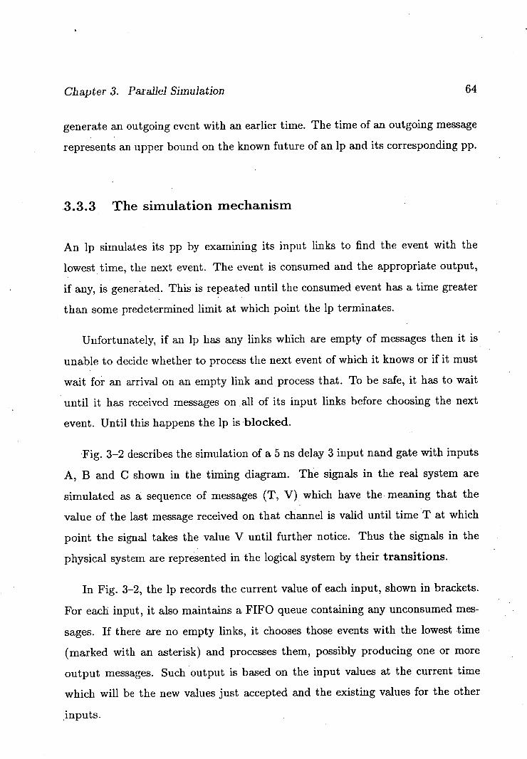
Chapter 3. Parallel Simulation 64
generate an outgoing event with an earlier time. The time of an outgoing message
represents an upper bound on the known future of an ip and its corresponding pp.
.3.3.3 The simulation mechanism
An ip simulates its pp by examining its input links to find the event with the
lowest time, the next event. The event is consumed and the appropriate output,
if any, is generated. This is repeated until the consumed event has a time greater
than some predetermined limit at which point the ip terminates.
Unfortunately, if an ip has any links which are empty of messages then it is
unable to decide whether to process the next event of which it knows or if it must
wait for an arrival on an empty link and process that. To be safe, it has to wait
until it has received messages on all of its input links before choosing the next
event. Until this happens the lp is blocked.
Fig. 3-2 describes the simulation of a 5 ns delay 3 input nand gate with inputs
A l B and C shown in the timing diagram. The signals in the real system are
simulated as a sequence of messages (T, V) which have the meaning that the
value of the last message received on that channel is valid until time T at which
point the signal takes the value V until further notice. Thus the signals in the
physical system are represented in the logical system by their transitions.
In Fig. 3-2, the lp records the current value of each input, shown in brackets.
For each input, it also maintains a FIFO queue containing any unconsumed mes-
sages. If there are no empty links, it chooses those events with the lowest time
(marked with an asterisk) and processes them, possibly producing one or more
output messages. Such output is based on the input values at the current time
which will be the new values just accepted and the existing values for the other
inputs.
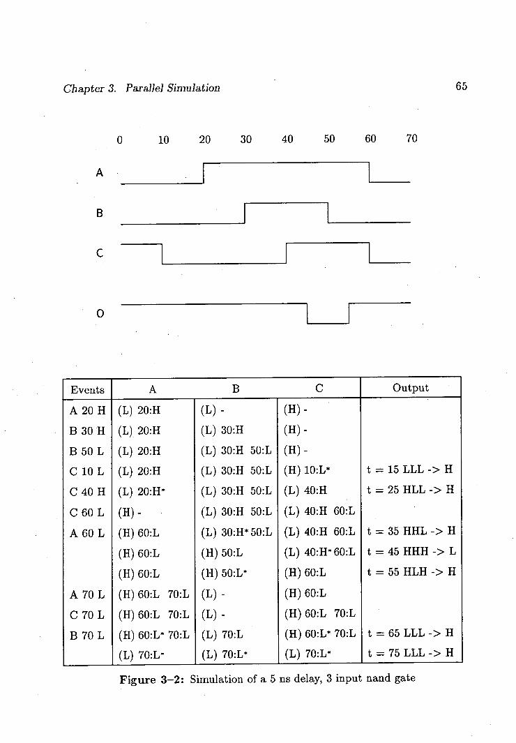
Chapter 3. Parallel Simulation 65
0 10 20 30 40 50 60 70
A
I:]
C
0 1
Events A B C Output
A 20 H (L) 20:H (L) - (H) -
B 30 H (L) 20:H (L) 30:H (H) -
B 50 L (L) 20:H (L) 30:H 50:L (H) -
C 10 L (L) 20:H (L) 30:H 50:L (H) 10 : L* t = 15 LLL -> H
C 40 H (L) 20 : H* (L) 30:H 50:L (L) 40:H t = 25 HLL -> H
C 60 L (H) - (L) 30:H 50:L (L) 40:H 60:L
A 60 L (H) 60:L (L) 30:H* 50:L (L) 40:H 60:L t = 35 HilL -> H
(H) 60:L (H) 50:L (L) 40:H* 60:L t = 45 HHH -> L
(H) 60:L (H) 50 : L* (H) 60:L t = 55 HLH -> H
A 70 L (H) 60:L 70:L (L) - (H) 60:L
C 70 L (H) 60:L 70:L (L) - (H) 60:L 70:L
B 70 L (H) 60:L* 70:L (L) 70:L (H) 60:L* 70:L t = 65 LLL -> H
(L) 70 : L* (L) 70 : L* (L) 70 : L* t = 75 LLL -> H
Figure 3-2: Simulation of a 5 ns delay, 3 input nand gate

Chapter 3. Parallel Simulation
Consider the arrival of (10, L) on input C. At this point there are messages
on each link so the ip can safely choose 10:L on input C as the next event. It
removes this event from its queue, sets the ip's clock value to 10 and outputs an
event. This event is computed as follows. At time 10, all inputs have become low
therefore in 5 ns time the output will become high. Note that the output may have
already been high, the new message simply extends the receiving ips' knowledge
by saying that the output is high until at least time 15.
Though they do not correspond to any transition in the physical system, the
events with time 70 are necessary. They ensure that the lp receives the full history
of each input signal up until the time limit of the simulation. If they were not
sent, the output of the gate would not be known for certain after time 55. Since
they are sent, the lp can provide definite values for the output of the gate until at
least the time limit.
Let us call a message with a time at or after the simulation time limit a
terminating message. Once an ip has received a terminating message on each of
its input channels, it is able to send out terminating messages of its own and for
itself to terminate. It is necessary that any source of signals into the system sends
a terminating message to ensure that all the lps can correctly terminate.
3.4 Deadlock and Failure to proceed
If for any reason an input link of an lp remains empty then the lp cannot proceed
beyond the time of the last message received on that link. Returning to the
doctors' surgery example of Fig. 3-1, if the waiting room attendant always sends
patients to Dr A then Exit will never receive any messages from Dr B. Therefore
the Exit ip fails to proceed since it cannot be sure that after processing events from
Dr A, events with earlier times will not arrive from Dr B. As soon as a message
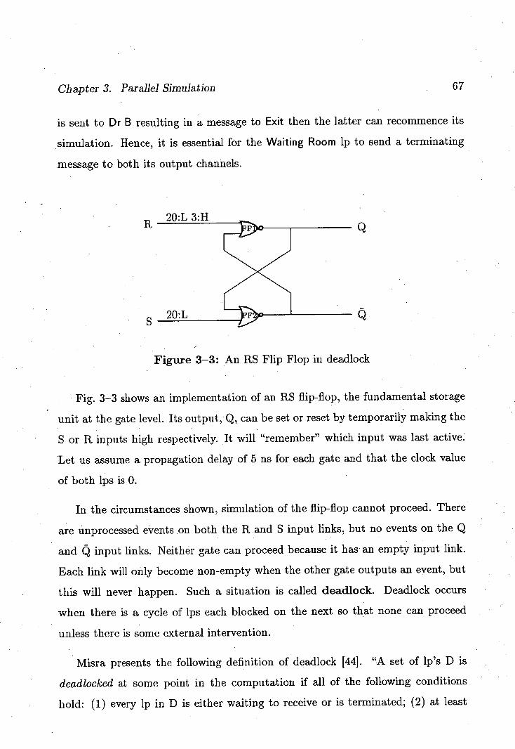
R 20:L 3:1-1
S
us
Eel
Chapter 3. Parallel Simulation 67
is sent to Dr B resulting in a message to Exit then the latter can recommence its
simulation. Hence, it is essential for the Waiting Room lp to send a terminating
message to both its output channels.
Figure 3-3: An RS Flip Flop in deadlock
• Fig. 3-3 shows an implementation of an RS flip-flop, the fundamental storage
unit at the gate level. its output, Q, can be set or reset by temporarily making the
S or R inputs high respectively. It will "remember" which input was last active.
Let us assume a propagation delay of 5 ns for each gate and that the clock value
of both lps isO.
In the circumstances shown, simulation of the flip-flop cannot proceed. There
are unprocessed events on both the Rand S input links, but no events on the Q
and Q input links. Neither gate can proceed because it has an empty input link.
Each link will only become non-empty when the other gate outputs an event, but
this will never happen. Such a situation is called deadlock. Deadlock occurs
when there is a cycle of ips each blocked on the next so that none can proceed
unless there is some external intervention.
Misra presents the. following definition of deadlock [44]. "A set of lp's D is
deadlocked at some point in the computation if all of the following conditions
hold: (1) every lp in D is either waiting to receive or is terminated; (2) at least
Chapter 3. Parallel Simulation 68
one ip in D is waiting to receive; (3) for any lp 3 in D that is waiting to receive
from some 1p3 , lp3 is also in D, and there is no message in transit from 1p i to lp."
Deadlock is different from the failure to proceed in the doctors' surgery example
because regardless of what other events might come along, the flip flop simulation
is permanently blocked. However, there is a possibility, if the terminating message
has not been received, that an event might arrive in the doctors' surgery example
which allows the simulation to proceed. Therefore, there might not actually be
a problem except that of storing all the unprocessed messages. The difficulty is
to distinguish between the failure to proceed which will be resolved when another
message eventually arrives and true deadlock when another message will never
arrive.
3.5 Deadlock avoidance and recovery
To avoid the problem of deadlock, Peacock et al. developed a more powerful test
on which to block lps [48,47]. Let net(i) be the minimum time of messages received
and waiting to be accepted at lp 2 and c(i,j) = 1 when there is a path of empty links
from 1pi to lp3 and 0 otherwise. If min{net(i) such that c(i,j) = 11 <net(j) then j
is blocked. It is guaranteed that the lp with the minimum net in the entire system
is not blocked and therefore the simulation cannot deadlock. Unfortunately, it is
very expensive to calculate c(i, j) in general making the algorithm unfeasible.
Consider Fig. 3-3, with knowledge of the state of both gates, it can be seen that
it is safe for the FF1 lp to accept the next event which it knows about, 3:H, since
whatever events arrive on its empty link will have a later time-stamp. Similarly,
it is safe for Exit to accept the events from Dr A even in the absence of messages
from Dr B. Unfortunately, such global knowledge is not available at the local level
of the lps.
Chapter 3. Parallel Simulation
MIS
The basic problem is the logical system's inability to simulate inaction. Mes-
sages are sent only when they are simulating an action in the physical system.
The simulation mechanism as described can only simulate the lack of action by
not sending any messages, but these messages are sometimes essential for the
simulation to succeed.
3.5.1 Null messages
Chandy and Misra [12] have proposed the use of null messages which can be sent
to say that nothing has changed allowing the receiving lps to proceed. In the
doctors' surgery example, the Waiting Room lp could send null messages to the Dr
B ip which would cause it to send null messages to Exit which could then happily
accept events from Dr A. In the flip-flop example, FF2 can send a null message to
FE1 with time 5 with safety, since whatever events arrive after its current clock
value of 0 will produce events with times greater than 5. Now that FF1 has no
empty links it can proceed to accept its next event.
To use null messages, the basic simulation mechanism is extended as follows.
At the end of every simulation cycle of an lp, the simulator ensures that the clock
value of each output channel is at least that of the clock channel of the ip by
sending out a null message on every output channel. If 1p i can predict that pp
will not send any more messages to pp, before time t 23 then it sends a null message
with time t ij to lp3 after sending the sequence of real messages. The times t, are
guaranteed to be at least that of the clock value of the ip.
Basically, if an lp is to send out a real message on one of its output channels,
it also sends out null messages on the other output channels. These null messages
might then cause other lp's to fire. Thus avoiding deadlock.
Even when the physical system being simulated deadlocks the simulator will

Chapter 3. Parallel Simulation 70
still proceed to completion since it can use null messages to describe the physical
system's inaction.
Misra presents a proof that a simulator based on such an extended mechanism
will never deadlock [44]. However, the proof is incomplete since the paper never
describes how the simulator is properly initialised. By defining the clock channel
value to be 0 if no message has been received along that channel, Misra implies that
input links begin empty. In both the basic and extended mechanisms, messages are
output only in response to an input message. Putting these two points together,
an ip will only output messages, null or otherwise, once it has received messages
on all its inputs which still leaves our flip-flop deadlocked. However, once the
deadlock has been recovered from, the flip-flop will not deadlock again.
Though it is not described in the text, by studying one of the example tables,
(table 6) it is revealed that Misra allows lps to send messages, which are not in
response to any input message. At the start of the simulation, every ip in the
system sends a null message with a time as far into the future as it can safely
predict. There are two disadvantages with this scheme. By requiring unprompted
messages, the data driven nature of the mechanism has been destroyed, compli-
cating the implementation. Secondly, such a scheme causes a flood of initial null
messages which can cause a cascade of further unnecessary null messages.
The simulator presented later in this thesis avoids these problems by initialising
all input queues to contain a (0, NULL) message. No null messages need be
sent and channel and ip clock values have a sensible initial value. The storage
requirements are well within that which is required for normal processing during
a simulation. With this extension, Misra's proof is now valid for the ordinary
data-driven extended simulation mechanism.
A major problem with the null message approach is that the acceptance of
any message, with a distinct time, even a null message, will cause the creation of
at least one new message for each output channel. If the network contains nodes
Chapter 3. Parallel Simulation 71
with a high branching factor or fanout, this can cause the simulator to become
overloaded with null messages. This becomes particularly acute when the system
contains cycles. A form of positive feedback in the generation of null messages can,
exist which leads to an explosion of null messages consuming all the simulator's
storage.
Such flooding of the system can be alleviated to some extent by allowing real
messages to subsume any null messages before them in an input queue. Since
a null message has no effect if it is followed by a real message it can be safely
eliminated when the next real message arrives on the same channel.
In a similar vein, it might improve performance if lps delayed transmission of
the null message in case a real message is generated soon after. If no real message
is generated within a certain time only then is the null message sent. This scheme
reduces to the ordinary null message scheme if the time-out is zero. However, an
extensive literature search has failed to find any empirical studies describing the
effect of non-zero time-outs.
Going one step further Misra[44] proposed that the simulator can have ips
which send null messages only when one is demanded of them. When an ip has
been waiting on an empty channel for too long, it queries that channel's driving
ip. If the driving lp has a higher clock value than that of the querying ip it is able.
to send a null message immediately which would allow the receiving lp to proceed.
Alternatively, the driving lp needs to advance its own clock value and so queries
those ips which it is in turn waiting on. Thus queries propagate backwards through
the network in a tree-like fashion with every query trying, directly or indirectly,
to advance the clock value of the originating root node.
It is quite possible for the graph of waiting ips to be cyclic in which case the
simulator deadlocks with each ip waiting on the next for a response to its query.
To detect such a deadlock cycle requires recognising when a chain of causally
related queries visits the same node twice. Since there may be many independent
Chapter 3. Parallel Simulation 72
query chains outstanding at a given moment the simulator must make sure not to
confuse them and falsely declare deadlock.
Misra suggests that every query message contains a list of all the nodes it has
passed through and if it arrives at one which is already in the list then deadlock
is declared [44]. However, when the number of ips is large as is the case in digital
logic simulation, this scheme becomes impractical.
Even if a cycle is found, it may only be a subcycle of the deadlocked set.
To proceed, the minimum of the next event times of each lp in the entire set
is needed. A second problem is that the simulator can become inundated with
query messages, particularly when components have a high fan-in, again typical
of digital logic simulation. It is quite likely that as deadlock approaches many of
the lps will start sending out queries further exacerbating the situation.
3.5.2 2 phase approach
The null message scheme was designed to avoid deadlock. An alternative approach
is to allow the basic simulation scheme to deadlock and then use a recovery mech-
anism to allow the simulation to continue. Chandy and Misra have developed a
scheme where the simulation proceeds by alternating phases; one where simulation
proceeds until deadlock is detected, the other recovering from this deadlock and
allowing the simulation to continue [13].
To detect deadlock, they propose a special type of message which circulates
through the network traversing every channel sometime during each circuit. The
marker message, as it is called, contains the number of consecutives ips it has
just visited which have neither sent nor received a message since the last time
the marker visited them. If this number reaches the number of channels in the
network, deadlock is declared. The marker message can also contain the identity
Chapter 3. Parallel Simulation
73
of the ip which has the minimum next event time over the whole network so the
simulator can cause that node to be fired thereby recovering from deadlock.
3.6 Optimistic schemes
A fundamental restriction of the schemes described so fax is that an lp cannot
proceed until it has received a message on each of its input channels for fear of
accepting a message out of order. Such schemes are considered very conservative;
they take no risks.
An alternative approach presented by Jefferson and Sowizral, called the Time
Warp mechanism is much more optimistic [31,32]. Rather than carefully waiting
until it knows its absolutely safe to accept an event, a Time Warp object carries
on regardless, only blocking when its single -merged input queue becomes empty
and then only until the next message arrives.
A Time Warp object gambles that incoming events never have time-stamps
earlier than its own clock value. If it wins the gamble then no time is wasted
in unnecessary blocking. If it loses then it must roll back to a previously saved
state and cancel any messages it should not have sent. This might in turn require
the roll back of other objects which have already processed the mistakenly sent
messages. Thus the simulation proceeds by repeatedly rushing on and rolling back,
but generally progressing forward. In Time Warp, simulation time is referred to
as virtual time to emphasise its "elastic" nature and to suggest an analogy with
virtual memory and page faulting.
To enable an object to roll back, copies of the object's state are saved and
a record is kept of every message the object has sent or received. If a message
from the past does arrive, a so called straggler, the object has to roll back to
a state previous to the time stamp of the message. It then proceeds forward

Chapter 3. Parallel Simulation 74
again, through the saved received messages, this time processing the straggler in
its correct position in virtual time. As well as restoring an earlier state, all of
the messages sent with times after that of the straggler's must be "unsent" or
cancelled.
To unsend each message, the object sends out anti-messages which are iden-
tical to the original messages apart from a sign flag which is set negative; ordinary
messages have positive sign. When a message and its anti-message are placed in
the same input or output queue the two annihilate each other.
If an anti-message arrives with a time-stamp earlier than the clock value of
the object, meaning that the original message has already been processed, then
the anti-message is treated like an ordinary straggler causing roll back as well as
the usual message anti-message annihilation. When the object proceeds forward
again it does so without processing the original erroneous message which has just
been annihilated.
One way to reduce the cost of roll back is not to apply the aggressive cancel-
lation which has just been described, but lazy cancellation. Rather than always
cancelling messages during roll back, lazy cancellation cancels messages only if
they are found to be incorrect. After an object has rolled back and is progressing
forward to take account of the straggler, it compares what it has already sent
with what it should have sent and only if there is a discrepancy is a message or
anti-message sent. This saves unnecessary cancellations. Furthermore, an object
might have acted upon an erroneous message which later turned out to be correct
resulting in the object correctly accepting an event ahead of time. [8].
It is claimed that "although some computation effort is 'wasted' when a pro-
jected future is thrown away, a conservative mechanism would keep the object
blocked for the same amount of time, so the time would be 'wasted' anyway" [31].
However, in implementations with many more objects than processors, a proces-
Chapter 3. Parallel Simulation 75
sor usually has some other event to process and so the time is rarely 'wasted' in
conservative mechanisms.
Time Warp contains the concept of global virtual time (GVT) which is an
approximation (from below) of the minimum time of the clock value of every
object and the time stamp of every outstanding message. This is calculated on an
occasional basis and distributed to all the objects. It has no effect on the logical
behaviour of the object, but it does allow the object to discard all but one of the
saved states with times earlier than the GVT. In addition all messages with time
stamps earlier than this one pre-GVT state can be likewise discarded. It can be
shown that GVT never decreases and given a fair scheduling policy will eventually
increase to complete the simulation.
Whether the gains of optimism outweigh the penalties of mistakes is still an
open question. It depends on the behaviour of the system being simulated as to
how often roll backs are required and how expensive it is to cancel the possible
cascades of erroneous messages. It also depends considerably on the scheduling
policy used. If some objects are allowed to proceed too far ahead then roll back
is inevitable.
3.7 Digital logic simulation
The simulation of digital logic circuits is distinguished from other classes of simu-
lations by the sheer number of its components. Circuits can contain over 100,000
gates without any regular structure which could ease the workload.
For any reasonably sized circuit, this means that several gates will need to be
simulated on a single processor. The effect of multiple processes per processor
on the performance of the simulation mechanisms just described is still an open
question.
Chapter. 3. Parallel Simulation 76
Digital circuits do not have a regular structure so the mapping of gates to
processors is not trivial. However, they are often designed hierarchically and this
superstructure can be used to produce a mapping with reduced inter-processor
communications as described in the previous chapter and demonstrated in later
chapters.
The simulator described in this thesis is a 3 value, gate level simulator with
an assignable delay model [17,56]. This means that the basic components of the
system are logic gates such as nand, not, or, etc. Their outputs can take one of
three values; high, low and unknown and the gate propagation delay is determined
by the type of gate. This provides a reasonably powerful model of a digital circuit.
An important feature of a gate level description is that it is quite natural to
restrict nodes to a single logical output, ie. a single stream of output events.
The events in this stream may be later duplicated, distributed and even inverted,
as would be required in an ECL simulation, but the node itself produces just one
stream. This allows the basic mechanism of Chandy and Misra to be used without
fear of deadlock. As there is at most one output link per ip and an output message
will always be scheduled as a delayed response to an incoming event, the clock
value of the output channel will always be greater than the clock value of the
lp. Thus the condition which guarantees the extended mechanism to be deadlock
free is satisfied without the need for null messages. Therefore, if the simulation is
properly initialised, it will never deadlock.
3.8 Summary
This chapter has presented a brief overview of the field of parallel discrete event
simulation. The two major approaches have been presented - the conservative and
the optimistic mechanisms - and issues such as deadlock and roll back have been
Chapter 3. Parallel Simulation 77
touched upon. For the sake of brevity, discussions of flow control and scheduling,
though of considerable importance, have been omitted.
Though they are very different in philosophy and implementation they can
still both be considered as a collection of processes communicating via message
passing. As such they are typical of complex asynchronous systems and present a
challenge to map.
The simulator described in the next chapter uses the conservative mechanism.
It would be interesting to explore also the behaviour of an optimistic simulator,
to study the relation between roll back performance and mapping and to compare
the level of synchronisation and congestion delays.
Chapter 4
The implementation of a simulator
This chapter describes a Chandy-Misra style simulator for digital logic circuits
implemented on the Edinburgh Concurrent Supercomputer. In so doing it presents
various techniques which can improve the performance of such simulators. It
also discusses the problem of deadlock within parallel programs and presents a
lightweight protocol, deadlock-free communications harness.
4.1 Overview
The digital logic simulator described here provides three logic values; High, Low
and Unknown and allows a different propagation delay for each type of logic func-
tion. Its basic structure is that of a batch simulator. A description of the circuit,
the net list and some driving events are read in when the program starts and at
its finish those events which have been sent to a sink node are output.
Though each gate's logical process is restricted to a single output so as to avoid
the deadlock problems described in chapter 3, events from this single output can
be distributed to many inputs. Thus gates can have a fanout greater than one.
The output connection of a gate is specified by a wire number which can be
given as an input connection of several gates.
W
Chapter 4. The implementation of a simulator 79
The Edinburgh Concurrent Supercomputer (ECS) upon which the simulator
was implemented is a Meiko Computing Surface consisting of several hundred T8
Transputers[7]. These are partitioned into fixed size domains each of which has
access to a file server.
The simulator was implemented on 65 11ansputers. One runs the master
process, the remaining 64 execute the simulator slaves (Fig. 4-8). Thus the
simulator consists of 64 processors which do the actual simulation and a master
process which initialises the slaves, collects the results and provides overall control.
Each slave processor is responsible for the simulation of a subset of the circuit's
gates as specified by the mapping.
To allow communication between the master and slaves and between the slaves
themselves, a communications harness was developed which allows event, initiali-
sation, result, control and debug messages to be transmitted. The harness, which
is a basic network layer, provides point to point transmission from any processor
to any other and a broadcast facility from the master to all of the slaves.
The simulator is written in a mixture of C and Occam; about 3600 lines. C
was used for the major parts of the simulator which are basically sequential and
Occam provided the parallel and communication constructs. The intention being
to use the language best suited to the task.
It was decided to use C as well as Occam, which is the native language for
the Transputers since C provides many data structure constructs which Occam
does not, eg. record structures and pointers which were essential in developing
the simulator. On the other hand, the version of C available on the ECS does not
provide the necessary communications and parallelism constructs.
Chapter 4. The implementation of a simulator 80
4.2 The master process
The master supervises the simulator. It handles all I/O with the file system. It
broadcasts initial data to the slaves, collects the results and tells the slaves when
to start and when to stop.
The master is not involved in the actual simulation apart from collecting the
result and termination messages. Its interference is kept to a minimum in order
not to upset the performance of the simulator proper. During the simulation
it accepts messages and simply stores them. It performs no I/O or any other
operations which could act as a bottleneck to the simulator.
The first task of the master process is to read in the net list. The net list
contains a one line description of each gate specifying its function and its input
and output wire numbers i 1 , ..., i and o, 0m in the format:
function-number: function-type [n] i 1 ... i -> [m]
As discussed in chapter 3, functions are limited to a single logical output and
therefore it must be the case that in < 1. The master also reads in the map file
which contains a line for each function of the form:
function-number ON (x, y)
where (x, y) is the coordinate of the target processor in the grid. (1, 1) refers to
the processor connected to the master.
The details of the net and map files are combined into a sequence of messages,
one per function, which, along with the simulation end time, are broadcast to all
of the slaves.
Chapter 4. The implementation of a simulator
The data file contains a collection of forced events; these are triples of the form:
wire-number time value
The master generates events with that time and value for each of the functions
driven by that wire and sends them to the appropriate processor.
Driving or forced events can only be used on source wires. These are wires
defined in the net list as input to the whole circuit and are "driven" by special
source functions which do nothing. It would be difficult to allow forced events
with time greater than zero on other wires due to the restriction to monotonically
non-decreasing time stamps of events sent along a channel.
Once all the initial events are distributed, the master broadcasts the GO mes-
sage to the slaves initiating the actual simulation. It then waits to receive result
and termination messages.
When an event is accepted by a sink node, no output event is generated.
Instead, a result message is sent to the master detailing the wire number and the
time and value of the event. The master collects these messages for display once
the simulation proper has finished.
Each slave is responsible for simulating a certain number of logical processes.
When all of its ips have terminated, ie. accepted an event with time greater than
or equal to the simulation end time, then the slave sends its termination message
to the master. When the master has received a DONE message from each of the
slaves, it orders them all to shutdown. In response to the SHUTDOWN message
broadcast by the master, the slaves respond with various statistical information
and then terminate. The master outputs the result events and the statistical
information and terminates, finishing the simulation.
One last feature of the master is that it accepts messages from the user which
cause it to broadcast a QUERY message. The slaves respond with some details
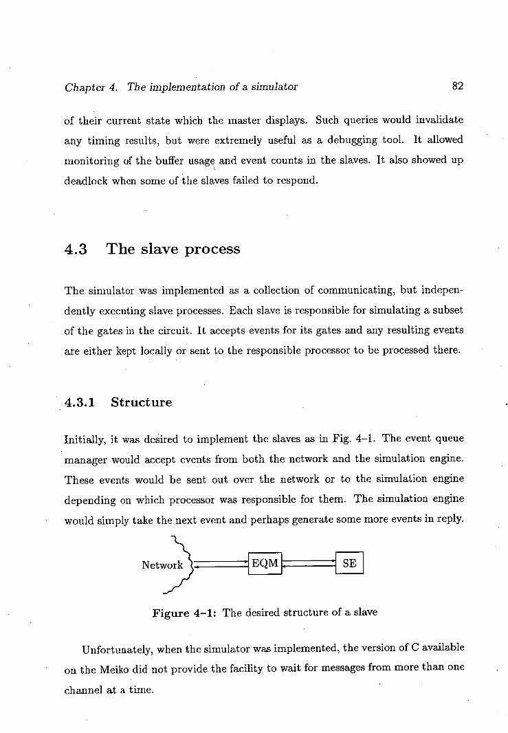
Chapter 4. The implementation of a simulator 82
of their current state which the master displays. Such queries would invalidate
any timing results, but were extremely useful as a debugging tool. It allowed
monitoring of the buffer usage and event counts in the slaves. It also showed up
deadlock when some of the slaves failed to respond.
4.3 The slave process
The simulator was implemented as a collection of communicating, but indepen-
dently executing slave processes. Each slave is responsible for simulating a subset
of the gates in the circuit. It accepts events for its gates and any resulting events
are either kept locally or sent to the responsible processor to be processed there.
4.3.1 Structure
Initially, it was desired to implement the slaves as in Fig. 4-1. The event queue
manager would accept events from both the network and the simulation engine.
These events would be sent out over the network or to the simulation engine
depending on which processor was responsible for them. The simulation engine
would simply take the next event and perhaps generate some more events in reply.
Netw4 E § H SE
Figure 4-1: The desired structure of a slave
Unfortunately, when the simulator was implemented, the version of C available
on the Meiko did not provide the facility to wait for messages from more than one
channel at a time.
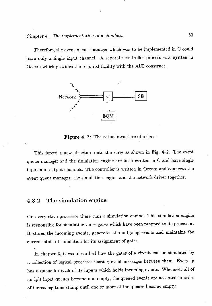
Chapter 4. The implementation of a simulator
Therefore, the event queue manager which was to be implemented in C could
have only a single input channel. A separate controller process was written in
Occam which provides the required facility with the ALT construct.
Net
Figure 4-2: The actual structure of a slave
This forced a new structure onto the slave as shown in Fig. 4-2. The event
queue manager and the simulation engine are both written in C and have single
input and output channels. The controller is written in Occarn and connects the
event queue manager, the simulation engine and the network driver together.
4.3.2 The simulation engine
On every slave processor there runs a simulation engine. This simulation engine
is responsible for simulating those gates which have been mapped to its processor.
It stores the incoming events, generates the outgoing events and maintains the
current state of simulation for its assignment of gates.
In chapter 3, it was described how the gates of a circuit can be simulated by
a collection of logical processes passing event messages between them. Every ip
has a queue for each of its inputs which holds incoming events. Whenever all of
an lp's input queues become non-empty, the queued events are accepted in order
of increasing time stamp until one or more of the queues become empty.
Chapter 4. The implementation of a simulator 84
In addition to the input queues, an ip also maintains the values of each input
which are valid for the time of the next event. These current values are updated
when an event is accepted and are the input values to the gate's logic function.
The central data structure of the simulation engine is the function table. It
describes the gates being simulated and their connections. There is an entry for
each gate, source and sink in the circuit.
The initial state of the function table is derived from the net list read in by
the master and broadcast to each of the slaves. Each entry of the table contains
the following:
. The time of the last event accepted; the ip's simulation time.
. The current input values.
. Pointers to the input queues
. The output wire number, if any.
. The value and time of the last event output.
A pointer to a C routine which generates output values from input values.
. The ID of the processor on which the gate is to be simulated.
Once the simulation engine is initialised, it enters a cycle which is terminated
only by a shutdown message from the master. This cycle starts by waiting for and
receiving the next event from the event queue manager. The event message, of the
form (f, i, t, v) contains the function, f, and input, i, to which the event is addressed
and the time, t, and value, v, of that event. If the simulation time of lp f is greater
than or equal to the simulation end time then the event is ignored. Otherwise
it is placed on the end of the specified function/input queue. If this reduces the
Chapter 4. The implementation of a simulator 85
number of empty input queues to zero then the function is fired repeatedly until
one of the queues becomes empty.
When a function is fired, the time stamps of the events in each queue are
examined to find the minimum, ie. the time of the next event. Events which have
this minimum time are removed from their input queue and their values overwrite
the current value for that input. The current time of the ip is updated to this new
time. Note that storing an ip's current time is not necessary for the simulation
mechanism, but this time is used by the logic function to generate the time of
output events.
There may be several events, some possibly on the same queue, with time equal
to the time of the next event. It is important for reasons of performance which are
discussed later that they are all accepted in one go before the gate's logic function
is invoked.
Once all the new input values have been accepted the logic function is invoked
on the function table entry. If it is a sink node then a result message is sent to the
master, otherwise the output value is computed and an event is sent out with its
time stamp set to the ip's current time plus the propagation delay for that logic
function. The output wire number of the gate is used to determine the recipient
functions and copies of the event addressed to each function/input pair are sent
to the event queue manager for distribution to the appropriate processor.
For every source node within a simulation engine's assignment of logical pro-
cesses, a terminating event is sent on its output wire. If an ip accepts an event
with time greater than or equal to the simulation end time, it is considered ter -
minated. When all of a slave's non-source functions have terminated, the slave
sends a message to the master informing it that the slave has finished its share of
the simulation.
In chapter 3 it was described how it was possible for the Chandy-Misra sim-

Chapter 4. The implementation of a simulator 86
ulation mechanism to deadlock if it was not initialised properly. The solution
proposed was to place a null message on each input of every logical process. This
is done in each simulation engine by placing an event with time 0 and value Un-
known into each of the input queues of every active function.
One of the problems which can arise in the basic Misra-Chandy mechanism is
the explosion of the number of events due to the presence of cycles. If nothing is
done to prevent it, the simulator can be flooded with event messages which will
overflow buffers or at least cause a lot of unnecessary processing.
Consider the case where an ip accepts only one event at a time. For example,
Fig. 4-3 shows a very simple circuit. Input A is used to introduce an event and
follows it with a terminating event which keeps that input queue non-empty. Every
time the lp fires it produces two events with identical time stamps, but as it only
accepts one event at a time, the queues get progressively longer until some buffer
limit is reached. The problem to avoid is that of the ip generating consecutive
events with the same time stamp since all but the last are made redundant and
are possibly incorrect.
Figure 4-3: An explosion of events
• It is a simple, but important step, to allow the ip to accept all of the events
at the head of its input queues which have the same minimum time. One can
and should go one step further to allow the lp to accept all of the events in its
input queues with the minimum time, not just the ones at the head of its queues.
Because of the time ordering of messages, the lp has only to accept events from
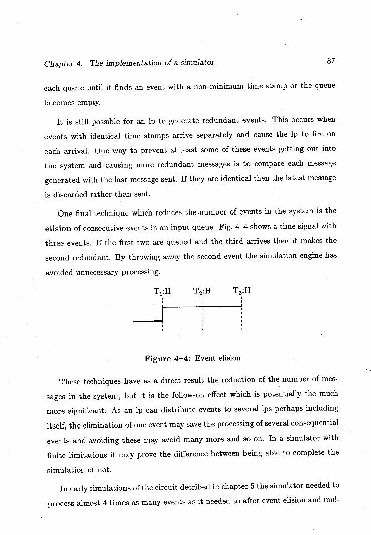
Chapter 4. The implementation of a simulator
EYi
each queue until it finds an event with a non-minimum time stamp or the queue
becomes empty.
It is still possible for an ip to generate redundant events. This occurs when
events with identical time stamps arrive separately and cause the ip to fire on
each arrival. One way to prevent at least some of these events getting out into
the system and causing more redundant messages is to compare each message
generated with the last message sent. If they are identical then the latest message
is discarded rather than sent.
One final technique which reduces the number of events in the system is the
elision of consecutive events in an input queue. Fig. 4-4 shows a time signal with
three events. If the first two are queued and the third arrives then it makes the
second redundant. By throwing away the second event the simulation engine has
avoided unnecessary processing.
T1 :H T2 :H T3 :H
Figure 4-4: Event elision
These techniques have as a direct result the reduction of the number of mes-
sages in the system, but it is the follow-on effect which is potentially the much
more significant. As an ip can distribute events to several lps perhaps including
itself, the elimination of one event may save the processing of several consequential
events and avoiding these may avoid many more and so on. In a simulator with
finite limitations it may prove the difference between being able to complete the
simulation or not.
In early simulations of the circuit decribed in chapter 5 the simulator needed to
process almost 4 times as many events as it needed to after event, elision and mul-
Chapter 4. The implementation of a simulator 88
tiple acceptances were introduced. Often it was the case that the simulation did
not complete at all due to the overflowing of memory limitations in the simulation
engine and the event queue manager.
4.3.3 The event queue manager
The event queue manager provides a simple FIFO queue server. Event messages
are accepted originating from one of the simulation engines somewhere in the
system. If the event is destined for the local simulation engine it is stored in the
queue. Otherwise, the correct address is found and the event is sent off to the
remote processor.
Due to the fixed memory constraints, there is a limit to the number of messages
which can be stored at any one time. With the current implementation, if the
queue overflows it is a fatal error and the simulation aborts.
4.3.4 The controller process
The task of the controller is to route messages between the event queue manager,
the simulation engine and the network driver. The main problem to be solved is
to do this without allowing the processes to deadlock.
As has been mentioned a number of times before, deadlock can occur in a
collection of processes if and only if there is a cycle of processes each waiting on
the next. This could be waiting to receive an event, but that would only occur if
there are no events left in the system, a termination condition or a problem in the
simulator as a whole.
Therefore, the problem faced is one of deadlock caused by processes blocking
on output. This is made particularly acute by the Occam/CSP model disallowing
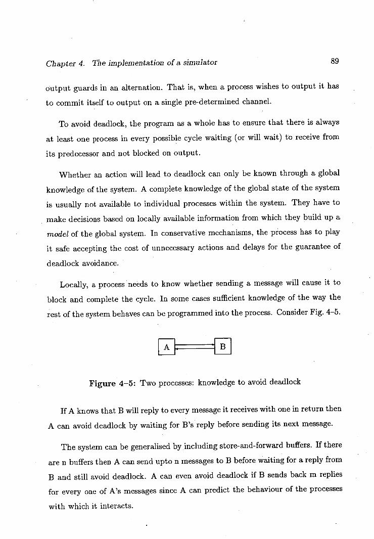
Chapter 4. The implementation of a simulator 89
output guards in an alternation. That is, when a process wishes to output it has
to commit itself to output on a single pre-determined channel.
To avoid deadlock, the program as a whole has to ensure that there is always
at least one process in every possible cycle waiting (or will wait) to receive from
its predecessor and not blocked on output.
Whether an action will lead to deadlock can only be known through a global
knowledge of the system. A complete knowledge of the global state of the system
is usually not available to individual processes within the system. They have to
make decisions based on locally available information from which they build up a
model of the global system. In conservative mechanisms, the process has to play
it safe accepting the cost of unnecessary actions and delays for the guarantee of
deadlock avoidance.
Locally, a process needs to know whether sending a message will cause it to
block and complete the cycle. In some cases sufficient knowledge of the way the
rest of the system behaves can be programmed into the process. Consider Fig. 4-5.
FUMM MMR Figure 4-5: Two processes: knowledge to avoid deadlock
If A knows that B will reply to every message it receives with one in return then
A can avoid deadlock by waiting for B's reply before sending its next message.
The system can be generalised by including store-and-forward buffers. If there
are n buffers then A can send upto n messages to B before waiting for a reply from
B and still avoid deadlock. A can even avoid deadlock if B sends back m replies
for every one of A's messages since A can predict the behaviour of the processes
with which it interacts.
Chapter 4. The implementation of a simulator 90
This approach fails if A cannot predict B's behaviour, eg. if in reply to A's
messages, B replies with an unpredictably varying number of messages. A can-
not know, simply by counting the replies, whether to wait for more messages or
whether it has received them all and B is waiting for it to send some more.
In this situation, extra information must be communicated from B to A either
as part of the data or by some extra control messages. It is important to note
that though buffers can increase the number of outstanding messages allowed they
can never prevent deadlock if the processes cannot predict the communications
behaviour of their neighbours.
For a process to maintain sufficient knowledge to decide when it is safe to
send, ahand-shaking protocol is required. The receiving process sends a control
message to the sender acknowledging the previous p messages and informing the
sender it is OK to send another n messages. Typically, p = n = 1
The simulation engine receives the next event message and replies with zero
or more events to be sent to the event queue manager. The controller forwards
events to the event queue manager which will possibly reply with a single message
for the network driver. Since the controller cannot predict how many messages
the simulation engine and the event queue manager will send in reply to a single
message, a hand-shaking protocol must be used. All three processes, including
the network driver, send a special control message to the controller when they are
ready to receive another message.
Using hand-shaking, the controller knows when not to send a message, but
what is it to do with an incoming message destined for a process which is not
ready for it? It could buffer it, but as we have seen, no finite number of buffers
can guarantee a deadlock free system. The alternative is for the controller not to
receive it in the first place.
Guards are placed on the controller's input channels which allow messages to
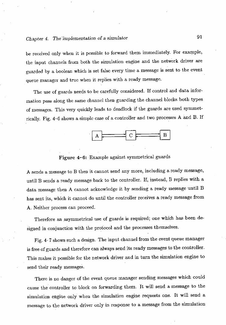
Chapter 4. The implementation of a simulator 91
be received only when it is possible to forward them immediately. For example,
the input channels from both the simulation engine and the network driver are
guarded by a boolean which is set false every time a message is sent to the event
queue manager and true when it replies with a ready message.
The use of guards needs to be carefully considered. If control and data infor-
ination pass along the same channel then guarding the channel blocks both types
of messages. This very quickly leads to deadlock if the guards are used symmet-
rically. Fig. 4-6 shows a simple case of a controller and two processes A and B. If
Figure 4-6: Example against symmetrical guards
A sends a message to B then it cannot send any more, including a ready message,
until B sends a ready message back to the controller. If, instead, B replies with a
data message then A cannot acknowledge it by sending a ready message until B
has sent its, which it cannot do until the controller receives a ready message from
A. Neither process can proceed.
Therefore an asymmetrical use of guards is required; one which has been de-
signed in conjunction with the protocol and the processes themselves.
Fig. 4-7 shows such a design. The input channel from the event queue manager
is free of guards and therefore can always send its ready messages to the controller.
This makes it possible for the network driver and in turn the simulation engine to
send their ready messages.
There is no danger of the event queue manager sending messages which could
cause the controller to block on forwarding them. It will send a message to the
simulation engine only when the simulation engine requests one. It will send a
message to the network driver only in response to a message from the simulation
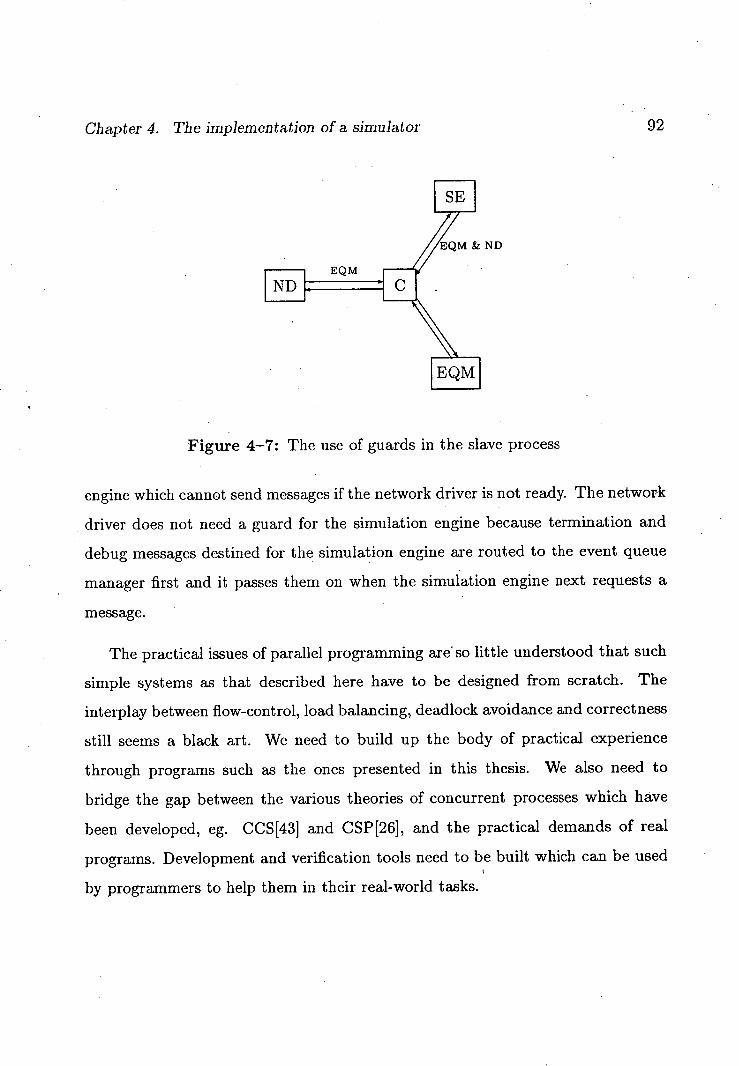
Chapter 4. The implementation of a simulator 92
ND
Figure 4-7: The use of guards in the slave process
engine which cannot send messages if the network driver is not ready. The network
driver does not need a guard for the simulation engine because termination and
debug messages destined for the simulation engine are routed to the event queue
manager first and it passes them on when the simulation engine next requests a
message.
The practical issues of parallel programming are so little understood that such
simple systems as that described here have to be designed from scratch. The
interplay between flow-control, load balancing, deadlock avoidance and correctness
still seems a black art. We need to build up the body of practical experience
through programs such as the ones presented in this thesis. We also need to
bridge the gap between the various theories of concurrent processes which have
been developed, eg. CCS[43] and CSP[26], and the practical demands of real
programs. Development and verification tools need to be built which can be used
by programmers to help them in their real-world tasks.
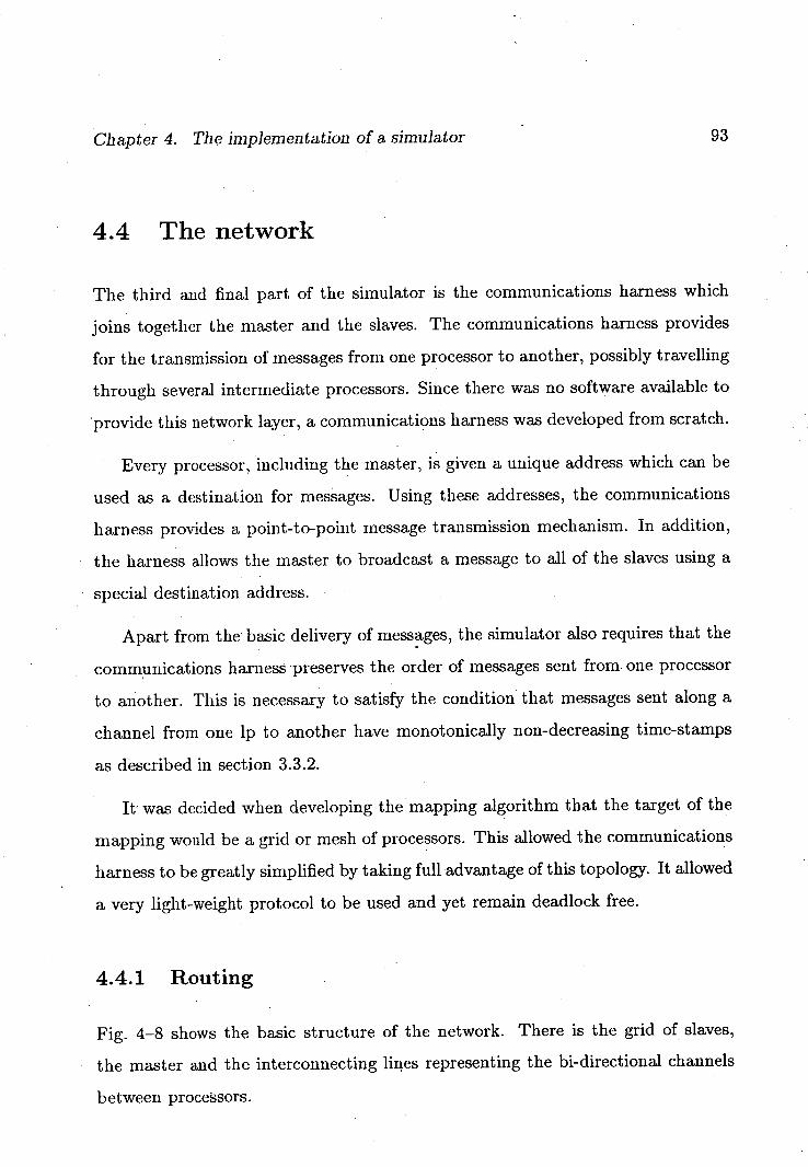
Chapter 4. The implementation of a simulator 93
4.4 The network
The third and final part of the simulator is the communications harness which
joins together the master and the slaves. The communications harness provides
for the transmission of messages from one processor to another, possibly travelling
through several intermediate processors. Since there was no software available to
provide this network layer, a communications harness was developed from scratch.
Every processor, including the master, is given a unique address which can be
used as a destination for messages. Using these addresses, the communications
harness provides a point-to-point message transmission mechanism. In addition,
the harness allows the master to broadcast a message to all of the slaves using a
special destination address.
Apart from the basic delivery of messages, the simulator also requires that the
communications harness preserves the order of messages sent from one processor
to another. This is necessary to satisfy the condition that messages sent along a
channel from one ip to another have monotonically non-decreasing time-stamps
as described in section 3.3.2.
It was decided when developing the mapping algorithm that the target of the
mapping would be a grid or mesh of processors. This allowed the communications
harness to be greatly simplified by taking full advantage of this topology. It allowed
a very light-weight protocol to be used and yet remain deadlock free.
4.4.1 Routing
Fig. 4-8 shows the basic structure of the network. There is the grid of slaves,
the master and the interconnecting lines representing the bi-directional channels
between processors.
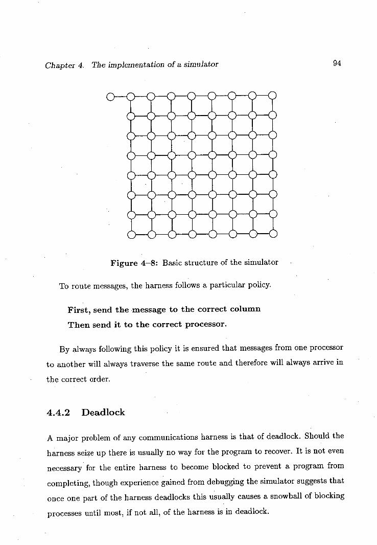
Chapter 4. The implementation of a simulator 94
Figure 4-8: Basic structure of the simulator
To route messages, the harness follows a particular policy.
First, send the -message to the correct column
Then send it to the correct processor.
By always following this policy it is ensured that messages from one processor
to another will always traverse the same route and therefore will always arrive in
the correct order.
4.4.2 Deadlock
A major problem of any communications harness is that of deadlock. Should the
harness seize up there is usually no way for the program to recover. It is not even
necessary for the entire harness to become blocked to prevent a program from
completing, though experience gained from debugging the simulator suggests that
once one part of the harness deadlocks this usually causes a snowball of blocking
processes until most, if not all, of the harness is in deadlock.
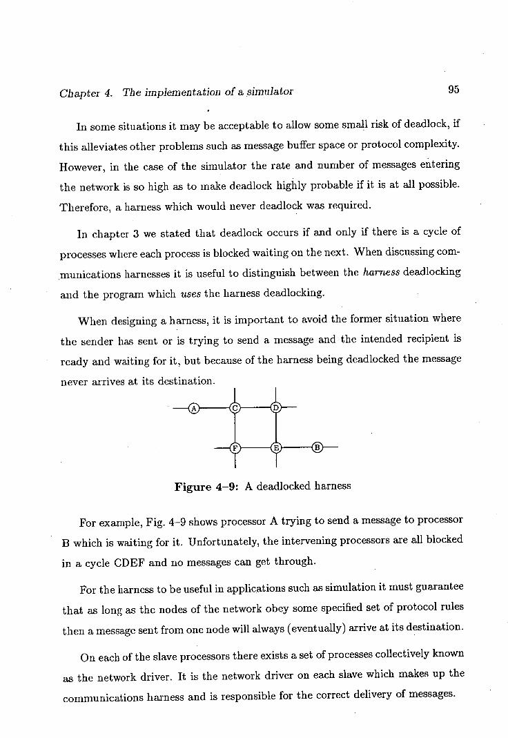
Chapter 4. The implementation of a simulator 95
In some situations it may be acceptable to allow some small risk of deadlock, if
this alleviates other problems such as message buffer space or protocol complexity.
However, in the case of the simulator the rate and number of messages entering
the network is so high as to make deadlock highly probable if it is at all possible.
Therefore, a harness which would never deadlock was required.
In chapter 3 we stated that deadlock occurs if and only if there is a cycle of
processes where each process is blocked waiting on the next. When discussing com-
munications harnesses it is useful to distinguish between the harness deadlocking
and the program which uses the harness deadlocking.
When designing a harness, it is important to avoid the former situation where
the sender has sent or is trying to send a message and the intended recipient is
ready and waiting for it, but because of the harness being deadlocked the message
never arrives at its destination.
Figure 4-9: A deadlocked harness
For example, Fig. 4-9 shows processor A trying to send a message to processor
B which is waiting for it. Unfortunately, the intervening processors are all blocked
in a cycle CDEF and no messages can get through.
For the harness to be useful in applications such as simulation it must guarantee
that as long as the nodes of the network obey some specified set of protocol rules
then a message sent from one node will always (eventually) arrive at its destination.
On each of the slave processors there exists a set of processes collectively known
as the network driver. It is the network driver on each slave which makes up the
communications harness and is responsible for the correct delivery of messages.
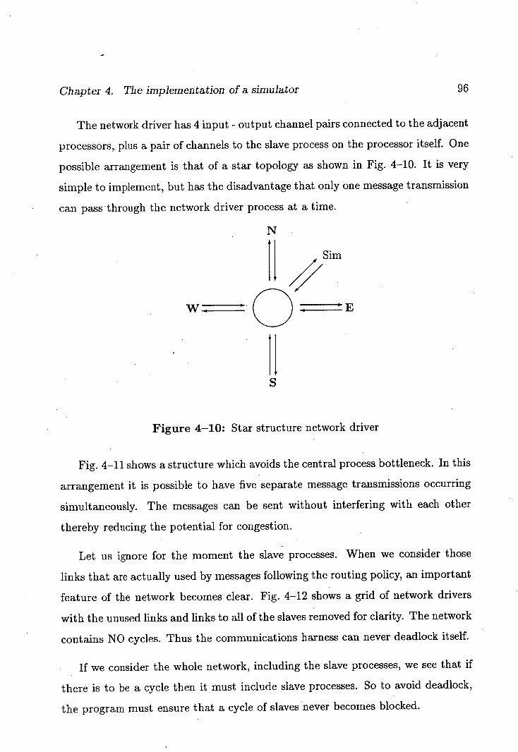
Chapter 4. The implementation of a simulator
9119
The network driver has 4 input - output channel pairs connected to the adjacent
processors, plus a pair of channels to the slave process on the processor itself. One
possible arrangement is that of a star topology as shown in Fig. .4-10. It is very
simple to implement, but has the disadvantage that only one message transmission
can pass 'through the network driver process at a time.
// Sim
W . • Q LI
Figure 4-10: Star structure network driver
Fig. 4-11 shows a structure which avoids the central process bottleneck. In this
arrangement it is possible to have five separate message transmissions occurring
simultaneously. The messages can be sent without interfering with each other
thereby reducing the potential for congestion.
Let us ignore for the moment the slave processes. When we consider those
links that are actually used by messages following the routing policy, an important
feature of the network becomes clear. Fig. 4-12 shows a grid of network drivers
with the unused links and links to all of the slaves removed for clarity. The network
contains NO cycles. Thus the communications harness can never deadlock itself.
If we consider the whole network, including the slave processes, we see that if
there is to be a cycle then it must include slave processes. So to avoid deadlock,
the program must ensure that a cycle of slaves never becomes blocked.
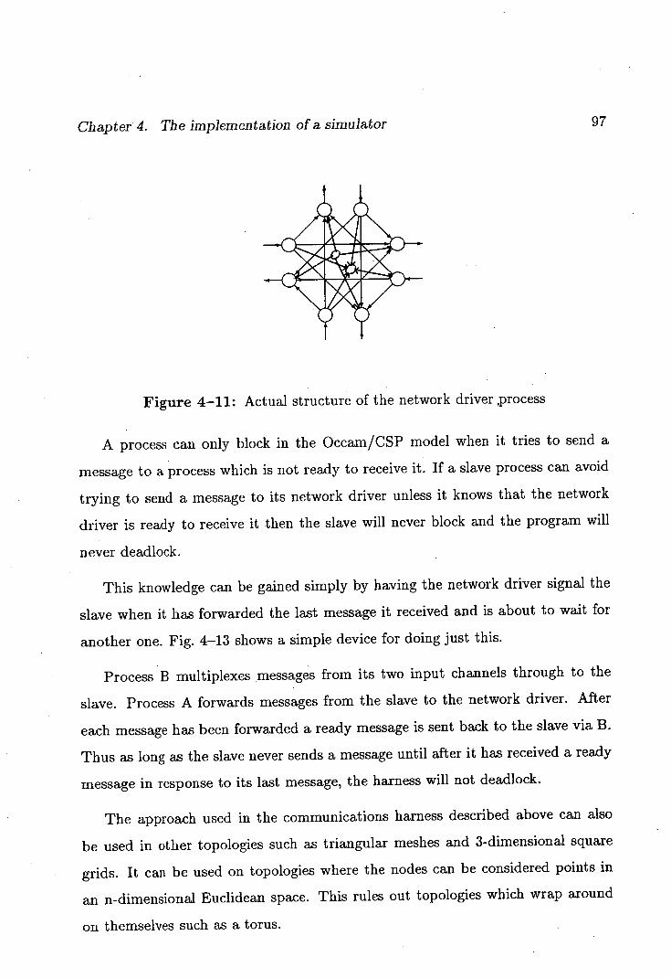
Chapter 4. The implementation of a simulator WN
Figure 4-11: Actual structure of the network driver .process
A process can only block in the Occam/CSP model when it tries to send a
message to a process which is not ready to receive it. If a slave process can avoid
trying to send a message to its network driver unless it knows that the network
driver is ready to receive it then the slave will never block and the program will
never deadlock.
This knowledge can be gained simply by having the network driver signal the
slave when it has forwarded the last message it received and is about to wait for
another one. Fig. 4-13 shows a simple device for doing just this.
Process B multiplexes messages from its two input channels through to the
slave. Process A forwards messages from the slave to the network driver. After
each message has been forwarded a ready message is sent back to the slave via B.
Thus as long as the slave never sends a message until after it has received a ready
message in response to its last message, the harness will not deadlock.
The approach used in the communications harness described above can also
be used in other topologies such as triangular meshes and 3-dimensional square
grids. It can be used on topologies where the nodes can be considered points in
an n-dimensional Euclidean space. This rules out topologies which wrap around
on themselves such as a torus
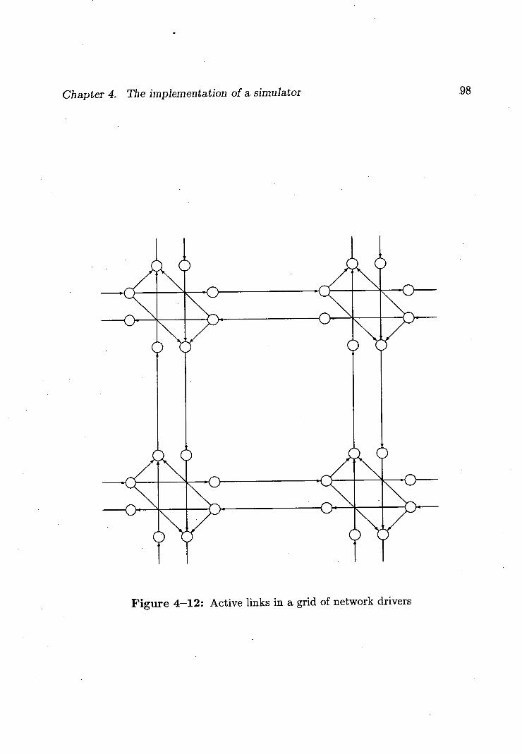
Chapter 4. The implementation of a simulator
Figure 4-12: Active links in a grid of network drivers
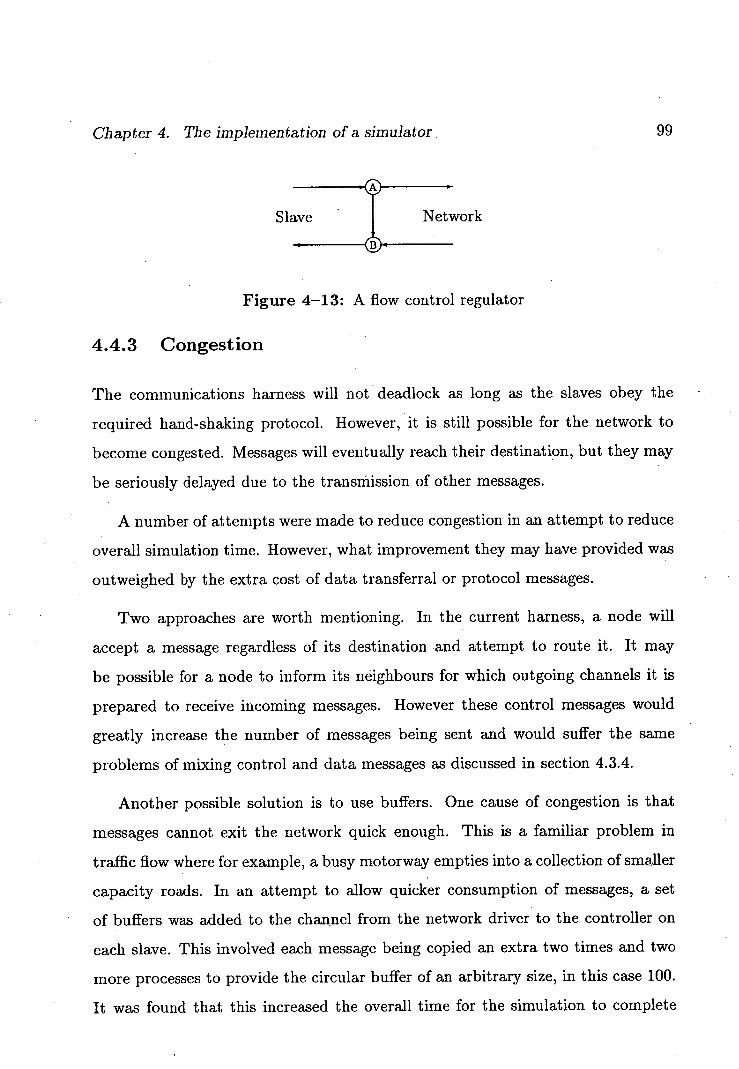
Chapter 4. The implementation of a simulator.
TBSlave Network
__
Figure 4-13: A flow control regulator
4.4.3 Congestion
The communications harness will not deadlock as long as the slaves obey the
required hand-shaking protocol. However, it is still possible for the network to
become congested. Messages will eventually reach their destination, but they may
be seriously delayed due to the transmission of other messages.
A number of attempts were made to reduce congestion in an attempt to reduce
overall simulation time. However, what improvement they may have provided was
outweighed by the extra cost of data transferral or protocol messages.
Two approaches are worth mentioning. In the current harness, a node will
accept a message regardless of its destination and attempt to route it. It may
be possible for a node to inform its neighbours for which outgoing channels it is
prepared to receive incoming messages. However these control messages would
greatly increase the number of messages being sent and would suffer the same
problems of mixing control and data messages as discussed in section 4.3.4.
Another possible solution is to use buffers. One cause of congestion is that
messages cannot exit the network quick enough. This is a familiar problem in
traffic flow where for example, a busy motorway empties into a collection of smaller
capacity roads. In an attempt to allow quicker consumption of messages, a set
of buffers was added to the channel from the network driver to the controller on
each slave. This involved each message being copied an extra two times and two
more processes to provide the circular buffer of an arbitrary size, in this case 100.
It was found that this increased the overall time for the simulation to complete

Chapter 4. The implementation of a simulator LIII]
by at least 10%. Again, the costs of extra complexity outweighed any benefits of
reduced congestion.
Chapter 5
Results and Discussion
The previous chapters described a new structural approach to the mapping prob-
lem and presented digital logic simulation as an application to test this new ap-
proach. The simulator is equivalent to an operating system where the gates being
simulated are the processes, albeit simple ones, which communicate by sending
event messages. It provides a testbed in which the effects of different mappings
can be explored.
In this chapter, two families of mappings are studied. One is generated by the
new structural approach and is directed towards reducing communication costs.
The second family endeavours to give each processor an equal computation load.
It is shown that the new approach does indeed reduce the level of communication
traffic in comparison to the control mapping and that, under limitations of load
imbalance, results in lower overall completion times.
101
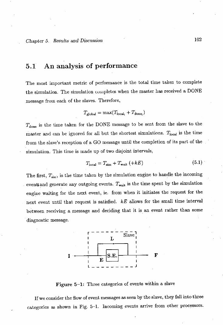
Chapter 5. Results and Discussion 102
5.1 An analysis of performance
The most important metric of performance is the total time taken to complete
the simulation. The simulation completes when the master has received a DONE
message from each of the slaves. Therefore,
Tglobal = max(Tiocai. + Td0111 )
Tdone is the time taken for the DONE message to be sent from the slave to the
master and can be ignored for all but the shortest simulations. Tk is the time
from the slave's reception of a GO message until the completion of its part of the
simulation. This time is made up Of two disjoint intervals,
Tiocai = 1 im + T.ait (+kE) (5.1)
The first, 1,, is the time taken by the simulation engine to handle the incoming
evenland generate any outgoing events. is the time spent by the simulation
engine waiting for the next event, ie. from when it initiates the request for the
next event until that request is satisfied. kE allows for the small time interval
between receiving a message and deciding that it is an event rather than some
diagnostic message.
Slavel
F E I
L---------J
Figure 5-1: Three categories of events within a slave
If we consider the flow of event messages as seen by the slave, they fall into three
categories as shown in Fig. 5-1. Incoming events arrive from other processors.
Chapter 5. Results and Discussion 103
Foreign events are generated by the slave and destined for other slaves and Local
events are generated and consumed within the same slave. The number of events
in each category is denoted by I, F and L respectively. The total number of events
processed by a slave, ie. the sum of I and L, is denoted by E.
The time spent in the simulation phase depends on several factors. Part of the
time is spent handling events arriving at the simulation engine and part is spent
transmitting resulting events back out to the event queue manager. This latter
time is independent of whether the event is local or foreign bound. In addition
there is some complex overhead due to communications which we will consider in
greater detail later. Thus simulation time can be written as,
Tim = ( L + I)Thandle + ( L + F)Tsend + 1comms {?} (5.2)
The time the simulation engine spends idle is by definition due to delays. The
simulation engine has to wait for an event that is coming from elsewhere whether it
be from its event queue manager or from some other slave. It cannot proceed until
that next event arrives. These delays are very complex in makeup, but one feature
which can be isolated is the minimum time for the simulation engine to request
and receive the next event. This represents a necessary cost of the implementation
due to the slave protocol and is independent of delays due to interference or an
empty event queue.
= (L + I)Tletch + Twcomms {?}
The remaining delay Twcommg , like 7COmm81 is dependent on many factors. Be-
cause of the parallel nature of the Transputer and the slave processes, particularly
the overlapping of communications and computation, many of the overheads are
independent of the phase of the simulation engine and cannot be wholly assigned
to one phase or the other. Therefore we introduce the overall communications
overhead Tcomm s
Tcomms = 'comm8 + Twcomms
Chapter 5. Results and Discussion 104
Tcomms is the time penalty for distributing the simulation amongst several proces-
sors. Against this penalty is the time saved through processing several events in
parallel.
There are two basic classes of delays to be considered. One class contains
all the delays which arise from the implementation of the simulator. The other
contains the delays which are due to the behaviour of the simulation itelf.
5.1.1 Implementation derived delays
Though designed to support a parallel computation model, the Transputer can
execute only one process at a time. When an event is sent to another slave, it
passes through several processes within the communication harness each of which
consumes processing time. The use of cycle-stealing by the DMA communication
links of the Transputer can also slow down the execution of the simulation engine.
Similar delays occur due to incoming messages. These can be considered indirect
or invisible overheads since they are best measured by the difference their presence
makes to the timings of the simulation engine and the simulation as a whole.
Another indirect delay is due to the processing of through messages. These
are messages passing through the processor on the way from one slave to an-
other. They are totally invisible to the slave, being handled completely within the
communication harness.
A second category of delays which are implementation derived consists of those
arising from protocol and congestion. The protocol used within a slave can cause
messages to be delayed in order to avoid deadlock. This can occur when messages
are sent to or received from the network. The simulation engine will be prevented
from outputting messages whenever the controller is waiting for the communica-
tions harness or the event queue manager to signal its readiness to receive.
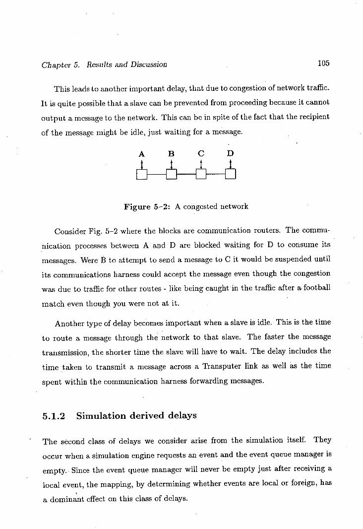
Chapter 5. Results and Discussion 105
This leads to another important delay, that due to congestion of network traffic.
It is quite possible that a slave can be prevented from proceeding because it cannot
output a message to the network. This can be in spite of the fact that the recipient
of the message might be idle, just waiting for a message.
Figure 5-2: A congested network
Consider Fig. 5-2 where the blocks are communication routers. The commu-
nication processes between A and D are blocked waiting for D to consume its
messages. Were B to attempt to send a message to C it would be suspended until
its communications harness could accept the message even though the congestion
was due to traffic for other routes - like being caught in the traffic after a football
match even though you were not at it.
Another type of delay becomes important when a slave is idle. This is the time
to route a message through the network to that slave. The faster the message
transmission, the shorter time the slave will have to wait. The delay includes the
time taken to transmit a message across a 'fransputer link as well as the time
spent within the communication harness forwarding messages.
5.1.2 Simulation derived delays
- The second class of delays we consider arise from the simulation itself. They
occur when a simulation engine requests an event and the event queue manager is
empty. Since the event queue manager will never be empty just after receiving a
local event, the mapping, by determining whether events are local or foreign, has
a dominant effect on this class of delays.
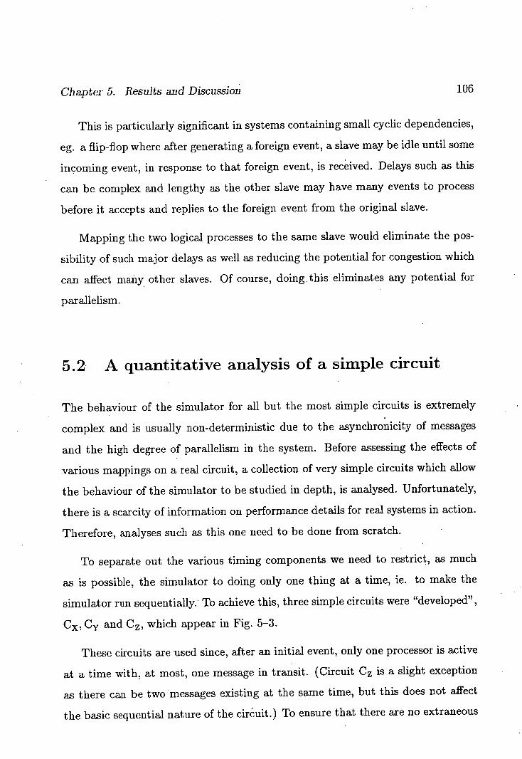
Chapter 5. Results and Discussion 106
This is particularly significant in systems containing small cyclic dependencies,
eg. a flip-flop where after generating a foreign event, a slave may be idle until some
incoming event, in response to that foreign event, is received. Delays such as this
can be complex and lengthy as the other slave may have many events to process
before it accepts and replies to the foreign event from the original slave.
Mapping the two logical processes to the same slave would eliminate the pos-
sibility of such major delays as well as reducing the potential for congestion which
can affect many other slaves. Of course, doing this eliminates any potential for
parallelism.
5.2 A quantitative analysis of a simple circuit
The behaviour of the simulator for all but the most simple circuits is extremely
complex and is usually non-deterministic due to the asynchronicity of messages
and the high degree of parallelism in the system. Before assessing the effects of
various mappings on a real circuit, a collection of very simple circuits which allow
the behaviour of the simulator to be studied in depth, is analysed. Unfortunately,
there is a scarcity of information on performance details for real systems in action.
Therefore, analyses such as this one need to be done from scratch.
To separate out the various timing components we need to restrict, as much
as is possible, the simulator to doing only one thing at a time, ie. to make the
simulator run sequentially. To achieve this, three simple circuits were "developed",
C, Cy and C, which appear in Fig. 5-3.
These circuits are used since, after an initial event, only one processor is active
at a time with, at most, one message in transit. (Circuit C z is a slight exception
as there can be two messages existing at the same time, but this does not affect
the basic sequential nature of the circuit.) To ensure that there are no extraneous
Chapter 5. Results and Discussion 107
Circuit X Circuit Y
Circuit Z
Figure 5-3: Simple circuits X, Y and Z
messages, the initial null events, normally stored in each input queue, as described
in section 3.5.1, are omitted.
The circuits C, C y and Cz were each mapped onto the simulator using the
families of mappings, X, Y and Z respectively. Each family of mappings partitions
its corresponding circuit into two as shown by the dashed lines of Fig. 5-3 then
maps them either to the same processor, (ie. mappings X o , Yo and Z0 ), or to
two processors separated by n links (X v , Y. and Zn ). We collectively refer to the
mappings with n > 0, ie. those which use two processors, as X >0, Y>o and Z >o.
In the case of Y >° and Z>0, the behaviour of the two slaves is different. They
are distinguished by referring to the one with fewer events as Y' or Z' and the
other as Y" or Z".
The three circuits consist of nand, buffer and inverter gates each with a propa-
gation delay of 5 nominal time units. After an initial event each circuit is simulated
Chapter 5. Results and Discussion 108
for 50000 time units. There are no sinks in the circuits and therefore no potential
for bottlenecks caused by communication with the simulation master.
As only one event is in circulation the simulator does not suffer from delays
due to congestion or other interactions between messages. Those delays that are
incurred for messages between processors are the minimum times for messages
to travel through the communication harnesses and inter-Transputer links and
should be directly proportional to the number of inter-Transputer messages sent
and received. In the case of the X 0 , Y0 and Z0 mappings there are no such messages
so the communication overheads
Tscomms = Twcomm s = 0
Table 5-1 shows a summary of timing results from a series of simulations of
the simple circuits. Twajt and T101 were measured in clock ticks using the
internal low priority clock of the T800 Transputer which has a clock period of
64s. Note that the clock measures absolute real time and not process time. It
needs to be treated carefully when processes can be context switched since, in
particular, 1jm can include time spent processing the event queue manager and
the network driver.
In order to reduce experimental error, the results in Table 5-1 are an average of
three experiments including a mapping where the processors are swapped to allow
for differences in individual processor performance. The results were found to be
consistent with those produced during six other sessions. Since the two slaves in
the X>0 mappings have very similar performances only their averaged results are
presented.
5.2.1 The simulation phase of X, Y and Z
The simulation phase of the simulation engine begins with the arrival of an event
and ends just before the next NEXT message is sent. 7jm is the sum of all the
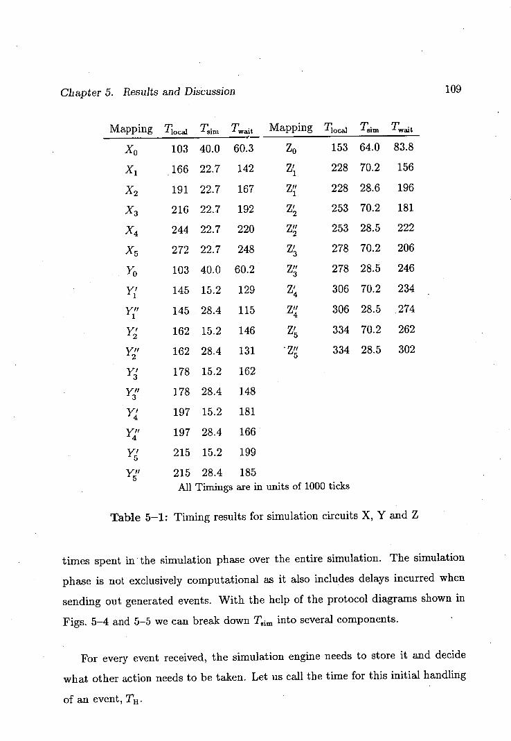
Chapter 5. Results and Discussion 109
Mapping TI., ai 7 im Twait Mapping Tiocai 1 im TWtht
X 0 103 40.0 60.3 Z0 153 64.0 83.8
X 1 166 22.7 142 228 70.2 156
X 2 191 22.7 167 228 28.6 196
216 22.7 192 ZI 253 70.2 181
244 22.7 220 z1f 253 28.5 222
X5 272 22.7 248 278 70.2 206
YO 103 40.0 60.2 z1f 278 28.5 246
Y11 145 15.2 129 306 70.2 234
Y111 145 28.4 115 Z 306 28.5 274
162 15.2 146 Z 334 70.2 262
162 28.4 131 zg 334 28.5 302
178 15.2 162
178 28.4 148
197 15.2 181
197 28.4 166
215 15.2 199
Y 11 215 28.4 185 All Timings are in units of 1000 ticks
Table 5-1: Timing results for simulation circuits X, Y and Z
times spent in the simulation phase over the entire simulation. The simulation
phase is not exclusively computational as it also includes delays incurred when
sending out generated events. With the help of the protocol diagrams shown in
Figs. 5-4 and 5-5 we can break down Tsjm into several components.
For every event received, the simulation engine needs to store it and decide
what other action needs to be taken. Let us call the time for this initial handling
of an event, TH.
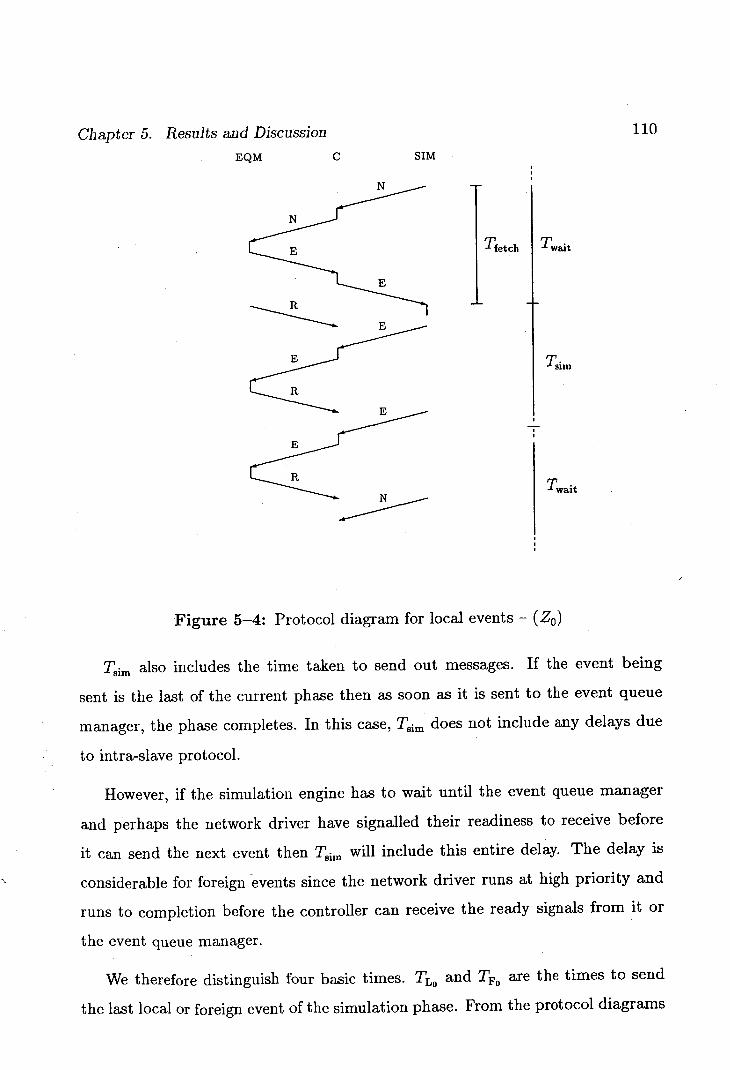
Chapter 5. Results and Discussion 110
EQM C SIM
Tf.tch iTwait
Figure 5-4: Protocol diagram for local events - (Z0 )
2im also includes the time taken to send out messages. If the event being
sent is the last of the current phase then as soon as it is sent to the event queue
manager, the phase completes. In this case, Tsjm does not include any delays due
to intra-slave protocol.
However, if the simulation engine has to wait until the event queue manager
and perhaps the network driver have signalled their readiness to receive before
it can send the next event then Tim will include this entire delay. The delay is
considerable for foreign events since the network driver runs at high priority and
runs to completion before the controller can receive the ready signals from it or
the event queue manager.
We therefore distinguish four basic times. TL ,, and TF0 are the times to send
the last local or foreign event of the simulation phase. From the protocol diagrams
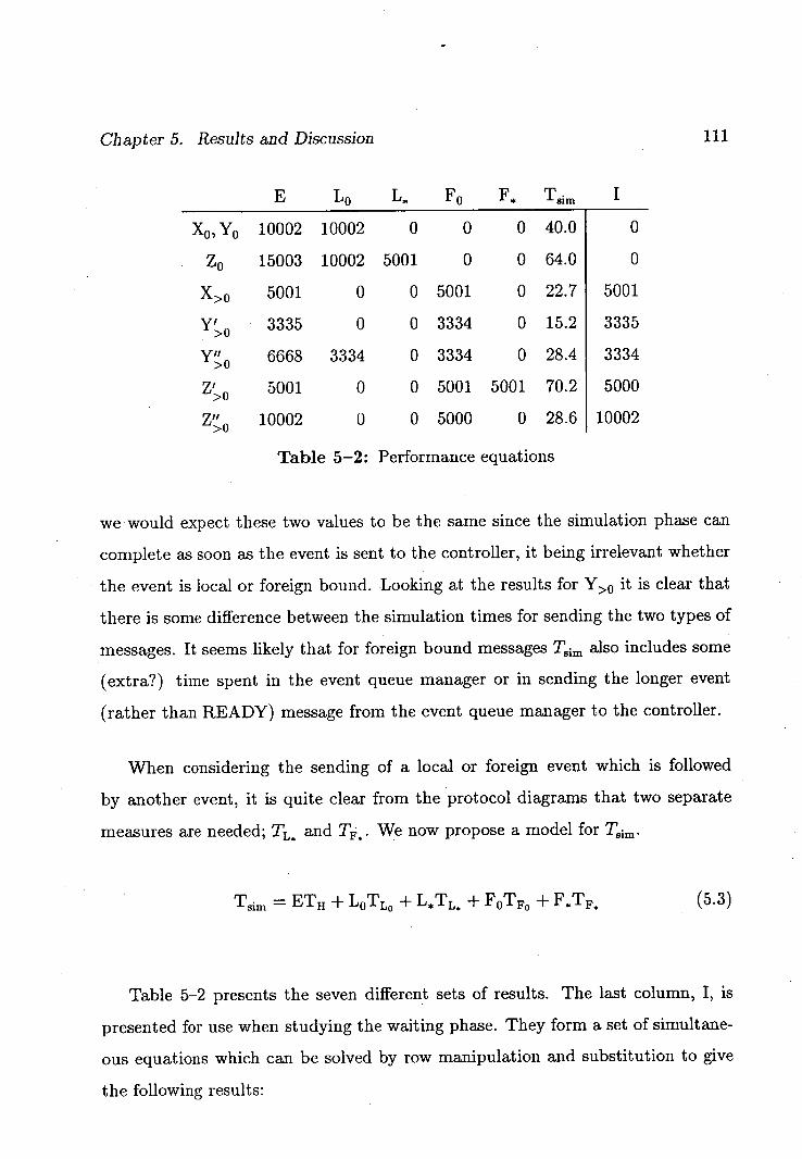
Chapter 5. Results and Discussion 111
E L0 L F0 F Tsim 1
X0 ,Y0 10002 10002 0 0 0 40.0 0
Z0 15003 10002 5001 0 0 64.0 0
X>. 0 5001 0 0 5001 0 22.7 5001
Y 0 3335 0 0 3334 0 15.2 3335
6668 3334 0 3334 0 28.4 3334
Z 0 5001 0 0 5001 5001 70.2 5000
10002 0 0 5000 0 28.6 10002
Table 5-2: Performance equations
we would expect these two values to be the same since the simulation phase can
complete as soon as the event is sent to the controller, it being irrelevant whether
the event is local or foreign bound. Looking at the results for Y>0 it is clear that
there is some difference between the simulation times for sending the two types of
messages. It seems likely that for foreign bound messages Tsjm also includes some
(extra?) time spent in the event queue manager or in sending the longer event
(rather than READY) message from the event queue manager to the controller.
When considering the sending of a local or foreign event which is followed
by another event, it is quite clear from the protocol diagrams that two separate
measures are needed; TL. and TF.. We now propose a model for Tsim .
Tsim = ETH + LOTL0 + LTL. + FOTF0 + FTF. (5.3)
Table 5-2 presents the seven different sets of results. The last column, I, is
presented for use when studying the waiting phase. They form a set of simultane-
ous equations which can be solved by row manipulation and substitution to give
the following results:
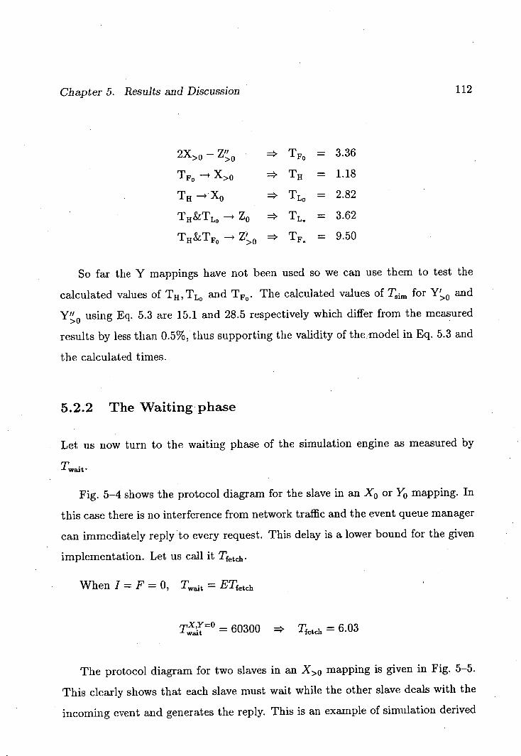
Chapter 5. Results and Discussion 112
2X>0 - => TF, = 3.36
TF0 X>o TH = 1.18
TH—*Xo = T 0 = 2.82
TH&TLO 4 Zo => TL = 3.62
TH &TFO Z >O => T = 9.50
So fax the Y mappings have not been used so we can use them to test the
calculated values of TH, TL0 and TF0 . The calculated values of Tj m for Y10 and
Y 0 using Eq. 5.3 are 15.1 and 28.5 respectively which differ from the measured
results by less than 0.5%, thus supporting the validity of the--model in Eq. 5.3 and
the calculated times.
5.2.2 The Waiting phase
Let us now turn to the waiting phase of the simulation engine as measured by
Twait .
Fig. 5-4 shows the protocol diagram for the slave in an X 0 or Y0 mapping. In
this case there is no interference from network traffic and the event queue manager
can immediately reply to every request. This delay is a lower bound for the given
implementation. Let us call it Tfet th.
When I = F = 0, Twait = ETf etch
T' ° = 60300 Tf,,tch = 6.03 wait
The protocol diagram for two slaves in an X >0 mapping is given in Fig. 5-5.
This clearly shows that each slave must wait while the other slave deals with the
incoming event and generates the reply. This is an example of simulation derived
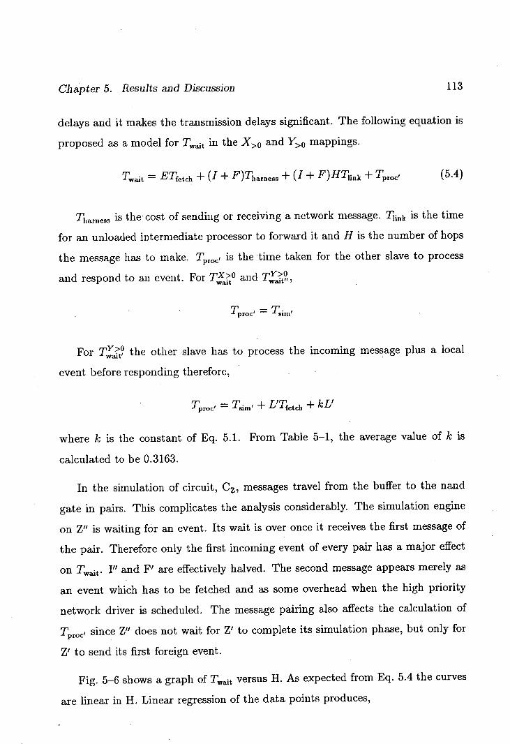
Chapter 5. Results and Discussion 113
delays and it makes the transmission delays significant. The following equation is
proposed as a model for Ywait in the X>0 and Y>° mappings.
Ywait = ETfth + (I + F)Tharness + (I + F)HTlflk + Tproc i ( 5.4)
Titarness is the cost of sending or receiving a network message. 7'Iink is the time
for an unloaded intermediate processor to forward it and H is the number of hops
the message has to make. Tproc i is the time taken for the other slave to process
and respond to an event. For T° and
wait wait" I
Tproc ; = T.i. ,
For T9 the other slave has to process the incoming message plus a local
event before responding therefore,
Tproc i = 1 im' + L'T td, + kL'
where k is the constant of Eq. 5.1. From Table 5-1, the average value of k is
calculated to be 0.3163.
In the simulation of circuit, C, messages travel from the buffer to the nand
gate in pairs. This complicates the analysis considerably. The simulation engine
on Z" is waiting for an event. Its wait is over once it receives the first message of
the pair. Therefore only the first incoming event of every pair has a major effect
on Twait . I" and F' are effectively halved. The second message appears merely as
an event which has to be fetched and as some overhead when the high priority
network driver is scheduled. The message pairing also affects the calculation of
Tproc i since Z" does not wait for Z' to complete its simulation phase, but only for
Z' to send its first foreign event.
Fig. 5-6 shows a graph of Twa i t versus H. As expected from Eq. 5.4 the curves
are linear in H. Linear regression of the data points produces,
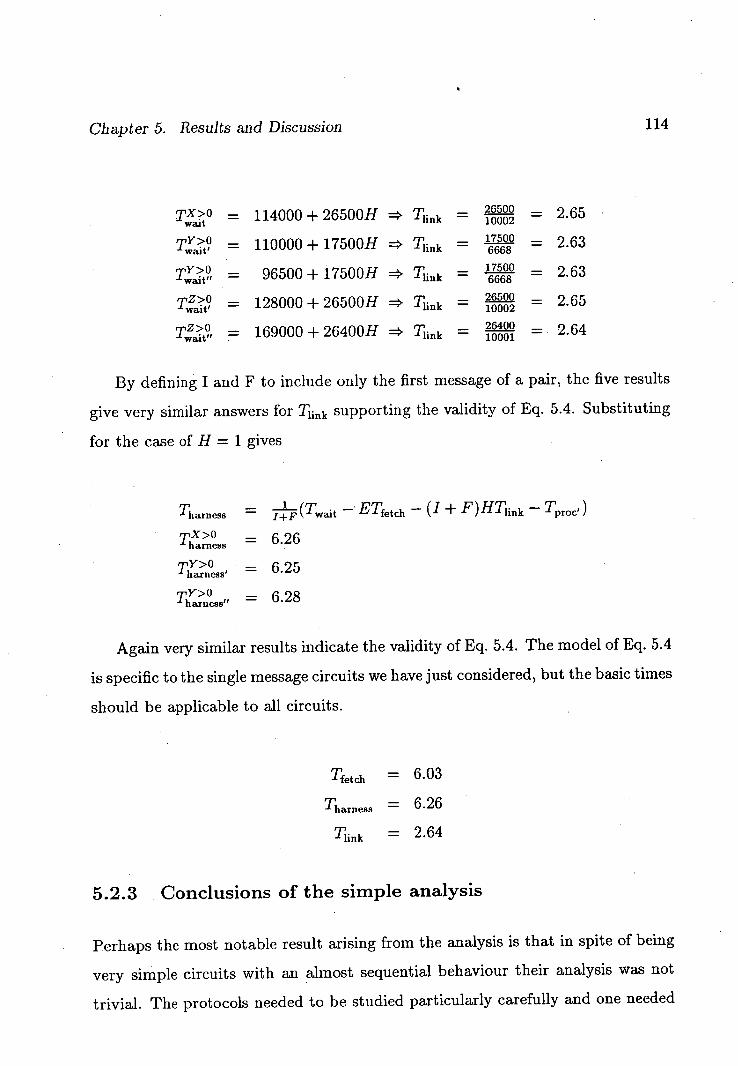
Chapter 5. Results and Discussion 114
Tx>0 wait = 114000+26500H =
10002 - - 2.65
° T1'>it' wa - - 110000+17500H 3' = 6668
- - 2.63
wai t " - — 96500+17500H link = 17500
6668 - - 2.63
Tz>o wait' - - 128000 + 26500H = Thfl, = 2QQ
10002 - - 2.65
Tz>O wait" - - 169000 + 26400H = 10001 - - 2.64
By defining I and F to include only the first message of a pair, the five results
give very similar answers for TlIk supporting the validity of Eq. 5.4. Substituting
for the case of H = 1 gives
Th - - ETfetch - ( I + F)HTlk - Tproc i) arness - I+ \ wait F
= 6.26 harness
- 6.25 har ness' -
rnY>O " - 6.28 harness -
Again very similar results indicate the validity of Eq. 5.4. The model of Eq. 5.4
is specific to the single message circuits we have just considered, but the basic times
should be applicable to all circuits.
Tfetth = 6.03
Th arness = 6.26
Tlik = 2.64
5.2.3 Conclusions of the simple analysis
Perhaps the most notable result arising from the analysis is that in spite of being
very simple circuits with an almost sequential behaviour their analysis was not
trivial. The protocols needed to be studied particularly carefully and one needed
Chapter 5. Results and Discussion 115
an insight into the scheduling policy of the processor. There is a definite need of
tools to help find out what a program is doing and where it is spending its time.
Turning to the results themselves, it is of considerable importance to note that
the slaves spend much of their time waiting. Even in the best cases, X 0 and Y0
as seen in Table 5-1, the simulation engine is idle 58.5% of the time. We have
also seen from Z that during the simulation phase itself there can be considerable
delays. This does not mean the processor is idle for this time as it will be processing
the event queue manager and controller, but it does mean the processor spends
more of its time supporting the simulation than doing the simulation itself. We
can expect this figure to be much higher for simulations where there are many
inter-processor messages and simulation derived delays.
The high cost of communication foreshadows the desirability of reducing the
number of inter-processor messages even at the cost of a more imbalanced execu-
tion load. The issue is not simply a matter of reducing the time spent communi-
cating messages though it is true that a foreign event is 2 1 times as costly as a
local one. To send an inter-slave message increases the probability of congestion
and protocol delays. Furthermore, it introduces the possibility of simulation de-
rived delays as now processors may be idle waiting for messages. Such messages
act as a catalyst for many significant overheads over and above the actual costs of
sending.
5.2.4 Lessons for a new implementation
The high simulation idle time which is solely due to fetching next events underlines
the high cost of communication in comparison to computation within a slave. An
improved simulator would result if greater emphasis was placed on reducing intra-
slave communications to a minimum.
Chapter 5. Results and Discussion 116
This could be achieved by replacing the controller and event queue manager
with a single event queue manager as originally planned. This would require
rewriting the event queue manager in Occam, but the disadvantage in using an
unsuitable language - one with no support for records or linked lists - would be
outweighed by the reduction in communications which turned out to be signifi-
cantly more expensive than originally envisaged. It would eliminate much of the
protocol derived delays and eliminate half of the data transfers.
A single event queue manager could include buffering for outgoing messages
avoiding the separate process which required extra data traansfers. As discussed
in section 4.4.3, buffering would allow the simulation engine to continue simulating
when it would normally be blocked by a blocked network driver.
The second major improvement would be to avoid READY or NEXT messages.
Instead, the outgoing data messages should be tagged signifying when it is safe
to send a message in the opposite direction. READY or NEXT messages would
only be needed if there were no data messages to be sent. This would marginally
increase the computational complexity, but give significant savings by reducing
communication traffic and avoiding unnecessary delays waiting for messages.
5.3 A qualitative analysis of a complex circuit
The analysis of the simple circuits of the previous section has given us an insight
into the "molecular" view of the simulator in action. We identified and measured
individual actions which was only possible due to the almost sequential behaviour
of the system.
Analysis of a complex circuit will be very different in its method and type of
results due to the different nature of the subject of analysis. Individual actions are
no longer identifiable. When simulating the test circuit many millions of events
Chapter 5. Results and Discussion 117
occur and their interactions are very complex because of the parallel execution
of the system. We are limited to studying the "bulk" behaviour of the system;
dealing with aggregate and average counts and timings. We cannot draw protocol
diagrams such as in Figs. 5-4 and 5-5 or state a total ordering of the events
because of the distributed nature of simulation time over the processors[37]. Like
a physicist modelling a gas, we need both a molecular and a bulk model.
When studying a large asynchronous system we need to consider its robustness.
It is possible for a very small change in the system or even the random fluctuations
of the implementation to upset the ordering of events and cause dramatic changes
in behaviour; such is the basis of Chaos theory. For example, a processor, X,
is waiting for two messages; one, A, is to be forwarded to another processor, Y,
where a large amount of computation will occur as a result; the other, B, will
cause a large amout of computation on X.
If A is accepted before B then the two processors can compute in parallel. On
the other hand, if B is accepted before A, Y is idle while X is computing B then
after X has accepted and forwarded A, it is idle while Y computes. Thus the
computation can degenerate into a sequential execution depending on the arrival
order of its messages and this is subject to the system, the mapping and the
implementation. If the two messages would normally arrive close together then
small delays can have a dramatic effect on the behaviour of the system.
In our simulator, the units of computation resulting from a message are small
and so the system should be reasonably robust. However, it is possible for the
network to become congested quite suddenly. Slight fluctuations in timing can
cause messages to be delayed by significantly varying amounts. This Butterfly
effect [23] means that there will always be a level of unpredictability when consid-
ering mappings for asynchronous systems.
Chapter 5. Results and Discussion 118
5.3.1 The circuit
The complex circuit used to study the effects of various mappings was developed
within the Department of Electrical Engineering at the University of Edinburgh.
It implements an 8 bit serial multiplier using VLSI technology as part of a signal
processing chip. It is based on circuits presented by Smith and Denyer[53].
There are three key features of the circuit for our purposes. The first is that
it contains many more logical processes (gates) than the simulator has physical
processors. Secondly, the interconnection graph is irregular so there are no obvious
simple mappings. Finally, there are many cycles which are a major problem for
other distributed simulators.
The circuit was designed using the SOLO 1000 computer aided design system [38].
SOLO 1000 is based on Model, a hierarchial HDL (Hardware Description Lan-
guage). It allows parts to be defined as the interconnection of subparts which are
either similarly defined or one of a collection of primitive parts. Once defined, a
part can be instantiated throughout the circuit. A circuit is simply an instance
of a single part which causes the instantiation of the part's subparts and their
subparts and so on forming an instantiation tree defining the whole circuit.
It is this hierarchical tree which guides the generation of a structural mapping.
There are nine levels in the hierarchy of the test circuit containing a total of 504
internal nodes, 1060 gates and 2463 (input) wires. The test data contains 117
initial events, the majority of which are clock transitions which are distributed to
much of the circuit.
5.3.2 The mappings
22 different mappings were studied in detail. In addition, a further six points
were studied before the imbalance limit p (section 2.3.2) was implemented. The
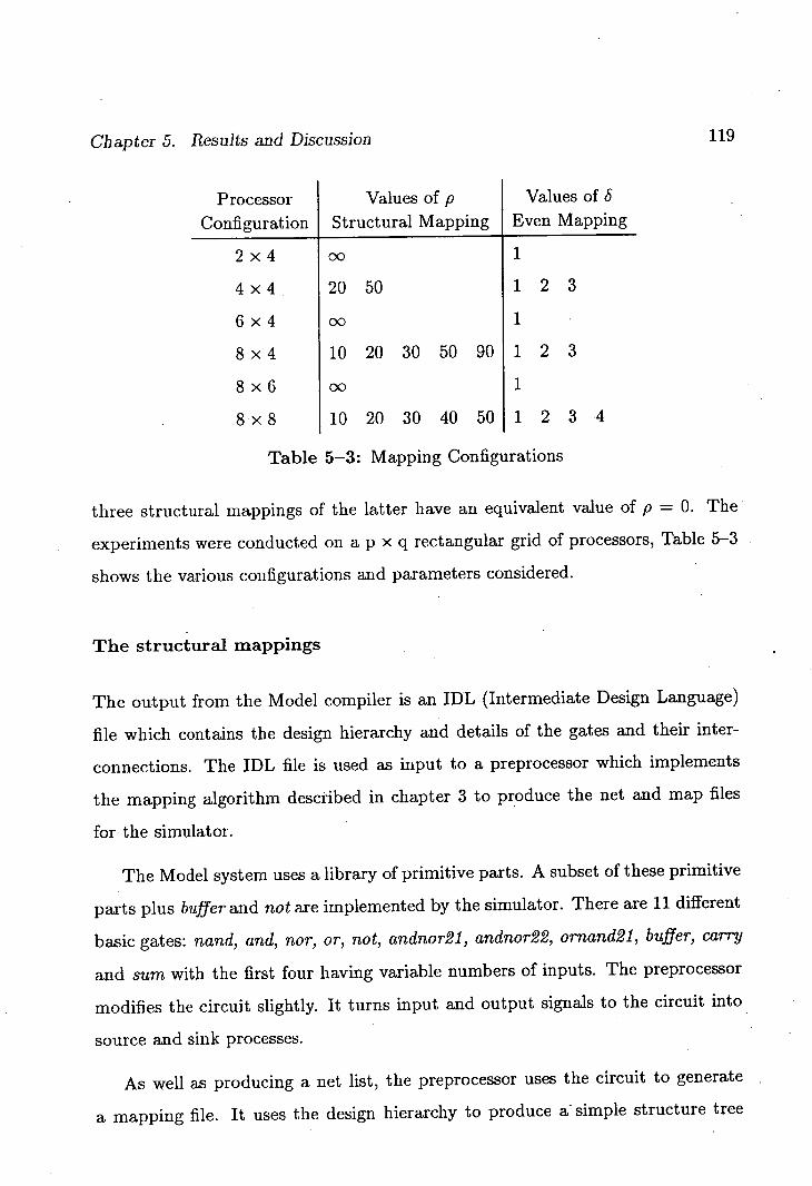
Chapter 5. Results and Discussion 119
Processor Values of p Values of 5
Configuration I Structural Mapping I Even Mapping
2 x 4 00 1
4x4 20 50 1 2 3
6 x 4 00 1
8 x 4 10 20 30 50 90 1 2 3
8 x 6 00 1
8 x 8 10 20 30 40 50 1 2 3 4
Table 5-3: Mapping Configurations
three structural mappings of the latter have an equivalent value of p = 0. The
experiments were conducted on a p x q rectangular grid of processors, Table 5-3
shows the various configurations and parameters considered.
The structural mappings
The output from the Model compiler is an IDL (Intermediate Design Language)
file which contains the design hierarchy and details of the gates and their inter-
connections. The IDL file is used as input to a preprocessor which implements
the mapping algorithm described in chapter 3 to produce the net and map files
for the simulator.
The Model system uses a library of primitive parts. A subset of these primitive
parts plus buffer and not are implemented by the simulator. There are 11 different
basic gates: nand, and, nor, or, not, andnor2l, andnor2, ornand2l, buffer, carry
and sum with the first four having variable numbers of inputs. The preprocessor
modifies the circuit slightly. It turns input and output signals to the circuit into
source and sink processes.
As well as producing a net list, the preprocessor uses the circuit to generate
a mapping file. It uses the design hierarchy to produce a simple structure tree
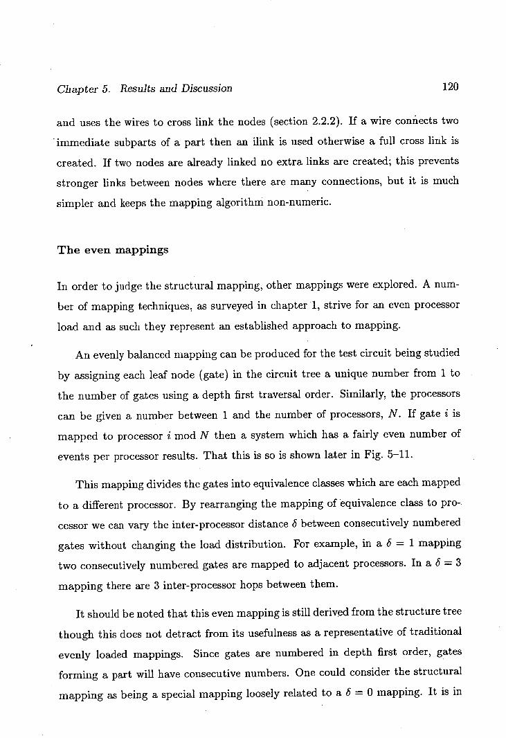
Chapter 5. Results and Discussion 120
and uses the wires to cross link the nodes (section 2.2.2). If a wire connects two
immediate subparts of a part then an ilink is used otherwise a full cross link is
created. If two nodes are already linked no extra links are created; this prevents
stronger links between nodes where there are many connections, but it is much
simpler and keeps the mapping algorithm non-numeric.
The even mappings
In order to judge the structural mapping, other mappings were explored. A num-
ber of mapping techniques, as surveyed in chapter 1, strive for an even processor
load and as such they represent an established approach to mapping.
An evenly balanced mapping can be produced for the test circuit being studied
by assigning each leaf node (gate) in the circuit tree a unique number from 1 to
the number of gates using a depth first traversal order. Similarly, the processors
can be given a number between 1 and the number of processors, N. If gate i is
mapped to processor i mod N then a system which has a fairly even number of
events per processor results. That this is so is shown later in Fig. 5-11.
This mapping divides the gates into equivalence classes which are each mapped
to a different processor. By rearranging the mapping of equivalence class to pro-
cessor we can vary the inter-processor distance 6 between consecutively numbered
gates without changing the load distribution. For example, in a 6 = 1 mapping
two consecutively numbered gates are mapped to adjacent processors. In a 6 = 3
mapping there are 3 inter-processor hops between them.
It should be noted that this even mapping is still derived from the structure tree
though this does not detract from its usefulness as a representative of traditional
evenly loaded mappings. Since gates are numbered in depth first order, gates
forming a part will have consecutive numbers. One could consider the structural
mapping as being a special mapping loosely related to a 6 = 0 mapping. It is in
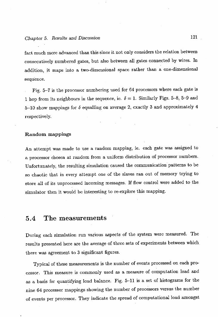
Chapter 5. Results and Discussion 121
fact much more advanced than this since it not only considers the relation between
consecutively numbered gates, but also between all gates connected by wires. In
addition, it maps into a two-dimensional space rather than a one-dimensional
sequence.
Fig. 5-7 is the processor numbering used for 64 processors where each gate is
1 hop from its neighbours in the sequence, ie. 5 = 1. Similarly Figs. 5-8, 5-9 and
5-10 show mappings for 5 equalling on average 2, exactly 3 and approximately 4
respectively.
Random mappings
An attempt was made to use a random mapping, ie. each gate was assigned to
a processor chosen at random from a uniform distribution of processor numbers.
Unfortunately, the resulting simulation caused the communication patterns to be
so chaotic that in every attempt one of the slaves ran out of memory trying to
store all of its unprocessed incoming messages. If flow control were added to the
simulator then it would be interesting to re-explore this mapping.
5.4 The measurements
During each simulation run various aspects of the system were measured. The
results presented here are the average of three sets of experiments between which
there was agreement to 3 significant figures.
Typical of these measurements is the number of events processed on each pro- -
cessor. This measure is commonly used as a measure of computation load and
as a basis for quantifying load balance. Fig. 5-11 is a set of histograms for the
nine 64 processor mappings showing the number of processors versus the number
of events per processor. They indicate the spread of computational load amongst

Chapter 5. Results and Discussion 122
the processors. The top five arise from the structural mapping with values of
p = 10,20,30,40 and 50. The bottom four are based on the even mapping with
6 = 1, 2,3 and 4.
One can see that the evenly loaded mappings are just that - evenly loaded.
They are tightly clustered in a normal bell-shaped distribution with no processor
handling significantly more or less events than any other processor. They are also
identical as would be expected since the same gates are being grouped together in
each case, just the distance between groups is being changed. The fact that they
are different indicates varying amounts of event message elision (section 4.3.2).
The distributions for the structural mappings are quite different. They are
much more spread out allowing significant load imbalances; nor are .they normally
distributed being either skewed or bi-modal. Therefore such measures of load im-
balance as the variance of the processor loads are invalid. Given that the overall
simulation time depends on the maximum of the slave simulation times, the dis-
tribution is irrelevant. A better measure of load spread would be the difference
between maximum and minimum loadings, ie. the range.
Using the range of the processor load distribution as a measure of load im-
balance, we can see from Fig. 5-11 that p does indeed have the desired effect on
the load imbalance. However it would be difficult to quantify the relation as p
controls the number of gates assigned to a processor which only indirectly affects
the number of events handled by that processor.
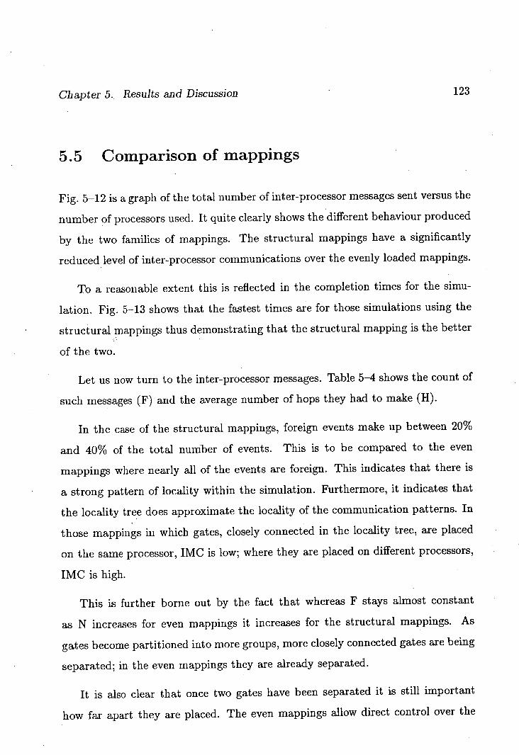
Chapter 5. Results and Discussion 123
5.5 Comparison of mappings
Fig. 5-12 is a graph of the total number of inter-processor messages sent versus the
number of processors used. It quite clearly shows the different behaviour produced
by the two families of mappings. The structural mappings have a significantly
reduced level of inter-processor communications over the evenly loaded mappings.
To a reasonable extent this is reflected in the completion times for the simu-
lation. Fig. 5-13 shows that the fastest times are for those simulations using the
structural mappings thus demonstrating that the structural mapping is the better
of the two.
Let us now turn to the inter-processor messages. Table 5-4 shows the count of
such messages (F) and the average number of hops they had to make (H).
In the case of the structural mappings, foreign events make up between 20%
and 40% of the total number of events. This is to be compared to the even
mappings where nearly all of the events are foreign. This indicates that there is
a strong pattern of locality within the simulation. Furthermore, it indicates that
the locality tree does approximate the locality of the communication patterns. In
those mappings in which gates, closely connected in the locality tree, are placed
on the same processor, 1MG is low; where they are placed on different processors,
IMC is high.
This is further borne out by the fact that whereas F stays almost constant
as N increases for even mappings it increases for the structural mappings. As
gates become partitioned into more groups, more closely connected gates are being
separated; in the even mappings they are already separated.
It is also clear that once two gates have been separated it is still important
how far apart they are placed. The even mappings allow direct control over the
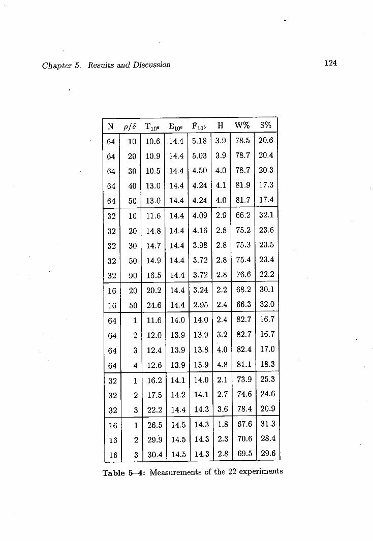
124 Chapter 5. Results and Discussion
N p/ö T106 E106 F 106 H W% S%
64 10 10.6 14.4 5.18 3.9 78.5 20.6
64 20 10.9 14.4 5.03 3.9 78.7 20.4
64 30 10.5 14.4 4.50 4.0 78.7 20.3
64 40 13.0 14.4 4.24 4.1 81.9 17.3
64 50 13.0 14.4 4.24 4.0 81.7 17.4
32 10 11.6 14.4 4.09 2.9 66.2 32.1
32 20 14.8 14.4 4.16 2.8 75.2 23.6
32 30 14.7 14.4 3.98 2.8 75.3 23.5
32 50 14.9 14.4 3.72 2.8 75.4 23.4
32 90 16.5 14.4 3.72 2.8 76.6 22.2
16 20 20.2 14.4 3.24 2.2 68.2 30.1
16 50 24.6 14.4 2.95 2.4 66.3 32.0
64 1 11.6 14.0 14.0 2.4 82.7 16.7
64 2 12.0 13.9 13.9 3.2 82.7 16.7
64 3 12.4 13.9 13.8 4.0 82.4 17.0
64 4 12.6 13.9 13.9 4.8 81.1 18.3
32 1 16.2 14.1 14.0 2.1 73.9 25.3
32 2 17.5 14.2 '14.1 2.7 74.6 24.6
32 3 22.2 14.4 14.3 3.6 78.4 20.9
16 1 26.5 14.5 14.3 1.8 67.6 31.3
16 2 29.9 14.5 14.3 2.3 70.6 28.4
16 3 30.4 14.5 14.3 2.8 69.5 29.6
Table 5-4: Measurements of the 22 experiments
Chapter 5. Results and Discussion 125
inter-module distance by changing 6. Fig. 5-13 shows that increasing 6 has a
direct effect on the completion times. This means that not only is the partitioning
of the problem important so too is the mapping.
As indicated by Table 5-4, H is much higher for structural mappings than for
the even 6 = 1 mappings, but that the actual number of messages sent is 2 to 3
times lower. This supports the assertion that the structural mapping significantly
reduces the number of short distance messages; messages between closely con-
nected gates being localised to within a processor. Thus inter-processor messages
would tend to be between bigger structures over longer distances.
The reduction in the number of inter-processor messages has a number of
effects. We know from our analysis of the simple circuits that non-local events
have a much higher overhead than local events, not only do they increase delays
within the slave, but the through-routing of messages not destined for the processor
also consumes processing time. Fewer foreign events should also lead to reduced
simulation derived delays.
The decrease of communication overheads using the structural mapping is re-
flected in general by the increase in the percentage of time spent simulating, S%.
We should note that due to the large numbers of foreign events, the value of S%
for the even mappings will be inflated as was found in the simulation of circuit C.
This strengthens the point that reducing the number of inter-processor messages
and the distance they travel leads to fewer and shorter delays and to more efficient
simulators, and consequently faster ones.
Chapter 5. Results and Discussion 126
•5.6 General Performance
When we consider Fig. 5-13 a number of aspects are worth noting. With both
mappings there is a marked flattening of the curves as the number of processors
increases. This is to be expected. For a problem of fixed size, as the number of
processors increases, the grain size, ie. the amount of calculation each processor
has to do, decreases. Opposed to this is the increase in communication required
as more gates need to communicate with gates on other processors. Thus the sim-
ulation becomes dominated by communication- costs as the number of processors
increases. Using the terminology of Fox et al. [20], the volume-to-surface ratio gets
worse.
It is this increase in communication costs which limits the speed up of the
system. As the number of processors used is increased there will come a point
after which further processors will increase the overall completion time. Irregular
problems are particularly susceptible to communication dominance since as well
as requiring communication between distant parts of the system, this increase in
communication incurs higher protocol and congestion costs.
We can see from Table 5-4 that apart from one case, the fraction of the total
processing time (T) when the simulation engine is idle (W%) increases with the
number of processors (N). In the case of 16 processors it is about 68% rising to
almost 82% for N = 64. This is to be compared with 58% of the time spent idle
in a quiet system fetching events (section 5.2.3).
It is worth noting that there are 3.5% fewer events processed when using the
even mappings. This is due to event elision as described in section 4.3.2. It is
more likely for this to occur when their are foreign events since delays in foreign
events arriving allow for elision on the other inputs of a gate. In spite of causing
less work, the even mappings are still inferior to the structural mappings.
Chapter 5. Results and Discussion 127
If we look at Fig. 5-11 and Table 5-4 we can see that the structural mapping
can produce several quite different mappings depending on the value of p. From
Fig. 5-13 we can see that for 64 processors there are two distinct clusters of points.
This shows up in the difference in percentage idle times in Table 5-4 and quite
clearly in the different shaped distributions of Fig. 5-11. The better performance
comes with the more restricted load balancing determined by a lower value of
p.. Thus although reducing 1MG is of primary importance, it is still relevant to
consider load balance.
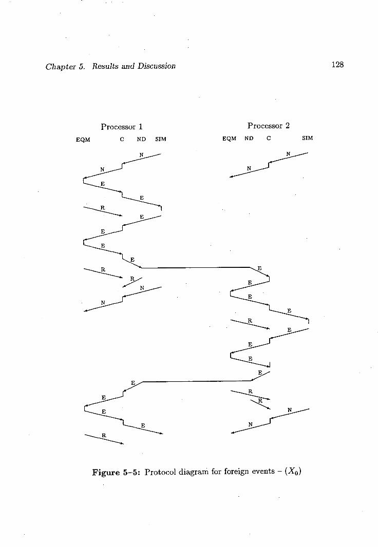
Chapter 5. Results and Discussion 128
Processor 1
Processor 2
EQM C ND SIM EQM ND C SIM
:I,
R
<E N
:E
Figure 5-5: Protocol diagram for foreign events - ( X0)
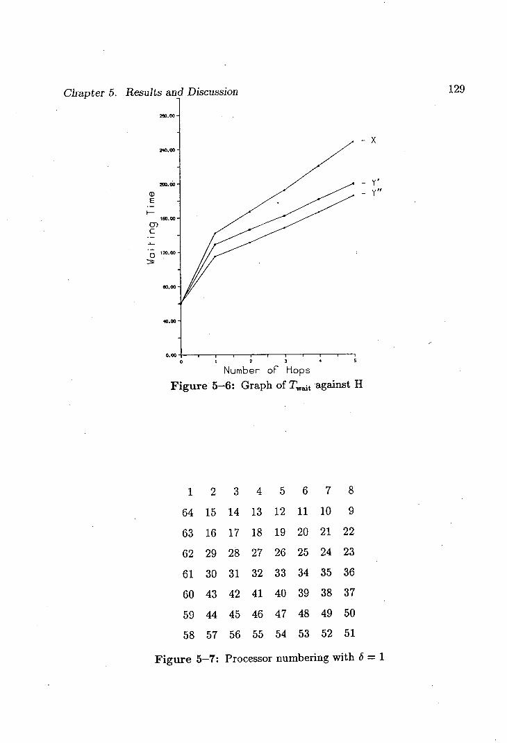
-
-
y if
200.00
240.00
200.00
M E
100.00
0) C
4-
120.00
00.00
40.00
Chapter 5. Results and Discussion 129
0.00 I I I I
0 Number or Hops
Figure 5-6: Graph of against H
123 4 5 678
64 15 14 13 12 11 10 9
63 16 17 18 19 20 21 22
62 29 28 27 26 25 24 23
61 30 31 32 33 34 35 36
60 43 42 41 40 39 38 37
59 44 45 46 47 48 49 50
58 57 56 55 54 53 52 51
Figure 5-7: Processor numbering with 6 = 1
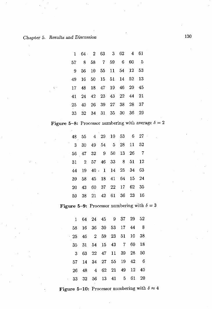
Chapter 5. Results and Discussion 130
1 64 2 63 3 62 4 61
57 8 58 7 59 6 60 5
9 56 10 55 11 54 12 53
49 16 50 15 51 14 52 13
17 48 18 47 19 46 20 45
41 24 42 23 43 22 44 21
25 40 26 39 27 38 28 37
33 32 34 31 35 30 36 29
Figure 5-8: Processor numbering with average 6 = 2
48 55 4 29 10 53 6 27
3 30 49 54 5 28 11 52
5647 32 9 50 13 26 7
31 2 57 46 33 8 51 12
44 1940. 1 14 25 34 63
39 58 45 18 41 64 15 24
20 43 60 37 22 17 62 35
59 38 21 42 61 36 23 16
Figure 5-9: Processor numbering with 6 = 3
1 64 24 45 9 37 29 52
58 16 36 30 53 17 44 8
25 46 2 59 23 51 10 38
35 31 54 15 43 7 60 18
3 63 22 47 11 39 28 50
57 14 34 27 55 19 42 6
26 48 4 62 21 49 12 40
33 32 56 13 41 5 61 20
Figure 5-10: Processor numbering with 6 4
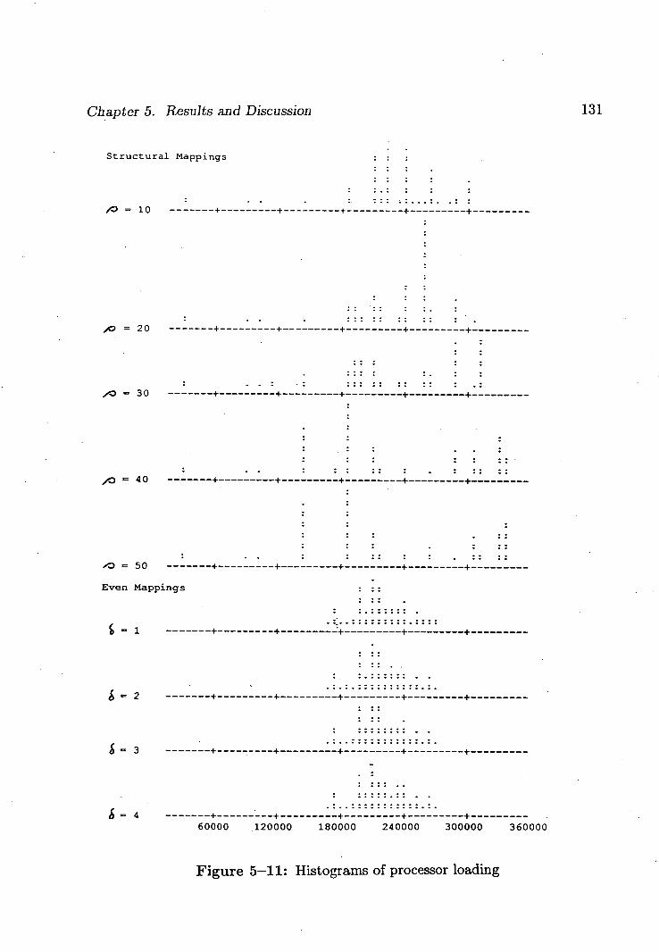
Chapter 5. Results and Discussion 131
Structural Mappings
/0 = 10 -------+---------+---------+---------+---------+---------
= 20 -------+---------+---------+---------+---------+---------
= 30 -------+---------+---------+---------+---------+---------
= 40 ---------------------------------------------------------
'O = 50 -------+---------+---------+---------+---------+--------
Even Mappings
= 1 -------+---------+-------------------+---------+---------
2 -------+---------+--------.
£ = 3 -------+---------+---------+---------+---------+_________
= 4 -------+---------+---------+-------------------+--------- 60000 120000 180000 240000 300000 360000
Figure 5-11: Histograms of processor loading
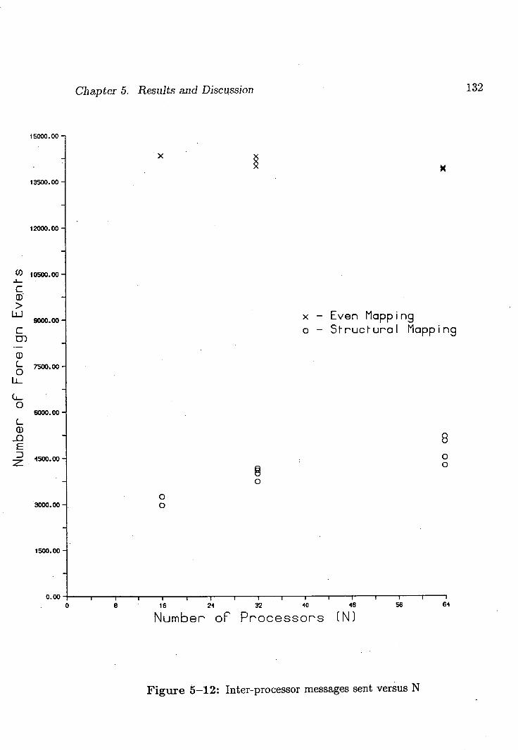
132 Chapter 5. Results and Discussion
8 16 24 32 40 48 56 64
Number oF Processors (N)
Figure 5-12: Inter-processor messages sent versus N
0.00 0
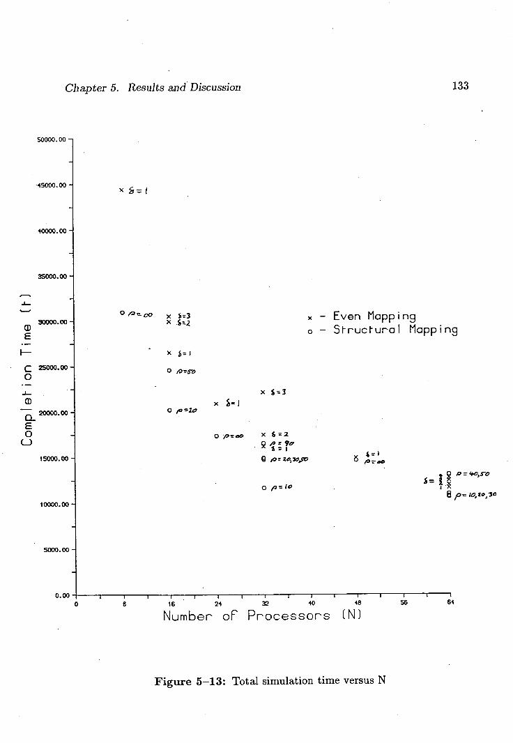
133 Chapter 5. Results and Discussion
8 16 24 32 40 48 56 54
Number of' Processors (N)
50000.00
45000.00
40000.00
35000.00
10000.00
5000.00
0. oc 0
Figure 5-13: Total simulation time versus N
30000.00
E
F-
c 25000.00
0
U) 20000.00
E 0
(-)
15000.00
P = '#, s -e'
jO= 10,90,30
Chapter 6
Summary and Conclusions
Previous attempts at automatic mapping, as surveyed in chapter 1, have all relied
on a deterministic model of behaviour in the form of an objective function. This
latter, a deterministic function of a few measurable and controllable parameters, is
a model or predictor of the time required to complete the application. By finding
a mapping which optimises (perhaps approximately) this objective function, the
surveyed techniques assume that they will find one which will optimise overall
completion time.
Such an assumption is valid where the objective function is an accurate model
of the completion time, but accuracy depends on the completeness of the model. If
the completion time is simply the sum of costs such as computation and communi-
cation then existing techniques can be used. This can be the case in synchronous
problems where the implementation proceeds by alternate phases of computation
and communication each of which is easily measured.
However, if the completion time also includes other costs, in particular, costs
of interaction which are practically impossible to quantify then the objective func-
tion fails and therefore so too do the traditional mapping techniques. Unlike syn-
chronous problems with their restricted patterns of communication, asynchronous
problems introduce synchronisation delays where a processor may be idle wait-
134
Chapter 6. Summary and Conclusions 135
ing for a signal from another processor. These delays depend on the relative
behaviours of the components of the system and usually cannot be isolated or
determined. Typically they are problem specific.
If it were possible to model the interactive behaviour of an asynchronous prob-
lem at a macro level avoiding the need for a complete and detailed model of
computation then this would be a sound basis for a mapping technique.
Chapter 2 presents such a model: the locality tree - an approximate descrip-
tion of the interaction between modules. Through the structure of the tree it
indicates various levels of interaction. Closely related nodes, such as siblings,
represent modules which communicate a lot and are likely to be closely tied to-
gether in their behaviour. Distantly related nodes represent modules which are
much more independent of each other. By assigning closely related modules to the
same processor, or at least to closely related processors, it is intended to reduce
transmission, congestion and synchronisation delays.
As well as the hierarchy, a locality tree may include cross links. These indicate a
secondary and subordinate level of closeness across the tree. Whereas the hierarchy
provides the vertical structure, the cross links provide the horizontal. They allow
different parts within a tree to be drawn together without upsetting the basic
hierarchic structure.
A recursive algorithm was presented in chapter 2 which mapped a locality tree
onto a grid of processors. The hierarchy, in general, determines the partitioning
of modules into groups which are then mapped to the different processors. It
determines the subset of processors to which a module can be assigned. Within
this framework, the cross links are used to arrange the subsets so that inter-module
distance is reduced.
A very simple computation model was added to the locality tree to provide
various levels of load balance. It was assumed that each gate performed an equal
Chapter 6. Summary and Conclusions 136
amount of work and the results of chapter 5 did not invalidate this assumption.
The load imbalance factor p was used to discard mappings which contained too
great a variation in the number of modules assigned to a grid of processors. Chap-
ter 5 showed that reducing p did reduce the range of processor loads, but that the
relation was not clear cut.
For the locality tree to be useful as a concept, it must be possible to construct
one for a given problem. Whereas other mapping methods require detailed infor-
mation of the problem, the structural approach suffices with general, structural
information. In their attempt at generality, traditional approaches discard any
problem specific structure, but as this thesis shows, this is throwing away valuable
information.
One application where the required structural information exists is digital logic
simulation where the circuit has been designed hierarchically. The design hierarchy
can be used to build a locality tree and as the results of chapter 5 show it provides
a reasonable description of the interactive behaviour of the circuit's simulation.
The theory and implementation of a parallel discrete event simulator were
presented in chapters 3 and 4. The two major approaches - conservative and op-
timistic - were described. One characteristic common to both approaches is the
high level of communication involved in comparison to the amount of computa-
tion. A number of techniques such as event elision and multiple acceptances were
presented which reduced the level of communication considerably.
In order to implement the simulator, a communication harness was required to
support processor to processor communication and thus avoid the limitations of
the underlying architecture. To be of use, the harness needed to be deadlock free
and to use a minimum of computation resources. Such a harness was presented in
chapter 4. The requirement for such a harness is general to irregular problems. Its
efficiency and transfer rate have a serious performance impact on problems such
Chapter 6. Summary and Conclusions 137
as logic simulation and therefore it is an area where hardware support would be
useful.
Chapter 5 began with a discussion of the types of delays one could expect in
an asynchronous problem's execution. They fall into two classes; those that are
due to the implementation and those that arise from the the simulation itself.
The former are general to all simulations and can be measured, the latter are
interactive delays and are practically impossible to quantify.
A series of simple experiments was conducted to measure the implementa-
tion delays. It was found that communications dominated the execution of the
simulator. Several suggestions were made on how to reduce the amount of im-
plementation derived communication, in particular the tagging of data messages
instead of sending extracontrol messages.
It is common philosophy amongst the Occam and Transputer community that
processes are cheap and the use of many processes should be encouraged. However,
this ignores the consequent effect of increased communication. It is not just the
extra transfers of data which should be considered, but the increase in protocol
complexity and the consequent delays which can occur.
The simple experiments also highlighted the need for performance analysis
tools. Since the order of processing can have a dramatic effect on performance, it
is important for a programmer to be able to analyse the behaviour of a program
in detail. It is hoped that synthesis and verification tools will become available
in the future. However, as they are normally concerned with program correctness
rather than performance and because of the non-determinism involved there will
still need to be tools which analyse the program in its execution environment.
Any monitoring tool will potentially interfere with the behaviour of the system
being studied. An extra piece of software to be run or another piece of hardware
loading the signal lines may delay an interaction sufficiently to upset the original
Chapter 6. Summary and Conclusions 138
order of events. However, it is specious to say that monitoring tools therefore
give misleading results and should not be used. In many cases, the systems will
be robust enough to absorb the interference without upset. Simply comparing
results with and without monitoring should indicate any problems in this respect.
Even if the tools are intrusive, when used with a knowledge of their limitations,
they can still be of considerable use in understanding the behaviour of the system.
We should also distinguish between tools which give details of the individual
actions of a program and those which give aggregate measures of performance.
The former are important, particularly in debugging, but also because, as was
noted in chapter 5, a minor reordering of actions can have a significant impact on
performance. Such tools would only be used to study small sections of a program.
The aggregate monitoring tools are needed to give an overview of the behaviour
of the system as a whole; to reduce the enormous amounts of monitoring infor -
mation down to a manageable size. These tools would be used to study levels of
communication, congestion and other macro-properties of the system.
Finally, the structural mapping method was used to map a real circuit. Though
the traditional mapping approaches were inapplicable to the program at hand,
one of the goals common to several of them was to produce an evenly balanced
computation load over the processors in the system. From the design hierarchy it
was possible to produce a family of such mappings and they were used to provide
a comparison for the structural approach.
It was found that the structural mapping did indeed result in a much lower level
of inter-module communication than the evenly balanced mapping, thus demon-
strating the usefulness of locality trees. It also shows that the design hierarchy
of the circuit provides locality information for the simulation of that circuit. The
clustering provided by the design hierarchy corresponded to groups of closely re-
lated modules with a high level of interaction. By placing these clusters on the
Chapter 6. Summary and Conclusions 139
same processor the number of inter-processor messages was reduced to 1/3 of the
number resulting from the even mapping.
The reduction of IMC (Inter-Module Communication) also resulted, in general,
in lower overall completion times. However, it was found that although a secondary
factor, load balancing was still important. By constraining the excesses of load
imbalance within the structural framework, the best results were produced.
The variation of results is of particular interest when considering speedup.
As was seen in the case of 32 processors, changing the mapping can double the
completion time. If completion time is significantly affected by interactive delays
such as synchronisation then graphs of performance versus number of processors
need to be treated with considerable caution.
6.1 Future Directions
One disadvantage of a purely structural approach is that it assumes an homoge-
neous level of activity throughout the whole circuit. There will be many circuits
where this is not the case, where the state of different parts of a circuit will be
stable or undergo rapid change depending on the functional nature of the circuit's
subsystems. As a result of this uneven behaviour, processors simulating clusters
of gates can have significantly different amounts of work compared with the rest
of the system and this work load can change dramatically over time. This raises
the possibility of a processor being idle because its cluster of gates has become
inactive, perhaps because the gates are waiting for some trigger or enabling signal
or perhaps because they have completed their simulation before other parts of the
circuit.
To tackle this problem, a hybrid structural/scattered approach is proposed.
As was seen in chapter 5, a large amount of communication is local. Therefore
Chapter 6. Summary and Conclusions 140
the structural approach has greatest effect at the lower levels of the locality tree.
However, as we move lip the locality tree there is less inter-cluster communication
and it is expected that locality will be of less importance for these super clusters.
Therefore, rather than using the structural approach for the entire locality tree,
it is proposed that for the upper levels the super clusters are scattered over the
processors in order to reduce the chance that at any one time all of the gates
assigned to a processor are blocked.
One way to do this is to use the structural approach to map the lower clusters
onto a grid of virtual processors several times larger than the actual topology then
fold the virtual topology over onto itself so that several unrelated clusters are
mapped onto the same real processor. This hybrid approach retains the localised
nature of the structural model at the levels where communication levels are high
and introduces a scattered decomposition at the higher levels in order to even out
load fluctuations.
Another direction for future work is to explore the use of a structural approach
in other applications. Two applications which are similar in structure to logic
simulation are the simulation of air traffic and of packet based networks. In both
cases, geographical locality could be used to provide the structural information.
The sky and the network can reasonably be described in terms of national, regional
and local groupings which can be used to map a simulation.
The structural method represents a completely different approach to mapping.
Whereas traditional methods try to be as general as possible, only using metrics
common to all parallel programs such as communication and execution costs, this
thesis argues that for the more difficult case of asynchronous, irregular problems
knowledge specific to the problem should be used. In the application studied here,
the knowledge is structural. In other applications, there may be other types of
knowledge which can be used to produce good mappings.
This thesis has explored a number of the difficulties encountered when imple-

Chapter 6. Summary and Conclusions 141
menting irregular asynchronous problems on a parallel distributed memory archi-
tecture. It has shown why traditional mapping techniques are inapplicable to such
problems and has presented an alternative: the structural approach.
Bibliography
P. America.
Definition of the programming language POOL-T.
Doc. nr. 0091, Philips Research Laboratories, Sept. 1985.
P. America.
Rationale for the design of POOL.
Doc. nr. 0053, Philips Research Laboratories, Jan. 1986.
P. America, J. de Bakker, J. Kok, and J. Rutten.
Operational semantics of a parallel object-oriented language.
In proc. 13th ACM symp. on the Princs. of Prog. Langs., pages 194 - 208,
Jan. 1986.
R. K. Arora and S. P. Rana.
Analysis of the module assignment problem in distributed computing
systems with limited storage.
Inf. Process. Lett., 10(3):111 - 115, Apr. 1980.
R. K. Arora and S. P. Rana.
Heuristic algorithms for process assignment in distributed computing
systems.
Inf. Process. Lett., 11(4,5):199 - 203, Dec. 1980.
L. Augusteijn, J. M. Jansen, F. Van DerLinden, and F. Sijstermans.
Programmer controlled object allocation.
142
Bibliography 143
Doc. nr. 0286, Philips Research Laboratories, Esprit Project 415A, May
1987.
I. M. Barron, P. Cavill, D. May, and P. Wilson.
The transputer.
Electronics, page 109, Nov 17 1983.
0. Berry.
Performance evaluation of the Time Warp distributed simulation
mechanism.
PhD thesis, Univ. Southern California, 1986.
S. H. Bokari.
On the mapping problem.
IEEE Trans. Comput., C-30(3):207 - 214, Mar. 1981.
S. H. Bokhari.
Dual processor scheduling with dynamic reassignment.
IEEE Trans. Softw. Eng., SE-5(4):341 - 349, July 1979.
R. E. Bryant.
Simulation of packet communication architecture computer systems.
Technical Report LCS TR-188, MIT, 1977
K. M. Chandy and J. Misra.
Distributed simulation: A case study in design and verification of
distributed programs
IEEE Trans. Softw. Eng., SE-5(9):440 - 452, Sept. 1979.
K. M. Chandy and J. Misra.
Asynchronous distributed simulation via a sequence of parallel
computations.
Commun. ACM, 24(11):198 - 206, Apr. 1981.
Bibliography 144
T. C. K. Chou and J. A. Abraham.
Load balancing in distributed systems.
IEEE Trans. Softw. Eng., SE-8(4):401 - 412, July 1982.
W. W. Chu, M. T. Lan, and J. Hellerstein.
Estimation of inter-module communication and its application in
distributed processing systems.
IEEE Trans. Comput., C33(8):691 - 699, Aug. 1984.
E. G. Coffman, Jr., editor.
Computer and Job-shop scheduling theory.
Wiley, 1976.
M. A. d'Abreu.
Gate-level simulation.
IEEE Design and Test of Computers, pages 63 - 71, Dec. 1985.
J. G. Donnett, M. Starkey, and D. B. Skillicorn.
Effective algorithms for partitioning distributed programs.
Unpublished report. Queen's University Kingston Canada.
K. Efe.
Heuristic models of task assignment scheduling in distributed systems.
Computer, pages 50 - 56, June 1982.
G. Fox, M. Johnson, G. Lysenga, S. Otto, J. Salmon, and D. Walker.
Solving problems on concurrent processors.
Prentice-Hall International, 1988.
W. R. Franta.
The process view of simulation.
North-Holland, NY, 1977.
M. R. Garey and D. S. Johnson.
Bibliography 145
Computers and Intractability: A guide to the theory of NP-Completeness.
Freeman and Co., 1979.
J. Gleick.
Chaos: Making a new science.
Sphere, 1988.
V. B. Gylys and J. A. Edwards.
Optimal partitioning of workload for distributed systems.
In Digest of papers Compcon Fall, pages 353 - 357, 1976.
M. Hanan and J. M. Kurtzberg.
A review of the placement and quadratic assignment problems.
SIAM Review, 14(2):324 - 342, Apr. 1972.
C. A. R. Hoare.
Communicating Sequential Processes.
Commun. ACM, 21(8):666-677, Aug. 1978.
E. Horowitz and S. Sahni.
Fundamentals of computer algorithms.
Pitman, 1978.
P. Hudak.
Para-functional programming.
Computing, 19(8):60 - 71, Aug. 1986.
P. Hudak and L. Smith.
Para-functional programming: A paradigm for programming multiprocessor
systems.
In proc. 13th ACM symp. on the Princs. of Frog. Langs., pages 243 - 254,
1986.
M. A. Iqbal, J. H. Saltz, and S. H. Bokhari.
Bibliography 146
A comparative analysis of static and dynamic load balancing strategies.
In proc. of the 1986 mt. Conf. on Parallel Processing, pages 1040 - 1047,
1986.
D. Jefferson and H. Sowizral.
Fast concurrent simulation using the Time Warp mechanism. Part 1: local
control.
Technical report, The Rand Corporation, June 1983.
D. Jefferson and H. Sowizral.
Fast concurrent simulation using the Time Warp mechanism.
In proc. SCS distributed simulation conference, pages 63 - 69, 1985.
A. K. Jones.
The object model: a conceptual tool for structuring software.
In R. Bayer, editor, Operating Systems, chapter 2, pages 7 - 16.
Springer-Verlag, 1979.
A. V. Karzanov.
Determining the maximal flow in a network by the method of preflows.
Soviet Math. Dokiady, 15(2):434 - 437, 1974.
S. Kirkpatrick, C. D. Gelatt, Jr, and M. P. Vecchi.
Optimization by simulated annealing.
Science, 220(4598):671 - 680, May 1983.
T. Koopmans and M. Beckmann.
Assignment problems and the location of economic activities.
Econornetrica, 25:53 - 76 7 1957.
L. Lamport.
Time, clocks and the ordering of events in a distributed system.
Commun. ACM, 21(7):558 - 565, July 1978.
Bibliography 147
Lattice Logic Ltd., Edinburgh.
CHIPSMITH, A random logic compiler for gate arrays, optimised arrays
and standard cell implementations, 1985.
S.-Y. Lee and J. K. Aggarwal.
A mapping strategy for parallel processing.
IEEE Trans. Comput., C-36(4):433 - 442, Apr. 1987.
P. R. Ma, E. Y. S. Lee, and M. Tsuchiya.
A task allocation model for distributed computing systems.
IEEE Trans. Comput., C-31(1):41 - 47, Jan. 1982.
D. May.
Occam 2 language definition.
Technical report, Inmos Ltd, Feb. 1987.
N. Metropolis, A. Rosenbiuth, M. Rosenbluth, A. Teller, and E. Teller.
Equation of state -calculations by fast computing machines.
J. Chem. Phys., 21:1087 - 1091, 1953.
R. Milner.
Communication and concurrency.
Prentice Hall International, 1989.
J. Misra.
Distributed discrete-event simulation.
Computing Surveys, 18(1):39 - 65, Max. 1986.
Morison, Peeling, and Thorp.
Ella, a hardware description language.
In IEEE, mt. conf on circuits and computers, 1982.
N. J. Nilsson.
Principles of Artificial Intelligence.
Tioga, 1980.
Bibliography
J. K. Peacock, J. W. Wong, and E. G. Manning.
A distributed approach to queueing theory.
In 1979 Winter simulation conference, pages 399 - 406, 1979.
J. K. Peacock, J. W. Wong, and E. G. Manning.
Distributed simulation using a network of processors.
Computer Networks, 3(1):44 - 56, Feb. 1979.
J. L. Peterson and A. Silberschatz.
Operating system concepts, 2nd ed.
Addison-Wesley, 1985.
G. S. Rao, H. S. Stone, and T. C. Hu.
Assignment of tasks in a distributed processor system with limited memory.
IEEE Trans. Comput., C-28(4):291 - 299, Apr. 1979.
S. Sahni and T. Gonzalez.
P-complete approximation problems.
J. ACM, 23(3):555 - 565, July 1976.
C.-C. Shen and W.-H. Tsai.
A graph matching approach to optimal task assignment in distributed
computing systems using a minimax criterion.
IEEE Trans. Comput., C-34(3):197 - 203, Mar. 1985.
S. G. Smith and P. B. Denyer.
Serial-Data Computation.
Kluwer Academic Publishers, 1988.
H. S. Stone.
Multiprocessor scheduling with the aid of network flow algorithms.
IEEE Trans. Softw. Eng., SE-3(1):85 - 93, Jan. 1977.
H. S. Stone and S. H. Bokhari. I
Bibliography 149
Control of distributed processes.
Computer, pages 97 - 106, July 1978.
S. A. Szygenda and E. W. Thompson.
Digital logic simulation in a time-based, table-driven environment Part-1.
Design verification.
Computer, 8(3):24 - 36, Mar. 1975.
The Xerox Learning Research Group.
The Smalltalk-80 system.
Byte, pages 36 - 48, Aug. 1981.
Appendix A
Published paper
The following paper was published in the Proceedings of the SCS Multiconference
on Distributed Simulation, 28-31 March, 1989, Tampa Florida.
The publishers accept that I retain the right to republish this paper in whole
or in part in any book of which I am an author or editor and to make personal
use of this work in lectures, courses, or otherwise.
150
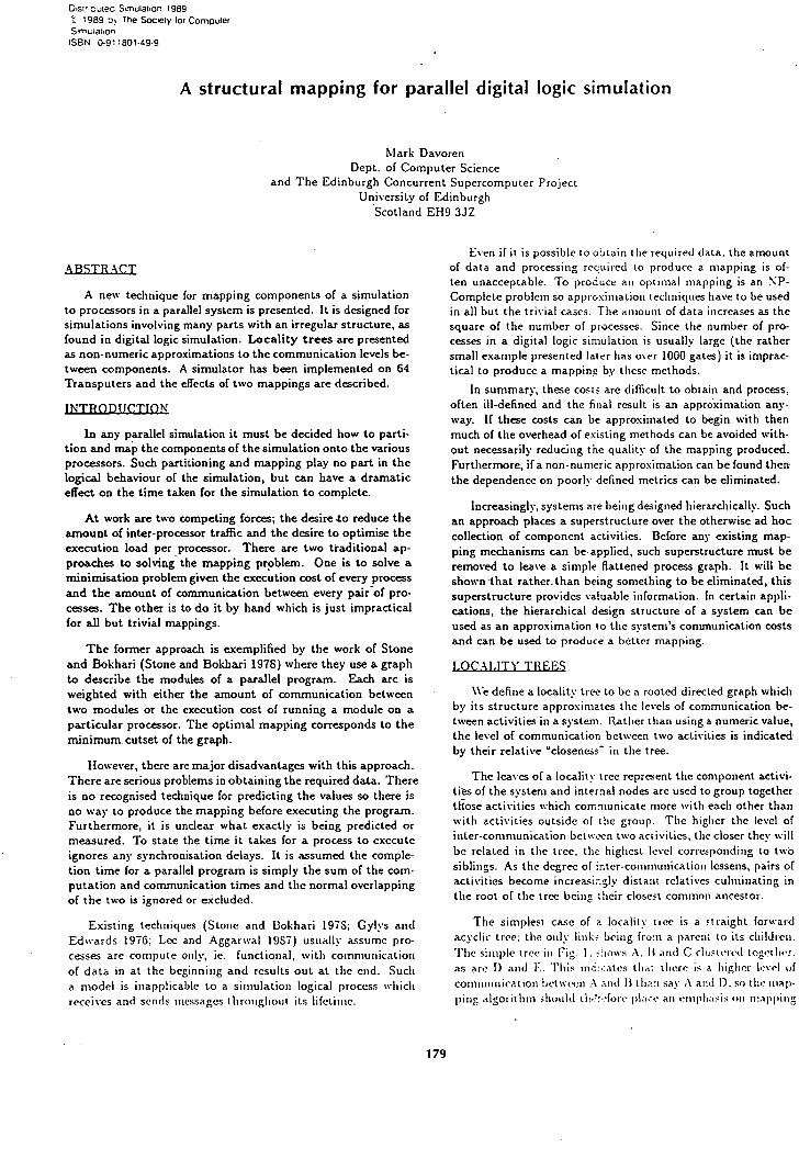
Dis1rutec Simulation 1989 1989 The Society for Computer
Smuator, ISBN 0-911801.49-9
A structural mapping for parallel digital logic simulation
Mark Davoren Dept. of Computer Science
and The Edinburgh Concurrent Supercomputer Project University of Edinburgh
Scotland EH9 3JZ
ABSTRACT
A new technique for mapping components of a simulation to processors in a parallel system is presented. It is designed for simulations involving many parts with an irregular structure, as found in digital logic simulation. Locality trees are presented as non-numeric approximations to the communication levels be-tween components. A simulator has been implemented on 64 Transputers and the effects of two mappings are described.
kP;(IJI1I1•ilfI)
In any parallel simulation it must be decided how to parti-tion and map the components of the simulation onto the various processors. Such partitioning and mapping play no part in the logical behaviour of the simulation, but can have a dramatic effect on the time taken for the simulation to complete.
At work are two competing forces; the desire ,to reduce the amount of inter-processor traffic and the desire to optimise the execution load per processor. There are two traditional ap-proaches to solving the mapping problem. One is to solve a minimisation problem given the execution cost of every process and the amount of communication between every pair of pro-cesses. The other is to do it by hand which is just impractical for all but trivial mappings.
The former approach is exemplified by the work of Stone and Bokhari (Stone and Bokhari 1978) where they use a graph to describe the modules of a parallel program. Each arc is weighted with either the amount of communication between two modules or the execution cost of running a module on a particular processor. The optimal mapping corresponds to the minimum cutset of the graph.
However, there are major disadvantages with this approach. There are serious problems in obtaining the required data. There is no recognised technique for predicting the values so there is no way to produce the mapping before executing the program. Furthermore, it is unclear what exactly is being predicted or measured. To state the time it takes for a process to execute ignores any synchronisation delays. It is assumed the comple-tion time for a parallel program is simply the sum of the com-putation and communication times and the normal overlapping of the two is ignored or excluded.
Existing techniques (Stone and Bokhari 197$; Cylvs and Edwards 1976: Lee and Aggarwal 1937) usually assume pro-cesses are compute only, ie. functional, with communication of data in at the beginning and results out at the end. Such a model is inapplicable to a simulation logical process which receives and sends messages throughout its lifetime.
Even if it is possible to obtain the requited data, the amount of data and processing required to produce a mapping is of-ten unacceptable. To produce an optimal mapping is an NP-Complete problem so approximation techniques have to be used in all but the trivial cases. The amount of data increases as the square of the number of processes. Since the number of pro-cesses in a digital logic simulation is usually large (the rather small example presented later has over 1000 gates) it is imprac-tical to produce a mapping by these methods.
In summary, these costs are difficult to obtain and process, often ill-defined and the final result is an approximation any-way. If these costs can be approximated to begin with then much of the overhead of existing methods can be avoided with-out necessarily reducing the quality of the mapping produced. Furthermore, if a non-numeric approximation can be found then the dependence on poorly defined metrics can be eliminated.
Increasingly, systems are being designed hierarchically. Such an approach places a superstructure over the otherwise ad hoc collection of component activities. Before any existing map-ping mechanisms can be-applied, such superstructure must be removed to leave a simple flattened process graph. It will be shown that rather. than being something to be eliminated, this superstructure provides valuable information. In certain appli-cations, the hierarchical design structure of a system can be used as an approximation to the system's communication costs and can be used to produce a better mapping.
We define a locality tree to be a rooted directed graph which by its structure approximates the levels of communication be-tween activities in a system. Rather than using a numeric value, the level of communication between two activities is indicated by their relative "closeness in the tree.
The leaves of a locality tree represent the component activi-ties of the system and internal nodes are used to group together those activities which communicate more with each other than with activities outside of the group. The higher the level of inter-communication between two activities, the closer they will be related in the tree, the highest level corresponding to two siblings. As the degree of inter-communication lessens, pairs of activities become increasingly distant relatives culminating in the toot of the tree being hteir closest common ancestor.
The simplest case of a locality tree is a straight forward acyclic tree: the only link- being fro.n a parent to its children. The SitU pie tree in Fig. 1. tows A. II and C ci us t cted toii.et I icr. as are I) and F. This ine:.:ates that there is a higher level of communication bet wecti :\ :eid II t 11:1:1 say A and I). SO the map-ping algorithm should tlt.?:.'fote >1517c all (!tiih ) lI;tSis Ott tltappiutg
179
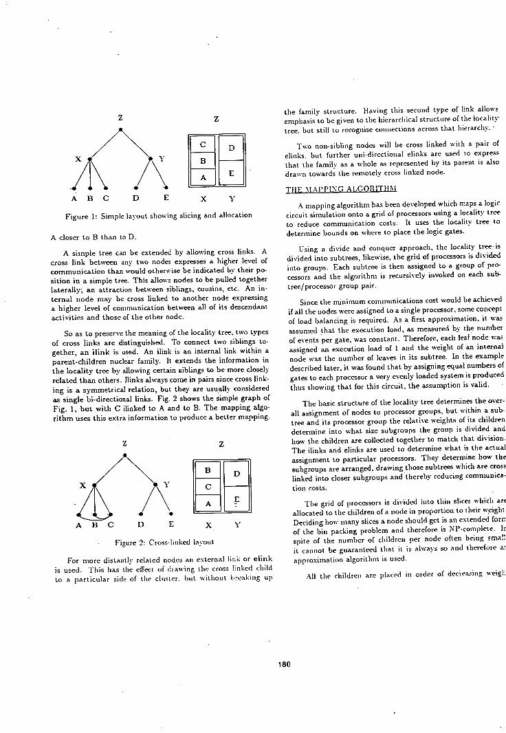
ABC D E x Y
Figure 1: Simple layout showing slicing and allocation
A closer to B than to D.
A simple tree can be extended by allowing cross links. A cross link between any two nodes expresses a higher level of communication than would otherwise be indicated by their po-sition in a simple tree. This allows nodes to be pulled together laterally; an attraction between siblings, cousins, etc. An in-ternal node may be cross linked to another node expressing a higher level of communication between all of its descendant activities and those of the other node.
So as to preserve the meaning of the locality tree, two types of cross links are distinguished. To connect two siblings to-gether, an junk is used. An ilink is an internal link within a parent-children nuclear family. It extends the information in the locality tree by allowing certain siblings to be more closely related than others. Ilinks always come in pairs since cross link-ing is a symmetrical relation, but they are usually considered as single bi-directional links. Fig. 2 shows the simple graph of Fig. 1, but with C ilinked to A and to B. The mapping algo-
rithm uses this extra information to produce a better mapping.
Z
EXY
Figure 2: Cross-linked layout
For more distantly related nodes an external link or elink is used. This has the effect of drawing the cross !nked child to a particular side of the cluster, b ut without breaking Uj)
the family structure. having this second type of link allows emphasis to be given to the hierarchical structure of the locality tree, but still to recognise connections across that hierarchy.
Two non-sibling nodes will be cross linked with a pair of clinks. but further uni-directional elinks are used to express that the family as a whole as represented by its parent is also drawn towards the remotely cross linked node.
THE MAPPING ALGORITHM
A mapping algorithm has been developed which maps a logic circuit simulation onto a grid of processors using a locality tree to reduce communication costs. It uses the locality tree to determine bounds on where to place the logic gates.
Using a divide and conquer approach, the locality tree is divided into subtrees, likewise, the grid of processors is divided into groups. Each subtree is then assigned to a group of pro- -
cessors and the algorithm is recursively invoked on each sub-
tree/processor group pair.
Since the minimum communications cost would be achieved if all the nodes were assigned to a single processor, some concept of load balancing is required. As a first approximation, it was assumed that the execution load, as measured by the number of events per gate, was constant. Therefore, each leaf node was assigned an execution load of 1 and the weight of an internal node was the number of leaves in its subtree. In the example described later, it was found that by assigning equal numbers of gates to each processor a very evenly loaded system is produced thus showing that for this circuit, the assumption is valid.
The basic structure of the locality tree determines the over-all assignment of nodes to processor groups, but within a sub-tree and its processor group the relative weights of its children determine into what size subgroups the group is divided and how the children are collected together to match that division. The ilinks and elinks are used to determine what is the actual assignment to particular processors. They determine how the subgroups are arranged, drawing those subtrees which are cross linked into closer subgroups and thereby reducing communica-
tion costs.
The grid of processors is divided into thin slices which are allocated to the children of a node in proportion to their w right.
Deciding how many slices a node should get is an extended form of the bin packing problem and therefore is NP-complete. In spite of the number of children per node often being small
it cannot. be guaranteed that it is always so and therefore a::
approximation algorithm is used.
All the children are placed in order of deci'eaitig weigL
180
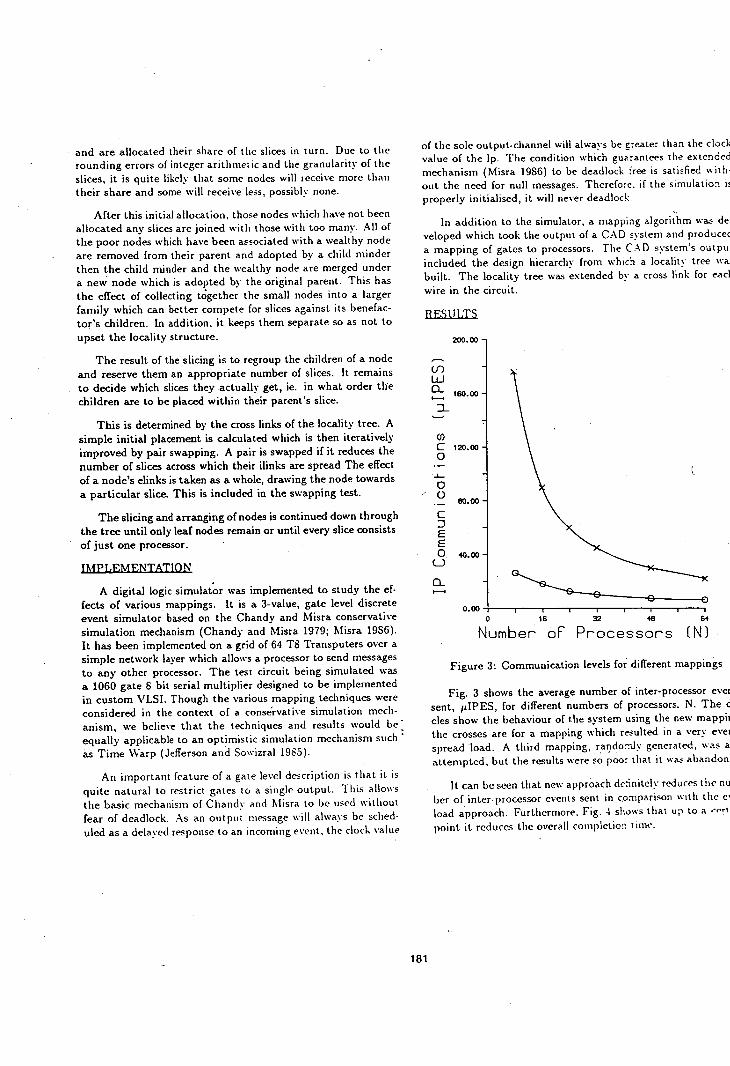
and are allocated their share of the slices in turn. Due to the rounding errors of integer arithmetic and the granularity of the slices, it is quite likely that some nodes will receive more than their share and some will receive less, possibly none.
After this initial allocation, those nodes which have not been allocated any slices are joined with those with too many. All of the poor nodes which have been associated with a wealthy node are removed from their parent and adopted by a child minder then the child minder and the wealthy node are merged under a new node which is adopted by the original parent. This has the effect of collecting together the small nodes into a larger family which can better compete for slices against its benefac-tor's children. In addition, it keeps them separate so as not to upset the locality structure.
The result of the slicing is to regroup the children of a node and reserve them an appropriate number of slices. It remains to decide which slices they actually get, ie. in what order the children are to be placed within their parent's slice.
This is determined by the cross links of the locality tree. A simple initial placement is calculated which is then iteratively improved by pair swapping. A pair is swapped if it reduces the number of slices across which their ilinks are spread The effect of a node's elinks is taken as a whole, drawing the node towards a particular slice. This is included in the swapping test.
The slicing and arranging of nodes is continued down through the tree until only leaf nodes remain or until every slice consists of just one processor.
A digital logic simulator was implemented to study the ef-fects of various mappings. It is a 3-value, gate level discrete event simulator based on the Chandy and Misra conservative simulation mechanism (Chandy and Misra 1979; Misra 19S6). It has been implemented on a grid of 64 T8 Transputers over a simple network layer which allows a processor to send messages to any other processor. The test circuit being simulated was a 1060 gate 8 bit serial multiplier designed to be implemented in custom \'LSI. Though the various mapping techniques were considered in the context of a conservative simulation mech-anism, we believe that the techniques and results would be equally applicable to an optimistic simulation mechanism such as Time Warp (Jefferson and Sowizral 1985).
An important feature of a gate level description is that it is quite natural to restrict gates to a single output. This allows the basic mechanism of Chandv and Misra to be used without fear of deadlock. As an output message will always be sched-uled as a delayed response to an incoming event, the clock value
of the sole output-channel will always be greater than the clod value of the Ip. The condition which guarantees the extendec mechanism (Misra 1986) to be deadlock free is satisfied with out the need for null messages. Therefore, if the simulation i properly initialised, it will never deadlock.
In addition to the simulator, a mapping algorithm was de veloped which took the output of a CAD system and produce a mapping of gates to processors. The CAD system's ouspu included the design hierarchy from which a locality tree wa built. The locality tree was extended by a cross link for cad
wire in the circuit.
0 16 32 48 64
Number oP Processors (N)
Figure 3: Communication levels for different mappings
Fig. 3 shows the average number of inter-processor evei sent, tIPES, for different numbers of processors. N. The des show the behaviour of the system using the new mappil the crosses are for a mapping which resulted in a very eve spread load. A third mapping, randoTJy generated, was a attempted, but the results were so poor that It was abandon
It can be seen that new approach definitely reduces the n her of inter-processor events sent in comparison with the c load approach. Furthiernlore. Fig. 4 shows that u; to a .-f'ri
point it reduces the overall completion time.
200.00
In LU
160.00
:3-
(I) C 120.00 0
.1
0
80.00
C :3 E E o 40.00
I-)
0
0.00
181
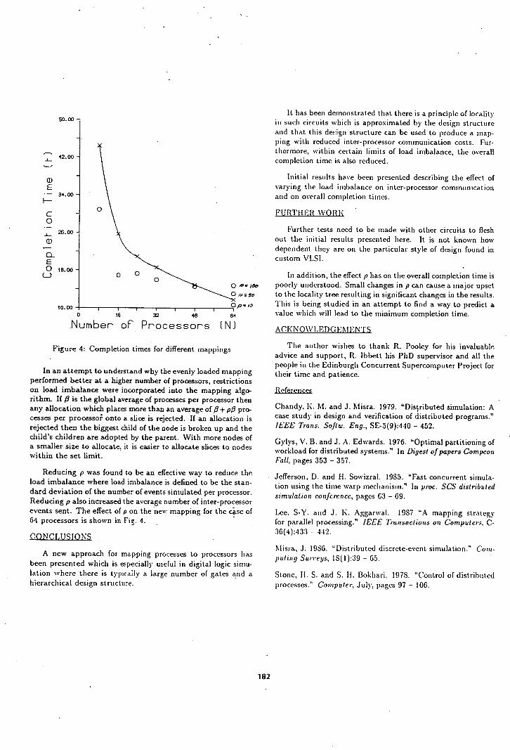
42.00
CD E
34.00 F-
0
26.00
U)
0 E o 18.00
C-)
10.00
50.00
0 16 32 48 64
Number oP Processors (N)
It has been demonstrated that there is a principle of locality in such circuits which is approximated by the design structure and that this derign structure can be used to produce a map-ping with reduced Inter-processor communication costs. Fur-thermore, within certain limits of load imbalance, the overall completion time is also reduced.
Initial results have been presented describing the effect of varying the load imbalance on inter- processor communication and on overall completion times.
FURTHER WORK
Further tests need to be made with other circuits to flesh out the initial results presented here. It is not known how dependent they are on the particular style of design found in custom VLSI.
In addition, the effect p has on the overall completion time is e poorly understood. Small changes in p can cause a major upset ss to the locality tree resulting in significant changes in the results.
,.,, This is being studied in an attempt to find a way to predict a value which will lead to the minimum completion time.
ACKNO\\TLEDC EMENTS
Figure 4: Completion times for different mappings
In an attempt to understand why the evenly loaded mapping performed better at a higher number of processors, restrictions on load imbalance were incorporated into the mapping algo-rithm. If 13 is the global average of processes per processor then any allocation which places more than an average of 13 + p/3 pro-cesses per processoi onto a slice is rejected. If an allocation is rejected then the biggest child of the node is broken up and the child's children are adopted by the parent. With more nodes of a smaller size to allocate, it is easier to allocate slices to nodes within the set limit.
Reducing p was found to be an effective way to reduce the load imbalance where load imbalance is defined to be the stan-dard deviation of the number of events simulated per processor. Reducing p also increased the average number of inter-processor events sent. The effect of p on the new mapping for the cse of 64 processors is shown in Fig. 4.
A new approach for mapping processes to processors has been presented which is especially useful in digital logic sintu-lation where there is typically a large number of gates and a hierarchical design structure.
The author wishes to thank R. Pooley for his invaluable advice and support, R. lbbett his PhD supervisor and all the people in the Edinburgh Concurrent Supercomputer Project for their time and patience.
References
Chandy, K. M. and J. Misra. 1979. "Distributed simulation: A case study in design and verification of distributed programs." IEEE Trans. Softw. Eng., SE-5(9):440 - 452.
Gylys, V. B. and J. A. Edwards. 1976. "Optimal partitioning of workload for distributed systems." In Digest of papers Corn peon Fall, pages 353 - 357.
Jefferson, D. and H. Sowizral. 1985. "Fast concurrent simula-tion using the time warp mechanism." In proc. SC'S distributed simulation conference, pages 63 - 69.
Lee, S-Y. and J. K. Aggarval. 1987 "A mapping strategy for parallel processing." IEEE Transactions on Computers. C-36(4):433 - 442.
Misra, J. 1986. "Distributed discrcte.evcnt simulation." Corn-puling Surreys, 18(l):39 - 65.
Stone, H. S. and S. H. Bokhari. 1978. "Control of distributed processes." Computer, July, pages 97 - 106.
182