Embed Size (px)
Citation preview

Advanced Control and Optimisation of DC-DC Converters with Application to Low Carbon Technologies Maganga. O.G
Submitted version deposited in Coventry University’s Institutional Repository Original citation: Maganga. O.G. (2015) Advanced Control and Optimisation of DC-DC Converters with Application to Low Carbon Technologies. Unpublished PhD Thesis. Coventry: Coventry University Copyright © and Moral Rights are retained by the author. A copy can be downloaded for personal non-commercial research or study, without prior permission or charge. This item cannot be reproduced or quoted extensively from without first obtaining permission in writing from the copyright holder(s). The content must not be changed in any way or sold commercially in any format or medium without the formal permission of the copyright holders. Some materials have been removed from this thesis due to Third Party Copyright. Pages where material has been removed are clearly marked in the electronic version. The unabridged version of the thesis can be viewed at the Lanchester Library, Coventry University.

Advanced Control and Optimisation ofDC-DC Converters with Application to
Low Carbon Technologies
Othman G MagangaB.Eng, MSc, MInstMC
A Thesis submitted in partial fulfillment of the University’s requirements for the
Degree of Doctor of Philosophy
September 2015
Control Theory and Applications Centre
Coventry University
Acknowledgement: Support of European Thermodynamics Limited, Kibworth,
Leicester, UK
Abstract
Prompted by a desire to minimise losses between power sources and loads,
the aim of this Thesis is to develop novel maximum power point tracking (MPPT)
algorithms to allow for efficient power conversion within low carbon technologies.
Such technologies include: thermoelectric generators (TEG), photovoltaic (PV)
systems, fuel cells (FC) systems, wind turbines etc. MPPT can be efficiently
achieved using extremum seeking control (ESC) also known as perturbation based
extremum seeking control. The basic idea of an ESC is to search for an extrema
in a closed loop fashion requiring only a minimum of a priori knowledge of the
plant or system or a cost function.
In recognition of problems that accompany ESC, such as limit cycles,
convergence speed, and inability to search for global maximum in the presence
local maxima this Thesis proposes novel schemes based on extensions of ESC. The
first proposed scheme is a variance based switching extremum seeking control
(VBS-ESC), which reduces the amplitude of the limit cycle oscillations. The
second scheme proposed is a state dependent parameter extremum seeking control
(SDP-ESC), which allows the exponential decay of the perturbation signal. Both
the VBS-ESC and the SDP-ESC are universal adaptive control schemes that can
be applied in the aforementioned systems. Both are suitable for local maxima
search. The global maximum search scheme proposed in this Thesis is based
on extensions of the SDP-ESC. Convergence to the global maximum is achieved
by the use of a searching window mechanism which is capable of scanning all
available maxima within operating range. The ability of the proposed scheme
to converge to the global maximum is demonstrated through various examples.
Through both simulation and experimental studies the benefit of the SDP-ESC
has been consistently demonstrated.
i

Acknowledgements
I am deeply indebted to my Director of studies Dr Malgorzata Sumislawska, my
Supervisors Prof. Keith Burnham and Joe Mahtani from the Control Theory
and Applications Centre (CTAC) for their advice, kindness, encouragement and
stimulating suggestions which motivated me while working on this Thesis. Also,
I would like to thank Kevin Simpson and other members of European Thermody-
namics Limited for the support they have given me while conducting my research.
Furthermore, I pass on my thanks to Andrea Montecucco from Glasgow Univer-
sity and my colleague Navneesh Phillip and all of those who supported me in
any respect during the completion of my Thesis. Lastly, I offer my regards and
blessings to my lovely wife Martyna Maganga and my family for their advice and
encouragement that enabled me to complete this work.
ii

Contents
Page
Abstract i
Acknowledgements ii
Contents iii
List of Figures vi
Nomenclature xii
Abbreviations . . . . . . . . . . . . . . . . . . . . . . . . . . . . . . . . . . . xii
Notation . . . . . . . . . . . . . . . . . . . . . . . . . . . . . . . . . . . . . . xiii
1 Introduction 1
1.1 Introduction . . . . . . . . . . . . . . . . . . . . . . . . . . . . . . . . . 1
1.2 Statement of the problem . . . . . . . . . . . . . . . . . . . . . . . . . 2
1.2.1 Local maxima search for mismatch reduction . . . . . . . . 2
1.2.2 Global maximum search in the presence of local maxima . 4
1.3 Scope and goals of this Thesis . . . . . . . . . . . . . . . . . . . . . . 4
1.4 List of publications . . . . . . . . . . . . . . . . . . . . . . . . . . . . . 7
1.5 Original contributions . . . . . . . . . . . . . . . . . . . . . . . . . . . 8
1.6 Outline of the Thesis . . . . . . . . . . . . . . . . . . . . . . . . . . . 10
2 A review of maximum power point tracking algorithms 13
2.1 Introduction . . . . . . . . . . . . . . . . . . . . . . . . . . . . . . . . . 13
2.2 Perturb and observe (P & O)/ Hill climbing . . . . . . . . . . . . . 14
2.3 Incremental conductance . . . . . . . . . . . . . . . . . . . . . . . . . 17
2.4 Open circuit voltage/short circuit current . . . . . . . . . . . . . . . 21
2.4.1 Open circuit voltage . . . . . . . . . . . . . . . . . . . . . . . 21
2.4.2 Short circuit current . . . . . . . . . . . . . . . . . . . . . . . 24
iii

CONTENTS
2.5 Artificial intelligence methods . . . . . . . . . . . . . . . . . . . . . . 24
2.6 Hybrid methods . . . . . . . . . . . . . . . . . . . . . . . . . . . . . . 26
2.7 Performance comparison . . . . . . . . . . . . . . . . . . . . . . . . . 29
2.8 Critical appraisal and conclusions . . . . . . . . . . . . . . . . . . . . 32
3 Extremum seeking control 34
3.1 Introduction . . . . . . . . . . . . . . . . . . . . . . . . . . . . . . . . . 34
3.2 Survey on extremum seeking control . . . . . . . . . . . . . . . . . . 35
3.2.1 Non constraints based ESC . . . . . . . . . . . . . . . . . . . 43
3.3 PESC concept, analysis and design . . . . . . . . . . . . . . . . . . . 44
3.3.1 Problem description . . . . . . . . . . . . . . . . . . . . . . . . 45
3.3.2 Gradient search . . . . . . . . . . . . . . . . . . . . . . . . . . 47
3.3.3 Plant dynamics and learning time scale . . . . . . . . . . . . 50
3.3.4 PESC parameter design . . . . . . . . . . . . . . . . . . . . . 55
3.4 Limit cycle minimisation . . . . . . . . . . . . . . . . . . . . . . . . . 56
3.4.1 Lyapunov function based switching (LBS) extremum seek-
ing control . . . . . . . . . . . . . . . . . . . . . . . . . . . . . 56
3.4.2 Variance Based Switching (VBS) ESC . . . . . . . . . . . . . 59
3.5 Critical appraisal and conclusions . . . . . . . . . . . . . . . . . . . . 61
4 State dependent parameter (SDP) extremum seeking control 62
4.1 Introduction . . . . . . . . . . . . . . . . . . . . . . . . . . . . . . . . . 62
4.2 SDP-ESC intuitive explanation . . . . . . . . . . . . . . . . . . . . . 64
4.3 Convergence analysis . . . . . . . . . . . . . . . . . . . . . . . . . . . 66
4.3.1 SDP-ESC for a static map . . . . . . . . . . . . . . . . . . . . 66
4.4 Stability analysis . . . . . . . . . . . . . . . . . . . . . . . . . . . . . . 71
4.5 SDP-ESC design for single parameter scheme . . . . . . . . . . . . . 79
4.5.1 Algorithm design guideline . . . . . . . . . . . . . . . . . . . . 79
4.6 Simulation examples . . . . . . . . . . . . . . . . . . . . . . . . . . . . 82
4.6.1 SDP-ESC for LTI system . . . . . . . . . . . . . . . . . . . . 82
4.6.2 SDP-ESC for plant with dynamics . . . . . . . . . . . . . . . 85
4.7 Sensitivity analysis . . . . . . . . . . . . . . . . . . . . . . . . . . . . . 86
4.7.1 SDP-ESC tuning parameters . . . . . . . . . . . . . . . . . . 88
4.7.2 Measurement noise . . . . . . . . . . . . . . . . . . . . . . . . 90
4.8 Critical appraisal and conclusions . . . . . . . . . . . . . . . . . . . . 94
5 Extended SDP extremum seeking control 95
5.1 Introduction . . . . . . . . . . . . . . . . . . . . . . . . . . . . . . . . . 95
iv

CONTENTS
5.2 Problem statement . . . . . . . . . . . . . . . . . . . . . . . . . . . . . 97
5.2.1 GM scanning scheme . . . . . . . . . . . . . . . . . . . . . . . 98
5.3 Simulation study . . . . . . . . . . . . . . . . . . . . . . . . . . . . . . 102
5.3.1 Static nonlinear map: Example 1 . . . . . . . . . . . . . . . . 102
5.3.2 Static nonlinear map: Example 2 . . . . . . . . . . . . . . . . 105
5.3.3 Static nonlinear map: Example 3 . . . . . . . . . . . . . . . . 105
5.3.4 Plant with dynamics: Example 4 . . . . . . . . . . . . . . . . 110
5.4 Critical appraisal and conclusions . . . . . . . . . . . . . . . . . . . . 112
6 Simulation study: Application in thermoelectric generator sys-
tems 113
6.1 Introduction . . . . . . . . . . . . . . . . . . . . . . . . . . . . . . . . . 113
6.2 TEG overview . . . . . . . . . . . . . . . . . . . . . . . . . . . . . . . . 114
6.3 Power conditioning unit (PCU) modelling . . . . . . . . . . . . . . . 117
6.3.1 DC-DC converter modelling . . . . . . . . . . . . . . . . . . . 118
6.3.2 Control technique modelling: . . . . . . . . . . . . . . . . . . 121
6.4 MPPT performance criterion . . . . . . . . . . . . . . . . . . . . . . . 121
6.5 Simulation study: Phase I . . . . . . . . . . . . . . . . . . . . . . . . 123
6.5.1 Findings and observations . . . . . . . . . . . . . . . . . . . . 125
6.6 Simulation study: Phase II . . . . . . . . . . . . . . . . . . . . . . . . 125
6.7 Critical appraisal and conclusions . . . . . . . . . . . . . . . . . . . . 134
7 Experimental work 135
7.1 Introduction . . . . . . . . . . . . . . . . . . . . . . . . . . . . . . . . . 135
7.2 Experiment-setup: Phase I . . . . . . . . . . . . . . . . . . . . . . . . 136
7.2.1 Synchronous DC-DC converter . . . . . . . . . . . . . . . . . 136
7.2.2 dSPACE interface . . . . . . . . . . . . . . . . . . . . . . . . . 138
7.2.3 TEG test rig and electrical characterisation . . . . . . . . . 139
7.2.4 Steady state analysis . . . . . . . . . . . . . . . . . . . . . . . 140
7.2.5 TEG emulation: fast transients analysis . . . . . . . . . . . . 141
7.2.6 Transient analysis with actual TEG . . . . . . . . . . . . . . 143
7.2.7 Findings and observations . . . . . . . . . . . . . . . . . . . . 145
7.3 Experimental set-up: Phase II . . . . . . . . . . . . . . . . . . . . . . 146
7.3.1 TEG test rig and electrical characterisation . . . . . . . . . 146
7.3.2 TEG emulation via power supply unit . . . . . . . . . . . . . 148
7.3.3 Transients analysis with real TEG system . . . . . . . . . . 151
7.4 Critical appraisal and conclusions . . . . . . . . . . . . . . . . . . . . 159
v

CONTENTS
8 Conclusions and Further work 160
8.1 Conclusions and Further work . . . . . . . . . . . . . . . . . . . . . . 160
8.1.1 VBS-ESC for local maxima search . . . . . . . . . . . . . . . 160
8.1.2 SDP-ESC for local maxima search . . . . . . . . . . . . . . . 161
8.1.3 Extended SDP-ESC for global maximum search . . . . . . . 162
8.1.4 Modelling, simulation and experimental validation: TEG . 163
8.2 Further work . . . . . . . . . . . . . . . . . . . . . . . . . . . . . . . . 164
8.2.1 Constrained VBS-ESC/SDP-ESC scheme . . . . . . . . . . . 165
8.2.2 Experimental validation global maximum searching scheme 165
8.2.3 Embedding VBS-ESC/SDP-ESC for stand-alone operation 166
8.2.4 Degradation of PCU components . . . . . . . . . . . . . . . . 166
References 166
Appendices 180
A Description of the TEG model 181
A.1 Thermal electric module (TEM) . . . . . . . . . . . . . . . . . . . . . 181
A.2 Heat exchange (HX) subsystem . . . . . . . . . . . . . . . . . . . . . 183
B Simulink block diagram for MPPT algorithms 185
B.1 Simulink models of MPPT algorithms . . . . . . . . . . . . . . . . . 185
C Components/Instruments used in the HIL set-up 192
C.1 Cartridge heater and temperature control box . . . . . . . . . . . . 193
C.2 Synchronous DC-DC buck-boost converter . . . . . . . . . . . . . . 195
C.3 GM250-127-28-12 TEMs characteristics . . . . . . . . . . . . . . . . 196
vi

List of Figures
1.1 Maximum power point tracking configuration with various systems 2
1.2 Structural representation of a logical flow of the developments of
this Thesis . . . . . . . . . . . . . . . . . . . . . . . . . . . . . . . . . . 12
2.1 Power conditioning unit (PCU) . . . . . . . . . . . . . . . . . . . . . 14
2.2 A flow chart algorithm for perturb and observe (P&O) . . . . . . . 16
2.3 Curve for Power Vs Source voltage . . . . . . . . . . . . . . . . . . . 18
2.4 A flow chart algorithm for incremental conductance (IC) . . . . . . 20
2.5 A flow chart of open circuit voltage method . . . . . . . . . . . . . . 22
2.6 A generic flow chart for hybrid methods . . . . . . . . . . . . . . . . 27
3.1 Block diagram of perturbation based extremum seeking control . . 45
3.2 Extremum seeking control scheme . . . . . . . . . . . . . . . . . . . . 47
3.3 Perturbation extremum seeking control . . . . . . . . . . . . . . . . 51
3.4 PESC with Lyapunov based switching . . . . . . . . . . . . . . . . . 58
3.5 PESC with variance based switching . . . . . . . . . . . . . . . . . . 60
4.1 Illustrates state dependent parameter (SDP) ESC scheme . . . . . 65
4.2 Simplified SDP-ESC scheme . . . . . . . . . . . . . . . . . . . . . . . 67
4.3 Illustrates output of the ESC and the SDP-ESC for LTI system . . 84
4.4 Illustrates estimates of the PESC and the SDP-ESC for LTI system 84
4.5 Illustrates steady-state percentage error of the estimated input ob-
tained using the PESC and the SDP-ESC, respectively. . . . . . . . 85
4.6 u parameter for ESC and SDP-ESC . . . . . . . . . . . . . . . . . . 87
4.7 Output measurement for PESC and SDP-ESC . . . . . . . . . . . . 87
4.8 Illustrates estimates of the SDP-ESC for different α . . . . . . . . . 88
4.9 Illustrates output of the SDP-ESC for different α . . . . . . . . . . 89
4.10 Illustrates perturbation gain amplitude of the SDP-ESC for differ-
ent α . . . . . . . . . . . . . . . . . . . . . . . . . . . . . . . . . . . . . 89
4.11 Illustrates output of the SDP-ESC for different k . . . . . . . . . . 90
vii

LIST OF FIGURES
4.12 Illustrates estimates of the SDP-ESC for different k . . . . . . . . . 91
4.13 Illustrates perturbation gain amplitude of the SDP-ESC for differ-
ent k . . . . . . . . . . . . . . . . . . . . . . . . . . . . . . . . . . . . . 92
4.14 Noise level effects on estimates for PESC and SDP-ESC . . . . . . 93
5.1 Block diagram of the extended SDP-ESC scheme for global maxi-
mum search . . . . . . . . . . . . . . . . . . . . . . . . . . . . . . . . . 98
5.2 Extended SDP-ESC scheme for global maximum search in the pres-
ence of local maxima . . . . . . . . . . . . . . . . . . . . . . . . . . . . 100
5.3 Flow chart for global maximum searching using extended SDP-
ESC scheme . . . . . . . . . . . . . . . . . . . . . . . . . . . . . . . . . 101
5.4 Control input for PESC, SDP-ESC and extended SDP-ESC for
global maximum search of example in Section 5.3.1 . . . . . . . . . 103
5.5 Output of example in Section 5.3.1 . . . . . . . . . . . . . . . . . . . 104
5.6 Input-output map of example in Section 5.3.1 . . . . . . . . . . . . . 104
5.7 Control input for PESC, SDP-ESC and extended SDP-ESC for
global maximum search of example in Section 5.3.2 . . . . . . . . . 106
5.8 Output of example 5.3.2 . . . . . . . . . . . . . . . . . . . . . . . . . 106
5.9 Input-output map of example 5.3.2 . . . . . . . . . . . . . . . . . . . 107
5.10 Control input for PESC, SDP-ESC and extended SDP-ESC for
global maximum search of example in Section 5.3.3 . . . . . . . . . 108
5.11 Output of example in Section 5.3.3 . . . . . . . . . . . . . . . . . . . 108
5.12 Input-output map of example in Section 5.3.3 . . . . . . . . . . . . . 109
5.13 Control input for PESC, SDP-ESC and extended SDP-ESC for
plant with dynamics . . . . . . . . . . . . . . . . . . . . . . . . . . . . 111
5.14 Output of example in Section 5.3.4 . . . . . . . . . . . . . . . . . . . 111
6.1 Thermoelectric module (TEM) . . . . . . . . . . . . . . . . . . . . . 115
6.2 Block diagram of waste heat recovery from engine exhaust . . . . . 116
6.3 TEG model integration of subsystems . . . . . . . . . . . . . . . . . 117
6.4 Schematic diagram of a synchronous DC-DC buck-boost converter 119
6.5 Waveform for CCM and DCM, where dTs denote period when
switch is closed and Ts denote switching period . . . . . . . . . . . . 120
6.6 Block diagram for the pulse width modulation (PWM) . . . . . . . 122
6.7 Simulation results for theoretical power, output power with ESC,
P&O and Fixed Duty Cycle: Losses reduced to within 5% . . . . . 124
6.8 Simulation results of Vmpp, Impp and d using PESC, LBS-ESC,
VBS-ESC and SDP-ESC MPPT algorithms . . . . . . . . . . . . . . 127
viii

LIST OF FIGURES
6.9 Variance of state x for SDP-ESC scheme . . . . . . . . . . . . . . . . 128
6.10 Simulation results for PESC, LBS-ESC, VBS-ESC and SDP-ESC
MPPT algorithms while PSU voltage increased from 12V to 16V
by step increment of 2V . . . . . . . . . . . . . . . . . . . . . . . . . . 129
6.11 Variance of state x for SDP-ESC algorithm while PSU voltage
increased from 12V to 16V by step increment of 2V . . . . . . . . . 130
6.12 Lyapunov function for the LBS-ESC while PSU voltage increased
from 12V to 16V by step increment of 2V . . . . . . . . . . . . . . . 131
6.13 Simulation results for PESC, LBS-ESC, VBS-ESC and SDP-ESC
MPPT algorithms while PSU voltage increased from 12V to 16V
and then reduced from 16V to 14V . . . . . . . . . . . . . . . . . . . 132
6.14 Variance of state x for VBS-ESC algorithm while PSU voltage
increased from 12V to 16V by step increment of 2V . . . . . . . . . 133
6.15 Lyapunov function for the LBS-ESC while PSU voltage increased
from 12V to 16V and then reduced from 16V to 14V . . . . . . . . 133
7.1 Schematic diagram of the connections between instrumentals and
devices used for the experimental tests . . . . . . . . . . . . . . . . . 137
7.2 Picture of the top layer of the converters PCB. The bottom layer
hosts the inductor and the capacitors. . . . . . . . . . . . . . . . . . 138
7.3 Electrical characterisation for TEG-2 and for three different tem-
perature gradients: 100 C, 150 C, and 200 C between the hot
and cold sides of the thermoelectric module. . . . . . . . . . . . . . 140
7.4 Steady-state performance of perturb and observe and ESC algo-
rithms for 100 C, 150 C, and 200 C temperature difference . . . . 141
7.5 Converter’s operating input voltage during PSU open-circuit volt-
age transients (12V,15V,18V ) with the perturb and observe con-
troller. Expected theoretical input voltage would be: 6V,7.5V,9V .
Time div. = 100ms; voltage div. = 1V . . . . . . . . . . . . . . . . . . 142
7.6 Converter’s operating input voltage during PSU open-circuit volt-
age transients (12V,15V,18V ) with the ESC. Expected theoretical
input voltage would be: 6V,7.5V,9V . Time div. = 100ms; voltage
div. = 1V . . . . . . . . . . . . . . . . . . . . . . . . . . . . . . . . . . . 143
7.7 Thermal transient test of the TEGs from ∆T = 100 C to ∆T =
200 C, connected to the converter with the perturb and observe
MPPT algorithm. Tracking with accuracy around 5% the transient
maximum estimated TEG. . . . . . . . . . . . . . . . . . . . . . . . . 144
ix
LIST OF FIGURES
7.8 Thermal transient test of the TEGs from ∆T = 200 C to ∆T =
100 C, connected to the converter with the ESC MPPT algorithm.
Tracking with accuracy around 5% the transient maximum esti-
mated TEG. . . . . . . . . . . . . . . . . . . . . . . . . . . . . . . . . . 145
7.9 Rig provided by ETL used for experiment tests phase II . . . . . . 147
7.10 Schematic diagram of coolant of the rig used in experiment phase II147
7.11 Input current at MPP for emulated TEG at steady-state operation 149
7.12 Input voltage at MPP with emulated TEG at steady-state operation150
7.13 Illustrates duty cycle for a standard ESC and SDP-ESC . . . . . . 151
7.14 Zoomed input current at MPP (Impp) for variable open circuit voltage152
7.15 Zoomed input voltage at MPP (Vmpp) for variable open circuit voltage153
7.16 Transient response of emulated TEG with PESC and SDP-ESC
MPPT algorithms . . . . . . . . . . . . . . . . . . . . . . . . . . . . . 154
7.17 Hot side temperature measurements for the real TEG system with
PESC and SDP-ESC MPPT algorithms . . . . . . . . . . . . . . . . 155
7.18 Cold side temperature measurements for the real TEG system with
PESC and SDP-ESC MPPT algorithms . . . . . . . . . . . . . . . . 155
7.19 Temperature difference (∆T ) measurements for the real TEG sys-
tem with PESC and SDP-ESC MPPT algorithms . . . . . . . . . . 156
7.20 Duty cycle measurements for the real TEG system with the use of
PESC and SDP-ESC MPPT algorithms . . . . . . . . . . . . . . . . 156
7.21 Input voltage at MPP (Vmpp) for the real TEG system with PESC
and SDP-ESC MPPT algorithms . . . . . . . . . . . . . . . . . . . . 157
7.22 Comparison of limit cycle minimisation between PESC and SDP-
ESC MPPT algorithms when applied to the real TEG system.
SDP-ESC tracking with an accuracy around of 4% of the transient
maximum estimated TEG . . . . . . . . . . . . . . . . . . . . . . . . 158
A.1 TEG subsystem configuration in comparison to physical system . . 182
A.2 TEG HX/TEM configuration . . . . . . . . . . . . . . . . . . . . . . 184
B.1 Simulink block diagram for P&O, PESC, LBS-ESC, VBS-ESC and
SDP-ESC subsystems . . . . . . . . . . . . . . . . . . . . . . . . . . . 186
B.2 Simulink block diagram for PESC subsystem . . . . . . . . . . . . . 187
B.3 Simulink block diagram for sensor measurements from ADCs . . . 188
B.4 Simulink block diagram for LBS-ESC subsystem . . . . . . . . . . . 189
B.5 Simulink block diagram for VBS-ESC subsystem . . . . . . . . . . . 189
B.6 Simulink block diagram for SDP-ESC subsystem . . . . . . . . . . . 190
x

LIST OF FIGURES
B.7 Simulink block diagram for extended SDP-ESC subsystem . . . . . 190
B.8 Simulink block diagram for window search subsystem . . . . . . . . 191
C.1 Schematic diagram of control box used in experiment test phase II 193
C.2 Specifications for cartridge heater block used in experiment phase II194
C.3 Schematic diagram of DC-DC buck-boost converter used for ex-
periment tests . . . . . . . . . . . . . . . . . . . . . . . . . . . . . . . . 195
xi

Nomenclature
Abbreviations
ABS . . . . . . . . . . anti-locking brake systems
AI . . . . . . . . . . . . artificial intelligence
AP-ESC . . . . . . approximation extremum seeking control
AESC . . . . . . . . . adaptive extremum seeking control
BPF . . . . . . . . . . band pass filter
DC . . . . . . . . . . . . direct current
EKF . . . . . . . . . . extended Kalman filter
ESC . . . . . . . . . . extremum seeking control
ESR . . . . . . . . . . equivalent series resistor
FC . . . . . . . . . . . . fuel cells
FLC . . . . . . . . . . fuzzy logic controller
GA . . . . . . . . . . . genetic algorithm
GM . . . . . . . . . . . global maximum
GMPP . . . . . . . . global maximum power point
HC . . . . . . . . . . . . hill climbing
HPF . . . . . . . . . . high pass filter
IAE . . . . . . . . . . . integral absolute error
IC . . . . . . . . . . . . incremental conductance
LBS . . . . . . . . . . . Lyapunov based switching
LBS-ESC . . . . . Lyapunov based switching extremum seeking control
LPF . . . . . . . . . . low pass filter
LTI . . . . . . . . . . . linear time invariant
LTV . . . . . . . . . . linear time varying
MIMO . . . . . . . . . multiple-input multiple-output
MPC . . . . . . . . . . model predictive control
MPP . . . . . . . . . . maximum power point
MPPT . . . . . . . . maximum power point tracking
NN . . . . . . . . . . . neural network
NN-ESC . . . . . . neutral network extremum seeking control
OCV . . . . . . . . . . open circuit voltage
PCU . . . . . . . . . . power conditioning unit
PESC . . . . . . . . . perturbation extremum seeking control
xii
Nomenclature
PEM . . . . . . . . . . polymer electrolyte membrane
PEM-FC . . . . . . polymer electrolyte membrane fuel cell
PESC . . . . . . . . . perturbation based extremum seeking control
PID . . . . . . . . . . . proportional integral derivative
PO . . . . . . . . . . . . perturb and observe
PSU . . . . . . . . . . power supply unit
PV . . . . . . . . . . . . photovoltaic
RUL . . . . . . . . . . remaining useful life
SCC . . . . . . . . . . short circuit current
SDP . . . . . . . . . . state dependent parameter
SDP-ESC . . . . . state dependent parameter extremum seeking control
SISO . . . . . . . . . . single-input single-output
SM-ESC . . . . . . slide mode extremum seeking control
SSE . . . . . . . . . . . sum squared error
TEG . . . . . . . . . . thermoelectric generator
TEM . . . . . . . . . . thermoelectric module
VBS . . . . . . . . . . variance based switching
VBS-ESC . . . . . variance based switching extremum seeking control
VPO . . . . . . . . . . Van der pol oscillator
VPO-ESC . . . . . Van der pol oscillator based extremum seeking control
Notation
Latin variables
C(s) . . . . . . . . . . compensator
Cmin . . . . . . . . . . minimum value of the capacitor
Di(s) . . . . . . . . . input dynamics of a plant
Do(s) . . . . . . . . . output dynamics of a plant
d . . . . . . . . . . . . . . duty cycle
dmin . . . . . . . . . . minimum duty cycle
χ . . . . . . . . . . . . . state vector of nonlinear system
x . . . . . . . . . . . . . . estimated state x
f(x) . . . . . . . . . . state dependent function
k . . . . . . . . . . . . . . integrator gain
kc . . . . . . . . . . . . . compensator gain
kd . . . . . . . . . . . . . product of kc and k
L . . . . . . . . . . . . . inductor
Lmin . . . . . . . . . . minimum value of the inductor
Ltem . . . . . . . . . . length of TE module
g . . . . . . . . . . . . . . nonlinear vector
h . . . . . . . . . . . . . . output performance map
u . . . . . . . . . . . . . . control input
uc . . . . . . . . . . . . . smooth control law
xiii

Nomenclature
ue . . . . . . . . . . . . . estimation error
u∗ . . . . . . . . . . . . . control input at extremum point
u . . . . . . . . . . . . . . tracking error
u . . . . . . . . . . . . . . estimated input
R . . . . . . . . . . . . . resistance
V . . . . . . . . . . . . . voltage
Vref . . . . . . . . . . . reference voltage
∆V . . . . . . . . . . . incremental voltage
I . . . . . . . . . . . . . . current
∆I . . . . . . . . . . . . incremental current
P . . . . . . . . . . . . . power
Vmpp . . . . . . . . . . voltage at maximum power point
Vk . . . . . . . . . . . . voltage at time instant k
Impp . . . . . . . . . . current at maximum power point
Ik . . . . . . . . . . . . . current at time instant k
Pmpp . . . . . . . . . . power at maximum power point
Pk . . . . . . . . . . . . power at time instant k
Rtem . . . . . . . . . . module internal resistance
RL(max),RL(min) maximum and minimum load resistance, respectively
Z . . . . . . . . . . . . . Figure of merit
e(t) . . . . . . . . . . . noise term
y(t) . . . . . . . . . . . measured output
y∗ . . . . . . . . . . . . . maximum output value
y . . . . . . . . . . . . . . tracking output
Greek variables
α . . . . . . . . . . . . . . . . . . . . . . . exponential decay positive constant
δ . . . . . . . . . . . . . . . . . . . . . . . . small positive constant
β . . . . . . . . . . . . . . . . . . . . . . . perturbation gain
ϕ . . . . . . . . . . . . . . . . . . . . . . . phase angle
ω . . . . . . . . . . . . . . . . . . . . . . . perturbation frequency
ωh . . . . . . . . . . . . . . . . . . . . . . high pass filter cut-off frequency
ωl . . . . . . . . . . . . . . . . . . . . . . low pass filter cut-off frequency
ξ . . . . . . . . . . . . . . . . . . . . . . . . low pass filter output
µ . . . . . . . . . . . . . . . . . . . . . . . variance of state x
γ . . . . . . . . . . . . . . . . . . . . . . . time varying parameter present ratio between α and µ
τ . . . . . . . . . . . . . . . . . . . . . . . time constant
κ . . . . . . . . . . . . . . . . . . . . . . . high pass filter gain
σe . . . . . . . . . . . . . . . . . . . . . . electrical resistivity
xiv

Chapter 1
Introduction
1.1 Introduction
In the past few decades, investigation into low carbon technologies (e.g thermo-
electric generators (TEGs), photovoltaic (PV) systems, fuel cell (FC) systems,
wind turbines, etc.) has seen several advancements. This is attributed to the
requirement of green energy and emission reduction. A wide range of research
has been conducted on technologies such as material selection, system configu-
ration, development of estimation models, etc. Despite these advances, however,
the science of low carbon technologies still remains an open area of research.
One area, for example, is the optimisation of the electrical interface between the
power source and the load. This electrical interface or power conditioning unit
(PCU) includes a DC-DC converter controlled by a maximum power point track-
ing (MPPT) algorithm to maximise power transfer from the power source to the
load. The MPPT is a method to obtain the optimum power generating point
for a given system and load. Fig.1.1 illustrates the configuration of a MPPT
with low carbon technologies. The need for MPPT algorithms exists mainly for
systems with variable outputs such as low carbon technologies, where output
power reduction due to load mismatch occurs. As an example, for TEGs, this
1

1. Introduction
power reduction is caused by the variable temperature across the devices during
its normal operation. MPPT the enables efficient interfacing of TEG and/or PV
systems with a DC-DC converter to transfer maximum power at a fixed voltage,
which in automotive applications is most often the 12V battery.
Fuel Cells
AC-DCConverter
Thermoelectric
GeneratorsWind
TurbinesPhotovoltaic
Systems
DC-DC Converter DC-DC Converter DC-DC ConverterDC-DC Converter
MPPTMPPTMPPTMPPT
Load
Figure 1.1: Maximum power point tracking configuration with various systems
1.2 Statement of the problem
1.2.1 Local maxima search for mismatch reduction
There are several MPPT techniques for mismatch reduction between the power
source (e.g. TEG, PV, FC, etc.) and the load (see Chapter 2). However, there
are still problems associated with these techniques, such as the trade-off between
convergence/tracking speed and steady-state performance. It is relatively difficult
to simultaneously achieve fast convergence speed and optimal performance at a
steady state via traditional MPPTs. As an example, perturbation based MPPT
techniques attempt to improve the tracking speed by employing a large step-size in
2

1. Introduction
the algorithm. However, this affects the steady-state performance by increasing
oscillations at the maximum power point (MPP). On the other hand, hybrid
approaches combine offline MPPT methods which provide fast convergence to
the MPP, and perturbation based techniques with the use of small step-size to
provide fine tuning. Nevertheless, there still are some problems associated with
this approach (see Chapter 2). Another problem of MPPT techniques is their
limited adaptation capability, mainly due to rapid variations of the power source
terminal voltage, which causes most traditional MPPT converters to fail to adapt,
leading to a reduction in system efficiency; for example, TEG terminal voltage
change due to the variation of temperature between the hot side and cold side of
the TEG.
Similar problems arise in PV systems when atmospheric conditions rapidly
change. Apart from that, steady-state oscillations arise as a result of continuous
perturbation of the terminal voltage or terminal current of the power source.
This, consequently, increases power losses and reduces system efficiency. There
are three types of steady-state oscillations, namely; forced, conservative, and limit
cycles. Forced oscillations are usually referred to as a systematic response whose
amplitude and frequency depends on forcing signal amplitude and forcing signal
frequency, respectively. The other two types of oscillations (i.e. conservative,
limit cycle) are types of behavioral modes of unforced systems. While conservative
forced oscillations are an initial condition dependent periodic mode occurring in
nondissipatives systems, a limit cycle is an initial condition independent response
occurring in dissipative systems. Limit cycles occur in traditional MPPTs such
as perturb and observe (P&O), incremental conductance (IC), and extremum
seeking control (ESC) are undesirable. For instance, in a standard ESC, limit
cycles are caused by the dither signal (e.g sine wave, square wave or triangle)
which is applied to seek for an extremum point. Therefore the type of steady-
state referred to in this Thesis is known as an undesirable limit cycle.
3

1. Introduction
1.2.2 Global maximum search in the presence of local
maxima
Global maximum search in the presence of multiple maxima is still an open
problem. Multiple maxima are a problem that commonly occurs in PVs due to the
shading effect. When a PV panel is shaded, multiple maxima may occur, hence
the MPPT converter may become inefficient by failing to converge to the global
maximum. This is due to the fact that most of the traditional MPPTs are based
on gradient search techniques. Once the MPPT converter has located the nearest
MPP, it converges and oscillates around it. Several studies have been published in
this area that utilise stochastic based approaches (reviewed in Chapter 2). These
approaches require the pre-training of the system, hence the implementation cost
is much higher, as a large memory is required to store these models. Being model
dependent, the aforementioned approaches, cannot be applied directly to different
systems, since each individual system has its own characteristics. For instance,
TEGs are temperature dependent and their power-voltage relation is parabolic
whereas PVs are temperature and irradiance dependent and their power-voltage
relationship is logarithmic.
1.3 Scope and goals of this Thesis
The main goal of this research is to develop an advanced control scheme for
DC-DC converters with application to low carbon technologies. So far, there is
no advanced controller MPPT algorithm which addresses all the aforementioned
issues in Sections 1.2.1 and 1.2.2 simultaneously. Most of the existing techniques
attempt to solve one issue at a time. It has been found through a literature
survey that, compared to other MPPTs, ESC is an ideal candidate which can
be extended to resolve all of the mentioned issues. The reason for this is the
adaptation capability to rapid variation in the terminal voltage of the power
4

1. Introduction
source, as compared to other MPPT algorithms. However, the extension requires
the resolution of the following drawback or issues of the standard ESC: Limit cycle due to periodic perturbation, which makes it more difficult for
the true MPP to be achieved Trade-off between convergence speed and minimisation of losses. A small
tuning parameter results in a slow convergence speed and also failure to
excite the system or plant. On the other hand, a large tuning parameter
achieves a fast convergence speed, however this introduces oscillations and
losses Inability of the ESC to find global maximum search in the presence of local
maxima
A DC-DC converter model developed in the MATLAB/Simulink environment
serves as a surrogate and is used to develop the scheme performance. To achieve
the goals, the models must combine static (very low bandwidth) and dynamic
(including medium and high bandwidth) characteristics. Having obtained the
converter model(s), an advanced non-model based adaptive control scheme is
developed along with the associated re-configurable structures such that can be
applied to different power sources as shown in Fig.1.1. To gain confidence in the
simulation results, the novel scheme(s) will be validated experimentally using an
emulated TEG (power supply unit (PSU) in series with a resistor) as well as a real
TEG system. Additionally, in order to address all the issues described in Section
1.2 along with making the developed control scheme suitable for TEGs and PVs
working under rapid varying environmental conditions such as temperature and
irradiance, the scheme should comprise the following key features: Non-constraints based : In order to design a universal advanced control
scheme for stand-alone PCU which can be easily applied in several areas
without pre-requisite knowledge/pre-training of the system, the MPPT con-
verter should be non-constraints based and self-adaptive. Only input/output
5

1. Introduction
measurement should be needed for the designer to achieve these objectives.
There are some approaches existing, also known as online methods (see
Chapter 2), but most of them do not achieve the trade-off between MPP
tracking speed and steady-state performance. On the other hand, ESC
is a non-model based adaptive controller that can be extended for multi-
applications. Therefore, in this Thesis an advanced controller based on the
extension of the standard ESC scheme is proposed. Limit cycle minimisation : Most of the commonly used MPPT tech-
niques in the aforementioned power sources tend to enter undesirable limit
cycles due to periodic perturbation. Consequently, this increases losses and
reduces the overall system efficiency. Limit cycle minimisation is required
to increase the efficiency as well as minimising losses. Additionally, limit cy-
cle is associated with ripple currents of the power converter and may cause
components such as capacitors and inductors to degrade much faster, hence,
limit cycle minimisation may improve the life time of the power converter. Implementation complexity and cost : Most of the MPPT converters
which are either inexpensive or easy to implement tend to be inefficient.
The idea of this Thesis is to a develop universal MPPT converter that is
relatively inexpensive and easy to implement, whilst also being efficient.
The scheme developed in this Thesis incorporates the trade-off between
implementation complexity, efficiency and cost. Global maximum search in the presence of local maxima : This
feature allows the MPPT converter to be used within PV systems and
improve their overall efficiency. As compared to other existing approaches,
the developed technique is less expensive due to the fact that it is non-
constraints based. Additionally, it can be applied to any system or sub-
system which requires a global maximum search in the presence of multiple
maxima without pre-training of the system.
6

1. Introduction Robust and reliable: The scheme should be robust and reliable in differ-
ent operating conditions such as noise, harsh driving conditions, etc. Ad-
ditionally, it should maintain optimal performance as the system degrades.
Most of the model based approaches are inefficient as the system degrades.
It should be noted that, the study of controller performance for the de-
graded system or converter is out of the scope of this Thesis. Limit cycle
minimisation however, can be used as an indicator of degradation reduction
and reliability.
1.4 List of publications
This Section contains is the list of patents, journals and conference papers pub-
lished as part of the research work undertaken in this Thesis.
Patents:
[1] ”State dependent electricity controller”, UK patent No. GB1604935.5
Journal papers:
[2] Maganga, O., Phillip, N., Burnham, K. J., Montecucco, A., Siviter, J.,
Knox, A. & Simpson, K. (2014), Hardware implementation of maximum
power point tracking for thermoelectric generators , Journal of Electronic
Materials 43(6), 2293-2300.
[3] Phillip, N., Maganga, O., Burnham, K. J., Ellis, M. A., Robinson, S., Dunn,
J. & Rouaud, C. (2013), Investigation of maximum power point tracking for
thermoelectric generators , Journal of electronic materials 42(7), 1900-1906.
Conference papers:
[4] Maganga, O., Sumislawska, M. & Burnham, K.J. (2015) Review of a model
free adaptive extremum seeking control for maximum point tracking , 24th
7

1. Introduction
International Conference on Systems Engineering (ICSE), Coventry, UK,
September, 2015.
[5] Phillip, N., Maganga, O., Burnham, K.J., Dunn, J., Rouaud, C., Ellis, M.
& Robinson, S. (2012), Modeling and simulation of a thermoelectric gener-
ator for waste heat energy recovery in low carbon vehicles , in Environment
Friendly Energies and Applications (EFEA), Newcastle, UK, pp. 9499.
[6] Maganga, O., Larkowski, T. & Burnham, K.J. (2012),Model complexity
reduction of a DC-DC buck-boost converter, 22nd International Conference
on Systems Engineering (ICSE), Coventry, UK, September 2012
[7] Maganga, O., & Burnham, K.J. Modeling and control of a waste heat en-
ergy recovery system utilising maximum power transfer for hybrid electric
vehicles , Proceeding of 2nd International Conference on Mechanical and
Industrial Engineering (MIE), Arusha, Tanzania, 2012.
1.5 Original contributions
A list of original contributions by the author as a part of the research work under-
taken in this Thesis is presented is this section. References in square brackets refer
to contributions listed in Section 1.4, these are listed in order of their importance
as perceived by the author. An improved ESC scheme known as the state dependent parameter ex-
tremum seeking control (SDP-ESC) with the benefit of reducing limit cy-
cles, improved convergence speed, ability to track the MPP adaptively as
well as to preserve stability and simplicity of the standard ESC. SDP-ESC
is a universal self-adaptive control scheme that can be applied in various
systems/sub-systems (TEGs, PVs, FCs, wind turbines, etc.) to maximise
output power without requirement for a cost function or knowledge of the
8
1. Introduction
system. The only limitation of the SDP-ESC is its inability to search for
the global maximum in the presence of local maxima, therefore, it is suitable
for local maxima search. (Chapter 4). Following the limitation of the SDP-ESC for global maximum search, an
extended SDP-ESC scheme is developed (Chapter 5). The scheme is ca-
pable of searching for the global maximum in the presence of local maxima
and can be applied to both TEG and PV systems. It is able to locate the
global maximum quickly (within seconds) and is less expensive compared to
stochastic based approaches. A simplified scheme for limit cycle minimisation is known as variance based
switching (VBS) ESC. This scheme is a simplified version of Lyapunov
based switching (LBS) ESC, it also preserves the simplicity of a standard
ESC. Similar to the SDP-ESC it can be applied to the aforementioned power
sources. It is also suitable for local maxima searches (Chapter 3). Simulation study for application of the ESC within TEGs. The application
of the ESC within TEG was presented as part of this research for the first
time and published in [3]. A well-known perturb and observe P&O served
as a benchmark (Chapter 6). Simulation study of the SDP-ESC within TEGs, whereby standard ESC and
Lyapunov based switching (LSB-ESC) serves as a benchmark (Chapter 6). Experimental validation (Phase I) which validates simulation results of the
ESC application to the TEG which was presented in [3]. In this phase,
for the first time, ESC was implemented in the actual TEG and thereafter
published in [2] (Chapter 7). Following limitations of the standard ESC observed in experiment phase I
and superior simulation results of the SDP-ESC over the standard ESC.
Experimental validation (Phase II), which compares, various MPPT con-
trollers such as P&O, ESC, LBS-ESC, VBS-ESC and SDP-ESC is pre-
9

1. Introduction
sented (Chapter 7).
1.6 Outline of the Thesis
This section gives a brief description of the chapters forming this Thesis. A gen-
eralised review of MPPT algorithms used in a wide range of applications such as
TEGs, PVs, FCs, etc., is presented in Chapter 2.
State of art of ESC, as well as the methodological background concepts,
upon which this Thesis is based, are introduced in Chapter 3. This comprises
fundamental understanding of the ESC feedback loop such as learning time scale,
averaging, gradient search, ESC designing procedures and limit cycle minimisa-
tion. Also, in this Chapter a simplified scheme known as variance based (VBS)-
ESC for limit cycle minimisation is proposed. The VBS-ESC is compared with
other ESC schemes for limit cycle minimisation, such as LBS-ESC.
Chapter 4 presents an improved ESC scheme known as SDP-ESC. Stability
analysis of the SDP-ESC is presented to demonstrate the ability of the proposed
scheme to preserve stability. Also, the ability to reduce limit cycles, and improve
the convergence speed as compared to the standard ESC is demonstrated, using
linear time invariant (LTI) and linear time varying (LTV) examples. Moreover,
the design procedure for the proposed SDP-ESC scheme is discussed.
In Chapter 5, an extended SDP-ESC scheme for the global maximum search
in the presence of local maxima is presented. Various polynomials with multiple
maxima (emulate shading effects in PV systems) are used as surrogates to demon-
strate the extended SDP-ESC performance, such as time taken, to converge to
the global maximum power point(GMPP).
Chapter 6 is concerned with a simulation study to investigate the perfor-
mance of the SDP-ESC in comparison to other MPPT algorithms such as P&O,
ESC, LBS-ESC, VBS-ESC and SDP-ESC. A simplified TEG model is used for
10

1. Introduction
MPPT performance at transients and steady-state.
Subsequently, in Chapter 7, two phases of experimental validation for the
MPPT algorithms are presented. Phase (I) demonstrates performance of the
current existing MPPT algorithms and their limitations. In this phase, three dif-
ferent analyses are presented: steady-state, transient using emulated TEG (power
supply unit (PSU) connected in series with a resistor), and transient via actual
TEG. Steady-state analysis is conducted to determine limit cycles as well as
losses. On the other hand, transient analysis using emulated TEG aimed to test
the performance of MPPT algorithms and their adaptation capability under rapid
variations of terminal voltage. Based on similar analysis as in phase (I), phase
(II) presents improved results with the use of the SDP-ESC. The performance of
the SDP-ESC is compared with all MPPT algorithms presented in phase (I).
Chapter 8 Provides conclusions on a chapter by chapter basis of the overall
achievements of the Thesis and also discusses items for further-work. Fig. 1.2
illustrates a structural representation of a logical flow of the Thesis.
11

1. Introduction
Chapter 3
State dependent parameterextremum seeking controlfor local maxima search
Chapter 4
Extremum seeking control
Extended state dependent parameter extremum seekingcontrol for global maximum
search
Chapter 5
Simulation study:Application in thermoelectric
generator (TEG) system
Chapter 6
Experimental validation usingemulated and real TEG system
Chapter 7
Chapter 2
Review
Figure 1.2: Structural representation of a logical flow of the developments ofthis Thesis
12
Chapter 2
A review of maximum power
point tracking algorithms
2.1 Introduction
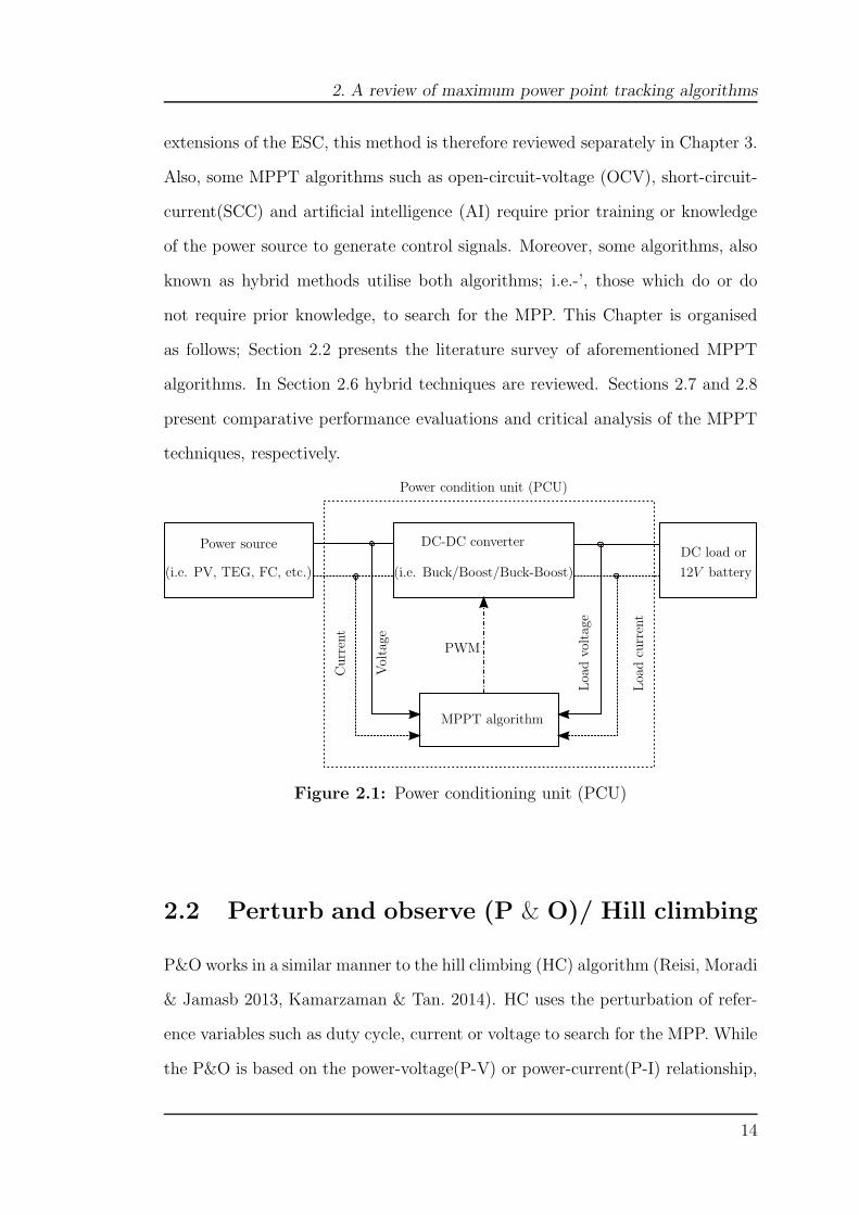
A power conditioning unit (PCU) is essential in a system which comprises un-
stable heat sources and loads. Fig. 2.1 illustrates the block diagram of the PCU
considered in this Thesis. The output of the power source is connected to the
DC-DC converter and the output of the converter is connected to the DC load
or 12V battery. Voltage and current measurements taken from the power source
are applied to the maximum power point tracking (MPPT) controller as inputs
and pulse width modulation as an output. The MPPT controller is implemented
within a PCU (see Fig. 2.1) to alter the operating point of the power source
in order to extract the maximum available power. This power is transferred to
a DC load, or most often a 12V battery in automotive applications. Some of
the MPPT algorithms do not require any prior knowledge, whereas input/output
measurements are sufficient to find the maximum power point (MPP). Such algo-
rithms include: perturb and observe (P&O), incremental conductance (IC), and
extremum seeking control (ESC). Since the contribution of this Thesis is based on
13
2. A review of maximum power point tracking algorithms
extensions of the ESC, this method is therefore reviewed separately in Chapter 3.
Also, some MPPT algorithms such as open-circuit-voltage (OCV), short-circuit-
current(SCC) and artificial intelligence (AI) require prior training or knowledge
of the power source to generate control signals. Moreover, some algorithms, also
known as hybrid methods utilise both algorithms; i.e.-’, those which do or do
not require prior knowledge, to search for the MPP. This Chapter is organised
as follows; Section 2.2 presents the literature survey of aforementioned MPPT
algorithms. In Section 2.6 hybrid techniques are reviewed. Sections 2.7 and 2.8
present comparative performance evaluations and critical analysis of the MPPT
techniques, respectively.
DC-DC converter
(i.e. Buck/Boost/Buck-Boost)
PWM
12V battery
Voltage
Loadvoltage
DC load or
Power condition unit (PCU)
MPPT algorithm
Current
Loadcurrent
Power source
(i.e. PV, TEG, FC, etc.)
Figure 2.1: Power conditioning unit (PCU)
2.2 Perturb and observe (P & O)/ Hill climbing
P&O works in a similar manner to the hill climbing (HC) algorithm (Reisi, Moradi
& Jamasb 2013, Kamarzaman & Tan. 2014). HC uses the perturbation of refer-
ence variables such as duty cycle, current or voltage to search for the MPP. While
the P&O is based on the power-voltage(P-V) or power-current(P-I) relationship,
14

2. A review of maximum power point tracking algorithms
HC is based on the power-duty cycle (P-D), as compared to other MPPT algo-
rithms, P&O is most widely used in practical applications. It is also used as the
benchmark controller by most researchers due to its simplicity of implementation
(Phillip, Maganga, Burnham, Dunn, Rouaud, Ellis & Robinson 2012).
Fig. 2.2 illustrates a flow chart of the most commonly used P&O algorithm
which works as follows: Current and voltage (i.e. Ik and Vk) at time instance k
are sensed and used to compute current power Pk. Current power Pk is compared
to the power at the previous time instance Pk−1. If Pk is greater than Pk−1 and
current voltage Vk is also greater than Vk−1, it indicates that the power point is
moving toward the MPP, hence duty cycle d will be increased by step-size C.
However, if Vk is less than Vk−1 it implies the power point is moving away from
the MPP, therefore d will be decreased by C. Also, if Pk is less than Pk−1 and Vk
is greater than Vk−1 it indicates that the power point is moving away from MPP,
therefore d will be decremented by C. On the other hand, if Pk is less than Pk−1
and Vk is less than Vk−1 it indicates that the power point is moving towards the
MPP, therefore d will be incremented by C.
As compared to the MPPT algorithms for PV systems, development of MPPTs
for TEGs is still immature. As an example, early research on MPPTs for the
TEGs utilising P&O algorithm emerged more than a decade ago (Nagayoshi, Ka-
jikawa & Sugiyama 2002, Eakburanawat & Boonyaroonate 2006, Nagayoshi &
Kajikawa 2006, Nagayoshi, Tokumisu & Kajikawa 2007). In Eakburanawat &
Boonyaroonate (2006), the battery voltage is considered to be constant and the
MPP is obtained via current measurements only. Also, Eakburanawat & Boon-
yaroonate (2006) present the comparison of battery charging in three different
methods, namely: directly, with a fixed duty cycle and MPPT utilising P&O
algorithm. It has been claimed that,-the efficiency of the MPPT converter in-
creased by 15% when P&O is used. Nagayoshi & Kajikawa (2006) and Nagayoshi
et al. (2007) presented P&O with the use of the buck-boost converter within a
15
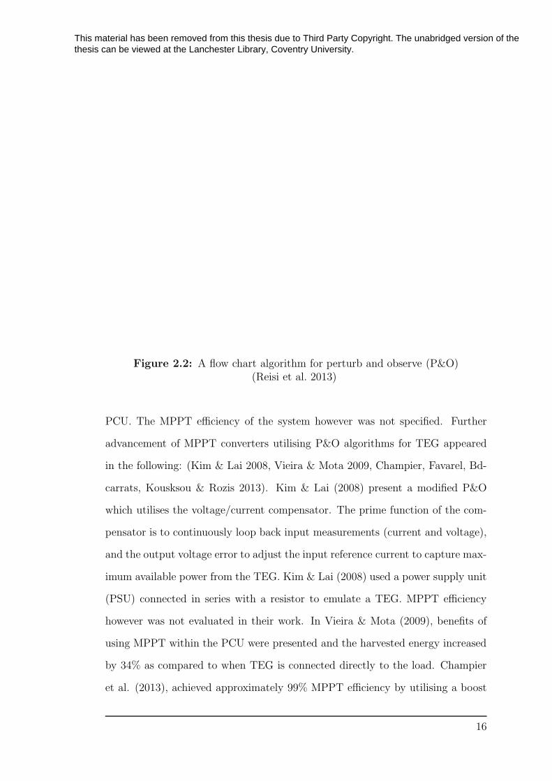
Figure 2.2: A flow chart algorithm for perturb and observe (P&O)(Reisi et al. 2013)
PCU. The MPPT efficiency of the system however was not specified. Further
advancement of MPPT converters utilising P&O algorithms for TEG appeared
in the following: (Kim & Lai 2008, Vieira & Mota 2009, Champier, Favarel, Bd-
carrats, Kousksou & Rozis 2013). Kim & Lai (2008) present a modified P&O
which utilises the voltage/current compensator. The prime function of the com-
pensator is to continuously loop back input measurements (current and voltage),
and the output voltage error to adjust the input reference current to capture max-
imum available power from the TEG. Kim & Lai (2008) used a power supply unit
(PSU) connected in series with a resistor to emulate a TEG. MPPT efficiency
however was not evaluated in their work. In Vieira & Mota (2009), benefits of
using MPPT within the PCU were presented and the harvested energy increased
by 34% as compared to when TEG is connected directly to the load. Champier
et al. (2013), achieved approximately 99% MPPT efficiency by utilising a boost
16
This material has been removed from this thesis due to Third Party Copyright. The unabridged version of the thesis can be viewed at the Lanchester Library, Coventry University.

2. A review of maximum power point tracking algorithms
converter and the P&O within the PCU. Despite its simplicity and low imple-
mentation cost, the major drawback of the P&O is its inability to track the MPP
effectively when rapid variations occur (e.g. irradiance variation in PV systems
or hot side and cold side temperatures in TEGs). Also, continuous perturbations
make P&O oscillate around the MPP, hence the algorithm fails to converge to the
actual MPP. More research has been conducted on improving the tracking ability
of the P&O/HC as well as reducing the steady-state error (limit cycle minimisa-
tion) by utilising adaptive (variable) step-size (Xiao & Dunford 2004, Wai, Wang
& Lin 2006).
The idea behind variable step-size is that large step-size is used to allow
fast convergence when the operating point is far away from the MPP. On the
other hand, when the operating point is close to the MPP, small step-size is used
to reduce steady-state error. Xiao & Dunford (2004), achieved a variable step size
by introducing a auto-tuning parameter and control mode switching. The control
mode switching in Xiao & Dunford (2004) aimed to eliminate the deviation from
the MPP when rapid variations of power source (i.e. temperature, irradiance)
occurs. In Wai et al. (2006), adaptive step-size is based on incremental refer-
ence voltage and only the trade-off between transients and steady-state error was
targeted. It has been reported in Moradi & Reisi (2011) that,- despite utilising
a variable step-size to overcome the trade-off between transient and steady-state
responses, when the system operating point changes quickly, the algorithm may
fail to converge to the actual MPP.
2.3 Incremental conductance
This method is based on slope finding and utilises the fact that the slope is
calculated as the derivative of power with respect to voltage as zero at the MPP
(Reisi et al. 2013). For a voltage smaller than that of the MPP, the slope is
17

2. A review of maximum power point tracking algorithms
positive. On the other hand, when voltage is greater than that at the MPP, this
slope is negative, i.e:
∂P
∂V= 0,at MPP (2.1a)
∂P
∂V> 0, V < Vmpp (2.1b)
∂P
∂V< 0, V > Vmpp (2.1c)
where P and V denote power and voltage, respectively, I denotes the source
current, and Vmpp is the voltage at the MPP. Fig. 2.3 illustrates the P-V curve
with respect to the power voltage relationship presented in (2.1). From (2.1a) it
follows that the derivative of MPP with respect to voltage is:
P
∂P∂V> 0
∂P∂V= 0
∂P∂V< 0
V
Figure 2.3: Curve for Power Vs Source voltage
∂P
∂V=∂(IV )
∂V= 0 (2.2a)
∂P
∂V= I + V
∂I
∂V= 0 (2.2b)
∂I
∂V=−I
V(2.2c)
∂I
∂V≈
∆I
∆V=−I
V= −
Impp
Vmpp
(2.2d)
18
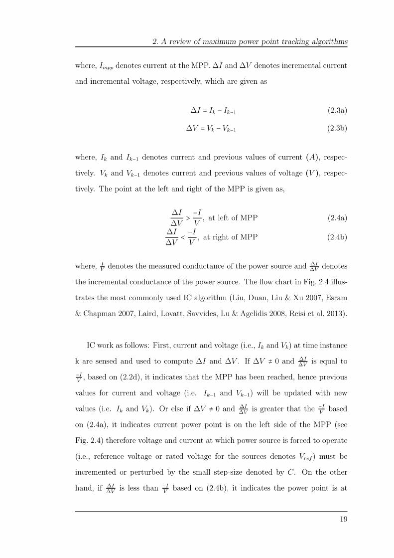
2. A review of maximum power point tracking algorithms
where, Impp denotes current at the MPP. ∆I and ∆V denotes incremental current
and incremental voltage, respectively, which are given as
∆I = Ik − Ik−1 (2.3a)
∆V = Vk − Vk−1 (2.3b)
where, Ik and Ik−1 denotes current and previous values of current (A), respec-
tively. Vk and Vk−1 denotes current and previous values of voltage (V ), respec-
tively. The point at the left and right of the MPP is given as,
∆I
∆V>−I
V, at left of MPP (2.4a)
∆I
∆V<−I
V, at right of MPP (2.4b)
where, IVdenotes the measured conductance of the power source and ∆I
∆Vdenotes
the incremental conductance of the power source. The flow chart in Fig. 2.4 illus-
trates the most commonly used IC algorithm (Liu, Duan, Liu & Xu 2007, Esram
& Chapman 2007, Laird, Lovatt, Savvides, Lu & Agelidis 2008, Reisi et al. 2013).
IC work as follows: First, current and voltage (i.e., Ik and Vk) at time instance
k are sensed and used to compute ∆I and ∆V . If ∆V ≠ 0 and ∆I∆V
is equal to
−IV, based on (2.2d), it indicates that the MPP has been reached, hence previous
values for current and voltage (i.e. Ik−1 and Vk−1) will be updated with new
values (i.e. Ik and Vk). Or else if ∆V ≠ 0 and ∆I∆V
is greater that the −IV
based
on (2.4a), it indicates current power point is on the left side of the MPP (see
Fig. 2.4) therefore voltage and current at which power source is forced to operate
(i.e., reference voltage or rated voltage for the sources denotes Vref) must be
incremented or perturbed by the small step-size denoted by C. On the other
hand, if ∆I∆V
is less than −IV
based on (2.4b), it indicates the power point is at
19

Figure 2.4: A flow chart algorithm for incremental conductance (IC)(Reisi et al. 2013)
right side of the MPP therefore Vref must be decremented by C. Also, if ∆V = 0
and ∆I = 0 based on (2.1a) it implies the power point is exactly at the MPP,
hence previous values of current and voltage will be updated with present values
(see Fig. 2.4). Moreover, if ∆V = 0 and ∆I > 0 it indicates power point is at
right side of the MPP therefore Vref must be decremented by C followed by
updating the Ik−1 and Vk−1 values (see Fig. 2.4). Furthermore, if ∆V = 0 and
∆I < 0 it implies the power point is at the left side of the MPP hence Vref will
be incremented to allow the power point to move towards the MPP followed by
updating Ik−1 and Vk−1. The convergence speed of IC depends on C. A large
value of C indicates fast convergence, however this reduces the accuracy of IC
on tracking the MPP. Some research has been done to improve the convergence
speed and the accuracy of the standard IC, particularly in application to PVs,
see (Lee, Bae & Cho 2006, Liu et al. 2007). Lee et al. (2006) achieved this by
20
This material has been removed from this thesis due to Third Party Copyright. The unabridged version of the thesis can be viewed at the Lanchester Library, Coventry University.

2. A review of maximum power point tracking algorithms
using a variable increment or decrement denoted by C(k) with similar a concept
as the one used in (Xiao & Dunford 2004, Wai et al. 2006). Convergence speed
is achieved by selecting a large C(k) while the operating point of the source is
away from the MPP and a small C(k) is chosen when the operating point of the
source is relatively close to the MPP (Liu et al. 2007). The standard IC and the
adaptive IC are based on the assumption that the MPP will be reached when the
slope equal to zero, which is not feasible in practice (Laird et al. 2008).
2.4 Open circuit voltage/short circuit current
2.4.1 Open circuit voltage
There are several open circuit voltage (OCV) algorithms for the MPPT with
application to low carbon technologies (Cho, Kim, Park & Kim 2010, Kim, Cho,
Kim, Baatar & Kwon 2011, Schwartz 2012, Montecucco, Siviter & Knox 2012,
Laird & Lu 2013, Kamarzaman & Tan. 2014, Esram & Chapman 2007). The idea
behind OCV methods is to find the voltage at the MPP via OCV measurements,
denoted Voc. This approach is based on assumption that Voc is linearly related to
voltage at the MPP and is presented as
Vmpp ≈ aVoc (2.5)
where a is an empirically derived parameter based on Voc and Vmpp measure-
ments in different environmental conditions. The flow chart in Fig. 2.5 depicts
commonly used OCV method which work as follows: initially, the power source is
isolated from the load and Voc measurements are recorded. Using the relationship
shown in (2.5), the voltage at the MPP is evaluated. Voc measurements are ob-
tained by repeating this process periodically. It is difficult to determine optimal
value of a, however, there is a suitable range for this parameter. For instance,
21

2. A review of maximum power point tracking algorithms
in PV applications a range from 0.73 to 0.80 (Kamarzaman & Tan. 2014, Esram
& Chapman 2007). On the other hand, in thermoelectric generator (TEG) ap-
plications a is 0.5, hence the OCV for the TEGs is termed as fractional OCV
(Schwartz 2012, Montecucco, Siviter & Knox 2012, Laird & Lu 2013, Montecucco
& Knox 2014).
Figure 2.5: A flow chart of open circuit voltage method(Reisi et al. 2013)
Despite its simplicity and low cost of implementation, the actual MPP may
not be accurately tracked for both applications (PV/TEG). The reason is the
assumption that Voc and Vmpp are linearly related, which is unrealistic (Laird
et al. 2008), hence true the MPP can not be achieved. Both the OCV and the
fractional OCV suffer from periodic disconnections of the power source from the
load to measure the Voc and this may cause the unexpected interference of the
circuit operation and lead to more losses.
To overcome this problem, various researchers focused on improving Voc
22
This material has been removed from this thesis due to Third Party Copyright. The unabridged version of the thesis can be viewed at the Lanchester Library, Coventry University.
This material has been removed from this thesis due to Third Party Copyright. The unabridged version of the thesis can be viewed at the Lanchester Library, Coventry University.
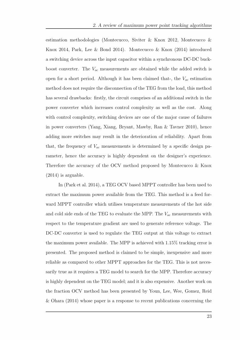
2. A review of maximum power point tracking algorithms
estimation methodologies (Montecucco, Siviter & Knox 2012, Montecucco &
Knox 2014, Park, Lee & Bond 2014). Montecucco & Knox (2014) introduced
a switching device across the input capacitor within a synchronous DC-DC buck-
boost converter. The Voc measurements are obtained while the added switch is
open for a short period. Although it has been claimed that-, the Voc estimation
method does not require the disconnection of the TEG from the load, this method
has several drawbacks: firstly, the circuit comprises of an additional switch in the
power converter which increases control complexity as well as the cost. Along
with control complexity, switching devices are one of the major cause of failures
in power converters (Yang, Xiang, Bryant, Mawby, Ran & Tavner 2010), hence
adding more switches may result in the deterioration of reliability. Apart from
that, the frequency of Voc measurements is determined by a specific design pa-
rameter, hence the accuracy is highly dependent on the designer’s experience.
Therefore the accuracy of the OCV method proposed by Montecucco & Knox
(2014) is arguable.
In (Park et al. 2014), a TEG OCV based MPPT controller has been used to
extract the maximum power available from the TEG. This method is a feed for-
ward MPPT controller which utilises temperature measurements of the hot side
and cold side ends of the TEG to evaluate the MPP. The Voc measurements with
respect to the temperature gradient are used to generate reference voltage. The
DC-DC converter is used to regulate the TEG output at this voltage to extract
the maximum power available. The MPP is achieved with 1.15% tracking error is
presented. The proposed method is claimed to be simple, inexpensive and more
reliable as compared to other MPPT approaches for the TEG. This is not neces-
sarily true as it requires a TEG model to search for the MPP. Therefore accuracy
is highly dependent on the TEG model; and it is also expensive. Another work on
the fraction OCV method has been presented by Youn, Lee, Wee, Gomez, Reid
& Ohara (2014) whose paper is a response to recent publications concerning the
23

2. A review of maximum power point tracking algorithms
effectiveness of impedance matching techniques for the MPP search. Youn, Lee,
Wee, Gomez, Reid & Ohara (2014) analytically justify that the V-I characteristic
curve is approximately linear. It is argued that,- impedance matching approach
can still be used as an effective way to evaluate the MPP.
2.4.2 Short circuit current
The short circuit current (SCC) method is very similar to the OCV and is based
on the assumption that, the SCC, denoted as Isc, is linearly related to the current
at MPP denoted as Impp. The mathematical relationship between Isc and Impp is
presented as:
Impp ≈ aIsc (2.6)
Similar to the a parameter in the OCV method, a is empirically determined and it
ranges between 0.8 and 0.9 (for PV applications). As compared to the OCV, the
SCC is more efficient and accurate (Reisi et al. 2013). It is however sophisticated
to obtain measurements of Isc and, as a consequence, the implementation cost of
SCC is usually very high.
2.5 Artificial intelligence methods
Recently, the interest in artificial intelligence (AI) based methods such as the
fuzzy logic controller (FLC), the neural network (NN) and the genetic algo-
rithm (GA) for MPPT has shown tremendous growth (Patcharaprakiti, Prem-
rudeepreechacharn & Sriuthaisiriwong 2005, Esram & Chapman 2007, Hiyama,
Kouzuma & Imakubo 1995, Elobaid, Abdelsalam & Zakzouk 2012, Messai, Mel-
lit, Guessoum & Kalogirou 2011). These methods have been mainly applied in
PV systems for global maximum searches in presence of local maxima. Tradi-
tional FLC is an offline method in which expert knowledge of the designer is
24

2. A review of maximum power point tracking algorithms
essential. One of the advantages of the FLC is its ability to work effectively with
less accurate mathematical models as well as handling non-linearities (Esram &
Chapman 2007). Fixed parameters within the FLC may become inadequate, es-
pecially in applications whereby the operating conditions change in a wider range
and the expert knowledge is limited. Patcharaprakiti et al. (2005) proposed an
adaptive FLC to eliminate this problem by making FLC less dependent on the
expert knowledge. The adaptive FLC continuously tunes its membership function
and the rule based table, hence it achieves a fast response, and a good perfor-
mance. However, the computational cost of the proposed method is much higher
than that of the traditional FLC due to the inclusion of the learning mechanism.
The NN is an off-line method which requires prior training to track the MPP
effectively, see,- (Hiyama et al. 1995, Elobaid et al. 2012, Reisi et al. 2013, Ka-
marzaman & Tan. 2014). Applications of the NN have significantly increased due
to its ability to perform nonlinear tasks (Kamarzaman & Tan. 2014). Similar to
the FLC, it has been used for a global maximum search in PV systems (Elobaid
et al. 2012). In comparison to other methods, the NN does not require any
programming it totally depends on the learning process. It can provide accu-
racy in tracking the MPP without requiring significant knowledge of the power
source (e.g TEG/PV). On other the hand, it is only suitable for a particular
power source, since different power sources have different characteristics. Also,
most power sources are nonlinear in nature (time-varying), hence the NN must
be trained regularly to guarantee reasonable tracking performance, which is time
consuming. Hiyama et al. (1995) presented the first research work of NN for the
MPP search. In (Hiyama et al. 1995), Voc is used as the input and voltage as
the output of the NN. The PI controller was used to eliminate any error between
the Voc and the output voltage. Elobaid et al. (2012) propose a two stage NN
structure. The role of the first stage is to estimate temperature and irradiance
from the PV measurements (voltage and current). The second NN stage uses
25

2. A review of maximum power point tracking algorithms
the estimates of the temperature and the irradiance to determine the MPP. The
proposed approach offers the following advantages: it reduces the training set
due to its cascaded structure and it does not require temperature or irradiance
measurements. In (Messai et al. 2011), GA is used to optimise the FLC by tuning
membership functions to optimal values to track the MPP under varying atmo-
spheric conditions. On other the hand, Ramaprabha & Mathur (2011) use GA
to optimise the values used to train the NN to track the MPP.
2.6 Hybrid methods
Hybrid methods are mostly used in PV applications (Irisawa, Saito, Takano &
Sawada 2000, D’Souza, Lopes & Liu 2005, Kobayashi, Takano & Sawada 2006,
Moradi, Tousi, Nemati, Basir & Shalavi 2013, Zhang, Thanapalan, Procter, Carr
& Maddy 2013) and are usually comprise of two control loops. The first loop
(inner loop) is based on methods which do require prior information and it is
dependent on the system (e.g TEG, PV, etc.) variables, see (Fig. 2.6). The prime
function of the inner loop is to adapt the fast variation of environmental conditions
in order to improve the transient response to converge fast and close to the
MPP. The second loop (outer loop) utilises approaches which do not require prior
knowledge of the system, aiming to minimise steady-state error to ensure that the
algorithm converges to the exact MPP by providing fine-tuning. Fig. 2.6 portrays
a generic flow chart of a hybrid methods which comprises two aforementioned
loops for set-point calculation and fine tuning.
In (Moradi & Reisi 2011, Zhang et al. 2013), a hybrid method comprising
two loops is proposed. The first loop determines the set-point calculations via
OCV at a constant temperature. The second loop performs fine tuning utilising
a standard P&O algorithm. It has been shown that, the proposed method gives
higher accuracy as well as better convergence speed compared to the standard
26

2. A review of maximum power point tracking algorithms
P&O. Better convergence speed is achieved due to its ability to pre-determine
Voc which allows for the faster evaluation of the Vmpp. Although it is difficult for
the classic P&O to achieve concurrently fast transience as well as high accuracy,
by allowing the standard P&O to converge slowly (keeping amplitude and fre-
quency of perturbation small), the same accuracy as the proposed method can be
achieved. Contrary to the method proposed by Moradi & Reisi (2011), Moradi
et al. (2013) proposed to take into account the effect of the load and the battery
characteristics which are modelled using a Thevenin equivalent circuit in order to
27
This material has been removed from this thesis due to Third Party Copyright. The unabridged version of the thesis can be viewed at the Lanchester Library, Coventry University.

2. A review of maximum power point tracking algorithms
design the offline loop. It has been claimed that, compared to the method pro-
posed in (Moradi & Reisi 2011), the method of Moradi et al. (2013) tracks the
MPP efficiently when load variation occurs as well as when the battery degrades.
Irisawa et al. (2000) and Kobayashi et al. (2006) proposed a hybrid algorithm
that utilises an offline method to allow the PV system to quickly converge close
to the MPP and online IC method, to minimise steady-state error, respectively.
Fast convergence of these methods is achieved by matching the power converter
initial operating point with the load resistance. As compared to other hybrid
methods, the proposed method is capable of searching the global maximum in
the presence of local maxima and, as a consequence, ensures the actual MPP is
effectively tracked when PV system is partially shaded. Efficiency of the MPPT
converter was not evaluated in Kobayashi et al. (2006).
D’Souza et al. (2005) proposed a modified P&O that utilises FLC to determine
the direction and magnitude of the next perturbation. This approach simul-
taneously improves both the transient and the steady-state performance. Addi-
tionally, the method can achieve a faster transient response by adjusting the duty
cycle of the power converter, which forces the operating point toward the MPP as
quickly as possible. Benchmark results with the standard P&O was not presented
in (D’Souza et al. 2005), hence the significance of the announced improvement
is not demonstrated. Jain & Agarwal (2004) proposed a hybrid method that
comprises the transient and the steady-state loops. The transient loop is deter-
mined by the PV cells dependent parameter which is obtained empirically. As
compared to other MPPT methods, in transient, the proposed algorithm tracks
this parameter instead of the power; Subsequently, the actual MPP is obtained
via fine tuning with the P&O or the IC. In Koizumi & Kurokawa (2005), the of-
fline loop utilises a linear function to identify the neighbourhood of the operating
point relative to the MPP, to apply appropriate perturbation. This function is
developed from PV cells characteristics. The online loop utilises the IC method.
28

2. A review of maximum power point tracking algorithms
Shadmand, Balog & Abu Rub (2014) use a hybrid method to improve the perfor-
mance of the standard P&O. This is achieved by using a model predictive control
(MPC) and P&O. The MPC determines the reference current using P&O and
uses this current as the input as well as the PV’s voltage and current. The MPC
predicts the future error, in addition to the next switching state based on the
defined optimisation cost function. The result shows that the MPC-MPPT con-
verges faster, compared to the standard P&O. Daraban, Petreus & Morel (2014)
proposed a modified GA which utilises P&O. Population size and number of it-
erations of the traditional GA are reduced by embedding a classic P&O inside
the structure of the GA, hence the time required to search for the global MPP is
reduced.
2.7 Performance comparison
Depending on the application, the choice of the MPPT technique should be made
based on the algorithm’s ability to track the actual MPP, its convergence speed,
implementation complexity, cost, robustness, reliability and sensitivity. Table. 2.1
summarises different features of the reviewed MPPT algorithms. The OCV and
the SCC can be implemented in both analog or digital systems. Both methods
have a medium convergence speed and low efficiency. However, implementation
of the SCC is more complex and it is more costly compared to the OCV. The NN,
the FLC and the GA can be implemented in digital systems only. These methods
provide high efficiency. On the other hand, the implementation cost and com-
plexity is high for both methods. P&O with fixed step size can be implemented in
digital systems only. Also, it offers high efficiency with low implementation costs.
However, it converges slower than the P&O a with variable step size. IC can be
implemented on digital systems only and has high efficiency. The convergence
speed of the IC is highly dependent on step size. Hybrid methods are suitable
29

2. A review of maximum power point tracking algorithms
for digital systems only. They provide high efficiency and fast convergence speed.
The implementation cost however is high. ESC is suitable for both digital and
analogue systems. It provides high efficiency and a fast convergence speed with
moderate implementation complexity and cost.
30
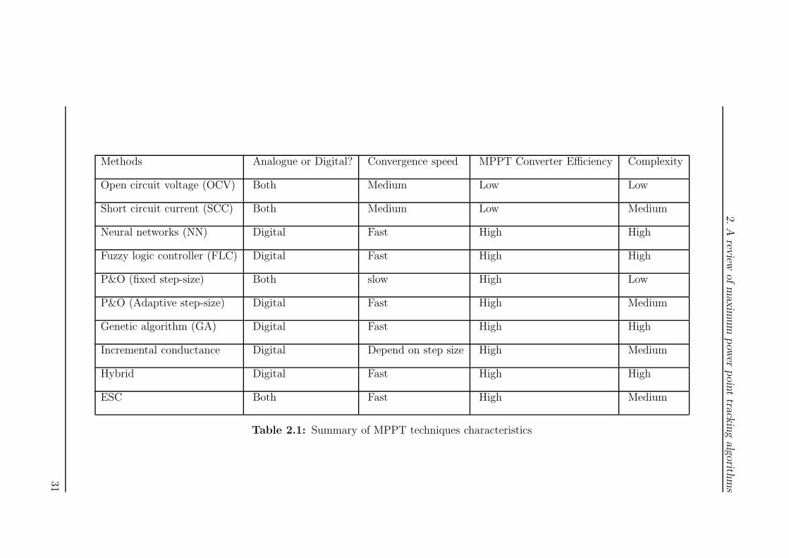
2.A
review
ofmax
imum
pow
erpoin
ttrack
ingalgorith
ms
Methods Analogue or Digital? Convergence speed MPPT Converter Efficiency Complexity
Open circuit voltage (OCV) Both Medium Low Low
Short circuit current (SCC) Both Medium Low Medium
Neural networks (NN) Digital Fast High High
Fuzzy logic controller (FLC) Digital Fast High High
P&O (fixed step-size) Both slow High Low
P&O (Adaptive step-size) Digital Fast High Medium
Genetic algorithm (GA) Digital Fast High High
Incremental conductance Digital Depend on step size High Medium
Hybrid Digital Fast High High
ESC Both Fast High Medium
Table 2.1: Summary of MPPT techniques characteristics
31

2. A review of maximum power point tracking algorithms
2.8 Critical appraisal and conclusions
The OCV method does not require current sensing therefore it is considered as
the least computationally intensive. Also, the voltage at MPP is determined by
known empirical values in PVs or by taking half of the open circuit voltage in
TEGs. This, however, requires the intermittent disconnection of the power source
from the load to establish the prevailing open circuit voltage value. Disconnection
of the power source can lead to undesired transients and reduced efficiency. For
instance, undesired transients in TEG applications can be due to the operation
in dynamic thermal environments. Conversely, IC is able to identify if the MPP
has been reached or not, but is computationally intensive and, as a consequence,
converges more slowly to the MPP than the OCV. The true MPP cannot be
achieved using P&O due to continuous perturbations which cause the operating
point to oscillate around the MPP. One disadvantage of the P&O and the IC
methods is that for an accurate tracking of the MPP the perturbation gain is
required to be small in order to minimise the amplitude of the limit cycle which
in turn degrades the algorithm’s transient tracking ability. Despite extensions of
P&O, OCV, IC and hybrid methods to address the trade-off between transient
and steady-state performances, an optimal solution does not yet exist. Also,
these methods are suitable only for local maxima searches. NN, FC and GA
have shown great success in searching the global maximum in presence of local
maxima. However, these algorithms require prior knowledge or training. Since
the objective of this Thesis is to create a universal MPPT converter for different
aforementioned power sources, model dependent algorithms are not considered
here.
To address the deficiencies found for the MPPT algorithms presented in this chap-
ter, the requirement is for an algorithm which can work without disconnecting
the power source and load and perform optimally in a transient and steady state
32

2. A review of maximum power point tracking algorithms
operation as well as search for global maximum. One such algorithm is the ESC,
which has shown superior performance to other well-known MPPT methods such
as P&O for PV systems (Phillip, Maganga, Burnham, Ellis, Robinson, Dunn &
Rouaud 2013). The perceived advantage is attributed to the ability of the ESC
to converge more rapidly whilst retaining steady-state performance similar to the
P&O method. Therefore, extensions of an ESC for the MPP is proposed in this
Thesis.
33

Chapter 3
Extremum seeking control
3.1 Introduction
This Chapter presents a detailed analysis of perturbation based extremum seek-
ing control (ESC) methods, and a novel simplified scheme for limit cycle min-
imisation. The novel scheme proposed in this Chapter is known as variance
based switching extremum seeking control (VBS-ESC). It achieves limit cycles
minimisation based on variance detection of the estimated input. There are dif-
ferent types of ESC schemes, some of which do not require any constraints and
some which do require constraints. As compared to constraints based ESC, non-
constraints based ESC is considered to be the most favourable option for the MPP
search, if negligible parameter uncertainty in the plant or system exists (Guay &
Zhang 2003). The main reason for this is that no constraints are imposed on the
objective function (Guay 2014). On the other hand, in constraints based ESC,
the cost function is considered to be known; therefore, it provides optimal results
by quickly identifying the optimum point and converging towards it (Guay &
Zhang 2003). Taking into consideration that non-constraints based ESC meth-
ods have shown great success in the domain of low carbon technologies, such as
FCs, PVs, and most recently TEGs, this Thesis aims to contribute to the domain
34

3. Extremum seeking control
of the non-constraints based ESC. However, for the sake of completeness, con-
straints based ESC is also reviewed in this Thesis. This Chapter is constructed
as follows: firstly the state of the art for ESC is presented in Section 3.2, fol-
lowed by the perturbation (P)ESC feedback loop design in Section 3.3.4. Limit
cycle minimisation techniques and an improved scheme for reducing limit cycles
are given in Section 3.4.1 and Section 3.4.2, respectively. Section 3.5 presents
conclusions and critical appraisals.
3.2 Survey on extremum seeking control
ESC is an approach which seeks the extremum for steady state online optimi-
sation without knowing the plant model and/or the cost function in a closed
loop fashion. However, it is assumed that measurements of the plant’s input and
output signals are available. Early work on ESC goes back to 1922 by Leblanc
(1922), where control mechanism that maintain the desirable maximum power
transfer was proposed. However, neither mathematical analysis of the scheme’s
dynamics nor practical evaluation was provided. Despite these limitations, ESC
became a powerful and popular tool for either maximising or minimising the un-
known output of functions. Significant use of the ESC method occurred between
the 1940’s to 1960’s. For instance, in the early 1940’s (during World War II)
tremendous research interest in the area of ESC appeared in the Soviet Union.
As an example, Kazakevich a Russian PhD student wrote his Thesis titled ”On
extremum seeking”. On other the hand, presumably the first English article on
ESC was written by Draper & Li (1951), who described ESC and its perfor-
mance. In the aforementioned article, internal combustion engine optimisation
using ESC, or more precisely, a technique for selecting input (ignition timing) to
achieve maximum power output was discussed. Generally speaking, most of the
ESC research work between 1950’s and 1960’s emphasized either implementation
35
3. Extremum seeking control
of the algorithm (ESC) or explored the algorithm performance for a specific appli-
cation. Thereafter interest was lost for almost three decades (between 1970’s to
1990’s) due to the lack of a proof of stability. Nevertheless, ESC gained renewed
interest after Krstic (2000) proved local stability for a single-input single-output
(SISO) system. The averaging technique and singular perturbations were used to
demonstrate that ESC converges to the neighbourhood of the extremum. It was
also proven that the neighbourhood is inversely proportional to the perturbation
gain, the amplitude and the perturbation frequency of the dither signal used to
search for the extremum. Due to its robustness and reliability, non-constraints
based ESC has been used in a wide range of applications including: anti-locking
brake systems (ABS) (Zhang 2007, Tanelli, Astolfi & Savaresi 2006), control sys-
tem and optimisation of bio processes (Krstic & Bastin 1999, Guay, Dochain
& Perrier 2004, Zhang, Guay & Dochain 2002), proportional integral controller
(PID) tuning (Killingsworth & Krstic 2006), flow control problems (Chang &
Moura 2009, Kim, Kasnakoglu, Serrani & Samimy 2008), internal combustion
engine (Draper & Li 1951, Haskara, Zhu & Winkelman 2006), ESC with limit cy-
cle detector has been applied in subsonic cavity flow (Kim, Kasnakoglu, Serrani
& Samimy 2009).
It has also been used to reduce the tuning time of various parameters of the
combustion timing controller as well as finding the optimal combustion timing set
point (Popovic, Jankovic, Magner & Teel 2006). Moreover, non-constraints based
ESC has been used for optimising NN/FLC (Gurvich 2004, Hu & Zuo 2005),
autonomous vehicle control and most recently ESC has been applied in TEGs
(Phillip et al. 2013, Maganga, Phillip, Burnham, Montecucco, Siviter, Knox &
Simpson 2014). Non-constraints ESC can either be based on gradient search or
slope seeking. Gradient search is the most commonly used non-constraints based
ESC, and usually utilises both the high pass filter (HPF) and the low pass filter
(LPF) to calculate the gradient of the cost function. Slope seeking is an extension
36

3. Extremum seeking control
of the standard non-constraints based ESC and has attracted significant interest
(Ariyur & Krystic 2003, Wiederhold, King, Noack, Neuhaus, Neise, Enghardt &
Swoboda 2009, King, Petz & Lemke 2006). This method usually drives the plant
to the value of the reference slope of the reference-output map at steady-state.
Slope seeking ESC has been applied to improve the aerodynamic performance of
axial turbo machine (Wiederhold et al. 2009). This approach has been useful in
some applications such as the axial turbo machine, as the peak point between
the input-output map is not distinctly visible. Interest in ESC is based on the
fact that it is non-constraints based and adaptive. ESC is suitable for situations
where non-linearity in the system has a local minimum or local maximum (Ariyur
& Krystic 2003).
For example, in TEG applications it finds a set point which keeps the out-
put power of the TEG at the MPP. As compared to other traditional MPPT
controllers reviewed in Chapter 2, the ESC controller offers a faster convergence
speed and adaptation capability. Within the aforementioned ESC groups there
are five different categories which include: slide mode (SM) ESC, neural network
(NN) ESC, approximation (AP) ESC, perturbation (P) ESC and adaptive (A)
ESC. The main advantage of non-constraints based ESC is that it can be applied
to any system where the input-output relationship has local maxima or local
minima requiring only minimum knowledge of the actual system. On the other
hand, constraints based ESC requires prerequisite-knowledge or information of
the system. All non-constraints based ESC are highly dependent on the time
separation between the learning and the dynamics to be optimised (Guay 2014).
Compared to non-constraints based ESC, constraints based ESC converge to the
true peak point. The drawback of constraints based ESC is that it requires a
model of the system as well as storage of the models, which make constraints
based ESC more expensive compared to non-constraints based ESC.
37
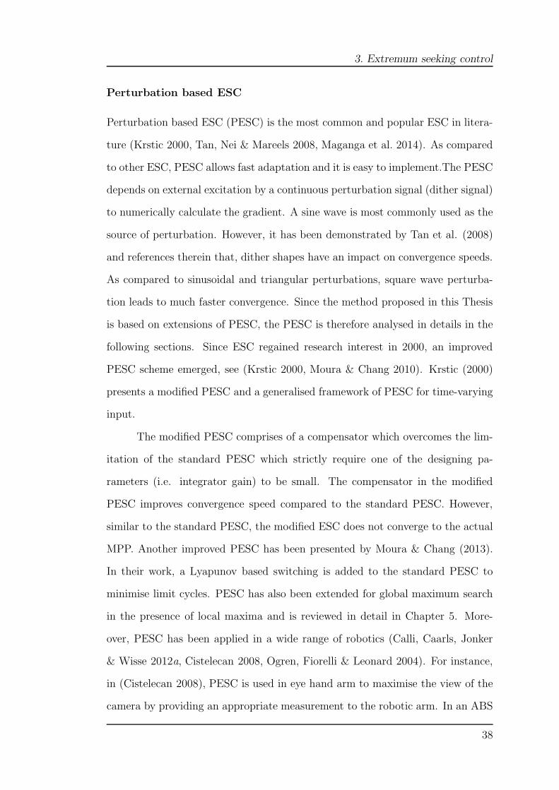
3. Extremum seeking control
Perturbation based ESC
Perturbation based ESC (PESC) is the most common and popular ESC in litera-
ture (Krstic 2000, Tan, Nei & Mareels 2008, Maganga et al. 2014). As compared
to other ESC, PESC allows fast adaptation and it is easy to implement.The PESC
depends on external excitation by a continuous perturbation signal (dither signal)
to numerically calculate the gradient. A sine wave is most commonly used as the
source of perturbation. However, it has been demonstrated by Tan et al. (2008)
and references therein that, dither shapes have an impact on convergence speeds.
As compared to sinusoidal and triangular perturbations, square wave perturba-
tion leads to much faster convergence. Since the method proposed in this Thesis
is based on extensions of PESC, the PESC is therefore analysed in details in the
following sections. Since ESC regained research interest in 2000, an improved
PESC scheme emerged, see (Krstic 2000, Moura & Chang 2010). Krstic (2000)
presents a modified PESC and a generalised framework of PESC for time-varying
input.
The modified PESC comprises of a compensator which overcomes the lim-
itation of the standard PESC which strictly require one of the designing pa-
rameters (i.e. integrator gain) to be small. The compensator in the modified
PESC improves convergence speed compared to the standard PESC. However,
similar to the standard PESC, the modified ESC does not converge to the actual
MPP. Another improved PESC has been presented by Moura & Chang (2013).
In their work, a Lyapunov based switching is added to the standard PESC to
minimise limit cycles. PESC has also been extended for global maximum search
in the presence of local maxima and is reviewed in detail in Chapter 5. More-
over, PESC has been applied in a wide range of robotics (Calli, Caarls, Jonker
& Wisse 2012a, Cistelecan 2008, Ogren, Fiorelli & Leonard 2004). For instance,
in (Cistelecan 2008), PESC is used in eye hand arm to maximise the view of the
camera by providing an appropriate measurement to the robotic arm. In an ABS
38
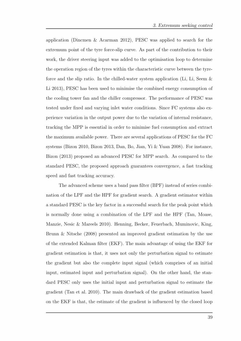
3. Extremum seeking control
application (Dincmen & Acarman 2012), PESC was applied to search for the
extremum point of the tyre force-slip curve. As part of the contribution to their
work, the driver steering input was added to the optimisation loop to determine
the operation region of the tyres within the characteristic curve between the tyre-
force and the slip ratio. In the chilled-water system application (Li, Li, Seem &
Li 2013), PESC has been used to minimise the combined energy consumption of
the cooling tower fan and the chiller compressor. The performance of PESC was
tested under fixed and varying inlet water conditions. Since FC systems also ex-
perience variation in the output power due to the variation of internal resistance,
tracking the MPP is essential in order to minimise fuel consumption and extract
the maximum available power. There are several applications of PESC for the FC
systems (Bizon 2010, Bizon 2013, Dan, Bo, Jian, Yi & Yuan 2008). For instance,
Bizon (2013) proposed an advanced PESC for MPP search. As compared to the
standard PESC, the proposed approach guarantees convergence, a fast tracking
speed and fast tracking accuracy.
The advanced scheme uses a band pass filter (BPF) instead of series combi-
nation of the LPF and the HPF for gradient search. A gradient estimator within
a standard PESC is the key factor in a successful search for the peak point which
is normally done using a combination of the LPF and the HPF (Tan, Moase,
Manzie, Nesic & Mareels 2010). Henning, Becker, Feuerbach, Muminovic, King,
Brunn & Nitsche (2008) presented an improved gradient estimation by the use
of the extended Kalman filter (EKF). The main advantage of using the EKF for
gradient estimation is that, it uses not only the perturbation signal to estimate
the gradient but also the complete input signal (which comprises of an initial
input, estimated input and perturbation signal). On the other hand, the stan-
dard PESC only uses the initial input and perturbation signal to estimate the
gradient (Tan et al. 2010). The main drawback of the gradient estimation based
on the EKF is that, the estimate of the gradient is influenced by the closed loop
39

3. Extremum seeking control
performance. To overcome this issue Gelberta, Moeck, Paschereit & King (2012)
proposed an alternative way to obtain the input which consequently eliminates
the influence of the closed loop performance. Gelberta, Moeck, Paschereit & King
also extended the application to dual input and single output. Thermo-acoustic
instabilities in an atmospheric combustion were used to demonstrate the effective-
ness of the proposed scheme by Gelberta, Moeck, Paschereit & King. Benefits of
degradation detection in PV systems using square wave perturbation was demon-
strated by Lei & Li (2010). When PV systems degrade, the internal resistance
changes (i.e. an increase in series resistance and a decrease in shunt resistance).
Change in the internal resistance of the PV system due to degradation can affect
the rise time in the transient response. Therefore, the change in the rise time
is used as a degradation indicator. This benefit however remains inconclusive
due to lack of experimental results. Apart from the aforementioned perturbation
signals, stochastic signals also have been applied as a source of perturbation (Liu
& Krstic 2012, Zhang & Ordonez 2012).
Stochastic based perturbation offers better solutions for systems where pre-
dictability associated with the period is difficult (e.g biological systems)(Zhang
& Ordonez 2012). For instance, Manzie & Kristic (2009b) and references therein,
applied stochastic perturbation to demonstrate its ability to guarantee the con-
vergence of the PESC. Proportional and derivative acceleration terms were incor-
porated within the feedback loop of a simple PESC to improve the convergence
speed (Zhang, Siranosian & Kristic 2009). The modified scheme was applied in
Monod and Williams Otto models. Dan et al. (2008), presented PESC for the
FC system which uses BPF utilising harmonics of the output signal. It has been
stated that inclusion of the third harmonic of the output signal offers better track-
ing. No benchmark results however were given to demonstrate the effectiveness
of the proposed approach. Since the standard PESC is suitable for plants that
are open loop stable, Zhang, Siranosian & Kristic (2007) proposed an extension
40
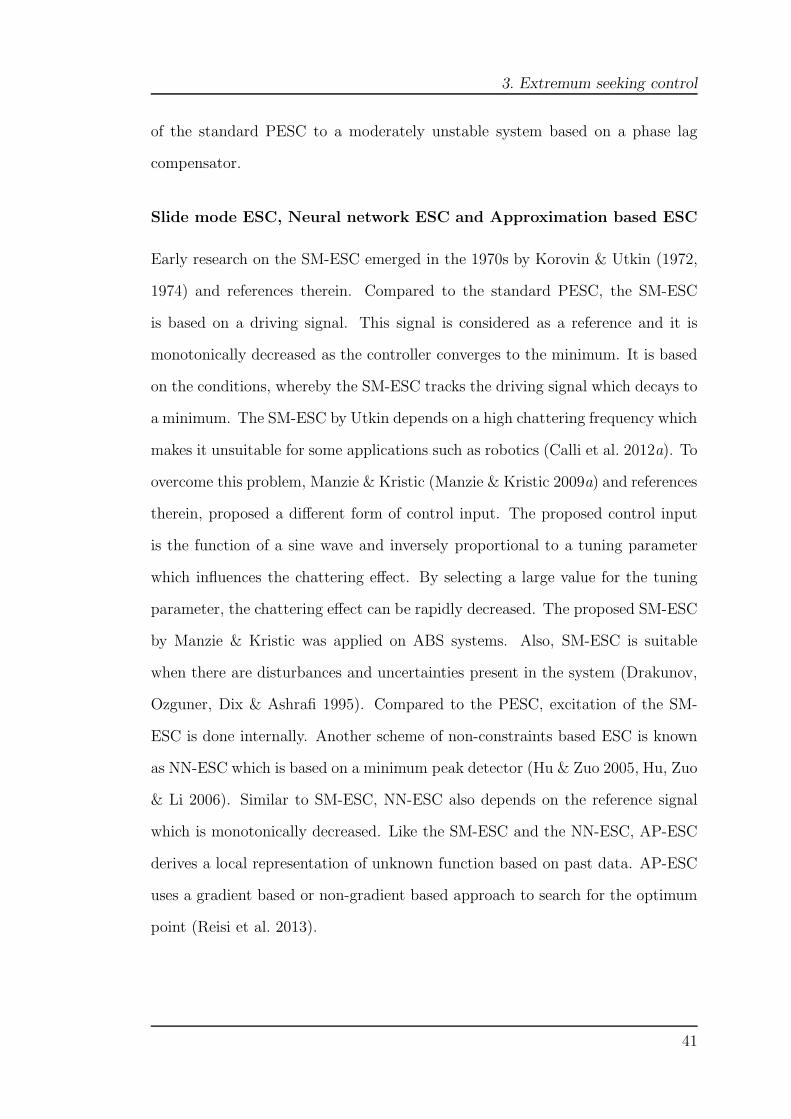
3. Extremum seeking control
of the standard PESC to a moderately unstable system based on a phase lag
compensator.
Slide mode ESC, Neural network ESC and Approximation based ESC
Early research on the SM-ESC emerged in the 1970s by Korovin & Utkin (1972,
1974) and references therein. Compared to the standard PESC, the SM-ESC
is based on a driving signal. This signal is considered as a reference and it is
monotonically decreased as the controller converges to the minimum. It is based
on the conditions, whereby the SM-ESC tracks the driving signal which decays to
a minimum. The SM-ESC by Utkin depends on a high chattering frequency which
makes it unsuitable for some applications such as robotics (Calli et al. 2012a). To
overcome this problem, Manzie & Kristic (Manzie & Kristic 2009a) and references
therein, proposed a different form of control input. The proposed control input
is the function of a sine wave and inversely proportional to a tuning parameter
which influences the chattering effect. By selecting a large value for the tuning
parameter, the chattering effect can be rapidly decreased. The proposed SM-ESC
by Manzie & Kristic was applied on ABS systems. Also, SM-ESC is suitable
when there are disturbances and uncertainties present in the system (Drakunov,
Ozguner, Dix & Ashrafi 1995). Compared to the PESC, excitation of the SM-
ESC is done internally. Another scheme of non-constraints based ESC is known
as NN-ESC which is based on a minimum peak detector (Hu & Zuo 2005, Hu, Zuo
& Li 2006). Similar to SM-ESC, NN-ESC also depends on the reference signal
which is monotonically decreased. Like the SM-ESC and the NN-ESC, AP-ESC
derives a local representation of unknown function based on past data. AP-ESC
uses a gradient based or non-gradient based approach to search for the optimum
point (Reisi et al. 2013).
41

3. Extremum seeking control
Comparison of non-constraints based ESC
This section summarises the performance of the reviewed non-constraints based
ESC methods. Their performance is based on their sensitivity to noise and sys-
tem dynamics, smooth reference tracking and multivariate extensions. A similar
performance is achieved between SM-ESC and NN-ESC when the effect of noise
is negligible. However, this is true only when the chattering effect in the SM-
ESC is taken into account. The NN-ESC also offers a robust performance due
to its hysteresis mechanism, except for small steady state irregularities. SM-ESC
is highly sensitive to noise in a transient response and a change in the driving
signal causes large amplitudes at steady state. AP-ESC converges much closer to
the optimum operating point in the absence of noise. Dynamic effects can cause
performance to deteriorate in both, NN-ESC and SM-ESC. In term of SM-ESC,
control performance can further be affected by causing the system to drift at
steady-state, mainly due to the growth of the driving signal. Since most of the
practical systems suffer from noise effect, both SM-ESC and AP-ESC are not the
best choices for practical systems.
Compared to all other non-constraints based ESC, it appears that PESC is
the least sensitive to noise and is a better choice when the system is affected by
measurement noise. However, when applied to systems with negligible measure-
ment noise, its performance (e.g. settling time) reduces significantly. Under the
effect of system dynamics, PESC and AP-ESC provide robust performance. On
the other hand, SM-ESC and NN-ESC experience minor distortion in the tran-
sient. Considering its consistent performance in various circumstances (e.g. noise,
system dynamics, multivariate extensions, etc.), PESC has been suggested to be
the best choice among the non-constraints based ESC (Calli, Caarls, Jonker &
Wisse 2012b). Taking account of the findings in the literature, further extension
of PESC is proposed in this Thesis.
42
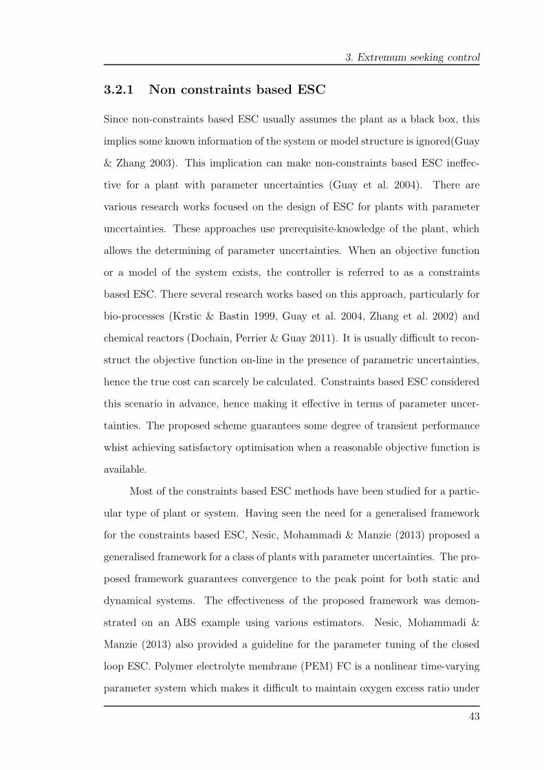
3. Extremum seeking control
3.2.1 Non constraints based ESC
Since non-constraints based ESC usually assumes the plant as a black box, this
implies some known information of the system or model structure is ignored(Guay
& Zhang 2003). This implication can make non-constraints based ESC ineffec-
tive for a plant with parameter uncertainties (Guay et al. 2004). There are
various research works focused on the design of ESC for plants with parameter
uncertainties. These approaches use prerequisite-knowledge of the plant, which
allows the determining of parameter uncertainties. When an objective function
or a model of the system exists, the controller is referred to as a constraints
based ESC. There several research works based on this approach, particularly for
bio-processes (Krstic & Bastin 1999, Guay et al. 2004, Zhang et al. 2002) and
chemical reactors (Dochain, Perrier & Guay 2011). It is usually difficult to recon-
struct the objective function on-line in the presence of parametric uncertainties,
hence the true cost can scarcely be calculated. Constraints based ESC considered
this scenario in advance, hence making it effective in terms of parameter uncer-
tainties. The proposed scheme guarantees some degree of transient performance
whist achieving satisfactory optimisation when a reasonable objective function is
available.
Most of the constraints based ESC methods have been studied for a partic-
ular type of plant or system. Having seen the need for a generalised framework
for the constraints based ESC, Nesic, Mohammadi & Manzie (2013) proposed a
generalised framework for a class of plants with parameter uncertainties. The pro-
posed framework guarantees convergence to the peak point for both static and
dynamical systems. The effectiveness of the proposed framework was demon-
strated on an ABS example using various estimators. Nesic, Mohammadi &
Manzie (2013) also provided a guideline for the parameter tuning of the closed
loop ESC. Polymer electrolyte membrane (PEM) FC is a nonlinear time-varying
parameter system which makes it difficult to maintain oxygen excess ratio under
43
3. Extremum seeking control
all operating conditions. Since the net power of the PEM FC is highly dependent
on the oxygen excess ratio in the cathode, the net output power is also affected.
To maximise the output of the PEM FC, Chang & Moura (2009) proposed a
constraints based ESC. The proposed constraints based ESC incorporated soft
constraints based on a quadratic cost function and it is claimed to offer a faster
convergence speed to that of the standard PESC.
3.3 PESC concept, analysis and design
This section presents concepts of PESC, detailed analysis and design guidance
of the standard PESC scheme. As aforementioned contribution on the Thesis
is based on extension of the PESC therefore, analysis presented here can also
be found in (Ariyur & Krstic 2010). The concept of PESC is briefly explained
followed by the problem description and some key assumptions. Also, the analysis
key features of the PESC are included, such as gradient searching, plant dynamics
and learning time scale. Gradient search will be presented to demonstrate the
ability of the PESC to converge within a small region around the MPP. Also, time
scales of plant dynamics and learning time scales will be analysed to investigate
time separation between the plant or system and the PESC feedback loop. PESC
operates in a closed loop fashion and it comprises a LPF, a HPF, an integrator
and a perturbation signal, see Fig. 3.1. The plant or system is considered to be
unknown; however it is known that its reference-output map has an extremum
point. The gradient search within the PESC is determined by series combination
of the HPF and the LPF. The gradient is searched as follows: a perturbation
signal with an initial input is modulated and fed to the unknown system. Then the
output of the system is filtered through the HPF to remove any DC components.
This signal is then demodulated with a perturbation signal and filtered through
the LPF to attenuate high frequencies. The initial value of the modulated signal
44

3. Extremum seeking control
is then compared with the new value. This is iteratively repeated until the MPP
is found at the point which the PESC enters the stable limit cycle. Adaptation
within the PESC feedback loop is determined by an integrator gain.
Figure 3.1: Block diagram of perturbation based extremum seeking control(Ariyur & Krystic 2003)
3.3.1 Problem description
Consider a nonlinear system (i.e. unknown system in Fig. 3.1) given as
χ = g(χ,uc) (3.1a)
y = h(χ) (3.1b)
where χ ∈ Rn is the state vector, uc is the smooth control law, g ∈ Rn is the
nonlinear vector field, h is the output performance map, and y ∈ R is the output
of the system. Let us assume the smooth control law in (3.1) is known and given
as
uc = Γ(χ,u) (3.2)
and is parametrised by a scalar input u. It can be stated that the system has
been parametrised by u at equilibrium. Also, let us adopt assumptions used in
45
This material has been removed from this thesis due to Third Party Copyright. The unabridged version of the thesis can be viewed at the Lanchester Library, Coventry University.

3. Extremum seeking control
(Ariyur & Krstic 2010) about the closed loop system in Fig. 3.1.
Assumption 1 There exists a smooth function l ∶ R ∈ Rn such that
g(χ,Γ(χ,u)) = 0 (3.3)
if and only if χ = l(u)
Assumption 1 signifies that the function is differentiable and the steady-state
characteristic is well defined.
Assumption 2 For each u, the equilibrium χ = l(u) of the system in (3.1) is
exponentially stable
Assumption 2 ensures that the steady-state characteristic of system in (3.1) is
stable.
Assumption 3 There exists u∗ ∈ R such that
y′ = 0, (3.4a)
y′′ < 0. (3.4b)
where y(u) = h(l(u)) and scalars y′ = dy(u∗)du
and y′′ = d2y(u∗)du2
Assumption 3 ensures that the steady-state characteristic has a unique maximum
(i.e. output equilibrium map y = h(l(u)) and is considered to have its maximum
point at u = u∗). The objective of the PESC is to maximise the steady-state
value of y without requiring knowledge of either functions (i.e. h and l) or u∗.
Assumptions (1), (2), and (3) were first proposed in (Ariyur & Krystic 2003). A
new operator is defined as follows:
Definition 1 y = F (s) [u]46

3. Extremum seeking control
It is used to perform different analyses in this Thesis such as gradient search,
convergence stability: where the time domain signal y is equal to the time domain
signal u filtered with the transfer function F (s). The operator defined in 1 will
be used in the remainder of this Thesis.
3.3.2 Gradient search
This section presents a numerical gradient search of the MPP using PESC. For
simplicity, the MPP search is considered for a single parameter PESC scheme and
the LPF is also removed from the PESC feedback loop (see Fig. 3.2). Prior to the
gradient search analysis, let us define the PESC design parameters as shown in
Table. 3.1. Output of the high pass filter signal, i.e., y − η in Fig. 3.2 is obtained
as follows:
Figure 3.2: Extremum seeking control scheme(Ariyur & Krstic 2010)
47
This material has been removed from this thesis due to Third Party Copyright. The unabridged version of the thesis can be viewed at the Lanchester Library, Coventry University.

3. Extremum seeking control
η =ωh
s + ωh
[y] (3.5a)
[y] − η = [y] − ωh
s + ωh
[y] (3.5b)
[y] − η = s
s + ωh
[y] (3.5c)
Hereafter, high pass filter will be in Fig.3.2 presented using a single block, i.e.,
ss+ωh
where input to the filter will be time domain signal y and output from the
filter will be time domain signal y − η.
A static map of the nonlinear system in (3.1) can be approximated using second
order Taylor series expansion as
y ≈ y∗ +y′′
2(u − u∗)2 (3.6)
where u is the control input value, u∗ is the optimum value at peak, and y′′ < 0.
Name Notation UnitPerturbation gain β
Cut-off frequency of the HPF ωh [ rads]
Cut-off frequency of the LPF ωl [ rads]
Perturbation frequency ω [ rads]
Phase angle ϕ [rad]Integrator gain k
Table 3.1: Designing parameters of the PESC
The objective is to minimise the quantity (u − u∗) such that the output function,
denoted f(u) approaches its maximum value at y∗ (i.e. when u=u∗). The esti-
mated value of the unknown u∗ is denoted u. The perturbation signal βsinωt is
the input to the plant, which is used for measuring the gradient information of
the function g(u). The estimation error of the control input denoted ue is given
48

3. Extremum seeking control
as,
ue = u∗ − u (3.7)
The quantity u is modulated by βsinωt to obtain u. Note that the difference
between u and u∗ is given as
u − u∗ = βsinωt − ue (3.8)
Substituting (3.8) into (3.6) the function h(l(u)) becomes
y ≈ y∗ +y′′
2(ue − βsinωt)2 (3.9)
Expanding (3.9) and replacing sin2ωt with 1
2(1 − cos2ωt) yield to
y ≈ y∗ +y′′
4β2 +
y′′
2u2e − βy
′′uesinωt −y′′
4β2cos2ωt (3.10)
The time domain signal y in (3.10) is filtered in order to remove unwanted high
frequencies through a high pass filter. The high pass filtered signal becomes
ξ ≈y′′
2u2
e − βy′′uesinωt −
y′′
4β2cos2ωt (3.11)
This signal is demodulated by multiplying with a dither signal sinωt
ξ ≈y′′
2u2
esinωt − βy′′uesin
2ωt −y′′
4β2cos2ωtsinωt (3.12)
Replacing the 2cos2ωtsinωt term with (sin3ωt − sinωt), the demodulated signal
becomes
ξ ≈ −βy′′
2ue +
βy′′
2uecos2ωt −
β2y′′
8(sin3ωt − sinωt) + y′′
2u2
esinωt (3.13)
49

3. Extremum seeking control
The magnitude of u2e is considered to be small and can be neglected accordingly.
Equation (3.13) is then reduced to
ξ ≈ −βy′′
2ue +
βy′′
2uecos2ωt −
β2y′′
8(sin3ωt − sinωt) (3.14)
Equation (3.14) comprises a number of high frequency signals which when passed
through the integrator i.e., 1
s[ξ], yields to (3.14)
u ≈ −k
s[βy′′
2]ue (3.15)
So the derivative of u in (3.15) is given as
˙u ≈ −(kβy′′2)ue (3.16)
Given that u∗ is constant in (3.7), therefore the derivative of (3.7) is written as
ue ≈ − ˙u (3.17)
Substituting (3.16) into (3.17) gives
ue ≈ (kβy′′
2)ue (3.18)
Given that (kβy′′2) < 0, the system is stable and it can be concluded that ue Ð→ 0
and u converges within a small region of u∗ which corresponds to the MPP.
3.3.3 Plant dynamics and learning time scale
The overall PESC feedback loop is considered to have three time scales, namely
fastest, medium and slow (Ariyur & Krystic 2003). The plant or system is con-
sidered to have the fastest dynamics as compared to periodic perturbation and
50

3. Extremum seeking control
filters (i.e. LPF and HPF). On the other hand, periodic perturbation is assumed
to have medium dynamics. Filters are considered to have the slowest dynamics.
Prior to time separation analysis, let us define how a function can be bounded.
Definition 2 The big O notation describes the limiting behavior of a function
when the argument tends to a particular value or infinity. For example, O(n2) is
any function g = g(n) such that ∣g(n)n2 ∣ remain bounded as n Ð→ +∞
In order to analyse the time scale of the PESC scheme, let us begin by determining
the overall closed loop system (see Fig. 3.3). The state of the system is given as
Figure 3.3: Perturbation extremum seeking control(Ariyur & Krstic 2010)
χ = g(χ,Γ(χ,u)) (3.19)
Given that the modulated input u = u+βsinωt, therefore (3.19) can be expressed
as
χ = g(χ,Γ(χ, (u + βsinωt)) (3.20)
51
This material has been removed from this thesis due to Third Party Copyright. The unabridged version of the thesis can be viewed at the Lanchester Library, Coventry University.

3. Extremum seeking control
Also estimated input u is obtained when a time domain signal ξ is passed through
a low pass filter such that:
u =k
s[ξ] (3.21a)
˙u = kξ (3.21b)
Output of the low pass filtered signal ξ is determined as follows:
ξ =ωl(s + ωl) [(y − η)] sinωt (3.22a)
(s + ωl) [ξ] = ωl [(y − η)] sinωt (3.22b)
ξ = −ωl [ξ] + ωl [(y − η)] sinωt (3.22c)
Time domain signal y when passed through high pass filter becomes
[(y − η)] = s
(s + ωh) [y] (3.23a)
s [y] = (s + ωh) [(y − η)] (3.23b)
η = −ωh [η] + ωh [y] (3.23c)
Using (3.20), (3.21b), (3.22c) and (3.23c) the overall closed loop system in Fig.3.3
is summarised as
χ = g(χ,Γ(χ, (u + βsinωt)) (3.24a)
˙u = kξ (3.24b)
ξ = −ωl [ξ] + ωl [(y − η)] sinωt (3.24c)
η = −ωh [η] + ωh [y] (3.24d)
ξ term captures the fastest dynamics of system (3.24). The medium fast varia-
tions are usually represented by the perturbation signal, i.e., βsinωt. The learning
52

3. Extremum seeking control
process is usually considered to be the slowest and is governed by integrator gain
k.
Let us define new coordinate as follows
u = u − u∗ (3.25a)
η = η − y(u∗) (3.25b)
Using time scale τ = ωt and substituting (3.25) into the overall closed system in
(3.24), the system can be rewritten as
ωdχ
dτ= g(χ,α(χ, (u + u∗ + βsinτ)) (3.26)
ω (dudτ+du∗
dτ) = kξ (3.27)
Given that u∗ is fixed parameter for a static map, therefore dy(u∗)dτ= 0. Equation
(3.27) is reduced to
ωdu
dτ= kξ (3.28)
where k is a design parameter and be selected such that, k = ωδK′(Ariyur &
Krystic 2003) where ω and δ are small positive constants, K′is O(1) positive constant.
Substituting k into (3.28) gives
du
dτ= δK ′ξ (3.29)
From (3.24c) can be rewritten as
ωdξ
dτ= −ωlξ + ωl(y − η − y(u∗))sinτ (3.30)
53

3. Extremum seeking control
Given that y = g(x), therefore (3.30) becomes
ωdξ
dτ= −ωlξ + ωl(h(x) − η − y(u∗))sinτ (3.31)
From (3.31) ωl is another designing parameter and can be selected in a similar
manner as k, therefore ωl = ωδω′Lwhere ω
′L is O(1) positive constant. Substituting
ωl into (3.31) yields to
dξ
dτ= −δω
′Lξ + δω
′L(h(x) − η − y(u∗))sinτ (3.32)
Also (3.24d )can be rewritten as
ω (dηdτ+dy(u∗)dτ
) = −ωh (η + y(u∗)) + ωhy (3.33)
Similarly y(u∗) is fixed parameter, therefore dy(u∗)dτ= 0. Equation (3.33) is reduced
to
ωdη
dτ= −ωh (η + y(u∗)) + ωhy (3.34)
Given that ωh = ωδω′H where ω
′H is a positive constant. Equation (3.34)can be
expressed as
dη
dτ= −ω
′H (η + y(u∗)) + ω′Hy (3.35)
Eq. 3.35 can be written as
dη
dτ= −ω
′H η + ω
′H (h(x) + y(u∗)) (3.36)
The overall system with time scale τ = ωt is summarised using (3.26), (3.29),
(3.32) and (3.36)
ωdx
dτ= g(χ,α(χ, (u + u∗ + βsinτ)) (3.37)
54

3. Extremum seeking control
⎡⎢⎢⎢⎢⎢⎢⎢⎢⎢⎣
dudτ
dξdτ
dη
dτ
⎤⎥⎥⎥⎥⎥⎥⎥⎥⎥⎦=
⎡⎢⎢⎢⎢⎢⎢⎢⎢⎢⎣
δK ′ξ
−δω′Lξ + δω
′L(h(x) − η − y(u∗))sinτ
−δω′H η + δω
′H (h(x) + y(u∗))
⎤⎥⎥⎥⎥⎥⎥⎥⎥⎥⎦(3.38)
From the system in (3.37), based on the assumption that both u+u∗ and the
perturbation signal, i.e., βsinωt are slowly time varying as compared to transients
in χ-dynamics, it is possible to obtain the approximate solution of χ as follows
x = l (u + u∗ + βsinτ) (3.39)
Equation (3.39) can be used to discard fast time response in the χ-dynamics. The
time-invariant system which captures the main trend of the learning dynamics can
be obtained by averaging out the time variations. For more details in averaging
analysis of the PESC feedback loop see (Ariyur & Krstic 2010).
3.3.4 PESC parameter design
This section presents design guidance for a single parameter PESC scheme. The
PESC comprises of tuning parameters namely: β, k, ω, ωh, and ωl, ϕ. PESC
feedback performance is highly dependent on these parameters. For instance, ω,
should be larger with respect to k. However, too large a value for ω may trig-
ger un-modeled dynamics and causes oscillations in the system output Ariyur &
Krystic (2003). Also, ω must be large than ωh and ωl. On other the hand, ω must
have a smaller cut off frequency than the input dynamics to separate the frequen-
cies corresponding to the perturbation signal and the inner dynamics Ariyur &
Krystic (2003).
55
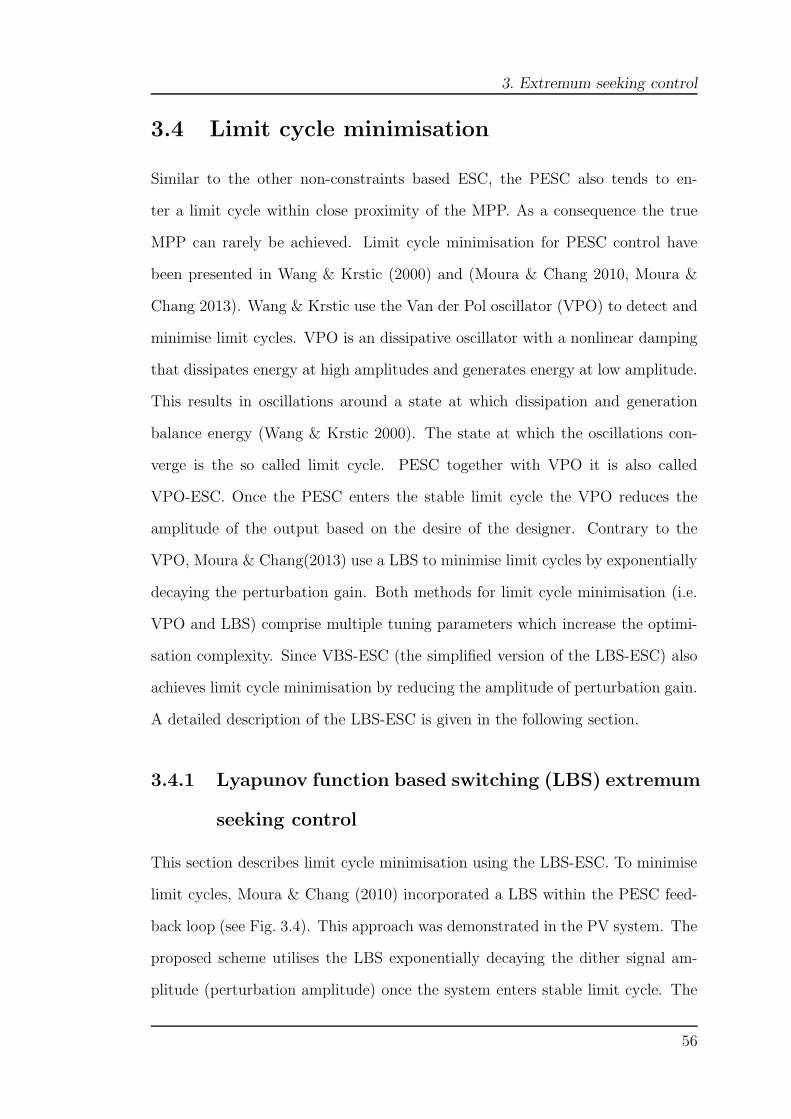
3. Extremum seeking control
3.4 Limit cycle minimisation
Similar to the other non-constraints based ESC, the PESC also tends to en-
ter a limit cycle within close proximity of the MPP. As a consequence the true
MPP can rarely be achieved. Limit cycle minimisation for PESC control have
been presented in Wang & Krstic (2000) and (Moura & Chang 2010, Moura &
Chang 2013). Wang & Krstic use the Van der Pol oscillator (VPO) to detect and
minimise limit cycles. VPO is an dissipative oscillator with a nonlinear damping
that dissipates energy at high amplitudes and generates energy at low amplitude.
This results in oscillations around a state at which dissipation and generation
balance energy (Wang & Krstic 2000). The state at which the oscillations con-
verge is the so called limit cycle. PESC together with VPO it is also called
VPO-ESC. Once the PESC enters the stable limit cycle the VPO reduces the
amplitude of the output based on the desire of the designer. Contrary to the
VPO, Moura & Chang(2013) use a LBS to minimise limit cycles by exponentially
decaying the perturbation gain. Both methods for limit cycle minimisation (i.e.
VPO and LBS) comprise multiple tuning parameters which increase the optimi-
sation complexity. Since VBS-ESC (the simplified version of the LBS-ESC) also
achieves limit cycle minimisation by reducing the amplitude of perturbation gain.
A detailed description of the LBS-ESC is given in the following section.
3.4.1 Lyapunov function based switching (LBS) extremum
seeking control
This section describes limit cycle minimisation using the LBS-ESC. To minimise
limit cycles, Moura & Chang (2010) incorporated a LBS within the PESC feed-
back loop (see Fig. 3.4). This approach was demonstrated in the PV system. The
proposed scheme utilises the LBS exponentially decaying the dither signal am-
plitude (perturbation amplitude) once the system enters stable limit cycle. The
56

3. Extremum seeking control
LBS scheme (see Fig. 3.4) comprises an averaging operator, a quadratic Lyapunov
function, a switch and a perturbation signal. The averaging operator is obtained
by linearising the entire PESC feedback loop about the MPP. The averaging op-
erator is also referred to as the Jacobian (i.e. average model) that approximates
the plant or system dynamics near the equilibrium point. The obtained average
model is used to develop a quadratic Lyapunov function denoted by V (xβ) togovern the switching process. xβ is the average state variable of the estimated
input, LPF output, and HPF output of the PESC feedback loop see Fig. 3.4.xβ
is given as
xβ = [u ξ η] (3.40)
where u, ξ and η are new coordinates defined based on (3.25). If V (xβ) is smaller
than the threshold, denoted ǫlbs, the dither signal with decaying amplitude will
be used, otherwise the same dither signal as in the standard PESC will be used.
This process will continue until V (xβ) drops below ǫlbs. Once this happens, the
integrator resets to its initial condition and the original dither signal will be used.
It has been shown in Moura & Chang (2010) that the Jacobian of the closed loop
system shown in Fig. 3.4 near the equilibrium is given as
J =
⎡⎢⎢⎢⎢⎢⎢⎢⎢⎢⎣
0 k 0
ωlb2βo −ωl 0
ωhb1 0 −ωh
⎤⎥⎥⎥⎥⎥⎥⎥⎥⎥⎦(3.41)
where, b1 = 0 and b2 < 0. Having obtained the Jacobian of system in Fig. 3.4, the
V (xβ) used in the LSB is obtained by solving the following Lyapunov equation
for P:
PJ + JTP +Q = 0 (3.42)
57
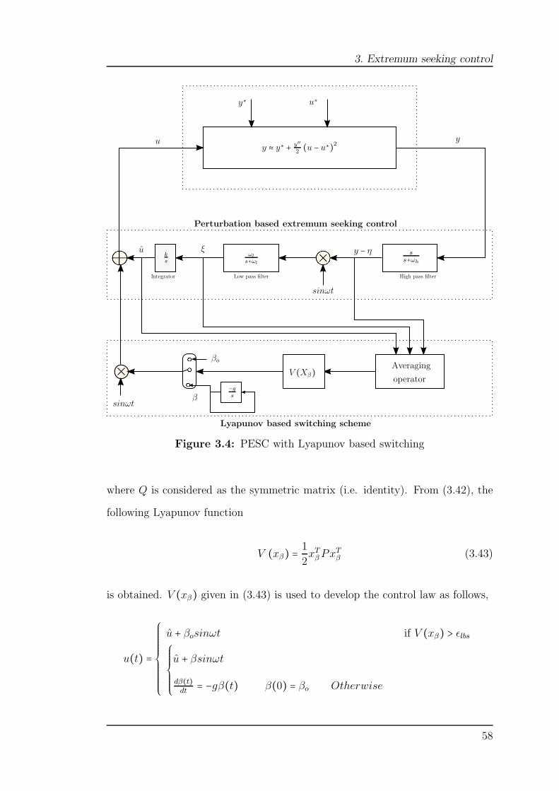
3. Extremum seeking controlreplacemen
y ≈ y∗ + y′′
2(u − u∗)2u y
ss+ωh
sinωt
sinωt
ks
u ξ y − η
y∗ u∗
V (Xβ)βo
β
ωl
s+ωl
−gs
Perturbation based extremum seeking control
Lyapunov based switching scheme
Averaging
operator
High pass filterLow pass filterIntegrator
Figure 3.4: PESC with Lyapunov based switching
where Q is considered as the symmetric matrix (i.e. identity). From (3.42), the
following Lyapunov function
V (xβ) = 12xTβPxT
β (3.43)
is obtained. V (xβ) given in (3.43) is used to develop the control law as follows,
u(t) =⎧⎪⎪⎪⎪⎪⎪⎪⎪⎪⎨⎪⎪⎪⎪⎪⎪⎪⎪⎪⎩
u + βosinωt if V (xβ) > ǫlbs⎧⎪⎪⎪⎪⎪⎨⎪⎪⎪⎪⎪⎩u + βsinωt
dβ(t)dt= −gβ(t) β(0) = βo Otherwise
58

3. Extremum seeking control
where: u(t) denotes the control input signal, u denotes the estimated input, βo
denotes the initial perturbation amplitude, β denotes the perturbation amplitude
based on exponential decay. Parameters −g and ǫlbs ensure system stability due
to disturbances. V (xβ) estimates how close to the MPP the ”average model”
converges. If V (xβ) is within the pre-defined threshold denote ǫlbs, therefore as
xβ Ð→ 0 then V (xβ)Ð→ 0. As the PESC converges close enough to the MPP, the
perturbation signal (i.e. sinusoidal) decays exponentially to zero, hence uÐ→ u∗.
However, due to disturbances V (xβ)may drift away from the ǫlbs therefore control
law will work as follows: if V (xβ) is greater than ǫlbs then the LBS-ESC will
operate as the standard PESC with u(t) = u + βosinωt until the plant converges
back to the MPP. On the other hand, if V (xβ) drops below ǫlbs, the integrator
will reset the initial condition β(0) = βo it will operate with u(t) = u + βsinωt.
3.4.2 Variance Based Switching (VBS) ESC
As aforementioned, both the VPO-ESC and the LBS-ESC comprise multiple
tuning parameters, hence this may lead to an increase in complexity for online
optimisation. To address these issues, in this Section a simplified VBS-ESC
scheme for limit cycle minimisation is proposed (see Fig. 3.5). The proposed
scheme is a simplified version of the LBS-ESC and it also retains the simplicity
of the PESC. The simplification is achieved by removing the averaging operator
hence there is no need for linearising the entire feedback loop. Also, the Lyapunov
function integrator within a LBS scheme and its tuning time varying parameter
g are removed (see Fig. 3.4). A variance detection sub-system is introduced to
minimise limit cycles by detecting variance in the estimated input. The VBS-
ESC comprises of the PESC and the VBS scheme (see Fig. 3.5). The VBS is
used to reduce the amplitude of oscillations once the PESC has entered stable
limit cycle. Detection of the amplitude of oscillations is based on determining
the variance of u. As the PESC scheme approaches steady-state, the variance of
59
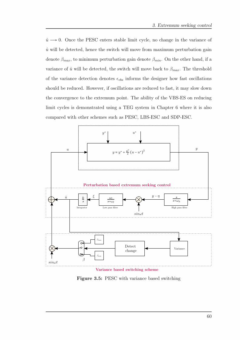
3. Extremum seeking control
u Ð→ 0. Once the PESC enters stable limit cycle, no change in the variance of
u will be detected, hence the switch will move from maximum perturbation gain
denote βmax, to minimum perturbation gain denote βmin. On the other hand, if a
variance of u will be detected, the switch will move back to βmax. The threshold
of the variance detection denotes ǫvbs informs the designer how fast oscillations
should be reduced. However, if oscillations are reduced to fast, it may slow down
the convergence to the extremum point. The ability of the VBS-ES on reducing
limit cycles is demonstrated using a TEG system in Chapter 6 where it is also
compared with other schemes such as PESC, LBS-ESC and SDP-ESC.
y ≈ y∗ + y′′2(u − u∗)2u y
ss+ωh
sinωt
sinωt
ks
u ξ y − η
y∗ u∗
Variance
β
ωl
s+ωl
βmax
βmin
Perturbation based extremum seeking control
Variance based switching scheme
Detectchange
High pass filterLow pass filterIntegrator
Figure 3.5: PESC with variance based switching
60
3. Extremum seeking control
3.5 Critical appraisal and conclusions
In this chapter, non-constraints based and constraints based ESC have been re-
viewed. Detailed analysis of several key features of the PESC such as gradient
search, learning and dynamic time scale and limit cycle minimisation have been
presented. Considering its consistent performance in various circumstances (e.g.
noise sensitivity, sensitivity to system dynamics, multivariate extensions, etc.),
the PESC has been suggested to be the best choice among the non-constraints
based ESC in literature. However, limit cycles due to periodic perturbation makes
it more difficult for the true MPP to be achieved using PESC. The improved
scheme known as VBS-ESC based on simplification of the LBS-ESC for limit
cycle minimisation is presented. VBS-ESC is considered to be simpler based on
the following reasons, Compared to the LBS-ESC, it doesn’t require linearisation
of the entire PESC feedback loop, and it also comprises fewer tuning parameters
and it does not require the solving of the Lyapunov function. Although both
methods minimise limit cycles in a similar manner, neither of them take into
consideration the trade-off between convergence speed and the minimisation of
losses. To address these issues an improved PESC scheme known as the SDP-ESC
is presented in Chapter 5.
61
Chapter 4
State dependent parameter
(SDP) extremum seeking control
4.1 Introduction
This Chapter presents an advanced control strategy based on an extension of the
standard PESC known as SDP-ESC. While the VBS-ESC proposed in Chapter 3
minimises the limit cycle based on variance detection, both the SDP-ESC and the
LBS-ESC minimise limit cycles by decaying the perturbation gain exponentially.
However, the SDP-ESC approach introduces dependency between the estimated
input and perturbation gain which allows the automated exponential decay of
the perturbation signal, instead of linearising the entire feedback loop and defin-
ing a Lyapunov function as is the case in LBS-ESC. Compared to the LSB-ESC,
the SDP-ESC in addition to limit cycle minimisation, also takes into account
the trade-off between the convergence speed and the minimisation of losses. For
that reason the convergence speed is improved by introducing a compensator (PI
controller). Nevertheless, the proposed scheme can be initialised with a large per-
turbation gain, hence making it possible to achieve the required excitation for the
duration of the operation. The main advantages of the SDP-ESC as compared to
62
4. State dependent parameter (SDP) extremum seeking control
LBS-ESC include its simplicity because it does not have a switch (with multiple
tuning parameters). It does not require calculating a Lyapunov function as well
as not having the need to average the feedback loop. This chapter is organised
as follows; intuitive explanation of the proposed scheme is given in Section 4.2.
Convergence and stability analysis of the proposed scheme is discussed in Sec-
tion 4.3 and Section 4.4, respectively. Section 4.5 describes the design procedure
of the SDP-ESC for a single parameter scheme. Section 4.6 presents simulation
examples for both plant with and without dynamics. The sensitivity analysis of
the SDP-ESC is presented in Section 4.7. Section 4.8 presents the critical ap-
praisal and conclusions.
Similar to other traditional ESCs, the PESC also tends to enter a limit
cycle due to periodic perturbation. When applied to an MPP search within low
carbon technologies (e.g TEGs, PVs, FCs, wind turbines, etc.) the true MPP can
hardly ever be achieved. Apart from that, limit cycle is associated with ripple
currents across the load and the inductor within DC-DC converter (Chen, Chou
& Wu 2005). A large limit cycle indicates high ripple current which can cause
the core temperature of the capacitor to rise and hence reduce the electrolyte
of the capacitor. Reduction of the electrolyte causes both the capacitance and
the equivalent series resistance (ESR) to increase. The ESR is usually used as a
health indicator of capacitors (Chen et al. 2005). An increase of the ESR implies
the reduction of the remaining useful life (RUL) of a DC-DC converter which may
lead to decreased reliability. This justifies the need for a more advanced PESC
which can minimise limit cycles, improve convergence speed and reliability whilst
preserving the stability and simplicity of the standard PESC.
63
4. State dependent parameter (SDP) extremum seeking control
4.2 SDP-ESC intuitive explanation
The SDP function and the compensator form a modified loop within the PESC.
The PESC with the modified loop is shown in Fig. 4.1 and is further referred to
as the state dependent parameter (SDP) ESC. It is named SDP-ESC due to the
dependence of the perturbation gain parameter on the system state x. In this
Thesis, the study of limit cycle minimisation and improving speed of convergence
via SDP-ESC is considered only for a single parameter scheme in a continuous
time domain (see Fig. 4.1). The plant in Fig. 4.1 is considered to have faster
dynamics than the SDP-ESC feedback loop. This will ensure that the plant
appears as a static non-linearity from the viewpoint of the SDP-ESC feedback
loop. A slow perturbation signal will cause time separation between the SDP-
ESC feedback loop and the plant and as a consequence the dynamics of the plant
will not interfere with the peak seeking scheme. Cut-off frequencies of high and
low pass filters are lower than the perturbation frequency ω .
The estimated value u of unknown optimal input u∗ is modulated with a
perturbation signal (sine wave with the gain f (x)) which decays exponentially to
a small yet sufficient value to allow the SDP-ESC feedback loop to detect changes
in the system input. It should be noted that f (x) must not be allowed to decay
to zero, but rather to a small value close to zero. Allowing f (x) to decay to zero
implies no perturbation to the system and as a consequence, the SDP-ESC will
fail to adapt. The rate at which f(x) decays depends on α. If u is on either side
of u∗ with minimal limit cycle, a periodic response of the output y which is either
in-phase or out-of-phase with the perturbation signal will be created. The rate of
decay of the perturbation signal depends on the variance of the integrator output
x. The variance of x decays to a small value as the system enters a stable limit
cycle. DC components are removed from output y when it passes through the
washout filter (i.e. HPF). The output of the filter is then demodulated with a
64

4. State dependent parameter (SDP) extremum seeking control
dither signal (sine wave with a fixed perturbation gain). The LPF removes high
frequencies from the demodulated signal. The SDP function should have the
slowest dynamics in the closed loop system to allow the SDP-ESC feedback loop
via perturbation signal f(x)sinωt to search for the gradient and reach steady
state. Mathematically, f(x) is expressed as
f(x) =⎧⎪⎪⎪⎪⎨⎪⎪⎪⎪⎩
βe−αµ if µ < α and µ ≠ 0
β otherwise
where µ is the variance of the state x, β is the perturbation gain, α > 0 denotes the
exponential decay constant. The variance of x is calculated as a moving averaging
window where the window length is based on a number of samples. Adaptation
within the SDP-ESC is achieved via an integrator and a compensator is used to
improve the convergence time. As f (x) decays to a small value the limit cycle is
minimised.
Plant
Modified loop
Low pass filter High pass filterIntegrator
State dependentperturbation function
Compensator
y ≈ y∗ + y′′2(u − u∗)2u y
ss+ωh
skc+1s
f(x)
sinωt
ks
u ξ
y∗ u∗
ωl
s+ωl
x y − η
Figure 4.1: Illustrates state dependent parameter (SDP) ESC scheme
65

4. State dependent parameter (SDP) extremum seeking control
4.3 Convergence analysis
It is important to ensure that the developed SDP-ESC scheme is capable of con-
verging to the MPP as well as minimising limit cycles. The convergence analysis
using the SDP-ESC is demonstrated using the same problem described in Sec-
tion 3.3.1. Assumptions 1, 2 and 3 (see Section 3.3.1 ) are also considered. Con-
vergence analysis for a single parameter SDP-ESC scheme is considered. Before
proceeding with the convergence analysis, let us make the following assumption:
Assumption 4 µ is a windowed variance hence γ is considered to be constant
for a period of time
Definition 3 γ is a time varying parameter which presents ratio between α and
µ
therefore f(x) can be presented as:
f (x) = βe−γ (4.1)
4.3.1 SDP-ESC for a static map
Fig. 4.2 presents a simplified form of the SDP-ESC closed loop where the plant
dynamics are neglected.
Preposition 1 The perturbation signal of the system in Fig. 4.2 is sufficiently
slow to allow the plant to appear as a static nonlinear map from the SDP-ESC
viewpoint. LPF is not essential for convergence analysis since the integrator
attenuates high frequencies, however it should be noted that for practical imple-
mentation, LPF is required.
66

4. State dependent parameter (SDP) extremum seeking control
Plant
Modified loop
High pass filterIntegrator
State dependentperturbation function
Compensator
y ≈ y∗ + y′′
2(u − u∗)2u y
ss+ωh
skc+1s
f(x)
sinωt
ks
u ξ
y∗ u∗
x y − η
Figure 4.2: Simplified SDP-ESC scheme
Using second order Taylor series expansion, the static nonlinear map of the
system in Fig. 4.2 can be approximated as
y(u) ≈ y∗ + y′′2(u − u∗)2 (4.2)
The objective is to minimise quantity (u − u∗), such that y ≈ y∗.
Denote ue as the estimation error which is the difference between u∗ and u
ue = u∗ − u (4.3)
The quantity u is modulated by f(x)sinωt to obtain u. The difference between
u and u∗ is given as
u − u∗ = f(x)sinωt − ue (4.4)
Substitute (4.4) into (4.2) gives
y ≈ y∗ +y′′
2(ue − βe
−γsinωt)2 (4.5)
67

4. State dependent parameter (SDP) extremum seeking control
Expanding (4.5) and replacing sinωt with 1
2(1 − cos2ωt) yield to
y ≈ y∗ +y′′u2e
2+y′′
4β2e−2γ − y
′′ueβe
−γsinωt −y′′
4β2e−2γcos2ωt (4.6)
The time domain signal y in 4.6 is filtered in order to remove any unwanted slow
DC components. The high pass filtered signal becomes
ξ ≈y′′u2e
2+y′′
4β2e−2γ − y
′′ueβe
−γsinωt −y′′
4β2e−2γcos2ωt (4.7)
The signal in (4.7) is demodulated by multiplying with dither signal sinωt to
obtain
ξ ≈y′′u2e
2sinωt +
y′′
4β2e−2γsinωt − y
′′ueβe
−γsin2ωt −y′′
4β2e−2γcosωtsinωt (4.8)
Replacing cosωtsinωt with 1
2(sin3ωt − sinωt) the demodulated signal in (4.8)
becomes
ξ ≈y′′u2e
2sinωt +
y′′
4β2e−2γsinωt − y
′′ueβe
−γsin2ωt −y′′
8β2e−2γ (sin3ωt − sinωt)
(4.9)
The magnitude of u2e is considered to be small and can be neglected accordingly.
Equation (4.9) is then reduced to
ξ ≈ −y′′
2ueβe
−γ +y′′
4β2e−2γsinωt +
y′′
2ueβe
−γcos2ωt −y′′
8β2e−2γ (sin3ωt − sinωt)
(4.10)
Equation (4.10) comprises a number of high frequency signals which when passed
through the integrator i.e., 1
s[ξ], yields to 4.11
x ≈ −k
s[e−γβy′′
2]ue (4.11)
68

4. State dependent parameter (SDP) extremum seeking control
The approximation of the optimal perturbation signal u is obtained by passing
the approximated time signal x through a compensator, such that:
u =skc + 1
s[x] (4.12)
substituting (4.11) into (4.12) yields to the approximation of the rate of change
of the optimal perturbation signal, i.e.,
˙u ≈ −zkcue − zue (4.13)
where z = kβe−γy′′2
since u∗ is constant in (4.3), its derivative can be written as
ue = − ˙u (4.14)
Substituting (4.14) into (4.13) yields to the rate of change of the input estimation
error, i.e.,
ue =z
1 − zkcue (4.15)
since kβe−γy′′
2< 0 then the system is stable. As ue Ð→ 0, and e−γ converge to a
small region so that 0 < e−γ < 1, then u converge within a small region of u∗ with
minimised limit cycle.
Theorem 1 For the simplified SDP-ESC scheme given in Fig. 4.2, the output
error y − y∗ achieves local exponential convergence to an O(β2e−2γ) of the origin
with minimised limit cycle, provided the exponential decay is 0 < e−γ < 1.
69

4. State dependent parameter (SDP) extremum seeking control
Proof of theorem 1
From (4.2) output error is expressed as
y − y∗ ≈y′′
2(ue − βe
−γsinωt)2 (4.16)
Expanding (4.16) gives
y − y∗ ≈y′′
2ue − y
′′ueβe
−γsinωt + β2e−2γy′′
2sin2ωt (4.17)
as ue Ð→ 0 (4.17) reduced to
y − y∗ ≈ β2e−2γy′′
2sin2ωt (4.18)
Using definition (2) in Section 3.3.3, the right hand side term in (4.18) is bounded
as follows
β2e−2γy′′
2sin2ωt = O(β2e−2γ) (4.19)
hence,
y − y∗ ≈ O(β2e−2γ) (4.20)
70

4. State dependent parameter (SDP) extremum seeking control
4.4 Stability analysis
Stability analysis of the SDP-ESC is performed in the continuous time domain.
Stability is analysed via the averaging technique which is a suitable method for
analysing periodic systems (Ariyur & Krystic 2003). Stability analysis via the
averaging technique includes the following steps:
1. transform a system with a new coordinate to obtain a simplified system,
2. use an averaging method to obtain the average of a reduced system and its
equilibrium point,
3. compute the Jacobian of the average reduced system,
4. find the determinant of the average reduced system to check whether the
system is stable or not.
System transformation:
Consider the non-linear system in Fig. 4.1 presented using state equations as,
⎡⎢⎢⎢⎢⎢⎢⎢⎢⎢⎢⎢⎢⎢⎢⎢⎢⎢⎣
˙u = kdξ + x
˙x = kξ
ξ = −ωlξ − ηωlsinωt + ωly(u)sinωtη = −ηωh + y(u)ωh
u = u + βe−γsinωt
⎤⎥⎥⎥⎥⎥⎥⎥⎥⎥⎥⎥⎥⎥⎥⎥⎥⎥⎦
(4.21)
where: u is the control input, y is the optimal value as the function of control input, kd = kkc is the product of compensator and integrator gains.
Let us define new coordinates in order to shift the nominal optimal operating
point, denoted as:
u = u − u∗ (4.22)
71
4. State dependent parameter (SDP) extremum seeking control
η = η − y(u∗) (4.23)
Nonlinear system in (4.21) can be translated as follows
⎡⎢⎢⎢⎢⎢⎢⎢⎢⎢⎢⎢⎢⎢⎣
˙u = kdξ + x
˙x = kξ
ξ = −ωlξ − ηωlsinwt + ωl [y (u + u∗ + βe−γsinωt) − y(u∗)] sinωt˙η = −ηωh − ωh [y (u + u∗ + βe−γsinωt) − y(u∗)]
⎤⎥⎥⎥⎥⎥⎥⎥⎥⎥⎥⎥⎥⎥⎦
(4.24)
Set τ = ωt and V (ur + βe−γsinωt) = y (u + u∗ + βe−γsinτ) − y(u∗) to obtain a
reduced system in the following form
d
dτ
⎡⎢⎢⎢⎢⎢⎢⎢⎢⎢⎢⎢⎢⎢⎣
ur
xr
ξr
ηr
⎤⎥⎥⎥⎥⎥⎥⎥⎥⎥⎥⎥⎥⎥⎦
=1
ω
⎡⎢⎢⎢⎢⎢⎢⎢⎢⎢⎢⎢⎢⎢⎣
kdξr + x
kξr
−ωlξr − ωlηrsinτ + ωlV (ur + βe−γsinτ) sinτ−ωhηr − ωhV (ur + βe−γsinτ)
⎤⎥⎥⎥⎥⎥⎥⎥⎥⎥⎥⎥⎥⎥⎦
(4.25)
Adopting design parameters selection used in (Ariyur & Krystic 2003), normalized
parameters are given as
k = ωK = ωδK′= O(ωδ) (4.26a)
kd = ωKd = ωδK′d = O(ωδ) (4.26b)
ωl = ωωL = ωδω′L = O(ωδ) (4.26c)
ωh = ωωH = ωδω′H = O(ωδ) (4.26d)
72

4. State dependent parameter (SDP) extremum seeking control
where ω and δ are small positive constants and K′d, ω
′L, and ω
′H are O(1) positive
constants.
d
dτ
⎡⎢⎢⎢⎢⎢⎢⎢⎢⎢⎢⎢⎢⎢⎣
ur
xr
ξr
ηr
⎤⎥⎥⎥⎥⎥⎥⎥⎥⎥⎥⎥⎥⎥⎦
= δ
⎡⎢⎢⎢⎢⎢⎢⎢⎢⎢⎢⎢⎢⎢⎣
K′dξr + x
K′ξr
−ω′Lξr − ω
′Lηrsinτ + ω
′LV (ur + βe−γsinτ) sinτ
−ω′H ηr − ω
′HV (ur + βe−γsinτ)
⎤⎥⎥⎥⎥⎥⎥⎥⎥⎥⎥⎥⎥⎥⎦
(4.27)
Averaging method
In order to analyse the reduced periodic system in (4.27) an averaging technique
is used. The averaging equation is defined as,
xa =1
2π ∫2π
0
x (σ)d (σ) (4.28)
where (σ) = τNote that: the average of sinτ = 0, hence ω
′Lηrsinτ = 0
Equation ( 4.27) can be expressed as
d
dτ
⎡⎢⎢⎢⎢⎢⎢⎢⎢⎢⎢⎢⎢⎢⎣
uar
xar
ξar
ηar
⎤⎥⎥⎥⎥⎥⎥⎥⎥⎥⎥⎥⎥⎥⎦
= δ
⎡⎢⎢⎢⎢⎢⎢⎢⎢⎢⎢⎢⎢⎢⎣
K′dξ
ar + x
ar
K′ξar
−ω′Lξ
ar +
ω′L
2π ∫ 2π
0V (ua
r + βe−γsinτ) sinτdτ
−ω′H η
ar −
ω′H
2π ∫ 2π
0V (ua
r + βe−γsinτ) dτ
⎤⎥⎥⎥⎥⎥⎥⎥⎥⎥⎥⎥⎥⎥⎦
(4.29)
The equilibrium of system (ua,er , x
a,er , ξ
a,er , η
a,er ) presented in (4.29) must satisfy
0 =
⎡⎢⎢⎢⎢⎢⎢⎢⎢⎢⎢⎢⎢⎢⎣
K′dξ
a,er + x
a,er
K′ξa,er
−ω′Lξ
a,er +
ω′L
2π ∫ 2π
0V (ua,e
r + βe−γsinτ) sinτdτ−ω
′H η
a,er −
ω′H
2π ∫ 2π
0V (ua,e
r + βe−γsinτ)dτ
⎤⎥⎥⎥⎥⎥⎥⎥⎥⎥⎥⎥⎥⎥⎦
(4.30)
73

4. State dependent parameter (SDP) extremum seeking control
where
ξa,er = 0 (4.31a)
xa,er = 0 (4.31b)
∫2π
0
V (ua,er + βe
−γsinτ) sinτdτ = 0 (4.31c)
ηa,er =1
2π ∫2π
0
V (ua,er + βe
−γsinτ) dτ (4.31d)
In view of assumption (3), it is clear that:
V (0) = 0 (4.32a)
V ′ (0) = y′ (u∗) = 0 (4.32b)
V ′′ (0) = y′′ (u∗) < 0 (4.32c)
Substituting V (0) , V ′ (0) and V ′′ (0) into a Taylor expansion gives :
V (x) = V (0) + V ′ (0)x + V ′′ (0)2!
x2 + .... (4.33)
Postulating in a similar manner to (Ariyur & Krystic 2003), ua,er is expressed
as,
ua,er = a1β + a2β
2 +O(β3) (4.34)
74

4. State dependent parameter (SDP) extremum seeking control
Substituting (4.34) into (4.31c) and using (4.33), followed by integrating and
equating same power of β yield to,
∫2π
0
V (ua,er + βe
−γsinτ) sinτdτ = ∫ 2π
0
V ′′(0)2!(ua,e
r + βe−γsinτ)2 sinτdτ+
∫2π
0
V ′′′(0)3!
(ua,er + βe
−γsinτ)3 sinτdτ = 0 (4.35)
V ′′(0)πβe−γ (ua,er ) + V ′′′(0)
8πβ3e−3γ +
V ′′′(0)2
πβ3e2γ (ua,er )2 = 0 (4.36)
Simplifying by a bound higher power gives,
V ′′(0)πβ2e−γa1 + V ′′(0)πβ3e−γa2 +V ′′′(0)
8πβ3e−3γ = 0 (4.37)
hence,
a1 = 0 (4.38a)
a2 = −V ′′′(0)8V ′′(0)e−2γ (4.38b)
Substituting (4.38) into (4.34) gives
ua,er = −
V ′′′(0)8V ′′(0)e−2γβ2 +O(β3) (4.39)
Using (4.32) followed by integrating, (4.31d) yields to
ηa,er =1
2π ∫2π
0
V (ua,er + βe
−γsinτ) dτ = 1
2π[∫ 2π
0
V ′′(0)2!(ua,e
r + βe−γsinτ)2 dτ]+
1
2π[∫ 2π
0
V ′′′(0)3!
(ua,er + βe
−γsinτ)3 dτ] (4.40)
75

4. State dependent parameter (SDP) extremum seeking control
ηa,er =1
2π[V ′′(0)
2!π(e−2γβ2 + 2(ua,e
r )2)] + 1
2π[V ′′′(0)
3!πua,e
r (3e−2γβ2 + 2(ua,er )2)](4.41)
ηa,er =V ′′′(0)
4e−2γβ2 +
V ′′(0)2(ua,e
r )2 + V ′′(0)4e−2γβ2(ua,e
r )+ V ′′′(0)6(ua,e
r )3 (4.42)
Bound higher terms with big O yields to
ηa,er =V ′′(0)
4e−2γβ2 +O(β3) (4.43)
The equilibrium of the average model in (4.29) in compact form is expressed as
⎡⎢⎢⎢⎢⎢⎢⎢⎢⎢⎢⎢⎢⎢⎣
ua,er
xa,er
ξa,er
ηa,er
⎤⎥⎥⎥⎥⎥⎥⎥⎥⎥⎥⎥⎥⎥⎦
=
⎡⎢⎢⎢⎢⎢⎢⎢⎢⎢⎢⎢⎢⎢⎣
− V ′′′(0)8V ′′(0)e
−2γβ2 +O(β3)0
0
V ′′(0)4
e−2γβ2 +O(β3)
⎤⎥⎥⎥⎥⎥⎥⎥⎥⎥⎥⎥⎥⎥⎦
(4.44)
The Jacobian of an average system
The Jacobian of (4.29) can be presented as,
Jar =
⎡⎢⎢⎢⎢⎢⎢⎢⎢⎢⎢⎢⎢⎢⎣
0 1 K′d 0
0 0 K′
0
ω′L
2π ∫ 2π
0V ′ (ua
r + βe−γsinτ) sinτdτ 0 −ω
′L 0
−w′H
2π ∫ 2π
0V ′ (ua
r + βe−γsinτ) dτ 0 0 −ω
′H
⎤⎥⎥⎥⎥⎥⎥⎥⎥⎥⎥⎥⎥⎥⎦
(4.45)
76

4. State dependent parameter (SDP) extremum seeking control
Approximate V ′ (uar + βe
−γsinτ) from (4.45) using (4.33) and taking derivatives
of V (x) yields to
V ′ (uar + βe
−γsinτ) = V ′ (0) + V ′′ (0) (uar + βe
−γsinτ)+V ′′′ (0)
2!(ua
r + βe−γsinτ)2 (4.46)
solvingω′L
2π ∫ 2π
0V ′ (ua
r + βe−γsinτ) sinτdτ from (4.45) yields to
ω′L
2π ∫2π
0
V ′ (uar + βe
−γsinτ) sinτdτ = ω′L
2π ∫2π
0
V ′′ (0) (uar + βe
−γsinτ) sinτdτ+ω′L
2π ∫2π
0
V ′′′ (0)2(ua
r + βe−γsinτ) sinτdτ (4.47)
For simplicity let higher order terms in (4.47) be bounded as
ω′L
2π ∫2π
0
V ′′′ (0)2(ua
r + βe−γsinτ) sinτdτ = O (β2) (4.48)
Solving (4.47) yields to
ω′L
2π ∫2π
0
V ′ (uar + βe
−γsinτ) sinτdτ = ω′Le−γ
2V ′′ (0)β +O (β2) (4.49)
Solving−ω′H
2π ∫ 2π
0V ′ (ua
r + βe−γsinτ) dτ from (4.45) yields to
−ω′H
2π ∫2π
0
V ′ (uar + βe
−γsinτ) dτ = −ω′H
2π ∫2π
0
V ′′ (0) (uar + βe
−γsinτ) dτ+−ω
′H
2π ∫2π
0
V ′′′ (0)2(ua
r + βe−γsinτ) dτ (4.50)
For simplicity let higher order terms in (4.50) be bounded as
−ω′H
2π ∫2π
0
V ′′′ (0)2(ua
r + βe−γsinτ) dτ = O (β2) (4.51)
77

4. State dependent parameter (SDP) extremum seeking control
hence (4.50) become
−ω′H
2π ∫2π
0
V ′ (uar + βe
−γsinτ) dτ = −ω′H u
arV′′ (0)β + O (β2) (4.52)
The Jacobian of (4.45) is then expressed as
Jar =
⎡⎢⎢⎢⎢⎢⎢⎢⎢⎢⎢⎢⎢⎢⎣
0 1 K′d
0
0 0 K′
0
ω′Le−γ
2V ′′ (0)β +O (β2) 0 −ω
′L 0
−ω′H u
arV′′ (0)β +O (β2) 0 0 −ω
′H
⎤⎥⎥⎥⎥⎥⎥⎥⎥⎥⎥⎥⎥⎥⎦
(4.53)
The stability can further be investigated by solving the determinant as
det (λI − Jar ) =⎛⎜⎜⎜⎜⎜⎜⎜⎜⎜⎝
⎡⎢⎢⎢⎢⎢⎢⎢⎢⎢⎢⎢⎢⎢⎣
λ 0 0 0
0 λ 0 0
0 0 λ 0
0 0 0 λ
⎤⎥⎥⎥⎥⎥⎥⎥⎥⎥⎥⎥⎥⎥⎦
− δ
⎡⎢⎢⎢⎢⎢⎢⎢⎢⎢⎢⎢⎢⎢⎣
0 1 K′d 0
0 0 K′
0
ω′Le−γ
2V ′′ (0)β +O (β2) 0 −ω
′L 0
−ω′H u
arV′′ (0)β +O (β2) 0 0 −ω
′H
⎤⎥⎥⎥⎥⎥⎥⎥⎥⎥⎥⎥⎥⎥⎦
⎞⎟⎟⎟⎟⎟⎟⎟⎟⎟⎠(4.54)
The determinant of (4.54) can further simplified and expressed as:
det (λI − Jar ) = (λ + δω′H) (λ3 + pλ2 + cβλ + bβ) +O (β2δ2) (4.55)
whereas: c = −K′de−γω
′Lδ2
2V ′′ (0) b = −
K′e−γω
′Lδ3
2V ′′ (0) p = ω
′Lδ
In view of V ′′ (0) = y (u∗) < 0 parameters c and b are positive. Using the Routh-
Hurwitz criterion, expression (λ3 + pλ2 + cβλ + bβ) can be solved as follows:
78

4. State dependent parameter (SDP) extremum seeking control
λ3 1 cβ
λ2 p bβ
λ1 (cp−b)βp
λ0 bβ
Hence it has proven that Jar is Hurwitz for (cp−b)β
p≥ 0
4.5 SDP-ESC design for single parameter scheme
The SDP-ESC comprises of seven main tuning parameters namely: integrator
gain k, compensator gain kc, exponential decay constant α, perturbation gain β,
perturbation frequency ω, high pass filter and low pass filter cut off frequencies ωh,
ωl, respectively. Each parameter independently or dependently, affects overall the
performance of the SDP-ESC such as the tracking accuracy and steady-state per-
formance. For instance, tracking accuracy and steady state error are influenced
by β, k and α. In order to insure fine-tuning of the SDP-ESC, Section 4.5.1
provides guidance for designing an optimal SDP-ESC for the LTI and the LTV
dynamical systems.
4.5.1 Algorithm design guideline
As aforementioned the SDP-ESC comprises of the PI controller (compensator)
and the SDP function (see Fig. 4.1). With respect to the choice of parameters
themselves, there are a number of consideration that must be made. This Sec-
tion, therefore provides a suitable way of optimising these parameters to achieve
optimal performance.
[1] ω should be selected slightly larger than the plant bandwidth
Firstly, the frequency ω of the perturbation signal must be sufficiently large but
not equal to the frequency of any noise components else the tracking error will
79
4. State dependent parameter (SDP) extremum seeking control
increase. The bounded noise is assumed to be uncorrelated with the perturbation
signal, therefore the frequency of noise can be bounded as per Eq. 4.56
fn = limT→∞
1
T∫
T
0
nsinωtdt (4.56)
where fn is the noise frequency and T is the period of the perturbation signal.
[2] Perturbation gain β must be large enough to excite the plant as well as to
achieve a desired convergence speed
A large β will increase the speed of convergence with minimum oscillations due
to the exponentially decaying effect cause by the SDP function. If β is too small
it may fail to excite the plant, especially when the SDP-ESC algorithm is applied
to low voltage applications. As the SDP function will decay exponentially close
to zero, β can be selected to increase the rate of convergence to the extremum,
as well as providing sufficient excitation to the plant.
[3] Cut-off frequencies for high pass and low pass filter should be selected such
that(ωh, ωl << ω)
The upper corner frequency ωh and the lower corner frequency ωl should be chosen
after determining the frequency ω of the perturbation signal such that (ωh, ωl <<
ω). The upper corner frequency ωh and the lower corner frequency ωl should be
bounded such that the HPF removes any unwanted DC components. On the other
hand, the LPF should attenuate the any unwanted high frequency components.
The dynamics of these filters (i.e. HPF and LPF) should be sufficiently fast to
respond to the perturbations.
[4] Set kc and k sufficiently large to adapt to the changes in the plant without
detecting small variations caused by noise
80
4. State dependent parameter (SDP) extremum seeking control
MPP tracking by the SDP-ESC depends on kc and k. These parameters should
be selected such that, noise is not detected within the feedback loop. Large k
and kc may increase oscillations due to the continuous detection of every small
variation within the feedback loop.
[5] It is important to select the exponential decaying constant α such that var(x) <α
If α = 0, there will be no effect on limit cycle minimisation, and the resulting
SDP-ESC will merely provide the same performance as the conventional PESC.
Conversely, if α < 0 is selected f(x) will increase exponentially, causing the controlsystem to become unstable. Since the state dependent function f(x) causes theperturbation gain β to decay exponentially to a small value when α > 0 is selected,
it is therefore apparent that selecting a large value of β introduces the system
neither unwanted oscillations nor sensitivity to noise. In order to successfully
minimise limit cycle as well as ensure the system responds correctly, α should be
bounded such that var(x) < α.Remark 1 In order to successfully design the SDP-ESC scheme, one should start
by designing the PESC tuning parameters (i.e. β, ω, ωh and ωl, ϕ and k), followed
by modified scheme (see Fig. 4.1) parameters (i.e. α and kc).
Remark 2 Depending on the design requirement, the compensator in the modi-
fied scheme (see Fig. 4.1) can be designed as Cz .s+1Cp.s+1
where: Cz and Cp are com-
pensator zero and compensator pole, respectively. If one sets Cz and Cp equals 1
it implies no compensation effect on the SDP-ESC feedback loop. Other tuning
parameters such as β and k can be used to improve the convergence speed.
81

4. State dependent parameter (SDP) extremum seeking control
4.6 Simulation examples
This section presents simulation studies for a nonlinear plant given in Eq. 3.1. It
should be noted that examples used here aim to demonstrate advantages of the
SDP-ESC over the standard PESC on limit cycle minimisation, convergence speed
and preserving the simplicity of the PESC. Also, these examples aim to verify
all the assumptions made in this chapter and chapter 3. Comparison between
SDP-ESC with other MPPT algorithms such as the LBS-ESC and the VBS-ESC
is therefore presented separately in Chapter 6. The effectiveness of the SDP-
ESC has been demonstrated for both systems with and without input/output
dynamics. Prior to present simulation results, let us define the following terms.
Definition 4 The power conditioning unit (PCU) or MPPT converter is the
combination of DC-DC converter and MPPT algorithm.
Definition 5 The MPPT efficiency or percentage accuracy is the ratio between
output power of the PCU and input power of the PCU.
Definition 6 PCU efficiency or percentage accuracy of the PCU is the ratio
between output power and input power of the converter.
Definition 7 The tracking error accuracy refer the amplitude of oscillations be-
tween the desired value and the value achieved by MPPT algorithm
4.6.1 SDP-ESC for LTI system
Consider a LTI system with a static nonlinear map given as
j(u) = j∗ − (u − u∗)2 (4.57)
where j∗ = 0.8 is the maximum value of function j and u∗ = 0.8 is the point at
which maximum value is achieved. For the given LTI system, it is considered
82

4. State dependent parameter (SDP) extremum seeking control
that,- there are no dynamics in the input or output. The function in (4.57) is
differentiable therefore, it satisfies assumption 1. In addition, the steady-state
characteristic of the function in (4.57) is well defined hence, satisfies assumption
2. The static nonlinear map in (4.57) has a unique maximum at j∗ = 0.8 at steady-
state hence, it verifies assumption 3. The system is simulated and performance
of the SDP-ESC is compared with the standard PESC (see Fig. 4.3 and Fig. 4.4).
Compared to the standard PESC, the SPD-ESC converges much faster to the
extremum point as well as minimising limit cycles. Both the standard PESC and
the SDP-ESC are optimised with the same tuning parameters for β, ω, ωh, ωl, ϕ
and k (see Table. 4.1).
Name Notation PESC SDP-ESCExponential decay constant α - 10−6
Perturbation gain β 0.1 0.1
High pass filter cut-off frequency ωh [ rads ] 2.5 2.5
Perturbation frequency ω [ rads] 5 5
Integrator gain k 5 5Phase angle ϕ [rad] π
2
π2
Compensator zero Cz - 2Compensator pole Cp - 1
Table 4.1: PESC and SDP-ESC tuning parameters for LTI system
Based on algorithm design guidelines described in Section 4.5.1, ω is selected
such that ω > ωh. Based on the fact that the variance of x reduces close to
zero as the system enters stable limit cycles, in order to achieve ∣f (x)∣ < ∣β∣, asmall positive constant α is selected (see Table. 4.1). This ensures limit cycle
minimisation once the system has entered stable limit cycle. A moving average
variance with N = 300, where N is the number of sample, is used. The moving
average variance is a windowed and is considered to be constant for a period of
time. Hence it satisfies assumption 4. At steady-state the percentage error of
the estimated input is reduced to 2% and 10% by the SDP-ESC and the PESC,
respectively (see Fig. 4.5).
83

4. State dependent parameter (SDP) extremum seeking control
0 5 10 15 20 25 30 35 400.5
0.6
0.7
0.8
0.9
1
1.1
Time[s]
y
PESCSDP−ESCy*
Figure 4.3: Illustrates output of the ESC and the SDP-ESC for LTI system
0 5 10 15 20 25 30 35 400.2
0.4
0.6
0.8
1
1.2
1.4
Time[s]
u
PESCSDP−ESCu*
Figure 4.4: Illustrates estimates of the PESC and the SDP-ESC for LTI system
84

4. State dependent parameter (SDP) extremum seeking control
0 5 10 15 20 25 30 35 400
10
20
30
40
50
60
70
80
90
100
Time[s]
err
or[%
]
PESCSDP−ESC
Figure 4.5: Illustrates steady-state percentage error of the estimated input ob-tained using the PESC and the SDP-ESC, respectively.
4.6.2 SDP-ESC for plant with dynamics
Effectiveness of the proposed SDP-ESC scheme over the standard PESC for plants
with dynamics is demonstrated using the system presented in (Ariyur & Krystic
2003). The system behaviour is presented with set of equations as follows,
Di(s) = s − 1
s2 + 3s + 2(4.58a)
Do(s) = 1
s + 1(4.58b)
j(u) = j∗(t) + (u − u∗(t))2 (4.58c)
j∗(t) = 0.01(t − 10) (4.58d)
u∗(t) = 0.01e0.01t (4.58e)
λuℸu(s) = 0.01
s − 1(4.58f)
λpℸp(s) = 0.01e−10ss
(4.58g)
where
85

4. State dependent parameter (SDP) extremum seeking control Di(s) and Do(s) denote input and output dynamics, respectively. j∗(t) and u∗(t) denote minimum value and point at minimum, respectively.
The PESC is optimised with the same tuning parameters as in(Ariyur & Krystic
2003) as summarised in Table. 4.2. The SDP-ESC is optimised with same tuning
Name Notation PESC SDP-ESCExponential decay constant α - 10−5
Perturbation gain β 0.05 0.05
High pass filter cutoff frequency ωh [ rads ] 5 5
Perturbation frequency ω [ rads] 5 5
Phase angle ϕ [rad] 0.7955 0.7955Integrator gain k 107.7 107.7
Compensator pole Cp 4Compensator zero Cz 0.01
Table 4.2: PESC and SDP-ESC tuning parameters for plant with dynamics
parameter values as the PESC with addition parameter α (see Table 4.2), hence
validates the simplicity of the proposed scheme. A slide moving average variance
withN = 300 is used. The minimum output value of the SDP function is limited at
10−6 to limit the function to decay to zero. As shown in Fig. 4.6 compared to the
PESC, the SDP-ESC converges faster to the optimum value of control input with
minimised limit cycle. Fig. 4.7) illustrates output measurement obtained using
the PESC and the SDP-ESC. Compared to the PESC, the SDP-ESC converge
much faster to the optimum value with smaller overshoot.
4.7 Sensitivity analysis
Robustness and performance of a non constraints based controller is highly de-
pendent on tuning parameters. Also, assumptions of a noise free system is rather
unrealistic particularly in practice, as measurement and system noise are always
present and can affect the overall performance of a controller. On this basis, this
section presents effects of the SDP-ESC tuning parameters, i.e., β, α, kc, k and
86
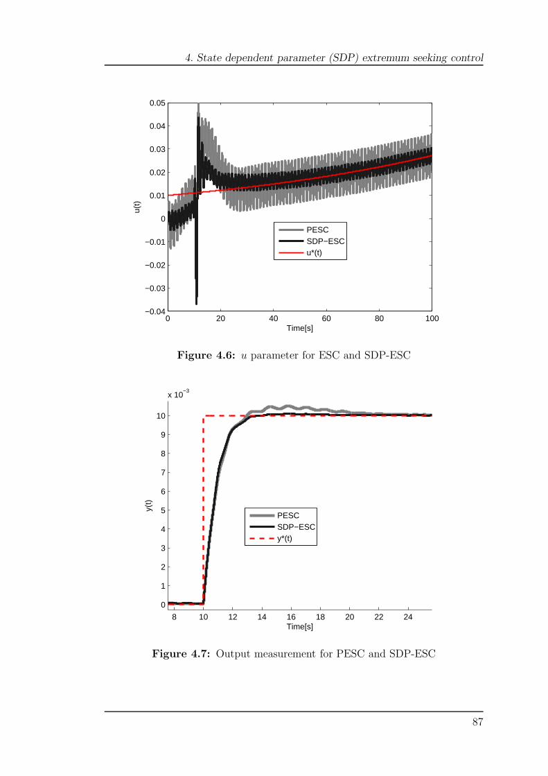
4. State dependent parameter (SDP) extremum seeking control
0 20 40 60 80 100−0.04
−0.03
−0.02
−0.01
0
0.01
0.02
0.03
0.04
0.05
Time[s]
u(t)
PESCSDP−ESCu*(t)
Figure 4.6: u parameter for ESC and SDP-ESC
8 10 12 14 16 18 20 22 24
0
1
2
3
4
5
6
7
8
9
10
x 10−3
Time[s]
y(t)
PESCSDP−ESCy*(t)
Figure 4.7: Output measurement for PESC and SDP-ESC
87
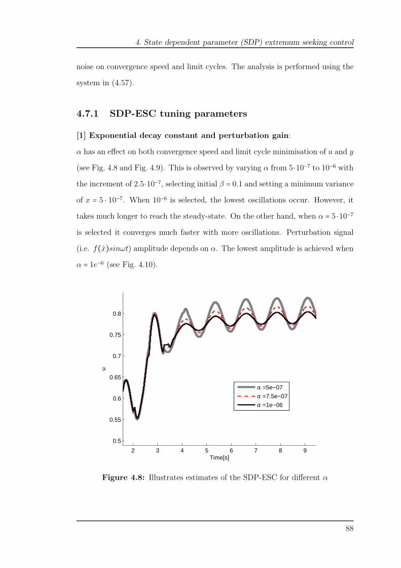
4. State dependent parameter (SDP) extremum seeking control
noise on convergence speed and limit cycles. The analysis is performed using the
system in (4.57).
4.7.1 SDP-ESC tuning parameters
[1] Exponential decay constant and perturbation gain:
α has an effect on both convergence speed and limit cycle minimisation of u and y
(see Fig. 4.8 and Fig. 4.9). This is observed by varying α from 5 ⋅10−7 to 10−6 with
the increment of 2.5⋅10−7, selecting initial β = 0.1 and setting a minimum variance
of x = 5 ⋅ 10−7. When 10−6 is selected, the lowest oscillations occur. However, it
takes much longer to reach the steady-state. On the other hand, when α = 5 ⋅10−7
is selected it converges much faster with more oscillations. Perturbation signal
(i.e. f(x)sinωt) amplitude depends on α. The lowest amplitude is achieved when
α = 1e−6 (see Fig. 4.10).
2 3 4 5 6 7 8 9
0.5
0.55
0.6
0.65
0.7
0.75
0.8
Time[s]
u
α =5e−07
α =7.5e−07
α =1e−06
Figure 4.8: Illustrates estimates of the SDP-ESC for different α
88
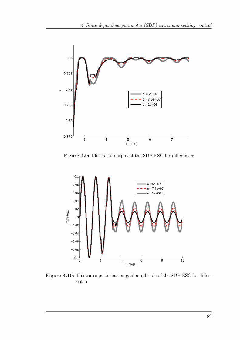
4. State dependent parameter (SDP) extremum seeking control
3 4 5 6 70.775
0.78
0.785
0.79
0.795
0.8
Time[s]
y
α =5e−07
α =7.5e−07
α =1e−06
Figure 4.9: Illustrates output of the SDP-ESC for different α
0 2 4 6 8 10−0.1
−0.08
−0.06
−0.04
−0.02
0
0.02
0.04
0.06
0.08
0.1
Time[s]
f(x)sin
ωt
α =5e−07
α =7.5e−07
α =1e−06
Figure 4.10: Illustrates perturbation gain amplitude of the SDP-ESC for differ-ent α
89

4. State dependent parameter (SDP) extremum seeking control
The initial value of β affects the convergence speed and the limit cycle min-
imisation in a similar manner to α. To guarantee a faster convergence speed as
well as enough excitation, the SDP-ESC should be initialised with a sufficiently
large value of β.
[2] Integrator and compensator gains:
Large values of kc and k improves converge speed. kc is set equal to 2.5 and k
is varied from 2.5 to 3.5 with an increment of 0.5 (see Fig. 4.11, Fig. 4.12, and
Fig. 4.13). For the SPD-ESC, kc and k affect only the convergence speed. How-
ever these parameters should be carefully selected to avoid failure to converge to
true value at steady-state as well as to detect noise in the feedback loop.
1 2 3 4 5 6 7 8
0.55
0.6
0.65
0.7
0.75
0.8
Time[s]
y
k =2.5k =3k =3.5
Figure 4.11: Illustrates output of the SDP-ESC for different k
4.7.2 Measurement noise
It is rather difficult to eliminate measurement noise in practice, therefore it is
crucial to eliminate its influence. For this example, normally distributed white
90

4. State dependent parameter (SDP) extremum seeking control
0 5 10 15 20 25 30
0.4
0.5
0.6
0.7
0.8
0.9
Time[s]
u
k =2.5k =3k =3.5
Figure 4.12: Illustrates estimates of the SDP-ESC for different k
noise is considered. Fig. 4.14 illustrates the simulation results of the PESC and
the SDP-ESC, corresponding to different noise variances denoted σ2. It appeared
that as compared to the PESC, the SDP-ESC is affected more by noise. When the
variance of noise is low as σ2 = 1 ⋅ 10−7 the SDP-ESC achieves better performance
on both limit cycle minimisation and convergence speed. However, when the
variance of noise is as high as σ2 = 1 ⋅10−6 the SDP-ESC performance on tracking
extremum point deteriorates. Both controllers are affected when the variance of
noise is increased beyond σ2 = 1 ⋅ 10−4.
Remark 3 Tracking parameter/control input u is affected more in the SDP-ESC,
compared to the PESC due to higher noise sensitivity of tuning parameter α, as
a consequence one should carefully select this parameter.
91

4. State dependent parameter (SDP) extremum seeking control
0 1 2 3 4 5 6 7−0.1
−0.08
−0.06
−0.04
−0.02
0
0.02
0.04
0.06
0.08
0.1
Time[s]
f(x)sin
ωt
k =2.5k =3k =3.5
Figure 4.13: Illustrates perturbation gain amplitude of the SDP-ESC for differ-ent k
92

4. State dependent parameter (SDP) extremum seeking control
0 2 4 6 8 10 12 14 16 18
0.2
0.4
0.6
0.8
Time[s]
u
Variance of σ2 = 1 · 10−7
0 2 4 6 8 10 12 14 16 18
0.2
0.4
0.6
0.8
Time[s]
u
Variance of σ2 = 1 · 10−6
0 2 4 6 8 10 12 14 16 180
0.2
0.4
0.6
0.8
Time[s]
u
Variance of σ2 = 1 · 10−4
PESCSDP−ESC u
PESCSDP−ESC u
PESCSDP−ESC u
Figure 4.14: Noise level effects on estimates for PESC and SDP-ESC
93

4. State dependent parameter (SDP) extremum seeking control
4.8 Critical appraisal and conclusions
In this chapter a novel scheme for MPPT known as SDP-ESC is proposed. Nu-
merical analysis on the ability of the proposed scheme to converge to the MPP
whilst minimising losses has been investigated for a single parameter SDP-ESC
scheme. Also, stability analysis of the proposed scheme is investigated using the
averaging technique. Moreover, SDP-ESC design guideline and sensitivity analy-
sis are presented. Superiority of the SDP-ESC over the standard PESC on limit
cycle minimisation and convergence speed has been demonstrated using simula-
tion examples, i.e., for plants with and without dynamics. It also preserves the
stability and simplicity of the standard PESC. Comparison between the SDP-ESC
and other algorithms, i.e., the VBS-ESC and the LBS-ESC on the trade-off be-
tween the convergence speed and minimisation of losses is presented in Chapter 6.
Similar to other schemes such as PESC, LBS-ESC, VBS-ESC, the drawback of
the SDP-ESC is its inability to search for the global maximum in the presence of
local maxima. To eliminate this issue, an extension of the SDP-ESC is required.
Chapter 5 presents a detailed explanation of the extended SDP-ESC.
94

Chapter 5
Extended SDP extremum seeking
control
5.1 Introduction
There are several research developments on the global maximum (GM) search
in the presence of local maxima. Most of these advancements have been seen in
PV systems. However, as aforementioned in Chapter 1, the GM search is still an
open problem. Methods for the GM search reviewed in Chapter 2 are based on
stochastic approaches which require pre-training of the system. Therefore, these
approaches are considered to be expensive (Tan, Nesic, Mareels & Astolfi 2009).
Since this Thesis aim to provide an inexpensive solution for the GM search, the
GM is based on an extension of the SDP-ESC proposed in Chapter 4. There
are few pieces of literature which the propose extension of the ESC for the GM.
ESC which searches for the GM was first proposed by Tan et al. (2009). The
proposed scheme is able to converge to the GM if a large set of initial conditions
are satisfied. One such condition is to initialise the ESC with a large perturba-
tion gain which will force convergence to the GM (Tan et al. 2009). However, the
method proposed by Tan et al. (2009) is shown to be ineffective when Azar, Per-
95

5. Extended SDP extremum seeking control
rier & Srinivasan (2011) use a function with large number of local maxima. For
instance, when a 6th order polynomial was considered, the ESC scheme by Tan
et al. (2009) failed to locate the GM. Azar, Perrier & Srinivasan (2011) proposed
a multi-unit ESC for the GM search. Different static nonlinear functions with
multiple maxima were used to verify the ability of the scheme proposed by Azar,
Perrier & Srinivasan (2011) to search the GM. The proposed scheme comprises
two identical units within a plant or process which operates at different set points
and the difference between these set points is referred to as an offset. The finite
difference for a given offset is applied to estimate the gradient. It also utilises
an integrator within the multi-framework scheme to force the gradient to zero.
It has been claimed in Azar, Perrier & Srinivasan (2011), that by starting with
a large offset, reducing monotonically to zero and also using switching control
strategy, it is possible to search for the GM.
Particle swarms have been combined with ESC to search for the GM (Yu,
Chen & Kong 2010). The particle swarm algorithm generates a sequence based
on an online cost function which is used to guide the ESC to search for the GM.
However, this method has the disadvantage of taking a longer time to compute
every loop of the ESC. Khong, Nesic, Manzie & Tan (2013) adopted a DIRECT
search algorithm within ESC for a multi-dimensional GM search. DIRECT search
is a method for solving optimisation problems that does not require any informa-
tion about the gradient of the objective function. Apart from that, Doostabad,
Keypour & Khalghani (2013) present a modified ESC with a GM search under
uniform and non-uniform irradiance conditions. Compared to the standard ESC,
the proposed ESC uses a single perturbation signal, hence ripples of lower fre-
quency is achieved. It also uses series configuration of a LPF and a HPF which
acts as BPF and allows a certain range of frequency (e.g. the derivative of power
and voltage of the PV) to pass through as the results converge directly to the
GM. This is also achieved by the inclusion of the partial shading effect detect-
96
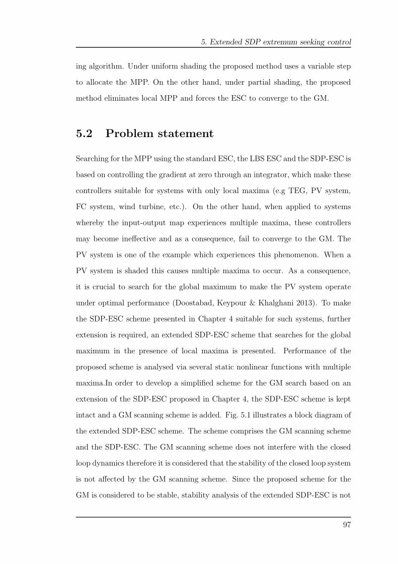
5. Extended SDP extremum seeking control
ing algorithm. Under uniform shading the proposed method uses a variable step
to allocate the MPP. On the other hand, under partial shading, the proposed
method eliminates local MPP and forces the ESC to converge to the GM.
5.2 Problem statement
Searching for the MPP using the standard ESC, the LBS ESC and the SDP-ESC is
based on controlling the gradient at zero through an integrator, which make these
controllers suitable for systems with only local maxima (e.g TEG, PV system,
FC system, wind turbine, etc.). On the other hand, when applied to systems
whereby the input-output map experiences multiple maxima, these controllers
may become ineffective and as a consequence, fail to converge to the GM. The
PV system is one of the example which experiences this phenomenon. When a
PV system is shaded this causes multiple maxima to occur. As a consequence,
it is crucial to search for the global maximum to make the PV system operate
under optimal performance (Doostabad, Keypour & Khalghani 2013). To make
the SDP-ESC scheme presented in Chapter 4 suitable for such systems, further
extension is required, an extended SDP-ESC scheme that searches for the global
maximum in the presence of local maxima is presented. Performance of the
proposed scheme is analysed via several static nonlinear functions with multiple
maxima.In order to develop a simplified scheme for the GM search based on an
extension of the SDP-ESC proposed in Chapter 4, the SDP-ESC scheme is kept
intact and a GM scanning scheme is added. Fig. 5.1 illustrates a block diagram of
the extended SDP-ESC scheme. The scheme comprises the GM scanning scheme
and the SDP-ESC. The GM scanning scheme does not interfere with the closed
loop dynamics therefore it is considered that the stability of the closed loop system
is not affected by the GM scanning scheme. Since the proposed scheme for the
GM is considered to be stable, stability analysis of the extended SDP-ESC is not
97
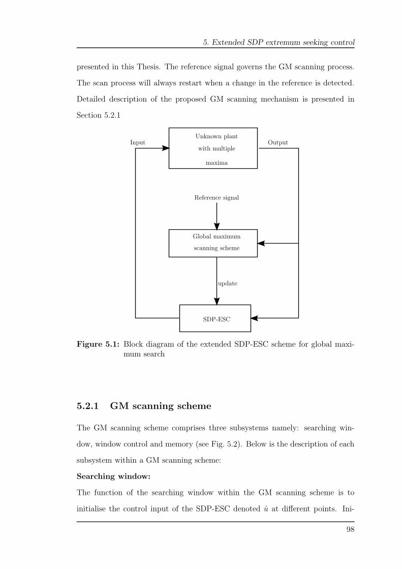
5. Extended SDP extremum seeking control
presented in this Thesis. The reference signal governs the GM scanning process.
The scan process will always restart when a change in the reference is detected.
Detailed description of the proposed GM scanning mechanism is presented in
Section 5.2.1
Unknown plant
with multiple
maxima
Global maximum
scanning scheme
update
SDP-ESC
Reference signal
Input Output
Figure 5.1: Block diagram of the extended SDP-ESC scheme for global maxi-mum search
5.2.1 GM scanning scheme
The GM scanning scheme comprises three subsystems namely: searching win-
dow, window control and memory (see Fig. 5.2). Below is the description of each
subsystem within a GM scanning scheme:
Searching window:
The function of the searching window within the GM scanning scheme is to
initialise the control input of the SDP-ESC denoted u at different points. Ini-
98

5. Extended SDP extremum seeking control
tialisation is based on prior knowledge of the system’s operational range. For
instance, a PCU operational range usually has a duty cycle which varies between
0% to 100% and hence the searching window can be initialised between 0 to 1.
The searching window can be initialised using a look-up table of data points.
However, the GM is efficiently searched when the searching window is treated as
a ramp signal. This will allow the scanning of all available maxima. The length
of the searching window is determined by the system operational range. For in-
stance, if the system operational range is between 0 to 10 the searching window
length will be 10. The minimum value of the searching window denoted Wmin
will be 0 and the maximum value of the searching window denoted Wmax will be
10. Input to the searching window subsystem is window control denoted Wc and
output is the initial point of the control input denoted uin.
Memory block:
The memory blocks stores the measured output denoted y and its corresponding
initialisation point at each time step. The amount of stored data depends on the
size of the searching window denoted W . Mathematically W is calculated as
W =Tp
Ts
(5.1)
where Tp and Ts denote window period and sampling time, respectively. For
instance, if Tp = 2 and Ts = 0.1 therefore based on (5.1) W will be equal to 20.
This implies that 20 data points will be stored in the memory block.
Window control:
It governs the GM searching process by controlling the searching window. Every
time the reference signal (denoted as REF in Fig 5.2) such as the irradiance of
the PV system etc. changes, the scanning process will resume.
99

5. Extended SDP extremum seeking control
Unknown plant
with multiple
maxima
Memory(uin, y)
Compensator Integrator Low pass filter High pass filter
uin
uin
(u∗in)
WcSearchingwindow
Windowcontrol
REF
Update
u y
ss+ωh
f(x)
sinωt
ks
u ξx y − ηωl
s+ωl
Global maximum scanning scheme
State dependent parameter ESC scheme
Cz .s+1Cp.s+1
Figure 5.2: Extended SDP-ESC scheme for global maximum search in the pres-ence of local maxima
GM searching process
First, the searching window is initialised with Wmin. Also, the reference signal
is initialised as 0. The initialisation point of the searching window and output
measurements of the unknown plant are stored in the memory. If change on
reference signal occurs, then the searching window will be reset to Wmin. On
the other hand, if no change is detected in the reference signal the next step
will be to check whether the searching window has reached Wmax. When the
searching window equals to Wmax, the memory block will return the point which
corresponds to the GM. This is done by determining the highest value of the
output within the searching window period. The index of the searching window
corresponding to the highest output value is noted and the SDP-ESC will be
updated with u∗in, i.e., the index corresponding to the GM (highest output value).
100

5. Extended SDP extremum seeking control
On the other hand, if the searching window has not reached to Wmax, then the
searching window will be incremented by a chosen step size denoted C. Once the
extended SDP-ESC converges to the GM, the searching (scanning) process will
stop until change in reference signal is detected causing the scanning process to
resume. Convergence speed to the GM is highly dependent on C. If the searching
window is incremented by a smaller C this will result in a slow convergence speed
to the GM. However, it will usually guarantee convergence to the actual GM.
STARTReference signal=0
Searching window =Wmin
Store input/outputmeasurements
No
No
No
Yes
Yes
Yes
Reference signal
changed ?
Searching window==Wmax
Update SDP-ESCwith new initialisationpoints corresponding
to the GM
Searching window=Searching window+C
Reference signal
changed ?
end
Figure 5.3: Flow chart for global maximum searching using extended SDP-ESCscheme
101

5. Extended SDP extremum seeking control
5.3 Simulation study
This section presents simulation examples of several functions with multiple max-
ima to demonstrate the ability of the extended SDP-ESC to search the GM in
the presence of local maxima. Examples in Sections 5.3.1, 5.3.2 and 5.3.3 are also
considered by Tan et al. (2009) and Azar, Perrier & Srinivasan (2011). These
examples are based on assumptions that there is no input/output dynamics to the
system. A simulation study for a plant with input/output dynamics is presented
in Section 5.3.4.
5.3.1 Static nonlinear map: Example 1
Consider a static nonlinear map presented as sum of exponentials as
j(u) = e 1
(1+0.2u2)+ e
1
(1+5(u−15)2) (5.2)
j(u) has two local maxima at u = 0 and u = 15. The GM is located at u = 15.
Fig. 5.6 illustrates the input-output map of the system given in (5.2) (i.e., the
map searched using the PESC, the SDP-ESC and the extended SDP-ESC). As
shown in Fig. 5.4, both the PESC and the SDP-ESC converge to local maximum
at u = 0. According to Azar, Perrier & Srinivasan (2011), global PESC scheme
proposed by Tan et al. (2009) was unable to converge to the accurate GM.
On the other hand, the extended SDP-ESC converges to the GM due to its
pre-scanning mechanism, which allows to the scanning to all available maxima
within a W . Once the extended SDP-ESC has converged to the GM, it thereafter
decays exponentially to minimise limit cycles (see Fig 5.5). W of the extended
SDP-ESC is incremented as a ramp input and initialised between −1 and 20.
Since both maxima are located between −1 and 15, the searching period of 20s
(see Fig. 5.4) is considered enough to the reach maximum value of the W . Given
102

5. Extended SDP extremum seeking control
that Ts = 0.01s and Tp = 20s therefore, maximum size of the W is calculated
using (5.1) as: W =Tp
Ts= 20
0.01= 2000 samples. Table 5.1 illustrates the tuning
parameters of the PESC, the SDP-ESC, and the extended SDP-ESC.
Parameter PESC SDP-ESC Extended SDP-ESCα - 10−6 5 ⋅ 10−6
β 0.1 0.1 0.1
ωh [ rads ] 2.5 2.5 2.5
ω [ rads] 5 5 5
ϕ [rad] π2
π2
π2
W [TpTs] - - 2000k 1 1 1
Cp - 2 2Cz - 1 1
Table 5.1: PESC and SDP-ESC and extended SDP-ESC tuning parameters forthe global maximum search of example in Section 5.3.1
10 20 30 40 50 60 70−5
0
5
10
15
Time[s]
Con
trol
inpu
t
PESCSDP−ESCExtended−SDP−ESC
Figure 5.4: Control input for PESC, SDP-ESC and extended SDP-ESC forglobal maximum search of example in Section 5.3.1
103

5. Extended SDP extremum seeking control
0 20 40 60 80 1002
2.2
2.4
2.6
2.8
3
3.2
3.4
3.6
3.8
Time[s]
Output
PESCSDP−ESCExtended−SDP−ESC
Figure 5.5: Output of example in Section 5.3.1
−2 0 2 4 6 8 10 12 14 162
3
4
Control input
Out
put
Extended SDP−ESC
0 2 4 6 8 10 123.4
3.6
3.8
Control input
Out
put
SDP−ESC
0 2 4 6 8 10 123.4
3.6
3.8
Control input
Out
put
ESC
Figure 5.6: Input-output map of example in Section 5.3.1
104

5. Extended SDP extremum seeking control
5.3.2 Static nonlinear map: Example 2
Consider a static nonlinear map of the 6th order polynomial given as
j(u) = −u6+
1
10u5+
623
400u4−
659
4000u3−
11287
20000u2+
259
4000u +
637
20000(5.3)
The polynomial given in (5.3) has three maxima at u = −0.8985, u = 0.0 and
u = 0.8951. The global maximum is located at u = −0.8985. The maxima of (5.3)
are located between −1 and 2. As in example 5.3.1, in 5.3.2 the W is incremented
as a ramp input. Ts = 0.01 is selected, therefore based on (5.1), W = 200 samples.
As shown in Fig. 5.7, both the PESC and the SDP-ESC converge to the nearest
local maximum at u = 0. On the other hand, the extended SDP-ESC converges
to the GM at u = −0.8985 within 1s. Compared to the PESC and the SDP-
ESC, the extended SDP-ESC is able to scan all available maxima (see Fig. 5.9)
and accurately converge to the GM (see Fig. 5.8). The tuning parameters (i.e.
β,ωh, ω,ϕ,Cp,Cz) of the PESC, the SDP-ESC, and the extended SDP-ESC for
system in (5.3) are the same as the system in (5.2). However, k = 5 for controllers,
α = 2.5 ⋅ 10−6 for the SDP-ESC and α = 3.5 ⋅ 10−6 for the extended SDP-ESC.
5.3.3 Static nonlinear map: Example 3
Consider a static nonlinear map presented as
j(u) = −3u4+ 64sin2u3
+ 12u2+ 4u − 80 (5.4)
The static nonlinear map in (5.4) has several maxima and a unique GM at u =
1.68. The maxima of the system in ( 5.4) are located between −2 to 1. Similar to
the previous examples, Ts = 0.01 is selected. Using Ts and Tp therefore W = 100
samples. As shown in Fig. 5.10, both the PESC and the SDP-ESC converge to the
local maximum at u = −1.15. On the other hand, the extended SDP-ESC scheme
105
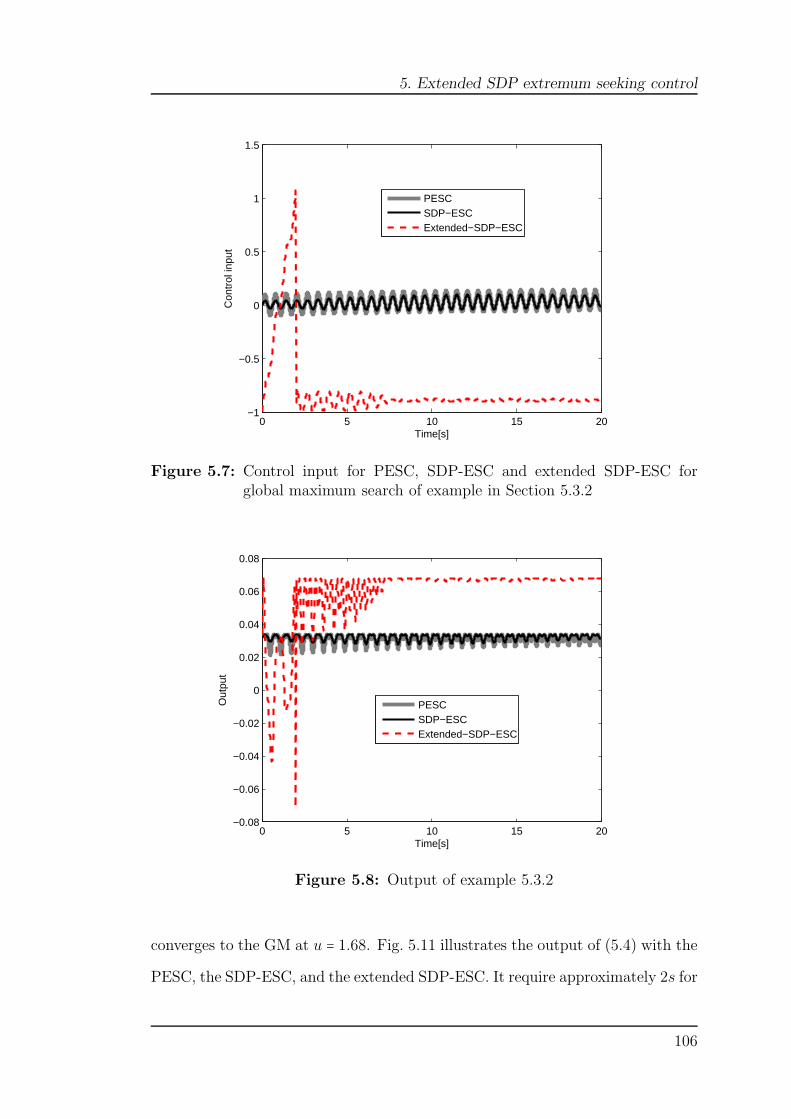
5. Extended SDP extremum seeking control
0 5 10 15 20−1
−0.5
0
0.5
1
1.5
Time[s]
Con
trol
inpu
t
PESCSDP−ESCExtended−SDP−ESC
Figure 5.7: Control input for PESC, SDP-ESC and extended SDP-ESC forglobal maximum search of example in Section 5.3.2
0 5 10 15 20−0.08
−0.06
−0.04
−0.02
0
0.02
0.04
0.06
0.08
Time[s]
Out
put
PESCSDP−ESCExtended−SDP−ESC
Figure 5.8: Output of example 5.3.2
converges to the GM at u = 1.68. Fig. 5.11 illustrates the output of (5.4) with the
PESC, the SDP-ESC, and the extended SDP-ESC. It require approximately 2s for
106
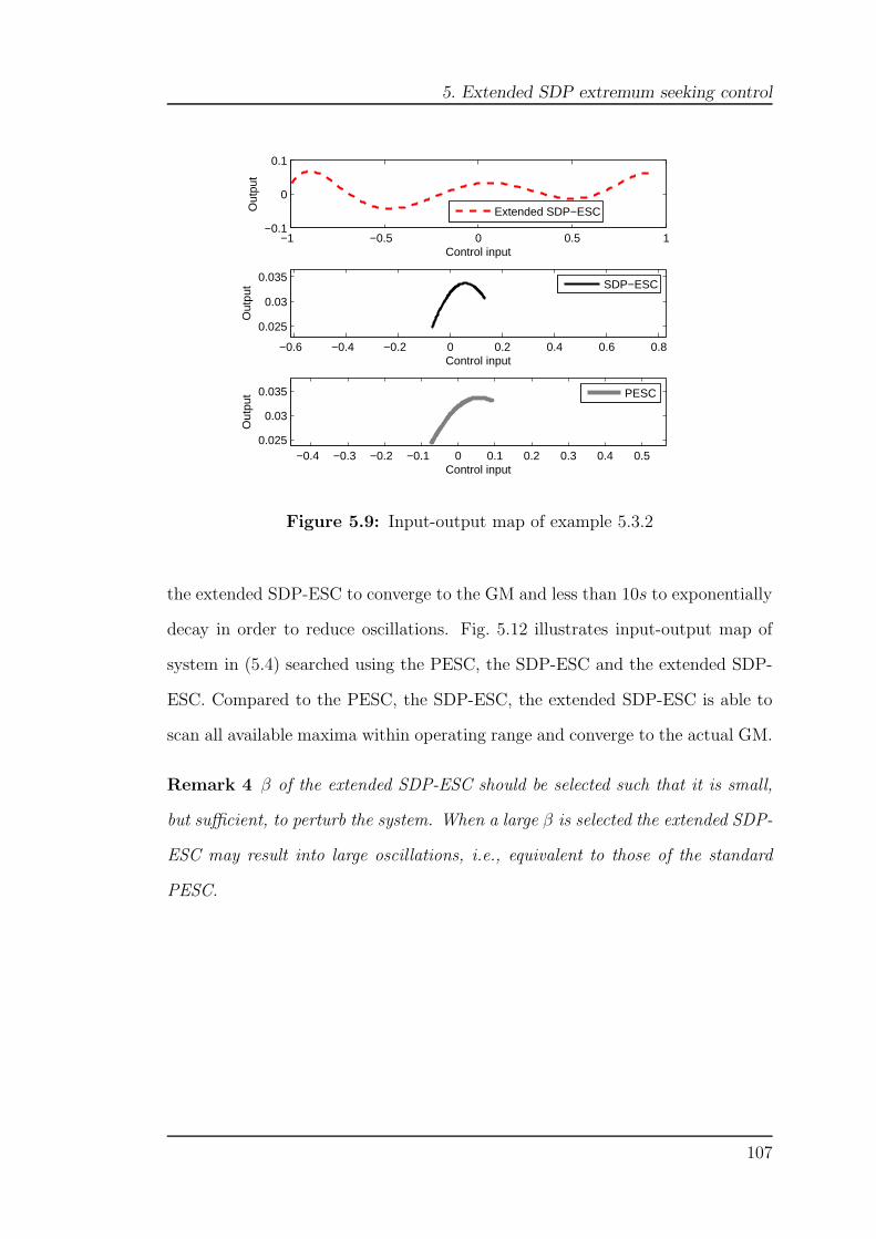
5. Extended SDP extremum seeking control
−1 −0.5 0 0.5 1−0.1
0
0.1
Control inputO
utpu
t
Extended SDP−ESC
−0.6 −0.4 −0.2 0 0.2 0.4 0.6 0.8
0.025
0.03
0.035
Control input
Out
put
SDP−ESC
−0.4 −0.3 −0.2 −0.1 0 0.1 0.2 0.3 0.4 0.50.025
0.03
0.035
Control input
Out
put
PESC
Figure 5.9: Input-output map of example 5.3.2
the extended SDP-ESC to converge to the GM and less than 10s to exponentially
decay in order to reduce oscillations. Fig. 5.12 illustrates input-output map of
system in (5.4) searched using the PESC, the SDP-ESC and the extended SDP-
ESC. Compared to the PESC, the SDP-ESC, the extended SDP-ESC is able to
scan all available maxima within operating range and converge to the actual GM.
Remark 4 β of the extended SDP-ESC should be selected such that it is small,
but sufficient, to perturb the system. When a large β is selected the extended SDP-
ESC may result into large oscillations, i.e., equivalent to those of the standard
PESC.
107
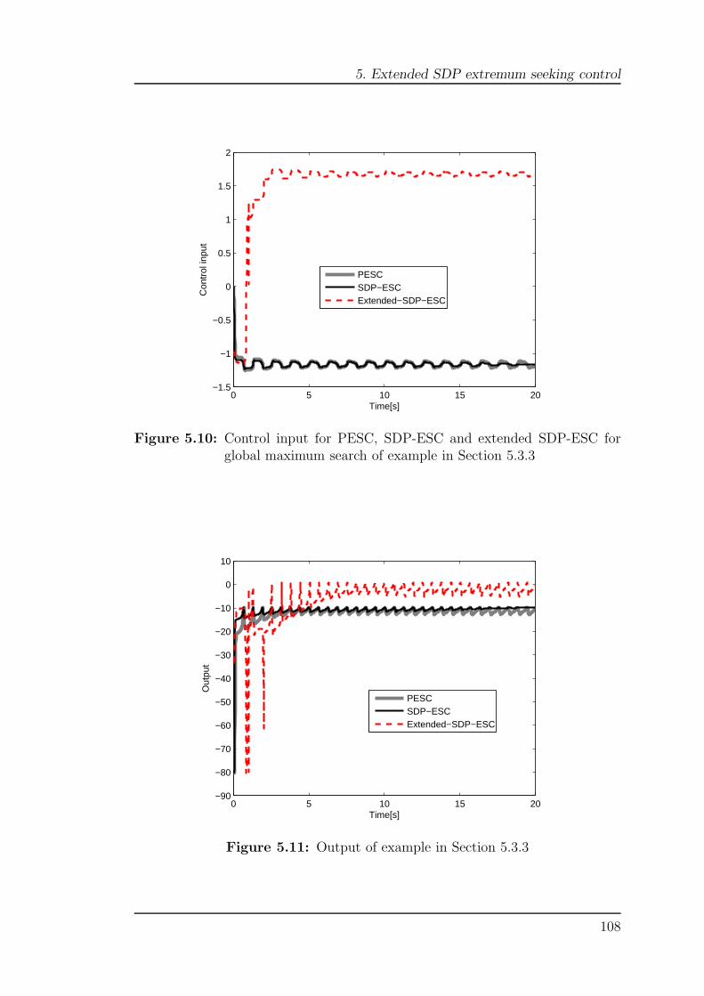
5. Extended SDP extremum seeking control
0 5 10 15 20−1.5
−1
−0.5
0
0.5
1
1.5
2
Time[s]
Con
trol
inpu
t
PESCSDP−ESCExtended−SDP−ESC
Figure 5.10: Control input for PESC, SDP-ESC and extended SDP-ESC forglobal maximum search of example in Section 5.3.3
0 5 10 15 20−90
−80
−70
−60
−50
−40
−30
−20
−10
0
10
Time[s]
Out
put
PESCSDP−ESCExtended−SDP−ESC
Figure 5.11: Output of example in Section 5.3.3
108
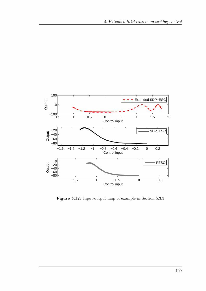
5. Extended SDP extremum seeking control
−1.5 −1 −0.5 0 0.5 1 1.5 2−100
0
100
Control input
Out
put
Extended SDP−ESC
−1.6 −1.4 −1.2 −1 −0.8 −0.6 −0.4 −0.2 0 0.2
−80−60−40−20
Control input
Out
put
SDP−ESC
−1.5 −1 −0.5 0 0.5−80−60−40−20
0
Control input
Out
put
PESC
Figure 5.12: Input-output map of example in Section 5.3.3
109

5. Extended SDP extremum seeking control
5.3.4 Plant with dynamics: Example 4
Consider a nonlinear system given as
j(u) = −u6− 3u3
+ u + 1 (5.5a)
Di(s) = 1
3s + 1(5.5b)
Do(s) = 1
0.2s + 1(5.5c)
where, j(u) in (5.5a) has two maxima j1 = 2.12 and j = 1.21 at u = −1.11 and u =
0.33, respectively. Di(s) and Do(s) are input and output dynamics, respectively.
The maxima are located between −2 and 3. Ts = 0.01 is selected, therefore
based on (5.1), W = 300 samples. As illustrated in Fig. 5.13, both the PESC
and the SDP-ESC converge to the neighbourhood maximum at u = 0.33. On
the other hand, the extended SDP-ESC converges to the GM at u = −1.11. As
shown in Fig. 5.14, due to the presence of the input/output dynamics, the time
taken for the extended SDP-ESC to converge to the GM is increased. It takes
approximately 30s for the extended SDP to converge to the GM and another 20s
to exponentially decay the perturbation gain in order to minimise oscillations.
Table. 5.2 presents the tuning parameters for the PESC, the SDP-ESC and the
extended SDP-ESC.
Parameter PESC SDP-ESC Extended SDP-ESCα - 10−6 10−6
β 0.1 0.1 0.1
ωh [ rads ] 2.5 2.5 2.5
ω [ rads] 5 5 5
ϕ [rad] π2
π2
π2
k 1 1 1
W [Tp
Ts] - - 300
Cp - 2 2Cz - 1 1
Table 5.2: PESC and SDP-ESC and extended SDP-ESC tuning parameters forplant with dynamics
110
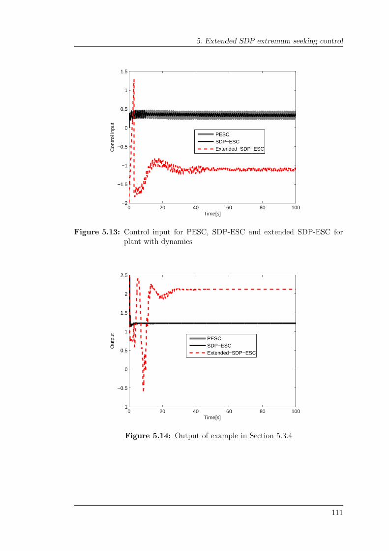
5. Extended SDP extremum seeking control
0 20 40 60 80 100−2
−1.5
−1
−0.5
0
0.5
1
1.5
Time[s]
Con
trol
inpu
t
PESCSDP−ESCExtended−SDP−ESC
Figure 5.13: Control input for PESC, SDP-ESC and extended SDP-ESC forplant with dynamics
0 20 40 60 80 100−1
−0.5
0
0.5
1
1.5
2
2.5
Time[s]
Out
put
PESCSDP−ESCExtended−SDP−ESC
Figure 5.14: Output of example in Section 5.3.4
111

5. Extended SDP extremum seeking control
5.4 Critical appraisal and conclusions
In this chapter, a novel scheme for the GM search in the presence of local max-
ima has been presented. The scheme is based on an extension of the SDP-ESC
scheme presented in Chapter 4. The extended SDP-ESC algorithm has been
demonstrated using several examples comprised of multiple maxima. The pro-
posed scheme has been shown to be effective in converging to the GM regardless of
the available number of maxima. Some of the advantages of the proposed scheme
are: it preserves the stability and simplicity of the SDP-ESC, it converges quickly
to the GM, it can be applied for local maxima search, and it is does not require
any cost function. The convergence period is based on the control input opera-
tional range as well as the step size of the searching window. When a large step
size is selected, a faster convergence speed to the GM will be achieved. However,
when very a large step is selected the extended SDP-ESC may barely converge
to the true GM. On the other hand, a smaller step will guarantee convergence to
the true GM almost every time. This may however result in a slow convergence.
112
Chapter 6
Simulation study: Application in
thermoelectric generator systems
6.1 Introduction
This Chapter presents simulation studies of the MPPT algorithms discussed in
Chapter 2, 3 and 4 in application to the TEG system. Some of the results in this
Chapter were also published in Phillip et al. (2013). In the last decade, inves-
tigation into TEGs for waste heat recovery in automotive applications has seen
several advancements and the operational understanding of TEGs as a system has
significantly improved. This is attributed to initial developments of models for the
estimation of fuel economy benefits (Hussain, Brigham & Maranville 2009, Sto-
bart & Milner 2009), more in-depth modelling and design of heat exchangers
(Crane & Jackson 2002, Esarte, Min & Rowe 2001) and TE module subsys-
tems (Montecucco, Buckle & Knox 2012, Lineykin & Ben-Yaakov 2007), as well
as research into material selection (Rowe 2005, Snyder & Toberer 2008). As
aforementioned in Chapter 1, despite these advances the science of TEGs still
remains open to research in many areas. One such area is the optimisation of the
electrical interface between a TEG system and a load for mismatch reduction.
113

6. Simulation study: Application in thermoelectric generator systems
MATLAB/Simulink has been used for the modelling and simulation of the TEG
system as well as for the implementation of the control strategy. This chapter
is organised as follows: Section 6.2 and Section 6.3 present an overview of the
TEG system and modelling of the PCU subsystem, respectively. Section 6.5 and
Section 6.6 presents two Phases of simulation studies, i.e., Phase I and Phase
II, respectively. Phase I presents advantages of using an MPPT algorithm as
well as comparison between P&O and PESC algorithms. Section 6.5.1 presents
findings and observations of the simulation study of Phase I. Phase II presents
improved results with the use of the VBS-ESC and the SDP-ESC, where PESC
and LBS-ESC serves as benchmarks. Section 6.7 presents critical appraisals and
conclusions.
6.2 TEG overview
TEGs are devices which use a temperature difference to generate electricity. The
conversion is based on the phenomenon known as the Seebeck effect, named after
Johann Seebeck who discovered the phenomenon in the early 18th century (Rowe
2005). Essentially such an effect is formed, when two dissimilar metals of N-type
and P-type semiconductor material are connected together and give rise to a
thermoelectric module (TEM), as shown in Fig. 6.1. By keeping the junction of
these metals at different temperatures an electric voltage is generated. However,
the generated voltage depends on other factors such as size of the TEM and the
types of materials used. Performance of the material is typically quoted using
the figure of merit denoted Z (Rowe 2005). The figure of merit Z of the material
is given as
Z =σS2
kth(6.1)
where, σ denotes electrical conductivity (S/m), kth denotes thermal conductivity
[ Wm.K] and S denote the Seebeck coefficient [ V
K]. For the intended automotive
114
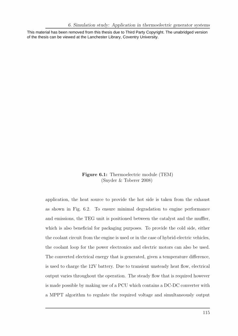
6. Simulation study: Application in thermoelectric generator systems
Figure 6.1: Thermoelectric module (TEM)(Snyder & Toberer 2008)
application, the heat source to provide the hot side is taken from the exhaust
as shown in Fig. 6.2. To ensure minimal degradation to engine performance
and emissions, the TEG unit is positioned between the catalyst and the muffler,
which is also beneficial for packaging purposes. To provide the cold side, either
the coolant circuit from the engine is used or in the case of hybrid-electric vehicles,
the coolant loop for the power electronics and electric motors can also be used.
The converted electrical energy that is generated, given a temperature difference,
is used to charge the 12V battery. Due to transient unsteady heat flow, electrical
output varies throughout the operation. The steady flow that is required however
is made possible by making use of a PCU which contains a DC-DC converter with
a MPPT algorithm to regulate the required voltage and simultaneously output
115
This material has been removed from this thesis due to Third Party Copyright. The unabridged version of the thesis can be viewed at the Lanchester Library, Coventry University.

6. Simulation study: Application in thermoelectric generator systems
the maximum possible power for the highest PCU efficiency.
Figure 6.2: Block diagram of waste heat recovery from engine exhaust(Phillip et al. 2013)
The TEG model developed by Phillip et al. (2013) has been used as a tool to
investigate the performance of the developed MPPT algorithms in this Thesis.
The TEG model comprises three systems, namely: HX, TEM and PCU. Fig. 6.3
illustrates the input/output relations between the individual subsystems. Inputs
to the HX subsystem are: exhaust temperature denotes Te(K), coolant inlet
temperature denotes Tw(K), exhaust mass flow rates denotes me [kgs ] and coolant
inlet mass flow rates mw [kgs ]. The gas to liquid HX takes these four inputs to
simulate the hot and cold side temperatures, Th(K) and Tc(K), for the TEM.
The TEM system utilises hot and cold side temperatures as the input to generate
the voltage, Vin(V ), and current,Iin(A) as its outputs. Equations (A.1a) and
(A.1b) are used within the TEM to compute Vin and Iin. Vin and Iin are used as
inputs to the PCU where the voltage, Vout and current Iout are the outputs. The
resulting power out to the load is regulated at 14.4V by a synchronous DC-DC
buck-boost converter. The load in this case is the 12V car battery. Based on
116
This material has been removed from this thesis due to Third Party Copyright. The unabridged version of the thesis can be viewed at the Lanchester Library, Coventry University.
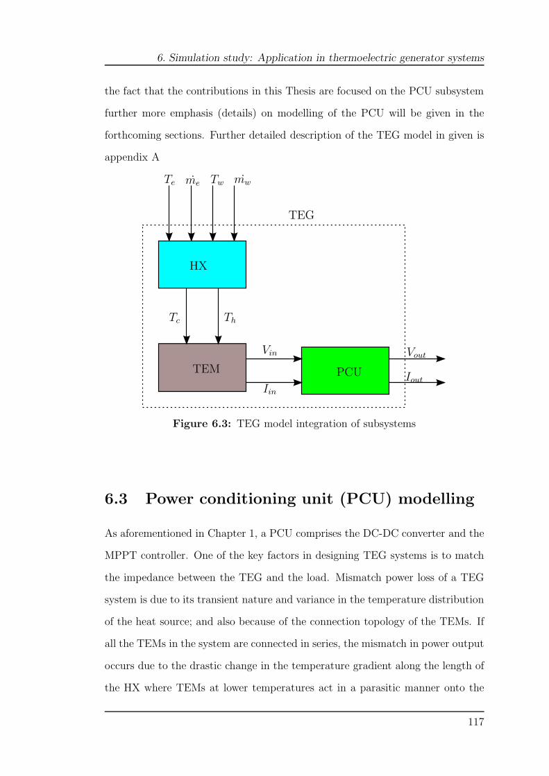
6. Simulation study: Application in thermoelectric generator systems
the fact that the contributions in this Thesis are focused on the PCU subsystem
further more emphasis (details) on modelling of the PCU will be given in the
forthcoming sections. Further detailed description of the TEG model in given is
appendix A
HX
Te me Tw mw
TEM
Vin
Iin
PCU
Vout
Iout
TEG
ThTc
Figure 6.3: TEG model integration of subsystems
6.3 Power conditioning unit (PCU) modelling
As aforementioned in Chapter 1, a PCU comprises the DC-DC converter and the
MPPT controller. One of the key factors in designing TEG systems is to match
the impedance between the TEG and the load. Mismatch power loss of a TEG
system is due to its transient nature and variance in the temperature distribution
of the heat source; and also because of the connection topology of the TEMs. If
all the TEMs in the system are connected in series, the mismatch in power output
occurs due to the drastic change in the temperature gradient along the length of
the HX where TEMs at lower temperatures act in a parasitic manner onto the
117

6. Simulation study: Application in thermoelectric generator systems
TEMs at the high temperature region. The need for a PCU is thus essential in a
system which comprises of unstable heat sources and loads for outputting power
at a fixed voltage.
6.3.1 DC-DC converter modelling
A DC-DC converter is an electronics circuit that converts a source of DC from
one voltage level to another (Maganga, Larkowski & Burnham 2012). There are
several DC-DC converter topologies which can be used within a PCU. For in-
stance, in Phillip et al. (2012), two DC-DC converters namely the single ended
primary inductor capacitor (SEPIC) and the buck-boost converter were used
within the PCU where the latter is suggested to provide higher efficiency. Taking
into account the advantage of stepping up or down without inverting (reversing
terminals) its output voltage as well as having higher efficiency than a standard
buck-boost, in this Thesis a synchronous DC-DC buck-boost converter is con-
sidered. As shown in Fig. 6.4, a synchronous DC-DC buck-boost comprises of
an input filter capacitor denoted Cin, a Schottky power diode denoted D4, three
metal-oxide-semiconductor field-effect transistors (MOSFETs) denoted M1, M2,
M3, and an output filter capacitor denoted Cout. The Schottky power diode D4
replaces the commonly used fourth MOSFET to block the reverse current flow
and prevent the battery connected at the output from discharging through the
converter during discontinuous conduction mode (DCM). Also, M1 and M3 and
must be on-state while M2 is in the off-state. The converter provides a control-
lable and/or constant output DC voltage despite variation of the input voltage.
Similar to the standard buck-boost converter, the synchronous DC-DC buck-
boost converter operates in two different modes, namely a continuous conduction
mode (CCM) and a DCM. In CCM, the inductor current flows continuously for
the entire period and never falls to zero. On the other hand, in the DCM, the in-
118

6. Simulation study: Application in thermoelectric generator systems
Figure 6.4: Schematic diagram of a synchronous DC-DC buck-boost converter(Maganga et al. 2014)
ductor current reduces to zero and remains at a zero level for the remainder of the
period before it begins to rise again (see Fig. 6.5). In this Thesis, the synchronous
DC-DC converter is considered to operate in the DCM mode. Advantages of the
DCM operation over the CCM are: no zero is located at the right half plane in
the s-domain which allows for a higher transient response bandwidth. Zero in
the right half plane in s-domain is nearly impossible to compensate. Also, while
operating in DCM, the converter is considered to have a single pole transfer func-
tion which is easier to compensate for compared to a double pole response. On
the other hand, compared to CCM, DCM requires larger inductors/transformers
for the same output power. A high-fidelity white-box model of a synchronous
DC-DC converter with each component modelled by including its corresponding
physical characteristics, is developed in Simulink/Simscape environment. Conse-
quently, it is deemed that this model provides a realistic representation of a real
synchronous DC-DC buck-boost converter. Here, a synchronous DC-DC buck-
boost converter for a low power application with a variable input voltage and the
output voltage regulated at 12V is considered.
In order to design a synchronous DC-DC buck-boost which provides high effi-
ciency, the design criteria plays a major role. One such criteria is the appropriate
119
This material has been removed from this thesis due to Third Party Copyright. The unabridged version of the thesis can be viewed at the Lanchester Library, Coventry University.

6. Simulation study: Application in thermoelectric generator systems
ILIL
dTsdTs TsTs TT
CCM operation DCM operation
Figure 6.5: Waveform for CCM and DCM, where dTs denote period whenswitch is closed and Ts denote switching period
sizing and selection of individual components, in particular, elements that result
in low power losses. Here, the component sizing focuses on the selection of the
inductor and the output filter capacitance. Components are sized to allow the
synchronous DC-DC converter to operate at a switching frequency of 20kHz.
The minimal value of the inductance required, i.e. Lmin, is calculated as
Lmin =RL(max)
2fs(1 − dmin)2 (6.2)
where: RL(max) is the maximal load resistance, fs is the switching frequency and
dmin is the minimal duty cycle. The minimal value of the output filter capacitance
Cmin is calculated as follows
Cmin =dmin
fsRL(min)
Vout
Vrcpp
(6.3)
where: RL(min) is the minimum load resistance, Vout is the output voltage and
Vrcpp- the ripple voltage across the filter capacitor. As the Vout is considered to be
constant, a change in the input voltage Vin and the duty cycle d will only affect
the output current Iout. At steady-state the input current Iin and the output
current Iout are related as
Iout =(1 − d)
dIin (6.4)
120

6. Simulation study: Application in thermoelectric generator systems
Name Unit ValueInductor (L) uH 33
Input capacitor (Cin) uF 470Output capacitor(Cout) uF 220
Diode forward voltage(VD) V 0.8On resistance MOSFET (Ron) Ω 0.008
Table 6.1: Design parameters for synchronous DC-DC buck-boost convertermodel
6.3.2 Control technique modelling:
The control strategy for the MPPT converter is implemented in two different
subsystems, namely the pulse width modulator (PWM) and the MPPT controller.
The PWM is modelled such that it compares the ramp signal with the variable
duty cycle which is generated by the MPPT controller. If the difference of these
signals is greater or equal to 0, then the value will be held at the same value
for one period and then wait for the new value of the duty cycle. The resultant
waveform in Fig. 6.6 illustrates the PWM generated for the variable duty cycle.
The MPPT controller is implemented with 5 different control algorithms which
are: P&O, PESC, LBS-ESC, VBS-ESC, and SDP-ESC and their Simulink models
are presented in appendix B.
6.4 MPPT performance criterion
There are several ways of assessing the performance of a given system. For
instance, the performance can either be assessed based on tracking error, MPPT
efficiency or percentage accuracy, etc. (see definition in section ) The performance
criterion for the MPPT converter can either be measured by energy efficiency,
available power or input voltage at the MPP. Energy efficiency at MPP is given
as
ηe =Pcov
Pmpp
100% (6.5)
121

6. Simulation study: Application in thermoelectric generator systems
SawtoothSignal
Variable dutycycle
Comparator
≥
Figure 6.6: Block diagram for the pulse width modulation (PWM)
where: ηe denotes MPPT converter efficiency, Pcov denotes power absorbed by
the converter and Pmpp denotes power available from the TEG. For the TEG it is
considered that at MPP, the input voltage is half of the open circuit due to load
matching, i.e.,
Vin = Vmpp =Voc
2(6.6)
Theoretically the maximum available power from the TEG can be calculated as
Pmpp =V 2oc
4Rin
(6.7)
where: Rin is the internal resistance of the TEG. Hereafter criterion (6.5), (6.6)
and (6.7) will be used as the performance index as well as other factors such as
speed of convergence and limit cycle minimisation.
122

6. Simulation study: Application in thermoelectric generator systems
6.5 Simulation study: Phase I
This section presents the simulation results of the TEG with the use of a fixed duty
cycle, P&O and PESC algorithms. When a MPPT controller is not used within
the PCU (i.e. a synchronous DC-DC converter is driven by a fixed duty cycle) this
is termed as a fixed duty cycle control. Operating a converter with a fixed duty
cycle is aimed to demonstrate the benefits of using a MPPT controller. When the
synchronous DC-DC converter is driven at a fixed duty cycle, simulation results
show that it is only for the 700K to 800K temperature range that a reasonable
output power is achieved. Table. 6.2 presents a range of fixed duty cycle values
for various temperatures as well as corresponding input voltage values at matched
load for the specific system configuration. This is considered to be due to the
inability of the controller to remove the mismatch of the internal resistance values
between the TEG and the DC-DC converter over a wider range of temperatures.
When a fixed duty cycle is used, it implies that the controller will provide
optimal performance only at a specific operating point. This justifies the need for
an MPPT controller. For the results presented in this Section, the fixed duty cycle
has been set to 48.53% for optimal performance at 700K. At the user’s discretion
the duty cycle can be changed for high efficiency at different temperature ranges.
Knowing the characteristic of a TEG system, a look-up table can be used to store
optimal duty cycle values at different operating temperatures. This process, i.e.,
an empirical process, however only works for a specific configuration. ESC on
the other hand, i.e., non-constraints based, can be reconfigured to any system
(e.g. a different power source). The duty cycle can be calculated using (6.4) if
the DC-DC converter input voltage at match load is known. Table. 6.3 shows the
output power of the TEG comparing the implementation of a fixed duty cycle,
P&O and ESC (i.e. PESC), as well as the efficiencies of each MPPT method
compared to ideal matched load (power at MPP ) results. For the simulation
123

6. Simulation study: Application in thermoelectric generator systems
∆T (K) Vmpp d% VBat
600 10.93 56.85 14.4700 15.27 48.53800 19.68 42.25900 24.11 37.39
Table 6.2: Optimum duty cycle at corresponding temperatures
results presented, the hot side temperature varies from 600K to 900K and the
cold side temperature is maintained at 363K. Simulation results demonstrate
that both the P&O and the PESC converge to a similar output power. When
compared to the P&O however, the output power of the PESC converges much
faster to the MPP, as is illustrated in Fig. 6.7.
Figure 6.7: Simulation results for theoretical power, output power with ESC,P&O and Fixed Duty Cycle: Losses reduced to within 5%
(Phillip et al. 2013)
124
This material has been removed from this thesis due to Third Party Copyright. The unabridged version of the thesis can be viewed at the Lanchester Library, Coventry University.

6. Simulation study: Application in thermoelectric generator systems
Power at MPP Fixed d Fixed d P& O P& O PESC PESCTemp(K) P(W) P(W) ηe% P(W) ηe% P(W) ηe%
600 47.61 40.80 85.70 46.50 98.19 47.40 99.56700 90.00 87.40 97.11 88.37 98.18 89.00 98.87800 144.72 132.60 91.63 141.00 97.43 142.50 98.47900 210 177.60 83.37 204.40 97.10 206.60 98.15
Table 6.3: TEG results with different MPPT algorithms
6.5.1 Findings and observations
The results obtained in Phase I show that the PESC MPPT algorithm in combi-
nation with a synchronous buckboost DC-DC converter is able to condition the
output power of the TEG device effectively. This finding reinforces the case for
utilising the PESC approach as a candidate for an efficient MPPT algorithm for
use in PCUs for TEGs. After conducting experimental work using hardware in the
loop (HIL) testing however, these findings were inconclusive. Limitations found
in the HIL testing are discussed in detail in Chapter 7. These findings lead to the
development of the novel algorithms presented in previous chapters. Upcoming
sections present simulation studies of the TEG with novel MPPT schemes.
6.6 Simulation study: Phase II
This Phase presents improved results at both transients and steady-state. Perfor-
mance of the PESC, the LBS-ESC, the VBS-ESC and the SDP-ESC were anal-
ysed using an emulated TEG Simulink model. Convergence speeds of the MPPT
algorithms were determined by setting the PSU voltage at 12V and Rin = 6.8Ω.
In order to achieve a fast convergence speed, the SDP-ESC was initialised with
a large value of k, therefore no compensator was needed within SDP-ESC feed-
back loop. The compensator was omitted simply by setting values of Cz and
Cp equal to 1. Also, as aforementioned in Chapter 3, the LBS-ESC MPPT al-
gorithm required linearisation (computing its Jacobian) around its equilibrium.
125

6. Simulation study: Application in thermoelectric generator systems
The Jacobian of the LBS-ESC is calculated using the design parameters shown
in Table. 6.4. Substituting these parameters in (3.41) in Section (3.4.1), the
Jacobian is given as
J =
⎡⎢⎢⎢⎢⎢⎢⎢⎢⎢⎣
0 20 0
−2.5 −50 0
0 0 −25
⎤⎥⎥⎥⎥⎥⎥⎥⎥⎥⎦(6.8)
Utilising (6.8), the P matrix of the Lyapunov function is obtained by solving
(3.42) in Section 3.4.1. The P matrix is given as
P =
⎡⎢⎢⎢⎢⎢⎢⎢⎢⎢⎣
−0.59 −0.025 0
0.025 −0.0113 0
0 0 −0.02
⎤⎥⎥⎥⎥⎥⎥⎥⎥⎥⎦(6.9)
The symmetric matrix of P , i.e., Q, is selected as identity (i.e.)
Q =
⎡⎢⎢⎢⎢⎢⎢⎢⎢⎢⎣
−1 0 0
0 −1 0
0 0 −1
⎤⎥⎥⎥⎥⎥⎥⎥⎥⎥⎦(6.10)
The Lyapunov function V (xβ) governs switching based on the calculation of
xβ which comprises of uβ. Inaccurate estimates of uβ may cause the LBS-ESC
to fail to satisfy the switching conditions. This can either cause the LBS-ESC
to generate into the standard PESC, or fail to adapt the changes due insufficient
perturbation to the LBS-ESC scheme. This problem can be avoided by selecting
appropriate parameters for ǫlbs and g. On the other hand, it is relatively difficult
to obtain appropriate values for ǫlbs and g for a wide range. Simulation results
shows that while the PESC, the LBS-ESC and the VBS-ESC take around 250ms
to reach steady-state, the SDP-ESC take only 150ms to converge to the steady-
state (see
126

6. Simulation study: Application in thermoelectric generator systems
0 0.1 0.2 0.3 0.4 0.5 0.60
2
4
6
8
Time[s]
Vm
pp
PESC VBS−ESC SDP−ESC LBS−ESC Theoretical Vmpp
0 0.1 0.2 0.3 0.4 0.5 0.60.4
0.6
0.8
1
1.2
1.4
1.6
Time[s]
Impp
PESC VBS−ESC SDP−ESC LBS−ESC Theoretical Impp
0 0.1 0.2 0.3 0.4 0.5 0.60
0.1
0.2
0.3
0.4
0.5
Time[s]
d
PESC VBS−ESC SDP−ESC LBS−ESC
Figure 6.8: Simulation results of Vmpp, Impp and d using PESC, LBS-ESC, VBS-ESC and SDP-ESC MPPT algorithms
Fig. 6.8). Once the SDP-ESC enters stable limit cycle, it then requires an-
other 100ms to decay exponentially in order to minimise electrical losses within
the PCU. Although both LBS-ESC and VBS-ESC minimises losses, both require
a much longer time to converge compared to the SDP-ESC. Fig. 6.11 illustrates
the variance of the state x with respect to time. The variance of the signal x is
127

6. Simulation study: Application in thermoelectric generator systems
0 0.1 0.2 0.3 0.4 0.5 0.6
0.005
0.01
0.015
0.02
0.025
Time[s]
Variance
ofx
Figure 6.9: Variance of state x for SDP-ESC scheme
Parameters PESC LBS-ESC VBS-ESC SDP-ESCk 20 20 20 25β 0.05 0.05 n/a 0.05
βmax n/a n/a 0.05 n/aβmin n/a n/a 0.01 n/a
ω 250 250 250 250ωh 25 25 25 150ωl 50 50 50 100φ 0 0 0 0α 10−5 n/a n/a n/a
Cp n/a n/a n/a 1Cz n/a n/a n/a 1g -0.05 n/a n/a n/a
ǫlbs n/a -0.0565 n/a n/aǫvbs n/a 0 2.5 ⋅ 10−6 n/a
Table 6.4: Tuning parameters for PESC, LSB-ESC, VBS-ESC and SDP-ESCMPPT algorithms
increases rapidly, which indicates that the SDP-ESC scheme starts with a higher
perturbation gain, and then decreases in order to minimise oscillations. Also, the
performance of the MPPT algorithms at a different voltage range was tested by
increasing from 12V to 16V with increment of 2V .
128

6. Simulation study: Application in thermoelectric generator systems
Simulation results shows that compared to the PESC, the VBS-ESC and the
0 0.5 1 1.5 2 2.5 30
2
4
6
8
10
12
Time[s]
Vm
pp
PESC VBS−ESC SDP−ESC LBS−ESC Theoretical Vmpp
0 0.5 1 1.5 2 2.5 30.4
0.6
0.8
1
1.2
1.4
1.6
Time[s]
Impp
PESC VBS−ESC SDP−ESC LBS−ESC Theoretical Impp
0 0.5 1 1.5 2 2.5 30
0.1
0.2
0.3
0.4
0.5
Time[s]
d
PESC VBS−ESC SDP−ESC LBS−ESC
Figure 6.10: Simulation results for PESC, LBS-ESC, VBS-ESC and SDP-ESCMPPT algorithms while PSU voltage increased from 12V to 16Vby step increment of 2V
LBS-ESC, the SDP-ESC achieves a faster convergence speed at different voltage
ranges (see Fig. 6.10). Although the VBS-ESC and the LBS-ESC achieve a sim-
129

6. Simulation study: Application in thermoelectric generator systems
0 0.5 1 1.5 2 2.5 3
0.002
0.004
0.006
0.008
0.01
0.012
0.014
0.016
0.018
0.02
0.022
Time[s]
Variance
ofx
Figure 6.11: Variance of state x for SDP-ESC algorithm while PSU voltageincreased from 12V to 16V by step increment of 2V
ilar performance on limit cycle minimisation, it is relatively difficult to optimise
LBS-ESC for optimal performance, due to its large number of tuning parameters.
Based on the fact that the adaptation within SDP-ESC is achieved through an in-
tegrator gain when change is detected, the variance will also increase and start to
decrease again as the system approaches steady-state. As shown in Fig. 6.11, the
variance change of state x is detected at three different voltage steps: Voc = 12V ,
Voc = 14V and Voc = 16V . Moreover, the performance of the MPPT algorithms for
a varying voltage (i.e., increasing or decreasing), was performed by first increas-
ing the PSU voltage from 12V to 16V and then reducing it from 16V to 14V .
As shown in Fig. 6.13 Compared to the LBS-ESC, both the VBS-ESC and the
SDP-ESC consistently perform for the entire tested range. On the other hand,
LBS-ESC was unable to converge to the optimal current and voltage due to the
failure of the switch within the LBS-ESC scheme to detect change (see Fig. 6.15).
130

6. Simulation study: Application in thermoelectric generator systems
0.5 1 1.5 2 2.5
−0.06
−0.055
−0.05
−0.045
−0.04
−0.035
Time[s]
Lypu
nov
fun
Lyapunov fcnSwitch threshold
Figure 6.12: Lyapunov function for the LBS-ESC while PSU voltage increasedfrom 12V to 16V by step increment of 2V
131

6. Simulation study: Application in thermoelectric generator systems
0 0.5 1 1.5 2 2.5 30
5
10
15
Time[s]
Vm
pp
PESC VBS−ESC SDP−ESC LBS−ESC Theoretical Vmpp
0 0.5 1 1.5 2 2.5 30.2
0.4
0.6
0.8
1
1.2
1.4
1.6
Time[s]
Impp
PESC VBS−ESC SDP−ESC LBS−ESC Theoretical Impp
0 0.5 1 1.5 2 2.5 3
0
0.1
0.2
0.3
0.4
0.5
0.6
Time[s]
d
PESC VBS−ESC SDP−ESC LBS−ESC
Figure 6.13: Simulation results for PESC, LBS-ESC, VBS-ESC and SDP-ESCMPPT algorithms while PSU voltage increased from 12V to 16Vand then reduced from 16V to 14V
132
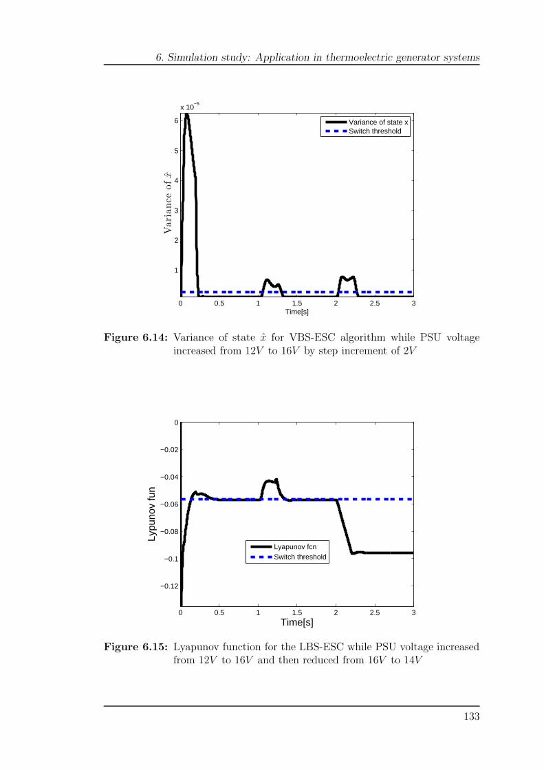
6. Simulation study: Application in thermoelectric generator systems
0 0.5 1 1.5 2 2.5 3
1
2
3
4
5
6
x 10−5
Time[s]
Variance
ofx
Variance of state xSwitch threshold
Figure 6.14: Variance of state x for VBS-ESC algorithm while PSU voltageincreased from 12V to 16V by step increment of 2V
0 0.5 1 1.5 2 2.5 3
−0.12
−0.1
−0.08
−0.06
−0.04
−0.02
0
Time[s]
Lypu
nov
fun
Lyapunov fcnSwitch threshold
Figure 6.15: Lyapunov function for the LBS-ESC while PSU voltage increasedfrom 12V to 16V and then reduced from 16V to 14V
133
6. Simulation study: Application in thermoelectric generator systems
6.7 Critical appraisal and conclusions
In this Chapter, two phases of simulation studies were presented. In Phase I,
simulation results for the P&O and the PESC algorithms for the TEG were
presented. Also, the benefit of using MPPT algorithms within the TEG was
demonstrated by operating with and without (i.e. fixed duty cycle) MPPT al-
gorithms. Simulation results show that in comparison to P&O, PESC achieves
a faster convergence speed. Due to the limitations of the PESC observed in
Phase I of hardware 7, Phase II presents improved results using novel MPPT
algorithms for both transients and steady-state. The VBS-ESC and the SDP-
ESC schemes were compared with PESC and LBS-ESC schemes. Compared to
others’ schemes, SDP-ESC achieves a faster convergence speed with minimised
electrical losses. This is due to an additional compensator as well as the ability to
be initialised with a large perturbation gain. Also, compared to LBS-ESC, both
VBS-ESC and LBS-ESC consistently perform for a varying source voltage.
134

Chapter 7
Experimental work
7.1 Introduction
This Chapter presents two Phases of the experimental validation of the simulation
results presented in Chapter 6. Phase I demonstrates the performance of current
existing MPPT algorithms and their limitations. In this phase, three different
analyses were performed, namely, steady-state, transient using emulated TEG
and transient via actual TEG. Steady-state analysis is conducted to investigate
limit cycles and losses within the PCU. Transient analysis using emulated TEG
is aimed to test the performance of the MPPT algorithms and their adaptation
capability under rapid variations of terminal voltage. On the other hand, tran-
sient analysis with the real TEG system aims to investigate the performance of
the MPPT algorithms for the slow dynamics of the TEG. The results of the ex-
perimental validation Phase I were published in Maganga et al. (2014). Phase
II presents improved results with the use of the VBS-ESC and the SDP-ESC for
similar analysis as that of Phase I. This chapter is organised as follows. Sec-
tion 7.2 provides a description of the experiment-set up for Phase I. Section 7.2.5
and 7.2.6 presents experimental results with emulated TEG and actual TEG,
respectively. Section 7.2.7 presents findings and observations of the experimental
135
7. Experimental work
Phase I. Section 7.3 describes the set-up of the experimental Phase II. This is
followed by experimental results in Section 7.3.2 with emulated TEG and actual
TEG in Section 7.3.3, utilising novel algorithms.
7.2 Experiment-setup: Phase I
This section describes the instrumentation and devices used to gather the exper-
imental results obtained with actual TEGs and with an emulation behaviour of
the TEGs. The actual TEG is used for transients analysis whereas emulation be-
haviour of the TEG is used for steady-state and fast transients analysis. Fig. 7.1
illustrates the schematic diagram of the connections between instrumentations
and devices used for experimental tests. A battery is emulated using a PSU
connected in series with an electronic load in constant-resistance mode, whereas
TEG is emulated using a PSU connected in series with a resistor. A synchronous
DC-DC buck boost converter is interfaced between the source (TEG/PSU) and
the emulated battery. Inputs to the synchronous DC-DC converter are: current
and voltage (i.e. Vin, Iin). Outputs of the converter are: voltage and current
(i.e. Vout, Iout). Inputs and outputs of the converter are fed to dSPACE (i.e.
MicroAutobox) as analog inputs which are used to manipulate the control inputs
of the converter via MPPT algorithms implemented in MATLAB/Simulink in a
PC. The manipulated control input is used to drive the PWM1 and PWM2 (see
Fig. 7.1).
7.2.1 Synchronous DC-DC converter
The synchronous DC-DC buck-boost converter provided by Glasgow University
was used for testing MPPT algorithms. The schematic of the synchronous DC-DC
converter and its principle of operation were presented in Chapter 6. Input and
output currents of the converter are sensed through the differential amplification
136

7. Experimental work
Buck/Synchronous Buck-Boost
PWM1 PWM2
Rin
Voc
CV
ElectrLoad
MicroAutoBoxdSPACE
MPPT algorithms:
PESC, LBS-ESC
VBS-ESC, and SDP-ESC
Vin, Iin Vout, Iout
MATLAB/Simulink (PC)
TEG or PSU Battery emulation
Figure 7.1: Schematic diagram of the connections between instrumentals anddevices used for the experimental tests
of the voltage across high precision/ power sense resistors placed in series with the
converter’s input and output terminals. The nominal input power of the converter
is 35W at 17.5V,2A. Its electrical efficiency at 34W input power (11.35V,3A) is88.2%. The converter’s printed circuit board (PCB) is shown in Fig. 7.2.
Sensor accuracy
The synchronous DC-DC buck boost converter (see the schematic diagram in
C.2) comprises of two current sensors: one for the input and one for the output
current measurements. Each of the sensor has ±10% error. A small value of
sensing resistor is used in order to keep the voltage drop on it small (with minimal
losses). The voltage drop across the resistor is then amplified by a factor of 100 by
a differential amplifier. The differential amplifier has a differential input voltage
offset (in millivolts) that constitutes an error. This error is the which is amplified
137
7. Experimental work
Figure 7.2: Picture of the top layer of the converters PCB. The bottom layerhosts the inductor and the capacitors.
by the differential amplifier, resulting in a fixed offset error in both input and
output measurements.
7.2.2 dSPACE interface
The MicroAutoBox is a portable dSPACE hardware used for real-time application
to perform various rapid control prototyping. MicroAutoBox is used in Phase I
for hardware in the loop (HIL) testing. It comprises of multiple in-built PWM
channels of which two are used to drive the MOSFET gate drivers of the syn-
chronous buck-boost the DC-DC converter. Via the ’drives control center aligned’
feature in the MicroAutoBox a dead-band of 400ns between PWM1 and inverted
PWM2 is initialised. It provides a maximum switching frequency fs of 20 kHz
138
This material has been removed from this thesis due to Third Party Copyright. The unabridged version of the thesis can be viewed at the Lanchester Library, Coventry University.
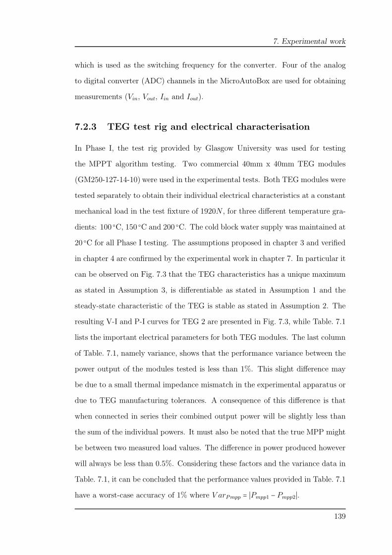
7. Experimental work
which is used as the switching frequency for the converter. Four of the analog
to digital converter (ADC) channels in the MicroAutoBox are used for obtaining
measurements (Vin, Vout, Iin and Iout).
7.2.3 TEG test rig and electrical characterisation
In Phase I, the test rig provided by Glasgow University was used for testing
the MPPT algorithm testing. Two commercial 40mm x 40mm TEG modules
(GM250-127-14-10) were used in the experimental tests. Both TEG modules were
tested separately to obtain their individual electrical characteristics at a constant
mechanical load in the test fixture of 1920N , for three different temperature gra-
dients: 100 C, 150 C and 200 C. The cold block water supply was maintained at
20 C for all Phase I testing. The assumptions proposed in chapter 3 and verified
in chapter 4 are confirmed by the experimental work in chapter 7. In particular it
can be observed on Fig. 7.3 that the TEG characteristics has a unique maximum
as stated in Assumption 3, is differentiable as stated in Assumption 1 and the
steady-state characteristic of the TEG is stable as stated in Assumption 2. The
resulting V-I and P-I curves for TEG 2 are presented in Fig. 7.3, while Table. 7.1
lists the important electrical parameters for both TEG modules. The last column
of Table. 7.1, namely variance, shows that the performance variance between the
power output of the modules tested is less than 1%. This slight difference may
be due to a small thermal impedance mismatch in the experimental apparatus or
due to TEG manufacturing tolerances. A consequence of this difference is that
when connected in series their combined output power will be slightly less than
the sum of the individual powers. It must also be noted that the true MPP might
be between two measured load values. The difference in power produced however
will always be less than 0.5%. Considering these factors and the variance data in
Table. 7.1, it can be concluded that the performance values provided in Table. 7.1
have a worst-case accuracy of 1% where V arPmpp = ∣Pmpp1 − Pmpp2∣.139
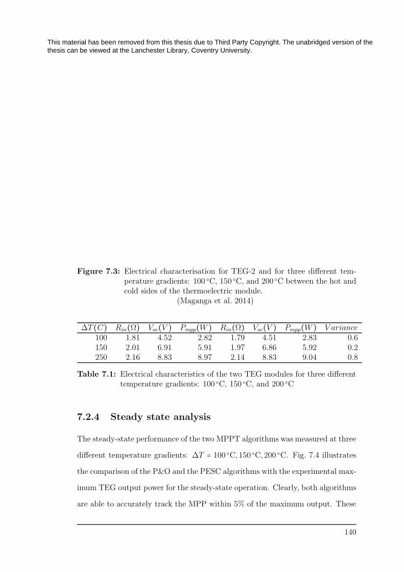
Figure 7.3: Electrical characterisation for TEG-2 and for three different tem-perature gradients: 100 C, 150 C, and 200 C between the hot andcold sides of the thermoelectric module.
(Maganga et al. 2014)
∆T (C) Rin(Ω) Voc(V ) Pmpp(W ) Rin(Ω) Voc(V ) Pmpp(W ) V ariance
100 1.81 4.52 2.82 1.79 4.51 2.83 0.6150 2.01 6.91 5.91 1.97 6.86 5.92 0.2250 2.16 8.83 8.97 2.14 8.83 9.04 0.8
Table 7.1: Electrical characteristics of the two TEG modules for three differenttemperature gradients: 100 C, 150 C, and 200 C
7.2.4 Steady state analysis
The steady-state performance of the two MPPT algorithms was measured at three
different temperature gradients: ∆T = 100 C,150 C,200 C. Fig. 7.4 illustrates
the comparison of the P&O and the PESC algorithms with the experimental max-
imum TEG output power for the steady-state operation. Clearly, both algorithms
are able to accurately track the MPP within 5% of the maximum output. These
140
This material has been removed from this thesis due to Third Party Copyright. The unabridged version of the thesis can be viewed at the Lanchester Library, Coventry University.

7. Experimental work
results however are conservative and the power extracted by the two MPPT algo-
rithms is often even closer to the MPP. When compared to the simulated outputs,
the experimental results have a slightly lower accuracy which is due primarily to
the various losses not incorporated within the simulation model, as well as the
electrical noise present on the acquired data. Despite these issues, the algorithms
are shown to perform in an accurate manner at steady-state.
Figure 7.4: Steady-state performance of perturb and observe and ESC algo-rithms for 100 C, 150 C, and 200 C temperature difference
(Maganga et al. 2014)
7.2.5 TEG emulation: fast transients analysis
The transient performance of the two MPPT algorithms is investigated using a
PSU in series with a fixed value (6.8Ω) power resistor to emulate the behaviour
of the TEG. The experimental set-up using the PSU is illustrated in Fig. 7.1.
This experiment demonstrates the ability of the P&O and the PESC to converge
to the MPP after fast changes in the open-circuit voltage. The PSU voltage is
141
This material has been removed from this thesis due to Third Party Copyright. The unabridged version of the thesis can be viewed at the Lanchester Library, Coventry University.

7. Experimental work
programmed to increase from 12V to 18V in 3V steps within 1 second. Figures 7.5
and 7.6 illustrate the results for P&O and PESC, respectively.
Figure 7.5: Converter’s operating input voltage during PSU open-circuit volt-age transients (12V,15V,18V ) with the perturb and observe con-troller. Expected theoretical input voltage would be: 6V,7.5V,9V .Time div. = 100ms; voltage div. = 1V
(Maganga et al. 2014)
It is evident that for each PSU voltage both controllers converge to a value
very close to the MPP. Whilst P&O provides a smaller limit cycle oscillation
around the MPP, the PESC acquires the MPP faster, in around 50ms, compared
to 200ms for the P&O. Also, it can be observed in Fig.7.5 and Fig.7.6, that the
steady-state characteristics of the TEG system is stable as stated in Assumption
2. Whilst transient performance is assessed via experiment, due to the limitations
of the switching frequency fs in the MicroAutoBox, comparison of convergence
between P&O and PESC is not conclusive. As aforementioned, in order to con-
verge faster to the MPP, high values of β and k should be selected. This may
however introduce ripples to the input voltage. The ripples are more significant
when switching at a lower frequency. To avoid this problem, lower values of β
142
This material has been removed from this thesis due to Third Party Copyright. The unabridged version of the thesis can be viewed at the Lanchester Library, Coventry University.

7. Experimental work
and k were chosen, as a consequence, poorer convergence but good steady state
performance was observed.
Figure 7.6: Converter’s operating input voltage during PSU open-circuit volt-age transients (12V,15V,18V ) with the ESC. Expected theoreticalinput voltage would be: 6V,7.5V,9V . Time div. = 100ms; voltagediv. = 1V
(Maganga et al. 2014)
7.2.6 Transient analysis with actual TEG
The last two tests aimed to compare the operating points chosen by the MPPT
algorithms to the maximum estimated TEG power during a long temperature
gradient transient across the TEGs. In Fig. 7.7 the converter is running the P&O
algorithm. The TEGs are rapidly heated from ∆T = 100 C to ∆T = 200 C in
420s. In Fig. 7.8 the converter is running the PESC algorithm and the TEG
electrical connection is unchanged. The TEGs are cooled from ∆T = 200 C to
∆T = 100 C in 410 seconds. As aforementioned, the estimated TEG power pro-
vided by the mathematical fitting technique has a worse-case accuracy of 5% and
143
This material has been removed from this thesis due to Third Party Copyright. The unabridged version of the thesis can be viewed at the Lanchester Library, Coventry University.

7. Experimental work
this uncertainty range has been marked in the plots, denoted by Pmax and Pmin.
In both figures, the average temperature difference across both TEG modules is
also plotted for reference as ”Temp Diff AVG” Some points related to the power
extracted by the P&O and the PESC fall outside the Pmax − Pmin boundary.
The reason for this is that the two multimeter units used to measure voltage
and current were not synchronized, therefore the V-I values taken for each point
might not be referenced to the same time instant. The transient response time
of the MPPT algorithms is several orders of magnitude faster than the thermal
response time of the system; therefore this experiment effectively corresponds to
setting numerous steady-state thermal operating points. The results presented
show that both algorithms track the maximum available power with efficiency
close to 100%.
Figure 7.7: Thermal transient test of the TEGs from ∆T = 100 C to ∆T =200 C, connected to the converter with the perturb and observeMPPT algorithm. Tracking with accuracy around 5% the transientmaximum estimated TEG.
(Maganga et al. 2014)
144
This material has been removed from this thesis due to Third Party Copyright. The unabridged version of the thesis can be viewed at the Lanchester Library, Coventry University.

Figure 7.8: Thermal transient test of the TEGs from ∆T = 200 C to ∆T =100 C, connected to the converter with the ESC MPPT algorithm.Tracking with accuracy around 5% the transient maximum esti-mated TEG.
(Maganga et al. 2014)
7.2.7 Findings and observations
In this phase of the experiment, multiple problems were observed. For instance,
the PESC was unable to excite the system with a smaller perturbation gain. Large
perturbations were therefore used to excite the system, which results into large
oscillations. Also, the advantage of the PESC over P&O seen in the simulation
study was inconclusive. This is thought to be due to the limited switching fre-
quency of the MicroAutoBox hardware used to implement the MPPT algorithms,
as well as the difficulty in obtaining the optimal PESC tuning parameters and the
effects of electrical noise during the data acquisition. In order to overcome these
issues, an additional phase of experiments was conducted. The latter sections
describe the experimental set-up and the improved results.
145
This material has been removed from this thesis due to Third Party Copyright. The unabridged version of the thesis can be viewed at the Lanchester Library, Coventry University.

7. Experimental work
7.3 Experimental set-up: Phase II
7.3.1 TEG test rig and electrical characterisation
A similar set-up as that of Phase I was also adopted in Phase II. Based on
the findings presented in Section 7.2.7, however, the MicroAutobox was replaced
by dSPACE board ds1104 in order to overcome the limitation of the switching
frequency. In this phase, a switching frequency of 50kHz was used to drive PWM1
and PWM2 of the synchronous DC-DC converter. Also, four commercial 62mm x
62mm TEMs provided by European Thermodynamics Ltd. (GM250-127-28-12)
were used in the experimental tests. Each of these modules is rated at P = 25W ,
Voc = 5.6V for ∆T=220 C. For more details on characteristics of the GM250-
127-28-12 see appendix C.3. From Fig. 7.9, A-denotes the control box, B-denotes
the thermocouple, C-denotes the heater block, D-denotes TE modules, E-denotes
the outlet channel, F-denotes the inlet channel, G-denotes the top end of the cold
plate and H denotes the inner side of cold plate. As shown in Fig. 7.9 the cartridge
heater block (10mm x 150mm) rated at 300W (see more details in appendix C.1)
was fitted at the bottom end of the rig and the coolant loop was created using 2mm
pipes. Water from the chiller was supplied to the test rig via 5-inlet and 5 outlet
channels. Fig. 7.10 illustrates the schematic diagram of the coolant loop of the
rig used in this phase of the experiments. To improve the thermal conductivity of
the TEMs, graphite sheets were placed between both the cold end and the TEMs
and the hot end and TEMs. The TEMs were place in a device designed from a
sandwich maker (see Fig. 7.9). Three thermocouples were used for reading cold
and hot side temperatures. Two of the thermocouples were fitted at the rear and
the front of the heater block, whereas one was fitted at the cold end. The heater
block was controlled by the control box (more details are given in appendix C.1).
The control box allows the temperature of the heater to be regulated at a certain
range depending on the desire of the user. As compared to Phase I, in Phase II
146
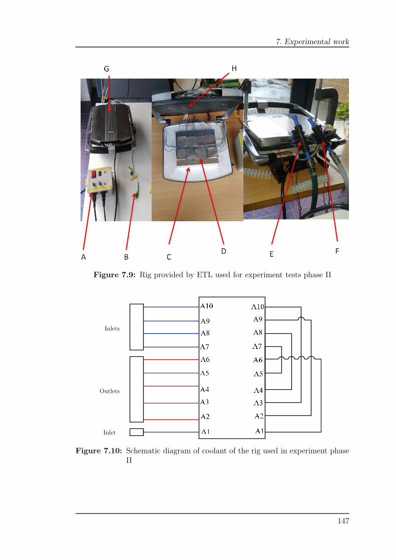
7. Experimental work
Figure 7.9: Rig provided by ETL used for experiment tests phase II
A9
A8
A9
A8Inlets
Outlets
Inlet
Figure 7.10: Schematic diagram of coolant of the rig used in experiment phaseII
147

7. Experimental work
all modules were characterised as a group of four TEMs connected electrically in
series. Electrical characterisations of the TEMs was performed for 20 different
temperature gradients: 50 C to 140 C with increments of 5 C between the hot
and cold side of the TEMs. Table. 7.2 presents electrical characterisation of four
TEMs connected in series.
Th( C) Tc( C) ∆T ( C) Voc(V ) Vmpp(V )202 62 140 5.6 2.8195 60 135 5.5 2.75189 59 130 5.4 2.7183 58 125 5.3 2.65176 56 120 5.2 2.6170 55 115 5.18 2.59164 54 110 5 2.5158 53 105 4.8 2.4151 51 100 4.6 2.3145 50 95 4.47 2.235138 48 90 4.3 2.15132 47 85 4.18 2.09126 46 80 3.9 1.95120 45 75 3.7 1.85116 46 70 3.5 1.75110 45 65 3.3 1.65105 45 60 3.1 1.5598 43 55 2.8 1.491 41 50 2.5 1.25
Table 7.2: Electrical characterisation of four TEMs electrically connected in se-ries
7.3.2 TEG emulation via power supply unit
The aim of this test is to validate the steady-state performance of the TEG seen
in Chapter 6. Also, it aims to demonstrate the ability of the SDP-ESC to track
fast transient of the TEG. For these purposes the PESC serves as benchmark.
For the steady-state analysis, the PSU was connected in series with a resistor
Rin = 3.2Ω and its voltage was maintained at 9.20V which is equivalent to the
open circuit voltage.
148

7. Experimental work
0 10 20 30 40 501
1.1
1.2
1.3
1.4
1.5
1.6
Time[s]
Impp
[A]
61.0439% Ripple reduction by SDP−ESC
PESCSDP−ESCTheoretical Impp
Figure 7.11: Input current at MPP for emulated TEG at steady-state operation
Using (6.6) and (6.7) in Section 6.4, the theoretical power and input voltage
at MPP is given as
Vmpp =9.2
2= 4.6V
Pmpp =9.22
4 ∗ 3.2= 6.61W
Using values of Vmpp and Pmpp, the theoretical input current at MPP can be
calculated as Impp =6.614.6= 1.436A. Fig. 7.11 shows a steady-state comparison
of a conventional PESC scheme and an SDP-ESC scheme. At steady-state con-
ventional PESC results in large oscillations. Conversely, the SDP-ESC results
in significantly smaller oscillations (61.04% current ripple reduction) for Impp
at steady-state. Similarly, SDP-ESC also achieves smaller oscillation for Vmpp
(67.97% voltage ripple reduction) at steady-state, see Fig. 7.12. Fig. 7.13 illus-
149

7. Experimental work
trates the duty cycle for both the PESC scheme and the SDP-ESC scheme while
the emulated TEG is operating at steady-state. Compared to the PESC, the
SDP-ESC achieves significantly smaller oscillations.
0 10 20 30 40 503.5
4
4.5
5
5.5
Time[s]
Vm
pp[V
]67.9696% Ripple reduction by SDP−ESC
PESCSDP−ESCTheoretical Vmpp
Figure 7.12: Input voltage at MPP with emulated TEG at steady-state opera-tion
Also, the PSU voltage was varied between 10V to 13.0V . Fig. 7.14 shows a
comparison of a typical input voltage for a conventional PESC scheme and an
SPD-ESC scheme. The upper plot in Fig. 7.14 shows the voltage at the extremum
Vmpp for the TEG system using conventional PESC and the lower plot shows the
voltage at the extremum Vmpp for the TEG system using an SDP-ESC. As can
be seen in Fig. 7.14, there is significantly less noise for the SDP-ESC than for
the PESC. This is due to the oscillations introduced by the PESC system when
large initial amplitudes are used. These oscillations hinder the performance of the
system and thus the SDP-ESC is clearly an improvement over the conventional
PESC method. Fig. 7.16 shows that similar performance is also achieved for the
current at the extremum Impp.
As shown in Figures 7.14 and 7.15, compared to conventional PESC, the SDP-
150
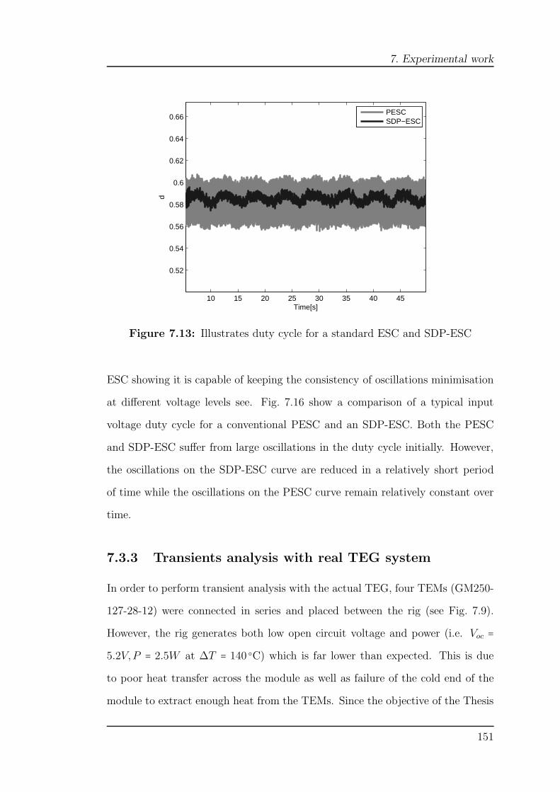
7. Experimental work
10 15 20 25 30 35 40 45
0.52
0.54
0.56
0.58
0.6
0.62
0.64
0.66
Time[s]
d
PESCSDP−ESC
Figure 7.13: Illustrates duty cycle for a standard ESC and SDP-ESC
ESC showing it is capable of keeping the consistency of oscillations minimisation
at different voltage levels see. Fig. 7.16 show a comparison of a typical input
voltage duty cycle for a conventional PESC and an SDP-ESC. Both the PESC
and SDP-ESC suffer from large oscillations in the duty cycle initially. However,
the oscillations on the SDP-ESC curve are reduced in a relatively short period
of time while the oscillations on the PESC curve remain relatively constant over
time.
7.3.3 Transients analysis with real TEG system
In order to perform transient analysis with the actual TEG, four TEMs (GM250-
127-28-12) were connected in series and placed between the rig (see Fig. 7.9).
However, the rig generates both low open circuit voltage and power (i.e. Voc =
5.2V,P = 2.5W at ∆T = 140 C) which is far lower than expected. This is due
to poor heat transfer across the module as well as failure of the cold end of the
module to extract enough heat from the TEMs. Since the objective of the Thesis
151

7. Experimental work
16 18 20 22 24 26 28 30 32
1.5
1.6
1.7
1.8
1.9
2
Time[s]
Impp
[A]
PESC
14 16 18 20 22 24 26 28 30
1.4
1.6
1.8
2
Time[s]
Impp
[A]
SDP−ESC
Figure 7.14: Zoomed input current at MPP (Impp) for variable open circuitvoltage
is to maximise power generated by the TEG as well as minimise losses, however,
the low power generated by the TEG did not hinder the investigation of the
performance of novel algorithms proposed in this Thesis.
Two MPPT controllers namely; PESC and SDP-ESC were tested. The tran-
sients performance of the proposed SDP-ESC at a much lower power was tested.
The modules were heated up in open loop and once the temperature on hot end
reached 200 C and 60 C on cold end then the heater blocks were turned off to
allow the modules to cool and one controller at a time was turned on. The signif-
icance of such test was to determine performance of the proposed MPPTs during
TEG thermal cooling.
Fig. 7.17 illustrates the hot side temperature measurements for the real TEG
system with the conventional PESC and the SDP-ESC algorithms. Due to the
152

7. Experimental work
16 18 20 22 24 26 28 30
5
5.5
6
6.5
7
Time[s]
Vm
pp[V
]
PESC
14 16 18 20 22 24 26 284.5
5
5.5
6
6.5
7
Time[s]
Vm
pp[V
]
SDP−ESC
Figure 7.15: Zoomed input voltage at MPP (Vmpp) for variable open circuitvoltage
ability of the SDP-ESC to minimise losses between the TEG system and the
synchronous DC-DC converter, it results in a higher temperature gradient ( ap-
proximately 5 C over 600 seconds) compared to the conventional PESC.
Fig. 7.18 illustrates the cold side temperature measurements for the TEG sys-
tem with conventional PESC and the SDP-ESC MPPT algorithms. SDP-ESC
achieves a higher temperature gradient (approximately 10 C over 600 seconds).
Fig. 7.19 illustrates the temperature difference ∆T measurements for the real
TEG system with the conventional PESC and the SDP-ESC. As observed pre-
viously, due to the ability of the SDP-ESC to minimise oscillations results in a
higher temperature difference ∆T than the conventional PESC. The difference
between ∆T ′s for the PESC and the SDP-ESC is slightly larger between 200s to
400s. This is due to effect observed at the cold side end temperature.
153
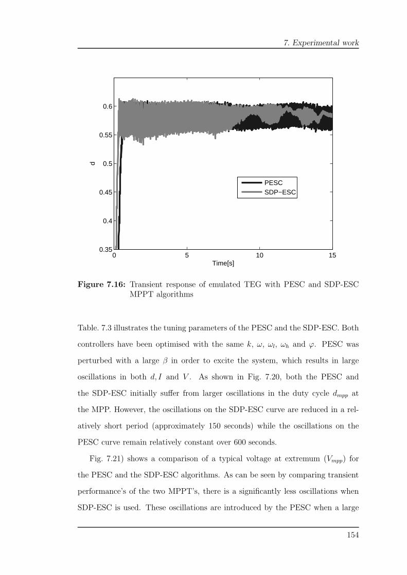
7. Experimental work
0 5 10 150.35
0.4
0.45
0.5
0.55
0.6
Time[s]
d
PESCSDP−ESC
Figure 7.16: Transient response of emulated TEG with PESC and SDP-ESCMPPT algorithms
Table. 7.3 illustrates the tuning parameters of the PESC and the SDP-ESC. Both
controllers have been optimised with the same k, ω, ωl, ωh and ϕ. PESC was
perturbed with a large β in order to excite the system, which results in large
oscillations in both d, I and V . As shown in Fig. 7.20, both the PESC and
the SDP-ESC initially suffer from larger oscillations in the duty cycle dmpp at
the MPP. However, the oscillations on the SDP-ESC curve are reduced in a rel-
atively short period (approximately 150 seconds) while the oscillations on the
PESC curve remain relatively constant over 600 seconds.
Fig. 7.21) shows a comparison of a typical voltage at extremum (Vmpp) for
the PESC and the SDP-ESC algorithms. As can be seen by comparing transient
performance’s of the two MPPT’s, there is a significantly less oscillations when
SDP-ESC is used. These oscillations are introduced by the PESC when a large
154

7. Experimental work
100 200 300 400 500 600
100
120
140
160
180
200
220
Time[s]
Thot
PESCSDP−ESC
Figure 7.17: Hot side temperature measurements for the real TEG system withPESC and SDP-ESC MPPT algorithms
100 200 300 400 500 60040
45
50
55
60
65
70
Time[s]
Tcold
PESCSDP−ESC
Figure 7.18: Cold side temperature measurements for the real TEG system withPESC and SDP-ESC MPPT algorithms
155
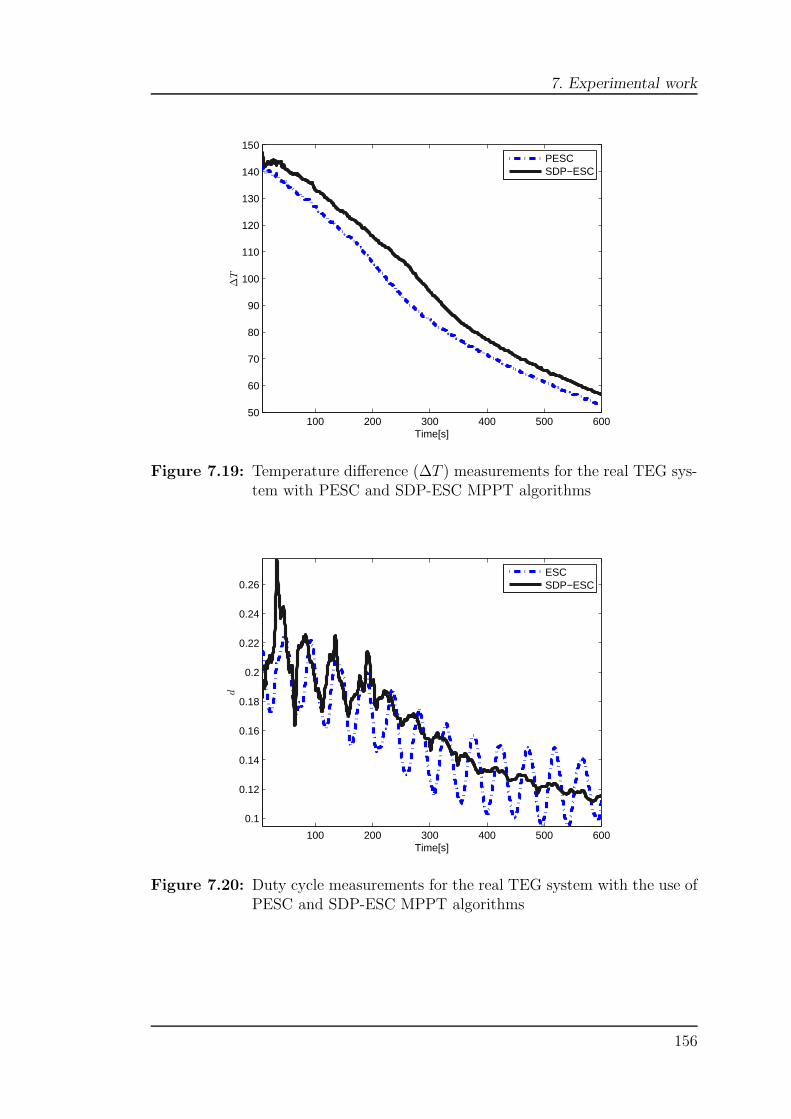
7. Experimental work
100 200 300 400 500 60050
60
70
80
90
100
110
120
130
140
150
Time[s]
∆T
PESCSDP−ESC
Figure 7.19: Temperature difference (∆T ) measurements for the real TEG sys-tem with PESC and SDP-ESC MPPT algorithms
100 200 300 400 500 600
0.1
0.12
0.14
0.16
0.18
0.2
0.22
0.24
0.26
Time[s]
d
ESCSDP−ESC
Figure 7.20: Duty cycle measurements for the real TEG system with the use ofPESC and SDP-ESC MPPT algorithms
156
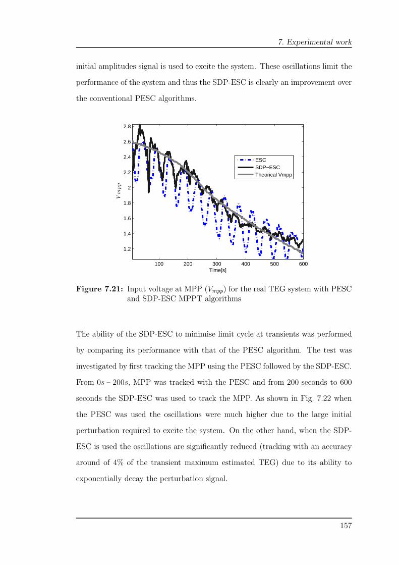
7. Experimental work
initial amplitudes signal is used to excite the system. These oscillations limit the
performance of the system and thus the SDP-ESC is clearly an improvement over
the conventional PESC algorithms.
100 200 300 400 500 600
1.2
1.4
1.6
1.8
2
2.2
2.4
2.6
2.8
Time[s]
Vmpp
ESCSDP−ESCTheorical Vmpp
Figure 7.21: Input voltage at MPP (Vmpp) for the real TEG system with PESCand SDP-ESC MPPT algorithms
The ability of the SDP-ESC to minimise limit cycle at transients was performed
by comparing its performance with that of the PESC algorithm. The test was
investigated by first tracking the MPP using the PESC followed by the SDP-ESC.
From 0s − 200s, MPP was tracked with the PESC and from 200 seconds to 600
seconds the SDP-ESC was used to track the MPP. As shown in Fig. 7.22 when
the PESC was used the oscillations were much higher due to the large initial
perturbation required to excite the system. On the other hand, when the SDP-
ESC is used the oscillations are significantly reduced (tracking with an accuracy
around of 4% of the transient maximum estimated TEG) due to its ability to
exponentially decay the perturbation signal.
157

7. Experimental work
Parameter PESC SDP-ESCk 1 1β 0.025 0.1
ω [ rads] 25 25
ωh [ rads ] 1.5 1.5
ωl [ rads ] 1.5 1.5ϕ(rad) 0 0
α - 3.5 ⋅ 10−6
Cp - 5Cz - 1
Table 7.3: Tuning parameters for PESC and SDP-ESC used to obtain transientperformance for the real TEG system
0 100 200 300 400 500 6000
0.5
1
1.5
2
2.5
3
3.5
Time[s]
Pow
er[W
]
PESC and SDP−ESCTheoretical PmppPmaxPmin
PESC
SDP−ESC
Figure 7.22: Comparison of limit cycle minimisation between PESC and SDP-ESC MPPT algorithms when applied to the real TEG system.SDP-ESC tracking with an accuracy around of 4% of the transientmaximum estimated TEG
158

7. Experimental work
7.4 Critical appraisal and conclusions
This Chapter presented two phases of experimental work which compared perfor-
mances of the controllers simulated in Chapter 6. Two different HIL set-ups with
the use of MicroAutoBox and ds1104 dSPACE were performed. These set-ups
include: TEG emulation via PSU in series with a resistor and real TEG system.
Using these two set-ups, three different analyses were performed in both phases
which are: steady-state, fast transients using emulated TEG, and actual tran-
sients with real TEG. Experiment Phase I presented a comparison of the P&O
and the PESC MPPT algorithms. Whilst the results show that the MPPT algo-
rithms accurately track the MPP, the perceived advantage of the PESC seen in
simulation was inconclusive. This is thought to be due to the limited switching
frequency of the MicroAutoBox hardware used to implement the MPPT algo-
rithms as well as the difficulty in obtaining the optimal PESC tuning parameters
and the effects of electrical noise during data acquisition. In Phase II, the Mi-
croAutoBox was replaced by ds1104 in order to increase the switching frequency.
One of the issues accounted for in experiment Phase II is that the power generated
by the rig was much lower than expected. This is due to poor heat transfer across
the TEMs as well as the inability of the coolant loop to extract enough heat from
the TEMs. Despite this issue the performance of the proposed MPPT controllers
were successfully tested. Compared to the PESC, the SDP-ESC achieved both
fast convergence speed as well as smaller oscillations. The VBS-ESC and the
LBS-ESC were not experimentally tested as ETL decided to replace the rig with
a much better optimised one.
159

Chapter 8
Conclusions and Further work
8.1 Conclusions and Further work
This Section summarises key achievements of the research work undertaken in
this Thesis.
8.1.1 VBS-ESC for local maxima search
In Chapter 3, the scheme for limit cycle minimisation known, as variance based
switching extremum seeking control (VBS-ESC) has been proposed. One of the
issues addressed in this chapter are limit cycles which are caused by continu-
ous perturbation within a perturbation based extremum seeking control (PESC).
VBS-ESC minimises oscillations based on variance detection. VBS-ESC is usu-
ally initialised with a large perturbation gain. As the output of the system enters
a stable limit cycle, no change in variance will be detected. Once no variance is
detected the VBS-ESC will switch to the smaller perturbation gain, hence oscilla-
tions will be reduced. As compared to other schemes proposed by Moura & Chang
(2010) and Wang & Krstic (2000), the VBS-ESC is simpler and comprises fewer
tuning parameters. In terms of limit cycle minimisation both schemes achieve
similar output results, hence the proposed method can be viewed as an extension
160

8. Conclusions and Further work
which provides a simplified scheme for limit cycle minimisation. Including the
VBS-ESC, all proposed methods do not take into account the trade-off between
convergence speed and minimisation of electrical losses within the power condi-
tioning unit (PCU). To address this issue, an improved PESC scheme known as
the state dependent parameter extremum seeking control (SDP-ESC) is presented
in Chapter 4.
8.1.2 SDP-ESC for local maxima search
In Chapter 4 a SDP-ESC based on the extension of PESC is proposed. It is simi-
lar to the method known as Lyapunov based switching extremum seeking control
(LBS-ESC) proposed by Moura & Chang (2010) which linearises the entire feed-
back loop, defining a Lypunov function, and using a switch to control the decay
process. The proposed scheme introduces a dependency between the perturbation
gain and the estimated input which allows an automated exponential decay of the
perturbation signal. As compared to VBS-ESC as well as methods proposed by
Moura & Chang (2010) and Wang & Krstic (2000), the proposed SDP-ESC is not
limited only to limit cycle minimisation. It also takes into account the trade-off
between the convergence speed and the minimisation of electrical losses within
the PCU. For that reason, the convergence speed is improved by introducing a
proportional integral (PI) controller within the SDP-ESC loop. The proposed
scheme therefore can be initialised with a large perturbation gain, making it pos-
sible to achieve excitation of the system at almost all times. Other advantages of
the SDP-ESC as compared the aforementioned schemes include: ability to track
adaptively (auto) as well as preserve the stability and simplicity of a standard
PESC.
Similar to PESC, VBS-ESC, and LBS-ESC, the drawback of the SDP-ESC
is its inability to search for the global maximum in the presence of local maxima.
This is based on fact that these methods search the extremum point by control-
161
8. Conclusions and Further work
ling the gradient at zero through the integrator. Once the nearest peak is found
they will converge to it. To eliminate this issue, an extension of the SDP-ESC is
proposed in Chapter 5.
8.1.3 Extended SDP-ESC for global maximum search
In Chapter 5, a novel scheme for the global maximum (GM) search in the presence
of local maxima has been presented. The scheme is based on an extension of the
SDP-ESC scheme presented in Chapter 4. A searching window mechanism has
been incorporated within the SDP-ESC in order to effectively search for the GM.
The searching window is designed such that the control input of the SDP-ESC
is initialised at different operating points. Initialisation of the control input is
based on designer knowledge and it can be initialised with either data stored in a
look-up table or as a ramp signal. In this Thesis, the scanning window has been
initialised using a ramp signal where the range of the ramp signal is based on the
operational range. Initialising the SDP-ESC at a different operating point will
allow the scanning of all available maxima. Once the true GM has been found,
the controller will be switched back to the initialisation point which corresponds
to the GM. The scheme has been demonstrated using several examples comprising
multiple maxima. Some of the examples presented by Tan et al. (2009) and Azar,
Perrier & Srinivasan (2011) were used to demonstrate the ability of the proposed
scheme to search the GM. The proposed scheme was shown to be effective in
converging to the GM regardless of available number of maxima. Some of the
advantages of the proposed scheme are: it preserves the stability and simplicity of
the SDP-ESC, it converges faster to the GM, it can be applied for both the GM
and local maxima search and it is model-free. The convergence period depends
on the operational range of the system as well as the step size of the searching
window. When a large step size is selected, faster convergence speed to the GM
will be achieved. When a very large step is selected however, the extended SDP-
162

8. Conclusions and Further work
ESC may barely converge to the true GM. On the other hand, a smaller step will
usually guarantee convergence to the true GM. This may however result in a slow
convergence speed to the GM.
8.1.4 Modelling, simulation and experimental validation:
TEG
In Chapters 6 and 7, the simulation studies and experimental work of novel max-
imum power point tracking (MPPT) algorithms has been presented. First, a
simulation study of perturb and observe (P&O )and PESC was applied to the
thermoelectric generator (TEG) as part of the research work undertaken in this
Thesis. The simulation results showed that the PESC converged much faster
to the maximum power point (MPP) with a 5% reduction of electrical losses.
Following this achievement, the experimental work was carried out. Three dif-
ferent analyses were performed which are: steady-state, fast transient with em-
ulated TEG, and transient with the actual TEG. Whilst the results show that
the MPPT algorithms accurately track the MPP, the perceived advantage of the
PESC seen in simulation was inconclusive. This is thought to be due to the lim-
ited switching frequency of the MicroAutoBox hardware used to implement the
MPPT algorithms, as well as the difficulty in obtaining the optimal PESC tuning
parameters and the effects of electrical noise during the data acquisition. The
dSPACE MicroAutoBox hardware however, does allow the user to investigate
the hardware implementation of the MPPTs. These limitations led to the devel-
opment of novel algorithms (i.e. VBS-ESC and SDP-ESC) which incorporated
adaptability of the parameters to ensure optimal performance in both transient
and steady-state operations. In addition, the dSPACE MicroAutobox was re-
placed with ds1104 dSPACE which allowed the switches of a synchronous direct
current (DC)-DC converter to be driven at a much higher switching frequency.
163

8. Conclusions and Further work
Performance of the VBS-ESC and the SDP-ESC were compared with the
PESC and the LBS-ESC in simulation study Phase II. To validate these find-
ings, experimental test Phase II was conducted. Similar types of tests conducted
in Phase I were repeated in Phase II. SDP-ESC achieved both fast convergence
speed to the MPP as well as reduced oscillations compared to the PESC when
an emulated TEG was used.
Actual transient analysis was performed using the rig provided by Eu-
ropean Thermodynamics (ETL), however, the rig was unable to generate the
required power as expected. This is due to poor heat transfer across the modules
as well as the inability of the coolant loop to extract heat from the thermoelec-
tric modules (TEMs). Since the objective is investigating the performance of the
algorithms therefore, this limitation was considered as minor and did not hinder
the experiment. However, in order to give sufficient excitation, both the PESC
and the SDP-ESC were perturbed with large perturbation gains. As compared
to the PESC, the SDP-ESC achieved relatively smaller oscillations due to its
ability to exponentially decay the perturbation gain. Due to the low power gen-
erated by the rig, rather than characterising each TEM individually, the electrical
characterisations of all TEMs connected in series was performed. Open circuit
measurements at different temperatures where taken. As aforementioned, for the
TEG, the maximum available power is achieved when the input voltage is half
of the open circuit voltage. Smaller limit cycles indicate less degradation to the
components. Other MPPT controllers (i.e. VBS-ESC and LBS-ESC) were not
tested experimentally.
8.2 Further work
This Section, proposes some directions which could be taken for further improve-
ments.
164

8. Conclusions and Further work
8.2.1 Constrained VBS-ESC/SDP-ESC scheme
Both the VBS-ESC and the SDP-ESC are model-free which assumes no a priori
knowledge of the plant or system (neither model nor cost function is available).
Based on these assumptions, there are no constraints imposed to the system.
These controllers seemed to give optimal performance when applied to the TEG
system. Experiments carried out in this Thesis however were conducted under
well-controlled environmental conditions. On the other hand, when applied to
systems where uncertainties are significant, the proposed MPPT controllers may
result in less optimal performance than that seen in the laboratory. To address
these concerns it may be useful to further investigate the possibilities and ad-
vantages of imposing constraints particularly for systems where prior knowledge
exists.
8.2.2 Experimental validation global maximum searching
scheme
Simulation studies showed that the extended SDP-ESC scheme proposed in this
Thesis is able to search for the GM regardless of the number of maxima. As
compared to stochastic based approaches for the GM, this is considered to be
inexpensive solution as it is model-free. It will therefore be beneficial to validate
these findings experimentally as well as imposing constraints to the extended
SDP-ESC if needed. One possible example which can be used to validate these
findings is PV systems due to shading effects which causes multiple maxima to
occur.
165
8. Conclusions and Further work
8.2.3 Embedding VBS-ESC/SDP-ESC for stand-alone op-
eration
Experimental work carried out through hardware in the loop (HIL) testing demon-
strates the ability of the SDP-ESC to minimise limit cycle as well as converging
faster to the MPP compared to the standard PESC. It will therefore be useful
to implement the SDP-ESC for stand-alone operations. The SDP-ESC algorithm
can be embedded into a microcontroller, further integrated within a TEG and
tested in a complete drive cycle. This will validate the robustness of the SDP-ESC
particularly under harsh driving conditions and other uncertainties (e.g. noise,
disturbances, etc.).
8.2.4 Degradation of PCU components
Limit cycles are associated with the degradation of components (e.g. electrolyte
capacitors) within a PCU. Large ripples may increase the equivalent series resis-
tance as well as decrease the capacitance of the capacitor. It will be beneficial
to investigate the performance of the novel MPPT algorithms as the components
degrade. One possible way to achieve this is by incorporating degradation effects
within the DC-DC converter. Based on performance of the MPPT algorithm,
necessary improvements can be performed.
166

References
Ariyur, K. & Krstic, M. (2010), Real-Time Optimization by Extremum-Seeking
Control.
Ariyur, K. & Krystic, M. (2003), Real-Time Optimization by Extremum-Seeking
Control, John Wiley & Sons.
Azar, F., Perrier, M. & Srinivasan, B. (2011), ‘A global optimization method
based on multi-unit extremum-seeking for scalar nonlinear systems’, Com-
puters and Chemical Engineering 35.
Bizon, N. (2010), ‘On tracking robustness in adaptive extremum seeking control
of the fuel cell power plants’, Applied energy 87, 3115–3130.
Bizon, N. (2013), ‘Fc energy harvesting using the mpp tracking based on ad-
vanced extremum seeking control’, International Journal of Hydrogen Energy
38(4), 1952–1966.
Calli, B., Caarls, W., Jonker, P. & Wisse, M. (2012a), ‘Comparison of extremum
seeking control algorithms for robotic applications’, International Conference
on Intelligent Robots and Systems 39, 3195–3202.
Calli, B., Caarls, W., Jonker, P. & Wisse, M. (2012b), Comparison of extremum
seeking control algorithms for robotic applications, in ‘Intelligent Robots and
Systems (IROS), 2012 IEEE/RSJ International Conference on’, pp. 3195–
3202.
167

REFERENCES
Champier, D., Favarel, C., Bdcarrats, J., Kousksou, T. & Rozis, J. (2013), ‘Pro-
totype combined heater/thermoelectric power generator for remote applica-
tions’, Journal of Electronic Materials 42(7), 1888–1899.
Chang, Y. & Moura, S. (2009), Air flow control in fuel cell systems: An ex-
tremum seeking approach, in ‘American Control Conference, 2009. ACC
’09.’, pp. 1052–1059.
Chen, Y., Chou, M. & Wu, H. (2005), Electrolytic capacitor failure prediction
of lc filter for switching-mode power converters, in ‘Fourtieth IAS Annual
Meeting’.
Cho, S., Kim, N., Park, S. & Kim, S. (2010), A coreless maximum power point
tracking circuit of thermoelectric generators for battery charging systems, in
‘Solid State Circuits Conference (A-SSCC), 2010 IEEE Asian’, pp. 1–4.
Cistelecan, M. (2008), Power control in mobile wireless networks using sliding
mode extremum seeking control implementing bifurcations, in ‘Control Ap-
plications, 2008. CCA 2008. IEEE International Conference on’, pp. 67–72.
Crane, D. & Jackson, G. (2002), Systems-level optimization of low-temperature
thermoelectric waste heat recovery, in ‘Energy Conversion Engineering Con-
ference, 2002. IECEC ’02. 2002 37th Intersociety’, pp. 583–591.
Dan, Z., Bo, H., Jian, X., Yi, G. & Yuan, R. (2008), ‘Adaptive maximum power
point tracking control of fuel cell power plants’, Journal of Power Sources
176(1), 259–269.
Daraban, S., Petreus, D. & Morel, C. (2014), ‘A novel mppt(maximum power
point tracking) algorithm based on a modified genetic algorithm specialized
on tracking the global maximum power point in photovoltaic systems affected
by partial shading’, Energy 74(0), 374 – 388.
168

REFERENCES
Dincmen, Erkin., G. B. & Acarman, T. (2012), ‘Extremum-seeking control of abs
braking in road vehicles with lateral force improvement’, IEEE Transactions
on Control Systems Technology 22, 230–237.
Dochain, D., Perrier, M. & Guay, M. (2011), ‘Extremum seeking control and its
application to process and reaction systems: A survey’, Mathematics and
Computers in Simulation 82(3), 369–380.
Doostabad, H., Keypour, R. & Khalghani, M. (2013), ‘A new approach in mppt
for photovoltaic array based on extremum seeking control under uniform and
non-uniform irradiances’, Solar Energy 94.
Drakunov, S., Ozguner, U., Dix, P. & Ashrafi, B. (1995), ‘Abs control using op-
timum search via sliding modes’, Control Systems Technology, IEEE Trans-
actions on 3(1), 79–85.
Draper, C. & Li, Y. (1951), ‘Principles of optimalizing control systems and an
application to the internal combustion engine’.
D’Souza, N., Lopes, L. & Liu, X. (2005), An intelligent maximum power point
tracker using peak current control, in ‘Power Electronics Specialists Confer-
ence, 2005. PESC ’05. IEEE 36th’.
Eakburanawat, J. & Boonyaroonate, I. (2006), ‘Development of a thermoelectric
battery-charger with microcontroller-based maximum power point tracking
technique’, Applied Energy 83(7), 687–704.
Elobaid, L., Abdelsalam, A. & Zakzouk, E. (2012), Artificial neural network based
maximum power point tracking technique for pv systems, in ‘IECON 2012
- 38th Annual Conference on IEEE Industrial Electronics Society’, pp. 937–
942.
169

REFERENCES
Esarte, J., Min, G. & Rowe, D. (2001), ‘Modelling heat exchangers for thermo-
electric generators’, Journal of Power Sources 93(12), 72 – 76.
Esram, T. & Chapman, P. (2007), ‘Comparison of photovoltaic array maximum
power point tracking techniques’, Energy Conversion, IEEE Transactions
on 22(2), 439–449.
Gelberta, G., Moeck, J., Paschereit, C. & King, R. (2012), ‘Advanced algorithms
for gradient estimation in one-and two parameter extremum seeking con-
trollers’, Journal of Process Control 22, 700–709.
Guay, M. (2014), ‘A time-varying extremum-seeking control approach for discrete-
time systems’, Journal of Process Control 24, 98–112.
Guay, M., Dochain, D. & Perrier, M. (2004), ‘Adaptive extremum seeking con-
trol of continuous stirred tank bioreactors with unknown growth kinetics’,
Automatica 40(5), 881–888.
Guay, M. & Zhang, T. (2003), ‘Adaptive extremum seeking control of nonlinear
dynamic systems with parametric uncertainties’, Automatica 39, 1283–1293.
Gurvich, L. (2004), Fuzzy logic base extremum seeking control system, in ‘Elec-
trical and Electronics Engineers in Israel, 2004. Proceedings. 2004 23rd IEEE
Convention of’, pp. 18–21.
Haskara, I., Zhu, G. & Winkelman, J. (2006), Multivariable egr/spark timing con-
trol for ic engines via extremum seeking, in ‘American Control Conference,
2006’.
Henning, L., Becker, R., Feuerbach, G., Muminovic, R., King, R., Brunn, A.
& Nitsche, W. (2008), ‘Extensions of adaptive slope-seeking for active flow
control’, Journal of Systems and Control Engineering 222, 309–322.
170

REFERENCES
Hiyama, T., Kouzuma, S. & Imakubo, T. (1995), ‘Identification of optimal oper-
ating point of pv modules using neural network for real time maximum power
tracking control’, Energy Conversion, IEEE Transactions on 10(2), 360–367.
Hu, Y. & Zuo, B. (2005), ‘An annealing recurrent neural network for extremum
seeking control’, International Journal of Information Technology 11.
Hu, Y., Zuo, B. & Li, X. (2006), The application of an annealing recurrent neu-
ral network for extremum seeking algorithm to optimize uav tight formation
flight, in ‘Computational Engineering in Systems Applications, IMACS Mul-
ticonference on’, Vol. 1, pp. 613–620.
Hussain, Q. E., Brigham, D. R. & Maranville, C. W. (2009), Thermoelectric
exhaust heat recovery for hybrid vehicles, Technical report, SAE Technical
Paper.
Irisawa, K., Saito, T., Takano, I. & Sawada, Y. (2000), Maximum power point
tracking control of photovoltaic generation system under non-uniform inso-
lation by means of monitoring cells, in ‘Photovoltaic Specialists Conference,
2000. Conference Record of the Twenty-Eighth IEEE’, pp. 1707–1710.
Jain, S. & Agarwal, V. (2004), ‘A new algorithm for rapid tracking of approximate
maximum power point in photovoltaic systems’, Power Electronics Letters,
IEEE 2(1), 16–19.
Kamarzaman, N. & Tan., C. (2014), ‘A comprehensive review of maximum power
point tracking algorithms for photovoltaic systems’, Renewable and Sustain-
able Energy Reviews 37, 585 – 598.
Khong, S., Nesic, D., Manzie, C. & Tan, Y. (2013), ‘Multidimensional global
extremum seeking via the direct optimisation algorithm’, Automatica 49.
171

REFERENCES
Killingsworth, N. & Krstic, M. (2006), ‘Pid tuning using extremum seeking: on-
line, model-free performance optimization’, IEEE Control Systems Magazine
26, 70–79.
Kim, K., Kasnakoglu, C., Serrani, A. & Samimy, M. (2008), Extremum-seeking
control of subsonic cavity flow, in ‘Proceedings of the 46th AIAA aerospace
science meeting and exhibit’.
Kim, K., Kasnakoglu, C., Serrani, A. & Samimy, M. (2009), ‘Extremum-seeking
control of subsonic cavity flow’, AIAA 47, 195–205.
Kim, R. & Lai, J. (2008), ‘A seamless mode transfer maximum power point track-
ing controller for thermoelectric generator applications’, Power Electronics,
IEEE Transactions on 23(5), 2310–2318.
Kim, S., Cho, S., Kim, N., Baatar, N. & Kwon, J. (2011), ‘A digital coreless max-
imum power point tracking circuit for thermoelectric generators’, Journal of
Electronic Materials 40(5), 867–872.
King, R., Petz, R. & Lemke, O. (2006), ‘Adaptive flow control using slope seek-
ing’, Mediterranean Conference on Control and Automation 14.
Kobayashi, K., Takano & Sawada, Y. (2006), ‘A study of a two stage maximum
power point tracking control of a photovoltaic system under partially shaded
insolation conditions’, Solar Energy Materials and Solar Cells 90(1819), 2975
– 2988. 14th International Photovoltaic Science and Engineering Conference
14th International Photovoltaic Science and Engineering Conference.
Koizumi, H. & Kurokawa, K. (2005), A novel maximum power point tracking
method for pv module integrated converter, in ‘Power Electronics Specialists
Conference, 2005. PESC ’05. IEEE 36th’, pp. 2081–2086.
172

REFERENCES
Korovin, S. & Utkin, V. (1972), ‘Use of the slide mode in problems of static
optimization’, Automatic and Remote Control .
Korovin, S. & Utkin, V. (1974), ‘Using sliding modes in static optimization and
nonlinear programming’, Automatica 10.
Krstic, M. (2000), ‘Performance improvement and limitations in extremum seek-
ing control’, Systems and Control Letters 39, 313–326.
Krstic, M. & Bastin, G. (1999), ‘Optimizing bioreactors by extremum seeking’,
International Journal of Adaptive Control and Signal Processing 13, 651–
669.
Laird, I., Lovatt, H., Savvides, N., Lu, D. & Agelidis, V. (2008), Comparative
study of maximum power point tracking algorithms for thermoelectric gen-
erators, in ‘Power Engineering Conference, 2008. AUPEC ’08. Australasian
Universities’, pp. 1–6.
Laird, I. & Lu, D. (2013), ‘High step-up dc/dc topology and mppt algorithm for
use with a thermoelectric generator’, Power Electronics, IEEE Transactions
on 28(7), 3147–3157.
Leblanc, M. (1922), ‘Sur llectrification des chemins de fer au moyen de courants
alternatifs de frquence leve’, Revue Generale delElectricit .
Lee, J., Bae, H. & Cho, B. (2006), Advanced incremental conductance mppt
algorithm with a variable step size, in ‘Power Electronics and Motion Control
Conference, 2006. EPE-PEMC 2006. 12th International’, pp. 603–607.
Lei, P. & Li, Y. (2010), ‘Extremum seeking control based integration of mppt and
degradation detection for photovoltaic arrays’, American Control Conference
pp. 3536–3541.
173

REFERENCES
Li, X., Li, Y., Seem, J. & Li, P. (2013), ‘Dynamic modeling and self-optimizing
operation of chilled water systems using extremum seeking control’, Energy
and Buildings 58, 172–182.
Lineykin, S. & Ben-Yaakov, S. (2007), ‘Modeling and analysis of thermoelectric
modules’, Industry Applications, IEEE Transactions on 43(2), 505–512.
Liu, B., Duan, S., Liu, F. & Xu, P. (2007), Analysis and improvement of maximum
power point tracking algorithm based on incremental conductance method
for photovoltaic array, in ‘Power Electronics and Drive Systems, 2007. PEDS
’07. 7th International Conference on’, pp. 637–641.
Liu, S. & Krstic, M. (2012), Stochastic Averaging and Stochastic Extremum Seek-
ing.
Maganga, O., Larkowski, T. & Burnham, K. (2012), Model complexity reduc-
tion of a dc-dc buck-boost converter, in ‘22nd International Conference on
Systems Engineering (ICSE)’.
Maganga, O., Phillip, N., Burnham, K. J., Montecucco, A., Siviter, J., Knox,
A. & Simpson, K. (2014), ‘Hardware implementation of maximum power
point tracking for thermoelectric generators’, Journal of Electronic Materials
43(6), 2293–2300.
Manzie, C. & Kristic, M. (2009a), Extremum-seeking control via sliding mode
with periodic search signals, in ‘IEEE Conference on Decision and Control’,
Vol. 41.
Manzie, C. & Kristic, M. (2009b), ‘Extremum seeking with stochastic perturba-
tions’, IEEE Transactions on Automatic Control 54.
174

REFERENCES
Messai, A., Mellit, A., Guessoum, A. & Kalogirou, S. (2011), ‘Maximum power
point tracking using a ga optimized fuzzy logic controller and its fpga im-
plementation’, Solar Energy 85(2), 265 – 277.
Montecucco, A., Buckle, J. & Knox, A. (2012), ‘Solution to the 1-d unsteady heat
conduction equation with internal joule heat generation for thermoelectric
devices’, Applied Thermal Engineering 35(0), 177 – 184.
Montecucco, A. & Knox, A. (2014), ‘Maximum power point tracking converter
based on the open-circuit voltage method for thermoelectric generators’,
IEEE Transactions on Power Electronics .
Montecucco, A., Siviter, J. & Knox, A. (2012), Simple, fast and accurate maxi-
mum power point tracking converter for thermoelectric generators, in ‘En-
ergy Conversion Congress and Exposition (ECCE), 2012 IEEE’, pp. 2777–
2783.
Moradi, M. & Reisi, A. (2011), ‘A hybrid maximum power point tracking method
for photovoltaic systems’, Solar Energy 85(11), 2965–2976.
Moradi, M., Tousi, S., Nemati, M., Basir, N. & Shalavi, N. (2013), ‘A robust
hybrid method for maximum power point tracking in photovoltaic systems’,
Solar Energy 94(0), 266–276.
Moura, S. & Chang, Y. (2010), Asymptotic convergence through lyapunov-based
switching in extremum seeking with application to photovoltaic systems, in
‘American Control Conference (ACC), 2010’, pp. 3542–3548.
Moura, S. & Chang, Y. (2013), ‘Lyapunov-based switched extremum seeking for
photovoltaic power maximization’, Control Engineering Practice 21(7), 971–
980.
175
REFERENCES
Nagayoshi, H. & Kajikawa, T. (2006), Mismatch power loss reduction on thermo-
electric generator systems using maximum power point trackers, in ‘Ther-
moelectrics, 2006. ICT ’06. 25th International Conference on’, pp. 210–213.
Nagayoshi, H., Kajikawa, T. & Sugiyama, T. (2002), Comparison of maximum
power point control methods for thermoelectric power generator, in ‘Thermo-
electrics, 2002. Proceedings ICT ’02. Twenty-First International Conference
on’, pp. 450–453.
Nagayoshi, H., Tokumisu, K. & Kajikawa, T. (2007), Evaluation of multi mppt
thermoelectric generator system, in ‘Thermoelectrics, 2007. ICT 2007. 26th
International Conference on’, pp. 318–321.
Nesic, D., Mohammadi, A. & Manzie, C. (2013), ‘Framework for extremum seek-
ing control of systems with parameter uncertainties’, IEEE Transactions on
Automatic Control 58, 435–448.
Ogren, P., Fiorelli, E. & Leonard, N. (2004), ‘Cooperative control of mobile
sensor networks:adaptive gradient climbing in a distributed environment’,
Automatic Control, IEEE Transactions on 49(8), 1292–1302.
Park, J., Lee, H. & Bond, M. (2014), ‘Uninterrupted thermoelectric energy har-
vesting using temperature-sensor-based maximum power point tracking sys-
tem’, Energy Conversion and Management 86, 233–240.
Patcharaprakiti, N., Premrudeepreechacharn, S. & Sriuthaisiriwong, Y. (2005),
‘Maximum power point tracking using adaptive fuzzy logic control for grid-
connected photovoltaic system’, Renewable Energy 30(11), 1771 – 1788.
Phillip, N., Maganga, O., Burnham, K., Dunn, J., Rouaud, C., Ellis, M. &
Robinson, S. (2012), Modelling and simulation of a thermoelectric generator
for waste heat energy recovery in low carbon vehicles, in ‘2nd International
176
REFERENCES
Symposium on Environment Friendly Energies and Applications (EFEA),
2012’, pp. 94–99.
Phillip, N., Maganga, O., Burnham, K. J., Ellis, M. A., Robinson, S., Dunn, J.
& Rouaud, C. (2013), ‘Investigation of maximum power point tracking for
thermoelectric generators’, Journal of electronic materials 42(7), 1900–1906.
Popovic, D., Jankovic, M., Magner, S. & Teel, A. (2006), ‘Extremum seeking
methods for optimization of variable cam timing engine operation’, Control
Systems Technology, IEEE Transactions on 14(3), 398–407.
Ramaprabha, R. & Mathur, B. (2011), ‘Intelligent controller based maximum
power point tracking for solar pv system’, International Journal of Computer
Applications 12(10), 37 – 41.
Reisi, A., Moradi, M. & Jamasb, S. (2013), ‘Classification and comparison of max-
imum power point tracking techniques for photovoltaic system: A review’,
Renewable and Sustainable Energy Reviews 19, 433 – 443.
Rowe, D. (2005), Thermoelectrics Handbooks.
Schwartz, D. (2012), A maximum-power-point-tracking control system for ther-
moelectric generators, in ‘Power Electronics for Distributed Generation Sys-
tems (PEDG), 2012 3rd IEEE International Symposium on’, pp. 78–81.
Shadmand, M., Balog, R. & Abu Rub, H. (2014), Maximum power point tracking
using model predictive control of a flyback converter for photovoltaic appli-
cations, in ‘Power and Energy Conference at Illinois (PECI), 2014’, pp. 1–5.
Snyder, G. J. & Toberer, E. S. (2008), ‘Complex thermoelectric materials’, Nature
materials 7(2), 105–114.
Stobart, R. & Milner, D. (2009), The potential for thermo-electric regeneration
of energy in vehicles, Technical report, SAE Technical Paper.
177

REFERENCES
Tan, Y., Moase, W., Manzie, C., Nesic, D. & Mareels, I. (2010), Extremum
seeking control from 1922 to 2010, in ‘Proceeding of the 29th Chinese Control
Conference’, pp. 14–26.
Tan, Y., Nei, D. & Mareels, I. (2008), ‘On the choice of dither in extremum
seeking systems: A case study’, Automatica 44(5), 1446–1450.
Tan, Y., Nesic, D., Mareels, I. & Astolfi, A. (2009), ‘On global extremum seeking
in the presence of local extrema’, Automatica 45, 245–251.
Tanelli, M., Astolfi, A. & Savaresi, S. (2006), Non-local extremum seeking control
for active braking control systems, in ‘International Conference on Control
Applications’, pp. 891–896.
Vieira, J. & Mota, A. (2009), Thermoelectric generator using water gas heater
energy for battery charging, in ‘Control Applications, (CCA) Intelligent Con-
trol, (ISIC), 2009 IEEE’, pp. 1477–1482.
Wai, R., Wang, W. & Lin, J. (2006), Grid-connected photovoltaic generation sys-
tem with adaptive step-perturbation method and active sun tracking scheme,
in ‘IEEE Industrial Electronics, IECON 2006 - 32nd Annual Conference on’,
pp. 224–228.
Wang, H. & Krstic, M. (2000), ‘Extremum seeking for limit cycle minimisation’,
IEEE Transactions on Automatic Control 45.
Wiederhold, O., King, R., Noack, B., Neuhaus, L., Neise, W., Enghardt, L. &
Swoboda, M. (2009), ‘Extensions of extremum-seeking control to improve the
aerodynamic performance of axial turbomachines’, AIAA Fluid Dynamics
Conference 39, 22–25.
178

REFERENCES
Xiao, W. & Dunford, W. (2004), A modified adaptive hill climbing mppt method
for photovoltaic power systems, in ‘Power Electronics Specialists Conference,
2004. PESC 04. 2004 IEEE 35th Annual’, Vol. 3, pp. 1957–1963 Vol.3.
Yang, S., Xiang, D., Bryant, A., Mawby, P., Ran, L. & Tavner, P. (2010), ‘Con-
dition monitoring for device reliability in power electronic converters: A
review’, Power Electronics, IEEE Transactions on 25(11), 2734–2752.
Youn, N., Lee, H., Wee, D., Gomez, M., Reid, R. & Ohara, B. (2014), ‘Achieving
maximum power in thermoelectric generation with simple power electronics’,
Journal of Electronic Materials 43(6), 1597–1602.
Yu, S., Chen, H. & Kong, L. (2010), ‘Particle swarm optimization-based ex-
tremum seeking control’, Advanced Intelligent Computing Theories and Ap-
plications 6215, 185–196.
Zhang, C. (2007), ‘Numerical optimization-based extremum seeking control
with application to abs design’, IEEE Transactions on Automatic Control
52, 454–467.
Zhang, C. & Ordonez, R. (2012), Extremum Seeking Control and Applications, A
Numerical Optimization-Based Approach.
Zhang, C., Siranosian, A. & Kristic, M. (2007), ‘Extremum seeking for moder-
ately unstable systems and for autonomous target tracking without position
measurements’, Automatica 43, 1832–1839.
Zhang, C., Siranosian, A. & Kristic, M. (2009), ‘Design of extremum seeking
control with pd accelerator and its application to monod and williams-otto
models’, Engineering and Technology 3, 1154–1158.
179

REFERENCES
Zhang, F., Thanapalan, K., Procter, A., Carr, S. & Maddy, J. (2013), ‘Adaptive
hybrid maximum power point tracking method for a photovoltaic system’,
Energy Conversion, IEEE Transactions on 28(2), 353–360.
Zhang, T., Guay, M. & Dochain, D. (2002), ‘Adaptive extremum seeking control
of continuous stirred tank bioreactors’, IFAC (6).
180

Appendix A
Description of the TEG model
Similar to the physical system, the TEG model is set-up with multiples of the
three subsystems with each multiple representing a section of the system in the
stream of the exhaust as shown in Fig. A. The TEG model requires the exhaust
and coolant inlet temperature (Tai, Twi) and mass flow rate (ma, mw) as inputs
and outputs of the voltage and current (V ,I) generated by the TEG. The tran-
sient analysis capability of the model makes it possible to account for the initial
warm up period and also provides the capability to integrate with a vehicle model
for fuel consumption analysis over defined drive cycles.
A.1 Thermal electric module (TEM)
TEMs can either be connected electrically in series or parallel to increase the
operating voltage or decrease the thermal resistance, respectively. The TEM
subsystem uses the hot and cold side temperature inputs from the heat exchanger
181

A. Description of the TEG model
Figure A.1: TEG subsystem configuration in comparison to physical system
subsystem to give the electrical power generated using the following equations
Voc = ncouple (sn + sp)∆T (A.1a)
Rin =ncouple (ρn + ρp)Ltem
A(A.1b)
Km =ncouple (κn − κp)Ltem
A(A.1c)
where sn denotes Seebeck coefficient of n thermal couple, κn denotes thermal
conductivity of n thermal couple. Voc denotes the open circuit voltage (V), ρ
denotes the electrical resistivity Ω−m, Rin denotes the module internal resistance
(Ω), Km denotes the module thermal conductivity (W /Km), A denotes the cross-
sectional area (m2), ncouple denotes the number of couples, Ltem denotes leg length
182
A. Description of the TEG model
(m), subscripts ”n” and ”p” refer to n-type and p-type legs.
A.2 Heat exchange (HX) subsystem
The HX subsystem in Phillip et al. (2013) is modelled as a stack of several ther-
mal layers (see Fig. A.2). The interactions between individual thermal layers are
described using convection and conduction thermodynamic energy balance equa-
tions. Convection and conduction thermodynamics energy balance equations were
used to describe the interactions between individual thermal layers. The energy
balanced equations were formulated based on the assumption that, the tempera-
ture distribution within the layers is homogeneous, hence simplifying the overall
computation whilst retaining the main dynamic features. A further detailed de-
scription of the model together with governing equations can be found in Phillip
et al. (2012). The HX is divided into several control volumes along the flow of the
exhaust gas stream. Heat flow from the exhaust layer to the coolant layer, i.e.,
from hot to cold, is assumed to be uniform, a function of the mean temperature
of the individual layer, and a function of time. The TEG model does not includes
the heat losses to adjacent control volumes and heat losses to ambient, given the
uncertainty of environmental effects within the system. Considering (A.1a) and
(A.1b), it is apparent that the TEM is modelled using material data for n-type
and p-type legs of n-couple number of couples. The Bismuth telluride (Bi2Te3)
TEM was validated in Phillip et al. (2013) in order to provide confidence in the
modelling methodology. The validated TEM model (TEM subsystem) achieves
an output with 94.6% accuracy at steady state.
183

A. Description of the TEG model
Control
volume 1
Control
volume 2
Contro l
volume 3
Control
volume 4
Heat flow
load
TE layer
Coolant layer
Coolant layer
Exhaust layer
Figure A.2: TEG HX/TEM configuration
184

Appendix B
Simulink block diagram for
MPPT algorithms
B.1 Simulink models of MPPT algorithms
This appendix presents Simulink models of the MPPT algorithms implemented
in this Thesis. As shown in Fig. B.1 duty cycle from a selected controller are
fed into a DS1104-DSP-PWM3 which generates 6 PWM signals of which 3 are
in same phase and 3 are out of phase. Two PWM signals were used to drive the
synchronous DC-DC converter. The analog signals from the converter reading
were taken from ADC-5 to ADC-8. Iout and Iin scaled by 1:1 and Vout scaled
by 1:4 and Vin scaled by 1:16. In order to obtain the temperature reading in
dSPACE from K-type thermal couples AD-595 were used. The scale of 1:100 was
used to rescale these readings.
185

B.Sim
ulin
kblock
diagram
forMPPT
algorithmsFigure B.1: Simulink block diagram for P&O, PESC, LBS-ESC, VBS-ESC and SDP-ESC subsystems
186

B. Simulink block diagram for MPPT algorithms
Figure B.2: Simulink block diagram for PESC subsystem
187
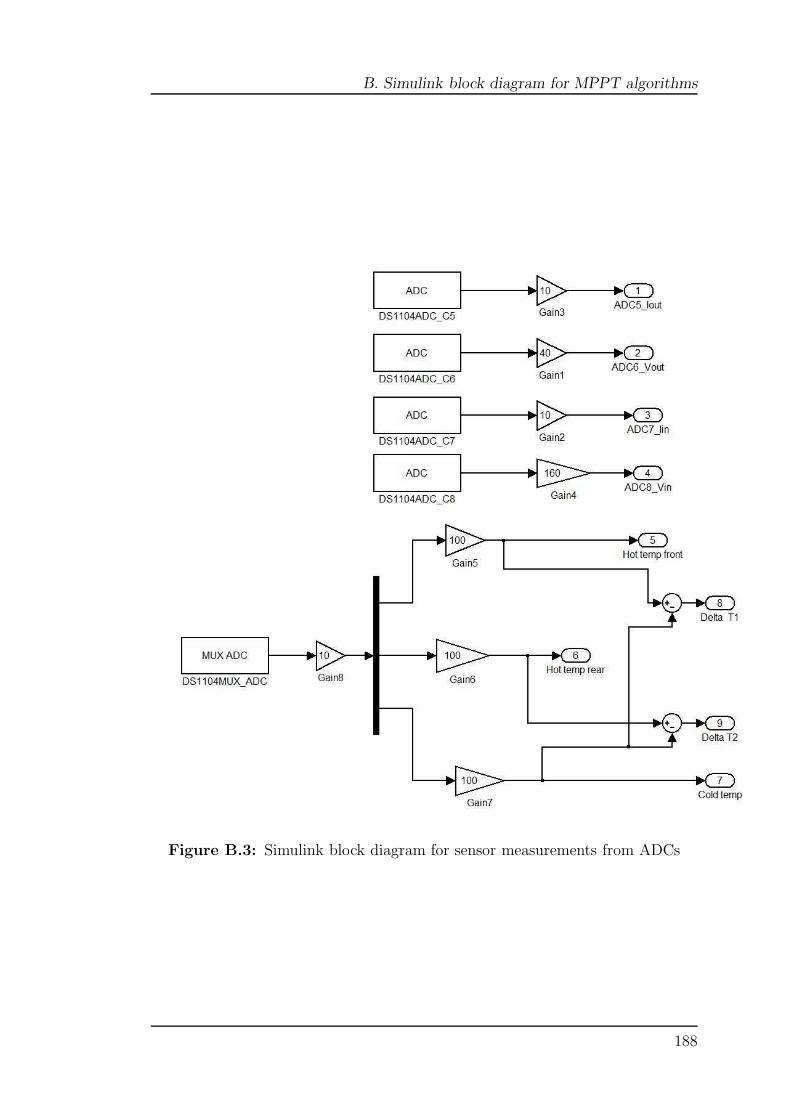
B. Simulink block diagram for MPPT algorithms
Figure B.3: Simulink block diagram for sensor measurements from ADCs
188
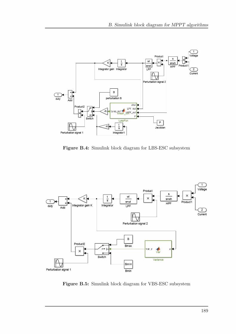
B. Simulink block diagram for MPPT algorithms
Figure B.4: Simulink block diagram for LBS-ESC subsystem
Figure B.5: Simulink block diagram for VBS-ESC subsystem
189

B. Simulink block diagram for MPPT algorithms
Figure B.6: Simulink block diagram for SDP-ESC subsystem
Figure B.7: Simulink block diagram for extended SDP-ESC subsystem
190
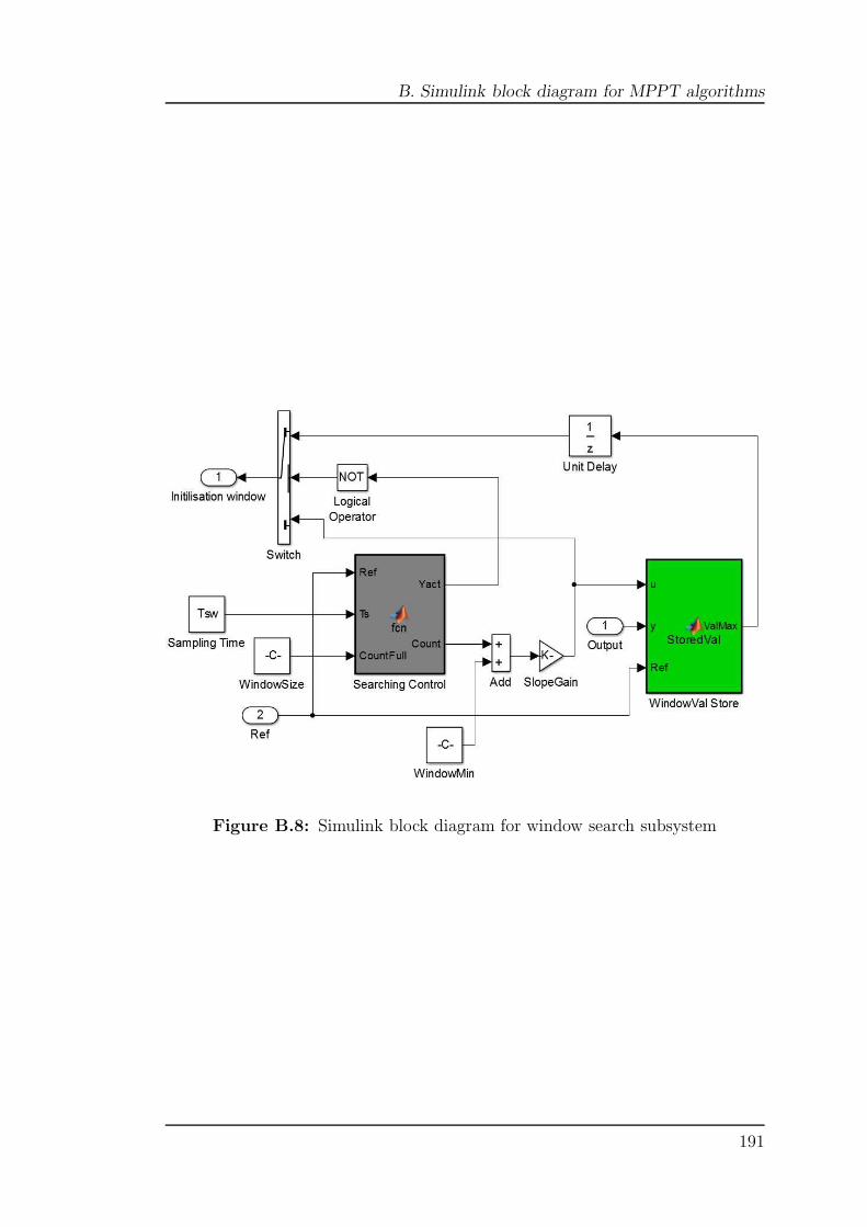
B. Simulink block diagram for MPPT algorithms
Figure B.8: Simulink block diagram for window search subsystem
191
Appendix C
Components/Instruments used in
the HIL set-up
This appendix presents instruments and components used in the HIL set-up via
dSPACE which are: Temperature control box, cartridge heater, synchronous DC-
DC converter and GM250-127-28-12 TE modules. The main information provided
in this appendix includes: the schematic diagram of the temperature control box
and the synchronous DC-DC converter also, data sheets for the heater cartridge
and the TE modules. Both schematics (i.e. the temperature control box and
synchronous DC-DC converter) comprises all components and these schematics
were used for designing the PCB layout.
192

C. Components/Instruments used in the HIL set-up
C.1 Cartridge heater and temperature control
box
Figure C.1: Schematic diagram of control box used in experiment test phase II
193

C. Components/Instruments used in the HIL set-up
Figure C.2: Specifications for cartridge heater block used in experiment phaseII
194

C. Components/Instruments used in the HIL set-up
C.2 Synchronous DC-DC buck-boost converter
Figure C.3: Schematic diagram of DC-DC buck-boost converter used for exper-iment tests
195

C. Components/Instruments used in the HIL set-up
C.3 GM250-127-28-12 TEMs characteristics
196
This material has been removed from this thesis due to Third Party Copyright. The unabridged version of the thesis can be viewed at the Lanchester Library, Coventry University.

C. Components/Instruments used in the HIL set-up
197
This material has been removed from this thesis due to Third Party Copyright. The unabridged version of the thesis can be viewed at the Lanchester Library, Coventry University.

C. Components/Instruments used in the HIL set-up
198
This material has been removed from this thesis due to Third Party Copyright. The unabridged version of the thesis can be viewed at the Lanchester Library, Coventry University.