An efficient branch-and-bound algorithm for the two-machine bicriteria flowshop scheduling problem

Journal of Manufacturing Systems Vol. 20/No. 2,

2001

An Efficient Branch-and-Bound Algorithm for the Two-Machine Bicriteria Flowshop Scheduling Problem W e i - C h a n g Yeh, Dept. of Industrial Engineering, Feng Chia University, Taichung, Taiwan. E-mail: wcyeh @ fcu.edu.tw

Abstract In this study, the two-machine bicriteria flowshop schedul-

ing problem is addressed. The objective is to minimize a weighted sum of total flowtime and makespan. Different branch-and-bound algorithms have already appeared in the literature for this problem. In this study, a more efficient branch-and-bound algorithm is presented. The proposed algorithm and the existing ones are compared on randomly generated problems. The computational analysis on problems up to 20 jobs shows that the proposed branch-and- bound algorithm is more efficient than the others, including the best-known algorithm. The upper bound used in the proposed branch-and-bound algorithm, a two-phase hybrid heuristic method, is also shown to be efficient. Its overall average error on the randomly generated problems is 0.000139, that is, almost equal to the optimal solution.

Keywords: Scheduling, Flowshop, Bicriteria, Branch-and- Bound Algorithm, Heuristic Algorithm

1. Introduction Machine scheduling has been a popular area of

research and received significant attention during the past four decades. ~6 The need for scheduling arises from the limited resources available to the decision maker. The primary task in the majority of flowshop scheduling problems is to determine the sequence of jobs for processing on a given set of machines.

The two-machine bicriteria flowshop scheduling problem considered here can be stated as follows. There is a set of n independent jobs {J~, J2, ..., J,} that must be scheduled in a two-machine flowshop. The processing time t o , which includes setup times for the job J /on machine j , i -- l, 2, ..., n , j = 1, 2, is known in advance. Let Cmax and F denote the makespan and flowtime, respectively. The objective is to minimize a linear combination of Cm,x and F, which can be denoted by etF + ~Cmax .7 The coeffi- cients c~ and 13 represent the weights associated with total flowtime and makespan (0 -< a -< 1, 0 -< 13 -<

1, and ot + 13 = 1), respectively. The jobs and machines are all continuously and simultaneously available from time zero onward. The jobs are mul- tistage in nature and are to be processed in the same order on each machine. Each job has two operations associated with it. The first operation is performed by the first machine and the second operation is performed by the second machine. There is an infinite buffer between the machines, but each machine cannot process two or more jobs at the same time. The total flowtime is the sum of flowtime of all jobs, where the flowtime of a job is defined to be the time the job spends in the system. The makespan is defined to be the completion time of the last job on the last machine.

When c~ -- 0, this problem reduces to a two- machine flowshop problem with the single objective of minimizing makespan. It is well known that this reduced problem can be solved using the Johnson's algorithm, s'9 However, if 0 < ~ -< 1, the problem is NP-hard? °'11 For further details on the complexity of general scheduling problems, the reader is referred to Lawler et al? 2 and Allahverdi, Gupta, and Aldowiasan.13

The two-machine flowshop problem has many applications in real life. For example, in the steel industry, each job undergoes wire drawing first and annealing next. Similarly, at the aggregate planning or macro level of manufacturing industries, each job must undergo fabrication first and assembly next. 3a

The two-machine flowshop scheduling problem with minimum makespan objective function was solved first by Johnson. 9 Since then, several gener- alized problems with solution methods have been proposed? a~s However, the two-machine flowshop problem with bicriteria of makespan and flowtime is only addressed by a few papers. Nagar, Haddock, and Heragu 3 were the first to address the two- machine flowshop problem with the weighted sum

113

Journal of Manufacturing Systems Vol. 20/No. 2 2001

of makespan and total flowtime criteria. Sivrikaya- Serifoglu and Ulusoy 14 also addressed the same problem but with the weighted sum of makespan and mean flowtime criteria instead of total flowtime. Nagar, Haddock, and Heragu 3 presented a branch- and-bound algorithm with one lower bound and one upper bound that works well for special cases. Both their lower bound and upper bound are obtained without considering the idle t ime of the remaining unscheduled jobs according to their shortest processing t ime sequence on machine 2 (SPT2). Therefore, the lower bound is underest imated and the upper bound is overestimated. This results in more iterations to determine the optimal schedule. In Yeh, ~9 both the lower-bound and upper-bound procedures proposed by Nagar, Haddock, and Heragu 3 were improved by adding the min imum idle time and completion time induced by the unscheduled jobs into the lower bounds. The computational analysis indicated that this whole branch-and-bound method can efficiently obtain optimal solutions for only small problems.

The purpose o f this paper is to develop a more efficient branch-and-bound algorithm to solve this problem. Tighter lower/upper-bound procedures, along with some powerful dominance rules and new methods of calculating these bounds, are implemented in the proposed branch-and-bound algorithm. To show the efficiency of the proposed branch-and-bound algorithm, it is compared to five different branch-and-bound algorithms, including the bes t -known a lgor i thm proposed in Yeh. 19 Computational analysis is conducted on problems with up to 20 jobs. The analysis shows the superiority o f the proposed branch-and-bound algorithm over the existing ones. The average error o f the upper bound on randomly generated problems is 0.00013, showing the efficiency of the upper bound.

2. Terminology and Problem Formulation

In the rest of this study, the following notation is used:

J~, JIn = job i and the job that occupies the position i in the sequence of jobs, respectively; i = 1, 2, ..., n;

t~, t[,1, i = processing time of J, and ./[,1 on machine j , respectively, where i = 1, 2, ..., n, j = 1, 2;

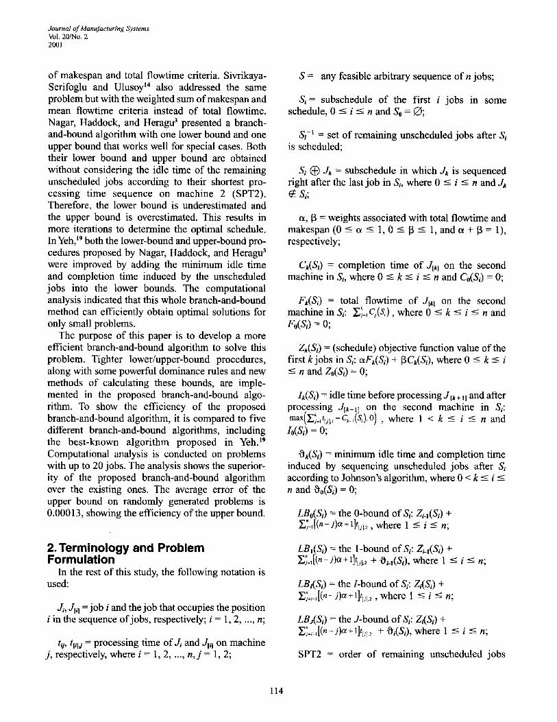
S = any feasible arbitrary sequence of n jobs;

St = subschedule o f the first i jobs in some schedule, 0 -< i -< n and So = Q~;

S, -~ = set of remaining unscheduled jobs after S, is scheduled;

S, Q Jk = subschedule in which Jk is sequenced right after the last job in S~, where 0 -< i -< n and Jk

s,;

tx, [3 = weights associated with total flowtime and makespan (0 -< oL <- 1, 0 ~ [3 ~ 1, and et + [3 = 1), respectively;

Ck(Si) = completion t ime of JIkl on the second machine in S,, where 0 -< k <- i -< n and Co(St) = 0;

Fk(S,) = total flowtime of Jl*l on the second machine in Si: Z~=, cj(s,), where 0 - k <- i -< n and Fo(S,) = O;

Zk(S,) = (schedule) objective function value o f the first k jobs in Si: etFk(S3 + [3Ck(St), where 0 -< k -< i -< n and Zo(S,) = 0;

Ik(S,) = idle time before processing JIk+ II and after processing Jtk-i] on the second machine in S,: max(Y.]=,%,-ck_,(s,),o), where 1 < k -< i -< n and

t0(s , ) = 0;

Ok(S,) = min imum idle time and completion time induced by sequencing unscheduled jobs after St according to Johnson's algorithm, where 0 < k --- i -- n and Oo(S,) = 0;

LBo(Si) = the 0-bound of Si: Zi.l(Si) + ~-~:,[(n-J)°t+l]tul.2 , where 1 -< i -< n;

LBI(Si) = the 1-bound of Si: Zl.l(Si) + ~-~=,[(n-J)°t+l]t[A2 + ~.~i.l(Si), where 1 -< i -< n;

LB,(St) = t h e / - b o u n d of St: Z,{Si) + E~=,+,[(n-j)a+qtH.2, where 1 <- i ----- n;

LBs(SI) = the J -bound of Si: Z,{St) + Y~=,+.[(n-J)a+l]ttjl.2 + O,{St), where 1 <- i <-- n;

SPT2 = order of remaining unscheduled jobs

114

Journal of Manufacturing Systems Vol. 20/No. 2

2001

according to their shortest processing time sequence on machine 2;

AX, 2XI -- upper-bound procedures proposed in the existing best-known method 19 and this study, respectively;

The problem considered here is to schedule n jobs on two machines and determine the optimal weighted combination of total flowtime and makespan so that the objective function3

zo ( s ) = aF. (S) + (S,) =

o~{~_~i"_,(n-i+ 1)[,[/1.2 +/, (S)]} +

fl{]~i~, ['[i].2 + Ii(S)]}

is minimized. Because c~ + 13 = 1, the objective function can be simplified as follows

Zn(S)= Y~in=l [(l~ -- i)0~ + 1][t[il, 2 + li(S) ]

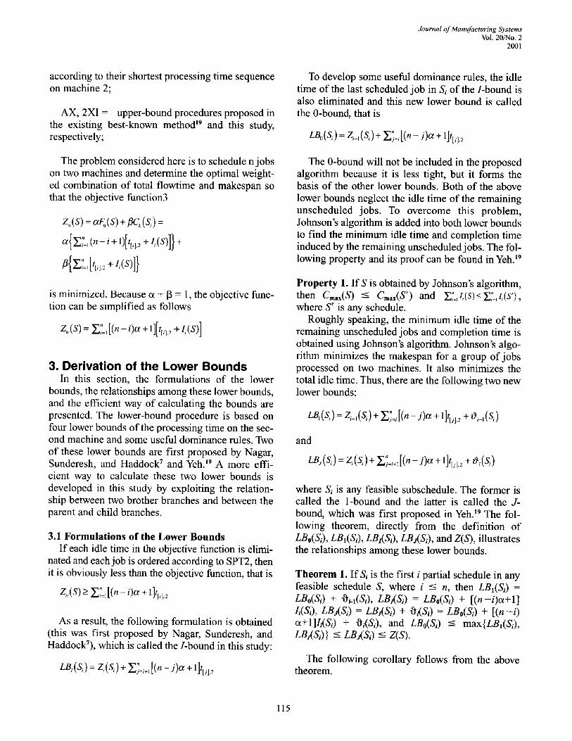
3. Derivation of the Lower Bounds In this section, the formulations of the lower

bounds, the relationships among these lower bounds, and the efficient way of calculating the bounds are presented. The lower-bound procedure is based on four lower bounds of the processing time on the second machine and some useful dominance rules. Two of these lower bounds are first proposed by Nagar, Sunderesh, and Haddock 7 and Yeh) 9 A more efficient way to calculate these two lower bounds is developed in this study by exploiting the relationship between two brother branches and between the parent and child branches.

3.1 Formulations of the Lower Bounds If each idle time in the objective function is elimi-

nated and each job is ordered according to SPT2, then it is obviously less than the objective function, that is

Z,,(S) > ~-~7=1 [(n - i)t~ + 1]t[il, 2

As a result, the following formulation is obtained (this was first proposed by Nagar, Sunderesh, and Haddock7), which is called the/-bound in this study:

.lt_ n LB~(S~)= Z~(Si) ]~j=i+,[(n-j)ot + l]t[j].2

To develop some useful dominance rules, the idle time of the last scheduled job in S~ of the/-bound is also eliminated and this new lower bound is called the 0-bound, that is

LBo( S, ) = Z,_, ( S~ ) + ]~=,[ (n - j)a + l lttj].:

The 0-bound will not be included in the proposed algorithm because it is less tight, but it forms the basis of the other lower bounds. Both of the above lower bounds neglect the idle time of the remaining unscheduled jobs. To overcome this problem, Johnson's algorithm is added into both lower bounds to find the minimum idle time and completion time induced by the remaining unscheduled jobs. The following property and its proof can be found in Yeh. 19

Property 1. If S is obtained by Johnson's algorithm, then Cm,~(S) -< Cmax(S') and Z7=,Ii(S)<_Z7=,I,(S'), where S' is any schedule.

Roughly speaking, the minimum idle time of the remaining unscheduled jobs and completion time is obtained using Johnson's algorithm. Johnson's algorithm minimizes the makespan for a group of jobs processed on two machines. It also minimizes the total idle time. Thus, there are the following two new lower bounds:

LBI(Si)= Zi_,(Si)+ ]~=~[(n- j )a + 1]t[d.2 + O~_,(Si)

and

LBj(Si)= Zi(Si)+ ]~=i+i [(n- j)a + 1]t[d.2 + O,(Si)

where S,. is any feasible subschedule. The former is called the 1-bound and the latter is called the J- bound, which was first proposed in Yehfl 9 The following theorem, directly from the definition of LBo(SI), LBI(SI), LBt(S3, LBs(SI), and Z(S), illustrates the relationships among these lower bounds.

Theorem 1. If Si is the first i partial schedule in any feasible schedule S, where i -< n, then LBI(S3 = LBo(Si) + Oi.l(Si), LBI(SI) = LBo(SI) + [(n-i)ot+l] I~($3, LBs(S3 = LB.(S3 + 0,{$3 = LBo(S3 + [ (n- i ) a+l]I,(S3 + O,{Si), and LBo(Si) <- max{LB,(Si). LB.(S3} <-- LB.(S3 <-- Z(S).

The following corollary follows from the above theorem.

115


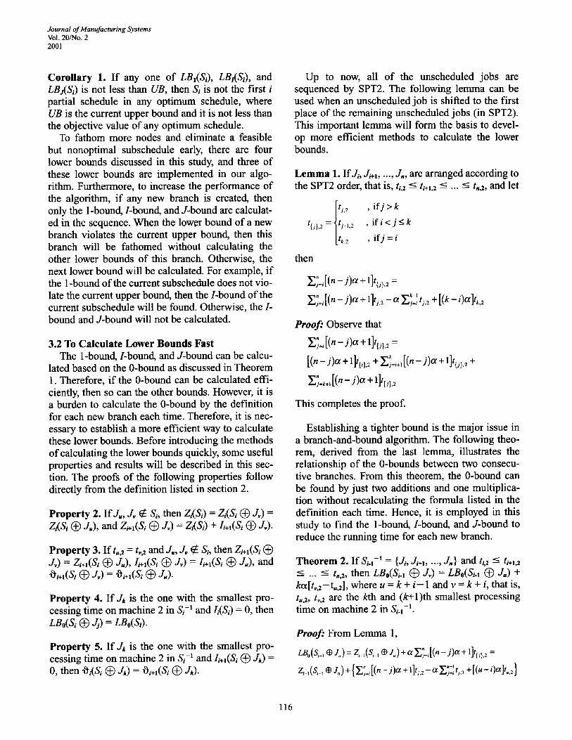
Corollary 1. If any one of LBI(Si), LB~(S~), and LBa(Ss) is not less than UB, then S~ is not the first i partial schedule in any optimum schedule, where UB is the current upper bound and it is not less than the objective value of any optimum schedule.

To fathom more nodes and eliminate a feasible but nonoptimal subschedule early, there are four lower bounds discussed in this study, and three of these lower bounds are implemented in our algorithm. Furthermore, to increase the performance of the algorithm, if any new branch is created, then only the 1-bound,/-bound, and J-bound are calculated in the sequence. When the lower bound of a new branch violates the current upper bound, then this branch will be fathomed without calculating the other lower bounds of this branch. Otherwise, the next lower bound will be calculated. For example, if the 1-bound of the current subschedule does not vio- late the current upper bound, then the/-bound of the current subschedule will be found. Otherwise, the I- bound and J-bound will not be calculated.

3.2 To Calculate Lower Bounds Fast The 1-bound,/-bound, and J-bound can be calcu-

lated based on the 0-bound as discussed in Theorem 1. Therefore, if the 0-bound can be calculated efficiently, then so can the other bounds. However, it is a burden to calculate the 0-bound by the definition for each new branch each time. Therefore, it is nec- essary to establish a more efficient way to calculate these lower bounds. Before introducing the methods of calculating the lower bounds quickly, some useful properties and results will be described in this section. The proofs of the following properties follow directly from the definition listed in section 2.

Property 2. IfJ., Jr then Z,(Ss) = Z,(S @ .Iv) = Z,(Si @ J.), and Zi+l(S i @ Jr) = Z,(Si) q'- Ii+l(Si @ Jr).

Property 3. If t~ a = tr,2 and J~, .Iv q~ Si, then Zi+l(S i @ Jr) = Zi+l(Si @ Ju), Ii+l(Si @ Jv) = / / + l ( S i @ Ju), and O~+,(S, @ .Iv) = O~+,(S, @ J~).

Property 4. If Jk is the one with the smallest processing time on machine 2 in S~ -~ and I,~S~) = 0, then LBo(Si @ J)) = LBo(Si).

Property 5. If Jk is the one with the smallest processing time on machine 2 in Si -1 and Ii+l(Si 0 Jk) = 0, then "[~t~Si @ Jk) = Oi+l(Si (~ Jk).

Up to now, all of the unscheduled jobs are sequenced by SPT2. The following lemma can be used when an unscheduled job is shifted to the first place of the remaining unscheduled jobs (in SPT2). This important lemma will form the basis to develop more efficient methods to calculate the lower bounds.

Lemma 1. Ifd~, d~_~, ..., J., are arranged according to the SPT2 order, that is, 6a <- 6+~,z <- ... <- t.a, and let

tj, , ifj > k

t{j}, 2 = Jtj_l, 2 , if i < j < k

| ttk,2 , ifj = i

then

X~=i[(n- j )a + 1]t{j}, z = k-I Z~=,[(n- j )a + 1]tj,: - Ot Y~j=i tj,: + [(k -i)~]t,, 2

Proof." Observe that

XT=/[(n- j)o~ + 1]t{)}, 2 =

[(n- j )a + 1]t{/), 2 + ~_,~=i+,[(n- j)ot + l]t{j}, 2 +

X~=,+, [(n- j )a + 1]tu},:

This completes the proof.

Establishing a tighter bound is the major issue in a branch-and-bound algorithm. The following theorem, derived from the last lemma, illustrates the relationship of the 0-bounds between two consecu- tive branches. From this theorem, the 0-bound can be found by just two additions and one multiplica- tion without recalculating the formula listed in the definition each time. Hence, it is employed in this study to find the 1-bound,/-bound, and J-bound to reduce the running time for each new branch.

Theorem 2. If SI.C ! = {J/, Ji+l, ..., Jn} and ti, 2 ~ //+i,2 < < t.,2, then LBo(Si.I @ .Iv) = LBo(Si., Q Ju) + ka[tr,2-tua], where u = k + i - 1 and v = k + i, that is, t~,:, tr,2 are the kth and (k+l)th smallest processing time on machine 2 in Si_1-L

Proof: From Lemma 1,

LBo(S,_ , ~ J.) = Z,_, (S,_, • J.) + a ~.~_, [(n - j)ot + 1]tu}.2 =

Zi-i (Si-1 ~ Ju ) + {X~=I [(• - J ) ~ + lltj,2 -- ~ ~ - i t,,2 + [ (u - i)otlt., 2 }

116


2001

where

] t~,~ , ifj > u

t{~}. 2=lt~_~,z , i f i < j < u

it,, z , ifj = i

and

LBo(Si_ , ~ J~) = Z~_, (Si_ , • J~) + o¢ ET:i[(n - j)o¢ + 1]~'~,~ :

Z ,(S_, ~) J~)+ {]~7=,[(n - j)o¢ + 1]t~, 2 -o~ ~'~-=it~,~ +[(v-i)oc]t~,~}

where

T j,2 I ts, 2 , ifj > v

, if i < j < v

I t , 2 , ifj = i

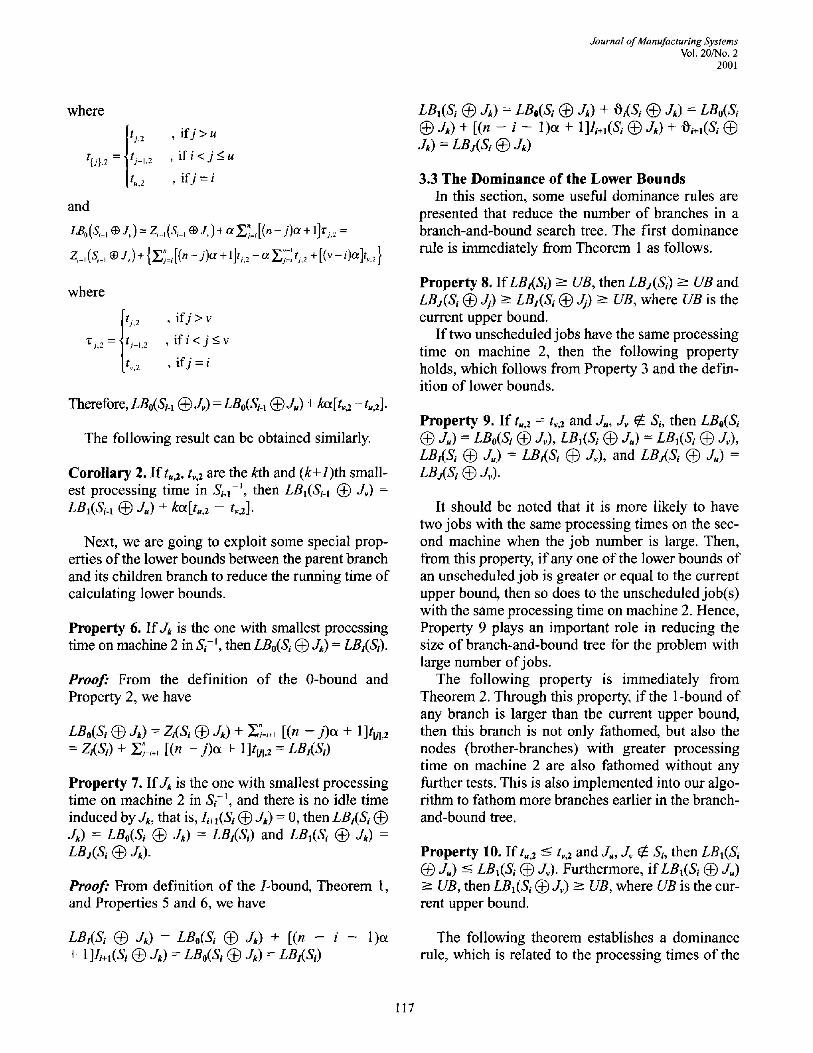
Therefore, LBo( S~., ~ Jv) = LBo( Si_~ ~ J.) + kcx[ tva - t.a ].

The following result can be obtained similarly.

Corollary 2. Ift~a, tva are the kth and (k+l) th smallest processing time in S/.~ -~, then LB~(Si.~ (~) JO = LB~(Siq (~ Ju) + kot[t.a - t~a].

Next, we are going to exploit some special properties of the lower bounds between the parent branch and its children branch to reduce the running time of calculating lower bounds.

Proper ty 6. IfJk is the one with smallest processing time on machine 2 in Si -1, then LBo(SI ~ Jk) = LBI(Si).

Proof: From the definition of the 0-bound and Property 2, we have

LBo(Si @ Jk) = Z,(Si (~ Jk) + Y~=,+, [(n -j)oL + l]tt/i. 2 = Z,(SI) + ~=,+, [(n - j )c~ + 1]tt/la = LBt(Si)

Property 7. IfJk is the one with smallest processing time on machine 2 in S~-1, and there is no idle time induced by J,, that is, li+~(Si (~ Jk) = 0, then LB~(S~ (~ Jk) = LBo(Si ~ Jk) = LB~(S~) and LB~(Sg @ Jk) = LBj(S, @ Jk).

Proof: From definition of the/-bound, Theorem 1, and Properties 5 and 6, we have

LB (Si @ Jk) = LBo(Si @ Jk) + [ ( n - - i - -

+ 1]I /+,(S, ® J , ) = LBo(S, @ = LB,(Si)

LB,(S~ (~ Jk) = LBo(S~ (~) Jk) + O,(Si (~ Jk) = LB,(S~ (~ Jk) + [(n - i - 1)~ + 1]//,,(Si (~ Jk) + Oi+,(Si (~ Jk) = LBj(S~ (~ Jk)

3.3 The D o m i n a n c e o f the Lower Bounds In this section, some useful dominance rules are

presented that reduce the number of branches in a branch-and-bound search tree. The first dominance rule is immediately from Theorem 1 as follows.

Property 8. If LB~(S~) >- UB, then LBj(S~) >- UB and LBj(S~ ~ Jj) >- LBt(Si ~ Jj) >- UB, where UB is the current upper bound.

If two unscheduled jobs have the same processing time on machine 2, then the following property holds, which follows from Property 3 and the definition of lower bounds.

Property 9. If t. a = tv, z and J,, Jv ~ Si, then LBo(Si @ J.) = LBo(S, @ Jv), LB,(S, (~ J.) = LB,(S~ @ J~), LB~S~ (~) J.) = LBt(S~ (~ J.), and LBs(Si 0 J.) = LBj(S~ (~ J.).

It should be noted that it is more likely to have two jobs with the same processing times on the second machine when the job number is large. Then, from this property, if any one of the lower bounds of an unscheduled job is greater or equal to the current upper bound, then so does to the unscheduled job(s) with the same processing time on machine 2. Hence, Property 9 plays an important role in reducing the size of branch-and-bound tree for the problem with large number o f jobs.

The following property is immediately from Theorem 2. Through this property, if the 1-bound of any branch is larger than the current upper bound, then this branch is not only fathomed, but also the nodes (brother-branches) with greater processing time on machine 2 are also fathomed without any further tests. This is also implemented into our algorithm to fathom more branches earlier in the branch- and-bound tree.

Property 10. If t.,z <- tv,2 and Ju, Jv ~ S, then LB~(S~ 0 J.) <- LB,(S~ (~ JO. Furthermore, ifLB,(S~ Q J.) >- UB, then LB~(Si • JO >- UB, where UB is the current upper bound.

The following theorem establishes a dominance rule, which is related to the processing times of the

117

Journal o f Manufacturing Systems Vol. 20/No. 2 2001

jobs on machine 1. It is not implemented in the proposed branch-and-bound procedure as a result of its heavy calculation requirements. However, it may be improved to establish a more powerful dominance rule in the future. The following result is established before presenting this dominance rule.

Lemma 2. I f LBo(Si @ 3",) <- UB and LBt(Si @ J,) >-- UB, then Ii+~(Si @ Jk) = Z'J=,tlJl,, + t,,2 - - Ci(Si (~ Jk) -- O, where J, ~ Si and UB is the current upper bound.

Proof: IfI~+,(Si @ A) = 0, then LB~(Si @ 3",) = LBo(S~ @ J',) + [(n - i + 1)or + 1]. Ii+,(S~ @ J,) = LBo(S~ @ 3",) < UB. This contradicts the fact that LB~(S~ @ 3",) > UB. Hence, it now follows that Im(S~ @ 3",) = max( Z,'mtH., + t,a - C,(Si @ J,), O) = E~,%, + t, a -C,(S~ @ J,) > O.

Theorem 3. Assume UBo = LBo(Si @ J,) <- UB, UBI UB - UB o

= ~-'~'j=,t[jl,, - - [ n - ( i + l ) ] a + l , andLB~(S~ (~J , ) >-- U B ,

where Jk ~ St and UB is the current upper bound. If t.,l >- C,(S~ @ J,) - UB~, then LBt(S~ @ J.) >- UB, where t,,~ <- t.,~ and for all J . ~ St.

Proof: If t.,, >-- C,(Si (~) 3",) - UB, = C,(Sa @ A) - UB-UBo

)"~=,tu],, + [n-(i+l)]ct+l , then Ii+,(Si @ du) = ~'~='ttJl,'

UB-UBo + tua -- C,(Si @ J,) >- [n- (i + 0]a + 1. Hence, UBo +

[(n - i + 1)oL + 1]Ii+l(Si @ J,) >-- UB. Moreover, LBo(S, @ J.) >- LBo(S, @ J,) = UBo for t,,, -< t. a. Thus, LBo(SI ~) J.) + [(n - i + 1)or + 1]Ii+l(Si (~ J.) >-- UBo + [(n - i + 1)a + 1]Im(S~ @ d.) >- UB

4. A Two-Phase Hybrid Heuristic Upper-Bound Procedure

A two-phase hybrid heuristic upper-bound procedure (2XI) is presented to compute an initial upper bound for the objective value of the problem at the beginning of the branch-and-bound algorithm. In the first phase, a simple greedy procedure is used to produce a feasible schedule. Then a procedure com- bining two known local improvement methods, the pairwise exchange and insert methods, is implemented in the second phase to improve the schedule obtained from the first phase.

The upper bound is updated each time a feasible schedule with a better upper bound is generated during the branching process. If the lower bound of a subschedule is not less than the current upper bound, then this subschedule cannot yield a better solution, and hence we need not continue to branch from the corresponding node in the search tree. The smaller the upper bound is, the more branches is eliminated. The proposed upper bound is shown to perform better than the best known bound? 9

4.1 First Phase of 2XI At the first phase of 2XI, an initial schedule is

constructed based on a simple greedy procedure. In this greedy procedure, the remaining unscheduled jobs are sequenced in consideration of both the processing time on each machine and the idle time induced after sequencing. The procedure of the first phase of 2XI is listed as follows.

Let T ,-- 0 and C *-- 0.

FOR p= 1 TO n If J / i s an unscheduled job such that ti, 1 + fi,2 +

Max(0, T + ha - C) --- tj,1 + tja + Max(0, T + tj,~ - C), where for all unscheduled jobs 3"~, then assign job i in the position p.

Let T ~ T + tia, and C ,-- C + Max(0, T + tia - C) + t/a.

NEXTp

4.2 Second Phase of 2Xl At the second phase, a hybrid method combin-

ing the pairwise exchange procedure and the insert procedure is employed to improve the initial schedule. In the pairwise exchange procedure, the positions of a pair of jobs are exchanged. In the insert procedure, a job is removed from its current position and inserted into the other positions. Assume that the current schedule is S. The second phase of 2XI is proceeded with the pairwise exchange procedure until the objective function value cannot be improved. The pairwise exchange procedure (XP) and the insert procedure (IP) are described as follows.

PROCEDURE XP

FOR a = 1 TO n

118


2001

FOR b = 1 TO n

Exchange the ath job to the bth job in S, and name this new schedule to be Sc (arab).

If Z(Sc) < Z(S) then S~- Sc, else proceed with the insert procedure IP.

NEXT b

NEXT a

RETURN

bound, then this node and all of its brother branches that have not been searched yet are eliminated by Property 10. Otherwise, the /-bound is calculated next by the method developed in Theorems 1 and 2 and Properties 3 and 4. If the/-bound of this new branch is less than the current upper bound, then the J-bound is calculated by Theorems 1 and 2 and Properties 3-5. Besides, if the/-bound or J-bound are violated the current upper bound, then the branch is fathomed by Property 8. Furthermore, if the current job is discarded and the next job has the same processing time on machine 2, then also eliminate this next job by Property 9.

PROCEDURE IP

FOR i = 1 TO n

FOR j--1 TO n

Remove the ith job in Sc and insert it into the j th position in Sc (i:~j).

Let the new schedule be St, and if Z(S1) < Z(Sc), then Sc , - S~.

N E X T j

NEXT i

If Z(Sc) < Z(S) then S ~-Sc.

RETURN

5. The Branch-and-Bound Algorithm This section outlines the proposed branch-and-

bound algorithm for solving the n/m/Flowshop/ c~F+~C~,a~ problem. The branch-and-bound algorithm uses the depth-first search (DFS) strategy to search the tree.

First, all jobs are arranged in SPT2. Then, the two-phase heuristic procedure provided in section 4 is applied to calculate the initial upper bound. The upper bound is updated whenever a feasible schedule that improves the upper bound is generated during the branching process. For each new node (branch) in the search tree, the 1-bound is calculated first by applying the method discussed in Corollary 2. If the 1-bound is larger than the current upper

6. Computational Results Two separate experiments are conducted to com-

pare the efficiency (running time) of the entire branch-and-bound algorithm proposed in this paper and the quality of its upper-bound procedure against the best-known existing method. All of the algorithms are coded in C++ and run on a Pentium II- 266 personal computer. The unit of the running time is the CPU second. Job processing times on each machine are randomly generated in discrete uniform distribution with the range U[10, 99].

6.1 Different Branch-and-Bound Algorithms No matter how efficient the bounds (lower and

upper) and dominance rules are, problems of a certain size can be solved by a branch-and-bound algorithm. Therefore, in our experimentation, we consider problems with n = 5, ..., 15. For each.job number, 10 problems have been generated and each problem is evaluated for various value of ot = 0.1, 0.2, ..., 1. It took almost no time to solve the problem when the total processing time on the second machine was greater than that of the first machine. As a result, to make a more practical experiment, the processing times on machines 1 and 2 were exchanged and then rerun for e~ = 0.1, 0.2, ..., 1. The branch-and-bound algorithm is evaluated at certain levels, resulting in six algorithms or methods (Methods 1-6), to show the effects of different lower and upper bounds and dominance rules. The entire branch-and-bound algorithm (including all the bounds and dominance rules) proposed in this study is called Method 1. To demonstrate the influence of the dominance of the lower bounds, Methods 2 and 3 are just like Method 1 but without implementing Properties 9 and 10,

119


respectively. Method 4 is the branch-and-bound algorithm proposed by Yeh. z9 To compare the efficiency and quality of the upper-bound procedures AX and 2XI, Method 5 uses AX with the proposed branch-and-bound procedure, and Method 6 uses 2XI with the branch-and-bound procedure proposed by Yeh, ~9 respectively.

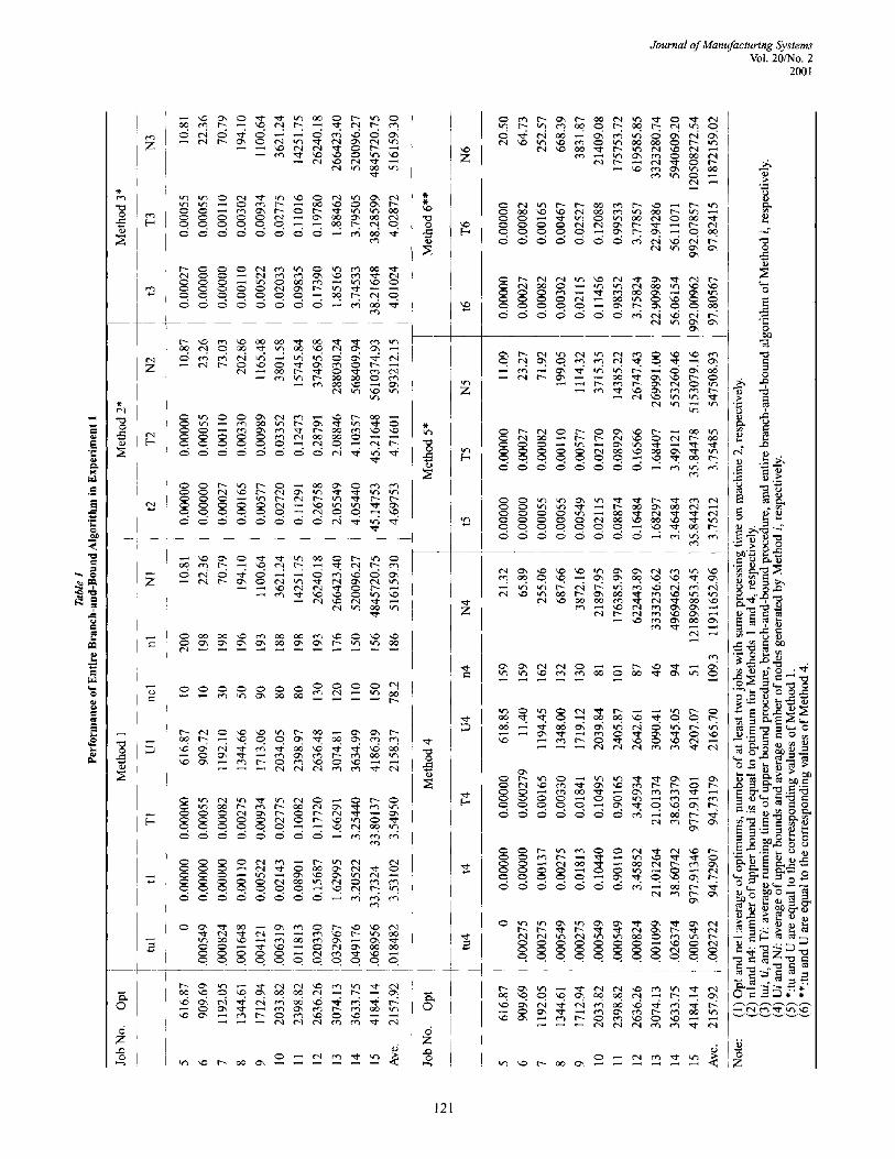
Table 1 provides the average CPU times for each of the six methods for each job number. The average number of nodes created by each of these methods is also measured and reported in Table 1. To evaluate the effectiveness of Property 10 and compare Method 1 to Method 2, the number of the cases when the processing times on the second machine being equal in each group problem is also listed in the last column.

Table 1 shows that the average CPU time and the number of nodes searched by Method 1 is increased slowly less than those of Method 2. This is due to the fact that the larger the number of jobs the more likely two jobs will have the same amount of processing time on machine 2. This increases the likelihood of Property 9 being satisfied. Moreover, Method 1 is also more effective that Method 3 as a result of the imple- mentation of Property 10. The comparison of Methods 1, 2, and 3 indicates the role of the lower bounds.

Table 1 illustrates that the proposed algorithm (Method 1) is not only better than the existing known algorithm (Method 4) in terms of running time and node fathoming, but also more efficient than both algorithms using the same upper bound (Methods 5 and 6).

6.2 Experiment on Maximum Job Number We also experimented with large-sized problems to

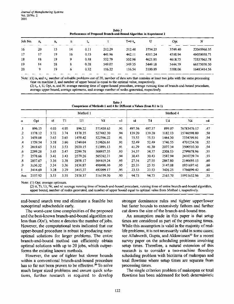
determine the maximum job number for a scheduling problem that can be solved by the proposed branch- and-bound algorithm. Table 2 presents the aggregated computational results tested on five group problems (for job numbers of 16, 17, ..., 20). Each group con- tained 20 data sets and all were run for ot = 0.5. To prevent excessive running time, the computation of a group was abandoned when it was not solved within the time limit of 1 hour. The results include the average running time in seconds, the average number of nodes created, the number of solved groups (out of 20), and the number of the upper bound generated by 2XI being equal to the optimum. Note that all of the above items in Table 2 do not include the results for the abandoned problems. Table 2 shows that the proposed branch-and-bonnd algorithm can almost solve

half of the problems up to job number is 20 with an average running time of 116.54 seconds and with the average nodes created as 16483414.56. The proposed branch-and-bound algorithm can solve larger problems (larger than 20 jobs) on a more efficient computer, for example a Pentium 4 processor machine or a supercomputer.

6.3 Influence of ot Finally, the influence of oL on the performance of

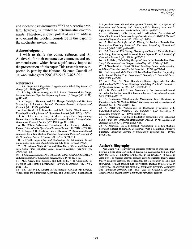
the algorithms is investigated. From the experiments of section 6.1, the corresponding result for different values of a, from 0.1 to 1 (in incremental steps of 0.1), were collected and compared in Table 3. In Table 3, there is a total of 220 different data sets for each eL. In Table 3, the following variables for both Methods of 1 and 4 are shown: average CPU time of both the upper-bound procedure and the branch-and- bound procedure, average upper bound, average number of nodes generated, and average number of the upper bound being equal to the optimum.

It can be seen from Table 3 that the running time and the number of nodes generated are the largest when ot = 0.1 for both Methods 1 and 4. This indicates the problem with a = 0.1 is the most difficult to solve. This is expected because the role of the total flowtime is not significant when (x = 0.1.

Both nl and n4 tend to increase as a increases. It is interesting to note that the gap between the upper bound and optimum reaches to the maximum for (x = 0.4 but not when (x = 0.1 for both methods. From Table 3, it can be seen that the running times of the upper-bound procedures of both methods are all less than 1 second on average. In particular, the values of tl and T1 are almost the same. Similarly, both values oft4 and T4 are almost the same. Hence, the running times of the upper-bound procedure of both methods are not significant.

In short, the above experimentations indicate the superiority of Method 1 in terms of both running time and the number of nodes searched.

7. Conclusions The two-machine flowshop scheduling problem

with bicriteria of makespan and total flowtime was addressed. A branch-and-bound algorithm based on powerful lower and upper-bound procedures was presented. Some dominance rules were also derived to fathom more unpromising nodes in the branch-

120


2001

. m

1 1

k

g ~ N ~ N ~ N N ~ N

m

q ~ q q q q q ~ ~ ~ ~ ~

m

...~.

121


Table 2 Performance of Proposed Branch-and-Bound Algorithm in Experiment 2

Job No. n, r~ n t, t T--t+t, U Opt N

16 20 15 14 0.11 212.29 212.40 3754.25 3749.40 22065966.35 17 17 19 16 0.15 441.96 442.11 4311.24 4310.94 46050038.71 18 18 19 9 0.18 552.79 552.96 4621.81 4618.75 73337665.78 19 14 18 8 0.28 549.07 549.35 5449.18 5444.79 66575070.50 20 9 19 6 0.32 116.22 116.54 5500.89 5500.06 16483414.56

Note : (1) n, and n,: number of solvable problems out of 20, number of data sets that contains at least two jobs with the same processing time on machine 2, and number of upper bound is equal to the optimal value, respectively. (2) tu, t, U, Opt, n, and N: average running time of upper-bound procedure, average running time of branch-and-bound procedure, average upper bound, average optimums, and average number of nodes generated, respectively.

Table 3 Comparison of Methods 1 and 4 for Different a Values (from 0.1 to 1)

Method 1 Method 4

et Opt tl T1 U1 N1 nl t4 T4 U4 N4 n4

.1 896.15

.2 1178.12

.3 1459.08

.4 1739.54

.5 2019.65

.6 2299.28

.7 2578.66

.8 2857.67

.9 3136.32 1 3414.69

4.03 4.05 8 9 6 . 3 2 571458.63 .91 3.72 3.74 1 1 7 8 . 3 5 527482.30 .94 3.63 3.65 1 4 5 9 . 4 2 522596.22 .91 3.58 3.60 1 7 4 0 . 0 4 519626.61 .91 3.51 3.53 2 0 2 0 . 1 5 513891.13 .91 3.45 3.47 2 2 9 9 . 7 8 508937.35 .93 3.41 3.43 2579.26 505392.21 .94 3.36 3.38 2 8 5 8 . 1 7 501619.24 .95 3.34 3.36 3 1 3 6 . 8 7 498490.10 .95 3.28 3.29 3 4 1 5 . 3 7 492099.17 .95

497.56 497.57 899.07 76783476.17 .47 139.20 1 3 9 . 2 0 1182 .13 15746598.00 .50 75.52 75.53 1 4 6 4 . 3 0 7334799.91 .54 52.49 52.49 1746 .55 4701234.58 .52 41.29 41.30 2027.34 3500510.30 .54 34.37 34.37 2 3 0 8 . 5 3 2799878.96 .55 30.43 30.43 2587.94 2410739.74 .55 27.54 27.55 2867.80 2140695.15 .60 25.35 25.35 3 1 4 7 . 0 8 1931697.41 .60 23.53 23.53 3 4 2 6 . 2 5 1766899.42 .60

Ave. 2157.92 3.53 3.55 2 1 5 8 . 3 7 516159.30 .93 94.73 94.73 2165.70 11911652.96 .55

Note: (1) Opt: average optimum. (2) ti, Ti, Ui, Ni, and ni: average running time of branch-and-bound procedure, running time of entire branch-and-bound algorithm, upper bound, number of nodes generated, and number of upper bound equal to optimal value from Method i, respectively.

and-bound search tree and el iminate a feasible but nonopt imal subschedule early.

The wors t -case t ime complexi t ies o f the p roposed and the bes t -known b ranch-and-bound a lgor i thm are less than O(n!) , where n denotes the number o f jobs. However , the computa t iona l tests indicated that our upper -bound procedure is robust in p roduc ing near- opt imal solut ions for larger problems. The entire b ranch-and-bound me thod can ef f ic ient ly obtain opt imal solut ions wi th up to 20 jobs , which outper- fo rms the exist ing known methods .

However , the use o f t ighter but slower bounds within a convent ional b ranch-and-bound procedure has so far not been proven to be effective. 20 To solve m u c h larger s ized problems and ensure quick solu- t ions , f u r the r r e sea rch is r equ i r ed to d ev e lo p

s t ronger dominance rules and t ighter upper / lower but faster bounds to extensively f a thom and fur ther cut down the size o f the b ranch-and-bound tree.

An assumption made in this paper is that setup t imes are considered as part o f the processing times. While this assumption is valid in the majori ty o f real- life problems, it is not necessari ly valid in some cases; see Allahverdi, Gupta, and Aldowiasan ma for a recent survey paper on the scheduling problems involving setup times. Therefore , a natural extension o f this research is to consider a two-machine f lowshop scheduling problem with bicriteria o f makespan and total f lowtime where setup t imes are separate f rom processing times.

The single cr i ter ion p rob lem o f makespan or total f lowt ime has been addressed for both determinis t ic

122


2001

and stochastic environments, z124 The bicriteria problem, however, is limited to deterministic environments. Therefore, another potential area to address is to extend the problem considered in this paper to the stochastic environments.

Acknowledgment I wish to thank the editor, referees, and Ali

Allahverdi for their constructive comments and rec- ommendations, which have significantly improved the presentation of this paper. This research was sup- ported in part by the National Science Council of Taiwan under grant NSC 87-2213-E-025-001.

References 1. S.K. Gupta and J. Kyparisis, "Single Machine Scheduling Research,"

Omega (v15, 1987), pp207-227. 2. "I.D. Fry, R.D. Armstrong, and H.A. Lewis, "Framework for Single

Machine Multiple Objective Sequencing Research," Omega (v17, 1979), pp595-607.

3. A. Nagar, J. Haddock, and S.S. Heragu, "Multiple and Bicriteria Scheduling: A Literature Review," European Journal of Operational Research (v81, 1995), pp88-104.

4. R.A. Dudek, S.S. Panwalker, and M.L. Smith, "The Lessons of Flowshop Scheduling Research," Operations Research (v40, 1992), pp7-13.

5. W.J. Selen and D. Hott, "A Mixed Integer Goal Programming Formulation of the Standard Flowshop Scheduling Problem," Journal of the Operational Research Society (v37, 1986), pp 1121 - 1128.

6. J.M. Wilson, "Alternative Formulations of a Flowshop Scheduling Problem," Journal of the Operational Research Society (v40, 1989), pp395-399.

7. A. Nagar, S.H. Sunderesh, and J. Haddock, "A Branch-and-Bound Approach for a Two-Machine Flowshop Scheduling Problem," Journal of the Operational Research Society (v46, 1995), pp721-734.

8. S, French, Sequencing and Scheduling: An Introduction to the Mathematics of the Job-Shop (Chichester, UK: Ellis Horwood, 1982).

9. S.M. Johnson, "Optimal Two and Three-Stage Production Schedules with Setup Times Included," Naval Research Logistics Quarterly (vl, 1954), pp61-68. 10. T. Gonzalez and T. Sen, "Flowshop and Jobshop Schedules: Complexity and Approximations," Operations Research (v26, 1978), pp36-52. 11. M.R. Garey, D.S. Johnson, and R.R. Sethi, "The Complexity of Flowshop and Jobshop Scheduling," Operations Research (v l, 1976), pp117-129. 12. E.L. Lawler, L.K. Lenstra, A.H.G. Rinnooy Kan, and D.B. Shmoys, "Sequencing and Scheduling: Algorithms and Complexity," in Handbooks

in Operations Research and Management Science, Vol. 4, Logistics of Production and Inventory, S.C. Graves, A.H.G. Rinnooy Kan, and P. Zipkin, eds. (Amsterdam: North-Holland, 1993), pp455-522. 13. A. Allahverdi, J.N.D. Gupta, and T. Aldowiasan, "A Review of Scheduling Research Involving Setup Considerations," OMEGA The lnt'l Journal of Mgmt. Sciences (v27, 1999), pp219-239. 14. E Sivrikaya-Serifoglu and G. Ulusoy, "A Bicriteria Two-Machine Permutation Flowshop Problem," European Journal of Operational Research (v107, 1998), pp414-430. 15. D.R. Sule and K.Y. Huang, "Sequency on Two and Three Machines with Setup, Processing and Removal Times Separated," lnt'l Journal oJ Production Research (v21, 1983), pp723-732. 16. K.R. Baker, "Scheduling Groups of Jobs in the Two-Machine Flow Shop," Mathematical and Computer Modeling (v13, 1990), pp29-36. 17. T. Yoshida and K. Hitomi, "Optimal Two-Stage Production Scheduling with Setup Times Separated," AllE Trans. (vl 1, 1979), pp261-263. 18. D.-L. Yang and M.-S. Chern, "A Two-Machine Flowshop Sequencing with Limited Waiting Time Constraints," Computers & Industrial Engg. (v28, 1995), pp63-70. 19. W.C. Yeh, "A New Branch-and-Bound Approach for the n/2/Flowshop/"a"F+"b"C,,.~ FIowshop Scheduling Problem," Computers & Operations Research (v26, 1999), pp 1293-1310. 20. C.N. Potts and L.N. van Wassenhove, "A Branch-and-Bound Algorithm for the Total Weighted Tardiness Problem," Operations Research (v33, 1985), pp363-77. 21. A. Allahverdi, "Stochastically Minimizing Total Flowtime in Flowshops with No Waiting Space," European Journal of Operational Research (v113, 1999), ppl01-112. 22. A. Allahverdi, "Scheduling in Stochastic Flowshops with Independent Setup, Processing, and Removal Times," Computers & Operations Research (v24, 1997), pp955-960. 23. A. Allahverdi, "Two-Stage Production Scheduling with Separated Setup Times and Stochastic Breakdowns," Journal of the Operational Research Society (v46, 1995), pp896-904. 24. A. Allahverdi and J. Mittenthal, "Scheduling on a Two-Machine Flowshop Subject to Random Breakdowns with a Makespan Objective Function," European Journal of Operational Research (v81, 1995), pp376-387.

Author's Biography Wei-Chang Yeh is currently an associate professor of industrial engi-

neering at Feng Chia University in Taiwan. He received his MS and PhD from the Dept. of Industrial Engineering at the University of Texas at Arlington. His research interests include network reliability theory, graph theory, deadlock problem, and scheduling. He is a member of IEEE and INFORMS. He has published in such prestigious journals as the Journal oJ Algorithms, the International Journal of Production Research, Computers and Operations Research, and IEEE Trans. on Reliability, Reliability Engineering & System Safety, Control and Intelligent Systems.

123

Documents

An efficient branch-and-bound algorithm for the two-machine bicriteria flowshop scheduling problem