APE: An Automated Performance Engineering Process for Software as a Service Environments Jerry Rolia, Diwakar Krishnamurthy, Min Xu, and Sven Graupner

HP Laboratories HPL-2008-65 Keyword(s): Benchmarking, Business Applications, Performance Sizing, Optimization, Software as a Service. Abstract: The Software as a Service (SaaS) paradigm is changing the way in which businesses procure software solutions. A service provider hosts the software solution amortizing management and infrastructure costs across the businesses it serves. For complex software offerings, each business may use a given software platform in very different ways. This need for customization can pose performance challenges and risks for those hosting the software as a service. This paper presents an Automated Performance Engineering (APE) process for transaction oriented enterprise applications that supports infrastructure selection, sizing, and performance validation for customized service instances in hosted software environments. It enables the rapid deployment of a customized service instance while lowering performance related risks by automating the creation of a customized performance model and customized benchmark model. Case study results demonstrate the effectiveness of the approach for a TPC-W system.

External Posting Date: June 7, 2008 [Fulltext] Approved for External Publication

Internal Posting Date: June 7, 2008 [Fulltext]

© Copyright 2008 Hewlett-Packard Development Company, L.P.

1

1Hewlett Packard Labs, Bristol, UK, 2University of Calgary, AB, Canada, 3Hewlett Packard Labs, Palo Alto, CA, USA {jerry.rolia@hp.com, dkrishna@ucalgary.ca, m.xu@ucalgary.ca, sven.graupner@hp.com}

Abstract-- The Software as a Service (SaaS) paradigm is changing the way in which businesses procure software solutions. A service provider hosts the software solution amortizing management and infrastructure costs across the businesses it serves. For complex software offerings, each business may use a given software platform in very different ways. This need for customization can pose performance challenges and risks for those hosting the software as a service. This paper presents an Automated Performance Engineering (APE) process for transaction oriented enterprise applications that supports infrastructure selection, sizing, and performance validation for customized service instances in hosted software environments. It enables the rapid deployment of a customized service instance while lowering performance related risks by automating the creation of a customized performance model and customized benchmark model. Case study results demonstrate the effectiveness of the approach for a TPC-W system.

Index Terms--Benchmarking, Business Applications, Performance Sizing, Optimization, Software as a Service.

I. INTRODUCTION

t is anticipated that by 2015 more than 75% of information technology (IT) infrastructure will

be purchased as a service from external and internal hosting providers [1]. There are many

reasons for this trend. Those businesses that need IT infrastructure can acquire it quickly, with

lower deployment risks, capital expenditures, and a reduced need for certain IT skills. Service

providers can offer services with greater process maturity and improved efficiency while

amortizing infrastructure and labor costs across the many businesses that they serve. For service

providers to be successful this paradigm requires a great deal of automation to reduce human

effort. Ideally, the incremental effort to support each additional instance of Software as a Service

(SaaS) should approach zero. This paper describes an Automated Performance Engineering

(APE) process that reduces performance risks associated with hosting customized enterprise

applications. In particular the process chooses an appropriate infrastructure alternative, estimates

quantities of resources needed to satisfy service level expectations, and creates a performance

validation test for a deployed system.

There are many kinds of IT infrastructure offered as a service. Servers, storage, and networking

can be offered by internal corporate IT providers or Internet service providers [2]. Email, word

Jerry Rolia1, Diwakar Krishnamurthy2, Min Xu2, and Sven Graupner3

APE: An Automated Performance Engineering Process for Software as a Service Environments

I

2

processing, and other desktop functionality are now offered by many providers [3]. More

complex enterprise applications are also offered as a service [4][5][6]. These support business

processes such as customer relationship management and supply chain management. Our focus is

on complex transaction oriented enterprise applications where different customized instances of a

service can cause significantly different resource usage, and, on mass service providers that aim to

offer services to a very large number of businesses.

For today’s mass service providers, at best, service level agreements include service uptime

guarantees. Performance is rarely addressed. However, performance will become more critical as

the SaaS paradigm matures to support key business functions, high transaction rates, and supply

chain management for all sizes of business. SaaS providers will require systematic methods for

characterizing the performance of new application instances, their impact on shared resource

environments, and the impact of changes to the applications or other aspects of the SaaS platform

on performance for the businesses that use the service. It is important for mass service providers

to fully exploit their resources to reduce their own costs, including facilities and power. As a

result, understanding the initial resource needs of a service instance, understanding the impact of

changes to requirements for a service instance upon resource needs, and understanding the impact

of changes to a software platform on resource needs are all important issues for service providers.

For this paper, we define sizing as a method for estimating the resources needed by a service

instance to satisfy its mean response time requirements.

The classic approach for sizing enterprise applications exploits a small number of software

vendor specific benchmarks that stress key components of the vendor’s software platform upon

infrastructure alternatives. An infrastructure includes the servers, networking, storage, and

operating systems that support the platform. The results of the benchmark runs are not meant to

predict how any business’s customized application instance would behave, but instead aim to

categorize the relative capacities of various infrastructure design alternatives. For example, certain

infrastructures may support small, medium, and large numbers of benchmark users by exploiting

features of hardware and software platforms. A business with a medium number of users would

tend towards the infrastructure alternative that supports the medium number of users.

When performance and cost are considered as risks, more sizing effort is required. Experts with

software performance engineering and performance modeling experience [7][8] and knowledge of

3

how a business is expected to use a software platform work with hardware platform vendors to

derive precise sizing estimates. This usually involves characterizing how a business will use the

platform’s business objects, i.e., software modules. The business object mix reflects the

customized use of the platform. However, the manual and hence expensive nature of such

exercises limits their use. Automated methods are needed to reduce performance and cost related

risks for mass service providers.

The APE approach was developed to support the Model Information Flow (MIF) paradigm for

automated SaaS configuration, deployment, and on-going management [9]. The MIF approach

was developed as part of a joint research project on SaaS by Hewlett Packard Labs and SAP

Research.

APE differs from the classic approach for sizing enterprise applications. It relies upon a larger

number of benchmarks that is proportional to the number of business objects supported by a

platform. Each benchmark aims to capture the impact of a set of business objects on performance

as well as the impact of software platform features. A distinct feature of APE is that it does not

directly attempt to characterize the resource usage of each business object separately but instead

aims to consider the natural joint use of multiple business objects to execute typical use cases for

the platform. We exploit a workload matching technique [10] to relate the expected usage of

business objects for a particular business to a specific ratio of the benchmarks. In effect, we reuse

the results from the large number of benchmarks to support many different performance modeling

exercises. The technique enables the creation of customized performance models for a business

that are used to choose among the infrastructure design alternatives and to estimate the numbers

of resources needed for each alternative. Furthermore, it enables the creation of customized

benchmark model that matches the expected usage of business objects but is synthesized using a

combination of the pre-existing benchmarks. The customized benchmark can be run against a

corresponding deployed system to validate a design and support a final tuning exercise. Case

study results from two distinct TPC-W [34] systems show that the approach is able to predict the

resource demands and mean response time for one use of the system based on benchmark runs

that stress other uses of the system.

The remainder of the paper is organized as follows. Section II describes related work. Section

III introduces a model-driven provisioning process that gives the context for APE and explains

4

the models APE employs. Section IV discusses how APE uses the models to implement its

automated performance engineering process. A case study is offered in Section V that

quantitatively verifies and validates the modeling techniques used by APE. Summary and

concluding remarks are given in Section VI.

II. RELATED WORK This section covers a range of topics that contribute to automated performance engineering for

SaaS. These include benchmarking, workload generation, performance models, software

performance engineering, automatic model generation, regression, as well as topics that relate to

SaaS including tenancy models and model-driven automation.

Benchmarking is a well accepted method for evaluating the behaviour of software and hardware

platforms [11]. In general, the purpose of benchmarking is to rank the relative capacity,

scalability, and cost/performance of alternative combinations of software and hardware. It does

not attempt to directly predict performance behaviour for any customized use of platforms.

Instead, benchmarks aim to stress key features of platforms that are likely to be bottlenecks.

Dujmovic describes benchmark design theory that models benchmarks using an algebraic space

and minimizes the number of benchmark tests needed to provide maximum information [12].

Dujmovic’s seminal work also informally describes the concept of interpreting the results of a

ratio of different benchmarks to better predict the behaviour of a customized system but no formal

method is given to compute the ratio. Krishnaswamy and Scherson [13] also model benchmarks

as an algebraic space but also do not consider the problem of finding such a ratio.

Krishnamurthy et al. [10] [14] introduce SWAT which includes a method that automatically

selects a subset of pre-existing user sessions from a session based e-commerce system, each with

a particular URL mix, and computes a ratio of sessions to achieve specific workload

characteristics. For example, the technique can reuse the existing sessions to simultaneously

match a new URL mix and a particular session length distribution and to prepare a corresponding

synthetic workload to be submitted to the system. They showed how such workload features

impact the performance behaviour of session based systems. APE exploits the ratio computation

technique in this work to automatically compute a ratio of benchmarks that enables the creation of

customized performance and benchmark models for a service instance. However, APE is more

than the use of the ratio computation technique. APE is the overall approach for organizing and

5

exploiting various kinds of model information to enable automated performance engineering.

Queuing Network Models (QNM) have been used as predictive models for enterprise

computing systems since the early 1970’s [15][16]. Predictive models such as Layered Queuing

Models (LQM) [17][18] enhance queuing network models by taking layered software interactions

into account. These include synchronous and asynchronous interactions between client, web,

application logic, and database servers and have been shown to improve the accuracy of

performance predictions for multi-tier environments [19]. Tiwari et al. [20] report that layered

queuing networks were more appropriate for modeling a J2EE application than a Petri-Net based

approach [20] because they better addressed issues of scale. Balsamo et al. [21] conclude that

extended QNM-based approaches, such as layered queuing models, are the most appropriate

modeling abstraction for multi-tiered software environments. The customized performance models

we consider in this paper are LQMs.

Software performance engineering (SPE) offers a systematic approach that supports the design

and sizing of enterprise software systems [7]. Software control flow diagrams are used to describe

execution paths through software modules that cause the use of system resources, e.g., CPU and

memory. Modules that are expected to affect performance most are considered in greatest detail.

The resulting information is used to create predictive performance models. By representing

control flow and resource usage, the impact of software design or hardware changes on

performance can be explored. Vetland [22] considers the challenge of systematically creating a

library of resource demand models for a system’s software components so that they can be

integrated through SPE based methods to support design and sizing. Hrischuk et al. [23] and Qin

et al. [39] explore methods for automating the capture of control flow in software design

environments and support automated model building. Petriu et al. [24] consider the use of UML

and other techniques to better enable software designers to directly exploit performance

engineering concepts.

SPE related techniques all require methods to predict the resource demands of software

components. However, predicting the resource demands of business objects in a software system

is a challenging task. The two main reasons are: CPU and input-output usage are not typically

measured with respect to software operations; and, per request demands are not deterministic.

Measurement is difficult because today’s application servers are complex. They are typically

6

multi-threaded, execute on hosts that often have multiple CPUs, may execute on virtualized hosts,

and have many layers of caching that frequently delay input-output activity. Furthermore,

demands by requests for the same operation can often cause very different resource demands

depending on the state of the system. For this reason it is very difficult to create reusable resource

demand models for software components that can be composed to reflect specific behaviours.

Many researchers have looked towards statistical regression to estimate resource demands. The

earliest work we are aware of is from Bard who used regression techniques to estimate difficult to

measure CPU demand overheads in a virtualized mainframe environment [25]. Rolia, Vetland, and

Sun used Ordinary Least Squares (OLS) [26] and the Random Coefficients Method (RCM) for

regression [27] to estimate per-method resource demands for objects with many methods to

support the creation of LQMs. RCM aims to overcome issues of non-determinism in demands.

However, they found the general use of regression methods for the characterization of demands

to be problematic because the assumptions of regression are violated, e.g., deterministic

distribution for per-request demands. Furthermore, it can be difficult to decide how to group data

for the regression. Stewart et al. considered Least Absolute Residual (LAR) regression techniques

to predict demands for systems with different request types [28]. A case study showed good

results when characterization could be done under conditions where there was little contention for

system resources, which they note is often the case for production environments. They also

integrate an ad-hoc queuing formula into the regression formula to also predict response times.

For the data they considered, they found that characterizing the demands for different types of

requests enabled better utilization predictions than not distinguishing demands by request type,

that using LAR worked better than OLS, and that their response time prediction technique

behaved best for systems with low utilization levels. Zhang et al. apply a non-negative OLS

regression technique to estimate the per-URL demands of a TPC-W system [29]. They used the

demand estimates to create a simulation model and a QNM for the system. The simulation and

QNM models resulted in similar prediction accuracy. Both predicted the throughput of emulated

users often up to high system utilization. Mean response time estimates were not compared with

measured values for the analytic model.

APE differs from the straightforward application of SPE and doesn’t have to use a regression

technique to predict demands. In contrast to SPE, APE focuses on system configuration and

7

sizing through the selection of pre-existing business processes rather than on software design from

scratch. We assume that each business process has a pre-existing control flow model that

describes its expected execution of business process steps – based on the usage behaviour of other

SaaS service instances. However, SPE complements APE. If typical control flows are not

representative of how a particular business will use business processes, they can be altered using

SPE techniques. The resulting control flows and impact would automatically be taken into

account by APE.

The APE process helps to overcome the demand estimation problem by raising the abstraction

level and predicting resource demands aggregated over many business objects rather than

predicting per-business object resource demands. Business objects are rarely used in isolation so it

can be difficult to characterize them separately and then predict their joint resource usage. Our

new approach to demand estimation is evaluated later in the paper.

We now consider issues relating to SaaS and model-driven automation. There are several

different paradigms for how service instances can be rendered into shared resource environments.

These can be classified as multi-tenancy, isolated-tenancy, and hybrid-tenancy [30] . Multi-

tenancy hosts many service instances on one instance of a software platform. Isolated-tenancy

creates a separate service platform for each service instance. A hybrid may share some portion of

a platform such as a database across many service instances while maintaining isolated application

servers. Multi-tenancy systems can reduce maintenance and management challenges for service

providers, but it can be more difficult to ensure customer specific service levels. Isolated-tenancy

systems provide for greatest opportunity for customization, performance flexibility and greatest

security, but present greater maintenance challenges. Hybrid-tenancy approaches have features of

both approaches. This paper focuses on isolated-tenancy systems that operate in shared

virtualized resource pools. However, the technique could also be adapted to reduce the

performance related risks of the multi-tenancy and hybrid-tenancy paradigms as well.

Model-driven techniques have been considered by many researchers and exploited in real world

environments [4][6]. In general, the techniques capture information in models that can be used to

automatically generate code, configuration information, or changes to configuration information.

The general goal of model-driven approaches is to increase automation and reduce the human

effort needed to support IT systems. Automation reduces costs, decreases the likelihood of errors

8

when making changes to systems, and increases the rate at which systems are able to adapt based

on business needs. The MIF approach presented in Section III describes a model-driven approach

for provisioning enterprise applications in a SaaS environment [9]. It aims to automate many of

the tasks associated with configuring, deploying, and maintaining enterprise applications

according to the SaaS paradigm. APE was developed to support the MIF approach. Zhang et al.

[31] describe a policy driven approach for specifying configuration alternatives for service

instances.

III. MODEL DRIVEN PROVISIONING

This section describes a model-driven provisioning approach for hosting SaaS service instances.

The approach implements a Model Information Flow (MIF) that provides the context for APE

[9]. The MIF presents a sequence of models and model transformations that support lifecycle

management for information about a service instance. It captures requirements for a service

instance, information about software platforms that may implement the instance, alterative feasible

infrastructure designs, and information about a shared environment for hosting service instances.

Model transformations support the manipulation of information about a service instance as it

traverses its lifecycle. This section describes pertinent models and transformations that explain the

following.

• How to choose an infrastructure design alternative for a service instance and estimate its

number of resource instances so that it meets throughput requirements and response

time goals.

• How a performance validation test can be deduced for a deployed service instance.

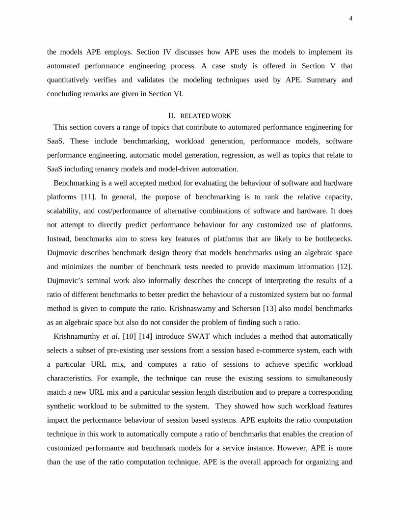
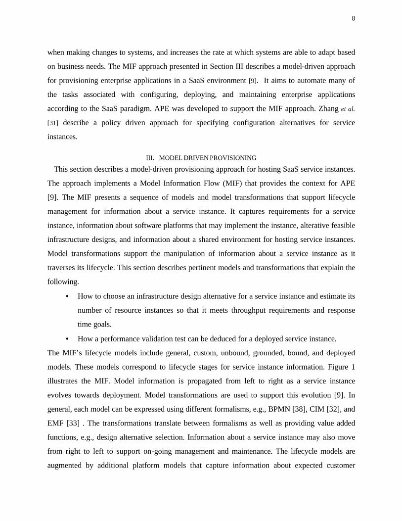
The MIF’s lifecycle models include general, custom, unbound, grounded, bound, and deployed

models. These models correspond to lifecycle stages for service instance information. Figure 1

illustrates the MIF. Model information is propagated from left to right as a service instance

evolves towards deployment. Model transformations are used to support this evolution [9]. In

general, each model can be expressed using different formalisms, e.g., BPMN [38], CIM [32], and

EMF [33] . The transformations translate between formalisms as well as providing value added

functions, e.g., design alternative selection. Information about a service instance may also move

from right to left to support on-going management and maintenance. The lifecycle models are

augmented by additional platform models that capture information about expected customer

9

usage, and configuration and performance information about the vendor specific software and

infrastructure platforms that ultimately realize the service instance. In this paper we focus on the

models and transformations that explain the APE approach to automated performance engineering

for transaction oriented enterprise applications and SaaS.

Fig. 1: The Model Information Flow

The general model describes business processes that can be deployed in an automated manner.

It is a collection of business process models. Each business process model may have many

variants and configuration alternatives that are captured in its model. Each variant has business

process steps that must be realized by a software platform. Sales and distribution is an example of

a business process. It may have business process variants that deal with orders, with orders for

preferred customers, and with returns. Its business process steps may require information about

items, may update an order, and may cause an order to ship.

The custom model includes only those business process variants needed by a particular service

instance for a business. Additional business specific information is included in the customized

model that expresses non-functional requirements such as each chosen variant’s expected

throughput and mean interactive response time goal.

The unbound model elaborates further on how software platforms implement the chosen

business process variants. This model relates the variants to software platform business objects

and technologies needed to implement the variants, e.g., Web servers, application logic servers,

general

custom

unbound

grounded

bound

deployed

Software platform model

Infrastructure design alternative model

Software platform benchmark model

Benchmark infrastructurealternative model

Business processcontrol flow model

10

and database servers.

The grounded model is a design for the system. It relates the unbound model to a particular

infrastructure configuration alternative from a catalog of feasible alternatives that can be

automatically deployed to the shared environment. The grounded model includes estimates for the

number of resource instances needed to support non-functional requirements. In includes

sufficient information to enable the deployment of the service instance.

The bound model captures the assignment of real resource instances from a shared resource

environment to the service instance. Bound resource instances are configured with software

needed to participate in the software platform and management software needed to support on-

going management.

The deployed model describes resource instances participating in an operational service

instance. Finally, we note that a service for a business may have several deployed instances

operating in parallel. Different instances may correspond to development, testing, and production

environments. For example, a deployed service instance may be used for a performance validation

test then discarded.

Platform models augment the lifecycle models with vendor specific platform information. As

examples of platform models, we introduce the following: business process control flow model;

software platform model; software platform benchmark model; infrastructure design alternative

model; and, benchmark-infrastructure-alternative model. They directly support APE.

The business process control flow model describes the expected execution paths of customers

through business process steps. For example, a control flow model may express loops to indicate

that a step is executed multiple times and branches to indicate different alternatives for execution.

The control flow models have estimates for loop counts and branch probabilities that are based on

typical customer usage. Each business process variant has as at least one control flow model.

Multiple control flow models may reflect the differing usage of a business process variant by

different industries such as manufacturing or utilities.

The application packaging model expresses how a particular software platform implements

business process variants from the general model using business objects and how the business

objects relate to application servers. For example, a business process step that requires

information about an item needs to access a business object for items. The software platform

11

vendor also needs to estimate the number of visits to each business object by each process variant

that it implements. The number of visits must correspond to the business process control flow

models for the typical use cases of the variant. Finally, the aggregate business object usage for the

software platform may require a particular subset of application server and database technologies.

Such information is known by software platform vendors and is also an input to this approach.

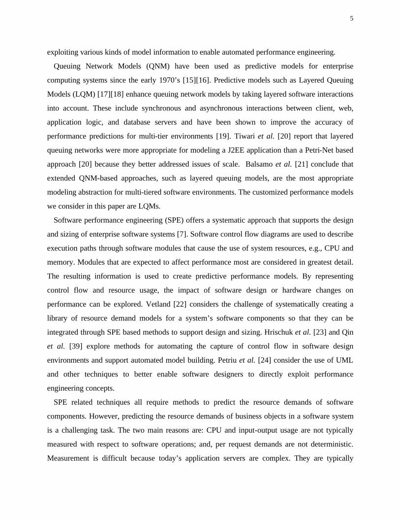
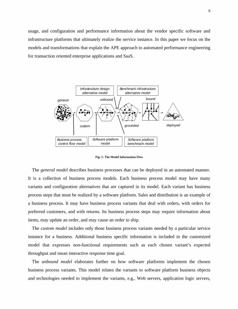
Fig. 2: Models Contributing to Business Object Mix M

Figure 2 illustrates the relationship between the general, business process control flow, custom,

software platform, and unbound models. It shows how information from the general model,

business process control flow, custom model and software platform model are used to compute a

desired business object mix M for a customized service instance. The custom model includes a

subset of process variants from the general model with specific control flows from the business

process control flow model. Each of the variants is annotated with a required throughput, e.g.,

number of sales orders per hour, and a mean response time goal for interactive response times.

Each business process variant causes visits to one or more business objects from the packaging

model. The product of throughput and visits enables the computation of M. Finally, the identity of

the business objects that are used also determines which of the software platform’s software

servers are needed in an infrastructure design alternative.

We now consider benchmarks for a software platform. The benchmarks help to automate the

creation of customized performance models and customized benchmark models. The software

Business object

Business processProcess variantcontrol flow model

Process variantcontrol flow model

Business process steps

General model

Process variant 1 Process variant P

Business process steps

Custom modelX1 – throughputG1 – response time goal

Software platform model

Business objectV - Visits

Application Server DB Server

UsesUses

O Business objects

O1

O2

OO

X x V

Business object mix M

Software platform model

Custom model

M1

M2

MO

• Mi = 1, i = 1...O

Business objects

Unbound model

ApplicationServer

DB Server

SW ServersXP – throughputGP – response time goal

Business processProcess variant Process variant

Business process control flow model

12

platform benchmark model includes many benchmarks for a software platform. The benchmarks

are chosen to provide coverage over the platform’s business objects. Each benchmark is fully

automatable in its execution and can be run on many different infrastructure alternatives. Each

benchmark exercises a small number of objects in a manner typical for the platform. Together, the

benchmarks exercise all the objects of the platform. Each benchmark aims to exercise an

infrastructure to achieve the highest throughput while certain response time expectations are

satisfied. Further details about benchmark design are given in the following section.

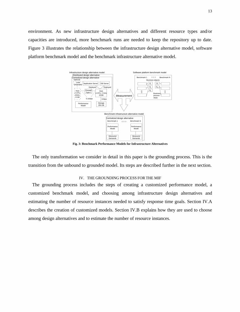
The infrastructure design alternative model expresses different ways in which a software

platform can be realized in the shared resource environment. For example, one infrastructure

alternative may have all software platform technologies executing entirely on one host with a

specific capacity. This is referred to as a centralized design alternative. A distributed design

alternative may use many hosts to realize a more scalable multi-tier system with each instance of a

web, application, and database server running in a separate host. Furthermore, some alternatives

may use hosts that are implemented as virtual machines. Finally, each infrastructure design

alternative has a predictive performance model that is used to predict the behaviour of the

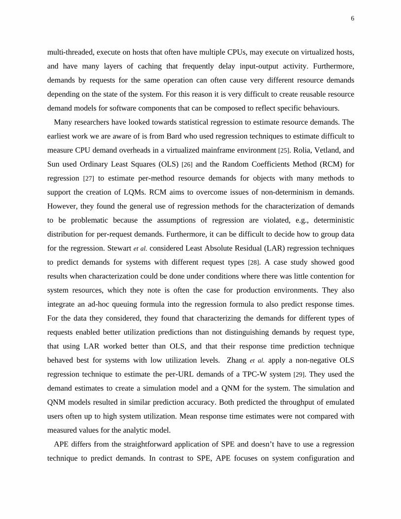
infrastructure when operating with different numbers of resource instances. Figure 3 illustrates the

components of the infrastructure design alternative model. The figure illustrates some of the

details considered in a model, e.g., logical and physical resources, resource capacities and

networking relationships. The performance model reflects the behaviour of the resources and their

relationships.

The creation of infrastructure design alternatives is the role of the service provider for the SaaS

system. The service provider must create and test a number of alternatives that are appropriate for

the hardware platform and that satisfy the needs of various customers for throughput and

responsiveness. Once the alternatives are defined, they can be re-used and customized for many

service instances.

The benchmark-infrastructure-alternative model acts a repository of reusable performance

information for APE. All benchmarks from an application platform benchmark model are run

against each infrastructure design alternative. The results of each run include measured resource

demands that are used as parameters for the corresponding predictive model. This process is

automated with benchmarks being executed during non-peak periods for the shared resource

13

environment. As new infrastructure design alternatives and different resource types and/or

capacities are introduced, more benchmark runs are needed to keep the repository up to date.

Figure 3 illustrates the relationship between the infrastructure design alternative model, software

platform benchmark model and the benchmark infrastructure alternative model.

Fig. 3: Benchmark Performance Models for Infrastructure Alternatives

The only transformation we consider in detail in this paper is the grounding process. This is the

transition from the unbound to grounded model. Its steps are described further in the next section.

IV. THE GROUNDING PROCESS FOR THE MIF

The grounding process includes the steps of creating a customized performance model, a

customized benchmark model, and choosing among infrastructure design alternatives and

estimating the number of resource instances needed to satisfy response time goals. Section IV.A

describes the creation of customized models. Section IV.B explains how they are used to choose

among design alternatives and to estimate the number of resource instances.

Infrastructure design alternative model

Application Server DB Server

Host4 CPU, 2 GHz

32GB

FirewallType 1

Storage250 GB

1Gbps0.1Gbps

DeployedDeployed

Host2 CPU,2GHz,8 GB

LoadGenerator

OptionalCentralized design alternative

Software platform benchmark model

Benchmark 1 Benchmark N

Oi

Oj

Ok

Ol

Om

Business objects

Benchmark infrastructure alternative model

PerformanceModel

PerformanceModel

Benchmark 1 Benchmark N

Measurement

PerformanceModel

MeasuredDemands

MeasuredDemands

Business process steps

Centralized design alternative

Distributed design alternative

14

Benchmark infrastructure alternative model

Benchmark 1 Benchmark N

Benchmark aRa

Benchmark QRQ

• Ri = 1, i = a...Q

Compute WorkloadIntegration Ratio R

PerformanceModel

PerformanceModel

MeasuredDemands

MeasuredDemands

PerformanceModel

AverageDemandsFor Mix M

Customized performance model

Customized benchmark model for business object mix M

Benchmark aRa

Benchmark QRQ

PerformanceModel

PerformanceModel

MeasuredDemands

MeasuredDemands

O1

O2

OO

Business object mix M

M1

M2

MO

• Mi = 1, i = 1...O

Business objects

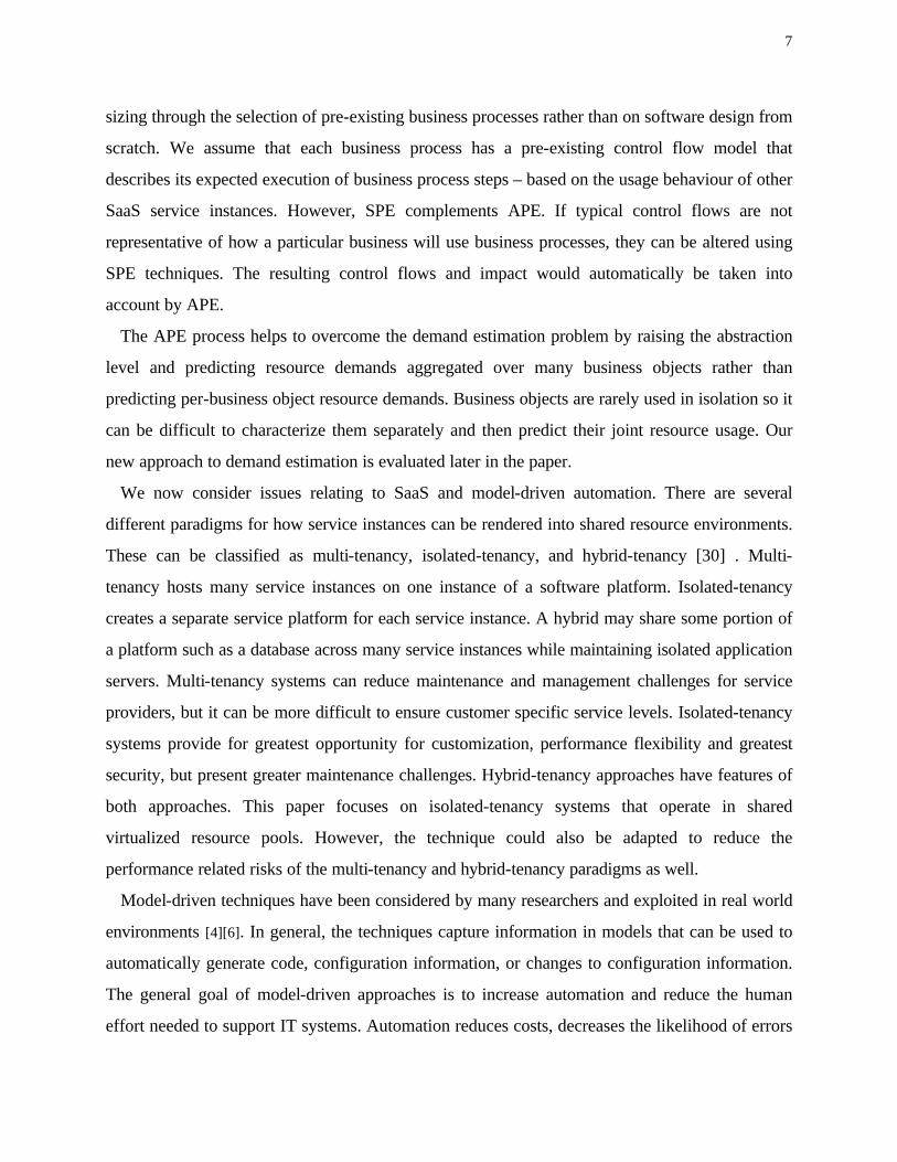
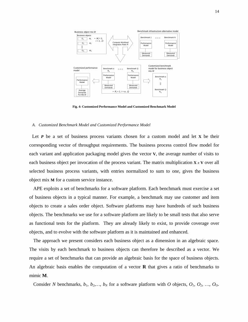
Fig. 4: Customized Performance Model and Customized Benchmark Model

A. Customized Benchmark Model and Customized Performance Model

Let P be a set of business process variants chosen for a custom model and let X be their

corresponding vector of throughput requirements. The business process control flow model for

each variant and application packaging model gives the vector V, the average number of visits to

each business object per invocation of the process variant. The matrix multiplication X x V over all

selected business process variants, with entries normalized to sum to one, gives the business

object mix M for a custom service instance.

APE exploits a set of benchmarks for a software platform. Each benchmark must exercise a set

of business objects in a typical manner. For example, a benchmark may use customer and item

objects to create a sales order object. Software platforms may have hundreds of such business

objects. The benchmarks we use for a software platform are likely to be small tests that also serve

as functional tests for the platform. They are already likely to exist, to provide coverage over

objects, and to evolve with the software platform as it is maintained and enhanced.

The approach we present considers each business object as a dimension in an algebraic space.

The visits by each benchmark to business objects can therefore be described as a vector. We

require a set of benchmarks that can provide an algebraic basis for the space of business objects.

An algebraic basis enables the computation of a vector R that gives a ratio of benchmarks to

mimic M.

Consider N benchmarks, b1, b2,…, bN for a software platform with O objects, O1, O2, …, OO.

15

Each benchmark bi has a particular business object mix bi,1, bi,2,…, bi,O, with most values likely to

be zero. Let A be a matrix with N rows and O columns that includes the business object mix for

the benchmarks.

Suppose a business object mix M exploits Q business objects. In this case, M is a vector with

dimension Q x 1. Solving for a Q x 1 dimensional ratio vector R involves finding a subset of Q

benchmarks from A to create a matrix A* with dimensions Q x Q that yields a solution for R such

that A* R = M. A more detailed explanation of the method is described in Appendix A.

Figure 4 illustrates the creation of a customized performance model and customized benchmark

model. A customized benchmark is created for a business object mix M by replaying the Q

selected benchmarks, from the benchmark infrastructure alternative model, in parallel with

proportion of benchmark sessions defined by R. This customized benchmark can be used as a

performance validation test for a deployed service instance.

To support the creation of a customized performance model, each benchmark bi has a

performance model that is from the infrastructure design alternative model of Figure 3. It includes

features such as networking, hosts, application servers, and resource demand information. The

resource demand information for benchmark bi is defined as Di where Di is a C x 1 vector of

demand values upon the C capacity attributes, e.g., CPU, Disk, of the performance model. The

information is shown as Measured Demands in the Figure 3’s Benchmark infrastructure

alternative model. While the structure of each model is the same for each benchmark for an

infrastructure design alternative, the average resource demand values Di that are measured for

each of the N benchmarks are likely to be different.

Let D be the resource demand estimates for a customized performance model for a business

object mix M. The customized performance model has the same C capacity attributes as the

benchmark performance models. We estimate the resource demands D as a ratio of the resource

demands from the selected benchmarks from A* weighted using the computed vector R. Let D*

be a Q x C matrix of demand values for the Q selected benchmarks. The customized performance

model for the design alternative has demands D = D*T R where D is a C x 1 vector. The case

study in Section V demonstrates the effectiveness of this demand estimation approach compared

to statistical regression.

A summary of the above notation for APE is offered in Appendix B. The following subsection

16

describes how the customized performance model and customized benchmark model are used in

the MIF.

B. Choosing a Design Alternative and Validating a Design for Performance

Figure 5 illustrates the evaluation of design alternatives. This section describes this evalutation

in more detail.

The customized performance model for a infrastructure design alternative is used determine

whether the alterative is able to support the throughput requirements and response time goals for

the service instance. For example, a centralized design may not have enough capacity to support

throughput or response time requirements. A certain distributed design alternative may enable up

to a certain number of application servers and application server hosts. The performance model is

used iteratively to find the appropriate number of application servers and hosts that best satisfy

the performance requirements. We do not discuss this iterative process further in this paper, but at

present we exploit a simple one factor at a time optimization that varies numbers of resource

instances until throughput requirements and response time goals are satisfied. Other non-

functional aspects, such as cost or the need of a service instance to rapidly support increased

throughputs, are also used to choose among design alternatives that are all otherwise able to

satisfy the performance requirements.

Fig. 5: Choosing a Design Alternative

Figure 5 shows a chosen design alternative along with its estimated number of resource

instances and a customized benchmark model. Choosing a design alternative and specifying its

Infrastructure design alternative model

Application Server DB Server

Host4 CPU, 2 GHz

32GB

FirewallType 1

Storage250 GB

1Gbps0.1Gbps

DeployedDeployed

Host2 CPU,2GHz,8 GB

LoadGenerator

Optional

Centralized design alternative

PerformanceModel

Distributed design alternative

PerformanceModel

AverageDemandsFor Mix M

Customized performance model

Centralized design

Distributed design

Evaluate design alternatives

PerformanceModel

AverageDemandsFor Mix M

Chosen design alternative

Numbers of resource instancesneeded to satisfy

service levelexpectations

Benchmark aRa

Benchmark QRQ

Customized benchmark model

Satisfy throughput X and response time goals G

17

number of resource instances completes the grounding process. The design can then be bound to

resources and deployed. The deployed system may include an optional load generator that is able

to stress the service instance with the customized benchmark to verify that throughput and

response time goals are met.

The following section demonstrates and applies the techniques introduced in Section IV.

V. CASE STUDY

The case study has the following three objectives.

• Demonstrate the effectiveness of computations for the workload integration ratio R.

• Demonstrate the accuracy of APE’s demand prediction approach and compare with

regression.

• Demonstrate the effectiveness of the performance models by validating with respect to

benchmark measurements.

For the case study, we rely on measurements from two different TPC-W [34] systems that were

collected for unrelated studies [10][29]. Measurement data was gathered for these systems for

other purposes but is reused to demonstrate and validate the concepts presented in this paper. We

translate from the terminology of TPC-W to that introduced in Sections III and IV. The systems,

their performance models, and the performance evaluation technique are described in Section

V.A. Measurements from the systems are used in Sections V.B through V.D. The performance

models are used in Section V.D.

A. TPC-W System Descriptions, Performance Models, and Predictive Modeling Technique

The first TPC-W system we consider was deployed at Carleton University in Ottawa, Canada

[10][14]. The 2nd system was deployed at HP Labs in Palo Alto, USA [29]. We refer to the

systems as C-TPC-W and H-TPC-W, respectively. We note that the results presented for these

systems are not intended to be compliant TPC-W benchmark runs. The TPC-W bookstore system

merely serves as an example system for the study. Detailed descriptions for the systems are

available in their given references.

For each of the systems we offer a LQM as a performance model. Performance estimates for

the models are found using the Method of Layers [18]. However, we note that the TPC-W

18

systems are complex session based systems. These systems have bursty request behaviour that is

not well addressed using straightforward QNM or LQM-based technologies. As a result, for

performance evaluation, the LQMs are combined with a population distribution estimation

technique, conceptually related to the hybrid Markov Chain-QNM technique described by

Menasce and Almeida [35]. The technique we use is called the Weighted Average Method

(WAM) [19]. It improves the accuracy of performance predictions by taking into account the

impact of bursts of competition for resources. Such bursts are typical for these session based

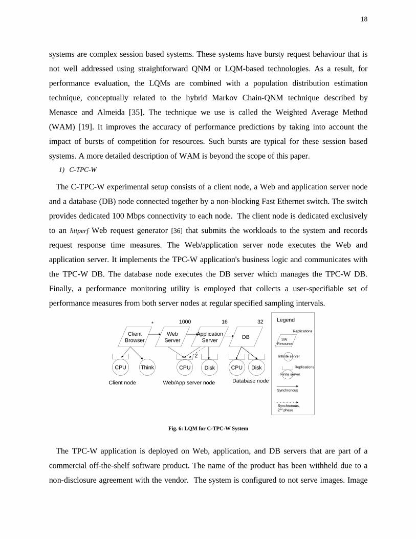
systems. A more detailed description of WAM is beyond the scope of this paper. 1) C-TPC-W

The C-TPC-W experimental setup consists of a client node, a Web and application server node

and a database (DB) node connected together by a non-blocking Fast Ethernet switch. The switch

provides dedicated 100 Mbps connectivity to each node. The client node is dedicated exclusively

to an httperf Web request generator [36] that submits the workloads to the system and records

request response time measures. The Web/application server node executes the Web and

application server. It implements the TPC-W application's business logic and communicates with

the TPC-W DB. The database node executes the DB server which manages the TPC-W DB.

Finally, a performance monitoring utility is employed that collects a user-specifiable set of

performance measures from both server nodes at regular specified sampling intervals.

ClientBrowser

WebServer

ApplicationServer DB

ThinkCPU CPU CPU Disk

2

1000 16 32

Client node Web/App server node Database node

Legend

SWResource

Replications

Replications

Infinite server

Finite server

Synchronous

Synchronous,2nd phase

*

Disk

Fig. 6: LQM for C-TPC-W System

The TPC-W application is deployed on Web, application, and DB servers that are part of a

commercial off-the-shelf software product. The name of the product has been withheld due to a

non-disclosure agreement with the vendor. The system is configured to not serve images. Image

19

requests were not submitted in any of the experiments. The workloads that are considered are

variants of the TPC-W workloads that include Hi-Mix, Med-Mix and Low-Mix workloads [10]

with high, medium, and low resource demand variation, respectively. The mixes are given in

Appendix C.

The number of server processes and the threading levels are set in the system as follows. The

number of Web server threads is 1000. This was much greater than the maximum number of

concurrent connections encountered in the experiments. The number of application server

processes is fixed at 16, an upper limit imposed by the application. The number of DB server

threads for the DB server was set to the upper limit of 32.

The primary performance metric of interest for the study is the user-perceived mean response

time (Rmean) for the requests at the TPC-W system. This metric is of interest for system sizing,

capacity planning, and service level management exercises. We define response time as the time

between initiating a TCP connection for a HTTP request and receiving the last byte of the

corresponding HTTP response. The measured response time is a good indicator of the delay

suffered by the request at the TPC-W system because the network and the client workload

generator nodes are not saturated for the examples we considered.

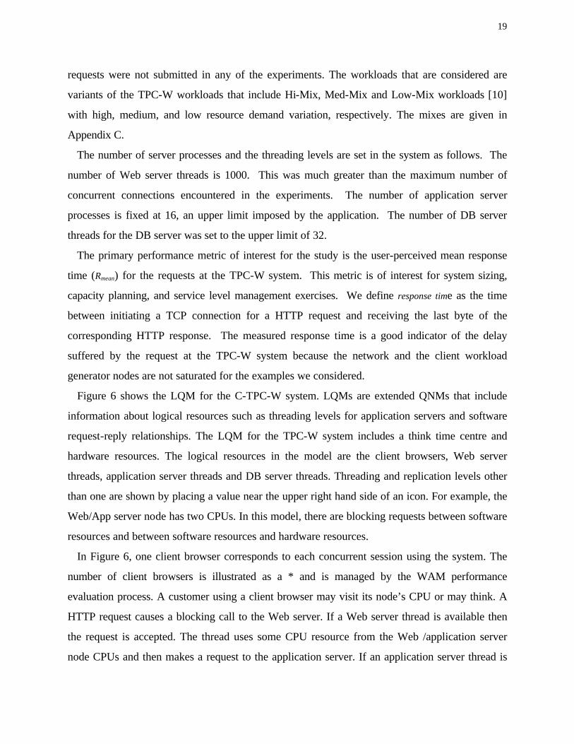
Figure 6 shows the LQM for the C-TPC-W system. LQMs are extended QNMs that include

information about logical resources such as threading levels for application servers and software

request-reply relationships. The LQM for the TPC-W system includes a think time centre and

hardware resources. The logical resources in the model are the client browsers, Web server

threads, application server threads and DB server threads. Threading and replication levels other

than one are shown by placing a value near the upper right hand side of an icon. For example, the

Web/App server node has two CPUs. In this model, there are blocking requests between software

resources and between software resources and hardware resources.

In Figure 6, one client browser corresponds to each concurrent session using the system. The

number of client browsers is illustrated as a * and is managed by the WAM performance

evaluation process. A customer using a client browser may visit its node’s CPU or may think. A

HTTP request causes a blocking call to the Web server. If a Web server thread is available then

the request is accepted. The thread uses some CPU resource from the Web /application server

node CPUs and then makes a request to the application server. If an application server thread is

20

available then the request is accepted. The application server thread uses some CPU resource

from the Web /application server node CPUs and then makes a request to the DB server. If a DB

server thread is available then the request is accepted. The thread uses some CPU and disk

resource from the database server node and releases the calling thread. The released calling thread

from the application server can then complete its first phase of work and release the calling thread

from the Web server.

From Figure 6, after finishing its first phase and releasing the calling thread from the Web server

the application server thread continues on to a second phase of service. The second phase of

service keeps the application server thread busy so that it cannot service another calling thread.

However at the same time the calling thread from the Web Server that was released after the first

phase of service can complete its work and release the calling thread from the client browser. This

completes an HTTP request. The reasons for modeling the request-reply relationship of the

application server in this manner are discussed shortly.

During an HTTP request, if a thread is not available when a server is called, the calling thread

blocks until a thread becomes available. Once a thread completes its work it is available to serve

another caller. Such threading can lead to software queuing delays in addition to any contention

for hardware resources that are incurred by active threads. The numbers of threads used for each

tier in the model reflect the actual application settings.

To obtain resource demand values for the model, each measured run collects CPU utilization

for the Web server threads, application server threads, and the DB server threads. We also

measured the CPU and disk utilizations for the Web/application server node and the database

server node, the elapsed time of the run, and the number of request completions. This enables us

to compute the average resource demand per request for the Web server threads, application

server threads, DB server threads, and for the Web/application server node and database server

node as a whole.

Finally, we observed from measurement runs with one concurrent session that mean response

times were often lower than the aggregate demand upon the hardware resources. This is an

indication of two phases of processing at a server. We reflected this in the LQM by placing 25%

of the application server thread demands in a second phase of service [18][17]. This modeling

choice was found to produce good model predictions.

21

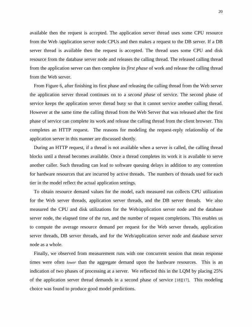
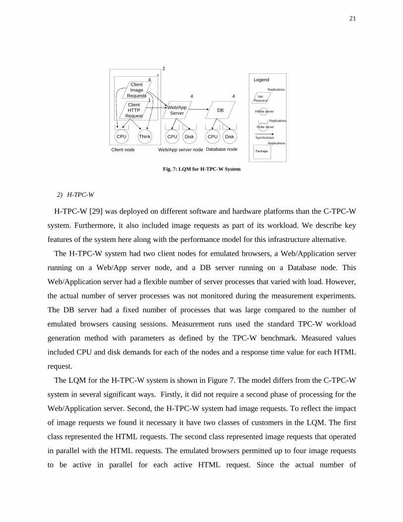
Fig. 7: LQM for H-TPC-W System

2) H-TPC-W

H-TPC-W [29] was deployed on different software and hardware platforms than the C-TPC-W

system. Furthermore, it also included image requests as part of its workload. We describe key

features of the system here along with the performance model for this infrastructure alternative.

The H-TPC-W system had two client nodes for emulated browsers, a Web/Application server

running on a Web/App server node, and a DB server running on a Database node. This

Web/Application server had a flexible number of server processes that varied with load. However,

the actual number of server processes was not monitored during the measurement experiments.

The DB server had a fixed number of processes that was large compared to the number of

emulated browsers causing sessions. Measurement runs used the standard TPC-W workload

generation method with parameters as defined by the TPC-W benchmark. Measured values

included CPU and disk demands for each of the nodes and a response time value for each HTML

request.

The LQM for the H-TPC-W system is shown in Figure 7. The model differs from the C-TPC-W

system in several significant ways. Firstly, it did not require a second phase of processing for the

Web/Application server. Second, the H-TPC-W system had image requests. To reflect the impact

of image requests we found it necessary it have two classes of customers in the LQM. The first

class represented the HTML requests. The second class represented image requests that operated

in parallel with the HTML requests. The emulated browsers permitted up to four image requests

to be active in parallel for each active HTML request. Since the actual number of

ClientHTTP

Request

Web/AppServer DB

ThinkCPU CPU Disk

4 4

Client node Web/App server node Database node

Legend

SWResource

Replications

Replications

Infinite server

Finite server

SynchronousCPU Disk

ClientImage

Requests

4

Package

*2

Replications

1

22

Web/Application server processes was not known, we fixed the numbers of Web/Application

server processes and DB processes as 4 and 4. This offered accurate mean response time and

throughput predictions for the full suite of experiments. Finally, Figure 7 introduces the package

concept into the LQM [37]. A package groups modeled entities together in a manner that they

can be replicated in unison. The dual client node is reflected in the model as a package with 2

replicates. Within each client node there are * active HTTP requests, each with 4 active image

requests. During the performance evaluation process, the value of * is varied by the WAM

technique.

B. The Effectiveness of Computing a Workload Integration Ratio R

This section demonstrates the effectiveness of using a set of benchmarks to synthesize a

business object mix. We use 100 sessions chosen randomly from TPC-W Browsing, Shopping,

and Ordering measurement runs to act as a surrogate for software platform benchmarks of Figure

3. Each of the 100 TPC-W URL sessions corresponds to a benchmark. Each of the multiple URLs

in a session, i.e., benchmark, corresponds to a business object of the software platform model of

Figure 2. We consider two examples.

The first example uses the workload matching technique from Section III.A with 100

benchmarks to synthesize the Browsing, Shopping, and Ordering mixes, respectively. The

Browsing, Shopping, and Ordering URL mixes act as business object mixes of Figure 4. We

expect the matching to do very well at synthesizing the mixes since sessions used as the

benchmarks were obtained from a workload generator that created sessions that corresponded to

the specifications for these mixes. The second example presents detailed results for these three

cases and 7 additional, but more diverse, business object mixes. The second example shows that

workload matching can synthesize mixes for complex service instance scenarios.

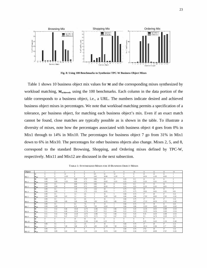
Figure 8 shows the desired and synthesized business object mixes that correspond to the

TPC-W Browsing, Shopping, and Ordering mixes. As expected, the 100 benchmark sessions

were able to match the desired mixes precisely.

23

Fig. 8: Using 100 Benchmarks to Synthesize TPC-W Business Object Mixes

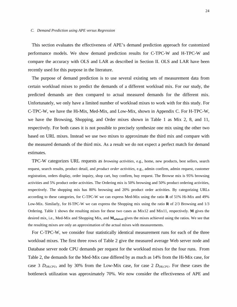
Table 1 shows 10 business object mix values for M and the corresponding mixes synthesized by

workload matching, Machieved, using the 100 benchmarks. Each column in the data portion of the

table corresponds to a business object, i.e., a URL. The numbers indicate desired and achieved

business object mixes in percentages. We note that workload matching permits a specification of a

tolerance, per business object, for matching each business object’s mix. Even if an exact match

cannot be found, close matches are typically possible as is shown in the table. To illustrate a

diversity of mixes, note how the percentages associated with business object 4 goes from 0% in

Mix1 through to 14% in Mix10. The percentages for business object 7 go from 31% in Mix1

down to 6% in Mix10. The percentages for other business objects also change. Mixes 2, 5, and 8,

correspond to the standard Browsing, Shopping, and Ordering mixes defined by TPC-W,

respectively. Mix11 and Mix12 are discussed in the next subsection.

TABLE 1: SYNTHESIZED MIXES FOR 10 BUSINESS OBJECT MIXES

Object 1 2 3 4 5 6 7 8 9 10 11 12 13 14M 0 0 12 0 0 0.5 31 12 0 0 21 12 11 1Mach 0 0 11.95 0 0 0.45 30.86 11.95 0 0 20.91 11.95 10.95 1

M 0.09 0.1 11 0.69 0.75 0.82 29 11 0.25 0.3 21 12 11 2Mach 0.09 0.09 11.01 0.69 0.75 0.82 29.02 11.01 0.25 0.25 21.01 12.01 11.01 2

M 0.09 0.1 8 0.69 0.75 0.82 26 8 0.25 0.3 21 15 14 5Mach 0.09 0.09 8 0.69 0.75 0.82 26.02 8 0.25 0.25 21.01 15.01 14.01 5

M 0.09 0.1 7 1.19 1.75 2.32 20 7 0.75 0.8 19 16 15 9Mach 0.09 0.09 7 1.19 1.75 2.32 20.01 7 0.75 0.75 19.01 16.01 15.01 9.01

M 0.09 0.1 5 1.2 2.6 3 16 5 0.66 0.75 17 20 17 11.6Mach 0.09 0.09 5.01 1.2 2.6 3 16.02 5.01 0.66 0.66 17.02 20.02 17.02 11.61

M 0.09 0.1 3 3.2 4.6 3 16 3 0.66 0.75 17 20 17 11.6Mach 0.09 0.09 3.06 3.06 3.06 3.06 16.31 3.06 0.67 0.67 17.33 20.39 17.33 11.82

M 0.09 0.1 1 6.2 7.6 8 14 1 0.66 0.75 15 18 15 12.6Mach 0.09 0.09 1 6.21 7.61 7.95 14.02 1 0.66 0.66 15.03 18.03 15.03 12.62

M 0.11 0.12 0.46 10.18 12.73 12.86 9.12 0.46 0.22 0.25 12.35 14.53 13.08 13.53Mach 0.11 0.11 0.46 10.18 12.74 12.87 9.12 0.46 0.22 0.22 12.35 14.54 13.09 13.54

M 0.11 0.12 0.46 12.18 14.73 13.86 7.12 0.46 0.22 0.25 9.35 14.53 13.08 13.53Mach 0.11 0.11 0.47 12.37 13.75 13.75 7.23 0.47 0.22 0.22 9.5 14.76 13.29 13.75

M 0 0 0 14 16 16 6 0 0 0 8 14 11 15Mach 0 0 0 13.4 15.46 15.46 6.19 0 0 0 8.25 14.43 11.34 15.46

M 0.09 0.1 5 1.2 2.6 3 16 5 0.66 0.75 17 20 17 11.6Mach 0.1 0.1 7.49 3.86 4.74 4.85 22.38 7.49 0.24 0.24 18.14 12.84 11.7 5.84

M 0.09 0.1 5 0 0 3 9 5 0.66 0.75 27.8 20 17 11.6Mach 0.09 0.09 5.02 0.61 1.33 1.54 19.74 5.02 0.34 0.34 17.07 20.09 17.07 11.65

Mix 9

Mix 10

Mix 11

Mix 12

Mix 5

Mix 6

Mix 7

Mix 8

Mix 1

Mix 2

Mix 3

Mix 4

Browsing Mix Shopping Mix Ordering Mix

24

C. Demand Prediction using APE versus Regression

This section evaluates the effectiveness of APE’s demand prediction approach for customized

performance models. We show demand prediction results for C-TPC-W and H-TPC-W and

compare the accuracy with OLS and LAR as described in Section II. OLS and LAR have been

recently used for this purpose in the literature.

The purpose of demand prediction is to use several existing sets of measurement data from

certain workload mixes to predict the demands of a different workload mix. For our study, the

predicted demands are then compared to actual measured demands for the different mix.

Unfortunately, we only have a limited number of workload mixes to work with for this study. For

C-TPC-W, we have the Hi-Mix, Med-Mix, and Low-Mix, shown in Appendix C. For H-TPC-W,

we have the Browsing, Shopping, and Order mixes shown in Table 1 as Mix 2, 8, and 11,

respectively. For both cases it is not possible to precisely synthesize one mix using the other two

based on URL mixes. Instead we use two mixes to approximate the third mix and compare with

the measured demands of the third mix. As a result we do not expect a perfect match for demand

estimates.

TPC-W categorizes URL requests as browsing activities, e.g., home, new products, best sellers, search

request, search results, product detail, and product order activities, e.g., admin confirm, admin request, customer

registration, orders display, order inquiry, shop cart, buy confirm, buy request. The Browse mix is 95% browsing

activities and 5% product order activities. The Ordering mix is 50% browsing and 50% product ordering activities,

respectively. The shopping mix has 80% browsing and 20% product order activities. By categorizing URLs

according to these categories, for C-TPC-W we can express Med-Mix using the ratio R of 51% Hi-Mix and 49%

Low-Mix. Similarly, for H-TPC-W we can express the Shopping mix using the ratio R of 2/3 Browsing and 1/3

Ordering. Table 1 shows the resulting mixes for these two cases as Mix12 and Mix11, respectively. M gives the

desired mix, i.e., Med-Mix and Shopping Mix, and Macheived gives the mixes achieved using the ratios. We see that

the resulting mixes are only an approximation of the actual mixes with measurements.

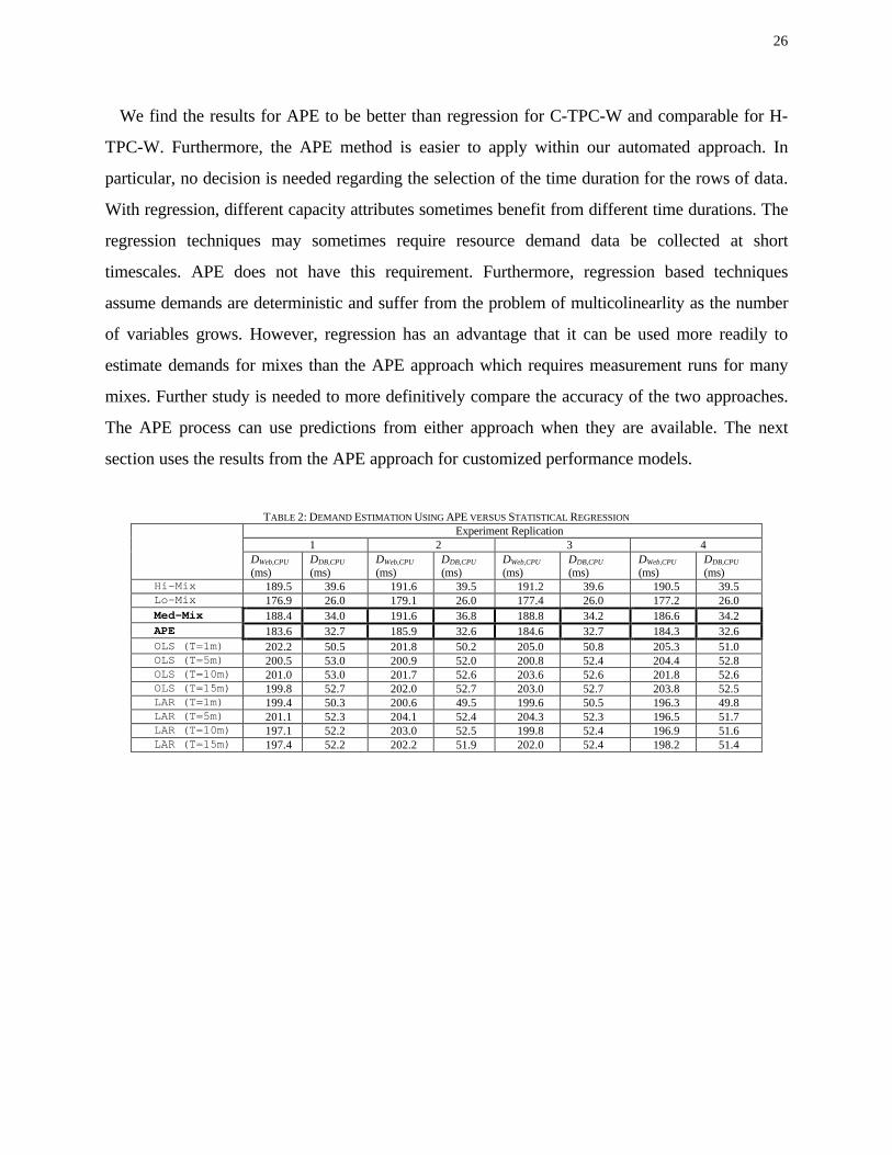
For C-TPC-W, we consider four statistically identical measurement runs for each of the three

workload mixes. The first three rows of Table 2 give the measured average Web server node and

Database server node CPU demands per request for the workload mixes for the four runs. From

Table 2, the demands for the Med-Mix case differed by as much as 14% from the Hi-Mix case, for

case 3 DDB,CPU, and by 30% from the Low-Mix case, for case 2 DDB,CPU. For these cases the

bottleneck utilization was approximately 70%. We now consider the effectiveness of APE and

25

regression for estimating Med-Mix demands.

The APE row in Table 2 shows APE’s estimates for CPU demands for Med-Mix. We see that

7 of the 8 estimates are within 5% of the measured demand values. DDB,CPU for case 2 differs from

the measured value for Med-Mix by 11.5%. We note that the estimate is actually for the Mix11

Machieved so a perfect match is not expected. Subsequent rows of the table give demand estimates

found using the regression techniques.

We now consider the use of the regression techniques. The input values for the regression

techniques for a capacity attribute, e.g., CPU, are multiple rows of data, each with a measured

aggregate demand value and two count values, one for browsing activities and one for product

order activities, that contribute to the demand value. For this example, the rows of data were

obtained from Hi-Mix and Lo-Mix measurement runs. One application of a regression technique is

used to estimate average per activity resource demand for one capacity attribute. The process is

repeated for each capacity attribute. The demands are then used to predict the resource demands

for the Med-Mix according to the ratio R of 51% and 49%.

We considered several time durations for data that applies to each row, namely 1, 5, 10, and 15

minutes. The 1 minute interval is the shortest interval we could consider since our CPU

measurements were made on a per-minute basis. From Table 2, all the results are similar.

Estimates for DWeb,CPU have errors between 5% to 10%. However, DDB,CPU have errors that are

typically greater than 50%. Regression with respect to the browsing and product ordering

activities would benefit from shorter durations for rows of data rather than longer time durations.

Unfortunately, there wasn’t sufficient information in each row of data that we have to enable

better estimates.

Table 3 shows the measured and estimated demands for the H-TPC-W cases as obtained via

APE and the best cases we found for OLS and LAR. For these cases, the utilization for the

system bottleneck ranged from a low value to 99%. The estimates from APE for Web server CPU

demands are all accurate to with 4%. The estimates for the database CPU demands had larger

errors, up to 24%. OLS and LAR’s estimates for Web server CPU demand were within 3% and

4%, respectively. Their estimates for database CPU demands had errors up to 19%. Regression

did slightly better than APE for the H-TPC-W scenario. However, from Mix11 in Table 1 we note

that the measurements are for a slightly different workload mix.

26

We find the results for APE to be better than regression for C-TPC-W and comparable for H-

TPC-W. Furthermore, the APE method is easier to apply within our automated approach. In

particular, no decision is needed regarding the selection of the time duration for the rows of data.

With regression, different capacity attributes sometimes benefit from different time durations. The

regression techniques may sometimes require resource demand data be collected at short

timescales. APE does not have this requirement. Furthermore, regression based techniques

assume demands are deterministic and suffer from the problem of multicolinearlity as the number

of variables grows. However, regression has an advantage that it can be used more readily to

estimate demands for mixes than the APE approach which requires measurement runs for many

mixes. Further study is needed to more definitively compare the accuracy of the two approaches.

The APE process can use predictions from either approach when they are available. The next

section uses the results from the APE approach for customized performance models.

TABLE 2: DEMAND ESTIMATION USING APE VERSUS STATISTICAL REGRESSION

Experiment Replication 1 2 3 4

DWeb,CPU (ms)

DDB,CPU (ms)

DWeb,CPU (ms)

DDB,CPU (ms)

DWeb,CPU (ms)

DDB,CPU (ms)

DWeb,CPU (ms)

DDB,CPU (ms)

Hi-Mix 189.5 39.6 191.6 39.5 191.2 39.6 190.5 39.5 Lo-Mix 176.9 26.0 179.1 26.0 177.4 26.0 177.2 26.0 Med-Mix 188.4 34.0 191.6 36.8 188.8 34.2 186.6 34.2 APE 183.6 32.7 185.9 32.6 184.6 32.7 184.3 32.6 OLS (T=1m) 202.2 50.5 201.8 50.2 205.0 50.8 205.3 51.0 OLS (T=5m) 200.5 53.0 200.9 52.0 200.8 52.4 204.4 52.8 OLS (T=10m) 201.0 53.0 201.7 52.6 203.6 52.6 201.8 52.6 OLS (T=15m) 199.8 52.7 202.0 52.7 203.0 52.7 203.8 52.5 LAR (T=1m) 199.4 50.3 200.6 49.5 199.6 50.5 196.3 49.8 LAR (T=5m) 201.1 52.3 204.1 52.4 204.3 52.3 196.5 51.7 LAR (T=10m) 197.1 52.2 203.0 52.5 199.8 52.4 196.9 51.6 LAR (T=15m) 197.4 52.2 202.2 51.9 202.0 52.4 198.2 51.4

27

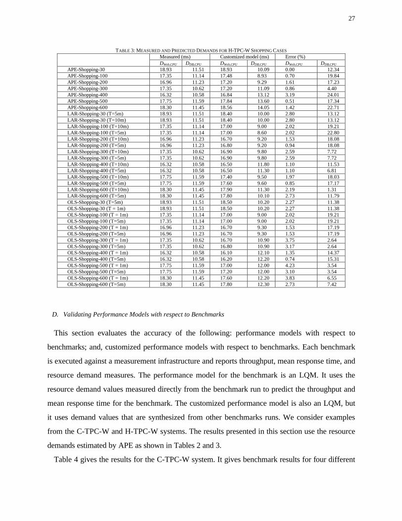
TABLE 3: MEASURED AND PREDICTED DEMANDS FOR H-TPC-W SHOPPING CASES Measured (ms) Customized model (ms) Error (%) DWeb,CPU DDB,CPU DWeb,CPU DDB,CPU DWeb,CPU DDB,CPU

APE-Shopping-30 18.93 11.51 18.93 10.09 0.00 12.34 APE-Shopping-100 17.35 11.14 17.48 8.93 0.70 19.84 APE-Shopping-200 16.96 11.23 17.20 9.29 1.61 17.23 APE-Shopping-300 17.35 10.62 17.20 11.09 0.86 4.40 APE-Shopping-400 16.32 10.58 16.84 13.12 3.19 24.01 APE-Shopping-500 17.75 11.59 17.84 13.60 0.51 17.34 APE-Shopping-600 18.30 11.45 18.56 14.05 1.42 22.71 LAR-Shopping-30 (T=5m) 18.93 11.51 18.40 10.00 2.80 13.12 LAR-Shopping-30 (T=10m) 18.93 11.51 18.40 10.00 2.80 13.12 LAR-Shopping-100 (T=10m) 17.35 11.14 17.00 9.00 2.02 19.21 LAR-Shopping-100 (T=5m) 17.35 11.14 17.00 8.60 2.02 22.80 LAR-Shopping-200 (T=10m) 16.96 11.23 16.70 9.20 1.53 18.08 LAR-Shopping-200 (T=5m) 16.96 11.23 16.80 9.20 0.94 18.08 LAR-Shopping-300 (T=10m) 17.35 10.62 16.90 9.80 2.59 7.72 LAR-Shopping-300 (T=5m) 17.35 10.62 16.90 9.80 2.59 7.72 LAR-Shopping-400 (T=10m) 16.32 10.58 16.50 11.80 1.10 11.53 LAR-Shopping-400 (T=5m) 16.32 10.58 16.50 11.30 1.10 6.81 LAR-Shopping-500 (T=10m) 17.75 11.59 17.40 9.50 1.97 18.03 LAR-Shopping-500 (T=5m) 17.75 11.59 17.60 9.60 0.85 17.17 LAR-Shopping-600 (T=10m) 18.30 11.45 17.90 11.30 2.19 1.31 LAR-Shopping-600 (T=5m) 18.30 11.45 17.80 10.10 2.73 11.79 OLS-Shopping-30 (T=5m) 18.93 11.51 18.50 10.20 2.27 11.38 OLS-Shopping-30 (T = 1m) 18.93 11.51 18.50 10.20 2.27 11.38 OLS-Shopping-100 (T = 1m) 17.35 11.14 17.00 9.00 2.02 19.21 OLS-Shopping-100 (T=5m) 17.35 11.14 17.00 9.00 2.02 19.21 OLS-Shopping-200 (T = 1m) 16.96 11.23 16.70 9.30 1.53 17.19 OLS-Shopping-200 (T=5m) 16.96 11.23 16.70 9.30 1.53 17.19 OLS-Shopping-300 (T = 1m) 17.35 10.62 16.70 10.90 3.75 2.64 OLS-Shopping-300 (T=5m) 17.35 10.62 16.80 10.90 3.17 2.64 OLS-Shopping-400 (T = 1m) 16.32 10.58 16.10 12.10 1.35 14.37 OLS-Shopping-400 (T=5m) 16.32 10.58 16.20 12.20 0.74 15.31 OLS-Shopping-500 (T = 1m) 17.75 11.59 17.00 12.00 4.23 3.54 OLS-Shopping-500 (T=5m) 17.75 11.59 17.20 12.00 3.10 3.54 OLS-Shopping-600 (T = 1m) 18.30 11.45 17.60 12.20 3.83 6.55 OLS-Shopping-600 (T=5m) 18.30 11.45 17.80 12.30 2.73 7.42

D. Validating Performance Models with respect to Benchmarks

This section evaluates the accuracy of the following: performance models with respect to

benchmarks; and, customized performance models with respect to benchmarks. Each benchmark

is executed against a measurement infrastructure and reports throughput, mean response time, and

resource demand measures. The performance model for the benchmark is an LQM. It uses the

resource demand values measured directly from the benchmark run to predict the throughput and

mean response time for the benchmark. The customized performance model is also an LQM, but

it uses demand values that are synthesized from other benchmarks runs. We consider examples

from the C-TPC-W and H-TPC-W systems. The results presented in this section use the resource

demands estimated by APE as shown in Tables 2 and 3.

Table 4 gives the results for the C-TPC-W system. It gives benchmark results for four different

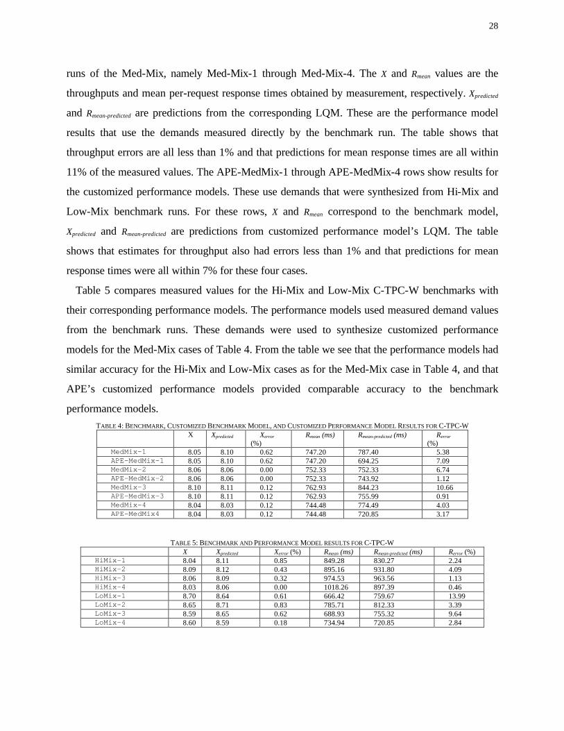
28

runs of the Med-Mix, namely Med-Mix-1 through Med-Mix-4. The X and Rmean values are the

throughputs and mean per-request response times obtained by measurement, respectively. Xpredicted

and Rmean-predicted are predictions from the corresponding LQM. These are the performance model

results that use the demands measured directly by the benchmark run. The table shows that

throughput errors are all less than 1% and that predictions for mean response times are all within

11% of the measured values. The APE-MedMix-1 through APE-MedMix-4 rows show results for

the customized performance models. These use demands that were synthesized from Hi-Mix and

Low-Mix benchmark runs. For these rows, X and Rmean correspond to the benchmark model,

Xpredicted and Rmean-predicted are predictions from customized performance model’s LQM. The table

shows that estimates for throughput also had errors less than 1% and that predictions for mean

response times were all within 7% for these four cases.

Table 5 compares measured values for the Hi-Mix and Low-Mix C-TPC-W benchmarks with

their corresponding performance models. The performance models used measured demand values

from the benchmark runs. These demands were used to synthesize customized performance

models for the Med-Mix cases of Table 4. From the table we see that the performance models had

similar accuracy for the Hi-Mix and Low-Mix cases as for the Med-Mix case in Table 4, and that

APE’s customized performance models provided comparable accuracy to the benchmark

performance models. TABLE 4: BENCHMARK, CUSTOMIZED BENCHMARK MODEL, AND CUSTOMIZED PERFORMANCE MODEL RESULTS FOR C-TPC-W

X Xpredicted Xerror (%)

Rmean (ms) Rmean-predicted (ms) Rerror (%)

MedMix-1 8.05 8.10 0.62 747.20 787.40 5.38 APE-MedMix-1 8.05 8.10 0.62 747.20 694.25 7.09 MedMix-2 8.06 8.06 0.00 752.33 752.33 6.74 APE-MedMix-2 8.06 8.06 0.00 752.33 743.92 1.12 MedMix-3 8.10 8.11 0.12 762.93 844.23 10.66 APE-MedMix-3 8.10 8.11 0.12 762.93 755.99 0.91 MedMix-4 8.04 8.03 0.12 744.48 774.49 4.03 APE-MedMix4 8.04 8.03 0.12 744.48 720.85 3.17

TABLE 5: BENCHMARK AND PERFORMANCE MODEL RESULTS FOR C-TPC-W

X Xpredicted Xerror (%) Rmean (ms) Rmean-predicted (ms) Rerror (%) HiMix-1 8.04 8.11 0.85 849.28 830.27 2.24 HiMix-2 8.09 8.12 0.43 895.16 931.80 4.09 HiMix-3 8.06 8.09 0.32 974.53 963.56 1.13 HiMix-4 8.03 8.06 0.00 1018.26 897.39 0.46 LoMix-1 8.70 8.64 0.61 666.42 759.67 13.99 LoMix-2 8.65 8.71 0.83 785.71 812.33 3.39 LoMix-3 8.59 8.65 0.62 688.93 755.32 9.64 LoMix-4 8.60 8.59 0.18 734.94 720.85 2.84

29

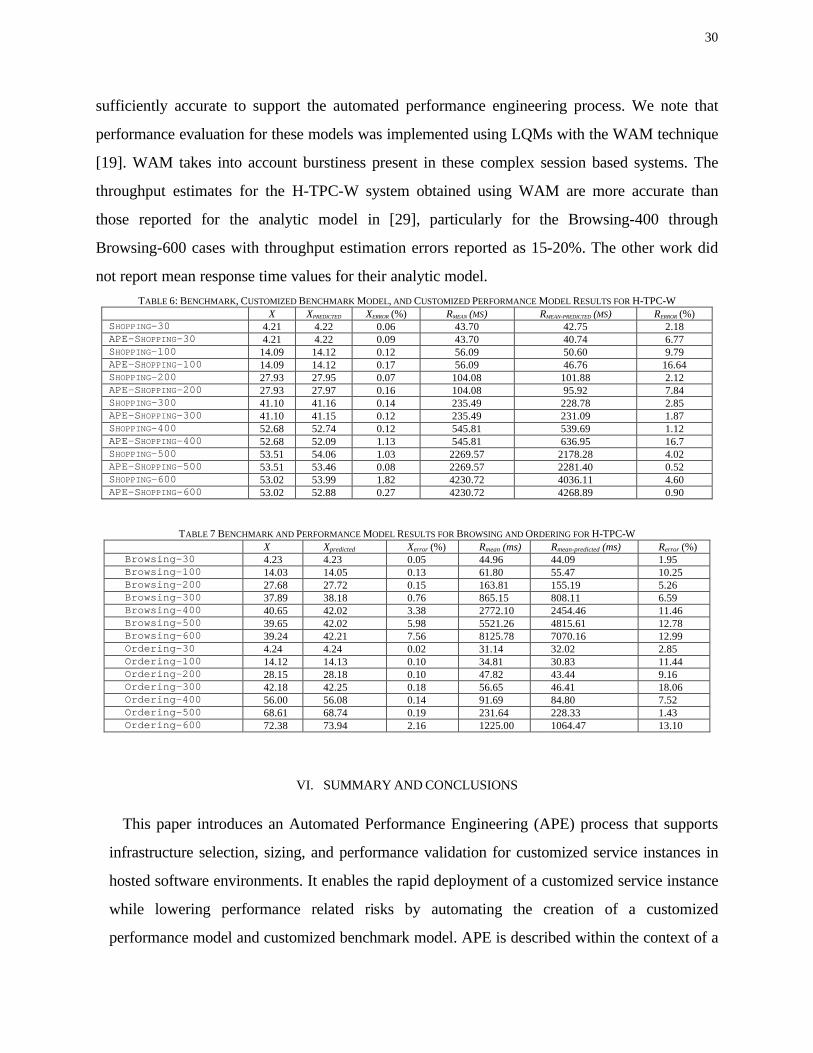
Table 6 gives results for the H-TPC-W system. For this system the Shopping workload mix was

synthesized using Browsing and Ordering workload mixes. In this case results are given for

between 30 and 600 emulated browsers. The results show that the customized benchmark’s

performance model was well able to match throughputs, to within 1%, of the actual

measurements. Response time estimates for the benchmark performance models for the Shopping

mix are all within 10% of the measured values. The estimated throughputs for APE’s customized

performance models are also within 1% of measured values. Response time estimates for the

customized performance models are all within 17% of the measured values.

Table 7 compares measured values for the Browsing and Ordering benchmarks with their

corresponding performance models. The performance models used measured demand values from

the benchmark runs. The demands from these models were used to synthesize the customized

performance models for the Shopping cases of Table 6. The response time estimates for these

cases had higher errors that for the benchmark Shopping mix cases. The greatest error for a

benchmark performance model mean response time estimate was 19%, for the Ordering-300 case.

We see that throughput estimates diverge from the measured values for the Browsing-400

through Browsing-600 cases. We note the system incurred periods of saturation for these

workloads. The high measured mean response times Rmean for these cases illustrate the impact of

the saturation, e.g., the response time values increase from 163 ms for Browsing-200 to 8100 ms

for Browsing-600. The tripling of the number of emulated browsers caused mean response time to

increase by a factor of 50! Ordering-600 shows similar behaviour with respect to Ordering-500.

Despite this significant non-linear behaviour, the customized models for the Shopping mix did

well at predicting mean response times and throughputs.

Table 3 shows that for H-TPC-W our estimates for DWeb,CPU were within 5% and that the

estimates for DDB,CPU had errors of up to 24%. All in all, the errors for DDB,CPU do not appear to

have had a big impact on our performance predictions for throughput or mean response time for

the Shopping mixes. Contention at the Web server node appears to have had the biggest impact

on performance. Finally, we repeated the same experiments using the resource demand estimates

from OLS and LAR. The results were very similar to those for APE and are shown in Appendix

D.

The throughput and mean response time estimates for the customized performance models are

30

sufficiently accurate to support the automated performance engineering process. We note that

performance evaluation for these models was implemented using LQMs with the WAM technique

[19]. WAM takes into account burstiness present in these complex session based systems. The

throughput estimates for the H-TPC-W system obtained using WAM are more accurate than

those reported for the analytic model in [29], particularly for the Browsing-400 through

Browsing-600 cases with throughput estimation errors reported as 15-20%. The other work did

not report mean response time values for their analytic model. TABLE 6: BENCHMARK, CUSTOMIZED BENCHMARK MODEL, AND CUSTOMIZED PERFORMANCE MODEL RESULTS FOR H-TPC-W

X XPREDICTED XERROR (%) RMEAN (MS) RMEAN-PREDICTED (MS) RERROR (%) SHOPPING-30 4.21 4.22 0.06 43.70 42.75 2.18 APE-SHOPPING-30 4.21 4.22 0.09 43.70 40.74 6.77 SHOPPING-100 14.09 14.12 0.12 56.09 50.60 9.79 APE-SHOPPING-100 14.09 14.12 0.17 56.09 46.76 16.64 SHOPPING-200 27.93 27.95 0.07 104.08 101.88 2.12 APE-SHOPPING-200 27.93 27.97 0.16 104.08 95.92 7.84 SHOPPING-300 41.10 41.16 0.14 235.49 228.78 2.85 APE-SHOPPING-300 41.10 41.15 0.12 235.49 231.09 1.87 SHOPPING-400 52.68 52.74 0.12 545.81 539.69 1.12 APE-SHOPPING-400 52.68 52.09 1.13 545.81 636.95 16.7 SHOPPING-500 53.51 54.06 1.03 2269.57 2178.28 4.02 APE-SHOPPING-500 53.51 53.46 0.08 2269.57 2281.40 0.52 SHOPPING-600 53.02 53.99 1.82 4230.72 4036.11 4.60 APE-SHOPPING-600 53.02 52.88 0.27 4230.72 4268.89 0.90

TABLE 7 BENCHMARK AND PERFORMANCE MODEL RESULTS FOR BROWSING AND ORDERING FOR H-TPC-W

X Xpredicted Xerror (%) Rmean (ms) Rmean-predicted (ms) Rerror (%) Browsing-30 4.23 4.23 0.05 44.96 44.09 1.95 Browsing-100 14.03 14.05 0.13 61.80 55.47 10.25 Browsing-200 27.68 27.72 0.15 163.81 155.19 5.26 Browsing-300 37.89 38.18 0.76 865.15 808.11 6.59 Browsing-400 40.65 42.02 3.38 2772.10 2454.46 11.46 Browsing-500 39.65 42.02 5.98 5521.26 4815.61 12.78 Browsing-600 39.24 42.21 7.56 8125.78 7070.16 12.99 Ordering-30 4.24 4.24 0.02 31.14 32.02 2.85 Ordering-100 14.12 14.13 0.10 34.81 30.83 11.44 Ordering-200 28.15 28.18 0.10 47.82 43.44 9.16 Ordering-300 42.18 42.25 0.18 56.65 46.41 18.06 Ordering-400 56.00 56.08 0.14 91.69 84.80 7.52 Ordering-500 68.61 68.74 0.19 231.64 228.33 1.43 Ordering-600 72.38 73.94 2.16 1225.00 1064.47 13.10

VI. SUMMARY AND CONCLUSIONS

This paper introduces an Automated Performance Engineering (APE) process that supports

infrastructure selection, sizing, and performance validation for customized service instances in

hosted software environments. It enables the rapid deployment of a customized service instance

while lowering performance related risks by automating the creation of a customized

performance model and customized benchmark model. APE is described within the context of a

31

model-driven approach for automating the deployment of service instances in a shared

environment. The approach implements a model information flow that organizes the information

needed for APE and other aspects of management.

APE supports the following tasks.

• Choosing an appropriate infrastructure design from a set of alternatives for a service

instance.

• Estimating the numbers of resources that are needed for the alternative to satisfy

throughput requirements and response time goals.

• Creating a validation test that can be executed against a corresponding deployed service

instance to verify its resource usage and performance characteristics.

Service providers can apply APE to estimate the initial resource needs of a service instance,

predict the impact of changes to requirements for a service instance upon resource needs, and

to predict the impact of changes to a software or infrastructure platform on resource needs for

all service instances.

APE depends on the ability to compute a workload integration ratio as a vector R, the ability

to estimate the resource demands for a customized service instance, and on the ability of

performance models to predict the behaviour of complex multi-tier session based systems. We

used previously existing measurement results from two significantly different TPC-W systems

to demonstrate the following: the effectiveness of the workload matching method for computing

R; the effectiveness of our new method for predicting demands; and, the effectiveness of APE’s

customized performance models for predicting throughput and mean response time for

customized service instances. The demand estimation technique that we introduced in this paper

performs well with respect to regression techniques for demand prediction and is easier to use.

It is also less sensitive to the problem of multi-colinearity that exists when applying regression

to benchmark runs [28]. APE’s performance models, along with WAM, outperformed other

performance models that used the same data sets.

We conclude that the technologies needed to support APE are promising. Their effectiveness

has been shown for two TPC-W systems. Further work is needed to better validate the new

demand prediction approach.

Our future work includes applying APE to other classes of multi-tier systems. We will further

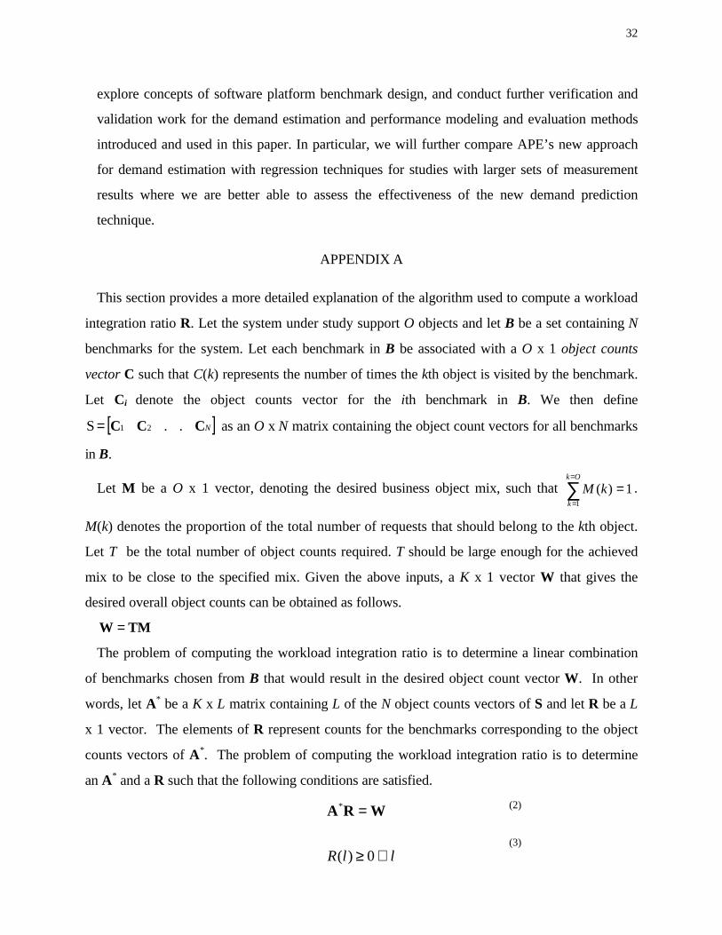
32

llR 0 )(

*

∀≥

= WRA

explore concepts of software platform benchmark design, and conduct further verification and

validation work for the demand estimation and performance modeling and evaluation methods

introduced and used in this paper. In particular, we will further compare APE’s new approach

for demand estimation with regression techniques for studies with larger sets of measurement

results where we are better able to assess the effectiveness of the new demand prediction

technique.

APPENDIX A

This section provides a more detailed explanation of the algorithm used to compute a workload

integration ratio R. Let the system under study support O objects and let B be a set containing N

benchmarks for the system. Let each benchmark in B be associated with a O x 1 object counts

vector C such that C(k) represents the number of times the kth object is visited by the benchmark.

Let Ci denote the object counts vector for the ith benchmark in B. We then define

[ ]NCCC .. S 21= as an O x N matrix containing the object count vectors for all benchmarks

in B.

Let M be a O x 1 vector, denoting the desired business object mix, such that 1)(1

=∑=

=

Ok

kkM .

M(k) denotes the proportion of the total number of requests that should belong to the kth object.

Let T be the total number of object counts required. T should be large enough for the achieved

mix to be close to the specified mix. Given the above inputs, a K x 1 vector W that gives the

desired overall object counts can be obtained as follows.

TMW =

The problem of computing the workload integration ratio is to determine a linear combination

of benchmarks chosen from B that would result in the desired object count vector W. In other

words, let A* be a K x L matrix containing L of the N object counts vectors of S and let R be a L

x 1 vector. The elements of R represent counts for the benchmarks corresponding to the object

counts vectors of A*. The problem of computing the workload integration ratio is to determine

an A* and a R such that the following conditions are satisfied.

(2)

(3)

33

Equation (2) specifies that the object counts achieved by combining the benchmarks in A*

according to the benchmark counts in R should equal the desired object counts given by W.

Equation (3) restricts the computed benchmark counts to be non-negative values.

To solve the problem, we devised an algorithm which iteratively determines the A* matrix and

the R vector that satisfy the conditions given by Eq. (2) and Eq. (3). To begin, an initial A*

matrix is determined by identifying a small subset of distinct benchmarks from B. This relies on

the computation of an algebraic basis set for a set of object count vectors from S. At each step

of the iteration, linear programming is used to find a value of R for a given A* such that the

difference between the desired object counts (W) and the achieved object counts (A*R) is

minimized. Equation (3) forms one of the constraints of the LP problem. The second constraint is

obtained by relaxing the condition specified by (1) to

This change facilitates an iterative solution by which A* is progressively modified by adding

more benchmarks from B until an R that satisfies the stricter constraint given by (1), i.e.,

corresponding to a better match between W and A*R is found. Specifically, the difference

between the desired object counts and the achieved object counts is calculated as a K x 1 slack

vector RAWE * −= . The benchmark that offsets E the most is identified from B. The new

benchmark to be selected is determined by computing the Euclidean distances between E and the

vectors in S. The vector in S that yields the minimum distance is selected and appended to A* as

an additional column. This is followed by another iteration of the algorithm.

The algorithm is guaranteed to terminate when the goal is to match an object mix that results

from B. This is because in the worst case all benchmarks from S will be included to achieve the

match. The algorithm terminates if the mismatches in object counts, given by the elements of E,

are less than or equal to user-specified tolerance thresholds for object counts or if a user-specified

maximum number of iterations is reached. The workload integration ratio is computed by

normalizing the elements of the R vector so that they sum to one. A more detailed description of

the algorithm can be found in our previous publication [10].

(5) WRA ≤*

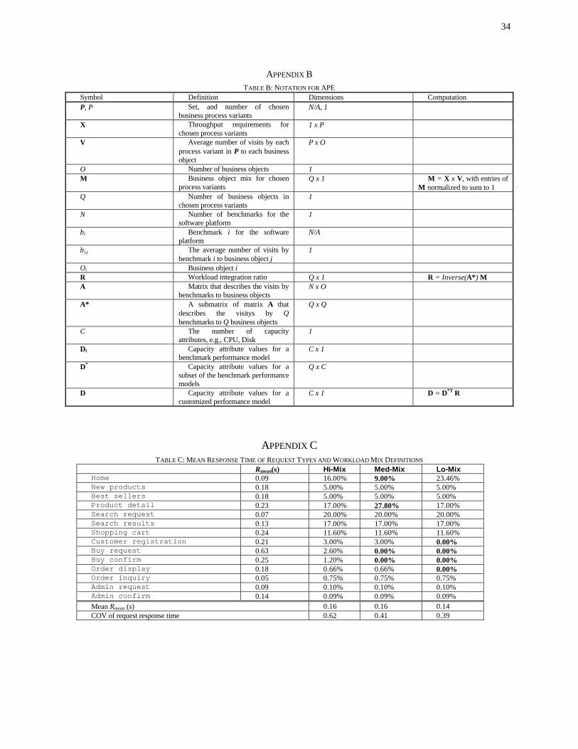
34

APPENDIX B TABLE B: NOTATION FOR APE

Symbol Definition Dimensions Computation P, P Set, and number of chosen

business process variants N/A, 1

X Throughput requirements for chosen process variants

1 x P

V Average number of visits by each process variant in P to each business object

P x O

O Number of business objects 1 M Business object mix for chosen

process variants Q x 1 M = X x V, with entries of

M normalized to sum to 1 Q Number of business objects in

chosen process variants 1

N Number of benchmarks for the software platform

1

bi Benchmark i for the software platform

N/A

bi,j The average number of visits by benchmark i to business object j

1

Oi Business object i R Workload integration ratio Q x 1 R = Inverse(A*) M A Matrix that describes the visits by

benchmarks to business objects N x O

A* A submatrix of matrix A that describes the visitys by Q benchmarks to Q business objects

Q x Q

C The number of capacity attributes, e.g., CPU, Disk

1

Di Capacity attribute values for a benchmark performance model

C x 1

D* Capacity attribute values for a subset of the benchmark performance models

Q x C

D Capacity attribute values for a customized performance model

C x 1 D = D*T R

APPENDIX C TABLE C: MEAN RESPONSE TIME OF REQUEST TYPES AND WORKLOAD MIX DEFINITIONS

Rmean(s) Hi-Mix Med-Mix Lo-Mix Home 0.09 16.00% 9.00% 23.46% New products 0.18 5.00% 5.00% 5.00% Best sellers 0.18 5.00% 5.00% 5.00% Product detail 0.23 17.00% 27.80% 17.00% Search request 0.07 20.00% 20.00% 20.00% Search results 0.13 17.00% 17.00% 17.00% Shopping cart 0.24 11.60% 11.60% 11.60% Customer registration 0.21 3.00% 3.00% 0.00% Buy request 0.63 2.60% 0.00% 0.00% Buy confirm 0.25 1.20% 0.00% 0.00% Order display 0.18 0.66% 0.66% 0.00% Order inquiry 0.05 0.75% 0.75% 0.75% Admin request 0.09 0.10% 0.10% 0.10% Admin confirm 0.14 0.09% 0.09% 0.09% Mean Rmean (s) 0.16 0.16 0.14 COV of request response time 0.62 0.41 0.39

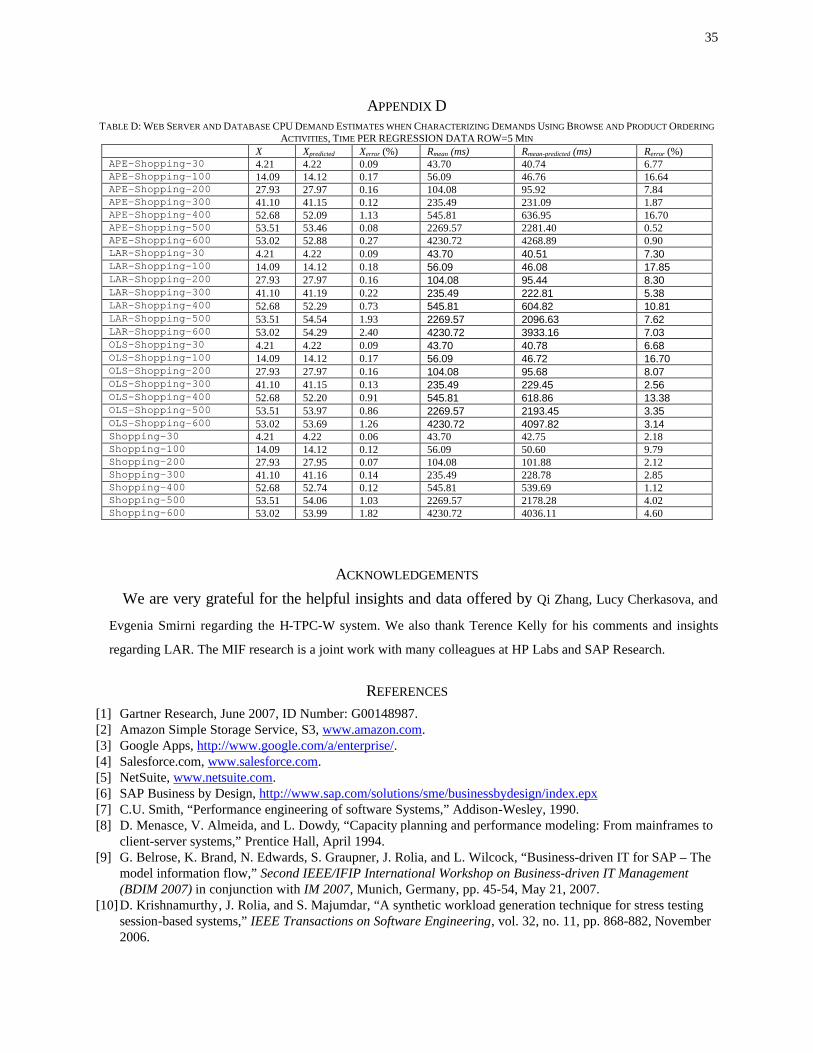
35

APPENDIX D TABLE D: WEB SERVER AND DATABASE CPU DEMAND ESTIMATES WHEN CHARACTERIZING DEMANDS USING BROWSE AND PRODUCT ORDERING

ACTIVITIES, TIME PER REGRESSION DATA ROW=5 MIN X Xpredicted Xerror (%) Rmean (ms) Rmean-predicted (ms) Rerror (%) APE-Shopping-30 4.21 4.22 0.09 43.70 40.74 6.77 APE-Shopping-100 14.09 14.12 0.17 56.09 46.76 16.64 APE-Shopping-200 27.93 27.97 0.16 104.08 95.92 7.84 APE-Shopping-300 41.10 41.15 0.12 235.49 231.09 1.87 APE-Shopping-400 52.68 52.09 1.13 545.81 636.95 16.70 APE-Shopping-500 53.51 53.46 0.08 2269.57 2281.40 0.52 APE-Shopping-600 53.02 52.88 0.27 4230.72 4268.89 0.90 LAR-Shopping-30 4.21 4.22 0.09 43.70 40.51 7.30 LAR-Shopping-100 14.09 14.12 0.18 56.09 46.08 17.85 LAR-Shopping-200 27.93 27.97 0.16 104.08 95.44 8.30 LAR-Shopping-300 41.10 41.19 0.22 235.49 222.81 5.38 LAR-Shopping-400 52.68 52.29 0.73 545.81 604.82 10.81 LAR-Shopping-500 53.51 54.54 1.93 2269.57 2096.63 7.62 LAR-Shopping-600 53.02 54.29 2.40 4230.72 3933.16 7.03 OLS-Shopping-30 4.21 4.22 0.09 43.70 40.78 6.68 OLS-Shopping-100 14.09 14.12 0.17 56.09 46.72 16.70 OLS-Shopping-200 27.93 27.97 0.16 104.08 95.68 8.07 OLS-Shopping-300 41.10 41.15 0.13 235.49 229.45 2.56 OLS-Shopping-400 52.68 52.20 0.91 545.81 618.86 13.38 OLS-Shopping-500 53.51 53.97 0.86 2269.57 2193.45 3.35 OLS-Shopping-600 53.02 53.69 1.26 4230.72 4097.82 3.14 Shopping-30 4.21 4.22 0.06 43.70 42.75 2.18 Shopping-100 14.09 14.12 0.12 56.09 50.60 9.79 Shopping-200 27.93 27.95 0.07 104.08 101.88 2.12 Shopping-300 41.10 41.16 0.14 235.49 228.78 2.85 Shopping-400 52.68 52.74 0.12 545.81 539.69 1.12 Shopping-500 53.51 54.06 1.03 2269.57 2178.28 4.02 Shopping-600 53.02 53.99 1.82 4230.72 4036.11 4.60

ACKNOWLEDGEMENTS We are very grateful for the helpful insights and data offered by Qi Zhang, Lucy Cherkasova, and

Evgenia Smirni regarding the H-TPC-W system. We also thank Terence Kelly for his comments and insights

regarding LAR. The MIF research is a joint work with many colleagues at HP Labs and SAP Research.

REFERENCES [1] Gartner Research, June 2007, ID Number: G00148987. [2] Amazon Simple Storage Service, S3, www.amazon.com. [3] Google Apps, http://www.google.com/a/enterprise/. [4] Salesforce.com, www.salesforce.com. [5] NetSuite, www.netsuite.com. [6] SAP Business by Design, http://www.sap.com/solutions/sme/businessbydesign/index.epx [7] C.U. Smith, “Performance engineering of software Systems,” Addison-Wesley, 1990. [8] D. Menasce, V. Almeida, and L. Dowdy, “Capacity planning and performance modeling: From mainframes to

client-server systems,” Prentice Hall, April 1994. [9] G. Belrose, K. Brand, N. Edwards, S. Graupner, J. Rolia, and L. Wilcock, “Business-driven IT for SAP – The

model information flow,” Second IEEE/IFIP International Workshop on Business-driven IT Management (BDIM 2007) in conjunction with IM 2007, Munich, Germany, pp. 45-54, May 21, 2007.

[10] D. Krishnamurthy, J. Rolia, and S. Majumdar, “A synthetic workload generation technique for stress testing session-based systems,” IEEE Transactions on Software Engineering, vol. 32, no. 11, pp. 868-882, November 2006.

36

[11] R. Grace, “The benchmark book,” Prentice Hall, 1996. [12] J. J. Dujmovic, “Universal benchmark suites,” Proceedings of IEEE MASCOTS Conference, pp. 197-205,

1999. [13] U. Krishnaswamy and D. Scherson, “A framework for computer performance evaluation using benchmark

sets,” IEEE Transactions on Computers, vol. 49, no. 12, pp. 1325-1338, December 2000. [14] D. Krishnamurthy, “Synthetic Workload Generation for Stress Testing Session-Based Systems,” PhD thesis,

Dept. of Systems and Computer Eng., Carleton Univ., Ottawa, Canada, Jan. 2004. [15] J.P. Buzen, “Computation algorithms for closed queuing networks with exponential servers,” Communications

of the ACM, vol. 16, no. 9, pp. 527-531, September 1973. [16] M. Reiser, “A queuing network analysis of computer communication networks with window flow control,”

IEEE Transactions on Communications, vol. 27, no. 8, pp. 1201-1209, August 1979. [17] M. Woodside, J. E. Nielsen, D. C. Petriu, and S. Majumdar, “The stochastic rendezvous network model for

performance of synchronous client-server-like distributed software,” IEEE Transactions on Computers, vol. 44, no. 1, pp, 20-34, January 1995.

[18] J.A. Rolia and K.C. Sevcik, “The method of layers,” IEEE Transactions on Software Engineering, vol. 21, no. 8, pp. 689-700, August 1995.

[19] D. Krishnamurthy, J. Rolia, and M. Xu, “WAM – The weighted average method for predicting the performance of systems with bursts of customer sessions,” HP Labs Technical Report, HPL-2008-66.

[20] N. Tiwari and P. Mynampati, “Experiences of using LQN and QPN tools for performance modeling of a J2EE application,” International Computer Measurement Group (CMG) Conference, pp. 537-548, 2006.

[21] S. Balsamo, A. Di Marco, P. Inverardi, and M. Simeoni, “Model-based performance prediction in software development: A survey,” IEEE Transactions on Software Engineering, vol. 30, no. 5, pp, 295-310, May 2004.

[22] V. Vetland, “Measurement-based composite computational work modeling of software,” Ph.D. Thesis, University of Trondheim, August 1993.

[23] C. E. Hrischuk, M. Woodside, and J.A. Rolia, “Trace-based load characterization for generating performance software models,” Hrischuk, C.E.; Murray Woodside, C.; Rolia, J.A., IEEE Transactions on Software Engineering, vol. 25, no. 1, pp. 122-135, January-February 1999.

[24] D. C. Petriu, C. M. Woodside, D. B. Petriu, J. Xu, T. Israr, G. Georg, R. France, J. M. Bieman, S. H. Houmb, and J. Jurjens, "Performance Analysis of security aspects in UML models", Proceedings of the 6th ACM International Workshop on Software and Performance (WOSP07), pp 91-102, Buenos Aires, February 2007.

[25] Y. Bard and M. Schatzoff, “Statistical methods in computer performance analysis,” Current Trends in Programming Methodology- Vol. III, Prentice-Hall.

[26] J. Rolia and V. Vetland, “Correlating resource demand information with ARM data for application services,” Proceedings of the ACM Workshop on Software and Performance (WOSP '98), pages 219-230, Santa Fe, NM, USA, October 1998.

[27] X. Sun, “Estimating resource demands for application services,” M. Sc. Thesis, Department of Systems and Computer Engineering, Carleton University, Ottawa, Canada, 1999.

[28] C. Stewart, T. Kelly, and A. Zhang, “Exploiting non-stationarity for performance prediction,” Proceedings of the EuroSys Conference, pp. 31-34, Lisbon, Portugal, March 2007.

[29] Q. Zhang, L. Cherkasova, and E. Smirni, “A regression-based analytic model for dynamic resource provisioning of multi-tier applications,” 4th International Conference on Autonomic Computing, pp. 27-27, June 2007.

[30] C. Guo, W. Sun, Y. Huang, Z. Wang, and B. Gao, “A framework for native multi-tenancy application development and management,” E-Commerce Technology and the 4th IEEE International Conference on Enterprise Computing, E-Commerce, and E-Services, pp. 551-558, July 2007.

[31] K. Zhang, X. Zhang, W. Sun, L. Wei, H. Liang, Y. Huang, L. Zeng, and X. Liu “A Policy-driven approach for Software-as-Services Customization,” E-Commerce Technology and the 4th IEEE International Conference on Enterprise Computing, E-Commerce, and E-Services, pp.123 – 130, July 2007.

[32] Common Information Model, http://www.dmtf.org/standards/cim/ [33] Eclipse Modelling Framework, http://www.eclipse.org/modeling/emf/ [34] TPC-W Benchmark, http://www.tpc.org/tpcw/default.asp [35] D. Menasce, and V. Almeida, “Capacity planning for Web services: Metrics, models and methods,” Prentice

Hall, 2001.

37

[36] D. Mosberger and T. Jin, “httperf - a tool for measuring Web server performance,” Workshop on Internet Server Performance, pp. 59-67, 1998.

[37] U. Herzog and J. Rolia, “Performance validation tools for software/hardware systems,” Performance Evaluation, vol. 45, no. 2-3, pp. 125-146, 2001.

[38] Business Process Markup Language www.bpmn.org. [39] M. Qin, R. Lee, A. El Rayess, V. Vetland, and J. Rolia, “Automatic generation of performance models for

distributed application systems,” Proceedings of IBM/NRC CASCON, 1996.