Applications of GPS Derived data to the Atmospheric Sciences

Jaclyn Secora Trzaska

Overview

History of GPS How GPS occultations work 3 GPS campaigns Applications of GPS Characterizing the Atmosphere

using GPS: Zonal Means and Arctic

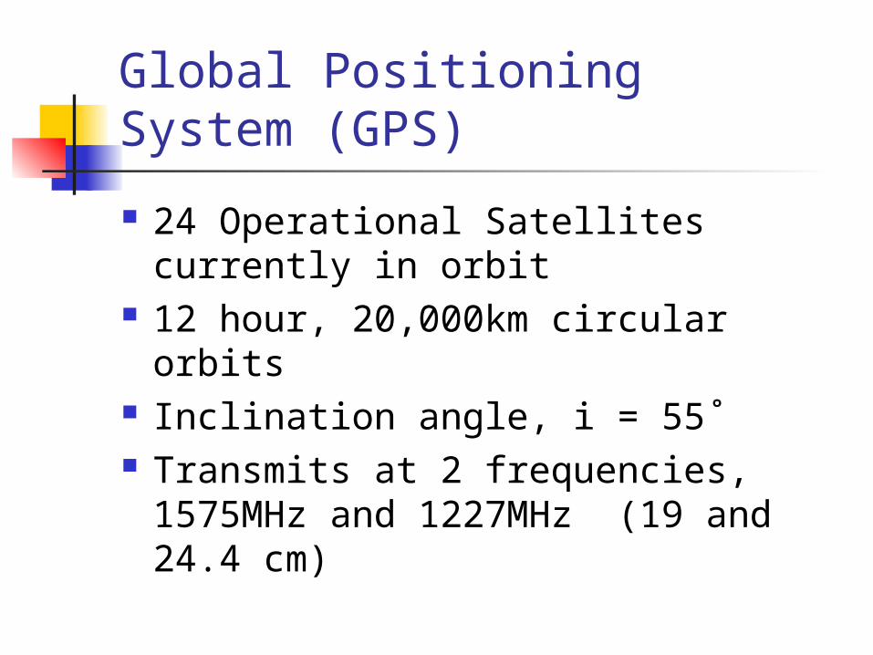
Global Positioning System (GPS)

24 Operational Satellites currently in orbit

12 hour, 20,000km circular orbits Inclination angle, i = 55˚ Transmits at 2 frequencies,

1575MHz and 1227MHz (19 and 24.4 cm)

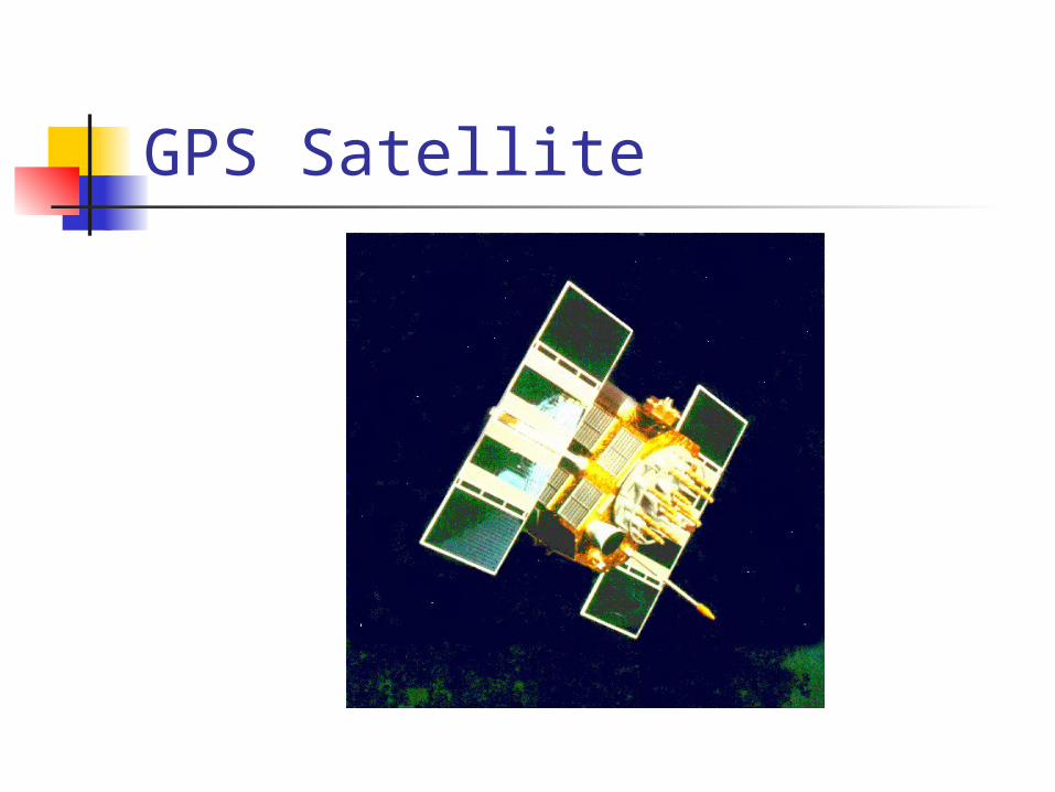
GPS Satellite

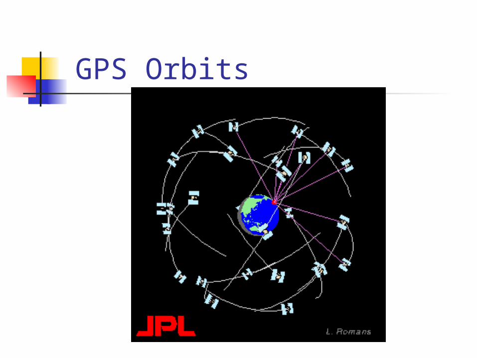
GPS Orbits

History of GPS

Originally called Navigation System with Timing And Ranging (NAVSTAR)

Developed by the US Department of Defense to provide all-weather round-the-clock navigation capabilities for military ground, sea, and air forces

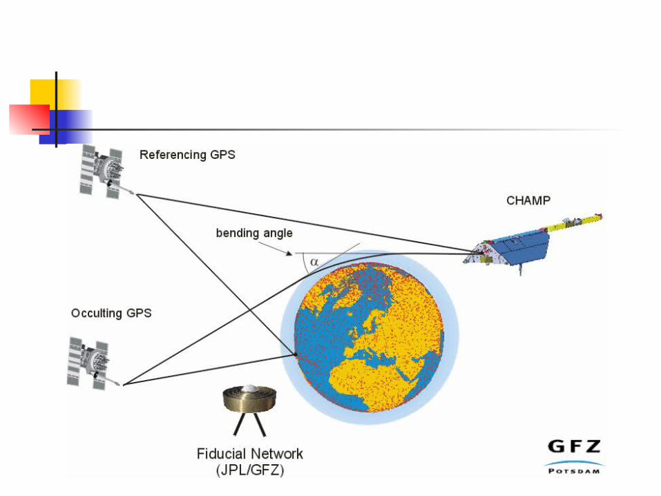
Radio Occultations Been used for over 30 years to

characterize planetary atmospheres Occultation occurs as satellite “rises or

sets” on the horizon as viewed by receiver Uses a microwave transmitter (GPS) to

send a signal to a receiver (LEO) on the opposite side of some medium of interest (atmosphere)

Medium characterized by effect it has on radio signal

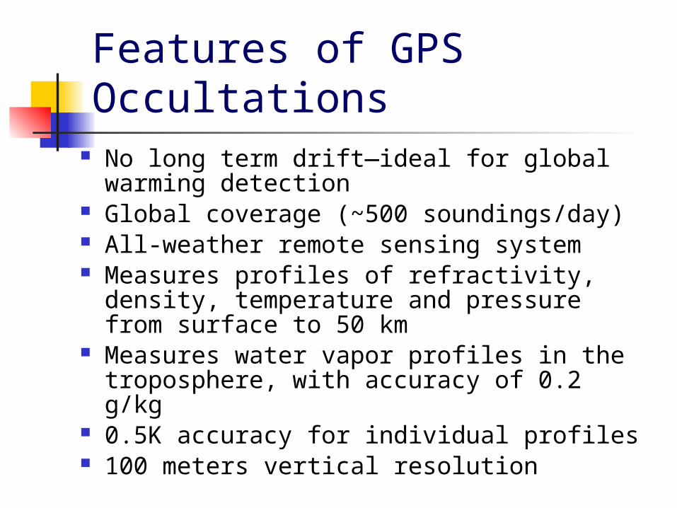
Features of GPS Occultations

No long term drift—ideal for global warming detection

Global coverage (~500 soundings/day) All-weather remote sensing system Measures profiles of refractivity,

density, temperature and pressure from surface to 50 km

Measures water vapor profiles in the troposphere, with accuracy of 0.2 g/kg

0.5K accuracy for individual profiles 100 meters vertical resolution

Some Theory

Assume spherical symmetry (no horizontal variations in temperature or moisture)

Relationship formed between refractive index and bending angle

Assume dry atmosphere, pressure and temperature are found

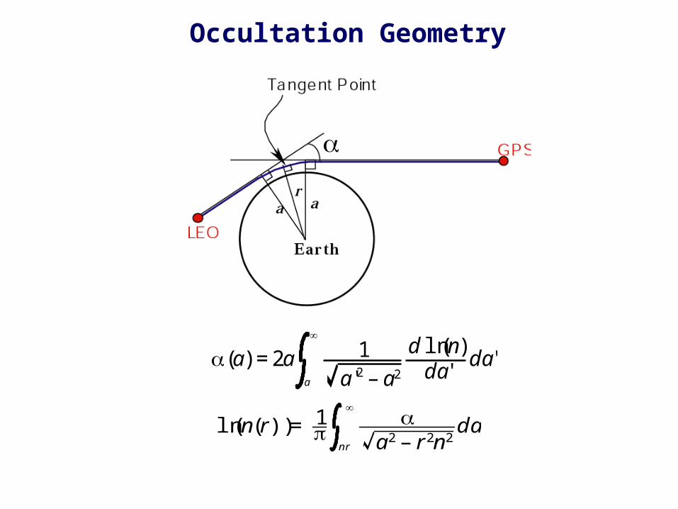
Occultation Geometry

ln(n(r)) = 1

a2 – r2n2da

nr

(a) = 2a 1

a'2 – a2

d ln(n)da'

da'a

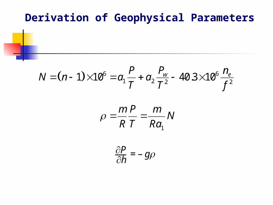
Derivation of Geophysical Parameters

6 61 2 2 2

1 10 40.3 10w eP P nN n a a

T T f

Ph

= – g

1

m P mN

R T Ra

Occultation Movie

http://genesis.jpl.nasa.gov/zope/GENESIS/Background/Movie

GPS/MET: The First Campaign

April 3, 1995 to March, 1997 100 to 150 occultations per day 1 Low Earth Orbiting Receiver

orbiting at ~775km

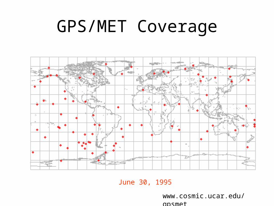
GPS/MET Coverage

June 30, 1995

www.cosmic.ucar.edu/gpsmet

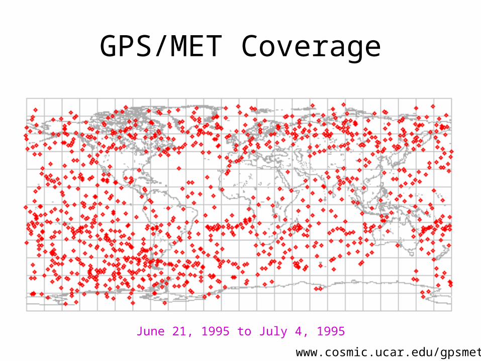
GPS/MET Coverage

June 21, 1995 to July 4, 1995

www.cosmic.ucar.edu/gpsmet

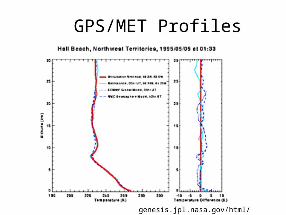
GPS/MET Profiles

genesis.jpl.nasa.gov/html/missions/gpsmet

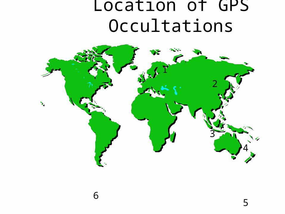
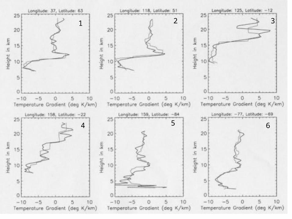
Location of GPS Occultations

1

2

3

4

56

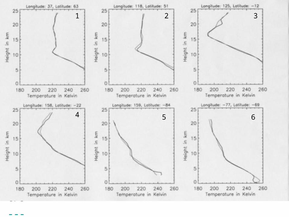
4 5 6

--- GPS

--- ECMWF

1 2 3

4 5 6

4 5 6

--- GPS

--- ECMWF

1 2 3

4 5 6

CHAMP

German satellite, launched in 2000 Collecting data since February 2001 Approximately 250 occultations per

day Scheduled to be in orbit for 5 years Used for gravity field magnetic field

and electric field recovery and atmospheric limb sounding

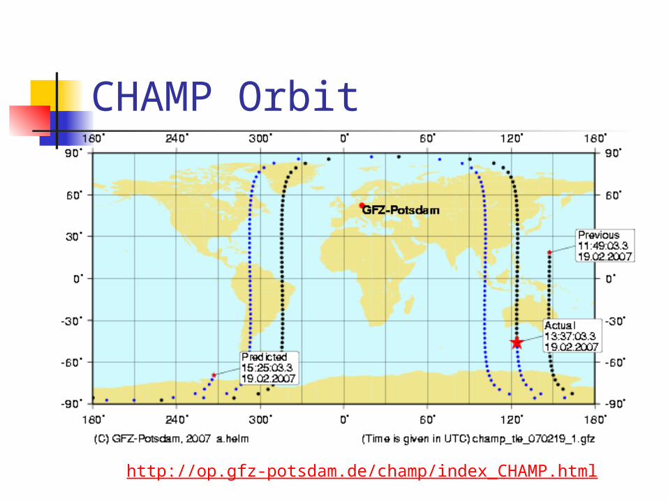
CHAMP Orbit

http://op.gfz-potsdam.de/champ/index_CHAMP.html

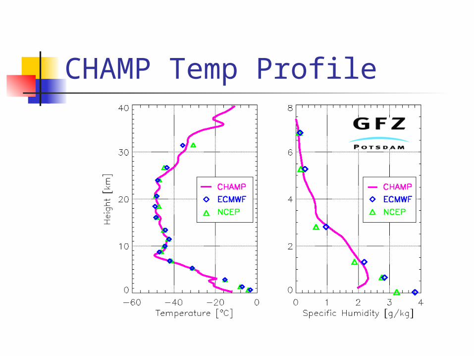
CHAMP Temp Profile

SuomiNet Network of GPS receivers located

at or near universities GPS receivers are ground based provide realtime atmospheric

precipitable water vapor measurements and other geodetic and meteorological information.

http://www.suominet.ucar.edu

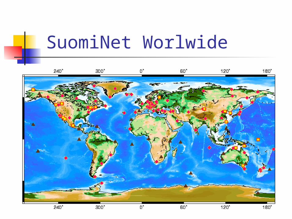
SuomiNet Worlwide

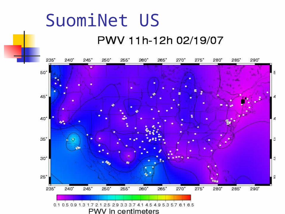
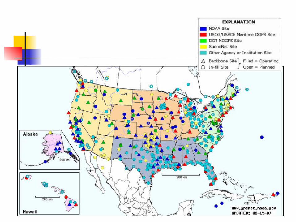
SuomiNet US

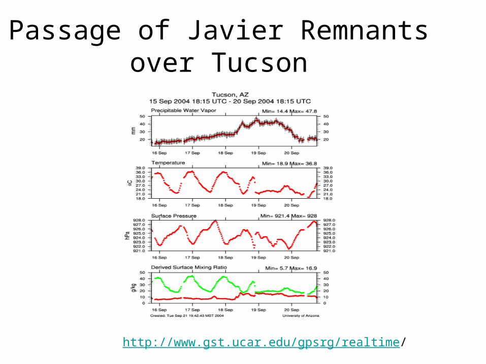
Passage of Javier Remnants over Tucson

http://www.gst.ucar.edu/gpsrg/realtime/

Hurricane Katrina

• http://www.suominet.ucar.edu/katrina/katrina.mov

Applications of GPS

Temperature Measurement Water Vapor Measurement Planetary Boundary Layer Ionosphere

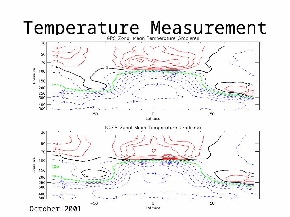
Temperature Measurement

October 2001

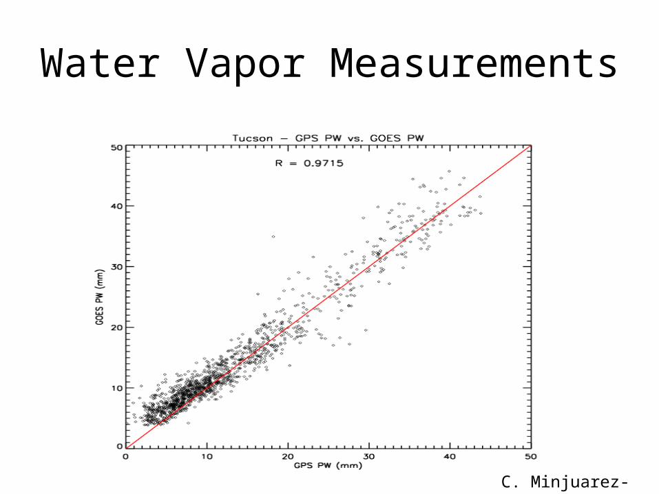
Water Vapor Measurements

C. Minjuarez-Sosa

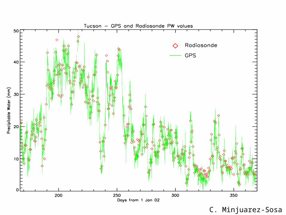
C. Minjuarez-Sosa

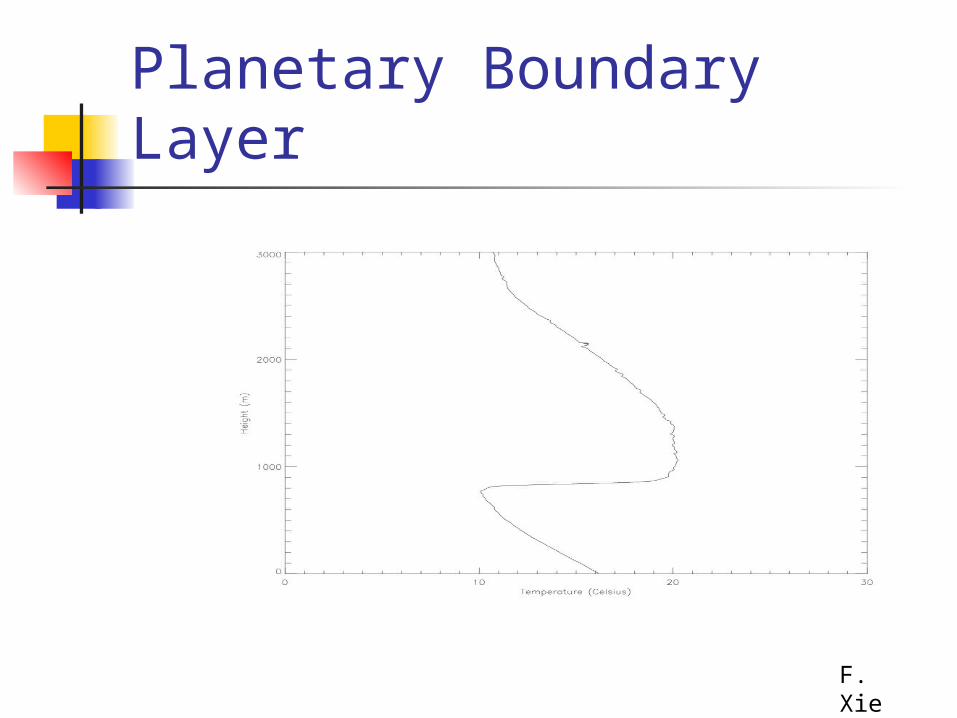
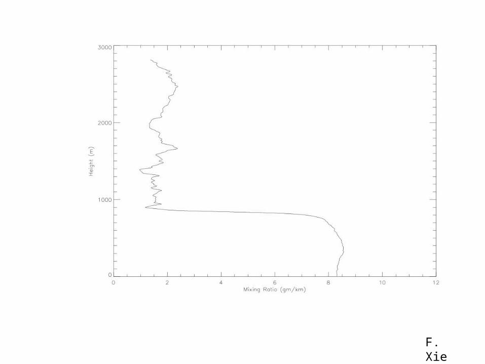
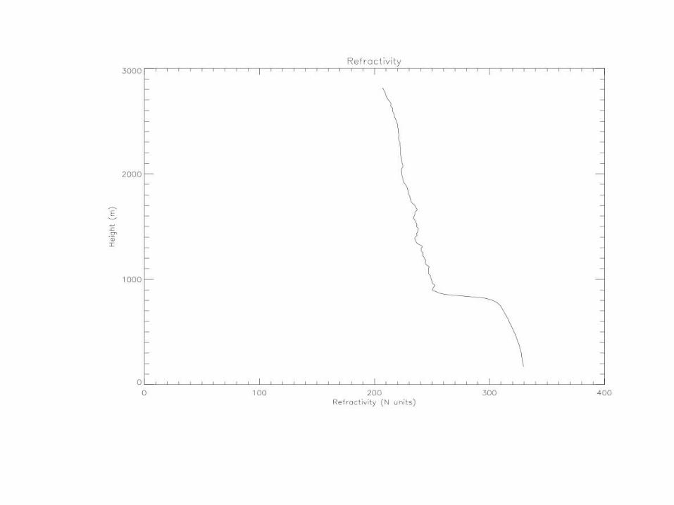
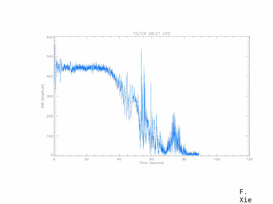
Planetary Boundary Layer

F. Xie

F. Xie

F. Xie

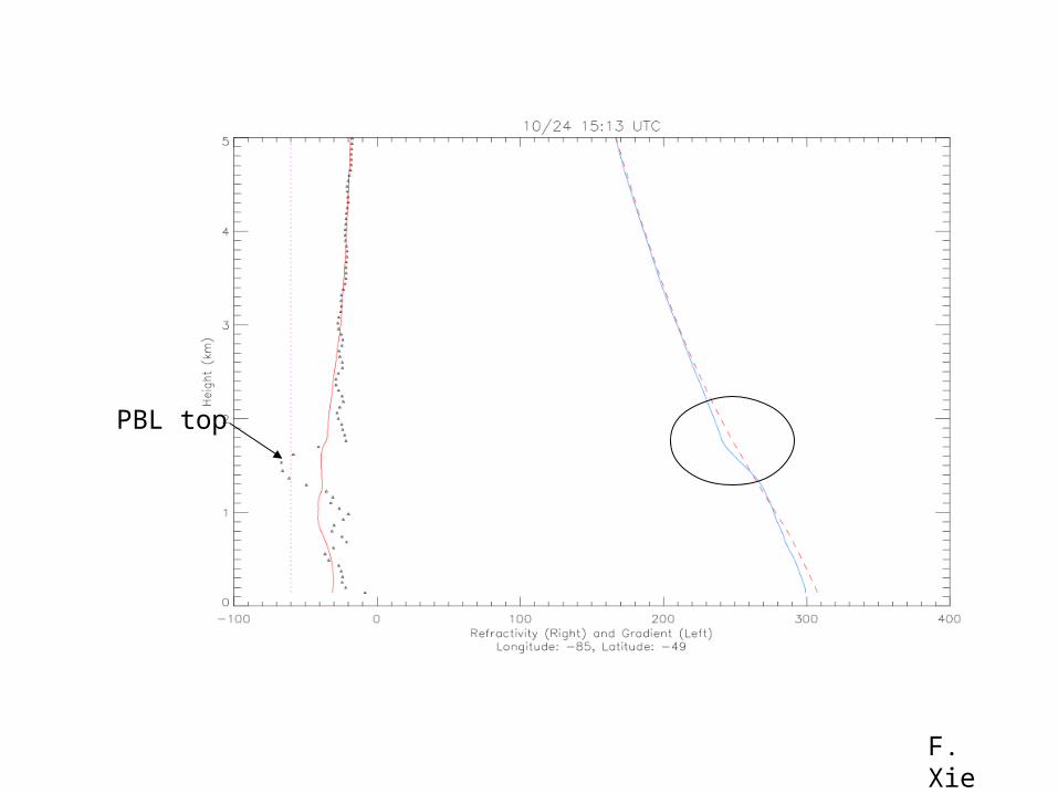
F. Xie

PBL top

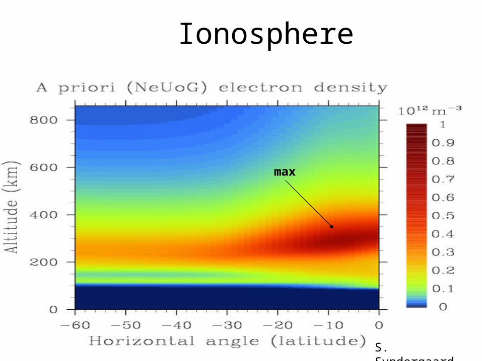
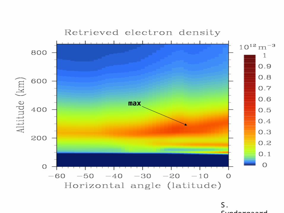
Ionosphere

S. Syndergaard

max

S. Syndergaard

max

Some Other Applications Climate research

all weather viewing Global dataset Unaffected by aerosols Long term accuracy

Assimilation into Weather Forecasts Tropopause dynamics Gravity field, magnetic field

An Investigation into Observed and Modeled Global Atmospheric Stability

Jaci Secora, Rob Kursinski, Andrea Hahmann, Dan

Hankins

Overview

Motivation of Study GPS/MET Mission ECMWF Analysis NCAR Community Climate Model GPS/ECMWF/CCM3 Comparisons Conclusions

Motivation of Study

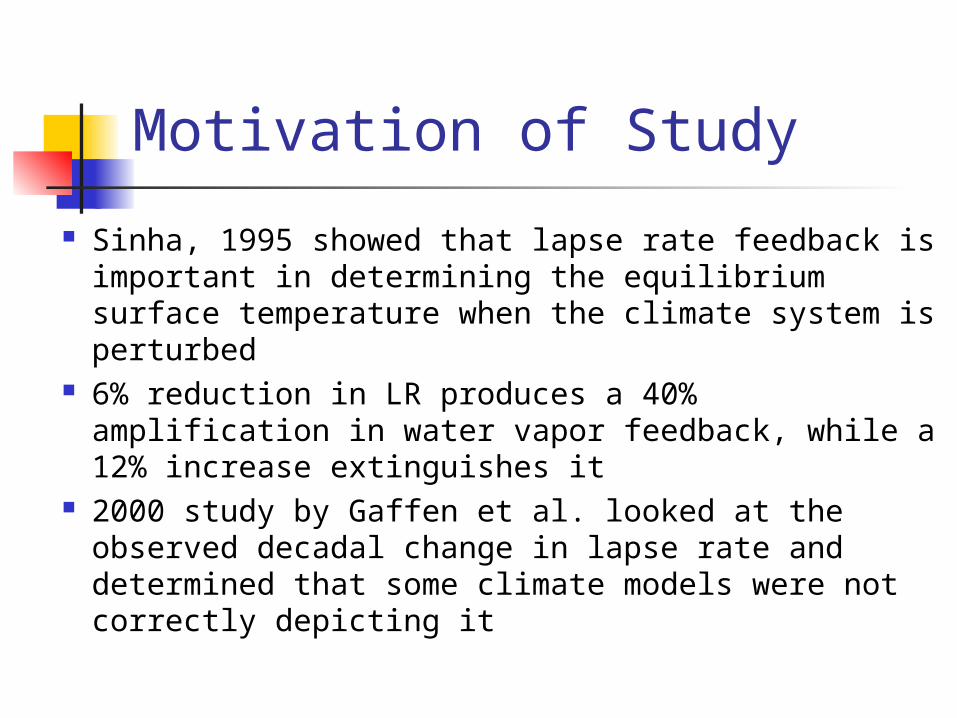
Sinha, 1995 showed that lapse rate feedback is important in determining the equilibrium surface temperature when the climate system is perturbed

6% reduction in LR produces a 40% amplification in water vapor feedback, while a 12% increase extinguishes it

2000 study by Gaffen et al. looked at the observed decadal change in lapse rate and determined that some climate models were not correctly depicting it

Purpose of Study

Study evaluates representation and variability of stability in climate models as well as characterizing the stability in the real atmosphere

Gaffen et al. (2000)

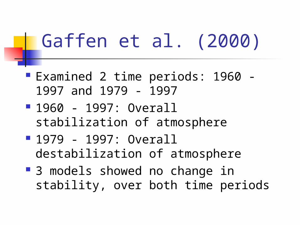
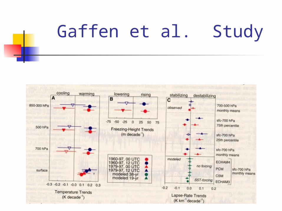
Examined 2 time periods: 1960 -1997 and 1979 - 1997

1960 - 1997: Overall stabilization of atmosphere

1979 - 1997: Overall destabilization of atmosphere

3 models showed no change in stability, over both time periods

Gaffen et al. Study

Data Sets Used in this Study

GPS: Observations

ECMWF: Analysis = Model + Observations (Not GPS Observations)

CCM3: Model

GPS/MET Data GPS occultation data offers unique combination

of high vertical resolution, accuracy and global coverage needed for this study

GPS/MET Mission from April 1995 - February 1997 Current study focused on June 21 to July 4, 1995 - Anti - Spoofing encryption turned off - Over 800 occultations collected during period - Period falls during the northern summer/

southern winter near the solstice (24 hours of day/night in the poles)

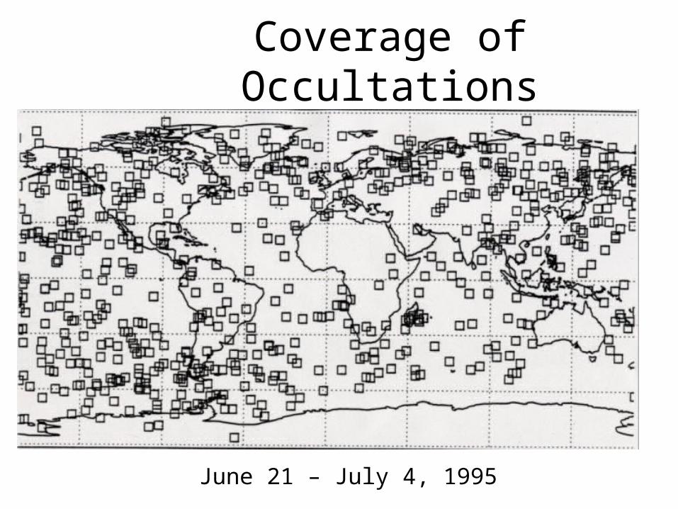
Coverage of Occultations

June 21 – July 4, 1995

ECMWF Data Global 6 hour analyses (not

reanalyses) 1º x 1º horizontal resolution 31 vertical levels (up to 30mb) High resolution and accuracy make it

a good comparison to GPS Interpolated to GPS occultation

locations in the JPL Processing System

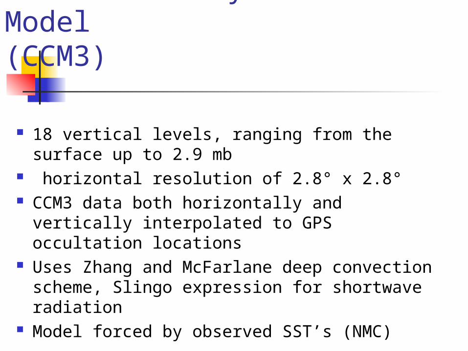
NCAR Community Climate Model (CCM3)

18 vertical levels, ranging from the surface up to 2.9 mb

horizontal resolution of 2.8° x 2.8° CCM3 data both horizontally and vertically

interpolated to GPS occultation locations Uses Zhang and McFarlane deep convection

scheme, Slingo expression for shortwave radiation

Model forced by observed SST’s (NMC)

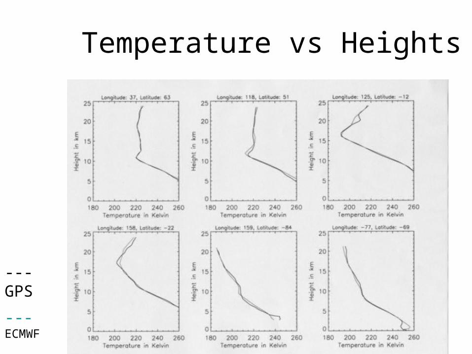
Temperature vs Heights

4 5 6

--- GPS

--- ECMWF

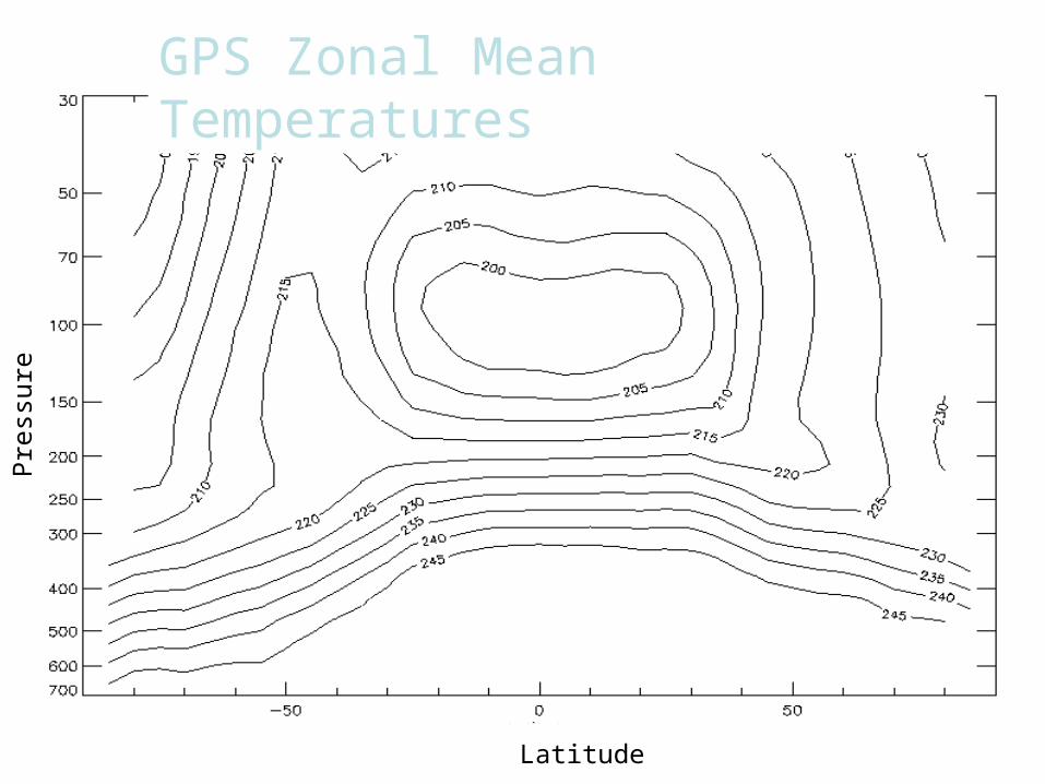
GPS Zonal Mean Temperatures

Latitude

Pre

ssur

e

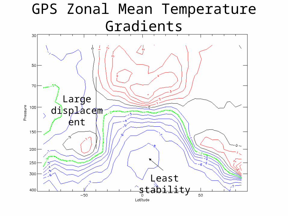
Large displacement

Least stability

GPS Zonal Mean Temperature Gradients

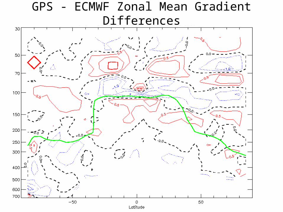
GPS - ECMWF Zonal Mean Gradient Differences

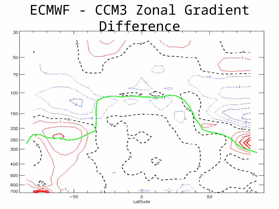
ECMWF - CCM3 Zonal Gradient Difference

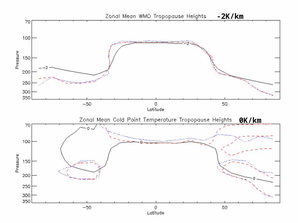
-2K/km

0K/km

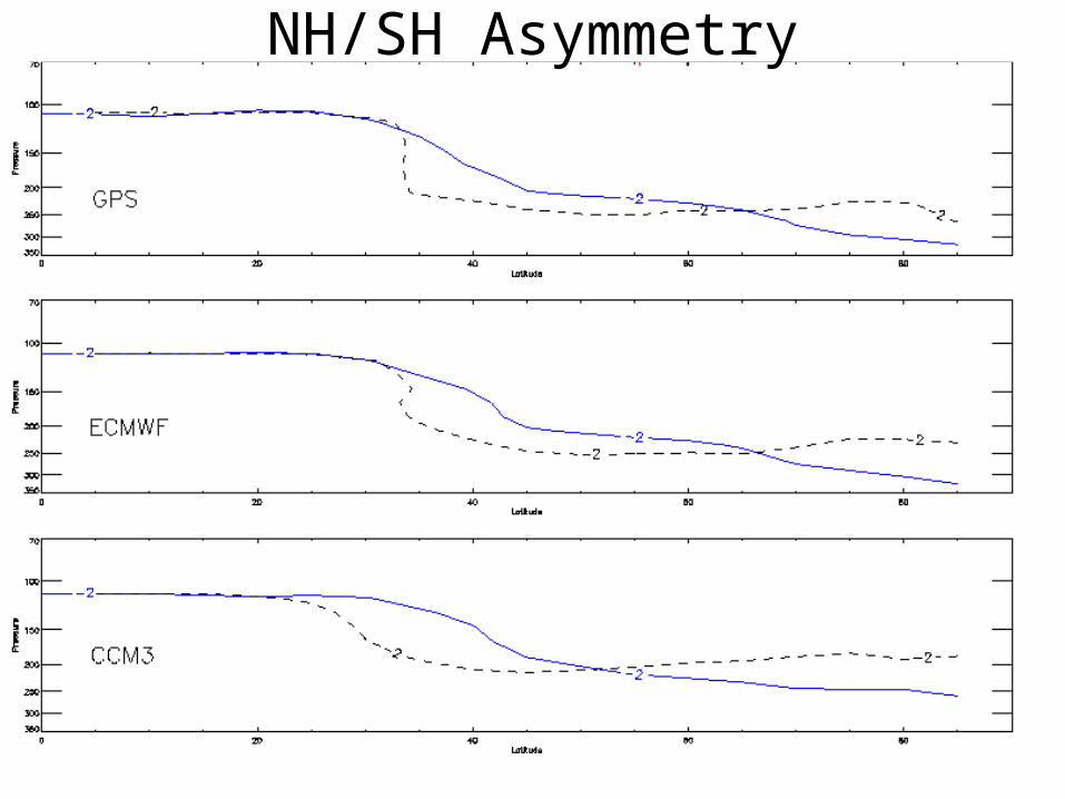
NH/SH Asymmetry

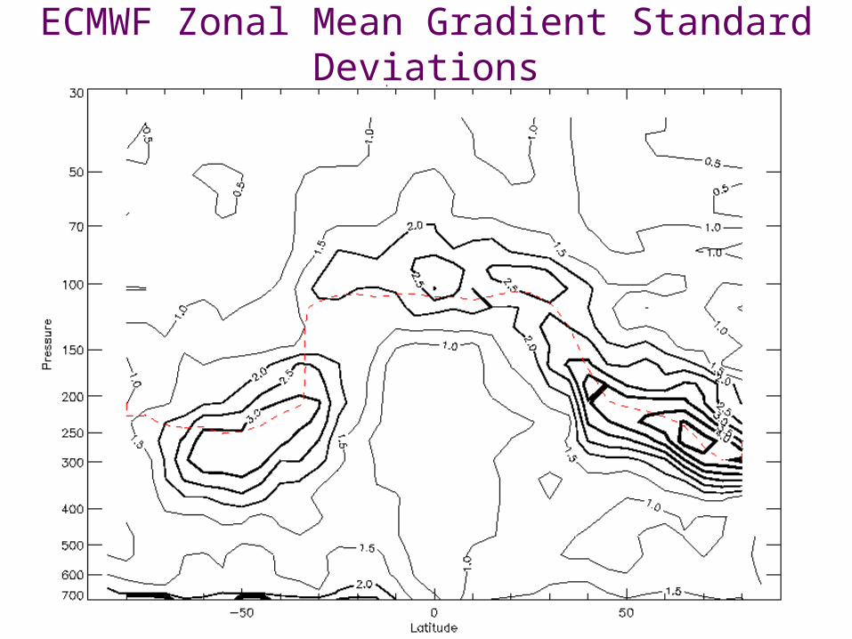
ECMWF Zonal Mean Gradient Standard Deviations

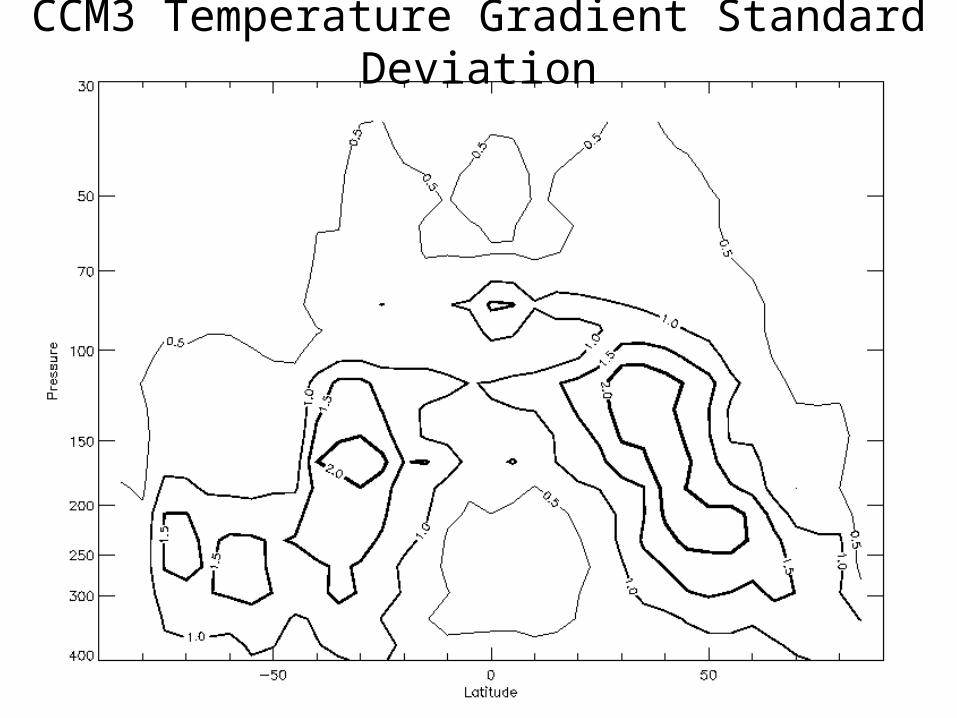
CCM3 Temperature Gradient Standard Deviation

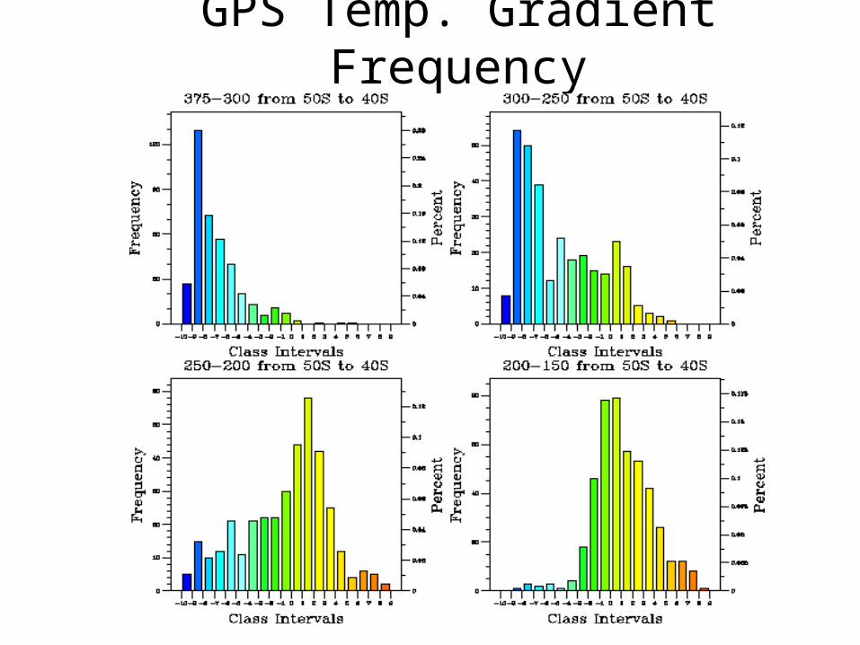
GPS Temp. Gradient Frequency

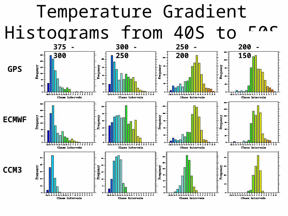
Temperature Gradient Histograms from 40S to 50S

GPS

ECMWF

CCM3

375 - 300 300 - 250 250 - 200 200 - 150

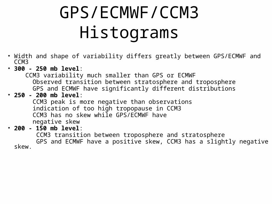
GPS/ECMWF/CCM3 Histograms

• Width and shape of variability differs greatly between GPS/ECMWF and CCM3• 300 - 250 mb level: CCM3 variability much smaller than GPS or ECMWF Observed transition between stratosphere and troposphere GPS and ECMWF have significantly different distributions• 250 - 200 mb level: CCM3 peak is more negative than observations indication of too high tropopause in CCM3 CCM3 has no skew while GPS/ECMWF have negative skew• 200 - 150 mb level: CCM3 transition between troposphere and stratosphere GPS and ECMWF have a positive skew, CCM3 has a slightly negative skew.

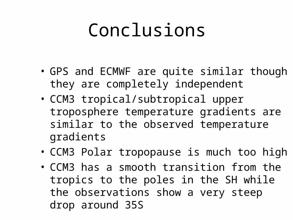
Conclusions

• GPS and ECMWF are quite similar though they are completely independent

• CCM3 tropical/subtropical upper troposphere temperature gradients are similar to the observed temperature gradients

• CCM3 Polar tropopause is much too high• CCM3 has a smooth transition from the tropics

to the poles in the SH while the observations show a very steep drop around 35S

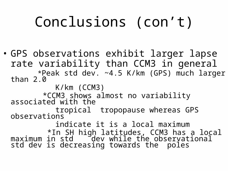
Conclusions (con’t)

• GPS observations exhibit larger lapse rate variability than CCM3 in general

*Peak std dev. ~4.5 K/km (GPS) much larger than 2.0 K/km (CCM3) *CCM3 shows almost no variability associated with the tropical tropopause whereas GPS observations indicate it is a local maximum *In SH high latitudes, CCM3 has a local maximum in std

dev while the observational std dev is decreasing towards the poles

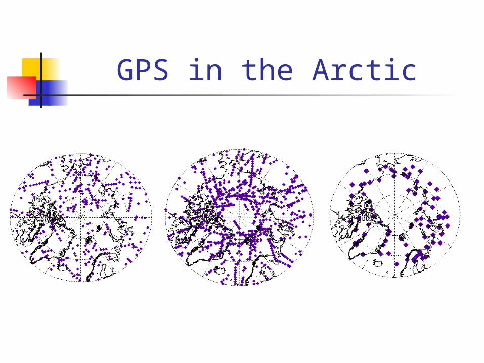
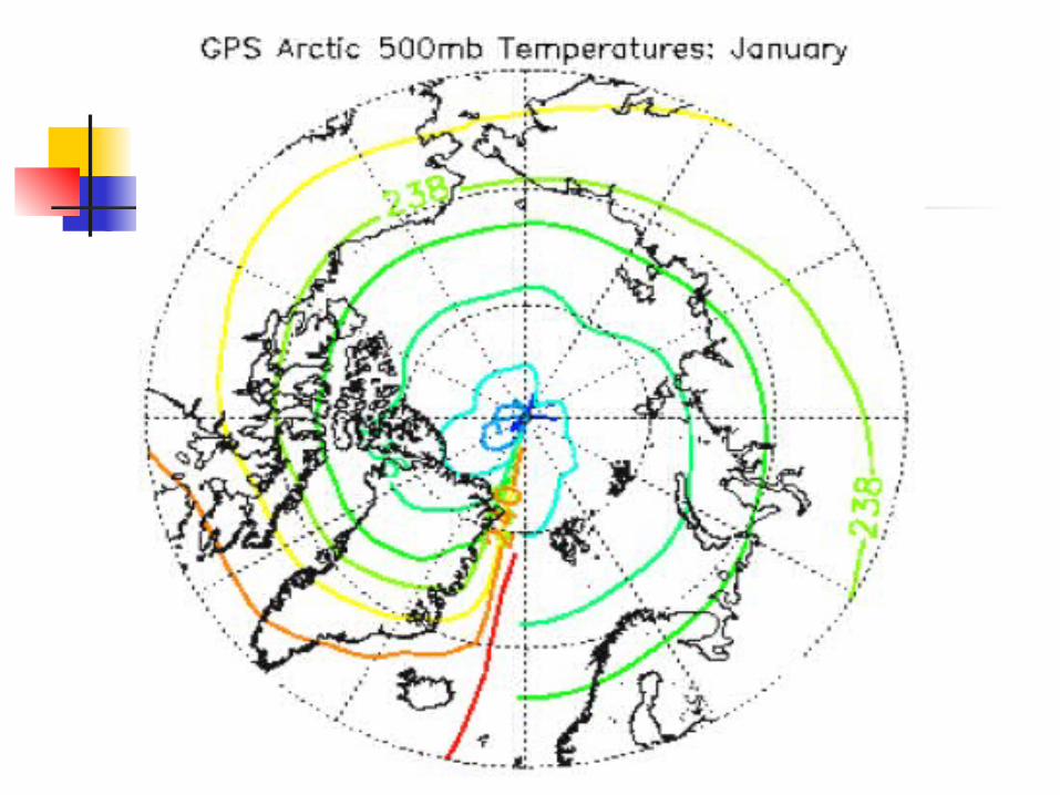
GPS in the Arctic

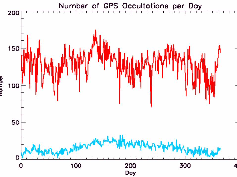
Global

Arctic

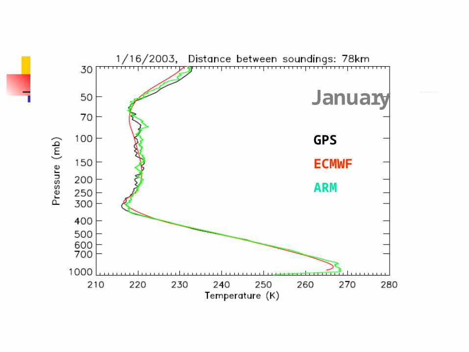
GPS

ECMWF

ARM

January

GPS

ECMWF

ARM

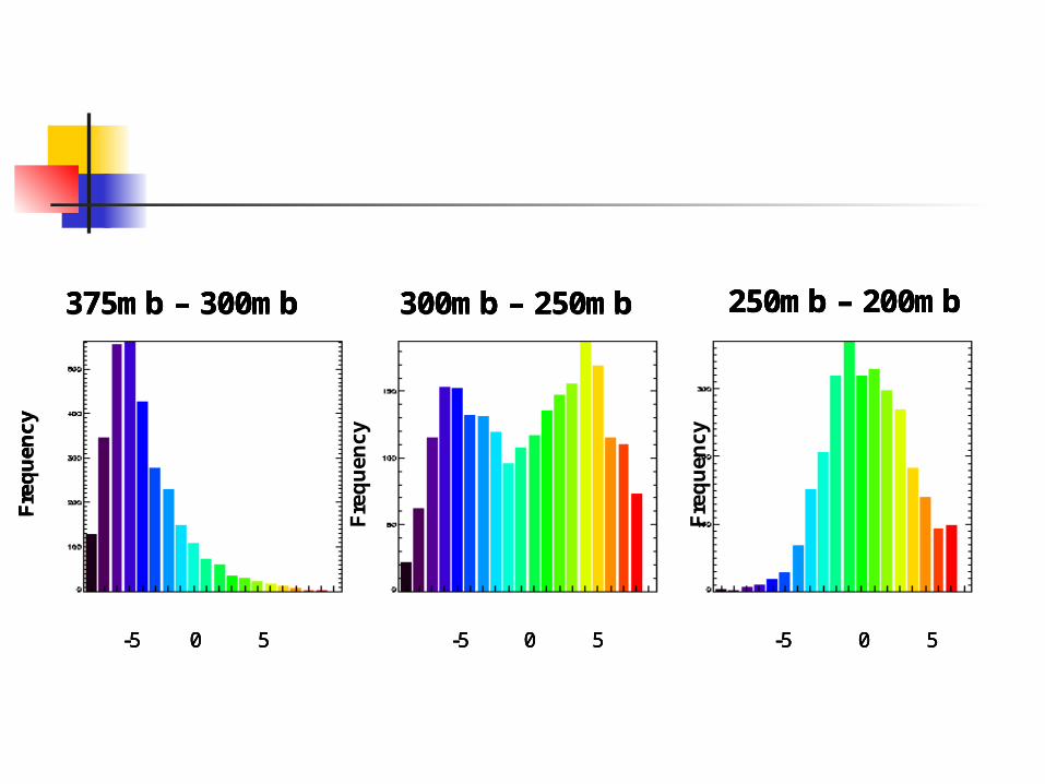
0-5 5 0-5 5 0-5 5

375mb – 300mb 300mb – 250mb 250mb – 200mb

Fre

qu

enc

y

Fre

qu

enc

y

Fre

qu

enc

y

0-5 50-5 5 0-5 50-5 5 0-5 50-5 5

375mb – 300mb 300mb – 250mb 250mb – 200mb

Fre

qu

enc

y

Fre

qu

enc

y

Fre

qu

enc

y

375mb – 300mb 300mb – 250mb 250mb – 200mb375mb – 300mb 300mb – 250mb 250mb – 200mb

Fre

qu

enc

y

Fre

qu

enc

y

Fre

qu

enc

y