Embed Size (px)
Citation preview

The Centre for Australian Weather and Climate Research A partnership between CSIRO and the Bureau of Meteorology
An Enhanced Tsunami Scenario Database:T2 Diana J.M. Greenslade, M. Arthur Simanjuntak, Stewart C. R. Allen CAWCR Technical Report No. 014 August 2009


An Enhanced Tsunami Scenario Database:T2
Diana J.M. Greenslade1, M. Arthur Simanjuntak1, Stewart C. R. Allen1
CAWCR Technical Report No. 014
August 2009
1Centre for Australian Weather and Climate Research: a Partnership between the Bureau of Meteorology and CSIRO, Melbourne, Australia
ISSN: 1836-019X
National Library of Australia Cataloguing-in-Publication entry
Author: Greenslade, Diana J. M.
Title: An enhanced tsunami scenario database : t2 / Diana J. M. Greenslade, M. Arthur Simanjuntak, Stewart C. R. Allen.
ISBN: 9781921605376 (pdf.)
Series: CAWCR technical report ; 14
Notes: Bibliography.
Subjects:Tsunamis--Australia--Data bases. Tsunamis--Australia--Mathematical models. Tsunami Warning System--Australia--Data bases. Tsunami Warning System--Australia--Mathematical models.
Other Authors/Contributors: Simanjuntak, M. Arthur, Allen, Stewart C. R. (Stewart Charles Richard), 1976-
Centre for Australian Weather and Climate Research. Australia. Bureau of Meteorology.
Dewey Number: 551.46370113

Enquiries should be addressed to: Diana Greenslade Centre for Australian Weather and Climate Research: A Partnership between the Bureau of Meteorology and CSIRO GPO Box 1289 Melbourne VIC 3001 Australia [email protected]
Copyright and Disclaimer
© 2009 CSIRO and the Bureau of Meteorology. To the extent permitted by law, all rights are
reserved and no part of this publication covered by copyright may be reproduced or copied in any
form or by any means except with the written permission of CSIRO and the Bureau of Meteorology.
CSIRO and the Bureau of Meteorology advise that the information contained in this publication
comprises general statements based on scientific research. The reader is advised and needs to be
aware that such information may be incomplete or unable to be used in any specific situation. No
reliance or actions must therefore be made on that information without seeking prior expert
professional, scientific and technical advice. To the extent permitted by law, CSIRO and the Bureau
of Meteorology (including each of its employees and consultants) excludes all liability to any person
for any consequences, including but not limited to all losses, damages, costs, expenses and any other
compensation, arising directly or indirectly from using this publication (in part or in whole) and any
information or material contained in it.

i
Contents
1. Introduction..........................................................................................................5
2. Enhanced aspects of T2......................................................................................5 2.1 Source locations ....................................................................................................... 5 2.2 Domain ..................................................................................................................... 7 2.3 Rupture modelling..................................................................................................... 8 2.4 Other model details................................................................................................. 12
3. Scaling strategy .................................................................................................13 3.1 Scaling beyond 9.2 ................................................................................................. 15 3.2 Scaling below 7.3.................................................................................................... 17
4. Evaluation...........................................................................................................18 4.1 Tonga 2006............................................................................................................. 18 4.2 Sumatra 2007 ......................................................................................................... 22 4.3 Hypothetical Bay of Bengal event........................................................................... 25
5. Further work.......................................................................................................26
6. Acknowledgements ...........................................................................................29
7. References .........................................................................................................29

ii An enhanced tsunami scenario database: T2
List of Figures Figure 1. (a) Source locations and domain for T2 scenario database for the Indian and Pacific
Ocean sources. (b) Source locations and recursive domain for South Sandwich plate sources. T1 source locations are designated in blue.............................................................6
Figure 2. Initial conditions for (a) scenario 45d from the T2 scenario database and (b) the equivalent T1 scenario (138d)..............................................................................................10
Figure 3. Locations of the centroids of each rupture element that contributes to scenarios 43a, 43b, 43c and 43d..................................................................................................................11
Figure 4. Value of the dip for subduction zones in the Indian and Pacific Oceans....................11
Figure 5. Maximum amplitude map for scenario 262d from the T2 scenario database..............13
Figure 6. (a) Coastal warnings resulting from scaling scenario 403d by a factor of 5.6 to represent a Mw = 9.5 event (b) Same as (a) but scaled by a factor of 2.0 to replicate a Mw = 9.2 event...............................................................................................................................16
Figure 7. Maximum tsunami amplitude from T2 during the May 3rd, 2006 Tonga event. The locations of the tsunameters are shown here by the blue diamonds near Hawaii. .............19
Figure 8. (a) Map showing the epicentre of the May 3rd, 2006 Tonga event (red asterisk) and the centre points of the rupture elements in the region that contribute to scenarios in the T2 scenario database (black crosses). The closest rupture element to the event is designated by a cross that is slightly bolder than the others. (b) Same as Figure 11(a) but with the centre points of the ruptures for the T1 scenarios indicated by the relevant number..........20
Figure 9. (a) Comparison of observed and modelled sea-level at the DART II for the Mw = 7.9 event of 3rd May, 2006. (b) Same as (a) but for the ETD....................................................21
Figure 10. Maximum tsunami amplitude from T2 during the September 12th 2007 Sumatra event. The Thai DART II buoy is designated by a white diamond. ......................................22
Figure 11. (a) Map showing the epicentre of the September 12th 2007 Sumatra event (red asterisk), the Thai DART II buoy (blue diamond) and the locations of the rupture elements in the region that contribute to scenarios in the T2 scenario database (black crosses). The closest rupture element to the event is designated by a cross that is bolder than the others. (b) Same as Figure 11(a) but with T1 scenario numbers. ...................................................23
Figure 12. Comparison of observed and modelled sea-level for the Mw = 8.4 event of 12th September 2007...................................................................................................................24
Figure 13. Initial conditions for a hypothetical event in the Bay of Bengal from (a) T2 scenario 22d and (b) T1 scenario 197d. .............................................................................................25
Figure 14. Time series of surface elevation from T1 scenario 197d and T2 scenario 22d at (115.467oE, 31.933oS), just offshore from Perth..................................................................26

iii
List of Tables Table 1. Details of the initial conditions used for the scenarios in the T2 scenario database. ..... 9
Table 2 Scaling factors (Fs) required to produce a new scenario of Magnitude Mw(new) from the existing T2 scenarios. Existing scenarios are denoted by bold type. ........................... 14
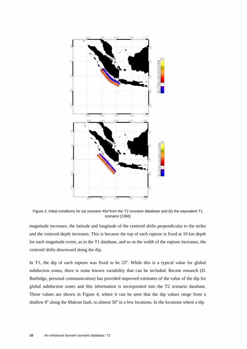
Table 3. Details of the initial conditions used for the Mw = 7.0 scenarios in the T2 scenario database. ............................................................................................................................. 18
Table 4. Scaling factors (Fs) required to produce a new scenario of Magnitude Mw(new) from the existing T2 Mw = 7.0 scenarios. Existing scenarios are denoted by bold type. ............ 18

iv An enhanced tsunami scenario database: T2

5
1. INTRODUCTION
A first-generation tsunami scenario database was developed as a part of the Joint Australian
Tsunami Warning Centre (JATWC). This is called T1 and is described in detail in Greenslade et
al. (2007). T1 was developed rapidly as a first-generation solution to the provision of numerical
guidance for the tsunami warning service and so several limitations were included in the model
runs. For example, the domain was relatively small and focussed on the Australian region. The
model run-time was only 10 hours, which in some cases prevented the tsunami waves from
propagating across the full extent of the domain. There are other aspects to T1 that have the
potential to be improved, such as minor bug fixes and enhancements based on new scientific
knowledge.
This research report describes the changes in the scenario database following the transition from
T1 to T2. Section 2 describes the T2 scenario database in detail, in particular those aspects that
are changed from T1. Section 3 presents a description of the method used to scale the scenarios
in order to provide guidance for intermediate earthquake magnitudes. Section 5 provides a brief
evaluation of the scenarios, and demonstrates the improvement that T2 provides over T1, and
the final section includes some indications of further work.
2. ENHANCED ASPECTS OF T2
2.1 Source locations
The basis for the source locations within T1 was the set of subduction zones as defined by Bird
(2003). This is also the basic set for T2; however in addition to the subduction zones located
within the Australian region, all subduction zones within the Indian and Pacific Oceans are
included. This incorporates subduction zones such as the Makran subduction zone south of
Pakistan and the “Ring of Fire” around the Pacific Ocean rim. In addition, several source
locations that are not designated as subduction zones by Bird (2003) are included. These non-
subduction zone sources are located:
• along the Timor trench to the north of Australia (as in T1)
• to the north of Timor
• in the Manus region (north of PNG)

6 An enhanced tsunami scenario database: T2
• between the Cascadia fault and Alaska
• along the Hjort trench, near Macquarie Island (Meckel et al., 2003)
• and the Sunda arc is extended northwards, according to Cummins (2007).
Figure 1. (a) Source locations and domain for T2 scenario database for the Indian and Pacific Ocean sources. (b) Source locations and recursive domain for South Sandwich plate sources. T1 source locations
are designated in blue.
These are all included in the set of source locations shown in Figure 1(a). Source locations
existing in both T1 and T2 are shown in blue, while the source locations included only in T2 are
shown in red. In addition to the locations in Figure 1(a), tsunamis generated by earthquakes on
the South Sandwich subduction zone are included (see Figure 1(b)). Note that scenarios along
the South Shetlands trench (along the tip of the Antarctic Peninsula, south of South America)
are not included here because it is very unlikely that there could be a tsunamigenic event along

7
this trench that impacts Australia. This is because the trench is very distant from and oriented
away from Australia and also because it is not long enough to support a large magnitude event.
These additional sources result in a total of 522 source locations for T2, increased from 230 for
T1. When all 4 magnitude scenarios are included (see Section 2.3), this results in a total of
1,865 individual scenarios, compared to 741 for T1.
2.2 Domain
As mentioned in Section 1, the T1 scenario database had a limited domain, covering only the
Australian region. Given the new sources described in the previous section, the T2 domain has
been expanded to cover the entire Indian and Pacific Oceans. There are two different domain
configurations represented in the database. The main domain is (69.4oS to 70oN) and (30oE to
300oE) and is shown in Figure 1(a) with the T2 source locations.
The southern boundary of the domain presents an interesting problem. As can be seen in Figure
1, part of this boundary incorporates the Antarctic land mass, and the remainder is an open
boundary. In reality, much of this southern portion of the domain would be covered by sea-ice
for at least some of the year. It is not clear what happens when a tsunami meets the Antarctic ice
edge (this is noted as potential further research in Section 5) but certainly some of the energy
would be reflected and some transmitted through or under the ice. Within the MOST model,
tsunami energy propagates freely through open boundaries with no reflection (apart from some
minor numerical effects in some cases). This suggests that an open boundary is not appropriate
in this case and the ice-edge would be more appropriately represented as a land boundary. The
Antarctic sea-ice extent is in fact highly variable on a monthly basis with the northern extent of
the ice-edge occurring anywhere between 70oS and 60oS (Simmonds and Jacka, 1995). It is
impossible to represent this accurately in a static database and so as a conservative assumption,
the open component of the southern boundary at 69.4oS (between approximately 160oE and
70oW) is replaced by a land boundary.
The horizontal grid spacing for T2 is 4 arc mins and due to the convergence of longitude lines,
this means that the actual spatial resolution ranges from ~7 km at the equator to 2.6 km at
69.4oS. Through the CFL criterion, this 2.6 km grid size imposes a limit of 12 seconds on the
time step. Note that the southern boundary of the T1 domain was at 76oS, which imposed an
even more stringent requirement of 8 seconds on the time step. Shifting the southern boundary

8 An enhanced tsunami scenario database: T2
slightly northwards therefore has the additional advantage of decreasing the computational time
by one third.
Another change to the domain that has been incorporated in T2 is that some parts of the ocean
that are irrelevant to tsunami propagation in the Indian or Pacific Oceans are designated as land,
in order to avoid unnecessary computations, e.g. the Atlantic Ocean. These areas can be seen in
Figure 1 (a).
A second domain is required to model the South Sandwich plate sources since they are outside
the domain of Figure 1(a). The main propagation path for tsunamis from this subduction zone
to the Australian coast is via the South Atlantic Ocean, so this new domain spans the entire 360o
of the globe. This is shown in Figure 1(b).
2.3 Rupture modelling
The T1 scenario database had 4 earthquake magnitudes of Mw = 7.5, 8.0, 8.4 and 9.0 at each
source location. This strategy is maintained in the T2 scenario database with the 8.4 amended to
8.5. One of the limitations of T1 was that all earthquakes at each location were defined to have
only a single strike value and therefore large events on curved subduction zones were not
aligned with the subduction zone along their entire lengths. In T2 the ruptures for large
earthquakes are represented as the sum of a number of smaller 100 km long rupture elements,
each of which has their strike more closely aligned with the local subduction zone. For example,
for a Mw = 8.0 scenario, two adjacent rupture elements are combined to create one rupture with
length approximately 200 km (this will not be exact due to the curvature of the subduction
zone), width of 65 km and slip of 2.2m. Details of the rupture dimensions for each magnitude
are shown here in Table 1. These have been derived from the relationship between magnitude
and rupture dimensions as follows. The magnitude (Mw) is related to seismic moment (Mo) as:
( )1.9log32
10 −= ow MM (1)
and seismic moment is related to the rupture characteristics of the earthquake as:
oo LWuM μ= (2)
where μ is the shear modulus and L, W and uo are the length, width and slip of the rupture
respectively (in metres). Here we take μ to be 4.5 x 10¹⁰ Nm-2.

9
Note that the rupture elements are not identical for each magnitude event, i.e. this is not a unit
source technique as used in as NOAA’s SIFT database (Gica et al., 2008) as the widths and slip
of the ruptures (and therefore the rupture elements) are different for each magnitude. Note also
that the details of the Mw = 9.0 event on the South Sandwich subduction zone (see Figure 1(b))
are slightly different to all other Mw = 9.0 events in the database. This is due to the fact that this
subduction zone is not long enough to support an event of length 1000 km.
Table 1. Details of the initial conditions used for the scenarios in the T2 scenario database.
Magnitude (Mw) Seismic
moment (Mo) (Nm)
Width (W) (km)
Number of rupture elements
Length (approximate)
(L) (km)
Slip (uo) (m)
7.5 2.24 x 10²⁰ 50 1 100 1
8.0 1.26 x 10²¹ 65 2 200 2.2
8.5 7.2 x 10²¹ 80 4 400 5
9.0 4.0 x 10²² 100 10 1000 8.8
9.0 (Sandwich
only) 4.0 x 10²² 100 8 800 11
An example of the difference in Mw = 9.0 ruptures between T1 and T2 is shown in Figure 2. It
can be seen that the T1 initial conditions have some small portions of the rupture that occur
away from the subduction zone, which is not physically realistic. This does not occur with the
enhanced rupture modelling in T2.
A result of the T2 multiple rupture element technique is that the source location for each T2
scenario is provided as a set of locations, rather than as an individual source location. This has
some advantages when the rupture direction is not known in real-time, as a set of scenarios can
be selected to provide warning guidance, as opposed to a single scenario. Figure 3 shows the
locations of the centroid of each rupture element that contributes to scenarios 43a, 43b, 43c and
43d. Note that the Mw = 7.5 scenario (43a) is staggered relative to the locations of the rupture
elements of the other magnitude scenarios. This was specified so that the mid-point of the top
edges of the ruptures would be co-located for all scenarios of any magnitude at a particular mid-
point. Mid-points were spaced 100 km along the strike of the fault. Note also that as the
10 An enhanced tsunami scenario database: T2
Figure 2. Initial conditions for (a) scenario 45d from the T2 scenario database and (b) the equivalent T1 scenario (138d)
magnitude increases, the latitude and longitude of the centroid shifts perpendicular to the strike
and the centroid depth increases. This is because the top of each rupture is fixed at 10 km depth
for each magnitude event, as in the T1 database, and so as the width of the rupture increases, the
centroid shifts downward along the dip.
In T1, the dip of each rupture was fixed to be 25o. While this is a typical value for global
subduction zones, there is some known variability that can be included. Recent research (D.
Burbidge, personal communication) has provided improved estimates of the value of the dip for
global subduction zones and this information is incorporated into the T2 scenario database.
These values are shown in Figure 4, where it can be seen that the dip values range from a
shallow 8o along the Makran fault, to almost 50o in a few locations. In the locations where a dip

11
Figure 3. Locations of the centroids of each rupture element that contributes to scenarios 43a, 43b, 43c and 43d.
Figure 4. Value of the dip for subduction zones in the Indian and Pacific Oceans

12 An enhanced tsunami scenario database: T2
rate has not been established, for example, the Manus region, a standard dip value of 25o is
used.
In the T1 scenario database, the source locations were misplaced perpendicular to the
subduction zone by a distance of δδ
cosWtan
+D , where W is the assumed width of the
rupture, δ is the dip and D is the depth at the top of the rupture (see Greenslade et al., 2007,
Appendix A). This feature has been corrected in T2. This can be seen by inspection of Figure 2
where it can be seen that even if the T1 rupture was curved so that it was aligned with the
subduction zone, it would still be further from the Indonesian coast than the T2 rupture.
2.4 Other model details
The model run-time for each scenario is increased from 10 hours to 24 hours. This ensures that
reflections off underwater features or distant coasts are captured in the scenarios. It also ensures
that tsunamis propagating across the Pacific Ocean are appropriately simulated at least for the
first arrival.
As in T1, the MOST model (Titov and Synolakis, 1998) is used to generate the scenarios with
some slight alterations made to the code. The most significant of these is that the maximum
tsunami amplitude is calculated at each time step, rather than from the output (at 2 minute
frequency) after completion of the full model run. This ensures that all peaks are accurately
captured in the maximum amplitude maps. For T2, only positive amplitudes are considered in
the determination of maximum tsunami amplitude, while T1 used the maximum absolute value
of the amplitudes. This change was made in order to be consistent with procedures used in other
national and international centres. Other minor changes have been made to the code in order to
optimise it for the Bureau of Meteorology’s computing systems.
The same underlying bathymetry is used in both T1 and T2 at 4 arc min spatial resolution. In
addition, the 2 minute output frequency is maintained. As in T1, all of the T2 scenarios have the
same rake (90o) and depth (top of rupture = 10 km) of the hypocentre. An example of the
maximum amplitude (hmax) map for scenario 262d (Mw = 9.0) is shown in Figure 5.
The method for issuing tsunami warnings based on the T2 scenarios has been modified from the
T1 technique. The T1 method (Allen and Greenslade, 2008) considers the maximum value of
the maximum modelled wave amplitude within pre-defined coastal waters zones and uses

13
Figure 5. Maximum amplitude map for scenario 262d from the T2 scenario database.
this as a proxy for the potential impact on the coast. This has been modified for T2 to consider a
percentile value of the maximum modelled wave amplitude. The method is described in detail
and evaluated in Allen and Greenslade (2009).
3. SCALING STRATEGY
There is a need to provide guidance for tsunamis that are generated by earthquakes with
magnitudes not represented in the database, e.g. magnitudes equal to 7.3 or 8.2. Wave heights
(Hnew) from an intermediate event with seismic moment, Mo(new) = FsMo can be generated with
the same rupture length and width as the closest database event but with a modified slip, i.e.
uo(new) = Fsuo (see Equations (1) and (2)). Exploiting the linearity of the physics of tsunami
generation and propagation in the ocean, we can further assume that the wave heights from an
event generated with a slip of Fsuo are Fs times the wave heights (H) of an event with identical
length and width, but a slip of uo, i.e.,
HFH snew =)( (3)
The appropriate value for Fs can be easily found for specific magnitude earthquakes from
equations (1) and (2) as:
( )wneww MMsF
−=
)(23
10 (4)

14 An enhanced tsunami scenario database: T2
For example, if a new event of Mw = 8.1 is to be obtained from the simulated Mw = 8.0
scenario, the waveheights from the Mw = 8.0 scenario should be multiplied by a factor
of 1.41. A summary of the scaling factors used in T2 is provided in Table 2. In each
case, the new scenario is scaled from the existing scenario that is closest in magnitude.
Table 2 Scaling factors (Fs) required to produce a new scenario of Magnitude Mw(new) from the existing T2 scenarios. Existing scenarios are denoted by bold type.
Mw(new
) Existing
Mw Fs Fsuo (m) W (km) L (km)
7.3 7.5 0.50 0.50 50 100 7.4 7.5 0.71 0.71 50 100 7.5 7.5 1.00 1.00 50 100 7.6 7.5 1.41 1.41 50 100 7.7 7.5 1.90 1.90 50 100 7.8 8.0 0.52 1.14 65 200 7.9 8.0 0.71 1.56 65 200 8.0 8.0 1.00 2.20 65 200 8.1 8.0 1.41 3.10 65 200 8.2 8.0 1.90 4.18 65 200 8.3 8.5 0.52 2.60 80 400 8.4 8.5 0.71 3.55 80 400 8.5 8.5 1.00 5.00 80 400 8.6 8.5 1.41 7.05 80 400 8.7 8.5 1.90 9.50 80 400 8.8 9.0 0.53 4.66 100 1000 8.9 9.0 0.71 6.25 100 1000 9.0 9.0 1.00 8.80 100 1000 9.1 9.0 1.41 12.41 100 1000 9.2 9.0 2.00 17.60 100 1000
For actual events of intermediate magnitudes, it is likely that there will also be variations in the
width and length of the rupture compared to the closest T2 scenario, whereas here, the width
and length are constrained to those of the closest relevant scenario. Changes in the length of a
rupture will alter the geographic distribution of the energy. It is not possible to account for
changes of this type without re-running the numerical model. It is however, possible to partially
account for changes in the width of the rupture, because the width is related to the tsunami
wavelength. Changes in the wavelength will affect the characteristics of wave dispersion, as

15
well as how the wave interacts with bathymetric features. Simanjuntak and Greenslade (in
prep.) have developed estimates of the maximum error that an assumed discrepancy in the width
of a rupture will produce in the resulting field of maximum amplitude. These results can be
incorporated in the numerical forecasts as a guide to the level of uncertainty.
3.1 Scaling beyond 9.2
It should be noted that the range of earthquake magnitudes for which guidance is provided is
currently limited to the range Mw = 7.3 to 9.2. It is not recommended to continue to use linear
scaling for events beyond these magnitudes. This results in assumed ruptures that are
unrealistic, and is likely to result in inaccurate wave heights and subsequently to inaccurate
warning levels. For example, to produce a Mw = 9.5 scenario from the existing scenario database
using this scaling approach, the waveheights from the relevant Mw = 9.0 scenario would need to
be multiplied by a factor of 5.6, according to Equation 4. This is equivalent to assuming that the
Mw = 9.5 rupture had a length of 1000 km, a width of 100 km and a mean slip of 49.5 m. The
only previous event of this magnitude that is known to have occurred is the 1960 Mw = 9.5
(according to USGS) South Chile earthquake. Kanamori and Cipar (1974) estimate that the
rupture for this event had dimensions 800 km by 200 km with a mean slip distribution of 24 m,
while Barrientos and Ward (1990) estimate it to be 900 km by 150 km with a mean slip of 17 m.
Both authors also provide estimates of a variable slip rupture in which the peak slip is up to 30
m (Kanamori and Cipar, 1974) and 40 m (Barrientos and Ward, 1990). However, in both cases,
these peak slips occur over only a small area of the rupture and can not be compared to a mean
slip over the entire rupture.
This suggests that it is extremely unlikely that an earthquake with mean slip of almost 50 m
could ever occur. It is more likely, as noted above, that a very large event would have increased
length and width. However it is not possible to incorporate this through scaling. The impacts of
such length or width changes on the subsequent warnings are expected to be small for large
distances (Simanjuntak and Greenslade, in preparation). In the event of an earthquake occurring
with magnitude beyond 9.2, it is recommended to simply use the scaling for a Mw = 9.2
scenario.
A practical example of the recommendation not to scale beyond the present Mw = 9.2 limit can
be seen by considering the Mw = 9.5 event that occurred off the coast of Chile on May 22 1960.
This event caused a tsunami that propagated across the Pacific Ocean, causing a number of

16 An enhanced tsunami scenario database: T2
Figure 6. (a) Coastal warnings resulting from scaling scenario 403d by a factor of 5.6 to represent a Mw = 9.5 event (b) Same as (a) but scaled by a factor of 2.0 to replicate a Mw = 9.2 event.
fatalities and a considerable amount of damage. Allen and Greenslade (2009) discuss the
selection of the appropriate scenario for this event, application of the coastal warnings scheme
and also present a summary of the known impacts on Australia. If we apply the scaling
approach described above to produce a Mw = 9.5 event from the closest scenario (i.e. by using
the 5.6 scaling factor) and then consider the coastal warnings that would be produced from the
scaled Mw = 9.5 event, the resulting warning scheme is that shown in Figure 6(a). This has

17
produced land warnings for almost the entire NSW coast and marine warnings for a
considerable portion of the remainder of the Australian coastline. On the other hand, application
of the coastal warnings scheme to the Mw = 9.2 scaled version of the closest scenario provides
the warnings shown in Figure 6(b). Allen and Greenslade (2009) show that this distribution of
warnings is highly appropriate, given the known impacts seen during this event. Further work
will include the generation of a number of very large magnitude scenarios in order to extend
upwards the range of magnitudes for which the scenario database is valid.
3.2 Scaling below 7.3
Similarly it is recommended not to scale the Mw = 7.5 scenarios to magnitudes below Mw = 7.3
as this will result in simulated ruptures that have very small slips relative to their areas.
Inspection of the warnings that result from all Mw = 7.3 events (according to the technique in
Allen and Greenslade, 2009) shows that there are only two Mw = 7.3 scenarios that produce
warnings and these are for just one location. Specifically, scenarios 206a and 208a scaled down
to Mw = 7.3 will produce marine warnings for Macquarie Island, with 207a being borderline.
These scenarios are, not surprisingly, those closest to Macquarie Island along the Hjort trench.
This does demonstrate that there is a need to provide a certain number of Mw = 7.0 scenarios in
order to provide guidance for the Mw = 7.2 and below events. As a start, these have been
produced for the three scenario locations specified above.
These Mw = 7.0 scenarios are located such that the mid-points of the top edges of the ruptures
are co-located with those of the Mw = 7.5 scenarios and their rupture details are shown in Table
3. Scaling for magnitudes between Mw = 6.8 and Mw = 7.2 can be derived from these scenarios,
and the recommended scaling factors are shown in Table 4. Inspection of the warnings from
these scaled scenarios shows that the lowest magnitude event that will produce any warnings for
Australia according to this technique is a Mw = 7.1 event at source location 206 impacting on
Macquarie Island. In other words, any tsunami event occurring anywhere in the globe with
magnitude Mw = 7.0 or below would not require any warnings for Australia. Despite this, one of
the main priorities for future updates to the database will be a full series of Mw = 7.0 scenarios at
all of the existing Mw = 7.5 locations. This will be done partly in support of the Indian Ocean
Tsunami Warning System.
18 An enhanced tsunami scenario database: T2
Table 3. Details of the initial conditions used for the Mw = 7.0 scenarios in the T2 scenario database.
Magnitude (Mw) Seismic
moment (Mo) (Nm)
Width (W) (km)
Number of rupture elements
Length (approximate)
(L) (km)
Slip (uo) (m)
7.0 3.98 x 10¹⁹ 35 1 80 0.32
Table 4. Scaling factors (Fs) required to produce a new scenario of Magnitude Mw(new) from the existing T2 Mw = 7.0 scenarios. Existing scenarios are denoted by bold type.
Mw(new) Existing Mw Fs Fsuo (m) W (km) L (km)
6.8 7.0 0.52 0.17 35 80 6.9 7.0 0.71 0.23 35 80 7.0 7.0 1.00 0.32 35 80 7.1 7.0 1.41 0.45 35 80 7.2 7.0 1.90 0.61 35 80
4. EVALUATION
Here we compare the surface elevation from the T2 scenarios with observations of sea level in
the open ocean for two recent tsunami events. Historically, there have been very few open
ocean observations available. However since the Indian Ocean Tsunami of 26th December
2004, the number of deep ocean buoys deployed specifically for tsunami detection has increased
considerably and is expected to continue to do so in the near future, particularly in the Indian
Ocean. In this section, we consider two recent events for which tsunameter observations are
available. These are the same events as those considered in Greenslade and Titov (2008), where
forecasts from the T1 scenario database were compared to the US NOAA/PMEL system and to
observations.
4.1 Tonga 2006
This event occurred on May 3, 2006 at 15:26:40 (UTC) about 160 km northeast of Nuku’Alofa,
Tonga. Geoscience Australia has analysed the event as Mw = 7.9 at 55 km depth and located at
(174.219°W, 20.088°S). Observations of sea-level in the deep ocean were available for this
event from a Deep Ocean Assessment and Reporting of Tsunamis (DART) buoy (51407) at
(203.493oE, 19.634oN) and an Easy-To-Deploy (ETD) DART buoy at (201.887oE, 20.5095oN),

19
Figure 7. Maximum tsunami amplitude from T2 during the May 3rd, 2006 Tonga event. The locations of the tsunameters are shown here by the blue diamonds near Hawaii.
both near Hawaii. These locations are shown, along with the maximum modelled tsunami
amplitude from T2 (see below) in Figure 7. The minimum contour level contoured in this plot is
1 cm. It can be seen that the locations of the tsunameters are quite distant from the main tsunami
signal. Nevertheless, the tsunami was observed by these buoys with a maximum amplitude of
approximately 1 cm.
In order to obtain the forecast sea-level from the T2 scenario database, we need to find the
closest (in space) Mw = 8.0 scenario and multiply the sea-level by a factor of 0.71, according to
Table 2 to derive the appropriate wave amplitudes for a Mw = 7.9 event. As mentioned in
Section 2.3, the T2 scenarios are initiated as a set of 100 km long rupture elements, as opposed
to a single rupture in T1. There are 2 individual 100 km rupture elements that make up a Mw =
8.0 rupture, and so for this event, there are 2 Mw = 8.0 scenarios that contain the closest rupture
element (see Figure 8(a)) to the earthquake: scenarios 245b and 246b. For the operational
warning system, both of these scenarios would be used to determine the appropriate level of
warning. However, for post-event analysis and evaluation as here, we consider just the
individual closest scenario. In this case, eyeball comparisons of the sea-level time series from

20 An enhanced tsunami scenario database: T2
Figure 8. (a) Map showing the epicentre of the May 3rd, 2006 Tonga event (red asterisk) and the centre points of the rupture elements in the region that contribute to scenarios in the T2 scenario database (black crosses). The closest rupture element to the event is designated by a cross that is slightly bolder than the others. (b) Same as Figure 11(a) but with the centre points of the ruptures for the T1 scenarios indicated
by the relevant number.
the two potential scenarios with the observations show that the most appropriate T2 scenario is
246b. For the T1 scenario database, the closest scenario to this event is scenario 47b (see Figure
8(b)). Again, we multiply the raw sea-level from this scenario by a factor of 0.71 to derive the
Mw = 7.9 forecast.
The time series of surface elevation from the DART II buoy and from the scenario databases is
shown in Figure 9(a). For this location, it can be seen that there is not much difference between
the T1 and T2 scenarios. Both have predicted the arrival time and amplitude of the first wave
and the overall frequency of the wave reasonably well. A more significant difference between
the two scenario databases can be seen at the ETD location shown in Figure 9(b). While the
arrival time and first few wave amplitudes are again captured reasonably well by both

21
Figure 9. (a) Comparison of observed and modelled sea-level at the DART II for the Mw = 7.9 event of 3rd
May, 2006. (b) Same as (a) but for the ETD.
scenarios, T2 does a considerably better job at capturing the maximum positive peak, while T1
misses it completely. This suggests that this peak is probably due to reflection or scattering of
the wave from a bathymetric feature outside the T1 domain. In Figure 2(b) of Greenslade and
Titov (2008) it can be seen that the SIFT system also captures this peak quite well. SIFT
includes the entire Pacific domain, lending weight to this explanation. This is examined further
in Tang et al (2008) where it is shown that many of the waves arriving at Hawaii during this

22 An enhanced tsunami scenario database: T2
event are due to bathymetric scattering from features outside or near the boundary of the T1
domain.
4.2 Sumatra 2007
This event occurred on September 12, 2007 at 11:10:26 (UTC) off southern Sumatra. This event
had some significant impacts with 25 fatalities and numerous people injured. According to
Geoscience Australia, this event was Mw = 8.4 and occurred at (101.451°E, 4.351°S) at a depth
of 30 km. During this event, a DART II buoy recently deployed in the Indian Ocean by the
Thailand Meteorological Department observed the tsunami. The tsunameter is located to the
west-northwest of Phuket at (88.54oE, 8.9oN). Figure 10 shows the maximum modelled
amplitude from the closest T2 scenario (see below) along with the location of this tsunameter.
As for the Tonga event, the tsunameter observation is not located in the main beam of the
tsunami energy, but did register a tsunami signal.
Within the T2 scenario database, there are 4 individual 100 km rupture elements that comprise a
Mw = 8.5 rupture, and so for this event, there are 4 Mw = 8.5 scenarios that contain the closest
Figure 10. Maximum tsunami amplitude from T2 during the September 12th 2007 Sumatra event. The Thai DART II buoy is designated by a white diamond.

23
rupture element (see Figure 11(a)) to the earthquake: scenarios 41c, 42c, 43c and 44c. As for the
Tonga event, we want to consider just the individual closest scenario which in this case is
scenario 43c. For T1, the scenario that would have been selected in real-time is scenario 136c,
as this is the rupture that has its mid-point closest to the given epicentre location, as can be seen
in Figure 11(b). In hindsight however, we can do better than this and the most appropriate
scenario, given the known rupture direction, is in fact 138c.
Figure 11. (a) Map showing the epicentre of the September 12th 2007 Sumatra event (red asterisk), the Thai DART II buoy (blue diamond) and the locations of the rupture elements in the region that contribute to
scenarios in the T2 scenario database (black crosses). The closest rupture element to the event is designated by a cross that is bolder than the others. (b) Same as Figure 11(a) but with T1 scenario
numbers.

24 An enhanced tsunami scenario database: T2
Figure 12 shows a comparison of the observed sea-level from the tsunameter and the output
from the two scenario databases. Note that both modelled time series have been multiplied by a
factor of 0.71 (see Table 2) in order to reduce each scenario from Mw = 8.5 to Mw = 8.4. It can
Figure 12. Comparison of observed and modelled sea-level for the Mw = 8.4 event of 12th September 2007.
be seen that both T1 and T2 do a good job of forecasting the tsunami arrival time, with T2
arriving slightly early and T1 slightly late. The amplitudes of both the crest and trough
components of the first wave are captured very well by T2, but underestimated by T1, and T1
also misses the location of the trough. This first crest is where the maximum amplitudes occur
and so it is an important input into the warning process (see Allen and Greenslade, 2009). The
second small crest is missed by both T1 and T2 but the third peak is well predicted by T1 and
overestimated by T2. Note also that the high frequency oscillations in the T1 time series do not
appear in the T2 time series. Although the observations of the tsunami contain a similar high-
frequency component, this is not likely to be a physical aspect of the tsunami wave because
these oscillations also occur in the observed sea-level before the tsunami arrives at the
tsunameter. Overall, given that the first wave from T2 is so well predicted, we conclude that the
T2 scenario provides a significant improvement over the T1 scenario for this event.

25
4.3 Hypothetical Bay of Bengal event
The analysis of the Tonga 2006 event in Section 4.1 and the results of Tang (2008) indicate that
it is important to include extended model run-time in the scenarios in order to capture
reflections and scattering off distant bathymetry features. This is also very important in the
Figure 13. Initial conditions for a hypothetical event in the Bay of Bengal from (a) T2 scenario 22d and (b) T1 scenario 197d.
Indian Ocean, indeed possibly more so as the basin is considerably smaller than the Pacific
Ocean and it might be expected that reflections would therefore play a larger role. In this
section, we consider an event in the Bay of Bengal. This is a hypothetical event – the main point
here is to demonstrate differences in the T1 and T2 scenarios and how these differences may
impact on the tsunami warnings.
We consider a large event (Mw = 9) occurring at northern end of the Sunda arc. Figure 13 shows
potential ruptures from the T2 scenario database (scenario 22d) and the equivalent scenario
from T1 (197d). Note again the erroneous displacement of the rupture perpendicular to the
subduction zone in T1 and the more physically realistic T2 rupture which fits more closely
along the subduction zone.
Time series of surface elevation from the two scenarios for a model grid point located near
Perth (115.467oE, 31.933oS) are shown in Figure 14. The first few waves are very similar for
the two scenarios, and the small differences are likely to be due to the differences in the shape
of the initial rupture. The important feature in this figure is the maximum amplitude value that
occurs in the T2 time series approximately 13.5 hours after the event, about 7 hours after the

26 An enhanced tsunami scenario database: T2
Figure 14. Time series of surface elevation from T1 scenario 197d and T2 scenario 22d at (115.467oE,
31.933oS), just offshore from Perth.
arrival of the first wave. Clearly this is not going to be captured in the T1 scenario database
since the T1 model run-time was only 10 hours. This later maximum wave is likely to be caused
by scattering off bathymetric features in the Indian Ocean or reflection from coastlines
(Pattiaratchi and Wijeratne, 2009).
In summary, inspection of these events, both historical and hypothetical, has demonstrated that
forecasts of sea-level from the T2 scenario database provide a considerable improvement over
those from the T1 database, particularly in cases where the maximum amplitude is caused by
reflection or scattering from a feature that cannot appear in T1 due to its limited domain or
model run-time.
5. FURTHER WORK
This report has described the T2 scenario database and some aspects of how it will be used
operationally within the JATWC to provide guidance for tsunami warnings in the Australian
region. Evaluations against tsunameter observations show that the scenario database provides
more accurate deep-water sea-level predictions during a tsunami event than T1. There are
several aspects to the work which are currently undergoing development, or that require further
research.

27
Predicted arrival times are an important component of tsunami warnings and can also be used
for assessing the warning characteristics of an observing network (e.g. see Warne and
Greenslade, 2008). The JATWC currently determines arrival times using the TTT software
(Geoware, 2007). It should be possible to determine accurate arrival times directly from the T2
scenarios (see, for example, Figure 9 and Figure 12) and this might be expected to produce
more accurate arrival times than TTT, given that the ruptures are more physically realistic than
the point sources typically used in the TTT calculations.
There are a number of different ways to define arrival time, and thus a number of different
arrival times that can be calculated from the scenarios. A tsunami glossary that is currently
being developed by the ICG/IOTWS WG4 incorporates the following three definitions:
• Arrival time (AT): Time of arrival of the first crest of the tsunami.
• Maximum Arrival Time (MAT): Time of arrival of the maximum amplitude of the tsunami.
• First Detectable Arrival: Time at which the tsunami is first detected. This may be either
positive or negative, and can be expressed as an amount by which the sea-level first deviates
from an expected value.
These are all useful for tsunami warning purposes but they are not always easy to determine
from numerical model output, so some effort would be required to develop these products.
Figure 9 shows that there is scope for further improvement in the sea-level predictions (for
example the maximum amplitudes are under-estimated) and future work will involve
investigation into this and additional validation studies as more tsunami events are observed by
the expanding tsunameter network.
One current area of active research involves the development of a tsunami data assimilation
scheme. The initial aim of such a scheme is to use observations of sea-level from deep ocean
tsunameters to modify the T2 scenarios during an event and provide improved estimates of
coastal sea-level as a basis for the issuing of tsunami warnings. Preliminary results of this
research have been encouraging.
In order to forecast coastal impacts, the deep-water numerical model output would ideally feed
into an inundation model, either in real-time or via a set of inundation scenarios connected to
the deep-water scenarios. Tsunami warnings could then be based on output from these
inundation forecasts or scenarios. It is currently not feasible to perform this, partly due to
computational limitations and partly due to the lack of gridded coastal bathymetry and

28 An enhanced tsunami scenario database: T2
topography data at the necessary fine scales. With the collection of appropriate high resolution
data, it will be possible to run detailed inundation models for limited sections of the Australian
coastline, using the T2 scenarios as boundary conditions. This would then provide inundation
scenarios that could provide guidance for the local response to tsunami warnings in certain
areas.
Further improvements that could be made to the scenario database involve the development of
more appropriate boundary conditions for the southern boundary, i.e. at the Antarctic ice-edge
and the incorporation of improved global or regional bathymetric data sets when they become
available. As subduction zone science develops, for example, as knowledge of the dip of a
particular subduction zone improves, this could also be incorporated into the scenario database.
It may that in the cases of the most distant subduction zones, tsunami waves might be expected
to arrive beyond the 24-hour limit. This will be addressed in the future by inspecting these
extreme cases and extending the run-time if necessary. All of these improvements would
necessitate re-running scenarios.
With the availability of more disk space and/or better compression methods, further scenarios
can be added to the scenario database. The highest priority for these will be the addition of a full
series of Mw = 7.0 scenarios, focusing first on the Indian Ocean. In addition, a number of higher
magnitude scenarios will be generated in order to provide appropriate guidance for events of Mw
= 9.3 and above. The precise magnitude of these large scenarios will need to be considered. For
example, if they are generated for Mw = 9.5 events, then this allows scaling up to Mw = 9.7 and it
is not clear whether this would really be necessary. It may be more appropriate to generate the
scenarios for Mw = 9.3 earthquakes which would provide guidance for events up to Mw = 9.5.
Eventually, it is envisaged that when a potentially tsunamigenic earthquake occurs, the deep-
water component of the tsunami model will be run in real-time on the Bureau of Meteorology’s
supercomputing facilities, initialised using event-specific rupture details obtained from seismic
data and incorporating a sophisticated data assimilation scheme for sea-level observations.
Detailed inundation models could then be run for areas identified to be at risk, using boundary
conditions from the real-time deep-water forecast. Tsunami warnings could be refined based on
the output of the inundation models. Significant computational resources would be required for
this sort of system, and research into optimising the MOST code for real-time integration would
be necessary. This could incorporate a nested grid scheme, variable spatial resolution, or some
alternative techniques to reduce the computational time.

29
6. ACKNOWLEDGEMENTS
Thanks to NOAA/PMEL for providing the DART II and ETD data for the Tonga 2006 event
and thanks also to Liujuan (Rachel) Tang and Vasily Titov of NOAA/PMEL for their useful
comments regarding that event. David Burbidge and Oscar Alves provided valuable reviews
that significantly improved the manuscript and David Burbidge is also thanked for providing
details of the dip values for global subduction zones.
7. REFERENCES
Allen, S.C.R. and Greenslade, D.J.M. (2008). Developing Tsunami Warnings from Numerical
Model Output, Nat. Hazards, 46, No 1 , pp 35 - 52, doi:10.1007/s11069-007-9180-8
Allen, S.C.R. and Greenslade, D.J.M. (2009). Design of coastal warnings for use with the T2
tsunami scenario database: A report produced for the ATWS project, August 2009,
Unpublished report, Bureau of Meteorology
Barrientos, S.E. and S. N. Ward (1990). The 1960 Chile earthquake: inversion for slip
distribution from surface deformation, Geophys. J. Int., 103(3), pp 589 – 589.
Bird, P. (2003). An updated digital model of plate boundaries, Geochemistry Geophysics
Geosystems, 4(3), 1027, doi:10.1029/2001GC000252.
Cummins, P.R. (2007). The potential for giant tsunamigenic earthquakes in the northern Bay of
Bengal, Letters to Nature, 449, doi:10.1038/nature06088
Geoware (2007). TTT - A tsunami travel time calculator.
Gica, E., Spillane, M.C., Titov, V.V., Chamberlin, C.D. and Newman, J.C., (2008).
Development of the Forecast Propagation Database for NOAA’s Short-Term Inundation
Forecast for Tsunamis (SIFT), NOAA Technical Memorandum OAR PMEL-139, 2008.
Greenslade, D.J.M, Simanjuntak, M.A., Chittleborough, J. and Burbidge, D. (2007). A first-
generation real-time tsunami forecasting system for the Australian region, BMRC
Research Report No. 126, Bur. Met., Australia.
Greenslade, D.J.M. and V.V. Titov (2008). A Comparison Study of Two Numerical Tsunami
Forecasting Systems, Pure Appl. Geophys. Topical Volume, 165, No. 11/12.

30 An enhanced tsunami scenario database: T2
Kanamori, H. And J.J.Cipar, (1974). Focal process of the great Chilean earthquake May 22,
1960, Phys. Earth. Plan. Int. 9(2), pp 128 – 136.
Meckel, T.A., Coffin, M.F., Mosher, S., Symonds, P., Bernardel, G. and Mann, P. (2003).
Underthrusting at the Hjort Trench, Australian-Pacific plate boundary: Incipient
subduction?, Geochem. Geophys. Geosyst., 4(12), 1099, doi:10.1029/2002GC000498.
Pattiaratchi, C.B. and E.M.S. Wijeratne, (2009) Tide Gauge Observations of 2004-2007 Indian
Ocean Tsunamis for Sri Lanka and Western Australia, Pure Appl. Geophys. Topical
Volume, 166, pp 233 – 258.
Simanjuntak, M.A. and Greenslade, D.J.M. Magnitude-based scaling of tsunami propagation, in
preparation.
Simmonds, I. and T.H.Jacka, (1995). Relationships between the Interannual Variability of
Antarctic Sea Ice and the Southern Oscillation, J. Clim., 8 (3), pp 637 – 647.
Tang, L., V.V. Titov, Y.Wei, H.O.Mofjeld, M. Spillane, D.Arcas, E.N.Bernard, C.Chamberlin,
E.Gica and J. Newman, (2008), Tsunami forecast analysis for the May 2006 Tonga
tsunami, J. Geophys. Res., 113, C12015,doi:10.1029/2008JC004922.
Titov, V.V. and Synolakis, C.E. (1998). Numerical Modeling of Tidal Wave Runup, J. Waterw.
Port Coast. Ocean Eng, 124(4), pp157 – 171.
Warne, J. and Greenslade, D.J.M. (2008) Tsunami Network Design and Review – How do you
know the tsunami will be observed by your network? Proceedings of the International
Conference on Tsunami Warning, Bali, Indonesia, November, 2008.