Chapter Key Ideas - University of Daytonacademic.udayton.edu/PMAC/IM/Macro08.pdf · Chapter Key Ideas Our Economy’s Anchor A. The economy is like a boat on a rolling sea. Potential

167

8 THE ECONOMY AT FULL EMPLOYMENT: THE CLASSICAL MODEL**

* * This is Chapter 24 in Economics.

C h a p t e r K e y I d e a s

Our Economy’s Anchor

A. The economy is like a boat on a rolling sea. Potential GDP provides an anchor for the economy.

B. The Classical Model explains how potential GDP is determined.

C. Specifically, forces of demand and supply in labor and capital markets determine the real wage rate, the real interest rate, and the level of potential GDP.

O u t l i n e

I. The Classical Model: A Preview

The Classical Model is introduced.

1. There are two distinct categories of variables that describe macroeconomic performance:

a) Real variables: real GDP, employment and unemployment, the real wage rate, consumption, saving, investment, and the real interest rate.

b) Nominal variables: the price level (CPI or GDP deflator), the inflation rate, nominal GDP, the nominal wage rate, and the nominal interest rate.

2. The separation of macroeconomic performance into a real part and a nominal part is the basis of the classical dichotomy.

3. The classical dichotomy states: “At full employment, the forces that determine real variables are independent of those that determine nominal variables.”

4. The classical model is a model of an economy that determines the real variables at full employment.

5. Most economists believe that the economy fluctuates around full employment, but that the classical model provides powerful insights into the level of full employment and potential GDP around which the economy fluctuates.

C h a p t e r

1 6 8 C H A P T E R 8

II. Real GDP and Employment

A. Production Possibilities

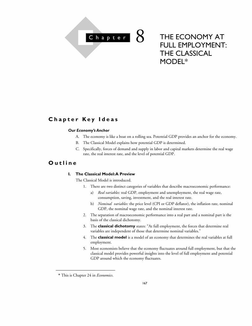
1. The production possibilities frontier (PPF) is the boundary between those combinations of goods and services that can be produced and those that cannot.

2. Figure 8.1(a) illustrates a production possibilities frontier between leisure time and real GDP.

3. The more leisure time forgone, the greater is the quantity of labor employed and the greater is the real GDP.

4. The PPF showing the relationship between leisure time and real GDP is bowed-out, which indicates an increasing opportunity cost: As real GDP increases, each additional unit of real GDP costs an increasing amount of forgone leisure.

5. Opportunity cost is increasing because the most productive labor is used first and as more labor is used, the labor used becomes increasingly less productive.

B. The Production Function

1. The production function is the relationship between real GDP and the quantity of labor employed when all other influences on production remain the same.

2. One more hour of labor employed means one less hour of leisure, therefore the production function is the mirror image of the leisure time-real GDP PPF.

3. Figure 8.1(b) illustrates the production function that corresponds to the PPF shown in Figure 8.1(a).

III. The Labor Market and Potential GDP

A. The Demand for Labor

1. The quantity of labor demanded is the labor hours hired by all the firms in the economy.

T H E E C O N O M Y A T F U L L E M P L O Y M E N T : T H E C L A S S I C A L M O D E L 1 6 9

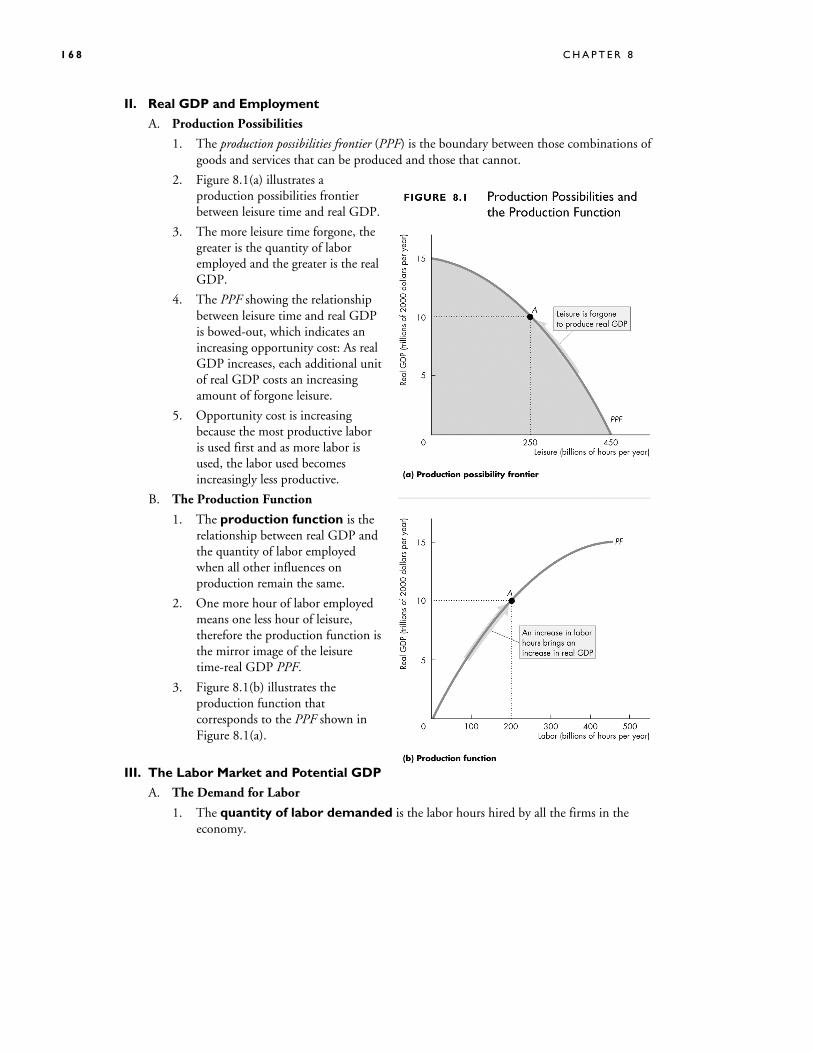
2. The demand for labor, Figure 8.2, is the relationship between the quantity of labor demanded and the real wage rate when all other influences on firms’ hiring plans remain the same.

3. The real wage rate is the quantity of good and services that an hour of labor earns.

a) The money wage rate is the number of dollars an hour of labor earns.

b) The average real wage rate is the average money wage rate divided by the price level multiplied by 100.

c) It is the real wage rate, not the money wage rate, that determines the quantity of labor demanded.

4. The demand for labor depends on the marginal product of labor, which is the additional real GDP produced by an additional hour of labor when all other influences on production remain the same.

a) The marginal product of labor is calculated as the change in real GDP divided by the change in the quantity of labor employed.

b) The marginal product of labor diminishes as the quantity of labor employed increases, other things remaining the same. Diminishing marginal product occurs because all the labor employed works with the same fixed capital and technology, and is an example of the law of diminishing returns.

c) The diminishing marginal product of labor limits the demand for labor.

1 7 0 C H A P T E R 8

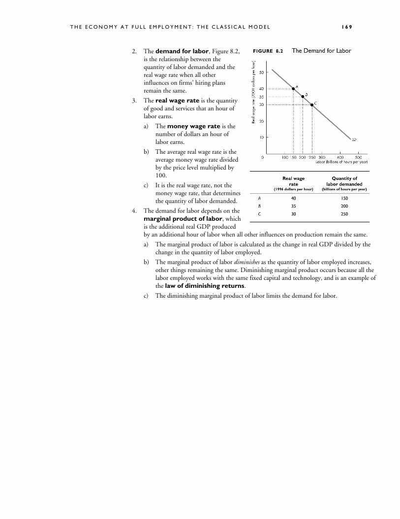
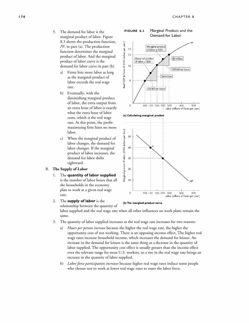
5. The demand for labor is the marginal product of labor. Figure 8.3 shows the production function, PF, in part (a). The production function determines the marginal product of labor. And the marginal product of labor curve is the demand for labor curve in part (b).

a) Firms hire more labor as long as the marginal product of labor exceeds the real wage rate.

b) Eventually, with the diminishing marginal product of labor, the extra output from an extra hour of labor is exactly what the extra hour of labor costs, which is the real wage rate. At this point, the profit-maximizing firm hires no more labor.

c) When the marginal product of labor changes, the demand for labor changes. If the marginal product of labor increases, the demand for labor shifts rightward.

B. The Supply of Labor

1. The quantity of labor supplied is the number of labor hours that all the households in the economy plan to work at a given real wage rate.

2. The supply of labor is the relationship between the quantity of labor supplied and the real wage rate when all other influences on work plans remain the same.

3. The quantity of labor supplied increases as the real wage rate increases for two reasons:

a) Hours per person increase because the higher the real wage rate, the higher the opportunity cost of not working. There is an opposing income effect. The higher real wage rates increase household income, which increases the demand for leisure. An increase in the demand for leisure is the same thing as a decrease in the quantity of labor supplied. The opportunity cost effect is usually greater than the income effect over the relevant range for most U.S. workers, so a rise in the real wage rate brings an increase in the quantity of labor supplied.

b) Labor force participation increases because higher real wage rates induce some people who choose not to work at lower real wage rates to enter the labor force.


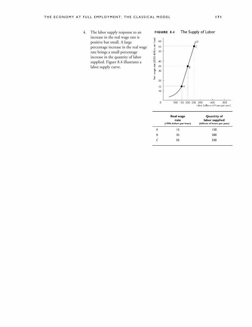
4. The labor supply response to an increase in the real wage rate is positive but small. A large percentage increase in the real wage rate brings a small percentage increase in the quantity of labor supplied. Figure 8.4 illustrates a labor supply curve.

1 7 2 C H A P T E R 8

C. Labor Market Equilibrium and Potential GDP

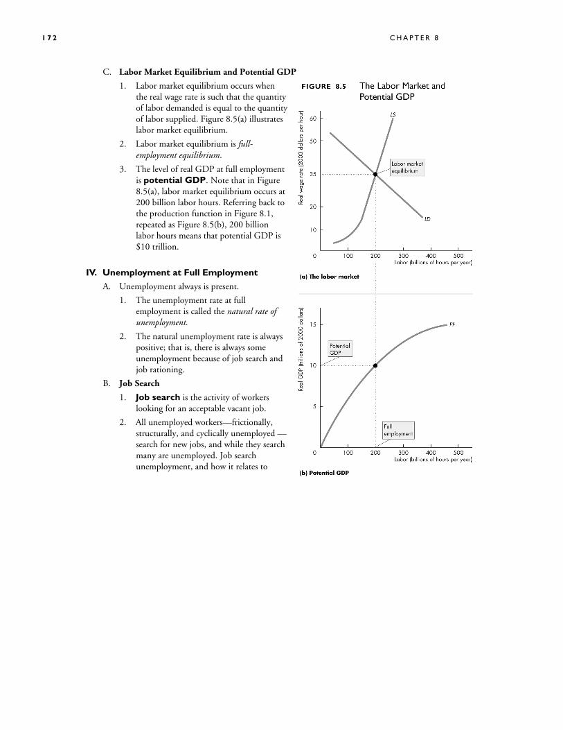
1. Labor market equilibrium occurs when the real wage rate is such that the quantity of labor demanded is equal to the quantity of labor supplied. Figure 8.5(a) illustrates labor market equilibrium.

2. Labor market equilibrium is full-employment equilibrium.

3. The level of real GDP at full employment is potential GDP. Note that in Figure 8.5(a), labor market equilibrium occurs at 200 billion labor hours. Referring back to the production function in Figure 8.1, repeated as Figure 8.5(b), 200 billion labor hours means that potential GDP is $10 trillion.

IV. Unemployment at Full Employment

A. Unemployment always is present.

1. The unemployment rate at full employment is called the natural rate of unemployment.

2. The natural unemployment rate is always positive; that is, there is always some unemployment because of job search and job rationing.

B. Job Search

1. Job search is the activity of workers looking for an acceptable vacant job.

2. All unemployed workers—frictionally, structurally, and cyclically unemployed — search for new jobs, and while they search many are unemployed. Job search unemployment, and how it relates to


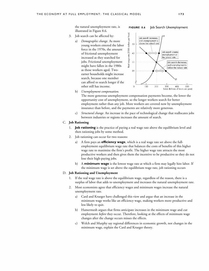
the natural unemployment rate, is illustrated in Figure 8.6.

3. Job search can be affected by:

a) Demographic change. As more young workers entered the labor force in the 1970s, the amount of frictional unemployment increased as they searched for jobs. Frictional unemployment might have fallen in the 1980s as those workers aged. Two-earner households might increase search, because one member can afford to search longer if the other still has income.

b) Unemployment compensation. The more generous unemployment compensation payments become, the lower the opportunity cost of unemployment, so the longer workers search for better employment rather than any job. More workers are covered now by unemployment insurance than before, and the payments are relatively more generous.

c) Structural change. An increase in the pace of technological change that reallocates jobs between industries or regions increases the amount of search.

C. Job Rationing

1. Job rationing is the practice of paying a real wage rate above the equilibrium level and then rationing jobs by some method.

2. Job rationing can occur for two reasons:

a) A firm pays an efficiency wage, which is a real wage rate set above the full-employment equilibrium wage rate that balances the costs of benefits of this higher wage rate to maximize the firm’s profit. The higher wage rate attracts the most productive workers and then gives them the incentive to be productive so they do not lose their high-paying jobs.

b) A minimum wage is the lowest wage rate at which a firm may legally hire labor. If the minimum wage is set above the equilibrium wage rate, job rationing occurs

D. Job Rationing and Unemployment

1. If the real wage rate is above the equilibrium wage, regardless of the reason, there is a surplus of labor that adds to unemployment and increases the natural unemployment rate.

2. Most economists agree that efficiency wages and minimum wages increase the natural unemployment rate.

a) Card and Krueger have challenged this view and argue that an increase in the minimum wage works like an efficiency wage, making workers more productive and less likely to quit.

b) Hamermesh argues that firms anticipate increases in the minimum wage and cut employment before they occur. Therefore, looking at the effects of minimum wage changes after the change occurs misses the effects.

c) Welch and Murphy say regional differences in economic growth, not changes in the minimum wage, explain the Card and Krueger theory.

1 7 4 C H A P T E R 8

V. Investment, Saving, and the Interest Rate

A. Potential GDP depends on the quantity of productive resources, including capital.

1. The capital stock is the total amount of plant, equipment, buildings, and inventories, physical capital.

2. Gross investment is the purchase of new capital. Depreciation is the wearing out and scrapping of the capital stock. Net investment equals gross investment minus depreciation; net investment is the addition to the capital stock. Investment is financed by saving, which equals income minus consumption.

3. The return on capital is the real interest rate , which is equal to the nominal interest rate adjusted for inflation. The real interest rate is approximately equal to the nominal interest rate minus the inflation rate.

B. Investment Decisions

Business investment decisions are influenced by: 1. The expected profit rate. The expected profit rate is relatively high during expansions and

relatively low during recessions. Increases in technology can increase the expected profit rate. Taxes affect the expected profit rate because firms are concerned about the after-tax profit rate.

2. The real interest rate. The real interest rate is the opportunity cost of investment. An increase in the real interest rate decreases the number of investment projects that are profitable.

C. Investment Demand

1. Investment demand is the relationship between investment and the real interest rate, other things remaining the same.

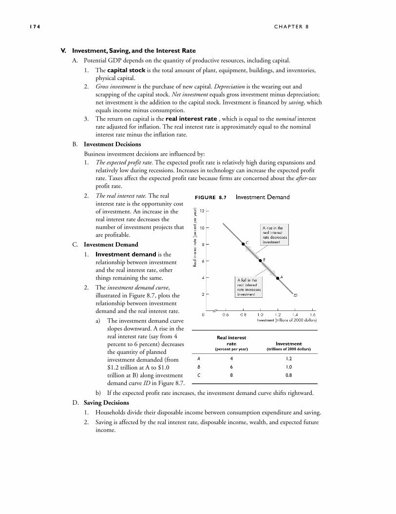
2. The investment demand curve, illustrated in Figure 8.7, plots the relationship between investment demand and the real interest rate.

a) The investment demand curve slopes downward. A rise in the real interest rate (say from 4 percent to 6 percent) decreases the quantity of planned investment demanded (from $1.2 trillion at A to $1.0 trillion at B) along investment demand curve ID in Figure 8.7.

b) If the expected profit rate increases, the investment demand curve shifts rightward.

D. Saving Decisions

1. Households divide their disposable income between consumption expenditure and saving.

2. Saving is affected by the real interest rate, disposable income, wealth, and expected future income.


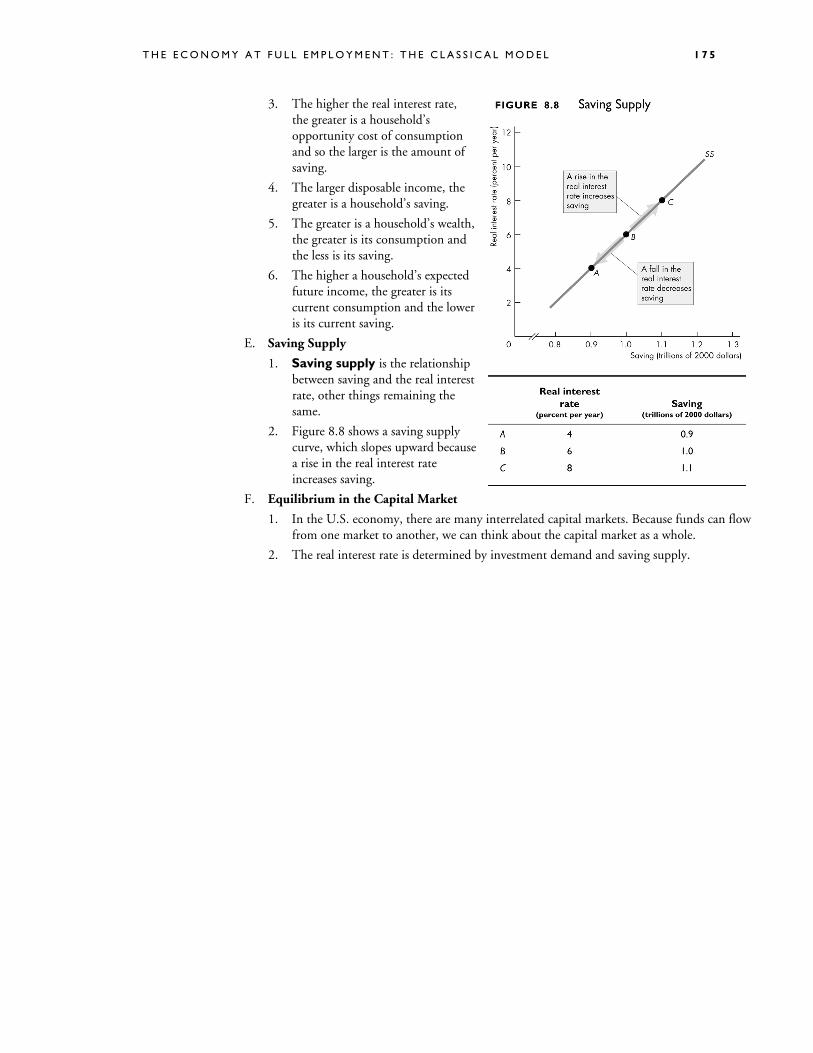
3. The higher the real interest rate, the greater is a household’s opportunity cost of consumption and so the larger is the amount of saving.

4. The larger disposable income, the greater is a household’s saving.

5. The greater is a household’s wealth, the greater is its consumption and the less is its saving.

6. The higher a household’s expected future income, the greater is its current consumption and the lower is its current saving.

E. Saving Supply

1. Saving supply is the relationship between saving and the real interest rate, other things remaining the same.

2. Figure 8.8 shows a saving supply curve, which slopes upward because a rise in the real interest rate increases saving.

F. Equilibrium in the Capital Market

1. In the U.S. economy, there are many interrelated capital markets. Because funds can flow from one market to another, we can think about the capital market as a whole.

2. The real interest rate is determined by investment demand and saving supply.

1 7 6 C H A P T E R 8

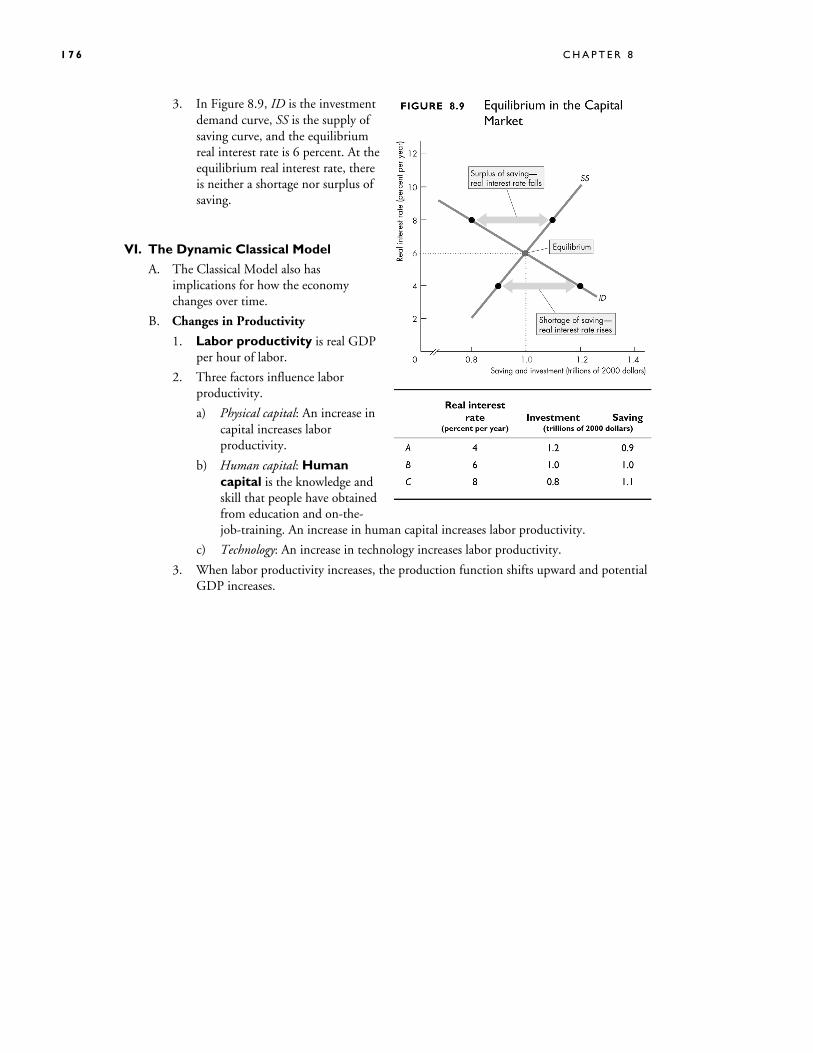
3. In Figure 8.9, ID is the investment demand curve, SS is the supply of saving curve, and the equilibrium real interest rate is 6 percent. At the equilibrium real interest rate, there is neither a shortage nor surplus of saving.

VI. The Dynamic Classical Model

A. The Classical Model also has implications for how the economy changes over time.

B. Changes in Productivity

1. Labor productivity is real GDP per hour of labor.

2. Three factors influence labor productivity.

a) Physical capital: An increase in capital increases labor productivity.

b) Human capital: Human capital is the knowledge and skill that people have obtained from education and on-the-job-training. An increase in human capital increases labor productivity.

c) Technology: An increase in technology increases labor productivity.

3. When labor productivity increases, the production function shifts upward and potential GDP increases.


C. An Increase in Population

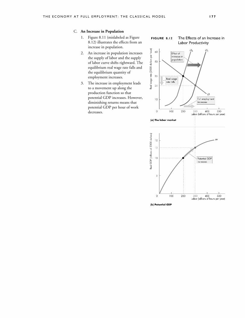
1. Figure 8.11 (mislabeled as Figure 8.12) illustrates the effects from an increase in population.

2. An increase in population increases the supply of labor and the supply of labor curve shifts rightward. The equilibrium real wage rate falls and the equilibrium quantity of employment increases.

3. The increase in employment leads to a movement up along the production function so that potential GDP increases. However, diminishing returns means that potential GDP per hour of work decreases.

1 7 8 C H A P T E R 8

D. An Increase in Labor Productivity

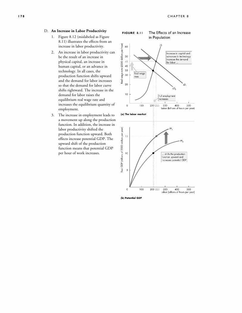
1. Figure 8.12 (mislabeled as Figure 8.11) illustrates the effects from an increase in labor productivity.

2. An increase in labor productivity can be the result of an increase in physical capital, an increase in human capital, or an advance in technology. In all cases, the production function shifts upward and the demand for labor increases so that the demand for labor curve shifts rightward. The increase in the demand for labor raises the equilibrium real wage rate and increases the equilibrium quantity of employment.

3. The increase in employment leads to a movement up along the production function. In addition, the increase in labor productivity shifted the production function upward. Both effects increase potential GDP. The upward shift of the production function means that potential GDP per hour of work increases.


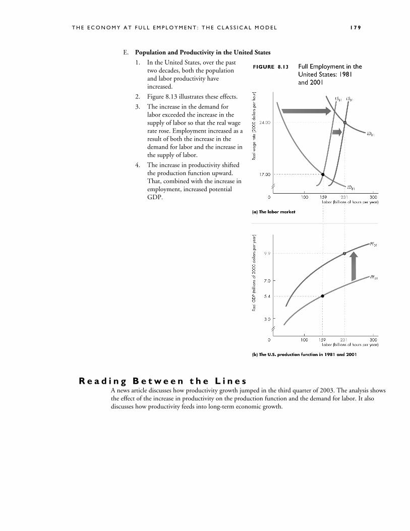
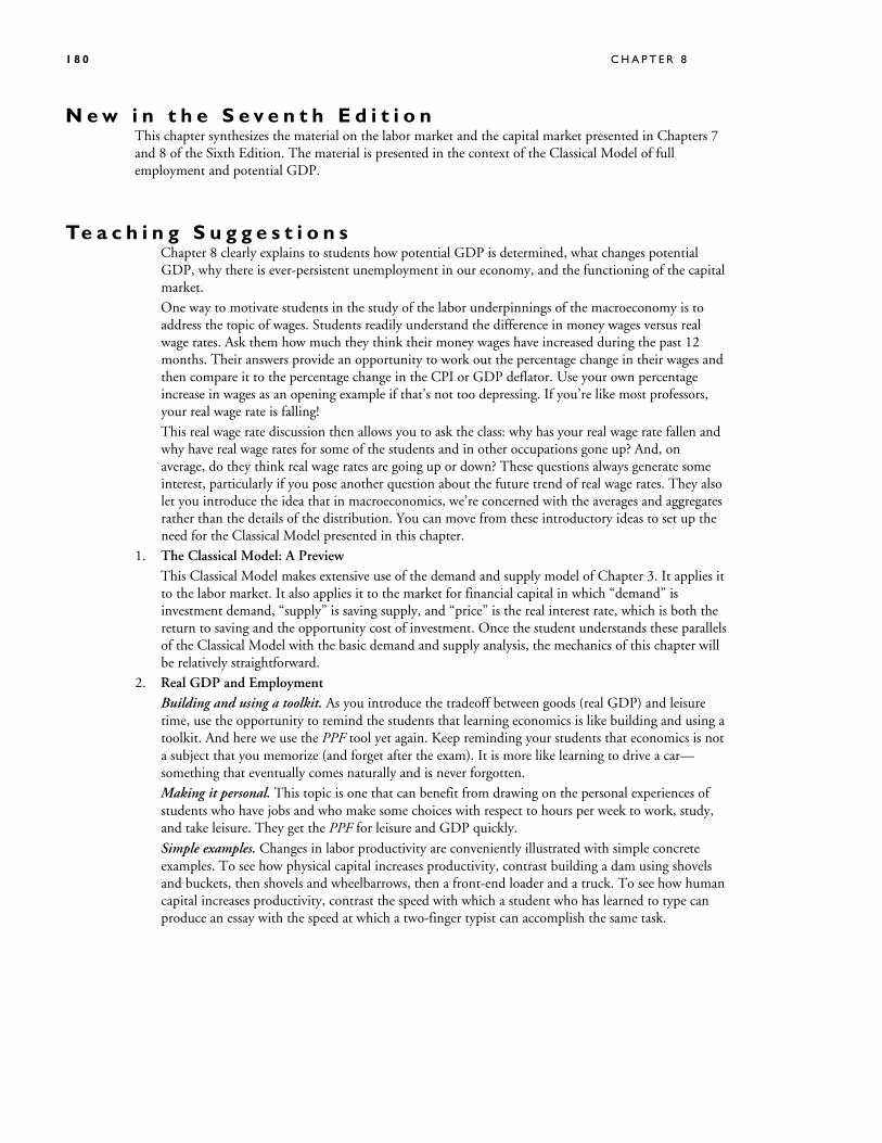
E. Population and Productivity in the United States

1. In the United States, over the past two decades, both the population and labor productivity have increased.

2. Figure 8.13 illustrates these effects.

3. The increase in the demand for labor exceeded the increase in the supply of labor so that the real wage rate rose. Employment increased as a result of both the increase in the demand for labor and the increase in the supply of labor.

4. The increase in productivity shifted the production function upward. That, combined with the increase in employment, increased potential GDP.

R e a d i n g B e t w e e n t h e L i n e s A news article discusses how productivity growth jumped in the third quarter of 2003. The analysis shows the effect of the increase in productivity on the production function and the demand for labor. It also discusses how productivity feeds into long-term economic growth.

1 8 0 C H A P T E R 8

N e w i n t h e S e v e n t h E d i t i o n This chapter synthesizes the material on the labor market and the capital market presented in Chapters 7 and 8 of the Sixth Edition. The material is presented in the context of the Classical Model of full employment and potential GDP.

Te a c h i n g S u g g e s t i o n s Chapter 8 clearly explains to students how potential GDP is determined, what changes potential

GDP, why there is ever-persistent unemployment in our economy, and the functioning of the capital market.

One way to motivate students in the study of the labor underpinnings of the macroeconomy is to address the topic of wages. Students readily understand the difference in money wages versus real wage rates. Ask them how much they think their money wages have increased during the past 12 months. Their answers provide an opportunity to work out the percentage change in their wages and then compare it to the percentage change in the CPI or GDP deflator. Use your own percentage increase in wages as an opening example if that’s not too depressing. If you’re like most professors, your real wage rate is falling!

This real wage rate discussion then allows you to ask the class: why has your real wage rate fallen and why have real wage rates for some of the students and in other occupations gone up? And, on average, do they think real wage rates are going up or down? These questions always generate some interest, particularly if you pose another question about the future trend of real wage rates. They also let you introduce the idea that in macroeconomics, we’re concerned with the averages and aggregates rather than the details of the distribution. You can move from these introductory ideas to set up the need for the Classical Model presented in this chapter.

1. The Classical Model: A Preview This Classical Model makes extensive use of the demand and supply model of Chapter 3. It applies it

to the labor market. It also applies it to the market for financial capital in which “demand” is investment demand, “supply” is saving supply, and “price” is the real interest rate, which is both the return to saving and the opportunity cost of investment. Once the student understands these parallels of the Classical Model with the basic demand and supply analysis, the mechanics of this chapter will be relatively straightforward.

2. Real GDP and Employment Building and using a toolkit. As you introduce the tradeoff between goods (real GDP) and leisure

time, use the opportunity to remind the students that learning economics is like building and using a toolkit. And here we use the PPF tool yet again. Keep reminding your students that economics is not a subject that you memorize (and forget after the exam). It is more like learning to drive a car—something that eventually comes naturally and is never forgotten.

Making it personal. This topic is one that can benefit from drawing on the personal experiences of students who have jobs and who make some choices with respect to hours per week to work, study, and take leisure. They get the PPF for leisure and GDP quickly.

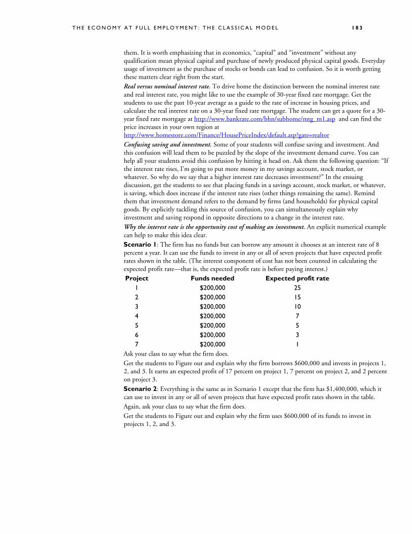
Simple examples. Changes in labor productivity are conveniently illustrated with simple concrete examples. To see how physical capital increases productivity, contrast building a dam using shovels and buckets, then shovels and wheelbarrows, then a front-end loader and a truck. To see how human capital increases productivity, contrast the speed with which a student who has learned to type can produce an essay with the speed at which a two-finger typist can accomplish the same task.


3. The Labor Market and Potential GDP Marginal product of labor. Although you are teaching a macroeconomics course, you can’t neglect

some crucial microeconomic underpinnings. And the marginal product of labor is one of these underpinnings. You can though avoid being too technical and can focus on the intuition. Some of your students might have completed the principles of microeconomics and seen the concept of marginal productivity before. This background enables you to encourage their participation in a classroom discussion on this topic. Also, drawing on the life experience of students with jobs whose work hours change from day to day or week to week can be useful. Get the students to see intuitively that it is not worth while for a firm to hire an hour of labor unless the value of the production of that labor at least covers the wage cost to the firm.

Labor supply. Your main goal in teaching this topic is to explain why in total, hours increase as the real wage rate increases. Again, drawing on the life experience of students with jobs whose work hours change from day to day or week to week can be useful. The two key points are: Even though some workers might have a backward-bending labor supply curves (playing golf on weekday afternoons when the wage rate rises enough), most have upward-sloping labor supply curves. The labor force participation rate increases as the real wage rate increases. These two features of individual behavior imply that the supply curve to labor in aggregate—the supply of aggregate hours—increases as the real wage rate rises, other things remaining the same.

Is immigration bad for us? Many people think that immigration is bad for existing citizens and lowers their living standard. Part of the popular political discussion, especially in Europe during 2002, has a racist dimension, which you will want to avoid. But the raw economic dimension is worth examining. When you discuss the effects of an increase in population, you will conclude that an increase in population, ceteris paribus, increases real GDP but lowers real GDP per person and lowers the real wage rage. You might then ask: does this outcome mean that immigration is bad for us?

The answer, of course, is absolutely not. Historically, immigrants have brought capital and entrepreneurship, and been some of the most creative sources of technological change. When you combine the effects of capital accumulation and technological change with an increase in population, you see that real GDP increases but the change in the wage rate is ambiguous. Add the historical fact that capital accumulation and technological change have outstripped population growth, and you reach the conclusion that immigration has been (and probably continues to be) a positive economic force.

Why the Luddites were wrong. This chapter provides you with a wonderful opportunity to explain to your students why the Luddites were wrong—and why the modern neo-Luddite movement is wrong. (You can learn more than you need to know about Luddism and the Luddites, ancient and modern, at http://carbon.cudenver.edu/~mryder/itc_data/luddite.html)

The Dynamic Classical Model. Explain that more capital and more productive capital that uses new technologies increases productivity, shifts the production function upward, and shifts the demand for labor curve rightward. Real GDP increases and on the average, the real wage rate rises.

You might then spend a few minutes agreeing that capital accumulation and technological change decrease the demand for the labor that the new capital replaces. But it increases the demand for other types of labor—complementary labor. People must acquire more skill—some people learn to work with the new capital, some learn how to maintain it in good condition, some learn how to build it, some learn how to market and sell it, some learn to design new ways of using it, some work on thinking up new goods and services to produce with it, and so on. All of these people are more productive that they were before.

New technologies that create new products have even more obvious effects on productivity. The development of the CD in the early 1980s is a good example. Suddenly thousands of people became

1 8 2 C H A P T E R 8

very productive converting the heritage of recorded music into digital format, cleaning up the sound, and making and selling millions of CDs. The same type of thing is now happening with the DVD.

If you want to get side-tracked into philosophical disputes about man and machines, we can’t help you in that area!

4. Unemployment at Full Employment Where is unemployment in the demand and supply diagram? Thoughtful students often ask about

the relationship between the (microeconomic-based) labor demand and labor supply model and unemployment. They can’t “see” any unemployment in labor market equilibrium. Where is it, they want to know.

Explain that in the labor market, people use their time in two economically productive ways: they work and they job search. Working is supplying labor and this is the activity that the demand-supply model shows. It shows the quantity of labor demanded and supplied and the price (real wage rate) that equates the quantities demanded and supplied. The demand and supply model does not determine the quantity of job-search activity. People supply job-search activity because firms have imperfect information about job seekers and workers have imperfect knowledge about available jobs. During the time spent on job search, people are unemployed. You can draw a diagram if you wish that shows the quantity of job search on the x-axis and the real wage rate on the y-axis. The higher the real wage rate, other things remaining the same, the greater is the amount of job search activity. The equilibrium wage rate determined by demand and supply in the labor market determines the point on the job search curve at which the labor market operates and determines the quantity of job-search unemployment.

Only if there were no uncertainty would the supply of job search (and unemployment) be zero. In such a case, a person out of work would not need to search for a new job. He or she would simply report to the new job on the day the worker knew that the job started! Thus, workers would never be unemployed because they would never search for jobs. Clearly, this happy state of affairs is not a description of reality.

One way to dramatize the fact that natural unemployment never hits zero is to bring in data on unemployment rates during World War II. Here are the numbers for the United States. Tell the students that more than 6 million people, mainly men, were recruited into the armed forces and that millions of others, mainly women, were mobilized to produce arms. Ask the students to guess the unemployment rate at the peak of war activity. Few will guess the unemployment rates correctly. (It is pretty remarkable that the rate could have fallen to such a low level.)

Civilian population and labor force, 1941–1945

Civilian labor force

Year Civilian

population Total EmploymentUnemploy-

ment

Not in labor force

Labor force participation

rate

Employ- ment-to-

population ratio

Unemploy- ment rate

Thousands of persons 14 years of age and over Percent

1941 99,900 55,910 50,350 5,560 43,990 56.0 50.4 9.9

1942 98,640 56,410 53,750 2,660 42,230 57.2 54.5 4.7

1943 94,640 55,540 54,470 1,070 39,100 58.7 57.6 1.9

1944 93,220 54,630 53,960 670 38,590 58.6 57.9 1.2

1945 94,090 53,860 52,820 1,040 40,230 57.2 56.1 1.9

Source: Economic Report of the President, 2002 5. Investment, Saving, and the Interest Rate Definitions and the meaning of investment in economics. The student has met the key definitions of

this section in Chapter 5, but to be absolutely sure that they are remembered, this chapter repeats


them. It is worth emphasizing that in economics, “capital” and “investment” without any qualification mean physical capital and purchase of newly produced physical capital goods. Everyday usage of investment as the purchase of stocks or bonds can lead to confusion. So it is worth getting these matters clear right from the start.

Real versus nominal interest rate. To drive home the distinction between the nominal interest rate and real interest rate, you might like to use the example of 30-year fixed rate mortgage. Get the students to use the past 10-year average as a guide to the rate of increase in housing prices, and calculate the real interest rate on a 30-year fixed rate mortgage. The student can get a quote for a 30-year fixed rate mortgage at http://www.bankrate.com/bhn/subhome/mtg_m1.asp and can find the price increases in your own region at http://www.homestore.com/Finance/HousePriceIndex/default.asp?gate=realtor

Confusing saving and investment. Some of your students will confuse saving and investment. And this confusion will lead them to be puzzled by the slope of the investment demand curve. You can help all your students avoid this confusion by hitting it head on. Ask them the following question: “If the interest rate rises, I’m going to put more money in my savings account, stock market, or whatever. So why do we say that a higher interest rate decreases investment?” In the ensuing discussion, get the students to see that placing funds in a savings account, stock market, or whatever, is saving, which does increase if the interest rate rises (other things remaining the same). Remind them that investment demand refers to the demand by firms (and households) for physical capital goods. By explicitly tackling this source of confusion, you can simultaneously explain why investment and saving respond in opposite directions to a change in the interest rate.

Why the interest rate is the opportunity cost of making an investment. An explicit numerical example can help to make this idea clear.

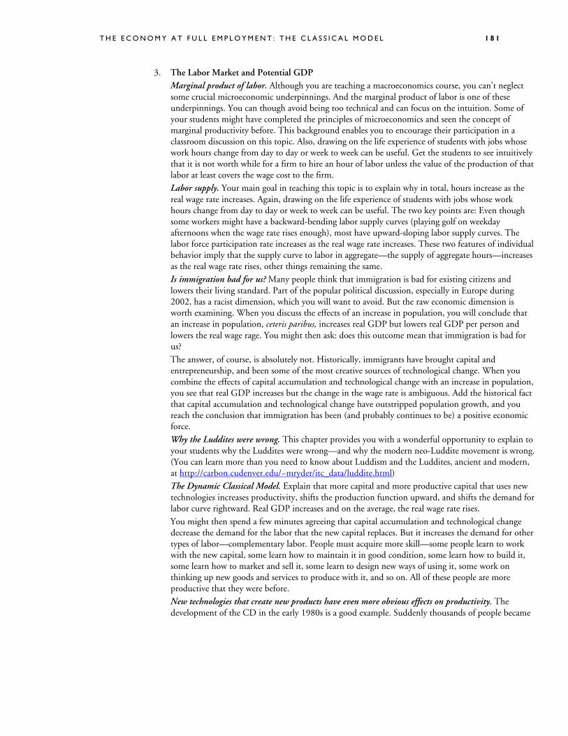
Scenario 1: The firm has no funds but can borrow any amount it chooses at an interest rate of 8 percent a year. It can use the funds to invest in any or all of seven projects that have expected profit rates shown in the table. (The interest component of cost has not been counted in calculating the expected profit rate—that is, the expected profit rate is before paying interest.)

Project Funds needed Expected profit rate 1 $200,000 25 2 $200,000 15 3 $200,000 10 4 $200,000 7 5 $200,000 5 6 $200,000 3 7 $200,000 1

Ask your class to say what the firm does. Get the students to Figure out and explain why the firm borrows $600,000 and invests in projects 1,

2, and 3. It earns an expected profit of 17 percent on project 1, 7 percent on project 2, and 2 percent on project 3.

Scenario 2: Everything is the same as in Scenario 1 except that the firm has $1,400,000, which it can use to invest in any or all of seven projects that have expected profit rates shown in the table.

Again, ask your class to say what the firm does. Get the students to Figure out and explain why the firm uses $600,000 of its funds to invest in

projects 1, 2, and 3.

1 8 4 C H A P T E R 8

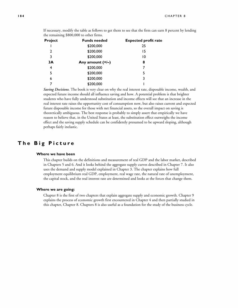
If necessary, modify the table as follows to get them to see that the firm can earn 8 percent by lending the remaining $800,000 to other firms.

Project Funds needed Expected profit rate 1 $200,000 25 2 $200,000 15 3 $200,000 10 3A Any amount (+/–) 8 4 $200,000 7 5 $200,000 5 6 $200,000 3 7 $200,000 1

Saving Decisions. The book is very clear on why the real interest rate, disposable income, wealth, and expected future income should all influence saving and how. A potential problem is that brighter students who have fully understood substitution and income effects will see that an increase in the real interest rate raises the opportunity cost of consumption now, but also raises current and expected future disposable income for those with net financial assets, so the overall impact on saving is theoretically ambiguous. The best response is probably to simply assert that empirically we have reason to believe that, in the United States at least, the substitution effect outweighs the income effect and the saving supply schedule can be confidently presumed to be upward sloping, although perhaps fairly inelastic.

T h e B i g P i c t u r e

Where we have been

This chapter builds on the definitions and measurement of real GDP and the labor market, described in Chapters 5 and 6. And it looks behind the aggregate supply curves described in Chapter 7. It also uses the demand and supply model explained in Chapter 3. The chapter explains how full employment equilibrium real GDP, employment, real wage rate, the natural rate of unemployment, the capital stock, and the real interest rate are determined and looks at the forces that change them.

Where we are going:

Chapter 8 is the first of two chapters that explain aggregate supply and economic growth. Chapter 9 explains the process of economic growth first encountered in Chapter 4 and then partially studied in this chapter, Chapter 8. Chapters 8 is also useful as a foundation for the study of the business cycle.


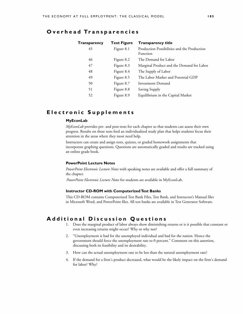
O v e r h e a d Tr a n s p a r e n c i e s

Transparency Text Figure Transparency title

45 Figure 8.1 Production Possibilities and the Production Function

46 Figure 8.2 The Demand for Labor

47 Figure 8.3 Marginal Product and the Demand for Labor

48 Figure 8.4 The Supply of Labor

49 Figure 8.5 The Labor Market and Potential GDP

50 Figure 8.7 Investment Demand

51 Figure 8.8 Saving Supply

52 Figure 8.9 Equilibrium in the Capital Market

E l e c t r o n i c S u p p l e m e n t s MyEconLab

MyEconLab provides pre- and post-tests for each chapter so that students can assess their own progress. Results on these tests feed an individualized study plan that helps students focus their attention in the areas where they most need help.

Instructors can create and assign tests, quizzes, or graded homework assignments that incorporate graphing questions. Questions are automatically graded and results are tracked using an online grade book.

PowerPoint Lecture Notes

PowerPoint Electronic Lecture Notes with speaking notes are available and offer a full summary of the chapter.

PowerPoint Electronic Lecture Notes for students are available in MyEconLab.

Instructor CD-ROM with Computerized Test Banks

This CD-ROM contains Computerized Test Bank Files, Test Bank, and Instructor’s Manual files in Microsoft Word, and PowerPoint files. All test banks are available in Test Generator Software.

A d d i t i o n a l D i s c u s s i o n Q u e s t i o n s 1. Does the marginal product of labor always show diminishing returns or is it possible that constant or

even increasing returns might occur? Why or why not?

2. “Unemployment is bad for the unemployed individual and bad for the nation. Hence the government should force the unemployment rate to 0 percent.” Comment on this assertion, discussing both its feasibility and its desirability.

3. How can the actual unemployment rate to be less than the natural unemployment rate?

4. If the demand for a firm’s product decreased, what would be the likely impact on the firm’s demand for labor? Why?

1 8 6 C H A P T E R 8

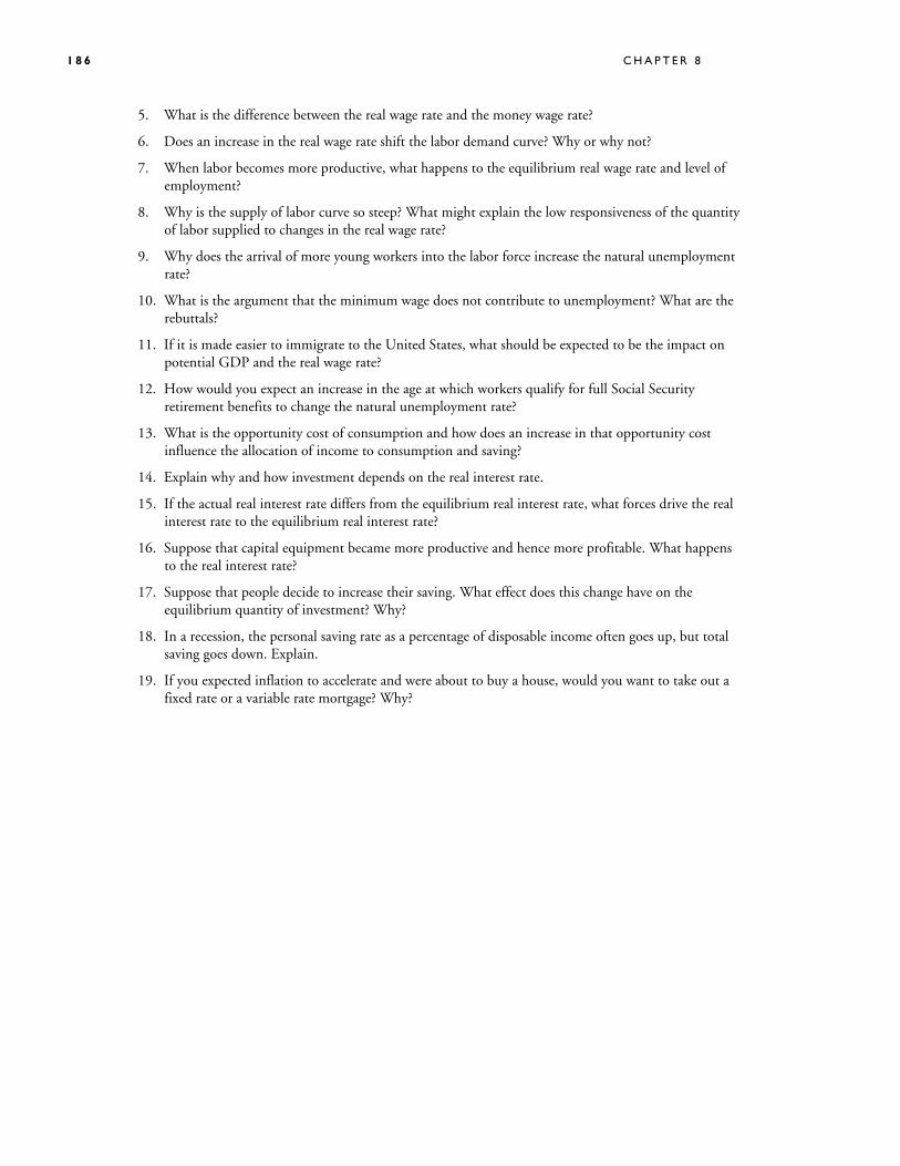
5. What is the difference between the real wage rate and the money wage rate?

6. Does an increase in the real wage rate shift the labor demand curve? Why or why not?

7. When labor becomes more productive, what happens to the equilibrium real wage rate and level of employment?

8. Why is the supply of labor curve so steep? What might explain the low responsiveness of the quantity of labor supplied to changes in the real wage rate?

9. Why does the arrival of more young workers into the labor force increase the natural unemployment rate?

10. What is the argument that the minimum wage does not contribute to unemployment? What are the rebuttals?

11. If it is made easier to immigrate to the United States, what should be expected to be the impact on potential GDP and the real wage rate?

12. How would you expect an increase in the age at which workers qualify for full Social Security retirement benefits to change the natural unemployment rate?

13. What is the opportunity cost of consumption and how does an increase in that opportunity cost influence the allocation of income to consumption and saving?

14. Explain why and how investment depends on the real interest rate.

15. If the actual real interest rate differs from the equilibrium real interest rate, what forces drive the real interest rate to the equilibrium real interest rate?

16. Suppose that capital equipment became more productive and hence more profitable. What happens to the real interest rate?

17. Suppose that people decide to increase their saving. What effect does this change have on the equilibrium quantity of investment? Why?

18. In a recession, the personal saving rate as a percentage of disposable income often goes up, but total saving goes down. Explain.

19. If you expected inflation to accelerate and were about to buy a house, would you want to take out a fixed rate or a variable rate mortgage? Why?


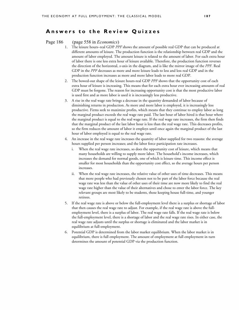
A n s w e r s t o t h e R e v i e w Q u i z z e s

Page 186 (page 558 in Economics) 1. The leisure hours–real GDP PPF shows the amount of possible real GDP that can be produced at

different amounts of leisure. The production function is the relationship between real GDP and the amount of labor employed. The amount leisure is related to the amount of labor. For each extra hour of labor there is one less extra hour of leisure available. Therefore, the production function reverses the direction of the horizontal, x-axis in the diagram, and is like the mirror image of the PPF. Real GDP in the PPF decreases as more and more leisure leads to less and less real GDP and in the production function increases as more and more labor leads to more real GDP.

2. The bowed-out shape of the leisure hours-real GDP PPF shows that the opportunity cost of each extra hour of leisure is increasing. This means that for each extra hour ever increasing amounts of real GDP must be forgone. The reason for increasing opportunity cost is that the most productive labor is used first and as more labor is used it is increasingly less productive.

3. A rise in the real wage rate brings a decrease in the quantity demanded of labor because of diminishing returns in production. As more and more labor is employed, it is increasingly less productive. Firms seek to maximize profits, which means that they continue to employ labor as long the marginal product exceeds the real wage rate paid. The last hour of labor hired is that hour where the marginal product is equal to the real wage rate. If the real wage rate increases, the firm then finds that the marginal product of the last labor hour is less than the real wage rate. This decreases profits, so the firm reduces the amount of labor it employs until once again the marginal product of the last hour of labor employed is equal to the real wage rate.

4. An increase in the real wage rate increases the quantity of labor supplied for two reasons: the average hours supplied per person increases; and the labor force participation rate increases. i. When the real wage rate increases, so does the opportunity cost of leisure, which means that

many households are willing to supply more labor. The household’s income increases, which increases the demand for normal goods, one of which is leisure time. This income effect is smaller for most households than the opportunity cost effect, so the average hours per person increases.

ii. When the real wage rate increases, the relative value of other uses of time decreases. This means that more people who had previously chosen not to be part of the labor force because the real wage rate was less than the value of other uses of their time are now more likely to find the real wage rate higher than the value of their alternatives and chose to enter the labor force. The key relevant groups are most likely to be students, those keeping house full-time, and younger retirees.

5. If the real wage rate is above or below the full-employment level there is a surplus or shortage of labor that then causes the real wage rate to adjust. For example, if the real wage rate is above the full-employment level, there is a surplus of labor. The real wage rate falls. If the real wage rate is below the full-employment level, there is a shortage of labor and the real wage rate rises. In either case, the real wage rate adjusts until the surplus or shortage is eliminated and the labor market is in equilibrium at full-employment.

6. Potential GDP is determined from the labor market equilibrium. When the labor market is in equilibrium, there is full employment. The amount of employment at full employment in turn determines the amount of potential GDP via the production function.

1 8 8 C H A P T E R 8

Page 189 (page 561 in Economics) 1. The economy always experiences unemployment, even when the labor market is in equilibrium.

There are two principle reasons for this: job search and job rationing. The amount of unemployment at full employment is called the natural unemployment rate.

2. There are three main factors that cause the natural unemployment rate to fluctuate: demographic changes; unemployment compensation; and structural changes. Demographic changes such as changes in the birth rate or changes in the number of workers per household leads to changes in the natural unemployment rate. The more generous unemployment benefits, the greater is the natural unemployment rate. The decline of industries is a structural change that can lead to an increase in the natural unemployment rate. Changes in the institutional arrangements in the labor market, or information flows (such as the internet), may also change the natural rate.

3. Job rationing is the practice of paying a real wage rate above the equilibrium level and then rationing jobs by some method. The two main methods are efficiency wages and the minimum wage. Efficiency wages exist because firms believe they can maximize profits by offering a higher wage. This wage rate balance the extra productivity gains at a higher wage against the extra cost. Minimum wages are legislated by the government and establish a legal minimum that serves to ration jobs if the minimum wage is above the equilibrium wage.

4. An efficiency wage is set above the market equilibrium in an attempt to hire more productive workers and reduce job turnover. At the efficiency real wage rate there is a surplus of labor. Employment is less and unemployment is greater than with a market equilibrium real wage rate.

5. The minimum wage creates unemployment if it is set higher than the equilibrium wage. Then, just as with the case of an efficiency wage, there is a labor surplus. Less labor is employed than if the wage rate was lower. The surplus of labor is equal to the amount of unemployment. The more the minimum wage exceeds the equilibrium wage, the greater is the surplus and the greater is the amount of extra unemployment generated.

Page 194 (page 566 in Economics) 1. If the real interest rate falls and nothing else changes, the quantity of investment demanded increases.

Conversely, if the real interest rate rises and everything else remains the same, the quantity of investment demanded decreases. Movements along the investment demand curve illustrate these events.

2. If the expected profit rate increases and nothing else changes, investment increases and the investment demand curve shifts rightward. If the expected profit decreases and everything else remains the same, investment decreases and the investment demand curve shifts leftward.

3. An increase in the real interest rate increases the quantity of saving; a decrease in the real interest rate decreases the quantity of saving. An increase in disposable income increases saving; a decrease in disposable income decreases saving. An increase in wealth decreases saving; a decrease in wealth increases saving. An increase in expected future income decreases saving; a decrease in expected future income increases saving.

4. The real interest rate is determined by saving supply and investment demand.

Page 199 (page 571 in Economics) 1. An increase in population, increases labor supply, which leads to an increase in employment. Real

GDP increases, but because of diminishing returns real GDP per hour of work falls. 2. An increase in capital shifts the production function higher so that labor productivity increases. As a

result, the demand for labor increases, which leads to a higher real wage rate and an increase in full employment. Potential GDP increases because the production function shifts upward and because full employment increases.


3. An increase in technology shifts the production function higher so that labor productivity increases. As a result, the demand for labor increases, which leads to a higher real wage rate and an increase in full employment. Potential GDP increases because the production function shifts upward and because full employment increases.

1 9 0 C H A P T E R 8

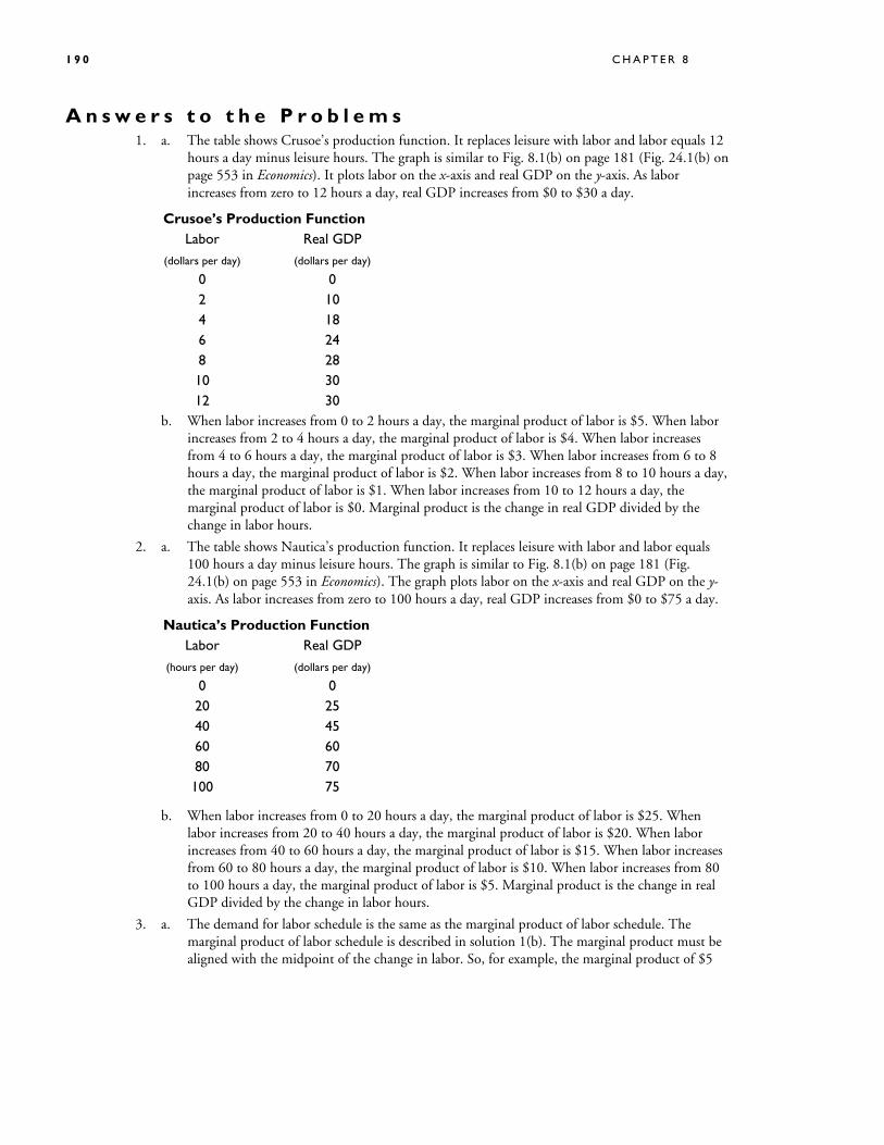
A n s w e r s t o t h e P r o b l e m s 1. a. The table shows Crusoe’s production function. It replaces leisure with labor and labor equals 12

hours a day minus leisure hours. The graph is similar to Fig. 8.1(b) on page 181 (Fig. 24.1(b) on page 553 in Economics). It plots labor on the x-axis and real GDP on the y-axis. As labor increases from zero to 12 hours a day, real GDP increases from $0 to $30 a day.

Crusoe’s Production Function Labor Real GDP (dollars per day) (dollars per day)

0 0 2 10 4 18 6 24 8 28 10 30 12 30

b. When labor increases from 0 to 2 hours a day, the marginal product of labor is $5. When labor increases from 2 to 4 hours a day, the marginal product of labor is $4. When labor increases from 4 to 6 hours a day, the marginal product of labor is $3. When labor increases from 6 to 8 hours a day, the marginal product of labor is $2. When labor increases from 8 to 10 hours a day, the marginal product of labor is $1. When labor increases from 10 to 12 hours a day, the marginal product of labor is $0. Marginal product is the change in real GDP divided by the change in labor hours.

2. a. The table shows Nautica’s production function. It replaces leisure with labor and labor equals 100 hours a day minus leisure hours. The graph is similar to Fig. 8.1(b) on page 181 (Fig. 24.1(b) on page 553 in Economics). The graph plots labor on the x-axis and real GDP on the y-axis. As labor increases from zero to 100 hours a day, real GDP increases from $0 to $75 a day.

Nautica’s Production Function Labor Real GDP (hours per day) (dollars per day)

0 0 20 25 40 45 60 60 80 70 100 75

b. When labor increases from 0 to 20 hours a day, the marginal product of labor is $25. When labor increases from 20 to 40 hours a day, the marginal product of labor is $20. When labor increases from 40 to 60 hours a day, the marginal product of labor is $15. When labor increases from 60 to 80 hours a day, the marginal product of labor is $10. When labor increases from 80 to 100 hours a day, the marginal product of labor is $5. Marginal product is the change in real GDP divided by the change in labor hours.

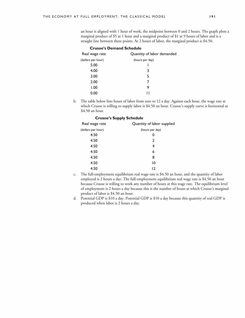
3. a. The demand for labor schedule is the same as the marginal product of labor schedule. The marginal product of labor schedule is described in solution 1(b). The marginal product must be aligned with the midpoint of the change in labor. So, for example, the marginal product of $5


an hour is aligned with 1 hour of work, the midpoint between 0 and 2 hours. The graph plots a marginal product of $5 at 1 hour and a marginal product of $1 at 9 hours of labor and is a straight line between these points. At 2 hours of labor, the marginal product is $4.50.

Crusoe’s Demand Schedule Real wage rate Quantity of labor demanded

(dollars per hour) (hours per day)

5.00 1 4.00 3 3.00 5 2.00 7 1.00 9 0.00 11

b. The table below lists hours of labor from zero to 12 a day. Against each hour, the wage rate at which Crusoe is willing to supply labor is $4.50 an hour. Crusoe’s supply curve is horizontal at $4.50 an hour.

Crusoe’s Supply Schedule Real wage rate Quantity of labor supplied

(dollars per hour) (hours per day)

4.50 0 4.50 2 4.50 4 4.50 6 4.50 8 4.50 10 4.50 12

c. The full-employment equilibrium real wage rate is $4.50 an hour, and the quantity of labor employed is 2 hours a day. The full-employment equilibrium real wage rate is $4.50 an hour because Crusoe is willing to work any number of hours at this wage rate. The equilibrium level of employment is 2 hours a day because this is the number of hours at which Crusoe’s marginal product of labor is $4.50 an hour.

d. Potential GDP is $10 a day. Potential GDP is $10 a day because this quantity of real GDP is produced when labor is 2 hours a day.

1 9 2 C H A P T E R 8

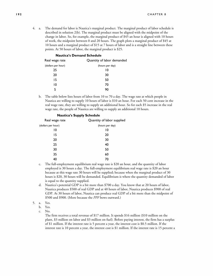
4. a. The demand for labor is Nautica’s marginal product. The marginal product of labor schedule is described in solution 2(b). The marginal product must be aligned with the midpoint of the change in labor. So, for example, the marginal product of $45 an hour is aligned with 10 hours of work, the midpoint between 0 and 20 hours. The graph plots a marginal product of $45 at 10 hours and a marginal product of $15 at 7 hours of labor and is a straight line between these points. At 50 hours of labor, the marginal product is $25.

Nautica’s Demand Schedule Real wage rate Quantity of labor demanded (dollars per hour) (hours per day)

25 10 20 30 15 50 10 70 5 90

b. The table below lists hours of labor from 10 to 70 a day. The wage rate at which people in Nautica are willing to supply 10 hours of labor is $10 an hour. For each 50 cent increase in the real wage rate, they are willing to supply an additional hour. So for each $5 increase in the real wage rate, the people of Nautica are willing to supply an additional 10 hours.

Nautica’s Supply Schedule Real wage rate Quantity of labor supplied (dollars per hour) (hours per day) 10 10 15 20 20 30 25 40 30 50 35 60 40 70

c. The full-employment equilibrium real wage rate is $20 an hour, and the quantity of labor employed is 30 hours a day. The full-employment equilibrium real wage rate is $20 an hour because at this wage rate 30 hours will be supplied; because when the marginal product of 30 hours is $20, 30 hours will be demanded. Equilibrium is where the quantity demanded of labor is equal to the quantity supplied.

d. Nautica’s potential GDP is a bit more than $700 a day. You know that at 20 hours of labor, Nautica produces $500 of real GDP and at 40 hours of labor, Nautica produces $900 of real GDP. At 30 hours of labor, Nautica can produce real GDP of a bit more than the midpoint of $500 and $900. (More because the PPF bows outward.)

5. a. Yes. b. Yes. c. No.

The firm receives a total revenue of $17 million. It spends $16 million ($10 million on the plant, $3 million on labor and $3 million on fuel). Before paying interest, the firm has a surplus of $1 million. If the interest rate is 5 percent a year, the interest cost is $0.5 million. If the interest rate is 10 percent a year, the interest cost is $1 million. If the interest rate is 15 percent a


year, the interest cost is $1.5 million. So the firm earns a profit at 5 percent, breaks even at 10 percent, and incurs a loss at 15 percent. The firm will not invest to incur a loss.

6. a. Yes. b. Yes. c. No.

The firm receives a total revenue of $40 million. It spends $36 million. Before paying interest, the firm has a surplus of $4 million. If the interest rate is 5 percent a year, the interest cost on the $36 million it invests in the project is $1.8 million. If the interest rate is 10 percent a year, the interest cost is $3.6 million. If the interest rate is 15 percent a year, the interest cost is $5.4 million. So the firm earns a profit at 5 percent, earns a smaller profit at 10 percent, and incurs a loss at 15 percent. The firm will not invest if it incurs a loss, which it will at an interest rate of 15 percent.

7. a. The graph has saving on the x-axis and the interest rate on the y-axis. Three points are plotted at $10,000 and 4 percent; $12,500 and 6 percent; and $15,000 and 8 percent. The saving supply curve passes through these points.

b. Saving decreases, and the saving supply curve shifts leftward.

8. a. The graph has saving on the x-axis and the interest rate on the y-axis. Three points are plotted at $10,000 and 4 percent; $15,000 and 6 percent; and $20,000 and 8 percent. The saving supply curve passes through these points.

b. Saving decreases, and the saving supply curve shifts leftward.

9. a. Potential GDP would decrease. A crack down on illegal immigrants and millions of workers returned to their country of origin would decrease the supply of labor. The equilibrium quantity of labor would decrease. Full employment would decrease and potential GDP would decrease.

b. Employment would decrease. A crack down on illegal immigrants and millions of workers returned to their country of origin would decrease the supply of labor. The equilibrium quantity of labor would decrease.

c. The real wage rate would rise. When the supply of labor decreases, there is a movement up the demand for labor curve and the real wage rate rises.

10. a. Potential GDP would increase. A freeing up of immigration into the United States would increase the supply of labor. The equilibrium quantity of labor would increase. Full employment would increase and potential GDP would increase.

b. Employment would increase. A freeing up of immigration into the United States would increase the supply of labor. The equilibrium quantity of labor would increase.

c. The real wage rate would fall. With no change in the demand for labor an increase in the supply of labor would create a movement up the demand for labor curve and the real wage rate would fall.

11. a. Potential GDP would increase. A increase in investment that increased productivity would increase the demand for labor. The equilibrium quantity of labor would increase. Full employment would increase and potential GDP would increase.

b. Employment would increase. A increase in investment that increased productivity would increase the demand for labor. The equilibrium quantity of labor would increase.

1 9 4 C H A P T E R 8

c. The real wage rate would rise. When the demand for labor increases, there is a movement up the supply of labor curve and the real wage rate rises.

12. a. Potential GDP would decrease. A severe drought that brought a fall in productivity would decrease the demand for labor. The equilibrium quantity of labor would decrease. Full employment would decrease and potential GDP would decrease.

b. Employment would decrease. A severe drought that brought a fall in productivity would decrease the demand for labor. The equilibrium quantity of labor would decrease.

c. The real wage rate would fall. When the demand for labor decreases, there is a movement down the supply of labor curve and the real wage rate falls.

Documents

Chapter Key Ideas - University of Daytonacademic.udayton.edu/PMAC/IM/Macro08.pdf · Chapter Key Ideas Our Economy’s Anchor A. The economy is like a boat on a rolling sea. Potential