Decision Support System for Run Suitability Checking and Explorative Method Validation in Electrothermal Atomic Absorption Spectrometry

P. VANKEERBERGHEN, J. SMEYERS-VERBEKE AND D. L. MASSART

ChemoAc, .Pharmaceutical Institute, Vrije Universiteit Brussel, Laarbeeklaan 103, B-1090 Brussels, Belgium

Journal of Analytical Atomic Spectrometry

A decision support system for the run suitability check and an explorative method validation for electrothermal atomic absorption calibration lines is described. The first sub-system, the run suitability check, investigates whether the quality of calibration and standard addition lines meets the pre-established standards. When this is not the case, the system identifies the problem for which remedies may be proposed, when appropriate. The second sub-system, the explorative method validation, is based on parts of the run suitability check and investigates whether candidate methods are promising or need further exploration.

Keywords: Calibration in routine analysis; run suitability check; explorative method validation; electrothermal atomic absorption spectrometry; decision support system

A suitability check investigates whether validated methods behave as expected in routine analysis. One of the parameters to be investigated is the quality of the calibration line because of its predominant influence on the precision and accuracy of the predicted sample concentration. Possible causes for unac- ceptable calibration lines are: (i) a wrong blank correction, (ii) non-linearity when a straight line is expected, (iii) the presence of outliers and (iv) a bad over-all precision charac- terized by a general large spread of data points around the calibration line. A visual inspection of the regression lines generally allows most of these problems to be identified but a more objective and automatic way of evaluation is necessary to include it in a quality assurance programme. This work describes how such an evaluation can be performed by means of a decision support system. It is based on a preliminary decision scheme developed for the diagnosis of calibration problems in electrothermal atomic absorption spectrometry (ETAAS).'

Here, we focus on the evaluation of the calibration line but the evaluation of the standard addition lines is of course very similar. Standard addition lines may be used to check for the presence of matrix interferences that affect the sensitivity and result in a proportional bias. These matrix interferences are then evaluated by the comparison of the slopes of the aqueous calibration line and the standard addition line. The possibility to make such a comparison is also offered by the decision support system presented here. In this way, the system can also be used to perform an explorative validation during method development or as part of a suitability check. In the former case it allows one to evaluate whether a new method that is being developed is promising or shows major matrix interferences and consequently requires further research. In the latter case it might be useful as a rapid check for matrix interferences when adopting a method that was validated for a sample matrix that is similar to, but not identical with, the samples to be analysed.

The different components of the system are described and

their integration is discussed. If problems are diagnosed, rem- edies to solve the problem are proposed. The evaluation of the system as a run suitability check is performed by comparing the conclusions of experts on a large set of calibration lines with the diagnoses provided by the system.

The system was implemented as a decision support system, functioning as an expert system. The literature describes several existing rule-based expert systems for AAS. Wolters et a1.' built an expert system for the quantitative validation of the results of analytical methods. The system was not developed for a specific analytical technique but an example for ETAAS was given. The strategy and statistical tests used in this system are inappropriate for suitability checking owing to the require- ments on data set size. For example, the analysis of variance lack-of-fit (ANOVA-LOF) procedure, used to evaluate the calibration model, requires genuine replicate measurements which are generally not available in routine analysis (see later). Lahiri and Stillman3 developed a rule-based expert system to diagnose problems in flame AAS. They focused on the physical aspects of the flame, the amount of noise, baseline drift or the shape of the signal as symptoms for providing a diagnosis.

EXPERIMENTAL

Measurements

One hundred and forty-one routine calibration lines containing five or six data points were obtained during routine analysis for the elements Mn, Cu, Pb, Cd and Al. All calibration lines include a blank measurement. The standard solutions were prepared using 1000 mg I-' stock solutions (Titrisol, Merck). The measurements were obtained with a Perkin-Elmer Zeeman 3030 electrothermal atomic absorption spectrometer equipped with an HGA-600 graphite furnace and an AS 60 autosampler. The signals were recorded on a PR-100 printer both in peak height and in peak area. Peak height data are only presented for illustrative purposes but are not recommended for routine analysis. Standard graphite tubes were used for the measure- ments of Cu, A1 and Mn without the addition of any chemical modifier. Pyrolytic graphite coated graphite tubes with a L'vov platform were used when making measurements of Cd and Pb. The chemical modifier for Cd was ammonium phosphate or a mixture of palladium and ammonium nitrate. For the Pb determinations, ammonium phosphate or a combination of palladium and magnesium nitrate was used.

The Decision Support System

Originally, the system was developed as an MS DOS character- based application, written with Microsoft C Optimising Compiler 5.1. In order to increase ease of maintenance and user-friendliness, the system was re-implemented as a hybrid system4 and now runs under MS Windows 3.x on a 486-based PC. The user interface, data collection and verification routines were written in Asymetrix Toolbook 1.5 whereas the numerical

Journal of Analytical Atomic Spectrometry, February 1996, Vol. 11 (I 49-1 58) 149

Publ

ishe

d on

01

Janu

ary

1996

. Dow

nloa

ded

by U

nive

rsity

of

Mas

sach

uset

ts -

Am

hers

t on

25/1

0/20

14 1

4:01

:04.

View Article Online / Journal Homepage / Table of Contents for this issue

and graphical routines were written in C using Borland C+ + version 3.1 and compiled as a library module. This module or dynamic link library (DLL) is called at run time by the Toolbook application. The advantages of this approach are that the benefits of Toolbook (graphical user interface, ease of construction and maintenance) are combined with the benefits of the use of the DLL (re-use of existing C source code and fast execution of compiled object code).

The computation of the second-degree polynomial is based on decomposition of the information matrix in a lower and upper triangle (LU) matrix and back-substitution as given in Press et a!.' The C routines for the calculation of the signifi- cance level of t-values for the squared term of the second- degree polynomial were obtained from Moshier.6

RUN SUITABILITY CHECK

In this section, the different components of the run suitability check are explained. These include the quality coefficient, the module to detect non-linear lines and the module for outlier detection.

Methods to Define the Quality of the Calibration Line: the Quality Criterion

First, the system checks the general quality of the calibration line through the quality coefficient (QC). The quality obtained is compared with a threshold value. Lines with a QC larger than this limit are considered problem lines, the others are accepted. This implies that small departures from linearity are tolerated, as is, for example, the shape of Cu calibration lines, which curve very slightly over the whole calibration range. However, if the QC is acceptable, there is no need to correct for these very small deviations from the linear model.

In the preliminary scheme proposed by Hu et a/.' a QC was defined which was very similar to the QC of de Galan et aL7 or Knecht and Stork.' An adapted version of the QC assuming a constant absolute standard deviation was later proposed by us9 and this is implemented here

correct. However, when a lack-of-fit is detected, it is not possible to differentiate between, for example, the presence of an outlier and the non-linearity of the calibration line. Moreover, owing to the lack of genuine replicate measurements in routine analysis, ANOVA-LOF cannot be used to detect problems with calibration lines. In routine AAS, each standard solution is generally measured at least twice. However, these replicates are obtained in the same run and consequently they do not adequately reflect the pure experimental error. This invalidates the ANOVA-LOF procedure in routine analysis.

The slope ranking method (SRM)" has been proposed to detect deviations from linearity or blank problems with routine calibration lines. The principle is based on the ranking of the individual slopes, Soi, between each data point and the origin. When the calibration line is linear, the slopes Soi are in a random sequence owing to the random error of the measure- ments. On the other hand, the slopes Soi of a curved calibration line follow a systematic ranking sequence. When the slopes Soi are in a descending sequence, this implies that the line is curvilinear over the whole range or that there is a blank problem. The difference between curvature and blank problems is found by considering the slopes between the second data point, the origin being the first data point, and the other data points. One of the major advantages of SRM is that it is model-independent. Most curved AAS calibration lines can be fitted with a second-order polynomial, but a hyperbolic or exponential model would also be possible. In all cases, SRM will detect curvature. Disadvantages of the SRM are: (i) the influence of the variance model on the probabilities for the different rankings of the slopes, as pointed out by Kalantar," (ii) the rather large probability of concluding that there is a blank problem when the calibration line really deviates from the linear model12 and (iii) the difficulty to evaluate relatively large calibration data sets (n > 6).12

Since, as shown in our previous work," a second-degree model seems to fit most curved ETAAS calibration lines, the significance of the squared term b2 of the second-order mode1I3 is used here to detect non-linearity over the whole concen- tration range. When b2 differs significantly from zero (a = 5%), the conclusion is that the calibration line curves. Note that the quadratic model is not validated for curved lines. The most important reason for implementing this approach is that there is no restriction concerning the maximum number of data points for the calibration line. We chose to apply the latter method.

where n represents the number of data points including the blank, yi the absorbance measured for standard i, ji the absorbance for standard i predicted by the model and the mean of the measured absorbances.

A threshold value of 5% is used as a user-definable default value. This limit was considered to be acceptable for our purposes. The acceptable limit should be obtained during the full method validation. When the line is considered unaccept- able because the QC value exceeds the threshold, the reason for the bad quality is identified. This is performed with the methods explained later.

Methods to Detect Non-linearity

The ANOVA lack-of-fit procedure (ANOVA-LOF), used in method validation, investigates if the model chosen is appro- priate. Basically, one compares the spread of the data points around the regression line with the pure experimental error. When the spread is significantly larger, the model is not

Detection of Outliers in Calibration Lines

A problem with least squares (LS) is that the LS regression line is very much influenced by the presence of outliers. Some outlier diagnostics compare the standardized LS residuals with a cut-off value of 2 or 3. The performance of these diagnostics is generally not very good. The residual for the outlier might not be much larger than those of the 'good' points if the outlier is a leverage point that attracts the LS regression line. Other outlier detection methods such as Cook's squared di~tance'~ are based on the change in the regression parameters when the data point is omitted. However, this diagnostic may fail when multiple outliers are present or when the outlier is not a leverage point and consequently does not have a large influence on the LS regression parameters.

Another approach is to apply robust regression methods. Hu et a1." have investigated the use of the single median method, the repeated median method and the least median of squares (LMS) method for outlier detection. They also con- sidered fuzzy calibration. The conclusion of this study is that fuzzy calibration and the LMS method are more efficient than

150 Journal of Analytical Atomic Spectrometry, February 1996, Vol. 1 1

Publ

ishe

d on

01

Janu

ary

1996

. Dow

nloa

ded

by U

nive

rsity

of

Mas

sach

uset

ts -

Am

hers

t on

25/1

0/20

14 1

4:01

:04.

View Article Online

the others for outlier detection in routine analysis. LMS is selected here because (i) the fuzzy method requires some knowledge about the precision of the analytical method and (ii) LMS is easier to implement.

The LMS robust regression and outlier detection method, as proposed by Rousseeuw,’6 has been described for outlier diagnosis in chemical analysis by Massart et al.,17 Rutan and Carrl’ and Danzer.lg Ortiz et aL2’ used LMS for calibration and for the calculation of the detection limit in adsorptive stripping volt ammetry.

Computation of least median of squares16

The LMS method minimizes the median of the squared residuals. The LMS solution is given by

minimize med(y, - bixi - bo)2 ( 2 ) I

where bi and bo are the LMS slope and intercept, respectively. From these robust LMS parameters an initial scale estimator

is calculated

so = 1.4826. (1 + L, Jmedo n - 2 (3)

where n is the number of data points and ri are the LMS residuals.

When the LMS residual of a data point is larger than 2.5 times this initial scale estimate, the data point is omitted for the calculation of the final scale estimate s*

(4)

where n* is the number of data points retained. Finally, when the LMS residual of a data point is larger than 2.5 times s*, the point is considered to be an outlier. The sign of the residual of the outlier gives information about the position of the outlier with respect to the LMS regression line and is used for later diagnosis.

The breakdown point, i.e., ‘the smallest percentage of con- taminated data that can cause the estimator (or regression parameters) to take on arbitrarily large aberrant values’16 is 50% for LMS. The breakdown point for LS, on the other hand, equals 0% since a single outlier can cause aberrant values. Note that these values are extrapolated for an infinite number of data points. For LMS, this means in practice that only two outliers can be detected with six data points, since with three outliers, one cannot distinguish the good from the bad data points.

In their LMS program Progress, Rousseeuw and Leroy2’ use the ‘shortest halves’ algorithm to compute the intercept. The adaptation of Hu et al.’ of the LMS algorithm lacks this ‘shortest halves’ algorithm and consequently the LMS line is forced through two data points. During the validation of the system it was found that this simplified LMS version too often diagnoses bad over-all precision, which means that it does not always detect the outlier(s). Since the intercept is not optimized, the median squared residual and consequently the robust scale estimate are larger and this explains the decreased detection power. Therefore, at this point we incorporated the ‘shortest halves’ algorithm. Rousseeuw and Leroy2’ suggest that the optimum intercept term be estimated at each trial slope and not only once at the end when the optimum slope is obtained. They did not implement this optimization step to avoid loss of computing performance with the available hardware of the mid-1980s. We included this optimization step and found that

the difference in computing time for our data sets is not important on the current hardware.

Algorithm

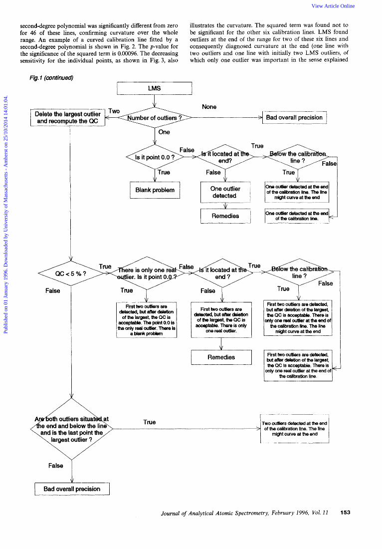
The user starts the system by answering whether he wants to perform (i) a run suitability check or (ii) an explorative method validation or a suitability check. The last two options are discussed later in this paper. After selecting the run suitability check, the user continues with the input of the calibration data. The system assumes that the concentrations of the standards are more or less equally spaced over the calibration range. For the moment, data sets of four to six data points (the reason for this limitation to six data points is explained later) and up to six replicates per data point are currently allowed but the program will be adapted to support larger data sets. The mean values for the individual data points are calculated and blank-corrected. Consequently, the QC value is computed (Fig. 1).

This QC value is compared with the threshold value. If the QC value is acceptable, the user can continue with measuring samples and predicting concentrations using the calibration line. On the other hand, if the QC value is too large, the diagnosis module is activated. Problems can of course only be diagnosed when the data set is sufficiently large. For a cali- bration line consisting of four data points including the blank, the conclusion is that the calibration line is unacceptable but that more points are necessary to identify the problem.

For a larger data set, the system continues with the compu- tation of the significance of the squared term of a second- degree polynomial. If this is significantly different from zero, the conclusion is that the calibration line curves over the whole range. If b2 is not significant, the calibration line is considered not to curve over the whole range and the system calls LMS to detect possible outliers.

Further diagnosis depends on the number of outliers found, as illustrated in Fig. 1. If LMS does not find outliers, the calibration line is considered to be have an unacceptable over-all precision.

If one outlier is detected, the diagnosis depends on the location of that outlier in the calibration line. When the point 0.0 is the outlier, the diagnosis is that there is a blank problem. Otherwise, the system checks whether the last calibration point is the outlier and, if this is the case, whether the point is located below the LMS line. In that case, the conclusion is that there is no curvature over the whole range (since the squared term is not significantly different from zero) but that the calibration line might curve locally to the concentration axis at the upper end. The diagnosis ‘One outlier detected’ is given in all other cases.

Another possibility concerns the presence of two outliers. The system looks for the largest outlier, deletes it and re-computes the QC. When this new QC value becomes acceptable, the conclusion is that the smallest LMS outlier is not important and that there is only one real outlier. The same logic is then applied as previously described for one LMS outlier: investigation as to whether the outlier (i) is the blank, (ii) is situated at the end below the LMS line or (iii) is located in the middle of the range or at the end, above the line. For each of these cases the information given by the system is that there are two LMS outliers of which only one is real. On the other hand, when the two LMS outliers are important, the QC value computed after deletion of the largest one will still be unacceptable. The system continues by investigating the location of both outliers. When the two outliers are located at the end, below the LMS regression line, and the residual of the last but one data point is smaller than the residual of the last data point, the conclusion is that the calibration line does not curve over the whole range, but that it curves at the upper

Journal of Analytical Atomic Spectrometry, February 1996, Vol. 11 i51

Publ

ishe

d on

01

Janu

ary

1996

. Dow

nloa

ded

by U

nive

rsity

of

Mas

sach

uset

ts -

Am

hers

t on

25/1

0/20

14 1

4:01

:04.

View Article Online

end. All other cases with two outliers lead to the conclusion that there is a bad over-all precision.

The algorithm for standard addition lines is the same as for calibration lines, except for the following two points. The spread of the data points is again measured by the QC given in eqn. (I) , but with the difference that jj now is obtained as b,x. This is required to ensure that the concentration of the sample does not influence the QC. The second point concerns the diagnosis module. When the first point is an LMS outlier, the diagnosis is not that there is a blank problem but that there is an outlier problem.

Note that the algorithm proposed here only handles lines with up to six data points which corresponds to the size of our routine calibration lines. Although for larger data sets the QC, the second-degree polynomial and the LMS regression line can of course also be obtained, the diagnosis, when LMS outliers are detected, has to be adapted. Indeed for lines consisting of six data points, a maximum of two outliers can be found (see under Computation of least median of squares), but with, for example, eight data points, three outliers can be detected. An adaptation of the algorithm is therefore necessary.

False

Additional Information Presented by the System

In order to avoid the use of this system as a black box, supplementary information is provided. This includes the LS parameters, the LS plot, the LMS parameters, the LMS plot, details on the second-degree polynomial and the sensitivity plot as described by Dorschel et a1.22 This sensitivity plot, in which the ratio of the absorbance to the concentration of each data point (= the individual sensitivity) is plotted as a function of the concentration, is a useful visual tool to illustrate non- linearity of calibration and standard addition lines. Blank problems are illustrated with the LS plot and parameters computed from the data set where the point 0,O has been removed.

Remedies

It would be a loss of resources to reject all measurements of an unacceptable calibration or standard addition line when only one point is outlying owing to, for example, a wrongly prepared standard solution. On the other hand, fundamental problems such as curvature over the whole calibration range cannot be remedied by the simple application of a second- degree polynomial, even if this model fits the data points very well, if the method has only been fully validated for the straight line model. Therefore, a distinction has to be made between a bad quality of the calibration line caused fortuitously (single outlier) or as the result of fundamental problems (blank problems, curvature and bad over-all precision).

Remedies, therefore, are only provided for a single outlier. Firstly, we consider an outlier in the middle of the range. In that case one can remove or re-measure the data point. This is followed by the recalculation of the QC. When the new QC value is acceptable, the analyst can use the line. If the remedy does not solve the problem (QC is still unacceptable), further investigation is needed, for example, by preparing a new standard solution for that concentration. Secondly, an outlier at the extreme concentration can be: (i) a real outlier or (ii) it can be due to the fact that the model deviates from the straight line. In order to differentiate between both, one has to prepare and measure the last standard again. When the previous diagnosis is confirmed, the final conclusion is that the line deviates at the end from the linear model. On the other hand, when the QC value becomes acceptable, the line can be used since the bad quality was due to the presence of an outlier. Note that simple removal of the outlier at the end would not be an acceptable practice since this would restrict the original

calibration range. This is unacceptable since the model has been validated for that range before.

Results and Discussion

The test criteria used in the validation of the run suitability check module were the accuracy and the completeness of the diagnosis. The accuracy of the decision support system diag- nosis is defined as the rate of consistency between the solution given by the decision support system and the expert’s solution. The completeness of the system is the way in which the system covers all possible cases.

The validation of the whole system was restricted to cali- bration lines only because, as explained earlier, the handling of standard addition lines is similar. A total of 141 calibration lines was obtained; 53 were considered to be acceptable and this was confirmed by their QC being smaller than 5%. The 88 unacceptable calibration lines, for which the QC was larger than the threshold value, were classified by experts according to the different possibilities of diagnosis that are present in the system.

Fifty-two calibration lines were visually classified as showing curvature over the whole range. The squared term of the

Calculation QC I

\I/

I Ise ,- Use Least squares calibration line for analysis

I I

rue , Data set is too small to identify problems

< Line IS whole range

False

whole range

-1 Fig. 1 Decision scheme for the diagnosis of problem calibration lines

152 Journal of Analytical Atomic Spectrometry, February 1996, VoZ. 1 1

Publ

ishe

d on

01

Janu

ary

1996

. Dow

nloa

ded

by U

nive

rsity

of

Mas

sach

uset

ts -

Am

hers

t on

25/1

0/20

14 1

4:01

:04.

View Article Online

second-degree polynomial was significantly different from zero for 46 of these lines, confirming curvature over the whole range. An example of a curved calibration line fitted by a second-degree polynomial is shown in Fig. 2. The p-value for the significance of the squared term is 0.00096. The decreasing sensitivity for the individual points, as shown in Fig. 3, also

illustrates the curvature. The squared term was found not to be significant for the other six calibration lines. LMS found outliers at the end of the range for two of these six lines and consequently diagnosed curvature at the end (one line with two outliers and one line with initially two LMS outliers, of which only one outlier was important in the sense explained

Delete the largest outlier ’

and recompute the QC

Fig. 1 (continued)

> Bad overall precision

True >

i Blank problem

Two outliers detected at the end of the calibration line. The line

might curve at the end

G h l

False

One outlier detected

v

One outlier detected at the end of the calibration line. The line

m*@t curve at the end

I J 1 J

First two attlirs are detected,butrrftercWetion of the largest, the QC is

acceptable. The point 0.0 is the only real outlier. There is

First two outliers are detected, but after deletion

ofthe largest, the QC is

one real outlier. accBpbbk. met6 is Only

Remedies

First two outliers me detected, but after deletion of the largest, the QC is acceptable. There is

only one reel outlier at the end ol the calibration line. The line

might curve at the end

but after deletion of the largest, the QC is acceptable. There is

only one real outlier at the end of the calibration line.

Journa2 of Analytical Atomic Spectrometry, February 1996, Vol. 1 1 153

Publ

ishe

d on

01

Janu

ary

1996

. Dow

nloa

ded

by U

nive

rsity

of

Mas

sach

uset

ts -

Am

hers

t on

25/1

0/20

14 1

4:01

:04.

View Article Online

0.794

0.691

0.584

E *$ 0.416 I

0.220

0 40.0 80.0 120.0 160.0 200.0

Concentration/ng mi-'

Fig. 2 A curved calibration line (Pb measured in peak height) fitted by a second-order polynomial. The significance of the squared term equals 0.000 96

1 1 I 1 1 I 40.0 80.0 120.0 160.0 200.0

ConcentrationIng mi-l

Fig. 3 The sensitivity plot for the calibration line from Fig. 2 shows a decrease in sensitivity and illustrates the curvature

I

I /

E .- 0, a I

Fig. 5

0 60.0 120.0 180.0 240.0 300.0 Concentration/ng m1-l

Curved calibration line (Pb measured in peak height) fitted by LMS. The system incorrectly diagnoses a blank problem

1.149

0.961

0.769

-

-

- m

v

0 100.0 200.0 300.0 400.0 500.0 Concentration/ng ml-l

Fig. 6 A non-uniformly curved calibration line (Pb measured in peak area) fitted by LMS. The system incorrectly diagnoses a blank problem

0 60.0 120.0 180.0 240.0 300.0 Concentration/ng m1-l

0 60.0 120.0 180.0 240.0 300.0 Concentration/ng mi-'

Fig. 4 Curved calibration line (Pb measured in peak area) fitted by LMS. The system diagnoses curvature at the end, which is con- sidered acceptable

under Algorithm). Fig. 4 illustrates with the LMS plot the deviation from linearity due to two outliers. The diagnosis of curvature at the end was finally considered to be acceptable since, with the small data sets examined, it is not always obvious to differentiate between deviation from the linear model over the whole range or only at the end. For two of the other six curved lines the curvature was not detected and the system incorrectly diagnosed a bad over-all precision for one and a blank problem for the other calibration line. The latter line is shown in Fig. 5. The remaining two calibration lines were also incorrectly diagnosed as suffering from a blank problem owing to the non-uniform curvature which could not

Fig. 7 A slightly curved calibration line (Pb measured in peak area) containing an outlying point and fitted by LMS. The significance of the squared term equals 0.11099. LMS does not identify the outlier due to the deviation from the linear model

be fitted by the second-degree polynomial. Fig. 6 shows one of these two curved lines. The p-value for the significance of the squared term only slightly exceeds the threshold ( p = 0.050 42).

For one calibration line, shown in Fig. 7, there is a combi- nation of deviation from the linear model over the whole range, together with the presence of an outlier in the middle of the range. Owing to the presence of the outlier, the p - value for the squared term equals 0.111 and owing to the cur- vature, the residual variance is large and the outlier is not detected. The system incorrectly diagnosed this as a case of bad over-all precision.

154 Journal of Analytical Atomic Spectrometry, February 1996, Vol. 1 1

Publ

ishe

d on

01

Janu

ary

1996

. Dow

nloa

ded

by U

nive

rsity

of

Mas

sach

uset

ts -

Am

hers

t on

25/1

0/20

14 1

4:01

:04.

View Article Online

The data set contains only one calibration line with a blank problem given in Fig. 8 and this was correctly diagnosed.

Ten calibration lines have been classified as suffering from an outlier problem in the middle of the concentration range. The system diagnosed this correctly for nine lines. Fig. 9 shows a linear calibration line with the LMS regression line revealing the outlier at 24ngml-l. For five of these nine calibration lines, LMS initially identified two outliers, of which finally only one was important. For these calibration problems, remedies are applied which consist in the removal of the outlier and re-computation of the QC. For all nine calibration lines, removal of the outlier resulted in an acceptable QC. The diagnosis of bad over-all precision was considered not to be correct for one line, shown in Fig. 10, since LMS did not detect the deviating data point due to the rather large residual variance. The ratio of the residual of this data point to the initial and final scale estimate equals 2.41 and 1.19, respectively. As the latter is smaller than 2.5, the point is not identified as an LMS outlier.

For one calibration line, the last data point was outlying in the direction for larger signals and was properly detected by LMS.

Eight other calibration lines contained one outlier at the end of the range, indicating deviation from linearity at the highest concentration. The system confirmed this diagnosis for the eight lines (five lines with only one outlier, three lines where LMS first found two outliers of which only one is important). Fig. 11 shows one of the latter lines. When the largest outlier (100 ng ml-l) is omitted from the data set to

0.330

0.280

-

-

cp 0.196 2 Q

-

0 40.0 80.0 120.0 150.0 Concentration/ng m1-I

Fig. 8 Calibration line with a blank problem (Pb measured in peak area) as illustrated by the LMS regression line

Concen trati on/ng m I-'

Fig.9 Calibration line with an outlier (Cd measured in peak area) fitted by LMS

t 0.674 /I 0.523 - 0.454 -

cp I a

0.271 -

0.122 -

- 0 2 .o 4.0 6 .O 8 .O 10.0

Concentration/ng mi-'

Fig. 10 Calibration line (Cd measured in peak area) fitted by LMS. The system incorrectly diagnoses a bad over-all precision

0.784 - 0.719 -

E 0.538 Q,

- .- 2

0.360

0.203 -

-

I

0 20.0 40.0 60.0 80.0 100.0 Concentrationlng mi-'

Fig. 11 Calibration line (Mn measured in peak height) fitted by LMS. The system diagnoses one outlier at the end, indicating possible curvature at the end

define whether both outliers initially detected (at 20 and 100 ng m1-I) are real, the recalculated QC is 2.62%.

Two calibration lines deviated from the linear model at the upper end of the concentration range and contained an outlier in the middle. Owing to the combination of problems, both lines were diagnosed as bad over-all precision (squared term second-degree polynomial was not significant and LMS detected two outliers at the lower end of the calibration range).

Six calibration lines were diagnosed as linear but deviating from the linear model at the end of the concentration range. In contrast to the former lines where only the last data point

I I I I I 0 6.0 12.0 18.0 24.0 30.0

Concentration/ng mi-'

Fig. 12 A calibration line (Cd measured in peak height) for which the system diagnoses correctly a bad over-all precision

Journal of Analytical Atomic Spectrometry, February 1996, Vol. 11 155

Publ

ishe

d on

01

Janu

ary

1996

. Dow

nloa

ded

by U

nive

rsity

of

Mas

sach

uset

ts -

Am

hers

t on

25/1

0/20

14 1

4:01

:04.

View Article Online

Start system

Propose diagnosis and remedy, if applicable

Propose diagnosis and remedy, if applicable

-

Do not pool variances and compute t value

-7------L compute classical t value <

value value

I / I I

I rue

No matrix interferences

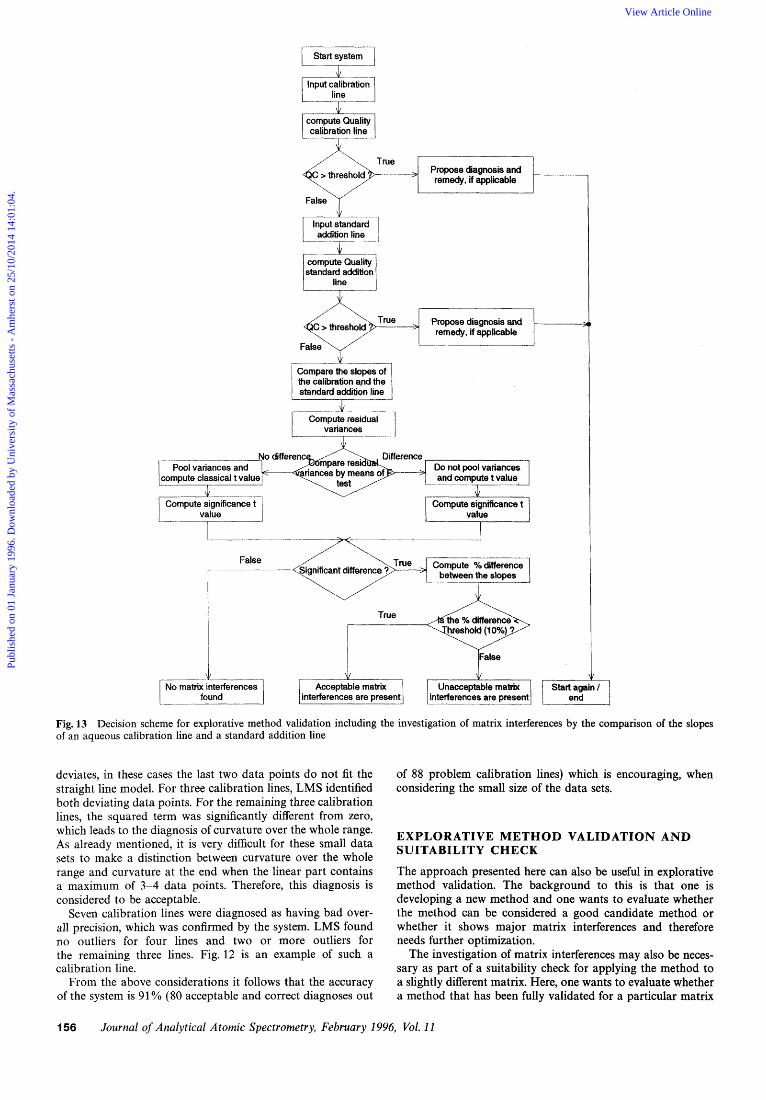
Fig. 13 Decision scheme for explorative method validation including the investigation of matrix interferences by the comparison of the slopes of an aqueous calibration line and a standard addition line

deviates, in these cases the last two data points do not fit the straight line model. For three calibration lines, LMS identified both deviating data points. For the remaining three calibration lines, the squared term was significantly different from zero, which leads to the diagnosis of curvature over the whole range. As already mentioned, it is very difficult for these small data sets to make a distinction between curvature over the whole range and curvature at the end when the linear part contains a maximum of 3-4 data points. Therefore, this diagnosis is considered to be acceptable.

Seven calibration lines were diagnosed as having bad over- all precision, which was confirmed by the system. LMS found no outliers for four lines and two or more outliers for the remaining three lines. Fig. 12 is an example of such a calibration line.

From the above considerations it follows that the accuracy of the system is 91% (80 acceptable and correct diagnoses out

of 88 problem calibration lines) which is encouraging, when considering the small size of the data sets.

EXPLORATIVE METHOD VALIDATION AND SUITABILITY CHECK

The approach presented here can also be useful in explorative method validation. The background to this is that one is developing a new method and one wants to evaluate whether the method can be considered a good candidate method or whether it shows major matrix interferences and therefore needs further optimization.

The investigation of matrix interferences may also be neces- sary as part of a suitability check for applying the method to a slightly different matrix. Here, one wants to evaluate whether a method that has been fully validated for a particular matrix

156 Journal of Analytical Atomic Spectrometry, February 1996, Vol. 11

Publ

ishe

d on

01

Janu

ary

1996

. Dow

nloa

ded

by U

nive

rsity

of

Mas

sach

uset

ts -

Am

hers

t on

25/1

0/20

14 1

4:01

:04.

View Article Online

(e.g., full-cream milk) can be applied to analyse samples with a different matrix (e.g., skimmed milk).

Evaluation of the Quality of Calibration and Standard Addition Lines in Explorative Method Validation

As explained earlier, the presence of matrix interferences is investigated by the comparison of the slopes of an aqueous calibration line and a standard addition line. For this compari- son, acceptable regression lines are of course required. Therefore, a validation of both regression lines is performed first, using the algorithm of the run suitability check. Fig. 13 depicts the scheme for the explorative method validation.

Detection of Matrix Interferences

Matrix interferences that introduce relative systematic errors can be detected by the comparison of the slopes of a calibration line and a standard addition line. This comparison is performed basically by means of a t-test as shown in the decision tree of Fig. 13. Before applying the t-test, the residual variances are compared with an F-test. If the variances do not differ statisti- cally, a pooled variance is computed and a classical t-test is applied. When the variances are significantly different, the t-value is calculated as

where bl and b2 are the slopes of the calibration and standard addition lines, respectively, and Sb12, Sb; are their correspond- ing variances. The number of degrees of freedom (df) to be used with the classical Student’s t distribution is obtained by an approximation proposed by Satterthwaite, which is described by Snedecor and C ~ c h r a n ~ ~

which is a weighted average of the degrees of freedom of both variances. This is very similar to the Cochran test24 where the critical t-value is a weighted average of the individual t-values for each line. The former approach, however, is used in classical statistical packages such as SPSS2’ and allows the estimation

of the p-value, which gives additional information. When this p-value exceeds the 5% significance level, major matrix interferences are considered to be absent.

Since a difference between both slopes might be statistically significant without being relevant for the problem at hand the percentage difference is also compared with a threshold value, which is considered to be acceptable. Here, 10% is used as a user-definable default value, which means that a statistically significant difference that is less than 10% leads to the con- clusion that matrix interferences are present, but that they are acceptable.

When the slopes are not significantly different, the percentage difference is not used in the decision-making process but is given for information purposes.

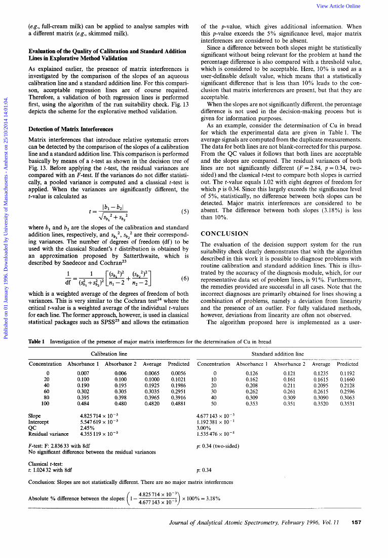
As an example, consider the determination of Cu in bread for which the experimental data are given in Table 1. The average signals are computed from the duplicate measurements. The data for both lines are not blank-corrected for this purpose. From the QC values it follows that both lines are acceptable and the slopes are compared. The residual variances of both lines are not significantly different ( F = 2.84, p = 0.34, two- sided) and the classical t-test to compare both slopes is carried out. The t-value equals 1.02 with eight degrees of freedom for which p is 0.34. Since this largely exceeds the significance level of 5%, statistically, no difference between both slopes can be detected. Major matrix interferences are considered to be absent. The difference between both slopes (3.18%) is less than 10%.

CONCLUSION

The evaluation of the decision support system for the run suitability check clearly demonstrates that with the algorithm described in this work it is possible to diagnose problems with routine calibration and standard addition lines. This is illus- trated by the accuracy of the diagnosis module, which, for our representative data set of problem lines, is 91 %. Furthermore, the remedies provided are successful in all cases. Note that the incorrect diagnoses are primarily obtained for lines showing a combination of problems, namely a deviation from linearity and the presence of an outlier. For fully validated methods, however, deviations from linearity are often not observed.

The algorithm proposed here is implemented as a user-

Table 1 Investigation of the presence of major matrix interferences for the determination of Cu in bread

Calibration line Standard addition line

Concentration Absorbance 1 Absorbance 2 Average Predicted Concentration Absorbance 1 Absorbance 2 Average Predicted

0 0.007 0.006 0.0065 0.0056 0 0.126 0.121 0.1235 0.1192 20 0.100 0.100 0.1000 0.1021 10 0.162 0.161 0.1615 0.1660 40 0.190 0.195 0.1925 0.1986 20 0.208 0.21 1 0.2095 0.2128 60 0.302 0.305 0.3035 0.2951 30 0.262 0.261 0.2615 0.2596 80 0.395 0.398 0.3965 0.3916 40 0.309 0.309 0.3090 0.3063

100 0.484 0.480 0.4820 0.4881 50 0.353 0.351 0.3520 0.3531

Slope 4.825 714 x loW3 Intercept 5.547 619 x 10-3 QC 2.45% Residual variance 4.355 119 x lo-’

F-test: F 2.83633 with 8df No significant difference between the residual variances

Classical t-test: t: 1.02432 with 8df

4.677 143 x 1.192381 x 10-1

1.535476 x 3.00%

p: 0.34 (two-sided)

p : 0.34

Conclusion: Slopes are not statistically different. There are no major matrix interferences

Absolute YO difference between the slopes: 1 - 4.825 714 x 100% = 3.18% ( 4.677143 x

Journal of Analytical Atomic Spectrometry, February 1996, Vol. 11 157

Publ

ishe

d on

01

Janu

ary

1996

. Dow

nloa

ded

by U

nive

rsity

of

Mas

sach

uset

ts -

Am

hers

t on

25/1

0/20

14 1

4:01

:04.

View Article Online

friendly, interactive decision support system, which assists the analyst in his or her conclusions about routine calibration lines. Further development might include an interface with the spectrometer such that the absorbance readings are transferred automatically to the system without human interaction. In this way, the system is a step towards the development of a fully automated instrument complying with quality assurance requirements.

REFERENCES

1

2

3 4

5

6

7

8 9

10

Hu, Y., Smeyers-Verbeke, J., and Massart, D. L., J. Anal. At . Spectrom., 1989, 4, 605. Wolters, R., Van Den Broek, A. C. M., and Kateman, G., Chemometr. Intell. Lab. Syst., 1990, 9, 143. Lahiri, S. L., and Stillman, M. J., Anal. Chem., 1992, 64, 283A. Vankeerberghen, P., Smeyers-Verbeke, J., and Massart, D. L., submitted for publication. Press, W. H., Flannery, B. P., Teukolsky, S. A., and Vetterling, W. T., in Numerical Recipes in C , The Art of ScientiJic Computing, Cambridge University Press, Cambridge, NY, 1988, p. 217. Moshier, S. , in Methods and Programs for Mathematical Functions, Ellis Horwood, Chichester, 1989. de Galan, L., van Dalen, H. P. J., and Kornblum, G. R., Analyst, 1985, 110, 323. Knecht, J., and Stork G., Fresenius’ 2. Anal. Chem., 1974,270,97. Vankeerberghen, P., and Smeyers-Verbeke, J., Chemometr. Intell. Lab. Syst., 1992, 15, 195. Vankeerberghen, P., Smeyers-Verbeke, J., and Massart, D. L., Analusis, 1992, 20, 103.

11 1.2

13

14

15

16 17

18 19 20

21

22

23

24.

25.

Kalantar, A. H., Analusis, 1993, 21, 119. Vankeerberghen, P., Smeyers-Verbeke, J., and Massart, D. L., Analusis, in the press. Massart, D. L., Vandeginste, B. G. M., Deming, S. N., Michotte, Y., and Kaufman, L., in Chemometrics, a Textbook, Elsevier, Amsterdam, 1988, p. 172. Rius, F. X., Smeyers-Verbeke, J., and Massart, D. L., TrAC, Trends Anal. Chem., 1989, 8, 8. Hu, Y., Smeyers-Verbeke, J., and Massart, D. L., Chemometr. Intell. Lab. Syst., 1990, 9, 31. Rousseeuw, P. J., J. Am. Stat. Assoc., 1984, 79, 871. Massart, D. L., Kaufman, L., Rousseeuw, P. J., and Leroy, A., Anal. Chim. Acta, 1986, 187, 171. Rutan, S. C., and Carr, P. W., Anal. Chim. Acta, 1988, 215, 131. Danzer, K., Fresenius’ 2. Anal. Chem., 1989, 335, 869. Ortiz, M. C., Arcos, J., Juarros, J. V., Lopez-Palacios, J., and Sarabia, L. A., Anal. Chem., 1993, 65, 678. Rousseeuw, P. J., and Leroy, A., in Robust Regression and Outlier Detection, Wiley, New York, 1987. Dorschel, A. C., Ekmanis, J. L., Oberholtzer, J. E., Warren, F. V., Jr., and Bildlingmeyer, B. A., Anal. Chem., 1989, 61, 951A. Snedecor, G. W., and Cochran, W. G., Statistical Methods, The Iowa State University Press, Ames, Iowa, USA, 7th edn., 1980, p. 97. Massart, D. L., Smeyers-Verbeke, J., and Rius, F. X., TrAC, Trends Anal. Chem., 1989, 8, 49. Statistical Package for Social Sciences (SPSS for Windows), version 5.01, Chicago, 1992.

Paper 5/06277B Received September 22, 1995

Accepted October 25, 1995

158 Journal of Analytical Atomic Spectrometry, February 1996,, Vol. 1 1

Publ

ishe

d on

01

Janu

ary

1996

. Dow

nloa

ded

by U

nive

rsity

of

Mas

sach

uset

ts -

Am

hers

t on

25/1

0/20

14 1

4:01

:04.

View Article Online