2019 IEEE INTERNATIONAL WORKSHOP ON MACHINE LEARNING FOR SIGNAL PROCESSING, OCT. 13–16, 2019, PITTSBURGH, PA, USA

EEG SIGNAL DIMENSIONALITY REDUCTION AND CLASSIFICATION USING TENSORDECOMPOSITION AND DEEP CONVOLUTIONAL NEURAL NETWORKS

Mojtaba Taherisadr, Mohsen Joneidi, and Nazanin RahnavardDepartment of Electrical & Computer Engineering

University of Central Florida, Orlando, USAEmails: {taherisadr@knights, joneidi@ece, nazanin@ece}.ucf.edu

ABSTRACTA new deep learning-based electroencephalography (EEG)signal analysis framework is proposed. While deep neu-ral networks, specifically convolutional neural networks(CNNs), have gained remarkable attention recently, theystill suffer from high dimensionality of the training data.Two-dimensional input images of CNNs are more vulnerableto be redundant versus one-dimensional input time-series ofconventional neural networks. In this study, we propose anew dimensionality reduction framework for reducing thedimension of CNN inputs based on the tensor decompositionof the time-frequency representation of EEG signals. Theproposed tensor decomposition-based dimensionality reduc-tion algorithm transforms a large set of slices of the inputtensor to a concise set of slices which are called super-slices.Employing super-slices not only handles the artifacts andredundancies of the EEG data but also reduces the dimensionof the CNNs training inputs. We also consider different time-frequency representation methods for EEG image generationand provide a comprehensive comparison among them. Wetest our proposed framework on HCB-MIT data and as resultsshow our approach outperforms other previous studies.

Index Terms— EEG, Convolutional Neural Networks,Time-frequency, Tensor Data Analysis, Dimensionality Re-duction.

1. INTRODUCTION

Electroencephalography (EEG) as a diagnostic tool has beenwidely used in a wide variety of applications [1, 2]. Ac-quiring and analyzing EEG signals are challenging. Variousalgorithms have been developed to efficiently process theEEG data, such as frequency analysis [3], wavelet transform[4], filter banks [5], hidden Markov models [6], support vec-tor machines [7], and artificial neural networks [8].

All the stated methods involve extraction of hand-craftedfeatures from EEG signals. Such hand-crafted feature ex-traction techniques are ad hoc, time-consuming and may notgive the optimal representation of signals. Moreover, forfeature extraction one requires a deep domain knowledge

This material is based upon work supported by the National ScienceFoundation under Grant No. CCF-1718195.

to extract effective features. Moreover, the impact of noiseinterference and particularly artifacts (e.g, eye blink) on datamakes the task of extracting relevant and robust featuresvery challenging [9]. Recently, deep learning approaches,especially CNNs, have gained significant attention in thefield of EEG signal analysis due to their remarkable perfor-mances [10, 11]. CNNs handle the ad-hoc feature extractionprocess. They also combine the feature extraction and clas-sification steps together. Although CNNs outperform otherEEG signal processing methods, they still suffer from thecurse of dimensionality of the input training data. Convertingeach one-dimensional (1D) EEG vector to a two-dimensional(2D) time-frequency (TF) image increases the dimension ofthe training data, which in turn, increases the required storagespace significantly. The challenge of high dimensionality ofthe CNN model’s training data is still open and has to beaddressed to improve CNNs’ efficiency in terms of storagespace and running time.

Tensor decomposition is a powerful tool for analysis ofhigh-dimensional data. The collection of TF representationsof EEG channels generates a three-way tensor over time, fre-quency, and channel. This tensor is able to capture temporaland spectral correlations in addition to dependencies of dif-ferent channels over its third way [12]. EEG signals are verysensitive to noise. However, sensing long time series froma large number of channels facilitates utilization of dimen-sionality reduction techniques in which the impact of noise isdiminished in the low-dimensional representation [13].

In this paper, we propose an algorithm based on low-rankdecomposition of tensors to reduce the size of TF represen-tations of EEG data. Low-rank assumption is a realistic sideinformation for many scenarios in signal processing and com-munication systems [14, 15, 16]. Firstly, a set of super-slices,which are robust superposition of all slices, is computed.Each slice of the input tensor corresponds to one channel.Then, the reduced-dimension super-slices are fed to a CNNin order to find the most efficient features and perform classi-fication automatically. Our contributions in this study cab besummarized as following:

• Proposing a new framework for reducing the dimen-sionality of TF representation of EEG data based on the

978-1-7281-0824-7/19/$31.00 c©2019 IEEE

arX

iv:1

908.

1043

2v1

[ee

ss.S

P] 2

7 A

ug 2

019

tensor decomposition, and feeding the reduced data toa CNN to increase the model’s efficiency and decreaseits training complexity.

• Handling noise, artifacts, and redundancies of EEG sig-nals by tensor decomposition-based dimensionality re-duction.

• Providing a comprehensive comparison and evaluationof different TF representation approaches for CNN-based EEG signal analysis.

Notations: Hereafter, vectors, matrices, and tensors aredenoted by bold lowercase, bold uppercase, and bold under-lined uppercase letters, respectively. A fiber is defined by fix-ing every index of a tensor but one. For example, for T ∈RN×M×K , T :,j,k is a vector of length N , also known as themode-1 fiber of T . T 1, T 2, and T 3 are unfolded matriceswhose columns are fibers of the first, second and third dimen-sions of T , respectively. Slices are two-dimensional sectionsof a tensor, defined by fixing all but two indices. Moreover, ◦denotes the outer product. The n-mode product of a tensor Xwith a proper sized transformation matrix U is a tensor anddenoted by X ×n U . It transfers each fiber of the nth modeof tensor to the corresponding fiber in the final tensor. Mathe-matically, Y = X ×n U ↔ Y n = UXn, in which Xn andY n are unfolded replicas of tensor X and Y w.r.t. differentdimensions. If the vector, u is used instead of the transfer ma-trix, the result of the n-mode product will be a matrix whichis called cotradication of tensor X w.r.t. vector u.

2. TENSOR-BASED TIME-FREQUENCYDIMENSIONALITY REDUCTION OF EEG SIGNALS

In this section, we explain the steps of our proposed frame-work, as depicted in Fig. 1. Popularity of CNN has recentlyincreased due to the fact that they outperform classic machinelearning approaches. CNN requires 2D images as its input.For this purpose, EEG signals are segmented to equal chunksto then be converted to images using TF representation meth-ods. Each TF method affects the overall performance of thesystem differently. Therefore, we consider different state-of-the-art TF algorithms to not only optimize performance of oursystem, but also provide a comprehensive comparison on TFrepresentations of EEG signals. On one hand, more trainingTF images improve the performance of the CNN models, buton the other hand, it adversely adds to the complexity of thecomputation. Hence, to reduce the dimensionality of the gen-erated TF images, we employ the tensor decomposition tech-nique. Collecting TF representation of EEG segments overKchannels, we generate a 3-way tensor over time, frequency,and channel. Tensor decomposition is capable of alleviatingartifacts’ effects and additionally is able to capture spectro-temporal correlations and dependencies of different channelsof EEG signals on its third way. Therefore, as tensor is able tohandle artifacts and redundancies of EEG data, we reduce thedimension of the decomposed tensor in its third way which

is associated with EEG channels. After reducing the third di-mension of the tensor to R (R << K), we feed it to CNNto train the model for further predictions. Each step of ourproposed algorithm is elaborated in the following.

2.1. Time-frequency representation

Time-frequency (TF) analysis of an EEG signal is calculatingthe spectrum at regular time intervals to identify the time atwhich different frequency components present. TF is a suit-able representation for non-stationary and multi-componentEEG signals because of its ability to describe the energydistribution of the signals over time and frequency simul-taneously. Previous studies have applied a large numberof TF approaches to select a proper methodology for theirapplication, helping to improve the resolution, robustness,precision, or performance. Based on the previous studies, thesuitability of a TF approach is data- and application-oriented[17]. A review of the recent methods for TF representationreveals that they can be categorized in six groups as follows:Gaussian kernel (GK), Wigner–Ville (WV), spectrogram(SPEC), modified-B (MB), smoothed-WV (SWV), and sepa-rable kernel (SPEK). Reduced interference approaches suchas Smoothed-WV are capable of improving the quality of therepresentation. This is because decreasing the interference re-sults in a reduction in the effect of cross-terms [18]. Our aimis to assess the mentioned state-of-the-art approaches to de-termine their performance regarding our specific applicationin this study (i.e., CNN-based EEG classification).

2.2. Tensor-based Dimensionality Reduction

As shown in Fig. 1, the time series of each EEG channelis transformed to a TF representation. An efficient dimen-sionality reduction framework is necessary for processing alarge set of 2D images generated from 1D EEG data usingTF representation. Let the matrix X ∈ RT×K denote thecollection of all time series from K channels and the ten-sor X ∈ RT×F×K denote the collection of TF representa-tions of the channels. Since time series of different chan-nels are highly correlated, this matrix and the correspond-ing tensor can be approximated by their low-rank represen-tations. In the matrix format, temporal correlation and cor-relation between channels can be captured via dimensional-ity reduction techniques such as principle component analy-sis (PCA). However, for the tensor representation there ex-ist three types of correlation. Efficient dimensionality reduc-tion of tensors implies employing tensor rank decomposition.It should be noted that, performing PCA on data structuredin tensors requires matricization of tensors. After matriciza-tion of a tensor, correlation over the unfolded way of thetensor will be neglected. A dimensionality reduction frame-work that preserves the intrinsic structure of tensors and ex-ploits low-rank tensor decomposition provides a more con-cise and robust low-dimensional representation. The CAN-DECOMP/PARAFAC (CP) decomposition of the tensor X

4 – Predictive Model (CNN) Training with the Reduced

Tensors

3 - Dimensionality Reduction

Using Tensor DecompositionTime

Freq

uen

cy Time

Fre

qu

enc

y

2 – Time Frequency Representation and

Tensor Structure Generation1 – EEG Signal Acquisition and Preprocessing

EEG Signal

Acquisition1D Representation and

Preprocessing

Class 1

Class 2

Model Training (CNN) Decision Making

Fig. 1. Flow chart of the proposed framework. First step visualizes the data acquisition and preprocessing of EEG. In the next step, eachsegment of the EEG is represented in time-frequency domain as the slices of a 3-way tensor. Finally, tensor decomposition-based techniquereduces the tensor to a set of super-slices which is fed to a CNN to train the model and make the decision.

into R rank-one tensors is given by

X =

R∑r=1

ar ◦ br ◦ cr, (1)

in which, ar, br and cr are called CP factors. Collection ofall ar’s in columns of a matrix results in the matrix A andsimilarly we define B and C matrices. Mode-1 fibers arelinear combination of columns of A and similarly mode-2and mode-3 fibers are linear combination of columns of Band C, respectively. The minimum integer R for which (1)holds is called the rank of X . Fig. 2 shows the decomposi-tion of a rank-R tensor into a summation of R rank-1 tensors.Definition of rank for tensors is similar to its definition formatrices, however, there are several fundamental differencesbetween matrix rank decomposition (SVD) and tensor rankdecomposition (CP) [20]. These fundamental differences en-courage us to keep the multi-way structure of the underlyingtensor and perform dimensionality reduction utilizing tensorCP decomposition. Let z denote a mode-3 fiber of X . Lin-ear combination of columns of matrix C is able to generatez. The representation of any fiber in the third way of X interms of columns of C can be found by solving the problemof z̃ = argmin

z̃‖z − Cz̃‖22. The closed-form solution w.r.t.

z̃ is equal to (CTC)−1CTz. Transformation matrix fromthe originalK-dimensional space to the reducedR-dimensionrepresentation is defined by P = (CTC)−1CT . Accord-ing to this transformation matrix, the original tensor can bereduced as X̃ = X ×3 P . Here, X̃ is the low-dimensionalrepresentation of X which is a set of super-slices. Mathemat-ically speaking

=𝑎1

𝑏1

𝑐1

+ … +𝑎𝑅

𝑏𝑅

𝑐𝑅

𝑿

𝐴 =

𝑎1

…

𝑎𝑅

𝐵 =

𝑏1

…

𝑏𝑅

𝐶 =

𝑐1

…

𝑐𝑅

Fig. 2. Schematic of decomposition of a rank-R tensor to a summa-tion of R rank-1 tensors.

X̃ :,:,r︸ ︷︷ ︸rth super-slice

= X ×3 P r,:.

Here, P r,: indicates the rth row of P . Each super-slice is thecontradiction of the original tensor w.r.t. the correspondingrow of P . Fig. 3 shows the relation between super-slicesand the slices of the given tensor. Each row of matrix P in-dicates the weights for generating the corresponding super-slice. Please note that we only reduced the dimension of thethird way and the first and second dimensions are preserved inorder to extract spectro-temporal patterns using CNN. Usingthis framework, number of EEG channels is reduced from Kto only R super slices (K >> R).

𝑿

Low-dimensional representation

𝑿 first super-slice

𝑪𝑇𝑪 −1𝑪𝑇first row of

Fig. 3. The input tensor as a collection of slices is transformedto a set of super-slices. Each super-slice is a superposition of allslices and weights are driven from Matrix P = (CTC)−1CT . Forexample, the first super-slice is summation of all slices weighted bythe first row of P .

2.3. Deep Convolutional Neural Networks (DCNN)

With CNNs we seek a general-purpose tool for brain-signaldecoding capable of extracting a comprehensive set of fea-tures without the need for expert knowledge. Therefore, wedeveloped a fully supervised CNN model for EEG data anal-ysis. The model takes a super-slice of X̃ (an image) andgenerates a prediction probability of belonging to differentclasses (seizure or non-seizure). We train the model usinglabeled super-slices to minimize a SoftMax loss functionwith respect to network parameters such as weights and biasesusing a gradient descent method and network parameters areupdated using back propagation. We used four main buildingblocks in the CNN model including convolution, pooling,rectified linear unit (ReLU), and fully connected layer.

The primary purpose of convolution layer is to extractfeatures from the input image. Convolution layer preserves

the spatial relationship between pixels by learning image fea-tures using small squares of input data. The convolution layerperforms convolution of input with a set of predefined filters.

Spatial pooling reduces the dimensionality of each fea-ture map but retains the most important information. It canbe of different types such as maximum and average. In caseof Max pooling, we define a spatial neighborhood (for exam-ple, a 2 × 2 window) and take the largest element from therectified feature map within that window. In practice, MaxPooling has been shown to work better [26].

The ReLU is a non-linear activation function that in-troduces the non-linearity when applied to the feature map.ReLU leaves the size of its input unchanged and it only mapsthe non-negative values to zero. An additional ReLU hasbeen used after every convolution layer. In fully connectedlayer each neuron in one layer is connected to all neurons inthe next layer. As the output from the convolutional and pool-ing layers represent high-level features of the input image,we utlize the fully connected layer to use these features forclassifying the input image into various classes based on thetraining dataset [26].

3. FRAMEWORK EVALUATION AND RESULTANALYSIS

We evaluate our proposed method on the CHB-MIT dataset[27]. Different types of epileptic seizures and the diversity ofpatients contained in this dataset make it ideal for assessingthe performance of our framework in realistic settings. In thisstudy, for cross-patient detection, the goal is to detect whethera 30 second segment of signal contains a seizure or not, asannotated in the dataset.

Different TF methods, as discussed in Section 2.1, havebeen considered to generate TF images from EEG segments.Parameters for GKD and MBD have been chosen as α = 0.8and β = 0.02, respectively. These values have been selectedbased on the previous research studies and investigations ontheoretical and practical applications of TF representation ofEEG signal using GKD and MBD approaches [23] (Sections7.4 and 15.5). A Hanning window is chosen for SPEC andSWVD, with length Fs/4 samples, where Fs = 256. Fig. 4illustrates TF representations of a one second interval of EEGsignal from one channel using different methods and above-mentioned parameters.

Time (S)

A)

10

30

20

Freq

uen

cy

(H

z)

0 0.2 0.60.4 0.8 1

10

30

20

0 0.2 0.60.4 0.8 1 0 0.2 0.60.4 0.8 1

0

B) C)

D) E) F)

Fig. 4. TF representations of a 1 second EEG signal using:A) SWV, B) GK, C) WV, D) SPEC, E) MB, and F) SPEKapproaches.

Next, Tensor composition has been generated by collect-ing TF representation of the previous step across all channels.The normalized error of CP decomposition is defined by

normalized error =‖X −

∑r ar ◦ br ◦ cr‖F‖X‖F

, (2)

where, ‖.‖F is the Frobenius norm. Fig. 5 presents the nor-malized error of CP decomposition for EEG tensor data. AsFig. 5 demonstrates, increasing the rank of CP decomposition(number of super-slices) results in a lower normalized error.As Fig. 5 shows, the rank around 15 falls into the intervalof normalized error of [0.2, 0.3], which is acceptable for ourapplication.

For the DCNN model, the architecture guidelines as men-

Super Slices

No

rma

lize

d

Err

or

0 10 20 30 40 50 600

0.10.20.30.4

0.50.60.70.8

15

Fig. 5. Normalized error of CP decomposition versus assumed rankof decomposition.

tioned in [24] were followed. The designed model consists ofseveral layers including (CONV, ReLU, POOL) and one fullyconnected layer as shown in Fig. 6. Two filter sizes including2 × 2 and 3 × 3 were tested. ReLU activation layers wereused across the CNN after each convolution and pooling pairto bring in element-wise non-linearity. In order to estimatethe generalization accuracy of the predictive models on theunseen data, 10-fold cross validation (10-CV) was used. 10-CV divides the total input data of n samples into ten equalparts. There is no overlap between the test sample set (10%of data) with the validation and training sample set (90% ofdata). The latter set is further divided into 4:1 ratio of trainingand validation data samples. The sets were permuted over 10iterations to generate an overall estimate of the generalizationaccuracy. The CNN model was trained using the training setand validation set and tested independently with the testingset. Table 1 reports the selected parameters to train the CNNmodel.

Then, after defining the parameters of TF representationand CNN model we tested the performance of the designedframework. Fig. 7 depicts the classification accuracy of the

Inputs

3@256*256Feature

maps

Hidden

units

100

Fully

connected

Outputs

2

Feature

maps

Feature

mapsFeature

maps

Feature

mapsFeature

maps

Feature

maps

Feature

maps

Conv+ReLU Conv+ReLU Conv+ReLU Conv+ReLUMax-pool Max-pool Max-pool Flatten

Fig. 6. The CNN architecture proposed in this study. This structurehas 10 layers and input image size is 256*256.

Table 1. CNN predefined parametersParameter Values

Learning Rate 0.001Momentum Coefficient 0.9

No. of Feature Maps 32, 64No. of Neurons in Fully Connected Layer 64

Batch Size 40Epoch Number 19

0

20

40

60

80

100

FS 2 FS 3 FS 2 FS 3 FS 2 FS 3 FS 2 FS 3 FS 2 FS 3 FS 2 FS 3

SPEK SPEK SWV SWV GK GK MB MB SPEC SPEC WV WV

12 layers 11 layers 10 layers 9 layers

8 layers 7 layers 6 layers

Acc

ura

cy (

%)

Fig. 7. Accuracy of EEG signal classification for different TF meth-ods and different CNN parameters. Parameters are different numberof layers, and filter sizes are 2 × 2 (FS 2) and 3 × 3 (FS 3). SPEK,SWV, GK, MB, SPEC, and WV indicate different TF representationmethods.

proposed framework associated with different CNN parame-ters and TF approaches. FS indicates filter size and SPEK,GK, SWV, WV, MB, and SPEC are TF methods. Seven ar-chitectures with different number of layers from 6 to 12, andtwo filter sizes of 2 × 2 and 3 × 3 are considered. As resultspresent, 10 layers of CNN, filter size of 3 × 3, and SWV TFmethod outperform other sizes and methods. We use thesehereafter.

3.1. Comparison with Other State-of-the-art and base-line algorithms

In this section we compare our proposed framework withother 1D and 2D baselines. First we consider 1D wavelettransformation as a 1D baseline and then we compare ourframework with PCA as a 2D dimensionality reduction base-line.

3.1.1. Wavelet TransformationWe extract a set of features from the sub-bands of discretewavelet transform (DWT). Low- and high-pass filters are re-peatedly applied to the signal, followed by decimation by 2,to produce the sub-band tree decomposition to some desiredlevel. DWT of 5 levels was applied to the EEG to reach theapproximate frequency ranges of the α, β, δ, and θ sub-bands[25]. After decomposing the signal in each window, featuresincluding average power, mean, and standard deviationof the coefficients were extracted from the sub-bands. Thenwe feed extracted features to 3 predictive models includingcomplex decision tree (CDT), support vector machine (SVM),and K-nearest neighborhood (KNN). The choice of predic-tive methods was made based on different and complementaryproperties among them [30].

3.1.2. Principal component analysisWe applied PCA to 2D TF data to reduce the dimension andprovide the results to compare with our proposed approach.We employed PCA to the TF data and analyzed the result-ing principal components (PCs) in order to detect the mostdescriptive bases of artifacts data. Since the PC space is or-thonormal, we can simply remove the dimensions without af-fecting others. Based on the results of PCA component con-tributions, we realized that most of the contribution to thevariance of the data (> 85%) was summarized in the first 15principal components (PCs). Therefore, we kept the first 15components of the data for the subsequent predictive modeltraining.

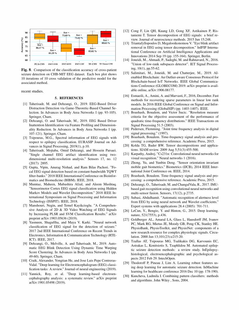
Fig. 8 summarizes the results of the comparison between1D and 2D methods considered in this study. It illustrates boxplots of 10 iterations of 10-CV algorithm. For 1D analysis, asresults show, wavelet transform using SVM outperforms oth-ers including KNN and CDT. The figure also provides com-parison between PCA and the Tensor-based dimensionalityreduction schemes and confirms that the tensor-based outper-forms the PCA-based dimensionality reduction (callsificationaccuracy of 89.63% vs. 86.17%). Tensor considers all ofthe channels together and is capable of capturing temporaland spectral correlations in addition to dependencies of dif-ferent channels over its third way. While PCA works on eachTF image separately and it is prone to ignoring the correla-tions between different channels. Moreover, as Fig. 8 shows,the tensor-based dimensionality reduction (TF-tenosr-CNN)framework, due to its capability of reducing the redundanciesand handling artifacts, outperforms the TF-CNN frameworkwithout dimensionality reduction.

Comparing our result (89% of accuracy) with previousstudies (less than 86% accuracy), our algorithm has improvedthe results of cross-patient seizures detection in CHB-MITdataset [28, 29].

4. CONCLUSION

In this study, we proposed a new tensor-based frameworkto enhance the classification accuracy and efficiency ofthe deep learning models, specifically convolutional neuralnetworks (CNNs), for EEG signals. We proposed a ten-sor decomposition-based dimentionality reduction of time-frequency (TF) inputs of CNN model to improve its per-formance in terms of storage space and running time. Ourproposed method transforms a large set of slices of the inputtensor to a concise set of super-slices, which is capable of notonly handling the artifacts and redundancies of the EEG databut also reducing the dimension of the CNNs training inputs.We also considered different TF approaches and evaluatedtheir performances to provide a comprehensive comparisonof different TF methods for this classification problem. Weimplemented our proposed method on a publicly availabledataset (CHB-MIT). Our results showed the superiority ofour scheme compared to the state-of-the-art methods and

PCA-CNN DWT-KNN DWT-CDT TF-CNN TF-Tensor-CNN

Acc

ura

cy (

%)

DWT-SVM

90

85

80

75

70

65

60

Ave =

89.63 %

Ave =

85.82 %

Ave =

73.42 %

Ave =

75.69 %

Ave =

81.29 %

Ave =

86.17 %

Fig. 8. Comparison of the classification accuracy of cross-patientseizure detection on CHB-MIT EEG dataset. Each box plot shows10 iterations of 10 cross validation of the predictive model for theassociated method.

recent studies.

5. REFERENCES

[1] Taherisadr, M. and Dehzangi, O., 2019. EEG-Based DriverDistraction Detection via Game-Theoretic-Based Channel Se-lection. In Advances in Body Area Networks I (pp. 93-105).Springer, Cham.

[2] Dehzangi, O. and Taherisadr, M., 2019. EEG Based DriverInattention Identification via Feature Profiling and Dimension-ality Reduction. In Advances in Body Area Networks I (pp.107-121). Springer, Cham.

[3] Tsipouras, M.G., Spectral information of EEG signals withrespect to epilepsy classification. EURASIP Journal on Ad-vances in Signal Processing, 2019(1), p.10.

[4] Taherisadr, Mojtaba, Omid Dehzangi, and Hossein Parsaei.”Single channel EEG artifact identification using two-dimensional multi-resolution analysis.” Sensors 17, no. 12(2017): 2895.

[5] Gupta, Vipin, Anurag Nishad, and Ram Bilas Pachori. ”Fo-cal EEG signal detection based on constant-bandwidth TQWTfilter-banks.” 2018 IEEE International Conference on Bioinfor-matics and Biomedicine (BIBM). IEEE, 2018.

[6] Mumtaz, Maheen, Mubashira Afzal, and Aleem Mushtaq.”Sensorimotor Cortex EEG signal classification using HiddenMarkov Models and Wavelet Decomposition.” 2018 IEEE In-ternational Symposium on Signal Processing and InformationTechnology (ISSPIT). IEEE, 2018.

[7] Manshouri, Negin, and Temel Kayikcioglu. ”A Comprehen-sive Analysis of 2D & 3D Video Watching of EEG Signalsby Increasing PLSR and SVM Classification Results.” arXivpreprint arXiv:1903.05636 (2019).

[8] Yasmeen, Shaguftha, and Maya V. Karki. ”Neural networkclassification of EEG signal for the detection of seizure.”2017 2nd IEEE International Conference on Recent Trends inElectronics, Information & Communication Technology (RTE-ICT). IEEE, 2017.

[9] Dehzangi, O., Melville, A. and Taherisadr, M., 2019. Auto-matic EEG Blink Detection Using Dynamic Time WarpingScore Clustering. In Advances in Body Area Networks I (pp.49-60). Springer, Cham.

[10] Craik, Alexander, Yongtian He, and Jose Luis Pepe Contreras-Vidal. ”Deep learning for Electroencephalogram (EEG) classi-fication tasks: A review.” Journal of neural engineering (2019).

[11] Yannick, Roy, et al. ”Deep learning-based electroen-cephalography analysis: a systematic review.” arXiv preprintarXiv:1901.05498 (2019).

[12] Cong F, Lin QH, Kuang LD, Gong XF, Astikainen P, Ris-taniemi T. Tensor decomposition of EEG signals: a brief re-view. Journal of neuroscience methods. 2015 Jun 15;248.

[13] Triantafyllopoulos D, Megalooikonomou V. ”Eye blink artifactremoval in EEG using tensor decomposition.” InIFIP Interna-tional Conference on Artificial Intelligence Applications andInnovations 2014 Sep 19 (pp. 155-164). Springer, Berlin.

[14] Joneidi, M., Ahmadi, P., Sadeghi, M. and Rahnavard, N., 2016.”Union of low-rank subspaces detector”. IET Signal Process-ing, 10(1), pp.55-62.

[15] Salimitari, M., Joneidi, M. and Chatterjee, M., 2019. AI-enabled Blockchain: An Outlier-aware Consensus Protocol forBlockchain-based IoT Networks. IEEE Global Communica-tions Conference (GLOBECOM) 2019. arXiv preprint is avail-able online, arXiv:1906.08177.

[16] Esmaeili, A., Amini, A. and Marvasti, F., 2016, December. Fastmethods for recovering sparse parameters in linear low rankmodels. In 2016 IEEE Global Conference on Signal and Infor-mation Processing (GlobalSIP) (pp. 1403-1407). IEEE.

[17] Boashash, Boualem, and Victor Sucic. ”Resolution measurecriteria for the objective assessment of the performance ofquadratic time-frequency distributions.” IEEE Transactions onSignal Processing 51.5 (2003).

[18] Pedersen, Flemming. ”Joint time frequency analysis in digitalsignal processing.” (1997).

[19] Boashash, Boualem. Time-frequency signal analysis and pro-cessing: a comprehensive reference. Academic Press, 2015.

[20] Kolda TG, Bader BW. Tensor decompositions and applica-tions. SIAM review. 2009 Aug 5;51(3):455-500.

[21] Karpathy, Andrej. ”Cs231n: Convolutional neural networks forvisual recognition.” Neural networks 1 (2016).

[22] Zhong, Yu, and Yunbin Deng. ”Sensor orientation invariantmobile gait biometrics.” Biometrics (IJCB), 2014 IEEE Inter-national Joint Conference on. IEEE, 2014.

[23] Boashash, Boualem. Time-frequency signal analysis and pro-cessing: a comprehensive reference. Academic Press, 2015.

[24] Dehzangi, O., Taherisadr, M. and ChangalVala, R., 2017. IMU-based gait recognition using convolutional neural networks andmulti-sensor fusion. Sensors, 17(12), p.2735.

[25] Subasi, Abdulhamit. ”Automatic recognition of alertness levelfrom EEG by using neural network and Wavelet coefficients.”Expert systems with applications 28.4 (2005): 701-711.

[26] LeCun, Y., Bengio, Y. and Hinton, G., 2015. Deep learning.nature, 521(7553), p.436.

[27] Goldberger AL, Amaral LA, Glass L, Hausdorff JM, IvanovPC, Mark RG, Mietus JE, Moody GB, Peng CK, Stanley HE.PhysioBank, PhysioToolkit, and PhysioNet: components of anew research resource for complex physiologic signals. Circu-lation. 2000 Jun 13;101(23):e215-20.

[28] Tzallas AT, Tsipouras MG, Tsalikakis DG, Karvounis EC,Astrakas L, Konitsiotis S, Tzaphlidou M. Automated epilep-tic seizure detection methods: a review study. InEpilepsy-histological, electroencephalographic and psychological as-pects 2012 Feb 29. IntechOpen.

[29] Thodoroff P, Pineau J, Lim A. Learning robust features us-ing deep learning for automatic seizure detection. InMachinelearning for healthcare conference 2016 Dec 10 (pp. 178-190).

[30] Kuncheva, Ludmila I. Combining pattern classifiers: methodsand algorithms. John Wiley , Sons, 2004.