Distribution of the euryhaline squid Lolliguncula brevis in

MARINE ECOLOGY PROGRESS SERIESMar Ecol Prog Ser

Vol. 226: 235–247, 2002 Published January 31

INTRODUCTION

Most squids are unable to osmoregulate and toleratelow salinities (Hendrix et al. 1981, Mangum 1991), pre-venting the vast majority of squids from invading freshor estuarine waters — 2 significant aquatic habitats

where cephalopods are poorly represented. Onenotable squid, the brief squid Lolliguncula brevis, isthe only species of cephalopod frequently found inlow-salinity estuaries (Vecchione 1991a), where ittolerates salinities as low as 8.5‰ for brief periods(Laughlin & Livingston 1982). Within shallow bays andestuaries, there is evidence that L. brevis withstandslow dissolved oxygen levels (Vecchione 1991b) and a

© Inter-Research 2002 · www.int-res.com

*E-mail: [email protected]

Distribution of the euryhaline squid Lolligunculabrevis in Chesapeake Bay: effects of selected

abiotic factors

I. K. Bartol1,*, R. Mann2, M. Vecchione3

1Department of Organismic Biology, Ecology, and Evolution, University of California, Los Angeles, 621 Charles E. YoungDrive South, Los Angeles, California 90095-1606, USA

2School of Marine Science, Virginia Institute of Marine Science, College of William and Mary, Gloucester Point, Virginia 23062, USA

3National Oceanic and Atmospheric Administration, National Marine Fisheries Service, Systematics Laboratory, National Museum of Natural History, 10th and Constitution NW, Washington, DC 20560, USA

ABSTRACT: The majority of cephalopods are thought to have limitations arising from physiology andlocomotion that exclude them from shallow, highly variable, euryhaline environments. The briefsquid Lolliguncula brevis may be a notable exception because it tolerates low salinities, withstands awide range of environmental conditions, and swims readily in shallow water. Little is known aboutthe distribution of L. brevis in Chesapeake Bay, a diverse and highly variable estuary. Therefore, asurvey of L. brevis was conducted in the Virginia portion of Chesapeake Bay from 1993 to 1997 usinga 9.1 m otter trawl, and the effects of selected factors on squid presence were assessed using logisticregression analysis. During spring through fall, L. brevis was collected over a wide range of bottom-water salinities (17.9 to 35.0‰), bottom-water temperatures (8.1 to 29.6°C), bottom-water dissolvedoxygen levels (1.9 to 14.6 mg O2 l–1), and depths (1.8 to 29.9 m), but it was not present in trawls con-ducted during winter in. L. brevis, especially juveniles < 60 mm dorsal mantle length (DML), wereabundant, frequently ranking in the upper 12% of overall annual nektonic trawl catches, and duringthe fall of some years, ranking second to anchovies. The probability of catching a squid increased inChesapeake Bay at higher salinities and water temperatures, and was much greater in normoxic thanin hypoxic waters; these variables had a profound influence on both annual and seasonal variabilityin distribution. Salinity had the largest influence on squid distribution, with squid being completelyabsent from the bay when salinity was <17.9‰ and most abundant in the fall when salinity was high-est (despite declines in water temperature). Squid were most prevalent at depths between 10 and15 m. The results of this study suggest that L. brevis is an important component of the ChesapeakeBay ecosystem when salinities and water temperatures are within tolerance limits and that unlikeother squids, L. brevis may be well-equipped for an inshore, euryhaline existence.

KEY WORDS: Squid · Estuaries · Salinity · Water temperature · Dissolved oxygen · Lolliguncula brevis

Resale or republication not permitted without written consent of the publisher

Mar Ecol Prog Ser 226: 235–247, 2002

wider range of water temperatures than most cephalo-pods (Hixon 1980, Roper et al. 1984). This species issmaller than most loliginids, seldom reaches sizesgreater than 110 mm in dorsal mantle length (DML)(Hixon 1980, Vecchione et al. 1989), has rounded widefins, and appears to swim at low velocities (Finke et al.1996, Bartol et al. 2001a, b). These traits are beneficialfor maneuvering in nearshore waters of the Gulf ofMexico and along the western Atlantic coast fromDelaware to Brazil, where L. brevis is commonly found(Vecchione et al. 1989).

Little is known about Lolliguncula brevis distributionin Chesapeake Bay. This is surprising, given that L.brevis presumably has exceptional tolerance amongcephalopods to salinity and other physical conditionsand that Chesapeake Bay is one of the largest, mostdiverse, physically variable estuaries in the world, withtributaries and rivers within the system constituting ashoreline a few thousand kilometers long. WithinChesapeake Bay, physical and biological processesoperate rapidly and intensely on many different tem-poral and spatial scales: large-scale pycnoclinesextending almost the entire length of the bay fre-quently develop throughout the spring (Brandt et al.1986); significant phytoplankton blooms arise in thelate spring/early summer (Pinet 1992); regions of bot-tom-water hypoxia may develop in the late summer forweeks or even between tides when organic matterdeposition is high and vertical mixing is difficultbecause of water-column stratification (Webb & D’Elia1980); hundreds of northern and southern species offishes converge in the bay throughout the year (Geer &Austin 1995); and dramatic decreases in salinity andwater temperature occur rapidly in the spring and win-ter, respectively (Brandt et al. 1986). Given that mostsquids evolved to reside in physically stable, offshoreenvironments where interactions with fishes are lowrelative to inshore environments (O’Dor & Webber1986, Wells 1994), the presence of L. brevis in a highlyvariable, euryhaline environment rich in nektonicfauna such as Chesapeake Bay is intriguing. Under-standing the distribution of L. brevis in ChesapeakeBay in relation to physical factors promises insight intothe ecology of a unique squid that lives in an environ-ment that tests its physiological limitations.

To learn about the distribution of brief squid inChesapeake Bay, a survey was conducted in the Vir-ginia portion of the bay from 1993 to 1997 using anotter trawl. The primary objective of this study was todetermine what and how selected abiotic factors affectbrief squid presence within Chesapeake Bay. The abi-otic factors of greatest interest were: tidal stage, bot-tom depth, salinity, water temperature, dissolved oxy-gen and water clarity. Since temporal variation in theChesapeake Bay ecosystem is high, the effects of year

and season also were considered. Two secondary ob-jectives of the study were to provide some assessmentof the abundance of brief squid in Chesapeake Bay rel-ative to other nekton and to document the size distrib-ution of brief squid in Chesapeake Bay throughout theyear.

MATERIALS AND METHODS

Sampling design. Data on Lolliguncula brevis distri-bution were collected from 1993 to 1997 during theVirginia Institute of Marine Science (VIMS) Trawl Sur-vey Monitoring Program, which was established togenerate annual indices for juvenile marine and estu-arine finfish and invertebrates within Virginia waters.During this study, both the mainstem of the lowerChesapeake Bay from the Bay mouth to 37°40’ N and 3major Virginia tributaries, the James, York, and Rap-pahanock Rivers, were sampled (see Fig. 1). The gearused consisted of a 9.1 m semi-balloon otter trawl with3.8 cm body mesh, 3.2 cm cod-end mesh, 1.3 cm cod-end liner mesh, a tickler chain, and steel China-Vdoors (71 cm × 48 cm). Each tow lasted 5 min (bottomtime) and was performed at a speed of 1.29 m s–1.

A stratified random design with stratification by lati-tude and water depth was used to sample sites withinthe Chesapeake Bay mainstem. Three latitudinal strata(36°55’ – 37°10’ N; 37°10’ – 37°25’N; and 37°25’ –37°40’N) and 4 depth strata (eastern bay shoal areas[3.6–9.1 m]; western bay shoal areas [3.6–9.1 m]; plainareas [9.1–13 m]; and deep areas [>13 m]) were consid-ered, resulting in a total of 12 strata. The strata werefixed in time and did not change with tidal cycles. Sam-pling sites were selected randomly within the 12 stratausing computerized files of the National Ocean Sur-vey’s Chesapeake Bay bathymetric grid system. Sam-pling within the Chesapeake Bay mainstem was con-ducted monthly from April through December and inFebruary of each year. Within each of the 3 latitudinalstrata for every month considered during a given year,sampling included 4 stations within the plain stratum, 3stations within the deep stratum, and either 3 (in Maythrough November) or 2 (in December, February, andApril) stations within each of the 2 shoal strata. There-fore, 33 to 39 stations were sampled each month (exceptJanuary and March when no samples were collected)within the mainstem of Chesapeake Bay.

Within the 3 tributaries, fixed stations located in thecenter of the river channels at 8 km intervals from theriver mouths to the freshwater interfaces were sam-pled monthly from 1993 to 1997. In 1996 and 1997,additional stations were sampled using a stratified ran-dom design partitioned by region and depth. Eachriver was divided into 4 regions, but the number of

236

Bartol et al.: Lolliguncula brevis in Chesapeake Bay

depth strata (2 to 5) within each region varied accord-ing to the dimensions of the tributaries. Generally, 25to 62 tributary stations were sampled each monthwithin the 3 tributaries.

Bottom depth, bottom-water salinity, bottom-watertemperature, bottom-water dissolved oxygen, and Sec-chi depth (a measure of water clarity) were recorded atall stations immediately following each tow. Bottomdepth (±0.1 m) was measured using an ultrasonicdepth sounder, salinity (±0.1‰), water temperature(±0.1°C) and dissolved oxygen (±0.1 mg O2 l–1) weremeasured using a Hydrolab multiprobe (HydrolabCorporation, Austin, Texas); and Secchi depth (±0.1 m)was measured using a Secchi disk. Tidal stage wasestimated using Chesapeake tidewater tide logs(Pacific Publishers, Bolinas, California) and Tide andCurrents Version 2.0 software (Nautical Software, Inc.,Beaverton, OR). Latitude and longitude at the begin-ning and ending of each tow were determined usingLoran C conversions or a Global Positioning System(GPS) receiver. Tow distance was defined as the dis-tance between beginning and ending latitude/longi-tude coordinates.

The number and DMLs of squid and the number andtypes of vertebrate nekton captured in the trawls wererecorded. Occasionally, squid were dissected to char-acterize the approximate stage of gonad maturity.Male squid were considered mature when they had awell-developed penis, tightly packed spermatophoreswithin the spermatophoric sac, and a yellowish orwhitish testis. Female squid were considered ripewhen their internal oviduct was filled with mature,amber-colored eggs.

One limitation of the trawl survey data was thatsquid captured prior to 1997 in Chesapeake Bay weresimply classified as squid and assumed to be Lolligun-cula brevis. Examinations of squid captured in 1997and 1998 revealed that several large (>110 mm DML)squid captured in trawls at the Chesapeake Bay mouthin high salinities were Loligo pealei, a loliginid that istypically larger than Lolliguncula brevis, reachingsizes up to 500 mm DML (Vecchione et al. 1989). Thenumber of squid identified in 1997 and 1998 as Loligopealei was small relative to those identified as Lolli-guncula brevis, however, and no squid less than 110mm has been identified to date as Loligo pealei. SinceLolliguncula brevis rarely grows larger than 110 mmDML (Hixon 1980), all squid ≥110 mm DML were con-sidered to be Loligo pealei and eliminated from theanalysis. Conversely, all squid <110 mm were consid-ered to be Lolliguncula brevis and included in theanalysis. Although this does not guarantee that only L.brevis were considered in this study, the number ofLoligo pealei in the samples was probably negligible.This assertion is based on: (1) independent trawling

performed in the Chesapeake Bay ecosystem for pur-poses of collecting specimens for separate swimmingphysiology studies, where 1 out of 1243 squid capturedwere L. pealei; (2) identifications of present and pasttrawl-survey specimens, which reveal small numbersof L. pealei, and (3) the physiology and ecology of L.pealei (L. pealei avoids euryhaline environments, pre-ferring areas >32‰ and >40 m [Hixon 1980], whichare rare in Chesapeake Bay).

Statistical analysis to assess the effects of selectedfactors on squid presence. Since the primary objectiveof this study was to determine what and how selectedphysical variables influence squid presence withinChesapeake Bay, the outcome or dependent variablewas simply the presence or absence of squid at eachsampling site and the independent variables were theselected factors of interest (e.g. depth, salinity, etc.).Logistic regression using the logit link, a standardmethod of analyzing dichotomous, discrete outcomevariables (Hosmer & Lemeshow 1989), was used tomodel the presence/absence of brief squid in trawlcatches. The specific form of the logistic regressionmodel is as follows:

where p = event probability (i.e., probability of catch-ing at least 1 squid), α is a constant, Xi is an indepen-dent variable, i (e.g. salinity, temperature, etc.), and βi

is a coefficient of the independent variable, Xi .The coefficients (β) of the variables included in the

model are most interpretable when expressed in termsof the odds ratio (ψ): ψ = eβ. Both scaled continuous anddiscrete variables are considered in the logistic regres-sion model. For scaled continuous independent vari-ables, the odds ratio (ψ) is a measure of how muchmore likely (or unlikely if the odds ratio is <1) it is forthe outcome (in this case, the presence of at least 1squid in a trawl) to be present when the variable isincreased by 1 unit. Consequently, the interpretationof a continuous independent variable within a logisticregression model will depend heavily on what scalingunits (e.g. 2‰ or 2°C) are selected for the variable, andthus selected units should be of biological relevance(Hosmer & Lemeshow 1989). For example, it may bemore biologically informative to determine how catchprobabilities vary with every 2°C change in water tem-perature rather than with every 0.2°C change whenecological variations may be very slight. Therefore,continuous variables were scaled and coded accordingto units of reasonable biological relevance and toensure there was a sufficient sample size in each cate-gory level. Continuous variables considered in thisanalysis with their respective scaling units denoted inparentheses were: bottom depth (2 m), bottom salinity

pX X X

X X Xi i

i i

= + ++ + +exp( )

exp( )

α β β βα β β β

1 1 2 2

1 1 2 21

K

K

237

Mar Ecol Prog Ser 226: 235–247, 2002

(2‰), bottom temperature (2°C), bottom dissolved oxy-gen (3 mg O2 l–1), tow distance (100 m) and Secchidepth (0.5 m).

For discrete independent variables, the odds ratio isa measure of how much more likely (or unlikely) it isfor the outcome to be present relative to a referencecategory (Hosmer & Lemeshow 1989, Agresti 1990).For example, within a discrete variable such as season,the coefficients of fall, summer, and winter may beexpressed relative to the coefficient of spring. The dis-crete variables considered in this analysis were: year(1993, 1994, 1995, 1996, and 1997), season (spring, fall,summer, and winter), and tidal stage (early flood, max-imum flood, late flood, slack before ebb, early ebb,maximum ebb, late ebb, and slack before flood).

Two significant findings were detected during theearly stages of logistic regression model construction:(1) no squid were caught in trawls during winter, and(2) no squid were caught in areas with salinities below17.5‰. Since there was a zero probability of catchingsquid in areas sampled during the winter or in waters<17.5‰, all sites meeting these criteria were elimi-nated and not used in logistic regression models. Atotal of 2762 sampling sites were eliminated, leaving2393 sampling sites for consideration within the logis-tic regression models.

Logistic regression model construction and refine-ment were performed following procedures suggestedby Hosmer & Lemeshow (1989: Chapter 4). First, uni-variate logistic regression analyses were performed oneach variable. Significance was assessed at α = 0.25using the –2 log likelihood estimation chi-square, andnon-significant variables were eliminated from consid-eration. This level of significance, rather than the con-ventional α = 0.05 level, was selected to minimize thechance of excluding variables that might be importantoutcome predictors when considered collectively withother variables in a multivariate analysis (Mickey &Greenland 1989). At the univariate stage, scaling ofdiscrete variables also was examined; when severalcategories within a discrete variable had similar coeffi-cients and odds ratios, they were combined to formbroader categories (Hosmer & Lemeshow 1989).

Upon completion of the univariate analyses, all sig-nificant variables were included in a multivariatemodel. Variables that were not significant at the α =0.05 level within the multivariate model and that didnot contribute to wide fluctuations in coefficients afterremoval were eliminated, and further multivariatelogistic regression models were performed. Once allessential variables were determined, the scale of con-tinuous variables was examined so that assumptions oflinearity in the logit were not violated. Linearity ofscaled continuous variables was examined by dividingvalues into quartiles (or smaller groupings when

higher resolution was necessary) and treating continu-ous variables as discrete variables in the multivariatemodel using the lowest quartile (or group) as the refer-ence level. This procedure revealed that it was some-times necessary to truncate the range of categorieswithin a variable, increase unit size, and treat somescaled continuous variables as discrete and nominalwhen assumptions of linearity were violated. Althoughthis scaling may reduce resolution within the model, itstabilizes parameter estimates, produces goodness-of-fit measures of greater reliability, and makes the modelmore interpretable (Hosmer & Lemeshow 1989,Agresti 1990).

Once all relevant variables were determined andexpressed in the correct scale, further model refine-ment involved the consideration of interactions.Because of practical considerations, it is not possible toinclude all interactions in logistic regression modelsthat have many variables. Only those interactions thatmake biological sense should be investigated (Hosmer& Lemeshow 1989). Thus, we restricted our search forinteractions to those involving the 4 abiotic factors ofgreatest interest: depth, salinity, water temperature,and dissolved oxygen level. Each interaction involvingthese factors was added separately to the final, main-effects-only, multivariate model. A determination as towhether to include the interaction in further modelswas based on both the significance of the –2 log likeli-hood estimation of the new model and the p-value ofthe interaction. Interactions that were significant at α =0.05 and that provided significant improvement overthe main-effects-only model were added to the finalmodel. To decouple the effects of factors involved insignificant interactions, logits for all factor combina-tions were computed and significance assessed at α = 0.05 using procedures described in detail onp. 102–106 of Hosmer & Lemeshow. The fit of the final,most parsimonious model was assessed using Hosmerand Lemeshow goodness-of-fit tests and various logis-tic regression diagnostics (Hosmer & Lemeshow 1989:p 149-170). There was no overdispersion in the model,i.e., data did not deviate significantly from the ex-pected binomial distribution.

NMFS/NEFSC bottom trawl surveys. Size distri-bution and catch location data on Lolliguncula breviscollected during spring and autumn bottom-trawlsurveys by the National Marine Fisheries Service(NMFS)/Northeast Fisheries Science Center (NEFSC)for 1993 to 1997 were considered in this study. Thesesurveys were conducted within coastal waters (30 to1200 m) of the Atlantic Ocean from Cape Hatteras,North Carolina, to the Gulf of Maine. Approximately300, 30 min tows were performed biannually at ran-domly selected sites using a #36 otter trawl with a1.26 cm cod-end mesh liner. Dorsal mantle lengths of

238


L. brevis captured in each tow were recorded, andcapture location and depth were noted. Further infor-mation on NMFS/NEFSC bottom-trawl proceduresmay be found in ‘Fisherman’s Reports’ for 1993to 1997 (NMFS, NEFSC, Woods Hole, Massachusetts02543) and at: http://www.nefsc.nmfs.gov/sos/vesurv/vesurv.html.

RESULTS

Lolliguncula brevis was captured at545 of the 5155 sampling sites. Intrawls containing squid, the mode was1 squid caught per trawl, the medianwas 4 squid caught per trawl, themean was 16.2 ± 31.9 (SD) squidcaught per trawl, and the range was 1to 325 squid caught per trawl. Themajority of L. brevis captured duringthe survey were collected in the main-stem of Chesapeake Bay and not thetributaries, and the greatest overallnumber of squid collected in trawlsoccurred within the central channel ofthe lower bay and along the easternportion of the bay (Fig. 1). L. breviswere captured during spring, summer,and fall, but no squid were captured intrawls conducted during winter. Estu-arine waters of 0.9 to 43.9 m, 0.0 to37.1‰, 0.3 to 31.0°C, 0.1 to 14.6 mgO2 l–1, and were sampled; brief squidwere collected over a wide range ofdepths (1.8 to 29.9 m), bottom-watersalinities (17.9 to 35.0 ‰), bottom-water temperatures (8.1 to 29.6°C),and bottom-water dissolved oxygenlevels (1.9 to 14.6 mg O2 l–1).

In terms of overall numbers of ani-mals caught annually in trawls, Lolli-guncula brevis ranked 9 out of 94 totalfish/squid species in 1993 (90th per-centile), 18 out of 92 total fish/squidspecies in 1994 (80th percentile), 6 outof 94 total fish/squid species in 1995(94th percentile), 46 out of 98 totalfish/squid species in 1996 (53rd per-centile), and 12 out of 103 total fish/squid species in 1997 (88th percentile).When distinctions are made betweenChesapeake Bay mainstem and tribu-tary sites, it is clear that squid rankedconsistently higher annually withinthe Chesapeake Bay mainstem than

within the tributaries (Fig. 2). Moreover, squid gener-ally ranked higher in the summer and fall than in thewinter and spring both in the Chesapeake Bay main-stem and the tributaries. Brief squid were especiallyabundant within the Chesapeake Bay mainstem dur-ing the fall of 1995, when squid ranked second (behindbay anchovies Anchoa mitchilli) out of 53 (96th per-centile) squid/fish caught (Fig. 2).

Most of the squid captured during this survey were<60 mm DML, although some larger squid (≥70 mmDML) were present in the spring of most years (i.e.,

239

Fig. 1. Map of Chesapeake Bay study site. Mainstem of lower Chesapeake Bayfrom the bay mouth (southern sampling limit) to 37º40’N (northern samplinglimit) and 3 Virginia tributaries, the James, York, and Rappahanock Rivers,were sampled. Upstream and downstream tributary boundaries are depicted.Number of brief squid Lolliguncula brevis captured in trawls from 1993 to 1997in Chesapeake Bay are shown (circles) as well as locations where egg capsuleswere found (x). All squid in this figure were <110 mm in dorsal mantle length.Each tow lasted 5 min (bottom time) and was performed at a speed of 9.7 km–1h

Mar Ecol Prog Ser 226: 235–247, 2002

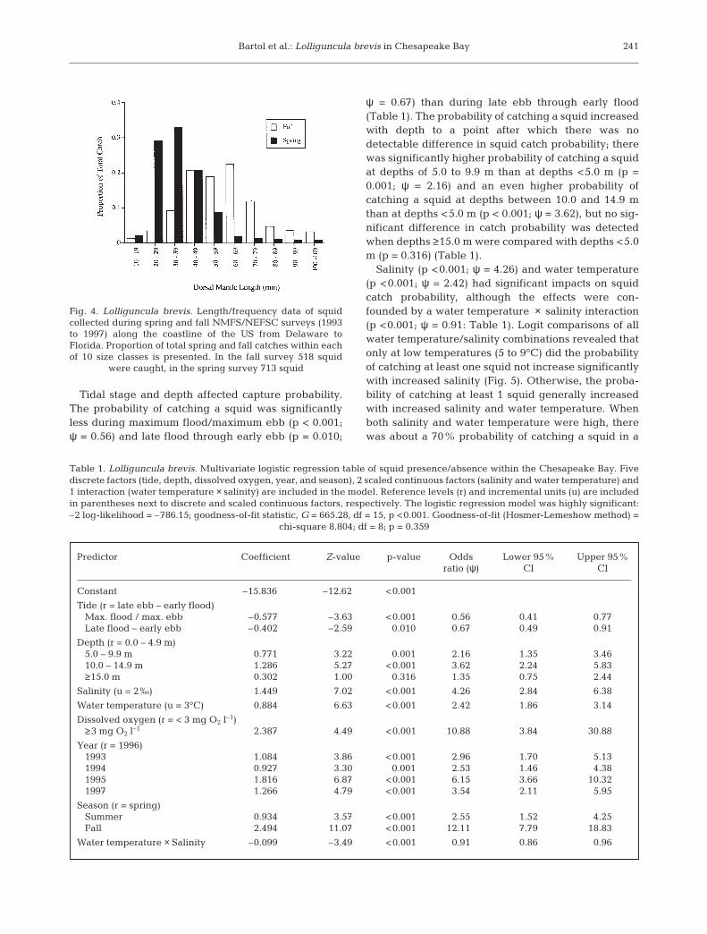
1993, 1995, 1996, 1997) and comprised a notice-able proportion of spring catches (Fig. 3). Themean DML of squid decreased from spring tosummer in each year of the study. However,with the exception of 1994, when size increasedsubstantially from summer to fall, there was lit-tle difference in the mean DML of squid caughtin summer and fall. In contrast, a clear increasein Lolliguncula brevis mantle length fromspring to fall was observed in coastal watersfrom Delaware to Florida in NMFS/NEFSC sur-veys. In these surveys, mean L. brevis DML was32 mm DML (±12 SD) during the spring and 62mm DML (±23 SD) during the fall (Fig. 4). Inthe NMFS/NEFSC surveys, L. brevis werecaught in depths shallower than 36 m, with the

majority of squid being caught in waters shallowerthan 23 m.

Tow distance and Secchi depth did not significantlyinfluence the probability of catching at least 1 squidin a trawl, and were thus eliminated from the finallogistic regression model. The factors and respectivecategories considered in the final, most parsimoniousmodel are shown in Table 1. The logistic regressionmodel was highly significant (–2 log-likelihood chisquare =–786.15; goodness-of-fit statistic, G = 665.28;df = 15; p <0.001), and the model adequately fit thedata (Hosmer & Lemeshow test, p = 0.359) (Table 1).

240

Fig. 2. Lolliguncula brevis. Seasonal (winter, spring, sum-mer, and fall) and annual (year) rankings for brief squidcaught by trawl in mainstem and tributary sections ofChesapeake Bay in 1993 to 1997. Rankings are expressed aspercentiles and are based on the total number of brief squidcaught relative to the total number of each fish speciescaught per season or per year at mainstem and tributaryregions of Chesapeake Bay. Fractions above bars denote theexact rank of squid out of the total number of squid/fish spe-cies considered: lower fractions are results from mainstem

stations, upper fractions for tributary stations

Fig. 3. Lolliguncula brevis. Length/frequency data ofbrief squid captured in spring, summer, and fall dur-ing the VIMS trawl surveys from 1993 to 1997.Annual data as well as cumulative data for the entiresampling period (lower right graph) are depicted. Foreach of the 3 seasons, proportion of total catcheswithin each of 11 size classes is presented. Total num-ber (n) and mean dorsal length (m) of squid caughtwithin the 3 seasons are included above the graphs


Tidal stage and depth affected capture probability.The probability of catching a squid was significantlyless during maximum flood/maximum ebb (p < 0.001;ψ = 0.56) and late flood through early ebb (p = 0.010;

ψ = 0.67) than during late ebb through early flood(Table 1). The probability of catching a squid increasedwith depth to a point after which there was nodetectable difference in squid catch probability; therewas significantly higher probability of catching a squidat depths of 5.0 to 9.9 m than at depths <5.0 m (p =0.001; ψ = 2.16) and an even higher probability ofcatching a squid at depths between 10.0 and 14.9 mthan at depths <5.0 m (p < 0.001; ψ = 3.62), but no sig-nificant difference in catch probability was detectedwhen depths ≥15.0 m were compared with depths <5.0m (p = 0.316) (Table 1).

Salinity (p <0.001; ψ = 4.26) and water temperature(p <0.001; ψ = 2.42) had significant impacts on squidcatch probability, although the effects were con-founded by a water temperature × salinity interaction(p <0.001; ψ = 0.91: Table 1). Logit comparisons of allwater temperature/salinity combinations revealed thatonly at low temperatures (5 to 9°C) did the probabilityof catching at least one squid not increase significantlywith increased salinity (Fig. 5). Otherwise, the proba-bility of catching at least 1 squid generally increasedwith increased salinity and water temperature. Whenboth salinity and water temperature were high, therewas about a 70% probability of catching a squid in a

241

Fig. 4. Lolliguncula brevis. Length/frequency data of squidcollected during spring and fall NMFS/NEFSC surveys (1993to 1997) along the coastline of the US from Delaware toFlorida. Proportion of total spring and fall catches within eachof 10 size classes is presented. In the fall survey 518 squid

were caught, in the spring survey 713 squid

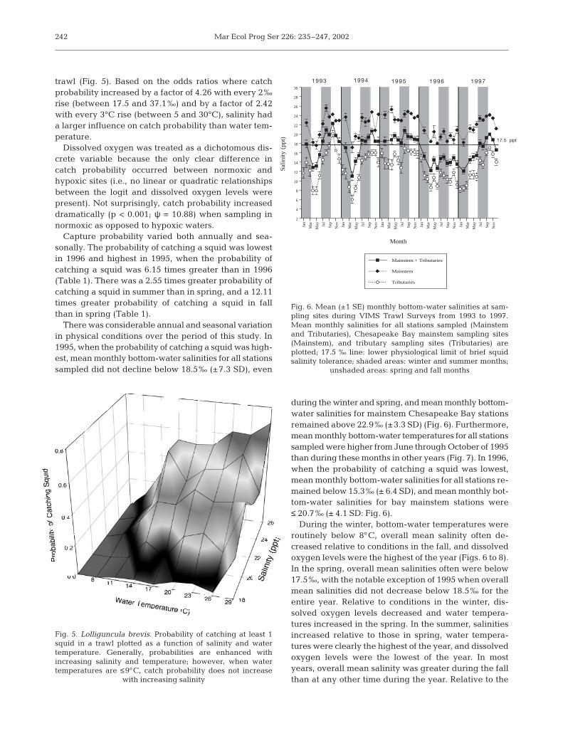
Predictor Coefficient Z-value p-value Odds Lower 95% Upper 95%ratio (ψ) CI CI

Constant –15.836–0 –12.62–0 <0.001>

Tide (r = late ebb – early flood)Max. flood / max. ebb –0.577– –3.63– <0.001> 0.56 0.41 0.77Late flood – early ebb –0.402– –2.59– 0.010 0.67 0.49 0.91

Depth (r = 0.0 – 4.9 m)5.0 – 9.9 m 0.771 3.22 0.001 2.16 1.35 3.4610.0 – 14.9 m 1.286 5.27 <0.001> 3.62 2.24 5.83≥15.0 m 0.302 1.00 0.316 1.35 0.75 2.44

Salinity (u = 2‰) 1.449 7.02 <0.001> 4.26 2.84 6.38

Water temperature (u = 3°C) 0.884 6.63 <0.001> 2.42 1.86 3.14

Dissolved oxygen (r = < 3 mg O2 l–1)≥3 mg O2 l–1 2.387 4.49 <0.001> 10.880 3.84 30.880

Year (r = 1996)1993 1.084 3.86 <0.001> 2.96 1.70 5.131994 0.927 3.30 0.001 2.53 1.46 4.381995 1.816 6.87 <0.001> 6.15 3.66 10.3201997 1.266 4.79 <0.001> 3.54 2.11 5.95

Season (r = spring)Summer 0.934 3.57 <0.001> 2.55 1.52 4.25Fall 2.494 11.070 <0.001> 12.110 7.79 18.830

Water temperature × Salinity –0.099– –3.49– <0.001> 0.91 0.86 0.96

Table 1. Lolliguncula brevis. Multivariate logistic regression table of squid presence/absence within the Chesapeake Bay. Fivediscrete factors (tide, depth, dissolved oxygen, year, and season), 2 scaled continuous factors (salinity and water temperature) and1 interaction (water temperature × salinity) are included in the model. Reference levels (r) and incremental units (u) are includedin parentheses next to discrete and scaled continuous factors, respectively. The logistic regression model was highly significant:–2 log-likelihood = –786.15; goodness-of-fit statistic, G = 665.28, df = 15, p <0.001. Goodness-of-fit (Hosmer-Lemeshow method) =

chi-square 8.804; df = 8; p = 0.359

Mar Ecol Prog Ser 226: 235–247, 2002

trawl (Fig. 5). Based on the odds ratios where catchprobability increased by a factor of 4.26 with every 2‰rise (between 17.5 and 37.1‰) and by a factor of 2.42with every 3°C rise (between 5 and 30°C), salinity hada larger influence on catch probability than water tem-perature.

Dissolved oxygen was treated as a dichotomous dis-crete variable because the only clear difference incatch probability occurred between normoxic andhypoxic sites (i.e., no linear or quadratic relationshipsbetween the logit and dissolved oxygen levels werepresent). Not surprisingly, catch probability increaseddramatically (p < 0.001; ψ = 10.88) when sampling innormoxic as opposed to hypoxic waters.

Capture probability varied both annually and sea-sonally. The probability of catching a squid was lowestin 1996 and highest in 1995, when the probability ofcatching a squid was 6.15 times greater than in 1996(Table 1). There was a 2.55 times greater probability ofcatching a squid in summer than in spring, and a 12.11times greater probability of catching a squid in fallthan in spring (Table 1).

There was considerable annual and seasonal variationin physical conditions over the period of this study. In1995, when the probability of catching a squid was high-est, mean monthly bottom-water salinities for all stationssampled did not decline below 18.5‰ (±7.3 SD), even

during the winter and spring, and mean monthly bottom-water salinities for mainstem Chesapeake Bay stationsremained above 22.9‰ (±3.3 SD) (Fig. 6). Furthermore,mean monthly bottom-water temperatures for all stationssampled were higher from June through October of 1995than during these months in other years (Fig. 7). In 1996,when the probability of catching a squid was lowest,mean monthly bottom-water salinities for all stations re-mained below 15.3‰ (± 6.4 SD), and mean monthly bot-tom-water salinities for bay mainstem stations were≤ 20.7‰ (± 4.1 SD: Fig. 6).

During the winter, bottom-water temperatures wereroutinely below 8°C, overall mean salinity often de-creased relative to conditions in the fall, and dissolvedoxygen levels were the highest of the year (Figs. 6 to 8).In the spring, overall mean salinities often were below17.5‰, with the notable exception of 1995 when overallmean salinities did not decrease below 18.5‰ for theentire year. Relative to conditions in the winter, dis-solved oxygen levels decreased and water tempera-tures increased in the spring. In the summer, salinitiesincreased relative to those in spring, water tempera-tures were clearly the highest of the year, and dissolvedoxygen levels were the lowest of the year. In mostyears, overall mean salinity was greater during the fallthan at any other time during the year. Relative to the

242

2

4

6

8

10

12

14

16

18

20

22

24

26

28

30

Sal

init

y (p

pt)

Jan

Mar

May Ju

l

Sep

Nov Jan

Mar

May Ju

l

Sep

Nov Jan

Mar

May Ju

l

Sep

Nov Jan

Mar

May Ju

l

Sep

Nov Jan

Mar

May Ju

l

Sep

Nov

Month

Tributaries

Mainstem

Mainstem + Tributaries

1993 1994 1995 1996 1997

17.5 ppt

Fig. 6. Mean (±1 SE) monthly bottom-water salinities at sam-pling sites during VIMS Trawl Surveys from 1993 to 1997.Mean monthly salinities for all stations sampled (Mainstemand Tributaries), Chesapeake Bay mainstem sampling sites(Mainstem), and tributary sampling sites (Tributaries) areplotted; 17.5 ‰ line: lower physiological limit of brief squidsalinity tolerance; shaded areas: winter and summer months;

unshaded areas: spring and fall months

Fig. 5. Lolliguncula brevis. Probability of catching at least 1squid in a trawl plotted as a function of salinity and watertemperature. Generally, probabilities are enhanced withincreasing salinity and temperature; however, when watertemperatures are ≤9°C, catch probability does not increase

with increasing salinity


summer, water temperatures decreased and dissolvedoxygen levels increased during the fall (Figs 6 to 8).

During the course of this study, Lolliguncula brevisegg masses were occasionally observed within thetrawl mesh. These masses were collected in Septemberand October within sandy bottom habitats along theeastern portion of the Chesapeake Bay mainstem(Fig. 1). Individual egg cases were generally <2.5 cmin length and contained <30 L. brevis paralarvae. Fur-thermore, mature males and ripe females wereobserved in late July to September.

DISCUSSION

Salinity, water temperature, and dissolved oxygenlevels all play critical roles in determining Lolligunculabrevis distribution in Chesapeake Bay. The data in thisstudy indicate that there are salinity (17.9‰) and watertemperature (8.1°C) thresholds below which L. brevisis absent from Chesapeake Bay. There is also a level ofdissolved oxygen (3 mg O2 l–1) below which L. brevispresence decreases dramatically; however, L. brevis isfound in Chesapeake Bay waters with as low as 1.9 mgO2 l–1. Above salinity and water temperature thresh-

olds, the probability of catching a squid increasessteadily with increased salinity and water temperatureup to conditions of 35‰ and 29.6°C, respectively. Innormoxic waters (3.0 to 14.6 mg O2 l–1), as opposed tohypoxic waters (<3.0 mg O2 l–1), the probability ofcatching a squid increases by a factor of 10. Conse-quently, seasonal and annual variation in one or moreof these factors has a significant impact on squid distri-bution in Chesapeake Bay.

The physical limits detected in this study are consis-tent with those in previous studies on Lolliguncula bre-vis, and provide further evidence that this euryhalinesquid has exceptional tolerance limits relative to othercephalopods. In controlled laboratory studies, Hendrixet al. (1981) determined that L. brevis tolerates salini-ties down to 17.5‰, a limit close to that detected in thepresent study and below which L. brevis demonstratessigns of hypoosmotic stress. The respiratory pigment of L. brevis, hemocyanin, is insensitive to salinitychanges, has high oxygen affinity, and has little pHdependence over a broad range of salinities — charac-teristics that are important for life in euryhaline waters.Conversely, hemocyanin in stenohaline squid, e.g.Loligo pealei, is sensitive to salinity changes, has rela-tively low oxygen affinity, and has large pH depen-dence, preventing these squids from entering low-salinity areas for extended periods (Mangum 1991).The salinity limit determined in the present study is in

243

0

2

4

6

8

10

12

14

16

18

20

22

24

26

28

30

Tem

pera

ture

(C

)

Jan

Mar

May Ju

l

Sep

Nov Jan

Mar

May Ju

l

Sep

Nov Jan

Mar

May Ju

l

Sep

Nov Jan

Mar

May Ju

l

Sep

Nov Jan

Mar

May Ju

l

Sep

Nov

Month

Tributaries

Mainstem


1993 1994 1995 1996 1997

Fig. 7. Mean (±1 SE) monthly bottom-water temperatures atsampling sites during VIMS trawl surveys from 1993 to 1997.Mean monthly temperatures for all stations sampled (Main-stem and Tributaries), Chesapeake Bay mainstem samplingsites (Mainstem), and tributary sampling sites (Tributaries)are plotted. Boxes: conditions from June–October; shadedareas: winter and summer months; unshaded areas: springand fall months. Since there was little variability in water tem-perature between sites during a given month, standard error

bars are not always visible

0

1

2

3

4

5

6

7

8

9

10

11

12

13

Dis

solv

ed O

xyge

n (m

g O

2/l)

Jan

Mar

May Ju

l

Sep

Nov Jan

Mar

May Ju

l

Sep

Nov Jan

Mar

May Ju

l

Sep

Nov Jan

Mar

May Ju

l

Sep

Nov Jan

Mar

May Ju

l

Sep

Nov

Month

Tributaries

Mainstem


1993 1994 1995 1996 1997

Fig. 8. Mean (±1 SE) monthly dissolved oxygen levels of bot-tom-water at sampling sites during VIMS trawl surveys from1993 to 1997. Mean monthly dissolved oxygen levels for all sta-tions sampled (Mainstem and Tributaries), Chesapeake Baymainstem sampling sites (Mainstem), and tributary samplingsites (Tributaries) are plotted. Shaded areas: winter and sum-mer months; unshaded areas: spring and fall months

Mar Ecol Prog Ser 226: 235–247, 2002

reasonable agreement with the field-salinity limits of18.2‰ determined by Dragovich & Kelly (1967) alongthe western coast of Florida and 20.0‰ determined byHixon (1980) in the northwest Gulf of Mexico. A lowerlimit of 8.5‰ was reported by Laughlin & Livingston(1982) in an estuary in north Florida, however. Thelow-end salinity thresholds reported in the presentstudy and in previous studies are lower than those doc-umented for other squids in the north Atlantic, such asL. pealei, L. plei, and Illex illecebrosus, which are typ-ically found in waters >30‰ (O’Dor et al. 1977, Hixon1980).

In the Gulf of Mexico, Dragovich & Kelly (1967),Hixon (1980) and Laughlin & Livingston (1982) cap-tured Lolliguncula brevis in waters of 12.6 to 31.6°C,11 to 31°C, and 15 to 31°C, respectively. The results ofthe present study reveal that L. brevis may be found inslightly cooler waters near the northern limit of itsrange. In a study on the respiratory and cardiac func-tion of L. brevis performed in circulating and non-cir-culating respirometers, Wells et al. (1988) determinedthat L. brevis functions well at water temperatures 14to 27°C. Although Wells et al. did not report on thephysiology of L. brevis below 14°C, they did find thatL. brevis demonstrates clear signs of stress, such asdecreased heartbeat frequency and increased strokevolume, at higher water temperatures (27 to 30°C) —temperatures at which the squid were frequentlycaught during the present study. Wells et al. attributedthe ability of L. brevis to tolerate water temperatures upto 31°C in nature to long acclimation periods. Loligoplei has a wide range of temperature tolerances (13 to30°C), like that of Lolliguncula brevis, but most squidshave more restricted temperature ranges, e.g. Illex ille-cebrosus and Loligo pealei, which are found predomi-nantly in waters of 8 to 15°C and 7 to 22°C, respectively(Hixon 1980, Whitaker 1980, Roper et al. 1984).

The discovery of Lolliguncula brevis in hypoxicwaters of Chesapeake Bay is consistent with previousstudies, and distinguishes L. brevis from other squids.Vecchione & Roper (1991) observed L. brevis inhypoxic waters (0.7 mg O2 l–1) of the western NorthAtlantic using remotely operated submersibles, andVecchione (1991b) documented L. brevis in hypoxicwaters (<3 mg O2 l–1) within coastal and estuarinewaters of southwestern Louisiana during trawl sur-veys. The unique characteristics of the hemocyanin ofL. brevis, especially its high O2 affinity, and the abilityof L. brevis to build up large oxygen debts (unlikeother coastal squids) are beneficial for L. brevis inwaters with low dissolved oxygen levels (Mangum1991, Finke et al. 1996). Wells et al. (1988) determinedthat L. brevis activity levels generally decrease whendissolved oxygen levels are <3 mg O2 l–1, but theyfound that some L. brevis show no behavioral changes

down to levels of 2 mg O2 l–1. Because energy avail-ability for cellular ATPases declines rapidly underhypoxic conditions, Finke et al. (1996) and Zielinski etal. (2000) suggested that L. brevis may spend only briefperiods in hypoxic waters. Excursions by L. brevis intohypoxic waters, however short in duration, may beperformed to exploit a food niche or avoid predation asproposed by Vecchione (1991a). Two possible fishesupon which L. brevis may prey in hypoxic waters (pro-vided they are within the proper size range [i.e., lengthof squid arms or less]) are the spot Leiostomus xanthu-rus and the Atlantic croaker Micropongonias undula-tus — the fishes most commonly encountered in suchwaters during VIMS Trawl Surveys

The synergistic and independent effects of salinity,water temperature and dissolved oxygen, which allincrease catch probabilities when elevated, drive sea-sonal and annual distribution patterns in ChesapeakeBay. Although high dissolved oxygen levels wereobserved throughout Chesapeake Bay during the win-ter, salinity decreased (relative to conditions in the fall)and water temperature dropped below 8°C, triggeringan exodus of Lolliguncula brevis from the bay. Whenwater temperatures increased to approximately 10°Cin April and May (spring), squid re-entered Chesa-peake Bay in areas where salinity was >17.5‰. Similarmigratory responses of L. brevis to water temperatureswere reported by Hixon (1980), who found that L. bre-vis move offshore from Galveston Bay, Texas, inDecember through February, when mean water tem-peratures are 12.8 to 13.9°C, and re-enter inshore bayhabitats in March, when temperatures are above 15°C.The extent to which L. brevis enters Chesapeake Bayin the spring and throughout the year depends heavilyon salinity. In years when salinity was low throughoutthe year, e.g. 1996, squid entered Chesapeake Baylater (May as opposed to April), were captured less intrawls, and were found exclusively in the lower, high-salinity regions of the bay. In years when salinity washigh in the spring and throughout the year, e.g. 1995,squid entered Chesapeake Bay early (April as opposedto May), were more prevalent in trawls, and were cap-tured in a wider region of the bay. High water temper-atures from June through October also contributed tothe observed high catch probabilities in 1995.

High salinity and water temperatures or high salinityalone contributed to greater squid catch probabilitiesin the summer and fall than in the winter and spring.Given that squid catch probabilities were highest inthe fall, when waters were less hypoxic, often moresaline, but cooler relative to waters during the summer,it appears that the benefits of high salinity and morewidespread normoxia outweigh the disadvantages oflower water temperatures. This is not surprising con-sidering the fact that salinity had a greater impact on

244


squid catch probability than water temperature in thelogistic regression model, and hypoxic water lowerscatch probabilities substantially. Laughlin & Livingston(1982) also found that the spatial distribution of briefsquid within a Florida estuary is strongly influenced bysalinity as well as habitat structure, while temperatureplays a lesser role. Interestingly, in non-estuary set-tings where salinity does not fluctuate as significantly,there is considerably less seasonal variation in the fre-quency of occurrence of loliginids (Whitaker 1980).

The regions where squid were encountered mostfrequently (i.e., central Chesapeake Bay near themouth and along eastern portions of the bay wherewaters are deepest and heavily influenced by intrud-ing salt wedges) typically have the highest salinitiesthroughout the year. Consequently, salinity assuredlyplayed an important role in the observed distributionpatterns; however, depth played a significant role aswell. Brief squid are shallow-water cephalopods, pre-ferring habitats <30 m in Galveston Bay, Texas (LaRoe1967, Hixon 1980) and along the eastern US coast, asshown in the NMFS/NEFSC surveys. The bathymetryof Chesapeake Bay is predominantly <20 m, and con-sequently the bay provides optimal depths for squidresidence. The data presented is this study indicatethat there are further preferences at depths less than30 m within the Chesapeake Bay ecosystem, withsquid favoring depths of 10 to 15 m even over deeperwaters, which are more saline but also more hypoxic.These depths are found in the central channels ofChesapeake Bay—areas where the highest overallnumber of squid were encountered. Therefore, whensalinities and water temperatures are within tolerancelimits, brief squid prefer central channel areas 10 to 15m in depth. Laughlin & Livingston (1982) found a simi-lar preference for channels by brief squid inAppalachicola estuary, Florida.

The higher catch probability observed during lateebb through early flood compared with maximumflood/maximum ebb or late flood through early ebbraises some interesting questions. This result may be,in part, a product of a reduction in water volume withinthe Chesapeake Bay ecosystem and the consequentconcentration of squid communities, resulting in easierentrapment of squid in trawls. However, it also proba-bly reflects a behavioral preference. Lolliguncula bre-vis swims at low speeds; it has a critical swimmingspeed of <25 cm s–1, and demonstrates parabolic oxy-gen consumption curves as a function of speed, withoxygen consumption minima at low/intermediatespeeds (6 to 12 cm s–1: Bartol et al. 2001 a,b). Conse-quently, lower currents associated with late ebbthough early flood tides may be advantageous formaneuvering in the bay environment and for keepingpace with the oncoming current (hovering), which is

frequently observed by squids in nature (O’Dor et al.1994). Given that Laughlin & Livingston (1982) found L.brevis to be more abundant in deep channels wherecurrents are higher than in shallow (<4 m), enclosedregions, there may be a lower limit to flow velocity, withL. brevis seeking out currents matching optimal swim-ming speeds, as reported for other squids (O’Dor et al.2001). One important question not addressed directly inthe study is: where do squid go during tidal cycles whencatch probabilities are low? Given that trawls conductedin this survey sampled only the lower water column ofthe Chesapeake Bay system, it is conceivable that squidswam higher in the water column during the differenttidal phases or simply swam out to sea. Future study,possibly involving the deployment of autonomousunderwater vehicles (AUVs), is necessary to determinesquid movements and behaviors within ChesapeakeBay as a function of tidal phase and flow speed.

Brief squid are clearly abundant in Chesapeake Bayrelative to other nekton captured in the VIMS trawlsurveys from 1993 to 1997, ranking in the upper 6 to12% of nektonic catches in terms of total number oforganisms captured in 3 of the 5 sampling years and inthe upper 20% in all years but 1996. Moreover, duringthe fall of some years, squid ranked second to bayanchovies. The results of this study indicate that 2 sizeclasses of Lolliguncula brevis use Chesapeake Bay:one class (<60 mm DML) uses the bay in the springthrough the fall, and a second, less abundant class(≥70 mm DML) is most prevalent in the spring. Theabsence of a distinct intermediate size class (~60 mmDML) in Chesapeake Bay in the fall (or at any othertime during the year), as was detected in theNMFS/NEFSC surveys performed along the Atlanticcoast, suggests that L. brevis may leave the bay once aspecific size is reached and head for coastal waters ofthe Atlantic Ocean. Heavy utilization of certain habi-tats by smaller individuals and subsequent migrationof larger individuals is common among cephalopods(Whitaker 1980, Hixon 1983, Nesis 1983, Okutani1983, Summers 1983, Nagasawa et al. 1993, Hanlon &Messenger 1996).

Limited field observations suggest that larger briefsquid may be using Chesapeake Bay as spawninggrounds, at least during late July through early Sep-tember. This is consistent with the study of Vecchione(1982), who found paralarvae near the mouth ofChesapeake Bay during the warmest months of latesummer. Within the Gulf of Mexico, spawning occursto some degree year-round, with peak spawningoccurring during April to July and September toNovember (LaRoe 1967, Hixon 1980, Jackson et al.1997). More work on fecundity and paralarval ecologyneeds to be performed in Chesapeake Bay to deter-mine if spawning occurs in the spring (when larger

245

Mar Ecol Prog Ser 226: 235–247, 2002

Lolliguncula brevis are most abundant), summer, andfall, and if there are peak spawning events throughoutthe year. Given that statolith studies have revealedthat L. brevis live approximately 100 to 200 d in theGulf of Mexico (Jackson et al. 1997), it is likely thatspawning occurs to some degree most of the time thatbrief squid are in Chesapeake Bay. Early juveniles thateither hatch in Chesapeake Bay or that migrate intothe bay from offshore habitats may remain in the bayto exploit its rich food supply, i.e., crustaceans andjuvenile finfishes.

The common occurrence of brief squid within Chesa-peake Bay, a euryhaline, highly variable environmentthat is home to hundreds of species of fishes each year,is intriguing. Squid in general are thought to be ham-pered by a deficient physiology and are notorious forpossessing an inefficient means of propulsion. Conse-quently, squid are thought to have evolved in environ-ments such as deep-sea or offshore, pelagic habitatswhere interaction with more efficient nekton is mini-mized (O’Dor & Webber 1986, Wells 1994). Nonethe-less, brief squid are present in an inshore, physiologi-cally taxing habitat rich with nektonic fauna. Furtherresearch into the physiology and locomotive abilities ofbrief squid, especially the smaller individuals thatappear to be most abundant within Chesapeake Bay,may further our evolutionary and ecological under-standing of this unique cephalopod.

Acknowledgements. We thank M. R. Patterson, S. L. Sander-son, W. M. Kier, and M. Luckenbach for intellectual input andconstructive comments on earlier drafts. We also thank mem-bers of the VIMS Trawl Survey for data collection, especiallyP. Geer, who also assisted in the retrieval of trawl data onsquid. Financial support for the VIMS Trawl Survey was pro-vided by Wallop Breaux and the U.S. Fish and Wildlife Ser-vice Sportfish Restoration Project F104. Financial support dur-ing the writing phase of this manuscript was provided by theOffice of Naval Research under contract N00014-96-0607 toM.S. Gordon.

LITERATURE CITED

Agresti A (1990) Categorical data analysis. John Wiley &Sons, Inc., New York

Bartol IK, Mann R, Patterson MR (2001a) Aerobic respiratorycosts of swimming in the negatively buoyant brief squidLolliguncula brevis. J Exp Biol 204:3639–3653

Bartol IK, Patterson MR, Mann R (2001 b) Swimming mechan-ics and behavier of the negatively buoyant, brief squidLolliguncula brevis. J Exp Biol 204:3655–3682

Brandt A, Sarabun CC, Seliger HH, Tyler MA (1986) Theeffects of a broad spectrum of physical activity on the bio-logical processes in the Chesapeake Bay. In: Nihoul JCL(ed) Marine interface ecohydrodynamics, Elsevier, Ams-terdam, p 361–284

Dragovich A, Kelly JA Jr (1967) Occurrence of the squid, Lol-liguncula brevis, in some coastal waters of westernFlorida. Bull Mar Sci 17:840–844

Finke E, Pörtner HO, Lee PG, Webber DM (1996) Squid (Lol-liguncula brevis) life in shallow waters: oxygen limitationof metabolism and swimming performance. J Exp Biol 199:911–921

Geer PJ, Austin HM (1995) Juvenile fish and blue crab stockassessment program bottom trawl survey annual datasummary report. Special Scientific Report no. 124: vol.1995, College of William and Mary, School of Marine Sci-ence, Virginia Institute of Marine Science, GloucesterPoint, VA 23062

Hanlon RT, Messenger JB (1996) Cephalopod behaviour.Cambridge University Press, Cambridge

Hendrix JP Jr, Hulet WH, Greenberg MJ (1981) Salinity toler-ances and the response to hypoosmotic stress of the baysquid Lolliguncula brevis, a euryhaline cephalopod mol-lusc. Comp Biochem Physiol 69A:641–648

Hixon RF (1980) Growth, reproductive biology, distributionand abundance of three species of loliginid squid (Myop-sida, Cephalopoda) in the Northwest Gulf of Mexico. PhDthesis, University of Miami, Miami

Hixon RF (1983) Loligo opalescens. In: Boyle PR(ed) Cephalo-pod life cycles, Vol. 1. Species accounts. Academic PressLtd, London, p 95–114

Hosmer DW, Lemeshow S (1989) Applied logistic regression.John Wiley & Sons, Inc. New York

Jackson GD, Forsythe JW, Hixon RF, Hanlon RT (1997) Age,growth, and maturation of Lolliguncula brevis (Cephalo-poda: Loliginidae) in the northwestern Gulf of Mexicowith a comparison of length-frequency versus statolithage analysis. Can J Fish Aquat Sci 54:2907–2919

Laughlin RA, Livingston RJ (1982) Environmental and trophicdeterminants of the spatial/temporal distribution of thebrief squid (Lolliguncula brevis) in the Apalochicola Estu-ary (North Florida, USA). Bull Mar Sci 32:489–497

LaRoe ET (1967) A contribution to the biology of the Lolig-inidae (Cephalopoda: Myopsida) of the tropical westernAtlantic. Master’s thesis, University of Miami, Miami

Mangum CP (1991) Salt sensitivity of the hemocyanin of eury-and stenohaline squids. Comp Biochem Physiol A 99:159–161

Mickey J, Greenland S (1989) A study on the impact of con-founder-selection criteria on effect estimation. Am J Epi-demiol 129:125–137

Nagasawa K, Takayanagi S, Takami T (1993) Cephalopod tag-ging and marking in Japan: a review. In: Okutani T, O’DorRK, Kubodera T (eds) Recent advances in cephalopod fish-eries biology. Tokai University Press, Tokyo, p 313–329

Nesis KN (1983) Dosidicus gigas. In: Boyle PR (ed) Cephalo-pod life cycles, Vol. 1. Species accounts. Academic PressLtd, London, p 215–231

O’Dor RK, Webber DM (1986) The constraints on cephalo-pods: why squid aren’t fish. Can J Zool 64:1591–1605

O’Dor RK, Durward RD, Balch N (1977) Maintenance andmaturation of squid (Illex illecebrosus) in a 15-m circularpool. Biol Bull (Woods Hole) 153:322–335

O’Dor RK, Hoar JA, Webber DM, Carey FG, Tanaka S, Mar-tins H, Portiero FM (1994) Squid (Loligo forbesi) perfor-mance and metabolic rates in nature. Mar Freshw BehavPhysiol 25:163–177

O’Dor RK, Aitken JP, Andrade Y, Finn J, Jackson GD (2001)Currents as environmental constraints on the behavior,energetics and distribution of squid and cuttlefish. BullMar Sci (in press)

Okutani T (1983) Todarodes pacificus. In: Boyle PR (ed)Cephalopod life cycles, Vol. 1. Species accounts. Acade-mic Press Ltd, London, p 201–214

Pinet PR (1992) Oceanography: an introduction to the planet

246


oceanus. West Publishing Company, St. Paul, MNRoper CFE, Sweeney MJ, Nauen CE (1984) FAO species cat-

alogue, Vol. 3. Cephalopods of the world. An annotatedand illustrated catalogue of species of interest to fisheries.FAO Fish Synop, No. 125, Vol. 3, 277 p

Summers WC (1983) Loligo opalescens. In: Boyle PR (ed)Cephalopod life cycles, Vol. 1. Species accounts. Acade-mic Press, London, p 115–142

Vecchione M (1982) Larval distribution of a euryhaline squidnear its northern range limit. Bull Am Malacol Union 81:36

Vecchione M (1991a) Dissolved oxygen and the distribution ofthe euryhaline squid Lolliguncula brevis. Bull Mar Sci 49:668–669

Vecchione M (1991b) Observations on the paralarval ecologyof a euryhaline squid Lolliguncula brevis (Cephalopoda:Loliginidae). Fish Bull (Wash DC) 89:515–521

Vecchione M, Roper CF (1991) Cephalopods observed fromsubmersibles in the western North Atlantic. Bull Mar Sci49:433–445

Vecchione M, Roper CF, Sweeney MJ (1989) Marine flora andfauna of the eastern United States mollusca: Cephalopoda.NOAA Tech Rep NMFS 73:23

Webb KL, D’Elia CF (1980) Nutrient and oxygen redistribu-tion during a spring neap tidal cycle in a temperate estu-ary. Science 207:983–985

Wells MJ (1994) The evolution of the racing snail. Mar FreshwBehav Physiol 25:1–12

Wells MJ, Hanlon RT, Lee PG, Dimarco FP (1988) Respiratoryand cardiac performance in Lolliguncula brevis (Cephalo-pods, Myopsida): the effects of activity, temperature, andhypoxia. J Exp Biol 138:17–36

Whitaker JD (1980) Squid catches resulting from trawl sur-veys off the southeastern United States. Mar Fish Rev42:39–43

Zielinski S, Lee PG, Pörtner HD (2000) Metabolic perfor-mance of the sguid Lolliguncula brevis (Cephalopoda)during hypoxia: an analysis of the critical PO2. J Exp MarBiol Ecol 243:241–259

247

Editorial responsibility: Kenneth Sherman (Contribution Editor),Narragansett, Rhode Island, USA

Submitted: June 1, 2000; Accepted: March 13, 2001Proofs received from author(s): January 15, 2002

Documents

Distribution of the euryhaline squid Lolliguncula brevis in