Embed Size (px)
Citation preview
Early adolescence behavior problems and timing of poverty during childhood: A comparison of lifecourse models Julia Rachel S.E. Mazza1
Jean Lambert1
Maria Victoria Zunzunegui1
Richard E. Tremblay2,3
Michel Boivin4,5
Sylvana M. Côté1,6 1Department of Social and Preventive Medicine, University of Montreal, Montreal H3N 1X9, Canada 2Department of Psychology, University of Montreal, Montreal H2V 2S9, Canada 3School of Public Health, Physiotherapy and Population Science, University College Dublin, Belfield, Dublin 4, Ireland 4School of Psychology, University of Laval, Quebec G1V 0A6, Canada 5Institute of Genetic, Neurobiological, and Social Foundations of Child Development, Tomsk State University, Tomsk 634050, Russian Federation 6INSERUM U1219 Bordeaux, University of Bordeaux, Bordeaux 33076, France Corresponding author: Julia Rachel S.E. Mazza, UHC Ste Justine, 3175, chemin de la Côte Sainte-Catherine, Bloc 5, room A571, Montreal (QC), H3T 1C5, Canada.
Email: [email protected]
1
Abstract
Context: Poverty is a well-established risk factor for the development of behavior problems,
yet little is known about how timing of exposure to childhood poverty relates to behavior
problems in early adolescence. Objective: To examine the differential effects of the timing of
poverty between birth and late childhood on behavior problems in early adolescence by
modeling lifecourse models, corresponding to sensitive periods, accumulation of risk and
social mobility models. Methods: We used the Quebec Longitudinal Study of Child
Development (N=2120). Poverty was defined as living below the low-income thresholds
defined by Statistics Canada and grouped into three time periods: between ages 0-3 years, 5-7
years, and 8-12 years. Main outcomes were teacher’s report of hyperactivity, opposition and
physical aggression at age 13 years. Structured linear regression analyses were conducted to
estimate the contribution of poverty during the three selected time periods to behavior
problems. Partial F-tests were used to compare nested lifecourse models to a full saturated
model (all poverty main effects and possible interactions). Results: Families who
experienced poverty at all time periods were 9.3% of the original sample. Those who were
poor at least one time period were 39.2%. The accumulation of risk model was the best fitting
model for hyperactivity and opposition. The risk for physical aggression problems was
associated only to poverty between 0-3 years supporting the sensitive period. Conclusion:
Early and prolonged exposure to childhood poverty predicted higher levels of behavior
problems in early adolescence. Antipoverty policies targeting the first years of life and long
term support to pregnant women living in poverty are likely to reduce behavior problems in
early adolescence.
Keywords: Poverty; Hyperactivity; Physical aggression; Opposition; Lifecourse
2
1. Introduction
Poverty has been associated to behavior problems during childhood and adolescence in many
regions of the developed world, including North America and Europe (Russell, Ford,
Rosenberg, & Kelly, 2014; Shaw, Lacourse, & Nagin, 2005). However, it remains unclear
whether behavior problems in adolescence are more likely because of exposure to poverty
during certain periods of childhood, or whether it is a matter of prolonged exposure over the
years. This study is grounded in the lifecourse framework (Lynch & Smith, 2005) which
describes how exposure to adversity throughout the lifecycle relates to disease risk later in
life. Several lifecourse models have been proposed (Kuh et al., 2003; Hallqvist et al., 2004)
and correspond to: (1) the sensitive period model describing a time period when exposure has
a stronger effect on disease risk than it would at another times; (2) the accumulation of risk
model asserting that exposure accumulates overtime increasing disease risk; and (3) the social
mobility model proposing that instability in exposure overtime leads to disease occurrence.
The current paper examined the timing and duration of childhood poverty in association with
three subtypes of behavior problems that are prevalent in adolescence (Polanczyk, Salum,
Sugaya, Caye, & Rohde, 2015): hyperactivity, opposition, and physical aggression.
1.1 Poverty and behavior problems: A lifecourse approach
Numerous studies have addressed lifecourse poverty in relation to behavior problems across
development using a variety of research methods. There is evidence that the adverse prenatal
environment and earliest years of life constitute a sensitive period for the development of
later-life behavior problems (Côté, Vaillancourt, LeBlanc, Nagin, & Tremblay, 2006;
Pingault et al., 2013). Other studies support the accumulation of risk model which states that
3
poverty and low income effects accumulate in childhood and lead to behavior problems in
adolescence (McLaughlin et al., 2011; Rekker et al., 2015). However, there is little evidence
simultaneously examining different lifecourse models of adversity relative to behavior
problems. Of the few studies which have examined these models, the evidence is mixed. An
Australian study showed that exposure to maternal depression was more important at age 2
years than exposure later in life or time spent in poverty in explaining aggressive and
delinquent problems at age 9.5 years (Giles et al., 2011). Despite the fact that this study did
not consider poverty as its measure of adversity (but rather maternal depression), it
demonstrated early childhood (i.e. before age 5 years) as a sensitive period of adversity for
behavior problems while considering other lifecourse processes such as accumulation of risk
and social mobility. This study is particularly interesting as it reported results using a model-
building framework to test for several competing lifecourse models (Mishra et al., 2009).
One study from the United States showed that low income during middle childhood (6-12
years) was associated with behavior problems beyond the effect of low income during early
childhood (0-5 years), thus providing evidence of accumulation of risk for behavior problems
which in turn in was better quantified by middle childhood adversity (Tsal, Shalev, &
Mevorach, 2005). In this study, timing of exposure to poverty was isolated using
accumulation of inputs modeling to test for poverty effects in two distinct points (i.e. early
and middle childhood) on behavior problems.
Limitations of these studies should be noted. First, studies yield conflicting results and are
limited in terms of comparability due to differences in the analytical strategy used to address
lifecourse models. Nor can they be compared in terms of variability in behavioral outcomes
and the age distribution of children. Another concern is variation in social policies across
high-income countries for which research is available. Second, studies do not rely on annual
4
or biannual measurements of poverty during early and middle childhood years. Repeated and
annual measurements allow for the careful control of the timing of exposure to poverty when
considering an effect-modification hypothesis, as is required in a lifecourse framework.
Finally, few studies have separately examined different subtypes of behavior problems in
adolescence (Leis, Heron, Stuart, & Mendelson, 2013; Nomura, Rajendran, Brooks-Gunn, &
Newcorn, 2008). It is important to establish whether lifecourse models of poverty holds
across different types of behavior problems or if they are specific to certain subtypes because
they have different developmental trajectories and require specific corrective interventions
(Tremblay, 2010). Thus, it remains unclear whether the association between childhood
poverty and behavior problems in adolescence vary in strength across different periods of
time.
1.2. Objectives of the present study
Objectives of the present study were: (1) to model lifecourse models of poverty (0 to 12
years) corresponding to sensitive periods, accumulation of risk, and mobility models to
predict hyperactivity, physical aggression and opposition at 13 years (2) to identify the
lifecourse model that best describes the poverty-behavior problem link. We apply a structured
modelling approach (Mishra et al., 2009) as a model-building framework. Based on this
approach, nested lifecourse models of poverty in relation to behavior problems are contrasted
to a saturated model, an all-inclusive model with as many poverty parameters as there are
possible sequences of exposure, to assess which model is most consistent with the data. We
hypothesized that prolonged exposure to childhood poverty and possibly exposure during
sensitive periods, such as the early childhood (i.e. before age 5 years), would increase
behavior problems in early adolescence. We also hypothesized that the identification of
5
lifecourse models would differ across subtypes of behavior problems due to variations of
behavior problems trajectories overtime. In addition, the distinct contribution of the study
resides in examining the role of timing and duration as well as intermittent exposure to
childhood poverty underlying the development of behavior problems in early adolescence.
2. Methodology
2.1. Data
Data originated from the Quebec Longitudinal Study of Child Development (QLSCD)
collected between 1998 and 2011. The target population was children born in 1997-1998 and
whose mothers resided in Quebec, Canada (Jetté & Groseilliers, 2000). The initial sample
comprised of 2120 children aged 3-8 months (mean age 5 months). Data were collected
yearly until 2006 when the interview schedule shifted to a biennial design. Interviews were
conducted by trained research assistants through home interviews and directed to the person
most knowledgeable about the child (mothers in 98% of cases). Written informed consent
was obtained from all respondents. We used 12 assessments points at ages: 5 months, 1½,
2½, 3½, 4½, 5, 6, 7, 8, 10, 12, and 13 years. When participants were 13 years of age, 1290
participants from the initial sample remained in the study (i.e. 60.8% retention rate), of which
a total of 983 had nonmissing values on at least one of the three subtypes of behavior
problems. The characteristics of the QSLCD sample present at 13 years of age and sub-
sample with missing data are presented in the Appendix (see Table S1).
2.2. Attrition and Non- participation
6
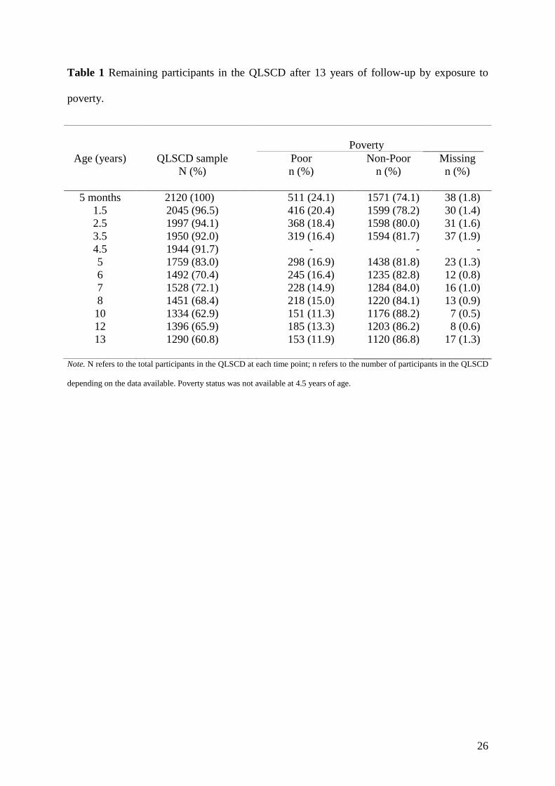
QLSCD retention rate was high until children aged 4.5 years (92%) with attrition increasing
afterwards. By age 13, attrition was nearly 40%. The highest attrition rates were observed for
respondents living in poverty, with a high school diploma or less, as well as being in single-
parent and immigrant families. Specifically, the proportion of participants exposed to poverty
at 5 months of age was 24.1% but only 11.9% using the active or complete case sample at age
13 years, which in turn indicates differential study attrition. Table 1 presents remaining
participants in the QLSCD over sampling period by exposure to poverty.
2.3. Measures
Behavior problems. Teachers rated participants’ behavior problems at 13 years of age using
the early childhood behavior scale from the Canadian National Longitudinal Study of
Children and Youth (Human Resources Development Canada and Statistics Canada, 1996).
Teachers rated behavior problems on a frequency scale of whether the participant never (0),
sometimes (1), or often (2) exhibited hyperactivity, physical aggression and opposition
behavior. For hyperactivity (Cronbach's α =0.87), items used were: 1) “cannot sit still, is
restless”, 2) “is impulsive, acts without thinking”, 3) “has difficulty waiting his/her turn”, and
4) “cannot settle down to do anything for more than a few moments”. For opposition
(Cronbach's α=0.85), items used were: 1) “is defiant or refuses to comply with adults’ request
or rules?”, 2) “does not seem to feel guilty after misbehaving?”, and 3) “punishment doesn't
change his/her behavior?”. For physical aggression (Cronbach's α=0.84), items were as
follow: 1) “gets into fights?”, 2) “physically attacks others”, and 3) “hits, bites, kicks other
children”. For all behavior measures, higher scores indicated higher levels of behavior
problems (range 0 to 10).

7
Poverty. Poverty was defined according to the Canadian Low Income Cut-Offs (LICOs)
calculated by Statistic Canada. The calculation is based on family income, the number of
people in the household, and the level of urbanisation of the place of residence in the past 12-
months (Giles, 2004). A family was considered to be poor when attributing 20% or more of
their household income than the average Canadian family to food, shelter, and clothing. For
instance, in 2013 LICOs were $ 24 934, $ 28 537, $ 31 835, $ 32 236 and $ 38 117 (CAD) for
a family of four living after taxes in rural areas, towns (< 30,000 inhabitants), towns between
30,000 and 99,999 inhabitants, cities between 100,000 and 499,999 inhabitants, and large
cities (> 500,000 inhabitants) respectively (Statistics Canada, 2013). In this study, exposure
to poverty was grouped into three time periods: a) exposure between ages 0-3 years (P1 and
coded 1=yes; 0=otherwise); b) exposure between ages 5-7 years (P2 and coded 1=yes;
0=otherwise); and c) exposure between ages 8-12 years (P3 and coded 1=yes; 0=otherwise).
Child and family confounders. Confounders assessed at baseline included: (a) immigration
status (1=immigrant mother and 8.4% of the sample; 0=otherwise); (b) maternal history of
antisocial behavior in which higher scores indicate higher levels of antisocial behavior before
the end of high school (range 0 to 5 and Mean = .82; SD = .94; e.g. “Before the end of high
school, did you more than once get into fights that you had started?”) ; and (c) child’s sex
(1=boys and 46.7% of the sample; 0=girls). For confounders measured at multiple time
points, we used low maternal education and whether both biological parents were living with
the child at ages 0, 3, and 8 years. Low maternal education indicated if mothers did not
complete high-school a (1=yes and 44.4% of the sample at age 5 months, 40.2% at age 3, and
24.7% at age 8; 0=no). Children whose biological parents were separated or single were
coded as 1 (8.4% at age 5 months, 13.2% at age 3 years, and 19.2% at age 8 years) vs
children living with both their biological parents regardless of their marital status coded as
8
0.Confounders were selected according to their reported association in the literature (Essex et
al., 2006; Kim-Cohen, Moffitt, Taylor, Pawlby, & Caspi, 2005; Tremblay et al., 2004) or to
their association with behavior problems and poverty in bivariate analyses.
2.4. Analytic Design
We conducted two sets of analyses: (1) Modeling competing lifecourse models of the
association between childhood poverty across three time periods (i.e. P1, P2 and P3) and
behavior problems at 13 years of age; and (2) Selecting the lifecourse model that best
described the association between childhood poverty and behavior problems in early
adolescence. Analyses were conducted with SPSS v.22.0 and R software. We used a
threshold for significance at p < .05.
We used a structured modelling approach (Mishra et al., 2009) to model and compare
lifecourse models. Using separate multiple linear regressions, this approach allows for
variation around the outcome mean given a binary exposure grouped into three time points
(in our case, P1, P2 and P3) as well as all possible permutations. A total of eight possible
permutations corresponded to each combination of timing periods P1, P2 and P3. To test for
rival lifecourse models given P1, P2 and P3, the structured approach compares a set of
nested/reduced models - corresponding to the accumulation of risk, sensitive periods and
mobility models - to a saturated/complete model. Specifically, a saturated model included all
three main effects, all 2-ways interactions, and a 3-way interaction. With this formulation, β1,
β2 and β3 are slope parameters of all three main effects. The second parameterization is the
expression of all possible main effects interactions and referred as θ12, θ13, θ23 and θ123.
Another parameterization is α for the variation around the outcome mean given no exposure

9
to poverty over the three time periods and representing the simplest model (null model or
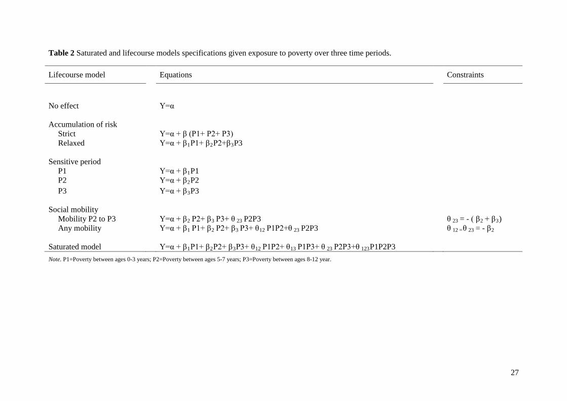
intercept only-model). Table 2 presents corresponding equations for all nested models within
the saturated model given poverty at all three time periods.
Based on the structured modelling approach hypothesized lifecourse models were as follows:
1) Three sensitive period models assuming that the association between poverty and
behavior problems is particularly stronger during a certain time period (in our
case, P1, P2, or P3) than it would be at other time periods.
2) Two accumulation of risk models: (a) accumulation of risk strict assuming that
the longer the time spent in poverty, regardless of the time period, the higher the
risk for behavior problems. The causal parameter of interested here is represented
by the sum of exposure to poverty across three time periods (range 0 to 3) and
assumes all three time points contribute equally to the risk for behavior problems.
Specifically, for this model no exposure to poverty was compared to those who
were poor >=1 time period. And, (b) accumulation of risk relaxed assuming that
all three time points increase the risk for behavior problems but not necessarily in
an equal manner (i.e. no equality constraint).
3) Two social mobility models: (a) mobility P2 to P3 assuming that behavior
problems risk may differ (enhanced or diminished) with later effect-modification.
This model suggests that downward changes (i.e. becoming poor) would equally
increase behavior problems risk whereas upwards changes (i.e. moving out of
poverty) would equally decrease behavior problems risk between P2 and P3,
irrespective of early exposure poverty (i.e. P1). Hence, those exposed to poverty
in both P2 and P3 would have equal expected means to those who remain non-
poor in both P2 and P3 (i.e. testing whether Y00 = Y11, where Y is the outcome
10
variable given exposure to P2 and P3). And (b) any mobility assuming that
upwards changes decreases behavior problems risk and that downwards changes
increases behavior problems risk in an equal manner between P1, P2 and P3.
Specifically, this model suggests that all upwards changes preceded by
downwards changes (Y010, where Y is the outcome variable given exposure to P1,
P2 and P3) decreases behavior problems risk as would downwards changes
preceded by upwards changes (Y101) increase behavior problems risk.
Next, we used partial F-tests to compare different lifecourse models against the saturated
model. Non-significant partial F-tests (p>.05) indicated that lifecourse models (i.e. nested
models) did not differ from saturated models in fitting the data. Hence, the corresponding
lifecourse model was supported by the data as the added variables in the saturated model
would not improve significantly the accuracy of the model. The selection of the best fit and
most parsimonious lifecourse model was based on two criteria: a) the largest p-value
resulting from a partial F-test given a lifecourse model against the saturated model; and b)
only lifecourse models tested against the saturated model with significant poverty estimates.
All models were successively adjusted for confounders using the log-likelihood ratio test and
employing a backward approach to retain variables below the threshold for significance.
Assumptions of linearity, homoscedasticity of the variance, normality, independence among
explanatory variables and outliers were examined and met using the studentized deleted
residuals, leverage, and Cook’s distances.
Because of the high attrition rates in the QLSCD, we conducted multiple imputation to
handle missing data (Mostafa & Wiggins, 2015). We imputed values for our initial sample
(N=2120) allowing for the inclusion of individuals with missing data in the analyses.
11
Information on the imputation process is described below on the basis of previous research on
the reporting of multiple imputation (Rezvan, Lee & Simpson, 2015). We ran an exploratory
analysis to verify patterns of missing values in the data, before imputation, and found that the
percentage of incomplete cases was 22.5% (21,478 observations) within these same variables.
A nonmonotone missingness was observed indicating that missing patterns were arbitrary
.We adopted a MAR mechanism (i.e. Missing at Random) whereby individual missing values
are likely to depend on observed data. Explanatory variables used in the imputation process
(a total of 5 imputed datasets) to predict missing values were: all behavior problems (13
years), poverty (0-12 years), low maternal education (0-12 years), living with both biological
parents (0-12 years) and all baseline confounders. A total of 5 imputed datasets were
generated and deemed sufficient in terms of statistical efficiency (as compared to 20
imputations, see Appendix Table S3). Pooled F-values were not available in SPSS 22.0 as
final estimates do not come directly from a single model. To address this issue, we combined
several F- statistics from imputed datasets using an approximation based on χ2 statistics with
R software (Robitzsch, Grund, & Henke, 2016). Results addressing modeling and the
selection of lifecourse models were reported using imputed data.
3. Results
3.1. Descriptive analysis
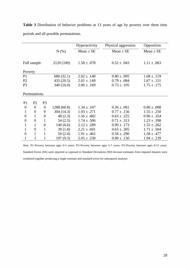
Table 3 presents the distribution of behavior problems at age 13 years by all possible poverty
permutations given P1, P2 and P3. Among all poverty permutations, those who remained
poor across all time periods were about 9.3% and those who were poor at least during one
time period were 39.2% of the participants. Further, the number of observations for some
permutations was particularly small (e.g. permutation 101 observed in 39 participants and

12
indicating upwards change followed by downwards change in poverty or exposure in P1 and
P3 but not in P2). Those who were never exposed to poverty showed lower levels of behavior
problems than those who were exposed to poverty at least during one time period (p<.001 for
all behavior problems). For all outcomes, children exposed in P1 had significant higher levels
of behavior problems than those exposed in P2 and/or P3 permutations (i.e. permutations 100,
110, 101 and 111; p<.001 for all behavior problems).
3.2. Modeling and comparing lifecourse models
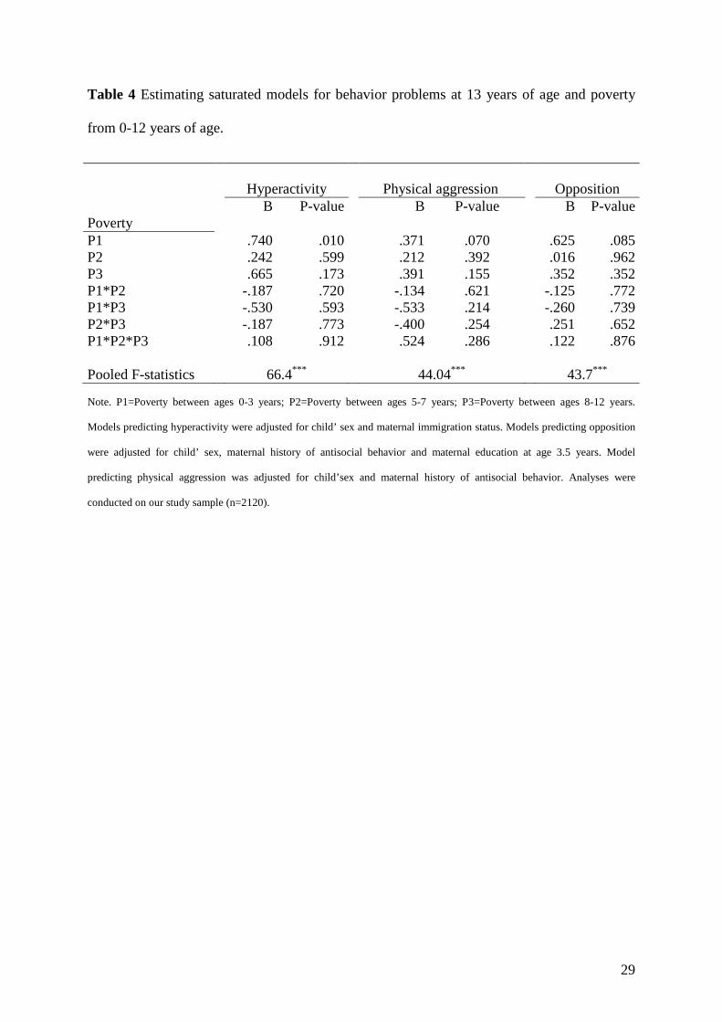
Table 4 describes saturated models for each subtype of behavior problems. For all outcomes,
linear regression models were fitted to the data corresponding to all three main effects and
interaction terms of P1, P2 and P3. Saturated models were adjusted for previously defined
confounders (see foot of Table 4).
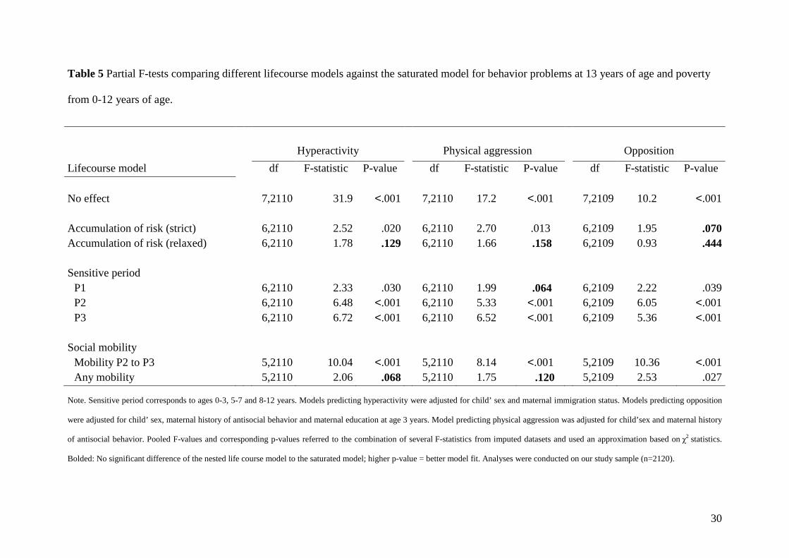
Table 5 presents the comparison of the all lifecourse models to the saturated model. The
majority of the lifecourse models differed significantly in fitting the data from the saturated
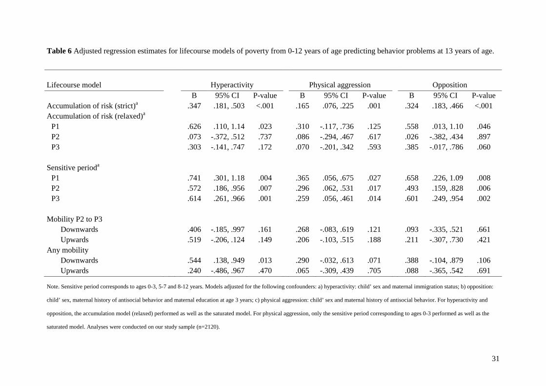
model. Table 6 presents adjusted regression coefficients for poverty parameterization in each
lifecourse model. Lifecourse models were adjusted for the same set of confounders retained
previously in the saturated models with the exception of null models (see foot of Tables 5
and 6).
For hyperactivity, results indicated that both the accumulation of risk (relaxed) and any
mobility models explained the data as well as the saturated model observed given partial F-
tests (p>.05 in Table 5). The accumulation of risk (relaxed) was the best fitting model given
the highest p-value. In this model, the best predictor was the most frequent poverty exposure
13
P1 (see Table 6). Specifically, children exposed between ages 0-3 had significant increased
hyperactivity levels of 0.63 units (p=.023 whereas BP2=0.07, p=.737; and BP3=0.30, p=.172).
For physical aggression, three lifecourse models showed a particularly good fit of the data as
they did not significantly differ from the saturated model observed given partial F-tests.
Lifecourse models were (p>.05 in Table 5): accumulation of risk (relaxed), sensitive period
P1, and any mobility. The accumulation of risk (relaxed) model had the highest p-value
followed by the any mobility model, which was almost as large. Further, poverty estimates in
both the accumulation of risk (relaxed) and the any mobility model were not significantly
associated with physical aggression (p>.07, see Table 6). So that, physical aggression was
best described by the sensitive period P1 model as (1) did not significantly differ from the
saturated model and (2) displayed poverty estimates that significantly predicted higher levels
of physical aggression. In this model, children exposed between ages 0-3 had significant
increased physical aggression levels of 0.37 units (p=.027).
For opposition, results indicated that accumulation of risk models performed equally well as
the saturated models when fitting the data. The accumulation of risk relaxed showed a
particularly better fit (highest p-value, in Table 5) and thus was selected as best fitting model.
In this model, the best prediction was the most frequent P1 with this group having the
greatest disparity in opposition levels (see Table 6). This model revealed that children
exposed between ages 0-3 had significant increased opposition levels of 0.56 units (p=.046).
3.3. Complementary analyses
The following analyses aimed to re-estimate lifecourse models accounting for changes in
sample composition overtime. We restricted the analyses to a sub-sample of 1290 participants
14
that remained in the study by age 13 years and to a sub-sample of 983 participants with
complete data on at least one of the outcomes variables by age 13 years. Then, we compared
the best fitting lifecourse models across this two-staged complete case analysis to those from
the initial analysis (as presented in Table 5). Variations in the predictive power of lifecourse
models were taken into account to analyse magnitude of bias given sample loss and non-
response. Analysis given n=983 and our initial findings showed not identical but similar
estimates whereas analysis given n=1290 showed mixed results. Restricting samples, without
any adjustments to deal with missingness, may produce biased estimates resulting from
nonrandom selection (i.e. exclusion of respondents living in poverty). Therefore, unless we
retain observations missing from children who had not participated at one or more previous
QLSCD assessments, it is not possible to minimize the bias from attrition. For lifecourse
models based on restricted samples by age 13 years, see Appendix (Tables S4-S5).
4. Discussion
This paper compared different lifecourse models and identified the model that best described
poverty from birth to 12 years predicting hyperactivity, opposition and physical aggression at
age 13 years. Findings revealed that association between poverty and behavior problems
across the lifecourse, spanning from birth to 13 years of age, correspond to both accumulation
of risk and sensitive period models. For physical aggression, the sensitive period between
ages 0-3 years seemed to be the most appropriate relative to more complex models
accounting for more time periods. Findings are consistent with prior research emphasising the
importance of the accumulation of economic disadvantaged across the lifespan (Evans &
Cassells, 2014; Gerard & Buehler, 2004) as well as the focus on the earliest years of life
15
(Murray, Irving, Farrington, Colman, & Bloxsom, 2010; Nomura et al., 2008) for behavior
problems risk among adolescents and criminal behavior among adults.
These findings are important for several reasons. First, this study highlighted the importance
of considering outcome specificity of lifecourse models of poverty predicting behavior
problems in early adolescence. While childhood poverty predicted hyperactivity and
opposition behavior in a cumulative manner, we found a sensitive period within the early
childhood years, between ages 0-3, for physical aggression. Second, we also found a strong
association for early life poverty (i.e. 0 and 3 years) derived from the accumulation of risk
model for hyperactivity and opposition. One of the reasons for this may be that, when
equality constraints are relaxed so that exposure across all time periods predicts behavior
problems in an unequal manner it allows for the identification of combined models of
sensitive periods and accumulation (Mishra et al., 2009). Hence this notion of accumulation
of risk posits that not only poverty does accumulate overtime, but also that early life exposure
outperforms subsequent exposures in shaping later-life behavior problems. Emerging
evidence suggests physiologic and functional plasticity over the first years of life persists
throughout development (Noble et al., 2015). Given the importance of exposure to poverty
between ages 0-3 observed in this study, interventions targeting time points during early
childhood (i.e., before age 5) may have substantial benefits in reducing behavior problems in
early adolescence. Recent findings in low-income populations suggest that family
intervention programs initiated during early childhood are vital to reduce children’s behavior
problems, including opposition and physical aggression (Dishion et al., 2014; Leijten et al.,
2015).
16
Patterns of findings resemble that of previous research examining growth/decline in behavior
problems across development. The finding of a sensitive period even as the time spent in
poverty increased for physical aggression may indicate that the association between poverty
and physical aggression is fairly stable across development. Prior work has suggested that
differences in physical aggression trajectories between poor and non-poor children are
established as early as age 1.5 years and, rather than increasing with age, remained constant
up to age 8 years (Mazza et al., 2016). It is possible that Gene x Environment interactions
might precipitate increases in normative aggressive behavior which are in turn likely to
persist later in life (Shaw, Bell, & Gilliom, 2000; Tremblay, 2010). Further, several studies
suggest that individual differences and growth rate in physical aggression are due to genetic
vulnerability which in turn are moderated by prenatal and post-natal environmental risk
(Boivin et al., 2013; Lacourse et al., 2014). Nonetheless, our findings supported the
accumulation of risk model indicating that differences in hyperactivity and opposition levels
increased with time spent in poverty. This confirms results from previous studies suggesting
that differences in behavior problems (including hyperactivity and opposition) that were
initially small between poor and non-poor children, appeared to increase overtime for
children in persistent poverty (Flouri, Midouhas, & Joshi, 2014; Mazza et al., 2016). It may
be that both hyperactivity and opposition are more susceptible to change than physical
aggression if interventions were to target poverty in any given period from early-to-middle
childhood.
Selection bias is an important problem in poverty research given nonrandom exclusion of
disadvantaged participants. Complete case analysis for longitudinal data can produce biased
results and undertaking data augmentation (in our case 22.5% increase) with imputation
techniques is recommended to reduce selection bias (Mostafa & Wiggins, 2015). Excluding
17
participants with incomplete data or those lost to follow-up is inadequate and potentially
undermines valid inference.
Finally, most studies on behavior problems- poverty link pertain to children who live in the
United States where poverty rates are higher than in most high-income countries (UNICEF,
2012). Our findings suggest that behavior problems risk relates to poverty at different ages
during childhood despite lower poverty rates reflecting health care and social policies that are
specific to Canada.
4.1. Strengths and limitations
Strengths of this study include the empirical testing of competing lifecourse models of
childhood poverty predicting behavior problems in early adolescence using a well-defined
model-building framework. A second strength lies in the assessment of behavior problems
reported by teachers, rather than by parents. Teacher reports allow for the identification of
behavior problems that are not isolated to the home context, but rather informs about
psychopathology expressed across school and extracurricular activities (Reyes, 2011). A third
strength lies in the use of repeated and robust measures of exposure to poverty using national
thresholds (i.e., LICOs). A fourth strength was the examination of three subtypes of behavior
problems suggesting lifecourse models that are specific for hyperactivity and opposition as
well as for physical aggression. Finally, lifecourse models of poverty predicting behavior
problems were robust after carefully controlling for several confounders described in the
literature. Several limitations of the study deserve mention. First, the lack of power may be an
issue when examining lifecourse models that includes interaction terms. Specific analyses in
the structure modelling approach (Mishra et al., 2009) require even larger samples as is the
18
case for the mobility models. This pleads for collaborations with other longitudinal studies.
Second, differential attrition could underestimate the observed associations if attrition was
dependent on both being poor and having high levels of behavior problems. Reassuringly,
this issue was addressed analytically using multiple imputation procedure. Third, it is
possible that one or more sensitive periods exist outside of the periods of exposure that were
grouped for the analyses and are therefore not detected in analyses. The decision to group
exposure to poverty between ages 0-3, 5-7 and 8-12 years was based on assessments
approximating different stages of development such as infancy, middle childhood and late
childhood. Forth, if missingness depends on explanatory variables, then model
misspecification in the multiple imputation procedure could be an alternative explanation
worth considering. Lastly, this study is observational and, as such, is limited to make causal
inferences of the association between childhood poverty and behavior problems in
adolescence.
5. Conclusion
Findings highlight that the length of time spent in poverty across childhood increased the risk
for hyperactivity and opposition behavior and that this association may be driven by early
poverty. For physical aggression, we found evidence for effects of sensitive period between
birth and age 3. Additional research, as with any study, is needed to explore whether these
patterns of findings can be replicated in other samples.
This study supports not only the cumulative effect of poverty overtime but also the long-
lasting effects of early poverty, and in particular identifies a sensitive period within early
childhood years that may compromise mental health in early adolescence. Long term support
19
to pregnant women living in poverty is likely to reduce behavior problems during childhood
and adolescence. Also, this paper emphasises the importance of policies to reduce child
poverty by boosting income and service delivery to poor families with children and even in a
high-income country like Canada. Support programs extending financial benefits to poor
families suggest that increasing tax credits is likely to decrease children’s and adolescent’s
behavior problems (Akee, Copeland, Keeler, Angold, & Costello, 2010; Hamad & Rehkopf,
2016). Other support programs, including center-based child care and parent training, are
increasingly recognized to benefit children from low-income families in achievement
domains as well as to play a protective role in the development of behavior problems (Côté et
al., 2007; Dishion et al., 2014; Laurin et al., 2015).
References
Akee, R. K. Q., Copeland, W. E., Keeler, G., Angold, A., & Costello, E. J. (2010). Parents’
Incomes and Children’s Outcomes: A quasi-experiment using transfer payments from
casino profits. American Economic Journal: Applied Economics, 2(1), 86–115.
Boivin, M., Brendgen, M., Vitaro, F., Forget-Dubois, N., Feng, B., Tremblay, R. E., &
Dionne, G. (2013). Evidence of gene–environment correlation for peer difficulties:
Disruptive behaviors predict early peer relation difficulties in school through genetic
effects. Development and Psychopathology, 25(Special Issue 01), 79–92.
Côté, S. M., Boivin, M., Nagin, D. S., Japel, C., Xu, Q., Zoccolillo, M., … Tremblay, R. E.
(2007). The role of maternal education and nonmaternal care services in the
prevention of children’s physical aggression problems. Archives of General
Psychiatry, 64(11), 1305–1312.
20
Côté, S., Vaillancourt, T., LeBlanc, J. C., Nagin, D. S., & Tremblay, R. E. (2006). The
development of physical aggression from toddlerhood to pre-adolescence: A nation
wide longitudinal study of Canadian children. Journal of Abnormal Child Psychology,
34(1), 68–82.
Dishion, T. J., Brennan, L. M., Shaw, D. S., McEachern, A. D., Wilson, M. N., & Jo, B.
(2014). Prevention of problem behavior through annual family check-ups in early
childhood: Intervention effects from home to early elementary school. Journal of
Abnormal Child Psychology, 42(3), 343–354.
Essex, M. J., Kraemer, H. C., Armstrong, J. M., Boyce, W. T., Goldsmith, H. H., Klein, M.
H., … Kupfer, D. J. (2006). Exploring risk factors for the emergence of children’s
mental health problems. Archives of General Psychiatry 63, 1246–1256.
Evans, G. W., & Cassells, R. C. (2014). Childhood poverty, cumulative risk exposure, and
mental health in emerging adults. Clinical Psychological Science, 2(3), 287–296.
Flouri, E., Midouhas, E., & Joshi, H. (2014). Family poverty and trajectories of children’s
emotional and behavioural problems: The moderating roles of self-regulation and
verbal cognitive ability. Journal of Abnormal Child Psychology, 42(6), 1043–1056.
Gerard, J. M., & Buehler, C. (2004). Cumulative environmental risk and youth problem
behavior. Journal of Marriage and Family, 66(3), 702–720.
Giles, P. (2004). ‘‘Low Income Measurement in Canada.’’ Statistics Canada, Income
Research Paper Series, 75F0002MIE. Ottawa, ON: Statistics Canada.
Giles, L., Davies, M., Whitrow, M., Rumbold, A., Lynch, J., Sawyer, M., & Moore, V.
(2011). Structured regression analyses of life course processes: An example exploring
how maternal depression in early childhood affects children’s subsequent
internalizing behavior. Annals of Epidemiology, 21(9), 654–659.

21
Hallqvist, J., Lynch, J., Bartley, M., Lang, T., & Blane, D. (2004). Can we disentangle life
course processes of accumulation, critical period and social mobility? An analysis of
disadvantaged socio-economic positions and myocardial infarction in the Stockholm
Heart Epidemiology Program. Social Science & Medicine, 58(8), 1555-1562.
Hamad, R., & Rehkopf, D. H. (2016). Poverty and child development: A longitudinal study
of the impact of the earned income tax credit. American Journal of Epidemiology,
183(9), 775–784.
Human Resources Development Canada and Statistics Canada. (1996). National Longitudinal
Survey of Children and Youth, user’s handbook and microdata guide. Special Surveys
Division, Statistics Canada, Ottawa. Microdata documentation: 89M0015GPE.
Kim-Cohen J., Moffitt T. E., Taylor A., Pawlby S. J., & Caspi A. (2005). Maternal
depression and children’s antisocial behavior: Nature and nurture effects. Archives of
General Psychiatry, 62(2), 173–181.
Lacourse, E., Boivin, M., Brendgen, M., Petitclerc, A., Girard, A., Vitaro, F., … Tremblay,
R. E. (2014). A longitudinal twin study of physical aggression during early childhood:
Evidence for a developmentally dynamic genome. Psychological Medicine, 44(12),
2617–2627.
Laurin, J. C., Geoffroy, M.-C., Boivin, M., Japel, C., Raynault, M.-F., Tremblay, R. E., &
Côté, S. M. (2015). Child care services, socioeconomic inequalities, and academic
performance. Pediatrics, 136(6), 1112–1124.
Leijten, P., Shaw, D. S., Gardner, F., Wilson, M. N., Matthys, W., & Dishion, T. J. (2015).
The family check-up and service use in high-risk families of young children: A
Prevention strategy with a bridge to community-based treatment. Prevention Science,
16(3), 397–406.
22
Leis, J. A., Heron, J., Stuart, E. A., & Mendelson, T. (2013). Associations between maternal
mental health and child emotional and behavioral problems: Does prenatal mental
health matter? Journal of Abnormal Child Psychology, 42(1), 161–171.
https://doi.org/10.1007/s10802-013-9766-4
Lynch, J., & Smith, G. D. (2005). A life course approach to chronic disease epidemiology.
Annual Review of Public Health, 26, 1–35.
Jetté, M., & Des Groseilliers, L. (2000). Survey description and methodology in longitudinal
study of child development in Québec (ÉLDEQ 1998-2002). Institut de la statistique
du Québec. Retrieved from http://www.iamillbe.stat.gouv.qc.ca/nouvelle_bref_an.htm
Kuh, D., Ben-Shlomo, Y., Lynch, J., Hallqvist, J., & Power, C. (2003). Life course
epidemiology. Journal of Epidemiology and Community Health, 57(10), 778.
Mazza, J. R. S. E., Boivin, M., Tremblay, R. E., Michel, G., Salla, J., Lambert, J., … Côté, S.
M. (2016). Poverty and behavior problems trajectories from 1.5 to 8 years of age: Is
the gap widening between poor and non-poor children? Social Psychiatry and
Psychiatric Epidemiology, 1–10.
McLaughlin, K. A., Breslau, J., Green, J. G., Lakoma, M. D., Sampson, N. A., Zaslavsky, A.
M., & Kessler, R. C. (2011). Childhood socio-economic status and the onset,
persistence, and severity of DSM-IV mental disorders in a US national sample. Social
Science & Medicine, 73(7), 1088–1096.
Mishra, G., Nitsch, D., Black, S., Stavola, B. D., Kuh, D., & Hardy, R. (2009). A structured
approach to modelling the effects of binary exposure variables over the life course.
International Journal of Epidemiology, 38(2), 528–537.
Mostafa, T., & Wiggins, R. (2015). The impact of attrition and non-response in birth cohort
studies: a need to incorporate missingness strategies. Longitudinal and Life Course
Studies, 6(2), 131–146.
23
Murray, J., Irving, B., Farrington, D. P., Colman, I., & Bloxsom, C. A. J. (2010). Very early
predictors of conduct problems and crime: Results from a national cohort study.
Journal of Child Psychology and Psychiatry, 51(11), 1198–1207.
Noble, K. G., Houston, S. M., Brito, N. H., Bartsch, H., Kan, E., Kuperman, J. M., … Sowell,
E. R. (2015). Family income, parental education and brain structure in children and
adolescents. Nature Neuroscience, 18(5), 773–778.
Nomura, Y., Rajendran, K., Brooks-Gunn, J., & Newcorn, J. H. (2008). Roles of perinatal
problems on adolescent antisocial behaviors among children born after 33 completed
weeks: A prospective investigation. Journal of Child Psychology and Psychiatry,
49(10), 1108–1117.
Pingault, J.-B., Côté, S. M., Galéra, C., Genolini, C., Falissard, B., Vitaro, F., & Tremblay, R.
E. (2013). Childhood trajectories of inattention, hyperactivity and oppositional
behaviors and prediction of substance abuse/dependence: A 15-year longitudinal
population-based study. Molecular Psychiatry, 18(7), 806–812.
Polanczyk, G. V., Salum, G. A., Sugaya, L. S., Caye, A., & Rohde, L. A. (2015). Annual
research review: A meta-analysis of the worldwide prevalence of mental disorders in
children and adolescents. Journal of Child Psychology and Psychiatry, 56(3), 345–
365.
Rekker, R., Pardini, D., Keijsers, L., Branje, S., Loeber, R., & Meeus, W. (2015). Moving in
and out of poverty: The within-Individual Association between Socioeconomic Status
and Juvenile Delinquency. PLOS ONE, 10(11), e0136461.
Reyes, A. D. L. (2011). More than measurement error: Discovering meaning behind
informant discrepancies in clinical assessments of children and adolescents. Journal
of Clinical Child & Adolescent Psychology, 40(1), 1–9.
24
Rezvan, P. H., Lee, K. J., & Simpson, J. A. (2015). The rise of multiple imputation: a review
of the reporting and implementation of the method in medical research. BMC Medical
Research Methodology, 15(1), 1.
Robitzsch, A., Grund, S., & Henke, T. (2016). Some additional multiple imputation
functions, Especially for “MICE.” Retrieved August 16, 2016, from
http://cran.stat.sfu.ca/web/packages/miceadds/miceadds.pdf
Russell, G., Ford, T., Rosenberg, R., & Kelly, S. (2014). The association of attention deficit
hyperactivity disorder with socioeconomic disadvantage: Alternative explanations and
evidence. Journal of Child Psychology and Psychiatry, 55(5), 436–445.
Shaw, D. S., Bell, R. Q., & Gilliom, M. (2000). A truly early starter model of antisocial
behavior revisited. Clinical Child and Family Psychology Review, 3(3), 155–172.
Shaw, D. S., Lacourse, E., & Nagin, D. S. (2005). Developmental trajectories of conduct
problems and hyperactivity from ages 2 to 10. Journal of Child Psychology and
Psychiatry, 46(9), 931–942.
Statistics Canada. (2013). Low income lines, 2011 to 2012. Statistics Canada, income
research paper series. 75F0002M. Statistics Canada, Ottawa. Available
from: http://www.statcan. gc.ca/pub/75f0002m/75f0002m2013002-eng.pdf
UNICEF Innocenti Research Centre (2012), ‘Measuring Child Poverty: New league tables of
child poverty in the world’s rich countries’, Innocenti Report Card 10, UNICEF
Innocenti Research Centre, Florence.
Tremblay, R. E. (2010). Developmental origins of disruptive behaviour problems: The
“original sin” hypothesis, epigenetics and their consequences for prevention. Journal
of Child Psychology and Psychiatry, and Allied Disciplines, 51(4), 341–367.

25
Tremblay, R. E., Nagin, D. S., Séguin, J. R., Zoccolillo, M., Zelazo, P. D., Boivin, M., …
Japel, C. (2004). Physical aggression during early childhood: Trajectories and
Predictors. Pediatrics, 114(1).
Tsal, Y., Shalev, L., & Mevorach, C. (2005). The diversity of attention deficits in ADHD:
The prevalence of four cognitive factors in ADHD versus controls. Journal of
Learning Disabilities, 38(2), 142–157.
26
Table 1 Remaining participants in the QLSCD after 13 years of follow-up by exposure to
poverty.
Note. N refers to the total participants in the QLSCD at each time point; n refers to the number of participants in the QLSCD
depending on the data available. Poverty status was not available at 4.5 years of age.
Poverty
Age (years) QLSCD sample N (%)
Poor n (%)
Non-Poor n (%)
Missing n (%)
5 months 2120 (100) 511 (24.1) 1571 (74.1) 38 (1.8)
1.5 2045 (96.5) 416 (20.4) 1599 (78.2) 30 (1.4) 2.5 1997 (94.1) 368 (18.4) 1598 (80.0) 31 (1.6) 3.5 1950 (92.0) 319 (16.4) 1594 (81.7) 37 (1.9) 4.5 1944 (91.7) - - - 5 1759 (83.0) 298 (16.9) 1438 (81.8) 23 (1.3) 6 1492 (70.4) 245 (16.4) 1235 (82.8) 12 (0.8) 7 1528 (72.1) 228 (14.9) 1284 (84.0) 16 (1.0) 8 1451 (68.4) 218 (15.0) 1220 (84.1) 13 (0.9) 10 1334 (62.9) 151 (11.3) 1176 (88.2) 7 (0.5) 12 1396 (65.9) 185 (13.3) 1203 (86.2) 8 (0.6) 13 1290 (60.8) 153 (11.9) 1120 (86.8) 17 (1.3)
27
Table 2 Saturated and lifecourse models specifications given exposure to poverty over three time periods.
Note. P1=Poverty between ages 0-3 years; P2=Poverty between ages 5-7 years; P3=Poverty between ages 8-12 year.
Lifecourse model Equations Constraints
No effect Y=α Accumulation of risk
Strict Y=α + β (P1+ P2+ P3) Relaxed Y=α + β1P1+ β2P2+β3P3
Sensitive period P1 Y=α + β1P1 P2 Y=α + β2P2 P3 Y=α + β3P3
Social mobility
Mobility P2 to P3 Y=α + β2 P2+ β3 P3+ θ 23 P2P3 θ 23 = - ( β2 + β3) Any mobility Y=α + β1 P1+ β2 P2+ β3 P3+ θ12 P1P2+θ 23 P2P3 θ 12 =θ 23 = - β2
Saturated model Y=α + β1P1+ β2P2+ β3P3+ θ12 P1P2+ θ13 P1P3+ θ 23 P2P3+θ 123P1P2P3
28
Table 3 Distribution of behavior problems at 13 years of age by poverty over three time
periods and all possible permutations.
Note. P1=Poverty between ages 0-3 years; P2=Poverty between ages 5-7 years; P3=Poverty between ages 8-12 years.
Standard Errors (SE) were reported as opposed to Standard Deviations (SD) because estimates from imputed datasets were
combined together producing a single estimate and standard errors for subsequent analyses
Hyperactivity Physical aggression Opposition
N (%) Mean ± SE Mean ± SE Mean ± SE
Full sample 2120 (100) 1.58 ± .078 0.52 ± .043 1.11 ± .063 Poverty P1 680 (32.1) 2.02 ± .140 0.80 ± .095 1.68 ± .119 P2 435 (20.5) 2.01 ± .149 0.79 ± .084 1.67 ± .151 P3 340 (16.0) 2.00 ± .169 0.73 ± .105 1.75 ± .175 Permutations
P1 P2 P3 0 0 0 1288 (60.8) 1.34 ± .107 0.36 ± .061 0.80 ± .088 1 0 0 304 (14.3) 1.93 ± .271 0.77 ± .156 1.55 ± .250 0 1 0 48 (2.3) 1.56 ± .482 0.63 ± .225 0.96 ± .324 0 0 1 54 (2.5) 1.74 ± .506 0.71 ± .313 1.23 ± .398 1 1 0 140 (6.6) 2.12 ± .289 0.90 ± .173 1.55 ± .262 1 0 1 39 (1.8) 2.21 ± .691 0.63 ± .305 1.71 ± .504 0 1 1 50 (2.4) 1.91 ± .465 0.58 ± .290 1.58 ± .477 1 1 1 197 (9.3) 2.05 ± .230 0.80 ± .130 1.94 ± .239
29
Table 4 Estimating saturated models for behavior problems at 13 years of age and poverty
from 0-12 years of age.
Note. P1=Poverty between ages 0-3 years; P2=Poverty between ages 5-7 years; P3=Poverty between ages 8-12 years.
Models predicting hyperactivity were adjusted for child’ sex and maternal immigration status. Models predicting opposition
were adjusted for child’ sex, maternal history of antisocial behavior and maternal education at age 3.5 years. Model
predicting physical aggression was adjusted for child’sex and maternal history of antisocial behavior. Analyses were
conducted on our study sample (n=2120).
Hyperactivity
Physical aggression
Opposition
Poverty
B P-value B P-value B P-value
P1 .740 .010 .371 .070 .625 .085 P2 .242 .599 .212 .392 .016 .962 P3 .665 .173 .391 .155 .352 .352 P1*P2 -.187 .720 -.134 .621 -.125 .772 P1*P3 -.530 .593 -.533 .214 -.260 .739 P2*P3 -.187 .773 -.400 .254 .251 .652 P1*P2*P3 .108 .912 .524 .286 .122 .876 Pooled F-statistics 66.4*** 44.04*** 43.7***
30
Table 5 Partial F-tests comparing different lifecourse models against the saturated model for behavior problems at 13 years of age and poverty
from 0-12 years of age.
Note. Sensitive period corresponds to ages 0-3, 5-7 and 8-12 years. Models predicting hyperactivity were adjusted for child’ sex and maternal immigration status. Models predicting opposition
were adjusted for child’ sex, maternal history of antisocial behavior and maternal education at age 3 years. Model predicting physical aggression was adjusted for child’sex and maternal history
of antisocial behavior. Pooled F-values and corresponding p-values referred to the combination of several F-statistics from imputed datasets and used an approximation based on χ2 statistics.
Bolded: No significant difference of the nested life course model to the saturated model; higher p-value = better model fit. Analyses were conducted on our study sample (n=2120).
Hyperactivity Physical aggression Opposition
Lifecourse model df F-statistic P-value df F-statistic P-value df F-statistic P-value No effect 7,2110 31.9 <.001 7,2110 17.2 <.001 7,2109 10.2 <.001 Accumulation of risk (strict) 6,2110 2.52 .020 6,2110 2.70 .013 6,2109 1.95 .070 Accumulation of risk (relaxed) 6,2110 1.78 .129 6,2110 1.66 .158 6,2109 0.93 .444 Sensitive period
P1 6,2110 2.33 .030 6,2110 1.99 .064 6,2109 2.22 .039 P2 6,2110 6.48 <.001 6,2110 5.33 <.001 6,2109 6.05 <.001 P3 6,2110 6.72 <.001 6,2110 6.52 <.001 6,2109 5.36 <.001
Social mobility
Mobility P2 to P3 5,2110 10.04 <.001 5,2110 8.14 <.001 5,2109 10.36 <.001 Any mobility 5,2110 2.06 .068 5,2110 1.75 .120 5,2109 2.53 .027
31
Table 6 Adjusted regression estimates for lifecourse models of poverty from 0-12 years of age predicting behavior problems at 13 years of age.
Note. Sensitive period corresponds to ages 0-3, 5-7 and 8-12 years. Models adjusted for the following confounders: a) hyperactivity: child’ sex and maternal immigration status; b) opposition:
child’ sex, maternal history of antisocial behavior and maternal education at age 3 years; c) physical aggression: child’ sex and maternal history of antisocial behavior. For hyperactivity and
opposition, the accumulation model (relaxed) performed as well as the saturated model. For physical aggression, only the sensitive period corresponding to ages 0-3 performed as well as the
saturated model. Analyses were conducted on our study sample (n=2120).
Lifecourse model Hyperactivity Physical aggression Opposition B 95% CI P-value B 95% CI P-value B 95% CI P-value Accumulation of risk (strict)a .347 .181, .503 <.001 .165 .076, .225 .001 .324 .183, .466 <.001 Accumulation of risk (relaxed)a
P1 .626 .110, 1.14 .023 .310 -.117, .736 .125 .558 .013, 1.10 .046 P2 .073 -.372, .512 .737 .086 -.294, .467 .617 .026 -.382, .434 .897 P3 .303 -.141, .747 .172 .070 -.201, .342 .593 .385 -.017, .786 .060
Sensitive perioda
P1 .741 .301, 1.18 .004 .365 .056, .675 .027 .658 .226, 1.09 .008 P2 .572 .186, .956 .007 .296 .062, .531 .017 .493 .159, .828 .006 P3 .614 .261, .966 .001 .259 .056, .461 .014 .601 .249, .954 .002
Mobility P2 to P3
Downwards .406 -.185, .997 .161 .268 -.083, .619 .121 .093 -.335, .521 .661 Upwards .519 -.206, .124 .149 .206 -.103, .515 .188 .211 -.307, .730 .421
Any mobility Downwards .544 .138, .949 .013 .290 -.032, .613 .071 .388 -.104, .879 .106 Upwards .240 -.486, .967 .470 .065 -.309, .439 .705 .088 -.365, .542 .691

32
Appendix : Supplementary materials
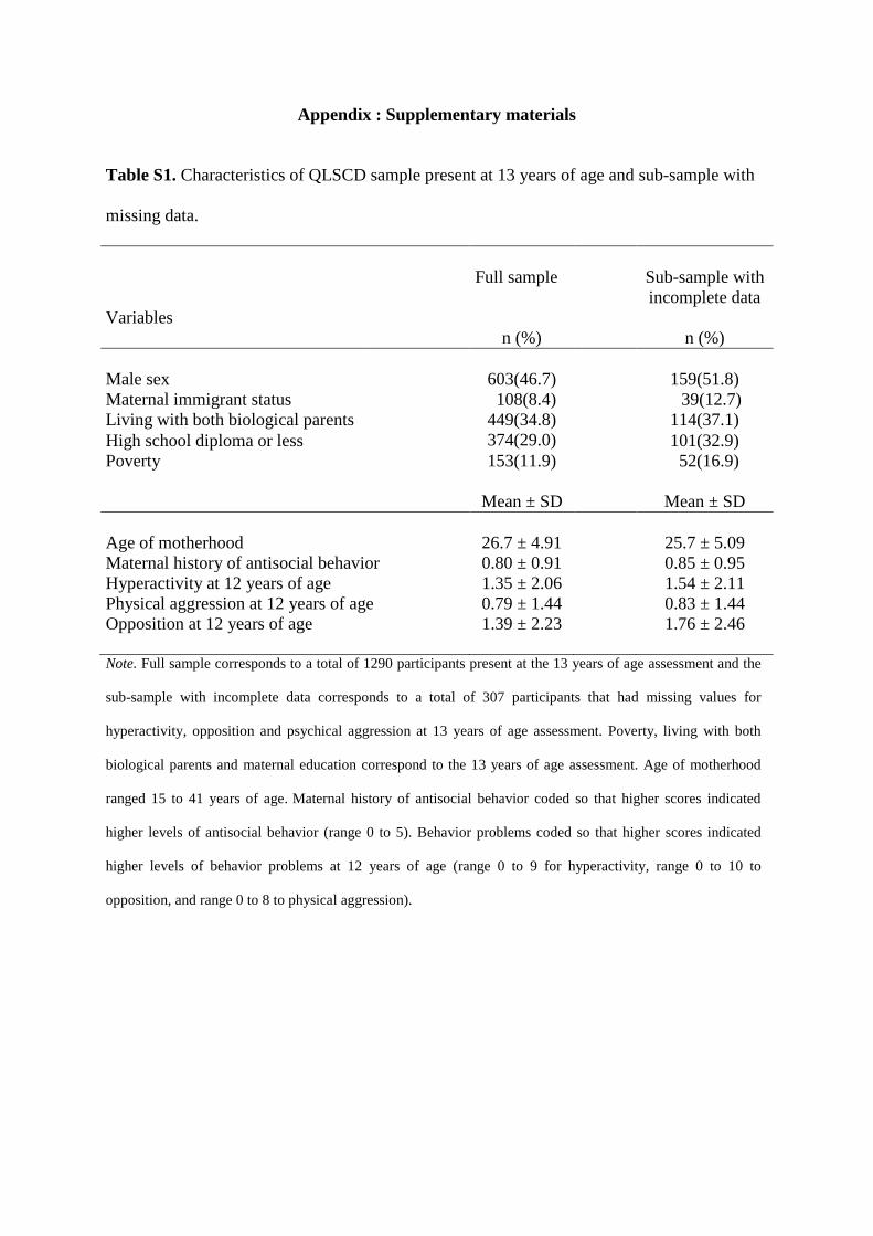
Table S1. Characteristics of QLSCD sample present at 13 years of age and sub-sample with
missing data.
Variables
Full sample
Sub-sample with incomplete data
n (%)
n (%)
Male sex
603(46.7)
159(51.8) Maternal immigrant status 108(8.4) 39(12.7) Living with both biological parents 449(34.8)
114(37.1)
High school diploma or less 374(29.0)
101(32.9) Poverty 153(11.9) 52(16.9) Mean ± SD Mean ± SD Age of motherhood 26.7 ± 4.91
25.7 ± 5.09
Maternal history of antisocial behavior 0.80 ± 0.91
0.85 ± 0.95 Hyperactivity at 12 years of age 1.35 ± 2.06
1.54 ± 2.11
Physical aggression at 12 years of age 0.79 ± 1.44
0.83 ± 1.44 Opposition at 12 years of age 1.39 ± 2.23
1.76 ± 2.46
Note. Full sample corresponds to a total of 1290 participants present at the 13 years of age assessment and the
sub-sample with incomplete data corresponds to a total of 307 participants that had missing values for
hyperactivity, opposition and psychical aggression at 13 years of age assessment. Poverty, living with both
biological parents and maternal education correspond to the 13 years of age assessment. Age of motherhood
ranged 15 to 41 years of age. Maternal history of antisocial behavior coded so that higher scores indicated
higher levels of antisocial behavior (range 0 to 5). Behavior problems coded so that higher scores indicated
higher levels of behavior problems at 12 years of age (range 0 to 9 for hyperactivity, range 0 to 10 to
opposition, and range 0 to 8 to physical aggression).
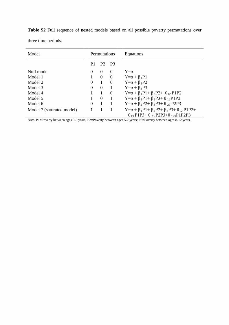
Table S2 Full sequence of nested models based on all possible poverty permutations over
three time periods.
Model Permutations Equations
P1 P2 P3
Null model 0 0 0 Y=α Model 1 1 0 0 Y=α + β1P1 Model 2 0 1 0 Y=α + β2P2 Model 3 0 0 1 Y=α + β3P3 Model 4 1 1 0 Y=α + β1P1+ β2P2+ θ12 P1P2 Model 5 1 0 1 Y=α + β1P1+ β3P3+ θ 13P1P3 Model 6 0 1 1 Y=α + β2P2+ β3P3+ θ 23 P2P3 Model 7 (saturated model)
1 1 1 Y=α + β1P1+ β2P2+ β3P3+ θ12 P1P2+ θ13 P1P3+ θ 23 P2P3+θ 123P1P2P3
Note. P1=Poverty between ages 0-3 years; P2=Poverty between ages 5-7 years; P3=Poverty between ages 8-12 years.
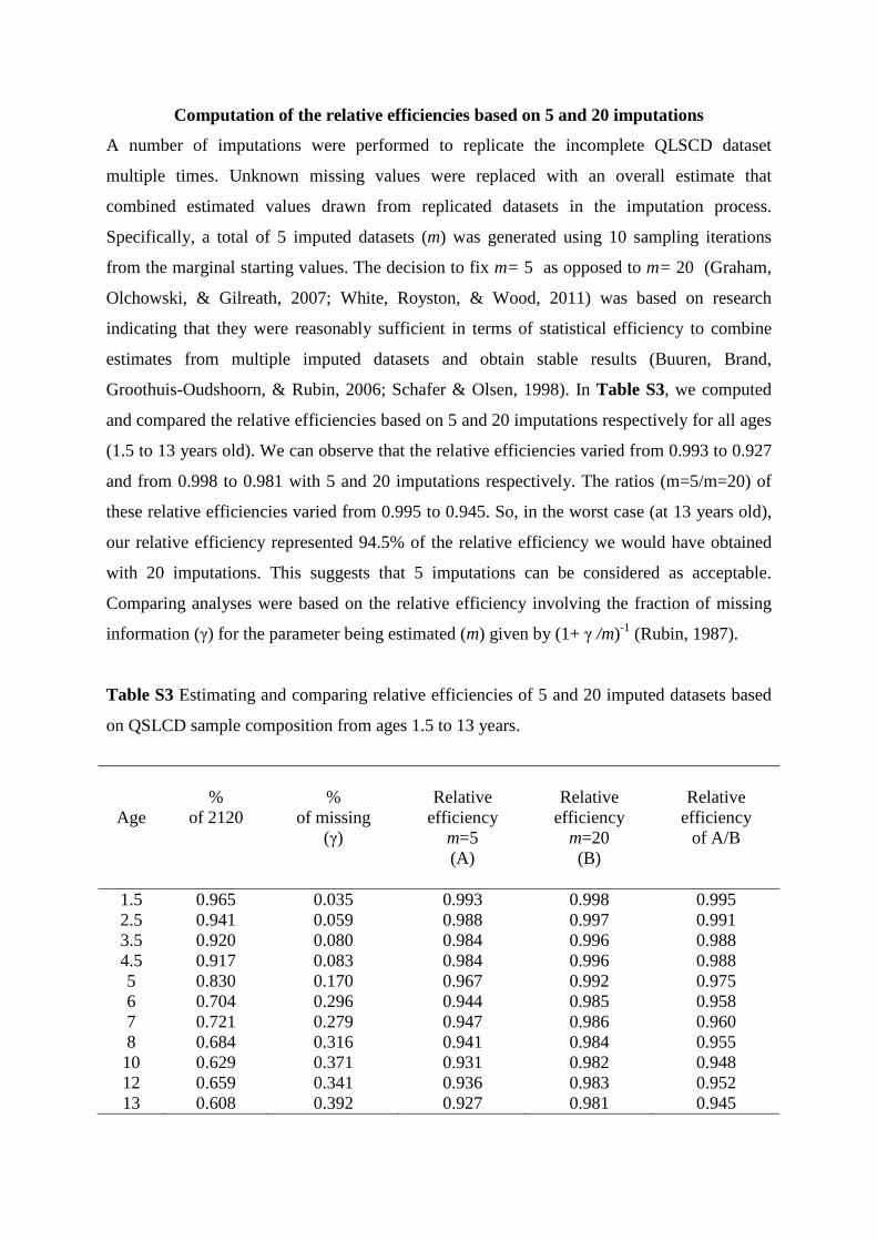
Computation of the relative efficiencies based on 5 and 20 imputations
A number of imputations were performed to replicate the incomplete QLSCD dataset
multiple times. Unknown missing values were replaced with an overall estimate that
combined estimated values drawn from replicated datasets in the imputation process.
Specifically, a total of 5 imputed datasets (m) was generated using 10 sampling iterations
from the marginal starting values. The decision to fix m= 5 as opposed to m= 20 (Graham,
Olchowski, & Gilreath, 2007; White, Royston, & Wood, 2011) was based on research
indicating that they were reasonably sufficient in terms of statistical efficiency to combine
estimates from multiple imputed datasets and obtain stable results (Buuren, Brand,
Groothuis-Oudshoorn, & Rubin, 2006; Schafer & Olsen, 1998). In Table S3, we computed
and compared the relative efficiencies based on 5 and 20 imputations respectively for all ages
(1.5 to 13 years old). We can observe that the relative efficiencies varied from 0.993 to 0.927
and from 0.998 to 0.981 with 5 and 20 imputations respectively. The ratios (m=5/m=20) of
these relative efficiencies varied from 0.995 to 0.945. So, in the worst case (at 13 years old),
our relative efficiency represented 94.5% of the relative efficiency we would have obtained
with 20 imputations. This suggests that 5 imputations can be considered as acceptable.
Comparing analyses were based on the relative efficiency involving the fraction of missing
information (γ) for the parameter being estimated (m) given by (1+ γ /m)-1 (Rubin, 1987).
Table S3 Estimating and comparing relative efficiencies of 5 and 20 imputed datasets based
on QSLCD sample composition from ages 1.5 to 13 years.
Age
%
of 2120
%
of missing (γ)
Relative
efficiency m=5 (A)
Relative
efficiency m=20 (B)
Relative
efficiency of A/B
1.5 0.965 0.035 0.993 0.998 0.995 2.5 0.941 0.059 0.988 0.997 0.991 3.5 0.920 0.080 0.984 0.996 0.988 4.5 0.917 0.083 0.984 0.996 0.988 5 0.830 0.170 0.967 0.992 0.975 6 0.704 0.296 0.944 0.985 0.958 7 0.721 0.279 0.947 0.986 0.960 8 0.684 0.316 0.941 0.984 0.955 10 0.629 0.371 0.931 0.982 0.948 12 0.659 0.341 0.936 0.983 0.952 13 0.608 0.392 0.927 0.981 0.945
Graham, J. W., Olchowski, A. E., & Gilreath, T. D. (2007). How many imputations are really needed? Some practical clarifications of multiple imputation theory. Prevention Science, 8(3), 206-213. Rezvan, P. H., Lee, K. J., & Simpson, J. A. (2015). The rise of multiple imputation: a review of the reporting and implementation of the method in medical research. BMC medical research methodology, 15(1), 1. Rubin, D. B. (1987). Multiple imputation for nonresponse in surveys. New York: Wiley. Schafer, J. L., & Olsen, M. K. (1998). Multiple imputation for multivariate missing-data problems: A data analyst's perspective. Multivariate behavioral research, 33(4), 545-571. Van Buuren, S., Brand, J. P., Groothuis-Oudshoorn, C. G. M., & Rubin, D. B. (2006). Fully conditional specification in multivariate imputation. Journal of statistical computation and simulation, 76(12), 1049-1064. White, I. R., Royston, P., & Wood, A. M. (2011). Multiple imputation using chained equations: issues and guidance for practice. Statistics in medicine, 30(4), 377-399.
Complementary analyses
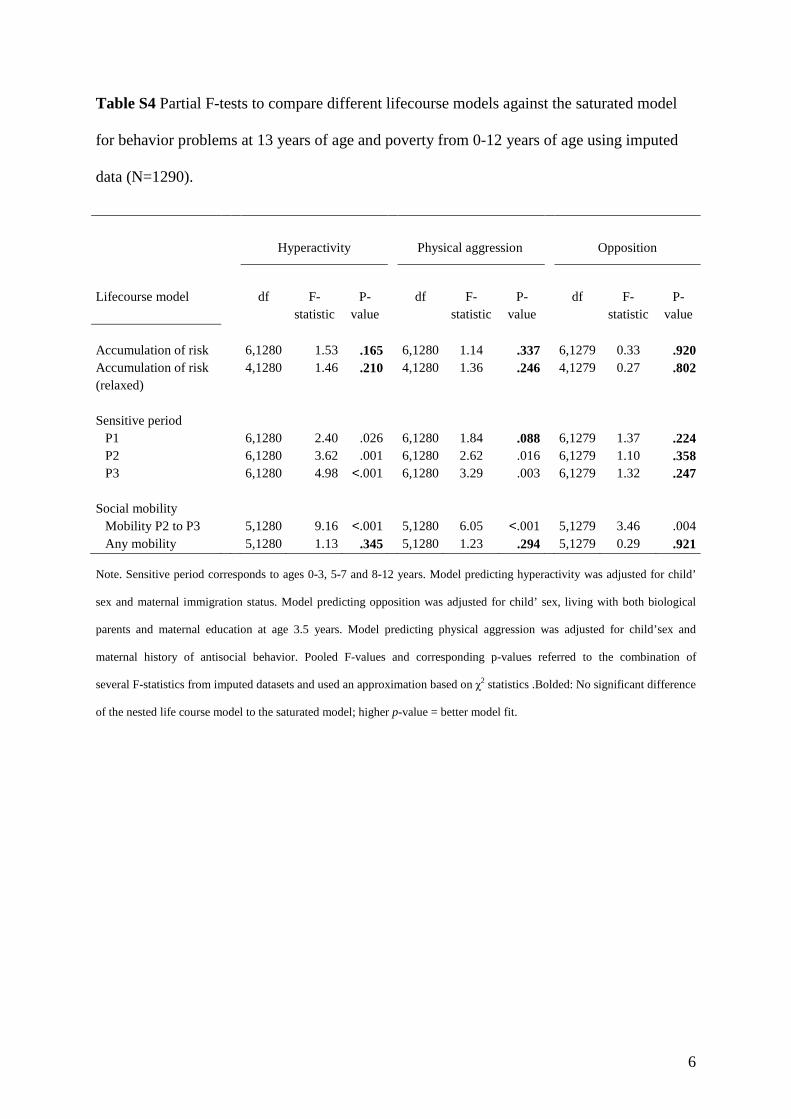
Table S4 presents re-estimated lifecourse models restricting analysis to n=1290. Results
indicated that the best fitting lifecourse models were the any mobility model for hyperactivity
(pany mobility against the saturated model =.345), the accumulation of risk strict for opposition and
physical aggression (pstrict against the saturated model =.921 for opposition; pstrict against the saturated model
=.337 for physical aggression). Results deviated substantially from our initial findings on
N=2120 suggesting a less accurate model. Particularly, the accumulation of risk (relaxed)
model was no longer the best fit of the data for hyperactivity and opposition nor was the
sensitive period P1 model for physical aggression. Results restricting analysis to =1290 were
reported using imputed data (i.e. 307 cases were included due to non-response of outcomes
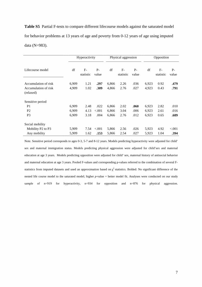
and explanatory variables). When restricting analysis to n=983, we found similar results to
our initial findings across all outcomes (see Table S5). For hyperactivity the accumulation of
risk (relaxed) was the best fitting model (prelaxed against the saturated model =.309) with P1 as the best
predictor (BP1=0.66, p=.001). For physical aggression, the sensitive period P1 was the
selected model (pP1 against the saturated model =.060). And finally, for opposition the superior
lifecourse model was the accumulation of risk relaxed (prelaxed against the saturated model =.791).
However, the latter differed from our initial findings in terms of the best predictor.
Specifically, we found larger effects for P3 (BP3=0.71, p=.004) as opposed to P1 found in our
initial findings. Results restricting analysis to n=983 were reported using imputed data (i.e
250 cases included due to non-response of explanatory variables). To keep the manuscript
within the word limit, we have added this paragraph in the supplemental material.
In sum, complete case analysis given n=983 and initial analyses of N=2120 showed not
identical but similar estimates. However, mixed results between our initial findings and
findings from n=1290 imply a loss of information due to attrition that accumulates overtime.
Restricting analyses to participant’s sub-samples with partially complete or complete data,
without any adjustments to deal with missingness (i.e. attrition and non-response) is likely to
produce misleading results and possibly biased estimates (Carrigan, Barnett, Dobson, &
Mishra, 2007; Mostafa & Wiggins, 2015)
Carrigan, G., Barnett, A. G., Dobson, A. J., & Mishra, G. (2007). Compensating for missing data from longitudinal studies using WinBUGS. Journal of Statistical Software, 19(7), 1-17. Mostafa, T., & Wiggins, R. (2015). The impact of attrition and non-response in birth cohort studies: a need to incorporate missingness strategies. Longitudinal and Life Course Studies, 6(2), 131–146.
6
Table S4 Partial F-tests to compare different lifecourse models against the saturated model
for behavior problems at 13 years of age and poverty from 0-12 years of age using imputed
data (N=1290).
Note. Sensitive period corresponds to ages 0-3, 5-7 and 8-12 years. Model predicting hyperactivity was adjusted for child’
sex and maternal immigration status. Model predicting opposition was adjusted for child’ sex, living with both biological
parents and maternal education at age 3.5 years. Model predicting physical aggression was adjusted for child’sex and
maternal history of antisocial behavior. Pooled F-values and corresponding p-values referred to the combination of
several F-statistics from imputed datasets and used an approximation based on χ2 statistics .Bolded: No significant difference
of the nested life course model to the saturated model; higher p-value = better model fit.
Hyperactivity Physical aggression Opposition
Lifecourse model df F-statistic
P-value
df F-statistic
P-value
df F-statistic
P-value
Accumulation of risk 6,1280 1.53 .165 6,1280 1.14 .337 6,1279 0.33 .920 Accumulation of risk (relaxed)
4,1280 1.46 .210 4,1280 1.36 .246 4,1279 0.27 .802
Sensitive period
P1 6,1280 2.40 .026 6,1280 1.84 .088 6,1279 1.37 .224 P2 6,1280 3.62 .001 6,1280 2.62 .016 6,1279 1.10 .358 P3 6,1280 4.98 <.001 6,1280 3.29 .003 6,1279 1.32 .247
Social mobility
Mobility P2 to P3 5,1280 9.16 <.001 5,1280 6.05 <.001 5,1279 3.46 .004 Any mobility 5,1280 1.13 .345 5,1280 1.23 .294 5,1279 0.29 .921
7
Table S5 Partial F-tests to compare different lifecourse models against the saturated model
for behavior problems at 13 years of age and poverty from 0-12 years of age using imputed
data (N=983).
Note. Sensitive period corresponds to ages 0-3, 5-7 and 8-12 years. Models predicting hyperactivity were adjusted for child’
sex and maternal immigration status. Models predicting physical aggression were adjusted for child’sex and maternal
education at age 3 years. Models predicting opposition were adjusted for child’ sex, maternal history of antisocial behavior
and maternal education at age 3 years. Pooled F-values and corresponding p-values referred to the combination of several F-
statistics from imputed datasets and used an approximation based on χ2 statistics. Bolded: No significant difference of the
nested life course model to the saturated model; higher p-value = better model fit. Analyses were conducted on our study
sample of n=919 for hyperactivity, n=934 for opposition and n=876 for physical aggression.
Hyperactivity Physical aggression Opposition
Lifecourse model df F-statistic
P-value
df F-statistic
P-value
df F-statistic
P-value
Accumulation of risk 6,909 1.21 .297 6,866 2.26 .036 6,923 0.92 .479 Accumulation of risk (relaxed)
4,909 1.02 .309 4,866 2.76 .027 4,923 0.43 .791
Sensitive period
P1 6,909 2.48 .022 6,866 2.02 .060 6,923 2.82 .010 P2 6,909 4.13 <.001 6,866 3.04 .006 6,923 2.61 .016 P3 6,909 3.18 .004 6,866 2.76 .012 6,923 0.65 .689
Social mobility
Mobility P2 to P3 5,909 7.54 <.001 5,866 2.56 .026 5,923 4.92 <.001 Any mobility 5,909 1.62 .153 5,866 2.54 .027 5,923 1.04 .394

8

9